common laplace transform - the cern accelerator school
TRANSCRIPT

1CAS Accelerator Physics, Sep 2007-S. Simrock
Introduction to Feedback
2CAS Accelerator Physics, Sep 2007-S. Simrock
Outline
Feedback Systems in Accelerators
Concept of Feedback
Modelling Dynamic Systems
Analysis of Feedback
Design of Feedback
3CAS Accelerator Physics, Sep 2007-S. Simrock
Feedback Systems in AcceleratorsPublications 2006/2007 in JACOW
Commissioning of the LEP Transverse Feedback System
Multi-bunch Feedback Activities at Photon Factory advanced Ring.
State of the SLS Multi-bunch Feedback
Real Time feedback on Beam parameters
Computation of Wake fields and Impedances for the PETRA III Longitudinal Feedback Cavity
The design and Performance of the prototype Digital Feedback RFControl System For the PLS Storage
The P0 feedback Control System Blurs the Line between IOC and FPGA
4CAS Accelerator Physics, Sep 2007-S. Simrock
Operation Experiences of the bunch feedback system for TLS
Compensation of BPM Chamber Motion in PLS Orbit Feedback System
LCLS RF Gun Feedback Control
Comparison of ILC Fast Beam-Beam Feedback Performance in the e-e-and e+e- Modes of OperationA Digital Ring Transverse feedback Low-Level RF Control System
Performance of the New Coupled Bunch Feedback System at HERA-p
Transverse Feedback Development at SOLEIL
Publications 2006/07 (C’tnd)
Reference: http://cernsearch.web.cern.ch/cernsearch/Default.aspx?query=doctype:application/pdf%20url:abstract%20url:accelconf/jacow%20url:accelconf%20title:feedback
5CAS Accelerator Physics, Sep 2007-S. Simrock
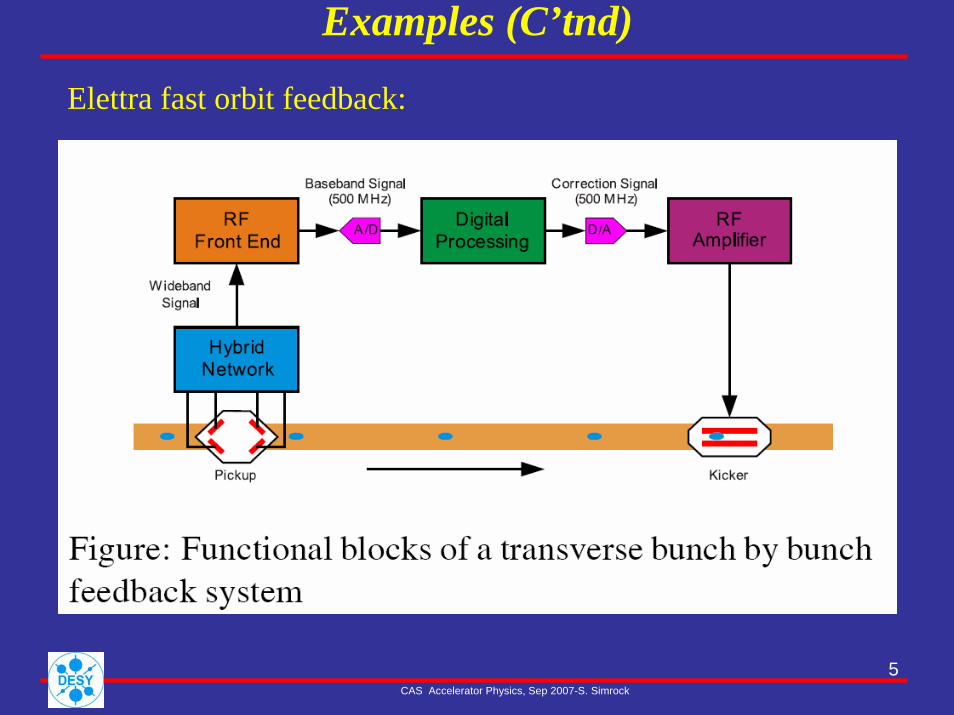
Examples (C’tnd)
Elettra fast orbit feedback:

6CAS Accelerator Physics, Sep 2007-S. Simrock
Examples (C’tnd)Beam based feedback for tune, coupling and chromaticity
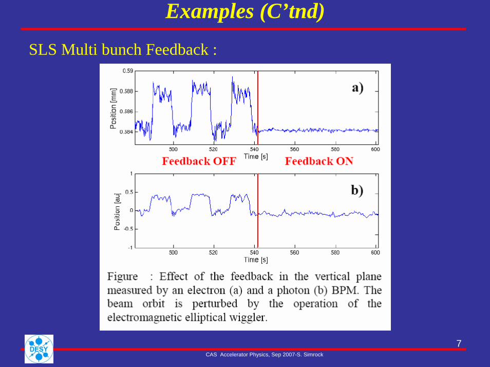
7CAS Accelerator Physics, Sep 2007-S. Simrock
Examples (C’tnd)
SLS Multi bunch Feedback :
8CAS Accelerator Physics, Sep 2007-S. Simrock
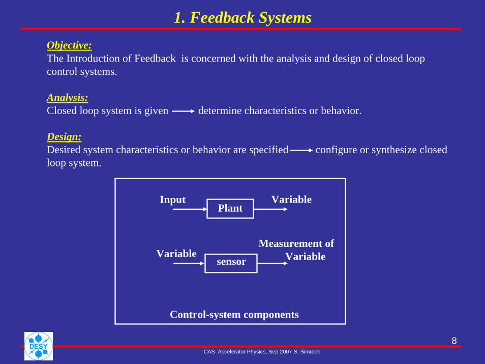
1. Feedback SystemsObjective:The Introduction of Feedback is concerned with the analysis and design of closed loop control systems.
Analysis:Closed loop system is given determine characteristics or behavior.
Design:Desired system characteristics or behavior are specified configure or synthesize closed loop system.
Plant
sensor
Input
VariableMeasurement of
Variable
Variable
Control-system components

9CAS Accelerator Physics, Sep 2007-S. Simrock
1. Feedback SystemsDefinition:A closed-loop system is a system in which certain forces (we call these inputs) are determined, at least in part, by certain responses of the system (we call these outputs).
Systeminputs
Systemoutputs
Closed loop system
O O

10CAS Accelerator Physics, Sep 2007-S. Simrock
Definitions:The system for measurement of a variable (or signal) is called a sensor.A plant of a control system is the part of the system to be controlled.The compensator (or controller or simply filter) provides satisfactory characteristics for the total system.
Two types of control systems:
A regulator maintains a physical variable at some constant value in thepresence of perturbances.A servomechanism describes a control system in which a physical variable is required to follow, or track some desired time function (originally applied in order to control a mechanical position or motion).
System input Error Plant
Sensor
Manipulated variable
Closed loop control system
System output
Compensator+
1. Feedback Systems

11CAS Accelerator Physics, Sep 2007-S. Simrock
1. Feedback SystemsExample 1: RF control system
Goal:Maintain stable gradient and phase.
Solution:Feedback for gradient amplitude and phase.
continued…Phase detector
~~
+-
Phase controller
amplitudecontroller Klystron cavity
Gradientset point
Controller

12CAS Accelerator Physics, Sep 2007-S. Simrock
1. Feedback SystemsModel:Mathematical description of input-output relation of components combined with block diagram.
Amplitude loop (general form):
Klystroncavity
amplifier
controllerReferenceinput outputRF power
amplifier
Monitoring transducer
_
Gradient detector
plant+error
13CAS Accelerator Physics, Sep 2007-S. Simrock
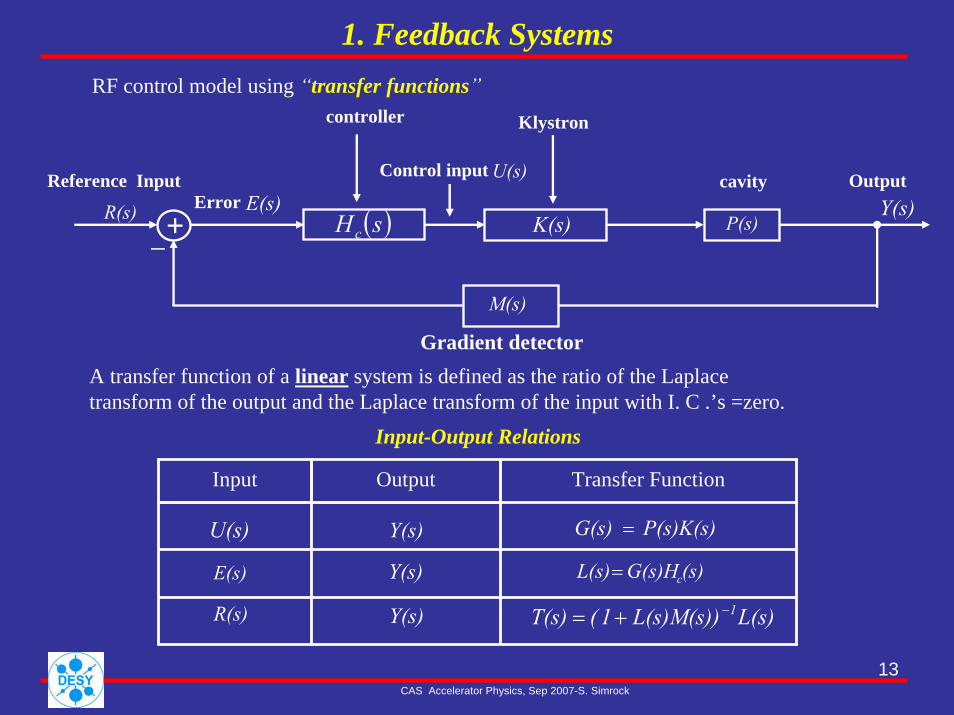
1. Feedback SystemsRF control model using “transfer functions”
A transfer function of a linear system is defined as the ratio of the Laplace transform of the output and the Laplace transform of the input with I. C .’s =zero.
Input-Output Relations
Transfer FunctionOutputInput
U(s) Y(s) P(s)K(s)G(s) =
E(s) Y(s)
Y(s)
(s)G(s)HL(s) c=
R(s) L(s)L(s)M(s))1(T(s) 1−+=
Gradient detector
Klystron
cavity
controller
Reference InputError
Output
_
Control input
P(s)K(s)R(s) ( )sHc
M(s)
Y(s)E(s)U(s)
+

14CAS Accelerator Physics, Sep 2007-S. Simrock
1. Feedback SystemsExample2: Electrical circuit
Differential equations:( ) (t)ν dττi
C1 i(t)R i(t)R 1
t
021 =++ ∫
( ) (t)ν dττiC1 i(t)R 2
t
02 =+ ∫
Laplace Transform:(s)VI(s)
Cs1 I(s)R I(s)R 121 =⋅
++
(s)VI(s)Cs
1 I(s)R 22 =⋅
+
Transfer function:
1s)CR(R1sCR
(s)V(s)VG(s)
21
2
1
2
+⋅++⋅⋅
==
(t)V1 (t)V2
i(t) 1R
2RC
1 VInput ,output 2V
15CAS Accelerator Physics, Sep 2007-S. Simrock
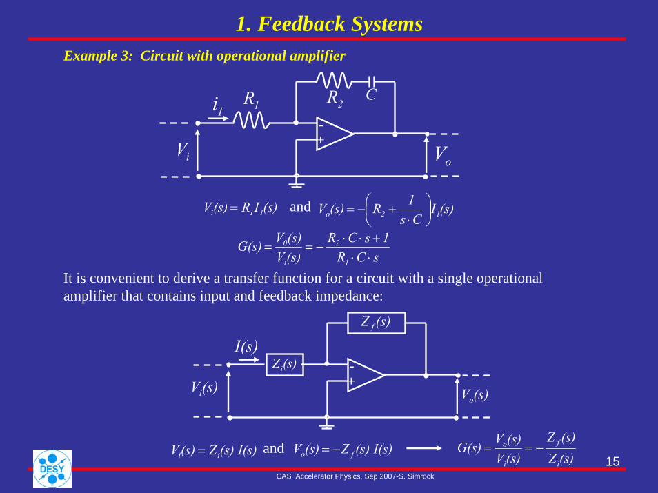
1. Feedback SystemsExample 3: Circuit with operational amplifier
+-
.
sCR1sCR
(s)V(s)VG(s)
1
2
i
0
⋅⋅+⋅⋅
−==
It is convenient to derive a transfer function for a circuit with a single operational amplifier that contains input and feedback impedance:
+-
(s)Z f
(s)Zi
I(s)
(s)Vi (s)Vo
.
iVoV
1i 1R 2R C
(s) IR(s)V 11i = (s)ICs
1R(s)V 12o ⎟⎠⎞
⎜⎝⎛
⋅+−=and
(s) I(s) Z(s)V ii = (s)Z(s)Z
(s)V(s)VG(s)
i
f
i
o −==(s) I(s)Z(s) V fo −=and
16CAS Accelerator Physics, Sep 2007-S. Simrock
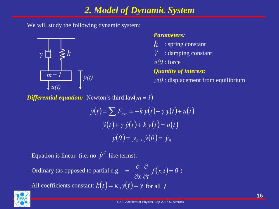
2. Model of Dynamic SystemWe will study the following dynamic system:
y(t)u(t)
γ k
1m =
Parameters:: spring constant: damping constant: force
Quantity of interest:: displacement from equilibrium
kγu(t)
y(t)
Differential equation: Newton’s third law
( ) ( ) ( ) ( )tutyγ tk yFty ext +−−== ∑ &&&
( ) ( ) ( ) ( )
tutk ytyγty =++ &&&
( ) ( ) 00 y0y , y0y && ==
( )1m =
-Equation is linear (i.e. no like terms).
-Ordinary (as opposed to partial e.g. )
-All coefficients constant:
( ) 0x,tftx
=∂∂
∂∂
=
( ) ( ) γ tκ ,γt k ==
2y&
for all t
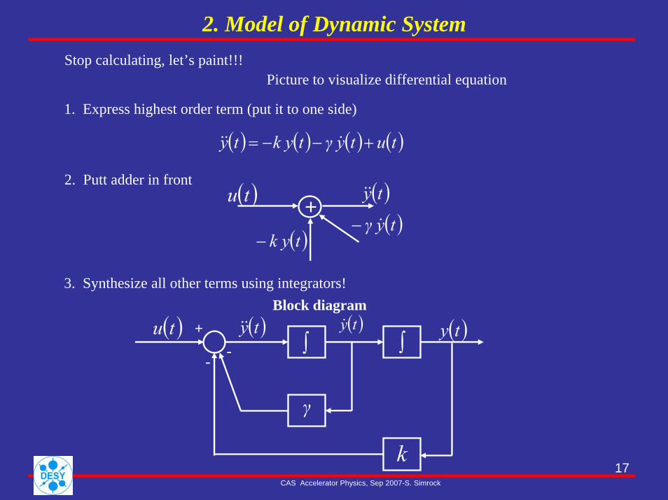
17CAS Accelerator Physics, Sep 2007-S. Simrock
2. Model of Dynamic SystemStop calculating, let’s paint!!!
Picture to visualize differential equation
1. Express highest order term (put it to one side)
( ) ( ) ( ) ( )tutyγ tk yty +−−= &&&
2. Putt adder in front
3. Synthesize all other terms using integrators!
( )tu ( )ty&&
( )tk y−( )tyγ &−
+
Block diagram+
--
( )tu ( )ty& ( )ty
γ
k
( )ty&&∫ ∫
18CAS Accelerator Physics, Sep 2007-S. Simrock
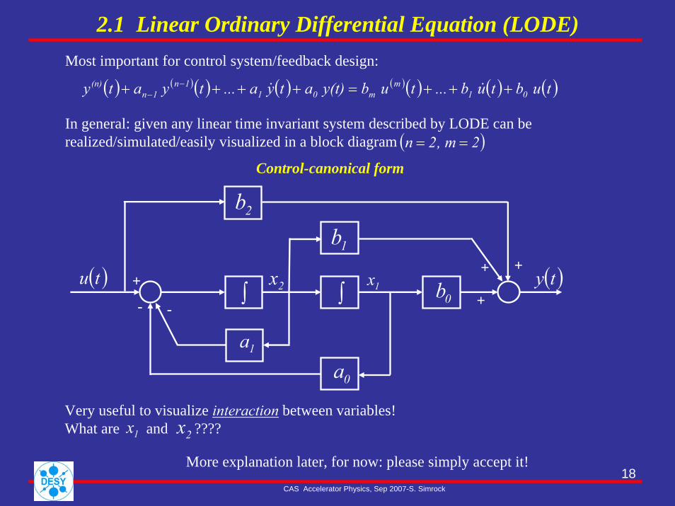
2.1 Linear Ordinary Differential Equation (LODE)Most important for control system/feedback design:
( ) ( )( )
In general: given any linear time invariant system described by LODE can be realized/simulated/easily visualized in a block diagram
( ) ( )( ) ( ) ( )t ubtu b...t ub y(t)aty a...t yaty 01m
m011n
1n(n) +++=++++ −
− &&
( )2, m2n ==
Control-canonical form
+
--
( )tu
1a
0a
2x0b ( )ty
2b
1b
1x+
+ +
∫∫
Very useful to visualize interaction between variables!What are and ????1x 2x
More explanation later, for now: please simply accept it!
19CAS Accelerator Physics, Sep 2007-S. Simrock
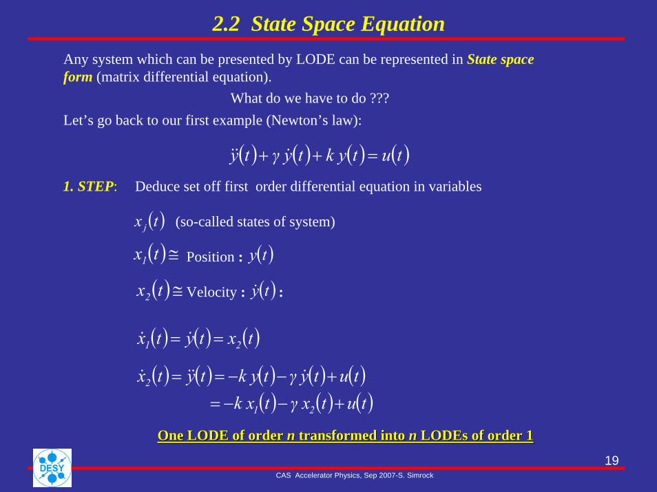
2.2 State Space EquationAny system which can be presented by LODE can be represented in State space form (matrix differential equation).
Let’s go back to our first example (Newton’s law):
One LODE of order One LODE of order nn transformed into transformed into n n LODEs of order 1LODEs of order 1
What do we have to do ???
( ) ( ) ( ) ( )tutk ytyγ ty =++ &&&
Deduce set off first order differential equation in variables
(so-called states of system)
Position :
Velocity : :
( )tx j
( ) ≅tx1
( ) ≅tx2
1. STEP:
( ) ( ) ( )
( ) ( ) ( ) ( ) ( )( ) ( ) ( )tutγ xtk x
tutyγ tk ytytx
txtytx
21
2
2
1
+−−=+−−==
==
&&&&
&&
( )ty
( ) ty&
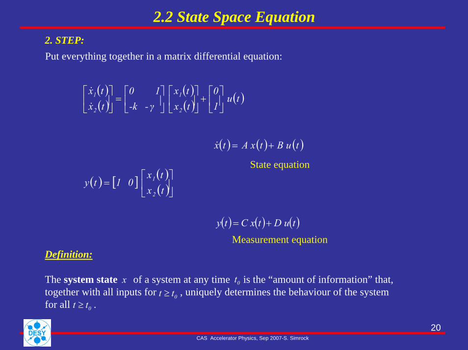
20CAS Accelerator Physics, Sep 2007-S. Simrock
2.2 State Space Equation2. STEP:Put everything together in a matrix differential equation:
( ) ( ) ( ) tD utC xty +=
Measurement equation
( )( )
( )( ) ( )t u
10
txtx
-k - γ
1 0txtx
2
1
2
1⎥⎦
⎤⎢⎣
⎡+⎥
⎦
⎤⎢⎣
⎡⎥⎦
⎤⎢⎣
⎡=⎥
⎦
⎤⎢⎣
⎡&
&
State equation
( ) ( ) ( ) tB utA xtx +=&
( ) [ ] ( )( ) txtx
0 1ty2
1⎥⎦
⎤⎢⎣
⎡=
Definition:
The system state of a system at any time is the “amount of information” that, together with all inputs for , uniquely determines the behaviour of the system for all .
0t
0tt ≥0tt ≥
x
21CAS Accelerator Physics, Sep 2007-S. Simrock
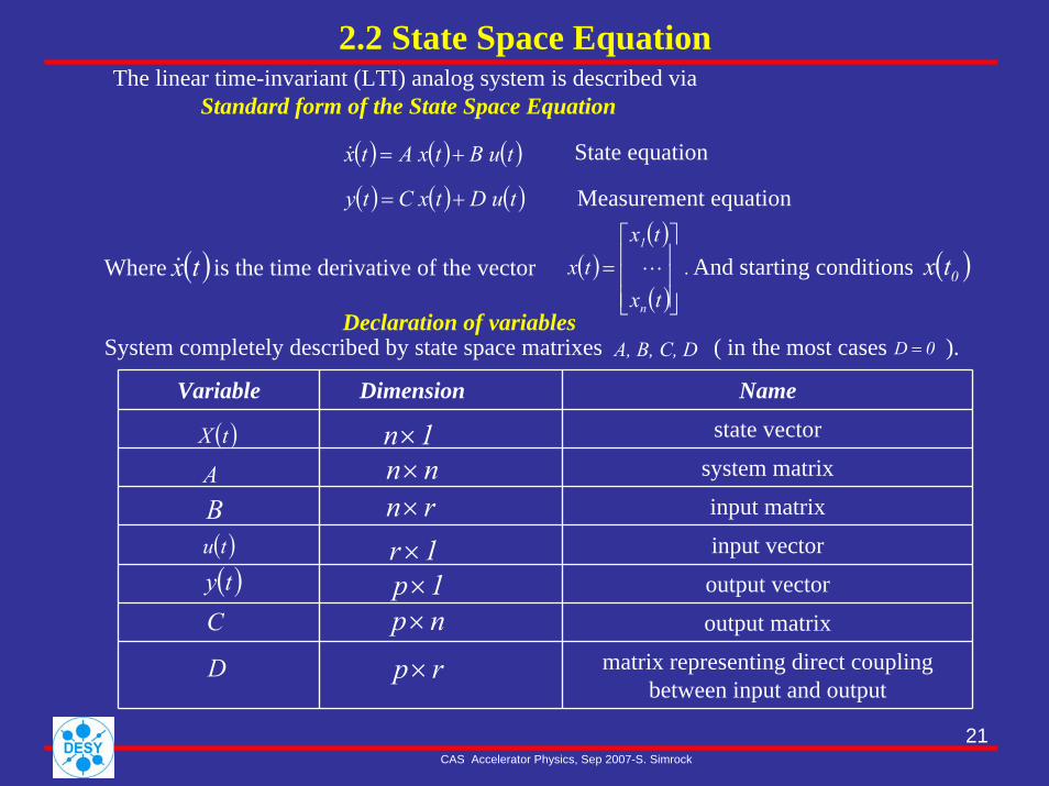
2.2 State Space EquationThe linear time-invariant (LTI) analog system is described via
Standard form of the State Space Equation
Variable Dimension Name
state vector
system matrix
input matrix
input vector
output vector
output matrix
matrix representing direct coupling between input and output
( )tX
AB( )tu
( )tyC
D
Declaration of variables
( ) ( ) ( )tB utA xtx +=& State equation
( ) ( ) ( ) tD utC xty += Measurement equation
( )( )
( ) .
tx
txtx
n
1
⎥⎥⎥
⎦
⎤
⎢⎢⎢
⎣
⎡⋅⋅⋅=Where is the time derivative of the vector ( )tx&
System completely described by state space matrixes ( in the most cases ). A, B, C, D 0D =
1n×nn×rn×1r×1p×np×
rp×
And starting conditions ( )0tx

22CAS Accelerator Physics, Sep 2007-S. Simrock
2.2 State Space EquationWhy all this work with state space equation? Why bother with?
( ) ( ) ( )( ) ( ) ( ) tD utC xty
tB utA xtx+=+=&
with e.g. Control-Canonical Form (case ):
[ ] 3210
210
b , D b bb , C100
, Ba a a
1 0 0 0 1 0
A ==⎥⎥⎥
⎦
⎤
⎢⎢⎢
⎣
⎡=
⎥⎥⎥
⎦
⎤
⎢⎢⎢
⎣
⎡
−−−=
or Observer-Canonical Form:
[ ] 3
2
1
0
2
1
0
b ,D1 0 0 ,Cbbb
,Ba 1 0a 0 1a 0 0
A ==⎥⎥⎥
⎦
⎤
⎢⎢⎢
⎣
⎡=
⎥⎥⎥
⎦
⎤
⎢⎢⎢
⎣
⎡
−−−
=
Notation is very compact, But: not unique!!!Computers love state space equation! (Trust us!)Modern control (1960-now) uses state space equation.General (vector) block diagram for easy visualization.
( )( ) ( )( ) ( ) ( ) ( )( ) ( ) ( )t ubtu b...t ubt yaty a...t yaty 01m
m011n
1nn +++=++++ −
− &&
BECAUSE: Given any system of the LODE form
Can be represented as
3 ,m3n ==
23CAS Accelerator Physics, Sep 2007-S. Simrock
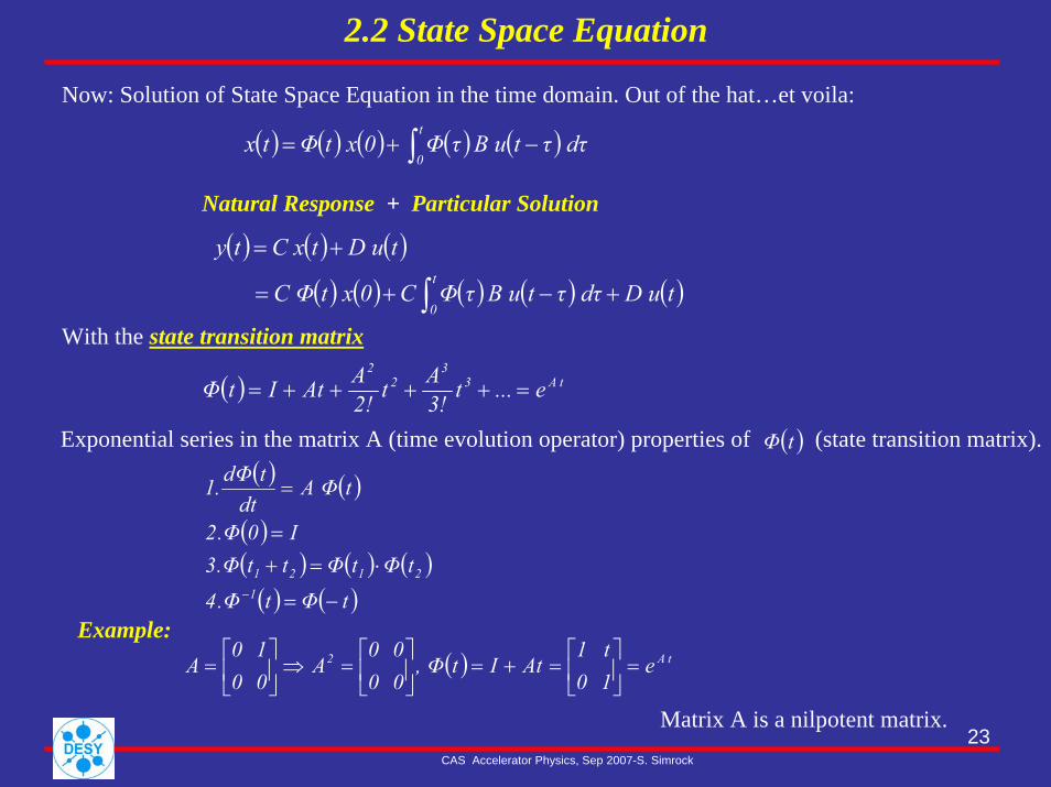
2.2 State Space Equation
Now: Solution of State Space Equation in the time domain. Out of the hat…et voila:
( ) ( ) ( ) ( ) ( ) dττt B uτΦ0 xtΦtx t
0 −+= ∫
Natural Response + Particular Solution
( ) ( ) ( )( ) ( ) ( ) ( ) ( )tD u dττt B uτΦC0 xtC Φ
tD utC xty t
0 +−+=
+=
∫With the state transition matrix
( ) tA33
22
e...t!3At!2
AAtItΦ =++++=
( ) ( )
( )( ) ( ) ( )( ) ( )tΦt.Φ4
tΦtΦtt.Φ3I0.Φ2
tA Φdt
tdΦ.1
12121
−=
⋅=+=
=
−
Exponential series in the matrix A (time evolution operator) properties of (state transition matrix).( )tΦ
Example:( ) tA2 e
1 0 t1
AtIt, Φ0 00 0
A0 01 0
A =⎥⎦
⎤⎢⎣
⎡=+=⎥
⎦
⎤⎢⎣
⎡=⇒⎥
⎦
⎤⎢⎣
⎡=
Matrix A is a nilpotent matrix.

24CAS Accelerator Physics, Sep 2007-S. Simrock
2.4 Transfer Function G (s)Continuous-time state space model
( ) ( ) ( )( ) ( ) ( )tD utC xty
tB utA xtx+=+=& State equation
Measurement equation
Transfer function describes input-output relation of system.
( ) ( ) ( ) ( )sB UsA X0xss X +=−
( ) ( ) ( ) ( ) ( )( ) ( ) ( ) ( )s B Us xs
sB UAsIxAsIsXΦ+Φ=
−+−= −−
00 11
( ) ( ) ( )( ) ( ) ( ) ( )( ) ( ) ( ) ( ) ( )sD Us B UsC xsC
sD]UBAsI[c]xAsIC[
sD UsC XsY
+Φ+Φ=+−+−=
+=−−
00 11
( ) ( ) ( ) D BsC DBAsICsG +Φ=+−= −1
System( )sU ( )sY
Transfer function ( pxr ) (case: x(0)=0):( )sG
25CAS Accelerator Physics, Sep 2007-S. Simrock
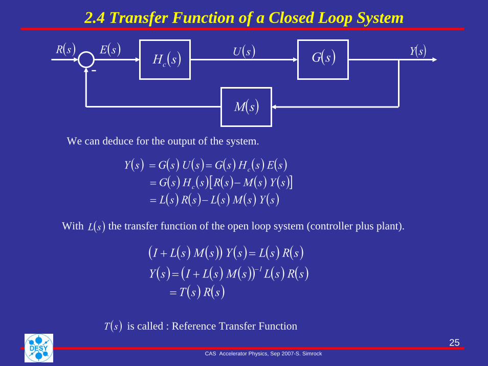
2.4 Transfer Function of a Closed Loop System
( )sR ( )sE ( )sU ( )sY( )sHc( )sG
( )sM
-
( ) ( ) ( ) ( ) ( ) ( )( ) ( ) ( ) ( ) ( )[ ]( ) ( ) ( ) ( ) ( )s Ys MsLs RsL
s YsMsRs HsG s Es HsGs UsG sY
c
c
−=−=
==
We can deduce for the output of the system.
( ) sLWith the transfer function of the open loop system (controller plus plant).
( ) ( )( ) ( ) ( ) ( )( ) ( ) ( )( ) ( ) ( )
( ) ( )s RsT s RsLs MsLIsY
s RsLs Ys MsLI 1
=+=
=+−
( ) sT is called : Reference Transfer Function

26CAS Accelerator Physics, Sep 2007-S. Simrock
2.5 Sensitivity and Disturbance Rejection
r(t) - reference inputd(t) – output disturbancen(t) – measurement noisey(t) – controlled output
)( sCr
d
)( sG y
n
ue
Consider the following closed loop system:
dGCInrGCGCIynyrCu
dGuy
11 )()()()(
−− ++−+=
−−=substituting :
The controlled output : +=
Now define the transfer functions for:
yields :
G(s)C(s)G(s)C(s))(IT(s)sCsGIsS
1
1))()(()(−
−
+=
+=Sensitivity:
ComplementarySensitivity:
IST =+
27CAS Accelerator Physics, Sep 2007-S. Simrock
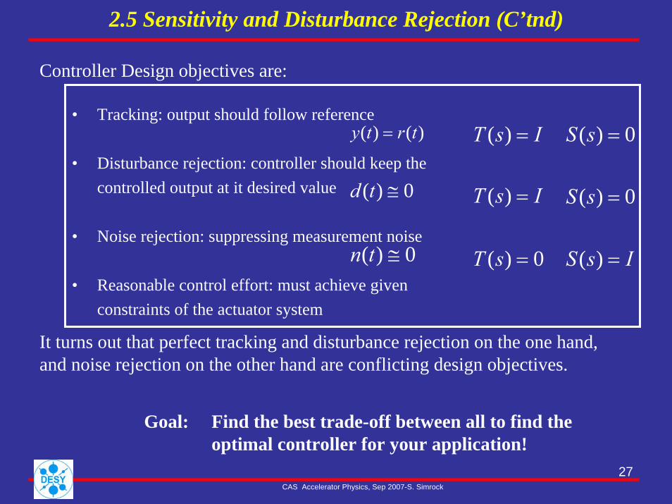
2.5 Sensitivity and Disturbance Rejection (C’tnd)
• Tracking: output should follow reference
• Disturbance rejection: controller should keep the controlled output at it desired value
• Noise rejection: suppressing measurement noise
• Reasonable control effort: must achieve given constraints of the actuator system
)()( trty =
Controller Design objectives are:
0)( ≅td
0)( ≅tn
IsT =)(
IsT =)(
0)( =sS
0)( =sT IsS =)(
0)( =sS
It turns out that perfect tracking and disturbance rejection on the one hand, and noise rejection on the other hand are conflicting design objectives.
Goal: Find the best trade-off between all to find the optimal controller for your application!
28CAS Accelerator Physics, Sep 2007-S. Simrock
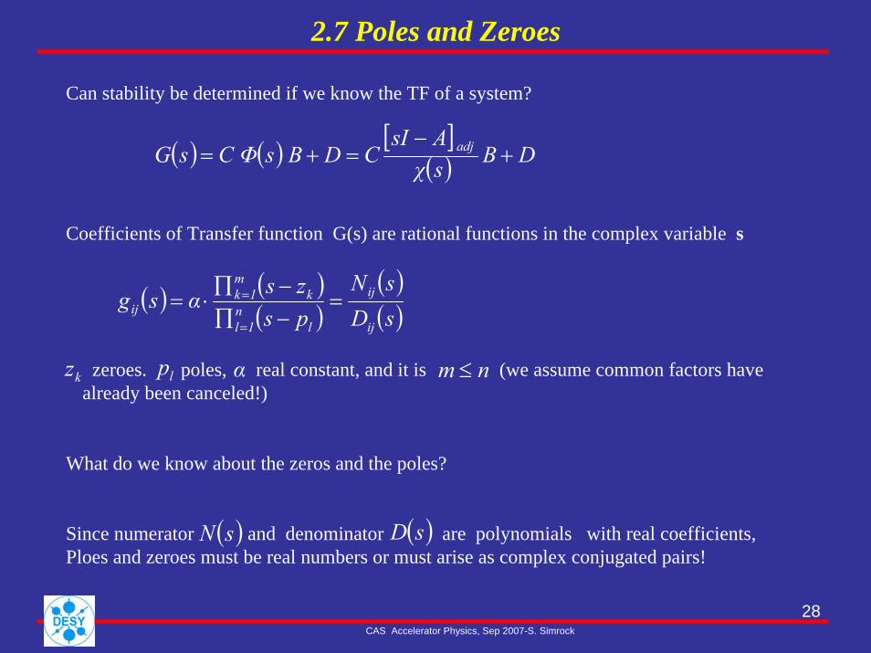
2.7 Poles and Zeroes
Can stability be determined if we know the TF of a system?
( ) ( ) [ ]( ) DBsχAsI
CD BsC ΦsG adj +−
=+=
( ) ( )( )
( )( )sDsN
pszsαsg
ij
ij
ln
1l
km
1kij =
−∏−∏
⋅==
=
Coefficients of Transfer function G(s) are rational functions in the complex variable s
What do we know about the zeros and the poles?
Since numerator and denominator are polynomials with real coefficients, Ploes and zeroes must be real numbers or must arise as complex conjugated pairs!
( )sN ( )sD
kz lp α nm ≤zeroes. poles, real constant, and it is (we assume common factors havealready been canceled!)

29CAS Accelerator Physics, Sep 2007-S. Simrock
2.7 Poles and Zeroes
( )B AsICadj −
Stability directly from state-space
Assuming D=0 (D could change zeros but not poles)
Assuming there are no common factors between the poly and i.e. no pole-zero cancellations (usually true, system called “ minimal” ) then we can identify
( ) ( ) DBAsICscall : HRe 1 +−= −
( ) ( )( )
( )( )sasb
AsIBAsICsH adj=
−−
=det
( )AsIdet −
( ) ( ) BAsIC sb adj−=
( ) ( )AsI detsa −=
and
i.e. poles are root of ( )AsI det −
iλ thiLet be the eigenvalue of A
=>≤ i }{λi allfor 0Reif System stable
So with computer, with eigenvalue solver, can determine system stability directly from coupling matrix A.
30CAS Accelerator Physics, Sep 2007-S. Simrock
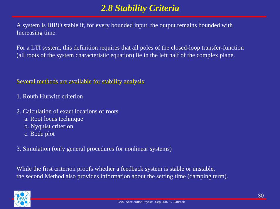
2.8 Stability Criteria
Several methods are available for stability analysis:
1. Routh Hurwitz criterion
2. Calculation of exact locations of rootsa. Root locus techniqueb. Nyquist criterionc. Bode plot
3. Simulation (only general procedures for nonlinear systems)
A system is BIBO stable if, for every bounded input, the output remains bounded with Increasing time.
For a LTI system, this definition requires that all poles of the closed-loop transfer-function(all roots of the system characteristic equation) lie in the left half of the complex plane.
While the first criterion proofs whether a feedback system is stable or unstable, the second Method also provides information about the setting time (damping term).

31CAS Accelerator Physics, Sep 2007-S. Simrock
2.8 Poles and Zeroes
S-Plane
Medium oscillation Medium decay
X XX
X
X
No Oscillation Fast Decay
X
X
X
XNo oscillationNo growth
Fast oscillation No growth
Medium oscillationMedium growth
ω(s)Im =
σ(s)Re =
No oscillationFast growth
Pole locations tell us about impulse response i.e. also stability:
32CAS Accelerator Physics, Sep 2007-S. Simrock
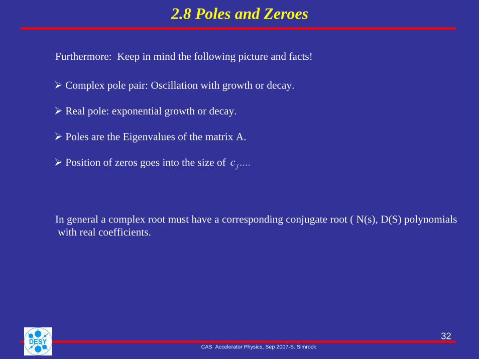
2.8 Poles and Zeroes
Furthermore: Keep in mind the following picture and facts!
Complex pole pair: Oscillation with growth or decay.
Real pole: exponential growth or decay.
Poles are the Eigenvalues of the matrix A.
Position of zeros goes into the size of ....c j
In general a complex root must have a corresponding conjugate root ( N(s), D(S) polynomialswith real coefficients.

33CAS Accelerator Physics, Sep 2007-S. Simrock
2.8 Bode Diagram
Phase Marginmφ
00
0180−
Gain Margin
dB
mG
ω
ω1ω
2ω
2ω 1ω090−
The closed loop is stable if the phase of the unity crossover frequency of the OPEN LOOP Is larger than-180 degrees.

34CAS Accelerator Physics, Sep 2007-S. Simrock
2.8 Root Locus AnalysisDefinition: A root locus of a system is a plot of the roots of the system characteristicEquation (the poles of the closed-loop transfer function) while some parameter of thesystem (usually the feedback gain) is varied.
( ) ( ) ( ) ( )321 ps ps psKsK H
−−−=
XXX1p2p3p
( ) ( )( ) ( ) .0sK H1roots at sK H1
sHKsGCL =++
=
How do we move the poles by varying the constant gain K?
( )sR ( )sY
-
+( )sH K
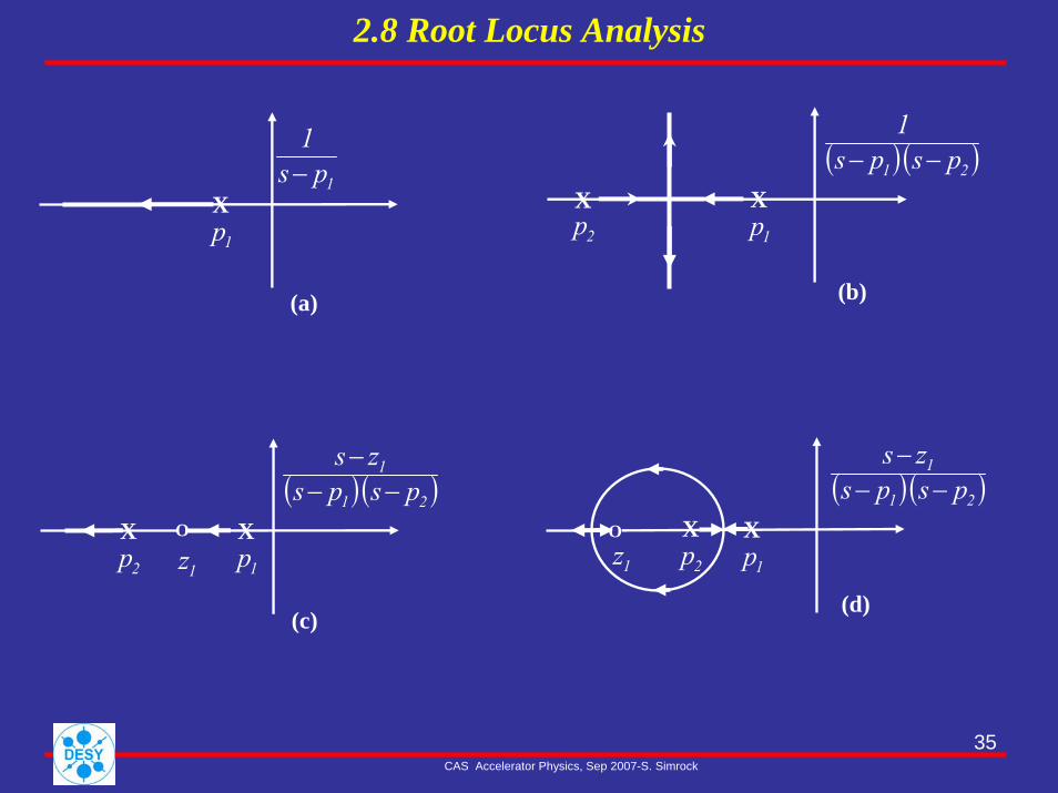
35CAS Accelerator Physics, Sep 2007-S. Simrock
2.8 Root Locus Analysis
X1p
1ps1−
X1p
( ) ( )21 psps1−−
X2p
X1p
( ) ( )21
1
pspszs−−
−
X2p
O
1zX
1p
( ) ( )21
1
pspszs−−
−
X2p
O
1z
(a) (b)
(c)(d)
36CAS Accelerator Physics, Sep 2007-S. Simrock
X1p
( ) ( ) ( )321 pspsps1
−−− X
2pX
3pX
1p
( ) ( ) ( )321 pspsps1
−−− X
2p
X3p
( ) ( ) ( )321 pspsps1
−−− X
1p
X2p
X3p
( ) ( ) ( )321
1
pspspszs
−−−−
OX2p
X3p 1z
X1p
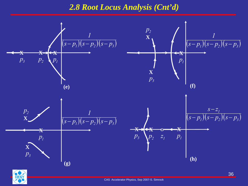
2.8 Root Locus Analysis (Cnt’d)
(e) (f)
(g)(h)

37CAS Accelerator Physics, Sep 2007-S. Simrock
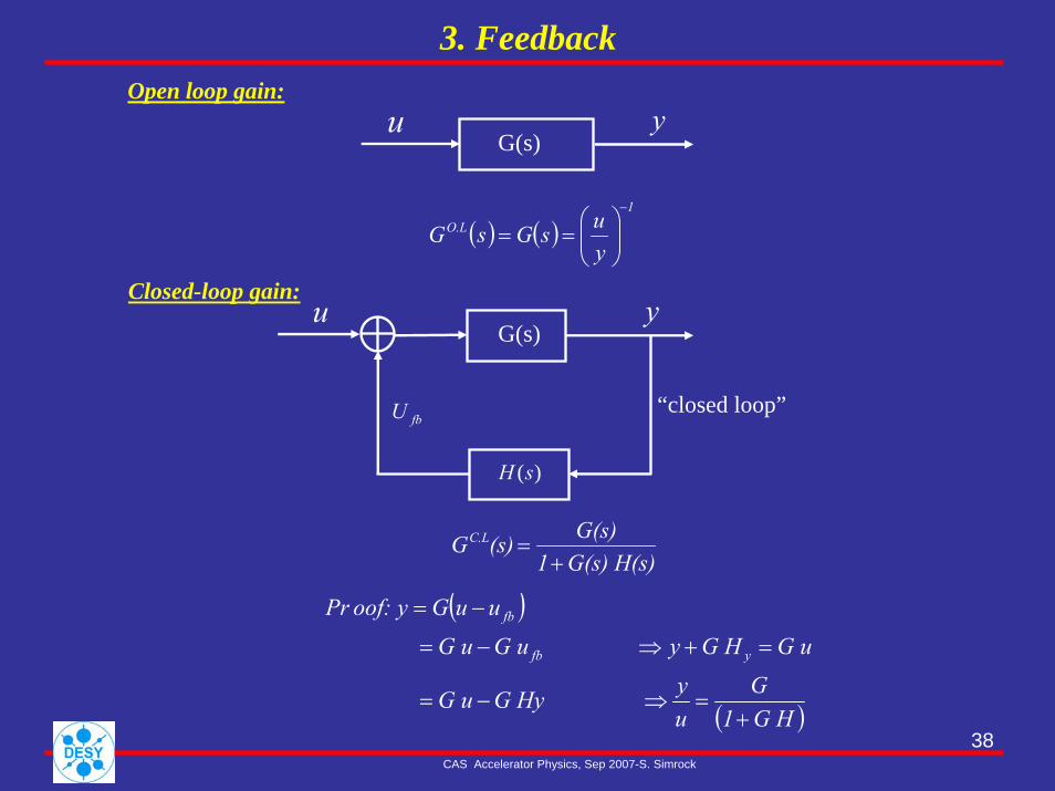
3. FeedbackThe idea:Suppose we have a system or “plant”
We want to improve some aspect of plant’s performance by observing the output and applying a appropriate “correction” signal. This is feedback
plant
“open loop”
“closed loop”plant
?
Ufeedback
r
Question: What should this be?
38CAS Accelerator Physics, Sep 2007-S. Simrock
3. FeedbackOpen loop gain:
Closed-loop gain:
G(s)u y
( ) ( )1
O.L
yusGsG
−
⎟⎟⎠
⎞⎜⎜⎝
⎛==
G(s) H(s)1G(s)(s)GC.L
+=
( )
( )G H1G
uy G Hy G u
G uG Hy G uG u
uuGoof: yPr
yfb
fb
+=⇒−=
=+⇒−=
−=
“closed loop”
uG(s)
y
)(sH
fbU
39CAS Accelerator Physics, Sep 2007-S. Simrock
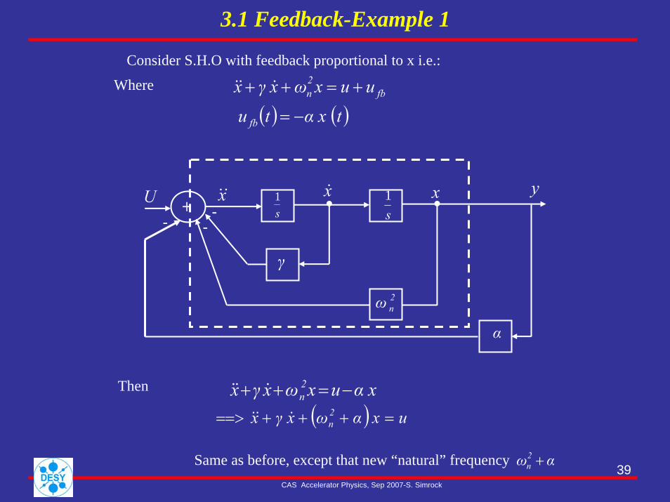
3.1 Feedback-Example 1
Consider S.H.O with feedback proportional to x i.e.:
( ) ( )tα x t u
uuxωxγ x
fb
fb2n
−=
+=++ &&&
Then
Same as before, except that new “natural” frequency αω2n +
Where
+ s1
s1 y
2nω
α
U-
--
x&& x& x
γ
α xuxωxγ x 2 n −=++ &&&
( ) u xαωxγ x 2n =+++==> &&&
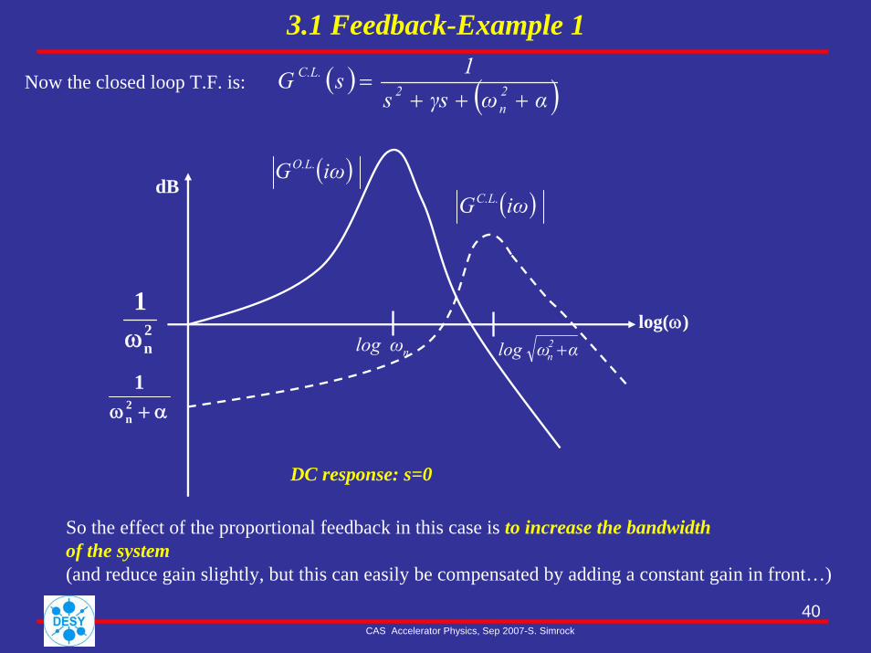
40CAS Accelerator Physics, Sep 2007-S. Simrock
3.1 Feedback-Example 1
So the effect of the proportional feedback in this case is to increase the bandwidth of the system(and reduce gain slightly, but this can easily be compensated by adding a constant gain in front…)
)log(ω2n
1ω
α+ω2n
1n ωlog αω log 2
n +
( ) iωGO.L.
( ) iωGC.L.
DC response: s=0
dB
( ) ( )αωγss1sG 2
n2
C.L.
+++=Now the closed loop T.F. is:

41CAS Accelerator Physics, Sep 2007-S. Simrock
3.1 Feedback-Example 2
( ) ( ) dτ τxαtut
0fb ∫−=
( )∫−=++t
0
2n dττxαu xωxγ xi.e &&&
Differentiating once more yields: uα xx ωxγ x 2n &&&&&&& =+++
No longer just simple S.H.O., add another state
In S.H.O. suppose we use integral feedback:
+ s1
sα
--
-
y
2nω
U x&& x& x
γ
s1

42CAS Accelerator Physics, Sep 2007-S. Simrock
3.1 Feedback-Example 2
( )
( )
( ) αωγssss
αωγss1
sα1
ωγss1
sG
2n
2
2n
2
2n
2C.L.
+++=
⎟⎟⎠
⎞⎜⎜⎝
⎛+++
⎟⎠⎞
⎜⎝⎛+
++=
Observe that1.2. For large s (and hence for large )
( )00GC.L. =ω
( ) ( ) ( )sGωγss
1sG O.L.2n
2C.L. ≈
++≈dB
2nω
1
( )iωGO.L.
( )iωGC.L.
)log(ω
So integral feedback has killed DC gaini.e system rejects constant disturbances
43CAS Accelerator Physics, Sep 2007-S. Simrock
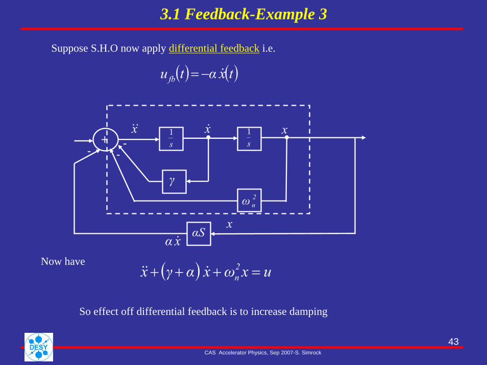
3.1 Feedback-Example 3
Suppose S.H.O now apply differential feedback i.e.
( ) ( )txα tufb &−=
( ) uxωx αγx 2n =+++ &&&
Now have
So effect off differential feedback is to increase damping
+
αS
--
-
xα &
s1
2nω
x&& x& x
γ
s1
x

44CAS Accelerator Physics, Sep 2007-S. Simrock
3.1 Feedback-Example 3
dB
2nω
1
( )iωGO.L.
)log(ω
( )iωGC.L.
Now ( ) ( ) 2n
2C.L.
ω sαγs1sG
+++=
So the effect of differential feedback here is to “flatten the resonance” i.e. damping is increased.
Note: Differentiators can never be built exactly, only approximately.

45CAS Accelerator Physics, Sep 2007-S. Simrock
3.1 PID Controller(1) The latter 3 examples of feedback can all be combined to form a
P.I.D. controller (prop.-integral-diff).
ldpfb uuuu ++=
(2) In example above S.H.O. was a very simple system and it was clear what physical interpretation of P. or I. or D. did. But for large complex systems not obvious
==> Require arbitrary “ tweaking ”
That’s what we’re trying to avoid
S.H.O+
/sKsKK lDp ++
P.I.D controller
-
yx =u

46CAS Accelerator Physics, Sep 2007-S. Simrock
For example, if you are so smart let’s see you do this with your P.I.D. controller:
Damp this mode, but leave the other two modes undamped, just as they are.
This could turn out to be a tweaking nightmare that’ll get you nowhere fast!
With modern control theory this problem can be solved easily.
G
ω
6th order system3 resonant poles3 complex pairs6 poles
3.1 PID Controller