USING THE RJMCMC PROCEDURE FOR IDENTIFYING AND ESTIMATING TAR MODELS

Fabio H. Nieto

Universidad Nacional de Colombia

Hanwen Zhang

Universidad Santo Tomás

Wen Li

Singapore Clinical Research Institute

Reporte Interno de Investigación No. 13

Departamento de Estadística

Facultad de Ciencias

Universidad Nacional de Colombia

Bogotá, COLOMBIA

Using the RJMCMC procedure for identifying and

estimating univariate TAR models∗

Fabio H. Nieto†

Universidad Nacional de Colombia

Hanwen Zhang

Universidad Santo Tomas

Wen Li

Singapore Clinical Research Institute

June 14, 2010

Abstract

One way that has been used for identifying and estimating threshold autoregres-

sive (TAR) models for nonlinear time series follows the MCMC approach via the

Gibbs sampler. This route has major computational difficulties, specifically, in get-

ting convergence to the parameter distributions. In this paper, a new procedure for

identifying a TAR model and for estimating its parameters is developed, following

∗This research was sponsored by DIB, the investigation division of Universidad Nacional de

Colombia at Bogota, under contract COL0022265-2007†Corresponding author: fhnietos@unal.edu.co

1

the RJMCMC sampler. It is found that the proposed procedure conveys a Markov

chain with convergence properties.

Keywords: Bayesian model choice; Nonlinear time series; Regime-switching

models; RJMCMC sampler; Threshold autoregressive (TAR) models

1 Introduction

Nieto (2005) developed a procedure for identifying univariate TAR models, which

are nonlinear, based on that of Carlin and Chib (1995) for Bayesian model choice.

As quoted by those authors, the so-called link distributions are crucial for obtaining

efficient mixing in the Gibbs sampler defined in their paper. This aspect was noted by

Nieto (2005) and he found major difficulties in implementing the method in practice,

especially, because of the very small values of the model likelihood function, a fact

which signals that the likelihood present in the data is not being extracted optimally.

In order to have an alternative to Nieto’s (2005) approach, we present in this pa-

per a procedure based on Green’s (1995) RJMCMC (Reversible Jump Markov Chain

Montecarlo) sampler. There are some papers that are close to our problem, as, for

example, Campbell’s (2004) and Vermaak , et al. (2004). The first one is developed

in the context of the so-called SETAR (selfexciting threshold autoregressive) models,

where the number of regimes is assumed to be known a priori and the focus is ba-

sically in estimating the autoregressive orders. In the second, linear autoregressive

processes are considered and the interest is to estimate the unknown model order. For

choosing another type of time series models, Vrontos et al. (2000) used the RJMCMC

procedure for making full Bayesian inference of GARCH and EGARCH models.

Our main concern in this paper is to identify (estimate) the so-called structural

parameters, i.e. the number of regimes and the autoregressive orders in each regime,

2

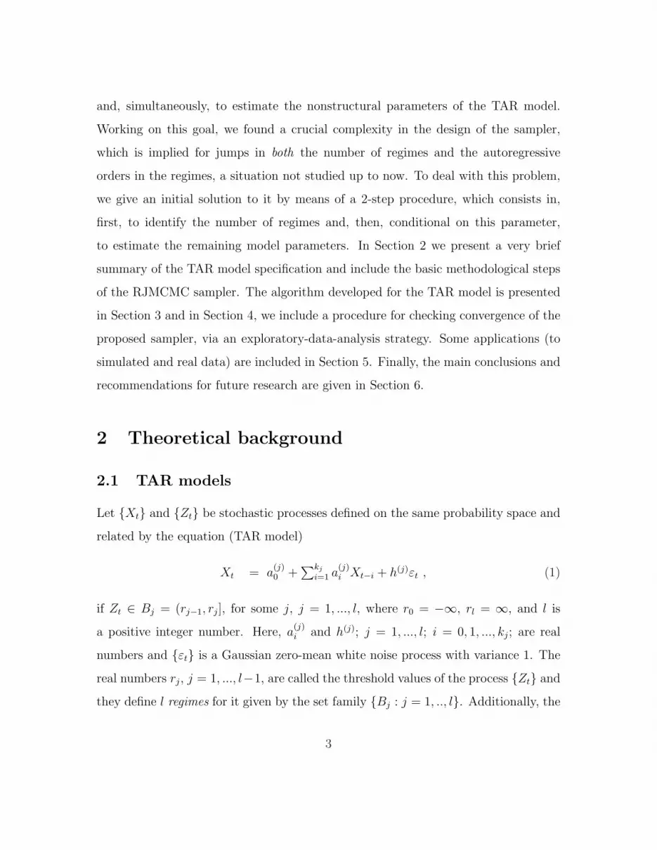
and, simultaneously, to estimate the nonstructural parameters of the TAR model.

Working on this goal, we found a crucial complexity in the design of the sampler,

which is implied for jumps in both the number of regimes and the autoregressive

orders in the regimes, a situation not studied up to now. To deal with this problem,

we give an initial solution to it by means of a 2-step procedure, which consists in,

first, to identify the number of regimes and, then, conditional on this parameter,

to estimate the remaining model parameters. In Section 2 we present a very brief

summary of the TAR model specification and include the basic methodological steps

of the RJMCMC sampler. The algorithm developed for the TAR model is presented

in Section 3 and in Section 4, we include a procedure for checking convergence of the

proposed sampler, via an exploratory-data-analysis strategy. Some applications (to

simulated and real data) are included in Section 5. Finally, the main conclusions and

recommendations for future research are given in Section 6.

2 Theoretical background

2.1 TAR models

Let {Xt} and {Zt} be stochastic processes defined on the same probability space and

related by the equation (TAR model)

Xt = a(j)0 +

∑kj

i=1 a(j)i Xt−i + h(j)εt , (1)

if Zt ∈ Bj = (rj−1, rj], for some j, j = 1, ..., l, where r0 = −∞, rl = ∞, and l is

a positive integer number. Here, a(j)i and h(j); j = 1, ..., l; i = 0, 1, ..., kj; are real

numbers and {εt} is a Gaussian zero-mean white noise process with variance 1. The

real numbers rj, j = 1, ..., l−1, are called the threshold values of the process {Zt} and

they define l regimes for it given by the set family {Bj : j = 1, .., l}. Additionally, the

3

nonnegative integer numbers k1, ..., kl denote, respectively, the autoregressive orders

of {Xt} in each regime. We shall use the symbol TAR(l; k1, ..., kl) to denote this

model and call l; r1, ..., rl−1; and k1, ..., kl the model structural parameters.

This kind of models was introduced by Tong(1978) and Tong and Lim (1980),

specifically, in which case the threshold variable is the lagged variable Xt−d, where d

is some positive integer. In this case, the model is known as the self-exciting TAR

(SETAR) model and, at present, there is a lot of literature about the topic of analyzing

these models, under the frequent assumption that we know the number l of regimes

and the autoregressive orders k1, ..., kl.

Under the scope of open-loop systems (Tong, 1990), we also assume that {Zt} is

exogenous in the sense that there is no feedback of {Xt} towards it and that {Zt} is

a homogeneous pth order Markov chain with initial distribution F0(z, θz) and kernel

distribution Fp(zt|zt−1, ..., zt−p,θz), where θz is a parameter vector in an appropriate

numerical space. Furthermore, we assume that these distributions have densities in

the Lebesgue-measure sense. Let f0(z, θz) and fp(zt|zt−1, ..., zt−p,θz) be, respectively,

the initial and kernel density functions of the distributions above. In what follows,

we assume that the p-dimensional Markov chain {Zt} has an invariant or stationary

distribution fp(z, θz).

Nieto (2005) developed the methodolgy for analyzing (identifying, estimating, and

verifying) the TAR model, in the pressence of missing data; then, Nieto (2008) devel-

oped a procedure for forecasting variable X with the TAR model, in the pressence of

missing data, too. Of course, if the time series are complete, Nieto’s methods are also

applicable with minor modifications. Tsay (1999) developed the multivariate version

of the TAR model for complete time series, with the threshold variable Zt−d, where

d > 1, while in Nieto’s (2005) model d = 0 is allowed. As noted above, previously to

these approaches, Tong (1990) considered a very similar version of this model that

called open-loop models and, under this concept, what the TAR model means is that

4

the nonlinear dynamical behavior of variable X is explained by the exogenous vari-

able Z, according to its values in the sets of a partition of its sample space. The TAR

model can explain certain stylized facts of financial and hidrological/meteorological

time series like, for example, the presence of extreme-values clusters. Also, the model

can explain the regime-switching characteristic of Markov chains, with the advantage

that the state space can be general, i.e., not necessarily discrete.

2.2 The RJMCMC procedure

The material we are going to include here is referred to Chen et al.’s (2000) book.

For a more specific presentation the reader can consult Green’s (1995) paper.

Suppose that we have a countable collection of candidate models {Mk|k ∈ M},where M ⊆ N, the set of natural numbers. Model Mk is parameterized by the

unknown vector θ(k) of dimension pk, which may vary from model to model. Under

model Mk, the posterior distribution of θ(k) takes the form

π(θ(k)|D,Mk) ∝ π∗(θ(k)|D,Mk)p(k)/p(Mk|D) ,

with π∗(θ(k)|D,Mk) = L(θ(k),Mk|D)π(θ(k)|Mk), where D denotes the data set,

L(θ(k),Mk|D) is the likelihood function, π(θ(k)|Mk) is the prior distribution for the

parameter vector under model Mk, and p(k) is a prior distribution for k (or Mk).

Notice that π∗(θ(k)|D,Mk) is the unnormalized posterior density, given Mk. Then,

the joint distribution of (k, θ(k)) given the data D, the distribution of interest, is given

by

π(k, θ(k)|D) = π(θ(k)|D,Mk)p(Mk|D) ∝ π∗(θ(k)|D,Mk)p(k) .

The idea is to obtain joint samples for the model number k and the parameter vec-

tor θ(k) from this joint posterior distribution. The main property of the RJMCMC

algorithm is that the underlying Markov chain is designed in a such way that it can

5

jump between models with parameter spaces of different dimensions, while retaining

a detailed balance that ensures the correct limiting distribution, provided the chain

is irreducible and aperiodic.

Remark. Strictly speaking, k must be seen as a realization of a discrete random

variable K, whose sample space is M .

The algorithm

Let us assume that the current state of the chain is (k, θ(k)), then:

Step 1. Propose a new model Mk∗ with probability j(k∗|k) (this means, given k,

one needs to put a probability distribution for choosing moves among the models).

Step 2. Generate u, of certain dimension, from a specified proposal density qk(u|θ(k), k, k∗).

Step 3. Set (θ(k∗),u∗) = gk,k∗(θ(k),u), where gk,k∗ is a bijective transformation

between Euclidian subspaces of dimension pk + dim(u) = pk∗ + dim(u∗) (thus, one

needs some kind of dimension matching and for that purpose one uses the proposal

distribution qk(·|·)).Step 4. Let rn = p(k∗)π∗(θ(k∗)|D,Mk∗)j(k

∗|k)qk∗(u∗|θ(k∗), k∗, k),

rd = p(k)π∗(θ(k)|D,Mk)j(k|k∗)q(u|θ(k), k, k∗), and J be the Jacobian of the trans-

formation gk,k∗ . Then, accept the proposed move to (k∗,θ(k∗)) with probability

α = min{1, rnJ/rd}.As quoted by Green (1995), the probability distribution for doing the moves among

models, the q distributions, function g, etc., depends strongly on the data at hand.

The idea is to assure that the chain thus defined is aperiodic and irreducible and this

is our goal in the next section.

6

3 Identifying and estimating the TAR model

Following Green’s (1995) example about estimating a step function in a multidimen-

sional change-point problem, our initial interest is on the posterior distribution of the

random vector (l,kl, θl), where l = 2, ..., l0, for some known l0, kl = (k1l, ..., kll), and

θl = (θ1l, ..., θll), with θjl = (a(j)0 , a

(j)1 , ..., a

(j)kj

, h(j)), for j = 1, ..., l. Notice that that

vector has dimension k1 + ... + kl + 2l; hence, if l or kjl changes, for some j = 1, ..., l,

the vector dimension changes. Also, note that the vector itself changes if θl changes,

equivalently, if θjl changes for some j, j = 1, ..., l.

In this paper, we consider a modification of the usual RJMCMC sampler, which

consists in a 2-step approach. In the first step, we design an RJMCMC sampler for

the whole parameter vector (l,kl,θl) and, in the second, we fix the estimated value

for l, l say, and re-estimate the remaining parameters (kl,θ l) via a simplification of

the previous sampler. This 2-step proposal was motivated for the fact that there is

a double nested movement among models, i.e., first a move for l and, then, a move

for kl, a problem does not considered up to now, in the authors knowledge. This

can cause a very low mixing for kl. Consequently, an important problem for future

research is to design an RJMCMC sampler for all the parameter vector, as one would

desire at first.

Thinking in the RJMCMC sampler for (l,kl, θl), we consider three types of tran-

sitions in the underlying Markov chain to be developed. These are: (i) a change in

the number of regimes l (R), (ii) a change in some autoregressive order kj, j = 1, ..., l,

(O), and (iii) a change in the total nonstructural parameter vector θl (V).

When transition R happens, we also need to consider intrinsic changes in autore-

gressive (AR) orders and, consequently, in θl. Following Green’s (1995) paper, the

changes in the number of regimes is circumscribed to the so-called birth and death

moves, that is, a birth happens if the number of regimes moves from l to l + 1 and

7

a death, if there is a move from l + 1 to l. For doing these moves, a subprobability

distribution is needed, which is obtained as follows.

Let bl = Pr(Birth) = c minl{1, p(l+1)/p(l)} and dl+1 = Pr(Death) = c minl{1, p(l)/p(l+

1)}, where p(·) denotes a prior distribution for L and c is a constant such that

bl + dl ≤ 0.9 for all l = 2, · · · , l0. For the boundaries, we put d2 = bl0 = 0. From

the perspective of being at the (i − 1)th iteration, the above definitions give condi-

tional probabilities for the move types, the conditioning being at the value of L at

the (i − 1)th iteration, l(i−1) say. Now, c is such that c maxl{b′l + d′l} ≤ 0.9, where

b′l = min{1, p(l + 1)/p(l)} and d′l = min{1, p(l − 1)/p(l)}. In this way,

c ≤ 0.9

maxl{b′l + d′l}.

Notice that given p(·) and the heuristic value 0.9, the upper bound above for c is

computable.

Because of the birth/death moves described above for the number of regimes, it

is convenient to say that R splits into the moves B (birth) and D (death), that is,

R=(B,D), and thus the full set of transitions for the TAR model is (B,D,O,V). To

choose among these transitions, we design a probability distribution ql = (bl, dl, ol, vl),

where ol = P (O|l) and vl = P (V |l), and bl + dl + ol + vl = 1. We can put ol = vl.

Now, we describe the mathematical form of each one of the move (jump) ratios,

which act as weights of the posterior ratios (=likelihood ratio × prior ratio) in the

computation of the acceptance probabilities. We keep in mind that the chain is going

to move from the (i− 1)th iteration to the ith one. First, we assume that move B is

chosen, then, as indicated previously, we also need to consider changes in AR orders.

To do that, and following Campbell’s (2004) paper, we choose at random one of the

l(i) regimes via the probability mass function (uniform distribution) [l(i)]−1 defined

on the set {1, · · · , l(i)}. Then, we do an intrinsic death/birth move for changing

the AR order k(i−m)j corresponding to the selected regime j, where m denotes the

8

minimum value in the set {1, .., i − 1} for which l(i−m) = l(i). We denote here these

intrinsic birth and death probabilities as bk and dk, respectively, where the constant c

described previously can be taken now to be the same. However, in this autoregressive

setting, we need to consider a remain move with probability 1− bk − dk. After this,

if the intrinsic move is a birth, we update the corresponding nonstructural parameter

vector using a proposal density q(·|θ(i−m)j ) as given by Campbell (2004), where the

superscript (i−m) has the same meaning as before. At contrary, this density is taken

to be 1. Below, we present explicitly the way in which q is computed.

In summary, the move and proposal ratios become:

(1) For transition B there are three possibilities:

(i) A birth for AR order, then the ratio is

(bl/dl+1)× (bk/dk+1)× (1/q) .

(ii) A death in an AR order,

(bl/dl+1)× (dk/bk−1) .

(iii) A remain in an AR order, then simply bl/dl+1 is the move ratio.

2. For D, we also have the same three possibilities as for B, then the ratios

are similar, the only difference being in replacing dl/bl−1 for bl/dl+1 in the above

expressions.

3. For transition O, we proceed exactly as in Campbell’s (2004) paper, that is to

say, we have three possibilities:

(i) A birth in the AR order, then the ratio is (bk/dk+1)× (1/q).

(ii) A death in the AR order, the ratio is dk/bk−1.

(iii) Remain move, then, trivially the ratio is 1.

4. If transition V is chosen, trivially, the jump ratio is 1.

9

We remark here that in the case of jump ratios equal to 1 for moves in the

AR orders, we can do Gibbs sampling for updating the non structural parameters

in the selected regime, using Nieto’s (2005, Section 3.2) results. For the purpose

of computing the posterior ratio, in the case of a death in the chosen AR order, we

simply delete the last AR coefficient in the corresponding non structural parameter, as

Campbell (2004) did in his procedure. Of course, another alternative to this updating

of non structural parameters might be to use a single-site Metropolis-Hastings random

walk algorithm, as Campbell (2004) did.

It is important to note here that intrinsic estimates for the autoregressive or-

ders and the nonstructural parameters are obtained, in a manner similar to that of

estimating statistical model parameters using, for example, the Akaike Information

Criterium (AIC) for identifying a model. Now, once l has been estimated, we sim-

plify the procedure above deleting steps 1 and 2, in order to estimate the remaining

TAR model parameters. Nieto (2005) proposed a 3-step procedure in which in the

second stage, vector kl was fixed. From our proposed strategy, the second step is

unnecessary.

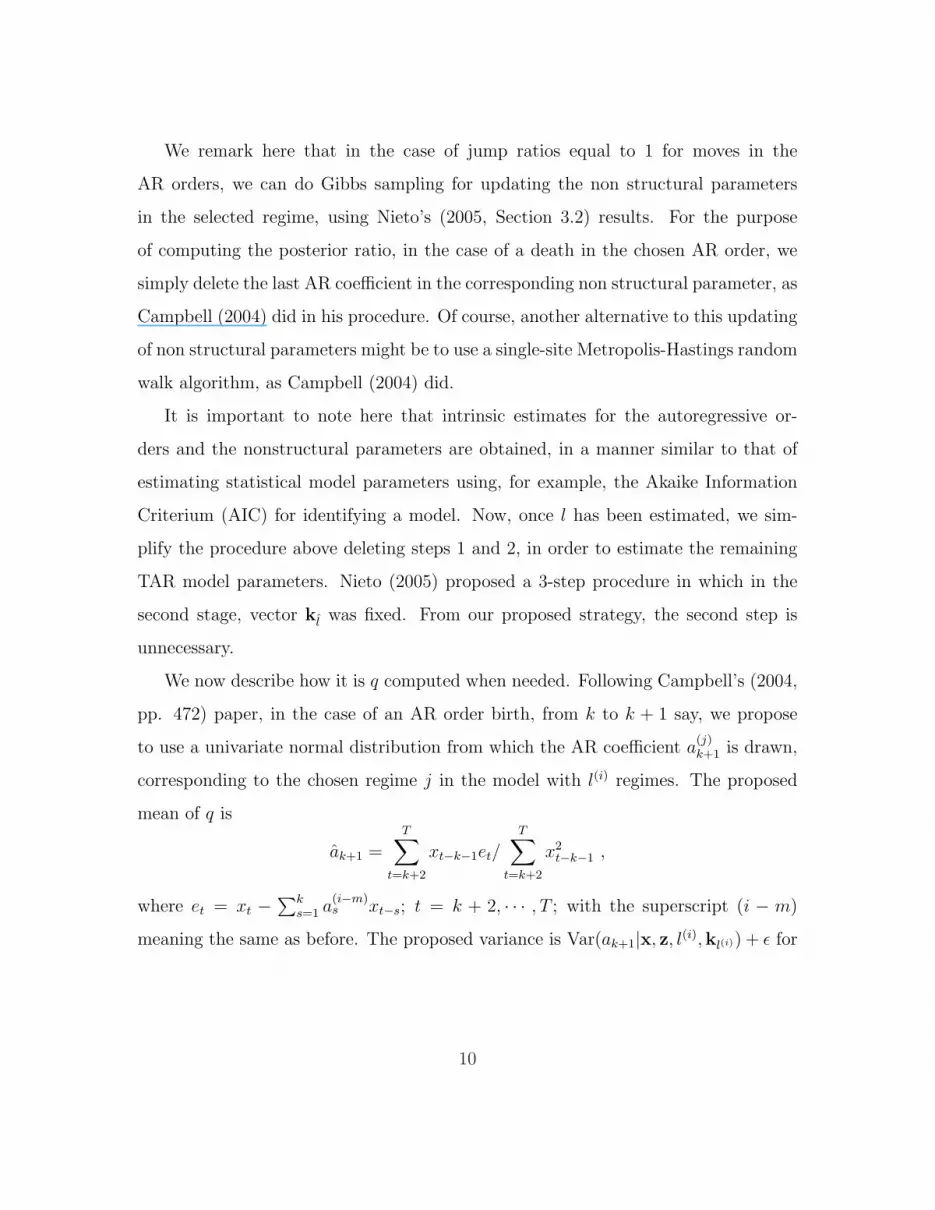
We now describe how it is q computed when needed. Following Campbell’s (2004,

pp. 472) paper, in the case of an AR order birth, from k to k + 1 say, we propose

to use a univariate normal distribution from which the AR coefficient a(j)k+1 is drawn,

corresponding to the chosen regime j in the model with l(i) regimes. The proposed

mean of q is

ak+1 =T∑

t=k+2

xt−k−1et/

T∑

t=k+2

x2t−k−1 ,

where et = xt −∑k

s=1 a(i−m)s xt−s; t = k + 2, · · · , T ; with the superscript (i − m)

meaning the same as before. The proposed variance is Var(ak+1|x, z, l(i),kl(i)) + ε for

10

some ε > 0 (small according to Campbell, 2004); where

Var(ak+1|x, z, l(i),kl(i)) =T∑

t=k+2

e2t /[(T − k − 1)

T∑

t=k+2

x2t−k−1] .

That is, we seek to set the proposal variance to be a little more than the marginal

posterior variance.

It is important to note that the numerator (denominator) in the product likelihood ratio×prior ratio is giving in general, for a fixed value of l, by

L(y|l,kl, θl)π(l,kl,θl) = L(y|l,kl,θl)π(l)π(kl|l)π(θl|l,kl)

= L(y|l,kl,θl)π(l)l∏

j=1

π(kjl|l)l∏

j=1

π(θjl|l,kl)

where L(·| · · · ) denotes the likelihood function for the whole parameter vector, which

is based on all the sample (given by Nieto (2005)), π(l) is the unconditional prior for

l and π(·|·) denotes appropriate conditional priors. The priors for the nonstructural

parameters are obtained from Nieto’s (2005) paper and for the number of regimes

and autoregressive orders, from truncated Poisson distributions as will be shown in

the examples below.

4 Convergence diagnostics

Following Castelloe and Zimmerman (2002), we implement a procedure for checking

the convergence of our proposed RJMCMC sampler. As the parameter of interest,

we choose λ =∑l

j=1 pj[h(j)]2, where pj = P(Zt ∈ Bj). The reason for that is the

following: Nieto (2008) found that the conditional distribution of Xt given xt−1, ..., x1

and zt is Gaussian with mean a(j)0 +

∑kj

i=1 a(j)i xt−i and standard deviation h(j) if zt ∈ Bj,

for some j = 1, ..., l. We denote its density as fj(xt|xt−1, ..., x1, zt). Also, he showed

that the conditional distribution of Xt given xt−1, ..., x1 is a mixture distribution with

11

density function

f(xt|xt−1, ..., x1) =l∑

j=1

pjfj(xt|xt−1, ..., x1, zt ∈ Bj) . (2)

Here, we remark importantly that one of the two types of conditioning considered

above, depends on xt−1, ..., x1 and zt ∈ Bj and, the other one depends on xt−1, ..., x1

only. We shall call regime-based conditioning to the first one and conditioning to the

second. From expression (2) and following Nieto’s (2008) TAR-model characteristics,

we found that the conditional variance of Xt, σ2t|t−1 say, is given by

σ2t|t−1 =

l∑j=1

pj[h(j)]2 +

l∑j=1

pjµ2j,t − [

l∑j=1

pjµj,t]2 , (3)

where µj,t = a(j)0 +

∑kj

i=1 a(j)i xt−i. We can note that

∑lj=1 pj[h

(j)]2 is something like

a ”communality” in the conditional variances above because it does not depend on

neither t nor xt−1, ..., x1. Moreover, this quantity is a weighted average of the regime-

based conditional variances of the process Xt. Notice that {σ2t|t−1 : t = 2, ...} defines

the conditional variance function of process {Xt}, a key element in the GARCH-model

family.

Defined in that way the so-called interest parameter, we run C ≥ 2 parallel chains

of length 2T each and discard the first T iterations. Let M be the number of distinct

models, λrcm be the value of λ for the r-th occurrence of model m in chain c and Rcm

the number of times model m occurred in chain c. Then, the convergence diagnostic

is based on the following estimates of variation (note that the subscripts on the left-

hand side are parts of the names, and do not correspond to values of indices on the

right-hand side):

V (λ) =1

CT − 1

C∑c=1

M∑m=1

Rcm∑r=1

(λrcm − λ)2 (4)

Wc(λ) =1

C(T − 1)

C∑c=1

M∑m=1

Rcm∑r=1

(λrcm − λc·)2 (5)

12

Wm(λ =1

CT −M

C∑c=1

M∑m=1

Rcm∑r=1

(λrcm − λ·m)2 (6)

WmWc(λ) =1

C(T −M)

C∑c=1

M∑m=1

Rcm∑r=1

(λrcm − λ·cm)2 (7)

These quantities may be interpreted as total variation (V ), variation within chains

(Wc), variation within models (Wm), and variation due to interaction between models

and chains (WmWc). Based on a strict two-way ANOVA with interactions and un-

balanced data, Castelloe and Zimmerman (2002) found some properties for the ratios

E(V )E(Wc)

and E(Wm)E(WmWc)

, when there is almost convergence of the RJMCMC sampler. In

practice, they suggest the use of the ratios VWc

and Wm

WmWc, because it may help to

narrow down the cause of any violations of convergence. More precisely, define the

following potential scale reduction factors for a general parameter, say θ:

PSRF1(θ) =V (θ)

Wc(θ)(8)

and

PSRF2(θ) =Wm(θ)

WmWc(θ). (9)

Then, implement the following procedure as a convergence assessment technique:

1. For simulating each chain use over-dispersed values.

2. Choose a base batch sise b (Brooks and Gelman, 1998) recommend, for example,

b ≈ T/20).

3. Plot PSRF(q)1 (θ) v.s. q and PSRF

(q)2 (θ) v.s. q.

4. Plot the numerator and denominator of PSRF(q)1 (θ) together v.s. q.

5. Plot the numerator and denominator of PSRF(q)2 (θ) together v.s. q.

6. Determine q0 such that for q ≥ q0 the plots in step 3 have settled close to 1,

and the the plots in step 4 have settled approximately to a common value, and the

plots in step 5 have settled approximately to a common value.

13

7. Discard the first q0b sweeps from each chain, and then pool the remaining ones

together to use for inference.

5 Some examples

The RJMCMC-sampler based procedure for analyzing TAR models presented in Sec-

tion 3, was designed for obtaining draws of the whole parameter vector (l,kl, θl),

by means of a 2-step approach. We present now four examples for illustrating the

adequacy and implementation of our proposed method. In order to check the con-

vergence of the sampler, using the procedure proposed in Section 4, we run in each

example below, three parallel chains. It seems that this number of chains is enough

for our simulated and empirical data.

Another issue of main concern that we have found when running our proposed

sampler, has to dealt with the choice of parameter ε (see on pp. 9). Contrary to

Campbell’s (2004) suggestion of a very small value, we have found for the TAR

models considered in the examples, that this value depends on the entertained model

for fitting the time series. Our recommendation goes on the line of letting the data to

speak by themselves and to check the adequacy of its value via a quick convergence

and a satisfactory mixing of the chains.

5.1 Two simulations

Here we consider two simulated models. The first one is a TAR(2; 1, 1) model given

by

Xt =

−0.5 + 0.6Xt−1 + εt , Zt ≤ 0

0.9− 0.7Xt−1 + 2.0εt , Zt > 0 ,

where {Zt} is an AR(1) process given by the model Zt = 0.5Zt−1 + at, with {at}a Gaussian zero-mean white noise process with variance σ2

a = 1. The length of

14

the simulated time series was 100. Fixing the known parameters for process {Zt}and the threshold r1 = 0, we used our proposed RJMCMC sampler for identifying

and estimating the simulated model, using the following prior distributions: for the

number of regimes L we used a truncated Poisson distribution on the set {2, 3, 4} with

parameter 3. For any given number of regimes, we also chose a truncated Poisson

distribution for the autoregressive orders on the set {0, 1, 2, 3} with parameter 1.

And, giving the corresponding number of regimes and autoregressive orders, we took,

for the nonstructural parameters, the multivariate normal and inverse-Gamma priors

suggested by Nieto (2005). The main results were the following.

We run a chain with 5000 iterations and left the first 2500 as the burn in period.

To check the chain convergence, we used the procedure described in the last section for

the last 2500 draws and the obtained results are presented in Figure 1 and Figure 2.

As we can see there, the convergence of the chain is guaranteed. With this sample size,

we found the posterior distribution for the number of regimes L, which is presented

in Table 1. Clearly, we observe that l = 2 regimes is the mode of the distribution.

As for the autoregressive orders, we run a chain with 5000 iterations with fixed

value L = 2 in order to estimate both the autoregressive orders and the nonstruc-

tural parameters. As we can see in Figure 3 and Figure 4, the chain convergence is

accomplished. In Table 2 we can see the corresponding posterior distributions, which

signal that k1 = k2 = 1. To study the sensitivity of the sampler to prior distributions,

we used different priors for the autoregressive orders and looked at the posterior dis-

tributions for L and the nonstructural parameters. We tried the values 3, 4, ..., 14

for the maximum order of these parameters and, for example, for 8 as the maximum

value, we chose a truncated Poisson distribution with parameters 4, 5 and 6. We

found that the method is robust against changes in the prior distribution for the au-

toregressive orders since the sampler always identified the correct value of L = 2 and

no drastic changes were detected in the posteriors for the nonstructural parameters.

15

5 10 15 20

1.00

01.

015

PSRF1

batch number

PSFR

1

5 10 15 20

0.99

50.

998

PSRF2

batch number

PSFR

2

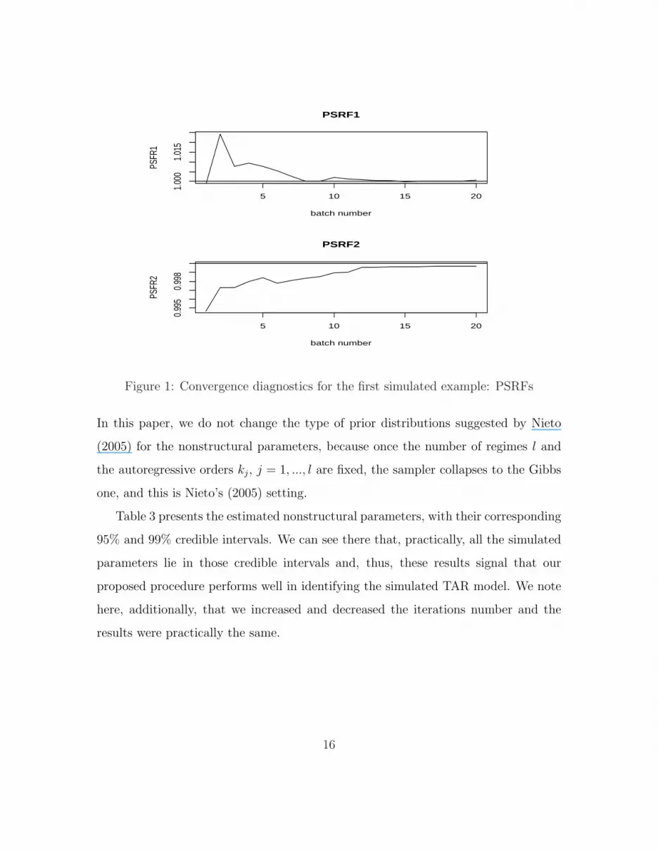
Figure 1: Convergence diagnostics for the first simulated example: PSRFs

In this paper, we do not change the type of prior distributions suggested by Nieto

(2005) for the nonstructural parameters, because once the number of regimes l and

the autoregressive orders kj, j = 1, ..., l are fixed, the sampler collapses to the Gibbs

one, and this is Nieto’s (2005) setting.

Table 3 presents the estimated nonstructural parameters, with their corresponding

95% and 99% credible intervals. We can see there that, practically, all the simulated

parameters lie in those credible intervals and, thus, these results signal that our

proposed procedure performs well in identifying the simulated TAR model. We note

here, additionally, that we increased and decreased the iterations number and the

results were practically the same.

16

5 10 15 20

0.11

50.

130

PSRF1

batch number

VWc

5 10 15 20

0.11

50.

130

PSRF2

batch number

WmWcWm

Figure 2: Convergence diagnostics for the first simulated example: comparison of

numerators and denominators

17

5 10 15 20

1.00

01.

020

PSRF1

batch number

PSFR

1

5 10 15 20

0.96

0.98

1.00

PSRF2

batch number

PSFR

2

Figure 3: Convergence diagnostics for the first simulated example with fixed L:

PSRFs

18

5 10 15 20

0.10

50.

120

0.13

5

PSRF1

batch number

VWc

5 10 15 20

0.10

50.

120

PSRF2

batch number

WmWcWm

Figure 4: Convergence diagnostics for the first simulated example with fixed L: nu-

merators and denominators

19

Number of regimes l Posterior probability

2 0.9988

3 0.0012

4 0.000

Table 1. Posterior probabilities for the number of regimes in the first simulated example

Regime

Autoregressive order k 1 2

0 0.000 0.0696

1 0.5956 0.4792

2 0.3056 0.2656

3 0.0988 0.1856

Table 2. Posterior probabilities for the autoregressive orders in the first simulated example

Regimej

Parameter 1 2

-0.49 0.59

a(j)0 95% (-0.78, -0.22) 95% (0.13, 1.05)

99% (-0.93, -0.1) 99% (-0.02, 1.28)

0.49 -0.46

a(j)1 95% (0.37, 0.63) 95% (-0.75, -0.2)

99% (0.33, 0.68) 99% (-0.83, -0.07)

1.07 1.81

h(j) 95% (0.92, 1.25) 95% (1.48, 2.18)

99% (0.88, 1.38) 99% (1.44, 2.3)

Table 3. Nonstructural parameter estimates for the model in the first simulated example.

95% and 99% mean credible sets at those levels.

20

0 20 40 60 80 100

−30

020

Index

cum

0 20 40 60 80 100

0.0

0.4

0.8

Index

cum

q

Figure 5: CUSUM and CUSUMSQ charts for the first simulated example

In order to check slightly the goodness-of-fit property of the proposed estimation

procedure, we examined the CUSUM and CUSUMSQ charts of the standardized

model residuals, as suggested by Nieto (2005). These charts are plotted in Figure 5,

and as we can see there, they signal an adequate fitting of the model.

Next, we simulated a TAR(3;2,1,1) model given by

Xt =

−0.5 + 0.6Xt−1 − 0.7Xt−2 + εt , Zt ≤ −1.0

0.9 + 0.2Xt−1 + 2.0εt , −1.0 < Zt ≤ 1.0

−1.0− 0.7Xt−1 + 3.0εt , 1.0 < Zt ,

where process {Zt} was simulated as before, with white noise process {at} having

variance σ2a = 1. The sample size was 100 and we also fix the parameters of process

{Zt} at their simulated values and the thresholds r1 = −1.0 and r2 = 1.0. The whole

set of prior distributions considered here was similar to that of the first example.

The posterior distribution for L is presented in Table 4, where we observe that the

21

5 10 15 20

1.00

1.10

1.20

PSRF1

batch number

PSFR

1

5 10 15 20

0.99

20.

996

1.00

0

PSRF2

batch number

PSFR

2

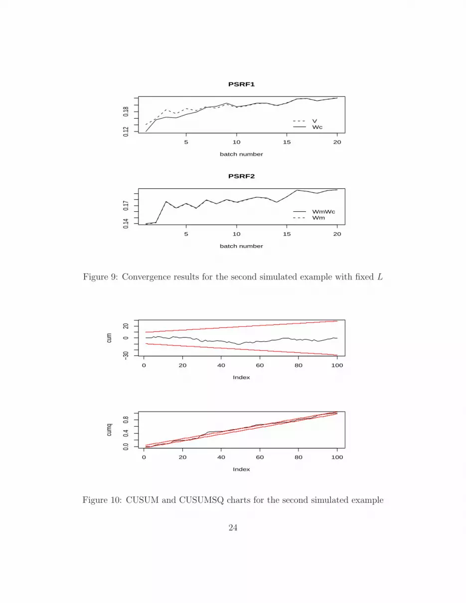
Figure 6: Convergence results for the second simulated example

distribution mode is l = 3. The chains convergence can be assessed in Figures 6 and 7.

Fixing l, there is also convergence of the chains as can be noted in Figures 8 and 9. The

posterior distributions for the autoregressive orders and the nonstructural parameters

are presented in Table 5. As we can see there, the identified autoregressive orders

were k1 = 2, k2 = 1 and k3 = 1 after using kmax = 3. The estimated nonstructural

parameters are presented in Table 6 with their 95% and 99% credible intervals and

we observe that all of the simulated values lie in their corresponding 95% and 99%

credible intervals. In Figure 10, we present the CUSUM and CUSUMSQ functions,

observing that only the last one has segments that, slightly, does not lie in the 95%

band. Overall, we have a good fitting of the TAR model to the simulated data.

22

5 10 15 20

0.14

0.20

PSRF1

batch number

VWc

5 10 15 20

−0.4

0.2

PSRF2

batch number

WmWcWm

Figure 7: Convergence results for the second simulated example

5 10 15 20

1.00

1.10

PSRF1

batch number

PSFR

1

5 10 15 20

0.990

0.996

PSRF2

batch number

PSFR

2

Figure 8: Convergence results for the second simulated example with fixed L

23

5 10 15 20

0.12

0.18

PSRF1

batch number

VWc

5 10 15 20

0.14

0.17

PSRF2

batch number

WmWcWm

Figure 9: Convergence results for the second simulated example with fixed L

0 20 40 60 80 100

−30

020

Index

cum

0 20 40 60 80 100

0.0

0.4

0.8

Index

cum

q

Figure 10: CUSUM and CUSUMSQ charts for the second simulated example

24

Number of regimes l Posterior probability

2 0.004

3 0.9544

4 0.0416

Table 4. Posterior probabilities for the number of regimes in the second simulated model

Regime

Autoregressive order k 1 2 3

0 0 0.0436 0.018

1 0 0.584 0.5464

2 0.5884 0.2684 0.3112

3 0.4116 0.104 0.1244

Table 5. Posterior probabilities for the autoregressive orders in the second simulated example

25

Regimej

Parameter 1 2 3

-0.41 0.62 -1.19

a(j)0 95% (-0.71, -0.05) 95% (0.1, 1.21) 95% (-2.01, -0.35)

99% (-0.82, 0.09) 99% (-0.01, 1.46) 99% (-2.36, 0.03)

0.60 0.37 -0.63

a(j)1 95% (0.45, 0.75) 95% (0.17, 0.58) 95% (-1.02, -0.25)

99% (0.33, 0.82) 99% (0.08, 0.64) 99% (-1.1, 0.01)

-0.72

a(j)2 95% (-0.85, -0.59)

99% (-0.92, -0.48)

1.17 1.92 2.66

h(j) 95% (0.95, 1.46) 95% (1.55, 2.39) 95% (2.12, 3.49)

99% (0.84, 1.68) 99% (1.5, 2.54) 99% (1.98, 4.00)

Table 6. Nonstructural parameter estimates in the second simulated example.

95% and 99% mean credible sets at those levels

5.2 An application in the hidrology/meteorology field

Nieto (2005) presented a real-data application for illustrating his methodology. The

time series considered were the daily rainfall (in mm.), as the threshold variable, and a

daily river flow (in m3/s), as the response variable, in a certain Colombian geograph-

ical region. The rainfall was measured at the San Rafael Lagoon’s meteorological

station, with an altitude of 3420 meters and geographical coordinates 2.23 north (lat-

itude) and 76.23 west (longitude). The flow corresponds to Bedon river, a small one

in hydrological terms, and was measured at the San Rafael Lagoon’s hydrological

station, with an altitude of 3300 meters and coordinates 2.19 north and 76.15 west.

26

These stations are located close to the earth equator and in a very dry geographi-

cal zone. This last characteristic permits to control for hydrological/meteorological

factors, which may distort the kind of dynamical relationship explained by the TAR

model. The data set corresponds to the sample period from January 1, 1992, up to

November 30, 2000 (3256 data), and it was assembled by IDEAM, the official Colom-

bian agency for hydrological and meteorological studies. In Figure 11 one can see

the two time series, where it can be noted the dynamical relationship between the

two variables, in the sense that the more the precipitation the more the river flow.

Additionally, one can see certain stable path in both variables although there are

bursts of large values. This fact is a major characteristic to be taken into account for

explaining the river flow dynamical behavior in terms of precipitation.

Here, we apply our proposed procedure to those real-data time series. We used,

as prior distributions for our interest parameter vector, analogous distributions to

those in the simulated examples above. For the number of regimes the parameter of

the truncated Poisson distribution was 3 and we put l0 = 4. For the autoregressive

orders we used truncated Poisson distributions with parameter 2 and put kmax = 3.

It is important to remark here that we obtained as thresholds the following potential

values: 6.0 mm for l = 2; 6.0 mm and 10.3 mm for l = 3; and 6.0 mm, 10.3 mm and

17.18mm for l = 4. These values were computed via the minimum NAIC criterion

(Tong, 1990), in the following way: we fixed a value for l and then we chose the

thresholds values for which the NAIC is minimum among the empirical quantiles of

the rainfall variable. In Table 7 we present the posterior distribution for the number

of regimes, finding that its mode is l = 4, contrary to Nieto’s (2005) result that

was l = 2. This finding is in accordance with the known fact that in that Colombian

geographical zone, there are two periods of rains and two periods of dry meteorological

conditions, which alternate trough the whole year in this way: first dry season from

middle December to middle March; first rain season from middle March to middle

27

July; second dry period from middle July to middle September and second rain season

from middle September to Middle December. Thus, there are four regimes of rains

in that geographical zone.

For this data set, we needed to set ε = 10, a very large quantity when it is

compared with the respective values for the simulated examples. And even so, we

must signal remarkably that with this large value, the posterior distribution for the

autoregressive orders in some regimes are almost degenerate (exactly degenerate in

the first regime). This fact signals some dependence of this parameter on the data set

at hand. In Table 8, we show the posterior distributions for the autoregressive orders

in each regime. Table 9 includes the estimates for the nonstructural parameters. In

this way, the fitted model is given by

Xt =

1.36 + 0.74Xt−1 − 0.27Xt−2 + 0.12Xt−3 + 1.3εt , Zt ≤ 6.0

1.89 + 0.76Xt−1 − 0.34Xt−2 + 0.13Xt−3 + 1.64εt , 6.0 < Zt ≤ 10.3

2.08 + 0.80Xt−1 − 0.31Xt−2 + 2.15εt , 10.3 < Zt ≤ 17.18

2.89 + 0.64Xt−1 − 0.41Xt−2 + 0.26Xt−3 + 3.17εt , 17.18 < Zt.

It is interesting to note that in each regime, (i) the flow river has an autoregressive

dynamic up to lag 3 and (ii) the numeric signs of the coefficients of lagged values of

the flow river are the same and, quantitatively, very close for the first two lags. In

approximate terms, this fact signals that the autoregressive dynamics of the flow river

is the same through the different regimes for the precipitation variable. This empirical

characteristic was also detected by Nieto’s (2005) TAR(2;1,1) model. Thus, at a first

sight, one might say that the influence of the regimes on the actual value of the flow

river is trough the model intercepts and the regime-based variability. However, model

interpretations other than the previous ones will be explained in more detail in the

next paragraph.

Using Nieto’s (2008) TAR model characteristics, we can derive from the fitted

28

model above the following important facts. First, working with the distribution of

Xt, the contribution of each regime to the mean of X at time t, which is computed as

µj,t,1 = [a(j)0 +h(j)]/φj(1), j = 1, ..., l0, is 6.49 m3/sec., 8 m3/sec., 10 m3/sec., and 10.90

m3/sec., for the first, second, and third regime, respectively. This is in agreement with

the fact that the more the precipitation the more the river flow. The same observation

holds for the regime-conditional variability of the river flow variable as measured by

1.32, 1.642, 2.152 and 3.172. Here, we note that the autoregressive polynomials in each

regime have their roots outside the unit circle. Notice also that these contributions

do not depend on t. Second, we also found that E(Xt|xt−1, ..., x1) = 1.67+0.75xt−1−0.3xt−2 + 0.12xt−3, where we have used p1 = 0.61, p2 = 0.20, p3 = 0.12 and p4 = 0.08

and that, in general,

E(Xt|xt−1, ..., x1) =4∑

j=1

pja(j)0 + (

4∑j=1

pja(j)1 )xt−1 + (

4∑j=1

pja(j)2 )xt−2 + (

4∑j=1

pja(j)3 )xt−3 .

The figures p1, p2, p3 and p4 indicate that it is more possible to have low-intensity

rainfall than either medium- or high-intensity rainfall, a result that agrees strongly

with the fact that the Colombian geographical region for which the analysis is per-

formed is very dry in the whole solar year. Third, the marginal mean of the river

flow is 7.63 m3/sec. for any day t, indicating that the mean function of the stochastic

process {Xt} is constant in the analyzed sample period, an empirical characteristic

observed in the data.

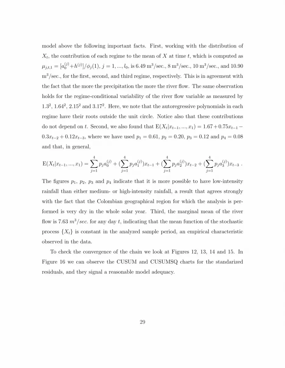
To check the convergence of the chain we look at Figures 12, 13, 14 and 15. In

Figure 16 we can observe the CUSUM and CUSUMSQ charts for the standarized

residuals, and they signal a reasonable model adequacy.

29

Time

Z

1992 1994 1996 1998 2000

020

4060

Time

X

1992 1994 1996 1998 2000

05

1015

20

Figure 11: (a) Precipitation. (b) Flow.

5 10 15 20

1.0

1.4

1.8

PSRF1

Q.cuenta

V/W

c

5 10 15 20

0.99

20.

996

1.00

0

PSRF2

Q.cuenta

Wm

/Wm

Wc

Figure 12: Convergence results for the hydrological/meteorological time series

30

5 10 15 20

0.00

20.

005

PSRF1

batch number

VWc

5 10 15 20

0.00

20.

004

PSRF2

batch number

WmWcWm

Figure 13: Convergence results for the hydrological/meteorological time series

Number of regimes l Posterior probability

2 0.000

3 0.0036

4 0.9964

Table 7. Posterior probabilities for the number of regimes in the precipitation/flow example

Regime

Autoregressive order k 1 2 3 4

0 0 0 0 0

1 0 0 0 0

2 0 0.106 0.5087 0.4207

3 1 0.894 0.4913 0.5793

Table 8. Posterior probabilities for the autoregressive orders in the hydrological/meteorological example

31

5 10 15 20

1.00

1.03

1.06

PSRF1

Q.cuenta

V/W

c

5 10 15 20

−1.5

0.0

1.0

PSRF2

Q.cuenta

Wm

/Wm

Wc

Figure 14: Convergence results for the hydrological/meteorological time series with

fixed L

32

5 10 15 20

0.00

400.

0055

PSRF1

batch number

VWc

5 10 15 20

−0.0

30.

00

PSRF2

batch number

WmWcWm

Figure 15: Convergence results for the hydrological/meteorological time series with

fixed L

33

0 500 1000 1500 2000 2500 3000

−150

010

0

Index

cum

0 500 1000 1500 2000 2500 3000

0.0

0.4

0.8

Index

cum

q

Figure 16: CUSUM and CUSUMSQ charts for the residuals of the hydrologi-

cal/meteorological TAR model

34

Regimej

Parameter 1 2 3 4

1.36 1.89 2.08 2.89

a(j)0 95% (1.24, 1.45) 95% (1.66, 2.14) 95% (1.69, 2.6) 95% (1.95, 3.68)

0.74 0.76 0.8 0.64

a(j)1 95% (0.71, 0.77) 95% (0.71, 0.82) 95% (0.72, 0.87) 95% (0.48, 0.78)

-0.27 -0.34 -0.31 -0.41

a(j)2 95% (-0.3, -0.24) 95% (-0.41, -0.24) 95% (-0.42, -0.17) 95% (-0.64, -0.23)

0.12 0.13 0.26

a(j)3 95% (0.09, 0.14) 95% (0.07,0.17) 95% (0.15, 0.41)

1.3 1.64 2.15 3.17

h(j) 95% (1.27, 1.33) 95% (1.59, 1.71) 95% (2.01, 2.25) 95% (2.94, 3.4)

Table 9. Nonstructural parameter estimates for the hidrological/meteorological time series.

95% mean credible sets at those levels.

5.3 An application in economy

Now, we apply our proposed procedure to a USA quarterly macroeconomic data set

in the sample period 1970:01-2004:02. These time series correspond to the seasonally-

adjusted Gross Domestic Product (GDP) growth rate as the output variable and the

spread between Three Years Constant Maturity Yield (R1) and 3 Months Treasury

Bill Discount Yield (R2) as the input variable. More exactly, we define the following

variables

Xt = [ln(GDPt)− ln(GDPT−4)]× 100%

and

Zt = R1t −R2t.

35

These variables were also used by Harvey (1997) in another econometric context. The

input variable Z and output X are not contemporary, because the non-linearity test

of Tsay (1998) shows strong non-linearity in X, with a delay d = 5 for the variable Z;

hence, we set Zt = Zt−5 in order to use our proposed methodology. In Figure 17 we

display the two X and Z variables and we can see there that, approximately, the more

the values of Z the less the values of X and viceversa and that the important fact of

extreme-values clusters in variable X, explained by a TAR model, is not so evident in

this case. However, given the strong nonlinearity of variable X, which is explained by

Z, it seems plausible to fit of a TAR model to these real-data time series. An exploring

fit indicated that the TAR model cannot explain the actual conditional variability of

X (i.e. σ2t|t−1); hence, we adjusted the original x-data with a GARCH(1,1) model in

order to help the TAR model to explain the remaining conditional heteroscedasticity.

This kind of transformation, previous to the TAR model fitting, was also used by

Nieto (2005) in the application of his methodology to the hidrological/meteorological

field.

The prior distributions used in this application are similar to the former applica-

tions, although the prior for (h−2t )(j) is Gam(0.3, 1.5), j = 1, 2. For the number of

regimes, the parameter of the truncated Poisson distribution was 3 and we put l0 = 4

[following Hoyos’s (2006) work]. For the autoregressive orders, we used truncated

Poisson distributions with parameter 2 and put kmax = 3. We obtained as thresholds

(numerical values in parenthesis) the quantiles 0.11 (0.16) for l = 2; 0.11 (0.16), 0.68

(1.6) for l = 3; and 0.11 (0.16), 0.40 (1.03) and 0.68 (1.6) for l = 4. The threshold

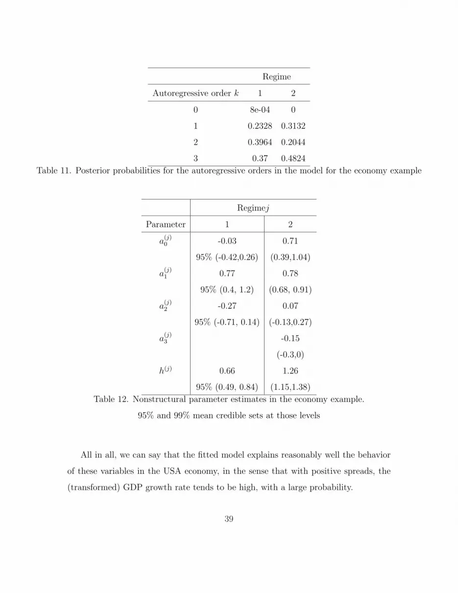
values were computed as in Example 3. The posterior distribution for the number

of regimes is presented in Table 10, the posterior distributions for the autoregressive

orders in Table 11, and the nonstructural parameter estimates are presented in Table

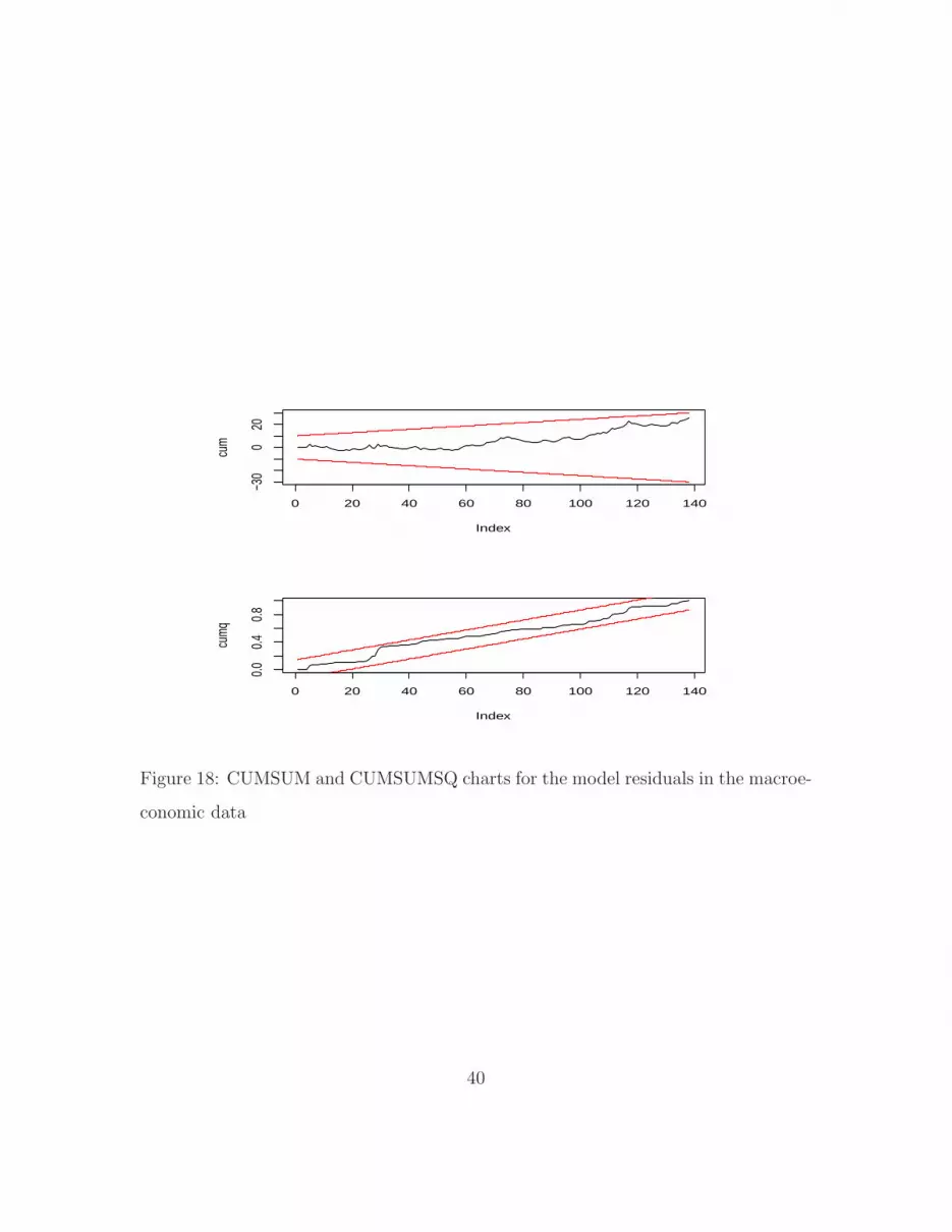
12. A rough verification of the model specification is presented in Figure 18, using

the CUSUM and CUSUMSQ charts for the standardized residuals. We observe there

36

that these charts signal an adequate fit of the model. To check the convergence of

the underlying Markov chain, we used the procedure suggested in Section 4 and the

graphs of the interest statistics are presented in Figure 19, 20, 21 and 22. We can see

there that the convergence of the chains are guaranteed.

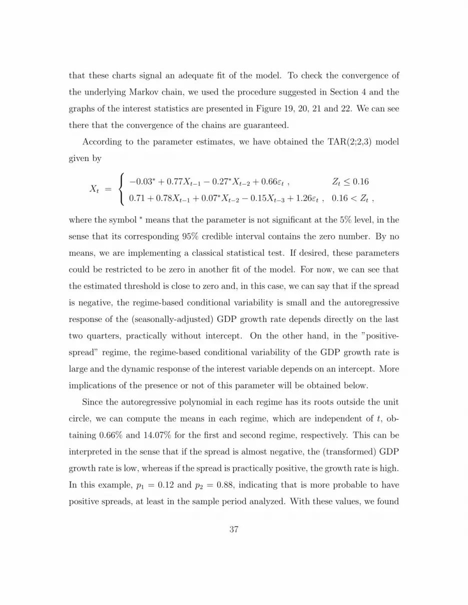
According to the parameter estimates, we have obtained the TAR(2;2,3) model

given by

Xt =

−0.03∗ + 0.77Xt−1 − 0.27∗Xt−2 + 0.66εt , Zt ≤ 0.16

0.71 + 0.78Xt−1 + 0.07∗Xt−2 − 0.15Xt−3 + 1.26εt , 0.16 < Zt ,

where the symbol ∗ means that the parameter is not significant at the 5% level, in the

sense that its corresponding 95% credible interval contains the zero number. By no

means, we are implementing a classical statistical test. If desired, these parameters

could be restricted to be zero in another fit of the model. For now, we can see that

the estimated threshold is close to zero and, in this case, we can say that if the spread

is negative, the regime-based conditional variability is small and the autoregressive

response of the (seasonally-adjusted) GDP growth rate depends directly on the last

two quarters, practically without intercept. On the other hand, in the ”positive-

spread” regime, the regime-based conditional variability of the GDP growth rate is

large and the dynamic response of the interest variable depends on an intercept. More

implications of the presence or not of this parameter will be obtained below.

Since the autoregressive polynomial in each regime has its roots outside the unit

circle, we can compute the means in each regime, which are independent of t, ob-

taining 0.66% and 14.07% for the first and second regime, respectively. This can be

interpreted in the sense that if the spread is almost negative, the (transformed) GDP

growth rate is low, whereas if the spread is practically positive, the growth rate is high.

In this example, p1 = 0.12 and p2 = 0.88, indicating that is more probable to have

positive spreads, at least in the sample period analyzed. With these values, we found

37

Time

Z

1970 1975 1980 1985 1990 1995 2000 2005

−11

3

Time

X

1970 1975 1980 1985 1990 1995 2000 2005

−22

6

Figure 17: The USA macroeconomic time series.

that E(Xt) = 12.46% for all quarter t, signaling a stable marginal mean function

for GDP growth rate process. Note that this value is close to the ”positive-spread”

conditional mean, which is a relative high growth rate (in economy terms).

Number of regimes l Posterior probability

2 0.9964

3 0.0036

4 0

Table 10. Posterior probabilities for the number of regimes in the economy time series

38

Regime

Autoregressive order k 1 2

0 8e-04 0

1 0.2328 0.3132

2 0.3964 0.2044

3 0.37 0.4824

Table 11. Posterior probabilities for the autoregressive orders in the model for the economy example

Regimej

Parameter 1 2

a(j)0 -0.03 0.71

95% (-0.42,0.26) (0.39,1.04)

a(j)1 0.77 0.78

95% (0.4, 1.2) (0.68, 0.91)

a(j)2 -0.27 0.07

95% (-0.71, 0.14) (-0.13,0.27)

a(j)3 -0.15

(-0.3,0)

h(j) 0.66 1.26

95% (0.49, 0.84) (1.15,1.38)

Table 12. Nonstructural parameter estimates in the economy example.

95% and 99% mean credible sets at those levels

All in all, we can say that the fitted model explains reasonably well the behavior

of these variables in the USA economy, in the sense that with positive spreads, the

(transformed) GDP growth rate tends to be high, with a large probability.

39

0 20 40 60 80 100 120 140

−30

020

Index

cum

0 20 40 60 80 100 120 140

0.0

0.4

0.8

Index

cum

q

Figure 18: CUMSUM and CUMSUMSQ charts for the model residuals in the macroe-

conomic data

40

5 10 15 20

1.00

1.04

1.08

PSRF1

batch number

PSFR

1

5 10 15 20

−0.5

0.5

PSRF2

batch number

PSFR

2

Figure 19: Convergence plots for the Markov chain in the macroeconomic data

5 10 15 20

0.01

300.

0155

PSRF1

batch number

VWc

5 10 15 20

−0.0

40.

02

PSRF2

batch number

WmWcWm

Figure 20: Convergence plots for the Markov chain in the macroeconomic data

41

5 10 15 20

1.00

01.

010

1.02

0

PSRF1

batch number

PSFR

1

5 10 15 20

0.96

0.98

1.00

PSRF2

batch number

PSFR

2

e

Figure 21: Convergence plots for the Markov chain in the macroeconomic data with

fixed L

42

5 10 15 20

0.01

40.

018

PSRF1

batch number

VWc

5 10 15 20

0.01

40.

020

PSRF2

batch number

WmWcWm

Figure 22: Convergence plots for the Markov chain in the macroeconomic data with

fixed L

43

6 Conclusions

An RJMCMC-sampler based method has been developed for identifying and estimat-

ing a TAR model (except the thresholds), which constitutes an alternative to the

Gibbs-sampling based approach of Nieto (2005), avoiding to use the so-called link-

ing priors. Basically, the new procedure consists of two steps: in the first one, the

number of regimes is identified, using a sampler that takes into account the varying

dimension of the whole parameter space, when the chain moves from one state to

another. In the second, the identified number of regimes is fixed and, conditional

on it, the remaining model parameters are estimated, including the autoregressive

orders. The new 2-step sampler reaches quickly the stationary distribution of the

underlying Markov chain and offers adequate mixing for the number-of-regimes and

the nonstructural-parameters chains. This is verified via a variance-decomposition

heuristic tool, in the lines of the exploratory-data-analysis philosophy. Additionally,

the proposed method improves the previous 3-step Gibbs-sampling based method, in

the sense of (i) using only two steps and (ii) producing a better mixing for the number

of regimes.

It is important to remark here that, strictly speaking, the varying dimension of

the whole parameter space is due to a nested movement, i.e., first, the underlying

chain moves for changing the number of regimes and, then, it moves intrinsically for

changing the autoregressive order in a previously chosen regime. This nested move-

ment causes some degree of complexity for designing a global RJMCMC sampler, in

the sense of avoiding the 2-step procedure developed in this paper. This complexity

is reflected, at least, in a poor mixing for the autoregressive orders. In this last situa-

tion, additional research must be conducted for finding the sources of this low mixing

of the chain. Also, the design of an analytical procedure for checking the conver-

gence of the underlying chain, should be investigated in the future. Nevertheless, the

44

results obtained in the simulated examples and in the real-data applications, where

we obtained coherent interpretations of the fitted models, led one to claim that this

proposed sampler is very adequate for analyzing a TAR model.

References

Brooks, S.P. and Giudici, P. (2000). Markov Chain Monte Carlo Convergence As-

sessment via Two-Way Analysis of Variance, Journal of Computational and Graphical

Statistics, 9(2), 266-285.

Brooks, S.P. and Gelman, A. (1998). General Methods for Monitoring Convergence

of Iterative Simulations, 7(4), 434-455.

Campbell, E.P. (2004). Bayesian Selection of Threshold Autoregressive Models, Jour-

nal of Time Series Analysis, 25, 467-482.

Carlin, B.P. and Chib, S. (1995). Bayesian Model Choice via Markov Chain Monte-

carlo Methods, Journal of the Royal Statistical Society Series B, 57, 473-484.

Castelloe, J.M. and Zimmerman, D.L. (2002). Convergence Assesment for Reversible

Jump MCMC Samplers, Mimeo SAS Institute Inc..

Chen, M., Shao, Q., and Ibrahim, J.G. (2000). Monte carlo Methods in Bayesian

Computation, Springer-Verlag: New York.

Gelman, A. and Rubin, D.B. (1992). Inference from Iterative Simulation Using Mul-

tiple Sequences, Statistical Science, 7(4), 457-511.

Green, P.J. (1995). Reversible Jump Markov Chain Monte Carlo Computation and

45

Bayesian Model Determination, Biometrika, 82, 711-732.

Hoyos, N.M. (2006). Una aplicacion del modelo no lineal TAR en economıa, Master

in Statistics’s dissertation, Universidad Nacional de Colombia, Bogota.

Nieto, F.H. (2005). Modeling bivariate threshold autoregressive processes in the

pressence of missing data, Communications in Statistics: Theory and Methods, 34,

905-930.

Nieto, F.H. (2008). Forecasting with univariate TAR models, Statistical Methodology,

5, 263-276.

Vermaak, J., Andrieu, C., Doucet, A., and Godsill, S.J. (2004). Reversible jump

Markov chain Montecarlo strategies for Bayesian model selection in autoregressive

processes, Journal of Time Series Analysis, 25, 785-809.

Vrontos, I.D., Dellaportas, P. and Politis, D.N. (2000). Full Bayesian inference for

GARCH and EGARCH models, Journal of Business & Economic Statistics, 18, 187-

198.

46