distributions, and sampling

Binoniial Distributions, Geonietric Distributions, and Sampling

Distributions

". i

.

' -~ .. ' • •

IN THIS CHAPTER

Summary: ln this chapter we finish laying the mathematical (probabllity) basis for inference Ьу considering the Ьinomial and geometric situations that occur often enough to warrant our study. ln the last part of this chapter, we begin our study of inference Ьу introducing the idea of а sa-!!'pling distribution, one of the most important concepts in statistics. Once.we've mastered this material, we will Ье ready to plunge into а study of formal inference (Chapters 11-14).

Кеу ldeas

О Binomial Distributions О Normal Approximation to the Binomial О Geometric Distributions О Sampling Distributions О Central Limit Theorem

Binomial Distributions

174 )

А Ьinomial experiment has the following properties:

• The experiment consists of а fixed number, п, of identical trials. • There are only two possiЫe outcomes (that's the 'Ъi" jn "blnomial"): success (S) or

fШlure (F).

Binomial Distributions, Geometric Distributions, and Sampling Distributions ( 175

• The probaЬility of success, р, is the same for each trial. • The trials are independent ( that is, knowledge of the outcomes of earlier trials does not

affect the probabllity of success of the next trial). • Our interest is in а binomial random variaЬle Х, which is the count of successes in п

trials. The probabllity distribution of Х is the Ьinomial distribution.

(Taken together, the second, third, and fourth bullets above are called Bernoulli trials. One way to think of а binomial setting is as а fixed number п of Bernoulli trials in which our random variaЬle of interest is the count of successes Х in the п trials. You do not need to know the term Bernoulli trials for the АР exam.)

The short version of this is to say that а binomial experiment consists of п independent trials of an exper.iment that has two possiЬle outcomes (success or failure), each trial having the same probability of success (р). The binomial random variable Xis the count of successes.

In practice, we may consider а situation to Ье Ьinomial when, in fact, the independence condition is not quite satisfied. This occurs when the probabllity of occurrence of а given trial is affected only slightly Ьу prior trials. For example, suppose that the probabllity of а defect in а manufacturing process is 0.0005. That is, there is, on average, only 1 defect in 2000 items. Suppose we check а sample of 10,000 items for defects. When we check the first item, the proportion of defects remaining changes slightly for the remaining 9,999 items in the sample. We would expect 5 out of 10,000 (О.0005) to Ье defective. But if the first one we look at is not defective, the probabllity of the next one being defective has changed to 5/9999 or 0.0005005. It's а small change but it means that the trials are not, strictly speaking, independent. А common rule of thumb is that we will consider а situation to Ье Ьinomial if the population size is at least 1 О times the sample size.

Symbolically, for the Ьinomial random variaЫe Х, we say Xhas В(п, р).

example: Suppose Dolores is а 65% free throw shooter. If we assume that that repeated shots are independent, we could ask, "What is the probability that Dolores makes exactly 7 of her next 1 О free throws?" If Х is the Ьinomial random variaЬle that gives us the count of successes for this experiment, then we say that Xhas B(l0,0.65). Ош question is then: Р(Х = 7) = ?.

We can think of В(п,р,х) as а particular Ьinomial probabllity. In this example, then, B(I0,0.65,7) is the probability that there are exactly 7 successes in 10 repetitions of а Ьinomial experiment where р = 0.65. This is handy because it is the same syntax used Ьу the TI-83/84 calculator (Ьinompdf (n, р, х)) when doing Ьinomial proЬlems.

If Xhas В(п, р), then Х сап take on the values 0,1,2, ... , п. Then,

В(п,р,х) =Р(Х =х)={: )Рх (1-р )"-х

gives the Ьinomial probaЬility of exactly х successes for а Ьinomial random variaЬle Х that has В(п, р).

Now,

(п) п! х = х!(п-х)! ·

On the Tl-83/84,

(п)- с х -n r'

17 6 } Step 4. Review the Knowledge You Need to Score High

and this is found in the МАТН PRB menu. п! ('n factorial") means п(п - l)(n - 2) ... (2)(1,), and the factorial symbol can also Ье found in the МАТН PRB menu.

example: Find В(15,.3,5). That is, find Р(Х = 5) for а 15 trials of а Ьinomial random variaЬle Х that succeeds with probability 0.3.

solution:

Р(Х =5)=(~)<0.3)5(1-О.3)15-5

=1.2!_(0.3)5 (0.7)10 =.206. 5!10!

(Оп rhe 11-83/84, (;) • n,,c.r cm Ье /Uund

in the МАТН PRB menu. То get (1;), enter 15nCr5.)

example: Consider once again our free-throw shooter (Dolores) from the earlier example. Dolores is а 65о/о free-throw shooter and each shot is independent. If Х is the count of free throws made Ьу Dolores, then Х has B(l О, 0.65) if she shoots 10 free throws. What is Р(Х = 7)?

solution:

Р(Х = 7) = (l 0)(0.65)7 (О.35)3 = l О! (О.65)7 (О.65)3 7 7!3!

=Ьinompdf (10,0. 65,7)=0.252.

example: What is the probaЬility that Dolores makes по more than 5 free throws? That is, what is Р(Х s 5)?

solution:

Р(Х s5)=P(X =О)+Р(Х =1)+Р(Х =2)+Р(Х =3)

+Р(Х = 4)+Р(Х = 5) =(10° )<о.65)0 (0.35)10 +е0

)(0.65)1(0.35)9

+"·+(15°)(о.65)5 (о.з5)5 =О.249.

There is about а 25о/о chance that she will make 5 or fewer free throws. The .solution to this proЬlem using the calculator is given Ьу Ьinomcdf (10,0.65,5).

Binomial Distributions, Geometric Distributions, and Sampling Distributions { 177

example: What is the probaЬility that Dolores makes at least 6 free throws?

solution: Р(Х?:. 6) = Р(Х = 6) + Р(Х = 7) + ... + Р(Х = 1 О) = 1-Ьinomcdf (10, О .65, 5) =О. 751.

(Note that Р(Х > 6) = 1 - Ьinomcdf ( 10, О. 65, 6 )).

The mean and standard deviation of а blnomial random variaЬle Х are given Ьу µх = пр; ах = J пр(l - р) . А Ьinomial distribution for а given п and р (meaning you have

all possiЬle values of х along with their corresponding probaЬilities) is an example of а probaЬility distributioп as defined in Chapter 7. The mean and standard deviation of а Ьinomial random variaЬle Х could Ье found Ьу using the formulas from Chapter 7,

but clearly the formulas for the Ьinomial are easier to use. Ве careful that you don't try to use the formulas for the mean and standard deviation of а Ьinomial random variaЬle for а discrete random variaЬle that is поt Ьinomial.

example: Find the mean and standard deviation of а Ьinomial raiidom variaЬle Х that has В(85, 0.6).

solution: µх = (85)(0.6) = 51; ах= ~85(0 . 6)(0.4) = 4.52.

Normal Approximation to the Binomial Under the proper conditions, the shape of а Ьinomial distribution is approximately normal, and Ьinomial probaЬiliries can Ье estimated using normal probaЬilities. Generally, this is true when пр?:. 10 and п(l - р)?:. 10 (some books use пр?:. 5 and п(l - р)?:. 5; that's ОК). These conditions are not satisfied in Graph А (Х has В(20, 0.1)) below, but they are sacis-fied in Graph В (Xhas В(20, 0.5)) .

Graph А: В (20, 0.1) Graph В: В (20, 0.5)

It should Ье clear that Graph А is noticeaЬly skewed to the right, and Graph В is approximately normal in shape, so it is reasonaЬle that а normal curve would approximate Graph В better than Graph А. The approximating normal curve clearly fits the Ьinomial histogram better in Graph В than in Graph А.

When пр and п(l - р) are sufficiently large (that is, they are both greater than or equal to 5 or 10), the Ьinomial random variaЬle Xhas approximately а normal distribution with

µ=пр and а= ~пр(l- р).

178 > Step 4. Review the Knowledge You Need to Score High

Anorher way to say this is: If Xhas В(п,р), rhen Xhas approximately N(пр,~пр(l-р )) , provided that пр<!: 10 and п(l - р) <!: 10 (or пр<!: 5 and п(l - р) О!: 5).

exarnple: Nationally, 15о/о of community college students live more than 6 miles from campus. Data from а simple random sample of 400 students at one community college are analyzed.

(а) What are the mean and standard deviation for rhe number of students in the sample who live more rhan 6 miles from campus?

(Ь) Use а normal approximation to calculate the probabllity rhat at least 65 of rhe students in the sample live more than 6 miles from campus.

solution: If Х is rhe number of students who live more than 6 miles from campus, then Xhas В(400, 0.15).

(а) µ == 400(0.15) = 60; а =~400(0.15)(0.85) =7.14.

(Ь) Because 400(0.15) = 60 and 400(0.85) = 340, we can use rhe normal approximation to rhe Ьinomial with mean 60 and standard deviation 7.14. The situation is pictured below:

60 65

1 1

UsingTaЬle А, we have Р(Х О!: 65) = P(z <!: 65

-60

= 0.70) = 1 - 0.7580 = 0.242. 7.14

Ву calculator, this can Ье found as noпnalcdf ( 65, 1000, 60, 7 .14) =О. 242.

The exact Ьinomial solution to rhis proЬlem is given Ьу

1-Ьinomcdf ( 400, О .15, 64) = О. 261 (you use х = 64 since Р(Х<!= 65) = 1 - Р(Х s 64)).

ln reality, you will need to use а normal approximation to the blnomial only in limited circumstances. In the example above, the answer can Ье arrived at quite easily using the exact Ьinomial capabllities of your calculator. The only time you might want to use а normal approximation is if the size of rhe binomial exceeds the capacity of your calculator (for example, enter Ьinomcdf ( 5 О О О О О О О, О . 7 , З 2 5 О О О О). You'll most likely see ERR: DOМAIN, which means you have exceeded the capacity of your calculator, and you didn't have access to а computer. The real concept that you need to understand the normal approximation to а Ьinomial is that another way of looking at Ьinomial data is in terms of the proportioп of successes rather than the count of successes. We will approximate а distribution of sample proportions with а normal distribution and the concepts and conditions for it are the same.

/

i /


Geometric Distributions In the Вinomial Distributions section of this chapter, we defi.ned а Ьinomial setting as а experiment in which the following conditions are present:

• The experiment consists of а fixed number, п, of identical trials. • There are only two possiЬle outcomes: success (5) or failure (F). • The probabllity of success, р, is the same for each trial. • The trials are independent ( that is, knowledge of the outcomes of earlier trials does not

affect the probability of success of the next trial). • Our interest is in а Ьinomial random variaЬle Х which is the count of successes in п

trials. The probability distribution of Х is the blnomial distribution.

There are times we are interested not in the count of successes out of п flxed trials, but in the probabllity that the flrst success occurs on а given ·trial, or in the average number of trials until the first success. А geometric setting is defined as follows.

• There are only two possiЬle outcomes: success (5) or failure (F). • The probaЬility of success, р, is the same for each trial. • The trials are independent (that is, knowledge of the outcomes of earlier trials does not

affect фе probabllity of success of the next trial).

• Our i~1 terest is in а geometric random variaЬle Х which is the number of trials neces

sary t obtain the first success.

Note at if Х is а Ьinomial, then Х can take on the values О, 1, 2, ... , п. If Х is geometric, then it takes n the values 1, 2, 3" ... There can Ье zero successes in а binomial, but the earliest а first success can come in а geornetric setting is оп the first trial.

If Х is geometric, the probabllity that the first success occurs on the nth trial is given Ьу Р(Х = п) = p(l - р)п- 1 • The value of Р(Х = п) in а geometric setting can Ье found on the ТI-83/84 calculator, in the DISTR menu, as geometpdf ( р, n) (note that the order of р and п are, for reasons known only to the good folks at TI, reversed from the Ьinomial). Given the relative simplicity of the formula for Р(Х = п) for а geometric setting, it's рrоЬаЫу just as easy to calculate the expression direccly. There is also а geornetcdf function that behaves analogously to the Ьinomcdf function, but is not much needed in this course.

example: Reme:mber Dolores, the basketball player whose free-throw shooting percentage was 0.65? What is the probability that the flrst free throw she manages to hit is on her fourth attempt?

solution: Р(Х = 4) = (О.65) (1-0.65)4•1 = (О.65) (О.35)3 = 0.028. Тhis can Ье done on the n-83/84 as follows: geornetpdf ( р, n) = geornetpdf (о. 65, 4) = 0.028.

example: ln а standard deck of 52 cards, there are 12 face cards. So the probaЬility of drawing а face card from а full deck is 12/52 = 0.231.

(а) If you draw cards with replacement (that is, you replace the card in the deck before drawing the next card), what is the probabllity that the first face card you draw is the 1 Oth card?

(Ь) If you draw ,cards without replacement, what is the probabllity that the first face card you draw is the 1 Oth card?

solution:

(а) Р(Х = 10) = (0.231) (1 - 0.231)9 = 0.022. On the TI-83/84: geome tpdf ( О . 2З1 , 1 О ) = О • О 21 7 ).

180 ) Step 4. Review the Knowledge You Need to Score High

(Ь) If you don't replace the card each time, the probability of drawing а face card on each trial is different because the proportion of face cards in the deck changes each time а card is removed. Hence, this is not а geometric setting and cannor Ье answered Ьу the techniques of this section. It сап Ье answered, but no.t easily, Ьу the techniques of the previous chapter ..

Rather than the probability that the first success occurs on а specified trial, we may Ье interested in the average wait until the first success. The average wait until the first success of а geometric random variaЬle is 1/р. (This can Ье derived Ьу summing (1) · Р(Х = 1) + (2) · Р(Х = 2) + (3) · Р(Х = 3) + ... = 1р + 2р(1 - р) + 3р(1 - р)2 + .. " which can Ье done using algebraic techniques for summing an infinite series with а common ratio less rhan 1.)

example: On average, how many free throws will Dolores have to take before she makes one (remember, р = 0.65)?

solution: Уо.65 = 1.54.

Since, in а geometric distribution Р(Х = п) = p(l - р)п- 1 , the probaЬilities Ьесоmе less likely as п increases since we are multiplying Ьу 1 - р, а number less than one. The geometric distribution has а step-ladder graph that looks like this:

Sampling Distributions Suppose we drew а sample of size 10 from а normal populacion with unknown mean and srandard deviation and got х = 18.87. Two questions _Wse;-{1) whar does this sample rell us about the population from which the sample )YaSdrawn, and (2) what would happen if we drew more samples?

Suppose we drew 5 more samples of size 1 О from this population and got х = 20.35, х = 20.04, х = 19.20, х = 19.02, and х = 20.35. ln answer to question (1), we

might believe that the population from which these samples was drawn had а mean around 20 because these averages tend to group there (in fact, the six samples were drawn from а normal popularion whose mean is 20 and whose standard deviation is 4). The mean of the 6 samples is 19.64, which supports our feeling that the mean of the original population might have been 20.

The standard deviation of the 6 ~amples is 0.68 and you might not have any inruitive sense about how that relates to the population standard deviation, alrhough you might suspect rhat the standard deviation of the samples should Ье less than the standard deviation of the popularion because the chance of an extreme value for an average should Ье less than that for an individual term (it just doesn't seem very likely that we would draw а lot of extreme values in а single sample).

Binomial Distributions, Geometric Distributions, and Sampling Distributions < 181

Suppose we continued to draw samples of size 1 О from this population until we were exhausted or until we had drawn all possiЬle samples of size 1 О. If we did succeed in drawing all possiЬle samples of size 1 О, and computed the mean of each sample, the distribution of these sample means would Ье the sampling distribution of х.

Remembering that а "statistic" is а value that describes а sample, the sampling distribution of а statistic is the distribution of that statistic for all possiЬle samples of а given size. It's important to understand that а dotplot of а few samples drawn from а population is not а distribution (it's а simulation of а distribution)-it becomes а distribucion only wh~~-;Ц-possibksamples of а given size are drawn.

Sampling Distribution of а Sample Mean Suppose we have the sampling distribution of х. That is, we have formed а distribution of the means of а11 possiЬle samples of size п from an unknown population ( thus, we know little about its shape, center, or spread). Let µх and ах represent the mean and standard deviation of the sampling distribution of х, respectively.

Then

for any population with mean µ and standard deviation б. (Note:. the value given for ах above is generally considered correct only if the sample

size (п) is small relative to N, the number in the population. А general rule is that п should Ье no more than 5% of N to use the value given for ах (that is, N > 20п). If п is more than 5% of N, the exact value for the standard deviation of the sampling distribution is

In practice this usually isn't а major issue because

~

"~ is close to one whenever N is large in comparison to п. {You don't have to know this for the АР exam.)

example: А large population is know to have а mean of 23 and а standard deviation of 2.5. What are the mean and standard deviation of the sampling distribution of means of samples of size 20 drawn from this population?

solution:

23 а 2.5

µ_ = µ = , а_ = г = г:::;: = 0.559. х х vn v20

Central Limit Theorem The discussion above gives us measures of center and spread for the sampling distribution of х but tells us nothing about the shape of the sampling distribution. It turns out that the shape of the sampling distribution is determined Ьу (а) the shape of the original population and (Ь) п, the sample size. If the original population is normal, then it's easy: the shape of the sampling distribution will Ье normal if the population is normal.


If the shape of the original population is not normal, or unknown, and the sample size is small, then the shape of the sampling distribution will Ье similar to that of the original population. For example, if а population is skewed to the right, we would expect the sampling distribution of the mean for small samples also to Ье somewhat skewed to the right, although not as much as the original population.

When the sample size is large, we have the following result, known as the central lim.it theorem: For large п, the sampling distribution of х will Ье approximately normal. The larger is п, the more normal will Ье the shape of the sampling distribution.

А rough rule-of-thumb for using the central limit theorem is that п should Ье at least 30, although the sampling distribution may Ье approximately normal for much smaller values of п if the population doesn't depart much from normal. The central limit theorem allows us to use normal calcularions to do proЬlems involving sampling distributions without having to have knowledge of the original population. Note that calculations involving z-procedures require that you know the value of о, the population standard deviation. Since you will rarely know о, the large sample size essentially says that the sampling distribution is approximately, but not exaccly, normal. That is, technically you should not Ье using z-procedures unless you know о bur, as а practicaI matter, z-procedures are numerically close ro correct for large п. Given that the population size (N) is large in relation to the sample size (n), the information presented in this section can Ье summarized in the following tаЫе:

POPULATION SAMPLING DISTRIBUTION

Mean µ µх = µ

Standard а а

Deviation ах= J;

Shape Normal Normal

Undetermined If п is "small" shape is similar (skewed, etc.) to shape of original graph

OR If п is "large" (rule of thumb: пс::: 30) shape is approximately normal (central limit theorem)

example: Describe the sampling distribution of х for samples of size 15 drawn from а normal population with mean 65 and standard deviation 9.

solution: Because the original population is normal, х is normal with mean 65

and standard deviation k = 2.32. Тhatis, XhasN ( 65, k} example: Describe the sampling distribution of х for samples of size 15 drawn

from а population that is strongly skewed to the left (like the scores on а very easy test) wirh mean 65 and standard deviation 9.


solution: µх = 65 and ах = 2.32 as in the above example. However this time the population is skewed to the left. The sample size is reasonaЬly large, but not large enough to argue, based on our rule-of-thumb (пс::: 30), that the sampling distribution is normal. The best we can say is that the sampling distribution is рrоЬаЫу more mound shaped than the original but might still Ье somewhat skewed to the left.

example: The average adult has completed an average of 11.25 years of education with а standard deviation of 1.75 years. А random sample of 90 adults is obtained. What is the probabllity that the sample will have а mean

(а) greater than 11 :S years?

(Ь) between 11 and 11.5 years?

solution: The sampling distribution of х has µх = 11 .25 and

1.75 4 а_= ~=0.18.

х v90

Because the sample size is large (п = 90), the central limit theorem tells us that large sample techniques are appropriate. Accordingly,

(а) The graph of the sampling distribution is shown below:

11 11.25 11.5

1 1 1

P(X>11.5)=P[z> ll.5-ll25

= 025

=136]=0.0869. 1.75/ 0.184 / ./90

(Ь) From part (а), the area to the left of 11.5 is 1 - 0.0869 = 0.9131. Since the sampling distribution is approximately normal, it is symmetric. Since 11 is the same distance со the left of the mean as 11.5 is to the right, we know that Р(х < 11) = Р(х > 11.5) = 0.0869. Hence, Р(11 < х < 11.5) = 0.9131 -0.0869 = 0.8262. The calculator solution is normalcdf ( 11, 11 . 5, 11,

0.184)"0.8258.

example: Over the years, the scores on the final exam for АР Calculus have been normally distributed with а mean of 82 and а standard deviation of 6. The instructor thought that this year's class was quite dull and, in fact, they only averaged 79 on their final. Assuming that this class is а random sample of


32 students from АР Calculus, what is the probability that the average score on the final for this class is no more than 79? Do you think the instructor was right?

solution:

(

79-82 -3 ] P(xs79)=P zs~ =-=-2.83 =0.0023. 6 с 1.06

...;32

If this group really were typical, there is less than а 1 о/о probability of getting an , average this low Ьу chance alone. That seems unlikely, so we have good evidence that the instructor was correct.

(The calculator solution for this proЬlem is normalcdf (-1000, 79, 82, 1. Об).)

Sampling Distributions of а Sample Proportion If Х is the count of successes in а sample of п trials of а Ьinomial random variaЬle, then the proportion of success is given Ьу р = Х/п. р is what we use for the sample proportion (а statistic). The true population proportion would then Ье given Ьу р.

Digression: Before introducing р, we have used х and s as statistics, and µ and а as parameters. Ofren we represent statistics with English letters and parameters with Greek letters. However, we depart from that convention here Ьу using р as а statistic and р as а parameter. There are texts that are true to the English/Greek convention Ьу using р for the sample proportion and П for the population proportion.

We learned in the first section of this chapter that, if Х is а Ьinomial random variaЬle, the mean and standard deviation of the sampling distribution of Х are given Ьу

We know that if we divide each term in а dataset Ьу the same value п, then the mean and standard deviation of the transformed dataset will Ье the mean and standard deviation of the original dataset divided Ьу п. Doing the algebra, we find that the mean and standard deviation of the sampling distribution of р are given Ьу:

Like the Ьinomial, the sampling distribution of р will Ье approximately normally distributed if п and р are large enough. The test is exactly the same as it was for the Ьinomial: If Xhas В(п,р), and р =Х /п, then р has approximately

provided that пр 2 10 and п(I - р) 2 10 (or пр~ 5 and n(l - р) :<!:: 5).


example: Harold fails to study for his statistics final. The final has 100 multiplechoice questioпs, each with 5 choices. Harold has по choice but to guess randomly at all 100 questioпs. What is the probability that Harold will get at least 30% on the test?

solution: Since 100(0.2) and 100(0.8) are both greater than 10, we сап use the normal approximation to the sampling distribution of р . Since

р = 0.2, µр = 0.2 and а; = 0·2(l-0.2) = 0.04. 100

Therefore,

P(p2:0.3)=P(z2: О.З-О.2 =2.5)=0.0062. The TI-83/84 solution is given Ьу 0.04

normalcdf(0.3,100,0.2,0.040)=0.0062.

Harold should have studied.

> Rapid Review

1. А coin is known to Ье unbalanced in such а way that heads only comes up 0.4 of the time.

(а) What is the probability the first head appears on the 4th toss? (Ь) How many tosses would it take, on average, to flip two heads?

Answer:

(а) P(first head appears on fourth toss) = 0.4 (1 - О.4)4- 1 = О.4(0.6) 3 = 0.0864

(Ь) Average wait to flip two heads = 2(average wait to flip one head) = 2(-1-) = 5 .

0.4

2. The coin of proЬlem #1 is flipped 50 times. LetXbe the number ofheads. What is

(а) the probability of exactly 20 heads? (Ь) the probability of at least 20 heads?

Answer:

(а) Р(Х =20) = (~~ )(0.4)20

(0.6)30

= 0.115 [оп the TI-83/84: Ьinompdf ( 50,

о. 4, 20 ).]

(Ь) Р(Х2: 20) = (~~)<0.4)20 (0.6)30 +(~~)со.4)21 (0.6)29 + ... +(~~)(о.4)50 (0.6)0 = 1-Ьinomcdf (50, О. 4, 19) =О. 554.

3. А Ьinomial random variaЬle Xhas В(300, 0.2). Describe the sampling distribution of р.

Answer: Siпce 300(0.2) = 60 2: 10 and 300(0.8) = 240 2: 10, р has approximately а

а1 d. ·ь · · h d 0·2<1- 0·2) о 023 norm istп utюn w1t µ л = U.2 an ал = = . . р р 300

4. А distribution is knowп to Ье highly skewed to the left with mean 25 and standard deviation 4. Sarnples of size 1 О are drawn from this population and the mean of each sample is calculated. Describe the sampling distribution of х.


Answer: µ_ = 25, а_ = ~ = 1.26. х х vlO

Siпce the samples are small, the shape of the sampliпg distributioп would probaЬly show some left-skewness but would Ье more mound-shaped than the original population.

5. What is the probability rhat а sample of size 35 drawп from а population with mean 65 and standard deviation 6 will have а mean less than 64?

Answer: The sample size is large enough that we can use large-sample procedures. Hence,

- ( 64-65 ] Р(х <64)-Р z< у,/35 -099 -0.1611.

On the TI-83/84, the solution is given Ьу normalcdf (-100, 64, 65, У J35 ).

Practice ProЫems Multiple-Choice 1. А Ьinomial event has п = 60 trials. The probaЬility of success on each trial is 0.4.

Let Х Ье the couпt of successes of the event during the 60 trials. What are µх and ах?

(а) 24, 3.79 (Ь) 24, 14.4 (с) 4.90, 3.79 (d) 4.90, 14.4 (е) 2.4, 3.79

2. Consider repeated trials of а Ьinomial random v:iriaЬle. Suppose the probability of the first success occurriпg оп the secoпd trial is 0.25. What is the probaЬility of success оп the first trial?

(а) 114 (Ь) 1 (с) 1/2

(d) 1 1в (е) 3116

3. То use а normal approximation to the Ьinomial, which of the following does not have to Ье true?

(а) пр<!: 5, п(l -р)<!= 5 (or: пр<!: 10, п (1-р) <!:10). (Ь) The individual trials must Ье independent. (с) The sample size in the proЬlem must Ье too large to permit doing the proЬlem оп

а calculator. (d) For the binomial, the population size must Ье at least 10 times as large as the

sample size. (е) All of the above are true.


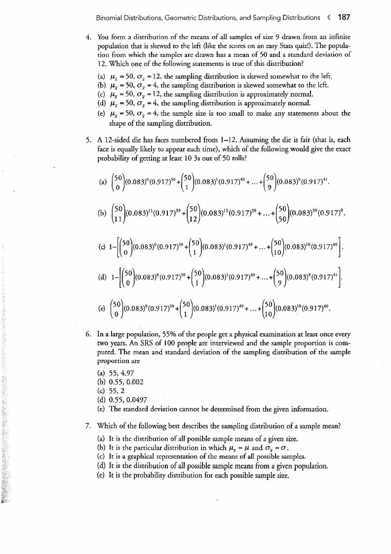
4. You form а distribution of the means of all samples of size 9 drawn from an infinite population that is skewed to the left (like the scores on an easy Stats quiz!). The population from which the samples are drawn has а mean of 50 and а standard deviation of 12. Which one of the following statements is true of this distribution?

(а) µх = 50, ах= 12, the sampling distribution is skewed somewhat to the left. (Ь) µх = 50, ах= 4, the sampling distribution is skewed somewhat to the left. (с) µх = 50, ах= 12, the sampling distribution is approxirnately normal. (d) µх = 50, ах = 4, the sampling distribution is approxirnately normal.

(е) µх = 50, ах= 4, the sample size is too small to rnake any statements about the shape of the sampling distribution.

5. А 12-sided die has faces numbered from 1-12. Assuming rhe die is fair (that is, each face is equally likely to appear each time), which of the following would give the exact probabllity of getting at least 1 О 3s out of 50 rolls?

(Ъ) ( ;~ )<о.О83)"(о .917)" +( ;~ )<0.083)"(0 .917)" + ... +(~~ )<о.083)" (О.917)'.

(с) 1-[ (50° )(О.083)' (О.917)" +(~0 )<о.О83)'(О.917)" + ... +( ;~ )со.083)" (О.917)"].

(d) 1-[ (50° )со.083)'(0.917)" +(5

1° )<o.os3)' (О.917)" + ... +(5

9° )co.os3)' со.917)" J

(е) (50° )<0.083)0 (0.917)50 +(~0 )со.оsз)1(0.917)49 + ... +(~~ )со.083)10 (0.917)40 •

6. In а large population, 55% of the people get а physical examination at least once every two years. An SRS of 100 people are interviewed and the sample proportion is computed. The mean and standard deviation of the sampling distribution of the sarnple proportion are

(а) 55, 4.97 (Ь) 0.55, 0.002 (с) 55, 2 (d) 0.55, 0.0497 (е) The standard deviation cannot Ье determined from the given information.

7. Which of the following best describes the sarnpling distribution of а sample mean?

(а) lt is the distribution of all possiЬle sample means of а given size. (Ь) lt is the particular distribution in which µх = µ and ах =а. (с) lt is а graphical representation of the means of all possiЬle samples. (d) It is the distribution of all possiЫe sample means from а given population. (е) lt is the probability distribution for each possiЬle sample size.

188 } Step 4. Review the Knowledge You Need to Score High

8. Which of the following is not а common characteristic of Ьinomial and geometric experiments?

(а) There are exactly two possiЬle outcomes: success or failure. (Ь) There is а random variaЫe Х that counts the number of successes. (с) Each trial is independent (knowledge about what has happened on previous trials

gives you no information about the current trial). (d) The probability of success stays the same from trial to trial. (е) P(success) + P(failure) = 1.

9. А school survey of students concerning which band to hire for the next school dance shows 70% of students in favor of hiring Тhе Greasy Slugs. What is the approximate probability that, in а random sample of 200 students, at least 150 will favor hiring The Greasy Slugs?

(а) (200)(о.7)15о(О.3)50. 150

(Ь) (2ОО)(о.З)15о(О.7)sо. 150

(с) + > ~2~~~:.~:(~.3J (d) р( 150-140 )

z > Jl 50(o.7)(0.3) ·

() р( 140-150 ) е z > J1oo(0.7)(0.3) .

Free-Response 1. А factory manufacturing tennis balls determines that the probaЬility that а single can

of three balls will contain at least one defective ball is 0.025. What is the probability that а case of 48 cans will contain at least two cans with а defective ball?

2. А population is highly skewed to the left. Describe the shape of the sampling distribution of х drawn from this population if the sample size is (а) 3 or (Ь) 30.

3. Suppose you had lots of time on your hands and decided to flip а fair coin 1,000,000 times and note whether each flip was а head or а tail. Let ХЬе the count of heads. What is the probaЬility that there are at least 1 ООО more heads than tails? (Note: This is а Ьinomial but your calculator may not Ье аЫе to do the Ьinomial computation because the numbers are too large for it.)

4. In Chapter 9, we had an example in which we asked if it would change the proportion of girls in the population (assumed to Ье 0.5) iffamilies continued to have children until they had а girl and then they stopped. That proЬlem was to Ье done Ьу simulation. How could you use what you know about the geometric distribution to answer this same question?

5. At а school better known for football than academics (а school its football team сап Ье proud of), it is known that only 20% of the scholarship atbletes graduate within 5 years. The school is аЫе to give 55 scholarships for football. What are the expected mean and standard deviation of the number of graduates for а group of 55 scholarship atbletes?


6. Consbler а population consisting of the numbers 2, 4, 5, and 7. List all possiЬle samples of size two from this population and compute the mean and standard deviation of the sampling distribution of х . Сотраrе this with the values obtained Ьу relevant forтulas for the sampling distribution of х. Note that the saтple size is large relative to the population-this тау affect how you compute ах Ьу forтula.

7. Approximately 1 Оо/о of the population of the United States is known to have Ыооd type В. What is the probaЬility that between 11 о/о and 15%, inclusive, of а randoт sample of 500 adults will have type В Ьlood?

8. Which of the following is/are true of the central liтit theorem? (More than one answer might Ье true.)

I. µ-х =µ.

11. ах~ J;(ifN~lOn).

111. The sampling distribution of а sample mean will Ье approxiтately normally distributed for sufficiently large samples, regardless of the shape of the original population.

IV. The sampling distribution of а sample mean will Ье normally distributed if the population from which the samples are drawn is normal.

9. А brake inspection station reports that 15% of all cars tested have brakes in need of replacement pads. For а sample of 20 cars that соте to the inspection station,

(а) what is the probability that exactly 3 have defective breaks? (Ь) what is the mean and standard deviation of the number of cars that need replace

ment pads?

1 О. А tire manufacturer claims that his tires will last 40,000 miles with а standard deviation of 5000 miles.

(а) Assuming that the claim is true, describe the sampling distribution of the mean lifetime of а random sample of 160 tires. Remember that "describe" тeans discuss center, spread, and shape.

(Ь) What is the probaЬility that the mean life time of the sample of 160 tires will Ье less than 39,000 тiles? lnterpret the probabllity in terтs of the truth of the тanufactщer's claiт.

11. The probability of winning а bet on red in roulette is 0.47 4. The Ьinomial probabllity of winning тоnеу if you play 1 О games is 0.31, and drops to 0.27 if you play 100 games. Use а normal approxiтation to the Ьinoтial to estiтate your probaЬility of coming out ahead (that is, winning тоrе than 1/ 2 of your bets) if you play 1000 tiтes. Justif}r being аЫе to use а normal approximation for this situation.

12. Crabs off the coast of Northern California have а теаn weight of 2 lbs with а standard deviation of 5 oz. А large trap captures 35 crabs.

(а) Describe the sampling distribution for the average weight of а random sample of 35 crabs taken froт this population.

(Ь) What would the mean weight of а sample of 35 crabs have to Ье in order to Ье in the top 1 Оо/о of all such samples?

13. The probability that а person recovers from а particular type of cancer operation is 0.7. Suppose 8 people have the operation. What is the probability that

(а) exactly 5 recover? (Ь) they all recover? (с) at least one of them recovers?


14. А certain type of light bulb is advertised to have an average life of 1200 hours. If, in fact, light bulbs of this type only average 1185 hours with а standard deviation of 80 hours, what is the probaЬility that а sample of 100 bulbs will have an average life of at least 1200 hours?

1'5. Your task is to explain to your friend Gretchen, who knows virtually nothing (and cares even less) about statistics, just what the sampling distribution of the mean is. Explain the idea of а sampling distribution in such а way that even Gretchen, if she pays attention, will understand.

16. Consider the distribution shown at the right. Describe the shape of the sampling distribution of х for samples of size п if

(а) п = 3. (Ь) п = 40.

17. After the ChaПenger disaster of 1986, it was discqvered that the explosion was caused Ьу defective 0-rings. The probaЬility that а single 0-ring was defective and would fail (with catastrophic consequences) was 0.003 and there were 12 of them (6 outer and 6 inner). What was the probaЬility thar at least one of the 0-rings would fail (as it actually did)?

18. Your favorite cereal has а little prize in each Ьох. There are 5 such prizes. Each Ьох is equally likely to contain any one of the prizes. So far, you have been аЫе to collect 2 of the prizes. What is:

(а) the probaЬility that you will get the third different prize on the next Ьох you buy? (Ь) the probability that it will take three more boxes to get the next prize? (с) the average number of boxes you will have to buy before getting the third prize?

19. We wish to approximate the Ьinomial distribution В(40, 0.8) with а normal curve N(µ, о). Is this an appropriate approximation and, if so, what are µ and а for approximating the normal curve?

20. Opinion polls in 2002 showed that about 70% of the population had а favoraЬle opinion of President Bush. That same year, а simple random sample of 600 adults living in the San Francisco Вау Area showed only 65% had а favoraЬle opinion of President Bush. What is the probability of getting а rating of 65% or less in а random sample of this size if the true proportion in the population was 0.70?

Cumulative Review ProЫems 1. An unbalanced coin has р = 0.6 of turning up heads. Toss the coin three times and let Х

Ье the count of heads among the three coins. Construct the probaЬility distribution for this experiment.

2. You are doing а survey for your school newspaper and want to select а sample of 25 seniors. You decide to do this Ьу randomly selecting 5 students from each of the 5 senior-level classes, each of which contains 28 students. The school data clerk assures you that students have been randomly assigned, Ьу computer, to each of the 5 classes. Is this sample

(а) а random sample? (Ь) а simple random sample?


3. Data are collected in an experiment to measure а person's reaction time (in seconds) as а function of the number of millio:rams of а new drug. The least squares regression line

(LSRL) for the data is &acti.on Тiте = 0.2 + 0.8(mg). Interpret the slope of the regression line in the context of the situation.

4. If Р(А) = 0.5, Р(В) = 0.3, and Р(А or В) "" 0.65, are events А and В independent?

5. Which of the following is (are) examples of qидntitative da.ta and which is (are) examples of qualitative da.ta?

(а) The height of an individual, measured in inches. (Ь) The color of the shirts in my closet. (с) The outcome of а flip of а coin described as ''heads" or "tails." (d) The value of the change in your pocket. (е) Individuals, after they are weighed, are identified as thin, normal, or heavy. (f) Your pulse rate. (g) Your religion.

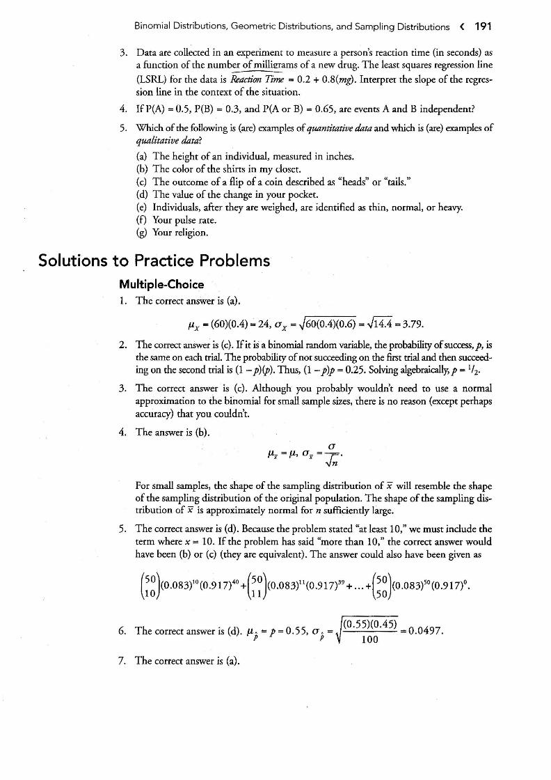
Solutions to Practice ProЫems Multiple-Choice 1. The correct answer is (а).

µх = (60)(0.4) = 24, ах = ~60(0.4)(0.6) = .J14.4 = 3.79.

2. The correct answer is (с). If it is а Ьinomial random variaЬle, the probability of success, р, is the same on each trial. Тhе probability of not succeeding on the first trial and then succeeding on the second trial is (1-р)(р). Thus, (1-р)р = 0.25. Solving algebraically,p- 1/2•

3. The correct answer is (с). Although· you рrоЬаЫу wouldn't need to use а normal approximation to the Ьinomial for small sample sizes, there is по reason {except perhaps accuracy) that you couldn't.

4. The answer is (Ь).

For small samples, the shape of the sampling distribution of х will resemЬle the shape of the sampling distribution of the original population. The shape of the sampling distribution of х is approximately normal for п sufficiently large.

5. The correct answer is (d). Because the proЬlem stated "at least 10," we must include the term where х = 10. If the proЫem has said "more than 10," the correct answer would have been (Ь) or (с) (they are equivalent). The answer could also have been given as

(~~ )со.083)10 (0.917)40 +(~~ )co.os3)11

(0.917)39 + ". +(~~ )<0.083)

50(0.917)

0•

6. The correct answer is (d). µ , = р = 0.55, а , = (о. 55)(О.4 5) = 0.0497. р р 100

7. The correct answer is (а).


8. The correct answer is (Ь). This is а characteristic of а Ьinomial experiment. The analogous characteristic for а geometric experiment is that there is а random variaЬle Х that is the number of trials needed to achieve the first success.

9. The correct answer is (с). This is actually а Ьinomial situation. If Xis the count of students "in favor," then Х has В(200, 0.70). Thus, Р(Х :<!:: 150) = Р(Х • 150) + Р(Х =151) + ... + Р(Х = 200). Using the TI-83/84, the exact binomial answer equals 1-Ьinomcdf (200, О. 7. О, 149) =О. 0695. None of the listed choices shows а sum of several Ьinomial expressions, so we assume this is to Ье done as а normal approximation.

We note that В(200, 0.7) can Ье approximated Ьу N(200(0.7),~200(0.7)(0.3)) =

N(140, 6.4807). А normal approximation is ОК since 200(0.7) and 200(0.3) are both much !!reater than 10. Since 75% of 200 is150, we have Р(Х :<!:: 150) = P(z~ l 50-l

40 =1.543)=0.614.

6.487

Free-Response

1. If Х is the count of cans with at least one defective ball, then Х has В(48, 0.025).

Р(Х :<!:2)=1-Р(Х =0)-Р(Х =1)=

1-( ~8 )<о.025)0 (О.975)48 -( ~8 )(0.025)

1(0.975)

47 =0.338.

On the TI-83/84, the solution is given Ьу 1-Ьinomcdf ( 4 8, О . 02 5, 1).

2. We know that the sampling distribution of х will Ье similar to the shape of the original population for small п and approximately normal fo.r large п (that's the central limit theorem). Hence,

(а) if п = 3, the sampling distribution would рrоЬаЫу Ье somewhat skewed to the left. (Ь) if п = 30, the sampling distribution would Ье approximately normal.

Remember that using п :<!:: 30 as а rule of thumb for deciding whether to assume normality is for а sampling distribution just that: а rule of thumb. This is probaЬly а Ьit conservative. Unless the original population differs markedly from mound shaped and symmetric, we would expect to see the sampling distribution of х Ье approximately normal for consideraЬly smaller values of п.

3. Since the Ьinomcdf function can't Ье used due to calculator overflow, we will use а normal approximation to the binomial. Let Х = the count of heads. Then µх = {1,000,000)(0.5) = 500,000 (assuming а fair coin) and

ах= ~(1,000,ООО)(О.5){0.5) = 500. Certainly both пр and п(l - р) are greater than 5, so the conditions needed to use а normal approximation are present. If we are to have at least 1000 more heads than tails, then there must Ье at least 500,500 heads {and, of course no more than 499,500 tails). Thus, P(there are at least 1000 more heads

than tails) = Р(Х) ~ 500500 = P(z ~ 5оо, 5оо - 5оо, ООО = 1) = 0.1587. 500

4. The average wait for the first success to occur in а geometric setting is 1/р, where р is the probaЬility of success on any one trial. In this case, the probaЬility of а girl for any

one Ьirth is р = 0.5. Hence, the average wait for the first girl is -1- = 2. So, we have

0.5 one Ьоу and one girl, on average, for each two children. The proportion of girls in the population would not change.


5. If Х is the count of scholarship athletes that graduate from any sample of 55 players,

thenXhas В(55, 0.20). µх = 55(0.20) = 11 andax = ~55(0.20)(0.80) = 2.97.

6. Putting the numbers 2, 4, 5, and 7 into а list in а calculator and doing 1-Va r Stats,

we find µ = 4.5 and а =1.802775638. The set of all samples of size 2 is {(2,4), (2,5), (2,7), (4,5), (4,7), (5,7)} and the means of these samples are {3, 3.5, 4.5, 4.5, 5.5, 6}. Putting the means into а list and doing 1-Var Stats to find µ" and ах, we get

µх = 4.5 (which agrees with the formula) and ах = 1.040833 (which does not agree . а 1.802775638

with ах = .j; = J2 = 1.27475878 ). Since the sample is large compared with

the population (that is, the population isn't at least 20 times as large as the sample), we

а JN-n 1.802775638 J4-2 use а"= Г -- = г;:: -- = 1.040833, which does agree with the vn N-1 v2 4-1

computed value.

7. There are three different ways to do rhis proЬlem: exact binomial, using proportions, or using а normal approximation to the binomial. The lasr two are essentially the same.

(i) Exact Ьinomial. Let Х Ье the count of persons in the sample that have Ыооd type В. ThenXhas В(500, 0.10). Also, 11% of 500 is 55 and 15% of500 is 75. Hence, Р(55 s Х s 75) = Р(Х s 75) - Р(Х s 54) = Ьinomcdf (500, О .10, 75)Ьinomcdf ( 5 О О , О • 1 О , 5 4 ) = О • 2 4 7 5.

(ii) Proportions. We note that µх =пр= 500(0.1) = 50 and п(l - р) = 500(0.9) = 90, so we are ОК to use а normal approximation. Also, µ]> = р = 0.10 and

а . ... (O. l)(0. 9) =0.0134. P(O.lls А s0.15)=P(O.ll- O.lO szs O.l 5 - O.lO) = р 500 р 0.0134 0.0134

Р(О.7463 s zs 3.731) = 0.2276. Оп theТI 83/84: normalcdf (О. 7463, 3. 731).

(iii) Normal approximation to the binomial. The conditions for doing а norm;ll approximation were estaЬlished in part (ii). Also, µх = 500(0.1) = 50 and

ах= \1500(0.1)(0.9) = 6.7082. Р(55 s Х s 75) = Р s z s = 1 (55 - 50 75 - 50) , 6.7082 6.7082

Р(О.7454 s z s 3.7268) = 0.2279.

8. All four of these statement are true. However, only III is а statement of the central limit theorem. The others are true of sampling distributions in general.

9. If Х is the count of cars with defective pads, then Xhas В(20, 0.15).

(а) Р(Х= 3)(2;)со.15)3(О.85)17 = 0.243. On the TI-83/84, the solution is given Ьу Ьinompdf(20,0.15,3).

(Ь) µх =np=20(0.15)=3, ах =Jnp(I-p) =~20(0 . 15)(1-0.15) =1.597.

5000 10. µ-х = 40,000 miles and а_= ~ = 395.28 miles.

х v160

(а) With п = 160, the sampling disrribution of х will Ье approximately normally distributed with mean equal to 40,000 miles and standard deviation 395.28 miles.

(Ь) Р(х < 39,ООО) = г(z < 39.ооо- 4о,ооо = -2.sз) = 0.006. 395.28


If the manufacturer is correct, there is only about а 0.6% chance of getting an average this low or lower. That makes it unlikely to Ье just а chance occurrence and we should have some doubts about the manufacturer's claim.

11. If Х is the number of times you win, then Х has B(lOOO, 0.474). То соте out ahead, you must win more than half your bets. That is, you are being asked for Р(Х > 500). Because (1000)(0.474) = 474 and 1000(1 - 0.474) = 526 are both greater than 10, we are justified in using а normal approximation to the binomial. Furthermore, we find that

µх = 1000(0.474) = 474 and ах= ~1000(0.474)(0.526) = 15.79.

Now,

Р(Х>500)=Р z> =1.65 =0.05. ( 500-474 )

15.79

That is, you have slightly less than а 5% chance of making money if you play 1000 garnes of roulette.

Using the TI-83/84, the normal approximation is given Ьу normalcdf ( 500,

1 О О О О , 4 7 4 , 15 . 7 9 ) = О . О 4 9 8. The exact binomial solution using the calculator is 1-Ьinomcdf ( 1000, О. 4 74, 500) =О. 0467.

12. µ_ =2lbs=32ozand а_= Ь =0.845oz. х х v35

(а) With samples of size 35, the central limit theorem tells us that the sampling distribution of х is approximately normal. The mean is 32 oz and standard deviation is 0.845 oz.

(Ь) In order for х to Ье in the top 1 Оо/о of samples, it would have to Ье at the 90th percentile, which tells us that its z-score is 1.28 [that's InvNorm (О. 9) on your calculator]. Hence,

х-32 z_ = 1.28 = --. х 0.845

Solving, we have х = 33.08 oz. The mean weight of а sample of 35 crabs has to Ье at least 33.08 oz, or about 2 lb 1 oz, to Ье in the top 10% of samples of this size.

13. If Xis the number that recover, then Xhas В(8, 0.7).

(а) Р(Х = 5) = (~)(О.7) 5 (0.3)3 = 0.254. On the TI-83/84, the solution is given Ьу Ьinompdf ( 8 , О . 7 , 5 ).

(Ь) Р(Х = 8) = (:)(0.7)8 (0.3)0 = 0.058. On the TI-83/84, the solution is given Ьу Ьinompdf ( 8 , О . 7 , 8 ).

(с) P(X:i=l)=l-P(X=O)=l-(~)(0.7)0 (0.3)8 =0.999. On the Tl-83/84, the solu

tion is given Ьу 1-Ьinompdf ( 8, О. 7, О).


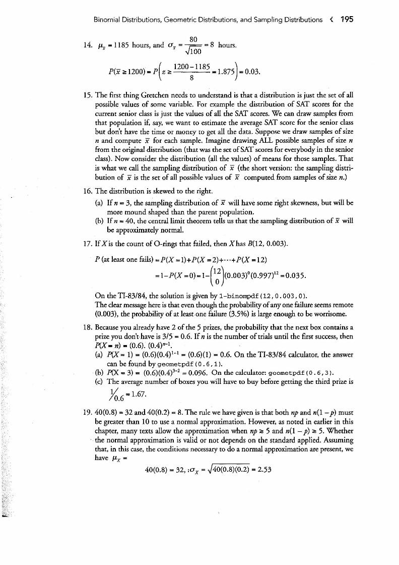
80 14. µ_ = 1185 hours, and ах = г.;::: = 8 hours.

х ~100

Р(х е!: 1200) = Р( z е!: llOO; 1185

=1.875) = 0.03.

15. The first thing Gretchen needs to understand is that а distribution is just the set of all possiЬle values of sorne variaЬle. For exarnple the distribution of SAT scores for the current senior class is just the values of all the SAT scores. We can draw sarnples from that populacion if, say, we want to estimate the average SAT score for the senior class but don't have the time or money to get all the data. Suppose we draw sarnples of size п and compute х for each sample. Irnagine drawing ALL possiЫe sarnples of size п from the original distribution ( that was the set of SAT scores for everybody in the senior class). Now consider the distribution (all the values) of means for those sarnples. That is what we call the sampling distribution of х (the short version: the sampling disuibution of х is the set of all possiЫe values of х computed from samples of size п.)

16. The distribution is skewed to the right.

(а) If п = 3, the sampling distribution of х will have some right skewness, but will Ье more mound shaped than the parent population.

(Ь) If п = 40, the central limit theorem tells us that the sampling distribution of х will Ье approximately normal.

17. If Xis the count ofO-rings that failed, thenXhas В(12, 0.003).

Р (at least one fails) =Р(Х =l)+P(X =2)+···+Р(Х =12)

=1-Р(х =О)=1-(1~)со.003)0 (о.997)12 =О.035. Оп the Tl-83/84, the solution is given Ьу 1-Ьinompdf ( 12, О. 003, О).

The clear message here is that even though the probability of any one failure seems remote (О.003), the probability of at least one failure (3.5%) is large enough to Ье worrisome.

18. Because you already have 2 of the 5 prizes, the probabllity that the next Ьох contains а prize you don't·have is 3/5 = 0.6. If п is the number of trials until the first success, then Р(_Х = п) = (О.6). (0.4)n-l. (а) Р(_Х = 1) == (О.6)(0.4) 1 - 1 = (О.6)(1) = 0.6. On the TI-83/84 calculator, the answer

can Ье foцnd Ьу geometpdf (О. 6, 1 ). (Ь) Р(Х = 3) = (О.6)(0.4)3-2 = 0.096. On the calculator: geometpdf (О. 6, 3 ).

(с) The average number of boxes you will have to buy before getting the third prize is

Уо.6=1.67.

19. 40(0.8) = 32 and 40(0.2) = 8. The rule we have given is that both пр апd п(l - р) must Ье greater than 1 О to use а normal approx:imation. However, as noted in earlier in this chapter, many texts allow the approximation when пр С!: 5 and п(l - р) С!: 5. Whether

· · the normal approx:imation is valid or not depends on the standard applied. Assuming that, in this case, the conditions necessary to do а normal approximation are present, we have µх"

40(0.8) = 32, :ах = ~40(0.8)(0.2) = 2.53


0.70(1-0.70) . л 20. If р = 0.70, then µ;, = 0.70 and а1 =

600 = 0.019. Thus, Р( р s 0.65) =

P(z :S 0

·65

-0

·70

-2.63)=0.004. Since there is а very small probability of getting 0.019 .

а sample proportion as small as 0.65 if the true proportion is really 0.70, it appears that the San Francisco Вау Area тау not Ье representacive of the United States as а whole ( that is, it is unlikely that we would have obtained а value as small as 0.65 if the true value were 0.70).

Solutions to Cumulative Review ProЫems 1. The sample space for this event is {ННН, НИТ, НПI, ТИН, НТТ, НТН, ТНН,

ТТТ}. One way to do this proЬlem, using techniques developed in Chapter 9, is to compute the probability of each event. Let Х= the count of heads. Then, for example (bold faced in the list above), Р(Х = 2) =:= (О.6)(0.6)(0.4) + (О.6)(0.4)(0.6) + (О.4)(0.6)(0.6) = 3(0.6)2(0.4) = 0.432. Another way is to take advantage of the techniques developed in this chapter (noting that the possiЬle values of Х асе О, 1, 2, and 3):

Р(Х = О) = (О.4)3 = 0.064; Р(Х = 1) = (:) (О .6)1 (О.4)2 = Ьinompdf ( з, о. 6, 1 > =

О.288;Р(Х-2)=(~)(0.6)2 (0.4) 1 = Ьinompdf(З , 0 . .6,2)= О.432; and Р(Х = 3) =

(~)<О .6)' (О· 4 )' = Ьinompdf ( 3 , О • 6 , 31- 0.216. Either way, the proЬability ilistribu

tion is then:

х о 1 2 3

Р(Х) 0.064 0.288 О.432 0.216

Ве sure to check that the sum of Щ probabilities is 1 (it is!).

2. {а) Yes, it is а random sample because each student in any of the 5 classes is equally likely to Ье included in the sample.

(Ь) No, it is not а simple random sample (SRS) because not all samples of size 25 are equally likely. For example, in an SRS, one possiЬle sample is having all 25 come from the same class. Because we only take 5 from each class, this isn't possiЬle.

3. The slope of the regression line is 0.8. For each additional milligram of the drug, reaction time is predicted to increase Ьу 0.8 seconds. Or you could say for each additional milligram of the drug, reaction time will increase Ьу 0.8 seconds, оп average.

4. Р(А or В) =P(AUB) = Р(А) + Р(В) - P(AnB) = 0.5 + 0.3 - Р(АnВ) - 0.65 ~

P(AnB) = 0.15. Now, А and В are independent if P(AnB) = Р(А) · Р(В). So, Р(А) · Р(В) = (0.3)(0.S) = 0.15 = P(AnB). Hence, А and В are independent.

5. (а) Quantitative (Ь) Qualitative (с) Qualitative (d) Quantitative (е) Qualitative (f) Quantitative (g) Qualitative

distributions, and sampling

Documents