quantile estimation with adaptive importance sampling

arX

iv:1

002.

4946

v1 [

mat

h.ST

] 2

6 Fe

b 20

10

The Annals of Statistics

2010, Vol. 38, No. 2, 1244–1278DOI: 10.1214/09-AOS745c© Institute of Mathematical Statistics, 2010

QUANTILE ESTIMATION WITH ADAPTIVE IMPORTANCESAMPLING

By Daniel Egloff and Markus Leippold

QuantCatalyst and University of Zurich

We introduce new quantile estimators with adaptive importancesampling. The adaptive estimators are based on weighted samplesthat are neither independent nor identically distributed. Using anew law of iterated logarithm for martingales, we prove the con-vergence of the adaptive quantile estimators for general distributionswith nonunique quantiles thereby extending the work of Feldman andTucker [Ann. Math. Statist. 37 (1996) 451–457]. We illustrate the al-gorithm with an example from credit portfolio risk analysis.

1. Introduction. We introduce a new sample-based quantile estimatorswith adaptive importance sampling. Importance sampling is a widely usedtechnique for variance reduction to improve the statistical efficiency of MonteCarlo simulations. It reduces the number of samples required for a given levelof accuracy. The basic idea is to change the sampling distribution so thata greater concentration of samples are generated in a region of the sam-ple space which has a dominant impact on the calculations. The change ofdistribution is then compensated by weighting the samples using the Radon–Nikodym derivative of the original measure with respect to the new measure.However, in a multivariate setting, it is far from obvious how such a changeof measure should be obtained.

Given its importance for practical applications, especially for risk man-agement in the finance industry, the literature on sample-based quantileestimation with variance reduction is rather sparse.1 The focus of variancereduction schemes is almost exclusively geared towards the estimation ofexpected values. The reason might lie in the additional intricateness that

Received March 2009; revised August 2009.AMS 2000 subject classifications. Primary 62L20, 65C05; secondary 65C60.Key words and phrases. Quantile estimation, law of iterated logarithm, adaptive im-

portance sampling, stochastic approximation, Robbins–Monro.

This is an electronic reprint of the original article published by theInstitute of Mathematical Statistics in The Annals of Statistics,2010, Vol. 38, No. 2, 1244–1278. This reprint differs from the original inpagination and typographic detail.

1An early contribution is the control variate approach of [18]. Later work includes [4, 16]and [19].

1

http://arxiv.org/abs/1002.4946v1

http://www.imstat.org/aos/

http://dx.doi.org/10.1214/09-AOS745

http://www.imstat.org

http://www.ams.org/msc/

http://www.imstat.org

http://www.imstat.org/aos/

http://dx.doi.org/10.1214/09-AOS745

2 D. EGLOFF AND M. LEIPPOLD

sample-based quantile estimators exhibit. The quantile function, viewed asa map on the space of distribution functions, generally fails to be differen-tiable in the sense of Hadamard. For certain distributions, the quantile maybe nonunique. If the lower and upper quantiles of a random variable Y fora probability level α ∈ (0,1), defined as

qα(Y ) = inf{y | P(Y ≤ y)≥ α},qα(Y ) = sup{y | P(Y ≤ y)≤ α},

are distinct, then the ordinary quantile estimator Y⌊nα⌋,n based on the orderstatistics Y1,n, . . . , Yn,n of samples Y1, . . . , Yn is not consistent anymore. Forthe special case of independent and identically distributed (i.i.d.) samplesY1, . . . , Yn, Feldman and Tucker [12] prove that Y⌊nα⌋,n oscillates across theinterval [qα(Y ), qα(Y )] infinitely often. Using the classical law of iteratedlogarithm for sequences of i.i.d. random variables, they also show that con-sistency can be retained for the modified estimator Yν(n),n if the functionν(n) ∈N satisfies

(1 + k)√

2n log logn≤ ⌊nα⌋ − ν(n)≤Kn1/2+γ(1.1)

for some positive constants γ, k,K.For the estimation of expected values with importance sampling, a com-

mon procedure is to apply the change of measure suggested by a large devi-ation upper bound. Although this approach often leads to an asymptoticallyoptimal sampling estimator, it can also fail completely, as shown in Glasser-man and Wang [14].

Our method for quantile estimation does not rely on large deviation prin-ciples. Instead, it is adaptive. Adaptive algorithms, but only for expectedvalues and not for quantiles, are introduced in the work of [2] and [3]. Theyapply the truncated Robbins–Monro algorithm of Chen, Guo and Gao in [7]for pricing financial options under different assumptions on the underlyingprocess. Robbins–Monro methods and stochastic approximation date backto the historical work of Robbins and Monro [30] and Kiefer and Wolfowitz[21]. See also [23] and the more recent references [5, 24] and [25].

Using an adaptive strategy to obtain a quantile estimator means thatevery new sample is used to improve the parameters of the importance sam-pling density. Therefore, we cannot rely on the results of Feldman and Tucker[12]. Our quantile estimators, derived from weighted samples, are neitherindependent nor identically distributed. However, we derive a new law of it-erated logarithms for martingales which allows us to prove the convergenceof the adaptive quantile estimators for distributions with nondifferentiableand nonunique quantiles without requiring the i.i.d. assumption thereby ex-tending the result of Feldman and Tucker.

ADAPTIVE QUANTILE ESTIMATION 3

Our paper is structured as follows. In Section 2, we present the generalsetup and we introduce the notation. Section 3 gives a brief review of adap-tive importance sampling for estimating the mean. In Section 4, we startwith the discussion of the metric structure underlying our adaptive algo-rithm. We then derive two theorems, Theorems 4.1 and 4.2, which extendFeldman and Tucker [12]. The proof of the theorems build on a new resultfor the law of iterated logarithms for martingales which we present in Theo-rem 4.4. Finally, in Section 5 we provide an application of our new quantileestimator which we borrow from credit risk management. All proofs aredelegated to the Appendix.

2. Setup and notation. Let ϕθ(x) be a probability density depending ona parameter θ of a random variable X relative to some reference measureλ, defined on a measurable space (X ,F) with a countably generated σ-fieldF . We assume that the parameters θ take their values in a metric space(Θ, d) for some fixed metric d and equip it with the Borel σ-algebra B(Θ).For now, we do not have to further distinguish the parameter space Θ andthe set of densities {ϕθ(x) | θ ∈Θ}. For the expectation, under the measureϕθ dλ, we write

Eθ[f(X)] =

∫

X

f(x)ϕθ(x)dλ(x)(2.1)

and we define for all p, 1≤ p≤∞,

Lp(θ) = {f :X →R | f is F-measurable,‖f‖pθ,p = Eθ[|f(X)|p]<∞}.

Let ϕθ0(x) be our reference or sample density. We assume that all densitiesin Θ are absolutely continuous with respect to the reference density ϕθ0(x)and we denote by

wx(θ) =ϕθ0(x)

ϕθ(x)(2.2)

the likelihood ratio or Radon–Nikodym derivative. In particular, wx :x 7→wx(θ) is measurable for all θ ∈Θ. If f ∈L1(θ0), we have

Eθ[wX(θ)f(X)] = Eθ0 [f(X)] ∀θ ∈Θ.(2.3)

For p≥ 1, we introduce the (weighted) moments

mf,p(θ) = Eθ[|wX(θ)f(X)|p] = Eθ0 [wX(θ)p−1|f(X)|p].(2.4)

We use the abbreviation mf (θ) =mf,2(θ) for the second moment and

σ2f (θ) = Varθ[wX(θ)f(X)] =mf (θ)−Eθ0 [f(X)]2(2.5)

for the variance.


3. Review: Adaptive importance sampling for estimation of means. Be-fore we derive our adaptive quantile estimators, we start this section with abrief review of adaptive importance sampling for the estimation of means.Consider a function f ∈ L1(θ0). Static importance sampling estimates theexpectation Eθ0 [f(X)] by the weighted sample average

es(n, f) =1

n

n∑

i=1

wXi(θ)f(Xi)(3.1)

with Xi ∼ ϕθ dλ i.i.d. The usual error estimates based on the central limittheorem indicate that the most advantageous choice for θ would be thevariance minimizer

θ∗ = argminθ∈Θ

σ2f (θ) = argmin

θ∈Θmf (θ).(3.2)

Unfortunately, in most cases (3.2) cannot be solved explicitly. An alternativeto the approach on the basis of large deviation upper bounds is an adaptivestrategy. The solution θ∗ is estimated by a sequence (θn)n≥0, generated,for instance, by a stochastic approximation algorithm of Kiefer–Wolfowitzor Robbins–Monro type. Replacing the fixed parameter θ in (3.1) by thesequentially generated parameters (θn)n≥0 leads to the adaptive importancesampling estimator

ea(n, f) =1

n

n∑

i=1

wXi(θi−1)f(Xi),(3.3)

where Xn ∼ ϕθn−1(x)dλ(x) is simulated from the importance sampling dis-tribution determined from the parameter θn−1. In contrast to static impor-tance sampling, the random variables wXn(θn−1) and f(Xn) in (3.3) areneither independent nor identically distributed. However, we still obtain amartingale.

Lemma 3.1. Let θn be a sequence of parameters and Xn ∼ ϕθn−1 dλ.Define Fn = σ(θ0, . . . , θn,X1, . . . ,Xn). Then, for f ∈L1(θ0),

Mn =

n∑

i=1

(wXi(θi−1)f(Xi)−Eθ0 [f(X)])(3.4)

is a martingale with respect to the filtration F= (Fn)n≥0.

Proof. If (Zn)n≥0 is a sequence of integrable random variables, then

Mn =n∑

i=1

(Zi − E[Zi | Z1, . . . ,Zi−1])(3.5)


is a martingale. The integrability of wXi(θi−1)f(Xi) and the martingaleproperty for (3.4) follow from

E[wXi(θi−1)f(Xi) | Fi−1] = Eθi−1[wXi(θi−1)f(Xi)] = Eθ0 [f(X)],(3.6)

where the second equality is a consequence of (2.3). �

A strong law of large numbers and a central limit theorem for (3.3) hasbeen obtained in [2] by applying classical martingale convergence results forwhich we refer to [17] and [15]. For a proof of the theorem below, we referto [2].

Theorem 3.1. Let θn, Xn, and F= (Fn)n≥0 be as in Lemma 3.1. As-sume that θn → θ∗ ∈Θ converges almost surely and that there exists a > 1such that for all θ ∈Θ

Eθ[|wX(θ)f(X)|2a]<∞,(3.7)

the function mf,2a : θ 7→mf,2a(θ) is continuous in θ∗, and

E[mf,2a(θn)]<∞ ∀n≥ 0.(3.8)

Then

limn→∞

1

n

n∑

i=1

wXi(θi−1)f(Xi) = Eθ0 [f(X)] almost surely,(3.9)

and

√n

(

1

n

n∑

i=1

wXi(θi−1)f(Xi)−Eθ0 [f(X)]

)

d→N(0, σ2f (θ∗)),(3.10)

whered→ denotes convergence in distribution.

4. Adaptive importance sampling for quantile estimation. Having re-viewed the estimation of the mean with adaptive importance sampling inthe previous section, we introduce now the metric structure and the algo-rithm that underlies our new adaptive quantile estimation.

4.1. Riemannian structure for parameter tuning. The procedure to esti-mate the variance optimal parameter (3.2) crucially depends on the metricstructure of the parameter space Θ. The metric is not only important ifit comes to the actual numerical implementation, but is also material todetermine existence and uniqueness of a solution.

Let the parameter space Θ be a smooth manifold. It is known that thecanonical metric on a family of densities {ϕθ(x) | θ ∈Θ} is induced by theRiemannian structure given by the Fisher information metric

g = Eθ[dlX ⊗ dlX ].(4.1)


Here, lx(θ) = logϕθ(x) is the log-likelihood function with differential

dlx :Θ→ T ∗Θ,(4.2)

considered as a one-form on Θ and with T ∗Θ, the co-tangent space of themanifold Θ. In particular, (4.1) defines a nondegenerate symmetric bilinearform on the tangent space TΘ, hence a Riemannian metric.2

Having equipped the parameter space Θ with a Riemannian metric, wecan formulate the first order condition for (3.2) in terms of the Riemanniangradient ∇ as

∇mf (θ) = 0.(4.3)

Under suitable assumptions on X and the likelihood ratio wx(θ), we canexchange integration and differentiation to arrive at

∇mf (θ) =−Eθ0 [f(X)2wX(θ)∇lX(θ)] =−Eθ[f(X)2wX(θ)2∇lX(θ)](4.4)

with ∇lx(θ) the Riemannian gradient of the log-likelihood. To approximatea solution ∇mf (θ

∗) = 0, we can now use the representation (4.4) and astochastic approximation scheme

θn+1 = θn + γn+1H(Xn+1, θn), Xn+1 ∼ ϕθn dλ,(4.5)

with average descent direction

H(X,θ) =−f(X)2wX(θ)2∇lX(θ).(4.6)

In this paper, we want to keep the focus on adaptive importance samplingfor quantile estimation and we therefore restrict ourselves to vector spaces.An example with a flat metric is provided by the Gaussian densities

Θ= {N(θ,Σ) | θ ∈Rk}(4.7)

with fixed covariance structure Σ.3 The first and second order differentialsof the likelihood lx(θ) are

dlx(θ) = Σ−1(x− θ), d2lx(θ) =−Σ−1.(4.10)

2For the basic concepts of Riemannian geometry, we refer to [20, 22] and the referencestherein. The usage of the Riemannian metric based on the Fisher information goes backto [28].

3A well-known example of a nonflat Riemannian structure on a space of distributionsis the Fisher information metric of a location scale family of densities

Θ=

{

ϕ(µ,σ)(x) =1

σϕ

(

x− µ

σ

)

∣

∣

∣(µ,σ) ∈R×R

+

}

.(4.8)

A second example is given by the space of all multivariate normal distributions

Θ= {N(θ,Σ) | θ ∈Rk,Σ ∈ S+(k)}(4.9)

which is not flat anymore.


Hence, the Fisher metric on Θ is

gΣ(u, v) =−Eθ[d2lX(θ)(u, v)] = u⊤Σ−1v.(4.11)

Because

gΣ(∇lx(θ), u) =∇lx(θ)⊤Σ−1u= dlx(θ)(u) = (x− θ)⊤Σ−1u,(4.12)

the gradient of the likelihood with respect to the metric (4.11) is

∇lx(θ) = (x− θ).(4.13)

Note that the gradient ∇ of the Fisher metric defers by a factor of Σ−1 fromthe gradient induced by the standard Euclidian metric.

4.2. Parameter tuning with adaptive truncation. In practical applica-tions, the parameter space Θ is often noncompact or it is difficult to apriori identify a bounded region to which the optimal parameter must be-long. We therefore suppose that the parameter sequence (θn)n≥0 is generatedby an algorithm that enforces recurrence and boundedness of the sequenceθn by adaptive truncation. A series of work [6–10] shows that stochastic ap-proximation algorithms with adaptive truncation behave numerically moresmoothly and converge under weaker hypotheses. No restrictive conditionson the mean field or a-priori boundedness assumptions have to be imposed.We follow Andrieu, Moulines and Priouret [1] who analyze the convergence ofstochastic approximation algorithms with more flexible truncation schemesand Markov state-dependent noise. To specify the algorithm, we let (Kj)j∈Nbe an increasing compact covering of Θ satisfying

Θ=

∞⋃

j=1

Kj,Kj ⊂ int(Kj+1)(4.14)

and

γ = (γn)n∈N, ǫ= (ǫn)n∈N,(4.15)

two monotonically decreasing sequences. We introduce the counting vari-ables

(κn, νn, ζn)n∈N ∈N×N×N,(4.16)

where κn records the active truncation set in the compact covering, νn countsthe number of iterations since the last re-initialization (truncation) and ζn isthe index in the sequences γ, ǫ introduced in (4.15). If νn 6= 0, the algorithmoperates in the active truncation set Kκn so that

θj ∈Kκn ∀j ≤ n with νj 6= 0.(4.17)


If νn = 0, the update at iteration n caused a jump outside of the activetruncation set Kκn and triggers a re-initialization at the next iteration n+1.We assume that a stochastic vector field is generated from a measurable map

H :X ×Θ→Θ,(4.18)

where X and Θ are both equipped with countably generated σ-fields B(X )and B(Θ), respectively. We also suppose that Θ is an open subset of someEuclidian vector space.

To handle jumps outside the parameter space Θ, we introduce an isolatedpoint θc taking the role of a cemetery point. Let Θ = Θ ∪ {θc}. For an

arbitrary γ ≥ 0, we define a kernel Qγ on X × Θ by

Qγ(x, θ;A×B) =

∫

APθ(dy)1{θ+γH(y,θ)∈B}

(4.19)

+ 1{θc∈B}

∫

APθ(dy)1{θ+γH(y,θ)/∈B},

where (x, θ) ∈X ×Θ and A ∈ B(X ), B ∈ B(Θ), and Pθ(dx) is a measure onX parameterized by θ. For a sequence of step sizes γ, we define the process(Xn, θn) by

(Xn+1, θn+1)∼Qγn+1(Xn, θn; ·)(4.20)

unless θn = θc, in which case we stop the process and set θn+1 = θc, Xn+1 =Xn. The law of the nonhomogeneous Markov process (4.20) with initialconditions (x, θ), represented on the product space (X × Θ)N, is denoted byPγ

x,θ. Let X0 ⊂X be a compact subset

Φ :X ×Θ→X0 ×K0,(4.21)

be a measurable map and φ :N→ Z with φ(n)>−n.

Algorithm 4.1. The stochastic approximation algorithm with adap-tive truncation is the homogeneous Markov chain defined by the followingtransition law from step n to n+ 1:

(i) If νn = 0, then we perform a reset operation which starts in X0 ×K0

and draws

(Xn+1, θn+1)∼Qγζn(Φ(Xn, θn);dx× dθ).

Otherwise, we simulate

(Xn+1, θn+1)∼Qγζn(Xn, θn;dx× dθ).


(ii) If ‖θn+1 − θn‖ ≤ ǫζn and θn+1 ∈Kκn , then we update

νn+1 = νn +1, ζn+1 = ζn + 1, κn+1 = κn;

else we prepare for a reset operation in the next iteration by setting

νn+1 = 0, ζn+1 = φ(ζn), κn+1 = κn +1.

The convergence of Algorithm 4.1 under suitable conditions on the mea-sure Pθ(dx), the mean field h defined as

h(θ) =

∫

X

H(x, θ)Pθ(dx)(4.22)

and the sequences γ, ǫ are established in [1].4

4.3. Quantile estimation. After having introduced the metric structureand the parameter tuning in the previous sections, we can now turn ourfocus to the estimation of quantiles of a real-valued random variable

Y =Ψ(X), Ψ:X →R,

defined in terms of an F -measurable function Ψ. We denote by

qα = qα(Y ) = inf{y | P(Y ≤ y)≥ α}, 0< α< 1,

the lower α-quantile of Y . Furthermore, let (θn)n≥0 be a sequence of tuningparameters. In favor of a more compact notation, we introduce the abbrevi-ations

wn =wXn(θn−1), Yn =Ψ(Xn), n≥ 1.(4.23)

We recall that, under the assumptions of Theorem 3.1, the weights wn satisfy

E[wn | Fn−1] = Eθn−1 [wn] = 1,1

n

n∑

i=1

wi → 1 almost surely.(4.24)

We first consider generalizations of the empirical distribution function toweighted samples. Because the sum of the weights

∑ni=1wi is not neces-

sarily normalized to one, we introduce the renormalized weighted empiricaldistribution function

Fn,w(y) =1

∑ni=1wi

n∑

i=1

wi1{Yi≤y}(4.25)

4In fact, [1] treat the more general case of state dependent noise where the measurePθ(dy) takes the form of a Markov kernel Pθ(x,dy).


and set

Fn,w,ν(y) =1

ν(n)Fn,w(y),(4.26)

where ν :N→ R+ is a normalization function, which we determine later to

prevent the oscillation of the quantile estimators. We can use the increasingfunction Fn,w,ν to define the quantile estimator

qn,w,ν(α) = F←n,w,ν(α) = inf{y | Fn,w,ν(y)≥ α},(4.27)

where F←n,w,ν is the generalized inverse of Fn,w,ν . Besides the re-normalizedweighted empirical distribution function (4.25), there are alternative waysto generalize the empirical distribution function to weighted samples. Forexample,

F ln,w,ν(y) =

1

ν(n)

n∑

i=1

wi1{Yi≤y}(4.28)

puts the emphasis on the left tail of the distribution. However, if the concernis on the right tail, then

F rn,w,ν(y) =

1

ν(n)

n∑

i=1

wi1{Yi≤y} +

(

1− 1

ν(n)

n∑

i=1

wi

)

(4.29)

= 1− 1

ν(n)

n∑

i=1

wi1{Yi>y}

is the proper choice. We denote the corresponding quantile estimators by

qln,w,ν(α) = F l←n,w,ν(α), qrn,w,ν(α) = F r←

n,w,ν(α).(4.30)

The functions (4.26), (4.28) and (4.29) are no longer genuine empirical distri-bution functions because conditions limx→−∞F (x) = 0 and limx→∞F (x) =1 may be violated. However, we still have

limy→−∞

Fn,w,ν(y) = 0, limy→−∞

F ln,w,ν(y) = 0, lim

y→∞F rn,w,ν(y) = 1.

For studying the convergence of the weighted quantile estimators, we as-sume that the sequence (θn)n≥0 is generated by any adaptive algorithm asdescribed in Section 4.2 which converges to some limit value θ∗. We wouldlike to point out that it is not required that θ∗ is the solution of a vari-ance minimization problem such as given by (3.2). Later, we will propose aspecific tuning algorithm and state verifiable conditions that guarantee itsconvergence.


Assumption 4.1. (Kj)j∈N is a compact exhaustion of the parameterspace as in (4.14). The sequence (θn)n≥0 satisfies

θn → θ∗ ∈Θ almost surely.(4.31)

For any ρ ∈ (0,1), there exists a constant C(ρ) such that

P

(

supn≥1

κn ≥ j)

≤C(ρ)ρj ,(4.32)

where κn is the counter of the active truncation set of (θn)n≥0 defined insuch a way that (4.17) holds. For some p∗ > 1, there exists W ∈Lp∗(θ0) suchthat for any compact set K⊂Θ,

1{θ∈K}wx(θ)≤Cp∗(diam(K))W (x),(4.33)

where Cp∗(diam(K)) is a constant only depending on p∗ and the diameterof K. The compact covering (4.14) is selected such that

Cp∗(diam(Kj))≤ ekp∗+mp∗j(4.34)

for some positive constants kp∗ , mp∗ .

Because of (4.32), the number of truncations remains almost surely finiteand every path of θn remains in a compact subset of Θ. However, thisdoes not imply that there exists a compact set K∗ such that θn ∈K∗ almostsurely for all n.5 Condition (4.33) guarantees the continuity of moments as afunction of the parameters θ. Condition (4.34) provides a growth restrictionon the compact exhaustion (4.14).

We first address convergence when quantiles are unique but without im-posing differentiability of the distribution function at the quantiles.

Theorem 4.1. Assume that the distribution function F (y) = P(Y ≤ y)is strictly increasing at qα. Under Assumption 4.1,

qn,w,ν(α)→ qα almost surely (n→∞),

for the normalization function ν(n)≡ 1, and

qrn,w,ν(α)→ qα, qln,w,ν(α)→ qα almost surely (n→∞),

for ν(n) = n.

If the quantiles are not unique, a proper choice of the normalization func-tion ν(n) eliminates the oscillatory behavior and leads to consistent estima-tors. For notational convenience, let

v = σ21(θ∗) and vα = σ2

1(−∞,qα]◦Ψ(θ∗) = σ2

1(qα,∞)◦Ψ(θ∗).(4.35)

5We would like to thank the anonymous referee for pointing this out to us.


Theorem 4.2. Suppose the conditions in Assumption 4.1 are satisfied.If there exists η > 0, k > 0, and 0< γ < 1

2 such that

n− kn1/2+γ

n− (1 + η)√

2nv log log(nv)(4.36)

≤ ν(n)≤ n− (1 + η)/α√

2nvα log log(nvα)

n+ (1+ η)√

2nv log log(nv),

then

qn,w,ν(α)→ qα almost surely (n→∞).(4.37)

If there exists η > 0, k > 0, and 0< γ < 12 such that

n+1+ η

1−α

√

2nvα log log(nvα)≤ ν(n)≤ n+ kn1/2+γ ,(4.38)

then

qrn,w,ν(α)→ qα almost surely (n→∞).(4.39)

If there exist η > 0, k > 0, and 0< γ < 12 such that

n− kn1/2+γ ≤ ν(n)≤ n− 1 + η

α

√

2nvα log log(nvα),(4.40)

then

qln,w,ν(α)→ qα almost surely (n→∞).(4.41)

The proofs of Theorems 4.1 and 4.2 are given in Section 6. They rely on alaw of iterated logarithm for martingales which we present in a later section(Section 4.6).

The normalization functions used in Theorem 4.2 are difficult to imple-ment, because vα depends on the unknown quantile qα and the unknownlimit parameter θ∗. In this regard, the following corollary is helpful.

Corollary 4.1. If θ∗ = argminθ σ21(qα,∞)◦Ψ(θ), then

vα = σ21(qα,∞)◦Ψ(θ

∗)

≤ σ21(qα,∞)◦Ψ(θ0) = Pθ0(Ψ(X)> qα)− Pθ0(Ψ(X)> qα)

2 ≤ 14 .

Therefore, the conclusions of Theorem 4.2 hold, if vα in conditions (4.36),(4.38), and (4.40) is replaced by 1

4 .To compare Theorem 4.2 with Theorem 4 of Feldman and Tucker in [12],

we state here a refined version of their result.


Theorem 4.3. Let Y1,n, . . . , Yn,n be the order statistics of i.i.d. samplesY1, . . . , Yn of a random variable Y . Let

wα = P(Y ≤ qα(Y ))− P(Y ≤ qα(Y ))2.(4.42)

If the normalization function ν(n) ∈N satisfies

(1 + k)√

2wαn log logn≤ ⌊nα⌋ − ν(n)≤Kn1/2+γ(4.43)

with γ, k,K positive constants, then Yν(n),n → qα(Y ) almost surely.

We omit the proof, as it is similar to the proof of Theorem 4.2. Condition(4.43) is now expressed in a way that allows a direct comparison with (4.38).We recall the original condition in Theorem 4 of Feldman and Tucker,

(1 + k)√

2n log logn≤ ⌊nα⌋ − ν(n)≤Kn1/2+γ ,(4.44)

which apparently does not depend on the variance of the tail probabilities.However, because wα ≤ 1

4 we see that (4.43) is indeed a weaker assumptionthan (4.44) used in [12].

4.4. Sequential parameter tuning for quantile estimation. We still haveto provide a strategy to determine the limit parameter θ∗ and the construc-tion of an approximation sequence θn converging to θ∗ almost surely. For theestimation of the expected value E[f(X)], Theorem 3.1 suggests that the op-timal parameter θ∗ is the variance minimizer θ∗ = argminθ σ

2f (θ) which can

be estimated by a stochastic approximation algorithm. However, for quan-tile estimation, the choice of an optimal parameter θ∗ is less obvious. If thedistribution function F of the random variable Y =Ψ(X) is differentiable ina neighborhood of qα, the functional delta-method applied to the empiricalprocess (see, e.g., Corollary 21.5 of [33]) suggests to minimize the varianceof the weighted tail event wX(θ)1{Ψ(X)>qα} such that

θ∗ = argminθ

m1(qα,∞)◦Ψ(θ).(4.45)

Instead of arguing with the delta-method as above, we can also use The-orem 4.2 to motivate the choice (4.45) even in the most general situation, inwhich quantiles may not be unique. For instance, let us consider the quan-tile estimator qrn,w,ν. The bounds for ν(n) in (4.38) lead to a bias for qrn,w,ν.To minimize this bias, we must ensure that ν(n) is as close as possible ton while, at the same time, satisfying condition (4.38). This means that wemust select vα such that the term

√

2nvα log log(nvα) becomes as small aspossible. From the definition of vα in (4.35), we see that the parameter θ∗

satisfying (4.45) provides the smallest value for vα. The same argumentshold for qln,w,ν.


For the estimator qn,w,ν(α) defined in (4.27), we must keep ν(n) as close aspossible to 1 in order to minimize the bias. From condition (4.36), we see thatwe must not only minimize

√

2nvα log log(nvα), but also√

2nv log log(nv).Hence, for qn,w,ν(α) we have to choose θ to make both the variance of theweighted tail event wX(θ)1{Ψ(X)>qα} and the variance of the weights wX(θ)as small as possible.

Unfortunately (4.45) is not constructive either because the quantile qα isnot yet known and must be replaced by a suitable estimator. Suppose nowthat we could find a rough estimate qα for the quantile qα; then the scheme(4.5) based on the stochastic gradient,

Hqα(Xn+1, θn), Xn+1 ∼ ϕθn dλ(4.46)

with

Hq(x, θ) =−1{Ψ(x)>q}wx(θ)2∇lx(θ)(4.47)

could be used to generate a sequence (θn)n≥0 approximating the solutionθ∗ for the first order condition ∇m1(qα,∞)◦Ψ(θ

∗) = 0. However, if qα is an

extreme quantile, the simulated values for the stochastic gradient (4.46)would be mostly zero for parameter values θn close to the starting value θ0.Even worse, if the simulation produces a nonvanishing stochastic gradient,it is generally very inaccurate and could drive the parameter values to awrong region of the parameter space. As a consequence, the convergencerate of the algorithm is very poor. It freezes at an early stage and onemight be tempted to use a sufficiently large step size. However, in practicalapplications, compensating an erratic stochastic gradient with a large stepsize is not a solution, as it increases the risk that the algorithm fails toconverge.

A simple and practically very efficient approach is to gradually bridgefrom a moderate tail event to an extreme tail event during the simulation.More precisely, let

Mq1,q2(θ) = b(n)m1(q1,∞)◦Ψ(θ) + (1− b(n))m1(q2,∞)◦Ψ(θ)(4.48)

with b(n) weighting functions depending on the sample index n. The val-ues qi are selected such that qα ∈ [q1, q2]. We choose q1 such that {Ψ(X)>q1} is a moderate tail event. Hence, the corresponding stochastic gradientHq1(Xn+1, θn) can be estimated with sufficient accuracy for θn in a neigh-borhood of θ0. The value q2 is selected in the range of qα or even larger.A preliminary simulation or some initial samples can be used to obtain acrude estimate for qα, including a confidence interval. The function b(n)is assumed to converge to zero as n→∞. A suitable choice would be, forexample, b(n) = 1/ log(n + 1) which decays sufficiently slow such that thecomponent (4.46) of the stochastic gradient from q1 drives θn towards a


solution for the extreme tail event. Stochastic approximation with adap-tive truncation can then be used to generate a sequence of parameters θnconverging to

θ∗ = argminθ

Mq1,q2(θ)(4.49)

as we will see below.6

4.5. Verifiable convergence criteria. Each of the above criterion is basedon a stochastic vector field generated by a map H(x, θ). For instance, in caseof (4.48), we have

H(x, θ) = b(n)Hq1(x, θ) + (1− b(n))Hq2(x, θ).(4.50)

We provide verifiable conditions onH(x, θ), its mean field, and the sequencesγ, ǫ, which imply the convergence of Algorithm 4.1 for state independenttransition kernels. To this end, we introduce for any compact set K⊂Θ thepartial sum

Sl,n(γ,ǫ,K) = 1{σ(K,ǫ)≥n}

n∑

k=l

γk(H(Xk, θk−1)− h(θk−1)),

(4.51)1≤ l≤ n,

where σ(K,ǫ) = σ(K) ∧ ν(ǫ) and σ(K) and ν(ǫ) are the stopping times

σ(K) = inf{k ≥ 1 | θk /∈K},(4.52)

ν(ǫ) = inf{k ≥ 1 | |θk − θk−1| ≥ ǫk}.(4.53)

If a= (al)l∈N is a sequence, we write

a←k = (al+k)l∈N

for the sequence shifted by the offset k.

Assumption 4.2. The parameter set Θ is an open subset of Rd. Forsome p > 1, there exists a function W ∈ Lp(θ0) such that for every compactset K⊂Θ,

supx∈X

supθ∈K

‖H(x, θ)‖pwx(θ)W (x)p

≤CK <∞(4.54)

6Yet another approach is to sequentially update an estimator qα for the quantile alongthe simulation as well to improve the upper value q2 in (4.49), leading to a coupled stochas-tic approximation scheme for the parameters (θn, qn). A sequential quantile estimator hasbeen proposed in [32] (see also [31]). Because the quantile estimator does interfere withthe update scheme for the tuning parameter θn, the convergence of the joint parameterset is more subtle.


with CK a constant only depending on K. The mean field

h(θ) = Eθ[H(X,θ)](4.55)

is continuous and there exists a C1 Lyapunov function w :Θ→ [0,∞) satis-fying the following conditions:

(i) There exists 0<M0 <∞ such that

L≡ {θ ∈Θ | 〈h(θ),∇w(θ)〉= 0} ⊂ {θ ∈Θ |w(θ)<M0}.(ii) ForM > 0, letWM = {θ ∈Θ |w(θ)≤M}. There existsM1 ∈ (M0,∞]

such that WM1 is a compact subset of Θ.(iii) For any θ ∈Θ \ L it holds that 〈h(θ),∇w(θ)〉< 0.(iv) The closure of w(L) has empty interior.

The sequences γ, ǫ are nonincreasing, positive, and satisfy ǫn → 0,

∞∑

n=0

γn =∞,

∞∑

n=0

(

γ2n +

(

γnǫn

)p)

<∞.(4.56)

The existence of a Lyapunov function in (i) simplifies, if h = ∇m is agradient field of a continuously differentiable function m. In this case, we canchoose w=m. The next result is along the lines of Proposition 5.2 in [1]. Itsproof is similar to the proof of [1], Proposition 5.2, but less involved becausewe consider only state-independent transition probabilities. Therefore, wedo not need to consider the existence and regularity of the solution of thePoisson equation. The convergence of the algorithm is then a consequenceof [1], Theorem 5.5.

Proposition 4.1. Let

A(δ,M,γ,ǫ) = sup(x,θ)∈X0×K0

{

Pγ

Φ(x,θ)

(

supn≥1

‖S1,n(γ,ǫ,WM )‖> δ)

(4.57)

+ Pγ

Φ(x,θ)(ν(ǫ)<WM)}

.

If K0 ⊂ WM0 , then for every M ∈ [M0,M1) there exist n0, δ0 > 0, and aconstant C > 0 such that for all j > n0,

P

(

supk≥1

κk ≥ j)

≤C(

supk≥n

A(δ0,M,γ←k,ǫ←k))j

.(4.58)

Under Assumption 4.2, we have for every M ∈ [M0,M1) and δ > 0,

limk→∞

A(δ,M,γ←k,ǫ←k) = 0.(4.59)

In particular, the key requirements, (4.31) and (4.32), of Assumption 4.1are satisfied.


To completely specify the stochastic approximation algorithm, we firsthave to make some selections for the initial parameter θ0. Because our targetcriterion puts more emphasis on a moderate tail event at the beginning ofthe simulation, it is sensible to start with the reference density. Alternatively,we can start with a large deviation approximation.

The performance of a stochastic approximation algorithm usually dependsstrongly on an appropriate selection of the step size sequence. However, withthe bridging strategy in (4.48), our algorithm is considerably less sensitiveto the choice of the step size parameters. Since the sequence of step sizeparameters γn must satisfy condition (4.56), we simply set

γn =a

n+ 1(4.60)

and select ǫn accordingly to satisfy the second condition in (4.56). The pa-rameter a serves as a tuning parameter. A practical approach is to followa greedy strategy which starts with a large value for a and reduces it aftereach re-initialization. Alternatively we can determine a by some step sizeselection criteria based, for example, on an approximation of the Hessian ofthe target criterion.

The algorithm can be further robustified by Polyak’s averaging principle.The idea is to use a large step size γn of the order n−2/3 which convergesmuch slower to zero than n−1 but is still fast enough to ensure convergence.The larger step size prevents the algorithm from freezing at an early stageof the algorithm far off the local minimum. Polyak and Juditsky show in[27] that the averaged parameters converge at an optimal rate.

4.6. Law of iterated logarithm for martingales. Before we discuss an ap-plication for our adaptive quantile estimator, we present the law of iter-ated logarithm for the sequence of martingale differences wXn(θn−1)f(Xn)−E[f(X)] which we require as an ingredient for the proofs of Theorems 4.1and 4.2. We state the main result below and present the proof in Section6. We use the following notation. If Mn is a square integrable martingaleadapted to a filtration (Fn)n≥0 with ∆Mi =Mi−Mi−1, then we denote thepredictable quadratic variation by

〈M〉0 = 0, 〈M〉n =

n∑

i=1

E[∆M2i | Fi−1], n≥ 1,(4.61)

the total quadratic variation by

[M ]0 = 0, [M ]n =n∑

i=1

∆M2i , n≥ 1,(4.62)

and by s2n =∑n

i=1E[∆M2i ] the total variance.


Theorem 4.4. Suppose the conditions in Assumption 4.1 are satisfied,and let f :X →R be a measurable function in Lp(θ0). Assume that

p(p∗ + 1)

p+ p∗> 4,(4.63)

where p∗ is from condition (4.33). Let

wx : θ 7→wx(θ)(4.64)

be continuous in θ∗ for almost all x ∈ X . Define

ξn =wXn(θn−1)f(Xn)−E[f(X)].(4.65)

Then Mn =∑n

i=1 ξi is a square integrable martingale and

limn→∞

[M ]n〈M〉n

= 1,(4.66)

limn→∞

s2nn

= (mf (θ∗)− E[f(X)]2) = σ2

f (θ∗).(4.67)

Moreover, if we let φ(t) =√

2t log log(t), then

lim supn→∞

φ(Wn)−1Mn =+1,(4.68)

lim infn→∞

φ(Wn)−1Mn =−1,(4.69)

almost surely, where the weighting sequence Wn is given by either Wn =[M ]n, Wn = 〈M〉n, or Wn = s2n.

5. Applications. We next provide an explicit example for our adaptivequantile estimator and compare it to crude Monte Carlo simulation. Weborrow our application from the financial industry, more precisely fromportfolio credit risk. The so-called Value at Risk (VaR) is by far the mostwidely adopted measure of risk and represents the maximum level of lossesthat can be exceeded only with a small probability. This quantile-based riskmeasure is of particular importance to market participants and supervisors.For credit risk, supervisors require banks to calculate the credit VaR as the99.9% quantile of the loss distribution.

5.1. Importance sampling for portfolio credit risk. The aim of portfoliocredit risk analysis is to provide a distribution of future credit losses fora portfolio of obligers based on historically observed losses and possiblycombined with market views. In a simplified setting, the outstanding creditamount for each obligor i= 1, . . . ,m is aggregated to a net credit exposure


ci. Defaults are tracked over a single period. At the end of the period, theportfolio loss is

L=m∑

i=1

ciYi,(5.1)

where Yi ∼ Ber(pi) are the default indicators. For portfolios of illiquid com-mercial loans or corporate credits, the exposures ci are generally assumedto be constant which gives rise to a discrete loss distribution. The quan-tiles are nondifferentiable and not unique. Hence, to construct an adaptiveimportance sampling algorithm, we can rely on the results of the previoussections.

For our application, we start from a Gaussian copula framework (see, e.g.,[11]), in which the default indicators are modeled as

Yi = 1{Ai∈(−∞,θi]}.(5.2)

The credit quality variable Ai is given by

Ai =√

1− v2s(i)Xs(i) + vs(i)ǫi, i= 1, . . . ,m,(5.3)

for some classification function s :{1, . . . ,m}→ {1, . . . , k}. Usually in creditrisk management, the m obligors are classified into k industry sectors. Thedefault thresholds θi are calibrated to match the obligors’ default proba-bilities. The common factors X = (Xs)s=1,...,k ∼ N(0,Σ) are multivariateGaussian. The idiosyncratic part ǫ= (ǫi)i=1,...,m ∼N(0,1m) is independentfrom X . We restrict ourselves to the adjustment of the mean of the commonfactors X and keep the covariance structure Σ fixed. We note that impor-tance sampling on the common factors can also be combined seamlessly withimportance sampling on the idiosyncratic variables ǫ= (ǫi)i=1,...,m.7

Given the above setup, we are in the setting of Section 4.3 with Y = L=Ψ(X) and Ψ :Rk →R given as8

Ψ(x) =

m∑

i=1

ci1{√

1−v2s(i)

xs(i)+vs(i)ǫi≤θi}.(5.4)

For the implementation of the adaptive importance sampling scheme, weuse the criterion (4.48) and determine the values for q1, q2 as describedin Section 4.4, that is, we start with a moderate q1 and choose q2 by aneducated guess in the region of interest.

7For instance, [13] and [26] apply an exponential twist to the conditional default indi-

cators Yi |X ∼ Ber(pi(X)) where pi(x) = Φ((θi −√

1− v2s(i)xs(i))/vs(i)), is the conditional

default probability.8For notational convenience, we drop the dependency of Ψ on ǫ as it is not affected by

the importance sampling scheme.


5.2. Verifying convergence criteria for Gaussian distributions. For ourcredit risk application, assume a fixed covariance structure, and endow theGaussian distributions (4.9) with the Fisher information metric gΣ in (4.11).Before we can proceed, we need to make sure that Assumptions 4.1 and4.2 hold in our setup. The noncompactness of the parameter space andexponentially unbounded likelihood ratios call for adaptive truncation andmake it a challenging test case, even though the Gaussian distributions havemany special analytical properties. From the expression

wx(θ) = exp(−gΣ(x, θ) +12gΣ(θ, θ))

for the likelihood ratio, it follows that

wx(θ)≤ exp

(

h+2

4gΣ(θ, θ)

)

exp

(

1

hgΣ(x,x)

)

∀h≥ 1.(5.5)

The verification of Assumptions 4.1 and 4.2 for the Gaussian distributionsis now a straightforward consequence of (5.5) and Holder’s inequality.

Lemma 5.1. If ‖f‖θ0,h <∞ for some h > 2, we can exchange differen-tiation and integration to obtain ∇mf (θ) = Eθ[H(X,θ)] with

H(x, θ) = (θ − x)f(x)2wx(θ)2.

The Hessian with respect to the Fisher information metric gΣ, given by

∇2mf (θ) = Eθ[(idk+(θ−X)(θ −X)⊤)f(X)2wX(θ)2],(5.6)

is positive definite. If P(f(X)> 0)> 0, then mf (θ)→∞ for gΣ(θ, θ)→∞.In particular, there is a unique minimizer

θ∗ = argminθ

mf (θ) ∈Rk.(5.7)

Moreover, for some p > 1 there exists W ∈ Lp(θ0) satisfying (4.33) and(4.54).

The parametrization (4.9) works rather well if the ratio of the largest andsmallest eigenvalue of Σ is not too far away from one and the dimension of Σis not too large. For many practical applications, the correlation ellipsoid isvery skewed. The first few principal components explain most of the varianceand the last few are negligibly small. Even though the metric defined in(4.11) properly respects the covariance structure, and we use the gradientrelative to this metric, we require a suitable dimension reduction. Therefore,we translate the mean in the span of the eigenvalues of the first few principalcomponents. Let Σ =UΛUT where U is the orthogonal matrix with columns


given by the eigenvectors, and Λ is the diagonal matrix of eigenvalues. Wewrite

Jl :Rl →R

k(5.8)

for the embedding of Rl into Rk; that is, Jl sets the last k − l coordinates

to zero with corresponding projection J⊤l :Rk →Rl. Let

Θl = {N(UJl(a),Σ) | a ∈Rl}.(5.9)

The first and second order differential of the likelihood lx(a) is

dlx(a) = J⊤l Λ−1(U⊤x− Jla), d2lx(a) =−J⊤Λ−1J.(5.10)

Hence, the Fisher metric on Θl is

ga(u, v) =−Ea[d2lX(a)(u, v)] = u⊤J⊤Λ−1Jv.(5.11)

Because

ga(∇lx(a), u) =∇lx(a)⊤J⊤l Λ−1Jlu= dlx(a)(u) = (x⊤U − a⊤J⊤l )Λ−1Jlu

and x⊤UΛ−1Jlu= x⊤UJlJ⊤l Λ−1Jlu, the gradient of the likelihood with re-

spect to the metric (4.11) is

∇lx(a) = (J⊤l U⊤x− a).(5.12)

We adapt Lemma 5.1 to the parametrization given in (5.9).

Lemma 5.2. If ‖f‖θ0,q <∞ for some q > 2, we can exchange differenti-ation and integration to obtain ∇mf(a) = Eθ(a)[H(X,a)] with

H(x,a) = (a− J⊤l U⊤x)f(x)2wx(θ(a))2

and θ(a) = UJl(a). The Hessian with respect to the Fisher information met-ric ga, given by

∇2mf (θ) = Eθ[(idl+(a− J⊤l U⊤X)(a− J⊤l U⊤X)⊤)f(X)2wX(θ(a))2],

is positive definite. If P(f(X)> 0)> 0, then mf (a)→∞ for ga(a, a)→∞.In particular, there is a unique minimizer

a∗ = argmina

mf (a) ∈Rl.(5.13)

Moreover, for some p > 1 there exists W ∈ Lp(θ0) satisfying (4.33) and(4.54).


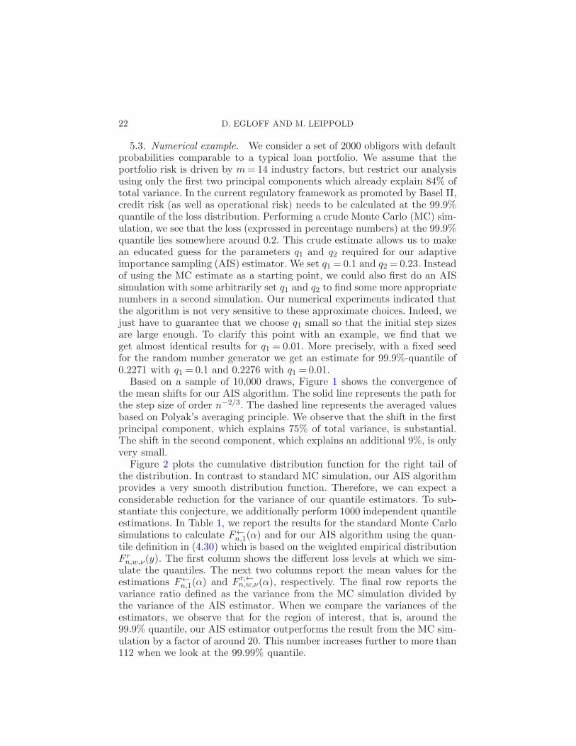
5.3. Numerical example. We consider a set of 2000 obligors with defaultprobabilities comparable to a typical loan portfolio. We assume that theportfolio risk is driven by m= 14 industry factors, but restrict our analysisusing only the first two principal components which already explain 84% oftotal variance. In the current regulatory framework as promoted by Basel II,credit risk (as well as operational risk) needs to be calculated at the 99.9%quantile of the loss distribution. Performing a crude Monte Carlo (MC) sim-ulation, we see that the loss (expressed in percentage numbers) at the 99.9%quantile lies somewhere around 0.2. This crude estimate allows us to makean educated guess for the parameters q1 and q2 required for our adaptiveimportance sampling (AIS) estimator. We set q1 = 0.1 and q2 = 0.23. Insteadof using the MC estimate as a starting point, we could also first do an AISsimulation with some arbitrarily set q1 and q2 to find some more appropriatenumbers in a second simulation. Our numerical experiments indicated thatthe algorithm is not very sensitive to these approximate choices. Indeed, wejust have to guarantee that we choose q1 small so that the initial step sizesare large enough. To clarify this point with an example, we find that weget almost identical results for q1 = 0.01. More precisely, with a fixed seedfor the random number generator we get an estimate for 99.9%-quantile of0.2271 with q1 = 0.1 and 0.2276 with q1 = 0.01.

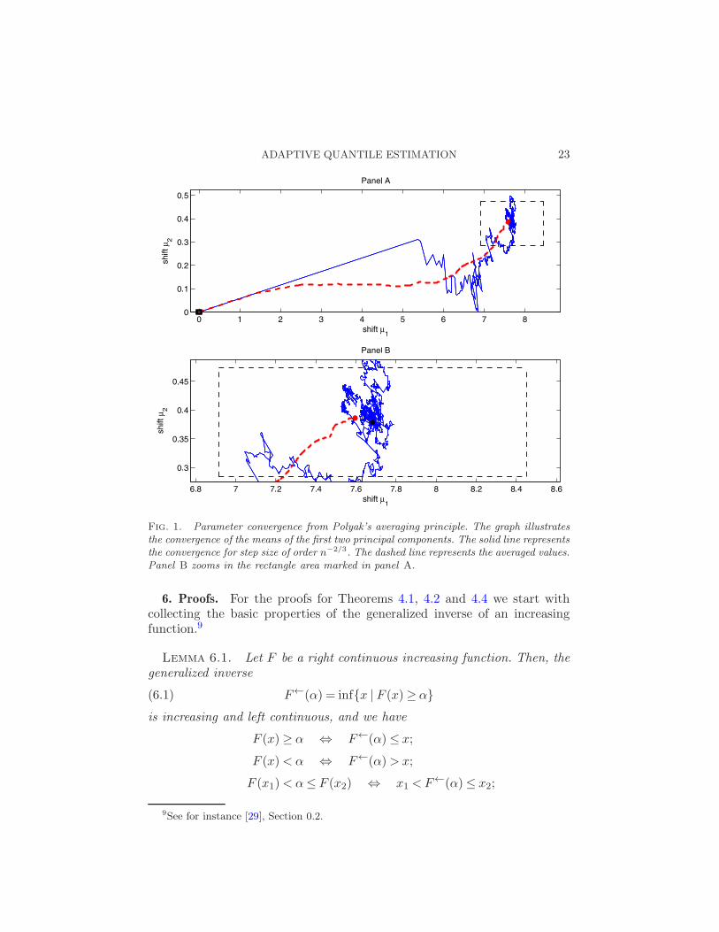
Based on a sample of 10,000 draws, Figure 1 shows the convergence ofthe mean shifts for our AIS algorithm. The solid line represents the path forthe step size of order n−2/3. The dashed line represents the averaged valuesbased on Polyak’s averaging principle. We observe that the shift in the firstprincipal component, which explains 75% of total variance, is substantial.The shift in the second component, which explains an additional 9%, is onlyvery small.

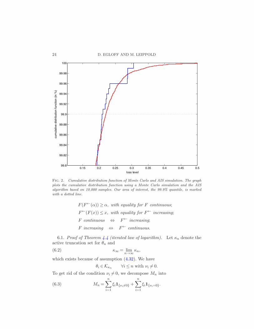
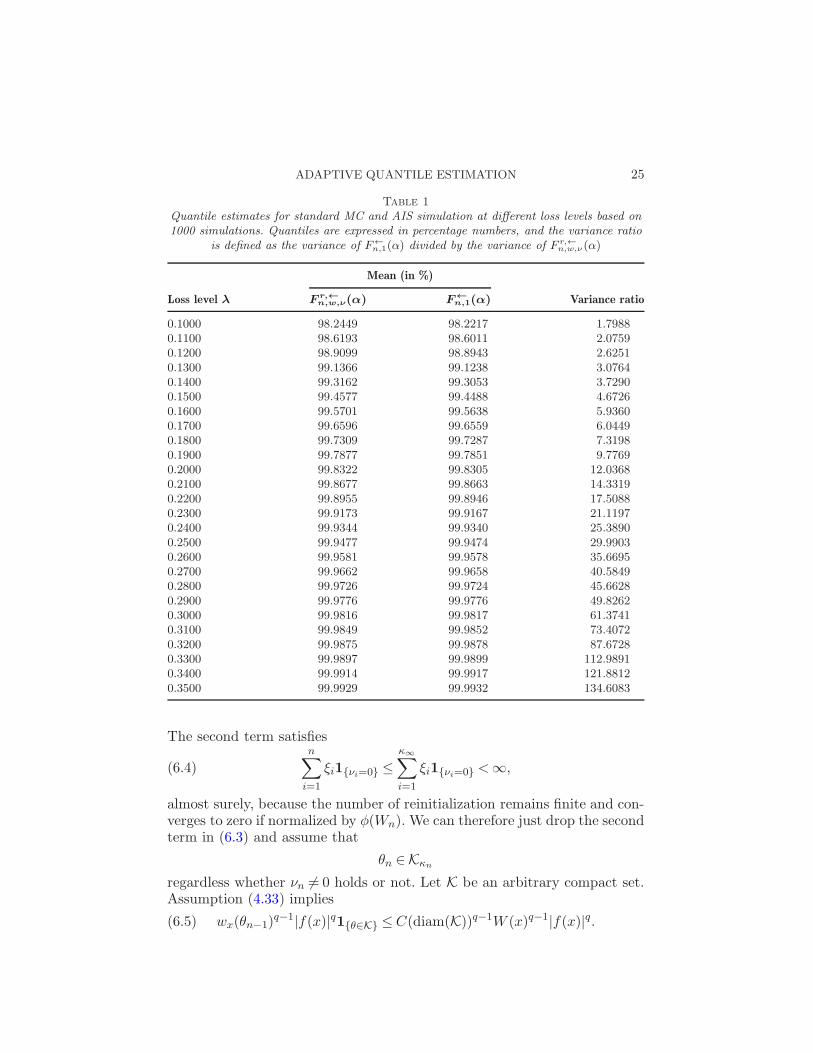
Figure 2 plots the cumulative distribution function for the right tail ofthe distribution. In contrast to standard MC simulation, our AIS algorithmprovides a very smooth distribution function. Therefore, we can expect aconsiderable reduction for the variance of our quantile estimators. To sub-stantiate this conjecture, we additionally perform 1000 independent quantileestimations. In Table 1, we report the results for the standard Monte Carlosimulations to calculate F←n,1(α) and for our AIS algorithm using the quan-tile definition in (4.30) which is based on the weighted empirical distributionF rn,w,ν(y). The first column shows the different loss levels at which we sim-

ulate the quantiles. The next two columns report the mean values for theestimations F←n,1(α) and F r,←

n,w,ν(α), respectively. The final row reports thevariance ratio defined as the variance from the MC simulation divided bythe variance of the AIS estimator. When we compare the variances of theestimators, we observe that for the region of interest, that is, around the99.9% quantile, our AIS estimator outperforms the result from the MC sim-ulation by a factor of around 20. This number increases further to more than112 when we look at the 99.99% quantile.


Fig. 1. Parameter convergence from Polyak’s averaging principle. The graph illustrates

the convergence of the means of the first two principal components. The solid line represents

the convergence for step size of order n−2/3. The dashed line represents the averaged values.

Panel B zooms in the rectangle area marked in panel A.

6. Proofs. For the proofs for Theorems 4.1, 4.2 and 4.4 we start withcollecting the basic properties of the generalized inverse of an increasingfunction.9

Lemma 6.1. Let F be a right continuous increasing function. Then, thegeneralized inverse

F←(α) = inf{x | F (x)≥ α}(6.1)

is increasing and left continuous, and we have

F (x)≥ α ⇔ F←(α)≤ x;

F (x)< α ⇔ F←(α)>x;

F (x1)< α≤ F (x2) ⇔ x1 <F←(α)≤ x2;

9See for instance [29], Section 0.2.


Fig. 2. Cumulative distribution function of Monte Carlo and AIS simulation. The graph

plots the cumulative distribution function using a Monte Carlo simulation and the AIS

algorithm based on 10,000 samples. Our area of interest, the 99.9% quantile, is marked

with a dotted line.

F (F←(α)) ≥ α, with equality for F continuous;

F←(F (x))≤ x, with equality for F← increasing;

F continuous ⇔ F← increasing;

F increasing ⇔ F← continuous.

6.1. Proof of Theorem 4.4 (iterated law of logarithm). Let κn denote theactive truncation set for θn and

κ∞ = limn→∞

κn,(6.2)

which exists because of assumption (4.32). We have

θi ∈Kκn ∀i≤ n with νi 6= 0.

To get rid of the condition νi 6= 0, we decompose Mn into

Mn =n∑

i=1

ξi1{νi 6=0} +n∑

i=1

ξi1{νi=0}.(6.3)


Table 1

Quantile estimates for standard MC and AIS simulation at different loss levels based on

1000 simulations. Quantiles are expressed in percentage numbers, and the variance ratio

is defined as the variance of F←n,1(α) divided by the variance of F r,←n,w,ν (α)

Mean (in %)

Loss level λ Fr,←

n,w,ν(α) F←

n,1(α) Variance ratio

0.1000 98.2449 98.2217 1.79880.1100 98.6193 98.6011 2.07590.1200 98.9099 98.8943 2.62510.1300 99.1366 99.1238 3.07640.1400 99.3162 99.3053 3.72900.1500 99.4577 99.4488 4.67260.1600 99.5701 99.5638 5.93600.1700 99.6596 99.6559 6.04490.1800 99.7309 99.7287 7.31980.1900 99.7877 99.7851 9.77690.2000 99.8322 99.8305 12.03680.2100 99.8677 99.8663 14.33190.2200 99.8955 99.8946 17.50880.2300 99.9173 99.9167 21.11970.2400 99.9344 99.9340 25.38900.2500 99.9477 99.9474 29.99030.2600 99.9581 99.9578 35.66950.2700 99.9662 99.9658 40.58490.2800 99.9726 99.9724 45.66280.2900 99.9776 99.9776 49.82620.3000 99.9816 99.9817 61.37410.3100 99.9849 99.9852 73.40720.3200 99.9875 99.9878 87.67280.3300 99.9897 99.9899 112.98910.3400 99.9914 99.9917 121.88120.3500 99.9929 99.9932 134.6083

The second term satisfiesn∑

i=1

ξi1{νi=0} ≤κ∞∑

i=1

ξi1{νi=0} <∞,(6.4)

almost surely, because the number of reinitialization remains finite and con-verges to zero if normalized by φ(Wn). We can therefore just drop the secondterm in (6.3) and assume that

θn ∈Kκn

regardless whether νn 6= 0 holds or not. Let K be an arbitrary compact set.Assumption (4.33) implies

wx(θn−1)q−1|f(x)|q1{θ∈K} ≤C(diam(K))q−1W (x)q−1|f(x)|q.(6.5)


By Holder’s inequality, we have for q < p and all θ ∈K,

mq,f(θ)1{θ∈K} = Eθ0 [wX(θ)q−1|f(X)|q1{θ∈K}]

≤ ‖f‖qθ0,pC(diam(K))q−1Eθ0 [W (X)p(q−1)/(p−q)](p−q)/q(6.6)

<∞as long as q satisfies the condition

q <p(p∗ +1)

p+ p∗.(6.7)

Note that (6.7) implies also q < p because p(p∗+1)p+p∗ ≤ p for p ≥ 1. Condition

(4.63) implies

mq,f (θ)<∞ ∀1≤ q ≤ 4.(6.8)

Let K be a compact neighborhood of θ∗. Lebesgue’s theorem together withthe continuity condition (4.64) and the upper bound (6.5), which is inte-grable by (6.6), shows that

mf,q : θ 7→mf,q(θ)(6.9)

is continuous for q ≤ 4. Without loss of generality, we assume from now onthat E[f(X)] = 0. By assumptions (4.33) and (4.34), we have for q < p anda > 1

E[wXn(θn−1)q|f(Xn)|q1{κ∞=j} | Fi−1]

= Eθ0 [wXn(θn−1)q−1|f(Xn)|q1{κ∞=j}]

≤ ‖f‖qθ0,pEθ0 [wXn(θn−1)p(q−1)/(p−q)

1{κ∞=j}](p−q)/p

≤ ‖f‖qθ0,pP(κ∞ = j)(p−q)/p1/a,

Eθ0 [wXn(θn−1)p(q−1)/(p−q)a/(a−1)

1{κ∞=j}](p−q)/p(a−1)/a

≤ ‖f‖qθ0,pC(ρ)(p−q)/p1/aekp∗(p−q)/p1/a

× (ρ(p−q)/p1/a+p(q−1)/(p−q)mp∗ logρ(e))j‖W‖q−1θ0,q1<∞,

if q1 ≤ p∗ holds for

q1 =p(q− 1)

p− q

a

a− 1.(6.10)

We may choose a arbitrarily large at the expense of increasing the constantin the above estimate. Therefore, q1 ≤ p∗ holds if

p(q − 1)

p− q< p∗(6.11)


which is equivalent to (6.7). Next, we choose

ρ < e−amp∗p(q−1)/(p−q),(6.12)

such that we can sum over j = 1, . . . ,∞ to obtain

mf,q(θn−1) = E[wXn(θn−1)q|f(Xn)|q | Fn−1]

=∞∑

j=1

E[wXn(θn−1)q|f(Xn)|q1{κ∞=j} | Fn−1]

<C(ρ, a, p, p∗, q,‖f‖θ0,p,‖W‖θ0,p∗)

with an upper bound independent of n. Assumption (4.63) implies that

supn

E[mf,q(θn−1)]<∞ ∀1≤ q ≤ 4.(6.13)

We have

〈M〉n =

n∑

i=1

(mf,2(θi−1)−E[f(X)]2).(6.14)

Because θ 7→ mf,2(θ) is continuous at θ∗ and θi−1 → θ∗ almost surely, weobtain from Cesaro’s lemma that

〈M〉nn

=1

n

n∑

i=1

(mf,2(θi−1)−E[f(X)]2) → mf,2(θ∗)−E[f(X)]2 = σ2

f (θ∗),

almost surely. By (6.13) and Lebesgue’s dominated convergence theorem,

s2nn

=E[〈M〉n]

n→ σ2

f (θ∗).(6.15)

Set

Mn =n∑

i=1

(ξ2i − E[ξ2i | Fi−1]).

By (6.13) Mn is a square integrable martingale because

E[∆M2i | Fi−1] = E[(ξ2i − E[ξ2i | Fi−1])

2 | Fi−1]

≤ 8(mf,4(θi−1) +E[f(X)]4).

More precisely,

E[∆M2i | Fi−1] =mf,4(θi−1)−mf,2(θi−1)

2 − 4mf,3(θi−1)E[f(X)]

+ 8mf,2(θi−1)E[f(X)]2 − 4E[f(X)]4.


The continuity of θ 7→mf,p(θ) in θ∗ for 1≤ p≤ 4 and Cesaro’s lemma imply

1

n

n∑

i=1

E[∆M2i | Fi−1]

→mf,4(θ∗)−mf,2(θ

∗)2 − 4mf,3(θ∗)E[f(X)](6.16)

+ 8mf,2(θ∗)E[f(X)]2 − 4E[f(X)]4,

almost surely, which together with (6.15) implies

limn→∞

s−2n

n∑

i=1

(ξ2i − E[ξ2i | Fi−1]) = limn→∞

1

n

n∑

i=1

(ξ2i − E[ξ2i | Fi−1]) = 0,(6.17)

almost surely. Therefore,

limn→∞

[M ]n〈M〉n

= 1+ limn→∞

(〈M〉nn

)−1 1n

n∑

i=1

(ξ2i −E[ξ2i | Fi−1]) = 1,(6.18)

almost surely. To apply Corollary 4.2 in [15], we need to verify the threeconditions:

s−2n [M ]n → η2 > 0 almost surely;(6.19)

∀ε > 0

∞∑

n=1

s−1n E[|ξn|1{|ξn|>εsn}]<∞;(6.20)

∃δ > 0∞∑

n=1

s−4n E[|ξn|41{|ξn|≤δsn}]<∞.(6.21)

Condition (6.19) holds because

limn→∞

[M ]ns2n

= limn→∞

(

s2nn

)−1 〈M〉nn

+ limn→∞

s−2n

n∑

i=1

(ξ2i −E[ξ2i | Fi−1])(6.22)

= 1,

almost surely, as a consequence of (6.15) and (6.17). By (6.15), we mayreplace s2n by n for the verification of conditions (6.20) and (6.21).

Let 1< a < 2. We first approach (6.20). From Holder’s and Chebyshev’sinequalities, we have

√n−1

E[|ξn|1{|ξn|>ε√n}]

≤√n−1

E[|ξn|2a]1/(2a)P(|ξn|> ε√n)1−1/(2a)


(6.23)

≤√n−1

E[|ξn|2a]1/(2a)E[|ξn|2a]1−1/(2a)(

1

ε√n

)2a−1

≤ ε1−2aE[|ξn|2a]n−a

for every fixed ε > 0. Therefore,

∞∑

n=1

√n−1

E[|ξn|1{|ξn|>ε√n}]≤ ε1−2a

∞∑

n=1

E[|ξn|2a]n−a <∞.(6.24)

This last equation implies condition (6.20). To check condition (6.21), notethat

∞∑

n=1

n−2E[|ξn|41{|ξn|≤δ√n}]≤∞∑

n=1

n−2E[(δ√n)4−2a|ξn|2a1{|ξn|≤δ√n}]

(6.25)

≤ δ4−2a∞∑

n=1

n−aE[|ξn|2a]<∞.

The sums (6.24) and (6.25) are finite because

E[|ξn|2a | Fn−1]≤ 22a−1(mf,2a(θn) +E[f(X)]2a),(6.26)

and supnE[mf,2a(θn)]<∞, as shown in (6.13).

6.2. Proof of Theorem 4.2. Under the assumptions of Theorem 4.2, theboundedness of the functions

fy = 1(−∞,y] ◦Ψ, 1− fy, y ∈R(6.27)

allows us to apply the law of iterated logarithm (Theorem 4.4). We verifythe convergence statement by proving that

P(qn,w,ν(α)≤ qα − δ i.o.) = 0 ∀δ > 0,(6.28)

and

P(qn,w,ν(α)> qα i.o.) = 0,(6.29)

where i.o. stands for infinitely often and is defined as

An i.o. = limsupn

An =∞⋂

n=1

∞⋃

k=n

Ak.(6.30)

Let F (y) = P(Y ≤ y) denote the distribution function of Y =Ψ(X). We firstanalyze the estimator qn,w,ν(α). Define

An(δ) = {qn,w,ν(α)≤ qα − δ}.(6.31)


It follows from (4.26) and Lemma 6.1 that

An(δ) =

{

1

ν(n)∑

iwi

∑

i

wi1{Yi≤qα−δ} ≥ α

}

(6.32)

=

{

∑

i

(wi1{Yi≤qα−δ} −F (qα − δ))≥ ν(n)α∑

i

wi − nF (qα − δ)

}

.

Let

Wn(η) =

{∣

∣

∣

∣

∑

i

(wi − 1)

∣

∣

∣

∣

≤ (1 + η)φ(nv)

}

.(6.33)

We consider

An(δ)⊂An(δ) ∩Wn(η) ∪ ∁Wn(η).(6.34)

Then

An(δ) ∩Wn(η)

⊂{

∑

i

(wi1{Yi≤qα−δ} − F (qα − δ))(6.35)

≥ ν(n)α(n− (1 + η)φ(nv))− nF (qα − δ)

}

.

Similarly, we have

Bn = {qn,w,ν(α)> qα}(6.36)

=

{

∑

i

(wi1{Yi≤qα} −F (qα))< ν(n)α∑

i

wi − nF (qα)

}

and

Bn ∩Wn(η)

⊂{

∑

i

(wi1{Yi≤qα} −F (qα))(6.37)

< ν(n)α(n+ (1 + η)φ(nv))− nF (qα)

}

.

For arbitrary η > 0, let

ALILn (δ, η) =

{

∑

i

(wi1{Yi≤qα−δ} −F (qα − δ))≥ (1 + η)φ(nvqα−δ)

}

(6.38)


and

BLILn (η) =

{

∑

i

(wi1{Yi≤qα} −F (qα))≤−(1 + η)φ(nvα)

}

.(6.39)

Then1+ η

αφ(nvqα−δ) +

F (qα − δ)

αn≤ ν(n)(n− (1 + η)φ(nv))

(6.40)=⇒ An(δ) ∩Wn(η)⊂ALIL

n (δ, η)

and

ν(n)(n+ (1 + η)φ(nv))≤ F (qα)

αn− 1 + η

αφ(nvα)

(6.41)=⇒ Bn ∩Wn(η)⊂BLIL

n (δ, η).

Recall that

lim supn

(An ∪Bn) = limsupn

An ∪ lim supn

Bn.(6.42)

Hence, if (6.40) is satisfied, we have

P(An(δ) i.o.)≤ P(An(δ) ∩Wn(η) i.o.) + P(∁Wn(η) i.o.)(6.43)

≤ P(ALILn (δ, η) i.o.) + P(∁Wn(η) i.o.).

From the law of iterated logarithm in Theorem 4.4, we know that

P(ALILn (δ, η) i.o.) = 0, P(∁Wn(η) i.o.) = 0.(6.44)

Therefore, P(An(δ) i.o.) = 0 for all δ > 0. In the same way, we obtain

P(Bn i.o.) = 0.(6.45)

To verify that condition (4.36) implies (6.41) and (6.41), it is sufficient tonote that F (qα)≥ α. Because F (qα − δ)<α, it follows that

1 + η

αφ(nvqα−δ) +

F (qα − δ)

αn≤ n− kn1/2+γ

for n large enough and for all δ > 0.The convergence proof for qrn,w,ν(α) is slightly simpler. From (4.29) and

Lemma 6.1, we get

Arn(δ) = {qrn,w,ν(α)≤ qα − δ}

=

{

1− 1

ν(n)

∑

i

wi1{Yi>qα−δ} ≥ α

}

(6.46)

=

{

∑

i

(wi1{Yi>qα−δ} − (1− F (qα − δ)))

≤ ν(n)(1−α)− n(1−F (qα − δ))

}


and

Brn = {qrn,w,ν(α)> qα}

=

{

∑

i

(wi1{Yi>qα} − (1−F (qα)))(6.47)

> ν(n)(1−α)− n(1− F (qα))

}

.

For arbitrary η > 0, let

Ar,LILn (δ, η) =

{

∑

i

(wi1{Yi>qα−δ} − (1− F (qα − δ)))

(6.48)

≤−(1 + η)φ(nvqα−δ)

}

and

Br,LILn (η) =

{

∑

i

(wi1{Yi>qα} − (1− F (qα)))≥ (1 + η)φ(nvα)

}

.(6.49)

We have

ν(n)≤ 1− F (qα − δ)

1−αn− 1 + η

1−αφ(nvqα−δ)

(6.50)=⇒ Ar

n(δ)⊂Ar,LILn (δ, η),

and

1+ η

1− αφ(nvα) +

1− F (qα)

1−αn≤ ν(n) =⇒ Br

n ⊂Br,LILn (η).(6.51)

By the law of iterated logarithm (Theorem 4.4), we obtain

P(Ar,LILn (δ, η) i.o.) = 0,P(Br,LIL

n (η) i.o.) = 0.(6.52)

Therefore, conditions (6.50) and (6.51) are sufficient to guarantee (6.28) and(6.29) for qrn,w,ν. Because 1− F (qα)≤ 1− α and 1− F (qα − δ) > 1− α forall δ > 0, condition (4.38) is sufficient for (6.50) and (6.51).

In a completely analogous manner, we obtain

Aln(δ) = {qln,w,ν(α)≤ qα − δ}

(6.53)

=

{

∑

i

(wi1{Yi≤qα−δ} − F (qα − δ))≥ ν(n)α− nF (qα − δ)

}


and

Bln = {qln,w,ν(α)> qα}

(6.54)

=

{

∑

i

(wi1{Yi≤qα} −F (qα))< ν(n)α− nF (qα)

}

.

This time, let, for η > 0,

Al,LILn (δ, η) =

{

∑

i

(wi1{Yi≤qα−δ} −F (qα − δ))≥ (1 + η)φ(nvqα−δ)

}

(6.55)

and

Bl,LILn (η) =

{

∑

i

(wi1{Yi≤qα} − F (qα))≤−(1 + η)φ(nvα)

}

.(6.56)

We have

1 + η

αφ(nvqα−δ) +

F (qα − δ)

αn≤ ν(n) =⇒ Al

n(δ)⊂Al,LILn (δ, η)(6.57)

and

ν(n)≤ F (qα)

αn− 1 + η

αφ(nvα) =⇒ Bl

n ⊂Bl,LILn (η).(6.58)

By the law of iterated logarithm, equations (6.57) and (6.58) are a sufficientcondition to guarantee (6.28) and (6.29) for qln,w,ν. Similarly as above, (4.40)is sufficient for (6.57) and (6.58). This proves Theorem 4.2.

6.3. Proof of Theorem 4.1. We again apply the law of iterated logarithm4.4. We only prove the result for qn,w,ν(α). The other estimators are treatedanalogously. Because F is increasing in qα, it follows that F

← is continuousin α. It is sufficient to prove for any δ > 0 that

P(qn,w,ν(α)≤ qα − δ i.o.) = 0(6.59)

and

P(qn,w,ν(α)> qα + δ i.o.) = 0.(6.60)

For ν(n)≡ 1, we obtain from (6.40),

1 + η

αφ(nvqα−δ) +

F (qα − δ)

αn+ (1 + η)φ(nv)≤ n

(6.61)=⇒ An(δ) ∩Wn(η)⊂ALIL

n (δ, η).


If we define

Bn(δ) = {qn,w,ν(α)> qα + δ}(6.62)

=

{

∑

i

(wi1{Yi≤qα+δ} −F (qα + δ))<α∑

i

wi − nF (qα + δ)

}

,

we deduce

n≤ F (qα + δ)

αn− (1 + η)φ(nv)− 1 + η

αφ(nvqα+δ)

(6.63)=⇒ Bn(δ) ∩Wn(η)⊂BLIL

n (δ, η).

For any δ > 0, F (qα − δ) < α and F (qα + δ) > α. Therefore, if n is largeenough, conditions (6.61) and (6.63) are satisfied. We conclude as in theproof of Theorem 4.2.

6.4. Proof of Proposition 4.1. Let K be a compact subset ofW . We applyMarkov’s and Burkholder’s inequality,

P

(

maxk≤n

‖S1,k(γ,ǫ,K)‖> δ)

≤ Bp

δpE

[(

1{n≤σ(K,ǫ)}

n∑

k=1

γ2k‖H(Xk, θk−1)− h(θk−1)‖2)p/2]

≤ 2pBp

δp

(

n∑

k=1

γ2kE[1{k−1≤n≤σ(K,ǫ)}(‖H(Xk, θk−1)‖p

+ ‖h(θk−1)‖p)]2/p)p/2

,

where Bp is a universal constant only depending on p. To estimate

E[1{k−1≤n≤σ(K,ǫ)}(‖H(Xk, θk−1)‖p)]2/p,

note that by our assumptions

E[1{k−1≤n≤σ(K,ǫ)}‖H(Xk, θk−1)‖p]2/p

= E[1{k−1≤σ(K,ǫ)}Eθk−1[‖H(Xk, θk−1)‖p]]2/p

= E

[

1{k−1≤σ(K,ǫ)}Eθ0

[ ‖H(Xk, θk−1)‖pwθk−1

(Xk)W p(Xk)W p(Xk)

]]2/p

=C2KE[1{k−1≤σ(K,ǫ)}Eθ0 [W

p(Xk)]]2/p ≤C2

K‖W‖2θ0,p ,


where the constant CK comes from assumption (4.54). Because h is contin-uous and K compact, 1{k−1≤σ(K,ǫ)}‖h(θk−1)‖ is bounded as well. Therefore,we arrive at the estimate

P

(

maxk≤n

‖S1,k(γ,ǫ,K)‖> δ)

≤C1

δp

(

n∑

k=1

γ2k

)p/2

.

The bound

Pγ

Φ(x,θ)(ν(ǫ)<K)≤C

n∑

k=1

(

γkǫk

)p

is derived similarly as in the proof of Proposition 5.2 in [1] .

Acknowledgments. We would like to thank Michael Wolf and seminarparticipants at the IBM Research Lab, Ruschlikon, and the Deutsche Bun-desbank in Frankfurt for their comments. Part of this research has beencarried out within the National Center of Competence in Research “Fi-nancial Valuation and Risk Management” (NCCR FINRISK). The NCCRFINRISK is a research program supported by the Swiss National ScienceFoundation.

REFERENCES

[1] Andrieu, C., Moulines, E. and Priouret, P. (2005). Stability of stochastic ap-proximation under verifiable conditions. SIAM J. Control Optim. 44 283–312.MR2177157

[2] Arouna, B. (2004). Adaptive Monte Carlo method, a variance reduction technique.Monte Carlo Methods Appl. 10 1–24. MR2054568

[3] Arouna, B. (2004). Robbins–Monro algorithms and variance reduction in finance.J. Computational Finance 7 35–62.

[4] Avramidis, A. N. and Wilson, J. R. (1998). Correlation-induction techniques forestimating quantiles in simulation experiments. Oper. Res. 46 574–591.

[5] Benveniste, A., Metiver, M. and Priouret, P. (1990). Adaptive Algorithms and

Stochastic Approximations. Springer, Berlin. MR1082341[6] Chen, H. F. (2002). Stochastic Approximation and Its Applications. Nonconvex Op-

timization and Its Applications 64. Kluwer, Dordrecht. MR1942427[7] Chen, H. F., Guo, L. and Gao, A. J. (1988). Convergence and robustness of the

Robbins–Monro algorithm truncated at randomly varying bounds. StochasticProcess. Appl. 27 217–231. MR0931029

[8] Delyon, B. (1996). General results on the convergence of stochastic algorithms.IEEE Transactions on Automatic Control 41 1245–1256. MR1409470

[9] Delyon, B. (2000). Stochastic approximation with decreasing gain: Convergence andasymptotic theory. Technical report, Publication Interne 952, IRISA.

[10] Delyon, B., Lavielle, M. and Mouliens, E. (1999). Convergence of a stochasticapproximation version of the EM algorithm. Ann. Statist. 27 94–128. MR1701103

[11] Egloff, D., Leippold, M. and Vanini, P. (2007). A simple model of credit conta-gion. Journal of Banking and Finance 8 2475–2492.

http://www.ams.org/mathscinet-getitem?mr=2177157








[12] Feldman, D. and Tucker, H. G. (1966). Estimation of non-unique quantiles. Ann.Math. Statist. 37 451–457. MR0189189

[13] Glasserman, P. and Li, J. (2005). Importance sampling for portfolio credit risk.Management Sci. 51 1643–1656.

[14] Glasserman, P. and Wang, Y. (1997). Counterexamples in importance samplingfor large deviation probabilities. Ann. Appl. Probab. 7 731–746. MR1459268

[15] Hall, P. and Heyde, C. C. (1980). Martingale Limit Theory and its Applications.Academic Press, New York. MR0624435

[16] Hesterberg, T. and Nelson, B. L. (1998). Control variates for probability andquantile estimation. Management Sci. 44 1295–1312.

[17] Heyde, C. C. (1977). On central limit and iterated logarithm supplements to themartingale convergence theorem. J. Appl. Probab. 14 758–775. MR0517475

[18] Hsu, J. C. and Nelson, B. L. (1990). Control variates for quantile estimation.Management Sci. 36 835–851. MR1069856

[19] Jin, X., Fu, M. C. and Xiong, X. (2003). Probabilistic error bounds for simulationquantile estimators. Management Sci. 14 230–246.

[20] Jost, J. (2005). Riemannian Geometry and Geometric Analysis. Springer, Berlin.MR2165400

[21] Kiefer, J. and Wolfowitz, J. (1952). Stochastic estimation of the maximum of aregression function. Ann. Math. Statist. 23 462–466. MR0050243

[22] Kobayashi, S. and Nomizu, K. (1996). Foundations of Differential Geometry. I, II.Wiley, Chichester.

[23] Kushner, H. J. and Clark, D. S. (1978). Stochastic Approximation Methods for

Constrained and Unconstrained Systems. Springer, New York. MR0499560[24] Kushner, H. J. and Yin, G. G. (1997). Stochastic Approximation Algorithms and

Applications. Springer, New York. MR1453116[25] Ljung, L., Pflug, G. and Walk, H. (1992) Stochastic Approximation and Opti-

mization of Random Systems. Birkhaeuser, Basel. MR1162311[26] Merino, S. and Nyfeler, M. (2004). Applying importance sampling for estimating

coherent credit risk contributions. Quantitative Finance 4 199–207.[27] Polyak, B. and Juditsky, A. (1992). Acceleration of stochastic approximation by

averaging. SIAM J. Control Optim. 30 838–855. MR1167814[28] Rao, C. R. (1945). Information and the accuracy atainable in the estimation of

statistical parameters. Bull. Calcutta Math. Soc. 37 81–91. MR0015748[29] Resnick, S. (1987). Extreme Values, Regular Variation, and Point Processes.

Springer, New York. MR0900810[30] Robbins, H. andMonro, S. (1951). A stochastic approximation method. Ann. Math.

Statist. 22 400–407. MR0042668[31] Smirnov, N. (1952). Limit distribution for the terms of a variational series. Amer.

Math. Soc. Translation 1952 64. MR0047277[32] Tierney, L. (1983). A space-efficient recursive procedure for estimating a quantile of

an unknown distribution. SIAM J. Sci. Statist. Comput. 4 706–711. MR0725662[33] van der Vaart, A. W. (1998). Asymptotic Statistics. Cambridge Univ. Press, Cam-

bridge. MR1652247

QuantCatalyst

8000 Zurich

Switzerland

E-mail: [email protected]

Swiss Banking Institute

University of Zurich

Plattenstrasse 14

8032 Zurich

Switzerland

E-mail: [email protected]


















mailto:[email protected]

mailto:[email protected]

quantile estimation with adaptive importance sampling

Documents