automatic bayesian quantile regression curve fitting
TRANSCRIPT
Stat Comput (2009) 19: 271–281DOI 10.1007/s11222-008-9091-x
Automatic Bayesian quantile regression curve fitting
Colin Chen · Keming Yu
Received: 26 August 2006 / Accepted: 31 July 2008 / Published online: 3 October 2008© Springer Science+Business Media, LLC 2008
Abstract Quantile regression, including median regression,as a more completed statistical model than mean regres-sion, is now well known with its wide spread applications.Bayesian inference on quantile regression or Bayesian quan-tile regression has attracted much interest recently. Most ofthe existing researches in Bayesian quantile regression focuson parametric quantile regression, though there are discus-sions on different ways of modeling the model error by aparametric distribution named asymmetric Laplace distrib-ution or by a nonparametric alternative named scale mix-ture asymmetric Laplace distribution. This paper discussesBayesian inference for nonparametric quantile regression.This general approach fits quantile regression curves us-ing piecewise polynomial functions with an unknown num-ber of knots at unknown locations, all treated as parame-ters to be inferred through reversible jump Markov chainMonte Carlo (RJMCMC) of Green (Biometrika 82:711–732, 1995). Instead of drawing samples from the posterior,we use regression quantiles to create Markov chains for theestimation of the quantile curves. We also use approximateBayesian factor in the inference. This method extends thework in automatic Bayesian mean curve fitting to quan-tile regression. Numerical results show that this Bayesianquantile smoothing technique is competitive with quan-tile regression/smoothing splines of He and Ng (Comput.Stat. 14:315–337, 1999) and P-splines (penalized splines)
C. Chen (�)SAS Institute Inc., SAS Campus Drive, Cary, NC 27513, USAe-mail: [email protected]
K. YuDepartment of Mathematical Sciences, Brunel University,Uxbridge, UB8 3PH, UKe-mail: [email protected]
of Eilers and de Menezes (Bioinformatics 21(7):1146–1153,2005).
Keywords Asymmetric Laplace distribution · Piecewisepolynomials · Quantile regression · Reversible jumpMarkov chain Monte Carlo · Splines
1 Introduction
Quantile regression, which computes conditional quantiles,has become a valuable alternative to conditional meanbased regression techniques (Koenker 2005). Nonparamet-ric quantile regression assumes that the conditional quan-tile of the response variable as a function of the explana-tory variable belongs to a nonparametric function class,for example, splines. Such nonparametric functions areusually fitted to generate smoothing quantile curves. Bothkernel-based functions (Chaudhuri 1991; Yu and Jones1998) and spline-based functions (Koenker et al. 1994;He and Ng 1999) have been used for smoothing quantilecurve fitting. However, as in the conditional mean basedsmoothing techniques, the bandwidth of the kernel methodand the smoothing parameters (or knots) of the splinemethod need to be specified a priori.
In this paper, we develop automatic quantile curve fit-ting with a Bayesian method. The Bayesian method appliesthe reversible jump Markov chain Monte Carlo approach ofGreen (1995), which has the ability to travel across func-tion spaces with different dimensions. This flexibility in ad-dition to the free choice of a prior empowers the RJMCMCto fit various smoothing or non-smoothing functions withhigh accuracy as shown in the conditional mean case byDenison et al. (1998), DiMatteo et al. (2001), Hansen andKooperberg (2002), and others. The method is automatic in
272 Stat Comput (2009) 19: 271–281
the sense that the smoothing parameters and knots are auto-matically selected in the fitting procedure based on data.
To fit conditional quantile functions (curves), we use awell-defined likelihood function—the asymmetric Laplacelikelihood function with both location and scale parameters
gτ (y|μ,σ) = τ(1 − τ)
σe− τ (y−μ)++(1−τ )(y−μ)−
σ , (1)
where (·)+ and (·)− represent the positive and negative partof the quantity, respectively. With this likelihood function,we are able to approximate the marginal likelihood ratioof the number of knots and their locations. This ratio, alsocalled the Bayesian factor, plays an important rule in modelselection through the accept/reject probability in RJMCMCas shown by DiMatteo et al. (2001) in the case of conditionalmean.
By fitting constrained quantile regression for each speci-fied model, the Bayesian method can fit constrained quantilesmoothing curves, which was studied by He and Ng (1999)using smoothing and regression B-splines.
Nonparametric quantile regression with RJMCMC hasbeen studied by Yu (2002) with an emphasis on quantileclouds. The current paper has two improvements. First, in-stead of the check function used by Yu (2002)
ρτ (y,μ) = τ(y − μ)+ + (1 − τ)(y − μ)−, (2)
we use the proper likelihood function gτ (y|μ,σ) in (1),which is more flexible with the extra scale parameter σ .Such flexibility improves the convergence speed of RJM-CMC as experienced in our implementations. Second, theplug-in method of Denison et al. (1998) for knot-selectionused by Yu (2002) does not consider the penalty on dimen-sionality; therefore, it always overfits as pointed out by Di-Matteo et al. (2001). In this paper we implement a morecomplete Bayesian method on quantile curve fitting. We ex-plore various prior specifications and moving strategies withRJMCMC. We also compare our method with the adaptiveregression spline method of He and Ng (1999) and the P-spline method of Eilers and de Menezes (2005).
In Sect. 2 we introduce Bayesian quantile regression withthe asymmetric Laplace likelihood and piecewise polyno-mial functions. In Sect. 3 we discuss the choice of priorsand likelihood ratio approximation, which decide the knot-selection rule. Section 4 describes the moving strategies forRJMCMC. The complete algorithm is described in Sect. 5.Section 6 illustrates our approach with some examples. Wealso provide performance comparison and robustness analy-sis with numerical results in Sect. 6. Some discussion isgiven in Sect. 7.
2 Bayesian quantile regression with asymmetricLaplace likelihood
Assume that (yi, xi), i = 1, . . . , n, are independent bivari-ate observations from the pair of response-explanatory vari-ables (Y,X). Our goal is to find the τ th conditional quantileQτ(x) of Y given X = x. The method in this paper uses themodel with the asymmetric Laplace likelihood
fτ (y|x,σ ) = τ(1 − τ)
σe− τ (y−Qτ (x))++(1−τ )(y−Qτ (x))−
σ . (3)
The standard asymmetric Laplace distribution has the likeli-hood (1). Its unique mode μ, which satisfies
∫ μ
−∞ gτ (y|μ,σ)
dy = τ , is the τ th quantile. This property guarantees theconsistency of the maximum likelihood estimator (MLE) asan estimator of the τ th quantile. If σ is considered constant,the MLE of Qτ(x) is equivalent to the regression quantileintroduced by Koenker and Bassett (1978). Thus, regard-less of the original distribution of (Y,X), the asymmetricLaplace distribution of (3) is used to model the τ th regres-sion quantile. With the likelihood specified, Bayesian quan-tile regression provides posterior inference on parameters orfunctions of parameters in the model as described by Yu andMoyeed (2001).
As in typical nonparametric regression, the τ th condi-tional quantile of Y given X = x is assumed to be a non-parametric function, which belongs to the closure of a linearfunction space—here the piecewise polynomials
Pk,l(x) =l∑
v=0
βv,0(x − t0)v+ +
k∑
m=1
l∑
v=l0
βv,m(x − tm)v+, (4)
where ti , i = 0, . . . , k + 1, indexed in ascending order, arethe knot points with the boundary knots t0 = min{xi, i =1, . . . , n} and tk+1 = max{xi, i = 1, . . . , n}. Without loss ofgenerality, we assume that xi , i = 1, . . . , n, are in ascend-ing order. So, t0 = x1 and tk+1 = xn. l (≥ 0) is the order ofthe piecewise polynomials and l0 (≥ 0) controls the degreeof continuity at the knots. The special case with l = l0 = 3corresponds to the cubic splines. Piecewise polynomials Pk,l
were used by Denison et al. (1998) for mean-based curve fit-ting. In this paper, we assume that the nonparametric func-tion Qτ(x) is such a piecewise polynomial with l and l0 pre-decided, while the coefficients βv,m, the number of knotsk, and their locations ti are estimated with the data (yi, xi)
by RJMCMC of Green (1995). Let β = {βv,m,0 ≤ v ≤l,1 ≤ m ≤ k}, t = {ti ,1 ≤ i ≤ k}. (k, t, β, σ ) represents thefull vector of parameters in the model. RJMCMC estimatesQτ(x) as a function of (k, t, β, σ ). The following sectiondescribes the prior specification of (k, t, β, σ ).
Stat Comput (2009) 19: 271–281 273
3 Prior specification and likelihood ratio approximation
We specify a prior for parameters (k, t, β, σ ) hierarchically,
πk,t,β,σ (k, t, β, σ ) = πk,t (k, t)πβ(β|k, t, σ )πσ (σ ). (5)
First, we specify a prior for the model space, which is char-acterized by the first two parameters k and t . Then, we spec-ify a prior for the quantile function Qτ(x) in the specifiedmodel space. For the scale parameter σ , we use the nonin-formative prior πσ (σ ) = 1.
For the model space, a prior πk,t (k, t) can be further de-composed as
πk,t (k, t) = πk(k)πt (t |k). (6)
So, we first need to specify a prior πk(k) for the number ofknots k. We explore several proposals in the literature forfitting the conditional mean. The first one is a simple Pois-son distribution with mean γ suggested by Green (1995),and also used by Denison et al. (1998) and DiMatteo etal. (2001). The second one is the uniform prior on the setkmin, . . . , kmax, which has been used by Smith and Kohn(1996) and Hansen and Kooperberg (2002). The third one isthe geometric prior πk(k) ∝ exp(−ck) proposed by Hansenand Kooperberg (2002) based on the model selection crite-rion SIC (Schwarz-type information criterion).
With the number of knots k specified, the sequence ofknots ti , i = 1, . . . , k, are considered order statistics from theuniform distribution with candidate knot sites {x1, . . . , xn}as the state space. We also consider the candidate knots fromthe continuous state space (x1, xn).
When the model space has been specified, the τ th condi-tional quantile function
Qτ(x) =l∑
v=0
βv,0(x − t0)v+ +
k∑
m=1
l∑
v=l0
βv,m(x − tm)v+ (7)
is specified through the coefficients β . Let z be the vector ofthe basis of piecewise polynomials evaluated at x, then
Qτ(x) = z′β. (8)
Yu and Moyeed (2001) has considered a noninformativeprior on Rd for β , where d = l + 1 + k(l − l0 + 1), andverified that the posterior of β is proper. We show that thisprior also maintains the consistency between the marginallikelihood ratio of (k, t) and SIC.
A key step in RJMCMC is to decide the accept/rejectprobability for moves from one model (k, t) to anothermodel (k′, t ′). As shown by Green (1995) and Denison et al.(1998), the acceptance probability for our problem is
α = min
{
1,p(y|k′, t ′)p(y|k, t)
πk,t (k′, t ′)
πk,t (k, t)
q(k, t |k′, t ′)q(k′, t ′|k, t)
}
, (9)
where
p(y|k, t) =∫ ∫ n∏
i=1
fτ (yi |xi, σ )πβ(β|k, t, σ )πσ (σ )dβdσ
(10)
is the marginal likelihood of (k, t) and q(k, t |k′, t ′) is theproposal probability of the equilibrium distribution.
The prior ratio πk,t (k′,t ′)
πk,t (k,t)can be computed once the priors
are specified. The proposal ratio q(k,t |k′,t ′)q(k′,t ′|k,t)
can be computedaccording to the moving strategy, which will be discussed inthe next section. The hard part is to compute the marginallikelihood ratio p(y|k′,t ′)
p(y|k,t). In the literature of mean curve fit-
ting, Denison et al. (1998) used the conditional likelihoodratio evaluated at the MLE of β . DiMatteo et al. (2001)pointed out that the conditional likelihood ratio incurs over-fitting and penalty due to the uncertainty of the coefficientβ should be considered. They showed the closed form ofthe marginal likelihood ratio in the Gaussian case and theSIC approximation in other cases of an exponential fam-ily. Hansen and Kooperberg (2002) also used the conditionallikelihood ratio. However, they evaluated this ratio at a pe-nalized smoothing estimator of β , which is a Bayesian so-lution with a partially improper prior. Kass and Wallstrom(2002) pointed out that the Hansen-Kooperberg method canbe approximately Bayesian and will not overfit, if a propersmoothing parameter is chosen.
In our case, using a noninformative prior of β , we areable to get the approximation
p(y|k′, t ′)p(y|k, t)
=((
n
Dτ (k′, t ′)
)d−d ′ (Dτ (k, t)
Dτ (k′, t ′)
)n−d)
× (1 + o(1)), (11)
where Dτ (k, t) = ∑ni=1 ρτ (yi − z′β̂τ (k, t)), d ′ = l + 1 +
k′(l − l0 + 1), and β̂τ (k, t) is the τ th regression quantile forthe model (k, t). A simple derivation of this approximationis given in the Appendix.
Once this likelihood ratio is computed, the remainingwork with the Metropolis-Hastings accept/reject probabilityα in RJMCMC is to compute the proposal ratio q(k,t |k′,t ′)
q(k′,t ′|k,t).
This ratio acts as a symmetric correction for various moves.The following section describes a scheme that involves thesemoves and their corresponding proposal ratio.
4 Moving strategies in RJMCMC
Following the scheme of Green (1995) and Denison et al.(1998), we describe moves that involve knot addition, dele-tion, and relocation. For each move (k, t) → (k′, t ′), the po-tential destination models (k′, t ′) form a subspace, called
274 Stat Comput (2009) 19: 271–281
allowable space by Hansen and Kooperberg (2002). Forthe same type of moves, for example knot addition (k′ =k + 1, t ′ = (t, tk+1)), the subspace is defined by all possi-ble choices of the (k + 1)st knot. Denote Mk = (k, t) andMk+1 = (k + 1, (t, tk+1)).
Different ways to restrict the subspace provide differentmoving strategies in RJMCMC. Denison et al. (1998) andHansen and Kooperberg (2002) chose the candidate knotuniformly from data points and required that it is at leastnsep data points away from the current knots to avoid nu-merical instability. We call it the discrete proposal. On thecontrary, DiMatteo et al. (2001) used continuous proposaldistributions. This continuous strategy, which follows a lo-cality heuristic observation by Zhou and Shen (2001), at-tempts to place knots close to existing knots in order to catchsharp changes.
Denison et al. (1998) required nsep ≥ l to avoid numericalinstability. Using a different set of basis functions of piece-wise polynomials, such as the Boor basis, rather than the ex-plosive truncated power basis as in (4) significantly reducesthe condition number of the design matrix, thus the numer-ical instability. However, in quantile regression, the lack ofdata between two knots may cause serious crossing. So, weusually require a larger nsep, for example nsep ≥ 2l.
Our experiences suggest that, in quantile regression curvefitting, the discrete proposal works as well as or better thanthe continuous proposal, especially with middle or large datasets (n ≥ 200). One explanation is that placing too manyknots near a point, where data may form some suspiciouspatterns, would result in a chance of overfitting locally, in-flating the design matrix and impairing the computationalefficiency.
Following Denison et al. (1998), the probabilities of addi-tion, deletion, and relocation steps of the RJMCMC samplerare
bk = c min{1,πk(k + 1)/πk(k)},dk = c min{1,πk(k − 1)/πk(k)},ηk = 1 − bk − dk,
where c is a constant in (0, 12 ), which controls the rate of di-
mension change among these moves as illustrated by Deni-son et al. (1998). These probabilities ensure that bkπk(k) =dk+1πk(k + 1), which will be used to maintain the detailedbalance requested by RJMCMC. With these probabilities,RJMCMC cycles among proposals of addition, deletion, andrelocation.
Knot Addition. A candidate knot is uniformly selected fromthe allowable space. Assume that currently there are k
knots from the n data points. Then, the allowable spacehas n − Z(k) data points, where
Z(k) = 2(nsep + 1) + k(2nsep + 1). (12)
In this case the jump probability is
q(Mk+1|Mk) = bk
n − Z(k)
n. (13)
Knot Deletion. A knot is uniformly chosen from the exist-ing set of knots and deleted. The jump probability from Mk
to Mk−1 is
q(Mk−1|Mk) = dk
1
k. (14)
Knot Relocation. A knot ti∗ is uniformly chosen from theexisting set of knots and relocated within the allowableintervals between its two neighbors. Relocation does notchange the order of the knots. Let MC be the current modeland MR be the model after relocation. The jump probabil-ity from MR to MC is
q(MR|MC) = ηk
1
k
n(ti∗) − 2nsep
n(ti∗), (15)
where n(ti∗) is the number of data points between thetwo neighboring knots of ti∗ . Due to the symmetry,q(MR|MC) = q(MC |MR).
5 The algorithm
In this section we describe details of the RJMCMC algo-rithm for quantile regression, especially the initialization ofRJMCMC. Our experience shows that the initialization hasimpact on the performance of RJMCMC.
To set up an initial model configuration, we choose λ
locations between x1 and xn, where λ could be the pre-specified mean of the distribution of the number of knots.The λ locations take the values of [hJ ]th observations of xi ,i = 1, . . . , n, where h = [ n
λ+1 ] and J = 1, . . . , λ. In this way,we evenly assign h − 1 observations between two neigh-boring knots. Compared with other initial knot assignmentmethods, this even observation assignment (EOA) is morenatural for the implementation of our strategy to add a knot,which prefers certain symmetric distribution of observationsbetween neighboring knots. Our experience shows that EOAperforms better than other initial knot assignment methods,for example, evenly spacing on (x1, xn).
To implement a full Bayesian version of RJMCMC forquantile regression, we need to draw β from its posteriordistribution, which does not have a closed form in our case.Instead, we use the posterior mode β̂ , which is the regres-sion quantile for the given model (k, t) and scale parame-ter σ . These regression quantiles create different Markovchains from the ordinary Markov chains by drawing samplesfrom the posterior. We believe that estimated quantile curvesfrom these regression quantile chains have better conver-gence rates than those estimated from the ordinary Markov
Stat Comput (2009) 19: 271–281 275
chains sampled from the posterior. In addition, using regres-sion quantiles improves computation efficiency, since theposterior mode β̂ has already been computed when we com-pute the acceptance probability of (k, t) with the given σ .
With these details clarified, the algorithm of RJMCMCfor quantile regression is described as the following steps:
1. Sort the data by the independent variable. Then, normal-ize the independent variable to interval [0,1].
2. Assign initial knots according to the method describedearly in this section.
3. Run RJMCMC Nb iterations for the burn-in process fromstep a to e.
a. Take knot steps: addition, deletion, relocation. Thisrecommends a new model (k, t).
b. Compute regression quantile β̂τ (k, t) for model (k, t).c. Compute the acceptance probability α based on
β̂τ (k, t).d. Update the model according to the accept/reject
scheme.e. Draw σ with the Gibbs sampling method.
4. Run RJMCMC Ns iterations for the sampling process af-ter the Nb iterations of burn-in. Within each iteration, inaddition to the steps a to e in 3, sequentially run the fol-lowing step f:
f. Using β̂τ (k, t), obtain the τ th regression quantilecurve fit Q̂τ (x), objective function value D̂τ (k, t),number of modes of Q̂τ (x), and other interested sum-mary statistics.
5. From the sampling process, obtain mean and median es-timates of the quantile function values Qτ(x) and meansof the objective function value Dτ (k, t) and the numberof modes of Qτ(x), respectively.
It should be noted that the mean and median estimatesobtained from the algorithm are the approximations to theposterior mode and median, respectively. The difference be-tween these two estimates are not significant due to largenumber of samples used in the sampling process. In this pa-per, we use mean in our numerical studies.
In the algorithm, several parameters need to be speci-fied. Most of them should be specified problem-wise. Forthe number of iterations in the burn-in process, we require itlarge enough so that the mean of objective function valuesbecomes stable. We recommend Nb = 5000 in practice. Thenumber of iterations in the sampling process depends moreon the requirement of accuracy of the summary statistics.We recommend Ns = 10,000 in practice.
With the Laplace likelihood in (3), the posterior of σ
given (k, t) and β follows an inverse gamma distribution.The Gibbs sampler draws σ from this inverse gamma distri-bution.
The most computationally intensive part of the algorithmis computing the regression quantile β̂τ (k, t). We use twomost efficient algorithms in quantile regression, the inte-rior point algorithm and the smoothing algorithm. Since thesmoothing algorithm outperforms the interior point algo-rithm when there are a large number of covariates, we useit in RJMCMC when we know that the quantile curve fittinginvolves a large number of knots. Details about these twoalgorithms can be found in Chen (2007).
The final evaluation of the fitted quantile regression curvecan be taken on all the observed values or a grid of the in-dependent variable. We measure the goodness-of-fit of theestimated Bayesian quantile regression curve based on themean squared error on observed values
mse = 1
n
n∑
i=1
(Q̂τ (xi) − Qτ(xi))2. (16)
It should be pointed out that to fit constrained quan-tile curves, we can add the constrains and fit the con-strained regression quantile β̂τ (k, t) in step b for each spec-ified model (k, t). Bayesian average with the computed con-strained curves usually will not break these constrains.
6 Numerical results
In this section, we present numerical results with the algo-rithm we developed. First, we use simulations to show howour method works to fit various kinds of quantile regres-sion curves. Then, we compare our algorithm with the adap-tive quantile regression spline (AQRS) method and adaptivequantile smoothing spline (AQSS) method of He and Ng(1999) and the quantile P-spline (QPS) method for quan-tile smoothing by Eilers and de Menezes (2005). Numericresults show that our Bayesian quantile regression smootherhas advantages in all cases of the simulation study. For anapplication on real data, we fit conditional quantile curvesfor the well-known motorcycle data with our automaticBayesian method. Finally, we present how our method canbe used on denoising image data with outliers.
We implemented our automatic Bayesian quantile regres-sion (ABQR) smoother in SAS/C, which is an enrichedcomputing environment with various basic routines in C lan-guage. The methods of He and Ng (1999) have been imple-mented in the R package COBS, which emphases on con-strained quantile smoothing with the unconstrained quantilesmoothing as an option. In this paper, we focus on uncon-strained quantile smoothing. Since COBS only applies lin-ear or quadratic splines, we compare our Bayesian methodwith the methods of He and Ng (1999) on continuous quan-tile curve fitting. For discontinuous quantile curve fitting,we compare our Bayesian method with the quantile P-spline(QPS) method of Eilers and de Menezes (2005), who pro-vided a simple implementation of the method in R.
276 Stat Comput (2009) 19: 271–281
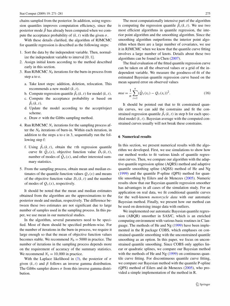
Fig. 1 Automatic Bayesian median curve fit for Wave
6.1 Performance comparison
We simulate data from three underlying median curves on(0,1):
Wave: f (x) = 4(x − .5) + 2exp(−256(x − .5)2), (17)
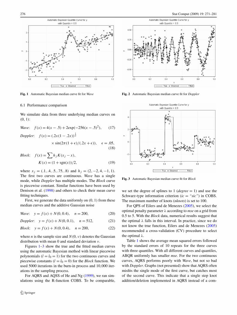
Doppler: f (x) = (.2x(1 − .2x))12
× sin(2π(1 + ε)/(.2x + ε)), ε = .05,
(18)
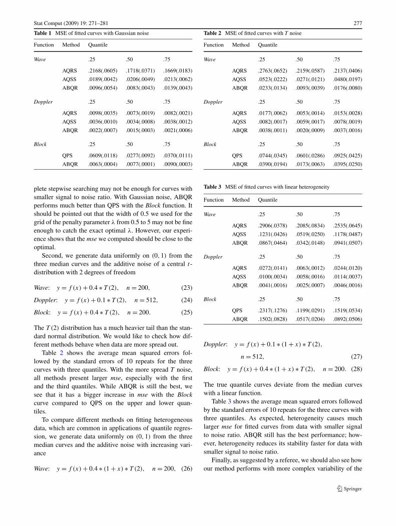
Block: f (x) =∑
hjK(xj − x),
K(x) = (1 + sgn(x))/2, (19)
where xj = (.1, .4, .5, .75, .8) and hj = (2,−2,4,−1,1).The first two curves are continuous. Wave has a singlemode, while Doppler has multiple modes. The Block curveis piecewise constant. Similar functions have been used byDenison et al. (1998) and others to check their mean curvefitting techniques.
First, we generate the data uniformly on (0,1) from thesemedian curves and the additive Gaussian noise
Wave: y = f (x) + N(0,0.4), n = 200, (20)
Doppler: y = f (x) + N(0,0.1), n = 512, (21)
Block: y = f (x) + N(0,0.4), n = 200, (22)
where n is the sample size and N(0, ν) denotes the Gaussiandistribution with mean 0 and standard deviation ν.
Figures 1–3 show the true and the fitted median curvesusing the automatic Bayesian method with linear piecewisepolynomials (l = l0 = 1) for the two continuous curves andpiecewise constants (l = l0 = 0) for the Block function. Weused 5000 iterations in the burn-in process and 10,000 iter-ations in the sampling process.
For AQRS and AQSS of He and Ng (1999), we ran sim-ulations using the R-function COBS. To be comparable,
Fig. 2 Automatic Bayesian median curve fit for Doppler
Fig. 3 Automatic Bayesian median curve fit for Block
we set the degree of splines to 1 (degree = 1) and use theSchwarz-type information criterion (ic = “sic”) in COBS.The maximum number of knots (nknots) is set to 100.
For QPS of Eilers and de Menezes (2005), we select theoptimal penalty parameter λ according to mse on a grid from0.5 to 5. With the Block data, numerical results suggest thatthe optimal λ falls in this interval. In practice, since we donot know the true function, Eilers and de Menezes (2005)recommended a cross-validation (CV) procedure to selectthe optimal λ.
Table 1 shows the average mean squared errors followedby the standard errors of 10 repeats for the three curveswith three quantiles. With all different curves and quantiles,ABQR uniformly has smaller mse. For the two continuouscurves, AQRS performs poorly with Wave, but not so badwith Doppler. Graphs (not presented) show that AQRS oftenmisfits the single mode of the first curve, but catches mostof the second curve. This indicate that a single step knotaddition/deletion implemented in AQRS instead of a com-
Stat Comput (2009) 19: 271–281 277
Table 1 MSE of fitted curves with Gaussian noise
Function Method Quantile
Wave .25 .50 .75
AQRS .2168(.0605) .1718(.0371) .1669(.0183)
AQSS .0189(.0042) .0206(.0049) .0213(.0062)
ABQR .0096(.0054) .0083(.0043) .0139(.0043)
Doppler .25 .50 .75
AQRS .0098(.0035) .0073(.0019) .0082(.0021)
AQSS .0036(.0010) .0034(.0008) .0038(.0012)
ABQR .0022(.0007) .0015(.0003) .0021(.0006)
Block .25 .50 .75
QPS .0609(.0118) .0277(.0092) .0370(.0111)
ABQR .0063(.0004) .0077(.0001) .0090(.0003)
plete stepwise searching may not be enough for curves withsmaller signal to noise ratio. With Gaussian noise, ABQRperforms much better than QPS with the Block function. Itshould be pointed out that the width of 0.5 we used for thegrid of the penalty parameter λ from 0.5 to 5 may not be fineenough to catch the exact optimal λ. However, our experi-ence shows that the mse we computed should be close to theoptimal.
Second, we generate data uniformly on (0,1) from thethree median curves and the additive noise of a central t-distribution with 2 degrees of freedom
Wave: y = f (x) + 0.4 ∗ T (2), n = 200, (23)
Doppler: y = f (x) + 0.1 ∗ T (2), n = 512, (24)
Block: y = f (x) + 0.4 ∗ T (2), n = 200. (25)
The T (2) distribution has a much heavier tail than the stan-dard normal distribution. We would like to check how dif-ferent methods behave when data are more spread out.
Table 2 shows the average mean squared errors fol-lowed by the standard errors of 10 repeats for the threecurves with three quantiles. With the more spread T noise,all methods present larger mse, especially with the firstand the third quantiles. While ABQR is still the best, wesee that it has a bigger increase in mse with the Blockcurve compared to QPS on the upper and lower quan-tiles.
To compare different methods on fitting heterogeneousdata, which are common in applications of quantile regres-sion, we generate data uniformly on (0,1) from the threemedian curves and the additive noise with increasing vari-ance
Wave: y = f (x) + 0.4 ∗ (1 + x) ∗ T (2), n = 200, (26)
Table 2 MSE of fitted curves with T noise
Function Method Quantile
Wave .25 .50 .75
AQRS .2763(.0652) .2159(.0587) .2137(.0406)
AQSS .0523(.0222) .0271(.0121) .0480(.0197)
ABQR .0233(.0134) .0093(.0039) .0176(.0080)
Doppler .25 .50 .75
AQRS .0177(.0062) .0053(.0014) .0153(.0028)
AQSS .0082(.0017) .0059(.0017) .0078(.0019)
ABQR .0038(.0011) .0020(.0009) .0037(.0016)
Block .25 .50 .75
QPS .0744(.0345) .0601(.0286) .0925(.0425)
ABQR .0390(.0194) .0173(.0063) .0395(.0250)
Table 3 MSE of fitted curves with linear heterogeneity
Function Method Quantile
Wave .25 .50 .75
AQRS .2906(.0378) .2085(.0834) .2535(.0645)
AQSS .1231(.0426) .0519(.0250) .1178(.0487)
ABQR .0867(.0464) .0342(.0148) .0941(.0507)
Doppler .25 .50 .75
AQRS .0272(.0141) .0063(.0012) .0244(.0120)
AQSS .0100(.0034) .0058(.0016) .0114(.0037)
ABQR .0041(.0016) .0025(.0007) .0046(.0016)
Block .25 .50 .75
QPS .2317(.1276) .1199(.0291) .1519(.0534)
ABQR .1502(.0828) .0517(.0204) .0892(.0506)
Doppler: y = f (x) + 0.1 ∗ (1 + x) ∗ T (2),
n = 512, (27)
Block: y = f (x) + 0.4 ∗ (1 + x) ∗ T (2), n = 200. (28)
The true quantile curves deviate from the median curveswith a linear function.
Table 3 shows the average mean squared errors followedby the standard errors of 10 repeats for the three curves withthree quantiles. As expected, heterogeneity causes muchlarger mse for fitted curves from data with smaller signalto noise ratio. ABQR still has the best performance; how-ever, heterogeneity reduces its stability faster for data withsmaller signal to noise ratio.
Finally, as suggested by a referee, we should also see howour method performs with more complex variability of the
278 Stat Comput (2009) 19: 271–281
Table 4 MSE of fitted curves with quadratic heterogeneity
Function Quantile (ABQR) Mean (BARS)
.25 .50 .75
Wave .2057(.0543) .0547(.0323) .1774(.1029) .6421(.5097)
Doppler .0085(.0016) .0051(.0006) .0072(.0013) .0091(.0044)
Block .0782(.0441) .0276(.0181) .0527(.0195) .1383 (.0381)
noise. Here we assume the variability quadratic in x:
Wave: y = f (x) + 0.4 ∗ (1 + x2) ∗ T (2),
n = 200, (29)
Doppler: y = f (x) + 0.1 ∗ (1 + x2) ∗ T (2),
n = 512, (30)
Block: y = f (x) + 0.4 ∗ (1 + x2) ∗ T (2),
n = 200. (31)
With the two continuous curves, simulation results showthat the mse becomes larger for all methods with quadraticheterogeneity. However, with the discontinuous Block curve,the mse becomes smaller. Again, ABQR presents the small-est mse for all quantiles. Table 4 shows these mse values.
This demonstrates that the piecewise linear functionsused for fitting the two continuous curves do a better jobwith linear heterogeneity than with quadratic heterogeneity,especially for the lower and upper quantiles. The piecewiseconstant functions used for the Block curve should not begood enough for either cases. The smaller mse is due toa smaller noise to signal ratio. This indicates that ABQRshould use piecewise polynomials with higher degrees formore complex heterogeneity.
Data with heterogeneity are common in practice. It isinteresting to see how the quantile regression method per-forms compared to the usual least squares method for es-timating the mean function. We implemented the Bayesianadaptive regression spline (BARS) method of DiMatteo etal. (2001) for mean estimates. For data simulated from(29)–(31) with quadratic heterogeneity, similarly we runBARS with 10 repeats. Table 4 compares mse values forthe mean using BARS with those for the three quantiles us-ing ABQR. Although the noise distributions are symmet-ric, BARS presents much larger mse. While quantile basedmethods still performs reasonably well for estimating thequantile functions, mean based methods could incur disas-trous results for data with heterogeneity. An alternative issimultaneously estimating the mean function and modelingthe heterogeneity as done by Leslie et al. (2007).
The next example provides a real application of ourBayesian quantile regression method on the data with com-plex variability.
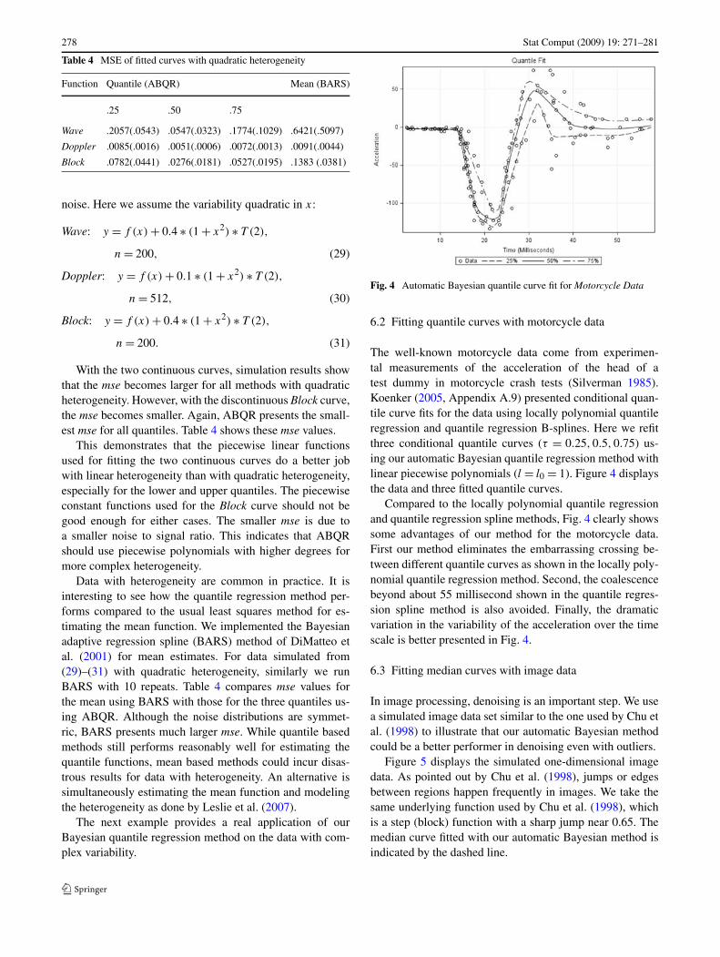
Fig. 4 Automatic Bayesian quantile curve fit for Motorcycle Data
6.2 Fitting quantile curves with motorcycle data
The well-known motorcycle data come from experimen-tal measurements of the acceleration of the head of atest dummy in motorcycle crash tests (Silverman 1985).Koenker (2005, Appendix A.9) presented conditional quan-tile curve fits for the data using locally polynomial quantileregression and quantile regression B-splines. Here we refitthree conditional quantile curves (τ = 0.25,0.5,0.75) us-ing our automatic Bayesian quantile regression method withlinear piecewise polynomials (l = l0 = 1). Figure 4 displaysthe data and three fitted quantile curves.
Compared to the locally polynomial quantile regressionand quantile regression spline methods, Fig. 4 clearly showssome advantages of our method for the motorcycle data.First our method eliminates the embarrassing crossing be-tween different quantile curves as shown in the locally poly-nomial quantile regression method. Second, the coalescencebeyond about 55 millisecond shown in the quantile regres-sion spline method is also avoided. Finally, the dramaticvariation in the variability of the acceleration over the timescale is better presented in Fig. 4.
6.3 Fitting median curves with image data
In image processing, denoising is an important step. We usea simulated image data set similar to the one used by Chu etal. (1998) to illustrate that our automatic Bayesian methodcould be a better performer in denoising even with outliers.
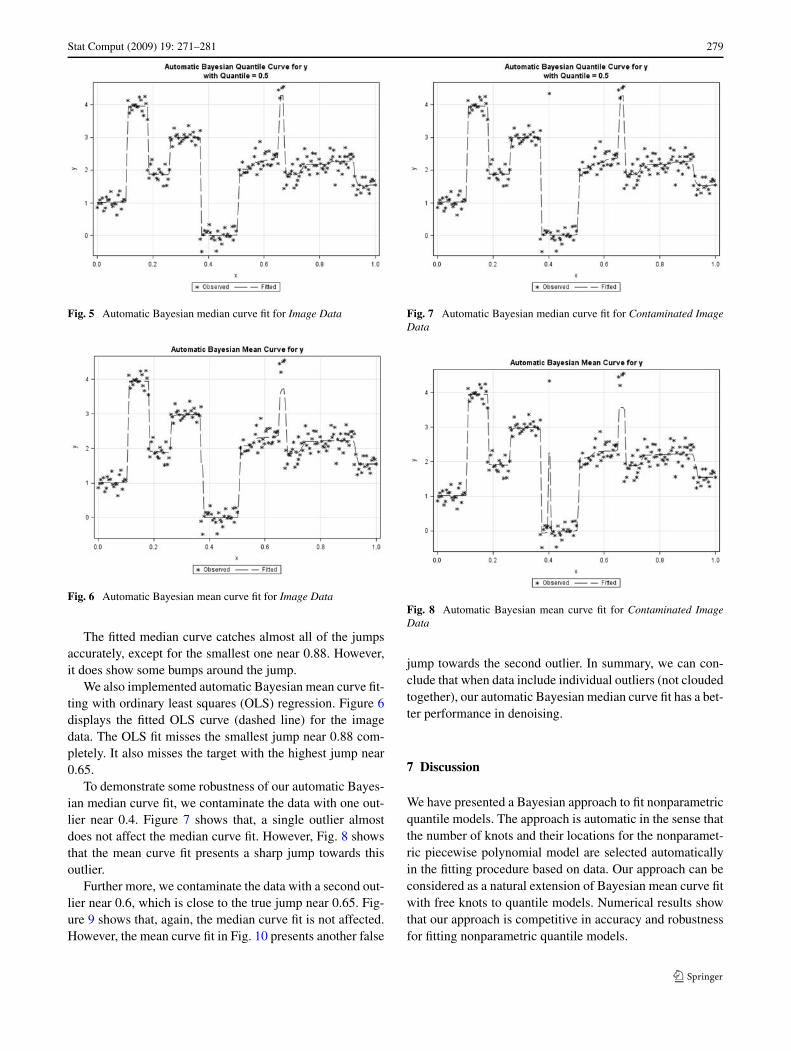
Figure 5 displays the simulated one-dimensional imagedata. As pointed out by Chu et al. (1998), jumps or edgesbetween regions happen frequently in images. We take thesame underlying function used by Chu et al. (1998), whichis a step (block) function with a sharp jump near 0.65. Themedian curve fitted with our automatic Bayesian method isindicated by the dashed line.
Stat Comput (2009) 19: 271–281 279
Fig. 5 Automatic Bayesian median curve fit for Image Data
Fig. 6 Automatic Bayesian mean curve fit for Image Data
The fitted median curve catches almost all of the jumpsaccurately, except for the smallest one near 0.88. However,it does show some bumps around the jump.
We also implemented automatic Bayesian mean curve fit-ting with ordinary least squares (OLS) regression. Figure 6displays the fitted OLS curve (dashed line) for the imagedata. The OLS fit misses the smallest jump near 0.88 com-pletely. It also misses the target with the highest jump near0.65.
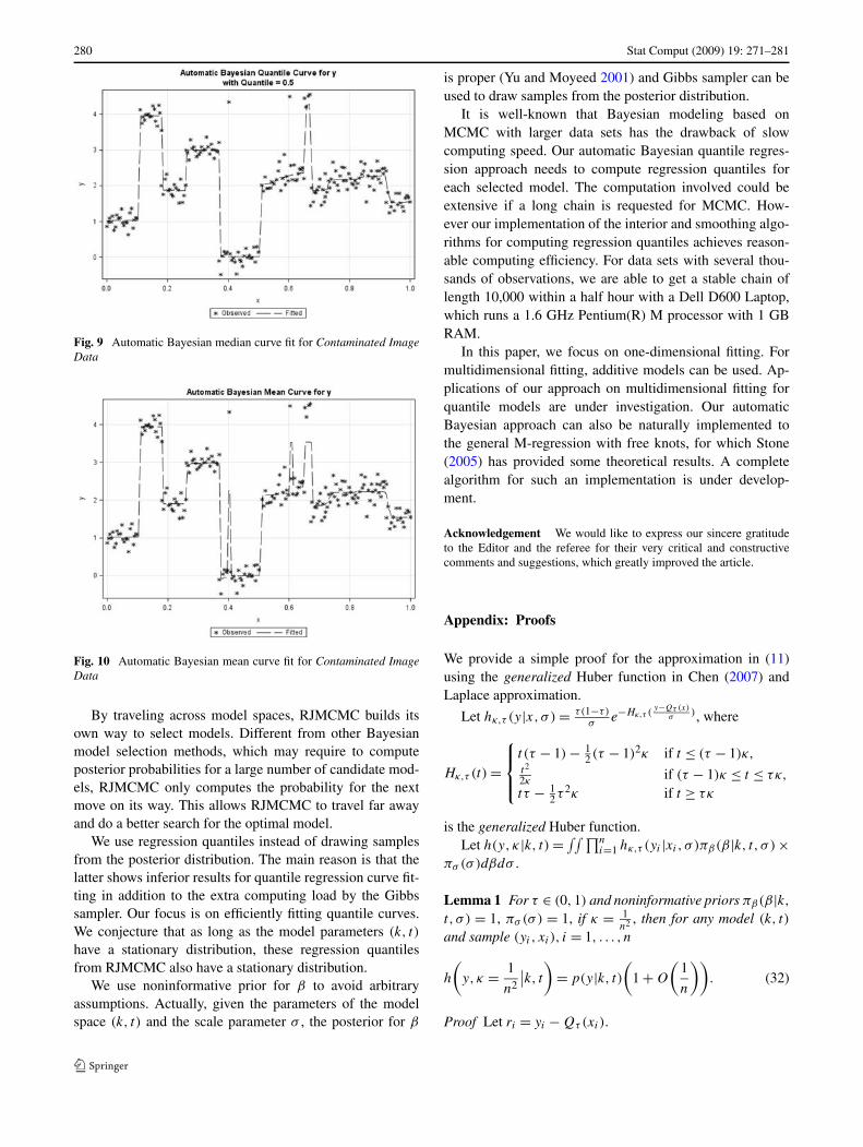
To demonstrate some robustness of our automatic Bayes-ian median curve fit, we contaminate the data with one out-lier near 0.4. Figure 7 shows that, a single outlier almostdoes not affect the median curve fit. However, Fig. 8 showsthat the mean curve fit presents a sharp jump towards thisoutlier.
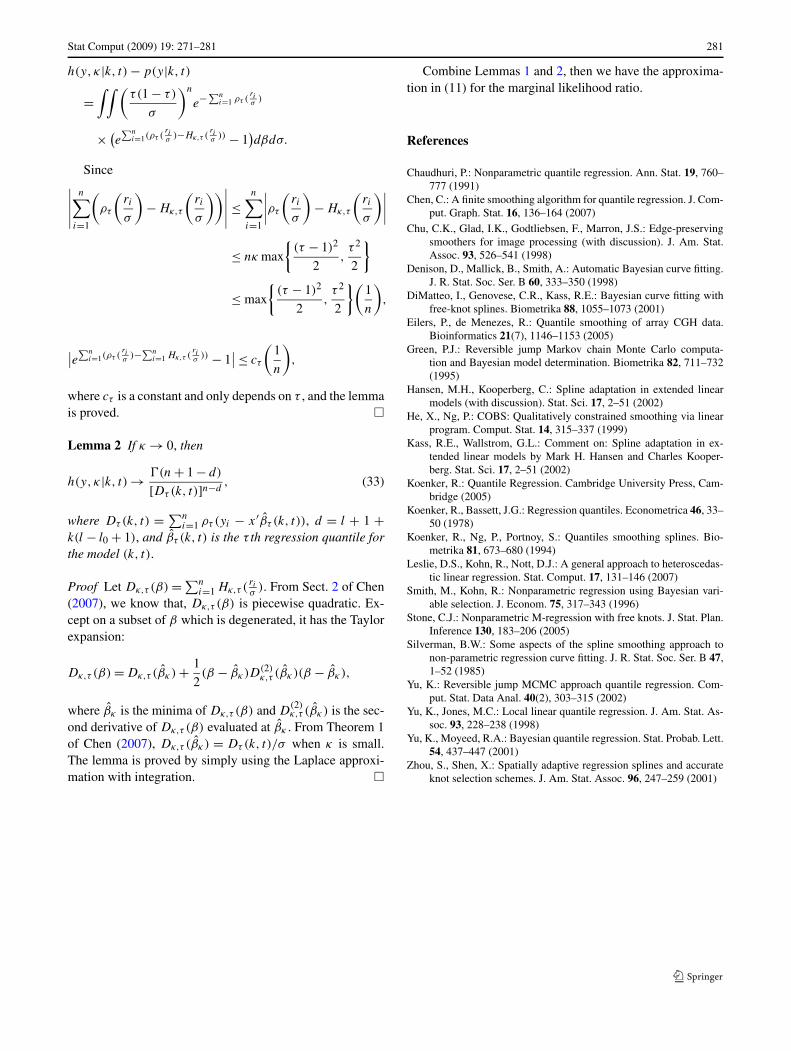
Further more, we contaminate the data with a second out-lier near 0.6, which is close to the true jump near 0.65. Fig-ure 9 shows that, again, the median curve fit is not affected.However, the mean curve fit in Fig. 10 presents another false
Fig. 7 Automatic Bayesian median curve fit for Contaminated ImageData
Fig. 8 Automatic Bayesian mean curve fit for Contaminated ImageData
jump towards the second outlier. In summary, we can con-clude that when data include individual outliers (not cloudedtogether), our automatic Bayesian median curve fit has a bet-ter performance in denoising.
7 Discussion
We have presented a Bayesian approach to fit nonparametricquantile models. The approach is automatic in the sense thatthe number of knots and their locations for the nonparamet-ric piecewise polynomial model are selected automaticallyin the fitting procedure based on data. Our approach can beconsidered as a natural extension of Bayesian mean curve fitwith free knots to quantile models. Numerical results showthat our approach is competitive in accuracy and robustnessfor fitting nonparametric quantile models.
280 Stat Comput (2009) 19: 271–281
Fig. 9 Automatic Bayesian median curve fit for Contaminated ImageData
Fig. 10 Automatic Bayesian mean curve fit for Contaminated ImageData
By traveling across model spaces, RJMCMC builds itsown way to select models. Different from other Bayesianmodel selection methods, which may require to computeposterior probabilities for a large number of candidate mod-els, RJMCMC only computes the probability for the nextmove on its way. This allows RJMCMC to travel far awayand do a better search for the optimal model.
We use regression quantiles instead of drawing samplesfrom the posterior distribution. The main reason is that thelatter shows inferior results for quantile regression curve fit-ting in addition to the extra computing load by the Gibbssampler. Our focus is on efficiently fitting quantile curves.We conjecture that as long as the model parameters (k, t)
have a stationary distribution, these regression quantilesfrom RJMCMC also have a stationary distribution.
We use noninformative prior for β to avoid arbitraryassumptions. Actually, given the parameters of the modelspace (k, t) and the scale parameter σ , the posterior for β
is proper (Yu and Moyeed 2001) and Gibbs sampler can beused to draw samples from the posterior distribution.
It is well-known that Bayesian modeling based onMCMC with larger data sets has the drawback of slowcomputing speed. Our automatic Bayesian quantile regres-sion approach needs to compute regression quantiles foreach selected model. The computation involved could beextensive if a long chain is requested for MCMC. How-ever our implementation of the interior and smoothing algo-rithms for computing regression quantiles achieves reason-able computing efficiency. For data sets with several thou-sands of observations, we are able to get a stable chain oflength 10,000 within a half hour with a Dell D600 Laptop,which runs a 1.6 GHz Pentium(R) M processor with 1 GBRAM.
In this paper, we focus on one-dimensional fitting. Formultidimensional fitting, additive models can be used. Ap-plications of our approach on multidimensional fitting forquantile models are under investigation. Our automaticBayesian approach can also be naturally implemented tothe general M-regression with free knots, for which Stone(2005) has provided some theoretical results. A completealgorithm for such an implementation is under develop-ment.
Acknowledgement We would like to express our sincere gratitudeto the Editor and the referee for their very critical and constructivecomments and suggestions, which greatly improved the article.
Appendix: Proofs
We provide a simple proof for the approximation in (11)using the generalized Huber function in Chen (2007) andLaplace approximation.
Let hκ,τ (y|x,σ ) = τ(1−τ)σ
e−Hκ,τ (y−Qτ (x)
σ), where
Hκ,τ (t) =
⎧⎪⎨
⎪⎩
t (τ − 1) − 12 (τ − 1)2κ if t ≤ (τ − 1)κ,
t2
2κif (τ − 1)κ ≤ t ≤ τκ,
tτ − 12τ 2κ if t ≥ τκ
is the generalized Huber function.Let h(y, κ|k, t) = ∫∫ ∏n
i=1 hκ,τ (yi |xi, σ )πβ(β|k, t, σ ) ×πσ (σ )dβdσ .
Lemma 1 For τ ∈ (0,1) and noninformative priors πβ(β|k,
t, σ ) = 1, πσ (σ ) = 1, if κ = 1n2 , then for any model (k, t)
and sample (yi, xi), i = 1, . . . , n
h
(
y, κ = 1
n2
∣∣k, t
)
= p(y|k, t)
(
1 + O
(1
n
))
. (32)
Proof Let ri = yi − Qτ(xi).
Stat Comput (2009) 19: 271–281 281
h(y, κ|k, t) − p(y|k, t)
=∫ ∫ (
τ(1 − τ)
σ
)n
e−∑ni=1 ρτ (
riσ
)
× (e∑n
i=1(ρτ (riσ
)−Hκ,τ (riσ
)) − 1)dβdσ.
Since∣∣∣∣∣
n∑
i=1
(
ρτ
(ri
σ
)
− Hκ,τ
(ri
σ
))∣∣∣∣∣≤
n∑
i=1
∣∣∣∣ρτ
(ri
σ
)
− Hκ,τ
(ri
σ
)∣∣∣∣
≤ nκ max
{(τ − 1)2
2,τ 2
2
}
≤ max
{(τ − 1)2
2,τ 2
2
}(1
n
)
,
∣∣e
∑ni=1(ρτ (
riσ
)−∑ni=1 Hκ,τ (
riσ
)) − 1∣∣ ≤ cτ
(1
n
)
,
where cτ is a constant and only depends on τ , and the lemmais proved. �
Lemma 2 If κ → 0, then
h(y, κ|k, t) → �(n + 1 − d)
[Dτ (k, t)]n−d, (33)
where Dτ (k, t) = ∑ni=1 ρτ (yi − x′β̂τ (k, t)), d = l + 1 +
k(l − l0 + 1), and β̂τ (k, t) is the τ th regression quantile forthe model (k, t).
Proof Let Dκ,τ (β) = ∑ni=1 Hκ,τ (
riσ). From Sect. 2 of Chen
(2007), we know that, Dκ,τ (β) is piecewise quadratic. Ex-cept on a subset of β which is degenerated, it has the Taylorexpansion:
Dκ,τ (β) = Dκ,τ (β̂κ ) + 1
2(β − β̂κ )D(2)
κ,τ (β̂κ )(β − β̂κ ),
where β̂κ is the minima of Dκ,τ (β) and D(2)κ,τ (β̂κ ) is the sec-
ond derivative of Dκ,τ (β) evaluated at β̂κ . From Theorem 1of Chen (2007), Dκ,τ (β̂κ ) = Dτ (k, t)/σ when κ is small.The lemma is proved by simply using the Laplace approxi-mation with integration. �
Combine Lemmas 1 and 2, then we have the approxima-tion in (11) for the marginal likelihood ratio.
References
Chaudhuri, P.: Nonparametric quantile regression. Ann. Stat. 19, 760–777 (1991)
Chen, C.: A finite smoothing algorithm for quantile regression. J. Com-put. Graph. Stat. 16, 136–164 (2007)
Chu, C.K., Glad, I.K., Godtliebsen, F., Marron, J.S.: Edge-preservingsmoothers for image processing (with discussion). J. Am. Stat.Assoc. 93, 526–541 (1998)
Denison, D., Mallick, B., Smith, A.: Automatic Bayesian curve fitting.J. R. Stat. Soc. Ser. B 60, 333–350 (1998)
DiMatteo, I., Genovese, C.R., Kass, R.E.: Bayesian curve fitting withfree-knot splines. Biometrika 88, 1055–1073 (2001)
Eilers, P., de Menezes, R.: Quantile smoothing of array CGH data.Bioinformatics 21(7), 1146–1153 (2005)
Green, P.J.: Reversible jump Markov chain Monte Carlo computa-tion and Bayesian model determination. Biometrika 82, 711–732(1995)
Hansen, M.H., Kooperberg, C.: Spline adaptation in extended linearmodels (with discussion). Stat. Sci. 17, 2–51 (2002)
He, X., Ng, P.: COBS: Qualitatively constrained smoothing via linearprogram. Comput. Stat. 14, 315–337 (1999)
Kass, R.E., Wallstrom, G.L.: Comment on: Spline adaptation in ex-tended linear models by Mark H. Hansen and Charles Kooper-berg. Stat. Sci. 17, 2–51 (2002)
Koenker, R.: Quantile Regression. Cambridge University Press, Cam-bridge (2005)
Koenker, R., Bassett, J.G.: Regression quantiles. Econometrica 46, 33–50 (1978)
Koenker, R., Ng, P., Portnoy, S.: Quantiles smoothing splines. Bio-metrika 81, 673–680 (1994)
Leslie, D.S., Kohn, R., Nott, D.J.: A general approach to heteroscedas-tic linear regression. Stat. Comput. 17, 131–146 (2007)
Smith, M., Kohn, R.: Nonparametric regression using Bayesian vari-able selection. J. Econom. 75, 317–343 (1996)
Stone, C.J.: Nonparametric M-regression with free knots. J. Stat. Plan.Inference 130, 183–206 (2005)
Silverman, B.W.: Some aspects of the spline smoothing approach tonon-parametric regression curve fitting. J. R. Stat. Soc. Ser. B 47,1–52 (1985)
Yu, K.: Reversible jump MCMC approach quantile regression. Com-put. Stat. Data Anal. 40(2), 303–315 (2002)
Yu, K., Jones, M.C.: Local linear quantile regression. J. Am. Stat. As-soc. 93, 228–238 (1998)
Yu, K., Moyeed, R.A.: Bayesian quantile regression. Stat. Probab. Lett.54, 437–447 (2001)
Zhou, S., Shen, X.: Spatially adaptive regression splines and accurateknot selection schemes. J. Am. Stat. Assoc. 96, 247–259 (2001)