a new hybrid optimization algorithm for the optimal

Int. J. Nonlinear Anal. Appl.Volume 12, Special Issue, Winter and Spring 2021, 146-160ISSN: 2008-6822 (electronic)http://dx.doi.org/10.22075/IJNAA.2021.4932

A New Hybrid Optimization Algorithm for theOptimal Allocation of Goods in Shop Shelves

Maliheh Khatami∗

Department of Software Engineering, Damghan University, Damghan, Iran

Abstract

In retail operation management, shelf space allocation problem is an important problem that affectsprofitability. Various researches have demonstrated that the shelf space allocation of a product affectsthat product’s sales. The decision that how much of which product, where and when should be placedon shelves is a critical issue in retail operation management. In this paper a new hybrid meta-heuristicalgorithm based on forest optimization algorithm (FOA) and simulated annulling (SA) is presentedto address the shop shelf allocation problem. To apply FOA for shelf space allocation problem, thebasic arithmetic operators of FOA have been modified regarding the characteristics of this problemand FOA is improved by SA. Results obtained from an expensive experimental phase show thebetter performance of the proposed algorithm in comparison with other presented algorithm fromthe literature. Also, results show the suitability and benefits of the proposed algorithm in findinghigh-quality solutions and robustness.

Keywords: retailing, shelf space allocation problem, optimization, forest optimization algorithm,simulated annulling

1. Introduction

The aim of retail management is developing a product mix to satisfy customers’ demand and affectcustomers’ shopping decisions. In this way, well-managed shelf space can improve the return of inven-tory investment, raise consumer satisfaction by reducing out-of-stock occurrences, and increase salesand profit margins (Yang, 2001). According to Reyes and Frazier (2007), most shopping decisionsoccur in the store and only 1/3 of shopping decisions is planned beforehand. So, one of the mostimportant issues in marketing is designing of products in an attractive presentation. In this way, ifa product is given a large shelf space, it is more likely seen by customers in a shop and is purchasedmore frequently (Desmet and Renaudin, 1998; Dreze et al, 1994).

∗Corresponding author: Maliheh KhatamiEmail address: [email protected] (Maliheh Khatami)

Received: June 2020 Accepted: January 2021

http://dx.doi.org/10.22075/IJNAA.2021.4932

A New Hybrid Optimization Algorithm ...Volume 12, Special Issue, Winter and Spring 2021,146-160 147

Shelf space allocation problem is based on two basic terms. The first one is stock keeping unit(SKU) which is used to identify a specific product and is the smallest management unit in a retailstore. Another term is facing that denotes the number of slots on the front of a retail shelf. In factthe number of the facing of an SKU is defined as the quantity of a product that can be directly seenon the shelves by the customers. Using these definitions, different planograms have been introduceduntil now to deal with shelf space operations. A major consequence of lack of planogram integrity isthe loss of a substantial level of efficiency both in terms of the marketing strategy as well as in theoperational executions. In fact in addition to complexity of shelf space allocation problem, inabilityof the planogram tools to deal with real life situations also can be a motivation to introduce newsimple, practicable and efficient algorithms for shelf space allocation problem.

Optimization algorithms used different area of Management and industrial problems such as:project scheduling (Zareei & Hassan-Pour, 2015), design of logistics network (Yadegari, et al., 2015),inventory Control (Orand et al., 2015) and facility problems (Maadi et al., 2017). In this paper,we propose a hybrid optimization algorithm based on forest optimization and simulated annullingalgorithms for the shelf space allocation problem. According to characteristics of shelf space problem,the basic operators of these optimization algorithms are modified and new adapted operators areproposed for shelf space allocation problem. The proposed algorithm has an excellent execution tofind the best solutions in comparison with other presented algorithms of the literature.

This paper is organized as follows: in the next section a review of related works is presented.Afterward, mathematical formulations of shelf space allocation problem are described in ”Problemformulation” section. After that, in the “Forest Optimization Algorithm” and “Simulated Annulling”sections the Basic FOA and SA are studied. The idea of hybrid algorithm to solve shelf space alloca-tion problem is presented in ”Proposed hybrid algorithm to solve SSAP” section. In ”Computationalresults” section the parameters tuning are executed and experimental evaluations of proposed algo-rithm on various instances are investigated and compared to other algorithms from the literaturefollowing by conclusions of the paper in the final section.

2. Related works

There are various factors such as shelf location, shopping path, shelf space, level to which productsare located and so on that can excite customers to purchase (Reyes & Frazier, 2007). So in theliterature, so many papers have investigated different factors that are involved in attracting customersto purchase. Among different papers shelf space allocation problem has been considered as one ofthe most important factor in marketing. As many retail companies have been faced with shelf spaceproblem in real world and shelf spaces are expensive resources for many retail stores, many researchershave been executed on shelf space allocation problem in marketing until now.

In recent years, Eisend (2014) studied the shelf space at the category or brand level. Generally,space elasticity is not simple tool for shelf space allocation.

In addition to experimental approaches, mathematical models are also used to solve this problem.Anderson and Amato developed a mathematical model for simultaneously optimizing the productvariety and shelf space allocation. Yang and Chen (1999) developed shelf space allocation problem(SSAP) as a knapsack problem with multiple constraints. This model was later used in variousstudies and researchers extending this model with different constraints, for example Gajjar and Adil(2010) extended this model considering space elasticity and developed a new mathematical modelfor it. The focus of this article is on SSAP and in continues we will review related studies to solvethe SSAP.

148 Khatami

According to Yang and Chen (1999) shelf space allocation problem (SSAP) is an NP-hard prob-lem, so heuristic and meta-heuristic algorithm are needed for solving large scale and real worldinstances of this problem. Yang (2001) developed a heuristic algorithm consisted of four main phasesfor solving SSAP. These four phases are: Preparatory phase for checking particular problems andbuilding the set of priority indexes, Allocation phase for allocated space to items according to pri-ority, Adjustment phase for improvement solution using three methods and Termination phase forcalculation of objective value of the final solution. Lim, Rodrigues, and Zhang (2004) modified Yang’sproposed heuristics and improved them. In addition, they proposed two meta-heuristic algorithms(Tabu Search and Squeaky-Wheel Optimization) for solving SSAP.

Hansen, Raut and Swami (2010) developed a heuristic algorithm consisted of four major phases.First, ranking orders all products by average profit without shelf consideration. Second, createthe initial solution as follows: starting with the most profitable product and allocating the minimumnumber of facings for each product. Third, using a neighborhood search and moving the configurationof (e.g., number of facings) a product around on the same shelf. Forth, swap pairs of products aroundon the same shelf and between shelves to determine. This swap is accepted if the new configurationsshelf-space profit is increased. Also Hansen, Raut and Swami (2010) proposed a simple geneticalgorithm for solving SSAP. The results showed that performance of genetic algorithm is better thanthe heuristic algorithm.

Gijjar and Adil (2011) proposed three heuristics to solve SSAP. These heuristics consist of con-struction of initial solution and improvement using neighborhood searches.

Castelli and Vanneschi (2014) proposed a hybrid algorithm that combines a genetic algorithmwith a variable neighborhood search (GA-VNS) to solve SSAP. In their algorithm in the each iterationof genetic algorithm a variable neighborhood search with four Neighborhood structure is performedfor improved GA performance.

3. Problem formulation

In this section, we describe the Mathematical model of the SSAP proposed by Yang and Chen (1999).The parameters and indices are:

n Number of product itemsm Number of shelvesi Index of product itemsk Index of shelvesli The length of each facing of product i, i ∈ {1, 2, . . . , n }Tk The length of shelf k, k ∈ {1, 2, . . . ,m }pik The profit per facing of product i displayed on shelf kxik The allocated amount of facings of product i on shelf k.Li Lower bound for the amount of facings of product iUi Upper bound for the amount of facings of product i

Using above parameters and indices, the objective function and the constraints of SSAP modelcan be expressed as following:


Maximizen∑

i=1

m∑k=1

pikxik (3.1)

s.t :n∑i=1

li xik ≤ Tk k = 1, 2, . . . , m (3.2)

Li ≤m∑k=1

xik ≤ Ui i = 1, 2, . . . , n (3.3)

xik ∈ N ∪ {0} i = 1, 2, . . . , n, k = 1, 2, . . . , m (3.4)

Eq. (3.1) is objective function of SSAP that equals to total profit of store and obtained by multiplyingthe allocated amount and the unit profit. Constraint (3.2) determines the shelf capacity constraintwhich ensures that the length of each shelf is greater than the total length of the facing allocatedto that shelf. Constraint (3.3) checks that upper and lower bounds of each product are satisfied.Constraint (3.4) ensures the allocated amount of facings of each product is positive integer and zero.

4. Forest Optimization Algorithm

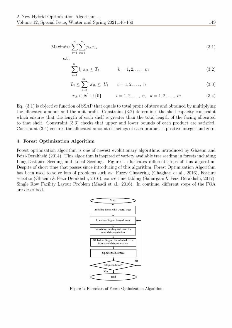
Forest optimization algorithm is one of newest evolutionary algorithms introduced by Ghaemi andFeizi-Derakhshi (2014). This algorithm is inspired of variety available tree seeding in forests includingLong-Distance Seeding and Local Seeding. Figure 1 illustrates different steps of this algorithm.Despite of short time that passes since introducing of this algorithm, Forest Optimization Algorithmhas been used to solve lots of problems such as: Fuzzy Clustering (Chaghari et al., 2016), Featureselection(Ghaemi & Feizi-Derakhshi, 2016), course time tabling (Sahargahi & Feizi Derakhshi, 2017),Single Row Facility Layout Problem (Maadi et al., 2016). In continue, different steps of the FOAare described.

Figure 1: Flowchart of Forest Optimization Algorithm

150 Khatami

4.1. Initialize forest trees

Like other evolutionary algorithms, FOA starts by an initial population of trees that each tree can bea solution of the problem. In FOA, a tree is represented as an array of variables. Beside of variableamount, a tree has a part that indicates the age of the tree. The age of a new generated tree in FOAis considered zero at first. In general, every tree is represented as an array of 1× (1 +NV AR) whereNV AR is the dimension of the of optimization problem.

4.2. Local seeding operator

In this operator, for the trees by age zero, at first, a cell is selected randomly. Then a random numberlike r in range of (−∆x,∆x) is determined. After that, r adds to the value of selected tree cell. ∆xis a small value less than the upper bound of problem variables. This process repeats Local seedingchanges (LSC) times. In fact LSC shows the number of trees that should be generated from thetrees with age of zero in the step of Local Seeding Operator. After this operation, the age of thetrees that are generated in this step are set zero and the age of other trees add by one.

4.3. Population limiting

Two parameters are applied for limitation of trees in forest. The first parameter is Life Time thatmentions the maximum age of each tree and another parameter is Area Limit which is equal to max-imum trees that can be existed in the forest. After Local Seeding operator, initially, the trees whichtheir ages have been arrived to Life Time are omitted and add to candidate population (Candidatepopulation includes the trees which omitted from forest). Then, if the number of remaining treesin the forest were more than Area Limit parameter, the available trees in forest will be sorted onamount of their objective function values and the best trees for survival in forest to the number ofArea Limit parameter are selected and other trees will add to the candidates population.

4.4. Global seeding Operator

In this step, at first some of available trees from the candidate population are selected. The num-ber of selected variables is determined by Transfer Rate parameter which illustrates the percentageof available trees in candidate population. Then, the specific number of cells of any tree is selectedrandomly and the value of each selected cell is replaced by another randomly generated value in therelated variable range. The number of selected cell of each tree is determined by another parameterof the algorithm named Global Seeding Changes (GSC).

4.5. Updating the best tree

After every repetition of the algorithm, the best tree according to its objective function value ischosen and its age is set zero. By doing this, through local seeding operator in the next repetition,the best tree is able to locally optimize its location.

4.6. Stop conditions

Like other Meta- heuristic algorithms, three stop conditions can be considered for the Forest Opti-mization Algorithm. First, specified number of repetition, second no change seen in value of objectivefunction of the best tree during several repeats and third access to a specified accuracy level.


5. Simulated Annealing (SA)

The main idea of Simulated Annealing (SA)) Algorithm is inspired of metropolis algorithm to assesstemperature changes of solid mass. In this process, at first, the temperature of mass is increasedup to the melting point. Then, to decrease the inner energy of the mass, the atoms of the massmove. This movement is done between two atoms. After that, in neighborhood of the atom, anotheratom is chosen and replaced by it. Choosing the atom to move or replace is completely random andthere is no sequence to do it. Later, Kirkpatrick, Gellat, and Vecchi (1989) applied this methodto other optimization problems. The main advantage of SA is its ability to solve the difficulty ofmoving the local optimization point to the optimized point. SA starts from an initial answer andfinds a neighborhood for it, if that neighborhood is better than the current state (amount of goal

function is optimizing), holds it as the new answer unless by possibility of e−dfT0 and if this possibility is

higher than a random steady number between [0, 1], selects the unsuitable answer. The T0 conductorvariable is equal to the initial temperature and df is equal to the difference in the goal function.

6. Proposed hybrid algorithm to solve SSAP

In FOA, the purpose of the Global Seeding step is global seeking in the space of the problem. Butsince by applying vast changes in trees structures in this step, there is possibility of adding lessoptimized trees to forest, therefore applying this operator in the way described in the main versionof algorithm can be cause to create a weak forest for the next steps, we must modify it so that theresulted trees from this step are better than the trees which are selected for change in this step by theoptimization. Of course the modification has to done in a way so that the algorithm is not involvedin local optimization. Thus the suggested algorithm for this step has gradually been implementedby using the simulated Annealing Algorithm mechanism. In a way that at first the seeking spaceof problem is searched globally and in the final steps, trees are only added to the forest if theyare better than those selected from candidate collection otherwise just the chosen trees are added toforest. Moreover with concerns to the properties of the sequence problem with regards to the prioritylimitation we need to make some changes to the algorithm operators, in a way so that they are incoordination with the limitations of the problem.

6.1. Tree (solution) representation

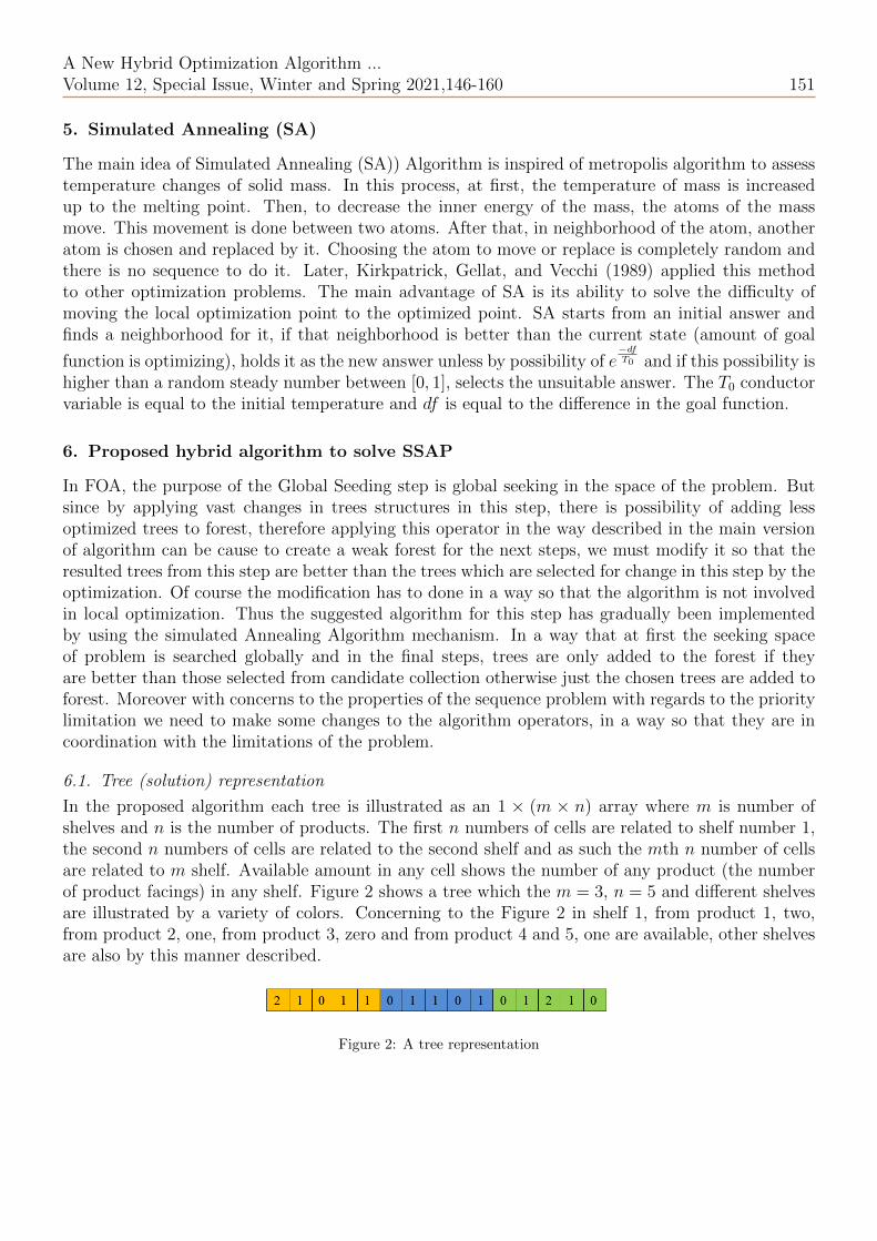
In the proposed algorithm each tree is illustrated as an 1 × (m × n) array where m is number ofshelves and n is the number of products. The first n numbers of cells are related to shelf number 1,the second n numbers of cells are related to the second shelf and as such the mth n number of cellsare related to m shelf. Available amount in any cell shows the number of any product (the numberof product facings) in any shelf. Figure 2 shows a tree which the m = 3, n = 5 and different shelvesare illustrated by a variety of colors. Concerning to the Figure 2 in shelf 1, from product 1, two,from product 2, one, from product 3, zero and from product 4 and 5, one are available, other shelvesare also by this manner described.

Figure 2: A tree representation

152 Khatami

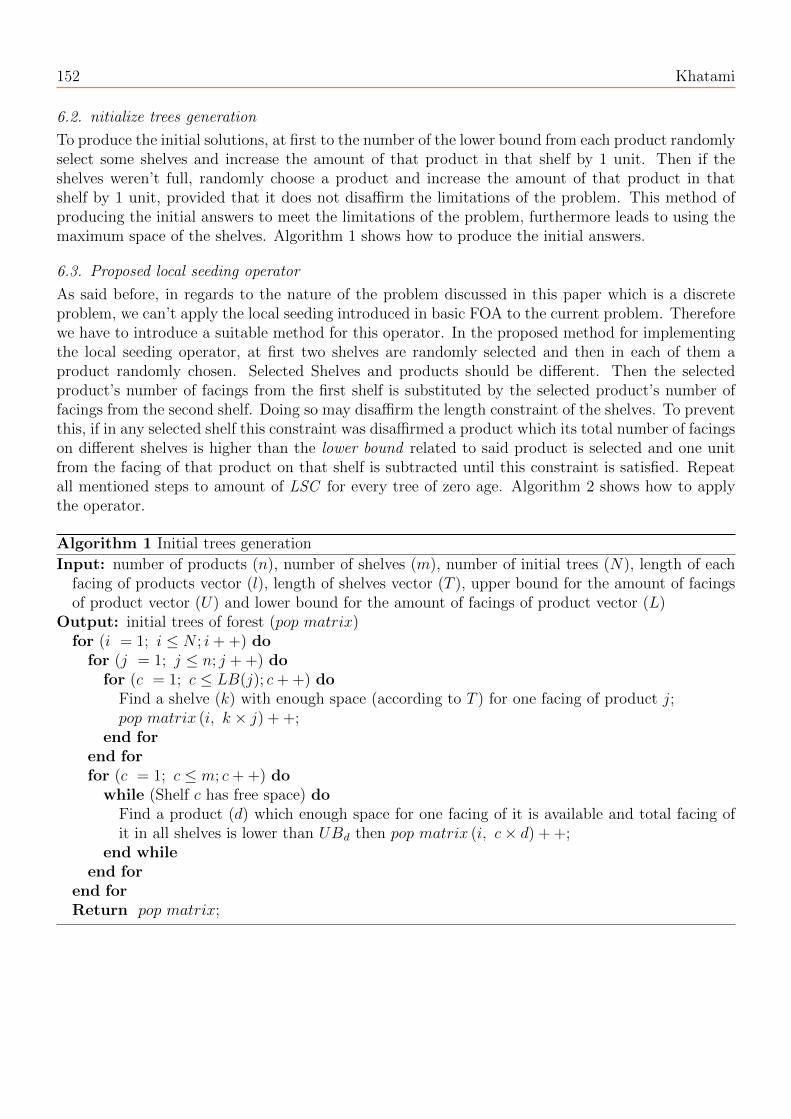
6.2. nitialize trees generation

To produce the initial solutions, at first to the number of the lower bound from each product randomlyselect some shelves and increase the amount of that product in that shelf by 1 unit. Then if theshelves weren’t full, randomly choose a product and increase the amount of that product in thatshelf by 1 unit, provided that it does not disaffirm the limitations of the problem. This method ofproducing the initial answers to meet the limitations of the problem, furthermore leads to using themaximum space of the shelves. Algorithm 1 shows how to produce the initial answers.

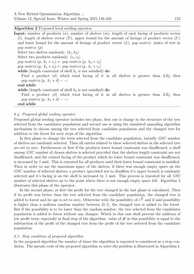
6.3. Proposed local seeding operator

As said before, in regards to the nature of the problem discussed in this paper which is a discreteproblem, we can’t apply the local seeding introduced in basic FOA to the current problem. Thereforewe have to introduce a suitable method for this operator. In the proposed method for implementingthe local seeding operator, at first two shelves are randomly selected and then in each of them aproduct randomly chosen. Selected Shelves and products should be different. Then the selectedproduct’s number of facings from the first shelf is substituted by the selected product’s number offacings from the second shelf. Doing so may disaffirm the length constraint of the shelves. To preventthis, if in any selected shelf this constraint was disaffirmed a product which its total number of facingson different shelves is higher than the lower bound related to said product is selected and one unitfrom the facing of that product on that shelf is subtracted until this constraint is satisfied. Repeatall mentioned steps to amount of LSC for every tree of zero age. Algorithm 2 shows how to applythe operator.

Algorithm 1 Initial trees generation

Input: number of products (n), number of shelves (m), number of initial trees (N), length of eachfacing of products vector (l), length of shelves vector (T ), upper bound for the amount of facingsof product vector (U) and lower bound for the amount of facings of product vector (L)

Output: initial trees of forest (pop matrix)for (i = 1; i ≤ N ; i+ +) dofor (j = 1; j ≤ n; j + +) dofor (c = 1; c ≤ LB(j); c+ +) do

Find a shelve (k) with enough space (according to T ) for one facing of product j;pop matrix (i, k × j) + +;

end forend forfor (c = 1; c ≤ m; c+ +) dowhile (Shelf c has free space) do

Find a product (d) which enough space for one facing of it is available and total facing ofit in all shelves is lower than UBd then pop matrix (i, c× d) + +;

end whileend for

end forReturn pop matrix;


Algorithm 2 Proposed local seeding operator

Input: number of products (n), number of shelves (m), length of each facing of products vector(l), length of shelves vector (T ), upper bound for the amount of facings of product vector (U)and lower bound for the amount of facings of product vector (L), pop matrix ,index of tree inpop matrix (p)Select two shelves randomly. (k1, k2)Select two products randomly. (i1, i2)pop matrix (p, k1 × i1)← pop matrix (p, k2 × i2)pop matrix (p, k2 × i2)← pop matrix (p, k1 × i1)while (length constraint of shelf k1 is not satisfied) do

Find a product (d) which total facing of it in all shelves is greater than LBd thenpop matrix (p, k1 × d)−−;

end whilewhile (length constraint of shelf k2 is not satisfied) do

Find a product (d) which total facing of it in all shelves is greater than LBd thenpop matrix (p, k2 × d)−−;

end while

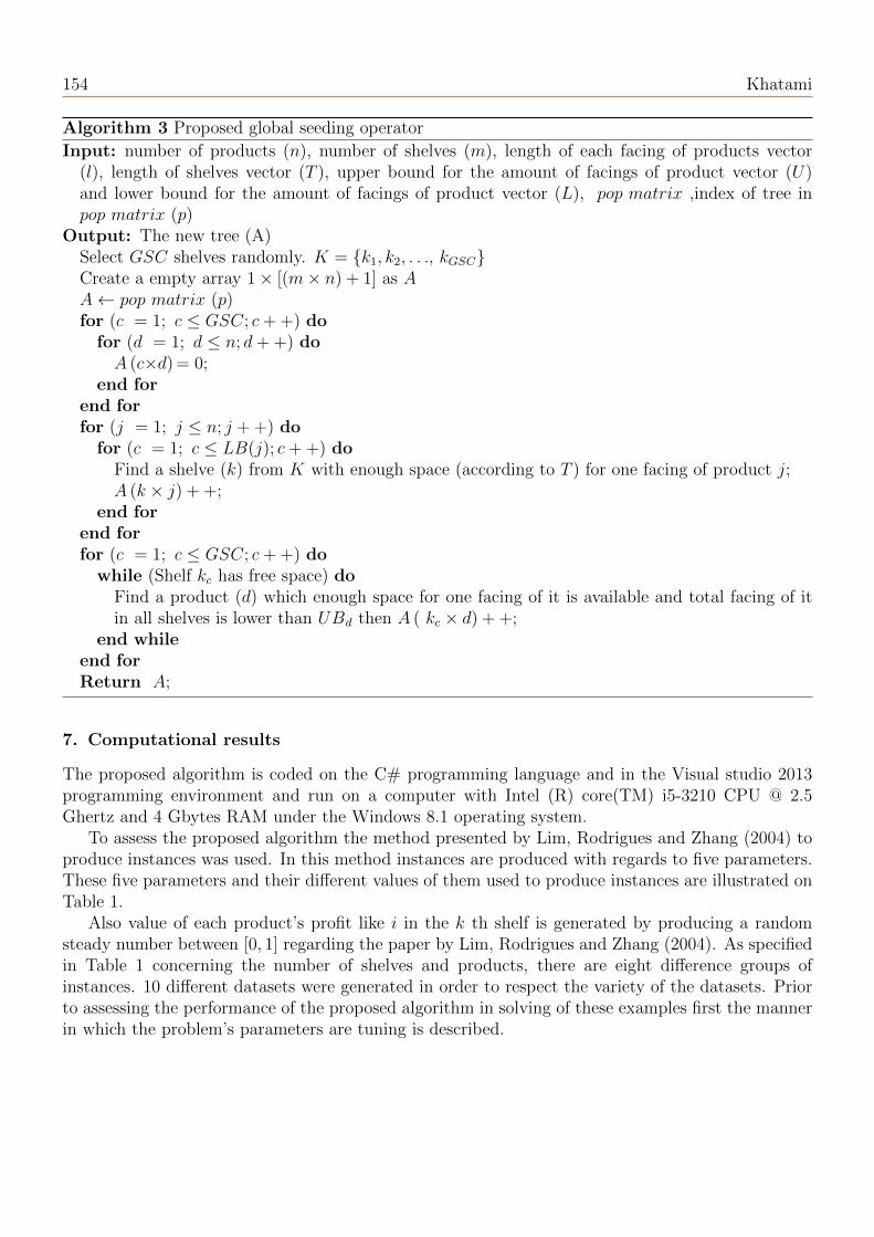
6.4. Proposed global seeding operator

Proposed global seeding operator includes two phase, first one is change in the structure of the treeselected from the candidates population and second one is using the simulated annealing algorithmmechanism to choose among the tree selected from candidate population and the changed tree foraddition to the forest for next steps of the algorithm.

In first phase to change the trees selected from the candidate population, initially GSC numberof shelves are randomly selected. Then all entries related to these selected shelves in the selected treeare set to zero. Furthermore at first if the products lower bound constraint was disaffirmed, a shelfamong GSC number of chosen shelves is selected provided that the shelves length constraint are notdisaffirmed, and the related facing of the product which its lower bound constraint was disaffirmed,is increased by 1 unit. This is repeated for all products until their lower bound constraint is satisfied.Then in order to use the maximum space of the shelves, if there was enough empty space on theGSC number of selected shelves, a product (provided not to disaffirm it’s upper bound) is randomlyselected and it’s facing is on the shelf is increased by 1 unit. This process is repeated for all GSCnumber of selected shelves up to the point where there is not enough empty space left. Algorithm 3illustrates this phase of the operator.

In the second phase, at first the profit for the tree changed in the last phase is calculated. Thenif its profit was better than the tree selected from the candidate population, the changed tree is

added to forest and its age is set to zero. Otherwise with the possibility of edfT and if said possibility

is higher than a uniform random number between [0, 1], the changed tree is added to the forest.But if the possibility is to be lower than the random number, the tree selected from the candidatespopulation is added to forest without any changes. Which in this case shall prevent the addition oflow profit trees, especially in final step of the algorithm. value of df in this possibility is equal to thesubtraction of the profit of the changed tree from the profit of the tree selected from the candidatepopulation.

6.5. Stop condition of proposed algorithm

In the proposed algorithm the number of times the algorithm is repeated is considered as a stop con-dition. The pseudo code of the proposed algorithm to solve the problem is illustrated in Algorithm 4.

154 Khatami

Algorithm 3 Proposed global seeding operator

Input: number of products (n), number of shelves (m), length of each facing of products vector(l), length of shelves vector (T ), upper bound for the amount of facings of product vector (U)and lower bound for the amount of facings of product vector (L), pop matrix ,index of tree inpop matrix (p)

Output: The new tree (A)Select GSC shelves randomly. K = {k1, k2, . . ., kGSC}Create a empty array 1× [(m× n) + 1] as AA← pop matrix (p)for (c = 1; c ≤ GSC; c+ +) dofor (d = 1; d ≤ n; d+ +) doA (c×d) = 0;

end forend forfor (j = 1; j ≤ n; j + +) dofor (c = 1; c ≤ LB(j); c+ +) do

Find a shelve (k) from K with enough space (according to T ) for one facing of product j;A (k × j) + +;

end forend forfor (c = 1; c ≤ GSC; c+ +) dowhile (Shelf kc has free space) do

Find a product (d) which enough space for one facing of it is available and total facing of itin all shelves is lower than UBd then A ( kc × d) + +;

end whileend forReturn A;

7. Computational results

The proposed algorithm is coded on the C# programming language and in the Visual studio 2013programming environment and run on a computer with Intel (R) core(TM) i5-3210 CPU @ 2.5Ghertz and 4 Gbytes RAM under the Windows 8.1 operating system.

To assess the proposed algorithm the method presented by Lim, Rodrigues and Zhang (2004) toproduce instances was used. In this method instances are produced with regards to five parameters.These five parameters and their different values of them used to produce instances are illustrated onTable 1.

Also value of each product’s profit like i in the k th shelf is generated by producing a randomsteady number between [0, 1] regarding the paper by Lim, Rodrigues and Zhang (2004). As specifiedin Table 1 concerning the number of shelves and products, there are eight difference groups ofinstances. 10 different datasets were generated in order to respect the variety of the datasets. Priorto assessing the performance of the proposed algorithm in solving of these examples first the mannerin which the problem’s parameters are tuning is described.


Algorithm 4 Proposed global seeding operator

Input: number of products (n), number of shelves (m), length of each facing of products vector (l),length of shelves vector (T ), upper bound for the amount of facings of product vector (U) and lowerbound for the amount of facings of product vector (L), pop matrix ,index of tree in pop matrix(p)number of products (n), number of shelves (m), number of initial trees (N), length of eachfacing of products vector (l), length of shelves vector (T ), upper bound for the amount of facingsof product vector (U) and lower bound for the amount of facings of product vector (L), maximumnumber of iterations (max iterations), local seeding change (LSC), global seeding change (GSC),transfer rate, life time, area limit, Cooling rate (α)

Output: An approximation of an optimal solution to the SSAP instanceInitialize forest with N trees using Algorithm 1.The age of each tree is initially set zero.Find the worst fitness value and copy that to Temp.for (iter = 1; iter ≤ max iterations; iter + +) dofor (each trees with age 0) dofor (counter = 1; counter ≤ LSC; counter + +) do

Perform local seeding on selected trees using Algorithm 1.end for

end forIncrease the age of all trees by 1, except for the newly generated trees with local seeding operator;

Remove the trees with age greater than life time parameter from forest and add them to thecandidate population;Sort trees according to their profit;Remove the extra trees that exceed the area limit parameter from the end of forest and addthem to the candidate population;for (counter = 1; counter ≤ (transferrate × |candidate population|); counter + +) do

Select a tree from candidate population randomly as R;Calculate profit of R as F ;Perform global seeding using Algorithm 3;Calculate profit of new generated tree (A) that returned from Algorithm 3 as F ′;if (F ′ greater than F ) then

Add A to the forest and set age cell of A by zero;else

Generate a random number between [0, 1] as r;

if (eF ′−FTemp ≥ r) then

Add A to the forest and set age cell of A by zero;else

Add R to the forest and set age cell of R by zero;end if

end ifend forUpdate best tree;temp = α×temp;

end forReturn the best tree as the result.

156 Khatami

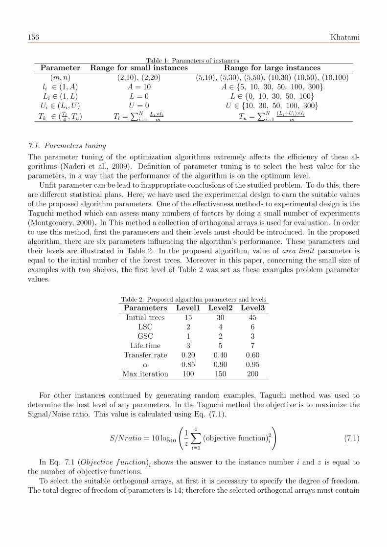
Table 1: Parameters of instancesParameter Range for small instances Range for large instances

(m,n) (2,10), (2,20) (5,10), (5,30), (5,50), (10,30) (10,50), (10,100)li ∈ (1, A) A = 10 A ∈ {5, 10, 30, 50, 100, 300}Li ∈ (1, L) L = 0 L ∈ {0, 10, 30, 50, 100}Ui ∈ (Li, U) U = 0 U ∈ {10, 30, 50, 100, 300}Tk ∈ (Tl

4, Tu) Tl =

∑Ni=1

Li×lim

Tu =∑N

i=1(Li+Ui)×li

m

7.1. Parameters tuning

The parameter tuning of the optimization algorithms extremely affects the efficiency of these al-gorithms (Naderi et al., 2009). Definition of parameter tuning is to select the best value for theparameters, in a way that the performance of the algorithm is on the optimum level.

Unfit parameter can be lead to inappropriate conclusions of the studied problem. To do this, thereare different statistical plans. Here, we have used the experimental design to earn the suitable valuesof the proposed algorithm parameters. One of the effectiveness methods to experimental design is theTaguchi method which can assess many numbers of factors by doing a small number of experiments(Montgomery, 2000). In This method a collection of orthogonal arrays is used for evaluation. In orderto use this method, first the parameters and their levels must should be introduced. In the proposedalgorithm, there are six parameters influencing the algorithm’s performance. These parameters andtheir levels are illustrated in Table 2. In the proposed algorithm, value of area limit parameter isequal to the initial number of the forest trees. Moreover in this paper, concerning the small size ofexamples with two shelves, the first level of Table 2 was set as these examples problem parametervalues.

Table 2: Proposed algorithm parameters and levels

Parameters Level1 Level2 Level3Initial trees 15 30 45

LSC 2 4 6GSC 1 2 3

Life time 3 5 7Transfer rate 0.20 0.40 0.60

α 0.85 0.90 0.95Max iteration 100 150 200

For other instances continued by generating random examples, Taguchi method was used todetermine the best level of any parameters. In the Taguchi method the objective is to maximize theSignal/Noise ratio. This value is calculated using Eq. (7.1).

S/Nratio = 10 log10

(1

z

z∑i=1

(objective function)2i

)(7.1)

In Eq. 7.1 (Objective function)i shows the answer to the instance number i and z is equal tothe number of objective functions.

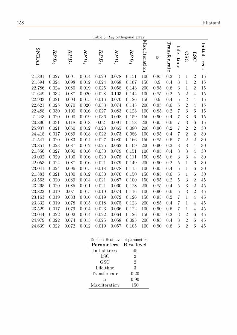
To select the suitable orthogonal arrays, at first it is necessary to specify the degree of freedom.The total degree of freedom of parameters is 14; therefore the selected orthogonal arrays must contain


at least 14 experiments. In this paper we have used array L27. Also To determine objective functionfor any group of instances, one of the 10 generated datasets is selected. Then in every test theproposed algorithm is run on it for 5 times. In the end Eq.6 is used to calculate the value of RelativePercentage Deviation (PRD) and is used as the related objective function to that test in the studiedinstance.

objective functioni= RPDi=

∑5j=1

UBi−ProfitijUBi

5(7.2)

In Eq. 7.2, Profitij is equal to profit of the ith instances in the jth repetition and UBi is equalto best result acquired for ith instances in all tests. Since there are six different groups of instances,value of z in Eq. 7.1 is six. In other words, RPD1 for instance (5,10), RPD2 for (5,30), RPD3 for(5,50), RPD4 for (10,30), RPD5 for (10,50), RPD6 for (10,100).

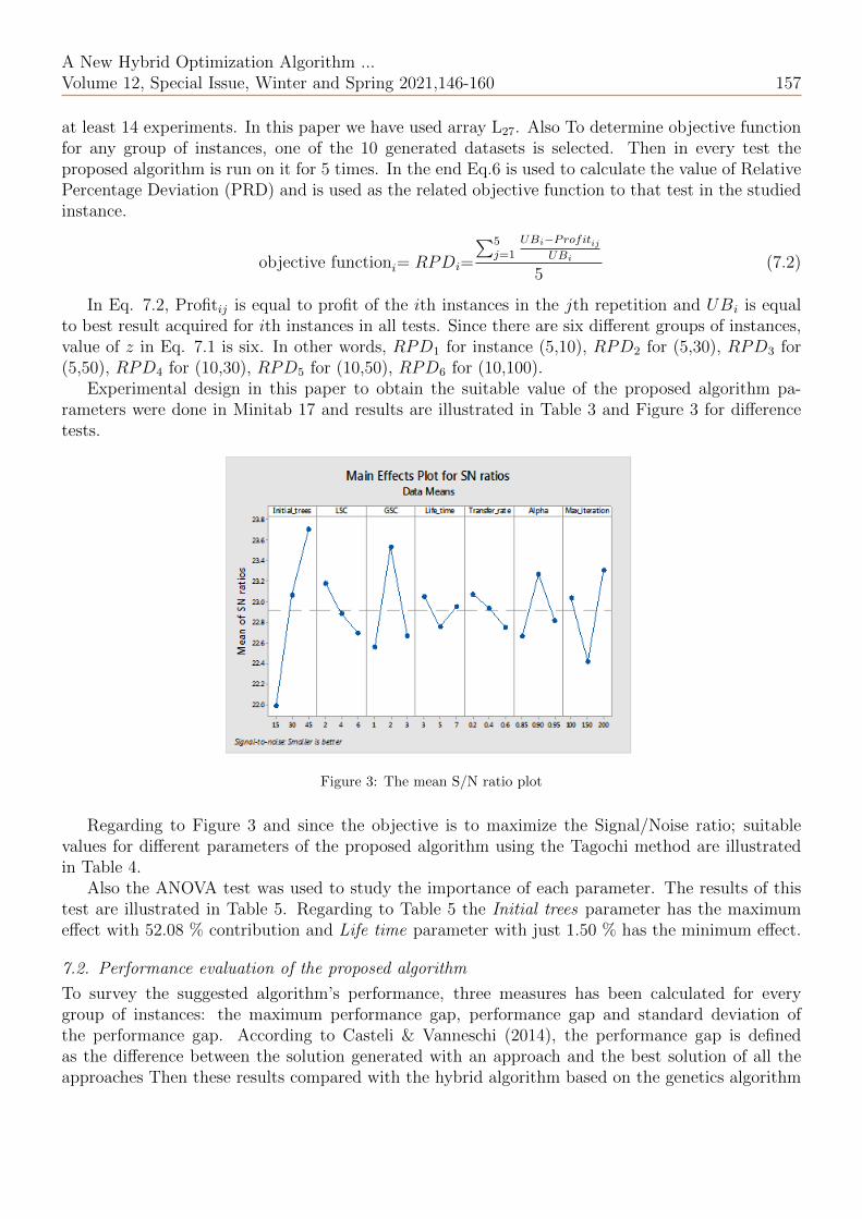
Experimental design in this paper to obtain the suitable value of the proposed algorithm pa-rameters were done in Minitab 17 and results are illustrated in Table 3 and Figure 3 for differencetests.

Figure 3: The mean S/N ratio plot

Regarding to Figure 3 and since the objective is to maximize the Signal/Noise ratio; suitablevalues for different parameters of the proposed algorithm using the Tagochi method are illustratedin Table 4.

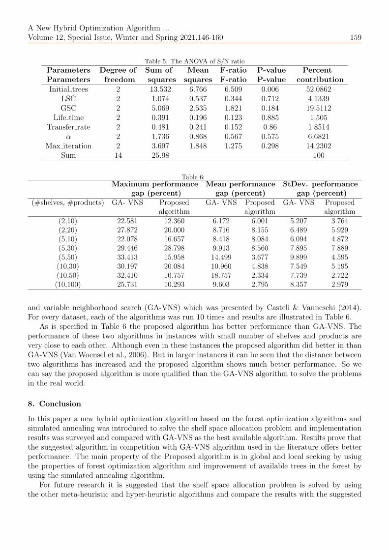
Also the ANOVA test was used to study the importance of each parameter. The results of thistest are illustrated in Table 5. Regarding to Table 5 the Initial trees parameter has the maximumeffect with 52.08 % contribution and Life time parameter with just 1.50 % has the minimum effect.

7.2. Performance evaluation of the proposed algorithm

To survey the suggested algorithm’s performance, three measures has been calculated for everygroup of instances: the maximum performance gap, performance gap and standard deviation ofthe performance gap. According to Casteli & Vanneschi (2014), the performance gap is definedas the difference between the solution generated with an approach and the best solution of all theapproaches Then these results compared with the hybrid algorithm based on the genetics algorithm

158 Khatami

Table 3: L27 orthogonal array

SNRA1

RPD

6

RPD

5

RPD

4

RPD

3

RPD

2

RPD

1

Maxite

ratio

n

α

Tra

nsfe

rra

te

Life

time

GSC

LSC

Initia

ltre

es

21.891 0.027 0.091 0.014 0.029 0.078 0.151 100 0.85 0.2 3 1 2 1521.394 0.024 0.098 0.012 0.024 0.068 0.167 150 0.9 0.4 3 1 2 1522.786 0.024 0.080 0.019 0.025 0.058 0.143 200 0.95 0.6 3 1 2 1521.649 0.032 0.087 0.020 0.028 0.103 0.144 100 0.85 0.2 5 2 4 1522.933 0.021 0.094 0.015 0.016 0.070 0.126 150 0.9 0.4 5 2 4 1522.621 0.025 0.070 0.020 0.033 0.074 0.143 200 0.95 0.6 5 2 4 1522.488 0.030 0.100 0.016 0.027 0.083 0.123 100 0.85 0.2 7 3 6 1521.243 0.020 0.090 0.019 0.036 0.098 0.159 150 0.90 0.4 7 3 6 1520.890 0.031 0.118 0.018 0.02 0.091 0.158 200 0.95 0.6 7 3 6 1525.937 0.021 0.060 0.012 0.023 0.065 0.080 200 0.90 0.2 7 2 2 3024.418 0.017 0.089 0.018 0.022 0.073 0.086 100 0.95 0.4 7 2 2 3021.541 0.020 0.083 0.014 0.027 0.080 0.166 150 0.85 0.6 7 2 2 3023.851 0.023 0.087 0.012 0.025 0.062 0.109 200 0.90 0.2 3 3 4 3021.856 0.027 0.090 0.016 0.030 0.079 0.151 100 0.95 0.4 3 3 4 3023.002 0.029 0.100 0.016 0.020 0.078 0.111 150 0.85 0.6 3 3 4 3022.053 0.024 0.087 0.016 0.021 0.079 0.149 200 0.90 0.2 5 1 6 3023.041 0.024 0.096 0.015 0.018 0.078 0.115 100 0.95 0.4 5 1 6 3021.883 0.021 0.100 0.012 0.030 0.070 0.150 150 0.85 0.6 5 1 6 3023.563 0.020 0.089 0.014 0.021 0.087 0.100 150 0.95 0.2 5 3 2 4523.265 0.020 0.085 0.011 0.021 0.060 0.128 200 0.85 0.4 5 3 2 4523.823 0.019 0.07 0.015 0.019 0.074 0.116 100 0.90 0.6 5 3 2 4523.163 0.019 0.083 0.016 0.019 0.072 0.126 150 0.95 0.2 7 1 4 4523.332 0.019 0.078 0.015 0.018 0.075 0.123 200 0.85 0.4 7 1 4 4523.529 0.017 0.079 0.014 0.023 0.066 0.122 100 0.90 0.6 7 1 4 4523.044 0.022 0.092 0.014 0.022 0.064 0.126 150 0.95 0.2 3 2 6 4524.979 0.022 0.074 0.015 0.025 0.058 0.095 200 0.85 0.4 3 2 6 4524.639 0.022 0.072 0.012 0.019 0.057 0.105 100 0.90 0.6 3 2 6 45

Table 4: Best level of parameters

Parameters Best levelInitial trees 45

LSC 2GSC 2

Life time 3Transfer rate 0.20

α 0.90Max iteration 150


Table 5: The ANOVA of S/N ratio

Parameters Degree of Sum of Mean F-ratio P-value PercentParameters freedom squares squares F-ratio P-value contributionInitial trees 2 13.532 6.766 6.509 0.006 52.0862

LSC 2 1.074 0.537 0.344 0.712 4.1339GSC 2 5.069 2.535 1.821 0.184 19.5112

Life time 2 0.391 0.196 0.123 0.885 1.505Transfer rate 2 0.481 0.241 0.152 0.86 1.8514

α 2 1.736 0.868 0.567 0.575 6.6821Max iteration 2 3.697 1.848 1.275 0.298 14.2302

Sum 14 25.98 100

Table 6:Maximum performance Mean performance StDev. performance

gap (percent) gap (percent) gap (percent)(#shelves, #products) GA- VNS Proposed GA- VNS Proposed GA- VNS Proposed

algorithm algorithm algorithm(2,10) 22.581 12.360 6.172 6.001 5.207 3.764(2,20) 27.872 20.000 8.716 8.155 6.489 5.929(5,10) 22.078 16.657 8.418 8.084 6.094 4.872(5,30) 29.446 28.798 9.913 8.560 7.895 7.889(5,50) 33.413 15.958 14.499 3.677 9.899 4.595(10,30) 30.197 20.084 10.960 4.838 7.549 5.195(10,50) 32.410 10.757 18.757 2.334 7.739 2.722(10,100) 25.731 10.293 9.603 2.795 8.357 2.979

and variable neighborhood search (GA-VNS) which was presented by Casteli & Vanneschi (2014).For every dataset, each of the algorithms was run 10 times and results are illustrated in Table 6.

As is specified in Table 6 the proposed algorithm has better performance than GA-VNS. Theperformance of these two algorithms in instances with small number of shelves and products arevery close to each other. Although even in these instances the proposed algorithm did better in thanGA-VNS (Van Woensel et al., 2006). But in larger instances it can be seen that the distance betweentwo algorithms has increased and the proposed algorithm shows much better performance. So wecan say the proposed algorithm is more qualified than the GA-VNS algorithm to solve the problemsin the real world.

8. Conclusion

In this paper a new hybrid optimization algorithm based on the forest optimization algorithms andsimulated annealing was introduced to solve the shelf space allocation problem and implementationresults was surveyed and compared with GA-VNS as the best available algorithm. Results prove thatthe suggested algorithm in competition with GA-VNS algorithm used in the literature offers betterperformance. The main property of the Proposed algorithm is in global and local seeking by usingthe properties of forest optimization algorithm and improvement of available trees in the forest byusing the simulated annealing algorithm.

For future research it is suggested that the shelf space allocation problem is solved by usingthe other meta-heuristic and hyper-heuristic algorithms and compare the results with the suggested

160 Khatami

algorithm. In addition regarding to the ability of the proposed hybrid algorithm, it is suggested touse this algorithm to solve other optimization problems.

References

[1] M. Castelli and L. Vanneschi, Genetic algorithm with variable neighborhood search for the optimal allocation ofgoods in shop shelves, Oper. Res. Lett. 42(5) (2014), 355–360.

[2] A. Chaghari, M. R. Feizi-Derakhshi and M. A. Balafar, Fuzzy clustering based on Forest optimization algorithm,J. King Saud Univer. Comp. Infor. Sci. 30(1) (2018), 25–32.

[3] P. Desmet and V. Renaudin, Estimation of product category sales responsiveness to allocated shelf space, Inter,J. Res. Mark. 15(5) (1998), 443–457.

[4] X. Dreze, S. J. Hoch and M. E. Purk, Shelf management and space elasticity, J. Reta. 70(4) (1994), 301–326.[5] M. Eisend, Shelf space elasticity: A meta-analysis, J. Reta. 90(2) (2014), 168–181.[6] M. Ghaemi and M. R. Feizi-Derakhshi, Forest optimization algorithm, Exp. Syst. Appl. 41(15) (2014), 6676–6687.[7] M. Ghaemi and M. R. Feizi-Derakhshi, Feature selection using forest optimization algorithm., Patt. Recog. 60

(2016), 121–129.[8] H. K. Gajjar G. K. Adil, A piecewise linearization for retail shelf space allocation problem and a local search

heuristic, Ann. Oper. Res. 179(1) (2010), 149–167.[9] J. M. Hansen, S. Raut, and S. Swami, Retail shelf allocation: a comparative analysis of heuristic and meta-

heuristic approaches, J. Reta. 86(1) (2010), 94–105.[10] S. Kirkpatrick, C. D. Gelatt and M. P. Vecchi, Optimization by simulated annealing, Sci., 220(4598) (1983),

671–680.[11] A. Lim, B. Rodrigues and X. Zhang, Metaheuristics with local search techniques for retail shelf-space optimization,

Manag. Sci. 50(1) (2004), 117–131.[12] M. Maadi, M. Javidnia and M. Ghasemi, Applications of two new algorithms of cuckoo optimization (CO) and

forest optimization (FO) for solving single row facility layout problem (SRFLP), J. AI Data Min. 4(1) (2016),35–48.

[13] M. Maadi, M. Javidnia and R. Jamshidi, Two Strategies based on meta-heuristic algorithms for parallel rowordering problem (PROP), Iran. J. Manag. Stud. 10(2) (2017), 467–498.

[14] D. C. Montgomery, Design and analysis of experiments, John Wiley & Sons, 2017.[15] B. Naderi, M. Khalili and R. Tavakkoli-Moghaddam, A hybrid artificial immune algorithm for a realistic variant

of job shops to minimize the total completion time. Comput. Indust. Engin. 56(4) (2009), 1494–1501.[16] S. M. Orand, A. Mirzazadeh, F. Ahmadzadeh and F. Talebloo, Optimization of the inflationary inventory control

model under stochastic conditions with Simpson approximation: Particle swarm optimization approach, Iran. J.Manag. Stud. 8(2) (2015), 203–220.

[17] V. Sahargahi and M. R. Feizi-Derakhshi, Course timetabling using Forest algorithm, Inter. J. Comput. Sci.Network Security, 17(2) (2017), 83–93.

[18] P. M. Reyes and G. V. Frazier, Goal programming model for grocery shelf space allocation, Europ. J. Oper. Res.181(2) (2007), 634–644.

[19] T. Van Woensel, R. A. C. M. Broekmeulen, K. H. van Donselaar and J. C. Fransoo, Planogram integrity: aserious issue, ECR J. 6 (2006), 4–5.

[20] M. H. Yang and W. C. Chen, A study on shelf space allocation and management, Inter. J. Produc. Econ. 60(1999), 309–317.

[21] M. H. Yang, An efficient algorithm to allocate shelf space, Europ. J. Oper. Res. 131(1) (2001), 107–118.[22] E. Yadegari, H. Najmi, M. Ghomi-Avili and M. Zandieh, A flexible integrated forward/reverse logistics model with

random path-based memetic algorithm, Iran. J. Manag. Stud. 8(2) (2015), 287–313.[23] M. Zareei and H. A. Hassan-Pour, A multi-objective resource-constrained optimization of time-cost trade-off

problems in scheduling project, Iran. J. Manag. Stud. 8(4) (2015), 653–685.

a new hybrid optimization algorithm for the optimal

Documents