water cycle algorithm – a novel metaheuristic optimization method for solving constrained...
TRANSCRIPT

Computers and Structures 110–111 (2012) 151–166
Contents lists available at SciVerse ScienceDirect
Computers and Structures
journal homepage: www.elsevier .com/locate /compstruc
Water cycle algorithm – A novel metaheuristic optimization methodfor solving constrained engineering optimization problems
Hadi Eskandar a, Ali Sadollah b, Ardeshir Bahreininejad b,⇑, Mohd Hamdi b
a Faculty of Engineering, Semnan University, Semnan, Iranb Faculty of Engineering, University of Malaya, 50603 Kuala Lumpur, Malaysia
a r t i c l e i n f o a b s t r a c t
Article history:Received 21 June 2012Accepted 27 July 2012Available online 26 August 2012
Keywords:Water cycle algorithmMetaheuristicGlobal optimizationConstrained problemsEngineering designConstraint handling
0045-7949/$ - see front matter � 2012 Elsevier Ltd. Ahttp://dx.doi.org/10.1016/j.compstruc.2012.07.010
⇑ Corresponding author. Tel.: +60 379675266; fax:E-mail addresses: [email protected] (H.
hoo.com (A. Sadollah), [email protected] (Am.edu.my (M. Hamdi).
This paper presents a new optimization technique called water cycle algorithm (WCA) which is applied toa number of constrained optimization and engineering design problems. The fundamental concepts andideas which underlie the proposed method is inspired from nature and based on the observation of watercycle process and how rivers and streams flow to the sea in the real world. A comparative study has beencarried out to show the effectiveness of the WCA over other well-known optimizers in terms of compu-tational effort (measures as number of function evaluations) and function value (accuracy) in this paper.
� 2012 Elsevier Ltd. All rights reserved.
1. Introduction
Over the last decades, various algorithms have been developedto solve a variety of constrained engineering optimization prob-lems. Most of such algorithms are based on numerical linear andnonlinear programming methods that may require substantial gra-dient information and usually seek to improve the solution in theneighborhood of a starting point. These numerical optimizationalgorithms provide a useful strategy to obtain the global optimumsolution for simple and ideal models.
Many real-world engineering optimization problems, however,are very complex in nature and quite difficult to solve. If there ismore than one local optimum in the problem, the results may de-pend on the selection of the starting point for which the obtainedoptimal solution may not necessarily be the global optimum. Fur-thermore, the gradient search may become unstable when theobjective function and constraints have multiple or sharp peaks.
The drawbacks (efficiency and accuracy) of existing numericalmethods have encouraged researchers to rely on metaheuristicalgorithms based on simulations and nature inspired methods tosolve engineering optimization problems. Metaheuristic algo-rithms commonly operate by combining rules and randomness toimitate natural phenomena [1].
ll rights reserved.
+60 379675330.Eskandar), ali_sadollah@ya-. Bahreininejad), hamdi@u-
The phenomena may include the biological evolutionary pro-cess such as genetic algorithms (GAs) proposed by Holland [2]and Goldberg [3], animal behavior such as particle swarm optimi-zation (PSO) proposed by Kennedy and Eberhart [4], and the phys-ical annealing which is generally known as simulated annealing(SA) proposed by Kirkpatrick et al. [5].
Among the optimization methods, the evolutionary algorithms(EAs) which are generally known as general purpose optimizationalgorithms are known to be capable of finding the near-optimumsolution to the numerical real-valued test problems. EAs have beenvery successfully applied to constrained optimization problems [6].
GAs are based on the genetic process of biological organisms[2,3]. Over many generations, natural populations evolve accordingto the principles of natural selections (i.e. survival of the fittest). InGAs, a potential solution to a problem is represented as a set ofparameters. Each independent design variable is represented by agene. Combining the genes, a chromosome is produced which rep-resents an individual (solution).
The efficiency of the different architectures of evolutionaryalgorithms in comparison to other heuristic techniques has beentested in both generic [7–9] and engineering design [10] problems.Recently, Chootinan and Chen [11] proposed a constraint-handlingtechnique by taking a gradient-based repair method. The proposedtechnique is embedded into GA as a special operator.
PSO is a recently developed metaheuristic technique inspired bychoreography of a bird flock developed by Kennedy and Eberhart[4]. The approach can be viewed as a distributed behavioral algo-rithm that performs a multidimensional search. It makes use of a

152 H. Eskandar et al. / Computers and Structures 110–111 (2012) 151–166
velocity vector to update the current position of each particle inthe swarm.
In Ref. [12], there are some suggestions for choosing the param-eters used in PSO. He and Wang [13] proposed an effective co-evo-lutionary PSO for constrained problems, where PSO was applied toevolve both decision factors and penalty factors. In these methods,the penalty factors were treated as searching variables and evolvedby GA or PSO to the optimal values. Recently, Gomes [14] appliedPSO on truss optimization using dynamic constraints.
The present paper introduces a novel metaheuristic algorithmfor optimizing constrained functions and engineering problems.The main objective of this paper is to present a new global optimi-zation algorithm for solving the constrained optimization prob-lems. Therefore, a new population-based algorithm named as thewater cycle algorithm (WCA), is proposed. The performance ofthe WCA is tested on several constrained optimization problemsand the obtained results are compared with other optimizers interms of best function value and the number of functionevaluations.
The remaining of this paper is organized as follows: in Section 2,the proposed WCA and the concepts behind it are introduced in de-tails. In Section 3, the performance of the proposed optimizer isvalidated on different constrained optimization and engineeringdesign problems. Finally, conclusions are given in Section 4.
2. Water cycle algorithm
2.1. Basic concepts
The idea of the proposed WCA is inspired from nature and basedon the observation of water cycle and how rivers and streams flowdownhill towards the sea in the real world. To understand this fur-ther, an explanation on the basics of how rivers are created andwater travels down to the sea is given as follows.
A river, or a stream, is formed whenever water moves downhillfrom one place to another. This means that most rivers are formedhigh up in the mountains, where snow or ancient glaciers melt. Therivers always flow downhill. On their downhill journey and even-tually ending up to a sea, water is collected from rain and otherstreams.
Fig. 1 is a simplified diagram for part of the hydrologic cycle.Water in rivers and lakes is evaporated while plants give off (tran-spire) water during photosynthesis. The evaporated water is car-ried into the atmosphere to generate clouds which thencondenses in the colder atmosphere, releasing the water back tothe earth in the form of rain or precipitation. This process is calledthe hydrologic cycle (water cycle) [15].
In the real world, as snow melts and rain falls, most of waterenters the aquifer. There are vast fields of water reserves under-ground. The aquifer is sometimes called groundwater (see percola-tion arrow in Fig. 1). The water in the aquifer then flows beneaththe land the same way water would flow on the ground surface(downward). The underground water may be discharged into astream (marsh or lake). Water evaporates from the streams andrivers, in addition to being transpired from the trees and othergreenery, hence, bringing more clouds and thus more rain as thiscycle counties [15].
Fig. 2 is a schematic diagram of how streams flow to the riversand rivers flow to the sea. Fig. 2 resembles a tree or roots of a tree.The smallest river branches, (twigs of tree shaped figure in Fig. 2shown in bright green1), are the small streams where the riversbegins to form. These tiny streams are called first-order streams(shown in Fig. 2 in green colors).
1 For interpretation of color in Fig. 2, the reader is referred to the web version ofthis article.
Wherever two first-order streams join, they make a second-or-der stream (shown in Fig. 2 in white colors). Where two second-or-der streams join, a third-order stream is formed (shown in Fig. 2 inblue colors), and so on until the rivers finally flow out into the sea(the most downhill place in the assumed world) [16].
Fig. 3 shows the Arkhangelsk city on the Dvina River. Arkhan-gelsk (Archangel in English) is a city in Russia that drapes bothbanks of the Dvina River, near where it flows into the White Sea.A typical real life stream, river, sea formation (Dvina River) isshown in Fig. 3 resembling the shape in Fig. 2.
2.2. The proposed WCA
Similar to other metaheuristic algorithms, the proposed methodbegins with an initial population so called the raindrops. First, weassume that we have rain or precipitation. The best individual(best raindrop) is chosen as a sea. Then, a number of good rain-drops are chosen as a river and the rest of the raindrops are consid-ered as streams which flow to the rivers and sea.
Depending on their magnitude of flow which will be describedin the following subsections, each river absorbs water from thestreams. In fact, the amount of water in a stream entering a riversand/or sea varies from other streams. In addition, rivers flow to thesea which is the most downhill location.
2.2.1. Create the initial populationIn order to solve an optimization problem using population-
based metaheuristic methods, it is necessary that the values ofproblem variables be formed as an array. In GA and PSO terminol-ogies such array is called ‘‘Chromosome’’ and ‘‘Particle Position’’,respectively. Accordingly, in the proposed method it is called‘‘Raindrop’’ for a single solution. In a Nvar dimensional optimizationproblem, an raindrop is an array of 1 � Nvar. This array is defined asfollows:
Raindrop ¼ ½x1; x2; x3; . . . ; xN� ð1Þ
To start the optimization algorithm, a candidate representing amatrix of raindrops of size Npop � Nvar is generated (i.e. populationof raindrops). Hence, the matrix X which is generated randomly isgiven as (rows and column are the number of population and thenumber of design variables, respectively):
Population of raindrops ¼
Raindrop1
Raindrop2
Raindrop3
..
.
RaindropNpop
266666664
377777775
¼
x11 x1
2 x13 � � � x1
Nvar
x21 x2
2 x23 � � � x2
Nvar
..
. ... ..
. ... ..
.
xNpop1 xNpop
2 xNpop3 � � � xNpop
Nvar
2666664
3777775ð2Þ
Each of the decision variable values ðx1; x2; . . . ; xNvar Þ can be rep-resented as floating point number (real values) or as a predefinedset for continuous and discrete problems, respectively. The costof a raindrop is obtained by the evaluation of cost function (C) gi-ven as:
Ci ¼ Costi ¼ f xi1; x
i2; . . . ; xi
Nvar
� �i ¼ 1;2;3; . . . ;Npop ð3Þ
where Npop and Nvars are the number of raindrops (initial popula-tion) and the number of design variables, respectively. For the firststep, Npop raindrops are created. A number of Nsr from the best

Fig. 1. Simplified diagram of the hydrologic cycle (water cycle).
Fig. 2. Schematic diagram of how streams flow to the rivers and also rivers flow tothe sea.
Fig. 3. Arkhangelsk city on the Dvina River (adopted from NASA, Image Source:http://asterweb.jpl.nasa.gov/gallery-detail.asp?name=Arkhangelsk).
H. Eskandar et al. / Computers and Structures 110–111 (2012) 151–166 153
individuals (minimum values) are selected as sea and rivers. Theraindrop which has the minimum value among others is consideredas a sea. In fact, Nsr is the summation of Number of Rivers (which is auser parameter) and a single sea as given in Eq. (4). The rest of thepopulation (raindrops form the streams which flow to the rivers ormay directly flow to the sea) is calculated using Eq. (5).
Nsr ¼ Number of Riversþ 1|{z}Sea
ð4Þ
NRaindrops ¼ Npop � Nsr ð5Þ
In order to designate/assign raindrops to the rivers and sea depend-ing on the intensity of the flow, the following equation is given:
NSn ¼ roundCostnPNsri¼1Costi
����������� NRaindrops
( ); n ¼ 1;2; . . . ;Nsr ð6Þ
where NSn is the number of streams which flow to the specific riversor sea.
2.2.2. How does a stream flow to the rivers or sea?As mentioned in subsection 2.1, the streams are created from
the raindrops and join each other to form new rivers. Some ofthe streams may also flow directly to the sea. All rivers and streamsend up in sea (best optimal point). Fig. 4 shows the schematic viewof stream’s flow towards a specific river.
As illustrated in Fig. 4, a stream flows to the river along the con-necting line between them using a randomly chosen distance givenas follow:
X 2 ð0;C � dÞ; C > 1 ð7Þ
where C is a value between 1 and 2 (near to 2). The best value for Cmay be chosen as 2. The current distance between stream and riveris represented as d. The value of X in Eq. (7) corresponds to a distrib-uted random number (uniformly or may be any appropriate distri-bution) between 0 and (C � d). The value of C being greater than oneenables streams to flow in different directions towards the rivers.

Fig. 4. Schematic view of stream’s flow to a specific river (star and circle representriver and stream respectively).
Fig. 5. Exchanging the positions of the stream and the river where star representsriver and black color circle shows the best stream among other streams.
154 H. Eskandar et al. / Computers and Structures 110–111 (2012) 151–166
This concept may also be used in flowing rivers to the sea. There-fore, the new position for streams and rivers may be given as:
Xiþ1Stream ¼ Xi
Stream þ rand� C � XiRiver � Xi
Stream
� �ð8Þ
Xiþ1River ¼ Xi
River þ rand� C � XiSea � Xi
River
� �ð9Þ
where rand is a uniformly distributed random number between 0and 1. If the solution given by a stream is better than its connectingriver, the positions of river and stream are exchanged (i.e. streambecomes river and river becomes stream). Such exchange can sim-ilarly happen for rivers and sea. Fig. 5 depicts the exchange of astream which is best solution among other streams and the river.
2.2.3. Evaporation conditionEvaporation is one of the most important factors that can pre-
vent the algorithm from rapid convergence (immature conver-gence). As can be seen in nature, water evaporates from riversand lakes while plants give off (transpire) water during photosyn-thesis. The evaporated water is carried into the atmosphere to formclouds which then condenses in the colder atmosphere, releasingthe water back to earth in the form of rain. The rain creates thenew streams and the new streams flow to the rivers which flowto the sea [15].
This cycle which was mentioned in subsection 2.1 is calledwater cycle. In the proposed method, the evaporation processcauses the sea water to evaporate as rivers/streams flow to thesea. This assumption is proposed in order to avoid getting trappedin local optima. The following Psuocode shows how to determinewhether or not river flows to the sea.
if XiSea � Xi
River
��� ��� < dmax i ¼ 1;2;3; . . . ;Nsr � 1
Evaporation and raining process
end
where dmax is a small number (close to zero). Therefore, if the dis-tance between a river and sea is less than dmax, it indicates thatthe river has reached/joined the sea. In this situation, the evapora-tion process is applied and as seen in the nature after some ade-quate evaporation the raining (precipitation) will start. A largevalue for dmax reduces the search while a small value encouragesthe search intensity near the sea. Therefore, dmax controls the searchintensity near the sea (the optimum solution). The value of dmax
adaptively decreases as:
diþ1max ¼ di
max �di
max
max iterationð10Þ
2.2.4. Raining processAfter satisfying the evaporation process, the raining process is
applied. In the raining process, the new raindrops form streamsin the different locations (acting similar to mutation operator inGA). For specifying the new locations of the newly formed streams,the following equation is used:
XnewStream ¼ LBþ rand� ðUB� LBÞ ð11Þ
where LB and UB are lower and upper bounds defined by the givenproblem, respectively.
Again, the best newly formed raindrop is considered as a riverflowing to the sea. The rest of new raindrops are assumed to formnew streams which flow to the rivers or may directly flow to thesea.
In order to enhance the convergence rate and computationalperformance of the algorithm for constrained problems, Eq. (12)is used only for the streams which directly flow to the sea. Thisequation aims to encourage the generation of streams which di-rectly flow to the sea in order to improve the exploration nearsea (the optimum solution) in the feasible region for constrainedproblems.
Xnewstream ¼ Xsea þ
ffiffiffiffilp � randnð1;NvarÞ ð12Þ
where l is a coefficient which shows the range of searching regionnear the sea. Randn is the normally distributed random number. Thelarger value for l increases the possibility to exit from feasible re-gion. On the other hand, the smaller value for l leads the algorithmto search in smaller region near the sea. A suitable value for l is setto 0.1.
In mathematical point of view, the termffiffiffiffilp in Eq. (12) repre-
sents the standard deviation and, accordingly, l defines the con-cept of variance. Using these concepts, the generated individualswith variance l are distributed around the best obtained optimumpoint (sea).
2.2.5. Constraint handlingIn the search space, streams and rivers may violate either the
problem specific constraints or the limits of the design variables.In the current work, a modified feasible-based mechanism is usedto handle the problem specific constraints based on the followingfour rules [17]:
� Rule 1: Any feasible solution is preferred to any infeasiblesolution.� Rule 2: Infeasible solutions containing slight violation of the
constraints (from 0.01 in the first iteration to 0.001 in the lastiteration) are considered as feasible solutions.

Fig. 6. Schematic view of WCA.
H. Eskandar et al. / Computers and Structures 110–111 (2012) 151–166 155
� Rule 3: Between two feasible solutions, the one having the bet-ter objective function value is preferred.� Rule 4: Between two infeasible solutions, the one having the
smaller sum of constraint violation is preferred.
Using the first and fourth rules, the search is oriented to the fea-sible region rather than the infeasible region. Applying the thirdrule guides the search to the feasible region with good solutions[17]. For most structural optimization problems, the global mini-mum locates on or close to the boundary of a feasible design space.By applying rule 2, the streams and rivers approach the boundariesand can reach the global minimum with a higher probability[18].
2.2.6. Convergence criteriaFor termination criteria, as commonly considered in metaheu-
ristic algorithms, the best result is calculated where the termina-tion condition may be assumed as the maximum number ofiterations, CPU time, or e which is a small non-negative valueand is defined as an allowable tolerance between the last two re-sults. The WCA proceeds until the maximum number of iterationsas a convergence criterion is satisfied.
2.2.7. Steps and flowchart of WCAThe steps of WCA are summarized as follows:
� Step 1: Choose the initial parameters of the WCA: Nsr, dmax, Npop,max_iteration.� Step 2: Generate random initial population and form the initial
streams (raindrops), rivers, and sea using Eqs. (2), (4), and (5).� Step 3: Calculate the value (cost) of each raindrops using Eq. (3).� Step 4: Determine the intensity of flow for rivers and sea using
Eq. (6).� Step 5: The streams flow to the rivers by Eq. (8).� Step 6: The rivers flow to the sea which is the most downhill
place using Eq. (9).� Step 7: Exchange positions of river with a stream which gives
the best solution, as shown in Fig. 5.� Step 8: Similar to Step 7, if a river finds better solution than the
sea, the position of river is exchanged with the sea (see Fig. 5).� Step 9: Check the evaporation condition using the Psuocode in
subsection 2.2.3.� Step 10: If the evaporation condition is satisfied, the raining
process will occur using Eqs. (11) and (12).� Step 11: Reduce the value of dmax which is user defined param-
eter using Eq. (10).
� Step 12: Check the convergence criteria. If the stopping criterionis satisfied, the algorithm will be stopped, otherwise return toStep 5.
The schematic view of the proposed method is illustrated inFig. 6 where circles, stars, and the diamond correspond to streams,rivers, and sea, respectively. From Fig. 6, the white (empty) shapesrefer to the new positions found by streams and rivers. Fig. 6 is anextension of Fig. 4.
The following paragraphs aim to offer some clarifications on thedifferences between the proposed WCA and other metaheuristicsmethods such as PSO for example.
In the proposed method, rivers (a number of best selectedpoints except the best one (sea)) act as ‘‘guidance points’’ forguiding other individuals in the population towards better posi-tions (as shown in Fig. 6) in addition to minimize or preventsearching in inappropriate regions in near-optimum solutions(see Eq. (8)).
Furthermore, rivers are not fixed points and move toward thesea (the best solution). This procedure (moving streams to the riv-ers and, then moving rivers to the sea) leads to indirect move to-ward the best solution. The procedure for the proposed WCA isshown in Fig. 7 in the form of a flowchart.
In contrast, only individuals (particles) in PSO, find the bestsolution and the searching approach based on the personal andbest experiences.
The proposed WCA also uses ‘‘evaporation and raining condi-tions’’ which may resemble the mutation operator in GA. The evap-oration and raining conditions can prevent WCA algorithm fromgetting trapped in local solutions. However, PSO does not seemto posses such criteria/mechanism.
3. Numerical examples and test problems
In this section, the performance of the proposed WCA is testedby solving several constrained optimization problems. In order tovalidate the proposed method for constraint problems, first, fourconstrained benchmark problems have been applied and then,the performance of the WCA for seven engineering design prob-lems (widely used in literatures) were examined and the optimiza-tion results were compared with other optimizers.
The benchmark problems include the objective functions of var-ious types (quadratic, cubic, polynomial and nonlinear) with vari-ous number of the design variables, different types and numberof inequality and equality constraints. The proposed algorithmwas coded in MATLAB programming software and simulationswere run on a Pentium V 2.53 GHz with 4 GB RAM. The task ofoptimizing each of the test functions was executed using 25 inde-pendent runs. The maximization problems were transformed intominimization ones as �f(x). All equality constraints were con-verted into inequality ones, |h(x)| � d 6 0 using the degree of viola-tion d = 2.2E�16 that was taken from MATLAB.
For all benchmark problems (except of multiple disc clutchbrake problem), the initial parameters for WCA, (Ntotal, Nsr anddmax) were chosen as 50, 8, and 1E�03, respectively. For the multi-ple disc clutch brake design problem, the predefined WCA userparameters were chosen as 20, 4, and 1E�03. Different iterationnumbers were used for each benchmark function, with smalleriteration number for smaller number of design variables and mod-erate functions, while larger iteration number for large number ofdesicion variables and complex problems. The mathematical for-mulations for constrained benchmark functions (problems 1–4)are given in Appendix A. Similarly, the mathematical objectivefunction and their constraints for the mechanical engineering de-sign problems are presented in Appendix B.

Fig. 7. Flowchart of the proposed WCA.
Table 1Comparison of the best solution given by previous studies for constrained problem 1.
DV IGA [21] HS [1] WCA Optimal
X1 2.330499 2.323456 2.334238 2.330499X2 1.951372 1.951242 1.950249 1.951372X3 �0.477541 �0.448467 �0.474707 �0.477541X4 4.365726 4.361919 4.366854 4.365726X5 �0.624487 �0.630075 �0.619911 �0.624487X6 1.038131 1.03866 1.030400 1.038131X7 1.594227 1.605348 1.594891 1.594227g1(X) 4.46E�05 0.208928 1E�13 4.46E�05g2(X) �252.561723 �252.878859 252.569346 �252.561723g3(X) �144.878190 �145.123347 144.897817 �144.878190g4(X) 7.63E�06 �0.263414 2.2E�12 7.63E�06f(X) 680.630060 680.641357 680.631178 680.630057
Table 2Comparison of statistical results for various algorithms for constrained problem 1.‘‘NFEs’’, ‘‘SD’’ and ‘‘NA’’ stand for number of function evaluations, standard deviation,and not available, respectively.
Methods Worst Mean Best SD NFEs
HM [19] 683.1800 681.1600 680.9100 4.11E�02 1400,000ASCHEA [20] NA 680.6410 680.6300 NA 1500,000IGA [21] 680.6304 680.6302 680.6301 1.00E�05 NAGA [11] 680.6538 680.6381 680.6303 6.61E�03 320,000GA1 [22] NA NA 680.6420 NA 350,070SAPF [24] 682.081 681.246 680.7730 0.322 500,000SR [26] 680.7630 680.6560 680.6321 0.034 350,000HS [1] NA NA 680.6413 NA 160,000DE [27] 680.1440 680.5030 680.7710 0.67098 240,000CULDE [28] 680.6300 680.6300 680.6300 1E�07 100,100PSO [25] 684.5289 680.9710 680.6345 5.1E�01 140,100CPSO�GD [29] 681.3710 680.7810 680.6780 0.1484 NASMES [23] 680.7190 680.6430 680.6320 1.55E�02 240,000DEDS [30] 680.6300 680.6300 680.6300 2.9E�13 225,000HEAA [32] 680.6300 680.6300 680.6300 5.8E�13 200,000ISR [31] 680.6300 680.6300 680.6300 3.2E�13 271,200a Simplex [33] 680.6300 680.6300 680.6300 2.9E�10 323,426PESO [34] 680.6300 680.6300 680.6310 NA 350,000CDE [35] 685.1440 681.5030 680.7710 NA 248,000ABC [36] 680.6380 680.6400 680.6340 4E�03 240,000WCA 680.6738 680.6443 680.6311 1.14E�02 110,050
156 H. Eskandar et al. / Computers and Structures 110–111 (2012) 151–166
3.1. Constrained problem 1
For this minimization problem (see Appendix A.1), the bestsolution given by a number of optimizers was compared in Table 1.Table 2 presents the comparison of statistical results for theconstrained problem 1 obtained using WCA and compared withprevious statistical result reported by homomorphous mappings(HM) [19], adaptive segregational constraint handling evolutionary
algorithm (ASCHEA) [20], improved genetic algorithm (IGA) [21],GA [11], GA1 [22], simple multi-membered evolution strategy(SMES) [23], self adaptive penalty function (SAPF) [24], PSO [25],stochastic ranking (SR) [26], differential evolution (DE) [27], cul-tured differential evolution (CULDE) [28], harmony search (HS)[1], coevolutionary particle swarm optimization using gaussiandistribution (CPSO–GD) [29], differential evolution with dynamicstochastic selection (DEDS) [30], improved stochastic ranking(ISR) [31], hybrid evolutionary algorithm and adaptive constrainthandling technique (HEAA) [32], the a constraint Simplex method(a Simplex) [33], particle evolutionary swarm optimization (PESO)[34], co-evolutionary differential evolution (CDE) [35], and artifi-cial bee colony (ABC) [36].
As shown in Table 2, in terms of the number of function evalu-ations, the proposed method shows superiority to other algorithms(except for the CULDE method which requires 100,100 functionevaluations). In terms of the optimum solution, the WCA offeredbetter or close to the best value compared with other algorithms.
3.2. Constrained problem 2
This minimization function (see Appendix A.2) was previouslysolved using HM, ASCHEA, SR, cultural algorithms with evolution-ary programming (CAEP) [37], hybrid particle swarm optimization(HPSO) [38], changing range genetic algorithm (CRGA) [39], DE,

Table 3Comparison of the best solution given by various algorithms for the constrained problem 2.
DV CULDE [28] HS [1] GA1 [22] WCA Optimal
X1 78.000000 78.000000 78.0495 78.000000 78.00000X2 33.000000 33.000000 33.007000 33.000000 33.00000X3 29.995256 29.995000 27.081000 29.995256 29.99526X4 45.000000 45.000000 45.000000 45.000000 45.00000X5 36.775813 36.776 44.940000 36.775812 36.77581g1(X) 1.35E�08 4.34E�05 1.283813 �1.96E�12 �9.71E�04g2(X) �92.000000 �92.000043 �93.283813 �91.999999 �92.000000g3(X) �11.15945 �11.15949 �9.592143 �11.159499 �1.11E+01g4(X) �8.840500 �8.840510 �10.407856 �8.840500 �8.870000g5(X) �4.999999 �5.000064 �4.998088 �5.000000 �5.000000g6(X) 4.12E�09 6.49E�05 1.91E�03 0.000000 9.27E�09f(X) �30665.5386 �30665.5000 �31020.8590 �30665.5386 �30665.5390
Table 4Comparison of statistical results for reported algorithms for constrained problem 2.
Methods Worst Mean Best SD NFEs
HM [19] �30645.9000 �30665.3000 �30664.5000 NA 1400,000ASCHEA [20] NA �30665.5000 �30665.5000 NA 1500,000SR [26] �30665.5390 �30665.5390 �30665.5390 2E�05 88,200CAEP [37] �30662.2000 �30662.5000 �30665.5000 9.300 50,020PSO [25] �30252.3258 �30570.9286 �30663.8563 81.000 70,100HPSO [38] �30665.5390 �30665.5390 �30665.5390 1.70E�06 81,000PSO�DE [25] �30665.5387 �30665.5387 �30665.5387 8.30E�10 70,100CULDE [28] �30665.5386 �30665.5386 �30665.5386 1E�07 100,100DE [27] �30665.5090 �30665.5360 �30665.5390 5.067E�03 240,000HS [1] NA NA �30665.5000 NA 65,000CRGA [39] �30660.3130 �30664.3980 �30665.5200 1.600 54,400SAPF [24] �30656.4710 �30655.9220 �30665.4010 2.043 500,000SMES [23] �30665.5390 �30665.5390 �30665.5390 0.000 240,000DELC [40] �30665.5390 �30665.5390 �30665.5390 1.0E�11 50,000DEDS [30] �30665.5390 �30665.5390 �30665.5390 2.70E�11 225,000HEAA [32] �30665.5390 �30665.5390 �30665.5390 7.40E�12 200,000ISR [31] �30665.5390 �30665.5390 �30665.5390 1.10E�11 192,000a Simplex [33] �30665.5390 �30665.5390 �30665.5390 4.20E�11 305,343WCA �30665.4570 �30665.5270 �30665.5386 2.18E�02 18,850
Table 5Comparison of best solution for the constrained problem 3 given by two algorithms.
DV CULDE [28] WCA Optimal solution
X1 0.304887 0.316011 0.316227X2 0.329917 0.316409 0.316227X3 0.319260 0.315392 0.316227X4 0.328069 0.315872 0.316227X5 0.326023 0.316570 0.316227X6 0.302707 0.316209 0.316227X7 0.305104 0.316137 0.316227X8 0.315312 0.316723 0.316227X9 0.322047 0.316924 0.316227
H. Eskandar et al. / Computers and Structures 110–111 (2012) 151–166 157
CULDE, particle swarm optimization with differential evolution(PSO–DE) [25], PSO, HS, SMES, SAPF, differential evolution with le-vel comparison (DELC) [40], DEDS, ISR, HEAA, and a Simplexmethod.
Table 3 compares the reported best solutions for the CULDE, HS,GA1, and WCA. The statistical results of different algorithms are gi-ven in Table 4. From Table 4, the PSO method found the best solu-tion (�30663.8563) in 70,100 function evaluations. The proposedWCA reached the best solution (�30665.5386) in 18,850 functionevaluations. The WCA offered modest solution quality in less num-ber of function evaluations for this problem.
X10 0.309009 0.316022 0.316227h(X) 9.91E�04 0.000000 0f(X) �0.995413 �0.999981 �1
3.3. Constrained problem 3This minimization problem (see Appendix A.3) has n decisionvariables and one equality constraint. The optimal solution of theproblem is at X� ¼ ð 1ffiffi
np ; � � � ; 1ffiffi
np Þ with a corresponding function value
of f(x) = 1. For this problem n is considered equal to 10. This func-tion was previously solved using HM, ASCHEA, PSO–DE, PSO, CUL-DE, SR, DE, SAPF, SMES, GA, CRGA, DELC, DEDS, ISR, HEAA, aSimplex method, and PESO.
The comparison of best solutions is shown in Table 5. The statis-tical results of seventeen algorithms including the WCA are shownin Table 6. From Table 6, the WCA obtained its best solution in103,900 function evaluations (which is considerably less thanother compared algorithms except for the CRGA). However, thestatistical results obtained by WCA are more accurate than theCRGA.
3.4. Constrained problem 4
For this maximization problem (see Appendix A.4) which isconverted to the minimization problem, the feasible region of thesearch space consists of 729 disjoint spheres. A point (x1, x2, x3)is feasible, if and only if, there exist p, q, and r such that theinequality holds, as given in Appendix A [41]. For this problem,the optimum solution is X⁄ = (5,5,5) with f(X⁄) = �1.
This problem was previously solved using HM, SR, CULDE, CAEP,HPSO, ABC, PESO, CDE, SMES, and teaching-learning-based optimi-zation (TLBO) [42]. The statistical results of eleven optimizersincluding the WCA are shown in Table 7. From Table 7, the WCA

Table 6Comparison of statistical results given by various algorithms for constrained problem3.
Methods Worst Mean Best SD NFEs
HM [19] �0.997800 �0.998900 �0.999700 NA 1400,000ASCHEA [20] NA �0.999890 �1.000000 NA 1500,000PSO [25] �1.004269 �1.004879 �1.004986 1.0E+0 140,100PSO�DE [25] �1.005010 �1.005010 �1.005010 3.8E�12 140,100CULDE [28] �0.639920 �0.788635 �0.995413 0.115214 100,100CRGA [39] �0.993100 �0.997500 �0.999700 1.4E�03 67,600SAPF [24] �0.887000 �0.964000 �1.000000 3.01E�01 500,000SR [26] �1.00000 �1.000000 �1.000000 1.9E�04 229,000ISR [31] �1.001000 �1.001000 �1.001000 8.2E�09 349,200DE [27] �1.025200 �1.025200 �1.025200 NA 8000,000SMES [23] �1.000000 �1.000000 �1.000000 2.09E�04 240,000GA [11] �0.999790 0.999920 0.999980 5.99E�05 320,000DELC [40] �1.000000 �1.000000 �1.000000 2.1E�06 200,000DEDS [30] �1.000500 �1.000500 �1.000500 1.9E�08 225,000HEAA [32] �1.000000 �1.000000 �1.000000 5.2E�15 200,000a Simples [33] �1.000500 �1.000500 �1.000500 8.5E�14 310,968PESO [34] �0.464000 �0.764813 �0.993930 NA 350,000WCA �0.999171 �0.999806 �0.999981 �1.91E�04 103,900
Table 7Comparison of statistical results given by various algorithms for constrained problem4.
Methods Worst Mean Best SD NFEs
HM [19] �0.991950 �0.999135 �0.999999 NA 1400,000SR [26] �1 �1 �1 0 350,000CAEP [37] �0.996375 �0.996375 �1 9.7E�03 50,020HPSO [38] �1 �1 �1 1.6E�15 81,000CULDE [28] �1 �1 �1 0 100,100SMES [23] �1 �1 �1 0 240,000PESO [34] �0.994 �0.998875 �1 NA 350,000CDE [35] �1 �1 �1 0 248,000ABC [36] �1 �1 �1 0 240,000TLBO [42] �1 �1 �1 0 50,000WCA �0.999998 �0.999999 �0.999999 2.51E�07 6100
Table 8Comparison of the best solution obtained from the previous algorithms for three-bartruss problem.
DV DEDS [30] PSO-DE [25] WCA
X1 0.788675 0.788675 0.788651X2 0.408248 0.408248 0.408316g1(X) 1.77E�08 �5.29E�11 0.000000g2(X) �1.464101 �1.463747 �1.464024g3(X) �0.535898 �0.536252 �0.535975f(X) 263.895843 263.895843 263.895843
Table 9Comparison of statistical results obtained from various algorithms for the three-bartruss problem.
Methods Worst Mean Best SD NFEs
SC [43] 263.969756 263.903356 263.895846 1.3E�02 17,610PSO–DE [25] 263.895843 263.895843 263.895843 4.5E�10 17,600DEDS [30] 263.895849 263.895843 263.895843 9.7E�07 15,000HEAA [32] 263.896099 263.895865 263.895843 4.9E�05 15,000WCA 263.896201 263.895903 263.895843 8.71E�05 5250
158 H. Eskandar et al. / Computers and Structures 110–111 (2012) 151–166
reached its best solution considerably faster than other reportedalgorithms using 6100 function evaluations.
3.5. Constrained benchmark engineering and mechanical designproblems
3.5.1. Three-bar truss design problemThe three-bar truss problem (see Appendix B.1) is one of the
engineering test problems for constrained algorithms. The compar-ison of the best solution among the WCA, DEDS, and PSO–DE is pre-sented in Table 8. The comparison of obtained statistical results forthe WCA with previous studies including DEDS, PSO–DE, HEAA,and society and civilization algorithm (SC) [43] is presented in Ta-ble 9. The proposed WCA obtained the best solution in 5250 func-tion evaluations which is superior to other considered algorithms.
3.5.2. Speed reducer design problemIn this constrained optimization problem (see Appendix B.2),
the weight of speed reducer is to be minimized subject to con-straints on bending stress of the gear teeth, surface stress, trans-verse deflections of the shafts, and stresses in the shafts [44]. Thevariables x1 to x7 represent the face width (b), module of teeth(m), number of teeth in the pinion (z), length of the first shaft be-tween bearings (l1), length of the second shaft between bearings(l2), and the diameter of first (d1) and second shafts (d2), respec-tively. This is an example of a mixed integer programmingproblem. The third variable x3 (number of teeth) is of integer val-ues while all left variables are continuous.
This engineering problem previously was optimized using SC,PSO–DE, DELC, DEDS, HEAA, (l + k) � ES [44], modified differentialevolution (MDE) [45,46], and ABC. The comparison of the best solu-tion of reported methods is presented in Table 10. The statisticalresults of six algorithms were compared with the proposed WCAand are given in Table 11. The WCA, DELC and DEDS outperformedother considered optimization engines as shown in Table 11. Interms of the number of function evaluations, the WCA methodreached the best solution faster than other reported algorithmsusing 15,150 function evaluations.
3.5.3. Pressure vessel design problemIn pressure vessel design problem (see Appendix B.3), proposed
by Kannan and Kramer [47], the target is to minimize the total cost,including the cost of material, forming, and welding. A cylindricalvessel is capped at both ends by hemispherical heads as shownin Fig. 8. There are four design variables in this problem: Ts (x1,thickness of the shell), Th (x2, thickness of the head), R (x3, inner ra-dius), and L (x4, length of the cylindrical section of the vessel).Among the four design variables, Ts and Th are expected to be inte-ger multiples of 0.0625 in, and R and L are continuous designvariables.
Table 12 shows the comparisons of the best solutions obtainedby the proposed WCA and other compared methods. This problemhas been solved previously using GA based co-evolution model(GA2) [48], GA through the use of dominance-based tour tourna-ment selection (GA3) [49], CPSO, HPSO, hybrid nelder-mead sim-plex search and particle swarm optimization (NM–PSO) [41],gaussian quantum-behaved particle swarm optimization (G-QPSO), quantum-behaved particle swarm optimization (QPSO)[50], PSO, and CDE and compared with the proposed WCA as givenin Table 13.
From Table 13, the WCA was executed for obtaining two sets ofstatistical results for comparative study. The first set of statisticalresults was obtained for 27,500 function evaluations using andthe second set of statistical results was obtained for 8000 functionevaluations using WCA. As can be seen from Table 13, in terms ofthe best solution and number of function evaluations, the proposedmethod is superior to other optimizer.
Considering the statistical and comparison results in Table 13, itcan be concluded that the WCA is more efficient than the otheroptimization engines for the pressure vessel design problem, in

Table 10Comparison of the best solution obtained from the previous algorithms for the speed reducer problem.
DV DEDS [30] DELC [40] HEAA [32] MDE[45,46] PSO�DE [25] WCA
X1 3.5 + 09 3.5 + 09 3.500022 3.500010 3.500000 3.500000X2 0.7 + 09 0.7 + 09 0.700000 0.700000 0.700000 0.700000X3 17.000000 17.000000 17.000012 17.000000 17.000000 17.000000X4 7.3 + 09 7.3 + 09 7.300427 7.300156 7.300000 7.300000X5 7.715319 7.715319 7.715377 7.800027 7.800000 7.715319X6 3.350214 3.350214 3.350230 3.350221 3.350214 3.350214X7 5.286654 5.286654 5.286663 5.286685 5.2866832 5.286654f(X) 2994.471066 2994.471066 2994.499107 2996.356689 2996.348167 2994.471066
Table 11Comparison of statistical results obtained from various algorithms for the speed reducer problem.
Methods Worst Mean Best SD NFEs
SC [43] 3009.964736 3001.758264 2994.744241 4.0 54,456PSO–DE [25] 2996.348204 2996.348174 2996.348167 6.4E�06 54,350DELC [40] 2994.471066 2994.471066 2994.471066 1.9E�12 30,000DEDS [30] 2994.471066 2994.471066 2994.471066 3.6E�12 30,000HEAA [32] 2994.752311 2994.613368 2994.499107 7.0E�02 40,000MDE [45,46] NA 2996.367220 2996.356689 8.2E�03 24,000(l + k) � ES [44] NA 2996.348000 2996.348000 0.0 30,000ABC [36] NA 2997.058000 2997.058000 0.0 30,000WCA 2994.505578 2994.474392 2994.471066 7.4E�03 15,150
Fig. 8. Schematic view of pressure vessel problem.
H. Eskandar et al. / Computers and Structures 110–111 (2012) 151–166 159
this paper. Fig. 9 depicts the function values versus the number ofiterations for the pressure vessel design problem.
One of the advantages of the proposed method is that the func-tion values are reduced to near optimum point in the early itera-tions (see Fig. 9). This may be due to the searching criteria andconstraint handling approach of WCA where it initially searchesa wide region of problem domain and rapidly focuses on the opti-mum solution.
3.5.4. Tension/compression spring design problemThe tension/compression spring design problem (see Appendix
B.4) is described in Arora [51] for which the objective is to mini-mize the weight (f(x)) of a tension/compression spring (as shown
Table 12Comparison of the best solution obtained from various studies for the pressure vessel pro
DV CDE [35] GA3 [49] CPSO [29] H
X1 0.8125 0.8125 0.8125 0.X2 0.4375 0.4375 0.4375 0.X3 42.0984 42.0974 42.0913 42X4 176.6376 176.6540 176.7465 17g1(X) �6.67E�07 �2.01E�03 �1.37E�06 �g2(X) �3.58E�02 �3.58E�02 �3.59E�04 �g3(X) �3.705123 �24.7593 �118.7687 3.g4(X) �63.3623 �63.3460 �63.2535 �f(X) 6059.7340 6059.9463 6061.0777 60
in Fig. 10) subject to constraints on minimum deflection, shearstress, surge frequency, limits on outside diameter and on designvariables. The independent variables are the wire diameter d(x1),the mean coil diameter D(x2), and the number of active coils P(x3).
The comparisons of the best solutions among several reportedalgorithms are given in Table 14. This problem has been used asa benchmark problem for testing the efficiency of numerous opti-mization methods, such as GA2, GA3, CAEP, CPSO, HPSO, NM–PSO,G-QPSO, QPSO, PSO–DE, PSO, DELC, DEDS, HEAA, SC, DE, ABC, and(l + k) � ES. The obtained statistical results using the reportedoptimizers and the proposed WCA are given in Table 15.
For comparison of statistical results obtained by WCA, two setsof statistical results are presented as shown in Table 15. The firstset of results corresponds to 11,750 function evaluations and thesecond set corresponds to 2000 function evaluations using WCA.The best function value is 0.012630 with 80,000 function evalua-tions obtained by NM–PSO. From Table 15, the proposed WCA pro-duced equally best result in the same number of functionevaluations as G-QPSO method. In terms of solution quality, onlyNM–PSO was superior to all other considered algorithms (includ-ing WCA). However, WCA and G-QPSO offer competitive best solu-tions in much less number of function evaluations than offered bythe NM–PSO method.
Fig. 11 demonstrates the function values with respect to thenumber of iterations for the tension/compression spring designproblem. From Fig. 11, the initial population of the algorithm
blem.
PSO [38] NM–PSO [41] G-QPSO [50] WCA
8125 0.8036 0.8125 0.77814375 0.3972 0.4375 0.3846.0984 41.6392 42.0984 40.31966.6366 182.4120 176.6372 �200.0000
8.80E�07 3.65E�05 �8.79E�07 �2.95E�113.58E�02 3.79E�05 �3.58E�02 �7.15E�111226 �1.5914 �0.2179 �1.35E�0663.3634 �57.5879 �63.3628 �40.000059.7143 5930.3137 6059.7208 5885.3327

Table 13Comparison of statistical results given by different optimizers for the pressure vesselproblem.
Methods Worst Mean Best SD NFEs
GA2 [48] 6308.4970 6293.8432 6288.7445 7.4133 900,000GA3 [49] 6469.3220 6177.2533 6059.9463 130.9297 80,000CPSO [29] 6363.8041 6147.1332 6061.0777 86.4500 240,000HPSO [38] 6288.6770 6099.9323 6059.7143 86.2000 81,000NM�PSO [41] 5960.0557 5946.7901 5930.3137 9.1610 80,000G-QPSO [50] 7544.4925 6440.3786 6059.7208 448.4711 8000QPSO [50] 8017.2816 6440.3786 6059.7209 479.2671 8000PSO [25] 14076.3240 8756.6803 6693.7212 1492.5670 8000CDE [35] 6371.0455 6085.2303 6059.7340 43.0130 204,800WCA 6590.2129 6198.6172 5885.3327 213.0490 27,500
7319.0197 6230.4247 5885.3711 338.7300 8000
Fig. 9. Function values versus number of iterations for the pressure vessel problem.
Fig. 10. Schematic view of tension/compression spring problem.
Table 15Comparisons of statistical results obtained from various algorithms for the tension/compression spring problem.
Methods Worst Mean Best SD NFEs
GA2 [48] 0.012822 0.012769 0.012704 3.94E�05 900,000GA3 [49] 0.012973 0.012742 0.012681 5.90E�05 80,000CAEP [37] 0.015116 0.013568 0.012721 8.42E�04 50,020CPSO [29] 0.012924 0.012730 0.012674 5.20E�04 240,000HPSO [38] 0.012719 0.012707 0.012665 1.58E�05 81,000NM–PSO [41] 0.012633 0.012631 0.012630 8.47E�07 80,000G-QPSO [50] 0.017759 0.013524 0.012665 0.001268 2000QPSO [50] 0.018127 0.013854 0.012669 0.001341 2000PSO [25] 0.071802 0.019555 0.012857 0.011662 2000DE [27] 0.012790 0.012703 0.012670 2.7E�05 204,800DELC [40] 0.012665 0.012665 0.012665 1.3E�07 20,000DEDS [30] 0.012738 0.012669 0.012665 1.3E�05 24,000HEAA [32] 0.012665 0.012665 0.012665 1.4E�09 24,000PSO–DE [25] 0.012665 0.012665 0.012665 1.2E�08 24,950SC [43] 0.016717 0.012922 0.012669 5.9E�04 25,167(l + k)�ES [44] NA 0.013165 0.012689 3.9E�04 30,000ABC [36] NA 0.012709 0.012665 0.012813 30,000WCA 0.012952 0.012746 0.012665 8.06E�05 11,750
0.015021 0.013013 0.012665 6.16E�04 2000
Fig. 11. Function values with respect to the number of iterations for tension/compression spring problem.
160 H. Eskandar et al. / Computers and Structures 110–111 (2012) 151–166
was in the infeasible region in the early iterations of WCA. Afterfurther iterations, the population was adjusted to the feasible re-gion and the function values were reduced at each iteration.
The constraint violation values with respect to the number ofiterations for the tension/compression spring problem are shownin Fig. 12. From Fig. 12, the obtained solutions did not satisfy theconstraints in the early iterations. As the algorithm continued,the obtained results satisfied the constraints, while the value ofconstraint violation decreased.
3.5.5. Welded beam design problemThis design problem (see Appendix B.5), which has been often
used as a benchmark problem, was proposed by Coello [48]. In this
Table 14Comparison of the best solution obtained from various algorithms for the tension/compre
DV DEDS [30] GA3 [49] CPSO [29] H
X1 0.051689 0.051989 0.051728X2 0.356717 0.363965 0.357644X3 11.288965 10.890522 11.244543 1g1(X) 1.45E�09 �1.26E�03 �8.25E�04g2(X) �1.19E�09 �2.54E�05 �2.52E�05 �g3(X) �4.053785 �4.061337 �4.051306 �g4(X) �0.727728 �0.722697 �0.727085 �f(X) 0.012665 0.012681 0.012674
problem, a welded beam is designed for the minimum cost subjectto constraints on shear stress (s), bending stress (r) in the beam,buckling load on the bar (Pb), end deflection of the beam (d), andside constraints. There are four design variables as shown inFig. 13: h(x1), l(x2), t(x3) and b(x4).
The optimization engines previously applied to this problem in-clude GA2, GA3, CAEP, CPSO, HPSO, NM–PSO, hybrid genetic algo-rithm (HGA) [52], MGA [53], SC, and DE. The comparisons for thebest solutions given by different algorithms are presented in Ta-ble 16. The comparisons of the statistical results are given inTable 17.
Among those previously reported studies, the best solution wasobtained using NM–PSO with an objective function value of
ssion spring problem.
EAA [32] NM–PSO [41] DELC [40] WCA
0.051689 0.051620 0.051689 0.0516800.356729 0.355498 0.356717 0.3565221.288293 11.333272 11.288965 11.3004103.96E�10 1.01E�03 �3.40E�09 �1.65E�133.59E�10 9.94E�04 2.44E�09 �7.9E�144.053808 �4.061859 �4.053785 �4.0533990.727720 �0.728588 �0.727728 �0.7278640.012665 0.012630 0.012665 0.012665

Fig. 12. Constraint violation values with respect to the number of iterations fortension/compression spring problem.
Fig. 13. Schematic view of welded beam problem.
Table 16Comparison of the best solution obtained from various algorithms for the welded beam p
DV GA3 [49] CPSO [29] CAEP [37]
X1(h) 0.205986 0.202369 0.205700X2(l) 3.471328 3.544214 3.470500X3(t) 9.020224 9.048210 9.036600X4(b) 0.206480 0.205723 0.205700g1(X) �0.103049 �13.655547 1.988676g2(X) �0.231747 �78.814077 4.481548g3(X) �5E�04 �3.35E�03 0.000000g4(X) �3.430044 �3.424572 �3.433213g5(X) �0.080986 �0.077369 �0.080700g6(X) �0.235514 �0.235595 �0.235538g7(X) �58.646888 �4.472858 2.603347f(X) 1.728226 1.728024 1.724852
Table 17Comparison of the statistical results obtained from different optimization engines forthe welded beam problem.
Methods Worst Mean Best SD NFEs
GA2 [48] 1.785835 1.771973 1.748309 1.12E�02 900,000GA3 [49] 1.993408 1.792654 1.728226 7.47E�02 80,000CAEP [37] 3.179709 1.971809 1.724852 4.43E�01 50,020CPSO [29] 1.782143 1.748831 1.728024 1.29E�02 240,000HPSO [38] 1.814295 1.749040 1.724852 4.01E�02 81,000PSO–DE [25] 1.724852 1.724852 1.724852 6.7E�16 66,600NM–PSO [41] 1.733393 1.726373 1.724717 3.50E�03 80,000MGA [53] 1.995000 1.919000 1.824500 5.37E�02 NASC [43] 6.399678 3.002588 2.385434 9.6E�01 33,095DE [27] 1.824105 1.768158 1.733461 2.21E�02 204,800WCA 1.744697 1.726427 1.724856 4.29E�03 46,450
1.801127 1.735940 1.724857 1.89E�02 30,000
Fig. 14. Function values versus number of iterations for the welded beam problem.
Fig. 15. Schematic view of rolling element bearing problem.
H. Eskandar et al. / Computers and Structures 110–111 (2012) 151–166 161
f(x) = 1.724717 after 80,000 function evaluations. Using the pro-posed WCA, the best solution of f(x) = 1.724856 was obtained using46,450 function evaluations. The proposed WCA was also per-formed for 30,000 function evaluations offering a best solution off(x) = 1.724857.
The optimization statistical results obtained by the WCA out-performed the obtained results by other considered algorithms, ex-cept the NM–PSO, PSO–DE, HPSO and CAEP in terms of cost value.However, WCA could offer a competitive set of statistical results inless number of function evaluations as shown in Table 17. Fig. 14illustrates the function values with respect to the number of itera-tions for the welded beam design problem.
3.5.6. Rolling element bearing design problemThe objective of this problem (see Appendix B.6) is to maximize
the dynamic load carrying capacity of a rolling element bearing, asdemonstrated in Fig. 15. This problem has 10 decision variables
roblem.
HGA [52] NM–PSO [41] WCA
0.205700 0.205830 0.2057283.470500 3.468338 3.4705229.036600 9.036624 9.0366200.205700 0.20573 0.2057291.988676 �0.02525 �0.0341284.481548 �0.053122 �3.49E�050.000000 0.000100 �1.19E�06�3.433213 �3.433169 �3.432980�0.080700 �0.080830 �0.080728�0.235538 �0.235540 �0.235540
2.603347 �0.031555 �0.0135031.724852 1.724717 1.724856

Table 18Comparison of the best solution obtained using three algorithms for the rollingelement bearing problem.
DV GA4 [54] TLBO [42] WCA
X1 125.717100 125.7191 125.721167X2 21.423000 21.42559 21.423300X3 11.000000 11.000000 11.001030X4 0.515000 0.515000 0.515000X5 0.515000 0.515000 0.515000X6 0.415900 0.424266 0.401514X7 0.651000 0.633948 0.659047X8 0.300043 0.300000 0.300032X9 0.022300 0.068858 0.040045X10 0.751000 0.799498 0.600000g(X1) 0.000821 0.000000 0.000040g(X2) 13.732999 13.15257 14.740597g(X3) 2.724000 1.525200 3.286749g(X4) 3.606000 0.719056 3.423300g(X5) 0.717000 16.49544 0.721167g(X6) 4.857899 0.000000 9.290112g(X7) 0.003050 0.000000 0.000087g(X8) 0.000007 2.559363 0.000000g(X9) 0.000007 0.000000 0.000000g(X10) 0.000005 0 0.000000f(X) 81843.30 81859.74 85538.48
Table 19Comparison of statistical results using four optimizers for the rolling element bearingproblem.
Methods Worst Mean Best SD NFEs
GA4 [54] NA NA 81843.30 NA 225,000ABC [36] 78897.81 81496.00 81859.74 0.69 10,000TLBO [42] 80807.85 81438.98 81859.74 0.66 10,000WCA 83942.71 83847.16 85538.48 488.30 3950
Fig. 16. Comparison of convergence rate for the rolling element bearing problemusing: (a) TLBO and ABC, (b) WCA.
Fig. 17. Schematic view of multiple disc clutch brake design problem.
Table 20Comparison of the best solution obtained using three algorithms for the multiple discclutch brake problem.
DV NSGA-II [56] TLBO [42] WCA
X1 70.0000 70.000000 70.000000X2 90.0000 90.000000 90.000000X3 1.5.0000 1.000000 1.000000X4 1000.0000 810.000000 910.000000X5 3.0000 3.000000 3.000000g(X1) 0.0000 0.000000 0.000000g(X2) 22.0000 24.000000 24.000000g(X3) 0.9005 0.919427 0.909480g(X4) 9.7906 9830.371000 9.809429g(X5) 7.8947 7894.696500 7.894696g(X6) 3.3527 0.702013 2.231421g(X7) 60.6250 37706.250000 49.768749g(X8) 11.6473 14.297986 12.768578f(X) 0.4704 0.313656 0.313656
162 H. Eskandar et al. / Computers and Structures 110–111 (2012) 151–166
which are pitch diameter (Dm), ball diameter (Db), number of balls(Z), inner and outer raceway curvature coefficients (fi and fo), KDmin
,KDmax , e, e, and f, as shown in Fig. 15. The five latter appear in con-straints and indirectly affect the internal geometry. Z is the discrete
design variable and the remainder are continuous design variables.Constraints are imposed based on kinematic and manufacturingconsiderations.
The problem of the rolling element bearing was optimized pre-viously using GA4 [54], ABC, and TLBO. Table 18 shows the com-parison of the best solutions for the three optimizers and theproposed method in terms of design variables and function values,and constraints accuracy. The statistical optimization results forreported algorithms are given in Table 19.
From Table 19, the proposed method detected the best solution(the maximum dynamic load carrying capacity of a rolling elementbearing) with considerable improvement compared with otheroptimizers. In terms of statistical results, WCA offered better re-sults using less number of function evaluations (NFEs) comparedwith other considered algorithms. Fig. 16 compares the conver-gence rates.
From Fig. 16a, the convergence rates for ABC and TLBO are close(with a slightly higher mean searching capability for TLBO). How-ever, WCA reached the best solution at 79 iterations (iterationnumber for obtained best solution = NFEs/Ns). Meanwhile, theWCA also found the best solution, as shown in Table 19.
3.5.7. Multiple disk clutch brake design problemThis minimization problem (see Appendix B.7), which is catego-
rized as discrete optimization problem, is taken from [55]. Fig. 17illustrates a schematic view of multiple disc clutch brake. Theobjective is to minimize the mass of the multiple disc clutch brake

H. Eskandar et al. / Computers and Structures 110–111 (2012) 151–166 163
using five discrete design variables: inner radius (ri = 60, 61, 62, . . .,80), outer radius (ro = 90, 91, 92, . . ., 110), thickness of the disc(t = 1, 1.5, 2, 2.5, 3), actuating force (F = 600, 610, 620, . . ., 1000),and number of friction surfaces (Z = 2, 3, 4, 5, 6, 7, 8, 9).
The problem of the multiple disc clutch brake was also at-tempted by Deb and Srinivasan [56] using NSGA-II, TLBO, andABC. The comparisons of best solutions and the statistical optimi-zation results are given in Tables 20 and 21, respectively.
All the reported optimizers give the same optimal solution forthe multiple disc clutch brake problem as shown in Table 21. How-ever, in terms of statistical results including worst, mean, and stan-dard deviation, the proposed WCA shows superiority comparedwith other optimization engines. Fig. 18 shows the comparison ofconvergence rate for three optimizers.
From Fig. 18a, it can be seen that the convergence rate for theTLBO method is faster than ABC in earlier generations. However,as the number of iterations increase, the convergence rate for bothalgorithms becomes nearly the same. As shown in Fig. 18b, the pro-posed method detected the best solution faster than other consid-ered optimizers at 25 iterations (500 function evaluations), whileTLBO and ABC methods found the best solution at over 45 itera-tions (more than 900 function evaluations).
These overall optimization results indicate that the WCA hasthe capability in handling various combinatorial optimizationproblems (COPs) and can offer optimum solutions (near or betterthan to the best-known results) under lower computational efforts(measured as the number of function evaluations). Therefore, it canbe concluded that the WCA is an attractive alternative optimizer
Table 21Comparison of statistical results obtained using three optimizers for the multiple discclutch brake problem.
Methods Worst Mean Best SD NFEs
ABC [36] 0.352864 0.324751 0.313657 0.54 >900TLBO [42] 0.392071 0.327166 0.313657 0.67 >900WCA 0.313656 0.313656 0.313656 1.69E�16 500
Fig. 18. Comparison of convergence rate for the multiple disc clutch brake problemusing: (a) TLBO and ABC, (b) WCA.
for constrained and engineering optimization challenging othermetaheuristic methods especially in terms of computationalefficiency
4. Conclusions
This paper presented a new optimization technique called thewater cycle algorithm (WCA). The fundamental concepts andideas which underlie the method are inspired from nature andbased on the water cycle process in real world. In this paper,the WCA with embedded constraint handling approach is pro-posed for solving eleven constrained benchmark optimizationand engineering design problems. The statistical results, basedon the comparisons of the efficiency of the proposed WCAagainst numerous other optimization methods, illustrate theattractiveness of the proposed method for handling numeroustypes of constraints. The obtained results show that the pro-posed algorithm, (generally), offers better solutions than otheroptimizers considered in this research in addition to its effi-ciency in terms of the number of function evaluations (computa-tional cost) for almost every problem. In general, the WCA offerscompetitive solutions compared with other metaheuristic opti-mizers based on the reported and experimental results in thisresearch. However, the computational efficiency and quality ofsolutions given by the WCA depends on the nature and complex-ity of the underlined problem. This applies to the efficiency andperformance of numerous metaheuristic methods. The proposedmethod may be used for solving the real world optimizationproblems which require significant computational efforts effi-ciently with acceptable degree of accuracy for the solutions.However, further research is required to examine the efficienciesof the proposed WCA on large scale optimization problems.
Acknowledgments
The authors would like to acknowledge the Ministry of HigherEducation of Malaysia and the University of Malaya, Kuala Lumpur,Malaysia for the financial support under grant number UM.TNC2/IPPP/UPGP/628/6/ER013/2011A.
Appendix A
A.1. Constrained problem 1
f ðxÞ ¼ ðx1 � 10Þ2 þ 5ðx2 � 12Þ2 þ x43 þ 3ðx4 � 11Þ2 þ 10x6
5 þ 7x26
þ x47 � 4x6x7 � 10x6 � 8x7
subject to:
g1ðxÞ ¼ 127� 2x21 � 3x4
2 � x3 � 4x24 � 5x5 P 0
g2ðxÞ ¼ 282� 7x1 � 3x2 � 10x23 � x4 þ x5 P 0
g3ðxÞ ¼ 196� 23x1 � x22 � 6x2
6 þ 8x7 P 0g4ðxÞ ¼ �4x2
1 � x22 þ 3x1x2 � 2x2
3 � 5x6 þ 11x7 P 0�10 6 xi 6 10 i ¼ 1;2;3;4;5;6;7
A.2. Constrained problem 2
f ðxÞ ¼ 5:3578547x33 þ 0:8356891x1x5 þ 37:293239x1 þ 40729:141
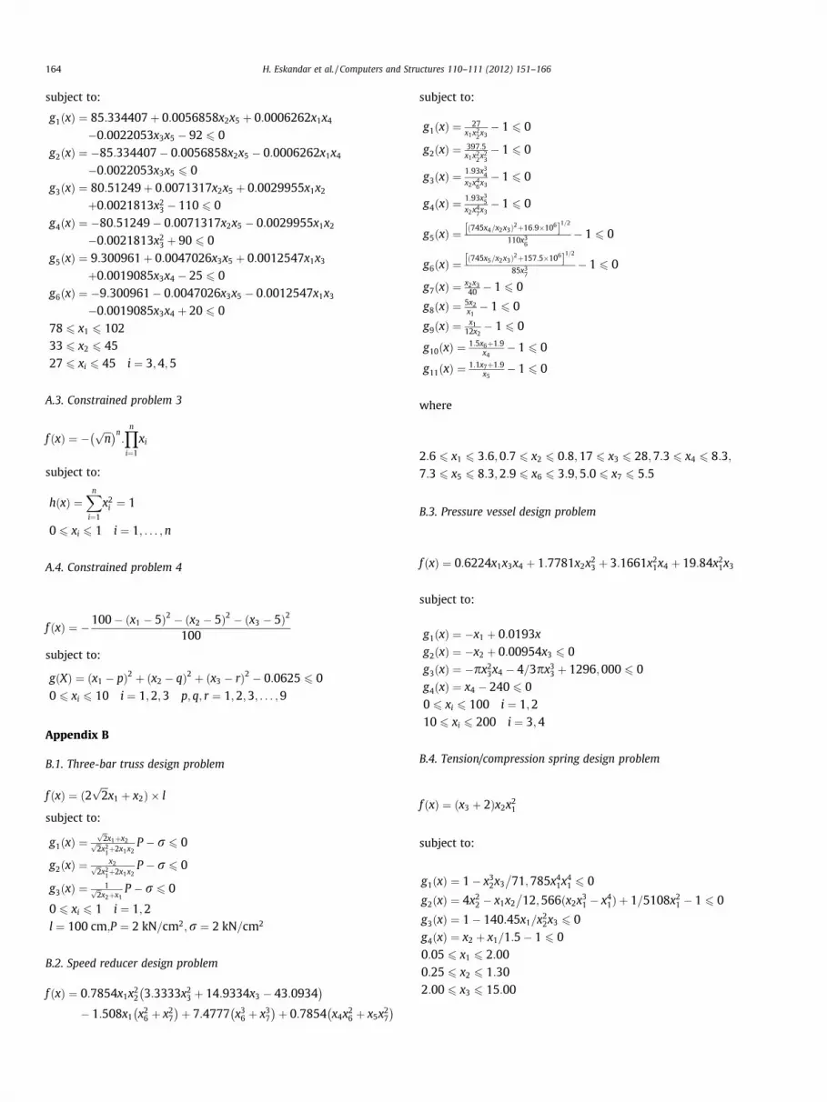
164 H. Eskandar et al. / Computers and Structures 110–111 (2012) 151–166
subject to:
g1ðxÞ ¼ 85:334407þ 0:0056858x2x5 þ 0:0006262x1x4
�0:0022053x3x5 � 92 6 0g2ðxÞ ¼ �85:334407� 0:0056858x2x5 � 0:0006262x1x4
�0:0022053x3x5 6 0g3ðxÞ ¼ 80:51249þ 0:0071317x2x5 þ 0:0029955x1x2
þ0:0021813x23 � 110 6 0
g4ðxÞ ¼ �80:51249� 0:0071317x2x5 � 0:0029955x1x2
�0:0021813x23 þ 90 6 0
g5ðxÞ ¼ 9:300961þ 0:0047026x3x5 þ 0:0012547x1x3
þ0:0019085x3x4 � 25 6 0g6ðxÞ ¼ �9:300961� 0:0047026x3x5 � 0:0012547x1x3
�0:0019085x3x4 þ 20 6 078 6 x1 6 10233 6 x2 6 4527 6 xi 6 45 i ¼ 3;4;5
A.3. Constrained problem 3
f ðxÞ ¼ �ffiffiffinp� �n
:Yn
i¼1
xi
subject to:
hðxÞ ¼Xn
i¼1
x2i ¼ 1
0 6 xi 6 1 i ¼ 1; . . . ;n
A.4. Constrained problem 4
f ðxÞ ¼ �100� ðx1 � 5Þ2 � ðx2 � 5Þ2 � ðx3 � 5Þ2
100
subject to:
gðXÞ ¼ ðx1 � pÞ2 þ ðx2 � qÞ2 þ ðx3 � rÞ2 � 0:0625 6 00 6 xi 6 10 i ¼ 1;2;3 p; q; r ¼ 1;2;3; . . . ;9
Appendix B
B.1. Three-bar truss design problem
f ðxÞ ¼ ð2ffiffiffi2p
x1 þ x2Þ � l
subject to:
g1ðxÞ ¼ffiffi2p
x1þx2ffiffi2p
x21þ2x1x2
P � r 6 0
g2ðxÞ ¼ x2ffiffi2p
x21þ2x1x2
P � r 6 0
g3ðxÞ ¼ 1ffiffi2p
x2þx1P � r 6 0
0 6 xi 6 1 i ¼ 1;2l ¼ 100 cm;P ¼ 2 kN=cm2;r ¼ 2 kN=cm2
B.2. Speed reducer design problem
f ðxÞ ¼ 0:7854x1x22 3:3333x2
3 þ 14:9334x3 � 43:0934� �
� 1:508x1 x26 þ x2
7
� �þ 7:4777 x3
6 þ x37
� �þ 0:7854 x4x2
6 þ x5x27
� �
subject to:
g1ðxÞ ¼ 27x1x2
2x3� 1 6 0
g2ðxÞ ¼ 397:5x1x2
2x23� 1 6 0
g3ðxÞ ¼1:93x3
4x2x4
6x3� 1 6 0
g4ðxÞ ¼1:93x3
5x2x4
7x3� 1 6 0
g5ðxÞ ¼745x4=x2x3ð Þ2þ16:9�106½ �1=2
110x36
� 1 6 0
g6ðxÞ ¼745x5=x2x3ð Þ2þ157:5�106½ �1=2
85x37
� 1 6 0
g7ðxÞ ¼ x2x340 � 1 6 0
g8ðxÞ ¼ 5x2x1� 1 6 0
g9ðxÞ ¼ x112x2� 1 6 0
g10ðxÞ ¼ 1:5x6þ1:9x4
� 1 6 0
g11ðxÞ ¼ 1:1x7þ1:9x5
� 1 6 0
where
2:6 6 x1 6 3:6;0:7 6 x2 6 0:8;17 6 x3 6 28;7:3 6 x4 6 8:3;7:3 6 x5 6 8:3;2:9 6 x6 6 3:9;5:0 6 x7 6 5:5
B.3. Pressure vessel design problem
f ðxÞ ¼ 0:6224x1x3x4 þ 1:7781x2x23 þ 3:1661x2
1x4 þ 19:84x21x3
subject to:
g1ðxÞ ¼ �x1 þ 0:0193x
g2ðxÞ ¼ �x2 þ 0:00954x3 6 0g3ðxÞ ¼ �px2
3x4 � 4=3px33 þ 1296;000 6 0
g4ðxÞ ¼ x4 � 240 6 00 6 xi 6 100 i ¼ 1;210 6 xi 6 200 i ¼ 3;4
B.4. Tension/compression spring design problem
f ðxÞ ¼ ðx3 þ 2Þx2x21
subject to:
g1ðxÞ ¼ 1� x32x3 71;785x4
1x41
�6 0
g2ðxÞ ¼ 4x22 � x1x2 12;566ðx2x3
1 � x41Þ
�þ 1=5108x2
1 � 1 6 0
g3ðxÞ ¼ 1� 140:45x1=x22x3 6 0
g4ðxÞ ¼ x2 þ x1=1:5� 1 6 00:05 6 x1 6 2:000:25 6 x2 6 1:302:00 6 x3 6 15:00

Structures 110–111 (2012) 151–166 165
B.5. Welded beam design problem
H. Eskandar et al. / Computers and
f ðxÞ ¼ 1:10471x21x2 þ 0:04811x3x4ð14þ x2Þ
subject to:
g1ðxÞ ¼ sðxÞ � smax 6 0g2ðxÞ ¼ rðxÞ � rmax 6 0g3ðxÞ ¼ x1 � x4 6 0
g4ðxÞ ¼ 0:10471x21 þ 0:04811x3x4ð14þ x2Þ � 5 6 0
g5ðxÞ ¼ 0:125� x1 6 0g6ðxÞ ¼ dðxÞ � dmax 6 0g7ðxÞ ¼ P � PcðxÞ 6 00:1 6 xi 6 2 i ¼ 1;40:1 6 xi 6 10 i ¼ 2;3
where,
sðxÞ ¼ffiffiffiffiffiffiffiffiffiffiffiffiffiffiffiffiffiffiffiffiffiffiffiffiffiffiffiffiffiffiffiffiffiffiffiffiffiffiffiffiffiffiffiffiffiffiffiffiffiffiðs0Þ2 þ 2s0s00 x2
2Rþ ðs00Þ2
rs0 ¼ Pffiffiffi
2p
x1x2s00 ¼ MR
J
M ¼ P Lþ x2
2
� �; R ¼
ffiffiffiffiffiffiffiffiffiffiffiffiffiffiffiffiffiffiffiffiffiffiffiffiffiffiffiffiffiffiffiffiffix2
2
4þ x1 þ x3
2
� �2r
;
J ¼ 2ffiffiffi2p
x1x2x2
2
12þ x1 þ x3
2
� �2 � �
rðxÞ ¼ 6PLx4x2
3
; dðxÞ ¼ 4PL3
Ex33x4
; PcðxÞ ¼4:013E
ffiffiffiffiffiffiffix2
3x6
436
qL2 1� x3
2L
ffiffiffiffiffiffiE
4G
r !
P ¼ 6000lb; L ¼ 14in; E ¼ 30� 106 psi; G ¼ 12� 106 psismax ¼ 13;600 psi; rmax ¼ 30;000 psi; dmax ¼ 0:25in
B.6. Rolling element bearing design problem
max Cd ¼ fcZ2=3D1:8b if D 6 25:4 mm
Cd ¼ 3:647f cZ2=3D1:4b if D � 25:4 mm
subject to:
g1ðxÞ ¼/0
2 sin�1ðDb=DmÞ� Z þ 1 P 0
g2ðxÞ ¼ 2Db � KD minðD� dÞP 0g3ðxÞ ¼ KD maxðD� dÞ � 2Db P 0g4ðxÞ ¼ fBw � Db 6 0g5ðxÞ ¼ Dm � 0:5ðDþ dÞP 0g6ðxÞ ¼ ð0:5þ eÞðDþ dÞ � Dm P 0g7ðxÞ ¼ 0:5ðD� Dm � DbÞ � eDb P 0g8ðxÞ ¼ fi P 0:515g9ðxÞ ¼ fo P 0:515
where,
fc ¼ 37:91 1þ 1:041� c1þ c
�1:72 fið2f o � 1Þfoð2f i � 1Þ
�0:41( )10=3
24
35�0:3
� c0:3ð1� cÞ1:39
ð1þ cÞ1=3
" #2f i
2f i � 1
0:41
/o ¼2p�2
� cos�1fðD�dÞ=2�3ðT=4Þg2þfD=2�T=4�Dbg2�fd=2þT=4g2h i
2fðD�dÞ=2�3ðT=4ÞgfD=2�T=4�Dbg
0@
1A
c ¼ Db
Dm; f i ¼
ri
Db; f 0 ¼
r0
DbT ¼ D� d� 2Db
D ¼ 160; d ¼ 90; Bw ¼ 30; ri ¼ ro ¼ 11:0330:5ðDþ dÞ 6 Dm 6 0:6ðDþ dÞ;0:15ðD� dÞ 6 Db 6 0:45ðD� dÞ;4 6 Z 6 50;0:515 6 fi and f o 6 0:6;
0:4 6 KDmin 6 0:5;0:6 6 KDmax 6 0:7;0:3 6 e 6 0:4;0:02 6 e 6 0:1;0:6 6 f 6 0:85:
B.7. Multiple disk clutch brake design problem
f ðxÞ ¼ pðr2o � r2
i ÞtðZ þ 1Þq
subject to:
g1ðxÞ ¼ ro � ri � Dr P 0g2ðxÞ ¼ lmax � ðZ þ 1Þðt þ dÞP 0g3ðxÞ ¼ pmax � prz P 0g4ðxÞ ¼ pmaxv sr max � przv sr P 0g5ðxÞ ¼ v sr max � vsr P 0g6ðxÞ ¼ Tmax � T P 0g7ðxÞ ¼ Mh � sMs P 0g8ðxÞ ¼ T P 0
where,
Mh ¼23lFZ
r3o � r3
i
r20 � r2
i
; prz ¼F
pðr20 � r2
i Þ;
v rz ¼2pnðr3
o � r3i Þ
90ðr20 � r2
i Þ; T ¼ Izpn
30ðMh þMf Þ
Dr ¼ 20 mm, Iz = 55 kgmm2, pmax = 1 MPa, Fmax = 1000 N,Tmax = 15 s, l = 0.5, s = 1.5, Ms = 40 Nm, Mf = 3 Nm, n = 250 rpm,vsrmax = 10 m/s, lmax = 30 mm, rimin = 60, rimax = 80, romin = 90, ro-max = 110, tmin = 1.5, tmax = 3, Fmin = 600, Fmax = 1000, Zmin = 2,Zmax = 9.
References
[1] Lee KS, Geem ZW. A new meta-heuristic algorithm for continuous engineeringoptimization: harmony search theory and practice. Comput Meth Appl MechEng 2005;194:3902–33.
[2] Holland J. Adaptation in natural and artificial systems. Ann Arbor,MI: University of Michigan Press; 1975.
[3] Goldberg D. Genetic algorithms in search, optimization and machinelearning. Reading, MA: Addison-Wesley; 1989.
[4] Kennedy J, Eberhart R. Particle swarm optimization. In: Proceedings of the IEEEinternational conference on neural networks. Perth, Australia: 1995. p. 1942–8.
[5] Kirkpatrick S, Gelatt C, Vecchi M. Optimization by simulated annealing. Science1983;220:671–80.
[6] Coello CAC. Theoretical and numerical constraint-handling techniques usedwith evolutionary algorithms: a survey of the state of the art. Comput MethAppl Mech Eng 2002;191:1245–87.
[7] Areibi S, Moussa M, Abdullah H. A comparison of genetic/memetic algorithmsand other heuristic search techniques. Las VeGAs, Nevada: ICAI; 2001.
[8] Elbeltagi E, Hegazy T, Grierson D. Comparison among five evolutionary-basedoptimization algorithms. Adv Eng Inf 2005;19:43–53.
[9] Youssef H, Sait SM, Adiche H. Evolutionary algorithms, simulated annealingand tabu search: a comparative study. Eng Appl Artif Intell 2001;14:167–81.
[10] Giraud-Moreau L, Lafon P. Comparison of evolutionary algorithms formechanical design components. Eng Optim 2002;34:307–22.
[11] Chootinan P, Chen A. Constraint handling in genetic algorithms using agradient-based repair method. Comput Oper Res 2006;33:2263–81.
[12] Trelea IC. The particle swarm optimization algorithm: convergence analysisand parameter selection. Inform Process Lett 2003;85:317–25.
[13] He Q, Wang L. An effective co-evolutionary particle swarm optimization forengineering optimization problems. Eng Appl Artif Intell 2006;20:89–99.
[14] Gomes HM. Truss optimization with dynamic constraints using a particleswarm algorithm. Expert Syst Appl 2011;38:957–68.

166 H. Eskandar et al. / Computers and Structures 110–111 (2012) 151–166
[15] David S. The water cycle, illustrations by John Yates. New York: ThomsonLearning; 1993.
[16] Strahler AN. Dynamic basis of geomorphology. Geol Soc Am Bull1952;63:923–38.
[17] Montes EM, Coello CAC. An empirical study about the usefulness of evolutionstrategies to solve constrained optimization problems. Int J Gen Syst2008;37:443–73.
[18] Kaveh A, Talatahari S. A particle swarm ant colony optimization for trussstructures with discrete variables. J Const Steel Res 2009;65:1558–68.
[19] Koziel S, Michalewicz Z. Evolutionary algorithms, homomorphous mappings,and constrained parameter optimization. IEEE Trans Evol Comput 1999;7:19–44.
[20] Ben Hamida S, Schoenauer M. ASCHEA: new results using adaptivesegregational constraint handling. IEEE Trans Evol Comput 2002:884–9.
[21] Tang KZ, Sun TK, Yang JY. An improved genetic algorithm based on a novelselection strategy for nonlinear programming problems. Comput Chem Eng2011;35:615–21.
[22] Michalewicz Z. Genetic algorithms, numerical optimization, and constraints.In: Esheman L, editor. Proceedings of the sixth international conference ongenetic algorithms. San Mateo: Morgan Kauffman; 1995. p. 151–8.
[23] Mezura-Montes E, Coello CAC. A simple multimembered evolution strategy tosolve constrained optimization problems. IEEE Trans Evol Comput 2005;9:1–17.
[24] Tessema B, Yen GG. A self adaptive penalty function based algorithm forconstrained optimization. IEEE Trans Evol Comput 2006:246–53.
[25] Liu H, Cai Z, Wang Y. Hybridizing particle swarm optimization with differentialevolution for constrained numerical and engineering optimization. Appl SoftComput 2010;10:629–40.
[26] Runarsson TP, Xin Y. Stochastic ranking for constrained evolutionaryoptimization. IEEE Trans Evol Comput 2000;4:284–94.
[27] Lampinen J. A constraint handling approach for the differential evolutionalgorithm. IEEE Trans Evol Comput 2002:1468–73.
[28] Becerra R, Coello CAC. Cultured differential evolution for constrainedoptimization. Comput Meth Appl Mech Eng 2006;195:4303–22.
[29] Renato AK, Leandro Dos Santos C. Coevolutionary particle swarm optimizationusing gaussian distribution for solving constrained optimization problems.IEEE Trans Syst Man Cybern Part B Cybern 2006;36:1407–16.
[30] Zhang M, Luo W, Wang X. Differential evolution with dynamic stochasticselection for constrained optimization. Inform Sci 2008;178:3043–74.
[31] Runarsson TP, Xin Y. Search biases in constrained evolutionary optimization.IEEE Trans Syst Man Cybern Part C Appl Rev 2005;35:233–43.
[32] Wang Y, Cai Z, Zhou Y, Fan Z. Constrained optimization based on hybridevolutionary algorithm and adaptive constraint handling technique. StructMultidisc Optim 2009;37:395–413.
[33] Takahama T, Sakai S. Constrained optimization by applying the a; constrainedmethod to the nonlinear simplex method with mutations. IEEE Trans EvolComput 2005;9:437–51.
[34] A.E.M. Zavala, A.H. Aguirre, E.R.V. Diharce, Constrained optimization viaevolutionary swarm optimization algorithm (PESO). In: Proceedings of the2005 conference on genetic and evolutionary computation. New York, USA:2005. p. 209–16.
[35] Huang FZ, Wang L, He Q. An effective co-evolutionary differential evolution forconstrained optimization. Appl Math Comput 2007;186(1):340–56.
[36] Karaboga D, Basturk B. Artificial bee colony (ABC) optimization algorithm forsolving constrained optimization problems. LNAI 2007;4529:789–98 [Berlin:Springer-Verlag].
[37] Coello CAC, Becerra RL. Efficient evolutionary optimization through the use ofa cultural algorithm. Eng Optim 2004;36:219–36.
[38] He Q, Wang L. A hybrid particle swarm optimization with a feasibility-basedrule for constrained optimization. Appl Math Comput 2007;186:1407–22.
[39] Amirjanov A. The development of a changing range genetic algorithm. ComputMeth Appl Mech Eng 2006;195:2495–508.
[40] Wang L, Li LP. An effective differential evolution with level comparison forconstrained engineering design. Struct Multidisc Optim 2010;41:947–63.
[41] Zahara E, Kao YT. Hybrid Nelder–Mead simplex search and particle swarmoptimization for constrained engineering design problems. Expert Syst Appl2009;36:3880–6.
[42] Rao RV, Savsani VJ, Vakharia DP. Teaching-learning-based optimization: anovel method for constrained mechanical design optimization problems.Comput Aided Des 2011;43:303–15.
[43] Ray T, Liew KM. Society and civilization: an optimization algorithm based onthe simulation of social behavior. IEEE Trans Evol Comput 2003;7:386–96.
[44] Mezura-Montes E, Coello CAC. Useful infeasible solutions in engineeringoptimization with evolutionary algorithms, MICAI 2005. Lect Notes Artif Int2005;3789(2005):652–62.
[45] Montes E, Reyes JV, Coello CAC. Modified differential evolution for constrainedoptimization. In: IEEE congress on evolutionary computation. CEC; 2006a. p.25–32.
[46] Montes E, Coello CAC, Reyes JV. Increasing successful offspring and diversity indifferential evolution for engineering design. In: Proceedings of the seventhinternational conference on adaptive computing in design and manufacture.2006b. p. 131–9.
[47] Kannan BK, Kramer SN. An augmented lagrange multiplier based method formixed integer discrete continuous optimization and its applications tomechanical design. J Mech Des 1994;116:405–11.
[48] Coello CAC. Use of a self-adaptive penalty approach for engineeringoptimization problems. Comput Ind 2000;41:113–27.
[49] C Coello CA, Mezura Montes E. Constraint-handling in genetic algorithmsthrough the use of dominance-based tournament selection. Adv Eng Inf2002;16:193–203.
[50] Coelho LDS. Gaussian quantum-behaved particle swarm optimizationapproaches for constrained engineering design problems. Expert Syst Appl2010;37:1676–83.
[51] Arora JS. Introduction to optimum design. New York: McGraw-Hill; 1989.[52] Yuan Q, Qian F. A hybrid genetic algorithm for twice continuously
differentiable NLP problems. Comput Chem Eng 2010;34:36–41.[53] Coello CAC. Constraint-handling using an evolutionary multiobjective
optimization technique. Civ Eng Environ Syst 2000;17:319–46.[54] Gupta S, Tiwari R, Shivashankar BN. Multi-objective design optimization of
rolling bearings using genetic algorithm. Mech Mach Theory 2007;42:1418–43.[55] Osyczka A. Evolutionary algorithms for single and multicriteria design
optimization: studies in fuzzyness and soft computing. Heidelberg: Physica-Verlag; 2002.
[56] Deb K, Srinivasan A. Innovization: innovative design principles throughoptimization, Kanpur genetic algorithms laboratory (KanGAL). IndianInstitute of Technology Kanpur, KanGAL report number: 2005007; 2005.