solving nonlinearly constrained global optimization problem via an auxiliary function method

Journal of Computational and Applied Mathematics 230 (2009) 491–503

Contents lists available at ScienceDirect

Journal of Computational and AppliedMathematics

journal homepage: www.elsevier.com/locate/cam

Solving nonlinearly constrained global optimization problem via anauxiliary function methodI

Wenxing Zhu a,∗, M.M. Ali ba Center for Discrete Mathematics and Theoretical Computer Science, Fuzhou University, Fuzhou 350002, Chinab School of Computational and Applied Mathematics, University of the Witwatersrand, Wits 2050, Johannesburg, South Africa

a r t i c l e i n f o

Article history:Received 3 July 2008Received in revised form 20 September2008

Keywords:Nonlinearly constrained globalminimization problemAuxiliary function methodConvergence

a b s t r a c t

This paper considers the nonlinearly constrained continuous globalminimization problem.Based on the idea of the penalty function method, an auxiliary function, which hasapproximately the same global minimizers as the original problem, is constructed.An algorithm is developed to minimize the auxiliary function to find an approximateconstrained global minimizer of the constrained global minimization problem. Thealgorithm can escape from the previously converged local minimizers, and can convergeto an approximate global minimizer of the problem asymptotically with probability one.Numerical experiments show that it is better than some other well known recent methodsfor constrained global minimization problems.

© 2008 Elsevier B.V. All rights reserved.

1. Introduction

Consider the following nonlinearly constrained continuous global minimization problem,

(P)

min f (x)s.t. gi(x) ≤ 0, i ∈ Ihj(x) = 0, j ∈ Jx ∈ X,

(1)

where I , J are sets of finite indices, X is a bounded closed box in Rn, i.e., X = {x ∈ Rn : a ≤ x ≤ b}, f (x) ∈ C1, gi(x) ∈ C1,i ∈ I , hj(x) ∈ C1, j ∈ J .Global optimization has many applications in engineering, decision science and operations research. The task of global

optimization is to find a solution with the smallest objective function value. A number of methods has been developed forconstrained global optimization problems. Roughly speaking, these methods can be classified into two categories [1,2], theexact methods [3–5] and the heuristic methods [2,5,6].The exact methods include the Branch and Bound method and the cutting plane method. These methods are applicable

to certain well-structured problems of type, such as the concave programming, D.C. programming, Lipschitz optimization,and others [3–5]. The exact methods can obtain verified optimal solutions of constrained global optimization problems, butare time consuming.The heuristic methods do not guarantee the quality of global optimum, but give satisfactory results for much larger

range of global optimization problems in a relatively short time. Some methods, e.g., the simulated annealing, and genetic

I Research supported by the National Natural Science Foundation of China under Grants 60773126, 10301009, the Program for NCET, and the ScienceFoundation of Fujian Province under Grant 2006J0030.∗ Corresponding author.E-mail address:[email protected] (W. Zhu).

0377-0427/$ – see front matter© 2008 Elsevier B.V. All rights reserved.doi:10.1016/j.cam.2008.12.017

http://www.elsevier.com/locate/cam

http://www.elsevier.com/locate/cam

mailto:[email protected]

http://dx.doi.org/10.1016/j.cam.2008.12.017

492 W. Zhu, M.M. Ali / Journal of Computational and Applied Mathematics 230 (2009) 491–503

algorithms, use different techniques to avoid getting entrapment in poor local minima, and overcome the difficultiesencountered in gradient based local optimization methods. These methods usually use the penalty function method toconvert the constrained global minimization problem to an unconstrained one, by adding a penalty term to the objectivefunction [7].However, it is difficult or impossible to choose a static value of the penalty parameter such that the penalty problem and

the original problem have the same global minimizers. So dynamic or adaptive penalties are proposed in GA literatures [8–11,7]. Dynamic penalty functions are sensitive to certain parameters related to run time [12]. In [13–15], Wah et al.introduced the Lagrangian based Simulated Annealing method for constrained global optimization, which avoid parametricproblems in penalty functions. Their algorithms adopt an ascending approach for the Lagrangian parameters. Basing on theidea of multiobjective optimization, Hedar and Fukushima [16] reformulated problem (P) as a multiobjective optimizationproblem, and then solved the reformulated problem by the multi-start Simulated Annealing method. Their method doesnot use penalty functions, and has no parametric problems. Furthermore, there has been relatively little work relatedto the incorporation of constraints into the Particle Swarm Optimization (PSO) algorithm. In [17], Cabrera and Coelloassigned a fitness function without parameters to a solution, and developed a PSO algorithm for problem (P) using a smallpopulation size.An important class of heuristic methods for continuous global optimization are gradient-based methods, which

try to minimize some auxiliary functions to descend from one local minimizer to another better one of the originalproblem [5]. The methods using auxiliary functions include the terminal repeller unconstrained sub-energy tunnelingmethod (TRUST) [18,19], the filled functionmethod [20], the diffusion equationmethod [21], and the tunnelingmethod [22,23]. However, these methods [24–26] have not been developed extensively for constrained global optimization, such thattheir performances have been compared or can be comparable with other heuristic methods, e.g., the simulated annealing,genetic algorithms, etc.In this paper, basing on the idea of the penalty function method, we propose an auxiliary function, which has no

parametric problems, and propose a gradient-based method for the constrained global optimization problem. The paperis organized as follows. In Section 2, we introduce an auxiliary function for the constrained global minimization problem(P), and analyze some properties of the proposed function. In Section 3, we propose a global optimizationmethod called theauxiliary functionmethod, whichminimizes the auxiliary function dynamically to obtain approximately a global minimizerof the constrained global minimization problem (P). Moreover, we prove the asymptotic convergence property of themethod in Section 4. Numerical experiments of the method are presented in Section 5.

2. Auxiliary function and its properties

Suppose that problem (P) is feasible. Let x∗1 be a point in X , and let f∗

1 be a finite number such that, if x∗

1 is a feasible pointof problem (P), then f ∗1 = f (x

∗

1); otherwise f∗

1 is an upper bound on the global minimal value of problem (P).Let S = {x ∈ X : gi(x) ≤ 0, i ∈ I, hj(x) = 0, j ∈ J}. Take p(x) be a differentiable penalty term of problem (P), such that

for all x ∈ X , p(x) = 0 if and only if x ∈ S, say,

p(x) =∑i∈I

max2{0, gi(x)} +∑j∈J

h2j (x).

Given a small positive constant ε, we relax problem (P) as the following problem,

(RP)

{min f (x)s.t. p(x) ≤ εx ∈ X .

Since if ε → 0, then a global minimizer of problem (RP)will tend to a global minimizer of problem (P), we think that if wecan find a global minimizer of problem (RP), then problem (P) is solved approximately.Furthermore, let

F(x) = v(f (x)− f ∗1 + ε)+ p(x), (2)

let v(t) be a univariate function, which is a continuously differentiable, and monotonically increasing function for t > 0such that,

v(t) = 0, for all t ≤ 0; and v′(t) > 0, for all t > 0. (3)

Obviously, F(x) ≥ 0, and F(x) = 0 if and only if f (x) ≤ f ∗1 − ε and p(x) = 0.Construct the following auxiliary function

T (x, k, l) = f (x)− f ∗1 + [F(x)+ k‖x− x∗

1‖ − (f (x)− f∗

1 )]u(lF(x)), (4)

where k, l are nonnegative parameters, ‖ · ‖ designates the Euclidean norm, u(t) is a continuously differentiable andmonotonically increasing univariate function of t , and has the following property,

u(0) = 0, u(t) = 1 for t ≥ 1;

u′(t) > 0, for 0 < t < 1; and u′(t) = 0, for t ≥ 1. (5)

W. Zhu, M.M. Ali / Journal of Computational and Applied Mathematics 230 (2009) 491–503 493

Obviously, for all x ∈ X and x 6= x∗1 , T (x, k, l) is a continuously differentiable function of x. And by (2) and (5), it is easy tosee that,

T (x, k, l) =

f (x)− f ∗1 , if F(x) = 0;

f (x)− f ∗1 + [F(x)+ k‖x− x∗

1‖ − (f (x)− f∗

1 )]u(lF(x)), if 0 < F(x) <1l;

F(x)+ k‖x− x∗1‖, if F(x) ≥1l.

(6)

In the function T (x, k, l), we classify the value of F(x) into three cases. For the three cases, we have the following results.

Theorem 1. Let l satisfy that

l > max{1v(ε)

,1ε

}. (7)

For x ∈ X, we have,

(1) if F(x) = 0, then p(x) = 0 and f (x) ≤ f ∗1 − ε;(2) if 0 < F(x) < 1

l , then f (x) < f∗

1 , and p(x) < ε;(3) if F(x) ≥ 1

l , then either p(x) > 0, or f (x) ≥ f∗

1 − ε + v−1( 1l ) > f

∗

1 − ε.

Proof. (1) If F(x) = 0, then by (2),

v(f (x)− f ∗1 + ε)+ p(x) = 0. (8)

Since v(t) and p(x) are nonnegative, equality (8) leads to p(x) = 0, and

v(f (x)− f ∗1 + ε) = 0. (9)

Furthermore, by (3) and (9), we have f (x) ≤ f ∗1 − ε.(2) If 0 < F(x) < 1

l , then by (2), p(x) <1l . So if we take l such that inequality (7) holds, then p(x) <

1l < ε. Moreover,

we also have v(f (x)− f ∗1 + ε) <1l , which leads to

f (x) < f ∗1 − ε + v−1(1l

). (10)

So if we take l such that inequality (7) holds, then 1l < v(ε), v−1( 1l ) < ε, and by (10) we have f (x) < f ∗1 − ε+ v−1( 1l ) < f

∗

1 .(3) If F(x) ≥ 1

l , and if x is not a feasible solution of problem (P), then p(x) > 0 and case (3) holds; if x is a feasible solutionof problem (P), i.e., p(x) = 0, then by (2), v(f (x)− f ∗1 + ε) ≥

1l , and

f (x) ≥ f ∗1 − ε + v−1(1l

). (11)

Thus if we take l such that it satisfies inequality (7), then 0 < v−1( 1l ) < ε, and by (11), case 3 of Theorem 1 holds. �

Theorem 1 means that, for x ∈ X , if F(x) = 0, then such a point x is a feasible solution of problem (P), and is lower thanf ∗1 ; if 0 < F(x) <

1l , then such a point x is a feasible solution of problem (RP), and is lower than f

∗

1 ; and if F(x) ≥1l , then

such a point x is either not a feasible solution of problem (P), or not lower than f ∗1 enough.The objective of this paper is to find an approximate constrained global minimizer of problem (P), or problem (RP),

by minimizing the function T (x, k, l) over the bounded closed box X . According to the above analysis, while minimizingT (x, k, l) over X , if we can find a point x such that F(x) < 1

l , then we have found a feasible solution of problem (RP), whichis lower than f ∗1 ; and if F(x) ≥

1l , then such a point is either infeasible or not lower enough than f

∗

1 of problem (P). Sowhile using a local search method to minimize the function T (x, k, l), we hope that the method can find a point in the set{x ∈ X : F(x) < 1

l }, but not getting stuck in {x ∈ X : F(x) ≥1l }.

Firstly, we analyze properties of the function T (x, k, l) on X . We construct the following auxiliary global minimizationproblem

(AP){min T (x, k, l)s.t. x ∈ X .

Lemma 1. For all x ∈ {x ∈ X : F(x) = 0}, for all y ∈ {x ∈ X : F(x) ≥ 1l }, it holds that T (x, k, l) < T (y, k, l).

Proof. For all x ∈ {x ∈ X : F(x) = 0}, by (6), T (x, k, l) = f (x)− f ∗1 < 0. Moreover, for all y ∈ {x ∈ X : F(x) ≥1l }, F(y) ≥

1l ,

and by (6)


T (y, k, l) = F(y)+ k‖y− x∗1‖ > 0.

Hence T (x, k, l) < T (y, k, l). �

By Lemma 1, it is obvious that the following corollary holds.

Corollary 1. If {x ∈ X : F(x) = 0} 6= ∅, then all global minimizers of problem (AP) are in the set {x ∈ X : F(x) < 1l }.

Theorem 2. Suppose that {x ∈ X : F(x) = 0} 6= ∅, and suppose that y is a local minimizer of problem (AP). If F(y) = 0, then yis a constrained local minimizer of problem (P).

Proof. If F(y) = 0, then by (6), T (y, k, l) = f (y) − f ∗1 < 0. If y is a local minimizer of problem (AP), then there exists aneighborhood N(y) of y such that

T (y, k, l) = f (y)− f ∗1 ≤ T (x, k, l), for all x ∈ N(y) ∩ X . (12)

Thus, for any x ∈ N(y) ∩ S, if F(x) = 0, then by (6), T (x, k, l) = f (x) − f ∗1 , and by (12), it holds that f (y) ≤ f (x); and ifF(x) > 0, then by (2), F(x) = v(f (x)− f ∗1 + ε)+ p(x) > 0. Since x ∈ S and p(x) = 0, we have F(x) = v(f (x)− f

∗

1 + ε) > 0.Thus, f (x) > f ∗1 − ε. But F(y) = 0, and by (1) of Theorem 1, f (y) ≤ f

∗

1 − ε. So, f (x) > f (y).The above two cases implies that for all x ∈ N(y) ∩ S, f (x) ≥ f (y), i.e., y is a constrained local minimizer of problem (P).�

Theorem 3. Suppose that l satisfies inequality (7), and {x ∈ X : F(x) = 0} 6= ∅. Let f ∗ be the global minimal value of problem(P). If y∗ is a global minimizer of problem (AP), then p(y∗) < 1

l and f (y∗) ≤ f ∗. Specially, if p(y∗) = 0, then y∗ is a global

minimizer of problem (P).

Proof. Since {x ∈ X : F(x) = 0} 6= ∅, there exists an x ∈ X such that p(x) = 0, and v(f (x)− f ∗1 + ε) = 0, i.e., f (x) ≤ f∗

1 − ε.Thus for a global minimizer x∗ of problem (P), it holds that p(x∗) = 0, and f (x∗) ≤ f ∗1 − ε, T (x

∗, k, l) = f (x∗)− f ∗1 .If y∗ is a global minimizer of problem (AP), then

T (y∗, k, l) ≤ T (x∗, k, l) = f (x∗)− f ∗1 . (13)

Moreover, by Corollary 1, F(y∗) < 1l , which is equivalent to

v(f (y∗)− f ∗1 + ε)+ p(y∗) <

1l. (14)

Inequality (14) leads to

p(y∗) <1l, (15)

and

v(f (y∗)− f ∗1 + ε) <1l. (16)

For inequality (16), we have

f (y∗)− f ∗1 + ε < v−1(1l

),

i.e.,

f (y∗) < f ∗1 − ε + v−1(1l

). (17)

Thus if l satisfies inequality (7), then (17) results in f (y∗) < f ∗1 . In this case,−(f (y∗)− f ∗1 ) > 0, and

T (y∗, k, l) = f (y∗)− f ∗1 + [F(y∗)+ k‖y∗ − x∗1‖ − (f (y

∗)− f ∗1 )]u(lF(y∗))

≥ f (y∗)− f ∗1 . (18)

So combining (13) and (18), we have

f (y∗) ≤ f (x∗). (19)

Hence by (15) and (19), y∗ is an approximate global minimizer of problem (P).Furthermore, if p(y∗) = 0, then y∗ is a feasible solution of problem (P), and by (19), y∗ is a global minimizer of problem

(P). �


Theorem3means that, under the assumptions of Theorem3, the globalminimizers of problem (AP) are feasible solutionsof problem (RP), and are not worse than the global minimizers of problem (P). Hence, since problem (RP) is a relaxationof problem (P), if we can find a global minimizer of problem (AP), then we can solve problem (RP), and solve problem (P)approximately.

3. Auxiliary function method

The method presented in this paper tries to find a feasible solution of problem (RP) lower than f ∗1 , using a local searchmethod to minimize the function T (x, k, l) over the bounded closed box X . While using a local search method to minimizethe function T (x, k, l), we hope that the method can find a point in the set {x ∈ X : F(x) < 1

l }, but not getting stuck in{x ∈ X : F(x) ≥ 1

l }, since in the first case we have found a point x such that F(x) <1l . This point is either a feasible solution

of problem (P), which is lower then f ∗1 , or a feasible solution of problem (RP), which is lower then f∗

1 .In the second case, we show in the following that, if the value of parameter k is large enough, then any point except x∗1

in {x ∈ X : F(x) ≥ 1l }will not be a stationary point of T (x, k, l).

Theorem 4. For any x ∈ Gk = {x ∈ X : F(x) ≥ 1l , ‖∇F(x)‖ < k}, x 6= x

∗

1 , x∗

1 − x is a descent direction of T (x, k, l) at x, and xis not a stationary point of T (x, k, l).

Proof. By (4), for x ∈ X , x 6= x∗1 , the gradient of T (x, k, l) is

∇T (x, k, l) = ∇f (x)+[∇F(x)+ k

x− x∗1‖x− x∗1‖

− ∇f (x)]u(lF(x))

+ [F(x)+ k‖x− x∗1‖ − (f (x)− f (x∗

1))]u′(lF(x))l∇F(x). (20)

For any x ∈ Gk = {x ∈ X : F(x) ≥ 1l , ‖∇F(x)‖ < k}, x 6= x

∗

1 , we have lF(x) ≥ 1, and by (5), u(lF(x)) = 1, u′(lF(x)) = 0. So

equality (20) leads to

∇T (x, k, l) = ∇F(x)+ kx− x∗1‖x− x∗1‖

, (21)

and

(x∗1 − x)T

‖x− x∗1‖∇T (x, k, l) =

(x∗1 − x)T

‖x− x∗1‖∇F(x)− k.

Since ‖∇F(x)‖ < k, we have

(x∗1 − x)T

‖x− x∗1‖∇F(x)− k ≤

∥∥∥∥ (x∗1 − x)T‖x− x∗1‖

∥∥∥∥ · ‖∇F(x)‖ − k= ‖∇F(x)‖ − k< 0.

Hence (x∗1−x)

T

‖x−x∗1‖∇T (x, k, l) < 0, and Theorem 4 holds. �

In Theorem 4, it is obvious that G0 = ∅, and G0 ⊆ Gk1 ⊆ Gk2 ⊆ · · · ⊆ Gkm ⊆ GL ⊆ {x ∈ X : F(x) ≥1l }, where

0 < k1 < k2 < · · · < km, and L is an upper bound of ‖F(x)‖ over X . Moreover, if k > L, then Gk = {x ∈ X : F(x) ≥ 1l }.

Corollary 2. Let x∗1 ∈ X. Suppose that F(x∗

1) >1l , or suppose that F(x

∗

1) ≥1l but x

∗

1 is a local minimizer of F(x) over X. If k > L,then x∗1 is a local minimizer of T (x, k, l) over X.

Proof. For x∗1 ∈ X such that F(x∗

1) >1l , or F(x

∗

1) ≥1l but x

∗

1 is a local minimizer of F(x) over X , there exists a neighborhoodN(x∗1) of x

∗

1 such that for all x ∈ N(x∗

1) ∩ X , F(x) ≥1l . Thus if k > L, then by Theorem 4, for all x ∈ N(x

∗

1) ∩ X , x 6= x∗

1 , x∗

1 − xis a descent direction of T (x, k, l) at x, which means that x∗1 is a local minimizer of T (x, k, l) over X . �

Theorem 4 and Corollary 2 suggest that, if minimization of T (x, k, l) over X gets stuck at a local minimizer in the set{x ∈ X : F(x) ≥ 1

l }, then by increasing the value of k, minimization of T (x, k, l) can escape from the local minimizer. Henceif we increase the value of k sufficiently, then minimizing T (x, k, l) over X , we will finally reach the set {x ∈ X : F(x) < 1

l },or converge to x∗1 .However, too large value of parameter k is not good for finding better solutions of T (x, k, l) over X . Suppose that y ∈ X is

a local minimizer of T (x, k, l)with k = 0, which is lower than x∗1 , and B(y) is an attraction region of T (x, k, l)with k = 0 at y.Then minimizing T (x, k, l) over X from an initial point x′ ∈ B(y)with F(x′) ≥ 1

l will converge to y. But from x′ to minimize


T (x, k, l) with a large value of k may escape from the attraction region B(y), and cannot guarantee to converge to a betterlocal minimizer y, since by Theorem 4, if k is large enough, then x∗1 − x

′ is always a descent direction of T (x, k, l) at x′.Sowe have one questionwhich is, whether or not theminimization of T (x, k, l) on X from the initial point could converge

to the local minimizer lower than the current best one. The essence of such a question is linked to, whether or not we canmake T (x, k, l) keep the descent directions of F(x) at the points in the region {x ∈ X : F(x) ≥ 1

l }, since in this regionT (x, k, l) = F(x)+ k‖x− x∗1‖. In fact, we have the following result.

Theorem 5. Suppose that d is a descent direction of F(x) at an x ∈ {x ∈ X : F(x) ≥ 1l , x 6= x

∗

1}, i.e., dT∇F(x) < 0. Then d is a

descent direction of T (x, k, l) if and only if one of the following conditions holds:

1. k = 0;2. k > 0, and dT(x− x∗1) ≤ 0;3. k > 0, dT(x− x∗1) > 0, and

k < −dT∇F(x)‖x− x∗1‖dT(x− x∗1)

.

Proof. By (21), for any x ∈ X such that x 6= x∗1 and F(x) ≥1l , we have

dT∇T (x, k, l) = dT∇F(x)+ kdT(x− x∗1)‖x− x∗1‖

.

Thus, dT∇T (x, k, l) < 0 if and only if

dT∇F(x)+ kdT(x− x∗1)‖x− x∗1‖

< 0,

which leads to

kdT(x− x∗1)‖x− x∗1‖

< −dT∇F(x). (22)

The right hand side of inequality (22) is positive, since dT∇F(x) < 0. So if k = 0, or k > 0 and dT(x−x∗1) ≤ 0, then inequality(22) holds; otherwise if k > 0 and dT(x− x∗1) > 0, then inequality (22) holds if and only if

k < −dT∇F(x)‖x− x∗1‖dT(x− x∗1)

. �

Theorem 5 implies that T (x, k, l)might not keep the descent directions of F(x) at a point in the region {x ∈ X : F(x) ≥1l , x 6= x

∗

1} if k is too large. So while minimizing T (x, k, l) on X from an initial point in the region {x ∈ X : F(x) ≥1l , x 6= x

∗

1},to keep the descent directions of F(x), the value of k should not be too large.But by Theorem 4, to bypass a previously converged local minimizer while minimizing T (x, k, l) on X , k should be large

enough. This contradicts the above conclusion of Theorem 5. So in the algorithm presented in the sequel, we take k = 0initially, and increase the value of k sequentially.The basic idea of the algorithm can be described as follows.By Theorem 3, we can solve problem (P) approximately by minimizing T (x, k, l) over X . And by Theorem 4, parameter

k is used for escaping previously converged local minimizers. So we minimize T (x, k, l) with k = 0 over X firstly, from arandom initial point using any local search method.If theminimization sequence converges to a point x′with F(x′) < 1

l , then by Theorem1, the algorithmhas found a feasiblesolution of problem (RP), which is lower than f ∗1 . Hence we update the current best local minimizer and local minimal valueof problem (RP), by taking x∗1 = x

′, f ∗1 = f (x′), and repeat the above process.

If the minimization sequence converges to a point x′ with F(x′) ≥ 1l and F(x

′) ≤ F(x∗1), then

T (x′, 0, l) = F(x′) ≤ F(x∗1) = T (x∗

1, 0, l).

In this case x′ is not worse than x∗1 for problem (AP) with k = 0, so we still let x∗

1 = x′, and repeat the above process; if the

minimization sequence converges to a point x′ with F(x′) ≥ 1l and F(x

′) > F(x∗1), then T (x′, 0, l) > T (x∗1, 0, l). In this case,

by Theorem 4, we can try to escape from the current local minimizer x′ of problem (AP) obtained with k = 0, by settingk = δk.Now for k > 0, we minimize T (x, k, l) over X from a uniformly generated x′ using any local search method. Denote also

by x′ an obtained local minimizer. If F(x′) < 1l , then as before we let x

∗

1 = x′, f ∗1 = f (x

∗

1), and repeat the above process.But if F(x′) ≥ 1

l , then by Theorem 4, the algorithm may have escaped from the previously converged local minimizer,and by Theorem 5, x′ might be in another attraction region of some local minimizer of T (x, 0, l) over X , which is lower


than x∗1 . So we minimize T (x, 0, l) over X from x′ using any local search method. Suppose that x′′ is an obtained local

minimizer. If F(x′′) < 1l , then as before we let x

∗

1 = x′′, f ∗1 = f (x

∗

1), and repeat the above process; if1l ≤ F(x

′′) ≤ F(x∗1),i.e., T (x′′, 0, l) ≤ T (x∗1, 0, l), then let x

∗

1 = x′′, and repeat the above process; or else if F(x′′) > F(x∗1), then x

′ is not in anotherattraction region of T (x, 0, l) lower than x∗1 , so we set k = k + δk, and minimize T (x, k, l) over X from x

′ again, till theminimization sequence converges to x∗1 , and repeat the above process.The algorithm is described as follows.

Algorithm (Auxiliary Function Method). Step 1. Let ε be a small positive number, and let l > max{ 1v(ε), 1ε}. Let NL be a

sufficiently large integer, and let δk be a positive number. Set N = 0.Let f ∗1 be an upper bound on the global minimal value of problem (P). Select randomly a point x ∈ X . If F(x) >

1l , then

let x∗1 = x; if F(x) ≤1l , then use the exterior penalty function method to find a feasible solution x

′ of problem (P) from x, letx∗1 = x

′, and let f ∗1 = f (x∗

1).Step 2. Set k = 0, and N = N + 1. If N ≥ NL, then go to Step 4; otherwise draw randomly an initial point y in X , go to

Step 3.Step 3. Minimize T (x, k, l) over X from y using any local search method. Suppose that x′ is an obtained local minimizer.Step 3.1. If F(x′) < 1

l , then let x∗

1 = x′, f ∗1 = f (x

∗

1), and go to Step 2.Step 3.2. If 1l ≤ F(x

′) ≤ F(x∗1) and k = 0, then let x∗

1 = x′, and go to Step 2; if F(x′) > F(x∗1) and k = 0, then set k = δk,

y = x′, and repeat Step 3.Step 3.3. If F(x′) ≥ 1

l and k > 0, then minimize T (x, 0, l) over X from x′ using any local search method. Suppose that x′′

is an obtained local minimizer. If F(x′′) < 1l , then let x

∗

1 = x′′, f ∗1 = f (x

∗

1), and go to Step 2; if1l ≤ F(x

′′) ≤ F(x∗1), then letx∗1 = x

′′, and go to Step 2; else if F(x′′) > F(x∗1), then set k = k+ δk, y = x′, and repeat Step 3.

Step 4. Stop the algorithm, if p(x∗1) ≤ ε, then output x∗1 and f (x∗

1) as an approximate global minimal solution and anapproximate global minimal value of problem (P) respectively.

In the above algorithm at Step 3.2, we have the case 1l ≤ F(x′) ≤ F(x∗1). This case may happen. To prove it, we need the

following result.

Lemma 2. Suppose that x′ is a local minimizer of T (x, 0, l) over X. If F(x′) ≥ 1l , then x

′ is a local minimizer of F(x) over X.

Proof. Since x′ is a local minimizer of T (x, 0, l) over X , there exists a neighborhood N(x′) of x′ such that,

T (x, 0, l) ≥ T (x′, 0, l), for all x ∈ N(x′) ∩ X . (23)

Since F(x′) ≥ 1l , and by (6), we have T (x

′, 0, l) = F(x′) ≥ 1l . Thus inequality (23) leads to

T (x, 0, l) ≥ F(x′) ≥1l, for all x ∈ N(x′) ∩ X . (24)

Furthermore, for any x ∈ N(x′) ∩ X , if F(x) ≥ 1l , then by (6), T (x, 0, l) = F(x), and by (24), we have F(x) ≥ F(x

′); if0 < F(x) < 1

l , then by Theorem 1, f (x) < f∗

1 . So F(x)− (f (x)− f∗

1 ) > 0, and

T (x, 0, l) = f (x)− f ∗1 + [F(x)− (f (x)− f∗

1 )]u(lF(x))< f (x)− f ∗1 + [F(x)− (f (x)− f

∗

1 )]

= F(x) <1l. (25)

But inequality (25) contradicts inequality (24). So the case 0 < F(x) < 1l will not happen; moreover, if F(x) = 0, then by

(6) and Theorem 1, T (x, 0, l) = f (x)− f ∗1 < 0, which also contradicts inequality (24), and means that the case F(x) = 0 willnot happen. Hence for all x ∈ N(x′) ∩ X , F(x) ≥ F(x′), i.e., x′ is a local minimizer of F(x) over X . �

Theorem 6. In the algorithm, if x∗1 is a local minimizer of F(x) over X, then F(x∗

1) ≥1l ; else F(x

∗

1) >1l .

Proof. In the algorithm at Step 1, we select randomly a point x ∈ X . If F(x) > 1l , then let x

∗

1 = x. So we have F(x∗

1) >1l . If

F(x) ≤ 1l , then we use the exterior penalty function method to find a feasible solution x

′ of problem (P) from x, let x∗1 = x′,

and let f ∗1 = f (x∗

1). In this case,

F(x∗1) = v(f (x∗

1)− f∗

1 + ε)+ p(x∗

1) = v(ε).

Since we take l such that l > max{ 1v(ε), 1ε}, we have F(x∗1) >

1l , and Theorem 6 holds.

In the algorithm at Step 3.1, if F(x′) < 1l , then we let x

∗

1 = x′, f ∗1 = f (x

∗

1). In this case,

F(x∗1) = v(f (x∗

1)− f∗

1 + ε)+ p(x∗

1) = v(ε)+ p(x∗

1) ≥ v(ε).

Since we take l such that l > max{ 1v(ε), 1ε}, we have F(x∗1) >

1l , and Theorem 6 holds.


In the algorithm at Step 3.2, we have 1l ≤ F(x′) ≤ F(x∗1). Moreover, by Step 3 and Step 3.2, x

′ is a local minimizer ofT (x, 0, l) over X . Hence by Lemma 2, x′ is a local minimizer of F(x) over X . Thus if we let x∗1 = x

′, then F(x∗1) ≥1l , and x

∗

1 is alocal minimizer of F(x) over X , and Theorem 6 holds.Step 3.3 can be analyzed similar to Steps 3.1 and 3.2. �

By Theorem 6, in the above algorithm we always have F(x∗1) ≥1l , so the case

1l ≤ F(x

′) ≤ F(x∗1) may happen. Moreover,Theorem 6 also suggests that the condition of Corollary 2 will always hold for the above algorithm.

4. Convergence of the algorithm

For ease of description, we introduce the following notations. Suppose that f ⊕ is the global minimal value of problem(RP). During the i-th iteration of the above algorithm, let xi be the i-th random point drawn uniformly in X at Step 2 of thealgorithm.Let Fi(x) = v(f (x)− f ∗i +ε)+p(x). Take f

∗

i+1 and x∗

i+1 such that, in the algorithm at Steps 3.1 and 3.3, if the case Fi(x′) < 1

lhappens, then let x∗i+1 = x

′, f ∗i+1 = f (x′), and by Theorem1, it is obvious that f ∗i+1 < f

∗

i , and p(x∗

i+1) <1l ; if the case Fi(x

′′) < 1l

happens, then let x∗i+1 = x′′, f ∗i+1 = f (x

′′), we also have f ∗i+1 < f∗

i , and p(x∗

i+1) <1l .

Moreover, in the algorithm at Steps 3.2 and 3.3 of the i-th iteration, if the case 1l ≤ Fi(x′) ≤ Fi(x∗i ) happens, we only let

x∗i+1 = x′, but take f ∗i+1 = f

∗

i ; if the case1l ≤ Fi(x

′′) ≤ Fi(x∗i ) happens, we still only let x∗

i+1 = x′′, but take f ∗i+1 = f

∗

i .So we have two sequences, x∗i and f

∗

i , i = 1, 2, . . .. For the two sequences, we have the following result.

Theorem 7. (1) f ∗1 ≥ · · · ≥ f∗

i ≥ f∗

i+1 ≥ · · · ≥ f⊕. (2) If there exists an index i such that Fi(x∗i ) < 2v(ε), then for all j > i, we

have Fj(x∗j ) < 2v(ε).

Proof. (1) By the above analysis, it holds that f ∗1 ≥ · · · ≥ f∗

i ≥ f∗

i+1 ≥ · · ·. We only need to prove that f∗

i ≥ f⊕, for all i ≥ 1.

In fact, for f ∗1 , by Step 1 of the algorithm, we have f∗

1 ≥ f⊕. Suppose that for some i ≥ 1, we have f ∗i ≥ f

⊕. Now for f ∗i+1, iff ∗i+1 is taken from Step 3.1, i.e., Fi(x

′) < 1l , f∗

i+1 = f (x′), then x′ is feasible solution of problem (RP), and f ∗i+1 = f (x

′) ≥ f ⊕. Iff ∗i+1 is taken from Step 3.2, then f

∗

i+1 = f∗

i , and we have f∗

i+1 ≥ f⊕. If f ∗i+1 is taken from Step 3.3, then we have two cases. If

Fi(x′′) < 1l , then f

∗

i+1 = f (x′′), and by the same reason for Step 3.1, we have f ∗i+1 ≥ f

⊕. If 1l ≤ Fi(x′′) ≤ Fi(x∗i ), then f

∗

i+1 = f∗

i ,and we have f ∗i+1 ≥ f

⊕. So assertion (1) of Theorem 7 holds.(2) If there exists an index i such that Fi(x∗i ) < 2v(ε), then we consider how the algorithm takes the value of x

∗

i+1. If x∗

i+1is taken from Step 3.1, i.e., Fi(x′) < 1

l , x∗

i+1 = x′, f ∗i+1 = f (x

′), then p(x′) < 1l , and by (2) and (7),

Fi+1(x∗i+1) = v(f (x∗

i+1)− f∗

i+1 + ε)+ p(x∗

i+1)

= v(ε)+ p(x∗i+1) = v(ε)+ p(x′) < v(ε)+

1l< 2v(ε).

If x∗i+1 is taken from Step 3.2, then Fi(x′) ≤ Fi(x∗i ), x

∗

i+1 = x′, f ∗i+1 = f

∗

i . So we have

Fi+1(x∗i+1) = v(f (x∗

i+1)− f∗

i+1 + ε)+ p(x∗

i+1)

= v(f (x′)− f ∗i + ε)+ p(x′) = Fi(x′) ≤ Fi(x∗i ) < 2v(ε).

If x∗i+1 is taken from Step 3.3, then we have two cases. If Fi(x′′) < 1

l , then x∗

i+1 = x′′, f ∗i+1 = f (x

′′), and by the same reasonfor Step 3.1, we have Fi+1(x∗i+1) < 2v(ε). If

1l ≤ Fi(x

′′) ≤ Fi(x∗i ), then f∗

i+1 = f∗

i , and we still have Fi+1(x∗

i+1) < 2v(ε). Soassertion (2) of Theorem 7 holds. �

Assertion (2) of Theorem 7 implies that, if we take v(t) and ε such that 2v(ε) ≤ ε, then if there exists i such thatFi(x∗i ) < 2v(ε) ≤ ε, then for all j > i, Fj(x∗j ) < 2v(ε) ≤ ε. Moreover, it also implies that p(x∗j ) < ε, i.e., x∗j is a feasiblesolution of problem (RP).Next we prove the asymptotic convergence property of the above algorithm.Let S∗ be the set of global minimizers of problem (P). Note that x∗ ∈ X is called a global minimizer of problem (P) if

f (x∗) ≤ f (x), ∀x ∈ X and p(x) = 0. This leads to a definition of the set of points that are in the vicinity of global minimizers.

Definition 1. Given ε > 0, the set of ε-optimal solutions is defined by

S∗ε = {x ∈ X : f (x)− f (x∗) < ε, p(x) < ε}.

Without loss of generality, suppose that the Lebesgue measure of S∗ε is positive, i.e., µ(S∗ε ) > 0. And without loss of

generality, suppose that S∗ε 6= X . Thus, it is obvious that 0 < µ(S∗ε ) < µ(X).


Lemma 3. The probability that xi 6∈ S∗ε satisfies that

0 < Pr{xi 6∈ S∗ε } = 1−µ(S∗ε )µ(X)

< 1, (26)

and

Pr{xi 6∈ S∗ε } = Pr{xi+1 6∈ S∗

ε }, i = 1, 2, 3, . . . . (27)

Proof. Since µ(S∗ε ) > 0, and xi is a random point drawn uniformly and independently in X , it is obvious that (26) and (27)hold. �

Lemma 4. Let q = Pr{xi 6∈ S∗ε }. The probability that f∗

i − (f∗+ ε) ≥ 0 satisfies that

Pr{f ∗i − (f∗+ ε) ≥ 0} ≤ qi−1, i = 1, 2, 3, . . . .

Proof. f ∗i+1 is a random variable dependent on xi, which is drawn randomly at Step 2 of the algorithm, i = 1, 2, . . .. Let Eibe the event that f ∗i ≥ f

∗+ ε, i = 1, 2, 3, . . .. Let Fi be the event that at the i-th iteration of the algorithm, draw uniformly

an xi ∈ X at Step 2, minimize T (x, k, l) on X among Steps 3.1–3.3, and get f ∗i+1 < f∗+ ε. Then Ei+1 = Ei ∩ F̄i, i = 1, 2, . . ..

Furthermore, it is obvious that {xi ∈ S∗ε } ⊆ Fi, and F̄i ⊆ {xi 6∈ S∗ε }, so we have

Pr{Ei+1} = Pr{Ei ∩ F̄i} ≤ Pr{Ei ∩ {xi 6∈ S∗ε }}. (28)

Since xi is drawn independently of Ei, and by Eqs. (26) and (27), inequality (28) leads to

Pr{Ei+1} ≤ Pr{Ei} · Pr{xi 6∈ S∗ε }≤ · · ·

≤ Pr{E1} ·i∏j=1

Pr{xj 6∈ S∗ε }

≤

i∏j=1

Pr{xj 6∈ S∗ε }

=

i∏j=1

q

= qi.

Hence Lemma 4 holds. �

Theorem 8. For the sequence f ∗i , i = 1, 2, 3, . . ., we have

Pr{ limi→∞{f ∗i − (f

∗+ ε) < 0}} = 1.

Proof. The proof of Theorem 8 is equivalent to proving that

Pr

{∞⋂i=1

∞⋃j=i

{f ∗j − (f∗+ ε) ≥ 0}

}= 0. (29)

Since f ∗i , i = 1, 2, 3, . . ., is a nonincreasing sequence, and by Lemmas 3 and 4, we have

Pr

{∞⋂i=1

∞⋃j=i

{f ∗j − (f∗+ ε) ≥ 0}

}≤ limi→∞

Pr

{∞⋃j=i

{f ∗j − (f∗+ ε) ≥ 0}

}

≤ limi→∞

∞∑j=i

Pr{f ∗j − (f∗+ ε) ≥ 0}

≤ limi→∞

∞∑j=i

qj−1

= limi→∞

qi−1

1− q= 0.

So (29) holds. �


Theorem 9. Let l satisfy inequality (7). Take v(t) and ε such that

v(ε) ≤ min{ε

2,12v(2ε)

}. (30)

Then x∗i converges to a point in the set {x ∈ X : f (x)− f∗ < 2ε, p(x) < ε} with probability one.

Proof. Without loss of generality, suppose that at Step 1 of the algorithm, f ∗1 ≥ f (x∗)+ ε, where x∗ is a global minimizer of

problem (P). Thus by the algorithm, the event that {f ∗i − (f∗+ ε) < 0} implies that there exists j < i, such that f ∗j < f

∗

j−1.In the algorithm, we may get this f ∗j at Step 3.1 or Step 3.3.At Step 3.1, we have Fj−1(x′) < 1

l , x∗

j = x′, f ∗j = f (x

′). So

Fj(x∗j ) = v(f (x∗

j )− f (x∗

j )+ ε)+ p(x∗

j ) = v(ε)+ p(x∗

j ). (31)

Since Fj−1(x′) < 1l , we have p(x

′) = p(x∗j ) <1l . Hence inequality (31) leads to Fj(x

∗

j ) < v(ε) + 1l . And by (7), we have

Fj(x∗j ) < 2v(ε). At Step 3.3, we have Fj−1(x′′) < 1

l , x∗

j = x′′, f ∗j = f (x

′′), and by the same reason, we also have Fj(x∗j ) < 2v(ε).Thus by Theorem 7, for allm ≥ j, Fm(x∗m) < 2v(ε). Furthermore, by (2), p(x

∗m) < 2v(ε), and v(f (x

∗m)− f

∗m + ε) < 2v(ε).

And by (30), we have p(x∗m) < ε, and f (x∗m)− f∗m + ε < 2ε, i.e.,

p(x∗m) < ε, (32)

and f (x∗m)− (f∗+ 2ε) < f ∗m − (f

∗+ ε). Hence

{f ∗m − (f∗+ ε) < 0} ⊆ {f (x∗m)− (f

∗+ 2ε) < 0}. (33)

Now, letm = i. By (32) and (33), we have {f ∗i − (f∗+ ε) < 0} ⊆ {f (x∗i )− (f

∗+ 2ε) < 0, p(x∗i ) < ε}. And by Theorem 8,

it is easy to know that

Pr{ limi→∞{f (x∗i )− (f

∗+ 2ε) < 0, p(x∗i ) < ε}} = 1. �

It must be remarked that, there exist ε and v(t) such that inequalities (3) and (30) hold. For example, we can take ε < 0.5,and v(t) = max2{0, t}.

5. Numerical experiments

In this section, we test the algorithm on a set of standard test problems G1–G13 [16,27,10,11] except G2, since theobjective function of problem G2 is not differentiable. These test problems are considered diverse enough to cover manykinds of difficulties that constrained global optimization faces [16], and have been used to test performances of algorithmsfor constrained global optimization.For the function T (x, k, l), we take p(x) =

∑i∈I max

2{0, gi(x)} +

∑j∈J h

2j (x), ε = 0.0001, v(t) = max

2{0, t}, and

u(t) = 1−max2{0, 1− t}. We use the BFGS local search method as the local minimization method in the algorithm.The objective function of problem (P) can be changed as f (x) + αp(x), where α ≥ 0, since f (x) + αp(x) has the same

global minimizers as problem (P) over the feasible set of problem (P). In this way, the algorithm works for a wide range ofvalues of α, with slight variations in the number of function calls. We take α = 10, and present the results in this sectionfor all test problems.For ease of comparison of computational efforts, the stopping criterion of our algorithm is changed as: if our algorithm

finds a solution x such that

|f (x)− f ∗| < 10−4|f ∗|, p(x) < 10−7, (34)

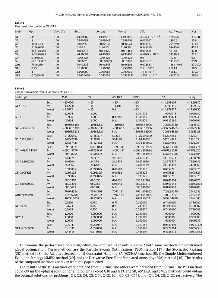
where f ∗ 6= 0, and f ∗ is the globalminimal value of a problembeing solved, then stop the algorithm; otherwise if inequalities(34) can not be satisfied in 107 evaluations of T (x, k, l), then we stop the algorithm and output the results.We take δk = 1, and use the algorithm to solve each problem 30 times. We put in Table 1 the best known objective

function value in the second column. We report in Table 1 the best and the worst optimal values obtained from 30 runsfor each test problem. To understand quality of the obtained solutions, we report in Table 1 for each problem the averageoptimal value and the standard deviation of the obtained objective function values for all 30 runs. Moreover, the successrate, the average number of function evaluations of T (x, k, l), per run, and the average number of local searches, per run,used to obtained these results in 30 runs, are reported in the third and the last two columns of Table 1 for each problemrespectively. It needs to point out that the number of function evaluations of T (x, k, l) is equal to the number of functionevaluations of f (x).It can be seen from Table 1 that, our algorithmworks out all problems, for all runs with low standard deviations, and not

too high computational costs.


Table 1Test results for problems G1–G13.

Prob. Opt. Succ. (%) Best Av. opt. Worst S.D. Av. T -evals NLS

G1 −15 100 −14.99985 −14.99912 −14.99850 4.54746× 10−4 92032.6 3307.8G3 1 100 0.999987 0.999945 0.999901 0.000047 1190.6 15.8G4 −30665.539 100 −30665.50 −30665.32 −30665.23 0.063547 76989.9 1134.1G5 5126.4981 100 5126.5 5126.65 5126.96 0.145896 64413.6 455.7G6 −6961.81388 100 −6961.774 −6961.620 −6961.484 0.099685 4818.1 37.0G7 24.3062091 100 24.30694 24.30789 24.30863 4.9999× 10−4 51710.3 275.3G8 0.095825 100 0.095825 0.095825 0.095825 0.0 192.8 6.3G9 680.630057 100 680.6376 680.67833 680.6980 0.016262 51125.2 73.9G10 7049.250 100 7049.333 7049.545 7049.603 0.071513 1382179.6 37040.4G11 0.75 100 0.750000 0.750002 0.750007 2.2× 10−6 9581.1 96.5G12 1 100 1.000000 0.999988 0.999935 1.7× 10−5 4661.9 179.6G13 0.0539498 100 0.0539499 0.0539531 0.0539552 1.559× 10−4 42537.5 366.4

Table 2Comparison of test results for problems G1-G13.

Prob.: opt. PSO SR ASCHEA SMES FSA Our alg.

Best −15.0001 −15 −15 −15 −14.999105 −14.99985G1 :−15 Av. −13.2734 −15 −14.84 −15 −14.993316 −14.99912

Worst −9.7012 −15 N.A. −15 −14.979977 −14.99850Best 1.0004 1.000 1 1.001038 1.0000015 0.999987

G3: 1 Av. 0.9936 1.000 0.99989 1.000989 0.9991874 0.999945Worst 0.6674 1.000 N.A. 1.000579 0.9915186 0.999901Best −30665.5398 −30665.539 −30665.5 −30665.53906 −30665.5380 −30665.50

G4:−30665.539 Av. −30665.5397 −30665.539 −30665.5 −30665.53906 −30665.4665 −30665.32Worst −30665.5338 −30665.539 N.A. −30665.53906 −30664.6880 −30665.23Best 5126.6467 5126.497 5126.5 5126.599609 5126.4981 5126.5

G5: 5126.4981 Av. 5495.2389 5128.881 5141.65 5174.492301 5126.4981 5126.65Worst 6272.7423 5142.472 N.A. 5304.166992 5126.4981 5126.96Best −6961.8371 −6961.814 −6961.81 −6961.813965 −6961.81388 −6961.774

G6:−6961.81388 Av. −6961.8370 −6875.940 −6961.81 −6961.283984 −6961.81388 −6961.620Worst −6961.8355 −6350.262 N.A. −6961.481934 −6961.81388 −6961.484Best 24.3278 24.307 24.3323 24.326715 24.310571 24.30694

G7: 24.3062091 Av. 24.6996 24.374 24.6636 24.474926 24.3795271 24.30789Worst 25.2962 24.642 N.A. 24.842829 24.644397 24.30863Best 0.095825 0.095825 0.09582 0.095826 0.095825 0.095825

G8: 0.095825 Av. 0.095825 0.095825 0.09582 0.095826 0.095825 0.095825Worst 0.095825 0.095825 N.A. 0.095826 0.095825 0.095825Best 680.6307 680.630 680.630 680.631592 680.63008 680.6376

G9: 680.630057 Av. 680.6391 680.656 680.641 680.643410 680.63642 680.67833Worst 680.6671 680.763 N.A. 680.719299 680.69832 680.6980Best 7090.4524 7054.316 7061.13 7051.902832 7059.86350 7049.333

G10: 7049.250 Av. 7747.6298 7559.192 7497.434 7253.047005 7509.32104 7049.545Worst 10533.6658 8835.655 N.A. 7638.366211 9398.64920 7049.603Best 0.7499 0.750 0.75 0.749090 0.7499990 0.750000

G11: 0.75 Av. 0.7673 0.750 0.75 0.749358 0.7499990 0.750002Worst 0.9925 0.750 N.A. 0.749830 0.7499990 0.750007Best 1.0000 1.000000 N.A. 1.000000 1.000000 1.000000

G12: 1 Av. 1.0000 1.000000 N.A. 1.000000 1.000000 0.999988Worst 1.0000 1.000000 N.A. 1.000000 1.000000 0.999935Best 0.05941 0.053957 N.A. 0.053986 0.0539498 0.0539499

G13: 0.0539498 Av. 0.81335 0.057006 N.A. 0.166385 0.2977204 0.0539531Worst 2.44415 0.216915 N.A. 0.468294 0.4388511 0.0539552

To examine the performance of our algorithm, we compare its results in Table 2 with some methods for constrainedglobal optimization. These methods are the Particle Swarm Optimization (PSO) method [17], the Stochastic Ranking(SR) method [28], the Adaptive Segregational Constraint Handling EA (ASCHEA) method [9], the Simple MultimemberedEvolution Strategy (SMES) method [29], and the Derivative-Free Filter Simulated Annealing (FSA) method [16]. The resultsof the compared methods are taken from the papers cited.The results of the PSO method were obtained from 50 runs. The others were obtained from 30 runs. The PSO method

could obtain the optimal solution for all problems except G10 and G13. The SR, ASCHEA, and SMES methods could obtainthe optimal solutions for problems {G1, G3, G4, G8, G11, G12}, {G4, G6, G8, G11}, and {G1, G4, G8, G12}, respectively. The


Table 3Comparison of our Algorithm with FSA.

Prob. Opt. Av. opt. S.D. Av. func. evals.FSA Our alg. FSA Our alg. FSA Our alg.

G1 −15 −14.993316 −14.99912 0.004813 4.54746×10−4 293449 184065.2G3 1 0.9991874 0.999945 0.001653 0.000047 433342 2381.2G4 −30665.539 −30665.4665 −30665.32 0.173218 0.063547 123154 153979.8G5 5126.4981 5126.4981 5126.65 0.000000 0.145896 65418 128827.2G6 −6961.81388 −6961.81388 −6961.620 0.000000 0.099685 60355 9636.2G7 24.3062091 24.3795271 24.30789 0.071635 4.9999×10−4 575730 103420.6G8 0.095825 0.095825 0.095825 0.0 0.0 79695 385.6G9 680.630057 680.63642 680.67833 0.014517 0.016262 471604 102250.4G10 7049.3307 7509.32104 7049.545 542.3421 0.071513 337187 2764359.2G11 0.75 0.749999 0.750002 0.0 2.2× 10−6 32207 19162.2G12 1.0 1.0 0.999988 0.0 1.7× 10−5 85173 9323.6G13 0.0539498 0.2977204 0.0539531 0.188652 1.559× 10−4 162536 85075

Table 4Comparison of our algorithm with PSO.

Prob. Opt. Av. opt. S.D. Av. obj. evals.PSO Our alg. PSO Our alg. PSO Our alg.

G1 −15 −13.2734 −14.99912 1.41E+ 00 4.54746×10−4 240000 92032.6G3 1 0.9936 0.999945 4.71E−02 0.000047 240000 1190.6G4 −30665.539 −30665.5397 −30665.32 6.83E−04 0.063547 240000 76989.9G5 5126.4981 5495.2389 5126.65 4.05E+ 02 0.145896 240000 64413.6G6 −6961.81388 −6961.8370 −6961.620 2.61E−04 0.099685 240000 4818.1G7 24.3062091 24.6996 24.30789 2.52E−01 4.9999×10−4 240000 51710.3G8 0.095825 0.095825 0.095825 0.0 0.0 240000 192.8G9 680.630057 680.6391 680.67833 6.68E−03 0.016262 240000 51125.2G10 7049.3307 7747.6298 7049.545 5.52E+ 02 0.071513 240000 1382179.6G11 0.75 0.7673 0.750002 6.00E−02 2.2× 10−6 240000 9581.1G12 1.0 1.0000 0.999988 0.0 1.7× 10−5 240000 4661.9G13 0.0539498 0.81335 0.0539531 3.81E−01 1.559× 10−4 240000 42537.5

FSA method could obtain the optimal solutions for problems {G5, G6, G8, G11, G12}. Our method can obtain the optimalsolutions for all problems.Itmust be pointed out specially that, problemG10 cannot be solved to optimality by the othermethods. But our algorithm

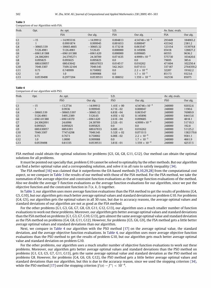
can find a better optimal value and a corresponding solution, and solve it in all runs to satisfy inequality (34).The FSA method [16] was claimed that it outperforms the EA-based methods [9,10,29,28] from the computational cost

aspect, so we compare in Table 3 the results of our method with those of the FSA method. For the FSA method, we take thesummation of the average objective and constraint function evaluations as the average function evaluations of the method.Also we double the average T-function evaluations as the average function evaluations for our algorithm, since we put theobjective function and the constraint function in T (x, k, l) together.In Table 3, our algorithm usesmore average function evaluations than the FSAmethod to get the results of problems {G4,

G5, G10}, but our algorithm getsmuch better average optimal values and standard deviations on problemG10. For problems{G4, G5}, our algorithm gets the optimal values in all 30 runs, but due to accuracy reasons, the average optimal values andstandard deviations of our algorithm are not as good as the FSA method.For the other problems {G1, G3, G6, G7, G8, G9, G11, G12, G13}, our algorithm uses a much smaller number of function

evaluations towork out these problems.Moreover, our algorithmgets better average optimal values and standard deviationsthan the FSAmethod on problems {G1, G3, G7, G10, G13}, gets almost the same average optimal value and standard deviationas the FSA method on problems {G4, G8, G11, G12}. However, for problems {G5, G6, G9}, the FSA method gets a little betteraverage optimal values and standard deviations than our algorithm.Next, we compare in Table 4 our algorithm with the PSO method [17] on the average optimal value, the standard

deviation, and the average objective function evaluations. In Table 4, our algorithm uses more average objective functionevaluations than the PSO method to get the results of problem G10, but our algorithm gets much better average optimalvalue and standard deviation on problem G10.For the other problems, our algorithm uses a much smaller number of objective function evaluations to work out these

problems. Moreover, our algorithm gets better average optimal values and standard deviations than the PSO method onproblems {G1, G3, G5, G7, G11, G13}, gets the same average optimal value and standard deviation as the PSO method onproblems G8. However, for problems {G4, G6, G9, G12}, the PSO method gets a little better average optimal values andstandard deviations than our algorithm, but this is due to the accuracy reason, since we used the stopping criterion (34),while the PSO method [17] used the stopping criterion |f (x)− f ∗| < 10−4.


6. Conclusions

We have proposed an auxiliary function T (x, k, l) for problem (P), which is based on the penalty method, and has noparametric problems. The global minimizers of T (x, k, l) lie in the vicinity of global minimizers of problem (P). By takingthe value of parameter k increasingly, minimization of T (x, k, l) can successfully escape from a previously converged localminimizer. An algorithm has been designed tominimize T (x, k, l) on X to find an approximate constrained global minimizerof problem (P) from random initial points. Numerical experiments were conducted on a set of standard test problems, andshow that the algorithm is better than some well known recent constrained global minimization methods.

References

[1] J.D. Pinter, Continuous global optimization software: A brief review, Optima 52 (1996) 1–8.[2] P.M. Pardalos, H.E. Romeijn (Eds.), Handbook of Global Optimization, Kluwer, Dordrecht, 2002.[3] R. Horst, P.M. Pardalos, N.V. Thoai, Introduction to Global Optimization, 2nd edition, Kluwer Academic Publishers, Dordrechet, The Netherlands, 2000.[4] P.M. Pardalos, J.B. Rosen, Constrained Global Optimization: Algorithms and Applications, Springer, Berlin, 1987.[5] P.M. Pardalos, H.E. Romeijn, H. Tuy, Recent developments and trends in global optimization, Journal of Computational and Applied Mathematics 124(2000) 209–228.

[6] A. Törn, A. Zilinskas, Global Optimization, Springer, Berlin, 1989.[7] O. Yeniay, Penalty function methods for constrained optimization with genetic algorithms, Mathematical & Computational Applications 10 (2005)45–56.

[8] K. Deb, An efficient constraint handling method for genetic algorithms, Computational Methods in Applied Mechanics and Engineering 186 (2000)311–338.

[9] S.B. Hamida, M. Schoenauer, ASCHEA: New results using adaptive segregational constraint handling, in: Proceedings of the Congress on EvolutionaryComputation (CEC2002), Piscataway, New Jersey, IEEE Service Center, 2002, pp. 884–889.

[10] S. Koziel, Z. Michalewicz, Evolutionary algorithms, homomorphous mappings, and constrained parameter optimization, Evolutionary Computation 7(1) (1999) 19–44.

[11] Z. Michalewicz, M. Schoenauer, Evolutionary algorithms for constrained parameter optimization problems, Evolutionary Computation 4 (1) (1996)1–32.

[12] Z. Michalewicz, G. Nazhiyath, GENOCOP III: A coevolutionary algorithm for numerical optimization problems with nonlinear constraints,in: Proceedings of the Second IEEE International Conference on Evolutionary Computation, IEEE Press, 1995, pp. 647–651.

[13] B.W. Wah, Y.X. Chen, Optimal anytime constrained simulated annealing for constrained global optimization, in: R. Dechter (Ed.), in: LNCS, vol. 1894,Springer-Verlag, 2000, pp. 425–440.

[14] B.W. Wah, T. Wang, Constrained simulated annealing with applications in nonlinear continuous constrained global optimization, in: Proceedings ofthe 11th IEEE International Conference on Tools with Artificial Intelligence, 1999, pp. 381–388.

[15] B.W. Wah, T. Wang, Tuning strategies in constrained simulated annealing for nonlinear global optimization, International Journal on ArtificialIntelligence Tools 9 (2000) 3–25.

[16] A.-R. Hedar, M. Fukushima, Derivative-free filter simulated annealing method for constrained continuous global optimization, Journal of GlobalOptimization 35 (2006) 521–549.

[17] J.C.F. Cabrera, C.A.C. Coello, Handling constraints in Particle SwarmOptimization using a small population size, in: Alexander Gelbukh, Angel FernandoKuriMorales (Eds.), MICAI 2007: Advances in Artificial Inteligence, 6th International Conference on Artificial Intelligence, in: Lecture Notes in ArtificialIntelligence, vol. 4827, Springer, Aguascalientes, Mexico, 2007, pp. 41–51.

[18] J. Barhen, V. Protopopescu, D. Reister, TRUST: A deterministic algorithm for global optimization, Science 276 (1997) 1094–1097.[19] B.C. Cetin, J. Barhne, J.W. Burdick, Terminal repeller unconstrained subenergy tunneling (TRUST) for fast global optimization, Journal of Optimization

Theory and Applications 77 (1) (1993) 97–126.[20] R.P. Ge, A filled function method for finding a global minimizer of a function of several variables, Mathematical Programming 46 (1990) 191–204.[21] J. Kostrowicki, L. Piela, Diffusion equation method of global minimization: Performance for standard test functions, Journal of Optimization Theory

and Applications 69 (2) (1991) 97–126.[22] A.V. Levy, A. Montalvo, The tunneling algorithm for the globalminimization of functions, SIAM Journal on Scientific and Statistical Computing 6 (1985)

15–29.[23] Y. Yao, Dynamic tunneling algorithm for global optimization, IEEE Transactions on Systems, Man, and Cybernetics, Part A 19 (1989) 1222–1230.[24] R.P. Ge, The theory of filled functionmethod for finding globalminimizers of nonlinearly constrainedminimizationproblems, Journal of Computational

Mathematics 5 (1987) 1–9.[25] S. Gomez, A. Levy, The Tunneling Method for Solving the Constrained Global Optimization Problem with Several Non-connected Feasible Regions,

in: Lecture Notes in Mathematics, vol. 909, Springer-Verlag, 1982, pp. 34–47.[26] Z.Y. Wu, F.S. Bai, H.W.J. Lee, et al., A filled function method for constrained global optimization, Journal of Global Optimization 39 (2007) 495–507.[27] W. Hock, K. Schittkowski, Test Examples for Nonlinear Programming Codes, Springer-Verlag, Berlin, Heidelberg, 1981.[28] T.P. Runarsson, X. Yao, Stochastic ranking for constrained evolutionary optimization, IEEE Transactions on Evolutionary Computation 4 (3) (2000)

284–294.[29] E.M.Montes, C.A.C. Coello, A simplemultimembered evolution strategy to solve constrained optimization problems, IEEE Transactions on Evolutionary

Computation 9 (1) (2005) 1–17.

solving nonlinearly constrained global optimization problem via an auxiliary function method

Documents