simulation and optimization of cologne's tram schedule

Simulation and optimization of Cologne's tram schedule TN-1

Simulation and optimization of Cologne's tram schedule

Oliver Ullrich, Sebastian Franz, Ewald Speckenmeyer, University of Cologne, Germany

Daniel Lückerath, University of Cologne, Cologne University of Applied Science, Germany

{ullrich|lueckerath|franz|speckenmeyer}@informatik.uni-koeln.de

In many tram networks multiple lines share tracks and stations, thus requiring robust schedules which pre-

vent inevitable delays from spreading through the network. Feasible schedules also have to fulfill various

planning requirements originating from political and economical reasons.

In this article we present a tool set designed to generate schedules optimized for robustness, which also satis-

fy given sets of planning requirements. These tools allow us to compare time tables with respect to their ap-

plicability and evaluate them prior to their implementation in the field.

This paper begins with a description of the tool set focusing on optimization and simulation modules. These

software utilities are then employed to generate schedules for our hometown Cologne's tram network, and to

subsequently compare them for their applicability.

1 Introduction

In many tram networks, several lines share resources

like platforms and tracks. This results in very dense

schedules, with vehicles leaving platforms every

minute at peak times. In order to prevent inevitable

local delays from spreading through the network, a

feasible schedule has to be robust.

Many additional planning requirements of real world

tram schedules originate from political, economical

and feasibility reasons. Thus it is not sufficient to

exclusively consider general criteria like robustness

or operational costs when generating time tables.

Typical requirements include fixed start times at

certain stations, e.g. interfaces to national railway

systems, core lines to relieve high passenger load, e.g.

for lines which traverse city centers, warranted con-

nections at certain stations, and safety distances to be

complied with at bidirectional tracks.

In this paper we present an introduction to our project

to generate and evaluate robust time tables which also

satisfy given sets of planning requirements. We de-

scribe a tool chain which enables us to generate opti-

mized schedules, compare their feasibility and evalu-

ate them prior to application to real world networks.

This paper continues with a description of the current

state of the project, focusing on our approaches on

optimization and simulation (Section 2). We then

present some experimental results obtained by apply-

ing the described software to our hometown Co-

logne's tram network (Section 3). The paper closes

with a short summary of lessons learned and some

thoughts on further research (Section 4).

2 Simulating and optimizing tram

schedules

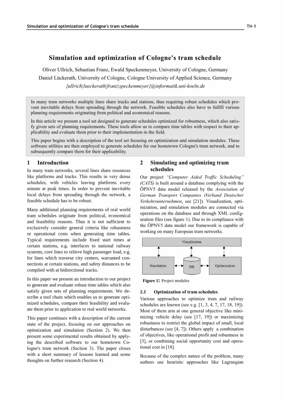
Our project “Computer Aided Traffic Scheduling”

(CATS) is built around a database complying with the

ÖPNV5 data model released by the Association of

German Transport Companies (Verband Deutscher

Verkehrsunternehmen, see [21]). Visualization, opti-

mization, and simulation modules are connected via

operations on the database and through XML config-

uration files (see figure 1). Due to its compliance with

the ÖPNV5 data model our framework is capable of

working on many European tram networks.

Figure 1: Project modules

2.1 Optimization of tram schedules

Various approaches to optimize tram and railway

schedules are known (see e.g. [1, 3, 4, 7, 17, 18, 19]).

Most of them aim at one general objective like mini-

mizing vehicle delay (see [17, 19]) or maximizing

robustness to restrict the global impact of small, local

disturbances (see [4, 7]). Others apply a combination

of objectives, like operational profit and robustness in

[3], or combining social opportunity cost and opera-

tional cost in [18].

Because of the complex nature of the problem, many

authors use heuristic approaches like Lagrangian

TN-2 Simulation and optimization of Cologne's tram schedule

heuristics (see [3]) or simulated annealing (see [18]).

Others, like Bampas et al. in [1] introduce exact algo-

rithms for restricted subclasses, like chain and spider

networks.

In our project, we combine heuristics and exact

methods to generate optimal synchronized time tables

for tram networks, targeting maximal robustness and

adherence to transport planning requirements at the

same time.

We use the scheduled time offset between two con-

secutive lines departing from a platform as an indica-

tor for robustness. In an assumed tact interval of ten

minutes, two lines could be scheduled with equidis-

tant offsets of five minutes, which means that one or

both involved vehicles could be late for more than

four minutes without consequences for the following

tram. Under an extremely unequal split of the availa-

ble time span into a nine minute offset followed by a

one minute offset, the first tram could have a delay of

more than eight minutes without consequences to the

following vehicle. On the other hand, would the se-

cond vehicle be even slightly late, the delay would

spread to the follow-up tram. Since we are assuming

typically small delays, we see an equidistant distribu-

tion as very robust, the occurrence of very small off-

sets as not robust.

So, to calculate the robustness of a time table 𝜆 we

examine at each platform h of the network the sched-

uled time offset 𝛿 𝜆 ℎ between any trip

𝑓and its predecessor 𝑝𝑟𝑒𝑑 𝑓 , i.e. the time elapsed

between the departures of 𝑝𝑟𝑒𝑑 𝑓 and 𝑓 at the ex-

amined platform.

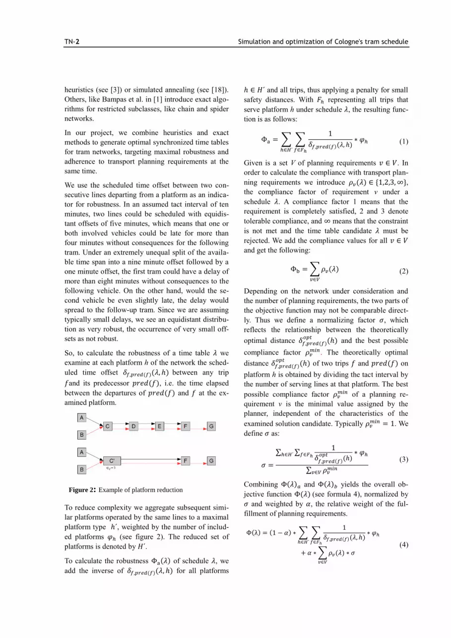
Figure 2: Example of platform reduction

To reduce complexity we aggregate subsequent simi-

lar platforms operated by the same lines to a maximal

platform type ℎ´, weighted by the number of includ-

ed platforms 𝜑 (see figure 2). The reduced set of

platforms is denoted by 𝐻´.

To calculate the robustness Φ 𝜆 of schedule 𝜆, we

add the inverse of 𝛿 𝜆 ℎ for all platforms

ℎ ∈ 𝐻´ and all trips, thus applying a penalty for small

safety distances. With 𝐹 representing all trips that

serve platform h under schedule 𝜆, the resulting func-

tion is as follows:

Φ = ∑ ∑1

𝛿 𝜆 ℎ ∗ 𝜑

∈ ∈ ´

(1)

Given is a set V of planning requirements 𝑣 ∈ 𝑉. In

order to calculate the compliance with transport plan-

ning requirements we introduce 𝜌 𝜆 ∈ {1 2 3 ∞},

the compliance factor of requirement v under a

schedule 𝜆. A compliance factor 1 means that the

requirement is completely satisfied, 2 and 3 denote

tolerable compliance, and ∞ means that the constraint

is not met and the time table candidate 𝜆 must be

rejected. We add the compliance values for all 𝑣 ∈ 𝑉

and get the following:

Φ = ∑𝜌 𝜆

∈

(2)

Depending on the network under consideration and

the number of planning requirements, the two parts of

the objective function may not be comparable direct-

ly. Thus we define a normalizing factor 𝜎, which

reflects the relationship between the theoretically

optimal distance 𝛿

ℎ and the best possible

compliance factor 𝜌 . The theoretically optimal

distance 𝛿

ℎ of two trips 𝑓 and 𝑝𝑟𝑒𝑑 𝑓 on

platform h is obtained by dividing the tact interval by

the number of serving lines at that platform. The best

possible compliance factor 𝜌 of a planning re-

quirement v is the minimal value assigned by the

planner, independent of the characteristics of the

examined solution candidate. Typically 𝜌 = 1. We

define 𝜎 as:

𝜎 =

∑ ∑1

𝛿

ℎ ∗ 𝜑 ∈ ∈ ´

∑ 𝜌

∈

(3)

Combining Φ 𝜆 and Φ 𝜆 yields the overall ob-

jective function Φ 𝜆 (see formula 4), normalized by

𝜎 and weighted by 𝛼, the relative weight of the ful-

fillment of planning requirements.

Φ = 1 𝛼 ∗ ∑ ∑1

𝛿 𝜆 ℎ ∗ 𝜑

∈ ∈ ´

𝛼 ∗ ∑𝜌 𝜆 ∗ 𝜎

∈

(4)


We identify seven types of transport planning con-

straints: Interval constraints, start time constraints,

core line constraints, bidirectional track constraints,

turning point constraints, warranted connection con-

straints and follow-up connection constraints.

Upon closer inspection it becomes clear that interval

and start time constraints are fundamental and all

other constraint types can be expressed using these

two. E.g. a bidirectional track constraint can be ex-

pressed by two interval constraints covering opposing

platforms. Subsequently only interval and start time

constraints are considered in the remainder of this

paper.

A valid solution also has to adhere to some more

restrictions. The first restriction requires each start

time 𝜇 to be inside the tact interval, with 𝑡

being the duration of the interval (see formula 5).

∀𝜇 ∈ 𝜆: 0 ≤ 𝜇 < 𝑡 (5)

Another restriction requires an offset of at least one

minute between two departures f and pred(f) at each

platform ℎ ∈ 𝐻 (see formula 6). This means that no

platform can be blocked by more than one train at any

point of time, the schedule has to be free of collisions.

∀ℎ ∈ 𝐻: ∀𝑓 ∈ 𝐹: 𝛿 𝜆 ℎ > 0 (6)

To accelerate the computational process the imple-

mented branch-and-bound solver starts with an initial

solution computed by a genetic algorithm. The genet-

ic algorithm encodes a time table as one individual,

consisting of the first trip start time of each line, i.e.

the offset in minutes from the start of the operational

day. All other trips follow by the global tact interval.

The application generates a start population using

random start time values, testing validity against

planning constraints and collisions on network nodes.

To reduce computational complexity we apply simple

deterministic tournament selection and two-point-

crossover (as described in [5]). After evaluation of

several mutation methods, including random, mini-

mal, and maximum enhancement mutation we choose

a minimal random mutation method that only allows

start times to be altered by one minute. We utilize a

steady state replacement method, also described in

[5]. At the end of each run a hill climbing algorithm is

applied to the best individual to further improve its

fitness.

As described above we use the best individual en-

countered by the genetic algorithm to provide the

branch-and-bound solver with an initial upper bound,

thus avoiding a cold start. Each inner node of the

search tree represents a partial solution of the prob-

lem. The root of the tree corresponds to a solution in

which no line's start time is fixed. With each level of

the tree admissible start times for an additional line

are set. For a more detailed discussion of the branch-

and-bound method, see e.g. [8].

In order to cut branches off the tree as soon as possi-

ble, the objective function of the branch-and-bound

algorithm is modified. The set of lines 𝐿 is divided

into subset �̂� of lines that are already fixed and subset

�̃� of lines that are not yet fixed. Accordingly the set of

platforms 𝐻 is divided into �̂� and 𝐻. �̂� includes all

platforms which are exclusively served by lines al-

ready fixed, while platforms in �̃� are also (or exclu-

sively) served by lines that are not yet fixed. The set

of transport planning constraints 𝑉 is divided into sets

�̂� and �̃�. Set �̂� includes all constraints which are

dependent on already set lines, correspondingly con-

straints in �̃� are dependent on lines not yet set. The

modified objective function Φ´ 𝜆 is shown below

(formulas 7 to 9).

Φ´ = 1 α ∗ Φ´ α ∗ Φ´ ∗ 𝜎 (7)

Φ´ =

(

∑ ∑1

𝛿𝑓 𝑝𝑟𝑒𝑑 𝑓 𝜆 ℎ ∗ 𝜑

ℎ

𝑓∈𝐹ℎℎ∈�̂�

∑ ∑1

�̃�𝑓 𝑝𝑟𝑒𝑑 𝑓 𝜆 ℎ ∗ 𝜑

ℎ

𝑓∈𝐹ℎℎ∈�̃� )

(8)

Φ´ = ∑𝜌 𝜆

∈ ̂

∑𝜌 𝜆

∈ ̃

(9)

Here 𝛿 𝜆 ℎ represents the theoretically best

safety distance value under consideration of lines

already fixed. Again, 𝜌 denotes the optimal com-

pliance factor for constraint v. These values are ap-

plied in order to find a lower bound for solution can-

didates in the current branch of the search tree.

For further implementation details, see [6].

2.2 Simulation of tram schedules

Most rail-bound traffic simulations are designed for

long distance train or railway networks, see e.g. [14,

16]. While those systems feature similarities to tram

networks, e.g. passenger exchange or maneuvering

capabilities, they differ greatly in important aspects.

Tram networks are often mixed, i.e. trams travel on

underground tracks as well as on street level, and are


thus subject to individual traffic and corresponding

traffic regulation strategies. Subsequently, tram be-

havior is a mixture between train and car behavior,

e.g. line-of-sight operating/driving. Therefore a sim-

ple adaption of railway simulation methodologies is

not feasible.

Bearing the similarities with individual traffic in mind

Joisten (see [9]) implemented an adapted Nagel/

Schreckenberg model (see [15]) for tram simulation,

which suffered from the setbacks of the high aggrega-

tion inherent to cellular automatons (see [11]). There-

fore Lückemeyer developed an event based simula-

tion model which avoids some of those setbacks as

described in [10, 11]. To further eliminate inaccura-

cies we apply an updated model, which is described

in detail in the accompanying article “Modeling time

table based tram traffic” (see [13]).

Our application is based upon a model-based parallel-

ization framework (described in [20]), which exploits

the embedded model's intrinsic parallelism. The

mixed tram network is modeled as a directed graph

with platforms, tracks and track switches represented

by nodes. Connections between nodes are represented

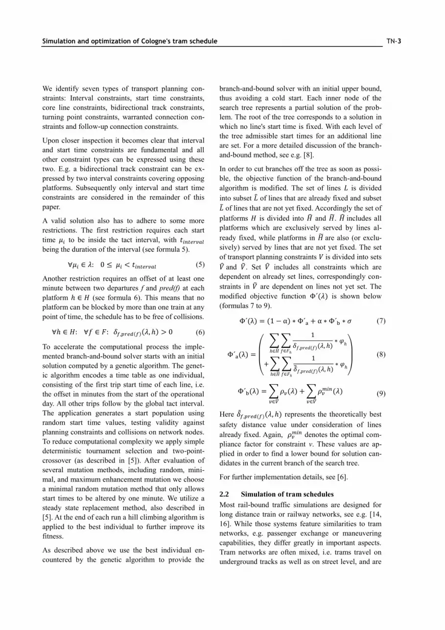
as edges. Figure 3 shows part of an example network,

which is mapped on the graph depicted in figure 4,

where squares represent platforms, rectangles tracks

and triangles track switches. The dark rectangles

around platforms indicate that these platforms form a

station.

Figure 3: Part of a tram network

The distributions for the duration of passenger ex-

change are specific to platform and tram type with the

combined duration of opening and closing the vehicle

doors as minimum value.

Vehicles encapsulate most of the simulation dynam-

ics, which are based upon the event based simulation

approach (as described in [2]). Thus trams change

their state at events of certain types, like stopping or

accelerating, which happen at discrete points in time.

These state changes may trigger a change in the over-

all system state and generate follow-up events, which

are administrated in a priority queue.

Main tram attributes are specified by the type of tram,

which holds functions for the maneuvering capabili-

ties, e.g. acceleration and braking.

Figure 4: Example graph

3 Optimizing Cologne's tram network

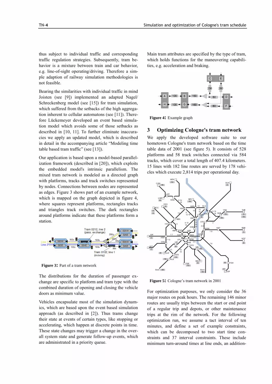
We apply the developed software suite to our

hometown Cologne's tram network based on the time

table data of 2001 (see figure 5). It consists of 528

platforms and 58 track switches connected via 584

tracks, which cover a total length of 407.4 kilometers.

15 lines with 182 line routes are served by 178 vehi-

cles which execute 2,814 trips per operational day.

Figure 5: Cologne’s tram network in 2001

For optimization purposes, we only consider the 36

major routes on peak hours. The remaining 146 minor

routes are usually trips between the start or end point

of a regular trip and depots, or other maintenance

trips at the rim of the network. For the following

optimization run, we assume a tact interval of ten

minutes, and define a set of example constraints,

which can be decomposed to two start time con-

straints and 37 interval constraints. These include

minimum turn-around times at line ends, an addition-


al core line 1A to satisfy high demand for line 1 in

Cologne's town center, guaranteed connections be-

tween certain lines, and fixed start times at the Bonn

national railway hub.

A more detailed description of the conducted experi-

ments can be found in [20].

3.1 Comparing tram schedules

From the genetic algorithm's initial pool of valid

solution candidates we randomly pick a schedule A

with an objective function value of 214.714 (see table

1). After a 8.5 hours run, the optimizer yields a pool

of 60 best solutions with objective function values of

180.696, from which schedule B (again, see table 1)

is randomly selected.

To begin with a more general view, we pick ten more

schedules each out of both solution pools and execute

ten simulations runs for each of those 20 schedules.

The runs under the initial schedules yield an average

delay of departures of 18.9 seconds. Under the best

schedules the average delay is 15.4 seconds, which

means a reduction of 18.6 percent or 3.5 seconds.

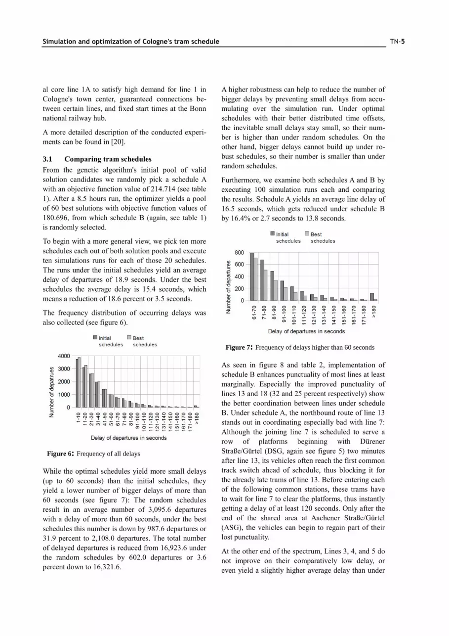
The frequency distribution of occurring delays was

also collected (see figure 6).

Figure 6: Frequency of all delays

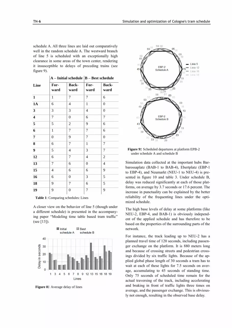
While the optimal schedules yield more small delays

(up to 60 seconds) than the initial schedules, they

yield a lower number of bigger delays of more than

60 seconds (see figure 7): The random schedules

result in an average number of 3,095.6 departures

with a delay of more than 60 seconds, under the best

schedules this number is down by 987.6 departures or

31.9 percent to 2,108.0 departures. The total number

of delayed departures is reduced from 16,923.6 under

the random schedules by 602.0 departures or 3.6

percent down to 16,321.6.

A higher robustness can help to reduce the number of

bigger delays by preventing small delays from accu-

mulating over the simulation run. Under optimal

schedules with their better distributed time offsets,

the inevitable small delays stay small, so their num-

ber is higher than under random schedules. On the

other hand, bigger delays cannot build up under ro-

bust schedules, so their number is smaller than under

random schedules.

Furthermore, we examine both schedules A and B by

executing 100 simulation runs each and comparing

the results. Schedule A yields an average line delay of

16.5 seconds, which gets reduced under schedule B

by 16.4% or 2.7 seconds to 13.8 seconds.

Figure 7: Frequency of delays higher than 60 seconds

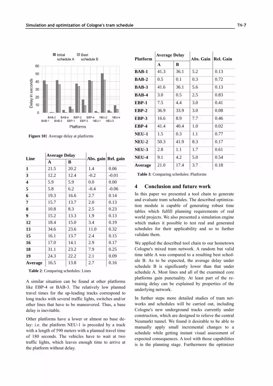
As seen in figure 8 and table 2, implementation of

schedule B enhances punctuality of most lines at least

marginally. Especially the improved punctuality of

lines 13 and 18 (32 and 25 percent respectively) show

the better coordination between lines under schedule

B. Under schedule A, the northbound route of line 13

stands out in coordinating especially bad with line 7:

Although the joining line 7 is scheduled to serve a

row of platforms beginning with Dürener

Straße/Gürtel (DSG, again see figure 5) two minutes

after line 13, its vehicles often reach the first common

track switch ahead of schedule, thus blocking it for

the already late trams of line 13. Before entering each

of the following common stations, these trams have

to wait for line 7 to clear the platforms, thus instantly

getting a delay of at least 120 seconds. Only after the

end of the shared area at Aachener Straße/Gürtel

(ASG), the vehicles can begin to regain part of their

lost punctuality.

At the other end of the spectrum, Lines 3, 4, and 5 do

not improve on their comparatively low delay, or

even yield a slightly higher average delay than under


schedule A. All three lines are laid out comparatively

well in the random schedule A. The westward branch

of line 5 is scheduled with an exceptionally high

clearance in some areas of the town center, rendering

it insusceptible to delays of preceding trains (see

figure 9).

Line

A – Initial schedule B – Best schedule

For-

ward

Back-

ward

For-

ward

Back-

ward

1 1 7 7 6

1A 6 4 1 0

3 3 3 4 0

4 7 0 6 7

5 5 2 9 6

6 1 7 7 6

7 0 9 7 0

8 6 7 1 7

9 5 4 3 7

12 6 7 4 2

13 7 6 0 4

15 4 6 6 9

16 6 0 3 5

18 9 7 6 5

19 9 0 7 9

Table 1: Comparing schedules: Lines

A closer view on the behavior of line 5 (though under

a different schedule) is presented in the accompany-

ing paper “Modeling time table based tram traffic”

(see [13]).

Figure 8: Average delay of lines

Figure 9: Scheduled departures at platform EPB-2

under schedule A and schedule B

Simulation data collected at the important hubs Bar-

barossaplatz (BAB-1 to BAB-4), Ebertplatz (EBP-1

to EBP-4), and Neumarkt (NEU-1 to NEU-4) is pre-

sented in figure 10 and table 3. Under schedule B,

delay was reduced significantly at each of those plat-

forms, on average by 3.7 seconds or 17.6 percent. The

increase in punctuality can be explained by the better

reliability of the frequenting lines under the opti-

mized schedule.

The high base levels of delay at some platforms (like

NEU-2, EBP-4, and BAB-1) is obviously independ-

ent of the applied schedule and has therefore to be

based on the properties of the surrounding parts of the

network.

For instance, the track leading up to NEU-2 has a

planned travel time of 120 seconds, including passen-

ger exchange on the platform. It is 880 meters long

and because of crossing streets and pedestrian cross-

ings divided by six traffic lights. Because of the ap-

plied global phase length of 30 seconds a tram has to

wait at each of these lights for 7.5 seconds on aver-

age, accumulating to 45 seconds of standing time.

Only 75 seconds of scheduled time remain for the

actual traversing of the track, including accelerating

and braking in front of traffic lights three times on

average, and the passenger exchange. This is obvious-

ly not enough, resulting in the observed base delay.


Figure 10: Average delay at platforms

Line Average Delay

Abs. gain Rel. gain A B

1 21.5 20.2 1.4 0.06

3 12.2 12.4 -0.2 -0.01

4 5.9 5.9 0.0 0.00

5 5.8 6.2 -0.4 -0.06

6 19.3 16.6 2.7 0.14

7 15.7 13.7 2.0 0.13

8 10.8 8.3 2.5 0.23

9 15.2 13.3 1.9 0.13

12 18.4 15.0 3.4 0.19

13 34.6 23.6 11.0 0.32

15 16.1 13.7 2.4 0.15

16 17.0 14.1 2.9 0.17

18 31.1 23.2 7.9 0.25

19 24.3 22.2 2.1 0.09

Average 16.5 13.8 2.7 0.16

Table 2: Comparing schedules: Lines

A similar situation can be found at other platforms

like EBP-4 or BAB-3. The relatively low planned

travel times for the up-leading tracks correspond to

long tracks with several traffic lights, switches and/or

other lines that have to be maneuvered. Thus, a base

delay is inevitable.

Other platforms have a lower or almost no base de-

lay: i.e. the platform NEU-1 is preceded by a track

with a length of 590 meters with a planned travel time

of 180 seconds. The vehicles have to wait at two

traffic lights, which leaves enough time to arrive at

the platform without delay.

Platform Average Delay

Abs. Gain Rel. Gain

A B

BAB-1 41.3 36.1 5.2 0.13

BAB-2 0.5 0.1 0.3 0.72

BAB-3 41.6 36.1 5.6 0.13

BAB-4 3.0 0.5 2.5 0.83

EBP-1 7.5 4.4 3.0 0.41

EBP-2 36.9 33.9 3.0 0.08

EBP-3 16.6 8.9 7.7 0.46

EBP-4 41.4 40.4 1.0 0.02

NEU-1 1.5 0.3 1.1 0.77

NEU-2 50.3 41.9 8.3 0.17

NEU-3 2.8 1.1 1.7 0.61

NEU-4 9.1 4.2 5.0 0.54

Average 21.0 17.4 3.7 0.18

Table 3: Comparing schedules: Platforms

4 Conclusion and future work

In this paper we presented a tool chain to generate

and evaluate tram schedules. The described optimiza-

tion module is capable of generating robust time

tables which fulfill planning requirements of real

world projects. We also presented a simulation engine

which makes it possible to test real and generated

schedules for their applicability and so to further

validate them.

We applied the described tool chain to our hometown

Cologne's mixed tram network. A random but valid

time table A was compared to a resulting best sched-

ule B. As to be expected, the average delay under

schedule B is significantly lower than that under

schedule A. Most lines and all of the examined core

platforms gain punctuality. At least part of the re-

mainig delay can be explained by properties of the

underlying network.

In further steps more detailed studies of tram net-

works and schedules will be carried out, including

Cologne's new underground tracks currently under

construction, which are designed to relieve the central

Neumarkt tunnel. We found it desirable to be able to

manually apply small incremental changes to a

schedule while getting instant visual assessment of

expected consequences. A tool with those capabilities

is in the planning stage. Furthermore the optimizer


module will be parallelized to further reduce its run

time. Especially the applied branch-and-bound algo-

rithm's load can be balanced relatively easy, so the

application should scale well.

Acknowledgments

This work was partially supported by Rhein Energie

Stiftung Jugend Beruf Wissenschaft under grant num-

ber W-10-2-002. We thank the other members of our

work group Patrick Kuckertz and Bert Randerath.

An abbreviated version of this paper was previously

published in Liu-Henke, X., Buchta, R., Quantmeyer,

F. (Ed.): Proceedings of ASIM-Workshop STS/

GMMS 2012. ARGESIM/ASIM Pub. TU Vienna/

Austria, Wolfenbüttel, Feb. 23-24, 2012, 279-289.

References

[1] Bampas, E., Kaouri, G., Lampis, M., Pa-

gourtzis, A.: Periodic Metro Scheduling. In:

Proceedings of ATMOS, 2006

[2] Banks, J., Carson, J.S., Nelson B.L., Nicol

D.M.: Discrete-Event System Simulation.

Pearson, 2010

[3] Cacchiana, V., Caprara, A., Fischetti, M.: A

Lagrangian Heuristic for Robustness, with an

Application to Train Timetabling. Transporta-

tion Science, to appear

[4] Caimi, G., Fuchsberger, M., Laumanns, M.,

Schüpbach, K.: Periodic Railway Timetabling

with Event Flexibility. In: Networks, 2010,

Volume 57, Number 1, pp. 3-18

[5] Dréo, J., Pétrowski, A., Siarry, P., Taillard, E.:

Metaheuristics for Hard Optimization. Spring-

er, 2006

[6] Franz, S.: Entwurf und Entwicklung eines

mehrstufigen Optimierungsverfahrens für

Stadtbahnfahrpläne unter Berücksichtigung

verkehrsplanerischen Vorgaben. Diplomarbe-

it, Univ. Köln, 2011

[7] Genç, Z.: Ein neuer Ansatz zur Fahrplanopti-

mierung im ÖPNV: Maximierung von zeitli-

chen Sicherheitabständen. Dissertation, Math-

ematisch-Naturwissenschaftliche Fakultät,

Universität zu Köln, 2003

[8] Hu, T.C.: Combinatorial Algorithms, Addison

Wesley, 1982

[9] Joisten, M.: Simulation von Fahrplänen für

den ÖPNV mittels Zellularautomaten. Diplo-

marbeit, Univ. Köln, 2002

[10] Lückemeyer, G.: A Traffic Simulation System

Increasing the Efficiency of Schedule Design

for Public Transport Systems Based on Scarce

Data. Dissertation, Shaker Verlag, 2007

[11] Lückemeyer, G., Speckenmeyer, E.: Compar-

ing Applicability of Two Simulation Models in

Public Transport Simulation. In: Becker, M.,

Szczerbicka, H. (Ed.): Proceedings of ASIM

2006, Hannover, 2006

[12] Lückerath, D.: Entwurf und Entwicklung einer

Anwendung zur parallelen Simulation von

schienengebundenem Öffentlichen Personen-

nahverkehr. Diplomarbeit, Univ. Köln, 2011

[13] Lückerath, D., Ullrich, O., Speckenmeyer, E.:

Modeling time table based tram traffic. In:

Simulation Notes Europe (SNE), ARGESIM/

ASIM Pub., TU Vienna, Volume 22, Number

2, 2012

[14] Middelkoop, D., Bouwman, M.: SIMONE:

Large Scale Train Network Simulations. In:

B.A. Peters, J.S. Smith, D.J. Medeiros, M.W.

Rohrer (Ed.): Proceedings of the 2011 Winter

Simulation Conference, Arlington, 2001

[15] Nagel, K., Schreckenberg, M.: A cellular au-

tomaton model for freeway traffic. In: Journal

de Physique I, Volume 2, Issue 12, December

1992, pp. 2221-2229

[16] Nash, A., Huerlimann, D.: Railroad Simula-

tion Using OpenTrack. In: Allan, J., R.J. Hill,

C.A. Brebbia, G. Sciutto, S. Sone (Ed.): Com-

puters in Railways IX, WIT Press, Southamp-

ton, 2004, pp. 45-54

[17] Schöbel, A.: A Model for the Delay Manage-

ment Problem based on Mixed-Integer-Pro–

gramming. In: Proceedings of ATMOS, 2001

[18] Speckenmeyer, E., Li, N., Lückerath, D.,

Ullrich, O.: Socio-Economic Objectives in

Tram Scheduling. Technical Report, Universi-

tät zu Köln, to appear

[19] Suhl, L., Mellouli, T.: Managing and prevent-

ing delays in railway traffic by simulation and

optimization. In: Mathematical Methods on


Optimization in Transportation Systems 2001,

pp. 3–16

[20] Ullrich, O.: Ein dynamisch-adaptiver Ansatz

zur modellbasierten Parallelisierung von Si-

mulationsanwendungen. Mathematisch-Natur-

wissenschaftliche Fakultät, Univ. Köln, work

in progress.

[21] Verband Deutscher Verkehrsunternehmen

e.V.: VDV-Standardschnittstelle Linien-

netz/Fahrplan, VDV-Schriften 452, 2008

simulation and optimization of cologne's tram schedule

Documents