2.5d reconstruction of building from very high resolution sar
TRANSCRIPT

2.5D RECONSTRUCTION OF
BUILDING FROM VERY HIGH
RESOLUTION SAR AND OPTICAL
DATA BY USING OBJECT-
ORIENTED IMAGE ANALYSIS
TECHNIQUE]
NAMHYUN KIM
February, 2011
SUPERVISORS:
Ms. Dr. Ir. Wietske Bijker
Dr. Valentyn Tolpekin

Thesis submitted to the Faculty of Geo-Information Science and Earth
Observation of the University of Twente in partial fulfilment of the
requirements for the degree of Master of Science in Geo-information Science
and Earth Observation.
Specialization: Geoinformatics
SUPERVISORS:
Ms. Dr. Ir. Wietske Bijker
Dr. Valentyn Tolpekin
THESIS ASSESSMENT BOARD:
Prof. Dr. Ir. Alfred Stein (Chair)
Dr. Tsehaie Woldai (External Examiner, ESA Department, ITC)
2.5D RECONSTRUCTION OF
BUILDING FROM VERY HIGH
RESOLUTION SAR AND OPTICAL
DATA BY USING OBJECT-
ORIENTED IMAGE ANALYSIS
NAMHYUN KIM
Enschede, the Netherlands, February, 2011

DISCLAIMER
This document describes work undertaken as part of a programme of study at the Faculty of Geo-Information Science and
Earth Observation of the University of Twente. All views and opinions expressed therein remain the sole responsibility of the
author, and do not necessarily represent those of the Faculty.
i
ABSTRACT
2.5D building modelling is of great interest for visualization, simulation and monitoring purposes in
different cases like city and military mission planning or rapid disaster assessment. Manual and automatic
extraction of building information from SAR interferometry is complicated by layover, foreshortening,
shadowing and multi-bounce scattering, especially in dense urban areas with tall buildings. This can be
overcome by using optical imagery to provide the shapes of the building footprints whereas SAR data is
used for the refinement of the detected footprints and for providing building height information.
Two TerraSAR-X images were used in this research, with High Resolution Spotlight Mode (azimuth
resolution 1.1m) together with the QuickBird image. The study area is located in Delft, the Netherlands.
First, a digital Surface Model (DSM) was estimated from SAR interferometry processing. Different levels
of external height information from Shuttle Topography Mission Digital Elevation Model (SRTM),
LIDAR Digital Terrain Model (LIDAR DTM) and LIDAR Digital Surface Model (LIDAR DSM) were
used for phase flattening and registration to investigate how they influence the overall accuracy of SAR
interferometry processing. Building footprints were extracted with an Object Oriented Analysis (OOA)
method from the QuickBird image, with input of the InSAR DSM as external knowledge. Due to spectral
complexity of urban areas, it is impossible to extract correctly buildings from the QuickBird image only
based on spectral information. OOA including the building height information from InSAR DSM
improved the extraction of building footprints from the QuickBird image. Then, the 2.5D building model
was derived by combining the building footprints and the building height from InSAR DSM. Finally, the
vertical accuracy of the model was assessed with a reference from the LIDAR DSM and the field data
from a clinometer.
The 2π height ambiguity was determined as 45.94 m from the baseline estimation (131.35 m) of the InSAR
pair. If the baseline is larger, the height ambiguity is smaller; so it yields more fringes in the interferogram
and is more sensitive to topography or structures such as buildings. The SAR interferometry processing
with the LIDAR DSM reduced the phase unwrapping error and helped the registration of the SAR pair,
so it was more accurate than the processing with the other external height information. Assessment of
vertical accuracy for the 4 buildings in the two study sites showed +1.53m, -0.57m, -0.78m and -1.49m
mean height difference, and 3.83m, 3.00m, 3.44m and 4.26m RMSE comparing the building height from
the InSAR result to the building height from the LIDAR nDSM. From the comparison with the field data,
the result showed -1.15m mean height difference and 2.91m RMSE.
In conclusion, building height from SAR interferometry can improve building footprint extraction from
optical images and can be combined with the extracted footprints to generate a 2.5D building model.
Keywords: SAR interferometry, digital surface model, object oriented analysis, building footprint extraction, 2.5D
modelling

ii
ACKNOWLEDGEMENTS
Studying Geoinformatics in ITC, the Netherlands was one of the most rewarding times in my life. This
thesis is the end result of the last 18 months in ITC. The research documented in this thesis could be done
with many grateful supports from my country and many persons. I wish to take this opportunity to
express my sincere gratitude to them.
I would like to express my first thanks to the Republic of Korea Army (ROKA) which gave this
opportunity to broaden my perspectives. After coming back to my country, it will be my great chance for
enthusiastic dedication to strengthen ROKA.
This research could be completed thanks to the efforts and discussions with my two supervisors: Dr.
Wietske Bijker and Dr. Valentyn Tolpekin. I want to give my heartfelt acknowledgement for all the time
they dedicated me during the last 6 months and for their inspiration and advice when I was doing
research. Without their constructive and tireless guidance, this thesis would not have been possible to go
in the right direction.
I want to give many thanks to DLR (German Aerospace Center) for accepting my proposal (LAN 0955)
and providing the TerraSAR-X data.
I show appreciation to Dr. Tsehaie Woldai for his motivation and enthusiasm during the advanced SAR
module and this research. Special thanks to Dr. Sander Oude Elberink for his clear advice in DEM
manipulation and to Dr. Norman Kerle for giving the access into ITC OOA club and many good
materials.
I would also like to thank our director Gerrit Huurneman for the critical discussions about SAR
interferometry despite his busy schedule. And I want to extend my gratitude to Mr. Wan Bakx for giving
lots of energies from his training sessions during Run for Fun and to Mr. Sokhon Phem for his effort to
manage 3D cluster for the research period.
It was my pleasure having my GFM classmates. For last 18 months, I shared great memories with all of
my GFM classmates. Without them, my MSc period would not have been great time. I cannot mention all
of their names. But, I would like to pay special thanks to our class representative, Benard Langat for his
warm friendship, to Diego, Aminah and Siqi for being the best cluster-mates.
To my Korean friend; Bro. Byungyong and his wife Hyounwook, I would like to give my warm
appreciation. I cannot imagine the past 6 months without them. We shared wonderful times of travelling,
cooking, shopping, drinking.....
To my lovely wife Kyungmi, I owe you a tremendous debt of gratitude. You sacrificed a lot for me;
cheering me all through the study period and bringing fruitful times into my life. Thanks to your unlimited
love and warm devotion, I could concentrate on this research and complete the thesis successfully.
I love you, my wife
Last but not least, how I can forget to express my emotional gratefulness to my parents for their
continuous supports, loves and patience throughout the study period.

iii
TABLE OF CONTENTS
1. Introduction ........................................................................................................................................................... 7
1.1. Motivation and problem statements ........................................................................................................................ 7 1.2. Research identification ............................................................................................................................................... 8 1.3. Thesis structure ............................................................................................................................................................ 9
2. Related theories .................................................................................................................................................. 10
2.1. Review on height estimation by SAR interferometry with TerraSAR-X data in urban area ...................... 10 2.2. Review on building footprint extraction by OOA ............................................................................................. 12
3. Method ................................................................................................................................................................ 14
3.1. Study area and data ................................................................................................................................................... 15 3.2. Data pre-processing ................................................................................................................................................. 19 3.3. DSM generation by SAR interferometry processing .......................................................................................... 25 3.4. Building Footprint Extraction by OOA ............................................................................................................... 32 3.5. Generation of 2.5D Building model ..................................................................................................................... 37 3.6. Height accuracy assessment of 2.5D building model ........................................................................................ 38
4. Result and Anaysis ............................................................................................................................................. 39
4.1. DSM generation by SAR interferometry processing .......................................................................................... 39 4.2. Building Footprint Extraction by OOA ............................................................................................................... 44 4.3. 2.5D building model ................................................................................................................................................ 48 4.4. Height accuracy of the 2.5D building model ....................................................................................................... 52
5. Discussion ........................................................................................................................................................... 55
5.1. Factors influencing DSM generation by SAR interferometry processing ...................................................... 55 5.2. Factors influencing the building footprint extraction by OOA ....................................................................... 57 5.3. Alternative methods for building modelling ........................................................................................................ 58 5.4. Limitations and possible solutions ........................................................................................................................ 58 5.5. Discussion in relation to the objective and research questions ........................................................................ 60
6. Conclusion and Recommendation .................................................................................................................. 61
6.1. Conclusion ................................................................................................................................................................. 61 6.2. Recommendation ..................................................................................................................................................... 62
References .................................................................................................................................................................... 63
Appendix I: SAR Interferometry processing with SARscape ............................................................................. 66
Appendix II: Outputs from SAR Interferometry processing with SARscape .................................................. 69
Appendix III: Metadata of TerraSAR-X images .................................................................................................... 75
Appendix IIII: Photographs of Study site .............................................................................................................. 76

iv
LIST OF FIGURES
Figure 1-1: Thesis outline flow .................................................................................................................................... 9
Figure 2-1: InSAR geometry ...................................................................................................................................... 11
Figure 2-2: Phenomena caused by side-looking illumination ............................................................................... 12
Figure 3-1: The workflow of the methodology ...................................................................................................... 14
Figure 3-2: Study area of the research ...................................................................................................................... 16
Figure 3-3: Layout of the SAR and the QuickBird imagery, from Google Earth ............................................ 17
Figure 3-4: AHN-1 data (Delft area) ........................................................................................................................ 18
Figure 3-5: The resampled SRTM (2.8 m) data with the statistics ...................................................................... 19
Figure 3-6: Subset of SLC images, study site 1 ....................................................................................................... 20
Figure 3-7: Subset of SLC images, study site 2 ....................................................................................................... 20
Figure 3-8: Comparison of pan sharpening method ............................................................................................. 21
Figure 3-9: The generated model (Model maker on the ERDAS software) ...................................................... 22
Figure 3-10: Example of the replacement of missing value ................................................................................. 22
Figure 3-11: DTM generation on the study site 1 .................................................................................................. 23
Figure 3-12: DTM generation on the study site 2 .................................................................................................. 24
Figure 3-13: InSAR DSM generation workflow ..................................................................................................... 25
Figure 3-14: Phase unwrapping process .................................................................................................................. 30
Figure 3-15: Flow chart of the Building Footprint Extraction ............................................................................ 32
Figure 3-16: Example of spectral characteristics in the study site 2 .................................................................... 33
Figure 3-17: Multi-resolution segmentation concept flow diagram .................................................................... 34
Figure 3-18: Schematic diagram for the Rule set (with InSAR DSM) ................................................................ 35
Figure 3-19: Determination of the normalized DSM (nDSM) ............................................................................ 37
Figure 4-1: Interferometric phase after interferogram calculation ...................................................................... 39
Figure 4-2: Flattened interferogram ......................................................................................................................... 40
Figure 4-3: The reason for the selection the coherence threshold (0.4) for further process .......................... 41
Figure 4-4: Comparison between the unwrapped phases with coherence threshold 0.15 and 4.0 ................ 42
Figure 4-5: Generated InSAR DSM and coherence map ..................................................................................... 43
Figure 4-6: Overview of the study area on the QuickBird image ........................................................................ 44
Figure 4-7: Segments of the images .......................................................................................................................... 45
Figure 4-8: The extracted building footprint without the InSAR DSM ............................................................. 45
Figure 4-9: Application of the InSAR DSM in the building footprint extraction ............................................ 46
Figure 4-10: Comparison between the building extraction without/with InSAR DSM ................................. 46
Figure 4-11: Example of the building Refinement step and result ...................................................................... 47
Figure 4-12: The extracted final building footprint ............................................................................................... 47
Figure 4-13: nDSM generation process ................................................................................................................... 48
Figure 4-14: Estimation of the building height ...................................................................................................... 49
Figure 4-15: 2.5D building model with RGB from the QuickBird image and grey values, study site 1 ....... 50
Figure 4-16: 2.5D building model with RGB from the QuickBird image and grey values, study site 2 ....... 51
Figure 4-17: LIDAR building nDSM ....................................................................................................................... 52

v
LIST OF TABLES
Table 3-1: TerraSAR-X HS Mode Characteristic values ...................................................................................... 16
Table 3-2: Description of the SAR data used in the research ............................................................................. 17
Table 3-3: QuickBird Spacecraft Characteristics ................................................................................................... 17
Table 3-4: AHN-1 product information ................................................................................................................. 18
Table 4-1: Baseline estimation result ....................................................................................................................... 39
Table 4-2: RMSE with different levels of the external DEMs-........................................................................... 43
Table 4-3: Visual image interpretation of the study areas .................................................................................... 44
Table 4-4: Comparison between InSAR building nDSM and LIDAR building nDSM ................................. 52
Table 4-5: Assessment of the height accuracy (InSAR building nDSM) by the field data, study site 2 ....... 53

2.5D RECONSTRUCTION OF BUILDING FROM VERY HIGH RESOLUTION SAR AND OPTICAL DATA BY USING OOA TECHNIQUE
7
1. INTRODUCTION
1.1. Motivation and problem statements
2.5D reconstruction in built-up areas is of great interest for visualization, simulation and monitoring
purposes in different cases [1]. A typical application is the visualization of the influence of a planned
building to the surrounding townscape for city and regional planning. Additionally, there is a growing
demand for 2.5D model in civil and military mission planning. Furthermore, 2.5D information could be
used for monitoring and emergency response to natural disaster (e.g. earthquakes, tsunamis), man-made
conflict events (e.g. large scale destruction) and rapid situation assessment.
Modern spaceborne SAR sensors like TerraSAR-X, SAR-Lupe or Cosmo-SkyMed provide slant range
resolution of one meter or even smaller in special spotlight modes. In data of such kind, man-made
structures in urban areas can be visible in detail independently from daylight or weather influence. Also,
the opportunity of recording of huge areas in a short time and from a long distance can be another
advantage of SAR. In addition, even though current spaceborne optical satellites like QuickBird provide
sub-meter resolutions, the optical systems have the limitation due to the dependency on daylight and
cloud free weather conditions during the acquisition phase [2]. So, when the emergency response with
urban 2.5D information from the satellite images is required for monitoring rapid disaster situations, the
passive optical sensors cannot provide clear images during night or cloud weather situation. But,
nowadays, active sensors such as LIDAR and SAR have played an important role for 2.5D modelling,
solving the hindrances from passive sensors. Despite of the strengths of LIDAR like elevation accuracy
(decimeters in LIDAR, centimeters in InSAR) and viewing aspect (nadir or side-looking in LIDAR, side-
looking in SAR), laser is attenuated by rain or fog. Additionally, it cannot record large areas in a short time
and from a large distance in comparison with SAR sensors because LIDAR is not available as a
spaceborne sensor [1]. Based on the mentioned advantages of SAR, 2.5D reconstruction of urban areas
from SAR data has been done in recent years [3].
However, phenomena, due to the side-looking scene illumination of the SAR sensor, complicate
interpretability [4]. Layover, foreshortening, shadowing and multi-bounce scattering of the RADAR signal
hamper manual and automatic analysis especially in dense urban areas with tall buildings. For example, the
layover area is the building signal situated the closest to the sensor because it has the smallest distance to
the sensor. It usually appears bright due to superposition of backscatter from ground, façade and roof.
Such drawbacks may partly be overcome using additional information from optical imagery [5], and SAR
acquisition from multiple aspects [6]. Among two approaches for solving the drawbacks, using optical data
is the most straightforward since the second approach requires many aspects of SAR imagery. In addition,
optical data can help SAR data processing with easier interpretation of image e.g. building boundaries
delimitation, even if it is acquired at different dates due to dependency on daylight and cloud-free
conditions [7].
Recently, there have been several studies aimed at extraction of building information by merging SAR and
optical imagery. VHR optical data mainly provides the shapes of the building footprints whereas VHR
SAR data is used for the improvement of the detected building footprints by fusion with optical data as
well as height information by SAR Interferometry [3, 7-8]. Sportouche et al. [8] proposed a sequence of
methods providing, in a semi-automatic way, the extraction and the reconstruction of buildings in large
urban areas by the joint use of only one high resolution SAR image and a high resolution optical image for
2.5D reconstruction. From monoscopic optical data, neighbouring pixels of same spectral value were

2.5D RECONSTRUCTION OF BUILDING FROM VERY HIGH RESOLUTION SAR AND OPTICAL DATA BY USING OOA TECHNIQUE
8
extracted to a building footprint based on the morphological tool, built by using opening and closing
operators. But, if different neighbouring objects (e.g. road and building) are constructed with the same
material or an object (e.g. building) is constructed with different materials, it is impossible to extract
correctly objects from the optical data due to spectral complexity, especially in dense urban areas [9]. Also,
Tupin [7] developed a methodology based on a Markovian framework to merge 2.5D SAR information
like interferometric or radargrammetric data and optical image of same area. The main idea of the
approach was to feed an over-segmentation of the optical image with 2.5D SAR features. Then the height
of each region was computed using the SAR information and contextual knowledge expressed in a
Markovian framework. But, this methodology just used low level tools to help the interpretation process.
High level methods should be developed working at the object level, especially in urban areas.
To overcome the limitations in two approaches, object oriented analysis (OOA) technique can be a
potential solution for urban object extraction. During the extraction of the objects from VHR optical
image using OOA technique, the approach is based not only on individual pixels and their spectral
characteristics, but also on the spatial, contextual, textural information and semantic knowledge about the
objects under observation [10]. In addition, the height information from VHR SAR data can be used as
the external knowledge in the rule set of OOA method to classify the building object [11]. Therefore,
VHR SAR and optical data will complement each other to reconstruct 2.5D building model. But, 2.5D
reconstruction from VHR SAR and optical data in OOA is not documented yet. This research is
motivated toward developing a method for 2.5D building reconstruction from VHR SAR and optical data
by using OOA method.
1.2. Research identification
This research is to develop an approach to integrate the estimated building height from SAR
interferometry processing and the extracted building footprint from VHR QuickBird image using OOA
method in order to reconstruct 2.5D building model.
In this research, the following frequently used terms are defined for consistency. DEM (Digital Elevation
Model) refers to the digital representation of the topography of earth surface [12]. DEM is a general term
used to represent any type of elevation data of the earth surface. It can be used to present the bare surface
of the earth without any natural or artificial object on the earth (DTM: Digital Terrain Model) or actual
surface of the earth with all types of object like building, tree on the earth (DSM: Digital Surface Model),
or absolute elevation of the objects from ground level (nDSM: normalized Digital Surface Model). In this
research, InSAR DSM is generated from VHR SAR data since VHR SAR interferometry technique can
estimate the height of actual surface of the earth with the objects which are larger than the image
resolution. And the absolute height information of the objects is extracted from nDSM which is derived
by subtracting a DTM from InSAR DSM [13].
1.2.1. Research objectives
The main objective of this research is to develop a method for reconstruction of 2.5D building model
from VHR SAR and VHR optical image using OOA technique. This can be sub-divided into the
following specific objectives to achieve the main objective.
i. To get accurate building height information from SAR interferometry
ii. To improve the method of the building footprint detection from VHR optical image by OOA technique, using the height information of the objects from SAR interferometry
iii. To combine the detected building footprint with the estimated building height from SAR interferometry for 2.5D building model

2.5D RECONSTRUCTION OF BUILDING FROM VERY HIGH RESOLUTION SAR AND OPTICAL DATA BY USING OOA TECHNIQUE
9
1.2.2. Research questions
i. How can the building height information be estimated from SAR interferometry?
ii. What is the accuracy of the estimated heights?
iii. Which information can be used to extract the building footprint using OOA technique:
a) What inputs and parameters can be used for image segmentation?
b) What feature properties can be analysed for the extraction of the building footprint?
c) How can the estimated objects heights support the extraction of the building footprint?
iv. How can a 2.5D building model be reconstructed based on the detected building footprint with the estimated building height?
1.2.3. Innovation aimed at
As mentioned before, this research is to develop a new approach for 2.5D building reconstruction from
VHR SAR and optical data using OOA technique. This research investigates how the estimated heights
from SAR interferometry can help to extract building footprints in OOA technique and how 2.5D
building models can be generated by combining the extracted building footprint with the estimated
heights.
1.3. Thesis structure
This thesis is presented in six main chapters. Chapter 1 is a general introduction to the research and states
the main objective, motivation and the proposed research questions. Chapter 2 gives some review on the
related theories used in the research. Chapter 3 explains not only the methods used in the research but
also study area, its characteristics, the reasoning behind the choice of the study sites and further
information of the data used in the research and the data pre-processing. Chapter 4 deals with the results
by the proposed methods and analysis of the results. In Chapter 5, the results are discussed and concluded
against the research objectives and questions. The limitations of the research are also mentioned in this
chapter. Chapter 6 describes the conclusion of the research and the recommendation for the future works.
Chapter 1
Introduction
Chapter 2
Related theories
Chapter 3
Method
Chapter 4 results and analysis
Building height
estimation by InSAR
Building footprint
extraction by OOA
Generation of 2.5D
building model
Chapter 5
Discussion
Chapter 6
Conclusion and
recommendation
Figure 1-1: Thesis outline flow

2.5D RECONSTRUCTION OF BUILDING FROM VERY HIGH RESOLUTION SAR AND OPTICAL DATA BY USING OOA TECHNIQUE
10
2. RELATED THEORIES
For 2.5D building modelling, SAR interferometry and OOA technique are studied in the research. This
chapter deals with brief review of the related theories used in the research. First section reviews height
estimation by SAR interferometry with TerraSAR-X data, and second section shows brief review of
building footprint extraction by OOA method.
2.1. Review on height estimation by SAR interferometry with TerraSAR-X data in urban area
TerraSAR-X is a German radar satellite that was launched in mid 2007. It carries a high frequency X-band
SAR sensor with different modes and polarisation. It provides high resolution SAR images for detailed
analysis as well as wide swath data whenever a larger coverage is needed [14]. Previous spaceborne SAR
sensors usually provided 25 m resolution which is suitable to differentiate urban areas from other land use
and extract the city bodies. But, the level of details visible in the SAR images was increased by the high
resolution TerraSAR-X data. The detection and mapping of buildings, man-made structures and
infrastructure like roads and bridges came to be possible. Its short wavelength (3.1cm), its short revisit
cycle (11 days), and, in particular, its 1.1m azimuth resolution in high resolution spotlight mode distinguish
it significantly from previous SAR systems. These parameters promise high-resolution mapping and
monitoring capabilities in urban areas, particularly when used in repeat-pass interferometric mode [15].
2.1.1. General principle of SAR sensor
The basic principle of SAR sensor is to illuminate large areas on the ground with the radar signal and to
sample the backscatter. From the different time-of-flight of the incoming signal the range between the
sensor and the scene objects is obtained. The analysis of single SAR images is usually restricted to the
signal amplitude.
For SAR interferometry processing, two SAR images are required, which were taken from different
positions [16]. Due to the geometric displacement of sensors, the distances from the sensors to the scene
differ, which results in a phase difference in the interferogram.
2.1.2. Height estimation from SAR interferometry
The phase information of two radar datasets representing the same region is used to extract the
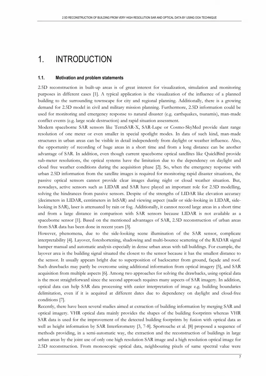
topographic information of that region. In Figure 2-1, the corresponding elements of two datasets are
acquired at two slightly different antenna positions (A1 and A2). The spatial baseline is formed by the
connection between these positions. This baseline has a length (B) between these positions and an
orientation ( ) relative to the horizontal direction. These positions belonging to a target can be extracted
from the platform orbits or flight passes. The difference in antenna position results a difference in the
range ( and ) from the target to those positions. This difference in range ( ) is translated into a phase
difference ( ). This phase difference is computed from the phase differences in the corresponding
elements in the datasets. The height of the target is a function of the phase difference ( ), the baseline (B),
some additional orbit parameters and a reference system.
2.5D RECONSTRUCTION OF BUILDING FROM VERY HIGH RESOLUTION SAR AND OPTICAL DATA BY USING OOA TECHNIQUE
11
Figure 2-1: InSAR geometry (source: [17])
The illustration in the figure above shows a simplified representation of the method for height calculation
using the phase information.
The difference in range is given by:
( ⁄ ) ( ) 2-1
Where is the look angle.
And thus:
(
⁄ ) 2-2
The height z at point (x, y) is expressed as:
( ) ( ) 2-3
The phase difference is:
2-4
Where z is the height above the chosen geoid in point (x, y), h is the satellite height above the geoid, is
the wavelength of the microwave.
Combining Equation 2-3 and 2-4 gives:
( ) ( (
⁄ ) ) 2-5
2.1.3. Appearance of buildings in SAR images
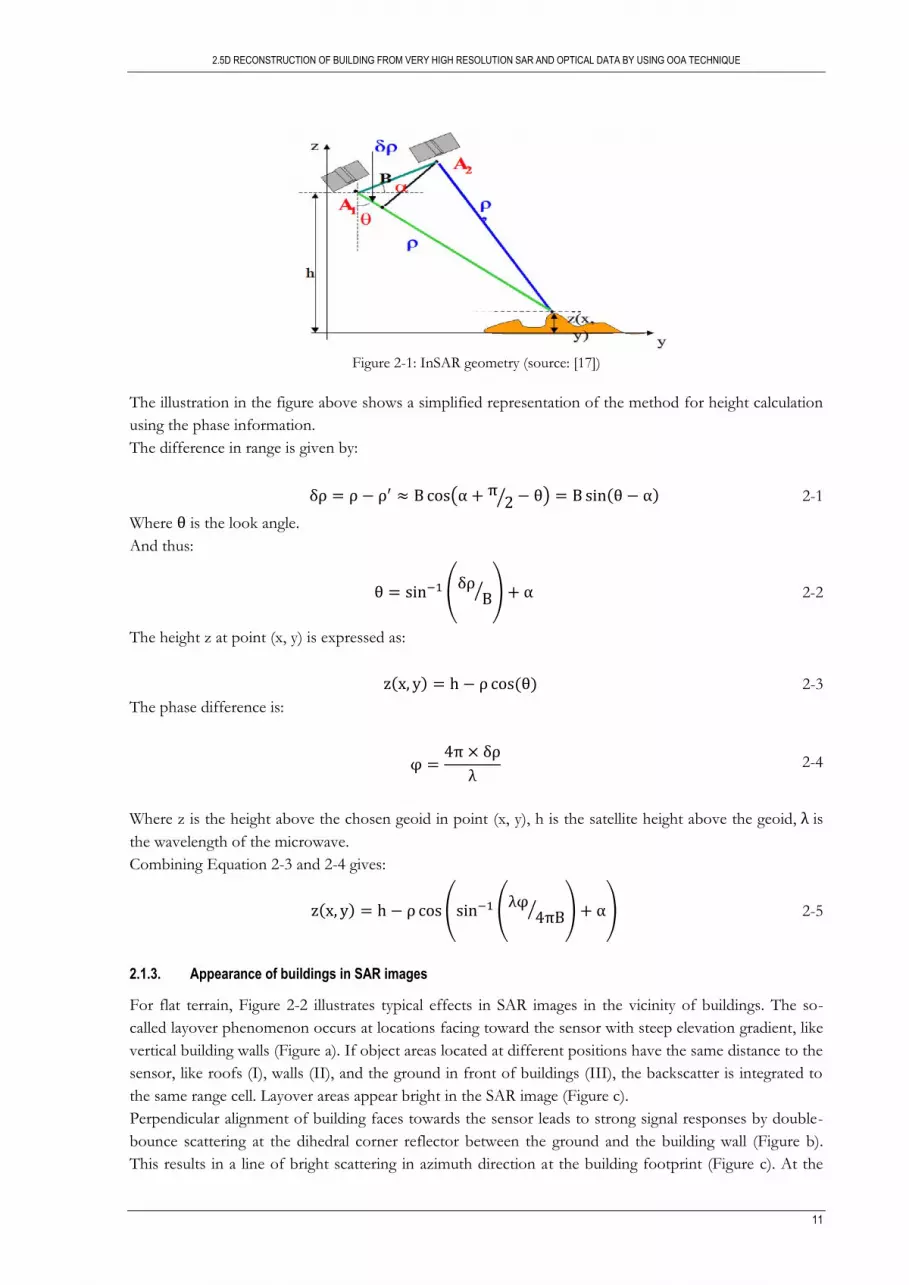
For flat terrain, Figure 2-2 illustrates typical effects in SAR images in the vicinity of buildings. The so-
called layover phenomenon occurs at locations facing toward the sensor with steep elevation gradient, like
vertical building walls (Figure a). If object areas located at different positions have the same distance to the
sensor, like roofs (I), walls (II), and the ground in front of buildings (III), the backscatter is integrated to
the same range cell. Layover areas appear bright in the SAR image (Figure c).
Perpendicular alignment of building faces towards the sensor leads to strong signal responses by double-
bounce scattering at the dihedral corner reflector between the ground and the building wall (Figure b).
This results in a line of bright scattering in azimuth direction at the building footprint (Figure c). At the

2.5D RECONSTRUCTION OF BUILDING FROM VERY HIGH RESOLUTION SAR AND OPTICAL DATA BY USING OOA TECHNIQUE
12
opposite building side the ground is partly occluded from the building shadow. This region appears dark
in the SAR image, because no signal returns into the related range bins.
(c) SAR range line
Figure 2-2: Phenomena caused by side-looking illumination (source: [18])
Because of these geometrical constraints, the mapping in dense urban areas by high resolution TerraSAR-
X data is complicated. Typical SAR imaging phenomena such as layover, shadowing and the strong
dependence of backscatter on the geometric features and topology of the illuminated objects need to be
carefully considered. Especially in dense urban areas, these effects may occur very commonly, seriously
affecting the appearance and ability to differentiate buildings. Layover and double-bounce scattering
resulted in displacement of the building footprint and features in the SAR image.
2.2. Review on building footprint extraction by OOA
2.2.1. Background of OOA
Building footprint extraction in urban areas has been studied and many methods have been developed for
it by remote sensing technology [19]. Building footprint can be extracted from several data sources using
diverse techniques. The main requirements for the extraction of required information from the images in a
up-to-date image analysis scheme are proposed in [20] to know the sensor characteristics, to recognize
fitting analysis scales and their combination, to find typical context and hierarchical dependencies, and to
(b) Corner reflector
(a) Layover

2.5D RECONSTRUCTION OF BUILDING FROM VERY HIGH RESOLUTION SAR AND OPTICAL DATA BY USING OOA TECHNIQUE
13
reflect the inherent uncertainties of the whole information extraction process, starting from the sensor, to
fuzzy concepts for the requested information.
Extraction of information from satellite images can be done from “the smallest processing unit of the
image” with its features applied for processing such as classification [21]. The smallest processing unit can
be determined as a pixel or an object (group of similar pixels) in the image. Its spectral characteristics, DN
value and textures, etc. for a pixel or spectral, spatial characteristics, texture, context and semantic
knowledge for an object can be used as its feature properties for further processing like segmentation or
classification.
In the past, the single pixel characteristics by the measurement of reflectance value from surface of the
Earth have been mainly used for the most of the methods in information extraction from images [22].
These traditional pixel based methods are not fully effective to extract information from very high
resolution images, because of spectral complexity (similar spectral reflectance from more than one class
and different spectral reflectance from one class) without paying attention to spatial relationship among
the neighbour, inapplicability of the semantic knowledge about the object and class [22].
The OOA method can solve the above mentioned limitations of pixel based analysis in information
extraction as explained in the following section [23].
2.2.2. OOA for building footprint extraction
The idea of OOA in this research is to segment images into spectrally homogenous segments or objects.
The shape and size of such segments can be constrained by a number of parameters which control the
maximum acceptable heterogeneity within a segment [20]. Additional thematic data layers like DSM can be
used to create meaningful segments in the image [24]. Various characteristics of the segments such as the
spatial, spectral, contextual or textural information can be used to develop rule sets which are applied to
classify the segments. The most important characteristic of OOA is to integrate different data sources like
optical data and DSM data, different processing algorithms and semantic knowledge about features, which
is not possible with most of the other image analysis techniques.
OOA is not only based on the spectral properties of the objects in the image but also based on the spatial
and semantic knowledge about the objects and its context, texture, association with spatial arrangement
and neighbourhood. The main benefit of the OOA in building footprint extraction is to take a
homogenous object element or image segments as a fundamental building block for classification, to
consider spatial relationship between the neighbouring objects, and to apply semantic and prior knowledge
of the objects for further processing [20]. The main components of OOA and the steps are discussed in
Section 3.4.
2.5D RECONSTRUCTION OF BUILDING FROM VERY HIGH RESOLUTION SAR AND OPTICAL DATA BY USING OOA TECHNIQUE
14
3. METHOD
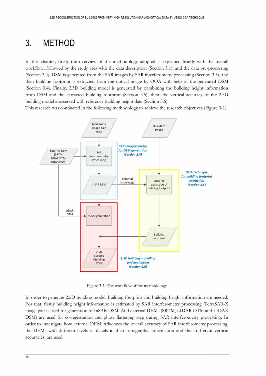
In this chapter, firstly the overview of the methodology adopted is explained briefly with the overall
workflow, followed by the study area with the data description (Section 3.1), and the data pre-processing
(Section 3.2). DSM is generated from the SAR images by SAR interferometry processing (Section 3.3), and
then building footprint is extracted from the optical image by OOA with help of the generated DSM
(Section 3.4). Finally, 2.5D building model is generated by combining the building height information
from DSM and the extracted building footprint (Section 3.5), then, the vertical accuracy of the 2.5D
building model is assessed with reference building height data (Section 3.6).
This research was conducted in the following methodology to achieve the research objectives (Figure 3-1).
TerraSAR-X image pair
(HS)
SAR Interferometry
Processing
InSAR DSM
External DEM(SRTM,
LIDAR DTM, LIDAR DSM)
QuickBird image
OOA for extraction of
building footprint
nDSM generation
2.5D building (Building nDSM)
LIDAR DTM
Building footprint
External knowledge
SAR Interferometryfor DSM generation
(Section 3.4)
OOA techniquefor building footprint
extraction(Section 3.5)
2.5D building modellingand evaluation
(Section 3.6)
Figure 3-1: The workflow of the methodology
In order to generate 2.5D building model, building footprint and building height information are needed.
For that, firstly building height information is estimated by SAR interferometry processing. TerraSAR-X
image pair is used for generation of InSAR DSM. And external DEMs (SRTM, LIDAR DTM and LIDAR
DSM) are used for co-registration and phase flattening step during SAR interferometry processing. In
order to investigate how external DEM influences the overall accuracy of SAR interferometry processing,
the DEMs with different levels of details in their topographic information and their different vertical
accuracies, are used.

2.5D RECONSTRUCTION OF BUILDING FROM VERY HIGH RESOLUTION SAR AND OPTICAL DATA BY USING OOA TECHNIQUE
15
Then, building footprint is extracted by OOA method. QuickBird image is used for detection of building
footprint with help of the generated DSM as external knowledge.
By combining the extracted building footprint and the estimated building height information, 2.5D
building is modelled and the vertical accuracy of 2.5D building is assessed with reference building model,
generated by using the LIDAR DSM and the field visit with a clinometer.
3.1. Study area and data
3.1.1. Study area
The study area for this research is Delft, a city and municipality in the province of South Holland, the
Netherlands. Delft is located at 52º0′0″ N and 4º21′30″ E and it is a crowded city, more or less having
typical characteristics like heterogeneous built up areas with many houses, buildings and roads, parking
areas and some areas with vegetation, such as trees.
(a) Overview of the Delft city (QuickBird image)
Site 1 Site 2
2.5D RECONSTRUCTION OF BUILDING FROM VERY HIGH RESOLUTION SAR AND OPTICAL DATA BY USING OOA TECHNIQUE
16
(b) Study site 1
(c) Study site 2
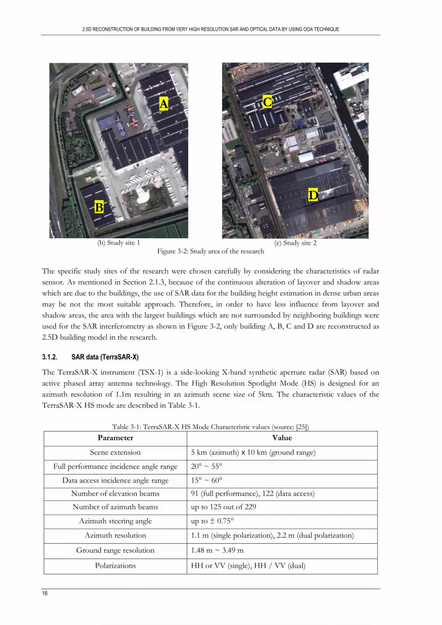
Figure 3-2: Study area of the research
The specific study sites of the research were chosen carefully by considering the characteristics of radar
sensor. As mentioned in Section 2.1.3, because of the continuous alteration of layover and shadow areas
which are due to the buildings, the use of SAR data for the building height estimation in dense urban areas
may be not the most suitable approach. Therefore, in order to have less influence from layover and
shadow areas, the area with the largest buildings which are not surrounded by neighboring buildings were
used for the SAR interferometry as shown in Figure 3-2, only building A, B, C and D are reconstructed as
2.5D building model in the research.
3.1.2. SAR data (TerraSAR-X)
The TerraSAR-X instrument (TSX-1) is a side-looking X-band synthetic aperture radar (SAR) based on
active phased array antenna technology. The High Resolution Spotlight Mode (HS) is designed for an
azimuth resolution of 1.1m resulting in an azimuth scene size of 5km. The characteristic values of the
TerraSAR-X HS mode are described in Table 3-1.
Table 3-1: TerraSAR-X HS Mode Characteristic values (source: [25])
Parameter Value
Scene extension 5 km (azimuth) x 10 km (ground range)
Full performance incidence angle range 20° ~ 55°
Data access incidence angle range 15° ~ 60°
Number of elevation beams 91 (full performance), 122 (data access)
Number of azimuth beams up to 125 out of 229
Azimuth steering angle up to ± 0.75°
Azimuth resolution 1.1 m (single polarization), 2.2 m (dual polarization)
Ground range resolution 1.48 m ~ 3.49 m
Polarizations HH or VV (single), HH / VV (dual)
A
B
C
D
2.5D RECONSTRUCTION OF BUILDING FROM VERY HIGH RESOLUTION SAR AND OPTICAL DATA BY USING OOA TECHNIQUE
17
Two SAR images captured by the TerraSAR-X were used in this research. The images were captured in
April 27, 2008 and May 8, 2008 with High Resolution Spotlight Mode. The characteristics of the SAR data
used are described in Table 3-2.
Table 3-2: Description of the SAR data used in the research
SAR data SLC_0427 SLC_0508
Acquisition time 2008-04-27-05:59:44 2008-05-08-05:59:45
Path Direction Descending
Look Direction Right
Polarizations VV
Projection Slant range
Azimuth resolution 1.1 m
Ground range resolution 1.48 m ~ 3.49 m
Product type /
Data format
Single Look Slant Range Complex (SSC) /
COSAR format (Complex SAR: Real and Imaginary parts)
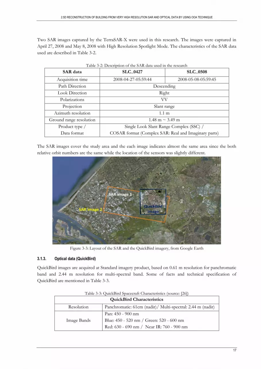
The SAR images cover the study area and the each image indicates almost the same area since the both
relative orbit numbers are the same while the location of the sensors was slightly different.
Figure 3-3: Layout of the SAR and the QuickBird imagery, from Google Earth
3.1.3. Optical data (QuickBird)
QuickBird images are acquired at Standard imagery product, based on 0.61 m resolution for panchromatic
band and 2.44 m resolution for multi-spectral band. Some of facts and technical specification of
QuickBird are mentioned in Table 3-3.
Table 3-3: QuickBird Spacecraft Characteristics (source: [26])
QuickBird Characteristics
Resolution Panchromatic: 61cm (nadir)/ Multi-spectral: 2.44 m (nadir)
Image Bands
Pan: 450 - 900 nm
Blue: 450 - 520 nm / Green: 520 - 600 nm
Red: 630 - 690 nm / Near IR: 760 - 900 nm
2.5D RECONSTRUCTION OF BUILDING FROM VERY HIGH RESOLUTION SAR AND OPTICAL DATA BY USING OOA TECHNIQUE
18
3.1.4. External DEMs
During SAR interferometry processing, external DEMs are applied for registration of the SAR pair and
InSAR flattening process to eliminate the phase components of the flat earth and the available
topography. The LIDAR DSM, the generated LIDAR DTM from the LIDAR DSM and the SRTM data
were used respectively, because the outputs with the external DEMs are compared to investigate which
external DEM will be more effective in terms of accuracy of InSAR DSM.
1) LIDAR AHN-1 data (DSM)
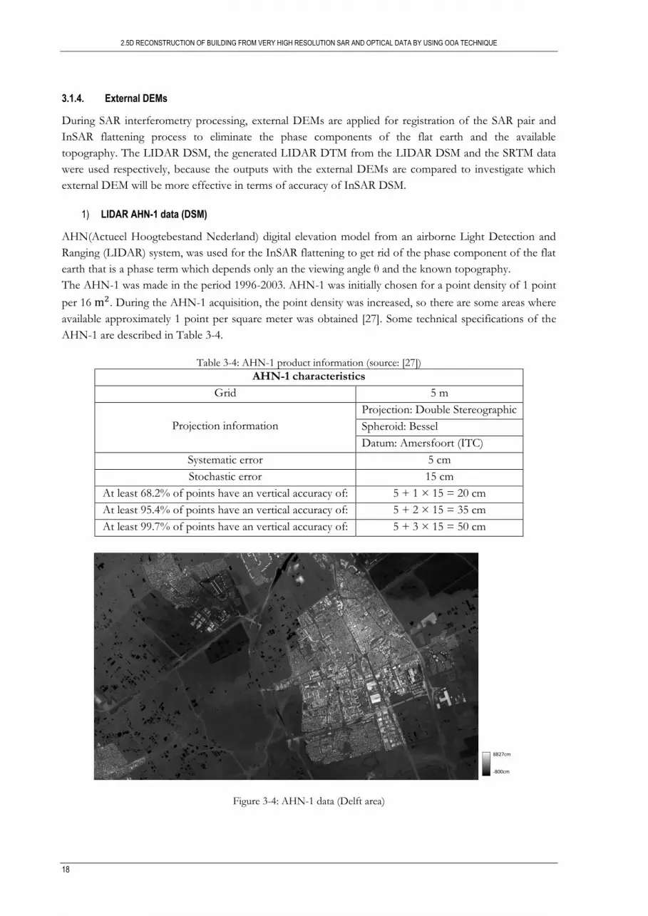
AHN(Actueel Hoogtebestand Nederland) digital elevation model from an airborne Light Detection and
Ranging (LIDAR) system, was used for the InSAR flattening to get rid of the phase component of the flat
earth that is a phase term which depends only an the viewing angle θ and the known topography.
The AHN-1 was made in the period 1996-2003. AHN-1 was initially chosen for a point density of 1 point
per 16 . During the AHN-1 acquisition, the point density was increased, so there are some areas where
available approximately 1 point per square meter was obtained [27]. Some technical specifications of the
AHN-1 are described in Table 3-4.
Table 3-4: AHN-1 product information (source: [27])
AHN-1 characteristics
Grid 5 m
Projection information
Projection: Double Stereographic
Spheroid: Bessel
Datum: Amersfoort (ITC)
Systematic error 5 cm
Stochastic error 15 cm
At least 68.2% of points have an vertical accuracy of: 5 + 1 × 15 = 20 cm
At least 95.4% of points have an vertical accuracy of: 5 + 2 × 15 = 35 cm
At least 99.7% of points have an vertical accuracy of: 5 + 3 × 15 = 50 cm
Figure 3-4: AHN-1 data (Delft area)
8827cm
-800cm
2.5D RECONSTRUCTION OF BUILDING FROM VERY HIGH RESOLUTION SAR AND OPTICAL DATA BY USING OOA TECHNIQUE
19
2) SRTM-3 version 4
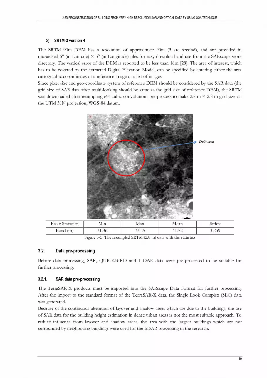
The SRTM 90m DEM has a resolution of approximate 90m (3 arc second), and are provided in
mosaicked 5° (in Latitude) × 5° (in Longitude) tiles for easy download and use from the SARscape work
directory. The vertical error of the DEM is reported to be less than 16m [28]. The area of interest, which
has to be covered by the extracted Digital Elevation Model, can be specified by entering either the area
cartographic co-ordinates or a reference image or a list of images.
Since pixel size and geo-coordinate system of reference DEM should be considered by the SAR data (the
grid size of SAR data after multi-looking should be same as the grid size of reference DEM), the SRTM
was downloaded after resampling (4th cubic convolution) pre-process to make 2.8 m × 2.8 m grid size on
the UTM 31N projection, WGS-84 datum.
Basic Statistics Min Max Mean Stdev
Band (m) 31.36 73.55 41.52 3.259
Figure 3-5: The resampled SRTM (2.8 m) data with the statistics
3.2. Data pre-processing
Before data processing, SAR, QUICKBIRD and LIDAR data were pre-processed to be suitable for
further processing.
3.2.1. SAR data pre-processing
The TerraSAR-X products must be imported into the SARscape Data Format for further processing.
After the import to the standard format of the TerraSAR-X data, the Single Look Complex (SLC) data
was generated.
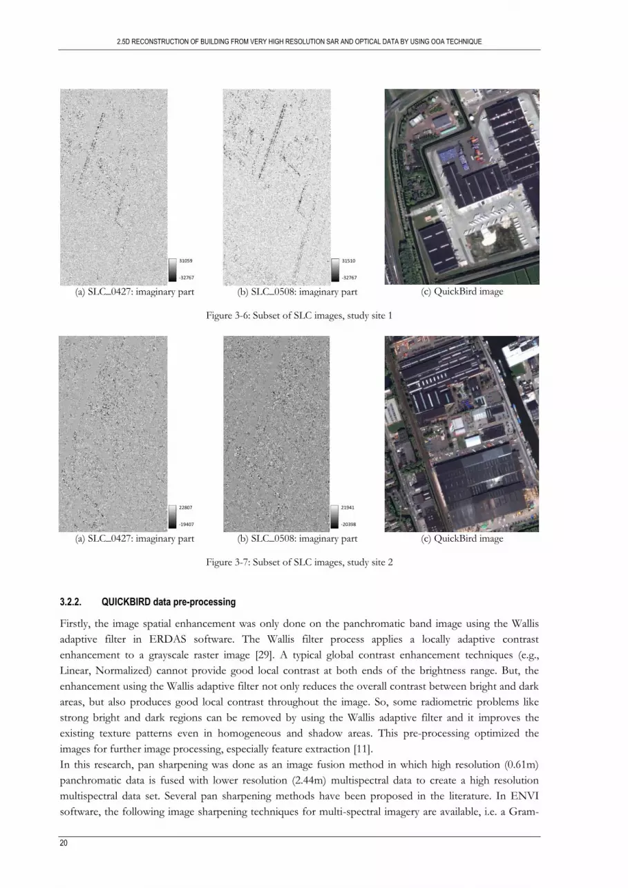
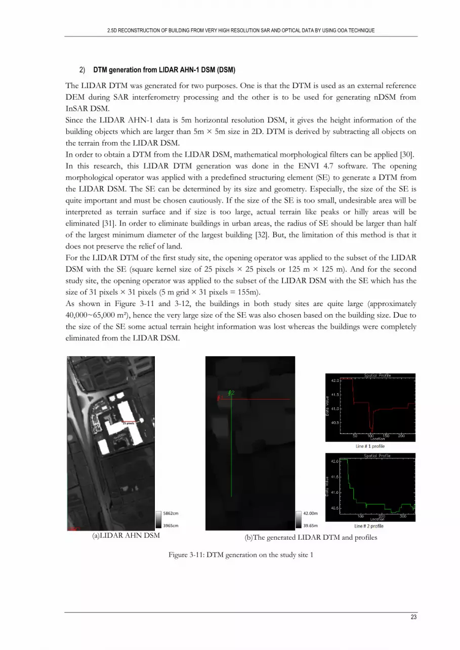
Because of the continuous alteration of layover and shadow areas which are due to the buildings, the use
of SAR data for the building height estimation in dense urban areas is not the most suitable approach. To
reduce influence from layover and shadow areas, the area with the largest buildings which are not
surrounded by neighboring buildings were used for the InSAR processing in the research.
Delft area
2.5D RECONSTRUCTION OF BUILDING FROM VERY HIGH RESOLUTION SAR AND OPTICAL DATA BY USING OOA TECHNIQUE
20
(a) SLC_0427: imaginary part
(b) SLC_0508: imaginary part
(c) QuickBird image
Figure 3-6: Subset of SLC images, study site 1
(a) SLC_0427: imaginary part
(b) SLC_0508: imaginary part
(c) QuickBird image
Figure 3-7: Subset of SLC images, study site 2
3.2.2. QUICKBIRD data pre-processing
Firstly, the image spatial enhancement was only done on the panchromatic band image using the Wallis
adaptive filter in ERDAS software. The Wallis filter process applies a locally adaptive contrast
enhancement to a grayscale raster image [29]. A typical global contrast enhancement techniques (e.g.,
Linear, Normalized) cannot provide good local contrast at both ends of the brightness range. But, the
enhancement using the Wallis adaptive filter not only reduces the overall contrast between bright and dark
areas, but also produces good local contrast throughout the image. So, some radiometric problems like
strong bright and dark regions can be removed by using the Wallis adaptive filter and it improves the
existing texture patterns even in homogeneous and shadow areas. This pre-processing optimized the
images for further image processing, especially feature extraction [11].
In this research, pan sharpening was done as an image fusion method in which high resolution (0.61m)
panchromatic data is fused with lower resolution (2.44m) multispectral data to create a high resolution
multispectral data set. Several pan sharpening methods have been proposed in the literature. In ENVI
software, the following image sharpening techniques for multi-spectral imagery are available, i.e. a Gram-
21941
-20398
22807
-19407
31510
-32767
31059
-32767

2.5D RECONSTRUCTION OF BUILDING FROM VERY HIGH RESOLUTION SAR AND OPTICAL DATA BY USING OOA TECHNIQUE
21
Schmidt transform, a principal components (PC) transform. The Gram-Schmidt and PC spectral
sharpening tools both create pan-sharpened images, but using different techniques. Both methods were
implemented and compared below.
(a) Original multi-spectral image
(b)Gram-Schmidt fused image
(C) PC fused image
Figure 3-8: Comparison of pan sharpening method
Gram-Schmidt is typically more accurate because it uses the spectral response function of a given sensor
to estimate what the panchromatic data look like. And a visual comparison of the fused images shows that
the Gram-Schmidt method generated the shaper edges of building. Based on two factors, the Gram-
Schmidt fused image was chosen for subsequent image analysis.
3.2.3. AHN-1 data Pre-processing
In the original AHN-1 data, there are missing values which are represented by the zero value. In statistics,
missing values occur when no data value is stored for the variable in the current observation. Missing
values are a common occurrence and it can severely disturb the conclusions drawn from the data. Since
missing values of AHN DSM can affect a significant error during the SAR interferometry flattening
process, it should be eliminated by interpolating with neighbouring values.
For the replacement of the missing values in AHN data, the model was generated by using the model
maker in the ERDAS software. Firstly, the small kernel size of the matrix during the interpolation was
chosen for the small pixel size of the missing values, and then the manually defined matrix kernel size was
applied to interpolate the larger remaining pixel size of the missing values.

2.5D RECONSTRUCTION OF BUILDING FROM VERY HIGH RESOLUTION SAR AND OPTICAL DATA BY USING OOA TECHNIQUE
22
Figure 3-9: The generated model (Model maker on the ERDAS software)
(a)Original DSM with missing value
(b)DSM after the replacement of missing value
Figure 3-10: Example of the replacement of missing value
1) Re-projection, Re-calculation of the elevation values and Resampling
The original projection system of the LIDAR AHN-1 DSM is the Double Stereographic, Bessel Spheroid
and the vertical datum is the Amersfoort (ITC, Coordinate Frame). But, in order to match it with the SAR
projection on the SARscape software, it was re-projected to the UTM 31N projection, and the vertical
datum of it was recalculated to WGS 84. Then, the LIDAR DSM was resampled by cubic convolution
algorithm to make 2.8 m × 2.8 m grid size to be matched with multi-looked SAR data.
2.5D RECONSTRUCTION OF BUILDING FROM VERY HIGH RESOLUTION SAR AND OPTICAL DATA BY USING OOA TECHNIQUE
23
2) DTM generation from LIDAR AHN-1 DSM (DSM)
The LIDAR DTM was generated for two purposes. One is that the DTM is used as an external reference
DEM during SAR interferometry processing and the other is to be used for generating nDSM from
InSAR DSM.
Since the LIDAR AHN-1 data is 5m horizontal resolution DSM, it gives the height information of the
building objects which are larger than 5m × 5m size in 2D. DTM is derived by subtracting all objects on
the terrain from the LIDAR DSM.
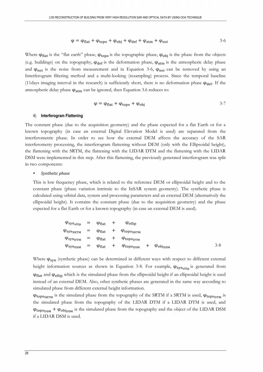
In order to obtain a DTM from the LIDAR DSM, mathematical morphological filters can be applied [30].
In this research, this LIDAR DTM generation was done in the ENVI 4.7 software. The opening
morphological operator was applied with a predefined structuring element (SE) to generate a DTM from
the LIDAR DSM. The SE can be determined by its size and geometry. Especially, the size of the SE is
quite important and must be chosen cautiously. If the size of the SE is too small, undesirable area will be
interpreted as terrain surface and if size is too large, actual terrain like peaks or hilly areas will be
eliminated [31]. In order to eliminate buildings in urban areas, the radius of SE should be larger than half
of the largest minimum diameter of the largest building [32]. But, the limitation of this method is that it
does not preserve the relief of land.
For the LIDAR DTM of the first study site, the opening operator was applied to the subset of the LIDAR
DSM with the SE (square kernel size of 25 pixels × 25 pixels or 125 m × 125 m). And for the second
study site, the opening operator was applied to the subset of the LIDAR DSM with the SE which has the
size of 31 pixels × 31 pixels (5 m grid × 31 pixels = 155m).
As shown in Figure 3-11 and 3-12, the buildings in both study sites are quite large (approximately
40,000~65,000 m²), hence the very large size of the SE was also chosen based on the building size. Due to
the size of the SE some actual terrain height information was lost whereas the buildings were completely
eliminated from the LIDAR DSM.
(a)LIDAR AHN DSM
(b)The generated LIDAR DTM and profiles
Figure 3-11: DTM generation on the study site 1
42.00m
39.65m
5862cm
3965cm
25 pixels

2.5D RECONSTRUCTION OF BUILDING FROM VERY HIGH RESOLUTION SAR AND OPTICAL DATA BY USING OOA TECHNIQUE
24
(a) LIDAR AHN DSM
(b)LIDAR AHN DTM
Figure 3-12: DTM generation on the study site 2
42.00m
39.65m
9293cm
4020cm

2.5D RECONSTRUCTION OF BUILDING FROM VERY HIGH RESOLUTION SAR AND OPTICAL DATA BY USING OOA TECHNIQUE
25
3.3. DSM generation by SAR interferometry processing
InSAR processing was done by using the SARscape software in ENVI 4.7 as the following approach in
Figure 3-13.
TerraSAR-XSLC data pair
Baseline Estimation
Synthetic PhaseGeneration
InterferogramCalculation
InterferogramFlattening
Adaptive filtering and Coherence
Generation
Phase Unwrapping
Orbital Refinement
Phase to Height Conversion
Reference DEM
Synthetic Phase
InSAR DSM
Figure 3-13: InSAR DSM generation workflow
3.3.1. Baseline Estimation
This function enables to obtain information about the baseline values and other orbital parameters related
to the input pair. The extracted parameters are intended as approximate measurements aimed at a
preliminary data characteristics and Interferometric quality assessment. The baseline value itself is not used
in any part of the Interferometric processing chain.
For InSAR DSM generation, the 2π ambiguity height (m) that is dependent on the perpendicular baseline
determines the sensitivity of the Interferogram. There is a simple formula that determines height
ambiguity ( ) based on the perpendicular baseline (B) [33]:
( ) 3-1
Where λ is the radar wavelength, θ is the look angle from nadir and α is the baseline orientation angle.
Interferogram Generation

2.5D RECONSTRUCTION OF BUILDING FROM VERY HIGH RESOLUTION SAR AND OPTICAL DATA BY USING OOA TECHNIQUE
26
If the baseline length increases when SAR interferometry technique is used to measure the height of
topographic map, the baseline decorrelation will be increased, but the height measurement sensitivity will
be increased as well because the 2π ambiguity height decreases (Equation 3-1), it will yield more fringes
with smaller 2π ambiguity height in the Interferogram. Terrain height measurement accuracy increases
with baseline since height measurement sensitivity increases with it. But, if baseline decorrelation is too
significant with increasing baseline length, two SAR images become completely uncorrelated. Therefore,
there is a trade-off of baseline [34]. The value of baseline is called critical baseline when baseline de-
correlation leads to uncorrelated SAR echoes. So, critical baseline is an indication if the pair of images is
useful for interferometry or not. When the perpendicular component of the baseline increases beyond the
critical baseline, no phase information is preserved, coherence is lost, so interferogram cannot be
generated [35]. The critical baseline , can be calculated as:
3-2
Where is the wavelength, is the slant range distance, is the slant range resolution, and is the
incidence angle.
3.3.2. Interferogram Generation
This step includes the co-registration of the two SAR images, the multi-looking, the interferogram
calculation and the interferogram flattening as following 4 section.
1) Co-registration
The registration of the interferometric geometry is one of the most important steps in InSAR DSM
generation process [36]. Co-registration between the two images of the same scene makes it possible to
use them in the same geometry. One of them is taken as a reference which is defined as master image. By
opposition, the other image is called slave.
Geometric registration (master / external DEM)
At the time of this first step, the master image was registered with respect to the external DEM used
with a precision of a fraction order of the DEM pixel (2.8 m× 2.8 m). In fact, it made the object of a
radiometric simulation according to the geometry of slant range direction of the master image. The
image of the DEM projected in radar geometry was then similar to the master image. It is then
possible to carry out a correlation between these two images by pairing of homogeneous group pixels,
for which one obtains a peak of correlation. This module of the software provided the shift in
distance, azimuth and the rate of correlation between the main image and simulation. From these
shifts, it generated a more precisely registration.
In this step, the grid of the DEM must be sufficiently small since it is necessary to use ground control
points between the images. In addition, it is preferable to have a well distinguished relief of the
topography on the images to have good ground control points [36].
Registration (image master / slave)
Spatial registration of the SAR images is necessary. In cases where two SAR images cover the same
region, it is necessary that pixels in different images correspond so that pixel-by-pixel comparisons can
be carried out. Co-registration was carried out, based on maximising correlation in a set of windows
(cross correlation grid).

2.5D RECONSTRUCTION OF BUILDING FROM VERY HIGH RESOLUTION SAR AND OPTICAL DATA BY USING OOA TECHNIQUE
27
2) Multi-looking
Multi-looking processing has been used to reduce phase noise in SAR interferometry processing since
SAR interferometry techniques were developed in the late 1970’s [37]. Phase noise gives a difficulty to
create DEM from an interferogram. If the phase noise [38-39], which is mostly caused by radar thermal
noise, speckle due to coherent SAR processing, decorrelation, and registration noise, is too strong, some
fringes of an interferogram will be totally lost which will cause errors in InSAR DEM.
The goal is also to obtain in the multi-looked image approximately squared pixels considering the pixel
spacing in ground range (and not the pixel spacing in slant range) and the pixel spacing in azimuth. In
order to avoid over- or under-sampling effects in the geo-coded image, it is recommended to generate a
multi-looked image corresponding to approximately the same pixel spacing foreseen for the geo-coded
image product. The number of looks is determined by pixel spacing in azimuth, pixel spacing in slant
range, and incidence angle. The pixel range in ground range is defined as:
( ) 3-3
Where:
is the pixel spacing in ground range, is the pixel spacing in slant range and is the incidence angle.
In the research, the Single Look Complex data were processed with the following parameters:
Pixel spacing azimuth = 0.87 m
Pixel spacing slant range ( ) = 0.91 m
Incidence angle ( ) = 37.595°
The information of the parameters was available in the metadata of the SLC data (header file). So, the
pixel spacing in ground range is:
( ) 3-4
So, the pixel size of the SLC is (1.49m, 0.87m). In order to get an approximate squared pixel size of multi-
looked image, the 2:3 multi-looking factor was done on the SLC (Complex SAR format: real and
imaginary parts) to get (2.98m, 2.61m) pixel of multi-looked image. In this step, the multi-looked image
with a large multi-looking factor lost the original phase signal information by resampling whereas the
image without multi-looking (1:1) had distortion of the image in azimuth direction and too much phase
noise, therefore 2:3 was chosen for the multi-looking process.
The noticeable thing on the choice of multi-looking is that the final grid size (2.8m, 2.8m) of InSAR DSM
will be approximately same as the pixel size of multi-looked images to achieve high accuracy of DSM [36].
3) Interferogram Calculation
After the two single-complex images are co-registered, the interferogram is computed according to:
| | | | 3-5
Where S1 and S2 are the corresponding complex values of the co-registered images, * indicates the
conjugate of a complex variable and is the interferometric phase.
The interferometric phase can be written as [40]:
2.5D RECONSTRUCTION OF BUILDING FROM VERY HIGH RESOLUTION SAR AND OPTICAL DATA BY USING OOA TECHNIQUE
28
3-6
Where is the “flat earth” phase, is the topographic phase, is the phase from the objects
(e.g. buildings) on the topography, is the deformation phase, is the atmospheric delay phase
and is the noise from measurement and in Equation 3-6, can be removed by using an
Interferogram filtering method and a multi-looking (resampling) process. Since the temporal baseline
(11days imaging interval in the research) is sufficiently short, there is no deformation phase . If the
atmospheric delay phase can be ignored, then Equation 3.6 reduces to:
3-7
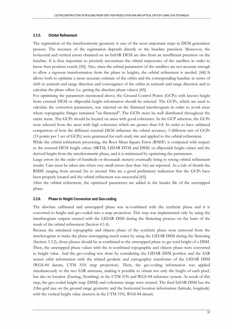
4) Interferogram Flattening
The constant phase (due to the acquisition geometry) and the phase expected for a flat Earth or for a
known topography (in case an external Digital Elevation Model is used) are separated from the
interferometric phase. In order to see how the external DEM affects the accuracy of the SAR
interferometry processing, the interferogram flattening without DEM (only with the Ellipsoidal height),
the flattening with the SRTM, the flattening with the LIDAR DTM and the flattening with the LIDAR
DSM were implemented in this step. After this flattening, the previously generated interferogram was split
in two components:
Synthetic phase
This is low frequency phase, which is related to the reference DEM or ellipsoidal height and to the
constant phase (phase variation intrinsic to the InSAR system geometry). The synthetic phase is
calculated using orbital data, system and processing parameters and an external DEM (alternatively the
ellipsoidal height). It contains the constant phase (due to the acquisition geometry) and the phase
expected for a flat Earth or for a known topography (in case an external DEM is used).
3-8
Where (synthetic phase) can be determined in different ways with respect to different external
height information sources as shown in Equation 3-8. For example, is generated from
and which is the simulated phase from the ellipsoidal height if an ellipsoidal height is used
instead of an external DEM. Also, other synthetic phases are generated in the same way according to
simulated phase from different external height information.
is the simulated phase from the topography of the SRTM if a SRTM is used,
is
the simulated phase from the topography of the LIDAR DTM if a LIDAR DTM is used, and
is the simulated phase from the topography and the object of the LIDAR DSM
if a LIDAR DSM is used.

2.5D RECONSTRUCTION OF BUILDING FROM VERY HIGH RESOLUTION SAR AND OPTICAL DATA BY USING OOA TECHNIQUE
29
Flattened Interferogram
This is high frequency phase, which is related to the difference with respect to an external DEM or an
ellipsoidal height. Flattened Interferogram is generated by subtracting synthetic phase from the
previously generated Interferogram. In this research, flattened interferogram will be called remaining
phase.
( ) 3-9
In Equation 3-9, the remaining phase can defined differently according to the use of different external
height information sources. For example, if the LIDAR DSM is used for flattening process,
will be subtracted from the interferometric phase ( ) to get:
3-10
3.3.3. Coherence generation and adaptive filtering
Given two co-registered complex SAR images ( and ), the interferometric coherence ( ) is defined as
the absolute value of the normalized complex cross correlation between the two signals [41].
|∑
( )
( ) |
√∑ | ( )
| ∑ |
( )|
3-11
Where N is the number of pixels in the moving window (5 × 5 pixels) for coherence estimation, and
are complex numbers and is the complex conjugate. The observed coherence which ranges between 0
and 1 is the indication of systemic spatial de-correlation, the additive noise, and the scene decorrelation
that takes place between the two acquisitions. In the research, coherence was used for a twofold purpose:
- To determine the quality of the measurement (i.e. interferometric phase). Before the phase unwrapping,
coherence threshold should be carefully chosen to avoid the unwrapping error from low coherent areas,
e.g. vegetated areas. So, pixels with coherence values smaller than this threshold will be not unwrapped. In
the research, phases having coherence values lower than 0.4 was not considered for the further processing.
- To extract thematic information about the object on the ground in combination with the backscattering
coefficient, i.e. the coherence of buildings is much higher than other areas.
And the filtering of the flattened interferogram generated the output product with reduced phase
noise. The coherence values were used to set the window size; the mean intensity difference among
adjacent pixels is used to identify a stationary area, which defines the maximum dimension and the shape
of the filtering windows. The process is aimed at preserving the smallest interferometric fringe patterns.
3.3.4. Phase unwrapping with region growing method
The phase of the Interferogram can only be modulo 2π; hence anytime the phase change becomes larger
than 2π the phase starts again and the cycle repeats itself. It is thus necessary to determine the multiple of
2π to add with the phase measured on each point to obtain an estimate of the real phase [36]. Phase
Unwrapping is the process that resolves this 2π ambiguity as shown in Figure 3-14. The unwrapping phase
thus consists in redistributing with each pixel its absolute phase.

2.5D RECONSTRUCTION OF BUILDING FROM VERY HIGH RESOLUTION SAR AND OPTICAL DATA BY USING OOA TECHNIQUE
30
Figure 3-14: Phase unwrapping process- Right figure: 3 dimensional (Source: [36])
Two algorithms (region growing, minimum cost flow) are available on the SARscape phase unwrapping
process; in essence, none of these is perfect and different or combined approaches should be applied on a
case by case basis to get optimal results. In two unwrapping algorithms, the accuracy of the result depends
on the path chosen to perform the unwrapping. Choosing the best path is difficult for many current
algorithms. A fast and robust solution for local phase unwrapping is the region growing algorithm [42].
The region growing algorithm minimizes unwrapping errors by starting at pixels of high data quality and
proceeding along dynamic paths where unwrapping confidence is high. Areas that are difficult to unwrap
are then approached from a number of directions. Thus, the algorithm is able to correct unwrapping
errors to a certain extent and stop their propagation. The basic idea of this algorithm is the following: The
pixels around an already solved region which have a sufficient number of unwrapped neighboring pixels
are decided to be growth pixels. From the unwrapped phase values a prediction of the absolute phase is
made providing to add the correct 2π multiple to the growth pixels. As described above, the success of
this method depends strongly upon the path chosen to perform the unwrapping and on the quality of the
prediction. Unwrapping errors are minimized by starting at pixels of high data quality or coherence and
then relaxing the coherence limit step by step. At a certain critical coherence limit the algorithm starts to
be unstable and wrong 2π-jumps are made.
Phase unwrapping is particularly difficult because of the side-looking scene illumination which causes
layover, shadowing and foreshortening effect [42]. Especially, if there are large areas of low coherence,
which are mainly caused by layover due to the extreme local topography, the interferogram is considered
to be difficult to unwrap. These areas of low coherence segment the interferogram into many pieces,
which creates structural difficulties for the unwrapping algorithm. So, two constraints burden this process
[36]: firstly, surface must be relatively regular; for this reason, it is preferable that it is smoothed
beforehand. Secondly, the absolute variation between two close pixels must be lower than π.
For these difficulties, an external DEM can be used as known topographic phase in the generated
synthetic phase as mentioned in Section 3.3.2 and subtracted from the interferogram. The remaining
phase, which is height difference with respect to the external DEM, is much easier for phase unwrapping
[43]. Then, the subtracted topographic and object phase from the interferometric phase is added back to
achieve the total height of DEM during phase to height conversion.
Based on the purpose of using an external DEM for InSAR processing, the assumption was made in this
phase unwrapping step that if the LIDAR DSM with the topographic and objects height is used as an
external DEM during the Interferogram flattening, the phase unwrapping process will be much easier than
using the ellipsoidal height information, the SRTM and the LIDAR DTM because the remaining phase,
flattened by subtracting the known topographic and object phase of the LIDAR DSM, has less variation
between local height differences.
2.5D RECONSTRUCTION OF BUILDING FROM VERY HIGH RESOLUTION SAR AND OPTICAL DATA BY USING OOA TECHNIQUE
31
3.3.5. Orbital Refinement
The registration of the interferometric geometry is one of the most important steps in DEM generation
process. The accuracy of the registration depends directly to the baseline precision. Moreover, the
horizontal and vertical errors obtained on an InSAR DEM are also from an insufficient precision on the
baseline. It is thus important to precisely reconstruct the orbital trajectories of the satellites in order to
know their position exactly [36]. Also, since the orbital parameters of the satellites are not accurate enough
to allow a rigorous transformation from the phase to heights, the orbital refinement is needed. [44] It
allows both to optimise a more accurate estimate of the orbits and the corresponding baseline in terms of
shift in azimuth and range direction and convergence of the orbits in azimuth and range direction and to
calculate the phase offset (i.e. getting the absolute phase values) [45].
For optimising the parameters mentioned above, the Ground Control Points (GCPs) with known height
from external DEM or ellipsoidal height information should be selected. The GCPs, which are used to
calculate the correction parameters, was selected on the flattened interferogram in order to avoid areas
where topographic fringes remained "un-flattened". The GCPs must be well distributed throughout the
entire scene. The GCPs should be located on areas with good coherence. In the GCP selection, the GCPs
were selected from the areas with high coherence which are greater than 0.8. In order to have unbiased
comparison of how the different external DEM influence the orbital accuracy, 3 different sets of GCPs
(15 points per 1 set of GCPs) were generated for each study site and applied to the orbital refinement.
While the orbital refinement processing, the Root Mean Square Error (RMSE) is computed with respect
to the external DEM height values (SRTM, LIDAR DTM and DSM) or ellipsoidal height values and the
derived height from the interferometric phase, and it is minimized by optimising the parameters.
Large errors (in the order of hundreds or thousands meters) eventually bring to wrong orbital refinement
results. Care must be taken also when very small errors (less than 1m) are reported. As a rule of thumb the
RMSE ranging from around 2m to around 10m are a good preliminary indication that the GCPs have
been properly located and the orbital refinement was successful [45].
After the orbital refinement, the optimised parameters are added in the header file of the unwrapped
phase.
3.3.6. Phase to Height Conversion and Geo-coding
The absolute calibrated and unwrapped phase was re-combined with the synthetic phase and it is
converted to height and geo-coded into a map projection. This step was implemented only by using the
interferogram outputs created with the LIDAR DSM during the flattening process on the basis of the
result of the orbital refinement (Section 4.1.4).
Because the simulated topographic and objects phase of the synthetic phase were removed from the
interferogram to make the phase unwrapping much easier by using the LIDAR DSM during the flattening
(Section 3.3.2), those phases should be re-combined to the unwrapped phase to get total height of a DSM.
Then, the unwrapped phase values with the re-combined topographic and objects phase were converted
to height value. And the geo-coding was done by considering the LIDAR DSM position and the SAR
sensor orbit information with the related geodetic and cartographic transforms of the LIDAR DSM
(WGS-84 datum, UTM 31N map projection). Then, the geo-coding information was applied
simultaneously to the two SAR antennae, making it possible to obtain not only the height of each pixel,
but also its location (Easting, Northing) in the UTM 31N and WGS-84 reference system. As result of this
step, the geo-coded height map (DSM) and coherence image were created. The final InSAR DSM has the
2.8m grid size on the ground range geometry and the horizontal location information (latitude, longitude)
with the vertical height value (meters) in the UTM 31N, WGS-84 datum.

2.5D RECONSTRUCTION OF BUILDING FROM VERY HIGH RESOLUTION SAR AND OPTICAL DATA BY USING OOA TECHNIQUE
32
3.4. Building Footprint Extraction by OOA
The overall method is described in Figure 3-15. First, the QuickBird image was visually interpreted and
analysed by different interpretation elements. It provided a general understanding of the image. Then, the
segmentation was applied to the image and the classification was done with the generated rule set using
the InSAR DSM external layer for building extraction in eCognition Developer 8 software.
QUICKBIRDImage
Visual Image Interpretation
Segmentation(Multi-resolution)
InSAR DEMExternal layer
Classification
Building FootprintExtraction and
Refinement
Export
Building FootprintShape file
If the segments meaningful
Yes
No
Rule setCreation
Figure 3-15: Flow chart of the Building Footprint Extraction
Elements for Rule setNDVINDWISSIAreaMean InSAR DEM HeightRel border to BuildingRel border to VegetationRel border to Water
RefinementChessboard segmentationMorphological operation (opening)Rel border to buildingPixel based resizing (Merge)

2.5D RECONSTRUCTION OF BUILDING FROM VERY HIGH RESOLUTION SAR AND OPTICAL DATA BY USING OOA TECHNIQUE
33
3.4.1. Visual Image Interpretation
Image visual interpretation is the act of examining images to identify objects and judge their significance.
It is important to not only get an insight of the QuickBird image, but also identify feature properties of
objects and their relationships which are useful for further analysis and supports building extraction from
the image [11]. The most important characteristics that can be studied on the image in visual image
interpretation are: shape, size, association, shadows, texture and tone [46]. Based on these characteristics,
the visual image interpretation was carried out.
Complexity of urban area in OOA
Due to spectral complexity of urban areas, it’s difficult to extract correctly objects from optical image.
Different neighbouring objects, e.g. building, parking areas or road, may be constructed with same
materials or an object may be made of different materials, e.g. a building is built with concrete, metal,
bricks, tiles or synthetic materials. So, single building may have different spectral characteristics from
different parts of the building. The different spectral properties of the building and the similar spectral
properties of the buildings and the parking area are shown in Figure 3-16.
Figure 3-16: Example of spectral characteristics in the study site 2
In this case, the building cannot be distinguished only on the basis of spectral properties. But, the
building can be extracted by integrating spectral, spatial and contextual information. The several
information can be used to create a rule set for building extraction, so that spatial and contextual
properties gives additional helps with spectral information to differentiate the buildings from the
other objects.
3.4.2. Multi-resolution Segmentation
Segmentation algorithms are required if creation of new image objects levels based on image layer
information is needed. The segmentation is desired to provide meaningful object primitives for further
feature recognition and thematic classification [47] and it is used to subdivide entire images at a pixel level,
or specific image objects from other domains into smaller image objects [48]. The eCognition Developer 8
software provides 7 segmentation algorithms, ranging from very simple algorithms, such as chessboard
and quadtree-based segmentation, to highly sophisticated methods such as multi-resolution segmentation
and contrast filter segmentation. For this research, the multi-resolution segmentation was done in this step
and the chessboard segmentation was used in the building refinement step (Section 3.4.4).
Multi-resolution segmentation algorithm is characterized as a bottom-up region-merging process starting
with one-pixel objects. Smaller image objects are subsequently merged into larger ones, forming
segmentations with objects in different scales [47]. The merging decision is based on a homogeneity

2.5D RECONSTRUCTION OF BUILDING FROM VERY HIGH RESOLUTION SAR AND OPTICAL DATA BY USING OOA TECHNIQUE
34
criterion, which defines the similarity among adjacent segments. This homogeneity criterion is defined as a
combination of spectral homogeneity and shape homogeneity [48]. The pair of image objects, having small
increment and within the user-defined threshold of the homogeneity criterion is merged. The process
continues until it finds the image objects fulfilling the defined criteria and terminates when the increment
on homogeneity exceeds the threshold [20]. In the homogeneity criterion, three parameters are computed:
scale, color and shape (Figure 3-17). The scale parameter is applied to determine the maximum acceptable
heterogeneity for the resulting image objects. For heterogeneous areas of data, the resulting objects for a
given scale parameter will be smaller than in more homogeneous areas. By modifying the value in the scale
parameter value, the size of image objects is changed, e.g. bigger image objects in size but less in numbers,
can be produced by applying higher scale parameter and vice versa.
And the homogeneity criterion further depends on a combination of color and shape parameters. The
value of the Shape field modifies the relationship between shape and color criteria; By modifying the
Shape criterion, the color criteria (color = 1 – shape) is defined.
Figure 3-17: Multi-resolution segmentation concept flow diagram (source: [48])
In effect, by decreasing the value assigned to the Shape field, it defines to which percentage the spectral
values of the image layers will contribute to the entire homogeneity criterion. This is weighted against the
percentage of the shape homogeneity, which is defined as a combination of smoothness and compactness.
The compactness parameter is used to optimize image objects with regard to compactness. This criterion
is used when different image objects which are rather compact, but are separated from non-compact
objects only by a relatively weak spectral contrast.
3.4.3. Rule-based Classification
1) Feature properties analysis / creation of rule set
The visual image interpretation, the semantic knowledge of the study areas from the observation and the
available InSAR DSM helped to generate a rule set for the extraction of buildings.
Firstly, in order to separate the distinct objects which can be extracted easily by using spectral properties
from the image, some customized rules were generated. NDVI (Normalized Difference Vegetation
Index), NDWI (Normalized Difference Water Index) and SSI (Spectral Shape Index) were made by
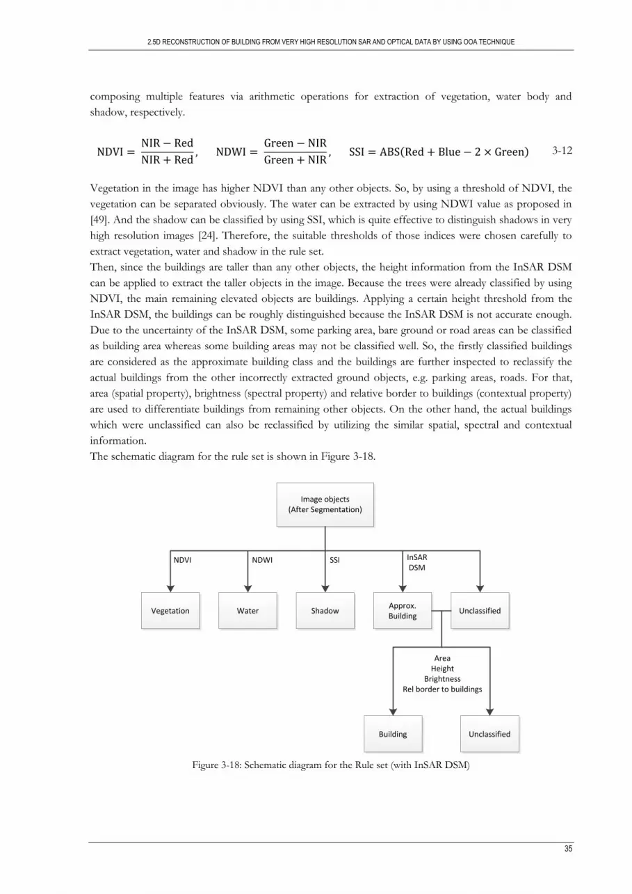
2.5D RECONSTRUCTION OF BUILDING FROM VERY HIGH RESOLUTION SAR AND OPTICAL DATA BY USING OOA TECHNIQUE
35
composing multiple features via arithmetic operations for extraction of vegetation, water body and
shadow, respectively.
( ) 3-12
Vegetation in the image has higher NDVI than any other objects. So, by using a threshold of NDVI, the
vegetation can be separated obviously. The water can be extracted by using NDWI value as proposed in
[49]. And the shadow can be classified by using SSI, which is quite effective to distinguish shadows in very
high resolution images [24]. Therefore, the suitable thresholds of those indices were chosen carefully to
extract vegetation, water and shadow in the rule set.
Then, since the buildings are taller than any other objects, the height information from the InSAR DSM
can be applied to extract the taller objects in the image. Because the trees were already classified by using
NDVI, the main remaining elevated objects are buildings. Applying a certain height threshold from the
InSAR DSM, the buildings can be roughly distinguished because the InSAR DSM is not accurate enough.
Due to the uncertainty of the InSAR DSM, some parking area, bare ground or road areas can be classified
as building area whereas some building areas may not be classified well. So, the firstly classified buildings
are considered as the approximate building class and the buildings are further inspected to reclassify the
actual buildings from the other incorrectly extracted ground objects, e.g. parking areas, roads. For that,
area (spatial property), brightness (spectral property) and relative border to buildings (contextual property)
are used to differentiate buildings from remaining other objects. On the other hand, the actual buildings
which were unclassified can also be reclassified by utilizing the similar spatial, spectral and contextual
information.
The schematic diagram for the rule set is shown in Figure 3-18.
Image objects(After Segmentation)
Vegetation Water ShadowApprox.Building
Unclassified
NDVI NDWI SSI InSAR DSM
Unclassified
AreaHeight
BrightnessRel border to buildings
Building
Figure 3-18: Schematic diagram for the Rule set (with InSAR DSM)

2.5D RECONSTRUCTION OF BUILDING FROM VERY HIGH RESOLUTION SAR AND OPTICAL DATA BY USING OOA TECHNIQUE
36
2) Building Footprint extraction without InSAR DSM
In this step, in order to see how the height information from the InSAR DSM helps to make the process
of building extraction easier, building extraction without the InSAR DSM was implemented for the
comparison with building extraction with the InSAR DSM.
As shown in Figure 3-18, the approach was applied to extract the buildings, but without the InSAR DSM
layer. Firstly, the vegetation, water body and shadow areas were classified by NDVI, NDWI and SSI,
respectively. But, as the spectral similarity among buildings and other objects (parking areas, cars, paved
roads, etc.), and spectral variability of a building was explained already, the extraction of buildings by only
using spectral properties was found difficult. Hence, the implementation was done by using different
spectral (brightness), spatial (area, length, rectangular fit) and contextual (relative border to building,
vegetation) properties.
3) Building Footprint extraction with InSAR DSM
The InSAR DSM was used as an external layer to help the classification of the image segments, especially
the buildings, because taller objects and other objects can be differentiated on the basis of height
information. Based on similar approach as described in the previous section, the vegetation, water and
shadow areas were classified by manipulating certain NDVI, NDWI and SSI thresholds. Then, the InSAR
DSM was applied with a height threshold of 49 m to classify the approximate buildings (The average
terrain height of the both study areas was around 42 m in the WGS-84 vertical datum). Then, all building
segments were merged to reshape into the actual building footprint. The same approach for the building
footprint extraction was repeated by utilizing the InSAR DSM in the both study areas.
3.4.4. Refinement of Building Footprint
Building footprint refinement was required since the extracted buildings were not in smooth shape. For
the refinement, the chessboard segmentation and morphological (opening) operation were mainly applied
to reshape the building footprint into final smooth shape. Finally, the extracted building footprint was
exported to the vector shape file.
1) Chessboard segmentation
The chessboard segmentation is based on the top down region splitting method and split the pixel domain
or an image object domain into square image objects [48]. It can be used for refining the image objects.
The image objects, which have already been identified, can be segmented with a small square size
parameter for more detailed analysis. The size of chessboard tile can be controlled by setting number of
pixels according to user’s requirement.
2) Object Reshaping algorithm
This reshaping algorithm was applied to modify the shape of the building after the chessboard
segmentation. The pixel based opening morphological operation was performed on the all building
segments. Then, contextual information (relative border to building) was used to make the smoother
boundary of the buildings and the final building segments were merged to become the building object.
3) Export (Vector shape file)
The extracted building footprints were exported to the vector shape file.

2.5D RECONSTRUCTION OF BUILDING FROM VERY HIGH RESOLUTION SAR AND OPTICAL DATA BY USING OOA TECHNIQUE
37
3.5. Generation of 2.5D Building model
In this step, firstly nDSM was generated by using the InSAR DSM and the LIDAR DTM (Section 3.2.3).
And the extracted building footprint was applied to get the nDSM of the only building footprint without
neighbouring areas around the buildings. Then, the building nDSM (2.5D model) was shown in ArcScene
to visualize as 2.5D.
3.5.1. nDSM creation
Since the InSAR DSM has surface elevation including terrain height, the terrain height should be
eliminated from it to only estimate the object height as shown in Figure 3-19.
Figure 3-19: Determination of the normalized DSM (nDSM) (source: [50])
For the generation of the terrain height model, there were two ways that implemented in this research; one
was by using the InSAR DSM and the other was by using the LIDAR DSM. From the both DSM, the
DTM could be extracted by using the morphological operator as described in Section 3.2.3. But, because
of the low coherence in the InSAR DSM due to vegetation near the buildings, there was error on the
height estimation of the ground areas near the buildings. So, it resulted in wrong height determination on
the vegetated and neighbouring areas in the generated DTM by using the InSAR DSM.
Differently, the LIDAR DSM has smaller error on the vegetated and neighbouring areas, so it was suitable
to be applied for the DTM creation. Therefore, the generated LIDAR DTM was used for this step. Since
the coordinate system and pixel size of the InSAR DSM and the LIDAR DTM are same, it was easy
process to subtract the DTM from the DSM.
3.5.2. 2.5D building modelling (Building nDSM)
As the objective of this research is to only generate 2.5D building model, elimination of any other object
height from the nDSM, except for the building height, was needed. This process was done in ENVI 4.7
software.
Firstly, the extracted building footprint vector layer was overlaid on the nDSM and the image mask was
built from the building footprint vector layer. The mask is a binary image that has values of 0 for the area
outside the building footprint layer and 1 for the area inside the layer. When the mask was applied to the
nDSM by using the generated processing function, that if the masked value is 0 (area outside the layer), it
changes the nDSM value to 0 value whereas the masked 1 value (area inside the layer) gives the original
nDSM value, it only gave the height information of the area inside the building footprint layer.
2.5D RECONSTRUCTION OF BUILDING FROM VERY HIGH RESOLUTION SAR AND OPTICAL DATA BY USING OOA TECHNIQUE
38
3.6. Height accuracy assessment of 2.5D building model
This step is to assess the height accuracy of the created building model with respect to reference model, in
order to understand potentials and limits of the method used in the 2.5D building modeling.
The assessment is done by 2 ways. One is compared with the reference building model from the LIDAR
DSM (Section 3.6.1). And the other is assessed by the height information from the field visit with the
measurement instruments, i.e. a clinometer, a measuring tape (Section 3.6.2).
3.6.1. Comparison by reference building model (LIDAR building nDSM)
1) Reference building modelling by LIDAR nDSM
Since the 2.5D building model was generated by the created nDSM from SAR interferometry processing, a
LIDAR nDSM should also be prepared for a reference model. So, based on the described method in
Section 3.5.1, the generated LIDAR DTM (Section 3.2.3) was subtracted from the LIDAR DSM to get
LIDAR nDSM.
Then, reference building model was created by using the extracted building footprint and the LIDAR
nDSM with same method described in Section 3.5.2.
2) Evaluation of the building model by the reference
The height accuracy of the generated 4 building models in the study sites was evaluated. The accuracy was
computed as mean, median, min and max value of height differences, and RMSE of height differences
between the tested building model and the reference building model.
For mean height difference, the height of the tested building model was subtracted by the height of the
reference building model and the height differences were averaged to achieve the mean height difference
between two models.
And for RMSE of the difference between two models, the following equation was applied.
√∑ ( )
3-13
Where is the height of the tested building model, is the height of the reference building model and
is the number of pixels, chosen for RMSE calculation.
3.6.2. Assessment by field data
To get an insight of the study buildings and height information, field work was done by a clinometer and a
measuring tape in the study sites. During the field work for measuring height, two buildings height of the
first study site couldn't be measured due to security issue. So, only 2 buildings height of the second study
site was measured by using the measurement instruments.
Clinometer
Suunto PM-5/1520 is an instrument for measuring heights, especially heights of trees or buildings.
When measured from distances of 15 m and 20 m, building heights can be read straight from the
instrument’s scales. Height can be estimated easily and fast by using the clinometer, but accuracy of
measurement varies because the accuracy depends on user’s expertise and environment of study area,
such as terrain undulation, building roof regularity, etc. Also, minimum scale of measurement of the
clinometer is 0.25 m; it means that there is 0.25 m uncertainty of between 1 scales.
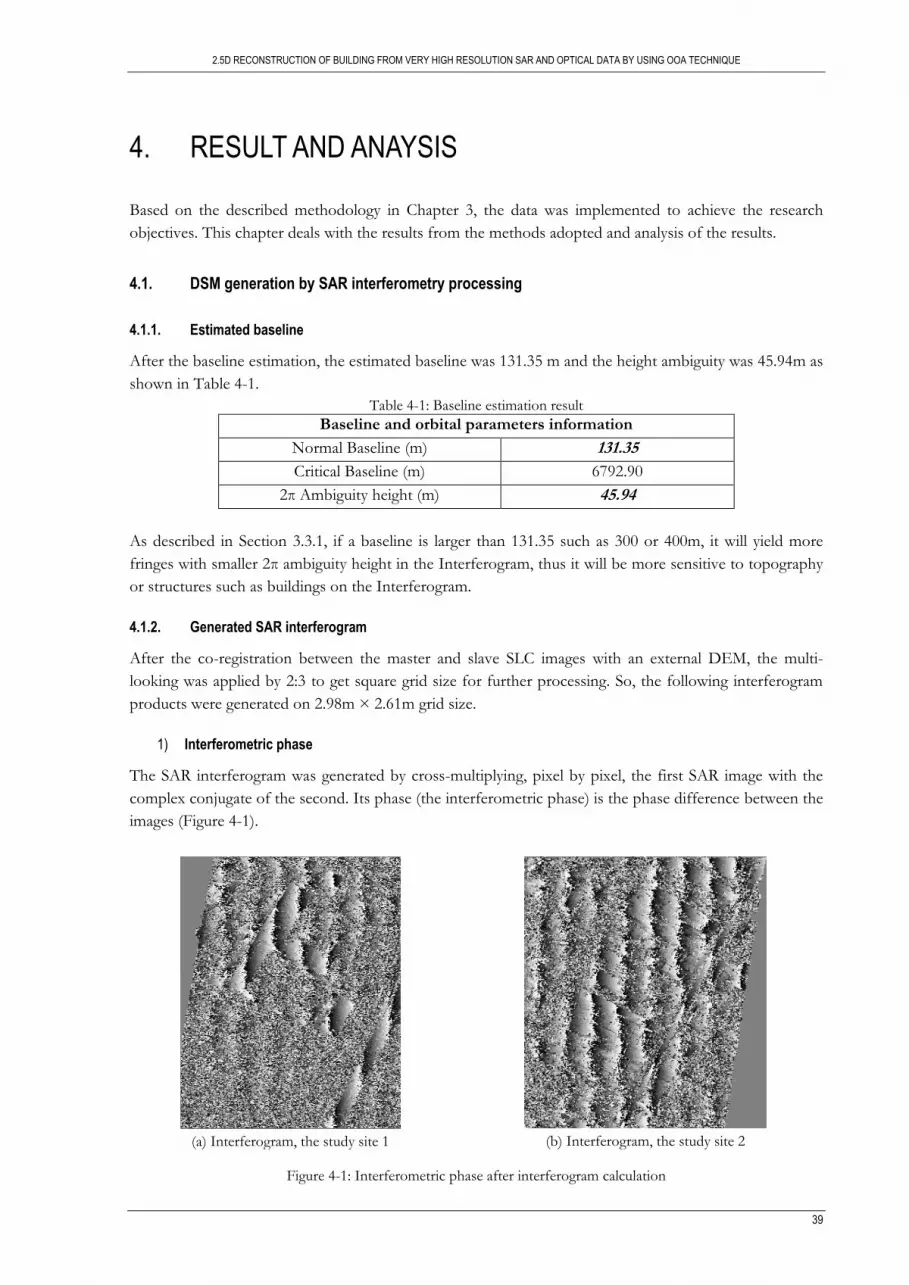
2.5D RECONSTRUCTION OF BUILDING FROM VERY HIGH RESOLUTION SAR AND OPTICAL DATA BY USING OOA TECHNIQUE
39
4. RESULT AND ANAYSIS
Based on the described methodology in Chapter 3, the data was implemented to achieve the research
objectives. This chapter deals with the results from the methods adopted and analysis of the results.
4.1. DSM generation by SAR interferometry processing
4.1.1. Estimated baseline
After the baseline estimation, the estimated baseline was 131.35 m and the height ambiguity was 45.94m as
shown in Table 4-1.
Table 4-1: Baseline estimation result
Baseline and orbital parameters information
Normal Baseline (m) 131.35
Critical Baseline (m) 6792.90
2π Ambiguity height (m) 45.94
As described in Section 3.3.1, if a baseline is larger than 131.35 such as 300 or 400m, it will yield more
fringes with smaller 2π ambiguity height in the Interferogram, thus it will be more sensitive to topography
or structures such as buildings on the Interferogram.
4.1.2. Generated SAR interferogram
After the co-registration between the master and slave SLC images with an external DEM, the multi-
looking was applied by 2:3 to get square grid size for further processing. So, the following interferogram
products were generated on 2.98m × 2.61m grid size.
1) Interferometric phase
The SAR interferogram was generated by cross-multiplying, pixel by pixel, the first SAR image with the
complex conjugate of the second. Its phase (the interferometric phase) is the phase difference between the
images (Figure 4-1).
(a) Interferogram, the study site 1
(b) Interferogram, the study site 2
Figure 4-1: Interferometric phase after interferogram calculation

2.5D RECONSTRUCTION OF BUILDING FROM VERY HIGH RESOLUTION SAR AND OPTICAL DATA BY USING OOA TECHNIQUE
40
As shown in Figure 4-1, only building and road areas have noticeably visible fringes, but no clear fringes
are detected in other areas since there are low coherent areas because of un-correlation due to vegetation,
no signal information from water body and the continuous alteration of layover/shadow areas due to the
buildings. Movement or growth of vegetation affects un-correlation between the SAR pair and water body
and the specular bounce from the water body results in no signal information. Also, tall buildings give
layover and shadow areas in neighboring areas.
2) Flattened interferogram
After the synthetic phase was subtracted from the interferometric phase, the flattened interferogram
(remaining phase, ) was remained (Figure 4-2).
Study
site 1
(a) with the Ellipsoidal
height (40.17m)
(b) with the SRTM-3
(c) with the LIDAR
DTM
(d) with the LIDAR
DSM
Study
site 2
(e) with the Ellipsoidal
height (42.68m)
(f) with the SRTM-3
(g) with the LIDAR
DTM
(h) with the LIDAR
DSM
Figure 4-2: Flattened interferogram
The noticeable thing is difference of the flattened interferogram with the LIDAR DSM from other
flattened interferogram outputs. As shown in Figure 4-2 (d) and (h), the object phase of building was also
flattened by subtracting the simulated object phase ( ) of the synthetic phase from the
interferometric phase. But, in other outputs, only topographic and flat earth phase was removed by
subtracting the simulated phase of the ellipsoidal height (a, e) and the DTMs (b, c, f and g) from the
interferometric phase, therefore, whole object phase of buildings was remained in the flattened
interferogram.

2.5D RECONSTRUCTION OF BUILDING FROM VERY HIGH RESOLUTION SAR AND OPTICAL DATA BY USING OOA TECHNIQUE
41
3) Generated Coherence image
To determine the quality of the measurement, i.e. interferometric phase and use the coherence value for
further processing, the coherence image was generated. As shown in Figure 4-3, the building areas and
roads are highly correlated, but the vegetated areas, the water body and the neighboring areas of the
buildings are almost un-correlated.
In the research, phases having coherence values lower than 0.4 was not considered for the further
processing. Before the phase unwrapping, coherence threshold was carefully chosen to avoid the
unwrapping error from low coherent areas, e.g. vegetated areas. So, pixels with coherence values smaller
than this threshold were not unwrapped. In the study sites, the neighboring areas around the target
buildings are covered with some vegetated areas. For both study sites, 0.4 was chosen as the coherence
threshold since the vegetated areas have the coherence range between 0~0.4 as shown in Figure 4-3.
Study
site 1
(a) QuickBird image
(b) Coherence image
(c) Coherence value profile of the X-
axis of the red cross lines on the coherence image
Study
site 2
(d) QuickBird image
(e) Coherence image
(f) Coherence value profile of the X-
axis of the red cross lines on the coherence image
Figure 4-3: The reason for the selection the coherence threshold (0.4) for further process
4.1.3. Unwrapped phase
Since the flattened interferogram is only modulo 2π, phase unwrapping process was done to this 2π
ambiguity of the interferogram.
As explained as that low coherent areas affect wrong phase unwrapping, the pixels which have coherence
value less than 0.4, were not used in this process. To see how much low coherent areas affect wrong
unwrapping output, the unwrapped phase with the coherence threshold 0.15 was also generated. In Figure
4-4, (a) and (c) has unwrapping error (2π-jumps) which cause approximately 45 m difference in InSAR
DSM, visualized in some parts as sudden change of grey colour.

2.5D RECONSTRUCTION OF BUILDING FROM VERY HIGH RESOLUTION SAR AND OPTICAL DATA BY USING OOA TECHNIQUE
42
Study
site 1
(a) coherence threshold 0.15
(b) coherence threshold 4.0
Study
site 2
(c) coherence threshold 0.15
(d) coherence threshold 4.0
Figure 4-4: Comparison between the unwrapped phases with coherence threshold 0.15 and 4.0
4.1.4. Refined Orbital information
The orbital refinement was done for not only refining possible orbital inaccuracies and calculating the
phase offset to get the absolute phase values, but also comparing the RMSEs of the orbital refinement
from the interferogram output with the ellipsoidal height and different levels of the external DEMs.
As described in Table 4-2, the RMSEs of the orbital refinement, which was calculated from the
interferogram output with the LIDAR DSM used in the interferogram flattening, are the smallest in the
both study sites. It means that the SAR interferometry processing with the LIDAR DSM is more accurate
since the LIDAR DSM helped registration of the SAR pair to be done more precisely and phase
unwrapping to be done easily with less unwrapping error as described in Section 3.3.4.
Therefore, the remaining process, i.e. Phase to Height conversion, was only implemented by using the
interferogram outputs processed with the LIDAR DSM and the refined orbital information from the A
and D sets of GCPs for each study site.
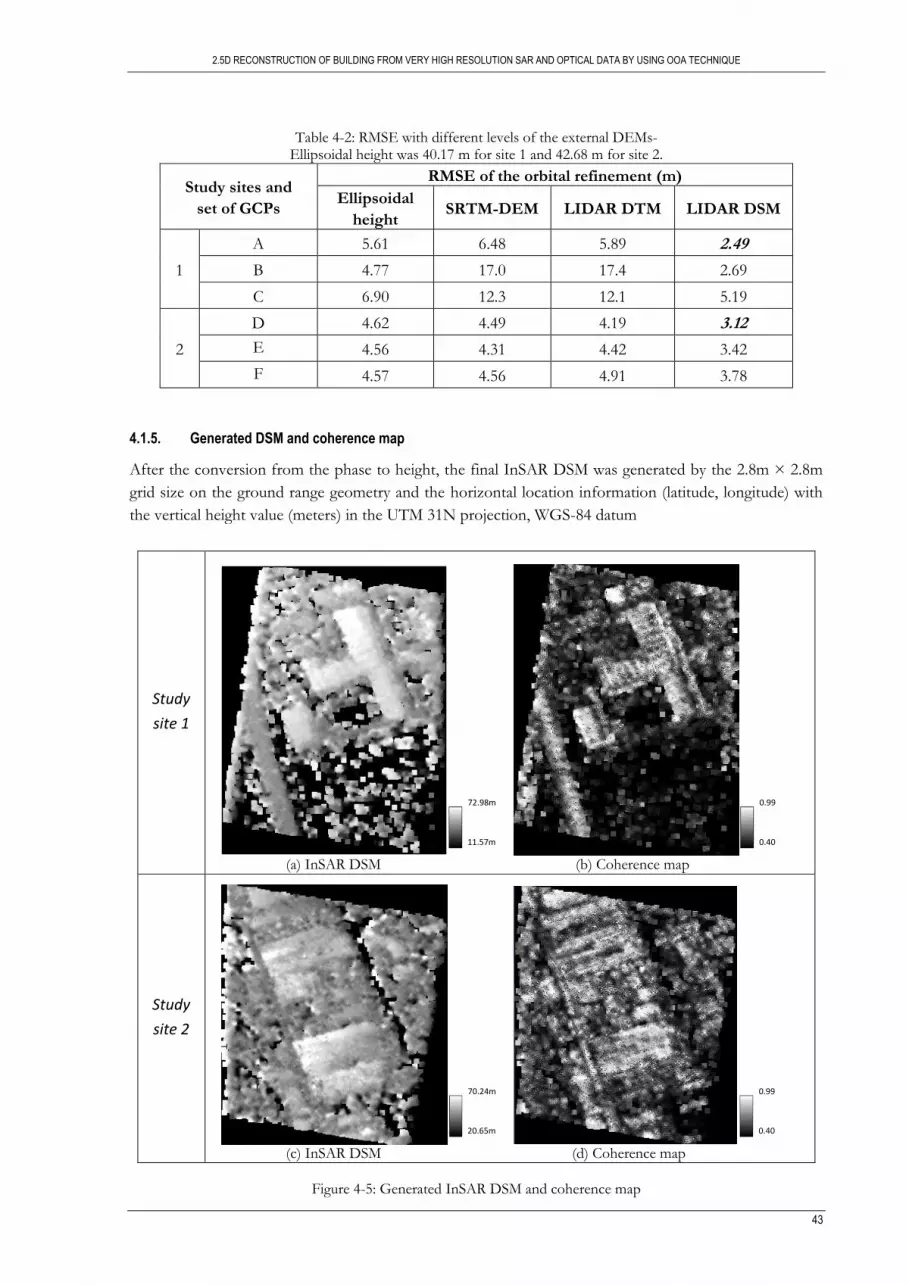
2.5D RECONSTRUCTION OF BUILDING FROM VERY HIGH RESOLUTION SAR AND OPTICAL DATA BY USING OOA TECHNIQUE
43
Table 4-2: RMSE with different levels of the external DEMs- Ellipsoidal height was 40.17 m for site 1 and 42.68 m for site 2.
Study sites and
set of GCPs
RMSE of the orbital refinement (m)
Ellipsoidal
height SRTM-DEM LIDAR DTM LIDAR DSM
1
A 5.61 6.48 5.89 2.49
B 4.77 17.0 17.4 2.69
C 6.90 12.3 12.1 5.19
2
D 4.62 4.49 4.19 3.12
E 4.56 4.31 4.42 3.42
F 4.57 4.56 4.91 3.78
4.1.5. Generated DSM and coherence map
After the conversion from the phase to height, the final InSAR DSM was generated by the 2.8m × 2.8m
grid size on the ground range geometry and the horizontal location information (latitude, longitude) with
the vertical height value (meters) in the UTM 31N projection, WGS-84 datum
Study
site 1
(a) InSAR DSM (b) Coherence map
Study
site 2
(c) InSAR DSM (d) Coherence map
Figure 4-5: Generated InSAR DSM and coherence map
0.99
0.40
70.24m
20.65m
0.99
0.40
72.98m
11.57m
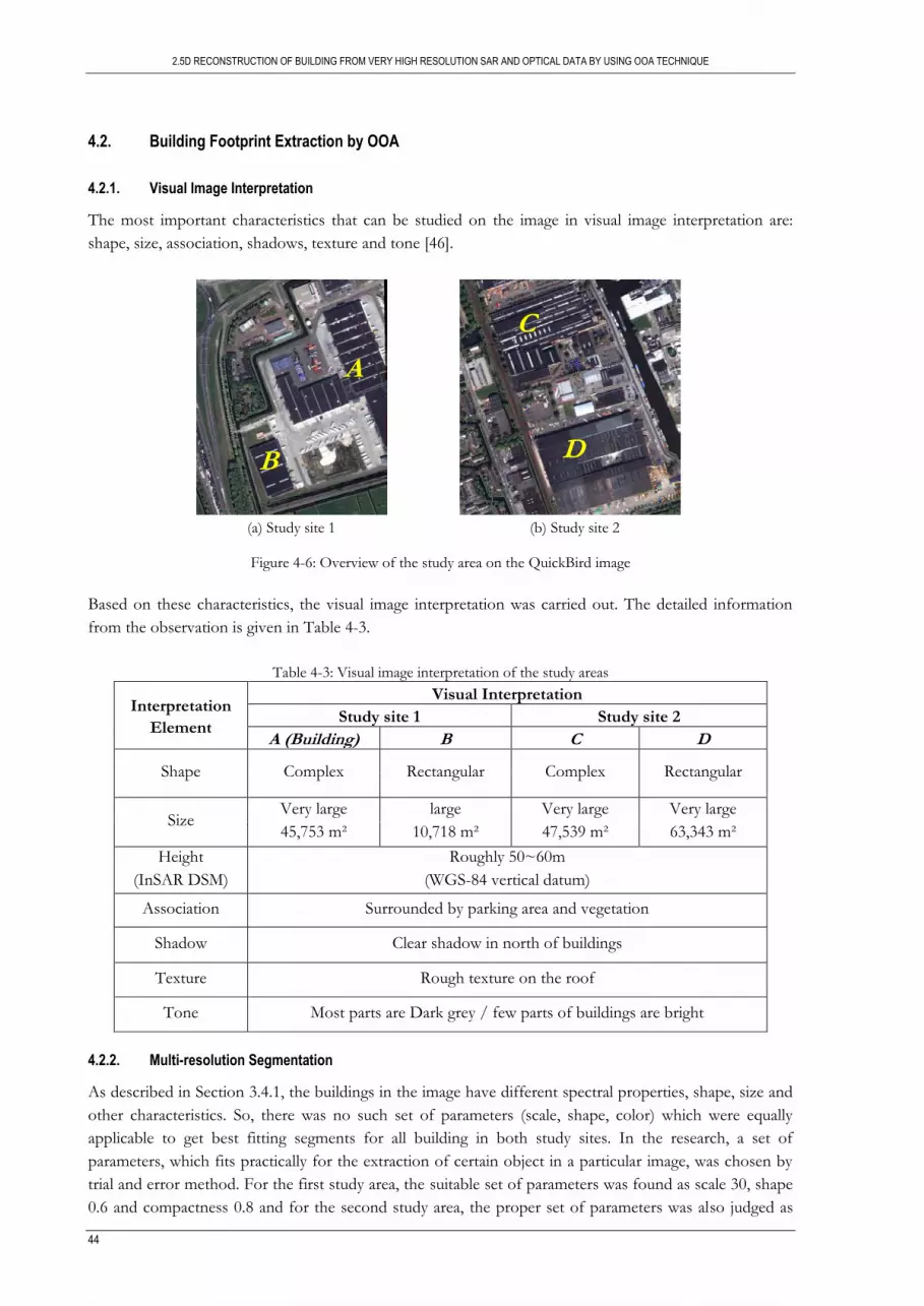
2.5D RECONSTRUCTION OF BUILDING FROM VERY HIGH RESOLUTION SAR AND OPTICAL DATA BY USING OOA TECHNIQUE
44
4.2. Building Footprint Extraction by OOA
4.2.1. Visual Image Interpretation
The most important characteristics that can be studied on the image in visual image interpretation are:
shape, size, association, shadows, texture and tone [46].
(a) Study site 1
(b) Study site 2
Figure 4-6: Overview of the study area on the QuickBird image
Based on these characteristics, the visual image interpretation was carried out. The detailed information
from the observation is given in Table 4-3.
Table 4-3: Visual image interpretation of the study areas
Interpretation
Element
Visual Interpretation
Study site 1 Study site 2
A (Building) B C D
Shape Complex Rectangular Complex Rectangular
Size Very large
45,753 m²
large
10,718 m²
Very large
47,539 m²
Very large
63,343 m²
Height
(InSAR DSM)
Roughly 50~60m
(WGS-84 vertical datum)
Association Surrounded by parking area and vegetation
Shadow Clear shadow in north of buildings
Texture Rough texture on the roof
Tone Most parts are Dark grey / few parts of buildings are bright
4.2.2. Multi-resolution Segmentation
As described in Section 3.4.1, the buildings in the image have different spectral properties, shape, size and
other characteristics. So, there was no such set of parameters (scale, shape, color) which were equally
applicable to get best fitting segments for all building in both study sites. In the research, a set of
parameters, which fits practically for the extraction of certain object in a particular image, was chosen by
trial and error method. For the first study area, the suitable set of parameters was found as scale 30, shape
0.6 and compactness 0.8 and for the second study area, the proper set of parameters was also judged as
A
B
C
D

2.5D RECONSTRUCTION OF BUILDING FROM VERY HIGH RESOLUTION SAR AND OPTICAL DATA BY USING OOA TECHNIQUE
45
scale 70, shape 0.5 and compactness 0.9. Since compact building boundaries are needed rather than fragile
or zigzag boundaries, high values of compactness were used.
(a) with scale, shape and compactness 30, 0.6, 0.7
study site 1
(b) with scale, shape and compactness 70, 0.5, 0.9
study site 2 Figure 4-7: Segments of the images
4.2.3. Rule-based Classification
1) Building Footprint extraction without InSAR DSM
After this step, the problem was occurred on the eastern edges of the buildings where there were not
enough contrast between the buildings and the surrounding areas to separate them. The colour of the
buildings was similar to the colour of the parking areas and the roads around the buildings. Shape couldn’t
discriminate the segments either. The clear context such as shadow areas was not there since the incidence
of the sun. Therefore, the building footprint was not extracted correctly as shown in Figure 4-8.
Figure 4-8: The extracted building footprint without the InSAR DSM (Red: Building class)

2.5D RECONSTRUCTION OF BUILDING FROM VERY HIGH RESOLUTION SAR AND OPTICAL DATA BY USING OOA TECHNIQUE
46
2) Building Footprint extraction with InSAR DSM
When the InSAR DSM was used as an external layer to help the classification of the image segments, most
of the building segments were classified as the buildings from the image objects, but due to the InSAR
DSM error, some parts of the buildings were unclassified as shown in the yellow circle and the some part
of the parking area was misclassified as a building as shown in the blue circle, Figure 4-9.
Figure 4-9: Application of the InSAR DSM (left image) in the building footprint extraction
In order to solve this problem, spatial properties of the object segments (compactness, rectangular fit, and
area) and contextual properties (relative border to building) were used to extract the correct building class
as described in Section 3.4.3.
Figure 4-10 shows that the improvement of the extracted building footprint (right image) using the InSAR
DSM is quite big comparing to the building footprint without the InSAR DSM (left image).
(a) Extracted building footprint without InSAR DSM
(b) Extracted building footprint with InSAR DSM
Figure 4-10: Comparison between the building extraction without/with InSAR DSM
Therefore, in the research the building extraction process by applying the InSAR DSM was better to
differentiate the taller objects from the ground objects in such areas where spectral, spatial and contextual
information cannot support completely the classification step.
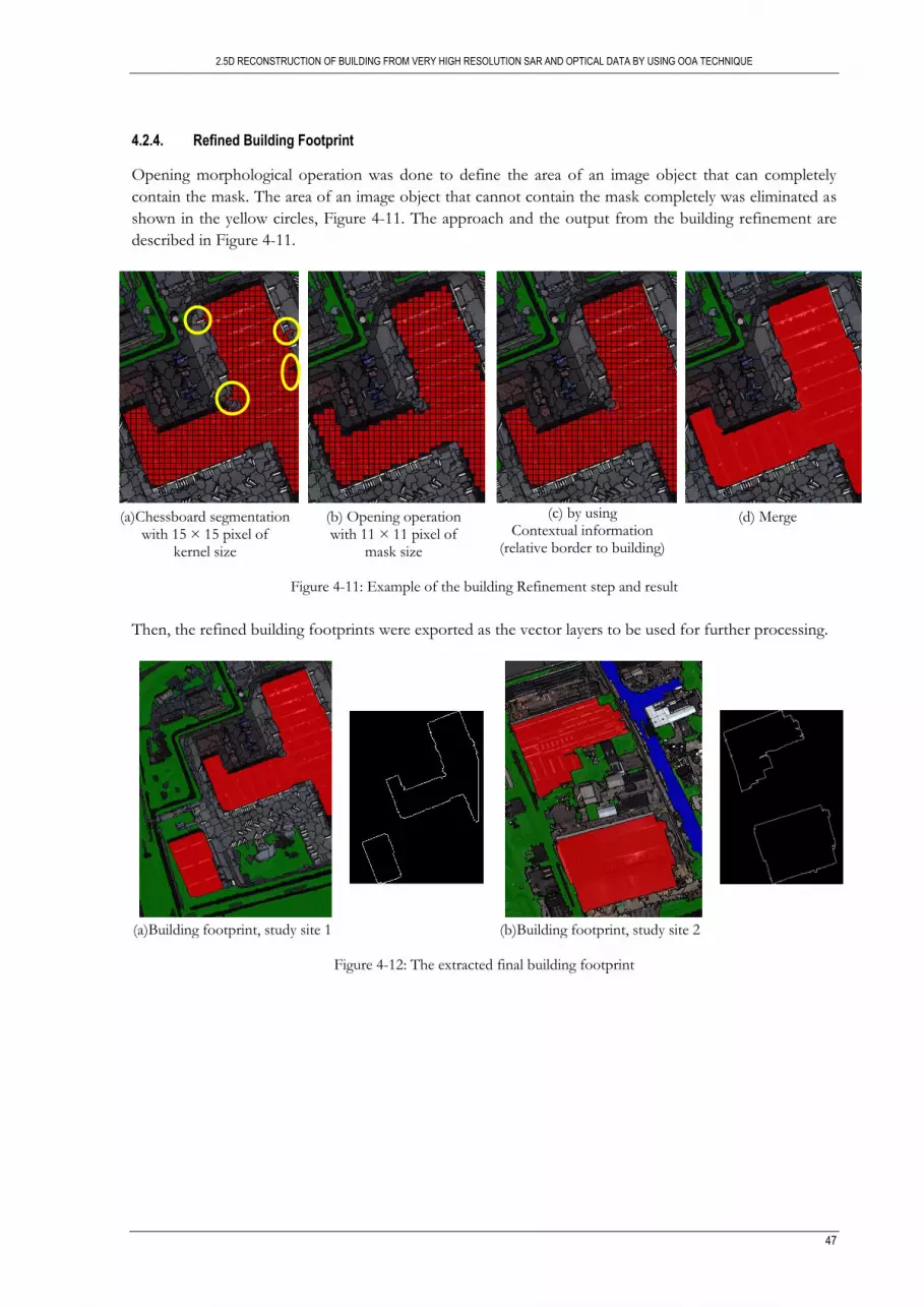
2.5D RECONSTRUCTION OF BUILDING FROM VERY HIGH RESOLUTION SAR AND OPTICAL DATA BY USING OOA TECHNIQUE
47
4.2.4. Refined Building Footprint
Opening morphological operation was done to define the area of an image object that can completely
contain the mask. The area of an image object that cannot contain the mask completely was eliminated as
shown in the yellow circles, Figure 4-11. The approach and the output from the building refinement are
described in Figure 4-11.
(a)Chessboard segmentation
with 15 × 15 pixel of kernel size
(b) Opening operation with 11 × 11 pixel of
mask size
(c) by using
Contextual information (relative border to building)
(d) Merge
Figure 4-11: Example of the building Refinement step and result
Then, the refined building footprints were exported as the vector layers to be used for further processing.
(a)Building footprint, study site 1
(b)Building footprint, study site 2
Figure 4-12: The extracted final building footprint
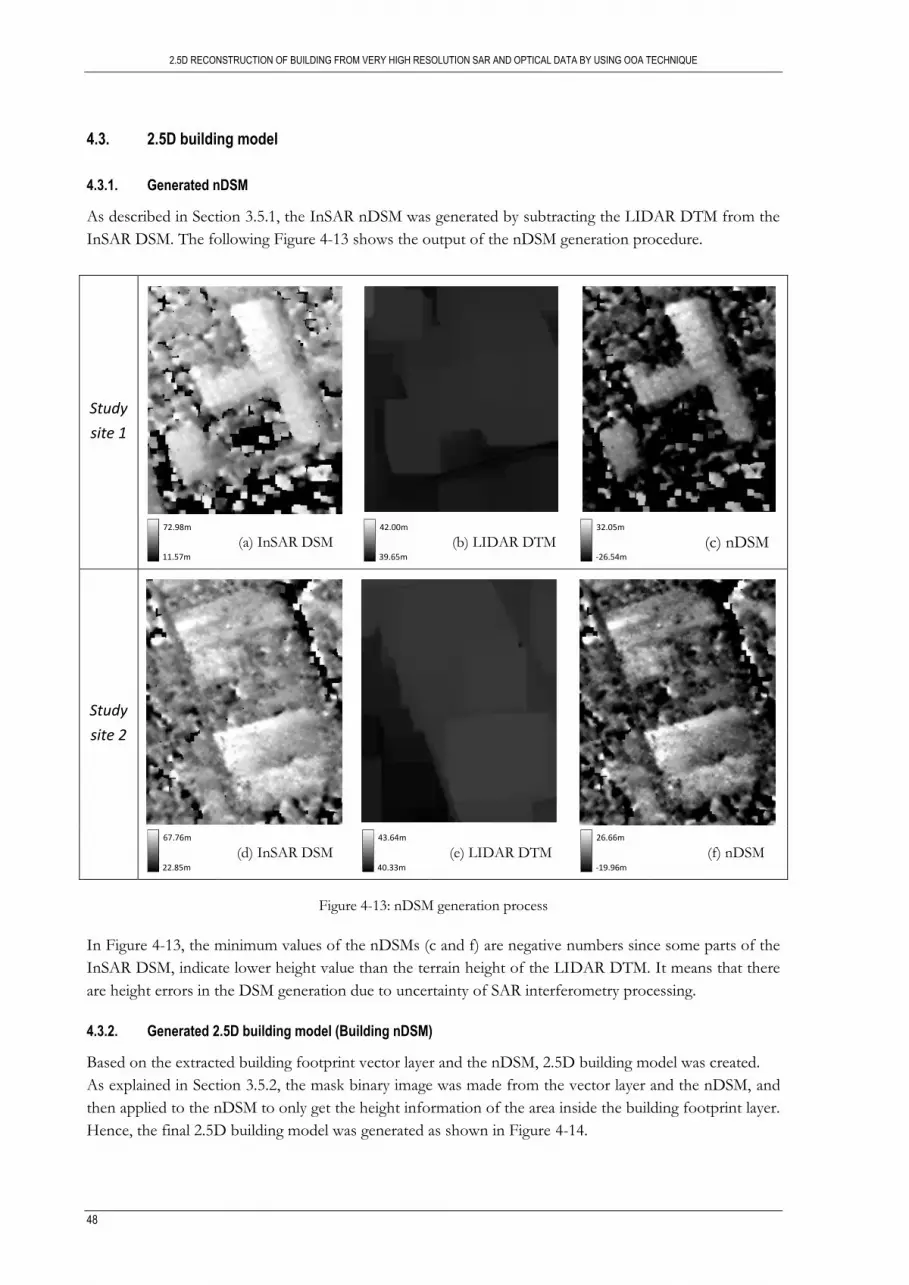
2.5D RECONSTRUCTION OF BUILDING FROM VERY HIGH RESOLUTION SAR AND OPTICAL DATA BY USING OOA TECHNIQUE
48
4.3. 2.5D building model
4.3.1. Generated nDSM
As described in Section 3.5.1, the InSAR nDSM was generated by subtracting the LIDAR DTM from the
InSAR DSM. The following Figure 4-13 shows the output of the nDSM generation procedure.
Study
site 1
(a) InSAR DSM
(b) LIDAR DTM
(c) nDSM
Study
site 2
(d) InSAR DSM
(e) LIDAR DTM
(f) nDSM
Figure 4-13: nDSM generation process
In Figure 4-13, the minimum values of the nDSMs (c and f) are negative numbers since some parts of the
InSAR DSM, indicate lower height value than the terrain height of the LIDAR DTM. It means that there
are height errors in the DSM generation due to uncertainty of SAR interferometry processing.
4.3.2. Generated 2.5D building model (Building nDSM)
Based on the extracted building footprint vector layer and the nDSM, 2.5D building model was created.
As explained in Section 3.5.2, the mask binary image was made from the vector layer and the nDSM, and
then applied to the nDSM to only get the height information of the area inside the building footprint layer.
Hence, the final 2.5D building model was generated as shown in Figure 4-14.
26.66m
-19.96m
43.64m
40.33m
67.76m
22.85m
32.05m
-26.54m
42.00m
39.65m
72.98m
11.57m
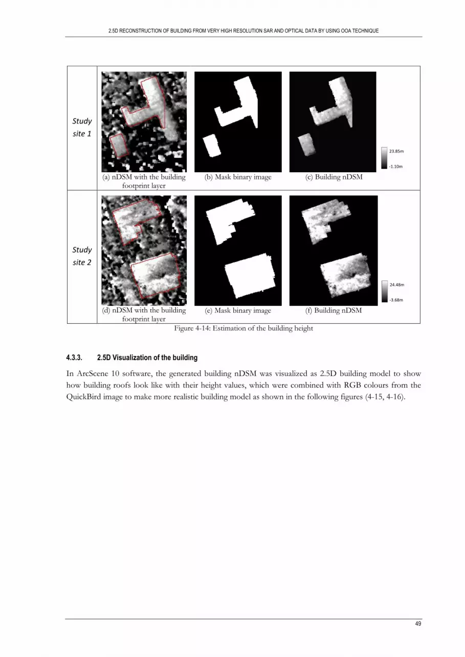
2.5D RECONSTRUCTION OF BUILDING FROM VERY HIGH RESOLUTION SAR AND OPTICAL DATA BY USING OOA TECHNIQUE
49
Study
site 1
(a) nDSM with the building
footprint layer
(b) Mask binary image
(c) Building nDSM
Study
site 2
(d) nDSM with the building
footprint layer
(e) Mask binary image
(f) Building nDSM
Figure 4-14: Estimation of the building height
4.3.3. 2.5D Visualization of the building
In ArcScene 10 software, the generated building nDSM was visualized as 2.5D building model to show
how building roofs look like with their height values, which were combined with RGB colours from the
QuickBird image to make more realistic building model as shown in the following figures (4-15, 4-16).
24.48m
-3.68m
23.85m
-1.10m

2.5D RECONSTRUCTION OF BUILDING FROM VERY HIGH RESOLUTION SAR AND OPTICAL DATA BY USING OOA TECHNIQUE
50
Figure 4-15: 2.5D building model with RGB colours from the QuickBird image and grey values, study site 1

2.5D RECONSTRUCTION OF BUILDING FROM VERY HIGH RESOLUTION SAR AND OPTICAL DATA BY USING OOA TECHNIQUE
51
Figure 4-16: 2.5D building model with RGB colours from the QuickBird image and grey values, study site 2
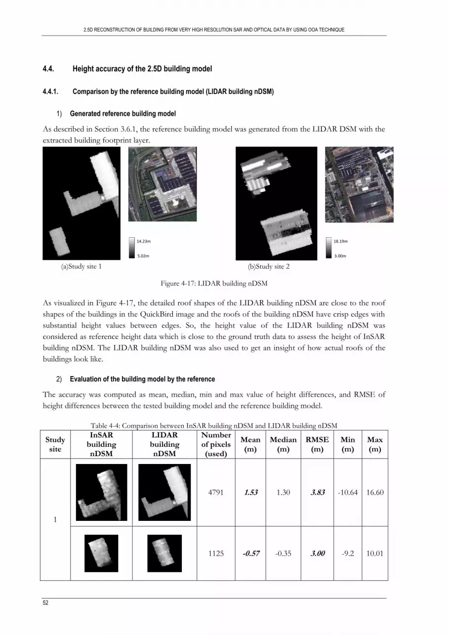
2.5D RECONSTRUCTION OF BUILDING FROM VERY HIGH RESOLUTION SAR AND OPTICAL DATA BY USING OOA TECHNIQUE
52
4.4. Height accuracy of the 2.5D building model
4.4.1. Comparison by the reference building model (LIDAR building nDSM)
1) Generated reference building model
As described in Section 3.6.1, the reference building model was generated from the LIDAR DSM with the
extracted building footprint layer.
(a)Study site 1
(b)Study site 2
Figure 4-17: LIDAR building nDSM
As visualized in Figure 4-17, the detailed roof shapes of the LIDAR building nDSM are close to the roof
shapes of the buildings in the QuickBird image and the roofs of the building nDSM have crisp edges with
substantial height values between edges. So, the height value of the LIDAR building nDSM was
considered as reference height data which is close to the ground truth data to assess the height of InSAR
building nDSM. The LIDAR building nDSM was also used to get an insight of how actual roofs of the
buildings look like.
2) Evaluation of the building model by the reference
The accuracy was computed as mean, median, min and max value of height differences, and RMSE of
height differences between the tested building model and the reference building model.
Table 4-4: Comparison between InSAR building nDSM and LIDAR building nDSM
Study site
InSAR building nDSM
LIDAR building nDSM
Number of pixels (used)
Mean (m)
Median(m)
RMSE(m)
Min (m)
Max (m)
1
4791 1.53 1.30 3.83 -10.64 16.60
1125 -0.57 -0.35 3.00 -9.2 10.01
18.19m
3.00m
14.23m
5.02m
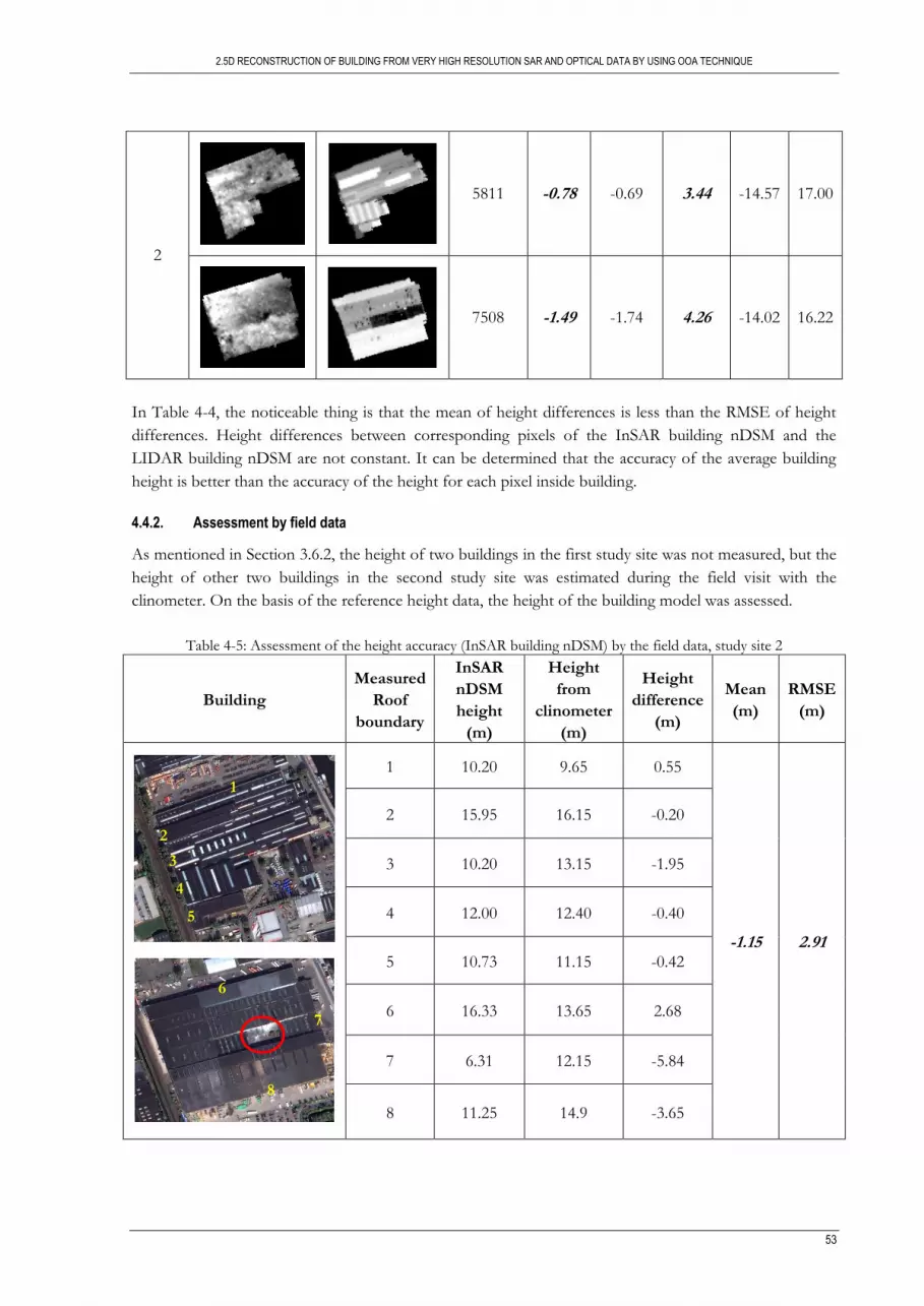
2.5D RECONSTRUCTION OF BUILDING FROM VERY HIGH RESOLUTION SAR AND OPTICAL DATA BY USING OOA TECHNIQUE
53
2
5811 -0.78 -0.69 3.44 -14.57 17.00
7508 -1.49 -1.74 4.26 -14.02 16.22
In Table 4-4, the noticeable thing is that the mean of height differences is less than the RMSE of height
differences. Height differences between corresponding pixels of the InSAR building nDSM and the
LIDAR building nDSM are not constant. It can be determined that the accuracy of the average building
height is better than the accuracy of the height for each pixel inside building.
4.4.2. Assessment by field data
As mentioned in Section 3.6.2, the height of two buildings in the first study site was not measured, but the
height of other two buildings in the second study site was estimated during the field visit with the
clinometer. On the basis of the reference height data, the height of the building model was assessed.
Table 4-5: Assessment of the height accuracy (InSAR building nDSM) by the field data, study site 2
Building
Measured
Roof
boundary
InSAR
nDSM
height
(m)
Height
from
clinometer
(m)
Height
difference
(m)
Mean
(m)
RMSE
(m)
1 10.20 9.65 0.55
-1.15 2.91
2 15.95 16.15 -0.20
3 10.20 13.15 -1.95
4 12.00 12.40 -0.40
5 10.73 11.15 -0.42
6 16.33 13.65 2.68
7 6.31 12.15 -5.84
8 11.25 14.9 -3.65
1
2
3
4
5
6
7
8

2.5D RECONSTRUCTION OF BUILDING FROM VERY HIGH RESOLUTION SAR AND OPTICAL DATA BY USING OOA TECHNIQUE
54
As shown in Table 4-5, for height measurement of the upper building, the heights of 5 parts (1~5) at
significant external roof boundaries were measured by the clinometer. Right part of the building was not
available to measure height since it was surrounded by a fence for security. So, only 5 height information
was used for evaluating the height of that building. And for height estimation of the lower building, the
heights of only 3 (6~8) parts at significant external roof boundaries were estimated.
From the assessment by the field data, the mean value of the height differences between the InSAR
building nDSM and the height data from the clinometer is also less than the RMSE of the height
differences. Especially, the height difference of the 7th part is noteworthy; the height value of the nDSM
on the 7th part is meaningfully small comparing to other measurements because the building has non-
building area (courtyard) inside the building, shown in the red circle, hence that area without height may
give error propagation during SAR interferometry processing.

2.5D RECONSTRUCTION OF BUILDING FROM VERY HIGH RESOLUTION SAR AND OPTICAL DATA BY USING OOA TECHNIQUE
55
5. DISCUSSION
In this chapter, factors, which can influence to quality of the reconstructed 2.5D building, are discussed
with respect to DSM generation by SAR interferometry processing and building footprint extraction by
OOA, separately. And alternative methods, which were recognized by this research, for 2.5D building
modelling, are explained. Then, the limitations of the developed method in this research and possible
solutions will be followed. Finally, the conclusion in relation to the research objective and questions are
discussed.
5.1. Factors influencing DSM generation by SAR interferometry processing
5.1.1. Choice of SAR data for DSM generation
The choice of suitable data sets for SAR interferometric processing has a substantial influence on the final
result. The data sets are affected by two types of decorrelation: the baseline decorrelation and the temporal
decorrelation.
The length of the baseline indicates the sensitivity to height change and the amount of baseline de-
correlation. As described in Section 3.3.1, terrain height measurement accuracy increases with baseline
since height measurement sensitivity increases with it, but the perpendicular baseline should be less than
the critical baseline to avoid the baseline de-correlation. In this research, the perpendicular baseline was
131.35m and the critical baseline was 6792.90m (Table 4-1). The perpendicular baseline is quite small
comparing to the critical baseline, so if the data is available with the baseline which is larger than 131.35m
and less than the critical baseline, it will give more sensitive interferogram output to respect to height
measurement accuracy. But, the optimal baseline of the TerraSAR-X HS mode data for InSAR DSM
generation in urban areas have not been documented well, so further study is needed to identify the
optimal baseline for InSAR DSM generation.
The temporal decorrelation was not considered as a factor which influenced the interferometry processing
in this research, because the difference in time between the two data acquisitions is only 11 days.
5.1.2. Methods used
Besides the analysis of the input data characteristics, the method used was investigated to see how it
influenced the final output from SAR interferometry processing.
1) Multi-looking
In SAR interferometry processing, multi-looking process is important since it decides square grid size of
the final output (InSAR DSM) and reduces the phase noise of the SAR images.
Without multi-looking
If the multi-looking is not done (same as 1:1), it means that no resampling was done, so gives the
smallest grid size of final output without any loss of original information of the SAR data. But, there
are two problems. One is about geometric distortion of the SAR images. Originally, the SAR SLC
image is stretched along the azimuth direction due to acquisition geometry, so it has 1.49m × 0.87m
grid size. These geometrically distorted images will give distorted InSAR DSM as well and also not be
matched with the external DEMs due to different geometry of grid.
Other problem is about the phase noise of the images. If multi-looking is done, it means that
resampling is also done to reduce the phase noise of the images, but without multi-looking, some
2.5D RECONSTRUCTION OF BUILDING FROM VERY HIGH RESOLUTION SAR AND OPTICAL DATA BY USING OOA TECHNIQUE
56
fringes of an interferogram will be totally lost which will cause errors in InSAR DEM due to strong
phase noise.
With multi-looking
In this research, 2:3 for number of looks was chosen to get 2.8 m × 2.8 m grid size of the InSAR
DSM. Depending user’s requirement for different applications, number of looks can be changed and
the change of number of looks gives different horizontal and vertical accuracy of final output due to
resampling. For building modelling, the smallest grid size for InSAR DSM is better to have more
detailed information from the SAR pair for better accuracy of the output, so this fact was considered
to choose the smallest number of looks 2:3.
2) Use of different levels of external DEMs
In this research, the use of different levels of external DEMs was investigated to see how they influence
the accuracy of the final output from SAR interferometry processing. The external DEMs were used for
reducing errors of phase unwrapping process and improving the precision of the registration between the
two SAR images.
Co-registration and phase unwrapping
From the external DEMs, the simulated topographic phase and object phase (in only case of using the
LIDAR DSM) were generated and they were subtracted from the interferometric phase to get the
remaining phase (flattened interferogram) which is easier for phase unwrapping. For that, the external
DEMs should be co-registered with the master SAR image on the basis of the SAR geometry. For the
co-registration between the external DEMs and the master SAR image, the GCPs are necessary.
Accurate GCPs between them gives precise co-registration, which influences accuracy of the final
output. In order to have good GCPs, it is preferable to have well distinguished relief of the
topography or objects on the external DEM. The LIDAR DSM is the most accurate DEM among the
external DEMs, so that it has more detailed surface information such as buildings. Distinguished
points on large buildings, which are well-detected in the LIDAR DSM and the SAR master image, can
be good GCPs. Therefore, the LIDAR DSM was most suitable for fine co-registration.
Also, for phase unwrapping, the LIDAR DSM was the most efficient to reduce the phase unwrapping
since it was used to make less remaining phase which is much easier to be unwrapped (Section 3.3.2,
Section 3.3.4).
Registration (orbital refinement)
The registration of interferometric geometry depends directly on the baseline precision [36]. It means
that insufficient precision on the baseline affects wrong registration, which gives errors obtained on a
DSM. Therefore, it is important to precisely refine the orbital information of the satellites in order to
know their position perfectly (Section 3.3.5).
The RMSE from the orbital refinement (Table 4-2) indicates the refined orbital accuracy of the
interferometry processing. The result of the RMSE showed that the use of the LIDAR DSM
improved the orbital accuracy of the interferometry processing, comparing to the use of other DEMs
or ellipsoidal height. It means that the LIDAR DSM was also used to improve the precision of the
registration between the two SAR images.
5.1.3. Geometric constraints
Due to the side-looking configuration of the SAR sensor, there are layover, shadowing and foreshortening
effect in dense urban area. So, the building footprints in SAR intensity images are mostly shifted from
actual locations or undetected in shadowing areas.

2.5D RECONSTRUCTION OF BUILDING FROM VERY HIGH RESOLUTION SAR AND OPTICAL DATA BY USING OOA TECHNIQUE
57
In order to have less influence by these constraints, the DSM generation was only focused on large
building areas without any neighbouring buildings in this research. And the extracted building footprints
from the QuickBird image could help the extraction of the building height with correct building footprint
from the InSAR DSM.
However, there were still challenges on the estimation of building height from the InSAR DSM. As shown
in Figure 4-14, the left upper part of the buildings are having more or less larger height values because the
SAR satellite acquired the data via descending orbit path with left side-looking configuration; the layover
effect occurred mainly on the left upper side of the buildings. Also, as shown in the second building image
in Table 4-5, there is a courtyard, which has no height, inside the building. This sudden height change on
the building can cause error propagation to the pixels which are located along the side-looking direction
during the interferometry processing. So, most of the right parts to the courtyard have smaller height
values than the actual values. Therefore, these geometric constraints are mainly recognized as one of the
most difficult problems during DSM generation by SAR interferometry.
5.2. Factors influencing the building footprint extraction by OOA
5.2.1. Parameters for multi-resolution segmentation
Multi-resolution segmentation was applied to the image in eCognition Developer 8 software. The
parameters (scale, shape, compactness) for segmentation were chosen by trial and error, they were found
carefully to have suitable size and shape of segments for classification. But, the parameters, which were
already used for one image, could not be applied again to other images since there are different fitting
parameters, chosen by trial and error, for different applications.
5.2.2. Feature properties used in rule-based classification for OOA
Several feature properties of the segmented image objects were analysed to identify the most applicable
ones for extracting building successfully. As mentioned in Section 3.4.3, classification of vegetation, water
and shadow was straightforward since their spectral characteristics were different from other objects,
hence feature properties like NDVI, NDWI and SSI can be used to extract them.
But, the main challenge was to separate buildings from road, bare objects, parking areas, etc. Spectral
characteristics were not sufficient because of the spectral variability of building object and spectral
similarity between building objects and neighbouring objects like parking area. Spatial properties, such as
shape and size of image objects, were also not consistent. Some of building objects were rectangular shape,
but others were not. All building segments did not follow the spatial feature properties like rectangular fit,
asymmetry and area, etc. And, contextual information like relative border to buildings supported in some
extent to classify building segments from other objects but was not completely worked out because there
were some other image objects which also have the similar contextual characteristics. In such cases, the
spectral, spatial and contextual information were not sufficient to extract the building footprint accurately.
Building extraction with the InSAR DSM
As explained above, only spectral, spatial and contextual information were not always sufficient to
detect the accurate building footprint.
In this research, the height information from the InSAR DSM provided extra support to extract
building since taller height is the common property in all buildings. In comparison with buildings, the
ground objects such as road, grass and parking areas have less height. Other taller object like tree was
easily separated by using NDVI feature property. Therefore, by using height information from the
InSAR DSM as an extra layer to apply a certain height threshold along with other feature properties,
2.5D RECONSTRUCTION OF BUILDING FROM VERY HIGH RESOLUTION SAR AND OPTICAL DATA BY USING OOA TECHNIQUE
58
the image segments of ground object were separated from building segments, and then only buildings
were extracted successfully.
5.3. Alternative methods for building modelling
5.3.1. Building modelling from SAR interferometry without optical image
If the QuickBird (optical) image is not available for extracting building footprint, only SAR data can be
used not only to estimate height information, but also to get rough building footprint by using SAR
interferometry processing.
After phase to height conversion (Section 4.1.5) was done, the geo-coded coherence map was generated
from the SAR pair. As shown in Figure 4-5, the building areas are highly correlated whereas other areas,
such as vegetated areas, water body or neighbouring area between buildings, have lower coherence value
than building areas. This observation means that building footprint can be extracted from the geo-coded
coherence map by applying different characteristics of coherence values between building areas and non-
building areas. So, the building footprint from the coherence map also can be used for 2.5D building
modelling.
5.3.2. SAR interferometry processing without LIDAR DSM
As explained in Section 5.1.2, the advantages of using the LIDAR DSM among different external DEMs
are on the finer co-registration and the easier phase unwrapping, and then they helped the SAR pair to
register more accurately by precise refinement of the orbital information of the satellites. Therefore, if
more accurate external DEM is used, more accurate InSAR DSM will be generated.
In reality, it is hard to find free-available accurate DSM like the LIDAR DSM or purchase it due to high
price. And it can be weird because if an accurate DSM is available, there is no need to generate a coarser
DSM like InSAR DSM from it. But, this research was done to investigate how different levels of external
DEMs influence the accuracy of SAR interferometry processing and to achieve more accurate InSAR
DSM as possible.
Usually, SRTM or ellipsoidal height information has been used without any difficulties to get them instead
of very accurate DSM such as the LIDAR DSM. For other purposes of SAR interferometry processing
such as a DTM generation or deformation mapping instead of 2.5D building reconstruction from accurate
InSAR DSM, SRTM or ellipsoidal height information can be used because the RMSE is not much
different between the cases of using the LIDAR DSM and using SRTM or ellipsoidal height information
as shown in Table 4-2. Therefore, if the RMSE from the case of using SRTM or ellipsoidal height
information is acceptable for user’s requirements, the use of SRTM or ellipsoidal height information can
be suitable.
5.4. Limitations and possible solutions
5.4.1. Generation of DSM in urban area by SAR interferometry processing
As explained in Section 5.1, there is uncertainty in height estimation by SAR interferometry processing
due to error propagation from data characteristics, adopted methods and geometric constraints, etc.
1) Error from geometric constraints
Especially in urban areas, the geometric constraints (layover, shadowing and foreshortening effect)
become more serious because of steep change in surface relief of tall buildings or any tall man-made

2.5D RECONSTRUCTION OF BUILDING FROM VERY HIGH RESOLUTION SAR AND OPTICAL DATA BY USING OOA TECHNIQUE
59
structures. It can gives various errors, e.g. shift of building location, change of building size, exclusion of
building (occlusions) and wrong height estimation, etc. and the errors is being propagated while SAR
interferometry processing. Therefore, common SAR interferometry processing with SAR data may be not
most suitable approach for DSM generation in dense urban areas.
Recently, InSAR techniques have been studied to solve the geometric constraints in dense urban area. For
example, Thiele in [6] proposed a method for building reconstruction from multi-aspect InSAR Data.
With multi-aspect InSAR data, occlusions, which occur in single aspect data, can be compensated with
information from another aspect. So, 2.5D building can be modelled without help of optical image.
2) Phase unwrapping
As explained in Section 3.3.4, phase unwrapping is particularly difficult if there are large areas of low
coherence and large local topographic height variations. In this research, high resolution TerraSAR-X data
in urban area (Delft city) with many tall buildings was used.
Tall buildings with adjacent lower flat areas give large height difference between them, which will cause
phase unwrapping errors. Also, tall buildings produce layover, shadowing effects in the neighbouring areas
like parking areas or other close buildings, and then the effects give low coherence values (cause
decorrelation) in the interferogram of those neighbouring areas. The decorrelation is the main challenge
for phase unwrapping process since it gives large unwrapping error (2π-jumps).
For this particular case in the research, low coherent areas were not considered to be processed in the
phase unwrapping process by applying the coherence threshold (0.4) and the interferogram was flattened
by subtracting simulated buildings phase of the LIDAR DSM from the interferogram, so the phase
variations in the interferogram became very small to make easier phase unwrapping. Due to the use of the
LIDAR DSM during SAR interferometry, phase unwrapping process could reduce its error. In the other
hand, the phase unwrapping process without high resolution external DSM like the LIDAR DSM in such
kind of urban areas will be very difficult because of large phase variation between close pixels.
As mentioned in Section 5.3.2, fine resolution DSM is not commonly used to generate coarser resolution
DSM from it, but in this research coarser InSAR DSM generation with the finer LIDAR DSM was
experimented to see how the LIDAR DSM influence the accuracy of the interferogram output in terms of
phase unwrapping and registration. But, if high resolution external DSM is not available for InSAR DSM
generation in urban areas, finding alternatives can be a challenge.
3) Bias of the vertical accuracy assessment
In this research, the LIDAR DSM was mainly used to improve the accuracy of SAR interferometry
processing to achieve more accurate InSAR DSM. Even if the height values of the InSAR DSM were not
replaced by the corresponding height values of the LIDAR DSM during the processing, the height values
of the LIDAR DSM were used in the processing to improve the accuracy of the processing. Therefore,
the vertical accuracy evaluation of the InSAR nDSM with respect to the LIDAR nDSM is not most
appropriate approach. For avoiding this bias in the assessment, the other reference height data was also
acquired during the field visit; however the number of reference heights was not enough to assess the
heights of the InSAR nDSM as described in Section 3.6.2.
5.4.2. Building footprint extraction by OOA
The rule sets created for extraction of building footprint in the study sites were not tested for the other
areas of the Delft city, so they may be only suitable for the study sites. If study site is changed to other
area, new rule set should be created for considering feature properties of objects in the area.

2.5D RECONSTRUCTION OF BUILDING FROM VERY HIGH RESOLUTION SAR AND OPTICAL DATA BY USING OOA TECHNIQUE
60
In order to solve this challenge, a rule set can be created by an ontological approach for building
extraction everywhere. But, due to complexity of urban areas, it is impossible to have perfect rule set to
classify building everywhere.
5.5. Discussion in relation to the objective and research questions
The main objective of this research is to develop a method for reconstruction of 2.5D building model
from VHR SAR and VHR optical image using OOA technique. To achieve the main objective, three sub-
objectives were considered. These sub-objectives are related to get accurate building height information
from SAR interferometry, to improve the method of the building footprint extraction from the QuickBird
image by OOA, with help of the height information (DSM) from SAR interferometry and to combine the
extracted building footprint with the building height from InSAR DSM for 2.5D building model.
The research questions were proposed to obtain these objectives. The first two questions are about the
method of building height estimation by SAR interferometry and assessment of the estimated building
height. For building height estimation in this research, SAR interferometry processing was done to
generated the DSM. In addition to the proposed question, different levels of the external DEMs were
investigated during SAR interferometry processing to see how they influence to the final output and to
find which DEM is suitable for this 2.5D building reconstruction application. For vertical accuracy of the
estimated building height, the comparison with LIDAR DSM and field visit with the clinometer were
done. The overall vertical accuracy was approximately 1m mean height difference and approximately
3~4m RMSE. It was not accurate enough for 2.5D building modelling according to the user’s requirement
since centimeters vertical accuracy of the building height estimated by the proposed method was expected
before the start of the research. As explained in Section 5.4.1, there was uncertainty so that the expected
vertical accuracy was not achieved. However, if the average height of building is considered, the vertical
accuracy is improved up to 1m difference as described Section 4.4.1. So, in case of the application which
needs rough or average building height information, the adopted method in this research can be useful for
such kind of case.
And the next main research question is about the extraction of building footprint using OOA. The results
show that the building footprint was extracted successfully by using several feature properties with help of
the InSAR DSM. The final question is about how 2.5D building model is reconstructed with the estimated
building height and the detected building footprint. With the building footprint and height, the building
was modelled as 2.5D easily.
2.5D RECONSTRUCTION OF BUILDING FROM VERY HIGH RESOLUTION SAR AND OPTICAL DATA BY USING OOA TECHNIQUE
61
6. CONCLUSION AND RECOMMENDATION
This chapter deals with the conclusion of this research and recommendation for future study. The first
section concludes the main results of the research and the following section recommends some issues for
future study.
6.1. Conclusion
Based on the results and the discussion, the main conclusion of this research is drawn as follows:
For the estimation of building height, the TerraSAR-X high resolution spotlight (HS) mode
images were used, the HS mode is suitable for generating fine resolution DSM in comparison with
other modes, e.g. stripmap mode, scanSAR mode.
After the baseline estimation, the 2π ambiguity height, which is inversely proportional to the
perpendicular baseline length, was 45.94m. In generation of InSAR DSM, the sensitivity to height
change in a fringe determines the quality of height measurement. If SAR pair was available with
the larger perpendicular baseline than 131.35m which was from the data used in this research, the
sensitivity of height measurement would be better to achieve more accurate InSAR DSM.
During SAR interferometry processing for DSM generation, different levels of external height
information from the SRTM, the LIDAR DTM and the LIDAR DSM were used to improve the
overall accuracy of InSAR processing, to investigate how they influence the accuracy, and to find
the most suitable external height information for the research. From the result, the LIDAR DSM
is the most suitable among those external DEM since it gave finer co-registration with better
GCPs, easier phase unwrapping with less unwrapping error and more precise orbital refinement
with less RMSE. Therefore, it can be determined that if more accurate DEM is used as an
external DEM for SAR interferometry processing , more accurate InSAR DSM will be generated.
Due to spectral complexity in urban areas, it is impossible to exactly classify objects with spectral
characteristics. In OOA, various feature properties like spectral, spatial and contextual
information were used to separate object classes, but in complex urban environment, the use of
these feature properties only, cannot give accurate building extraction. In such cases, the InSAR
DSM can be used to help building extraction by applying certain height threshold.
Because of uncertainty in the InSAR DSM, it was difficult to detect building footprint in the DSM
image. But, the extracted building footprint from the QuickBird image made it possible to extract
the height information of the buildings from the InSAR DSM. So, the InSAR DSM and the
building footprint from the QuickBird image were complementary to help each other to get finer
result.
From the height accuracy assessment, the vertical accuracy of the final output was defined. When
the vertical accuracy is acceptable to user’s requirement in some applications, the method
developed in the research can be proper approach for that.

2.5D RECONSTRUCTION OF BUILDING FROM VERY HIGH RESOLUTION SAR AND OPTICAL DATA BY USING OOA TECHNIQUE
62
In conclusion, building height from SAR interferometry can improve building footprint extraction from
optical images and can be combined with the extracted footprints to generate a 2.5D building model.
6.2. Recommendation
The following recommendations are made for future study:
SAR pair data with larger perpendicular baseline length than the baseline length used in this
research can give more suitable interferogram output with more sensitivity to height measurement
for DSM generation.
The geometric constraints such as layover, shadowing and foreshortening effect are the main
challenge to get accurate DSM of urban area in SAR interferometry processing. In this research,
the optical image was helping to extract building height from the InSAR nDSM, but there was no
way to reduce height error from the geometric constraints in the InSAR DSM. For solving this
limitation, recently developed method with multi-aspect InSAR data can be used. Then,
generation of DSM in dense urban area with small buildings may be possible.
In OOA, the rule set generated for the extraction of building footprint can be validated in other
areas and then improved to be applied also for other areas.
2.5D RECONSTRUCTION OF BUILDING FROM VERY HIGH RESOLUTION SAR AND OPTICAL DATA BY USING OOA TECHNIQUE
63
REFERENCES
[1] U. Stilla, U. Soergel, and U. Thoennessen, "Potential and limits of InSAR data for building reconstruction in built-up areas," ISPRS Journal of Photogrammetry and Remote Sensing, vol. 58, pp. 113-123, 2003.
[2] D. Brunner, G. Lemoine, and L. Bruzzone, "Height estimation of man made structures using hybrid VHR optical and SAR imagery," in Proc. EARSeL Joint Workshop, Remote Sensing - New challenges of High Resolution, Carsten Juergens,Ed., pp. 186 - 193, 2008.
[3] J. D. Wegner and U. Soergel, "Building extraction in urban scenes from high resolution InSAR data and optical imagery," presented at the 2009 Urban Remote Sensing Joint Event, 2009.
[4] G. Schreier, "Geometrical properties of SAR images," In : Schreier G. (ed) SAR geocoding : data and systems. Wichmann, Karlsruhe, pp. 103 - 134, 1993.
[5] F. Tupin, "Merging of SAR and optical features for 3D reconstruction in a radargrammetric framework," in Geoscience and Remote Sensing Symposium, 2004. IGARSS '04. Proceedings. 2004 IEEE International, 2004.
[6] A. Thiele, J. Wegner, and U. Soergel, "Building Reconstruction from Multi-aspect InSAR Data," Radar Remote Sensing of Urban Areas, vol. 15, pp. 187 - 214, 2010.
[7] F. Tupin, "Fusion of Optical and SAR images: Joint Use of SAR Interferometry and Optical Data for 3D Reconstruction," Radar Remote Sensing of Urban Areas, vol. 15, pp. 151 - 159, 2010.
[8] H. Sportouche, F. Tupin, and L. Denise, "Building extraction and 3D reconstruction in urban areas from high-resolution optical and SAR imagery," in 2009 Urban Remote Sensing Joint Event, 2009, pp. 1-11.
[9] I. Sebari and H. Dong Chen, "New object-oriented approach for urban objects extraction from VHSR images," in Geoscience and Remote Sensing Symposium, 2007. IGARSS 2007. IEEE International, 2007, pp. 4814-4817.
[10] O. D. Mavrantza and D. P. Argialas, "Identification of urban features using Object-Oriented Image Analysis," presented at the PIA07 - Photogrammetric Image Analysis, Munich, Germany, 2007.
[11] J. R. Joshi, "Improving the quality of digital surface model generated from very high resolution satellite stereo imagery by using object oriented image analysis technique," M.Sc.thesis, Geoinformatics, ITC, University of Twente, Enschede, 2010.
[12] D. F. Maune, Digital elevation model technologies and applications : the DEM users manual, Second edition ed. Bethesda: American Society for Photogrammetry and Remote Sensing (ASPRS), 2007.
[13] T. Krauß, M. Lehner, and P. Reinartz, "Generation of coarse 3D models of urban areas from high resolution stereo satellite images," presented at the ISPRS Congress, Beijing, China, 2008.
[14] A. Roth, J. Hoffmann, and T. Esch, "TerraSAR-X: How can high resolution SAR data support the observation of urban areas?," 2005.
[15] M. Eineder, N. Adam, R. Bamler, N. Yague-Martinez, and H. Breit, "Spaceborne Spotlight SAR Interferometry With TerraSAR-X," Geoscience and Remote Sensing, IEEE Transactions on, vol. 47, pp. 1524-1535, 2009.

2.5D RECONSTRUCTION OF BUILDING FROM VERY HIGH RESOLUTION SAR AND OPTICAL DATA BY USING OOA TECHNIQUE
64
[16] R. Bamler and P. Hartl, "Synthetic aperture radar interferometry," Inverse problems, vol. 14, p. R1, 1998.
[17] G. Huurneman, "SAR Interferometry," ed. Enschede, the Netherlands: Faculty of ITC, Earth Observation Science department, University of Twente, 2004.
[18] U. Soergel, K. Schulz, and U. Thoennessen, "Building reconstruction from interferometric SAR data: potential and limits," presented at the earsel, 2005.
[19] E. P. Baltsavias, A. Gruen, and L. Van Gool, Automatic extraction of man-made objects from aerial and space images (III): Taylor & Francis, 2001.
[20] U. C. Benz, P. Hofmann, G. Willhauck, I. Lingenfelder, and M. Heynen, "Multi-resolution, object-oriented fuzzy analysis of remote sensing data for GIS-ready information," ISPRS Journal of Photogrammetry and Remote Sensing, vol. 58, pp. 239-258, 2004.
[21] Y. Liu, M. Li, L. Mao, F. Xu, and S. Huang, "Review of remotely sensed imagery classification patterns based on object-oriented image analysis," Chinese Geographical Science, vol. 16, pp. 282-288, 2006.
[22] T. Blaschke and J. Strobl, "What’s wrong with pixels? Some recent developments interfacing remote sensing and GIS," GeoBIT/GIS 6/01, pp. 12-17, 2001.
[23] T. Blaschke, "Object based image analysis for remote sensing," ISPRS Journal of Photogrammetry and Remote Sensing, vol. 65, pp. 2-16, 2010.
[24] Y. Chen, W. Su, J. Li, and Z. Sun, "Hierarchical object oriented classification using very high resolution imagery and LIDAR data over urban areas," Advances in Space Research, vol. 43, pp. 1101-1110, 2009.
[25] DLR, "TerraSAR-X Ground Segment Basic Product Specification Document," ed: T.Fritz, M.Eineder, 2009.
[26] DigitalGlobe, "QuickBird Imagery Products; Product Guide," ed. Longmont, Colorado 80503, 2006.
[27] H. Waterschapshuis, "Kwaliteitsdocument AHN-2 (Quality Document)," ed: N. van der Zon, 2010.
[28] CGIAR-CSI. (2004, February 1, 2011). SRTM 90m Digital Elevation Data. Available: http://srtm.csi.cgiar.org/
[29] MicroImages, "Wallis Filter: Locally Adaptive Contrast Enhancement," ed. Lincoln NE, USA, 2010.
[30] U. Weidner and W. Förstner, "Towards automatic building extraction from high-resolution digital elevation models," ISPRS Journal of Photogrammetry and Remote Sensing, vol. 50, pp. 38-49, 1995.
[31] J. Schiewe, "Integration of multi-sensor data for landscape modeling using a region-based approach," ISPRS Journal of Photogrammetry and Remote Sensing, vol. 57, pp. 371-379, 2003.
[32] T. Krauß and P. Reinartz, "Refinement of urban digital elevation models from very high resolution stereo satellite images," 2009, pp. 02-05.
[33] ESA, "InSAR Principles: Guidelines for SAR Interferometry Processing and Interpretation," ed. ESA Publications, ESTEC, Postbus 299, 2200 AG Noordwijk, The Netherlands: Karen Fletcher, 2007.

2.5D RECONSTRUCTION OF BUILDING FROM VERY HIGH RESOLUTION SAR AND OPTICAL DATA BY USING OOA TECHNIQUE
65
[34] H. Xu, Y. Zhou, and C. Li, "Analysis and simulation of spaceborne SAR interferometric baseline," in Radar, 2001 CIE International Conference on, Proceedings, 2001, pp. 639-643.
[35] D. Small, Generation of digital elevation models through spaceborne SAR interferometry. Zurich: University of Zurich, Department of Geography, 1998.
[36] O. Sahraoui, B. Hassaine, and C. Serief, "Radar Interferometry with Sarscape Software," Photogrammetry and Remote Sensing, 2006.
[37] Y. Huang and J. Van Genderen, "Comparison of Several Multi-Look Processing Procedures in Insar Processing for ERS-1&2 Tandem Mode," 1997, p. 215.
[38] A. Moreira, "Improved multilook techniques applied to SAR and SCANSAR imagery," Geoscience and Remote Sensing, IEEE Transactions on, vol. 29, pp. 529-534, 2002.
[39] H. A. Zebker and J. Villasenor, "Decorrelation in interferometric radar echoes," Geoscience and Remote Sensing, IEEE Transactions on, vol. 30, pp. 950-959, 2002.
[40] J. Yu and L. Ge, "Digital Elevation Model generation using ascending and descending multi-baseline ALOS/PALSAR radar images," presented at the FIG Congress 2010, Sydney, Australia, 2010.
[41] S. R. Cloude and K. P. Papathanassiou, "Polarimetric SAR interferometry," IEEE Transactions on geoscience and remote sensing, vol. 36, pp. 1551-1565, 1998.
[42] X. Wei and I. Cumming, "A region-growing algorithm for InSAR phase unwrapping," Geoscience and Remote Sensing, IEEE Transactions on, vol. 37, pp. 124-134, 1999.
[43] Z. Chunxia, G. Linlin, E. Dongchen, and C. Hsingchung, "A case study of using external DEM in InSAR DEM generation," Geo-Spatial Information Science, vol. 8, pp. 14-18, 2005.
[44] L. P. Singh, "Application of SAR interferometry in landslide studies with special reference to generation of input data for statistical susceptibility assessment," MSc thesis, ITC, University of Twente, Enschede, 2003.
[45] SARMAP, "Synthetic Aperture Radar and SARscape (SAR-Guidbook)," ed, August, 2009.
[46] M. Lazaridou and E. Patmios, "Optical data processing. Visual image interpretation," presented at the ISPRS 2007, Stuttgart, Germany, 2007.
[47] J. Tian and D.-M. Chen, "Optimization in multi-scale segmentation of high-resolution satellite images for artificial feature recognition," International Journal of Remote Sensing, vol. 28, pp. 4625 - 4644, 2007.
[48] DEFINIENS, "eCognition Developer 8 Reference Book," ed. Trappentreustr. 1, D-80339 München, Germany, 2009.
[49] S. McFeeters, "The use of the Normalized Difference Water Index (NDWI) in the delineation of open water features," International Journal of Remote Sensing, vol. 17, pp. 1425-1432, 1996.
[50] S. Elberink and H. Maas, "The use of anisotropic height texture measures for the segmentation of airborne laser scanner data," International archives of photogrammetry and remote sensing, vol. 33, pp. 678-684, 2000.

2.5D RECONSTRUCTION OF BUILDING FROM VERY HIGH RESOLUTION SAR AND OPTICAL DATA BY USING OOA TECHNIQUE
66
APPENDIX I: SAR INTERFEROMETRY PROCESSING WITH SARSCAPE
The processing steps in SAR interferometry depend on the software being used. For this research, the
SARscape software (in ENVI 4.7) developed by SARMAP (http://www.sarmap.ch), a Swiss company,
was used. In each processing step, the outputs are generated on the basis of the specific format of the
software.
a) Data import
Since the original data format of TerraSAR-X-1 is not readable in the software, the first step is to covert
the original data format into the standard format of the software.
For TerraSAR-X-1, there are four kinds of data type:
- HS: Spotlight High Resolution (Slant Range, Ground Range or Geo-coded) Single and Dual
Polarization
- SC: ScanSAR Geo-coded Single Polarization (not available as slant range product)
- SL: Spotlight (Slant Range, Ground Range or Geo-coded) Single and Dual Polarization
- SM: Stripmap (Slant Range, Ground Range or Geo-coded) Single and Dual Polarization
For the research, the TerraSAR-X data on HS mode with single polarization (VV) was used.
Figure I-1: Data import
b) Baseline estimation
This function enables to obtain information about the baseline values and other orbital parameters related
to the input pair.
Following output parameters are provided in Figure I-2:
- Normal baseline: Perpendicular baseline (m) between master and slave orbit
- Critical baseline: Maximum theoretical baseline (m) suitable for Interferometric processing
- 2π ambiguity height: Height difference corresponding to an Interferometric fringe (2π cycle)
- Range shift (pixel), which will be applied in range direction during the master-slave coarse co-
registration
- Azimuth shift (pixel), which will be applied in azimuth direction during the master-slave coarse
co-registration
- Doppler Centroid difference: Difference (Hz) between master and slave Doppler Centroid
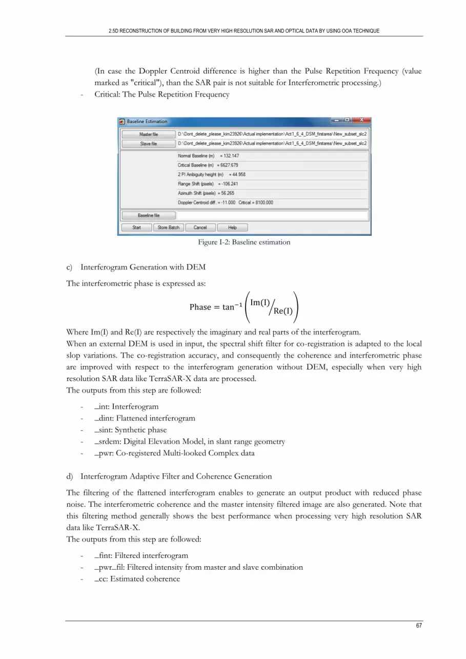
2.5D RECONSTRUCTION OF BUILDING FROM VERY HIGH RESOLUTION SAR AND OPTICAL DATA BY USING OOA TECHNIQUE
67
(In case the Doppler Centroid difference is higher than the Pulse Repetition Frequency (value
marked as "critical"), than the SAR pair is not suitable for Interferometric processing.)
- Critical: The Pulse Repetition Frequency
Figure I-2: Baseline estimation
c) Interferogram Generation with DEM
The interferometric phase is expressed as:
( ( )
( )⁄ )
Where Im(I) and Re(I) are respectively the imaginary and real parts of the interferogram.
When an external DEM is used in input, the spectral shift filter for co-registration is adapted to the local
slop variations. The co-registration accuracy, and consequently the coherence and interferometric phase
are improved with respect to the interferogram generation without DEM, especially when very high
resolution SAR data like TerraSAR-X data are processed.
The outputs from this step are followed:
- _int: Interferogram
- _dint: Flattened interferogram
- _sint: Synthetic phase
- _srdem: Digital Elevation Model, in slant range geometry
- _pwr: Co-registered Multi-looked Complex data
d) Interferogram Adaptive Filter and Coherence Generation
The filtering of the flattened interferogram enables to generate an output product with reduced phase
noise. The interferometric coherence and the master intensity filtered image are also generated. Note that
this filtering method generally shows the best performance when processing very high resolution SAR
data like TerraSAR-X.
The outputs from this step are followed:
- _fint: Filtered interferogram
- _pwr_fil: Filtered intensity from master and slave combination
- _cc: Estimated coherence
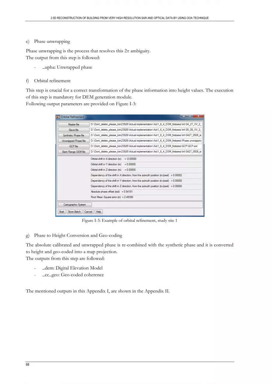
2.5D RECONSTRUCTION OF BUILDING FROM VERY HIGH RESOLUTION SAR AND OPTICAL DATA BY USING OOA TECHNIQUE
68
e) Phase unwrapping
Phase unwrapping is the process that resolves this 2π ambiguity.
The output from this step is followed:
- _upha: Unwrapped phase
f) Orbital refinement
This step is crucial for a correct transformation of the phase information into height values. The execution
of this step is mandatory for DEM generation module.
Following output parameters are provided on Figure I-3:
Figure I-3: Example of orbital refinement, study site 1
g) Phase to Height Conversion and Geo-coding
The absolute calibrated and unwrapped phase is re-combined with the synthetic phase and it is converted
to height and geo-coded into a map projection.
The outputs from this step are followed:
- _dem: Digital Elevation Model
- _cc_geo: Geo-coded coherence
The mentioned outputs in this Appendix I, are shown in the Appendix II.

2.5D RECONSTRUCTION OF BUILDING FROM VERY HIGH RESOLUTION SAR AND OPTICAL DATA BY USING OOA TECHNIQUE
69
APPENDIX II: OUTPUTS FROM SAR INTERFEROMETRY PROCESSING WITH SARSCAPE
Study site 1 a) Input
0427_SLC
0508_SLC
LIDAR DSM (external)
Figure II-1: Input data for SAR interferometry, study site 1
b) Output
0428_pwr
0508_pwr
int
srdem
sint
dint
fint
cc
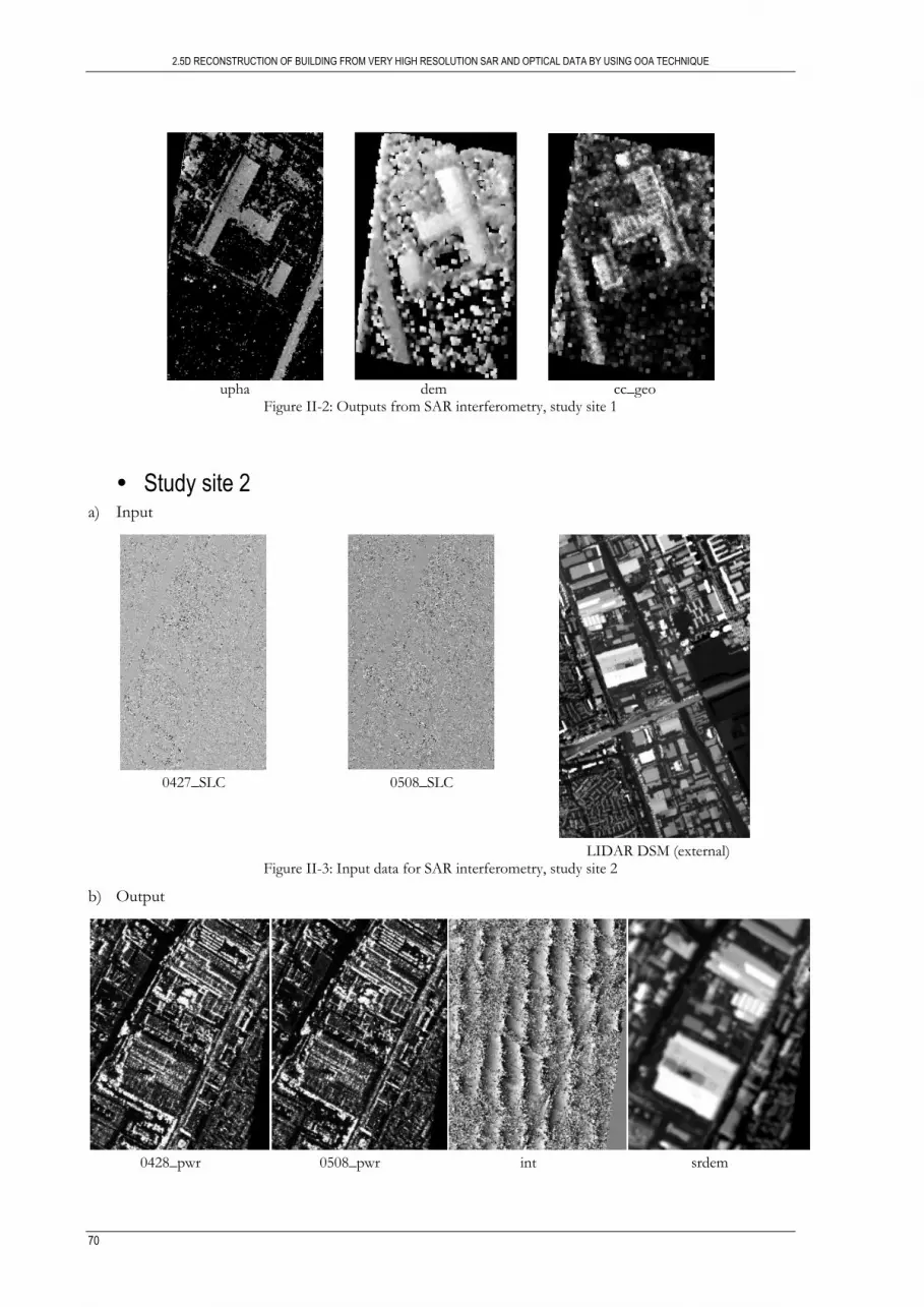
2.5D RECONSTRUCTION OF BUILDING FROM VERY HIGH RESOLUTION SAR AND OPTICAL DATA BY USING OOA TECHNIQUE
70
upha dem cc_geo
Figure II-2: Outputs from SAR interferometry, study site 1
Study site 2 a) Input
0427_SLC
0508_SLC
LIDAR DSM (external)
Figure II-3: Input data for SAR interferometry, study site 2
b) Output
0428_pwr
0508_pwr
int
srdem
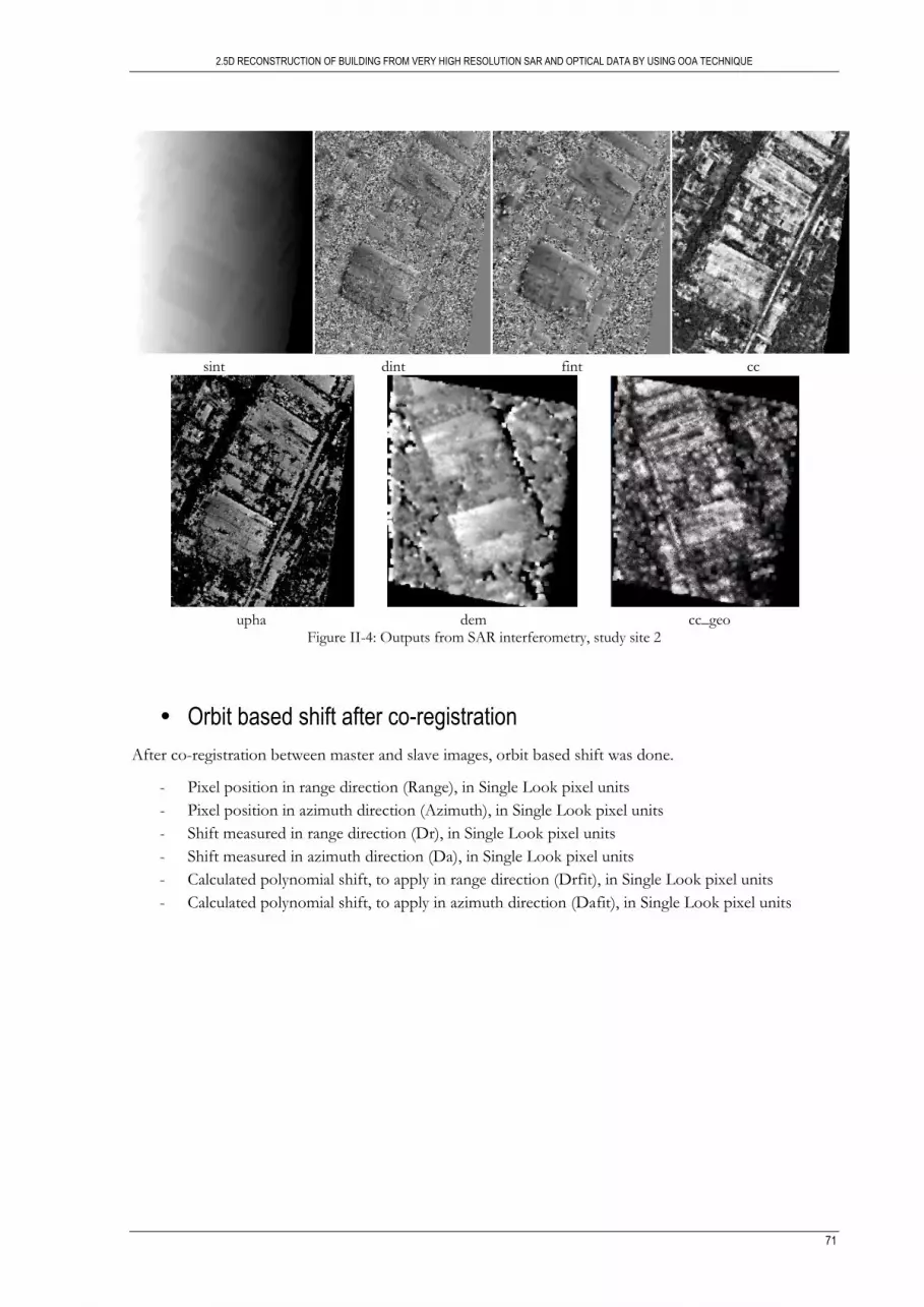
2.5D RECONSTRUCTION OF BUILDING FROM VERY HIGH RESOLUTION SAR AND OPTICAL DATA BY USING OOA TECHNIQUE
71
sint
dint
fint
cc
upha dem cc_geo
Figure II-4: Outputs from SAR interferometry, study site 2
Orbit based shift after co-registration
After co-registration between master and slave images, orbit based shift was done.
- Pixel position in range direction (Range), in Single Look pixel units
- Pixel position in azimuth direction (Azimuth), in Single Look pixel units
- Shift measured in range direction (Dr), in Single Look pixel units
- Shift measured in azimuth direction (Da), in Single Look pixel units
- Calculated polynomial shift, to apply in range direction (Drfit), in Single Look pixel units
- Calculated polynomial shift, to apply in azimuth direction (Dafit), in Single Look pixel units

2.5D RECONSTRUCTION OF BUILDING FROM VERY HIGH RESOLUTION SAR AND OPTICAL DATA BY USING OOA TECHNIQUE
72
Study site 1 Range Azimuth Dr Da Drfit Dafit Valid
64 128 -9999 -9999 105.938 -53.9979 0
158 128 106.252 -54.1324 105.965 -53.9999 1
252 128 106.277 -54.1329 105.991 -54.0014 1
346 128 106.306 -54.1332 106.017 -54.0024 1
440 128 106.331 -54.1338 106.042 -54.003 1
534 128 -9999 -9999 106.067 -54.0032 0
64 243 106.226 -54.1295 105.938 -53.9975 1
158 243 106.252 -54.1285 105.965 -53.9995 1
252 243 106.283 -54.1333 105.991 -54.001 1
346 243 106.304 -54.1301 106.017 -54.002 1
440 243 106.33 -54.1364 106.042 -54.0026 1
534 243 -9999 -9999 106.067 -54.0028 0
64 358 106.226 -54.128 105.938 -53.9971 1
158 358 106.253 -54.1282 105.965 -53.9991 1
252 358 106.281 -54.1311 105.991 -54.0006 1
346 358 106.305 -54.1299 106.017 -54.0016 1
440 358 106.331 -54.1315 106.042 -54.0022 1
534 358 -9999 -9999 106.067 -54.0024 0
64 473 106.227 -54.1288 105.938 -53.9967 1
158 473 106.257 -54.1311 105.965 -53.9986 1
252 473 106.282 -54.1317 105.991 -54.0002 1
346 473 106.308 -54.1288 106.017 -54.0012 1
440 473 106.332 -54.136 106.042 -54.0018 1
534 473 -9999 -9999 106.067 -54.002 0
64 588 106.226 -54.1243 105.938 -53.9963 1
158 588 106.255 -54.1303 105.965 -53.9982 1
252 588 106.279 -54.1297 105.991 -53.9997 1
346 588 106.304 -54.1317 106.017 -54.0008 1
440 588 106.33 -54.1289 106.042 -54.0014 1
534 588 -9999 -9999 106.067 -54.0015 0
64 703 106.227 -54.1245 105.938 -53.9959 1
158 703 106.253 -54.131 105.965 -53.9978 1
252 703 106.279 -54.132 105.991 -53.9993 1
346 703 106.309 -54.1285 106.017 -54.0004 1
440 703 106.33 -54.1323 106.042 -54.001 1
534 703 -9999 -9999 106.067 -54.0011 0
64 818 106.227 -54.1273 105.938 -53.9955 1
158 818 106.253 -54.124 105.965 -53.9974 1
252 818 106.279 -54.1324 105.991 -53.9989 1
346 818 106.305 -54.129 106.017 -54 1
440 818 106.331 -54.1315 106.042 -54.0006 1
534 818 -9999 -9999 106.067 -54.0007 0
64 933 106.227 -54.1249 105.938 -53.9951 1
158 933 106.253 -54.1263 105.965 -53.997 1
252 933 106.279 -54.1312 105.991 -53.9985 1
346 933 106.305 -54.1324 106.017 -53.9996 1
440 933 106.331 -54.1311 106.042 -54.0002 1
534 933 -9999 -9999 106.067 -54.0003 0
64 1048 106.227 -54.1278 105.938 -53.9947 1
158 1048 106.253 -54.1239 105.965 -53.9966 1
252 1048 106.279 -54.1316 105.991 -53.9981 1
346 1048 106.305 -54.1295 106.017 -53.9992 1
440 1048 106.331 -54.1309 106.042 -53.9998 1
534 1048 -9999 -9999 106.067 -53.9999 0
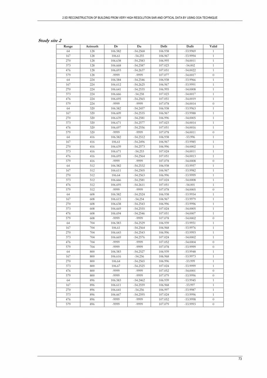
2.5D RECONSTRUCTION OF BUILDING FROM VERY HIGH RESOLUTION SAR AND OPTICAL DATA BY USING OOA TECHNIQUE
73
Study site 2 Range Azimuth Dr Da Drfit Dafit Valid
64 128 106.582 -54.2568 106.938 -53.9969 1
167 128 106.61 -54.255 106.967 -53.9994 1
270 128 106.638 -54.2583 106.995 -54.0011 1
373 128 106.668 -54.2587 107.023 -54.002 1
476 128 106.693 -54.2637 107.051 -54.0022 1
579 128 -9999 -9999 107.077 -54.0017 0
64 224 106.584 -54.2546 106.938 -53.9966 1
167 224 106.612 -54.2625 106.967 -53.9991 1
270 224 106.641 -54.2535 106.995 -54.0008 1
373 224 106.666 -54.258 107.023 -54.0017 1
476 224 106.695 -54.2565 107.051 -54.0019 1
579 224 -9999 -9999 107.078 -54.0014 0
64 320 106.582 -54.2457 106.938 -53.9963 1
167 320 106.609 -54.2535 106.967 -53.9988 1
270 320 106.639 -54.2581 106.996 -54.0005 1
373 320 106.671 -54.2577 107.023 -54.0014 1
476 320 106.697 -54.2556 107.051 -54.0016 1
579 320 -9999 -9999 107.078 -54.0011 0
64 416 106.582 -54.2512 106.938 -53.996 1
167 416 106.61 -54.2496 106.967 -53.9985 1
270 416 106.639 -54.2573 106.996 -54.0002 1
373 416 106.671 -54.253 107.024 -54.0011 1
476 416 106.695 -54.2564 107.051 -54.0013 1
579 416 -9999 -9999 107.078 -54.0008 0
64 512 106.582 -54.2532 106.938 -53.9957 1
167 512 106.611 -54.2505 106.967 -53.9982 1
270 512 106.64 -54.2563 106.996 -53.9999 1
373 512 106.666 -54.2581 107.024 -54.0008 1
476 512 106.695 -54.2611 107.051 -54.001 1
579 512 -9999 -9999 107.078 -54.0005 0
64 608 106.582 -54.2524 106.938 -53.9954 1
167 608 106.615 -54.254 106.967 -53.9979 1
270 608 106.638 -54.2543 106.996 -53.9996 1
373 608 106.669 -54.2555 107.024 -54.0005 1
476 608 106.694 -54.2546 107.051 -54.0007 1
579 608 -9999 -9999 107.078 -54.0002 0
64 704 106.583 -54.2529 106.939 -53.9951 1
167 704 106.61 -54.2564 106.968 -53.9976 1
270 704 106.643 -54.2543 106.996 -53.9993 1
373 704 106.669 -54.2576 107.024 -54.0002 1
476 704 -9999 -9999 107.052 -54.0004 0
579 704 -9999 -9999 107.078 -53.9999 0
64 800 106.583 -54.2527 106.939 -53.9948 1
167 800 106.616 -54.256 106.968 -53.9973 1
270 800 106.64 -54.2565 106.996 -53.999 1
373 800 106.67 -54.2525 107.024 -53.9999 1
476 800 -9999 -9999 107.052 -54.0001 0
579 800 -9999 -9999 107.079 -53.9996 0
64 896 106.583 -54.2462 106.939 -53.9945 1
167 896 106.611 -54.2559 106.968 -53.997 1
270 896 106.641 -54.256 106.997 -53.9987 1
373 896 106.667 -54.2595 107.024 -53.9996 1
476 896 -9999 -9999 107.052 -53.9998 0
579 896 -9999 -9999 107.079 -53.9993 0
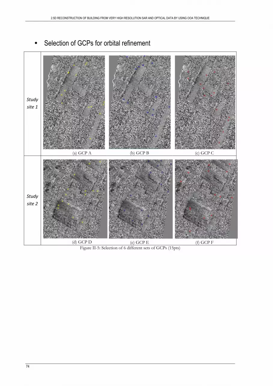
2.5D RECONSTRUCTION OF BUILDING FROM VERY HIGH RESOLUTION SAR AND OPTICAL DATA BY USING OOA TECHNIQUE
74
Selection of GCPs for orbital refinement
Study
site 1
(a) GCP A
(b) GCP B
(c) GCP C
Study
site 2
(d) GCP D
(e) GCP E
(f) GCP F
Figure II-5: Selection of 6 different sets of GCPs (15pts)
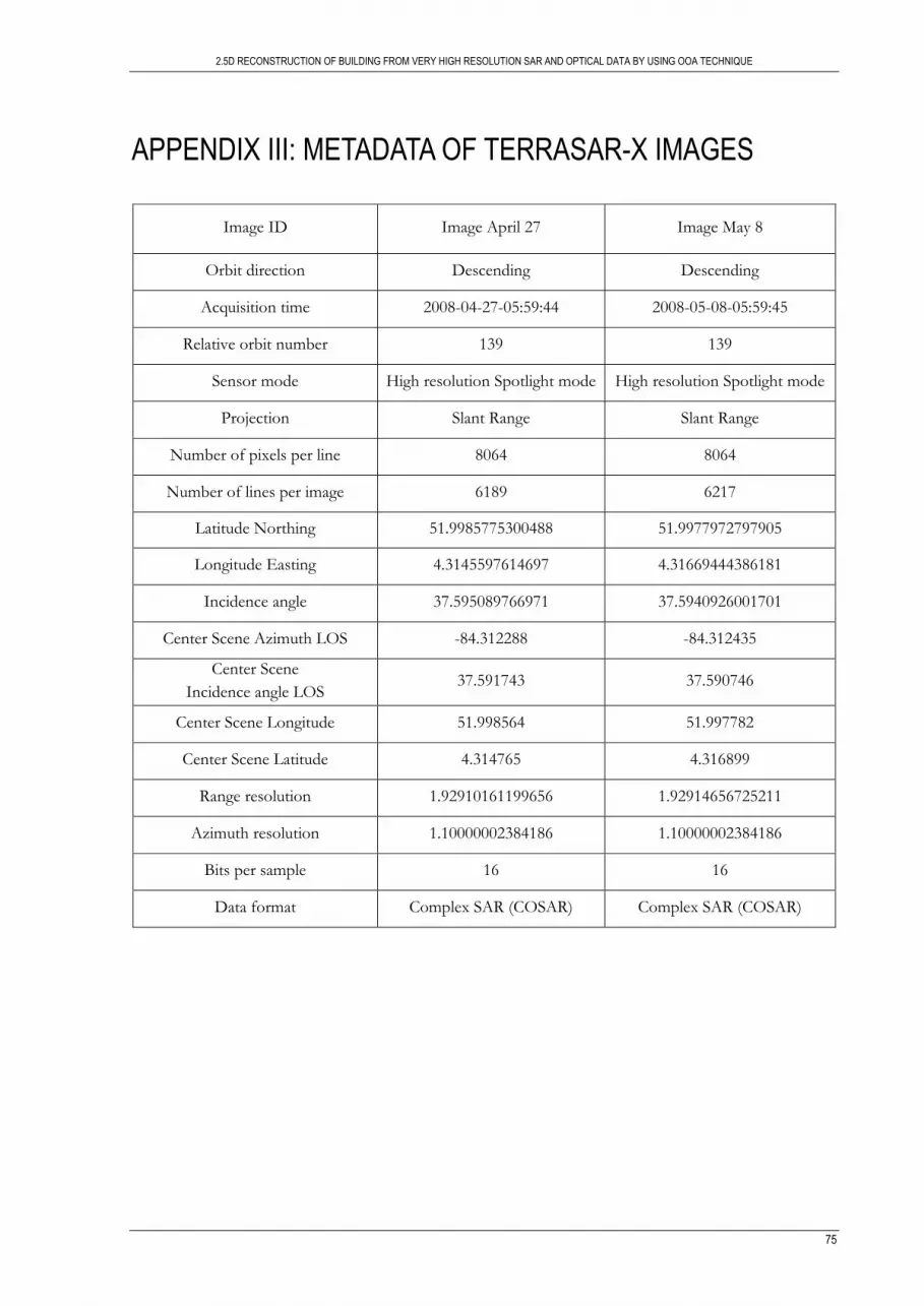
2.5D RECONSTRUCTION OF BUILDING FROM VERY HIGH RESOLUTION SAR AND OPTICAL DATA BY USING OOA TECHNIQUE
75
APPENDIX III: METADATA OF TERRASAR-X IMAGES
Image ID Image April 27 Image May 8
Orbit direction Descending Descending
Acquisition time 2008-04-27-05:59:44 2008-05-08-05:59:45
Relative orbit number 139 139
Sensor mode High resolution Spotlight mode High resolution Spotlight mode
Projection Slant Range Slant Range
Number of pixels per line 8064 8064
Number of lines per image 6189 6217
Latitude Northing 51.9985775300488 51.9977972797905
Longitude Easting 4.3145597614697 4.31669444386181
Incidence angle 37.595089766971 37.5940926001701
Center Scene Azimuth LOS -84.312288 -84.312435
Center Scene
Incidence angle LOS 37.591743 37.590746
Center Scene Longitude 51.998564 51.997782
Center Scene Latitude 4.314765 4.316899
Range resolution 1.92910161199656 1.92914656725211
Azimuth resolution 1.10000002384186 1.10000002384186
Bits per sample 16 16
Data format Complex SAR (COSAR) Complex SAR (COSAR)

2.5D RECONSTRUCTION OF BUILDING FROM VERY HIGH RESOLUTION SAR AND OPTICAL DATA BY USING OOA TECHNIQUE
76
APPENDIX IIII: PHOTOGRAPHS OF STUDY SITE
During the field visit to measure the roof boundary height of the buildings, the photographs were taken to
get an insight how the roofs look like.
Figure III-1: Building A, study site 1
Figure III-2: Building C, study site 2
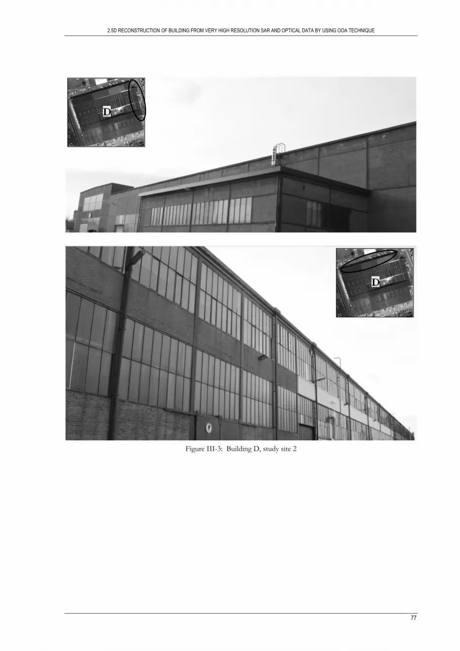
2.5D RECONSTRUCTION OF BUILDING FROM VERY HIGH RESOLUTION SAR AND OPTICAL DATA BY USING OOA TECHNIQUE
77
Figure III-3: Building D, study site 2