radiometric correction in range-specan sar processing
TRANSCRIPT
Radiometric Correction in
Range-SPECAN SAR Processing
by
Haleh Hobooti B.A.SC. EE., The University of Windsor, 1992
A THESIS SUBMITTED IN PARTIAL FULFILLMENT OF THE REQUIREMENTS FOR THE DEGREE OF
MASTER OF APPLffiD SCIENCE
in
THE FACULTY OF GRADUATE STUDffiS DEPARTMENT OF ELECTRICAL ENGINEERING
We accept this thesis as conforming to the required standard
THE UNIVERSITY OF BRITISH COLUMBIA May 1995
© Haleh Hobooti, 1995

In presenting this thesis in partial fulfilment of the requirements for an advanced
degree at the University of British Columbia, I agree that the Library shall make it
freely available for reference and study. I further agree that permission for extensive
copying of this thesis for scholarly purposes may be granted by the head of my
department or by his or her representatives. It is understood that copying or
publication of this thesis for financial gain shall not be allowed without my written
permission.
Department of S-lecifyC*! ff/iS ?V\ ft t A
The University of British Columbia Vancouver, Canada
Date At ^
DE-6 (2/88)
Abstract
This thesis investigates the reasons for, and proposes correction methods to reduce the
scalloping inherent in the range dimension in images processed using the SPECAN SAR
processing algorithm. These corrections methods are successfully tested using ERS-1 satellite
data.
The SPECAN algorithm was developed in 1979 by MacDonald Dettwiler and Associates, as
a multilook version of the deramp/FFT method of pulse compression. The algorithm provides
an efficient method of producing spaceborne SAR imagery of modest resolution, which makes it
ideal for quicklook imaging. Widespread use of the algorithm in quicklook imaging, however,
is hindered by the scalloping present in both the range and azimuth dimensions of the image.
This thesis concentrates on correction of range scalloping by presenting explanations for the
two types of scalloping present in the range dimension of SPECAN processed images. The basic
scalloping present in all scenes is due to the time variation in the envelope of the transmitted
signal. The extra scalloping seen in some scenes is due to clipping of the ERS-1 raw data.
Because of the geometry of the SPECAN processing cycles, the radiometry of the output is
sensitive to the transmitted chirp amplitude. The 0.5 dB power difference between the beginning
and end of the transmitted chirp is reflected in each compressed output segment, creating a
periodic lightening and darkening throughout the image. This banding effect is especially
noticeable in low contrast scenes. This problem is corrected using the chirp replica which
is embedded in the data header as an estimate of the pulse shape.
The extra scalloping observed in some high reflectivity scenes is attributed to the clipping
of the ERS-1 raw data in these scenes. Clipping causes attenuation in the output power. This
power loss varies along range according to the degree of saturation, and is different for each
compressed data block, thereby creating a discontinuity between adjacent compressed segments
ii:

which adds to (or subtracts from) the basic scalloping effect. This problem is corrected using the
relationship between power loss and degree of saturation in the Gaussian distributed raw data.
Contents
Abstract ii
List of Figures vii
List of Tables xi
Acknowledgments xif
Chapter 1 Introduction 1
Section 1.1 What is Radar Remote Sensing? 1
1.1.1 Real Aperture Radar 2
1.1.2 Synthetic Aperture Radar 3
1.1.3 Other Uses of SAR Data 4
1.1.4 Summary of Advantages and Disadvantages of SAR Imagery 4
Section 1.2 Thesis Overview 6
Chapter 2 Fundamentals of Synthetic Aperture Radar 8
Section 2.1 SAR Components 8
Section 2.2 The SAR Signal 10
Section 2.3 SAR Processing 13
2.3.1 The Matched Filter 14
2.3.2 Radar Performance and Post-Processing 17
Chapter 3 The Spectral Analysis Method of SAR and Quicklook Processing . 19
Section 3.1 Motivation 19
Section 3.2 Explanation of the Method 20
3.2.1 Deramping 20
3.2.2 DFT Operations 22
3.2.3 Analytical Representation 22
3.2.4 Graphical Representation 25
Chapter 4 Radiometric Degradation in Range-SPECAN 37
Section 4.1 Scalloping 37
Section 4.2 Cause of Scalloping 40
Section 4.3 Proposed Solution of Scalloping Problem 42
Section 4.4 Point Target Simulation 46
Chapter 5 Range-SPECAN on ERS-1 Data 51
Section 5.1 The ERS-1 Satellite 51
Section 5.2 The Chirp Replica 53
Section 5.3 Properties of the ERS-1 Raw Data 56
5.3.1 Statistical Properties 57
5.3.2 Spectrum of Raw Data 58
Section 5.4 Scenes Chosen for Study 59
Section 5.5 Analysis of SPECAN Output 61
5.5.1 Nova Scotia Ocean Scene 62
5.5.2 Rhine River Scene 70
5.5.3 Mountain Scene 74

Chapter 6 Effects of Raw Data Saturation on SPECAN Scalloping 78
Section 6.1 Scene Content and Saturation 78
Section 6.2 Further Saturation of Raw Data Prior to Range Processing 79
Section 6.3 Effect of Saturation on Range Scalloping 82
Section 6.4 Raw Data Simulation 85
6.4.1 Model . 86
6.4.2 Simulated Cases 87
6.4.3 Output 88
Section 6.5 Correction of Residual Scalloping Caused by Saturation 92
Chapter 7 Discussion 96
Section 7.1 Summary 96
Section 7.2 Future Work 98
Bibliography 100
vi.

List of Figures
Figure 1.1 Observational requirements for various applications 6
Figure 2.1 Synthetic aperture radar geometry 9
Figure 2.2 SAR system onboard satellite or aircraft 10
Figure 2.3 Doppler frequency determination 11
Figure 2.4 Fast-convolution 16
Figure 2.5 Deramp-FFT 16
Figure 3.1 Deramping a single linear FM signal by time multiplication . . . . 26
Figure 3.2 Extending the deramping operation to multiple point targets . . . 27
Figure 3.3 8 deramped targets constituting one parallelogram processing
region 28
Figure 3.4 Parallelogram regions showing the placement of the DFT blocks
in the single look case 30
Figure 3.5 Output of each DFT block shown separately . 32
Figure 3.6 Calculation of good DFT output points 33
Figure 3.7 Comparison between SPECAN and fast convolution in terms of
resolution and computation requirements 35
Figure 4.1 Ocean scene processed using SPECAN in range, scalloping is
present 38
Figure 4.2 SPECAN output: sum of 2048 lines of the digital image 38
Figure 4.3 Ocean scene processed by fast convolution method, no
scalloping is observed . . 39
Figure 4.4 Fast convolution output: sum of 2048 range lines of the digital
image 39
v i i

Figure 4.5 Typical envelope of ERS-1 chirp replica 40
Figure 4.6 Illustrating effect of ideal deramped targets (a) on detected
targets (b) 42
Figure 4.7 Illustrating effect of deramped targets of varying envelope
amplitude (a) on detected targets (b) 42
Figure 4.8 Magnitude displacement of first and last detected targets 44
Figure 4.9 Single point target in time and frequency domain. The target has
a rectangular envelope 47
Figure 4.10 Point targets compressed using SPECAN 48
Figure 4.11 Real part (a), and spectrum (b) of chirp with a linear envelope
superimposed 48
Figure 4.12 Output showing scalloping at the DFT boundary 49
Figure 4.13 Output corrected for scalloping 49
Figure 5.1 ERS-1 SAR strip-mapping geometry 52
Figure 5.2 Envelope of the chirp replica (a), and approximation of the
envelope to a straight line (b) 55
Figure 5.3 Correction vector derived from the chirp replica envelope . . . . 56
Figure 5.4 Raw data spectrum 59
Figure 5.5 Histograms showing distribution of raw SAR data 60
Figure 5.6 Near range image of Nova Scotia ocean(A) scene. Pixels 0 to
2047 63
Figure 5.7 Far range image of Nova Scotia ocean(A) scene. Pixels 3500 to
5547 63
Figure 5.8 Histograms of Nova Scotia ocean(A) raw data 63
'Viii

Figure 5.9 Averaged 5000 range processed lines of Nova Scotia ocean(A)
(a), (b), average ground reflectivity (c) 65
Figure 5.10 Effect of correction scheme on output of Nova Scotia ocean(A)
scene 66
Figure 5.11 Near range image of Nova Scotia ocean(B) scene. Pixels 0 to
2047 67
Figure 5.12 Far range image of Nova Scotia ocean(B) scene. Pixels 3500 to
5547 67
Figure 5.13 Histograms of Nova Scotia ocean(B) raw data 68
Figure 5.14 Averaged 5000 range processed lines of Nova Scotia ocean(B)
(a), (b), average ground reflectivity (c) 68
Figure 5.15 Effect of correction scheme on output of Nova Scotia ocean(B)
scene 69
Figure 5.16 Near range image of Rhine river scene. Pixels 0 to 2047 71
Figure 5.17 Far range image of Rhine river scene. Pixels 3500 to 5547. . . 71
Figure 5.18 Histograms of the Rhine river scene raw data 71
Figure 5.19 Average of 5000 lines of the Rhine river scene 72
Figure 5.20 Effect of correction scheme on output of Rhine river scene . . . 73
Figure 5.21 Near range image of the mountain scene. Pixels 0 to 2047. . . 74
Figure 5.22 Far range image of the mountain scene. Pixels 3500 to 5547. . 74
Figure 5.23 Histograms of mountain scene raw data 75
Figure 5.24 Average of 5000 lines of the mountain scene 76
Figure 5.25 Effect of correction scheme on output of mountain scene . . . . 77
Figure 6.1 Effect of introducing excess clipping in raw data prior to
SPECAN range processing 80
IX

Figure 6.2 Relationship between scalloping and saturation 81
Figure 6.3 Demonstrating power loss with increasing standard deviation for
fixed ADC range 83
Figure 6.4 Output power loss as function of increasing input power of signal
to ADC 83
Figure 6.5 Plot A shows the ideal output, plot B shows the result of
saturation on the output, and plot C shows the result of the
combination of chirp amplitude and saturation 85
Figure 6.6 Simulated ground reflectivity and transmitted chirp envelope . . 88
Figure 6.7 SPECAN output, constant chirp amplitude and constant ground
reflectivity 89
Figure 6.8 SPECAN output. Varying ground reflectivity, constant chirp
amplitude 89
Figure 6.9 SPECAN output. Constant ground reflectivity, positive slope on
chirp envelope 90
Figure 6.10 SPECAN output. Varying ground reflectivity, positive slope on
chirp envelope 91
Figure 6.11 Averaged 5000 range processed lines of Nova Scotia ocean(A). . 94
List of Tables
Table 3.1 Variation of efficiency and resolution with the SPECAN DFT
length 35
Table 4.2 ERS-1 SAR parameters for the transmitted signal 46
Table 5.3 ERS-1 SAR parameters 52
Table 6.4 Standard deviation of raw data for each output block of Figures
6.7 to 6.10 92
xi

Acknowledgments
I would like to thank Dr. Ian Cumming for his supervision during this thesis and for
recommending this interesting and challenging topic. I also wish to thank Gordon Davidson,
Mike Seymour, and Dave Michelson for their technical feedback during the progress of this
thesis, and Rick Dorbolo for his valuable suggestions and help in proof reading.
I would like to acknowledge the technical assistance of Paul Lim, Melanie Dutkiewicz and
Frank Wong of MacDonald Dettwiler. ERS-1 data has been provided by ESA. Financial support
for the work has been provided by the University of Windsor, NSERC, BC Advanced Systems
Institute, BC Science Council, and MacDonald Dettwiler.
X J I
Chapter 1 Introduction
This thesis concerns an efficient, real-time synthetic aperture radar processing algorithm
used for fast processing of radar data in earth imaging applications. The algorithm, Spectral
Analysis (SPECAN), was developed for quicklook processing by MacDonald Dettwiler and
Associates, Ltd. in 1979 [1], under contract to the European Space Agency [2]. Despite its
computational efficiency this algorithm has not had widespread use because images obtained by
it show an unacceptable amount of degradation. This thesis investigates the causes for the poor
image quality and implements a new method of correcting for the degradation which does not
significantly detract from the algorithm's main advantage which is efficiency in computation.
Section 1.1 What is Radar Remote Sensing?
Remote sensing, as explained by Wall, et al. [3], refers to the monitoring of the earth's
surface or atmosphere from a distant location. Remote sensing can be performed either passively
or actively. Passive systems do not provide target illumination, but operate by measuring the
amount of a certain type of radiation from the earth's surface or atmosphere (Hovannessian [4]).
The most useful passive remote sensing tools are optical multispectral sensors which operate
in the visible and infrared regions. Such systems need only to be equipped with a receiver.
Active systems, such as laser and radar imaging systems, provide a controlled source of target
illumination. These systems must be equipped with both transmitter and receiver.
A potentially very useful active imaging tool is the synthetic aperture radar, which operates
by transmitting a microwave beam, receiving, and measuring the strength and time delay of
the echo from the surface. The power returned is a function of the reflection coefficient of the
ground and depends on the geometric and dielectric properties of the medium (see Rees [5,
p. 61]. Digital signal processing techniques are used on the returned signal to extract the ground
1

reflectivity map. The image obtained in this manner is a function of the physical properties,
including orientation, roughness, topography, and moisture content of the objects on the imaged
surface.
Optical systems are widely used because of the very high resolution they provide. Optical
images are a measure of the chemical composition of the imaged surface. However, they are
useless at night and through cloud cover. Microwaves are not affected by atmospheric moisture,
making them ideal for imaging planet surfaces through cloud cover. In the Magellan mission,
as described by Johnson [6], a synthetic aperture radar was used to image the surface of Venus
through its very dense atmosphere.
Radar remote sensing by satellite offers wide coverage of land at fixed intervals regardless
of weather, clouds or time of the day. The European Remote-Sensing satellite (ERS-1), for
example, has different orbital patterns with repeat periods of 3, 35, and 176 days where each
individual orbit in the pattern will last approximately 100 minutes, Francis, et al. [7, p. 28].
This includes coverage of areas which are inaccessible by other means due to political, or
geographical difficulties.
1.1.1 Real Aperture Radar
Radar has been used for many years in military applications for tracking targets, in air traffic
control, speed measurement and other uses. From military applications the term "target" has
been used to refer to the aircraft or ship being tracked. In remote sensing, "target" refers to the
area of ground from which the backscatter is received. A radar (as described by Tomiyasu [8])
is an electromagnetic wave sensor having a pulsed microwave transmitter, antenna and receiver.
The antenna can be time shared between the transmitter and receiver. A pulse is transmitted,
reflected off the target and received. The antenna is carried by the aircraft and produces a fan
beam to the side of the flight track.
2

In real aperture radar (RAR) the antenna is unfocused because the receiver does not accurately
conserve the phase of each reflected pulse. For this type of imaging system a high resolution will
be obtained by transmitting a very narrow beam, or effectively, by having a small wavelength,
large antenna, and smallest possible distance to target. Wavelengths of microwave beams are
from 3 cm to 30 cm, and the distance from the satellite to ground is on the order of hundreds of
kilometers. Thus the only way to increase the resolution is to increase the size of the antenna.
The resolution of both RAR and optical systems is of the order of the beamwidth, XR/l,
where R is the range to the target, A is the wavelength, and / is the diameter of the antenna
aperture or lens (Ulaby [9, p. 651]). For example, for a resolution of 100 m, with A -0.03 m
and R=700 km, the antenna length would have to be approximately 200 m\ Such an antenna
would be extremely costly, and would have power and stability problems in space. Optical
systems, however, acquire good resolution with reasonable sized antennas because of the very
small wavelength of the electromagnetic energy, Elachi [10].
1.1.2 Synthetic Aperture Radar
The principles of synthetic aperture radar (SAR) we're first introduced by Carl Wiley in 1951
with the observation that a radar carried on board a moving platform with its beam oriented at an
angle to the platform velocity would receive signals which are offset from the radar frequency
due to the motion of the radar which causes the Doppler effect. By filtering this signal the
beamwidth can be made effectively narrower (or equivalently, the aperture will be longer). This
technique enables very high resolution images to be obtained without a need to increase the
antenna's physical size.
In SAR the demodulation of the signal return to baseband is performed very accurately to
conserve the phase between adjacent samples. This phase history is used to filter the data in the
along-track dimension, whereas in RAR filtering is only performed in the across-track dimension.
3

1.1.3 Other Uses of SAR Data
Besides two-dimensional terrain imaging, SAR data is used in polarimetry and interferome
try. Polarimetry is based on the principle that different types of terrain and ground cover have
different radar reflectivity based on the polarization of the transmitted beam. Most SAR anten
nas are linearly polarized, that is, they send and receive the same polarization. In polarimetric
SAR the complete polarization response of the target is measured by interleaving orthogonally
polarized radar pulses on transmission and measuring the amplitude and phase of the co-polar
and cross-polar returns on reception. The ratio of like to cross polarized return can be used to
extract significant geophysical and biophysical parameters such as surface roughness, moisture
content of soil, biomass content of a forest, or thickness of thin sea ice. For a detailed discussion
on the applications of polarimetry to geoscience refer to Ulaby, et al. [11].
Interferometry is the process of estimating terrain topography from SAR images by using
two complex images of the same scene taken from different angles. After the images have
been shifted appropriately to align identical points, the phase difference between the two images
(called the interferogram) is calculated and used along with other parameters such as the angle
and position shift of the sensor to calculate the height of each pixel. For more explanation on
interferometry refer to Graham, et al. [12], and Zebker, et al. [13].
1.1.4 Summary of Advantages and Disadvantages of SAR Imagery
Some advantages of a microwave imaging system can be listed as:
• Continuous coverage (at night and through cloud cover).
• Continuous, homogeneous coverage of large areas which would not be possible by other
means. That is, SAR imagery provides the "big picture".
• High resolution imagery is obtainable independent of radar distance to target.
• Controlled polarization allows classification of features.
4

• Terrain height estimation is possible by interferometry. This is especially useful for snow
covered mountainous areas where terrain height cannot be "seen".
• Some features are distinguished only by a microwave beam. For example, ancient drainage
channels under desert sand would not have been detected by an optical system. Also, the
microwave beam will provide a picture of the physical surface roughness which is useful in
distinguishing such things as effects of erosion and different land coverage.
Some disadvantages are as follows:
• Images are degraded by speckle. (Speckle noise is a result of the coherent reflection from
each point target in the resolution cell adding constructively or destructively in a random
fashion; multilooking will reduce speckle at the expense of resolution, see Ulaby [9, p. 585],
and Kirk [14]).
• The resolution is not as high as can be achieved in an optical system.
• Some visible features are not easily noticed because they are imaged differently from an
optical system. For example, mountain ranges perpendicular to the flight path will not be
recognizable as such.
• SAR does not measure the chemical properties of the surface. For example, healthy and
rotten vegetation is imaged identically, whereas Landsat-type sensors can distinguish them
by their different infrared reflectivity.
• Geometric distortion in the range dimension. For example, if two points are located (for
example on a slope) such that the range from radar to both points is the same they will be
registered as the same point.
5
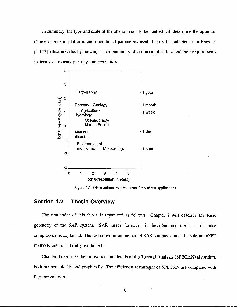
In summary, the type and scale of the phenomenon to be studied will determine the optimum
choice of sensor, platform, and operational parameters used. Figure 1.1, adapted from Rees [5,
p. 173], illustrates this by showing a short summary of various applications and their requirements
in terms of repeats per day and resolution.
4
£ 2
as T3
a> £ 1 o a>
8" 0
o -1
-2
-3
Cartography
Forestry - Geology Agriculture
Hydrology Oceanograpy/ Marine Pollution
Natural disasters
Environmental monitoring Meteorology
1 year
1 month
1 week
1 day
1 hour
1 2 3 4 5 Iog10(resolution, meters)
Figure 1.1 Observational requirements for various applications
Section 1.2 Thesis Overview
The remainder of this thesis is organized as follows. Chapter 2 will describe the basic
geometry of the SAR system. SAR image formation is described and the basis of pulse
compression is explained. The fast convolution method of SAR compression and the deramp/FFT
methods are both briefly explained.
Chapter 3 describes the motivation and details of the Spectral Analysis (SPECAN) algorithm,
both mathematically and graphically. The efficiency advantages of SPECAN are compared with
fast convolution.
6

Chapter 4 describes and shows examples of the degradation in SPECAN processed images.
The cause of the problem is analyzed using the geometry of the SPECAN algorithm and a
correction function is derived. The correction is tested in a point target simulation.
Chapter 5 derives the correction vector corresponding to the ERS-1 satellite SAR. The
correction is then tested on real SAR data and its performance evaluated on different types of
terrain. In some scenes residual scalloping remains after the basic correction.
Chapter 6 analyses the impact of raw data saturation on SPECAN image quality and the
residual scalloping. A theory is formed to explain the effect of raw data saturation on scalloping,
and the results of a raw data simulation are presented which verify the theory. A correction
scheme is proposed and tested on the worst case of saturation seen in Chapter 5.
Chapter 7 will provide a summary and describe the significance of this work. Also, methods
to reduce saturation are proposed, and the need for a practical implementation of the method
is discussed.
7
Chapter 2 Fundamentals of Synthetic Aperture Radar
This chapter explains the basic geometry of the SAR system, the mathematical form of the
ideal received SAR signal, the basis of pulse compression, and current signal processing methods
used to generate an image from SAR raw data.
Section 2.1 SAR Components
The main components of the SAR system are the antenna, pulsed transmitter, and coherent
receiver, carried on a platform which is either a satellite, or an airplane. The satellite or airplane
carrying the SAR antenna moves across the surface of the earth at a constant velocity while
transmitting microwave pulses at regular intervals and receiving the returned pulse.
The boresight of the antenna is aligned perpendicular to the flight path, and to one side of
the platform. The direction of travel of the antenna is called the azimuth direction. The direction
of travel of the transmitted pulse is referred to as the range direction (which is perpendicular
to the direction of travel). Pulses are transmitted at the pulse repetition frequency (PRF) and
the echo is received and stored for processing. The received data can be modelled as a matrix
where each row is the echo from one transmitted pulse. These transmissions build up in the
azimuth direction to form the matrix. Each row, or pulse echo, is a function of fast time, t, and
each column is a function of slow time, rj. The image is formed by measuring the range distance
of the echo. Because the antenna and the imaged swath are on different planes, the distance
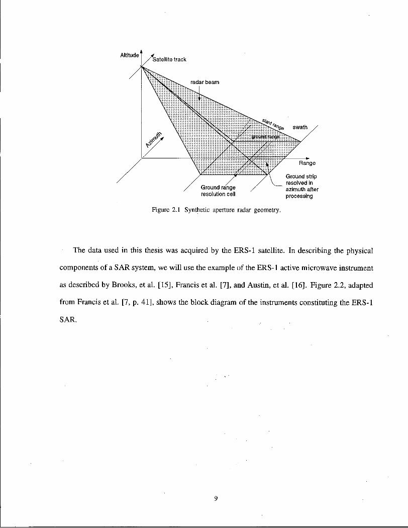
measured is in slant range as seen in Figure 2.1.
8
The data used in this thesis was acquired by the ERS-1 satellite. In describing the physical
components of a SAR system, we will use the example of the ERS-1 active microwave instrument
as described by Brooks, et al. [15], Francis et al. [7], and Austin, et al. [16]. Figure 2.2, adapted
from Francis et al. [7, p. 41], shows the block diagram of the instruments constituting the ERS-1
SAR.
9

M
High Power Amplifier
Circulator Assembly
Converter Unit
Up Converter
Calibration Unit
calibration replica p,ulsa
pulse Down
Converter
IF Radar >—<- SAR
Processor
3 CO — K C 3 CD
a
T DJ
3 cn
Q .
Timing Signal Transmit / Receive Path Calibration Pulse and Replica Path Waveguide Path
Frequency Generator
CD 3 to to to 6 3
Figure 2.2 SAR system onboard satellite or aircraft
In the SAR imaging mode the transmit timing pulse is obtained from the SAR processor
and provided to the intermediate frequency (TP) radar. The IF radar produces a linear frequency
modulated (FM) pulse1. This pulse is fed to the up-converter to produce the radio frequency
signal which is fed to the high power amplifier. The circulator assembly routes the signal to the
SAR antenna. In the receive path the signal is downconverted to baseband, quantized and either
sent to a ground station, or recorded for future transmission.
Section 2.2 The SAR Signal
As explained by Munson, et al. [17] the radar signal must be a pulse with enough power
that the received signal has good signal-to-noise ratio. A n impulse like waveform would have
these qualities, but would require very high peak power. In SAR systems a large bandwidth
dispersed-energy pulse is transmitted and the received signal is processed to a narrow pulse by a
By means of a surface acoustic wave (SAW) device.
10

method called pulse compression. The waveform generally used for transmission is the linear FM
chirp. A study has been done by Marcus, et al. [18] in using a coherent laser pulse instead of a
linear FM chirp in a one-dimensional SAR, however this work is still in the experimental stages.
The two-dimensional point target equation will be developed in the following sections. The
point target equation is the recieved signal if only one scatterer were present on ground. The
SAR is a linear system to which the principle of superposition applies, therefore the process
developed for a point target can be applied to the real recieved signal where the received signal
is modelled as the sum of many point targets.
The Azimuth Signal In real aperture radar, the transmitted pulse must be very narrow in order
to illuminate each target separately. Because the beam widens with distance, the resolution in
the azimuth direction will also depend on the distance between sensor and target. SAR takes
advantage of the fact that the motion of the antenna with respect to ground causes each target
to have a different Doppler signature with respect to adjacent targets. By using digital signal
processing the different Doppler signals can be resolved to form a narrow pulse at the location
of each target. This has been covered in more detail by Curlander [19], Bonfield, et al. [20],
and Tomiyasu [8].
Figure 2.3 shows how the range of a target to the radar changes as the beam passes over the
target. Note that the perspective of this figure is a position above the satellite.
X
Figure 2.3 Doppler frequency determination
11

As the target passes through the radar beam the range distance, and therefore the phase of
the received signal from the target changes. It is this change in phase with respect to time that
constitutes the Doppler frequency. The simple expression for the Doppler frequency ignoring
the effects of earth curvature and motion is derived as follows.
From the geometry of Figure 2.3, the target is at its closest range, R0, to the satellite at
time TJ — TJ o- When the target is at some arbitrary position x with respect to the satellite, the
separation R(x) is calculated as:
1/2 R(x) = \{x - x0)2 + R2
0\ (2.1)
From the satellite velocity, Vs, the distance can be written as (x-x0) = Vs(rj - r/0), where rj
is the time variable corresponding to the position x. Because R0 » (x - x0) equation (2.1) can
be written using the first two terms of the binomial series:
RM g a. + V K \ - R f . (2.2,
The phase, 4>a(t), of the returned signal in azimuth is:
The Doppler frequency, ijjr>(ri), is the rate of change of the phase with time:
(2.3)
»Din) = ^ - - ^ - ^ rad/s (2.4) ar/ XK0
So the received signal in the azimuth dimension is a linear chirp centered on zero frequency.
The FM rate of this signal, Ka, will be:
-2K 2
K - = - J t (2-5)
The value of Ra changes for each range bin, therefore the FM rate of the azimuth signal changes
also, and this must be taken into account when processing the data from different range locations. 12
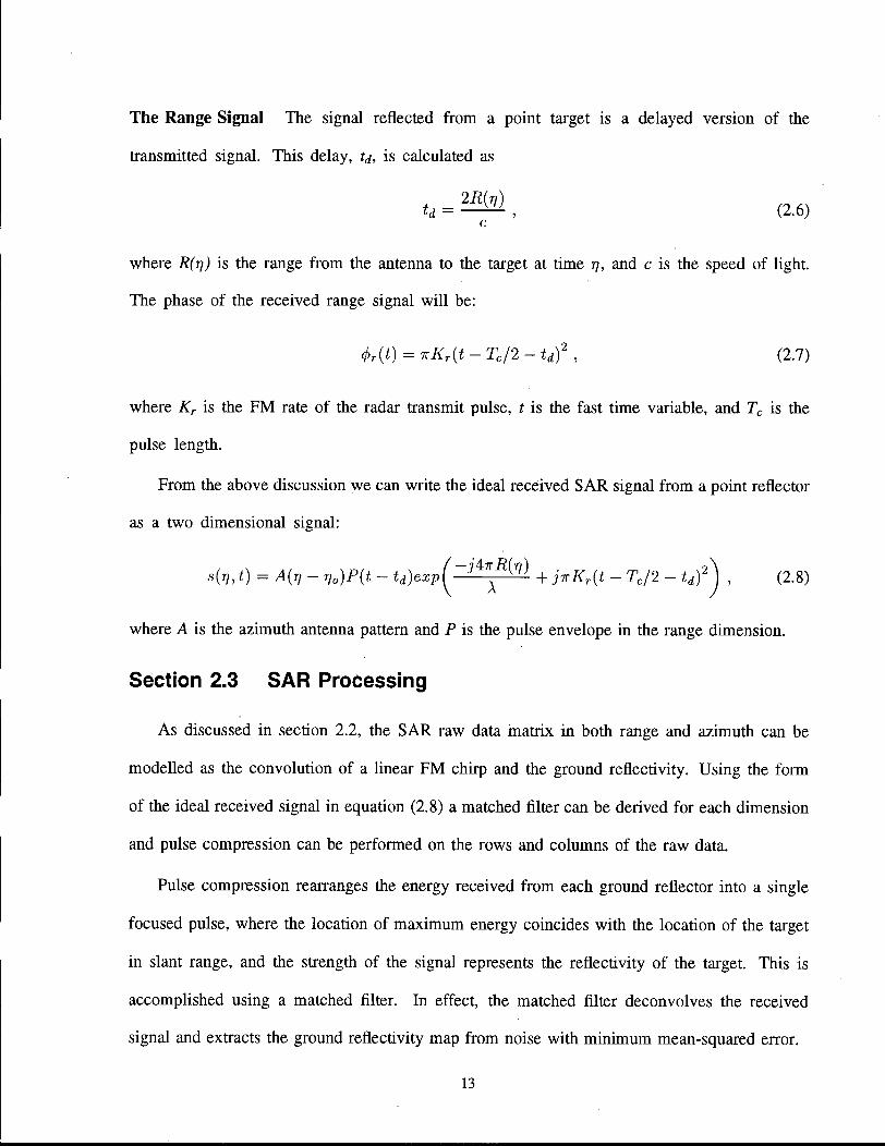
The Range Signal The signal reflected from a point target is a delayed version of the
transmitted signal. This delay, td, is calculated as
U = ^ , (2.6) C
where R(rj) is the range from the antenna to the target at time r), and c is the speed of light.
The phase of the received range signal will be:
<f>r(t) = *Kr(t-Tc/2-td)2 , (2.7)
where Kr is the FM rate of the radar transmit pulse, t is the fast time variable, and Tc is the
pulse length.
From the above discussion we can write the ideal received SAR signal from a point reflector
as a two dimensional signal:
s(r,,t) = A{r, - r,0)P(t - td)exp(^~ji7r
x
R{-v) + jirKr(t - Tc/2 - td)2^j , (2.8)
where A is the azimuth antenna pattern and P is the pulse envelope in the range dimension.
Section 2.3 SAR Processing
As discussed in section 2.2, the SAR raw data matrix in both range and azimuth can be
modelled as the convolution of a linear FM chirp and the ground reflectivity. Using the form
of the ideal received signal in equation (2.8) a matched filter can be derived for each dimension
and pulse compression can be performed on the rows and columns of the raw data.
Pulse compression rearranges the energy received from each ground reflector into a single
focused pulse, where the location of maximum energy coincides with the location of the target
in slant range, and the strength of the signal represents the reflectivity of the target. This is
accomplished using a matched filter. In effect, the matched filter deconvolves the received
signal and extracts the ground reflectivity map from noise with minimum mean-squared error.
13

2.3.1 The Matched Filter
The matched filter is derived as the conjugate of the time reversed ideal received signal. For
a transmitted signal, s(t), the echo, r(t), is received after a delay td (see Equation 2.6):
r(t) = as(t - td) + n(t) , (2.9)
where n(t) is white noise, and a is the attenuation. The matched filter is derived as a signal
which when convolved with r(t) extracts the input with the highest possible power above noise.
This is found to be the time-reversed conjugate of the transmitted signal, that is, s*(-t). The
compressed output, y(t), is the convolution of the matched filter and the received signal: oo
y(t)= J r(t-td)s*(-td)dr (2.10) —oo
For details of the derivation refer to Curlander [19] and Levanon [21]. Because the slow and
fast times are orders of magnitude different, two matched filters are derived using the range
and azimuth parameters of the radar, respectively, and the received signal can be processed in
two independent stages.
Range Resolution The result of applying the range matched filter to the point target of equation
(2.8) is a compressed pulse of envelope p(t):
/ \ rr m sin(irKrTct) p(t) = KTTc r*.c), (2.11) 7 T i \ r 1 ct
where Kr is the range FM rate, and Tc is the time duration of the transmitted pulse. The
resolution, <!>r, is measured as the 3 dB width of this signal:
^ i k - ( 2 - 1 2 )
where KrTc is the bandwidth of the transmitted pulse. This indicates that a pulse of time
span Tc seconds is compressed by the time-bandwidth product, KrTc
2. Increasing the average
14
power will boost the signal to noise ratio, while increasing the bandwidth will produce finer
resolution imagery. The main sidelobes of the compressed pulse are approximately 13 dB below
the mainlobe; various windowing methods are used to reduce the sidelobes, at the expense
of broadening the mainlobe width and decreased resolution. For a study of various window
functions and their properties refer to Nuttal [22].
Azimuth Resolution The azimuth resolution in real aperture radar is only equal to the along
track length of ground illuminated by the beam. As the antenna distance to ground is increased,
the beam widens, and therefore the azimuth resolution becomes coarser. In SAR, however it
can be shown that the azimuth resolution of a fully focused synthetic aperture is independent
of sensor distance to target and wavelength.
By using the matched filtering technique on the azimuth signal the resulting resolution will be
of the order of the inverse of the bandwidth. The ratio of bandwidth to time duration of a linear
FM pulse is the FM rate of the signal, Ka = BW/T. The time duration of the azimuth signal is the
time during which the target is illuminated by the radar beam and is calculated as T = \Ra/VsD.
Using the FM rate of the azimuth signal from equation (2.5), the bandwidth can be calculated:
BW = 2VS Hz (2.13) D
Therefore the resolution, 6a, is:
m (2.14)
15
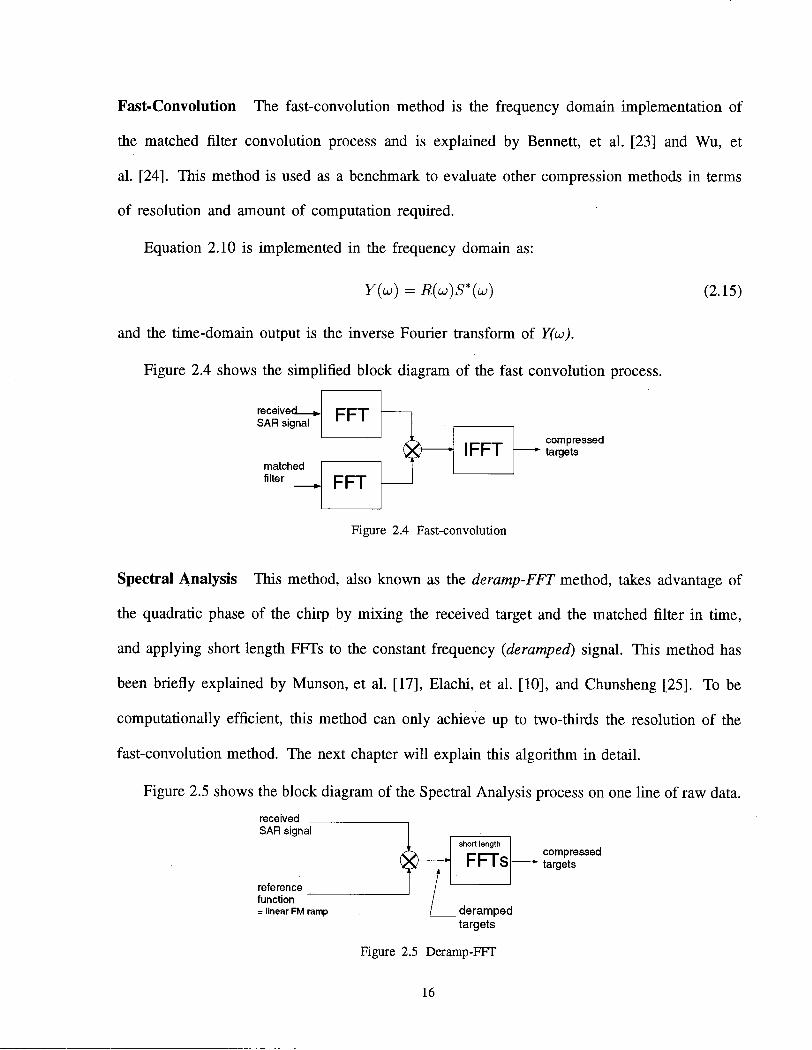
Fast-Convolution The fast-convolution method is the frequency domain implementation of
the matched filter convolution process and is explained by Bennett, et al. [23] and Wu, et
al. [24]. This method is used as a benchmark to evaluate other compression methods in terms
of resolution and amount of computation required.
Equation 2.10 is implemented in the frequency domain as:
Y(u>) = R(UJ)S*(LO)
and the time-domain output is the inverse Fourier transform of Y(u>).
Figure 2.4 shows the simplified block diagram of the fast convolution process.
(2.15)
receive* SAR signal
matched filter
compressed targets
Figure 2.4 Fast-convolution
Spectral Analysis This method, also known as the deramp-FFT method, takes advantage of
the quadratic phase of the chirp by mixing the received target and the matched filter in time,
and applying short length FFTs to the constant frequency {deramped) signal. This method has
been briefly explained by Munson, et al. [17], Elachi, et al. [10], and Chunsheng [25]. To be
computationally efficient, this method can only achieve up to two-thirds the resolution of the
fast-convolution method. The next chapter will explain this algorithm in detail.
Figure 2.5 shows the block diagram of the Spectral Analysis process on one line of raw data. received _ SAR signal
reference function
compressed targets
= linear FM ramp / deramped targets
Figure 2.5 Deramp-FFT
16

It must be mentioned that although satellite and airborne processing principles are identical,
processing of satellite SAR data is generally more complicated. This is because the very high
altitude of the satellite causes a larger area to be under illumination for a longer period of time,
therefore the movement of the target as a result of earth rotation must be taken into account.
Also, the effect of range migration must be corrected in satellite imagery. For more details on
range migration effects the reader is refered to Tomiyasu [8].
2.3.2 Radar Performance and Post-Processing
The radar performance is measured by examination of its impulse response. The impulse
response is the output of the system when the input is the signal from a single reflector. This
can be done by examining the point targets in the SAR image. The point targets are either
natural (eg. ships in the ocean) or man-made objects with known reflection coefficients. The
following parameters are measured on the image point targets and compared with the theoretical
values [19, p. 256], [26].
1. Mainlobe broadening (the actual 3 dB width, compared with the value calculated assuming
no system errors).
2. The Integrated Sidelobe Ratio (ratio of sum of point target sidelobes to the 3 dB area of
the mainlobe).
3. Peak Sidelobe ratio (ratio of the largest sidelobe outside the mainlobe to the mainlobe peak).
Post-processing of the image usually consists of radiometric and geometric corrections.
Geometric correction involves relating the spatial coordinates on the image to the corresponding
coordinates on the ground. This is done by using the location of known targets on ground and
resampling the image to new coordinates.
Radiometric correction is required to establish a relationship between the detector output and
the input radiation intensity. The radiometric correction function as described by Curlander [19,
17

p. 477] is a scalar array which varies with range image pixels. This function depends on factors
such as the antenna pattern, slant range, resolution cell size and system gain/losses. In this
thesis, however, we are only concerned with correction of scalloping, which is the radiometric
degradation specific to SPECAN images.
18

Chapter 3 The Spectral Analysis Method of SAR and Quicklook Processing
This chapter explains the motivation for developing SPECAN followed by the details of
the algorithm as explained in the 1979 MDA report [1]. A comparison is made between the
resolution of targets in the fast convolution versus the SPECAN method, and the limitations of
SPECAN are reviewed.
Section 3.1 Motivation
In conventional SAR processing methods the signal is range compressed using the fast
convolution method. As will be explained in detail later in the chapter, the SPECAN method
will reduce the computation time required for each range line processing by approximately a
factor of eight. This makes the algorithm suitable for use in on-board real-time processors and
quicklook ground processors. The trade-off is that the resulting SPECAN image will have up to
two-thirds the resolution of a fast convolution image of the same scene. This trade-off makes
the algorithm suitable for applications where lower resolution is acceptable, such as real-time
monitoring of ocean oil slicks, ship positions, and ice formations.
A real-time SAR processor breadboard has been developed (see Schotter [27], and the
MDA report [28]) which uses the SPECAN algorithm for azimuth compression. Also, a SAR
processor (the Brazil Quicklook processor) has been developed by MDA which uses the SPECAN
algorithm for both range and azimuth compression (MDA report [29]). The rather limited use
of the algorithm has been due to the image quality problems which will be dealt with in the
next chapter.
19

Section 3.2 Explanation of the Method
This section explains the SPECAN algorithm in detail. The algorithm can be used for
both range and azimuth compression. Most of the problems regarding azimuth-SPECAN image
quality have been solved by an accurate estimation of the Doppler centroid, see Wong, et al. [30].
Range-SPECAN has similar problems which are still unsolved and which render the algorithm
unsuitable for use. Since this thesis was aimed at solving the range-SPECAN problems, the
following sections emphasize range processing.
SPECAN performs target compression in two stages. The first operation is called deramping.
In this stage the received signal will be transformed from a linear FM signal to a constant
frequency signal, that is, the phase of the received signal is transformed from quadratic to linear.
The constant instantaneous frequency of the deramped signal will be proportional to the time
position of the signal. In the second stage, DFT operations, short length DFT's across the
constant frequency signal compress most of the energy of each target into a single frequency
bin. The output of the SPECAN processor is the output of the DFT operations, and therefore
must be resampled to represent the input range correctly. Each of these operations will be
explained in greater detail below.
3.2.1 Deramping
The concept of deramping in the time domain is derived from the stretch technique [31].
The stretch technique allows linear manipulation of the time and bandwidth coordinates of a
linear FM signal by means of mixing with another signal of different frequency-time slope in
order to slow down, speed up, or time reverse the signal.
A linear FM signal has the following form:
2 2
20
where K is the FM rate of the signal, Tc is the time extent of the pulse, and rc is the time position
of the zero frequency of the signal. The zero frequency of the target is the static phase point,
the time at which the phase rate goes from positive to negative (or vice versa). If the phase
switch-over occurs in the middle of the signal time duration, the zero frequency will coincide
with the centre frequency.
The instantaneous frequency of a linear FM chirp is equal to the derivative of its phase, 6.
The phase, 0s(t), and instantaneous frequency, u>imt(t), of the signal in 3.1 will be:
es(t) = irK(t-rc)2
d9 (t) (3-2) <«w(<) = = 2*K(t - TC)
The instantaneous frequency is a linear function of time.
If the signal in Equation (3.1) is multiplied with another linear FM signal sj(t) which has
a different FM rate Kj, and is shifted in time with respect to s(t), the product will be a linear
FM signal with FM rate (K+Kj).
8l(t) = e>*K>W - y < * < y
The first term on the right hand side of Equation 3.3 represents a linear FM signal with
FM rate equal to (K+Kj). The second term is a constant frequency signal, and the third term
is a constant complex number.
In SPECAN the same technique is applied. However, to transform the targets from linear
FM chirps into constant frequency signals Kj is chosen to be -K. The resulting deramped signal,
d(t), will be
d(t) = e2j*K(T'-TJie?*K(r2-r?) (3.4)
21
The phase, Od(t), and instantaneous frequency, w'inst(t) of the deramped signal will be:
ed(t) = TK[2(Tr-Tc)t+(r?-T?)}
Jinst(t) = 2ir K(rr-rc), (3.5)
where we can see that u>'inst(t) does not vary with time.
In SPECAN the FM rate of the transmitted pulse is used to generate the conjugate of the
ideal received signal which then deramps the received data by a complex multiplication in the
time domain. The generated function is the SPECAN matched filter and is called the reference
function.
3.2.2 DFT Operations
After deramping, each target will have a constant frequency value proportional to the time
position of its zero Doppler frequency with respect to that of the reference function as seen from
Equation (3.5). A DFT performed on this signal will confine most of the energy of each target to
a single frequency bin. The relative positions of these detected energies in the frequency domain
will be proportional to the relative positions of the targets' time locations, therefore the targets
will be detected at the correct positions relative to each other. Short length DFT blocks will be
placed along the deramped signal such that each target's trajectory is included in at least one
DFT input vector. The DFT block placement will be explained in more detail later in the chapter.
3.2.3 Analytical Representation
As we saw in Chapter 2 compression of radar signals is accomplished by cross correlating
the received signal with the conjugate of the ideal received signal. In this section we will show
that the cross correlation operation is equivalent to deramping followed by a DFT operation.
22

The ideal received signal is a linear FM signal of the form
stdeal(n) = e-WW -N _ N
(3.6)
where
Kr = FM rate of ideal received signal [Hz/s]
N = number of samples in ideal received signal
r = sample spacing [s]
The compressed output, y(n) is derived by cross correlating the received signal, s(n) (linear FM
plus noise), and the conjugate of the ideal received signal, r(n)=si(ieai*(n).
Multiplying the right-hand side of Equation (3.7) by eircKrT n N
e - i * K r T 2 n N w i n r e s u l t i n .
(3.7)
(n) _ eJirKrn2T2
e-jwKrT2nN 2 _ 1
eJ-KKrr2i2
e2jwKr(niT2+T2n N/2)
ejnKrr2(n2-nN) ,jwKrT2i2
e2jwKrnT2(i+N/2) (3.8)
The first term in the right-hand side of Equation ( 3.8) is a phase rotation term and can be
ignored if the next operation is the detection operation which removes the phase information.
23
The second term on the right of the summation is the conjugate of the ideal received signal,
r(n). Therefore Equation (3.8) can be rewritten as
2 1
y(n) = ^2 s(i)r(i)e2irK^(i+T) ( 3 9 )
If the product of the signal and its complex conjugate is denoted by p(n) = s(n)r(n), by
a change in limits the output can be written as:
N-l V(n)= £ p ( i - j ) e 2 i * K ' n i 3 i (3.10)
The number of samples in the reference function is N = F2/Kr. Substituting for Kr in
Equation (3.10) we can further simplify the compressed output.
N-l e2j-xin/N
2J
N-l — eJ 52p(t)e2i™'N (3.11)
«=o
The ej7rn term before the summation is a phase rotation term which again can be ignored if the
next operation is detection. Equation 3.11 shows that the result of cross-correlating the input
signal with the conjugate of the ideal received signal is equivalent to performing a DFT on the
product of the received signal and the reference function. The above derivation can only be
carried out if the signals have a linear FM form. Therefore the SPECAN algorithm is only valid
for linear FM signals.
24
3.2.4 Graphical Representation
Greater understanding of the SPECAN method is possible by graphically examining the
deramping and DFT operations. This section will use the geometry of point reflectors as they
undergo SPECAN compression operations to show how the algorithm determines target location.
In SAR the time-bandwidth product1 of the transmitted signal is usually higher than 100.
Thus the principle of stationary phase can be used to simplify the relationship between the time
(T) and instantaneous frequency (f) of the linear FM signal as
/ = KT (3.12)
This one-to-one correspondence between time and frequency allows the linear FM signal to be
well represented in the frequency-time plane which will be used extensively in the following
sections.
Deramping This section shows the deramping operation with the aid of Figure 3.1. The
receiver sampling rate is greater than the Nyquist rate of the received signal. The reference
function is generated using the same FM rate as the transmitted pulse, but with bandwidth equal
to the sampling frequency. Therefore, according to Equation (3.12), the reference function will
have a longer time duration than the received point reflector as demonstrated in Figure 3.1a.
If the target and reference function had equal time locations for their zero Doppler frequencies
the frequency of the product would be zero Hz. This would be the: case in Equation (3.4) for
T c = r r. In this case the equation of the deramped target would simplify to d{t) = 1. In the
general case, however, the zero Doppler frequency of the target is displaced in time from that
of the reference function, and the resulting product has a non-zero constant frequency (as seen
in Figure 3.Id) proportional to the displacement as seen in Equation (3.4).
1 The time-bandwidth product is the product of the duration of the dispersed pulse and its bandwidth.
25 ••'

Because the target is shifted in time with respect to the reference function, the reference
function is repeated in time to encompass the entire length of the target. This causes a frequency
shift of y ±F in the deramped target, where F is the sampling frequency. Aliasing by ±F will
restore the signal to fd.
(b) Frequency-time diagram of point target
(c) Frequency-time diagram of deramped target before aliasing
fd^_
(d) Frequency-time diagram of deramped target
Figure 3.1 Deramping a single linear FM signal by time multiplication
The operations in Figures 3.1a, b, c, d must be extended to an entire line of received data.
The received signal, which is modelled as the convolution of the transmitted pulse and the ground
reflectivity [17], can be represented as a sum of point reflectors. This is shown in 3.2a. The
reference function is repeated in time to encompass the entire length of the received data. The
sawtooth frequency-time diagram of the reference function is shown in Figure 3.2b. The result
of deramping a number of equally spaced point reflectors is shown in 3.2c.
26
1 2 3 4 6 6 7 _8__.9 K L _ J L _
(a) Frequency-time history of a set of equally spaced point reflectors
FHz
(b) Frequency-time history of the reference function
J2 12
11
10
FHz
(c) Frequency-time history of the product functions when the signals in (a) are multiplied by the reference function in (b)
Figure 3.2 Extending the deramping operation to multiple point targets
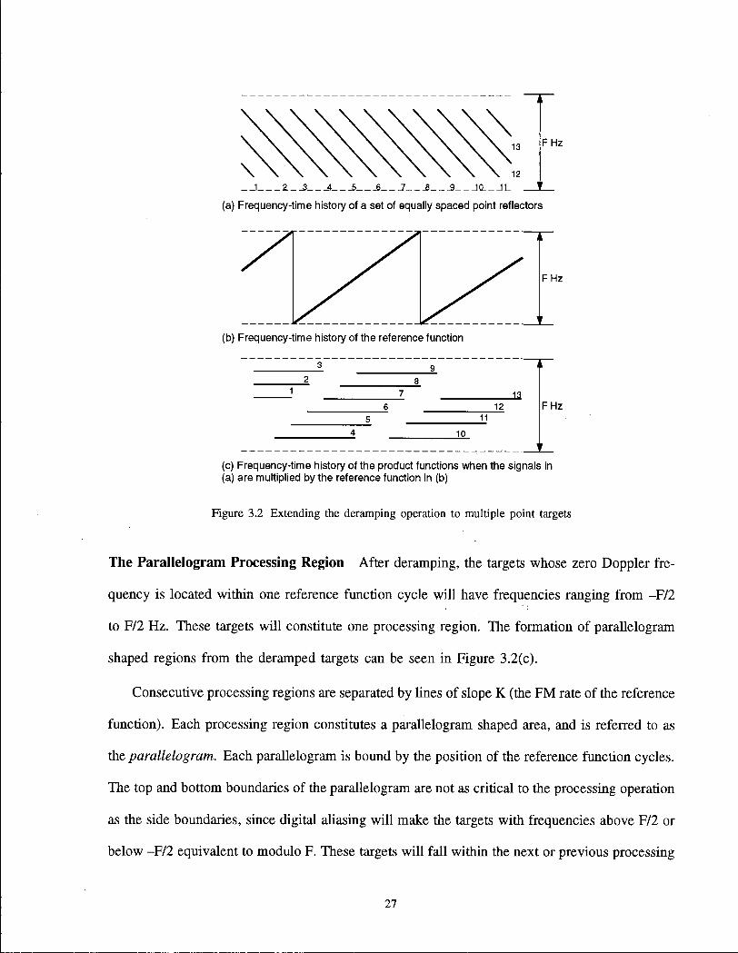
The Parallelogram Processing Region After deramping, the targets whose zero Doppler fre
quency is located within one reference function cycle will have frequencies ranging from -F/2
to F/2 Hz. These targets will constitute one processing region. The formation of parallelogram
shaped regions from the deramped targets can be seen in Figure 3.2(c).
Consecutive processing regions are separated by lines of slope K (the FM rate of the reference
function). Each processing region constitutes a parallelogram shaped area, and is referred to as
the parallelogram. Each parallelogram is bound by the position of the reference function cycles.
The top and bottom boundaries of the parallelogram are not as critical to the processing operation
as the side boundaries, since digital aliasing will make the targets with frequencies above F/2 or
below -F/2 equivalent to modulo F. These targets will fall within the next or previous processing
27
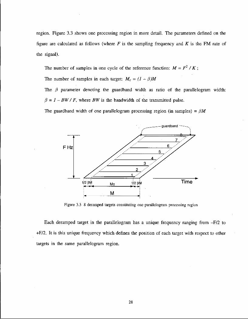
region. Figure 3.3 shows one processing region in more detail. The parameters defined on the
figure are calculated as follows (where F is the sampling frequency and K is the FM rate of
the signal).
The number of samples in one cycle of the reference function: M = F2 / K ;
The number of samples in each target: Mc = (1 - f3)M
The f3 parameter denoting the guardband width as ratio of the parallelogram width:
(3 = 1- BW / F, where BW is the bandwidth of the transmitted pulse.
The guardband width of one parallelogram processing region (in samples) = (3M
M
Figure 3.3 8 deramped targets constituting one parallelogram processing region
Each deramped target in the parallelogram has a unique frequency ranging from -F/2 to
+F/2. It is this unique frequency which defines the position of each target with respect to other
targets in the same parallelogram region.
28

The Guard Band The guard band is the region between successive parallelograms, shown in
Figure 3.2, which does not contain valid target samples. It can also be seen as the dotted region
on each side of the parallelogram in Figure 3.3.
The reason for the formation of the guardband in range processing is the longer time duration
of the reference function, explained in section 3.2.4. This longer time duration ensures that the
entire bandwidth of each target is limited to within one processing region and the deramped targets
do not overflow into adjacent parallelograms. The guard band region, therefore, corresponds to
regions outside the time interval of the radar pulse. The number of samples in the guardband
can be calculated using the target bandwidth as shown from Figure 3.3.
DFT Block Placements The next step in the imaging process is to separate the targets into
different energy cells with regard to their position in the time domain. As mentioned earlier the
deramped targets in each processing region have unique frequencies ranging from -F/2 to +F/2.
Short length DFT operations performed across the deramped data will separate the energy of
each target into a unique DFT bin.
The number of points in the DFT is usually chosen as a power of 2 to facilitate the Fast
Fourier Transform algorithm for the DFT (see Oppenheim [32, p. 587-605]). The placement
of the DFT blocks is shown in Figure 3.4. The placement of the first DFT block is arbitrary.
The next DFT block must be placed such that it covers the trajectory of the first target which
is not completely covered by the previous DFT block. To do this a horizontal line (shown as
ab in Figure 3.4) is extended from the point where the first DFT rectangle first coincides with
the guardband to the guardband on the opposite side of the same parallelogram. The next DFT
block is placed such that it contains the time domain samples (b - N + 1) to b, where TV is the
DFT length.
29
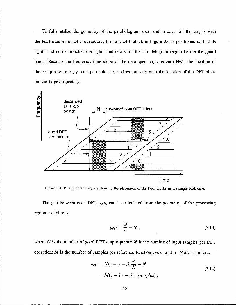
To fully utilize the geometry of the parallelogram area, and to cover all the targets with
the least number of DFT operations, the first DFT block in Figure 3.4 is positioned so that its
right hand corner touches the right hand corner of the parallelogram region before the guard
band. Because the frequency-time slope of the deramped target is zero Hz/s, the location of
the compressed energy for a particular target does not vary with the location of the DFT block
on the target trajectory.
o c cr
discarded DFT o/p points N = number of input DFT points
Time
Figure 3.4 Parallelogram regions showing the placement of the DFT blocks in the single look case.
The gap between each DFT, gdft, can be calculated from the geometry of the processing
region as follows:
G 9dft = N ,
a (3.13)
where G is the number of good DFT output points; N is the number of input samples per DFT
operation; M is the number of samples per reference function cycle, and a=N/M. Therefore,
9 d f t = N(l-a-(3)^-N
= M(l - 2a - B) [samples] . (3.14)
30
As seen in Figure 3.4, the first DFT block contains N points of each of the trajectories of
targets 1 to 5. The second DFT block is placed such that it covers the targets immediately
after target 5 up to target 8 of the current parallelogram and targets 9 and 10 from the next
parallelogram region.
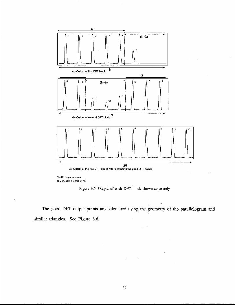
Calculating the Good DFT Output Points Not all the DFT output points constitute valid
image data. Part of the output points of each DFT correspond to guard band samples and
incomplete sections of target trajectories. To see the division between valid and invalid DFT
output points see the DFT1 block of Figure 3.4. The DFT rectangle can be divided into two
regions by a horizontal line where the left-hand side of the rectangle touches the guard band. The
upper section of the rectangle contains invalid output samples which must be discarded, output
points corresponding to the lower section of the rectangle are kept in a buffer as the good DFT
output points. Figure 3.5a and b shows an example of detected targets from two DFT blocks
before extracting the good output points. The number of good output points are calculated (as
shown later), stored in a buffer and concatenated together. The final output of the two DFT
blocks is shown in 3.5c. The rest of the output points of each DFT block are discarded.
31
(a) Output of first DFT block
G
N (b) Output of second DFT block
1 A 2 f f I 7 9
I" J u LJ u U
2 G (c) Output of the two DFT blocks after extracting the good DFT points
N = DFT input samples
G = good DFT output points
Figure 3.5 Output of each DFT block shown separately
The good DFT output points are calculated using the geometry of the parallelogram and
similar triangles. See Figure 3.6.
32

Time
Figure 3.6 Calculation of good DFT output points
From the following relationship between similar triangles we can calculate the number of
good output points.
ad as T = — (3-15) dp sp
From this the good output points (G) can be calculated as follows (note that a denotes the
N/M ratio):
TV G M (M-BM-N)
and rearranging the equation gives:
(3.16)
G = N(\-a - B) [samples] (3.17)
Similarly we can calculate the distance between the starting point of successive DFT blocks (7)
in the single look case (where 7 is the distance qc in Figure 3.6):
G__ N_ 7 ~ *f (3.18) 7 a.
33
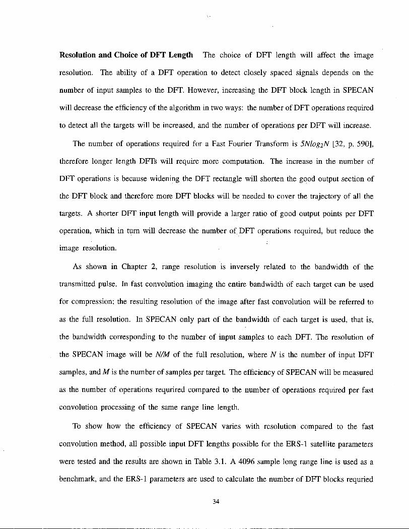
Resolution and Choice of DFT Length The choice of DFT length will affect the image
resolution. The ability of a DFT operation to detect closely spaced signals depends on the
number of input samples to the DFT. However, increasing the DFT block length in SPECAN
will decrease the efficiency of the algorithm in two ways: the number of DFT operations required
to detect all the targets will be increased, and the number of operations per DFT will increase.
The number of operations required for a Fast Fourier Transform is 5Nlog2N [32, p. 590],
therefore longer length DFTs will require more computation. The increase in the number of
DFT operations is because widening the DFT rectangle will shorten the good output section of
the DFT block and therefore more DFT blocks will be needed to cover the trajectory of all the
targets. A shorter DFT input length will provide a larger ratio of good output points per DFT
operation, which in turn will decrease the number of DFT operations required, but reduce the
image resolution.
As shown in Chapter 2, range resolution is inversely related to the bandwidth of the
transmitted pulse. In fast convolution imaging the entire bandwidth of each target can be used
for compression; the resulting resolution of the image after fast convolution will be referred to
as the full resolution. In SPECAN only part of the bandwidth of each target is used, that is,
the bandwidth corresponding to the number of input samples to each DFT. The resolution of
the SPECAN image will be N/M of the full resolution, where N is the number of input DFT
samples, and M is the number of samples per target. The efficiency of SPECAN will be measured
as the number of operations requrired compared to the number of operations required per fast
convolution processing of the same range line length.
To show how the efficiency of SPECAN varies with resolution compared to the fast
convolution method, all possible input DFT lengths possible for the ERS-1 satellite parameters
were tested and the results are shown in Table 3.1. A 4096 sample long range line is used as a
benchmark, and the ERS-1 parameters are used to calculate the number of DFT blocks requried
34

for the SPECAN compresssion. The first column of Table 3.1 shows the input lengths; the
second column is the number of operations required for the SPECAN as a percentage of what
is required for the fast convolution. The third column is the value of N/M, that is the resolution
of SPECAN as a factor of the resolution of fast convolution.
FFT Length Operations (% of fast convolution )
Resolution (% of fast convolution)
32 0.78 4.55 64 1.81 9.09 128 4.82 18.18 256 13.91 36.36 512 61.69 72.73
Table 3.1 Variation of efficiency and resolution with the SPECAN DFT length
From the table it is apparent that as the FFT length (and therefore resolution) is doubled
the efficiency is quartered. This is illustrated in Figure 3.7 which is the plot of the polynomial
fit to the values in Table 3.1.
Efficiency vs resolution of SPECAN
E o
O ^ 0 . 4
0 . 2
I 1
/ \ o 1 1 0
I (O 1 IV>
/ \ o 1 1 0
I (O 1 IV>
*N=
512
!
i 1
j
(£> LO CM J L
!
CM ^ -
^ If
\N=
12
8
1 0 0.1 0 . 2 0 . 3 0 . 4 0 . 5 0 . 6 0 . 7 0 . 8 0 . 9 1
% Resolution
Figure 3.7 Comparison between SPECAN and fast convolution in terms of resolution and computation requirements.
35

Figure 3.7 shows that at high resolutions SPECAN does not provide much efficiency over
fast convolution considering the loss of resolution. For ERS-1 parameters, a sample size of 256
is advantageous for quicklook processing. At this input length 36% of the full resolution is
obtained by expending only 14% of the computation required.
36
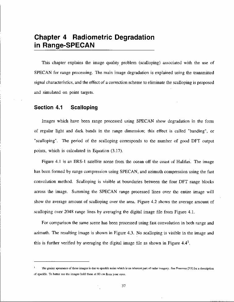
Chapter 4 Radiometric Degradation in Range-SPECAN
This chapter explains the image quality problem (scalloping) associated with the use of
SPECAN for range processing. The main image degradation is explained using the transmitted
signal characteristics, and the effect of a correction scheme to eliminate the scalloping is proposed
and simulated on point targets.
Section 4.1 Scalloping
Images which have been range processed using SPECAN show degradation in the form
of regular light and dark bands in the range dimension; this effect is called "banding", or
"scalloping". The period of the scalloping corresponds to the number of good DFT output
points, which is calculated in Equation (3.17).
Figure 4.1 is an ERS-1 satellite scene from the ocean off the coast of Halifax. The image
has been formed by range compression using SPECAN, and azimuth compression using the fast
convolution method. Scalloping is visible at boundaries between the four DFT range blocks
across the image. Summing the SPECAN range processed lines over the entire image will
show the average amount of scalloping over the area. Figure 4.2 shows the average amount of
scalloping over 2048 range lines by averaging the digital image file from Figure 4.1.
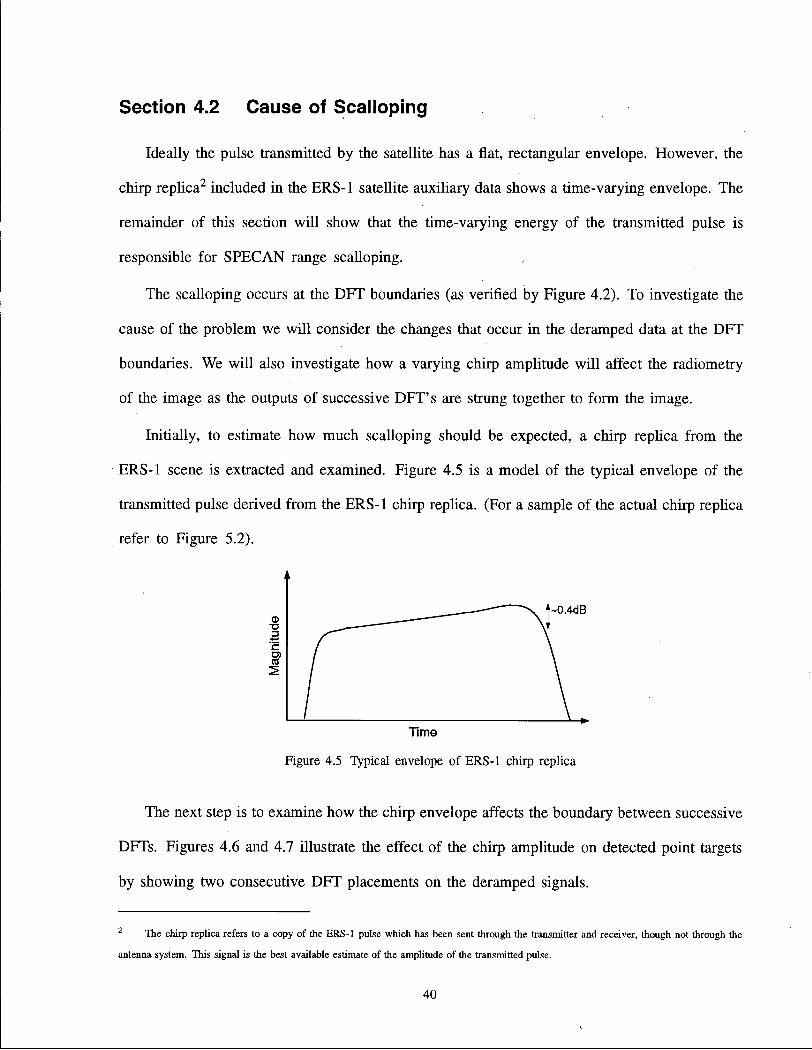
For comparison the same scene has been processed using fast convolution in both range and
azimuth. The resulting image is shown in Figure 4.3. No scalloping is visible in the image and
this is further verified by averaging the digital image file as shown in Figure 4.41.
The grainy apearance of these images is due to speckle noise which is an inherent part of radar imagery. See Freeman [33] for a description
of speckle. To better see the images hold them at 80 cm from your eyes.
37
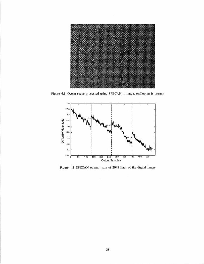
Figure 4.1 Ocean scene processed using S P E C A N in range, scalloping is present
13 5 I I 1 1—1 I i _ l 1 1 1 1 1 1 0 50 100 150 200 250 300 350 400 450 500
Output Samples
Figure 4.2 S P E C A N output: sum of 2048 lines of the digital image
38
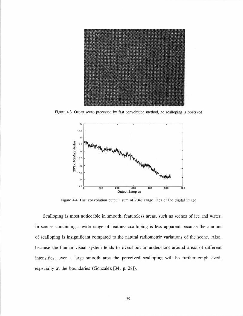
Figure 4.3 Ocean scene processed by fast convolution method, no scalloping is observed
1 8
17.5 -
17 -
13 5 I i 1 1 1 1 1 0 100 200 300 400 500 600
Output Samples
Figure 4.4 Fast convolution output: sum of 2048 range lines of the digital image
Scalloping is most noticeable in smooth, featureless areas, such as scenes of ice and water.
In scenes containing a wide range of features scalloping is less apparent because the amount
of scalloping is insignificant compared to the natural radiometric variations of the scene. Also,
because the human visual system tends to overshoot or undershoot around areas of different
intensities, over a large smooth area the perceived scalloping will be further emphasized,
especially at the boundaries (Gonzalez [34, p. 28]).
39
Section 4.2 Cause of Scalloping
Ideally the pulse transmitted by the satellite has a fiat, rectangular envelope. However, the
chirp replica2 included in the ERS-1 satellite auxiliary data shows a time-varying envelope. The
remainder of this section will show that the time-varying energy of the transmitted pulse is
responsible for SPECAN range scalloping.
The scalloping occurs at the DFT boundaries (as verified by Figure 4.2). To investigate the
cause of the problem we will consider the changes that occur in the deramped data at the DFT
boundaries. We will also investigate how a varying chirp amplitude will affect the radiometry
of the image as the outputs of successive DFT's are strung together to form the image.
Initially, to estimate how much scalloping should be expected, a chirp replica from the
ERS-1 scene is extracted and examined. Figure 4.5 is a model of the typical envelope of the
transmitted pulse derived from the ERS-1 chirp replica. (For a sample of the actual chirp replica
refer to Figure 5.2).
CD TJ *^ C D) CO
Time
Figure 4.5 Typical envelope of ERS-1 chirp replica
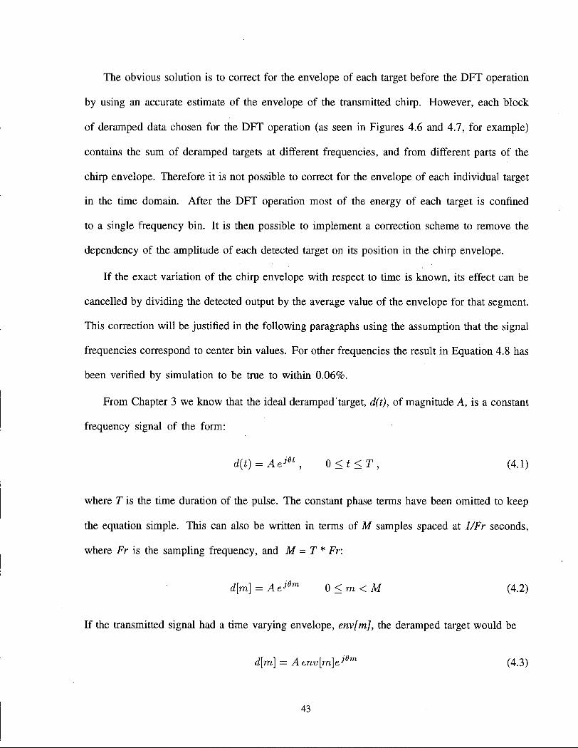
The next step is to examine how the chirp envelope affects the boundary between successive
DFTs. Figures 4.6 and 4.7 illustrate the effect of the chirp amplitude on detected point targets
by showing two consecutive DFT placements on the deramped signals.
2 The chirp replica refers to a copy of the ERS-1 pulse which has been sent through the transmitter and receiver, though not through the
antenna system. This signal is the best available estimate of the amplitude of the transmitted pulse.
-0.4dB
40

Figure 4.6a represents the situation where the chirp amplitude is constant. Correspondingly
the detected targets in 4.6b have equal amplitudes. Figure 4.7a shows the case where the
amplitude of the transmitted pulse, and consequently each deramped target, increases with time
(this is represented by a thickening of the lines representing the frequency-time profile of the
deramped targets). The magnitude of each output point target is the summation of energy through
the gray shaded part of its exposure (DFT input samples). Figure 4.7b shows that the amplitude
of each detected target depends on the average energy of. the section of the transmitted pulse
from which the deramped target samples are chosen. Because of the varying chirp envelope,
the average energy of the deramped targets varies, causing the scalloping effect. The amount
of scalloping corresponds to the energy difference between the beginning and end of the chirp
spectrum.
Note that the detected targets in Figures 4.6b and 4.7b only illustrate detection of the position
of maximum energy for each target, and do not show the actual compressed pulse shape or
sidelobes which are a result of the finite pulse length.
41
Time (a)
DFT bin (b)
Figure 4.6 Illustrating effect of ideal deramped targets (a) on detected targets (b).
1 2 3 4 5 i 6 7 8 9 10
Time (a) DFT bin
(b)
Figure 4.7 Illustrating effect of deramped targets of varying' envelope amplitude (a) on detected targets (b).
Scalloping is a phenomena unique to SPECAN and is a result of the way the matched filter
is applied to the deramped signal. The matched filter changes its center frequency as a function
of time, as it is moved along the raw data compressing blocks of the received signal; in fast
convolution methods the matched filter is stationary in frequency space. The output of SPECAN,
therefore, is dependent on the position of the matched filter with respect to the deramped signal.
The following section will explain the correction implemented to compensate for the varying
energy of the transmitted chirp.
Section 4.3 Proposed Solution of Scalloping Problem
In this section a scheme to correct for the effect of the varying chirp envelope will be
proposed by studying the point target compression equations.
42
The obvious solution is to correct for the envelope of each target before the DFT operation
by using an accurate estimate of the envelope of the transmitted chirp. However, each block
of deramped data chosen for the DFT operation (as seen in Figures 4.6 and 4.7, for example)
contains the sum of deramped targets at different frequencies, and from different parts of the
chirp envelope. Therefore it is not possible to correct for the envelope of each individual target
in the time domain. After the DFT operation most of the energy of each target is confined
to a single frequency bin. It is then possible to implement a correction scheme to remove the
dependency of the amplitude of each detected target on its position in the chirp envelope.
If the exact variation of the chirp envelope with respect to time is known, its effect can be
cancelled by dividing the detected output by the average value of the envelope for that segment.
This correction will be justified in the following paragraphs using the assumption that the signal
frequencies correspond to center bin values. For other frequencies the result in Equation 4.8 has
been verified by simulation to be true to within 0.06%.
From Chapter 3 we know that the ideal deramped target, d(t), of magnitude A, is a constant
frequency signal of the form:
d(t) = Ae]8t, 0<t<T, (4.1)
where T is the time duration of the pulse. The constant phase terms have been omitted to keep
the equation simple. This can also be written in terms of M samples spaced at 1/Fr seconds,
where Fr is the sampling frequency, and M = T * Fr:
d[m] = A ej6m 0 < m < M (4.2)
If the transmitted signal had a time varying envelope, envfm], the deramped target would be
d[m] = Aenv[m]ejdm (4.3)
43

Using the point target arrangement from Figure 4.6, target 1 corresponds to the beginning,
and target 5 to the end of the chirp spectrum. The two segments are shown on the same
envelope in Figure 4.8 for comparison.
lenv(m)
0.4dB
Figure 4.8 Magnitude displacement of first and last detected targets.
(4.4)
Let Yi be the compressed output of the ith target. Using Yj(k) and Ys(k) from the two
extremes of the chirp envelope of Figure 4.8 we can write:
Yx(k) = A - D F T [ e m ; ( m ) e ^ m l m 2
Y5(k) = B-BFT\env(m)ejem
Where A and B are scalars denoting the strength of the reflection from points 1 and 5 on the
ground, respectively.
Using the relationship between convolution and multiplication, the equation can be rewritten
as follows, where "*" is the convolution operator.
J m i
n»3
J6m
J6m 77Z4
m 3
(4.5) Yi(k) = A-DFT[env(m)]™l * DFT
Y5(k) = B-DFT[env{m)]™l * DFT |
For ideal, identical point targets differing only in magnitude, |F i (&) | = \Ys(k)\A/B. For both
Yj(k) and Ys(k) the second term on the right hand side of Equation (4.5) is an impulse of
magnitude N. Therefore the only source of difference in the two detected targets is the DFT of
44

the envelope segments. Denoting the peak value of \Yj(k)\ and \ Ys(k)\ as Y] and Ys respectively,
we can wnte
Yi _ Apeak(DFT[env(m)]™l) Y5 ~ Bpeak(DFT[env(m)]™*)
(4.6)
For the case where the envelope is slowly varying and can be approximated by a straight
line of constant slope the two sections are related by a constant b; for m; < m < m.2,
env(m) = ai(m), and for m.3 < m < m.4, env(m) = 02(m) = a\(m) + b. Because
DFT( a + b ) = DFT( a ) + DFT( b ), the ratio of the two sequences will be:
DFT[oi(m)] DFT[a 2(m)]
N-l
E ai(m) m-0 N-l '
m=0
1, 1, 1, . . . (4.7)
and the only difference between aj(m) and a.2(m) will occur in the first (peak) term. The ratio
of the peak value of the two point targets reduces to
N-l
AJ2 aiim) £l_ _ m=0
B }~2 a2(m) m=0
(4.8)
This verifies that to correct the amplitude difference resulting from the varying chirp envelope
it suffices to normalize each detected target by the mean value of the segment of the envelope
corresponding to the position of the target. The correction vector, C(l), will correct one DFT
output block, and therefore will be G samples long, where G is the number of good DFT output
points. The equation for C(l) will be
ld+Nr-l
Nr
C(l) = 1 /
j ld+Nr-
env (-0 i=ld
0<1<G (4.9)
where d determines the distance between each Nr long section of the amplitude envelope (in
samples). For M being the number of samples in the chirp replica, d is calculated as: d = (M -
Nr) / G. The reason for time-reversing the envelope vector is that the arrangement of output
45
samples (as seen in Figure 4.6, for example) is such that the first output sample of each DFT
block corresponds to the last segment of the deramped target envelope.
This solution has the advantage that its implementation adds very little computation to the
algorithm. Each detected range line must be multiplied by the correction vector, which needs
to be calculated only once. This is important since the main advantage of using SPECAN is its
efficiency compared to other imaging algorithms, therefore a computationally intensive correction
would nullify the main advantage of the algorithm.
In the next section the effect of varying chirp amplitude and correction for it will be tested
on simulated point targets.
Section 4.4 Point Target Simulation
Point target analysis is usually performed to measure the quality of an imaging algorithm,
and the effects of changing parameters on the image quality. We are able to extrapolate our
findings to real data because SAR processing is a linear operation to which superposition applies.
In this section a number of point targets are simulated and the effect of the chirp envelope
shape on the output is observed. It is shown that the correction method explained in the previous
section will eliminate the scalloping. This thesis is concerned with SPECAN range compression,
therefore point targets will be simulated in the range dimension only. The ERS-1 parameters
relevant to the point target simulation and range processing which are used in out simulation
are shown in Table 4.2.
Bandwidth (BW) 15.55 MHz Pulse Length (T) 37.1 fis
Analog to digital complex sampling rate (Fr) 18.96 MHz FM Rate (Kr) 0.4191 MHz/ lis
Table 4.2 ERS-1 SAR parameters for the transmitted signal
46
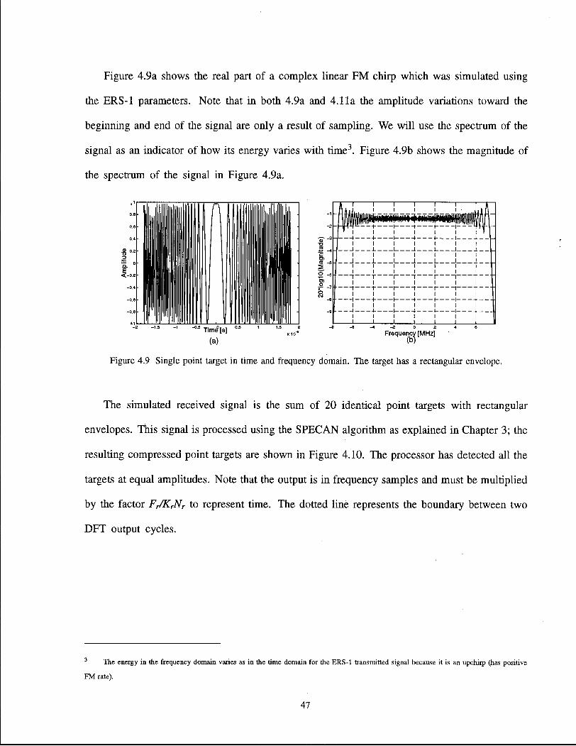
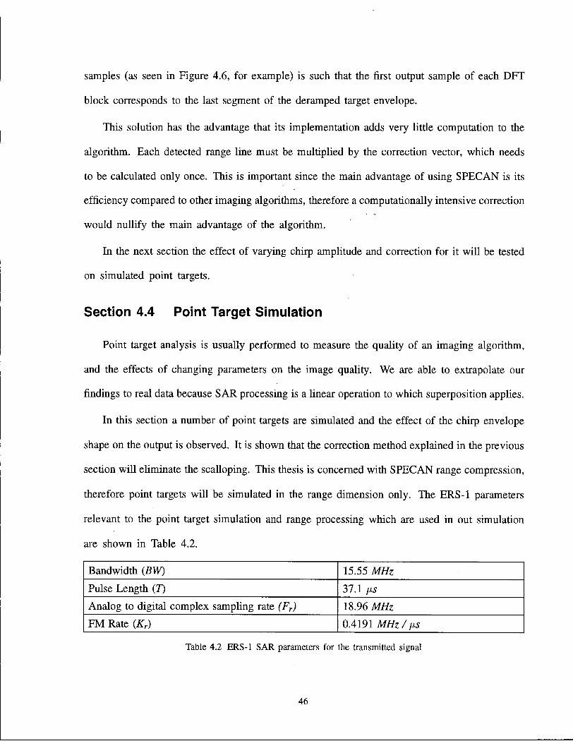
Figure 4.9a shows the real part of a complex linear FM chirp which was simulated using
the ERS-1 parameters. Note that in both 4.9a and 4.11a the amplitude variations toward the
beginning and end of the signal are only a result of sampling. We will use the spectrum of the
signal as an indicator of how its energy varies with time3. Figure 4.9b shows the magnitude of
the spectrum of the signal in Figure 4.9a.
F r e q u e n c y [ M H z ]
Figure 4.9 Single point target in time and frequency domain. The target has a rectangular envelope.
The simulated received signal is the sum of 20 identical point targets with rectangular
envelopes. This signal is processed using the SPECAN algorithm as explained in Chapter 3; the
resulting compressed point targets are shown in Figure 4.10. The processor has detected all the
targets at equal amplitudes. Note that the output is in frequency samples and must be multiplied
by the factor Fr/KrNr to represent time. The dotted line represents the boundary between two
DFT output cycles.
The energy in the frequency domain varies as in the time domain for the ERS-1 transmitted signal because it is an upchirp (has positive
F M rate).
47

o — -25 O
620 640 660 680 700 720 740 760 780 800
Output samples
Figure 4.10 Point targets compressed using SPECAN
Next, the case is shown where the envelope of the transmitted signal is a straight line with
a constant slope. Figure 4.11a shows the real part of the linear F M chirp, and Figure 4.11b is
the spectrum of the signal. The 2 dB gain across the envelope of the signal translates directly
to a 2 dB gain across the spectrum of the signal.
2dB
Figure 4.11 Real part (a), and spectrum (b) of chirp with a linear envelope superimposed
The predicted scalloping is the amount A* = (T,X2 - Hxi)/Nr, which for this example equals
1.38 dB. Nr is the DFT input sample size.
Figure 4.12 is the range compressed output when the input contains 20 equally spaced
identical targets of the form in Figure 4.11. We see the time varying chirp envelope causes
48
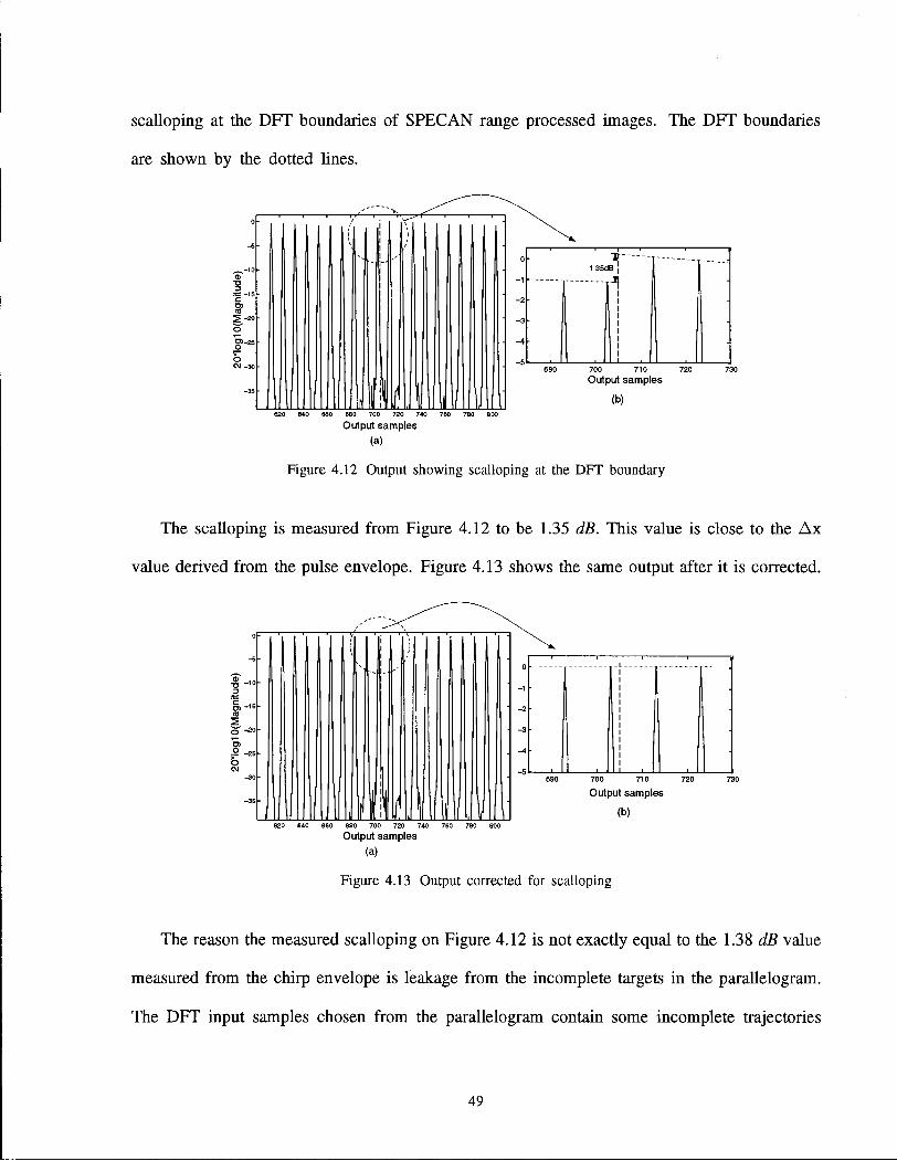
scalloping at the DFT boundaries of SPECAN range processed images. The DFT boundaries
are shown by the dotted lines.
820 840 880 880 700 720 740 780 780 800
Output samples (a)
Figure 4.12 Output showing scalloping at the DFT boundary
The scalloping is measured from Figure 4.12 to be 1.35 dB. This value is close to the Ax
value derived from the pulse envelope. Figure 4.13 shows the same output after it is corrected.
700 710 720
Output samples
(b) 700 720 740 760 780 800
Output samples (a)
Figure 4.13 Output corrected for scalloping
The reason the measured scalloping on Figure 4.12 is not exactly equal to the 1.38 dB value
measured from the chirp envelope is leakage from the incomplete targets in the parallelogram.
The DFT input samples chosen from the parallelogram contain some incomplete trajectories
49

of targets from the next and previous DFT blocks. These incomplete targets contain a non-
integer number of cycles. Although the output points corresponding to these incomplete targets
is discarded, part of their energy is introduced in the good DFT output points as leakage and
cannot be removed. However the amount of energy leakage introduced in this way is in the
hundredths of dBs and not significant.
Comparing Figures 4.10 and 4.13 shows that the correction factor eliminates the scalloping
resulting from the varying chirp envelope to at least 0.03 dB in the point target simulation.
50

Chapter 5 Range-SPECAN on ERS-1 Data
This chapter presents the results of SPECAN range compression on ERS-1 data. The
functions of the ERS-1 synthetic aperture radar are outlined; the properties of the raw satellite
data and their impact on SPECAN range processing is described.
Section 5.1 The ERS-1 Satellite
To verify the results of the point target simulation of the previous chapter, SPECAN range
processing and scalloping correction are carried out on ERS-1 satellite data. This satellite was
launched on July 17, 1991 by the European Space Agency (ESA). Its main objective is to
increase the understanding of the interaction between the earth's atmosphere and oceans on a
global scale. Other major benefits it provides are ice-coverage measurements, monitoring of
pollution, and land use changes.
Figure 5.1 shows the geometry of the ERS-1 satellite in strip-mapping mode. In this mode
the satellite obtains high resolution imagery of a strip of ground by sending a microwave beam
towards the ground at regular intervals and receiving the echo while moving at a constant
velocity. The ERS-1 is placed in a polar orbit with a mean altitude of 780 km, and images 100
km wide strips of terrain.
51

imaged swath 100 km
Figure 5.1 ERS-1 SAR strip-mapping geometry
Some of the ERS-1 SAR engineering parameters are given in Table 5.3.
SAR antenna size 10 m long, 1 m wide Frequency 5.3 GHz (C band) Bandwidth 15.55 MHz Pulse Length 37.1 fis
FM rate 0.4191 MHz/ps Polarization linear vertical AID complex sampling rate 18.96 Msamples/sec
I and Q quantisation 5 bits Sampling window duration 299 fxs
Swath width 100 km
Incidence angle 23° at midswath Data rate 105 Mbps
Table 5.3 ERS-1 SAR parameters
The operations of the ERS-1 Active Microwave Instrument (AMI) which also includes the
SAR module have been explained fully by Carter [35], Blisset [36], and Francis [7]. The SAR
module of the ERS-1 satellite transmits pulses, amplifies and filters the received signal. The
module has two modes of operation: image mode, and wave mode. Image mode obtains the
52

high resolution imagery with which we are concerned in this thesis, so all ERS-1 operations
mentioned from now on are image mode operations. The transmit module of the SAR outputs a
linearly chirped pulse of 15.55 MHz bandwidth and 37.1 fis length at the intermediate frequency
of 123 MHz. The up-converter converts the output to 5.3 GHz, amplifies to 250 mW and sends
to the high power amplifier (HPA). The signal is then amplified to about 4.5 kW and sent to the
circulator assembly and the SAR antenna. The circulator allows the antenna to be time-shared
between transmitter and receiver. The receiver filters the echo and down-converts it to baseband
(zero center frequency). The demodulator creates sine and cosine channels in quadrature. The
receiver also amplifies the received signal to adapt its level to that of the analog-to-digital
convenor. After analog to digital conversion, where the data is quantized to 5 bits for each
of the in-phase (I) and quadrature (Q) channels, and adding auxiliary data, the signal is either
sent to a receiving ground station if one is within transmission distance, or recorded for future
transmission.
Section 5.2 The Chirp Replica
As we have seen in the previous chapter, removal of scalloping requires accurate knowledge
of the profile of the transmitted chirp. The calibration unit of the ERS-1 satellite SAR intercepts
the transmitted chirp after it passes through the HPA and before it reaches the antenna (see Figure
2.2). A copy of this signal is fed back to the receiver and recorded in the echo line as auxiliary
data to be used for on-ground range compression. Thus, this replica of the transmitted signal
contains all the system distortions except those induced by the antenna which are negligible.
For our purpose, the replica pulse is extracted from the raw data header and used as the
most accurate available representative of the transmitted chirp envelope. Figure 5.2a, the absolute
value of one pulse replica, shows that the transmitted signal is noisy and has a non-rectangular
envelope. The SAR receiver thermal noise contributes to the replica noise. As Figure 2.2 shows,
53
the chirp replica is intercepted after passing through the high power amplifier, this is another cause
for the distortion seen in the chirp replica. The total distortion, as shown by Blisset [36], can be
divided into linear, quadratic, ripple and noise components. The ripple and noise components
will not have a particular effect at the DFT boundaries and therefore will not affect scalloping.
The linear and quadratic components will be accounted for by the correction vector.
A number of replicas from different scenes have been examined and altogether there is
very little variation in the transmitted signal from scene to scene. A study by Laur [37] has
shown that the ERS-1 replica pulse total power is quite stable (to within ±0.1 dB), that is, the
transmitted signal power does not vary significantly from pulse to pulse. Therefore the degree
of scalloping resulting from the chirp profile should be constant throughout each scene. By
averaging 256 point sections of the chirp replica to derive the correction we are cancelling the
effects of the noise, since 256 points is large enough to mask the short term perturbations of the
replica. Figure 5.2b is the least squares fit straight line derived to show the noiseless envelope,
and the approximately 0.5 dB increase from the beginning to the end of the chirp profile.
54
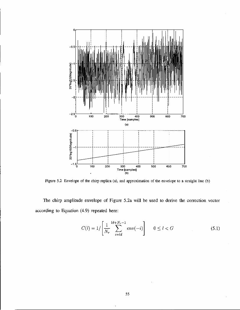
The chirp amplitude envelope of Figure 5.2a will be used to derive the correction vector
according to Equation (4.9) repeated here:
C(l) = 1/ ^ ld+Nr-1
env(-i) i=ld
0<1<G (5.1)
55

The good DFT output points are derived from the ERS-1 satellite parameters in Table 5.3 and
Equation (3.17) to be 133. The 133 point correction vector derived from the envelope of Figure
5.2a is shown in Figure 5.3 below.
Output samples
Figure 5.3 Correction vector derived from the chirp replica envelope
The effect of scalloping and the correction implemented was tested on a number of ERS-1
scenes. A significant difference in the amount of scalloping was observed between scenes of
land and those of water and ice. The results of testing different combinations of water and
land have been included. The reasons and significance of the differences between the output
of different scene contents is mainly due to saturation of the raw data, and will be explained
in the next chapter.
Section 5.3 Properties of the ERS-1 Raw Data
Prior to processing, it is necessary to verify that the data has not been corrupted during
on-board processes such as in-phase (I) and quadrature (Q) channel separation and analog to
digital conversion, and also that the methods of reading the raw data from the tape are correct.
ERS-1 SAR raw data is received from the ADC output as a string of 5 bit in-phase (I) and
5 bit quadrature (Q) values unpacked to 8 bit integers. The statistical properties of SAR raw
56
data are the initial indicators of the quality of the data. Other ways to test the raw data include
examining the spectrum of the raw data, and forming an image.
5.3.1 Statistical Properties
The "central-limit theorem" states that the sum of N independent random variables approaches
Gaussian distribution as N becomes large. The received SAR echo has a Gaussian probability
density function because the antenna footprint is large and the received SAR echo is the reflection
from a diverse area [19]. Each resolution cell is a few square meters of ground area; the complex
number representing the reflection from this cell is the coherent sum of the many reflections from
each point in this area. The I and Q channels each have Gaussian distribution with 0 mean.
Any dc bias or channel gain imbalance is removed prior to processing1. The validity of using a
Gaussian distribution for ERS-1 raw data has also been verified by Laur [37] by comparing and
showing the agreement of the percent saturation versus the standard deviation plots of simulated
Gaussian data and ERS-1 raw data.
The ERS-1 ADC linearly quantizes the I and Q channel inputs to 5 bit values. The saturation
level of a linear quantizer is set to ka, and for 5 bit quantization of Gaussian signals the optimum
value of k which would minimize the quantization and saturation errors is approximately 2.9. A
larger value of k will decrease saturation noise, and a lower value will decrease the quantization
noise as described by Gray [38] and Richards [39].
Saturation is calculated as the percentage of samples occupying the highest and lowest
quantization levels in excess of the expected percentage of samples at those bins. In general, the
amount of saturation decreases from near range to far range because the strength of the received
backscatter is higher at near range. The amount of saturation in the raw data also depends on
the scene content. Areas with high backscattering level, such as water during storms, will have
1 Channel gain imbalance refers to the ratio of the total power of the I and Q channels which is ideally one.
57
the most amount of raw data saturation. Checking the histogram of the received SAR data and
comparing it with the theoretical Gaussian distribution is one way to evaluate the integrity of the
data. The results of this comparison for the scenes used in the thesis are shown in Figure 5.5.
5.3.2 Spectrum of Raw Data
Ideally, the spectrum of the raw data in the range direction should be that of the transmitted
chirp. The received signal as a function of time, s(t), is the convolution of the transmitted
signal, r(t), and the ground reflectivity, g(t).
s(t) = r(t) * g(t) (5.2)
Using the properties of convolution, the spectrum of the above, S(u>), can be rewritten in
terms of the spectrum of the ground reflectivity, G(u>) and transmitted signal, R(u).
S{u) = R(OJ) G{LO) (5.3)
Summing over a number of range lines will cancel out the effects of G(u>) which is a
random Gaussian variable, revealing the spectrum of the transmitted signal. The shape of S(u)
is rectangular in range and proportional to the squared Sine function in azimuth (see Curlander
[19, p. 86]) representing the antenna pattern. Therefore this test will also verify that the raw
data matrix is oriented with rows corresponding to range lines and columns to azimuth lines.
ERS-1 data from the scenes chosen for this study were validated by the above two methods
prior to processing.
Figure 5.4a shows the range spectrum, and Figure 5.4b the azimuth spectrum of the raw
data from a 512 line by 512 pixel sample of ERS-1 raw data. As expected, the azimuth
spectrum reveals the antenna pattern and the range spectrum corresponds to the spectrum of
a linear FM signal. If the ground reflectivity were constant, the tilt of the range spectrum
58

would be a direct function of the transmitted chirp profile. The ERS-1 does not have automatic
gain control, however, and the ground reflectivity slope is reflected in the slope of the range
spectrum. Therefore the exact envelope of the transmitted signal cannot be recovered from the
range spectrum. (a) Range Spectrum
DFT samples
(b) Azimuth Spectrum
0 50 1 00 150 200 250 300 350 400 450 500 DFT samples
Figure 5.4 Raw data spectrum
Section 5.4 Scenes Chosen for Study
The processing results of four scenes used for the analysis of the SPECAN correction are
presented in this thesis. These scenes are chosen to contain combinations of different types of
features to demonstrate the performance of the correction scheme on different imaged areas.
The scenes will be named and referred to according to their locations or content as the
Nova Scotia ocean scene(A) and (B), the Rhine river scene, and the mountain scene. Each raw
59

data set is 5616 pixels wide by approximately 30000 lines long (approximately 360 Mbytes)
corresponding to a 100 km by 100 km strip of ground.
The mountain scene is of a mountainous, high contrast area; the Nova Scotia(A) scene is
of a homogeneous section of the ocean with high raw data saturation at near range; the Nova
Scotia(B) scene shows some features of ice and turbulent water; the Rhine river scene shows a
sharp radiometric contrast between dark, calm water and bright, turbulent water.
Figure 5.5 shows the histogram of a 500 x 100 sample section of raw data, superimposed is
the dotted line representing the expected normal distribution for that particular standard deviation.
The histogram shows the frequency percentage of raw data at each of the quantization levels.
10
8
(a) Nova Scotia ocean scene (A)
a = 9.66 saturation = 10.86%
10
8
(b) Nova Scotia ocean scene (B)
a = 5.35 saturation = 0.38%
10
8
cy
6 c CD 3 cr 2
4 LL
-10 0 10 Quantized value
(c) Mountain scene
o = 6.22 saturation = 1.26%
-10 0 10 Quantized value
10
8
>> u 6 c CD
-eq 4
LL
2
0
-10 0 10 Quantized value
(d) Rhine river scene a = 4.17 saturation = 0.02%
-10 0 10 Quantized value
Figure 5.5 Histograms showing distribution of raw SAR data
From the plots we can see that the raw data follows the normal distribution closely in the
case of the Rhine scene; the Nova Scotia ocean(B) and mountain scenes show a small degree of
60

saturation, and the Nova Scotia ocean(A) scene shows a high degree of saturation. The effect
of this saturation on the output of SPECAN is described in the next chapter.
Section 5.5 Analysis of SPECAN Output
The degree of scalloping and the effect of the correction scheme will be measured for
different scene contents. To show the scene content two quicklook images will be shown of
the near and far range sections of the range swath. These images are obtained by compressing
2048 pixel by 2048 line segments of raw data from near and far range. SPECAN and fast
convolution are used for range and azimuth compression, respectively. The resulting image is
averaged by four in azimuth to make the ground range/azimuth aspect ratio close to one, and
to reduce the speckle noise.
Also, for each scene the histogram of three sample sections of the raw data chosen at equal
distances from near, mid, and far range will be shown to display the trend in raw data saturation
along the range dimension.
To see the scalloping effects, 5000 lines of each scene will be range compressed using
SPECAN. The magnitude of the range compressed data is averaged over the 5000 range lines
and displayed along with its corrected version. Summing the range lines will cancel out the
noise and the random fluctuations due to the scene features resulting in a relatively smooth line
disjointed at regular intervals due to scalloping. The sum of the magnitude of the 5000 lines
of raw data is also displayed to show the general radiometry of the scene; the shaded sections
indicate the segments of raw data which have been used as input to the SPECAN matched filter.
For scenes of water where the radiometry is smooth a smaller number of lines are needed to show
the scalloping clearly. For scenes of land where the range compressed data has a wider dynamic
range and more frequent fluctuations the scalloping effect can be seen better by summing a
larger number of range lines.
61

The amount of scalloping between sucessive blocks is indicated on the figure showing the
SPECAN output. The scalloping is measured as the amplitude difference between the first output
sample of one block and the last output sample of the preceding block. This measurement does
not take into account the fluctuations in the output which are a result of the natural variations
in the radiometry. To account for these variations the amplitude difference between adjacent
samples is plotted, and the amount of scalloping is alternatively measured as the amount by
which the natural radiometry is exceeded at the DFT block boundary.
5.5.1 Nova Scotia Ocean Scene
The Nova Scotia ocean scene was acquired on February 7, 1994 from the ocean off the coast
of Halifax. The different image contents cause the top and bottom parts of this scene to have
different statistical properties which affect their output after SPECAN compression. Therefore
we have divided this scene into two sections and processed each separately. The section towards
the top of the scene, referred to as Nova Scotia ocean(A), is 5000 lines of featureless water
showing a large amount of saturation in the raw data. Nova Scotia ocean(B) is a 5000 line
section towards the bottom of the scene and contains features of new and old ice; the raw data
in this section has very little saturation.
62

Nova Scotia Ocean(A) Figures 5.6 and 5.7 are the quicklook images of Nova Scotia ocean(A).
Figure 5.6 Near range image of Nova Scotia ocean(A) scene. Pixels 0 to 2047.
Figure 5.7 Far range image of Nova Scotia ocean(A) scene. Pixels 3500 to 5547.
Figure 5.8 shows the histograms of three sample sections of the raw data chosen at equal
distances from near to far range from the Nova Scotia ocean(A) scene. The histogram shows
a high degree of saturation at near range. The saturation decreases along the range direction
because the power of the received signal decreases along range.
10
8
(a) Near range
o=9.66 sat= 10.86%
-10 0 10 Quantized value
(b) Mid range
-10 0 10 Quantized value
(c) Far range
-10 0 10 Quantized value
Figure 5.8 Histograms of Nova Scotia ocean(A) raw data
63

Figure 5.9 shows the result of SPECAN range compression, the chirp replica correction, and
raw data range line summation in Nova Scotia ocean(A). The shaded areas in 5.9c, numbered
from 1 to 12, indicate the samples of raw data which have been used in the SPECAN processing.
The corresponding outputs of each of the input blocks in 5.9a and 5.9b have also been numbered.
The scalloping is quite high in the uncorrected output and there is significant residual scalloping
in the corrected output.
64
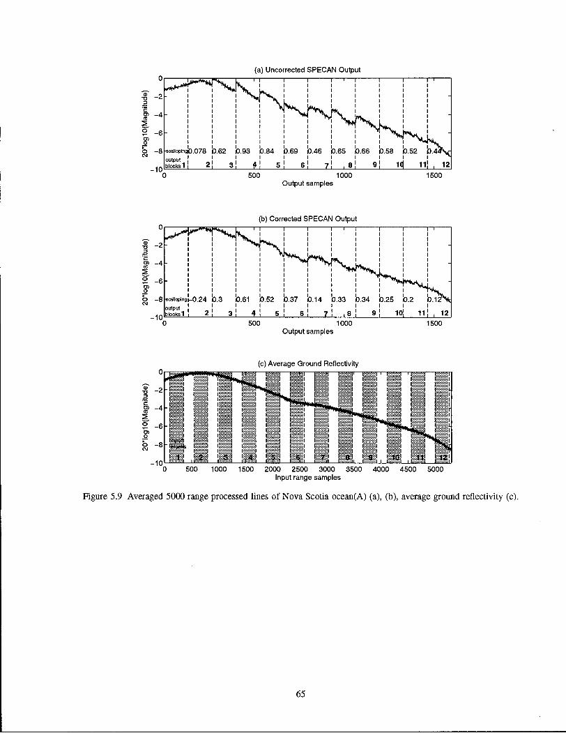
(a) Uncorrected SPECAN Output
0 500 1000 1500 Output samples
(b) Corrected SPECAN Output
0 500 1000 1500 Output samples
65
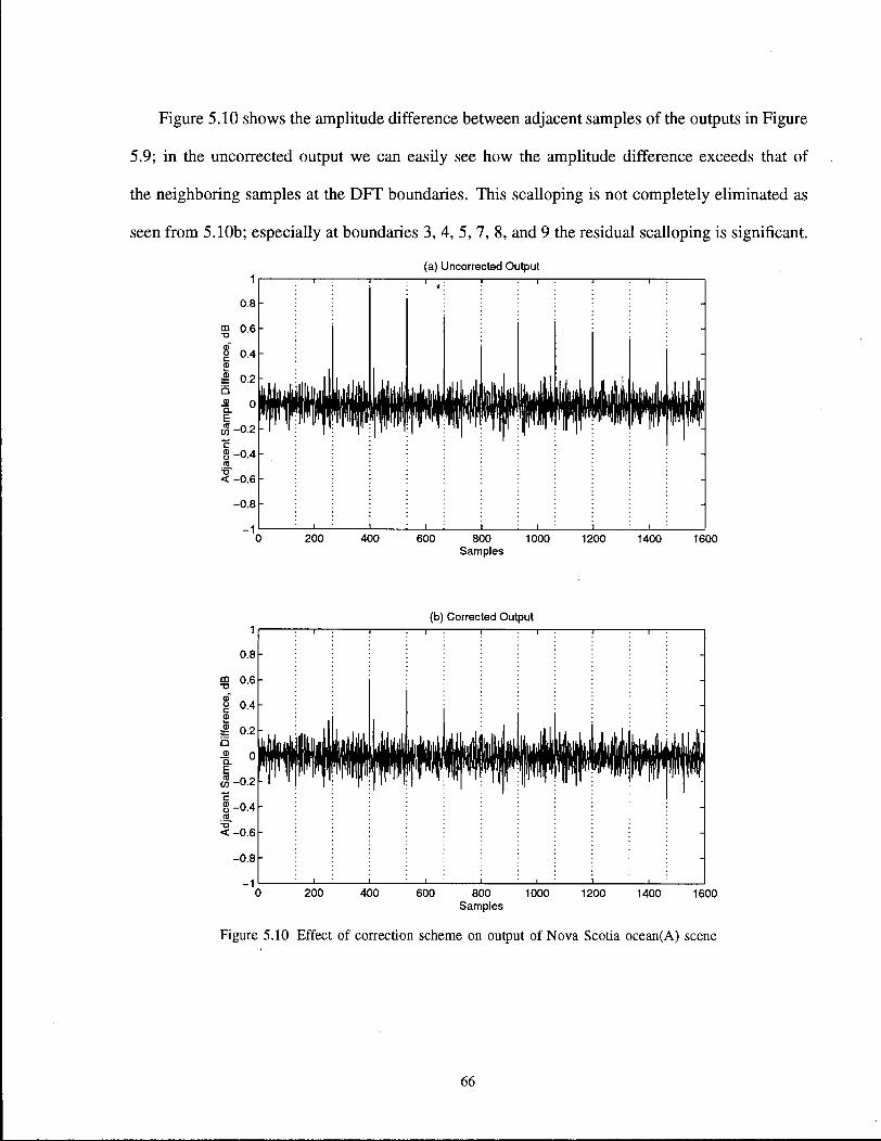
Figure 5.10 shows the amplitude difference between adjacent samples of the outputs in Figure
5.9; in the uncorrected output we can easily see how the amplitude difference exceeds that of
the neighboring samples at the DFT boundaries. This scalloping is not completely eliminated as
seen from 5.10b; especially at boundaries 3, 4, 5, 7, 8, and 9 the residual scalloping is significant. (a) Uncorrected Output
200 400 600 800 1000 Samples
1200 1400 1600
(b) Corrected Output
Figure 5.10 Effect of correction scheme on output of Nova Scotia ocean(A) scene
66

Nova Scotia Ocean(B) Figures 5.11 and 5.12 are the quicklook images of Nova Scotia
ocean(B).
Figure 5.11 Near range image of Nova Scotia ocean(B) scene. Pixels 0 to 2047.
Figure 5.12 Far range image of Nova Scotia ocean(B) scene. Pixels 3500 to 5547.
Figure 5.13 shows the histograms of three sample sections of the raw data chosen at equal
distances from near to far range from the Nova Scotia ocean(B) scene. The degree of saturation
in this scene is far less than the Nova Scotia ocean(A) scene. Note that the missing bin in
5.13c could be due to an error in the ADC in that portion of the data. Figure 5.14 shows the
range-SPECAN output of Nova Scotia ocean(B).
67
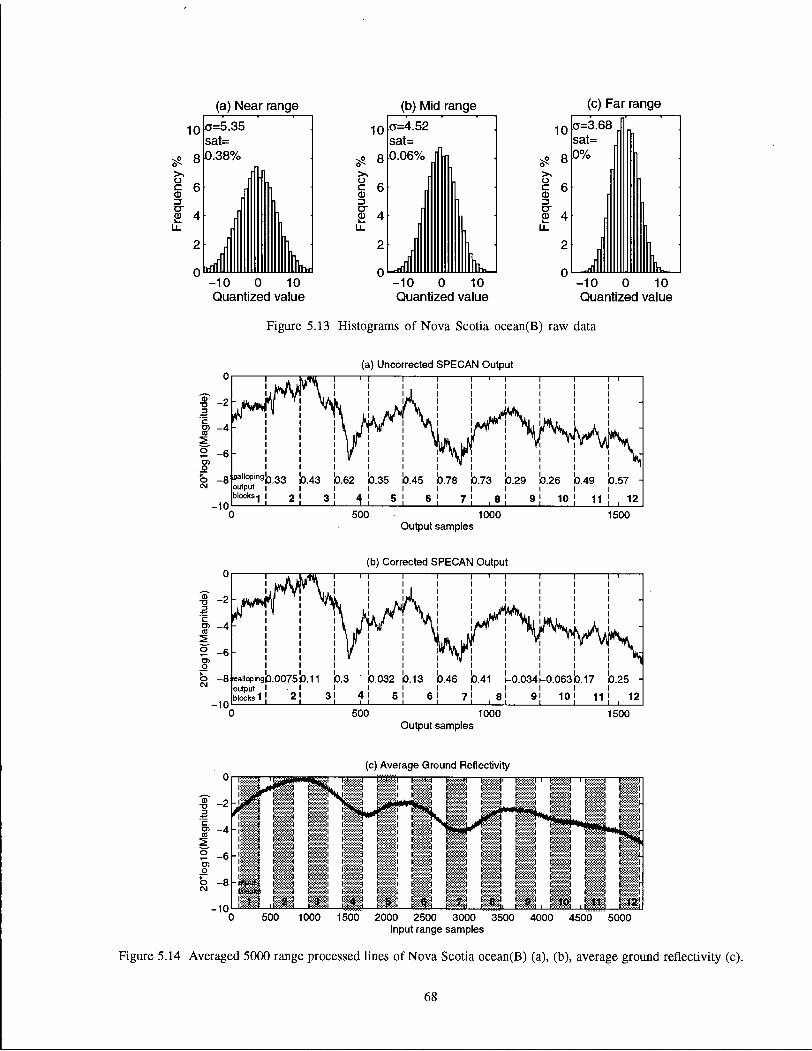
(a) Near range
-|Q 0=5.35 sat=
^ 8 0.38%
-10 0 10 Quantized value
(b) Mid range
1 0 o=4.52 sat=
5? 8 >> c 6 0 ) 3
2 4
-10 0 10 Quantized value
(c) Far range
-10 0 10 Quantized value
Figure 5.13 Histograms of Nova Scotia ocean(B) raw data
-10
-4
-6
_g: callopingjg gg output 1 blocks^ I 2
(a) Uncorrected SPECAN Output
500 Output samples
1000 1500
T3
Ul <0
£ -6 ro
. 0
b -8 -10
(b) Corrected SPECAN Output
1 1 1 1 1 1
teallopingb.0075b.11 output I I blocks 1 ' 2 ]
0.3 0.032 0.13 0.46 0.41 i i
i-0.034l-0.063b. 17 9| 10 j 11
0.25
12 500 1000 1500
Output samples
(c) Average Ground Reflectivity 0 ~l t—rr
i Jr\ * I I Q '* ' it i i i ! I
F :l F 1
Y»i E i i r ! ! E ! E
"1 1 1 1 IF. I 1 1 ! F 1 J 1 J t )
F. 1 F 1
-jjr» 1 1 t -:-:-:| T|fc£j":v:'| 1 iUfc.. 1 E I t I E 1 t 1 £ ) F 4. jr t t ] t ''̂ Sifcli fcSBjfel F 1 t <*U. I- 1 E ) F 1 " t r ) (
I I 1 t ^nb k i 1 j^n F
t 1 1 1 ) t I I I ! 1 t 1 N l L i 1 F , £ 1
-1 1 ) I I I I F 1 E J |«IKpf^ E 1 F 1 1 ! 1 1 ( 1 J ! I I I 1. 1 E J t I F I t I I ) t 1
E 1 t r j 1 I I I F 1 F :l t I F I F 1 1 I F ) F "
.1 t 1 i ! I I I 1 1 F 1 1 1 F 1 t 1 1 ! £ 3 F X 1 t 1 -1 1 I I I 1 1 F 1 1 1 F 1 t 1 1 a E 3 F 1 1 t 1 1 1 I I I I- 1 t -1 E I t I F I I I E ] F 1 1. J 1 * f I I I i- 1 t 1 1 1 t 1 F 1 1 i F ) t 1
1 1 I 1 1 E 1 1 1 1 F ) £ T btosfat v w % r 1 E 4 | j F | | 1 1 1 F I E 1 1 « ( 1 1 * t 11 ! * i 1*1 •.I, \M , r«i
0 500 1000 1500 2000 2500 3000 3500 4000 4500 5000 Input range samples
gure 5.14 Averaged 5000 range processed lines of Nova Scotia ocean(B) (a), (b), average ground reflectivity (c).
68
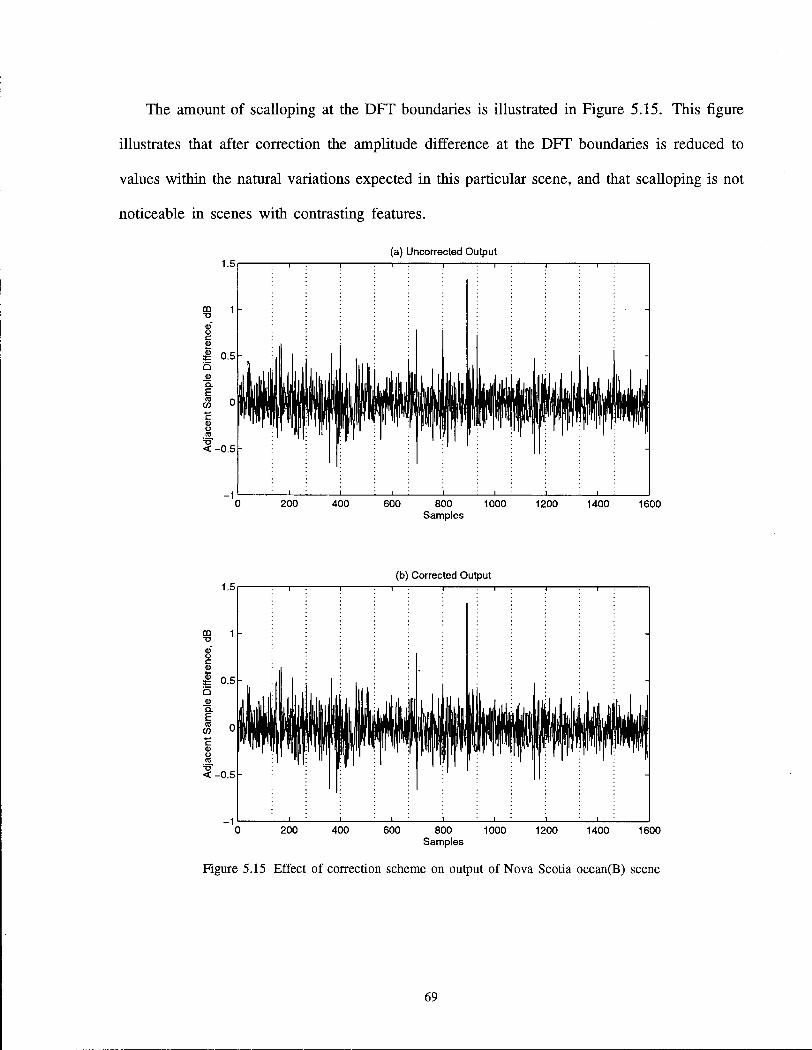
The amount of scalloping at the DFT boundaries is illustrated in Figure 5.15. This figure
illustrates that after correction the amplitude difference at the DFT boundaries is reduced to
values within the natural variations expected in this particular scene, and that scalloping is not
noticeable in scenes with contrasting features.
a) Uncorrected Output
600 800 1000 Samples
1200 1600
(b) Corrected Output
Figure 5.15 Effect of correction scheme on output of Nova Scotia ocean(B) scene
69

The Nova Scotia ocean(A) shows unexpectedly high amounts of scalloping at near range
(Figure 5.9a) tapering to approximately the predictable2 amount at far range; correspondingly,
Figure 5.8 shows a high amount of raw data saturation at near range, decreasing to no saturation at
far range for Nova Scotia ocean(A). The scalloping at far range is almost completely eliminated
by the correction scheme.
Figure 5.13 shows the amount of saturation is low all across range for Nova Scotia ocean(B).
Correspondingly, Figure 5.14a shows the amount of scalloping does not have a particular trend
with range. The corrected output in 5.14b shows no visible scalloping which is verified by 5.15b.
5.5.2 Rhine River Scene
The Rhine river scene was acquired on April 8, 1993 from the North Sea, adjacent to the
mouth of the Rhine river, along the coast of Holland.
The Rhine river scene is divided into sections of bright water, dark water, and land. Figure
5.16 is the quicklook image from near range of this scene. The bright area to the left shows the
choppy waters of the North Sea; the darker areas in the middle and to the right show calmer
waters. The bright spots in the middle of the scene are reflections from ships in the water. Figure
5.17 is the quicklook image from far range of this scene. The slanted line across the middle
is the land water boundary. The water on the left is more turbulent and therefore brighter, the
water adjacent to the land is calm and therefore darker.
The predictable amount is that estimated from the chirp replica envelope, i.e. approximately 0.36 dB.
70
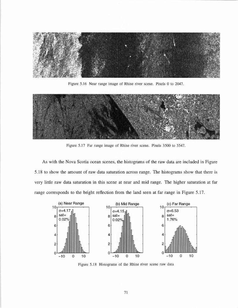
Figure 5.16 Near range image of Rhine river scene. Pixels 0 to 2047.
Figure 5.17 Far range image of Rhine river scene. Pixels 3500 to 5547
As with the Nova Scotia ocean scenes, the histograms of the raw data are included in Figure
5.18 to show the amount of raw data saturation across range. The histograms show that there is
very little raw data saturation in this scene at near and mid range. The higher saturation at far
range corresponds to the bright reflection from the land seen at far range in Figure 5.17.
Figure 5.18 Histograms of the Rhine river scene raw data
71
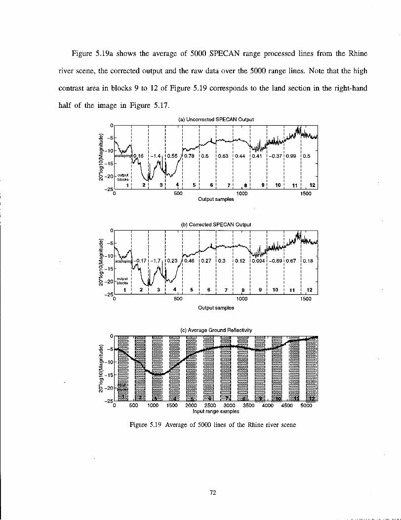
Figure 5.19a shows the average of 5000 SPECAN range processed lines from the Rhine
river scene, the corrected output and the raw data over the 5000 range lines. Note that the high
contrast area in blocks 9 to 12 of Figure 5.19 corresponds to the land section in the right-hand
half of the image in Figure 5.17. (a) Uncorrected SPECAN Output
-6 - a 3
I-10
-25
I j I I I 1 I J I
scallopingll 0 16 -1.4 j ] 0.55 / 0.78 10.6 [0.63 [0.44 [0.41 -0.37 0.99 i 0.5
.output \ blocks | X,
1| 2 3 j 4 ] 5 ! 6 ! 7 ! , 8 ! 9 10 11 ! 12
D 500 1000 1500
ro-io CO
2-15 O)
I - 2 0
Output samples
(b) Corrected SPECAN Output
-25
[
I i ! !
| 1 1 1 1 1
J I
scallop ind -0.17 -1.7, l 0.23 /o.46 10.27 !o.3 10.12 I 0.094 -0.69 0.67 l 0.18
output I "blocks I
i i _
1 [ 2 i 3 i 4 I 5 [ 6 1 7 ! 8 i 9 10 11 ' 12
500 1000 1500
Output samples
0
-5
-10
-15
-20
-25
(c) Average Ground Reflectivity F it T % 1 ET""! f F | F n " JI r j i t - j 11 t 9 F E:-:-:-:-:-:-:3 i 3 t « 3 F J E j F 1 i | j \ ! E )
^ 1 | 3 1 1 1 I 3 F 1 1 ^ i E i « E ) I E J F 4 1 3 F 1 r t F t:-:-:-:->:-:j E i i t 3 t' 1 1 1 F 1 -r i F fr*5jdr^ j>:-:-:w>|
i 1 f i i t i t j 1 * f r F E ' i s F 1 I F 1 E ) I 4 E 1 t E *k.F jjjPE-:-:-:-:) )>:*:•:•:•:•! i j F i I F i E i I t E 1
-F £ rs<#* i j t i I f 3 f j I 3 i i 1 F F i i i i t i \ 3 f 3 t I I 3 t. I i F i t f 1 p I i f t \ 1 f 3 t I 3 t l mm F t E
| [ (:•:•:•:•:•:•:•! i j £:•:•:•:•:•:•:) ! 1 i i ! f
^ EgSSJ f « i p i :
3 F 1 "teste F
t E | [ t i t ! i ;
i ; \ j ! 1 i i ! f ^ EgSSJ f « i p i :
i f r j i i
!..!.. • t a .1 tit... E.*4,.l t .S .I ! ?! F mi ,:::*H ...Al f ta! ,1 <
500 1000 1500 2000 2500 3000 3500 4000 4500 5000
0> TJ
'E o> 03
o CD O
Input range samples
Figure 5.19 Average of 5000 lines of the Rhine river scene
72
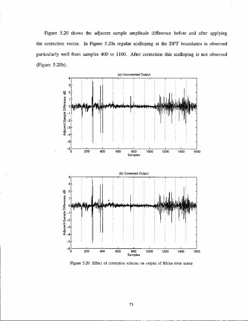
Figure 5.20 shows the adjacent sample amplitude difference before and after applying
the correction vector. In Figure 5.20a regular scalloping at the DFT boundaries is observed
particularly well from samples 400 to 1100. After correction this scalloping is not observed
(Figure 5.20b).
(a) Uncorrected Output
m 2
2 1
Q
1-1 E
§-3h (0
TJ" < -4h
200 400 600 800 Samples
1000 1200 1400 1600
(b) Corrected Output
400 600 800 1000 Samples
1200 1400 1600
Figure 5.20 Effect of correction scheme on output of Rhine river scene
73
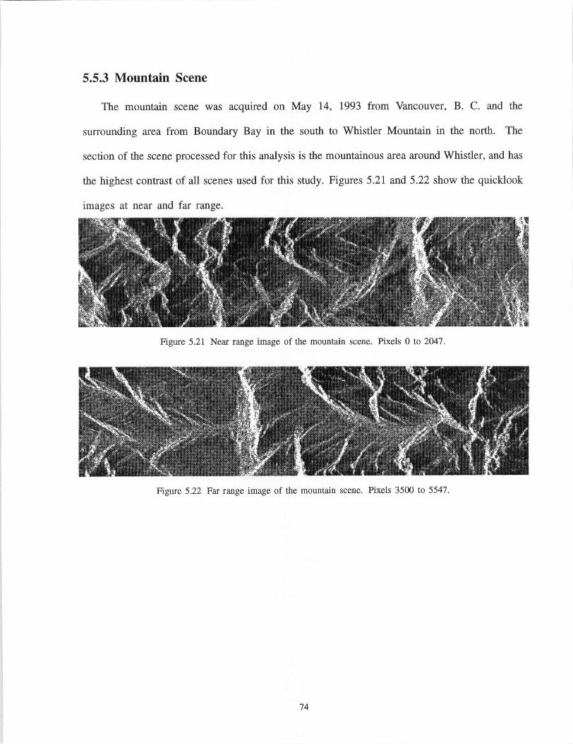
5.5.3 Mountain Scene
The mountain scene was acquired on May 14, 1993 from Vancouver, B. C. and the
surrounding area from Boundary Bay in the south to Whistler Mountain in the north. The
section of the scene processed for this analysis is the mountainous area around Whistler, and has
the highest contrast of all scenes used for this study. Figures 5.21 and 5.22 show the quicklook
images at near and far range.
Figure 5.21 Near range image of the mountain scene. Pixels 0 to 2047.
Figure 5.22 Far range image of the mountain scene. Pixels 3500 to 5547.
74
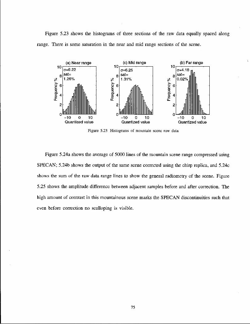
Figure 5.23 shows the histograms of three sections of the raw data equally spaced along
range. There is some saturation in the near and mid range sections of the scene.
Figure 5.23 Histograms of mountain scene raw data
Figure 5.24a shows the average of 5000 lines of the mountain scene range compressed using
SPECAN; 5.24b shows the output of the same scene corrected using the chirp replica, and 5.24c
shows the sum of the raw data range lines to show the general radiometry of the scene. Figure
5.25 shows the amplitude difference between adjacent samples before and after correction. The
high amount of contrast in this mountainous scene masks the SPECAN discontinuities such that
even before correction no scalloping is visible.
75
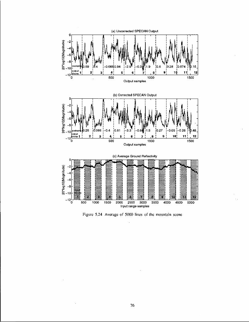
(a) Uncorrected SPECAN Output
0 500 1000 1500 Output samples
(b) Corrected SPECAN Output
0 500 1000 1500 Output samples
(c) Average Ground Reflectivity
0 500 1000 1500 2000 2500 3000 3500 4000 4500 5000 Input range samples
Figure 5.24 Average of 5000 lines of the mountain scene
76

(a) Uncorrected Output 41 : I : 1 : 1 : 1 : 1 : 1 : r
3 -CD
_4i : i : i : i : i : i : i : i : I 0 200 400 600 800 1000 1200 1400 1600
Samples
(b) Corrected Output 41 : 1 : 1 : 1 : 1 :
3 -m
_4l : i : i : i : i : i : i : i : I 0 200 400 600 800 1000 1200 1400 1600
Samples
Figure 5.25 Effect of correction scheme on output of mountain scene
This chapter has shown that the degree of scalloping varies from scene to scene, and
from near to far range in each scene. Significant scalloping is observed in scenes with low
contrast features, and particularly in the sections of these scenes which have high degree of raw
data saturation. The next chapter will discuss the effects of raw data saturation on SPECAN
scalloping.
77

Chapter 6 Effects of Raw Data Saturation on SPECAN Scalloping
In this chapter the effects of saturation in the ERS-1 analog to digital converter on scalloping
are analyzed.
Scalloping is caused because of the amplitude difference between the beginning and end of
the transmitted chirp. Because the transmitted chirps are almost identical the amount of scalloping
should be the same in all scenes. However, as graphs in the previous section indicate, the amount
of scalloping varies from scene to scene and with the range axis in each scene. Examining the
raw data shows that a direct correlation exists between the degree of saturation in the raw data
and the amount of scalloping. This section of the thesis will examine this correlation and verify
that saturation in the raw data is the main reason for the very high scalloping observed in some
scenes.
Section 6.1 Scene Content and Saturation
In some scenes the amount of scalloping is constant across range and corresponds to the
slope of the transmitted pulse as predicted in Chapter 4. In these scenes the amount of scalloping
is approximately 0.4 dB. This small degree of scalloping is still large enough to be seen in
uniform, low contrast scenes, and is therefore worth correcting. The scalloping in these scenes
is removed by the correction scheme of Chapter 4.
For other scenes, however, the amount of scalloping varies across range: high at near range
and decreasing gradually to the predicted value at far range. This variation may be explained by
the degree of saturation in the raw data. Because there is no automatic gain control incorporated
in the ERS-1 receiver, saturation will occur unpredictably. It has been observed in this study
78
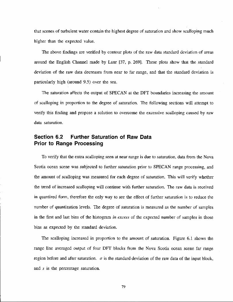
that scenes of turbulent water contain the highest degree of saturation and show scalloping much
higher than the expected value.
The above findings are verified by contour plots of the raw data standard deviation of areas
around the English Channel made by Laur [37, p. 269]. These plots show that the standard
deviation of the raw data decreases from near to far range, and that the standard deviation is
particularly high (around 9.5) over the sea.
The saturation affects the output of SPECAN at the DFT boundaries increasing the amount
of scalloping in proportion to the degree of saturation. The following sections will attempt to
verify this finding and propose a solution to overcome the excessive scalloping caused by raw
data saturation.
Section 6.2 Further Saturation of Raw Data Prior to Range Processing
To verify that the extra scalloping seen at near range is due to saturation, data from the Nova
Scotia ocean scene was subjected to further saturation prior to SPECAN range processing, and
the amount of scalloping was measured for each degree of saturation. This will verify whether
the trend of increased scalloping will continue with further saturation. The raw data is received
in quantized form, therefore the only way to see the effect of further saturation is to reduce the
number of quantization levels. The degree of saturation is measured as the number of samples
in the first and last bins of the histogram in excess of the expected number of samples in those
bins as expected by the standard deviation.
The scalloping increased in proportion to the amount of saturation. Figure 6.1 shows the
range line averaged output of four DFT blocks from the Nova Scotia ocean scene far range
region before and after saturation, a is the standard deviation of the raw data of the input block,
and s is the percentage saturation.
79
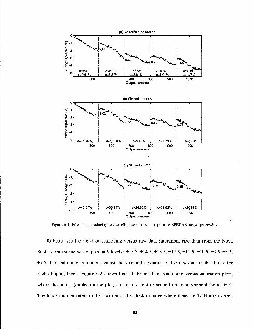
(a) No artificial saturation
500 600 700 800 900 1000 Output samples
(b) Clipped at ±11.5
500 600 700 800 900 1000 Output samples
(c) Clipped at ±7.5 i i i
1.16^W Wry
Jo.85
s=40.54%, s=33.84% ,s=26.62% j s=23.92°/o ! s=20,.63% 500 600 700 800 900 1000
Output samples
Figure 6.1 Effect of introducing excess clipping in raw data prior to SPECAN range processing.
To better see the trend of scalloping versus raw data saturation, raw data from the Nova
Scotia ocean scene was clipped at 9 levels: +15.5, +14.5, +13.5, +12.5, +11.5, +10.5, +9.5, +8.5,
±7.5; the scalloping is plotted against the standard deviation of the raw data in that block for
each clipping level. Figure 6.2 shows four of the resultant scalloping versus saturation plots,
where the points (circles on the plot) are fit to a first or second order polynomial (solid line).
The block number refers to the position of the block in range where there are 12 blocks as seen
8 0
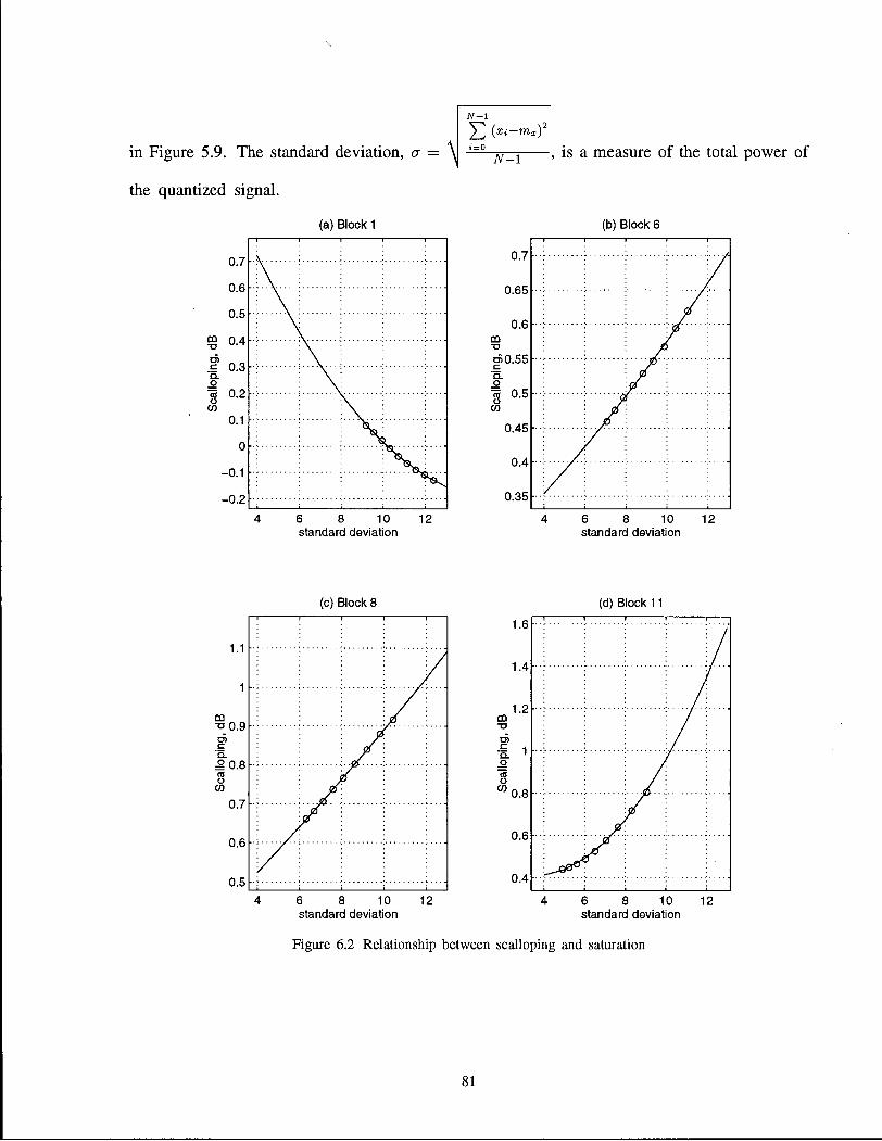
^2 (xi-mx)2
in Figure 5.9. The standard deviation, a = ^ , = 0
N - 1 , is a measure of the total power of
the quantized signal.
4 6 8 10 12 standard deviation
4 6 8 10 12 standard deviation
(c) Block 8 (d) Block 11
standard deviation standard deviation
Figure 6.2 Relationship between scalloping and saturation
81

With the exception of block 1, all the blocks show an increase in scalloping versus saturation
such that at zero saturation the scalloping can be predicted to be approximately 0.4 dB which
is the amount expected from the chirp replica amplitude. As we investigate the mechanism by
which saturation affects scalloping the reason for the anomalous result in block 1 will become
evident.
Section 6 . 3 Effect of Saturation on Range Scalloping
Comparing Figures 6.1a, b and c, we are able to ascertain the effect of saturation on the
SPECAN output. The following paragraphs explain this effect, which is verified by a raw data
simulation in the next section.
Saturation in the ERS-1 raw data occurs as a result of underestimation of the dynamic range
of the input signal to the ADC. In this case, the signal is overamplified, and its dynamic range
exceeds that of the quantizer. This results in overall loss of power in the ADC output.
To demonstrate this, data sets with Gaussian distribution and varying standard deviations
are simulated. Figure 6.3 shows three examples of data with standard deviations of 5, 9, and
13. To simulate the effect of the ERS-1 ADC operation, each data set is clipped at the dynamic
range of the ADC, i.e. at ±15.5. The power loss at each value of standard deviation is the
corresponding shaded area.
82
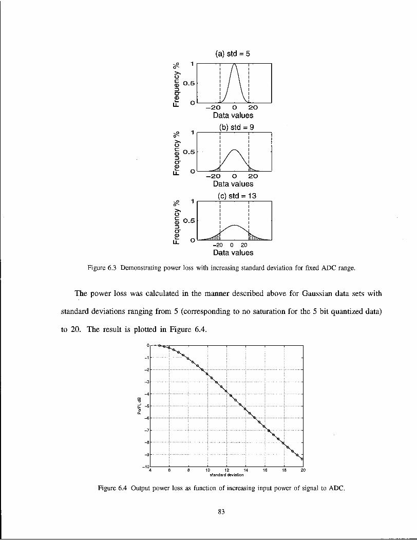
(a) std = 5
- 2 0 o 2 0
Data values (b) std = 9
- 2 0 o 2 0
Data values (c) std = 13
-20 0 20 Data values
Figure 6.3 Demonstrating power loss with increasing standard deviation for fixed ADC range.
The power loss was calculated in the manner described above for Gaussian data sets with
standard deviations ranging from 5 (corresponding to no saturation for the 5 bit quantized data)
to 20. The result is plotted in Figure 6.4.
10 12 14 standard deviation
Figure 6.4 Output power loss as function of increasing input power of signal to ADC.
83
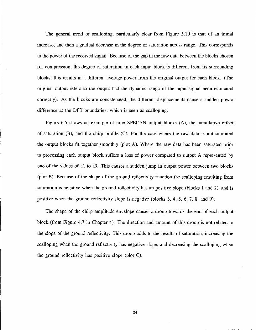
The general trend of scalloping, particularly clear from Figure 5.10 is that of an initial
increase, and then a gradual decrease in the degree of saturation across range. This corresponds
to the power of the received signal. Because of the gap in the raw data between the blocks chosen
for compression, the degree of saturation in each input block is different from its surrounding
blocks; this results in a different average power from the original output for each block. (The
original output refers to the output had the dynamic range of the input signal been estimated
correctly). As the blocks are concatenated, the different displacements cause a sudden power
difference at the DFT boundaries, which is seen as scalloping.
Figure 6.5 shows an example of nine SPECAN output blocks (A), the cumulative effect
of saturation (B), and the chirp profile (C). For the case where the raw data is not saturated
the output blocks fit together smoothly (plot A). Where the raw data has been saturated prior
to processing each output block suffers a loss of power compared to output A represented by
one of the values of al to a9. This causes a sudden jump in output power between two blocks
(plot B). Because of the shape of the ground reflectivity function the scalloping resulting from
saturation is negative when the ground reflectivity has an positive slope (blocks 1 and 2), and is
positive when the ground reflectivity slope is negative (blocks 3, 4, 5, 6, 7, 8, and 9).
The shape of the chirp amplitude envelope causes a droop towards the end of each output
block (from Figure 4.7 in Chapter 4). The direction and amount of this droop is not related to
the slope of the ground reflectivity. This droop adds to the results of saturation, increasing the
scalloping when the ground reflectivity has negative slope, and decreasing the scalloping when
the ground reflectivity has positive slope (plot C).
84
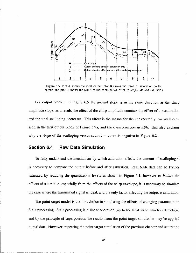
Figure 6.5 Plot A shows the ideal output, plot B shows the result of saturation on the output, and plot C shows the result of the combination of chirp amplitude and saturation.
For output block 1 in Figure 6.5 the ground slope is in the same direction as the chirp
amplitude slope; as a result, the effect of the chirp amplitude counters the effect of the saturation
and the total scalloping decreases. This effect is the reason for the unexpectedly low scalloping
seen in the first output block of Figure 5.9a, and the overcorrection in 5.9b. This also explains
why the slope of the scalloping versus saturation curve is negative in Figure 6.2a.
Section 6.4 Raw Data Simulation
To fully understand the mechanism by which saturation affects the amount of scalloping it
is necessary to compare the output before and after saturation. Real SAR data can be further
saturated by reducing the quantization levels as shown in Figure 6.1, however to isolate the
effects of saturation, especially from the effects of the chirp envelope, it is necessary to simulate
the case where the transmitted signal is ideal, and the only factor affecting the output is saturation.
The point target model is the first choice in simulating the effects of changing parameters in
SAR processing. SAR processing is a linear operation (up to the final stage which is detection)
and by the principle of superposition the results from the point target simulation may be applied
to real data. However, repeating the point target simulation of the previous chapter and saturating
85
the data before compression will not increase our understanding of the way saturation affects
SPECAN processing. The harmonics created in the spectrum of the signal due to saturation
add up in a deterministic pattern which depends on the spacing between the point targets. This
pattern is repeated with each DFT block, showing an effect which is similar to scalloping but
is only a result of the addition of harmonics in a certain pattern. The most significant effect
of saturation on real data is a loss of power; not distinct harmonics. Another reason for the
unsuitability of point target simulation in this case is that the results cannot be extended to real
data because saturation is a non-linear operation.
6.4.1 Model
To properly simulate the effects of saturation it is necessary to have as realistic a model of
the received signal as possible. For this, received raw data was simulated using the statistical
properties of SAR signals. Various raw signal simulators of three-dimensional scenes have been
presented such as the one by Franceschetti, et al. [40], but for the purpose of this experiment
only a simple model is considered as follows.
The backscatter received from each sampling cell in slant range will be the sum of the
reflection of the many point scatterers in that cell. These reflections will add up coherently
resulting in speckle, which is the grainy appearance of SAR images as described by Elachi [10].
The signal received from each cell in slant range, therefore, will be a delayed version of the
transmitted signal, with a random amplitude and phase.
The simulation is implemented by convolving the transmitted signal with the complex
Gaussian random vector representing the ground reflectivity. The transmitted signal is an ideal
linear FM ramp simulated using the ERS-1 parameters as outlined in Table 5.1. As a result of
introducing the random complex ground reflectivity, and a reflection from every resolution cell,
there will be no distinct harmonics as in the point target simulation.
86

The simulated raw data was quantized to 5 bit values before input to the SPECAN processor.
Using knowledge of the dynamic range of the data, the quantizer levels were chosen to minimize
saturation. To simulate saturation, the raw data was multiplied by a scalar to simulate a stronger
reflection while keeping the minimum and maximum levels of the quantizer unchanged.
6.4.2 Simulated Cases
The received power along the imaged swath is dependent upon the SAR viewing geometry,
the antenna gain pattern, and the terrain type as explained by Hawkins [41]. In many SAR
systems this dependence is estimated, and a sensitivity time control (STC) function with the
inverse shape is implemented to flatten the response and minimize saturation (see Teany [42]).
This is not done in the ERS-1 satellite, however, and range attenuation of the raw data must
also be simulated.
The raw data was simulated using the following four situations.
a. Ground reflectivity is constant across range representing ideal ground reflection, the chirp
amplitude is constant, representing the ideal transmitted signal.
b. Ground reflectivity varies across range representing the actual range attenuation, the chirp
amplitude is constant.
c. Ground reflectivity is constant across range, the chirp amplitude has a positive slope
representing the actual transmitted signal.
d. Ground reflectivity varies across range, the chirp amplitude has a positive slope. This
represents the actual received data.
87

The simulated chirp was multiplied by the function in Figure 6.6a to simulate the transmitted
pulse envelope in cases c and d. The simulated ground reflectivity is multiplied by the function
in Figure 6.6b to simulate the range attenuation in cases b and d. The pulse envelope function
has been exaggerated with respect to the actual function to emphasize the output results.
(a) Envelope of transmitted signal
0 100 200 300 400 500 600 Time samples
(b) Ground reflectivity
Range samples
Figure 6.6 Simulated ground reflectivity and transmitted chirp envelope
6.4.3 Output
For each of the cases a to d, SPECAN range processing was performed on 2000 lines of
simulated data, and 2000 lines of the same data after it was saturated and the averaged results
for each case are shown in Figures 6.7 to 6.10. For cases b and d, the saturation will vary
across range as a result of the varying ground reflectivity strength. For cases c and d the output
is corrected using the correction scheme derived from the chirp envelope in Figure 6.6a. The
scalloping shown on the blocks is measured as the amplitude difference between the last and
first samples of adjacent blocks.
88
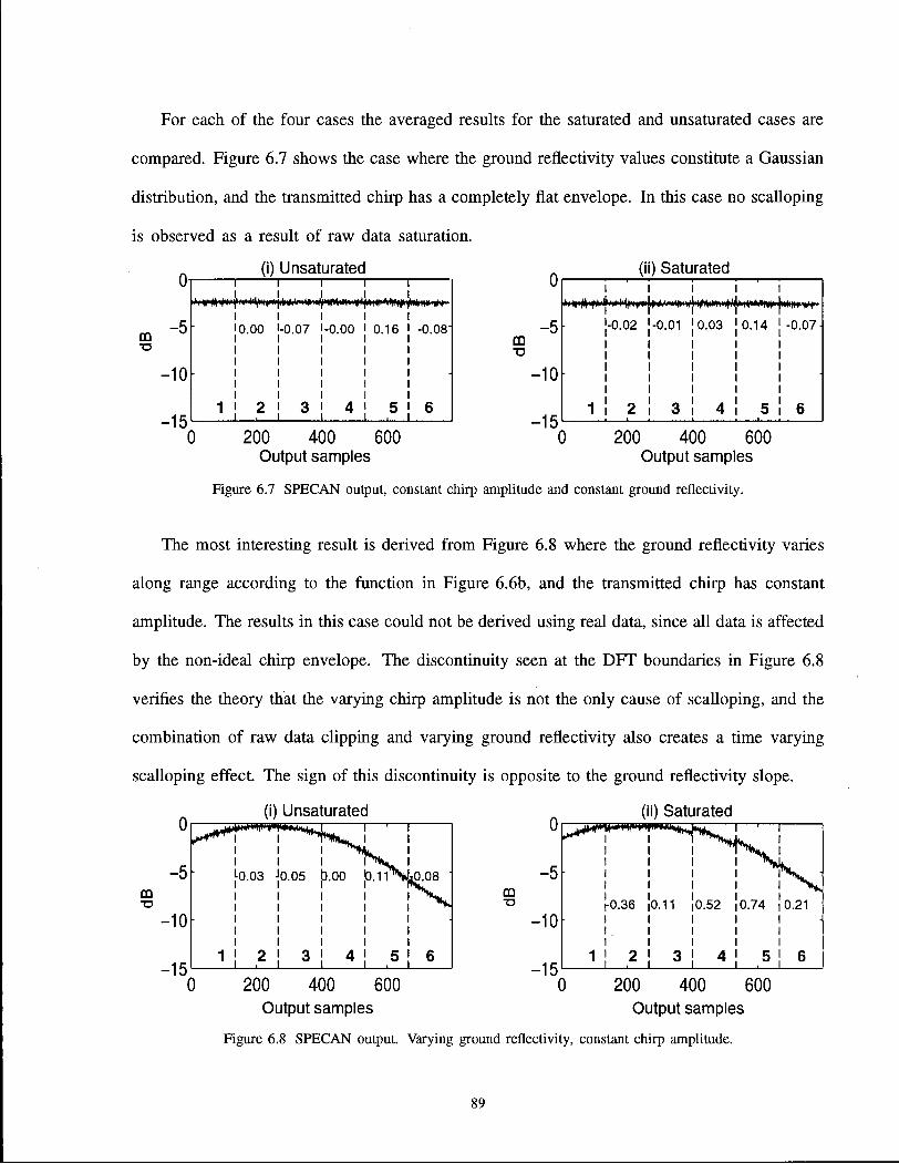
For each of the four cases the averaged results for the saturated and unsaturated cases are
compared. Figure 6.7 shows the case where the ground reflectivity values constitute a Gaussian
distribution, and the transmitted chirp has a completely flat envelope. In this case no scalloping
is observed as a result of raw data saturation.
m •o
0
-5
-10
-15
(i) Unsaturated — i 1 r
I I I I I 10.00 I-0.07 I-0.00 I 0.16 I -0.081
2 ! 3 ! 4 !
CD TJ
0 200 400 600 Output samples
0
-5
-10
-15
(ii) Saturated
,k, |.^nM*tw>|i^»r» •nr***^ M*+»w *m»*f
•0.02 ]-0.01
2 i 3
0.03 0.14 -0.07
0 200 400 600 Output samples
Figure 6.7 SPECAN output, constant chirp amplitude and constant ground reflectivity.
The most interesting result is derived from Figure 6.8 where the ground reflectivity varies
along range according to the function in Figure 6.6b, and the transmitted chirp has constant
amplitude. The results in this case could not be derived using real data, since all data is affected
by the non-ideal chirp envelope. The discontinuity seen at the DFT boundaries in Figure 6.8
verifies the theory that the varying chirp amplitude is not the only cause of scalloping, and the
combination of raw data clipping and varying ground reflectivity also creates a time varying
scalloping effect. The sign of this discontinuity is opposite to the ground reflectivity slope.
m •o
0
-5
-10
-15
(i) Unsaturated (ii) Saturated
1
03 •o
0 200 400 600 0 200 400 600 Output samples Output samples
Figure 6.8 SPECAN output. Varying ground reflectivity, constant chirp amplitude.
89
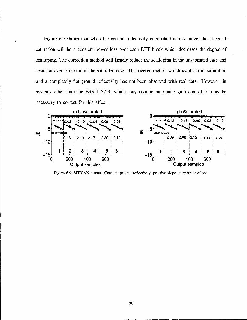
Figure 6.9 shows that when the ground reflectivity is constant across range, the effect of
saturation will be a constant power loss over each DFT block which decreases the degree of
scalloping. The correction method will largely reduce the scalloping in the unsaturated case and
result in overcorrection in the saturated case. This overcorrection which results from saturation
and a completely flat ground reflectivity has not been observed with real data. However, in
systems other than the ERS-1 SAR, which may contain automatic gain control, it may be
necessary to correct for this effect.
rx>
0
- 5
- 1 0
- 1 5
(i) Unsaturated
correctedp 0 2 [-0.10 ,-u.ut . u . u a , - u . u o
;orrecfed I I I I
12.18 | 2 .10 | 2 . 1 7 | 2 .30 i 2 .13
;te4n no ! _n 1 n ! . n n/i ! - 0 . 0 4 0 .09 -0 .08
0
m T3
0 2 0 0 4 0 0 6 0 0 Output samples
- 1 0
- 1 5
(ii) Saturated
corrected-0.12 1 -0 .15 1 - 0 . 0 9 1 0 .02 1 -0 .18
uncorrecjed
' 2 .06 2 . 0 9 2 .12 2 .22 2 .03
0 2 0 0 4 0 0 6 0 0 Output samples
Figure 6.9 SPECAN output. Constant ground reflectivity, positive slope on chirp envelope.
90
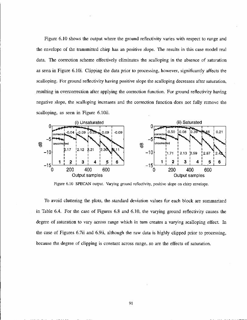
Figure 6.10 shows the output where the ground reflectivity varies with respect to range and
the envelope of the transmitted chirp has an positive slope. The results in this case model real
data. The correction scheme effectively eliminates the scalloping in the absence of saturation
as seen in Figure 6.10i. Clipping the data prior to processing, however, significantly affects the
scalloping. For ground reflectivity having positive slope the scalloping decreases after saturation,
resulting in overcorrection after applying the correction function. For ground reflectivity having
negative slope, the scalloping increases and the correction function does not fully remove the
scalloping, as seen in Figure 6.10ii.
T 3
0
- 5
- 1 0
- 1 5
(i) Unsaturated (ii) Saturated
uncorrected j N 1 I
JD.09 j -0.09
£.17 [2.12 £.21 I i i
2.3CrVte_11
I I 1 | 2 | 3 4 5 ! 6 X
0 2 0 0 4 0 0 6 0 0 Output samples
2 0 0 4 0 0 6 0 0 Output samples
Figure 6.10 SPECAN output. Varying ground reflectivity, positive slope on chirp envelope.
To avoid cluttering the plots, the standard deviation values for each block are summarized
in Table 6.4. For the case of Figures 6.8 and 6.10, the varying ground reflectivity causes the
degree of saturation to vary across range which in turn creates a varying scalloping effect. In
the case of Figures 6.7ii and 6.9ii, although the raw data is highly clipped prior to processing,
because the degree of clipping is constant across range, so are the effects of saturation.
91

block 1 block 2 block 3 block 4 block 5 block 6 (6.7i) a 5.69 5.70 5.69 5.70 5.69 5.69 (6.7ii) a 17.23 17.23 17.05 17.20 17.32 17.17 (6.8i) a 5.77 6.01 5.89 5.69 5.72 5.84 (6.8ii) a 10.69 11.71 11.31 9.77 7.55 5.81 (6.9i) a 5.69 5.71 5.68 5.71 5.70 5.70 (6.9ii) a 11.11 11.11 11.07 11.11 11.13 11.10 (6.10i) a 5.75 6.02 5.94 5.70 5.70 5.84 (6.10ii) a 10.59 11.75 11.50 10.05 7.84 5.91
Table 6.4 Standard deviation of raw data for each output block of Figures 6.7 to 6.10.
Section 6.5 Correction of Residual Scalloping Caused by Saturation
Using the relationship between power loss and standard deviation shown in Figure 6.4, and
the conclusions of the raw data simulation from the previous section, correction of the residue
scalloping should be possible by adjusting the mean power of each output block. This method is
tested on the Nova Scotia(A) scene (Figure 5.9). This scene has the highest raw data saturation
and lowest contrast in features, and therefore shows a significant degree of residual scalloping
(up to 0.4 dB) even after the basic correction.
Two operations per range line are required to correct the scalloping resulting from raw data
saturation. The first operation is the calculation of the standard deviation for each range block.
To get an accurate representation of the standard deviation it must be calculated over a number of
range lines. The optimum number of range lines over which the standard deviation is calculated
depends on how fast the scene content is changing.The second operation is to either calculate,
or find the power loss associated with the standard deviation from a lookup table, and correct
the output block by multiplication with the inverse of the power loss value.
A practical method to calculate the standard deviation of each raw data block during
processing must be devised. For the purpose of testing this correction method, however, the
92
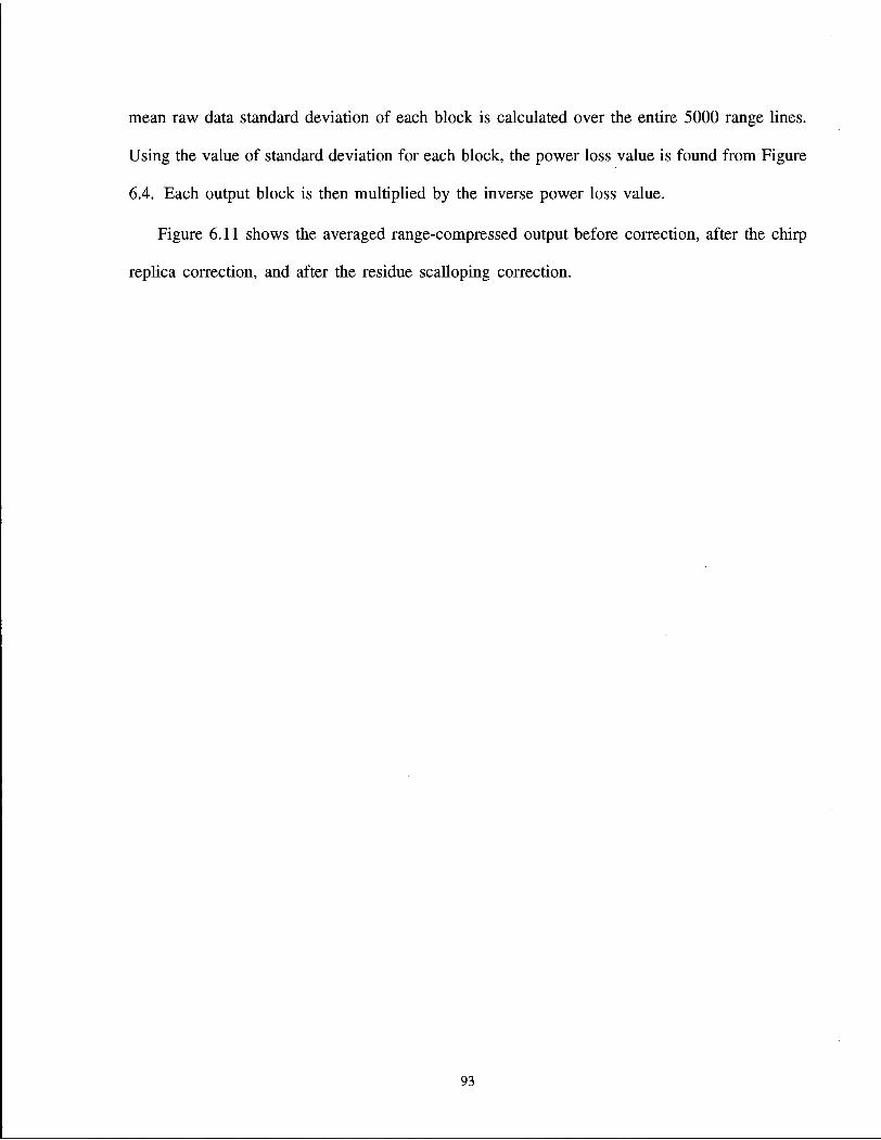
mean raw data standard deviation of each block is calculated over the entire 5000 range lines.
Using the value of standard deviation for each block, the power loss value is found from Figure
6.4. Each output block is then multiplied by the inverse power loss value.
Figure 6.11 shows the averaged range-compressed output before correction, after the chirp
replica correction, and after the residue scalloping correction.
93
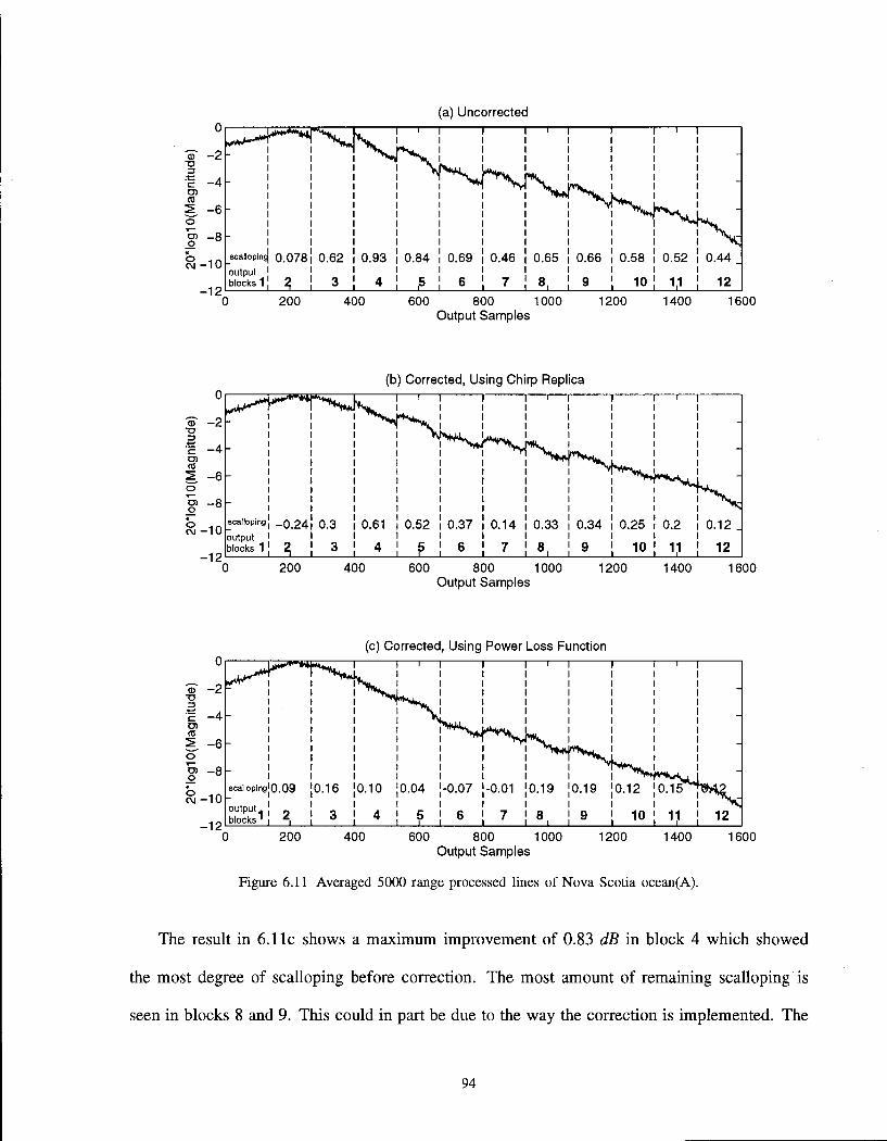
(c) Corrected, Using Power Loss Function
0 200 400 600 800 1000 1200 1400 1600 Output Samples
Figure 6.11 Averaged 5000 range processed lines of Nova Scotia ocean(A).
The result in 6.11c shows a maximum improvement of 0.83 dB in block 4 which showed
the most degree of scalloping before correction. The most amount of remaining scalloping is
seen in blocks 8 and 9. This could in part be due to the way the correction is implemented. The
94

average standard deviation of the blocks over the entire 5000 range lines is used to calculate
the amount of power loss. The relationship between the power loss and the standard deviation
is quadratic (see Figure 6.4); therefore if the standard deviation of the raw data has changed by
a significant amount in the course of these 5000 lines the corresponding power loss (from the
look-up table) will not reflect the average power loss. In this case the objective was to show
that a relationship between power loss and standard deviation exists and that compensating for
the power loss will significantly reduce SPECAN scalloping; this is illustrated by Figure 6.11.
95
Chapter 7 Discussion
Section 7.1 Summary
This thesis summarizes the work done in improving the range image quality of SAR data
processed using the SPECAN algorithm. This algorithm provides a unique method of efficiently
producing SAR images, by processing only chosen segments of the raw data and discarding the
rest. The drawback to using the algorithm has been the scalloping problem in both the range
and azimuth dimensions. The azimuth scalloping has been effectively dealt with; this thesis is
concerned with reducing the range scalloping to an acceptable level.
The work that must be done to effectively eliminate range scalloping can be divided into
two parts. First is correction of the basic scalloping which is due to the transmitted signal
envelope. Second is correction of the residual scalloping seen in some scenes which is due to
the combination of gaps in the raw data, raw data saturation, and range attenuation.
The basic scalloping is due to the fact that look frequencies vary with time, which allows
the amplitude of each output block to be affected by the envelope of the transmitted chirp. The
non-idealities of the transmitted chirp profile will cause distortion in the amplitude of the output
block. When the output blocks are put together to form the image, the amplitude distortion is seen
as a repeating pattern of light and dark bands across the image. By estimating the amplitude of
the transmitted chirp the effect of the distortion on each output block can reversed. In the ERS-1
satellite, a copy of the transmitted signal is recorded to be used for range compression. This
replica is used to estimate the envelope of the transmitted chirp and the SPECAN correction
function. In low saturation scenes the basic correction method reduces the scalloping from
(approximately) 0.5 dB to 0.1 dB.
96
The correction described above does not completely eliminate scalloping in all scenes. The
key cause of the residual scalloping is that the data chosen for the compression process is
from disjointed sections of the raw data. This, combined with raw data saturation and range
attenuation, amplifies the scalloping effect in some scenes. In high reflectivity scenes, such as
those of the ocean, the raw data is highly saturated in near range where the received signal
is strongest. As the received signal power decreases with range, the degree of saturation also
decreases. Correspondingly, images from these areas show a high degree of scalloping in near
range which gradually decreases to a negligible amount in far range. In sections of the scene
with significant raw data saturation the basic correction method reduces the scalloping from
(approximately) 1.1 dB to 0.7 dB.
To see how the range attenuation can cause extra scalloping we must consider that the main
effect of saturation is a loss of power in the saturated output compared to the ideal output. This
power loss varies across range according to the degree of saturation. As each processing block is
chosen from a different part of the raw data, each block has a different power loss from adjacent
blocks. This power loss difference is seen as a sudden amplitude gain between adjacent output
blocks increasing the scalloping effect.
To correct for the effect of raw data saturation on scalloping, a relationship is drawn between
the degree of saturation and the expected power loss in random Gaussian data. Using this function
and the average saturation of each SPECAN range block for one processed scene, the power loss
for each output range block is predicted and compensated for. This procedure was performed
for one of the scenes in this study which showed the highest degree of residual scalloping. The
results showed that this method, combined with the basic scalloping correction, can reduce the
scalloping to negligible amounts.
97
Section 7.2 Future Work
The basic scalloping has been largely eliminated by the correction method of Chapter 4.
The extra scalloping seen in high reflectivity scenes is a result of raw data saturation. Raw data
saturation also causes power loss in images and is identified as the major source of errors in
SAR calibration (Laur [37]). To reduce these problems, future remote sensing satellites should
be built with more quantization levels in the analogue-to-digital converter. In the worst case of
saturation seen in the ERS-1 data the standard deviation of the raw data had increased from 5
(which corresponds to no saturation) to 11. For a standard deviation of 11, 64 distinct levels,
corresponding to 6 bits, would be enough to decrease the saturation to less than 1%.
To reduce saturation with the current 32 quantization levels the receiver gain must be reduced.
The receiver amplifies the signal before it reaches the ADC. The strength of the signal from
high reflectivity areas has been underestimated in the ERS-1 receiver, and the gain levels have
been set such that the received signals' range is far higher than the ADC dynamic range. The
ERS-1 data should be used in future designs to gain a more accurate estimate of the dynamic
range of the received signal.
To continue using the SPECAN algorithm on ERS-1 data, the correction tested in Section 6.5
can be expanded into an efficient algorithm which will measure the standard deviation of each
range block, and using a lookup table estimate and compensate for the power loss of the block
by a scaling operation. The effectiveness of this correction method should be tested on different
scenes. In cases where the raw data is known to be from land or areas with low backscattering
this correction should be bypassed by the operator.
In general, scalloping in high contrast scenes cannot be detected by the human eye. In scenes
of homogeneous areas, however, the scalloping is quite noticeable and can be corrected using the
chirp replica. The chirp replica correction is not computationally intensive, and it is worthwhile
98

to correct all scenes using this method. In homogeneous scenes with raw data saturation, the
scalloping is very high and cannot be compensated for by the chirp replica. In these scenes
the scalloping can be removed by estimating, and compensating for, the power loss. Because
raw SAR data has a Gaussian distribution, the power loss can be predicted by measuring the
standard deviation of the data. This procedure must be integrated in the SPECAN processor by
an efficient and practical algorithm.
99
Bibliography
[1] I. G. Cumming, "Spectral Analysis Approach to the Compression of Linear FM Signals,"
Tech. Rep. TN-79-276-003, MacDonald Dettwiler and Associates, Ltd., Dec. 1979.
[2] ES A, "Method and Apparatus for Processing Data Generated by a Synthetic Aperture Radar,"
European Patent #0048704, Assigned to European Space Agency, Filed September 15, 1981,
Granted February 20, 1985.
[3] S. D. Wall and K. W. Ledbetter, Design of Mission Operations Systems for Scientific Remote
Sensing. Burgess Science Press, Basingstoke, GB, 1991.
[4] S. A. Hovanessian, Introduction to Sensor Systems. Artech House, Inc., Norwood, MA, 1988.
[5] W. G. Rees, Physical Principles of Remote Sensing. Cambridge University Press, 1990.
[6] W. T. K. Johnson and A. T. Edgerton, "Venus Radar Mapper - Multimode Radar System
Design," SPIE - The International Society for Optical Engineering, no. 589, pp. 158-164,
Nov. 1985.
[7] R. Francis, "The ERS-1 Spacecraft and its Payload," ESA Bulletin, vol. 65, pp. 27-48, Feb.
1991.
[8] K. Tomiyasu, "Tutorial Review of Synthetic Aperture Radar (SAR) with Applications to
Imaging of the Ocean Surface," Proceedings of the IEEE, vol. 66, no. 5, pp. 563-583, May
1978.
[9] F. T. Ulaby, R. K. Moore, and A. K. Fung, Microwave Remote Sensing, vol. 2. Addison-
Wesley Publishing Company, 1982.
[10] C. Elachi, T. Bicknell, R. L. Jordan, and C. Wu, "Spaceborne Synthetic-Aperture Imaging
Radars: Applications, Techniques, and Technology," Proceedings of the IEEE, vol. 70,
no. 10, pp. 1174-1196, Oct. 1982.
100

[11] F. T. Ulaby and C. Elachi, Radar Polarimetry for Geoscience Applications. Artech House,
Inc., Norwood, MA, 1990.
[12] L. C. Graham, "Synthetic Interferometer Radar for Topographic Mapping," Proceedings of
the IEEE, vol. 62, no. 6, pp. 763-8, June 1974.
[13] H. A. Zebker, R. P. Salazar, and T. H. Dixon, "Mapping the World's Topography Using
Radar Interferometry: the TOPSAR Mission," Proceedings of the IEEE, vol. 82, no. 12,
pp. 1774-86, December 1994.
[14] J. C. Kirk, "A Discussion of Digital Processing in Synthetic Aperture Radar," IEEE
Transactions on Aerospace and Electronic Systems, vol. AES-11, no. 3, pp. 326-337, 1975.
[15] S. R. Brooks, H. Joyce, F. G. Sawyer, and D. J. Smith, "The ERS-1 Synthetic Aperture
Radar and Scatterometer," GEC Journal of Research, vol. 3, no. 2, pp. 124-36, 1985.
[16] S. J. Austin, D. J. Q. Carter, and J. D. McCaughey, "ERS-1 Spacecraft - Active Microwave
Instrumentation: A Major Achievement," GEC Journal of Research, vol. 9, no. 1, pp. 2-12,
1991.
[17] D. C. Munson and R. L. Visentin, "A Signal Processing View of Strip-Mapping Synthetic
Aperture Radar," IEEE Transactions on Acoustics, Speech, and Signal Processing, vol. 37,
no. 12, pp. 2131-2147, Dec. 1989.
[18] S. Marcus, B. D. Colella, and T. J. Green, "Solid-state Laser Synthetic Aperture Radar,"
Applied Optics, vol. 33, no. 6, pp. 960-4, Feb. 1994.
[19] J. C. Curlander and R. N. McDonough, Synthetic Aperture Radar, Systems and Signal
Processing. John Wiley & Sons, Inc., Toronto, 1991.
[20] D. J. Bonfield and J. R. E. Thomas, "Synthetic Aperture Radar Real-time Processing," IEE
Proceedings, vol. 127, no. 2, pp. 155-159, April 1980.
[21] N. Levanon, Radar Principles. John Wiley & Sons, Inc., New York, 1988.
101

[22] A. H. Nuttal, "Some Windows with Very Good Sidelobe Behaviour," IEEE Transactions
on Acoustics, Speech and Signal Processing, vol. ASSP-29, no. 1, pp. 84-91, Feb. 1981.
[23] J. R. Bennett, I. G. Cumming, and R. A. Deane, "The Digital Processing of Seasat Synthetic
Aperture Radar Data," IEEE International Radar Conference, pp. 168-191, April 1980.
[24] C. Wu, K. Y. Lin, and M. Jin, "Modelling and a Correlation Algorithm for Spaceborne
SAR Signals," IEEE Transactions, AES-18, pp. 563-574, 1982.
[25] L. Chunsheng, L. Jingwen, and Z. Yinqing, "Azimuth Digital Signal Processing Algorithms
for Spaceborne SAR," International Conference on Circuits and Systems, pp. 475-7, June
1991.
[26] J. E. Harris, S. O. Randall, D. M. Chabries, and R. Christiansen, "Quality Measures for
SAR Images," pp. 1064-7.
[27] R. Schotter, R. Gunzenhauser, and H. Holzl, "Real Time SAR Processor," International
Geoscience and Remote Sensing Symposium (IGARSS), vol. 2, pp. 2.1-2.6, 1982.
[28] "The Construction and Testing of a Real-Time Digital Breadboard Processor for the ESA
Remote Sensing Satellite Synthetic Aperture Radar," Tech. Rep. 00-0778, MacDonald
Dettwiler and Associates, Ltd., Dec. 1984.
[29] "Brazil Quicklook SAR Processor High-Level Design," Tech. Rep. BZ-DS-50-2733,
MacDonald Dettwiler and Associates, Ltd., Jan. 29, 1992.
[30] "A Doppler Centroid Estimation Algorithm for the Processing of ScanSAR Data: Prelimi
nary Analysis and Results," Tech. Rep. RC-TN-MDA-SY-0002, MacDonald Dettwiler and
Associates, Ltd., April 18, 1988.
[31] W. J. Caputi, "Stretch: A Time Transformation Technique," IEEE Transactions on
Aerospace and Electronic Systems, vol. 7, no. 2, pp. 269-278, March 1971.
102
[32] A. V. Oppenheim and R. W. Schaffer, Discrete-Time Signal Processing. Prentice-Hall
International, Englewood Cliffs, New Jersey, 1989.
[33] A. Freeman, "SAR Calibration: An Overview," IEEE Transactions on Geoscience and
Remote Sensing, vol. 30, no. 6, pp. 1107-1121, Nov. 1992.
[34] R. C. Gonzalez and R. E. Woods, Digital Image Processing. Addison-Wesley Publishing
Company, Don Mills, Ontario, 1992.
[35] D. J. Q. Carter and S. Hartley, "ERS-1 Active Microwave Instrumentation Engineering
Model Performance," International Geoscience and Remote Sensing Symposium (IGARSS),
vol. 2, pp. 867-70, Sep 1988.
[36] R. J. Blisset and F. G. Sawyer, "ERS-1 SAR Performance Verification," GEC Journal of
Research, vol. 4, no. 1, pp. 47-56, 1986.
[37] H. Laur, P. Meadows, J. I. Sanchez, and E. Dwyer, "ERS-1 SAR Radiometric Calibration,"
SAR Calibration Workshop Proceedings, pp. 257-81, 20-24 Sep. 1993.
[38] G. A. Gray and G. W. Zeoli, "Quantization and Saturation Noise Due to Analog-to-Digital
Conversion," IEEE Transactions on Aerospace and Electronic Systems, pp. 222-3, Jan.
1971.
[39] B. E. Richards and D. C. Lancashire, "The Impacts of Quantization Noise on the ERS-
1 Synthetic Aperture Radar Performance," International Geoscience and Remote Sensing
Symposium (IGARSS), vol. 2, pp. 1159-61, September 1988.
[40] G. Franceschetti, M. Migliaccio, D. Riccio, and G. Schirinzi, "SARAS: A Synthetic
Aperture Radar (SAR) Raw Signal Simulator," IEEE Transactions on Geoscience and
Remote Sensing, vol. 30, no. 1, pp. 110-123, January 1992.
103
[41] R. K. Hawkins, C. E. Livingstone, A. L. Gray, R. B. Olsen, J. G. Halbertsma, and R. A.
Deane, "CCRS C-Band Airborne Radar: System Description and Test Results," Proceedings
of the 11th Canadian Symposium on Remote Sensing, pp. 503-515, 1987.
[42] L. D. Teany and R. K. Hawkins, "The CCRS Airborne SAR STC Function," SAR
Calibration Workshop Proceedings, pp. 177-184, 20-24 Sep. 1993.
104