A 2.5-D Scalar Helmholtz Wave Solution Employing theSpectral Lanczos Decomposition Method (SLDM)yWilliam H. Weedon, Weng Cho Chew and Jiun-Hwa LinDepartment of Electrical and Computer EngineeringUniversity of Illinois, Urbana, IL 61801Apo Sezginer and Vladimir L. DruskinSchlumberger-Doll ResearchOld Quarry Road, Ridgefield, CT 06877Keywords: Lanczos, spectral, scattering, absorbing boundaryAbstractA numerical method is derived for obtaining the solution to the 2.5-D scalar Helmholtzequation involving an arbitrary 2-D lossless inhomogeneous dielectric scatterer excitedby a point source in a closed waveguide. The spectral Lanczos decomposition method(SLDM) is used to solve the di�erential equation by polynomial approximation. Numericalresults indicate that a convergent solution to the 2.5-D problem in a bounded regionmay be achieved in O(N1:5) operations, in agreement with a theoretical upper bound ofO(N1:5 logN). Also, it is demonstrated that the method is accurate for resonant solutionsinvolving eigenvalues on the order of the machine precision. Extension to lossy dielectricsand the implementation of an absorbing boundary condition is discussed.

y This work is supported by the O�ce of Naval Research under grant N000-14-89-J1286, the ArmyResearch O�ce under contract DAAL03-91-G-0339 and a grant from Schlumberger-Doll Research. Computertime is provided by the National Center for Supercomputer Applications at the University of Illinois, Urbana-Champaign.File: lanmotl.tex, 8/29/1996 1

1. IntroductionThe Lanczos method was presented by Lanczos [1] in 1950 as an e�cient method ofcomputing the eigenpairs of a large sparse symmetric matrix. The method has su�ereddue to numerical instabilities whereby the eigenvectors produced by the Lanczos processlose their orthogonality as the algorithm progresses and spurious repeated eigenvalues areproduced. But in 1971, Paige showed that despite the numerical errors, reliable results areachievable [2]. In what has become known as the \Lanczos phenomenon," Paige showedthat if the Lanczos process is carried out far enough, eventually all of the eigenvalues ofthe original matrix will appear as eigenvalues of the tridiagonal matrix produced by theLanczos process (see also [3] and [4]).The idea behind the spectral Lanczos decomposition method (SLDM) proposed byDruskin and Knizhnerman [5, 6] is to use the Lanczos method to build up orthogonalpolynomials that approximate the solution to a di�erential equation. Previously, Lanczosmethods were used to calculate the solution to one-dimensional [7] and multi-dimensional[8] parabolic and hyperbolic problems. Methods similar to the SLDM approach were usedin computational chemistry to calculate spin relaxations in molecular dynamics [9] andalso in [10].Recently, it was shown by Allers, Sezginer and Druskin [11] and also by Tamarchenko[12] that the SLDM technique may be used to solve the 2.5-D Laplace equation e�ciently.The 2.5-D problem is characterized by an inhomogeneity that varies in two spatial dimen-sions, but �elds must be computed in three dimensions because the source is localized in3-D. The advantage to using the SLDM here is that the z-variation may be computedanalytically and numerical computations only need to be performed in a 2-D plane.We consider here the extension of the 2.5-D SLDM to the scalar Helmholtz equationfor an arbitrary lossless dielectric scatterer. Several di�culties naturally arise because thepropagation matrix is no longer de�nite and hence contains both positive and negativeeigenvalues corresponding to propagating and evanescent modes. One problem is that we2

do not have a general proof of convergence for the inde�nite case as we do for a de�nitematrix (see [5] and [6]). However, certain convergence proofs for the de�nite case maybe extended for bounded problems where there are relatively few propagating eigenvalues[13]. Our computer results indicate that convergence for the bounded problem can beachieved in M � O(pN) steps of the Lanczos process for an N � N matrix, yielding a2.5-D solution in O(N1:5) oating-point operations.Another issue is the question of the accuracy of the method in the presence of verysmall eigenvalues. We demonstrate using a computer simulation that we can recover smalleigenvalues on the order of the machine precision and therefore obtain an accurate solutionnear resonance. Problems involving a resonant solution with precisely zero eigenvalue arenot solvable using this method.The numerical example that we use to demonstrate the method consists of the compu-tation of the point source response in a rectangular waveguide with a Dirichlet boundarycondition. Comparison is made between the SLDM solution and closed-form solutions forboth a continuous and discretized waveguide. Finally, we discuss the addition of lossydielectrics and the implementation of an absorbing boundary condition in order to extendthe method to wave scattering problems in an unbounded homogeneous background.2. SLDM SolutionThe 2.5-D scalar wave equation for a planar source may be written as"r2s + @2@z2 + !2c2(�)#�(�; z) = s(�)�(z); (1)which becomes "r2s + !2c2(�) � k2z#�(�; kz) = s(�) (2)after a Fourier transform is applied in the z variable. Discretizing the above, we mayrewrite Equation (2) as �Ds +C ��2k2zI��(kz) = �2s (3)3

where Cjk = �2!2c2(�j)�jk; (4)and Ds is the normalized discrete 2-D Laplacian operator. For elements j interior to the�nite di�erence grid, Ds has the formhDs � �ij = �j+1 + �j�1 + �j+ny + �j�ny � 4�j (5)where ny is the number of discretization points in the y dimension.Now we let A = Ds +C and write the solution to Equation (3) for a particular valueof kz as �(kz) = �2 �A��2k2z I��1 � s: (6)We assume throughout this paper that the inhomogeneous medium is lossless, giving riseto a sparse real symmetric N �N matrix A. Forming the spectral Lanczos decompositionof A, A �Q = Q � T (7)where T is the M �M tridiagonal Lanczos matrix and Q = [q1; q2; : : : ; qM ] is the matrixcontaining the Lanczos vectors. The Lanczos process is started with the choiceq1 = Q � e1 = s=ksk: (8)Taking the spectral decomposition of the tridiagonal matrix T , we haveT = V �� � V t (9)where � = diag[�1; �2; : : : ; �M ]. Using the above, Equation (6) may be rewritten as�(kz) = �2kskQ � V � ��� k2z�2 I��1 � V t � e1: (10)Note that the manipulations leading up to Equation (10) do not depend on the orthogo-nality of the Lanczos vectors qi; i = 1; 2; : : : ;M . We believe that this is one of the main4

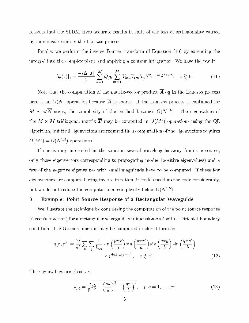
reasons that the SLDM gives accurate results in spite of the loss of orthogonality causedby numerical errors in the Lanczos process.Finally, we perform the inverse Fourier transform of Equation (10) by extending theintegral into the complex plane and applying a contour integration. We have the result[�(z)]j = �i�ksk2 MXk=1Qjk MXm=1VkmV1m��1=2m e�i�1=2m z=�; z >< 0: (11)Note that the computation of the matrix-vector product A � q in the Lanczos processhere is an O(N) operation because A is sparse. If the Lanczos process is continued forM � pN steps, the complexity of the method becomes O(N1:5). The eigenvalues ofthe M �M tridiagonal matrix T may be computed in O(M2) operations using the QLalgorithm, but if all eigenvectors are required then computation of the eigenvectors requiresO(M3) = O(N1:5) operations.If one is only interested in the solution several wavelengths away from the source,only those eigenvectors corresponding to propagating modes (positive eigenvalues) and afew of the negative eigenvalues with small magnitude have to be computed. If these feweigenvectors are computed using inverse iteration, it could speed up the code considerably,but would not reduce the computational complexity below O(N1:5).3. Example: Point Source Response of a Rectangular WaveguideWe illustrate the technique by considering the computation of the point source response(Green's function) for a rectangular waveguide of dimension a�b with a Dirichlet boundarycondition. The Green's function may be computed in closed form asg(r; r0) = 2iabXp Xq 1kpq sin�p�xa � sin�p�x0a � sin�q�yb � sin�q�y0b �� e�ikpq(z�z0); z >< z0: (12)The eigenvalues are given askpq = sk20 � �p�a �2 � �q�b �2; p; q = 1; : : : ;1 (13)5

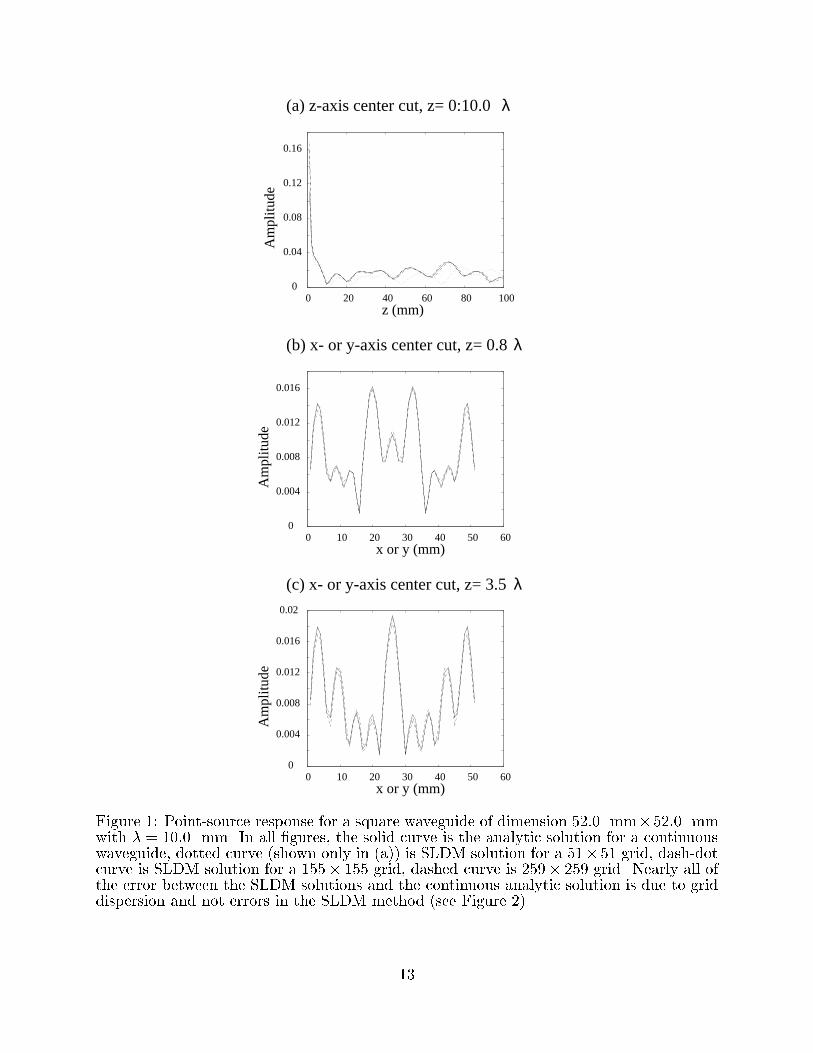
for a continuous waveguide andkpq = (k20 � 4(nx + 1)2a2 sin 2� p�2(nx + 1)�� 4(ny + 1)2b2 sin 2� q�2(ny + 1)�)1=2p = 1; : : : ; nx; q = 1; : : : ; ny (14)for a discretized waveguide, where nx and ny represent the number of discretization pointsalong the x and y axis. Note that the double summation in Equation (12) is carried outover an in�nite number of modes in the continuous case, but is limited to a �nite numberfor the discrete case.The solution was computed for a 5:2��5:2� square waveguide square waveguide usingboth the SLDM approach and the closed-form solution above. We used a value of k0 =:62832 (� = 10 mm) with waveguide dimensions a = b = 52 mm. The SLDM solutionwas computed for three di�erent discretization levels: a 51 � 51 grid (10 points=�), a155� 155 grid (29:8 points=�) and a 259� 259 grid (49:8 points=�).Figure 1 shows a comparison of the point source response computed using SLDM withthe three levels of discretization versus the analytic solution for the continuous waveguide.In Figure 1(a) it is clear that the solution for the 51� 51 grid does not agree well with theanalytic solution. Note in particular that the error in the solution increases with z. Thiserror is not inherent in the SLDM computation; it is a modeling error known as grid dis-persion that is due to discretization of the �eld inside the waveguide. As the discretizationdensity is increased in Figure 1(a), the SLDM solution approaches the analytic solutionfor the continuous waveguide.Figures 1(b) and 1(c) show a cross-section of the �eld in the waveguide at z = 0:8�and z = 3:5�. The SLDM solution for the 51� 51 grid is not shown in parts (b) and (c)because the amount of grid dispersion is so high.In Figure 2 we compare the SLDM solution to the analytic solution for a discretewaveguide. A z-axis cut for the 51� 51 grid is shown in (a) and a cross-section is shownin (b) for the 155 � 155 grid at z = 0:8�. The SLDM and the analytic solution for thediscretized waveguide are indistinguishable. The results in Figure 2 clearly show that6

nearly all of the errors that appear in Figure 1 are due to grid dispersion, and not errorsin the SLDM computation.Table 1 shows a breakdown of the computation times for various parts of the SLDMsolution along with memory usage and the number of steps of the Lanczos process requiredfor convergence. The number of steps required for convergence was determined by trial-and-error here, although more systematic methods are given in [4] and [14]. We found thatthe value of M required for convergence was well de�ned since the error in the solutionwas quite noticeable when the solution did not converge.The computation times reported in Table 1, with the exception of the CPU secondsreported by the operating system, are wallclock times accurate to the nearest second thatwere computed by averaging three trial runs of the code. The code was run on a ConvexC-240 supercomputer with 4 processors, 512 MB of RAM and 12 GB of disk space. Therow \Memory Required" in Table 1 was for temporary storage of the Lanczos vectors inthe Q matrix. These vectors were written temporarily to disk and read back in for the �eldcomputation. This operation of writing/reading the vectors to disk (reported as \TimeUsing I/O") appears to be the main bottleneck in the code and could probably be reduced.Apparently this disk swapping was unnecessary here since the CPU had enough RAM tocontain all of the Lanczos vectors.4. Discussion on Convergence of the MethodNote from Table 1 that we were able to achieve convergence of the method using2pN < M < 2:5pN . While there are no general convergence proofs in existence for theinde�nite problem, a recent analysis [13] indicates that for bounded problems where thereare only a relatively few propagating eigenmodes, the convergence is asymptotically thesame as for the de�nite case as N ! 1. By equating the grid dispersion error with theSLDM error, we can then derive a theoretical upper bound of M < pN logN . This logNfactor was not observed in our computer simulation results because logN grows slowlycompared to pN and our stopping criterion was somewhat arbitrary.7

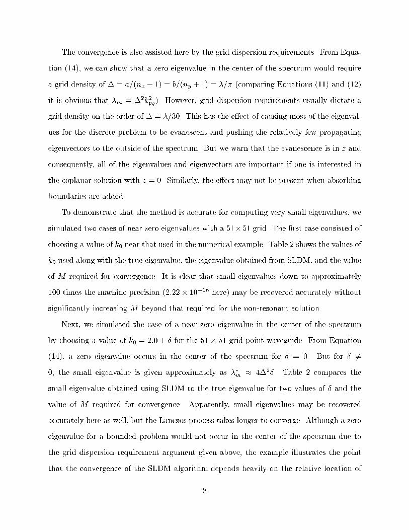
The convergence is also assisted here by the grid dispersion requirements. From Equa-tion (14), we can show that a zero eigenvalue in the center of the spectrum would requirea grid density of � = a=(nx + 1) = b=(ny + 1) = �=� (comparing Equations (11) and (12)it is obvious that �m = �2k2pq). However, grid dispersion requirements usually dictate agrid density on the order of � = �=30. This has the e�ect of causing most of the eigenval-ues for the discrete problem to be evanescent and pushing the relatively few propagatingeigenvectors to the outside of the spectrum. But we warn that the evanescence is in z andconsequently, all of the eigenvalues and eigenvectors are important if one is interested inthe coplanar solution with z = 0. Similarly, the e�ect may not be present when absorbingboundaries are added.To demonstrate that the method is accurate for computing very small eigenvalues, wesimulated two cases of near zero eigenvalues with a 51�51 grid. The �rst case consisted ofchoosing a value of k0 near that used in the numerical example. Table 2 shows the values ofk0 used along with the true eigenvalue, the eigenvalue obtained from SLDM, and the valueof M required for convergence. It is clear that small eigenvalues down to approximately100 times the machine precision (2:22� 10�16 here) may be recovered accurately withoutsigni�cantly increasing M beyond that required for the non-resonant solution.Next, we simulated the case of a near zero eigenvalue in the center of the spectrumby choosing a value of k0 = 2:0 + � for the 51� 51 grid-point waveguide. From Equation(14), a zero eigenvalue occurs in the center of the spectrum for � = 0. But for � 6=0, the small eigenvalue is given approximately as ��m � 4�2�. Table 2 compares thesmall eigenvalue obtained using SLDM to the true eigenvalue for two values of � and thevalue of M required for convergence. Apparently, small eigenvalues may be recoveredaccurately here as well, but the Lanczos process takes longer to converge. Although a zeroeigenvalue for a bounded problem would not occur in the center of the spectrum due tothe grid dispersion requirement argument given above, the example illustrates the pointthat the convergence of the SLDM algorithm depends heavily on the relative location of8

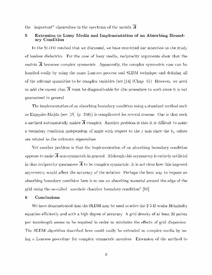
the \important" eigenvalues in the spectrum of the matrix A.5. Extension to Lossy Media and Implementation of an Absorbing Bound-ary ConditionIn the SLDM method that we discussed, we have restricted our attention to the studyof lossless dielectrics. For the case of lossy media, reciprocity arguments show that thematrix A becomes complex symmetric. Apparently, the complex symmetric case can behandled easily by using the same Lanczos process and SLDM technique and de�ning allof the relevant quantities to be complex variables (see [14] (Chap. 6)). However, we needto add the caveat that A must be diagonalizable for this procedure to work since it is notguaranteed in general.The implementation of an absorbing boundary condition using a standard method suchas Engquist-Majda (see [15] (p. 246)) is complicated for several reasons. One is that sucha method automatically makes A complex. Another problem is that it is di�cult to makea boundary condition independent of angle with respect to the z axis since the kz valuesare related to the unknown eigenvalues.Yet another problem is that the implementation of an absorbing boundary conditionappears to makeA non-symmetric in general. Although this asymmetry is entirely arti�cialin that reciprocity guarantees A to be complex symmetric, it is not clear how this imposedasymmetry would a�ect the accuracy of the solution. Perhaps the best way to impose anabsorbing boundary condition here is to use an absorbing material around the edge of thegrid using the so-called \anechoic chamber boundary condition" [16].6. ConclusionsWe have demonstrated that the SLDM may be used to solve the 2.5-D scalar Helmholtzequation e�ciently and with a high degree of accuracy. A grid density of at least 30 pointsper wavelength seems to be required in order to minimize the e�ects of grid dispersion.The SLDM algorithm described here could easily be extended to complex media by us-ing a Lanczos procedure for complex symmetric matrices. Extension of the method to9

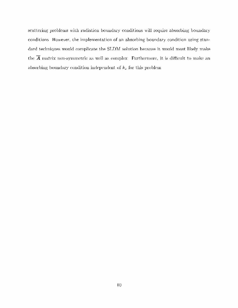
scattering problems with radiation boundary conditions will require absorbing boundaryconditions. However, the implementation of an absorbing boundary condition using stan-dard techniques would complicate the SLDM solution because it would most likely makethe A matrix non-symmetric as well as complex. Furthermore, it is di�cult to make anabsorbing boundary condition independent of kz for this problem.

10

References[1] C. Lanczos, \An iteration method for the solution of the eigenvalue problem of lin-ear di�erential and integral operators," J. Res. Nat. Bur. Standards, vol. 45, no. 4,pp. 225{282, 1950.[2] C. C. Paige, The Computation of Eigenvalues and Eigenvectors of Very Large SparseMatrices. PhD thesis, University of London, 1971.[3] C. C. Paige, \Accuracy and e�ectiveness of the lanczos algorithm for the symmetriceigenproblem," Linear Algebra Appl., vol. 34, pp. 235{258, 1980.[4] B. N. Parlett, The Symmetric Eigenvalue Problem. Englewood Cli�s: Prentice-Hall,1980.[5] V. Druskin and L. Knizhnerman, \On application of lanczos method to solution ofsome partial di�erential equations," Tech. Rep. EMG-92-27, Schlumberger-Doll Re-search, Apr. 1992.[6] V. Druskin and L. Knizhnerman, \Two polynomial methods of calculating functions ofsymmetric matrices," U.S.S.R. Comput. Maths. Math. Phys., vol. 29, no. 6, pp. 112{121, 1989. (Russian; translated into English).[7] B. Nour-Omid, \Lanczos method for heat conduction analysis," Int. J. Numer. Meth.Eng., vol. 24, pp. 251{262, 1987.[8] V. Druskin and L. Knizhnerman, \A spectral semi-discrete method for the numericalsolution of 3-D non-stationary problems in electrical prospecting," Izv. Acad. Sci.USSR: Phys. Solid Earth, no. 8, pp. 63{74, 1988. (Russian; translated into English).[9] D. J. Schneider and J. H. Freed, \Spin relaxation and motional dynamics," in Lasers,Molecules and Methods (J. O. Hirschfelder, R. E. Wyatt, and R. D. Coalson, eds.),ch. 10, New York: Wiley Interscience, 1989.[10] H. A. van der Vorst, \An iterative solution method for solving f(A)x = b, usingKrylov subspace information obtained for the symmetric positive de�nite matrix A,"J. Comput. Appl. Math., vol. 18, no. 2, pp. 249{263, 1987.[11] A. Allers, A. Sezginer, and V. Druskin, \2.5-Dimensional impedance tomography usingthe spectral lanczos method," Radio Sci., 1993. Submitted.[12] T. V. Tamarchenko, Fast Algorithms of Electromagnetic Forward Modeling in ComplexGeometry. PhD thesis, Moscow Geological-Prospecting Institute, 1988.[13] L. Knizhnerman. Private Communication, Mar. 1993.[14] J. K. Cullum and R. A. Willoughby, Lanczos Algorithms for Large Symmetric Eigen-value Computations, Vol. I: Theory. Boston: Birkhauser, 1985.[15] W. C. Chew, Waves and Fields in Inhomogeneous Media. New York: Van Nostrand,1990.[16] C. M. Rappaport and L. J. Bahrmasel, \An absorbing boundary condition basedon anechoic absorber for EM scattering computation," J. Electromag. Waves Appl.,vol. 6, no. 12, pp. 1621{1633, 1992.11

Table 1: Computation Times for Waveguide ExampleN = 2601 N = 24; 025 N = 67; 081Number of Lanczos Steps, M 120 340 550M=pN 2.35 2.19 2.12Memory Required (Mb) 2.49 65.3 295.2Time Lanczos Process (sec) .33 6.7 48.0Time QL Decomposition (sec) 1.0 7.0 69.0Time using I/O (sec) 1.0 20.3 168.0Time Computing Fields (sec) 0.0 1.66 13.3Total Time (sec) 2.3 35.7 298.3CPU Seconds Reported by O.S. 2.4 34.4 138.1Table 2: Accuracy of SLDM for Small Eigenvalues (N = 2601)True SLDM M Requiredk0 Eigenvalue Eigenvalue for Convergence.6156262927945929 1:0� 10�8 1:00000085395� 10�8 160.6156262846727906 1:0� 10�14 :847100907057� 10�14 1802.00000001 4:0� 10�8 3:99999987557� 10�8 6502.00000000000001 4:0� 10�14 3:88658103677� 10�14 700

12

(a) z-axis center cut, z= 0:10.0 λ

(b) x- or y-axis center cut, z= 0.8 λ

(c) x- or y-axis center cut, z= 3.5 λ

0 10 20 30 40 50 600

0.004

0.008

0.012

0.016

0 10 20 30 40 50 600

0.004

0.008

0.012

0.016

0.02

0 20 40 60 80 1000

0.04

0.08

0.12

0.16

x or y (mm)

x or y (mm)

z (mm)

Am

plitu

deA

mpl

itude

Am

plitu

de

Figure 1: Point-source response for a square waveguide of dimension 52:0 mm�52:0 mmwith � = 10:0 mm. In all �gures, the solid curve is the analytic solution for a continuouswaveguide, dotted curve (shown only in (a)) is SLDM solution for a 51� 51 grid, dash-dotcurve is SLDM solution for a 155� 155 grid, dashed curve is 259� 259 grid. Nearly all ofthe error between the SLDM solutions and the continuous analytic solution is due to griddispersion and not errors in the SLDM method (see Figure 2).13

(a) z-axis center cut, z= 0:10.0 λ

(b) x- or y-axis center cut, z= 0.8 λ

0 10 20 30 40 50 600

0.004

0.008

0.012

0.016

0 20 40 60 80 1000

0.04

0.08

0.12

0.16

x or y (mm)

z (mm)

Am

plitu

deA

mpl

itude

Figure 2: Comparison of SLDM solution with analytic solution for a discretized waveguide.In (a), z-axis cut for 51� 51 grid is shown and in (b) x- or y-axis cut for 155� 155 grid atz = 0:8� is shown. In both (a) and (b), SLDM solution and analytic solution for discretizedwaveguide are overlaid on top of each other, both using a solid line. The curves for theSLDM solution and the analytic solution are barely distinguishable, indicating excellentagreement.

14