arX

iv:0

911.

4114

v1 [

mat

h.N

A]

20

Nov

200

9

Fourier Based Fast Multipole Method for the

Helmholtz Equation

Cris Cecka a and Eric Darve a,b,∗aInstitute for Computational and Mathematical Engineering, Stanford University

bMechanical Engineering Department, Stanford University

Abstract

The fast multipole method (FMM) has had great success in reducing the computa-tional time required to solve the boundary integral form of the Helmholtz equation.We present a formulation of the Helmholtz FMM using Fourier basis functions ratherthan spherical harmonics that accelerates some of the time-critical stages of the al-gorithm. With modifications to the transfer function in the precomputation stageof the FMM, the interpolation and anterpolation operators become straightforwardapplications of fast Fourier transforms and the transfer operator remains diagonal.Using Fourier analysis, constructive algorithms are derived to a priori determine anintegration quadrature for a given error tolerance. Sharp error bounds are derivedand verified numerically. Various optimizations are considered to reduce the numberof quadrature points and reduce the cost of computing the transfer function.

Key words: fast multipole method, fast Fourier transform, Fourier basis,interpolation, anterpolation, Helmholtz, Maxwell, integral equations, boundaryelement method

1 Introduction1

Since the development of the fast multipole method (FMM) for the wave equa-2

tion in [1–5], the FMM has proven to be a very effective tool for solving scalar3

acoustic and vector electromagnetic problems. In this paper, we consider the4

application of the FMM to the scalar Helmholtz equations, although our re-5

sults can be immediately extended to the vector case as described in [6,7].6

∗ Corresponding authorEmail addresses: ccecka@stanford.edu (Cris Cecka), darve@stanford.edu

(Eric Darve).

Preprint submitted to Elsevier 20 November 2009

The application of the boundary element method to solve the integral form of7

the Helmholtz equation results in a dense linear system which can be solved8

by iterative methods such as GMRES or BCGSTAB. These methods require9

computing dense matrix-vector products which, using a direct implementa-10

tion, are performed in O(N2) floating point operations. The FMM uses an11

approximation of the dense matrix to perform the product in O(N logN) or12

O(N log2N) operations. This approximation is constructed from close pair in-13

teractions and far field approximations represented by spherical integrals that14

are accumulated and distributed through the domain via an octree.15

There are a number of difficulties in implementing the FMM, each of which16

must be carefully considered and optimized to achieve the improved com-17

plexity. The most significant complication is that the quadrature sampling18

rate must increase with the size of the box in the octree, requiring interpo-19

lation and anterpolation algorithms to transform the data between spherical20

quadratures of different levels of the tree. Local algorithms such as Lagrange21

interpolation and techniques which sparsify interpolant matrices are fast, but22

incur significant errors [8,7]. Spherical harmonic transforms are global inter-23

polation schemes and are exact but require fast versions for efficiency of the24

FMM. Many of these fast spherical transform algorithms are only approxi-25

mate, complicated to implement, and not always stable [9–11].26

In this paper, we use a multipole expansion which allows the use of 2D fast27

Fourier transforms (FFT) in the spherical coordinate system (φ, θ). The main28

advantages are two fold: i) high performance libraries are available for FFTs29

on practically all computer platforms, resulting in accurate, robust, and fast30

interpolation algorithms; ii) the resulting error analysis is simplified leading to31

sharp a priori error bounds on the calculation. One of the difficulties in using32

FFTs is that we are forced to use a uniform distribution of points along φ33

and θ in the spherical quadrature. This leads to a much increased quadrature34

size for a given accuracy compared to the original spherical harmonics-based35

FMM. The reason is as follows. The multipole expansion in the high frequency36

regime is derived from:37

eıκ|r+r0|

|r + r0|=∫ 2π

φ=0

∫ π

θ=0eıκs·r Tℓ,r0

(s) sin(θ) dθdφ

where s = [cos(φ) sin(θ), sin(φ) sin(θ), cos(θ)] is the spherical unit vector. It38

is apparent that we are integrating along θ a function which has period 2π.39

However the bounds of the integral are 0 to π, over which interval the func-40

tion has a discontinuity in its derivative. This results in a slow decay of the41

Fourier spectrum (essentially 1/frequency2) and consequently a large number42

of quadrature points along θ are required.43

We propose to use a variant of the scheme by J. Sarvas in [12] whereby the44

2

integration is extended from 0 to 2π and the integrand modified:45

eıκ|r+r0|

|r + r0|=

1

2

∫ 2π

φ=0

∫ 2π

θ=0eıκs·r Tℓ,r0

(s) | sin(θ)| dθdφ

We will describe in more details how an efficient scheme can be derived from46

this equation. The key property is that eıκs·r is approximately band-limited47

in θ and therefore it is possible to remove the high frequency components48

of Tℓ,r0(s)| sin(θ)| without affecting the accuracy of the approximation. Using49

this smooth transfer function, which is now band-limited in Fourier space, the50

number of quadrature points can be reduced dramatically. We show that the51

resulting number of quadrature points is reduced by about 40% compared to52

the original spherical harmonics-based FMM. Consequently, we now have a53

scheme which requires few quadrature points and enables the use of efficient54

FFT routines. The approach in [12] is similar. However, rather than smooth-55

ing Tℓ,r0(s) |sin(θ)| once during the precomputation phase as we will detail56

shortly, Sarvas instead incorporates the |sin(θ)| factor during the run-time57

phase of the FMM in the application of the transfer pass. This requires extra58

interpolations/anterpolations and a quadrature approximately twice the size59

during the time-critical transfer pass of the algorithm. The method presented60

in this paper retains a diagonal transfer pass operator and provides improved61

control over the error.62

We derive a new a priori error analysis which incorporates both effects from63

truncation of the Gegenbauer series (a problem well analyzed [6]) and the64

numerical quadrature. Our algorithm to predict the error is very sharp. This65

allows choosing the minimal number of quadrature points to guarantee a pre-66

scribed error. By comparison, the conventional approach can be shown to67

result in conservative error bounds. That is, the number of quadrature points68

is usually over-estimated and the error may be significantly below the target69

accuracy. Although not considered in this paper, our error analysis approach70

can also be applied to the spherical harmonics-based FMM to yield similarly71

accurate error bounds. This has practical importance since it allows guaran-72

teeing the error in the calculation while reducing the computational cost.73

The paper is organized as follows. In section 2, we introduce the critical74

parts of the classical FMM algorithm including the Gegenbauer series trunca-75

tion (2.1), the spherical quadrature (2.2), and a short overview of interpola-76

tion/anterpolation strategies (2.3). In section 2.4, the asymptotic complexity77

of the FMM is discussed. Section 3 details the Fourier basis approach. The78

transfer function must be modified to lower the computational cost and obtain79

a competitive scheme, as detailed in section 3.1. Section 3.2 applies an analysis80

of the integration error to derive an algorithm that determines a quadrature81

to yield an FMM with a prescribed error tolerance. The FFT based interpola-82

tion and anterpolation algorithms are described in section 3.3 and numerical83

results are given in section 3.4. Table 1 lists the notations used in this paper.84

3

Notation Description

λ wavelength

κ wavenumber, 2π/λ

θ polar angle

φ azimuthal angle

a complex conjugate of a

x vector in R3, x = |x| x

x · y inner product, x · y = |x| |y| cos(φx,y)

M matrix in Rn×m with elements Mij

S2 sphere, {s ∈ R3 : |s| = 1}

jn spherical Bessel function of the first kind

yn spherical Bessel function of the second kind

h(1)n spherical Hankel function of the first kind

Pn Legendre polynomial

Y mn normalized spherical harmonic of degree n, order m

F(m; f) mth frequency of the Fourier transform of f

Table 1. Table of notations

2 The Multilevel Fast Multipole Method85

The FMM reduces the computational complexity of the matrix-vector multi-86

plication87

σi =∑

j 6=i

eıκ|xi−xj |

|xi − xj |ψj =

∑

j

Mij ψj (1)

for i, j = 1, . . . , N from O(N2) to O(N log2N). This improvement is based on88

the Gegenbauer series89

eıκ|r+r0|

|r + r0|= ıκ

∞∑

n=0

(−1)n(2n+ 1)h(1)n (κ |r0|)jn(κ |r|)Pn(r · r0) (2)

The series converges absolutely and uniformly for |r0| ≥ 2√3|r| and has been90

studied extensively in [13,14].91

4

Truncating the Gegenbauer series at ℓ and using the identity92

∫

S2

eıκs·rPn(s · r0) dS(s) = 4πınjn(κ |r|)Pn(r · r0)

where the integral is over the unit sphere S2, then93

ıκℓ∑

n=0

(−1)n(2n+ 1)h(1)n (κ |r0|)jn(κ |r|)Pn(r · r0) =

∫

S2

eıκs·r Tℓ,r0(s) dS(s)

(3)

where the transfer function, Tℓ,r0(s), is defined as94

Tℓ,r0(s) =

ıκ

4π

ℓ∑

n=0

ın(2n+ 1)h(1)n (κ |r0|)Pn(s · r0). (4)

Consider two disjoint clusters of points {xi | i ∈ A} and {xi | i ∈ B} with radii95

rA ≥ rB ≥ 0 and centers cA and cB respectively. If |cA − cB| ≥ 2√3(rA + rB),96

then the matrix-vector product (1) is accelerated by using the approximation97

M ≈

MAA MAB

MBA MBB

where98

MAA = [Mij ]i∈A,j∈A

MAB =[∫

S2

eıκs·(cA−xi)Tℓ,cB−cA(s)eıκs·(xj−cB) dS(s)

]

i∈A,j∈B

For i ∈ A, this corresponds to computing99

σi =∫

S2

eıκs·(cA−xi)Tℓ,cB−cA(s)[∑

j∈B

eıκs·(xj−cB)ψj

]dS(s)

+∑

j∈A

eıκ|xi−xj |

|xi − xj|ψj + εℓ

where εℓ is the error introduced by the Gegenbauer series truncation.100

The reduced computational complexity of the FMM is achieved by construct-101

ing a tree of nodes, typically an octree, over the domain of the source and field102

points. Let U lα(s) be the outgoing field for Bl

α, the box α of the tree in level103

l ∈ [0, L] with center clα. The method is initialized by computing the outgoing104

plane-wave expansions for each cluster contained in a leaf of the tree:105

ULα (s) =

∑

i, xi∈Blα

eıκs·(xi−cLα)ψi

5

These outgoing expansions are then aggregated upward through the tree by106

accumulating the product of the child cluster expansions with the diagonal107

plane-wave translation function:108

U lα(s) =

∑

β, Bl+1

β⊂Bl

α

U l+1β (s)eıκs·(cl+1

β−c

lα)

Incoming plane-wave expansions, I lα(s) of box Bl

α, are computed from the109

outgoing by multiplication with the diagonal transfer function:110

I lα(s) =

∑

β

U lβ(s)Tℓ,cl

β−cl

α(s)

where the parent of Blβ is a neighbor of the parent of Bl

α, and Blβ is not a111

neighbor of Blα. The incoming plane-waves are then disaggregated downward112

through the tree to compute the local field Dlα(s):113

Dlα(s) = Dl−1

β (s)eıκs·(cl−1

β−c

lα) + I l

α(s)

where Blα ⊂ Bl−1

β . At the finest level, the integration over the sphere is finally114

performed and added to the near field contribution to determine the field value115

at the N field points:116

σi =∫

S2

DLα(s)eıκs·(cL

α−xi) dS(s) +∑

j 6=i

eıκ|xi−xj |

|xi − xj |ψj

where xi ∈ BLα and xj ∈ BL

β ∪ BLα where BL

β is any neighbor of BLα .117

2.1 Truncation Parameter in the FMM118

The truncation parameter ℓ must be chosen so that the Gegenbauer series (2)119

is converged to a desired accuracy. However, for n > x, jn(x) decreases super-120

exponentially while h(1)n (x) diverges. The divergence of the Hankel function121

causes the transfer function to oscillate wildly and become numerically un-122

stable. Even though the expansion converges, roundoff errors will adversely123

affect the accuracy if ℓ is too large. Thus, while one must choose ℓ > κ |r|124

so that sufficient convergence is achieved for the plane-wave, it must also be125

small enough to avoid the divergence of the transfer function.126

The selection the truncation parameter ℓ has been studied extensively and127

and a number of procedures for selecting it have been proposed.128

The empirical formula129

ℓ ≈ κ |r|+ C(ε) log(π + κ |r|)

6

appears to have been first proposed by Rokhlin [2]. This was considered and130

revised by Darve [14] using a detailed asymptotic analysis of the Gegenbauer131

series.132

The excess bandwidth formula (EBF) is derived from the convergence of the133

plane-wave expansion and is presented in [6]. To determine an appropriate134

truncature, the spectrum of a plane wave135

eıκs·r = eıκ|r| cos(φs,r) =∞∑

n=−∞ınJn(κ |r|)eınφs,r (5)

where φs,r is the angle between s and r, is used to estimate how many terms136

in the series are needed before the error in the summation is exponentially137

small. It can be shown that when n→∞ and x ∼ O(n),138

Jn(x) ∼ e√

n2−x2−n cosh−1(n/x)

√2π(n2 − x2)

which decays exponentially fast when n > x. Let n/x = 1 + δ where δ ≪ 1.139

Then cosh−1(n/x) ∼√

2δ and√n2 − x2 ∼ x

√2δ. Thus, the above becomes140

Jn(x) ∼ e(x−n)√

2δ

2x√πδ

=e−x

√2δ3/2

2x√πδ

This expression is exponentially small when xδ3/2 ≫ 1, or δ = Cx−2/3, where141

C ≫ 1. That is, when142

n

x− 1 ≈ Cx−2/3

Therefore, the number of terms we need can be approximated as143

ℓ ≈ κ |r|+ C(κ |r|)1/3

An empirically determined common choice is C = 1.8(d0)2/3, where d0 is the144

desired number of digits of accuracy. The EBF is one of the most popular145

choices to select the truncation parameter.146

The desired number of digits of accuracy cannot always be achieved due to147

the divergent nature of the transfer function. Thus, the EBF fails when high148

accuracy is desired or the box size and box separation are small. Some modi-149

fications in this regime are proposed in [15].150

A direct numerical computation of the Gegenbauer truncation error ℓ could151

be computed or approximated152

εG(ℓ) = ıκ∞∑

n=ℓ+1

(−1)n(2n+ 1)h(1)n (κ |r0|)jn(κ |r|)Pn(r · r0)

7

As Carayol and Collino showed in [13], an upper bound of this error for large153

values of |r| is obtained when Pn(r · r0) = Pn(±1) = (±1)n so that154

|εG| . κ

∣∣∣∣∣∣

∞∑

n=ℓ+1

(∓1)n(2n+ 1)h(1)n (κ |r0|)jn(κ |r|)

∣∣∣∣∣∣

which they showed can be computed in closed form155

= κ

√|r| |r0||r0| ± |r|

π

2

∣∣∣Hℓ+ 3

2

(κ |r0|)Jℓ+ 1

2

(κ |r|)±Hℓ+ 1

2

(κ |r0|)Jℓ+ 3

2

(κ |r|)∣∣∣

= κ2 |r| |r0||r0| ± |r|

∣∣∣h(1)ℓ+1(κ |r0|)jℓ(κ |r|)± h(1)

ℓ (κ |r0|)jℓ+1(κ |r|)∣∣∣

This fails for small |r| when the upper bound is instead given by the r · r0156

which causes the oscillation of Pn(r · r0) to compensate for the oscillation of157

(−1)nh(1)n (κ |r0|)jn(κ |r|).158

Using the EBF as an initial guess for ℓ and refining the choice using the above159

closed form when |r| is sufficiently large is a simple algorithm which yields an160

accurate value for ℓ.161

Carayol and Collino in [16] and [13] present an in-depth analysis of the Jacobi-162

Anger series and the Gegenbauer series. They find the asymptotic formula163

ℓ ≈ v − 1

2+(

1

2

)5/3

W 2/3

(v

4ε6

(1 + α

1− α)3/2

)

where v = κ |r|, α = u/v, u = κ |r0|, and W (x) is the Lambert function164

defined as the solution to165

W (x)eW (x) = x x > 0

This appears to be near optimal for large box sizes.166

The errors introduced by this truncation have been investigated in other pa-167

pers including [8,13,14].168

2.2 Spherical Quadrature in the FMM169

With the expansion formula170

(2n+ 1)Pn(p · q) = 4πn∑

m=−n

Y mn (p)Y m

n (q)

8

the transfer function (4) can be expressed as171

Tℓ,r0(s) = ıκ

ℓ∑

n=0

ınh(1)n (κ |r0|)

n∑

m=−n

Y mn (r0)Y

mn (s) =

ℓ∑

n=0

n∑

m=−n

tmn Ymn (s) (6)

Similarly, the Jacobi-Anger series,172

eıκs·r =∞∑

n=0

ın(2n+ 1)jn(κ |r|)Pn(s · r) (7)

becomes the spherical harmonic series173

eıκs·r = 4π∞∑

n=0

ınjn(κ |r|)n∑

m=−n

Y mn (r)Y m

n (s) =∞∑

n=0

n∑

m=−n

emn Y

mn (s) (8)

The error analysis simplifies if we use a scheme which exactly integrates spheri-174

cal harmonics, Y ml , up to some order. Below, we enumerate a number of choices175

that have previously been studied.176

(1) The simplest choice are sample points chosen uniformly in φ and θ. How-177

ever, this choice does not accurately integrate the spherical harmonics178

and requires approximately twice as many points as the Gauss-Legendre179

quadrature below [7].180

(2) The most common choice of sample points are uniform points for φ and181

Gauss-Legendre points for θ. With N+1 uniform points in the φ direction182

and N+12

Gauss-Legendre points in the θ direction, all Y mn , −n ≤ m ≤ n,183

0 ≤ n ≤ N are integrated exactly [7,8].184

(3) McLaren in [17] developed optimal choices of samples for general func-185

tions on S2 based on equally spaced points and derived from invariants186

of finite groups of rotations. He also proposes a method for constructing187

equally weighted integration formulas on sets of any desired number of188

points by taking the union of icosahedral configurations.189

2.3 Interpolation and Anterpolation in the FMM190

The quadrature sampling rate depends on the spectral content of the diagonal-191

ized translation operator, eıκs·r. These plane-waves contain more oscillatory192

modes as we go up in the tree. Its coefficient in the spherical harmonic ex-193

pansion emn [equation (8)] decreases super-exponentially roughly for n & κ |r|.194

Therefore, as we go up the tree in the aggregation step and |r| becomes larger,195

a larger quadrature is required to resolve these higher modes. These modes196

must be resolved since they interact with the modes in the transfer function,197

which do not significantly decay as ℓ increases.198

9

Similarly, as we go down the tree in the disaggregation step, |r| becomes199

smaller and the higher modes of the incoming field make vanishingly small200

contributions to the integral as a consequence of Parseval’s theorem. Thus, as201

the incoming field is disaggregated down the tree, a smaller quadrature can be202

used to resolve it. This makes the integration faster and is actually required to203

achieve an optimal asymptotic running time. See section 2.4 and appendix A.204

There have been several approaches to performing the interpolation and an-205

terpolation between levels in the FMM. Below, we enumerate a number of206

choices that have previously been studied.207

(1) General interpolation algorithms like Lagrange interpolation or B-splines208

are fast and provide for simple error analysis. In [8] it is shown that the209

error induced from Lagrange interpolation decreases exponentially as the210

number of interpolation points is increased for a given function of finite211

bandwidth. Thus, there is a trade-off between error and speed.212

(2) For a set of quadrature points (φk, θk), k = 1, . . . , K with respective213

weights ωk and corresponding function value fk, a spherical harmonic214

transform maps fk to a new quadrature (φ′k′, θ′k′), k′ = 1, . . . , K ′ via the215

linear transformation216

fk′ =∑

m,l≤K

Y ml (φ′

k′, θ′k′)∑

k

ωkY ml (φk, θk)fk =

∑

k

Ak′kfk (9)

This transform has nice properties analogous to those of the Fourier trans-217

form. A direct computation requires O(KK ′) operations which would218

result in an O(N2) FMM (see appendix A). Fast spherical transforms219

(FST) have been developed in [9–11,18] and applied to the FMM in [19].220

Using the FST reduces the interpolation and anterpolation procedures221

to O(K log2K), which results in an O(N log2N) FMM. However, the222

accuracy and stability of these algorithms remain in question.223

(3) Approximations of the spherical transform have also been investigated in224

[20,7]. The interpolation matrix Ak′k in (9) can be sparsified in a number225

of ways to provide an interpolation/anterpolation method that scales as226

O(K) with controllable relative error.227

(4) Many other interpolation schemes exist with varying running times and228

errors. Rokhlin presents a fast polynomial interpolator based on the fast229

multipole method in [21]. See also [22].230

2.4 Asymptotic Complexity231

In order to resolve a sufficient number of spherical harmonics, the number232

of points in the φ and θ directions must be O(ℓ) = O(κa), where a is the233

side length of the box. Therefore, the total number of quadrature points is234

10

O(ℓ2) = O((κa)2). If a0 is the side length of a box at the root of the octree235

(level l = 0), then the side length of a box at level l is al = 2−la0 and has236

O((κ2−la0)2) quadrature points.237

With these parameters defined, the asymptotic complexity of the FMM can238

be determined by carefully counting the number of operations required in each239

step. The is done in detail in Appendix A and the results are discussed below.240

In modeling a uniform distribution of point scatterers over a volumetric do-241

main, we take O(N) = O((κa0)3) and L ∼ log(N1/3) to achieve a total algo-242

rithmic complexity of O(N logN) using fast global interpolation methods. By243

using local methods, this can be reduced to O(N).244

In modeling the scattering from the surface of an object using a uniform dis-245

tribution of basis functions, we take O(N) = O((κa0)2) and L ∼ log(N1/2) to246

achieve a total algorithmic complexity of O(N log2(N)) using fast global inter-247

polation methods. By using local methods, this can be reduced to O(N logN).248

It should be noted again that for a given, fixed κa0 there is a minimum size249

for the leaves of the tree. Below this critical size, h(1)n oscillates wildly causing250

numerical instability in the transfer function. Therefore, when N is very large251

and the number of levels is saturated, this analysis fails and the algorithm is252

dominated by the O(N2) computation of the close field contribution, albeit253

with orders of magnitude speedup over a direct method. In the case when κa0254

is too small, broadband FMMs have been developed as detailed in [23,24].255

However, in many applications κa0 is large enough to allow for all practi-256

cal L and N . Furthermore, by keeping the number of points per wavelength257

constant, the O(N logN) behavior can always be achieved.258

3 Fourier Based Multilevel Fast Multipole Method259

The Fourier based fast multipole method is based on the identity260

∫

S2

eıκs·r Tℓ,r0(s) dS(s) =

∫ 2π

0

∫ 2π

0eıκs·r T s

ℓ,r0(s) dφdθ (10)

where s = [cos(φ) sin(θ), sin(φ) sin(θ), cos(θ)] and261

T sℓ,r0

(s) =1

2Tℓ,r0

(s) |sin(θ)| (11)

is the modified transfer function. Noting that the integrand is continuous and262

periodic, this formulation of the problem suggests the use of the Fourier func-263

tions {eınφeımθ} which form an orthonormal basis of L2([0, 2π]× [0, 2π]). This264

11

allows i) using two dimensional uniform quadratures; ii) fast Fourier trans-265

forms in the interpolation and anterpolation steps; iii) spectral arguments in266

the error analysis. Of these advantages, the most important is that the FFT267

interpolations and anterpolations are fast and exact. Since there is no interpo-268

lation error, only the finite quadrature and the truncation of the Gegenbauer269

series introduce error to the final solution. Thus, the error analysis is simpli-270

fied and we will determine in this paper precise bounds on the final error. In271

fact, our error analysis is fairly general and can be extended to the classical272

FMM with schemes that exactly integrate spherical harmonics (see direct and273

fast global methods in section 2.3 and appendix A). The result is a fast, easy274

to implement, and controllable version of the FMM, which we detail in the275

following sections.276

3.1 Computing the Modified Transfer Function277

Select a uniform quadrature with points (φi, θj) defined by278

φi = 2πi

Nφθj = 2π

j

Nθ

Noting that the plane wave eıκs·r and T sℓ,r0

(s) both have spherical symmetry,279

f(s)

∣∣∣∣s(φ,θ)

= f(s)

∣∣∣∣s(π+φ,2π−θ)

,

the computational and memory cost are reduced by computing and storing280

only half of the quadrature points.281

Additionally, in an FMM with a single octree, there are 316 distinct transfer282

vectors r0 per level. By enforcing symmetries in the quadrature, the number of283

modified transfer functions that must be precomputed is reduced. Specifically,284

by requiring Nθ to be a multiple of 2 and Nφ to be a multiple of 4, we enforce285

reflection symmetries in the z = 0, x = 0, y = 0, x = y, and x = −y286

planes. This reduces the number of modified transfer functions that need to287

be precomputed from 316 per level to 34 – saving a factor of 9.3 in memory288

and costing a negligible permutation of the values of a computed modified289

transfer function. See Fig. 1.290

A key step to constructing a fast algorithm is to remove the high frequencies291

in T sℓ,r0

(s) whose contribution to the final result is negligible. This reduces292

the number of needed quadrature points considerably. If T sℓ,r0

(s) were simply293

sampled, significant aliasing would occur unless we used an unreasonably large294

12

-x��y

6z

��

��

�� ���

��

�� ��

�� ��

��

��

���

��

��� -x���

y6z

��

���

��

���

��

���

��

���

��

���

��

���

��

��

���

��

�� ��

��

Fig. 1. The center of each box represents one transfer vector r0 which must becomputed. The pictures on the left and right panels represent the same set of boxesviewed under two different angles. Due to the symmetries of the quadrature, weneed only compute transfer vectors with x, y, z ≥ 0 and x ≥ y. We therefore end upwith essentially half of an octant. Specifically, 34 transfer vectors are required; theycan be reflected into any of the 316 needed.

quadrature. This is due to the slow decay of the Fourier series of |sin(θ)|,295

F(m; |sin(θ)|) =(−1)m + 1

π(1−m2)=

2π

11−m2 if m even

0 if m odd

Since the spectrum of the plane-wave function in equation (5) decays very296

rapidly for n & κ |r|, the high frequencies in θ of T sℓ,r0

(s) do not contribute297

to the final integral as a result of Parseval’s theorem. By removing these298

frequencies from the modified transfer function, a smaller quadrature can be299

used without affecting the final result.300

Suppose we have chosen a quadrature characterized by (Nθ, Nφ). With this301

quadrature we are able to exactly resolve the frequencies in eıκs·r between302

−Nθ/2 + 1 and Nθ/2 − 1 to the integral in equation (10). Consequently, we303

need to exactly calculate a band limited approximation of T sℓ,r0

, called T s,Lℓ,r0

,304

such that:305

F(m;T s,Lℓ,r0

) =

F(m;T s

ℓ,r0), if −Nθ/2 + 1 ≤ m ≤ Nθ/2− 1

0, otherwise

Since Tℓ,r0is bandlimited in θ with bandwidth 2ℓ + 1, only the frequencies306

|m| ≤ Nθ/2 − 1 + ℓ of |sin(θ)| contribute to the Nθ − 1 frequencies of T s,Lℓ,r0

.307

Therefore, the low-pass modified transfer function T s,Lℓ,r0

can be computed using308

the following pseudo-code:309

13

for φi, 0 ≤ i < Nφ/2, do1

Tk ← 12Tℓ,r0

(φi,2πk2ℓ+1

), k = 0, . . . , 2ℓ;2

Tm ← F(m,T );3

sm ← F(|m| ≤ Nθ/2− 1 + ℓ; |sin(θ)|);4

T s,Ln ← s⊗ T convolution of Fourier series;5

T s,Ln ← truncate to frequencies |n| ≤ Nθ/2− 1;6

T s,L(θj , φi)← inverse transform of T s,Ln ;7

310

This algorithm yields the low-pass modified transfer function at (φi, θj), 0 ≤311

i < Nφ/2, 0 ≤ j < Nθ which can be unwrapped to the remaining points312

by using the spherical symmetry (φi, θj) = (φNφ/2+i, θNθ−j). Note that this313

calculation can also be performed in the real space. It is equivalent to making314

a Fourier interpolation of Tk from 2ℓ+1 points toNθ+2ℓ−1 points, multiplying315

by a low-pass |sin(θ)|, and performing a Fourier anterpolation back to Nθ316

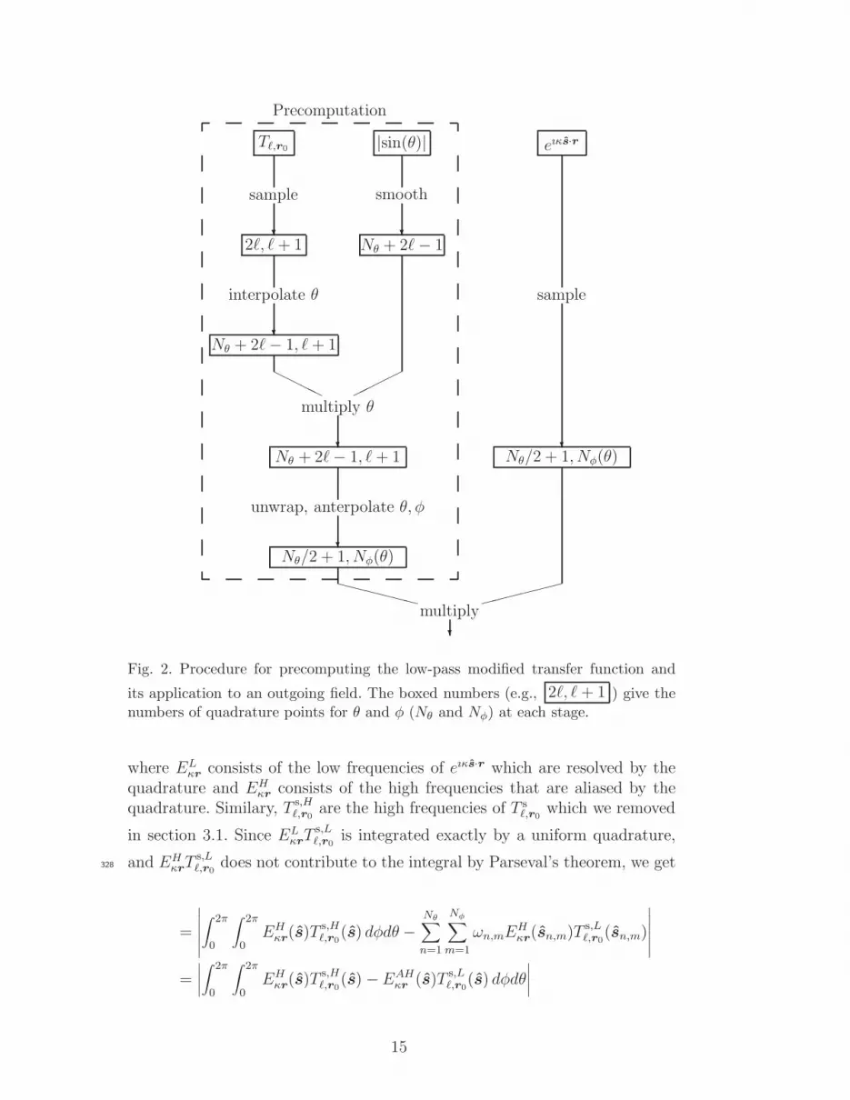
points, as shown in Figure 2.317

Because sampling the transfer function at a single point is an O(ℓ) operation,318

the algorithm as presented is O(ℓ3). The computation of the transfer function319

at all sample points can be accelerated to O(ℓ2) as in [25] by taking advantage320

of its symmetry about the r0 axis and using interpolation algorithms, but at321

the cost of introducing additional error.322

3.2 Choice of Quadrature323

The quadrature parameters can be constructively computed by determining324

the maximum error they incur. The error in computing the integral with a325

finite uniform quadrature is326

|εI | =∣∣∣∣∣∣

∫ 2π

0

∫ 2π

0eıκs·r T s

ℓ,r0(s) dφdθ −

Nθ∑

n=1

Nφ∑

m=1

ωn,meıκsn,m·r T s,L

ℓ,r0(sn,m)

∣∣∣∣∣∣

where sn,m = [cos(φm) sin(θn), sin(φm) sin(θn), cos(θn)] and T s,Lℓ,r0

(sn,m) is thelow-pass modified transfer function described in Section 3.1. This can be fur-ther expanded as:327

=∣∣∣∣∫ 2π

0

∫ 2π

0

[EL

κr(sn,m) + EH

κr(sn,m)

] [T s,L

ℓ,r0(s) + T s,H

ℓ,r0(s)]dφdθ

−Nθ∑

n=1

Nφ∑

m=1

ωn,m

[EL

κr(sn,m) + EH

κr(sn,m)

]T s,L

ℓ,r0(sn,m)

∣∣∣∣

14

Precomputation

Tℓ,r0

sample

?

2ℓ, ℓ+ 1

interpolate θ

?

Nθ + 2ℓ− 1, ℓ+ 1

HH

HH

|sin(θ)|

smooth

?

Nθ + 2ℓ− 1

��

��

multiply θ

?

Nθ + 2ℓ− 1, ℓ+ 1

unwrap, anterpolate θ, φ

?

Nθ/2 + 1, Nφ(θ)

XXXXXX

eıκs·r

sample

?

Nθ/2 + 1, Nφ(θ)

������

multiply?

Fig. 2. Procedure for precomputing the low-pass modified transfer function and

its application to an outgoing field. The boxed numbers (e.g., 2ℓ, ℓ+ 1 ) give thenumbers of quadrature points for θ and φ (Nθ and Nφ) at each stage.

where ELκr

consists of the low frequencies of eıκs·r which are resolved by thequadrature and EH

κrconsists of the high frequencies that are aliased by the

quadrature. Similary, T s,Hℓ,r0

are the high frequencies of T sℓ,r0

which we removed

in section 3.1. Since ELκrT s,L

ℓ,r0is integrated exactly by a uniform quadrature,

and EHκrT s,L

ℓ,r0does not contribute to the integral by Parseval’s theorem, we get328

=

∣∣∣∣∣∣

∫ 2π

0

∫ 2π

0EH

κr(s)T s,H

ℓ,r0(s) dφdθ −

Nθ∑

n=1

Nφ∑

m=1

ωn,mEHκr

(sn,m)T s,Lℓ,r0

(sn,m)

∣∣∣∣∣∣

=∣∣∣∣∫ 2π

0

∫ 2π

0EH

κr(s)T s,H

ℓ,r0(s)−EAH

κr(s)T s,L

ℓ,r0(s) dφdθ

∣∣∣∣

15

where we have denoted the aliased high frequencies of eıκs·r as EAHκr

(s),329

=

∣∣∣∣∫ 2π

0

∫ 2π

0

(EH

κr(s)− EAH

κr(s))T s

ℓ,r0(s) dφdθ

∣∣∣∣

In Fourier space, this becomes330

= 4π2

∣∣∣∣∣∣

ℓ∑

n=−ℓ

∞∑

m=−∞

(EH

κr(n,m)− EAH

κr(n,m)

)T s

ℓ,r0(−n,−m)

∣∣∣∣∣∣

Choosing Nθ using this expression for the error with a representative r andr0 leads to unpredictable cancelation effects and may result in a poor choice.Instead, we apply the triangle inequality,331

≤ 4π2ℓ∑

n=−ℓ

∞∑

m=−∞

∣∣∣EHκr

(n,m)− EAHκr

(n,m)∣∣∣∣∣∣T s

ℓ,r0(−n,−m)

∣∣∣

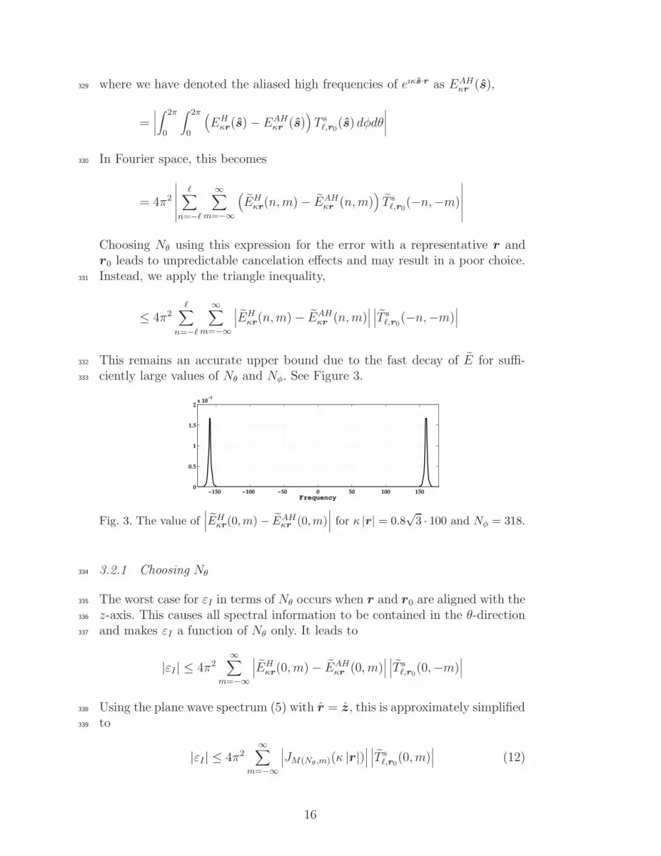
This remains an accurate upper bound due to the fast decay of E for suffi-332

ciently large values of Nθ and Nφ. See Figure 3.333

−150 −100 −50 0 50 100 1500

0.5

1

1.5

2x 10

−5

Frequency

Fig. 3. The value of∣∣∣EH

κr(0,m) − EAH

κr(0,m)

∣∣∣ for κ |r| = 0.8√

3 · 100 and Nφ = 318.

3.2.1 Choosing Nθ334

The worst case for εI in terms of Nθ occurs when r and r0 are aligned with the335

z-axis. This causes all spectral information to be contained in the θ-direction336

and makes εI a function of Nθ only. It leads to337

|εI | ≤ 4π2∞∑

m=−∞

∣∣∣EHκr

(0, m)− EAHκr

(0, m)∣∣∣∣∣∣T s

ℓ,r0(0,−m)

∣∣∣

Using the plane wave spectrum (5) with r = z, this is approximately simplified338

to339

|εI | ≤ 4π2∞∑

m=−∞

∣∣∣JM(Nθ,m)(κ |r|)∣∣∣∣∣∣T s

ℓ,r0(0, m)

∣∣∣ (12)

16

where340

M(Nθ, m) =

Nθ − |m| |m| ≤ Nθ/2− 1

|m| |m| > Nθ/2− 1(13)

This is an approximation because EAHκr

would in principle contribute an infi-341

nite sum to equation (12) rather than the single term used. However, given342

the exponential decay of the Jacobi-Anger series, the difference is negligible.343

Equation (12) can be used to search for a value Nθ via the algorithm sketched344

below:345

Choose Nnθ sufficiently larger than 2ℓ+ 1;1

Tk ← T s,Lℓ,|r0|z(0,

2πkNn

θ), k = 0, . . . , Nn

θ − 1;2

Tm ← |F(m;Tk)|;3

Em ← |Jm(κ |r|)|;4

for Nθ from 2ℓ to Nnθ by 2 do5

E∗m ← EM(Nθ ,m);6

if E∗ · T < ε/4π2 then7

return Nθ8

Since Nnθ is typically only a small constant larger than 2ℓ + 1, the algorithm346

as presented is dominated by the computation of the O(ℓ) modified transfer347

function values and requires O(ℓ2) operations. Important optimizations in-348

clude using more advanced searching methods (such as bisection), applying349

the symmetries E∗m = E∗

−m and Tm = T−m, and taking advantage of the very350

fast decay of Jn to neglect very small terms in the dot product.351

3.2.2 Choosing Nφ352

After determining an appropriate Nθ, letting Nφ be a function of θ allows353

reducing the number of quadrature points without affecting the error. The354

worst case for the integration error occurs when r and r0 are in the xy-plane.355

Without loss of generality, suppose r = x. Consider a constant θ = θj and356

note that the plane wave can be expressed as357

eıκs·r =∞∑

n=−∞inJn(κ |r| sin(θj)) e

inφ

Since Jn(κ |r| sin(θj)) is exponentially small when n & κ |r| sin(θj), the se-358

ries can be truncated at Nφ(θj) ∼ κ |r| sin(θj) without incurring any ap-359

preciable error. Estimates of Nφ(θj) can be developed by determining when360

Jn(κ |r| sin(θj)) becomes exponentially small, as in the computation of the361

excess bandwidth formula (EBF) in [6]. However, we find that the EBF gen-362

erated quadrature typically overestimates the sampling rate.363

17

To accurately compute Nφ(θj) the same procedure as in Sec. 3.2.1 is applied364

but with r and r0 in the xy-plane. This represents the worst case for the365

integration error as a function of Nφ. For a given θj , we search for a Nφ(θj)366

such that367

|εI | ≤ 4π2ℓ∑

n=−ℓ

∣∣∣JM(Nφ(θj),n)(κ |r| sin(θj))∣∣∣∣∣∣T s

ℓ,r0(n; θj)

∣∣∣ (14)

is bounded by a prescribed error. This is accomplished via the following368

sketched algorithm.369

Set Nφ at the poles: Nφ(θ0) = Nφ(θNθ/2) = 1;1

Choose Nnφ sufficiently larger than 2ℓ+ 1;2

for θj, j = 1, . . . , Nθ/2− 1 do3

Tk ← T s,Lℓ,|r0|x( 2πk

2ℓ+1, θj), k = 0, . . . , 2ℓ;4

Tm ← |F(m;Tk)|;5

Em ← |Jm(κ |r| sin(θj))|;6

for Nφ(θj) from 2 to Nnφ by 2 do7

E∗m ← EM(Nφ(θj),m);8

if E∗ · T < ε/4π2 then9

Save Nφ(θj)10

Since Nnφ is only a small constant larger than 2ℓ+1, the algorithm as presented370

is dominated by the computation of the modified transfer function and requires371

O(ℓ3) operations. Optimizations similar to those presented in Sec. 3.2.1 can372

be applied. Using the EBF as an initial guess in the search for Nφ(θj) further373

improves the searching speed. Additionally, only half of the Nφ(θj)’s may be374

computed due to symmetry about the z = 0 plane.375

We finally note that letting Nφ be a function of θj requires an additional step376

in the computation of the modified transfer function. Section 3.1 computed377

the transfer function on a Nθ/2 + 1 × Nφ grid. With Nφ → Nφ(θj), the data378

computed for each θj must be Fourier anterpolated from length Nφ to length379

Nφ(θj).380

3.2.3 Choosing |r| and |r0|381

The previous algorithms require representative values of |r| and |r0| for each382

level of the tree. The worst-case transfer vectors, r0, are those with smallest383

length. If al is the box size at level l, then |r0| = 2al is the smallest transfer384

vector length in the common one buffer box case.385

The worst case value of |r| is the largest. For a box of size al, |r| ≤ al

√3.386

However, using |r| = al

√3 in the previous methods is often too conservative.387

18

r0al

ric

rcj

i

j

Fig. 4. The worst case r and r0, projected from the 3D box. Here, |r0| = 2al and iand j are on the opposite corners of the box so that |r| = |ric|+ |rcj| = al

√3.

This case only occurs when two points are located in the exact corners of388

the boxes – a rare case indeed. See Figure 4. Instead, we let |r| = αal

√3 for389

some α ∈ [0, 1]. A high α guarantees an upper bound on the error generated390

by the quadrature, but the points which actually generate this error become391

increasingly rare. A lower value of α will yield a smaller quadrature, but more392

points may fall outside the radius |r| for which the upper bound on the error393

is guaranteed.394

3.2.4 Number of Quadrature Points395

Recall from section 2.2 that the typical approach in the FMM is to use N + 1396

uniform points in the φ direction and N+12

Gauss-Legendre points in the θ397

direction so that all Y mn , −n ≤ m ≤ n, 0 ≤ n ≤ N are integrated exactly.398

In [8], Chew et al. takes N+12

= ℓ + 1, which is an approximate choice based399

on the rapid decay of the coefficients in the spherical harmonics expansion of400

a plane wave. This results in approximately401

Mg = 2(ℓ+ 1)2 ≈ 2ℓ2

quadrature points.402

For a given Gegenbauer series truncation ℓ, the total number of quadrature403

points required in the Fourier based FMM is approximately404

Mf ≈Nθ

2

1

π

∫ π

0Nφ(θ) dθ

≈ (ℓ+ C1)1

π

∫ π

0(2ℓ+ C2(θ)) sin(θ) dθ

where C1, C2 ≥ 1 are small integers dependent on ℓ, numerically computed405

from the methods in Sec. 3.2.1, 3.2.2. Keeping only the leading term in ℓ:406

Mf ≈4

πℓ2 ≈ 1.3 ℓ2

Thus, the method presented in this paper uses approximately 0.64 times the407

number of quadrature points in the standard FMM. However, it is possible408

19

that the same Nφ optimization can be applied to the standard FMM for the409

same reasons it was applied in section 3.2.2 to reduce the standard quadrature410

to a comparable size.411

3.3 Interpolation and Anterpolation412

Most importantly, the Fourier based FMM directly uses FFTs in the inter-413

polation and anterpolation steps. This makes the time critical upward pass414

and downward pass especially fast and easy to implement while retaining the415

exactness of global methods.416

Characterize a quadrature by an array of length Nθ/2 + 1,417

Q = [1, Nφ(θ1), . . . , Nφ(θNθ/2−1), 1]

noting thatNφ(θj) = Nφ(θNθ/2+j) andNφ(θj) = Nφ(θNθ/2−j). The data F (φi, θj)418

sampled on a quadrature Q is transformed to a another quadrature Q′ by per-419

forming a sequence of Fourier interpolations and anterpolations. Let420

Nφ = max[

max0≤j≤Nθ/2

Nφ(θj), max0≤j≤N ′

θ/2N ′

φ(θj)]

Then, the following steps, as illustrated in Figure 5, perform an exact inter-421

polation/anterpolation using only FFTs.422

(1) For each θj , 0 ≤ j ≤ Nθ/2, Fourier interpolate the data [F (φi=0,...,Nφ(θj)−1, θj)]423

from length Nφ(θj) to Nφ.424

(2) For each φi, 0 ≤ i < Nφ/2, wrap the data to construct the periodic se-425

quence from the rest of the line [F (φi, θj=0,...,Nθ/2), F (φi+Nφ/2, θj=Nθ/2−1,...,1)].426

(3) For each φi, 0 ≤ i < Nφ/2, Fourier interpolate the data [F (φi, θj=0,...,Nθ−1)]427

from length Nθ to N ′θ.428

(4) For each φi, 0 ≤ i < Nφ/2, unwrap the data [F (φi, θj=0,...,N ′

θ−1)] to con-429

struct the sequences [F (φi, θj=0,...,N ′

θ/2)] and [F (φi+Nφ/2, θj=0,...,N ′

θ/2)].430

(5) For each θj , 0 ≤ j ≤ N ′θ/2, Fourier anterpolate the data [F (φi=0,...,Nφ(θj)−1, θj)]431

from length Nφ to N ′φ(θj).432

3.4 Numerical Results433

3.4.1 Error434

A direct computation was used to compute the optimal Gegenbauer truncation435

ℓ and the methods described in section 3.2 were used to construct a quadrature436

for use in computing the integral (10). For a given box size a, the quadrature437

20

Fig. 5. The data profile at each step in an anterpolation from a large quadratureQ with Nθ = 30 to a smaller quadrature Q′ with N ′

θ = 24. The angle φ is in the xdirection while the angle θ is in the y direction. The data corresponding to a polehas been darkened for clarity.

and truncation are constructed with |r| = 0.8a√

3, |r0| = 2a, and target error438

eps. The total measured error, ε, is defined as439

ε =eıκ|r+r0|

|r + r0|−

Nθ∑

m=1

Nφ(θm)∑

n=1

ωn,m eıκsn,m·r T s,L

ℓ,r0(sn,m)

The total Gegenbauer truncation error, εG, is440

εG =eıκ|r+r0|

|r + r0|− ıκ

ℓ∑

n=0

(−1)n(2n+ 1)h(1)n (κ |r0|)jn(κ |r|)Pn(r · r0)

The total integration error εI is441

εI = ε− εG

In Figure 6, the plotted errors represent the maximum found over many direc-442

tions r and magnitudes |r| ≤ 0.8s√

3. As is evident, as the box size increases,443

the target error eps is accurately achieved. The increase in error for small box444

sizes corresponds to the low frequency breakdown when the transfer function445

has very large amplitude and roundoff errors become dominant. In this regime446

the quadrature target error bound is also relaxed to improve efficiency - it is447

inefficient to have a large quadrature that provides a small integration error448

when the transfer function cannot provide comparable accuracy.449

On the same plot we show εEBFG , the Gegenbauer series error resulting from450

choosing the truncation with the EBF from section 2.1. Clearly, the EBF451

is overestimating ℓ, which causes the Gegenbauer error to fall far below the452

target error and will force the quadrature to be larger and less efficient.453

The bottom plot shows the ratio of the number of points in the quadrature454

presented in this paper to the number of quadrature points that would be455

used in a typical spherical harmonics based FMM. Each of these quadratures456

were computed for the same Gegenbauer truncation ℓ chosen by the direct457

calculation. The procedures presented in this paper result in a quadrature458

21

which is substantially smaller than what would typically be used. Notably,459

the analysis in Section 3.2.4 is supported.460

Together, these results demonstrate that by choosing ℓ and the quadrature461

as presented in this paper, the error is better controlled and the quadrature462

size at each level in the tree is reduced. Improved error control means that we463

can provide a sharp bound of the total final error of the method and optimize464

the running time of the method for that prescribed error. A reduction in the465

quadrature size improves memory usage and suggests an improved running466

time over similar algorithms.467

3.4.2 Speed468

As discussed in Section 3.3, the Fourier based FMM uses only FFTs in the469

upward pass and downward pass to perform the interpolations and anterpo-470

lations. FFTs make these steps easier to implement and very fast.471

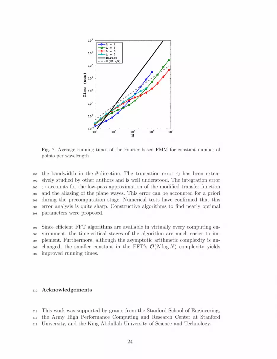
Figure 7 shows the recorded running times of the Fourier based FMM and the472

direct matrix-vector product on a Intel Core 2 Quad CPU Q9450 2.66GHz473

with 4GB of RAM. For N = 8.2 · 106 the points are uniformly distributed474

in a cube with side length 80λ and the wave number κ is scaled with N1/3.475

This provides a nearly constant density of points per wavelength as N is476

varied. As expected, by choosing the correct number of levels the running477

time is asymptotically O(N logN) as N is increased with a constant number478

of points per wavelength. Note that the cross-over point is less thanN = 4, 000.479

The code used to produce these results was not optimized for memory usage,480

preventing results for N & 106 when L = 7.481

4 Conclusion482

We have proposed using the Fourier basis eıpφeıqθ in the spherical variables φ483

and θ to represent the far field approximation in the FMM. By approximating484

the Helmholtz kernel with485

eıκ|r+r0|

|r + r0|≈∫ 2π

0

∫ 2π

0eıκs·r T s

ℓ,r0(s) dφdθ, T s

ℓ,r0(s) =

1

2Tℓ,r0

(s) |sin(θ)| ,

and using a uniform quadrature we can take advantage of very fast, exact, and486

well-known FFT interpolation/anterpolation methods. By exploiting symme-487

tries and a scheme to reduce the number of points in the φ direction, the total488

number of uniform quadrature points required is smaller than the number of489

Gauss-Legendre quadrature points typically used with spherical harmonics.490

22

1 10 100 1000

10−6

10−4

10−2

Box Size

Err

or

r0 ~ x, eps = 10 −4

|ε|

|εI|

|εG

|

|εG

EBF|

1 10 100 1000

10−6

10−4

10−2

Box Size

Err

or

r0 ~ z, eps = 10 −4

|ε|

|εI|

|εG

|

|εG

EBF|

1 10 100 10000.62

0.64

0.66

0.68

0.70

0.72

0.74

Quadrature Gain

Box Size

Ne

w Q

/ S

tan

da

rd Q

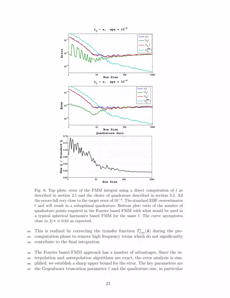
Fig. 6. Top plots: error of the FMM integral using a direct computation of ℓ asdescribed in section 2.1 and the choice of quadrature described in section 3.2. Allthe errors fall very close to the target error of 10−4. The standard EBF overestimatesℓ and will result in a suboptimal quadrature. Bottom plot: ratio of the number ofquadrature points required in the Fourier based FMM with what would be used ina typical spherical harmonics based FMM for the same ℓ. The curve asymptotesclose to 2/π ≈ 0.64 as expected.

This is realized by correcting the transfer function T sℓ,r0

(s) during the pre-491

computation phase to remove high frequency terms which do not significantly492

contribute to the final integration.493

The Fourier based FMM approach has a number of advantages. Since the in-494

terpolation and anterpolation algorithms are exact, the error analysis is sim-495

plified; we establish a sharp upper bound for the error. The key parameters are496

the Gegenbauer truncation parameter ℓ and the quadrature size, in particular497

23

103

104

105

106

107

10−1

100

101

102

103

104

105

106

N

Tim

e (

sec)

L = 4L = 5L = 6L = 7DirectO(NlogN)

Fig. 7. Average running times of the Fourier based FMM for constant number ofpoints per wavelength.

the bandwidth in the θ-direction. The truncation error εℓ has been exten-498

sively studied by other authors and is well understood. The integration error499

εI accounts for the low-pass approximation of the modified transfer function500

and the aliasing of the plane waves. This error can be accounted for a priori501

during the precomputation stage. Numerical tests have confirmed that this502

error analysis is quite sharp. Constructive algorithms to find nearly optimal503

parameters were proposed.504

Since efficient FFT algorithms are available in virtually every computing en-505

vironment, the time-critical stages of the algorithm are much easier to im-506

plement. Furthermore, although the asymptotic arithmetic complexity is un-507

changed, the smaller constant in the FFT’s O(N logN) complexity yields508

improved running times.509

Acknowledgements510

This work was supported by grants from the Stanford School of Engineering,511

the Army High Performance Computing and Research Center at Stanford512

University, and the King Abdullah University of Science and Technology.513

24

References514

[1] V. Rokhlin, Rapid solution of integral equations of scattering theory in two515

dimensions, J. Comput. Phys. 86 (2) (1990) 414–439.516

[2] R. Coifman, V. Rokhlin, S. Wandzura, The fast multipole method for the wave517

equation: A pedestrian prescription, Antennas and Propag. Magazine, IEEE518

35 (3) (1993) 7–12.519

[3] V. Rokhlin, Diagonal forms of translation operators for the Helmholtz equation520

in three dimensions, Applied and Computational Harmonic Analysis 1 (1993)521

82–93.522

[4] N. Engheta, W. D. Murphy, V. Rokhlin, M. S. Vassiliou, The fast multipole523

method (FMM) for electromagnetic scattering problems, IEEE Trans. Antennas524

Propag. 40 (1992) 634.525

[5] J. Rahola, Diagonal forms of the translation operators in the fast multipole526

algorithm for scattering problems, BIT 36 (1996) 333–358.527

[6] W. Chew, E. Michielssen, J. M. Song, J. M. Jin (Eds.), Fast and Efficient528

Algorithms in Computational Electromagnetics, Artech House, Inc., Norwood,529

MA, USA, 2001.530

[7] E. Darve, The fast multipole method: Numerical implementation, J. Comput.531

Phys. 160 (1) (2000) 195–240.532

[8] S. Koc, J. M. Song, W. C. Chew, Error analysis for the numerical evaluation of533

the diagonal forms of the scalar spherical addition theorem, SIAM J. Numer.534

Anal. 36 (3) (1999) 906–921.535

[9] J. R. Driscoll, D. Healy, Computing Fourier transforms and convolutions on the536

2-sphere, Adv. Appl. Math. 15 (2) (1994) 202–250.537

[10] D. Healy, D. Rockmore, P. Kostelec, S. Moore, FFTs for the 2-sphere -538

improvements and variations, J. Fourier Analysis and Applications 9 (4) (2003)539

341–385.540

[11] R. Suda, M. Takami, A fast spherical harmonics transform algorithm, Math. of541

Comp. 71 (238) (2001) 709–715.542

[12] J. Sarvas, Performing interpolation and anterpolation entirely by fast Fourier543

transform in the 3-D multilevel fast multipole algorithm, SIAM J. Numer. Anal.544

41 (6) (2003) 2180–2196.545

[13] Q. Carayol, F. Collino, Error estimates in the fast multipole method for546

scattering problems. Part 2: Truncation of the Gegenbauer series, ESAIM:547

M2NA 39 (1) (2004) 183–221.548

[14] E. Darve, The fast multipole method I: Error analysis and asymptotic549

complexity, SIAM J. Numer. Anal. 38 (1) (2000) 98–128.550

25

[15] M. L. Hastriter, S. Ohnuki, W. C. Chew, Error control of the translation551

operator in 3D MLFMA, Microwave and Optical Technology Letters 37 (3)552

(2003) 184–188.553

[16] Q. Carayol, F. Collino, Error estimates in the fast multipole method for554

scattering problems. Part 1: Truncation of the Jacobi-Anger series, ESAIM:555

M2NA 38 (2) (2004) 371–394.556

[17] A. D. McLaren, Optimal numerical integration on a sphere, Mathematics of557

Computation 17 (84) (1963) 361–383.558

[18] V. Rokhlin, M. Tygert, Fast algorithms for spherical harmonic expansions,559

SIAM J. Scientific Computing 27 (6) (2006) 1903–1928.560

[19] I. Chowdhury, V. Jandhyala, Integration and interpolation based on fast561

spherical transforms for the multilevel fast multipole method, Microwave and562

Optical Technology Letters 48 (10) (2006) 1961–1964.563

[20] R. Jakob-Chien, B. K. Alpert, A fast spherical filter with uniform resolution,564

J. Comput. Phys. 136 (2) (1997) 580–584.565

[21] A. Dutt, M. Gu, V. Rokhlin, Fast algorithms for polynomial interpolation,566

integration, and differentiation, SIAM J. Numer. Anal. 33 (5) (1996) 1689–567

1711.568

[22] J. Knab, Interpolation of bandlimited functions using the approximate prolate569

series (corresp.), Information Theory, IEEE 25 (6) (1979) 717–720.570

[23] E. Darve, P. Have, A fast multipole method for Maxwell equations stable at all571

frequencies, Phil. Trans. R. Soc. Lond. A 362 (1816) (2004) 603–628.572

[24] E. Darve, P. Have, Efficient fast multipole method for low-frequency scattering,573

J. Comput. Phys. 197 (1) (2004) 341–363.574

[25] O. Ergul, L. Gurel, Optimal interpolation of translation operator in multilevel575

fast multipole algorithm, IEEE Trans. Antennas Propag. 54 (12) (2006) 3822–576

3826.577

A Asymptotic Complexity578

In order to resolve a sufficient number of spherical harmonics, the number579

of points in the φ and θ directions must be O(ℓ) = O(κa), where a is the580

side length of the box. Therefore, the total number of quadrature points is581

O(ℓ2) = O((κa)2). If a0 is the side length of a box at the root of the octree582

(level l = 0), then the side length of a box at level l is al = 2−la0 and has583

O((κ2−la0)2) quadrature points.584

Suppose the octree has levels l = 0, . . . , L with boxes of side length al = 2−la0.585

A box at level l will contain a field approximation defined over a quadrature586

26

of size O((κ2−la0)2). We now determine the number of operations required for587

each step.588

(1) Initialization/Collection: This step requires sampling eıκs·r for each589

of the N source points at the leaves of the tree. Thus, this step is590

O(N(κ2−La0)2) = O(N2−2L(κa0)

2)

(2) Upward Pass: This step requires aggregating and interpolating each591

outgoing field upward through the tree. The type of interpolation algo-592

rithm is key to the running time of this step.593

At level l in the tree, the number of interpolations that must be per-594

formed is equal to the number of boxes at that level in the tree. The595

number of boxes depends on the distribution of source points. If the596

source points are uniformly distributed over a volumetric domain then597

the asymptotic number of boxes at level l in the octree is O(8l). How-598

ever, if the source points are uniformly distributed over the surface of an599

object then the asymptotic number of boxes at level l is O(4l).600

• Direct method: Each direct interpolation requires O(KLKL−1) =601

O((κ2−la0)2(κ2−(l−1)a0)

2) operations. Thus, the direct method has com-602

plexity603

Volume:L∑

l=3

O(8l(κ2−la0)2(κ2−(l−1)a0)

2) = O((κa0)4)

Surface:L∑

l=3

O(4l(κ2−la0)2(κ2−(l−1)a0)

2) = O((κa0)4)

• Fast global methods: By using a fast interpolation method, the com-604

plexity for an individual interpolation is reduced to O(Kl log(Kl)). The605

upward pass complexity then becomes606

Volume:L∑

l=3

O(8l(κ2−la0)2 log(κ2−la0)) = O(2L(κa0)

2(log(κa0)− L))

Surface:L∑

l=3

O(4l(κ2−la0)2 log(κ2−la0)) = O(L(κa0)

2(log(κa0)− L))

• Local methods: Local methods use a stencil of some given size to607

compute the interpolated values. Although these methods introduce608

additional error, they have fast execution times with O(Kl) operations.609

The upward pass complexity then becomes610

Volume:L∑

l=3

O(8l(κ2−la0)2) = O(2L(κa0)

2)

Surface:L∑

l=3

O(4l(κ2−la0)2) = O(L(κa0)

2)

27

(3) Transfer Pass: Since each box has a maximum of 189 transfers and the611

transfer function is diagonal, the running time of this step is612

Volume:L∑

l=2

O(8l(κ2−la0)2) = O(2L(κa0)

2)

Surface:L∑

l=2

O(4l(κ2−la0)2) = O(L(κa0)

2)

(4) Downward Pass: The downward pass is the adjoint operation of the613

Upward Pass and has the same asymptotic complexity.614

(5) Finalization: For each of the N field points, we integrate the spherical615

function at the leaf and compute the close contributions from neighboring616

boxes:617

O(N2−2L(κa0)2) +O(close)

In the worst case, the close interaction is O(N2) which occurs when there618

is an accumulation of points somewhere in the domain. In that case a619

different scheme is required since the expansions used in this paper are620

unstable at low frequency. When the field points are distributed roughly621

uniformly, then622

Volume: O(close) = O((N/8L)2) = O(2−6LN2)

Surface: O(close) = O((N/4L)2) = O(2−4LN2)

The total asymptotic running time then depends on the scaling of623

the number of points with a0, the scaling of L with N or a0, and the624

interpolation methods that are used.625

For a volume of scatters, we have O(N) = O((κa0)3) and let L ∼626

log(N1/3) to achieve a total algorithmic complexity of O(N logN) using627

fast global interpolation methods and O(N) by using approximate, local628

methods. For a surface of scatters, we have O(N) = O((κa0)2) and let629

L ∼ log(N1/2) to achieve a total algorithmic complexity of O(N log2N)630

using fast global interpolation methods and O(N logN) by using approx-631

imate, local methods.632

28

arX

iv:0

911.

4114

v1 [

mat

h.N

A]

20

Nov

200

9

Abstract

Key words:

PACS:

1

References

[1]

Preprint submitted to Elsevier 20 November 2009