double-layer potentials for a generalized bi-axially symmetric helmholtz equation
TRANSCRIPT
arX
iv:0
810.
3979
v1 [
mat
h.A
P] 2
2 O
ct 2
008
A double layer potentials for generalized bi-axially symmetric
equation
Anvar Hasanov
Institute of Mathematics, Uzbek Academy of Sciences,
29, F. Hodjaev street, Tashkent 100125, Uzbekistan
E-mail: [email protected]
Abstract
In the paper ”Fundamental solutions of generalized bi-axially symmetric Helmholtz equation”
(Complex Variables and Elliptic Equations, 52 (8), 2007, 673-683), fundamental solutions of general-
ized bi-axially symmetric Helmholtz equation (GBSHE)
Hλα,β (u) ≡ uxx + uyy +
2α
xux +
2β
yuy − λ
2u = 0, 0 < 2α, 2β < 1, α, β, λ = const,
were constructed in R+
2 = (x, y) : x > 0, y > 0 . In the present paper (in case of λ = 0) using the
constructed fundamental solutions, a double layer potentials are defined and investigated. Limiting
theorems are proved, and integral equations concerning a denseness of potentials of a double layer
are found.
MSC: Primary 35J15, 35J70.
Key Words and Phrases: Singular partial differential equation; Generalized bi-axially symmet-
ric equation; Degenerated Elliptic Equations; Generalized axisymmetric potentials; A double layer
potentials.
1 Introduction
In the monograph of Gilbert [1], by applying a method of complex analysis, integral representation of
solutions of the generalized bi-axially Helmholtz equation (GBSHE)
Hλα,β (u) ≡ uxx + uyy +
2α
xux +
2β
yuy − λ2u = 0,
(
Hλα,β
)
where 0 < 2α, 2β < 1, α, β, λ are constants, are constructed through analytic functions. When λ = 0
this equation is known as the equation of generalized axially symmetric potential theory (GASPT). This
name is due to Weinstein, who first considered fractional dimensional space in potential theory [2, 3]. The
special case where λ = 0 has also been investigated by Erdelyi [4, 5], Gilbert [6-12], Ranger [13], Henrici
[14, 16]. There are many works [17-29] in which some problems for the equation Hλα,β were studied. In
the paper [33] fundamental solutions of the equation Hλα,β are constructed. In case of λ = 0 fundamental
solutions look like
q1 (x, y;x0, y0) = k1
(
r2)−α−β
F2 (α+ β;α, β; 2α, 2β; ξ, η) , (1.1)
q2 (x, y;x0, y0) = k2
(
r2)α−β−1
x1−2αx1−2α0 F2 (1 − α+ β; 1 − α, β; 2 − 2α, 2β; ξ, η) , (1.2)
q3 (x, y;x0, y0) = k3
(
r2)−α+β−1
y1−2βy1−2β0 F2 (1 + α− β;α, 1 − β; 2α, 2 − 2β; ξ, η) , (1.3)
1

q4 (x, y;x0, y0) = k4
(
r2)α+β−2
x1−2αy1−2βx1−2α0 y1−2β
0 F2 (2 − α− β; 1 − α, 1 − β; 2 − 2α, 2 − 2β; ξ, η) ,
(1.4)
where
k1 =22α+2β
4π
Γ (α) Γ (β) Γ (α+ β)
Γ (2α) Γ (2β), (1.5)
k2 =22−2α+2β
4π
Γ (1 − α) Γ (β) Γ (1 − α+ β)
Γ (2 − 2α) Γ (2β), (1.6)
k3 =22+2α−2β
4π
Γ (α) Γ (1 − β) Γ (1 + α− β)
Γ (2α) Γ (2 − 2β), (1.7)
k4 =24−2α−2β
4π
Γ (1 − α) Γ (1 − β) Γ (2 − α− β)
Γ (2 − 2α) Γ (2 − 2β), (1.8)
r2
r21
r22
=
x
−
+
−
x0
2
+
y
−
−
+
y0
2
, ξ =r2 − r21r2
, η =r2 − r22r2
, (1.9)
F2 (a; b1, b2; c1, c2;x, y) =
∞∑
m,n=0
(a)m+n (b1)m (b2)n
(c1)m (c2)nm!n!xmyn, (1.10)
F2 (a; b1, b2; c1, c2;x, y) is a hypergeometric function of Appell ([31], p. 219 (7); [32], p. 14, (12)) and
(a)n = Γ (a+ n) /Γ (a) is symbol of Pochhammer ([31], p. 69; [32], p. 1, (2)). Fundamental solutions
(1.1) - (1.4) possess the following properties:
x2α ∂q1 (x, y;x0, y0)
∂x
∣
∣
∣
∣
x=0
= 0, y2β ∂q1 (x, y;x0, y0)
∂y
∣
∣
∣
∣
y=0
= 0, (1.11)
q2 (x, y;x0, y0)|x=0 = 0, y2β ∂q2 (x, y;x0, y0)
∂y
∣
∣
∣
∣
y=0
= 0, (1.12)
x2α ∂q3 (x, y;x0, y0)
∂x
∣
∣
∣
∣
x=0
= 0, q3 (x, y;x0, y0)|y=0 = 0, (1.13)
q4 (x, y;x0, y0)|x=0 = 0, q4 (x, y;x0, y0)|y=0 = 0. (1.14)
In this paper, using fundamental solutions (1.1) - (1.4) in the domain Ω ⊂ R2+ = (x, y) : x > 0, y > 0,
a double layer potentials for the equation H0α,β are investigated.
2 Green’s formula
Let’s consider identity
x2αy2β[
uH0α,β (v) − vH0
α,β (u)]
=∂
∂x
[
x2αy2β (vxu− vux)]
+∂
∂y
[
x2αy2β (vyu− vuy)]
. (2.1)
Integrating both parts of identity (2.1) on area Ω ⊂ R2+ = (x, y) : x > 0, y > 0, and using Green’s
formula, we find
x2αy2β[
uH0α,β (v) − vH0
α,β (u)]
dxdy =
∫
S
x2αy2βu (vxdy − vydx) − x2αy2βv (uxdy − uydx) , (2.2)
2
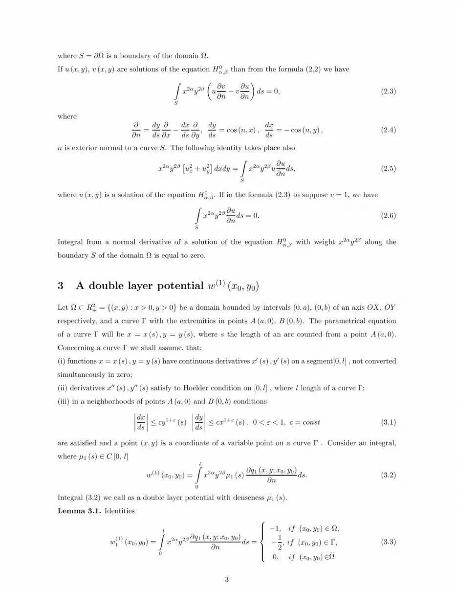
where S = ∂Ω is a boundary of the domain Ω.
If u (x, y), v (x, y) are solutions of the equation H0α,β than from the formula (2.2) we have
∫
S
x2αy2β
(
u∂v
∂n− v
∂u
∂n
)
ds = 0, (2.3)
where∂
∂n=dy
ds
∂
∂x−dx
ds
∂
∂y,dy
ds= cos (n, x) ,
dx
ds= − cos (n, y) , (2.4)
n is exterior normal to a curve S. The following identity takes place also
x2αy2β[
u2x + u2
y
]
dxdy =
∫
S
x2αy2βu∂u
∂nds, (2.5)
where u (x, y) is a solution of the equation H0α,β . If in the formula (2.3) to suppose v = 1, we have
∫
S
x2αy2β ∂u
∂nds = 0. (2.6)
Integral from a normal derivative of a solution of the equation H0α,β with weight x2αy2β along the
boundary S of the domain Ω is equal to zero.
3 A double layer potential w(1) (x0, y0)
Let Ω ⊂ R2+ = (x, y) : x > 0, y > 0 be a domain bounded by intervals (0, a), (0, b) of an axis OX , OY
respectively, and a curve Γ with the extremities in points A (a, 0), B (0, b). The parametrical equation
of a curve Γ will be x = x (s) , y = y (s), where s the length of an arc counted from a point A (a, 0).
Concerning a curve Γ we shall assume, that:
(i) functions x = x (s) , y = y (s) have continuous derivatives x′ (s) , y′ (s) on a segment[0, l] , not converted
simultaneously in zero;
(ii) derivatives x′′ (s) , y′′ (s) satisfy to Hoelder condition on [0, l] , where l length of a curve Γ;
(iii) in a neighborhoods of points A (a, 0) and B (0, b) conditions
∣
∣
∣
∣
dx
ds
∣
∣
∣
∣
≤ cy1+ε (s)
∣
∣
∣
∣
dy
ds
∣
∣
∣
∣
≤ cx1+ε (s) , 0 < ε < 1, c = const (3.1)
are satisfied and a point (x, y) is a coordinate of a variable point on a curve Γ . Consider an integral,
where µ1 (s) ∈ C [0, l]
w(1) (x0, y0) =
l∫
0
x2αy2βµ1 (s)∂q1 (x, y;x0, y0)
∂nds. (3.2)
Integral (3.2) we call as a double layer potential with denseness µ1 (s).
Lemma 3.1. Identities
w(1)1 (x0, y0) =
l∫
0
x2αy2β ∂q1 (x, y;x0, y0)
∂nds =
−1, if (x0, y0) ∈ Ω,
−1
2, if (x0, y0) ∈ Γ,
0, if (x0, y0) ∈Ω
(3.3)
3
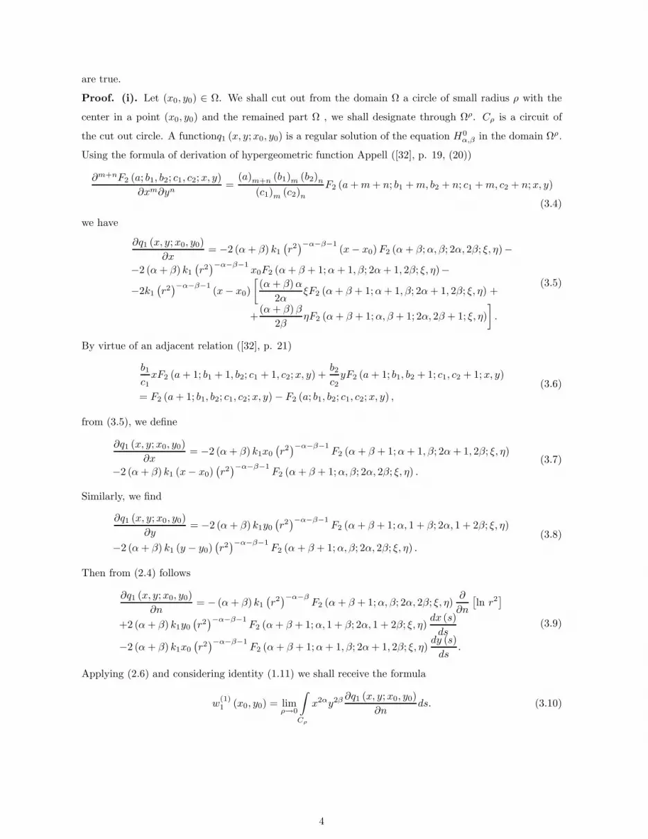
are true.
Proof. (i). Let (x0, y0) ∈ Ω. We shall cut out from the domain Ω a circle of small radius ρ with the
center in a point (x0, y0) and the remained part Ω , we shall designate through Ωρ. Cρ is a circuit of
the cut out circle. A functionq1 (x, y;x0, y0) is a regular solution of the equation H0α,β in the domain Ωρ.
Using the formula of derivation of hypergeometric function Appell ([32], p. 19, (20))
∂m+nF2 (a; b1, b2; c1, c2;x, y)
∂xm∂yn=
(a)m+n (b1)m (b2)n
(c1)m (c2)n
F2 (a+m+ n; b1 +m, b2 + n; c1 +m, c2 + n;x, y)
(3.4)
we have
∂q1 (x, y;x0, y0)
∂x= −2 (α+ β) k1
(
r2)−α−β−1
(x− x0)F2 (α+ β;α, β; 2α, 2β; ξ, η)−
−2 (α+ β) k1
(
r2)
−α−β−1x0F2 (α+ β + 1;α+ 1, β; 2α+ 1, 2β; ξ, η)−
−2k1
(
r2)
−α−β−1(x− x0)
[
(α+ β)α
2αξF2 (α+ β + 1;α+ 1, β; 2α+ 1, 2β; ξ, η) +
+(α+ β)β
2βηF2 (α+ β + 1;α, β + 1; 2α, 2β + 1; ξ, η)
]
.
(3.5)
By virtue of an adjacent relation ([32], p. 21)
b1c1xF2 (a+ 1; b1 + 1, b2; c1 + 1, c2;x, y) +
b2c2yF2 (a+ 1; b1, b2 + 1; c1, c2 + 1;x, y)
= F2 (a+ 1; b1, b2; c1, c2;x, y) − F2 (a; b1, b2; c1, c2;x, y) ,(3.6)
from (3.5), we define
∂q1 (x, y;x0, y0)
∂x= −2 (α+ β) k1x0
(
r2)−α−β−1
F2 (α+ β + 1;α+ 1, β; 2α+ 1, 2β; ξ, η)
−2 (α+ β) k1 (x− x0)(
r2)
−α−β−1F2 (α+ β + 1;α, β; 2α, 2β; ξ, η) .
(3.7)
Similarly, we find
∂q1 (x, y;x0, y0)
∂y= −2 (α+ β) k1y0
(
r2)−α−β−1
F2 (α+ β + 1;α, 1 + β; 2α, 1 + 2β; ξ, η)
−2 (α+ β) k1 (y − y0)(
r2)
−α−β−1F2 (α+ β + 1;α, β; 2α, 2β; ξ, η) .
(3.8)
Then from (2.4) follows
∂q1 (x, y;x0, y0)
∂n= − (α+ β) k1
(
r2)−α−β
F2 (α+ β + 1;α, β; 2α, 2β; ξ, η)∂
∂n
[
ln r2]
+2 (α+ β) k1y0(
r2)
−α−β−1F2 (α+ β + 1;α, 1 + β; 2α, 1 + 2β; ξ, η)
dx (s)
ds
−2 (α+ β) k1x0
(
r2)
−α−β−1F2 (α+ β + 1;α+ 1, β; 2α+ 1, 2β; ξ, η)
dy (s)
ds.
(3.9)
Applying (2.6) and considering identity (1.11) we shall receive the formula
w(1)1 (x0, y0) = lim
ρ→0
∫
Cρ
x2αy2β ∂q1 (x, y;x0, y0)
∂nds. (3.10)
4

Substituting (3.9) into (3.10), we define
w(1)1 (x0, y0)
= − (α+ β) k1 limρ→0
∫
Cρ
x2αy2β(
r2)−α−β
F2 (1 + α+ β;α, β; 2α, 2β; ξ, η)∂
∂n
[
ln r2]
ds
−2 (α+ β) k1x0 limρ→0
∫
Cρ
x2αy2β(
r2)−α−β−1
F2 (1 + α+ β; 1 + α, β; 1 + 2α, 2β; ξ, η)dy (s)
dsds
+2 (α+ β) k1y0 limρ→0
∫
Cρ
x2αy2β(
r2)−α−β−1
F2 (1 + α+ β;α, 1 + β; 2α, 1 + 2β; ξ, η)dx (s)
dsds
= − (α+ β) k1 limρ→0
J1 (x0, y0) − 2 (α+ β) k1x0 limρ→0
J2 (x0, y0) + 2 (α+ β) k1y0 limρ→0
J3 (x0, y0) .
(3.11)
Introducing polar coordinates x = x0 + ρ cosϕ, y = y0 + ρ sinϕ, we find
J1 (x0, y0) = −2 (α+ β) k1 limρ→0
2π∫
0
(x0 + ρ cosϕ)2α (y0 + ρ sinϕ)2β
·(
ρ2)
−α−βF2 (1 + α+ β;α, β; 2α, 2β; ξ, η, ζ) dϕ.
(3.12)
Using formulas ([30], p. 253, (26), [31], p. 113, (4))
F2 (a; b1, b2; c1, c2;x, y)
=
∞∑
i=0
(a)i (b1)i (b2)i
(c1)i (c2)i i!xiyiF (a+ i, b1 + i; c1 + i;x)F (a+ i, b2 + i; c2 + i; y) ,
(3.13)
F (a, b; c, x) = (1 − x)−bF
(
c− a, b; c,x
x− 1
)
, (3.14)
we define
F2 (a; b1, b2; c1, c2;x, y)
= (1 − x)−b1 (1 − y)−b2
∞∑
i=0
(a)i (b1)i (b2)i
(c1)i (c2)i i!
(
x
1 − x
)i (y
1 − y
)i
·
·F
(
c1 − a, b1 + i; c1 + i;x
x− 1
)
F
(
c2 − a, b2 + i; c2 + i;y
y − 1
)
,
(3.15)
where F (a, b; c;x) is hypergeometric function of Gauss ([31], p. 69, (2)). Hence
F2 (1 + α+ β;α, β; 2α, 2β; ξ, η)
=(
ρ2)α+β (
ρ2 + 4x20 + 4x0ρ cos ϕ
)
−α (
ρ2 + 4y20 + 4y0ρ sin ϕ
)
−βP11,
(3.16)
where
P11 =
∞∑
i=0
(1 + α+ β)i (α)i (β)i
(2α)i (2β)i i!j!
(
4x20 + 4x0ρ cos ϕ
ρ2 + 4x20 + 4x0ρ cos ϕ
)i (4y2
0 + 4y0ρ sin ϕ
ρ2 + 4y20 + 4y0ρ sin ϕ
)i
·F
(
α− β − 1, α+ i; 2α+ i;4x2
0 + 4x0ρ cos ϕ
ρ2 + 4x20 + 4x0ρ cos ϕ
)
·F
(
β − α− 1, β + i; 2β + i;4y2
0 + 4y0ρ sin ϕ
ρ2 + 4y20 + 4y0ρ sin ϕ
)
.
Using value of hypergeometric function of Gauss ([31], p. 112, (46))
F (a, b; c; 1) =Γ (c) Γ (c− a− b)
Γ (c− a) Γ (c− b), c 6= 0,−1,−2, ...,Re(c− a− b) > 0,
5
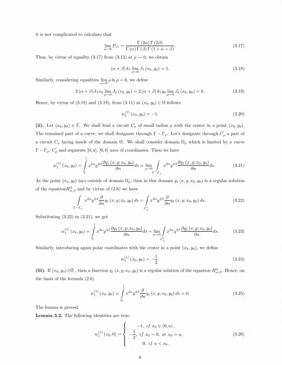
it is not complicated to calculate that
limρ→0
P11 =Γ (2α) Γ (2β)
Γ (α) Γ (β) Γ (1 + α+ β). (3.17)
Thus, by virtue of equality (3.17) from (3.12) at ρ→ 0, we obtain
(α+ β) k1 limρ→0
J1 (x0, y0) = 1. (3.18)
Similarly, considering equalities limρ→0
ρ ln ρ = 0, we define
2 (α+ β) k1x0 limρ→0
J2 (x0, y0) = 2 (α+ β) k1y0 limρ→0
J3 (x0, y0) = 0. (3.19)
Hence, by virtue of (3.18) and (3.19), from (3.11) at (x0, y0) ∈ Ω follows
w(1)1 (x0, y0) = −1. (3.20)
(ii). Let (x0, y0) ∈ Γ. We shall lead a circuit Cρ of small radius ρ with the center in a point (x0, y0).
The remained part of a curve, we shall designate through Γ − Γρ. Let’s designate through C′
ρ a part of
a circuit Cρ laying inside of the domain Ω. We shall consider domain Ωρ which is limited by a curve
Γ − Γρ, C′
ρ and segments [0, a], [0, b] axes of coordinates. Then we have
w(1)1 (x0, y0) =
l∫
0
x2αy2β ∂q1 (x, y;x0, y0)
∂nds = lim
ρ→0
∫
Γ−Γρ
x2αy2β ∂q1 (x, y;x0, y0)
∂nds. (3.21)
As the point (x0, y0) lays outside of domain Ωρ, then in this domain q1 (x, y;x0, y0) is a regular solution
of the equationH0α,β and by virtue of (2.6) we have∫
Γ−Γρ
x2αy2β ∂
∂nq1 (x, y;x0, y0) ds =
∫
C′
ρ
x2αy2β ∂
∂nq1 (x, y;x0, y0) ds. (3.22)
Substituting (3.22) in (3.21), we get
w(1)1 (x0, y0) =
l∫
0
x2αy2β ∂q1 (x, y;x0, y0)
∂nds = lim
ρ→0
∫
C′
ρ
x2αy2β ∂q1 (x, y;x0, y0)
∂nds. (3.23)
Similarly, introducing again polar coordinates with the center in a point (x0, y0), we define
w(1)1 (x0, y0) = −
1
2. (3.24)
(iii). If (x0, y0) ∈Ω , then a function q1 (x, y;x0, y0) is a regular solution of the equation H0α,β. Hence, on
the basis of the formula (2.6)
w(1)1 (x0, y0) =
l∫
0
x2αy2β ∂
∂nq1 (x, y;x0, y0) ds = 0. (3.25)
The lemma is proved.
Lemma 3.2. The following identities are true:
w(1)1 (x0, 0) =
−1, if x0 ∈ (0, a) ,
−1
2, if x0 = 0, or x0 = a,
0, if a < x0.
(3.26)
6

Proof. (i). Let x0 ∈ (0, a). We lead a straight line y0 = h (h is enough small number) and we consider
domain Ωh which is the part of area Ω laying above a straight line y0 = h . Applying the formula (2.6),
we obtain
w(1)1 (x0, 0) = lim
h→0
x1∫
0
x2αy2β ∂q1 (x, y;x0, 0)
∂y
∣
∣
∣
∣
y=h
dx, (3.27)
where x1 (ε) is an abscissa of a point intersection of a curve Γ from a straight line y0 = h. By virtue of
(3.8) from (3.27), follows
w(1)1 (x0, 0) = −2 (α+ β) k1 lim
h→0h1+2β
x1∫
0
x2α
F
(
α+ β + 1, α; 2α,−4xx0
(x− x0)2
+ h2
)
[
(x− x0)2
+ h2]α+β+1
dx. (3.28)
Using the formula (3.14) of equality (3.28), we have
w(1)1 (x0, 0) = −2 (α+ β) k1 lim
h→0h1+2β
x1∫
0
x2α
F
(
α− β − 1, α; 2α,4xx0
(x+ x0)2
+ h2
)
[
(x− x0)2 + h2
]β+1 [
(x+ x0)2 + h2
]αdx. (3.29)
Let’s introduce a new variable of an integration x = x0 + ht , then
w(1)1 (x0, 0) = −2 (α+ β) k1 lim
h→0
l2∫
l1
(x0 + ht)2α
F
(
α− β − 1, α; 2α,4x0 (x0 + ht)
(2x0 + ht)2 + h2
)
(1 + t2)β+1
[
(2x0 + ht)2+ h2
]α dt, (3.30)
where
l1 = −x0
h, l2 =
x1 − x0
h. (3.31)
By virtue of that
limh→0
F
(
α− β − 1, α; 2α,4x0 (x0 + ht)
(2x0 + ht)2+ h2
)
= F (α− β − 1, α; 2α, 1) =Γ (2α) Γ (1 + β)
(α+ β) Γ (α+ β) Γ (α),
and+∞∫
−∞
dt
(1 + t2)β+1
=πΓ (2β)
22β−1βΓ2 (β),
then from (3.30) follows
w(1)1 (x0, 0) = −1. (3.32)
(ii). Let x0 = 0 . Then from (3.31), we have l1 = 0, limh→0
l2 = x1/h = +∞ . Hence, from (3.30) it is
similarly defined
w(1)1 (0, 0) = −
1
2. (3.33)
(iii). Let x0 = a . Then from (3.31) by virtue of a condition (3.1), we have limh→0
l1 = −∞, limh→0
l2 =
(x1 − a) /h = 0. Hence, from (3.30) follows
w(1)1 (a, 0) = −
1
2. (3.34)
7
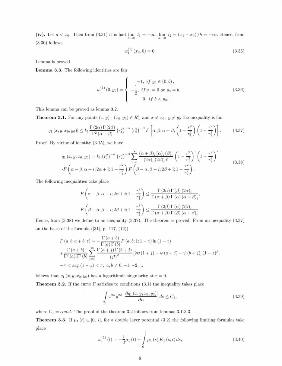
(iv). Let a < x0. Then from (3.31) it is had limh→0
l1 = −∞, limh→0
l2 = (x1 − x0) /h = −∞. Hence, from
(3.30) follows
w(1)1 (x0, 0) = 0. (3.35)
Lemma is proved.
Lemma 3.3. The following identities are fair
w(1)1 (0, y0) =
−1, if y0 ∈ (0, b) ,
−1
2, if y0 = 0 or y0 = b,
0, if b < y0.
(3.36)
This lemma can be proved as lemma 3.2.
Theorem 3.1. For any points (x, y) , (x0, y0) ∈ R2+ and x 6= x0, y 6= y0 the inequality is fair
|q1 (x, y;x0, y0)| ≤ k1Γ (2α) Γ (2β)
Γ2 (α+ β)
(
r21)−α (
r22)−β
F
[
α, β;α + β;
(
1 −r2
r21
)(
1 −r2
r22
)]
. (3.37)
Proof. By virtue of identity (3.15), we have
q1 (x, y;x0, y0) = k1
(
r21)
−α (
r22)
−β∞∑
i=0
(α+ β)i (α)i (β)i
(2α)i (2β)i i!
(
1 −r2
r21
)i(
1 −r2
r22
)i
·F
(
α− β, α+ i; 2α+ i; 1 −r2
r21
)
F
(
β − α, β + i; 2β + i; 1 −r2
r22
)
.
(3.38)
The following inequalities take place
F
(
α− β, α+ i; 2α+ i; 1 −r2
r21
)
≤Γ (2α) Γ (β) (2α)i
Γ (α+ β) Γ (α) (α+ β)i
,
F
(
β − α, β + i; 2β + i; 1 −r2
r22
)
≤Γ (2β) Γ (α) (2β)i
Γ (α+ β) Γ (β) (α+ β)i
.
Hence, from (3.38) we define to an inequality (3.37). The theorem is proved. From an inequality (3.37)
on the basis of the formula ([31], p. 117, (12))
F (a, b; a+ b; z) = −Γ (a+ b)
Γ (a) Γ (b)F (a, b; 1; 1 − z) ln (1 − z)
+Γ (a+ b)
Γ2 (a) Γ2 (b)
∞∑
j=0
Γ (a+ j) Γ (b+ j)
(j!)2 [2ψ (1 + j) − ψ (a+ j) − ψ (b+ j)] (1 − z)
j,
−π < arg (1 − z) < π, a, b 6= 0,−1,−2, ...
follows that q1 (x, y;x0, y0) has a logarithmic singularity at r = 0.
Theorem 3.2. If the curve Γ satisfies to conditions (3.1) the inequality takes place
∫
Γ
x2αy2β
∣
∣
∣
∣
∂q1 (x, y;x0, y0)
∂n
∣
∣
∣
∣
ds ≤ C1, (3.39)
where C1 = const. The proof of the theorem 3.2 follows from lemmas 3.1-3.3.
Theorem 3.3. If µ1 (t) ∈ [0, l], for a double layer potential (3.2) the following limiting formulas take
place
w(1)i (t) = −
1
2µ1 (t) +
l∫
0
µ1 (s)K1 (s, t) ds, (3.40)
8
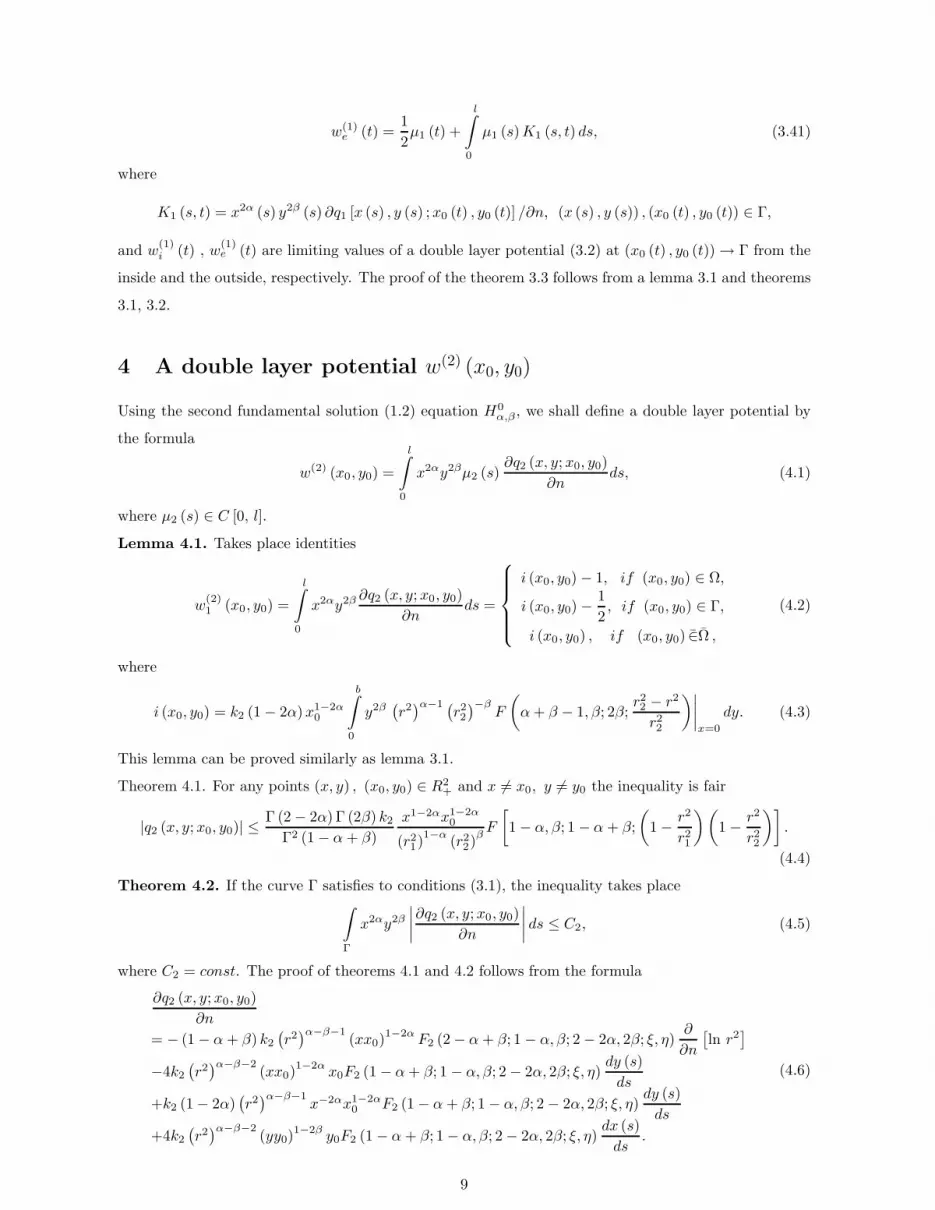
w(1)e (t) =
1
2µ1 (t) +
l∫
0
µ1 (s)K1 (s, t) ds, (3.41)
where
K1 (s, t) = x2α (s) y2β (s) ∂q1 [x (s) , y (s) ;x0 (t) , y0 (t)] /∂n, (x (s) , y (s)) , (x0 (t) , y0 (t)) ∈ Γ,
and w(1)i (t) , w
(1)e (t) are limiting values of a double layer potential (3.2) at (x0 (t) , y0 (t)) → Γ from the
inside and the outside, respectively. The proof of the theorem 3.3 follows from a lemma 3.1 and theorems
3.1, 3.2.
4 A double layer potential w(2) (x0, y0)
Using the second fundamental solution (1.2) equation H0α,β , we shall define a double layer potential by
the formula
w(2) (x0, y0) =
l∫
0
x2αy2βµ2 (s)∂q2 (x, y;x0, y0)
∂nds, (4.1)
where µ2 (s) ∈ C [0, l].
Lemma 4.1. Takes place identities
w(2)1 (x0, y0) =
l∫
0
x2αy2β ∂q2 (x, y;x0, y0)
∂nds =
i (x0, y0) − 1, if (x0, y0) ∈ Ω,
i (x0, y0) −1
2, if (x0, y0) ∈ Γ,
i (x0, y0) , if (x0, y0) ∈Ω ,
(4.2)
where
i (x0, y0) = k2 (1 − 2α)x1−2α0
b∫
0
y2β(
r2)α−1 (
r22)−β
F
(
α+ β − 1, β; 2β;r22 − r2
r22
)∣
∣
∣
∣
x=0
dy. (4.3)
This lemma can be proved similarly as lemma 3.1.
Theorem 4.1. For any points (x, y) , (x0, y0) ∈ R2+ and x 6= x0, y 6= y0 the inequality is fair
|q2 (x, y;x0, y0)| ≤Γ (2 − 2α) Γ (2β) k2
Γ2 (1 − α+ β)
x1−2αx1−2α0
(r21)1−α
(r22)βF
[
1 − α, β; 1 − α+ β;
(
1 −r2
r21
)(
1 −r2
r22
)]
.
(4.4)
Theorem 4.2. If the curve Γ satisfies to conditions (3.1), the inequality takes place∫
Γ
x2αy2β
∣
∣
∣
∣
∂q2 (x, y;x0, y0)
∂n
∣
∣
∣
∣
ds ≤ C2, (4.5)
where C2 = const. The proof of theorems 4.1 and 4.2 follows from the formula
∂q2 (x, y;x0, y0)
∂n
= − (1 − α+ β) k2
(
r2)α−β−1
(xx0)1−2α F2 (2 − α+ β; 1 − α, β; 2 − 2α, 2β; ξ, η)
∂
∂n
[
ln r2]
−4k2
(
r2)α−β−2
(xx0)1−2α
x0F2 (1 − α+ β; 1 − α, β; 2 − 2α, 2β; ξ, η)dy (s)
ds
+k2 (1 − 2α)(
r2)α−β−1
x−2αx1−2α0 F2 (1 − α+ β; 1 − α, β; 2 − 2α, 2β; ξ, η)
dy (s)
ds
+4k2
(
r2)α−β−2
(yy0)1−2β y0F2 (1 − α+ β; 1 − α, β; 2 − 2α, 2β; ξ, η)
dx (s)
ds.
(4.6)
9
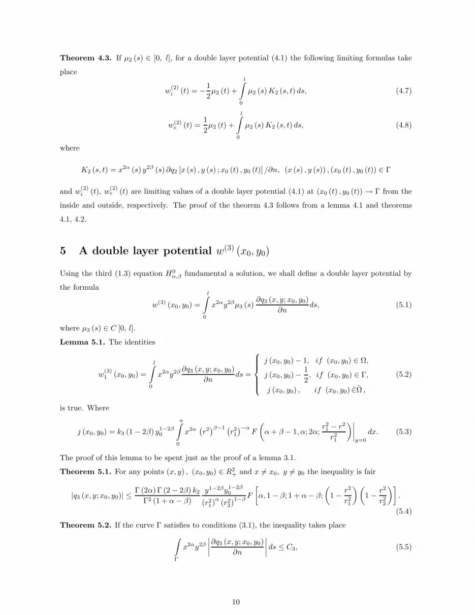
Theorem 4.3. If µ2 (s) ∈ [0, l], for a double layer potential (4.1) the following limiting formulas take
place
w(2)i (t) = −
1
2µ2 (t) +
l∫
0
µ2 (s)K2 (s, t) ds, (4.7)
w(2)e (t) =
1
2µ2 (t) +
l∫
0
µ2 (s)K2 (s, t) ds, (4.8)
where
K2 (s, t) = x2α (s) y2β (s) ∂q2 [x (s) , y (s) ;x0 (t) , y0 (t)] /∂n, (x (s) , y (s)) , (x0 (t) , y0 (t)) ∈ Γ
and w(2)i (t), w
(2)e (t) are limiting values of a double layer potential (4.1) at (x0 (t) , y0 (t)) → Γ from the
inside and outside, respectively. The proof of the theorem 4.3 follows from a lemma 4.1 and theorems
4.1, 4.2.
5 A double layer potential w(3) (x0, y0)
Using the third (1.3) equation H0α,β fundamental a solution, we shall define a double layer potential by
the formula
w(3) (x0, y0) =
l∫
0
x2αy2βµ3 (s)∂q3 (x, y;x0, y0)
∂nds, (5.1)
where µ3 (s) ∈ C [0, l].
Lemma 5.1. The identities
w(3)1 (x0, y0) =
l∫
0
x2αy2β ∂q3 (x, y;x0, y0)
∂nds =
j (x0, y0) − 1, if (x0, y0) ∈ Ω,
j (x0, y0) −1
2, if (x0, y0) ∈ Γ,
j (x0, y0) , if (x0, y0) ∈Ω ,
(5.2)
is true. Where
j (x0, y0) = k3 (1 − 2β) y1−2β0
a∫
0
x2α(
r2)β−1 (
r21)−α
F
(
α+ β − 1, α; 2α;r21 − r2
r21
)∣
∣
∣
∣
y=0
dx. (5.3)
The proof of this lemma to be spent just as the proof of a lemma 3.1.
Theorem 5.1. For any points (x, y) , (x0, y0) ∈ R2+ and x 6= x0, y 6= y0 the inequality is fair
|q3 (x, y;x0, y0)| ≤Γ (2α) Γ (2 − 2β) k2
Γ2 (1 + α− β)
y1−2βy1−2β0
(r21)α
(r22)1−β
F
[
α, 1 − β; 1 + α− β;
(
1 −r2
r21
)(
1 −r2
r22
)]
.
(5.4)
Theorem 5.2. If the curve Γ satisfies to conditions (3.1), the inequality takes place
∫
Γ
x2αy2β
∣
∣
∣
∣
∂q3 (x, y;x0, y0)
∂n
∣
∣
∣
∣
ds ≤ C3, (5.5)
10
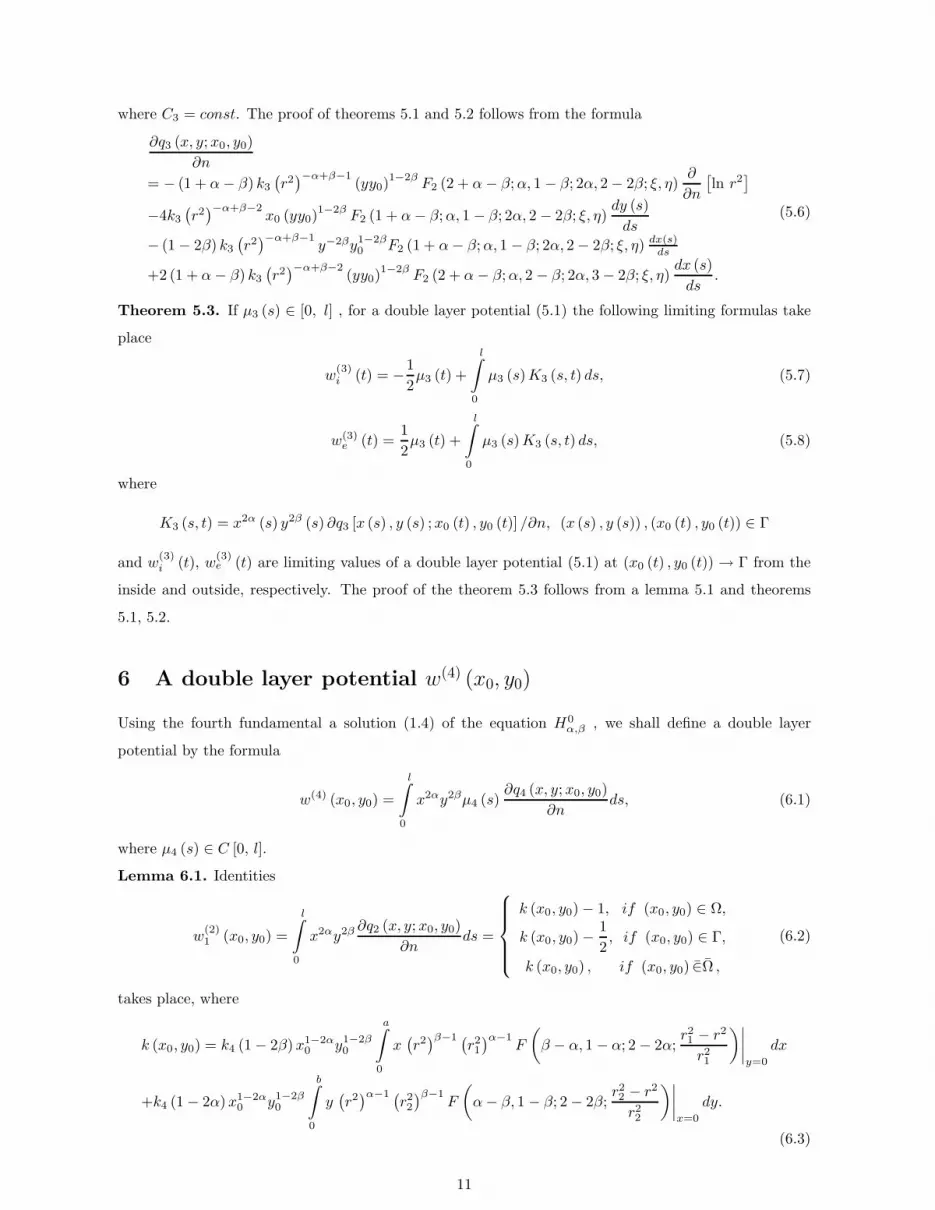
where C3 = const. The proof of theorems 5.1 and 5.2 follows from the formula
∂q3 (x, y;x0, y0)
∂n
= − (1 + α− β) k3
(
r2)
−α+β−1(yy0)
1−2βF2 (2 + α− β;α, 1 − β; 2α, 2 − 2β; ξ, η)
∂
∂n
[
ln r2]
−4k3
(
r2)
−α+β−2x0 (yy0)
1−2β F2 (1 + α− β;α, 1 − β; 2α, 2 − 2β; ξ, η)dy (s)
ds
− (1 − 2β) k3
(
r2)
−α+β−1y−2βy1−2β
0 F2 (1 + α− β;α, 1 − β; 2α, 2 − 2β; ξ, η) dx(s)ds
+2 (1 + α− β) k3
(
r2)
−α+β−2(yy0)
1−2β F2 (2 + α− β;α, 2 − β; 2α, 3 − 2β; ξ, η)dx (s)
ds.
(5.6)
Theorem 5.3. If µ3 (s) ∈ [0, l] , for a double layer potential (5.1) the following limiting formulas take
place
w(3)i (t) = −
1
2µ3 (t) +
l∫
0
µ3 (s)K3 (s, t) ds, (5.7)
w(3)e (t) =
1
2µ3 (t) +
l∫
0
µ3 (s)K3 (s, t) ds, (5.8)
where
K3 (s, t) = x2α (s) y2β (s) ∂q3 [x (s) , y (s) ;x0 (t) , y0 (t)] /∂n, (x (s) , y (s)) , (x0 (t) , y0 (t)) ∈ Γ
and w(3)i (t), w
(3)e (t) are limiting values of a double layer potential (5.1) at (x0 (t) , y0 (t)) → Γ from the
inside and outside, respectively. The proof of the theorem 5.3 follows from a lemma 5.1 and theorems
5.1, 5.2.
6 A double layer potential w(4) (x0, y0)
Using the fourth fundamental a solution (1.4) of the equation H0α,β , we shall define a double layer
potential by the formula
w(4) (x0, y0) =
l∫
0
x2αy2βµ4 (s)∂q4 (x, y;x0, y0)
∂nds, (6.1)
where µ4 (s) ∈ C [0, l].
Lemma 6.1. Identities
w(2)1 (x0, y0) =
l∫
0
x2αy2β ∂q2 (x, y;x0, y0)
∂nds =
k (x0, y0) − 1, if (x0, y0) ∈ Ω,
k (x0, y0) −1
2, if (x0, y0) ∈ Γ,
k (x0, y0) , if (x0, y0) ∈Ω ,
(6.2)
takes place, where
k (x0, y0) = k4 (1 − 2β)x1−2α0 y1−2β
0
a∫
0
x(
r2)β−1 (
r21)α−1
F
(
β − α, 1 − α; 2 − 2α;r21 − r2
r21
)∣
∣
∣
∣
y=0
dx
+k4 (1 − 2α)x1−2α0 y1−2β
0
b∫
0
y(
r2)α−1 (
r22)β−1
F
(
α− β, 1 − β; 2 − 2β;r22 − r2
r22
)∣
∣
∣
∣
x=0
dy.
(6.3)
11
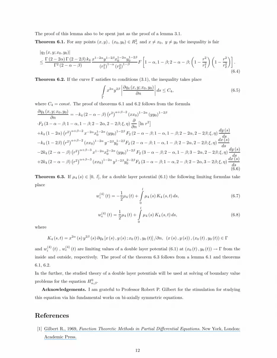
The proof of this lemma also to be spent just as the proof of a lemma 3.1.
Theorem 6.1. For any points (x, y) , (x0, y0) ∈ R2+ and x 6= x0, y 6= y0 the inequality is fair
|q2 (x, y;x0, y0)|
≤Γ (2 − 2α) Γ (2 − 2β) k4
Γ2 (2 − α− β)
x1−2αy1−2βx1−2α0 y1−2β
0
(r21)1−α
(r22)1−β
F
[
1 − α, 1 − β; 2 − α− β;
(
1 −r2
r21
)(
1 −r2
r22
)]
.
(6.4)
Theorem 6.2. If the curve Γ satisfies to conditions (3.1), the inequality takes place∫
Γ
x2αy2β
∣
∣
∣
∣
∂q4 (x, y;x0, y0)
∂n
∣
∣
∣
∣
ds ≤ C4, (6.5)
where C4 = const. The proof of theorems 6.1 and 6.2 follows from the formula
∂q4 (x, y;x0, y0)
∂n= −k4 (2 − α− β)
(
r2)α+β−2
(xx0)1−2α
(yy0)1−2β
·F2 (3 − α− β; 1 − α, 1 − β; 2 − 2α, 2 − 2β; ξ, η)∂
∂n
[
ln r2]
+k4 (1 − 2α)(
r2)α+β−2
x−2αx1−2α0 (yy0)
1−2βF2 (2 − α− β; 1 − α, 1 − β; 2 − 2α, 2 − 2β; ξ, η)
dy (s)
ds
−k4 (1 − 2β)(
r2)α+β−2
(xx0)1−2α y−2βy1−2β
0 F2 (2 − α− β; 1 − α, 1 − β; 2 − 2α, 2 − 2β; ξ, η)dx (s)
ds
−2k4 (2 − α− β)(
r2)α+β−3
x1−2αx2−2α0 (yy0)
1−2βF2 (3 − α− β; 2 − α, 1 − β; 3 − 2α, 2 − 2β; ξ, η)
dy (s)
ds
+2k4 (2 − α− β)(
r2)α+β−3
(xx0)1−2α
y1−2βy2−2β0 F2 (3 − α− β; 1 − α, 2 − β; 2 − 2α, 3 − 2β; ξ, η)
dx (s)
ds(6.6)
Theorem 6.3. If µ4 (s) ∈ [0, l], for a double layer potential (6.1) the following limiting formulas take
place
w(4)i (t) = −
1
2µ4 (t) +
l∫
0
µ4 (s)K4 (s, t) ds, (6.7)
w(4)e (t) =
1
2µ4 (t) +
l∫
0
µ4 (s)K4 (s, t) ds, (6.8)
where
K4 (s, t) = x2α (s) y2β (s) ∂q4 [x (s) , y (s) ;x0 (t) , y0 (t)] /∂n, (x (s) , y (s)) , (x0 (t) , y0 (t)) ∈ Γ
and w(4)i (t) , w
(4)e (t) are limiting values of a double layer potential (6.1) at (x0 (t) , y0 (t)) → Γ from the
inside and outside, respectively. The proof of the theorem 6.3 follows from a lemma 6.1 and theorems
6.1, 6.2.
In the further, the studied theory of a double layer potentials will be used at solving of boundary value
problems for the equation H0α,β .
Acknowledgements. I am grateful to Professor Robert P. Gilbert for the stimulation for studying
this equation via his fundamental works on bi-axially symmetric equations.
References
[1] Gilbert R., 1969, Function Theoretic Methods in Partial Differential Equations. New York, London:
Academic Press.
12
[2] Weinstein A., 1948, Discontinuous integrals and generalized potential theory. Trans. Amer. Math.
Soc., 63, 342-354.
[3] Weinstein A., 1953, Generalized axially symmetric potentials theory. Bull. Amer. Math. Soc., 59,
20-38.
[4] Erdelyi A. 1956, Singularities of generalized axially symmetric potentials. Comm. Pure Appl. Math.,
2, 403-414.
[5] Erdelyi A. 1965, An application of fractional integrals. J. Analyse. Math., 14, 113-126.
[6] Gilbert R., 1960, On the singularities of generalized axially symmetric potentials. Arch. Rational
Mech. Anal., 6, 171-176.
[7] Gilbert R., 1962, Some properties of generalized axially symmetric potentials. Amer. J. Math., 84,
475-484.
[8] Gilbert R, 1964, ”Bergman’s” integral operator method in generalized axially symmetric potential
theory. J. Mathematical Phys., 5, 983-987.
[9] Gilbert R., 1965, On the location of singularities of a class of elliptic partial differential equations in
four variables. Canad. J. Math., 17, 676-686.
[10] Gilbert R. and Howard H., 1965, On solutions of the generalized axially symmetric wave equation
represented by Bergman operators, Proc. London Math. Soc., 15 (2), 346-360.
[11] Gilbert R., 1967, On the analytic properties of solutions to a generalized axially symmetric Schrood-
inger equations. J. Differential equators, 3, 59-77.
[12] Gilbert, R., 1968, An investigation of the analytic properties of solutions to the generalized axially
symmetric, reduced wave equation in n+ 1 variables, with an application to the theory of potential
scattering. SIAM J. Appl. Math. 16 (1), 30-50.
[13] Ranger K. B., 1965, On the construction of some integral operators for generalized axially symmetric
harmonic and stream functions. J. Math. Mech., 14, 383-402.
[14] Henrici P., 1953, Zur Funktionentheorie der Wellengleichung, Comment. Math. Helv., 27, 235-293.
[15] Henrici P., 1957, On the domain of regularity of generalized axially symmetric potentials. Proc.
Amer. Math. Soc., 8, 29-31.
[16] Henrici P., 1960, Complete systems of solutions for a class of singular elliptic Partial Differential
Equations. Boundary Value Problems in differential equations, University of Wisconsin Press, Madi-
son, 19-34.
[17] Huber A., 1954, On the uniqueness of generalized axisymmetric potentials. Ann. Math., 60, 351-358.
13
[18] Weinacht R. J., 1974, Some properties of generalized axially symmetric Helmholtz potentials. SIAM
J. Math. Anal. 5, 147-152.
[19] Lo C.Y., 1977, Boundary value problems of generalized axially symmetric Helmholtz equations.
Portugaliae Mathematica. 36(3-4), 279-289.
[20] Marichev O.I., 1978, Integral representation of solutions of the generalized double axial symmetric
Helmholtz equation (Russian). Differencial’nye Uravnenija, Minsk, 14(10), 1824-1831.
[21] McCoy P.A., 1979, Polynomial approximation and growth of generalized axisymmetric potentials.
Canadian Journal of Mathematics, 31(1), 49-59.
[22] McCoy P.A., 1980, Best Lp - Approximation of Generalized bi-axisymmetric Potentials. Proceedings
of the American Mathematical Society, 79(3), pp. 435-440.
[23] Fryant A.J., 1979, Growth and complete sequences of generalized bi-axially symmetric potentials.
Journal of Differential Equations, 31(2), 155-164.
[24] Altin A., 1982, Solutions of type rm for a class of singular equations. International Journal of
Mathematical Science, 5(3), 613-619.
[25] Altin A., 1982, Some expansion formulas for a class of singular partial differential equations. Pro-
ceedings of American Mathematical Society, 85(1), 42-46.
[26] Ping N.P. and Bo L.X., 1983, Some notes on solvability of LPDO. Journal of Mathematical Research
and Expositions, 3(1), 127-129.
[27] Altin A. and Eutiquio Y., 1983, Some properties of solutions of a class of singular partial differential
equations. Bulletin of the Institute of Mathematics Academic Sinica, 11(1), 81-87.
[28] Kumar P., 2005, Approximation of growth numbers generalized bi-axially symmetric potentials.
Fasciculi Mathematics, 35, 51-60.
[29] Rassias J.M., and Hasanov A., 2007, Fundamental Solutions of Two Degenerated Elliptic Equa-
tions and Solutions of Boundary Value Problems in Infinite Area. International Journal of Applied
Mathematics and Statistics, 8(7), 87-95.
[30] Burchnall J.L., Chaundy T.W. Expansions of Appell’s double hypergeometric functions. // Quart.
J. Math. Oxford Ser. 11, 1940 p. 249-270.
[31] Erdelyi A., Magnus W., Oberhettinger F. and Tricomi F. G., 1973, Higher transcendental functions
(Russian), vol. I, Izdat. Nauka, Moscow.
[32] P. Appell and J. Kampe de Feriet, 1926, Fonctions Hypergeometriques et Hyperspheriques; Polynomes
d’Hermite, Gauthier - Villars. Paris.
14

[33] A. Hasanov, 2007, Fundamental solutions of generalized bi-axially symmetric Helmholtz equation.
Complex Variables and Elliptic Equations, 52(8), 673-683.
15