International Journal of Heat and Fluid Flow 24 (2003) 762–773

www.elsevier.com/locate/ijhff

Heat transfer to viscoplastic materials flowing axiallythrough concentric annuli

Edson J. Soares, Moonica F. Naccache, Paulo R. Souza Mendes *

Department of Mechanical Engineering, Pontif�ııcia Universidade Cat�oolica, Rua Marquees de S~aao Vicente 225,

Rio de Janeiro, RJ 22453-900, Brazil

Received 9 October 2002; accepted 9 April 2003

Abstract

Heat transfer in the entrance-region laminar axial flow of viscoplastic materials inside concentric annular spaces is analyzed. The

material is assumed to behave as a generalized Newtonian liquid, with a modified Herschel–Bulkley viscosity function. The gov-

erning equations are solved numerically via a finite volume method. Two different thermal boundary conditions at the inner wall are

considered, namely, uniform wall heat flux and uniform wall temperature. The outer wall is considered to be adiabatic. The effect of

yield stress and power-law exponent on the Nusselt number is investigated. It is shown that the entrance length decreases as the

material behavior departs from Newtonian. Also, it is observed that the effect of rheological parameters on the inner-wall Nusselt

number is rather small.

� 2003 Elsevier Inc. All rights reserved.

Keywords: Forced convection; Viscoplastic materials; Annulus; Herschel–Bulkley materials

1. Introduction

The flow of viscoplastic materials is present in a large

number of industrial processes. These include steriliza-

tion or packaging processes of foods, pharmaceutic

products, cosmetics and lubricants, the drilling process

of oil wells, and the extrusion of ceramic catalyst sup-ports, to name a few. In these processes, heat transfer

information is sometimes needed to predict temperature

levels, which either must or cannot be achieved for

successful results. In other applications, heat transfer

rates are to be controlled to cause a desired rheology of

the flowing material.

An interesting example is the drilling process of pe-

troleum wells. To accomplish a number of functions, thedrilling mud flows down through the column and then

up through the annular space between the column and

the rock formation. The drilling fluid must have the

appropriate properties to ensure the success of a drilling

operation. It should have the correct density to provide

* Corresponding author. Tel.: +55-21-529-9333; fax: +55-21-294-

9148.

E-mail address: pmendes@mec.puc-rio.br (P.R. Souza Mendes).

0142-727X/$ - see front matter � 2003 Elsevier Inc. All rights reserved.

doi:10.1016/S0142-727X(03)00066-3

the pressure needed for well integrity and for avoiding

premature production of hydrocarbons. As far as the

fluid rheology is concerned, a highly shear-thinning be-

havior is desired, to ensure the transport of the drilled

cuttings at reasonably low pumping power. However, in

order to assure the correct properties of the drilling fluid

during the process, especially the rheological ones whichare typically strong functions of temperature, the heat

transfer rates occurring during the process must be ac-

cessible a priori.

Escudier et al. (2002) analyzed the fully developed

laminar flow of a generalized Newtonian fluid through

annuli, with a power-law viscosity function. The effects

of eccentricity and inner-cylinder rotation were studied.

An extensive literature review about laminar flows ofnon-Newtonian fluids through annular spaces was also

presented. Round and Yu (1993) analyzed the develop-

ing flows of Herschel–Bulkley fluids through concentric

annuli. The effects of rheological parameters on velocity

and pressure profiles were investigated.

Numerous articles about heat transfer during axisym-

metric flows of non-Newtonian fluids can be found in the

literature. Several authors (Bird et al., 1987; Irvine andKarni, 1987; Joshi and Bergles, 1980a,b; Scirocco et al.,

Nomenclature

cp specific heat at constant pressure (J/kgK)

DH hydraulic diameter (m), DH ¼ 2ðRo � RiÞf Darcy friction factor

K consistency index (Pa sn)

n power-law exponent

Nu Nusselt number, Nu � hDH=jp pressure (Pa)

P 0 dimensionless pressure, P 0 � p=scPe P�eeclet number, Pe � qcp�uuDH=jqw inner wall heat flux (W/m2)

r0 dimensionless radial coordinate, r0 ¼ r=dRi inner radius (m)

Ro outer radius (m)

Re Reynolds number, Re � q�uuDH=gcT temperature (K)

Tb bulk temperature (K)Tin inlet fluid temperature (K)

Tw inner wall temperature (K)

u0 dimensionless axial velocity, u0 ¼ u=d _ccc�uu mean velocity vector (m/s)�uu

0mean velocity vector (m/s)

v0 dimensionless radial velocity, v0 ¼ v=d _cccv velocity vector (m/s)

x0 dimensionless axial coordinate, x0 ¼ x=d

Greeks

a fluid thermal diffusivity (m2/s)

d hydraulic radius (m), d ¼ Ro � Ri_ccc characteristic shear rate (1/s), _ccc � ððsc � soÞ=

KÞ1=n_cc rate-of-deformation tensor (1/s), _cc � gradv

þðgradvÞT

_cc magnitude of the rate-of-deformation tensor

(1/s), _cc �ffiffiffiffiffiffiffiffiffiffiffiffiffiffiffiffiffiffiffið1=2Þtr _cc2

pC auxiliary constant, C � ð2xqwÞ=ðjRoð1�x2ÞÞg viscosity function (Pa s)

gc characteristic viscosity (Pa s)

g0 dimensionless viscosity function, g0 ¼ g=gcj fluid thermal conductivity (W/mK)

k dimensionless radial coordinate where s0 ¼ 0k1 dimensionless radial coordinate where s0 ¼

�s00k2 dimensionless radial coordinate where s0 ¼ s00x radius ratio, x ¼ Ri=Roh dimensionless temperature for the uniform

heat flux boundary condition, h � ðT � TinÞ=ðqwDH=jÞ and for the uniform temperature

boundary condition, h � ðT � TwÞ=ðTin � TwÞhb dimensionless bulk temperature

hw dimensionless inner wall temperature

q fluid density (kg/m3)

sc characteristic shear stress (Pa), sc ¼ ð�dp=dxÞDH=4

s extra-stress tensor (Pa), s � Tþ P1s magnitude of the extra-stress tensor (Pa),

s �ffiffiffiffiffiffiffiffiffiffiffiffiffiffiffiffiffiffiffið1=2Þtrs2

ps0 yield stress (Pa)

s00 dimensionless yield stress, s0 ¼ s=scsrx rx component of shear stress (Pa)s0Ri dimensionless shear stress at inner wall

s0Ro dimensionless shear stress at outer wall

ss representative value of shear stress (Pa),

ss ¼ ðRojsRo j þ RijsRi jÞ=ðRo þ RiÞsw wall shear stress (Pa), sw ¼ 8l�uu=D

E.J. Soares et al. / Int. J. Heat and Fluid Flow 24 (2003) 762–773 763

1985) analyzed the heat transfer problem in flows of

power-law fluids through tubes and proposed correla-

tions for the Nusselt number.

Manglik and Fang (2002) investigated numerically

heat transfer to a power-law fluid flowing through an

eccentric annular space. The outer wall was adiabatic,

and two boundary conditions at the inner wall are an-

alyzed: uniform heat flux and uniform temperature.Numerical solutions for the velocity and temperature

fields are presented and discussed, for both shear-thin-

ning and shear-thickening fluids. They found that the

power-law index does not change significantly the

Nusselt number for concentric annular spaces.

Vradis et al. (1992) analyzed numerically the heat

transfer problem for developing flows of constant-

property Bingham materials through tubes. Theyfocused on the case of simultaneous velocity and tem-

perature development. Nouar et al. (1994) reported an

experimental and theoretical heat transfer study for

Herschel–Bulkley materials inside tubes, for fully de-

veloped velocity profiles and developing temperature

field. The impact of temperature-dependent rheological

properties on the velocity profiles and on the Nusselt

number was also discussed. Nouar et al. (1995) also

analyzed numerically the heat transfer to Herschel–

Bulkley materials flowing through tubes consideringtemperature-dependent consistency index and simulta-

neous velocity and temperature development, and ne-

glecting axial diffusion of heat. Correlations for the local

Nusselt number and pressure gradient were proposed.

Soares et al. (1999) studied the developing flow of

Herschel–Bulkley materials inside tubes, for constant

and temperature-dependent properties, taking axial

diffusion into account. Among other results, they ob-served that the temperature-dependent properties do not

affect qualitatively pressure drop or the Nusselt number.

764 E.J. Soares et al. / Int. J. Heat and Fluid Flow 24 (2003) 762–773

Also, it was shown that axial diffusion is important near

the tube inlet.

Heat transfer to viscoplastic materials through an-

nular flows was investigated experimentally by Naimiet al. (1990). In their work, the inner cylinder was able to

rotate, and secondary flows appear due to rotation. The

heat transfer coefficient was obtained as a function of

the axial coordinate and angular velocity of the inner

cylinder. Soares et al. (1998) studied heat transfer in a

fully developed flow of Herschel–Bulkley materials

through annular spaces, with insulated outer wall and

uniform heat flux at the inner wall. For that case it wasobserved that the Nusselt number depends rather little

on the rheological properties. Nascimento et al. (2002)

analyzed the developing flow of Bingham fluids through

concentric annuli using a finite transform technique. The

results obtained showed that the Nusselt number in-

creases with the dimensionless yield stress along the

thermal entry region, but is nearly insensitive to it at the

fully developed region.In the present work, heat transfer to Herschel–Bulk-

ley materials in laminar axial flow through concentric

annular spaces is analyzed numerically. The region of

simultaneous hydrodynamic and thermal development

is considered. The effects of rheological parameters on

the Nusselt number are investigated for two different

thermal boundary conditions at the inner wall. The

outer wall is assumed to be adiabatic.

2. Analysis

The flow under study is steady and axisymmetric. The

outer and inner radii of the concentric annulus are Roand Ri, respectively. In order to model the viscoplastic

behavior of the fluid, the generalized Newtonian liquid

constitutive equation is used, where s ¼ g _cc. s is the ex-

tra-stress tensor and _cc � gradvþ ðgradvÞT is the rate-of-deformation tensor, where v is the velocity vector. The

viscosity function for yield-stress materials is generallywell represented by the Herschel–Bulkley equation (Bird

et al., 1987):

g ¼s0_cc þ K _ccn�1; if s > so1; otherwise

(ð1Þ

In Eq. (1), so is the yield stress of the material,

s �ffiffiffiffiffiffiffiffiffiffiffiffiffiffiffiffiffiffiffið1=2Þtrs2

pis a measure of the magnitude of s,

_cc �ffiffiffiffiffiffiffiffiffiffiffiffiffiffiffiffiffiffiffið1=2Þtr _cc2

pis a measure of the magnitude of _cc, K is

the consistency index, and n is the power-law exponent.

These rheological parameters that appear in Eq. (1) are

assumed to be independent of temperature as a first

approximation.

In order to make the conservation equations dimen-

sionless, a few characteristic quantities are now intro-

duced. Firstly, the characteristic length is chosen to be

the gap of the annular space:

d ¼ DH

2¼ Ro � Ri ð2Þ

where DH ¼ 2ðRo � RiÞ is the hydraulic diameter for

annuli.

The characteristic shear stress, sc, shear rate, _ccc, andviscosity, gc, are chosen to be the values of these

quantities that would occur at the wall of a tube of di-

ameter DH for fully developed flow conditions:

sc � � dpdx

DH

4¼ � dp

dxRo2ð1� xÞ ð3Þ

x � Ri=Ro is the radius ratio.

_ccc �sc � so

K

h i1n ð4Þ

gc � gð _cccÞ ¼sc_ccc

ð5Þ

The dimensionless mass conservation equation for thisaxisymmetric flow is given by:

1

r0o

or0ðr0v0Þ þ o

ox0ðu0Þ ¼ 0 ð6Þ

The dimensionless radial and axial coordinates that

appear in Eq. (6) are defined respectively as r0 ¼ r=d andx0 ¼ x=d. The dimensionless axial and radial velocity

components are respectively defined as u0 ¼ u=d _ccc andv0 ¼ v=d _ccc.Momentum conservation in axial and radial direc-

tions, respectively, is assured when the following di-

mensionless equations are satisfied:

1

r0o

or0ðr0v0u0Þ þ o

ox0ðu0u0Þ

¼ 2�uu0

Re1

r0o

or0g0r0

ov0xor0

� ��þ o

ox0g0 ou

0

ox0

� �

þ og0

or0ov0

ox0þ og0

ox0ou0

ox0

� oP 0

ox0ð7Þ

1

r0o

or0ðr0v0v0Þ þ o

ox0ðv0u0Þ

¼ 2�uu0

Re1

r0o

or0g0r0

ov0

or0

� ��þ og0

or0ov0

or0

þ og0

ox0ou0

or0� g0 v

0

r02

� oP 0

or0ð8Þ

In the above expressions, g0 ¼ g=gc is the dimensionlessviscosity, P 0 ¼ p=sc is the dimensionless pressure and

Re � q�uuDH=gc is the Reynolds number.The dimensionless energy equation is given by:

1

r0o

or0ðr0v0hÞ þ o

ox0ðu0hÞ

¼ 2�uu0

Pe1

r0o

or0r0ohor0

� ��þ o

ox0ohox0

� �ð9Þ

In this equation h is the dimensionless temperature, to

be defined shortly, and Pe � qcp�uuDH=j is the P�eeclet

E.J. Soares et al. / Int. J. Heat and Fluid Flow 24 (2003) 762–773 765

number, where q is the mass density, cp the specific heatat constant pressure, �uu the mean axial velocity, and j thethermal conductivity.

The boundary conditions are the no slip at the solidwalls, uniform velocity and temperature profiles at the

inlet and developed flow at the outlet. Two thermal

boundary conditions are investigated for the inner wall:

uniform wall heat flux (qw ¼ constant) and uniform wall

temperature (Tw ¼ constant). The outer wall is assumed

to be perfectly insulated (qw ¼ 0). For the case of uni-

form wall heat flux boundary condition, h is defined as:

h � T � TinqwDH=j

where qw is the heat flux at the inner wall and Tin is theinlet fluid temperature. For cases pertaining to the uni-

form wall temperature boundary condition, h is given

by:

h � T � TwTin � Tw

where Tw is the inner wall temperature.

2.1. Nusselt number

For the case of uniform heat flux at the inner wall, theNusselt number can be expressed as:

Nu � hDH

j¼ 1

hwðx0Þ � hbðx0Þð10Þ

where h is the heat transfer coefficient and

hb ¼ ðTb � TinÞ=ðqwDH=jÞ is the dimensionless bulk

temperature. The bulk temperature, Tb, is given by:

Tb �R RoRi

uTrdrR RoRi

urdrð11Þ

For the case of uniform inner wall temperature, the

Nusselt number is given by:

Nu � hDH

j¼

�2 ohor0

x1�x ; x

0� �hbðx0Þ

ð12Þ

For this situation, hb ¼ ðTb � TwÞ=ðTin � TwÞ.

2.2. Range of yield stress

In this section, we present a discussion regarding the

range of yield stress values which are consistent with the

above formulation. As we will explain, for the case of

the axial flow of viscoplastic materials through annuli,

values of s0o � so=sc within a narrow range are expected

to be related to continuous, non-zero velocity fields.

Clearly, this information is needed prior to attempting

numerical solutions. The existence of this restrictingrange is not obvious a priori, and we now show how it is

determined.

We start this analysis with the axial-direction mo-

mentum equation, which, for fully developed flow, can

be written as follows:

1

rd

drðrsrxÞ ¼

dpdx

ð13Þ

Now we notice that the shear stress values at both the

outer and inner walls must have signs such that both

produce shear forces which oppose to the flow. There-

fore, it is clear that srxðRoÞ ¼ sc < 0 and srxðRiÞ ¼sRi > 0. Consequently, there is a radial position,

r ¼ kRo, where the rx shear stress component vanishes,i.e., srxðkRoÞ ¼ 0. Eq. (13) is then integrated, and the

constant of integration is eliminated in favor of k. Thedimensionless form of the solution is

s0 ¼ k2

ð1� xÞ2r0� r0 ð14Þ

where s0 ¼ srx=sc is the dimensionless shear stress. Eq.(14) can be evaluated at the outer wall (r0 ¼ 1=ð1� xÞ)and at the inner wall (r0 ¼ x=ð1� xÞ), yielding the fol-lowing expressions for the two wall shear stresses:

s0Ro ¼k2 � 1

1� x; s0Ri ¼

k2 � x2

xð1� xÞ ð15Þ

From Eq. (15) it is seen that, in general js0Ri j may be

larger, equal or smaller than js0Ro j, depending upon thevalue of k. Actually, k depends on the material behavior.For Newtonian fluids, for example, k ¼ffiffiffiffiffiffiffiffiffiffiffiffiffiffiffiffiffiffiffiffiffiffiffiffiffiffiffiffiffiffiffiffiffiffiffi

�ð1� x2Þ=2 lnxp

, and for a viscoplastic material it

depends on the dimensionless yield stress s0o (Fredrick-son and Bird, 1958).

We now introduce the dimensionless parameters k1and k2, such that s0ðk1RoÞ ¼ �s0o and s0ðk2RoÞ ¼ s0o. It isworth noting that, by definition, k1 > k2.If we now evaluate Eq. (14) at r0 ¼ k1=ð1� xÞ (where

s0 ¼ �s00) and at r0 ¼ k2=ð1� xÞ (where s0 ¼ s00) we ob-

tain the following expressions for k1 and k2:

k1 ¼ð1� xÞs00 þ

ffiffiffiffiffiffiffiffiffiffiffiffiffiffiffiffiffiffiffiffiffiffiffiffiffiffiffiffiffiffiffiffiffiffiffið1� xÞ2s020 þ 4k2

q2

ð16Þ

k2 ¼�ð1� xÞs00 þ

ffiffiffiffiffiffiffiffiffiffiffiffiffiffiffiffiffiffiffiffiffiffiffiffiffiffiffiffiffiffiffiffiffiffiffið1� xÞ2s020 þ 4k2

q2

ð17Þ

Eqs. (16) and (17) are combined to give the following

expression for s00:

s00 ¼k1 � k21� x

ð18Þ

This equation indicates that s00 represents the dimen-sionless size of the plug flow region. We also note that

when both k1 < 1 and k2 > x then flow will occur, and

the dimensionless yield stress satisfies the following re-

striction:

766 E.J. Soares et al. / Int. J. Heat and Fluid Flow 24 (2003) 762–773

s00 < 1 ð19ÞIn summary, it can be concluded that, when there is

flow, then the characteristic stress is larger than thematerial yield stress. Because we cannot determine kbefore specifying the constitutive behavior of the flowing

material, the above analysis does not allow us to con-

clude the reverse, namely, that whenever s00 < 1 then

necessarily flow occurs. We cannot affirm either that

there will be no flow when s00 > 1.

Actually, the discussion above indicates that there are

in principle four possible situations for viscoplasticmaterials, namely:

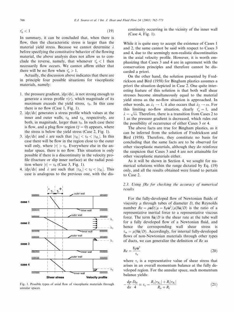
1. the pressure gradient, jdp=dxj, is not strong enough togenerate a stress profile sðrÞ, which magnitude of itsmaximum exceeds the yield stress, s0. In this case

there is no flow (Case 1, Fig. 1).

2. jdp=dxj generates a stress profile which values at the

inner and outer walls, sRi and sRo respectively, areboth, in magnitude, larger than s0. In such case thereis flow, and a plug flow region ( _cc ¼ 0) appears, where

the stress is below the yield stress (Case 2, Fig. 1).

3. jdp=dxj and k are such that jsRi j < s0 < jsRo j. In this

case there will be flow in the region close to the outer

wall only, where jsj > s0. Everywhere else in the an-

nular space, there is no flow. This situation is only

possible if there is a discontinuity in the velocity pro-file (fracture or slip inner surface) at the radial posi-

tion where jsj ¼ s0 (Case 3, Fig. 1).4. jdp=dxj and k are such that jsRo j < s0 < jsRi j. This

case is analogous to the previous one, with the dis-

Fig. 1. Possible types of axial flow of viscoplastic materials through

annular spaces.

continuity occurring in the vicinity of the inner wall

(Case 4, Fig. 1).

While it is quite easy to accept the existence of Cases 1and 2, the same cannot be said with respect to Cases 3

and 4, due to the seemingly non-realistic discontinuities

in the axial velocity profile. However, it is worth em-

phasizing that Cases 3 and 4 are in agreement with the

conservation principles and therefore cannot be dis-

carded a priori.

On the other hand, the solution presented by Fred-

rickson and Bird (1958) for Bingham plastics assumes apriori the situation depicted in Case 2. One quite inter-

esting feature of this solution is that both wall shear

stresses become simultaneously equal to the material

yield stress as the no-flow situation is approached. In

other words, as k1 ! 1, it also occurs that k2 ! x. Forthis limiting no-flow situation, clearly s0o ¼ 1, and

k ¼ffiffiffiffix

p. Therefore, there is a transition from Cases 2 to

1 as the pressure gradient is decreased, which rules outthe possibility of occurrence of either Cases 3 or 4.

The above facts are true for Bingham plastics, as it

can be inferred from the solution of Fredrickson and

Bird (1958). Therefore, they constitute no basis for

concluding that the same facts are to be observed for

other viscoplastic materials, although they do reinforce

the suspicion that Cases 3 and 4 are not attainable for

other viscoplastic materials either.As it will be shown in Section 4, we sought for nu-

merical solutions within the range dictated by Eq. (19)

only, and all the results obtained were found to pertain

to Case 2.

2.3. Using fRe for checking the accuracy of numerical

results

For the fully-developed flow of Newtonian fluids of

viscosity l through tubes of diameter D, the Reynoldsnumber Re ¼ q�uuD=l ¼ 8q�uu2=lð8�uu=DÞ is the ratio of a

representative inertial force to a representative viscous

force. The term 8�uu=D is the shear rate at the tube wall

for a fully developed flow of a Newtonian fluid, and

hence the corresponding wall shear stress is

sw ¼ lð8�uu=DÞ. Accordingly, for internal fully-developedflows of non-Newtonian materials through other types

of ducts, we can generalize the definition of Re as

Re ¼ 8q�uu2

ssð20Þ

where ss is a representative value of shear stress thatarises in an overall momentum balance at the fully de-

veloped region. For the annular space, such momentum

balance yields:

� dpdx

DH

4� ss ¼

RojsRo j þ RijsRi jRo þ Ri

ð21Þ

E.J. Soares et al. / Int. J. Heat and Fluid Flow 24 (2003) 762–773 767

It is noted that ss is a good choice for characteristic

stress, as we did in the present work. The friction factor

f is usually defined as

f ¼� dp

dx DH

12q�uu2

ð22Þ

Therefore, making use of the definition of Reynolds

number given by Eq. (20), the product between the

friction factor and the Reynolds number, fRe, becomes:

fRe ¼�16 dp

dx DH

ssð23Þ

It is seen that the product fRe can be conveniently in-

terpreted as the ratio of a characteristic pressure drop tothe shear stress that opposes to it. Moreover, if it is

defined as explained above, it is always true that

fRe ¼ 64 ð24Þ

regardless the rheological behavior and the duct geom-

etry.

Of course the result of Eq. (24) alone is useless for

determining the flow rate as a function of pressure drop,

because it is merely a manipulation of the momentum

balance (Eq. (21)), adding no new information to it. Forlaminar flow of Newtonian fluids through tubes, the fact

that fRe ¼ 64 can be used in this connection just because

we also know a priori, from the analytical solution, how

to relate ss to the flow rate, namely, ss ¼ lð8�uu=DÞ. Forflows of non-Newtonian materials through tubes or

other types of ducts, in general this information is not

available, because we need the velocity field to evaluate

the shear rate at the wall(s), which is needed for deter-mining ss.Nevertheless, Eq. (24) can be quite useful in these

cases while obtaining numerical solutions, during the

process of selecting an appropriate mesh for the prob-

lem. The numerically obtained shear rates can be em-

ployed to evaluate ss (through the constitutive equation)and subsequently fRe. Meshes that do not give values of

fRe close enough to 64 should not be used. This pro-cedure was employed in the present work.

2.4. Modified bi-viscosity model

The Herschel–Bulkley viscosity function given by Eq.

(1) is not easy to handle numerically. One of its incon-

veniences is that the field of second invariant of extra-

stress, s, must be evaluated at each iteration. However,its main problem is its inconsistency with certain types

of flows due to the imposition of rigid-body motion in

the regions where s < so (Lipscomb and Denn, 1984; AlKhatib and Wilson, 2001).

For example, along the entrance region of a tube

flow, the centerline velocity must increase with the axial

coordinate, to satisfy continuity. This implies exten-

sional deformation of all material elements located at

the centerline in the entrance region. However, at the

centerline the shear stress is null due to symmetry, and sis expected to decrease monotonically to zero with the

axial coordinate, as the flow develops. Therefore, therewill be a portion of the centerline, within the entrance

region and just upstream the fully-developed flow re-

gion, along which s < so and hence where no deforma-tion is allowed. This physical inconsistency should lead

to non-convergence in any attempt to use the Herschel–

Bulkley viscosity function in numerical formulations for

flows with characteristics similar to the one mentioned

in the just discussed example.To remedy this, two types of alternative viscosity

functions were proposed for Bingham materials, name-

ly, the bi-viscosity model (Lipscomb and Denn, 1984;

Gartling and Phan-Thien, 1984; O�Donovan and Tan-

ner, 1984), and the Papanastasiou model (Papanasta-

siou, 1987). Both modifications have been used

successfully in numerical simulations of different com-

plex flows (Ellwood et al., 1990; Abdali et al., 1992;Beverly and Tanner, 1992; Wilson, 1993; Wilson and

Taylor, 1996; Piau, 1996). The idea is to impose a very

high viscosity in the regions where s < so. This replacesthe rigid-body motion with a rather slow deformation,

thus removing the inconsistency discussed above. The

bi-viscosity model can be easily extended to Herschel–

Bulkley materials, and was used in this work. The re-

sulting expression for the viscosity function is given by:

g0 ¼s0o_cc0 þ ð1� s0oÞ _cc0n�1; if _cc0 > _cc0smallg0large; otherwise

(ð25Þ

In the above equations, _cc0 � _cc= _ccc is the dimensionlessshear rate, and g0

large is a large dimensionless num-

ber. Beverly and Tanner (1992) recommend g0large ¼

1000. Accordingly, _cc0small ¼ s0o=½1000� ð1� s0oÞ _cc0n�1small ’ s0o=1000.

3. Numerical method

The governing equations presented above were dis-

cretized with the aid of the finite volume method de-scribed by Patankar (1980). Staggered velocity

components were employed to avoid unrealistic pressure

fields. The SIMPLE algorithm (Patankar, 1980) was

used, in order to handle the coupling between pressure

and velocity. The resulting system of algebraic equations

was solved via the line-by-line TDMA (Patankar, 1980)

in conjunction with the block correction algorithm

(Settari and Aziz, 1973) to increase the convergence rate.The length of the computational domain was held

fixed at a value of L=d ¼ 40. A non-uniform mesh was

used, with an increasing concentration of grid points

toward the duct inlet. Extensive mesh tests were per-

formed in order to choose an adequate mesh, and one

τ0

'=0.6

δ/ R0=0.4

0

0.3

0.6

0.9

1.2

1.5

1.5 1.7 1.9 2.1 2.3 2.5

n=0.2

n=1.0

n=0.5

'/ u'

plug zoneplug zoneplug zone

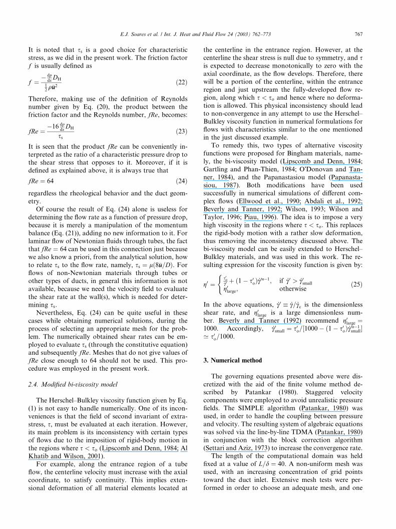
Fig. 2. Fully-developed velocity profile for different values of n.

0.3

0.6

0.9

1.2

1.5

τ0

,=0.25

τ0

,=0.38

τ0

,=0.30

n=0.5δ/ R

0=0.4

'/ u'

plug zoneplug zoneplug zone

768 E.J. Soares et al. / Int. J. Heat and Fluid Flow 24 (2003) 762–773

with 102 grid points in the axial direction and 62 grid

points in the radial direction were found to yield good

results. The error obtained for the fully-developed value

of the product fRe for a Newtonian fluid and d=Ro ¼ 0:5was 0:5%.For the thermal boundary conditions of adiabatic

inner wall and uniform temperature at the outer wall,

the error obtained for the Newtonian Nusselt number,

NuDh, was 1.6%. For the viscoplastic material and

Re ¼ 50, Pe ¼ 100, s00 ¼ 0; 17 and n ¼ 0; 5, fRe and Nuvalues were obtained with different meshes. The differ-

ence between results obtained with the mesh used andthe ones obtained with a 80� 50 mesh was of 0.4% for

fRe and 0.2% for Nu.The numerical solution was also compared with an-

alytical solutions some specific flows of non-Newtonian

materials. The velocity field obtained numerically was in

excellent agreement with the exact solution obtained by

Fredrickson and Bird (1958) for a Bingham plastic. The

velocity field for the flow of a viscoplastic materialthrough an annular space with radius ratio tending to

unity compared very well with the exact solution for the

flow of Herschel–Bulkley material with same rheological

parameters through a parallel plate channel. Finally, we

compared the numerical velocity field with the experi-

mental data obtained by Naimi et al. (1990). A good

agreement was obtained, except for a small difference

observed near the walls, which was probably due to ourdifficulty in accessing the exact values of rheological

parameters of the fluid used in the experiments.

0

1.5 1.7 1.9 2.1 2.3 2.5

Fig. 3. Fully-developed velocity profile for different values of s0o.

0

0.2

0.4

0.6

0.8

1

1.2

1 1.2 1.4 1.6 1.8 2

'/ u' x /δ =0.514

x /δ =1.624

x /δ =4.4612

Re=1000n=0.5

τ0

'=0.5

δ / R0=0.5

x /δ = 0

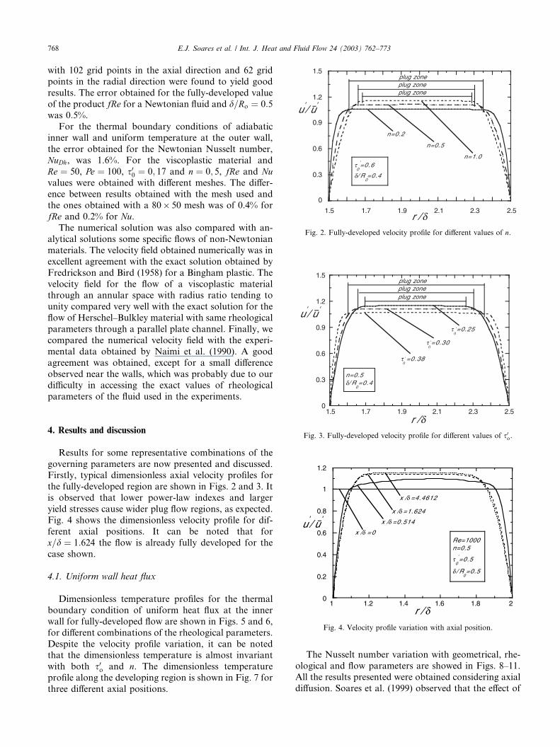
Fig. 4. Velocity profile variation with axial position.

4. Results and discussion

Results for some representative combinations of the

governing parameters are now presented and discussed.Firstly, typical dimensionless axial velocity profiles for

the fully-developed region are shown in Figs. 2 and 3. It

is observed that lower power-law indexes and larger

yield stresses cause wider plug flow regions, as expected.

Fig. 4 shows the dimensionless velocity profile for dif-

ferent axial positions. It can be noted that for

x=d ¼ 1:624 the flow is already fully developed for the

case shown.

4.1. Uniform wall heat flux

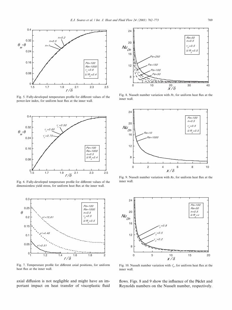
Dimensionless temperature profiles for the thermal

boundary condition of uniform heat flux at the inner

wall for fully-developed flow are shown in Figs. 5 and 6,

for different combinations of the rheological parameters.

Despite the velocity profile variation, it can be notedthat the dimensionless temperature is almost invariant

with both s0o and n. The dimensionless temperature

profile along the developing region is shown in Fig. 7 for

three different axial positions.

The Nusselt number variation with geometrical, rhe-

ological and flow parameters are showed in Figs. 8–11.All the results presented were obtained considering axial

diffusion. Soares et al. (1999) observed that the effect of

τ0,=0.6

δ / R0=0.4

Pe=100Re=1000

1.5 1.7 1.9 2.1 2.3 2.50

0.08

0.16

0.24

0.32

0.4

n=1

n=0.5n=0.2

w- θ

Fig. 5. Fully-developed temperature profile for different values of the

power-law index, for uniform heat flux at the inner wall.

n=0.5δ/ R

0=0.4

Pe=100Re=1000

0

0.08

0.16

0.24

0.32

0.4

1.5 1.7 1.9 2.1 2.3 2.5

τ0

,=0.75

τ0

,=0.60

τ0

,=0.50

w- θ

Fig. 6. Fully-developed temperature profile for different values of the

dimensionless yield stress, for uniform heat flux at the inner wall.

0

0.05

0.1

0.15

0.2

0.25

0.3

1 1.2 1.4 1.6 1.8 2

x'=0.51

x'=4.46

x'=15,61

Pe=100Re=1000n=0.5τ0=0.5

δ/ R0=0.5

Fig. 7. Temperature profile for different axial positions, for uniform

heat flux at the inner wall.

8

12

16

20

24

0 10 20 30 40

Dh

Pe=250

Pe=150

Pe=100

Pe=50

Re=50n=0.5

τ0

,=0.5

δ/ R0=0.5

Fig. 8. Nusselt number variation with Pe, for uniform heat flux at the

inner wall.

8

12

16

20

24

0 2 4 6 8 10

Re=10

Re=1000

Dh

Pe=100n=0.5

τ0

,=0.5

δ/ R0=0.5

Fig. 9. Nusselt number variation with Re, for uniform heat flux at the

inner wall.

8

12

16

20

24

0 5 10 15 20

Dh

τ0

,=0.2

τ0

,=0.5

τ0

,=0.8

Pe=100Re=50n=0.5δ/ R

0=v

Fig. 10. Nusselt number variation with s0o, for uniform heat flux at the

inner wall.

E.J. Soares et al. / Int. J. Heat and Fluid Flow 24 (2003) 762–773 769

axial diffusion is not negligible and might have an im-

portant impact on heat transfer of viscoplastic fluid

flows. Figs. 8 and 9 show the influence of the P�eeclet andReynolds numbers on the Nusselt number, respectively.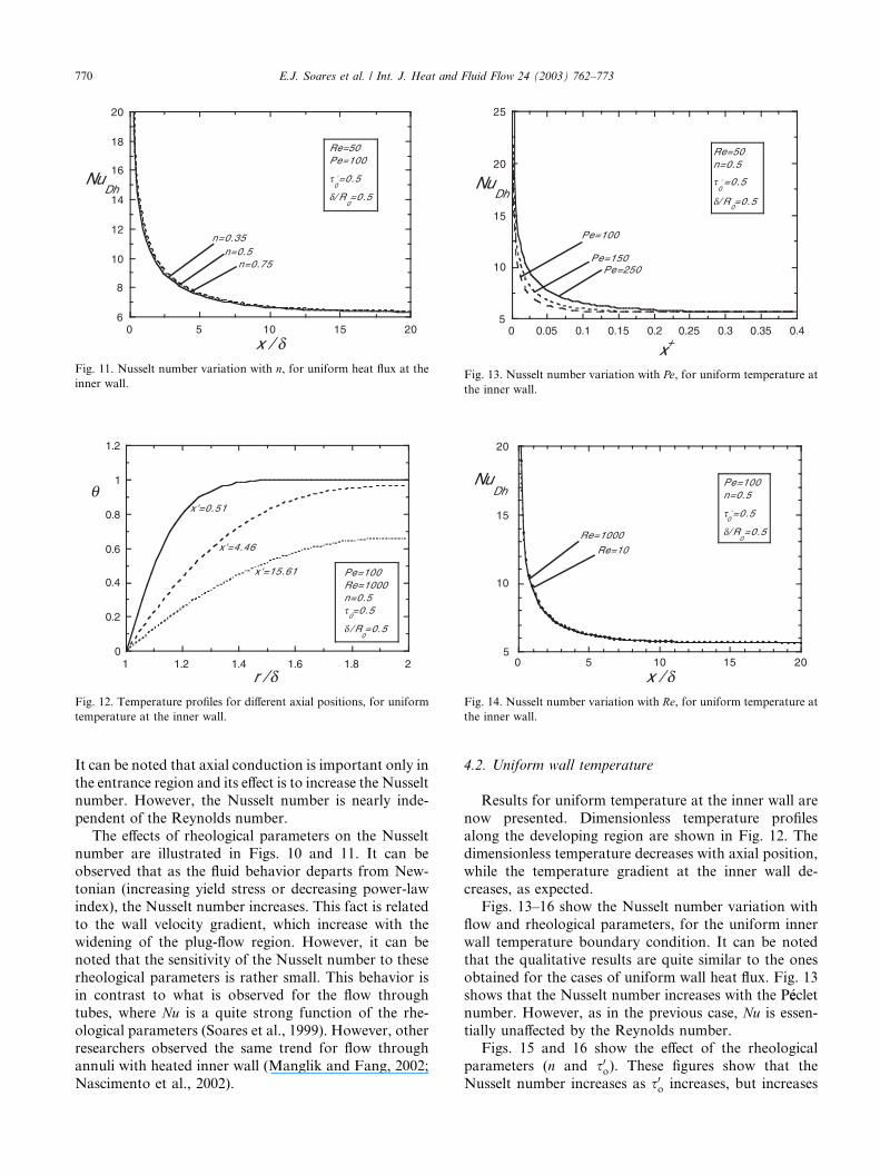

6

8

10

12

14

16

18

20

0 5 10 15 20

Dh

n=0.75

n=0.35n=0.5

Re=50Pe=100

τ0

,=0.5

δ/ R0=0.5

Fig. 11. Nusselt number variation with n, for uniform heat flux at the

inner wall.

0

0.2

0.4

0.6

0.8

1

1.2

1 1.2 1.4 1.6 1.8 2

Pe=100Re=1000n=0.5τ

0=0.5

δ / R0=0.5

x'=0.51

x'=4.46

x'=15.61

Fig. 12. Temperature profiles for different axial positions, for uniform

temperature at the inner wall.

5

10

15

20

25

0 0.05 0.1 0.15 0.2 0.25 0.3 0.35 0.4

Pe=100

Pe=150Pe=250

Re=50n=0.5

τ0

,=0.5

δ/ R0=0.5

Dh

Fig. 13. Nusselt number variation with Pe, for uniform temperature at

the inner wall.

5

10

15

20

0 5 10 15 20

Re=1000Re=10

Pe=100n=0.5

τ0

,=0.5

δ/ R0=0.5

Dh

Fig. 14. Nusselt number variation with Re, for uniform temperature at

the inner wall.

770 E.J. Soares et al. / Int. J. Heat and Fluid Flow 24 (2003) 762–773

It can be noted that axial conduction is important only in

the entrance region and its effect is to increase the Nusselt

number. However, the Nusselt number is nearly inde-

pendent of the Reynolds number.

The effects of rheological parameters on the Nusselt

number are illustrated in Figs. 10 and 11. It can be

observed that as the fluid behavior departs from New-

tonian (increasing yield stress or decreasing power-lawindex), the Nusselt number increases. This fact is related

to the wall velocity gradient, which increase with the

widening of the plug-flow region. However, it can be

noted that the sensitivity of the Nusselt number to these

rheological parameters is rather small. This behavior is

in contrast to what is observed for the flow through

tubes, where Nu is a quite strong function of the rhe-

ological parameters (Soares et al., 1999). However, otherresearchers observed the same trend for flow through

annuli with heated inner wall (Manglik and Fang, 2002;

Nascimento et al., 2002).

4.2. Uniform wall temperature

Results for uniform temperature at the inner wall are

now presented. Dimensionless temperature profiles

along the developing region are shown in Fig. 12. The

dimensionless temperature decreases with axial position,

while the temperature gradient at the inner wall de-

creases, as expected.Figs. 13–16 show the Nusselt number variation with

flow and rheological parameters, for the uniform inner

wall temperature boundary condition. It can be noted

that the qualitative results are quite similar to the ones

obtained for the cases of uniform wall heat flux. Fig. 13

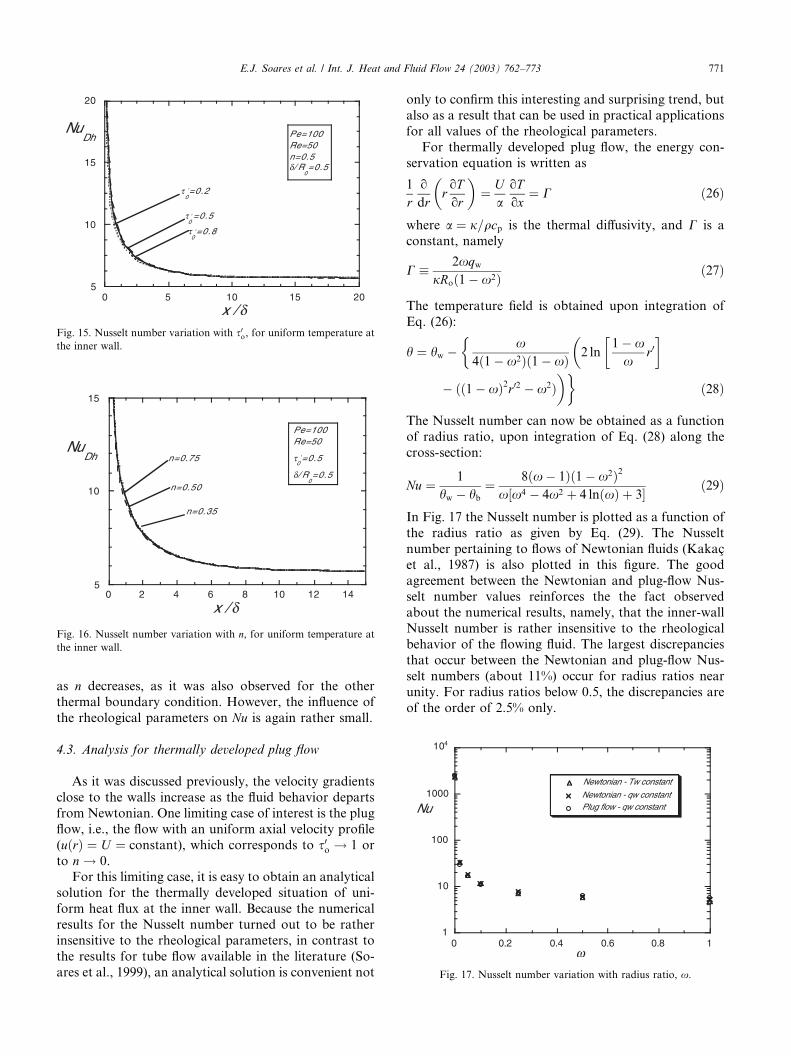
shows that the Nusselt number increases with the P�eecletnumber. However, as in the previous case, Nu is essen-tially unaffected by the Reynolds number.Figs. 15 and 16 show the effect of the rheological

parameters (n and s0o). These figures show that the

Nusselt number increases as s0o increases, but increases

1

10

100

1000

104

0 0.2 0.4 0.6 0.8 1

Newtonian - qw constantPlug flow - qw constant

Newtonian - Tw constant

Fig. 17. Nusselt number variation with radius ratio, x.

5

10

15

0 2 4 6 8 10 12 14

x / δ

n=0.75

n=0.50

n=0.35

Pe=100Re=50

τ0

,=0.5

δ/ R0=0.5

NuDh

Fig. 16. Nusselt number variation with n, for uniform temperature at

the inner wall.

5

10

15

20

0 5 10 15 20

τ0

,=0.2

τ0

,=0.5

τ0

,=0.8

Pe=100Re=50n=0.5δ/ R

0=0.5

Dh

Fig. 15. Nusselt number variation with s0o, for uniform temperature at

the inner wall.

E.J. Soares et al. / Int. J. Heat and Fluid Flow 24 (2003) 762–773 771

as n decreases, as it was also observed for the other

thermal boundary condition. However, the influence of

the rheological parameters on Nu is again rather small.

4.3. Analysis for thermally developed plug flow

As it was discussed previously, the velocity gradients

close to the walls increase as the fluid behavior departs

from Newtonian. One limiting case of interest is the plug

flow, i.e., the flow with an uniform axial velocity profile

(uðrÞ ¼ U ¼ constant), which corresponds to s0o ! 1 or

to n ! 0.For this limiting case, it is easy to obtain an analytical

solution for the thermally developed situation of uni-

form heat flux at the inner wall. Because the numerical

results for the Nusselt number turned out to be rather

insensitive to the rheological parameters, in contrast to

the results for tube flow available in the literature (So-

ares et al., 1999), an analytical solution is convenient not

only to confirm this interesting and surprising trend, but

also as a result that can be used in practical applications

for all values of the rheological parameters.

For thermally developed plug flow, the energy con-servation equation is written as

1

ro

drroTor

� �¼ U

aoTox

¼ C ð26Þ

where a ¼ j=qcp is the thermal diffusivity, and C is a

constant, namely

C � 2xqwjRoð1� x2Þ ð27Þ

The temperature field is obtained upon integration of

Eq. (26):

h ¼ hw � x4ð1� x2Þð1� xÞ 2 ln

1� xx

r0� ��

� ðð1� xÞ2r02 � x2Þ��

ð28Þ

The Nusselt number can now be obtained as a function

of radius ratio, upon integration of Eq. (28) along the

cross-section:

Nu ¼ 1

hw � hb¼ 8ðx � 1Þð1� x2Þ2

x½x4 � 4x2 þ 4 lnðxÞ þ 3 ð29Þ

In Fig. 17 the Nusselt number is plotted as a function of

the radius ratio as given by Eq. (29). The Nusselt

number pertaining to flows of Newtonian fluids (Kakac�et al., 1987) is also plotted in this figure. The good

agreement between the Newtonian and plug-flow Nus-selt number values reinforces the the fact observed

about the numerical results, namely, that the inner-wall

Nusselt number is rather insensitive to the rheological

behavior of the flowing fluid. The largest discrepancies

that occur between the Newtonian and plug-flow Nus-

selt numbers (about 11%) occur for radius ratios near

unity. For radius ratios below 0.5, the discrepancies are

of the order of 2.5% only.

772 E.J. Soares et al. / Int. J. Heat and Fluid Flow 24 (2003) 762–773

Finally, it is worth mentioning that, in the range of

radius ratios below 0.5, the Newtonian Nusselt number

found in the literature (Kakac� et al., 1987) is a little

larger than the plug-flow Nusselt number as given byEq. (29). This is quite surprising, because it seems

physically reasonable to expect that the plug-flow Nus-

selt number is largest, as the trends observed in the

numerical results indicate, and as it is the case for tube

flow (Soares et al., 1999).

5. Conclusions

This paper presented a study of the heat transfer

problem for the flow of Herschel–Bulkley materials

through concentric annular spaces. Two temperature

boundary conditions for the inner wall were analyzed:uniform heat flux and uniform temperature, while the

outer wall assumed to be adiabatic.

The governing equations were solved numerically via

a finite-volume technique. Results were presented in the

form of velocity and temperature profiles, and Nusselt

number as a function of rheological and geometrical

parameters.

It was noted that Nusselt numbers are a little moresensitive to the parameters for the case of uniform heat

flux. It was also observed that the higher is the velocity

gradient at the wall, the higher will be the Nusselt

number, as also observed for tube flow (Soares et al.,

1999).

However, for all cases investigated the inner-wall

Nusselt number is rather insensitive to the rheological

behavior of the fluid. A comparison between Newtonianand plug-flow Nusselt numbers confirms such trend.

This fact can be conveniently explored in practical ap-

plications, since the Newtonian Nusselt number avail-

able in the literature can be used regardless the

rheological behavior of the fluid, with acceptable error

for most engineering applications.

Acknowledgements

Financial support for the present research was par-

tially provided by CENPES/PETROBRAS, CNPq,

Faperj and MCT.

References

Abdali, S.S., Mitsoulis, E., Markatos, N.C., 1992. Entry and exit flows

of Bingham fluids. J. Rheol. 36, 389.

Al Khatib, M.A.M., Wilson, S.D.R., 2001. The development of

poiseulle flow of a yield-stress fluid. J. Non-Newton. Fluid Mech.

100, 1–8.

Beverly, C.R., Tanner, R.I., 1992. Numerical analysis of three-

dimensional Bingham plastic flow. J. Non-Newton. Fluid Mech.

42, 85–115.

Bird, R.B., Armstrong, R.C., Hassager, O., 1987. In: Dynamics of

Polymeric Liquids, vol. 1. Wiley.

Ellwood, K.R.J., Georgiou, G.C., Papanastasiou, C.J., Wilkes, J.O.,

1990. Laminar jets of Bingham-plastic liquids. J. Rheol. 34, 787–

812.

Escudier, M.P., Oliveira, P.J., Pinho, F.T., 2002. Fully developed

laminar flow of purely viscous non-Newtonian liquids through

annuli, including the effects of eccentricity and inner-cylinder

rotation. Int. J. Heat Fluid Flow 23, 52–73.

Fredrickson, A.G., Bird, R.B., 1958. Non-Newtonian flow in annuli.

Ind. Eng. Chem. 50, 347–352.

Gartling, D.K., Phan-Thien, N., 1984. A numerical simulation of a

plastic fluid in s parallel-plate plastometer. J. Non-Newton. Fluid

Mech. 14, 347–360.

Irvine Jr., T.F., Karni, J., 1987. Non-Newtonian fluid flow and heat

transfer. In: Kakac�, S., Shah, R.K., Aung, W. (Eds.), Handbook of

Single-phase Convective Heat Transfer. Wiley, pp. 20.1–20.57.

Joshi, S.D., Bergles, A.E., 1980a. Experimental study of laminar heat

transfer to in-tube flow of non-Newtonian fluids. J. Heat Transfer

102, 397–401.

Joshi, S.D., Bergles, A.E., 1980b. Analytical study of laminar heat

transfer to in-tube flow of non-Newtonian fluids, AICHE Sympo-

sium Series no. 199, vol. 76, pp. 270–281.

Kakac�, S., Shah, R.K., Aung, W., 1987. Handbook of Single-Phase

Convective Heat Transfer. John Wiley & Sons.

Lipscomb, G.G., Denn, M.M., 1984. Flow of Bingham fluids in

complex geometries. J. Non-Newton. Fluid Mech. 14, 337–346.

Manglik, R.M., Fang, P., 2002. Thermal processing of viscous non-

Newtonian fluids in annular ducts: effects of power-law rheology,

duct eccentricity, and thermal boundary conditions. Int. J. Heat

Mass Transfer 45, 803–814.

Naimi, M., Devienne, R., Lebouche, M., 1990. �EEtude dynamique et

th�eermique de l��eecoulement Couette-Taylor-Poiseuille; cas d�unfluide pr�eesentant en seuil d��eecoulement. Int. J. Heat Mass Transfer

33, 381–391.

Nascimento, U.C.S., Maceedo, E.N., Quaresma, J.N.N., 2002. Thermal

entry region analysis through the finite integral transform tech-

nique in laminar flow of Bingham fluids within concentric annular

ducts. Int. J. Heat Mass Transfer 45, 923–929.

Nouar, C., Devienne, R., Lebouche, M., 1994. Convection thermique

pour un fluide de Herschel–Bulkley dans la r�eegion d�entr�eee d�uneconduite. Int. J. Heat Mass Transfer 37, 1–12.

Nouar, C., Lebouche, M., Devienne, R., Riou, C., 1995. Numerical

analysis of the thermal convection for Herschel–Bulkley fluids. Int.

J. Heat Fluid Flow 16, 223–232.

O�Donovan, E.J., Tanner, R.I., 1984. Numerical study of the Binghamsqueeze film problem. J. Non-Newton. Fluid Mech. 15, 75–83.

Papanastasiou, T.C., 1987. Flows of materials with yield. J. Rheol. 31,

385–404.

Patankar, S.V., 1980. Numerical Heat Transfer and Fluid Flow.

Hemisphere Publishing Co.

Piau, J.M., 1996. Flow of a yield stress fluid in a long domain.

Application to flow on an inclined plane. J. Rheol. 40, 711–723.

Round, G.F., Yu, S., 1993. Entrance laminar flows of viscoplastic

fluids in concentric annuli. Canadian J. Chem. Eng. 71, 642–645.

Scirocco, V., Devienne, R., Lebouche, M., 1985. �EEcoulement laminaire

et transfert de chaleur pour un fluide pseudo-plastique dans la zone

d�entr�eee d�un tube. Int J. Heat Mass Transfer 28, 91–99.

Settari, A., Aziz, K., 1973. A generalization of the additive correction

methods for the iterative solution of matrix equations. SIAM J.

Numer. Anal. 10, 506–521.

Soares, E.J., Naccache, M.F., Souza Mendes, P.R., 1998. Heat transfer

to Herschel–Bulkley materials in annular flows. Proc. 7th Brazilian

Cong. Thermal Sciences, vol. 2, pp. 1146–1151.

E.J. Soares et al. / Int. J. Heat and Fluid Flow 24 (2003) 762–773 773

Soares, M., Naccache, M.F., Souza Mendes, P.R., 1999. Heat transfer

to viscoplastic liquids flowing laminarly in the entrance region of

tubes. Int. J. Heat Fluid Flow 20, 60–67.

Vradis, G.C., Dougher, J., Kumar, S., 1992. Entrance pipe flow and

heat transfer for a Bingham plastic. Int. J. Heat Mass Transfer 35,

543–552.

Wilson, S.D.R., 1993. Squeezing flow of a yield-stress fluid in a

wedge of slowly-varying angle. J. Non-Newton. Fluid Mech. 50,

45–63.

Wilson, S.D.R., Taylor, A.J., 1996. The channel entry problem

for a yield stress fluid. J. Non-Newton. Fluid Mech. 65, 165–

176.