POLITECNICO DI MILANO

Dipartimento di Elettronica e Informazione DOTTORATO DI RICERCA IN INGEGNERIA DELL’INFORMAZIONE

MINOR THESIS

YAW GEOMETRY IMPACT ON FMCW

SAR INTERFEROMETRY

Minor thesis of:

Ho Tong Minh Dinh

Supervisor:

Dr. Stefano Tebaldini

Tutor:

Prof. Andrea Monti Guarnieri

The Chair of the Doctoral Program:

Prof. Carlo Fiorini

2011 – XXV

Yaw geometry impact on FMCW SAR

interferometry

Ho Tong Minh Dinh

November 11, 2011

Contents

1 Introduction 2

2 FMCW SAR 22.1 Analog Dechirp . . . . . . . . . . . . . . . . . . . . . . . . . . . . 2

2.2 Resolution . . . . . . . . . . . . . . . . . . . . . . . . . . . . . . . 32.2.1 Range resolution . . . . . . . . . . . . . . . . . . . . . . . 3

2.2.2 Azimuth resolution . . . . . . . . . . . . . . . . . . . . . . 42.3 FMCW SAR signal . . . . . . . . . . . . . . . . . . . . . . . . . . 42.4 Range shift . . . . . . . . . . . . . . . . . . . . . . . . . . . . . . 62.5 Time domain backprojection focusing . . . . . . . . . . . . . . . 72.6 Impulse response function . . . . . . . . . . . . . . . . . . . . . . 9

3 Impact of yaw geometry on interferometric coherence 113.1 Yaw geometry and interferometric coherence . . . . . . . . . . . . 11

3.1.1 Yaw geometry . . . . . . . . . . . . . . . . . . . . . . . . 113.1.2 Interferometric coherence loss . . . . . . . . . . . . . . . . 12

3.2 Time domain common focusing . . . . . . . . . . . . . . . . . . . 133.3 Azimuth spectral shift and Common band filtering . . . . . . . . 15

3.3.1 Azimuth spectral shift . . . . . . . . . . . . . . . . . . . . 153.3.2 Common band filtering . . . . . . . . . . . . . . . . . . . 18

4 Conclusions 18

5 Acknowledgement 20

1

1 Introduction

The combination of frequency-modulated continuous-wave (FMCW) technologyand synthetic aperture radar (SAR) techniques leads to lightweight cost-effectiveimaging sensors capable of high resolution imaging. The conventional stop-and-go approximation used in pulse-radar algorithms is not valid in FMCW SARapplications under certain circumstances. Therefore, the continuous motionshould be treated carefully in focusing processing. Moreover, among many fac-tors impacted to inteferometric coherence, non common yaw geometry betweentwo acquisitions results in the interferometric coherence loss. In this minor re-search, the goal is to study the algorithm processing which takes into accountthe continuous platform motion during sweep time and recovers coherence bymeans of either time domain common band focusing directly from raw signalor filtering from focused data, enhancing the interferogram quality.

This work is organized as follows: in section 2 the FMCW SAR data modelis presented, in section 3 the yaw geometry impact to coherence and its com-pensation are shown and in section 4 conclusions are drawn.

2 FMCW SAR

This section is dedicated to introducing a FMCW SAR signal model, a rangeshift and a time domain focusing algorithm without using the stop-and-go ap-proximation.

2.1 Analog Dechirp

In FMCW SAR, the pulse length is maximized when the SAR is continuouslytransmitting, or equivalently when a single pulse fills the entire pulse-repetitioninterval (PRI). For a given transmit power, the SNR is maximized by maximiz-ing the pulse length. This requires bistatic operation, one antenna to continu-ously transmit and another antenna to continuously receive [1].

There exists one problem that the direct feedthrough from the transmitterto the receiver can have much higher power than the radar echoes from thetarget area. To prevent the feedthrough, it must be managed from drowningout the desired signal. Various methods have been developed for fullfill thistask completely. One method involves an analog dechirp in the received chain.The feedthrough is converted by this dechirp to a single frequency. So, it canbe filtered out in hardware. The analog dechirp also offers some other advan-tages particularly useful for FMCW SAR: a reduced sampling bandwidth anda simplified range compression computation [2].

With an analog dechirp, the received signal is mixed with a copy of thetransmit signal. The dechirp (deramped) signal can be a synchronous copy ofthe transmit signal for direct dechirp or a delayed version. In either cases, the

2

result is a frequency difference between the signals. For direct dechirp, thisfrequency difference, ∆f , corresponds directly to the distance from the target,

∆f =2Rα

c(1)

Where α is the frequency sweep rate and equal to the ratio between thetransmitted bandwidth B and the pulse repetition interval PRI.

The feedthrough generates a frequency difference corresponding to a rangenear zero, which is very different from the frequencies that correspond to theranges in the target area. A bandpass filter with high out-of-band rejection canbe used to attenuate the feedthrough power while passing the desired signal.

The dechirping operation also reduces the signal bandwidth from the fulltransmit bandwidth to a dechirped bandwidth determined by the maximumrange of interest, or the width of the bandpass filter. This dechirped bandwidthfor a direct dechirp is

BWdc =2Rmaxα

c(2)

where Rmax is the maximum range that can be imaged.The sampling and data storage requirements are reduced by using the analog

dechirp. Rather than continuously sampling at a rate sufficient to digitize thetransmit bandwidth, the data is continuously collected at a much lower rate,sufficient for the bandwidth of the dechirped signal.

2.2 Resolution

2.2.1 Range resolution

For the deramped data, range compression can be accomplished with a rangeFourier transform, which separates the frequencies. The range resolution isdetermined by the frequency resolution of the Fourier transform,

∆fr =1

PRI=fsN

(3)

Where fs is the sample rate of the analog to digital converter and N isthe number of samples collected for a single chirp. For deramped SAR data,frequencies correspond to ranges; thus this frequency resolution corresponds toa spatial range resolution, ∆R, calculated as

∆R = ∆fr.c

2.α=

c.fs2.N.α

(4)

For FMCW SAR, N/fs = PRI and PRI · α = B (the transmit bandwidth),so that equation 4 simplifies to

3

∆R =c

2.B(5)

which is equivalent to the range resolution calculation for pulsed SAR [3],[4], [5].

2.2.2 Azimuth resolution

The Doppler frequency of a target at the farthest extent of the antenna beamin azimuth is

fd =2.v

λsin

θa2

(6)

Where θa is the azimuth beamwidth, λ is the wavelength of the center fre-quency and v is the platform velocity. The Doppler bandwidth is

∆z =v

2.fd=

λ

4 sin θa2

(7)

Using the small angle approximation to estimate sin( θa2 ) ≈ θa2 , then esti-

mating the beamwidth from the physical length of the antenna in azimuth, Laz,we have that θa ≈ λ

Lazand

∆z =λ

4 sin θa2

≈λ

2θa≈Laz2

(8)

An important and useful characteristic of FMCW SAR imaging is evidentin these expressions for the azimuth resolution: the resolution is independent ofrange [2], [6]. The other is that it improves by decreasing the antenna length.This can be explained because a smaller antenna has a larger beamwidth andtherefore a larger Doppler bandwidth is available. However, reducing the an-tenna size also decreases its gain.

2.3 FMCW SAR signal

A FMCW radar continuously transmits a frequency modulated signal. Thissignal is a linear frequency ramp, or chirp [1]. In SAR, the radar is carriedon a platform and the radar illuminates the target area. Part of the signal isscattered back to the radar where the receive antenna continuously collects thereflected signal which can then be digitized and processed to form the SARimage [3].

When a linear frequency modulation is applied to CW radar, the transmittedsignal can be expressed as

4

st(t) = exp(j2π(fct+ 2αt2)) (9)

where fc is the carrier frequency, t is the time variable varying within thePRI. The transmitted frequency, is expressed as

fr = fc + αt (10)

In stationary scenarios, the received signal is a delayed version of the trans-mitted. The amplitude should be varied but it is not considered in this deriva-tion.

sr(t, η) = exp(j2π(fc(t− τ) + 2 ∗ α(t− τ)2)) (11)

where τ(t, η) is the time delay and η is the slow time. In dechirp-on-receivesystems, the received and transmitted signals are mixed in order to reduce the re-quired system-sampling rate. The mixing generates the intermediate frequencyor beat signal

sIF (t, η) = exp(j2π(fcτ + αtτ − 1

2ατ2)) (12)

The output of the mixer is then low-pass filtered before being sampled. Thebeat signal is a sinusoidal signal with frequency fb = ατ proportional to thetime delay; therefore, the target range is expressed as

R =cfb2α

=cfb

2B PRF(13)

where PRF is the pulse-repetition frequency. The maximum range is limitedby α and by the maximum-beat frequency, which are equal to half the samplingrate if real sampling is used. The range resolution is proportional to the beatfrequency resolution, which is equal to the inverse of the pulse duration. Inother words, the range resolution is related to the transmitted bandwidth. Thefrequency information can be extracted using a Fourier transform.

Any nonlinearity-range dependence can be removed by RVP (Residue videophase) technique [7]. In this work, we assume that this nonlinearity has beenremoved, leading to

sIF (t, η) = exp(j2π(fcτ + αtτ)) (14)

A Fourier transform of equation 14 results in a focused range response.

5

2.4 Range shift

The following analysis shows the details of range compression for FMCW SAR.The range compression now accounts for the Doppler shift.

Assuming no motion during the chirp is equivalent to assuming R is nota function of t. With τ = 2R

c , the range Fourier transform of equation 14 iscalculated with the integral, as follow:

SIF (frg) =

τ+PRI∫τ

exp(j2π(fcτ + αtτ)) exp(−j2πfrgt)dt (15)

= exp(jπΦrc)PRI sin c

[PRI(frg −

2αR

c)

](16)

Where frg is range frequency and

Φrc =2αR PRI

c− αPRI +

4αR2

c2+

4fcR

c− 4frgR

c(17)

The equation 16 shows that the CW range compressed signal is in the fre-quency domain.

In order to explore what happens when we include the motion during thechirp, we assume that the platform motion is linear, calculate the two way timeof flight to a target, and approximate the change in range as linear during asingle chirp. Assume only one target, τ is quadratic in time and is related toprojected slant range by:

τ =2√R2

0 + v2(η + t)2

c(18)

Approximation for range, then the delay τ is :

τ ≈2

c(R+

v2ηt

R) (19)

Where: R =√R2

0 + υ2η2, R0 is the range of closest approach.Substituting the approximation in equation 19 for τ in equation 14 and

rearranging the terms yields:

sIFm(t, η) = sIF (t, η) exp(jΦm) (20)

Where

Φm =4πv2ηfcRc

t+4παv2η

Rct2 (21)

6

The effects of continuous motion on the signal phase can be seen by inspect-ing equation 21 [8], [2], [9]. As the range to target changes during a chirp, achange in frequency is introduced. The t2 terms represents the chirp caused bythe platform motion, resulting in a spreading in impulse respone focused data,as shown in figure 1 and 3.

Moreover, the platform motion also induces an effect on the carrier frequency,visible in the t terms. Additional insight can be gained by noticing that the finalterm is the Doppler frequency.

If a scatterer is seen by the radar under an angle θs, the Doppler frequencycan be expressed :

fd =2v sin(θs)

λ= 2v

vη

R

fcc

(22)

The t term in equation 21 is the main effect of the platform motion: afrequency shift equal to the Doppler frequency, which translates into a rangeshift in the range compressed data, as is visible in figure 1. The figure 1 isgenerated with parameter: v = 100 m/s, fc = 10 GHz, PRI = 5ms, R = 100m,B = 400MHz, which shows the worst case when t equal the bounded PRI. Thedifference range shift rε in this case can be approximately expressed as :

rε ≈ −2v2ηPRI

R(23)

2.5 Time domain backprojection focusing

The advantages of time domain backprojection focusing include simplicity, par-allel structure, no assumptions about the platform path [10]. In using backpro-jection to process FMCW SAR data, it is important to account for the spreadingand shifting effects visible in the range compressed data due to the continuousplatform motion [8]. We can use the raw data directly or the range compresseddata after correcting the Doppler term in equation 22. In case, the trajectory islinear and Doppler term in equation 22 corrected, the frequency based focalizedapproaches can be done [11], [12], [13].

For a pixel located at (x0, y0, z0), by using the raw data directly, withoutrange compression, the platform position for each sample of raw data is usedand the backprojection operation can be expressed as:

P (x0, y0, z0) =

∫ ∫sIF (t, η) · exp(jΦe(t, η))dtdη (24)

Where P (x0, y0, z0) is the complex pixel power, Φe is the conjugate of thephase in 14, and the τ(t, η) buried inside sIF and Φe is the continuously changingtwo way time of flight to the point (x0, y0, z0).

7

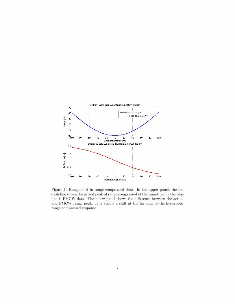
Figure 1: Range shift in range compressed data. In the upper panel, the reddash line shows the actual peak of range compressed of the target, while the blueline is FMCW data. The below panel shows the difference between the actualand FMCW range peak. It is visible a shift at the far edge of the hyperbolicrange compressed response.

8

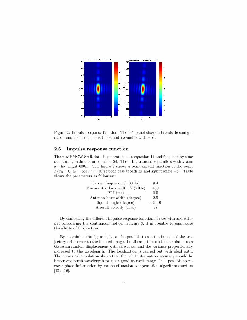
Figure 2: Impulse response function. The left panel shows a broadside configu-ration and the right one is the squint geometry with −50.

2.6 Impulse response function

The raw FMCW SAR data is generated as in equation 14 and focalized by timedomain algorithm as in equation 24. The orbit trajectory parallels with x axisat the height 600m. The figure 2 shows a point spread function of the pointP (x0 = 0, y0 = 651, z0 = 0) at both case broadside and squint angle −50. Tableshows the parameters as following :

Carrier frequency fc (GHz) 9.4Transmitted bandwidth B (MHz) 400

PRI (ms) 0.5Antenna beamwidth (degree) 2.5

Squint angle (degree) −5 , 0Aircraft velocity (m/s) 38

By comparing the different impulse response function in case with and with-out considering the continuous motion in figure 3, it is possible to emphasizethe effects of this motion.

By examining the figure 4, it can be possible to see the impact of the tra-jectory orbit error to the focused image. In all case, the orbit is simulated as aGaussian random displacement with zero mean and the variance proportionallyincreased to the wavelength. The focalization is carried out with ideal path.The numerical simulation shows that the orbit information accuracy should bebetter one tenth wavelength to get a good focused image. It is possible to re-cover phase information by means of motion compensation algorithms such as[15], [16].

9

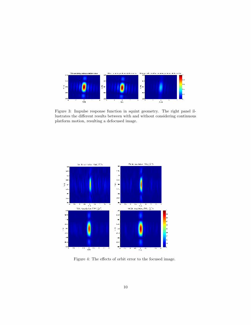
Figure 3: Impulse response function in squint geometry. The right panel il-lustrates the different results between with and without considering continuousplatform motion, resulting a defocused image.

Figure 4: The effects of orbit error to the focused image.

10

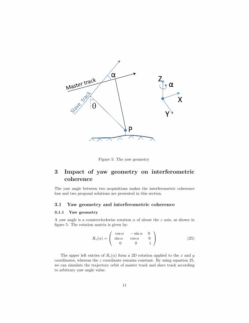
Figure 5: The yaw geometry

3 Impact of yaw geometry on interferometriccoherence

The yaw angle between two acquisitions makes the interferometric coherenceloss and two proposal solutions are presented in this section.

3.1 Yaw geometry and interferometric coherence

3.1.1 Yaw geometry

A yaw angle is a counterclockwise rotation α of about the z axis, as shown infigure 5. The rotation matrix is given by:

Rz(α) =

cosα − sinα 0sinα cosα 0

0 0 1

(25)

The upper left entries of Rz(α) form a 2D rotation applied to the x and ycoordinates, whereas the z coordinate remains constant. By using equation 25,we can simulate the trajectory orbit of master track and slave track accordingto arbitrary yaw angle value.

11

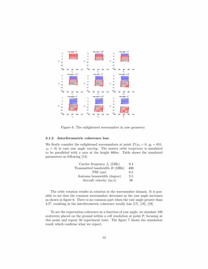
Figure 6: The enlightened wavenumber in yaw geometry.

3.1.2 Interferometric coherence loss

We firstly consider the enlightened wavenumbers at point P (x0 = 0, y0 = 651,z0 = 0) in case yaw angle varying. The master orbit trajectory is simulatedto be paralleled with x axis at the height 600m. Table shows the simulatedparameters as following [14]:

Carrier frequency fc (GHz) 9.4Transmitted bandwidth B (MHz) 400

PRI (ms) 0.5Antenna beamwidth (degree) 2.5

Aircraft velocity (m/s) 38

The orbit rotation results in rotation in the wavenumber domain. It is pos-sible to see that the common wavenumber decreases as the yaw angle increasesas shown in figure 6. There is no common part when the yaw angle greater than3.50, resulting in the interferometric coherence totally loss [17], [18], [19].

To see the expectation coherence as a function of yaw angle, we simulate 100scatterers placed on the ground within a cell resolution at point P, focusing atthis point and repeat 50 experiment tests. The figure 7 shows the simulationresult which confirms what we expect.

12

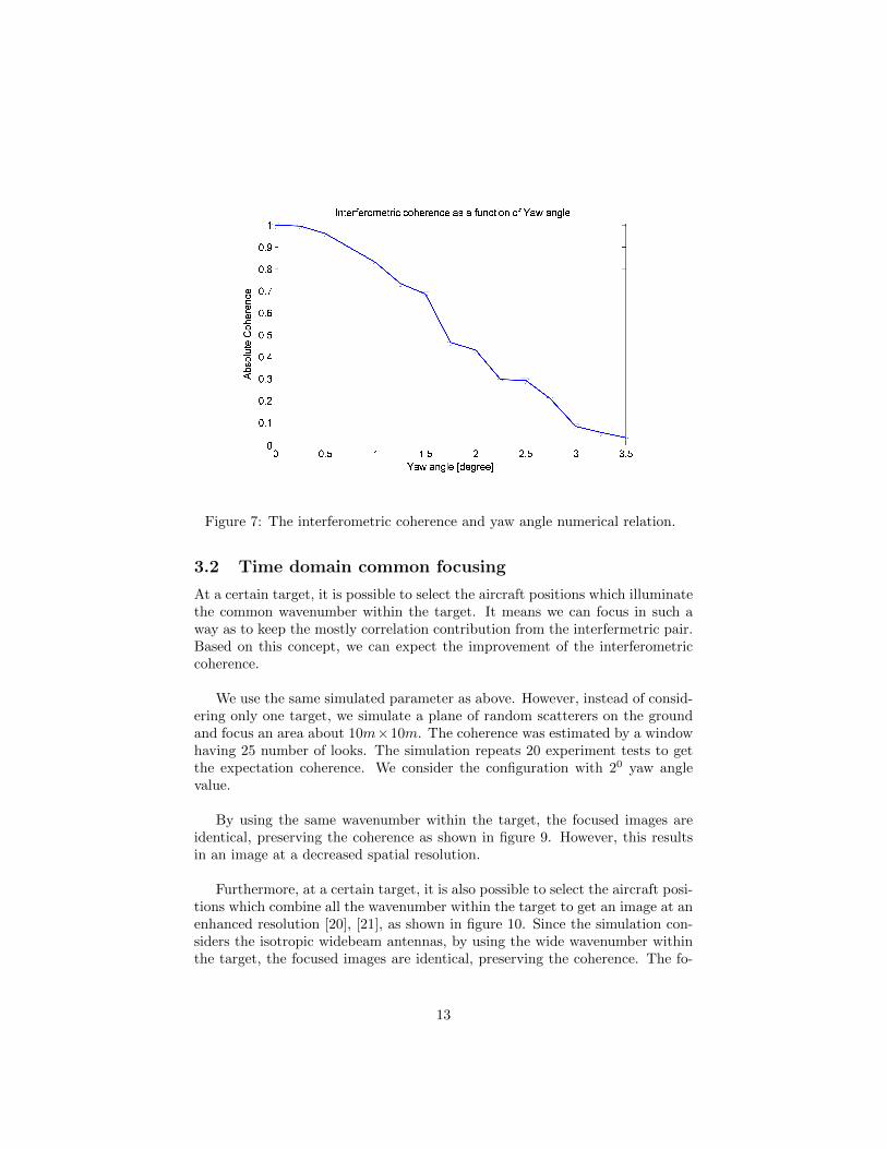
Figure 7: The interferometric coherence and yaw angle numerical relation.

3.2 Time domain common focusing

At a certain target, it is possible to select the aircraft positions which illuminatethe common wavenumber within the target. It means we can focus in such away as to keep the mostly correlation contribution from the interfermetric pair.Based on this concept, we can expect the improvement of the interferometriccoherence.

We use the same simulated parameter as above. However, instead of consid-ering only one target, we simulate a plane of random scatterers on the groundand focus an area about 10m×10m. The coherence was estimated by a windowhaving 25 number of looks. The simulation repeats 20 experiment tests to getthe expectation coherence. We consider the configuration with 20 yaw anglevalue.

By using the same wavenumber within the target, the focused images areidentical, preserving the coherence as shown in figure 9. However, this resultsin an image at a decreased spatial resolution.

Furthermore, at a certain target, it is also possible to select the aircraft posi-tions which combine all the wavenumber within the target to get an image at anenhanced resolution [20], [21], as shown in figure 10. Since the simulation con-siders the isotropic widebeam antennas, by using the wide wavenumber withinthe target, the focused images are identical, preserving the coherence. The fo-

13

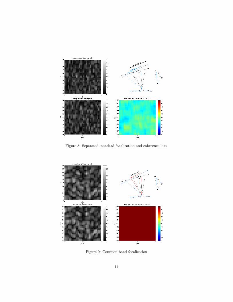
Figure 8: Separated standard focalization and coherence loss.

Figure 9: Common band focalization

14

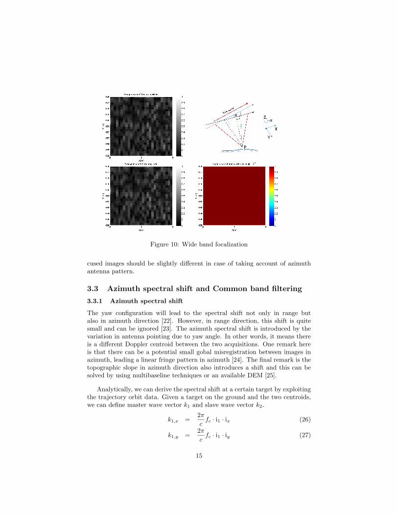
Figure 10: Wide band focalization

cused images should be slightly different in case of taking account of azimuthantenna pattern.

3.3 Azimuth spectral shift and Common band filtering

3.3.1 Azimuth spectral shift

The yaw configuration will lead to the spectral shift not only in range butalso in azimuth direction [22]. However, in range direction, this shift is quitesmall and can be ignored [23]. The azimuth spectral shift is introduced by thevariation in antenna pointing due to yaw angle. In other words, it means thereis a different Doppler centroid between the two acquisitions. One remark hereis that there can be a potential small gobal misregistration between images inazimuth, leading a linear fringe pattern in azimuth [24]. The final remark is thetopographic slope in azimuth direction also introduces a shift and this can besolved by using multibaseline techniques or an available DEM [25].

Analytically, we can derive the spectral shift at a certain target by exploitingthe trajectory orbit data. Given a target on the ground and the two centroids,we can define master wave vector k1 and slave wave vector k2.

k1,x =2π

cfc · i1 · ix (26)

k1,y =2π

cfc · i1 · iy (27)

15

k2,x =2π

cfc · i2 · ix (28)

k2,y =2π

cfc · i2 · iy (29)

Where i1, i2 are single unit vector in slant range direction of master andslave track respectively. ix, iy are the orthogonal unit vectors of x and y axiscoordinates.

Then, the wavenumber shift between the master and slave track is:

∆kx =2π

cfc · (i1 − i2) · ix (30)

∆ky =2π

cfc · (i1 − i2) · iy (31)

Assuming the flat topography, we can be explicitly expressed the normalizedazimuth shift fx as a function of the yaw angle as following:

fx =sin θ

θaα (32)

where θa is the azimuth beamwidth, θ is the look angle and α is the yawangle.

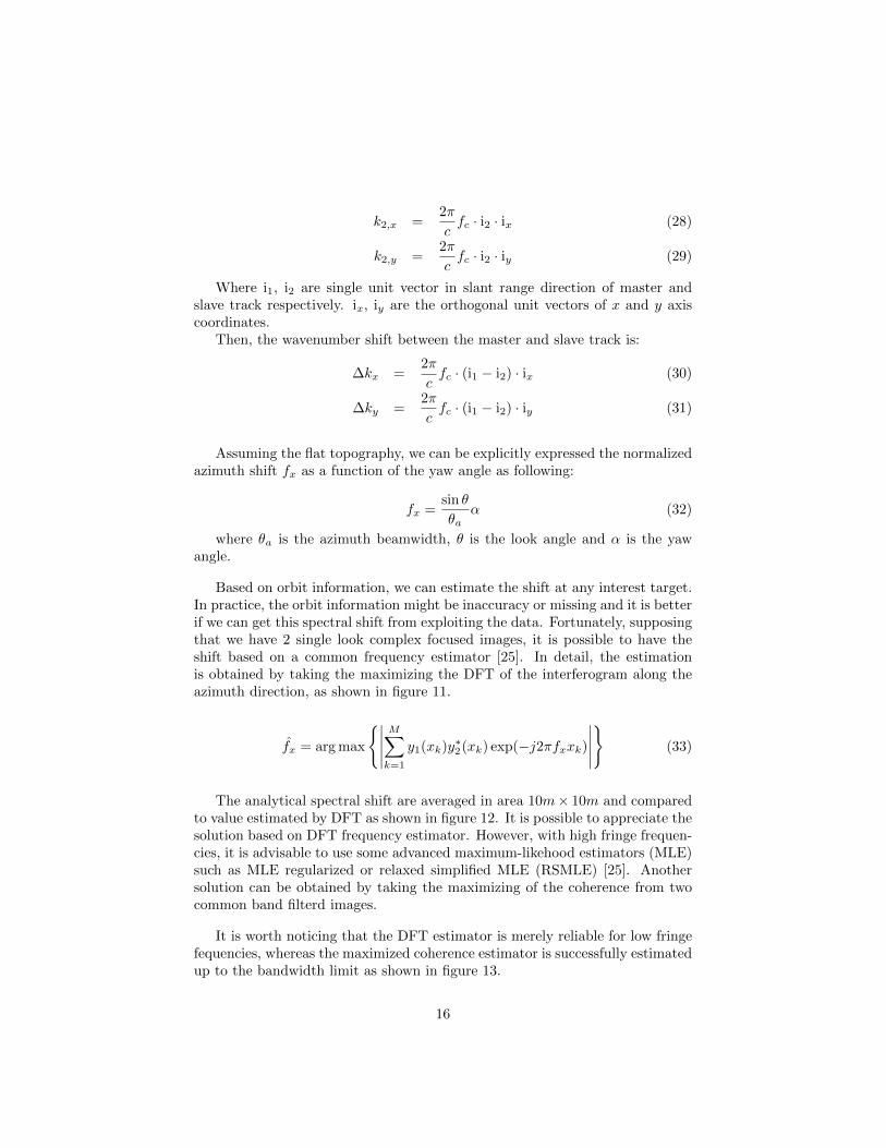
Based on orbit information, we can estimate the shift at any interest target.In practice, the orbit information might be inaccuracy or missing and it is betterif we can get this spectral shift from exploiting the data. Fortunately, supposingthat we have 2 single look complex focused images, it is possible to have theshift based on a common frequency estimator [25]. In detail, the estimationis obtained by taking the maximizing the DFT of the interferogram along theazimuth direction, as shown in figure 11.

f̂x = arg max

{∣∣∣∣∣M∑k=1

y1(xk)y∗2(xk) exp(−j2πfxxk)

∣∣∣∣∣}

(33)

The analytical spectral shift are averaged in area 10m× 10m and comparedto value estimated by DFT as shown in figure 12. It is possible to appreciate thesolution based on DFT frequency estimator. However, with high fringe frequen-cies, it is advisable to use some advanced maximum-likehood estimators (MLE)such as MLE regularized or relaxed simplified MLE (RSMLE) [25]. Anothersolution can be obtained by taking the maximizing of the coherence from twocommon band filterd images.

It is worth noticing that the DFT estimator is merely reliable for low fringefequencies, whereas the maximized coherence estimator is successfully estimatedup to the bandwidth limit as shown in figure 13.

16

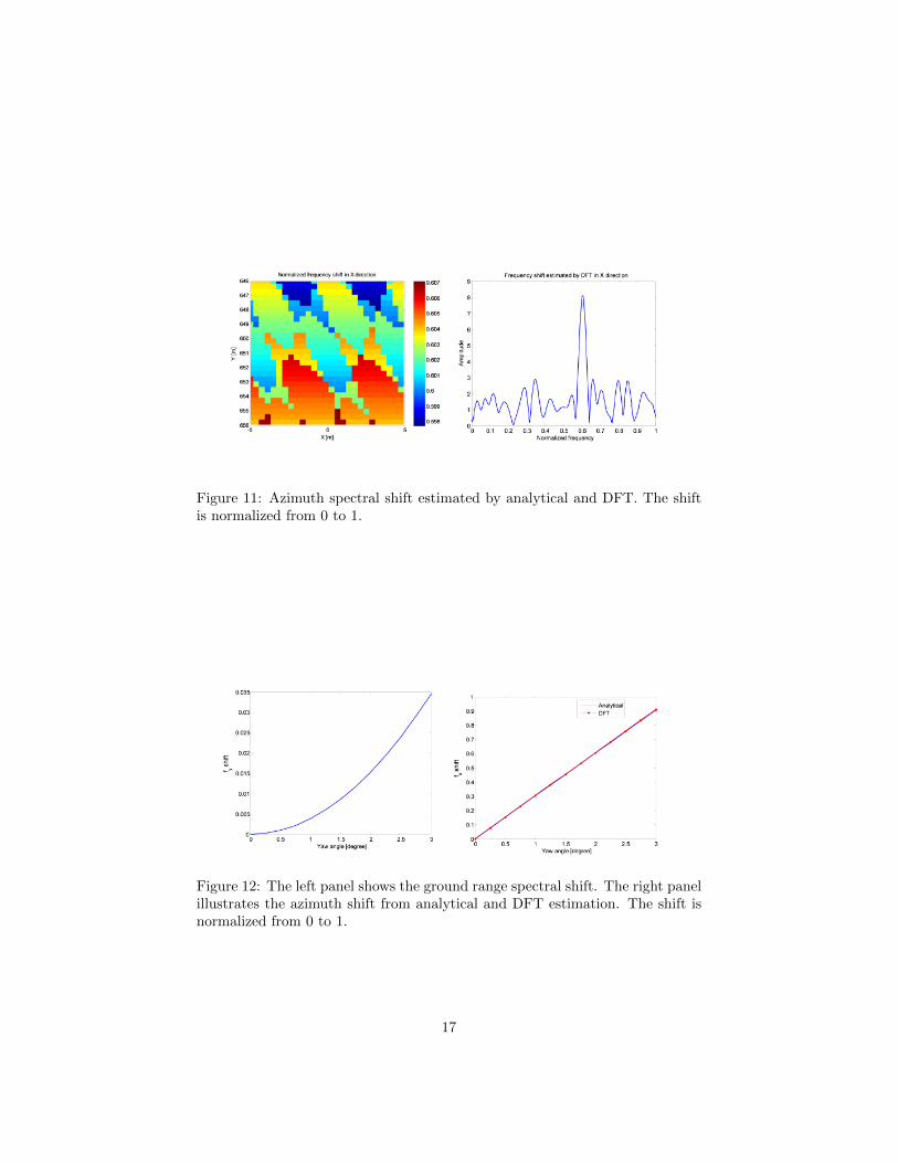
Figure 11: Azimuth spectral shift estimated by analytical and DFT. The shiftis normalized from 0 to 1.

Figure 12: The left panel shows the ground range spectral shift. The right panelillustrates the azimuth shift from analytical and DFT estimation. The shift isnormalized from 0 to 1.

17

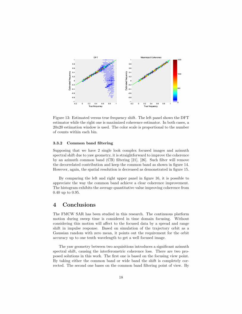
Figure 13: Estimated versus true frequency shift. The left panel shows the DFTestimator while the right one is maximized coherence estimator. In both cases, a20x20 estimation window is used. The color scale is proportional to the numberof counts within each bin.

3.3.2 Common band filtering

Supposing that we have 2 single look complex focused images and azimuthspectral shift due to yaw geometry, it is straightforward to improve the coherenceby an azimuth common band (CB) filtering [21], [26]. Such filter will removethe decorrelated contribution and keep the common band as shown in figure 14.However, again, the spatial resolution is decreased as demonstrated in figure 15.

By comparing the left and right upper panel in figure 16, it is possible toappreciate the way the common band achieve a clear coherence improvement.The histogram exhibits the average quantitative value improving coherence from0.40 up to 0.95.

4 Conclusions

The FMCW SAR has been studied in this research. The continuous platformmotion during sweep time is considered in time domain focusing. Withoutconsidering this motion will affect to the focused data by a spread and rangeshift in impulse response. Based on simulation of the trajectory orbit as aGaussian random with zero mean, it points out the requirement for the orbitaccuracy up to one tenth wavelength to get a well focused image.

The yaw geometry between two acquisitions introduces a significant azimuthspectral shift, causing the interferometric coherence loss. There are two pro-posed solutions in this work. The first one is based on the focusing view point.By taking either the common band or wide band the shift is completely cor-rected. The second one bases on the common band filtering point of view. By

18

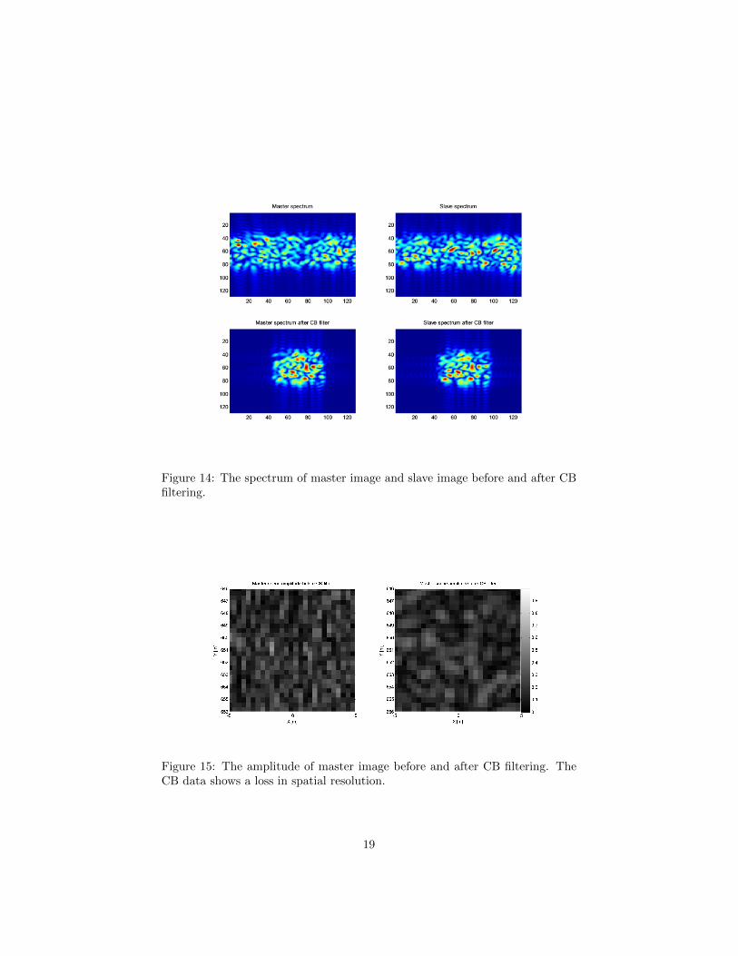
Figure 14: The spectrum of master image and slave image before and after CBfiltering.

Figure 15: The amplitude of master image before and after CB filtering. TheCB data shows a loss in spatial resolution.

19

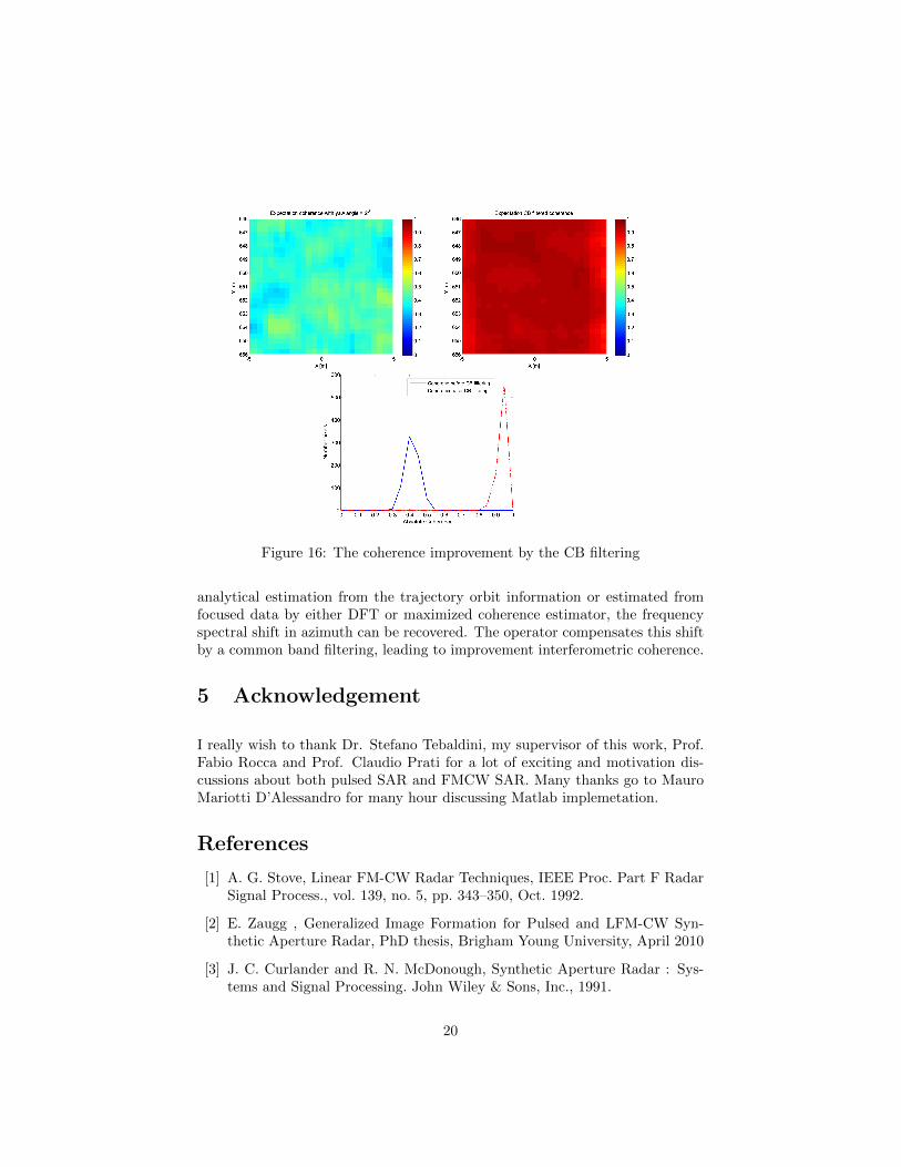
Figure 16: The coherence improvement by the CB filtering

analytical estimation from the trajectory orbit information or estimated fromfocused data by either DFT or maximized coherence estimator, the frequencyspectral shift in azimuth can be recovered. The operator compensates this shiftby a common band filtering, leading to improvement interferometric coherence.

5 Acknowledgement

I really wish to thank Dr. Stefano Tebaldini, my supervisor of this work, Prof.Fabio Rocca and Prof. Claudio Prati for a lot of exciting and motivation dis-cussions about both pulsed SAR and FMCW SAR. Many thanks go to MauroMariotti D’Alessandro for many hour discussing Matlab implemetation.

References

[1] A. G. Stove, Linear FM-CW Radar Techniques, IEEE Proc. Part F RadarSignal Process., vol. 139, no. 5, pp. 343–350, Oct. 1992.

[2] E. Zaugg , Generalized Image Formation for Pulsed and LFM-CW Syn-thetic Aperture Radar, PhD thesis, Brigham Young University, April 2010

[3] J. C. Curlander and R. N. McDonough, Synthetic Aperture Radar : Sys-tems and Signal Processing. John Wiley & Sons, Inc., 1991.

20

[4] W. G. Carrara, R. S. Goodman, and R. M. Majewski, Spotlight SyntheticAperture Radar. Boston, Artech House Inc., 1995.

[5] I. G. Cumming and F. H. Wong, Digital Processing of Synthetic ApertureRadar Data. Artech House, 2005.

[6] A. Meta, Signal Processing of FMCW Synthetic Aperture Radar Data,PhD thesis, Delft University of Technology, 2006

[7] A. Meta, P. Hoogeboom, and L. P. Ligthart, Range non-linearities correc-tion in FMCW SAR, in Proc. IEEE Int. Geoscience and Remote SensingSymp. IGARSS’06, Denver, CO, USA, July 2006.

[8] A. Meta, P. Hoogebbom, and L. P. Ligthart, Correction of the effects in-duced by the continuous motion in FMCW SAR, in Proc. IEEE RadarConf. ’06, Verona, NY, USA, Apr. 2006, pp. 358–365.

[9] A. Meta, P. Hoogeboom, and L.P. Ligthart, Signal Processing for FMCWSAR, in IEEE Trans. Geosci. Rem. Sens., vol.45, no.11, pp.3519-3532, Nov.2007.

[10] O. Frey, C. Magnard, M. Ruegg, and E. Meier, Focusing of airborne syn-thetic aperture radar data from highly nonlinear flight tracks, IEEE Trans-actions on Geoscience and Remote Sensing, vol. 47, no. 6, pp. 1844–1858,June 2009.

[11] J. J. M. de Wit, A. Meta, and P. Hoogeboom, Modified range-Doppler pro-cessing for FMCW synthetic aperture radar, IEEE Geosci. Remote SensingLetters, vol. 3, no. 1, pp. 83–87, Jan. 2006.

[12] F. Rocca, Synthetic aperture radar: A new application for wave equationtechniques, Stanford Exploration Project Report, vol. SEP-56, pp. 167–189,1987.

[13] Wang R., Loffeld O., Nies H., Knedlik S., Hagelen M., Essen H., Fo-cus FMCW SAR Data Using the Wavenumber Domain Algorithm, IEEETransactions on Geoscience and Remote Sensing, Vol 4, no.4, pp. 2109 -2118, April 2010

[14] A. Meta, P. Hakkaart, F. V. der Zwan, P. Hoogeboom, and L. P. Ligthart,First demonstration of an X-band airborne FMCW SAR, in Proc. EuropeanConf. on Synthetic Aperture Radar EUSAR’06, Dresden, Germany, May2006.

[15] E. Zaugg and D. Long, Theory and application of motion compensation forLFM-CW SAR, IEEE Transactions on Geoscience and Remote Sensing,vol. 46, no. 10, pp. 2990–2998, Oct. 2008. 7, 55, 57, 110

21

[16] P. Prats, K. Camara de Macedo, A. Reigber, R. Scheiber, and J. Mallorqui,Comparison of topography- and aperture-dependent motion compensationalgorithms for airborne SAR, IEEE Geoscience and Remote Sensing Let-ters, vol. 4, no. 3, pp. 349–353, July 2007.

[17] H. A. Zebker and J. Villasenor, Decorrelation in interferometric radarechoes, IEEE Transactions on Geoscience and Remote Sensing, vol. 30,no. 5, pp. 950–959, sept 1992.

[18] R. Bamler and P. Hartl, Synthetic aperture radar interferometry, InverseProblems, vol. 14, pp. R1–R54, 1998.

[19] R. F. Hanssen, Radar Interferometry: Data Interpretation and Error Anal-ysis, 2nd ed. Heidelberg: Springer Verlag, 2005.

[20] C Prati and F Rocca. Range resolution enhancement with multiple SARsurveys combination. In International Geoscience and Remote Sensing Sym-posium, Houston, Texas, USA, May 26-29 1992, pages 1576-1578, 1992

[21] A. Ferretti, A. Monti Guarnieri, C. Prati, F. Rocca and D. Massonnet,InSAR Pricinples: Guidelines for SAR Interferometry Processing and In-terpretation, ESA publication, Feb 2007.

[22] F. Gatelli, A. Monti Guarnieri, F. Parizzi, P. Pasquali, C. Prati, and F.Rocca, The wavenumber shift in SAR interferometry, IEEE Transactionson Geoscience and Remote Sensing, vol. 32, no. 4, pp. 855–865, July 1994.

[23] A. Monti Guarnieri and F Rocca. Combination of low- and high-resolutionSAR images for differential interferometry. IEEE Trans. on Geoscience andRemote Sensing, 37(4): 2035-2049, July 1999

[24] Reigber, A., Prats, P., Mallorqui, J.J., Refined estimation of time-varyingbaseline errors in airborne SAR interferometry, IEEE Geoscience and Re-mote Sensing Letters, vol. 3, no.1, pp. 145 - 149, Jan. 2006

[25] A. Monti Guarnieri and S. Tebaldini, ML-Based Fringe-Frequency Esti-mation for InSAR, IEEE Geoscience and Remote Sensing Letters, Vol 7,no. 1,pp. 136 - 140, Jan. 2010

[26] Fornaro G. and A. Monti Guarnieri. Minimum Mean Square Error Space-Varying Filtering Of Interferometric SAR Data, IEEE Trans. GARS, 39,2001

22