Speckle Interferometry

Outline

1 Full-Aperture Interferometry2 Labeyrie Technique3 Knox-Thompson Technique4 Bispectrum Technique5 Differential Speckle Imaging6 Phase-Diverse Speckle Imaging

Full-Aperture Interferometry

Diffraction Limit

Theoretical angular resolution of a telescope is proportional toλ/D where λ is the wavelength and D is the diameter of thetelescope

Diameter Wavelength Diffraction Limit10 cm 500 nm 1.0′′

100 cm 500 nm 0.′′1800 cm 500 nm 0.′′0125100 cm 5000 nm 1.0′′

Seeing

resolution limited by Earth’satmosphere to ≈ 0.′′5independent of D

refraction on changes in index ofrefraction

index of refraction of air dependson temperature

atmosphere is turbulent mediumwith small-scale temperaturefluctuations

Speckle-Interferometry: suitableobservational method andpost-facto reconstructionteqchnique to eliminate theangular smearing due to seeing

Interferencetelescope combines light thathas passed through differentparts of of the atmosphere

Seeing corresponds to manysmall telescopes that aredifferently affected by theatmosphere

quality of seeing described byFried’s Parameter r0, diameterof telescopes that would bediffraction-limited undercurrent seeing conditions

typical values in the visible r0:5–30 cm

Speckles

image of a point source isa cloud of small dots:Speckles

Speckles have diameterscorresponding todiffraction limit

life time of speckles in thevisible about 10 ms, longerat larger wavelengths

Seeing for Single and Binary Stars

Seeing and Solar Granulation

Mathematical Description of Seeing

image of a point source: Point Spread Function (PSF)

image formation due to time-varying PSF

i (t) = o ∗ s (t)

i observed imageo true object, constant in times point spread function∗ convolution

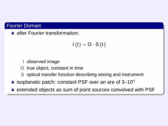
Fourier Domain

after Fourier transformation:

I (t) = O · S (t)

I observed imageO true object, constant in timeS optical transfer function describing seeing and instrument

isoplanatic patch: constant PSF over an are of 3–10′′

extended objects as sum of point sources convolved with PSF

Labeyrie Technique

Basic Ideadeveloped in 1970 by AntoineLabeyrie

exposure time shorter than timeconstant of seeing (≤ 20 ms inthe visible)

clever average of many imagesthat is free from atmosphericinfluences

assumption: PSF constant duringexposure time

image of binary star consists oftwo identical, overlapping speckleclounds

Average Autocorrelation

Autocorrelation can detect identical,but shifted speckle clouds

Labeyrie technique: averageautocorrelation containsdiffraction-limited information

autocorrelation in image spacecorresponds to power-spectrum inFourier Space⟨

|I|2⟩

= |O|2⟨|S|2

⟩speckle transfer function

⟨|S|2

⟩from

calibration point source

Labeyrie technique allowsreconstruction of Fourier amplitudes

average auto-correlation is not image

Autocorrelation 6= Image

Knox-Thompson Technique

Reconstructing the Fourier Phases

Knox and Thompson (1973)

phases are crucial for extended objects such as star clusters,galaxies, the Sun

phases Ψ(O) with Knox and Thompson (1974) technique:⟨I(~f )I∗(~f − ~δf )

⟩= O(~f )O∗(~f − ~δf )

⟨S(~f )S∗(~f − ~δf )

⟩Ψ

(O

(~f)

O∗(~f − ~δf

))= −Ψ

(O

(~f))

+ Ψ(

O(~f − ~δf

))∼ ∂Ψ

∂~fcan integrate phase differences in two directions to recoverphases

iterative approach that minimizes sum of squares of phasedifferences

Average and Best Frame of Image Series

Average and Knox-Thompson Reconstruction

Comparison of Techniques

Bispectrum Technique

Weigelt 1977

product of three Fourier components⟨

I(~f1)I(~f2)I∗(~f1 +~f2)⟩

phase of average atmospheric factor is again zero

phase of bispectrum: Ψ(~f1

)+ Ψ

(~f2

)−Ψ

(~f1 +~f2

)many more correlations between Fourier components

bispectrum is 4-dimensional ⇒ large computational effort

today most-often used speckle technique

Dutch Open Telescope Speckle Movie

DOT Blue Continuum Movie of AR10425

Differential Speckle Imaging

The Idea

narrow-band filter images do not have enough signal to do directspeckle imaging

measure PSF in broad-band channel (b) to deconvolvesimultaneous exposures in narrow-band channel (n)

In = OnS, Ib = ObS

approximation of On:

O′n =

⟨InS

⟩=

⟨InIb

⟩Ob.

avoid division by 0 via:

O′n =

⟨(In/Ib)|Ib|2

⟩⟨|Ib|2

⟩ Ob =

⟨InI∗b

⟩⟨|Ib|2

⟩Ob

Application to Solar Zeeman Polarimetry

BUT, in reality In = OnS + Nn, Ib = ObS + Nb

account for random photon noise with appropriate optimum filter

account for anisoplanatism by overlapping segmentation withsegment sizes on the order of the isoplanatic patch

high spatial resolution at good spectral resolution can beachieved

Phase-Diverse Speckle

Raw DataReconstruction

Adaptive Optics Real-Time Wavefront Correction

Evolution of Small-Scale Fields in the Quiet Sun

Speckle Interferometry

Summary

Earth’s atmosphere limits angular resolution of optical telescopes

speckle techniques use clever non-linear averages that preserveinformation out to the diffraction limit

speckle imaging is the standard data reduction technique at theDutch Open Telescope

Adaptive Optics (AO) can correct some of the aberrations

highest resolution achieved with combination of AO andreconstruction technique