DISSERTATION

Titel der Dissertation

„Macroscopic Matter-wave Interferometry“

Verfasser

Dipl.-Phys. Stefan Nimmrichter

angestrebter akademischer Grad

Doktor der Naturwissenschaften (Dr. rer. nat.)

Wien, im Juli 2013

Studienkennzahl lt. Studienblatt: A 091 411Dissertationsgebiet lt. Studienblatt: PhysikBetreuer: Univ.-Prof. Dr. Markus Arndt

Stefan Nimmrichter

Matter-waveInterferometry

Vienna 2013

Quantum Nanophysics Group

ComplexQuantumSystems

Co uS

AbstractIn this thesis I develop theoretical methods to facilitate, assess, and interpret macroscopicmatter-wave interference experiments with molecules and nanoparticles, as conceived andimplemented in the Quantum Nanophysics Group at the University of Vienna. Introducing atheoretical framework to describe the interaction of polarizable particles with light, I firststudy the feasibility of dissipative slowing and trapping of sub-wavelength molecules anddielectric nanospheres by means of high-finesse cavities and strong laser fields – an essentialprerequisite to facilitate matter-wave interferometry with heavy nanoparticles. I proceedwith an in-depth analysis of matter-wave near-field interferometry, focusing on the mostrecent implementation of the Talbot-Lau scheme with pulsed optical gratings. In particular, Iassess the feasible mass limits of this scheme, as well as the influence of hypotheticalmacrorealistic models. Finally, I turn to the question of how to quantify the macroscopicityof mechanical quantum phenomena in general, developing a systematic andobservation-based answer. From this I derive a physical measure for the degree ofmacroscopicity of superposition phenomena, which admits an objective comparisonbetween arbitrary quantum experiments on mechanical systems.

ZusammenfassungDie vorliegende Arbeit umfasst die theoretischen Grundlagen und Methoden zurBeschreibung makroskopischer Materiewelleninterferenzexperimente, wie sie in derQuantennanophysikgruppe an der Universität Wien mit Molekülen und anderenNanoteilchen durchgeführt werden. Ich bespreche zunächst die Wechselwirkung vonpolarisierbaren Teilchen mit Lichtfeldern, um anschließend die dissipative Wirkung vonLaserfeldern und optischen Resonatoren auf die Teilchen zu beschreiben. Damit lassen sichdie Voraussetzungen für das optische Bremsen und Einfangen großer Nanoteilchendiskutieren, das für Interferenzexperimente mit solch massiven Objekten benötigt wird. Esfolgt eine ausführliche theoretische Beschreibung von Nahfeldinterferometrie. Dabeikonzentriere ich mich auf das Wiener Talbot-Lau-Interferometer mit gepulsten Lasergitternund diskutiere, welchen Massenbereich man damit prinzipiell erreichen kann. Es zeigt sich,dass gängige makrorealistische Hypothesen zum quanten-klassischen Übergangüberprüfbar werden, was mich anschließend zu der Frage führt, was Makroskopizitäteigentlich bedeutet. Im letzten Abschnitt der Dissertation entwickle ich einephysikalisch-empirische Interpretation des Makroskopizitätsabegriffs für Quanteneffekte.Daraus lässt sich schließlich ein Maß für den Grad an Makroskopizität ableiten, mit dem manbeliebige Superpositionsexperimente in mechanischen Systemen objektiv erfassen undvergleichen kann.

Contents

1. Introduction 1

2. Interaction of polarizable particles with light 5

2.1. Mechanics of polarizable point particles in coherent light elds . . . . . . . . . . . . 52.1.1. e linear response of a polarizable point particle to light . . . . . . . . . . 62.1.2. Absorption, emission and Rayleigh scattering of photons . . . . . . . . . . 8

2.1.2.1. Photon absorption . . . . . . . . . . . . . . . . . . . . . . . . . . . 92.1.2.2. Photon emission into free space . . . . . . . . . . . . . . . . . . . 112.1.2.3. Elastic light scattering into free space . . . . . . . . . . . . . . . . 13

2.1.3. Classical dynamics of a polarizable point particle coupled to a stronglypumped cavity mode . . . . . . . . . . . . . . . . . . . . . . . . . . . . . . . . 142.1.3.1. Intra-cavity eld dynamics . . . . . . . . . . . . . . . . . . . . . . 142.1.3.2. Coupled cavity-particle dynamics . . . . . . . . . . . . . . . . . . 152.1.3.3. Estimated friction force . . . . . . . . . . . . . . . . . . . . . . . . 17

2.1.4. Optical gratings for matter waves . . . . . . . . . . . . . . . . . . . . . . . . 182.1.4.1. Coherent grating interaction . . . . . . . . . . . . . . . . . . . . . 202.1.4.2. Amplitude modulation by means of optical depletion gratings . 222.1.4.3. Momentum transfer by absorption and scattering . . . . . . . . . 23

2.2. Quantum mechanics of polarizable point particles in high-nesse cavities . . . . . 262.2.1. Quantum model of a PPP coupled to multiple cavity modes . . . . . . . . . 26

2.2.1.1. Quantum description of a driven cavity mode . . . . . . . . . . . 282.2.1.2. A particle, a driving laser, and a handful of empty cavity modes . 30

2.2.2. Eliminating the quantum eld dynamics in the weak coupling limit . . . . 312.2.2.1. e rst weak-coupling assumption . . . . . . . . . . . . . . . . . 312.2.2.2. e second weak-coupling assumption . . . . . . . . . . . . . . . 332.2.2.3. Eective time evolution of the reduced particle state . . . . . . . 35

2.2.3. Semiclassical description of friction and diusion . . . . . . . . . . . . . . . 372.2.3.1. Friction and diusion terms in the Fokker-Planck equation . . . 382.2.3.2. Conditions for cavity-induced slowing . . . . . . . . . . . . . . . 402.2.3.3. Case study: A single strongly pumped standing-wave mode . . . 412.2.3.4. Multimode enhancement in degenerate resonator congurations 44

2.3. Mechanics of spherical particles in coherent light elds . . . . . . . . . . . . . . . . 482.3.1. Light extinction and light-induced forces . . . . . . . . . . . . . . . . . . . . 50

2.3.1.1. e Poynting vector and the extinction power of the sphere . . . 512.3.1.2. Maxwell stress tensor and optical forces . . . . . . . . . . . . . . 53

2.3.2. Optical standing-wave gratings . . . . . . . . . . . . . . . . . . . . . . . . . . 572.3.2.1. Phase modulation eect . . . . . . . . . . . . . . . . . . . . . . . . 57

I

2.3.2.2. Amplitude modulation eect . . . . . . . . . . . . . . . . . . . . . 582.3.3. Slowing and trapping of microspheres by a cavity . . . . . . . . . . . . . . . 59

2.3.3.1. Cavity resonance shi induced by microspheres . . . . . . . . . . 602.3.3.2. Classical simulation of slowing and trapping . . . . . . . . . . . . 62

3. Near-®eld interference techniques with heavy molecules and nanoclusters 67

3.1. e Poisson spot interferometer (PSI) . . . . . . . . . . . . . . . . . . . . . . . . . . 683.1.1. Phase-space description of the ideal eect . . . . . . . . . . . . . . . . . . . 71

3.1.1.1. Ideal diraction pattern . . . . . . . . . . . . . . . . . . . . . . . . 713.1.1.2. Poisson’s spot . . . . . . . . . . . . . . . . . . . . . . . . . . . . . . 733.1.1.3. Classical ideal shadow projection . . . . . . . . . . . . . . . . . . 76

3.1.2. Modied eect in the presence of interaction . . . . . . . . . . . . . . . . . 773.1.2.1. Modied diraction pattern . . . . . . . . . . . . . . . . . . . . . 773.1.2.2. Modied shadow pattern . . . . . . . . . . . . . . . . . . . . . . . 783.1.2.3. Interaction potential at dielectric discs and spheres . . . . . . . . 803.1.2.4. Numerical analysis of realistic scenarios . . . . . . . . . . . . . . 81

3.2. Talbot-Lau interferometer (TLI) scheme . . . . . . . . . . . . . . . . . . . . . . . . . 833.2.1. Generic description of the Talbot-Lau scheme . . . . . . . . . . . . . . . . . 87

3.2.1.1. Coherent grating transformation in phase space . . . . . . . . . . 883.2.1.2. Step-by-step derivation of the Talbot-Lau fringe pattern . . . . . 893.2.1.3. Incoherent eects and decoherence events . . . . . . . . . . . . . 93

3.2.2. e Kapitza-Dirac Talbot-Lau interferometer (KDTLI) . . . . . . . . . . . . 953.2.2.1. Coherent description . . . . . . . . . . . . . . . . . . . . . . . . . 953.2.2.2. Modication due to the absorption of grating photons . . . . . . 96

3.2.3. e optical time-domain ionizing Talbot-Lau interferometer (OTITLI) . . 993.2.3.1. Coherent description and results . . . . . . . . . . . . . . . . . . . 993.2.3.2. Incoherent modication due to Rayleigh scattering . . . . . . . . 103

3.3. Absolute absorption spectroscopy in the TLI scheme . . . . . . . . . . . . . . . . . . 1053.3.1. Experimental setup and theoretical description . . . . . . . . . . . . . . . . 105

3.3.1.1. eoretical description . . . . . . . . . . . . . . . . . . . . . . . . 1063.3.1.2. Quantitative analysis . . . . . . . . . . . . . . . . . . . . . . . . . . 109

3.3.2. Dealing with uorescence . . . . . . . . . . . . . . . . . . . . . . . . . . . . . 1123.4. Mass limits of the OTITLI scheme . . . . . . . . . . . . . . . . . . . . . . . . . . . . . 114

3.4.1. Experimental methods and challenges . . . . . . . . . . . . . . . . . . . . . 1143.4.1.1. Particle candidates and sources . . . . . . . . . . . . . . . . . . . . 1143.4.1.2. Interferometer design . . . . . . . . . . . . . . . . . . . . . . . . . 1153.4.1.3. Signal detection . . . . . . . . . . . . . . . . . . . . . . . . . . . . 116

3.4.2. Standard mass limitations . . . . . . . . . . . . . . . . . . . . . . . . . . . . . 1173.4.2.1. Temporal stability and inertial forces . . . . . . . . . . . . . . . . 1173.4.2.2. Decoherence . . . . . . . . . . . . . . . . . . . . . . . . . . . . . . 1183.4.2.3. Particle size eect . . . . . . . . . . . . . . . . . . . . . . . . . . . 121

3.4.3. Test of spontaneous localization models . . . . . . . . . . . . . . . . . . . . 1233.4.3.1. e CSL master equation . . . . . . . . . . . . . . . . . . . . . . . 1243.4.3.2. Contrast reduction predicted by the model . . . . . . . . . . . . . 125

II

4. Classicalization and the macroscopicity of quantum superposition states 127

4.1. A minimal modication of quantum mechanics . . . . . . . . . . . . . . . . . . . . . 1284.1.1. e operational framework and the dynamical semigroup assumption . . . 1294.1.2. Galilean covariance . . . . . . . . . . . . . . . . . . . . . . . . . . . . . . . . 130

4.1.2.1. e Galilei symmetry group . . . . . . . . . . . . . . . . . . . . . 1314.1.2.2. e projective unitary representation of Galilean boosts . . . . . 1324.1.2.3. Galilean covariance of the modied time evolution . . . . . . . . 1334.1.2.4. Implications for the form of the modication . . . . . . . . . . . 134

4.1.3. e modied time evolution of a single particle . . . . . . . . . . . . . . . . 1354.1.3.1. Covariance with respect to rotations . . . . . . . . . . . . . . . . 1364.1.3.2. Decay of coherence . . . . . . . . . . . . . . . . . . . . . . . . . . 136

4.1.4. e modied time evolution of a many-particle system . . . . . . . . . . . . 1384.1.4.1. Basic consistency and scaling requirements . . . . . . . . . . . . 1394.1.4.2. Center-of-mass translations . . . . . . . . . . . . . . . . . . . . . . 1404.1.4.3. Single-particle translations . . . . . . . . . . . . . . . . . . . . . . 1414.1.4.4. Universality and scale invariance of the modication . . . . . . . 1434.1.4.5. General form of the modication . . . . . . . . . . . . . . . . . . 1444.1.4.6. Second quantization formulation . . . . . . . . . . . . . . . . . . 144

4.1.5. Center-of-mass motion of rigid compounds . . . . . . . . . . . . . . . . . . 1464.1.5.1. Case study:e two-particle modication . . . . . . . . . . . . . 1474.1.5.2. Rigid compounds of many particles . . . . . . . . . . . . . . . . . 149

4.2. Observable consequences of the modication . . . . . . . . . . . . . . . . . . . . . . 1504.2.1. Eects of the single-particle classicalization . . . . . . . . . . . . . . . . . . 150

4.2.1.1. Diusion and energy increase . . . . . . . . . . . . . . . . . . . . 1514.2.1.2. Discussion of the coherence decay eect . . . . . . . . . . . . . . 152

4.2.2. Explicit solution for harmonic potentials . . . . . . . . . . . . . . . . . . . . 1544.2.2.1. Derivation of the explicit solution . . . . . . . . . . . . . . . . . . 1544.2.2.2. Free propagation in the presence of a constant acceleration . . . 1564.2.2.3. e description of lower dimensional motion . . . . . . . . . . . 1574.2.2.4. Harmonic solution in 1D . . . . . . . . . . . . . . . . . . . . . . . 157

4.2.3. Classicalization of Bose-Einstein condensates . . . . . . . . . . . . . . . . . 1574.2.3.1. Eective single-particle description of BEC interference . . . . . 1584.2.3.2. Interference in terms of second order correlation functions . . . 159

4.2.4. Classicalization of Cooper-paired electrons . . . . . . . . . . . . . . . . . . . 1614.2.4.1. Experimental situation . . . . . . . . . . . . . . . . . . . . . . . . 1624.2.4.2. eoretical description of the superconducting state . . . . . . . 1634.2.4.3. Classicalization of current superposition states . . . . . . . . . . 165

4.3. e measure of macroscopicity . . . . . . . . . . . . . . . . . . . . . . . . . . . . . . 1684.3.1. Denition of the macroscopicity measure . . . . . . . . . . . . . . . . . . . . 169

4.3.1.1. e electron as a natural reference point particle . . . . . . . . . 1694.3.1.2. Minimizing parameter space with a Gaussian distribution . . . . 1704.3.1.3. Parameter limitations on the subatomic scale . . . . . . . . . . . 1704.3.1.4. Formal denition of the macroscopicity . . . . . . . . . . . . . . 170

III

4.3.2. Assessing the macroscopicity of quantum experiments . . . . . . . . . . . . 1714.3.2.1. De Broglie interference of point-like particles . . . . . . . . . . . 1724.3.2.2. Center-of-mass interference of extended objects . . . . . . . . . 1814.3.2.3. Superpositions of micromechanical oscillations . . . . . . . . . . 1824.3.2.4. Superpositions of persistent loop currents . . . . . . . . . . . . . 1834.3.2.5. Survey of past and future experiments . . . . . . . . . . . . . . . 184

4.3.3. Concluding remarks and future directions . . . . . . . . . . . . . . . . . . . 186

5. Conclusion and outlook 189

A. Light-matter interaction 193

A.1. Complex eld amplitude and quantization . . . . . . . . . . . . . . . . . . . . . . . . 193A.2. Gaussian modes . . . . . . . . . . . . . . . . . . . . . . . . . . . . . . . . . . . . . . . 194A.3. Phase space representation of states and observables . . . . . . . . . . . . . . . . . . 196A.4. Weak-coupling dynamics of N particles in M modes . . . . . . . . . . . . . . . . . . 197A.5. Spherical wave expansion . . . . . . . . . . . . . . . . . . . . . . . . . . . . . . . . . . 199A.6. Mie scattering at spherical dielectrics . . . . . . . . . . . . . . . . . . . . . . . . . . . 202

B. Matter-wave interferometry 205

B.1. Ideal Poisson spot diraction . . . . . . . . . . . . . . . . . . . . . . . . . . . . . . . . 205B.2. Classical Poisson spot of a point source . . . . . . . . . . . . . . . . . . . . . . . . . . 206B.3. Capture range of a spherical obstacle . . . . . . . . . . . . . . . . . . . . . . . . . . . 207B.4. General form of the Talbot-Lau fringe pattern . . . . . . . . . . . . . . . . . . . . . . 207B.5. Decoherence events in the general TLI scheme . . . . . . . . . . . . . . . . . . . . . 209

C. Classicalization and Macroscopicity 211

C.1. Decay of persistent current superpositions . . . . . . . . . . . . . . . . . . . . . . . . 211C.2. Geometry factors of spheres, cuboids and cylinders . . . . . . . . . . . . . . . . . . 213

C.2.1. Homogeneous spheres . . . . . . . . . . . . . . . . . . . . . . . . . . . . . . . 213C.2.2. Homogeneous cuboids . . . . . . . . . . . . . . . . . . . . . . . . . . . . . . 214C.2.3. Homogeneous cylinders . . . . . . . . . . . . . . . . . . . . . . . . . . . . . . 215

C.3. Superpositions of harmonic oscillator states . . . . . . . . . . . . . . . . . . . . . . . 215C.3.1. Superposition of the oscillatory ground and excited state . . . . . . . . . . . 216C.3.2. Coherent state superposition by photon entanglement . . . . . . . . . . . . 217

Acknowledgements 221

Bibliography 222

IV

Chapter 1.

Introduction

“e most essential characteristic of scientic technique is that itproceeds from experiment, not from tradition.”

— Bertrand Russell

It goes without saying that quantum mechanics has stood its grounds over the decades as an im-mensely powerful and successful theory to describe the physics on microscopic scales. Even moreso, it has proven to be astonishingly reliable and robust whenever one has tried to push it one stepfurther to the extreme; both into the relativistic subnuclear domain of high-energy physics, and intothe meso-to-macroscopic low-energy regime which was originally thought to be ruled by classicalphysics. In fact, relativistic quantum eld theory has led to the standard model of particle physics,which is currently being tested to an unprecedented degree at CERN, while research on standardquantummechanics has led to the discovery and understanding of large-scalemany-body quantumphenomena such as superconductivity, Bose-Einstein condensation, and molecular interference. Itis quite remarkable that, even with the continuous growth in system sizes over the years and upto the present day, no sign has appeared whatsoever that would indicate the slightest breakdownof good ol’ Schrödinger’s equation. Yet, many open questions are still to be answered and the two‘breaking points’ of the theory, the measurement problem and the incompatibility to general rela-tivity, have remained unsolved.Hence, although all previous attempts to falsify quantum mechanics on extreme and originally

unintended scales have utterly failed, people do raise serious doubts whether this might still be truefor long. Among others, Anthony Leggett was studying this problem intensely with the advent ofthe rst experiments verifying the collective quantum behaviour of billions of Cooper-paired elec-trons generating currents through superconducting loops [1, 2]. He regarded this as the rst trulymacroscopic quantum observation and coined the term “macroscopic realism” in his timely articleof 2002 [3], suggesting that there should be some kind of breakdown of the superposition principlesomewhere along the way from the atom to the feline if we want to reconcile quantum theory withour classical world view (including the concepts of gravity and measurements). At the same time,also matter-wave experiments took one major step beyond the atomic size regime when the rstlarge molecules were interfered at the turn of the millennium [4, 5]. Continued progress towardsthe macroscopic domain has occured in various elds ever since, and we may soon witness the rstquantum superposition experiments with heavy nanoobjects or even micromechanical oscillators.

1

e theoretical assessment of macroscopic quantum superposition phenomena is not just count-ing beans or, to be precise, atomic mass units in superposition. It rather breaks down into severalproblems which must be tackled separately and by quite dierent means:

Physical understanding of a system of interest e relevant physical behaviour of a givensystem must rst be understood suciently well to be able to devise means to interact withit and control it in the experiment. Molecule interferometry, for instance, requires that weknow how to produce, control, diract and detect large molecules.

Conception of feasible macroscopic quantum experiments We must identify a concretequantum phenomenon and develop a feasible experimental scheme that can be implementedin the lab. Needless to say, the theorymust produce quantitative predictions thatwouldmatchthe experimental data.

Theoretical consequences of macroscopic quantum experiments What can we learn aboutthe system or about possible new physics by measuring a given macroscopic quantum eectsystematically? Molecule interference data, for instance, can give us information on the struc-ture and dynamics of the molecules. It also allows us to assess environmental decoherenceor possible non-standard modications of quantum theory.

Meaningful de®nition of the term ‘macroscopic’ is may sound like nitpicking, but it is infact a fundamental and nontrivial theoretical task. How do we dene ‘macroscopicity’ in auniversal and objective manner, irrespectively of the concrete physics of an observed eect?What is it that makes a given quantum observation more macroscopic than another one?And what is the best way to improve in macroscopicity in future experiments?

Readers are invited to keep these basic issues in the back of their head when working through thefollowing text. ey can be regarded as the common thread connecting all the concrete problemsthat will be dealt with below.is thesis covers most of the theoretical and conceptual work I have contributed to the Quan-

tum Nanophysics group of Markus Arndt in Vienna in close collaboration with my experimentalcolleagues and with Klaus Hornberger, Klemens Hammerer, Helmut Ritsch and Claudiu Genes.e main results have all been published separately [6–14], but they are layed out here in moredetail and presented retrospectively in a common theoretical framework. What is to follow willbe divided into three main chapters, which can be regarded as three major steps in approachingthe macroscopic world and probing Schrödinger’s quantum mechanics by means of matter-waveexperiments with large objects.e rst and foremost step is to develop themeans to control andmanipulatematterwaves, and to

assess their basic quantum mechanical behaviour under experimental conditions. ese methodswill be the basis of all that is to follow. In Chapter Two, I will focus on coherent optical means,mostly lasers and cavities, to interact with matter waves. I will lay out general theoretical toolsto describe the motion of polarizable particles under the inuence of coherent light elds, opticalhigh-nesse resonators, or simply the vacuum radiation eld. Everything will revolve around thesomewhat complementary issues of light-induced dissipation and coherence, ultimately joining astale punchline: “size matters”. Nevertheless, the inclined reader can expect results less boring thanthat1.1 In addition, the appendix of this chapter features the longest and ugliest mathematical expressions of this thesis.

2

I will study how cavities can be employed to dissipatively slow down large polarizable particles,how laser elds can be employed as diractive elements for the very same particles, and how theseeects will scale as the particles approach the dimension of optical wavelengths in size. Such largeobjects may exhibit low-eld seeking behaviour, and they could even be dissipatively captured inGaussian cavity modes under realistic conditions. Aer all, optical diraction and cavity coolingtechniques have been studied, perfectionized and routinely implemented with atomic matter wavesfor decades [15–18], and it is time to take this over from this community and do some ‘big’ businessagain2.Having all necessary tools at hand,Chapterreewill be dedicated to the theory behindmodern

matter-wave interference techniques with nanoparticles, that is, with large molecules and clustersranging between several hundred and a billion atomic mass units. Naturally, the Talbot-Lau inter-ferometer (TLI) scheme will be at the center of attention there, as it is not only the top dog in thiseld holding the mass records of interference to date. In fact, the TLI is the only setup capable ofinterferingmolecules of several thousandmass units at themoment [13,19]. Despite the fact that sig-nicant progress has also been made in conventional far-eld interference of large molecules [20],and that conceptually dierent methods to show the wave nature of molecules [9, 21, 22] or largenanospheres [23–25] are currently pursued in various groups, the TLI scheme still oers greatestpotential to venture to the highest possible mass regime. And the experiment already works, too!I will therefore spend most of the time in the third chapter discussing the theoretical description

and the mass-limitating factors in Talbot-Lau interferometry. A time-domain implementation us-ing ionizing standing-wave laser pulses will turn out to be most promising for this purpose, and itmay facilitate the test of hypotheticalmodications of quantumphysics in themacroscopic domain.Moreover, I will show that the Talbot-Lau setup can also be employed as a sensitive measurementdevice for the optical properties of the interfering particles.In order to avoid the impression that I am truly obsessedwith Talbot and Lau, I will actually begin

the chapter with an in-depth discussion of another near-eld interference phenomenon, whichseems to be applicable to large masses as well: Poisson’s spot. At rst glance, the observation ofa bright spot in the shadow region behind a circular obstacle appears to be a clear signature ofquantum interference. But we will nd out that this is not true anymore when highly polarizableparticles are concerned, which interact dispersively with the walls of real-sized obstacle. On thelong run, Poisson’s spot will thus be more strictly limited in mass than the Talbot-Lau scheme, andone should better bet on the latter (hence my obsession).e detailed discussion of the mass limits of matter-wave interferometry, and of how far we can

push quantumwave behaviour towards the classical world of macroscopic objects, ultimately raisesthe pivotal question: What does it mean to be ‘macroscopic’? People working in molecule interfer-ometry would intuitively argue that it means to be as massive as possible. Obviously, this is howthey would try to persuade funding agencies.en again, there are many physicists working hardto realize superposition states of nanomechanical oscillators of much greater mass in the lab nowa-days [26, 27]. Atomic physicists, on the other hand, could argue that it is not only the mass thatcounts, but also the interference ‘arm separation’ and the time that separates macroscopic frommicroscopic superpositions, and the men from the boys. To make matters worse, one could alsocriticize that all the various interferometry experiments merely involve a single motional degreeof freedom, whereas truly macroscopic quantum phenomena should be many-body phenomena.

2No oence, if you are an atomic physicist. You’re doing a great job.

3

Purely formal arguments and intuition fail to give an answer to this very physical question ofmacro-scopicity.InChapter Four I develop a novel answer based on physical principles, which puts intuition back

on the ground of hard empirical facts. For this purpose I will adopt Leggett’s famous common-senseargument of “macroscopic realism” [3]: If we believe in our century-old classical reasoning to de-scribe the physics of the macroscopic everyday world we live in, and if, at the same time, we acceptthe quantum superposition principle in all its weirdness as we observe it on the microscopic scale,then there should be a breakdown of standard quantum theory somewhere in between3. Macro-scopicity can then be dened in an objective and physical manner by the amount to which an ob-served quantum phenomenon excludes such possible breakdown mechanisms of quantum theory.While this sounds like a fair and straightforward approach to settle the controversy ofmacroscopic-ity inmechanical quantum systems, there is no free lunch, of course. Turning this idea into a robustquantitative statement requires a whole lot of tedious and formal reasoning, which will await thebold reader in all its bone-dry glory throughout most of the fourth chapter.I will show that the mathematical form of reasonable breakdown mechanisms, or ‘classicalizing

modications’ of quantum mechanics, can be pinned down by demanding that fundamental sym-metry and consistency principles, such as the invariance underGalilean symmetry transformations,must not be violated. With this we will be able to quantify and compare the macroscopicity of arbi-trary quantum experiments withmechanical systems, past and proposed, in a neutral and objectivemanner. Yet, we will nd that molecule interferometry is still ahead by a nose at the moment, evenwithout bias.e pinnacle of my theoretical reasoning will be the description of an ordinary housecat as a 4 kg sphere of water just to prove that a superposition state à la Schrödinger would cor-respond to a macroscopicity value of something like 57—a value where everything quantum mustcertainly end, and also this thesis.I will close with a short conclusion and outlook in the h chapter.

3 For the sake of this fundamental argument, environmental decoherence cannot be the breakdown mechanism. Sup-porters of macrorealistic theories would argue that decoherence does not resolve the core issue of quantum theory,the measurement problem, nor does it exclude macroscopic superpositions by principle.

4

Chapter 2.

Interaction of polarizable particles with light

“More light!”— Johann Wolfgang von Goethe (last words)

A proper understanding of the mechanics and susceptibility of nanoparticles under the inuenceof coherent light elds will be a core ingredient throughout this thesis. It will be required for thedescription of new matter-wave interferometry schemes and of optical methods to manipulate themotion or measure the optical properties of molecules and clusters. is chapter is dedicated tothe light-matter interaction in the presence of coherent laser elds, of high-nesse cavity modesand not least of a (thermally occupied) radiation eld.e latter will mainly be useful to describedecoherence processes by the emission, absorption and scattering of photons, whereas the coherentinteraction with laser elds and cavity modes is the basis of optical interference gratings and cavity-induced slowing and trapping methods.I will start by introducing the basic eect of coherent light elds on the center-of-mass motion

of small particles in Section 2.1. In the limit of short interaction times this directly leads to thedescription of optical gratings, as commonly used in matter-wave interferometry. I will proceedwith the more complex long-time dynamics of polarizable point particles (PPP) coupled to stronglaser elds in Section 2.2, where I will present in detail the inuence of high-nesse cavity modes.ey can be used to dissipatively slow down single particles, or to cool themotion of a hot ensembleof particles, respectively [8].In Section 2.3 I eventually take a step beyond the point-particle approximation and study the

eect of standing-wave elds on wavelength-sized dielectric spheres using Mie theory [28,29].eresults derived there will be directly applied in Section 2.3.3 where I discuss the radial slowing andtrapping of microspheres in a strongly pumped cavity mode.

2.1. Mechanics of polarizable point particles in coherent light ®elds

In a rst and most elementary approach to the light-matter problem let us study the classical andquantum dynamics of a polarizable point particle (PPP) in the presence of a classical electromag-netic eldmode.e point-particle idealization is considered valid inmany experimental situationswhere subwavelength molecules or clusters are coupled to high-intensity light elds of laser beamsor strongly pumped cavity modes. Consequences and applications of the basic eect are discussed

5

here, before the restriction to point particles and classical light elds will successively be lied inthe next sections.For the moment let us represent the light by a single-mode electric and magnetic eld

E (r, t) = E0e−iωtu (r) , H (r, t) = E0iµ0ω

e−iωt∇× u (r) (2.1)

with a harmonic time dependence on the frequency ω = ck. It will be convenient to work withcomplexied elds and allow for complex mode-polarization functions u (r) ∈ C, as discussed inAppendix A.1. e physical elds are then represented by the real parts ReE and ReH. Wewill mostly deal with the important case of linearly polarized standing or running waves,

Esw (r, t) = E0e−iωtex f (x , y) cos (kz) , Hsw (r, t) = iE0µ0c

e−iωtey f (x , y) sin (kz) , (2.2)

Erw (r, t) = E0ex f (x , y) exp (ikz − iωt) , Hrw (r, t) = E0µ0c

ey f (x , y) exp (ikz − iωt) , (2.3)

with f (x , y) the transversemode prole. Realistic light elds occupy only a nite region in space, asdescribed by their mode volume V = ∫ d3r ∣u (r)∣2, and we may associate with the eld of strengthE0 a complex amplitude α =

√ε0V/2ħωE0 and a mean photon number ∣α∣2. With this the Hamil-

tonian, that is, the eld energy contained in the mode, takes the well-known form

Hf =12 ∫V d3r [ε0ReE (r, t)2 + µ0ReH (r, t)2] = ħω

2(α∗α + αα∗) = ħω ∣α∣2 . (2.4)

e amplitude is replaced by the photon annihilation operator a when generalizing to quantumelds. A Gaussian mode1 is described by two waist parameters wx ,wy and the transverse modeprole f (x , y) = exp (−x2/w2x − y2/w2y).

2.1.1. The linear response of a polarizable point particle to light

In order tomodel the interaction of a polarizable point particle with harmonic light elds one gener-ally associates to the particle a scalar polarizability χ = χ (ω), which represents its linear responseto the electric light eld E. In most cases beyond the level of a single atom, the polarizability istaken to be a phenomenological frequency-dependent parameter2. It determines the induced elec-tric dipole moment d = χE and the associated Lorentz force [32], F (r, t) = (Red ⋅ ∇)ReE+µ0Re∂td ×ReH. It involves only real physical quantities. e rst term represents the netCoulomb force of the electric eld component E (r) acting on the dipole d at position r, whereas

1e full mathematical description of Gaussian light elds, as generated by focused laser beams or found in curved-mirror cavities, is a little bit more involved than presented here. I give a detailed formula for symmetric Gaussianmode functions with wx = wy = w in Appendix A.2. Strictly speaking, the above representations (2.2) and (2.3) arezeroth order approximations of the Gaussian mode elds in the waist parameter 1/kw, and additional polarizationcomponents must be taken into account for higher orders.

2Note that the light-atom interaction can also be modeled by a complex linear polarizability provided the light is fardetuned from any internal electronic transition and the transition is not strongly driven. In the latter case the atom’sresponse saturates at suciently high eld intensities, as described by the Jaynes-Cummings model [30, 31].

6

the second term describes the force exerted by the magnetic eld component H (r′) on the asso-ciated current density j (r′) = ∂tdδ (r − r′). We nd that the overall force oscillates rapidly at thegiven optical frequency, and it is therefore expedient to restrict to the time-averaged expression3

⟨F (r)⟩t = ⟨(ReχE (r) e−iωt ⋅ ∇)ReE (r) e−iωt + µ0Re−iωχE (r) e−iωt ×ReH (r) e−iωt⟩t= 12Reχ [E (r) ⋅ ∇]E∗ (r) + 1

2ReχE (r) × [∇× E∗ (r)]

= Reχ4

∇ ∣E (r)∣2 − Imχ2

Im[∇ E∗ (r)]E (r) . (2.5)

In the absence of absorption, Imχ = 0, the average force is conservative, and it can be written asthe negative gradient of the time-averaged dipole interaction potential,

Hint (r) = −14Reχ ∣E (r)∣2 . (2.6)

e second term in (2.5) represents the non-conservative radiation pressure force related to thenet absorption of eld momentum per time. It appears only in the case of complex running-waveelds with a directed momentum ux, and it acts only on particles with a nonzero light absorptioncross-section σabs = σabs (ω), which determines the imaginary part of the complex polarizabilityχ. We nd the relation σabs = kImχ /ε0 between both parameters by looking at the averagepower absorbed by the dipole. It is determined by the average rate of work the eld does on thedipole [33, 34],

Pabs (r) = ⟨ ∫ d3r′Re j (r′, t) ⋅ReE (r′, t)⟩t= 12Re[∂td (r)]∗ ⋅ E (r)

= ω2Imχ ∣E (r)∣2 ≡ σabsI (r) , (2.7)

with I (r) = cε0 ∣E (r)∣2 /2 the local electric eld intensity.Another contribution to the radiation pressure eect on the particle is due to the Rayleigh scat-

tering of light from the coherent eld into free space. e absorption cross-section σabs is thuscomplemented by the elastic light scattering cross-section σsca = k4 ∣χ∣2 /6πε20, as given by the totalradiated power of the oscillating dipole [34],

Psca (r) =ω4

12πε0c3∣d∣2 = ck4 ∣χ∣2

12πε0∣E (r)∣2 ≡ σscaI (r) . (2.8)

e cross-section σext = σabs+σsca describes the combined extinction of the light by absorption andRayleigh scattering.e inuence of Rayleigh scattering on the force (2.5) can usually be neglectedfor point-like particles of diameter a ≪ λ. Since their polarizability is roughly determined by the

3e vector identities [33],

∇ (a ⋅ b) = a × (∇× b) + b × (∇× a) + (b ⋅ ∇) a + (a ⋅ ∇) b,(∇ b) a = a × (∇× b) + (a ⋅ ∇) b,

might occasionally be useful here and in the following. e dyadic term B = ∇ b is dened as the matrix B jk =∂bk/∂x j .

7

volume, χ ∼ a3, the scattering contribution to the total force is then strongly suppressed by thefactor (ka)3 ≪ 1.e conservative part of the interaction generalizes to the case of a quantumparticle in a straight-

forward manner; we simply replace the position r by the operator r and add the dipole potentialHint (r) to the Hamiltonian of the free particle,

HPPP =p2

2m− Reχ

4∣E (r)∣2 = p

2

2m+ ħU0 ∣α∣2 ∣u (r)∣2 . (2.9)

In the second equation I have introduced the coupling frequency

U0 = −ω2ε0V

Reχ , (2.10)

which represents the single-photon interaction strength or, in the case of a high-nesse cavity eld,the cavity resonance shi due to the presence of the particle. A full quantum treatment of bothlight and matter is obtained by replacing ∣α∣2 → a

†a and adding the single-mode Hamiltonian

Hf = ħωa†a.

e quantum counterpart of the non-conservative light-matter interaction cannot be obtained bysuch simple means as it cannot be expressed in terms of the particle’s Hamilton operator. We expectthat, apart from exerting a net radiation pressure force, it also contributes a diusion inmomentumspace as the particle randomly absorbs and scatters single photons from the eld mode.at is tosay, the full quantum dynamics of the particle must be phrased in terms of a Lindblad-type masterequation [35, 36].

2.1.2. Absorption, emission and Rayleigh scattering of photons

Aphysical derivation of the nonconservative radiation pressure forces, of momentum diusion andthe associated decoherence eects requires a full quantum description of the coupling to both thecoherent light eld and the free-space mode vacuum.is will be given in Section 2.2. At this pointwe take a more intuitive, operational approach to arrive at the same results based on a formulationin terms of quantum jumps [36].e absorption, emission, or scattering of single photons can be understood as a stochastic Pois-

son process, where the random variable N (t) ∈ N0 denotes the number of absorbed, emitted, orscattered photons at each point in time t starting from N (0) = 0. Given a mean rate of events Γ thePoisson process is determined by the time evolution of the probability P (n, t) of counting a totalof n events until time t,

ddt

P (n, t) = Γ [P (n − 1, t) − P (n, t)] , P (n, 0) = δn,0. (2.11)

As time evolves, the number of events increases stepwise by the increment dN (t) = N (t + dt) −N (t) ∈ 0, 1 in each coarse-grained time step4 dt, with the expectation value E [dN (t)] = Γdt.

4 Stochastic dierential equations can serve to describe the eective time evolution of open systems in contact with anenvironment inducing rapid (uncontrollable) state transitions that cannot be examined with the coarse-grained timeresolution of observation [35].e transitions thus show up as random events, or ’jumps’. Using a Poissonian modelwe assume single infrequent jumps that can be clearly distinguished.

8

e binary random variable dN (t) = dN2 (t) can now be employed in the stochastic time evo-lution of the quantum state of motion ∣ψ (t)⟩ of a particle absorbing, emitting or scattering pho-tons at an average rate Γ. Let us suppose that the system state undergoes the transition ∣ψ⟩ ↦A∣ψ⟩/

√⟨ψ∣A∣ψ⟩ in the case of an event (which would correspond to a momentum kick in our case),

while it evolves coherently under the inuence of the Hamiltonian H otherwise. e random tra-jectory of the system state is then described by the stochastic Schrödinger equation [36]

d∣ψ (t)⟩ = (− iħ

H + Γ ⟨ψ (t) ∣A†A∣ψ (t)⟩ − A

†A

2) ∣ψ (t)⟩dt

+⎛⎜⎝

A√⟨ψ (t) ∣A

†A∣ψ (t)⟩

− 1⎞⎟⎠∣ψ (t)⟩dN (t) , (2.12)

where the antihermitian addition to the coherent time evolution in the rst line ensures norm con-servation. An ensemble average over all random trajectories leads to a master equation for themotional state ρ of the system, which is of the renowned Lindblad form,

∂tρ = − iħ[H, ρ] + Γ (AρA

†− 12A†A, ρ) ≡ − i

ħ[H, ρ] +L (ρ) . (2.13)

Additional Lindblad superoperators L appear in the presence of several statistically independentjump processes inuencing the system.We are le with specifying the rate constants Γ and the jump operators A of the Lindblad terms

that correspond to photon absorption, emission and scattering at a PPP,

∂tρ = − iħ[HPPP, ρ] +Labs (ρ) +Lemi (ρ) +Lsca (ρ) (2.14)

2.1.2.1. Photon absorption

Complex polarizabilities represent point-like particles that absorb light. Dividing the average ab-sorption power (2.7) by the energy of a single photon yields the rate constant Γabs = Pabs/ħω ≡γabs ∣α∣2, which can be expressed as a product of the photon number in the eld times the single-photon absorption rate γabs = cσabs/V = ωImχ /ε0V .Each absorbed photon modies the particle momentum state according to the mode function

u (r) of the coherent light eld. In the simple case of a plane wave, for instance, the absorbed pho-ton shis the particle by ħk inmomentum space, so that the jump operator reads asA = exp (ik ⋅ r).Dierent mode structures emerge when plane waves are reected and transmitted at particular ge-ometries. We restrict our view here to modes with a xed (linear, circular or elliptic) polarizationvector, u (r) = єu (r).e spatial structure of the mode is then contained in the scalar mode func-tion5 u (r), which can be decomposed into a Fourier sum of polarized plane-wave components,

5Using a xed polarization є (r) = є is a good approximation in many practical cases such as Gaussian TEMmodes, where position-dependent corrections are negligibly small. A detailed description of modes with a position-dependent polarization vector is more involved and requires a specic physical model of the particle’s response dur-ing the absorption process.is is because the orientation of the induced dipole moment then contains informationabout the position of the particle in the eld mode, which is traced out when only the center-of-mass state is moni-tored.

9

u (r) = ∑k uk exp (ik ⋅ r). e momentum components uk being indistinguishable, photon ab-sorption transforms a momentum state ∣p⟩ of the particle into the superposition state

∣p⟩↦∑kuk ∣p + ħk⟩ =∑

kuke ik⋅r∣p⟩ = u (r) ∣p⟩, (2.15)

accordingly.e jump operator is thus given by A = u (r), and the corresponding Lindblad term ofphoton absorption reads as

Labs (ρ) = γabs ∣α∣2 [u (r) ρu∗ (r) − 12∣u (r)∣2 ρ − 1

2ρ ∣u (r)∣2] . (2.16)

Note that this form of the superoperator fully accounts for the local intensity distribution of theeld. If the particle state is localized, say, at the node of a standing-wave eld (2.2), where the modefunction vanishes, the Lindblad term will not contribute to the master equation of the particle. Incontrast, the particle is most strongly aected in the antinodes.From the resultingmaster equation ∂tρ = −i [HPPP, ρ] /ħ+Labs (ρ)we can deduce themean force

acting on the particle by means of the Ehrenfest theorem. e time derivative of the momentumoperator expectation value in the Heisenberg picture should correspond to the expected classicalforce expression (2.5). A straightforward calculation (using the commutator identity [p, f (r)] =−iħ∇ f (r)) reveals that this is indeed the case,

∂t ⟨p⟩ = tr(−iħ

p [HPPP, ρ] + pLabs (ρ))

= iħ⟨[Hint (r) ,p]⟩ + γabs

2∣α∣2 ⟨[u∗ (r) ,p]u (r) + u∗ (r) [p, u (r)]⟩

= −ħU0 ∣α∣2 ⟨∇ ∣u (r)∣2⟩ + ħγabs ∣α∣2 ⟨Imu∗ (r)∇u (r)⟩

= Reχ4

⟨∇ ∣E (r)∣2⟩ − Imχ2

⟨Im[∇ E∗ (r)]E (r)⟩ , (2.17)

with the electric eld E (r) = E0єu (r).e absorption superoperator (2.16) reproduces the classicalradiation pressure force correctly, but it also contributes a diusion of the particle momentum.etime derivative of the energy expectation value ∂t ⟨HPPP⟩ becomes non-zero due to the presence ofthe absorption-induced momentum diusion6,

∂t ⟨HPPP⟩ = tr(p2

2mLabs (ρ)) = γabs ∣α∣2

4m⟨[u∗ (r) ,p2]u (r) + u∗ (r) [p2, u (r)]⟩

= ħγabs ∣α∣2

m⟨Imu∗ (r)∇u (r) ⋅ p⟩ + ħ2γabs ∣α∣2

2m⟨∣∇u (r)∣2⟩ . (2.18)

e rst term is related to the radiation pressure force exerted by directed running waves; it van-ishes in the case of standing-wave modes u (r) ∈ R.e positive second term is always present, itdescribes the heating of the particle by momentum diusion, and it represents the main quantumcorrection to the classical derivation of the non-conservative radiation pressure force.

6Here I have used the identity [p2 , f (r)] = −ħ2∆ f (r) − 2iħ∇ f (r) ⋅ p = ħ2∆ f (r) − 2iħp ⋅ ∇ f (r), as well as the factthat the mode function by construction solves the Helmholtz equation ∆u = −k2u.

10

is raises the question as to whether, or when, the diusion correction becomes relevant inpractice. Given that the mode function solves the Helmholtz equation ∆u = −k2u we can estimatethe magnitude of the gradient by ∣∇u∣ ∼ k, which leads to an energy increase per time of the orderof γabs ∣α∣2 ħ2k2/2m = Γabsħωr due to diusion. at is, the energy grows at the total absorptionrate Γabs in units of the so-called recoil energy ħωr = ħ2k2/2m, or recoil frequency ωr if units of ħare discarded. is diusion heating must be compared to the rate of change in potential energy∼ 2ħkvU0 ∣α∣2 when the particle ismoving at the velocity v.e ratio of non-conservative heating tothe conservative change in potential energy γabsωr/2U0kv then scales as the quotient of recoil fre-quency over Doppler frequency ωr/kv = ħk/2mv—a tiny quantity in many practical cases dealingwith fast and large molecules or clusters.e diusion eect becomes relevant in the quantum limit of motion, where particles are so

slow that their momentum p = mv becomes comparable to the photon momentum ħk. e min-imal kinetic energy a particle can reach in the presence of the photon eld is then given by therecoil energy ħωr . e absorption, emission, or scattering of photons induces a random walk inmomentum space and thereby prevents the particle from reaching even lower velocities.A purely classical treatment of the radiation pressure forces may suce far above the quantum

limit as long as decoherence is of no concern. On the other hand, if the particle is prepared in anonclassical state of motion, the Lindblad superoperator (2.16) accounts for the coherence loss dueto photon absorption.

2.1.2.2. Photon emission into free space

e discussed absorption model eventually runs into constraints once the total absorbed photonenergy during the time scale of the experiment reaches a critical level where it signicantlymodiesor destroys the internal structure of the particle such that the linear response regime breaks down.On the other hand, an internally hot or excited particle may gradually reduce its internal energy

by uorescence or thermal emission of radiation, which results in a similar diusion and decoher-ence eect as in the absorption process.e associated Lindblad term can be modeled as a randomunitary process [37]. Each emitted photon with a wave vector k exerts a momentum kick of −ħkonto the particle, as described by the unitary transformation Uk = exp (−ik ⋅ r). Given the spec-tral emission rate γemi (ω) and the normalized angular distribution R (n) of the emitted radiation,∫∣n∣=1 d

2n R (n) = 1, the Lindblad term reads as

Lemi (ρ) = ∫ ∞

0dω γemi (ω) [ ∫ d2n R (n) e−iωn⋅r/cρe iωn⋅r/c − ρ] . (2.19)

While the details on the radiation spectrum γemi (ω) and pattern R (n) depend on the nature ofthe emission process, we should certainly expect that there is no preferred direction of emission,∫ d2n R (n) n = 0. is is fullled in the case of an isotropic radiation pattern, R (n) = 1/4π. Asa consequence, the emission process does not contribute another net force term to (2.17), but itnaturally contributes to the momentum diusion eect,

⟨p2Lemi (ρ)⟩ = ∫ ∞

0dω γemi (ω) (ħω

c)2, (2.20)

11

as well as to decoherence. For instance, nondiagonal elements in the position representation decaylike

⟨r∣Lemi (ρ) ∣r′⟩ = − ∫ ∞

0dω γemi (ω) [1 − ∫ d2n R (n) exp(−iωn ⋅ r − r′

c)] ⟨r∣ρ∣r′⟩ (2.21)

due to emission. e decay saturates at the maximum rate Γemi = ∫ dω γemi (ω) for nondiagonalelements that are further apart than the spectrum of emitted wavelengths. We can distinguish be-tween three types of emission spectra:

Fluorescence Some species of excited molecules or clusters may get rid of their excess en-ergy by emitting a uorescence photon, which typically happens within nanoseconds aerthe excitation [6].e emission spectrum is expected to be narrow, but it is oen red-shiedwith respect to the excitation energy due to fast internal relaxation before reemission. In fact,these energy conversion processes may be so ecient that the particle hardly uoresces at all.One generally observes a low quantum yield of uorescence Puo ≪ 1 in a variety of complexorganic molecules which may even absorb energies beyond the ionization threshhold emit-ting neither an electron nor a uorescence photon [38, 39]. Such particles then simply heatup internally and will cool down slowly by thermal radiation.

Thermal radiation of a hot particle Large and hot particles with many internal degrees offreedom can be regarded as a (microcanonical) heat bath of xed energy [40]. Neglectingsmall corrections due to the nite number of excited degrees of freedom (nite heat capac-itance CV < ∞), we may approximate the particle as a canonical heat bath at a temperatureT that is much higher than the temperature T0 of the environment. e particle can thusfreely emit photons into the essentially unoccupied free-space radiation eld, at a rate givenby the spectral free-space mode density, the frequency-dependent photon absorption (andemission) cross-section σabs (ω) and a Boltzmann factor relating the internal density of statesbefore and aer the emission of ħω [41],

γemi (ω) = ω2σabs (ω)π2c2

exp(− ħωkBT

) . (2.22)

If thermal emission is to be observed over a long period of time the gradual temperaturedecrease must be taken into account, which may also impact the absorption cross section.

Blackbody radiation in thermal equilibrium e radiation spectrum changes if the particleand the environment are in thermal equilibrium, T = T0. We may then approximate theparticle as a blackbody radiator with an aperture given by its photon absorption cross section,and the emission spectrum is of the well-known Planck form

γemi (ω) = ω2σabs (ω)π2c2

[exp( ħωkBT

) − 1]−1. (2.23)

e particle becomes a colored body if nite-size corrections are taken into account [41].

12

2.1.2.3. Elastic light scattering into free space

e eect of Rayleigh scattering on the particle can now be understood as a combination of photonabsorption from the coherent light eld followed by a reemission of the same energy into free space.Hence, the net momentum transfer of a single scattering event is described by applying the modefunction operator u (r) times the unitary operator exp (−ik ⋅ r) on the particle state, with ∣k∣ = kthe wave number of the original light mode. Averaging over all possible scattering directions (inthe same way as in the emission case (2.19)) yields the Lindblad term

Lsca (ρ) = γsca ∣α∣2 [ ∫ d2n R (n)u (r) e−ikn⋅rρe ikn⋅ru∗ (r) − 12∣u (r)∣2 , ρ] , (2.24)

with the single-photon scattering rate γsca = ck4 ∣χ∣2 /6πε20V . e Rayleigh scattering pattern ofthe PPP is that of a radiating dipole [34], R (n) = 3 sin2 θ/8π, where θ denotes the angle of n withrespect to the polarization direction є of the electric eld (and therefore of the induced dipole).Rayleigh scattering contributes to both the radiation pressure force and themomentum diusion

eect.e former has the same form as the absorption term in (2.17), as is immediately understoodby viewing a scattering event as a subsequent absorption and emission process.e latter does notinduce any net force since there is no preferred direction of emission, ∫ d2n R (n) n = 0.In summery, we nd that the total non-conservative radiation-pressure part of the force on a PPP

reads as

Fnc = ⟨p [Labs (ρ) +Lsca (ρ)]⟩ = ħ (γabs + γsca) ∣α∣2 ⟨Imu∗ (r)∇u (r)⟩ . (2.25)

It complements the conservative force from the optical potential, Fc = −ħU0 ∣α∣2 ⟨∇ ∣u (r)∣2⟩. Boththe absorption and the reemission part of the scattering process induce momentum diusion,

⟨p2Lsca (ρ)⟩ = ħγsca ∣α∣2 ⟨2Imu∗ (r)∇u (r) ⋅ p + ħ ∣∇u (r)∣2 + ħk2 ∣u (r)∣2⟩ . (2.26)

e total increase of kinetic energy due to absorption, emission and elastic light scattering thenbecomes

∂t ⟨HPPP⟩ =ħ (γabs + γsca) ∣α∣2

2m⟨2Imu∗ (r)∇u (r) ⋅ p + ħ ∣∇u (r)∣2⟩

+ ħ2k2 ∣α∣2

2mγsca ⟨∣u (r)∣2⟩ + ∫ ∞

0

dω2m

γemi (ω) (ħωc

)2. (2.27)

e emission part can be safely neglected in the presence of strong coherent elds, ∣α∣2 ≫ 1, andthe scattering part is only relevant if the particle does not absorb considerably at that particularwavelength.In the course of this work, I will focus on twomain types of applications of the developed formal-

ism, corresponding to two distinct interaction regimes between the PPP and the strong coherentlight eld:

Cavity-assisted motion control e non-conservative nature of the light-matter couplingcan be exploited to dissipatively manipulate and slow down the motion of hot and free-yingpolarizable particles while they interact with the strong coherent eld inside a high-nesse

13

optical cavity.is requires suciently long interaction times, as compared to the time scaleof the cavity eld dynamics. I will present a basic classical assessment of the general eectin the next Section 2.1.3, before turning to a more rigorous quantum model in Section 2.2,and before I generalize the description to objects beyond the point-particle approximationin Section 2.3.

Diªractionelements for matter-wave interferometry Coherent light elds act as beam split-ters and optical diraction elements for matter waves of polarizable particles in the limit ofshort interaction times (i.e. passage times through the eld mode). Modern-day interferenceexperiments with molecules and clusters [12] rely on the coherent part of the light-matterinteraction to create optical gratings for matter waves, while the non-conservative part of theinteraction plays only a minor role in these applications. I will discuss in Section 2.1.4 howlight elds can coherentlymodulate the phase or the amplitude ofmatter waves of polarizableparticles.is eect will be an essential ingredient in the general assessment of matter-waveinterferometry in Chapter 3 of this thesis.

2.1.3. Classical dynamics of a polarizable point particle coupled to a strongly

pumped cavity mode

Both the conservative and the non-conservative light forces can be employed to dissipate kineticenergy of a PPP when it is coupled to the retarded dynamics of a high-nesse optical resonator.O-resonant cavity-assisted slowing is a well-studied eect [15, 42, 43] (so far only observed inexperiments with atoms [44–47]), whose potential lies in its applicability to arbitrary polarizableparticles without the need to address a distinct internal level structure [8, 48].To begin with, let me present the cavity-assisted slowing eect by the example of a PPP inside

an ideal Fabry-Pérot standing-wave cavity. A sketch of the geometry is given in Figure 2.1. For thetime being, I shall restrict the view to a classical one-dimensional treatment of the particle motion,assuming that it stays far above the quantum limit of motion (where momentum diusion wouldhave a strong impact) and that wemay neglect weak light forces perpendicular to the standing-wavedirection due to the nite-size intensity prole f (x , y) of the cavity mode7.

2.1.3.1. Intra-cavity ®eld dynamics

e eld dynamics is comprised of the pump laser power Pin leaking through the mirrors into theFabry-Pérot resonator and the power loss Pout leaking out. In the steady-state situation when noparticle is present, the net power ow must cancel, Pin = Pout (assuming other scattering losses atthe mirrors are negligible).e description of the eld dynamics is based on the simple dierentialequation

∂tα (t) = −iωcα (t) + ηe−iωP t − κα (t) . (2.28)

It complements the harmonic oscillation of the intra-cavity eld amplitude α (t) at its resonancefrequency ωc by the input term η exp (−iωP t) and the output term −κα (t).e former representsthe driving of the amplitude by a strong pump laser at frequency ωP that leaks into the resonatorvolume at a rate η.e latter represents the loss of eld amplitude due to the nite reectivity of the

7 In this approximation, the intensity prole merely limits the interaction time between the eld mode and the PPPtraversing the cavity volume.

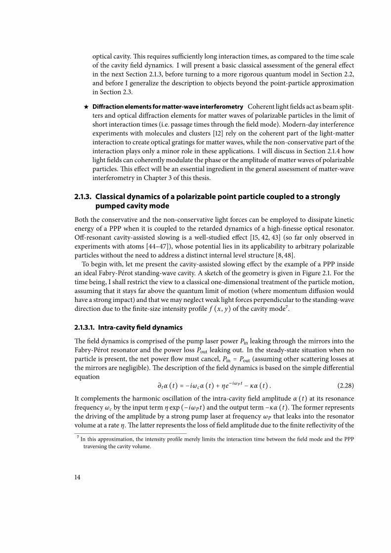
14

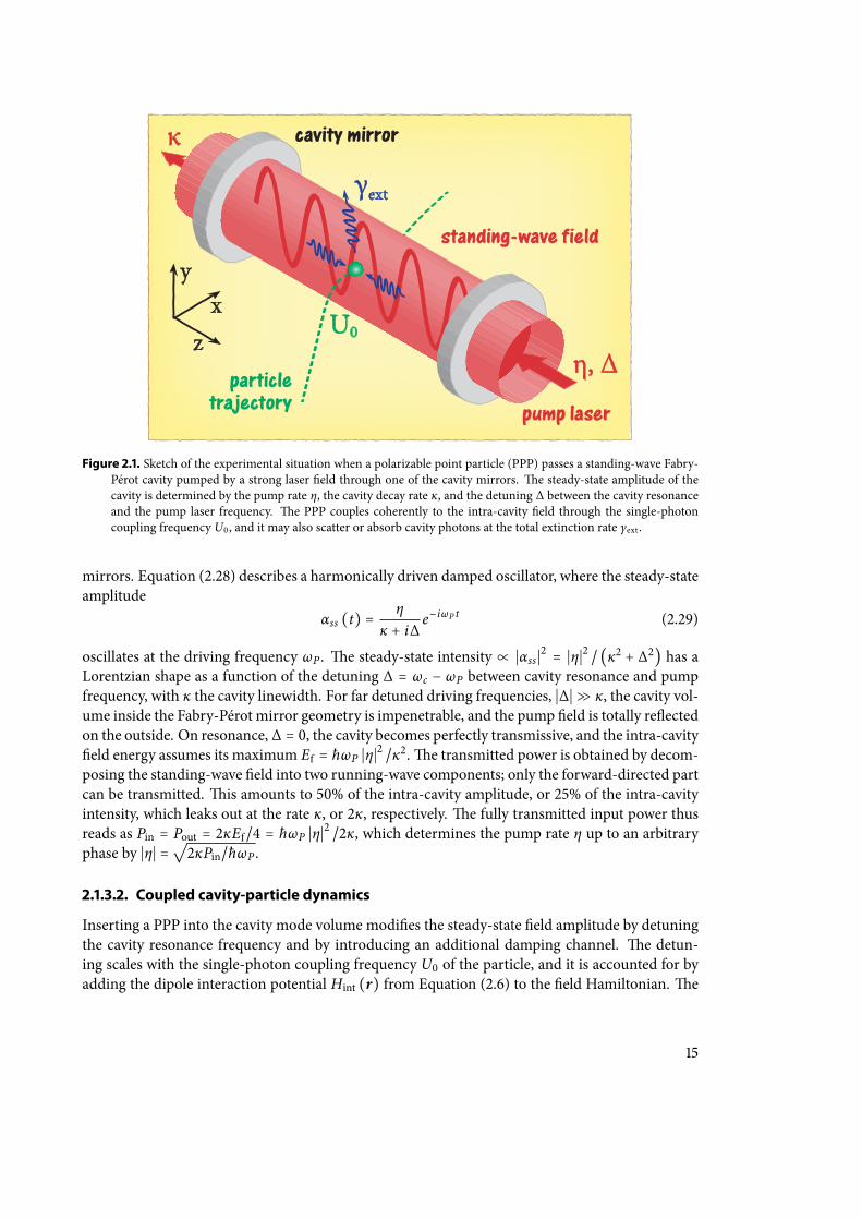
Figure 2.1. Sketch of the experimental situation when a polarizable point particle (PPP) passes a standing-wave Fabry-Pérot cavity pumped by a strong laser eld through one of the cavity mirrors. e steady-state amplitude of thecavity is determined by the pump rate η, the cavity decay rate κ, and the detuning ∆ between the cavity resonanceand the pump laser frequency. e PPP couples coherently to the intra-cavity eld through the single-photoncoupling frequency U0 , and it may also scatter or absorb cavity photons at the total extinction rate γext .

mirrors. Equation (2.28) describes a harmonically driven damped oscillator, where the steady-stateamplitude

αss (t) =η

κ + i∆e−iωP t (2.29)

oscillates at the driving frequency ωP . e steady-state intensity ∝ ∣αss ∣2 = ∣η∣2 / (κ2 + ∆2) has aLorentzian shape as a function of the detuning ∆ = ωc − ωP between cavity resonance and pumpfrequency, with κ the cavity linewidth. For far detuned driving frequencies, ∣∆∣ ≫ κ, the cavity vol-ume inside the Fabry-Pérot mirror geometry is impenetrable, and the pump eld is totally reectedon the outside. On resonance, ∆ = 0, the cavity becomes perfectly transmissive, and the intra-cavityeld energy assumes its maximum Ef = ħωP ∣η∣2 /κ2.e transmitted power is obtained by decom-posing the standing-wave eld into two running-wave components; only the forward-directed partcan be transmitted. is amounts to 50% of the intra-cavity amplitude, or 25% of the intra-cavityintensity, which leaks out at the rate κ, or 2κ, respectively. e fully transmitted input power thusreads as Pin = Pout = 2κEf/4 = ħωP ∣η∣2 /2κ, which determines the pump rate η up to an arbitraryphase by ∣η∣ =

√2κPin/ħωP .

2.1.3.2. Coupled cavity-particle dynamics

Inserting a PPP into the cavity mode volume modies the steady-state eld amplitude by detuningthe cavity resonance frequency and by introducing an additional damping channel. e detun-ing scales with the single-photon coupling frequency U0 of the particle, and it is accounted for byadding the dipole interaction potential Hint (r) from Equation (2.6) to the eld Hamiltonian.e

15

time in units of 1/κ

position in units of λ

trapping

acceleration

0 50 100 150 2000

5

10

15

20

25

time in units of 1/κ

velo

city

in u

nits

of

λκ

0 50 100 150 200−0.1

−0.05

0

0.05

0.1

0.15

0.2∆ = +κ∆ = −κ

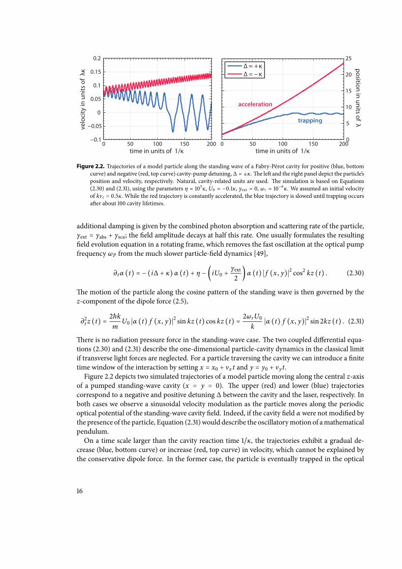
Figure 2.2. Trajectories of a model particle along the standing wave of a Fabry-Pérot cavity for positive (blue, bottomcurve) and negative (red, top curve) cavity-pump detuning, ∆ = ±κ.e le and the right panel depict the particle’sposition and velocity, respectively. Natural, cavity-related units are used. e simulation is based on Equations(2.30) and (2.31), using the parameters η = 103κ, U0 = −0.1κ, γext = 0, ωr = 10−6κ. We assumed an initial velocityof kvz = 0.5κ. While the red trajectory is constantly accelerated, the blue trajectory is slowed until trapping occursaer about 100 cavity lifetimes.

additional damping is given by the combined photon absorption and scattering rate of the particle,γext = γabs + γsca; the eld amplitude decays at half this rate. One usually formulates the resultingeld evolution equation in a rotating frame, which removes the fast oscillation at the optical pumpfrequency ωP from the much slower particle-eld dynamics [49],

∂tα (t) = − (i∆ + κ) α (t) + η − (iU0 +γext2

) α (t) ∣ f (x , y)∣2 cos2 kz (t) . (2.30)

e motion of the particle along the cosine pattern of the standing wave is then governed by thez-component of the dipole force (2.5),

∂2t z (t) =2ħkm

U0 ∣α (t) f (x , y)∣2 sin kz (t) cos kz (t) = 2ωrU0k

∣α (t) f (x , y)∣2 sin 2kz (t) . (2.31)

ere is no radiation pressure force in the standing-wave case.e two coupled dierential equa-tions (2.30) and (2.31) describe the one-dimensional particle-cavity dynamics in the classical limitif transverse light forces are neglected. For a particle traversing the cavity we can introduce a nitetime window of the interaction by setting x = x0 + vx t and y = y0 + vy t.Figure 2.2 depicts two simulated trajectories of a model particle moving along the central z-axis

of a pumped standing-wave cavity (x = y = 0). e upper (red) and lower (blue) trajectoriescorrespond to a negative and positive detuning ∆ between the cavity and the laser, respectively. Inboth cases we observe a sinusoidal velocity modulation as the particle moves along the periodicoptical potential of the standing-wave cavity eld. Indeed, if the cavity eld α were not modied bythe presence of the particle, Equation (2.31) would describe the oscillatorymotion of amathematicalpendulum.On a time scale larger than the cavity reaction time 1/κ, the trajectories exhibit a gradual de-

crease (blue, bottom curve) or increase (red, top curve) in velocity, which cannot be explained bythe conservative dipole force. In the former case, the particle is eventually trapped in the optical

16

potential, and its total energy becomes negative. Its velocity then oscillates between negative andpositive values as it bounces between the walls of the standing-wave potential.It is the delayed reaction of the cavity to the particle that is responsible for the eective dissipation

(or heating) of the kinetic energy.is eect establishes the basis of potential cavity-induced slow-ing and trapping methods for molecules, clusters and other polarizable objects. In the following Iwill study this eect in more detail, including also an assessment of its strength and applicabilityunder realistic conditions.

2.1.3.3. Estimated friction force

e characteristics of the dissipation eect are best studied in a rst order approximation of thedelayed reaction of the cavity to the moving particle. For this we expand the eld amplitude α (t) =α0 (t) + α1 (t) into the modied steady-state term

α0 (t) =η

κ + i∆ + (iU0 + γext/2) cos2 kz (t)=∶ ηΩ (t) , (2.32)

which would be the solution if the eld adjusted instantaneously to the current position z (t) ofthe particle, and the term α1 (t) incorporating the corrections due to the nite reaction time scaleof the cavity. Here I have absorbed the transverse coordinates into the coupling parameters U0 =U0 ∣ f (x , y)∣2, γext = γext ∣ f (x , y)∣2. Neglecting again their time dependence, we nd that the cor-rection term evolves according to

∂tα1 (t) = η ∂tΩ (t)Ω2 (t) −Ω (t) α1 (t) , (2.33)

which can be formally solved by applying the same expansion procedure iteratively,α1 (t) = η∂tΩ/Ω3 + α2 (t) etc. Let us, however, stop the iteration at the rst order correctionterm, α1 (t) ≈ η∂tΩ (t) /Ω3 (t), neglecting all higher-order delayed reaction contributions.is isvalid if the particle does not couple too strongly to the cavity and moves slowly along the standingwave prole so that the eld amplitude can keep up. In other words, the approximation holds forcoupling frequencies U0 and Doppler frequencies kv smaller than the parameters κ and ∆ whichdetermine the reaction time scale of the cavity.e approximate eld amplitude now also dependson the velocity v (t) = ∂tz (t) of the particle,

α (t) ≈ ηΩ (t) [1 − kv (t)

Ω2 (t) (iU0 +γext2

) sin 2kz (t)] , (2.34)

which results in a velocity-dependent force when inserted into the equation of motion (2.31). Look-ing only at the friction force term that is linear in velocity, Fv = mβv, we nd as the approximatefriction coecient

β = −ωr ∣ηΩ3

∣2sin2 2kz [−8κ∆U20 − 2 (κ2 − ∆2) U0γext

−2κU0 (γ2ext + 4U20) cos2 kz − U0γext (γ2ext + 2U20) cos4 kz] . (2.35)

Only the rst two terms in the square brackets can change their sign by varying the detuning ∆.Given that most polarizable particles in question are high-eld seeking, U0 < 0, we observe that

17

a negative friction coecient β can only be obtained for positive detuning ∆ > 0. at is to say,dissipative slowing requires the pump laser to be red-detuned with respect to the cavity resonance,whereas a blue-detuned laser will always lead to the opposite eect.e basic physical picture underlying the slowing eect is sketched in Figure 2.3. Suppose the

pump laser is red-detuned to the steep ank of the Lorentzian cavity resonance line, ∆ ∼ κ, andthe particle moves towards the antinode of the intra-cavity standing-wave eld. As it enters thehigh-insensity region its potential energy decreases immediately, and it speeds up until it reachesthe potential minimum at the antinode. At the same time, the particle shis the cavity resonancetowards the laser frequency, thereby eectively decreasing the detuning ∆ and increasing the eldintensity.is leads to a slightly delayed lowering of the optical potential ’valley’, while the particleis already moving out of the minimum and up the potential ’hill’, which is now higher than it waswhen the particle came in. Hence, if the cavity delay matches the particle’s velocity, kv < κ, thelatter must on average climb up more than it falls down, gradually losing kinetic energy.Are the simulated results comparable to a realistic scenario? I list the light coupling parame-

ters of dierent polarizable particles in Table 2.1. e selection covers a mass range of 9 ordersof magnitude between a single lithium atom and a gold nanosphere. e coupling parameters areevaluated for a standing-wave cavity operating at the IR wavelength λ = 1.56 µm with κ = 1MHzlinewidth, which is pumped at the detuning ∆ = −κ by a laser of Pin = 1W continuous-wavepower. ese rather demanding parameters should be feasible using a resonator geometry with25mm curved mirrors that are positioned at L = 1mm distance [56]8. By pumping a GaussianTEM00 mode with a waist of w = 40 µm it should be possible to achieve a mode volume as smallas V = πLw2/4 = 0.0013mm3, which trumps our earlier estimates for the light-matter couplingparameters in [8] by orders of magnitude. is leads to considerable friction rates ∣β∣, as given bythe position-averaged expression (2.35).e latter predicts an average dissipation of the z-velocityon a time scale ∼ 1/ ∣β∣. Within the boundaries of the above model, the obtained values that canbe as small as a few nanoseconds for the heaviest nanoparticles in the table. Being 100nm largein diameter, these are at the top end of the point particle regime; the description of larger objectswill be discussed in Section 2.3. Moreover, a more rigorous quantum treatment of the dissipativeslowing eect in the limit of weakly coupling point particles will be discussed in detail in Section2.2.

2.1.4. Optical gratings for matter waves

Having discussed the classical long-time dynamics of a PPP in the presence of a (classical) strongcavity eld I now turn to quite the opposite regime:e short-time eect of strong coherent eldson the propagation of PPP matter waves. Rather than trying to explicitly solve the time evolutionin the presence of the eld, I am going to adhere to the scattering picture and implement the shortpresence of the eld as a scattering event that transforms an incoming matter-wave state ρ to anoutgoing, scattered state ρ′ = S (ρ).e coherent standing-wave (or running-wave) light eld in question shall be generated by a

strong laser that is (or is not) retroreected o a mirror (rather than by a driven high-nesse res-

8A cavity linewidth of 1MHz corresponds to a so-called cavity nesse parameter F = πc/2κL ≈ 5 × 10−5 . e latter isrelated to the reectivity R of both mirrors via the relation F = π

√R/ (1 − R) in the absence of additional losses in

the resonator [57].e suggested cavity setup requires 1 − R ≈ 7 × 10−6 .

18

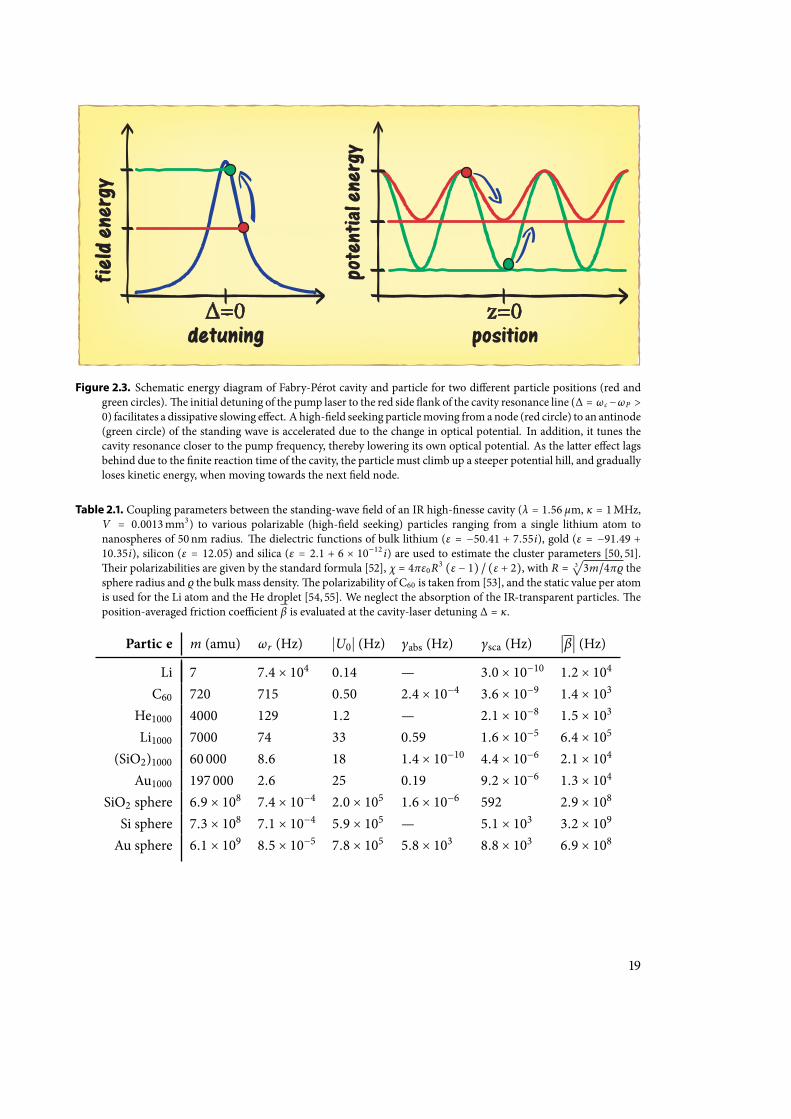
Figure 2.3. Schematic energy diagram of Fabry-Pérot cavity and particle for two dierent particle positions (red andgreen circles).e initial detuning of the pump laser to the red side ank of the cavity resonance line (∆ = ωc−ωP >0) facilitates a dissipative slowing eect. A high-eld seeking particlemoving fromanode (red circle) to an antinode(green circle) of the standing wave is accelerated due to the change in optical potential. In addition, it tunes thecavity resonance closer to the pump frequency, thereby lowering its own optical potential. As the latter eect lagsbehind due to the nite reaction time of the cavity, the particle must climb up a steeper potential hill, and graduallyloses kinetic energy, when moving towards the next eld node.

Table 2.1. Coupling parameters between the standing-wave eld of an IR high-nesse cavity (λ = 1.56 µm, κ = 1MHz,V = 0.0013mm3) to various polarizable (high-eld seeking) particles ranging from a single lithium atom tonanospheres of 50 nm radius. e dielectric functions of bulk lithium (ε = −50.41 + 7.55i), gold (ε = −91.49 +10.35i), silicon (ε = 12.05) and silica (ε = 2.1 + 6 × 10−12 i) are used to estimate the cluster parameters [50, 51].eir polarizabilities are given by the standard formula [52], χ = 4πε0R3 (ε − 1) / (ε + 2), with R = 3

√3m/4πρ the

sphere radius and ρ the bulk mass density.e polarizability of C60 is taken from [53], and the static value per atomis used for the Li atom and the He droplet [54, 55]. We neglect the absorption of the IR-transparent particles.eposition-averaged friction coecient β is evaluated at the cavity-laser detuning ∆ = κ.

Particle m (amu) ωr (Hz) ∣U0∣ (Hz) γabs (Hz) γsca (Hz) ∣β∣ (Hz)

Li 7 7.4 × 104 0.14 — 3.0 × 10−10 1.2 × 104

C60 720 715 0.50 2.4 × 10−4 3.6 × 10−9 1.4 × 103

He1000 4000 129 1.2 — 2.1 × 10−8 1.5 × 103

Li1000 7000 74 33 0.59 1.6 × 10−5 6.4 × 105

(SiO2)1000 60 000 8.6 18 1.4 × 10−10 4.4 × 10−6 2.1 × 104

Au1000 197 000 2.6 25 0.19 9.2 × 10−6 1.3 × 104

SiO2 sphere 6.9 × 108 7.4 × 10−4 2.0 × 105 1.6 × 10−6 592 2.9 × 108

Si sphere 7.3 × 108 7.1 × 10−4 5.9 × 105 — 5.1 × 103 3.2 × 109

Au sphere 6.1 × 109 8.5 × 10−5 7.8 × 105 5.8 × 103 8.8 × 103 6.9 × 108

19

onator mode, as in the previous section).e laser may either be shortly pulsed9 or continuous, inwhich case we shall assume the particle to be fast in traversing the light mode.is regime providesthe means to employ light elds as diractive elements in matter-wave interferometry, as will bediscussed in the following with a focus on the Viennese near-eld interference experiments withmolecules and clusters [12].

2.1.4.1. Coherent grating interaction

In the absence of photon absorption and Rayleigh scattering the interaction between the laser eldand the particle is entirely coherent. at is to say, the impact of the short eld presence on thequantum state of motion can be described by a unitary scattering transformation S (ρ) = SρS

†,

S†S = I. An explicit form is obtained in the basis of plane wave states by the renowned eikonal

approximation [58–60],

⟨r∣p⟩↦ ⟨r∣S∣p⟩ = exp [− iħ ∫

∞

−∞dt Hint (r +

ptm

)] ⟨r∣p⟩, (2.36)

with Hint (r) = −Reχ ∣E (r)∣2 /4 the optical dipole potential of the particle in the eld. eapproximation holds in a semiclassical high-energy limit where the classical action associated tothe motion of the particle over the course of the short interaction time exceeds by far the eikonalaction integral over the optical potential in (2.36) [60]. e transformation describes a coher-ent phase modulation of incoming matter waves. In the case of a standing-wave eld, E (r) =E0є f (x , y) cos kz, it constitutes a one-dimensional periodic phase grating.In practice, one can employ an even simpler form of the transformation that acts only on the

reduced one-dimensional state of motion along the z-axis, thus omitting the generally weak mod-ulation eect in the x- and y-direction due to the transverse mode prole f (x , y). Moreover, if thevelocities vz constituting the state of motion of the particle are suciently small10, we may take theposition distribution on the z-axis to be at rest during interaction time. We arrive at the transfor-mation rule

⟨z∣ψ⟩↦ exp (iϕ0 cos2 kz) ⟨z∣ψ⟩ (2.37)

for any state vector ∣ψ⟩ for the one-dimensional z-motion of the particle that complies with theabove constraints.is longitudinal eikonal approximation is commonly used to describe thin opti-cal transmission gratings inmatter-wave interferometry [7,18,61], and it will be presumed through-out the remainder of the manuscript. I refer the reader to [59, 60] for an exhaustive study of semi-classical corrections to the eikonal approximation. e eikonal phase factor ϕ0 is obtained by in-tegrating the interaction potential over the intensity prole of the laser. We distinguish two imple-mentations regarding the interferometry of large molecules and clusters:

Kapitza-Dirac Talbot-Lau interferometer (KDTLI) e KDTLI setup is a three-grating near-eld interferometer where the interference eect is related to the periodic phase modulationat the central grating, a standing laser wave [7]. A collimated beam of fast molecules traverses

9 Since the wavelength of the laser is required to be suciently well dened for the present purposes, ultrashort pulseswith a broad frequency spectrum are excluded here.

10 To be more concrete, the travelled distance vzτ during the interaction period τ between the particle and the eld mustbe small compared to the laser wavelength, ∣vzτ∣ ≪ λ. Given the reduced one-dimensional quantum state of motionρz , the condition should cover its entire velocity distribution ⟨mvz ∣ρ∣mvz⟩.

20

the three-grating geometry along the x-axis, and it is aligned in such a way that it crosses thelaser grating centrally and (almost) perpendicular to the standing-wave z-axis11.is ismadepossible by using a cylindrical lens system to narrow the laser spot (down to a few tens ofmicrons) in the direction of ight x, while keeping a large waist (of roughly one millimeter)along y. We may thus assume that the collimated molecule beam passes the laser grating inthe xz-plane, setting y ≈ 0.e phase factor (2.37) then reads as

ϕ0 =Reχ ∣E0∣2

4ħ ∫ ∞

−∞

dxv

f 2 (x , 0) , (2.38)

assuming a xed longitudinal velocity v of the molecules12. Assuming a Gaussian intensityprole f (x , y) = exp (−x2/w2x − y2/w2y)withwaist parameterswx ,y and an input laser powerPL, we nd [7]

ϕ0 =4√2πReχ PLhcε0vwy

. (2.39)

Given molecular velocities of the order of 100m/s and an x-waist of wx = 20 µm each mole-cule spends less than a microsecond in the laser grating. It can travel not more than 100nmalong the grating axis during that period, as themolecule beam is typically collimated to a fewmilliradians opening angle. Hence, the longitudinal eikonal approximation is well justied.

Optical time-domain ionizing Talbot-Lau interferometer (OTITLI) eOTITLI13 is a Talbot-Lau setup in the time domain where the gratings are generated by three short laser pulses,which are retroreected o a mirror [10]. A small cloud of nanoparticles ying alongside themirror surface illuminated this way may be ionized in the antinodes of the pulses; they playthe role of the thin transmission gratings of a regular Talbot-Lau setup.e phasemodulationin each pulse is given by

ϕ0 =4πReχ EL

hcε0aL(2.40)

if we assume that the particle ensemble is always well localized in the center of focus,f (x , y) ≈ f (0, 0) = 1, when illuminated by grating laser pulses of suciently large spot sizeaL = ∫ dxdy f 2 (x , y) (or a at-top shaped spot prole). e pulse energy EL = ∫τ dt PL (t)is obtained by integrating the laser power over the temporal pulse shape of length τ. Again,the eikonal expression (2.37) is only valid if the particles are approximately at rest over thepulse duration τ. e present experimental realization of the OTITLI setup in the Viennagroup operates with vacuum-ultraviolet (VUV) laser pulses of τ ≲ 10 ns at a wavelength ofλ = 157 nm.e particle velocities therefore must be restricted to below 10m/s in z-directionby means of collimation, for instance.

11Note that the direction of the grating is commonly referred to as the x-axis in the interferometry literature, whereasthe standing wave is directed along z in the present notation, which is conventionally used in the description of lightscattering at spherical particles. I will resort to the x-notation in Chapter 3.

12A realistic description of the molecular beam state involves a broad distribution of velocities v, and the resulting ϕ0-dependent interferogram must be averaged accordingly.

13Also referred to as OTIMA: optical time-domain ionizing matter-wave interferometer.

21

e general working principle of Talbot-Lau interferometry will be discussed in detail in Chapter3.ere I will show how the periodic phase modulation at a standing-wave grating leads to matter-wave interferograms. A full assessment of thin optical gratings, however, must also account fornon-conservative eects, most prominently, photon absorption.

2.1.4.2. Amplitude modulation by means of optical depletion gratings

e absorption of light from an optical standing-wave grating does not necessarily imply the loss ofmatter-wave coherence.e latter can be avoided (or suppressed) if the absorption of one or morephotons removes the particle from the interfering ensemble present in the experiment. Dependingon the internal properties of the particles and the selectivity of the detection scheme with respectto these properties, the removal can in principle be achieved by the ionization, fragmentation, iso-merization, excitation, or simply internal heating, that may be triggered by the deposited photonenergy. Consequently, the particle ensemble is depleted in the antinodes, whereas nothing happensin the nodes of the standing-wave grating. e resulting periodic modulation of the matter-waveamplitude renders the standing laser wave an optical generalization of a material diraction mask,with the nodes representing the apertures and the antinodes representing (semi-transmissive) wallsof the grating.Optical depletion gratings of this kind have been used in atom interferometry [62], where the

absorption of a single photon induces an internal state transition and the atoms are post-selectedaccording to their energy level in the detector.e experimentalists working on the OTITLI setupin the Vienna lab make use of photon-induced ionization to generate depletion gratings fromVUVlaser pulses14, as the energy of a single UV photon exceeds the ionization threshold of most molec-ular and atomic cluster particles.Let me now describe the action of an optical depletion grating on the matter waves interact-

ing with the standing-wave eld, in analogy to material diraction masks. An ideally thin one-dimensional diraction grating, where the slits are periodically arranged along the z-axis, is de-scribed by a periodic aperture function P (z), which can only take the values zero (wall) or one(opening). Given an incoming matter-wave state ψ (z) = ⟨z∣ψ⟩ we nd the density distribution ofparticles behind the grating to be P (z) ∣ψ (z)∣2.at is to say, the grating transformationmodulatesthe matter-wave state by the square root of the transmission probability, ψ (z) ↦

√P (z)ψ (z), up

to a prefactor that accounts for the renormalization of the state vector.In the case of a thin optical depletion grating, the transmission probability P (z) may take any

value between zero and one, depending on the local standing-wave intensity (with P (z) = 1 at thenodes of the standing wave). Including also the phase modulation eect (2.37) due to the dipole in-teraction, as discussed in the preceding section, we can introduce a complex transmission functiont (z) to describe the full modulation of the matter-wave state,

⟨z∣ψ⟩↦√P (z) exp (iϕ0 cos2 kz) ⟨z∣ψ⟩ ≡ t (z) ⟨z∣ψ⟩. (2.41)

e density operator ρ transforms as ρ ↦ t (z) ρt∗ (z). Using a Poissonian model for the pho-ton absorption, as discussed in Section 2.1.2, and following the same arguments as for the phasemodulation, we can express the transmission probability in terms of the mean number of absorbed

14e ionized particles are in practice removed from the ensemble with the help of a constant electric eld applied tothe interferometer setup.

22

photons, n (z) = n0 cos2 kz. In the case of fast particles crossing a stationary thin laser beam ofpower PL, the value n0 at the antinodes reads as

n0 =8σabsPLλ√2πhcvwy

, (2.42)

and in the case of illumination by a short laser pulse of energy EL as

n0 =4σabsELλhcaL

. (2.43)

When a single absorbed photon suces to remove a particle from the ensemble (e.g. by ionization)the transmission probability can be written as the Poisson probability p0 (z)of zero absorption,P (z) = p0 (z) = exp [−n (z)], and the transmission function becomes

t (z) = exp [(−n02+ iϕ0) cos2 kz] . (2.44)

In the inverted situation, where it is the non-absorbing particles that are removed from the ensem-ble, we arrive at

tinv (z) =√1 − exp (−n0 cos2 kz) exp (iϕ0 cos2 kz) . (2.45)

More generally, one could also conceive situations where the depletion threshold is reached by ab-sorbing N or more independent photons, in which case the transmission function reads as

tN (z) =

¿ÁÁÀN−1∑n=0

1n!

(n0 cos2 kz)n exp [(−n02+ iϕ0) cos2 kz] . (2.46)

Here one must be careful with using the simple Poissonian model of absorption.e latter is onlymeaningful when subsequent absorption events can be regarded as statistically independent, andit ceases to be valid when the internal state and the absorption cross-section σabs of the particle arenoticeably modied by each absorption. Moreover, one must also take into account the photonmomenta transferred to all those particles that did not absorb enough photons to be removed.

2.1.4.3. Momentum transfer by absorption and scattering

Any full description of optical elements, which are not based on single-photon depletion, must in-clude the momentum transfer due to the possible absorption and Rayleigh scattering of laser pho-tons.is generally comes with the loss of matter-wave coherence, an unwanted side-eect in opti-cal gratings. For instance, it would be inexpedient to try interfering strongly absorptive moleculesin a KDTLI setup, where the purpose of the laser grating is to modulate coherently the phase ofthe matter waves. On the other hand, for most polarizable subwavelength particles the inevitablecoherence loss due to Rayleigh scattering is usually a negligible eect in the short-time interactionregime relevant for interferometry at optical gratings.

23

Absorption I presented amodel of the absorption-inducedmomentum transfer in Section 2.1.2.1.In accordancewith the longitudinal eikonal approximation for the coherent grating transformation,let me omit any action of the Lindblad term (2.16) on the transverse motion in the eld mode.isresults in the eective one-dimensional transformation

Labs (ρ) = Γabs (t) [cos (kz) ρ cos (kz) − 12cos2 (kz) , ρ] (2.47)

of the quantum state ρ of motion along the standing-wave axis z. e time-dependent rate termrelates to the mean number of absorbed photons n0 = ∫ dt Γabs (t) through an integration overthe transverse laser beam prole in a co-moving frame along the particle trajectory, Eq. (2.42), orover the temporal shape of the laser pulse, Eq. (2.43). e above part of the master equation canbe explicitly integrated in the position representation ⟨z∣ρ∣z′⟩, which amounts again to omittingmotion during the interaction time,

⟨z∣eLabs tρ∣z′⟩ = exp [−n0 (cos2 kz2

+ cos2 kz′

2− cos kz cos kz′)] ⟨z∣ρ∣z′⟩

= exp [−2n0 sin2 (kz + z′

2) sin2 (k z − z′

2)] ⟨z∣ρ∣z′⟩ ≡Rabs (z, z′) ⟨z∣ρ∣z′⟩. (2.48)

e decohering eect is evident: All nondiagonalmatrix elements are damped except for z−z′ = nλ,the strongest eect occuring between nodes and antinodes15.In the position representation the transformation simply reduces to a multiplication of the den-

sity matrix by the positive decoherence function 0 < Rabs (z, z′) ≤ 1. Recalling that the coher-ent grating transformation also contributes a mere multiplication by t (z) t∗ (z′) in this repre-sentation, we are allowed to combine both factors to obtain the overall grating transformation⟨z∣ρ∣z′⟩↦ t (z) t∗ (z′)Rabs (z, z′) ⟨z∣ρ∣z′⟩.

Scattering e Rayleigh scattering of photons into free-space discussed in Section 2.1.2.3, nomatter how weak in practice, can be incorporated in the same manner. Tracing out the transversepart of the motion, the reduced one-dimensional version of the scattering Lindblad term (2.24)reads as

Lsca (ρ) = Γsca (t) [ ∫ d2n R (n) cos (kz) e−iknzzρ cos (kz) e iknzz − 12cos2 (kz) , ρ]

= Γsca (t) [ ∫ dΩ 3 sin2 θ

8πcos (kz) e−ik sin θ sin φzρ cos (kz) e ik sin θ sin φz − 1

2cos2 (kz) , ρ] .

(2.49)

Note that the solid angle integration over the dipole radiation pattern R (n) = 3 sin2 θ/8π must beperformed on a sphere with its poles oriented along the polarization є of the electric light eld,

15is is intuitively clear since the absorption of a photon reveals the information that the particle is not located at anode. On the other hand, the photon cannot distinguish two positions z and z′, which dier by an integer multipleof the wavelength.

24

which is perpendicular to the z-axis. e explicit expression for the decoherence function be-comes16,

Rsca (z, z′) = exp−nsca [cos2 kz + cos2 kz′

2− 3 cos kz cos kz

′

8π ∫ dΩ sin2 θe ik(z′−z) sin θ sin φ]

= exp−nsca [cos2 kz + cos2 kz′

2− 3 cos kz cos kz

′

2 ∫ π/2

0sin3 θdθ J0 (k (z′ − z) sin θ)]

= exp−nsca [cos2 kz + cos2 kz′

2− 3 cos kz cos kz′ sin k (z′ − z) − j1 (k (z′ − z))

2k (z′ − z) ] .

(2.50)

Here, nsca gives the mean number of scattered photons in the antinodes. It is obtained from theexpressions (2.42) and (2.43) by replacing the absorption cross section with σsca.A slightly dierent and somewhat simpler result would be obtained if the particle scattered the

light isotropically, a frequently used simplication,

Rsca,iso (z, z′) = exp−nsca [cos2 kz + cos2 kz′

2− cos kz cos kz′ sinck (z′ − z)] . (2.51)

In most cases relevant for interferometry, however, the mean number of scattered photons is negli-gibly small, nsca ≪ 1, and one may omit the Rayleigh scattering eect alltogether.Taking both the absorption and the scattering eect into account, the overall matter-wave state

transformation at an optical standing-wave grating becomes

⟨z∣ρ∣z′⟩↦ t (z) t∗ (z)Rabs (z, z′)Rsca (z, z′) ⟨z∣ρ∣z′⟩. (2.52)

We note that the present absorption and scattering transformations are based on an elementaryMarkovianmodel where the lasermode is linearly coupled to an initially cold reservoir of free-spacevauum modes (in case of scattering) and of internal degrees of freedom of the particle (in case ofabsorption). In particular, the model accounts for the correct momentum state of a standing-wavephoton, a superposition of two counterpropagating plane waves, which is coherently transferred tothe particle upon absorption.is improves the probabilistic argument presented in [7], where theabsorption of standing-wave photons is implemented as a purely classical binary randomwalk with50% chance to be kicked by +ħk or −ħk.is classical model is indistinguishable from the present treatment in the case of photon ab-

sorption from a running-wave eld, say, directed into the positive z-direction.e correspondingLindblad term is then of random unitary type,Labs (ρ) = Γabs [exp (ikz) ρ exp (−ikz) − ρ], and the

16 I made use of the integral representation of the Bessel function ∫ 2π0 dφ exp (iξ sinφ) = 2πJ0 (ξ), as well as of the

integral identity [63]

∫ π/2

0dθ J0 (β sin θ) sin θ cos2r+1 θ = 2rβ−1−rΓ (r + 1) Jr+1 (β) ,

with r = ±1/2 and the Gamma function Γ (3/2) =√

π/2 = 2Γ (1/2).e identity leads naturally to spherical Besselfunction expressions jn (β) =

√π/2βJn+1/2 (β), where j0 (β) = sincβ.

25

quantum state of motion transforms as

⟨z∣ρ∣z′⟩↦ exp−n0 [1 − e ik(z−z′)] ⟨z∣ρ∣z′⟩ = e−n0

∞

∑n=0

nn0n!

⟨z∣e inkzρe−inkz′ ∣z′⟩

≡ ⟨z∣∞

∑n=0

pnUnρU†n∣z′⟩. (2.53)

is expression is a probabilistic sum of unitarymomentum kick transformationsUn = exp (inkz),which also follows from a classical Poissonian ansatz.

2.2. Quantum mechanics of polarizable point particles in

high-®nesse cavities

e preceding study of polarizable point particles interacting with coherent light elds has lead to arst assessment of cavity-induced slowing in Section 2.1.3, where both the PPPmotion and the eldwere treated classically, and to the description of optical diraction gratings of PPP matter wavesin Section 2.1.4, where the strong coherent eld remained a classical degree of freedom.Let me now proceed with a full quantum treatment of both the light and the particle, a neces-

sary prerequisite to assess the diusive and dissipative eects arising from the coupling betweena PPP and one or more driven or empty high-nesse cavity modes. A rigorous derivation of thefriction and diusion parameters in the presence of one strongly driven pump mode will be givenin the weak-coupling limit where the particle-induced eld uctuations are small.is assumptionof weak coupling holds true for many subwavelength molecules and clusters, which do not exhibita distinct internal resonance that could be addressed by the cavity light. Table 2.1 lists several ex-amples where the rateU0 dened in Equation (2.10), at which the particle may induce eld shis, isby orders of magnitude smaller than realistic decay rates κ ∼ 1MHz of optical high-nesse cavities.is does not mean, however, that it is a lost cause to study the dynamics of weakly coupling par-

ticles in a cavity. I will show how a large coherent driving eld can eectively enhance the couplingto the empty cavity modes by orders of magnitude. e weak coupling model, as presented in thefollowing, will then admit a systematic assessment of the main dissipative eects of the enhancedcoupling. In particular, we will nd that the cavity-induced friction force increases with each emptycavity mode that is accessible for the pump light—a potential application for confocal resonator ge-ometries with a large spectrum of degenerate modes. e presented results have been publishedin [8].

2.2.1. Quantum model of a PPP coupled to multiple cavity modes

I start by quantizing the light-matter interaction model of Section 2.1 for the generic congurationof one particle in the presence ofM empty cavitymodes and one strongly driven pumpmode, whichprovides the necessary eld input to enhance the coupling of the PPP with the cavity. In practice,one of the cavitymodes can play the role of the pumpmodewhen driven by a strongmode-matchedlaser. An alternative two-dimensional implementation is sketched in Figure 2.4, where the pumpeld is generated in a dierent (free laser or driven cavity) mode oriented perpendicularly to theempty cavity axis.is congurationmay be favourable in practice, as it avoids a strong dipole force

26

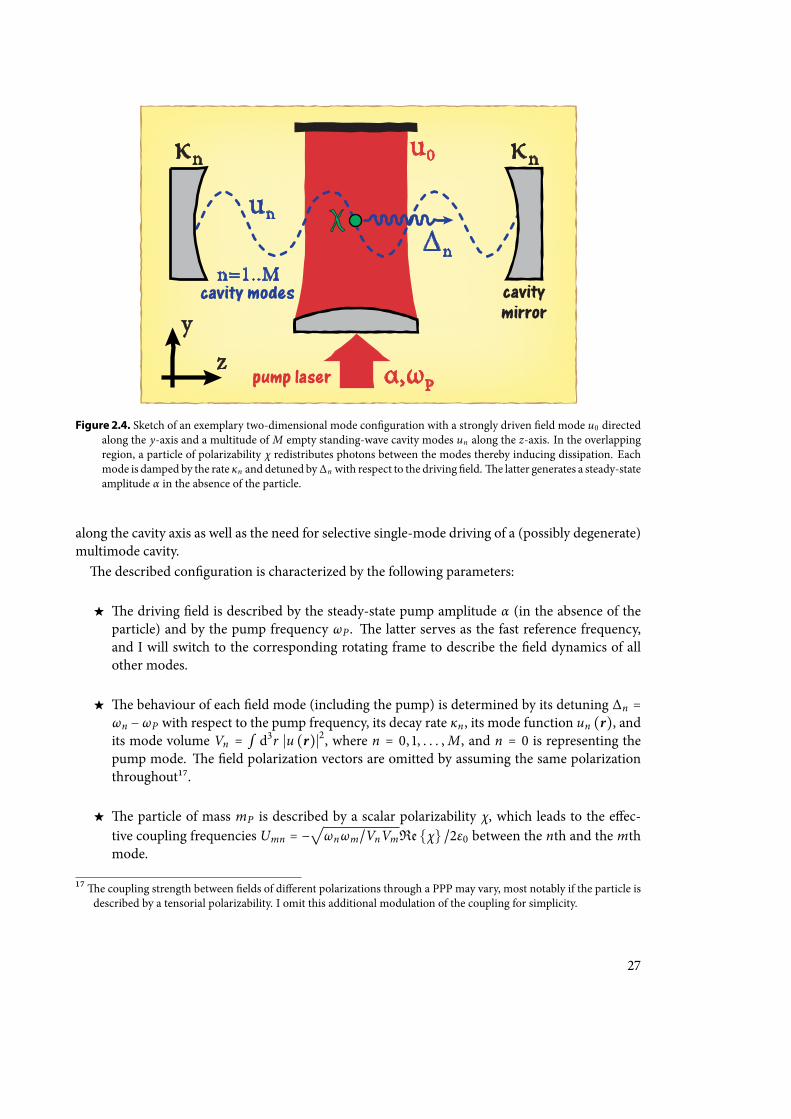
Figure 2.4. Sketch of an exemplary two-dimensional mode conguration with a strongly driven eld mode u0 directedalong the y-axis and a multitude of M empty standing-wave cavity modes un along the z-axis. In the overlappingregion, a particle of polarizability χ redistributes photons between the modes thereby inducing dissipation. Eachmode is damped by the rate κn and detuned by ∆n with respect to the driving eld.e latter generates a steady-stateamplitude α in the absence of the particle.

along the cavity axis as well as the need for selective single-mode driving of a (possibly degenerate)multimode cavity.e described conguration is characterized by the following parameters:

e driving eld is described by the steady-state pump amplitude α (in the absence of theparticle) and by the pump frequency ωP . e latter serves as the fast reference frequency,and I will switch to the corresponding rotating frame to describe the eld dynamics of allother modes.

e behaviour of each eld mode (including the pump) is determined by its detuning ∆n =ωn −ωP with respect to the pump frequency, its decay rate κn, its mode function un (r), andits mode volume Vn = ∫ d3r ∣u (r)∣2, where n = 0, 1, . . . ,M, and n = 0 is representing thepump mode. e eld polarization vectors are omitted by assuming the same polarizationthroughout17.

e particle of mass mP is described by a scalar polarizability χ, which leads to the eec-tive coupling frequencies Umn = −

√ωnωm/VnVmReχ /2ε0 between the nth and the mth

mode.

17e coupling strength between elds of dierent polarizations through a PPP may vary, most notably if the particle isdescribed by a tensorial polarizability. I omit this additional modulation of the coupling for simplicity.

27

2.2.1.1. Quantum description of a driven cavity mode

Before introducing the coupling to the particle, I rst translate the classical description of a drivenhigh-nesse cavity mode in Section 2.1.3.1 into the quantum picture. Here I make use of the canon-ical eld quantization procedure [64–66] and replace the coherent eld amplitude and its complexconjugate by the annihilation and creation operators in the expressions for the physical elds,

E (r, t)↦√2ħω0ε0V0

a0єu0 (r) , H (r, t)↦ −ic¿ÁÁÀ 2ħ

µ0ω0V0a0∇× єu0 (r) . (2.54)

is results in the free eldHamiltonianH0 = ħω0 (a†0a0 + 1/2), where the constant term is dropped

for convenience. In order to describe a driven cavitymode onemust include the driving eld leakinginto the cavity and the losses leaking out. Both eects are covered by a linear couplingmodel, wherethe exchange of eld amplitude with an external mode b is described by a coupling Hamiltonian ofthe form18 ∝ a0b

†+ h.c.at is, the coupling of the modes can be understood as an exchange of

single photons between the eld states.Based on this physical picture we may pin down the loss and driving terms heuristically. e

cavity eld loss can be seen as a random and uncontrolled elimination of photons as they escapethrough the cavitymirrors or by scattering into free space at a total rate 2κ0. Inmathematical terms,this is well modelled by a Poisson jump process of the same type as in (2.13), with the jump operatorgiven by the photon annihilator a0, Lloss (ρ) = κ0 (2a0ρa

†0 − a

†0a0, ρ).

e same linear description can be applied to the driving by the mode b of a strong laser illu-minating the cavity mirror.e quantum representation of a strong coherent laser eld is given interms of coherent states [65]

∣β⟩ = D (β) ∣0⟩ = e−∣β∣2/2

∞

∑n=0

βn√n!

∣n⟩ = exp (βb†− β∗b) ∣0⟩, (2.55)

with β the complex eld amplitude and ∣β∣2 the mean photon number. Coherent states are denedas displaced vacuum states, and they are the eigenvectors of the annihilation operator, b∣β⟩ = β∣β⟩.Mimicing the behaviour of classical monochromatic light elds they oscillate harmonically at thelaser frequency ωP , ∣β (t)⟩ = exp (−iωP tb

†b) ∣β⟩ = ∣β exp (−iωP t)⟩. ey can be understood as

the vacuum state in a displaced and rotating frame19. In the classical limit ∣β∣ ≫ 1 the vacuumeld uctuations around the displacement amplitude are small compared to ∣β∣, and we may sub-stitute the laser mode operator b by β exp (−iωP t) (assuming there is no relevant backaction ofthe cavity eld onto the state of the driving laser).e driving Hamiltonian thus assumes the formHpump (t) ∝ β∗ exp (iωP t) a0 + h.c. We get rid of the time dependence by switching to a frame

18e form is easily obtained by adding the quantized physical elds (2.54) of the modes a0 and b to an overall electricand magnetic eld. When the corresponding eld energy density is integrated over the volume in (2.4) the crossterms between both modes yield the above linear coupling Hamiltonian. Terms of the form a0b and a

†0b are omitted

in the rotating wave approximation [65], since they oscillate rapidly at twice an optical frequency, ωP + ω0 , and thusdo not aect the actual mode coupling.

19A rotating frame is dened through the unitary state transformation U (t) = exp (iωP∑n a†nan), with ωP the cor-

responding rotation frequency. Given the quantum state ρ (t) of a system of eld modes an in the Schrödingerpicture, the state in the rotating picture reads as ρ′ = U (t) ρ (t)U

†(t). Analogously, a displaced frame is dened via

the unitary displacement operator, ρ′ = D†(β) ρD (β). Field observables are displaced as D

†(β)bD (β) = b + β.

28

rotating at the optical pump frequency ωP , introducing the cavity-pump detuning ∆0 = ω0 − ωPand the eective pump rate η.is leaves us with the master equation for the eld state of a drivencavity mode,

∂tρ = −i [∆0a†0a0 + iηa

†0 − iη∗a0, ρ] + κ0 (2a0ρa

†0 − a

†0a0, ρ) . (2.56)

e quantumexpectation value of the eld amplitude evolves in the sameway as the classical version(2.28),

∂t ⟨a0⟩ = − (i∆0 + κ0) ⟨a0⟩ + η. (2.57)

It is then straightforward to show that the coherent state ρss = ∣α⟩⟨α∣ is the steady-state solution ofthe above master equation for the same steady-state amplitude α = η/ (κ0 + i∆0) as in the classicalcase. An elegant and convenient way to incorporate the driving is to work with quantum states inthe displaced frame, ρ ↦ ρα = D

†(α) ρD (α), where the steady-state amplitude shis the state of

the mode from ∣α⟩⟨α∣ to the ground state↦ ∣0⟩⟨0∣.e resulting master equation,

∂tρα = −i [∆0a†0a0, ρα] + κ0 (2a0ραa

†0 − a

†0a0, ρα) , (2.58)

does not contain the explicit driving term anymore, and the eld operator a0 now represents thequantum eld uctuations on top of the coherent steady state.

Derivation of the loss term Note that the non-Hamiltonian loss term in the master equation(2.56) can also be derived using a standard textbook approach [35, 67]. For this let us couplethe cavity mode linearly to a bath of harmonic oscillators, Henv = ∑ j ħω jb

†j b j. It represents the

environmental vacuum of modes, which can be populated by a photon escaping the cavity. Weshall assume a linear coupling term of the form Hint = ∑ j ħg ja0b

†j + h.c., with g j the eective

photon exchange rates between cavity and environment. e coupled dynamics of the combinedstate ρSE (t) of system and environment is most conveniently assessed in the interaction frame,ρSE ,I (t) = U (t) ρSE (t)U

†(t), with U (t) = exp [i (H0 + Henv) t/ħ]. A formal integration and re-

insertion of the von Neumann equation yields the integro-dierential equation for the combinedstate,

∂tρSE ,I (t) = −iħ[HI (t) , ρSE ,I (0)] −

1ħ2 ∫

t

0dτ [HI (t) , [HI (τ) , ρSE ,I (τ)]] , (2.59)

whereHI (t) = U (t)HintU

†(t) =∑

jħg je i(ω j−ω0)ta0b

†j + h.c. (2.60)

We obtain a closed equation for the reduced cavity state ρI = trE (ρSE ,I) by tracing out the envi-ronment and subsequently applying the so-called Born approximation: e cavity leaves the en-vironment practically unaected at all times, ρSE ,I (t) ≈ ρI (t) ⊗ ∣vac⟩⟨vac∣. Every photon thatespaces disperses almost immediately, and the cavity is thus eectively surrounded by vacuum20 on

20Optical frequencies in the environmental mode spectrum are practically unoccupied even at nite temperatures. Ithus use the zero-temperature vacuum state here, since the cavity only couples to modes of similar frequencies.

29

all relevant time scales. We nd

∂tρI (t) = −1ħ2 ∫

t

0dτ trE ([HI (t) , [HI (t − τ) , ρI (t − τ)⊗ ∣vac⟩⟨vac∣]])

=∑j∫ t

0dτ ∣g j∣

2 e−i(ω j−ω0)τ a0ρI (t − τ) a†0 − a

†0a0ρI (t − τ) + h.c. (2.61)

Next we can apply theMarkov approximation:e environment shall notmemorize the cavity stateat earlier times and the time evolution equation shall become time-local.at is to say, we may setρI (t − τ) ≈ ρI (t) and integrate up to innity.is is formally justied if the cavity eld couples toa suciently broad frequency range such that∑ j ∣g j∣

2 exp [i (ω0 − ω j) τ] ≈ κδ (τ) and

∂tρI (t) ≈ κ [2a0ρI (t) a†0 − a

†0a0ρI (t) − ρI (t) a

†0a0] . (2.62)

e desired master equation (2.56) follows by combining this with the above driving term of aclassical coherent laser eld.

2.2.1.2. A particle, a driving laser, and a handful of empty cavity modes

With the quantum model of a driven cavity mode at hand we can now collect all ingredients tomodel the system of a single pump mode, M empty cavity modes and a PPP, as sketched in Figure2.4. It will be expedient to work in a frame rotating at the optical frequency ωP of the driving laser,with the pump mode displaced by the steady-state amplitude α. is results in a master equationterm of the above form (2.58) for each of theM + 1 modes.e presence of a polarizable particle comes with an additional Hamiltonian representing the

optical potential, as well as with scattering and absorption contributions, which couple the motionof the particle to the eld degrees of freedom. We obtain directly the optical potential term byquantizing the electric eld expression E (r) in the PPP Hamiltonian (2.9). However, we must bearin mind that the electric eld is now given by a sum of allM cavity modes plus the displaced pumpmode.is results in the total particle Hamiltonian

HPPP =

≡HP³¹¹¹¹¹¹¹¹¹¹¹¹¹¹¹¹¹¹¹¹¹¹¹¹¹¹¹¹¹¹¹¹¹¹¹¹¹¹¹¹¹¹¹¹¹¹¹¹¹¹¹¹¹¹¹¹¹¹¹¹¹¹·¹¹¹¹¹¹¹¹¹¹¹¹¹¹¹¹¹¹¹¹¹¹¹¹¹¹¹¹¹¹¹¹¹¹¹¹¹¹¹¹¹¹¹¹¹¹¹¹¹¹¹¹¹¹¹¹¹¹¹¹¹¹µp2

2mP+ ħU00 ∣αu0 (r)∣2 +

≡HI³¹¹¹¹¹¹¹¹¹¹¹¹¹¹¹¹¹¹¹¹¹¹¹¹¹¹¹¹¹¹¹¹¹¹¹¹¹¹¹¹¹¹¹¹¹¹¹¹¹¹¹¹¹¹¹¹¹¹¹¹¹¹¹¹¹¹¹¹¹¹¹¹¹¹¹¹¹¹¹¹¹¹¹¹¹¹¹¹¹¹¹¹¹¹¹¹¹¹¹¹¹¹·¹¹¹¹¹¹¹¹¹¹¹¹¹¹¹¹¹¹¹¹¹¹¹¹¹¹¹¹¹¹¹¹¹¹¹¹¹¹¹¹¹¹¹¹¹¹¹¹¹¹¹¹¹¹¹¹¹¹¹¹¹¹¹¹¹¹¹¹¹¹¹¹¹¹¹¹¹¹¹¹¹¹¹¹¹¹¹¹¹¹¹¹¹¹¹¹¹¹¹¹¹¹µM∑n=0

ħU0n [αa†nu∗n (r)u0 (r) + h.c.]+

M∑k,n=0

ħUkna†naku∗n (r)uk (r) .

(2.63)

e rst termHP describes the particle motion in the steady-state dipole potential, the second termHI represents the pump-enhanced linear coupling of the particle to the eld uctuations in eachcavitymode, and the remainder represents the inter-mode coupling, which also causes the position-dependent resonance shi of the modes.e above Hamiltonian must be complemented by the eld energy term in the displaced and

rotating frame, HC = ∑n ħ∆na†nan.e free elds are thus included via the superoperator

LC (ρ) = −iM∑n=0∆n [a

†nan , ρ] +

M∑n=0

κn (2anρa†n − a

†nan , ρ) . (2.64)

30

It describes the eld evolution in the absence of the particle. In addition, the time evolution of thecombined state of cavity and particle contains another two eld loss terms Labs and Lsca due toabsorption and scattering,

∂tρ = − iħ[HPPP, ρ] +LC (ρ) +Labs (ρ) +Lsca (ρ) . (2.65)

Both cause additional coupling between the particle motion and the eld uctuations.e explicitform of these terms is found by combining the original expressions (2.16) and (2.24) for a classicaleld with the above derivation of the Lindblad term (2.62), which represents the incoherent loss ofsingle eld quanta. Keeping the displacement of the pump mode in mind, we arrive at

Labs (ρ) =M∑n=0

cσabsVn

[(an + αδn0)un (r) ρ (an + αδn0)†u∗n (r)

− 12(an + αδn0)

†(an + αδn0) ∣un (r)∣2 , ρ] , (2.66)

Lsca (ρ) =M∑m=0

cσscaVm

[ ∫ d2n R (n) (am + αδm0)um (r) e−ikn⋅rρ (am + αδm0)†e ikn⋅ru∗m (r)

− 12(am + αδm0)

†(am + αδm0) ∣um (r)∣2 , ρ] . (2.67)

ermal or uorescent photon emission from the particle into free space is neglected, as well asinternal heating of the particle due to photon absorption21. In the following I will simplify theoverall master equation (2.65) to the case of weak coupling.

2.2.2. Eliminating the quantum ®eld dynamics in the weak coupling limit

With the quantum model of the coupled cavity-particle dynamics at hand, I will now assess thegeneral eect of the dynamical quantum eld on the motion of the PPP. e goal is to nd aneective description of the reduced particle state by eliminating the explicit eld dynamics. Weshould expect that such a separation can formally be achieved only in the limit of weak couplingbetween the particle and the eld. I will therefore introduce two weak coupling assumptions whichwill facilitate a low-order expansion of the coupling eect. Although the resulting model will bestrictly valid under those assumptions only, we might retain its qualitative predictions even beyondthe weak coupling limit.

2.2.2.1. The ®rst weak-coupling assumption

I assume that the coupling rates of the polarizable particle to the modes are signicantly smallerthan the mode damping rates, ∣Umn∣ ≪ κn ∀m, n. is means that the particle-induced cavityeld uctuations are limited to a few photons, as they typically escape the cavity much faster thanthey can be redistributed by the particle. e strong pump amplitude ∣α∣ ≫ 1 then represents theonly potential source of large photon numbers that may populate empty modes through coherent

21 Practical implementations of the present cavity dissipation scheme are restricted to non-absorbing particle species.e typically large pump eld intensities might otherwise lead to the destruction of the particle.

31

scattering at the particle. We may thus omit those coupling terms in the Hamiltonian (2.63) whichare of second order in the eld uctuations, HPPP ≈ HP + HI .Secondly, if we extend the above weak-coupling assumption for the coherent inter-mode scat-

tering rates to the rates of photon absorption and Rayleigh scattering, we may approximate theLindblad terms (2.66) and (2.67) as

Labs (ρ) ≈ γabs ∣α∣2 [u0 (r) ρu∗0 (r) − 12∣u0 (r)∣2 , ρ] , (2.68)

Lsca (ρ) ≈ γsca ∣α∣2 [ ∫ d2n R (n)u0 (r) e−ikn⋅rρe ikn⋅ru∗0 (r) − 12∣u0 (r)∣2 , ρ] . (2.69)

e terms γabs,sca = cσabs,sca/V0 denote the absorption and the Rayleigh scattering rate with respectto the pumpmode volumeV0. According to our assumption, both the absorption and the scatteringrate must be small compared to the cavity decay rates, and we can safely neglect their contributionto the particle-cavity dynamics. We are le with the momentum diusion caused by the absorptionand scattering of pump photons in (2.68) and (2.69); the only relevant non-conservative contribu-tions to the model, apart from the cavity damping terms in LC .e rst weak-coupling assumption simplies considerably the quantum description of cavity

and particle at almost no costs. In fact, the assumption is very well fullled in practice by a widerange of nanoparticles, as can be seen from the exemplary Table 2.1. Using infrared light it remainsvalid up to a mass of roughly 108 amu. e quantum description of the weakly coupling systemsplits into the two separate superoperators LC and LP (ρ) = −i [HP , ρ] /ħ + Labs (ρ) + Lsca (ρ)acting solely on the cavity and particle subspace, respectively. e coupling of both subsystems ismediated by the eective interaction Hamiltonian

HI =M∑n=0

ħU0nαa†nu∗n (r)u0 (r) + h.c. (2.70)

It resembles the standard linear coupling Hamiltonian, but with a coupling rate ∣U0nα∣ enhancedby the strong pump eld α. In principle, this allows a weakly coupling particle to enter the strongcoupling regime ∣U0nα∣ ≳ κn with the help of a suciently strong pump laser. Note that it requiresonly one driving mode to enhance the coupling of the particle to all the other modes that overlapwith the pump eld. However, cavity modes with a large detuning ∆n cannot be addressed in prac-tice, given that their oscillating amplitude an averages out in the interaction Hamiltonian. Whatcounts are degenerate or near-degenerate resonator modes with a detuning of the order of the cav-ity linewidth. Only they contribute to the interaction. I will analyze the benet of a large degeneratemode spectrum for cavity-induced cooling in Section 2.2.3.4.While previous weak-coupling approaches towards the cavity-induced slowing of atoms [68] did

not yet consider the pump enhancement (because it was not necessary there), it is a practiced tech-nique in the eld of optomechanics [26] to reach the strong coupling regime [69, 70].ere, how-ever, the interaction is restricted to a single oscillatory degree of freedom of a rigid system such asa mirror or membrane. It is typically coupled to a single driven cavity mode a0, and a low-orderexpansion of the respective mode function u0 (r) around the equilibrium value of the oscillatoryields the standard optomechanical interaction Hamiltonian [71].e pump enhancement facilitates the strong coupling of a weakly interacting nanoparticle to

high-nesse cavity modes. It thus has the potential of inducing a substantial dissipative slowing

32

eect. We have seen this already in the simple classical model calculation in Section 2.1.3.1, andI will study the strong coupling regime further in Section 2.3.3. On the other hand, an eectivemaster equation for the reduced particle state can only be derived by adiabatically eliminating thecavity degrees of freedom.is requires an even stronger assumption.

2.2.2.2. The second weak-coupling assumption

I now assume in addition that even the pump-enhanced coupling rates are small compared to thedecay rates of all relevant cavity modes, ∣U0nα∣ ≪ κn ∀n. In other words, any excitation of thecavity eld will always leak out much faster than it can be built up by the in-mode scattering ofpump photons o the particle. As a consequence, the M cavity modes (and the pump mode) willremain empty (relative to the pump displacement) at almost all times, ⟨a

†nan⟩ ≪ 1.

Obviously, the second weak-coupling assumption represents a very restrictive condition, whichone should be anxious to violate in actual experiments in order to achieve a signicant slowingeect. Still, I make the assumption here to dene an eective quantum description of the particlemotion under the dissipative inuence of the cavity. It will provide us with a clear and rigorousunderstanding of the origin of cavity-induced friction and diusion eects. Judging from com-plementary semiclassical treatments and numerical simulations [17,68], we should expect the basicfeatures and qualitative behaviour of those eects to remain valid in a strong-coupling regimewhereour eective quantum model will break down.In the following I derive the eective master equation for the reduced particle state by employing

the projection formalism [72–74]. For this let me dene a superoperator P as the projection of thecombined cavity-particle state on the cavity ground state in the displaced frame, Pρ = trC (ρ) ⊗∣vac⟩⟨vac∣.e complementary projection shall be denoted byQ = id−P . As both superoperatorsrepresent orthogonal projections in operator space (P2 = P , Q2 = Q and PQ = QP = 0), themaster equation ∂tρ = −i [HI , ρ] /ħ + LC (ρ) + LP (ρ) can be divided into two coupled equationsfor Pρ andQρ with help of the following relations:

Both superprojectors P and Q commute with the master equation term LP , that is, PLP =LPP = PLPP andQLP = LPQ = QLPQ.e reason is that the projectors act solely on theeld degrees of freedom, whereas LP operates on the particle subspace.

e relation LCP = 0 is obviously true since P singles out the cavity vacuum state.

e ipped relation PLC = 0 holds as well since LC is restricted to the cavity subspace andtraceless by construction, tr (LCρ) = trC (LCρ) = 0.

It follows immediately from the previous two points thatQLC = LCQ = QLCQ.

e relation PLIP = 0, with LI (ρ) = −i [HI , ρ] /ħ, can easily be veried by plugging in theexplicit form of the coupling Hamiltonian (2.70) and noting that ⟨vac∣HI ∣vac⟩ = 0.

Putting everything together we arrive at the coupled equations

∂tPρ (t) = PLPPρ (t) +PLIQρ (t) , (2.71)∂tQρ (t) = Q (LP +LC)Qρ (t) +QLIPρ (t) +QLIQρ (t) . (2.72)

33

e initial conditions at time t = 0 shall be given by the initial state ρP (0) of the particle and thesteady state of the cavity system, Pρ (0) = ρP (0) ⊗ ∣vac⟩⟨vac∣ and Qρ (0) = 0. e second weak-coupling assumption will now form the basis of three steps of approximation that will nally leadto a closed equation for Pρ (t) and for the reduced particle state ρP (t) = ⟨vac∣Pρ (t) ∣vac⟩.Recall that any particle-induced eld excitations in the weak-coupling limit are assumed to decay

before they can add up or disperse over the system of modes. e state of the cavity is thus wellapproximated by the vacuum at almost all times, and the componentQρ can be regarded as a smallcorrection to the full quantum state ρ = Pρ + Qρ. is component will only be occupied at theeective coupling rates ∣U0nα∣ via the term QLIPρ in (2.72), while the term QLCQρ causes it todecay on amuch faster time scale of the order of the cavity lifetimes 1/κn.e assumption ∣U0nα∣ ≪κn allows us to neglect the ‘second order’ term QLIQρ, which would describe the back-action ofpersistent eld excitations on the particle.e remainder can be formally integrated respecting theinitial conditionQρ (0) = 0,

Qρ (t) = ∫ t

0dτQe(LC+LP)(t−τ)QLIPρ (τ) . (2.73)

Inserting this into Equation (2.71), we arrive at a closed integro-dierential equation for the vacuumcomponent,

∂tPρ (t) = PLPPρ (t) + ∫ t

0dτPLIQe(LC+LP)(t−τ)QLIPρ (τ)

= LPPρ (t) + ∫ t

0dτPLIe(LC+LP)τLIPρ (t − τ) , (2.74)

which depends on the whole past trajectory of Pρ.e integral represents the small correction tothe particle state evolution in the absence of eld uctuations. A standard way of converting theabove expression to a time-local dierential equation is to expand it as Pρ = Pρ0 +Pρ1 + . . . usingthe following iteration process: First one formally solves the time-local equation in the absence ofthe integral term to obtain the zeroth order solution Pρ0 (t) = exp [LP (t − t0)]Pρ0 (t0). is isthen plugged into the correction term to obtain an equation for the rst-order term Pρ1, which isagain solved in the absence of the next-order correction, and so forth. Here we are only interestedin the lowest order, which leaves us with the equation

∂tPρ (t) ≈ LPPρ (t) + ∫ t

0dτPLIeLC τeLPτLIeLP(t−τ−t0)Pρ (t0) , (2.75)

with t0 > 0 an arbitrary initial time. I have separated the time evolution underLC andLP since thesuperoperators commute as they act on distinct subsystems.Unfortunately, we are now running into trouble when we try to make this equation time-local

by setting t0 = t. Temporal inversion of the particle evolution LP is not allowed due to the non-unitary contributions Labs,sca of absorption and Rayleigh scattering, which increase the entropy ofthe particle state by diusion.Fortunately, we can generally neglect the non-unitary parts when the weak-coupling conditions

hold.is is because the past-trajectory integral in (2.75) involves only time periods τ of the orderof the cavity lifetimes 1/κn as the rapid cavity decay term in exp (LCτ) suppresses the coupling termLI . During that period, absorption and scattering events changing the particle momentum in units

34

of ħk occur at the rates γabs,sca ∣α∣2. We can safely ignore them if they do not modify the particle’smomentum mPv = ⟨∣p∣⟩ too much,

γabs,sca ∣α∣2

κn∣2ωrkv

∣ ≪ 1 ∀n. (2.76)

As once again illustrated in Table 2.1 typical nanoparticles (in the absence of strong internal reso-nances close to the laser frequency) exhibit scattering and absorption rates smaller than their re-spective coupling frequencies. e weak-coupling limit thus implies γabs,sca ∣α∣ ≪ ∣U0α∣ ≪ κn.At the same time, the massive molecules and nanoparticles of interest feature sub-kHz recoil fre-quencies ωr = ħk2/2mP when interacting with infrared light. is must be compared to Dopplerfrequencies of kv ∼ 4MHz≫ ωr at rather low velocities of v ∼ 1m/s; such slow particles are stillorders of magnitude away from the quantum limit of motion.Moreover, given that the integral in (2.75) is restricted by the integrand to times τ ≲ 1/κn, we can

replace the upper integral bound by innity.is leaves us with the time-local equation

∂tPρ (t) ≈ [LP + ∫ ∞

0dτPLIeLC τLI (τ)]Pρ (t) , (2.77)

where LI (τ) represents the von Neumann commutator with the back-in-time-evolved couplingHamiltonian

HI (τ) = e−iHPτ/ħHIe iHPτ/ħ =M∑n=0

ħU0nαa†nu∗n (r,p; τ)u0 (r,p; τ) + h.c., (2.78)

un (r,p; τ) = un (exp [−ip2τ2mPħ

− iU00 ∣αu0 (r)∣2 τ] r exp [ ip2τ2mPħ

+ iU00 ∣αu0 (r)∣2 τ]) . (2.79)

2.2.2.3. Eªective time evolution of the reduced particle state

e time-local expression (2.77) is now easily turned into an eective time evolution equation forthe reduced particle state ρP (t) = trC [ρ (t)],

∂tρP (t) = ⟨vac∣∂tPρ (t) ∣vac⟩ = − iħ[HP , ρP (t)]

− 1ħ2 ∫

∞

0dτ trC [HI , eLC τ [HI (τ) , ρP (t)⊗ ∣vac⟩⟨vac∣]] . (2.80)

e free evolution under LC and the trace over the cavity subsystem can be performed straightfor-wardly22,

∂tρP (t) = LPρP (t) −M∑n=0

∣U0nα∣2 ([u∗0 (r)un (r) , gnρP (t)] + h.c.) . (2.81)

Here I introduce the so-calledmemory operators

gn = ∫ ∞

0dτ e−(κn+i∆n)τu∗n (r,p; τ)u0 (r,p; τ) . (2.82)

22Applying the interaction Hamiltonian to the vacuum state leads to nondiagonal elements of the form ∣1n⟩⟨vac∣, with∣1n⟩ = a

†n ∣vac⟩ a single-excitation multimode Fock state. One can easily show that these nondiagonals evolve like

exp (LC t) ∣1n⟩⟨vac∣ = exp (−κn t − i∆n t) ∣1n⟩⟨vac∣

35

ey collect the particle-induced coupling between the pump eld and the cavity modes over ashort period of time before the present time t. In other words, they represent the delayed reactionof each cavity mode to the position of the particle that continuously scatters pump light into them.e delay, or memory time scale, is determined by the damping rate κn and the detuning ∆n of eachmode.Once again, we can approximate the past trajectory of suciently fast particles by neglecting the

inuence of the optical potential on short time scales. We may follow the same line of argument asin the case of absorption and Rayleigh scattering. e optical dipole potential of a standing-wavepumpmode23 can be viewed as a coherent backscattering process of pumpphotonswithin themodeand at the rate U00 ∣α∣2. As each backscattering event transfers 2ħk of momentum to the particle,we nd that the optical potential is negligible in the limit of

∣U00 ∣α∣2

κn

4ωrkv

∣ ≪ 1 ∀n. (2.83)

If this is the case we can explicitly write

gn ≈ ∫ ∞

0dτ e−(κn+i∆n)τu∗n (r − pτ

mP)u0 (r − pτ

mP) . (2.84)

e memory operators then average the inter-mode coupling over an approximately straight par-ticle trajectory reaching a few mode lifetimes into the past. Note that the above condition (2.83) isonly relevant for a standing-wave pumpmode directed along the axis of the other cavity modes. Inan orthogonal conguration with a running-wave pump eld, as depicted in Figure 2.4, the opticaldipole force merely scales with the transverse pump laser prole24.I will discuss in the following section that the delay eect is responsible for cavity-induced fric-

tion forces and the potential slowing of the particle. It vanishes in the limit of far-detuned or badcavity modes, when the eld uctuations can follow the moving particle almost instantaneously.is happens in the limit of ∣kv∣ ≪ κn , ∣∆n∣, as the Doppler frequency determines the rate atwhich the particle-induced coupling changes during motion. We may then approximate gn ≈u∗n (r)u0 (r) / (κn + i∆n) leaving us with the completely positive Lindblad-type master equation

∂tρP = −iħ[HP −

M∑n=0

ħ∆n ∣U0nα∣2

κ2n + ∆2n∣u0 (r)un (r)∣2 , ρP] +LabsρP +LscaρP

+M∑n=0

κn ∣U0nα∣2

κ2n + ∆2n[2u∗n (r)u0 (r) ρPu∗0 (r)un (r) − ∣u0 (r)un (r)∣2 , ρP] . (2.85)

Apart from the addition to the Hamiltonian, it features a positive Lindblad term, which is form-equivalent to the Rayleigh scattering term (2.69). Bad cavity modes simply act as an additionaldiusion channel for the particle. On the other side, even good cavity modes will result in a meremomentum diusion when the particle is suciently slow.

23 Running-wave modes do not exhibit a wavelength-scale oscillatory intensity pattern. eir inuence on the particlethrough the optical potential is considerably weaker.

24 Condition (2.83) would be alleviated by a factor kw ≪ 1 in the case of a Gaussian prole with waist w.

36

2.2.3. Semiclassical description of friction and diªusion

Based on the eective evolution equation (2.81) and the memory operator (2.84) for a particle inthe presence of a strongly driven pump and M empty cavity modes, I will formulate the resultingdissipative dynamics using a semiclassical phase-space picture.To keep things simple and clear let me trace out the particle’s xy-motion and resort to a one-

dimensional version of the presentmodel along the z-axis of the standing-wavemodes of the cavity,un (x , y, z) ↦ fn (x , y)un (z).is is where a moving particle can cause the fastest eld modula-tion and the most delayed reaction by the cavity. Dissipative eects, and indeed any eld-inducedforces on the particle, are expected to bemuchweaker in the xy-directions, given that the transversemode proles of the cavity fn (x , y) extend over muchmore than a wavelength. To be concrete, thedelayed cavity-backaction on the transverse motion is negligible for velocities ∣vx ,y/wn∣ ≪ κn , ∆n,with wn the characteristic transverse width of the nth mode (as given by the waist in case of anxy-symmetric Gaussian mode prole).We are le with the one-dimensional memory operator

g(z)n = ∫ ∞

0dτ e−(κn+i∆n)τu∗n (z − pτ

mP)u0 (z − pτ

mP) . (2.86)

for the z-state of the particle, at xed transverse coordinates x and y.e latter can be sucientlywell described by a straight classical trajectory (xt , yt) if we assume that the particle is hardlyaected in its transverse motion while it passes the high-intensity region of the cavity. is ef-fective parametric time dependence can be incorporated, if necessary, in the coupling frequen-cies, Umn (t) = Umn f ∗m (xt , yt) fn (xt , yt), as already done in the simple classical model of cavity-induced slowing in Section 2.1.3. For the time being I will simply ignore the transverse trajectorywhen assessing the one-dimensional friction and diusion eects. Nevertheless, one should takenotice of this time dependence when estimating the overall eect in realistic scenarios. e one-dimensional slowing of the z-motion of a particle crossing the cavity, for instance, would have tobe averaged over its limited residence time inside the pump mode. In the complementary case ofa trapped particle that overlaps with the cavity modes, one could average the slowing eect overeach trapping cycle. In such scenarios, the cavity system could well be given by the congurationsketched in Figure 2.4, or by the simpler setup of Figure 2.1, where a single Fabry-Pérot mode isdirectly pumped by a laser.e starting point shall now be the master equation for the one-dimensional state of motion ρ,

as obtained from (2.85) using the discussed simplications,

∂tρ = − iħ[ p2

2mP+ ħU00 ∣αu0 (z)∣2 , ρ]

−M∑n=0

∣U0nα∣2 ([u∗0 (z)un (z) , g(z)n ρ] + h.c.)

+ γabs ∣α∣2 [u0 (z) ρu∗0 (z) − 12∣u0 (z)∣2 , ρ]

+ γsca ∣α∣2 [ ∫ d2n R (n)u0 (z) e−iknzzρe iknzzu∗0 (z) − 12∣u0 (z)∣2 , ρ] . (2.87)

37

2.2.3.1. Friction and diªusion terms in the Fokker-Planck equation

e eective friction force and diusion eect can now be extracted in a standard procedure [75]from the phase-space representation of the above master equation (2.87); the resulting partial dif-ferential equation can be expanded in orders of ħ, and the respective friction and diusion termscan be identied by comparison to the standard form of a Fokker-Planck equation [35, 49, 76].For this purpose I introduce the Wigner function,

w (z, p) = 12πħ ∫ ds e ips/ħ⟨z −

s2∣ρ∣z + s

2⟩, (2.88)

which represents the one-dimensional quantum state of motion ρ in a phase-space picture withposition and momentum coordinates (z, p) ∈ R2. It is a real-valued and normalized function,∫ dzdpw (z, p) = 1, and it can be regarded as the natural quantum generalization of the phase-space distribution function f (z, p) ≥ 0 of a classical particle state [59, 77]. e Wigner functionof suciently mixed states, such as the thermal state ρth ∝ exp (−p2/2mPkBT), is in fact indistin-guishable from its counterpart in a purely classical description, the Maxwell-Boltzmann distribu-tion wth (z, p) = fth (z, p) ∝ exp (−p2/2mPkBT). At the same time, the time evolution equationfor theWigner function equals the classical Liouville equation up to second order in Planck’s quan-tum of action ħ if it is governed by a conservative force eld [77]. See Appendix A.3 for detailedexpressions. In particular, the time evolution under atmost harmonic potentialsV (z) = a+bz+cz2is exactly the same in both the quantum and the classical case.Using the phase-space translation rules given in Appendix A.3 we can translate the above master

equation (2.87) into a partial dierential equation for the corresponding Wigner function. If, inaddition, we omit any derivatives higher than second order in position and momentum we willarrive at a Fokker-Planck-type equation (FPE) of the generic form [35]

∂tw (z, p) = −∂z [gz (z, p)w (z, p)] − ∂p [gp (z, p)w (z, p)] + 12∂2z [Dzz (z, p)w (z, p)]

+ 12∂2p [Dpp (z, p)w (z, p)] + ∂z∂p [Dzp (z, p)w (z, p)] +O (ħ3) . (2.89)

We note that this approximation can also be understood as a semiclassical expansion of theWignertime evolution up to the second order in ħ. Each term in the FPE has a clear physicalmeaningwhichbecomes evident when looking at the time evolution of the position and momentum expectationvalues as well as their second moments25,

∂t ⟨z⟩ = ∫ dzdp z∂tw (z, p) = ∫ dzdp gz (z, p)w (z, p) , (2.90)

∂t ⟨p⟩ = ∫ dzdp gp (z, p)w (z, p) , (2.91)

∂t ⟨z2⟩ = ∫ dzdp [2zgz (z, p) + Dzz (z, p)]w (z, p) , (2.92)

∂t ⟨p2⟩ = ∫ dzdp [2pgp (z, p) + Dpp (z, p)]w (z, p) , (2.93)

∂t ⟨zp + pz⟩ = 2 ∫ dzdp [pgz (z, p) + zgp (z, p) + Dzp (z, p)]w (z, p) . (2.94)

25Here I make use of the procedure of integration by parts and of the fact that a well-behaved and normalizable Wignerfunction should vanish at the innities.

38

e term gz describes the overall dri of the position coordinate, the other dri term gp representsthe force eld acting on the ensemble state. e combined diusion of both the position and themomentumcoordinate, which leads to an increase in the occupied phase-space area, is related to thediusionmatrix26D jk (z, p). An alternative way to describe the semiclassical motion of a particle isto work with a set of stochastic Langevin equations for position and momentum random variables,which reproduces the same ensemble-averaged time evolution as the FPE [49].Let me split the phase-space representation of the state evolution (2.87) into a coherent part as

well as a dissipative and a diusive part,

∂tw (z, p) = [∂tw (z, p)]coh + [∂tw (z, p)]dis + [∂tw (z, p)]dif , (2.95)

following my notation in [8]. e rst part is associated to the rst line in (2.87) which describesthe conservative motion under the optical potential of the pumped mode. e second part repre-sents the second line and contains the delayed reaction of all cavity modes. e remainder, thatis, the momentum diusion by absorption and elastic light scattering, is contained in the last part.All three parts are Taylor-expanded and brought into the semiclassical FPE form in a tedious butstraightforward calculation with help of the tools in the appendix.

The coherent part A second-order expansion of the coherent part yields

[∂tw (z, p)]coh = −pmP

∂zw (z, p) + ħU00∂z ∣αu0 (z)∣2 ∂pw (z, p) +O (ħ3) . (2.96)

is equation describes a deterministic evolution of the system along classical trajectories in thedipole force eld the pump mode. e conservative motion does not lead to any diusion eect.is semiclassical approximation amounts to omitting any diraction eects and treating the mo-tion through the optical potential in a purely classical manner27.e lowest order quantum correc-tions originate from the non-conservative parts of the time evolution.

The dissipative part Ourmain interest lies in the dissipative part of the motion, which containsthe cavity-induced friction force.e phase-space representation of the memory operators (2.86),

Gn (z, p) = ∫ ∞

0dτ e−(κn+i∆n)τu∗n (z −

pτmP

)u0 (z −pτmP

) , (2.97)

and several steps of calculation lead to the following additions to the force and to the diusion:

g(dis)p (z, p) =M∑n=0

∣U0nα∣2Re2iħGn (z, p) ∂zu∗0 (z)un (z) − ħ2 [∂pGn (z, p)] ∂2zu∗0 (z)un (z) ,

(2.98)

D(dis)pp (z, p) =

M∑n=02ħ2 ∣U0nα∣2Re[∂zGn (z, p)] ∂zu∗0 (z)un (z) , (2.99)

D(dis)zp (z, p) = −

M∑n=0

ħ2 ∣U0nα∣2Re[∂pGn (z, p)] ∂zu∗0 (z)un (z) . (2.100)

26e diusion matrix generally should be positive semidenite in order to ensure that the occupied phase-space areaincreases and that the time evolution produces physical states at all times.

27is would be a bad approximation if the underlying quantum state would be a delocalized matter-wave state thatcould be diracted by the standing-wave structure of the pump mode (see Section 2.1.4).

39

ere is no dissipative contribution to the dri and the diusion of the position coordinate, g(dis)z =D(dis)

zz = 0.e memory eect due to the delayed cavity reaction lies in the memory termGn (z, p).It is responsible for the velocity dependence of the dissipation forcewhichmay result in a net frictioneect. I will analyze the dissipative contributions in more details for specic cavity congurationsbelow.

The diªusive part e absorption and elastic scattering of pump photons contributes an ad-ditional momentum diusion eect, as we have already seen in Section 2.1.2. It complements thenon-conservative inuence of the high-nesse cavity by the following terms:

g(dif)p (z, p) = 2ħ (γabs + γsca) ∣α∣2 Imu0 (z) ∂zu∗0 (z) , (2.101)

D(dif)pp (z, p) = ħ2 ∣α∣2 [(γabs + γsca) ∣∂zu0 (z)∣2 + γscak2 ⟨n2z⟩ ∣u0 (z)∣

2] . (2.102)

ey must be added to Eqs. (2.98) and (2.99), respectively. Scattering and absorption mainly en-hance the momentum diusion by D(dif)

pp ≥ 0. Only for complex running-wave modes u0 with adirected net momentum ow, there is a radiation-pressure addition g(dif)p to the dissipative force(2.98). e diusion eect consists of two parts related to the absorption and to the scattering ofpump photons. e latter depends on the angular scattering distribution of the particle, whichis given by the dipole pattern R (n) = 3 [1 − (n ⋅ є)2] /8π in the case of a PPP and a pump modepolarization є perpendicular to the z-axis28.is leaves us with ⟨n2z⟩ = ∫ d2n R (n) n2z = 2/5.

2.2.3.2. Conditions for cavity-induced slowing

e velocity-dependent part of the overall force acting on the particle lies solely in the expression(2.98) which is a sum over M + 1 single-mode force terms, g(dis)p (z, p) = ∑M

n=0 g(n)p (z, p). e

potential motional damping induced by each mode can be made explicit by a rst-order expansionin the limit of low particle velocities,

g(n)p (z, p) = g(n)p (z, 0) + β(n) (z) p +O (p2) . (2.103)

e delayed reaction of the nth cavity mode damps the motion when the respective friction coe-cient β(n) (z) is negative, otherwise it accelerates the particle. To be concrete, the above low-velocityexpansion is valid when theWigner function of the particle coversmainly those velocities v = p/mPthat correspond to a Doppler shi ∣kv∣ < κn.e eld uctuations in the nth mode then lag behindthe particle motion only a little and we may expand the memory function (2.97) to

Gn (z, p) =u∗n (z)u0 (z)

κn + i∆n− pmP

∂zu∗n (z)u0 (z)(κn + i∆n)2

+ p2

m2P

∂2zu∗n (z)u0 (z)(κn + i∆n)3

+O (p3) . (2.104)

We arrive at the friction coecient

β(n) (z) = −4ħ ∣U0nα∣2 κn

mP (κ2n + ∆2n)2

⎡⎢⎢⎢⎣∆n ∣∂zu∗0 (z)un (z)∣

2 +ħ (κ2n − 3∆2n)2mP (κ2n + ∆2n)

∣∂2zu∗0 (z)un (z)∣2⎤⎥⎥⎥⎦. (2.105)

28 Rayleigh scattering can be viewed as absorption and immediate reemission of a pump photon into free space. eabsorption is responsible for the radiation pressure force, whereas the reemission does not contribute on averagebecause there is no preferred direction of scattering, ⟨nz⟩ = ∫ d2n R (n) nz = 0.

40

Note that the z-derivative of the mode function is proportional to ∂z ∼ k. Hence, the two termsin the brackets correspond to rst and second orders in the recoil frequency ωr = ħk2/2mP , whichis assumed to be small, ωr ≪ κn , ∣∆n∣. We may thus neglect the second order contribution for allpractical purposes (except for the marginal cases where the rst order term vanishes) and focusentirely on the rst term.I conclude that damping may only occur for blue-detuned cavity modes, ∆n > 0, which agrees

with the classical model from Section 2.1.3 illustrated in Figure 2.3. Moreover, we nd a similar pa-rameter dependence as in the classical expression (2.35), which is was derived with less rigour froma slightly dierent set of assumptions. e slowing rate (2.105) is modulated by the z-dependenceof the mode, but it does not ip sign and accelerate the particle for a given set of cavity parameters.It appears strongest neither at the nodes nor at the antinodes of each cavity mode, but rather inbetween, at the steepest points of the overlap u∗0un. If we average over all z-positions we nd thateach cavity mode overlapping with the pump mode contributes a mean velocity damping rate of∣β(n)∣ ∼ 8ωrκn∆n ∣U0nα∣2 / (κ2n + ∆2n)

2. It is maximized for a detuning of ∆n = κn/√3.

2.2.3.3. Case study: A single strongly pumped standing-wave mode

It is instructive to apply the results to the most elementary case of a PPP inside a single drivenFabry-Pérot standing-wave mode, as already discussed earlier and sketched in Figure 2.1. If we setu0 (z) = cos kz we can compute the memory function explicitly,

G (z,mPv) =1

2 (κ + i∆) +14[ exp (2ikz)

κ + i (∆ + 2kv) +exp (−2ikz)

κ + i (∆ − 2kv)]

= 12ν

+ ν cos 2kz + 2kv sin 2kz2 [ν2 + (2kv)2]

, (2.106)

with the complex damping-detuning parameter ν = κ + i∆. e non-conservative force term be-comes

g(dis)p (z,mPv) = ħk ∣U0α∣2 [Im 1

ν+ ν cos 2kz + 2kv sin 2kz

ν2 + (2kv)2 sin 2kz

+Re

⎧⎪⎪⎨⎪⎪⎩

sin 2kzν2 + (2kv)2

− 2kv ν cos 2kz + 2kv sin 2kz[ν2 + (2kv)2]2

⎫⎪⎪⎬⎪⎪⎭4ωr cos 2kz

⎤⎥⎥⎥⎥⎦. (2.107)

Once again, we may neglect the second line because of its higher-order dependence on the recoilfrequency ωr . Let us, for the moment, focus on the velocity dependence of the remaining term byaveraging over the position in the standing wave,

g(dis)p (mPv) =−4 ∣U0α∣

2 ωrκ∆

∣ν2 + (2kv)2∣2mPv +O (ω2r) . (2.108)

I plot the velocity dependence for dierent positive detunings, which correspond to a net slowingeect, in Figure 2.5. Given a xed cavity-pump detuning ∆ > 0, we observe that only a limitedrange of velocities is eciently slowed. If we increase the detuning, the maximum of the friction

41

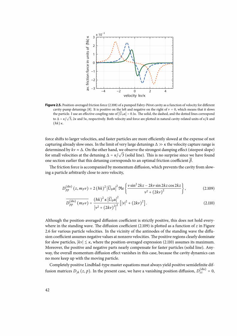
velocity kv/ĸ

av. f

rictio

n fo

rce

in u

nits

of

(ħk)

ĸ−4 −2 0 2 4

−3

−2

−1

0

1

2

3x 10−3

Figure 2.5. Position-averaged friction force (2.108) of a pumped Fabry-Pérot cavity as a function of velocity for dierentcavity-pump detunings [8]. It is positive on the le and negative on the right of v = 0, which means that it slowsthe particle. I use an eective coupling rate of ∣U0α∣ = 0.1κ.e solid, the dashed, and the dotted lines correspondto ∆ = κ/

√3, 2κ and 5κ, respectively. Both velocity and force are plotted in natural cavity-related units of κ/k and

(ħk) κ.

force shis to larger velocities, and faster particles are more eciently slowed at the expense of notcapturing already slow ones. In the limit of very large detunings ∆≫ κ the velocity capture range isdetermined by kv ≈ ∆. On the other hand, we observe the strongest damping eect (steepest slope)for small velocities at the detuning ∆ = κ/

√3 (solid line). is is no surprise since we have found

one section earlier that this detuning corresponds to an optimal friction coecient β.e friction force is accompanied bymomentum diusion, which prevents the cavity from slow-

ing a particle arbitrarily close to zero velocity,

D(dis)pp (z,mPv) = 2 (ħk)2 ∣U0α∣

2Reν sin2 2kz − 2kv sin 2kz cos 2kz

ν2 + (2kv)2 , (2.109)

D(dis)pp (mPv) =

(ħk)2 κ ∣U0α∣2

∣ν2 + (2kv)2∣2[∣ν∣2 + (2kv)2] . (2.110)

Although the position-averaged diusion coecient is strictly positive, this does not hold every-where in the standing wave.e diusion coecient (2.109) is plotted as a function of z in Figure2.6 for various particle velocities. In the vicinity of the antinodes of the standing wave the diu-sion coecient assumes negative values at nonzero velocities.e positive regions clearly dominatefor slow particles, ∣kv∣ ≲ κ, where the position-averaged expression (2.110) assumes its maximum.Moreover, the positive and negative parts nearly compensate for faster particles (solid line). Any-way, the overall momentum diusion eect vanishes in this case, because the cavity dynamics canno more keep up with the moving particle.Completely positive Lindblad-type master equations must always yield positive semidenite dif-

fusion matrices D jk (z, p). In the present case, we have a vanishing position diusion, D(dis)zz = 0,

42

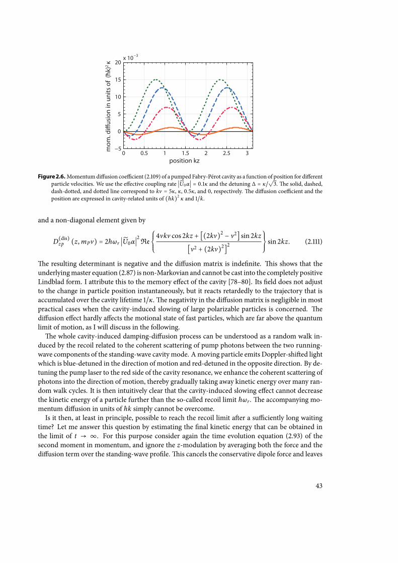
position kz

mom

. di

usio

n in

uni

ts o

f (ħ

k)2 ĸ

0 0.5 1 1.5 2 2.5 3−5

0

5

10

15

20x 10−3

Figure 2.6.Momentumdiusion coecient (2.109) of a pumped Fabry-Pérot cavity as a function of position for dierentparticle velocities. We use the eective coupling rate ∣U0α∣ = 0.1κ and the detuning ∆ = κ/

√3.e solid, dashed,

dash-dotted, and dotted line correspond to kv = 5κ, κ, 0.5κ, and 0, respectively. e diusion coecient and theposition are expressed in cavity-related units of (ħk)2 κ and 1/k.

and a non-diagonal element given by

D(dis)zp (z,mPv) = 2ħωr ∣U0α∣

2Re

⎧⎪⎪⎨⎪⎪⎩

4νkv cos 2kz + [(2kv)2 − ν2] sin 2kz

[ν2 + (2kv)2]2⎫⎪⎪⎬⎪⎪⎭sin 2kz. (2.111)

e resulting determinant is negative and the diusion matrix is indenite. is shows that theunderlyingmaster equation (2.87) is non-Markovian and cannot be cast into the completely positiveLindblad form. I attribute this to the memory eect of the cavity [78–80]. Its eld does not adjustto the change in particle position instantaneously, but it reacts retardedly to the trajectory that isaccumulated over the cavity lifetime 1/κ.e negativity in the diusionmatrix is negligible in mostpractical cases when the cavity-induced slowing of large polarizable particles is concerned. ediusion eect hardly aects the motional state of fast particles, which are far above the quantumlimit of motion, as I will discuss in the following.e whole cavity-induced damping-diusion process can be understood as a random walk in-

duced by the recoil related to the coherent scattering of pump photons between the two running-wave components of the standing-wave cavity mode. Amoving particle emits Doppler-shied lightwhich is blue-detuned in the direction of motion and red-detuned in the opposite direction. By de-tuning the pump laser to the red side of the cavity resonance, we enhance the coherent scattering ofphotons into the direction of motion, thereby gradually taking away kinetic energy over many ran-dom walk cycles. It is then intuitively clear that the cavity-induced slowing eect cannot decreasethe kinetic energy of a particle further than the so-called recoil limit ħωr .e accompanying mo-mentum diusion in units of ħk simply cannot be overcome.Is it then, at least in principle, possible to reach the recoil limit aer a suciently long waiting

time? Let me answer this question by estimating the nal kinetic energy that can be obtained inthe limit of t → ∞. For this purpose consider again the time evolution equation (2.93) of thesecond moment in momentum, and ignore the z-modulation by averaging both the force and thediusion term over the standing-wave prole.is cancels the conservative dipole force and leaves

43

us with the dissipative terms (in the absence of absorption and Rayleigh scattering). Given theabove expressions (2.108) and (2.110) in the limit of small particle velocities, ∣kv∣ ≪ κ, we nd thatthe average kinetic energy has a xed point at the value29

⟨ p2

2mP⟩∞

= −pD(dis)

pp (p)

4mP g(dis)p (p)≈ ħ8(∆ + κ2

∆) . (2.112)

Ensembles of initially faster particles are eventually slowed down towards this limitingmean kineticenergy value. It depends on the cavity reaction time scale, and it reads as ħκ/2

√3 in the case of the

optimal detuning ∆ = κ/√3. Note that this limit is considerably higher than the fundamental recoil

limit since ωr ≪ κ. It illustrates that the cavity-induced slowing eect is in practice already limitedby the nite cavity lifetime and the associated energy uncertainty. In the presence of absorption andRayleigh scattering we must take the respective diusion term (2.102) into account, which leads tothe increased slowing limit

⟨ p2

2mP⟩∞

≈ ħ8

⎡⎢⎢⎢⎢⎣∆ + κ2

∆+

(κ2 + ∆2)2

2U20κ∆(γabs +

75

γsca)⎤⎥⎥⎥⎥⎦. (2.113)

Concerning the interplay between friction and diusion, I conclude: While the friction force deter-mines the rate at which the kinetic energy of the particle is gradually dissipated through the cavityovermany lifetime cycles of its eld, the overall diusion term sets the kinetic energy of the limitingvelocity, which cannot be undercut in the present slowing scheme. Current sources for moleculesand nanoparticles, which are used in matter-wave interferometry, are typically far above this limit.Assuming a cavity linewidth of κ ∼ 1MHz, the cavity-slowing limit corresponds to motional tem-peratures of the order of microkelvins.

2.2.3.4. Multimode enhancement in degenerate resonator con®gurations

Having studied the generic dissipation eect in the instructive case of a single Fabry-Pérot cavitymode, I now turn to a more practical multimode conguration, as sketched in Figure 2.4. Each ofthe M > 1 empty cavity modes represents a dissipation channel which adds to the overall frictioneect along the z-axis of the cavity. e strong pump mode is directed along the y-direction andshould overlap with the cavity volume as much as possible to maximize the eective interactionregion for each passing particle.An experimental realization may be feasible in a setup where a large manifold of degenerate

modes can be created in a confocal resonator conguration with two circularly symmetric curvedmirrors. If the distance d between themirrors is exactly the same as their radii of curvature, then, inprinciple, the resonator will support an almost innite spectrum of higher-order transverse modesthat share the same resonance frequency with a given fundamental standing-wave mode. esehigher-order modes exhibit a larger eective mode waist, and the mode spectrum is in practicelimited to a nite numberM due to the nite aperture of real-life mirrors. In addition, if the setupis not precisely confocal, the contribution of higher-order modes to the friction force will decreasewith shiing resonance frequency.

29e expression (2.112) ceases to be valid for large velocities and at ∆ = 0, where the rst-order friction term (2.108)vanishes.

44

e controlled optical driving of one of the degenerate modes would require good mode match-ing, and it would lead to strong conservative dipole forces modulating themotion of particles alongthe standing wave. Both the modematching and the dipole force can be avoided by shining a broadrunning-wave laser mode perpendicular to the cavity axis. It acts as an optical pump mode whereit overlaps with the cavity modes, but it does not induce any signicant dipole force along the cavityaxis. Moreover, the absorption-induced momentum diusion along the z-axis is also suppressed.is perpendicular pump conguration comes at the price of less available pump power. It couldbe enhanced by means of another cavity, of course.In the following I will discuss the enhancement of the cavity-induced friction by the numberM

of accessible cavity modes. Once again, we restrict our view to the z-motion along the cavity axis,omitting any inuence on the transverse motion of the particle.e resulting friction and diusionterms still depend on the o-axis xy-coordinates of the particle, and we can average them over thetrajectory of a particle traversing the cavity for an estimate of their mean eects30.e modes of a confocal standing-wave resonator [57,81–83] are characterized by one longitudi-

nal mode index n ∈ N and two transverse mode indices m, ℓ ∈ N0. From the boundary conditionsat the curved mirror surfaces follow the respective resonance frequencies [83]

ωn,m,ℓ =πcd

(n +m + ℓ + 12

) , (2.114)

with d themirror distance (and radius of curvature). A given fundamental mode (n0, 0, 0) of wave-length λ = 2π/k shares the same resonance frequency with a huge manifold of transverse modes(n < n0,m, ℓ), since n0 = 2d/λ is typically a large number. We can assign the eective waist pa-rameter wn,m,ℓ = w0

√2m + ℓ + 1 to each higher-order transverse mode [82, 83]; it describes the

growing mode volume with respect to the fundamental mode of waist w0 =√dλ/2π. If the waist

is aperture-limited by wn,m,ℓ ≲ aw0, then both 2m and ℓ + 1 are restricted to values less or equalto a2, which leads to a total number of supported modes M ≲ a4/2. (e quantity a measures theaperture in units of w0.)e eld distribution of eachmode can be approximated by Laguerre-Gaussian functions31 in the

case of large-aperture mirrors [82], a2 ≫ 1. We obtain the explicit form of the three-dimensionalmode function [83] by assuming linear polarization and omitting any o-axis corrections to theeld polarization due to the transverse mode prole (see Appendix A.2 for the specic case of aGaussian mode, m = ℓ = 0). In cylindrical coordinates the full three-dimensional mode functionsun,m,ℓ (r) = є fm,ℓ (r, ϕ, z)un,m,ℓ (r, z) factorize into the on-axis standing-wave mode functionsun,m,ℓ, the Laguerre-Gaussian transverse mode proles fm,ℓ, and a xed polarization vector є,

un,m,ℓ (r, z) =⎧⎪⎪⎨⎪⎪⎩

cossin

⎫⎪⎪⎬⎪⎪⎭[kz (1 + 4r2

d2ξ2 (z)) − (2m + ℓ + 1) arctan(2zd

)] ∀⎧⎪⎪⎨⎪⎪⎩

n oddn even

⎫⎪⎪⎬⎪⎪⎭, (2.115)

fm,ℓ (r, ϕ, z) =cos (ℓϕ)

ξ (z) (√2r

w0ξ (z))ℓ

Lℓm ( 2r2

w20ξ2 (z)) exp( −r2

w20ξ2 (z)) . (2.116)

30is corresponds to the experimental situation when a dilute beam of molecules or nanoparticles crosses the cavity,such that there is on average only one particle inside the cavity at a given time.

31 Laguerre-Gaussian modes can only be used if the mirror system exhibits a cylindrical symmetry.is symmetry maybe violated in applications with birefringent mirrors. In this case one must use the rectangular Hermite-Gaussianmodes instead [82], which yield similar results as presented here.

45

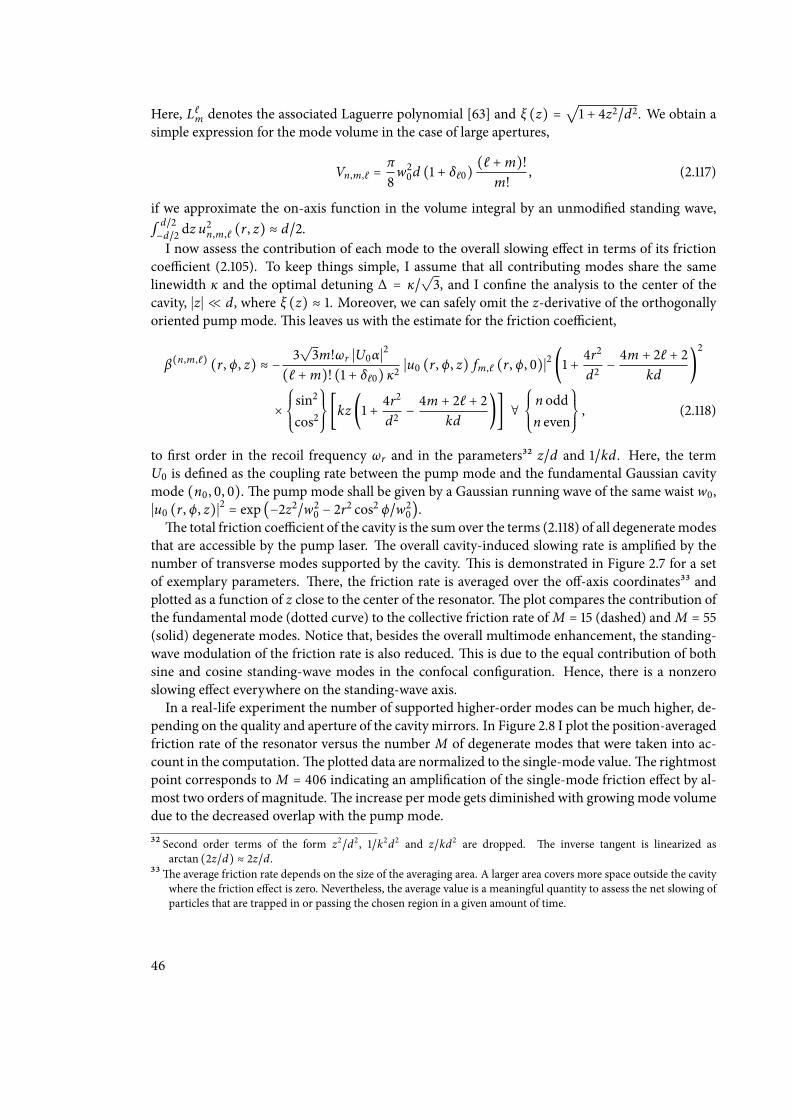
Here, Lℓm denotes the associated Laguerre polynomial [63] and ξ (z) =√1 + 4z2/d2. We obtain a

simple expression for the mode volume in the case of large apertures,

Vn,m,ℓ =π8w20d (1 + δℓ0)

(ℓ +m)!m!

, (2.117)

if we approximate the on-axis function in the volume integral by an unmodied standing wave,∫ d/2−d/2 dz u

2n,m,ℓ (r, z) ≈ d/2.

I now assess the contribution of each mode to the overall slowing eect in terms of its frictioncoecient (2.105). To keep things simple, I assume that all contributing modes share the samelinewidth κ and the optimal detuning ∆ = κ/

√3, and I conne the analysis to the center of the

cavity, ∣z∣ ≪ d, where ξ (z) ≈ 1. Moreover, we can safely omit the z-derivative of the orthogonallyoriented pump mode.is leaves us with the estimate for the friction coecient,

β(n,m,ℓ) (r, ϕ, z) ≈ − 3√3m!ωr ∣U0α∣2

(ℓ +m)! (1 + δℓ0) κ2∣u0 (r, ϕ, z) fm,ℓ (r, ϕ, 0)∣2 (1 +

4r2

d2− 4m + 2ℓ + 2

kd)2

×⎧⎪⎪⎨⎪⎪⎩

sin2

cos2⎫⎪⎪⎬⎪⎪⎭[kz (1 + 4r

2

d2− 4m + 2ℓ + 2

kd)] ∀

⎧⎪⎪⎨⎪⎪⎩

n oddn even

⎫⎪⎪⎬⎪⎪⎭, (2.118)

to rst order in the recoil frequency ωr and in the parameters32 z/d and 1/kd. Here, the termU0 is dened as the coupling rate between the pump mode and the fundamental Gaussian cavitymode (n0, 0, 0).e pump mode shall be given by a Gaussian running wave of the same waist w0,∣u0 (r, ϕ, z)∣2 = exp (−2z2/w20 − 2r2 cos2 ϕ/w20).e total friction coecient of the cavity is the sum over the terms (2.118) of all degeneratemodes

that are accessible by the pump laser. e overall cavity-induced slowing rate is amplied by thenumber of transverse modes supported by the cavity. is is demonstrated in Figure 2.7 for a setof exemplary parameters. ere, the friction rate is averaged over the o-axis coordinates33 andplotted as a function of z close to the center of the resonator.e plot compares the contribution ofthe fundamental mode (dotted curve) to the collective friction rate ofM = 15 (dashed) andM = 55(solid) degenerate modes. Notice that, besides the overall multimode enhancement, the standing-wave modulation of the friction rate is also reduced. is is due to the equal contribution of bothsine and cosine standing-wave modes in the confocal conguration. Hence, there is a nonzeroslowing eect everywhere on the standing-wave axis.In a real-life experiment the number of supported higher-order modes can be much higher, de-

pending on the quality and aperture of the cavity mirrors. In Figure 2.8 I plot the position-averagedfriction rate of the resonator versus the number M of degenerate modes that were taken into ac-count in the computation.e plotted data are normalized to the single-mode value.e rightmostpoint corresponds to M = 406 indicating an amplication of the single-mode friction eect by al-most two orders of magnitude.e increase per mode gets diminished with growing mode volumedue to the decreased overlap with the pump mode.

32 Second order terms of the form z2/d2 , 1/k2d2 and z/kd2 are dropped. e inverse tangent is linearized asarctan (2z/d) ≈ 2z/d.

33e average friction rate depends on the size of the averaging area. A larger area covers more space outside the cavitywhere the friction eect is zero. Nevertheless, the average value is a meaningful quantity to assess the net slowing ofparticles that are trapped in or passing the chosen region in a given amount of time.

46

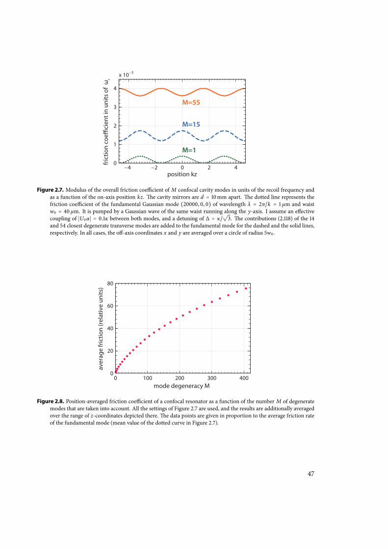
position kz

fric

tion

coe

cien

t in

units

of

ωr

M=1

M=15

M=55

−4 −2 0 2 40

1

2

3

4

x 10−3

Figure 2.7. Modulus of the overall friction coecient of M confocal cavity modes in units of the recoil frequency andas a function of the on-axis position kz. e cavity mirrors are d = 10mm apart. e dotted line represents thefriction coecient of the fundamental Gaussian mode (20000, 0, 0) of wavelength λ = 2π/k = 1 µm and waistw0 = 40 µm. It is pumped by a Gaussian wave of the same waist running along the y-axis. I assume an eectivecoupling of ∣U0α∣ = 0.1κ between both modes, and a detuning of ∆ = κ/

√3. e contributions (2.118) of the 14

and 54 closest degenerate transverse modes are added to the fundamental mode for the dashed and the solid lines,respectively. In all cases, the o-axis coordinates x and y are averaged over a circle of radius 5w0 .

mode degeneracy M

aver

age

fric

tion

(rel

ativ

e un

its)

0 100 200 300 4000

20

40

60

80

Figure 2.8. Position-averaged friction coecient of a confocal resonator as a function of the number M of degeneratemodes that are taken into account. All the settings of Figure 2.7 are used, and the results are additionally averagedover the range of z-coordinates depicted there.e data points are given in proportion to the average friction rateof the fundamental mode (mean value of the dotted curve in Figure 2.7).

47

Let me close this section on the cavity-induced slowing of a PPP in the weak coupling regimewith a few remarks. I have developed a rigorous quantum description of the dissipative motionof a particle in the presence of pump eld and cavity by means of an eective (non-Markovian)master equation. It has led us to the understanding of the emergent friction and diusion eectsusing a semiclassical phase-space approach. Aer studying the basic phenomena in an idealizedsingle-mode conguration, I have provided a detailed assessment of the multimode case. At thispoint we should note that not only the friction force is enhanced by the presence of many modes,but also the accompanying momentum diusion eect. While the former determines the eectiverate at which the motion of the particle is damped, the latter raises the ultimate cooling limit. Inother words, more modes imply a larger limiting kinetic energy value, down to which the particlecan be damped by the cavity. Absorption and Rayleigh scattering contribute to this limit as well.In many potential laboratory applications with molecules and clusters, one must oen deal with

particle ensembles whose initial temperature is far above this limit. In practice, it would be muchmore important to boost the eective damping rate from the unsuitably low values, as implied bythe parameters listed in Table 2.1, to a feasible regime.is requires one to leave the weak couplingregime by increasing the pump eld strength or by using even larger particles, as I will discuss in thenext section. Another option is to increase the number of particles that interact with the cavity atthe same time. In Appendix A.4 I show how to generalize our quantum treatment and the eectivemaster equation to N > 1 particles inM driven or empty modes.ere, however, the validity of theresulting friction and diusion terms is restricted to an even more rigid weak-coupling limit.isis because the individual eld uctuations induced by each particle may add up. By breaking theweak-coupling limitwithmany particles onemay benet from strong cavity-mediated inter-particlecorrelations and from collective phenomena such as self-organisation [84, 85].

2.3. Mechanics of spherical particles in coherent light ®elds

So far I have discussed the (o-resonant) light-matter interaction, and its mechanical action onmatter waves, in terms of point-like particles characterized by a scalar complex dipole polarizabil-ity χ. Whereas this is a good approximation for many molecules and clusters, which are by ordersof magnitude smaller than the wavelength of the light they interact with, it ceases to be valid fornano- and microparticles of the same size as the wavelength or larger. e light scattering prop-erties get more complex as higher-order multipole components take over, and a rigorous quantumdescription of both the light and the matter degrees of freedom is a dicult task due to severalreasons:

e quantization of the center-of-mass motion of the particle depends on explicit expres-sions for the force and the optical potential induced by the light eld. However, we will seebelow that the force on extended particles cannot be reduced to a simple analytical expres-sion anymore, but must be evaluated numerically in practice. Moreover, the result containsboth the conservative light force and the radiation pressure force due to light absorption andRayleigh scattering. Consequently, the optical potential cannot be directly deduced. We canavoid these diculties in the eectively one-dimensional situation ofmatter-wave diractionat optical standing-wave gratings in Section 2.3.2.

48

If a large particle couples strongly to a high-nesse cavity eld, itmay change the spatialmodestructure of the resonator.is is intuitively clear since the particle becomes a semitranspar-ent mirror for the cavity eld if it is large enough. Whereas one may benet from the strongcoupling when trying to observe cavity-induced slowing of large particles, the theoreticalmodelling requires a proper treatment of the modied boundary conditions. I will presentan approximate solution when I discuss the classical slowing of spherical particles in Section2.3.3.

A rigorous quantum description of the dynamics of both the light eld and the particle re-quires an elaborate model for light scattering at extended material objects. is is a matterof current research [86], and it has gained interest with the upcoming of proposals to ob-serve the ground-statemotion of optically trappedmicrospheres [23,24]. One possiblemodeltreats the extended object as an assembly of point-like scatterers at which single photons canscatter along multiple paths [86].e resulting master equation gives proper account to thescattering-induced decoherence and diusion eects, provided that the local elds are cor-rectly described for each scatterer. Another possibility is to model the particle as a dielectricmedium, which then requires the canonical quantization of the macroscopic eld inside thismedium [87]. However, this approach requires one to determine the precise momentum car-ried by the radiation eld inside the dielectricmediumwhen trying to assess the force densityacting on the material—an old and controversial issue [32, 88].

Apart from the center-of-mass eect, an extended dielectric object may also experience elas-tic stress due to light-induced bending and shearing forces. is may, in turn, deform theparticle and modify its response to the light eld depending on its stiness properties [89].Here, I avoid this additional complication by assuming rigid atomic clusters. Nevertheless,we must keep in mind that this might be an issue when dealing with hot or uid particles,such as nanodroplets.

In this thesis I focus on generally hot and fast ensembles of particles far above the quantum limitof motion, which interact with strong coherent light elds. In the eective description of suchparticles, we may therefore avoid many of the aforementioned diculties by assuming a stationarymode conguration and ignoring the full quantum nature of the photon eld dynamics.Moreover, I restrict the considerations to homogeneous dielectric spheres34, which is a good rep-

resentation of many heavy clusters consisting of N ≫ 1 atoms [52]. We can employ the Mie theoryof light scattering at spherical objects [28, 29, 34, 90] to understand the light-matter interaction, asoutlined in Appendix A.6.e idea is to start with a given light eld E0 in the absence of the sphere,and to expand it in the basis of spherical vector harmonics, that is, multipole components whichrespect the spherical symmetry of the problem.e origin of the coordinate systemmust be shiedto the center of the sphere r0, accordingly. e spherical wave expansion is outlined in AppendixA.5.Putting the sphere into the game introduces a dierent eld Eint inside the dielectric medium,

and it modies the external eld by adding a scattering component, E0 → Eext = E0 + Esca. e

34Nonspherical particles scatter light in dierent patterns, that is, themultipole composition of the scattered eld deviatesfrom the spherical case.e basic consequences of leaving the subwavelength size regime are similar to the sphericalcase, with the additional complication of coupling to the rotation of the object.

49

expansion coecients of the new eld components Eint and Esca are obtained from the boundaryconditions at the sphere surface. I have done this explicitly for plane running and standing waves,and for Gaussian modes in Appendix A.6. In the following, let me discuss the consequences for themechanical action of light onto the particle.

2.3.1. Light extinction and light-induced forces

Mie theory provides us with the eld conguration when a dielectric sphere of relative permittivityε is placed into an electromagnetic eld E0,H0 at the position r0. Following Appendix A.6, theeld outside of the sphere is then complemented by the scattering component

Esca =∞

∑ℓ=1

ℓ∑m=−ℓ

⎡⎢⎢⎢⎢⎣αℓC(M)

ℓ,m hℓ (kr) Xℓ,m (θ , ϕ) +βℓC(E)

ℓ,mk

∇× hℓ (kr) Xℓ,m (θ , ϕ)⎤⎥⎥⎥⎥⎦, (2.119)

with hℓXℓ,m and ∇ × Xℓ,mhℓ the partial-wave multipole solutions (see Appendix A.5). e termsC(M,E)ℓ,m are the multipole expansion coecients of the original eld E0, which depend on the po-sition r0 of the sphere. e coordinates r = (r, θ , ϕ) are dened relative to r0. e scattered elddiers from the original eld mainly by the scattering coecients αℓ and βℓ.ey read as

αℓ =jℓ (

√εkR) ∂R [Rjℓ (kR)] − jℓ (kR) ∂R [Rjℓ (

√εkR)]

hℓ (kR) ∂R [Rjℓ (√

εkR)] − jℓ (√

εkR) ∂R [Rhℓ (kR)], (2.120)

βℓ =ε jℓ (

√εkR) ∂R [Rjℓ (kR)] − jℓ (kR) ∂R [Rjℓ (

√εkR)]

hℓ (kR) ∂R [Rjℓ (√

εkR)] − ε jℓ (√

εkR) ∂R [Rhℓ (kR)], (2.121)

for a dielectric sphere of radius R, as given in theAppendix. (ere I also present the case of a hollowsphere, which leads to more cumbersome expressions.) Note that the coecients are independentof the chosen mode structure of the light eld, as given by the C(M,E)

ℓ,m . ey are the same in arunning wave as in a standing wave. In the case of a point-like particle, kR ≪ 1, we nd that thelowest-order contribution is given by35 β1 ≈ 2i (kR)3 (ε − 1) /3 (ε + 2). All other coecients are ofhigher order in kR and thus negligible. One can convince oneself, using the identities and relationsof Appendix A.5, that this yields the scattering eld of the induced dipole χE0 (r = 0), with thecomplex polarizability of a subwavelength sphere [52],

χ ≈ 4πε0R3ε − 1ε + 2 if kR ≪ 1. (2.122)

Hence, the point-particle limit is properly reproduced by the Mie expansion. Having the Mie ex-pression (2.119) at hand, we are now able to study the light extinction properties of the sphere, aswell as the light-induced force acting on it. I will focus on standing-wave light modes, as opposedto running waves, since they are the basis of the optical diraction gratings and the two-mirrorcavities studied here.

35 I use that the spherical Bessel functions can be approximated by jℓ (x) ≈ x ℓ/ [1 ⋅ 3 ⋅ . . . ⋅ (2ℓ + 1)] and yℓ (x) ≈− [1 ⋅ 3 ⋅ . . . ⋅ (2ℓ − 1)] /x ℓ+1 to lowest order in x ≪ 1, while the spherical Hankel function becomes hℓ (x) ≈ iyℓ (x).

50

2.3.1.1. The Poynting vector and the extinction power of the sphere

Scattering and absorption of light by nite geometries can be treated formally bymeans of the Poyn-ting vector S = ReE ×ReH. It has the dimension W/m2 and describes the net energy uxper unit surface ∣S∣ into the direction S/ ∣S∣ in vacuum36 [33,34,91].at is, the time-averaged eldenergy owing through a small surface element dA = r2dΩ at position r into direction n per unittime is given by Pn (r) = ⟨n ⋅ S⟩t = −r2dΩReE (r) ⋅ [n ×H∗ (r)] /2. From this it is intuitivelyclear how to obtain the total eld energy per time scattered or absorbed by the sphere.In order to assess the scattered power (2.123) we must take the outward-directed Poynting vector

corresponding to the scattering eld Esca and integrate it over the sphere surface [29, 34]. eabsorbed power (2.124) is given by the net energy ux into the sphere, that is, by the integratedinward-directed Poynting vector corresponding to the total external eld Eext = E0 + Esca. eextinction power (2.125) is dened as the sum of both contributions.

Psca = −R2

2 ∫ dΩReEsca (Rn) ⋅ [n ×H∗sca (Rn)] (2.123)

Pabs =R2

2 ∫ dΩReEext (Rn) ⋅ [n ×H∗ext (Rn)] (2.124)

Pext = Psca + Pabs =R2

2 ∫ dΩReE0 (Rn) ⋅ [n ×H∗sca (Rn)] + Esca (Rn) ⋅ [n ×H∗

0 (Rn)](2.125)

A straightforward calculation using the orthogonality properties of the multipole expansion givenin Appendix A.5 leads to the explicit forms

Psca =cε02k2 ∑ℓ,m

[∣αℓC(M)

ℓ,m ∣2+ ∣βℓC(E)

ℓ,m∣2] ,

Pext = −cε02k2 ∑ℓ,m

[Reαℓ ∣C(M)

ℓ,m ∣2+Reβℓ ∣C(E)

ℓ,m∣2] , (2.126)

and Pabs = Pext − Psca. If the medium is non-absorptive, that is, if the refractive index√

ε is real,then one can easily check that Pabs = 0 and ∣αℓ∣2 = −Reαℓ, ∣βℓ∣2 = −Reβℓ. We observe thatthe extinction power is a sum over the independent contributions of electric (E) and magnetic (M)multipole components.e expressions simplify further in the case of a cosine-type standing wave,

Psca,ext (z0) =πI0k2

[Π(+)

sca,ext +Π(−)

sca,ext cos 2kz0] , (2.127)

with z0 the z-coordinate of the sphere center and I0 = cε0 ∣E0∣2 /2 the eld intensity at the antinodes.e oset factors (+) and the modulation factors (−) read as

Π(±)sca =∑

ℓ(2ℓ + 1) (±)ℓ [∣αℓ∣2 ± ∣βℓ∣2] ,

Π(±)

ext = −∑ℓ(2ℓ + 1) (±)ℓ [Reαℓ ±Reβℓ] . (2.128)

36All the calculations can be done in the vacuum surrounding the sphere, thus avoiding the discussion [88] which formof the Poynting vector to choose inside the medium.

51

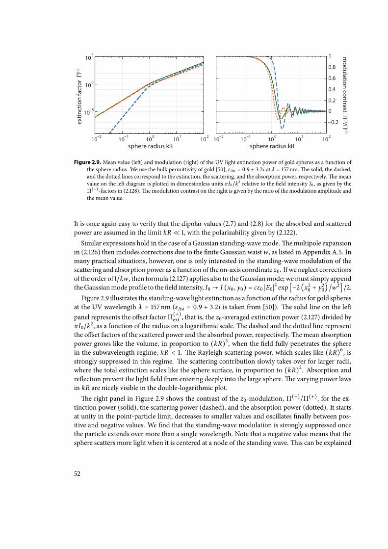
sphere radius kR

extin

ctio

n fa

ctor

Π(+

)

10−2 10−1 100 101 102

10−5

100

105

sphere radius kR

modulation contrast Π

(-)/Π(+)

−0.2

0

0.2

0.4

0.6

0.8

1

10−2 10−1 100 101 102

Figure 2.9. Mean value (le) and modulation (right) of the UV light extinction power of gold spheres as a function ofthe sphere radius. We use the bulk permittivity of gold [50], εAu = 0.9 + 3.2i at λ = 157 nm.e solid, the dashed,and the dotted lines correspond to the extinction, the scattering, and the absorption power, respectively.e meanvalue on the le diagram is plotted in dimensionless units πI0/k2 relative to the eld intensity I0 , as given by theΠ(+)-factors in (2.128).e modulation contrast on the right is given by the ratio of the modulation amplitude andthe mean value.

It is once again easy to verify that the dipolar values (2.7) and (2.8) for the absorbed and scatteredpower are assumed in the limit kR ≪ 1, with the polarizability given by (2.122).Similar expressions hold in the case of a Gaussian standing-wavemode.emultipole expansion

in (2.126) then includes corrections due to the nite Gaussian waistw, as listed in Appendix A.5. Inmany practical situations, however, one is only interested in the standing-wave modulation of thescattering and absorption power as a function of the on-axis coordinate z0. If we neglect correctionsof the order of 1/kw, then formula (2.127) applies also to theGaussianmode; wemust simply appendtheGaussianmodeprole to the eld intensity, I0 → I (x0, y0) = cε0 ∣E0∣2 exp [−2 (x20 + y20) /w2] /2.Figure 2.9 illustrates the standing-wave light extinction as a function of the radius for gold spheres

at the UV wavelength λ = 157 nm (εAu = 0.9 + 3.2i is taken from [50]). e solid line on the lepanel represents the oset factor Π(+)

ext , that is, the z0-averaged extinction power (2.127) divided byπI0/k2, as a function of the radius on a logarithmic scale.e dashed and the dotted line representthe oset factors of the scattered power and the absorbed power, respectively.e mean absorptionpower grows like the volume, in proportion to (kR)3, when the eld fully penetrates the spherein the subwavelength regime, kR < 1. e Rayleigh scattering power, which scales like (kR)6, isstrongly suppressed in this regime. e scattering contribution slowly takes over for larger radii,where the total extinction scales like the sphere surface, in proportion to (kR)2. Absorption andreection prevent the light eld from entering deeply into the large sphere.e varying power lawsin kR are nicely visible in the double-logarithmic plot.e right panel in Figure 2.9 shows the contrast of the z0-modulation, Π(−)/Π(+), for the ex-

tinction power (solid), the scattering power (dashed), and the absorption power (dotted). It startsat unity in the point-particle limit, decreases to smaller values and oscillates nally between pos-itive and negative values. We nd that the standing-wave modulation is strongly suppressed oncethe particle extends over more than a single wavelength. Note that a negative value means that thesphere scatters more light when it is centered at a node of the standing wave.is can be explained

52

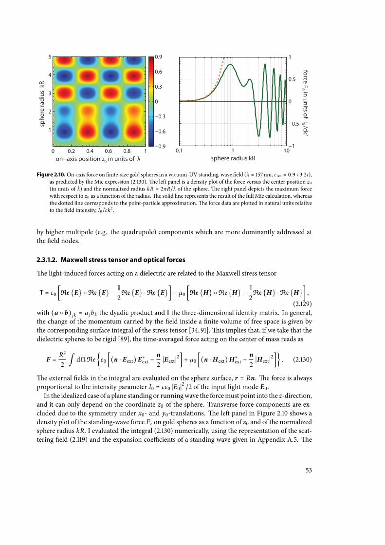
on−axis position z0 in units of λ

sphe

re ra

dius

kR

0 0.2 0.4 0.6 0.8 1

1

2

3

4

5

−0.9

−0.6

−0.3

0

0.3

0.6

0.9

sphere radius kR

force F0 in units of I0 /ck

2

0.1 1 10−1

−0.5

0

0.5

1

Figure 2.10.On-axis force on nite-size gold spheres in a vacuum-UV standing-wave eld (λ = 157 nm, εAu = 0.9+3.2i),as predicted by the Mie expression (2.130).e le panel is a density plot of the force versus the center position z0(in units of λ) and the normalized radius kR = 2πR/λ of the sphere. e right panel depicts the maximum forcewith respect to z0 as a function of the radius.e solid line represents the result of the full Mie calculation, whereasthe dotted line corresponds to the point-particle approximation.e force data are plotted in natural units relativeto the eld intensity, I0/ck2 .

by higher multipole (e.g. the quadrupole) components which are more dominantly addressed atthe eld nodes.

2.3.1.2. Maxwell stress tensor and optical forces

e light-induced forces acting on a dielectric are related to the Maxwell stress tensor

T = ε0 [ReE ReE − I2ReE ⋅ReE] + µ0 [ReH ReH − I

2ReH ⋅ReH] ,

(2.129)with (a b) jk = a jbk the dyadic product and I the three-dimensional identity matrix. In general,the change of the momentum carried by the eld inside a nite volume of free space is given bythe corresponding surface integral of the stress tensor [34, 91].is implies that, if we take that thedielectric spheres to be rigid [89], the time-averaged force acting on the center of mass reads as

F = R2

2 ∫ dΩReε0 [(n ⋅ Eext)E∗ext −n2∣Eext∣2] + µ0 [(n ⋅Hext)H∗

ext −n2∣Hext∣2] . (2.130)

e external elds in the integral are evaluated on the sphere surface, r = Rn. e force is alwaysproportional to the intensity parameter I0 = cε0 ∣E0∣2 /2 of the input light mode E0.In the idealized case of a plane standing or runningwave the forcemust point into the z-direction,

and it can only depend on the coordinate z0 of the sphere. Transverse force components are ex-cluded due to the symmetry under x0- and y0-translations. e le panel in Figure 2.10 shows adensity plot of the standing-wave force Fz on gold spheres as a function of z0 and of the normalizedsphere radius kR. I evaluated the integral (2.130) numerically, using the representation of the scat-tering eld (2.119) and the expansion coecients of a standing wave given in Appendix A.5. e

53

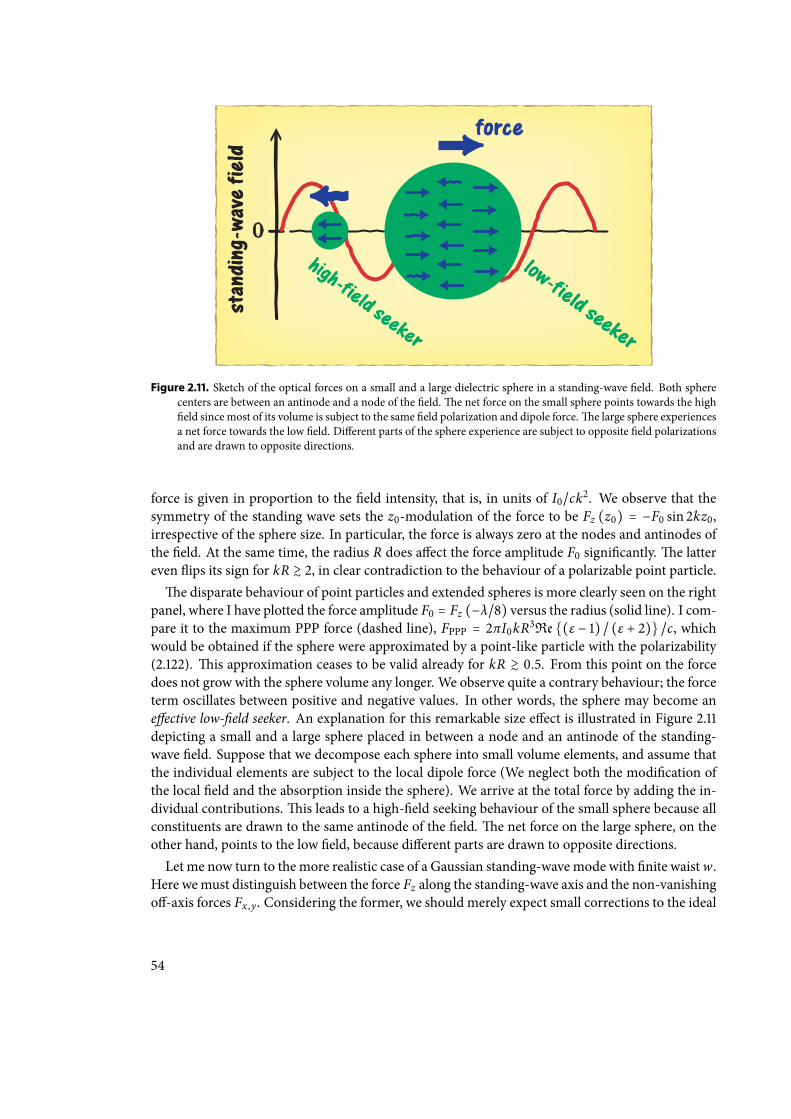
Figure 2.11. Sketch of the optical forces on a small and a large dielectric sphere in a standing-wave eld. Both spherecenters are between an antinode and a node of the eld.e net force on the small sphere points towards the higheld since most of its volume is subject to the same eld polarization and dipole force.e large sphere experiencesa net force towards the low eld. Dierent parts of the sphere experience are subject to opposite eld polarizationsand are drawn to opposite directions.

force is given in proportion to the eld intensity, that is, in units of I0/ck2. We observe that thesymmetry of the standing wave sets the z0-modulation of the force to be Fz (z0) = −F0 sin 2kz0,irrespective of the sphere size. In particular, the force is always zero at the nodes and antinodes ofthe eld. At the same time, the radius R does aect the force amplitude F0 signicantly.e lattereven ips its sign for kR ≳ 2, in clear contradiction to the behaviour of a polarizable point particle.e disparate behaviour of point particles and extended spheres is more clearly seen on the right

panel, where I have plotted the force amplitude F0 = Fz (−λ/8) versus the radius (solid line). I com-pare it to the maximum PPP force (dashed line), FPPP = 2πI0kR3Re(ε − 1) / (ε + 2) /c, whichwould be obtained if the sphere were approximated by a point-like particle with the polarizability(2.122). is approximation ceases to be valid already for kR ≳ 0.5. From this point on the forcedoes not grow with the sphere volume any longer. We observe quite a contrary behaviour; the forceterm oscillates between positive and negative values. In other words, the sphere may become aneective low-eld seeker. An explanation for this remarkable size eect is illustrated in Figure 2.11depicting a small and a large sphere placed in between a node and an antinode of the standing-wave eld. Suppose that we decompose each sphere into small volume elements, and assume thatthe individual elements are subject to the local dipole force (We neglect both the modication ofthe local eld and the absorption inside the sphere). We arrive at the total force by adding the in-dividual contributions.is leads to a high-eld seeking behaviour of the small sphere because allconstituents are drawn to the same antinode of the eld. e net force on the large sphere, on theother hand, points to the low eld, because dierent parts are drawn to opposite directions.Let me now turn to the more realistic case of a Gaussian standing-wave mode with nite waistw.

Here wemust distinguish between the force Fz along the standing-wave axis and the non-vanishingo-axis forces Fx ,y. Considering the former, we should merely expect small corrections to the ideal

54

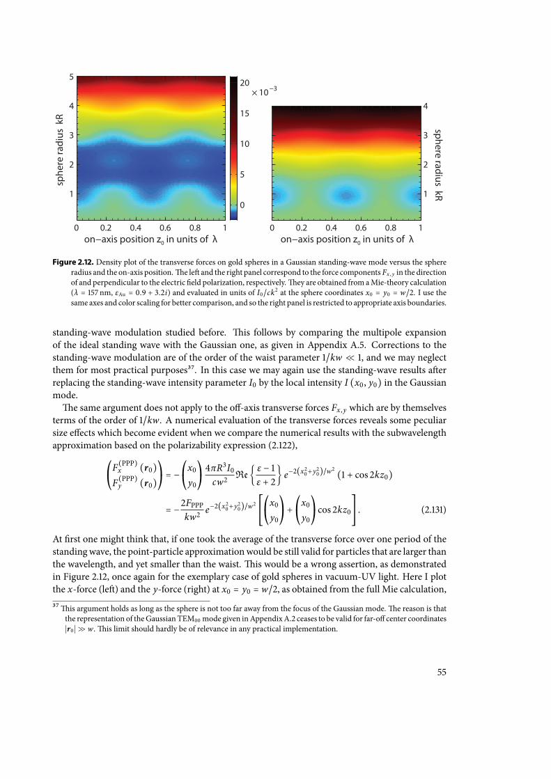
on−axis position z0 in units of λ

sphe

re ra

dius

kR

× 10 −3

0 0.2 0.4 0.6 0.8 1

1

2

3

4

5

0

5

10

15

20

sphere radius kR

0 0.2 0.4 0.6 0.8 1

1

2

3

4

on−axis position z0 in units of λ

Figure 2.12. Density plot of the transverse forces on gold spheres in a Gaussian standing-wave mode versus the sphereradius and the on-axis position.e le and the right panel correspond to the force components Fx ,y in the directionof and perpendicular to the electric eld polarization, respectively.ey are obtained from aMie-theory calculation(λ = 157 nm, εAu = 0.9 + 3.2i) and evaluated in units of I0/ck2 at the sphere coordinates x0 = y0 = w/2. I use thesame axes and color scaling for better comparison, and so the right panel is restricted to appropriate axis boundaries.

standing-wave modulation studied before. is follows by comparing the multipole expansionof the ideal standing wave with the Gaussian one, as given in Appendix A.5. Corrections to thestanding-wave modulation are of the order of the waist parameter 1/kw ≪ 1, and we may neglectthem for most practical purposes37. In this case we may again use the standing-wave results aerreplacing the standing-wave intensity parameter I0 by the local intensity I (x0, y0) in the Gaussianmode.e same argument does not apply to the o-axis transverse forces Fx ,y which are by themselves

terms of the order of 1/kw. A numerical evaluation of the transverse forces reveals some peculiarsize eects which become evident when we compare the numerical results with the subwavelengthapproximation based on the polarizability expression (2.122),

⎛⎝F(PPP)x (r0)

F(PPP)y (r0)

⎞⎠= −

⎛⎝x0y0

⎞⎠4πR3I0cw2

Re ε − 1ε + 2 e−2(x

20+y20)/w2 (1 + cos 2kz0)

= −2FPPPkw2

e−2(x20+y20)/w2

⎡⎢⎢⎢⎢⎣

⎛⎝x0y0

⎞⎠+⎛⎝x0y0

⎞⎠cos 2kz0

⎤⎥⎥⎥⎥⎦. (2.131)

At rst one might think that, if one took the average of the transverse force over one period of thestandingwave, the point-particle approximationwould be still valid for particles that are larger thanthe wavelength, and yet smaller than the waist.is would be a wrong assertion, as demonstratedin Figure 2.12, once again for the exemplary case of gold spheres in vacuum-UV light. Here I plotthe x-force (le) and the y-force (right) at x0 = y0 = w/2, as obtained from the full Mie calculation,

37is argument holds as long as the sphere is not too far away from the focus of the Gaussian mode.e reason is thatthe representation of theGaussianTEM00mode given inAppendixA.2 ceases to be valid for far-o center coordinates∣r0 ∣ ≫ w.is limit should hardly be of relevance in any practical implementation.

55

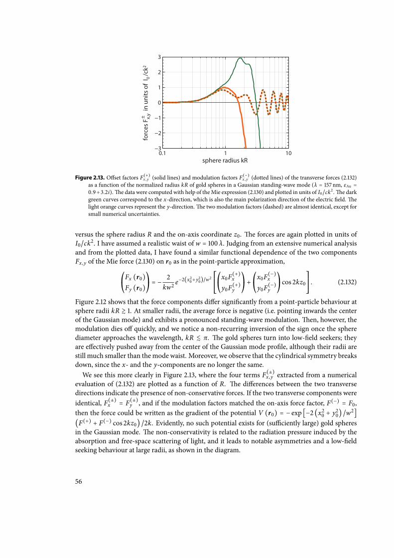
sphere radius kR

forc

es F

x,y±

in u

nits

of

I 0 /c

k2

0.1 1 10−3

−2

−1

0

1

2

3

Figure 2.13. Oset factors F(+)

x ,y (solid lines) and modulation factors F(−)

x ,y (dotted lines) of the transverse forces (2.132)as a function of the normalized radius kR of gold spheres in a Gaussian standing-wave mode (λ = 157 nm, εAu =0.9+3.2i).e data were computed with help of theMie expression (2.130) and plotted in units of I0/ck2 .e darkgreen curves correspond to the x-direction, which is also the main polarization direction of the electric eld.elight orange curves represent the y-direction.e two modulation factors (dashed) are almost identical, except forsmall numerical uncertainties.

versus the sphere radius R and the on-axis coordinate z0. e forces are again plotted in units ofI0/ck2. I have assumed a realistic waist of w = 100 λ. Judging from an extensive numerical analysisand from the plotted data, I have found a similar functional dependence of the two componentsFx ,y of the Mie force (2.130) on r0 as in the point-particle approximation,

⎛⎝Fx (r0)Fy (r0)

⎞⎠= − 2

kw2e−2(x

20+y20)/w2

⎡⎢⎢⎢⎢⎣

⎛⎝x0F(+)

x

y0F(+)y

⎞⎠+⎛⎝x0F(−)

x

y0F(−)y

⎞⎠cos 2kz0

⎤⎥⎥⎥⎥⎦. (2.132)

Figure 2.12 shows that the force components dier signicantly from a point-particle behaviour atsphere radii kR ≳ 1. At smaller radii, the average force is negative (i.e. pointing inwards the centerof the Gaussian mode) and exhibits a pronounced standing-wave modulation.en, however, themodulation dies o quickly, and we notice a non-recurring inversion of the sign once the spherediameter approaches the wavelength, kR ≲ π. e gold spheres turn into low-eld seekers; theyare eectively pushed away from the center of the Gaussian mode prole, although their radii arestill much smaller than themode waist. Moreover, we observe that the cylindrical symmetry breaksdown, since the x- and the y-components are no longer the same.We see this more clearly in Figure 2.13, where the four terms F(±)

x ,y extracted from a numericalevaluation of (2.132) are plotted as a function of R. e dierences between the two transversedirections indicate the presence of non-conservative forces. If the two transverse components wereidentical, F(±)

x = F(±)y , and if the modulation factors matched the on-axis force factor, F(−) = F0,

then the force could be written as the gradient of the potential V (r0) = − exp [−2 (x20 + y20) /w2](F(+) + F(−) cos 2kz0) /2k. Evidently, no such potential exists for (suciently large) gold spheresin the Gaussian mode. e non-conservativity is related to the radiation pressure induced by theabsorption and free-space scattering of light, and it leads to notable asymmetries and a low-eldseeking behaviour at large radii, as shown in the diagram.

56

One important practical consequence is the following: One cannot deduce the optical potentialof wavelength-sized particles coupled to Gaussianmodes from the electromagnetic force alone. Wemust nd a dierent method to extract the position-dependent coupling energy between such aparticle and a high-nesse cavity mode in order to assess cavity-induced dissipation eects. I willdeal with this issue in Section 2.3.3. Before that, let me briey discuss the eect of optical standing-wave gratings on extended spherical particles.

2.3.2. Optical standing-wave gratings

With the extensive discussion of Mie theory in the preceding section at hand, I will now generalizethe model of optical standing-wave gratings developed in Section 2.1.4. ere I discussed how acoherent standing-wave eld can act as a diraction grating for matter-wave states of polarizablepoint particles in the limit of short interaction times. Two separate processes can contribute to thediraction eect:e periodic phase modulation of the matter wave due to the action accumulatedin the optical dipole potential and the amplitude modulation that occurs if the absorption of singlephotons depletes the matter-wave state.In the following, I will generalize both eects to dielectric spheres of nite radius. Wewill see that

the eective grating modulation becomes less eective with growing particle size.A more detailedanalysis of the consequences for mater-wave interferometry will be given in Chapter 3.Note that the grating modulation acts along the standing-wave axis, and we are only concerned

with the reduced one-dimensional z-state of the matter waves. e latter are assumed to interactsuciently shortly with the light eld such that any transverse forces and corrections due to thenite mode waist can be safely omitted. We can therefore reduce our Mie-theory considerations tothe case of an ideal standing wave with a Gaussian intensity prole.

2.3.2.1. Phase modulation eªect

e phase modulation is described by the eikonal phase factor (2.36) for a point particle. If weneglect any z-motion during interaction time we arrive at the standing-wave expression (2.37). Itis equivalent to the transformation rule ⟨z∣ψ⟩ ↦ exp [i (ϕ0/2) cos 2kz] ⟨z∣ψ⟩ for a given matter-wave state ∣ψ⟩ up to a constant global phase.e term ϕ0 denotes the eikonal phase collected at theantinodes of the standing-wave eld.Fortunately, the transformation rule can be adopted to the case of dielectric spheres of larger

radii without further trouble. e reason is that, according to Section 2.3.1.2, the on-axis forceon a dielectric sphere is always of the form Fz (z) = −F0 sin 2kz, if higher-order corrections bythe Gaussian mode prole are neglected. Since there are no transverse forces to be consideredeither, we are le in a one-dimensional situation with no non-conservative corrections. e forcecan be integrated to obtain an expression for the optical potential (up to an arbitrary constant),V (z) = − (F0/2k) cos 2kz. e force factor F0 must be computed by means of the Mie formula(2.130); it will be proportional to the standing-wave intensity I0 = cε0 ∣E0∣2 /2 at the antinodes.Comparing this to the point-particle model in Section 2.1.4.1, we must simply substitute

Reχ↦ 4F0k ∣E0∣2

≡ 2cε0k

f0 (2.133)

57

in all the eikonal phase terms ϕ0 to generalize from point particles to nite-size spheres. Here Ihave removed the eld intensity using the convenient notation F0 = f0I0 in terms of the factor f0.

2.3.2.2. Amplitude modulation eªect

Standing-wave gratings can modulate the amplitude of matter waves by optical depletion if theabsorption of one or a few photons ionizes, fragments, or removes a particle by other means fromthe matter-wave ensemble. I have discussed in Section 2.1.4.2 that the corresponding transmissionprobability can be obtained in a Poissonian model from the mean number of absorbed photons.For point particles, this quantity can be written as n (z) = (n0/2) (1 + cos 2kz), where n0 ∝ σabsI0.e oset factor and the z-modulation factor are the same in this expression, and no photons areabsorbed in the eld nodes.is is dierent in the case of larger spheres. Here we must distinguish between the oset and

the standing-wave modulation. We must replace the PPP-absorption power σabsI0 by the Mie ex-pression Pabs (z) = Pext (z) − Psca (z), as obtained from (2.127). We arrive at the form n (z) =n+ + n− cos 2kz with two dierent coecients n±. e transformation n0/2 ↦ n± from the PPP-expressions given in Section 2.1.4.2 to the generalized form for nite spheres is done by substitutingthe absorption cross section, σabs ↦ 2πΠ(±)

abs /k2. e absorption terms Π(±)

abs = Π(±)

ext − Π(±)sca are

determined by the Mie expressions (2.128).Putting everything together, the following gratingmodulation parametersmust be used for sphe-

rical particles passing a thin standing-wave beam of input laser power PLandwaistwy at the velocityv:

ϕ0 =8 f0PL√2πħkvwy

, n± =4√2πΠ(±)

abs PLħck3vwy

. (2.134)

If the grating is realized by a short laser pulse of energy EL and spot area aL, we nd

ϕ0 =4 f0ELħkaL

, n± =4πΠ(±)

abs EL

ħck3aL. (2.135)

I will mostly refer to the case of single-photon depletion, where the absorption of one photon al-ready removes the particle from the ensemble.en the grating transmission function (2.41), whichdescribes the matter-wave state transformation ⟨z∣ψ⟩↦ t (z) ⟨z∣ψ⟩, reads as

t (z) = exp [−n+ + (i ϕ02− n−) cos 2kz] . (2.136)

We notice here a general complication for wavelength-sized spheres: While the position-averagedoverall transmission probability decreases exponentially with the term n+, the modulation contrastbetween the nodes and the antinodes of the grating depends on n−. As seen for the exemplarycase of gold spheres in vacuum-UV gratings in Figure 2.9, the ratio n−/n+ = Π(−)

abs /Π(+)

abs is stronglysuppressed for large spheres. at is to say, a pronounced optical grating mask goes along with amassive loss of matter-wave signal in the case of wavelength-large spheres.is will impose a hardmass limitation of optical matter-wave interferometry, as will be discussed in Chapter 3.

58

Another limitationmight arise from the decoherence associatedwith the increased scattering38 ofphotons at large dielectric spheres.is side eect does not generalize in a straightforward mannerfrom the point-particle case discussed in Section 2.1.4.3 to large spheres. e reason is that wecannot adopt the local eld coupling model, which describes the momentum transfer by scatteringand absorption in terms of Lindblad master equations Lsca,abs, if the coupling extends over a largevolume. A proper description of decoherence would, for instance, require a rigorous multipathscattering model of light at an extended dielectric object, as presented in [86]. is goes beyondthe scope of the present work. As I will show later, the proposed scheme of high-mass matter-wave interferometry [10, 11] studied in the present work is already more or less conned to thesubwavelength regime due to the above mentioned tradeo between transmission and modulationat optical depletion gratings.

2.3.3. Slowing and trapping of microspheres by a cavity

Let me conclude the present chapter with a nal glance at the cavity-induced slowing of polariz-able particles. I have started from a classical one-dimensional model of the mechanical action of adriven cavity mode on a polarizable particle in Section 2.1.3.ere I could simulate the slowing andtrapping of a strongly coupled particle in a high-nesse standing-wave cavity, as plotted in Figure2.2. Later I reassessed the eect in amore realistic scenario withmolecules and nanoclusters, whichexhibit a much weaker coupling strength and slowing rate.is led to the rigorous weak-couplingquantum model in Section 2.2.We are now in a position to be able to reconsider the strong-coupling situation. Mie theory oers

us the means to describe the optical properties of realistic particles that are suciently extended tocouple strongly enough to be eventually trapped by a cavity. Let me show that it is indeed feasiblein a realistic setting to trap wavelength-sized dielectric spheres crossing a strongly pumped cavitymode. e corresponding experiments are prepared and conducted in the labs of my group inVienna and elsewhere [25].I resort to the exemplary case of silicon spheres (ρSi = 2300 kg/m3) at the IR telecommunications

wavelength λ = 1560nm. e reason is that the silicon material is highly refractive and almostperfectly transparent at this wavelength. No heating losses or absorption-induced diusion needto be taken into account. I will estimate the sphere permittivity by the bulk value εSi = 12.1 [50].Moreover, I will consider the following demanding but feasible resonator conguration for the cav-ity [56]: Two 25mm-curved high-reectivity mirrors shall be placed at 1mm distance, constitutinga resonator with a narrow linewidth κ = 1MHz. e TEM00 standing-wave resonator mode shallhave the waist w = 40 µm, which results in the mode volume V = 0.0013mm3. (See Appendix A.2for details on the Gaussian mode.) It is driven by a laser with several Watts of continuous-waveinput power.For a preliminary assessment of the coupling let us assume that the silicon spheres of radius R

are described by the subwavelength polarizability (2.122).en both the cavity resonance shi andthe optical dipole force depend on a single coupling rate parameter, U0 = −2πω (R3/V) (εSi − 1) /(εSi + 2). A coupling rate of, say, U0 = −κ would correspond to R = 59nm. e subwavelengthapproximationmay still seem reasonable in this case, which represents the bottomendof the strong-

38Decoherence by absorption becomes relevant, too, but only if the optical depletion eect requires more than onephoton to be triggered.

59

coupling regime. Larger spheres should also be taken into consideration. Hence, before we cancontinue solving the classical cavity-particle equations of motion, we must address a yet omittedissue:e eect of the particle on the cavity eld.

2.3.3.1. Cavity resonance shift induced by microspheres

roughout the preceding sections I applied Mie theory to study the optical forces and the lightextinction properties of large spherical particles.e Mie ansatz is based on a stationary scatteringsituation: One starts from a given eld conguration E0,H0 in the absence of the scatterer, whichis, in principle, determined by some asymptotic boundary conditions at innite distance. Parts ofthese elds are scattered o the sphere in the form of outgoingmultipolar waves Esca,Hsca, whichdo not involve the asymptotic boundary conditions.is is where the Mie ansatz runs into problems. By construction, it cannot account for the

modied boundary conditions in a nite-size resonator due to the presence of the sphere. On theother hand, we know that small refractivemodications within the resonator conguration amplifyto a substantial change of the intra-cavity light that cycles many times between the mirrors. We didnot run into these diculties in the point-particle limit, since the optical dipole potential was thereresponsible for both the light-induced forces and the cavity resonance shi. In the present case, theoptical potential cannot be deduced from the light force anymore.One way to resolve this issue, at least to a reasonable degree of approximation, is to invoke the

principles of cavity perturbation theory [92]. Let us assume that the presence of the dielectric sphereleads to a small shi of the cavity resonance frequency, ∣δω∣ ≪ ω, which modies the Maxwellequations in the resonator volume,

∇×⎧⎪⎪⎨⎪⎪⎩

E0H0

⎫⎪⎪⎬⎪⎪⎭= iω

⎧⎪⎪⎨⎪⎪⎩

µ0E0−ε0H0

⎫⎪⎪⎬⎪⎪⎭→ ∇×

⎧⎪⎪⎨⎪⎪⎩

EH

⎫⎪⎪⎬⎪⎪⎭= i (ω + δω)

⎧⎪⎪⎨⎪⎪⎩

µ0E0−ε (r) ε0H0

⎫⎪⎪⎬⎪⎪⎭. (2.137)

Here I denote by E ,H the intra-cavity elds in the presence of the sphere.e permittivity ε (r)is piecewise constant; it assumes εSi inside the sphere and unity outside. Bymaking use of the vectoridentity ∇ ⋅ (a × b) = b ⋅ (∇× a) − a ⋅ (∇× b) we can combine the above four equations to obtainthe two mixed identities

∇ ⋅ (H × E∗0) = −i (ω + δω) ε (r) ε0E∗0 ⋅ E + iωµ0H∗0 ⋅H , (2.138)

∇ ⋅ (H∗0 × E) = iωε0E∗0 ⋅ E − iωµ0H∗

0 ⋅H . (2.139)

ese, in turn, can be combined to

− i∇ ⋅ (H × E∗0 +H∗0 × E) = ωε0 [1 − ε (r)]E∗0 ⋅ E − δω [ε (r) ε0E∗0 ⋅ E + µ0H∗

0 ⋅H] . (2.140)

At this point we can explicitly use the cavity boundary conditions by integrating the expressionover the resonator volume V . It follows from Gauss’ theorem that the le hand side must vanishdue to the vanishing boundary conditions at the mirror sufaces. We are le with an equation thatdetermines the shi δω from the elds,

δωω

=−ε0 ∫r<R d

3rRe(εSi − 1)Eint ⋅ E∗0∫V d

3rReε (r) ε0E ⋅ E∗0 + µ0H ⋅H∗0, (2.141)

60

where I have taken the real part to arrive at physical expressions in the end. e integral in thenumerator extends merely over the polarization density P = ε0 (εSi − 1)Eint inside the sphere.edenominator can be rewritten as

∫V d3rReεε0E ⋅ E∗0 + µ0H ⋅H∗0 = 4Hf + ∫V d3rReε0 [εE − E0] ⋅ E∗0 + µ0 [H −H0] ⋅H∗

0 ,(2.142)

with Hf = ħω ∣α∣2 the free energy of the unmodied cavity eld. We are still not able to computeδω in practice since we must know the exact form of the modied elds E ,H, which dependon the frequency shi, too. If we regard the sphere as a small perturbation, however, we shouldnot only expect that the relative shi δω/ω is small, but also that the elds are hardly modied inmost of the resonator volume. We can therefore neglect the addition to the eld energy term in thedenominator, and we can insert the Mie expression for the internal eld Eint from Appendix A.6,to obtain the approximate formula

δωω

= − ε04Hf ∫r<R d

3rRe(εSi − 1)Eint ⋅ E∗0 . (2.143)

A tedious but straightforward calculation using themultipole expansion properties fromAppendixA.5, and a few additional integration steps39, yield the expansion

δω = −ω2k3V ∣E0∣2

∑ℓ,m

[Imβℓ ∣C(E)ℓ,m∣

2+ Imαℓ ∣C(M)

ℓ,m ∣2] . (2.144)

Here I have used that εSi is real. If we focus again on the standing-wavemodulation of the resonanceshi, then we can neglect higher-order corrections in the waistw of the Gaussianmode prole.eresonance shi reduces to the simple form

δω (r0) =12e−2(x

20+y20)/w2 [U(+) +U(−) cos 2kz0] ,

U(±) = − πωk3V

∞

∑ℓ=1

(±)ℓ (2ℓ + 1)Imαℓ ± βℓ , (2.145)

with r0 the position of the sphere center.e form is very similar to the expression (2.127) for theextinction power in a standing wave. It is easily checked that the two coupling ratesU(±) reduce tothe point-particle value in the limit of small radii, U(±) ≈ U0 = −2πR3ω (εSi − 1) / (εSi + 2)V .Similar eective coupling rates can be dened for the on-axis z-force,

Fz (r0) = ħkUz ∣α∣2 exp [−2x20 + y20w2

] sin 2kz0, (2.146)

39e following integral identities for spherical Bessel functions must be used [63]:

∫ X

0dx x2 jℓ (x) jℓ (nx) =

X2

1 − n2[ jℓ+1 (X) jℓ (nX) − n jℓ (X) jℓ+1 (nX)]

∫ X

0dx ℓ (ℓ + 1) jℓ (x) jℓ (nx) + [x jℓ (x)]′ [x jℓ (nx)]′ =

X2

1 − n2[n2 jℓ+1 (X) jℓ (nX) − n jℓ (X) jℓ+1 (nX)]

+ (ℓ + 1) X jℓ (X) jℓ (nX)

61

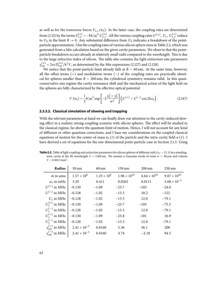
as well as for the transverse forces Fx ,y (r0). In the latter case, the coupling rates are determinedfrom (2.12) by the terms F(±)

x ,y = −ħk ∣α∣2U(±)x ,y . All the various coupling ratesU(±), Uz , U(±)

x ,y reduceto U0 in the limit R → 0. Any substantial dierence from U0 indicates a breakdown of the point-particle approximation. I list the coupling rates of various silicon sphere sizes inTable 2.2, whichwasgenerated from aMie calculation based on the given cavity parameters. We observe that the point-particle breakdown occurs already at relatively small radii compared to the wavelength.is is dueto the large refractive index of silicon. e table also contains the light extinction rate parametersγ(±)

ext = 2πcΠ(±)

ext /k2V , as determined by the Mie expressions (2.127) and (2.128).We notice that the point-particle limit already fails at R = 60nm. At the same time, however,

all the oset terms (+) and modulation terms (−) of the coupling rates are practically identi-cal for spheres smaller than R = 200nm; the cylindrical symmetry remains valid. In this quasi-conservative size regime the cavity resonance shi and the mechanical action of the light eld onthe spheres are fully characterized by the eective optical potential

V (r0) =12ħ ∣α∣2 exp [−2x

20 + y20w2

] (U(+) +U(−) cos 2kz0) . (2.147)

2.3.3.2. Classical simulation of slowing and trapping

With the relevant parameters at hand we can nally draw our attention to the cavity-induced slow-ing eect in a realistic strong-coupling scenario with silicon spheres. e eect will be studied inthe classical regime, far above the quantum limit of motion. Hence, I will not account for any kindof diusion or other quantum corrections, and I base my considerations on the coupled classicalequations of motion for the center-of-mass r0 (t) of the particle and the intra-cavity eld α (t). Ihave derived a set of equations for the one-dimensional point-particle case in Section 2.1.3. Using

Table 2.2. Table of light coupling and extinction parameters for silicon spheres of dierent radii (εSi = 12.1) in a standing-wave cavity at the IR wavelength λ = 1560nm. We assume a Gaussian mode of waist w = 40 µm and volumeV = 0.0013mm3 .

Radius 30 nm 60 nm 150 nm 200 nm 250 nm

m in amu 1.57 × 108 1.25 × 109 1.96 × 1010 4.64 × 1010 9.07 × 1010

ωr in mHz 3.29 0.411 0.0263 0.0111 5.68 × 10−3

U(+) in MHz −0.130 −1.09 −23.7 −103 −24.0U(−) in MHz −0.128 −1.02 −13.5 10.2 −122Uz in MHz −0.128 −1.02 −13.5 12.0 −79.1

U(+)x in MHz −0.130 −1.09 −23.7 −105 −75.5

U(−)x in MHz −0.128 −1.02 −13.5 12.0 −79.1

U(+)y in MHz −0.130 −1.09 −23.8 −101 16.9

U(−)y in MHz −0.128 −1.02 −13.5 12.0 −79.1

γ(+)

ext in MHz 2.41 × 10−3 0.0160 5.36 56.1 208γ(−)

ext in MHz 2.41 × 10−3 0.0160 4.74 −2.18 94.5

62

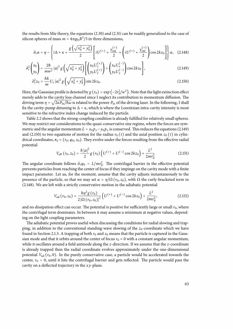
the results fromMie theory, the equations (2.30) and (2.31) can be readily generalized to the case ofsilicon spheres of mass m = 4πρSiR3/3 in three dimensions,

∂tα = η −⎧⎪⎪⎪⎨⎪⎪⎪⎩i∆ + κ +

g (√x20 + y20)2

⎡⎢⎢⎢⎢⎣iU(+) + γ(+)

ext2

+⎛⎝iU(+) + γ(+)

ext2

⎞⎠cos 2kz0

⎤⎥⎥⎥⎥⎦

⎫⎪⎪⎪⎬⎪⎪⎪⎭α, (2.148)

∂2t⎛⎝x0y0

⎞⎠= 2ħmw2

∣α∣2 g (√

x20 + y20)⎡⎢⎢⎢⎢⎣

⎛⎝x0U(+)

x

y0U(+)y

⎞⎠+⎛⎝x0U(−)

x

y0U(−)y

⎞⎠cos 2kz0

⎤⎥⎥⎥⎥⎦, (2.149)

∂2t z0 =ħkm

Uz ∣α∣2 g (√

x20 + y20) sin 2kz0. (2.150)

Here, theGaussian prole is denoted by g (r0) = exp (−2r20/w2). Note that the light extinction eectmerely adds to the cavity loss channel since I neglect its contribution to momentum diusion.edriving term η =

√2κPin/ħω is related to the power Pin of the driving laser. In the following, I shall

x the cavity-pump detuning to ∆ = κ, which is where the Lorentzian intra-cavity intensity is mostsensitive to the refractive index change induced by the particle.Table 2.2 shows that the strong-coupling condition is already fullled for relatively small spheres.

Wemay restrict our considerations to the quasi-conservative size regime, where the forces are sym-metric and the angularmomentum L = x0py−y0px is conserved.is reduces the equations (2.149)and (2.150) to two equations of motion for the radius r0 (t) and the axial position z0 (t) in cylin-drical coordinates, r0 = (r0, φ0, z0).ey evolve under the forces resulting from the eective radialpotential

Ve (r0, z0) =ħ ∣α∣2

2g (r0) (U(+) +U(−) cos 2kz0) +

L2

2mr20(2.151)

e angular coordinate follows ∂tφ0 = L/mr20. e centrifugal barrier in the eective potentialprevents particles from reaching the center of focus if they impinge on the cavity mode with a niteimpact parameter. Let us, for the moment, assume that the cavity adjusts instantaneously to thepresence of the particle, so that we may set α = η/Ω (r0, z0), with Ω the curly-bracketed term in(2.148). We are le with a strictly conservative motion in the adiabatic potential

Vad (r0, z0) =ħη2g (r0)2 ∣Ω (r0, z0)∣2

(U(+) +U(−) cos 2kz0) +L2

2mr20, (2.152)

and no dissipation eect can occur.e potential is positive for suciently large or small r0, wherethe centrifugal term dominates. In between it may assume a minimum at negative values, depend-ing on the light coupling parameters.e adiabatic potential proves useful when discussing the conditions for radial slowing and trap-

ping, in addition to the conventional standing-wave slowing of the z0-coordinate which we havefound in Section 2.1.3. A trapping of both r0 and z0 means that the particle is captured in the Gaus-sian mode and that it orbits around the center of focus r0 = 0 with a constant angular momentum,while it oscillates around a eld antinode along the z-direction. If we assume that the z-coordinateis already trapped then the radial coordinate evolves approximately under the one-dimensionalpotential Vad (r0, 0). In the purely conservative case, a particle would be accelerated towards thecenter, r0 = 0, until it hits the centrifugal barrier and gets reected. e particle would pass thecavity on a deected trajectory in the xy-plane.

63

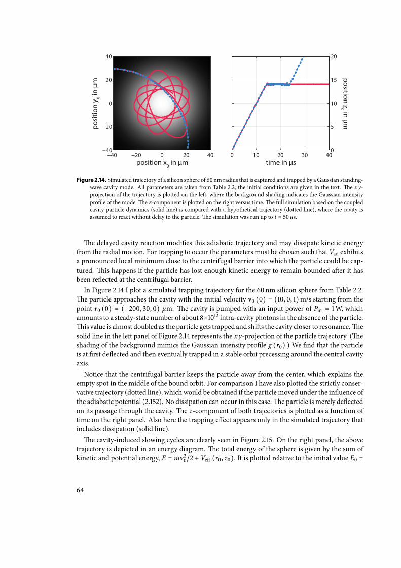
posi

tion

y 0 in µ

m

−40 −20 0 20 40−40

−20

0

20

40

0 10 20 30 400

5

10

15

20position z

0 in µm

position x0 in µm time in µs

Figure 2.14. Simulated trajectory of a silicon sphere of 60 nm radius that is captured and trapped by aGaussian standing-wave cavity mode. All parameters are taken from Table 2.2; the initial conditions are given in the text. e xy-projection of the trajectory is plotted on the le, where the background shading indicates the Gaussian intensityprole of the mode.e z-component is plotted on the right versus time.e full simulation based on the coupledcavity-particle dynamics (solid line) is compared with a hypothetical trajectory (dotted line), where the cavity isassumed to react without delay to the particle.e simulation was run up to t = 50 µs.

e delayed cavity reaction modies this adiabatic trajectory and may dissipate kinetic energyfrom the radial motion. For trapping to occur the parameters must be chosen such thatVad exhibitsa pronounced local minimum close to the centrifugal barrier into which the particle could be cap-tured. is happens if the particle has lost enough kinetic energy to remain bounded aer it hasbeen reected at the centrifugal barrier.In Figure 2.14 I plot a simulated trapping trajectory for the 60nm silicon sphere from Table 2.2.

e particle approaches the cavity with the initial velocity v0 (0) = (10, 0, 1)m/s starting from thepoint r0 (0) = (−200, 30, 0) µm. e cavity is pumped with an input power of Pin = 1W, whichamounts to a steady-state number of about 8×1012 intra-cavity photons in the absence of the particle.is value is almost doubled as the particle gets trapped and shis the cavity closer to resonance.esolid line in the le panel of Figure 2.14 represents the xy-projection of the particle trajectory. (eshading of the background mimics the Gaussian intensity prole g (r0).) We nd that the particleis at rst deected and then eventually trapped in a stable orbit precessing around the central cavityaxis.Notice that the centrifugal barrier keeps the particle away from the center, which explains the

empty spot in the middle of the bound orbit. For comparison I have also plotted the strictly conser-vative trajectory (dotted line), which would be obtained if the particlemoved under the inuence ofthe adiabatic potential (2.152). No dissipation can occur in this case.e particle is merely deectedon its passage through the cavity. e z-component of both trajectories is plotted as a function oftime on the right panel. Also here the trapping eect appears only in the simulated trajectory thatincludes dissipation (solid line).e cavity-induced slowing cycles are clearly seen in Figure 2.15. On the right panel, the above

trajectory is depicted in an energy diagram. e total energy of the sphere is given by the sum ofkinetic and potential energy, E = mv20/2 + Ve (r0, z0). It is plotted relative to the initial value E0 =

64

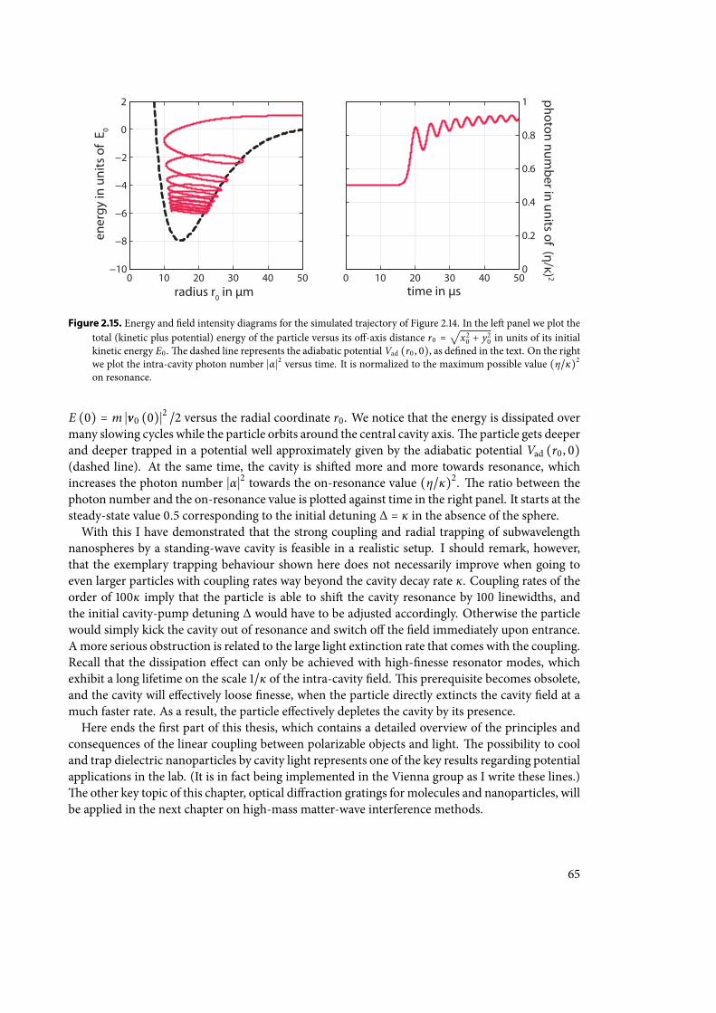
radius r0 in µm

ener

gy in

uni

ts o

f E 0

0 10 20 30 40 50−10

−8

−6

−4

−2

0

2 photon number in units of (η/κ) 20 10 20 30 40 50

0

0.2

0.4

0.6

0.8

1

time in µs

Figure 2.15. Energy and eld intensity diagrams for the simulated trajectory of Figure 2.14. In the le panel we plot thetotal (kinetic plus potential) energy of the particle versus its o-axis distance r0 =

√x20 + y20 in units of its initial

kinetic energy E0 .e dashed line represents the adiabatic potential Vad (r0 , 0), as dened in the text. On the rightwe plot the intra-cavity photon number ∣α∣2 versus time. It is normalized to the maximum possible value (η/κ)2

on resonance.

E (0) = m ∣v0 (0)∣2 /2 versus the radial coordinate r0. We notice that the energy is dissipated overmany slowing cycles while the particle orbits around the central cavity axis.e particle gets deeperand deeper trapped in a potential well approximately given by the adiabatic potential Vad (r0, 0)(dashed line). At the same time, the cavity is shied more and more towards resonance, whichincreases the photon number ∣α∣2 towards the on-resonance value (η/κ)2. e ratio between thephoton number and the on-resonance value is plotted against time in the right panel. It starts at thesteady-state value 0.5 corresponding to the initial detuning ∆ = κ in the absence of the sphere.With this I have demonstrated that the strong coupling and radial trapping of subwavelength

nanospheres by a standing-wave cavity is feasible in a realistic setup. I should remark, however,that the exemplary trapping behaviour shown here does not necessarily improve when going toeven larger particles with coupling rates way beyond the cavity decay rate κ. Coupling rates of theorder of 100κ imply that the particle is able to shi the cavity resonance by 100 linewidths, andthe initial cavity-pump detuning ∆ would have to be adjusted accordingly. Otherwise the particlewould simply kick the cavity out of resonance and switch o the eld immediately upon entrance.Amore serious obstruction is related to the large light extinction rate that comes with the coupling.Recall that the dissipation eect can only be achieved with high-nesse resonator modes, whichexhibit a long lifetime on the scale 1/κ of the intra-cavity eld.is prerequisite becomes obsolete,and the cavity will eectively loose nesse, when the particle directly extincts the cavity eld at amuch faster rate. As a result, the particle eectively depletes the cavity by its presence.Here ends the rst part of this thesis, which contains a detailed overview of the principles and

consequences of the linear coupling between polarizable objects and light. e possibility to cooland trap dielectric nanoparticles by cavity light represents one of the key results regarding potentialapplications in the lab. (It is in fact being implemented in the Vienna group as I write these lines.)e other key topic of this chapter, optical diraction gratings for molecules and nanoparticles, willbe applied in the next chapter on high-mass matter-wave interference methods.

65

Chapter 3.

Near-®eld interference techniques with heavy

molecules and nanoclusters

“Never express yourself more clearly than you are able to think.”—Niels Bohr

We will now devote our attention to one of the boldest enterprises in the eld of matter-wavephysics: Single-particle interference experiments with large molecules and clusters far beyond asingle atom.is chapter is dedicated to the drudgery of my experimental colleagues down in thegloomy basement vaults of the Quantum Nanophysics Group in Vienna, who are as committed asever to break their own current mass records and to demonstrate the quantum nature of larger andlarger objects.While atom interferometry has gained tremendously in (phase) sensitivity, stability and preci-

sion over the last decade, opening up for numerous applications in metrology [18, 93–95], the ex-perimentalists in Vienna have managed to observe quantum interference of molecules with massesfrom several hundred to about 104 atomic mass units [12, 96]. New and improved interferometerdesigns may promise a further increase by two orders of magnitude in lab-based experiments overthe next decade [10]. Starting from the rst far-eld diraction experiments with fullerenes [4] in1999, the group’s main interest shied towards the conceptually more dicult near-eld interfer-ometry, which turned out to be more suitable for higher masses. Apart from an ongoing branchof diraction experiments in the conventional far-eld geometry [20], the three-grating Talbot-Lau interferometer (TLI) scheme has become the working horse setup in the group’s striving forhighest masses. Most of this chapter thus will be dedicated to the TLI scheme and, in particular,to its modern manifestations employing optical standing-wave gratings. (Matter-wave Talbot-Lauinterferometry was pioneered by John Clauser using material gratings [97, 98].)e theoretical description of near-eld interference is more involved than the far-eld case,

and it must be properly distinguished from potential classical shadow eects in order to assure aquantum origin of the observed pattern.is is preferably done in the phase-space representationby means of Wigner functions [77], as it was advocated and worked out elsewhere [7, 40, 59].Before we will delve into the TLI scheme and its applications, I will rst discuss a dierent near-

eld interference eect with the help of the phase-space framework: e matter-wave analogueof Poisson’s spot, a diraction phenomenon originally proposed to demonstrate the wave natureof light [99] by the observation of a bright spot in the shadow region behind a circular aperture.At rst one may might think that, if the same idea were implemented with particles instead of

67

light, the appearance of such a bright spot would be a striking demonstration of quantum matter-wave interference. Poisson’s spot was in fact observed with electrons and deuterium molecules[21,100,101]. However, I will show that for the cases of largemolecules and nanoparticles interactingwith the diractive element during passage the appearance of a spot could also be explained byclassical theory [9]; it would not demonstrate the quantum wave nature of the particles.I will proceed with a detailed theoretical description of the generic TLI eect in Section 3.2,

focusing on its current implementations employing one optical phase grating (KDTLI) or threeoptical ionizing gratings (OTITLI).e KDTLI was rst proposed for molecules in [102]; its rstdemonstration can be found in [103], a detailed assessment in [7]. e OTITLI scheme was rstconceived in [104], fully worked out and proposed in [10], and rst observed in [13]. Both setups arealso suitable formetrological applications. In fact, deectometric measurements of static molecularpolarizabilities are regularly carried out in the Vienna group [105,106]. In Section 3.3 I will describea method to measure the absorption cross section of interfering particles in the TLI scheme, as wehave proposed it in [6].e chapter closes with an in-depth outlook on future time-domain experiments in the OTITLI

setup, which are most suited to reach masses beyond 105 amu. ere I will start by discussing thetechnical details and the rst measurement results of the present implementation of the OTITLIscheme in the Vienna lab [13].is sketch of the experimental methods and challenges will then behelpful in the subsequent analysis of all relevant eects that would eventually bound the reachablemass to less than about 109 amu in future experiments with the current scheme. Moreover, we willsee that macrorealistic modications to the Schrödinger equation may become testable with thepresent setup by operating in this high-mass regime [11].

3.1. The Poisson spot interferometer (PSI)

Poisson’s spot, or Arago’s spot, is an interference phenomenon dating back to the early 19th cen-tury, when Fresnel pushed his wave theory of light aer a century-old academic dispute. Poissondiscovered a peculiar implication of Fesnel’s diraction theory, which was then conrmed experi-mentally by Arago [99]: If a circular obstacle was illuminated by a (suciently collimated) beam oflight, a bright spot would appear in the center of the shadow region behind the obstacle—a strikingdemonstration of the wave nature of light.So far, Poisson’s spot has been demonstrated by means of matter waves only with electrons [100,

101] and deuteriummolecules [21]. Similar phenomena, such as the one-dimensional diraction atthin wires or the two-dimensional diraction at Fresnel zone plates, were observed with neutrons[107, 108] and atoms [109, 110]. Recent theoretical works, including our own, study the feasibility ofthe Poisson spot setup for fullerenes [22] and gold clusters [9].e generic layout of a Poisson spot interferometer (PSI) is sketched in Figure 3.1. It has a cylin-

drical symmetrywith respect to the interferometer axis z.e source, the obstacle and the detectionplane are located at z = 0, z = L1 and z = L1 + L2, respectively. In all practical implementations, thesource is given by a circular pinhole of radius R0. It represents the circular analogue of the primarycollimation slit in a conventional Young double-slit geometry, and it emits a rather uncollimatedbeam of particles (or light), which is to be diracted at an opaque circular obstacle of radius R atthe distance L1. In most cases, this obstacle is a thin disc (as depicted), but it could also be imple-mented by a sphere, as I will discuss later. e single-particle diraction pattern is then detected

68

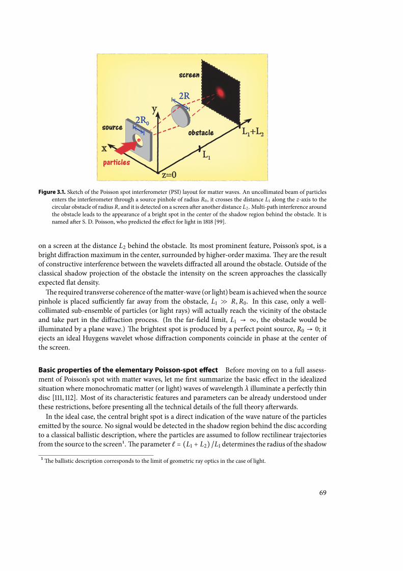
Figure 3.1. Sketch of the Poisson spot interferometer (PSI) layout for matter waves. An uncollimated beam of particlesenters the interferometer through a source pinhole of radius R0 , it crosses the distance L1 along the z-axis to thecircular obstacle of radius R, and it is detected on a screen aer another distance L2 . Multi-path interference aroundthe obstacle leads to the appearance of a bright spot in the center of the shadow region behind the obstacle. It isnamed aer S. D. Poisson, who predicted the eect for light in 1818 [99].

on a screen at the distance L2 behind the obstacle. Its most prominent feature, Poisson’s spot, is abright diractionmaximum in the center, surrounded by higher-order maxima.ey are the resultof constructive interference between the wavelets diracted all around the obstacle. Outside of theclassical shadow projection of the obstacle the intensity on the screen approaches the classicallyexpected at density.e required transverse coherence of thematter-wave (or light) beam is achievedwhen the source

pinhole is placed suciently far away from the obstacle, L1 ≫ R, R0. In this case, only a well-collimated sub-ensemble of particles (or light rays) will actually reach the vicinity of the obstacleand take part in the diraction process. (In the far-eld limit, L1 → ∞, the obstacle would beilluminated by a plane wave.) e brightest spot is produced by a perfect point source, R0 → 0; itejects an ideal Huygens wavelet whose diraction components coincide in phase at the center ofthe screen.

Basic properties of the elementary Poisson-spot eªect Before moving on to a full assess-ment of Poisson’s spot with matter waves, let me rst summarize the basic eect in the idealizedsituation where monochromatic matter (or light) waves of wavelength λ illuminate a perfectly thindisc [111, 112]. Most of its characteristic features and parameters can be already understood underthese restrictions, before presenting all the technical details of the full theory aerwards.In the ideal case, the central bright spot is a direct indication of the wave nature of the particles

emitted by the source. No signal would be detected in the shadow region behind the disc accordingto a classical ballistic description, where the particles are assumed to follow rectilinear trajectoriesfrom the source to the screen1.e parameter ℓ = (L1 + L2) /L1 determines the radius of the shadow

1e ballistic description corresponds to the limit of geometric ray optics in the case of light.

69

projection of the obstacle on the detection screen, Rcl = ℓR, as follows from elementary geometry(intercept theorem).Poisson’s spot can be observed with waves both in the near eld and in the far eld behind the

obstacle. e regimes are distinguished by the parameter k = R2/L2λ, which compares the char-acteristic length scale R2/λ of diraction patterns to the screen distance L2.e far-eld regime isgiven by k ≪ 1.e quasi-classical short-wave limit λ → 0, on the other hand, implies k →∞.Some characteristics of the ideal Poisson spot can be understood in terms of the Fresnel zone

construction [99]: e radius rn =√nλL1L2/ (L1 + L2) = R

√n/kℓ denes the nth Fresnel zone

on the obstacle plane (n > kℓ). It implies a path length of about L1 + L2 + nλ/2 from the centerof the source to the center of the screen. at is, the spherical Huygens wavelets emanating fromneighbouring zones interfere destructively at the screen center. Since the diraction angle requiredto reach the screen center from the nth zone (the so-called inclination angle according to [99])grows with n, higher-order zones contribute less to the central maximum on the screen. We thusexpect a most pronounced Poisson spot at small values of kℓ ∼ 1, which permits contributions oflow orders n.e exact shape of the ideal diraction pattern on the screen can be deducedwith help ofBabinet’s

principle [99]:e superposition principle implies that thewave amplitudesψP (r) behind a circularpinhole of radius R and ψD (r) behind the corresponding disc of the same radius must sum upto the at undisturbed solution in the absence of any diractive element, ψP (r) + ψD (r) = 1.e same principle holds trivially for the geometric shadow projections ID (r) = Θ (r − ℓR) andIP (r) = 1 − ID (r) obtained from a simple ray model. Hence, the diraction amplitudes on top ofthe geometric shadow projection diers in both cases merely by a negative sign, ψP (r) − IP (r) =ID (r) − ψD (r).Moreover, if the disc is illuminated by a perfect point source, we can roughly estimate the width

of the central diraction maximum: e distances between points r1 = (R cos ϕ, R sin ϕ) on thedisc edge to a point rs = (Rs , 0) on the screen range approximately between L2 + (R ± Rs)2 /2L2.e average path dierence of two arbitrary points r1,2 on the disc and the screen coordinate rsreads as RRs/L2. If we assume that the rst dark ring around the center spot corresponds to a meanpath dierence of λ/2, we arrive at the estimate Rs ≈ L2λ/2R = R/2k for the radius of the Poissonspot.In all realistic cases the Poisson spot is washed out due to the nite source coherence related to

a nonzero radius R0 of the source pinhole. For each o-center point in the source the Poisson spotmoves away from the screen center by at most L2R0/L1. A pronounced spot is observed as longas this shi is small compared to the spot size Rs, which results in the condition R0 < L1λ/2R =L1R/2L2k. At the same time, the source radius must be bounded by R0 < ℓR, or else there wouldbe no shadow region of the disc on the screen plane.e informed readermay notice that the condition on the required source coherence is similar to

the case of far-eld diraction at a grating [9]. Given the grating period d, an incoming beammusthave a divergence angle smaller than λ/d.is leads to the condition D < 2L1λ/d for a collimationslit of width D placed at the distance L1.e advantage of the PSI setup lies in the condition kℓ ∼ 1for observing a pronounced spot: It admits disc radii R larger than typical grating periods d for agiven wavelength λ, which should make the PSI suitable for heavy (and fast) particles with smallde Broglie wavelengths.

70

On the other hand, important features of the diraction pattern are modied in the presence of adispersive interaction between the matter waves and the obstacle. We will nd out in the followingthat this modies the width and the height of the central Poisson spot, invalidating the Fresnel zoneconstruction and Babinet’s principle. More importantly, I will show that a central bright spot couldalso appear in the case of classical particles passing the obstacle on deected trajectories due to theattractive force towards the obstacle. is obscures the distinction between the quantum and theclassical description for large interaction strengths, such that the appearance of the spot per se doesnot indicate the wave nature of the particles.

3.1.1. Phase-space description of the ideal eªect

e present theoretical model of the PSI for matter waves will be based on the phase-space repre-sentation of quantum states in terms of Wigner functions, which I have used already in Chapter2. e basic features of this representation are given in Appendix A.3. Most notably, it serves as acommon and descriptive framework for both quantum and classical descriptions of the setup.Moreover, I will consider only the paraxial regime, where the diraction eect is conned to

those transverse coordinates r = (x , y) on the source, the obstacle, and the detection plane, whichare small compared to the longitudinal extension of the interferometer, R, R0 ≪ L1,2. is repre-sents the standard regime for many matter-wave diraction experiments with collimated beams ofparticles. In this case the dimensionality of the problem reduces eectively to the two transversecoordinates (x , y). e only role of the longitudinal velocity vz is to determine the arrival timesT1,2 = L1,2/vz at the obstacle and the detection screen, and we may simply average the resultingdensity pattern on the screen over the velocity distribution of the particle ensemble.In the following I derive the diraction and shadow eect at an ideal circular aperture, that is,

at an arbitrarily thin and non-interacting disc of radius R.is will be the quantitative assessmentof the previously discussed properties. e dispersive interaction between the particles and theobstacle will be implemented aerwards.

3.1.1.1. Ideal diªraction pattern

e two-dimensional Wigner function for a given quantum state of motion ρ reads as

w (r, p) = 1(2πħ)2 ∫ d2s e ip⋅s/ħ⟨r −

s2∣ρ∣r + s

2⟩. (3.1)

It resembles a classical phase-space probability distribution f (r, p) in the case of incoherent mix-tures. I therefore describe the initially uncollimated ensemble state behind the source pinhole as

w0 (r, p) =1

πR20Θ (R0 − r)D (p) ≡ S (r)D (p) , (3.2)

71

with Θ the Heaviside function and D (p) an isotropic and normalized distribution of transversemomenta ejected from the source2. An ideal point source would correspond to the pure state3w0 (r, p) = S (r) = δ (r).e propagation of the beam from source to aperture is given by the shearing transformation

w0 (r, p)↦ w0 (r −pmT1, p) , (3.3)

withm the particle mass. We arrive at the plane of the obstacle, which acts here as an ideal circulartransmission mask for the matter waves. It modulates the matter-wave state by the isotropic trans-mission function t (r) = Θ (r − R) of the ideal disc, ⟨r∣ρ∣r′⟩ ↦ t (r) t∗ (r′) ⟨r∣ρ∣r′⟩ in the positionrepresentation.is corresponds to the Wigner function transformation [40, 59]

w (r, p)↦ ∫ d2q T (r, p − q)w (r, q) (3.4)

with the transmission kernel

T (r, p) = 1(2πħ)2 ∫ d2s e ip⋅s/ħt (r −

s2) t∗ (r + s

2) . (3.5)

Aer a subsequent free propagation to the screen plane we arrive at the Wigner function

w (r, p) = ∫ d2q T (r − pT2m, p − q)w0 (r −

pT2m

− qT1m, q) . (3.6)

e density pattern w (r) on the screen is obtained by integrating over the momentum coordinate.A substitution of the momentum coordinate leaves us with

w (r) = m2

T22 ∫ d2r0d2p0 S (r0)D (p0)T (r0 +p0T1m,m r − r0

T2− T1 + T2

T2p0) . (3.7)

At this point I make use of the Fourier transform of the momentum distribution (i.e. its character-istic function),

D (s) = D (s) = ∫ d2p e−ip⋅s/ħD (p) ,

D (p) = ∫ d2s(2πħ)2

e ip⋅s/ħD (s) (3.8)

with D (0) = 1. Aer plugging the explicit form of the kernel (3.5) into the density pattern (3.7),several steps of calculation lead to the expression

w (r) = [ m2πħ (T1 + T2)

]2

∫ d2r0d2s S (r0) D (s)ψ [r + T2T1

(r0 −s2)]ψ∗ [r + T2

T1(r0 +

s2)] ,

(3.9)

2is is admissible as long as the transverse coherence of the ensemble is of no concern, that is, if the occupied phase-space region is much larger than Planck’s quantum of action, R0P0 ≫ ħ, with P0 the width of the momentum distri-bution D (p).

3is state is an improper position eigenstate that cannot be normalized.e correspondingWigner function does notcontain a nite momentum distribution due to quantum uncertainty, whereas this would be very well possible in aclassical model.

72

with the dimensionless amplitude term

ψ (r) = mℓ2πħT2 ∫ d2r1 exp [

imħT2

( ℓ2r21 − r1 ⋅ r)] t (r1)

= kℓ ∫ d2u exp [iπkℓu2 − 2πiku ⋅ rR ] t (Ru) . (3.10)

Here I have introduced the dimensionless variable u = r1/R, which represents a two-dimensionalposition vector on the obstacle plane in units of the obstacle radius. is admits a convenient no-tation in terms of the geometry parameters k = mR2/hT2 and ℓ = (T1 + T2) /T1. See Appendix B.1for details on how to compute the diraction amplitude of an ideal disc in practice.

Weak-collimation approximation e amplitude term (3.10) can be read as the Fourier trans-form of a function of u with the characteristic length scale of variation δu ∼ 1, asmainly determinedby the transmission function. It is then possible to write ψ (r + δr) ≈ ψ (r) for ∣δr∣ ≪ R. Specif-ically, we can apply this approximation to drop the s-dependence in (3.9) if the ensemble exitingthe source is poorly collimated, that is, if the spread P0 of the momentum distribution D (p) islarge, P0R ≫ ħ.e reason is that the Fourier transform D (s) is then conned to small arguments∣s∣ ≪ R.is leaves us with the conventional form of the diraction pattern,

w (Ru) = m2D (0)π (T1 + T2)2 ∫u0≤1 d

2u0 ∣ψ (Ru + L2L1

R0u0)∣2, (3.11)

which is completely sucient for all practical purposes4. Note that I have plugged in the sourceaperture from (3.2) and introduced the dimensionless source coordinate u0 = r0/R0.e prefactor

I0 =m2D (0)(T1 + T2)2

(3.12)

is given by the constant particle density on the screen that would be obtained if the diractingdisc were removed and the matter waves could transit unobstructedly. is is shown explicitly inAppendix B.1.

3.1.1.2. Poisson’s spot

e characteristic features of the diraction pattern behind an ideal disc are most pronounced ifwe assume the disc to be illuminated by a perfect point source in the center of the source plane.e density distribution on the screen then reduces to the simple expression w (r) = I0 ∣ψ (r)∣2.We note that the diraction image (3.11) of a nite-size source may be viewed as an average ofdisplaced point-source images over the source aperture.

4e approximation ceases to be valid only in the limit kℓ ≫ 1, or if the obstacle were illuminated by a strongly colli-mated beam.e latter case would already imply diraction at the source pinhole.e former case would result ina very narrow Poisson spot that could hardly be observed in an experiment.

73

In Appendix B.1, I simplify the expression (3.10) for the diraction amplitude at an ideal disc,

ψ (r) = 2πkℓ ∫ ∞

1du u exp (iπkℓu2) J0 (2πku

rR)

= i exp(−iπ kr2

ℓR2) − 2πkℓ ∫ 10 du u exp (iπkℓu2) J0 (2πku

rR)

´¹¹¹¹¹¹¹¹¹¹¹¹¹¹¹¹¹¹¹¹¹¹¹¹¹¹¹¹¹¹¹¹¹¹¹¹¹¹¹¹¹¹¹¹¹¹¹¹¹¹¹¹¹¹¹¹¹¹¹¹¹¹¹¹¹¹¹¹¹¹¹¹¹¹¹¹¹¹¹¹¹¹¹¹¹¹¹¹¹¹¹¹¹¹¹¹¹¹¹¹¹¹¹¹¹¹¹¹¹¹¹¹¹¹¹¹¹¹¹¹¹¹¹¹¹¹¸¹¹¹¹¹¹¹¹¹¹¹¹¹¹¹¹¹¹¹¹¹¹¹¹¹¹¹¹¹¹¹¹¹¹¹¹¹¹¹¹¹¹¹¹¹¹¹¹¹¹¹¹¹¹¹¹¹¹¹¹¹¹¹¹¹¹¹¹¹¹¹¹¹¹¹¹¹¹¹¹¹¹¹¹¹¹¹¹¹¹¹¹¹¹¹¹¹¹¹¹¹¹¹¹¹¹¹¹¹¹¹¹¹¹¹¹¹¹¹¹¹¹¹¹¹¹¹¶≡ψ1(r)

. (3.13)

e second line represents a numerically stable form of the solution which shall be used in thecomputational analysis of the eect. e rst term in the second line is a pure phase factor ofmodulus one and the second term represents the diraction amplitude ψ1 (r) of a circular apertureof radius R, in accordance with Babinet’s principle.Let me rst discuss the asymptotic behaviour of the diraction amplitude far away from the

screen center, r ≫ R/k. For this we can approximate the Bessel function in the integral by itsasymptotic form for large arguments [113], J0 (x) ≈

√2/πx cos (x − π/4). I show in Appendix B.1

that the magnitude of ψ1 (r) is bounded from above by

∣ψ1 (r)∣ ≤4kℓ3

√RkrÐÐÐÐ→kr/R→∞

0. (3.14)

is conrms the intuitive picture that far outside the shadow projection (but still inside the screenarea illuminated by the weakly collimated matter-wave beam) the intensity on the screen is notaected by the diraction at the obstacle, w (r →∞)→ I0.At the same time, the density distribution exhibits a central diraction maximum in the shadow

region behind the disc, Poisson’s spot, as easily shown by evaluating the amplitude function (3.13)at r = 0. We nd that ψ (0) = i exp (iπkℓ), and that the central intensity, w (0) = I0, is as large as itwould be without the obstacle. In other words, the ideal diraction image of a point source alwaysexhibits a peak in the center of the disc shadow, whose height and position are independent of thePSI geometry and the particle velocities.O center, however, the diraction image does depend on these parameters, as demonstrated in

Figure 3.2. ere, I plot radial cuts of the Poisson-spot diraction images of a perfect monochro-matic point source for dierent geometry parameters.e density distributions are normalized tothe unobstructed value I0. e le and the right panels correspond respectively to k = 0.2 andk = 2. e distances L1,2 are assumed to be equal, ℓ = 2, in the top panels, whereas we chose anasymmetric conguration, ℓ = 1.2, for the bottom panels. We observe that the width of the centralspot depends mainly on the parameter k; it gets narrower with larger values of k. We can estimatethe width Rs of the central peak by the rst zero of the Bessel function5 in (3.13), J0 (2πkRs/R) = 0at Rs ≈ 0.4R/k. An upper limit for the source radius R0, at which a pronounced Poisson spot is stillvisible, is obtained in the same way,

R0 ≲ 0.4L1RL2k

= 0.4 hT1mR. (3.15)

5 For larger values r > Rs the integral in the second line of (3.13) extends over positive and negative intervals of theBessel function. ey cancel in parts and should therefore decrease the diraction amplitude ψ1 (r) signicantly.Of course, the quality of this estimate varies with dierent values of kℓ, which enters the same integral through thecomplex Gaussian function.

74

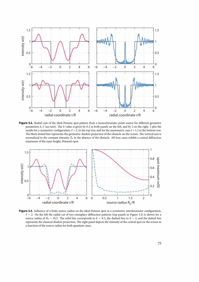
inte

nsity

w(r

)

−6 −4 −2 0 2 4 60

0.5

1

1.5

−6 −4 −2 0 2 4 60

0.5

1

1.5

radial coordinate r/R

inte

nsity

w(r

)

−6 −4 −2 0 2 4 60

0.5

1

1.5

radial coordinate r/R−6 −4 −2 0 2 4 6

0

0.5

1

1.5

Figure 3.2. Radial cuts of the ideal Poisson spot pattern from a monochromatic point source for dierent geometryparameters k, ℓ (see text). e k-value is given by 0.2 in both panels on the le, and by 2 on the right. I plot theresults for a symmetric conguration, ℓ = 2, in the top row, and for the asymmetric case ℓ = 1.2 in the bottom row.e black dotted line represents the geometric shadow projection of the obstacle on the screen.e vertical axis isnormalized to the constant intensity I0 in the absence of the obstacle. All four cases exhibit a central diractionmaximum of the same height, Poisson’s spot.

radial coordinate r/R

inte

nsity

w(r

)

−6 −4 −2 0 2 4 60

0.5

1

1.5

source radius R0 /R

spot maxim

um w

(0)

0 0.5 1 1.5 20

0.2

0.4

0.6

0.8

1

Figure 3.3. Inuence of a nite source radius on the ideal Poisson spot in a symmetric interferometer conguration,ℓ = 2. On the le the radial cut of two exemplary diraction patterns (top panels in Figure 3.2) is shown for asource radius of R0 = R/2. e solid line corresponds to k = 0.2, the dashed line to k = 2, and the dotted linerepresents the classical shadow projection.e right panel depicts the intensity of the central spot on the screen asa function of the source radius for both quantum cases.

75

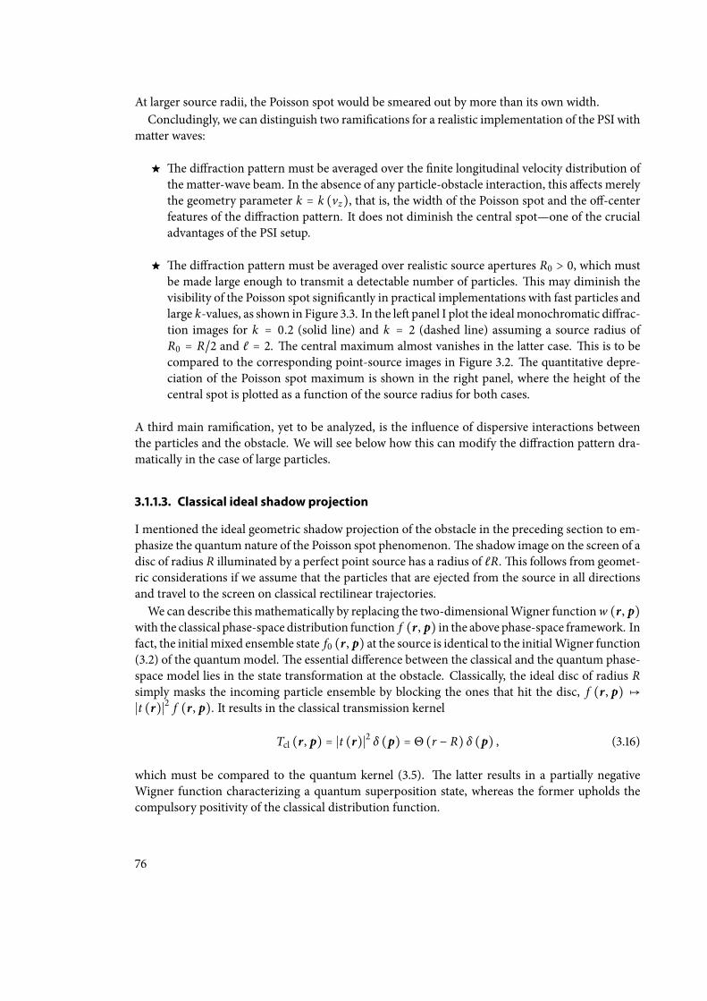
At larger source radii, the Poisson spot would be smeared out by more than its own width.Concludingly, we can distinguish two ramications for a realistic implementation of the PSI with

matter waves:

e diraction pattern must be averaged over the nite longitudinal velocity distribution ofthe matter-wave beam. In the absence of any particle-obstacle interaction, this aects merelythe geometry parameter k = k (vz), that is, the width of the Poisson spot and the o-centerfeatures of the diraction pattern. It does not diminish the central spot—one of the crucialadvantages of the PSI setup.

e diraction pattern must be averaged over realistic source apertures R0 > 0, which mustbe made large enough to transmit a detectable number of particles. is may diminish thevisibility of the Poisson spot signicantly in practical implementations with fast particles andlarge k-values, as shown in Figure 3.3. In the le panel I plot the idealmonochromatic dirac-tion images for k = 0.2 (solid line) and k = 2 (dashed line) assuming a source radius ofR0 = R/2 and ℓ = 2. e central maximum almost vanishes in the latter case. is is to becompared to the corresponding point-source images in Figure 3.2. e quantitative depre-ciation of the Poisson spot maximum is shown in the right panel, where the height of thecentral spot is plotted as a function of the source radius for both cases.

A third main ramication, yet to be analyzed, is the inuence of dispersive interactions betweenthe particles and the obstacle. We will see below how this can modify the diraction pattern dra-matically in the case of large particles.

3.1.1.3. Classical ideal shadow projection

I mentioned the ideal geometric shadow projection of the obstacle in the preceding section to em-phasize the quantum nature of the Poisson spot phenomenon.e shadow image on the screen of adisc of radius R illuminated by a perfect point source has a radius of ℓR.is follows from geomet-ric considerations if we assume that the particles that are ejected from the source in all directionsand travel to the screen on classical rectilinear trajectories.We can describe this mathematically by replacing the two-dimensionalWigner functionw (r, p)

with the classical phase-space distribution function f (r, p) in the above phase-space framework. Infact, the initialmixed ensemble state f0 (r, p) at the source is identical to the initialWigner function(3.2) of the quantummodel.e essential dierence between the classical and the quantum phase-space model lies in the state transformation at the obstacle. Classically, the ideal disc of radius Rsimply masks the incoming particle ensemble by blocking the ones that hit the disc, f (r, p) ↦∣t (r)∣2 f (r, p). It results in the classical transmission kernel

Tcl (r, p) = ∣t (r)∣2 δ (p) = Θ (r − R) δ (p) , (3.16)

which must be compared to the quantum kernel (3.5). e latter results in a partially negativeWigner function characterizing a quantum superposition state, whereas the former upholds thecompulsory positivity of the classical distribution function.

76

By replacing the transmission kernel in the quantum formula (3.7) we arrive at the classical den-sity distribution on the screen,

f (r) = m2

(T1 + T2)2 ∫ d2r0 S (r0)D (m r − r0

T1 + T2) ∣t (T1r + T2r0

T1 + T2)∣2. (3.17)

Once again, if we restrict to screen coordinates r = Ru that are well within reach of the unobstructedparticle beam we are le with the screen image of an uncollimated particle beam partially blockedby the disc,

f (Ru) = I0π ∫u0≤1 d2u0Θ (∣L1Ru + L2R0u0

L1 + L2∣ − R) . (3.18)

is is the classical counterpart of (3.11). It vanishes for all u < ℓ − L2R0/L1R. In other words,there exists a classical shadow region behind the disc as long as the source radius satises R0 <R (L1 + L2) /L2. Any observation of particles in this shadow region would indicate their quantumnature.

3.1.2. Modi®ed eªect in the presence of interaction

In practice, the quantum-classical distinction in a matter-wave PSI is obscured by the dispersiveinteraction between the circular obstacle and a passing particle. Given the polarizability of theparticle and the dielectric properties of the obstacle material, mutually induced virtual dipoles giverise to a van der Waals-type potential attracting the particle towards the obstacle if it is sucientlyclose to its walls. In the following I will restrict to (dielectric or metallic) spheres and thin discs, themost relevant obstacle candidates for practical implementations.So far I have modelled the obstacle as an arbitrarily thin opaque disc on the obstacle plane at

distance z = L1 from the source, as sketched in Figure 3.1. In the following I will consider obstacles,which are suciently thin so that we can still specify an obstacle plane and a two-dimensionalbinary function ∣t (r)∣ describing the transmission of matter waves through the plane6.

3.1.2.1. Modi®ed diªraction pattern

e weak short-time interaction between a collimated matter-wave beam and a thin diractiveelement can be assessed by means of the standard eikonal phase [40, 59, 60]

ϕ (x , y) = − 1ħvz ∫ dz V (x , y, z) . (3.19)

It approximates the classical action and the wave front curvature accumulated by the matter waveswhen they scatter at the interaction potential V (x , y, z) with a large longitudinal velocity vz . eexpression is valid in the longitudinal high-energy limit, where the kinetic energy of the particlesexceeds by far the average interaction strength, andwhere the transversemotion of thematter-wavestate is restricted to small momenta, ∣px ,y∣ ≪ mvz , playing no role during interaction. I refer thereader to my previous work [59, 60] for a detailed analysis of the eikonal approximation and itsvalidity.

6e use of thick obstacles would be counterproductive in practice, because it would also aggravate the interactioneect and its destructive inuence on the quantum visibility.

77

Here we consider a cylindrically symmetric potential V (x , y, z) = V (√x2 + y2, z) and append

the corresponding eikonal phase factor exp [iϕ (r)] to the transmission function of the obstacle. Inthe case of an attractive potential wemust not forget an important additional eect: Particles in closevicinity of the obstacle may be captured and absorbed by its walls, increasing the eective obstacleradius by ηR.e parameter η depends on the specic potential and on the particle velocity as well,which adds to the dispersive nature of the interaction eect. e modied transmission functionreads as t (r) = Θ (r − R − ηR) exp [iϕ (r)], and the modied diraction pattern is obtained byreplacing the amplitude function in (3.11) with

ψ (r) = 2πkℓ ∫ ∞

1+ηdu u exp [iπkℓu2 + iϕ (Ru)] J0 (2πku

rR) . (3.20)

e concrete evaluations of the modied amplitude will be implemented below using the numeri-cally stable expression

ψ (r) = i exp(−iπ kr2

ℓR2) − 2πkℓ ∫ 1+η

0du u exp (iπkℓu2) J0 (2πku

rR)

+ 2πkℓ ∫ ∞

1+ηdu u exp (iπkℓu2) J0 (2πku

rR) [e iϕ(Ru) − 1] . (3.21)

e rst line is given by the stable form of the ideal diraction amplitude with an increased obstacleradius, the second line is an innite integral over the dierence between the ideal and the modiedcase. I note that the latter converges much better than (3.20) in numerical implementations becausethe integrand drops to zero outside the limited range of the interaction potential.

3.1.2.2. Modi®ed shadow pattern

e particle-obstacle interaction potential V (r, z) also modies the classical shadow projectionon the screen, as the attractive force Fr = −∂rV (r, z) deects those particles towards the screencenter whose trajectories come close to the obstacle walls. e deection of each particle can beapproximated by the net momentum kick

q (r) = − ∫ dzvz ∂rV (r, z) rr= ħ∂rϕ (r) r

r(3.22)

given the same parameter constraints as for the eikonal phase (3.19). e classical transmissionkernel (3.16) is turned into

Tcl (r, p) = Θ (r − R − ηR) δ [p − q (r)] , (3.23)

which represents the classical counterpart of the eikonal approximation [59, 60]. It will be conve-nient to express the momentum kick in terms of the dimensionless function

Q (r) = − Rhk

q (r) ⋅ rr= Rhkvz ∫ dz ∂rV (r, z) = −R∂rϕ (r)

2πk, (3.24)

which is always non-negative in the case of an attractive interaction. Moreover, themomentumkickwill induce arbitrarily large deections of those trajectories that come close to the obstacle surface,Q (u → 1 + η) ≫ 1, if we assume a divergent van der Waals potential.

78

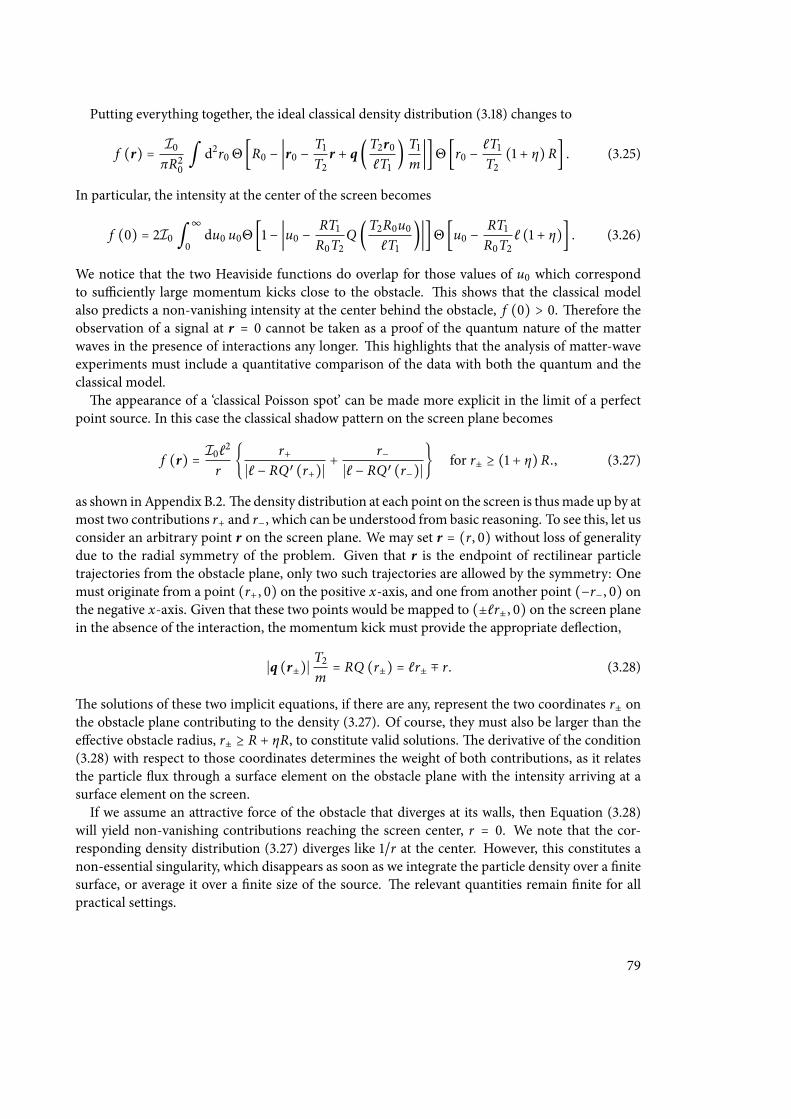
Putting everything together, the ideal classical density distribution (3.18) changes to

f (r) = I0πR20 ∫ d

2r0Θ [R0 − ∣r0 −T1T2

r + q (T2r0ℓT1

) T1m

∣]Θ [r0 −ℓT1T2

(1 + η)R] . (3.25)

In particular, the intensity at the center of the screen becomes

f (0) = 2I0 ∫ ∞

0du0 u0Θ [1 − ∣u0 −

RT1R0T2

Q (T2R0u0ℓT1

)∣]Θ [u0 −RT1R0T2

ℓ (1 + η)] . (3.26)

We notice that the two Heaviside functions do overlap for those values of u0 which correspondto suciently large momentum kicks close to the obstacle. is shows that the classical modelalso predicts a non-vanishing intensity at the center behind the obstacle, f (0) > 0. erefore theobservation of a signal at r = 0 cannot be taken as a proof of the quantum nature of the matterwaves in the presence of interactions any longer. is highlights that the analysis of matter-waveexperiments must include a quantitative comparison of the data with both the quantum and theclassical model.e appearance of a ‘classical Poisson spot’ can be made more explicit in the limit of a perfect

point source. In this case the classical shadow pattern on the screen plane becomes

f (r) = I0ℓ2

r r+∣ℓ − RQ′ (r+)∣

+ r−∣ℓ − RQ′ (r−)∣

for r± ≥ (1 + η)R., (3.27)

as shown inAppendix B.2.e density distribution at each point on the screen is thusmade up by atmost two contributions r+ and r−, which can be understood from basic reasoning. To see this, let usconsider an arbitrary point r on the screen plane. We may set r = (r, 0) without loss of generalitydue to the radial symmetry of the problem. Given that r is the endpoint of rectilinear particletrajectories from the obstacle plane, only two such trajectories are allowed by the symmetry: Onemust originate from a point (r+, 0) on the positive x-axis, and one from another point (−r−, 0) onthe negative x-axis. Given that these two points would be mapped to (±ℓr±, 0) on the screen planein the absence of the interaction, the momentum kick must provide the appropriate deection,

∣q (r±)∣T2m

= RQ (r±) = ℓr± ∓ r. (3.28)

e solutions of these two implicit equations, if there are any, represent the two coordinates r± onthe obstacle plane contributing to the density (3.27). Of course, they must also be larger than theeective obstacle radius, r± ≥ R + ηR, to constitute valid solutions.e derivative of the condition(3.28) with respect to those coordinates determines the weight of both contributions, as it relatesthe particle ux through a surface element on the obstacle plane with the intensity arriving at asurface element on the screen.If we assume an attractive force of the obstacle that diverges at its walls, then Equation (3.28)

will yield non-vanishing contributions reaching the screen center, r = 0. We note that the cor-responding density distribution (3.27) diverges like 1/r at the center. However, this constitutes anon-essential singularity, which disappears as soon as we integrate the particle density over a nitesurface, or average it over a nite size of the source. e relevant quantities remain nite for allpractical settings.

79

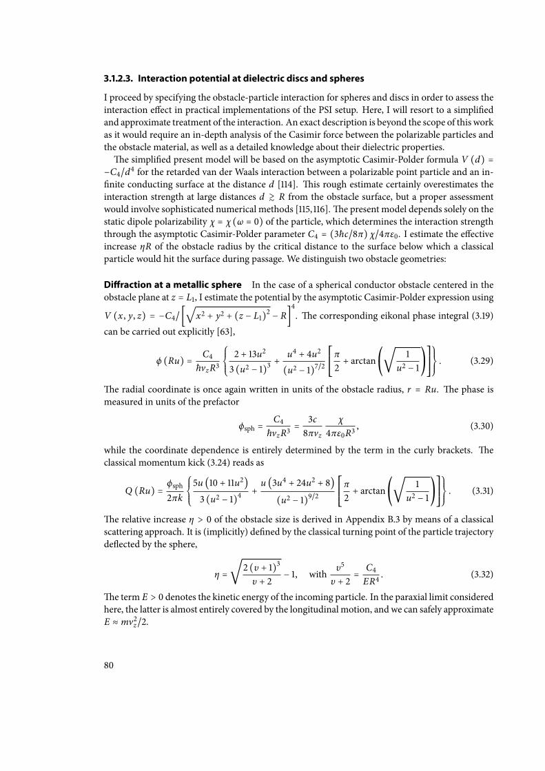
3.1.2.3. Interaction potential at dielectric discs and spheres

I proceed by specifying the obstacle-particle interaction for spheres and discs in order to assess theinteraction eect in practical implementations of the PSI setup. Here, I will resort to a simpliedand approximate treatment of the interaction. An exact description is beyond the scope of this workas it would require an in-depth analysis of the Casimir force between the polarizable particles andthe obstacle material, as well as a detailed knowledge about their dielectric properties.e simplied present model will be based on the asymptotic Casimir-Polder formula V (d) =

−C4/d4 for the retarded van der Waals interaction between a polarizable point particle and an in-nite conducting surface at the distance d [114]. is rough estimate certainly overestimates theinteraction strength at large distances d ≳ R from the obstacle surface, but a proper assessmentwould involve sophisticated numerical methods [115,116].e present model depends solely on thestatic dipole polarizability χ = χ (ω = 0) of the particle, which determines the interaction strengththrough the asymptotic Casimir-Polder parameter C4 = (3ħc/8π) χ/4πε0. I estimate the eectiveincrease ηR of the obstacle radius by the critical distance to the surface below which a classicalparticle would hit the surface during passage. We distinguish two obstacle geometries:

Diªraction at a metallic sphere In the case of a spherical conductor obstacle centered in theobstacle plane at z = L1, I estimate the potential by the asymptotic Casimir-Polder expression using

V (x , y, z) = −C4/ [√

x2 + y2 + (z − L1)2 − R]4. e corresponding eikonal phase integral (3.19)

can be carried out explicitly [63],

ϕ (Ru) = C4ħvzR3

⎧⎪⎪⎨⎪⎪⎩

2 + 13u2

3 (u2 − 1)3+ u4 + 4u2

(u2 − 1)7/2⎡⎢⎢⎢⎢⎣

π2+ arctan

⎛⎝

√1

u2 − 1⎞⎠

⎤⎥⎥⎥⎥⎦

⎫⎪⎪⎬⎪⎪⎭. (3.29)

e radial coordinate is once again written in units of the obstacle radius, r = Ru. e phase ismeasured in units of the prefactor

ϕsph =C4

ħvzR3= 3c8πvz

χ4πε0R3

, (3.30)

while the coordinate dependence is entirely determined by the term in the curly brackets. eclassical momentum kick (3.24) reads as

Q (Ru) =ϕsph2πk

⎧⎪⎪⎨⎪⎪⎩

5u (10 + 11u2)3 (u2 − 1)4

+u (3u4 + 24u2 + 8)

(u2 − 1)9/2⎡⎢⎢⎢⎢⎣

π2+ arctan

⎛⎝

√1

u2 − 1⎞⎠

⎤⎥⎥⎥⎥⎦

⎫⎪⎪⎬⎪⎪⎭. (3.31)

e relative increase η > 0 of the obstacle size is derived in Appendix B.3 by means of a classicalscattering approach. It is (implicitly) dened by the classical turning point of the particle trajectorydeected by the sphere,

η =√2 (υ + 1)3

υ + 2 − 1, with υ5

υ + 2 =C4ER4

. (3.32)

e term E > 0 denotes the kinetic energy of the incoming particle. In the paraxial limit consideredhere, the latter is almost entirely covered by the longitudinal motion, and we can safely approximateE ≈ mv2z/2.

80

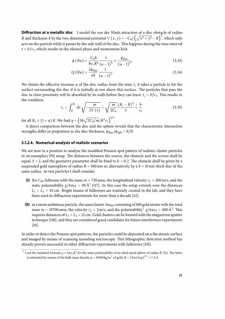
Diªraction at a metallic disc I model the van der Waals attraction of a disc obstacle of radiusR and thickness b by the two-dimensional potential V (x , y) = −C4/ (

√x2 + y2 − R)

4, which only

acts on the particle while it passes by the side wall of the disc.is happens during the time intervalt = b/vz , which results in the eikonal phase and momentum kick

ϕ (Ru) = C4bħvzR4

1(u − 1)4

≡ ϕdisc(u − 1)4

, (3.33)

Q (Ru) = 2ϕdiscπk

1(u − 1)5

. (3.34)

We obtain the eective increase η of the disc radius from the time tc it takes a particle to hit thesurface surrounding the disc if it is initially at rest above this surface. e particles that pass thedisc in close proximity will be absorbed by its walls before they can leave, tc < b/vz .is results inthe condition

tc = ∫ Rc

Rdr

√− m2V (r) =

√m2C4

(Rc − R)3

3!< bvz

(3.35)

for all Rc < (1 + η)R. We nd η = (3b√2C4/m/R3vz)

1/3.

A direct comparison between the disc and the sphere reveals that the characteristic interactionstrengths dier in proportion to the disc thickness, ϕdisc/ϕsph = b/R.

3.1.2.4. Numerical analysis of realistic scenarios

We are now in a position to analyze the modied Poisson spot pattern of realistic cluster particlesin an exemplary PSI setup. e distances between the source, the obstacle and the screen shall beequal, ℓ = 2, and the geometry parameter shall be xed to k = 0.2.e obstacle shall be given by asuspended gold nanosphere of radius R = 500nm or, alternatively, by a b = 10 nm-thick disc of thesame radius. As test particles I shall consider

(I) the C60 fullerene with the massm = 720 amu, the longitudinal velocity vz = 200m/s, and thestatic polarizability χ/4πε0 = 90Å3 [117]. In this case the setup extends over the distancesL1 = L2 = 45 cm. Bright beams of fullerenes are routinely created in the lab, and they havebeen used in diraction experiments for more than a decade [12].

(II) as amore ambitious particle, the nanocluster Au100 consisting of 100 gold atomswith the totalmass m = 19700 amu, the velocity vz = 2m/s, and the polarizability7 χ/4πε0 = 400Å3. isrequires distances of L1 = L2 = 12 cm. Gold clusters can be formedwith themagnetron sputtertechnique [118], and they are considered good candidates for future interference experiments[10].

In order to detect the Poisson spot patterns, the particles could be deposited on a at atomic surfaceand imaged by means of scanning tunneling microscopy. is lithographic detection method hasalready proven successful in other diraction experiments with fullerenes [119].

7 I use the standard formula χ = 4πε0R3 for the static polarizability of an ideal metal sphere of radius R [52].e latteris estimated by means of the bulk mass density ρ = 19300 kg/m3 of gold, R = (3m/4πρ)1/3 ≈ 7.4Å.

81

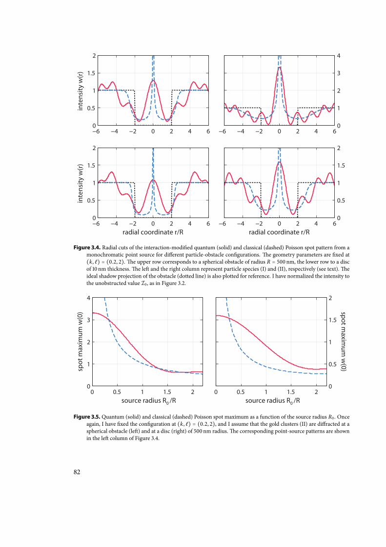
inte

nsity

w(r

)

−6 −4 −2 0 2 4 60

0.5

1

1.5

2

−6 −4 −2 0 2 4 60

1

2

3

4

radial coordinate r/R

inte

nsity

w(r

)

−6 −4 −2 0 2 4 60

0.5

1

1.5

2

radial coordinate r/R−6 −4 −2 0 2 4 6

0

0.5

1

1.5

2

Figure 3.4. Radial cuts of the interaction-modied quantum (solid) and classical (dashed) Poisson spot pattern from amonochromatic point source for dierent particle-obstacle congurations. e geometry parameters are xed at(k, ℓ) = (0.2, 2).e upper row corresponds to a spherical obstacle of radius R = 500nm, the lower row to a discof 10 nm thickness.e le and the right column represent particle species (I) and (II), respectively (see text).eideal shadow projection of the obstacle (dotted line) is also plotted for reference. I have normalized the intensity tothe unobstructed value I0 , as in Figure 3.2.

spot

max

imum

w(0

)

0 0.5 1 1.5 20

1

2

3

4

0 0.5 1 1.5 20

0.5

1

1.5

2

source radius R0 /Rsource radius R0 /R

spot maxim

um w

(0)

Figure 3.5. Quantum (solid) and classical (dashed) Poisson spot maximum as a function of the source radius R0 . Onceagain, I have xed the conguration at (k, ℓ) = (0.2, 2), and I assume that the gold clusters (II) are diracted at aspherical obstacle (le) and at a disc (right) of 500nm radius.e corresponding point-source patterns are shownin the le column of Figure 3.4.

82

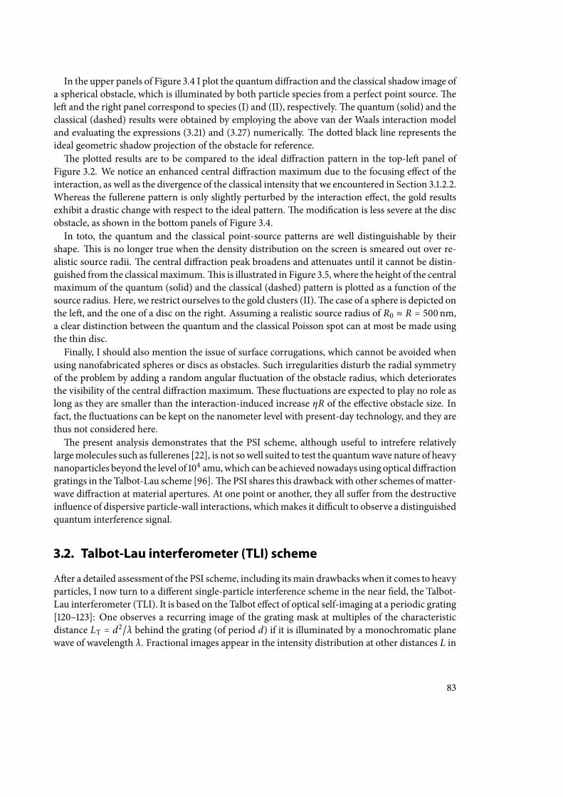
In the upper panels of Figure 3.4 I plot the quantum diraction and the classical shadow image ofa spherical obstacle, which is illuminated by both particle species from a perfect point source.ele and the right panel correspond to species (I) and (II), respectively.e quantum (solid) and theclassical (dashed) results were obtained by employing the above van der Waals interaction modeland evaluating the expressions (3.21) and (3.27) numerically. e dotted black line represents theideal geometric shadow projection of the obstacle for reference.e plotted results are to be compared to the ideal diraction pattern in the top-le panel of

Figure 3.2. We notice an enhanced central diraction maximum due to the focusing eect of theinteraction, as well as the divergence of the classical intensity that we encountered in Section 3.1.2.2.Whereas the fullerene pattern is only slightly perturbed by the interaction eect, the gold resultsexhibit a drastic change with respect to the ideal pattern.e modication is less severe at the discobstacle, as shown in the bottom panels of Figure 3.4.In toto, the quantum and the classical point-source patterns are well distinguishable by their

shape. is is no longer true when the density distribution on the screen is smeared out over re-alistic source radii. e central diraction peak broadens and attenuates until it cannot be distin-guished from the classical maximum.is is illustrated in Figure 3.5, where the height of the centralmaximum of the quantum (solid) and the classical (dashed) pattern is plotted as a function of thesource radius. Here, we restrict ourselves to the gold clusters (II).e case of a sphere is depicted onthe le, and the one of a disc on the right. Assuming a realistic source radius of R0 ≈ R = 500nm,a clear distinction between the quantum and the classical Poisson spot can at most be made usingthe thin disc.Finally, I should also mention the issue of surface corrugations, which cannot be avoided when

using nanofabricated spheres or discs as obstacles. Such irregularities disturb the radial symmetryof the problem by adding a random angular uctuation of the obstacle radius, which deterioratesthe visibility of the central diraction maximum.ese uctuations are expected to play no role aslong as they are smaller than the interaction-induced increase ηR of the eective obstacle size. Infact, the uctuations can be kept on the nanometer level with present-day technology, and they arethus not considered here.e present analysis demonstrates that the PSI scheme, although useful to intrefere relatively

largemolecules such as fullerenes [22], is not sowell suited to test the quantumwave nature of heavynanoparticles beyond the level of 104 amu, which can be achieved nowadays using optical diractiongratings in the Talbot-Lau scheme [96].e PSI shares this drawbackwith other schemes ofmatter-wave diraction at material apertures. At one point or another, they all suer from the destructiveinuence of dispersive particle-wall interactions, whichmakes it dicult to observe a distinguishedquantum interference signal.

3.2. Talbot-Lau interferometer (TLI) scheme

Aer a detailed assessment of the PSI scheme, including itsmain drawbacks when it comes to heavyparticles, I now turn to a dierent single-particle interference scheme in the near eld, the Talbot-Lau interferometer (TLI). It is based on the Talbot eect of optical self-imaging at a periodic grating[120–123]: One observes a recurring image of the grating mask at multiples of the characteristicdistance LT = d2/λ behind the grating (of period d) if it is illuminated by a monochromatic planewave of wavelength λ. Fractional images appear in the intensity distribution at other distances L in

83

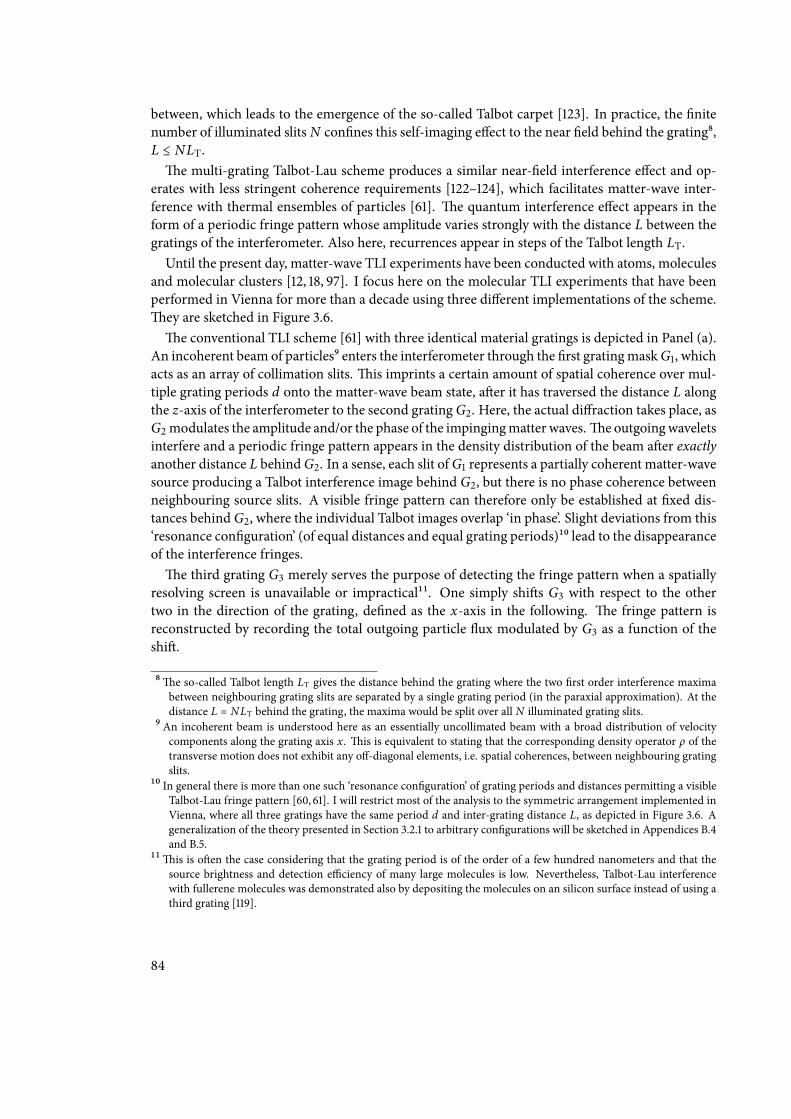
between, which leads to the emergence of the so-called Talbot carpet [123]. In practice, the nitenumber of illuminated slits N connes this self-imaging eect to the near eld behind the grating8,L ≤ NLT.e multi-grating Talbot-Lau scheme produces a similar near-eld interference eect and op-

erates with less stringent coherence requirements [122–124], which facilitates matter-wave inter-ference with thermal ensembles of particles [61]. e quantum interference eect appears in theform of a periodic fringe pattern whose amplitude varies strongly with the distance L between thegratings of the interferometer. Also here, recurrences appear in steps of the Talbot length LT.Until the present day, matter-wave TLI experiments have been conducted with atoms, molecules

and molecular clusters [12, 18, 97]. I focus here on the molecular TLI experiments that have beenperformed in Vienna for more than a decade using three dierent implementations of the scheme.ey are sketched in Figure 3.6.e conventional TLI scheme [61] with three identical material gratings is depicted in Panel (a).

An incoherent beam of particles9 enters the interferometer through the rst gratingmaskG1, whichacts as an array of collimation slits.is imprints a certain amount of spatial coherence over mul-tiple grating periods d onto the matter-wave beam state, aer it has traversed the distance L alongthe z-axis of the interferometer to the second gratingG2. Here, the actual diraction takes place, asG2modulates the amplitude and/or the phase of the impingingmatter waves.e outgoingwaveletsinterfere and a periodic fringe pattern appears in the density distribution of the beam aer exactlyanother distance L behindG2. In a sense, each slit ofG1 represents a partially coherent matter-wavesource producing a Talbot interference image behind G2, but there is no phase coherence betweenneighbouring source slits. A visible fringe pattern can therefore only be established at xed dis-tances behind G2, where the individual Talbot images overlap ‘in phase’. Slight deviations from this‘resonance conguration’ (of equal distances and equal grating periods)10 lead to the disappearanceof the interference fringes.e third grating G3 merely serves the purpose of detecting the fringe pattern when a spatially

resolving screen is unavailable or impractical11. One simply shis G3 with respect to the othertwo in the direction of the grating, dened as the x-axis in the following. e fringe pattern isreconstructed by recording the total outgoing particle ux modulated by G3 as a function of theshi.

8e so-called Talbot length LT gives the distance behind the grating where the two rst order interference maximabetween neighbouring grating slits are separated by a single grating period (in the paraxial approximation). At thedistance L = NLT behind the grating, the maxima would be split over all N illuminated grating slits.

9An incoherent beam is understood here as an essentially uncollimated beam with a broad distribution of velocitycomponents along the grating axis x. is is equivalent to stating that the corresponding density operator ρ of thetransverse motion does not exhibit any o-diagonal elements, i.e. spatial coherences, between neighbouring gratingslits.

10 In general there is more than one such ‘resonance conguration’ of grating periods and distances permitting a visibleTalbot-Lau fringe pattern [60, 61]. I will restrict most of the analysis to the symmetric arrangement implemented inVienna, where all three gratings have the same period d and inter-grating distance L, as depicted in Figure 3.6. Ageneralization of the theory presented in Section 3.2.1 to arbitrary congurations will be sketched in Appendices B.4and B.5.

11is is oen the case considering that the grating period is of the order of a few hundred nanometers and that thesource brightness and detection eciency of many large molecules is low. Nevertheless, Talbot-Lau interferencewith fullerene molecules was demonstrated also by depositing the molecules on an silicon surface instead of using athird grating [119].

84

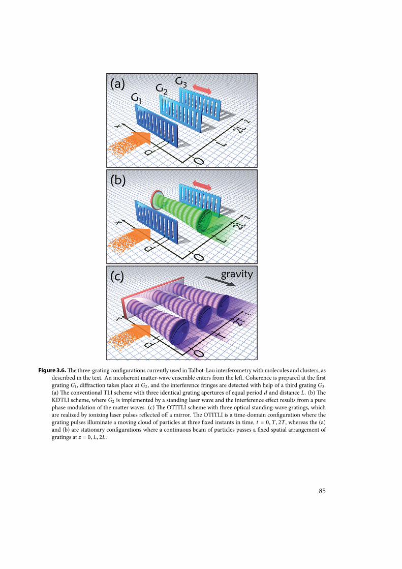
(a)

(b)

(c)

G1

G2

G3

gravity

Figure 3.6. e three-grating congurations currently used in Talbot-Lau interferometry withmolecules and clusters, asdescribed in the text. An incoherent matter-wave ensemble enters from the le. Coherence is prepared at the rstgrating G1 , diraction takes place at G2 , and the interference fringes are detected with help of a third grating G3 .(a)e conventional TLI scheme with three identical grating apertures of equal period d and distance L. (b)eKDTLI scheme, where G2 is implemented by a standing laser wave and the interference eect results from a purephase modulation of the matter waves. (c)e OTITLI scheme with three optical standing-wave gratings, whichare realized by ionizing laser pulses reected o a mirror. e OTITLI is a time-domain conguration where thegrating pulses illuminate a moving cloud of particles at three xed instants in time, t = 0, T , 2T , whereas the (a)and (b) are stationary congurations where a continuous beam of particles passes a xed spatial arrangement ofgratings at z = 0, L, 2L.

85

e TLI is a single-particle near-eld scheme where the dierent diraction orders behind G2overlap in space and interfere to form the fringe pattern, as opposed to, say, a three-grating Mach-Zehnder conguration in the far eld [125] where only a few diraction orders are involved. Twopoints speak in favour of the near-eld scheme. First, the setup requirements are less demanding forhigher masses than in the far eld.e fringe pattern can be observed when the distance betweenthe gratings is at least of the order of the Talbot length, L ≳ LT = md2vz/h, with m and vz the massand the longitudinal velocity of the particles [12]. At xed interferometer length L and growingmassm, the grating period d decreases merely like 1/√mvz , as opposed to a far-eld scheme with linearscaling. Second, unlike in far-eld diraction, there is no need to collimate the initial matter-wavebeam to a transverse momentum spread of less than the grating momentum h/d at the expense ofmost of the signal in order to observe the interference eect.It turns out, however, that the dispersive van der Waals interaction between the particles and

the walls of the second grating introduces a strong and uncontrollable velocity dependence of theinterference fringes [5,102].is is because near-eld interference involves many diraction ordersand is thus more sensitive to distortions of the exact shape and curvature of the diracted matter-wave fronts, which are induced by the van der Waals interaction close the grating walls. Slowerparticles are more strongly aected since they spendmore time in the vicinity of the grating. Hencethe dispersive nature (i.e. velocity dependence) of the interaction eect.For heavy particles a high fringe visibility can be achieved only by means of a narrow velocity

selection at the cost of overall signal [102]. It was found that one could alleviate this problem byreplacing the central grating with a standing laser wave [103], as depicted in Figure 3.6 (b). einterference eect in this Kapitza-Dirac Talbot-Lau Interferometer (KDTLI) scheme is induced bythe pure phase modulation of matter waves at the light grating, rather than by diraction at anaperture.e phase modulation is related to the dispersive dipole interaction of the particles withthe optical eld, which has a weaker velocity dependence and can be controlled by varying the laserpower. We will have a closer look on the KDTLI in Section 3.2.2. It is currently the working-horsesetup in Vienna and it has led to the latest mass records of the order of 104 amu [96].Still, the dispersive nature of such a stationary grating conguration represents a major obstacle

to reaching substantially greater masses, even more so since van der Waals interactions remainpresent in the rst and the third grating. Although the interaction-induced phase modulation ofthematter waves is of no concern atG1 andG3 (since their purpose is to actmerely as a transmissionmask), the attraction to the walls may become so strong that large particles will ultimately stick tothem and clog the grating slits [10]. One could consider making the walls of the grating masksthinner, but then they are more prone to break upon the heavy-particle bombardment.Such problems are alleviated by changing to a pulsed conguration with optical depletion grat-

ings, that is, with standing-wave gratings that remove particles in the matter-wave state at the eldantinodes. Figure 3.6 (c) depicts the current implementation of this scheme, the Optical Time-Domain Ionizing Talbot-Lau Interferometer (OTITLI), which has been applied so far to smallmolecular cluster particles [13]. Here, the gratings are generated by three equally timed vacuum-ultraviolet (VUV) laser pulses reected o a single mirror [10, 104]. Photo-ionizable particles areinjected in the form of dilute clouds ying alongside the mirror surface to the detector; they areexposed to the three grating pulses at xed moments in time, t = 0, T , 2T , irrespectively of theirprecise position and velocity (as opposed to a stationary congurationwhere the timing depends onthe particle velocity vz).e gratingsmodulate both the phase and the amplitude of the illuminated

86

matter waves, as they ionize and remove particles from the ensemble via single-photon absorptionin the eld antinodes. In this way, the standing-wave pulses form absorptive masks, as requiredfor the rst and the third grating. I have presented the working principle of optical depletion orionization gratings already in Chapter 2 on page 18. Here, I will develop a theoretical model of theOTITLI scheme in Section 3.2.3.An important property of the TLI scheme in general is that it admits a classical moiré shadow

eect.at is to say, a fringe patternmay as well appear in a classical hypothetical description of thescheme in terms of ballistic particle trajectories. As they are partially blocked and/or deected bythe grating apertures, a periodic density modulation can occur behind the second grating as well,albeit with a dierent dependence on the inter-grating distance (or particle velocity). erefore,a non-vanishing fringe contrast by itself does not prove that the particles have interfered. As inPoisson’s spot experiment, we must provide both the quantum and the classical model for the TLIand we must compare the results of both models quantitatively with the measured data.

3.2.1. Generic description of the Talbot-Lau scheme

Before discussing the details of the variousmanifestations of the TLI scheme, let me rst present theunderlying theoretical model applicable to all of them. It is based on the one-dimensional phase-space description of generic Talbot-Lau interferometry developed in [40, 59, 60]. e present for-mulation will be done entirely in the time domain, that is, I will describe the eect of the threegratings by quasi-instantaneous state transformations separated by two long stretches of free evo-lution in between [10]. e corresponding time intervals, T1 and T2, will be of the order of theTalbot time,

TT =md2

h. (3.36)

It depends on the particle mass m and on the grating period d. In a stationary TLI setup, wherethe gratings are arranged at xed distances L1,2 on the z-axis, the time intervals depend also onthe longitudinal velocity vz of the particles, T1,2 = L1,2/vz . is can easily be taken into accountin the description by averaging the results over the initial velocity distribution of the matter-waveensemble12. In the following assessment of the dispersive TLI scheme we will always assume (andthe results will be dependent on) a xed velocity parameter vz .e transverse y-coordinate can be omitted, provided that the gratings are suciently extended

along the y-axis and that thematter-wave ensemble is at all times located well within this extension.Generally speaking, I assume here that all particles see the same one-dimensional grating proles,irrespectively of their y-z-position13. Hence, we may work with the one-dimensionalWigner func-tion,

w (x , p) = 12πħ ∫ ds e ips/ħ⟨x −

s2∣ρ∣x + s

2⟩, (3.37)

12is parametric treatment is only allowed in the paraxial limit, where the transverse state of the matter-wave beamremains separable from its longitudinal motion taking place at much larger velocities, and where the gratings actsolely on the transverse part. e same formal limitation applies to the description of Poisson’s spot, as noted inSection 3.1.1. It is automatically fullled in all relevant experiments, where the grating structures are much smaller insize than the required distances between them.

13 In the case of the pulsed OTITLI scheme, this implies that the lasers have a suciently wide beam prole and that theparticle ensemble is well centered in the laser beam during each grating pulse.

87

as given in Appendix A.3.e classical description of the TLI will be given in the same framework,using the classical phase-space distribution f (x , p) instead of the Wigner function.

3.2.1.1. Coherent grating transformation in phase space

e coherent state transformation at each of the short (resp. thin) gratings k = 1, 2, 3, is convention-ally described in terms of a complex transmission function, t(k) (x) = ∣t(k) (x)∣ exp [iϕ(k) (x)],modulating both the amplitude and the phase of the matter waves. I have introduced it in Section2.1.4 on page 18. An incoming wavefunction transforms as ⟨x∣ψ⟩↦ t(k) (x) ⟨x∣ψ⟩.e periodicityof the grating admits a Fourier expansion of the transmission function,

t(k) (x) =∞

∑n=−∞

b(k)n exp(2πinxd

) , (3.38)

which unfolds the grating transformation in momentum space: A momentum eigenstate ∣p⟩ istransformed into a superposition of discrete plane-wave components ∣p+ nh/d⟩ separated by mul-tiples of the elementary grating momentum h/d,

⟨x∣p⟩↦ t(k) (x) ⟨x∣p⟩ =∞

∑n=−∞

b(k)n exp(2πinxd

) ⟨x∣p⟩ =∞

∑n=−∞

b(k)n ⟨x∣p + n hd⟩. (3.39)

Each Fourier component b(k)n corresponds to a dierent order of diraction.e modulus of the transmission function is responsible for the amplitude modulation eect;

its square determines the probability of transmission at each position x. e latter is given by theaperture function, ∣t(k) (x)∣2 = ∑n Θ ( f d/2 − ∣x − nd∣), for material gratings with a slit openingfraction f ∈ (0, 1).e phasemodulation term ϕ(k) (x) is determined in the eikonal approximationby an action integral over the particle-grating interaction potential, Eq. (3.19).is approximationis valid only for short (resp. thin) gratings, where the free transverse evolution of the matter wavescan be neglected during the interaction. We can describe the van der Waals-type interactions withthe walls of a material grating in the same way as done in the PSI case in Section 3.1.2. A detailedmodel for the transmission function of optical standing-wave gratings is presented in the precedingchapter, Section 2.1.4 on page 18. Incoherent modications of the grating transformation will beincluded below.In the phase-space representation, the coherent grating transformation is given by a convolution,

w (x , p) ↦ ∫ dp0 T(k) (x , p − p0)w (x , p0), with T(k) a one-dimensional transmission kernel ofthe same form as the two-dimensional kernel (3.5) in the Poisson-spot case. Let me introduce theTalbot coecients in Fourier space to obtain a convenient Fourier notation of the kernel,

B(k)n (ξ) =

∞

∑j=−∞

b(k)j (b(k)j−n)∗

exp [iπ (n − 2 j) ξ] , (3.40)

T(k) (x , p) =∑j,nexp(2πinx

d) b(k)j (b(k)j−n)

∗

δ [p − ( j − n2) hd]

= 12πħ∑n

exp(2πinxd

) ∫ ds e ips/ħB(k)n ( s

d) . (3.41)

88

e eect of the grating transformation on momentum states in (3.39) is reected in the explicitform of the transmission kernel (3.41), which sums over momentum displacements by multiples ofh/d. Note that the Talbot coecients are 2π-periodic in ξ, and that the Fourier components of thegrating transmission probability ∣t(k) (x)∣2 are given by B(k)

n (0) = B(k)n (2πN).

e classical phase-space transformation has two components, following the same line of argu-ment as in the description of Poisson’s spot in Sections 3.1.1.3 and 3.1.2.2.e rst component is theideal grating transformation, which masks an initial phase-space distribution by the aperture func-tion, f (x , p) ↦ ∣t(k) (x)∣2 f (x , p).is must be complemented a second component, the eikonalmomentum kick, q(k) (x) = ħ∂xϕ(k) (x). It represents the integrated particle-grating force trans-ferred to the classical ensemble, f (x , p)↦ f (x , p − q(k) (x)). Both components can be expandedin a Fourier series.e combined classical transmission kernel reads as

T(k)cl (x , p) = ∣t(k) (x)∣

2δ [p − q(k) (x)] = 1

2πħ∑nexp(2πinx

d) ∫ ds e ips/ħC(k)

n ( sd) ,

C(k)n (ξ) =∑

jB(k)n− j (0) c

(k)j (ξ) , c(k)n (ξ) = 1

d ∫ d/2

−d/2dx exp [−2πinx

d− iξ q

(k) (x) dħ

] .

(3.42)

e classical Talbot coecients C(k)n (ξ) are a convolution of the transmission mask coecients

B(k)n (0) with the eikonal kick coecients c(k)n (ξ). In contrast to the quantum coecients, theclassical ones are not periodic in the argument ξ. What can be said is that the quantum and theclassical Talbot coecients are identical at ξ = 0, where the particle-grating interaction has noinuence, C(k)

n (0) = B(k)n (0).

3.2.1.2. Step-by-step derivation of the Talbot-Lau fringe pattern

With the transmission kernels (3.41) and (3.42) at hand I now derive the Talbot-Lau fringe patternin a unied phase-space framefork; the quantum and classical results can be directly related byinterchanging B(k)

n (ξ)↔ C(k)n (ξ) at each grating.

e initial particle ensemble in front of the rst grating is assumed to be an incoherent mix-ture uniformly distributed over many grating slits14. In other words, the initial state occupies alarge phase-space area with a spatial extension X0 ≫ d and a momentum spread P0 ≫ h/d mak-ing it indistinguishable from a classical mixture of the same size. Introducing the normalized andpositive transverse momentum distribution D (p), the initial Wigner function reads asw0 (x , p) =D (p) /X0, and the passage throughG1 transforms it tow1 (x , p) = ∫ dp0T(1) (x , p − p0)D (p0) /X0.Note that the initial momentum distribution may depend on the longitudinal momentum pz =

mvz of the particle ensemble in a stationary TLI conguration, where the particle beam is char-acterized by a xed divergence angle α = P0/pz [60]. In the pulsed OTITLI scheme, the functionD (p) is given by the marginal of the full three-dimensional momentum distribution µ (p) of theparticle cloud, D (p) = ∫ dpydpzµ (p, py , pz) [10].

14 I disregard any fringe eects related to the nite number of illuminated grating slits. A way to incorporate theseeects is discussed in [59,60] for material grating masks. Here, I will assume an unlimited periodicity of the gratingsthroughout the calculation.

89

e free evolution to G2 is given by a shearing transformation in phase space, see (3.3) for thetwo-dimensional case. Let me add a constant acceleration a acting on the particles along the x-axis. It allows us to include, say, gravity or an external deection eld into the model, and it willlead to an eective shi of the resulting fringe pattern. Free propagation over a time t under theinuence of a then shears and displaces both the quantum and the classical state according to themap w (x , p) ↦ w (x − pt/m + at2/2, p −mat). We arrive at the particle state w3 (x , p) at G3 bysubsequently applying onw1 (x , p) the shearing-displacement rule for the time t = T1, then applyingthe second grating kernel T(2) (x , p), and then another shearing-displacement for t = T2.

w3 (x , p) =1X0 ∫ dp1 T(2) (x − pT2

m+ a2T22 , p − p1 −maT2)

× ∫ dp0 T(1) (x − pT2m

− p1T1m

+ a2(T21 + T22 ) , p1 − p0 −maT1)D (p0) (3.43)

e Talbot-Lau fringe pattern is to appear in the spatial density distribution at G3, which we ob-tain by integrating the w3 (x , p) over the momentum coordinate. Aer plugging in the Fourierexpansions (3.41) of the transmission kernels and a few steps of calculation, we are le with

w3 (x) =1X0∑ℓ,k

D (kT1 + ℓT2TT

d)B(1)k (kT1 + ℓT2

TT)B(2)

ℓ−k (ℓT2TT

)

× exp2πid

[ℓx − ℓ a2(T1 + T2)2 + (ℓ − k) a

2T21 ] . (3.44)

Here, I have introduced the Fourier transform of the momentum distribution (i.e. its characteristicfunction),

D (x) = ∫ dp e−ipx/ħD (p) , (3.45)

which is normalized to D (0) = 1 and whose characteristic width is given by h/P0 ≪ d.

Resonance approximation e sharply peaked function D narrows down the number of indexpairs (ℓ, k) that contribute appreciably to the Fourier sum in (3.44). Non-vanishing contributionscan only come from indices that fulll ∣kT1 + ℓT2∣ ≪ TT.is is always so for the zeroth component,k = ℓ = 0, which represents the constant average particle density transmitted through G1 and G2.Non-zero Fourier indices k, ℓ ≠ 0, which constitute the Talbot-Lau fringe oscillation, are uniquelypaired through the above relation. For each integer ℓ there is at most one integer k fullling theabove condition, if we restrict our attention to the relevant cases where the grating separation is atleast of the order of the Talbot time, T1,2 ≳ TT. Large integers ∣k∣ , ∣ℓ∣ ≫ 1 will hardly contribute tothe signal as the corresponding high-order Talbot coecients are expected to be vanishingly small.A pronounced fringe oscillation, if there is any, can only be due to small values of ∣k∣ and ∣ℓ − k∣.It depends very much on the ratio of grating distances T2/T1 whether such index pairs exist at all,according to the above pairing condition.Let us resort here to the most relevant case in practice, where the distance ratio is close to an

integer, T1 = T and T2 = NT+τ, with ∣τ∣ ≪ TT.emore general case, including also the possibilityof dierent grating periods, is presented in Appendix B.4. We can now simplify the expression(3.44) for the fringe pattern by means of the resonance approximation,

D (kT1 + ℓT2TT

d) ≈ δk,−NℓD ( ℓτTT

d) , (3.46)

90

which explicitly yields the pairing relation k = −Nℓ. We are le with the fringe pattern

w3 (x) =1X0∑ℓD ( ℓτ

TTd)B(1)

−Nℓ (ℓτTT

)B(2)(N+1)ℓ (ℓ

NT + τTT

) exp [2πiℓd

(x + δxa)] . (3.47)

It is eectively shied by the amount

δxa = −aT2

2N (N + 1) − aTτ (N + 1) − aτ2

2(3.48)

due to the acceleration a acting on the particles. Equation (3.47) is a Fourier sum, where each non-vanishing component of order ℓ ≠ 0 contributes to the oscillation amplitude of the fringe pattern.

Detection signal and visibility e fringe pattern is detected in practice bymeasuring the totaltransmitted particle density S (xS) behind the third grating and varying its shi xS with respect tothe other two. Here, in order to obtain S (xS), we must apply the shied transmission kernel of G3on the Wigner function (3.43) and integrate the transformed function over the whole phase space,S (xS) = ∫ dxdpdp0 T(3) (x − xS , p − p0)w3 (x , p0). One can easily check that this boils down toa convolution of the fringe pattern w3 (x) with the transmission probability at the shied grating,

S (xS) = ∫ dx w3 (x) ∣t(3) (x − xS)∣2=∑

ℓSℓ exp [

2πiℓd

(xS + δxa)] ,

Sℓ = D (ℓ τTT

d)B(1)−Nℓ (ℓ

τTT

)B(2)(N+1)ℓ (ℓ

NT + τTT

)B(3)−ℓ (0) . (3.49)

e signal gives the per-particle probability for transmission through the three gratings of the TLI.As follows from its Fourier components, it contains all the fringe amplitudes of w3 (x), multipliedby the Fourier coecients B(3)

−ℓ (0) of the third grating aperture. Hence, the third grating doesnothingmore thanmasking the outgoing particle state; the interaction of the particles withG3 doesnot inuence the signal15. We note that the fringe pattern can also be recorded without moving thethird grating if one is able to vary the deection shi δxa in the external acceleration eld a. eclassical moiré signal is obtained by replacing the Talbot coecients in (3.47) and (3.49) with theirclassical counterparts (3.42).e amplitude of the fringe oscillation exhibited by the positive-valued and periodic signal is

commonly measured in terms of the relative fringe contrast, or visibility,

V = Smax − SminSmax + Smin

. (3.50)

e terms Smin and Smax represent the minimum and the maximum values of the fringe signal, re-spectively. e visibility ranges from zero (no fringes) to a maximum of 100% if the local minimaof the signal are zero, Smin = 0. Oen the fringe oscillation is dominated by the rst Fourier ampli-tude, which results in a near-sinusoidal pattern. e fringe contrast is then well described by the

15is applies only to the interaction-induced phase modulation of the matter waves.e van der Waals attraction stillreduces the eective slit opening of material gratings. Particles in close vicinity to the walls may hit them and willnot be transmitted.

91

sinusoidal visibility,

Vsin = ∣2S1S0

∣ = 2RRRRRRRRRRRRD ( τd

TT)B(1)−N (τ/TT)B(2)

N+1 [(NT + τ) /TT]B(3)−1 (0)

B(1)0 (0)B(2)

0 (0)B(3)0 (0)

RRRRRRRRRRRR. (3.51)

One obtains this value experimentally by tting a sine curve to the recorded signal data. is isthe standard method of analysis in most TLI experiments. Note that Vsin may assume values largerthan 100% if the underlying fringe signal diers from a sinusoidal pattern.We nd that the grating separation time T enters the detected fringe amplitudes (3.49) and the

visibility (3.51) exclusively through the argument of theTalbot coecients (3.41), which are periodic.is explains the periodic revival of interference fringes in unit steps of the Talbot time (3.36),which also constitutes the characteristic mass dependence of the Talbot-Lau interference eect anddistinguishes it from a classical moiré eect.

Resonant and symmetric con®guration In order to observe a signicant fringe contrast inmost realistic settings, the grating asymmetry number N ∈ N in (3.49) and the resonance deviation∣τ∣ ≪ TT must be suciently small. From the visibility expression (3.51) we read that a large asym-metry N implies that the fringe oscillation is generated by high-order Talbot coecients. eseFourier coecients generally fall o rapidly with increasing order, which decreases the maximumachievable contrast to low values.erefore, the symmetric conguration N = 1 is most suitable forall practical purposes where distinct fringes are intended.For the same reason, the time deviation τ is also limited, ∣τ∣ ≲ hTT/P0d = md/P0, due to the

momentum spread P0 of the particle ensemble.e latter typically covers several thousand gratingmomenta in the molecular TLI experiments considered here, in which case we can safely neglectthe inuence of τ on the Talbot coecients and on the fringe shi in (3.49),

Sℓ ≈ D ( ℓτTT

d)B(1)−Nℓ (0)B

(2)(N+1)ℓ (

ℓNTTT

)B(3)−ℓ (0) , δxa ≈ −

aT2

2N (N + 1) . (3.52)

is implies that a resonancemismatch τ ≠ 0mainly diminishes the fringe visibility as it reduces thenon-zero Fourier components of the fringe pattern (3.47) and (3.49) by the factor ∣D (ℓτd/TT)∣ < 1for ℓ ≠ 0. Moreover, the result shows that no fringes would appear if G1 were a pure phase grating,since this would imply ∣t(1) (x)∣2 = 1 and B(1)

n (0) = δn,0. Both G1 and G3 must be amplitudegratings; their phase modulation properties do not enter the result.Let me remark that the situation is dierent if one works with a well-collimated ensemble of

particles, where P0 is of the order of the gratingmomentum h/d. In this case, larger time deviationsτ are permitted, and an o-resonant fringe pattern at τ ≠ 0 may appear even if G1 is a pure phasegrating. Such a transient eect was demonstrated with thermal atom ensembles in standing-wavegratings [62, 126]. Here, we restrict our view to the resonant and symmetric conguration, N = 1and τ = 0, which is best suited to achieve high contrast with incoherent particle ensembles.is hasbeen the standard conguration of all molecular TLI experiments so far.e quantum and classicalfringe signal dier solely by the Talbot coecients of G2,

⎧⎪⎪⎨⎪⎪⎩

S (xS)Scl (xS)

⎫⎪⎪⎬⎪⎪⎭=∑

ℓB(1)−ℓ (0)

⎧⎪⎪⎨⎪⎪⎩

B(2)2ℓ (ℓT/TT)

C(2)2ℓ (ℓT/TT)

⎫⎪⎪⎬⎪⎪⎭B(3)−ℓ (0) exp [2πiℓ

d(xS − aT2)] . (3.53)

92

3.2.1.3. Incoherent eªects and decoherence events

I have now presented a phase-space model for the coherent propagation of matter waves through ageneric TLI scheme. Yet, this will not necessarily suce to describe the Talbot-Lau eect in a real-istic setting. Environmental decoherence and other stochastic processes may aect the coherenceproperties of the state and modify the interference eect depending on the experimental condi-tions. In the following, I distinguish incoherent grating eects and free-space decoherence events.e latter can occur randomly at any time and any place while the particles evolve freely from onegrating to another. e former modify the grating transformation and take on the same periodicspatial dependence.For our purposes it will suce to consider only norm-preserving and stochastic momentum

transfer processes, which are described by state transformations of the form ⟨x∣ρ∣x′⟩ ↦ R (x , x′)⟨x∣ρ∣x′⟩. Such processes randomly redistribute momentum and thus aect the spatial coherenceproperties of the state, but they leave the spatial density distribution invariant,R (x , x) = 1 for allx.e latter follows from norm conservation,

∫ dxR (x , x) ⟨x∣ρ∣x⟩ = ∫ dx ⟨x∣ρ∣x⟩ = 1, (3.54)

which must hold for arbitrary density operators ρ. Explicit forms of the decoherence functionR (x , x′) will be specied later. e corresponding phase-space transformation is given by a mo-mentum convolution,

w (x , p)↦ ∫ dq R (x , q)w (x , p − q) ,

R (x , q) = 12πħ ∫ ds e iqs/ħR(x − s

2, x + s

2) . (3.55)

A phase-space transformation of this type can also be conceived in a purely classical picture: Astochastic process that kicks a particle at position x with a random kick distribution R (x , q) canbe described by the transformation f (x , p) ↦ ∫ dq R (x , q) f (x , p − q). It washes out the mo-mentum distribution of the ensemble state.

Incoherent grating eªects Apart from the coherent modulation of the matter-wave state, eachgrating Gk may also contribute an incoherent processR(k) (x , x′) if it couples to internal degreesof freedom of the particles in an uncontrollable manner.e absorption and the elastic scatteringof single photons from an optical standing-wave grating are the most important processes, whichwill be of relevance. I have elaborated on the corresponding decoherence functions,Rabs,sca (x , x′),in the context of the light-matter interaction in Section 2.1.4.3, see Eqs. (2.48) and (2.50) on page24f.e periodicity of the grating implies that the decoherence function is periodic in both x andx′, too. Hence, we can perform a Fourier expansion with respect to (x + x′) /2,

R(k) (x , x′) =∞

∑n=−∞

R(k)n (x

′ − xd

) exp [2πind

(x + x′

2)] ,

R(k)n (ξ) = 1

d ∫ d/2

−d/2dxR(k) (x − ξd

2, x + ξd

2) exp(−2πinx

d) , (3.56)

93

where R(k)n (0) = δn,0. Putting the coherent and the incoherent part together yields a double convo-

lution of theWigner function with the coherent transmission kernel T(k) (x , p) and the incoherentkernel R(k) (x , p), which can be subsumed under the modied grating kernel,

T(k) (x , p) = ∫ dq R(k) (x , p − q)T(k) (x , q)

= 12πħ∑n

exp(2πinxd

) ∫ ds e ips/ħ∑jB(k)n− j (

sd)R(k)

j ( sd) . (3.57)

We obtain the modied fringe pattern if we replace the quantum and classical Talbot coecientsby the modied versions,

B(k)n (ξ) =∑

jB(k)n− j (ξ)R(k)

j (ξ) , C(k)n (ξ) =∑

jC(k)n− j (ξ)R(k)

j (ξ) . (3.58)

Here, I implicitly assume that R(k) can be interpreted as amomentum averaging process that wouldact on a classical particle ensemble in the same way as it acts on a quantum state in phase space.We notice that the value of the Talbot coecients at ξ = 0 remains unchanged, B(k)

n (0) =B(k)n (0).e incoherent modication is therefore only relevant at the second grating, k = 2, wherethe spatial coherence properties (themomentum structure) of the particle state aect the nal fringesignal (3.53).

Free-space decoherence events e other important class of incoherent modications of theTalbot-Lau eect are free-space events thatmay occur uniformly during the propagation time.eyinclude, for instance, environmental decoherence by gas collisions, or by the absorption, emission,and scattering of thermal photons. Moreover, they can be employed in metrological applications,where such events are evoked on purpose to manipulate the fringe contrast in a controlled way. Iwill discuss the example of absorption spectrocopy in Section 3.3.Let us consider a single decoherence event R occuring at a time t ∈ [−T1, T2] before or aer

the second grating. If we assume that the underlying process is uniform in space, then the statetransformation will not depend on the position of each ensemble particle, R (x , x′) = R (x′ − x)and R (x , p) = R (p) in (3.55). is momentum averaging transformation must be inserted atthe right moment into the phase-space scheme that has led us to the Wigner function (3.43) andto the fringe pattern w3 (x) at G3. I do this explicitly for the general case in Appendix B.5. Here,the discussion is restricted to the resonant symmetric conguration where the fringe pattern iseectively smeared out by the kick distribution, w3 (x) = ∫ dq R (q)w3 [x − q (T − ∣t∣) /m], asfollows from (B.25).e form of the equation implies that the averaging eect is most severe if theevent occurs directly at the second grating, t = 0, and it does not depend on whether the eventtakes place before or aer G2. e modulated Fourier components of the detection signal (and ofthe fringe pattern) read as

Sℓ =R(ℓd T − ∣t∣TT

) Sℓ . (3.59)

Environmental decoherence can be understood as a random series of such events that may occuruniformly at all times t. One can establish a time-dependent rate equation based on the individualevent transformation (3.59) and solve it to obtain the mean overall contrast reduction by decoher-ence [40].

94

3.2.2. The Kapitza-Dirac Talbot-Lau interferometer (KDTLI)

Letme illustrate the just developed phase-spacemodel by discussing the basic features of theKDTLIsetup, Figure 3.6 (b), as currently operated in Vienna in measurements on large organic molecules.It replaces the former TLI setup with three material gratings, which had become obsolete due to thegrowing highly dispersive van der Waals interaction between the molecules and the grating walls.On the theoretical side, the beauty of the KDTLI scheme lies in the fact that it can be assessed inanalytic terms.e Vienna KDTLI is a horizontal grating arrangement, where G2 is a standing wave of period

d = λ/2 = 266nm, as generated in the focus of a green laser of wavelength λ illuminating a mirror.e other gratings are material masks of the same period with an opening fraction f ≲ 0.5. egrating distance is set to L = 10.5 cm, and the corresponding time T varies with the velocity of theinterfered particle species.Normally, there is no external acceleration acting on the particles, a = 0, that would shi the

nal fringe pattern16. For metrological applications, however, a static electric eld E can be appliedbetween two electrodes, which deects the particles on their way from G1 to G2 and shis the in-terference fringe pattern by the same amount. e deection is proportional to the dipole force,Fx = χ (0) ∂x ∣E∣2 /2, that acts on the particle while it passes the electrodes.e interference fringepattern allows one to resolve the deection on the sub-micrometer level and, therefore, to measurethe static electric polarizability χ (0) of the particles at high precision [105, 106, 117, 127, 128].

3.2.2.1. Coherent description

I will now give an overview of the theoretical description of the KDTL interference eect in theabsence of free-space Rayleigh scattering and absorption at the grating. An exhaustive treatmentcan also be found in [7]. e results will be required in the subsequent modication of the eectdue to single-photon absorption, drawing from the results of Chapter 2, page 18. ere, I havedeveloped a detailed description of the optical grating interaction.According to Section 2.1.4.1, the transmision function of a pure standing-wave phase grating can

be written as t(2) (x) = exp (iϕ0 cos2 kx), with k = 2π/λ = π/d the wave number of the laser andϕ0 the eikonal phase factor (2.39) dened on page 21.e latter is related to the dipole interactionwith the laser eld; it is proportional to the polarizability of the particle, the laser power, and theinverse of the longitudinal velocity vz . e d-periodic transmission function can be expanded asa Fourier sum of Bessel functions [113], Equation (3.38) with b(2)n = in exp (iϕ0/2) Jn (ϕ0/2). eassociated Talbot coecients (3.40) are obtained with help of Graf ’s addition theorem for Besselfunctions [113]. It states that

[u − v exp (−iφ)u − v exp (iφ) ]

±n/2

Jn (w) =∞

∑j=−∞

J j+n (u) J j (v) e±i jφ , (3.60)

where φ ∈ [0, π] without loss of generality. (e sign change allows for larger phase angles φ.)eterm w =

√u2 + v2 − 2uv cosφ = u

√1 + (v/u)2 − 2v cosφ/u is the analytic continuation of the

positive root, w → +u, in the limit v → 0.

16 Inertial forces such as the Coriolis force can be safely neglected in the velocity and mass regime considered so far.

95

In the present case, we have u = v = ϕ0/2 and φ = 2πξ, which leads to the Talbot coecients

B(2)n (ξ) = ine iπnξ∑

jJ j (

ϕ02) J∗j−n (

ϕ02) e−2πi jξ = Jn (ϕ0 sin πξ) . (3.61)

We immediately nd that B(2)n (N) = δn,0 for N ∈ N0, as expected from a pure phase grating. e

classical Talbot coecients are obtained from (3.42), using the eikonal momentum kick expressionq(2) (x) = − (πħ/d) sin 2πx/d [7].is yields

C(2)n (ξ) = c(2)n (ξ) = Jn (ϕ0πξ) . (3.62)

e rst and the third gratings are given by a periodic mask of material slit apertures, ∣t(1,3) (x)∣2 =∑n Θ ( f1,3d/2 − ∣x − nd∣), with the slit opening fractions f1,3. eir Fourier coecients read asB(1,3)n (0) = f1,3sinc (πn f1,3).is leaves us with the quantum and classical Fourier components ofthe detection signal,

⎧⎪⎪⎨⎪⎪⎩

S (xS)Scl (xS)

⎫⎪⎪⎬⎪⎪⎭=∑

ℓf1 f3sinc (πℓ f1) sinc (πℓ f3)

⎧⎪⎪⎨⎪⎪⎩

J2ℓ (ϕ0 sin πℓT/TT)J2ℓ (ϕ0πℓT/TT)

⎫⎪⎪⎬⎪⎪⎭exp(2πiℓxS

d) . (3.63)

It depends on the longitudinal particle velocities through ϕ0 and T = L/vz , and it must be averagedover a realistic vz-distributionwhen comparing it to experimental data. We notice that the quantumand the classical expression converge in the quasi-classical limit, vz →∞, or T/TT ≪ 1.e sinusoidal visibilities (3.51) read as

⎧⎪⎪⎨⎪⎪⎩

VsinVclsin

⎫⎪⎪⎬⎪⎪⎭= 2

RRRRRRRRRRRsinc (π f1) sinc (π f3)

⎧⎪⎪⎨⎪⎪⎩

J2 (ϕ0 sin πT/TT)J2 (ϕ0πT/TT)

⎫⎪⎪⎬⎪⎪⎭

RRRRRRRRRRR. (3.64)

e fringe contrast vanishes at T = 0 in both cases. However, only the quantum interference signalexhibits a periodic revival of this zero in visibility at integer multiples of the Talbot time. isis where the phase modulation at G2 cancels, and where a Talbot-Lau fringe pattern mimics theideal shadow projection of the aperture, as in the case of the ideal Talbot eect. A pure phasegrating cannot produce any interference fringes there, whereas the classical model may lead tovisible fringes due to the deection of the particle trajectories in the standing-wave eld. At thesame time, the achievable shadow fringe contrast decreases with growing grating separation T asthe oscillation amplitude of the Bessel function converges to zero.e sinusoidal visibility is largestwhen the Bessel function J2 (x) assumes its maximum, max J2 (x) ≈ 0.49, at x ≈ ±3.05. Fixingthe grating phase shi at ϕ0 ≳ π, this can only be reached at a single time T < TT in the classicalcase, whereas it appears repeatedly for periodic T-values between two subsequent Talbot ordersin the quantum case. e quantum nature of the fringe pattern can thus be easily veried in theexperiment by varying the grating distance L or the particle velocity vz .

3.2.2.2. Modi®cation due to the absorption of grating photons

e coherent description of the KDTLI is only valid for subwavelength particles with negligibleabsorption and Rayleigh scattering cross sections, that is, if the mean number of absorbed and

96

scattered grating photons n0,sca ≪ 1. See Eqs. (2.42) on page 23 and (2.50) on page 25 for a denitionof these terms.is limit can be appropriate for the assessment of experiments with a subset of non-absorbing molecules, such as the C60-fullerene. But there are other examples, such as C70, wherethe absorption of single photons does inuence the interference contrast noticeably [7]. On theother hand, Rayleigh scattering has not yet been an issue since all particles used so far were ordersof magnitude smaller than the grating wavelength.I have layed out everything necessary to incorporate the inuence of absorption and scattering

on the overall grating transformation in a few steps of calculation. e combined decoherencefunction, R(2) (x , x′) = Rabs (x , x′)Rsca (x , x′), consists of the absorption term (2.48) and thescattering term (2.50), which were obtained by solving the associated master equations in Section2.1.4.3.e coecients of the Fourier expansion (3.56) can be given explicitly in terms of modiedBessel functions [113] aer applying a few trigonometric identities,

R(2)n (ξ) = exp−n0

1 − cos πξ2

− nsca2

[1 − 3 cos πξ sin πξ − j1 (πξ)2πξ

]

× In n01 − cos πξ2

+ nsca2

[3sin πξ − j1 (πξ)2πξ

− cos πξ] . (3.65)

With this we arrive at the modied quantum and classical Talbot coecients (3.58) that includeboth eects.Let us now restrict to the point-particle limit where no free-space scattering takes place in the

grating, nsca ≈ 0. We can apply Graf ’s addition theorem (3.60) another time17 to obtain an explicitform of the modied Talbot coecients,

B(2)n (ξ) = e−ζabs(ξ) [ ζcoh (ξ) + ζabs (ξ)

ζcoh (ξ) − ζabs (ξ)]n/2

Jn [sgnζcoh (ξ) − ζabs (ξ)√

ζ2coh (ξ) − ζ2abs (ξ)] ,

(3.66)with ζcoh (ξ) = ϕ0 sin πξ and ζabs (ξ) = n0 sin2 (πξ/2) = βϕ0 (1 − cos πξ).e modied sinusoidalvisibility reads as

Vsin = 2 ∣sinc (π f1) sinc (π f3)∣ expβϕ0 [cos(πTTT

) − 1]

×RRRRRRRRRRRR

β + sin (πT/TT) − β cos (πT/TT)β − sin (πT/TT) − β cos (πT/TT)

J2⎡⎢⎢⎢⎢⎣ϕ0

√sin2 (πT

TT) − 4β2 sin4 ( πT

2TT)⎤⎥⎥⎥⎥⎦

RRRRRRRRRRRR. (3.67)

Both ϕ0 and n0 are controlled by the laser power. In order to mimic this dependence, it will beconvenient to introduce the parameter

β = n02ϕ0

= σabsλε02πReχ = σabsd

4π2α, (3.68)

17Here, we make use of the specic formulation [7]

[u − vu + v

]n/2

J−n [sgn (u + v)√u2 − v2] =

∞

∑j=−∞

J j (u) I j+n (v)

for u, v ∈ R, u ≠ v. It can be derived from the general form (3.60) using the relation In (v) = (−i)n Jn (iv).

97

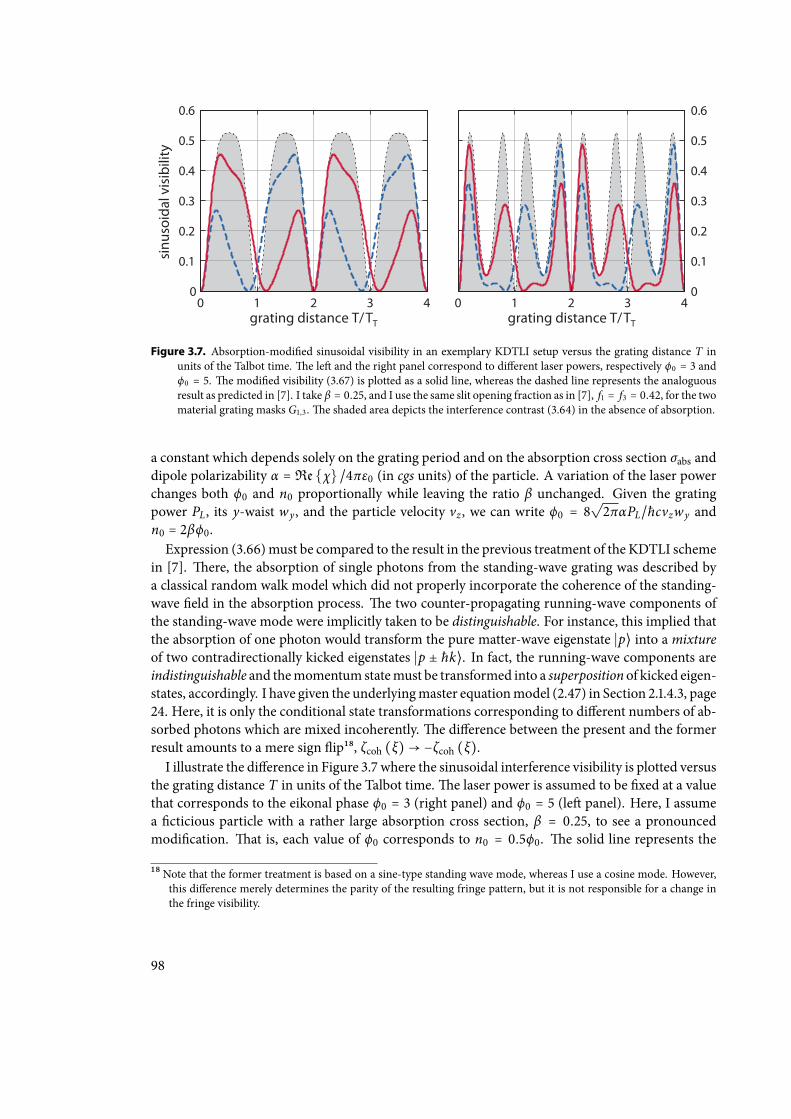
grating distance T/ TT

sinu

soid

al v

isib

ility

0 1 2 3 40

0.1

0.2

0.3

0.4

0.5

0.6

0 1 2 3 40

0.1

0.2

0.3

0.4

0.5

0.6

grating distance T/ TT

Figure 3.7. Absorption-modied sinusoidal visibility in an exemplary KDTLI setup versus the grating distance T inunits of the Talbot time.e le and the right panel correspond to dierent laser powers, respectively ϕ0 = 3 andϕ0 = 5. e modied visibility (3.67) is plotted as a solid line, whereas the dashed line represents the analoguousresult as predicted in [7]. I take β = 0.25, and I use the same slit opening fraction as in [7], f1 = f3 = 0.42, for the twomaterial grating masks G1,3 .e shaded area depicts the interference contrast (3.64) in the absence of absorption.

a constant which depends solely on the grating period and on the absorption cross section σabs anddipole polarizability α = Reχ /4πε0 (in cgs units) of the particle. A variation of the laser powerchanges both ϕ0 and n0 proportionally while leaving the ratio β unchanged. Given the gratingpower PL, its y-waist wy, and the particle velocity vz , we can write ϕ0 = 8

√2παPL/ħcvzwy and

n0 = 2βϕ0.Expression (3.66)must be compared to the result in the previous treatment of the KDTLI scheme

in [7]. ere, the absorption of single photons from the standing-wave grating was described bya classical random walk model which did not properly incorporate the coherence of the standing-wave eld in the absorption process. e two counter-propagating running-wave components ofthe standing-wave mode were implicitly taken to be distinguishable. For instance, this implied thatthe absorption of one photon would transform the pure matter-wave eigenstate ∣p⟩ into a mixtureof two contradirectionally kicked eigenstates ∣p ± ħk⟩. In fact, the running-wave components areindistinguishable and themomentum statemust be transformed into a superposition of kicked eigen-states, accordingly. I have given the underlyingmaster equationmodel (2.47) in Section 2.1.4.3, page24. Here, it is only the conditional state transformations corresponding to dierent numbers of ab-sorbed photons which are mixed incoherently.e dierence between the present and the formerresult amounts to a mere sign ip18, ζcoh (ξ)→ −ζcoh (ξ).I illustrate the dierence in Figure 3.7 where the sinusoidal interference visibility is plotted versus

the grating distance T in units of the Talbot time.e laser power is assumed to be xed at a valuethat corresponds to the eikonal phase ϕ0 = 3 (right panel) and ϕ0 = 5 (le panel). Here, I assumea cticious particle with a rather large absorption cross section, β = 0.25, to see a pronouncedmodication. at is, each value of ϕ0 corresponds to n0 = 0.5ϕ0. e solid line represents the

18Note that the former treatment is based on a sine-type standing wave mode, whereas I use a cosine mode. However,this dierence merely determines the parity of the resulting fringe pattern, but it is not responsible for a change inthe fringe visibility.

98

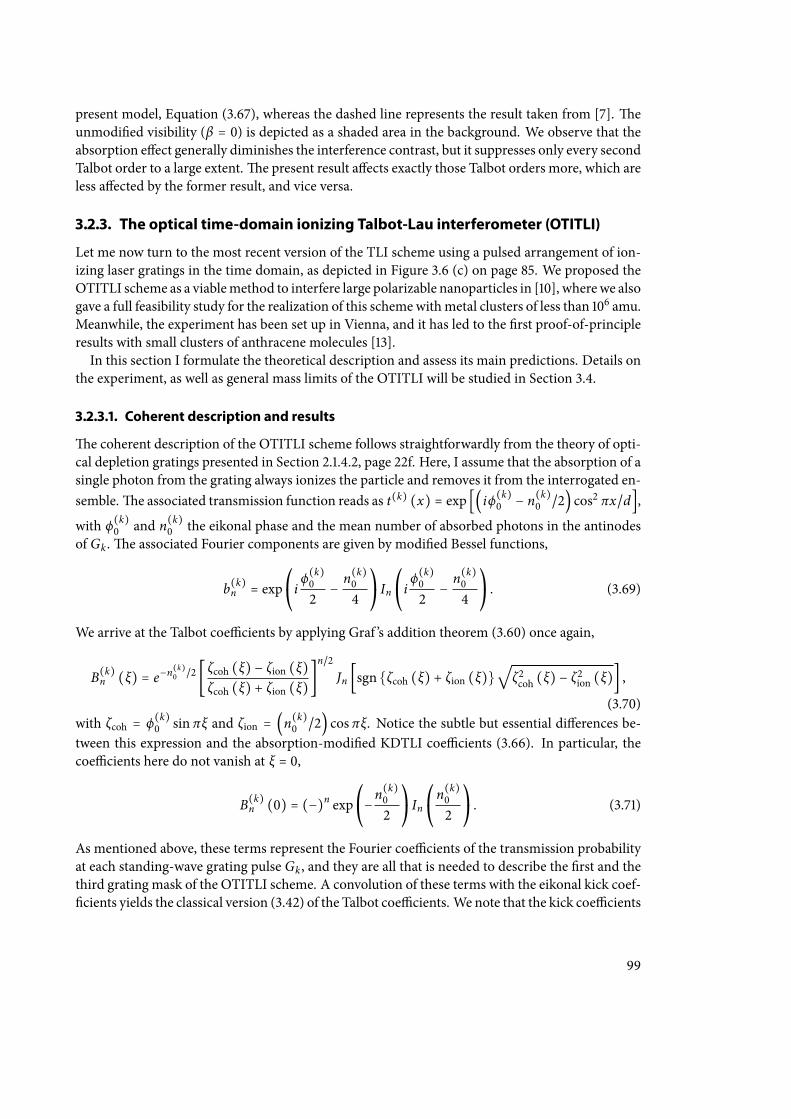
present model, Equation (3.67), whereas the dashed line represents the result taken from [7]. eunmodied visibility (β = 0) is depicted as a shaded area in the background. We observe that theabsorption eect generally diminishes the interference contrast, but it suppresses only every secondTalbot order to a large extent.e present result aects exactly those Talbot orders more, which areless aected by the former result, and vice versa.

3.2.3. The optical time-domain ionizing Talbot-Lau interferometer (OTITLI)

Let me now turn to the most recent version of the TLI scheme using a pulsed arrangement of ion-izing laser gratings in the time domain, as depicted in Figure 3.6 (c) on page 85. We proposed theOTITLI scheme as a viablemethod to interfere large polarizable nanoparticles in [10], wherewe alsogave a full feasibility study for the realization of this schemewithmetal clusters of less than 106 amu.Meanwhile, the experiment has been set up in Vienna, and it has led to the rst proof-of-principleresults with small clusters of anthracene molecules [13].In this section I formulate the theoretical description and assess its main predictions. Details on

the experiment, as well as general mass limits of the OTITLI will be studied in Section 3.4.

3.2.3.1. Coherent description and results

e coherent description of the OTITLI scheme follows straightforwardly from the theory of opti-cal depletion gratings presented in Section 2.1.4.2, page 22f. Here, I assume that the absorption of asingle photon from the grating always ionizes the particle and removes it from the interrogated en-semble.e associated transmission function reads as t(k) (x) = exp [(iϕ(k)

0 − n(k)0 /2) cos2 πx/d],

with ϕ(k)0 and n(k)

0 the eikonal phase and the mean number of absorbed photons in the antinodesof Gk .e associated Fourier components are given by modied Bessel functions,

b(k)n = exp⎛⎝iϕ(k)02

−n(k)04

⎞⎠In

⎛⎝iϕ(k)02

−n(k)04

⎞⎠. (3.69)

We arrive at the Talbot coecients by applying Graf ’s addition theorem (3.60) once again,

B(k)n (ξ) = e−n

(k)0 /2 [ ζcoh (ξ) − ζion (ξ)

ζcoh (ξ) + ζion (ξ)]n/2

Jn [sgnζcoh (ξ) + ζion (ξ)√

ζ2coh (ξ) − ζ2ion (ξ)] ,

(3.70)with ζcoh = ϕ(k)

0 sin πξ and ζion = (n(k)0 /2) cos πξ. Notice the subtle but essential dierences be-

tween this expression and the absorption-modied KDTLI coecients (3.66). In particular, thecoecients here do not vanish at ξ = 0,

B(k)n (0) = (−)n exp

⎛⎝−n(k)02

⎞⎠In

⎛⎝n(k)02

⎞⎠. (3.71)

As mentioned above, these terms represent the Fourier coecients of the transmission probabilityat each standing-wave grating pulse Gk , and they are all that is needed to describe the rst and thethird grating mask of the OTITLI scheme. A convolution of these terms with the eikonal kick coef-cients yields the classical version (3.42) of the Talbot coecients. We note that the kick coecients

99

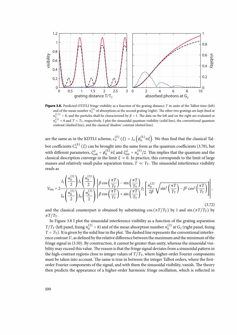
visi

bilit

y

0 0.5 1 1.5 2 2.5 30

0.2

0.4

0.6

0.8

1

1.2

absorbed photons at G2

0 2 4 6 8 100

0.2

0.4

0.6

0.8

1

grating distance T/ TT

visibility

Figure 3.8. Predicted OTITLI fringe visibility as a function of the grating distance T in units of the Talbot time (le)and of the mean number n(2)

0 of absorptions at the second grating (right).e other two gratings are kept xed atn(1,3)0 = 8, and the particles shall be characterized by β = 1. e data on the le and on the right are evaluated at

n(2)0 = 8 and T = TT , respectively. I plot the sinusoidal quantum visibility (solid line), the conventional quantumcontrast (dashed line), and the classical ‘shadow’ contrast (dotted line).

are the same as in the KDTLI scheme, c(k)n (ξ) = Jn (ϕ(k)0 πξ). We thus nd that the classical Tal-

bot coecients C(k)n (ξ) can be brought into the same form as the quantum coecients (3.70), but

with dierent parameters, ζclcoh = ϕ(k)0 πξ and ζclion = n(k)

0 /2.is implies that the quantum and theclassical description converge in the limit ξ → 0. In practice, this corresponds to the limit of largemasses and relatively small pulse separation times, T ≪ TT. e sinusoidal interference visibilityreads as

Vsin = 2I1⎛⎝n(1)02

⎞⎠I1⎛⎝n(3)02

⎞⎠

I0⎛⎝n(1)02

⎞⎠I0

⎛⎝n(3)02

⎞⎠

RRRRRRRRRRRRRRRRRR

β cos(πTTT

) − sin(πTTT

)

β cos(πTTT

) + sin(πTTT

)J2

⎡⎢⎢⎢⎢⎣

n(2)02β

√sin2 (πT

TT) − β2 cos2 (πT

TT)⎤⎥⎥⎥⎥⎦

RRRRRRRRRRRRRRRRRR

,

(3.72)and the classical counterpart is obtained by substituting cos (πT/TT) by 1 and sin (πT/TT) byπT/TT.In Figure 3.8 I plot the sinusoidal interference visibility as a function of the grating separation

T/TT (le panel, xing n(2)0 = 8) and of the mean absorption number n(2)

0 atG2 (right panel, xingT = TT). It is given by the solid line in the plot.e dashed line represents the conventional interfer-ence contrastV , as dened by the relative dierence between themaximumand theminimumof thefringe signal in (3.50). By construction, it cannot be greater than unity, whereas the sinusoidal visi-bilitymay exceed this value.e reason is that the fringe signal deviates from a sinusoidal pattern inthe high-contrast regions close to integer values of T/TT, where higher-order Fourier componentsmust be taken into account.e same is true in between the integer Talbot orders, where the rst-order Fourier components of the signal, and with them the sinusoidal visibility, vanish.e theorythen predicts the appearance of a higher-order harmonic fringe oscillation, which is reected in

100

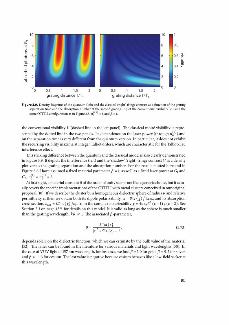
0 0.5 1 1.5 20

2

4

6

8

10

0 0.5 1 1.5 20

0.2

0.4

0.6

0.8

1

grating distance T/ TT grating distance T/ TT

abso

rbed

pho

tons

at G

2

0

2

4

6

8

10

visibility

Figure 3.9. Density diagrams of the quantum (le) and the classical (right) fringe contrast as a function of the gratingseparation time and the absorption number at the second grating. I plot the conventional visibility V using thesame OTITLI conguration as in Figure 3.8, n(1,3)

0 = 8 and β = 1.

the conventional visibility V (dashed line in the le panel). e classical moiré visibility is repre-sented by the dotted line in the two panels. Its dependence on the laser power (through n(2)

0 ) andon the separation time is very dierent from the quantum version. In particular, it does not exhibitthe recurring visibility maxima at integer Talbot orders, which are characteristic for the Talbot-Lauinterference eect.is striking dierence between the quantum and the classicalmodel is also clearly demonstrated

in Figure 3.9. It depicts the interference (le) and the ‘shadow’ (right) fringe contrast V as a densityplot versus the grating separation and the absorption number. For the results plotted here and inFigure 3.8 I have assumed a xed material parameter β = 1, as well as a xed laser power at G1 andG3, n(1)

0 = n(3)0 = 8.

At rst sight, amaterial constant β of the order of unity seems not like a generic choice, but it actu-ally covers the specic implementations of theOTITLI withmetal clusters conceived in our originalproposal [10]. If we describe the cluster by a homogeneous dielectric sphere of radius R and relativepermittivity ε, then we obtain both its dipole polarizability, α = Reχ /4πε0, and its absorptioncross section, σabs = kImχ /ε0, from the complex polarizability χ = 4πε0R3 (ε − 1) / (ε + 2). SeeSection 2.3 on page 48. for details on this model. It is valid as long as the sphere is much smallerthan the grating wavelength, kR ≪ 1.e associated β-parameter,

β = 3Imε∣ε∣2 +Reε − 2

, (3.73)

depends solely on the dielectric function, which we can estimate by the bulk value of the material[52]. e latter can be found in the literature for various materials and light wavelengths [50]. Inthe case of VUV light of 157 nm wavelength, for instance, we nd β = 1.0 for gold, β = 9.2 for silver,and β = −1.3 for cesium.e last value is negative because cesium behaves like a low-eld seeker atthis wavelength.

101

sinu

soid

al v

isib

ility

0 0.25 0.5 0.75 1 1.25 1.50

0.2

0.4

0.6

0.8

1

1.2

grating distance T/ TT

Figure 3.10. Sinusoidal interference visibility for dierent particles versus the grating distance in units of the Talbottime.e solid, the dashed and the dotted line are associated to particle species with β-values of 1.0, −1.3 and 9.2,respectively (see text).e three laser gratings are always set to the same absorption number, n(1,2,3)

0 = 8.

e three exemplary cases are compared in a visibility-versus-time plot in Figure 3.10.e solidline (β = 1.0) is a part of the respective curve in the le panel of Figure 3.8, whereas the dashedand the dotted lines correspond to the cesium (β = −1.3) and the silver (β = 9.2) case. All otherparameters are xed at the same values as before, n(1,2,3)

0 = 8. We observe that small values of∣β∣ shi the visibility maximum further away from integer multiples of the Talbot time than largevalues.e reason lies in the growing inuence of the coherent phase modulation at the grating thesmaller the magnitude of β.

Last but not least, the fringe contrast is also varied by tuning the laser power of the rst and thethird grating.e solid line in the le panel of Figure 3.11 shows how the sinusoidal visibility growsas the increasing absorption number n(3)

0 shrinks the eective aperture of transmission through thenodes of the third gratingmask.e right panel plots the associated overall transmission probabilitythrough the interferometer on a logarithmic scale. It is given by the zeroth Fourier coecient ofthe fringe signal, S0 = B(1)

0 (0)B(2)0 (0)B(3)

0 (0), and the plot looks the same no matter whether thepower of the rst, the second or the third grating is varied. Here, we vary only n(3)

0 , keeping theother gratings xed at n(1,2)

0 = 8, and setting T = TT and β = 1.

e dashed line shows the predicted visibility and transmission in an inverted detection scheme,where the recorded OTITLI fringe signal is not comprised of the neutral particles transmitted, butof the particles ionized at the third grating.is may be useful to facilitate the detection of particlesbehindG3 as it allows one to dispense with the ionization stage in conventionalmass spectrometers.e inverted grating is straightforwardly incorporated into the theoretical model by inverting thetransmission probability, ∣t(3) (x)∣2 ↦ 1 − ∣t(3) (x)∣2. is results in a change of the associatedFourier coecients, B(3)

n (0)↦ δn,0−B(3)n (0). In this case we nd that the transmissivity increases

with growing laser power since a larger fraction of the particle cloud is ionized atG3. However, thiscomes at the price of an overall reduction of visibility, because the antinodes of an inverted grating

102

sinu

soid

al v

isib

ility

0 2 4 6 8 100

0.2

0.4

0.6

0.8

1

transmission

0 2 4 6 8 10.001

0.01

0.1

absorbed photons at G3 absorbed photons at G3

Figure 3.11. Inuence of a varying power of the third grating laser on the sinusoidal interference visibility (le) and onthe transmission probability through the interferometer (right).e laser power is given in terms of the absorbedphoton number n(3)

0 .e other parameters are xed at the reference values of the preceding diagrams, n(1,2)0 = 8,

T = TT and β = 1. e dashed line corresponds to the inverted conguration, where the ionized particles aredetected behind G3 instead of the neutrally transmitted ones.

mimic an aperture with a broader eective slit width than the nodes of a conventional ionizationgrating.

3.2.3.2. Incoherent modi®cation due to Rayleigh scattering

Judging from the concrete predictions of the coherent model I have just assessed in detail, the OTI-TLI scheme appears to be the most promising implementation of the Talbot-Lau eect with heavyparticles. It oers full and exible control over all relevant setup parameters, while avoidingmost ofthe limitations associated to a stationary TLI conguration (with material grating masks). On theother hand, one incurs additional decoherence eects by employing optical gratings, which mayrestrict the scope of the interferometer to a limited range of particle species. We have observed inSection 3.2.2.2 how the interference visibility in the KDTLI scheme is diminished for particles withlarge absorption cross sections.Here, photon absorption, if it is always accompanied by ionization, is an explicit prerequisite

for the ionization gratings to work, and radiative decoherence may only arise due to the elasticscattering of grating photons into free space.e Fourier coecients R(2)

n (ξ) of the scattering de-coherence function can be taken from Equation (3.65), which describes the combined decoherenceeect of scattering and absorption in a pure phase grating. Setting the absorption number n0 = 0in that expression leaves us with the mere scattering eect,

R(2)n (ξ) = exp

⎧⎪⎪⎨⎪⎪⎩

n(2)sca2

[3 cos πξ sin πξ − j1 (πξ)2πξ

− 1]⎫⎪⎪⎬⎪⎪⎭In

⎧⎪⎪⎨⎪⎪⎩

n(2)sca2

[3sin πξ − j1 (πξ)2πξ

− cos πξ]⎫⎪⎪⎬⎪⎪⎭.

(3.74)e modied Talbot coecients of the second grating are then given by the convolution (3.58) ofthese coecients with the coherent Talbot coecients (3.70).e modication inuences neitherthe rst nor the third grating mask since R(1,3)

n (0) = δn,0, as already noted above.

103

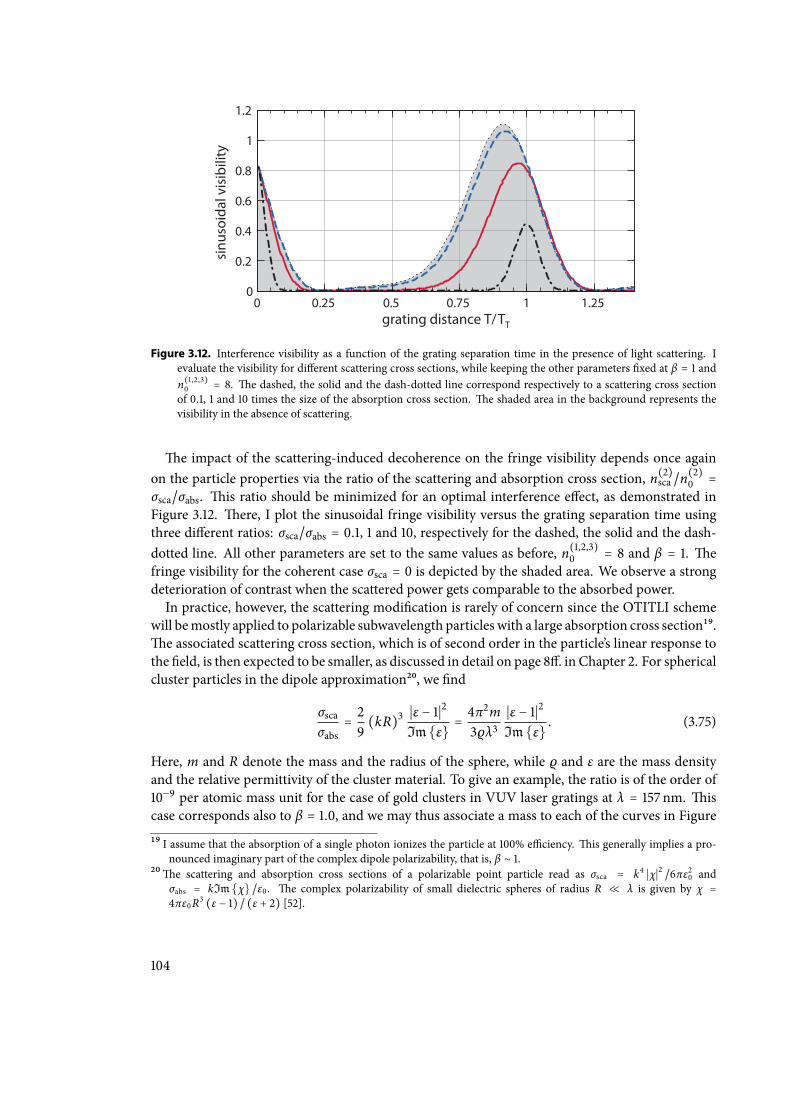
0 0.25 0.5 0.75 1 1.250

0.2

0.4

0.6

0.8

1

1.2

sinu

soid

al v

isib

ility

grating distance T/ TT

Figure 3.12. Interference visibility as a function of the grating separation time in the presence of light scattering. Ievaluate the visibility for dierent scattering cross sections, while keeping the other parameters xed at β = 1 andn(1,2,3)0 = 8. e dashed, the solid and the dash-dotted line correspond respectively to a scattering cross sectionof 0.1, 1 and 10 times the size of the absorption cross section. e shaded area in the background represents thevisibility in the absence of scattering.

e impact of the scattering-induced decoherence on the fringe visibility depends once againon the particle properties via the ratio of the scattering and absorption cross section, n(2)

sca /n(2)0 =

σsca/σabs. is ratio should be minimized for an optimal interference eect, as demonstrated inFigure 3.12. ere, I plot the sinusoidal fringe visibility versus the grating separation time usingthree dierent ratios: σsca/σabs = 0.1, 1 and 10, respectively for the dashed, the solid and the dash-dotted line. All other parameters are set to the same values as before, n(1,2,3)

0 = 8 and β = 1. efringe visibility for the coherent case σsca = 0 is depicted by the shaded area. We observe a strongdeterioration of contrast when the scattered power gets comparable to the absorbed power.In practice, however, the scattering modication is rarely of concern since the OTITLI scheme

will bemostly applied to polarizable subwavelength particles with a large absorption cross section19.e associated scattering cross section, which is of second order in the particle’s linear response tothe eld, is then expected to be smaller, as discussed in detail on page 8. in Chapter 2. For sphericalcluster particles in the dipole approximation20, we nd

σscaσabs

= 29(kR)3 ∣ε − 1∣2

Imε = 4π2m

3ρλ3∣ε − 1∣2

Imε . (3.75)

Here, m and R denote the mass and the radius of the sphere, while ρ and ε are the mass densityand the relative permittivity of the cluster material. To give an example, the ratio is of the order of10−9 per atomic mass unit for the case of gold clusters in VUV laser gratings at λ = 157 nm. iscase corresponds also to β = 1.0, and we may thus associate a mass to each of the curves in Figure

19 I assume that the absorption of a single photon ionizes the particle at 100% eciency. is generally implies a pro-nounced imaginary part of the complex dipole polarizability, that is, β ∼ 1.

20e scattering and absorption cross sections of a polarizable point particle read as σsca = k4 ∣χ∣2 /6πε20 andσabs = kImχ /ε0 . e complex polarizability of small dielectric spheres of radius R ≪ λ is given by χ =4πε0R3 (ε − 1) / (ε + 2) [52].

104

3.12.e dashed line corresponds to gold spheres of 108 amu in mass and 26nm in diameter, whichis where light scattering at G2 starts to aect the interference eect.e solid and the dash-dottedlines would then be related to a mass of 109 amu (56nm diameter) and 1010 amu (121 nm diameter),respectively.At about 109 amu, however, we are leaving the subwavelength regime and the present theoret-

ical model ceases to be valid. It turns out that this point constitutes a major mass limitation forconceivable implementations of the OTITLI scheme, as I will discuss in Section 3.4.

3.3. Absolute absorption spectroscopy in the TLI scheme

Aer having studied the theoretical description of Talbot-Lau interferometry in the preceding sec-tion, and before assessing its limits in the next section, I now turn to its application for themetrologyof large polarizable particles. In the beginning of Section 3.2.2 I mentioned already that the presentKDTLI experiment in Vienna is regularly used for deectometric measurements of the dipole po-larizability of the interfering molecules [105, 106, 117, 127, 128]. Let me focus here on a dierentexample proposed in [6], which is yet to be implemented in the lab.We can exploit the sensitivity of the Talbot-Lau interferogram to single-photon momenta im-

parted on the interfering particles to devise an absolute and precise measurement of their ab-sorption cross-section. is is of potential value in the eld of molecule and cluster spectroscopy[52,129,130], where the absolute absorption cross-sections of many large molecules and clusters arepoorly known. Conventional optical methods can be used to measure the overall absorption powerof a given particle gas or beam, but this does not conveymuch information about the single-particlecross section without prior knowledge about the particle density. In fact, optical absorption spectraare routinely measured nowadays, even with large nanoparticles, but the data is oen insignicantor imprecise when it comes to absolute values for the single-particle cross-sections (due to the di-culty of measuring particle densities precisely). Obviously, it would suce to measure the absolutecross-section σabs (ω) at a single optical frequency to normalize the whole spectrum.In the following I will present an interferometric technique to measure the value of σabs in a

non-destructive manner: By shining a laser in between the gratings of the TLI one can inducea controlled modulation of the interference fringe pattern as a function of the laser power andposition. I will show that this allows one to extract information about the optical absorption anduorescence properties of individual molecules.

3.3.1. Experimental setup and theoretical description

Talbot-Lau interferograms are periodic fringe structures sensitive to any kind of deection of thematter waves between the gratings and on the scale of the fringe period. e basic idea behindthe following measurement scheme is to trigger such deections by the absorption of one or morephotons from a running-wave laser (pulse) that is added to the interferometer and that illuminatesthe interfering particles either before or aer the second gratingG2.is results in amodied fringepattern which is a mixture of discretely shied interferograms, and, therefore, exhibits a reducedoverall contrast depending on the laser parameters and on σabs.e complemented three-grating Talbot-Lau arrangement is sketched in Figure 3.13 for the ex-

emplary case of a KDTLI scheme, where G2 is an optical phase grating.e reasoning applies also

105

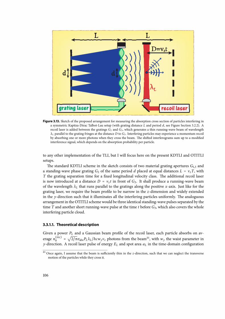
Figure 3.13. Sketch of the proposed arrangement for measuring the absorption cross section of particles interfering ina symmetric Kapitza-Dirac Talbot-Lau setup (with grating distance L and period d, see Figure Section 3.2.2). Arecoil laser is added between the gratings G2 and G3 , which generates a thin running-wave beam of wavelengthλL parallel to the grating fringes at the distance D to G3 . Interfering particles may experience a momentum recoilby absorbing one or more photons when they cross the beam. e shied interferograms sum up to a modiedinterference signal, which depends on the absorption probability per particle.

to any other implementation of the TLI, but I will focus here on the present KDTLI and OTITLIsetups.e standard KDTLI scheme in the sketch consists of two material grating apertures G1,3 and

a standing-wave phase grating G2 of the same period d placed at equal distances L = vzT , withT the grating separation time for a xed longitudinal velocity class. e additional recoil laseris now introduced at a distance D = vz t in front of G3. It shall produce a running-wave beamof the wavelength λL that runs parallel to the gratings along the positive x-axis. Just like for thegrating laser, we require the beam prole to be narrow in the z-dimension and widely extendedin the y-direction such that it illuminates all the interfering particles uniformly. e analoguousarrangement in the OTITLI scheme would be three identical standing-wave pulses separated by thetime T and another short running-wave pulse at the time t before G3, which also covers the wholeinterfering particle cloud.

3.3.1.1. Theoretical description

Given a power PL and a Gaussian beam prole of the recoil laser, each particle absorbs on av-erage n(rec)

0 =√2/πσabsPLλL/hcwyvz photons from the beam21, with wy the waist parameter in

y-direction. A recoil laser pulse of energy EL and spot area aL in the time-domain conguration

21Once again, I assume that the beam is suciently thin in the z-direction, such that we can neglect the transversemotion of the particles while they cross it.

106

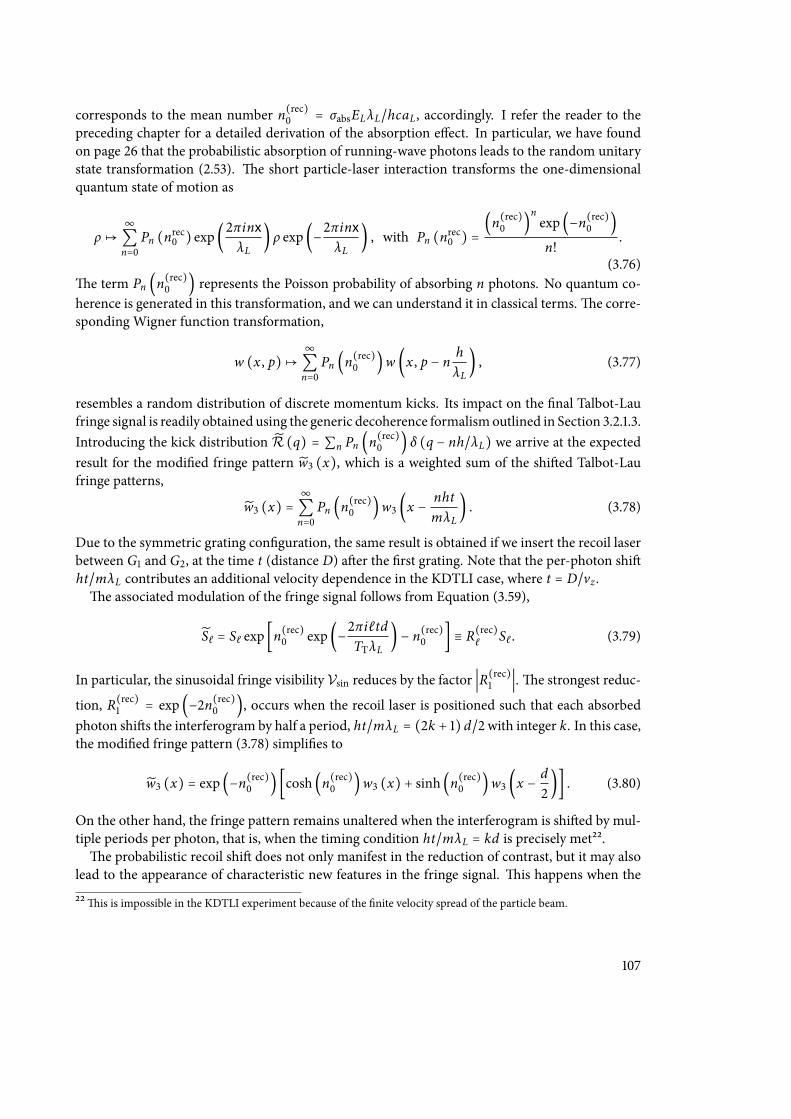
corresponds to the mean number n(rec)0 = σabsELλL/hcaL, accordingly. I refer the reader to the

preceding chapter for a detailed derivation of the absorption eect. In particular, we have foundon page 26 that the probabilistic absorption of running-wave photons leads to the random unitarystate transformation (2.53). e short particle-laser interaction transforms the one-dimensionalquantum state of motion as

ρ ↦∞

∑n=0

Pn (nrec0 ) exp(2πinxλL

) ρ exp(−2πinxλL

) , with Pn (nrec0 ) =(n(rec)0 )

nexp (−n(rec)

0 )n!

.

(3.76)e term Pn (n(rec)

0 ) represents the Poisson probability of absorbing n photons. No quantum co-herence is generated in this transformation, and we can understand it in classical terms.e corre-sponding Wigner function transformation,

w (x , p)↦∞

∑n=0

Pn (n(rec)0 )w (x , p − n h

λL) , (3.77)

resembles a random distribution of discrete momentum kicks. Its impact on the nal Talbot-Laufringe signal is readily obtained using the generic decoherence formalismoutlined in Section 3.2.1.3.Introducing the kick distribution R (q) = ∑n Pn (n

(rec)0 ) δ (q − nh/λL) we arrive at the expected

result for the modied fringe pattern w3 (x), which is a weighted sum of the shied Talbot-Laufringe patterns,

w3 (x) =∞

∑n=0

Pn (n(rec)0 )w3 (x −

nhtmλL

) . (3.78)

Due to the symmetric grating conguration, the same result is obtained if we insert the recoil laserbetween G1 and G2, at the time t (distance D) aer the rst grating. Note that the per-photon shiht/mλL contributes an additional velocity dependence in the KDTLI case, where t = D/vz .e associated modulation of the fringe signal follows from Equation (3.59),

Sℓ = Sℓ exp [n(rec)0 exp(−2πiℓtd

TTλL) − n(rec)

0 ] ≡ R(rec)ℓ Sℓ . (3.79)

In particular, the sinusoidal fringe visibility Vsin reduces by the factor ∣R(rec)1 ∣.e strongest reduc-

tion, R(rec)1 = exp (−2n(rec)

0 ), occurs when the recoil laser is positioned such that each absorbedphoton shis the interferogram by half a period, ht/mλL = (2k + 1) d/2 with integer k. In this case,the modied fringe pattern (3.78) simplies to

w3 (x) = exp (−n(rec)0 ) [cosh (n(rec)

0 )w3 (x) + sinh (n(rec)0 )w3 (x −

d2)] . (3.80)

On the other hand, the fringe pattern remains unaltered when the interferogram is shied by mul-tiple periods per photon, that is, when the timing condition ht/mλL = kd is precisely met22.e probabilistic recoil shi does not only manifest in the reduction of contrast, but it may also

lead to the appearance of characteristic new features in the fringe signal. is happens when the

22is is impossible in the KDTLI experiment because of the nite velocity spread of the particle beam.

107

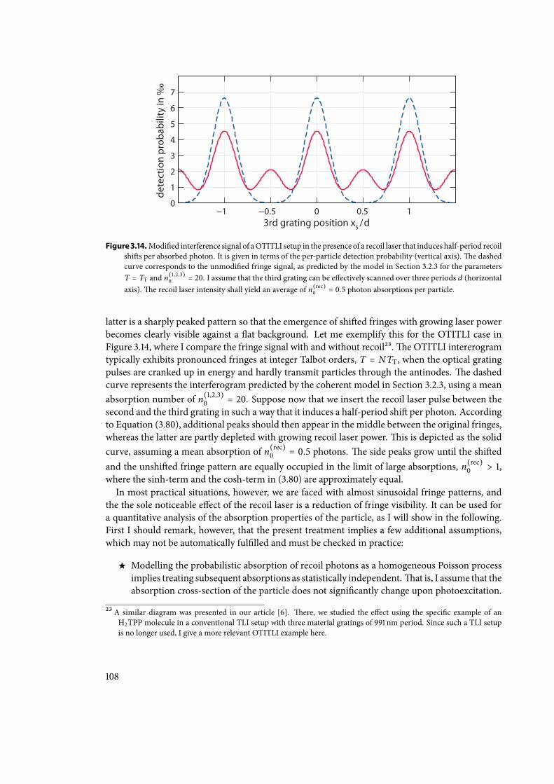
3rd grating position xS / d

dete

ctio

n pr

obab

ility

in ‰

−1 −0.5 0 0.5 10

1

2

3

4

5

6

7

Figure 3.14.Modied interference signal of aOTITLI setup in the presence of a recoil laser that induces half-period recoilshis per absorbed photon. It is given in terms of the per-particle detection probability (vertical axis).e dashedcurve corresponds to the unmodied fringe signal, as predicted by the model in Section 3.2.3 for the parametersT = TT and n(1,2,3)

0 = 20. I assume that the third grating can be eectively scanned over three periods d (horizontalaxis).e recoil laser intensity shall yield an average of n(rec)

0 = 0.5 photon absorptions per particle.

latter is a sharply peaked pattern so that the emergence of shied fringes with growing laser powerbecomes clearly visible against a at background. Let me exemplify this for the OTITLI case inFigure 3.14, where I compare the fringe signal with and without recoil23.e OTITLI intererogramtypically exhibits pronounced fringes at integer Talbot orders, T = NTT, when the optical gratingpulses are cranked up in energy and hardly transmit particles through the antinodes. e dashedcurve represents the interferogram predicted by the coherent model in Section 3.2.3, using a meanabsorption number of n(1,2,3)

0 = 20. Suppose now that we insert the recoil laser pulse between thesecond and the third grating in such a way that it induces a half-period shi per photon. Accordingto Equation (3.80), additional peaks should then appear in the middle between the original fringes,whereas the latter are partly depleted with growing recoil laser power.is is depicted as the solidcurve, assuming a mean absorption of n(rec)

0 = 0.5 photons. e side peaks grow until the shiedand the unshied fringe pattern are equally occupied in the limit of large absorptions, n(rec)

0 > 1,where the sinh-term and the cosh-term in (3.80) are approximately equal.In most practical situations, however, we are faced with almost sinusoidal fringe patterns, and

the the sole noticeable eect of the recoil laser is a reduction of fringe visibility. It can be used fora quantitative analysis of the absorption properties of the particle, as I will show in the following.First I should remark, however, that the present treatment implies a few additional assumptions,which may not be automatically fullled and must be checked in practice:

Modelling the probabilistic absorption of recoil photons as a homogeneous Poisson processimplies treating subsequent absorptions as statistically independent.at is, I assume that theabsorption cross-section of the particle does not signicantly change upon photoexcitation.

23A similar diagram was presented in our article [6]. ere, we studied the eect using the specic example of anH2TPP molecule in a conventional TLI setup with three material gratings of 991 nm period. Since such a TLI setupis no longer used, I give a more relevant OTITLI example here.

108

is is not guaranteed in practice, some molecules are indeed known to be ‘optically limited’absorbers [131]. We canminimize the inuence of such uncertainties if we restrict our analysisto low absorption powers, n(rec)

0 < 1.

Expression (3.79) for the recoil-induced fringe reduction implies that the detection eciencyof the particles behind the third grating does not depend on their internal state, that is, onthe number of absorbed photons. In principle, this assumption could be tested separately bylooking at the average transmission through the interferometer as a function of the absorp-tion power

An additional contrast reductionmay occur if the excited particles that have absorbed one ormore recoil photons decohere either by uorescence or by emitting thermal radiation. elatter eect is expected to be negligible for largemolecules with a heat capacityC ≫ kB.eirinternal temperature can only rise by at most ∆T = hc/λLC per photon. e uorescenceeect, on the other hand, must be taken into account if present. We can assess it separatelyin settings where the recoil laser induces full-period shis per photon, as I will discuss belowin Section 3.3.2.

Last but not least, I assume that it is possible to induce half- and full-period shis by posi-tioning or timing the recoil laser adequately. However, the largest possible shi is limited bythe restriction that the recoil laser cannot be farther away from the rst or third grating thanthe second one, t < T . Hence, a full-period shi can only be achieved if hT/mλL ≥ d.at is,one must go beyond the rst Talbot order if one uses a spectroscopy laser with a wavelengthlarger than the grating period, T/TT ≥ λL/d.

3.3.1.2. Quantitative analysis

Based on the explicit description of the recoil eect on the fringe signal, Equation (3.79), let me nowdevise a measurement routine for the absorption cross-section of the interfering particle species:One rst measures the unmodied fringe visibility Vsin in a given Talbot-Lau experiment with therecoil laser switched o. en one measures the reduced visibility, Vsin (PL) = ∣R(rec)

1 ∣Vsin, fordierent powers PL of the recoil laser and plots the data on a logarithmic scale versus PL.e abovemodel predicts a linear dependence,

ln Vsin = lnVsin − n(rec)0 [1 − cos( 2πtd

TTλL)] , (3.81)

since the mean number of absorbed photons is proportional to the product of the absorption cross-section and the power, n(rec)

0 ∝ σabsPL. e slope parameter of a straight line t through the datareveals the absorption cross-section, given the power and the time of the laser. Note that the particledensity does not enter the measurement result here (as opposed to other spectroscopy schemes)since it is based on single-particle interference eect. In a time-domain setting the power variableis replaced by the pulse energy EL.e relevant tting parameter is independent of the unmodied visibility; only the recoil-induced

reduction relative to the original value enters the routine. In principle, this renders our methodindependent of the precise theoretical prediction of the fringe contrast and robust against many

109

phase-averaging and decoherence eects in the experiment (that is, if they do not uctuate betweendierent steps of the measurement procedure). In practice, however, this is only strictly true in theOTITLI setting where the velocity of the particles does not enter the description. In a conventionalKDTLI scheme both the timing t and the the absorption strength n(rec)

0 are inversely proportionalto the longitudinal particle velocity vz , and we must average the results over a given velocity distri-bution. We are le with a more complicated expression of the ratio between the reduced and theunreduced fringe visibility,

R =RRRRRRRRRRRRR⟨B(2)2 ( πL

vzTT)⟩

−1

vz⟨B(2)2 ( πL

vzTT) exp

⎧⎪⎪⎨⎪⎪⎩

√2π

σabsPLλLhcwyvz

[exp(− 2πiDdTTλLvz

) − 1]⎫⎪⎪⎬⎪⎪⎭⟩vz

RRRRRRRRRRRRR, (3.82)

where L denotes the grating distance and B(2)2 is the Talbot coecient (3.66) determining the

KDTLI fringe visibility (3.67).e measured reduction must be compared to the averaged expres-sion R, and a simple t based on the linear form (3.81) for a xed velocity will introduce errors inthe measurement result for σabs. It can be kept at a minimum by optimizing the velocity depen-dence of the original fringe visibility and of the recoil shi per photon, hD/mvzλL. e former isachieved by adjusting the KDTLI setup to a visibility maximum, where ∂Vsin/∂vz is small at a givenmean velocity vz of the particles. e latter is achieved by keeping the mean recoil shi small buteective; the ideal value is one half period, hD/mvzλL = d/2. Larger shis would only lead to alarger variation of the reduction eect over the velocity.To be specic, let us consider a symmetric distribution of velocities over the interval of length

2∆vz around its mean value vz , which fullls those minimality criteria. In particular, the contrastreduction shall converge to exp(−2n(rec)

0 ) for ∆vz → 0. By performing a second-order Taylorexpansion of the bracketed terms in (3.82) with respect to the velocity deviation from the mean,vz − vz , we nd that the velocity-averaged reduction varies around this value like

R ≈ exp (−2n(rec)0 )1 + 2n(rec)

0 (∆vzvz

)2[(n(rec)

0 − 1)(1 − π2

4) + vz

∂ lnVsin∂vz

] . (3.83)

Here, n(rec)0 and Vsin are evaluated at the mean velocity vz . e relative uncertainty in the fringe

reduction is of merely quadratic order in the velocity width ∆vz . Hence, the systematic error ∆σabson the measured cross section, which we would disregard by modelling the data according to thesimple linear relation (3.81) at vz = vz , is of the same order in the velocity variance.Figure 3.15 demonstrates that a reasonable velocity selection of ∆vz/vz ≲ 10% suces to measure

the absorption cross-section with a precision on the percent level in practice. For this I have simu-lated a realistic KDTLI experimentwith a blue recoil laser of λL = 420nmwavelength in the existingVienna setup (L = 10.5 cm, d = 266nm, wy = 900 µm, f1 = f3 = 0.42)24. I take H2TPP moleculesat vz = 175m/s as test particles using an absorption cross-section of σabs = 15Å2 for the blue recoilphotons, and 0.17Å2 for the green grating photons at 532nmwavelength [38,39].e polarizabilityis approximated by the measured static value [132], α = 105Å3, which yields a β-parameter of 0.11,according to Equation (3.68). e grating laser shall have 8W input power, which corresponds tothe phase modulation factor ϕ0 = 3.4 and to Vsin = 29%. A recoil shi of d/2 is attained by placingthe recoil laser at D = 1.5 cm distance from the third grating. Both lasers in the experiment shallhave the same waist.24 See Section 3.2.2 for all necessary details to compute the KDTLI fringe signal.

110

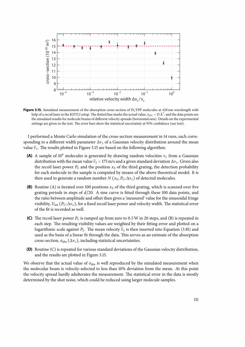
relative velocity width Δvz / vz

cros

s−se

ctio

n (1

0-20 m

2 )

10−4 10−3 10−2 10−1 1008

9

10

11

12

13

14

15

16

Figure 3.15. Simulated measurement of the absorption cross-section of H2TPP molecules at 420nm wavelength withhelp of a recoil laser in the KDTLI setup.e dotted linemarks the actual value, σabs = 15Å2 , and the data points arethe simulated results for molecule beams of dierent velocity spreads (horizontal axis). Details on the experimentalsettings are given in the text.e error bars show the statistical uncertainty at 95% condence (see text).

I performed a Monte Carlo simulation of the cross-section measurement in 14 runs, each corre-sponding to a dierent width parameter ∆vz of a Gaussian velocity distribution around the meanvalue vz .e results plotted in Figure 3.15 are based on the following algorithm:

(A) A sample of 104 molecules is generated by drawing random velocities vz from a Gaussiandistribution with themean value vz = 175m/s and a given standard deviation ∆vz . Given alsothe recoil laser power PL and the position xS of the third grating, the detection probabilityfor each molecule in the sample is computed by means of the above theoretical model. It isthen used to generate a random number N (xS , PL; ∆vz) of detected molecules.

(B) Routine (A) is iterated over 100 positions xS of the third grating, which is scanned over vegrating periods in steps of d/20. A sine curve is tted through these 100 data points, andthe ratio between amplitude and oset then gives a ‘measured’ value for the sinusoidal fringevisibility, Vsin (PL; ∆vz), for a xed recoil laser power and velocity width.e statistical errorof the t is recorded as well.

(C) e recoil laser power PL is ramped up from zero to 0.5W in 20 steps, and (B) is repeated ineach step. e resulting visibility values are weighted by their tting error and plotted on alogarithmic scale against PL. e mean velocity vz is then inserted into Equation (3.81) andused as the basis of a linear t through the data.is serves as an estimate of the absorptioncross-section, σabs (∆vz), including statistical uncertainties.

(D) Routine (C) is repeated for various standard deviations of the Gaussian velocity distribution,and the results are plotted in Figure 3.15.

We observe that the actual value of σabs is well reproduced by the simulated measurement whenthe molecular beam is velocity-selected to less than 10% deviation from the mean. At this pointthe velocity spread hardly adulterates the measurement. e statistical error in the data is mostlydetermined by the shot noise, which could be reduced using larger molecule samples.

111

Note that the suggested method is minimally invasive on the molecules because it does not relyon a strong optical depletion process to measure the net absorption of the molecular ensemble.erecoil laser in the given example yields an average of less than one photon absorption per molecule.Nevertheless, we can attain a shot-noise limited measurement accuracy on the percent level in real-istic settings25, irrespectively of the precise particle ux. Moreover, the latter could bemuch smallerthan what would be required for a conventional extinction measurement of the net absorption. Infact, Talbot-Lau interference is still observable with dilute and optically thin molecular beams.

3.3.2. Dealing with °uorescence

e simulation results suggest that an interferometric measurement of σabs is viable by means ofthe recoil-induced contrast reduction in the existing KDTLI setup. However, I have ignored hereanother contrast-reducing factor related to the absorption: uorescence. As long as no photo-depletion eect occurs, an excitedmolecule can either distribute the extra photon energy internallyamong its rovibrational degrees of freedom or it can reemit the energy in the form of a uorescencephoton. e former would lead to internal heating, which is oen negligible in the case of largemolecules. e latter corresponds to an immediate decoherence event, which is likely to occurwithin nanoseconds aer the excitation.e likelihood of this event is referred to as the quantumyield, Puo ≤ 1, of a given molecule. It is about 11% in the above example of H2TPP.e uorescence eect is readily incorporated into themodel by employing once again the generic

description of decoherence events outlined in Section 3.2.1.3. We merely require the knowledgeof the relative uorescence spectrum, F (ω), as an additional input. No absolute emission ratesare required, and the spectrum shall be normalized to ∫ dω F (ω) = 1. Moreover, it is reason-able to assume that each photon is emitted isotropically. Putting everything together, a singleuorescence event eectively transforms the one-dimensional center-of-mass state of the mole-cule as ρ ↦ ∫ d3k cF (ck) exp (−ikxx) ρ exp (ikxx).e associated decoherence function reads asRuo (x) = ∫∞0 dω F (ω) sinc (ωx/c), and the Fourier components of the interference fringe signalare modulated byRuo (ℓdt/TT), according to Equation (3.59). Because of the short uorescencetime scales, we may assume that the absorption and the emission events occur approximately at thesame point t in the interferometer.

With these ingredients the uorescence eect can be incorporated into the probabilistic recoilmodel in Equation (3.79). Given that n photons have been absorbed from the recoil laser, wemodel the conditional probability of reemitting k < n photons by a binomial distribution, p (k∣n) =(nk)P

kuo (1 − Puo)n−k . Once again, this implies that Puo does not change with the number of ex-

citations, like the absorption cross-section before. It is an uncritical assumption if we restrict tolow absorption numbers, n(rec)

0 < 1. e emission of k photons modulates the fringe signal by[Ruo (ℓdt/TT)]k in Fourier space; an average over all possible k leads to the uorescence-modied

25 Systematic errors due to the imprecise knowledge of the setup parameters, say, the laser powers, must be included inpractical implementations.

112

fringe amplitudes,

S(n)ℓ =n∑k=0

p (k∣n) [Ruo (ℓdtTT

)]kSℓ =

n∑k=0

(nk) (1 − Puo)n−k [PuoRuo (

ℓdtTT

)]kSℓ

= [1 − Puo + PuoRuo (ℓdtTT

)]nSℓ . (3.84)

given the absorption of n recoil photons. Finally, we multiply this conditional result by the phasefactor exp (2πiℓntd/TTλL) associated to n recoil shis and average it over n to arrive at the reducedfringe amplitudes,

Sℓ =∞

∑n=0

Pn (n(rec)0 ) exp(2πinℓtd

TTλL) S(n)ℓ

= expn(rec)0 [1 − Puo + PuoRuo (

ℓdtTT

)] exp(2πiℓtdTTλL

) − n(rec)0 Sℓ . (3.85)

is is the generalization of the above result (3.79) to nonzero quantum yields, Puo > 0.Let me close this section by discussing the primary cases of interest, half- and full-period shis.

Here, the sinusoidal fringe visibility reduces in the following way:

ln Vsin = lnVsin − 2n(rec)0 + Puon

(rec)0 [1 −Ruo (

λL2)] if td

TTλL= 12

(3.86)

ln Vsin = lnVsin − Puon(rec)0 [1 −Ruo (λL)] if td

TTλL= 1 (3.87)

Such linear models are valid descriptions for time-domain interference, and they can also be goodapproximations for velocity-selectedmolecule beams in the KDTLI conguration, as I have veriedexplicitly in the zero-uorescence case. Here, we nd the combined eect of reduction by recoiland by uorescence. Although the eect is still strongest for half-period shis, the absorption crosssection σabs is no more accessible by the devised measurement if the quantum yield Puo is notknown either. e latter should then be measured separately in a conguration where the recoillaser induces a full-period shi. e contrast is then solely aected by the reemission of photons,and a t of Equation (3.87) to the data would reveal the value of the term Puoσabs, provided therelative uorescence spectrum is known. Combining this with the results of the other half-periodmeasurement would then result in a value for both σabs and Puo. One could take this principleeven further and map the whole parameter space of absorption and uorescence with a movableand tunable recoil laser.Note, however, that this interferometric method can only measure thermally averaged values

of the cross-section and the quantum yield, which are predetermined by the available moleculesources. Additional measurement uncertainties not covered here could be caused by optical lim-iting or enhanced thermal radiation, as listed at the end of Section 3.3.1.1. A nonlinear power de-pendence of the logarithmic contrast reduction would be a rst indication of whether such eectsmight be relevant for a specic molecule. One should then restrict the analysis to the linear regimeat suciently small powers. e thermal eects could be studied separately by systematic heatingexperiments.

113

3.4. Mass limits of the OTITLI scheme

I close this chapter with an outlook into the future of matter-wave interferometry with ultra-heavyobjects, specically for Talbot-Lau interferometry with nanoclusters. What is the highest mass thatcould be brought to interference in a feasible experiment using available matter-wave techniques?In the following I will answer this question on the basis of the Talbot-Lau interferometer schemewith optical ionization gratings operating in the time domain. is OTITLI scheme was workedout in [10] and described in detail in Section 3.2.3.So far, Talbot-Lau interferometry has proven to be the method of choice for demonstrating the

quantum wave nature of ever larger objects. It holds the current mass record, and it oers a greaterexibility andmore favorablemass scaling than othermore conventional interference techniques, asI have illustrated throughout this chapter. In particular, the OTITLI scheme has been designed andoptimized precisely for the purpose of reaching the highest possible masses. Its limitations, whichI discuss in the following, will apply in a similar manner, if not more severely, to other conceivablematter-wave experiments.Finally, we will see in Section 3.4.3 that a class of alternative theories beyond the level of standard

quantummechanics will become testable in the reachable high-mass regime.ese theories predicta breakdown of the superposition principle and induce classical behaviour on the macro-scale.

3.4.1. Experimental methods and challenges

A concrete study of the required technology and the eort necessary to implement the OTITLIscheme of Section 3.2.3 with heavy metal clusters was provided when we rst proposed it [10]. Inaddition, the rst experimental demonstration with small molecular clusters in [13] has proven thatthe proposed design is indeed feasible with present-day technology.Let me give a short overview of the experimental methods and challenges related to this imple-

mentation, including the interferometer design as well as the creation and detection of appropriateparticle ensembles.

3.4.1.1. Particle candidates and sources

e amplitudemodulation eect of the optical gratings in the proposedOTITLI scheme is based onsingle-photon ionization. We must therefore choose the particles according to whether they ionizeat a given wavelength of the grating lasers. Moreover, the ionization process should take place ona short time scale and at an eciency close to 100%, since absorption events without subsequentionization would lead to additional decoherence.e proposedVUV laser gratings at 157 nmwave-length provide a single-photon energy of 7.9 eV, which exceeds the ionization threshold of manylarge molecules26 or the work function of most cluster materials. e latter has a typical value ofaround 5 eV such that ultraviolet or optical laser gratingswithwavelengths larger than about 250nmwould narrow down the range of usable materials signicantly. Nevertheless, optical depletion pro-cesses, such as multi-photon ionization, photo-isomerization or fragmentation, may still facilitateTalbot-Lau interferometry with optical absorptive gratings.

26 Complex biomolecules oen do not photoionize, or at best at low eciency, even if the absorbed photon providesenough energy. e latter is then deposited and distributed among many other internal degrees of freedom of themolecule.

114

e availability of large ionizable particles for OTITLI experiments is mostly related to the avail-ability of stable sources volatilizing a sucient amount of these particles that can be passed on tothe grating pulses. Viable sources for large and complex molecules exist for tailor-made species onthe 103-104 amu scale [19]. However, it seems more sensible with current technology to focus onatomic or molecular cluster aggregation sources, which oer a broad range of masses and hold outthe prospect of generating pulsed beams of nanoparticles up to 106 amu and beyond. Here, individ-ual atoms and molecules are typically desorbed or sputtered from a substrate and then swept awayin a cold gas jet where they condense and aggregate to clusters of a broad size distribution [118]. Ifnecessary, the ejected cluster ensemble can be slowed down in a buer gas cooling stage [133] toachieve suciently long residence times in the active interferometer region. e anthracene clus-ters in the rst demonstration of the OTITLI scheme were formed in a cold jet of noble gas aer thepulsed injection of anthracene vapour from an Even-Lavie valve [13, 134]. Although their interfer-ence was clearly observed, a systematic ab initio assessment of the measured results was obstructedby the fact that the optical properties of these clusters were practically unknown.

Laser acoustic desorption from atomic surfaces [135] represents an alternative way of produc-ing large nano- or even microclusters that could be used in matter-wave interferometry. Recently,there has been growing interest and progress in optical manipulation, cooling, and interferencetechniques with single levitated nanospheres on the quantum level of motion [23–25, 136, 137].

3.4.1.2. Interferometer design

Having a working pulsed particle source at hand, the design of the interferometer is a relativelysimple matter.e basic OTITLI setup consists of a single at high-reectivity mirror and a set ofone to three identical pulsed laser systems with tunable pulse energy and timing. I restrict here tothe working setup [13] with three F2 excimer lasers producing 7ns long pulses of a few mJ energyat the vacuum ultraviolet (VUV) wavelength λ = 157.63 nm. ey illuminate a polished highlyreective CaF2 surface of two inches in diameter vertically from below. Each pulse is retroreectedfrom the mirror and forms a short standing-wave grating of 80nm period that extends coherentlyover a longitudinal coherence length of roughly 1 cm. A weak electric eld is applied in the vacuumchamber containing the mirror to remove the particles ionized in each grating.

For the interference eect to occur it is vital to have precise control over the pulse timing. Weread from the resonance approximation in Section 3.2.1.2 that the delay times between the threegrating pulses must be equal up to a small deviation ∣τ∣ ≪ TT.e time window le for unavoidablepulse jitters and timing imprecisions can be adjusted by the initial collimation of the matter-waveensemble along the standing-wave axis. It was measured to be 48ns in the anthracene experiment[13], a value larger than the pulse duration and the jitter of the lasers.

Besides the initial collimation of the particles, it might be necessary to guarantee that they aresuciently slow and do not average over the standing-wave prole for the duration of each gratingpulse. e dimensions and positions of the laser spots must be optimized accordingly, becausedierent parts of the particle cloud may experience dierent laser intensities, and the observedvisibility is averaged over the ensemble spread in velocity and position.

115

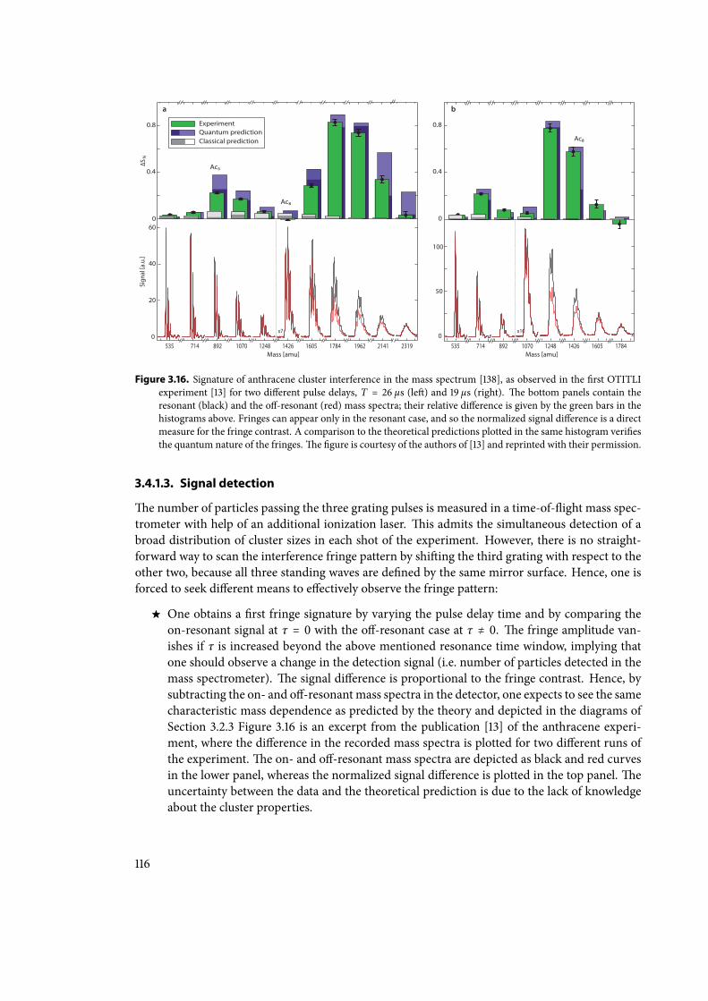
0

0.4

0.8

∆S

Ac5

Ac8

ExperimentQuantum predictionClassical prediction

Sign

al [a

.u.]

a

N

20

40

60

0x7

Mass [amu]

Ac8

x10

Mass [amu]

0

0.4

0.8

50

100

0

b

535 714 892 1070 1248 1426 1605 1784535 714 892 1070 1248 1426 1605 1784 1962 2141 2319

Figure 3.16. Signature of anthracene cluster interference in the mass spectrum [138], as observed in the rst OTITLIexperiment [13] for two dierent pulse delays, T = 26 µs (le) and 19 µs (right). e bottom panels contain theresonant (black) and the o-resonant (red) mass spectra; their relative dierence is given by the green bars in thehistograms above. Fringes can appear only in the resonant case, and so the normalized signal dierence is a directmeasure for the fringe contrast. A comparison to the theoretical predictions plotted in the same histogram veriesthe quantum nature of the fringes.e gure is courtesy of the authors of [13] and reprinted with their permission.

3.4.1.3. Signal detection

e number of particles passing the three grating pulses is measured in a time-of-ight mass spec-trometer with help of an additional ionization laser. is admits the simultaneous detection of abroad distribution of cluster sizes in each shot of the experiment. However, there is no straight-forward way to scan the interference fringe pattern by shiing the third grating with respect to theother two, because all three standing waves are dened by the same mirror surface. Hence, one isforced to seek dierent means to eectively observe the fringe pattern:

One obtains a rst fringe signature by varying the pulse delay time and by comparing theon-resonant signal at τ = 0 with the o-resonant case at τ ≠ 0. e fringe amplitude van-ishes if τ is increased beyond the above mentioned resonance time window, implying thatone should observe a change in the detection signal (i.e. number of particles detected in themass spectrometer). e signal dierence is proportional to the fringe contrast. Hence, bysubtracting the on- and o-resonantmass spectra in the detector, one expects to see the samecharacteristic mass dependence as predicted by the theory and depicted in the diagrams ofSection 3.2.3 Figure 3.16 is an excerpt from the publication [13] of the anthracene experi-ment, where the dierence in the recorded mass spectra is plotted for two dierent runs ofthe experiment.e on- and o-resonant mass spectra are depicted as black and red curvesin the lower panel, whereas the normalized signal dierence is plotted in the top panel.euncertainty between the data and the theoretical prediction is due to the lack of knowledgeabout the cluster properties.

116

Aneective grating scanwas also achieved in the anthracene experimentwith help of a simpletrick: By varying slightly the incidence angle of one of the lasers onto the mirror, the authorseected a change in the grating period along the standing-wave axis.is change was smallenough to not aect the Talbot-Lau resonance and the grating coherence length too much,but it accumulated a suciently large grating shi of up to one period a fewmillimeters awayfrom the mirror surface.

A cleaner way to scan and resolve the interference fringe pattern is to make use of an ex-ternal acceleration, which deects the particle trajectories in a controlled manner betweenthe gratings. A constant acceleration a along the standing-wave axis yields the eective shiδxa = −aT2 of the fringe pattern, as discussed in Section 3.2.1.2.e fringes can be scannedby varying either a or the grating separation time T . e latter also inuences the fringevisibility. A tunable acceleration, for instance, could be generated by a static electric eldthat produces a constant dipole force on polarizable particles along the grating axis. istechnique is commonly used for deectometric measurements in the KDTLI setup, as men-tioned in Section 3.2.2. Alternatively, one can simply employ gravity, a = g, in the verticalgrating alignment if the particles are suciently massive. A particle of, say, 105 amu corre-sponds to the Talbot time TT ≈ 1.6ms, and it would fall more than 300 grating periods in thecurrent OTITLI setup if we assume a pulse separation of T = TT. at is, one could easilyscan the fringe pattern by varying T over less than one per cent.

3.4.2. Standard mass limitations

Having discussed the experimental techniques, I proceed with the relevant mass-limitating factorsin the OTITLI scheme, as published in [11]. I resort to the currently available implementation usingVUV lasers with a grating period of d = 80nm and variable separation time T . Spherical goldclusters of variable radius R in the nanometer regime will be used as reference particles of massm = 4πρR3/3, adopting the bulk values for the mass density and the relative dielectric permittivity,ρ = 19320 kg/m3 and ε = 0.9 + 3.2i [50].

3.4.2.1. Temporal stability and inertial forces

e most obvious limitation is related to the feasibility and stability of long-time interferometers.Given a mass-proportional Talbot time of 16 ns per atomic mass unit, a reliable and distinguishedobservation of quantum interference fringes requires the particles not to leave the interferometerfor at least 2T ∼ 32ns per amu.is implies the following practical mass limitations:

Velocity limit A suciently rigid and at reference mirror for all three laser gratings cannotbe made arbitrarily large, and the use of separate mirrors for each grating would come atthe price of harsh stability and adjustment requirements. Particles must therefore be slowenough to stay within the range of themirror for at least the time 2T . Let us assume a realisticmirror length of about 5 cm, as currently used in the lab. A particle of, say, 106 amu mustthen be injected with a velocity of less than 1.6m/s to not traverse the mirror in less thanthe required 32ms27. Most known sources produce much faster particle ensembles. at

27A similar velocity limit applies along the other spatial directions in order to prevent the particles from leaving thecoherent high-intensity parts of the standing-wave beam prole.

117

is, one must rst develop and implement ecient methods to slow, guide, or even trap themotion of polarizable particles before being able to do interference experiments with massesof more than 105 amu. In this respect, optical and electromagnetic manipulation techniqueshave attracted growing interest and undergone progress over the years, see e.g. [8,23,48, 136,139–142].

Gravitational limit I have mentioned above that the presence of gravity may be of help inresolving the interference fringe pattern of large particles. At even higher masses, however,the free fall of particles must be balanced or suppressed in order to keep them in place for asuciently long time.e free-fall distance during interference increases quadratically withthe Talbot time from already 5mm at 106 amu to the out-of-reach value of 5 km at 109 amu.is would have to be counteracted on the nanometer or millimeter level in a vertical or hor-izontal grating arrangement. Experiments with trapped particles or in a microgravitationalenvironment [143] might be the only possibilities to beat the level of a million mass units.

3.4.2.2. Decoherence

Environmental decoherence is another limitating factor in high-mass interferometry. It is a well-understood phenomenon that was assessed both theoretically and experimentally in the contextof Talbot-Lau interferometry with molecules [40, 144, 145]. e two relevant free-space decoher-ence processes for matter waves propagating through the interferometer are due to collisions withresidual gas particles and due to the interaction with thermal radiation.e third relevant process,grating decoherence due to the elastic scattering of laser photons in each pulse, will be omittedhere. It has been covered in Section 3.2.3.2, and I have shown that it is hardly of signicance forsubwavelength particles with masses < 109 amu.e overall free-space decoherence rate depends on the internal temperature of the particles and

on the background pressure and temperature of the environment.e shielding of ever larger par-ticles from decoherence requires us to decrease both temperature and vacuum pressure to the sameextent as the cross-section for gas collisions, and for the emission, absorption, and Rayleigh scat-tering of thermal radiation increases.e inuence of free-space decoherence on the interference visibility can be obtained using the

formalism layed out in [40] and the terminology developed in Section 3.2.1.3. Each type of deco-herence is modelled as an independent random process of scattering events with a mean event rateΓ (t). A single scattering event transfers a randomly distributed momentum recoil ħk to the parti-cle, as described by the random unitary transformation, ρ ↦ ∫ d3k P (k) exp (ikxx) ρ exp (−ikxx),of the reduced one-dimensional state of motion. e probability distribution P (k) is normalizedto unity. Following the argumentation in Section 3.2.1.3, we arrive at the associated decoherencefunction in the position representation, R (∆x) = ∫ d3k P (k) exp (−ikx∆x). If we suppose thatthe event occurs at the time t before or aer the second grating, we can use (3.59) to establish therate equation,

ddt

Sℓ = Γ (t) [R(ℓd T − ∣t∣TT

) − 1] Sℓ , (3.88)

118

for the decay of the ℓth Fourier component of the interference fringe signal. Solving this dierentialequation yields a relation between the decohered and the unmodied signal components,

Rℓ =SℓSℓ

= exp ∫ T

−Tdt Γ (t) [R(ℓd T − ∣t∣

TT) − 1] , (3.89)

with R0 = 1. Each independent decoherence process contributes a separate reduction factor Rℓ. Iassume, for simplicity, that each scattering event is isotropic28, P (k) = P (k), and that the eventrate Γ does not change over time in all the following processes. So we are le with reduction factorsof the form

Rℓ = exp−2Γ [T − ∫ T

0dt ∫ ∞

0dk 4πk2P (k) sinc(ℓkd t

TT)] . (3.90)

Absorption and emission of thermal radiation e interfering nanoclusters can be regardedas hot composite systems constantly absorbing and emitting thermal photons from and into theradiation eld of the environment. For the present estimates I assume the clusters to be in thermalequilibrium with the environment, as also described in Section 2.1.2.2. Corrections of the radiationlaw due to the nite heat capacitance of the clusters, as given in [40], will be neglected.e spectralabsorption and emission rates are identical and given by the Planck formula, Equation (2.23) onpage 12, at the temperature Tenv,

4πΓk2P (k)dk = γemi (ω)dω = σabs (ω)ω2dωπ2c2 [exp (ħω/kBTenv) − 1]

. (3.91)

By plugging this into (3.90) we obtain the reduction factors of emission and absorption, R(abs)ℓ =

R(emi)ℓ . In the alternative case of a hot particle, Tint ≫ Tenv, the decoherence is dominantly dueto emission, and the temperature dependence of the spectral rate is given by a Boltzmann factor,Equation (2.22),

4πΓk2P (k)dk = σabs (ω)ω2dωπ2c2

exp(− ħωkBTint

) . (3.92)

Elastic scattering of thermal radiation An elastic photon scattering event can be understoodas a combined absorption and emission process, averaged over the in- and outgoing wave vec-tor with the scattering probability P (k → k′) proportional to γsca (ck) δ (k − k′) and the unitarydouble-recoil operator given by exp [i (kx − k′x) x]. e associated decoherence function reads asR (∆x) = ∫ d3kd3k′ P (k → k′) exp [−i (kx − k′x)∆x], and the reduction factor becomes

R(sca)ℓ = exp−2 ∫ ∞

0dω γsca (ω) [T − ∫ T

0dt sinc2 (ℓdωt

cTT)] . (3.93)

In full equivalence to the spectral emission rate (3.91), the scattering rate per frequency ω is takento be proportional to the Rayleigh scattering cross-section times the Planck energy density of thesurrounding radiation eld, γsca (ω) = (ω/π)2 σsca (ω) [exp (ħω/kBTenv) − 1]−1. We expect thatthe impact of scattering on nanoparticle interference is small, given the large average wavelengthsof thermal photons at temperatures below 1000K.

28e overall eect is practically the samewhether the scattering pattern is isotropic or, say, a dipolar patternwith respectto a xed polarization axis.

119

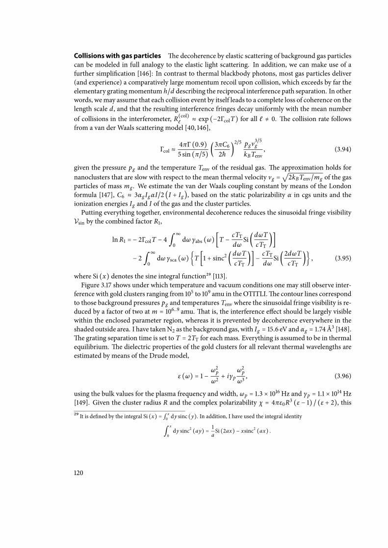
Collisions with gas particles e decoherence by elastic scattering of background gas particlescan be modeled in full analogy to the elastic light scattering. In addition, we can make use of afurther simplication [146]: In contrast to thermal blackbody photons, most gas particles deliver(and experience) a comparatively large momentum recoil upon collision, which exceeds by far theelementary gratingmomentum h/d describing the reciprocal interference path separation. In otherwords, wemay assume that each collision event by itself leads to a complete loss of coherence on thelength scale d, and that the resulting interference fringes decay uniformly with the mean numberof collisions in the interferometer, R(col)

ℓ ≈ exp (−2ΓcolT) for all ℓ ≠ 0. e collision rate followsfrom a van der Waals scattering model [40, 146],

Γcol ≈4πΓ (0.9)5 sin (π/5) (3πC6

2ħ)2/5 pgv3/5g

kBTenv, (3.94)

given the pressure pg and the temperature Tenv of the residual gas. e approximation holds fornanoclusters that are slow with respect to the mean thermal velocity vg =

√2kBTenv/mg of the gas

particles of mass mg . We estimate the van der Waals coupling constant by means of the Londonformula [147], C6 ≈ 3αg IgαI/2 (I + Ig), based on the static polarizability α in cgs units and theionization energies Ig and I of the gas and the cluster particles.Putting everything together, environmental decoherence reduces the sinusoidal fringe visibilityVsin by the combined factor R1,

lnR1 = − 2ΓcolT − 4 ∫ ∞

0dω γabs (ω) [T − cTT

dωSi(dωT

cTT)]

− 2 ∫ ∞

0dω γsca (ω)T [1 + sinc2 (dωT

cTT)] − cTT

dωSi(2dωT

cTT) , (3.95)

where Si (x) denotes the sine integral function29 [113].Figure 3.17 shows under which temperature and vacuum conditions one may still observe inter-

ference with gold clusters ranging from 105 to 109 amu in the OTITLI.e contour lines correspondto those background pressures pg and temperatures Tenv where the sinusoidal fringe visibility is re-duced by a factor of two at m = 106..9 amu. at is, the interference eect should be largely visiblewithin the enclosed parameter region, whereas it is prevented by decoherence everywhere in theshaded outside area. I have takenN2 as the background gas, with Ig = 15.6 eV and αg = 1.74Å3 [148].e grating separation time is set to T = 2TT for each mass. Everything is assumed to be in thermalequilibrium. e dielectric properties of the gold clusters for all relevant thermal wavelengths areestimated by means of the Drude model,

ε (ω) = 1 −ω2pω2

+ iγpω2pω3, (3.96)

using the bulk values for the plasma frequency and width, ωp = 1.3 × 1016Hz and γp = 1.1 × 1014Hz[149]. Given the cluster radius R and the complex polarizability χ = 4πε0R3 (ε − 1) / (ε + 2), this

29 It is dened by the integral Si (x) = ∫ x0 dy sinc (y). In addition, I have used the integral identity

∫ x

0dy sinc2 (ay) = 1

aSi (2ax) − xsinc2 (ax) .

120

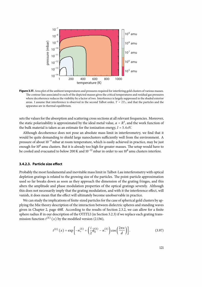
105 amu

106 amu

107 amu

108 amu

109 amu

1 200 400 600 800 1000temperature (K)

pres

sure

(mba

r)

10−14

10−13

10−12

10−11

10−10

10−9

10−8

10−7

Figure 3.17. Area plot of the ambient temperatures and pressures required for interfering gold clusters of variousmasses.e contour line associated to each of the depictedmasses gives the critical temperatures and residual gas pressureswhere decoherence reduces the visibility by a factor of two. Interference is largely suppressed in the shaded exteriorareas. I assume that interference is observed in the second Talbot order, T = 2TT , and that the particles and theapparatus are in thermal equilibrium.

sets the values for the absorption and scattering cross sections at all relevant frequencies. Moreover,the static polarizability is approximated by the ideal metal value, α = R3, and the work function ofthe bulk material is taken as an estimate for the ionization energy, I = 5.4 eV.Although decoherence does not pose an absolute mass limit in interferometry, we nd that it

would be quite demanding to shield large nanoclusters suciently well from the environment. Apressure of about 10−9mbar at room temperature, which is easily achieved in practice, may be justenough for 106 amu clusters. But it is already too high for greater masses.e setup would have tobe cooled and evacuated to below 200K and 10−12mbar in order to see 108 amu clusters interfere.

3.4.2.3. Particle size eªect

Probably themost fundamental and inevitable mass limit in Talbot-Lau interferometry with opticaldepletion gratings is related to the growing size of the particles.e point-particle approximationused so far breaks down as soon as they approach the dimension of the grating fringes, and thisalters the amplitude and phase modulation properties of the optical gratings severely. Althoughthis does not necessarily imply that the grating modulation, and with it the interference eect, willvanish, it does mean that the eect will ultimately become unobservable in practice.We can study the implications of nite-sized particles for the case of spherical gold clusters by ap-

plying the Mie theory description of the interaction between dielectric spheres and standing wavesgiven in Chapter 2, page 48. According to the results of Section 2.3.2, we can allow for a nitesphere radius R in our description of the OTITLI (in Section 3.2.3) if we replace each grating trans-mission function t(k) (x) by the modied version (2.136),

t(k) (x) = exp [−n(k)+ + ( i

2ϕ(k)0 − n(k)

− ) cos(2πxd

)] . (3.97)

121

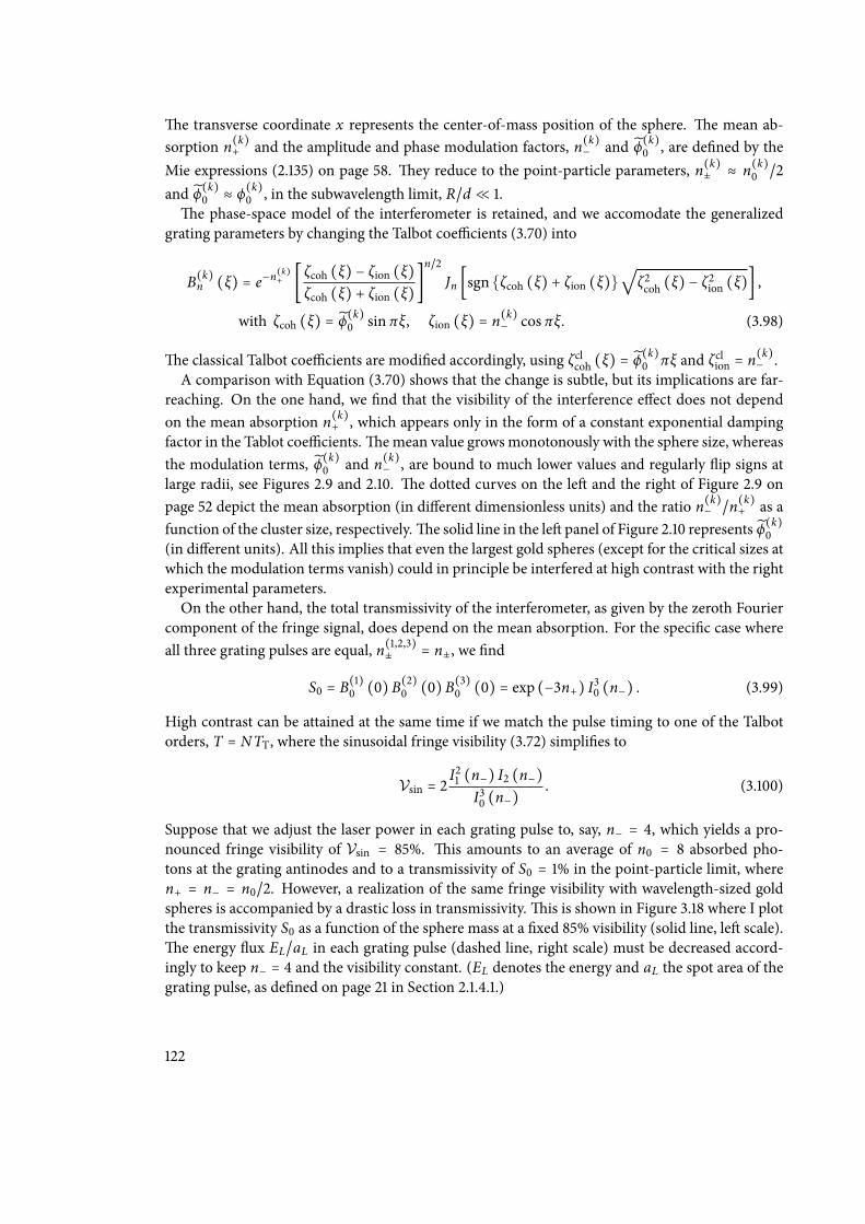
e transverse coordinate x represents the center-of-mass position of the sphere. e mean ab-sorption n(k)

+ and the amplitude and phase modulation factors, n(k)− and ϕ(k)

0 , are dened by theMie expressions (2.135) on page 58. ey reduce to the point-particle parameters, n(k)

± ≈ n(k)0 /2

and ϕ(k)0 ≈ ϕ(k)

0 , in the subwavelength limit, R/d ≪ 1.e phase-space model of the interferometer is retained, and we accomodate the generalized

grating parameters by changing the Talbot coecients (3.70) into

B(k)n (ξ) = e−n

(k)+ [ ζcoh (ξ) − ζion (ξ)

ζcoh (ξ) + ζion (ξ)]n/2

Jn [sgnζcoh (ξ) + ζion (ξ)√

ζ2coh (ξ) − ζ2ion (ξ)] ,

with ζcoh (ξ) = ϕ(k)0 sin πξ, ζion (ξ) = n(k)

− cos πξ. (3.98)

e classical Talbot coecients are modied accordingly, using ζclcoh (ξ) = ϕ(k)0 πξ and ζclion = n(k)

− .A comparison with Equation (3.70) shows that the change is subtle, but its implications are far-

reaching. On the one hand, we nd that the visibility of the interference eect does not dependon the mean absorption n(k)

+ , which appears only in the form of a constant exponential dampingfactor in the Tablot coecients.e mean value growsmonotonously with the sphere size, whereasthe modulation terms, ϕ(k)

0 and n(k)− , are bound to much lower values and regularly ip signs at

large radii, see Figures 2.9 and 2.10. e dotted curves on the le and the right of Figure 2.9 onpage 52 depict the mean absorption (in dierent dimensionless units) and the ratio n(k)

− /n(k)+ as a

function of the cluster size, respectively.e solid line in the le panel of Figure 2.10 represents ϕ(k)0

(in dierent units). All this implies that even the largest gold spheres (except for the critical sizes atwhich the modulation terms vanish) could in principle be interfered at high contrast with the rightexperimental parameters.On the other hand, the total transmissivity of the interferometer, as given by the zeroth Fourier

component of the fringe signal, does depend on the mean absorption. For the specic case whereall three grating pulses are equal, n(1,2,3)

± = n±, we nd

S0 = B(1)0 (0)B(2)

0 (0)B(3)0 (0) = exp (−3n+) I30 (n−) . (3.99)

High contrast can be attained at the same time if we match the pulse timing to one of the Talbotorders, T = NTT, where the sinusoidal fringe visibility (3.72) simplies to

Vsin = 2I21 (n−) I2 (n−)

I30 (n−). (3.100)

Suppose that we adjust the laser power in each grating pulse to, say, n− = 4, which yields a pro-nounced fringe visibility of Vsin = 85%. is amounts to an average of n0 = 8 absorbed pho-tons at the grating antinodes and to a transmissivity of S0 = 1% in the point-particle limit, wheren+ = n− = n0/2. However, a realization of the same fringe visibility with wavelength-sized goldspheres is accompanied by a drastic loss in transmissivity.is is shown in Figure 3.18 where I plotthe transmissivity S0 as a function of the sphere mass at a xed 85% visibility (solid line, le scale).e energy ux EL/aL in each grating pulse (dashed line, right scale) must be decreased accord-ingly to keep n− = 4 and the visibility constant. (EL denotes the energy and aL the spot area of thegrating pulse, as dened on page 21 in Section 2.1.4.1.)

122

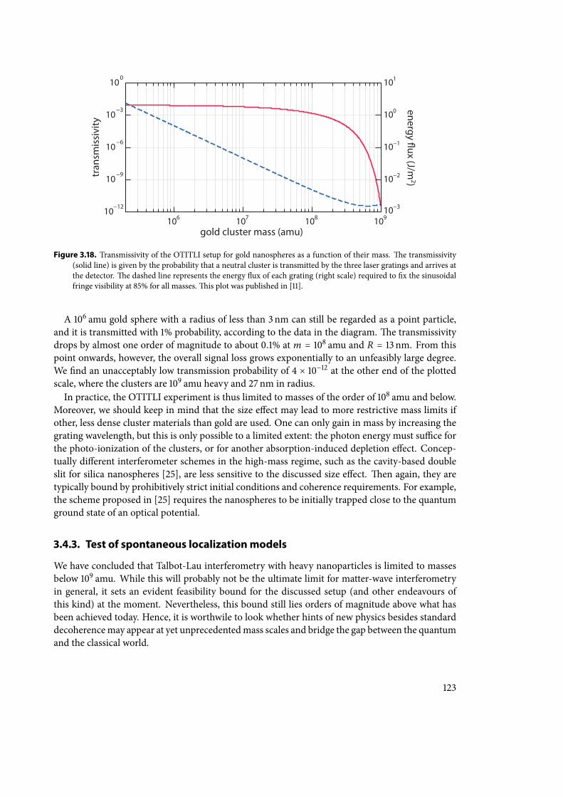
tran

smis

sivi

ty

106 107 108 10910

−12

10−9

10−6

10−3

100

gold cluster mass (amu)

energy ux (J/m2)

10−3

10−2

10−1

100

101

Figure 3.18. Transmissivity of the OTITLI setup for gold nanospheres as a function of their mass. e transmissivity(solid line) is given by the probability that a neutral cluster is transmitted by the three laser gratings and arrives atthe detector. e dashed line represents the energy ux of each grating (right scale) required to x the sinusoidalfringe visibility at 85% for all masses.is plot was published in [11].

A 106 amu gold sphere with a radius of less than 3nm can still be regarded as a point particle,and it is transmitted with 1% probability, according to the data in the diagram. e transmissivitydrops by almost one order of magnitude to about 0.1% at m = 108 amu and R = 13 nm. From thispoint onwards, however, the overall signal loss grows exponentially to an unfeasibly large degree.We nd an unacceptably low transmission probability of 4 × 10−12 at the other end of the plottedscale, where the clusters are 109 amu heavy and 27nm in radius.In practice, the OTITLI experiment is thus limited to masses of the order of 108 amu and below.

Moreover, we should keep in mind that the size eect may lead to more restrictive mass limits ifother, less dense cluster materials than gold are used. One can only gain in mass by increasing thegrating wavelength, but this is only possible to a limited extent: the photon energy must suce forthe photo-ionization of the clusters, or for another absorption-induced depletion eect. Concep-tually dierent interferometer schemes in the high-mass regime, such as the cavity-based doubleslit for silica nanospheres [25], are less sensitive to the discussed size eect. en again, they aretypically bound by prohibitively strict initial conditions and coherence requirements. For example,the scheme proposed in [25] requires the nanospheres to be initially trapped close to the quantumground state of an optical potential.

3.4.3. Test of spontaneous localization models

We have concluded that Talbot-Lau interferometry with heavy nanoparticles is limited to massesbelow 109 amu. While this will probably not be the ultimate limit for matter-wave interferometryin general, it sets an evident feasibility bound for the discussed setup (and other endeavours ofthis kind) at the moment. Nevertheless, this bound still lies orders of magnitude above what hasbeen achieved today. Hence, it is worthwile to look whether hints of new physics besides standarddecoherencemay appear at yet unprecedentedmass scales and bridge the gap between the quantumand the classical world.

123

emajority of postulates and theories on thismatter build upon the concept ofmacrorealism, ascoined by Leggett [3]. One modies standard quantum theory in such a way that a realist ‘classical’description of physics emerges on amacroscopic scale, whereas quantum superpositions of distinctstates are conned to the microscopic world. e growing inuence of gravity in large and mas-sive systems is oen held responsible for such a modication by researchers in this eld [150–152].Other suggestions stipulate a fundamental stochasticity of space or space-time that has the desiredeect and amplies with the system size [153–156]. ey all have in common that they introducea nonlinear stochastic addition to the Schrödinger equation, whose main observable consequenceis the eective destruction of quantum coherence in large systems similar to the eect of environ-mental decoherence. I will study a broad class of such models from a more general perspective inChapter 4.Here, we will focus on one of the best studied models of this kind, the full-edged theory of

continuous spontaneous localization (CSL) [154, 155, 157]. I will assess its concrete predictions forhigh-mass interferometry and show that it will become testable in the proposed OTITLI setup withthe heaviest gold clusters.

3.4.3.1. The CSL master equation

e CSL model adds a stochastic momentum diusion term to the Schrödinger equation of me-chanical systems, which continuously localizes the wave function in space. is diusion occursspontaneously and is not related to any kind of environmental interaction, as in the case of Brown-ian diusion, for instance. On the microscopic level, the predicted eect is too weak to be observedin quantum experiments to date. On the macroscopic level, however, the eect is amplied by thesystem mass to such an extent that any delocalized wave function would localize within unobserv-ably short times.e elementary quantum description of composite mechanical objects is given in terms of many

constituent species of bosons and fermions. According to theCSL hypothesis, each such constituentparticle experiences the localization eect in proportion to its mass mk , and the many-body wavefunction is then subject to an amplied diusion process that is the sum of the individual eects. Ina second-quantization formulation, it is represented by the position-averagedmass density operator

m (r) = ∫ d3r′ g (r − r′)∑kmknk (r′) , (3.101)

with nk (r) = ψ†k (r) ψk (r) the number density operator of the kth species. e function g (r) =

(2π)−3/2 r−3c exp (−r2/2r2c) is a normalized and isotropic Gaussian distribution, whose width rc isa free parameter of the model. It is commonly xed at rc = 100nm in the literature [155, 157, 158],although the precise value may dier within one order of magnitude [159,160]. An arbitrary many-body density operator ρ (in second quantization) is now subject to the modied time evolution∂t ρ = −i [H, ρ] /ħ + LCSL ρ, where the von Neumann equation is complemented by the Lindbladterm30

LCSL ρ = 8π3/2r3cλ0m20 ∫ d3r [m (r) ρm (r) − 1

2ρ,m2 (r)] . (3.102)

30Note that I will study generalizedmodications of this kind in Chapter 4.ere, I will construct them from basic prin-ciples, and their Lindblad operators will exhibit a similar mass dependence. Note also that the second-quantizationform already implies that the exchange symmetry of indistinguishable particles is conserved by the model.

124

e constant λ0, the second free parameter of the model, denotes the localization rate at a xedbut arbitrary reference mass m0. e reference rate is conventionally given at the nucleon mass,m0 = 1 amu. Superposition states of nuclei delocalized over more than rc = 100nm are decayedinto mixtures at this rate. It was originally assumed to be λ0 = 10−16Hz [153], a conservativeestimate, which made the originally proposed model [153] consistent with all quantum experi-ments on microscopic scales at the time. Later reasonings based on the image formation on pho-tographic plates or in the human eye, for instance, have led to the substantially larger estimateλ0 = 1010±2Hz [159, 161, 162].e divergence in the estimates is related to the quadratic mass dependence of the eective lo-

calization rate in heavier compound systems, such as molecules or nanoparticles. As long as theyare smaller in size than the localization length rc , their center-of-mass degree of freedom evolvesunder the modied master equation ∂tρ = −i [H, ρ] /ħ +Lρ,

Lρ = ( mm0

)2

λ0 [8π3/2r3c ∫ d3r g (R − r) ρg (R − r) − ρ] . (3.103)

Here,m andR denote themass and the center-of-mass position operator of the object.e origin ofthis Lindblad form can also be understood in terms of a stochastic process of single random events(instead of a continuous diusion process), where the events occur at the rate λ = λ0 (m/m0)2 andproject the wave function of the compound to localized Gaussian states of the form g (R − r).is indicates a formal resemblance to decoherence master equations [163]. In fact, a Fourier

transform of the Gaussian functions converts the CSL term (3.103) into the form

Lρ = ( mm0

)2

λ0⎡⎢⎢⎢⎢⎣( rc√

π)3

∫ d3k e−k2r2c exp (ik ⋅ R) ρ exp (−ik ⋅ R) − ρ⎤⎥⎥⎥⎥⎦. (3.104)

It resembles the standard collisional decoherence master equation with a Gaussian distribution ofmomentum kicks exerted on the particle.

3.4.3.2. Contrast reduction predicted by the model

e converted form (3.104) of the CSL modication allows us to treat it in full analogy to the deco-herence eects of Section 3.4.2.2.e decoherence function becomesR (x) = exp (−x2/4r2c), andwe nd that the corresponding reduction factors (3.89) take on the form

lnRℓ = −2λ0T ( mm0

)2[1 −

√πrcTTℓdT

erf( ℓdT2rcTT

)] . (3.105)

ey describe the reduction of the interference fringe amplitudes in the OTITLI setup as predictedby the CSL model. In particular, the sinusoidal fringe visibility reduces by

Vsin → Vsin exp−2ξλ0T0 (mm0

)3[1 −

√πrc

ξderf( ξd

2rc)] . (3.106)

Letme express the pulse separation in units of the Talbot time, T = ξTT, and introduce the referenceTalbot time T0 = m0d2/h ≈ 16 ns in order to highlight the cubic mass dependence of the predicted

125

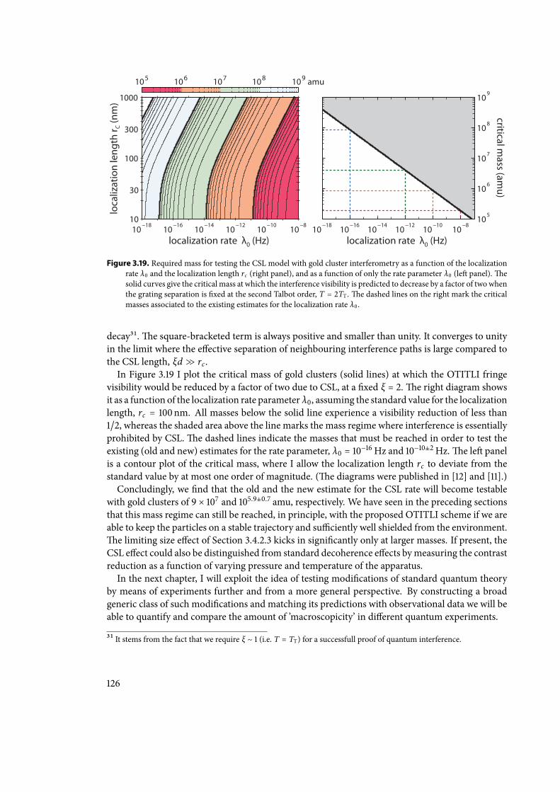
loca

lizat

ion

leng

th r C (

nm)

105 106 107 108 109 amu

localization rate λ0 (Hz)

10−18

10−16

10−14

10−12

10−10

10−8

10

30

100

300

1000

critical mass (am

u)

10−18

10−16

10−14

10−12

10−10

10−8

105

106

107

108

109

localization rate λ0 (Hz)

Figure 3.19. Required mass for testing the CSL model with gold cluster interferometry as a function of the localizationrate λ0 and the localization length rc (right panel), and as a function of only the rate parameter λ0 (le panel).esolid curves give the critical mass at which the interference visibility is predicted to decrease by a factor of twowhenthe grating separation is xed at the second Talbot order, T = 2TT .e dashed lines on the right mark the criticalmasses associated to the existing estimates for the localization rate λ0 .

decay31.e square-bracketed term is always positive and smaller than unity. It converges to unityin the limit where the eective separation of neighbouring interference paths is large compared tothe CSL length, ξd ≫ rc .In Figure 3.19 I plot the critical mass of gold clusters (solid lines) at which the OTITLI fringe

visibility would be reduced by a factor of two due to CSL, at a xed ξ = 2.e right diagram showsit as a function of the localization rate parameter λ0, assuming the standard value for the localizationlength, rc = 100nm. All masses below the solid line experience a visibility reduction of less than1/2, whereas the shaded area above the line marks the mass regime where interference is essentiallyprohibited by CSL.e dashed lines indicate the masses that must be reached in order to test theexisting (old and new) estimates for the rate parameter, λ0 = 10−16Hz and 10−10±2Hz.e le panelis a contour plot of the critical mass, where I allow the localization length rc to deviate from thestandard value by at most one order of magnitude. (e diagrams were published in [12] and [11].)Concludingly, we nd that the old and the new estimate for the CSL rate will become testable

with gold clusters of 9 × 107 and 105.9±0.7 amu, respectively. We have seen in the preceding sectionsthat this mass regime can still be reached, in principle, with the proposed OTITLI scheme if we areable to keep the particles on a stable trajectory and suciently well shielded from the environment.e limiting size eect of Section 3.4.2.3 kicks in signicantly only at larger masses. If present, theCSL eect could also be distinguished from standard decoherence eects bymeasuring the contrastreduction as a function of varying pressure and temperature of the apparatus.In the next chapter, I will exploit the idea of testing modications of standard quantum theory

by means of experiments further and from a more general perspective. By constructing a broadgeneric class of such modications and matching its predictions with observational data we will beable to quantify and compare the amount of ’macroscopicity’ in dierent quantum experiments.

31 It stems from the fact that we require ξ ∼ 1 (i.e. T = TT) for a successfull proof of quantum interference.

126

Chapter 4.

Classicalization and the macroscopicity of

quantum superposition states

“Under the ideal measure of values there lurks the hard cash.”—Karl Marx

e attentive reader should have recognized as a leitmotif throughout this thesis the explorationof the fundamental limits to controlling and interfering massive particles at the borderline to theclassical world. A concrete assessment of these limits was done in Section 3.4 of the preceding chap-ter, which showed the potential of the OTITLI scheme for time-domain Talbot-Lau interferometrywith nanoclusters. We have seen there that, apart from classical confounding factors due to inertialforces, nite particle size or setup imprecisions, the interference of heavy particles would mainlybe aected by environmental decoherence or by certain objective collapse models which have beenproposed for the sake ofmacroscopic realism [3]. Both eects lead to a decay of superposition statesin the position and in themomentumvariable of the interfering particle over time, while at the sametime maintaining the classical correspondence of the respective expectation values, as given by theEhrenfest theorem [164]. One generally describes the observable consequences of such a modiedtime evolution by adding a term to the von Neumann equation of the state operator ρ that repre-sents the motion of the particle. I will refer to the modication as classicalization, or classicalizingmodication, in the following.In this chapter I take a broader perspective and turn the question of the classical limitation to

heavy-particle interference into the question of themacroscopicity of quantum superposition statesin general. What makes, say, a particular many-body superposition state more macroscopic thananother one? If we stick to an intuitive conception of macroscopicity as some kind of yardstickindicating how far beyond the microscopic (atomic) scale quantum behaviour might still be ob-served in nature, then the answer to the latter question must be grounded in empirical facts. Sothe macroscopicity should rather be assigned to a concrete physical observation than to the formalrepresentation of the quantum state itself. Recall that I motivated this argument already in the In-troduction Chapter by referring to Leggett’s hypothesis of macroscopic realism [3, 165]. It will becarried out rigorously in what is to follow.e demonstration of the quantum superposition principle with ever larger systems has in fact

become a key challenge in modern-day experiments.ey range from atom interference with largepath separations and long interrogation times [166,167], observed superpositions withmany super-condensed electrons [1, 2, 168] or Bose-Einstein condensates [169], to proposed measurements of

127

quantum coherence with micromirrors in their oscillatory ground state [170]. In the cited exam-ples, as well as in many other realized and conceivable superposition experiments, the systemsunder investigation consist of material degrees of freedomwith a direct correspondence in classicalmechanics: One may associate with them a distribution of moving point masses. e time evolu-tion of the corresponding quantum states of motion is expected to be aected in a similar way bothby the same decoherence eects and by (speculative) classicalizing modications. So, in a sense,all those experiments are testing the same basic hypothesis, the validity of quantum mechanics, indierent settings and to a dierent degree—a common feature that may ultimately serve as a basisto compare all those experiments in an unbiased way.e central result of this chapter will be the denition of an objective measure of macroscopicity

in Section 4.3, which allows us to quantify how macroscopic various quantum superposition statesare, which have been or may soon be observed in past and future experiments on mechanical sys-tems. To achieve this I will rst construct a generic class of classicalizing modications in Section4.1, which aect standard quantum theory only minimally and leave its basic symmetry and consis-tency principles intact. Having studied their observable consequences in Section 4.2, we can thenassess the macroscopicity of quantum superposition states by quantifying the extent to which suchminimal modications are ruled out once they are observed in an experiment1.e present approach diers from the reasoning behind other measures of macroscopicity that

can be found in the literature [3, 165, 171–176]. ese measures are oen restricted to a subclass ofquantum systems and state representations, or they refer to a preferred choice of macroscopicallydistinct observables or operational resources required to analyze a given quantum state. Hence theyreveal an inherent problem underlying the denition of macroscopicity within quantum theory:e Hilbert space of complex many-body systems can be decomposed into many dierent tensorproducts, in some of which specic quantum states may look elementarily simple or particularlycomplex. De Broglie interference of large molecules is, aer all, described by one single center-of-mass degree of freedom. Iwill discuss in this chapter inwhich sensemolecule interference should beregardedmoremacroscopic than, say, neutron interference.e results of this work were publishedin a condensed form in [14].

4.1. A minimal modi®cation of quantum mechanics

As a rst step let me specify the form and the properties of a hypothetical modication of quantummechanics which shall be weakly invasive in the sense that it conserves basic symmetry princi-ples as well as the operational framework underlying both quantum and classical mechanics. eprincipal focus here lies on the conservation of Galilean invariance in order to avoid a preferred ref-erence frame of the modication, but we shall also account for the exchange symmetry of identicalquantum particles. Moreover, the modication shall consistently scale and apply to arbitrary sys-tems of mechanical degrees of freedom, from the free motion of individual particles to the complexdynamics of interacting many-body systems.e conditions sketched above will be sucient to specify the observable consequences of this

minimalmodication, that is, its explicit form on the level of the density operator ρ for themotional

1e concept of macroscopicity presented here only applies to quantum systems with a direct classical correspondencein nonrelativistic mechanics.is excludes, by denition, systems of genuinely quantum degrees of freedom such asspins.

128

state of an arbitrary mechanical system. It is important to note that there exist already explicitmacro-realistic theories [150, 155, 157, 177], which enforce classical behaviour on the macroscale byadding a nonlinear and stochastic term to the Schrödinger equation of a systemofmaterial particles.ey meet the above requirements and can thus be regarded as special cases of a classicalizingmodication.

4.1.1. The operational framework and the dynamical semigroup assumption

e theory of both quantum and classicalmechanics can be elegantly formulated in an common op-erational framework [178,179] of preparations, transformations and measurements.is approach,minimizing the interpretational overhead on top of the pure mathematical formalism, underlinesthe empirical and statistical nature of both theories and allows us to assess their common featuresmost clearly.One of these features is the general concept of the state ρ associated to a given ensemble of prepa-

rations of a system, a mathematical object that contains all the necessary information to reproducethe statistics of any measurement on that system. In quantum theory the state is given by a linear,positive and normalized2 operator ρ ∈ B (H) on the Hilbert spaceH associated to the underlyingquantum system.e most elementary quantum system with a counterpart in classical mechanicsis that of an elementary moving point mass m in free space, H = L2 (R3). In this case, a givenquantum state ρ may be represented in terms of the real-valued and normalizedWigner functionw (r, p) in phase space (see Appendix A.3 for the one-dimensional case). A classical state of thesame system is given by a positive and normalized distribution function f (r, p) of the phase spacecoordinates (r, p) ∈ R6.e respective distribution functions for general mechanical systems con-sisting of N particles with arbitrary masses are then dened on the 6N-dimensional phase spaceR6N .An important aspect of the operational concept of states is state mixing: Repeating many times a

routine P, where a given system is prepared in the state ρ1 with probability p1 or in a dierent stateρ2 with probability p2 = 1 − p1, yields the state ρ = p1ρ1 + p2ρ2 for the overall ensemble. at isto say, the set of all possible states is convex. Moreover, if the experimenter decides to transformthe state by Φ ∶ ρ ↦ Φ (ρ) each time aer preparing it, we can speak of a dierent mixing routineP’ of the states ρ′1 = Φ (ρ1) and ρ′2 = Φ (ρ2). Consistency then requires the transformation to be aconvex linear map,

Φ (p1ρ1 + p2ρ2) = p1Φ (ρ1) + p2Φ (ρ2) . (4.1)

In addition, the map Φmust then also conserve the normalization and the positivity of states (evenwhen the transformation is performed only on parts of a larger system). One speaks of a linear,completely positive and trace-preserving (LCPT) map. is must hold, in particular, for the freetime evolution of states, as described by a family of transformations Φt ∣ t ≥ 0. It should then beclear that any modication of the standard quantum time evolution must be LCPT in order to stayconsistent with the underlying operational framework.Standard time evolutions in both quantum and classical mechanics exhibit another important

property – their dynamical semigroup character – which should not be easily abandoned whenmodifying it. e semigroup property of a given one-parameter family Φt ∣ t ≥ 0 of LCPT time

2e normalization tr (ρ) = 1 implies that the state is a norm-bounded operator.e set of bounded operators B (H)on a separable Hilbert spaceH is also a Hilbert space.

129

transformations means that the time evolution of a state can be decomposed into successive timesteps by splitting the respective time evolution asΦtΦs = Φt+s, with t, s ≥ 0 andΦ0 = id [180].isproperty is also known as the Markov condition, which is usually only violated when the evolvingsystem is part of a larger system, and the (delayed) back-action of its other part on the degrees offreedom of the subsystem cannot be neglected.Nevertheless, we may always consider, at least in principle, mechanical systems that are su-

ciently well isolated from any environment and that evolve coherently in time, according to the vonNeumann equation ∂tρ = −i [H, ρ] /ħ or its classical counterpart. It is therefore natural to assumethat a modication of the coherent time evolution (of isolated systems) conserves the semigroupproperty of this equation. Recall that the modication is introduced solely for the purpose of in-ducing the quantum-classical transition on themacro-scale, where in both limits the time evolutionfor arbitrary self-contained systems is Markovian. One might argue that a physical realization ofsuch a modication could embody non-Markovian back-action eects on the small time scales ofan underyling physical process. We do not exclude this possibility from our considerations, imply-ing that the Markov condition might be strictly fullled only on the coarse-grained time scales ofactual experiments.e quantum dynamical semigroup of the modied time evolution Φt can be expressed in terms

of the master equation3

∂tρ (t) = LΦρ (t) = − iħ[H, ρ (t)] +Lρ (t) , (4.2)

with ρ (t) = Φt (ρ) the time-evolved initial state ρ and LΦ the generator of the semigroup [180].Aer subtracting the (unmodied) coherent time evolution under the inuence of the Hamiltonoperator H, one arrives at the generator L of the modication. It is of the Lindblad form [180–182]

Lρ =∑j

γ j (L jρL†j −12L†j L j , ρ) . (4.3)

e constituting Lindblad operators L j and coecients γ j ≥ 0 will be specied further using basicsymmetry and consistency arguments in the following.

4.1.2. Galilean covariance

Weare looking for amodicationwhose form is invariant under arbitraryGalilean symmetry trans-formations, that is, the modied time evolution must be interchangeable with arbitrary coordinatetransformations between dierent inertial reference frames. is property is called Galilean co-variance. It should hold universally, even if the concrete Hamiltonian H of the mechanical systemunder consideration is not invariant under Galilean transformations due to an external potential,for instance.In general, the symmetry covariance of a dynamical semigroup is dened with respect to a groupG of symmetry transformations g ∈ G. In a mechanical system they are given by transformationsof the phase space coordinates (r1, . . . , rN , p1, . . . , pN) of N arbitrary particles.e corresponding

3An additional technical assumption is required apart from the semigroup property and the LCPT nature of the one-parameter family Φt ∣ t ≥ 0: Expectation values must evolve continuously in time, that is, the function ⟨A (t)⟩ =tr (AΦt (ρ))must be continuous in t for any state ρ and any bounded operator A ∈ B (H).

130

transformations of a quantum state are represented by unitary operatorsUg associated to each groupelement. e semigroup of maps Φt is covariant with respect to G if Φt (UgρU

†g) = UgΦt (ρ)U

†g

holds for all ρ, g and t. Written in terms of the generator the covariance condition reads as

LΦ (UgρU†g) = UgLΦ(ρ)U

†g ∀ g , ρ. (4.4)

By inspecting Equations (4.2) and (4.3) one easily sees that covariance is fullled for G-symmetricHamiltonians H = UgHU

†g and for Lindblad operators that are symmetric up to a complex phase,

UgL jU†g = e iϕ jL j.

ings are a bit more complicated in case of Galilean transformations, which can be explicitlytime-dependent. Adierent equality holds then for the generator of the time evolution, corrected bythe kinetic energy of a mechanical system.e Lindblad-generatorL of the modication, however,fullls the above covariance condition (4.4), as will be shown in Section 4.1.2.3 below.

4.1.2.1. The Galilei symmetry group

e Galilei group G of transformations between inertial reference frames consists of time transla-tions, spatial translations, velocity boosts, rotations and combinations of those [183]. A space-timepoint transforms as

g ∶ (r, t)↦ (Rgr + sg +wg t, t + tg) , (4.5)

where Rg denotes a three-dimensional rotation matrix. Hence the group G is a direct product ofthe one-parameter group of time translations, the rotation group and the six-parameter group GBof Galilean boosts in position and velocity.e most natural physical representation of the Galileisymmetry is a free particle of mass m [183].I focus here on the boost subgroup GB, rotations will be discussed separately at a later stage.

Time translations will have to be excluded from our considerations. e invariance of a systemunder time translations is implies energy conservation, which is generally not compatible with aclassicalizing modication of the time evolution that leads to an overall loss of quantum coherencein mechanical systems, as we will see later4.We are now le with the abelian subgroup of general boost transformations

GB ∋ gs,w ∶ (r, t)↦ (r + s +wt, t) ,gs,w gs′ ,w′ = gs+s′ ,w+w′ . (4.6)

Each group element is determined by a position translation s and a velocity translation w. Obvi-ously, the group is abelian and isomorphic to R6. In order to nd a representation of the groupin terms of unitary transformations of quantum states in arbitrary mechanical systems, we need tointroduce the concept of characters: ey are the irreducible one-dimensional representations ofabelian groups such as GB and serve as the building blocks of the unitary representations on innitedimensional Hilbert spaces that we will be using [184]. A character χ is a continuous homomor-phism from GB to the set T = z ∈ C ∣ ∣z∣ = 1 of complex numbers of modulus one,

χ ∶ GB → T continuous, χ (g h) = χ (g) χ (h) ∀ g , h ∈ GB . (4.7)

4e unitary representation of time translations in a systemwithHamiltonianH is given by the time evolution operatorsU(tg) = exp [−iHtg/ħ]. e time translation-covariant Lindblad generator of a modication of the coherent timeevolution would require the Lindblad operators to commute with U (tg) up to a complex phase.

131

e set of all characters, together with the pointwisemultiplication, forms the dual group GB, whichis again isomorphic to R6. at is to say, every character is specied by two coordinates r, v andcan conveniently be written as

χr,v ∶ gs,w ↦ exp [iħm0 (v ⋅ s −w ⋅ r)] , (4.8)

with m0 an arbitrary reference mass to set the unit dimensions right.

4.1.2.2. The projective unitary representation of Galilean boosts

e standard representation of Galilean boosts on the Hilbert space L2 (R3) of a free particle ofmass m is expressed in terms of the unitaryWeyl operators [183, 185],

W1 (s,w) = exp [ iħ(p ⋅ s −mw ⋅ r)] (4.9)

= exp [ imw ⋅ s2ħ

] exp [ ip ⋅ sħ

] exp [− imw ⋅ rħ

]

= exp [− imw ⋅ s2ħ

] exp [− imw ⋅ rħ

] exp [ ip ⋅ sħ

] ,

with r and p the position andmomentum operators5.eWeyl operators are the quantum pendantof a phase space translation, as can be seen from

W1(s,w)∣r⟩ = e−imw⋅(2r−s)/2ħ∣r − s⟩, (4.10)

W1(s,w)∣p⟩ = e i(2p−mw)⋅s/2ħ∣p −mw⟩, (4.11)

W1(s,w)⎛⎝

r

p

⎞⎠

W†1 (s,w) =

⎛⎝

r + sp +mw

⎞⎠. (4.12)

e operators form a projective unitary representation (or unitary ray representation) of Galileanboosts [183–185], that is, they conserve the group operation and commute with each other up to acomplex phase,

W1 (s1,w1)W1 (s2,w2) = e im(w1 ⋅s2−w2 ⋅s1)/2ħW1 (s1 + s2,w1 +w2)= e im(w1 ⋅s2−w2 ⋅s1)/ħW1 (s2,w2)W1 (s1,w1) . (4.13)

is is also known as theWeyl relation [186]. e phase factor in the second line is given by thecharacter (4.8), with m0 = m.

5An operator exponential can be split according to eX+Y = eXeYe−[X,Y]/2 when the commutator is a C-number. Fromthis follows also the identity eXYe−X = Y + [X, Y].

132

In the general case ofN particles (withmassesm1, . . . ,mN ) the boosts are represented by a tensorproduct of the single-particle representations,

WN (s,w) =N⊗n=1exp [ i

ħ(pn ⋅ s −mnw ⋅ rn)] = exp [

iħ(P ⋅ s −Mw ⋅ R)] (4.14)

= exp [ iMw ⋅ s2ħ

]N⊗n=1exp [ ipn ⋅ s

ħ] exp [− imnw ⋅ rn

ħ]

= exp [− iMw ⋅ s2ħ

]N⊗n=1exp [− imnw ⋅ rn

ħ] exp [ ipn ⋅ s

ħ] .

Comparing the right hand side of the rst line with (4.9) we see that this eectively boosts only thecenter-of-mass coordinates R = ∑n mnrn/M and P = ∑n pn, with M = ∑n mn the total mass.erespective Weyl relation reads as

WN (s1,w1)WN (s2,w2) = e iM(w1 ⋅s2−w2 ⋅s1)/2ħWN (s1 + s2,w1 +w2) . (4.15)

e many-particle Weyl operators can also be formulated in second quantization by expressing theposition and momentum operators of identical particles in terms of Fock operators,

W(s,w) = exp [ iħ∑k

( ∫ d3p p ⋅ s a†k(p)ak(p) −mk ∫ d3rw ⋅ r ψ

†k(r)ψk(r))] . (4.16)

Here, the sum extends over dierent bosonic or fermionic particle species labeled by k. In partic-ular, it extends over the dierent spin states of each particle. e terms ak(p) and ψk(r) denotethe Fock annihilation operators for momentum p and position r, respectively. e Weyl relationbecomes

W (s1,w1)W (s2,w2) = e iM(w1 ⋅s2−w2 ⋅s1)/2ħW (s1 + s2,w1 +w2) , (4.17)with the operator M = ∑k mkNk counting the total mass via the number operators Nk of eachspecies. Projective unitarity holds within each subspace of xed particle number, where the expo-nential term reduces to a phase factor, as in (4.15). I will mostly use the rst quantization formin the following, when discussing the general implications of Galilean covariance on the modiedtime evolution of mechanical systems.

4.1.2.3. Galilean covariance of the modi®ed time evolution

e modied time evolution Φt of a mechanical system is covariant with respect to the Galileanboost transformations (4.6) if it stays the same whether one applies it in, say, the system’s rest frameor in another inertial frame. In mathematical terms, this condition reads as [187, 188]

Φt [WN (s,w) ρW†N (s,w)] = WN (s −wt,w)Φt (ρ)W

†N (s −wt,w) ∀ ρ, s,w , t. (4.18)

It diers from the covariance condition (4.4) due to the explicit time-dependence of the boost trans-formation:e system coordinates with respect to the moving reference frame are constantly relo-cated bywt over time.e covariance condition for the generatorLΦ is obtained by dierentiatingwith respect to time at t = 0,

LΦ [WN (s,w) ρW†N (s,w)] = WN (s,w)LΦ (ρ) − i

ħw ⋅ [∑

npn , ρ]W

†N (s,w) . (4.19)

133

As already mentioned, this only holds in systems where the coherent time evolution is governedby a Galilei-invariant Hamiltonian without external potential. In fact, the second term in the curlybrackets corrects for the phase-space translation of the kinetic energy term L0 (ρ) =−i∑n [p2n/2mn , ρ] /ħ, which is always part of the Hamiltonian. One checks this easily using theidentity (4.12). By subtracting the coherent part from the generator of the time evolution one ndsthat the Galilei-covariant modication (4.3) then must fulll the condition (4.4) in terms of theWeyl operators,

L [WN (s,w) ρW†N (s,w)] = WN (s,w)L (ρ)W

†N (s,w) . (4.20)

e identity shall hold universally, including the cases where theHamiltonianH breaks the Galileancovariance of the coherent time evolution.

4.1.2.4. Implications for the form of the modi®cation

A theorem by Holevo [189, 190] restricts the form of the modication generator L based on theabove condition (4.20). He studied the generic form of quantum dynamical semigroups which arecovariant with respect to a certain class of abelian symmetry groups, including the Galilean boostgroup GB studied here. I follow the proof presented in [189], which does not only apply to single-particle Hilbert spaces but to arbitrary many-body systems. Holevo states his result for unitaryrepresentations of the symmetry group, but the relevant steps in the proof remain valid also forprojective unitary representations, as in the present case. e result is valid for norm-boundedquantum dynamical semigroups Φt, that is, ∥Φt (A)∥ ≤ C ∥A∥ ∀A ∈ B (H), with C ≥ 0 and ∥A∥the operator norm [191].According to Holevo’s theorem, the GB-covariant generator (4.20) can be decomposed in terms

of an integral over the dual group GB ≅ R6 of characters (4.8),

L (ρ) =∑j∫ d3sd3w [L j (s,w) ρL

†j (s,w) − 1

2L†j (s,w) L j (s,w) , ρ] . (4.21)

e Lindblad operators fulll the relation

L j (s,w)WN (s′,w′) = χs,w (gs′ ,w′)WN (s′,w′) L j (s,w)

= exp [ iħm0 (w ⋅ s′ −w′ ⋅ s)]WN (s′,w′) L j (s,w) , (4.22)

and the operator-valued integral ∫ d3sd3w ∑ j L†j (s,w) L j (s,w) is pointwise convergent (i.e. it con-

verges to a nite value with respect to the weak-* topology in B (H) [191]). e latter, however,means that unbounded diusion terms such as double commutators [r, [r, ρ]] are excluded [188,192]. Such terms occur in the Caldeira-Leggett model of quantum Brownian motion [35, 193], forinstance. ey are typically the result of approximating scattering processes in the limit of weakmomentum exchange [194], and they give rise to a signicantly more drastic classicalizing modi-cation of the coherent time evolution when they are universally applied beyond that limit. I havetherefore omitted unbounded terms in the construction of a minimally invasive modication.We still have to account for the rotation transformations to obtain full Galilean covariance of the

modication. However, it will be more convenient to incorporate them aer studying the concreteimplications of the covariance condition (4.22) on the Lindblad operators L j (s,w).

134

4.1.3. The modi®ed time evolution of a single particle

In the case of a single particle of mass m one can explicitly construct the Lindblad operators of themodication (4.21) from the covariance condition (4.22), which reduces to

exp [− iħ(p ⋅ s′ −mw′ ⋅ r)] L j (s,w) exp [ i

ħ(p ⋅ s′ −mw′ ⋅ r)] = e im0(w⋅s

′−w′⋅s)/ħL j (s,w) . (4.23)

Since this must hold for arbitrary (s′,w′) ∈ R6, we obtain two independent conditions by settingeither the position or the velocity variable to zero. For w′ = 0 the matrix elements of the operatorin momentum representation fulll the identity

e i(p′−p)s′/ħ⟨p∣L j (s,w) ∣p′⟩ = e im0w⋅s

′/ħ⟨p∣L j (s,w) ∣p′⟩ ∀ s′. (4.24)

A non-zero value of the matrix element is only possible for p′ = p+m0w. Using the transformationrule (4.11) we may thus expand the operator as

L j (s,w) = L j (s,w;p) exp [iħm0w ⋅ r] , (4.25)

where the function L j can only depend on the momentum operator p of the particle. Plugging thisinto (4.23) for s′ = 0 leads to the condition

e imw′(r−r′)/ħ⟨r∣L j (s,w;p) ∣r′⟩ = e−im0w′⋅s/ħ⟨r∣L j (s,w;p) ∣r′⟩ ∀w′, (4.26)

in position representation. Here, a non-zero matrix element is only possible for r′ = r + m0s/m.e form of L j is thus obtained from the rule (4.10) and we are nally le with

L j (s,w) = ℓ j (s,w) exp [ iħm0 (w ⋅ r − p ⋅ s

m)] = ℓ j (s,w)W

†1 (

m0m

s, m0m

w) , (4.27)

where ℓ j denotes an arbitrary complex-valued function. Itmust be square-integrable since themod-ication (4.21) is norm-bounded.is allows us to introduce a time parameter τ > 0 and a positivephase-space distribution function g (s, q) by

1τ= ∫ d3sd3w ∑

j∣ℓ j (s,w)∣2 , (4.28)

g (s, q) = m3τm60∑j∣ℓ j (

mm0

s, qm0

)∣2, (4.29)

where the latter is normalized to ∫ d3sd3q g (s, q) = 1. e time parameter and the position-momentum distribution function specify completely the modication for a single particle,

L1 (ρ) = 1τ[ ∫ d3sd3q g (s, q)W

†1 (s,

qm

) ρW1 (s,qm

) − ρ] . (4.30)

135

4.1.3.1. Covariance with respect to rotations

In order to achieve full Galilean covariance of (4.30) rotational transformationsmust be consideredas well. ey are described in terms of orthogonal rotation matrices R ∈ SO (3), RRT = RTR = I,with unit determinant.eir unitary representation in mechanical systems transforms the positionand momentum operator of a particle as

UR⎛⎝

r

p

⎞⎠

U†R =⎛⎝Rr

Rp

⎞⎠. (4.31)

e identity a ⋅ Rb = (RTa) ⋅ b holds for scalar products of three-dimensional vectors. Given anarbitrary rotation R, we nd that the generator (4.30) transforms as

URL1 (ρ)U†R =

1τ[ ∫ d3sd3q g (s, q)W

†1 (R

T s, RTqm

)URρU†RW1 (RT s, R

Tqm

) − URρU†R]

= 1τ[ ∫ d3sd3q g (Rs, Rq)W

†1 (s,

qm

)URρU†RW1 (s,

qm

) − URρU†R] (4.32)

Rotational covariance is then obtained for isotropic (and inversion-symmetric) distribution func-tions, g (s, q) = g (s, q), where s = ∣s∣ and q = ∣q∣.e nal form of the Galilei-covariant modica-tion of the time evolution of a single particle then reads as

L1 (ρ) = 1τ[ ∫ d3sd3q g (s, q)W1 (s,

qm

) ρW†1 (s,

qm

) − ρ] . (4.33)

4.1.3.2. Decay of coherence

e main feature of the Galilei-covariant modication is its inherent classicalizing eect on thequantum state of a single particle. It induces a combined decay of o-diagonal matrix elements ofthe state operator ρ in both position and momentum representation.is becomes evident alreadyin the specic case where translations occur only in themomentumdirection, g (s, q) = δ (s) h (q).e modication (4.33) then resembles the generic form of collisional decoherence master equa-tions [195]. Such master equations can be interpreted as a random position measurement with alimited spatial resolution given by the spread of the Fourier transform of h (q). Quantum states re-main practically unaected if they are localized below this limit, whereas coherent superpositionsstretching over a larger distance decay into a classical mixture within the time scale τ.Moreover, the observable consequences of certain objective collapse models [150, 153, 155, 157,

177], which explicitly modify the quantum dynamics of mechanical systems on the level of theSchrödinger equation, are described by the same generic form [163]. In the model of continuousspontaneous localization [155, 157], for instance, the function h (q) is given by a Gaussian distri-bution (and the same holds true in the previous version [153] of that model). Diósi’s gravitationalcollapse model [150, 177] leads to the modication term

LD (ρ) = −κG4ħ ∫ d3s1d3s2 1

∣s1 − s2∣[ f (s1 − r) , [ f (s2 − r) , ρ]] (4.34)

136

for a single particle, with G the gravitational constant, κ a free scaling factor of the collapse rateand f (r) the local mass density of the particle6. e expression can be brought into the covari-ant standard form (4.33) by introducing the Fourier transform f (q) of the mass density f (s) =∫ d3q e iq⋅s/ħ f (q) / (2πħ)3, and by noting that the gravitational potential transforms as

∫ d3s exp (ik ⋅ s)s= lim

α→0 ∫ d3s exp (−αs + ik ⋅ s)s

= 4πk2

(4.35)

into Fourier space. We arrive at

LD (ρ) = κG(2πħ)2 ∫ d3q

∣ f (q)∣2

q2[W1 (0,

qm

) ρW†1 (0,

qm

) − ρ] , (4.36)

which is Galilei-covariant if f (s) = f (s).In the more general case (4.33) the classicalizing eect can be made explicit by representing the

state in terms of its characteristic function. e latter is given by the expansion coecients of thestate operator ρ in terms of the Weyl operators, which form a complete basis set of bounded oper-ators,

χ (r, p) ∶= tr(ρW†1 (r,

pm

)) = ∫ d3r′d3p′w (r′, p′) e i(p⋅r′−p′⋅r)/ħ . (4.37)

It is normalized to χ (0, 0) = 1, and it relates to theWigner functionw (r, p) by a Fourier transform.Spatial coherences, that is, o-diagonal matrix elements of ρ in position representation, can beextracted from the characteristic function via

⟨r0 −r2∣ ρ ∣r0 +

r2⟩ = ∫ d3p

(2πħ)3e−ip⋅r0/ħ χ (r, p) , (4.38)

and similarly for momentum coherences. e above single-particle modication (4.33) maps thecharacteristic function to

L1 ∶ χ (r, p)↦ 1τ[ ∫ d3sd3q g (s, q) e i(q⋅r−p⋅s)/ħ − 1] χ (r, p)

= − 1τ[1 − g (r, p)] χ (r, p) , (4.39)

where I have introduced the Fourier transform of the phase space distribution function

g (r, p) = ∫ d3sd3q g (s, q) exp [− iħ(p ⋅ s + r ⋅ q)]

= ∫ ∞

0dsdq (4πqs)2 g (s, q) sinc( ps

ħ) sinc(qr

ħ) . (4.40)

It is real and bounded by ∣g (r, p)∣ ≤ 1 due to the normalization of the distribution g. e modi-cation thus eects a decay of the characteristic function in (4.39) and, as a consequence, of o-diagonal matrix elements in position and momentum representation.is happens at a decay timescale given by the parameter τ.e range of aected superposition states is limited, as the decay is

6 Point particles with f (r) = mδ (r) are not allowed in this model because they would lead to a diverging modicationterm. One must assume a nite mass density, or nite size, for every particle, even including electrons, for instance.

137

suppressed for small-scale coherences extending only over distances r in position or p in momen-tum for which g (r, p) ≈ 1.It is interesting to note that the modication (4.33) for a free particle is covariant with respect to

time translations in the specic case of zero momentum translations, g (s, q) = h (s) δ (q). isis because the Lindblad operators commute with the free unitary time evolution operator U0 (t) =exp [−ip2t/2mħ], and the modication does not aect the conservation of energy. However, thisalso means that plane wave states7 ρ = ∣p⟩⟨p∣, which are delocalized and clearly non-classical, arenot aected by the modication. Momentum translations are therefore necessary to classicalize themotion of free particles.

4.1.4. The modi®ed time evolution of a many-particle system

While the form of the modication for a single particle can be specied up to a time constant anda phase space distribution function, this is not so in the case of N > 1 particles. Using (4.14) thecovariance condition (4.22) for the Lindblad operators can be stated as

exp [− iħ(P ⋅ s′ −Mw′ ⋅ R)] L j (s,w) exp [ i

ħ(P ⋅ s′ −Mw′ ⋅ R)]

= e im0(w⋅s′−w′⋅s)/ħL j (s,w) ∀ s′,w′, (4.41)

with M = ∑Nn=1mn the total mass. is relation means that the Lindblad operators must translate

the center-of-mass momentum P = ∑n pn by the amount −m0w, and the center-of-mass positionR = ∑n mnrn/M by −m0s/M. Let us therefore switch to center-of-mass and relative coordinatesand factorize the operator as

L j (s,w) = Lrelj (s,w)⊗ exp [ iħm0 (w ⋅ R − P ⋅ s

M)] = Lrelj (s,w)⊗W

†N (m0

Ms, m0

Mw) (4.42)

where the factor Lrelj (s,w) represents an operator acting solely on the Hilbert space of the relativecoordinates of theN-particle system. With this the covariance condition is fullled by construction.e possible choices of the remaining factor correspond to dierent ways of distributing the

phase-space translation of the center of mass over the individual constituents.e simplest way isto divide the translation equally among all constituents, which yields a unitary representation interms of the N-particle Weyl operator,

L(U) (s,w) =√

M3

τ(N)g(N) (s,Mw)W

†N (s,w) . (4.43)

It represents a straightforward generalization of the single-particle form (4.30), where I have re-scaled the argument of theWeyl operator accordingly and omitted the j-index.e parameter τ(N)

determines the time scale at which coherence decays in the system, while g(N) denotes a positiveand normalized phase-space distribution function.e latter must be isotropic to x the rotationalcovariance, as in the single-particle case. However, it will be explained below that this N-particle

7Although plane waves are improper states, i.e. not normalizable, they serve as a helpful idealization in many concretesituations.

138

form is not suitable to consistently describe a universal classicalizing modication for arbitrarymany-particle systems.Another natural way to eect the above center-of-mass translation is to superimpose individual

single-particle translations of all constituents,

L(S) (s,w) =N∑n=1

ℓn (s,w) exp [ iħ(m0w ⋅ rn −

m0mn

pn ⋅ s)] , (4.44)

where the weights ℓn of the summandsmust be equal for indistinguishable particles in order to con-serve the exchange symmetry of bosons and fermions. Each summand describes the translation ofthe position andmomentum of the nth particle by −m0s/mn and −m0w, which eects a net shi ofthe center-of-mass coordinates by −m0s/M and −m0w. Rotational covariance is again achieved byisotropic coecient functions8 ℓn (s,w), in analogy to the single-particle case discussed in Section4.1.3.1.e representation (4.44) treats individual particles independently, and a consistent scalingof the classicalization eect to arbitrary mechanical systems can be achieved, as will be demon-strated below.In principle, the N-particle Lindblad operators could also be constructed out of phase-space

translations of arbitrary subsets of 2, . . . ,N − 1 particles, or a linear combination of all these pos-sibilities. Picking one of these possibilities, however, would be an unduly complication of matterswithout any clear advantages to the natural N-particle form (4.44). In particular, it seems unlikelythat a scale invariance property similar to the one explained in Section 4.1.4.4 below would hold insuch a case.Finally there is also the possibility to ascribe independent generators L(n)

1 (ρ) to the individ-ual particles and add them up9 to LN (ρ) = ∑N

n=1L(n)1 (ρ) in the N-particle case. Each generator

must then be of the single-particle form (4.33). Such an approach was in fact pursued by the au-thors of the so-called GRWmodel [153], an earlier version of the continuous spontaneous localiza-tion model [155] which falls under the class of classicalizing modications studied here.is form,however, breaks the fundamental exchange symmetry in systems of indistinguishable quantumpar-ticles (as was pointed out in [196] for the GRW case). Separate generators L(k) could be admissibleonly for dierent particle species k, which are inherently distinguishable, but this would lead to acomplicated nonuniform scaling behaviour of the classicalizing eect in large systems consistingof various kinds of particles. I have avoided this complication by restricting to a single Lindbladgenerator to describe the modication in any mechanical system of N particles, that is, I droppedthe j-summation in the general form of the generator (4.21).

4.1.4.1. Basic consistency and scaling requirements

e selection of a specic N-particle form of the modication must be based on two other formalrequirements besides the Galilean covariance, which guarantee that the modication is universallyapplicable to any system of mechanical degrees of freedom.

8e coecient functions could actually share a common phase factor exp [iθ (s,w)] which needs not be isotropic.Such a global phase factor in the Lindblad operator L(S) (s,w) may, however, always be omitted without loss ofgenerality.

9is corresponds to the j-summation in the general Galilei-covariant form of the modication (4.21), which is other-wise omitted.

139

Bystander criterion Firstly, we demand a consistent treatment of single particles, whether theyare isolated or constituents in a larger (possibly interacting) system of particles. No additional cor-relations between individual particles should originate from the N-particle modication. at isto say, the single-particle form (4.33) must always be reobtained from the general N-particle mod-ication (4.21) aer tracing over N − 1 ‘bystanding’ particles. In particular, the local descriptionof the state of a particle should not be altered by appending the state of an uncorrelated system ofparticles, which may be completely detached and far away from the particle of interest.is avoidsany superluminar action at a distance induced by the modication.

Composition criterion In both quantum and classical mechanics we can describe the time evo-lution of a compoundmany-body system by a single center-of-mass degree of freedom if its internalstructure does not inuence the overallmotion.e notion of a ‘single particle’ thus not only appliesto elementary building blocks of matter, but may also be used to describe the motion of compositeobjects. In the same vein, we demand that the single-particle form (4.33) must eectively apply tothe center-of-mass description of a compound N-particle object, if the modication does not aectnotably the (coherent) internal dynamics of the constituents.is may be applicable (i) if the com-pound can be regarded as a point-like particle, that is, if the constituent particles extend over a smallregion where the modication shows no ponderable impact10, or (ii) if the constituent particles of alarger compound are rigidly localized around their equilibrium positions in the body-xed frame.In both cases we demand that the Lindblad operators (4.42) should (in some approximate sense)reduce to

L (s,w) ≈ e iθ(s,w)

¿ÁÁÀ m60

M3τcmgcm (m0

Ms,m0w)W

†N (m0

Ms, m0

Mw) , (4.45)

to obtain the form (4.33) for the center-of-mass degree of freedom, with a time parameter τcm anddistribution function gcm (s, q) determining the eective strength of the classicalizing eect on themotion of the compound. A complex phase θ j may appear in the approximation, which drops outagain in the corresponding generator.To achieve the required classicalization onmacroscopic scales, the modication should act more

strongly on the whole compound than on each constituent individually; there must be an ampli-cation of the eect with growing size of the compound object. I will show how this inuences thegeneral form of the modication in many-particle systems. Let me denote, in the following, by τnand gn the time parameter and the distribution function of the nth particle in the system.

4.1.4.2. Center-of-mass translations

As already mentioned, the simplest generalization of the modication to arbitrary states ρ of Nparticles is given by the Weyl operator (4.43),

L(U)N (ρ) = 1

τ(N)[ ∫ d3sd3q g(N) (s, q)WN (s, q

M) ρW

†N (s, q

M) − ρ] , (4.46)

10 It was noted in Section 4.1.3.2 that the single-particle modication is characterized by a minimal length scale whereit aects superpositions. Smaller-scale coherences are hardly inuenced, and the internal dynamics of a sucientlysmall compound object should therefore remain unaected under the same conditions.

140

with M = ∑n mn the total mass. Tracing over all but the nth particle in the system yields theexpression

trN−1 [L(U)N (ρ)] = 1

τ(N)[ ∫ d3sd3q g(N) (s, q)W1 (s,

qM

) ρnW†1 (s,

qM

) − ρn] (4.47)

= 1τ(N)

[M3

m3n ∫ d3sd3q g(N) (s, M

mnq)W1 (s,

qmn

) ρnW†1 (s,

qmn

) − ρn]

for its reduced state ρn = trN−1 [ρ]. We nd that for τ(N) = τn and g(N) (s, q) =(mn/M)3 gn (s,mnq/M) the bystander criterion is met, that is, the expression equals the single-particle form (4.33) for ρn. On the other hand, the composition criterion is met by construction,with τcm = τ(N) and gcm = g(N), as (4.46) acts only on the center-of-mass coordinate.With both criteria taken into account the present form of the modication is not capable of in-

ducing classical behaviour on the macro-scale, while imposing only a negligible disturbance of thedynamics of microscopic quantum systems. is is because the rate of coherence decay inducedby the modication does not amplify with the size of a compound system. e time parameterτ(N) = τn = τ is the same for all kinds of particles, irrespective of their mass and composition.eonly feature that grows with the mass M of the compound is the momentum spread of the phase-space distribution function g(N), which merely increases the range of aected superposition states,as discussed in Section 4.1.3.2. In addition, the time evolution of the relative coordinates within a(possibly large) compound system is not subject to any eect, because the modication only actson center-of-mass coordinates. Nomatter howmacroscopic the systemmay be, its internal degreesof freedom could stay in a superposition and would never be classicalized.

4.1.4.3. Single-particle translations

Having discarded the representation in terms of N-particle Weyl operators, let us proceed to de-scribe the N-particle Lindblad operators as the sum of single-particle translations (4.44),

L(S)N (ρ) =

N∑k,n=1

∫ d3sd3w ℓn (s,w) ℓ∗k (s,w) [W†1 (

m0mn

s, m0mn

w) ρW1 (m0mk

s, m0mk

w)

− 12W1 (

m0mk

s, m0mk

w)W†1 (

m0mn

s, m0mn

w) , ρ] . (4.48)

Here and in the following, the single-particleWeyl operators act on the Hilbert space of the particlen that is indicated by the mass variable mn in their argument. In order to check the bystandercriterion we must trace again over all but the nth particle, as denoted by trN−1, and obtain

trN−1 [L(S)N (ρ)] = ∫ d3sd3w ∣ℓn (s,w)∣2 [W

†1 (

m0mn

s, m0mn

w) ρnW1 (m0mn

s, m0mn

w) − ρn] + ∆ρ,(4.49)

with ∆ρ given by (4.51). Comparing the rst Lindblad term to the single-particle form gives

ℓn (s,w) = e iθn(s,m0w)

¿ÁÁÀ m60

m3nτngn (

m0mn

s,m0w), (4.50)

141

with θn (s,w) an arbitrary phase that may be dierent for each (distinguishable) particle in thesystem.e bystander criterion is now met if the remaining term,

∆ρ = i∑k≠n

∫ d3sd3w Imℓn (s,w) ℓ∗k (s,w)

× [W†1 (

m0mn

s, m0mn

w) , trN−1 (W1 (m0mk

s, m0mk

w) ρ)] , (4.51)

vanishes. is is achieved if the phases θn are multiples of π, notwithstanding any global phasefor all single-particle contributions. Moreover, the phases must be zero for identical particles toconserve their bosonic or fermionic exchange symmetry11.e composition criterion is also met, as can be seen explicitly by neglecting the relative motion

of the constituents in a point-like compound and approximating the coordinates of each particle byrn ≈ R and pn ≈ mnP/M. is leads to approximate Lindblad operators of the form (4.45), wherethe modication parameters for the center-of-mass motion are given by

1τcm

gcm (s, q) =RRRRRRRRRRR

N∑n=1

e iθn(Ms/m0 ,q)√

M3

m3nτngn (

Mmn

s, q)RRRRRRRRRRR

2

. (4.52)

Integrating this expression yields the decay rate 1/τcm of center-of-mass coherence,

1τcm

=∑n

1τn

+ 2∑k<n

∫ d3sd3q

√τnτk

¿ÁÁÀ m60

m3nm3kgn (

m0mn

s, q) gk (m0mk

s, q) cos [θn (s, q) − θk (s, q)]´¹¹¹¹¹¹¹¹¹¹¹¹¹¹¹¹¹¹¹¹¹¹¹¹¹¹¹¹¹¹¹¹¹¹¹¹¹¹¹¹¹¹¹¹¹¹¹¹¹¹¹¹¹¹¹¹¹¹¹¹¹¹¹¹¹¹¹¹¹¹¸¹¹¹¹¹¹¹¹¹¹¹¹¹¹¹¹¹¹¹¹¹¹¹¹¹¹¹¹¹¹¹¹¹¹¹¹¹¹¹¹¹¹¹¹¹¹¹¹¹¹¹¹¹¹¹¹¹¹¹¹¹¹¹¹¹¹¹¹¹¹¶

=±1

.

(4.53)A clearer view is obtained by introducing the normalized functions

fn (s, q) =

¿ÁÁÀm30

m3ngn (

m0mn

s, q) e iθn(s,q)´¹¹¹¹¹¹¹¹¹¸¹¹¹¹¹¹¹¹¹¶

=±1

(4.54)

for the square root of the phase-space distributions gn appearing in (4.50). e particle massmn must be replaced by the total mass M in the case of the center-of-mass compound, as rep-resented by fcm. Each function is real and square-integrable, fn ∈ L2 (R6), with norm ∥ fn∥ =√

( fn , fn) = 1 by construction. e L2-scalar product is dened in the usual way as ( f , g) =∫ d3sd3q f ∗ (s, q) g (s, q), and the Cauchy-Schwarz inequality implies −1 ≤ ( fk , fn) ≤ 1 ∀ k, n.Using this notation the composition criterion (4.52) can be expressed as

1√τcmfcm (s, q) =

N∑n=1

1√τnfn (s, q) , (4.55)

and, in particular,1

τcm= ∥

N∑n=1

1√τnfn∥

2

≤ ∣N∑n=1

1√τn∣2

. (4.56)

11 Invariance with respect to particle exchange is fullled if the Lindblad operators L(S) (s,w) of the modication com-mute with the exchange of any two out of N identical particles n,m up to a complex phase factor exp [iϕnm (s,w)].Since this must generally hold for any N ≥ 2, all relative phases θn between indistinguishable particles in (4.50) mustbe set to zero.is makes the Lindblad operators exchange-symmetric sums of single-particle operators.

142

Here it becomes evident how the use of single-particle translations produces the intended ampli-cation of the classicalizing eect with the system size (as opposed to the description in Section4.1.4.2): e center-of-mass coherence decay rate grows quadratically with the number N of con-stituents (for a nite number of particle species). Concretely, one obtains τcm = τ/N2 in the case ofN identical particles, with τn = τ.

4.1.4.4. Universality and scale invariance of the modi®cation

Using the single-particle descriptionwe are lewith the freedomof choosing the timeparameters τnand the real functions fn (s, q) of each individual particle species in order to fully specify the generalform of the classicalizing modication. Dierent functions (by e.g. varying their shapes, widthsand signs) for dierent constituents would lead to even another distribution for the compoundparticle, according to the composition rule (4.55). is compound could then be combined withanother species to a dierent compound, and so on, and each with its own distribution function.Ultimately, one would have to deliberately choose a xed reference set of elementary point particles,which serve as the building blocks for all matter subject to the classicalization, and assign individualphase-space distribution functions and rate parameters to each of them. Should one decomposethe superposition of, say, a C60-fullerene in terms of 60 carbon atoms or in terms of an overall 1080protons, neutrons and electrons?We can avoid such questions of preferred choice by once again taking advantage of the composi-

tion rule (4.55). It implies that theweighted function fn/√τn is an extensive property of (point-like)

composite systems which increases with each constituent. We thus obtain a universal description,which does not favour a particular decomposition of compound objects into smaller units, by re-lating the composition rule (4.55) to the mass—the basic extensive property of mechanical objects,which comes naturally with the Galilean covariance condition. at is to say, we can dene theweighted root function of any point-like particle with mass mn relative to a xed reference massm0,

1√τnfn (s, q) ∶=

mnm0

1√τ0f0 (s, q) , (4.57)

by introducing only a single reference time parameter τ0 and a single reference function f0. elatter boils down (without loss of generality) to a positive, normalized and isotropic reference distri-bution function g0 (s, q) = ∣ f0 (s, q)∣2, according to (4.54).e time parameter and the distributionfor each particle species n is then given by

τn = (m0mn

)2

τ0, gn (s, q) = (mnm0

)3g0 (

mnm0

s, q) , (4.58)

which holds consistently for point-like compound particles,

τcm = (m0M

)2

τ0, gcm (s, q) = ( Mm0

)3g0 (

Mm0

s, q) , (4.59)

as follows from the identities (4.55) and (4.56). e classicalization of point-like particles is thusuniversally described by the (mass-rescaled) expressions (4.58), which are independent of decom-

143

posing those particles into smaller mass units12.e classicalizing eect is obviously amplied forlarge particles, as the coherence decay time parameter τcm decreases quadratically with growingmass, according to (4.59). At the same time the distribution function is compressed in the positioncoordinate, weakening the classicalization-induced position diusion for heavy objects.

4.1.4.5. General form of the modi®cation

Putting everything together we arrive at a universal and consistent form of the classicalizing mod-ication for arbitrary mechanical systems comprised of N point-like particles,

LN (ρ) = 1τ0 ∫ d3sd3q g0 (s, q) [AN (s, q) ρA

†N (s, q) − 1

2A†N (s, q)AN (s, q) , ρ] , (4.60)

AN (s, q) =N∑n=1

mnm0exp [ i

ħ(pn ⋅

m0mn

s − q ⋅ rn)] =N∑n=1

mnm0

W1 (m0mn

s, qmn

) . (4.61)

It is completely determined by specifying the time parameter τ0 and the distribution functiong0 (s, q) at the reference mass m0.

4.1.4.6. Second quantization formulation

e general Lindblad operators (4.61) are sums of single-particle operators. Due to the constantweight for particles of identical mass, they conserve the exchange symmetry of indistinguishablebosons and fermions, that is, quantum particles of the same species j and in the same spin state σ .It follows that we may consistently formulate the modication generator (4.60) in second quanti-zation,

L (ρ) = 1τ0 ∫ d3sd3q g0 (s, q) [A (s, q) ρA

†(s, q) − 1

2A†(s, q)A (s, q) , ρ] , (4.62)

Here, the Lindblad operators can be expanded in terms of the single-particle creation and annihi-lation operators in the momentum or position basis,

A (s, q) =∑j,σ∫ d3pd3p′ A j,σ (s, q; p, p′) a

†j,σ (p) a j,σ (p′)

=∑j,σ∫ d3rd3r′ A j,σ (s, q; r, r′)ψ

†j,σ (r)ψ j,σ (r′) , (4.63)

or in any other basis of single-particle wavefunctions over conguration space13 [197, 198]. emomentum and the position basis represent the most natural choices; they fulll the canonical

12 Evidently, I assume that there exist (besides elementary point particles) point-like compound particles whose internalstructure remains practically unaected by the classicalizing eect.is is certainly a weaker prerequisite than estab-lishing a xed reference set of elementary particles with individual classicalization rates and distribution functions,and it can be justied a posteriori by limiting the strength of the classicalization eect in compliance with experimen-tal observations on the microscopic scale. In practice one should describe electrons, protons, neutrons and nuclei aspoint particles, or otherwise even femtometer-sized superpositions of elementary particles would be aected. In thiscase one could keep microscopic systems unaected only by limiting the classicalization rate of macroscopic systemsto unsatisfactorily low values, as was discussed in the case of spontaneous localization models in [160].

13 Spins are nite-dimensional degrees of freedom and their basis states are thus labelled by a single running index σ .e classicalizing modication only acts on mechanical degrees of freedom, and the internal dynamics of spin statesremains unaected.

144

commutation relations (CCR)

[aσ (p) , aσ ′ (p′)]± = [a†σ (p) , a

†σ ′ (p

′)]±= 0, [aσ (p) , a

†σ ′ (p

′)]±= δσσ ′δ (p − p′) ,

[ψσ (r) , ψσ ′ (r′)]± = [ψ†σ (r) , ψ

†σ ′ (r

′)]±= 0, [ψσ (r) , ψ

†σ ′ (r

′)]±= δσσ ′δ (r − r′) , (4.64)

where the anticommutator (+) is used for fermions and the commutator (−) for bosons. Any(spin-independent) single-particle operator is readily translated into second quantization by rstexpanding it, say, in themomentum representation and thenmapping ∣p′⟩⟨p∣↦ ∑σ a

†σ (p′) aσ (p).

e Lindblad operators (4.61) of the modication then become

A (s, q) =∑j

m j

m0 ∫ d3p e ip⋅m0s/m jħ∑σ

a†j,σ (p − q) a j,σ (p)

=∑j

m j

m0 ∫ d3r e−iq⋅r/ħ∑σ ψ†j,σ (r − m0

m js) ψ j,σ (r) , (4.65)

up to an irrelevant complex phase factor. e second line follows from the rst with help of thebasis transformation rule

ψ (r) = ∫ d3p(2πħ)3/2

a (p) e ip⋅r/ħ ↔ a (p) = ∫ d3r(2πħ)3/2

ψ (r) e−ip⋅r/ħ . (4.66)

In the case of one particle species of mass m the modication reads as

L (ρ) = 1τ ∫ d3sd3q g (s, q) [A (s, q) ρA

†(s, q) − 1

2A†(s, q)A (s, q) , ρ] ,

A (s, q) = ∫ d3p e ip⋅s/ħ∑σ

a†σ (p − q) aσ (p) ,

g (s, q) = ( mm0

)3g0 (

mm0

s, q) , τ = (m0m

)2

τ0. (4.67)

e eect of the modication (4.62) on single-particle expectation values of the form⟨ψ†σ (r′) ψσ (r)⟩, or arbitrary linear combinations of this, is the same as for the corresponding ma-

trix elements of the single-particle density operator, as discussed in Section 4.1.3.2.

Formulation with discretized momenta So far this chapter has covered themotion of particlesin free space, with a continuum of positions and momenta. When the motion is conned to anite volume V , as is the case for electrons in a crystal lattice, we must work instead with discretemomenta and a discretized formulation of the modication.A box geometry of the dimensionV = LxLyLz yields discretemomenta in steps of ∆p j = 2πħ/L j,

j ∈ x , y, z, each of which occupies a momentum cell of volume Vc = (2πħ)3 /V . Following theconvention to express momenta in terms of wave vectors k = p/ħ, let us introduce the discretemomentum annihilation operators

cσ (k) = ∫Vd3r√V

ψσ (r) e−ik⋅r ↔ ψσ (r) = 1√V∑k

cσ (k) e ik⋅r , (4.68)

145

which fulll the CCR [cσ (k) , c†σ ′ (k

′)]±= δσσ ′δkk′ . e summation extends over wave vectors

of the form k j = 2πn/L j, n ∈ Z. By integrating the phase-space distribution g (s, q) for identi-cal particles in (4.67) over the occupied momentum cell around each k we obtain the discretizeddistribution function

G (s, k) = ∫ πħ/Lx

−πħ/Lxdqx ∫ πħ/Ly

−πħ/Lydqy ∫ πħ/Lz

−πħ/Lzdqz g (s, ∣ħk − q∣) = ∫Vc

d3q g (s, ∣ħk − q∣) . (4.69)

It simplies in two limiting cases: (i) if the elementary cell volume Vc is so large that it covers thesupport of g in the momentum coordinate we have G (s, k) ≈ δk,0 ∫ d3q g (s, q), and (ii) if thevolume Vc is so small that g is approximately constant there then G (s, k) ≈ Vc g (s, ħk).In the generic case that the volume V is much larger than the support of the discretized distri-

bution in the s-coordinate, the latter is normalized to

∫V d3s∑k G (s, k) ≈ ∫ d3s∑kG (s, k) = 1. (4.70)

e discretized modication then reads as

L (ρ) = 1τ ∫V d3s∑k G (s, k) [A (s, k) ρA

†(s, k) − 1

2A†(s, k)A (s, k) , ρ] ,

A (s, k) =∑σ ,ℓ

e iℓ⋅sc†σ (ℓ − k) cσ (ℓ) . (4.71)

In the limit of truly macroscopic volumes V , a continuum approximationmay be applied aer car-rying out calculations in the discretized picture in order to evaluate the resulting expressions nu-merically. It consists of replacing sums over momentum-dependent terms by integrals,

∑kf (k)Ð→ V

(2π)3 ∫ d3k f (k) = 1Vc

∫ d3p f ( pħ) . (4.72)

is is a valid approximation, for instance, in large crystals where the dimensions are orders ofmagnitude larger than the lattice constants. It turns the discretized modication (4.71) into theoriginal one.

4.1.5. Center-of-mass motion of rigid compounds

With the general N-particle modication (4.60) at hand, one can compute the classicalizing eecton large compound systems, and see how it amplies with growing system size. While this canbe a hard task when studying the full N-body problem, the eective description of the classical-izing eect on the collective motion of the compound turns out to be manageable. Many tests ofthe quantum superposition principle with mechanical systems are in fact done by interfering com-pound objects (atoms, nanoparticles, micromirrors) in their center-of-mass coordinates, as will bediscussed below.It was shown in the previous section 4.1.4.4 how the composition property leads to an eective

single-particle treatment of the center-of-mass motion of point-like compound objects, where thejoint contribution of all constituents collectively enhances the classicalization of the center of mass.

146

is is related to the fact that a superposition state in the center-of-mass coordinate of the com-pound should in fact be viewed as an entangled state, where the N constituent particles are eitherall here or all there; even if only a single one of them gets localized due to classicalization the wholesuperposition state reduces to a classical mixture. In the following, this argument will be general-ized to spatially extended compounds of rigidly bound particles, provided that the constituents areconned around their xed equilibrium positions and that the center-of-mass motion decouplesfrom their relative motion.On the other hand, we expect a dierent behaviour of the classicalizing eect in a system of N

noninteracting particles, which need not be correlated andmay even be located far away from eachother.ey are subject to individual classicalizing modications, in accordance with the bystanderproperty of Section 4.1.4.1. erefore it is in general not possible to describe the center-of-masscoordinate as a single rigid particle.

4.1.5.1. Case study: The two-particle modi®cation

e dierent behaviour of compound and non-interacting systems of particles can be illustratedinstructively for the case of two particles of equal mass m, which for simplicity shall be given bythe reference mass, m = m0. Rewriting the two position and momentum operators r1,2 and p1,2 interms of the center-of-mass and relative coordinates, r1,2 = R ± r/2 and p1,2 = P/2 ± p, we nd thatthe Lindblad operators (4.61) of the modication factorize as

A2 (s, q) = exp [iħ(P ⋅ s2

− q ⋅ R)]⊗ (exp [ iħ(p ⋅ s − q ⋅ r

2)] + h.c.)

= 2 exp [ iħ(P ⋅ s2

− q ⋅ R)]⊗ cos(p ⋅ sħ

− q ⋅ r2ħ

) . (4.73)

We trace over the relative coordinates in the two-particle modication (4.60) to obtain the reducedcenter-of-mass form

trrel [L2 (ρ)] = 4τ0 ∫ d3sd3q g0 (s, q) (exp [

iħ(P ⋅ s2

− q ⋅ R)] trrel [cos2 (p ⋅ sħ

− q ⋅ r2ħ

) ρ]

× exp [− iħ(P ⋅ s2

− q ⋅ R)] − trrel [cos2 (p ⋅ sħ

− q ⋅ r2ħ

) ρ]) . (4.74)

is form resembles the generator L1 of the single-particle modication for a particle of total mass2m0, but it does not act directly on the reduced center-of-mass state ρcm = trrel (ρ). Instead, thestate of relative motion inuences the center-of-mass classicalization by modulating the eectivedistribution of phase-space translations imposed on the center of mass. is can be made explicitin the case of a product state ρ = ρcm ⊗ ρrel, where the reduced center-of-mass generator,

trrel [L2 (ρ)] = 4τ0 ∫ d3sd3q g0 (s, q) ⟨cos2 (

p ⋅ sħ

− q ⋅ r2ħ

)⟩rel

× (exp [ iħ(P ⋅ s2

− q ⋅ R)] ρcm exp [−iħ(P ⋅ s2

− q ⋅ R)] − ρcm) , (4.75)

147

is actually equivalent to the single-particle form (4.33), but with an eective time parameter anddistribution function14

1τcm

= 4τ0 ∫ d3sd3q g0 (s, q) ⟨cos2 (

p ⋅ sħ

− q ⋅ r2ħ

)⟩rel, (4.76)

gcm (s, q) = 4τcmτ08g0 (2s, q) ⟨cos2 (

2p ⋅ sħ

− q ⋅ r2ħ

)⟩rel, (4.77)

which both depend on the state of relative motion ρrel. We distinguish three limiting cases:

Point-like compound e two particles are closely bound in a point-like conguration, suchthat

⟨cos2 (p ⋅ sħ

− q ⋅ r2ħ

)⟩rel≈ 1 (4.78)

for all s, q where the distribution function g0 (s, q) diers (noticeably) from zero. If we char-acterize this region in phase space by the standard deviations σs and σq of g0, then the point-like conguration is attained once the variance in relative position and momentum is con-ned by ∆r =

√⟨r2⟩ − ⟨r⟩2 ≪ ħ/σq and ∆p ≪ ħ/σs, respectively. In practice, this would be

realized by, say, a diatomic molecule much smaller in size than ħ/σq. In this case the centerof mass can be treated like a point particle of total mass M = 2m0, as already discussed inSection 4.1.4.4. e classicalization rate 1/τcm ≈ 4/τ0 is quadratically enhanced by the masssince the contributions of both particles are added ‘in phase’.

Rigid dumbbell e above case can be generalized to a dumbbell-shaped conguration,where the two particles are rigidly bound at a relative position r = ⟨r⟩ like two weights xedto the ends of a rod,

⟨cos2 (p ⋅ sħ

− q ⋅ r2ħ

)⟩rel≈ cos2 (q ⋅ r

2ħ) = 12+ 12cos(q ⋅ r

ħ) . (4.79)

e uctuations of the relative coordinate around r are neglected for all relevant s, q in thiscase. Once again, this implies ∆r ≪ ħ/σq and ∆p ≪ ħ/σs, whereas the xed equilibriumdistance r can be arbitrarily large, in principle. One could think of two atoms bound in a sticrystal lattice at a distance ∼ ħ/σq, for instance.e center of mass classicalizes like a single2m0-particle at a reduced rate, 1/τcm ≈ 2 (1 + g0 (r, 0)) /τ0, with g0 the Fourier transform ofthe distribution g0 (which is real-valued and ≤ 1). It vanishes for large distances r in the caseof reasonably smooth distribution functions g0.

Unbound system If the particles are moving independently and far apart from each othersuch that their motional state covers a broad distribution with large values of the relativecoordinates, we may approximate

⟨cos2 (p ⋅ sħ

− q ⋅ r2ħ

)⟩rel≈ 12

(4.80)

14Note that the modulated distribution function in (4.75) is not normalized; a renormalization to unity leads to aneective center-of-mass time parameter 1/τcm < 4/τ0 . Note also that we have to substitute the integration variable sby s/2 to arrive at the single-particle form (4.33).

148

almost everywhere15.e center of mass then classicalizes at double the rate of each particle,1/τcm ≈ 2/τ0; a value one arrives at by treating the two particles independently and adding uptheir separate single-particle modications L1.is conforms to the general rule of treatinguncorrelated states of separated systems individually.

4.1.5.2. Rigid compounds of many particles

e rigid dumbbell conguration of two particles can be readily generalized to a rigid congurationof N constituents in extended molecules, clusters or solids, for example. To this end, one expandsthe single-particle position and momentum operators in terms of the center-of-mass operators R =∑n mnrn/M and P = ∑n pn, and the set of N − 1 relative coordinates,

rn = R +N−1∑j=1

cn jr j , pn =mnM

P +N−1∑j=1

dn jp j . (4.81)

e position expectation values of the N constituent particles in the body-xed frame are denotedby rn = ⟨∑N−1

j=1 cn jr j⟩, dened over the Hilbert space of the N − 1 relative coordinates16.A rigid conguration is given if the deviations of the relative coordinates from the mean equi-

librium conguration of the N-particle compound are negligible within the range of the classical-izing modication (4.60), as set by the standard deviations σs,q of the reference distribution g0.(Such deviations include vibrations of the constituents around their (stable) equilibria as well asrotations of the whole object.) In concrete terms, the variances of the N body-xed positions andmomentamust be small compared to ħ/σq and ħ/σs, respectively, in order to justify the approxima-tion rn ≈ R + rn and pn ≈ mnP/M.e Lindblad operators (4.61) of the modication then reduceto

AN (s, q) ≈∑n

mnm0exp [ i

ħ(P ⋅ m0

Ms − q ⋅ (R + rn))] =

ρ (q)m0

exp [ iħ(P ⋅ m0

Ms − q ⋅ R)] . (4.82)

e termρ (q) =∑

nmne−iq⋅rn/ħ = ∫ d3r ρ (r) e−iq⋅r/ħ (4.83)

represents the Fourier transformof the localmass density of the compound in the body-xed frame17,

ρ (r) =∑nmnδ (r − rn) , ∫ d3r ρ (r) = ρ (0) = M . (4.84)

e density can be replaced by a constant average value in the case of homogeneous solids, pro-vided that the microscopic structure of the crystal lattice is not aected by the classicalization.econtribution of free electrons in the solid can safely be neglected due to their much smaller mass.With the approximate Lindblad operators (4.82) we nd that the center of mass classicalizes like

a single particle, as given by equation (4.33), with an eective mass

me =√∫ d3sd3q ∣ρ (q)∣2 g0(s, q) ≤ M . (4.85)

15e approximation ceases to be valid suciently close to the origin s = q = 0, but we neglect this contribution to theintegral over the phase space distribution g0 (s, q).

16e N vectors rn are linearly dependent.ey sum up to∑n mnrn = 0.17is resembles the continuum approximation in [155, 157] for the specic case of spontaneous collapse models.

149

It determines the scaling of the eective single-particle time parameter and distribution functionfor the center-of-mass motion,

τe = ( m0me

)2

τ0, ge (s, q) = ( Mm0

)3g0 (

Mm0

s, q) ∣ρ (q)∣2

m2e. (4.86)

Note that the eective distribution function is not isotropic in q anymore if the shape of the com-pound is anisotropic, but the inversion symmetry q ↦ −q still holds.e eective mass is smallerthan the totalmassM, and for xedM it decreases with growing size of the compound. It reaches itsmaximum, me ≈ M, in the limit of a point-like compound, as discussed above. We can generallydistinguish two limiting cases by looking at the expressions (4.85) and (4.86):

Point-like compound If the mass density ρ (r) is suciently localized around the originr = 0, such that ρ (q) ≈ ρ (0) = M holds for all momenta q covered by the distributionfunction g0, the eective mass (4.85) becomes me ≈ M.e compound can then be treatedas a point particle of total mass M, since its internal structure is practically not aected bythe classicalization.is is exactly true for ρ (r) = Mδ (r).

Large rigid body In the limit of large and dense compounds (e.g. macroscopic pieces ofsolid matter) the Fourier transform of the density ρ (q) is narrowly peaked around q = 0.Once the peak width is smaller than the standard deviation σq, one may set

me ≈√∫ d3q ∣ρ (q)∣2 ∫ d3s g0(s, 0), (4.87)

ge (s, q) ≈mem30

g0 (mem0

s, 0) ∣ρ (q)∣2 . (4.88)

emomentumdependence of the eective phase-space distribution function is thenmainlydetermined by the mass density and geometrical shape of the compound.

4.2. Observable consequences of the modi®cation

Having derived the specic form of the classicalizing modication let me now analyze its eectin concrete physical situations where superposition states of mechanical systems are observed. Istudy in the following the destructive inuence of the modication on single-particle interference,including the accompanying diusion eect, as well as on superposition states of condensed quan-tum gases.

4.2.1. Eªects of the single-particle classicalization

Many interference experiments can be described by the state ρ of a single mechanical degree offreedom of mass m, which evolves under the inuence of a Hamiltonian H. e modied timeevolution is of the form

∂tρ = − iħ[H, ρ] + 1

τ[ ∫ d3sd3q g (s, q) e i(p⋅s−q⋅r)/ħρe−i(p⋅s−q⋅r)/ħ − ρ] . (4.89)

150

e terms τ and g are given by the expressions (4.58) in the case of a point particle, or by (4.86)in the case of a rigid compound. It was already discussed in Section 4.1.3.2 that the modicationinduces a decay of coherences in both the position and the momentum representation of the state.is alone, however, does not yet guarantee the emergence of classical behaviour. It should be

granted additionally that the particle moves according to the classical equations of motion of thesystem governed by the classical Hamilton function H (r, p) = p2/2m+V (r) corresponding to H.To this end, we must conrm the validity of Ehrenfest’s theorem [199] under the inuence of themodication, because it predicts that the centers of well-localized wave packets basically move onclassical trajectories in phase space. is is due to the quasi-classical time evolution equations forthe expectation values of the position andmomentum operators.ey are indeed unaected by themodication,

∂t ⟨r⟩ =⟨p⟩m

+ 1τE [s] = ⟨p⟩

m, (4.90)

∂t ⟨p⟩ = − ⟨∇V (r)⟩ + 1τE [q] = −∇ ⟨V (r)⟩ , (4.91)

since the rst moments E [s] and E [q] of the distribution function g vanish due to its inversionsymmetry. Here, I denote expectation values with respect to g by

E [ f (s, q)] = ∫ d3sd3q g (s, q) f (s, q) . (4.92)

4.2.1.1. Diªusion and energy increase

Whereas the time evolution equations for the expectation values of position and momentum areunaected by themodication, this does not hold for higher-order expectation values. In particular,the position andmomentum variances of the particle are inuenced, as the secondmoments E [q2]and E [s2] are generally positive (whereas E [q ⋅ s] = 0). is leads to position and momentumdiusion, as described by

∂t ⟨r2⟩ =1m

⟨p ⋅ r + r ⋅ p⟩ + 1τE [s2] , (4.93)

∂t ⟨p ⋅ r⟩ =1m

⟨p2⟩ − ⟨r ⋅ ∇V (r)⟩ = ∂t ⟨r ⋅ p⟩ , (4.94)

∂t ⟨p2⟩ = − ⟨p ⋅ ∇V (r) +∇V (r) ⋅ p⟩ + 1τE [q2] . (4.95)

ese equations, together with (4.90) and (4.91), are an explicitly solvable closed set of equationsin the case of free propagation (V = 0), constant acceleration (V ∝ r), or harmonic oscillation(V ∝ r2).As an important consequence, the modication induces an increase of the particle’s energy over

time at an average rate given (for time-independent Hamiltonians) by

∂t ⟨H⟩ = 12mτE [q2] + 1

τ⟨E [V (r + s) − V (r)]⟩ ≈ 1

2mτE [q2] + 1

2τE [s2] ⟨∇ ⋅ ∇V (r)⟩ . (4.96)

On the right the potential is Taylor-expanded up to second order, using the fact that the isotropy ofthe distribution g in s yields the relation E [s jsk] = E [s2] δ jk/3. In the case of free motion or con-stant acceleration the particle heats solely by the rate E [q2] /2mτ. A particle that is harmonically

151

bound with trapping frequencies ωx ,y,z experiences a mean heating rate of

∂t ⟨H⟩ = 12mτE [q2] +

m (ω2x + ω2y + ω2z)2τ

E [s2] , (4.97)

which constitutes a measureable side eect of the classicalization. Considering that no signicantheating eects of this kind have been observed in experiments on quantum systems so far, thisintroduces empirical upper bounds for the rate 1/τ and for the second moments of the distributionfunction18. e classicalization-induced heating, however, does not depend on how nonclassicala given system state is. Classically mixed states are aected in the same way as geniune quantumsuperposition states.In the case of a point-like particle we can express the heating rate in terms of the reference

time parameter, τ = (m0/m)2 τ0, and in terms of the standard deviations σs and σq of the ref-erence distribution function g0 (s, q), by noting that E [s2] = (m0/m)2 σ2s and E [q2] = σ2q , asfollows from equation (4.58). We arrive at a heating rate expression proportional to the mass,∂t ⟨H⟩ = (m/m0) [σ2q/2m0τ0 +m0σ2s (ω2x + ω2y + ω2z) /2τ0]. Similarly, the average increase of in-ternal energy U for an ideal gas of particles without internal degrees of freedom increases withgrowing particle numberM/m, ∂tU = Mσ2q/2m20τ0, whereM denotes the total mass of the gas.

4.2.1.2. Discussion of the coherence decay eªect

I have already discussed in Section 4.1.3.2 how the classicalizing modication leads to a decay ofcoherences in both position and momentum representation. e eect is most easily evaluated inthe characteristic function representation (4.37) of the single-particle state, where the modicationreads as L1 [χ (r, p)] = [g (r, p) − 1] χ (r, p) /τ, as given by (4.39). e Fourier transform g ofthe distribution function g is dened in Equation (4.40). Since g is a positive and normalizeddistribution function with nite moments, its Fourier transform g can also be regarded a well-behaved function that is bounded by ∣g (r, p)∣ ≤ g (0, 0) = 1 and that decays suciently fast for largearguments (r, p). e values of the characteristic function at dierent positions r or momenta preect the o-diagonal elements of the density operator in position or momentum representation,as seen from the expressions

χ (r, 0) = ∫ d3r0⟨r0 − r2∣ρ∣r0 +

r2⟩, (4.98)

χ (0, p) = ∫ d3p0⟨p0 − p2∣ρ∣p0 +

p2⟩, (4.99)

for the accumulated o-diagonals.Disregarding the coherent evolution of the quantum state, themodicationL1 describes a contin-

uous decay of the characteristic function almost everywhere, with the exception of small arguments(r, p) close to the origin where g (r, p) ≈ 1.at is to say, aer waiting a suciently long time the

18Note that, in particular, the classicalizing modication can only make physical sense if the distribution g (s, q) is awell-behaved function with nite moments.

152

characteristic function is basically reduced to a narrow peak around its xed value χ (0, 0) = 1 atthe origin—a state resembling a hot classical mixture19.Moreover, the rate at which coherences decay is limited by the time scale τ, the latter being deter-

mined by the reference time parameter τ0. Even superposition states of arbitrarily distant positionsand momenta will maintain coherence for a time scale of τ, if they are only subject to the classical-ization. Generally speaking, the coherence time of a mechanical object of mass m evolving under theinuence of the classicalizing modication must be at least (m0/m)2 τ0, given a xed time parameterτ0 at the reference massm0.is statement is not restricted to point particles; it holds for arbitrarycompound systems of total massm where the center-of-mass classicalization depends more weaklyon m, as was shown in Section 4.1.5.Putting everything together, we conclude that the main observable consequence of the modi-

cation is the classicalization of the motion of particles in the sense originally introduced in thebeginning of this Chapter: On the one hand, it predicts the described gradual decay of quantumcoherence over time. On the other hand, it leaves the Ehrenfest equations for position and mo-mentum unaected, (4.90) and (4.91). Both aspects indicate the emergence of classical behaviourin mechanical systems over time. is is supported by the fact that the single-particle modica-tion can be viewed as a generalization of the well-studied class of collisional decoherence masterequations with velocity-independent scattering amplitudes [194, 195], for wich σs = 0. is classis known to have solitonic pointer states as stable solutions in the long-time limit, which move onclassical trajectories [200].e classicalization eectmay happen almost instantaneously at themacro-scale and, at the same

time, be practically negligible if only a few elementarymasses are involved, depending on the choiceof time parameter τ0 and reference distribution g0.Finally, I would like to add that the existence of a minimal coherence time is related to the norm-

boundedness of the modication, and it will be essential for dening a measure of macroscopicitybased on the modication.is would be dierent if unbounded diusion terms were present. Infact, a standard diusion master equation,

Ldi (ρ) = −γpp

2[p, [p, ρ]] − γrr

2[r, [r, ρ]] − γpr [p, [r, ρ]] , (4.100)

also classicalizes the motion of a single particle, leaves the Ehrenfest equations untouched, yieldsa constant energy increase per time, and is even Galilei-covariant, as can be easily checked. (ediusion matrix γi j must be positive semi-denite in this case.) What distinguishes it from thebounded single-particle modication L1 is the rate at which it destroys coherences. We see thisagain most clearly in the characteristic function representation, where

Ldi [χ (r, p)] = −(γpp

2p2 + γrr

2r2 + γprp ⋅ r) χ (r, p) . (4.101)

19e thermal state ρ = exp (−p2/2mkBT) / (2πmkBT)3/2 of a free particle corresponds to the characteristic function

χ (r, p) = δ (p) exp (−mkBTr2/2ħ2). It is improperly normalized because the spatial coordinate extends over the

whole coordinate spaceR3 . Regardless of this issue, which could be xed by restricting to a nite volume, with grow-ing temperature T the peak of the characteristic function around the origin gets more narrow.e same happens tothe state under the inuence of the classicalizingmodicationwith growing time, which relates to the classicalization-induced diusion heating discussed before.

153

e decay rate grows quadratically with r and p, which approximates the bounded case in the limitof small arguments20. However, the unbounded case is valid for arbitrary arguments, that is, super-positions of far apart positions or momenta decay almost instantaneously. ere is no lower limitto the coherence time, not even for elementary particles. I have therefore discarded this muchmoreinvasive possibility in the rst place by restricting to a norm-bounded modication.

4.2.2. Explicit solution for harmonic potentials

e modied time evolution for a single particle, ∂tρ = −i [H, ρ] /ħ + L1 (ρ), can be integratedexplicitly in the presence of atmost harmonic potentials, that is, potentials with a linear or quadraticdependence on the position.e solution obtained can be used to describe many standard matter-wave interference experiments. Let me proceed by deriving the general solution in a rather lengthybut straightforward calculation, before I state the results for the most common cases.

4.2.2.1. Derivation of the explicit solution

It is well known that there exists an analytic solution to the Schrödinger evolution of a single-particlestate ρ in the presence of a harmonic potential,

V (r) = V0 −ma ⋅ r + 12rT ⋅ K ⋅ r, K = KT . (4.102)

e time evolution resembles its classical counterpart in the phase space representation, that is, theWigner function propagates in phase space along the classical trajectories corresponding to the po-tential, exactly like the classical phase space distribution does [77]. is is related to the fact thatthe classical equations of motion are linear and hence there exist closed expressions for the corre-sponding time-evolved quantum observables in the Heisenberg picture.e classical equations forthe position rt and the momentum pt as a function of the initial values r0 and p0 read as

ddt

⎛⎝rt (r0, p0)pt (r0, p0)

⎞⎠=⎡⎢⎢⎢⎢⎣

0 I/m−K C

⎤⎥⎥⎥⎥⎦´¹¹¹¹¹¹¹¹¹¹¹¹¹¹¹¹¹¹¹¹¹¹¹¹¸¹¹¹¹¹¹¹¹¹¹¹¹¹¹¹¹¹¹¹¹¹¹¹¹¹¶

=∶A

⎛⎝rt (r0, p0)pt (r0, p0)

⎞⎠+⎛⎝0ma

⎞⎠. (4.103)

Here I have introduced the additional traceless matrix C, tr (C) = 0, to account later for possibleconservative velocity-dependent forces such as the Coriolis force. Together with the spring matrixK of the potential, it forms the full evolution matrix A ∈ R6×6 which yields the solution (and itsinverse)

⎛⎝rtpt

⎞⎠= eAt

⎛⎝r0p0

⎞⎠+ ∫ t

0dτ eA(t−τ) ⎛

⎝0ma

⎞⎠,

20 To see the small-argument limit explicitly, expand the Fourier transform g (r, p) of the distribution function to thelowest non-vanishing order around the origin, g (r, p) ≈ 1 − E [s2] p2/2ħ2 − E [q2] r2/2ħ2 .is leads to

L1 [χ (r, p)] ≈ −⎛⎝E [s2]2ħ2τ

p2 +E [q2]2ħ2τ

r2⎞⎠

χ (r, p) ,

which is equivalent to the diusion expression (4.101).

154

⎛⎝r0p0

⎞⎠= e−At

⎛⎝rtpt

⎞⎠− ∫ t

0dτ e−Aτ ⎛

⎝0ma

⎞⎠. (4.104)

e inversion is guaranteed by construction because the matrix exponential is norm-conserving,det [exp (At)] = exp [tr (A) t] = exp [tr (C) t] = 1. e coherent time evolution of the quantumstate in the Wigner function representation is then given by

wt (r, p) ≡ wt

⎡⎢⎢⎢⎢⎣

⎛⎝rp⎞⎠

⎤⎥⎥⎥⎥⎦= w0

⎡⎢⎢⎢⎢⎣e−At

⎛⎝rp⎞⎠− ∫ t

0dτ e−Aτ ⎛

⎝0ma

⎞⎠

⎤⎥⎥⎥⎥⎦. (4.105)

Note that I use here a more convenient phase-space vector notation for the arguments which isbetter suited to implement the expression (4.104) for the classical trajectory. Let me rephrase thecharacteristic function (4.37) in a similar manner as

χt (r, p) ≡ χt⎡⎢⎢⎢⎢⎣

⎛⎝p−r

⎞⎠

⎤⎥⎥⎥⎥⎦= ∫ d3r′d3p′wt

⎡⎢⎢⎢⎢⎣

⎛⎝r′

p′⎞⎠

⎤⎥⎥⎥⎥⎦exp

⎡⎢⎢⎢⎢⎣

iħ⎛⎝p−r

⎞⎠

T⎛⎝r′

p′⎞⎠

⎤⎥⎥⎥⎥⎦. (4.106)

A negative sign is added to the argument in order to keep track of the variable substitutions in thefollowing steps. e time evolution is solved by plugging in the form of the time-evolved Wignerfunction (4.105) making a change of variables in the integral. We nd

χt⎡⎢⎢⎢⎢⎣

⎛⎝p−r

⎞⎠

⎤⎥⎥⎥⎥⎦= exp

⎡⎢⎢⎢⎢⎢⎣

iħ

⎡⎢⎢⎢⎢⎣eA

T t ⎛⎝p−r

⎞⎠

⎤⎥⎥⎥⎥⎦

T

∫ t

0dτ e−Aτ ⎛

⎝0ma

⎞⎠

⎤⎥⎥⎥⎥⎥⎦χ0

⎡⎢⎢⎢⎢⎣eA

T t ⎛⎝p−r

⎞⎠

⎤⎥⎥⎥⎥⎦. (4.107)

e time dependence can be absorbed by inverting the above expression (4.107),

χt⎡⎢⎢⎢⎢⎣

⎛⎝p−r

⎞⎠

⎤⎥⎥⎥⎥⎦∶= exp

⎡⎢⎢⎢⎢⎣− iħ⎛⎝p−r

⎞⎠

T

∫ t

0dτ e−Aτ ⎛

⎝0ma

⎞⎠

⎤⎥⎥⎥⎥⎦χt

⎡⎢⎢⎢⎢⎣e−A

T t ⎛⎝p−r

⎞⎠

⎤⎥⎥⎥⎥⎦. (4.108)

is adapted form is identical to the characteristic function at initial time, χ0 (s, q) = χ0 (s, q), andit remains constant over time, ∂t χt = 0.We are now in a position to add the classicalizing modication L1 from Equation (4.39) to the

coherent time evolution of the characteristic function,

L1⎧⎪⎪⎨⎪⎪⎩

χt⎡⎢⎢⎢⎢⎣

⎛⎝p−r

⎞⎠

⎤⎥⎥⎥⎥⎦

⎫⎪⎪⎬⎪⎪⎭= 1

τ

⎧⎪⎪⎪⎨⎪⎪⎪⎩∫ d3sd3q g (s, q) exp

⎡⎢⎢⎢⎢⎣− iħ⎛⎝p−r

⎞⎠

T⎛⎝sq⎞⎠

⎤⎥⎥⎥⎥⎦− 1

⎫⎪⎪⎪⎬⎪⎪⎪⎭χt

⎡⎢⎢⎢⎢⎣

⎛⎝p−r

⎞⎠

⎤⎥⎥⎥⎥⎦

= 1τ

⎧⎪⎪⎨⎪⎪⎩g⎡⎢⎢⎢⎢⎣

⎛⎝p−r

⎞⎠

⎤⎥⎥⎥⎥⎦− 1

⎫⎪⎪⎬⎪⎪⎭χt

⎡⎢⎢⎢⎢⎣

⎛⎝p−r

⎞⎠

⎤⎥⎥⎥⎥⎦. (4.109)

e only eect of this term is that it equips the adapted function (4.108) with a time dependence,

∂t χt⎡⎢⎢⎢⎢⎣

⎛⎝p−r

⎞⎠

⎤⎥⎥⎥⎥⎦= 1

τ

⎧⎪⎪⎨⎪⎪⎩g⎡⎢⎢⎢⎢⎣e−A

T t ⎛⎝p−r

⎞⎠

⎤⎥⎥⎥⎥⎦− 1

⎫⎪⎪⎬⎪⎪⎭χt

⎡⎢⎢⎢⎢⎣

⎛⎝p−r

⎞⎠

⎤⎥⎥⎥⎥⎦. (4.110)

155

is time-dierential equation is easily integrated, and via the relation (4.108) we arrive at the nalsolution of the modied time evolution,

χt⎡⎢⎢⎢⎢⎣

⎛⎝p−r

⎞⎠

⎤⎥⎥⎥⎥⎦= χ0

⎡⎢⎢⎢⎢⎣eA

T t ⎛⎝p−r

⎞⎠

⎤⎥⎥⎥⎥⎦exp

⎡⎢⎢⎢⎢⎣

iħ⎛⎝p−r

⎞⎠

T

∫ t

0dτ eAτ ⎛

⎝0ma

⎞⎠

⎤⎥⎥⎥⎥⎦

× exp⎡⎢⎢⎢⎢⎣

1τ ∫ t

0dτ

⎧⎪⎪⎨⎪⎪⎩g⎡⎢⎢⎢⎢⎣eA

T τ ⎛⎝p−r

⎞⎠

⎤⎥⎥⎥⎥⎦− 1

⎫⎪⎪⎬⎪⎪⎭

⎤⎥⎥⎥⎥⎦. (4.111)

e vector notation of the arguments will be dropped in the following discussion of common ex-amples.

4.2.2.2. Free propagation in the presence of a constant acceleration

In many cases of single-particle interference, the particles propagate freely or under the inuenceof a constant acceleration, say earth’s gravity.e free evolution matrix then reads as

A =⎡⎢⎢⎢⎢⎣

0 I/m0 0

⎤⎥⎥⎥⎥⎦, A2 = 0 ⇒ eAt =

⎡⎢⎢⎢⎢⎣

I It/m0 I

⎤⎥⎥⎥⎥⎦, (4.112)

and the modied time evolution of the state (4.111) yields

χt (r, p) = χ0 (r − ptm, p) exp i

ħ(p ⋅ a t

2

2−mat ⋅ r) + 1

τ[ ∫ t

0dτ g (r − p

τm, p) − t] , (4.113)

where it was used that g is of even parity in both arguments.e constant acceleration, if present,merely contributes a phase factor, but it does not aect the classicalization-induced decay term.isis because it does not aect the path dierence in phase space between two interfering trajectoriesof a superposition state.At this point it is appropriate to make a side remark on the role of the position and momentum

distribution g (s, q) of the modication. If we assume that the distribution involves only momenta,g (s, q) = h (q) δ (s), then quantum coherence will still be guaranteed to decay over time under anycircumstances. e reason is that the Fourier transform g (r, p) = h (r) predicts an exponentialdecay of the characteristic function in (4.113) for all arguments (r, p) ≠ (0, 0). e classicalizingeect does not vanish in the absence of position diusion.e situation is quite dierent in the absence of momentum translations, g (s, q) = f (s) δ (q),

where the freely evolving characteristic function would not be aected on the whole position axis(r, 0)21. Consequently, a delocalized and therefore highly nonclassical planewave state ρ = ∣p0⟩⟨p0∣,whose characteristic function is given by χ (r, p) = δ (p) exp (−ip0 ⋅ r/ħ), would not lose any ofits coherence. We see that the absence of momentum diusion undermines the classicalizing eectof the modication and should be excluded from our considerations. e reference distributiong0 (s, q) underlying the classicalizingmodicationmust therefore extend over nitemomenta, σq ≠0. Naturally, this comes at the price of an increase in kinetic energy over time.

21is casemight be appealing as it also conserves the energy of a free particle, i.e. the invariance under time translations.

156

4.2.2.3. The description of lower dimensional motion

Many mechanical superposition experiments probe coherence only with respect to the motion inone or two dimensions.e modied time evolution for the lower-dimensional degrees of freedomis then obtained by tracing over the irrelevant dimension(s) in the single-particle modication L1,which amounts to using the reduced phase-space distributions

g2D (sx , sy , qx , qy) = ∫ dszdqz g (s, q) , g1D (sx , qx) = ∫ dsydqydszdqz g (s, q) . (4.114)

In practice, the formal solution (4.111) is readily applied also to characteristic functions of one- ortwo-dimensional quantum states by replacing the term g (r, p) with its one- or two-dimensionalcounterpart g1D (x , p) = g (x , 0, 0, p, 0, 0) or g2D (x , y, px , py) = g (x , y, 0, px , py , 0), respectively.

4.2.2.4. Harmonic solution in 1D

As a nal example, let us consider the case of a one-dimensional harmonic oscillator. Assuming apoint mass m oscillating with a frequency ω, we obtain the time evolution matrix for position andmomentum as

A =⎡⎢⎢⎢⎢⎣

0 1/m−mω2 0

⎤⎥⎥⎥⎥⎦, A2 = −ω2I ⇒ eAt =

⎡⎢⎢⎢⎢⎣

cosωt sinωtmω

−mω sinωt cosωt

⎤⎥⎥⎥⎥⎦. (4.115)

Plugging this into the formal solution (4.111), reduced to one dimension, we nd

χt (x , p) = exp1τ[ ∫ t

0dt′ g1D (x cosωt′ − p

mωsinωt′, p cosωt′ +mωx sinωt′) − t]

× χ0 (x cosωt − pmω

sinωt, p cosωt +mωx sinωt) . (4.116)

4.2.3. Classicalization of Bose-Einstein condensates

Aer the detailed study of the classicalizing eect on the dynamics of single particles and point-likecompounds let us turn to quantum many-body systems. Bose-Einstein condensation is one of themost prominent and best-studied collective quantum eects, and such condensates have become astandard tool in the experimental observation of many-body phenomena [201].e coherence properties are related to the bosonic single-particle nature of the condensate wave

function, which gets macroscopically occupied when the BEC phase is formed below a certaincritical temperature. e state of the condensate may then be represented by a single collectivematter-wave eld Ψ (r, t), the “condensate wave function”. It follows the nonlinear Gross-Pitaevskiequation [202], which accounts for interactions between the condensed particles.is description,however, disguises the microscopic single-particle origin of the BEC state. It remains largely unaf-fected by the loss of single particles due to heating or diusion mechanisms, as induced also by theclassicalizing modication, for instance.Interference experiments with spatially separated BECs (e.g. [169, 203]) have clearly demon-

strated the coherence of the condensate state. So the natural question to ask is how this amountof coherence compares to superposition states of single atoms in the same conguration.

157

Note that the inuence of interactions on BEC interference will not be discussed in this work.It was shown elsewhere [204] that they do considerably modify the coherent time evolution of thecondensate wave function Ψ (r, t), and thus the observed interference pattern22. Here, we focusour attention on the expectation values of the observables that are actually used in the experimentto detect the interference eect, and on how they are classicalized over time.In the rst observation of interference between two separated sodium BECs [169], and in many

following experiments, the fringe pattern typically appears in snapshots of the single-particle den-sity n (x) = ψ

†(x) ψ (x) of the interfering condensates for each single run of the experiment.e

motion of the condensed atoms is described by a one-dimensional degree of freedom in secondquantization, where ψ (x) denotes the annihilation operator of a bosonic atom of mass m.e ex-periment [169] resembles the well-known double-slit conguration: Initially, a superposition of twocondensates separated by the center-to-center distance d is created in a double-well trap potential.It is then released, and a snapshot of the density is recorded aer a free time of ight t when bothcondensates have overlapped. In the ideal non-interacting case one should expect to see a fringemodulation of the density with period λ = ht/md. e latter must be adapted in the presence ofinteractions [204].e phase of the fringe pattern is random in each run since the relative phase between both con-

densates is not controlled when the double condensate is created. Consequently, the expectationvalue ⟨n (x)⟩ does not reproduce the fringe pattern since it corresponds to an average over manyruns. e in-depth analysis provided in [204, 208] suggests two approaches to model the inter-ference eect in single runs theoretically. In the rst approach the single-run interference patterncan be recovered in the single-particle density n (x) by replacing the bosonic operator ψ (x) withthe collective wave function Ψ (x , t) of the double condensate. e second, and more rigorous,solution is to seek signatures of the interference eect in second order correlation functions of thecondensate, rather than directly in the expectation value of the single-particle density.I will now discuss the inuence of classicalization in both approaches, using the second quanti-

zation formulation of the modication (4.67) for a single spinless boson species of mass m in onedimension,

L (ρ) = 1τ ∫ dsdq g1D (s, q) [A (s, q) ρA

†(s, q) − 1

2A†(s, q)A (s, q) , ρ] ,

A (s, q) = ∫ dp e ips/ħa†(p − q) a (p) = ∫ dx e−iqx/ħψ

†(x) ψ (x + s) . (4.117)

4.2.3.1. Eªective single-particle description of BEC interference

e free expansion of a BEC can be fully accounted for by using the second-quantization Heisen-berg picture in the absence of interactions.e expectation values of single-particle observables B,that is, operators of the form ψ

†(r) ψ (r′) and linear combinations thereof, evolve like their coun-

terparts in rst quantization (see Section 4.1.4.6 on page 144, where the second quantization form

22 Controllable nonlinear interactions are the crucial ingredient in interference experiments with squeezed multi-component BECs to achieve longer coherence times and better phase sensitivity [205–207].

158

of the modication is introduced).eir time evolution is eectively described by the Heisenbergequation of motion for the observable23, ∂tB = i [H, B] /ħ +L (B).As a consequence, the single-particle density n (x) evolves eectively like the spatial probability

distribution of a single particle.is can be made explicit by introducing the second quantizationform of the characteristic function,

χ (x , p) = ∫ dx0 e ipx0/ħψ†(x0 +

x2) ψ (x0 −

x2) = ∫ dp0 e−ip0x/ħa

†(p0 +

p2) a(p0 −

p2) ,(4.118)

in close analogy to the line of arguments in [204]. It eectively evolves in time like its counterpartin rst quantization. In particular, one can easily verify by means of the bosonic CCR (4.64) that itclassicalizes like a single particle of mass m,

L [ χ (x , p)] = 1τ[g1D (x , p) − 1] χ (x , p) . (4.119)

Solving the modied Heisenberg evolution of χ (x , p) for freely expanding BECs then yields thesame analytic result as given in Section 4.2.2.2 for a single particle.At the same time, the characteristic function is directly related to the Fourier amplitude of a

fringe modulation of the single-particle density with period λ,

χ (0,−hλ) = ∫ dx e−2πix/λn (x) . (4.120)

is expression serves to quantify the interference visibility observed in each run of a BEC inter-ference experiment. If no coherence is lost, the visibility is obtained by substituting the numberoperator with the fully evolved condensate wave function [204], n (x) ↦ ∣Ψ (x , t)∣2. e exactform of the wave function, as well as the amplitude and the period of the resulting fringe pattern,change in the presence of interactions.e Heisenberg analysis of the modied time evolution of χ (x , p), cf. Equation (4.119), indi-

cates that the collective BEC interference eect is merely subject to single-particle classicalization.at is to say, the double-condensate wave function decays at the rate of a comparable single-atomsuperposition state.is is conrmed by the following analysis.

4.2.3.2. Interference in terms of second order correlation functions

A more rigorous way to unveil the single-run BEC interference pattern was discussed in [208].Instead of looking at the expectation value of the single-particle density ⟨n (x)⟩, which ensemble-averages over the random relative phase of the double condensate, one should analyze the inter-ference eect by means of the normally ordered second-order correlation function C (x , ∆) =⟨ψ†(x) ψ

†(x + ∆) ψ (x + ∆) ψ (x)⟩.e latter is related to the joint probability of nding a boson

at position x and, at the same time, a second boson at position x + ∆. It is intuitively clear that thisjoint probability must reveal the interference fringe pattern irrespectively of its phase, given a xed

23e eective Heisenberg equation of motion for an observable B is obtained by taking the time derivative of the ex-pectation value, ⟨∂tB⟩ ≡ ∂t ⟨B⟩ = ∂ttr (ρB), and using the cyclic property of the trace to shi the master equation∂tρ = −i [H, ρ] /ħ+L (ρ) toB.is results in the conjugate equation ∂tB = i [H, B] /ħ+L

†(B), whereL

†(B) = L (B)

holds due to the isotropy of the classicalizing modication (4.117).

159

fringe period. We can illustrate this by the idealized case of a BEC superposition state, ρ = ∣Ψ⟩⟨Ψ∣,where 2N atoms are condensed in two dierent plane wave states,

∣Ψ⟩ =√2πħL1N!

[a†(−p0)]

N [a†(p0)]

N ∣0⟩. (4.121)

Here, the state vector is normalized with respect to a nite trap length L. One immediately checksthat the single-particle density does not show any signature of interference, ⟨n (x)⟩ = 2N/L, where-as the correlation function exhibits a fringe modulation with period λ = h/2p0,

C (x , ∆) L2 = 4N2 − 2N + 2N2 cos(2p0∆ħ

) . (4.122)

In order to account for the inuence of classicalization on this second order interference eect, it isexpedient to introduce the normally ordered second-quantization counterpart of the two-particlecharacteristic function,

χ2 (x1, p1, x2, p2) = ∫ dx0dy0 e i(p1x0+p2 y0)/ħψ†(x0 +

x12) ψ†(y0 +

x22) ψ (y0 −

x22) ψ (x0 −

x12) .

(4.123)e correlation function can be obtained from this expression by

C (x , ∆) = ∫ dp1dp2(2πħ)2⟨ χ2 (0, p1, 0, p2)⟩ e−ip1x/ħ−ip2(x+∆)/ħ . (4.124)

e modied Heisenberg time evolution of χ2 follows from a tedious but straightforward calcula-tion that mainly relies on the use of the bosonic CCR. In the absence of external forces one arrivesat the integro-dierential equation

∂t ⟨ χ2 (x1, p1, x2, p2)⟩ = [− p1m∂x1 −

p2m∂x2 +

g1D (x1, p1) + g1D (x2, p2) − 2τ

] ⟨ χ2 (x1, p1, x2, p2)⟩

−4τ ∫ dsdq g1D (s, q) sin( p2s − qx2

2ħ) sin( p1s − qx1

2ħ) ⟨ χ2 (x1 + s, p1 + q, x2 − s, p2 − q)⟩ .

(4.125)

Although a general solution of this equation is hard to nd, an upper bound to the rate of thecoherence decay can be given. Recall that ⟨ χ2⟩ corresponds to the characteristic function of a two-particle state in rst quantization. As such, its classicalization rate cannot be larger than four timesthe single-particle rate 1/τ, as seen in the exemplary discussion of the two-particle modication inSection 4.1.5.1. If the double-condensate superpositionwere to be observed bymeans of the second-order correlation functionC (x , ∆), it would classicalize notmore than a single particle ofmass 2m.is should come as no surprise: Genuine N-partite coherence, as would be the case if the particleswere entangled in a so-called NOON superposition state of being either altogether in the le orin the right well, can neither be established nor identied on the level of two-particle observablesalone.In summary, collective interference with many Bose-condensed atoms is not subject to an en-

hanced classicalization eect beyond the level of a single or few atoms as far as only single- or few-particle observables are concerned.e situation changes when higher order correlations are taken

160

into consideration, e.g. in experiments with so-called NOON states.ey may oer a high degreeof N-atom entanglement similar to center-of-mass superposition states of atomic compounds suchas molecules or clusters. Hence, they can be subject to an enhanced many-particle classicalization,but they are also increasingly hard to handle both experimentally and theoretically.

On the other hand, a detailed analysis of the coherence properties of strongly interacting con-densates, where repulsive interactions countervail the bosonic nature of the constituent particles,would require a better understanding of the many-body structure underlying the collective wavefunction Ψ. Interference experiments with such condensates might be more strongly aected byclassicalization than on the level of single particles, depending on what observables would be mea-sured. I leave this as a matter for future studies.

4.2.4. Classicalization of Cooper-paired electrons

Now that we have seen the inuence of classicalization on collective quantum interference eectswith Bose-condensed atoms, let me turn to macroscopic quantum superposition phenomena infermionic many-body systems. e single-particle nature of the collectively occupied condensatestate did not give rise to a pronounced many-particle amplication of the total classicalizing eectin the bosonic case. With fermions. however, the situation is somewhat dierent since no twofermions may occupy the same state. Collective quantum phenomena involve the condensation offermions into Cooper-pairs as in the case of electrons in superconductors [202].

In close analogy to the BEC case one may associate a macroscopic wave function Ψ (r, t) =√Ns/V exp (iφ (r, t)) to the condensate, which represents the collective state occupied by Ns

Cooper pairs and which embodies their macroscopic phase coherence throughout the supercon-ductor of volume V [3]. It can be used to explain the characteristic electrodynamical proper-ties of a superconductor: its perfect conductance and its perfect diamagneticity. e latter pre-vents magnetic elds from entering the superconducting material by building up a phase gradientin the pair wave function that compensates the corresponding electromagnetic vector potential,ħ∇φ (r, t) = 2eA(r, t).is results in the ux quantization eect [209, 210]:e magnetic ux Φthreading a closed superconducting loop must be quantized in units of the Cooper pair ux quan-tum Φ0 = h/2e, because the wave function Ψ is only well dened if the total phase accumulatedover the loop ∫∮ ∇φ ⋅ dr = 2e ∫∮ A ⋅ dr/ħ = 2eΦ/ħ is a multiple of 2π.I focus here on the exemplary situation where the many-electron state of a superconducting ring

is brought into a superposition of counter-rotating persistent current states; this was observed invarious experiments [1, 2, 168] and is commonly regarded as a paradigm of macroscopic quantumphenomena [3, 211]. e basic eect is intuitively understood by means of the ux quantizationcondition. If an external ux of Φ0/2 is applied to the loop, the superconducting state may take ontwo equivalent possibilities. One where a negative ux is induced to counteract the external ux,Φ = 0, or one where the external ux is augmented to one quantum, Φ = Φ0. e two states haveopposite phase gradients and can be understood as states of counter-rotating persistent currents, aswill shortly be discussed. Breaking the loop with a so-called Josephson junction allows both statesto tunnel and couple with each other giving rise to superposition states.

161

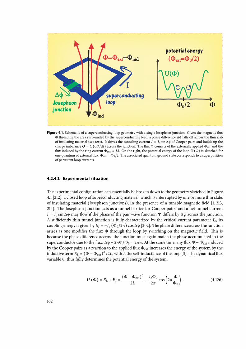
Figure 4.1. Schematic of a superconducting loop geometry with a single Josephson junction. Given the magnetic uxΦ threading the area surrounded by the superconducting lead, a phase dierence ∆ϕ falls o across the thin slabof insulating material (see text). It drives the tunneling current I = Ic sin ∆ϕ of Cooper pairs and builds up thecharge imbalance Q = C (dΦ/dt) across the junction. e ux Φ consists of the externally applied Φext and theux induced by the ring current Φind = LI. On the right, the potential energy of the loop U (Φ) is sketched forone quantum of external ux, Φext = Φ0/2. e associated quantum ground state corresponds to a superpositionof persistent loop currents.

4.2.4.1. Experimental situation

e experimental conguration can essentially be broken down to the geometry sketched in Figure4.1 [212]: a closed loop of superconducting material, which is interrupted by one or more thin slabsof insulating material (Josephson junctions), in the presence of a tunable magnetic eld [1, 213,214]. e Josephson junction acts as a tunnel barrier for Cooper pairs, and a net tunnel currentI = Ic sin ∆ϕ may ow if the phase of the pair wave function Ψ diers by ∆ϕ across the junction.A suciently thin tunnel junction is fully characterized by the critical current parameter Ic , itscoupling energy is given by EJ = −Ic (Φ0/2π) cos ∆ϕ [202].e phase dierence across the junctionarises as one modies the ux Φ through the loop by switching on the magnetic eld. is isbecause the phase dierence accross the junction must again match the phase accumulated in thesuperconductor due to the ux, ∆ϕ + 2πΦ/Φ0 = 2πn. At the same time, any ux Φ −Φext inducedby the Cooper pairs as a reaction to the applied ux Φext increases the energy of the system by theinductive term EL = (Φ −Φext)2 /2L, with L the self-inductance of the loop [3].e dynamical uxvariable Φ thus fully determines the potential energy of the system,

U (Φ) = EL + EJ =(Φ −Φext)2

2L− IcΦ02π

cos(2π ΦΦ0

) . (4.126)

162

On the other hand, the charge imbalance across the Josephson junction building up with grow-ing phase dierence must also be taken into account. It gives rise to a ‘kinetic’ energy term EC =C (dΦ/dt)2 /2, with C the capacitance of the junction24.e potential exhibits several local minima in Φ depending on the externally applied ux Φext

and on the systemparameters L, Ic . A symmetric double-well potential appears in the case of Φext =Φ0/2, as depicted on the right of Figure 4.1.eminima are separated by a tunnel barrier at the pointΦ = Φ0/2 where no ux is induced by the Cooper pairs. e two wells correspond to clockwise() and anti-clockwise () persistent loop currents, that is, to phase gradients of opposite signin the collective Cooper pair wave function.e quantummechanical ground state of such a double-well conguration is then given by a sym-

metric combination of both single-well ground states with a reduced energy, (∣⟩ + ∣⟩) /√2,

while the antisymmetric combination corresponds to a higher energy. A similar conguration holdswhen the loops are interrupted by more than a single Josephson junction [215].Microwave spectroscopy serves to measure the level splitting (also known as anti-crossing) in the

experiments [1, 2, 168], thereby verifying that the system has occupied the superposition state for asucient lifetime inversely proportional to the energy dierence.

4.2.4.2. Theoretical description of the superconducting state

e microscopic derivation and many-body description of the superconducting state of a metalis covered by the famous BCS theory [216]. It explains the pairing of conductance electrons ina solid material by means of an attractive electron-electron interaction which is mediated by thepolarization of the crystal lattice reacting to the Coulomb charge of a moving electron. at is tosay, two electrons may attract each other through the exchange of virtual phonons.When no external forces are present this leads to the pairing of electrons with opposite spin

and momentum25 (k ↑,−k ↓) close to the Fermi surface where electron-phonon scattering is notforbidden by the Pauli principle. e wave functions associated to the electron pairs are super-positions of those momenta, Ψ12 (r1, r2) = ∑k Ak exp [ik (r1 − r2)], which exhibit a large spatialextension26 [210]. From the coherent overlap of these states emerges the superconducting zero-current phase.e associated collective wave function Ψ (R) is determined by the center-of-massdependence exhibited by the states Ψ12 (R + r/2,R − r/2) of the participating Cooper pairs [202].One nds that Ψ (R) =

√Ns/V exp (iφ) is constant, and no phase gradient ∇φ is present, since

the momenta of each pair cancel. We will see later that this changes for nite-current states whereeach Cooper pair carries a non-zero momentum.e microscopic many-body nature of the superconducting state is made evident in the second

quantization formulation of Bardeen, Cooper and Schrieer [216]. At zero temperature the Fermi

24e law of induction tells us that any change of magnetic ux through an open loop induces an electric potentialdierence u = −dΦ/dt. Here, the voltage u must build up across the tunneling junction, which can be regarded asa capacitor C. is is in accordance with the Josephson equation d∆ϕ/dt = 2eu/ħ = 2πu/Φ0 that generally relatesthe phase dierence with the voltage across a Josephson junction [202].e voltage gives rise to a charge imbalanceQ = Cu and to a capacitive energy EC = Cu2/2.

25We restrict our view to s-type superconductors with electrons pairing in a spin singlet state.26e momentum spread of the superposition is much smaller than the Fermi wave number kF as only the momentumstates close to the Fermi surface are accessible by electron-phonon scattering.e spatial extension of the superpo-sition is therefore much larger than the de Broglie wavelength 2π/kF of the Fermi electrons.

163

sea of conductance electrons in a superconducting metal occupies the BCS ground state27

∣0⟩ =∏k

[uk + vkc†↑ (k) c

†↓ (−k)] ∣vac⟩, (4.127)

where ∣vac⟩ represents the electronic vacuum state. e product ranges over all discrete electronwave numbers k in the solid crystal, and v2k (u

2k = 1−v2k) represents the probability that the respective

pair of electrons (k ↑,−k ↓) is occupied (unoccupied),

v2k =12

⎛⎜⎝1 − k2 − k2F√

(k2 − k2F)2 + (2me∆k/ħ2)2

⎞⎟⎠. (4.128)

Electrons close to the Fermi surface, k ≈ kF , formCooper pairs due to the phonon-mediated attrac-tive interaction. is reduces their total energy by the the pairing energy ∆k > 0, whereas ∆k = 0for momentum states further away from the Fermi surface, which are inaccessible by phonon scat-tering. Given the characteristic Debye cuto frequency ωD of the lattice vibrations, Cooper pairsare only formed in a small energy shell at the Fermi surface, ∣k2 − k2F ∣ ≤ 2meωD/ħ. e occupa-tion of momentum states outside of the shell is the same as in a normal metal at zero temperature,vk = Θ (kF − k).e pairing term ∆k plays the role of an energy gap; it stabilizes the superconducting phase

against disturbances, since any excitation of the BCS ground state requires an energy input of atleast 2∆k to break a Cooper pair. If we approximate ∆k by a constant value ∆ within the Debye shell(and zero elsewhere), we can identify ∆ with the phenomenological value for the zero-temperatureenergy gap ∆ = 1.76kBTc , with Tc the critical temperature of the superconductor.Aer discussing the state of a superconductor ‘at rest’ let me turn to the description of stationary

dissipationless supercurrents. Assume that a given current density js = 2ensvs is carried by theentire pair condensate of density ns = Ns/V , which must be moving at the constant velocity vs.econtinuity equation for probability then relates the velocity to the phase gradient of the condensatewave function, as the current density associated to Ψ (R) is given by js (R) = 2eħns∇φ (R) /2me .is requires that the electrons are paired in the conguration (k +mevs/ħ ↑,−k +mevs/ħ ↓)withtotal momentum 2mevs, giving Ψ (R)∝ exp (2mevs ⋅ R/ħ).Hence, the quantum state underlying the persistent supercurrent derives from a momentum

translation of the zero-current BCS state. One achieves this formally applying the second quan-tization Weyl operator (4.16),

W (0, vs) = exp−iħ ∫ d3r mevs ⋅ r [ψ

†↑ (r) ψ↑ (r) + ψ

†↓ (r) ψ↓ (r)] , (4.129)

27 Strictly speaking, the BCS ground state does not describe a xed number of electrons, but rather a distribution ofnumbers around the expectation value N = ⟨BCS∣N∣BCS⟩. e eect of this uncertain number of electrons can beneglected as N is very large in most practical cases.

164

to the crystal electrons28. It describes a displacement of the electronic Fermi sphere in momentumspace, and the BCS state associated to the persistent supercurrent js = 2ensvs reads as

∣ js⟩ = W†(0, vs) ∣0⟩ =∏

k[uk + vkc

†↑ (k +

mevsħ

) c†↓ (−k +

mevsħ

)] ∣vac⟩. (4.130)

Note that, in realistic situations, the Cooper pair current density js is accompanied by the presenceof external elds represented by a vector potential A(r). In this case the measured net electricalcurrent density j = js + je contains also the canonical term je (r) = −2e2nsA(r) /me . e uxquantization eect discussed above follows from the condition j = 0 inside a superconducting leadwhich encircles an external magnetic eld.

4.2.4.3. Classicalization of current superposition states

Let me now show how the classicalization eect acts on superposition states of dierent supercur-rents, as they have been observed in experiments with Josephson loops. We shall assume in thefollowing that the two branches of the superposition correspond to the pure BCS states ∣ j1⟩ and∣ j2⟩, disregarding impurities due to nite temperature. ese states can be understood as BCS-Fermi spheres which are displaced by the momentum ħ∆k = me ( j1 − j2) /2ens with respect toeach other. We shall further assume macroscopically distinct supercurrents, that is, a signicantdisplacement ∆q between the branches so that the two Fermi spheres dier by more than a fewelectrons (in the non-overlapping region). In particular, this implies orthogonality, ⟨ j1∣ j2⟩ = 0.e classicalizing modication (4.71) of the electron motion in the crystal volume V reads as

L (ρ) = 1τ ∫V d3s∑k G (s, k) [A (s, k) ρA

†(s, k) − 1

2A†(s, k)A (s, k) , ρ] ,

A (s, k) =∑ℓe iℓ⋅s [c

†↑ (ℓ − k) c↑ (ℓ) + c

†↓ (ℓ − k) c↓ (ℓ)] . (4.131)

Here, the Lindblad operator A describes the phase-space displacement of a single (spin-↑ or -↓)electron by the momentum ħk and the position s.e above assumptions imply that the modication cannot induce direct transitions between

states of distinct supercurrents,

⟨ j1∣A (s, k) ∣ j2⟩ = 0, ⟨ j1∣A†(s, k)A (s, k) ∣ j2⟩ = 0. (4.132)

Nevertheless, it gradually undermines the coherence of the respective superposition by progres-sional dephasing and diusion of the displaced Fermi spheres.is can be estimated by means of the classicalization-induced decay rate of the nondiagonal

matrix element ⟨ j1∣ρt ∣ j2⟩ at initial time, Γ = −⟨ j1∣L (ρ0) ∣ j2⟩/⟨ j1∣ρ0∣ j2⟩, given that the initial stateis a coherent superposition of the form ρ0 = (a∣ j1⟩ + b∣ j2⟩) (h.c.). Note that a similar approachwas followed in [217] to study the impact of the continuous spontaneous localization model on

28Discretizedmomentamust be used, as introduced in Section 4.1.4.6 on page 145.eWeyl operatorW (r, v) describesa translation of both the position and the momentum coordinate, which transforms the momentum creation oper-ator toW (r, v) c

†σ (k)W

†(r, v) = exp (ik ⋅ r −mev ⋅ r/2ħ) c

†σ (k −mev/ħ), as can be checked in a straightforward

calculation using the CCR (4.64) on page 145.

165

superposition states of distinct currents. e present treatment contains the previous study as aspecial case29.At this point, it helps to recall theGalilean covariance of themodication.e Lindblad operators

A (s, k) commute with the Weyl translationsW (r, v) up to a phase,

W (r, v)A (s, k) = e imev⋅s/ħ−ik⋅rA (s, k)W (r, v) , (4.133)

as easily checked using the identity given in footnote 28. Combining this with the denition ofthe Weyl-translated BCS ground state (4.130), and with the above assumption (4.132), leads to theexpression

Γ = 1τ ∫V d3s∑k G (s, k) [⟨0∣A

†(s, k)A (s, k) ∣0⟩ − e i∆k⋅s ∣⟨0∣A (s, k) ∣0⟩∣2] . (4.134)

Both the overlap of the BCS ground statewith the vectorA (s, k) ∣0⟩ and the normof the latter can becomputed using the explicit form of the BCS ground state (4.127).e term A (s, k) ∣0⟩ describes astate where all but two electrons are paired with opposite momenta in the BCS conguration, whileone of the two remaining electrons obtains a phase shi and gets displaced in momentum by −ħk(provided the displaced momentum state is yet unoccupied).It follows immediately that the transformed vector overlaps with the unmodied BCS state ∣0⟩

only if no displacement takes place, k = 0. In this case the Lindblad operator simplies to theexpression A (s, 0) = ∑ℓ [n↑ (ℓ) + n↓ (ℓ)] exp (iℓ ⋅ s), which gives a phase shi to each occupiedmomentum state. Applied to the BCS state it yields

A (s, 0) ∣0⟩ =∑ℓ∏k′≠ℓ

[uk′ + vk′c†↑(k′) c

†↓(−k′)] e iℓ⋅svℓ∣ℓ ↑,−ℓ ↓⟩

+∑ℓ∏k′≠−ℓ

[uk′ + vk′c†↑(k′) c

†↓(−k′)] e iℓ⋅sv−ℓ∣ − ℓ ↑, ℓ ↓⟩

=∑ℓ2vℓ cos (ℓ ⋅ s)∏

k′≠ℓ[uk′ + vk′c

†↑(k′) c

†↓(−k′)] ∣ℓ ↑,−ℓ ↓⟩. (4.135)

Here, ∣k1 ↑, k2 ↓⟩ = c†↑(k1) c

†↓(k2) ∣vac⟩ denotes the vacuum state occupied by two electrons; one

with spin-↑ in the k1-state and one with spin-↓ in the k2-state. We thus nd the results

⟨0∣A (s, k) ∣0⟩ = δk,0∑ℓ2v2ℓ cos (ℓ ⋅ s) , (4.136)

⟨0∣A†(s, 0)A (s, 0) ∣0⟩ = [∑

ℓ2v2ℓ cos (ℓ ⋅ s)]

2

+∑ℓ4u2ℓv2ℓ cos2 (ℓ ⋅ s) . (4.137)

Clearly, the rst term of the right hand side in the second line is identical to the square of the rstline (for k = 0). ey both cancel in the expression (4.134) for the decay rate at k = s = 0, thatis, when neither dephasing nor diusion are present. e physical nature of the second term in(4.137), however, must be doubted. is is because it would produce a nonzero decay rate even in

29 Recall that the observable consequences of the CSLmodel [155,157] are described by a specic classicalizing modica-tion of the present form with a Gaussian momentum distribution and no position diusion, as discussed in Section4.1.3.2 on page 136.

166

the limit of vanishing classicalization, that is, if we switch o the classicalizing eect by setting thedistribution function to G (s, k) = δ (s) δk,0,

Γ no eectÐÐÐÐ→ 1τ∑ℓ

4u2ℓv2ℓ ≠ 0. (4.138)

e reason for the appearance of this term lies in the denition of the BCS ground state (4.127),which is not a Fock state of electrons, that is, an eigenstate of the number operator N = ∑ℓ,σ nσ (ℓ).e second quantization form of the classicalizing modication, however, presupposes a xed elec-tron number. Considering that A (0, 0) = N, the above term in fact represents the variance in thetotal electron number. A fully realistic description of the superconducting statemust assume a xednumber of electrons, and the term must therefore be regarded as an artefact of the BCS model. Itwill be subtracted from the expression (4.137) in the following.What remains open is the generalization of the expression (4.137) to the case of nonzeromomen-

tum displacement k ≠ 0. Here, the transformed vector

A (s, k) ∣0⟩ =∑ℓ∏

k′≠ℓ,ℓ−k[uk′ + vk′c

†↑(k′) c

†↓(−k′)] e iℓ⋅suℓ−kvℓ∣ℓ − k ↑,−ℓ ↓⟩

+∑ℓ∏

k′≠−ℓ,k−ℓ[uk′ + vk′c

†↑(k′) c

†↓(−k′)] e iℓ⋅suk−ℓv−ℓ∣ − ℓ ↑, ℓ − k ↓⟩

=∑ℓ∏

k′≠ℓ,ℓ−k[uk′ + vk′c

†↑(k′) c

†↓(−k′)] (uℓ−kvℓe iℓ⋅s + uℓvℓ−ke i(k−ℓ)⋅s) ∣ℓ − k ↑,−ℓ ↓⟩

(4.139)

represents a sum over BCS states where all but two of the Cooper pair states (k′ ↑,−k′ ↓) are oc-cupied by either no or both electrons.e remaining ℓ-th and ℓ− k-th Cooper pair congurationsare only singly occupied.erefore, in the scalar product of the vector (4.139) with itself, the onlynonzero summands are those where the same pairs are broken on both sides,

⟨0∣A†(s, k)A (s, k) ∣0⟩ =∑

ℓv2ℓu2ℓ−k + v2ℓ−ku

2ℓ + 2vℓuℓ−kvℓ−kuℓ cos [(2ℓ − k) ⋅ s] . (4.140)

Altogether, the coherence decay rate (4.134) consists of two distinct contributions, Γ = Γdeph + Γdi .e rst is a pure dephasing term which does not rely on any momentum displacement induced bythe classicalizing modication,

Γdeph =1τ ∫V d3s G (s, 0) [∑

ℓ2v2ℓ cos (ℓ ⋅ s)]

2

(1 − e i∆k⋅s) . (4.141)

It is sensitive to the momentum dierence ħ∆k between the two displaced Fermi spheres of thesuperposition. e further they are apart the more which-state information can be extracted bythe classicalization-induced dephasing.e rate thus grows quadratically with the number of elec-trons in each Fermi sphere which do not overlap with the other Fermi sphere, Γdeph ∼ (N∆k/kF)2,as follows from a thorough assessment of the decay rates in Appendix C.1. In a sense, it is merelythe electrons in those disjunct zones at the opposite ends of the two spheres that constitute thetwo separate ‘arms’ of the superposition in momentum space. e bulk of indistinguishable elec-trons occupies the same states in both branches, ∣ j1⟩ and ∣ j2⟩. Hence, the quadratic dependence of

167

the dephasing rate on the electron number (i.e. mass) in the two disjunct arms can be viewed asthe analogue to the quadratic mass dependence of the coherence decay rate for the center-of-masssuperpositions of compound particles studied in Section 4.1.5.e second decay term Γdi is related to heating (and pair-breaking) by momentum diusion,

Γdi =1τ ∫V d3s∑k≠0G (s, k)∑

ℓv2ℓu2ℓ−k + v2ℓ−ku

2ℓ + 2vℓuℓ−kvℓ−kuℓ cos [(2ℓ − k) ⋅ s] , (4.142)

which leads to a gradual coalescence of both Fermi spheres. Note that this decay rate generally em-bodies the heating loss of the occupation of the BCS ground state (whether it carries a supercurrentor not), and therefore does not depend on the actual displacement of the two superimposed persis-tent current states. Similar to the diusion heating of compound objects studied in Section 4.2.1.1,one would expect the diusion rate Γdi to grow linearly in proportion to the total number of avail-able electrons N = 2Ns. It is shown in Appendix C.1 that the rate is in fact limited by Γdi ≤ N/τ.is maximum, however, is only reached once the momentum standard deviation of the distribu-tion function G (s, k) is greater than the Fermi momentum, σq > ħkF . For lower values of σq, theinner electrons of the Fermi sea are inaccessible and cannot be lied into unoccupied momentumstates due to the Pauli exclusion principle and the superconducting energy gap.In summary, the classicalization-induced decay of a superposition state of distinct supercurrents

is generally enhanced by the number N of electrons in the metal. e larger the underlying su-perconducting loop the stronger the classicalizing eect would act on such superpositions in theexperiment. It turns out that, in practice, the diusion eect outdoes the dephasing part for themost part, and so the coherence decay scales at most linearly with the loop size. A concrete exam-ple will follow in Section 4.3.2.4.

4.3. The measure of macroscopicity

Aer the detailed discussion of the implications of generic classicalizing modications, we are -nally in a position to formulate the central result of this chapter: a quantitative measure of macro-scopicity. is measure µ, which will be introduced in the following, quanties the class of classi-calizing modications which are ruled out by the concrete observation of a quantum phenomenon,that is, the extent to which the validity of quantum mechanics is tested against the hypothesis ofclassical macroscopic realism. e latter being grounded in the striking empirical evidence thatthe everyday world follows the laws and principles of classical (Newtonian) physics, it qualies asthe most natural footing for quantifying and comparing the degree of macroscopicity achieved inquantum experiments on arbitrary mechanical systems.e benets of such an approach are clear. It depends neither on the formal representation of

quantum phenomena in terms of specic classes of states and observables nor on the complexitythereof. Quite contrarily, the measure µ is derived from the hypothetical predictions of classicaliz-ing modications and their falsication by observation.e natural scaling behaviour of the clas-sicalization eect with the size and complexity of mechanical systems is based on only two basicinvariance principles (see Section 4.1.4.1), and it thus provides a minimal and unbiased gauge forthe quantum-to-classical transition. Evenmore so, the approach respects and builds upon the well-established symmetry principles behind both Schrödinger quantummechanics andNewtonianme-chanics, most prominently Galilean covariance. It does not refer to any particular macro-realistic

168

extension of the standard Schrödinger equation by nonlinear and stochastic terms which mightembody new physics beyond the scope of standard nonrelativistic quantum theory, such as quan-tum eects of gravity [151, 177]. Instead it refers merely to the observable consequences of a generichypothetical classicalization eect that are described by the minimally invasive modication of thetime evolution of the many-body state operator studied in this chapter. Quantum superpositionstates decay into classical mixtures over time while the Newtonian equations of motion are keptintact.

4.3.1. De®nition of the macroscopicity measure

e strength of the classicalization eect is determined by the distribution function g0 (s, q) andthe time parameter τ0 associated with a xed but arbitrary reference mass m0. e realization ofnonclassical states in a given experiment immediately rules out a certain parameter set of the hypo-thetical modication which would predict a higher loss of quantum coherence than observed.erationale behind the present measure of macroscopicity is to call one quantum state more macro-scopic than another if the experimental demonstration of the former rules out a larger parameterset than the latter. What remains to be found is a robust way of quantifying the size of the excludedparameter set.As will be shown in the following, the time parameter τ0 turns out to be the apparent and most

natural candidate.e reason is that the classicalizing modication always predicts a minimal co-herence time for every given mechanical system and irrespectively of the functional form of thedistribution g0. It is, in a sense, the universal property of all modications falling under the genericclass studied here. Nevertheless, a concrete numerical assessment of the macroscopicity requiresadditional restrictions on the form of the distribution function (without aecting the generality ofthe results).ey will motivated in the following, before the formal denition of µ will eventuallybe given in Section 4.3.1.4. e remainder of this chapter will then be spent applying the measureto the various manifestations of quantum superpositions in large mechanical systems which havebeen and will be observed in past and future experiments.

4.3.1.1. The electron as a natural reference point particle

At this point it is time to decide for the reference mass m0 xing the reference time parameter andthe reference phase-space distribution in all the quantitative considerations to follow.e domainof standard, nonrelativistic, quantummechanics begins at the level of electrons and nuclei, and thetheory was originally developed to understand and assess the nonclassical behaviour of atoms.equantumdescription ofmore complex systems ofmatter is oen brokendown into these elementarybuilding blocks whose physical behaviour is well understood. Indeed, when observing quantumbehaviour in larger systems of matter, scientists are oen inclined to count the number of electronsor atoms involved in order to get an idea about the ‘size’ of the quantum observation.Hence the electron, being the canonical elementary point particle in (nonrelativistic) quantum

mechanics, qualies naturally as the reference mass unit for the present purposes. From now on,the reference mass is once and for all set to m0 = me . e classicalization eect is then fullydetermined by specifying the coherence time parameter τ0 = τe and the distribution functiong0 (s, q) = ge (s, q) for an electron.

169

4.3.1.2. Minimizing parameter space with a Gaussian distribution

roughout the discussion we have found that, when it comes to parametrizing the strength of theclassicalization eect, three parameters mainly determine its generic behaviour:e time parame-ter τe and the two standard deviations σs and σq of the positive, normalized and isotropic distribu-tion function ge (s, q). e most natural implementation of these parameters is then obtained bymeans of the Gaussian form

ge (s, q) =1

(2πσsσq)3 exp(−

s2

2σ2s− q2

2σ2q) . (4.143)

It represents the most natural choice of a zero-mean distribution function, which is solely deter-mined by its second moments, and it does not exhibit any particular dicult-to-justify featuresthat would involve additional parameters to describe them. I therefore operate with this Gaussianform in the following in order to minimize the numerical eort as well as the number of ad-hoc pa-rameters introduced with the classicalization eect. e Fourier transform (4.40) of the referencedistribution reads as

ge (r, p) = exp⎛⎝−

σ2q r2

2ħ2− σ2s p2

2ħ2⎞⎠. (4.144)

4.3.1.3. Parameter limitations on the subatomic scale

At rst sight, the three parameters (σs , σq , τe) of our model could in principle assume any valuelarger than zero, and they would only be constrained by the experimental observation of quantumphenomena in mechanical systems. ere is, however, also a fundamental restriction due to thelimited scope of the underlying framework. Although standard quantum theory is well suited toassess the electronic level structure of atoms, it fails in describing the internal binding and structureof nuclei.is is where nonrelativistic mechanics ceases to be valid, and, with it, the classicalizingmodication that builds upon its basic principles. We must therefore exclude the (sub-)nucleardomain from our considerations by restricting the parameter space in the following way:According to Section 4.1.5, the classicalization of a compound object will start depending on the

internal motion of its constituents once theirmean variance in the relative position andmomentumcoordinates becomes comparable to the parameters σs,q. For example, the classicalization of an atomwill depend on its electronic level structure if ħ/σq ≲ 1Å ≲ σs. Similarly, the relative state of motionof protons and neutrons inside atomic nuclei becomes relevant for ħ/σq ≲ 10 fm ≲ (me/1 amu) σs.In order to avoid this, the classicalization parameters should be limited to σs ≲ 20pm and ħ/σq ≳10 fm.e exact numbers will be of no relevance, and they could easily be varied by a few orders ofmagnitude without altering the upcoming results.

4.3.1.4. Formal de®nition of the macroscopicity

Let me nally state the formal denition of the measure of macroscopicity µ, assuming the Gaus-sian form (4.143) of the classicalization distribution and respecting the above nuclear constraint onσs,q. e macroscopicity of a quantum superposition state is dened with respect to to a concreteexperimental realization. Assuming the existence of the classicalizing modication, the measure-ment rules out those parameter values (σs , σq , τe) which would predict a lower ‘visibility’ of the

170

superposition state than observed. To be concrete, the experiment rules out all coherence timeparameters smaller than a certain boundary value τe (σs , σq) for any xed value of (σs , σq). efunction τe (σs , σq), which is dened on the constrained set of (σs , σq) in this way, separates theexcluded parameter range from the rest.I suggest to measure the macroscopicity by the maximum of this function, that is, by the greatest

excluded time parameter τmaxµ = log10 (

τmax1 s

) . (4.145)

e time is expressed in units of seconds to x a scale, and the logarithm is taken to handle the vastspread of τmax-values when comparing the numerous real experiments with one another. Positivevalues of µ are obtained, for instance, by demonstrating the wave nature of electrons over morethan one second.In the following, I will illustrate with the help of concrete examples why the greatest excluded

time parameter appears as the most natural and robust choice to quantify macroscopicity. I willthen proceed with the evaluation of µ for a broad selection of quantum superposition experiments.

4.3.2. Assessing the macroscopicity of quantum experiments

In order to compute the macroscopicity µ for a concrete quantum experiment, the classicalizingmodication must be incorporated into the underlying theoretical model, and the modied solu-tion must be compared with the measurement data as a function of the classicalization parameters(σs , σq , τe) ∈ R3+.is calls for an individual procedure in each case which results in the specica-tion of a functional dependence τe (σs , σq) describing the boundary between the compatible andthe incompatible parameter region. Nevertheless, the general form of the boundary, as well as ageneric estimate of the macroscopicity, can be obtained for most standard cases.Figure 4.2 provides an overview of typical experiments that narrow down the allowed parameter

range of the classicalization eect, as will be discussed one by one in the following. Here, the largestexcluded time parameters are plotted as a function of the length scale ħ/σq associated to the mo-mentumwidth σq of theGaussian reference distribution, and at the xed positionwidth σs = 20pm.e case of de Broglie interference with point particles is represented by the solid line, as obtainedfrom the optical Mach-Zehnder type interference experiment with cesium atoms in [166]30. A dif-ferent behaviour is observed when the interfering particles are composed of more than a singlenucleus. e dashed line in the diagram corresponds to the Talbot-Lau interference experimentwith gold clusters of 107 amu proposed in [11] and discussed in Chapter 3, page 114.e other endof the spectrum, where the interfering object is much larger than the interference path separation,is represented by the dash-dotted line. It derives from the proposed superposition experiment [170]with oscillatory states of ground-state cooled micromirrors. Finally, the dotted curve stands for agenuine many-body quantum phenomenon:e superposition of counter-rotating persistent cur-rents in a superconducting loop, as observed in [1].Before proceeding in the discussion of the listed cases I note once again that the classicalization

can also be tested by means of purely classical experiments. is is due to the inherent diusioneect which leads to an average energy increase in both classical and quantum systems alike. As an

30e atom mass is mainly concentrated in the femtometer-sized nucleus, and the small contribution of the electrons isnegligible. It can therefore be regarded as a point particle in the present context.

171

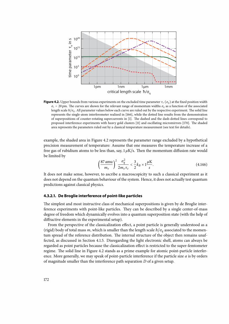
105

1010

1015

1020

critical length scale ħ/σq

time

para

met

er τ

e in

s

100

1mm1µm1nm1pm

Figure 4.2. Upper bounds from various experiments on the excluded time parameter τe (σq) at the xed position widthσs = 20 pm. e curves are shown for the relevant range of momentum widths σq as a function of the associatedlength scale ħ/σq . All parameter values below each curve are ruled out by the respective experiment.e solid linerepresents the single-atom interferometer realized in [166], while the dotted line results from the demonstrationof superpositions of counter-rotating supercurrents in [1]. e dashed and the dash-dotted lines correspond toproposed interference experiments with heavy gold clusters [11] and oscillating micromirrors [170]. e shadedarea represents the parameters ruled out by a classical temperature measurement (see text for details).

example, the shaded area in Figure 4.2 represents the parameter range excluded by a hypotheticalprecision measurement of temperature: Assume that one measures the temperature increase of afree gas of rubidium atoms to be less than, say, 1 µK/s. en the momentum diusion rate wouldbe limited by

(87 amume

)2 σ2q2meτe

< 32kB × 1

µKs. (4.146)

It does not make sense, however, to ascribe a macroscopicity to such a classical experiment as itdoes not depend on the quantum behaviour of the system. Hence, it does not actually test quantumpredictions against classical physics.

4.3.2.1. De Broglie interference of point-like particles

e simplest and most instructive class of mechanical superpositions is given by de Broglie inter-ference experiments with point-like particles. ey can be described by a single center-of-massdegree of freedom which dynamically evolves into a quantum superposition state (with the help ofdiractive elements in the experimental setup).From the perspective of the classicalization eect, a point particle is generally understood as a

(rigid) body of total mass m, which is smaller than the length scale ħ/σq associated to the momen-tum spread of the reference distribution. e internal structure of the object then remains unaf-fected, as discussed in Section 4.1.5. Disregarding the light electronic shell, atoms can always beregarded as point particles because the classicalization eect is restricted to the super-femtometerregime. e solid line in Figure 4.2 stands as a prime example for atomic point-particle interfer-ence. More generally, we may speak of point-particle interference if the particle size a is by ordersof magnitude smaller than the interference path separation D of a given setup.

172

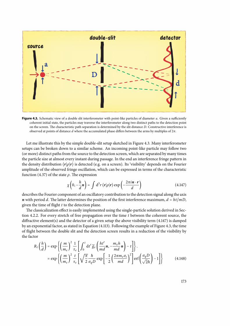
Figure 4.3. Schematic view of a double slit interferometer with point-like particles of diameter a. Given a sucientlycoherent initial state, the particles may traverse the interferometer along two distinct paths to the detection pointon the screen.e characteristic path separation is determined by the slit distance D. Constructive interference isobserved at points of distance d where the accumulated phase diers between the arms by multiples of 2π.

Let me illustrate this by the simple double-slit setup sketched in Figure 4.3. Many interferometersetups can be broken down to a similar scheme. An incoming point-like particle may follow two(ormore) distinct paths from the source to the detection screen, which are separated bymany timesthe particle size at almost every instant during passage. In the end an interference fringe pattern inthe density distribution ⟨r∣ρ∣r⟩ is detected (e.g. on a screen). Its ‘visibility’ depends on the Fourieramplitude of the observed fringe oscillation, which can be expressed in terms of the characteristicfunction (4.37) of the state ρ.e expression

χ (0,−hdn) = ∫ d3r ⟨r∣ρ∣r⟩ exp(−2πin ⋅ rd

) (4.147)

describes the Fourier component of an oscillatory contribution to the detection signal along the axisn with period d.e latter determines the position of the rst interference maximum, d = ht/mD,given the time of ight t to the detection plane.e classicalization eect is easily implemented using the single-particle solution derived in Sec-

tion 4.2.2. For every stretch of free propagation over the time t between the coherent source, thediractive element(s) and the detector of a given setup the above visibility term (4.147) is dampedby an exponential factor, as stated in Equation (4.113). Following the example of Figure 4.3, the timeof ight between the double slit and the detection screen results in a reduction of the visibility bythe factor

Rt (hd) = exp( m

me)2 1

τe[ ∫ t

0dt′ ge (

ht′

mdn,−meh

mdn) − t] .

= exp( mme

)2 t

τe[√π2

ħσqD

exp [− 12(2πmeσs

md)2] erf(

σqD√2ħ

) − 1] (4.148)

173

e propagation from the coherent source to the double slit must be taken into account as well. Ityields another factor of this form. e interference visibility is altogether reduced by Rt0Rt , withttot = t + t0 the time of ight from the source to the detector.Note that the position spread σs of the classicalization is an irrelevant factor for all practical pur-

poses, as it is bound by σs ≲ 20pm. e mass-rescaled width meσs/m for the classicalization ofatoms and other large particles is even smaller, and the fringe period d of any realistic interfer-ence pattern surpasses it by many orders of magnitude.e σs-dependence in (4.148) can safely beneglected.We distinguish two limiting cases for the visibility reduction by classicalization.

The saturated regime e strongest eect is achieved in the limit of large momentumspreads σq of the classicalization distribution where the associated length scale is muchsmaller than the arm separation, ħ/σq ≪ D. e decay of coherence then saturates at therate given by the mass-scaled coherence time scale, 1/τ = (m/me)2 /τe , and we may approx-imate the reduction factor (4.148) by

Rt ≈ exp [−( mme

)2 t

τe] . (4.149)

In total, the visibility is reduced by the factor Rt0Rt ≈ exp [−m2ttot/m2eτe].is is the strong-est reduction the classicalizing modication may cause. It explains the le part of the solidcurve in Figure 4.2, which saturates at length scales below the 1mm path separation of theinterferometer [166]. It also explains the at maximum of the dashed curve that roughlyextends from ħ/σq ∼ 10 nm to 100nm.e saturated classicalization of point-like particles isa valid approximation in the length scale regime a ≪ ħ/σq ≪ D.

Thediªusive regime If themomentumwidth σq is very small, ħ/σq ≫ D, the classicalizationeect hardly distinguishes the dierent paths through the interferometer, and the visibilityreduction is suppressed. We obtain the approximate reduction factor

Rt ≈ exp⎡⎢⎢⎢⎢⎣− 16(

σqDħ

)2

( mme

)2 t

τe

⎤⎥⎥⎥⎥⎦(4.150)

aer expanding the error function in (4.148) to the lowest order. e exponent is quadrat-ically suppressed by σqD/ħ ≪ 1 with respect to the saturated case. As before, the time tmust be replaced by the total time of ight ttot to obtain the full visibility reduction. equadratic dependence of the logarithmic reduction of visibility on the momentum width σqrepresents a general feature of the diusive limit where spatial superposition states are toosmall to be resolved31. In particular, it explains that the solid, the dashed and the dash-dottedinterference curves exhibit the same slope of 2 vertical orders of magnitude per horizontalorder of magnitude on the right side of the double-logarithmic plot in Figure 4.2. is iseasily checked by taking the logarithm of (4.150) and expressing the time parameter τe as afunction of log (ħ/σq).

31One observes the same behaviour in the case of thermal decoherence at low temperatures [218], where the averagephoton wavelength is greater than the path separation.

174

e visibility reduction by classicalization can now be compared to the measured fraction f < 1of the interference visibility predicted by standard quantum theory. In realistic interference ex-periments, the measurement is always aected by noise, uncertainties and limited accuracy, and ittherefore never reaches the full 100% of the theoretically predicted visibility. Even if the recordeddata ts to the theory within an error range of, say, 5%, then the fraction cannot be larger thanf = 95%.By varying the momentum width parameter σq we obtain time parameters τe (σq) that are ruled

out by the measurement, as plotted in Figure 4.2.eir maximum determines the macroscopicityvalue (4.145). For interference experiments with point-like particles the maximum is found in thesaturated regime, where the visibility reduction factor reads as (4.149). Given the observed fractionf , the reduction factor is bound from below by Rt ≥ f , and wemay approximate themacroscopicityby

µ ≈ log10 [∣1ln f

∣ ( mme

)2 ttot1 s

] . (4.151)

e time ttot should include all stretches of free propagation pieced together from the coherentsource to the detection plane32. In the case of the cesium interferometer in [166] coherence wasmaintained for over ttot = 320ms, and a fringe visibility of f = 62% instead of the ideally expected100%was recorded (see Figure 19 of [166]). Using amass ofm = 137 amu leads to themacroscopicityµ = 10.6.at is to say, the greatest time parameter excluded by this experiment is τmax = 4× 1010 s,the value to which the solid curve in Figure 4.2 saturates.In principle, the expression (4.151) can be used to compute the macroscopicity of arbitrary de

Broglie interference experiments with point-like particles (i.e. a ≪ D). In practice, however, it isnot always obvious how to obtain a value for the fraction f of condently measured versus theo-retically expected interference visibility. (If the latter is a loosely dened quantity, for instance.) Iproceed by presenting methods to extract estimated values for f and µ from various matter-waveexperiments.

Mach-Zehnder setup Mach-Zehnder-type interferometers [18] oer a direct relation betweenthe observed fringe visibility and the reduction factor f . Many modern high-precision atom in-terferometers with large arm lengths and long interrogation times, e.g. [166, 167], are based on anoptical Mach-Zehnder scheme comprised of a sequence of three laser pulses. Each pulse consistsof two counterpropagating laser waves driving a Raman transition between the initial state ∣0⟩ andthe metastable state ∣1⟩ of an atom. Each transition comes with a net momentum kick of ±ħk alongthe direction of the laser waves, denoted here as the x-axis.e center-of-mass motion of the atommay thus be treated in one dimension.e rst π/2-pulse splits the incoming atoms coherently among two diverging paths correspond-

ing to the internal states ∣0⟩ and ∣1⟩, where the latter diers in momentum by ħk.is is describedby the unitary splitting transformation

Uπ/2 =1√2(∣0⟩ + e ikx∣1⟩) ⟨0∣ + 1√

2(∣1⟩ − e−ikx∣0⟩) ⟨1∣ (4.152)

32We must only include those parts of the setup where a loss of coherence in the particle state aects the interferencevisibility.is excludes, for instance, anything that happens before the rst collimation slit in a double-slit experimentrepresenting the point source. In a Talbot-Lau setup we must only consider the passage from the rst to the secondand from the second to the third grating.

175

acting on the initial product state of the atomic ensemble ρ0⊗ ∣0⟩⟨0∣.e second π-pulse at time Tips the internal state and exerts opposite momentum kicks in each arm,

Uπ = e ikx∣1⟩⟨0∣ + e i∆ϕe−ikx∣0⟩⟨1∣, (4.153)

which makes both arms converge again. e term ∆ϕ is added here to account for a tunable netphase dierence between the two arms.ey rejoin aer another time T , where another π/2-pulseis applied to close the path scheme. By detecting the atoms aer the third pulse in one of its internalstates, say ∣0⟩, one records the sinusoidal interference pattern I (∆ϕ) = ⟨0∣tr (Uπ/2ρ2TU

†π/2) ∣0⟩ as a

function of the phase dierence ∆ϕ.e state ρ2T before applying the third laser pulse reads as

ρ2T = T Uπ [T (Uπ/2ρ0 ⊗ ∣0⟩⟨0∣U†π/2)]U

†π , (4.154)

where the superoperator T denotes the modied free evolution33 of the motional state by the timeT . We nd that the fringe contrastV is directly given by the characteristic function of the quasi-stateoperator ⟨0∣ρ2T ∣1⟩,

V = 2 ∣⟨0∣tr (e ikxρ2T) ∣1⟩∣ = 2 ∣χ⟨0∣ρ2T ∣1⟩ (0, ħk)∣ . (4.155)

A visibility of V = 100% is predicted in the absence of classicalization, and we may thus identify thefraction f with the measured interference contrast. e classicalizing modication contributes areduction factor RT (ħk) of the form (4.148) for each free propagation T , and the visibility reducesto

V = R2T (ħk) = exp( mme

)2 2T

τe[√π2

mσqkT

erf(σqkT√2m

) − 1] , (4.156)

where the σs-term has been neglected. Identifying this reduction with the measured visibility f < 1yields the critical time parameter,

τe (σq) = ∣ 1ln f

∣ ( mme

)2[2T −

√2πmσqk

erf(σqkT√2m

)] . (4.157)

All values below τe (σq) are ruled out by the experiment.e solid curve in Figure 4.2 displays thisfunction using the parameters m = 133 amu, T = 160ms and ħk/m = 7.0mm/s from [166].e function (4.157) saturates at the maximum value τmax = 2Tm2/m2e ∣ln f ∣ for large σq ≫

m/kT , which conrms the macroscopicity formula (4.151). A more recent experiment of the sametype [167] yielded a visibility of f ≈ 1/3 (as extracted from Figure 3 in the reference) at a time ofight 2T = 800ms, which results in amacroscopicity of the same size, µ = 10.6. Signicantly highervalues can be reached in atom interferometry only by increasing the interrogation time T beyondthe currently feasible range. In [219] the authors proposed to realize a similar cesium interferometerwith T ≈ 2000 s between far apart satellites in space. It would correspond to µ = 14.5 if a contrastof f = 0.5 were to be measured.Apart from the three-pulse interferometer, Mach-Zehnder schemes are also realized by means

of three material gratings [18]. e above reasoning applies here as well, except that the two armsare given by two subsequent diraction orders at the grating.

33e presence of a constant acceleration would only contribute to the phase dierence.

176

Specically, let us consider theNa2-interferometer setupwith three identical 200nmgratings and30% opening fraction in [125]. e two arms originate from the 0th and the 1st order diractioncomponents of the rst grating, followed by a 1st order and −1st order diraction at the secondgrating. Standard diraction theory states that their weight ratio P1/P2 is given by the squaredratio between the 1st and the 0th Fourier component of the periodic grating aperture function,P1/P0 = (b1/b0)2 = sinc2 (0.3π) = 0.74. Interactions with the grating walls are negligible. esinusoidal fringe pattern is detected through the movable third grating mask, which modulates thecontrast by another factor b1/b0 = 0.86. In total, the unmodied interference visibility is limitedto V = 2b1

√P1P0/b0 (P1 + P0) = 0.85. e authors of [125] depict a fringe pattern with about 30%

contrast in their Figure 4, that is, a fraction f = 0.3/0.85 = 0.35 of the theoretical value. e Na2molecules (m = 46 amu) traverse the total distance L = 2.1m from the coherent source to thethird grating at the mean velocity v = 820m/s [125, 220], which results in the macroscopicity valueµ = 7.2.

Ramsey-Bordé setup Besides the optical Mach-Zehnder setup, the coherent path splitting bylight coupled to an internal transition is also used in the Ramsey-Bordé interferometer scheme[221]. It consists of two separated pairs of co-propagating running-wave lasers, where each lasersplits an incoming particle beam into two momentum-displaced arms corresponding to dierentinternal states.e arms rejoin at the second laser pair pointing into the opposite direction, and theresulting interference pattern ismeasured by state-selective detection as a function of the phase shibetween the arms. In general, however, more than two arms are mixed into the detection signal.A Ramsey-Bordé experiment with I2 molecules (m = 254 amu) was realized in [222], where a

total of four dierent paths overlapped at the detector. Two of those paths are Doppler-shiedwith respect to each other, that is, their phase dierence depends on the transverse velocity of theparticles.eir interference is thus averaged out over the velocity distribution of the particle beam,and the fringe pattern is only due to the other two paths.is limits the fringe contrast to 50%. Wecan read o a measured value of roughly 400/2400 = 1/6 from the central fringe plotted in Figure2 of [222], which results in the fraction f = 1/3. e I2 molecules traverse the interferometer ofabout 35mm length with a mean velocity of 350m/s in t = 100 µs. Formula (4.151) then yields anapproximate macroscopicity of µ = 7.3.

Diªraction at one-dimensional structures e biggest class of matter-wave interference ex-periments involves the diraction at small one-dimensional structures in the near and far eld. Slits,double-slits and thin gratings are the most commonly used diractive elements; they are mathe-matically described by a transmission function t (x), which is multiplied to the wave function upontraversal. Standard Fresnel diraction theory in the paraxial approximation tells us that the result-ing interference pattern for particles from a monochromatic point source at x0 = 0 is given bySvz (x)∝ ∣∫ dx1 ψ (x1; x)∣2, with

ψ (x1; x) = t (x1) exp [im2ħ

(x21T1+ x21 − 2xx1

T2)] . (4.158)

e x-variable represents the position on the detection plane, the terms T1 and T2 denote the timesof ight from the source to the diractive element and from there to the detection plane, respec-tively. In most cases the latter depend on the velocity vz of the particles traversing the distances

177

L1 and L2 between the setup elements. We must therefore average the interference signal over thedistribution F (vz) of velocities present in the beam. In addition, the signal must be averaged overthe nite source aperture AS (xS) to account for realistic orices, and it must be convolved with thefunction AD (xD) to account for the nite x-resolution of a realistic detector. e resulting signalformula,

S (x) = ∫ dvz F (vz) ∫ dxS AS (xS) ∫ dxD AD (xD) Svz (x + xD −T2T1

xS) , (4.159)

may then be used to predict realistic values for the fringe visibility observed in the experiment. Onthe other hand, the averaging is irrelevant in the assessment of the coherence-reducing eect due tothe classicalizingmodication. Once again we nd that the latter modulates the ideal fringe patternby reduction factors of the form (4.148),

Svz (x) = ∫ dx1dx2 R (x2 − x1)ψ (x1; x)ψ∗ (x2; x) ,

R (x) = RT1 (mxT1

)RT2 (mxT2

)

≈ exp( mme

)2 T1 + T2

τe[√π2

ħσqxerf(

σqx√2ħ

) − 1] . (4.160)

e inuence of position translations is neglected in the last line; they are practically irrelevantas σs ≲ 20pm. Equation (4.160) is easily derived in the characteristic function representation,starting from the initial state of the coherent point source χ0 (x , p) ∝ δ (x) and ending at thesignal formula Svz (x) ∝ ∫ dp χT1+T2 (0, p) exp (−ipx/ħ) /2πħ. e diraction transformation⟨x∣ρ∣x′⟩ ↦ t (x) ⟨x∣ρ∣x′⟩t∗ (x′) yields the convolution χ (x , p) ↦ ∫ dq T (x , p − q) χ (x , q), withthe diraction kernel34

T (x , q) = 12πħ ∫ ds e iqs/ħt (s −

x2) t∗ (s + x

2) . (4.161)

Using Formula (4.113) for the modied time evolution we arrive at the expression for the nal state,

χT1+T2 (0, p) = T (− pT2m, p + pT2

T1)RT2 (−p)RT1 (p

T2T1

) . (4.162)

A few more steps of substitution result in the signal formula (4.160), up to a normalization factor.emacroscopicity of a concrete experiment is obtained bymatching the computed signal (4.160)

to the measured data as a function of the momentum spread, which yields the excluded time pa-rameter curve τe (σq). However, there is a way to avoid an elaborate tting procedure for everyindividual case and to estimate the macroscopicity by means of the approximation (4.151). Re-call that the greatest excluded time parameter is always found at the largest possible values of σq inpoint-particle interference, where the associated length scale ħ/σq is much smaller than any dirac-tive aperture used in practice. e reduction factor in (4.160) assumes its minimum R (∞) for allrelevant values ∣x2 − x1∣ ≫ ħ/σq. We may thus approximate

Svz (x) ≈ R (∞) ∣ ∫ dx1 ψ (x1; x)∣2+ ∫ dx2 [R (x2) − R (∞)]´¹¹¹¹¹¹¹¹¹¹¹¹¹¹¹¹¹¹¹¹¹¹¹¹¹¹¹¹¹¹¹¹¹¹¹¹¹¹¹¹¹¹¹¹¹¹¹¹¹¹¹¹¹¹¹¹¹¹¹¹¹¹¹¹¹¹¹¹¸¹¹¹¹¹¹¹¹¹¹¹¹¹¹¹¹¹¹¹¹¹¹¹¹¹¹¹¹¹¹¹¹¹¹¹¹¹¹¹¹¹¹¹¹¹¹¹¹¹¹¹¹¹¹¹¹¹¹¹¹¹¹¹¹¹¹¹¹¹¶

∼few ħ/σq

∫ dx1 ∣t (x1)∣2 , (4.163)

34e kernel is similar to the diraction kernels used in Chapter 3 to describe near-eld interference in the Wignerfunction representation, except that the integration is over the center position here. See for instance page 72.

178

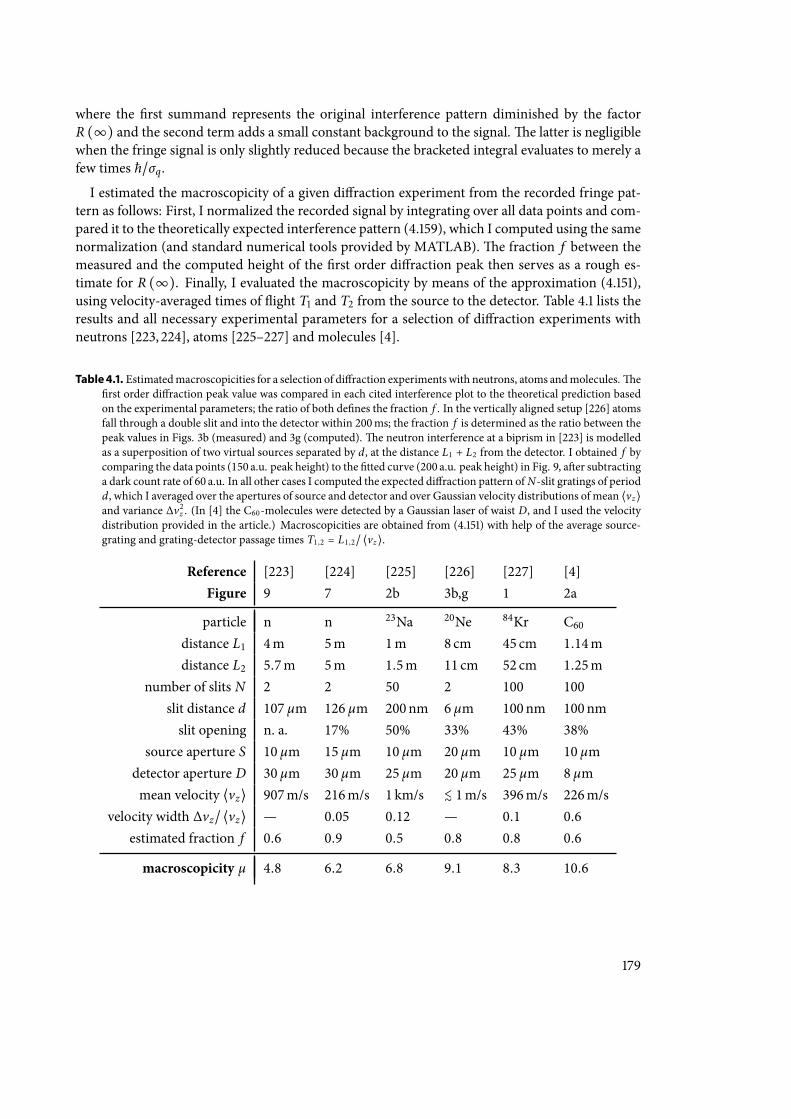
where the rst summand represents the original interference pattern diminished by the factorR (∞) and the second term adds a small constant background to the signal.e latter is negligiblewhen the fringe signal is only slightly reduced because the bracketed integral evaluates to merely afew times ħ/σq.I estimated the macroscopicity of a given diraction experiment from the recorded fringe pat-

tern as follows: First, I normalized the recorded signal by integrating over all data points and com-pared it to the theoretically expected interference pattern (4.159), which I computed using the samenormalization (and standard numerical tools provided by MATLAB).e fraction f between themeasured and the computed height of the rst order diraction peak then serves as a rough es-timate for R (∞). Finally, I evaluated the macroscopicity by means of the approximation (4.151),using velocity-averaged times of ight T1 and T2 from the source to the detector. Table 4.1 lists theresults and all necessary experimental parameters for a selection of diraction experiments withneutrons [223, 224], atoms [225–227] and molecules [4].

Table 4.1. Estimatedmacroscopicities for a selection of diraction experiments with neutrons, atoms andmolecules.erst order diraction peak value was compared in each cited interference plot to the theoretical prediction basedon the experimental parameters; the ratio of both denes the fraction f . In the vertically aligned setup [226] atomsfall through a double slit and into the detector within 200ms; the fraction f is determined as the ratio between thepeak values in Figs. 3b (measured) and 3g (computed).e neutron interference at a biprism in [223] is modelledas a superposition of two virtual sources separated by d, at the distance L1 + L2 from the detector. I obtained f bycomparing the data points (150 a.u. peak height) to the tted curve (200 a.u. peak height) in Fig. 9, aer subtractinga dark count rate of 60 a.u. In all other cases I computed the expected diraction pattern of N-slit gratings of periodd, which I averaged over the apertures of source and detector and over Gaussian velocity distributions of mean ⟨vz⟩and variance ∆v2z . (In [4] the C60-molecules were detected by a Gaussian laser of waist D, and I used the velocitydistribution provided in the article.) Macroscopicities are obtained from (4.151) with help of the average source-grating and grating-detector passage times T1,2 = L1,2/ ⟨vz⟩.

Reference [223] [224] [225] [226] [227] [4]Figure 9 7 2b 3b,g 1 2a

particle n n 23Na 20Ne 84Kr C60distance L1 4m 5m 1m 8cm 45 cm 1.14mdistance L2 5.7m 5m 1.5m 11 cm 52 cm 1.25m

number of slits N 2 2 50 2 100 100slit distance d 107 µm 126 µm 200nm 6 µm 100nm 100nmslit opening n. a. 17% 50% 33% 43% 38%

source aperture S 10 µm 15 µm 10 µm 20 µm 10 µm 10 µmdetector aperture D 30 µm 30 µm 25 µm 20 µm 25 µm 8 µmmean velocity ⟨vz⟩ 907m/s 216m/s 1 km/s ≲ 1m/s 396m/s 226m/s

velocity width ∆vz/ ⟨vz⟩ — 0.05 0.12 — 0.1 0.6estimated fraction f 0.6 0.9 0.5 0.8 0.8 0.6

macroscopicity µ 4.8 6.2 6.8 9.1 8.3 10.6

179

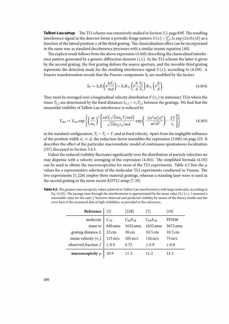
Talbot-Lau setup e TLI schemewas extensively studied in Section 3.2, page 83.e resultinginterference signal in the detector forms a periodic fringe pattern S (x) = ∑ℓ Sℓ exp (2πiℓx/d) as afunction of the lateral position x of the third grating.e classicalization eect can be incorporatedin the same way as standard decoherence processes with a similar master equation [40].e explicit result follows from the above expression (4.160) describing the classicalized interfer-

ence pattern generated by a generic diraction element t (x). In the TLI scheme the latter is givenby the second grating, the rst grating denes the source aperture, and the movable third gratingrepresents the detection mask for the resulting interference signal S (x), according to (4.159). AFourier transformation reveals that the Fourier components Sℓ are modied by the factors

Sℓ ↦ SℓR (ℓ hT2md

) = SℓRT1 (ℓhdT2T1

)RT2 (ℓhd) . (4.164)

ey must be averaged over a longitudinal velocity distribution F (vz) in stationary TLIs where thetimes T1,2 are determined by the xed distances L1,2 = vzT1,2 between the gratings. We nd that thesinusoidal visibility of Talbot-Lau interference is reduced by

Vsin ↦ Vsin exp⎧⎪⎪⎨⎪⎪⎩( mme

)2 ⎡⎢⎢⎢⎢⎣

erf (√2πσqT/md)

√2πσqτe/md

exp(−2π2m2eσ2sm2d2

) − 2Tτe

⎤⎥⎥⎥⎥⎦

⎫⎪⎪⎬⎪⎪⎭(4.165)

in the standard conguration, T1 = T2 = T , and at xed velocity. Apart from the negligible inuenceof the position width σs ≪ d, the reduction factor resembles the expression (3.106) on page 125. Itdescribes the eect of the particular macrorealistic model of continuous spontaneous localization[157] discussed in Section 3.4.3.Unless the reduced visibility uctuates signicantly over the distribution of particle velocities we

may dispense with a velocity averaging of the expression (4.165). e simplied formula (4.151)can be used to obtain the macroscopicities for most of the TLI experiments. Table 4.2 lists the µvalues for a representative selection of the molecular TLI experiments conducted in Vienna. etwo experiments [5, 228] employ three material gratings, whereas a standing laser wave is used asthe second grating in the more recent KDTLI setup [7, 19].

Table 4.2. e greatest macroscopicity values achieved in Talbot-Lau interferometry with large molecules, according toEq. (4.151).e passage time through the interferometer is approximated by the mean value 2L/ ⟨vz⟩. I assumed areasonable value for the ratio f between observed and predicted visibility by means of the theory results and theerror bars of the measured data at high visibilities, as provided in the references.

Reference [5] [228] [7] [19]

molecule C70 C60F48 C60F48 PFNS8mass m 840 amu 1632 amu 1632 amu 5672 amu

grating distance L 22 cm 38 cm 10.5 cm 10.5 cmmean velocity ⟨vz⟩ 115m/s 105m/s 116m/s 75m/sobserved fraction f ≳ 0.9 0.75 ≳ 0.9 ≳ 0.8

macroscopicity µ 10.9 11.3 11.2 12.1

180

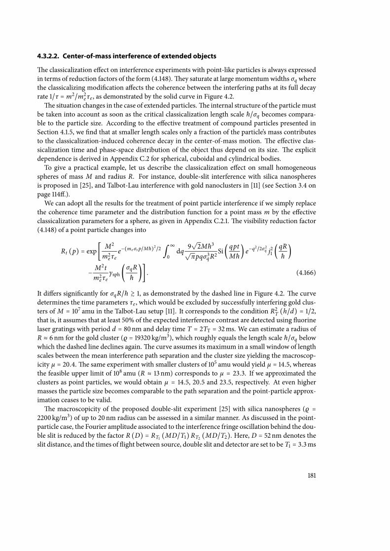
4.3.2.2. Center-of-mass interference of extended objects

e classicalization eect on interference experiments with point-like particles is always expressedin terms of reduction factors of the form (4.148).ey saturate at largemomentumwidths σq wherethe classicalizing modication aects the coherence between the interfering paths at its full decayrate 1/τ = m2/m2eτe , as demonstrated by the solid curve in Figure 4.2.e situation changes in the case of extended particles.e internal structure of the particlemust

be taken into account as soon as the critical classicalization length scale ħ/σq becomes compara-ble to the particle size. According to the eective treatment of compound particles presented inSection 4.1.5, we nd that at smaller length scales only a fraction of the particle’s mass contributesto the classicalization-induced coherence decay in the center-of-mass motion. e eective clas-sicalization time and phase-space distribution of the object thus depend on its size. e explicitdependence is derived in Appendix C.2 for spherical, cuboidal and cylindrical bodies.To give a practical example, let us describe the classicalization eect on small homogeneous

spheres of mass M and radius R. For instance, double-slit interference with silica nanospheresis proposed in [25], and Talbot-Lau interference with gold nanoclusters in [11] (see Section 3.4 onpage 114.).We can adopt all the results for the treatment of point particle interference if we simply replace

the coherence time parameter and the distribution function for a point mass m by the eectiveclassicalization parameters for a sphere, as given in Appendix C.2.1.e visibility reduction factor(4.148) of a point particle changes into

Rt (p) = exp [M2

m2eτee−(meσs p/Mħ)2/2 ∫ ∞

0dq 9

√2Mħ3√

πpqσ3qR2Si( qpt

Mħ) e−q2/2σ 2q j21 (

qRħ

)

− M2tm2eτe

γsph (σqRħ

)] . (4.166)

It diers signicantly for σqR/ħ ≳ 1, as demonstrated by the dashed line in Figure 4.2. e curvedetermines the time parameters τe , which would be excluded by successfully interfering gold clus-ters of M = 107 amu in the Talbot-Lau setup [11]. It corresponds to the condition R2T (h/d) = 1/2,that is, it assumes that at least 50% of the expected interference contrast are detected using uorinelaser gratings with period d = 80nm and delay time T = 2TT = 32ms. We can estimate a radius ofR ≈ 6nm for the gold cluster (ρ = 19320 kg/m3), which roughly equals the length scale ħ/σq belowwhich the dashed line declines again.e curve assumes its maximum in a small window of lengthscales between the mean interference path separation and the cluster size yielding the macroscop-icity µ = 20.4.e same experiment with smaller clusters of 105 amu would yield µ = 14.5, whereasthe feasible upper limit of 108 amu (R ≈ 13 nm) corresponds to µ = 23.3. If we approximated theclusters as point particles, we would obtain µ = 14.5, 20.5 and 23.5, respectively. At even highermasses the particle size becomes comparable to the path separation and the point-particle approx-imation ceases to be valid.e macroscopicity of the proposed double-slit experiment [25] with silica nanospheres (ρ =

2200 kg/m3) of up to 20nm radius can be assessed in a similar manner. As discussed in the point-particle case, the Fourier amplitude associated to the interference fringe oscillation behind the dou-ble slit is reduced by the factor R (D) = RT1 (MD/T1)RT2 (MD/T2). Here, D = 52nm denotes theslit distance, and the times of ight between source, double slit and detector are set to be T1 = 3.3ms

181

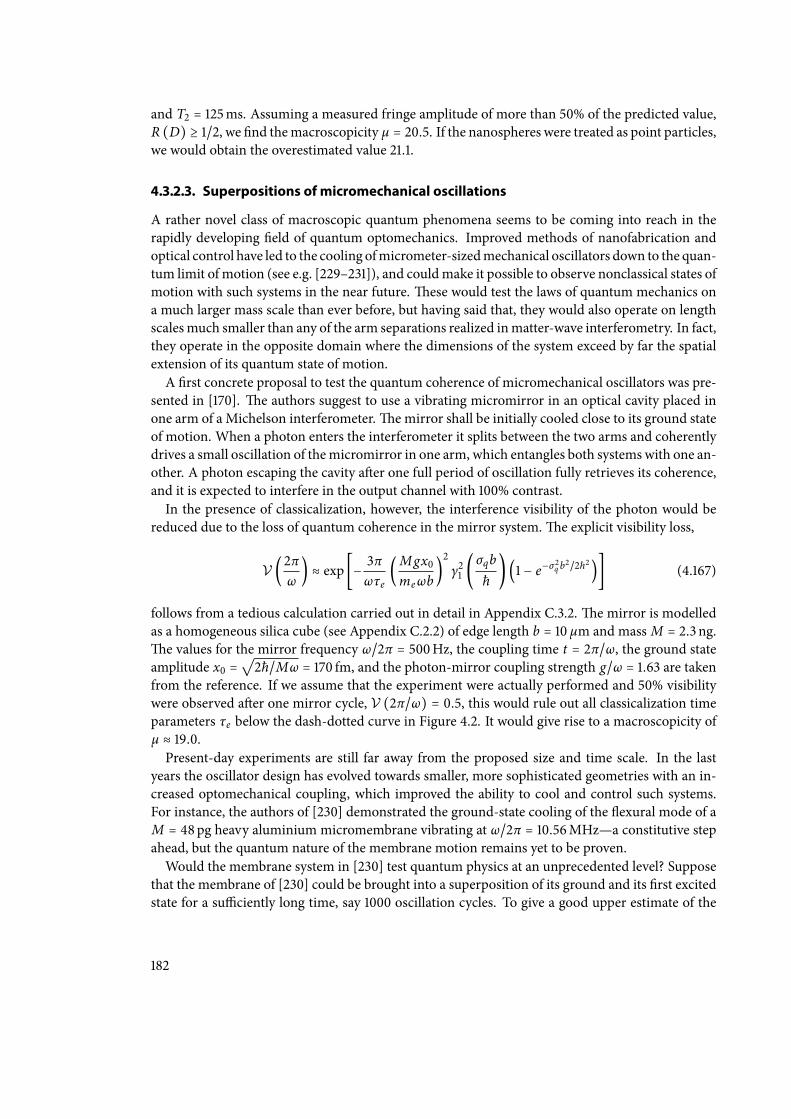
and T2 = 125ms. Assuming a measured fringe amplitude of more than 50% of the predicted value,R (D) ≥ 1/2, we nd themacroscopicity µ = 20.5. If the nanospheres were treated as point particles,we would obtain the overestimated value 21.1.

4.3.2.3. Superpositions of micromechanical oscillations

A rather novel class of macroscopic quantum phenomena seems to be coming into reach in therapidly developing eld of quantum optomechanics. Improved methods of nanofabrication andoptical control have led to the cooling ofmicrometer-sizedmechanical oscillators down to the quan-tum limit of motion (see e.g. [229–231]), and couldmake it possible to observe nonclassical states ofmotion with such systems in the near future.ese would test the laws of quantum mechanics ona much larger mass scale than ever before, but having said that, they would also operate on lengthscalesmuch smaller than any of the arm separations realized inmatter-wave interferometry. In fact,they operate in the opposite domain where the dimensions of the system exceed by far the spatialextension of its quantum state of motion.A rst concrete proposal to test the quantum coherence of micromechanical oscillators was pre-

sented in [170]. e authors suggest to use a vibrating micromirror in an optical cavity placed inone arm of a Michelson interferometer.e mirror shall be initially cooled close to its ground stateof motion. When a photon enters the interferometer it splits between the two arms and coherentlydrives a small oscillation of themicromirror in one arm, which entangles both systems with one an-other. A photon escaping the cavity aer one full period of oscillation fully retrieves its coherence,and it is expected to interfere in the output channel with 100% contrast.In the presence of classicalization, however, the interference visibility of the photon would be

reduced due to the loss of quantum coherence in the mirror system.e explicit visibility loss,

V (2πω

) ≈ exp [− 3πωτe

(Mgx0meωb

)2

γ21 (σqbħ

)(1 − e−σ 2q b2/2ħ2)] (4.167)

follows from a tedious calculation carried out in detail in Appendix C.3.2.e mirror is modelledas a homogeneous silica cube (see Appendix C.2.2) of edge length b = 10 µm and massM = 2.3 ng.e values for the mirror frequency ω/2π = 500Hz, the coupling time t = 2π/ω, the ground stateamplitude x0 =

√2ħ/Mω = 170 fm, and the photon-mirror coupling strength g/ω = 1.63 are taken

from the reference. If we assume that the experiment were actually performed and 50% visibilitywere observed aer one mirror cycle, V (2π/ω) = 0.5, this would rule out all classicalization timeparameters τe below the dash-dotted curve in Figure 4.2. It would give rise to a macroscopicity ofµ ≈ 19.0.Present-day experiments are still far away from the proposed size and time scale. In the last

years the oscillator design has evolved towards smaller, more sophisticated geometries with an in-creased optomechanical coupling, which improved the ability to cool and control such systems.For instance, the authors of [230] demonstrated the ground-state cooling of the exural mode of aM = 48pg heavy aluminium micromembrane vibrating at ω/2π = 10.56MHz—a constitutive stepahead, but the quantum nature of the membrane motion remains yet to be proven.Would the membrane system in [230] test quantum physics at an unprecedented level? Suppose

that the membrane of [230] could be brought into a superposition of its ground and its rst excitedstate for a suciently long time, say 1000 oscillation cycles. To give a good upper estimate of the

182

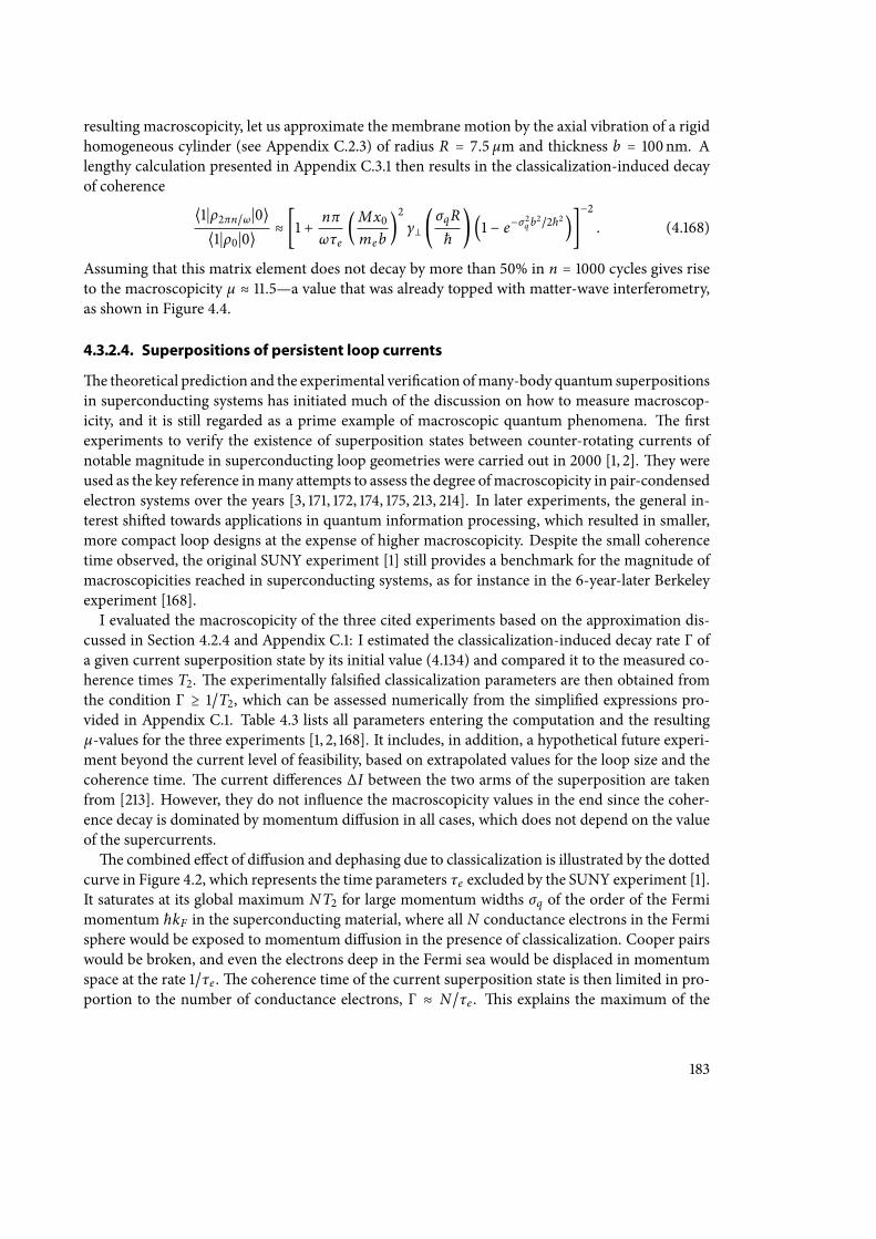
resulting macroscopicity, let us approximate the membrane motion by the axial vibration of a rigidhomogeneous cylinder (see Appendix C.2.3) of radius R = 7.5 µm and thickness b = 100nm. Alengthy calculation presented in Appendix C.3.1 then results in the classicalization-induced decayof coherence

⟨1∣ρ2πn/ω∣0⟩⟨1∣ρ0∣0⟩

≈ [1 + nπωτe

(Mx0meb

)2

γ (σqRħ

)(1 − e−σ 2q b2/2ħ2)]−2

. (4.168)

Assuming that this matrix element does not decay by more than 50% in n = 1000 cycles gives riseto the macroscopicity µ ≈ 11.5—a value that was already topped with matter-wave interferometry,as shown in Figure 4.4.

4.3.2.4. Superpositions of persistent loop currents

e theoretical prediction and the experimental verication ofmany-body quantum superpositionsin superconducting systems has initiated much of the discussion on how to measure macroscop-icity, and it is still regarded as a prime example of macroscopic quantum phenomena. e rstexperiments to verify the existence of superposition states between counter-rotating currents ofnotable magnitude in superconducting loop geometries were carried out in 2000 [1, 2].ey wereused as the key reference inmany attempts to assess the degree ofmacroscopicity in pair-condensedelectron systems over the years [3, 171, 172, 174, 175, 213, 214]. In later experiments, the general in-terest shied towards applications in quantum information processing, which resulted in smaller,more compact loop designs at the expense of higher macroscopicity. Despite the small coherencetime observed, the original SUNY experiment [1] still provides a benchmark for the magnitude ofmacroscopicities reached in superconducting systems, as for instance in the 6-year-later Berkeleyexperiment [168].I evaluated the macroscopicity of the three cited experiments based on the approximation dis-

cussed in Section 4.2.4 and Appendix C.1: I estimated the classicalization-induced decay rate Γ ofa given current superposition state by its initial value (4.134) and compared it to the measured co-herence times T2. e experimentally falsied classicalization parameters are then obtained fromthe condition Γ ≥ 1/T2, which can be assessed numerically from the simplied expressions pro-vided in Appendix C.1. Table 4.3 lists all parameters entering the computation and the resultingµ-values for the three experiments [1, 2, 168]. It includes, in addition, a hypothetical future experi-ment beyond the current level of feasibility, based on extrapolated values for the loop size and thecoherence time. e current dierences ∆I between the two arms of the superposition are takenfrom [213]. However, they do not inuence the macroscopicity values in the end since the coher-ence decay is dominated by momentum diusion in all cases, which does not depend on the valueof the supercurrents.e combined eect of diusion and dephasing due to classicalization is illustrated by the dotted

curve in Figure 4.2, which represents the time parameters τe excluded by the SUNY experiment [1].It saturates at its global maximum NT2 for large momentum widths σq of the order of the Fermimomentum ħkF in the superconducting material, where all N conductance electrons in the Fermisphere would be exposed to momentum diusion in the presence of classicalization. Cooper pairswould be broken, and even the electrons deep in the Fermi sea would be displaced in momentumspace at the rate 1/τe .e coherence time of the current superposition state is then limited in pro-portion to the number of conductance electrons, Γ ≈ N/τe . is explains the maximum of the

183

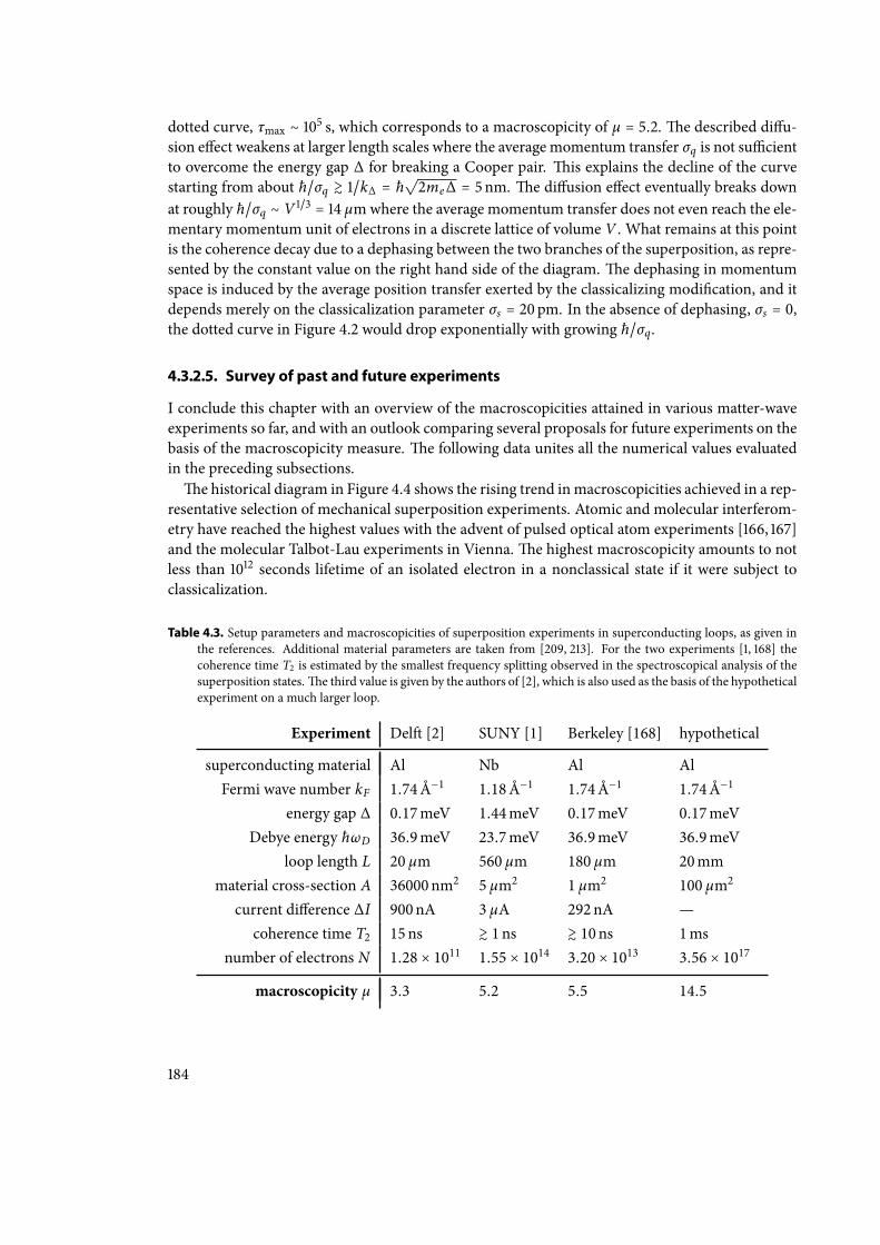
dotted curve, τmax ∼ 105 s, which corresponds to a macroscopicity of µ = 5.2.e described diu-sion eect weakens at larger length scales where the average momentum transfer σq is not sucientto overcome the energy gap ∆ for breaking a Cooper pair. is explains the decline of the curvestarting from about ħ/σq ≳ 1/k∆ = ħ

√2me∆ = 5nm. e diusion eect eventually breaks down

at roughly ħ/σq ∼ V 1/3 = 14 µmwhere the average momentum transfer does not even reach the ele-mentary momentum unit of electrons in a discrete lattice of volume V . What remains at this pointis the coherence decay due to a dephasing between the two branches of the superposition, as repre-sented by the constant value on the right hand side of the diagram. e dephasing in momentumspace is induced by the average position transfer exerted by the classicalizing modication, and itdepends merely on the classicalization parameter σs = 20pm. In the absence of dephasing, σs = 0,the dotted curve in Figure 4.2 would drop exponentially with growing ħ/σq.

4.3.2.5. Survey of past and future experiments

I conclude this chapter with an overview of the macroscopicities attained in various matter-waveexperiments so far, and with an outlook comparing several proposals for future experiments on thebasis of the macroscopicity measure. e following data unites all the numerical values evaluatedin the preceding subsections.e historical diagram in Figure 4.4 shows the rising trend inmacroscopicities achieved in a rep-

resentative selection of mechanical superposition experiments. Atomic and molecular interferom-etry have reached the highest values with the advent of pulsed optical atom experiments [166, 167]and the molecular Talbot-Lau experiments in Vienna.e highest macroscopicity amounts to notless than 1012 seconds lifetime of an isolated electron in a nonclassical state if it were subject toclassicalization.

Table 4.3. Setup parameters and macroscopicities of superposition experiments in superconducting loops, as given inthe references. Additional material parameters are taken from [209, 213]. For the two experiments [1, 168] thecoherence time T2 is estimated by the smallest frequency splitting observed in the spectroscopical analysis of thesuperposition states.e third value is given by the authors of [2], which is also used as the basis of the hypotheticalexperiment on a much larger loop.

Experiment Del [2] SUNY [1] Berkeley [168] hypothetical

superconducting material Al Nb Al AlFermi wave number kF 1.74Å−1 1.18Å−1 1.74Å−1 1.74Å−1

energy gap ∆ 0.17meV 1.44meV 0.17meV 0.17meVDebye energy ħωD 36.9meV 23.7meV 36.9meV 36.9meV

loop length L 20 µm 560 µm 180 µm 20mmmaterial cross-section A 36000nm2 5 µm2 1 µm2 100 µm2

current dierence ∆I 900nA 3 µA 292nA —coherence time T2 15ns ≳ 1ns ≳ 10ns 1ms

number of electrons N 1.28 × 1011 1.55 × 1014 3.20 × 1013 3.56 × 1017

macroscopicity µ 3.3 5.2 5.5 14.5

184

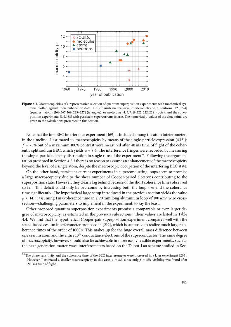
neutronsatomsmoleculesSQUIDs

year of publication

mac

rosc

opic

ity µ

1960 1970 1980 1990 2000 2010

4

6

8

10

12

Figure 4.4.Macroscopicities of a representative selection of quantum superposition experiments with mechanical sys-tems plotted against their publication date. I distinguish matter-wave interferometry with neutrons [223, 224](squares), atoms [166, 167, 169, 225–227] (triangles), or molecules [4, 5, 7, 19, 125, 222, 228] (dots), and the super-position experiments [1, 2, 168] with persistent supercurrents (stars).e numerical µ-values of the data points aregiven in the calculations presented in this section.

Note that the rst BEC interference experiment [169] is included among the atom inteferometersin the timeline. I estimated its macroscopicity by means of the single-particle expression (4.151):f = 75% out of a maximum 100% contrast were measured aer 40ms time of ight of the coher-ently split sodium BEC, which yields µ ≈ 8.4.e interference fringes were recorded by measuringthe single-particle density distribution in single runs of the experiment35. Following the argumen-tation presented in Section 4.2.3 there is no reason to assume an enhancement of themacroscopicitybeyond the level of a single atom, despite the macroscopic occupation of the interfering BEC state.On the other hand, persistent-current experiments in superconducting loops seem to promise

a large macroscopicity due to the sheer number of Cooper-paired electrons contributing to thesuperposition state. However, they clearly lag behind because of the short coherence times observedso far. is decit could only be overcome by increasing both the loop size and the coherencetime signicantly:e hypothetical large setup introduced in the previous section yields the valueµ ≈ 14.5, assuming 1ms coherence time in a 20mm long aluminium loop of 100 µm2 wire cross-section—challenging parameters to implement in the experiment, to say the least.Other proposed quantum superposition experiments promise a comparable or even larger de-

gree of macroscopicity, as estimated in the previous subsections. eir values are listed in Table4.4. We nd that the hypothetical Cooper-pair superposition experiment compares well with thespace-based cesium interferometer proposed in [219], which is supposed to realize much larger co-herence times of the order of 1000 s. is makes up for the huge overall mass dierence betweenone cesium atom and the entire 1017 conductance electrons of the superconductor.e same degreeof macroscopicity, however, should also be achievable in more easily feasible experiments, such asthe next-generation matter-wave interferometers based on the Talbot-Lau scheme studied in Sec-

35e phase sensitivity and the coherence time of the BEC interferometer were increased in a later experiment [203].However, I estimated a smaller macroscopicity in this case, µ ≈ 8.3, since only f = 15% visibility was found aer200ms time of ight.

185

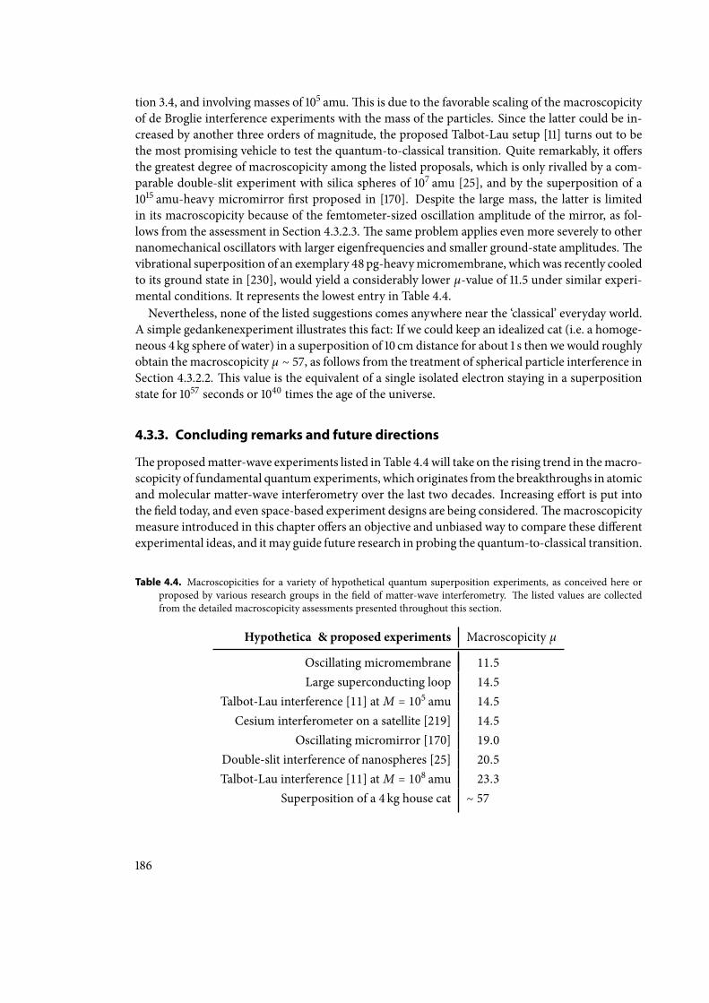
tion 3.4, and involving masses of 105 amu.is is due to the favorable scaling of the macroscopicityof de Broglie interference experiments with the mass of the particles. Since the latter could be in-creased by another three orders of magnitude, the proposed Talbot-Lau setup [11] turns out to bethe most promising vehicle to test the quantum-to-classical transition. Quite remarkably, it oersthe greatest degree of macroscopicity among the listed proposals, which is only rivalled by a com-parable double-slit experiment with silica spheres of 107 amu [25], and by the superposition of a1015 amu-heavy micromirror rst proposed in [170]. Despite the large mass, the latter is limitedin its macroscopicity because of the femtometer-sized oscillation amplitude of the mirror, as fol-lows from the assessment in Section 4.3.2.3.e same problem applies even more severely to othernanomechanical oscillators with larger eigenfrequencies and smaller ground-state amplitudes.evibrational superposition of an exemplary 48pg-heavymicromembrane, whichwas recently cooledto its ground state in [230], would yield a considerably lower µ-value of 11.5 under similar experi-mental conditions. It represents the lowest entry in Table 4.4.Nevertheless, none of the listed suggestions comes anywhere near the ‘classical’ everyday world.

A simple gedankenexperiment illustrates this fact: If we could keep an idealized cat (i.e. a homoge-neous 4 kg sphere of water) in a superposition of 10 cm distance for about 1 s then we would roughlyobtain the macroscopicity µ ∼ 57, as follows from the treatment of spherical particle interference inSection 4.3.2.2. is value is the equivalent of a single isolated electron staying in a superpositionstate for 1057 seconds or 1040 times the age of the universe.

4.3.3. Concluding remarks and future directions

e proposedmatter-wave experiments listed in Table 4.4 will take on the rising trend in themacro-scopicity of fundamental quantumexperiments, which originates from the breakthroughs in atomicand molecular matter-wave interferometry over the last two decades. Increasing eort is put intothe eld today, and even space-based experiment designs are being considered.emacroscopicitymeasure introduced in this chapter oers an objective and unbiased way to compare these dierentexperimental ideas, and itmay guide future research in probing the quantum-to-classical transition.

Table 4.4. Macroscopicities for a variety of hypothetical quantum superposition experiments, as conceived here orproposed by various research groups in the eld of matter-wave interferometry. e listed values are collectedfrom the detailed macroscopicity assessments presented throughout this section.

Hypothetical & proposed experiments Macroscopicity µ

Oscillating micromembrane 11.5Large superconducting loop 14.5

Talbot-Lau interference [11] atM = 105 amu 14.5Cesium interferometer on a satellite [219] 14.5

Oscillating micromirror [170] 19.0Double-slit interference of nanospheres [25] 20.5Talbot-Lau interference [11] atM = 108 amu 23.3

Superposition of a 4 kg house cat ∼ 57

186

Yet some questions remain to be answered about the notion of macroscopicity in general. epresent work provides a physical interpretation of this notion exclusively for mechanical systemswith a direct correspondence in classical Newtonian physics. In fact, the symmetries and consistentscaling principles underlying both quantum and classical mechanics are the essential ingredientsof the minimally invasive, classicalizing modication the present approach builds upon. It is clearfrom this standpoint that geniunely quantum degrees of freedom, most prominently spin systems,cannot classicalize as they do not have a classical counterpart. Spin superposition experiments thuscannot be assigned a macroscopicity if mechanical superpositions are absent, irrespective of thegreat number of entangled spins achieved nowadays [232].ere is simply no reasonable alternativeto quantum theory available in spin systems, hence there is also no classical ‘boundary’ of the theorythat could be probed in experiments and exploited to dene a notion of macroscopicity for spins.We encounter a similar problem in modern BEC interferometers [205–207], where nonlinear

interactions and superpositions of internal atomic states are employed to beat the classical precisionlimit in phase sensitivity by means of number squeezing. As in the case of spin ensembles, thesuperposition is made of many atoms entangled in their internal degrees of freedom, which are notdirectly subject to classicalization. A macroscopicity value can be assigned only to the motionalpart of such an entangled many-body state.One may think accordingly that photonic systems, which are not prone to the classicalization

eect developed here, are simply not accessible by this notion of macroscopicity either. At the sametime, we nd that current attempts to create nonclassical states of light involve an increasing numberof photons entangled or superimposed in various degrees of freedom [233–236]. It should be notedthat electromagnetic degrees of freedom do have a classical counterpart described by the Maxwellequations. e derivation of a minimally invasive classicalization eect from rst principles, andthe denition of a macroscopicity measure for quantum states of light, should be of priority insubsequent studies.Other attempts to dene a macroscopicity measure [3, 165, 171–176] have circumvented the men-

tioned restrictions by referring to specic many-body representations or classes of measurementoperations, which serve to characterize a given quantum state. e rst systematic assessment ofmacroscopicity was provided by Leggett [3, 165]. He identied two aspects of macroscopic super-position states: A large dierence in the expectation values of an appropriate observable betweenthe two branches of the superposition (so-called extensive dierence, measured in atomic referenceunits), and a large degree of entanglement between all the constituent atomic particles taking part inthe superposition (so-called disconnectivity)36. While these two aspects appear to be reasonable andintuitively clear characteristics for the size of typical quantum phenomena, they are not objectivelydened and therefore leave room for bias and interpretation37. Nevertheless, various measures ofmacroscopicity have been proposed that are related to one or the other aspect.

36is aspect preventsmany-body product states of the form ∣ψN⟩∝ (∣A⟩ + ∣B⟩)⊗N from being consideredmoremacro-scopic than the single-particle state ∣ψ1⟩ ∝ ∣A⟩ + ∣B⟩. On the other hand, the disconnectivity of a GHZ-type state,∣ψ⟩∝ ∣A⟩⊗N + ∣B⟩⊗N , would increase with the number of particles N .

37is triggered an interesting and illustrative debate on the macroscopicity of many-body quantum phenomena.Leggett’s prime example of a macroscopic quantum eect was the superposition of persistent currents in a super-conducting Josephson loop, rst observed in [1, 2]. He claimed that the disconnectivity of the measured state wasgiven by the total number of Cooper-paired electrons, more than a billion to be precise, owing either clockwise oranticlockwise through the loop. A proper many-body analysis, however, reveals that the state is given by a super-position of two slightly displaced but largely overlapping Fermi spheres, as found by Korsbakken et al. [213, 214].Hence, the vast majority of indistinguishable electrons occupies the same momentum space region in both branchesof the superposition, and only a few hundred to thousand are actually disconnected, i.e. found in dierent states.

187

Several proposals were derived from information-theoretic considerations and emphasize thehigh degree of many-body correlations in a given representation of macroscopic quantum states[171, 173, 174, 176], whereas others measure the sensitivity of such states to decoherence and de-phasing in a preferred basis of eigenstates [172, 175]. However, the decomposition of many-bodyquantum states into correlated constituent degrees of freedom is not unique, nor is the choice of arelevant basis to represent the state. Hence, there is a priori no unique standard of macroscopicitythat one could refer to.In this chapter, I have presented such a standard by referring to classical physics and by adhering

to the consistent mass scaling properties of composite mechanical systems, which makes it applica-ble to arbitrary such systems without bias. It exploits Leggett’s hypothesis of macrorealism, accord-ing to which the only way to reconcile the quantumdescription of the atomic world and the classicaldescription of the everyday world is to introduce a modication of quantum mechanics that car-ries out the quantum-classical transition somewhere in between. In principle, such a classicalizingmodication could be of almost any kind, as long as it assuredly turns quantum superpositions intoclassical mixtures and conserves the well-established classical equations of motions on large scales.Leggett proposed to test his hypothesis in the lab by trying to observe quantum phenomena as

macroscopic as possible; in this way one would exclude the possibility that those modicationswould have kicked in too early and induced a breakdown of the observed eect. Here, we havearrived at a universal macroscopicity benchmark by turning this statement upside down: We cancall an observed quantum phenomenon more macroscopic than another one if it leaves less roomfor the objective quantum-classical transition to occur.In order to derive a quantitative measure out of this, I have restricted the analysis in Section

4.1 to ‘minimal’ modications. ey are just intrusive enough to do the job and avert quantumsuperpositions in the macroworld without doing harm to fundamental symmetry and consistencyprinciples that are sacrosanct for both quantum and classical theory. By keeping other, more severemodications out of the game we could develop the logarithmic quantity µ in Section 4.3, whichnaturally meets the requirements for a sound measure of macroscopicity.

188

Chapter 5.

Conclusion and outlook

“People who have visions should go see a doctor.”—Helmut Schmidt

Let me close by reviewing the three main parts of this work, Chapter Two,ree and Four, from abroader perspective. In the rst two of these we were driven by concrete practical considerations inthe context of de Broglie wave interferometry, as pursued in Vienna: how to steer and interfere thecenter-of-massmotion of heavy nanoparticles. In summary, we developed a number of answers andpredictions that have proven useful, or will become important, for current and future experiments:

Feasibility of cavity-mediated cooling of molecules and nanoparticles Slow and cold en-sembles of molecules and nanoparticles are an essential prerequisite for high-mass matter-wave interferometry. However, unlike atoms, large molecules do not exhibit distinct inter-nal resonances that could be coherently addressed by conventional laser cooling techniques.us ecient methods of motional cooling and control are lacking. I discussed in ChapterTwo how and to what extent Sisyphus-type cooling can still be achieved for polarizable parti-cles with help of a strongly driven optical high-nesse cavity. Using the right parameters, thedelayed reaction of the cavity eld to themoving particle is able to cause a velocity-dependentfriction force as the particle modulates the cavity resonance while travelling across the eldmode. We saw that this eect is small in realistic settings, but it could be enhanced by em-ploying spherical resonator geometries with a large degenerate mode spectrum.ere, eachmode would contribute an additional velocity damping channel that increases the overallfriction eect.e eect was studied in a weak-coupling master equation model. Yet, a prac-tical implementation with single molecules remains challenging, and it would be interestingto combine it with ion-trapping techniques, or to study also collective self-organization ef-fects [84] in the case of many molecules.

Cavity cooling and trapping of large nanospheres e growing mass and polarizability oflarge nanoparticles alleviates the problem of weak coupling and thus facilitates an ecientcavity-induced slowing under realistic conditions. is goal is pursued by several groups atthe moment [23, 24, 137, 237, 238], mainly using silica nanospheres and infrared cavities. Wesaw with the help of Mie scattering theory in Chapter Two that not only the coupling of largenanospheres increases, but also the behaviour changes when their diameter gets comparableto the wavelength of the standing-wave cavity eld.eir absorption and scattering proper-ties get insensitive to the standing-wave eld modulation, the radiation pressure may turn

189

them into eective low-eld seekers at certain size regimes, and their overall eld extinctionpower increases to an extent that facilitates a position-sensitive detection via the scatteredlight. Moreover, I also assessed the transverse forces in a Gaussian light mode and showedfor a realistic setting that they can be employed to capture nanospheres in the center of themode. Practical simulations and the application in experiments of the Vienna group are amatter of ongoing research.

Optical gratings for matter waves From the detailed assessment of the light-matter inter-action between nanoparticles and standing waves, we could understand how the latter canbe employed as diractive elements for matter waves. Not only do they serve as phase grat-ings, as conventionally implemented in molecule interferometry, but they can also act asamplitude gratings by optical depletion—a convenient alternative to material grating masks.is requires the particles to be altered by photo-absorption such that they can be sortedout or distinguished from the others in a reliable fashion. In the simplest case, a single pho-ton suces to ionize the particle, which can then be removed by an electric eld; this waythe standing-wave acts as an absorptive masks with the nodes playing the role of the gratingslits. Such single-photon ionization gratings have been proven to work [13], demonstratingthe interplay between absorptive and diractive eects on the most elementary level. Otherpossible depletion methods involving more than a single photon and internal conversionprocesses are being considered and should be assessed next.

Poisson’s spot with large molecules In Chapterree I turned to matter-wave interferome-try techniques with molecules and nanoparticles, and I started by analyzing a peculiar near-eld phenomenon that had been conceived almost two centuries ago to verify thewave natureof light: Poisson’s spot, also known as Arago’s spot. Although the appearance of a bright in-tensity maximum in the shadow center behind an opaque disc seems to be a decisive proofof wave interference, I showed that this ceases to be the case for large nanoparticles.e rea-son is that a classical ballistic model may lead to a similar prediction due to the strong vander Waals interaction between the particles and the walls of the obstacle.is makes it hardto distinguish quantum interference from classical deection above a certain particle size.However, my analysis was based on a simplied treatment of the interaction potential, andmore rened predictions should be based more sophisticated models [116].

Talbot-Lau interferometry with optical gratings Apart from Poisson’s spot, Chapterreewas mostly about the Talbot-Lau near-eld scheme, which is most suited to interfere largemasses. I provided a full-edged phase-space model for Talbot-Lau interferometry with op-tical gratings, and the main result was the detailed description of a time-domain Talbot-Lauinterferometer with optical ionization gratings for heavy nanoclusters. e Vienna grouphas implemented the scheme in the lab by now, and the rst interference was observed withanthracene clusters [13].

Interferometric metrology techniques e nanometer-sized and periodic interference frin-ges produced in a Talbot-Lau setup are highly sensitive to random or controlled phase shisthat may occur while the matter waves pass the three gratings of the interferometer. iscan be utilized in precision metrology of the internal properties of the particle, such as thestatic polarizability or the optical absorption cross-section. e absolute value of the latter

190

can bemeasured at benchmark precision in the interferometric scheme discussed in Chapterree. By shining in an additional laser between the gratings we can make use of the photonrecoil upon absorption to extract the absorption cross section and uorescence yield fromthe subsequent reduction of interference contrast as a function of laser power.e idea wasoriginally proposed in [6] and awaits its rst implementation.

Mass limitations of matter-wave interferometry Finally, I took all relevant limitations inTalbot-Lau interferometry into consideration and gave an accurate estimation of the high-est possible masses that could be interfered in the time-domain Talbot-Lau scheme withvacuum-ultraviolet laser gratings, as conceived and developed in my group. We found onthe one hand that the combined inuence of gravity, environmental decoherence, and thenite cluster size limits the attainable mass to below a billion atomic mass units. On theother hand, we saw that hypothetical new physics at the macroscale may become testablealready at about a million amu. e famous model of continuous spontaneous localization(CSL) [155, 157] is expected to kick in at this scale, inducing an eective loss of coherencewhich would be reected in a mass-dependent drop of interference contrast.

The question of macroscopicity e long-term analysis of future mass limitations in macro-scopic cluster interferometry, as conceived and implemented in Vienna, led us away from practicalproblems and to the deeper theoretical question of what it means to be macroscopic. In ChapterFour, this forced us to look at the bigger picture, where center-of-mass interferometry is only oneexample of a macroscopic quantum phenomenon, and where the mass is only one aspect of macro-scopicity. As much as my colleagues and me are intuitively biased towards this aspect, so mayphysicists working on atom interference, many-body quantum phenomena, and nanomechanicaloscillators be biased towards other aspects.is is why we felt it is necessary to part from our pre-judice and conceive a general methodology to tackle the question of macroscopicity in arbitrarysettings.In Chapter Four I presented a universal way tomeasuremacroscopicity inmechanical systems by

referring to the hypothesis of macroscopic realism and by quantifying the extent to which this hy-pothesis is ruled out by the observation of a quantum phenomenon. Macroscopicity is thus denedby means of empirical facts rather than the theoretical representation of the given phenomenon.Hence, the quality and nature of the experiment matters as much as the formal complexity of theunderlying quantum state. It will be worthwile to study this connection further and explore thecommon features and interfaces between the formal size measures proposed by others [171–176]and the present empirical measure of macroscopicity.Finally, let me remark that the macroscopicity standard dened here can be applied only to sys-

tems with a direct counterpart in classical physics. Quantum spin states, however large and com-plex, are therefore excluded because they do not possess such a classical reference. is does notmean that one cannot go further than this.e discussion in Chapter Four was restricted to nonrel-ativistic mechanical systems having their counterpart in Newtonian mechanics, and it is clear whatto do next: One should try to extend the analysis also to relativistic and electromagnetic systems.is would eventually allow one to access the vast eld of photonic quantum experiments bymeansof the presented method.

191

Appendix A.

Light-matter interaction

A.1. Complex ®eld amplitude and quantization

e macroscopic Maxwell equations for electromagnetic elds refer to real-valued quantities. Incase of a source-free medium, they read as∇⋅D = ∇⋅B = 0,∇×H = ∂tD,∇×E = −∂tB. It is, how-ever, convenient to use a complexied version when dealing with time-harmonic electromagenticwaves, that is, elds oscillating at a xed (optical) frequency ω.e time dependence of all elds isthen of the form E (r, t) = E (r) exp (−iωt), and the time derivative can be replaced by ∂t ↦ −iω.I will always presuppose homogeneous, isotropic, linear and non-magnetic media characterized

by a relative dielectric permeability ε = ε (ω) and a magnetic permeability µ = 1. Note that ε cantake complex values in the case of absorbing media. e electric eld E and the magnetic eld Bare related to the electric displacement eld D and to the magnetizing eld H via D = εε0E andB = µ0H.e Maxwell equations become

H (r) = 1iµ0ω

∇× E (r) , E (r) = iεε0ω

∇×H (r) , (A.1)

interrelating the complex electric and magnetic elds, with∇ ⋅H = ∇ ⋅ εE = 0. Hence, this reducesto a single vector wave equation, or Helmholtz equation, for both elds,

∇×⎡⎢⎢⎢⎢⎣∇×

⎧⎪⎪⎨⎪⎪⎩

E (r)H (r)

⎫⎪⎪⎬⎪⎪⎭

⎤⎥⎥⎥⎥⎦= −∇2

⎧⎪⎪⎨⎪⎪⎩

E (r)H (r)

⎫⎪⎪⎬⎪⎪⎭= εk2

⎧⎪⎪⎨⎪⎪⎩

E (r)H (r)

⎫⎪⎪⎬⎪⎪⎭, (A.2)

where k = ω/c denotes the vacuum wavenumber throughout this thesis. I will only describe wavesin vacuum (ε = 1) or in piecewise homogeneous media, where the dielectric function ε does notdepend on position except on boundary surfaces.e physical elds are obtained from the complexied expressions by taking the real part,ReE

and ReH. In the case of a derived expression involving products of elds, this rule must beapplied to each factor [33]. For an arbitrary product ‘’ between two complexied vector elds aand b, we arrive at the physical expression by

a (r, t) b (r, t)→Re [a (r) e−iωt] Re [b (r) e−iωt] . (A.3)

Doing a time-average ⟨⋅⟩t over the fast optical oscillation then yields the simple form

⟨a (r, t) b (r, t)⟩t →12Re [a (r) b∗ (r)] . (A.4)

193

A standard way to describe both the coupling between distinguished wave components and toquantize wave elds lies in the separation of amplitude and mode. e mode denes the spatialstructure and polarization of the eld, whereas the complex amplitude encodes the stored energyand phase evolving in time. One rst chooses an orthogonal basis set of eigenfunctions un (r)that solve the above Helmholtz equation (A.2) and fulll the electric eld boundary conditions ofthe physical system in question. e complementary set of solutions k−1∇× un (r) must fulllthe boundary conditions of the magnetic eld, respectively. For example, the vector-valued func-tions can be plane waves with a xed polarization, uk (r) = є exp (i

√εk ⋅ r), or standing waves in a

Fabry-Pérot conguration. ey are called mode-polarization functions, or mode functions in thecase of a xed polarization vector є. I adhere to the convention [239] of dening them as dimen-sionless functions and introducing theirmode volume Vn through the orthogonality conditions

∫ d3r u∗n (r) ⋅ um (r) = 1k2 ∫ d3r [∇× u∗n (r)] ⋅ [∇× um (r)] = δnmVn . (A.5)

With this mode picture at hand, and allowing for dierent frequency components, we can expandany electric eld in vacuum as

E (r, t) =∑nEn (t)un (r) =∑

n

√2ħωnε0Vn

αn (t)un (r) , (A.6)

where the expansion coecients En (t) determine the amplitude of the eld. e expansion of Hfollows from (A.1) accordingly. e time evolution of the wave eld is now reduced to a (possi-bly coupled) time evolution of the individual complex amplitudes αn (t) =

√ε0Vn/2ħωnEn (t),

keeping the spatial mode structure xed1.In the canonical quantization procedure one simply replaces the complex amplitudes αn and α∗n

by bosonic annihilation and creation operators, an and a†n.e expression for the energy Hf stored

in the vacuum eld translates into the standard Hamiltonian of multiple harmonic oscillators,

Hf =12 ∫ d3r [ε0ReE (r, t)2 + µ0ReH (r, t)2] =∑

n

ħωn2

(α∗nαn + αnα∗n)

→ Hf =∑nħωn (a

†nan +

12) . (A.7)

e Heisenberg time evolution of the bosonic operators under the eld Hamiltonian Hf remainsharmonic, an (t) = an exp (−iωt).

A.2. Gaussian modes

Gaussian light modes are encountered in many experimental situations. e most common ex-amples are fundamental standing-wave cavity modes with spherical mirrors and running laserwaves. ey are described by TEM00-modes with a symmetric Gaussian mode prole of waistw [81, 82, 240]. e simple expression E (r) ∝ є exp (−r2/w2 + ikz) represents only a rough ap-proximation for a linearly polarized Gaussian running wave directed towards the positive z-axis. It

1A spatial motion of the wave eld would be described by a redistribution of amplitudes between dierent modes inthis picture.

194

solves theHelmholtz equation (A.2) only to zeroth order in the expansion parameter s = 1/kw. Tak-ing the rotation of this function yields also correction terms as compared to the linear polarizationof the corresponding magnetic eld.A rigorous formulation of Gaussian modes treating (on equal footing) electric and magnetic

eld components involves vector potentials of a xed polarization along the x- or y-axis [240]. As aconsequence, the linear eld polarization, say, along x, is appended by a longitudinal z-componentand a y-component of higher order in s. A Gaussian running wave directed towards the positive(+) or negative (−) z-direction, and centered at r = 0, is approximately described by the elds2

E± (r) = E0q±e−q±ρ2±ikz⎛⎜⎜⎝

1 + s2 (ρ2q2± + 2q2±x2/w2 − ρ4q3±) +O (s4)2s2q2±xy/w2 +O (s4)∓2isq±x/w +O (s3)

⎞⎟⎟⎠, (A.8)

H± (r) = ±cε0E0q±e−q±ρ2±ikz⎛⎜⎜⎝

2s2q2±xy/w2 +O (s4)1 + s2 (ρ2q2± + 2q2±y2/w2 − ρ4q3±) +O (s4)

∓2isq±y/w +O (s3)

⎞⎟⎟⎠, (A.9)

with ρ2 = (x2 + y2) /w2 and q± = 1/ (1 ± 2iz/kw2). I chose the parameters such that the electriceld is mainly x-polarized.e lowest order addition to both the electric and the magnetic eld is alongitudinal polarization component.e strict orthogonality between the direction of propagationand of polarization holds only for pure plane- or standing-wave modes. A cosine-type standingelectric-eldwave is obtained by combining Esw = (E+ + E−) /2.e correspondingmagnetizationeld Hsw = (H+ +H−) /2 is then of sine type.If we look at theGaussianwave from a coordinate system, which is shied to the neworigin r0, we

must simply replace r by r + r0 in the above eld expressions.is will be of use when consideringscattering situations at spherically symmetric geometries. If in addition the size of the scatteringobject in question is small compared to the waist of the eld, we should consider expanding thetranslated eld expressions in r/w ≪ 1 as well. Let me introduce the abbreviations

ρ20 =x20 + y20w2

, ρ21 =2xx0 + 2yy0

w2, (A.10)

A = ρ20 − ρ40 − 2z20w2

(ρ20 − 2)2 , B = ρ20 − 1 + (2 − ρ20) ρ21 , C = ρ41

2− ρ21 −

x2 + y2

w2. (A.11)

e following eld expressions are valid up to second order in both s and r/w (i.e. terms of the formsn (r/w)m are dropped if n +m ≥ 3).

E± (r + r0) ≈ E0e−ρ20±ik(z+z0)⎛⎜⎜⎝

1 + C ± 2is [Bz0 + (ρ20 − 1) z] /w + s2 (A+ 2x20/w2)2s2x0y0/w2

∓2is [(1 − ρ21 ) x0 + x] /w + 4s2 (ρ20 − 2) x0z0/w2

⎞⎟⎟⎠

(A.12)

H± (r + r0) ≈ ±cε0E0e−ρ20±ik(z+z0)⎛⎜⎜⎝

2s2x0y0/w2

1 + C ± 2is [Bz0 + (ρ20 − 1) z] /w + s2 (A+ 2y20/w2)∓2is [(1 − ρ21 ) y0 + y] /w + 4s2 (ρ20 − 2) y0z0/w2

⎞⎟⎟⎠(A.13)

2Note that I use a harmonic time dependence of the form exp (−iωt), as opposed to [240].e present eld expressionsare thus given by the complex conjugates of the ones from the reference.

195

A.3. Phase space representation of states and observables

Bound operators on the Hilbert space L2 (R) of a one-dimensional motional degree of freedomcan be represented by means of an arbitrary complete set of orthogonal operators (with respect tothe Hilbert-Schmidt scalar product (A, B) = tr (A

†B)).e Wigner-Weyl formulation of quantum

mechanics is obtained by using the basis of reection operators

Rz,p =12 ∫ ds e ips/ħ∣z +

s2⟩⟨z − s

2∣, tr (R

†z,pRz′ ,p′) = πħδ (z − z′) δ (p − p′) . (A.14)

One denes theWeyl symbol of an operator A as the expansion coecient

A(z, p) = 2tr (Rz,pA) = ∫ ds e ips/ħ⟨z − s2∣A∣z + s

2⟩, . (A.15)

e operator can be fully reconstructed from its Weyl symbol by A = ∫ dzdp A(z, p)Rz,p/πħ.eWigner function of a given quantum state ρ is dened as the normalized Weyl symbol

w (z, p) = 12πħ ∫ ds e ips/ħ⟨z −

s2∣ρ∣z + s

2⟩ ∈ R, ∫ dzdpw (z, p) = 1. (A.16)

We can interpret it as the quantum generalization of the phase space density distribution, f (z, p) ≥0, of a classical state of motion:

e Wigner function reproduces the same marginals as its classical counterpart. We obtainthe spatial density distribution by integrating over the momentum variable, ∫ dpw (z, p) =⟨z∣ρ∣z⟩, and the momentum distribution by integrating over position.

Classically mixed states with vanishing quantum coherence can be described by a positiveWigner function that is identical to the according phase-space distribution function in a clas-sical description.

Quantum expectation values of observables A can be expressed as a Wigner function aver-age of the corresponding Weyl symbol, ⟨A⟩ = ∫ dzdp A(z, p)w (z, p). e same is true forphase-space observables in a classical model.

Given that the quantum state evolves coherently under the inuence of the Hamiltonian H =p2/2mP + V (z), its Wigner function solves the quantum-Liouville equation [77]

[∂t +pmP

∂z − V ′ (z) ∂p]w (z, p) =∞

∑ℓ=1

(−ħ2/4)ℓ

(2ℓ + 1)! V(2ℓ+1) (z) ∂2ℓ+1p w (z, p) . (A.17)

It is identical to the classical Liouville equation in a semiclassical approximation to secondorder in ħ2, where all higher-than-second-order derivatives are omitted. More generally, ifLindblad-type master equations are translated into phase space the same semiclassical ap-proximation will yield a Fokker-Planck type equation (2.89) which has a clear classical cor-respondence.

196

e Weyl symbols of the position and the momentum observable are the respective phase-spacecoordinates. However, due to the noncommutative nature of quantum observables, there is nosuch simple correspondence most other cases. Given two non-commuting operators A and B wend that the Weyl symbols for their products read as [77]

(AB) (z, p) = A(z − ħ2i∂p , p +

ħ2i∂z)B (z, p) , (A.18)

(BA) (z, p) = [A∗ (z − ħ2i∂p , p +

ħ2i∂z)B∗ (z, p)]

∗

. (A.19)

e dierential operators in the arguments are to be understood by means of the Taylor expansion

A(z − ħ2i∂p , p +

ħ2i∂z) =

∞

∑n,m=0

1m!n!

A(m,n) (z, p) (− ħ2i∂p)

m( ħ2i∂z)

n. (A.20)

Any master equation can be translated to a phase-space partial dierential equation by subsequentapplications of the above translation rules.

A.4. Weak-coupling dynamics of N particles in M modes

Here I generalize the weak-coupling master equation (2.81) for a single particle in the presence of asingle driven andM empty cavity modes to a more general conguration of N (identical) particlesin M driven or empty modes. Each mode shall be either empty, αn = 0, or pumped to a largesteady-state amplitude, ∣αn∣ ≫ 1. I restrict my considerations to the simple yet relevant case wherethe driving is realized by a single laser of frequency ωP . Coupling it into the cavity thus singles outone or a few degenerate pump modes.If we apply the rst weak coupling assumption of Section 2.2.2.1, ∣Umn∣ ≪ κn, to each individual

particle, we arrive at the following light-matter master equation in the ωP-rotating and displacedframe,

∂tρ = − iħ[HP + HI , ρ] +LC (ρ) +Labs (ρ) +Lsca (ρ) , (A.21)

LC (ρ) = −i [M∑n=1∆na

†nan , ρ] +

M∑n=1

κn (2anρa†n − a

†nan , ρ) , (A.22)

HP =N∑j=1

⎡⎢⎢⎢⎢⎣

p2j

2mP+

M∑

m,n=1ħUmnα∗mαnu∗m (r j)un (r j)

⎤⎥⎥⎥⎥⎦, (A.23)

HI =N∑j=1

M∑

m,n=1ħUmnα∗manu∗m (r j)un (r j) + h.c. (A.24)

e apsorption and scattering terms are given by sums over all driven modes,

Labs (ρ) = γ(n)abs ∣αn∣2

N∑j=1

[un (r j) ρu∗n (r j) −12∣un (r j)∣

2 , ρ] , (A.25)

Lsca (ρ) = γ(n)sca ∣αn∣2

⎡⎢⎢⎢⎢⎣

N∑j=1∫ d2n R (n)un (r j) e−ikn⋅r j ρe ikn⋅r ju∗n (r j) −

12∣un (r j)∣

2 , ρ⎤⎥⎥⎥⎥⎦, (A.26)

197

with the respective extinction rates γ(n)abs,sca = cσabs,sca/Vn and the mode volumes Vn. In the next

step of the weak-coupling approximation I assume that all cavity modes remain empty (relative tothe steady-state amplitude) at almost all times. is requires the eective rate of eld uctuationsinduced by the entirety of particles to be small compared to the cavity decay rate. at is to say,the second weak coupling condition becomes ∣NUmnαn∣ ≪ κm ∀m, n, which places a quite rigidbound on the allowed particle number in practical situations.In full analogy to the line of arguments in Sections 2.2.2.2 and 2.2.2.3 we arrive at the eective

N-particle master equation

∂tρP = LPρP −N∑j=1

M∑

n,ℓ,m=1UℓmUmn (α∗ℓ αn [u∗ℓ (r j)um (r j) , gmnρP] + h.c.) , (A.27)

gmn ≈ ∫ ∞

0dτ e−(κm+i∆m)τ

N∑k=1

u∗m (rk −pkτmP

)un (rk −pkτmP

) . (A.28)

Note that, as a result of the second weak coupling condition, the non-retarded part of the timeevolution, LPρP = −i [HP , ρP] /ħ +LabsρP +LscaρP , reduces to a sum of uncoupled single-particleterms.e inter-particle coupling is mediated by the delayed cavity reaction, as represented by thememory operators gmn.With the eective N-particle master equation at hand we can identify the cavity-induced friction

and diusion eect in phase space. For this let me again restrict our view to the one-dimensionalmotion along the z-axis of the cavity. Introducing the N-particle Wigner function

w (z1, p1, . . . , zN , pN) =1

(2πħ)N ∫ ds1 . . . dsN exp⎛⎝iħ∑j

p js j⎞⎠⟨z1 −

s12, . . . ∣ρ∣z1 +

s12, . . .⟩ (A.29)

we can convert the above master equation into a semiclassical Fokker-Planck-type equation for the2N-dimensionalWigner function.e phase-space translation rules fromAppendix A.3 generalizenaturally to N particles. I once again dene the memory integrals per particle as the phase-spacecounterparts of the memory operators,

Gmn (z, p) = ∫ ∞

0e−(κm+i∆m)τu∗m (z − pτ

mP)un (z −

pτmP

) . (A.30)

A tedious but straightforward calculation reveals the dissipative force term

g(dis)p j (z1, p1, . . .) =M∑

n,ℓ,m=1ħUℓmUmnRe2iα∗ℓ αn [∂z ju∗ℓ (z j)um (z j)]

N∑k=1

Gmn (zk , pk)

− ħα∗ℓ αn [∂2z ju∗ℓ (z j)um (z j)] ∂p jGmn (z j , p j) (A.31)

as well as the diusion coecients

D(dis)p j pk (z1, p1, . . .) =

M∑

n,ℓ,m=12ħ2UℓmUmnReα∗ℓ αn [∂z ju∗ℓ (z j)um (z j)] ∂zkGmn (z j , p j) , (A.32)

D(dis)z j pk (z1, p1, . . .) = −

M∑

n,ℓ,m=1ħ2UℓmUmnReα∗ℓ αn [∂zku

∗ℓ (zk)um (zk)] ∂p jGmn (z j , p j) . (A.33)

198

e rst order friction force term (rst line) for the jth particle is aected by the accumulatedtrajectory of all other particles. at is, the particles couple through the cavity-mediated frictionforce. e second-order force terms for each particle are independent. e diusion coecientscorrelate all particles uniformly. A particle couples to the rst-order eld uctuations caused byitself or by any other particle via the same memory integral expression. We should expect thatthis would lead to a strongly correlated interacting many-body system beyond the weak couplingregime. As a consequence, collective self-organization eects are expected to occur [84, 85].

A.5. Spherical wave expansion

e spherical wave expansion is an essential method to work with elds under spherically sym-metric boundary conditions. Here, I use it to solve the Mie scattering problem of electromagneticwaves at spherical dielectrics [28, 29]. e idea is to expand the electric and magnetic elds in agiven setup in the basis of spherical vector harmonics [34]. Given a harmonic eld component offrequency ω = ck in a dielectric medium of (complex) refractive index n =

√ε, we may expand the

electric and the magnetization eld as

E (r) =∞

∑ℓ=1

ℓ∑m=−ℓ

[C(M)

ℓ,m fℓ (nkr) Xℓ,m (θ , ϕ) + 1kC(E)ℓ,m∇× gℓ (nkr) Xℓ,m (θ , ϕ)] , (A.34)

H (r) = cε0i

∞

∑ℓ=1

ℓ∑m=−ℓ

[n2C(E)ℓ,m gℓ (nkr) Xℓ,m (θ , ϕ) + 1

kC(M)

ℓ,m ∇× fℓ (nkr) Xℓ,m (θ , ϕ)] . (A.35)

e radial functions fℓ and gℓ must be linear combinations of spherical Bessel functions of the rstand second kind, jℓ and yℓ. In practice, two possibilities matter: Regular wave solutions, which arenite and dierentiable everywhere, must be given in terms of the Bessel functions fℓ = gℓ = jℓ.Outgoing scattered wave solutions are given by the spherical Hankel functions hℓ ∶= jℓ + iyℓ.eydiverge at r = 0, and they become spherical waves in the far eld, hℓ (kr) ≈ i−ℓ−1e ikr/kr for kr ≫ 1.e spherical vector harmonics are dened by [34]

Xℓ,m (θ , ϕ) = r ×∇i√ℓ (ℓ + 1)

Yℓ,m (θ , ϕ) = (−)m+1 X∗ℓ,−m (θ , ϕ)

= 12√ℓ (ℓ + 1)

⎛⎜⎜⎝

√(ℓ −m) (ℓ +m + 1)Yℓ,m+1 +

√(ℓ +m) (ℓ −m + 1)Yℓ,m−1

i√

(ℓ +m) (ℓ −m + 1)Yℓ,m−1 − i√

(ℓ −m) (ℓ +m + 1)Yℓ,m+12mYℓ,m

⎞⎟⎟⎠,

(A.36)

for ℓ > 0.ey are tangential to the unit sphere, r ⋅ Xℓ,m = 0, and they form an orthonormal set ofvector-valued functions on the unit sphere, just like thewell-known spherical harmonicsYℓ,m (θ , ϕ)do for scalar functions.e latter are dened in terms of associated Legendre polynomials [63],

Yℓ,m (θ , ϕ) =¿ÁÁÀ2ℓ + 1

4π(ℓ −m)!(ℓ +m)! e

imϕPmℓ (cos θ) , Yℓ,−m = (−)m Y∗

ℓ,m ,

Pmℓ (x) =

(−√1 − x2)

m

2ℓℓ!∂ℓ+mx (x2 − 1)ℓ ∀m ≥ 0. (A.37)

199

e orthogonality relations read as

∫ dΩ X∗ℓ′ ,m′ ⋅ Xℓ,m = ∫ dΩ [n × X∗

ℓ′ ,m′] ⋅ [n × Xℓ,m] = ∫ dΩY∗ℓ′ ,m′Yℓ,m = δℓℓ′δmm′ , (A.38)

with n = r/r the unit vector pointing in the directionΩ.e terms n × Xℓ,m form an independentand complementary set of basis functions, ∫ dΩ X∗

ℓ′ ,m′ ⋅ [n × Xℓ,m] = 0. Combining the vectorharmonics with the spherical Bessel functions leads to basis solutions of the vector wave equation,

∇× [∇× fℓ (nkr) Xℓ,m (θ , ϕ)] = εk2 fℓ (nkr) Xℓ,m (θ , ϕ) . (A.39)

is can be checked using the identity [34]

∇× f (r) Xℓ,m (θ , ϕ) = 1r∂r [r f (r)] n × Xℓ,m (θ , ϕ) +

i√ℓ (ℓ + 1)r

f (r) nYℓ,m (θ , ϕ) . (A.40)

e dierential equation underlying the Bessel-type functions and a few addition theorems [113]are also required,

ℓ (ℓ + 1) fℓ (x) = x2 f ′′ℓ (x) + 2x f ′ℓ (x) + x2 fℓ (x) , (A.41)

f ′ℓ (x) = fℓ−1 (x) −ℓ + 1x

fℓ (x) =ℓxfℓ (x) − fℓ+1 (x) , (A.42)

1x2

= jℓy′ℓ − j′ℓyℓ = −i [ jℓh′ℓ − j′ℓhℓ] . (A.43)

In a concrete physical situation, one is oen le with specic electromagnetic eld distributions,such as standing-wave modes or Gaussian modes, which must be expanded in the above partial-wave basis.e expansion coecients can be obtained by means of the integrals

C(E)ℓ,m gℓ (nkr) =

−ik√ℓ (ℓ + 1) ∫ dΩY∗

ℓ,m (θ , ϕ) [r ⋅ E (r, θ , ϕ)] , (A.44)

C(M)

ℓ,m fℓ (nkr) =k

cε0√ℓ (ℓ + 1) ∫ dΩY∗

ℓ,m (θ , ϕ) [r ⋅H (r, θ , ϕ)] . (A.45)

Whether the integrals on the right hand side evaluate to the Bessel-type dependence on the radialcoordinate imposed by the le hand side, depends verymuch on the (approximate) functional formof a given eld mode. One may be forced to invoke complicated numerical methods to extract thepartial-wave expansion coecients from the above relations [241].A direct evaluation of the integrals is possible for the most elementary cases. An x-polarized

vacuum plane-wave mode running along the positive or negative z-axis, E(±) = E0ex exp (±ikz),gets expanded as [34]

E(±) (r) = E02

∞

∑ℓ=1

(±)ℓ ιℓ ∑m=±1

[ jℓ (kr) Xℓ,m ±mk∇× jℓ (kr) Xℓ,m] , (A.46)

H(±) (r) = cε0E02i

∞

∑ℓ=1

(±)ℓ ιℓ ∑m=±1

[±mjℓ (kr) Xℓ,m +1k∇× jℓ (kr) Xℓ,m] . (A.47)

200

Here I have introduced the abbreviation ιℓ = iℓ√4π (2ℓ + 1). We notice that the plane wave only

supports partial waves with ’helicity numbers’m = ±1. (Each component represents one of the twocircular polarizations.)e same holds for standing waves. Let us consider a symmetric standing-wave eld from a

coordinate system where the origin is shied from zero to z0, Esw = E0ex cos k (z + z0). From alinear combination of the above expressions we obtain

Esw (r) = E02

∞

∑ℓ=1

ιℓ ∑m=±1

[ζℓ jℓ (kr) Xℓ,m + ζℓ+1mk∇× jℓ (kr) Xℓ,m] , (A.48)

Hsw (r) = cε0E02i

∞

∑ℓ=1

ιℓ ∑m=±1

[ζℓ+1mjℓ (kr) Xℓ,m + ζℓ1k∇× jℓ (kr) Xℓ,m] , (A.49)

with ζℓ = cos kz0 for even ℓ, and ζℓ = i sin kz0 for odd ℓ.ings get messier in the case of Gaussian modes. We can expand the approximate expressions

(A.12) and (A.13) for Gaussian running-wave elds in positive or negative z-direction explicitly. Aterribly tedious and dull calculation leaves us with seven ℓ-dependent expansion coecients cor-responding to ∣m∣ = 0, 1, 2, 3:

C(E,±)ℓ,0 = E±0

i (±)ℓ ιℓ√ℓ (ℓ + 1)x0

kw2[1 ∓ 2iz0

kw2(2 − ρ20)] ,

C(M,±)ℓ,0 = E±0

∓ (±)ℓ ιℓ√ℓ (ℓ + 1)y0

kw2[1 ∓ 2iz0

kw2(2 − ρ20)] (A.50)

C(E,±)ℓ,∣m∣=1 = (±)ℓ+1 ιℓE±0 m

2[1 ± 2iz0

kw2(ρ20 − 1)] −

iℓ (ℓ + 1) x0y02k2w4

+ m2k2w2

[A+ ℓ (ℓ + 1) x20w2

+ (ℓ − 1) (ℓ + 2)2

(ρ20 − 2)] ,

C(M,±)ℓ,∣m∣=1 = (±)ℓ ιℓE±0 1

2[1 ± 2iz0

kw2(ρ20 − 1)] +

mℓ (ℓ + 1) x0y02k2w4

+ 12k2w2

[A+ ℓ (ℓ + 1) y20w2

+ (ℓ − 1) (ℓ + 2)2

(ρ20 − 2)] (A.51)

C(E,±)ℓ,∣m∣=2 = (±)ℓ ιℓE±0

i√

(ℓ − 1) (ℓ + 2)2kw2

(i my0∣m∣ − x0)[1 ± 2iz0

kw2(ρ20 − 2)] ,

C(M,±)ℓ,∣m∣=2 = (±)ℓ ιℓE±0

∓√

(ℓ − 1) (ℓ + 2)2kw2

(i mx0∣m∣ + y0)[1 ± 2iz0

kw2(ρ20 − 2)] (A.52)

C(E,±)ℓ,∣m∣=3 = (±)ℓ ιℓE±0

∓m√

(ℓ − 2) (ℓ − 1) (ℓ + 2) (ℓ + 3)4 ∣m∣ k2w4 (i my0

∣m∣ − x0)2

,

C(M,±)ℓ,∣m∣=3 = (±)ℓ ιℓE±0

−√

(ℓ − 2) (ℓ − 1) (ℓ + 2) (ℓ + 3)4k2w4

(i my0∣m∣ − x0)

2

(A.53)

I use the notation of Appendix A.2, plus E±0 = E0 exp (−ρ20 ± ikz0). No other m-components areinvolved. e expansion coecients of the corresponding Gaussian standing-wave eld Esw =

201

(E+ + E−) /2 read as

C(E)ℓ,0 = ιℓE0e−ρ20

√ℓ (ℓ + 1)x0kw2

[iζℓ + ζℓ+12z0kw2

(2 − ρ20)] ,

C(M)

ℓ,0 = ιℓE0e−ρ20

√ℓ (ℓ + 1)y0kw2

[−ζℓ+1 + iζℓ2z0kw2

(2 − ρ20)] , (A.54)

C(E)ℓ,∣m∣=1 = ιℓE0e−ρ20 m

2[ζℓ+1 + iζℓ

2z0kw2

(ρ20 − 1)] − iζℓ+1ℓ (ℓ + 1) x0y02k2w4

+mζℓ+12k2w2

[A+ ℓ (ℓ + 1) x20w2

+ (ℓ − 1) (ℓ + 2)2

(ρ20 − 2)] ,

C(M)

ℓ,∣m∣=1 = ιℓE0e−ρ20 12[ζℓ + iζℓ+1

2z0kw2

(ρ20 − 1)] + iζℓmℓ (ℓ + 1) x0y0

2k2w4

+ ζℓ2k2w2

[A+ ℓ (ℓ + 1) y20w2

+ (ℓ − 1) (ℓ + 2)2

(ρ20 − 2)] , (A.55)

C(E)ℓ,∣m∣=2 = −ιℓE0e−ρ20

√(ℓ − 1) (ℓ + 2)2kw2

(my0∣m∣ + ix0)[ζℓ + iζℓ+1

2z0kw2

(ρ20 − 2)] ,

C(M)

ℓ,∣m∣=2 = −ιℓE0e−ρ20

√(ℓ − 1) (ℓ + 2)2kw2

(i mx0∣m∣ + y0)[ζℓ+1 + iζℓ

2z0kw2

(ρ20 − 2)] , (A.56)

C(E)ℓ,∣m∣=3 = −ιℓE0e−ρ20

m√

(ℓ − 2) (ℓ − 1) (ℓ + 2) (ℓ + 3)4 ∣m∣ k2w4 ζℓ+1 (i

my0∣m∣ − x0)

2

,

C(M)

ℓ,∣m∣=3 = −ιℓE0e−ρ20

√(ℓ − 2) (ℓ − 1) (ℓ + 2) (ℓ + 3)

4k2w4ζℓ (i

my0∣m∣ − x0)

2

. (A.57)

A.6. Mie scattering at spherical dielectrics

e Mie problem of electromagnetic wave scattering at spherical dielectrics has been assessed inits many facets since the beginning of the 20th century [28, 29, 34, 90]. In many cases the situationof a plane running wave impinging on a spherical dielectric has been studied, whereas here, I willconsider spherical particles brought into a Gaussian standing-wave mode.In the simplest case of a homogeneous dielectric sphere of relative permittivity ε, exposed to an

electromagnetic wave in vacuum, the Mie scattering problem is solved as follows: First the originalelds E0,H0 in the absence of the sphere are expanded in spherical harmonics, see AppendixA.5, Equations (A.34) and (A.35). As a regular wave solution with no divergencies, the expansionreads as

⎧⎪⎪⎨⎪⎪⎩

E0iH0/cε0

⎫⎪⎪⎬⎪⎪⎭=∑ℓ,m

⎡⎢⎢⎢⎢⎣

⎧⎪⎪⎨⎪⎪⎩

C(M)

ℓ,mC(E)ℓ,m

⎫⎪⎪⎬⎪⎪⎭jℓ (kr) Xℓ,m +

1k

⎧⎪⎪⎨⎪⎪⎩

C(E)ℓ,m

C(M)

ℓ,m

⎫⎪⎪⎬⎪⎪⎭∇× jℓ (kr) Xℓ,m

⎤⎥⎥⎥⎥⎦. (A.58)

Note that I chose the origin of the coordinate system to be the sphere center. In the presence ofthe sphere we can make the ansatz Eext = E0 + Esca for the eld outside of the sphere, with yet

202

undetermined outgoing scattered-wave elds

⎧⎪⎪⎨⎪⎪⎩

EscaiHsca/cε0

⎫⎪⎪⎬⎪⎪⎭=∑ℓ,m

⎡⎢⎢⎢⎢⎣

⎧⎪⎪⎨⎪⎪⎩

αℓC(M)

ℓ,mβℓC(E)

ℓ,m

⎫⎪⎪⎬⎪⎪⎭hℓ (kr) Xℓ,m +

1k

⎧⎪⎪⎨⎪⎪⎩

βℓC(E)ℓ,m

αℓC(M)

ℓ,m

⎫⎪⎪⎬⎪⎪⎭∇× hℓ (kr) Xℓ,m

⎤⎥⎥⎥⎥⎦. (A.59)

Due to the symmetrywe expect the same angular eld distribution, and that the unknown scatteringcoecients αℓ and βℓ depend only on the index ℓ of the radial part. A similar ansatz is used for theelds inside the dielectric sphere, which must be regular and nite at r = 0,

⎧⎪⎪⎨⎪⎪⎩

EintiHint/cε0

⎫⎪⎪⎬⎪⎪⎭=∑ℓ,m

⎡⎢⎢⎢⎢⎣

⎧⎪⎪⎨⎪⎪⎩

aℓC(M)

ℓ,mnbℓC(E)

ℓ,m

⎫⎪⎪⎬⎪⎪⎭jℓ (nkr) Xℓ,m +

1k

⎧⎪⎪⎨⎪⎪⎩

bℓC(E)ℓ,m/n

aℓC(M)

ℓ,m

⎫⎪⎪⎬⎪⎪⎭∇× jℓ (nkr) Xℓ,m

⎤⎥⎥⎥⎥⎦, (A.60)

with n =√

ε the (complex) refractive index. e unknown coecients are obtained from theboundary condition that the tangential components of the elds must be continuous everywhere.We thus have n × Eint (Rn) = n × [E0 (Rn) + Esca (Rn)] on the surface of the sphere with radiusR.e same holds for the magnetization elds.e tangential component of each summand in theexpansion is easily obtained with help of (A.40),

n × [∇× f (r) Xℓ,m] = −∂r [r f (r)] Xℓ,m . (A.61)

Recall that Xℓ,m and n × Xℓ,m form two independent orthonormal sets of functions on theunit sphere. e two boundary conditions for E and H thus yield four independent equations foreach ℓ to determine the unknown parameters by comparing the expansion coecients. We obtainthe well-known expressions for the scattering coecients [29],

αℓ =jℓ (nkR) ∂R [Rjℓ (kR)] − jℓ (kR) ∂R [Rjℓ (nkR)]hℓ (kR) ∂R [Rjℓ (nkR)] − jℓ (nkR) ∂R [Rhℓ (kR)]

=∶ AℓFℓ, (A.62)

βℓ =n2 jℓ (nkR) ∂R [Rjℓ (kR)] − jℓ (kR) ∂R [Rjℓ (nkR)]hℓ (kR) ∂R [Rjℓ (nkR)] − n2 jℓ (nkR) ∂R [Rhℓ (kR)]

=∶ BℓGℓ, (A.63)

and aℓ = 1/ikRFℓ, bℓ = n/ikRGℓ. ese radial coecients for a homogeneous sphere are usedthroughout this thesis to describe the light force, absorption and scattering at spherical particles.Finally I brieymention the slightly more involved example of a hollow dielectric sphere of outer

radius R and inner radius R0 < R. It hints at how to solve generic situations of spherically symmetricdielectrics with arbitrary interfaces. In this case we have three regions and two interfaces:e eldsin the outer region, r > R, are given by Eext,Hext like above. For the elds in the inner vacuumregion, r < R0, we startwith an undetermined expression similar to (A.59), where αℓ, βℓ are replacedby two dierent coecients cℓ, dℓ, and where the Hankel function hℓ is replaced by the regularBessel function jℓ.e latter guarantees that the eld is nite at the origin.is condition does nothave to be fullled inside the dielectric, R0 < r < R, anymore. at is to say, we replace the termsaℓ jℓ and bℓ jℓ in (A.60) by the general linear combinations of Bessel functions, aℓ jℓ + i aℓyℓ andbℓ jℓ + ibℓyℓ. We are le with eight unknown ℓ-coecients, which are determined by the boundaryconditions at the two interfaces. Using a short-hand notation without arguments for hℓ = hℓ (kR),jℓ = jℓ (kR), y(n)ℓ = yℓ (nkR), y(n,0)ℓ = yℓ (nkR0), j(n)ℓ = jℓ (nkR), j(n,0)ℓ = jℓ (nkR0), and j(0)ℓ =

203

jℓ (kR0), we nd

αℓ =1Cℓ

[ jℓ (Rj(n)ℓ )′

− j(n)ℓ (Rjℓ)′] [ j(0)ℓ (R0y(n,0)ℓ )′

− y(n,0)ℓ (R0 j(0)ℓ )′

]

− [ jℓ (Ry(n)ℓ )′

− y(n)ℓ (Rjℓ)′] [ j(0)ℓ (R0 j(n,0)ℓ )′

− j(n,0)ℓ (R0 j(0)ℓ )′

] , (A.64)

βℓ =1Dℓ

[ jℓ (Rj(n)ℓ )′

− n2 j(n)ℓ (Rjℓ)′] [ j(0)ℓ (R0y(n,0)ℓ )′

− n2y(n,0)ℓ (R0 j(0)ℓ )′

]

− [ jℓ (Ry(n)ℓ )′

− n2y(n)ℓ (Rjℓ)′] [ j(0)ℓ (R0 j(n,0)ℓ )′

− n2 j(n,0)ℓ (R0 j(0)ℓ )′

] , (A.65)

aℓ =y(n,0)ℓ (R0 j(0)ℓ )

′

− j(0)ℓ (R0y(n,0)ℓ )′

ikRCℓ, aℓ =

j(n,0)ℓ (R0 j(0)ℓ )′

− j(0)ℓ (R0 j(n,0)ℓ )′

kRCℓ, (A.66)

bℓ =n2y(n,0)ℓ (R0 j(0)ℓ )

′

− j(0)ℓ (R0y(n,0)ℓ )′

ikRDℓ/n, bℓ =

n2 j(n,0)ℓ (R0 j(0)ℓ )′

− j(0)ℓ (R0 j(n,0)ℓ )′

kRDℓ/n, (A.67)

cℓ =i

nk2RR0Cℓ, dℓ =

ink2RR0Dℓ

. (A.68)

e denominators are

Cℓ = [hℓ (Ry(n)ℓ )′

− y(n)ℓ (Rhℓ)′] [ j(0)ℓ (R0 j(n,0)ℓ )′

− j(n,0)ℓ (R0 j(0)ℓ )′

]

− [hℓ (Rj(n)ℓ )′

− j(n)ℓ (Rhℓ)′] [ j(0)ℓ (R0y(n,0)ℓ )′

− y(n,0)ℓ (R0 j(0)ℓ )′

] , (A.69)

Dℓ = [hℓ (Ry(n)ℓ )′

− n2y(n)ℓ (Rhℓ)′] [ j(0)ℓ (R0 j(n,0)ℓ )′

− n2 j(n,0)ℓ (R0 j(0)ℓ )′

]

− [hℓ (Rj(n)ℓ )′

− n2 j(n)ℓ (Rhℓ)′] [ j(0)ℓ (R0y(n,0)ℓ )′

− n2y(n,0)ℓ (R0 j(0)ℓ )′

] . (A.70)

204

Appendix B.

Matter-wave interferometry

B.1. Ideal Poisson spot diªraction

e Poisson spot diraction pattern behind an ideal disc of radius R is determined by the amplitudefunction (3.10) and the transmission function of the disc, t (r) = Θ (r − R),

ψ (r) = kℓ ∫u>1 d2u exp [iπkℓu2 − 2πiku ⋅ rR

] . (B.1)

e function is isotropic, ψ (r) = ψ (r), which can be made explicit by switching to polar co-ordinates and by employing the integral representation of the Bessel function [113], 2πJ0 (x) =∫ 2π0 dϕ exp (ix cos ϕ).

ψ (r) = 2πkℓ ∫ ∞

1du u exp (iπkℓu2) J0 (2πku

rR) (B.2)

A direct evaluation of this integral is problematic because of the asymptotic x−1/2-scaling of theBessel function which impedes the numerical convergence of the integral. On the other hand, theunrestricted integral over R2,

ψ0 (r) = kℓ ∫ d2u exp [iπkℓu2 − 2πiku ⋅ rR ] , (B.3)

must exist since it determines the unmodulated matter-wave density that would be observed inthe absence of the diracting obstacle.e integral represents the Fourier transform of a complexGaussian, which results in another complex Gaussian, as obtained from the formula [63]

∫ ∞

0dx xe±iax

2J0 (bx) = ±

i2a

e∓ib2/4a . (B.4)

We are le with a phase term of unit modulus,

ψ0 (r) = 2πkℓ ∫ ∞

0du u exp (iπkℓu2) J0 (2πku

rR) = i exp(−iπ kr2

ℓR2) . (B.5)

Plugging this into the expression (3.11) yields the constant density I0 = m2D (0) / (T1 + T2)2 of anuncollimated matter-wave beam that emerges from the source and hits the screen with no obstaclein between. e exact geometric projection of a beam with a nite collimation angle is obtainedfrom (3.9),

w0 (r) = [ m(T1 + T2)

]2

∫ d2r0 S (r0)D ( mT1 + T2

∣r + T2T1

r0∣) . (B.6)

205

e trick now is to apply Babinet’s principle and split the diraction amplitude intoψ (r) = ψ0 (r)−ψ1 (r).e dierence term,

ψ1 (r) = 2πkℓ ∫ 10 du u exp (iπkℓu2) J0 (2πkurR) , (B.7)

is a bound integral which can be easily computed using standard numerics soware, such as MAT-LAB. It represents the diraction amplitude of a circular aperture of radius R.A simple calculation reveals the amplitudes at the center of the screen, r = 0,

ψ1 (0) = i (1 − e iπkl) , ψ (0) = ie iπkl . (B.8)

e amplitude can also be given explicitly in the limit of large screen coordinates, r ≫ R/k. For this Iinsert the lowest-order asymptotic expansion of the Bessel function [113], J0 (x) ≈√2/πx cos (x − π/4), into the integral (B.7). Its magnitude is then asymptotically bounded from

above by

∣ψ1 (r)∣ ≈√4kℓ2R

r∣ ∫ 10 du

√u exp (iπkℓu2) cos(2πku r

R− π4)∣

≤√4kℓ2R

r ∫ 10 du√u = 4kℓ

3

√Rkr, (B.9)

which vanishes in the limit kr/R →∞.

B.2. Classical Poisson spot of a point source

In the limit of a perfect point source, R0 → 0, the modied classical density distribution (3.25) onthe screen behind the obstacle becomes

f (r) = I0 ∫ d2r0 δ [r0 −T1T2

r + q (T2r0ℓT1

) T1m

]Θ [r0 −ℓT1T2

(1 + η)R]

= I0ℓ2 ∫r0≥(1+η)Rd2r0 δ [ℓr0 − r + q (r0)T2

m] . (B.10)

We can split the δ-function into its x- and y-component, using polar coordinates and noting thatthe momentum kick q (r0) points into the inward radial direction,

δ [ℓr0 − r + q (r0)T2m

] = δ [ℓr0 − RQ (r0)] cos θ − r δ [ℓr0 − RQ (r0)] sin θ . (B.11)

e polar angle θ is denedwith respect to the screen coordinate r = (r, 0).e second term can beevaluated in the angular coordinate with help of the identity δ [g (x)] = ∑n δ (x − xn) / ∣g′ (xn)∣,where xn denote the simple zeros of the function g (x). Here, they are θ = 0, π, which leads to

δ [ℓr0 − r + q (r0)T2m

] = δ [ℓr0 − RQ (r0) − r] δ (θ) + δ [ℓr0 − RQ (r0) + r] δ (θ − π)∣ℓr0 − RQ (r0)∣

= δ [ℓr0 − RQ (r0) − r] δ (θ) + δ [ℓr0 − RQ (r0) + r] δ (θ − π)r

. (B.12)

206

Plugging this into the above expression (B.10) leaves us with the result

f (r) = I0ℓ2

r ∫ ∞

(1+η)Rdr0 r0 δ [ℓr0 − RQ (r0) − r] + δ [ℓr0 − RQ (r0) + r]

= I0ℓ2

r r+∣ℓ − RQ′ (r+)∣

+ r−∣ℓ − RQ′ (r−)∣

if r± ≥ (1 + η)R. (B.13)

e radii r± in the obstacle plane are the solutions of the transcendental equations ℓr±−RQ (r±)∓r =0, and they constitute the two contributions to the density distribution. Each contribution is presentonly if the respective solution is larger than the eective radius of the obstacle, r± ≥ (1 + η)R.

B.3. Capture range of a spherical obstacle

Consider the three-dimensional scattering of a particle at a sphere of radius R, which is located atr = 0. It shall attract the particle by means of the radial potential V (r) = −C4/ (∣r∣ − R)4. eparticle shall approach the sphere from z = −∞ with an asymptotic velocity vz > 0 and an impactparameter r0 > R. e goal is to nd the greatest value r0 = ηR at which the incoming particle iscaptured and ultimately collides with the sphere.Trajectories with a greater impact parameter are merely deected and leave the vicinity of the

sphere aerwards, that is, they are characterized by a perihelion ∣r∣ = rmin > R. At this point, theradial velocity vanishes, ∂t ∣r∣ = 0, and the particle velocity vmin is purely tangential to the sphere.Angular momentum conservation relates the perihelion to the initial values, r0vz = rminvmin. einitial kinetic energy, E = mv2z/2, is also conserved, E = mv2min/2 + V (rmin). Combining bothequations leads to a relation between the impact parameter and the turning point,

r0R= rmin

R

¿ÁÁÀ1 + C4

E (rmin − R)4= (υ + 1)

√1 + C4

ER4υ4, (B.14)

where I have expressed rmin = R (υ + 1). Given that there exists a turning point υ > 0, the for-mula yields the corresponding impact parameter r0 = r0 (υ). It turns out that this function has aunique minimum, r0 = ηR, which is easily found by setting the derivative to zero, ∂υr0 (υ) = 0, andplugging the solution υ back into the above form. is leads to the result (3.32) given in the maintext.

B.4. General form of the Talbot-Lau fringe pattern

I repeat the derivation of the Talbot-Lau fringe pattern for the more general case of dierent pulseseparation times, T1 ≠ T2, and a dierent periods of the rst two gratings, d1 ≠ d. I start from(3.43), plug in the Fourier expansions of the kernels with dierent periods and perform all possibleDirac-δ integrations to obtain

w3 (x) =1∆x∑n,k

D d T2TT

[k dd1

(1 + T1T2

) + n]B(1)k ( dT2

d1TT[k d

d1(1 + T1

T2) + n])

× B(2)n [(n + k d

d1) T2TT

] exp2πi (nd+ kd1

) [x − a2(T1 + T2)2] +

iπnad

T21 . (B.15)

207

Once again, we are only interested in the cases where the separation times are at least of the orderof the Tablot time, T1,2 ≳ TT, and where the grating constants d, d1 do not dier by orders ofmagnitude. (In practical implementations, the latter dier at most by a small integer factor.)enthe incoherent initial illumination, P0 ≫ h/d, implies that the only non-vanishing contributions to(B.15) are those summands which fulll

∣n + k dd1

(1 + T1T2

)∣ ≪ 1. (B.16)

is is because the width of the Fourier transform D of the initial momentum distribution is boundby about h/P0 ≪ d. Note that n and k are integers. In the limit of no coherence, P0 →∞, the relationcan only be fullled if the ratios of grating constants, ν = d1/d, and separation times, η = T2/T1, arerational numbers [60], (η + 1) /ην = r/s. e coprime integers r, s ∈ N constitute the completelyreduced representation of this resonance condition, and they restrict the double sum in (B.15) toindex pairs (n, k) with sn = −rk. In principle, almost any chosen set of pulse separation times andgrating periods will constitute a rational fraction r/s in the above sense. In practice, however, apronounced fringe visibility can only by expected for small values of r and s, which include low-order Talbot coecients in the Fourier sum.We can relax the formal resonance condition in realistic situations with limited momentum

spread by introducing the small deviations, ∣δ∣ ≪ d and ∣τ∣ ≪ T , from the resonance conguration,T1 = T , T2 = ηT + τ, d1 = νd + δ. We may then approximate

D d T2TT

[k dd1

(1 + T1T2

) + n] = D d ηT + τTT

[ kν + δ/d (1 + 1

η + τ/T ) + n]

≈ D d ηT + τTT

[k rs(1 − δ

νd− τ

η (η + 1)T ) + n]

≈ δsn,−rkD [− krsTT

(ηνTδ + dτ

η + 1)] . (B.17)

e remaining argument determines the loss of fringe visibility due to small deviations from reso-nance. It can be used to estimate the required precision in the adjustment of the TLI setup [60].Introducing a new summation index, sℓ = −k, we nd

w3 (x) =1∆x∑ℓ

D [ rℓTT

(ηνTδ + dτ

η + 1)]B(1)−sℓ [

rℓνTT

(ηνTδ + dτ

η + 1)]

× B(2)rℓ [ sℓT

νTT(1 + τ

ηT+ ηδ

νd)] exp [2πisℓx

ηνd(1 + ηδ

νd)]

× exp− iπarℓT2

d[η + ηδ

νd(η + 1) + 2τ

T] , (B.18)

to rst order in the deviations. e recorded signal behind the third grating, and its visibility, areobtained by a convolution with the third grating mask, as given in the main text. Notice, however,that the period of the fringe pattern is here given by

d3 =ηνds

(1 + ηδνd

)−1, (B.19)

208

and the period of G3 must be adapted accordingly. If we set d3 as the period of G3 then the Fouriercomponents of the detection signal S (xS) are obtained by multiplying the Fourier components in(B.18) with the mask coecients B(3)

−ℓ (0). e exponent in the third line of (B.18) represents theeective shi of the fringe pattern due to the acceleration a.

B.5. Decoherence events in the general TLI scheme

Here I study how the general Talbot-Lau fringe pattern is modied due to a single decoherenceevent R (x′ − x) occuring at the time t ∈ [−T1, T2] before or aer the second grating. e eventcorresponds to a momentum averaging transformation in (quantum and classical) phase space,w (x , p)↦ ∫ dq R (q)w (x , p − q), with R (q) the Fourier transform of the decoherence functionR, as dened in (3.55). We obtain the modied Wigner function at G3 by inserting this transfor-mation as an additional step into the phase-space derivation of the unmodied result (3.43). Wedistinguish two cases: If the event occurs before G2, t ∈ [−T1, 0], we arrive at

w3 (x , p) =1∆x ∫ dp0dp1dq R (q)D (p0)T(2) (x − pT2

m+ a2T22 , p − p1 −maT2)

× T(1) (x − pT2m

− p1T1m

+ qm

(T1 + t) + a2(T21 + T22 ) , p1 − p0 − q −maT1) . (B.20)

If it occurs later, t ∈ [0, T2], the Wigner function reads as

w3 (x , p) =1∆x ∫ dp0dp1dq R (q)D (p0)T(2) (x − pT2

m+ qtm+ a2T22 , p − p1 − q −maT2)

× T(1) (x − pT2m

− p1T1m

+ qtm+ a2(T21 + T22 ) , p1 − p0 −maT1) . (B.21)

e modied fringe pattern is given by the momentum-integrated Wigner function. In the lattercase we immediately obtain a simple result,

w3 (x) = ∫ dq R (q)w3 (x + q t − T2m

) , ∀t ∈ [0, T2] , (B.22)

with w3 (x) the unmodied pattern. e fringe pattern is eectively smeared out over the mo-mentum distribution. Expectedly, the eect on the fringe pattern is the strongest when the eventhappens close to the second grating, t = 0, and it vanishes when the event happens in the end,t = T2.e eect ismore complicated in the case of t ∈ [−T1, 0] due to the interplay between the coherent

grating kernels of G1 and G2,

w3 (x) =1∆x ∫ dpdp0dp1dq R (q)D (p0 + q t

T1)

× T(1) (x − qT2m

( tT1+ 1) − pT2

m− p1T1

m+ a2(T21 + T22 ) , p1 − p0 −maT1)

× T(2) (x − qT2m

( tT1+ 1) − pT2

m+ a2T22 , p − p1 −maT2) . (B.23)

209

However, the result can be simplied if we restrict our view to the incoherent limit, where the initialmomentum distribution D (p0) is much broader than the kick distribution R (q). In this case wemay approximate D (p0 + qt/T1) ≈ D (p0) in the above integral, and we obtain a similar result asin the other case. By introducing the relative event time,

ϑ =⎧⎪⎪⎨⎪⎪⎩

1 − t/T2 for t ∈ [0, T2]1 + t/T1 for t ∈ [−T1, 0]

⎫⎪⎪⎬⎪⎪⎭∈ [0, 1] , (B.24)

the modied fringe pattern can be expressed in a unied form,

w3 (x) ≈ ∫ dq R (q)w3 (x −qT2m

ϑ) . (B.25)

Inserting the Fourier expansion (B.18) of the unmodied fringe pattern in the resonance approxi-mation, w3 (x) = ∑ℓWℓ exp (2πiℓx/d3), we nd that each of its Fourier components is modulatedby a reduction factor,

w3 (x) =∑ℓR(hℓT2ϑ

md3)Wℓ exp(

2πiℓxd3

) , (B.26)

with d3 the fringe period (B.19).

210

Appendix C.

Classicalization and Macroscopicity

C.1. Decay of persistent current superpositions

e coherence decay rates (4.141) and (4.142) of current superposition states in superconductingloops, as dened in Section 4.2.4, become numerically accessible in the continuum approximation(4.72), where the sums over discrete wave vectors are replaced by integrals. We arrive at the expres-sions

Γdeph =4V 2

(2π)6 τ ∫ d3s ∫(2πħ)3/V

d3q g (s, q) (1 − e i∆k⋅s) ∣ ∫ d3k v2ke ik⋅s∣2, (C.1)

Γdi =2V

(2π)3 τ ∫ d3s ∫∣k1−k2 ∣≥2π/V 1/3

d3k1d3k2 g (s, ħ ∣k1 − k2∣)uk1vk2

× (uk1vk2 + uk2vk1 ei(k1+k2)⋅s) . (C.2)

It is assumed that the superconductor volumeV is suciently large to extend the s-integration to in-nity, and that both the distribution function g and the occupation amplitude vk = vk are isotropic.Recall that the latter takes the complicated form (4.128) only within a small shell k ∈ [k−, k+]around the Fermi surface k = kF which is determined by the phononic Debye cuto frequency,k± =

√k2F ± 2meωD/ħ. e occupation amplitude outside the shell is given by the simple Fermi

expression vk = Θ (kF − k) = v2k . With this we are able to compute the term

∫ d3k v2ke ik⋅s = ∫k≤kF d3k e ik⋅s + ∫k∈[k− ,k+] d3k [v2k −Θ (kF − k)] e ik⋅s

= 4πk2F

sj1 (kF s) + 4π ∫ k+

k−dk k

ssin (ks) [v2k −Θ (kF − k)]

= 4πk2F

sj1 (kF s) − 4π ∫ k+

k−dk k

ssin (ks)

⎡⎢⎢⎢⎢⎢⎣

k2 − k2F2√

(k2 − k2F)2 + k4∆

− sgn (k − kF)2

⎤⎥⎥⎥⎥⎥⎦

= 4πk2F

sj1 (kF s) −

πs ∫

k2D

−k2Ddξ sin(

√ξ + k2F s)

⎡⎢⎢⎢⎣ξ√

ξ2 + k4∆− sgn (ξ)

⎤⎥⎥⎥⎦, (C.3)

where j1 denotes a spherical Bessel function [113], kD =√2meωD/ħ and k∆ =

√2me∆/ħ. In the

last step the integrand k is substituted by ξ = k2−k2F . Aer expanding sin (√

ξ + k2F s) ≈ sin (kF s)+

211

ξs cos (kF s) /2kF we obtain the fully analytical expression

∫ d3k v2ke ik⋅s ≈ 4πk3F⎧⎪⎪⎪⎨⎪⎪⎪⎩

j1 (kF s)kF s

+ k4D4k4F

cos (kF s)⎡⎢⎢⎢⎢⎣1 −

¿ÁÁÀ1 +

k4∆k4D

− k2∆k2Dln

⎛⎝k2D +

√k4D + k4∆k2∆

⎞⎠

⎤⎥⎥⎥⎥⎦

⎫⎪⎪⎪⎬⎪⎪⎪⎭.

(C.4)is approximation builds upon the fact that typical Debye energies ħωD are roughly two orders ofmagnitude smaller than typical Fermi energies EF = ħ2k2F/2me . We infer from the expression thatwe can also safely neglect the Cooper pairing term since k4D ≪ k4F .is yields

Γdeph ≈36πN2

k2Fτ ∫ ∞

0ds j21 (kF s) [1 − sinc (∆ks)] ∫

(2πħ)3/Vd3q g (s, q) ,

≈ 6πτ

(N ∆kkF

)2

∫ ∞

0ds ∫

(2πħ)3/Vd3q s2 j21 (kF s) g (s, q) , (C.5)

where the total number N = 2Ns of electrons in the superconductor enters through the relationk3F = 3π2N/V . In the second line I assume that the distribution g (s, ⋅) covers only microscopicpositions, ∣s∣ ≪ 1/∆k, and that the displacement of the Fermi spheres is small compared to theirextension, ∆k ≪ kF , which is typically the case. In this limit the dephasing term is quadraticallyenhanced by the number of electrons found in the non-overlapping volume of the two displacedFermi spheres, Γdeph ∝ (N∆k/kF)2. e result can be used to compute realistic values for thedephasing term Γdeph.e diusion part (C.2) can be divided into two parts, Γdi = 2V (I1 + I2) / (2π)3 τ. e domi-

nant rst part represents the contribution of the integrals outside the pairing shell [k−, k+],

I1 = ∫k1≥k+ d3k1 ∫k2≤k− d3k2 ∫ d3s g (s, ħ ∣k1 − k2∣) . (C.6)

e smaller second part I2 contains the rest of the integral with k1, k2 ∈ [k−, k+] (assuming thatthe shell contains more than one elementary unit qV = 2πħ/V 1/3 of momentum). An estimatedupper bound can be obtained in the limit of a broad distribution function g (⋅, q), I1 ≲ 4πk3−/3. Ifwe neglect all corrections due to Cooper pairing, I2 ≈ 0 and k− ≈ k+ ≈ kF , we arrive at Γdi ≲ N/τ.We are now able to evaluate the decay rates in order to estimate the macroscopicity of concrete

experiments, as done in Section (4.3.2.4). For this I set τ = τe , and I use the Gaussian referencedistribution g (s, q) = ge (s, q)with thewidth parameters σs, σq. Aer a few steps of integration [63]we nd that the approximated dephasing part (C.5) becomes

Γdeph =34τe

(N ∆kkF

)2[erf( qV√

2σq) −

√2qV√πσq

exp(− q2V2σ2q

)]

×(kFσs)2 − 1 + [(kFσs)2 + 1] exp (−2k2Fσ2s )

(kFσs)4. (C.7)

212

An analytical, but rather cumbersome, expression can also be given for the dominant contributionI1 to the diusion part,

I1 =2π3

k3− − (k3+ + k3−) erf [ħ (k+ + k−)√

2σq] + (k3+ − k3−) erf [

ħ (k+ − k−)√2σq

]

+√2π2πσq3ħ

exp [−ħ2 (k+ + k−)2

2σ2q]⎛⎝k+k− − k2+ − k2− +

σ2qħ2

⎞⎠

+√2π2πσq3ħ

exp [−ħ2 (k+ − k−)2

2σ2q]⎛⎝k+k− + k2+ + k2− −

σ2qħ2

⎞⎠. (C.8)

e remaining part I2 must be evaluated by means of numerical quadrature methods,

I2 = ∫K d3k1d3k2 exp(−ħ2 ∣k1 − k2∣2

2σ2q)uk1vk2 [uk1vk2 + vk1uk2 exp(−

σ2s ∣k1 + k2∣2

2)] , (C.9)

where the integration volume K contains all k1,2 in the Debye shell, k− ≤ k1,2 ≤ k+, that fulllħ ∣k1 − k2∣ ≥ qV .

C.2. Geometry factors of spheres, cuboids and cylinders

e classicalization of the center-of-mass degree of freedom of rigid compound objects with massM generally depends on their geometrical shape and consistence, as studied in Section 4.1.5. eeective classicalization times τe andphase-space distributions ge must be used in caseswhere thespatial extension of the center-of-mass state is smaller than (or comparable to) the object size; theydier from the point-particle expressions τ = (me/M)2 τe and g (s, q) = (M/me)3 ge (Ms/me , q)as a function of the particle size and themomentumwidth σq of the Gaussian reference distributionge , dened in (4.143).Here the eective parameters are listed for the center-of-mass classicalization of elementary bod-

ies: homogeneous spheres, cuboids and cylinders. eir functional dependence is determined bytwo factors:e Fourier transform (4.86) of the homogeneous mass density ρ (r) of the body, andthe eective mass expression (4.85). e latter describes the reduction of the eective rate 1/τewith respect to the point-particle value, which will be denoted in the following by the geometryfactors

γ = ττe

= (meM

)2= ∫ d3q exp (−q

2/2σ2q)

(2πσ2q)3/2 ∣ ρ (q)

M∣2

. (C.10)

C.2.1. Homogeneous spheres

Homogeneous spheres of massM and radius R are described by the isotropic mass density ρ (r) =3MΘ (R − r) /4πR3. Its Fourier transform reads as

ρ (q) = 3Mħ3

q3R3[sin(qR

ħ) − qR

ħcos(qR

ħ)] = 3Mħ

qRj1 (

qRħ

) , (C.11)

213

with j1 a spherical Bessel function [113]. Several steps of integration yield the explicit form of thespherical geometry factor,

γs (ξ) = 32ξ6

[1 − 3ξ2 + (1 − ξ2) exp (−2ξ2) +√2πξ3erf (

√2ξ)] , (C.12)

as well as the resulting eective parameters,

1τe

= ( Mme

)2

γs (σqRħ

) 1τe,

ge (s, q) = ( M2πmeσsσq

)3

γ−1s (σqRħ

) exp(− M2s2

2m2eσ2s− q2

2σ2q)[ 3ħ

qRj1 (

qRħ

)]2

. (C.13)

One can easily verify the point-particle limit γs (ξ → 0) = 1. e characteristic momentum widthof the eective phase-space distribution is either governed by the σq-parameter, or by the inversesphere size ∼ ħ/R, depending on what quantity is smaller.is leads to the Fourier transform of the eective phase-space distribution,

ge (r, p) = exp(−m2eσ2s p2

2M2ħ2) γ−1s (

σqRħ

) ∫ ∞

0

√2dq√πσq

exp(− q2

2σ2q) sinc(qr

ħ)[ 3ħ

σqRj1 (

qRħ

)]2

.

(C.14)which is necessary to compute the classicalized time evolution of the sphere.e σs-term is safely negligible in the limit of macroscopic masses M ≫ me . Moreover, we may

expand the sinc-function in the integrand, sinc (x) ≈ 1 − x2/6, in the diusive regime where pathseparations are small, ∣r∣ ≪ R, ħ/σq.e integration can then be carried out, yielding

ge (r, p) ≈ ge (r) = 1 −3r2

4R2e−2(σqR/ħ)

2[1 + (σqR/ħ)

2] + (σqR/ħ)2 − 1

(σqR/ħ)4 γs (σqR/ħ)

. (C.15)

C.2.2. Homogeneous cuboids

A cuboid of constant mass density and side lengths bx ,y,z corresponds to

ρ (r) = Mbxbybz

Θ (bx2− ∣x∣)Θ(

by2− ∣y∣)Θ (bz

2− ∣z∣) ,

ρ (q) = Msinc(qxbx2ħ

) sinc(qyby2ħ

) sinc(qzbz2ħ

) . (C.16)

e resulting geometry factor is written, accordingly, as a product of three cartesian components,

γ1 (ξ) = 2ξ2

[exp(− ξ2

2) − 1 +

√π2

ξerf( ξ√2)] ,

1τe

= ( Mme

)2

γ1 (σqbxħ

) γ1 (σqbyħ

) γ1 (σqbzħ

) 1τe. (C.17)

214

If we restrict our considerations to the one-dimensional motion of the cuboid along, say, the x-axis,we are le with the eective distribution function

g1D (s, q) = M2πmeσsσq

γ−11 (σqbxħ

) exp(− M2s2

2m2eσ2s− q2

2σ2q) sinc2 (qbx

2ħ) (C.18)

Once again we can omit the s-distribution for the large masses M that are usually considered,g1D (s, q) ≈ g1D (q) δ (s).e momentum width is given by the smaller quantity among the refer-ence width σq and the inverse dimension ħ/bx of the cuboid.e diusion approximation of the Fourier transform g1D (x) = ∫ dq g1D (q) exp (−iqx/ħ) in

the limit of small arguments ∣x∣ ≪ ħ/σq , bx is obtained by expanding the integrand up to secondorder,

g1D (x) ≈ 1 − 2γ−11 (σqbxħ

) x2

b2x ∫dq√2πσq

e−q2/2σ 2q sin2 (qbx

2ħ) = 1 − x2

b2x

1 − exp (−σ2qb2x/2ħ2)γ1 (σqbx/ħ)

.

(C.19)

C.2.3. Homogeneous cylinders

A homogeneous cylinder of height b and radius R is best described in cylindrical coordinates r =(r, ϕ, z),

ρ (r) = MπR2b

Θ (b2− ∣z∣)Θ (R − r) , ρ (q) = 2Mħ

qRJ1 (

qRħ

) sinc(qzb2ħ

) . (C.20)

e Bessel function J1 is obtained using standard integral formulae from [63].e resulting geom-etry factor splits into a cartesian factor γ1 and the circular part

γ = ∫ d2q exp (−q2/2σ2q)

2πσ2q[2σqξq

J1 (ξqσq

)]2

= 2ξ2−2 exp (−ξ2)

ξ2[I0 (ξ2) + I1 (ξ2)] , (C.21)

which follows once again from nontrivial integral formulae [63]. is results in the eective timeparameter

1τe

= ( Mme

)2

γ1 (σqbħ

) γ (σqRħ

) 1τe. (C.22)

e one-dimensional distribution function of the cuboid, Equations (C.18) and (C.19), can be ap-plied also here (aer replacing the term bx by b) if we are only interested in the classicalizedmotionof the cylinder along its z-axis.

C.3. Superpositions of harmonic oscillator states

Here the dynamical inuence of the classicalizingmodication on twodierent superposition statesin harmonically oscillating mechanical systems is evaluated in one dimension. See Section 4.2.2.4for the explicit form of the modied time evolution of harmonic systems, given the eective timeparameter and the one-dimensional phase-space distribution.

215

C.3.1. Superposition of the oscillatory ground and excited state

Suppose that a harmonic oscillator (H = ħωa†a) of mass M is initially brought into the balanced

superposition of ground and rst excited state, ∣ψ0⟩ = (∣0⟩ + ∣1⟩) /√2. In the ideal unmodied

case the coherence between both states would be maintained, that is, the magnitude of the nondi-agonal matrix element ⟨1∣ρt ∣0⟩ would remain constant over time. is changes in the presence ofclassicalization, which heats up the system and thus depletes the low-energy state occupation andcoherence.e matrix element can be expressed in terms of the characteristic function with help of the

spatial representation of the energy eigenstates [164]

ψn (x) = ⟨x∣n⟩ = 1√2nn!

(Mωπħ

)1/4

Hn⎛⎝

√Mωħ

x⎞⎠e−Mωx2/2ħ , (C.23)

where the two lowest order Hermite polynomials read as H0 (x) = 1 and H1 (x) = 2x. A straight-forward calculation yields

⟨1∣ρt ∣0⟩ = ∫ dx1dx2 ψ∗1 (x1)ψ0 (x2) ⟨x1∣ρt ∣x2⟩

= ∫ dxdx0dpψ∗1 (x0)ψ0 (x + x0) χt (x , p) exp [−iħp (x0 +

x2)]

= −√

Mω2ħ ∫ dxdp2πħ

(x + i pMω

) exp [−E (x , p)2ħω

] χt (x , p) , (C.24)

with the energy function E (x , p) = (p2 +M2ω2x2) /2M.e modied time evolution of the char-acteristic function is given by Equation (4.116),

χt (x , p) = Rt (x , p) χ0 (x cosωt − pMω

sinωt, p cosωt +Mωx sinωt) ,

Rt (x , p) = exp [ ∫ t

0

dt′

τeg1D (x cosωt′ − p

Mωsinωt′, p cosωt′ +Mωx sinωt′) − t

τe] , (C.25)

and it remains to specify the characteristic function of the initial state. For this we note that the char-acteristic function can also be understood as the quantum expectation value of the displacementoperator D (α) = exp (αa

†− α∗a), with α =

√Mω/2ħ (x + ip/Mω).e energy state representa-

tion of the displacement operator is given by [242]

⟨m∣D (α) ∣n⟩ =√

n!m!

αm−ne−∣α∣2/2

n∑k=0

(−)k (n +mn − k

)∣α∣2k

k!(C.26)

which yields

χ0 (x , p) = tr⎛⎝

D⎡⎢⎢⎢⎢⎣

√Mω2ħ

(x + i pMω

)⎤⎥⎥⎥⎥⎦

ρ0⎞⎠= e−E(x ,p)/2ħω [1 − E (x , p)

2ħω+ i p√

2ħMω] . (C.27)

216

Switching into dimensionless integration variables we nally arrive at

⟨1∣ρt ∣0⟩ = ∫ dQdPπ(Q + iP) e−Q2−P2Rt

⎛⎝

√2ħMω

Q ,√2ħMωP

⎞⎠

× (Q2 + P2

2− 1 − iP cosωt − iQ sinωt) . (C.28)

e expression simplies considerably in the macroscopic diusion limit of large massesM ≫ meand small ground state oscillation amplitudes,

√Mω/2ħ ≪ 1Å, which admits the approximation

g1D (x , p) ≈ g1D (x) ≈ 1−Ax2. Explicit values for the term A are given in Appendix C.2 for oscillat-ing spheres, cuboids and cylinders. If we consider only full oscillation cycles, t = 2πn/ω, we obtainthe simplied reduction factor

R2πn/ω (x , p) ≈ exp [−2πnAωτe

(x2

2+ p2

2M2ω2)] = exp(− At

τeE (x , p)Mω2

) . (C.29)

It is an even function in both x and p. So the odd terms in the integral (C.28) cancel,

⟨1∣ρ2πn/ω∣0⟩ = ∫ dQdPπP2 exp [− (Q2 + P2)(1 + 2πħAn

Mω2τe)] = 1

2(1 + 2πħAn

Mω2τe)−2. (C.30)

C.3.2. Coherent state superposition by photon entanglement

Reference [170] describes a method to entangle an oscillating cubic mirror of mass M with a sin-gle photon and thereby test the quantum coherence between its oscillatory ground state ∣0⟩ anda displaced coherent state ∣α (t)⟩ driven by the interaction with the photon. is is achieved byplacing the oscillator as a cavity mirror in one arm of a Michelson interferometer and couplingin a single photon. A beam splitter brings the latter into a superposition of being either in arm Aor B, which coherently displaces the mirror in arm A and results in the entangled state ∣ψ (t)⟩ =cA∣A⟩∣α (t)⟩ + cB∣B⟩∣0⟩.Both arms are brought to interference when the outgoing photon hits the beam splitter once

again aer a time t and is detected in one of the output ports.e visibility depends on the degreeof photon-mirror entanglement, and it is therefore also sensitive to the amount of coherence thatcould be lost in the mirror system.e vibrating mirror shall be modeled as a single harmonic oscillator with frequency ω and free

Hamiltonian H0 = ħωa†a = (p2 +M2ω2x2) /2M, which is initially cooled to its ground state

∣0⟩. If the photon enters the corresponding cavity in arm A, the radiation pressure term H1 =−ħg (a + a

†) = −

√2ħMωgx is added to H0, which drives the the mirror into a displaced state with

amplitude α (t) = (g/ω) [1 − exp (−iωt)]. We nd that at each full oscillation cycle, tn = 2πn/ω,the displacement vanishes and the photon disentangles from the mirror. Any reduction of interfer-ence visibility at this point must be due to coherence loss in the mirror.Following the theoretical treatment in [243] the visibility can be given in terms of the o-diagonal

matrix element of the reduced photon state, V (t) = ∣⟨A∣tr (ρ) ∣B⟩∣ = ∣tr (ρAB)∣.e term ρ denotesthe combined state of photon and mirror system, whereas ρAB = ⟨A∣ρ∣B⟩ represents a quasi-stateoperator on the mirror system.e latter evolves according to the non-hermitian equation

∂tρAB (t) = −iω [a†a, ρAB (t)] + ig

√2Mωħ

xρAB (t) +L1 [ρAB (t)] , (C.31)

217

in the presence of the classicalizing modication L1.e initial value is given by the ground state,ρAB (0) = ∣0⟩⟨0∣.e solution to this dierential equation will be developed in the following.First the free harmonic evolution must be separated from the other terms by switching to the

interaction frame with respect toH0.e transformed state ρ(I)AB = exp (iH0t/ħ) ρAB exp (−iH0t/ħ)

fullls

∂tρ(I)AB (t) = ig

√2Mωħ

xt (x,p) ρ(I)AB (t) +L(I)

1 [ρ(I)AB (t)] , (C.32)

with the same initial condition.e harmonic trajectories are abbreviated by

xt (x , p) = x cosωt + pMω

sinωt, pt (x , p) = p cosωt −Mωx sinωt. (C.33)

Noting that the one-dimensional Weyl operators (4.9) transform as

exp( iħ

H0t)W1 (s,qM

) exp(− iħ

H0t) = W1 (x−t (s, q) ,1M

p−t (s, q)) , (C.34)

the classicalizingmodicationL(I)1 in the interaction frame is obtained bymapping the phase-space

distribution function g1D (s, q) to the time-dependent expression g(I)1D (s, q; t) =g1D (xt (s, q) , pt (s, q)).e non-hermitian term in the time evolution can be eliminated by introducing the unitary op-

erator

Vt = e ig2(ωt−sinωt)/ω2 exp

⎡⎢⎢⎢⎢⎣−ig

√2Mωħ ∫ t

0dt′ xt′ (x,p)

⎤⎥⎥⎥⎥⎦

= e ig2(ωt−sinωt)/ω2 exp

⎧⎪⎪⎨⎪⎪⎩i gω

√2Mωħ

[ pMω

(cosωt − 1) − x sinωt]⎫⎪⎪⎬⎪⎪⎭

= e ig2(ωt−sinωt)/ω2W1

⎛⎝gω

√2ħMω

(cosωt − 1) , gω

√2ħωMsinωt

⎞⎠, (C.35)

the time derivative of which yields ∂tVt = −ig√2Mω/ħxt (x,p)Vt . Note that the phase factor in

Vt accounts for the fact that the time derivative of the operator-valued exponent does not commutewith the exponent itself. Hence, another transformation of the state operator, ρ(V)

AB ∶= Vtρ(I)AB , cancels

the non-hermitian term and yields the simplied equation

∂tρ(V)

AB (t) = L(V)

1 [ρ(V)

AB (t)] = VtL(I)1 [V

†t ρ(V)

AB (t)] , (C.36)

with the initial value ρ(V)

AB (0) = ∣0⟩⟨0∣.e commutation rule for the Weyl operators (4.13) gives

VtW1 (s,qM

)V†t = W1 (s,

qM

) exp⎧⎪⎪⎨⎪⎪⎩i gω

√2Mωħ

[s sinωt − qMω

(cosωt − 1)]⎫⎪⎪⎬⎪⎪⎭

´¹¹¹¹¹¹¹¹¹¹¹¹¹¹¹¹¹¹¹¹¹¹¹¹¹¹¹¹¹¹¹¹¹¹¹¹¹¹¹¹¹¹¹¹¹¹¹¹¹¹¹¹¹¹¹¹¹¹¹¹¹¹¹¹¹¹¹¹¹¹¹¹¹¹¹¹¹¹¹¹¹¹¹¹¹¹¹¹¹¹¹¹¹¹¹¹¹¹¹¹¹¹¹¹¹¹¹¹¹¹¹¹¹¹¹¹¹¹¹¹¹¹¹¹¹¹¹¹¹¹¹¹¹¹¹¹¹¹¹¹¹¹¹¹¹¹¹¹¹¹¹¹¹¹¸¹¹¹¹¹¹¹¹¹¹¹¹¹¹¹¹¹¹¹¹¹¹¹¹¹¹¹¹¹¹¹¹¹¹¹¹¹¹¹¹¹¹¹¹¹¹¹¹¹¹¹¹¹¹¹¹¹¹¹¹¹¹¹¹¹¹¹¹¹¹¹¹¹¹¹¹¹¹¹¹¹¹¹¹¹¹¹¹¹¹¹¹¹¹¹¹¹¹¹¹¹¹¹¹¹¹¹¹¹¹¹¹¹¹¹¹¹¹¹¹¹¹¹¹¹¹¹¹¹¹¹¹¹¹¹¹¹¹¹¹¹¹¹¹¹¹¹¹¹¹¹¹¹¹¶=∶Ct(s,q)

. (C.37)

218

So the classicalizing modication in the (V)-picture is obtained by replacing the original distribu-tion function with

g(V)

1D (s, q; t) = g1D (xt (s, q) , pt (s, q))Ct (s, q) . (C.38)

is renders the dierential equation (C.36) formally equivalent to the modied time evolutionof a single particle in the interaction picture, as studied in Section 4.2.2. It can be solved in thecharacteristic function representation of ρ(V)

AB (t),

χ(V)

t (x , p) = tr(ρ(V)

AB (t)W†1 (x ,

pM

)) = exp [ ∫ t

0

dt′

τeg(V)

1D (x , p; t′) − tτe

] χ(V)

0 (x , p) , (C.39)

with the initial value

χ(V)

0 (x , p) = ⟨0∣W†1 (x ,

pM

) ∣0⟩ (C.27)= ⟨0∣D⎡⎢⎢⎢⎢⎣

√Mω2ħ

(x + i pMω

)⎤⎥⎥⎥⎥⎦∣0⟩

(C.26)= exp(−Mω4ħ

∣x + i pMω

∣2) , (C.40)

and the time-dependent function

g(V)

1D (x , p; t) = ∫ dsdq g1D (xt (s, q) , pt (s, q))Ct (s, q) e i(qx−ps)/ħ

= ∫ dsdq g1D (s, q) expi p−t (s, q) x − px−t (s, q)ħ

× exp⎧⎪⎪⎨⎪⎪⎩i gω

√2Mωħ

[x−t (s, q) sinωt − p−t (s, q)Mω

(cosωt − 1)]⎫⎪⎪⎬⎪⎪⎭

= g1D (xg (1 − cosωt) − xt (x , p) , pt (x , p) −Mωxg sinωt) . (C.41)

Here, I have introduced the mean position displacement xg = (g/ω)√2ħ/Mω. All this eventually

leads to the nal form of the visibility

V (t) = ∣tr (ρ(I)AB (t))∣ = ∣tr (V

†t ρ(V)

AB (t))∣ = χ(V)

t (xg (cosωt − 1) ,Mωxg sinωt)

= exp [ g2 (cosωt − 1)

ω2− t

τe+ ∫ t

0

dt′

τeg(V)

1D (xg (cosωt − 1) ,Mωxg sinωt; t′)]

= exp g2 (cosωt − 1)ω2

+ ∫ t

0

dt′

τe[g1D (xg (1 − cosωt′) ,Mωxg sinωt′) − 1] . (C.42)

e argument of g1D represents the path dierence in phase space between the ground state andthe dynamically displaced state of the mirror.e large mass ofM ∼ 1018me and the subatomic dis-placement xg ∼ 10−13m proposed in [170] admit the diusive approximation g1D (x , p) ≈ g1D (x) ≈1 − Ax2,

V (t) ≈ exp g2

ω2[cosωt − 1 − ħA

Mωτe(3t − 4

ωsinωt + 1

2ωsin 2ωt)] . (C.43)

Any reduction of the visibility at full oscillation cycles tn = 2πn/ω can then be attributed to theclassicalization eect, V (tn) = exp (−3πnAx2g/ωτe).

219

Acknowledgements

Over at last! Here ends my thesis, and with it an essential chapter of my life. It took me longer thanI had planned, but it was a great time and it even held a few pleasurable surprises in store for metowards the end. In other words, it could have beenmuchworse! I was lucky toworkwith a cohesiveteam of warm and supportive colleagues, who always appreciated my ‘optimism’. In particular, I amgrateful to those who have become dear friends ofmine; you knowwho you are. Some of them havele already, others had to bear my presence even beyond working hours. I owe you! Very specialthanks go out to my family for their support, to my two beloved atmates for literally spicing upmy life, and also to my fellow gourmands and movie addicts for sharing the passion for great foodand cinema with me.Coming back to science, let me thank my main supervisors Markus Arndt, Klaus Hornberger

and Klemens Hammerer, as well as my collaborators, who put a lot of trust in me and made surethat I could do something useful as a theorist in an experimental group (besides being the localMATLAB help desk). I have learned a lot and I am happy to continue working with you. I alsoacknowledge the support by the FWF project DK-W1210 (CoQuS).Finally, I feel that I should say something about that great old city of Vienna, splendorous and yet

rotten to the core. In retrospect, aer having spent more than ve years of my life as a Piefke guestworker among her grumpy dwellers, I must thank Vienna for teaching me the lesson that there isonly so much between courtesy and perdy, indulgence and indolence, and aection and disgust.

221

Bibliography

[1] J. R. Friedman, V. Patel, W. Chen, S. K. Tolpygo, and J. E. Lukens, Quantum superposition ofdistinct macroscopic states, Nature 406, 43 (2000).

[2] C. H. van der Wal, A. C. J. ter Haar, F. K. Wilhelm, R. N. Schouten, C. J. P. M. Harmans,T. P. Orlando, S. Lloyd, and J. E. Mooij, Quantum Superposition of Macroscopic Persistent-CurrentStates, Science 290, 773 (2000).

[3] A. J. Leggett, Testing the Limits of Quantum Mechanics: Motivation,State of Play, Prospects, Journalof Physics: Condensed Matter 14, R415 (2002).

[4] M. Arndt, O. Nairz, J. Vos-Andreae, C. Keller, G. van der Zouw, and A. Zeilinger, Wave-particle duality of C60 molecules, Nature 401, 680 (1999).

[5] B. Brezger, L. Hackermüller, S. Uttenthaler, J. Petschinka, M. Arndt, and A. Zeilinger,Matter-Wave Interferometer for Large Molecules, Physical Review Letters 88, 100404 (2002).

[6] S. Nimmrichter, K. Hornberger, H. Ulbricht, and M. Arndt, Absolute absorption spectroscopybased on molecule interferometry, Physical Review A 78, 063607 (2008).

[7] K. Hornberger, S. Gerlich, H. Ulbricht, L. Hackermüller, S. Nimmrichter, I. V. Goldt,O. Boltalina, and M. Arndt, eory and experimental verication of Kapitza-Dirac-Talbot-Lauinterferometry, New Journal of Physics 11, 43032 (2009).

[8] S. Nimmrichter, K. Hammerer, P. Asenbaum, H. Ritsch, and M. Arndt, Master equation for themotion of a polarizable particle in a multimode cavity, New Journal of Physics 12, 083003 (2010).

[9] T. Juffmann, S. Nimmrichter, M. Arndt, H. Gleiter, and K. Hornberger, New Prospects for deBroglie Interferometry, Foundations of Physics 42, 98 (2010).

[10] S. Nimmrichter, P. Haslinger, K. Hornberger, and M. Arndt, Concept of an ionizing time-domain matter-wave interferometer, New Journal of Physics 13, 075002 (2011).

[11] S. Nimmrichter, K. Hornberger, P. Haslinger, and M. Arndt, Testing spontaneous localizationtheories with matter-wave interferometry, Physical Review A 83, 43621 (2011).

[12] K. Hornberger, S. Gerlich, P. Haslinger, S. Nimmrichter, and M. Arndt, Colloquium: Quan-tum interference of clusters and molecules, Reviews of Modern Physics 84, 157 (2012).

[13] P. Haslinger, N. Dörre, P. Geyer, J. Rodewald, S. Nimmrichter, and M. Arndt, A universalmatter-wave interferometer with optical ionization gratings in the time domain, Nature Physics 9, 144(2013).

[14] S. Nimmrichter and K. Hornberger, Macroscopicity of Mechanical Quantum Superposition States,Physical Review Letters 110, 160403 (2013).

[15] P. Horak, G. Hechenblaikner, K. Gheri, H. Stecher, and H. Ritsch, Cavity-Induced Atom Cool-ing in the Strong Coupling Regime, Physical Review Letters 79, 4974 (1997).

[16] C. Wieman, D. Pritchard, and D. Wineland, Atom cooling, trapping, and quantum manipulation,Reviews of Modern Physics 71, S253 (1999).

[17] P. Domokos and H. Ritsch, Mechanical eects of light in optical resonators, Journal of the OpticalSociety of America B 20, 1098 (2003).

222

[18] A. D. Cronin and D. E. Pritchard, Optics and interferometry with atoms and molecules, Reviews ofModern Physics 81, 1051 (2009).

[19] S. Gerlich, S. Eibenberger, M. Tomandl, S. Nimmrichter, K. Hornberger, P. J. Fagan, J. Tüxen,M.Mayor, andM. Arndt, Quantum interference of large organic molecules, Nature Communications2, 263 (2011).

[20] T. Juffmann, A. Milic, M. Müllneritsch, P. Asenbaum, A. Tsukernik, J. Tüxen, M. Mayor,O. Cheshnovsky, andM. Arndt, Real-time single-molecule imaging of quantum interference, Naturenanotechnology 7, 297 (2012).

[21] T. Reisinger, A. Patel, H. Reingruber, K. Fladischer, W. Ernst, G. Bracco, H. Smith, andB. Holst, Poisson’s spot with molecules, Physical Review A 79, 053823 (2009).

[22] T. Reisinger, G. Bracco, and B. Holst, Particle-wave discrimination in Poisson spot experiments,New Journal of Physics 13, 065016 (2011).

[23] D. E. Chang, C. A. Regal, S. B. Papp, D. J. Wilson, J. Ye, O. Painter, H. J. Kimble, and P. Zoller,Cavity opto-mechanics using an optically levitated nanosphere, Proceedings of the National Academyof Science 107, 1005 (2010).

[24] O. Romero-isart, M. L. Juan, R. Quidant, and J. I. Cirac, Toward quantum superposition of livingorganisms, New Journal of Physics 12, 33015 (2010).

[25] O. Romero-Isart, A. C. Pflanzer, F. Blaser, R. Kaltenbaek, N. Kiesel, M. Aspelmeyer, and J. I.Cirac, Large Quantum Superpositions and Interference of Massive Nanometer-Sized Objects, PhysicalReview Letters 107, 20405 (2011).

[26] M. Poot and H. S. van der Zant, Mechanical systems in the quantum regime, Physics Reports 511,273 (2012).

[27] M. Aspelmeyer, T. J. Kippenberg, and F. Marquardt, Cavity Optomechanics, arXiv:1303.0733[cond-mat.mes-hall] (2013).

[28] H. C. van deHulst, Light scattering by small particles, Dover, 1981.[29] C. F. Bohren and D. R. Huffman, Absorption and Scattering of Light by Small Particles, Wiley-VCH,

1998.[30] A. P. Kazantsev, G. I. Surdutovich, andV. P. Yakovlev,Mechanical action of light on atoms, World

Scientic, Singapore, 1990.[31] S. Haroche and J.-M. Raimond, Exploring the Quantum: Atoms, Cavities, and Photons (Oxford

Graduate Texts), Oxford University Press, 2006.[32] S.M. Barnett andR. Loudon, On the electromagnetic force on a dielectricmedium, Journal of Physics

B: Atomic, Molecular and Optical Physics 39, S671 (2006).[33] B. Thidé, Electromagnetic Fieldeory (Online Version), Dover, 2011.[34] J. D. Jackson, Classical Electrodynamics, 3rd Edition, Wiley, 1999.[35] H.-P. Breuer and F. Petruccione, eeory of Open Quantum Systems, Oxford University Press,

2002.[36] H.M.Wiseman andG. J.Milburn, Quantummeasurement and control, Cambridge University Press,

2010.[37] M. Gallis and G. Fleming, Environmental and spontaneous localization, Physical Review A 42, 38

(1990).[38] H. Du, R.-C. A. Fuh, J. Li, L. A. Corkan, and J. S. Lindsey, PhotochemCAD: A Computer-Aided

Design and Research Tool in Photochemistry, Photochemistry and Photobiology 68, 141 (1998).

223

[39] J. M. Dixon, M. Taniguchi, and J. S. Lindsey, PhotochemCAD 2: A Rened Program with Accom-panying Spectral Databases for Photochemical Calculations, Photochemistry and Photobiology 81, 212(2007).

[40] K. Hornberger, J. E. Sipe, and M. Arndt, eory of Decoherence in a Matter Mave Talbot-LauInterferometer, Physical Review A 70, 53608 (2004).

[41] K. Hansen and E. Campbell, ermal radiation from small particles, Physical Review E 58, 5477(1998).

[42] M. Gangl and H. Ritsch, Collective dynamical cooling of neutral particles in a high-Q optical cavity,Physical Review A 61, 011402 (1999).

[43] V. Vuletić and S. Chu, Laser Cooling of Atoms, Ions, or Molecules by Coherent Scattering, PhysicalReview Letters 84, 3787 (2000).

[44] H. Chan, A. Black, and V. Vuletić, Observation of Collective-Emission-Induced Cooling of Atoms inan Optical Cavity, Physical Review Letters 90, 063003 (2003).

[45] P. Maunz, T. Puppe, I. Schuster, N. Syassen, P. W. H. Pinkse, and G. Rempe, Cavity cooling of asingle atom, Nature 428, 50 (2004).

[46] S. Nussmann, K. Murr, M. Hijlkema, B. Weber, A. Kuhn, and G. Rempe, Vacuum-stimulatedcooling of single atoms in three dimensions, Nature Physics 1, 122 (2005).

[47] M.Wolke, J. Klinner, H. Kess ler, andA.Hemmerich, Cavity cooling below the recoil limit, Science337, 75 (2012).

[48] B. Lev, A. Vukics, E. Hudson, B. Sawyer, P. Domokos, H. Ritsch, and J. Ye, Prospects for thecavity-assisted laser cooling of molecules, Physical Review A 77, 023402 (2008).

[49] C. Gardiner and P. Zoller, Quantum Noise: A Handbook of Markovian and Non-Markovian Quan-tum Stochastic Methods with Applications to QuantumOptics (Springer Series in Synergetics), Springer,2010.

[50] E. D. Palik and G. Ghosh, Handbook of optical constants of solids, Academic press, 1985.[51] M. L. Gorodetsky, A.D. Pryamikov, andV. S. Ilchenko, Rayleigh scattering in high-Qmicrospheres,

Journal of the Optical Society of America B 17, 1051 (2000).[52] U. Kreibig andM.Vollmer, Optical Properties ofMetal Clusters (Springer Series inMaterials Science),

Springer, 1995.[53] M. S. Dresselhaus, G. Dresselhaus, and P. C. Eklund, Science of Fullerenes and Carbon Nanotubes:

eir Properties and Applications, Academic Press, 1996.[54] G. Lach, B. Jeziorski, and K. Szalewicz, Radiative Corrections to the Polarizability of Helium, Phys-

ical Review Letters 92, 233001 (2004).[55] A. Miffre, M. Jacquey, M. Büchner, G. Trénec, and J. Vigué, Measurement of the electric polariz-

ability of lithium by atom interferometry, Physical Review A 73, 011603 (2006).[56] P. Asenbaum, Private Communication, 2012.[57] B. E. A. Saleh and M. C. Teich, Fundamentals of Photonics, Wiley-Interscience, 2nd edition, 2007.[58] R. J. Glauber, High-energy collision theory, in Lectures in theoretical physics: lectures delivered at the

Summer Institute foreoretical Physics, University of Colorado, Boulder, page 315, Wiley-Interscience,1959.

[59] S. Nimmrichter, Matter wave Talbot-Lau interferometry beyond the eikonal approximation, Diplomathesis, Technische Universität München, 2007.

224

[60] S. Nimmrichter and K. Hornberger, eory of near-eld matter-wave interference beyond theeikonal approximation, Physical Review A 78, 023612 (2008).

[61] P. R. Berman, Atom Interferometry, Academic Press, 1996.[62] A. Turlapov, A. Tonyushkin, and T. Sleator, Talbot-Lau eect for atomic de Broglie waves manip-

ulated with light, Physical Review A 71, 043612 (2005).[63] I. S. Gradshteyn, I. M. Ryzhik, A. Jeffrey, and D. Zwillinger, Table of Integrals, Series, and

Products, Academic Press, 2007.[64] S. M. Dutra, Cavity Quantum Electrodynamics: e Strange eory of Light in a Box, Wiley-

Interscience, 2005.[65] R. J. Glauber, Quantumeory of Optical Coherence, Wiley-VCH, 2006.[66] D. Walls and G. J. Milburn, Quantum Optics, Springer, 2nd edition, 2007.[67] G. J. Milburn, Lorentz invariant intrinsic decoherence, New Journal of Physics 8, 96 (2006).[68] G. Hechenblaikner, M. Gangl, P. Horak, and H. Ritsch, Cooling an atom in a weakly driven

high-Q cavity, Physical Review A 58, 3030 (1998).[69] F. Marquardt, A. Clerk, and S. Girvin, Quantum theory of optomechanical cooling, Journal of

Modern Optics 55, 3329 (2008).[70] S. Gröblacher, K. Hammerer, M. R. Vanner, and M. Aspelmeyer, Observation of strong coupling

between a micromechanical resonator and an optical cavity eld, Nature 460, 724 (2009).[71] M. Aspelmeyer, S. Gröblacher, K. Hammerer, and N. Kiesel, Quantum optomechanics–throwing

a glance, Journal of the Optical Society of America B 27, A189 (2010).[72] S. Stenholm, e semiclassical theory of laser cooling, Reviews of Modern Physics 58, 699 (1986).[73] J. Cirac, R. Blatt, P. Zoller, and W. Phillips, Laser cooling of trapped ions in a standing wave,

Physical Review A 46, 2668 (1992).[74] K. Jaehne, K. Hammerer, and M. Wallquist, Ground-state cooling of a nanomechanical resonator

via a Cooper-pair box qubit, New Journal of Physics 10, 095019 (2008).[75] P. Domokos, P. Horak, and H. Ritsch, Semiclassical theory of cavity-assisted atom cooling, Journal

of Physics B: Atomic, Molecular and Optical Physics 34, 187 (2001).[76] H. Risken and T. Frank,e Fokker-Planck Equation: Methods of Solution and Applications (Springer

Series in Synergetics), Springer, 2008.[77] W. P. Schleich, Quantum Optics in Phase Space, Wiley-VCH, 2001.[78] S. Barnett and S. Stenholm, Hazards of reservoir memory, Physical Review A 64, 033808 (2001).[79] J. Salo, S. M. Barnett, and S. Stenholm, Non-Markovian thermalisation of a two-level atom, Optics

Communications 259, 772 (2006).[80] J. Piilo, K. Härkönen, S. Maniscalco, and K.-A. Suominen, Open system dynamics with non-

Markovian quantum jumps, Physical Review A 79, 062112 (2009).[81] G. D. Boyd and J. P. Gordon, Confocal multimode resonator for millimeter through optical wavelength

masers, Bell Syst. Tech. J 40, 489 (1961).[82] N. Hodgson and H. Weber, Optical Resonators: Fundamentals, Advanced Concepts, Applications

(Springer Series in Optical Sciences), Springer, 2005.[83] P. Asenbaum, Towards Cavity Cooling of a Molecular Beam, Diploma thesis, Universität Wien, 2009.[84] P. Domokos and H. Ritsch, Collective Cooling and Self-Organization of Atoms in a Cavity, Physical

225

Review Letters 89, 253003 (2002).[85] A. Black, H. Chan, and V. Vuletić, Observation of Collective Friction Forces due to Spatial Self-

Organization of Atoms: From Rayleigh to Bragg Scattering, Physical Review Letters 91, 203001 (2003).[86] A. Pflanzer, O. Romero-Isart, and J. I. Cirac, Master-equation approach to optomechanics with

arbitrary dielectrics, Physical Review A 86, 013802 (2012).[87] B. Dalton, E. Guerra, and P. Knight, Field quantization in dielectric media and the generalized

multipolar Hamiltonian, Physical review A 54, 2292 (1996).[88] S. M. Barnett and R. Loudon,e enigma of optical momentum in a medium, Philosophical Trans-

actions A 368, 927 (2010).[89] L. D. Landau, L. P. Pitaevskii, and E. Lifshitz, Electrodynamics of Continuous Media, Second Edi-

tion: Volume 8 (Course ofeoretical Physics), Butterworth-Heinemann, 1984.[90] L. Tsang, J. A. Kong, and K.-H. Ding, Scattering of ElectromagneticWaves:eories and Applications,

Wiley-Interscience, 2000.[91] J. A. Stratton, Electromagneticeory, John Wiley & Sons, 2007.[92] D. M. Pozar, Microwave Engineering, Wiley, 4th edition, 2011.[93] H. Müller, A. Peters, and S. Chu, A precision measurement of the gravitational redshi by the

interference of matter waves, Nature 463, 926 (2010).[94] S.-w. Chiow, T. Kovachy, H.-C. Chien, and M. A. Kasevich, 102/hbar k Large Area Atom Interfer-

ometers, Physical Review Letters 107, 130403 (2011).[95] J. Schmiedmayer and M. Arndt, Embracing Quantum Metrology with Wide Arms, Physics 4, 74

(2011).[96] S. Eibenberger et al.,Molecular libraries for testing the quantum superposition principle beyond 10 000

amu, Physical Chemistry Chemical Physics (in press) (2013).[97] J. Clauser and S. Li, Talbot-vonLau atom interferometry with cold slow potassium, Physical Review

A 49, 2213 (1994).[98] J. Clauser, de Broglie-wave Interference of Small Rocks and Live Viruses, in Experimental Metaphysics,

edited by R. S. Cohen, M. Horne, and J. Stachel, chapter 1, pages 1–11, Kluwer Academic Publishers,1997.

[99] M. Born and E. Wolf, Principles of Optics: Electromagneticeory of Propagation, Interference andDiraction of Light, Cambridge University Press, 7th edition, 1999.

[100] J. Komrska, Scalar Diraction eory in Electron Optics, in Advances in Electronics and ElectronPhysics Vol. 30, edited by L. Marton, chapter 4, page 139, Academic Press, 1st edition, 1971.

[101] G. Matteucci, Electron wavelike behavior: A historical and experimental introduction, AmericanJournal of Physics 58, 1143 (1990).

[102] B. Brezger, M.Arndt, andA. Zeilinger, Concepts for near-eld interferometers with largemolecules,Journal of Optics B: Quantum and Semiclassical Optics 5, S82 (2003).

[103] S. Gerlich, L. H. Uller, K. Hornberger, A. Stibor, H. Ulbricht, M. Gring, F. Goldfarb,T. Savas, M.M. Uri, M.Mayor, andM. Arndt, AKapitza-Dirac-Talbot-Lau interferometer for highlypolarizable molecules, Nature Physics 3, 711 (2007).

[104] E. Reiger, L. Hackermüller, M. Berninger, andM.Arndt, Exploration of gold nanoparticle beamsfor matter wave interferometry, Optics Communications 264, 326 (2006).

[105] M. Gring, S. Gerlich, S. Eibenberger, S. Nimmrichter, T. Berrada, M. Arndt, H. Ulbricht,

226

K. Hornberger, M. Müri, M. Mayor, M. Böckmann, and N. L. Doltsinis, Inuence of conforma-tional molecular dynamics on matter wave interferometry, Physical Review A 81, 031604 (2010).

[106] S. Eibenberger, S. Gerlich, M. Arndt, J. Tüxen, and M. Mayor, Electric moments in moleculeinterferometry, New Journal of Physics 13, 043033 (2011).

[107] P. D. Kearney, A. G. Klein, G. I. Opat, and R. Gähler, Imaging and focusing of neutrons by a zoneplate, Nature 287, 313 (1980).

[108] R. Gähler and A. Zeilinger, Wave-optical experiments with very cold neutrons, American Journalof Physics 59, 316 (1991).

[109] S. Nowak, N. Stuhler, T. Pfau, and J. Mlynek, Charged Wire Interferometer for Atoms, PhysicalReview Letters 81, 5792 (1998).

[110] R. Doak, R. Grisenti, S. Rehbein, G. Schmahl, J. Toennies, and C. Wöll, Towards Realization ofan Atomic de Broglie Microscope: Helium Atom Focusing Using Fresnel Zone Plates, Physical ReviewLetters 83, 4229 (1999).

[111] J. E. Harvey and J. L. Forgham, e spot of Arago: New relevance for an old phenomenon, AmericanJournal of Physics 52, 243 (1984).

[112] R. L. Lucke, Rayleigh-Sommerfeld diraction and Poisson’s spot, European Journal of Physics 27, 193(2006).

[113] M. Abramowitz and I. A. Stegun, editors, Handbook of Mathematical Functions: With Formulas,Graphs, and Mathematical Tables, Courier Dover Publications, 1965.

[114] H. B. G. Casimir and D. Polder, e Inuence of Retardation on the London-van der Waals Forces,Physical Review 73, 360 (1948).

[115] S. Zaheer, S. J. Rahi, T. Emig, and R. L. Jaffe, Casimir interactions of an object inside a sphericalmetal shell, Physical Review A 81, 030502 (2010).

[116] C. Eberlein and R. Zietal, Exact dispersion-force potentials: Interaction of an atomwith a conductor-patched dielectric surface, Physical Review A 86, 052522 (2012).

[117] M. Berninger, A. Stefanov, S. Deachapunya, and M. Arndt, Polarizability measurements of amolecule via a near-eld matter-wave interferometer, Physical Review A 76, 013607 (2007).

[118] H. Haberland, M. Karrais, and M. Mall, A new type of cluster and cluster ion source, Zeitschrifür Physik D: Atoms, Molecules and Clusters 20, 413 (1991).

[119] T. Juffmann, S. Truppe, P. Geyer, A. G. Major, S. Deachapunya, H. Ulbricht, and M. Arndt,Wave and Particle in Molecular Interference Lithography, Physical Review Letters 103, 263601 (2009).

[120] H. Talbot, LXXVI. Facts relating to optical science. No. IV, Philosophical Magazine Series 3 9, 401(1836).

[121] L. Rayleigh, XXV. On copying diraction-gratings, and on some phenomena connected therewith,Philosophical Magazine Series 5 11, 196 (1881).

[122] K. Patorski, e Self-Imaging Phenomenon and its Applications, in Progress in Optics XXVII, editedby E. Wolf, volume 27 of Progress in Optics, chapter 1, pages 1–108, Elsevier, 1989.

[123] W. B. Case, M. Tomandl, S. Deachapunya, and M. Arndt, Realization of optical carpets in theTalbot and Talbot-Lau congurations, Optics Express 17, 20966 (2009).

[124] E. Lau, Beugungserscheinungen an Doppelrastern, Annalen der Physik 437, 417 (1948).[125] M. Chapman, C. Ekstrom, T. Hammond, R. Rubenstein, J. Schmiedmayer, S. Wehinger, and

D. E. Pritchard, Optics and Interferometry with Na2 Molecules, Physical Review Letters 74, 4783(1995).

227

[126] S. Cahn, A. Kumarakrishnan, U. Shim, T. Sleator, P. Berman, and B. Dubetsky, Time-Domainde Broglie Wave Interferometry, Physical Review Letters 79, 784 (1997).

[127] A. Stefanov, M. Berninger, andM.Arndt, Anovel design for electric eld deectometry on extendedmolecular beams, Measurement Science and Technology 19, 055801 (2008).

[128] H. Ulbricht, M. Berninger, S. Deachapunya, A. Stefanov, and M. Arndt, Gas phase sorting offullerenes, polypeptides and carbon nanotubes, Nanotechnology 19, 045502 (2008).

[129] G. Scoles, Atomic and Molecular Beam Methods, Vol. 1, Oxford University Press, 1988.[130] J. Berkowitz, Atomic and molecular photoabsorption: absolute total cross sections, Academic Press,

2002.[131] J. E. Wray, K. C. Liu, C. H. Chen, W. R. Garrett, M. G. Payne, R. Goedert, and D. Templeton,

Optical power limiting of fullerenes, Applied Physics Letters 64, 2785 (1994).[132] S. Deachapunya, A. Stefanov, M. Berninger, H. Ulbricht, E. Reiger, N. L. Doltsinis, and

M. Arndt, ermal and electrical properties of porphyrin derivatives and their relevance for moleculeinterferometry, Journal of Chemical Physics 126, 164304 (2007).

[133] D. Patterson, J. Rasmussen, and J. M. Doyle, Intense atomic and molecular beams via neon buer-gas cooling, New Journal of Physics 11, 055018 (2009).

[134] U. Even, J. Jortner, D. Noy, N. Lavie, and C. Cossart-Magos, Cooling of large molecules below 1K and He clusters formation, Journal of Chemical Physics 112, 8068 (2000).

[135] T. Geldhauser, F. Ziese, F. Merkt, A. Erbe, J. Boneberg, and P. Leiderer, Acoustic laser cleaningof silicon surfaces, Applied Physics A 89, 109 (2007).

[136] O. Romero-Isart, A. Pflanzer, M. Juan, R. Quidant, N. Kiesel, M. Aspelmeyer, and J. Cirac,Optically levitating dielectrics in the quantum regime: eory and protocols, Physical Review A 83,013803 (2011).

[137] G. A. T. Pender, P. F. Barker, F. Marquardt, J. Millen, and T. S. Monteiro, Optomechanicalcooling of levitated spheres with doubly resonant elds, Physical Review A 85, 021802 (2012).

[138] N. Dörre, Private Communication, 2013.[139] M. Schiffer, M. Rauner, S. Kuppens, M. Zinner, K. Sengstock, and W. Ertmer, Guiding, Focus-

ing, and Cooling of Atoms in a Strong Dipole Potential, Applied Physics A 67, 705 (1998).[140] R. Fulton, A. Bishop, and P. Barker, Optical StarkDecelerator forMolecules, Physical Review Letters

93, 243004 (2004).[141] A. E. Cohen, Control of Nanoparticles with Arbitrary Two-Dimensional Force Fields, Physical Review

Letters 94, 118102 (2005).[142] S. Y. T. van deMeerakker, H. L. Bethlem, and G.Meijer, Tamingmolecular beams, Nature Physics

4, 595 (2008).[143] H. Selig, H.Dittus, andC. Lämmerzahl, DropTowerMicrogravity Improvement Towards theNano-

g Level for the MICROSCOPE Payload Tests, Microgravity Science and Technology 22, 539 (2010).[144] L. Hackermüller, K. Hornberger, B. Brezger, A. Zeilinger, and M. Arndt, Decoherence in a

Talbot Lau Interferometer:e Inuence of Molecular Scattering, Applied Physics A 77, 781 (2003).[145] L. Hackermüller, K. Hornberger, B. Brezger, A. Zeilinger, and M. Arndt, Decoherence of

Matter Waves byermal Emission of Radiation, Nature 427, 711 (2004).[146] K. Hornberger, S. Uttenthaler, B. Brezger, L. Hackermüller, M. Arndt, and A. Zeilinger,

Collisional Decoherence Observed in Matter Wave Interferometry, Physical Review Letters 90, 160401(2003).

228

[147] F. London, Zureorie und Systematik der Molekularkräe, Zeitschri für Physik 63, 245 (1930).[148] D. R. Lide, editor, CRC Handbook of Chemistry and Physics, Taylor & Francis Group, 91st edition,

2010.[149] L. B. Scaffardi and J. O. Tocho, Size dependence of refractive index of gold nanoparticles, Nanotech-

nology 17, 1309 (2006).[150] L. Diósi, A universal master equation for the gravitational violation of quantum mechanics, Physics

Letters A 120, 377 (1987).[151] R. Penrose, On gravity’s role in quantum state reduction, General Relativity and Gravitation 28, 581

(1996).[152] S. Carlip, Is quantum gravity necessary?, Classical and Quantum Gravity 25, 154010 (2008).[153] G.C.Ghirardi, A. Rimini, andT.Weber, UniedDynamics forMicroscopic andMacroscopic Systems,

Physical Review D 34, 470 (1986).[154] P. Pearle, Combining Stochastic Dynamical State-Vector Reduction with Spontaneous Localization,

Physical Review A 39, 2277 (1989).[155] G. C. Ghirardi, P. Pearle, and A. Rimini, Markov processes in Hilbert space and continuous sponta-

neous localization of systems of identical particles, Physical Review A 42, 78 (1990).[156] P. Bonifacio, C. Wang, J. Mendonça, and R. Bingham, Dephasing of a non-relativistic quantum

particle due to a conformally uctuating spacetime, Classical and Quantum Gravity 26, 145013 (2009).[157] A. Bassi and G. Ghirardi, Dynamical Reduction Models, Physics Reports 379, 257 (2003).[158] G. Ghirardi, R. Grassi, and F. Benatti, Describing the macroscopic world: closing the circle within

the dynamical reduction program, Foundations of Physics 25, 5 (1995).[159] S. L. Adler, Lower and upper bounds onCSL parameters from latent image formation and IGMheating,

Journal of Physics A: Mathematical andeoretical 40, 2935 (2007).[160] W. Feldmann and R. Tumulka, Parameter diagrams of the GRW and CSL theories of wavefunction

collapse, Journal of Physics A: Mathematical andeoretical 45, 065304 (2012).[161] S. L. Adler and A. Bassi, Is Quantumeory Exact?, Science 325, 275 (2009).[162] A. Bassi, D.-A. Deckert, and L. Ferialdi, Breaking quantum linearity: Constraints from human

perception and cosmological implications, Europhysics Letters 92, 50006 (2010).[163] B. Vacchini, On the precise connection between the GRW master equation and master equations for

the description of decoherence, Journal of Physics A: Mathematical andeoretical 40, 2463 (2007).[164] A. Messiah, Quantum Mechanics, Dover Publications, 1999.[165] A. J. Leggett, Macroscopic quantum systems and the quantum theory of measurement, Progress of

eoretical Physics Supplement 69, 80 (1980).[166] A. Peters, K. Chung, and S. Chu, High-precision gravity measurements using atom interferometry,

Metrologia 38, 25 (2001).[167] K.-Y. Chung, S.-w. Chiow, S. Herrmann, S. Chu, and H. Müller, Atom interferometry tests of local

Lorentz invariance in gravity and electrodynamics, Physical Review D 80, 16002 (2009).[168] T. Hime, P. A. Reichardt, B. L. T. Plourde, T. L. Robertson, C.-E. Wu, A. V. Ustinov, and

J. Clarke, Solid-State Qubits with Current-Controlled Coupling, Science 314, 1427 (2006).[169] M. R. Andrews, C. G. Townsend, H.-J. Miesner, D. S. Durfee, D. M. Kurn, and W. Ketterle,

Observation of Interference Between Two Bose Condensates, Science 275, 637 (1997).[170] W. Marshall, C. Simon, R. Penrose, and D. Bouwmeester, Towards Quantum Superpositions of a

229

Mirror, Physical Review Letters 91, 130401 (2003).[171] W. Dür, C. Simon, and J. I. Cirac, Eective Size of Certain Macroscopic Quantum Superpositions,

Physical Review Letters 89, 210402 (2002).[172] G. Björk and P. G. L. Mana, A size criterion for macroscopic superposition states, Journal of Optics B:

Quantum and Semiclassical Optics 6, 429 (2004).[173] J. I. Korsbakken and Others, Measurement-based measure of the size of macroscopic quantum su-

perpositions, Physical Review A 75, 42106 (2007).[174] F. Marquardt, B. Abel, and J. von Delft, Measuring the size of a quantum superposition of many-

body states, Physical Review A 78, 12109 (2008).[175] C.-W. Lee and H. Jeong, Quantication of Macroscopic Quantum Superpositions within Phase Space,

Physical Review Letters 106, 220401 (2011).[176] F. Fröwis andW. Dür, Measures of macroscopicity for quantum spin systems, New Journal of Physics

14, 093039 (2012).[177] L. Diósi, Models for universal reduction of macroscopic quantum uctuations, Physical Review A 40,

1165 (1989).[178] K. Kraus, States, Eects, and Operations, in Lecture Notes in Physics, volume 190, Springer, 1983.[179] L. Diósi, A Short Course in Quantum Information eory: An Approach from eoretical Physics,

Springer Berlin / Heidelberg, 2nd edition, 2010.[180] R. Alicki and K. Lendi, Quantum Dynamical Semigroups and Applications, Springer, 2007.[181] G. Lindblad, On the generators of quantumdynamical semigroups, Communications inMathematical

Physics 48, 119 (1976).[182] V. Gorini, A. Kossakowski, and E. C. G. Sudarshan, Completely positive dynamical semigroups of

N-level systems, Journal of Mathematical Physics 17, 821 (1976).[183] J. M. Levy-Leblond, Galilei group and nonrelativistic quantum mechanics, Journal of Mathematical

Physics 4, 776 (1963).[184] G. W. Mackey, Induced representations of groups and quantum mechanics (Lectures given at Scuola

Normale, Posa, Italy, 1967), W. A. Benjamin, 1968.[185] V. Bargmann, On Unitary Ray Representations of Continuous Groups, Annals of Mathematics 59, 1

(1954).[186] M. Reed and B. Simon, Functional Analysis, Volume 1 (Methods of Modern Mathematical Physics),

Academic Press, 1981.[187] A. Barchielli and L. Lanz, Quantum mechanics with only positive-time evolution for an isolated

system, Il Nuovo Cimento B 44, 241 (1978).[188] A. S. Holevo, Covariant quantum dynamical semigroups: unbounded generators, Irreversibility and

Causality Semigroups and Rigged Hilbert Spaces 504, 67 (1998).[189] A. S. Holevo, A note on covariant dynamical semigroups, Reports on Mathematical Physics 32, 211

(1993).[190] A. S. Holevo, On conservativity of covariant dynamical semigroups, Reports onMathematical Physics

33, 95 (1993).[191] J. B. Conway, ACourse in Functional Analysis (Graduate Texts inMathematics), Springer, 2nd edition,

1990.[192] A. S. Holevo, On the structure of covariant dynamical semigroups, Journal of Functional Analysis

230

131, 255 (1995).[193] A. Caldeira and A. Leggett, Path integral approach to quantum Brownian motion, Physica A:

Statistical Mechanics and its Applications 121, 587 (1983).[194] B. Vacchini and K. Hornberger, Quantum linear Boltzmann equation, Physics Reports 478, 71

(2009).[195] E. Joos and H. D. Zeh,e emergence of classical properties through interaction with the environment,

Zeitschri für Physik B: Condensed Matter 59, 223 (1985).[196] G. C. Ghirardi, O. Nicrosini, A. Rimini, and T. Weber, Spontaneous localization of a system of

identical particles, Il Nuovo Cimento B 102, 383 (1988).[197] B. Robertson, Introduction to Field Operators in Quantum Mechanics, American Journal of Physics

41, 678 (1973).[198] F. Schwabl, Advanced Quantum Mechanics, Springer, 2008.[199] J. J. Sakurai, Modern Quantum Mechanics (Revised Edition), Addison-Wesley, 1994.[200] M. Busse and K. Hornberger, Pointer basis induced by collisional decoherence, Journal of Physics A:

Mathematical andeoretical 43, 15303 (2010).[201] O. Morsch and M. Oberthaler, Dynamics of Bose-Einstein condensates in optical lattices, Reviews

of Modern Physics 78, 179 (2006).[202] A. J. Leggett, Quantum liquids: Bose condensation and Cooper pairing in condensed-matter systems,

Oxford University Press, 2006.[203] G.-B. Jo, Y. Shin, S. Will, T. Pasquini, M. Saba, W. Ketterle, D. Pritchard, M. Vengalattore,

and M. Prentiss, Long Phase Coherence Time and Number Squeezing of Two Bose-Einstein Conden-sates on an Atom Chip, Physical Review Letters 98, 030407 (2007).

[204] H. Wallis, A. Röhrl, M. Naraschewski, and A. Schenzle, Phase-space dynamics of Bose conden-sates: Interference versus interaction, Physical Review A 55, 2109 (1997).

[205] M. F. Riedel, P. Böhi, Y. Li, T. W. Hänsch, A. Sinatra, and P. Treutlein, Atom-chip-based genera-tion of entanglement for quantum metrology, Nature 464, 1170 (2010).

[206] C. Gross, T. Zibold, E. Nicklas, J. Estève, and M. K. Oberthaler, Nonlinear atom interferometersurpasses classical precision limit, Nature 464, 1165 (2010).

[207] M. Egorov, R. Anderson, V. Ivannikov, B. Opanchuk, P. Drummond, B. Hall, and A. Sidorov,Long-lived periodic revivals of coherence in an interacting Bose-Einstein condensate, Physical Review A84, R021605 (2011).

[208] M. Naraschewski, H. Wallis, A. Schenzle, J. Cirac, and P. Zoller, Interference of Bose conden-sates, Physical Review A 54, 2185 (1996).

[209] C. Kittel, Introduction to solid state physics, Wiley, 1996.[210] K. Kopitzki and P. Herzog, Einführung in die Festkörperphysik, Vieweg+Teubner Verlag, 2007.[211] A. Leggett, Probing quantum mechanics towards the everyday world: Where do we stand?, Physica

Scripta T102, 69 (2002).[212] S. E. Shafranjuk and J. B. Ketterson, Principles of Josephson-Junction-Based Quantum Computa-

tion, in Superconductivity, Vol. 1, edited by K. H. Bennemann and J. Ketterson, page 315, Springer,2008.

[213] J. I. Korsbakken, F. K. Wilhelm, and K. B. Whaley, Electronic structure of superposition states inux qubits, Physica Scripta T137, 014022 (2009).

231

[214] J. I. Korsbakken, F. K. Wilhelm, and K. B. Whaley, e size of macroscopic superposition states inux qubits, Europhysics Letters 89, 30003 (2010).

[215] T.Orlando, J.Mooij, L. Tian, C.vanderWal, L. Levitov, S. Lloyd, and J.Mazo, Superconductingpersistent-current qubit, Physical Review B 60, 15398 (1999).

[216] J. Bardeen, L. N. Cooper, and J. R. Schrieffer, eory of superconductivity, Physical Review 108,1175 (1957).

[217] M. Buffa, O. Nicrosini, and A. Rimini, Dissipation and reduction eects of spontaneous localizationon superconducting states, Foundations of Physics Letters 8, 105 (1995).

[218] K. Hornberger, L. Hackermüller, and M. Arndt, Inuence of molecular temperature on the co-herence of fullerenes in a near-eld interferometer, Physical Review A 71, 023601 (2005).

[219] S. Dimopoulos, P. W. Graham, J. M. Hogan, M. A. Kasevich, and S. Rajendran, Gravitationalwave detection with atom interferometry, Physics Letters A 678, 37 (2009).

[220] M. Chapman, C. Ekstrom, T. Hammond, J. Schmiedmayer, B. Tannian, S. Wehinger, andD. Pritchard, Near-eld imaging of atom diraction gratings: e atomic Talbot eect, PhysicalReview A 51, R14 (1995).

[221] C. J. Bordé, C. Salomon, S. Avrillier, A. van Lerberghe, C. Bréant, D. Bassi, and G. Scoles,Optical Ramsey fringes with traveling waves, Physical Review A 30, 1836 (1984).

[222] C. J. Bordé, N. Courtier, F. Du Burck, A. N. Goncharov, and M. Gorlicki, Molecular interfer-ometry experiments, Physics Letters A 188, 187 (1994).

[223] H. Maier-Leibnitz and T. Springer, Ein Interferometer für langsame Neutronen, Zeitschri fürPhysik 167, 386 (1962).

[224] A. Zeilinger, R. Gaehler, C. G. Shull, and W. Treimer, Experimental status and recent results ofneutron interference optics, AIP Conference Proceedings 89, 93 (1982).

[225] D. Keith, M. Schattenburg, H. Smith, and D. Pritchard, Diraction of Atoms by a TransmissionGrating, Physical Review Letters 61, 1580 (1988).

[226] F. Shimizu, K. Shimizu, and H. Takuma, Double-slit interference with ultracold metastable neonatoms, Physical Review A 46, R17 (1992).

[227] R. Grisenti, W. Schöllkopf, J. Toennies, G. Hegerfeldt, and T. Köhler, Determination of Atom-Surface van der Waals Potentials from Transmission-Grating Diraction Intensities, Physical ReviewLetters 83, 1755 (1999).

[228] L. Hackermüller, S. Uttenthaler, K. Hornberger, E. Reiger, B. Brezger, A. Zeilinger, andM. Arndt, Wave Nature of Biomolecules and Fluorofullerenes, Physical Review Letters 91, 90408(2003).

[229] A. D. O’Connell, M. Hofheinz, M. Ansmann, R. C. Bialczak, M. Lenander, E. Lucero, M. Nee-ley, D. Sank, H. Wang, M. Weides, J. Wenner, J. M. Martinis, and A. N. Cleland, Quantumground state and single-phonon control of a mechanical resonator, Nature 464, 697 (2010).

[230] J. D. Teufel, T.Donner, D. Li, J.W.Harlow, M. S. Allman, K. Cicak, A. J. Sirois, J. D.Whittaker,K. W. Lehnert, and R. W. Simmonds, Sideband cooling of micromechanical motion to the quantumground state, Nature 475, 359 (2011).

[231] J. Chan, T. P. M. Alegre, A. H. Safavi-Naeini, J. T. Hill, A. Krause, S. Gröblacher, M. As-pelmeyer, and O. Painter, Laser cooling of a nanomechanical oscillator into its quantum groundstate, Nature 478, 89 (2011).

[232] K. Hammerer, A. S. Sörensen, and E. S. Polzik, Quantum interface between light and atomic en-sembles, Reviews of Modern Physics 82, 1041 (2010).

232

[233] A. Ourjoumtsev, H. Jeong, R. Tualle-Brouri, P. Grangier, and Others, Generation of optical’Schrödinger cats’ from photon number states, Nature 448, 784 (2007).

[234] S. Deléglise, I. Dotsenko, C. Sayrin, J. Bernu, M. Brune, J. M. Raimond, and S. Haroche, Re-construction of non-classical cavity eld states with snapshots of their decoherence, Nature 455, 510(2008).

[235] T. Gerrits, S. Glancy, T. S. Clement, B. Calkins, A. E. Lita, A. J. Miller, A. L. Migdall, S. W.Nam, R. P.Mirin, and E. Knill, Generation of optical coherent-state superpositions by number-resolvedphoton subtraction from the squeezed vacuum, Physical Review A 82, 31802 (2010).

[236] W. B. Gao, C. Y. Lu, X. C. Yao, P. Xu, O. Gühne, A. Goebel, Y. A. Chen, C. Z. Peng, Z. B. Chen, andJ. W. Pan, Experimental demonstration of a hyper-entangled ten-qubit Schrödinger cat state, NaturePhysics 6, 331 (2010).

[237] P. F. Barker andM. N. Shneider, Cavity cooling of an optically trapped nanoparticle, Physical ReviewA 81, 023826 (2010).

[238] N. Kiesel, F. Blaser, U. Delic, D. Grass, R. Kaltenbaek, and M. Aspelmeyer, Cavity cooling ofan optically levitated nanoparticle, arXiv:1304.6679 [quant-ph] (2013).

[239] C. C. Gerry and P. L. Knight, Introductory Quantum Optics, Cambridge University Press, 2005.[240] J. P. Barton and D. R. Alexander, Fih-order corrected electromagnetic eld components for a fun-

damental Gaussian beam, Journal of Applied Physics 66, 2800 (1989).[241] A. A. R. Neves, A. Fontes, L. A. Padilha, E. Rodriguez, C. H. D. B. Cruz, L. C. Barbosa, and

C. L. Cesar, Exact partial wave expansion of optical beams with respect to an arbitrary origin, OpticsLetters 31, 2477 (2006).

[242] K. Cahill and R. Glauber, Ordered Expansions in Boson Amplitude Operators, Physical Review 177,1857 (1969).

[243] A. Bassi, E. Ippoliti, and S. Adler, Towards Quantum Superpositions of a Mirror: An Exact OpenSystems Analysis, Physical Review Letters 94, 30401 (2005).

233

Lebenslauf – Stefan Nimmrichter

Persönliche Angaben Geburtsdatum: 03.04.1984

Geburtsort: Riga

Staatsangehörigkeit: deutsch

Akademische Laufbahn Mai 2002: Abitur am Schyren-Gymnasium Pfaffenhofen

Oktober 2002 – Dezember 2007: Studium der allgemeinen Physik mit Diplomabschluss an der TU München

Dezember 2006 – Dezember 2007: Diplomarbeit in theoretischer Quantenoptik („Matter wave Talbot-Lau interferometry beyond the eikonal approximation“) bei Dr. Klaus Hornberger, LMU München

Dezember 2007 – Juli 2013: Doktorarbeit in theoretischer Physik über molekulare Quantenoptik und Quantennanophysik („Macroscopic Matter-wave Interferometry“) in der Forschungsgruppe von Prof. Markus Arndt an der Universität Wien

Wissenschaftliche Aktivitäten

2007-2013: Mitglied im CoQuS-Doktoratskolleg an der Universität Wien

2008-2012: 5 Vorträge an internationalen Konferenzen (DPG-Frühjahrstagungen 2008-2010, 2012; APS spring meeting 2011)

September 2009: Gastvortrag auf Einladung in der Quantum-2-Cosmos-4-Konferenz in Bremen

September 2010: Organisation der CoQuS-Sommerschule „Frontiers of Modern Quantum Physics“ mit internationalen Gastprofessoren an der Universität Wien

2010 und 2012: Übungsleitung bei der Vorlesung „Theoretische Physik 1: Klassische Mechanik“

Mai 2013: Gastvorlesung in der WE-Heraeus-Sommerschule „Exploring the limits of the quantum superposition principle“ in Bad Honnef

Öffentlichkeitsarbeit Januar 2013: Öffentlicher Vortrag für Schüler bei der „Wiener Science Lecture 2013“

März 2013: Öffentlicher Vortrag bei der VÖGB-Veranstaltung „Jazz und Quantenphysik“

Auszeichnungen Preis für den besten Diplomabschluss in theoretischer Physik der TU München (2008)

Publikationen als Erstautor SN, K. Hornberger; Phys. Rev. A 78, 023612 (2008)Theory of near-field matter wave interference beyond the eikonal approximation

SN, K. Hornberger, H. Ulbricht, M. Arndt; Phys. Rev. A 78, 063607 (2008)Absolute absorption spectroscopy based on molecule interferometry

SN, K. Hammerer, P. Asenbaum, H. Ritsch, M. Arndt; New J. Phys. 12, 083003 (2010)Master equation for the motion of a polarizable particle in a multimode cavity

SN, P. Haslinger, K. Hornberger, M. Arndt; New J. Phys. 13, 075002 (2011) Concept of an ionizing time-domain matter-wave interferometer

SN, K. Hornberger, P. Haslinger, M. Arndt; Phys. Rev. A 83, 043621 (2011) Testing spontaneous localization theories with matter-wave interferometry

SN, K. Hornberger; Phys. Rev. Lett. 110, 160403 (2013) Macroscopicity of Mechanical Quantum Superposition States

Publikationen als Mitautor K.Hornberger et al.; New J. Phys. 11, 043032 (2009) Theory and experimental verification of Kapitza-Dirac-Talbot-Lau interferometry

M. Gring et al.; Phys. Rev. A 81, 031604(R) (2010) Influence of conformational molecular dynamics on matter wave interferometry

T. Juffmann, SN, M. Arndt, H. Gleiter, K. Hornberger; Found. Phys. 42, 98 (2012) New prospects for de Broglie interferometry

S. Gerlich et al.; Nature Comm. 2, 263 (2011) Quantum interference of large organic molecules

K. Hornberger, S. Gerlich, P. Haslinger, SN, M. Arndt; Rev. Mod. Phys. 84, 157 (2012)Colloquium: Quantum interference of clusters and molecules

P. Haslinger, N. Dörre, P. Geyer, J. Rodewald, SN, M. Arndt; Nature Phys. 9, 144 (2013) A universal matter-wave interferometer with optical ionization gratings in the time domain

P. Asenbaum, S. Kuhn, SN, U. Sezer, M. Arndt; preprint arXiv:1306.4617 [quant-ph] Cavity cooling of free silicon nanoparticles in high-vacuum