E. WOLF, PROGRESS IN OPTICS XXVI@ ELSEVIER SCIENCE PUBLISHERS 8.V., 1988

PHASE-MEASUREMENT INTERFEROMETRY TECHNIQUES

BY

V

KernpnrNn CREATH

IVYKO Corporation1955 East Sirth St., Tucson, AZ 85719, USA

PAGE

$ 1. INTRODUCTION 351

$ 2. MEANS OF SHIFTING AND DETERMINING PHASE . 352

$ 3. PHASE-MEASUREMENT ALGORITHMS . 35',7

$ 4. MEASUREMENT EXAMPLE 368

s 5. ERROR ANALYSIS . 373

$ 6. SIMULATTON RESULTS . . 379

$ 7. REMOVTNG SYSTEM ABERRATIONS 385

$ 8. APPLICATIONS OF PHASE-MEASUREMENT INTER-FEROMETRY 388

REFERENCES 391

CONTENTS

350

High-precision optical systems are generally tested using interferometry,

since it often is the only \ilay to achieve the desired.measurement precision. To

take full advantage of the accuracy available in an interferometric test, interfero-grams must be analyzedby a computer. The biggest problem is getting the data

from an interferogram inside the computer without losing the inherent accuracy

contained in the interferogram. In the 1960s, techniques using optical compara-

tors were developed for measuring the position of interference fringe centers,

which were sent to a computer for analysis. In the 1970s, faster techniques using

graphics tablets or video systems connected to computers were developed for

finding fringe centers.Unfortunately, there are three main problems with these fringe digitization

techniques. First, the accuracy of the measured positions of the fringe centers

is often less than desired. Generally, an elror as large as 1/10 fringe is present

in the measurement of â fringe center, whereas the interferometer should have

an inherent accuracy of at least an order of magnitude greater than this. Second,

not enough data points are obtained in most cases, and data are obtained only

at the location ofthe interference fringes. In order to increase the density ofdata

points, more fringes could be generated by introducing tilt into the interfero-

gram, but then, although more data points are obtained, the accuracy is reduced

because of our inability to measure the locations of fringe centers accurately'

Third, in most applications it is desirable to analyze fringe data on a uniform

square grid. With data obtained only at the location of fringe centers, it is

necessary to use some form of interpolation to obtain a square grid of data

points from the fringe center data. In addition, the interpolation process can

introduce error into the results.Phase-measurement interferometry (PMI) can be used to overcome these

problems. Although the basic techniques for phase-measurement interferome-

try have been known for several years (CannÉ [ 1966], BRUNING, HERRIof-r,

G¡llecHnn, RosENFeLD, WHITE and BReNcecclo [1974], SoulvlencnnN

[975], WveNr 119751, BnuNrNc [1978], MessIe [1980], Moone and

SrevuexrR [1980], WveNr [1982], WveNr and CRnntr [1985]). It is only

recently that PMI has become of practical use. Two major developments make

3 5 1

$ 1. Introduction

352

this possible, namely, solid-state detector arays and fast microprocessors.When a detector array is used to sense fringes, and a known phase change isinduced between the object and reference beams, the phase of a wavefront maybe directly calculated from recorded intensity data. Generally, a number of dataframes are recorded as the reference beam phase is changed in a knownmanner. The data are shipped to a computer where the phase at each detectorpoint is calculated. Information about the test surface is geometrically relatedto the calculated wavefront phase.

The direct measurement of phase information has many advantages oversimply recording interferograms and then digitizing them. First, the precisionof phase-measurement techniques is a factor of ten to a hundred greater thanthat of digitizing fringes. Second, it is simple. A detector array is placed at theinterferogram plane, and a phase-shifting device is placed in the referencebeam. Using state-of-the-art solid-state detector ¿rrrays, data can be taken veryrapidly, thereby reducing errors due to air turbulence or vibration. Third, thedata from phase-measurement systems are more precise because the tests canbe repeatable to a hundredth or thousandth of a wavelength. By using phase-shifting techniques a contour map of the surface can easily be obtained in a fewseconds.

Phase-measurement techniques have been applied to almost all types ofinterferometer systems. A few interferometer types include Twyman-Green,Mach-Zehnder, Smartt Point-Diffraction, and Mirau and Nomarski inter-ference microscopes. In addition, PMI has also been used with holographic,multiple-wavelength, and speckle interferometer techniques to produce surfacecountours and deformation measurements (see $ 8).

This study describes the basic principles of PMI and ways to implementthese techniques into practical interferometric optical testing. Emphasis hasbeen placed on a general treatment ofthe theory and data processing involvedin obtaining a direct measure of a test wavefront relative to a known referencewave. Means of shifting and detecting phase are also discussed. Errorsresulting frbm fundamental limitations, hardware, and software ¿lre explainedand analyzed. Finally, several applications of PMI are described.

$ 2. Means of Shifting and Determining Phase

There a¡e many ways to determine the phase of a wavefront. For alltechniques a temporal phase modulation (or relative phase shift between theobject and reference beams in an interferometer) is introduced to perform the

PMI TECHNIQUES l v , $ 2

v , $ 2 1

measurement. By measuring the interferogram intensity as the phase is shifted,

the phase of the wavefront can be determined with the aid of electronics or a

computer.

2.1. MEANS OF PHASE MODULATION

MEANs oF sHIFTTNG AND DETERMININc pHAsE 353

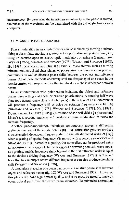
Phase modulation in an interferometer can be induced by moving a mirror,

tilting a glass plate, moving a gating, rotating a half-wave plate or analyzet,

using an acousto-optic or electro-optic modulator, or using a Zeeman laser

(Wvnr.rr [19751, Snecnvr and Wvaur [1978], WvaNr and Snncept [ 1978],

Hu [1983], KorHtver and Dnusl¡ [1985]). Phase shifters such as moving

mirrors, gratings, tilted glass plates, or polarization components can produce

continuous as well as discrete phase shifts between the object and reference

beams. All of these methods effectively shift the frequency of one beam in the

interferometer with respect to the other to introduce a phase difference between

beams.In an interferometer with polarization isolation, the object and reference

beams have orthogonal linear or circular polarizations. A rotating half-wave

plate (or a quarter-wave plate in double pass) in the output of an interferometer

will produce a frequency shift at twice its rotation frequency (see frg. 1A)(SHecerrl and WveNr [1978], WveNr and Snecerra [1978], Hu [1983]'Korury¿J- and Dr,usrr, t19851). (A rotation of 45' will yield a jz phase shift.)

Likewise, a rotating analyzer will produce a phase modulation at twice the

rotation frequency.Another phase-modulation technique continuously moves a diffraction

grating in one arm of the interferometer (fig. 1B). Diffraction gratings produce

a wavelength-independent frequency shift in the nth diffracted order of [rutf]when a $ating of spatial frequency /is moved with a velocity u (WvnNr and

SHecnu t1978]). Instead of a grating, the same effect can be produced using

an acousto-optic Bragg cell. In the Bragg cell a traveling acoustic wave serves

as a grating, and the frequency shift obtained in the first diffracted order is equal

to the device's driving frequency (V/velrr and Snncnu [1978]). AZeeman

laser that has an output oftwo different frequencies can also produce the phase

shift (Wvar.rr and Sn¡.cAM [1978]).A tilted glass placed in one beam can provide a relative phase shift between

object and reference beams (fig. lC) (WvaNr and Snecepr [1978]). However,

this plate must have high optical quality, and care must be taken to have an

equal optical path over the entire beam diameter. To minimize aberrations

354

CIRCULARLYPOLABIZED

LIGHT

45" ROTATION

(A) ROTATING HALF-WAVE PLATE

PMI TECHNIQUES

(C) TILTED GLASS PLATE

Fig. l. Means of producing a phase modulation to include (A) a rotating polarizer, (B) a movingdiffraction grating, (C) a tilted glass plate, and (D) a moving mirror.

introduced by the plate, it should be placed in a coltimated beam. Differentamounts of phase shift are achieved by tilting the plate to diferent angles.

Finally, a common, straightforward phase-shifting technique is the placementof a minor pushed by a piezo-electric transducer (PZT\ in the reference beam(fig. lD) (WvaNr [1982], Wyerqr and Cn¡ern t19851). Many brands ofPZTs a¡e available to move a mirror linearly over a l-¡rm range. A high-voltageamplifier is used to produce a linear ramping sþal from 0 to several hundredvolts. If there are nonlinearities in the PZT motion, they can be accounted forby using a progrârnmable waveform generator. If a phase-stepping techniqueis preferred to a continuous modulation, any calibrated pzr can be usedbecause only discrete voltage steps are needed.

2,2.. MEANS OF DETERMINING PHASE

(B) DIFFFACTION GRATING

l v , $ 2

MOVE0.01 mm

MovE r,/B .;* t'.;iff'

*rf,I \r'

PUSHINGMIRFOR

(D) MOVING MIRRoB

Techniques for determining phase can be split into two basic categories:electronic and analytical. To determine phase electronically, hardware such as

v , $ 2 1

zero-crossing detectors, phaseJock loops, and up-down counters are used to

monitor interferogram intensþ data as the phase is modulated. For analytical

techniques intensþ data are recorded while the phase is temporally modulated,

sent to a computer, and then used to compute phase. With the advent of

powerful desk-top computers and solid-state detector afrays, the analytical

techniques have provided the most innovations in this field in the last five years

(WvnNr and Cneern [1935]). For this reason we will concentrate on the

newer techniques and only briefly describe the electronic techniques.

One electronic technique utilizes the detection of a modulated test sþalpassing through a zero phase value in relation to a modulated reference signal.

Zero-crossing techniques measure the time difference between reference and

test sþals as they pass through azero (Wvervr and Ssecnu [1978])' The

wavefront phase is determined to be modul o 2nby taking the ratio between the

time measured between crossings and the period of the reference sþal. To

measure a two-dimensional map of the wavefront, the detector either needs to

be scanned or the circuitry must measure the zero a¡s5sings at each detector

element.Another technique has been coined phase-lock or ac interferometry

(Moonn, Munnev and N¡ves [ 1978], Moonn and Tnuex [1979], JoHNsoN'

LerNen and Moonn [1979]). In phase-lock techniques a phase shifter'in one

interferometer path is modulated sinusoidally with a small amplitude, pro-

ducing temporally modulated interference terms with cosine of sine and sine

of sine dependences. The detected optical sþal will çs¡fain terms with odd

and even order harmonics of the phase modulation frequency. A second,

coarser phase-shifter is used to change the path between the two beams in the

interferometer until the odd order harmonics (including the fundamental)

disappear. When high-order harmonics are filtered out, the resulting electrical

sþal is directly proportional to the optical phase modulo 2n. with the use of

frequency multipliers and up-down counters, phase-lock interferometry can

measure phase changes greater than2nwith #,i repeatabilities. Ho'ilever, to

measure over an area, the detector must be scanned.The last electronic method we will mention has the capability to measure

directly a phase change greater than 1 fringe (Wvevr and Snncnlvr [ 1978]).

Up-down counters enable the actual phase difference to be measured as long

as a continuous sþal is incident. As a fringe sweeps by the detector, the

counter ¡s ¡¡çþanged, incremented, or decremented depending on its relation-

ship to a known reference signal. Because only changes in phase are measured,

the detector must be scanned for area measurements and an unintemrpted

sipal received. Up-down counters are generally used in conjunction with

frequency multipliers in order to measure in units of less than one fringe.

MEANS oF SHIFTING AND DETERMINING PHÀSE 355

356

A phase-measurement technique that is analytical but does not use phase-shifting is the Fourier-transform method (Taxnoa, I¡¡a and Ko¡ayesnr

[1982], Wovrecr [1984a,b]). This method is really a fringe-pattern analysistechnique, but we will mention it because it does serve a purpose for systemsthat are subject to vibration and air turbulence. For this technique a singleinterferogram is recorded and Fourier transformed. The Fourier spectrum isthen bandpass filtered to isolate one of the sidebands. Now the sideband isfrequency shifted to be centered at zero frequency. The filtered and shiftedspectrum is then inverse Fourier transformed to yield a modulo 2 z phase map.This technique does not have as much accuracy as the analytical techniquesmentioned in the next section, which directly calculate the phase from a numberof phase-shifted interferograms. Because the sidebands are not always isolated,various filters can be used to improve the outcome of these techniques(Tereoe,IN¿, and KoseyesFrr ÍL9821, Woprecr [1984a,b], Knns [1986]).

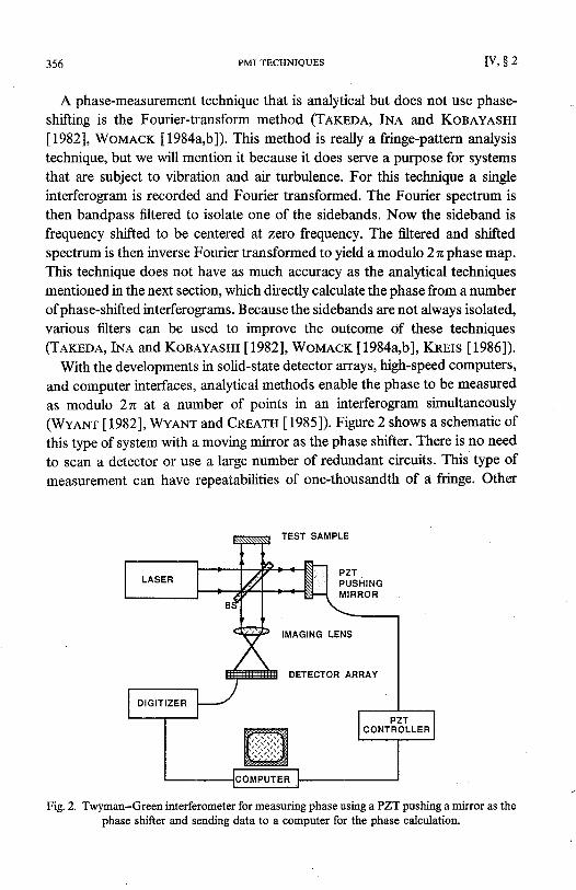
With the developments in solid-state detector ¿urays, high-speed computers,

and computer interfaces, analytical methods enable the phase to be measured

as modulo 2n at a number of points in an interferogr¿lm simultaneously(WveNr [1982], WveNr and Cnenrn [1985]). Figure 2 shows a schematic of

this type of system with a moving mirror as the phase shifter. There is no need

to scan a detector or use a large number of redundant circuits' This type of

measurement can have repeatabilities of one-thousandth of a fringe. Other

PMI TECHNIQUES l v , $ 2

TEST SAMPLE

Fig. 2. Twyman-Green interferometer for measuring phase using a PZT pushing a mirror as thephase shifrer and sending data to a computer for the phase calculation.

IMAGING LËNS

DETECTOR ARRAY

v , $ 3 1

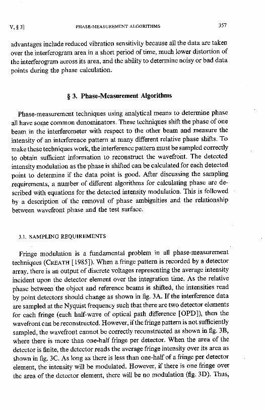
advantages include reduced vibration sensitivþ because all the data are taken

over the interferogram area in a short period of time, much lower distortion of

the interferogram across its area, and the ability to determine noisy or bad data

points during the phase calculation.

$ 3. Phase-Measurement Algorithms

Phase-measurement techniques using analytical means to determine phase

all have some common denominators. These techniques shift the phase of one

beam in the interferometer with respect to the other beam and measure the

intensity of an interference pattern at many different relative phase shifts. To

make these techniques work, the interference pattern must be sampled correctly

to obtain sufficient information to reconstruct the wavefront. The detected

intensity modulation as the phase is shifted can be calculated for each detected

point to determine if the data point is good. After discussing the sampling

requirements, a number of different algorithms for calculating phase are de-

scribed with equations for the detected intensity modulation. This is followed

by a description of the removal of phase ambiguities and the relationship

between wavefront phase and the test surface.

3.I. SAMPLING REQUIREMENTS

PHASE.MEASUREMENT ALGORITHMS 357

Fringe modulation is a fundamental problem in all phase-measurement

techniques (Cne4rn t19851). When a fringe pattern is recorded by a detector

array, there is an output ofdiscrete voltages representing the average intensity

incident upon the detector element over the integtation time' As the relative

phase between the object and reference beams is shifted, the intensities read

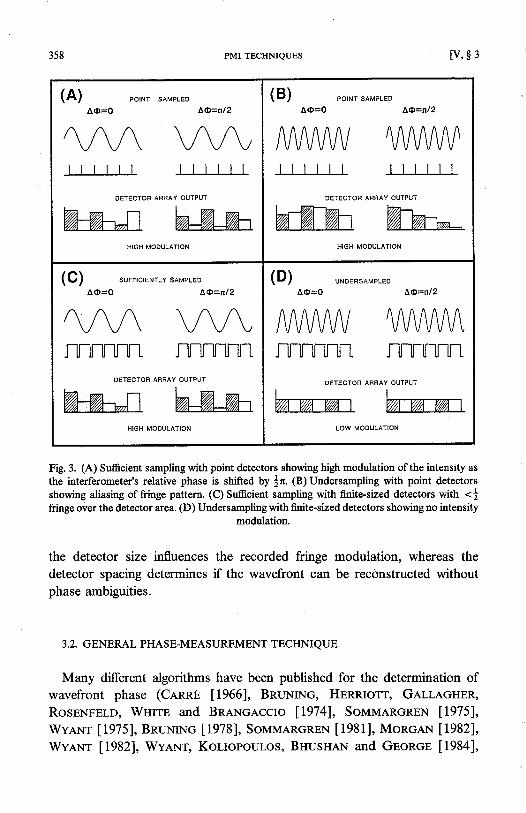
by point detectors should change as shown in fig. 34. If the interference data

are sampled at the Nyquist frequency such that there are two detector elements

for each fringe (each half-wave of optical path difference [OPD]), then the

wavefront can be reconstructed. However, if the fringe pattern is not sufficiently

sampled, the wavefront cannot be correctly reconstructed as shown in fig. 3B'

where there is more than one-half fringe per detector. When the area of the

detector is finite, the detector reads the average fiinge intensity over its area as

shown in fig. 3C. As long as there is less than one-half of a fringe per detector

element, the intensity will be modulated. However, if there is one fringe over

the area of the detector element, there will be no modulation (fig. 3D). Thus,

358

(A) porNr .AM'LED

.ÂO=O ^@=nlz

l l l l l l

OETECTOF ÂFRAY OIJTPUT

PMI TECHNIQUES

( C) suFFrcrENrLY SAMPLED

AO=0 A@=nl2

( B) PorNrÂo=0

HIGH MOOULÂTION

fFT-Il-n 1 finrll-]l-1DETECTOR ARRAY OUTPUT

t t t t t l

DETECTOR ARRAY OUTPUT

SAMPLED

[ v , $ 3

Fig. 3. (A) Sufficient sampling with point detectors showing high modulation of the intensity asthe interferometer's relative phase is shifted by ]2. (B) Undersampling with point detectorsshowing aliasing of fringe pattem. (C)Sufficient sampling with fnite-sized detectors with <åfringe over the detector area. (D) Undersampling with finì¡s-sized detectors showing no intensity

modulation.

( D) uNoERsAMpLEDAO=0 Ã@=nl2

HIGH MOOULÀTION

HIGH MODTJLATION

the detector size influences the recorded fringe modulation, whereas thedetector spacing determines if the wavefront can be reconstructed withoutphase ambiguities.

flI-T-I-nnrL J-lj-lj-ìt-T-nDETECTOR ARTIAY OIJTPUT

3.2. GENERAL PHASE-MEASUREMENT TECHNIOUE

Many different algorithms have been published for the determination ofwavefront phase (CanRÉ [1966], BnuNINc, HERRIorr, GeLLecHER,RosrNrer-o, WHrrE and BRANcAccIo U9741, SopruencnnN [1975],WveNr [1975], BnuNrNc [1978], SoIvruencnEN [981], MonceN [1982],WveNr ll982l, WyeNT, Kouopouros, BHUsHAN and GeoRce [1984],

LOW MODULÀTION

v , s 3 l

(A)

z

= } n-an

q

e, M4o

=

PHASE-MEASUREMENT ALGORITHMS

(B)

(c)

z9 . -õo

r M 4o

=

J

2

õc¡UFut-t¡lô

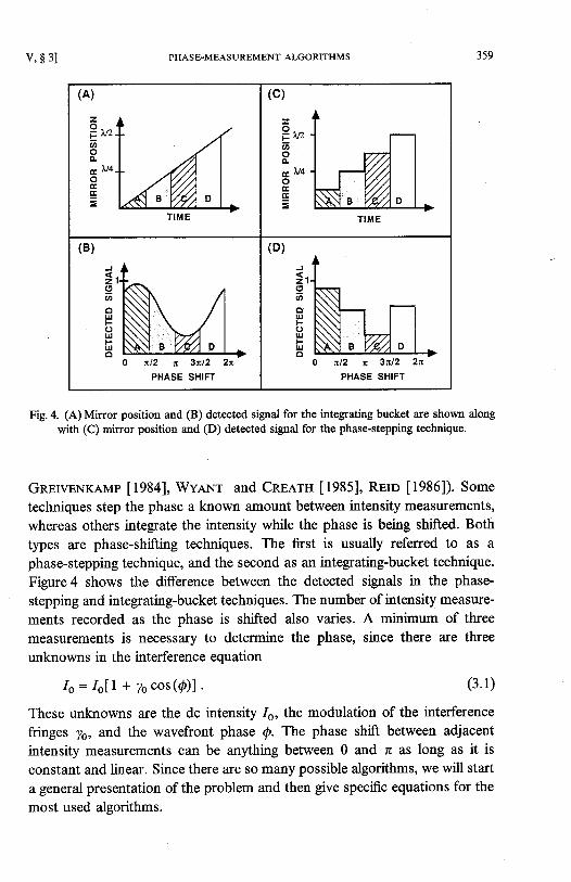
Fig.4. (A) Mirror position and (B) detected signal for the integrating bucket are shown alongwith (C) mirror position and (D) detected sipal for the phase-stepping technique.

GnnrvnNreMp [1984], WveNr and CREATH [1985], Rnn [1986]). Sometechniques step the phase a known amount between intensity measurements,whereas others integrate the intensity while the phase is being shifted. Bothtypes are phase-shifting techniques. The first is usually referred to as aphase-stepping technique, and the second as an integrating-bucket technique.Figure 4 shows the difference between the detected sþals in the phase-

stepping and integrating-bucket techniques. The number of intensity measure-ments recorded as the phase is shifted also varies. A minimum of threemeasurements is necessary to determine the phase, since there are threeunknowns in the interference equation

(D)

J

Í , t

õt!FoUFU

These unknowns are the dc intensity /o, the modulation of the interferencefringes Ïo, and the wavefront phase 4. Th" phase shift between adjacentintensity measurements can be anything between 0 and z as long as it isconstant and linear. Since there are so many possible algorithms, we will starta general presentation ofthe problem and then give specific equations for themost used algorithms.

Io= IoU + yocos(@)l . (3. 1)

Normally, N measurements of the intensity are recorded as the phase isshifted. For the general technique the phase shift is assumed to change duringthe detectors' integration time, and this change is the seme from data frame todata frame. The ¡mount of phase change from frame to frame may vary, butit must be known by calibrating the phase shifter or measuring the actual phasechange. Unless discrete phase steps are used, the detector array will integratethe fringe intensity data over a change in relative phase of Â. One set of recordedintensities will be written as (Gnnwr,Nrarrar [1984])

PMI TECHNIQUES

I,(x,y) =:l:::;

where /o(.x, y) is the average intensity at each detector point, yo is the modulationof the fringe pattern, ø, is the average value of the relative phase shift for thefth exposure, and þ(x,y) is the phase of the wavefront being measured at thepoint (x, y). The integration over a phase shift  makes this expressionapplicable for any phase-shifting technique. After integrating this expressionthe recorded intensþ is

Io(x, y) { I + yo cos [@(x, y) + d(t)]] dø(r) , (3.2)

where sinc]^ : (sin+^)/åÂ. It is important to note that the only differencebetween integrating the phase and stepping the phase is a reduction in themodulation of the interference fringes after detection. If the phase shift werestepped (^ = 0) and not integrated, the sinc function would have a value ofunity. Therefore, phase stepping is a simplification of the integrating-bucketmethod. At the other extreme, if A : 2n,there would be no modulation of theintensity. Since this technique relies on a modulation of the intensities as thephase is shifted, the phase shift per exposure needs to be between 0 and z.

For a total of ly'recorded intensity measurements the phase can be calculatedusing a least-squares technique. This type of approach is outlined in detail byboth GneIvENKAMp [984] and MoncnN [1982]. Equation (3.3) is firstrewritten in the form

I,(x,y) : Io(*,y) {1 + yo(sinc}Â) cos lQ@,y) + ø,1} ,

l v , $ 3

I,(x,y) : ao(x,y) + ar(x,y) cosø, + ar(x,y) sina,,

where

ao(x, y) = Io(x, y) ,

alx,y) = Io(x,y) yo(sinc]Â) cosQ(x,y),

az(x, y) : Io(x, y) yo(sinc jÂ) sin f (x, y) .

(3.3)

(3.4)

(3.s)

v , $ 3 1

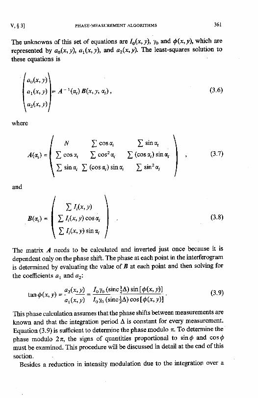
The unknowns of this set of equations are lo(x, y), lo md Q@, y), which are

represented by ao(x,y), at(x,y\, and ar(x,y'). The least-squa¡es solution to

these equations is

/o.(t, r)\

I o,,', rl= ̂ - 1(u,) B(x, r, d¡),

\u'(''ù I

PHASE.MEASUREMENT ALGORITHMS

where

l *A(u,) =l I "or*

\ r 'ro,

and

I cosø, I sinø,

I cos2 ø, | (cos ør) sin a,

I (cos ø,) sin a, I sin2 ø,

361

B(a,) = (,n::;r:,. )\ I r,t", v)sna' f

The matrix 1 needs to be calculated and inverted just once because it is

dependent only on the phase shift. The phase at each point in the interferogram

is determined by evaluating the value of B at each point and then solving for

the coefficients a, arrd ar:

(3.6)

)

, az(x, y) 1o7o (sinc jÂ) sin If (x, y)]mn9(x ' r r=

o l * , r \ :@

This phase calculation assumes that the phase shifts between measurements are

known and that the integration period  is constant for every measurement.

Equation (3.9) is sufficient to determine the phase modulo æ. To determine the

phase modulo 2n, the sþs of quantities proportional to sin f and cos @must be examined. This procedure will be discussed in detail at the end of this

section.Besides a reduction in intensity modulation due to the integration over a

(3.7)

(3.8)

(3.e)

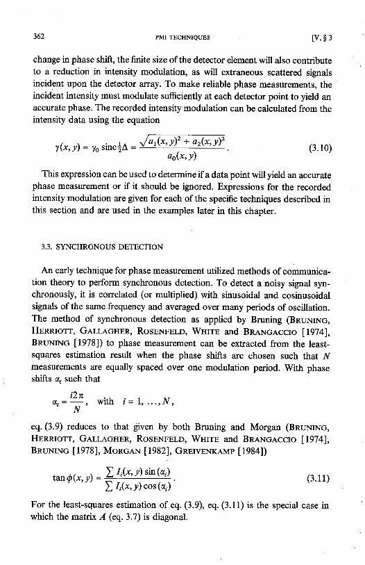
change in phase shift, the ûnite size of the detector element will also contributeto a reduction in intensity modulation, as will extraneous scattered sþalsincident upon the detector array. To make reliable phase measurements, theincident intensity must modulate sufficiently at each detector point to yield anaccurate phase. The recorded intensity modulation can be calculated from theintensity data using the equation

PMI TECHNIQUES

y(x, y): yo sinc|Â :

This expression can be used to determine if a data point will yield an accuratephase measurement or if it should be þored. Expressions for the recordedintensity modulation are given for each of the specific techniques described inthis section and a¡e used in the examples later in this chapter.

3.3. SYNCHRONOUS DETECTION

Jor(*,y)2 + ar(x,y)2

An early technique for phase measurement utilized methods of communica-tion theory to perform synchronous detection. To detect a noisy signal syn-chronously, it is correlated (or multiplied) with sinusoidal and cosinusoidalsþals of the same frequency and averaged over many periods of oscillation.The method of synchronous detection as applied by Bruning (BnuNrNc,Hnnnlorr, Gau¡cn¡,n, Rosnurnro, Wurln and BneNc¡,ccro [1974],BnuNrNc [978]) to phase measurement can be extracted from the least-squares estimation result when the phase shifts are chosen such that llmeasurements are equally spaced over one modulation period. With phaseshifts a, such that

i2nü , = 2 , w i t h j = 1 , . . . , N ,- ¡ r

eq. (3.9) reduces to that given by both Bruning and Morgan (BnuNrNc,Hennrorr, Geu-¿,cnrn, RosENFELD, WHITE and BneNcAcclo lI974l,BRuNrNc í19781, Monc¡.N [1982], GnervnNx¡ur [1984])

ao(x, Y)

l v , $ 3

(3 .10)

tanQ@,y) --

For the least-squares estimation of eq. (3.9), eq. (3.11) is the special case inwhich the matrix A (eq.3.7) is diagonal.

L I,(*,y) sin(ø,)

L I,(*,y) cos(ø,)(3 .1 1 )

v , $ 3 1

3.4. FOUR-BUCKET, OR FOUR.STEP, TECHNIQUE

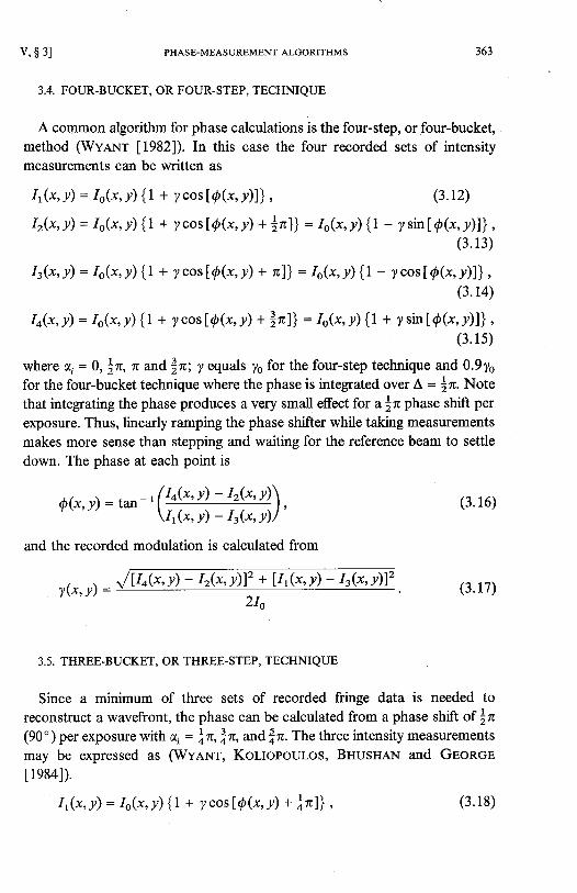
A common algorithm for phase calculations is the four-step, or four-bucket,method (WveNr [1982]). In this case the four recorded sets of intensitymeasurements can be written as

Ir(x,y) = Io(x, /) {1 + ycos[@(x,y)] ] , (3.12)

Ir(x,y) = Io(x, /) {1 + ycoslQ(x,y) + }"1} = Io(x, /) {1 - ysin[@(.x,y)] ] ,(3 .13)

I r ( r ,y )= Io@,y) {1 + ycos [p(x , y )+ n ] ] = Io@,y \ {1 - ycos [Q@,y) ] ] ,(3.r4)

Io (x ,y ) = Io (x , / ) {1 + ycos lQ@,y) + i " l } = Io (x , / ) {1 + vs in [@(x ,v ) ] ] ,(3.1s)

where ø, : 0, Ln, n mdln; y equals yo for the four-step technique and 0.9yofor the four-bucket technique where the phase is integrated over  : ]2. Notethat integrating the phase produces a very small effect for a jz phase shift perexposure. Thus, linearly ramping the phase shifter while taking measurementsmakes more sense than stepping and waiting for the reference beam to settledown. The phase at each point is

PHASE-MEASUREMENT ALGORITHMS

ôo. ù: ran - , (I¿@, Y) - Ir(x, Y)\ ,

\1,(x,y) - Ir(x,y)/

and the recorded modulation is calculated from

363

y(x, v) =

3.5. THREE-BUCKET, OR THREE-STEP, TECHNIQUE

Since a minimum of three sets of recorded fringe data is needed toreconstruct a wavefront, the phase can be calculated from a phase shift ofiz(90') per exposure with 4 : In,|n, andln. The three intensity measurementsmay be expressed as (WvaNr, Kouoeoulos, BHUsHex and GroRc¡

I le84]).

2Io

I r ( * ,y ) : Io (x ,y ) {1 + ycos [@(x ,y ) + i " ] ] ,

(3 .16)

(3.r7)

(3 .18)

364 PMI TECHNIQUES

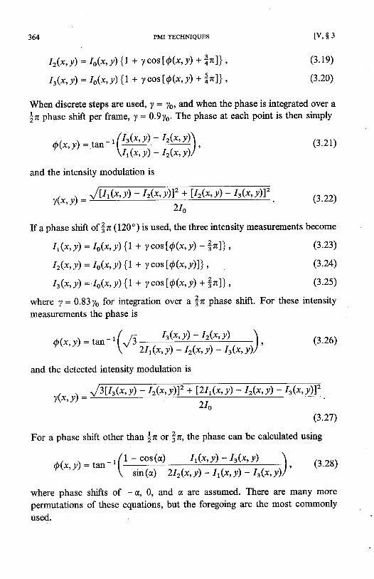
Ir(x,v) = Io(x'v) {1 + Tcos[f(x,v) +f,nj] ,

I t(x,v) = Io(r,v) {1 + rcos[f( 'x, v\ + 1"]] ,

When discrete steps ate used, T = To, and when the phase is integrated over a

|z phase shift per frame, y = 0.9yo. The phase at each point is then simply

/Ir(*,y) - 1r(",y)\þ(r,y):tan-'\ffi-;í¡,

and the intensity modulation is

y(x, v) =

If a phase shift of Jn (120e) is used, the three intensity measurements become

Ir(x,y) = Io(x,v) {1 + vcos[Q@,Y) -?n]\ ,

Ir(x,y) = Io(x,v) {1 + ycoslQ@,Y)l} '

Ir(r, y) = Io(x,/) {1 + y cosfQ(x, y) + ?"1},

where y= 0.83yo for integration over a lz phase shift. For these intensitymeasurements the phase is

l v , s 3

(3.1e)

(3.20)

Q @ , y ) = t a n - ' ( o f f i ) ,and the detected intensity modulation is

2Io

y(x, y) =

(3.2r)

For a phase shift other than |n or ]æ, the phase can be calculated using

ll - cos(a) Ir(x,y) - I'(x,y) \þ @ , y ) : t a n - t ( -

/ ' 5 \ ' - " / l , ( 3 . 2 8 )

f sin(ø) 2lr(x,y) - Ir(x,y) - It(x,y)/'

where phase shifts of - d, 0, and ø are assumed' There are many morepermutations of these equations, but the foregoing are the most commonlyused.

. (3.22)

(3.23)

(3.24)

(3.2s)

2Io

(3.26)

(3.27)

v , $ 3 1

3.6. CARRÉ TECHNIQUE

In the previous equations the phase shift is known either by calibrating thephase shifter or by measuring the amount of phase shift each time it is moved.

CennÉ [1966] presented a technique of phase measurement that is independentof the amount of phase shift. It assumes that the phase is shifted by ø betweenconsecutive intensity measurements to yield four equations

PHASE-MEASUREMENT ALGORITHMS

I ,(x, y) : Io(x,/) { I + y cos [@(x, y) - 2u]) ,

Ir.(x, y) : Io(x,/) { 1 + y cos [@(x, y) - Lal] ,

Ir(x, v) = Io(x, v) { 1 + r cos [@(x, v) + àal] ,

Io(x, y) : Io@, y) { 1 + 7 cos lQ@, y) + trol} ,

where the phase shift is assumed to be linear. From these equations the phase

shift can be calculated using

tan*r(.t. r') = l'' ",1 ÍIr(x, y) - It(x, y)l + flr(x, y) - Io'', y)l

' (3'33)

and the phase at each point is

(3.34)To calculate the phase modulo z, the preceding two equations are combined

to vield

tan Q (x, y) : t anllo(*, y)l

L a î E :

For this technique the intensity modulation is

(3.2e)

(3.30)

(3.3 1)

(3.32)

l.Ir(x, y) - It(x, y)l + lI r(x, y) - Io(x, y)l

llr(x, y) + It(x, y)l - lI r(x, y) + Io(x, y)l

I, . , f

- t o

where this equation assumes that a is near ln.If the phase shift is offby + l0',the estimation of ywill be offby !10%. An obvious advantage of the Carrétechnique is that this phase shift does not need to be calibrated. It also has theadvantage of working when a linear phase shift is introduced in a convergingor diverging beam where the amount of phase shift varies across the beam.

(Ir- L) + (1r - I)l ' + [(Ir+ Ir) - (1, + I)]2

( I r + I r ) - ( I r + I o )(3.3 s)

(3.36)

Equation (3.35) will calculate the phase modulo 2n at each point in the

interferogram without worrying about errors resulting from phase calibration

difference across the beam.

3.7. REMOVAL OF PHASE AMBIGUITIES

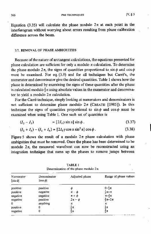
Because ofthe nature of arctangent calculations, the equations presented forphase calculation are sufficient for only a modulo æ calculation. To determinethe phase modulo 2n, the sþs of quantities proportional to sin @ and cos @must be examined. For eq. (3.9) and for all techniques but Carré's, thenumerator and denominator give the desired quantities. Table 1 shows how thephase is determined by examining the signs of these quantities after the phaseis calculated modulo jz using absolute values in the numerator and denomina-tor to yield a modulo 2ø calculation.

For the Carré technique, simply looking at numerators and denominators isnot sufficient to determine phase modulo 2z (CnenrH [1985]). In thistechnique the sips of quantities proportional to sin { and cos @ must beexamined when using Table 1. One such set of quantities is

PMI TECHNIQUES t v , $ 3

(Ir - L)

Figure 5 shows the result of a modulo 2n phase calculation with phase

ambiguities that must be removed. Once the phase has been determined to bemodulo 2n, the measured wavefront can no\il be reconstructed using anintegration technique that sums up the phases to remove jumps between

Determination iLtt:il"." modulo 2 r¡.

( I r+ Ir) - ( I t + I) : f2loycosø sin2al cosp.

: l2IoT sin øl sin @ .

Numerator

[sin@]

poslüvepositive

negativenegative0positivenegative

Denominator

[cos @]

positivenegativenegativepositiveanything00

(3.37)

(3.38)

Adjusted phase

an - Qn + q2 n - þ

! -2 t .

2 ' .

Range of phase values

o-à"àn-nn-trn

1 - i -2 'L-L 'L

! -2 ' "

2 ' .

v , $ 3 1 PHASE-MEASUREMENT ALGORITHMS

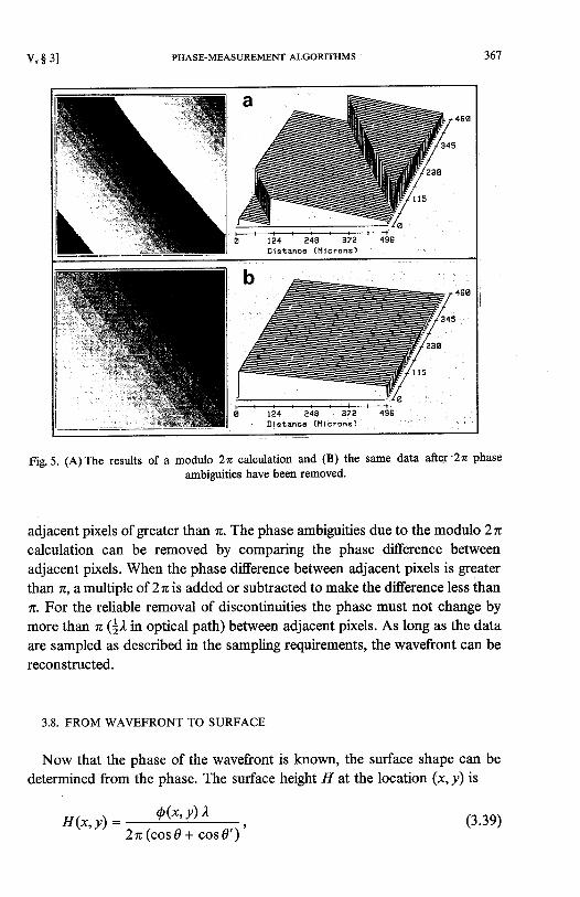
Fig.5. (A)The results of a modulo 2z calculation and (B) the same data after'22 phase

ambiguities have been removed.

adjacent pixels of greater than ø. The phase ambiguities due to the modulo 2ncalculation can be removed by comparing the phase difference betweenadjacent pixels. When the phase difference between adjacent pixels is greaterthan z, a multiple of 2n is added or subtracted to make the difference less thanz. For the reliable removal of discontinuities the phase must not change bymore than n (|)" in optical path) between adjacent pixels. As long as the dataare sampled as described in the sampling requirements, the wavefront can bereconstructed.

3.8. FROM WAVEFRONT TO SURFACE

t?4 248 37?D l s t ù n c 6 ( 1 1 i c ¡ o n s )

J O /

,;t.;.tl

ø t?4 248Dis tånc6 ( l ' l l

Now that the phase of the wavefront is known, the surface shape can be

determined from the phase. The surface height ä at the location (x, y) is

H(x- v\ : Q@'Y) I

2 n ( c o s 0 + c o s g ' ) '(3.3e)

368 PMI TECHNIQUES

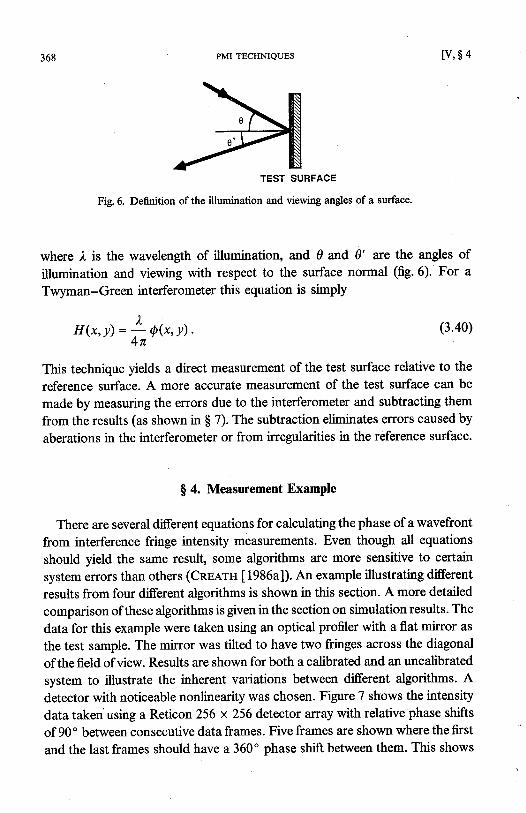
where l. is the wavelength of illumination, and 0 and 0' ate the angles of

illumination and viewing with respect to the surface normal (fig.6). For a

Twyman-Green interferometer this equation is simply

Fig. 6. Definition of the illumination and viewing angles of a surface.

H(x,y) = f iOfr,t l .

This technique yields a direct measurement of the test surface relative to the

reference surface. A more accurate measurement Of the test surface can be

made by measuring the errors due to the interferometer and subtracting them

from the results (as shown in S 7). The subtraction eliminates errors caused by

aberations in the interferometer or from irregularities in the reference surface.

$ 4. Measurement Example

TEST SURFACE

[ v , $ 4

There are several different equations for calculating the phase of a wavefront

from interference fringe intensity measurements. Even though all equations

should yield the same result, some algorithms afe more sensitive to certain

system errors than others (Cneers [1986a]). An example illustrating different

results from four different algorithms is shown in this section. A more detailed

comparison of these algorithms is given in the section on simulation results. The

data for this example were taken using an optical profiler with a flat mirror as

the test sample. The mirror was tilted to have two fringes across the diagonal

of the field of view. Results are shown for both a calibrated and an uncalibrated

system to illustrate the inherent variations between different algorithms. A

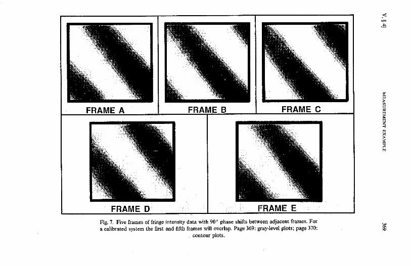
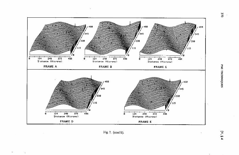
detector with noticeable nonlinearity was chosen. Figure 7 shows the intensity

data taken'using a Reticon 256 x 256 detector array with relative phase shifts

of 90' between consecutive data frames. Five frømes are shown where the first

and the last frames should have a 360" phase shift between them. This shows

(3.40)

FRAME FRAME B

FRAMEFig.7. Five frames of fringe intensity data with 90' phase shifts between adjacent frames. Fora calibrated system the first and fifth frames will overlap. Page 369: grayJevel plots; page 370:

contour plots.

FRAME

.è

FRAME

zõcll

õz-l

llX

3rE

t24 249 972D l s t è n ê o ( l , l l c ¡ o n s )

FRAME A

1 r ¿ ) Á a a 2 )

D l s t a n c ê ( H i c r o n s )

FRAME B

l ?4 249 372D l s t à n c 6 ( l l l c r o ñ s )

FRAME D

l r Á , ô e 1 t )

D l s t ã n c ê ( M i c ¡ o n s )

FRAME C

{

Fig.7. (cont'd).

4 9 6

L?4 248 37eD l s t a n c e ( l ' l l c ¡ o n s )

FRAME E

3

:lE

z

c¡lØ

"sÞ

(A) 3-Buckets

t24 248 372D i s t à n c o ( l l i c r o n s )

R M S = 1 . 2 1 n m

(B) 4'Buckets

124 ¿4A 372D i s t ã o c 6 ( M i c . o n s )

R M S = 1 . 1 7 n m

( C ) A v g . 3 & 3

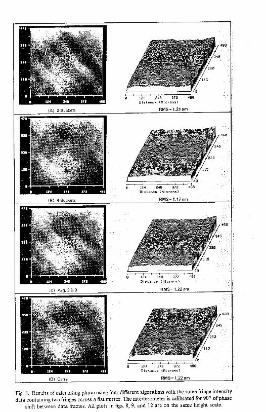
Fig. 8. Results of catculating phase using four different algorithms with the same fringe intensity

daia containing two fringes across a flat mirror. The interferometer is calibrated for 90' ofphase

shift between data frames. All plots in figs.8,9,and 12 are on the same height scale.

t24 248 372D i s t a ñ c € ( M l c r o n s )

(D) Car ré

RMS = '1 .22 nm

t?4 248 372D i s t à n c e ( M i c ¡ o n s )

F M S = 1 . 2 2 n m

(A) 3 -Buckets

'%^% i4l

M,.

(B) 4 .Buckets

t24 244 372D l s t À n c ê ( f l i c r o n s )

R I M S = 2 . 7 7 n m

{ C ) A v q . 3 & 3

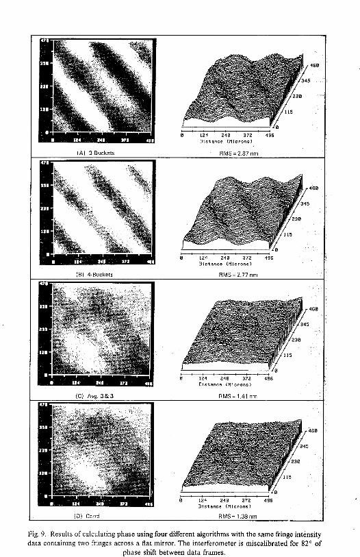
Fig. 9. Results of calculating phase using four different algorithms with the same fringe inténsitydata containing two fringes across a flat mirror. The interferometer is miscalibrated for 82' of

phase shift between data frames.

r24 24A 372D i s t a n c a ( l l i c ¡ o n s )

R I M S = 1 . 4 1 n m

{D) Car ré

t24 248 3??D l s t a n c e ( l l l c ¡ o ñ s )

R lVlS = i .38 nm

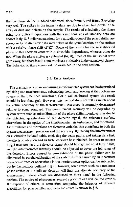
v , $ s l

that the phase shifter is indeed calibrated, since frame A and frame E overlap

very well. The spikes in the intensity data are due to either bad pixels in the

array or dust and defects on the sample. The results of calculating the phase

using four different equations with the same four sets of intensity data are

shown in fig. 8. Similar calculations for a miscalibration of the phase shifter are

shown in fig. 9 after new data were taken at the same location on the surface

with a relative phase shift of 82" . Some of the results for the miscalibratedphase shifter show an error with a sinusoidal dependence, whereas other do

not. When the phase shifter is calibrated (fig.8), much of the sinusoidal errorgoes away, but there is still some waviness noticeable in the calculated phases.

The behavior of these errors will be examined in the next section.

$ 5. Error Analysis

ERROR ANALYSIS

The precision of a phase-measuring interferometer system can be determined

by taking two measurements, subtracting them, and lookþg at the root-mean-

square of the difference wavefront. For a well-calibrated system this result

should be less than #,I. However, this method does not tell us much about

the actual accuracy of the measurement. Accuracy is normally determined

relative to some standard. The measurement accuracy will be degraded by

system errors such as miscalibration of the phase shifter, nonlinearities due to

the detector, quantization of the detector signal, the reference surface,

aberrations in the optics of the interferometer, air turbulence, and vibrations.

Air turbulence and vibrations are dynamic variables that contribute to both the

system measurement precision and the accuracy. By placing the interferometer

on a vibration-isolated table, enclosing the beam paths, and taking data fast,

the effects of vibration and air turbulence can be minl¡ni7sd. In order to achieve

a r*I1 measurement, the detector sþal should be digitized to at least 8 bits,

and the interferometer intensity should be adjusted to cover the full range of

the detector. Errors caused by miscalibration of the phase shifter can be

eliminated by careful calibration of the system. Errors caused by an inaccurate

reference surface or aberrations in the interferometer optics can be subtracted

out by the methods outlined in $ 7. However, some errors such as a nonlinear

phase shifter or a nonlinear detector wü limit the ultimate accuracy of the

measurement. These elrors are discussed in more detail in the following

section. The choice of phase-measurement algorithm can reduce one error at

the expense of others. A simulation comparing the behavior of different

algorithms for phase-shifter and detector errors is shown in $ 6.

3'14

5.I. PHASE.SHIFTER ERRORS

Phase errors caused by inaccurate phase-shifter calibration can be minimizedby adjusting the interferometer for a single fringe. However, with large amountsof aberration present, it may not be possible to obtain a single fringe. If aconstant calibration error is present, the phase shift may be written as

where ø is the desired phase shift, d' is the actual phase shift, and e is thenormalized error. For phase stepping it has been shown that the errors in phaseresulting from a calibration error or nonlinearity in the phase shifter willdecrease as the number of measurements increases (ScnwnER, BuRow,ELSSNER, GRzeNNe, Spoleczyx and Mrmnr [ 1983]). The same should betrue for integrating-bucket techniques. For a consistent phase-shift error, suchas a miscalibration, a periodic error is seen in the calculated phase, which hasa spatial frequency of twice the fringe spacing (see fig. 9). Nonlinear phase-shiftenors are not as easy to deal with or detect. A quadratic nonlinear phase-shift

PMI TECHNIQUES

a ' = a ( l + e ) ,

error can be written as

a ' = a ( l + e ø ) .

In normal operation a nonlinear phase shifter will be partially compensated inthe calibration of the interferometer by adding a linear bias to its movement.The most straightforward approach to calibration is to make sure that the phaseshifter actually moves 2n over a 2z desired change in phase. This error termcan be realized by adding a normalized linear compensation term of an equaland opposite amplitude to eq. (5.2). The phase shift is then replaced with

t v , $ 5

This function minimizes the error caused by nonlinear phase-shifter motion.Nonlinear phase-shifter errors can be reduced by applþg çsrtein algorithmssuch as the Carré technique and the averaging-three-and-three techniquedescribed later; however, they cannot be eliminated.

5.2. PHASE-SHIFTER CALIBRATION

a ' : a ( I + e ø - e ) .

(s.1)

The value of the phase shift ø can be determined in a number of ways. A goodindication of ø can be obtaineä by taking four frames of intensity data and usingeq. (3.33) to calculate the phase shift at each detector point. The phase-shift

(s.2)

(s.3)

v , $ s l

20 ,000

at)

'õo.(E

õ

oo¡¡

z

ERROR ANALYSIS

1 0 , 0 0 0

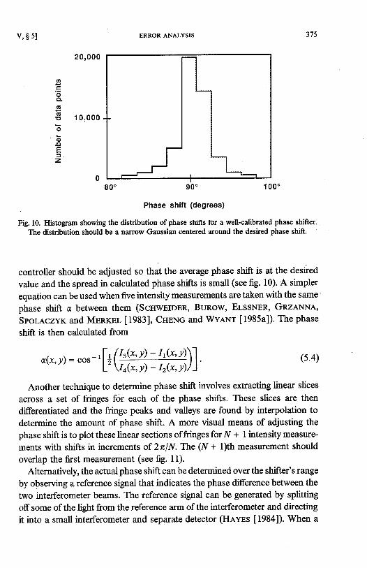
Fig. 10. Histogram showing the distribution ofphase shrtts tor a well-calibrated phase shifter.The distribution should be a narrow Gaussian centered around the desired phase shift.

controller should be adjusted so that the average phase shift is at the desired

value and the spread in calculated phase shifts is small (see fig. 10). A simpler

equation can be used when five intensity measurements are taken with the same

phase shift ø between them (ScnwEIDER, BuRow, EtssNnR, GRzaNNe,

Sporeczvr and Mrnrnl [1983], CseNc and WYANr [1985a]). The phase

shift is then calculated from

800 90"

Phase shif t (degrees)

3',15

a(x ,y )= "o r - ' [å

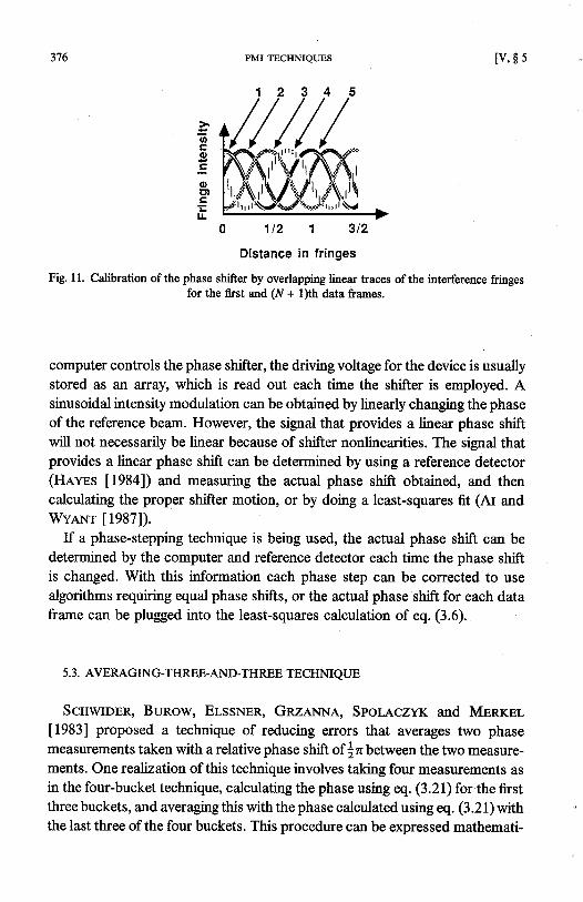
Another technique to determine phase shift involves extracting linear slices

across a set of fringes for each of the phase shifts. These slices are thendifferentiated and the fringe peaks and valleys are found by interpolation todetermine the amount of phase shift. A more visual means of adjusting thephase shift is to plot these linear sections of fringes for ll + 1 intensity measure-ments with shifts in increments of 2nlN. The (l/ + l)th measurement shouldoverlap the first measurement (see fig. 11).

Alternatively, the actual phase shift can be determined over the shifter's rangeby observing a reference signal that indicates the phase difference between thetwo interferometer beams. The reference sþal can be generated by splittingoff some of the light from the reference arm of the interferometer and directingit into a small interferometer and separate detector (Hevrs [1984]). When a

1 00 '

(I'(*,

\r1",v)v)

I t (

L(!x

, l

, y) l (s.4)

J / O PMI TECHNIQUES

.=3tco.g0)Þ)

' ilr

Fig. ll. Calibration ofthe phase shifter by overlapping linear traces ofthe interference fringesfor the first and (lf + l)th data frames.

computer controls the phase shifter, the driving voltage for the device is usuallystored as an ¿uray, which is read out each time the shifter is employed. Asinusoidal intensity modulation can be obtained by linearly changing the phaseof the reference beam. However, the sigral that provides a linear phase shiftwill not necessarily be linear because of shifter nonlinearities. The sþal thatprovides a linear phase shift can be determined by using a reference detector(Hnvns [1984]) and measuring the actual phase shift obtained, and thencalculating the proÞer shifter motion, or by doing a least-squares fit (Ar andWvexr [1987]).

If a phase-stepping technique is being used, the actual phase shift can bedetermined by the computer and reference detector each time the phase shiftis changed. With this information each phase step can be corrected to usealgorithms requiring equal phase shifts, or the actual phase shift for each dataframe can be plugged into the least-squares calculation of eq. (3.6).

s.3. AVERAGTNG-THREE-AND-THREE TECHNTQUE

D¡stance in fringes

1 t2 1 312

l v , $ 5

Scttwlorn, BuRow, ELSsNER, GnzeNNa, Sporaczyr and M¡nrnr[1983] proposed a technique of reducing errors that averages two phasemeasurements taken with a relative phase shift of jn between the two measure-ments. One realiz¿lion of this technique involves taking four measurements asin the four-bucket technique, calculating the phase ì¡sing eQ. (3.21) for the firstthree buckets, and avernging this with the phase calculated using eq. (3.21) withthe last three of the four buckets. This procedure can be expressed mathemati-

v , s 5 l ERROR ANALYSIS

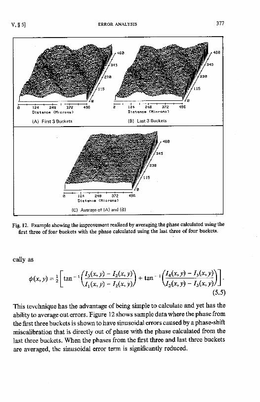
124 249 37?D l s t a n c e ( l ' l l c ¡ o n s )

(A) First 3 Buckets

t24 244 37?Dls tanco ( l ' l i c rons)

(B) Last 3 Buckets

Fig. 12. Example showing the improvement reâlized by averaging the phase calculated using the

ûrst three offour buckets with the phase calculated using the last three offour buckets.

37'l

t24 24A 372 496I ] l s t ù n c o ( H l c r o n s )

(C) Average of (A) and (B)

cally as

r , ( I r(* ,y)-1r(r ,y)\Q@,y)=ål t*- ' l - ---------- - ¡ + tan-L

\ I t (x ,y ) - I r (x ,y ) /

This tevchnique has the advantage of being simple to calculate and yet has the

ability to average out errors. Figure 12 shows sample data where the phase from

the first three buckets is shown to have sinusoidal errors caused by a phase-shift

miscalibration that is directly out of phase with the phase calculated from the

last three buckets. When the phases from the first three and last three buckets

are averaged, the sinusoidal error term is significantly reduced.

_ , ( Io@, y) - Ir(x, y)(; 'r(x,y) - It(x, )

(s.l; .5 )

t),(

3'78

5.4. DETECTOR NONLINEARITIES

A nonlinear response from a detector can introduce phase etrors, which areespecially noticeable ifthey a¡e not consistent from detector to detector in anaqay. Many CCD-type detector arrays read out the odd and even rows throughdifferent shift registers. If the gains in the two sets of registers are not equal andnonlinear, bothersome errors arise that must be removed.

Vy'hen a detector has a second-order nonlinear response, the measuredoptical irradiance I' çan be written in terms of the incident optical irradiance1 a s

PMI TECHNIQUES

where e is the nonlinear coefficient. Expanding the detected irradiance of thefringe pattern, the interference equation (3.1) becomes

I ' = Io Í l + ycos(@+ ø)+ e l l l l +2ycos(@+ a)+ y ' cos2( f+ d ) ] ,(s.7)

I ' : IoI I + elol +1o[1 + 2úo]ycos(Q + ø)+ el fyzcos2(þ + ø)1,

I ' = I + t 1 2 ,

where ø indicates the phase shift for a particular exposure. The nonlinearityin eq. (5.9) will cause phase errors. When eq. (5.9) is substituted into thefour-bucket calculation of eq. (3.16), the2Q dependent terms will cancel in thenumerator and denominator. Once the third terms cancel, the coefficients ofthe other terms in eq. (5.9) only reduce the measured fringe modulation and willnot affect the measurement. If, however, eq. (5.9) were substituted into thethree-bucket calculation of eq. (3.21), the nonlinea¡ities add and cause large

l v , $ 5

I' = I'o + Ifi ycos(rp + ø) + |elloyj2{1+ cos [2(@ + d)]] ,

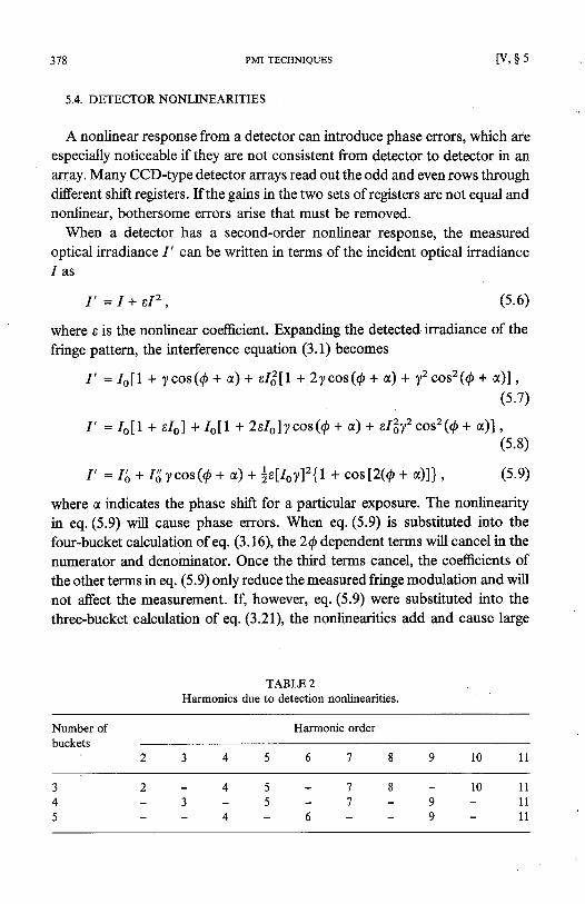
Number of

buckets

(5.6)

TABLE 2Harmonics due to detection nonlinearities.

2 - 4 5 - ' 1 8 - 1 03 - 5 - 1 - 9 -

4 - 6 - - 9

(s.8)

(5.e)

Harmonic order

1 l

il1 11 l

v , s 6 l

phase errors. Thus, when a second-order nonlinearity is present in the detectedirradiance, a minimum of four measurements is necessary to obtain an accuratephase calculation. For higher-order nonlinearities, SrEtsoN and Bnonnsrv

t1985] have determined which orders of detection errors will affect the

measurement for small numbers of phase steps. The dashes in Table 2 indicatewhich detection nonlinearity orders do not contribute to phase errors in the

various algorithms. In most cases the largest distortions affecting the measure-

ment are probably due to third-order harmonics,

SIMULATION RESULTS

so that five steps should be enough to reducenonlinearities.

$ 6. Simulation Results

I ' = I + Ê , 1 3 ,

The experimental results shown ea¡lier indicate that the results of PMI

calculations depend on the algorithm used. The most desirable algorithm

depends on the particular PMI system. In general, the more intensity measure-

ments, the less error there will be in the calculated phase values. This section

endeavors to find the best algorithm using the fewest number of measurements

for systems that are susceptible to phase-shifter and detector errors. The

techniques compared in these simulations are: (1)three-bucket technique of

eq.(3.21); (2)four-bucket technique of eq.(3.16); (3)Carré technique of

eq. (3.35); (4) averaging-three-and-three technique ofeq. (5.5); and (5) a five-

bucket technique using the synchronous detection outlined in eq. (3.11).

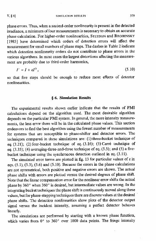
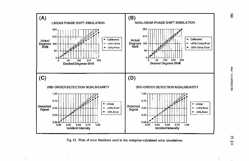
The simulated error terms are plotted ii fig. 13 for particular values of ¿ in

eqs. (5.1), (5.3), (5.6) and (5.10). Because the errors in the phase calculations

afe not symmetrical, both positive and negative elrors are shown. The actualphase shifts with errors are plotted versus the desired degrees of phase shift.

Note that the linear compensation error for the nonlinear error shifts the actual

phase by 360' when 360" is desired, but intermediate values are wrong. In the

integrating bucket techniques the phase shift is continuously moved along these

values, but for phase-stepping techniques there are discrete values at the desiredphase shifts. The detection nonlinearities show plots of the detector output

signal versus the incident intensity, assuming a perfect detector behaves

linearly.The simulations are performed by starting with a known phase function,

which varies from 0" to 360' over 1000 data points. The fringe intensity

(s. l0)

most effects of detector

(A)LINEAR PHASE SHIFT SIMULATION

360

270

ActualDegrees teo

shitton

o

(c)

0 90 180 270 360Desired Degrees Shift

ai/;'

ttiti1

,i '+I

2ND.ORDER DETECTION NONLINEARITY

(B )NONLINEAR PHASE SHIFT SIMULATION

360

270

ActualDegrees teo

shift90

0

(D )

Fig. 13. Plots oferror functions used in the computer-calculated error simulations.

0 90 180 270 360Desired Degrees Shift

-r

3RD-ORDER DETECTION NONLINEARITY

0.75

Detected n ÃñSignal

0.25

1 . 0 0

æ

0.00 ¡10.00

!.

l)'j

0.2s 0.50 0.75 1.00lnc¡dent Intens¡ty

-tEoz

cØ

v , $ 6 1

measurements for the different techniques are then calculated using the

appropriate equations by both the integrating-bucket technique and the phase-

stepping technique with an equivalent fringe modulation. If a phase-shift error

is present, it is applied when the fringe intensities are calculated. Detection

errors are added after the intensities have been calculated. Once the intensity

data are fabricated, the phase is calculated from these data. The error in the

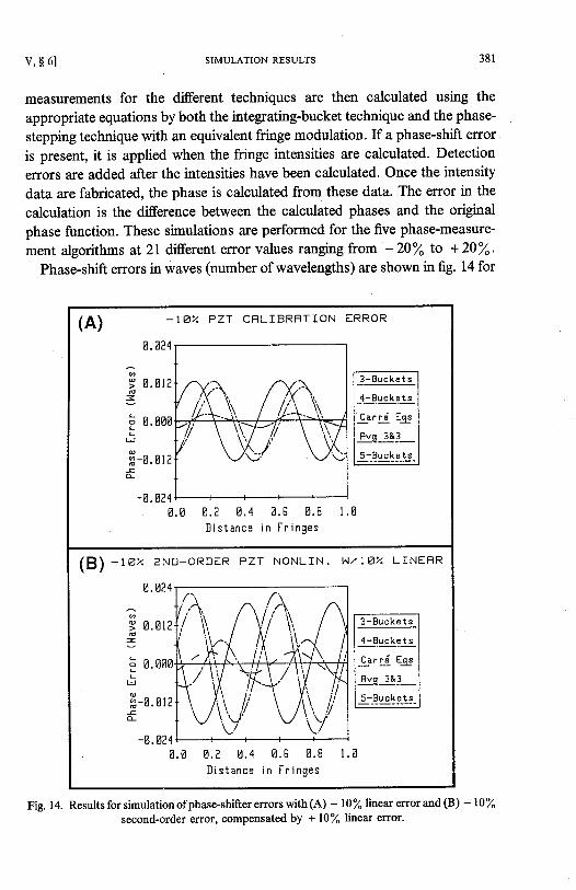
calculation is the difference between the calculated phases and the originalphase function. These simulations are performed for the five phase-measure-

ment algorithms at 2l different error values rangng from - 20/' to +20%.

Phase-shift errors in waves (number of wavelengths) are shown in fig' 14 for

SIMULATION RESULTS

(A) _ 1 ø Z P Z l C F L I B R F T I O N E R R O R

ø.ø?4

Ø9 ø.øt2=¿ ø .øøØ

U

o

n-ø.Ø12È

-ø.ø24

3 8 1

( B ) - l ø z 2 N D - o R D E R P z r N o N L r N . N / r ø z

Ø . Ø ø . 2 ø . 4 ø . 6 ø . 8 I . ø[ } i s t a n c e i n F r i n g e s

ø.Ø24

ø .ø t?øo

=

U

ØL

Ø .

-ø .

-ø.

Fig. 14. Resultsforsimulationofphase-shiftererrorswith(A) - l0l" linearerrorand(B) - 10l"

second-order error, compensated by + l0/" linear error.

ø12

ø24ø . ø ø . ? ø . 4 ø . 6 ø . 8

D i s t a n c e i n F r i n g e s

L I NEFìR

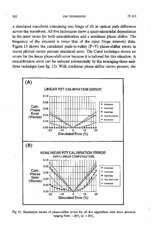
a simulated wavefront containing one fringe of tilt in optical path diferenceacross the wavefront. All five techniques show a quasi-sinusoidal dependencein the error terms for both miscalibration and a nonlinear phase shifter. Thefrequency of the sinusoid is twice that of the input fringe intensþ data.Figure 15 shows the calculated peak-to-valley (P-V) phase-shifter errors inwaves plotted versus percent simulated error. The Carré technique shows noerrors for the linear phase-shift error because it is tailored for this situation. Amiscalibration error can be reduced substantially by the avera€rrng-three-and-three technique (see frg. I2). With nonlinear phase-shifter effors present, the

PMI TECHNIQUES

(A)

0 .10

0.08(|al¡

P'hä;; 0.06

Error ^ ̂ ^(Waves) "'"-

0.02

0.00

LINEAR PZT CALIBRATION ERROR

l v , $ 6

(B )

0 .10

0.08lal¡

ffii" o'oqError ^ ̂ ¡

(Waves) "'"'0.02

0.00

- 1 0 0 1 0Simulated Error (T)

NONLINEAR PZT CALIBRATION ERROR(WITH LINEAR COMPENSATION)

Fig. 15. Simulation results of phase-shifter errors for all frve algorithms with error ¿rmor¡nts¡enging from - 20% to + 20%.

1 0 0 1 0

Simufated Error (/")

v , $ 6 1

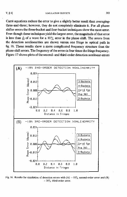
Carré equations reduce the error to give a slightly better result than averagrng-three-and-tb¡ee; however, they do not completely elininate it. For all phase-shifter errors the three-bucket and four-bucket techniques show the most error.Even though these techniques yield the largest error, the magnitude of that erroris less than fi of a wave for a l0/, error in the phase shift. The errors fromthe detection nonlinearities a¡e shown versu$ one fringe in optical path infig. 16. These results show a more complicated frequency structure than thephase-shift errors. The frequency of the errors is four times the fringe frequency.Figure 17 shows plots of the second- and third-order detection nonlinear en'ors

SIMULATION RESULTS

( A ) - 1 Ø z ? N D - o R D E R D E T E c r r o N N o N L T N E R R T T y

ø.ø?4

q

9 Ø . Ø t 2=

¿ ø .øøØU

Ø - ? l O , l 7

L

-ø.ø24

( B ) - t ø z 3 R D - o R D E R D E r E c r r o N N o N L r N E F R r r y

ø . ø ø . ? Ø . 4 ø . 6 ø . 8I l i s t ance i n F r i nqes

ø.ø?4

Ø . ø t ?

ø.ØØØ

ø . ø t ?

ø.ø?4

Øo

=

LJ

L

Fig. 16. Results for simulation of detection errors with (A) -10% second-order error and (B)- l0/" third-order error.

ø . ø ø . ? ø . 4 ø . 5 ø . 8D i s t a n c e i n F r i n g e s

384

(A)

0 .10

0.08Calc.Phase o'06Error o.o4

(Waves)

2ND-ORDER NONLINEAR DETECTIONERROR

PMI TECHNIQUES

(B )

Simulated

0 .10

0.08Calc.Phase o'06Error o.o4

(Waves)0.02

0.00

3RD-ORDER NONLINEAR DETECTIONERROR

l v , s6

1 0Error (þ

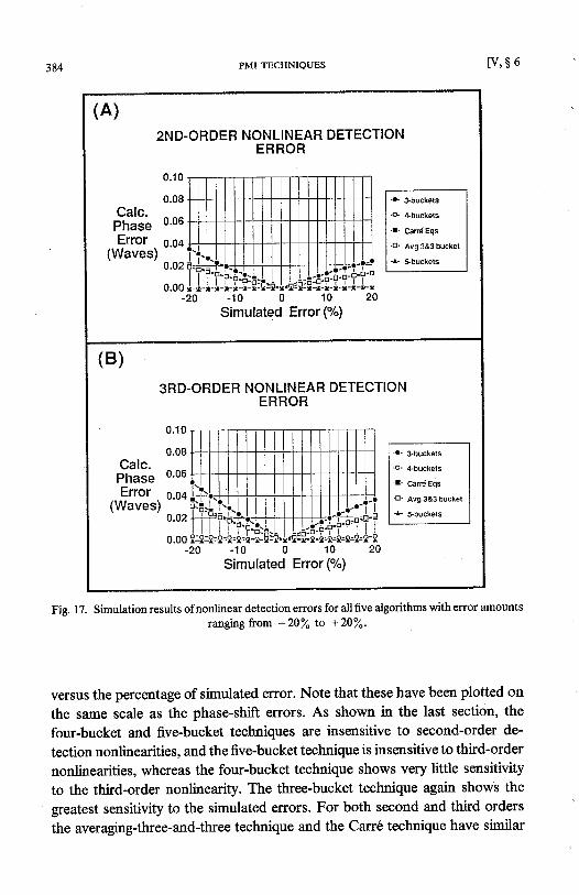
Fig. 17. Simulation results of nonlinear detection er¡ors for allûve algorithms with error amountsranging from -20/" to +20/..

versus the percentage of simulated error. Note that these have been plotted on

the same scale as the phase-shift elrors. As shown in the last section, the

four-bucket and five-bucket techniques are insensitive to second-order de-

tection nonlinearities, and the five-bucket technþe is insensitive to third-order

nonlinearities, whereas the four-bucket technique shows very little sensitivity

to the third-order nonlinearity. The three-bucket technique again shows the

greatest sensitivity to the simulated errors. For both second and third orders

the averagrng-three-and-three technique and the Carré technique have similar

1 0 0 1 0Simulated Error (/o)

v , $ 7 1

amounts of error, which a¡e a factor of two better than the three-buckettechnique, but not nearly as good as the four- and five-bucket techniques.

Looking back at the experimental results in $ 4 (figs. 8 and 9), which had twofringes of tilt in the field view, it is obvious that the Ca¡ré technique behavesthe best for a miscalibration and that the three- and four-bucket techniques arethe worst. When the system phase shifter is calibrated, there still is a wavinessin the results most likely caused by a detection nonlinearity. Because thefour-bucket results are best, most of the error is probably due to a detectionnonlinearity.

This simulation study has shown that certain phase-measurement algorithmsyield better results in the presence of some system errors than others. It alsoshows that the P-V pagnitude of these errors is well within fr of a wave evenwith a 20/o enor. In general,.the integrating-bucket methods give the sameresults as the phase-stepping methods except in the case of nonlinear phase-

shift errors, where the integrating-bhcket method is superior. The Carréalgorithm is the best to use for phase-shifting elrors, and the four- and five-bucket techniques are best for eliminating effects due to second- and third-orderdetection nonlinearities. Ifspeed ofcalculation is afactor, the averagrng-three-and-three technique, which averages errors, can give passable results in allcases. This study also found that the more buckets used, the less error due tothe system is seen in the result.

$ 7. Removing System Aberrations

REMOVING SYSTEM ABERRATIONS

Errors that reduce the measurement accuracy can be caused by referencesurface errors or aberrations present in the interferometer. The elinination ofthese errors depends on the type of measurement being performed. In all cases

a measurement of system elrors can be made using a very good mirror as the

test object. When the test mirror is of better quality than the optics contained

in the interferometer. the wavefront measured from this surface will represent

the aberrations in the interferometer. This aberrated wavefront can then be

subtracted from subsequent measurements using the test objects. The reference

wavefront must be measured again whenever the focus, tilt, or zoom of an

interferometer is changed, because these factors chânge the amount of

aberration.Ifrandom high-frequency errors are present, and a very good surface is not

available, a more involved technique is needed, for which many phase measure-

ments of the flat must be averaged (WveNr [ 1985]). In between measurements

386

the test surface is moved by a distance greater than the correlation length ofirregularities on the surface. This ensures statistically independent measure-ments. With the averaging of statistically independent portions of the testsurface, the test surface errors are reduced by the square root ofthe numberof measurements. The errors in the interferometer are then the major contri-butors to the averaged wavefront. Once the reference wavefront is obtained, itis subtracted from subsequent tests to improve accuracy. If only the root-mean-square (rms) of the test surface is desired, two measurements are needed(WveNr [1985]). First, the surface is measured, and then the test surface ismoved a distance greater than the correlation length and measured again. Therms of the difference in the phases for the two measurements yields /2 timesthe rms of the test surface independent of any errors in the reference surface.

The preceding technique works well for surface roughness measurement, butwhen surface figure is measured, a different approach is necessary. Absolutecalibration of any curved surface can bd performed using three measurements(JENSEN Í19731, BRUNINc [ 1978]). The test surface is first measured to yieldthe wavefront phase Wo", then rotated 180' and measured again to obtainWrro" . A third measurement lVço"u,is taken by translating the test surface untilthe apex ofthe test surface is at the focal point ofthe diverger (or converger)lens. The three measurements can be summed up as follows:

PMI TECHNIQUES l v , $ 7

Wo" = W"urî * Wr"¡ r W¿iu ,

Wr"o" =W"ur¡* Wr"r+ W6iu,

Wro"u" = Wr.r + L(llur" * froru) ,

where "surf" indicates the surface we are trying to measure, "ref' refers toerrors due to system aberrations in the reference arm, "div" refers to errors inthe test arm and the diverger lens, and the overscores indicate a 180' rotationofthat wavefront contribution. When all three wavefronts have been calculated.the wavefront resulting from the surface under test is given by

Likewise, the aberrations in the interferometer including the reference surfaceand the diverger lens can be calculated using

Wrb.r= Wr"r+ Woru=à(Wo" -Trro" * Wro"o"+Wro"u"). (7.5)

Once the system aberrations are measured, this wavefront (W^o") can besubtracted from subsequent measurements to provide an accurate measure ofthe test surface as long as the reference surface, diverging optics, and imaging

w"u,r= l lwo" +Wr*o. - wro.o" -Wro"u,) .

(7.1)

(7.2)

(7.3)

(7.4)

v , $ 7 1

optics are not moved. Flats can also be measured absolutely by comparingthree surfaces (Scuurz and Scnwroen [1976], FRlrz [1984]).

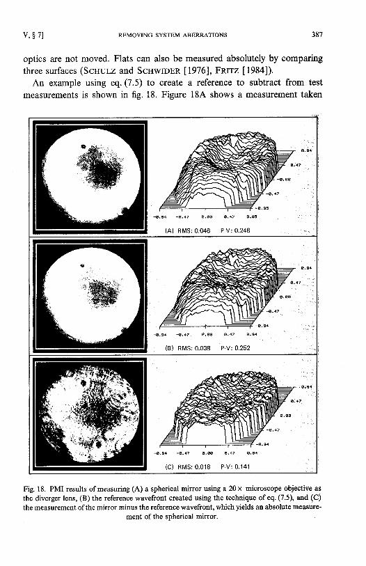
An example using eq. (7.5) to create a reference to subtract from testmeasurements is shown in fig. 18. Figure 184 shows a measurement taken

REMOVING SYSTEM ABERRATIONS

- ø . 9 4 - ø . 4 7 ø , ø ø ø . 1 7 ø . e 5

(A) RMS: 0.046 P-V: 0.248

- ø , s 4 - ø . 4 2 ó , ø ø ø - 4 ? ø . 9 4

(B) RMS:0.038 P'Y:0.252

Fig. 18. PMI results of measuring (A) a spherical rrirror using a 20 x microscope objective asthe diverger lens, (B) the reference wavefront created using the technique ofeq. (7.5), and (C)the measurement of the mirror minus the reference wavefront, which yields an absolute measure-

ment of the soherical mi¡ror.

- o . 9 4 - ø . 4 7 ø , ø ø ø , 4 7 ø , 9 1

(C ) RMS: 0 .018 P 'V : 0 .141

using,a Tw¡rman-Green interferometer with a PZT pushing the referencemirror as the phase shifter. Tilt and focus have been subtracted from all thewavefronts in the figure. A standard 20 x microscope objective was used togenerate a spherical wave to test an Fl2 mtrro4 which was good to -1.1 overthe F/8 measurement area. Because the microscope objective was used atincorrect conjugates, a lot of spherical aberration in the measurement limitedthe accuracy of the measurement. A reference wavefront was generated usingthe technique of eq. (7.5) to produce a wavefront containing the aberrations inthe interferometer and the microscope objective (fig. 188). \When this referenceis subtracted from the measurement of fig. 184, the result (fig. l8C) is indepen-dent of the interferometer accuracy. The results show a mirror with an rmssurface quality of -1,2,. Under normal circumstances better diverging opticswould',be used to test a spherical mirror; ho,wevgr, the best results will beobtained when a reference wavefront containing interferometer effors is sub-t r a c t e d f r o m t h e t e s t w a v e f r o n t . . , ' . ' , ' ' , . , . . . . ] ' ,

PMI TECHNIQUES

Phase-measurement interferometry (PMI) can be applied to any two-beamintederometer, including holographic interferomeiers. Applic ations can bedivided into three major types of measurement: surface figure, surfacerougþess, and metrology. The measurement of;sutface frg.ur9 finds$e sh4peof ar,test surface (usually an optical surface).relative to a reference mirror.

$urface roughness measurementsl are interested in the surface microstructure

and i!! statistics rather than the shape of the piece' Metrology is,used to findout properties of a sample such as the homogeneity of an optical material orthe deformatrgn. of a,sudace:i ì

8.I. SURFACE SHAPE MEASUREMENT

$.;8. Applications of ,Phase-Measurement Interferometry

[ v ;$ 8

, The traditional measurements in interferomet{y have been to measure theshape of an optical component- such as a,,lþ.p.s,or mirror. Sud4ce figuremeasurements can also include desensitized'tests such ¿s ¡sing computer-generated holograms, two-wavele¡gth holog¡aphy, or two-wavelength phase-shifting interferometry to measure surfaces with large departures from thereference surface. The desensitized tests either use a reference surface close tothe shape of the test surface created by a null lens or a computer-generated

1 ) i

v , $ 8 1

hologrem, or they synthesize a longer wavelength using interferograms from

different wavelength measurements (two-wavelength holography and two-

wavelength phase-shifting interferometry) or by projecting fringes onto the

object surface (digital moiré). Surface figure measurements are used to test both

smooth surfaces such as optical flats, spheres, and aspheres, and rough surfaces

of machined parts with arbitrary shapes.Recent techniques for measuring surface figures are the use ofa radial shea¡

or lateral shear interferometer to measure aspheric surfaces (HenrHeRnu'

Onns and Znou WeNzHI [1984], Ylrecet and KaNou [1983, 1984]). Since

the measurement is proportional to the slope of the surface under test, the

sensitivity can be varied by changing the amount of shear. Another shearing

interferometer using PMI techniques utilizes a Ronchi gfating to produce the

shear (Yera.cAr [1934]). For aspheric surfaces a useful technique based on

two-wavelength holography (wveNr, OREB and HARIH¡.RAN [1984]) for

measuring surface shape is two-wavelength phase-shifting interferometry

(CneNc and Wvelrr [ 1984, 1985b], FnncHnn, Hu and Vnv [ 1985], CREATH,

cnnNc and wye¡¡r [1985], CRrnrn and wyeNr [1986], Cneern [ 1986b]).

In this technique the phases measured at two different wavelengths are sub-

tracted and then 2z ambiguities are removed. This test synthesizes a wavefront

as if it were measured at an equivalent wavelength A"o= ).l"2llAt - )'rl'The

test sensitiyity is varied by changing wavelengths.

For measurements where the interferometer system is subject to vibration or

air turbulence, many techniques have been developed to obtain all the informa-

tion in a very short period of time. One method uses a gfating to code the

information on a single detector anay (McLeUGHLIN [1986]). Another

method uses a gfating in a Smartt point-diffraction interferometer to produce

fbur phase-shifted interferograms on four different detectors simultaneously(KwoN [1984]). Still other techniques produce the phase-shifted interfero-grams in different ways (Suvrsn and Moons [1984])'

For measurements of very irregular surfaces PMI has been applied to both

holographic interferometry techniques (Wveur, Ones and HRnlnnnnN

[1984], HanrnenRN and ORns [1984], TnaweuN and DÄN¡I-IKER [1984,1985a]), and moiré techniques (Yerecar, IDESewe, Ynprnsru and Suzurl

ÍIgï2l,Wovrecr [1984a,b], Belr and Korropoulos [1984]). In holographlc

techniques a hologram of the object is illuminated using either a different

wavelength of illumination or by changing the angle of the reference beam. In

moiré techniques, fringes are projected on the object and viewed (with or

without a reference grating) as the projected fringes are phase shifted using a

detector arrav.

APPLICÄTIONS

390

8.2. SURFACE ROUGHNESS MEASUREMENT

To measure the microstructure of a surface, an interference microscope isused to resolve l-pm surface areas laterally with height resolutions in theångstrom range. These instruments use the same phase-measurement tech-niques as the surface figure measurements. But rather than measuring asmooth, continuous surface figure, these instruments measure profiles ofrandom-looking surfaces. optical profilers have been used to test super-smoothoptical surfaces as well as magnetic tape, floppy disks, and magnetic read/writeheads.

optical profilers using PMI techniques have been based on different typesof interference microscopes. some have been based on the Nomarski type ofmicroscope, which splits the illumination into two polarizations and comparesone to the other, giving a measure of the surface slope (sorøuancner.r [19g1],Easrvew and ZewslaN [1983], ZevrsreN and EnsrvrnN [19g5], Jenn[1985]). others utilize objectives that compare the surface to a referencesurface with a Mirau, Michelson, or Linnik interferometric objective (wvaur,Korropoulos, BHusneN and Gponcn [1984], BHUSHRN, WyeNr andKorropoulos [1985], WyeNT, Korropourus, BHUsueN and Bnsrre[ 1985 ]). Still other optical profilers look more like standard interferometers thanmicroscopes (Merrnnws, HIMTLToN and Sn¡ppeno [1986], Sesarr andOrezeru [1986], PexrzER, Porrrcu and Ex [1986]).

8.3. METROLOGY

PMI TECHNIQUES l v , $ 8

The use of PMI techniques in optical metrology is relatively new. In additionto measuring þs¡m profiles (Hevns and LeNc¡ [1983]) and the homogeneityor index profile of an optical material (Moonn and Ryebr [ 1978, 1982]), thesetechniques enable the measurement of sample properties by determining thedeformation of an object caused by temperature changes, pressure changes,stress, or strain, as well as studying the vibration properties of mechanicalcomponents.

Holographic interferometry has traditionally been used to measure objectdeformations and vibrations, but only qualitative information was available.PMI has been applied to all types of holographic interferometric measurement,from looking at deformations (Sorrauencnew [ 1977], HARTHaRaN, Onnn andBnow¡¡ [1982, 1983a,b], DÄNorrr<en and Tneuvrer.rN [1985], HenrHeRaN[1985], Kners [1986]) to measuring the amplitude and phase of an object

vl

vibration (osuroe, Iwere and Nncere [1983], Nereonre [1986b],HeRrnen.lN and Onne t1986]). Recently, PMI measurements have also been

applied to speckle interferometry techniques, which are similar to holographic

interferometry techniques but do not require the making of an intermediate

hologram (wllleunr and DÄNouKER [1983], NeKaDeTn and Serro

[1985], SrersoN and BnosrNSKy [1985], CneeTn [1986c], ROstNsoN and

Wrlrnus [ 1986], Nereonrn [ 1986a]).

8.4. FUTURE POSSIBILITIES

REFERENCES

Future developments in phase-measurement interferometry will most likely

be continuations of these applications to more irregular surfaces. Larger

detector arrays will enable the measurement of steeper surfaces and allow

holographic applications without the need to produce an intermediate holo-

gram. Likewise, faster computers and parallel processing will allow us to view

wavefront measurements in real time'

References

At, C., and J.C. WveNr, 1987, Appl. Opl 26, lll2'

BELL, 8.W., and C.L. Kolloroulos, 1984' Opt. Lett. 9' l7l'

BHUSHAN, 8., J.C. Wveur and C.L. Kotloroulos, 1985, Appl' Opl 24' 1489'

BRUNTNG, J.H., 1978, Fringe scanning interferometers, in: optical shop Testing' ed. D. Malacara

(Wiley, New York).BRUNINc,J.H.,D.R.Hrnmort,J.E.Gelr¡,cr¡¡n,D'P'RosENFu-o,A'D'WHlrrandD'J'

BRANGAccIo, 1974, Appl. Opt. 13, 2693-

CnnnÉ, P., 1966, Metrologia 2, 13.CHENG, Y.-Y., ând J.C. Wvnur, 1984, Appl. Opt.23,4539'

CneNc, Y.-Y., and J.C. Wvanr, 1985a, Appl. Opt' 24,3049'

CspNc, Y.-Y., and J.C. WveNr, 1985b, Appl. OpT.4,804'

CREATH, K., 1985, Appl. OPt. 4,3053.CREATH, K., 1986a, Proc. SPIE 680, 19.

CREATH, K., 1986b, Proc. SPIE 6f1,296.CREATH, K., 1986c, Direct measurements of deformations using digital speckle-pattern inter-

ferometry, in: Proc. SEM Spring Conf. on Experimental Mechanics, New Orleans (Society for

Experimental Mechanics, Bethel' CT) p. 370.

Cxerrn, K., and J.C. Vy'veNr, 1986, Proc. SPIE 645, 101'

CREATH, K., Y.-Y. Cn¡Nc and J.C' Wve¡¡r, 1985, Opt' Acta 32, 1455'

DÄNDLIKER, R., and R. TueltuettN, 1985' Opt. Eng' 24,824'

EAsTMAN, J.M., and J.M. Znvlsler'¡, 1983, Proc. SPIE 429' 56'

FERcHER, ^.F.,H.2. Hu and U. Vnv, 1985, Appl' Opt' A' 2l8l'

391

392

Fntrz, B.S., 1984, Opt. Bng.23,379.Gn¡Iv¡Nx¡lr,tp, J.E., 1984, Opt. Eng. 23,350.HnntHennn, P., 1985, Opt. Eng. U,632.HentueneN, P., and B.F. Ones, 1984, Opt. Commun.,5l, 142.HanlHnneN, P., and B.F. Onrs, 1986, Opt. Commun..59,83.Hantunne,N, P., B.F. On¡s and N. BnowN, 1982, Op1. Commun. 41,393.Hnnrn,lreN, P., B.F. OREB and N. Bnowr.¡, 1983a, Appl. Opt. 22,8'16.HanrnluN, P., B.F. Ones and N. BnowN, 1983b, Proc. SPIE 370, 189.HenruauN, P., B.F. On¡s and ZHou WANzHr, 1984, Opt. Acta 31, 989.HAYES, J., and S. LeNcr, 1983, Proc. SPIE 429,22.HAYES, J.8., 1984, Linear Methods of Computer Controlled Optical Figuring, Ph.D. Dissertation

(Optical Sciences Center, University of Arizona, Tucson, AZ).Hu, H.2, 1983, Appl. Opt. 22,2052.Jnnt, S.lV.',, 1985;,Opt. Lett; 10, 526.JENSEN, 4.E., 1973, J. Opt. Soc. Am. 63; 1313.JonNsoN, G.W., D.C. L¡n¡¡n and D.T. MoonE, 1919, Opl Eng. 18, 46.KorHIyAL, M.P., and C. Drrrsre, 1985, Appl. Opt. ?A,2288.Knus, T., 1986, J. Opt. Soc. Am. A 3, 847.KwoN, O.Y., 1984, Opt. Lett. 9, 59.MAssrE, ,N.A j , '1980;App l . Opt . 19 , 154. i , ' : : , : : : ; .Mêlr¡HEwS, H:J.;,D,K: HAMTLToN and,C.J..R,;Snppn¡no.,.I986, Appl.,Opt .25,,2372. .r

MçlJôucHu\, J., 1986, f¡oq, sPIE 6E0, 35.Moonr, D.T., and D.P. RveN, 1978, J. Opt. Soc. Am. 68, 1157.Moonr, D.T., and D.P.'RveN, 1982, Appl. Opt.21, 1042. .: 'i '

Moon¡;,D.,T,,'and;8.E. Tnuex; 1979; Appl, Opt. lE, 91.Mo9.4p, D.T., R. MURRAv and F.B. NEvEs, !!7Q, Appl. Opt. 17,3959.MooRË,.R.C.,. and, F.H. Slnvnerun, 1980, Appl. Opt. 19, 2196.Monc¡,N, C.J., 1982, Opt. Lett. 7, 368.Nnxroete;,S,;'1986a, Appl. Opt. 25, 4155.Nexeoerr,.S.,: 1986b, Appl. Opt. 25, 4162.Nexeonrn, S., Aqd H Snrro, 1985, Appl. OpL U,2172.OsHrDA, Y., K. Iw¡r¡, and R. Nec¡.r.r, 1983, Opt. Lasers Eng. 4, 67.PÀNrzER; D.; J:,PoLrTcH and,L. 'Er, 1986; Appl: Opt;25, 4168.Run;1G.T.,. 1986,,Opt. Lasers Eng. 7, 37.BO.plNSoN, D.W., and D.C. W¡llrnvs., 19E6, Opt. Commun.57,26.SesexI, O., and H. Or¡2,¡rrct, 1986, Appl. Opt. 25,3137.ScHuLz, G., and J: Scnwroer, 1976, Interferometric testing of smooth surfaces, in: Progress

in Optics, Vol. XIII, ed. E. Wolf (North-Holland, Amsterdam) pp.93.ScHwrDER,J.R., R. Bunow, K.-E. ErssNEn, J. GnzenNe, R. Spol¡czyr and K. Mpnr¡r,

1983, Appl. Opt. 22, 342r.Su,loerrr, R.N., and J.C. Wyar.rr, i978, Appl. Opt. 17, 3034.Suvrs¡, R., and R. Moone, 1984, Opt. Bng.23,361.SonvnncnrN, G.E., 1975, J. Opt. Soc. Am. 65, 960.SovrrarncnnN, G.8., l9'l:1, Appl. Opt. 16, 1736.SoMMnncnEu, G.E., 1981, Appl. Opt. 20, 610.SrErsoN, K.4., and W.R. BnosrNsKy, 1985; Appl. Opt. 2A,3631.TAKEDA, M., H. I¡,¡a and S. KoBeynsnr, 1982, J. Opt. Soc. Am.72, 156.TueLueNN, R., and R. DÄNour¡n, 1984, Proc. SPIE 492,299.TuervenN, R., and R. DÄNDLTKER, 1985a, Opt.Bng.24,930.Tuelu.r,rlrN, R., and R. DÄNDLTKER, 1985b, Proc. SPIE 599, 141.WrLtnrrarru, J.-F., and R. DÄNDLTKER, 1983, Opt. Lett. 8, 102.

PMI TECHNIQUES tV

vl

WoMAcK, K.H., 1984a, OPt. Eng.23,391'

Woturcr, K.H., 1984b, Opt. Eng.23,396'

Wver¡r, J.C., 1975, Appl. Opt. 14' 2622'

Wvenr, J.C., 1982, Laser Focus (May)' p' 65'

WyÄNr, J.C., 1985, Acta Polytech. Scand' Phys' 1fi,241'

Wv,ort.¡r, J.C., and K. CREATH, 1985, Laser Focus (November)' p' 118'

WvlNr, ¡.C., and R.N. SHAGAM, 1978, Use of electronic phase measurement techniques in

ofti"ut testing, in: Optica Hoy y Mañana, Proc. llth_Congr. of the International Commission

f o r O p t i c s , M a d r i d , l 0 - l T S e p t e m b e r l g T S , e d s J ' B e s c o s ' A ' H i d a l g o ' L ' P l a z a a n d J 'Santamaria (Sociedad Española de Optica, Madrid) p' 659'

WvaNr, J.C., B.F. Onns anà P. HenIr¡ennN, 1984, Appl' Opt' 23' 402/0' -- - -WvaNr, J.C., C.L. KoLIoPouLos, B. BHUSHIw and O'E' Geonce' 1984' ASLE Trans' 27' l0l'

WvaNr,J.C.,C.L.KoLIoPouLos,B.BHUSHANandD'Bnsrle'1985'J'Tribology'Trans'ASME108, l .

Yerecel, T., 1984, APPI. OPt. 23,3676'

Yer,+cet, T., and T. KANou, 1983, Proc' SPIE 429' 136'

YATAcAI, T., and T. KANou, 1984, Opt' F;ng'23,351'

Yntecer, T., M. IDEsAwe, Y. Y¡.v¡'sr¡l and M' SuzurI' 1982' Opt' Eng' 2l' 901'

Znvrslett, ¡.t"t., an¿ J.M. Eesrlae¡{, 1985, Proc' SPIE 525' 169'

REFERENCES 393

Ao,rvrs, M.J.,219,222Acnnw¡r, G.P., 165, 168, l '70,1'14,178, 186,

I 88, I 97, 209¿r t, 2t 4, 2t 5, 22U222, 224,225

Ãt , C . ,376,391ArELLo, P., l l3, 119, 158ArNsLrE, 8J., 165,222AKHMANoV, S.4., 137, 157AKse, S., 180, 189, 192,193,222,224,225AKoPYAN, R.S., 119, 157ALFERNESS, R.C., 196, 20'1, 216, 223, 225ALLEN, L.8., 197,222ALMETDA, S.P., 148, 160ANDERsoN, JK.,215,224ANDREWS, L.C.,2'7,99ANTHoNY, P.J., 188, 207, 220, 222ANTREASYAN, A., 200, 222APosroLIDIs, 4.G., 152, 159ARAr, S., 180, 193, 195, 196, 225ARÀKELTAN, S.M., l14, 116-120, 130, 134,

136, 138, 146, t54, 156-159AREccHr, F.T., 13, 99ARMrrAcE, D., 128, 129,134, l5'1ARNoLD, Y.1., 29'1, 298, 337, 345ASADA, M.,209,222ASATRYAN, A.A., 246, 253, 255, 345AsHKrN,4., 108, 157AsPEcr, ,{., 55, 59, 6446, 68, 99, 101Au Y¡.ur.rc, J., l4'7,158

BBABrcH, V.M.,284,345Becs, 4., 63, 104BAHADUR,8. , 110, 158BerLua¡¡, H.4., 108, 157BALTES, H.P.,27,101Benarr.r, R., 20, 25, 26, 99, 100BARBERo, G., l l3, 119, 158BARNES, P.^., l'13,224BARroLrNo, R., l l9, 160

AUTHOR INDEX

BAsrLA, D., 390, 393Berne, 1.P., l2'7,158BELL, 8.W., 389, 391Brrr, T.E., 165,222B¡No¡e¡eLLes, C., 31, 102Brnan, M.J., 24, 100BËRRy, M.V., 256, 297, 298, 302, 338, 345BERroNr, H.L., 243, 254, 345BEsoMr, P., 199, 207, 224BEsPALov, V.I. , 137, 158BHUSHAN, 8., 358, 363, 390, 391,393BrcKERs, L.,215,222BTLGER, H.R., 81, 102Blscnorps¡nc¡n, T., 153, 158BröRK, G., 3, 51, 104BToRKHoLM, J.E., 144, 158BLAKE, J., 20, 25, 26, 100BLrNov, L.M., 107, l l0, 158Bonn, M., 9, 100, 139, 158, 169, 222,231,

241, 256, 2'.t2, 274, 2't7 , 345BoswoRrH, R., 196, 20'1, 225BowERs, 1.8., 213, 215, 222, 223BoYD, G.D., 108, 157,215,222BRAcTNSKY, V.8., 71, 100BRANcAccro, D.J., 351, 358, 362, 391BREKHoVSKTKH, L.M., 282, 345BRENNEcKE, W., 196, 207 ,222BREroN, M.E., 3, 91, 104Bruocrs, T.J.,216,223BRTNKMEYER, E., 196, 207, 222BRoBERc, 8., 189,223BRoHTNSKY, W.R., 379, 391, 392Bnow¡¡, N., 390, 392BnowN, R.G.W.,84, 100BnuNrNc, J.H., 351, 358,362,386, 391Busr, L.L.,216,223BULDYREV, V.S., 284, 345BuRcEss, R.E., 46, 100BURKHARDT, 8.G., 216, 223BURNHAM, D.C., 58, 68, 100

39s

396

BURNHAM, R.D., 180, 183, 184, 186, 192,204,225

Bunow, R, 37 4-3'l 6, 392BURRUS, C.A., 1: l6, l ' l8, 199,207,215,216,

220,222-224 ' t,

BurLER, J.K., 165,223 .-.',BuroRrN, D.1., 307, 345 :Buus, J., 187, l90i 20,9;.222,224 l

cCnùrn¡{or,¡, K.H., 198, 206, 224CnvpepLl- Jn, J.C., 216,223 lCAl.rron, 8.I . ,45, 96, 100, 104CeenSSo, F., 8l; 8G88, 99, 100; 104CeusoN, N.W., 196, 20'7, 223Cnnurcnerl, H.J., l3¡;ll; 43, 59,100Cnno;:R.G., 147, 158C n n n É , P . , 3 5 1 , 3 5 8 , 3 6 5 , 3 9 1 'Cnnnoll , J.8.,83, 100CARRUTHERS, P. ,71 , 100CASEY JR, H.C., 165,168,222'C¡,v¡Sa C.M.,4, 7lì; 86¡100 .CHnuona, N., 63, 100 ;CunxonnsprH¡,n, S., 107, 158'Cneule, D.S,, l35t 157,-158, 161 ,.

)CHEN, F.S., 108, 158 :CHEN, H., 134, 147,1:60CHeN, K.L.,204,222CHEN, S.H., 20, 100 :Cserqc, Y., 134, l4'l ; 160rCseNô, Y.-Y., 375, 389, 391,CHERNYT, F .8 . , 243,282, 345,CHERRY, T.M., 337, 345CHEUNG, M.M., 134, 153, 158iCnllrñoenreN, ¡t., 134, 157 , 111lCr¡ruñcenr¡H, :Yù:S., 130, 156,,157CHTLLAG, L., I 15, I f6, l l9, 134,138, 16l'Cso, 4.Y., 86, 100 ,.,,, . ,jCnor, H.K., 200,204,222', ,Cuouounnv, S . ,329,345CLrnr, N.4., 156, 159Coor, R.F., 133, 146, 158CorrEN, L.G.,216,223CoroneN, L. A, 200, 202-205, 207, 215, 222,', 223 :i

'; :

I Co¡ÍNELY, R.H., 197..t:.223'CoNNoR, J.N.L., 342, 345

CooK, R.J., 58, 100CorereNo, J.A., 176, 223Cox, D.R., 10, 19,43-45, 100

AUTHOR INDEX

Cnerc Jn, R.M., 197,222CREATH, K., 351, 35¿F357, 359, 366, 368,

389,391,393Cnrssrn, I .D., 13, 55, 100CnoNrN-Go¡-oMB, M¡, 147, 158 ;Cnow¡, J.W., 197,222Csrrrnc, L¡120, 12l, 158CuRrrs, P.R.,342,345

DDÀcENÁyS,iM., 3, 13,;55, [00, l0l j i ;DnLrnenr;iJ., 66,99 ,1., ::. i jDT{NDLTKERì¡R.,,389-392, -, : i " , : t

DnsnnN, R.,301, 346 - .9 :DATroLr, G., 97,.100 :,Devrs ,M.H.A. ,93 ;100 I g ¡ ¡ ,DAwsoN, R.W ., 216, 223 i , i )D a y , C . R . , 1 6 5 , 2 2 2 ' - I

!oEGnNNes, P.c., t07r ltol il4, I jo, r5tDEJEU, W.H., 123, 124, 133, 158DELTSLE, C.,353,392DrLwenr, S.M;; 1.28, 129, 134, 157Drrrer, A.G.,:176, 199, 223, 224Drscnarræs, CíAtt, 277, 327, 345 \DEVL¡N, W.1.,20/.,221,225 .")DEVoE, R.c., 64, 103 i

Drronrcu, F., 60, 77, 100Donoo¡qrrsvx,'A.A.,ì337,345 iDnpvBn, R.W,P:;71, 100 iDRoNov, 1.F.,342,,345DnuuvoNo, P., 59; 100Dunrv, M.T., 196,207,223': ìDursrri.uner,J.I.,297,338, 345 ¿ IDunrw,'S:b., ll4, ttÇl2o;:134, 1 36,.138,

146, 153, ì138 " ' " ' , , i : rDuîrA, N.K., 165, 168, l'10,.113, 174,..186,

188, 197, 207, 209, 215, 220,: 2Zi:, 224.Dz rnoz tc , J .M . , . 10Q, f57 i , , , 1 i , ,E iEnsru¡,r.¡, J.M., 390, 391, 393Enerruc, K.J., 27, 100, 207, 222Eoe, N., 189,222,225EDEN, D., 128, 158ErnoN, U., 135, 16lEtNsruN, 4., 16, 100ErsENSrErN, G., 216, 223Er, L., 390, 392Els¡n, W., 135, 160ELSSNER, K.-8., 37 4-37 6, 392

:1

ENNS, R.H., l2"l ,158EsPosrro, F., 45, 102Evenv, I.M., 63, 100

FI.-¡.sn¡, C., 70, 101F¡.No, U., 12, 100FnnnrLLv, D.,342,345FAYER, M.D., 126, 156, 15&FEDoRYUK, M.V., 33'7, 34'lFuNnnnc, E.L., 108, 135, 158,243,282,346FETNBERG, L, 147, 152, 158FErzuLrN, 2.1., 240, 346FEKETE, D., 147,158FELSEN, L.8., 243, 254, 27'1, 303, 324, 329,

336,345,346FERcHER, 4.F., 389, 391FERNANDEz, F.J.L., 139, 158FrlrPowrcz, P., 83, 100FINN, G.M., 134, 139,143,144, 159FlnrH, W.J., 123, 158FrsHER, 8., 135, 147, 158, l6LFlsHER, R.4., 147, 158FLAr-rÉ., S.M., 301, 346Fr-evrNc, M.W., 207, 219, 222FocK, V.4., 27'7, 282, 317, 318, 320, 346FoRRESTER, A.T.,24,25, 59, 100FRANcK, J.,78, 100FRASER, D.8., 108, 158FREDERTKS, V., 114, 158FRTBERc, S.,68, 101Fn¡rz, 8.S., 387,392Fuu, Y.G., 133, 146, 158FurrrA, T., 200, 20'7,215,222,224FuJrro, K.,215,222FURUYA, K., 189, 222, 223, 225Fv¡, D.,215,224Fv¡, D.M.,209,224

GGe,ron, D., 9, l0l , 145, 158Gecrr,+not, R.M., 10, 24,25,91,95, 101GALBRATTH, L, 123, 158Grrre.curn, J.E., 351, 358, 362, 391Gellenoo, J.,97, 100G,rnrov,r.r,r, O.V., 134, 158cARrro,4.F., 156, 158Gnnle,No, C.W., 128, 158G¡,rrr, E., 13, 99GAZARYAN, Yu.L., 290, 346

AUTHOR INDEX

Geonce, O.E., 358, 363, 390, 393GenRrrsnr, C.J., 133, 158GurnLvnrrr, F., 53, l0lGHroNE, G' 324, 336, 346Grncouuo, E.,70, l0lGrBBs, H.M., lM, 153,154, 158, l6lGlLrenr, E.N., 29, l0lGreurrn, R.J., 3, 13, 34, 35, 38,63, 10 l , 102,

104GLrNsKr, J., 188, 190,222G¡¡eucr, A.H.,216,223Gor-orunr, E.S., 134, 154, 158GooDBY, J.W., 109, 159GooDMAN, J., 16, 101GooseNs, W.J.A., 133, 158Gonoon, E.I., 91, 94, 101, 173, 20'7, 222, 223Gowr,n, M.C., 147, 158GnaNctrn, P., 55, 59, 65, 68, 99, l0lGneNr-ur.¡p, 5.W., 199, 207 , 224Gn¿.v, G.W., 109, 159GnErv¡Nrnr*rp, J.E., 359, 360, 362, 392Gnrxnrnc, J., 135, 161GnosHev, V.Y ¡., 290, 346GnzaNNa, J., 3'1 4-37 6, 392Guue, S., 144, 160GusuN-Znon, S.M., 337, 345

HHncax, DJ., 123,159HÄGER, J., 13, 55, 100Herl, J.L., 63, 104HnurrroN, D.K., 390, 392HAMMER, J.M., 196, 207, 223H¡,Nsunv-BnowN, R., 3, 15, 101Hnnorn, C., 2l'1, 218, 225HenrH¡nex, P., 389-393HARRrs, W.4., 78, 104Heus, H.4 . , 71 ,72 ,91 ,101, 104, 189,223Heves, J.,390,392HAYES, J.8., 375, 37 6, 392HETDMANN, 4., 55, 70, l0lHrrrwe,ntn, R.W., 135, 146, 147, 152,

158-160HELsrRoM, C.W., 91, 95, l0lHrNNrNc, 1.D.,219,222HeNnv, C.H., 91, 95,99, 101, 178, 186, 188,

t96, 197, 203, 204, 206, 207, 209, 210,2t5-2r9,22t-224

HrNnv, P.S., 178, 221, 223, 224HERMAN, R.M., 115, 134, 149,159

397

398

Henuaxu, J.4., 139, 159Hrnntnu, J.P., 152, 159HERRrorr, D.R., 351, 358, 362, 391Hrnrz, G., 78, 100HERvEr, H., l2' l ,159, 16lH¡ss, L.D., 135, 161H¡.ss¡1, A., 243, 254, 345HrLL, K.O., 134, 159Ho, S . -T . , 6 ,35 ,47 ,53 , 63 , 85 , 103HoENDERS, 8.1.,27, 101HoFFMANN, H.J., 108, l2'1, 130, 159Hollnrnc, L.W., 3, 64, 103HoNc, C.K., 58,68, 101HoRN, R.G., 126, 159HoRowrcz, R.J., 70, 101Hou, J.Y., 134, 139,143,153,154, 159HsruNc, H., 127, 128, 130-132, 159}Ju, H.2.,353, 389, 391,392HurcN¿.no, J.P., 133-135, 141,152,159, 160Huo, T.C.D., 216,223

IIorsewn, M., 389, 393Ion, K., 168, 200, 216, 222, 223, 225IKEcAMT, T., 180,223Iu¡.r, H., 189, 212, 223, 225Ivoro , N. , 3 ,51 ,65 , '71 ,72 ,83 ,84 , 101, 104Iu, H.,356,392Iee,rov, 8.8.,342,345IPArov, 8.V.,342,346IsHrrnw.+, H.,212,223IsHrNo, M., 200, 207,224Isnrzuxe, 5.,215,222Isozururr, 5.,212,223Ir¡.ye, Y., 83,90,102,180, 188, 193,223,225Iwnra, K.,391,392

JJ¡,sn, S.N., 390,392Jecrrw, R., 90, l0lJarN, R.K., 135, 159Jarennw, E., 14,20,25, 27, 43, 55, 59, 61, 68,

69, 73, 84-86, 91, 100-102, t04J¡.vns, G.L.,303,346JANossY, I . , 120, 121, 158JnveNntNEtr, J., 83, 100JaYlneueN, S., 107, 160JEFFERSoN, J.H., 68, l0lJ¡N, S., 156, 159JENSEN, ^.8.,386,392

AUTHOR INDEX

JoHNsoN, G.W., 355, 392JoRDAN, P., 78, 100

KK.uaNov, Yu.M.,93, 101Knoora, T.T., 94, 101KAMrNow, I.P., 178, 199,20'1,224KAMrrE, K.,212,223KANou, T., 389, 393KAPLAN,4.8' 144, 153, 154, 158, 159Keurnru,4.S., 130, 157Kennr, F.C.,324,346KARN, 4.J., 130, 134, 154, 159Krnp, S . , 10 ,24 ,25 ,91 ,95 , l0 lKrsran, 8.L., 178, 216, 223, 224Kers¡N¡r-rNsevu, 8.2., 303, 348Kewecur, M., 134, 159KAwAsAKr, 8.S., 134, 159KnzanrNov, R.F., 196, 197, 203, 204, 206,

207,215,221,223,224KELLER, 1.8.,229,303, 314, 324,327, 346,

J + I

KELLEy, P.L., 34, l0lKHorurlov, R.V., 137, 157KHoo, I.C., ll4-111, ll9-121, 12Ç128,

t30-t32, 134, 136, t39, 143, r44, 146, t4'1,149, l5l , t53, 154, 159-l6l

KrELrcH, S., 107, 130, 160KTHARA, K.,212,223Krrucnr, K.,220,223KTMBLE, H.J., 3, 13, 43,55,63,101, 104KrsHrNo, K., 168, 180, 193, 195, 196, 225Krsr-rNx, P.P., 197, 223KrreEvn, V.F., l15, 116,l l9-121,134, 138,

158, l6 rKtrecewa, M., 3, 51, 104Krr.ruune, M., 180, 192,223Kr-en, M.8., 135, 159KLuNrn, W.H.,34, l0lKLETNMAN, D.A., 197, 223KNrcHr, P.L.,4, 102Ko, J.S., 178,199,224Konavasnr, K., 180, 192,223Kon.lvlsur, S., 356, 392Kocu, T.L., 202-205, 213-216, 222-224Kocsenovsry , V.V., 236, 348Kocsenovsry, VL.V ., 236, 348Koñouser, J.,3, 102KoENrc, H.G., 197,222KoENuono, S., 189, 223