short-range leakage cancelation in fmcw radar

Submitted byAlexander Melzer

Submitted atInstitute ofSignal Processing

Supervisor andFirst ExaminerUniv.-Prof. Dr.Mario Huemer

Second ExaminerUniv.-Prof. Dr.Martin Vossiek

Co-SupervisorsDr. Alexander OnicDr. Rainer Stuhlberger

May 2017

JOHANNES KEPLERUNIVERSITY LINZAltenbergerstraße 694040 Linz, Osterreichwww.jku.atDVR 0093696

Short-Range Leakage Cancelationin FMCW Radar Transceiver MMICs

Doctoral Thesis

to obtain the academic degree of

Doktor der technischen Wissenschaften

in the Doctoral Program

Technische Wissenschaften

Abstract

Today’s cars are equipped with radar sensors, which provide precise information aboutthe distance, speed and angle to surrounding objects on the road. This information isessential for modern driver assistance systems such as adaptive cruise control or brakeassistance systems. Further, it enables future autonomous driving features. Most im-portantly, however, the accuracy and range of the radar sensors are critical for the safetyof the car occupants as well as other daily road users. This is of particular significancesince around 90 percent of all rear-end collisions with personal injuries occur due tohuman mistakes. Assuming all cars on the road to be equipped with emergency brakesystems, up to 72 percent of these collisions could be prevented.

For reasons of car appearance as well as protection of the device itself, the radar sensorsare often mounted right behind the bumper. This, however, causes unwanted signal re-flections from such. Particularly, the reflections yield so-called short-range (SR) leakage,which superimposes reflections of true objects that have to be detected most precisely.Together with the phase noise (PN) inherently present in the frequency modulated con-tinuous wave (FMCW) transmit signal, the bumper reflections limit the achievable sen-sitivity and accuracy of the radar sensor severely. As a consequence, driver assistancesystems may react delayed in critical situations.

In this thesis, novel concepts that aim to cancel the SR leakage in the automotive ap-plication are proposed. These are the first known solutions of their kind that can beintegrated holistically within a monolithic microwave integrated circuit (MMIC) oper-ating at 77 GHz. The concepts make use of an artificial on-chip target (OCT), whichmimics an object reflection on the chip. The tight design constraints regarding imple-mentation in the MMIC are circumvented by employing sophisticated statistical signalprocessing. Simulation as well as measurement results from the developed hardwareprototype show that the sensitivity can be more than doubled by applying the proposedconcepts.

Besides SR leakage cancelation, also the issue of PN power spectral density (PSD) estima-tion is addressed. Different to existing on-chip PN PSD estimation techniques, the inputsignal is considered as a linear FMCW signal rather than a pure continuous wave (CW)signal. Two methods to obtain estimates of the PN PSD are proposed. Both make useof the artificial OCT, and are evaluated with simulations as well as measurements. Theproposed techniques not only allow for a fast characterization after production of thechip, but also enable continuous monitoring of the PN during normal operation of theradar for the first time.

I

Kurzfassung

Moderne Automobile sind mit Radarsensoren ausgestattet, welche genaue Informationenuber Distanz, Geschwindigkeit und Winkel zu umliegenden Objekten im Straßenverkehrermitteln. Diese Informationen sind nicht nur wesentlich fur moderne Fahrerassistenz-systeme, wie etwa adaptive Fahrgeschwindigkeitsregler oder Bremsassistenten, sondernauch Voraussetzung fur die Realisierung autonom fahrender Autos. Bei den eingesetztenRadarsensoren sind dabei insbesondere Reichweite und Genauigkeit ausschlaggebendfur die Sicherheit der Insassen sowie anderer Verkehrsteilnehmer. Dies ist von uberausgroßer Bedeutung da etwa 90 Prozent aller Auffahrunfalle mit Personenschaden auf men-schliches Fehlverhalten zuruckzufuhren sind, wahrend bis zu 72 Prozent dieser Unfalledurch einen flachendeckenden Einsatz von Notbremssystemen zu verhindern waren.

Aus optischen Grunden aber auch zum Schutz der Linse werden die Radarsensorenhaufig unmittelbar hinter der Stoßstange des Autos verbaut. Dies fuhrt dazu, dass dasausgesendete Radarsignal permanent mit verhaltnismaßig großer Signalamplitude vonder Stoßstange reflektiert wird, und somit andere tatsachlich erwunschte Reflexionenuberlagert. In Kombination mit dem Phasenrauschen, welches inharent im Sendesignaldes frequenzmodulierten Dauerstrichradars enthalten ist, limitieren die unerwunschtenSignalreflexionen, welche als short-range (SR) leakage bezeichnet werden, die erreichbareSensitivitat und Genauigkeit des Radarsystems maßgeblich. Somit reagieren Fahreras-sistenzsysteme in kritischen Situationen moglicherweise verspatet.

In dieser Doktorarbeit werden neue Konzepte und Methoden zur Unterdruckung vonSR leakage vorgeschlagen, welche erstmals vollstandig in einer monolithisch integriertenMikrowellenschaltung (MMIC) realisiert werden konnen. Dafur wird ein kunstlichesRadar-Ziel am Chip (OCT), welches eine Objektreflexion imitiert, verwendet. Diestarken Einschrankungen hinsichtlich der Implementierung im MMIC werden durchstatistische Signalverarbeitung umgangen. Simulations- als auch Messergebnisse desentwickelten Prototyps zeigen, dass mit den vorgeschlagenen Konzepten die Sensitivitatdes Radarsystems mehr als verdoppelt werden kann.

Neben den Unterdruckungsmethoden fur SR leakage werden in der Arbeit auch zwei neueKonzepte zur Schatzung des Leistungsdichtespektrums des Phasenrauschens vorgeschla-gen. Herkommliche Methoden benotigen zur Schatzung ein kontinuierliches, unmod-uliertes Signal. Die vorgestellten Konzepte ermoglichen hingegen die Schatzung desLeistungsdichtespektrums des Phasenrauschens aus linearen frequenzmodulierten Sig-nalen, welche zumeist in Radarsensoren fur Autos eingesetzt werden. Beide Methodenverwenden wiederum das OCT, und werden mit Simulations- als auch Messergebnissenverifiziert. Diese Konzepte ermoglichen nicht nur eine schnelle Charakterisierung nachder Fertigung des Sensors, sondern erstmals auch eine Uberprufung des Phasenrauschenszur Laufzeit des Radarsystems.

III

Statutory Declaration

I hereby declare that the thesis submitted is my own unaided work, that I have not usedother than the sources indicated, and that all direct and indirect sources are acknowl-edged as references.This printed thesis is identical with the electronic version submitted.

Date Signature

V

Acknowledgements

First and foremost I thank my supervisor Univ.-Prof. Dr. Mario Huemer for givingme the opportunity to write my PhD thesis at the Institute of Signal Processing at theJohannes Kepler University Linz. He did not only contribute to this thesis with hisexceptional technical competence, but also supported my personal development in manyaspects. It is in particular his profound conviction for sophisticated research and histireless engagement for a sustainable education of future engineers, which makes him anabsolute role model.

I also wish to thank Dr. Alexander Onic for supervising this thesis from an industrypartner side, for the many fruitful technical discussions, for the support regarding signalprocessing related questions, and for the exceptionally valuable inputs to our papercontributions. I would further like to thank Dr. Rainer Stuhlberger for enabling andguiding my PhD thesis. Best thanks also to Dr. Florian Starzer, Dr. Herbert Jager andDr. Herbert Knapp for sharing their expertise regarding hardware and semiconductorrelated questions.

Further, I thank all my colleagues at the institute not only for always acting as closelyunified and collaborative team, but also for creating an inspiring and cozy workingatmosphere. In particular, I would like to thank Dr. Michael Lunglmayr, Dr. ChristianHofbauer, Dipl.-Ing. Oliver Lang, Dipl.-Ing. Carl Bock, Dipl.-Ing. Andreas Gebhard,Dipl.-Ing. Andreas Gaich and Dipl.-Ing. Michael Gerstmair for their collaboration inteaching and PR activities, as well as their friendship. Also, I express my gratitude toBirgit Bauer for always keeping administrative belongings at the institute well organized,and for being a contact also for personal needs.

Finally, I would like to thank my family, my friends, and my girlfriend Marlies for theirsupport throughout my PhD Thesis.

VII

If it wasn’t hard,everyone would do it.

It’s the hard that makes it great.- Tom Hanks

IX

Contents

1 Introduction 11.1 Automotive Radar Systems . . . . . . . . . . . . . . . . . . . . . . . . . . 11.2 The FMCW Radar Principle . . . . . . . . . . . . . . . . . . . . . . . . . 21.3 The Issue of Short-Range Leakage . . . . . . . . . . . . . . . . . . . . . . 51.4 State of the Art . . . . . . . . . . . . . . . . . . . . . . . . . . . . . . . . . 7

1.4.1 Cancelation of On-Chip Leakage . . . . . . . . . . . . . . . . . . . 71.4.2 Short-Range Leakage Cancelation . . . . . . . . . . . . . . . . . . 71.4.3 Estimation of the Phase Noise PSD . . . . . . . . . . . . . . . . . 9

1.5 Scope of this Work . . . . . . . . . . . . . . . . . . . . . . . . . . . . . . . 9

2 Short-Range Leakage in FMCW Radar Transceivers 132.1 System Model . . . . . . . . . . . . . . . . . . . . . . . . . . . . . . . . . . 13

2.1.1 Overview . . . . . . . . . . . . . . . . . . . . . . . . . . . . . . . . 132.1.2 Transmit (TX) Signal . . . . . . . . . . . . . . . . . . . . . . . . . 142.1.3 Receive (RX) Signal . . . . . . . . . . . . . . . . . . . . . . . . . . 162.1.4 Intermediate Frequency (IF) Signal . . . . . . . . . . . . . . . . . . 16

2.2 SR Leakage in the IF Domain . . . . . . . . . . . . . . . . . . . . . . . . . 182.2.1 SR Leakage Signal Components . . . . . . . . . . . . . . . . . . . . 182.2.2 Decorrelated Phase Noise (DPN) . . . . . . . . . . . . . . . . . . . 19

2.3 Impact of SR Leakage on System Performance . . . . . . . . . . . . . . . 262.4 Outlook: SR Leakage Cancelation . . . . . . . . . . . . . . . . . . . . . . 29

2.4.1 SR Leakage Beat Frequency Suppression . . . . . . . . . . . . . . . 292.4.2 SR Leakage Cancelation Including the DPN . . . . . . . . . . . . . 29

3 Short-Range Leakage Cancelation 313.1 Artificial On-Chip Target . . . . . . . . . . . . . . . . . . . . . . . . . . . 32

3.1.1 Overview . . . . . . . . . . . . . . . . . . . . . . . . . . . . . . . . 323.1.2 Restriction of Delay Lines in MMICs . . . . . . . . . . . . . . . . . 333.1.3 DPN Extraction from the On-Chip Target . . . . . . . . . . . . . . 33

3.2 Cross-Correlation Properties between DPN Terms . . . . . . . . . . . . . 353.2.1 DPN for Various Delays . . . . . . . . . . . . . . . . . . . . . . . . 353.2.2 Cross-Correlation Properties . . . . . . . . . . . . . . . . . . . . . 363.2.3 Optimum Lag . . . . . . . . . . . . . . . . . . . . . . . . . . . . . . 383.2.4 Linear MMSE Prediction . . . . . . . . . . . . . . . . . . . . . . . 403.2.5 Scaling Factor with Lowpass Filtered DPN . . . . . . . . . . . . . 40

3.3 SR Leakage Cancelation in Digital IF Domain . . . . . . . . . . . . . . . . 433.3.1 Cross-Correlation Properties Applied to the FMCW Radar System

Model . . . . . . . . . . . . . . . . . . . . . . . . . . . . . . . . . . 433.3.2 DPN Extraction from the OCT IF Signal . . . . . . . . . . . . . . 443.3.3 SR Leakage Cancelation Signal Generation . . . . . . . . . . . . . 453.3.4 Leakage Cancelation . . . . . . . . . . . . . . . . . . . . . . . . . . 483.3.5 MIMO Scenario . . . . . . . . . . . . . . . . . . . . . . . . . . . . . 483.3.6 System Performance Evaluation . . . . . . . . . . . . . . . . . . . . 49

XI

3.3.7 Optimum Delay and Limitations of DPN Extraction . . . . . . . . 513.4 SR Leakage Cancelation in RF Domain . . . . . . . . . . . . . . . . . . . 58

3.4.1 System Model . . . . . . . . . . . . . . . . . . . . . . . . . . . . . . 593.4.2 Cancelation Concept . . . . . . . . . . . . . . . . . . . . . . . . . . 603.4.3 MIMO Scenario . . . . . . . . . . . . . . . . . . . . . . . . . . . . . 663.4.4 System Performance Evaluation . . . . . . . . . . . . . . . . . . . . 66

3.5 Comparison of SR Leakage Cancelation Concepts . . . . . . . . . . . . . . 673.6 Adaptive SR Leakage Cancelation . . . . . . . . . . . . . . . . . . . . . . 69

3.6.1 Estimation of SR Leakage Beat Frequency . . . . . . . . . . . . . . 713.6.2 Phase and Amplitude Estimation . . . . . . . . . . . . . . . . . . . 763.6.3 Estimation Methods Applied to SR Leakage Cancelation . . . . . . 77

4 Hardware Prototype 854.1 Hardware Setup . . . . . . . . . . . . . . . . . . . . . . . . . . . . . . . . . 86

4.1.1 Analog Front-End . . . . . . . . . . . . . . . . . . . . . . . . . . . 864.1.2 Digital Signal Processing Hardware . . . . . . . . . . . . . . . . . . 88

4.2 Cross-Correlation Properties between DPN Terms . . . . . . . . . . . . . 894.3 Digital Design on FPGA . . . . . . . . . . . . . . . . . . . . . . . . . . . . 91

4.3.1 DPN Extraction from the OCT IF Signal . . . . . . . . . . . . . . 944.3.2 SR Leakage Cancelation Signal Generation . . . . . . . . . . . . . 944.3.3 Leakage Cancelation . . . . . . . . . . . . . . . . . . . . . . . . . . 95

4.4 Measurement Results . . . . . . . . . . . . . . . . . . . . . . . . . . . . . . 95

5 Online Phase Noise PSD Estimation from Linear FMCW Signals 1015.1 PN PSD Estimation with the Artificial On-Chip Target . . . . . . . . . . 102

5.1.1 Lowpass Filtered DPN . . . . . . . . . . . . . . . . . . . . . . . . . 1025.1.2 Estimation Constraints by Application . . . . . . . . . . . . . . . . 103

5.2 PN PSD Estimation from Extracted DPN of OCT IF Signal (EMT) . . . 1035.2.1 Spectral Properties of DPN . . . . . . . . . . . . . . . . . . . . . . 1035.2.2 Extraction of the DPN . . . . . . . . . . . . . . . . . . . . . . . . . 1045.2.3 PN PSD Extraction . . . . . . . . . . . . . . . . . . . . . . . . . . 1045.2.4 Practical Estimation Approach . . . . . . . . . . . . . . . . . . . . 105

5.3 Spectral Estimation of Modulated Band-Limited Noise . . . . . . . . . . . 1065.3.1 Spectral Estimation . . . . . . . . . . . . . . . . . . . . . . . . . . 1075.3.2 Practical Estimation Approach . . . . . . . . . . . . . . . . . . . . 1085.3.3 Example . . . . . . . . . . . . . . . . . . . . . . . . . . . . . . . . . 109

5.4 PN PSD Estimation from OCT IF Signal (EMF) . . . . . . . . . . . . . . 1105.4.1 Stochastic Part . . . . . . . . . . . . . . . . . . . . . . . . . . . . . 1125.4.2 Deterministic Part . . . . . . . . . . . . . . . . . . . . . . . . . . . 1125.4.3 PN PSD Extraction . . . . . . . . . . . . . . . . . . . . . . . . . . 1135.4.4 Practical Estimation Approach . . . . . . . . . . . . . . . . . . . . 113

5.5 Computational Complexity . . . . . . . . . . . . . . . . . . . . . . . . . . 1155.6 Experimental Hardware Setup . . . . . . . . . . . . . . . . . . . . . . . . . 1185.7 Simulation and Measurement Results . . . . . . . . . . . . . . . . . . . . . 120

5.7.1 System Parameters . . . . . . . . . . . . . . . . . . . . . . . . . . . 1205.7.2 Measurement of Reference PN PSD . . . . . . . . . . . . . . . . . 1215.7.3 Performance Analysis . . . . . . . . . . . . . . . . . . . . . . . . . 122

XII

5.7.4 Improvement of Estimation at Small Offset Frequencies . . . . . . 1255.7.5 PN PSD Estimation for Higher Bandwidths . . . . . . . . . . . . . 127

5.8 Comparison to Existing Work . . . . . . . . . . . . . . . . . . . . . . . . . 128

6 Conclusion 131

A Appendix 133A.1 PN Generation . . . . . . . . . . . . . . . . . . . . . . . . . . . . . . . . . 133A.2 Derivation of the Optimum Lag . . . . . . . . . . . . . . . . . . . . . . . . 134

A.2.1 Optimum Lag . . . . . . . . . . . . . . . . . . . . . . . . . . . . . . 135A.2.2 Cross-Correlation Properties for Different PN PSDs . . . . . . . . 136

A.3 Wiener Lee Identity Applied to Cross-Covariances . . . . . . . . . . . . . 140A.4 Prediction Filter for DPN Extraction . . . . . . . . . . . . . . . . . . . . . 141A.5 Realization of OCT in Monolithic Microwave Integrated Circuits . . . . . 142

A.5.1 Transmission Lines . . . . . . . . . . . . . . . . . . . . . . . . . . . 142A.5.2 Passive LC Filters . . . . . . . . . . . . . . . . . . . . . . . . . . . 143A.5.3 Inverter Chains . . . . . . . . . . . . . . . . . . . . . . . . . . . . . 144A.5.4 Summary . . . . . . . . . . . . . . . . . . . . . . . . . . . . . . . . 144

List of Abbreviations 145

Bibliography 147

Curriculum Vitae 153

XIII

1Introduction

1.1 Automotive Radar Systems

Distance measurement systems found their way into cars with the parking assistantsystem some decades ago. This assistant makes use of comparably cheap ultrasonicsensors, which allow for a coarse obstacle detection up to a few meters. Nevertheless,those sensors deliver sufficient resolution for parking guidance of a slowly moving car.In order to provide guidance also during the drive, radar sensors, currently able todetect objects in up to 250 meters distance, are employed. Therewith, a variety ofimportant new safety and convenience features emerge. Furthermore, with the highlyprecise information provided about the environment, radar sensors are one of the keyenablers for autonomous driving.

An overview of applications and ranges of radar and ultrasonic sensors, as well as camerasin modern cars is given in Figure 1.1. As mentioned, the ultrasonic sensors have a verylow range, and thus also a limited application field. Nevertheless, these sensors areextensively used for parking assistance systems in cars. In contrast, radar sensors havea much larger range, entailing a broad field of applications. Radar sensors are used foradaptive cruise control (ACC), forward collision warning (FCW), collision mitigation(CM), blind spot detection (BSD), side impact, line change assistant (LCA), or rearcrash protection (RCP), to mention a few. To fully cover all these applications, moderncars are equipped with up to eight radar sensors. Further, cameras may be placed inthe front and back of a car to support the distance measurement sensors.

State of the art automotive radar sensors facilitate up to twelve antennas, enabling todetect objects horizontally with high angular resolution. The left picture in Figure 1.2depicts a radar device with a monolithic microwave integrated circuit (MMIC) solderedonto a printed circuit board (PCB) with four antennas. For protection of the circuitry,the device is covered with a radome before it is mounted inside the car. In the rightpicture of Figure 1.2 the radar device is integrated into the bumper, such that the radomeis directly visible.

Mounting the radome directly visible in the front of the car has the advantage of anunaffected measurement accuracy. Unfortunately, thereby the radome is likely to bedamaged during lifetime of the car. To avoid this, more and more car manufacturers

1

1 Introduction

ACC

FCW,

CM

FCW,

CM

Parking

Parking

BSD,

side impact

BSD,

side impact

Parking

Parking

RCP

LCA

LCA

Radar Camera Ultrasonic

Figure 1.1: Applications and ranges of radars, cameras, and ultrasonic sensors in a modern car.

install the radar device right behind the bumper. Also, this entails a more appealingcar design. Yet, such a setup with the bumper mounted in front of the radar causesundesired signal reflections from such. These reflections play an important role in thiswork and are referred to as short-range (SR) leakage. As will be shown, the SR leakagemay cause a severe degradation of the performance of the radar.

The next section provides an introduction to the frequency modulated continuous wave(FMCW) radar principle, building the basis to explain the issue of SR leakage later on.

1.2 The FMCW Radar Principle

For distance measurements, automotive radars almost exclusively use an FMCW sig-naling scheme. The basic concept of an FMCW radar with one transmit and one re-ceive antenna is depicted in Figure 1.3 and described in the following. A phase lockedloop (PLL) generates the transmit (TX) signal s(t) in the radio frequency (RF) domain.In state of the art automotive radars, the TX signal has a frequency range from 76 GHzto 81 GHz (most commonly, such a radar system is referred to as 77 GHz radar) [1]. Fur-ther, the TX signal is most commonly a linear chirp/FMCW signal, i.e. the frequencyis increased linearly with time.

The TX signal is emitted through a transmit antenna, and the electromagnetic wavesare reflected by all the objects in front of such. The reflected waves are then sensed bythe receive antenna, which, all together, form the receive (RX) signal r(t). As shown inFigure 1.3, r(t) is multiplied with the instantaneous TX signal s(t). This multiplicationyields harmonics at the difference as well as the sum of the frequency components in s(t)

2

1.2 The FMCW Radar Principle

Figure 1.2: Opened radar device (left) and mounted radar device in a car (right).

and r(t). While the difference results in the wanted signal, the sum of the frequenciesyields the so-called image, which is unwanted and suppressed with a subsequent lowpassfilter (LPF). The output signal of this LPF is termed intermediate frequency (IF) signalin the radar literature, and denoted as y(t) throughout this work. Most importantly,y(t) contains the distance information to the objects in front of the radar.

In order to explain the distance measurement with FMCW radars, a single point targetis considered. This is the simplest type of a radar object, as the received signal can bemodeled as a delayed and scaled version of the transmit signal, i.e., r(t) = As(t − τ).Here, the attenuation A is proportional to the reflected power of the signal, while thedelay τ is the time that the radar waves require to propagate to the point target andback, and is often referred to as round trip delay time (RTDT), time of flight, or simplypropagation delay. In fact, this delay is proportional to the (one-way) distance d to thepoint target with

τ =2d

c0, (1.1)

where c0 = 3 · 108 m/s is the speed of light.

For further explanation of the distance measurement the RF signals are evaluated. Thefirst plot in Figure 1.4 depicts the instantaneous frequency course of the TX signals(t) and the RX signal r(t) = As(t − τ) for the point target over two consecutivechirps. In this idealized example, it is observed that the two chirps have a certainfrequency difference at every time t. This difference is termed beat frequency fB, and isproportional to the object distance d with

fB = k τ = k2d

c0, (1.2)

where k = B/T is the frequency slope of the chirp, whose bandwidth and duration are

3

1 Introduction

PLL

TX,

s(t)

Object reflections

(channel)

RX,

r(t)× LPF

y(t) Intermediate

frequency (IF)

signal

Figure 1.3: The FMCW radar principle.

Point target distance d Round-trip delay time (RTDT) τ Beat frequency fB

250 m 1.7µs 16.7 MHz

50 m 333.3 ns 3.3 MHz

3 m 20 ns 200 kHz

15 cm 1 ns 10 kHz

Table 1.1: Point target distance and corresponding RTDTs as well as beat frequencies.

B and T , respectively. In fact, by computing the IF signal y(t) for the single staticpoint target according to the FMCW radar principle shown in Figure 1.3, it results in asinusoidal with exactly the beat frequency fB defined in (1.2).

The beat frequency fB over two chirps is shown in the second plot in Figure 1.4. Notethat at the beginning and at the end of the chirp the beat frequency isn’t constant (grayarea). These segments are typically ignored for further evaluation of the radar IF signal.Anyhow, by rearranging (1.2) it immediately follows that the object distance d can bedetermined from the beat frequency fB together with the known system parameter k as

d =fB c0

2k. (1.3)

Consequently, to measure the distance d to the object, it requires an estimate of fB.In practice, this estimation is carried out by determining the spectrum of the IF signaly(t), for instance by using the fast Fourier transform (FFT). For the idealized examplewith the point target, the spectrum theoretically yields a single peak at fB, as is shownin the third plot in Figure 1.4. Note, however, that through the finite duration of theanalyzed IF signal in practice, this peak will always be spread around fB.

Note that in a real-world scenario the channel comprises of several object reflections.Thus, the spectrum reveals an effigy of the distance to all these objects – the higherthe beat frequency fB, the larger the object distance d according to (1.3). Some ex-ample values of the distance d together with the corresponding RTDT τ and the beatfrequency fB are provided in Table 1.1. For computation of the beat frequency, the chirpparameters of a state of the art automotive radar with B = 1 GHz and T = 100µs wereassumed.

4

1.3 The Issue of Short-Range Leakage

RF [Hz]

Time t [s]

TX (frequency course of s(t))

RX (frequency course of r(t))T

Bτ

fB

IF [Hz]

Time t [s]fB

Spectrum

Frequency f [Hz]fB

Figure 1.4: Schematic representation of time and frequency domain signals in an FMCW radar with alinear chirp as transmit signal (ideal example with a single point target).

Although the FMCW principle entails a lot of advantages, one major issue arises fromits continuous operation principle. This leads to permanent leakage from the transmitinto the receive path, such that the actual object reflections are interfered. Thus, thedetection accuracy is reduced.

In general, a distinction can be drawn between on-chip and free-space leakage in FMCWradar MMICs. The on-chip leakage represents any undesired coupling within the chipitself, and is caused by the limited isolation between the transmit and receive paths. Incontrast, the free-space leakage originates from undesired signal reflections from objectsin the channel. In this work, the particular issue of SR leakage is investigated. It can beseen as free-space leakage representing signal reflections from an object located right infront of the radar antennas. An important example for the issue of SR leakage is foundin an automotive radar application. There, the radar sensor is frequently mounted rightbehind the bumper of the car, which causes the undesired SR leakage. This applicationscenario is depicted in Figure 1.5. It is important to note that the SR leakage has similarcharacteristic as the on-chip leakage. However, as will be described in the sequel, thereare essential differences arising from this kind of free-space leakage.

1.3 The Issue of Short-Range Leakage

A simple yet realistic model for the on-chip as well as the SR leakage is to consider themas reflections from point targets. Thus, based on the earlier discussion, the respectivereceive signals resulting from these reflections can be modeled as a delayed and scaledversion of the transmit signal. In particular, the on-chip leakage is represented by a delay

5

1 Introduction

TXRX

Figure 1.5: SR leakage in automotive application.

τL and an attenuation AL. Using the same nomenclature, τS and AS is used to modelthe SR leakage. Hence, from a system model perspective, the two leakage paths are verysimilar. However, two essential differences arise, which can be immediately derived fromthe few introduced system parameters.

Firstly, the SR leakage signal is considered to have a significantly higher amplitude.This is due to the fact that the SR leakage originates from a reflection with only afew centimeters distance from the radar antennas. In particular for the automotiveapplication, the authors in [2,3] showed that the reflected power is huge if the bumperis coated with metallic paint. Hence, in this work it is considered that AS AL.

Secondly, the RTDT τS of the SR leakage is significantly larger than the propagationdelay τL of the on-chip leakage path. Through the direct coupling within the chip, τLis in the range of a few picoseconds only, thus the remaining beat frequency is closeto zero (that is why the on-chip leakage is often referred to as DC offset issue in theliterature). Clearly, due to the increased propagation delay τS of the SR leakage, alsoits beat frequency is proportionally larger than that of the on-chip leakage.

By combining the two differences between the on-chip and SR leakage, a highly crucialfact is revealed. It deals with a major non-ideality in the FMCW transmit signal of thePLL, which is the phase noise (PN). According to the FMCW radar principle, the PN istransferred also into the IF signal. This transfer is described by the range correlation [4],stating that the remaining, so-called residual PN or decorrelated phase noise (DPN) inthe IF signal increases with the delay of the leaked signal. Thus, since τS τL andassuming AS AL, the DPN of the SR leakage is significantly higher than that of theon-chip leakage.

Ultimately, it will be shown that the DPN, which is inseparably contained in the SR

6

1.4 State of the Art

leakage IF signal, may increase the overall noise floor of the system. This in turndeteriorates the sensitivity of the radar system, and thus also true objects can no longerbe detected as precise as it would be the case without SR leakage. It is important tonote that the beat frequency of the SR leakage could be easily suppressed, e.g., with ahighpass filter. Still, to mitigate its contained DPN, a more sophisticated approach willbe required which is able to cancel the SR leakage in a holistic way.

1.4 State of the Art

1.4.1 Cancelation of On-Chip Leakage

The issue of on-chip leakage is well known and predominant in every FMCW radar sys-tem. Due to their continuous operation principle, permanent leakage from the transmitinto the receive path is induced [5–7]. Clearly, leakage is tried to be avoided by em-ploying state of the art layout techniques. However, specifically in integrated circuits,isolation is limited. This limited isolation yields an induced leakage signal on chip, whichsuperimposes the receive signal, and is thus, together with the true object reflections,converted to the IF domain, where it generates the DC offset issue.

Cancelation concepts for on-chip leakage have been studied extensively in the past.These concepts compensate for the undesired crosstalk between the transmit and receivepath, and therewith relax the requirements with respect to circuit design and layout.In [6,8–10] an adaptive gradient search method is proposed to eliminate the DC offset.Among others, the major contribution of these papers is an error detection module.This module uses a heterodyne reference such that both amplitude and phase of theerror signal can be isolated from the mixer noise using a bandpass filter. The correctionsignal is computed on a digital signal processor before it is upconverted with an I/Qmodulator and fed into the receive path for cancelation. Since the leakage cancelationis performed in the RF domain right before the low noise amplifier (LNA), saturationis avoided. The heterodyne concept used in [6,9] was also applied in [11]. Therein itis shown that detection of close targets can be enhanced with the heterodyne FMCWradar concept, since the target information is shifted away from DC. Also, in contrastto [6,9] the heterodyne reference signal is generated in the digital domain in [11].

1.4.2 Short-Range Leakage Cancelation

The SR leakage is considered as free-space leakage originating from an object mountedright in front of the radar. Thus, compared to the on-chip leakage, the propagationdelay of the SR leakage signal is notably higher. In fact, this leads to a significantlyincreased residual PN from the SR leakage, which may exceed the overall noise floor ofthe system [12]. In contrast to the beat frequency signal of the SR leakage, its residualPN is a high-frequent noise term affecting the entire IF signal bandwidth. Hence, for

7

1 Introduction

a holistic cancelation of the SR leakage, the instantaneous time-domain signal of the(residual) PN is required to be known.

For cancelation of the SR leakage it is important to note that this error signal is coveredin the overall channel response. Hence, the SR leakage cannot be extracted directly fromthe transmit signal, as is done, for instance, in [6] for the on-chip leakage. Consequently,for mitigation of the SR leakage, the already mentioned on-chip leakage cancelationtechniques are not directly applicable.

Potential cancelation techniques for the SR leakage commonly introduce a radar referencepath. This path consists, in essence, of a delay line that imitates the RTDT of the radarwaves of a certain target in the channel. The reflected power canceler (RPC) introducedin [13] makes use of this concept. The authors claim to cancel reflections from a singletarget almost perfectly. This is achieved by adjusting the delay of the reference pathsuch that it matches the RTDT of the signal reflection that is to be compensated for.The system in [13] is built with discrete components, which, in contrast to integratedcircuit (IC)s, allow to realize the delay line length (and thus the propagation delay) overa wide range. In [14,15] the delay line is realized with surface acoustic wave (SAW)technology. Cancelation of multiple targets is possible since the phase distortions areproportionally increasing with the target distance (or, equivalently, the time of flight ofthe signal). Phase errors are compensated by sampling both the actual and referencesignal at constant phase spacings (rather than equidistant sampling in time). However,since the SAW technology has a transit frequency in the low GHz range, an additionallocal oscillator is required to downconvert the actual radar transmit signal.

The issue of leakage is well known also in many other fields, such as communications. Forinstance, in [16] a leakage canceler for a radio frequency identification (RFID) reader im-plemented on a single chip is proposed. Differently, [17,18] proposes a concept to cancelsecond-order intermodulation products originating from the portion of the transmit sig-nal leaking into the receive path in universal mobile telecommunications system (UMTS)and long term evolution (LTE) transceivers.

Further, recent developments in LTE-A carrier aggregation transceivers in frequencydivision duplex (FDD) operation revealed the issue of modulated spurs. The limitedduplexer isolation causes a considerable TX leakage signal, which is downconverted byspurs into the receiver baseband. There it severely deteriorates the receive signal tonoise ratio (SNR). The spurs are generated by the coupling between the multiple carrieraggregation receiver local oscillator signals. Also, non-linearities may produce intermod-ulation products at new frequencies, which possibly fall into sensitive frequency bands,and thereby cause an additional degradation of the SNR. These issues are investigatedin [19–22] together with potential cancelation concepts. Interestingly, the proposedmethods partly employ similar concepts and techniques as the leakage cancelation con-cepts for FMCW radars referenced before.

Regarding hardware requirements it is observed that the majority of cancelation tech-niques for the on-chip leakage in FMCW radars are realized with analog circuitry. Thesetechniques require, besides some control circuitry, additional analog components such as

8

1.5 Scope of this Work

(tunable) delay lines, reference oscillators, mixers and I/Q modulators [6,8]. Althoughto this date the high frequencies utilized in radar systems can only be handled withanalog circuitry, more and more digitally centered implementations arise. This entailsthe benefit of process and temperature independence as well as high flexibility and con-figurability.

1.4.3 Estimation of the Phase Noise PSD

Phase noise is the main signal distortion present in any practical frequency generatingcircuit. Specifically in FMCW radar systems it determines the accuracy and sensitivityfor object detection [12,23]. The PN power spectral density (PSD) of the PLL withina radar chip is typically measured once at production time to guarantee the specifiedperformance. However, with temperature variation and aging of the device, it may alterin an unpredictable way. Thus, on-chip PN PSD measurement techniques are developed.

Existing on-chip PN PSD estimation concepts most commonly make use of the so-calleddelay line discriminator (DLD) method [24]. Here, the signal from the device under testis split into two paths. The first path is fed into a delay line, while the second is fedinto a phase shifter. The corresponding two output signals are then multiplied with eachother in the phase detector. To obtain the PN PSD at the output of this mixer, it isrequired that the two signals are phase shifted by 90. The actual time delay of thedelay line is mostly fixed, such that the DLD method works only for a single frequency.

In [25] and [26], PN and jitter measurement techniques are proposed, respectively. Bothforgo the phase shifter of the DLD method. Similar to [27], the actual estimation ofthe PN PSD is done with signal processing in the digital domain. Other approachesfor on-chip PN PSD estimation rely on a reference clock and a phase frequency de-tector [28,29]. Even though PN PSD estimation techniques have been proposed fordedicated applications and signal schemes (for example in orthogonal frequency divisionmultiplexing (OFDM) systems [30,31]), the majority of these techniques constrain theinput signal to be a continuous wave (CW) signal. Hence, those techniques are notdirectly applicable to chirp signals used in FMCW radar systems. In this work a novelapproach will be presented, which is able to compute the PN PSD from a linear FMCWsignal.


Albeit there exists a vast literature on leakage cancelation in FMCW radars, the issueand mitigation of SR leakage, specifically regarding its contained DPN in the IF signal,has been an unaddressed issue previous to this thesis. Existing RPCs for on-chip leakagedo not treat the issue of DPN sufficiently, or neglect it at all. That is since for the on-chip leakage the DPN is less of a concern for the reasons mentioned earlier on. Further,a realization of the proposed concepts in state of the art radar MMICs is economically

9

1 Introduction

infeasible with respect to the required area. It is in particular the tough limitation ofdelay lines within MMICs, which motivates this thesis, and makes SR leakage cancelationfor FMCW radar transceivers highly challenging.

The outline of this work is as follows.

In Chapter 2 an in-depth analysis of the SR leakage in time and frequency domain isprovided. After introducing the FMCW radar system model, analytical investigationsshow that the residual PN of the SR leakage may dominate the overall system noise floor,thus degrading the sensitivity of the radar. The analytical derivations are supported bysimulations with state of the art parameters of an automotive FMCW radar.

The actual SR leakage cancelation is discussed in Chapter 3. For that, an artificialon-chip target (OCT), essentially consisting of a delay line, is introduced. At first,a trivial approach for leakage cancelation using the OCT is discussed. It turns outthat a realization of this approach is economically infeasible given the tough chip arearestrictions. However, based on the cross-correlation properties between the residualPN terms of the OCT and SR leakage IF signals, two potential concepts for SR leakagecancelation are proposed. These concepts minimize the area requirements of the OCT,making it economically feasible for integration in an MMIC. The first concept is mainlycarried out in the digital IF domain. Contrary, the second approach uses a cancelationsignal generated in the digital IF domain and an I/Q modulator to perform the leakagecancelation in the RF domain. Further, since in general the SR leakage cannot be simplyconsidered as a static object reflection, extensions to adaptive cancelers are proposed forboth concepts. Finally, the performance of the two concepts is compared in a systemsimulation.

In order to thoroughly validate the proposed leakage cancelation concepts, a hardwareprototype of an FMCW radar system with SR leakage cancelation is presented in Chap-ter 4. The prototype is built with discrete components, and the digital signal processingis performed in real-time on a field programmable gate array (FPGA). First, it allows toverify the analytically found cross-correlation properties between the residual PN termsof the OCT and SR leakage IF signals based on measurements. This is the underly-ing, fundamental principle of the proposed SR leakage cancelation concepts. Finally, byemploying one of the proposed SR leakage cancelation concepts, measurement resultsreveal the anticipated gain in sensitivity.

Chapter 5 presents two novel concepts for on-chip PN PSD estimation. Different toexisting work, the input signal is considered to be a linear FMCW signal rather thana simple CW signal. The concepts allow for online estimation of the PN PSD duringnormal operation of the radar, as well as for a fast characterization of the PN PSD afterproduction of the semiconductor. Both proposed concepts make use of the artificialOCT, which enables to efficiently integrate the PN PSD estimation in parallel to the SRleakage cancelation. The computational complexity as well as the estimation accuracy(evaluated using simulation as well as measurement results from a hardware prototype)are used to compare the two concepts.

10


The mathematical notation throughout this work is as follows. Continuous-time signalsare denoted with round brackets (e.g. x(t)), while for discrete-time signals square brack-ets (e.g. x[n]) are used. Likewise, for frequency domain representations, round bracketsindicate continuous spectra (e.g. X(f)), while discrete spectra are denoted with squarebrackets (e.g. X[k]). The operators ∗, F· and E· denote the convolution, the Fouriertransform and expectation, respectively. To indicate the asymptotic complexity of theproposed algorithms, the O-Notation is used. The auto-covariance function and thePSD of a random signal x(t) are denoted with cxx(u) and Sxx(f), respectively. Likewise,the cross-covariance function and the cross-PSD of two random signals x(t) and y(t) arewritten as cxy(u) and Sxy(f), respectively. A probability density function (PDF) of arandom variable is written as p(·). Vectors and matrices are written with bold face lowercase a and upper case A, respectively. The transpose of a vector/matrix is written asaT/AT, and the Hermitian of a matrix is AH.

11

2Short-Range Leakage in FMCW Radar

Transceivers

This chapter provides an in-depth analysis of the SR leakage in the IF domain of anFMCW radar transceiver. Based on the introduced system model, analytical investiga-tions are carried out in both time and frequency domain. For those, emphasis is laid onthe residual PN of the SR leakage, as it is identified to cause the major signal distortionwithin the IF signal. It will be shown that the induced error signal can be modeled as anexcerpt of a cyclostationary random signal in the IF domain. By evaluating the averagePSD of this error signal, it is observed that a severe sensitivity degradation may becaused by the SR leakage, specifically by the DPN contained therein. This degradationis verified by analyzing the averaged periodogram of the IF signal from a full FMCWradar system simulation.

The used radar system model is introduced in Section 2.1. Based on this model, anin-depth analysis of the SR leakage is provided in Section 2.2. In Section 2.3, an FMCWradar system simulation is used to evidence the analytical findings and the performancedegradation caused by the SR leakage. Finally, Section 2.4 gives a short outlook on thechallenges ahead for a holistic mitigation of the SR leakage.

The key findings of this chapter are published in [12].

2.1 System Model

2.1.1 Overview

The system model under consideration is depicted in Figure 2.1 for a typical automotiveapplication. For the sake of simplicity, a radar with a single transmit and a singlereceive antenna is assumed for now. According to the FMCW radar principle introducedalready in Section 1.2, the PLL generates the linear chirp as transmit signal s(t). It isamplified by a power amplifier with gain GT prior to radiation through the transmitantenna. The reflected waves form the channel, which comprises of M object reflectionsrT1(t), . . . , rTM (t), the SR leakage rS(t) and additive white Gaussian noise (AWGN) w(t).In parallel, the on-chip leakage rL(t) intersperses the channel response. All together,

13

2 Short-Range Leakage in FMCW Radar Transceivers

these signal components are amplified by the LNA with gain GL to form the receivesignal r(t). Prior to discussing further signal processing, the modelling of the radarchannel and the on-chip leakage is described.

The SR leakage represents the unwanted signal reflection from the object mounted infront of the radar antenna, and is modeled as point target. For the automotive ap-plication, the distance to the bumper is considered to be a few centimeters, thus thepropagation delay τS of the signal is in the range of a few nanoseconds. The reflectedpower is modeled with the attenuation AS , which, besides the distance itself, highlydepends on the material and paint of the bumper [2,3]. This leakage part can be consid-ered as slowly time-varying, altering with a changing environment such as temperatureor water from rain on the bumper.

True object/target reflections are modeled as point targets equivalently to the SR leakage.Each reflection comprises of a delay τTm and attenuation ATm for m = 1, ...,M , whereM is the total number of objects within the channel. Note that often several pointtargets (sometimes also referred to as scattering centers) may be used to model single,comparably large objects [32]. For instance, a car may be represented by reflections fromfour scattering centers.

As shown in Figure 2.1, the on-chip leakage intersperses the receive signal in parallel tothe channel. This leakage, caused by limited isolation between the transmit and receivecircuitry, is modeled with the delay τL and attenuation AL. For later discussion it isimportant to note that, due to the small propagation delay on chip, τL is considerablysmaller than τS and any τTm .

Finally, as shown in Figure 2.1, the receive signal r(t) is multiplied/mixed with theinstantaneous transmit signal s(t). Subsequently, intrinsic noise v(t) of the MMIC addsto the signal, before it is filtered with an LPF. This filtered signal is referred to as IFsignal y(t).

The system model depicted in Figure 2.1 will be used throughout this work. In thesequel, it is described mathematically. At first, the transmit and receive signals aredefined, before the IF signal is derived.

2.1.2 Transmit (TX) Signal

The transmit signal generated by the PLL is a linear chirp, defined as

s(t) = A cos(2πf0t+ πkt2 + Φ + ϕ(t)

), (2.1)

for t ∈ [0, T ], where T is the duration of a single chirp. Further, f0 is the chirp startfrequency, k = B/T is the slope of the chirp with bandwidth B, and Φ is a constantinitial phase.

The random signal ϕ(t) in (2.1) is the PN introduced by the PLL. The PN itself is a

14

2.1 System Model

PLL

s(t)

GT

Radar channel

Object reflections

τT1 AT1

rT1(t)

···

···

τTMATM

rTM (t)+

Short-range leakage

τS ASrS(t)

+

+w(t)

On-chip leakage

τL ALrL(t)

+

GL

r(t)

× +

v(t)

LPF

hL(t)

IF signal

y(t)

Figure 2.1: System model of a typical automotive FMCW radar. The channel comprises of SR leakageas well as true object reflections. In parallel to the channel on-chip leakage intersperses thereceive signal.

non-ideal behavior present in any frequency generating device. It describes the frequencystability of an oscillator, and is typically measured from a CW signal [33]. Clearly, thisphenomenon is also present in an FMCW signal used in radar systems.

From a signal processing point of view the PN is simply considered as colored noisewith lowpass characteristic. For subsequent investigations, the exemplary PLL PN PSDdepicted in Figure 2.2 will be used. It models the PN distortions present in a state of theart PLL from an automotive radar MMIC operating at 77 GHz. Note that in this worka purely linear frequency ramp is considered as transmit signal. An adaptive scheme tocompensate for non-linear ramps, caused by impairments on chip, is proposed in [5]. Anoverview of the generation of the discrete-time PN signal ϕ[n] from the PLL PN PSD,which is required for simulations, is provided in Appendix A.1.

15


102 103 104 105 106 107−120

−100

−80

−60

−40

Offset frequency f [Hz]

PN

PSD

[dB

c/H

z]

Figure 2.2: Exemplary PLL PN PSD.

2.1.3 Receive (RX) Signal

Based on Figure 2.1 the receive signal is determined as

r(t) = A′L s(t− τL)︸︷︷︸On-chip leakage

+A′S s(t− τS)︸︷︷︸SR leakage

+M∑m=1

A′Tm s(t− τTm)︸︷︷︸Object reflections (channel)

+GLw(t)︸︷︷︸AWGN

, (2.2)

where the overall attenuations of the on-chip leakage, the SR leakage and the objectreflections are A′L = GTALGL, A′S = GTASGL and A′Tm = GTATmGL. Therein, GTand GL determine the gains of the transmit power amplifier and the LNA, respectively.Further, w(t) represents the channel AWGN term.

2.1.4 Intermediate Frequency (IF) Signal

The IF signal y(t) is obtained by multiplying the instantaneous transmit signal s(t) withthe receive signal r(t). A subsequent LPF removes the image originating from the mixingprocess and acts as anti-aliasing filter for the analog to digital conversion later on. Thismultiplication and lowpass filtering will be referred to as downconversion throughoutthis work. For the sake of simplicity, the downconversion is mathematically carried outin detail for the SR leakage only. The result will then be transferred to the on-chipleakage and the object reflections.

16

2.1 System Model

Introducing the SR leakage contribution of the overall receive signal r(t) as

rS(t) = A′S s(t− τS)

= AA′S cos(2πf0(t− τS) + πk(t− τS)2 + Φ + ϕ(t− τS)

), (2.3)

the corresponding contribution to the IF signal y(t) evaluates to

yS(t) = [s(t) rS(t)] ∗ hL(t)

=[A cos

(2πf0t+ πkt2 + Φ + ϕ(t)

)×AA′S cos

(2πf0(t− τS) + πk(t− τS)2 + Φ + ϕ(t− τS)

) ]∗ hL(t), (2.4)

where ∗ denotes the convolution operator. For the further derivation of the SR leakageIF signal the LPF with impulse response hL(t) is assumed to have perfect attenuation ataround 2f0. Thus, the image originating from the mixing process is perfectly removed,such that

yS(t) =

[A2A′S

2cos(2πf0t+ πkt2 + Φ + ϕ(t)

− 2πf0(t− τS)− πk(t− τS)2 − Φ− ϕ(t− τS)) ]∗ hL(t)

=

[A2A′S

2cos(2πf0τS + 2πktτS − πkτ2

S + ϕ(t)− ϕ(t− τS))]∗ hL(t)

=

A2A′S2

cos

2πfBSt+ ΦS + ϕ(t)− ϕ(t− τS)︸︷︷︸∆ϕS(t)

∗ hL(t), (2.5)

where

fBS = kτS =B

TτS (2.6)

is the beat frequency, andΦS = 2πf0τS − πkτ2

S (2.7)

is a constant phase.

The signal ∆ϕS(t) in (2.5) is of particular significance. It is the so-called DPN, definedas the difference between the instantaneous PN and the PN delayed by τS , that is

∆ϕS(t) = ϕ(t)− ϕ(t− τS). (2.8)

It will be shown later on in Section 2.2.2 that it is affected by the lowpass filtering withhL(t).

In the following the on-chip leakage and the object reflections will play a less importantrole. Still, to show their contribution to the IF signal, the result from (2.5) is replicated

17


for them such that the overall IF signal yields

y(t) =

[A2A′L

2cos (2πfBLt+ ΦL + ∆ϕL(t))

+A2A′S

2cos (2πfBSt+ ΦS + ∆ϕS(t))

+

M∑m=1

A2A′Tm2

cos (2πfBTmt+ ΦTm + ∆ϕTm(t))

]∗ hL(t)

+ [w(t)GL s(t)] ∗ hL(t)︸︷︷︸wL(t)

+ v(t) ∗ hL(t)︸︷︷︸vL(t)

, (2.9)

where v(t) models intrinsic noise of the MMIC. Using the same nomenclature as in (2.5),we have that fBL = kτL, fBTm = kτTm , ΦL = 2πf0τL − πkτ2

L, and ΦTm = 2πf0τTm −πkτ2

Tm. Further, ∆ϕL(t) = ϕ(t) − ϕ(t − τL) and ∆ϕTm(t) = ϕ(t) − ϕ(t − τTm) for all

objects m = 1, ...,M in the channel.

By examining (2.9) in detail, it is observed that the on-chip and SR leakage act as noiseterms within the overall IF signal y(t), since they disturb the true object reflections. Asdiscussed already earlier, several contributions exist to mitigate the on-chip leakage [6,8,11]. Hence, in this work, the on-chip leakage is neglected. Instead, an in-depth analysisof the SR leakage IF signal, specifically the impact of its contained DPN, is provided inthe sequel. This will serve as a basis for the mitigation of the SR leakage in Chapter 3.

2.2 SR Leakage in the IF Domain

In the previous section it was shown that the SR leakage perturbs the overall IF signal.To evaluate its impact on such, this section provides an in-depth analysis of the SR leak-age signal both in time and frequency domain. At first, its individual signal componentsare introduced briefly.

2.2.1 SR Leakage Signal Components

From (2.9) the SR leakage contribution to the received IF signal is given as

yS(t) =

A2A′S2︸︷︷︸

attenuation

cos

2π fBS︸︷︷︸beat frequency

t + ΦS︸︷︷︸const. phase

+ϕ(t)− ϕ(t− τS)︸︷︷︸DPN, ∆ϕS(t)

∗ hL(t).

(2.10)As indicated, the SR leakage is essentially characterized by four components. These arean attenuation, the beat frequency fBS , the constant phase ΦS , and the DPN ∆ϕS(t).

The attenuation of the SR reflection is defined by the radar equation. This equationrelates the received to the transmitted signal power, and essentially depends on the

18


wavelength, the radar cross section (RCS) and the respective distances from the transmitand receive antenna to the object [34]. Among others, the RCS depends on the materialof the reflecting object. Since in our automotive application the bumper may be coatedwith metallic paint, the RCS and thus the reflected signal power may be significant [2,3].

The beat frequency fBS in (2.10) depends on the sweep slope k and the delay τS accordingto (2.6). These two parameter also define, together with the chirp start frequency f0,the constant phase ΦS given in (2.7). Both the beat frequency and the constant phaseare typically used for object detection in an FMCW radar system.

The last signal component in (2.10) is the DPN, determined as the difference betweenthe instantaneous PN and the delayed PN. It plays an important role throughout thiswork, and is now introduced and analyzed thoroughly.

2.2.2 Decorrelated Phase Noise (DPN)

In this section the DPN ∆ϕS(t) contained in yS(t) is analyzed. It can be considered asa random signal, which is actually affected by the lowpass filtering with hL(t). To showthis, the cosine sum identity is applied to (2.10), such that

yS(t) =

[A2A′S

2cos(2πfBSt+ ΦS) cos(∆ϕS(t))

−A2A′S

2sin(2πfBSt+ ΦS) sin(∆ϕS(t))

]∗ hL(t). (2.11)

Since ∆ϕS(t) is assumed to be sufficiently small (e.g. with τS = 1 ns we have |∆ϕS(t)| <0.03 for a time domain signal representation generated from the exemplary PN PSDfrom Figure 2.2),

cos(∆ϕS(t)) ≈ 1, (2.12)

andsin(∆ϕS(t)) ≈ ∆ϕS(t). (2.13)

Hence, (2.11) can be approximated as

yS(t) ≈[A2A′S

2cos(2πfBSt+ ΦS)−

A2A′S2

sin(2πfBSt+ ΦS) ∆ϕS(t)

]∗ hL(t). (2.14)

Finally, since fBS is located in the passband of the LPF we have that

yS(t) ≈A2A′S

2cos(2πfBSt+ ΦS)−

A2A′S2

sin(2πfBSt+ ΦS) ∆ϕSL(t), (2.15)

with the lowpass filtered DPN

∆ϕSL(t) = ∆ϕS(t) ∗ hL(t)

= [ϕ(t)− ϕ(t− τS)] ∗ hL(t). (2.16)

19


Note that through the approximation in (2.14) the random phase term ∆ϕS(t) from (2.10)was converted into a random amplitude. Furthermore, (2.15) shows the influence of thelowpass filter hL(t), which finally led to the lowpass filtered DPN ∆ϕSL(t) (as any othersignal filtered by the LPF with the impulse response hL(t), also this signal is denotedwith the additional subscript ’L’). In the sequel the abbreviation DPN will be used forboth ∆ϕS(t) and ∆ϕSL(t). It should be clear from context which one of them is referredto.

The DPN is considered as the main signal distortion throughout this work. In thefollowing, it is analyzed thoroughly both in time and frequency domain. This analysiswill reveal the already mentioned performance degradation caused by the DPN withinthe SR leakage.

Time Domain Analysis of the DPN in SR Leakage

The SR leakage signal from (2.15) can be split into two parts as

yS(t) ≈A2A′S

2cos(2πfBSt+ ΦS)︸︷︷︸

yS1(t)

−A2A′S

2sin(2πfBSt+ ΦS) ∆ϕSL(t)︸︷︷︸

yS2(t)

. (2.17)

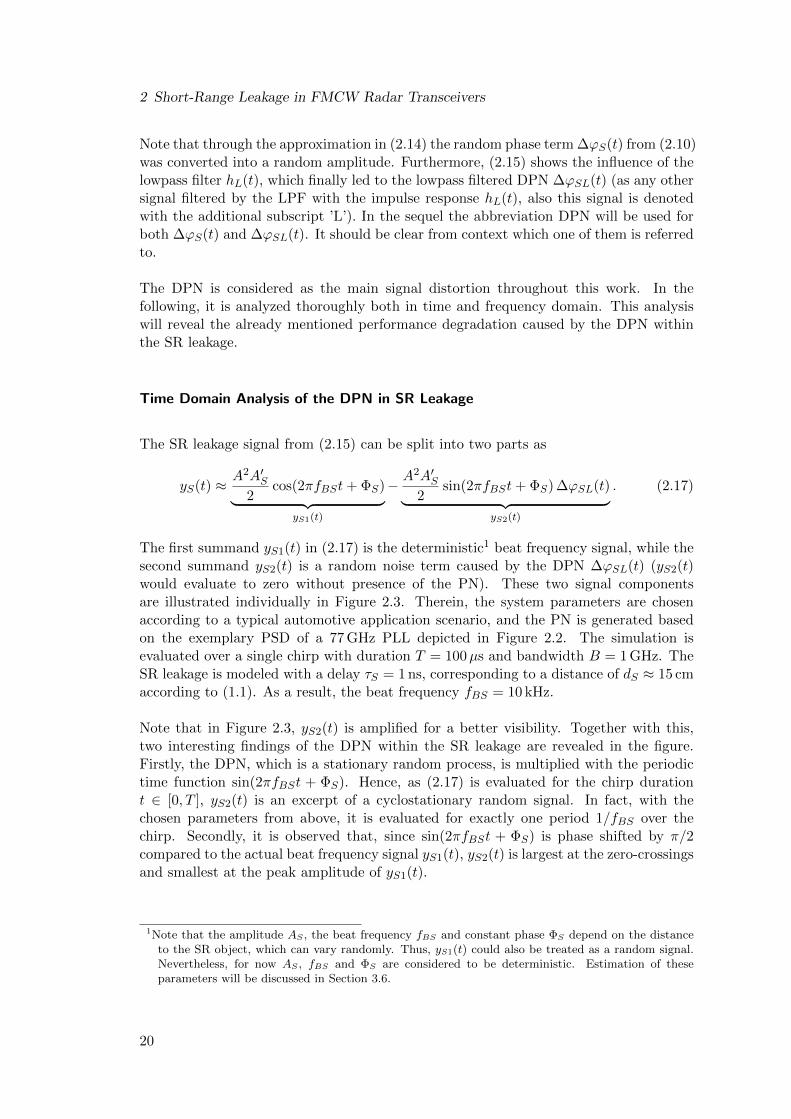
The first summand yS1(t) in (2.17) is the deterministic1 beat frequency signal, while thesecond summand yS2(t) is a random noise term caused by the DPN ∆ϕSL(t) (yS2(t)would evaluate to zero without presence of the PN). These two signal componentsare illustrated individually in Figure 2.3. Therein, the system parameters are chosenaccording to a typical automotive application scenario, and the PN is generated basedon the exemplary PSD of a 77 GHz PLL depicted in Figure 2.2. The simulation isevaluated over a single chirp with duration T = 100µs and bandwidth B = 1 GHz. TheSR leakage is modeled with a delay τS = 1 ns, corresponding to a distance of dS ≈ 15 cmaccording to (1.1). As a result, the beat frequency fBS = 10 kHz.

Note that in Figure 2.3, yS2(t) is amplified for a better visibility. Together with this,two interesting findings of the DPN within the SR leakage are revealed in the figure.Firstly, the DPN, which is a stationary random process, is multiplied with the periodictime function sin(2πfBSt + ΦS). Hence, as (2.17) is evaluated for the chirp durationt ∈ [0, T ], yS2(t) is an excerpt of a cyclostationary random signal. In fact, with thechosen parameters from above, it is evaluated for exactly one period 1/fBS over thechirp. Secondly, it is observed that, since sin(2πfBSt + ΦS) is phase shifted by π/2compared to the actual beat frequency signal yS1(t), yS2(t) is largest at the zero-crossingsand smallest at the peak amplitude of yS1(t).

1Note that the amplitude AS , the beat frequency fBS and constant phase ΦS depend on the distanceto the SR object, which can vary randomly. Thus, yS1(t) could also be treated as a random signal.Nevertheless, for now AS , fBS and ΦS are considered to be deterministic. Estimation of theseparameters will be discussed in Section 3.6.

20


0 10 20 30 40 50 60 70 80 90 100−0.3

−0.2

−0.1

0

0.1

0.2

0.3

Time t [µs]

Am

plitu

de

Beat frequency signal component yS1(t)

DPN component yS2(t) (scaled)

Figure 2.3: Short-range leakage signal components in IF domain over a single chirp for τS = 1 ns (dS ≈15 cm).

Frequency Domain Analysis of the DPN in SR Leakage

In (2.17) the SR leakage IF signal was split into the two signal components yS1(t) andyS2(t). Likewise, we may be interested in their individual contributions in frequencydomain. In FMCW radar systems typically methods based on the periodogram that mayinclude averaging (like the averaged periodogram) and/or the application of time domainwindowing are used to obtain the spectrum of the IF signal. Therewith the distancesto the objects within the radar channel are determined, since every reflection generatesa peak in the spectrum. Note, however, that through the evaluation of finite lengthsignals the peaks in the spectrum are spread over frequency. The shape of the spreadingdepends on the applied windowing. Regarding the SR leakage, the beat frequency signalyS1(t) generates such spread peaks around ±fBS in the spectrum. Note that since fBSis comparably small these spread peaks may intersect each other (again depending onthe window function).

At this point it is important to mention that the averaged periodogram or the averagedperiodogram of appropriately windowed time domain segments is also commonly usedto estimate the PSD of random signals [35]. In fact, yS2(t) is a classical random signal,since it contains the random DPN ∆ϕSL(t). Note, that through the multiplication withthe sinusoidal, yS2(t) becomes cyclostationary. Thus, we are interested in its averagePSD, which is derived in the following. It will be shown that this average PSD is ameaningful measure for the sensitivity degradation caused by the SR leakage, and thatit matches the averaged periodogram of the Hann-windowed and appropriately scaledIF signals of a simulated FMCW radar system well.

21


To start, the frequency domain characteristics of the DPN itself are evaluated. Sincethe DPN is assumed to have zero mean, its auto-covariance function is given as

c∆ϕS∆ϕS (u) = E∆ϕS(t) ∆ϕS(t+ u)= E[ϕ(t)− ϕ(t− τS)] [ϕ(t+ u)− ϕ(t+ u− τS)]= Eϕ(t)ϕ(t+ u) − Eϕ(t)ϕ(t+ u− τS)− Eϕ(t− τS)ϕ(t+ u)+ Eϕ(t− τS)ϕ(t+ u− τS), (2.18)

where E· is the expectation operator and u is the time lag. Further, with the auto-covariance function of the zero mean PN defined as

cϕϕ(u) = Eϕ(t)ϕ(t+ u), (2.19)

equation (2.18) can be rewritten as

c∆ϕS∆ϕS (u) = cϕϕ(u)− cϕϕ(u− τS)− cϕϕ(u+ τS) + cϕϕ(u)

= 2 cϕϕ(u)− cϕϕ(u− τS)− cϕϕ(u+ τS). (2.20)

Further, by applying the Wiener-Khintchine-Theorem the PSD of the DPN becomes

S∆ϕS∆ϕS (f) = Fc∆ϕS∆ϕS (u)= 2Sϕϕ(f)− Sϕϕ(f)ej2πfτS − Sϕϕ(f)e−j2πfτS

= 2Sϕϕ(f)− Sϕϕ(f)(ej2πfτS + e−j2πfτS

)= 2Sϕϕ(f) (1− cos(2πfτS)). (2.21)

This result was initially derived in [4]. With regard to (2.17), however, the PSD of thelowpass filtered DPN ∆ϕSL(t) is of interest. From (2.16) and the Wiener-Lee relationwe readily have that

c∆ϕSL∆ϕSL(u) = c∆ϕS∆ϕS (u) ∗ rEhLhL(u). (2.22)

Therein, rEhLhL(u) is the energy auto-correlation function of the LPF impulse responsehL(t). The corresponding PSD can thus be expressed as

S∆ϕSL∆ϕSL(f) = S∆ϕS∆ϕS (f) |HL(f)|2, (2.23)

where |HL(f)| is the magnitude response of the LPF. Plugging in (2.21), the PSD ofthe lowpass filtered DPN evaluates to

S∆ϕSL∆ϕSL(f) = 2Sϕϕ(f) |HL(f)|2 (1− cos(2πfτS)). (2.24)

Finally, the PSD of the cyclostationary random signal yS2(t) containing the DPN can bedetermined. The auto-covariance of the (infinitely long assumed) signal yS2(t) is time

22


dependent and evaluates to

cyS2yS2(t, t+ u) = E yS2(t) yS2(t+ u)

=(A2A′S)2

4E

1

2j

(ej(2πfBSt+ΦS) − e−j(2πfBSt+ΦS)

)∆ϕSL(t)

× 1

2j

(ej(2πfBS(t+u)+ΦS) − e−j(2πfBS(t+u)+ΦS)

)∆ϕSL(t+ u)

=

(A2A′S)2

16j2E ∆ϕSL(t) ∆ϕSL(t+ u)

[−(ej2πfBSu + e−j2πfBSu

)+(ej(2πfBS(2t+u)+2ΦS) + e−j(2πfBS(2t+u)+2ΦS)

)]=

(A2A′S)2

8c∆ϕSL∆ϕSL(u) [ cos(2πfBSu)

− cos(2πfBS(2t+ u) + 2 ΦS)] . (2.25)

Note that the remaining time dependency in the auto-covariance function would alsoresult in a time varying PSD. Thus, prior to evaluating (2.25) further, properties ofstationary and nonstationary random processes are investigated on a more generalizedlevel. In particular, the aim is to find an expression that describes the power of suchprocesses on average.

Mean Power and PSD of Stationary Zero Mean Random ProcessesLet xs(t) be a real-valued stationary and ergodic random process with zero mean. Itsmean power is

Pxs = Ex2s(t), (2.26)

which, due to the ergodicity, may also be obtained from a time average as

Pxs = limT→∞

1

T

∫ T

0x2s(t) dt. (2.27)

In practice, the mean power may thus be obtained from a sufficiently long realization ofxs(t). Further, the auto-covariance of xs(t) is

cxsxs(u) = E xs(t)xs(t+ u) , (2.28)

which, for u = 0, equals the mean power since

Pxs = cxsxs(0) = Ex2s(t). (2.29)

To further interpret this mean power, the Wiener-Khintchine-Theorem is utilized. Itstates that the PSD Sxsxs(f) of xs(t) is the Fourier transform of the auto-correlationfunction (and for zero mean processes of the auto-covariance function) [36]. Conversely,it holds that

cxsxs(u) =

∫ ∞−∞

Sxsxs(f) ej2πfudf. (2.30)

For u = 0 we thus have

Pxs = cxsxs(0) =

∫ ∞−∞

Sxsxs(f) df, (2.31)

which relates the mean power to the PSD of the stationary random process.

23


Average Mean Power and Average PSD of Nonstationary Random ProcessesNow, lets investigate a nonstationary random process xn(t) with mean power

Pxn(t) = Ex2n(t) (2.32)

and auto-covariance function

cxnxn(t, t+ u) = E xn(t)xn(t+ u) . (2.33)

Note, that in contrast to the stationary case, the mean power and auto-covariance func-tion are now time dependent. Anyhow, one may be interested in the average mean powerin some time interval of length T , which is

Pxn =1

T

∫ T

0Ex2n(t)

dt. (2.34)

With the average (over the interval T ) auto-covariance function

cxnxn(u) =1

T

∫ T

0cxnxn(t, t+ u) dt (2.35)

the average mean power also becomes

Pxn =1

T

∫ T

0cxnxn(t, t) dt = cxnxn(0), (2.36)

where cxnxn(0) is the average auto-covariance over the interval T , evaluated at lag u = 0.By introducing the average PSD as the Fourier transform of the average auto-covariancefunction (compare with the Wiener-Khintchine-Theorem)

Sxnxn(f) =

∫ ∞−∞

cxnxn(u) e−j2πfudu (2.37)

we similarly as in (2.31) obtain

Pxn =

∫ ∞−∞

Sxnxn(f) df. (2.38)

Interestingly, in the last equation the average mean power Pxn was related to the averagePSD Sxnxn(f), which can also be written as

Sxnxn(f) =

∫ ∞−∞

[1

T

∫ T

0cxnxn(t, t+ u) dt

]e−j2πfu du

=1

T

∫ T

0

[∫ ∞−∞

cxnxn(t, t+ u) e−j2πfu du

]dt, (2.39)

which suggests to define the time dependent PSD

Sxnxn(f, t) =

∫ ∞−∞

cxnxn(t, t+ u) e−j2πfu du, (2.40)

24


such that

Sxnxn(f) =1

T

∫ T

0Sxnxn(f, t) dt. (2.41)

For infinitely long arbitrary nonstationary random processes the average mean powerwithin t ∈ ]−∞,∞[ may be determined for letting T →∞ in the above equations. Onthe other hand, by considering xn(t) to be cyclostationary, it is meaningful to choose Tto be one period of this random process, and then determine its average mean power aswell as its average PSD. This will now be applied to obtain the average PSD of the SRleakage random signal yS2(t).

Average PSD of SR Leakage Random SignalWith the previous findings, the auto-covariance cyS2yS2(t, t+ u) from (2.25) can now beinvestigated further. Since yS2(t) follows a cyclostationary random process, its averageauto-covariance is determined over its period T . Together with (2.35) it immediatelyfollows to

cyS2yS2(u) =1

T

∫ T

0cyS2yS2(t, t+ u) dt

=(A2A′S)2

8c∆ϕSL∆ϕSL(u) cos(2πfBSu), (2.42)

where, through the integration over one period, the time dependent term in (2.25) van-ishes as it evaluates to zero. Therewith, from (2.42) the corresponding average PSD ofyS2(t) becomes

SyS2yS2(f) =(A2A′S)2

16[S∆ϕSL∆ϕSL(f − fBS) + S∆ϕSL∆ϕSL(f + fBS)] . (2.43)

Note that in reality the signal yS2(t) will almost never be evaluated exactly over oneperiod. Anyhow, a meaningful choice for the analytically computable average PSD of acyclostationary random process is to determine it over one period. Simulations show thatthis average PSD matches the later on regarded averaged periodograms of the Hann-windowed IF signals well, even when the chirp duration T does not exactly correspondto one period 1/fBS of the sinusoidal in yS2(t). In Chapter 5 a similar problem for thePN PSD estimation will be discussed.

As a final step, the average PSD SyS2yS2(f) shall be expressed as a function of the PLLPN PSD. This is easily obtained by substituting S∆ϕSL∆ϕSL(f) from (2.24), such that

SyS2yS2(f) =(A2A′S)2

8

[Sϕϕ(f − fBS) |HL(f − fBS)|2 (1− cos(2π(f − fBS) τS))

+ Sϕϕ(f + fBS) |HL(f + fBS)|2 (1− cos(2π(f + fBS) τS))]. (2.44)

A simplification of the above equation can be obtained by considering the beat frequencyfBS to be comparably small. For the automotive application it is in the range of somekHz only. Thus,

Sϕϕ(f) ≈ Sϕϕ(f − fBS) ≈ Sϕϕ(f + fBS), (2.45)

25


HL(f) ≈ HL(f − fBS) ≈ HL(f + fBS), (2.46)

(1− cos(2πfτS)) ≈ (1− cos(2π(f − fBS) τS)) ≈ (1− cos(2π(f + fBS) τS)), (2.47)

such that the average PSD from (2.44) can be approximated well by

SyS2yS2(f) ≈(A2A′S)2

4Sϕϕ(f) |HL(f)|2 (1− cos(2πfτS)). (2.48)

With this result a direct relation between Sϕϕ(f) and the noise term SyS2yS2(f) is estab-lished. Consequently, with the measurable PLL PN PSD, the perturbation on the overallradar system caused by the SR leakage can be specified. For the subsequent analysis,the exemplary PLL PN from Figure 2.2 is considered. Assuming typical gains for thetransmit power amplifier and LNA with GT,dB = 10 dB and GL,dB = 20 dB, respectively,and further AS,dB = −8 dB as well as an RTDT of τS = 1 ns (dS ≈ 15 cm) for the SRleakage, the average PSD from (2.48) is given as depicted in Figure 2.4. Further, forsimplicity, |HL(f)| = 1 is assumed in the passband. Interestingly, it is observed that theaverage PSD SyS2yS2(f) increases notably for IF frequencies above 100 kHz. Note, thatsince the PSDs in Figure 2.4 are depicted in dBc/Hz, they are normalized by the carrierpower.

The average noise PSD SyS2yS2(f) may exceed the intrinsic noise power as well as theAWGN from the channel, depending on the reflection factor of the SR leakage. In sucha case the overall system noise floor is raised, and sensitivity is given away. The nextsection provides a simulation example, which shows the impact of the SR leakage onthe overall system performance. As part of this analysis, the average PSD SyS2yS2(f)derived in this section, will be compared to the numerical results.

2.3 Impact of SR Leakage on System Performance

In this section a full FMCW radar system simulation is carried out to evidence theanalytical derivations and findings. The simulation environment is based on the systemmodel depicted in Figure 2.1. It considers the SR leakage and a single object (M = 1)in the channel. The on-chip leakage is neglected for reasons described already earlier(τL τS and AL AS).

For the sake of a fast simulation the FMCW chirp start frequency is set to f0 = 6 GHzinstead of the typically used 77 GHz for automotive applications. However, since theinterest is only in the IF signal, the start frequency is irrelevant. Instead, the sweepbandwidth and duration are crucial, which are chosen from a typical application scenarioto be B = 1 GHz and T = 100µs. The PLL output signal power is 0 dBm, whilethe transmit power amplifier and the receive LNA have a gain of GT,dB = 10 dB andGL,dB = 20 dB, respectively. The channel comprises of the SR leakage with an RTDTof τS = 1 ns (distance dS ≈ 15 cm), and AS,dB = −8 dB. The single target is consideredwith τT1 = 333 ns (distance dT1 ≈ 50 m), and AT1,dB = −101 dB. Further, the lowpassfiltered channel noise wL(t) = [w(t)GL s(t)] ∗ hL(t) and the lowpass filtered intrinsic

26

2.3 Impact of SR Leakage on System Performance

102 103 104 105 106 107−200

−150

−100

−50

0


PSD

[dB

c/H

z]

Exemplary PLL PN PSD, Sϕϕ(f)

2(1− cos (2πfτS)) with τS = 1 ns (dS ≈ 15 cm)

Resulting average PSD SyS2yS2(f)

Figure 2.4: Exemplary PLL PN PSD, range correlation term 2 (1 − cos(2πfτS)), and resulting averagePSD of the random signal yS2(t) contained in the SR leakage. For this simulation example,a distance of dS ≈ 15 cm was chosen.

noise vL(t) = v(t) ∗ hL(t) from (2.9), with PSDs SwLwL(f) and SvLvL(f), respectively,are bandlimited white Gaussian noise (WGN) processes and assumed to be statisticallyindependent. Together, they are assumed to have a noise contribution of SwLwL(f) +SvLvL(f) = −140 dBm/Hz in the IF domain.

To analyze the impact on the system performance, the averaged periodograms of the IFsignals with and without SR leakage are computed and depicted in Figure 2.5. As alreadynotified above, the periodograms are determined from two Hann-windowed segments perchirp (with 25% overlap)2. These averaged periodograms are properly scaled, and furtheraveraged over 8 chirps.

Without SR leakage the noise floor is defined by the channel and intrinsic transceivernoise, which is simulated with SwLwL(f) + SvLvL(f) = −140 dBm/Hz. This allows todetect the single target at 3.33 MHz. Now, by adding the SR leakage to the channelresponse, the two signal components yS1(t) and yS2(t) from (2.17) and their impactsbecome immediately visible in Figure 2.5.

Firstly, the beat frequency signal yS1(t) creates the expected peak at around fBS in thespectrum. Obviously, this peak is spread out over frequency through the windowing,

2Note that the described estimation technique for the averaged periodogram is equivalent to Welch’smethod, which is typically used for PSD estimation of stationary random processes. In the particularapplication, however, we aim to estimate the deterministic but unknown frequencies contained in theradar IF signal. Thus, in the following the resulting spectra are referred to as averaged periodogramsof the windowed IF signals.

27


0 0.5 1 1.5 2 2.5 3 3.5 4 4.5 5−145

−140

−135

−130

−125

−120

Frequency f [MHz]

Pow

er/fr

equen

cy[d

Bm

/H

z]With SR leakage

Without SR leakage

Averaged periodogram of beat frequency signal yS1(t)

Average PSD caused by DPN of SR leakage (SyS2yS2(f))

Figure 2.5: Averaged periodograms of the Hann-windowed IF signals with and without SR leakage, aswell as the analytically computed average noise PSD SyS2yS2(f) and the periodogram of thebeat frequency signal yS1(t). The radar channel contains a single object. The periodogramsare determined from two Hann-windowed segments per chirp (with 25% overlap), and furtheraveraged over 8 chirps each.

which was applied for computation of the periodogram. Secondly, the random noisesignal yS2(t) containing the DPN ∆ϕSL(t) has a significantly higher power than thechannel and intrinsic transceiver noise defined by wL(t) + vL(t). In particular, therandom noise with average PSD SyS2yS2(f) exceeds the sum of SwLwL(f) + SvLvL(f) byapproximately 6 dB for frequencies above 0.4 MHz. Hence, in the presence of SR leakagethe high-frequent DPN severely degrades the sensitivity of the radar. Ultimately, thesingle target with a beat frequency of around 3.33 MHz is covered and cannot be detected.

As reference, also the individual contributions of the SR leakage signal are shown inFigure 2.5. These are given by the averaged periodogram of the beat frequency signalyS1(t) (this signal is perfectly known in simulations) and the spectral contribution ofyS2(t), which is approximated by the analytically computed average PSD SyS2yS2(f),c.f. (2.48). Note that the averaged periodogram of the beat frequency signal yS1(t)and SyS2yS2(f) almost perfectly match the averaged periodogram determined from theIF signal of the FMCW radar system simulation with SR leakage below and above0.4 MHz, respectively. Clearly, this match is given only if SyS2yS2(f) is sufficiently largerthan SwLwL(f) +SvLvL(f), as otherwise the channel and intrinsic noise affect the overallsystem noise floor. Further simulations have shown that the average PSD SyS2yS2(f)matches the averaged periodogram also well in the case when the chirp duration T doesnot exactly correspond to one period 1/fBS of the sinusoidal in yS2(t) as in the particularsystem setup regarded in this section.

28

2.4 Outlook: SR Leakage Cancelation

2.4 Outlook: SR Leakage Cancelation

In the previous section it was shown that the detection sensitivity of the radar may beseverely affected by the SR leakage. Hence, the ultimate goal is to holistically mitigatethis unwanted, interspersed signal reflection, including its contained DPN. To motivatethe non-trivial cancelation problem at hand, a simple SR leakage canceler is now brieflyinvestigated.

2.4.1 SR Leakage Beat Frequency Suppression

In general, the SR leakage can be considered as an object reflection within the channel.It generates a peak in the periodogram of the IF signal at fBS . Thus, the beat frequencysignal could be estimated as

yS1(t) =A2A′S

2cos(2πfBSt+ ΦS), (2.49)

with fBS = kτS and ΦS = 2πf0τS − πkτ2S . Clearly, in practice the parameters A′S ,

fBS and ΦS are unknown and have to be determined accordingly (estimation of theseparameters will be discussed later on in Section 3.6). For now they are assumed to beperfectly known. Nevertheless, subtracting yS1(t) from the channel IF signal y(t) yieldscancelation of the SR leakage beat frequency signal only, but not of the random noiseterm yS2(t) containing the DPN.

The averaged periodogram with SR leakage cancelation with the signal from (2.49) isdepicted in Figure 2.6. By comparing it to the case with SR leakage (dashed line), itis observed that the beat frequency is almost perfectly suppressed (a small peak is stillvisible, which is caused by the phase distortions of the infinite impulse response (IIR)filter with impulse response hL(t)). Nevertheless, the noise term yS2(t) with the averagePSD SyS2yS2(f) remains. Unchanged, this noise term caused by the DPN dominates theoverall noise floor of the system.

In conclusion, this simple SR leakage cancelation concept is only of little help. Tomitigate the SR leakage holistically, sophisticated signal processing is required, whichalso compensates for the DPN.

2.4.2 SR Leakage Cancelation Including the DPN

The PN originates from the PLL operating in the GHz range. At a first glance, it thusseems to be impossible to mitigate this random signal, even if it has lowpass character-istic. The problem becomes even more challenging as the ultimate goal is to cancel theSR leakage in the digital IF domain, where the signals are sampled and processed withsome MHz only.

29


0 0.5 1 1.5 2 2.5 3 3.5 4 4.5 5−145

−140

−135

−130

−125

−120

Frequency f [MHz]

Pow

er/fr

equen

cy[d

Bm

/H

z]With SR leakage

Without SR leakage

With SR leakage cancelation (beat frequency signal yS1(t) only)


Figure 2.6: Averaged periodograms of the Hann-windowed IF signal with canceled beat frequency signalof the SR leakage. For reference, also the periodograms with and without SR leakage aredepicted. Obviously, suppression of the SR leakage beat frequency signal is of little help only.The periodograms are determined from two Hann-windowed segments per chirp (with 25%overlap), and further averaged over 8 chirps each.

Note, however, that due to the FMCW radar principle a distinct advantage arises. Thatis since the electromagnetic waves reflected by the objects are processed further on thesame device. Specifically, the instantaneous transmit signal is used for downconversion.Through this mixing process, the delayed PN of some reflection is subtracted from theinstantaneous PN, which then, after filtering with hL(t), forms the lowpass filtered DPN.As a result, instead of estimating the PN in the RF domain, it suffices to determine solelythe lowpass filtered DPN in the IF domain to perform a holistic mitigation of the SRleakage. This finding will be applied in the next section, wherein novel concepts forholistic SR leakage cancelation will be proposed.

30

3Short-Range Leakage Cancelation

In the previous chapter it was shown that the SR leakage causes a severe sensitivitydegradation of the FMCW radar. It turned out that this is especially due to the PNcontained within the transmit signal. Since it is a high-frequent random signal, it requiressophisticated signal processing techniques to compensate for this induced non-ideality. Inthis chapter two techniques for mitigation of the disturbing signal reflection are proposed.Both make use of an artificial OCT, which mimics an object reflection inside the radarMMIC.

The first SR leakage cancelation concept is performed in the digital domain of thetransceiver. This is achieved by extracting the DPN from the OCT IF signal. Then,using fundamental cross-correlation properties between the DPN terms of the OCT andSR leakage IF signals, the SR leakage cancelation signal is generated using a linear min-imum mean square error (MMSE) prediction. This cancelation signal is then subtractedfrom the digitized channel IF signal. The second proposed SR leakage cancelation con-cept also makes use of the cross-correlation properties between the DPN terms of theOCT and SR leakage IF signals. Different to the first concept, however, the actual SRleakage cancelation is performed in the RF domain of the transceiver.

The artificial OCT is introduced in Section 3.1 together with its physical limitationsregarding realization on chip. Then, the fundamental property of the leakage cancela-tion methods, which is the significant cross-correlation between the DPN terms of theOCT and SR leakage IF signals, is investigated in Section 3.2. Based on such, the SRleakage cancelation methods in the digital IF domain (Section 3.3) and analog RF do-main (Section 3.4) are proposed. These two are compared with respect to complexityand performance in Section 3.5. Finally, they are extended to adaptively cancel the SRleakage in Section 3.6.

The key concepts and findings of this chapter are published/accepted for publicationin [37–39], and related patents are filed/published in [40–42].

31

3 Short-Range Leakage Cancelation

PLL

s(t)

On-chip target

τO AO × +

vO(t)

LPF

hL(t)yO(t)

Figure 3.1: On-chip target signal path.

3.1 Artificial On-Chip Target

3.1.1 Overview

In this section the artificial OCT is introduced, and the radar system model in Fig-ure 2.1 is extended by such to perform SR leakage cancelation. The OCT is depictedin Figure 3.1 together with the surrounding signal processing. It comprises of a delayline on chip, and is modeled with the actual time delay and an attenuation (represent-ing the insertion loss), denoted by τO and AO, respectively. Without loss of generality,the bypass path in the block diagram in Figure 3.1, which directly feeds the mixer, isassumed with zero delay. The reader may already refer to Figure 3.2 to see how theOCT is integrated within the overall FMCW radar system model. Therein the on-chipleakage (with attenuation AL and delay τL) is neglected. It will also be ignored in allthe following considerations for the sake of simplicity.

Equivalent to the channel, the OCT is fed by the linear FMCW output signal s(t) fromthe PLL. Further, the same signal processing is applied, that is, the OCT output ismultiplied with the instantaneous transmit signal with subsequent lowpass filtering toremove the image. The resulting (ideally) lowpass filtered IF signal is in the same formof (2.10), such that

yO(t) = [AO s(t) s(t− τO) + vO(t)] ∗ hL(t)

=

[A2AO

2cos (2πfBOt+ ΦO + ∆ϕO(t))

]∗ hL(t) + vOL(t), (3.1)

wherefBO = kτO (3.2)

is the beat frequency,ΦO = 2πf0τO − kπτ2

O (3.3)

is a constant phase, and the DPN of the OCT is ∆ϕO(t) = ϕ(t) − ϕ(t − τO). Further,vO(t) models intrinsic noise, and vOL(t) = vO(t) ∗ hL(t) is its lowpass filtered version.Note that the OCT artificially mimics a radar target within the radar transceiver.

32

3.1 Artificial On-Chip Target

3.1.2 Restriction of Delay Lines in MMICs

At this point the SR leakage IF signal is reconsidered. From (2.10) it is given as

yS(t) =

[A2A′S


]∗ hL(t). (3.4)

Since (3.4) is in the form of (3.1), it is easily verified that choosing τO = τS and AO = A′S ,would yield yO(t) = yS(t). This includes the high-frequent random PN term since

τO = τS ⇒ ∆ϕO(t) = ∆ϕS(t). (3.5)

Obviously, this theoretically allows for perfect SR leakage cancelation, when subtractingthe OCT IF signal yO(t) from the channel IF signal y(t). This cancelation approach isshown in the extended system model depicted in Figure 3.2.

Note, that in the above considerations, the two noise sources v(t) and vO(t) have beendisregarded. These noise sources encompass intrinsic noise of the channel and OCTpath in the MMIC, specifically from the mixer. For now, they are neglected, but will bereconsidered later on in Section 3.3.7.

Although the presented concept would potentially mitigate the SR leakage well, thereis a severe limitation making it infeasible for realization in MMICs. This limitation iscaused by the required delay line of the OCT. Assuming the RTDT of the SR leakageto be in the range of a nanosecond, a delay line on chip, which achieves this amount ofdelay would increase the area significantly. Further, the insertion loss would be severe.This makes the requirement τO = τS untenable, and thus the leakage cancelation conceptfrom Figure 3.2 unfeasible.

As turns out from the discussion in Appendix A.5, a potential realization of the OCT ispossible with τO being significantly smaller than τS . To evaluate whether the SR leakagecancelation is possible even with this limitation, the OCT IF signal is evaluated further.

3.1.3 DPN Extraction from the On-Chip Target

Different to object reflections, which are perturbed by channel noise and other reflections,the impurity within the OCT IF signal is determined through intrinsic noise sources only.This entails the idea to extract the DPN from the OCT IF signal yO(t), which is shownin the sequel.

With the cosine sum identity (3.1) can be rewritten as

yO(t) =

[A2AO

2cos(2πfBOt+ ΦO) cos(∆ϕO(t))

− A2AO2

sin(2πfBOt+ ΦO) sin(∆ϕO(t))

]∗ hL(t) + vOL(t). (3.6)

33


PLL

s(t)

GT

Radar channel

Object reflections

Short-range leakage

τS ASrS(t)

+

+w(t)

GL

r(t)

× +

v(t)

LPF

hL(t)

y(t)

On-chip target

τO AO ×rO(t)

+

vO(t)

LPF

hL(t)

yO(t)

+

−z(t)

Figure 3.2: First approach for SR leakage cancelation with artificial OCT, with τO = τS and AO = A′S .

As for the SR leakage, the DPN ∆ϕO(t) is considered to be sufficiently small. Hence,together with cos(∆ϕO(t)) ≈ 1 and sin(∆ϕO(t)) ≈ ∆ϕO(t), (3.6) can be approximatedas

yO(t) ≈ A2AO2

cos(2πfBOt+ ΦO)

− A2AO2

sin(2πfBOt+ ΦO) ∆ϕOL(t) + vOL(t), (3.7)

where ∆ϕOL(t) is the lowpass filtered version of ∆ϕO(t), that is

∆ϕOL(t) = ∆ϕO(t) ∗ hL(t). (3.8)

This derivation is analogous to yonder carried out in Section 2.2.2 for the SR leakage,and, similarly, the DPN is converted to amplitude noise through the approximationin (3.7). Solving for it yields

∆ϕOL(t) ≈A2AO

2 cos(2πfBOt+ ΦO)− (yO(t)− vOL(t))A2AO

2 sin(2πfBOt+ ΦO). (3.9)

Thus, from the observable signal yO(t) the estimator

∆ϕOL(t) =A2AO

2 cos(2πfBOt+ ΦO)− yO(t)A2AO

2 sin(2πfBOt+ ΦO)(3.10)

34

3.2 Cross-Correlation Properties between DPN Terms

is obvious to perform the DPN extraction. Clearly, in practice the term yO(t) is accessibleas sampled version from an analog to digital converter (ADC) only. Denoting thissampled signal as yO[n] = yO(t)|t=nTs , where Ts is the sampling interval of the ADC,the estimate for the discrete-time DPN alters to

∆ϕOL[n] =A2AO

2 cos(2πfBOnTs + ΦO)− yO[n]A2AO

2 sin(2πfBOnTs + ΦO). (3.11)

Note that A, AO and τO are design parameters, and are thus well known. Consequently,the sine and cosine terms in (3.11) can be evaluated with fBO = kτO and ΦO = 2πf0τO−kπτ2

O. At this point it becomes clear already, that the quality of the extracted DPNhighly depends on the intrinsic noise vOL(t), and further on the quantization noise ofthe ADC. In Section 3.3.7 this will be discussed in detail, and a technique to optimallyconfigure the OCT delay line is proposed.


The analysis from the previous section revealed that the DPN can be extracted fromthe OCT IF signal. Specifically, since τO is tightly constrained, it is of interest how theDPN alters for various delays and how it is statistically related to the DPN of the SRleakage. Subsequently, this analysis is carried out on a generalized level.

3.2.1 DPN for Various Delays

Let the DPN of the delay τO be

∆ϕO(t) = ϕ(t)− ϕ(t− τO). (3.12)

The PN ϕ(t) is considered as a stationary random process, and is characterized by thePSD Sϕϕ(f). The DPN ∆ϕO(t) is depicted in Figure 3.3 for different delays τO ∈40 ps, 160 ps, 300 ps, 400 ps, 800 ps. For this analysis, a single realization of the PNϕ(t), generated from the exemplary PSD given in Figure 2.2, is regarded.

Interestingly, there is a noticeable similarity between the array of curves. The DPNterms seem to be shifted in time, and scaled in amplitude. The smaller the delay τO,the smaller the amplitudes are. This scaling arises from the range correlation derivedin (2.21). According to such, the PSD of ∆ϕO(t) is

S∆ϕO∆ϕO(f) = 2Sϕϕ(f) (1− cos(2πfτO)). (3.13)

The exemplary PN PSD Sϕϕ(f) is depicted in Figure 3.4 together with the corre-sponding, analytically computed PSD S∆ϕO∆ϕO(f) for different delays τO. Again,τO ∈ 40 ps, 160 ps, 300 ps, 400 ps, 800 ps is chosen. It is observed that, as was seenfrom a single PN realization in time domain in Figure 3.3 already, the DPN powerincreases with the delay τO.

35


0 1 2 3 4 5 6 7 8 9 10−1

−0.5

0

0.5

1

1.5·10−2

Time t [ns]

DP

N∆ϕO

(t)

τO = 40 ps

τO = 160 ps

τO = 300 ps

τO = 400 ps

τO = 800 ps

Figure 3.3: Exemplary DPN signals with different delays τO for a realization of the PN ϕ(t) over 10 ns.

3.2.2 Cross-Correlation Properties

For further analysis of the DPN, the simple model given in Figure 3.5 is considered.Therein, a second delay τS is introduced, for which it is assumed that τO ≤ τS . Analogousto (3.12) its DPN is introduced as

∆ϕS(t) = ϕ(t)− ϕ(t− τS). (3.14)

To quantify the similarity observed from the array of curves in Figure 3.3, the cross-covariance between ∆ϕO(t) and ∆ϕS(t) is employed. With the stationarity assumption,and the fact that the DPN terms have zero mean, it is given as

c∆ϕO∆ϕS (u) = E∆ϕO(t) ∆ϕS(t+ u). (3.15)

Note, that since the DPN has zero mean, the cross-covariance equals the cross-correlation.Further, the normalized cross-covariance between ∆ϕO(t) and ∆ϕS(t) is given as

ρ∆ϕO∆ϕS (u) =c∆ϕO∆ϕS (u)√σ2

∆ϕOσ2

∆ϕS

, (3.16)

where σ2∆ϕO

and σ2∆ϕS

are the variances of the two DPN processes.

A numerical approximation of the normalized cross-covariance ρ∆ϕO∆ϕS (u) is depicted inFigure 3.6 for a fixed τS = 800 ps. Further, τO ∈ 40 ps, 160 ps, 300 ps, 400 ps, 800 ps is

36


102 103 104 105 106 107

−200

−180

−160

−140

−120

−100

−80

−60


PN

/D

PN

PSD

[dB

c/H

z] Sϕϕ(f)

S∆ϕO∆ϕO (f), τO = 40 ps





Figure 3.4: Exemplary PN PSD Sϕϕ(f) together with the corresponding, analytically computed DPNPSD S∆ϕO∆ϕO (f) for different delays τO.

ϕ(t)

τS +−

∆ϕS(t)

τO +−

∆ϕO(t)

Figure 3.5: Model utilized to analyze and compare two DPN terms.

chosen again. The cross-covariances were evaluated in a discrete-time simulation, wherethe expectation operator was approximated over a statistically representative numberof samples. It is clear that with τO = τS perfect correlation is achieved, such that thenormalized cross-covariance evaluated at zero lag becomes

ρ∆ϕO∆ϕS (0)|τO=τS = 1. (3.17)

With decreasing delay τO the normalized cross-covariance steeply decays when evalu-ated at ρ∆ϕO∆ϕS (0) (dashed line in Figure 3.6). However, the maxima of each of thenormalized cross-covariance functions are shifted towards a negative lag with decreasingτO, or an increasing difference τS − τO. Note that this time shift was already observedintuitively in Figure 3.3 from a single PN realization. This time shift is computed in thefollowing.

37


−1.2 −1 −0.8 −0.6 −0.4 −0.2 0 0.2 0.4 0.6 0.8 1 1.2 1.4 1.6 1.8

−0.5

0

0.5

1

Lag u [ns]

ρ∆ϕO

∆ϕS

(u)

τO = 40 ps

τO = 160 ps

τO = 300 ps

τO = 400 ps

τO = 800 ps

Figure 3.6: Normalized cross-covariance ρ∆ϕO∆ϕS (u) for a fixed τS = 800 ps and various values for τO.It is evaluated in a discrete-time simulation, where the expectation operator is approximatedover a statistically representative number of samples. The PN time domain samples weregenerated from the exemplary PN PSD given in Figure 2.2.

3.2.3 Optimum Lag

Substituting the DPN terms in (3.15) with (3.12) and (3.14) gives

c∆ϕO∆ϕS (u) = E[ϕ(t)− ϕ(t− τO)] [ϕ(t+ u)− ϕ(t+ u− τS)]= Eϕ(t)ϕ(t+ u)− ϕ(t)ϕ(t+ u− τS)

− ϕ(t− τO)ϕ(t+ u) + ϕ(t− τO)ϕ(t+ u− τS). (3.18)

Thus, the optimum lag u that maximizes the normalized cross-covariance depends onthe delays τO and τS .

Note that (3.18) merely consists of auto-covariance functions. Introducing it for the zeromean PN as

cϕϕ(u) = Eϕ(t)ϕ(t+ u), (3.19)

the cross-covariance can be expressed as

c∆ϕO∆ϕS (u) = cϕϕ(u)− cϕϕ(u− τS)− cϕϕ(u+ τO) + cϕϕ(u− τS + τO). (3.20)

Further, utilizing the Wiener-Khintchine-Theorem, the auto-covariance function of thePN can be computed with

cϕϕ(u) =

∫ ∞−∞

Sϕϕ(f) ej2πufdf, (3.21)

38


100 200 300 400 500 600 700 8000

0.2

0.4

0.6

0.8

1

Delay τO [ps]

Norm

alize

dcr

oss

-cov

ari

ance

Sampled in origin (lag u = 0)

Sampled at optimal offset (lag u = uopt)

Figure 3.7: Normalized cross-covariance evaluated in the origin (u = 0) and at the optimum lag uopt.The latter shows a severely better correlation between the two DPN terms ∆ϕO(t) and∆ϕS(t). The PN time domain samples were generated from the exemplary PN PSD givenin Figure 2.2.

which, again equals the auto-correlation function of the PN due to the zero mean assump-tion. It is important to note, that, according to (3.21), the shape of cϕϕ(u) is defined bythe PSD Sϕϕ(f). Now, to analytically find the optimum lag, cϕϕ(u) is assumed as 4th

order polynomial in the range of 0≤u≤τS − τO. Applying this approximation to (3.20),differentiating it with respect to u, setting the result to zero, and solving for u revealsthe optimum lag that maximizes (3.15) depending on the delays τO and τS as

uopt =τS − τO

2. (3.22)

A detailed derivation and analysis on the optimum lag is provided in Appendix A.2.

The numerical approximation of the normalized cross-covariance ρ∆ϕO∆ϕS (u) evaluatedin the origin, that is u = 0, against ρ∆ϕO∆ϕS (u) evaluated at the optimum lag uopt isdepicted in Figure 3.7. For u = 0 the values of the normalized cross-covariance decayfast with τO becoming smaller. However, evaluating ρ∆ϕO∆ϕS (u) at the optimum lagsuopt results in significantly higher values. Note that the correlation is present up to verylarge τS/τO ratios. For instance, even with τS = 800 ps and τO = 40 ps, yielding a τS/τOratio of 20, a significant normalized cross-covariance of 0.94 is obtained.

39


3.2.4 Linear MMSE Prediction

The cross-correlation properties analyzed in the previous section suggest that ∆ϕS(t)can be estimated from a shifted version of ∆ϕO(t). Actually, a linear prediction can beperformed. With the two DPN terms having zero mean, the best linear estimator in theMMSE sense is given as [35]

∆ϕS(t− uopt) = α∆ϕO(t), (3.23)

with the DPN scaling factor

α =c∆ϕO∆ϕS (uopt)

c∆ϕO∆ϕO(0). (3.24)

Note that the optimum lag uopt is incorporated into the estimator in both (3.23) and (3.24).

3.2.5 Scaling Factor with Lowpass Filtered DPN

So far the PN has been considered as stationary random process with PSD Sϕϕ(f).However, according to the FMCW radar system model, the DPN is lowpass filtered.This filtering with the impulse response hL(t) is crucial for the computation of the DPNscaling factor. In this section the scaling factor for linear MMSE prediction after lowpassfiltering is derived.

The lowpass filtered versions of the two DPN terms ∆ϕO(t) and ∆ϕS(t) are given as

∆ϕOL(t) = ∆ϕO(t) ∗ hL(t) = [ϕ(t)− ϕ(t− τO)] ∗ hL(t) (3.25)

and∆ϕSL(t) = ∆ϕS(t) ∗ hL(t) = [ϕ(t)− ϕ(t− τS)] ∗ hL(t), (3.26)

respectively. Therewith, the linear MMSE prediction is carried out as

∆ϕSL(t− uopt) = αL ∆ϕOL(t), (3.27)

where the lowpass filtered DPN scaling factor αL becomes, according to (3.24),

αL =c∆ϕOL∆ϕSL(uopt)

c∆ϕOL∆ϕOL(0)

=E ∆ϕOL(t) ∆ϕSL(t+ uopt)

E ∆ϕOL(t) ∆ϕOL(t)

=E [∆ϕO(t) ∗ hL(t)] [∆ϕS(t+ uopt) ∗ hL(t)]

E [∆ϕO(t) ∗ hL(t)] [∆ϕO(t) ∗ hL(t)], (3.28)

and an estimate of ∆ϕOL(t) may be obtained with (3.10).

From (3.28) it can be seen that αL is computed from the filtered versions of the auto- andcross-covariance functions of the DPN terms ∆ϕO(t) and ∆ϕS(t). Using the Wiener-Leeidentity we have that

c∆ϕOL∆ϕOL(u) = c∆ϕO∆ϕO(u) ∗ rEhLhL(u), (3.29)

40


where rEhLhL(u) is the energy auto-correlation function of the impulse response hL(t)of the lowpass filter. It can be shown that the Wiener-Lee identity also holds for thecross-covariance (Appendix A.3), such that

c∆ϕOL∆ϕSL(u) = c∆ϕO∆ϕS (u) ∗ rEhLhL(u). (3.30)

With this result also the Fourier transforms of (3.29) and (3.30) can be written in similarand compact forms, which is

S∆ϕOL∆ϕOL(f) = S∆ϕO∆ϕO(f) |HL(f)|2 (3.31)

andS∆ϕOL∆ϕSL(f) = S∆ϕO∆ϕS (f) |HL(f)|2, (3.32)

respectively. For an analytic description of S∆ϕOL∆ϕOL(f) and S∆ϕOL∆ϕSL(f), however,it is desirable to express them in terms of the PN PSD Sϕϕ(f), which is well known fromthe design specifications. Using (2.21), (3.31) can be expressed as

S∆ϕO∆ϕO(f) = Sϕϕ(f)κτO(f), (3.33)

where κτO(f) = 2 (1−cos(2πfτO)). Based on (3.20) the cross-PSD between ∆ϕO(t) and∆ϕS(t) follows to

S∆ϕO∆ϕS (f) = Sϕϕ(f)− Sϕϕ(f) e−j2πfτS

− Sϕϕ(f) ej2πfτO + Sϕϕ(f) ej2πf(τO−τS)

= Sϕϕ(f)κτOτS (f), (3.34)

with κτOτS (f) = 1− e−j2πfτS − ej2πfτO + ej2πf(τO−τS).

Plugging in (3.33) and (3.34), the lowpass filtered PSDs from (3.31) and (3.32) become

S∆ϕOL∆ϕOL(f) = Sϕϕ(f)κτO(f) |HL(f)|2 (3.35)

andS∆ϕOL∆ϕSL(f) = Sϕϕ(f)κτOτS (f) |HL(f)|2, (3.36)

respectively. Finally, with the inverse Wiener-Khinchine theorem the DPN scaling factorfrom (3.28) becomes

αL =c∆ϕOL∆ϕSL(uopt)

c∆ϕOL∆ϕOL(0)

=

∫∞−∞ S∆ϕOL∆ϕSL(f) ej2πfuopt df∫∞

−∞ S∆ϕOL∆ϕOL(f) df

=

∫∞−∞ Sϕϕ(f)κτOτS (f) |HL(f)|2 ej2πfuopt df∫∞

−∞ Sϕϕ(f)κτO(f) |HL(f)|2 df. (3.37)

From (3.37) it is observed that the computation of αL merely requires knowledge ofthe delays τO, τS , the PN PSD Sϕϕ(f) and the LPF magnitude response |HL(f)|. For

41


τO τS τS/τO uopt DPN scaling DPN scaling

[ps] [ps] ratio [ps] factor α factor αL

40 800 20 380 11.76 19.974

80 800 10 360 6.45 9.987

160 800 5 320 3.28 4.993

400 800 2 200 1.43 1.995

Table 3.1: Exemplary values for the DPN scaling factors α and αL for different τS/τO ratios.

completeness, numerical approximations of α and αL are given in Table 3.1 for differentτS/τO ratios. For that, an ideal lowpass filter with a cutoff frequency of fc = 25 MHzand the exemplary PN PSD Sϕϕ(f) from Figure 2.2 are regarded. As can be seen fromTable 3.1, αL is larger than α for all τS/τO ratios.

In conclusion, α and αL are measures of how much the DPN signals ∆ϕO(t) and ∆ϕOL(t),respectively, need to be scaled to approximate ∆ϕS(t) and ∆ϕSL(t) well. This findingwill be applied in the next sections proposing SR leakage cancelation methods in FMCWradar systems.

Finally, for comparison, the normalized cross-covariance between the lowpass filteredDPN terms ∆ϕOL(t) and ∆ϕSL(t) is analyzed in the same way as it was done in Sec-tion 3.2.2 for the unfiltered DPN terms ∆ϕO(t) and ∆ϕS(t). It is defined as

ρ∆ϕOL∆ϕSL(u) =c∆ϕOL∆ϕSL(u)√σ2

∆ϕOLσ2

∆ϕSL

, (3.38)

where σ2∆ϕOL

and σ2∆ϕSL

are the variances of the two lowpass filtered DPN processes.

A numerical approximation of the normalized cross-covariance ρ∆ϕOL∆ϕSL(u) is depictedin Figure 3.8 for a fixed τS = 800 ps and various values for τO ∈ 40 ps, 160 ps, 300 ps,400 ps, 800 ps (exactly the same values were also used in Figure 3.6). It is important tonote that, in contrast to the normalized cross-covariance ρ∆ϕO∆ϕS (u) of the unfilteredDPN terms (Figure 3.6), ρ∆ϕOL∆ϕSL(u) is smoothed out over a wide range of the lagu (note the different ranges for the abscissa and ordinate between Figure 3.6 and Fig-ure 3.8). As a consequence, for the lowpass filtered case, the normalized cross-covarianceat u = 0 and at the optimum lag u = uopt do not differ noteworthy. Still, simulationsshow that the optimum lag uopt is unchanged to the lowpass filtered case (further dis-cussions on the optimum lag are provided in Appendix A.2). All these important findingwill be applied later on in Section 3.4.

42

3.3 SR Leakage Cancelation in Digital IF Domain

−6 −4 −2 0 2 4 6 80.8

0.85

0.9

0.95

1

Lag u [ns]

ρ∆ϕO

L∆ϕSL

(u)

τO = 40 ps

τO = 160 ps

τO = 300 ps

τO = 400 ps

τO = 800 ps

Figure 3.8: Normalized cross-covariance ρ∆ϕOL∆ϕSL(u) for a fixed τS = 800 ps and various values for τO.It is evaluated in a discrete-time simulation, where the expectation operator is approximatedover a statistically representative number of samples. The PN time domain samples weregenerated from the exemplary PN PSD given in Figure 2.2.


3.3.1 Cross-Correlation Properties Applied to the FMCW Radar SystemModel

In the previous section it was shown that there exists a noticeable correlation betweenthe two DPN terms for the delays τO of the OCT and τS of the SR leakage. Due to theaforementioned circuit design limitations we constrain τO ≤ τS , which was also assumedin Section 3.2. Further, the delays considered for τO and τS were assumed below onenanosecond. This equals a distance of up to 15 cm, which is realistic for the SR leakagein an automotive application. Consequently, the findings from the previous section allowto propose a first SR leakage cancelation algorithm, which is to be carried out in thedigital IF domain.

For leakage cancelation, the OCT is integrated into the system model as depicted inFigure 3.9. It is placed in parallel to the channel, and fed by the same transmit signals(t). Further, downconversion to the IF and subsequent lowpass filtering is done.

With regard to the system model at hand, the optimum lag uopt derived in Section 3.2.3,is realized in the FMCW radar system model by slightly delaying the sampling clock ofthe ADC of the channel signal path. This is indicated by Toffset in Figure 3.9. According

43


to (3.22) the optimum sampling clock offset is

Toffset =τS − τO

2. (3.39)

Given the physical constraints for τS and τO, the sampling clock offset Toffset will be inthe range of some hundred picoseconds. Assuming the ADC sampling frequency to bein the MHz range, Toffset is only a fraction of the sampling interval Ts. The DPN scalingfactor αL can be computed readily from (3.37). Therewith, the linear MMSE predictionof the lowpass filtered DPN of the SR leakage is carried out accoring to (3.27) as

∆ϕSL(t− Toffset) = αL ∆ϕOL(t). (3.40)

Considering the FMCW radar system model, all the parameters in (3.37) and (3.39)except τS are well known design parameters. However, since for a specific applicationscenario τS can be tightly constrained, an offline computation of the DPN scaling factoris feasible. In case τS changes slightly over time, a look up table could be used to readjustαL in a regular manner. Adaptive SR leakage cancelation will be discussed in detail inSection 3.6.

The aim of the leakage canceler introduced in Figure 3.9 is to find the cancelation signalyS [n] given yO[n], where the latter is the discrete-time version of yO(t) with time indexn. Since τO is smaller than τS , the resulting beat frequencies and the constant phaseoffsets in their respective IF signals are different. The leakage canceler therefore has toemploy the following steps:

1) Extract the DPN from the OCT IF signal with beat frequency fBO (Section 3.3.2).

2) Generate the expected sinusoidal corresponding to the SR leakage with beat frequencyfBS , including the DPN from step 1, to obtain yS [n] (Section 3.3.3).

3) Finally, to perform the cancelation, yS [n] is subtracted from the receive signal y[n](Section 3.3.4).

These steps are discussed in detail in the next three subsections.

3.3.2 DPN Extraction from the OCT IF Signal

The DPN extraction was presented in Section 3.1 already. Since the leakage cancelationis performed in the digital IF domain, the sampled version of the OCT IF signal is usedfor DPN extraction. From (3.7) it evaluates to

yO[n] ≈ A2AO2

cos(2πfBOnTs + ΦO)

− A2AO2

sin(2πfBOnTs + ΦO) ∆ϕOL[n] + vOL[n], (3.41)

44


PLL

s(t)

GT

Radar channel

Object reflections

Short-range leakage

τS ASrS(t)

+

+w(t)

GL

r(t)

× +

v(t)

LPF

hL(t)

y(t)ADC

Ts, Toffset

On-chip target

τO AO ×rO(t)

+

vO(t)

LPF

hL(t)

yO(t)ADC

Ts

yO[n]

Leakage

Canceler

y[n]

yS [n]

+

−z[n]

Figure 3.9: System model with the artificial OCT. The leakage canceler extracts the DPN from the OCTIF signal, and generates the cancelation signal yS [n] using the linear MMSE prediction.

where Ts = 1/fs is the sampling interval and fs is the sampling frequency. Therewith,the sampled lowpass filtered DPN and intrinsic noise are ∆ϕOL[n] = ϕ(nTs)−ϕ(nTs−τO)and vOL[n] = vOL(nTs), respectively. The DPN is then extracted as

∆ϕOL[n] =A2AO

2 cos(2πfBOnTs + ΦO)− yO[n])A2AO


Since the parameters τO and AO are known circuit design parameters, the OCT beatfrequency and the constant phase can be easily determined as fBO = kτO and ΦO =2πf0τO − kπτ2

O, respectively. For clarification, the OCT output signal yO[n] and theexpected beat frequency signal A2AO/2 cos(2πfBOnTs+ΦO) are depicted in Figure 3.10for a short cutout of a chirp. Therein, the errors induced by the DPN become visible.

3.3.3 SR Leakage Cancelation Signal Generation

In Section 3.2 it was shown that there exists a significant cross-correlation between twoDPN terms for delays with a ratio of up to 20. This finding is now utilized to generatethe cancelation signal yS [n].

45


24.5 24.6 24.7 24.8 24.9 25 25.1 25.2 25.3 25.4

0.11

0.11

0.11

0.11

0.11

Time t [µs]

Am

plitu

de

Expected OCT IF beat frequency signal

OCT IF signal carrying DPN

Figure 3.10: OCT IF signal with DPN as well as its expected version without DPN for a short part of achirp.

Using the linear MMSE prediction, the SR leakage cancelation signal is in the form of

yS [n] =A2A′S

2cos

2πfBS(nTs − Toffset) + ΦS + αL ∆ϕOL[n]︸︷︷︸∆ϕSL[n]

, (3.43)

where A′S = GT ASGL is the overall expected SR leakage reflection factor, fBS is the

expected beat frequency, and ΦS is the expected constant phase. Further, Toffset is thesampling clock offset from (3.39), αL is the DPN scaling factor from (3.28), and ∆ϕOL[n]is the extracted DPN from the OCT determined from (3.42). Note that in the aboveequation the discrete-time DPN estimate was introduced as

∆ϕSL[n] = αL ∆ϕOL[n], (3.44)

although, according to (3.40), the corresponding continuous-time version also considersToffset as

∆ϕSL(nTs − Toffset) = αL ∆ϕOL(nTs). (3.45)

From Figure 3.8 it becomes clear that for the lowpass filtered case the normalized cross-covariance at u = 0 and at the optimum lag u = uopt do not differ noteworthy. Hence,since Toffset is comparably small, ∆ϕSL[n] = ∆ϕSL(nTs− Toffset) was assumed in (3.43),and will also be used for simplicity from now on.

The OCT IF signal yO[n] and the SR leakage cancelation signal yS [n] are compared inFigure 3.11 for a τS/τO ratio of 5. As a result, the beat frequency of the SR leakage is 5times higher than that of the OCT IF signal. Further, in the zoom window of Figure 3.11the DPN contained in the SR leakage cancelation signal yS [n] can be seen in more detail.

46


0 10 20 30 40 50 60 70 80 90 100

−1

−0.5

0

0.5

1

Time t [µs]

Am

plitu

de

OCT IF signal

SR leakage cancelation signal

28 28.25 28.5

−0.21

−0.2

−0.19

Figure 3.11: OCT IF signal yO[n] and SR leakage cancelation signal yS [n] over a single chirp with τS/τO =5. In the zoom window the DPN incorporated into the SR leakage cancelation signal yS [n]becomes visible. The IF signals are normalized to have unit amplitude.

Note that the linear prediction of the DPN of the SR leakage in (3.43) for a given timeinstant n is carried out from a single sample of the extracted DPN ∆ϕOL[n]. In orderto try to reduce the influence of noise within this DPN term, a prediction filter conceptis discussed in Appendix A.4. It turns out, however, that for the chosen parameters ofa state of the art automotive radar such a prediction filter does not improve the simpleprediction used in (3.43).

Clearly, the parameters τS and A′S cannot be estimated as precise as those of the OCT asthe SR leakage reflections are superimposed by the channel reflections and the AWGN.Also, they may alter slowly over time and with a changing environment. To deal withsuch a changing environment, the presented SR leakage cancelation concept will beextended in Section 3.6 to an adaptive one.

The true SR leakage IF signal yS [n] and the cancelation signal yS [n] are depicted inFigure 3.12 for a short part of the chirp. It is observed that yS [n] can be estimatedalmost perfectly. Clearly, in reality yS [n] is not accessible, but is shown here to evidencethe effectiveness of the proposed method only.

47


24.5 24.6 24.7 24.8 24.9 25 25.1 25.2 25.3 25.4

−1

0

1

2

·10−2

Time t [µs]

Am

plitu

de

True SR leakage IF signal

SR leakage cancelation signal

Figure 3.12: True SR leakage IF signal and corresponding cancelation signal for a short cutout of a chirp.As has been shown in the derivation, with the extracted DPN from the OCT IF signal andthe linear prediction of the DPN, the SR leakage signal can be estimated almost perfectly.

3.3.4 Leakage Cancelation

The final step is to subtract the received signal from the expected SR leakage signal,that is

z[n] = y[n]− yS [n]. (3.46)

The cancelation error, which will be evaluated as part of the performance analysis, isdefined as

e[n] = yS [n]− yS [n], (3.47)

where yS [n] is the true SR leakage signal (which, as mentioned already, is accessible onlyin simulation) and yS [n] is the cancelation signal from (3.43).

3.3.5 MIMO Scenario

In order to measure not only the distance but also the angular position of objects,multiple input multiple output (MIMO) radars are utilized [43]. The angle is estimatedout of the different round-trip delay times from the transmit to the receive antennas.Consequently, the beat frequencies and phase terms in the IF domain differ for each ofthe receive paths.

48


In particular, for cancelation of the SR leakage, the parameters of the sinusoidals needto be adjusted to all these paths. However, due to the DPN cross-correlation propertiesfound in Section 3.2, a single OCT signal path is sufficient to perform the leakage can-celation. First, the DPN is extracted from the single OCT IF signal path. Then, severalSR leakage cancelation signals are generated, each of them with a different amplitude,beat frequency and constant phase. Each of these cancelation signals also contains adifferent DPN term. However, due to the cross-correlation properties, those can be esti-mated well using the linear prediction with the extracted DPN from the OCT IF signal.The scaling factor αL may be recomputed for each of the receive paths (although it willalter only marginally since the delay τS stays almost unaffected given the small antennaspacings of a state of the art 77 GHz radar).

3.3.6 System Performance Evaluation

In this section a full FMCW radar system simulation is carried out to show the effective-ness of the proposed leakage cancelation algorithm. The simulation environment is basedon Figure 3.9. The system parameters are chosen according to a typical automotive radarsystem.

As for the simulation carried out in Section 2.3 for the SR leakage analysis, the chirp startfrequency is set to f0 = 6 GHz for the sake of a fast simulation. However, the proposedconcept works in the same way for higher carrier frequencies as the essential signalprocessing is done in the IF domain. The sweep bandwidth is chosen to be B = 1 GHz,which is ramped within T = 100µs. The PLL output signal power is 0 dBm, whilethe transmit power amplifier and the receive LNA have a gain of GT,dB = 10 dB andGL,dB = 20 dB, respectively.

The channel comprises of the SR leakage with an RTDT τS = 1 ns (distance dS ≈ 15 cm),AS,dB = −8 dB, and a single target with τT1 = 333 ns (distance dT1 ≈ 50 m). The OCTparameters are chosen as τO = 192 ps (resulting dS/dO ratio is approximately 5) andAO,dB = −20 dB (further details on the OCT signal path will be provided in Section 3.3.7,wherein the optimum delay and the architecture for the OCT are investigated). Theresulting beat frequencies for the OCT and SR leakage are fBO = 1.9 kHz and fBS =10.0 kHz, respectively.

The AWGN wL(t) from the channel and the intrinsic noise vL(t) are assumed to havea total noise floor at SwLwL(f) + SvLvL(f) = −140 dBm/Hz in the IF domain. Theintrinsic noise of the OCT path vOL(t) is simulated with SvOLvOL(f) = −155 dBm/Hz.The noise sources w(t), v(t) and vO(t) are simulated as bandlimited WGN processes andassumed to be statistically independent.

Considering the sampling frequency of the ADC to be fs = 100 MHz, the cutoff fre-quencies of the lowpass filters are chosen as fc = 25 MHz. They are modeled as 6thorder infinite impulse response Butterworth filters. The ADC sampling offset Toffset andthe DPN scaling factor αL are computed according to (3.39) and (3.37). The ADC is

49


0 0.5 1 1.5 2 2.5 3 3.5 4 4.5 5−145

−140

−135

−130

−125

−120

Frequency f [MHz]

Pow

er/fr

equen

cy[d

Bm

/H

z]With SR leakage, no leakage cancelation

Without SR leakage

SR leakage canceled in the digital IF domain

Figure 3.13: Averaged periodograms of the Hann-windowed IF signals for different scenarios. The sys-tem simulated with SR leakage but without its cancelation results in a noise floor that isdominated by the DPN. Without SR leakage present at all, the AWGN sets the systemsnoise floor and therewith the target detection sensitivity. With the proposed SR leakagecancelation in place the DPN of the SR leakage is significantly suppressed, and the targetwith a beat frequency of around 3.33 MHz resolved well. The periodograms are determinedfrom two Hann-windowed segments per chirp (with 25% overlap), and further averaged over8 chirps each.

simulated with a resolution of 14 bit3.

The averaged periodograms of the IF signals for different scenarios are provided inFigure 3.13. Firstly, with SR leakage but no leakage cancelation a peak close to DCoriginating from the beat frequency fBS occurs. The overall system’s noise floor isincreased as has been observed already in Section 2.3. Consequently, the target witha beat frequency of around 3.33 MHz is covered in noise. Secondly, assuming that noSR leakage is present in the system, the AWGN sets the noise floor. Therewith, thetarget is resolved well. Thirdly, the averaged periodogram of the IF signal with SRleakage and the proposed cancelation algorithm with the OCT in place is depicted inFigure 3.13. It can be seen that the effect of the DPN from the SR leakage is suppressedby around 6.4 dB and that the target is resolved well. This evidences the effectivenessof the proposed method.

An interesting insight on the leakage cancelation performance is revealed by investigatingthe cancelation error e[n] = yS [n]−yS [n], depicted in Figure 3.14 over a single chirp. It isobserved that omitting the DPN within yS [n], i.e. αL = 0, results in a higher cancelation

3Note that the unit bit represents a binary symbol here (rather than a unit of information commonlyused in information theory).

50


0 10 20 30 40 50 60 70 80 90 100−1.5

−1

−0.5

0

0.5

1

1.5·10−3

Time t [µs]

Cance

lati

on

erro

re[n

]

Cancelation error with αL = 0

Cancelation error with optimum αL

Figure 3.14: SR leakage cancelation error with αL = 0 as well as with the optimum αL, evaluated overa single chirp.

error compared to the cancelation with the optimum αL. It is highly interesting that thecyclostationary nature of the error signal can also be deduced from this analysis. Note,that even with the optimum αL, a residual cancelation error remains. On the one handthis remaining error is due to the fact that there is no perfect correlation between theDPN terms. On the other hand, the error is defined by the channel and intrinsic noiseof the transceiver, as well as the quantization noise of the ADC.

3.3.7 Optimum Delay and Limitations of DPN Extraction

For SR leakage cancelation in the digital IF domain the DPN was extracted from theOCT IF signal based on (3.42). Clearly, this extraction is affected by the noise withinthe measureable OCT IF signal. Further, according to the range correlation [4], theDPN power decreases with smaller τO. Thus, a minimum on-chip delay is required suchthat the DPN power exceeds the intrinsic noise as well as the quantization noise of theADC. Also, note that according to (3.7) the DPN ∆ϕOL(t) is multiplied/scaled with asinusoidal with frequency fBO and constant phase ΦO. Both of these parameters dependon τO. It will turn out that the optimum delay τO has to be chosen in a way such thatthis sinusoidal reaches its maximum at the middle of the chirp. In the sequel all theseconstraints are taken into account to derive the optimum delay for realization of theOCT in an MMIC. For that, a refined system model of the OCT is introduced first.

51


PLL

s(t)GDL

On-chip target

τO AO ×

Gmix

+

vO(t)

LPF

hL(t)+

vADC(t)

yO(t)

Figure 3.15: Refined on-chip target signal path for realization in an MMIC.

Refined OCT System Model

To represent the OCT in the MMIC in a more realistic way, the signal path from Fig-ure 3.1 is slightly extended to the one depicted in Figure 3.15. In addition to the earlierused model, a preamplifier with gain GDL and the mixer gain Gmix are introduced. Aswill become clear later on, the preamplifier is required due to the high insertion loss ofdelay lines in MMICs. Note also that in Figure 3.15 the quantization noise vADC(t) ofthe ADC was added.

From (3.1) the modified OCT IF signal with the newly introduced system parametersimmediately follows to

yO(t) =[G2

DLAOGmix s(t) s(t− τO) + vO(t)]∗ hL(t) + vADC(t)

=

[A2G2

DLAOGmix


]∗ hL(t)

+ vOL(t) + vADC(t). (3.48)

For repetition, yO(t) is an observable signal defined by the amplitude A of the transmitsignal, the insertion loss of the delay line AO, the beat frequency fBO, a constant phaseΦO, the DPN ∆ϕO(t), and the impulse response hL(t) of the LPF. Further, vOL(t) =vO(t)∗hL(t) is the lowpass filtered intrinsic noise and vADC(t) is quantization noise fromthe ADC. Note, that since it is more convenient to conduct the following investigationsin the analog domain, also the ADC quantization noise is modeled as a continuous signalhere for simplicity reasons. By applying the approximations from (3.7) in (3.48), we havethat

yO(t) ≈A2G2

DLAOGmix

2cos(2πfBOt+ ΦO)

−A2G2

DLAOGmix

2sin(2πfBOt+ ΦO) ∆ϕOL(t) + vOL(t) + vADC(t), (3.49)

such that the DPN is extracted as

∆ϕOL(t) =

A2G2DLAOGmix

2 cos(2πfBOt+ ΦO)− yO(t)A2G2

DLAOGmix


In order to determine the variance of the estimator ∆ϕOL(t), (3.49) is plugged into (3.50),

52


which yields

∆ϕOL(t) =

A2G2DLAOGmix

2 sin(2πfBOt+ ΦO) ∆ϕOL(t)− vOL(t)− vADC(t)A2G2

DLAOGmix

2 sin(2πfBOt+ ΦO)

= ∆ϕOL(t)− vOL(t) + vADC(t)A2G2

DLAOGmix


Therewith, the variance of the estimator ∆ϕOL(t) becomes

Var(∆ϕOL(t)) =1

(A2G2DLAOGmix)2

4 sin2(2πfBOt+ ΦO)

(σ2vOL

+ σ2vADC

), (3.52)

where σ2vOL

and σ2vADC

are the variances of vOL(t) and vADC(t), respectively.

Now, to extract the DPN according to (3.50) with sufficient accuracy, it requires

σ2∆ϕOL

Var(∆ϕOL(t)), (3.53)

where σ2∆ϕOL

is the variance of the zero mean lowpass filtered DPN ∆ϕOL(t). Togetherwith (3.31) it can be readily determined by

σ2∆ϕOL

= E

∆ϕ2OL(t)

=

∫ fc

−fc2Sϕϕ(f) |HL(f)|2 (1− cos(2πfτO)) df, (3.54)

where fc is the cutoff frequency of the LPF.

Optimized Design of Delay Line

According to (3.52), the variance Var(∆ϕOL(t)) can be split into two product terms.Firstly, the term

1

sin2(2πfBOt+ ΦO), (3.55)

which is time dependent and a function of τO with fBO = kτO, and is required to beminimized to achieve minimum variance Var(∆ϕOL(t)). Secondly, a term containing thescaled intrinsic and quantization noise variances as

1

K

(σ2vOL

+ σ2vADC

), (3.56)

with

K =(A2G2

DLAOGmix)2

4. (3.57)

These two terms are individually investigated in the sequel in order to find the optimumτO.

53


180 190 200 210 220 230 240 250 260 270 2800

0.2

0.4

0.6

0.8

1

Delay τO [ps]

sin

2(2πkτ OT/2

+2πf 0τ O−πkτ

2 O)

Figure 3.16: Optimum choices of τO.

Minimization of Time Dependent TermAs was discussed earlier already, the beat frequency fBO of the OCT IF signal is compa-rably small, thus the term sin2(2πfBOt + ΦO) is evaluated for an excerpt of the period1/fBO only. Therewith, to minimize the variance Var(∆ϕOL(t)) for t ∈ [0, T ], τO shouldbe chosen such that the term sin2(2πfBOt+ ΦO) reaches its maximum at the middle ofthe chirp, i.e., at t = T/2. Hence, the optimum τO is determined as

τO,opt = arg maxτO∈R

sin2

(2πfBO

T

2+ ΦO

)= arg max

τO∈Rsin2

(2πkτO

T

2+ 2πf0τO − kπτ2

O

). (3.58)

Note that this optimization is ambiguous due to the periodicity of the sin function.Considering the same chirp parameters as from Section 3.3.6 with B = 1 GHz, T = 100µsand f0 = 6 GHz, the first five optimum values for τO that maximize sin2(2πfBOt+ ΦO)are

τO,opt ∈ 38 ps, 115 ps, 192 ps, 269 ps, 346 ps. (3.59)

Note that these values depend on the chirp start frequency f0 and slope k = B/T , andthus have to be recomputed for a different configuration. Anyhow, they can be easilyobtained by solving (

2πkτOT

2+ 2πf0τO − kπτ2

O

)= (2n− 1)

π

2, (3.60)

for n ∈ N. Figure 3.16 shows the terms sin2(2πkτOT/2 + 2πf0τO − πkτ2O) for 180 ps ≤

τO ≤ 280 ps. It can be seen that τO = 192 ps and τO = 269 ps would be optimal choicessince the maximization from (3.58) is achieved for both delays.

From Figure 3.16 it can be further deduced that a bad choice for τO would be, forinstance, 232 ps. Then the time dependent term sin2(2πfBOt+ΦO) would have its mini-mum at t = T/2, i.e., in the middle of the chirp. To show the impact of the choice of τO,the term sin2(2πfBOt+ΦO) as well as a scaled version of sin2(2πfBOt+ΦO) ∆ϕOL(t) aredepicted in Figure 3.17 for our example with τO = 192 ps and τO = 232 ps, respectively,

54


0 10 20 30 40 50 60 70 80 90 100

−0.5

0

0.5

1

Time t [µs]

Am

plitu

de

0 10 20 30 40 50 60 70 80 90 100

−0.5

0

0.5

1

Time t [µs]

Am

plitu

de

sin2(2πfBOt+ ΦO) sin2(2πfBOt+ ΦO) ∆ϕOL(t), scaled

Figure 3.17: OCT IF signal terms sin2(2πfBOt+ΦO) and a scaled version of sin2(2πfBOt+ΦO) ∆ϕOL(t)for τO = 192 ps and τO = 232 ps.

over the chirp duration T . It is observed that the resulting amplitudes for the DPNare significantly larger with τO = 192 ps, while for the case where τO = 232 ps the DPNalmost vanishes in the middle of the chirp. The impact of this bad choice for τO on theSR leakage cancelation performance will be shown after the next section.

Intrinsic and Quantization NoiseWith the values for τO,opt found in (3.59) in a first step, the impact of the intrinsicand quantization noise can now be analyzed. The intrinsic noise vO(t) is assumed to beWGN. Thus, the integrated noise power within the bandwidth of the ideally assumedLPF with cutoff frequency fc evaluates to

PvOL =

∫ fc

−fcSvOvO(f) df = 2SvOvO(f) fc. (3.61)

To obtain the variance σ2vOL

of vO(t), the power PvOL needs to be divided by the corre-sponding resistance.

On the other hand, the variance of the quantization noise of the ADC is given as

σ2vADC

=q2

12, (3.62)

55


whereq = 2−Q+1 (3.63)

equals one least significant bit (LSB). Here, Q is the bitwidth and a unit input voltagerange (±1V ) was assumed.

With the variances for the intrinsic and the quantization noise being defined, the re-quirement σ2

∆ϕOL Var(∆ϕOL(t)) can now be evaluated for the different delays τO,opt

from (3.59), which were found in the first step. For that, numerical computations arecarried out with the following assumptions. The gain GDL is chosen in a way such thatit compensates the insertion loss of the delay line AO, i.e., GDL = 1/AO. The insertionlosses are chosen based on an LC delay line integrated in MMICs (the reader may referto Appendix A.5 for details). Further, for the sake of a fair comparison, the mixer gainGmix is chosen such that K = 1V 2 is achieved. This way, the input voltage range of theOCT beat frequency signal to the ADC is ±1V independent of the delays τO,opt, andthus also the quantization noise remains the same for the different τO,opt. For this firstanalysis, an ADC with Q = 14 bit is considered (σ2

vADC= 1.24 nV2). Finally, based on

circuit simulations it is assumed that SvOLvOL(f) = −155 dBm/Hz, thus σ2vOL

= 0.79 nV2

according to (3.61) with fc = 25 MHz and a resistance of R = 50 Ω.

The most important parameters as well as the ratios of σ2∆ϕOL

/Var(∆ϕOL(t)), com-pare (3.53), are summarized in Table 3.2 for the different τO,opt values from (3.59) andan ADC bitwidth of Q = 14. The variance of the DPN σ2

∆ϕOLwas numerically de-

termined based on (3.54) together with the exemplary PLL PN PSD from Figure 2.2.Note again, that σ2

∆ϕOLdepends on the delay τO. From the table it is deduced that

for τO = 38 ps the ratio between σ2∆ϕOL

and Var(∆ϕOL(t)) is below 1. Thus, the ex-tracted DPN would be highly perturbed by the noise. For the case with τO = 115 psand τO = 192 ps ratios of 2.00 and 5.55, respectively, are achieved. This steady increaseis in line with the earlier finding that the DPN power increases with the delay τO (cf.Figure 3.4). The ratio of 5.55 can be considered to be sufficient for the DPN extractionas will be seen immediately in the upcoming system simulation example. For highervalues of τO, the ratio between σ2

∆ϕOLand Var(∆ϕOL(t)) raises further. Still, since the

aim is to find the minimum delay for the OCT, which allows to extract the DPN withsufficient accuracy,

τO,opt = 192 ps (3.64)

is chosen. Realization options of the OCT in an MMIC with this amount of delay arediscussed in Appendix A.5.

As mentioned, the quantization noise of the ADC highly affects the extraction of theDPN. To show this, the ratio of σ2

∆ϕOL/Var(∆ϕOL(t)) in dependence of the ADC

bitwidth Q is investigated. Assuming the optimum delay with τO = 192 ps, and varyingthe bitwidth Q ∈ 13, 14, 15 yields the ratios provided in Table 3.3. From this it followsthat for the particularly chosen parameters, Q = 13 bit may yield a poor DPN extractiondue to σ2

∆ϕOL/Var(∆ϕOL(t)) = 1.96 only. For Q = 14 and Q = 15 a significantly better

performance is expected. Detailed simulation results with exactly these three differentbitwidths will be provided as part of the analysis in the next section.

56


τO 38 ps 115 ps 192 ps 269 ps 346 ps

AO,dB = −GDL,dB −6.0 dB −15.6 dB −20.0 dB −22.9 dB −25.1 dB

Gmix,dB 19.9 dB 10.4 dB 6.0 dB 3.1 dB 0.9 dB

K 1V 2

Var(∆ϕOL(t)) 2.032e-9

σ2∆ϕOL

0.45e-9 4.06e-9 11.27e-9 22.10e-9 36.54e-9

σ2∆ϕOL

/Var(∆ϕOL(t)) 0.22 2.00 5.55 10.87 17.98

Table 3.2: Comparison of optimum delays and the resulting ratios of σ2∆ϕOL

/Var(∆ϕOL(t)) for an ADCbitwidth of Q = 14.

τO = 192 ps Q = 13 bit Q = 14 bit Q = 15 bit

σ2∆ϕOL

/Var(∆ϕOL(t)) 1.96 5.55 10.24

Table 3.3: Ratios of σ2∆ϕOL

/Var(∆ϕOL(t)) for different ADC bitwidths Q.

Impact on SR Leakage Cancelation Performance

In Section 3.3.3 the SR leakage cancelation concept was verified based on simulationsalready. Note that therein the optimized delay line with τO = 192 ps has been used.Hence, the findings from this chapter are incorporated properly in the earlier resultsalready. Anyhow, in the sequel the SR leakage cancelation performance with differentconfigurations is analyzed further.

Suboptimal OCT DelayIt was found previously that, to minimize the variance of ∆ϕOL(t), τO needs to be chosensuch that the sin2(·) term in (3.52) is evaluated around its peak value of 1 during thechirp. This way the optimum delay with τO = 192 ps was found, together with theconstraint on the intrinsic and quantization noise. Now, consider the suboptimal choicefor the delay of the OCT with τO = 232 ps. The resulting averaged periodogram of theSR leakage canceled IF signal is depicted in Figure 3.18. As can be seen, the choice ofτO = 232 ps leads to a poor SR leakage cancelation performance, since it yields a highvariance of the estimator ∆ϕOL(t). This poor performance may be explained with thelower plot of Figure 3.17, showing that for τO = 232 ps the DPN of the OCT IF signalalmost vanishes in the middle of the chirp. This way the DPN cannot be extracted well.

Quantization NoiseAlso the quantization noise plays an important role for the variance of the estimator∆ϕOL(t). To show the impact of the bitwidth on the SR leakage cancelation, again asystem simulation is regarded. Figure 3.19 shows the averaged periodograms of the SRleakage canceled IF signals for Q = 13, Q = 14 and Q = 15 bit (note that for thisanalysis the quantization was applied only for the ADC, and further signal processing

57


0 0.5 1 1.5 2 2.5 3 3.5 4 4.5 5−145

−140

−135

−130

−125

−120

Frequency f [MHz]

Pow

er/fr

equen

cy[d

Bm

/H


Without SR leakage

SR leakage canceled in the digital IF domain (τO = 232 ps)

Figure 3.18: Averaged periodograms of the Hann-windowed IF signals. For the SR leakage cancelationthe suboptimal OCT delay τO = 232 ps was chosen.

was done in double-precision format). It becomes evident that with Q = 14 and Q = 15a very good cancelation performance is achieved as the curves almost coincide with thecase without SR leakage. For Q = 13, however, the quantization noise starts to increasethe variance of ∆ϕOL(t) significantly. Thus, the optimum bitwidth for the particularchoice of the parameters is Q = 14.

3.4 SR Leakage Cancelation in RF Domain

In the previous section an SR leakage cancelation concept, which is carried out mainlyin the digital IF domain, was proposed. This concept makes use of the OCT, essen-tially consisting of a delay line. The cancelation is based on cross-correlation propertiesbetween the residual PN contained in the SR leakage and the OCT IF signal, even ifthe time delay of the OCT is much smaller than the actual round-trip delay time of theSR leakage. This enables SR leakage cancelation with significantly relaxed area require-ments. A slight drawback of this solution, however, is that the cancelation is limited byintrinsic noise of the MMIC, as well as quantization noise from the ADC.

In this section a novel mixed-signal based approach for SR leakage cancelation is pro-posed, which also makes use of the artificial OCT. Different to the first concept, however,the actual cancelation is carried out in the RF domain. The cancelation signal is gener-ated in the digital IF domain. It is modulated onto the OCT output signal in the RFdomain with an I/Q mixer with image rejection, and then subtracted from the receive

58


0 0.5 1 1.5 2 2.5 3 3.5 4 4.5 5−145

−140

−135

−130

−125

−120

Frequency f [MHz]

Pow

er/fr

equen

cy[d

Bm

/H

z]

With SR leakage, no leakage cancelation

Without SR leakage

SR leakage canceled in the digital IF domain (Q = 13 bit)



Figure 3.19: Averaged periodograms of the Hann-windowed IF signals with SR leakage cancelation fordifferent ADC bitwidths (Q = 13, Q = 14 and Q = 15 bit).

signal from the channel. Through the cancelation in the RF domain, requirements onthe intrinsic and ADC quantization noise floor can be relaxed. Also, the requirementson the resolution of the digital to analog converter (DAC) are low. That is since themain goal is to cancel the PN of the SR leakage, and the actual PN for its mitigation isadded to the cancelation signal in the (analog) RF domain.

It is important to mention that the herein suggested concept is similar to existing cance-lation/separation approaches for on-chip leakage [6,7,11]. However, for on-chip leakage,the PN can either be considered as negligible [37], or, compensated for since the referencepath on chip carries the same PN [6]. As was discussed in Chapter 2 already, for the SRleakage this is not as trivial due to the comparably large time delay.

3.4.1 System Model

Short-Range Leakage in RF DomainTo start, in the following the SR leakage in the RF domain is briefly described. Recapthe transmit signal, which is assumed as linear FMCW signal determined as

s(t) = A cos(2πf0t+ πkt2 + Φ + ϕ(t)

), (3.65)

for t ∈ [0, T ], with the chirp duration T . Further, A determines the output amplitude,f0 is the chirp start frequency, k is the linear chirp sweep slope, Φ is a constant initialphase, and ϕ(t) is the PN.

59


The radar channel depicted in Figure 3.20 consists of object reflections, the SR leakage,as well as channel noise w(t). For now, only the SR leakage contribution to the overallreceive signal r(t) is of interest. It is modeled as an attenuated and delayed version ofs(t), given as

rS(t) = GTAS s(t− τS), (3.66)

where GT determines the gain of the transmit power amplifier, and AS and τS modelthe reflected amplitude and the round-trip delay time of the SR leakage, respectively.

For this second approach the aim is to cancel the SR leakage signal rS(t) in the RFdomain. Still, for the derivation, its contribution to the IF signal will be regarded. TheIF signal (filtered with the LPF with impulse response hL(t), which is assumed to haveperfect attenuation at around 2f0) is readily given by (2.5) as

yS(t) =

[A2GTASGL


]∗ hL(t), (3.67)

where fBS = k τS is the beat frequency, ΦS = 2πf0τS − πkτ2S is a constant phase, and

∆ϕS(t) = ϕ(t)− ϕ(t− τS) is the DPN.

Trivial SR Leakage Cancelation in RF Domain Using the OCTBased on Figure 3.1 and (3.1) the ideally lowpass filtered OCT IF signal becomes

yO(t) =

[A2AOGL


]∗ hL(t), (3.68)

with fBO = k τO, ΦO = 2πf0τO − πkτ2O, and ∆ϕO(t) = ϕ(t)−ϕ(t− τO) being the DPN.

By comparing (3.67) and (3.68), it becomes clear that choosing AO = GTAS and τO = τSwould, theoretically, yield perfect SR leakage cancelation. To perform such in the RFdomain, the OCT output signal rO(t) could simply be subtracted from the received signalr(t) as depicted in Figure 3.20. However, as mentioned already, delay lines in MMICscannot fulfill these requirements due to the high insertion loss and the required area.This makes the trivial leakage cancelation concept in Figure 3.20 infeasible. Hence, ashas been done for the digital IF leakage cancelation in Section 3.3, the OCT delay τOwill be considered to be much smaller than τS for the following considerations. A firstimmediate consequence of this is that fBO becomes proportionally smaller with

fBO =τOτSfBS . (3.69)

To compensate for this frequency offset, the following leakage cancelation utilizes an I/Qmodulator in the RF domain.

3.4.2 Cancelation Concept

With the required basic signal processing presented in the previous section, the actualcancelation concept is proposed now. The model of such is depicted in Figure 3.21.

60


PLL

s(t)

GT

Radar channel

Object reflections

Short-range leakage

τS AS

rS(t)

+

+w(t)

r(t)

+

−GL × +

v(t)

LPF

hL(t)y(t)

On-chip target

τO AOrO(t)

Figure 3.20: System model of the FMCW radar transceiver with SR leakage. A trivial leakage cancelationconcept in the RF domain making use of the OCT is shown. Due to the limitations of delaylines, however, this concept is not feasible for realization within MMICs.

Modulation of OCT Output SignalThe OCT output signal in the RF domain is a delayed and scaled version of the transmitsignal s(t), given as

rO(t) = AO s(t− τO)

= AAO cos(2πf0(t− τO) + πk(t− τO)2 + Φ + ϕ(t− τO)

). (3.70)

This output signal is now modulated with an I/Q mixer with image rejection. Thesinusoidal modulation signal is generated in the digital domain. After digital to analogconversion (DAC) it can be written as

yM (t) = AM cos (2πfM t+ ΦM ) , (3.71)

wherein AM , fM , and ΦM are the amplitude, frequency and phase, respectively. Thislow-frequency signal is fed into a 90 hybrid, which splits it into two paths. The firstpath is output directly, while the second one is phase-shifted by 90. These two outputsare then multiplied with the OCT output signal rO(t), which forms the I and Q paths

61


as

rOM,I(t) = AAOAM cos(2πf0(t− τO) + πk(t− τO)2 + Φ + ϕ(t− τO)

)× cos (2πfM t+ ΦM )

=AAOAM

2

cos(2πf0(t− τO) + πk(t− τO)2 + Φ + ϕ(t− τO)− 2πfM t− ΦM

)+ cos

(2πf0(t− τO) + πk(t− τO)2 + Φ + ϕ(t− τO) + 2πfM t+ ΦM

) (3.72)

and

rOM,Q(t) = AAOAM cos(2πf0(t− τO) + πk(t− τO)2 + Φ + ϕ(t− τO)

)× sin (2πfM t+ ΦM )

=AAOAM

2

sin(2πf0(t− τO) + πk(t− τO)2 + Φ + ϕ(t− τO) + 2πfM t+ ΦM

)− sin

(2πf0(t− τO) + πk(t− τO)2 + Φ + ϕ(t− τO)− 2πfM t− ΦM

) , (3.73)

respectively. The two signals rOM,I(t) and rOM,Q(t) are merged in a second 90 hybrid.Therein, rOM,Q(t) is first phase-shifted by 90 as

r′OM,Q(t) =AAOAM

2

cos(2πf0(t− τO) + πk(t− τO)2 + Φ + ϕ(t− τO) + 2πfM t+ ΦM

)− cos


) , (3.74)

and subsequently subtracted from rOM,I(t). Therewith, the output of the second 90

hybrid yields

rOM (t) = rOM,I(t)− r′OM,Q(t)

=AAOAM

2

cos(2πf0(t− τO) + πk(t− τO)2 + Φ + ϕ(t− τO)− 2πfM t− ΦM

)+ cos


)− cos


)+ cos


) . (3.75)

Note that the upper image resulting from the mixing process is suppressed in the aboveequation, such that finally the modulated OCT output signal in the RF domain becomes

rOM (t) = AAOAM cos(2πf0t− 2πf0τO + πkt2 − 2πkτOt+ πkτ2

O + Φ + ϕ(t− τO)

− 2πfM t− ΦM ) . (3.76)

Without loss of generality, in this work solely an up-chirp, i.e. a positive slope k in (3.65),is considered. For a down-chirp, r′OM,Q(t) would simply have to be added to rOM,I(t)

62


(instead of subtracted from it) within the second 90 hybrid. Then, from (3.75) itbecomes obvious that the lower image from the mixing process would be suppressed.

For the SR leakage cancelation in the RF domain, rOM (t) is subtracted from the receivesignal r(t) according to Figure 3.21. It remains to identify the design parameters of themodulation signal yM (t). This identification will be done based on the IF domain signal.Still, it is important to keep in mind that the actual cancelation is performed fully inthe RF domain.

Identification of Modulation Signal ParametersIn order to identify the free design parameters AM , fM and ΦM in (3.71), the leakagecanceled IF signal is regarded. According to Figure 3.21 it is given as

y(t) = [(r(t)− rOM (t))GL s(t) + v(t)] ∗ hL(t)

= [GL r(t) s(t)−GL rOM (t) s(t) + v(t)] ∗ hL(t)

= [GL r(t) s(t)] ∗ hL(t)︸︷︷︸Channel IF signal

− [GL rOM (t) s(t)] ∗ hL(t)︸︷︷︸Modulated OCT IF signal yOM (t)

+ v(t) ∗ hL(t), (3.77)

where v(t) models intrinsic noise within the MMIC. Note that in the last step the channelsignal, containing the SR leakage, and the signal from the OCT were completely sepa-rated in the IF domain. Assuming the image from the mixing process to be suppressedby the LPF, the IF signal of the modulated OCT signal evaluates to

yOM (t) = [GL rOM (t) s(t)] ∗ hL(t)

=

[A2AOGLAM

2cos(2πf0t+ πkt2 + Φ + ϕ(t)− 2πf0t+ 2πf0τO − πkt2

+ 2πkτOt− πkτ2O − Φ− ϕ(t− τO) + 2πfM t+ ΦM

) ]∗ hL(t)

=

[A2AOGLAM

2cos (2π(kτO + fM ) t + ΦO + ΦM + ∆ϕO(t))

]∗ hL(t). (3.78)

This signal has a similar form as the SR leakage IF signal in (3.67), and contains theOCT attenuation AO, the delay τO, the constant phase ΦO = 2πf0τO − πkτ2

O as well asthe DPN ∆ϕO(t). Now, for SR leakage cancelation the free parameters AM , fM and ΦM

are targeted to be chosen such that (3.78) equals (3.67). Therewith, for the frequencyand constant phase it is immediately verified that they have to be chosen as

fM!

= fBS − kτO = fBS − fBO, (3.79)

and

ΦM!

= ΦS − ΦO

= 2πf0τS − πkτ2S − 2πf0τO + πkτ2

O, (3.80)

respectively.

63

3S

hort-R

ange

Leakage

Can

celation

PLL

s(t)

GT

Radar channel

Object reflections

Short-range leakage

τS ASrS(t)

+

+w(t)

+

−GL

r(t)× +

v(t)

LPF

hL(t)

y(t)ADC

Ts

y[n]

On-chip target

τO AO

×

×

rO(t) Leakage

cancelerDAC

yM (t)90

hybrid

90

hybrid

rOM,I(t)

rOM,Q(t)

rOM (t)

Figure 3.21: System model for SR leakage cancelation in the RF domain.

64


For the amplitude AM this choice is not as straightforward. In fact there are twocontradicting requirements. To show this, lets reconsider the lowpass filtered SR leakageIF signal, which from (2.17) is given as

yS(t) ≈ A2GTASGL2

cos(2πfBSt+ ΦS)︸︷︷︸yS1(t)

− A2GTASGL2

sin(2πfBSt+ ΦS) ∆ϕSL(t)︸︷︷︸yS2(t)

. (3.81)

Equivalently, the modulated OCT IF signal from (3.78) may be approximated by

yOM (t) ≈ A2AOGLAM2

cos (2π(kτO + fM ) t+ΦO+ΦM )

− A2AOGLAM2

sin (2π(kτO + fM ) t+ΦO+ΦM ) ∆ϕOL(t). (3.82)

Note, that within (3.81) and (3.82), the lowpass filtered DPN terms ∆ϕSL(t) = ∆ϕS(t)∗hL(t) and ∆ϕOL(t) = ∆ϕO(t) ∗ hL(t) became amplitude noise terms. Further, recapthat there exists the cross-correlation between ∆ϕSL(t) and ∆ϕOL(t), even if τO τS .Therewith, the DPN of the SR leakage can be estimated well by4

∆ϕSL(t) = αL ∆ϕOL(t), (3.83)

where αL is the DPN scaling factor computed from (3.37). Regarding the approximationsin (3.81) and (3.82) again, it becomes clear that choosing

AM!

=GTASAO

αL (3.84)

almost perfectly cancels the term yS2(t).

However, with this choice, the beat frequency signal yS1(t), which is described by thefirst summand in (3.81), isn’t suppressed perfectly. In fact, to cancel yS1(t),

AM!

=GTASAO

(3.85)

would have to be chosen. Anyhow, based on the earlier analysis, the term yS2(t) causesthe sensitivity degradation of the radar, and is thus more important for the cancelation.Consequently, AM is computed according to (3.84). In summary, the only drawback is,that after cancelation, a residual peak from the remaining beat frequency signal yS1(t)at fBS in the spectrum occurs. Still, as will be discussed in Section 3.4.4, this peak canbe suppressed with a highpass filter.

4The careful reader may notice that, compared to (3.45), the sampling offset Toffset is omitted in (3.83).This is due to the fact that for the SR leakage cancelation proposed in this section, the samplingoffset cannot be implemented. Anyhow, based on the discussion in Section 3.2.5, the sampling offsetis almost irrelevant after lowpass filtering the DPN with the LPF with impulse response hL(t).

65


3.4.3 MIMO Scenario

As for the SR leakage cancelation in the digital IF domain, the MIMO radar scenariois discussed also for the proposed cancelation in the RF domain. For the digital cance-lation it was found that the SR leakage IF signal in a MIMO scenario yields differentamplitudes, beat frequencies, constant phase terms as well as DPN terms (the latter arederived from a single OCT signal path).

To perform the SR leakage cancelation in the RF domain for a MIMO setup with severalreceive paths, each of these would require a DAC for the generation of the sine tone withthe different parameters. Further, each of the outputs of the DACs are required to beconnected to an extra I/Q modulator (including the 90 hybrids), which mixes it withthe OCT output signal. This is a significant disadvantage. Still, due to the correlationproperties of the DPN found in Section 3.2, also here a single OCT suffices to carry outthe cancelation for all receive paths.

3.4.4 System Performance Evaluation

In this section a system simulation is performed to show the effectiveness of the proposedmethod and to compare it to the cancelation in the digital IF domain. For that, exactlythe same parameters as in Section 3.3.6 are used. That is, the chirp bandwidth andduration are B = 1 GHz and T = 100µs, respectively, and the OCT and SR leakagetime delay are τO = 192 ps and τS = 1 ns, respectively. This gives a ratio of τS/τO ≈ 5,resulting in a comparably small area required for the OCT.

In Figure 3.22 the averaged periodograms of the IF signals for different scenarios areprovided. The first three scenarios are equivalent to the ones shown in Figure 3.13already. That is, a scenario with SR leakage but no leakage cancelation, and the casewith no SR leakage present at all in the system. Further, the averaged periodogram withthe SR leakage canceled in the digital IF domain is depicted. It is observed that withoutSR leakage the system noise floor is defined by the intrinsic and channel noise simulatedat −140 dBm/Hz. In presence of the SR leakage, however, its high-frequent DPN (withinthe IF signal bandwidth) degrades the sensitivity by approximately 6 dB. Consequently,the single target with a beat frequency of around 3.33 MHz cannot be detected. Usingthe SR leakage cancelation in the digital IF domain, the noise floor is suppressed almostdown to the intrinsic and channel noise, making the single target detectable.

To evaluate the performance of the cancelation in the RF domain, its averaged peri-odogram of the IF signal is also shown in Figure 3.22. Comparing the results to thecancelation in the digital IF domain, it is observed that the performance is fairly equalfor frequencies above 600 kHz. For smaller frequencies, the beat frequency signal itselfdominates in the spectrum. This results from AM being chosen such that the DPN iscanceled, instead of the beat frequency signal itself. Anyhow, the frequency range ofinterest for object reflections with tiny amplitudes is in the MHz-range with distances of10 meters and above. As mentioned, the beat frequency signal can be suppressed with

66

3.5 Comparison of SR Leakage Cancelation Concepts

a highpass filter. Ultimately, the noise floor at higher frequencies is reduced, and thesingle target within the channel at 3.33 MHz is resolved well in both cases. Without SRleakage cancelation it would be covered in the DPN.

Finally, note that through the leakage cancelation in the RF domain the requirements onthe intrinsic and ADC quantization noise are relaxed compared to the cancelation in thedigital IF domain presented in Section 3.3. To explain this, recap that the SR leakagecancelation in the digital IF domain operates with the DPN, while the cancelation in theRF domain directly cancels the PN in the receive signal. Specifically, for the cancelationin the digital IF domain the OCT output signal is downconverted, and the (lowpassfiltered) DPN ∆ϕOL[n] is used to generate the SR leakage cancelation signal yS [n]. Thisoperation is done after the mixing process in the IF domain, thus the DPN is dealt with.

On the other hand, for the SR leakage cancelation in the RF domain, the cancelationsignal rOM (t) (containing the PN ϕ(t− τO) of the OCT) is subtracted from the receivesignal r(t) (containing the PN ϕ(t − τS) of the SR leakage) in the RF domain. Thisoperation is done before the mixing process, thus the PN is dealt with.

In summary, for the SR leakage cancelation in the digital IF domain and the RF domainthe DPN and PN, respectively, are dealt with. Now, with the help of Figure 3.4 it isimmediately deduced that the PN power significantly exceeds the DPN power. Thus,in order to extract the DPN sufficiently accurate for the cancelation in the digital IFdomain, the requirements on the intrinsic noise (especially regarding the mixer noise andthe quantization noise of the ADC) become more stringent. As a result, the SR leakagecancelation in the RF domain is less sensitive to intrinsic noise.

3.5 Comparison of SR Leakage Cancelation Concepts

In Sections 3.3 and 3.4 two methods for the mitigation of SR leakage were proposed.The first concept performs the cancelation in the digital IF domain, while the secondone is a mixed-signal based approach with the actual cancelation being carried out in theanalog RF domain. It was shown already that the two concepts achieve almost the samecancelation performance, except for small frequencies. In this section the two conceptsare compared with respect to their hardware requirements and complexity.

An overview of the required hardware components and digital signal processing oper-ations for realization of the two concepts is provided in Table 3.4. From the earlierdiscussions it is clear that both methods make use of the artificial on-chip target. Sincefor the cancelation in the digital IF domain a full FMCW receive path has to be built, anadditional mixer, an LPF, and an ADC are required. On the other hand, for the leakagecancelation in the RF domain, an additional I/Q modulator (including the 90 hybrids)and a DAC is needed. It is important to note that the ADC for the cancelation in thedigital IF domain requires a comparably high vertical resolution. This is particularlyimportant since it needs to sample the DPN with comparably small amplitude from the

67


0 0.5 1 1.5 2 2.5 3 3.5 4 4.5 5−145

−140

−135

−130

−125

−120

Frequency f [MHz]

Pow

er/fr

equen

cy[d

Bm

/H


Without SR leakage


SR leakage canceled in the RF domain

Figure 3.22: Averaged periodograms of the Hann-windowed IF signals for different scenarios. The sys-tem simulated with SR leakage but without its cancelation results in a noise floor that isdominated by the DPN. Without SR leakage present at all the AWGN sets the systemsnoise floor and therewith the detection sensitivity. With both of the proposed SR leakagecancelation concepts the DPN of the SR leakage is significantly suppressed. Therewith thesingle simulated object reflection with a beat frequency of around 3.33 MHz is resolved well.The periodograms are determined from two Hann-windowed segments per chirp (with 25%overlap), and further averaged over 8 chirps each.

OCT IF signal. For the leakage cancelation in the RF domain, however, the modulationsignal yM (t) is a pure sine wave, where a comparably low vertical resolution is sufficientfor the DAC.

To avoid saturation of the ADC for the channel IF signal, both concepts may requirea highpass filter (HPF). This is due to the huge signal power of the SR leakage, whichin general can be considered to be stronger than any other signal reflection within thechannel. To suppress this beat frequency signal of the SR leakage the HPF may be used.Therewith not only saturation is avoided, but also the dynamic range of the ADC inputsignal is decreased, and thus quantization noise reduced. Since in state of the art radarMMICs a highpass filter is anyway part of the analog signal processing chain, it is notexplicitly listed in Table 3.4.

Regarding the digital signal processing part (last row in Table 3.4), it is obvious thatthe cancelation in the digital IF domain is computationally more complex. There, thelowpass filtered and digitized OCT IF signal is first used to extract the DPN accordingto (3.42). Then, the SR leakage cancelation signal is generated with (3.43), and sub-tracted from the channel IF signal. In contrast, for the cancelation in the RF domain therequired digital signal processing is straightforward, as simply a sine tone is generated.

68

3.6 Adaptive SR Leakage Cancelation

RequirementSR leakage cancelation in

digital IF domain(Section 3.3)

SR leakage cancelation inRF domain

(Section 3.4)

On-chip target 1 1

Mixer 1 0

I/Q modulator (incl. 90 hybrids) 0 1

LPF 1 0

ADC 1 0

DAC 0 1

Digital signal pro-cessing operations

DPN extraction,SR leakage cancelation

signal generation(including DPN)

Sine tone generation

Table 3.4: Comparison of required hardware components and digital signal processing operations for thetwo proposed SR leakage cancelation concepts.

Finally, note that both SR leakage cancelation methods can be performed online. Thatis, no additional memory is required. This even holds for the mitigation of the SR leakagein the digital IF domain. There, the cancelation signal at time instant n is generatedfrom a single sample from the digitized OCT IF signal according to (3.43).

In summary, from a complexity point of view, the leakage cancelation in the RF domainis considered to be less expensive for a single antenna radar setup. However, by usinga typical MIMO radar with four receive paths or more, this circumstance immediatelyreverses. That is since for the leakage cancelation in the digital IF domain the analoghardware components keep unchanged. As was discussed in Section 3.3.5, the individualSR leakage cancelation signals for all the receive paths can be simply generated from theextracted DPN in the digital domain. For the cancelation in the RF domain, however,it was identified in Section 3.4.3 that, besides generation of the cancelation signal inthe digital domain, each channel receive path requires an additional DAC and an I/Qmodulator. For this reason, the cancelation in the digital IF domain is considered asmore beneficial and flexible regarding implementation in a state of the art automotiveMIMO radar transceiver.


Up to now the SR leakage has been considered as a static signal reflection. This was alsoassumed for the development of the proposed leakage cancelers so far. In a real-worldscenario, however, this is not a valid assumption since the SR leakage will vary withenvironmental conditions. For instance, considering the automotive application withthe bumper again, the distance to such may change due to shrinkage/expansion of theplastic with temperature. Further, vibrations of the bumper during the car drive orwater from rain on it will certainly affect the reflected signals not only in amplitude, but

69


also the frequency and phase of the resulting beat frequency signal in the IF domain.Hence, in this section, the two proposed SR leakage cancelation concepts are extendedin order to adapt for such a changing environment.

By modeling the SR leakage with some attenuation AS and a delay τS , which is donethroughout this work, it was assumed that it is a reflection from a point target. Clearly,this is just a theoretical model. Still, as will be shown in Section 4.4 based on measure-ments, this simplification yields indeed a model close to reality. Therewith, accordingto (2.5), the SR leakage IF signal can be written in the form of

yS(t) =

[A2GTASGL


]∗ hL(t). (3.86)

Note, that the parameters AS , fBS and ΦS were assumed to be constants so far. Yet,for the reasons mentioned above, in practice this no longer holds true.

To develop an adaptive concept, it is important to bear in mind that the SR leakagein the automotive application results from a mechanical system. Hence, even vibrationsof the bumper during the car drive can be considered as comparably slow time-varying.That is due to the chirp duration T being in the range of microseconds. An interestinginvestigation on such a behavior is presented in [44]. Therein, vibrations of an engineare measured using a state of the art automotive radar sensor. The sensor is placed afew meters distant from the engine, which vibrates with frequencies in the range of somekilohertz. The authors state that the variations due to the vibrations in the radar signalduring one chirp are very small. Consequently, several consecutive chirps are taken intoaccount for the measurements. This allows to accurately detect the vibrations.

From these observations it is deduced that a sample based adaptive algorithm, whichwould operate continuously during the chirp of the radar, isn’t required. Instead, it issuggested to perform adaptions at the end of each chirp. Specifically, for the SR leakageit requires

the amplitude AS ,

the beat frequency fBS , and

the constant phase ΦS

to be estimated. As will be shown later on, this estimation can be carried out from alowpass filtered and highly downsampled version of the channel IF signal. That is sincethe SR leakage beat frequency is known to be in the range of a few kilohertz only. Forinstance, from Table 1.1 we have that fBS = 10 kHz for a distance of 15 cm.

The fundamental problem for estimating the amplitude, frequency and phase of a sinu-soidal is very common. It is even specified in the IEEE standard 1057 [45], and thereexists a vast literature on estimation techniques. In the following, suitable methods forthe problem at hand are investigated. This is done on a general level, departing againshortly from the radar application. After discussing methods for frequency estimationin Secton 3.6.1, an estimator for both the amplitude and phase of the sinusoidal will bepresented in Section 3.6.2.

70


3.6.1 Estimation of SR Leakage Beat Frequency

The easiest and most common approach to estimate the frequency of a sinusoidal is tocompute its periodogram. For that, typically the FFT is employed. To estimate thefrequency with sufficient accuracy, however, a long time sequence, and thus FFT length,is required. This in turn increases the computational complexity.

To further clarify this, the problem at hand, where the beat frequency fBS of the SRleakage has to be estimated, is regarded. System simulations show that the SR leakagecancelation performance starts to decrease with an estimation error of the beat frequencyof around 5%. Hence, assuming fBS = 10 kHz again, a frequency resolution of at least500 Hz for the estimation is required. To achieve this frequency resolution with a conven-tional periodogram estimator, it would require a total observation time of the channelIF signal of at least 1/500 Hz = 2 ms. However, chirps in state of the art 77 GHz FMCWradars have a duration of around 100µs only. Thus, to achieve the required frequencyresolution using a periodogram estimator, the underlying IF domain signal would haveto be massively zero-padded.

In the sequel, three different existing frequency estimation methods are summarized. Incontrast to the frequency estimation based on the periodogram, these algorithms areable to estimate the frequency from a comparably short observation time. Thus, theyare particularly suitable for beat frequency estimation of the SR leakage.

Frequency Estimation Using Random Basis Functions

In [46] a computationally efficient frequency estimation algorithm, which makes useof so-called random basis functions, is presented. This algorithm makes use of themethod of least squares (LS). Note that a conventional LS solution for the particularfrequency estimation problem is nonlinear. However, by using the method of randombasis functions, the estimation problem can be transformed into a stepwise linear one.This is achieved by assigning the unknown frequency an initial PDF. It is importantto mention that the method of random basis functions may be applied to arbitrarynonlinear parameter estimation problems. Still, for the sake of simplicity, the algorithmis explained exemplarily for the estimation of the frequency of a complex exponential(which is also the target application in [46]) in the following.

By using a conventional LS method, the cost function for the problem at hand is givenas

J(A, f0) =N−1∑n=0

|x[n]− s[n]|2, (3.87)

where x[n] is the observed data of length N and the signal model is

s[n] = A exp(j2πf0nTs) (3.88)

containing the unknown amplitude A and the unknown frequency f0. Further, Ts is the

71


sampling interval. Note that f0 is contained within the basis function exp(j2πf0nTs) asnonlinear parameter. Now, the problem in (3.87) could be solved by taking the derivativewith respect to A first. The result A(f0), which is a function of f0, is then plugged backinto (3.87). Finally, J(A, f0) can be minimized numerically. This frequency estimationproblem could, for instance, be solved with the help of the FFT. As mentioned, however,this would result in a high computational complexity.

In order to reduce the complexity, an alternative approach for frequency estimation isproposed in [46]. Therein, the key idea is to consider the unknown frequency f0 as arandom variable with a given PDF pF0(f0). Therewith the cost function from (3.87) canbe altered to

J(A) = EF0

[N−1∑n=0

|x[n]−A exp(j2πF0nTs)|2], (3.89)

where, as indicated, the expectation operator is taken with respect to F0. Minimizingthe cost function J(A) from (3.89), which is linear in the unknown parameter A, yieldsthe estimate A. It indicates the power |A|2 within the frequency range where pF0(f0) isnonzero.

To solve the estimation problem with the unknown frequency of the complex exponentialin (3.87) efficiently, the author in [46] proposed to use multiple nonoverlapping frequencybands with corresponding PDFs. This way an indication of the power within each bandis obtained. In [46] it is thus proposed to minimize the new cost function

J(A1, A2) = EF1,F2

[N−1∑n=0

|x[n]−A1 exp(j2πF1n)−A2 exp(j2πF2n)|2]. (3.90)

Therein, in contrast to (3.89), two new random variables F1 and F2 are introduced.These two random variables are uniformly distributed over the disjoint intervals [−a, 0]and [0, a]. Now, as will be shown, by minimizing (3.90), the estimates A1 and A2 areobtained. The larger one of these two indicates in which of the two intervals the unknownfrequency f0 is more likely to be located in. At this point it becomes clear already, thatfor the frequency estimation, this process of splitting the interval into two equal lengthand disjoint intervals can be repeated over and over again, with the search intervalbecoming smaller and smaller with each iteration. Prior to formulating this iterativeprocess explicitly, however, the cost function from (3.90) is evaluated. This will yieldanalytical expressions for the estimates A1 and A2.

In vector/matrix notation the cost function from (3.90) can be written as

J(A) = EΘ

[(x−H(Θ)A)H(x−H(Θ)A)

], (3.91)

where x = [x[0], x[1], . . . , x[N − 1]]T, A = [A1, A2]T, Θ = [F1, F2]T, and

H(Θ) =

1 1

exp(j2πF1) exp(j2πF2)...

...

exp(j2πF1(N − 1)) exp(j2πF2(N − 1)

. (3.92)

72


f1

pF1(f1)

−a 0

B

µ1

f2

pF2(f2)

0 a

B

µ2

Figure 3.23: Uniform PDFs pF1(f1) and pF2(f2). The parameters required for the frequency estimationare delineated.

Deriving the cost function from (3.91) with respect to A and setting the result to 0yields

EΘ

[HH(Θ)H(Θ)

]A = EH

Θ [H(Θ)] x. (3.93)

It is interesting to note that this equation is in the form of the conventional normalequations, except for the presence of the expectation operator. It turns out that byanalytically computing EΘ

[HH(Θ)H(Θ)

]and EH

Θ [H(Θ)], the final estimates for A1

and A2 are given by [46][A1

A2

]= M−1

[∑N−1n=0 x[n] sinc (πBn) exp [−j2πµ1n]∑N−1n=0 x[n] sinc (πBn) exp [−j2πµ2n]

], (3.94)

where

M =

[N∑N−1

n=0 sinc2 (πBn) exp [j2π (µ1 − µ2)n]∑N−1n=0 sinc2 (πBn) exp [−j2π (µ1 − µ2)n]

N

]. (3.95)

In (3.94) and (3.95), B is the bandwidth of each of the two frequency segments, whileµ1 and µ2 are their respective center frequencies. A graphical representation of theseparameters is provided in Figure 3.23.

As mentioned already, the actual frequency estimation can be carried out iteratively. Inthe first step, an initial PDF is chosen. This PDF is split into the two disjoint intervals

for the new random variables F(0)1 and F

(0)2 with their corresponding disjoint uniform

PDFs as shown in Figure 3.23, and the estimates for A(0)1 and A

(0)2 (the values in the

superscript indicate the iteration number) computed according to (3.94). The intervalyielding the larger |A(1)|2 is chosen for further processing. This interval is then again

split into two disjoint intervals, for which the estimates A(2)1 and A

(2)2 are computed.

This process is continued until a sufficiently small bandwidth is reached.

It is important to note that the matrix M is constant for a given (typically uniform)initial PDF. Thus, even its inverse can be stored in a lookup table (LUT) for each ofthe possibly visited frequency segments. This makes the estimation method efficient in

73


terms of required computations. Specifically, for the example provided in [46], the authorshowed that the required multiply/adds are only a third compared to an FFT with thesame frequency resolution. It is also worth mentioning that the phase of the complexexponential has not been considered so far. It turns out, however, that it is irrelevantfor the estimation of the frequency f0 [46]. The only drawback is that a sufficient SNRis required for the estimator to work well [46].

At this point the problem at hand, where the beat frequency is to be estimated from theSR leakage IF signal, is regarded. Unfortunately, the presented estimation technique isnot directly applicable here since the SR leakage IF signal is a real valued sinusoidal.Clearly, the basis function for the estimation could be altered from a complex exponen-tial to a real valued sinusoidal in the cost function. However, by determining the matrixM for this case, it turns out that the entries in the main diagonal of this matrix becomedependent on the initial phase of the sinusoidal (which may, as in our particular applica-tion, even be unknown). Thus, M is no longer a constant, pre-computable matrix, andfurther M−1 can no longer be stored in an LUT. This eliminates the benefits regardingcomputational complexity of the algorithm as the matrix M, as well as its inverse, wouldhave to be recomputed for each iteration.

An interesting alternative approach to use the algorithm from [46] in its proposed wayis to compute the analytic signal

x+[n] = x[n] + jHx[n], (3.96)

where H indicates the Hilbert transform, in case the input is real-valued. Hence, withthis manipulation, the technique presented in [46] can be applied for estimating the SRleakage beat frequency from the (real-valued) IF signal. Nevertheless, the complexityis increased through this additional preprocessing step. In the sequel an estimationtechnique with a significantly lower complexity is presented.

Frequency Estimation Using Trigonometric Identities

An alternative approach for frequency estimation of a real-valued sinusoidal is proposedin [47]. It is a very simple, yet effective sinewave fit algorithm, which operates on a fewdiscrete samples of the observed signal x[n] only. The signal model is in the form of

s[n] = A sin(2πf0nTs + Φ), (3.97)

with A being some amplitude, f0 the frequency to be estimated, Ts the sampling interval,and Φ a constant but unknown phase.

To estimate the frequency f0, the method makes use of the fundamental trigonometricidentity

sin(a)− sin(b) = 2 cos

(a+ b

2

)sin

(a− b

2

). (3.98)

74


Therewith, the difference between two timely spaced signal samples of s[n] can be ex-pressed by

s[n]− s[n−m] = A sin(2πf0nTs + Φ)−A sin(2πf0(n−m)Ts + Φ)

= 2A cos

(4πf0nTs − 2πf0mTs + 2Φ

2

)sin

(2πf0mTs

2

)= 2A cos

((n− m

2

)2πf0Ts + Φ

)sin (πf0mTs) . (3.99)

On the other hand, using the same computation steps, it can easily be shown that thedifference between four wisely chosen signal samples of s[n] may be obtained as

s[n+m]− s[n]+ s[n−m]− s[n− 2m] =

4A cos((n− m

2

)2πf0Ts + Φ

)sin (πf0mTs) cos (2πf0mTs) . (3.100)

Then, dividing (3.100) by (3.99) yields

s[n+m]− s[n]+ s[n−m]− s[n− 2m]s[n]− s[n−m]

= 2 cos (2πf0mTs) . (3.101)

Therewith the frequency can be determined as

f0 =1

2πmTsarccos

[1

2

s[n+m]− s[n]+ s[n−m]− s[n− 2m]s[n]− s[n−m]

]. (3.102)

Note that in the above equation the unknown amplitude A as well as the constant phaseΦ aren’t present anymore. They were reduced in the fraction in (3.101).

In practice the frequency estimation from the observed noisy signal x[n] is carried outas

f0 =1

2πmTsarccos

[1

2

x[n+m]− x[n]+ x[n−m]− x[n− 2m]x[n]− x[n−m]

]. (3.103)

Note that this estimation is obtained solely from four samples of the input signal, whichare x[n], x[n+m], x[n−m] and x[n−2m]. This brings along a very low complexity, butalso a high sensitivity regarding noise within the observed signal x[n]. To find a tradeoffbetween the complexity and estimation accuracy, an improved estimation technique forthis method was developed in [48].

Improved Frequency Estimation Using Trigonometric Identities

In order to reduce the sensitivity of the frequency estimation with respect to noise, thealgorithm from [47] is extended in [48]. The authors show that the optimum estimatorin the LS sense is given by

f0 =1

2πmTsarccos

[∑N−m−1n=2m a[n]b[n]∑N−m−1n=2m a2[n]

], (3.104)

75


where a[n] = x[n]− x[n−m], b[n] = (1/2) [x[n+m]− x[n]+ x[n−m]− x[n− 2m]],and N is the length of the observed signal x[n]. Note the similarity between (3.103)and (3.104). Clearly, compared to [47], the complexity is increased. However, due to theaveraging, the influence of the noise within the observed signal x[n] is reduced. In fact,by tweaking N and m, a trade-off between estimation accuracy and complexity can befound. Anyhow, for an optimum estimation performance the authors in [48] show thatthe optimum spacing m between the samples has to be chosen as m = 1/(3f0Ts). Thischoice is also optimum for the algorithm presented in [47].

3.6.2 Phase and Amplitude Estimation

In the previous section, three different frequency estimation methods have been pre-sented. Those were selected as for all of them the phase and amplitude of the sinusoidalto be estimated are irrelevant. This is of particular interest as in FMCW radar systemsthe phase in the IF domain of an object reflection is related to its distance, and thus alsoits propagation delay. Specifically, for the SR leakage it immediately follows from (2.6)and (2.7) that

τS =fBSk

(3.105)

andΦS = 2πf0τS − πkτ2

S . (3.106)

Consequently, with an estimate of the beat frequency fBS , the RTDT τS can be deter-mined together with the known system parameter k = B/T . Further, with the chirpstart frequency f0, the constant phase ΦS can be uniquely identified.

Nevertheless, in practice the computation of ΦS according to (3.106) may be inaccurate.Hence, in this section, also a phase estimation technique, which can be found in [49], isbriefly summarized. As will turn out, the presented technique also yields an estimate ofthe amplitude of the sinusoidal.

To start, a generalized estimation problem is regarded again. Let

s[n] = A cos(2πf0nTs + Φ), (3.107)

with A being an unknown amplitude, and Φ a constant but unknown phase. The fre-quency f0 is considered to be known (it may have been estimated with the techniquesdescribed in Section 3.6.1). Obviously, the phase Φ is contained as a nonlinear param-eter in (3.107). However, if a one-to-one transformation can be found, which yields alinear signal model, the problem can be solved in the conventional linear LS sense [49].Specifically, (3.107) can be rewritten with a basic trigonometric identity as

s[n] = A cos(2πf0nTs) cos(Φ)−A sin(2πf0nTs) sin(Φ). (3.108)

Now, let

γ1 = A cos(Φ) (3.109)

γ2 = −A sin(Φ), (3.110)

76


such thats[n] = γ1 cos(2πf0nTs) + γ2 sin(2πf0nTs). (3.111)

Note that the unknowns γ1 and γ2 are purely linear parameters in s[n]. Based on this,the signal model in vector/matrix notation becomes

s = Hγ, (3.112)

where s = [s[0], s[1], . . . , s[N − 1]]T,

H =

1 0

cos(2πf0Ts) sin(2πf0Ts)...

...

cos(2πf0(N − 1)Ts) sin(2πf0(N − 1)Ts)

, (3.113)

and γ = [γ1, γ2]T. Remember that f0 is assumed to be known, thus H is a given matrix.Ultimately, we may finally apply the linear LS method, which yields the estimate for γas [49]

γ = (HTH)−1HTx, (3.114)

with the observed/measured data vector x = [x[0], x[1], . . . , x[N − 1]]T. Now, to yieldestimates for both the amplitude and phase of the sinusoidal, the inverse transformationsof (3.109) and (3.110) are regarded. Finally, it is easily verified that with γ, the LSestimates for the amplitude and phase become[

A

Φ

]=

[ √γ2

1 + γ22

arctan(−γ2

γ1

)] . (3.115)

3.6.3 Estimation Methods Applied to SR Leakage Cancelation

In the previous sections estimators for the amplitude, frequency and phase of a real-valued sinusoidal have been presented. These estimators are now applied to the problemat hand with the SR leakage. For that, the estimation methods are integrated intothe two proposed leakage cancelation concepts in the digital IF and RF domain in thefollowing. Afterwards, their performance is evaluated.

Adaptive Cancelation in Digital IF Domain

To cancel the SR leakage in the digital IF domain, its amplitude, beat frequency andconstant phase have to be estimated. Most importantly, since the SR leakage signal maychange with environmental conditions, the parameters have to be readjusted in a regularmanner. Thus, for the reasons mentioned earlier on already, the sinusoidal parameterestimation is carried out after each chirp, and the estimates are used for cancelation inthe following one.

77


From (2.15) the discrete-time SR leakage IF signal is readily given as

yS [n] =A2A′S

2cos (2πfBSnTsΦS)︸︷︷︸

yS1[n]

−A2A′S

2sin (2πfBSnTsΦS) ∆ϕSL[n].︸︷︷︸

yS2[n]

(3.116)

Herein, yS1[n] is the beat frequency signal with high amplitude, and yS2[n] is the errorsignal caused by the random DPN ∆ϕSL[n]. Now, to estimate the unknown parametersA′S , fBS and ΦS , the channel IF signal is first filtered with a digital LPF with impulseresponse hD[n]. Therewith, the beat frequency signal yS1[n] remains, while the high-frequent noise term yS2[n] as well as all other object reflections from the channel aresuppressed. The cutoff frequency of the LPF can be chosen with knowledge aboutthe distance of the object reflection causing the SR leakage. For instance, using theautomotive example with dS = 15 cm for the bumper again, from Table 1.1 we have thatfBS = 10 kHz. Hence, a suitable choice for the cutoff frequency of the digital filter withimpulse response hD[n] would be 20 kHz.

With the reduced signal bandwidth, the filtered IF signal can be heavily downsampled.As a result, the complexity of further signal processing is minimized. In particular,the estimates A′S , fBS and ΦS are obtained using the earlier proposed methods froma few signal samples only. For the frequency estimation, one of the three presentedalgorithms [46–48] is applied. Finally, together with the estimate of the DPN ∆ϕSL[n],all parameters and signals required for SR leakage cancelation are known.

The adaptive SR leakage cancelation in the digital IF domain is carried out accordingto the block diagram in Figure 3.24. To cancel the actual beat frequency signal yS1[n],the highly lowpass filtered IF signal with a bandwidth of some kilohertz is subtractedfrom the channel IF signal y[n] (clearly, the delay introduced by the convolution withhD[n] needs to be compensated for prior to this subtraction). The second term yS2[n]is canceled by adding the generated sinusoidal with the estimates A′S , fBS , ΦS and∆ϕSL[n] to the IF signal y[n]. Note that, theoretically, also yS1[n] could be canceled bysubtracting a sinusoidal generated with the estimates A′S , fBS and ΦS from y[n] (thiswas done in Section 3.3, where the actual beat frequency signal of the SR leakage wasperfectly sinusoidal and its parameters assumed to be known). In practice, however,the SR leakage beat frequency signal is not perfectly sinusoidal. Thus, the alternativeapproach from Figure 3.24, which uses the lowpass filtered IF signal for cancelation ofyS1[n], is considered as a more suitable approach yielding a better overall cancelationperformance in a real-world scenario.

78


Channel

IF signal

y[n]

LPF

hD[n]

+

−

Cancel

yS1[n]

Parameter

estimation

A′S fBS ΦS

Sine

generator×

αL

∆ϕOL[n]∆ϕSL[n]

+

Cancel

yS2[n]

z[n]

Figure 3.24: Adaptive SR leakage cancelation in the digital IF domain. The sinusoidal parameter es-timation is carried out after each chirp, and the estimates are used for cancelation in thefollowing one.

Adaptive Cancelation in RF Domain

In this section the SR leakage canceler in the RF domain, which was presented in Sec-tion 3.4, is extended to operate in an adaptive manner. In fact, this is straightforward.Recap that the modulation signal generated in the IF domain from (3.71) is

yM (t) = AM cos (2πfM t+ ΦM ) , (3.117)

where the optimum parameters were identified to be

AM!

=GTASAO

αL, (3.118)

fM!

= fBS − fBO, (3.119)

and

ΦM!

= ΦS − ΦO. (3.120)

Since the OCT IF signal parameters AO, fBO and ΦO, as well as the transmissionpower amplifier gain GT are well known design parameters, it solely requires estimatesof the SR leakage’s amplitude AS , beat frequency fBS , and constant phase ΦS . Forthis estimation, the same procedure as for the SR leakage cancelation in the digital IFdomain as given in Figure 3.24 may be applied.

Performance Evaluation

In this section the performance of the presented adaptive SR leakage cancelation conceptsis investigated. Prior to that, the accuracy of the three different frequency estimationtechniques as well as the amplitude and phase estimation method presented earlier onare compared.

79


Performance of Sinusoidal Parameter Estimation Methods in FMCW Radar SystemSimulationTo start, reconsider the simulations used for the system performance evaluation of theSR leakage cancelation in the digital IF domain and the RF domain, discussed in Sec-tions 3.3.6 and 3.4.4, respectively. There, the channel IF signal was sampled withfs = 100 MHz. Now, according to the adaptive leakage cancelation concept in Fig-ure 3.24, this IF signal is lowpass filtered and subsequently downsampled. In the par-ticular example fBS = 10 kHz. Still, the beat frequency may slightly change over time.Thus, for this performance analysis, the radar system was readjusted to vary fBS overtime. Particularly, fBS ∼ U(8 kHz, 12 kHz) was chosen. The cutoff frequency of theLPF is set to 20 kHz, and the sampling rate is reduced to fs1 = 1/Ts1 = 200 kHz. To-gether with the chirp duration T = 100µs, this results in a total of 20 samples, whichare used for estimation of the parameters of the SR leakage beat frequency signal in thesequel.

For comparison, the beat frequency fBS is estimated with the three different methodsproposed in Section 3.6.1. These estimation methods are parametrized as follows. Sincethe expected frequency is located around fBS = 10 kHz, the first algorithm (Kay [46])uses an initial search bandwidth of 5 kHz, each to the left and right of this expectedfrequency. Hence, the frequency is estimated in the range from 5 kHz to 15 kHz. Thealgorithm is executed for 12 iterations, which yields a resolution of around 2 Hz afterthe last step. For the frequency estimation method based on trigonometric identities(Zhang [47]), as well as its extended version (Park [48]), the distance between the sam-ples is chosen such that the estimation performance is maximized, i.e. m = 1/(3fBSTs1)in (3.103) and (3.104) [48]. Further, the extended frequency estimation based on trigono-metric identities is configured to average the individual estimates over five evaluations,i.e. N = 3m + 5 in (3.104). In addition to the three presented frequency estimationmethods, also a periodogram based estimator is employed to perform the estimation. Ituses a 4096-point FFT, which yields a frequency resolution of 1/(4096 · Ts1) ≈ 49 Hz.Note that for the periodogram estimator solely 20 out of the 4096 considered samplesare non-zero.

For the performance analysis, the SR leakage beat frequency estimates were obtainedfrom 106 chirps. The analysis revealed that all the estimates are unbiased. The standarddeviation and the variance of the estimates are provided in the second and third columnin Table 3.5. As can be deduced, the algorithms [46,48] perform best and have a similarvariance. Not surprisingly [47] performs worse than [48]. This is due to the averagingprocess, which makes [48] more robust against noise. Nevertheless, even if the algorithmfrom [47] yields a significantly higher variance, the standard deviation of 234 Hz is stillreasonable for the initially required 500 Hz resolution for the particular application ex-ample. For comparison also the results based on the periodogram frequency estimatorare provided. Surprisingly, even if it makes use of a 4096-point FFT, this estimatorperforms worse than all the other algorithms.

Regarding computational complexity it is deduced that the algorithm proposed in [47]solely requires four samples, a few additions and multiplications, and a single trigono-metric computation to estimate the frequency. In the particular configuration example,

80


Parameter Frequency Amplitude Phase

Std. deviation [Hz] Variance [Hz2] Variance Variance [rad2]

Kay [46] 83 6875 3.3e-6 0.7e-3

Zhang [47] 234 54543 6.3e-6 5.9e-3

Park [48] 75 5566 2.6e-6 0.6e-3

Periodogram 552 305174 119e-6 31.6e-3

Table 3.5: Comparison of algorithms for estimation of the SR leakage beat frequency, as well as itsamplitude and phase. The frequency, which is input to the estimation of the amplitude andphase was determined with the respective frequency estimation algorithm.

five different sets of these four samples from the input vector are regarded for the exe-cution of the improved algorithm of [47] in [48]. Thus also approximately five times thecomplexity is required.

Even though it highly depends on the chosen parameters, the algorithm in [46] hasfor sure the highest complexity. First, the Hilbert transform needs to be computed toobtain the analytic signal. Then, the actual frequency estimation algorithm is executed.It requires around input vector length times number of iterations complex multiplicationsand additions [46]. Still, given a particular application (for example, in the automotivescenario the distance from the radar antennas to the bumper is very well known), theinitial search bandwidth of the algorithm might be severely restricted. This would allowto reduce the number of required iterations.

By using the estimated beat frequency from one of the proposed algorithms, the ampli-tude and phase can be further evaluated. The presented amplitude and phase estimationalgorithm from Section 3.6.2 requires the underlying frequency of the sinusoidal to beknown. Thus, these two parameters were estimated based on the respective frequencyestimation method given in the first column of Table 3.5. The obtained standard devia-tions for them are provided in the last two columns in Table 3.5. It can be observed thatthe frequency estimation errors propagate also to the estimation errors of the amplitudeand phase. While for [46–48] those are comparably small, the resulting variances for theamplitude and phase estimates based on the frequency estimate from the periodogramare significantly higher.

Given the fact that the amplitude and phase estimation is operated on a few samplesonly, the resulting computational complexity is comparably small. Still an LS problemhas to be solved. To compute such in a highly efficient way, the method of approximateleast squares (ALS) [50,51] may be applied.

Performance of Adaptive Leakage CancelationWith the accuracy of the sinusoidal parameter estimation methods being evaluated, theyare now applied within the framework of the SR leakage cancelation. In Figure 3.25 theaveraged periodograms of the leakage canceled IF signals with the proposed adaptiveleakage cancelation concepts are presented. By comparing the results to Figure 3.22,

81


0 0.5 1 1.5 2 2.5 3 3.5 4 4.5 5−145

−140

−135

−130

−125

−120

Frequency f [MHz]

Pow

er/fr

equen

cy[d

Bm

/H


Without SR leakage


SR leakage canceled in the RF domain

Figure 3.25: Averaged periodograms of the Hann-windowed IF signals for the same scenarios as in Fig-ure 3.22. However, in contrast, the amplitude, beat frequency and constant phase requiredfor SR leakage cancelation are estimated using the presented methods at the end of eachchirp. The true SR leakage parameters (AS and τS are kept constant throughout the wholesimulation).

wherein the SR leakage parameters were known, it is deduced that there is almost noloss in cancelation performance. Solely, due to the small estimation errors, a peak closeto DC remains as the SR leakage beat frequency signal is not perfectly suppressed in thecase of the cancelation in the digital IF domain. Note that for estimation of the beatfrequency signal [47] was used, i.e. the simplest algorithm with the worst estimationaccuracy (besides the periodogram). By using [46] or [48], the performance is improvedslightly.

To further show the impact of the estimation errors of the adaptive SR leakage cance-lation concept, the cancelation error in the digital IF domain is considered. In contrastto Figure 3.14, where the SR leakage signal parameters were assumed to be perfectlyknown, the estimation errors from the amplitude, frequency and phase become directlyvisible. This is shown in Figure 3.26, and explains the remaining peak in the spectrumclose to DC for the SR leakage cancelation in the digital IF domain. Nevertheless, bychoosing the optimum αL, the high-frequent DPN contained within the SR leakage issuppressed. This is fully verified by regarding Figure 3.25, and behaves unchanged tothe case where the SR leakage parameters are perfectly known.

The extensions of the presented SR leakage cancelation algorithms to adaptive ones makethem fully applicable also in changing environments.

82


0 10 20 30 40 50 60 70 80 90 100−8

−6

−4

−2

0

2

4

6

8·10−3

Time t [µs]

Cance

lati

on

erro

re[n

]

Cancelation error for αL = 0

Cancelation error for optimum αL

Figure 3.26: SR leakage cancelation error with αL = 0 as well as with the optimum αL. In contrast toFigure 3.14, where the SR leakage signal parameters were assumed to be perfectly known,the estimation errors from the amplitude, frequency and phase become directly visible.

83

4Hardware Prototype

The previous chapter proposed two novel concepts for SR leakage cancelation, whichwere verified based on simulations. For this verification, realistic parameters from astate of the art automotive radar, including the PLL PN, have been used. As a nextstep, to thoroughly prove the effectiveness of the SR leakage cancelation in the digitalIF domain, a hardware prototype with discrete components is presented in this chapter.Besides verification of the concept itself, the prototype also allows to evidence the foundcross-correlation statistics of the DPN between the OCT and SR leakage based on mea-surements. This suggests to implement the SR leakage cancelation in the anticipatedway. Albeit the SR leakage can be considered as a static object reflection, it containsthe random, high-frequent PN. To mitigate such efficiently, real-time signal processingis required. This signal processing will be carried out in the digital IF domain on anFPGA.

The hardware prototype itself emulates a real automotive application scenario. Forthat, a bumper, coated with metallic paint, is placed in front of the radar antennas.By applying the proposed cancelation concept, it is shown that the anticipated gain insensitivity by several decibels is achieved.

Section 4.1 presents the architecture and components of the hardware setup in detail.Then, in Section 4.2 the fundamental property of the leakage cancelation concept, whichis the cross-correlation of the DPN between the OCT and SR leakage in the IF domain,is evidenced by measurements. The real-time digital signal processing architecture isproposed in Section 4.3. Finally, measurement results from the automotive applicationare presented in Section 4.4.

The hardware prototype, the measurement results and the key findings of this chapterare accepted for publication in [52].

85

4 Hardware Prototype

PLL

PA

Short-range

(SR) leakage

(AS , τS)

Target reflections

× LPF ADC

Ts, Toffset

y[n]

On-chip

target (OCT)

(AO, τO)

× LPF ADC

Ts

yO[n]

SR Leakage

Cancelation

(FPGA)

Figure 4.1: Simplified block diagram of the SR leakage cancelation concept utilizing the OCT.

4.1 Hardware Setup

In this section the actual hardware setup and the used components for the SR leakagecancelation in the digital IF domain are described. An overview of the architecture ofthe prototype is provided in Figure 4.1. The analog front-end and the components usedfor the digital signal processing part are discussed now.

4.1.1 Analog Front-End

The detailed architecture of the analog front-end, including a power plan, is depictedin Figure 4.2. For generation of the FMCW transmit signal, the Analog Devices EV-ADF4159EB1Z evaluation board is used. It integrates the ADF4159 fractional-N fre-quency synthesizer and a voltage controlled oscillator (VCO) capable to generate outputfrequencies from 11.4 GHz to 12.8 GHz. The chirp parameters (f0, B, T ) are configuredvia a USB interface. In order to be able to control the PN, the on-board crystal oscillatoris bypassed and instead an external 20 MHz reference clock is supplied. This externalreference is obtained from a Keysight 33622A waveform generator. The nominal signaloutput power of the VCO is 3 dBm. A picture of the evaluation board, taken from theEV-ADF4159EB1Z user guide [53], is provided in Figure 4.3.

86

4.1H

ardw

areSetu

p

EV-ADF4159EB1Z (PLL)

11.4− 12.8 GHz

Supply: 5V, 15V

Control

interface

ADF4159

VCO

Reference

input

20 MHz

PC

3.0

Power amplifier

ZX60-183A+

Power @1 dB

compr.: 17.4 dBm

Supply: 5V

28 dB

17.4

Wilkinson

divider

ZX10-2-183+

−3.5 dB

13.9

Wilkinson

divider

ZX10-2-183+

−3.5 dB

13.9

Wilkinson

divider

ZX10-2-183+

−3.5 dB

10.4

10.4

10.4

TX

Short-range

(SR) leakage

(AS , τS)

Object reflections

RX

10.4

OCT (AO, τO)

RF

LO

× IF

−7 dB

Channel

mixer

ZX05-24MH+

LPF

−0.5 dB

Channel IF

y(t),

to ADC

LO

RF

× IF

−7 dB

OCT

mixer

ZX05-24MH+

3.4 LPF

−0.5 dB

2.9OCT IF

yO(t),

to ADC

Figure 4.2: Detailed architecture of the hardware prototype, including the power plan.

87


Figure 4.3: Picture of the ADF4159 evaluation board EV-ADF4159EB1Z taken from [53].

The VCO output signal of the evaluation board is first amplified with a power ampli-fier (PA). The gain of the used Mini-Circuits ZX60-183A+ is 28 dB. Still, its 1 dBcompression point is nominally 17.4 dBm, which is thus also the output power of thePA. This high amount of power is required since passive mixers are used in the followingsignal processing chain. The amplified signal is then split by three Wilkinson dividers.Specifically, ZX10-2-183+ dividers from Mini-Circuits, which feature 20 dB isolation, areused. This isolation ensures that only a small portion of the interfering reflections andreceived signals from the antenna enter the OCT and the mixer inputs.

The dividers have a loss of 3.5 dB each, thus the four output paths of the second stageof dividers have a power of 10.4 dBm each. Two of these paths are immediately fedinto the local oscillator (LO) ports of the passive mixers. The other two paths arefed into the TX antenna, and into a short coaxial cable representing the OCT. Therespective outputs from the RX antenna (received signal from the channel containingobject reflections and the SR leakage) and the OCT are connected to the RF ports ofthe mixers (see Figure 4.2). As mentioned, passive mixers (ZX05-24MH+ from Mini-Circuits) are used. Their IF outputs are lowpass filtered (SLP-21.4+ from Mini-Circuitswith a cutoff frequency of 22 MHz and around 0.5 dB insertion loss) and subsequentlyfeed the ADCs.

4.1.2 Digital Signal Processing Hardware

The digital signal processing of the SR leakage cancelation algorithm is carried out inreal-time on an FPGA. Specifically, the Altera DE2-115 evaluation board featuring theCyclone c© IV EP4CE115 FPGA, is chosen. As an extension to this evaluation board,the Terasic AD/DA data conversion card is connected through the HSMC connector.

88


This extension card comprises of two ADCs to sample the IF signals with a rate offs = 100 MHz and a vertical resolution of 14 bit. Further, it provides two DACs, whichwere used for debugging. The detailed implementation and digital architecture of theSR leakage cancelation on the FPGA will be described in Section 4.3.

The hardware prototype comprising of the PLL evaluation board, the analog RF signalprocessing, the TX and RX horn antennas, and the DE2-115 evaluation board with theAD/DA data conversion card is depicted in Figure 4.4. The leakage canceled IF signalsare transferred via ethernet to a PC. This allows to easily compute and evaluate theirperiodograms for different configurations.

Prior to investigating the implementation on the FPGA, the cross-correlation propertiesbetween the DPN terms of the OCT and the SR leakage in the IF domain are evaluatedbased on measurements.


In Section 3.2 it was shown that there exists a significant cross-correlation betweenthe DPN terms ∆ϕOL[n] and ∆ϕSL[n], even if τO τS . This is the underlying,fundamental property required for the proposed SR leakage cancelation concepts. In thesequel, this cross-correlation is evidenced based on measurements from the PLL.

As mentioned already, the Analog Devices EV-ADF4159EB1Z evaluation board is usedto generate the FMCW transmit signal for the hardware prototype. For the analysis inthis section, it is configured to generate a chirp between 11.4 GHz and 11.7 GHz withina duration of 100µs. The external 20 MHz reference clock was additionally modulatedwith random PN to achieve a PLL PN PSD of −80 dBc/Hz at an offset of 1 MHz (thereader may refer to Figure 4.8 for further details). The VCO output signal is sampledwith a high-end scope (Keysight DSOV134A) at a rate of 80 GHz and 8 bit of verticalresolution, before it is processed further on a PC. Note that for this analysis of the cross-correlation properties between the DPN terms, no further components of the hardwareprototype were used.

The frequency components outside the interval of 10.4 to 12.7 GHz, which is 1 GHzbelow/above the chirp start/stop frequency, are suppressed with a bandpass filter to getrid of the quantization noise. This preprocessed transmit signal is delayed by differentdelays τO and τS , prior to the multiplication with the undelayed signal according to theFMCW radar principle. The image originating from the mixing process is removed witha lowpass filter. From these lowpass filtered IF signals, the DPNs ∆ϕOL[n] and ∆ϕSL[n]are extracted. This extraction is analytically given by (3.9) - (3.11).

89

4H

ard

ware

Proto

typ

e

Reference

input

PA

Dividers

TX antenna

RX antenna

Channel

mixer

OCT

mixer

Power supply &

USB control

OCT IF

yO(t)

Channel IF

y(t)

ADCs

Ethernet

(to PC)

Figure 4.4: Picture of the hardware prototype together with the FPGA and the extension board providing the ADCs.

90

4.3 Digital Design on FPGA

Assuming the DPN terms ∆ϕOL[n] and ∆ϕSL[n] to be zero-mean, from (3.16) the nor-malized, continuous time cross-covariance is readily given as

ρ∆ϕOL∆ϕSL(u) =E∆ϕOL(t) ∆ϕSL(t+ u)√

σ2∆ϕOL

σ2∆ϕSL

, (4.1)

where σ2∆ϕOL

and σ2∆ϕSL

are the variances of the two lowpass filtered DPN processes.

For the cross-correlation analysis, τS = 887 ps is kept fixed, while the OCT delay isvaried as τO ∈ 150 ps, 412 ps, 587 ps, 712 ps, 887 ps. Note that these values for τO wereoptimized according to the technique presented in Section 3.3.7, but do not match theones computed in (3.59). This is due to the different chirp start frequency f0 and slopek used for the hardware prototype. The resulting numerical approximation of (4.1),based on the extracted DPN signals from the measured PLL output, is depicted inFigure 4.5. Clearly, for τS = τO = 887 ps there is a cross-correlation of 1 at zero lag.Most importantly, however, there is a significant correlation even for decreasing τO. Thereader is reminded that this correlation is maximized when evaluated at the optimumlag, which is

uopt = Toffset =τS − τO

2. (4.2)

This analytically computed offset derived in Section 3.2.3 perfectly matches the mea-surements given in Figure 4.5.

Concluding, it is observed that the cross-correlation is not as high as found in Section 3.2,wherein a normalized cross-correlation of 0.94 is observed, even for τS/τO = 20. This ismainly due to the low vertical resolution of the scope (8 bit). Thus, the extracted DPNterms are rather noisy, even though the delays for τO and τS in Figure 4.5 are chosenaccording to the method explained in Section 3.3.7 to minimize the noise influence.

Nevertheless, in conclusion, with the analysis of this section the anticipated cross-correlation between the DPN terms was evidenced. This suggests to implement theleakage cancelation in the earlier proposed way.

4.3 Digital Design on FPGA

The three steps for the SR leakage cancelation in the digital IF domain have beenidentified in Section 3.3 as follows:

1. Extract the DPN from the sampled and lowpass filtered IF signal yO[n] as

∆ϕOL[n] =A2AO



91


−1.2 −1 −0.8 −0.6 −0.4 −0.2 0 0.2 0.4 0.6 0.8 1 1.2 1.4−0.6

−0.4

−0.2

0

0.2

0.4

0.6

0.8

1

Lag u [ns]

ρ∆ϕO

∆ϕS

(u)

τO = 150 ps

τO = 412 ps

τO = 587 ps

τO = 712 ps

τO = 887 ps

Figure 4.5: Estimated normalized cross-covariances for various τO and a fixed τS = 887 ps, obtained fromthe measured PLL output signal. A significant cross-correlation is observed at the optimumlag uopt, even if τO τS .

2. Generate SR leakage cancelation signal yS [n] as

yS [n] =A2A′S

2cos(

2πfBS(nTs − Toffset) + ΦS + αL ∆ϕOL[n]). (4.4)

3. Cancel SR leakage by subtracting the SR leakage cancelation signal from the re-ceived IF signal, which is

z[n] = y[n]− yS [n]. (4.5)

This procedure is carried out thoroughly in the digital domain of the radar transceiver.It is important to note that for generation of the SR leakage cancelation signal at timeinstant n in step 2, a single sample of the extracted DPN ∆ϕOL[n] is required to formthe cancelation signal. Clearly, theoretically, one could store all samples of the channeland the OCT IF signal over one chirp, and perform the leakage cancelation offline. This,however, would massively increase the memory requirements, and a severe latency forthe subsequent signal processing chain would occur. To avoid this, the DPN extractionas well as the cancelation signal generation are required to be performed in real-time.

In the sequel the implementation of the SR leakage cancelation concept on the FPGA ispresented. An overview of the architecture is provided in Figure 4.6. The discussion issplit into the three steps described above.

92

4.3D

igitalD

esignon

FP

GA

Channel IF

y(t)ADC

Ts, Toffset

y[n]z−3

y[n− 3]

OCT IF

yO(t)ADC

Ts

yO[n]

Ramp start

triggerSync Ramp control

DPN extraction

CORDIC

AO/2, fBO,ΦO

+

cos(·)

−

+z−1 /

z−1

sin(·)

z−1∆ϕOL[n− 2]

SR leakage cancelation

signal generation

× +−

+

z−1

cos(·)

z−1

z−1

×

αL

CORDIC

AS/2, fBS , ΦS

sin(·)

yS [n− 3]

+

−

+

z[n]

Figure 4.6: Digital design concept for SR leakage cancelation in real-time.

93


4.3.1 DPN Extraction from the OCT IF Signal

In this first step the DPN extraction from the input signal yO[n] is carried out. Theextraction is initialized and enabled with a trigger signal from the ramp control moduledepicted in Figure 4.6. This trigger signal is generated based on the external ramp startinput signal from the PLL.

The sinusoidal parameters fBO and ΦO required for the DPN extraction in (4.3) can becomputed readily from known design parameters. For generation of the sine and cosinethe coordinate rotation digital computer (CORDIC) algorithm is used. The CORDIC isa highly beneficial hardware architecture for the problem at hand. Since the argumentsof the sine and cosine in (4.3) are equal, a single CORDIC instance is sufficient to retrievetheir respective signal samples. Clearly, due to the iterative nature of the CORDIC, theinputs have to be supplied already Niterations clock cycles earlier, where Niterations is thetotal number of iterations required for one CORDIC rotation. To obtain new valueswith each time step, a pipelined structure of the CORDIC is implemented.

4.3.2 SR Leakage Cancelation Signal Generation

The SR leakage cancelation signal is generated according to (4.4) incorporating theDPN extracted in the previous step. For its synthesis, again, the CORDIC algorithmis used. However, in contrast to the previous step, the argument of the sinusoid nowincorporates the random phase input given by αL ∆ϕOL[n]. Due to the iterative nature ofthe CORDIC, the respective output value would be valid Niterations (the same number ofiterations for the CORDIC computation as for the DPN extraction is considered here)clock cycles later. Although there exist many contributions to reduce the number ofrequired CORDIC iterations [54,55], here an approximation is used to avoid this latencyissue at all. Since ∆ϕSL[n] = αL∆ϕOL[n] is sufficiently small (4.4) can be approximatedas

yS [n] ≈A2A′S

2cos(

2πfBS(nTs − Toffset) + ΦS

)−A2A′S

2sin(

2πfBS(nTs − Toffset) + ΦS

)∆ϕSL[n]. (4.6)

Note that with this approximation the CORDIC can be computed with a constant phaseincrement as input and thus the delay in the signal processing chain by Niterations cycles isavoided. Furthermore, the multiplication of the sin(·) term and αL can be precomputedas shown in Figure 4.6. As for the DPN extraction, both the sine and cosine requiredin (4.6) are output by a single CORDIC instance. The cancelation signal generation isinitialized and enabled through the ramp control module.

The optimum sampling offset Toffset from (4.2), which is considered within (4.6), is in-corporated within the hardware prototype by delaying the sampling clock of the channelreceive path (see also Figure 4.6). To accomplish this delay in the hardware proto-

94

4.4 Measurement Results

type, a phase shifted version of the digital system clock, which is provided by a PLL, isgenerated.

4.3.3 Leakage Cancelation

The final step is to subtract the generated SR leakage cancelation signal from the channelIF signal y[n]. This subtraction is critical with respect to timing since the DPN termsof the OCT (∆ϕOL[n]) and SR leakage (∆ϕSL[n]) are correlated for relative time shiftsof a few hundred picoseconds only. For leakage cancelation it is thus crucial to subtractsamples that were drawn from the two ADCs at the same time instant. Specifically,due to the digital processing delay required for DPN extraction (2 clock cycles) and theSR leakage signal generation (1 clock cycle), the channel IF signal needs to be delayedby 3 clock cycles, indicated by the z−3 in Figure 4.6. This ensures that the subtractedvalues for leakage cancelation originate from the two ADC samples drawn at the samediscrete time n (actually the two ADCs sample slightly time delayed by Toffset, howeverthis delay is only a fraction of the sampling interval Ts).


Having the architecture and design of the hardware prototype well defined, this sectionpresents measurements with such in a real-world automotive scenario. For that, the radarsignals are transmitted and received using horn antennas (Flann Microwave standardgain horn with wave guide size 17 and a proper adapter to SMA). The antennas aremounted right behind a bumper coated with metallic paint. Figure 4.7 depicts themeasurement setup, comprising of the hardware prototype with the horn antennas andthe bumper.

For the subsequent measurements, the system parameters are chosen as follows. TheFMCW transmit signal has a start frequency of 11.9 GHz, and the chirp bandwidth andduration are 900 MHz and 100 µs, respectively. Note that state of the art automotiveradars have a higher PN since they transmit at much higher frequencies of around77 GHz. To compensate for this, the reference input signal of the PLL is modulatedwith PN to achieve −80 dBc/Hz at an offset of 1 MHz at the transmitter output. Thisapproximately resembles the performance of a state of the art 77 GHz radar.

To show this, the measured PN of the EV-ADF4159EB1Z is compared to that of theInfineon RCC1010. The latter is the currently used 77 GHz-PLL chip from Infineonfor automotive radars. The PN PSDs of the two devices are depicted in Figure 4.8.In fact, for the RCC1010, three PN PSDs are shown, each with a different loop filterbandwidth (chosen depending on the target application). It can be seen that the PNof the EV-ADF4159EB1Z is worse for low frequencies. However, starting from 1 MHz,which is the more important range, the PN of the EV-ADF4159EB1Z is in proximity tothe RCC1010 PN PSDs. Further, it is important to note that the EV-ADF4159EB1Z

95


Figure 4.7: Picture of the hardware prototype with a car bumper mounted in front of the transmit/receivehorn antenna.

PN decays rapidly at higher frequencies. From 3.5 MHz upwards, it even drops belowthe RCC1010 PN with the best configuration (loop filter BW2). The impact of thissteep decay will be discussed as part of the SR leakage cancelation performance in moredetail.

The coaxial cable representing the OCT has a length of 10.2 cm. Together with a typicalrelative dielectric constant εr = 2.1 for the used XLPE cable, the delay results to τO =493 ps. From measurements it was determined that τS = 3778 ps (fBS = 34 kHz) forthe specific setup shown in Figure 4.7. Hence, the OCT delay is more than seven timessmaller compared to the actual delay of the SR leakage (τS/τO = 7.66). With thetwo delays τS and τO, the optimum sampling offset is determined as Toffset = 1643 psaccording to (4.2). Further, the optimum DPN scaling factor evaluates to αL = 7.34with (3.37).

The averaged periodograms of the IF signals with and without SR leakage cancelationare depicted in Figure 4.9. For a fair comparison, αL = 0 was used when referringto no leakage cancelation. Having (4.4) in mind, this means that solely the sinusoidalwith frequency fBS is compensated for, but not the DPN ∆ϕSL[n]. It is observed that,with the optimum αL, the proposed technique increases the sensitivity by up to 5 dB.

96


104 105 106 107

−120

−100

−80

−60


PN

PSD

[dB

c/H

z]

ADF4159 (12 GHz)

Infineon RCC1010 (77GHz, loop filter BW1)



Figure 4.8: Measured PN PSDs of the EV-ADF4159EB1Z and the Infineon RCC1010. The latter isdepicted for different configurations of the loop filter within the PLL.

Along with this, the objects in the channel can be detected more precisely due to thesuppressed noise.

Note that in the presented measurement results the SR leakage was considered to bestatic since the bumper was placed at a fixed distance from the radar antennas. Still, theSR leakage cancelation was carried out adaptively as proposed in Section 3.6. Specifically,estimates of the SR leakage IF signal parameters AS , fBS and ΦS are obtained at theend of each chirp, and used in the subsequent one for cancelation. Further measurementsshow that the adaptive approach is successfully able to track the SR leakage IF signalin case the bumper is moved.

By observing Figure 4.9 in more detail, it is deduced that the SR leakage cancelationimproves the sensitivity up to frequencies of around 2.5 MHz. For higher frequencies theDPN contained in the SR leakage is below the noise floor of the system (this noise floorindicated in Figure 4.9 was determined with a terminated ADC input). To clarify thisfurther, the average PSD SyS2yS2(f) of the random noise signal yS2(t) of the SR leakage,containing the DPN, is depicted in Figure 4.9. As can be seen, it undergoes the systemnoise floor at around 2.5 MHz. Concluding, from this analysis it becomes clear that theSR leakage cancelation is neither possible nor required for frequencies above 2.5 MHz inthis particular configuration with the PLL PN PSD of the evaluation board.

To further evaluate this behavior, an additional simulation is regarded. For that, thesame parameters as for the SR leakage cancelation in Chapter 3 are considered. Solelythe reflection factor AS is adjusted to match the one of the hardware setup, and thePN is generated based on the measured one from the EV-ADF4159EB1Z. The resulting

97


0 0.2 0.4 0.6 0.8 1 1.2 1.4 1.6 1.8 2 2.2 2.4 2.6 2.8 3−150

−140

−130

−120

−110

−100

−90

Frequency f [MHz]

Pow

er/fr

equen

cy[d

Bm

/H

z]With SR leakage,

no leakage cancelation

SR leakage canceled

in the digital IF domain

Average PSD caused by

DPN of SR leakage (SyS2yS2(f))

System noise floor

Residual signal components

from SR leakage

Object reflections

Figure 4.9: Averaged periodograms of the Hann-windowed IF signals with and without SR leakage can-celation. With the proposed leakage cancelation technique up to 5 dB in sensitivity is gained.

periodograms of the IF signals are depicted in Figure 4.10. The shape of those are quitesimilar to the measurement results from Figure 4.9, except that there is only a singleobject simulated at the IF frequency of around 0.65 MHz. More importantly, however,also the simulations show that the DPN of the SR leakage undergoes the intrinsic noiseof the system at around 2.5 MHz. This evidences that the leakage cancelation is notrequired for higher frequencies. Note that this behavior highly depends on the actualhardware, since, for a different PN PSD, the impact immediately alters.

Finally, note that the SR leakage is considered to be a reflection as from a point target.Measurements of the IF signal from the hardware prototype show that this is a validassumption, as will be discussed subsequently by employing measurements from thehardware prototype. For that, the radar signal is transmitted with the horn antennas,and a bumper with metallic paint is mounted in front of it. To retrieve the SR leakageonly, no other targets were placed further away. Then, the lowpass filtered IF signalsfor various chirp bandwidths B and different chirp start frequencies f0 were sampled.The resulting signals for B = 500 MHz, B = 900 MHz, and B = 1.5 GHz, with startfrequencies f0 = 11.9 GHz, f0 = 11.8 GHz and f0 = 11.4 GHz, respectively, are depictedin Figure 4.11 (note that the used hardware prototype is capable to generate outputsignals between 11.4 GHz and 12.9 GHz only).

Clearly, the resulting IF signals are not perfectly sinusoidal. Thus, as is shown in Fig-ure 4.9, residual signal components close to DC remain in the canceled spectrum. How-ever, it can be deduced that the SR leakage has one major, indistinguishable frequencycontribution. This is further clarified in Figure 4.12, wherein the periodograms based on

98


0 0.2 0.4 0.6 0.8 1 1.2 1.4 1.6 1.8 2 2.2 2.4 2.6 2.8 3−150

−140

−130

−120

−110

−100

Frequency f [MHz]

Pow

er/fr

equen

cy[d

Bm

/H

z]

With SR leakage, no leakage cancelation

Without SR leakage



Object reflection

Figure 4.10: Averaged periodograms of the Hann-windowed IF signals with and without SR leakagecancelation. For the simulation the PN was generated based on the measured PLL PN PSDfrom the EV-ADF4159EB1Z.

an FFT of length 218 = 262144 of the Hann-windowed measured IF signals are shown(the signals were zero-padded to allow for this huge FFT). Even with this exorbitantlarge FFT and the resulting high frequency resolution, dispersive signal reflections can-not be observed for any of the three bandwidths. Similar measurement results have alsobeen obtained by Infineon using a 77 GHz automotive radar with typical patch antennas.Thus, the SR leakage is considered to be approximately equivalent to a point target.

99


0 5 10 15 20 25 30 35 40 45

−2

−1

0

1

2

3·10−2

Time t [µs]

Am

plitu

de

B = 500 MHz B = 900 MHz B = 1.5 GHz

Figure 4.11: Measured IF signals containing only the SR leakage. For the analysis, three different chirpbandwidths were used.

0 20 40 60 80 100 120 1400

2

4

6

8·10−7

Frequency [kHz]

Pow

er/fr

equen

cy[m

W/H

z]

B = 500 MHz

B = 900 MHz

B = 1.5 GHz

Figure 4.12: Periodograms of the Hann-windowed measured IF signals containing only the SR leakage.For the analysis, three different chirp bandwidths were used.

100

5Online Phase Noise PSD Estimation from

Linear FMCW Signals

Phase noise is a predominant signal distortion present in any practical frequency gen-erating circuit. As was shown in the previous chapters as well as in other works [23],specifically in FMCW radar systems it influences the accuracy and sensitivity for objectdetection. The PN PSD of the PLL within a radar chip is typically measured once atproduction time to guarantee the specified performance. However, with temperaturevariation and aging of the device, it may alter in an unpredictable way. Thus, on-chipPN PSD measurement techniques are developed.

Although many contributions investigate methods for PN PSD estimation on chip, al-most all of them consider a CW signal. Differently, in this chapter, the aim is to estimatethe PN PSD from a linear FMCW signal. For that, two methods utilizing the artificialOCT and further digital signal processing are proposed. In the first approach the DPNof the downconverted and lowpass filtered OCT signal is extracted. With its PSD anda frequency dependent scaling function, the actual PN PSD is obtained. This first es-timation technique will be referred to as PN estimation in time domain (EMT). Thesecond approach computes the PSD of the downconverted and lowpass filtered OCTsignal directly. Through time- and frequency dependent correction terms it is convertedinto the desired PN PSD. The second estimation technique will be referred to as PNestimation in frequency domain (EMF).

The two proposed methods are the first known solutions to determine PN PSD esti-mates during normal operation of an FMCW radar transceiver. Furthermore, withoutrequiring additional measurement equipment, these allow the PN PSD to be reliablyestimated after production as part of the characterization procedure. This saves costlytest time. Instead of testing the devices sequentially with a spectrum analyzer, the PNPSD estimation can be performed in parallel on all dies on a wafer.

The system model for the PN PSD estimation based on the OCT is presented in Sec-tion 5.1. Then, in Section 5.2, the first PN PSD estimation technique mainly performedin time domain (EMT), is proposed. Based on a more generalized estimation probleminvestigated in Section 5.3, the second PN PSD estimation technique (EMF), carriedout holistically in frequency domain, is proposed in Section 5.4. The two approaches arecompared in Section 5.5 with respect to their computational complexity. After proposingthe hardware setup for verification in Section 5.6, simulation and measurement results

101

5 Online Phase Noise PSD Estimation from Linear FMCW Signals

are presented in Section 5.7 together with an in-depth analysis. Finally, Section 5.8provides a brief comparison to existing work.

The key concepts and findings of this chapter are published in [56,57], and related patentsare filed in [58,59].

5.1 PN PSD Estimation with the Artificial On-Chip Target

In this chapter the OCT is used to carry out the PN PSD estimation from a linear FMCWsignal. The architecture with the OCT is similar to the DLD method often used forspectral estimation of PN [24] (the reader may also refer to Section 1.4.3 for an overviewof existing PN PSD estimation techniques). Nevertheless, almost all existing PN PSDestimation methods assume a CW input signal. Hence, they are not applicable to chirpsignals. Prior to proposing the two PN PSD estimation techniques from linear FMCWsignals with the OCT, the system model and related properties are briefly summarized.

5.1.1 Lowpass Filtered DPN

The OCT signal path used as a basis throughout this chapter is depicted in Figure 5.1.The signal processing is equivalent to the earlier considerations. Thus, disregarding theintrinsic noise for now, from (3.7) the lowpass filtered OCT IF signal is readily given as

yO(t) ≈ A2AO2

cos(2πfBOt+ ΦO)

− A2AO2

sin(2πfBOt+ ΦO) ∆ϕOL(t), (5.1)

for t ∈ [0, T ], where T is the duration of a single chirp. Further, A is the outputamplitude of the PLL, AO models the insertion loss of the OCT,

fBO = kτO =B

TτO (5.2)

is the beat frequency, andΦO = 2πf0τO − πkτ2

O (5.3)

is a constant phase.

The last signal in (5.1), ∆ϕOL(t), is of particular significance also in this chapter. It isthe lowpass filtered version of the DPN. Through the approximations in (3.7), it wasconverted into amplitude noise, and can be written as

∆ϕOL(t) = ∆ϕO(t) ∗ hL(t)

= [ϕ(t)− ϕ(t− τO)] ∗ hL(t). (5.4)

102

5.2 PN PSD Estimation from Extracted DPN of OCT IF Signal (EMT)

s(t)

On-chip target

τO AO × LPF yO(t)

Figure 5.1: On-chip target signal path.

In this chapter the aim is to estimate the PN PSD Sϕϕ(f) from ∆ϕOL(t), which iscontained in the (measurable) OCT IF signal yO(t). To highlight the particular issue ofthis estimation problem, an example of an FMCW radar system with state of the artparameters of an automotive application is given first.

5.1.2 Estimation Constraints by Application

In this example a chirp bandwidth of B = 1 GHz and a chirp duration of T = 100µsare assumed. Further, consider an economically realizable delay for the OCT withτO = 200 ps. From (5.2), the resulting beat frequency becomes fBO = 2 kHz, and thus,for this example, only a fifth of a full period of the term sin(2πfBOt + ΦO) in (5.1) isevaluated during the whole chirp duration T . In other words, only an excerpt of lessthan a period of a cyclostationary random signal is observed.

Despite this constraint, it will be shown that the PN PSD of the PLL can be estimatedfrom the OCT IF signal. In the next section the first approach to obtain the PN PSDestimate is proposed.

5.2 PN PSD Estimation from Extracted DPN of OCT IFSignal (EMT)

In this first approach, the PN PSD estimation is carried out mainly in time domain.Still, for completeness some spectral properties of the DPN are repeated.

5.2.1 Spectral Properties of DPN

The auto-covariance function of the lowpass filtered DPN having zero mean is given as

c∆ϕOL∆ϕOL(u) = E∆ϕOL(t) ∆ϕOL(t+ u). (5.5)

On the other hand, from (5.4) and the Wiener-Lee relation we readily have that

c∆ϕOL∆ϕOL(u) = c∆ϕO∆ϕO(u) ∗ rEhh(u). (5.6)

103


Therein, c∆ϕO∆ϕO(u) and rEhh(u) are the auto-covariance function of ∆ϕO(t) and the en-

ergy auto-correlation function of the LPF impulse response hL(t), respectively. Further,from (2.21) the PSD of the DPN is given by

S∆ϕO∆ϕO(f) = Fc∆ϕO∆ϕO(u)= 2Sϕϕ(f) (1− cos(2πfτO)). (5.7)

Hence, based on (5.6), the PSD of the lowpass filtered DPN can be written as

S∆ϕOL∆ϕOL(f) = S∆ϕO∆ϕO(f) |HL(f)|2, (5.8)

where |HL(f)| is the magnitude response of the LPF. Finally, plugging in (5.7), the PSDof the lowpass filtered DPN S∆ϕOL∆ϕOL(f) evaluates to

S∆ϕOL∆ϕOL(f) = 2Sϕϕ(f) |HL(f)|2 (1− cos(2πfτO)). (5.9)

5.2.2 Extraction of the DPN

In (5.9) a relation between the desired PN PSD Sϕϕ(f) and the PSD of the DPN ∆ϕOL(t)was developed. To obtain the latter the DPN can be extracted in time domain from theOCT IF signal yO(t). By rearranging (5.1), the DPN is readily extracted as

∆ϕOL(t) ≈A2AO

2 cos(2πfBOt+ ΦO)− yO(t)A2AO


Note that in the above equation the denominator has zeros depending on fBO and ΦO.These two parameters are adjusted with the sweep slope k and the OCT delay τO.The latter is a design parameter, and can thus be chosen to avoid the denominatorin (5.10) to become zero within the duration of a chirp. In Section 3.3.7 a techniqueto optimally choose the delay τO was presented. It not only avoids the zero-crossingwithin the duration of the chirp, but also maximizes the ratio of the power of the DPNto the intrinsic and quantization noise power contained in yO(t). The method fromSection 3.3.7 is also applied in this chapter.

5.2.3 PN PSD Extraction

By rearranging (5.9) the PN PSD can be expressed as

Sϕϕ(f) =S∆ϕOL∆ϕOL(f)

2 |HL(f)|2 (1− cos(2πfτO)). (5.11)

This identity relates the PSD of the DPN to that of the PN. With the known designparameters A, AO and τO, an estimate of S∆ϕOL∆ϕOL(f) can be obtained by applyinga state of the art PSD estimation of the sampled version of ∆ϕOL(t) in (5.10), andsubsequently the desired PN PSD can be derived from (5.11).

104

5.2 PN PSD Estimation from Extracted DPN of OCT IF Signal (EMT)

yO(t)DPN

extraction

∆ϕO(t)

PSD

estimation

S∆ϕOL∆ϕOL(f)

DPN

to PNSϕϕ(f)

Figure 5.2: PN PSD estimation from extracted DPN.

The PN PSD extraction procedure is summarized in the block diagram in Figure 5.2.Firstly, the DPN ∆ϕOL(t) is extracted from the OCT IF signal according to (5.10).Secondly, the DPN PSD S∆ϕOL∆ϕOL(f) is estimated. Thirdly, this PSD is converted tothe desired PN PSD with the identity from (5.11). In the sequel a practical estimationapproach for this technique is investigated.

5.2.4 Practical Estimation Approach

In practice the OCT IF signal is sampled by an ADC. The extracted DPN from thedigitized OCT IF signal is, based on (5.10), obtained as

∆ϕOL[n] =A2AO


2 sin(2πfBOnTs + ΦO), (5.12)

where n is the discrete time index, Ts is the sampling interval, and yO[n] is the sampledOCT IF signal. The circuit design parameters A, AO and τO are considered to beknown. Thus, also the beat frequency fBO and the constant phase ΦO can be determinedaccording to (5.2) and (5.3), respectively.

To estimate the PSD of ∆ϕOL[n], Welch’s method is used. Although it is a well-knowntechnique, it is briefly introduced, such that the notation and differences to the EMFapproach can be drawn later on. First, the DPN ∆ϕOL[n] is split into I overlapping

segments of length M as ∆ϕ(i)OL[n] = ∆ϕOL[n + iD], n = 0, ...,M − 1, i = 0, ..., I − 1,

where D defines the respective offset, and thus the overlap between the segments. Then,according to Welch’s method, the PSD estimate is

S∆ϕOL∆ϕOL [k] =1

I

I−1∑i=0

S(i)∆ϕOL∆ϕOL

[k], (5.13)

where the i-th segment is computed as

S(i)∆ϕOL∆ϕOL

[k] =1

MU

∣∣∣∣∣M−1∑n=0

∆ϕ(i)OL[n]wM [n] e−j

2πkM

n

∣∣∣∣∣2

. (5.14)

Therein, k is the discrete frequency index, and wM [n] is the applied window function,having length M and average power U . Finally, with the result from (5.11), the PN

105


PSD estimate becomes

Sϕϕ[k] =S∆ϕOL∆ϕOL [k]

2 |HL

(kfsM

)|2(

1− cos(

2π kfsM τO

)) , (5.15)

where fs = 1/Ts is the sampling frequency. To obtain a sampled version of the estimateof the analog PSD Sϕϕ(f) from Sϕϕ[k], a scaling by Ts is required such that

Sϕϕ

(kfsM

)= Ts Sϕϕ[k]. (5.16)

The PSD estimate from (5.13) can be computed efficiently using the FFT in (5.14).Nevertheless, as will become clear later on, EMT requires computation steps that canbe avoided, specifically regarding the DPN extraction in time domain. Hence, a methodto estimate the PN PSD, which does not require the DPN extraction, will be presented.This approach will be carried out holistically in frequency domain. Prior to formulatingthis method, a more generalized estimation problem is investigated in the next section.

5.3 Spectral Estimation of Modulated Band-Limited Noise

In this section a more generalized estimation problem is considered. The result will beapplied to the second method to estimate the PN PSD (EMF) in FMCW radars usingthe artificial OCT later on in Section 5.4.

For now we aim to estimate the PSD Sww(f) of band-limited, stationary and ergodicnoise w(t), which is modulated by a (slow) sinusoidal. For that, consider the observablesignal

x(t) = Ax sin(2πfxt+ Φx)w(t), (5.17)

where Ax is some amplitude, fx is the frequency, Φx is a constant phase, and w(t) iszero mean stationary and ergodic band-limited noise. The estimation shall be performedsolely in frequency domain. The parameters Ax, fx and Φx are assumed to be known.

Note that through the multiplication of the stationary w(t) with an infinite length sinu-soid, the resulting random signal is cyclostationary. In the sequel, the spectral estimationof this cyclostationary process is discussed. This will then reveal a practical estimatorfor the PSD of w(t) from x(t), for the case that x(t) is observable for an excerpt ofthe period of the sinusoidal only. This particular estimation problem is not found instandard literature.

106


5.3.1 Spectral Estimation

In order to solve the estimation problem at hand, the PSD of (5.17) is investigated first.The auto-covariance function of x(t) is determined as

cxx(t, t+ u) = E x(t)x(t+ u)

=A2x

4j2E[ej(2πfxt+Φx) − e−j(2πfxt+Φx)

]w(t)

×[ej(2πfx(t+u)+Φx)−e−j(2πfx(t+u)+Φx)

]w(t+u)

=A2x

4cww(u)

[ej2πfxu + e−j2πfxu

− ej(4πfxt+2Φx)ej2πfxu−e−j(4πfxt+2Φx)e−j2πfxu], (5.18)

where cww(u) is the auto-covariance function of the noise w(t). Note that within thelast two summands in the last step, the terms e±j(4πfxt+2Φx) do not depend on u. Toobtain the (time variant) PSD of x(t) the Fourier transform of (5.18) with respect to uis computed, which is

Sxx(f, t) =A2x

4

[Sww(f − fx) + Sww(f + fx)

− Sww(f − fx) ej(4πfxt+2Φx)

− Sww(f + fx) e−j(4πfxt+2Φx)]. (5.19)

To further simplify this equation, the frequency fx is assumed to be negligibly small.This assumption will also hold true for our particular application of estimating the PNPSD in an FMCW radar transceiver. Therefore, Sww(f) is approximated as

Sww(f) ≈ Sww(f − fx)

≈ Sww(f + fx), (5.20)

and thus

Sxx(f, t) ≈ A2x

4[2Sww(f)− 2Sww(f) cos(4πfxt+ 2Φx)]

=A2x

2Sww(f) γx(t), (5.21)

with the correction term

γx(t) = 1− cos(4πfxt+ 2Φx). (5.22)

Finally, solving (5.21) for Sww(f) yields

Sww(f) ≈ 2Sxx(f, t)

A2x γx(t)

. (5.23)

It is important to note that Sww(f), the PSD of a stationary random process, is obtainedfrom the PSD of a cyclostationary signal. To compensate for this cyclostationarity,

107


and thus for the time dependency within Sxx(f, t), the correction term γx(t) is applied.However, in practice it is not feasible to compute the PSD Sxx(f, t) for every time t, whichcould theoretically be obtained from an ensemble average of a statistically sufficientamount of realizations of x(t). Therefore, a practically feasible way to evaluate (5.23) issought.


The discrete time version of x(t) in (5.17) is given as

x[n] = Ax sin(2πfxnTs + Φx)w[n], (5.24)

where n is the discrete time index and Ts is the sampling interval. The noise is assumedto be band-limited such that aliasing is avoided.

To estimate the PSD of x[n], it is split into I overlapping segments of length M withx(i)[n] = x[n+ iD] as carried out in Section 5.2.4 as well. According to Welch’s method,each segment is multiplied with a window function wM [n] before the PSD of the segmentis computed using the discrete Fourier transform (DFT). Now, to compensate for thenon-stationarity of x[n], each segment is scaled with the correction term introducedin (5.22). Hence, together with (5.23), the PSD estimate of w[n] evaluates to

Sww[k] =2

A2x

1

I

I−1∑i=0

S(i)xx [k]

γ(i)x

, (5.25)

with the PSD of the i-th segment

S(i)xx [k] =

1

MU

∣∣∣∣∣M−1∑n=0

x(i)[n]wM [n] e−j2πkM

n

∣∣∣∣∣2

. (5.26)

Further, the correction term is

γ(i)x = 1− cos

[4πfx

(iD +

M − 1

2

)Ts + 2Φx

], (5.27)

which is evaluated at the center of the window of the i-th segment. Similar to (5.16),the analog PSD of Sww[k] in (5.25) may be obtained as

Sww

(kfsM

)= Ts Sww[k]. (5.28)

Note again that due to the scaling with γ(i)x the non-stationarity of x[n] is compensated.

Thus, the segments can be averaged and also the time index i omitted on the left handside of (5.25). The smaller the segment length is chosen, the more accurate the correctionis. Ultimately the proposed estimation procedure allows to estimate the PSD Sww[k],even if the signal x[n] is observable for an excerpt of its period 1/fx only. This particular

108


x[n] x(0)[n] x(1)[n] · · · x(I−1)[n]

Welch PSD

estimationS

(0)xx [k] S

(1)xx [k] · · · S

(I−1)xx [k]

Correction

term

· · ·×γ

(0)x

×γ

(1)x

×γ

(I−1)x

PSD averaging and scaling

Noise PSD

estimateSww[k]

Figure 5.3: Schematic representation of the estimation procedure. For better visualization no overlap(D = M) is assumed.

problem will be discussed in the following example, and will also be revisited for the PNPSD estimation in the FMCW radar system.

The overall estimation procedure is schematically represented in Figure 5.3 with nooverlap of the segments for better visualization. From a computational complexity pointof view it is interesting to note that the Welch estimate is simply extended by the scaling

with γ(i)x . Hence, computation of the PSD in (5.25) comes with almost no additional

complexity compared to a conventional Welch PSD estimation.

5.3.3 Example

Consider an example with Ax = 1, fx = 2 kHz and Φx = 0.31. The noise w[n] is WGNwith zero mean and variance σ2

w = 0.25, which is lowpass filtered. The applied filteris a 40th order finite impulse response (FIR) filter with a cutoff frequency of 3 MHz.Evaluating x[n] from (5.24) for n ∈ 0, 1, ..., 1999 with fs = 1/Ts = 10 MHz yields thesignal depicted in the upper plot in Figure 5.4. Note that in this case the signal x[n] isobserved for an excerpt of the period 1/fx only.

For the PSD estimation, M = 400 and D = 200 is used. The resulting continuous

correction function as well as the discrete correction terms γ(i)x are depicted in the lower

plot of Figure 5.4. The estimated PSD of w[n] with the proposed method is depicted inFigure 5.5. As reference, the true Welch PSD estimate from w[n] is provided.

It can be seen that the estimate delivers an almost perfect match to the reference.Still, slight errors may occur due to the following two reasons. Firstly, there is theapproximation from (5.20), which is contained within the estimator. Secondly, a single

correction value γ(i)x is used for scaling of the PSD estimate of one segment of length M .

109


0 20 40 60 80 100 120 140 160 180 200

−1

0

1

Time t [µs]

Am

plitu

de

x[n]

Ax sin(2πfxnTs + Φx)

0 20 40 60 80 100 120 140 160 180 2000

0.5

1

1.5

2

Time t [µs]

Am

plitu

de

Continuous correction function

Discrete correction factors γ(i)x

Figure 5.4: Exemplary modulated and lowpass filtered WGN signal as well as the sinusoidal without noise(upper plot), and continuous correction function together with discrete correction terms γ

(i)x

(lower plot).

The larger M is chosen, the larger is the effect of this non-ideality of the estimator.

In the sequel, the proposed estimation technique will be applied to the PN PSD estima-tion problem at hand.

5.4 PN PSD Estimation from OCT IF Signal (EMF)

With the findings of the previous section a second approach to perform the PN PSDestimation is now proposed. This approach performs the estimation solely from the PSDof the OCT IF signal. The important difference to the EMT is that the DPN extractionprocess in time domain is avoided.

110


0 0.5 1 1.5 2 2.5 3 3.5 4 4.5 5−160

−140

−120

−100

−80

−60

Frequency f [MHz]

PSD

[dB

]

True Welch PSD Sww[k] of w[n] (reference)

Sww[k] estimated from x[n]

1 1.2 1.4 1.6 1.8 2−78

−76

−74

−72

−70

Figure 5.5: Directly estimated PSD from w[n], and the same estimated from x[n].

To start, reconsider the approximation of the OCT IF signal from (5.1), which is

yO(t) ≈ A2AO2

cos(2πfBOt+ ΦO)︸︷︷︸yO1(t)

− A2AO2

sin(2πfBOt+ ΦO) ∆ϕOL(t)︸︷︷︸yO2(t)

. (5.29)

The ultimate goal is to estimate the PSD of the PN contained within ∆ϕOL(t). Toproceed, the PSD of (5.29) is computed. Since the DPN is assumed to have zero mean,the auto-covariance function of yO(t) is

cyOyO(t, t+ u) = EyO(t) yO(t+ u)= yO1(t) yO1(t+ u)︸︷︷︸

cyO1yO1(t,t+u)

+ EyO2(t) yO2(t+ u)︸︷︷︸cyO2yO2

(t,t+u)

. (5.30)

In the following sections the derivation of the PSD of yO(t) is discussed. It is importantto note that a PSD is defined for random signals only. Without loss of generality weare interested in the overall PSD of the random signal yO(t), containing not only therandom part yO2(t), but also the deterministic part yO1(t). Hence, for both signals thePSD is computed in the conventional way in the following, starting with the stochasticpart.

111


5.4.1 Stochastic Part

The signal yO2(t) represents a cyclostationary random signal. To obtain its PSD thefindings from Section 5.3 may be applied, as yO2(t) is in the form of (5.17). From (5.21)its time varying PSD follows to

SyO2yO2(f, t) ≈ (A2AO)2

8S∆ϕOL∆ϕOL(f) γ2(t), (5.31)

withγ2(t) = 1− cos (4πfBOt+ 2ΦO) . (5.32)

Note that in (5.31) the same approximations as in (5.20) were used, which are

S∆ϕOL∆ϕOL(f) ≈ S∆ϕOL∆ϕOL(f − fBO)

≈ S∆ϕOL∆ϕOL(f + fBO). (5.33)

By further applying (5.9), (5.31) evaluates to

SyO2yO2(f, t) ≈ (A2AO)2

4Sϕϕ(f) |HL(f)|2 [1− cos (2πfτO)] γ2(t). (5.34)

This relation readily contains the PN PSD we aim to estimate.

5.4.2 Deterministic Part

The deterministic part in (5.29) is given by yO1(t). Its auto-covariance yields

cyO1yO1(t, t+ u) = E yO1(t) yO1(t+ u)

=(A2AO)2

8

[ej(2πfBOt+ΦO) + e−j(2πfBOt+ΦO)

]×[ej(2πfBO(t+u)+ΦO)+e−j(2πfBO(t+u)+ΦO)

]=

(A2AO)2

8

[ej2πfBOu + e−j2πfBOu

+ ej(4πfBOt+2ΦO)ej2πfBOu+e−j(4πfBOt+2ΦO)e−j2πfBOu], (5.35)

and further its PSD becomes

SyO1yO1(f, t) =(A2AO)2

16

[δ(f − fBO) + δ(f + fBO)

+ δ(f − fBO) ej(4πfBOt+2ΦO)

+ δ(f + fBO) e−j(4πfBOt+2ΦO)], (5.36)

with δ(·) being the Dirac delta function. It will be shown in the practical estimationapproach that this PSD can be simplified due to windowing, which is applied as part ofthe Welch PSD estimation method.

112


yO(t)PSD

estimation

SyOyO (f, t)

PSD

correctionSϕϕ(f)

Figure 5.6: Direct PN PSD extraction from OCT IF signal in frequency domain.

5.4.3 PN PSD Extraction

With the results from the previous sections the PN PSD can now be determined. Basedon (5.30) we have that

SyOyO(f, t) = SyO1yO1(f, t) + SyO2yO2(f, t). (5.37)

Thus, with (5.34), the desired PN PSD is finally expressed as

Sϕϕ(f) ≈ 4 [SyOyO(f, t)− SyO1yO1(f, t)]

(A2AO)2 |HL(f)|2 [1− cos (2πfτO)] γ2(t). (5.38)

As indicated, SyOyO(f, t) and SyO1yO1(f, t) are time dependent PSDs. However, equiv-alent to the earlier discussion, the correction terms γ1(t) and γ2(t) compensate for thenon-stationarity.

The simplified extraction procedure is summarized in the block diagram in Figure 5.6.Firstly, the time dependent PSD of the OCT IF signal SyOyO(f, t) has to be determined.Secondly, the time dependency is compensated by the correction terms, and, togetherwith the other manipulations in (5.38), the desired PN PSD is obtained. In the sequela practical estimation approach for this technique is investigated.


To determine the PN PSD, an estimate for (5.38) shall be found. First, the PSD of yO(t),whose discretized version yO[n] is retrieved from the ADC, is estimated. Analogous tothe estimation in (5.26), this signal is split into I overlapping segments of length M with

y(i)O [n] = yO[n+ iD]. Then, individual PSDs using Welch’s method are estimated as

S(i)yOyO

[k] =1

MU

∣∣∣∣∣M−1∑n=0

y(i)O [n]wM [n] e−j

2πkM

n

∣∣∣∣∣2

. (5.39)

Next, the time dependent PSD of yO1[n] is regarded, which can be precomputed. It wasalready found in Section 5.4.2 that, theoretically, the deterministic sinusoid containedin yO1[n] yields Dirac impulses in frequency domain. However, through the Welch PSDestimation a shaping of these impulses is introduced because of the window function.

This needs to be considered since the PSD of yO1[n] is subtracted from S(i)yOyO [k].

113


Denoting the frequency response of the window function as WM (f), also a similar resultas in (5.31) is obtained, which yields an approximation of SyO1yO1(f, t) containing thewindowing effect. Based on (5.36) the windowed PSD of yO1(t) becomes

SyO1yO1,W (f, t) =(A2AO)2

16

[|WM (f − fBO)|2 + |WM (f + fBO)|2

+ |WM (f − fBO)|2 ej(4πfBOt+2ΦO)

+ |WM (f + fBO)|2 e−j(4πfBOt+2ΦO)]. (5.40)

Now, as in (5.33), the assumption that fBO is negligibly small can be used, i.e.,

|WM (f)| ≈ |WM (f − fBO)|≈ |WM (f + fBO)|, (5.41)

such that

SyO1yO1,W (f, t) ≈ (A2AO)2

8|WM (f)|2 γ1(t), (5.42)

whereγ1(t) = [1 + cos (4πfBOt+ 2ΦO)] . (5.43)

With the result from (5.42) the PSD approximations of the segments of yO1[n] become

S(i)yO1yO1,W

[k] =(A2AO)2

8|WM [k]|2 γ(i)

1 , (5.44)

where WM [k] is the known frequency response of the applied window function of length

M , and γ(i)1 is the correction term. From (5.43) the latter follows to

γ(i)1 =

[1 + cos

(4πfBO

(iD +

M − 1

2

)Ts + 2ΦO

)], (5.45)

which is evaluated at the center of the window of the i-th segment. Note that the PSD

S(i)yO1yO1,W

[k] from (5.44) can be stored up to the scaling factor γ(i)1 in a lookup table

with the known design parameters A and AO, as well as the window function wM [n].An example for the window function wM [n] is the often used Hann window. Accordingto [60] its discrete time Fourier transform (DTFT) can be analytically described by

WM (Ω) =1

2D(Ω) +

1

4

[D

(Ω− 2π

M

)+D

(Ω +

2π

M

)], (5.46)

where Ω is the normalized angular frequency and D(Ω) is the Dirichlet function. Thus,by evaluating (5.46) at the discrete angular frequencies Ωk = 2πk/M , (5.44) can be

precomputed up to the correction term γ(i)1 .

To finally obtain the PN PSD estimate, the individual PSD estimates are averaged andscaled. Thus, based on (5.38), we have

Sϕϕ[k] =4

(A2AO)2 |HL

(kfsM

)|2[1− cos

(2π kfsM τO

)]× 1

I

I−1∑i=0

S(i)yOyO [k]− S(i)

yO1yO1,W[k]

γ(i)2

, (5.47)

114

5.5 Computational Complexity

from which the estimate of the analog PSD is determined as

Sϕϕ

(kfsM

)= Ts Sϕϕ[k]. (5.48)

Note once again that through the scaling with γ(i)1 and γ

(i)2 the non-stationarity is com-

pensated for. The correction term γ(i)2 is, based on (5.32), determined as

γ(i)2 =

[1− cos

(4πfBO

(iD +

M − 1

2

)Ts + 2ΦO

)]. (5.49)

Thus, we may average over all I segments and omit the time index i on the left handside of (5.47).

5.5 Computational Complexity

In Section 5.2 and Section 5.4, EMT and EMF have been proposed to obtain PN PSDestimates from a linear FMCW signal using the OCT. This section compares the two es-timation methods with respect to computational complexity and memory requirements.The analysis is done based on the fundamental operations of EMT and EMF, depictedin Figure 5.2 and Figure 5.6, respectively. The required multiplications, additions aswell as read only memory (ROM) bits are provided in Table 5.1 and 5.2 for the twoalgorithms. The amount of required operations and ROM bits for each computationstep are determined from the equation(s) that are listed in the rightmost column withinthe tables. Further, the asymptotic complexity is given in the last row for each of thetables using the O-Notation.

Since a full-custom implementation of the PN PSD estimation techniques in an IC isaspired, a few assumptions about the implementation are made in the following. Theseare required in order to be able to analyze and compare them in more detail. Forthe DPN extraction (EMT) the CORDIC algorithm is utilized. As was encountered forimplementation of the SR leakage cancelation algorithm in Chapter 4 already, it is highlybeneficial for this purpose since the arguments within the sin(·) and cos(·) terms in (5.10)are identical. It allows both sinusoids to be retrieved with a single CORDIC instance atevery discrete time step. In Table 5.1, ADDCORDIC represents the number of additionsrequired for a whole CORDIC rotation. Further, a phase increment is required fromoutside the CORDIC together with a multiplication for the scaling. The ROM bitwidthis denoted by Nb. For the analysis carried out in this work, a CORDIC implementationwith 12 iterations and three additions for each micro-rotation is assumed. This resultsin ADDCORDIC = 36 additions required for each CORDIC rotation. Finally note thatfor computation of the FFT, complex multiplications are required. Even if there is somepotential for optimization here, a complex multiplication is considered to be realizedwith four real multiplications and two additions.

From Tables 5.1 and 5.2 it can be deduced that the PSD estimation step has equivalentcomplexity for both EMT and EMF. The essential difference is the DPN extraction

115

5O

nlin

eP

hase

Noise

PS

DE

stimation

fromL

inear

FM

CW

Sign

als

Operation Multiplications Additions ROM bits

DPNextractionEq. (5.12)

T fs︸︷︷︸CORDIC

scaling

+ T fs︸︷︷︸Division

by sin(·)

T fs︸︷︷︸cos(·)−yO[n]

+ T fs ADDCORDIC︸︷︷︸CORDIC

rotation

+ T fs︸︷︷︸CORDIC

phase

increment

0

PSDestimationEq. (5.13),

(5.14)

I

M︸︷︷︸wM

+ 4M/2 log2(M)︸︷︷︸FFT

+ M︸︷︷︸|·|2

+1

+1 I (2M log2(M))︸︷︷︸FFT

M Nb︸︷︷︸wM

DPN to PNEq. (5.15)

M 0 M Nb︸︷︷︸Denominator

of (5.15)

Asymptoticcomplexity

O(T fs + IM log2(M)) O(T fs + IM log2(M)) O(M Nb)

Table 5.1: Computational complexity for the PN PSD estimation from ∆ϕOL(t) (EMT) over one chirp.

116

5.5C

omp

utation

alC

omp

lexity

Operation Multiplications Additions ROM bits

PSDestimationEq. (5.39)

I

M︸︷︷︸wM

+ 4M/2 log2(M)︸︷︷︸FFT

+ M︸︷︷︸|·|2

+1

+1 I (2M log2(M))︸︷︷︸FFT

M Nb︸︷︷︸wM

DPNcorrectionEq. (5.47)

M︸︷︷︸Pre-scaling

factor

in (5.47)

+ I M︸︷︷︸γ(i)1

+ I M︸︷︷︸γ(i)2

I M︸︷︷︸Numerator

in sum

of (5.47)

M Nb︸︷︷︸Pre-scaling

factor

+ M Nb︸︷︷︸S

(i)yO1yO1,W [k]

+ I Nb︸︷︷︸γ(i)1

+ I Nb︸︷︷︸γ(i)2

Asymptoticcomplexity

O(IM log2(M)) O(IM log2(M)) O((M + I)Nb)

Table 5.2: Computational complexity for the PN PSD estimation from yO(t) in the frequency domain (EMF) over one chirp.

117


5 20 400

0.5

1

1.5

2·106

fs [MHz]

Mult

iplica

tions

EMT EMF

5 20 400

0.5

1

1.5

2·106

fs [MHz]

Addit

ions

5 20 400

2

4

6

·104

fs [MHz]

RO

Mbit

s

Figure 5.7: Computational complexity and memory requirements of EMT and EMF over the samplingfrequency fs.

in time domain for EMT and the DPN correction in frequency domain for EMF. Incontrast to EMT, the DPN correction is performed fully in the frequency domain forEMF. Consequently, signal processing is done solely on the M discrete frequency indicesrather than at all T fs samples in time domain. This becomes particularly obvious bycomparing the asymptotic complexity of the two algorithms.

To further evaluate this, the exact computational complexity for varying sampling fre-quencies fs is computed. This is done, since, as will turn out later on, the samplingfrequency is an important parameter for the proposed PN PSD estimation techniques.The chirp duration T is held constant, such that actually the number of samples to beprocessed alters with fs. For the complexity analysis, an FFT length of M = 1024,a segment overlap for the Welch PSD estimation with 50%, and a chirp duration ofT = 500µs are considered (the same parameters will be used for comparison of sim-ulation and measurement results in Section 5.7). Further, the used ROM bitwidth isNb = 16. The resulting number of multiplications, additions and ROM bits are depictedin Figure 5.7. It is observed that the number of multiplications is fairly equal for both ofthe algorithms. However, the number of additions and the required memory completelydiffers. While for EMT the number of additions is almost twice as high as for EMF, itis the other way round for the required memory.

5.6 Experimental Hardware Setup

In this section the hardware setup, which will be used to verify the proposed PN PSDestimation methods, is presented. A block diagram of the setup is provided in Fig-ure 5.8. As for the prototype for SR leakage cancelation, the Analog Devices EV-ADF4159EB1Z evaluation board is utilized for generation of the FMCW signal. Asinput to the ADF4159, a 20 MHz external reference is supplied. The output signal

118

5.6E

xp

erimen

talH

ardw

areS

etup

EV-ADF4159EB1Z (PLL)

11.4− 12.8 GHz

Supply: 5V, 15V

Control

interface

ADF4159

VCO

Reference

input

20 MHz

PC

3.0

Power amplifier

ZX60-183A+

Power @1dB

compr.: 17.4dBm

Supply: 5V

28 dB

17.4

Wilkinson

divider

ZX10-2-183+

−3.5 dB

Spectrum analyzer

(Reference PN PSD)

13.9

13.9

OCT

SR leakage

mixer

ZX05-24MH+

×LO

RF

IF

−7 dB

6.9 LPF

−0.5 dB

6.4Scope

Post-

processing

Figure 5.8: Block diagram of the experimental hardware setup.

119


Figure 5.9: Picture of the experimental hardware setup.

power of the VCO is 3 dBm.

As depicted in Figure 5.8 the VCO output signal is amplified with the Mini-CircuitsZX60-183A+ to 17.4 dBm. This is required since a passive mixer is used later on.The amplified VCO output signal is then split into two paths with a Wilkinson divider(Mini-Circuits ZX10-2-183+). The first path is fed directly into the LO port of thepassive mixer (Mini-Circuits ZX05-24MH+). The second path is fed into the OCT,which consists of a coaxial cable. Its output is connected to the RF port of the mixer.The used cable length is 10.2 cm. Together with a typical relative dielectric constantεr = 2.1 for the used XLPE cable, the delay results to τO = 493 ps. The IF output signalof the mixer is lowpass filtered and sampled with a scope subsequently. Further digitalsignal processing, i.e. the actual PN PSD estimation, is carried out in MATLAB. Apicture of the hardware prototype is shown in Figure 5.9, and the complete lab setup ispresented in Figure 5.10.

5.7 Simulation and Measurement Results

5.7.1 System Parameters

The FMCW system parameters are chosen equivalently for both simulations and mea-surements as follows. The chirp start frequency, bandwidth and duration are f0 =11.8 GHz, B = 200 MHz and T = 500µs, respectively. The two PN PSD estimationmethods EMT and EMF are applied to the lowpass filtered OCT IF signals (cutoff fre-

120


Figure 5.10: Lab setup depicting the hardware prototype, the power supply, the signal generator (refer-ence input for the PLL), the spectrum analyzer for measurement of the reference PN PSD,and the scope. The proposed algorithms are applied to the sampled data from the scope.

quency fc = 10 MHz), which are sampled with fs = 20 MHz. The Welch PSD estimatesare carried out with an FFT length of M = 1024 and D = 512 (50% overlap betweenthe segments). For generation of the PN in the simulation, the reference PN PSD wasused.

5.7.2 Measurement of Reference PN PSD

In contrast to existing PN PSD estimation techniques, the presented methods obtainthe PN PSD from a linear FMCW signal among a certain bandwidth B. To have a validreference PN PSD, it is measured at discrete frequencies within this bandwidth. Forthat, the EV-ADF4159EB1Z is temporarily configured to output a CW signal. Then,the PN PSD is measured with a spectrum analyzer (Rohde & Schwarz FSW26 with PNPSD measurement capability). This is indicated by the dashed line in Figure 5.8.

With regard to the system parameters from above, the PN PSD was measured at the car-rier frequencies 11.8 GHz, 11.9 GHz and 12.0 GHz. The three measurements are depictedin Figure 5.11. It is observed that the PN PSD slightly varies for these measurements.Thus, to provide a fair comparison, the reference PN PSD is averaged among all of thesethree measurements. At this point it is important to remark that this averaging is in-herently carried out by the two PN PSD estimation methods over the entire bandwidthof the chirp.

121


105 106 107

−120

−100

−80

−60


PN

PSD

[dB

c/H

z]11.8 GHz

11.9 GHz

12.0 GHz

Figure 5.11: Measured PN PSDs with a spectrum analyzer at the discrete carrier frequencies 11.8 GHz,11.9 GHz and 12.0 GHz from CW signals.

5.7.3 Performance Analysis

The reference PN PSD and the resulting PN PSD estimates for EMT and EMF areprovided in Figure 5.12 and Figure 5.13, respectively. In each of the figures the simulationand measurement results are compared. It is observed that for high frequencies EMTand EMF (for both simulation and measurement) almost perfectly match the referencePN PSD. The individual mismatches are explained in the sequel.

First, it is important to mention that the measured OCT IF signal is not perfect sinu-soidal due to hardware impairments. This can be observed in Figure 5.14, wherein themeasured and expected OCT IF signals are depicted over one chirp. As a result, forboth EMT and EMF, unavoidable estimation errors at small offset frequencies in thekHz-range with comparably large amplitude occur. For the EMT this can be observedintuitively by evaluating the DPN extraction in (5.12), as the subtracted cosine differsfrom yO[n].

To clarify this further, the PSD of the extracted DPN from the measured OCT IF signalyO[n], the expected DPN, and the scope noise floor are depicted in Figure 5.15. Theexpected DPN S∆ϕO∆ϕO(f) is obtained according to (5.7) together with the (measured)reference PN PSD. For frequencies below 150 kHz the expected and extracted DPNcompletely diverge due to the residual low frequency components. Obviously, this dis-torts the PN PSD estimates for small offset frequencies. Further interesting insights arerevealed by comparing the estimates from the measured data to the simulation results.While the EMT from simulations achieves almost perfect estimation over the entire

122


105 106 107−130

−120

−110

−100

−90

−80

−70

−60


PN

PSD

[dB

c/H

z]

Reference PN PSD

Estimated PN PSD using EMT (simulated)

Estimated PN PSD using EMT (measured)

Figure 5.12: Estimated and reference PLL PN PSD (simulated and measured) using EMT. The PSDestimation is averaged over 8 chirps.

105 106 107−130

−120

−110

−100

−90

−80

−70

−60


PN

PSD

[dB

c/H

z]

Reference PN PSD

Estimated PN PSD using EMF (simulated)

Estimated PN PSD using EMF (measured)

Figure 5.13: Estimated and reference PLL PN PSD (simulated and measured) using EMF. The PSDestimation is averaged over 8 chirps.

123


0 50 100 150 200 250 300 350 400 450−0.1

−5 · 10−2

0

5 · 10−2

0.1

0.15

Time t [µs]

Am

plitu

de

Measured OCT IF signal

Expected OCT IF signal

Figure 5.14: Measured and expected OCT IF signal over one exemplary chirp.

frequency range, the EMF performs worse for small offset frequencies. As mentionedalready, this may be caused by the approximation in (5.20). Possibilities to improve thisestimation will be presented in Section 5.7.4.

For large offset frequencies in the MHz-range it is observed that both EMT and EMFbased on the simulations almost perfectly estimate the reference PN PSD up to the cutofffrequency of the lowpass filter. The estimates based on the measured data, however,deviate from the reference PN PSD from 4 MHz upwards. The reason for this is againdelineated in Figure 5.15. Therein, it is observed that for frequencies beyond 4 MHz theexpected DPN PSD S∆ϕO∆ϕO(f) is below the noise floor of the oscilloscope. Thus, for theestimation based on the measured data, both methods cannot recover the reference PNPSD for these offset frequencies. From this analysis it becomes clear that the DPN PSDhighly depends on the shape of the PLL PN PSD. Also, as was discussed in Section 3.3.7,the time delay τO and insertion loss AO severely affect the DPN extraction, and thusthe PN PSD estimation.

For further performance comparison of EMT and EMF, their bias and standard deviationwith respect to the reference PN PSD is evaluated. The bias over the offset frequencyis shown in Figure 5.16, together with bars indicating the standard deviations at afew frequencies (note that in contrast to the other plots a linear frequency axis is usedin Figure 5.16). The standard deviations were obtained from 100 individual PN PSDestimates. As anticipated, EMT has a lower bias at small offset frequencies comparedto EMF, while for frequencies above 500 kHz both estimators are practically unbiased,and feature almost equal standard deviations. It is important to note that the providedvalues in Figure 5.16 are based on simulated PN PSD estimates. In fact, similar results

124


105 106 107−150

−145

−140

−135

−130

−125

−120

Frequency f [Hz]

PSD

[dB

m/H

z]

Expected DPN PSD S∆ϕO∆ϕO (f) from reference PN

PSD of extracted DPN

Scope (ADC) noise floor

Figure 5.15: Expected DPN PSD S∆ϕO∆ϕO (f) obtained from the reference PN PSD, PSD of extractedDPN from the OCT IF signal, and scope (ADC) noise floor.

are also obtained by evaluating the measurement data. However, they are statisticallyless representative due to the comparably low number of PN PSD estimates from themeasured data.

In conclusion, it is observed that EMT and EMF perform almost equivalently, exceptfor small offset frequencies. Note, however, that the frequency axis is logarithmic in allthe plots apart from Figure 5.16. On a linear frequency axis it becomes clear that thedifferences between the algorithms are actually marginal. Still, since, specifically for PNPSDs the values at low offset frequencies are of interest, in the sequel it is shown howthe estimation at low frequency offsets can be improved.

5.7.4 Improvement of Estimation at Small Offset Frequencies

As mentioned already, the measured OCT IF signal is not perfectly sinusoidal. Thus,both EMT and EMF contain residual low frequency components with comparably largeamplitude in the final estimates. These signal components could, of course, be eliminatedwith a highpass filter. However, depending on the frequency response of this filter,the PN PSD estimates would be distorted. Thus, a different approach to increase theresolution at small offset frequencies is investigated.

Through the windowing, which is carried out as part of the PSD estimation, the residuallow frequencies are spread out in the frequency domain. To notably reduce the windowing

125


0 0.5 1 1.5 2 2.5 3 3.5 4−5

0

5

10

15

20

Offset frequency f [MHz]

Bia

s[d

Bc/

Hz]

EMT

EMF

Figure 5.16: Estimation errors of EMT and EMF from simulations. The bars indicate the standarddeviation of the error obtained from 100 estimates.

impact, the actual length of the window in absolute time is required to be prolonged.Obviously, this is achieved with a larger FFT, which isn’t desired as it leads to a massivecomplexity increase. Instead, it is suggested to lower the sampling rate fs, which alsoyields a longer window in absolute time.

To show the effectiveness of this countermeasure, the data from the hardware prototypeis sampled with fs = 5 MHz, which is a quarter of the 20 MHz used earlier on. Alongwith this, the main lobe of the Hann window becomes narrowed by a factor of four,hence diminishing the impact of the unavoidable errors induced at low frequencies. Theresulting PN PSD estimates are depicted in Figure 5.17 for EMT and EMF. By com-paring the results to Figure 5.12 and Figure 5.13, it is observed that the estimates nowcoincide with the reference PN PSD down to 150 kHz. Ultimately, EMF now achievesalmost the same estimation performance as EMT. Note that the peaks at 200 kHz and400 kHz, induced by impairments in our hardware setup, become more visible due to thehigher frequency resolution.

Clearly, this simple, yet effective countermeasure of reducing the sampling frequency alsohas a drawback. Since the estimation is possible up to fs/2 only, the measurement rangeis reduced. However, as altering the sampling frequency in a real-world application iseasy, the PN PSD can be successively obtained first for low offset frequencies (small fs),and subsequently for high offset frequencies (large fs).

126


105 106 107−130

−120

−110

−100

−90

−80

−70

−60


PN

PSD

[dB

c/H

z]

Reference PN PSD

Estimated PN PSD using EMT (measured)

Estimated PN PSD using EMF (measured)

Figure 5.17: Estimated and reference PLL PN PSD (measured) using EMT and EMF. The samplingfrequency of the OCT IF signal is reduced to fs = 5 MHz, which allows for more accurateestimates at small offset frequencies.

5.7.5 PN PSD Estimation for Higher Bandwidths

Up to now, the PN PSD estimation has been carried out for a fixed chirp bandwidth ofB = 200 MHz only. However, the proposed methods can be applied to higher bandwidthsas well. This is shown in Figure 5.18 for EMT based on simulations for chirp bandwidthsofB = 200 MHz, B = 500 MHz, andB = 1 GHz. For each of the configurations, the OCTparameters were optimized such that the DPN can be extracted with minimum varianceaccording to the discussion in Section 3.3.7. It is observed that the PN PSD estimatesalmost perfectly coincide for all chirp bandwidths, there are solely small deviations at thefirst three discrete frequency bins. By estimating the PN PSDs from measured signalswith different chirp bandwidths, these deviations at small offset frequencies may becomeworse.

127


105 106 107−130

−120

−110

−100

−90

−80

−70

−60


PN

PSD

[dB

c/H

z]

Reference PN PSD

Estimated PN PSD using EMT (sim., B = 1 GHz)

Estimated PN PSD using EMT (sim., B = 500 MHz)

Estimated PN PSD using EMT (sim., B = 200 MHz)

Figure 5.18: Estimated and reference PLL PN PSD using EMT (simulated) for various chirp bandwidths.

5.8 Comparison to Existing Work

The proposed methods are the first known solutions enabling PN PSD estimation froma linear FMCW signal. Although existing works presenting on-chip PN PSD estimationtechniques most commonly consider a CW input signal, a comparison to such is brieflycarried out. In Table 5.3 an overview of existing work [25,26,28,29] is provided togetherwith the proposed methods in this chapter. It can be deduced that EMT and EMFexceed existing work with respect to the maximum frequency, and are able to estimatePN PSDs for similar offset frequency ranges. As for most of the other methods, noreference input is required.

128

5.8C

omp

arisonto

Existin

gW

ork

ApproachInputsignal

Maximuminput

frequency

Offsetfrequency

range

Referenceinput

Core concept

[28] CW n/a 100 Hz− 2 MHz yesAll-digital Σ∆-frequency dis-criminator

[29] CW 2 GHz 100 kHz− 3.2 MHz noVoltage-controlled delay linewith self-calibration

[25] CW 2 GHz 500 kHz− 12 MHz noDigital phase frequency detector,programmable charge pump

[26] CW 6 GHz 400 Hz− 1 MHz no In-phase/quadrature PN detec-tion with self-calibration

EMT(this work)

LinearFMCW

Measured: 12 GHz(but applicable to

arbitrary inputfrequencies)

150 kHz− 4 MHz noArtificial on-chip target, signalprocessing in time domain

EMF(this work)

LinearFMCW

Measured: 12 GHz(but applicable to

arbitrary inputfrequencies)

150 kHz− 4 MHz noArtificial on-chip target, signalprocessing in frequency domain

Table 5.3: Comparison to existing PN PSD estimation techniques.

129

6Conclusion

In this work, the issue of short-range leakage in FMCW radar systems was introducedand thoroughly discussed mainly from a signal processing perspective. The SR leakageoriginates from undesired signal reflections from an object located right in front of theradar antennas. Particularly in automotive applications the SR leakage plays an impor-tant role, since the radar sensors are mounted right behind the bumper of the car. Thisresults in a huge SR leakage signal, which superimposes reflections from true objectslocated in front of the car. Most importantly, it was identified that the DPN containedwithin the SR leakage IF signal may increase the overall noise floor of the system sig-nificantly. Thus sensitivity is given away and true object reflections can no longer bedetected as accurate as would be possible without SR leakage. Even, it may occur thatobjects are no longer detectable due to the increased noise floor.

To mitigate the SR leakage, the artificial on-chip target was introduced. It essentiallyconsists of a delay line and mimics an object reflection on chip. The obvious approachfor the delay of the OCT would be to mimic the round-trip delay time of the SR leakage,and to subtract the OCTs output signal from the actual receive signal. However, apractically useful delay in this range cannot be integrated into an MMIC. Fortunately,it turns out that a significantly smaller delay suffices to obtain a good estimate of theDPN, which was proven analytically by correlation statistics. This not only suggests tofully integrate the OCT in MMICs, but also the two presented SR leakage cancelationmethods.

The first proposed SR leakage cancelation method is carried out mainly in the digitalIF domain, while the second method performs the actual leakage cancelation in the RFdomain. Through the direct cancelation in the RF domain, the second method is morerobust against intrinsic as well as quantization noise. Still, in a MIMO radar scenarioit demands notably more circuitry compared to the leakage cancelation in the digital IFdomain. Anyhow, since the cancelation signal is generated in the digital domain for bothmethods, they are highly flexible. This is of particular importance as the SR leakagecharacteristics may change over time. For instance, in the automotive application, thebumper reflections alter with a changing environment, such as temperature or wateron the bumper from rainfall. In order to deal also with such changing environmentalconditions, the proposed SR leakage cancelers were extended to adaptive ones. For that,the parameters for the estimated SR leakage beat frequency signal are updated aftereach chirp.

131

6 Conclusion

In order to fully verify the SR leakage cancelation concepts, a hardware prototype withdiscrete components was built. First, the prototype was used to evidence the correlationstatistics of the DPN, which serve as basis for the proposed cancelation algorithms.Then, the complete SR leakage cancelation in the IF domain was implemented, with therequired digital signal processing being carried out in real-time on an FPGA. Finally, theimplementation was tested in a realistic setup, where a car bumper coated with metallicpaint was placed in front of the radar antennas. By evaluating the power spectrum ofthe leakage canceled IF signal, the anticipated gain in sensitivity by several decibels wasrevealed.

Besides SR leakage cancelation, two novel concepts to obtain the PN PSD were proposed.Different to existing on-chip PN PSD estimation techniques that use a CW signal asinput, the presented methods estimate the PN PSD from a linear FMCW signal. Bothmethods make use of the artificial OCT and further digital signal processing in thedigital IF domain. The first method (EMT) is carried out mainly in time domain,while the second method (EMF) performs the estimation in frequency domain. Forthe signal processing, emphasis on efficient realizations in hardware was put. Simulationand measurement results show that EMT reveals excellent estimation performance, whileEMF performs slightly worse at small offset frequencies. The computational complexityturns out to be approximately equivalent for both methods. Both concepts enable PNPSD estimation simultaneously to normal operation of an FMCW radar transceiver forthe first time.

132

AAppendix

A.1 PN Generation

In this work the PN is of utmost significance. It is typically described by its singlesideband (SSB) PSD [33]. Such a PN PSD is also available from circuit-level simulationsof an existing radar MMIC. This PN, which serves as a reference throughout this work,is depicted in Figure 2.2. In the sequel the generation of a time domain signal out of agiven PN PSD is explained.

The PN generation principle is depicted schematically in Figure A.1. Therein the inputPN PSD is denoted with the discrete frequency index k, which is a discretized version ofthe measured analog PN PSD. This discretized input SSB PSD Sϕϕ[k] is mirrored andscaled with a proper factor of 1/2 to represent a full spectrum, that is

S′ϕϕ[k] =

12 Sϕϕ[k] for k ≥ 0

12 Sϕϕ[−k] for k < 0

. (A.1)

Now, the PN is generated by regarding a linear time-invariant (LTI) system, whosemagnitude response is defined by

|Hϕ[k]| =√S′ϕϕ[k]. (A.2)

Thus, by transferring WGN through this system, the noise becomes colored, and isshaped according to the input PN PSD. To perform this operation efficiently, the DFTW [k] of the generated WGN time domain samples w[n] is computed first. Then, theoutput of the LTI system in frequency domain is determined by

Φ[k] = W [k] |Hϕ[k]|. (A.3)

Finally, to obtain the time domain samples ϕ[n], simply the inverse discrete Fouriertransform (IDFT) of Φ[k] is taken, and an appropriate number of samples at the begin-ning and at the end of the resulting sequence are removed.

It is important to note that the assumed LTI system with magnitude response |Hϕ[k]| hasan non causal impulse response since the phase response of the LTI system is set to allzeros by this approach. Note, that the multiplication in frequency domain (A.3) together

133

A Appendix

k

Sϕϕ[k]

k

S′ϕϕ[k]

Determine

|Hϕ[k]|

WGN w[n]Determine

W [k]

× IDFT ϕ[n]

Figure A.1: PN generation principle.

with the subsequently taken IDFT results in a cyclic convolution in time domain. Afterremoving an appropriate number of samples at the beginning and at the end of theresulting time domain sequence this procedure interestingly corresponds (apart from theremoved transients) to the linear convolution between w[n] and the non causal impulseresponse of the LTI system.

An alternative solution to generate the PN would be to take the IDFT of the system withmagnitude response |Hϕ[k]|, then make the corresponding time domain sequence causalto obtain the causal impulse response hϕ[n], and finally compute ϕ[n] through convolu-tion in time domain [61]. Anyhow, given the high number of samples of ϕ[n] requiredfor the FMCW radar system simulation, the PN generation method from Figure A.1 isutilized.

The actually generated PN PSD from the time domain signal ϕ[n], which was estimatedusing Welch’s method, is depicted in Figure A.2. As can be seen, the generated PN PSDmatches the reference PN PSD very well.

A.2 Derivation of the Optimum Lag

The fundamental property of the proposed SR leakage cancelation techniques is thecross-correlation between the DPN terms for different delays found in Section 3.2. Inthe sequel, the reason for this cross-correlation is investigated, and the optimum lag,which maximizes the cross-covariance between the two delays τO and τS , is derived.

From (3.20) the cross-covariance is given as

c∆ϕO∆ϕS (u) = cϕϕ(u)− cϕϕ(u− τS)− cϕϕ(u+ τO) + cϕϕ(u− τS + τO). (A.4)

Note that it consists solely of shifted versions of the auto-covariance function cϕϕ(u) ofthe PN. At this point it is important to recap that the PN has lowpass characteristic.This lets suggest that there is some kind of correlation induced. In fact, due to thislowpass characteristic, and together with the above equation, it can be readily assumedthat the DPN terms are indeed correlated for a small time difference τS − τO. Prior

134


104 105 106 107 108−140

−130

−120

−110

−100

−90

−80

−70


PN

PSD

[dB

c/H

z]

Generated PN PSD

Reference PN PSD

Figure A.2: Estimated PN PSD from the time domain signal ϕ[n] as well as the reference PLL PN PSD.

to investigating this cross-correlation in detail, the optimum lag, which maximizes thecross-covariance c∆ϕO∆ϕS (u), is derived.

A.2.1 Optimum Lag

To find the optimum lag, the derivative of the cross-covariance c∆ϕO∆ϕS (u) has to bedetermined, which is

∂ c∆ϕO∆ϕS (u)

∂ u=∂ cϕϕ(u)− cϕϕ(u− τS)− cϕϕ(u+ τO) + cϕϕ(u− τS + τO)

∂ u, (A.5)

and then set to zero prior to solving for the optimum u. To determine this derivative,however, an analytic expression for the auto-covariance cϕϕ(u) needs to be found. Sincethe PN PSD is well known, this auto-covariance can be determined as

cϕϕ(u) =

∫ ∞−∞

Sϕϕ(f) ej2πufdf. (A.6)

Computing (A.6) numerically from the reference PN, and fitting the resulting curve witha polynomial of order 4, that is

cϕϕ(u) ≈ a0 + a1u+ a2u2 + a3u

3 + a4u4, (A.7)

it turns out that all coefficients except a4 are almost zero. This polynomial fit wascarried out in the range of interest, which is 0≤ u≤ τS − τO according to (A.4). Notethat the found polynomial parameters depend on the actual PN PSD Sϕϕ(f).

135

A Appendix

Anyhow, for the reference PN a good analytic representation of the auto-covariance ofthe PN is, based on the above analysis, found to be cϕϕ(u) = a4u

4. Therewith, (A.4)can be rewritten as

c∆ϕO∆ϕS (u) = a4

[(u4 − (u− τS)4 − (u+ τO)4 + (u− τS + τO)4

]. (A.8)

To find the optimum lag, the derivative is computed and set to zero as

∂ c∆ϕO∆ϕS (u)

∂ u= a4 [−12τOτS(2u+ τO − τS)]

!= 0. (A.9)

Therewith, the optimum lag is

uopt =τS − τO

2. (A.10)

In the sequel, it is shown how the cross-correlation between the DPN terms ∆ϕO(t) and∆ϕS(t) is affected if ϕ(t) is generated from various PSDs Sϕϕ(f). Further, the optimumlag computed in (A.10) is analyzed based on simulations.

A.2.2 Cross-Correlation Properties for Different PN PSDs

To investigate the cross-correlation properties in more detail, a simple experiment iscarried out. For that, a similar cross-correlation analysis as in Section 3.2 is performedbased on simulations. In addition to the PN generated from the exemplary PN PSDfrom Figure 2.2, also WGN and filtered versions of it are now considered for generationof the underlying random signal ϕ(t). The specific PSDs used for generation of ϕ(t)are depicted in Figure A.3. The lowpass filtered versions of the WGN are obtained byshaping the PSDs according to the masks in Figure A.3, which have a cutoff frequencyof 1.5 GHz and 100 kHz. Note that, without loss of generality and for the sake of aclear plot, the WGN is considered to have a PSD of −80 dB/Hz, and so has its lowpassfiltered version in the passband. Since, in the sequel, the normalized cross-covariance iscomputed, this scaling is irrelevant.

In Figure A.4 the corresponding (normalized) auto-covariance functions of the PSDsfrom Figure A.3 are depicted. The auto-covariance function (ACF) of the WGN yieldsa Dirac impulse at zero lag. The ACF of the lowpass process with a cutoff frequencyof 1.5 GHz is also comparably narrow (see zoom window in Figure A.4). On the otherhand, the ACF of the reference PN and the lowpass process with a cutoff frequency of100 kHz are spread over a comparably wide range of the lag u.

Subsequently, for all the different random signals, the normalized cross-covariance isapproximated numerically with a fixed τS = 800 ps. Considering the case with WGNfirst, c∆ϕO∆ϕS (u) consists of Dirac impulses, which are depicted in Figure A.5. Accordingto (A.4), for τO = τS = 800 ps, these impulses are located at lags −800 ps, 0 ps and800 ps. With the configuration that τO = 160 ps and τS = 800 ps, the peaks are placed at−160 ps, 0 ps, 640 ps and 800 ps. Note that shifting the cross covariance by the optimumlag uopt = 320 ps would yield a symmetric distribution of the Dirac impulses.

136


103 104 105 106 107 108 109 1010

−140

−120

−100

−80

−60

Frequency [Hz]

PSD

[dB

/H

z]

PSD of lowpass filtered

WGN (fc = 1.5 GHz)

PSD of lowpass filtered

WGN (fc = 100 kHz)

PSD of WGN

PSD of reference PN

Figure A.3: PSDs used for generation of ϕ(t) for the cross-correlation analysis.

Clearly, for ϕ(t) being WGN there is only correlation between the two DPNs ∆ϕO(t)and ∆ϕS(t) for some finite number of lags u. However, lowpass filtering the WGN in-troduces correlation for an infinite number of lags u. In fact, it smoothes out the crosscovariance function around the peaks observed previously, as is depicted in Figure A.6for the lowpass filtered WGN with a cutoff frequency of 1.5 GHz. By reducing the cutofffrequency to 100 kHz (Figure A.7), ρ∆ϕO∆ϕS (u) is smoothed further, and the originalindividual peaks of the WGN case are no longer identifiable. Finally, the normalizedcross-correlation coefficient with the exemplary PLL PN is depicted in Figure A.8. It isinteresting to observe that the normalized cross-correlation coefficient of the exemplaryPLL PN and the lowpass filtered WGN with a cutoff frequency of 100 kHz (Figure A.8and Figure A.7, respectively) look rather different, even if their PSDs are similar. How-ever, the PSD of the lowpass filtered WGN decays much steeper, and thus also morecorrelation between the DPNs ∆ϕO(t) and ∆ϕS(t) is induced. This can be immediatelyverified together with (A.4) as well as the range correlation effects in radars [4]. As aresult, note that the correlation properties highly depend on the shape of the PSD ofthe PN.

137

A Appendix

−2,000 −1,500 −1,000 −500 0 500 1,000 1,500 2,000

0

0.5

1

1.5

Lag u [ns]

(Norm

alize

d)

AC

F

ACF of lowpass filtered

WGN (fc = 1.5 GHz)

ACF of lowpass filtered

WGN (fc = 100 kHz)

ACF of WGN

ACF of reference PN

−2 −1 0 1 2

0

0.5

1

Figure A.4: Normalized auto-covariance functions of the different ϕ(t) signals for the cross-correlationanalysis.

−2 −1.5 −1 −0.5 0 0.5 1 1.5 2

−0.5

0

0.5

1

Lag u [ns]

ρ∆ϕO

∆ϕS

(u)

τO = 800 ps

τO = 160 ps

Figure A.5: Cross-covariance function with WGN input and τS = 800 ps fixed.

138


−2 −1.5 −1 −0.5 0 0.5 1 1.5 2

−0.5

0

0.5

1

Lag u [ns]

ρ∆ϕO

∆ϕS

(u)

τO = 800 ps

τO = 160 ps

Figure A.6: Cross-covariance function with lowpass filtered WGN (cutoff frequency fc = 1.5 GHz) andτS = 800 ps fixed.

−10 −8 −6 −4 −2 0 2 4 6 8 100

0.2

0.4

0.6

0.8

1

Lag u [ns]

ρ∆ϕO

∆ϕS

(u)

τO = 800 ps

τO = 160 ps

Figure A.7: Cross-covariance function with lowpass filtered WGN (cutoff frequency fc = 100 kHz) andτS = 800 ps fixed.

139

A Appendix

−2 −1.5 −1 −0.5 0 0.5 1 1.5 2

−0.5

0

0.5

1

Lag u [ns]

ρ∆ϕO

∆ϕS

(u)

τO = 800 ps

τO = 160 ps

Figure A.8: Cross-covariance function with the reference PN and τS = 800 ps fixed.

A.3 Wiener Lee Identity Applied to Cross-Covariances

Let two zero-mean jointly stationary random signals be denoted as x1(t) and x2(t). Theircross-covariance is given as

cx1x2(u) = E x1(t)x2(t+ u) . (A.11)

Now, the aim is to determine the cross-covariance between the outputs of an LTI systemwith impulse response h(t), which is stimulated individually by the two signals x1(t) andx2(t), yielding the outputs y1(t) and y2(t), respectively. Denoting the impulse responseof the LTI system with h(t), the cross-covariance of the output signals becomes

cy1y2(u) = E [x1(t) ∗ h(t)][x2(t+ u) ∗ h(t)]

= E

∫ ∞−∞

x1(t− a)h(a) da

∫ ∞−∞

x2(t+ u− b)h(b) db

= E

∫ ∞−∞

∫ ∞−∞

x1(t− a)h(a)x2(t+ u− b)h(b) da db

=

∫ ∞−∞

∫ ∞−∞

E x1(t− a)x2(t+ u− b) h(a)h(b) da db

=

∫ ∞−∞

∫ ∞−∞

cx1x2(u+ a− b)h(a)h(b) da db. (A.12)

140

A.4 Prediction Filter for DPN Extraction

Further, with the substitution λ = b− a the equation simplifies as

cy1y2(u) =

∫ ∞−∞

∫ ∞−∞

cx1x2(u− λ)h(a)h(λ+ a) da dλ

=

∫ ∞−∞

cx1x2(u− λ)

∫ ∞−∞

h(a)h(λ+ a) da dλ

=

∫ ∞−∞

cx1x2(u− λ) rEhh(λ) dλ

= cx1x2(u) ∗ rEhh(u), (A.13)

where rEhh(u) is the energy auto-correlation function of the LTI system. This result isrequired for computation of the lowpass filtered cross-covariance between the DPN termsin Section 3.2.5.

A.4 Prediction Filter for DPN Extraction

According to (3.43) the linear MMSE prediction for the DPN of the SR leakage is carriedout as

∆ϕSL[n] = αL ∆ϕOL[n]. (A.14)

That is, a single sample of the extracted DPN ∆ϕOL[n] from the OCT IF signal is usedto generate the estimate ∆ϕSL[n], together with the scaling factor αL. From this onemight guess that the linear prediction in (A.14) is sensitive to noise within the DPN∆ϕOL[n].

In order to increase the robustness of the linear prediction, more than a single sampleof the extracted DPN ∆ϕOL[n] could be taken into account. In fact, this would allow toemploy a prediction filter, which estimates ∆ϕSL[n] from the current and several pastsamples of ∆ϕOL[n]. In general, a prediction filter improves the estimate in (A.14) onlyif the additional samples of ∆ϕOL[n] are correlated to ∆ϕSL[n].

To evaluate the meaningfulness of a prediction filter, its optimum coefficients are de-termined and analyzed. These optimum coefficients are computed according to theWiener-Hopf solution as [49]

copt = R−1∆ϕOL∆ϕOL

r∆ϕOL∆ϕSL , (A.15)

where R∆ϕOL∆ϕOL and r∆ϕOL∆ϕSL are the auto-correlation matrix and the cross-correlationvector, respectively. Now, by numerically estimating R∆ϕOL∆ϕOL and r∆ϕOL∆ϕSL fromsufficiently long realizations of ∆ϕOL[n] and ∆ϕSL[n] (both are filtered with a 6th orderIIR Butterworth LPF with cutoff frequency fc = 25 MHz), the normalized optimumfilter coefficients become

copt = [1,−0.1099, 0.0776,−0.0395, 0.0118]T.

Note that for this computation a prediction filter order of p = 5 was used. Nonetheless,all the filter coefficients are close to zero, except for the first one. That is, with fc =

141

A Appendix

25 MHz, i.e., a typical choice for state of the art automotive radar systems, a predictionfilter yields almost no difference compared to the linear prediction from the single sample∆ϕOL[n] in (A.14). In conclusion, a prediction filter with memory is thus of no particularhelp for this prediction problem.

A.5 Realization of OCT in Monolithic Microwave IntegratedCircuits

In this section realization options of the OCT in MMICs are investigated. Potential op-tions for such are transmission lines, passive LC filters and inverter chains. For the analy-sis and comparison, a realization in a Silicon (Si) / Germanium (Ge) process, specificallya SiGe:C bipolar technology with a maximum operating frequency of 250 GHz [62–64] isconsidered.

For the exemplary design of the delay line in this section state of the art radar system pa-rameters are regarded. Specifically, a start frequency of f0 = 76 GHz, a chirp bandwidthof B = 1 GHz, and a chirp duration of T = 100µs are assumed. Therewith optimumdelays, which can be computed according to the technique presented in Section 3.3.7,are given by

τO,opt ∈ 180 ps, 186 ps, 193 ps, 199 ps, 206 ps. (A.16)

For further investigations the delay, which is closest to the optimum delay τO = 192 psfound in Section 3.3.7 (for the chirp start frequency f0 = 6 GHz), is considered, i.e.τO = 193 ps.

A.5.1 Transmission Lines

Transmission lines are easy to design as they simply consist of a conductor path overa ground shield. The distance between both layers and width of the lines are welldefined. Its layout is typically in form of a straight line or a meander. Further, dueto the passive nature only the thermal noise perturbs the signal. On the other hand,measurements show a loss in signal power of approximately 1 dB/mm. With a typicalrelative permittivity of εr = 3.85 the velocity of propagation is given as

cMMIC =c0√εr

= 1.53 · 108 m

s, (A.17)

with the speed of light c0 = 3 · 108 m/s. Therewith, for a delay of 193 ps a delayline of approximately 3.0 cm in length is required. Realizing such using a width of4.9µm over a 14.7µm metal shield and a spacing of 20µm results in an effective areaof 3.0 mm × 180µm = 0.54 mm2. The total insertion loss is, together with the rule ofthumb from above with 1 dB/mm, 30 dB.

The microscopy of a prototype transmission line inside a test chip is provided in Fig-ure A.9. Further, a realization as slow-wave transmission line is given in Figure A.10.

142

A.5 Realization of OCT in Monolithic Microwave Integrated Circuits

Figure A.9: Microscopy of the transmission line inside the test chip.

Figure A.10: Microscopy of the slow-wave transmission line inside the test chip.

As can be seen, the slow-wave version is significantly smaller, while having the sameamount of delay. This is achieved by increasing the sheet-capacitance through an ad-ditional metal shield around the transmission line. In turn the relative permittivity εris increased [65], which decreases cMMIC. Hence, with this approach, the size of thetransmission line is significantly reduced. At the time of writing this thesis, the twodelay lines have not been characterized, such that, unfortunately, measurement resultsof the insertion losses of the two variants cannot be provided.

A.5.2 Passive LC Filters

An LC filter consists of a chain of inductors and capacitors, typically arranged in an LCladder [66]. Equivalent to the transmission line it is a purely passive circuit. Acting aslowpass filter, the actual delay originates from the group delay of the filter. The criticalfrequency and the delay are given as [67]

fc =2

2π√LC

(A.18)

andτ =√LC, (A.19)

respectively. To fulfill the required frequency range of up to 77 GHz, exemplarily L =0.2 nH and C = 80 fF are chosen. This results in fc = 79.58 GHz, τ = 4.0 ps andan impedance of Z0 =

√L/C = 50 Ω. With a square spiral inductor this can be

achieved with an area consumption of 0.0013 mm2 (with an outer diameter of 36µm) [68].Considering the size of the capacitance as comparably small, the 49 LC filters that arerequired to achieve τO = 193 ps occupy a total area of 0.064 mm2 only. Further, LCdelay lines have a comparably low insertion loss over transmission lines. For instance,the proposed metal insulator metal (MIM) based delay line in [67] with a total delayof 276 ps has a loss of merely 1.2 dB for low frequencies. However, the insertion lossincreases proportional to the frequency. For the problem at hand we assume it to be

143

A Appendix

Transmissionline

Passive LCfilter

Inverterchain

Propagation delay 6.7 ps / mm 4.0 ps / filter 3.9 ps / inverter

Requirement for τO = 193 ps 3.0 cm length 49 filters 50 inverters

Area [mm2] 0.54 0.064 0.00025

Area [% of die size (6x6 mm)] 1.4% 0.18% 0.0007%

Insertion loss [dB] 30 20 -

Current consumption low low high

Table A.1: Comparison of possible delay line realizations in MMICs with SiGe:C bipolar technology.

20 dB, which was approximated based on circuit-level simulations. Unfortunately, dueto the increased design and optimization effort of LC delay lines, this delay line was notrealized on a test chip.

A.5.3 Inverter Chains

Inverter chains use the load carrier distribution in transistors to achieve a delay. Forthe high carrier frequencies of up to 77 GHz only bipolar transistors are suitable. Thisresults in a significantly higher current consumption as compared to a realization withcomplementary metal oxide semiconductor (CMOS) technology. Different to the trans-mission line and the LC filter, the inverter chain is an active delay line. Consequentlythe noise increases with the amount of delay τO [29]. For the SiGe:C bipolar technologythe gate delay is 3.9 ps [62], therewith a total number of 50 inverters is required for the193 ps delay line. The area per inverter is assumed to be 5µm2, such that a total areaof 0.00025 mm2 is occupied.

A.5.4 Summary

An overview of the different delay line realizations is provided in Table A.1. Given thefact that the inverter chain has a severe impact on the current consumption, a passivedelay line is considered as a more practical solution. Among the presented ones, thepassive LC filter not only requires less area, but also has a considerably lower insertionloss compared to the transmission line. It is therefore the most promising candidate forrealization of the delay line in silicon.

144

List of Abbreviations

ACF auto-covariance function

ADC analog to digital converter

ALS approximate least squares

AWGN additive white Gaussian noise

CMOS complementary metal oxide semiconductor

CORDIC coordinate rotation digital computer

CW continuous wave

DAC digital to analog converter

DFT discrete Fourier transform

DLD delay line discriminator

DPN decorrelated phase noise

DTFT discrete time Fourier transform

EMF estimation in frequency domain

EMT estimation in time domain

FDD frequency division duplex

FFT fast Fourier transform

FIR finite impulse response

FMCW frequency modulated continuous wave

FPGA field programmable gate array

HPF highpass filter

IC integrated circuit

IDFT inverse discrete Fourier transform

IF intermediate frequency

IIR infinite impulse response

LNA low noise amplifier

LO local oscillator

LPF lowpass filter

LS least squares

LSB least significant bit

LTE long term evolution

LTI linear time-invariant

LUT lookup table

145

List of Abbreviations

MIM metal insulator metal

MIMO multiple input multiple output

MMIC monolithic microwave integrated circuit

MMSE minimum mean square error

OCT on-chip target

OFDM orthogonal frequency division multiplexing

PA power amplifier

PCB printed circuit board

PDF probability density function

PFD phase frequency detector

PLL phase locked loop

PN phase noise

PSD power spectral density

RCS radar cross section

RF radio frequency

RFID radio frequency identification

ROM read only memory

RPC reflected power canceler

RTDT round trip delay time

RX receive

SAW surface acoustic wave

SNR signal to noise ratio

SQNR signal to quantization noise ratio

SR short-range

SSB single sideband

TX transmit

UMTS universal mobile telecommunications system

VCO voltage controlled oscillator

WGN white Gaussian noise

146

Bibliography

[1] J. Hasch, E. Topak, R. Schnabel, T. Zwick, R. Weigel, and C. Waldschmidt,“Millimeter-Wave Technology for Automotive Radar Sensors in the 77 GHz Fre-quency Band,” In IEEE Transactions on Microwave Theory and Techniques,Vol. 60, No. 3, pp. 845–860, March 2012.

[2] R. Schnabel, D. Mittelstrab, T. Binzer, C. Waldschmidt, and R. Weigel, “Reflection,Refraction, and Self-Jamming,” In IEEE Microwave Magazine, Vol. 13, No. 3, pp.107–117, April 2012.

[3] D. Mittelstrass, D. Steinbuch, T. Walter, C. Waldschmidt, and R. Weigel, “DC-Offset Compensation in a Bistatic 77GHz-FMCW-Radar,” In Proceedings of theEuropean Radar Conference (EuRAD 2010), September 2010, pp. 447–450.

[4] M. Budge and M. Burt, “Range Correlation Effects in Radars,” In Record of theIEEE National Radar Conference, April 1993, pp. 212–216.

[5] C. Wagner, A. Stelzer, and H. Jager, “Adaptive Frequency Sweep LinearizationBased on Phase Accumulator Principle,” In Proceedings of the IEEE/MTT-S In-ternational Microwave Symposium (IMS 2007), June 2007, pp. 1319–1322.

[6] K. Lin, Y. E. Wang, C.-K. Pao, and Y.-C. Shih, “A Ka-Band FMCW Radar Front-End With Adaptive Leakage Cancellation,” In IEEE Transactions on MicrowaveTheory and Techniques, Vol. 54, No. 12, pp. 4041–4048, December 2006.

[7] A. Stove, “Linear FMCW Radar Techniques,” In IEE Proceedings F, Radar andSignal Processing, Vol. 139, No. 5, pp. 343–350, October 1992.

[8] K. Lin and Y. E. Wang, “Transmitter Noise Cancellation in Monostatic FMCWRadar,” In Proceedings of the IEEE/MTT-S International Microwave Symposium(IMS 2006), June 2006, pp. 1406–1409.

[9] K. Lin, R. H. Messerian, and Y. Wang, “A Digital Leakage Cancellation Schemefor Monostatic FMCW Radar,” In Proceedings of the IEEE/MTT-S InternationalMicrowave Symposium (IMS 2004), June 2004, pp. 747–750.

[10] K. Lin and Y. E. Wang, “Real-Time DSP for Reflected Power Cancellation inFMCW Radars,” In Proceedings of the 60th IEEE Vehicular Technology Conference(VTC 2004-Fall), September 2004, pp. 3905–3907.

[11] R. Feger, C. Wagner, and A. Stelzer, “An IQ-Modulator Based Heterodyne 77-GHzFMCW Radar,” In Proceedings of the German Microwave Conference (GeMIC),March 2011, 4 pages.

147

Bibliography

[12] A. Melzer, A. Onic, and M. Huemer, “On the Sensitivity Degradation Caused byShort-Range Leakage in FMCW Radar Systems,” In the Lecture Notes in ComputerScience (LNCS): Computer Aided Systems Theory (EUROCAST 2015), December2015, pp. 513–520.

[13] M. Gonzalez, J. Grajal, A. Asensio, D. Madueno, and L. Requejo, “A DetailedStudy and Implementation of an RPC for LFM-CW Radar,” In Proceedings of the3rd European Radar Conference (EuRAD 2006), September 2006, pp. 327–330.

[14] M. Vossiek, P. Heide, M. Nalezinski, and V. Magori, “Novel FMCW Radar SystemConcept with Adaptive Compensation of Phase Errors,” In Proceedings of the 26thEuropean Microwave Conference, Vol. 1, September 1996, pp. 135–139.

[15] L. Reindl, C. Ruppel, S. Berek, U. Knauer, M. Vossiek, P. Heide, and L. Ore-ans, “Design, Fabrication, and Application of Precise SAW Delay Lines used in anFMCW Radar System,” In IEEE Transactions on Microwave Theory and Tech-niques, Vol. 49, No. 4, pp. 787–794, April 2001.

[16] J. Lee, J. Choi, K. Lee, B. Kim, M. Jeong, Y. Cho, H. Yoo, K. Yang, S. Kim, S. M.Moon, J. Y. Lee, S. Park, W. Kong, J. Kim, T. J. Lee, B.-E. Kim, and B. K. Ko,“A UHF Mobile RFID Reader IC with Self-Leakage Canceller,” In Proceedings ofthe IEEE Radio Frequency Integrated Circuits Symposium (RFIC 2007), June 2007,pp. 273–276.

[17] C. Lederer and M. Huemer, “LMS Based Digital Cancellation of Second-Order TXIntermodulation Products in Homodyne Receivers,” In Proceedings of the IEEERadio and Wireless Symposium (RWS 2011), January 2011, pp. 207–210.

[18] ——, “Simplified Complex LMS Algorithm for the Cancellation of Second-OrderTX Intermodulation Distortions in Homodyne Receivers,” In the Record of the45th Asilomar Conference on Signals, Systems and Computers (ASILOMAR 2011),November 2011, pp. 533–537.

[19] R. S. Kanumalli, A. Gebhard, A. Elmaghraby, A. Mayer, D. Schwartz, and M. Hue-mer, “Active Digital Cancellation of Transmitter Induced Modulated Spur Inter-ference in 4G LTE Carrier Aggregation Transceivers,” In Proceedings of the 83rdIEEE Vehicular Technology Conference (VTC Spring 2016), May 2016, 5 pages.

[20] A. Gebhard, R. S. Kanumalli, B. Neurauter, and M. Huemer, “Adaptive Self-Interference Cancelation in LTE-A Carrier Aggregation FDD Direct-ConversionTransceivers,” In Proceedings of the IEEE Sensor Array and Multichannel SignalProcessing Workshop (SAM 2016), July 2016, 5 pages.

[21] A. Frotzscher and G. Fettweis, “Least Squares Estimation for the Digital Com-pensation of Tx Leakage in zero-IF Receivers,” In Proceedings of the IEEE GlobalTelecommunications Conference 2009, November 2009, 6 pages.

148

Bibliography

[22] A. Kiayani, L. Anttila, and M. Valkama, “Modeling and Dynamic Cancellationof TX-RX Leakage in FDD Transceivers,” In Proceedings of the 56th IEEE Inter-national Midwest Symposium on Circuits and Systems (MWSCAS 2013), August2013, pp. 1089–1094.

[23] K. Thurn, R. Ebelt, and M. Vossiek, “Noise in Homodyne FMCW Radar Systemsand its Effects on Ranging Precision,” In Proceedings of the IEEE/MTT-S Inter-national Microwave Symposium (IMS 2013), June 2013, 3 pages.

[24] Phase Noise Measurement Solutions Selection Guide, Keysight Technologies, Au-gust 2014.

[25] M. Ishida, K. Ichiyama, T. Yamaguchi, M. Soma, M. Suda, T. Okayasu, D. Watan-abe, and K. Yamamoto, “A Programmable On-Chip Picosecond Jitter-MeasurementCircuit Without a Reference-Clock Input,” In the IEEE International Solid-StateCircuits Conference Digest of Technical Papers (ISSCC 2005), February 2005, pp.512–614.

[26] H. Gheidi and A. Banai, “Phase-Noise Measurement of Microwave Oscillators UsingPhase-Shifterless Delay-Line Discriminator,” In IEEE Transactions on MicrowaveTheory and Techniques, Vol. 58, No. 2, pp. 468–477, February 2010.

[27] S. Gharavi and B. Daneshrad, “A New, Delay-Line-Discriminator-Based, HybridRF/Digital Phase Noise Cancellation Technique,” In Proceedings of the IEEE Inter-national Symposium on Circuits and Systems (ISCAS 2013), May 2013, pp. 1131–1134.

[28] M. Ouda, E. Hegazi, and H. Ragai, “Digital On-Chip Phase Noise Measurement,”In Proceedings of the 4th International Design and Test Workshop (IDT 2009),November 2009, 5 pages.

[29] W. Khalil, B. Bakkaloglu, and S. Kiaei, “A Self-Calibrated On-Chip Phase-NoiseMeasurement Circuit With -75 dBc Single-Tone Sensitivity at 100 kHz Offset,” InIEEE Journal of Solid-State Circuits, Vol. 42, No. 12, pp. 2758–2765, December2007.

[30] P. Mathecken, T. Riihonen, S. Werner, and R. Wichman, “Phase Noise Estimationin OFDM: Utilizing Its Associated Spectral Geometry,” In IEEE Transactions onSignal Processing, Vol. 64, No. 8, pp. 1999–2012, April 2016.

[31] K. Harada, “Nonparametric Spectral Estimation of Phase Noise in Modulated Sig-nals Based on Complementary Autocorrelation,” In IEEE Transactions on SignalProcessing, Vol. 62, No. 17, pp. 4479–4489, September 2014.

[32] L. Reichardt, J. Maurer, T. Fugen, and T. Zwick, “Virtual Drive: A Complete V2XCommunication and Radar System Simulator for Optimization of Multiple AntennaSystems,” In Proceedings of the IEEE, Vol. 99, No. 7, pp. 1295–1310, July 2011.

149

Bibliography

[33] IEEE Standard Definitions of Physical Quantities for Fundamental Frequency andTime Metrology - Random Instabilities, IEEE Standard 1139-1999, 1999.

[34] M. I. Skolnik, Introduction to Radar Systems. New York, USA: McGraw-Hill, 2001.

[35] S. Kay, Intuitive Probability and Random Processes using MATLAB. New York,NY, USA: Springer, 2006.

[36] A. Mertins, Signaltheorie. Wiesbaden, Germany: Springer Vieweg, 2013.

[37] A. Melzer, A. Onic, F. Starzer, and M. Huemer, “Short-Range Leakage Cancelationin FMCW Radar Transceivers Using an Artificial On-Chip Target,” In IEEE Jour-nal of Selected Topics in Signal Processing, Vol. 9, No. 8, pp. 1650–1660, December2015.

[38] A. Melzer, F. Starzer, H. Jager, and M. Huemer, “On-Chip Delay Line for Ex-traction of Decorrelated Phase Noise in FMCW Radar Transceiver MMICs,” InProceedings of the 23rd Austrian Workshop on Microelectronics (Austrochip 2015),September 2015, pp. 31–35.

[39] A. Melzer, A. Onic, and M. Huemer, “Novel Mixed-Signal Based Short-Range Leak-age Canceler for FMCW Radar Transceiver MMICs,” Accepted for Publication inthe Proceedings of the IEEE International Symposium on Circuits and Systems (IS-CAS 2017).

[40] A. Melzer, A. Onic, F. Starzer, R. Stuhlberger, and M. Huemer, “Radar DeviceWith Noise Cancellation,” German Patent 102 015 100 804A1, filed January 2015,published July 2016.

[41] ——, “Radar Device With Noise Cancellation,” U.S. Patent 2014P52 103, filed Jan-uary 2016.

[42] A. Melzer, A. Onic, R. Stuhlberger, and M. Huemer, “Radar Transceiver with PhaseNoise Cancellation,” German Patent 2 016 102 411 570 600, filed October 2016.

[43] R. Feger, C. Wagner, S. Schuster, S. Scheiblhofer, H. Jager, and A. Stelzer, “A 77-GHz FMCW MIMO Radar Based on an SiGe Single-Chip Transceiver,” In IEEETransactions on Microwave Theory and Techniques, Vol. 57, No. 5, pp. 1020–1035,May 2009.

[44] L. Ding, M. Ali, S. Patole, and A. Dabak, “Vibration Parameter Estimation UsingFMCW Radar,” In Proceedings of the IEEE International Conference on Acoustics,Speech and Signal Processing (ICASSP 2016), March 2016, pp. 2224–2228.

[45] IEEE Trial-Use Standard for Digitizing Waveform Recorders, IEEE Std 1057, July1989.

150

Bibliography

[46] S. Kay, “A Computationally Efficient Nonlinear Least Squares Method Using Ran-dom Basis Functions,” In IEEE Signal Processing Letters, Vol. 20, No. 7, pp. 721–724, July 2013.

[47] J. Q. Zhang, Z. Xinmin, H. Xiao, and S. Jinwei, “Sinewave Fit Algorithm Based onTotal Least-Squares Method with Application to ADC Effective Bits Measurement,”In IEEE Transactions on Instrumentation and Measurement, Vol. 46, No. 4, pp.1026–1030, August 1997.

[48] S. Y. Park, Y. S. Song, H. J. Kim, and J. Park, “Improved Method for FrequencyEstimation of Sampled Sinusoidal Signals Without Iteration,” In IEEE Transactionson Instrumentation and Measurement, Vol. 60, No. 8, pp. 2828–2834, August 2011.

[49] S. Kay, Fundamentals of Statistical Signal Processing, Volume I: Estimation Theory.New Jersey, USA: Prentice Hall, 2013.

[50] M. Lunglmayr, C. Unterrieder, and M. Huemer, “Approximate Least Squares,” InProceedings of the IEEE International Conference on Acoustics, Speech and SignalProcessing (ICASSP 2014), May 2014, pp. 4678–4682.

[51] ——, “Step-Adaptive Approximate Least Squares,” In Proceedings of the 23rd Euro-pean Signal Processing Conference (EUSIPCO 2015), August 2015, pp. 1108–1112.

[52] A. Melzer, F. Starzer, H. Jager, and M. Huemer, “Real-Time Mitigation of Short-Range Leakage in Automotive FMCW Radar Transceivers,” Accepted for Publica-tion in the IEEE Transactions on Circuits and Systems II: Express Briefs.

[53] EV-ADF4159EB1Z/EV-ADF4159EB3Z User Guide (UG-383), Analog Devices,2014.

[54] R. Shukla and K. C. Ray, “Low Latency Hybrid CORDIC Algorithm,” In IEEETransactions on Computers, Vol. 63, No. 12, pp. 3066–3078, December 2014.

[55] C.-S. Wu, A.-Y. Wu, and C.-H. Lin, “A High-Performance/Low-Latency VectorRotational CORDIC Architecture Based on Extended Elementary Angle Set andTrellis-Based Searching Schemes,” In IEEE Transactions on Circuits and SystemsII: Analog and Digital Signal Processing, Vol. 50, No. 9, pp. 589–601, September2003.

[56] A. Melzer, A. Onic, and M. Huemer, “Phase Noise Estimation in FMCW RadarTransceivers Using an Artificial On-Chip Target,” In Proceedings of the IEEE MTT-S International Microwave Symposium (IMS 2016), May 2016, 4 pages.

[57] ——, “Online Phase-Noise Estimation in FMCW Radar Transceivers Using an Ar-tificial On-Chip Target,” In IEEE Transactions on Microwave Theory and Tech-niques, Vol. 64, No. 12, pp. 4789–4800, December 2016.

151

Bibliography

[58] A. Melzer, A. Onic, F. Starzer, R. Stuhlberger, and M. Huemer, “Radar DeviceWith Phase Noise Estimation,” German Patent 2 015 113 013 210 900, filed Novem-ber 2015.

[59] ——, “Radar Device With Phase Noise Estimation,” U.S. Patent 2015P51 481, filedNovember 2016.

[60] F. J. Harris, “On the Use of Windows for Harmonic Analysis with the DiscreteFourier Transform,” In Proceedings of the IEEE, Vol. 66, No. 1, pp. 51–83, January1978.

[61] F. Horlin and A. Bourdoux, Digital Compensation for Analog Front-Ends: A NewApproach to Wireless Transceiver Design. Wiley, 2008.

[62] T. F. Meister, H. Schafer, K. Aufinger, R. Stengl, S. Boguth, R. Schreiter, M. Rest,H. Knapp, M. Wurzer, A. Mitchell, T. Bottner, and J. Bock, “SiGe Bipolar Tech-nology with 3.9 ps Gate Delay,” In Proceedings of the Bipolar/BiCMOS Circuitsand Technology Meeting, September 2003, pp. 103–106.

[63] F. Starzer, C. Wagner, D. Lukashevich, H. P. Forstner, L. Maurer, and A. Stelzer,“An Area and Phase Noise Improved 19-GHz Down-Converter VCO for 77-GHzAutomotive Radar Frontends in a SiGe Bipolar Production Technology,” In Pro-ceedings of the Bipolar/BiCMOS Circuits and Technology Meeting, October 2008,pp. 113–116.

[64] J. Bock and R. Lachner, “SiGe BiCMOS and eWLB Packaging Technologies forAutomotive Radar Solutions,” In Proceedings of the IEEE MTT-S InternationalConference on Microwaves for Intelligent Mobility (ICMIM 2015), April 2015, 4pages.

[65] A. Larie, E. Kerherve, B. Martineau, and D. Belot, “A Compact 60GHz PowerAmplifier using Slow-Wave Transmission Lines in 65nm CMOS,” In Proceedings ofthe European Microwave Integrated Circuits Conference (EuMIC 2013), October2013, pp. 61–64.

[66] A. M. Niknejad and R. G. Mayer, Design, Simulation and Applications of Inductorsand Transformers for Si RF ICs. Springer, October 2000.

[67] B. Analui and A. Hajimiri, “Statistical Analysis of Integrated Passive Delay Lines,”In Proceedings of the IEEE Custom Integrated Circuits Conference, September 2003,pp. 107–110.

[68] S. S. Mohan, M. del Mar Hershenson, S. P. Boyd, and T. H. Lee, “Simple AccurateExpressions for Planar Spiral Inductances,” In IEEE Journal of Solid-State Circuits,Vol. 34, No. 10, pp. 1419–1424, October 1999.

152

Curriculum Vitae

Personal Information

Alexander MelzerKaiserweg 1/68430 Neutillmitsch, Austria+43 (0)699 [email protected]

Education

2014 – 2017 PhD in Technical Sciences, Johannes Kepler University Linz

PhD thesis: ”Short-Range Leakage Cancelation in FMCWRadar Transceiver MMICs” conducted at the Institute of SignalProcessing (ISP), and in cooperation with Infineon Austria.

2010 – 2012 MSc (Dipl.-Ing.) in Telematics, Graz University ofTechnology, with distinction

Major in Digital Signal Processing and System-on-Chip Design. Master thesis: ”Holistic Low-power IIR Filter Design for

Wireless Communication Receivers using Differential Evolution”conducted at the Signal Processing and Speech CommunicationLaboratory (SPSC).

Master project: ”Design of a Digital Multi-Correlator IP forRF/LF Receivers in VHDL”.

Semester abroad at Halmstad University, Sweden.

2007 – 2010 BSc in Telematics, Graz University of Technology

Bachelor Thesis: ”JavaCard 3.0 Runtime Environment forServlets Based on an Embedded Linux Operating System(OpenEmbedded)” conducted at the Institute of AppliedInformation Processing and Communications.

2002 – 2007 Technical College (Automation Technology), HTBLAKaindorf a. d. Sulm

Degree project: ”Automatic control for measurement andclassification of defect tungsten carbide powder containers”.

153

Curriculum Vitae

Experience

Since03/2014

University Assistant at the Institute of Signal Processing,Johannes Kepler University Linz

PhD Thesis in cooperation with Infineon Austria Teaching of following problem classes: Digital Signal Processing,

Discrete-Time Signals and Systems, Optimum and AdaptiveSignal Processing Systems, Signal Processing Architectures,Information Engineering

Mentoring of three PhDs Supervised one master thesis, and two bachelor theses Involved in bilateral projects for signal processing in

hydrophones (GE Healthcare) and steel mills (PrimetalsTechnologies)

Reviewer for several journal and conference papers Various PR activities in form of talks, seminars, and exhibitions

01/2013 –02/2014

Digital IC Design for RF Transceivers, Maxim IntegratedGmbH, Graz-Lebring

System level and RTL design of digital signal processing andCPU subsystem modules

Verification and backend design support

05/2010 –12/2012

Digital IC Design and Firmware Development, MaximIntegrated GmbH (former SensorDynamics AG),Graz-Lebring, part-time besides studies

Firmware development for RF transceivers (control of datalinkfor keyless go/entry systems used in cars, 8051 basedmicrocontrollers)

Design and optimization of digital signal processing blocks inRF transceiver systems

Master project and master thesis in cooperation with GrazUniversity of Technology

07/2008 –04/2010

Software Development, RF-iT Solutions, Graz, part-timebesides studies

Software implementations for test automation of RFID readerframework

Applications for warehouse automation based on RFID

154

Language Skills

German (mother tongue)

English

Awards

Nominated for the five best projects of the Houska Award 2017 (Vienna, Austria).

Winner of the Infineon Austria Innovation Award 2017 in the category PhD Thesis(Villach, Austria).

German VDE ITG Award 2016 for the contribution ”Short-Range Leakage Cance-lation in FMCW Radar Transceivers Using an Artificial On-Chip Target” publishedin the IEEE Journal of Selected Topics in Signal Processing (Berlin, Germany).

3rd price at the Johann Puch Automotive Awards 2016 (Bad Radkersburg, Aus-tria).

U.R.S.I. Young Scientist Award of Excellence at the Kleinheubacher Tagung 2015(Miltenberg, Germany).

Hofrat Trummer Medaille 2007 received from the HTBLA Kaindorf a. d. Sulm.

Patents / Patent Applications

A. Melzer, A. Onic, F. Starzer, R. Stuhlberger and M. Huemer, ”Radar Devicewith Phase Noise Estimation,” U.S. Patent 2015P51481, filed November 2016.

A. Melzer, A. Onic, R. Stuhlberger and M. Huemer, ”Radar Transceiver with PhaseNoise Cancellation,” German Patent 2016102411570600, filed October 2016.

A. Melzer, A. Onic, F. Starzer, R. Stuhlberger and M. Huemer, ”Radar Devicewith Noise Cancellation,” U.S. Patent 2014P52103, filed January 2016.

A. Melzer, A. Onic, F. Starzer, R. Stuhlberger and M. Huemer, ”Radar Devicewith Phase Noise Estimation,” German Patent 2015113013210900, filed November2015.

A. Melzer, A. Onic, F. Starzer, R. Stuhlberger and M. Huemer, ”Radar Devicewith Noise Cancellation,” German Patent 102015100804A1, filed January 2015,published July 2016.

155

Curriculum Vitae

Journal Publications

A. Melzer, A. Onic and M. Huemer, ”Online Phase Noise Estimation in FMCWRadar Transceivers Using an Artificial On-Chip Target,” In IEEE Transactionson Microwave Theory and Techniques, Vol. 64, No. 12, pp. 4789–4800, December2016.

A. Melzer, F. Starzer, H. Jager and M. Huemer, ”Real-Time Mitigation of Short-Range Leakage in Automotive FMCW Radar Transceivers,” accepted for publi-cation in the IEEE Transactions on Circuits and Systems – II Express Briefs, 5pages.

A. Melzer, A. Onic, F. Starzer, and M. Huemer, ”Short-Range Leakage Cancela-tion in FMCW Radar Transceivers Using an Artificial On-Chip Target,” In IEEEJournal of Selected Topics in Signal Processing, Vol. 9, No. 8, December 2015.

A. Melzer, A. Pedross, and M. Mucke, ”Holistic Biquadratic IIR Filter Design forCommunication Systems Using Differential Evolution”, In the Journal of Electricaland Computer Engineering, Vol. 2013, Article ID 741251, 14 pages, 2013.

Conference Publications

A. Melzer, A. Onic and M. Huemer, ”Novel Mixed-Signal Based Short-Range Leak-age Canceler for FMCW Radar Transceiver MMICs,” accepted for publication inthe Proceedings of the IEEE International Symposium on Circuits and Systems(ISCAS 2017), May 2017.

A. Melzer, A. Onic and M. Huemer, ”Phase Noise Estimation in FMCW RadarTransceivers Using an Artificial On-Chip Target,” In Proceedings of the IEEEMTT-S International Microwave Symposium (IMS 2016), 4 pages, May 2016.

A. Melzer, A. Onic, and M. Huemer, “On the Sensitivity Degradation Caused byShort-Range Leakage in FMCW Radar Systems,” In the Lecture Notes in Com-puter Science (LNCS): Computer Aided Systems Theory (EUROCAST 2015), Vol.9520, pp. 513–520, December 2015.

A. Melzer, F. Starzer, H. Jager, and M. Huemer, “On-Chip Delay Line for Ex-traction of Decorrelated Phase Noise in FMCW Radar Transceiver MMICs,” InProceedings of the 23rd Austrian Workshop on Microelectronics (Austrochip 2015),pp. 31-35, September 2015.

156

short-range leakage cancelation in fmcw radar

Documents