Michigan Technological University Michigan Technological University

Digital Commons @ Michigan Tech Digital Commons @ Michigan Tech

Dissertations, Master's Theses and Master's Reports - Open

Dissertations, Master's Theses and Master's Reports

2014

TUNING, AVO, AND FLAT-SPOT EFFECTS IN A SEISMIC ANALYSIS TUNING, AVO, AND FLAT-SPOT EFFECTS IN A SEISMIC ANALYSIS

OF NORTH SEA BLOCK F3 OF NORTH SEA BLOCK F3

Qiang Guo Michigan Technological University

Follow this and additional works at: https://digitalcommons.mtu.edu/etds

Part of the Geophysics and Seismology Commons

Copyright 2014 Qiang Guo

Recommended Citation Recommended Citation Guo, Qiang, "TUNING, AVO, AND FLAT-SPOT EFFECTS IN A SEISMIC ANALYSIS OF NORTH SEA BLOCK F3", Master's Thesis, Michigan Technological University, 2014. https://doi.org/10.37099/mtu.dc.etds/800

Follow this and additional works at: https://digitalcommons.mtu.edu/etds

Part of the Geophysics and Seismology Commons

TUNING, AVO, AND FLAT-SPOT EFFECTS IN A SEISMIC

ANALYSIS OF NORTH SEA BLOCK F3

By

Qiang Guo

A THESIS

Submitted in partial fulfillment of the requirements for the degree of

MASTER OF SCIENCE

In Geophysics

MICHIGAN TECHNOLOGICAL UNIVERSITY

2014

© 2014 Qiang Guo

This thesis has been approved in partial fulfillment of the requirements for the Degree of

MASTER OF SCIENCE in Geophysics.

Department of Geological/Mining Engineering and Sciences

Thesis Advisor: Dr. Wayne D. Pennington

Committee Member: Dr. Roger M. Turpening

Committee Member: Dr. Gregory P. Waite

Committee Member: Dr. Zhen Liu

Department Chair: Dr. John S. Gierke

Table of Contents Acknowledgement ........................................................................................ iv

Abstract........................................................................................................... v

1. Introduction: Observations and Statement of Problem ........................ 1

2. Tuning Effects ............................................................................................ 5

2.1. Tuning Effects for Normal Incidence....................................................................... 5

2.2. Tuning Effects for Amplitude Variation with Offset ............................................... 8

2.3. NMO Correction, Stretch and Muting.................................................................... 10

3. Methodology and Application to the Dipping-Sand Model .................12

3.1. Rock-Physics Modeling ......................................................................................... 12

3.1.1. Rock Properties................................................................................................ 12

3.1.2. Rock-Physics Modeling Results ...................................................................... 14

3.2. Tuning Effect Analysis (Zero-Offset) .................................................................... 16

3.2.1. Synthetic Wedge Model .................................................................................. 16

3.2.2. Results from Tuning Effect Modeling ............................................................. 17

3.3. AVO & Stacking Beyond Critical Offset ............................................................... 19

3.3.1. AVO Analysis.................................................................................................. 19

3.3.2. Synthetic Stacked Seismograms (Combined Effect of Tuning & Stacking) ... 21

3.4. NMO Stretch and Muting Analysis ........................................................................ 26

3.4.1. Subsurface Model ............................................................................................ 26

3.4.2. NMO Stretch and Muting Analysis ................................................................. 28

3.4.3. Results and Comparison with Original Seismic Data ..................................... 28

4. Results and Discussion ............................................................................30

5. Conclusion ................................................................................................32

References .....................................................................................................33

Appendix A: Direct Hydrocarbon Indicators ...........................................35

Appendix B: Amplitude Variation with Offset (AVO) ............................38

Appendix C: NMO Correction and Stretch ..............................................41

Appendix D: Gassmann Fluid Substitution ..............................................43

iii

Acknowledgement My deepest appreciation goes to Dr. Wayne D. Pennington, for his kind advice, warm

encouragement, and the confidence he has given me throughout my graduate research.

Without his patient and persistent help this thesis would not have been possible.

I would also like to express my sincerest gratitude to my committee members Dr. Roger

M. Turpening, Dr. Gregory P. Waite and Dr. Zhen Liu, for their helpful guidance and

suggestions.

I want to show my special thanks to my fellows, in particular Nayyer Islam, I had greatly

benefited from working with you, and appreciate the help and advices you give me

during my research. Also thank you, Yeliz Egemen and Lu Yang, I appreciate your

support, and will always remember the courses and projects we had worked on and

discussed with together. In addition, I also want to express my appreciation to Dr. Wen

Xiaotao and Dr. Zhang Bo, for their kind help and suggestions on my thesis.

I want to thank the OpendTect (dGB Earth Sciences) who provided the data of the F3

Block and the software for me to display and analyze. I want to thank the CREWES at

University of Calgary, who created the Matlab codes for AVO analysis.

The last but the most important, I want to express my heartfelt appreciation to my parents,

Xindong Guo and Yuping Wu, and my girlfriend, Chunhui Zhang. Without your love,

support and understanding, I couldn’t be able to get my work done. I love you and bless

you forever.

iv

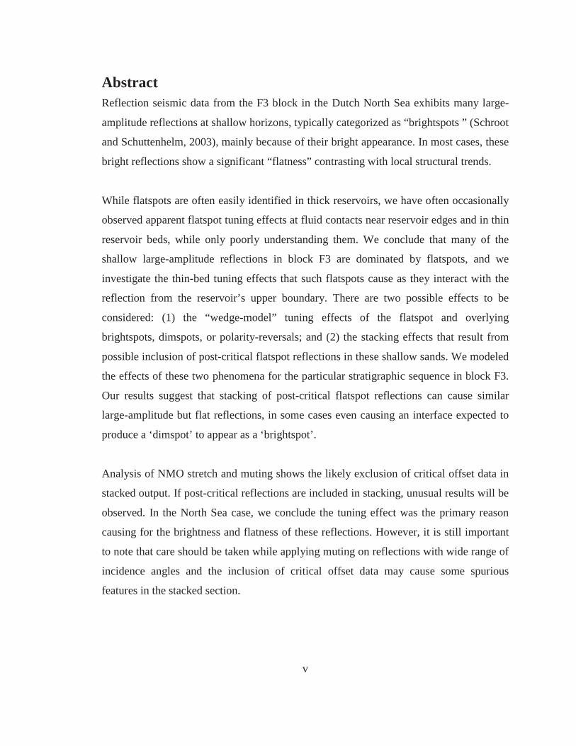
Abstract Reflection seismic data from the F3 block in the Dutch North Sea exhibits many large-

amplitude reflections at shallow horizons, typically categorized as “brightspots ” (Schroot

and Schuttenhelm, 2003), mainly because of their bright appearance. In most cases, these

bright reflections show a significant “flatness” contrasting with local structural trends.

While flatspots are often easily identified in thick reservoirs, we have often occasionally

observed apparent flatspot tuning effects at fluid contacts near reservoir edges and in thin

reservoir beds, while only poorly understanding them. We conclude that many of the

shallow large-amplitude reflections in block F3 are dominated by flatspots, and we

investigate the thin-bed tuning effects that such flatspots cause as they interact with the

reflection from the reservoir’s upper boundary. There are two possible effects to be

considered: (1) the “wedge-model” tuning effects of the flatspot and overlying

brightspots, dimspots, or polarity-reversals; and (2) the stacking effects that result from

possible inclusion of post-critical flatspot reflections in these shallow sands. We modeled

the effects of these two phenomena for the particular stratigraphic sequence in block F3.

Our results suggest that stacking of post-critical flatspot reflections can cause similar

large-amplitude but flat reflections, in some cases even causing an interface expected to

produce a ‘dimspot’ to appear as a ‘brightspot’.

Analysis of NMO stretch and muting shows the likely exclusion of critical offset data in

stacked output. If post-critical reflections are included in stacking, unusual results will be

observed. In the North Sea case, we conclude the tuning effect was the primary reason

causing for the brightness and flatness of these reflections. However, it is still important

to note that care should be taken while applying muting on reflections with wide range of

incidence angles and the inclusion of critical offset data may cause some spurious

features in the stacked section.

v

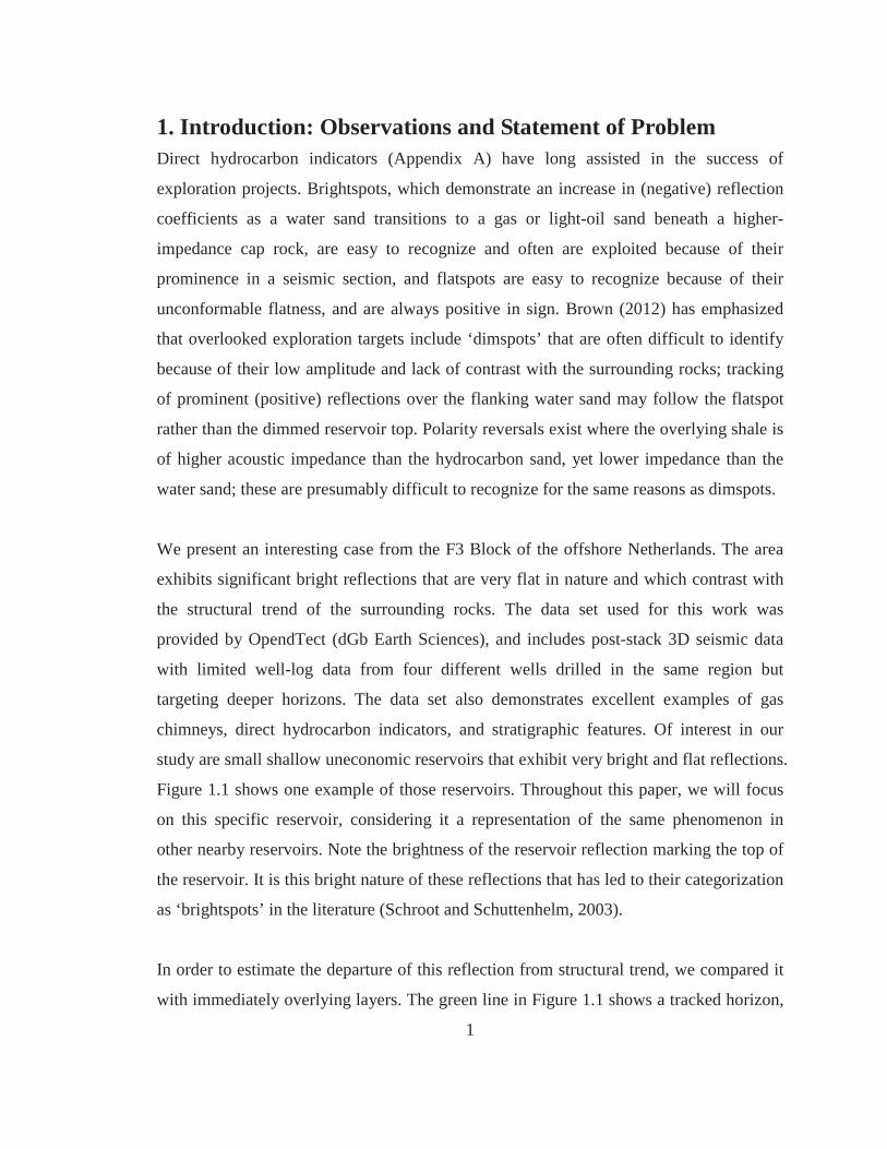
1. Introduction: Observations and Statement of Problem Direct hydrocarbon indicators (Appendix A) have long assisted in the success of

exploration projects. Brightspots, which demonstrate an increase in (negative) reflection

coefficients as a water sand transitions to a gas or light-oil sand beneath a higher-

impedance cap rock, are easy to recognize and often are exploited because of their

prominence in a seismic section, and flatspots are easy to recognize because of their

unconformable flatness, and are always positive in sign. Brown (2012) has emphasized

that overlooked exploration targets include ‘dimspots’ that are often difficult to identify

because of their low amplitude and lack of contrast with the surrounding rocks; tracking

of prominent (positive) reflections over the flanking water sand may follow the flatspot

rather than the dimmed reservoir top. Polarity reversals exist where the overlying shale is

of higher acoustic impedance than the hydrocarbon sand, yet lower impedance than the

water sand; these are presumably difficult to recognize for the same reasons as dimspots.

We present an interesting case from the F3 Block of the offshore Netherlands. The area

exhibits significant bright reflections that are very flat in nature and which contrast with

the structural trend of the surrounding rocks. The data set used for this work was

provided by OpendTect (dGb Earth Sciences), and includes post-stack 3D seismic data

with limited well-log data from four different wells drilled in the same region but

targeting deeper horizons. The data set also demonstrates excellent examples of gas

chimneys, direct hydrocarbon indicators, and stratigraphic features. Of interest in our

study are small shallow uneconomic reservoirs that exhibit very bright and flat reflections.

Figure 1.1 shows one example of those reservoirs. Throughout this paper, we will focus

on this specific reservoir, considering it a representation of the same phenomenon in

other nearby reservoirs. Note the brightness of the reservoir reflection marking the top of

the reservoir. It is this bright nature of these reflections that has led to their categorization

as ‘brightspots’ in the literature (Schroot and Schuttenhelm, 2003).

In order to estimate the departure of this reflection from structural trend, we compared it

with immediately overlying layers. The green line in Figure 1.1 shows a tracked horizon,

1

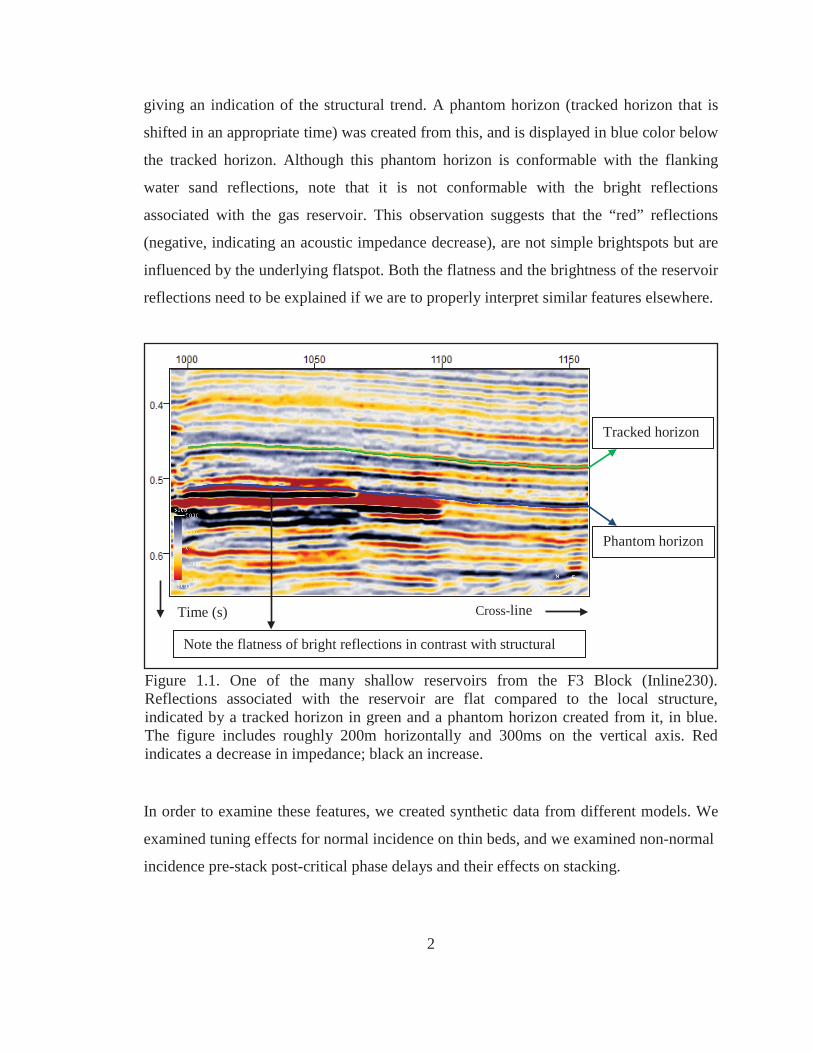
giving an indication of the structural trend. A phantom horizon (tracked horizon that is

shifted in an appropriate time) was created from this, and is displayed in blue color below

the tracked horizon. Although this phantom horizon is conformable with the flanking

water sand reflections, note that it is not conformable with the bright reflections

associated with the gas reservoir. This observation suggests that the “red” reflections

(negative, indicating an acoustic impedance decrease), are not simple brightspots but are

influenced by the underlying flatspot. Both the flatness and the brightness of the reservoir

reflections need to be explained if we are to properly interpret similar features elsewhere.

In order to examine these features, we created synthetic data from different models. We

examined tuning effects for normal incidence on thin beds, and we examined non-normal

incidence pre-stack post-critical phase delays and their effects on stacking.

Note the flatness of bright reflections in contrast with structural

Time (s) Cross-line

Tracked horizon

Phantom horizon

Figure 1.1. One of the many shallow reservoirs from the F3 Block (Inline230). Reflections associated with the reservoir are flat compared to the local structure,indicated by a tracked horizon in green and a phantom horizon created from it, in blue.The figure includes roughly 200m horizontally and 300ms on the vertical axis. Red indicates a decrease in impedance; black an increase.

2

These shallow layers consist of alternating thin beds of shale and sand. Tuning effects are

often a problem in such beds; Ricker (1953), Widess (1973), Kallweit et al. (1982) and

Chopra et al. (2006), and others have studied tuning effects in details and have

established tuning thicknesses and limits of resolution. The reservoirs under discussion

exhibit features that suggested to us that tuning plays an important role in the generation

of these flat reflections. We expected this tuning to arise from the reflections from the top

of the reservoir and from the gas water contact (GWC). First, we examine this issue from

a normal incidence assumption, as do most thin-bed studies.

The effect of post-critical reflections is usually not considered for stacking purposes. But

these reservoirs lie at very shallow depths (~500m), and it is likely that post-critical

reflections have been recorded; these post-critical reflections may or may not have been

muted prior to stacking. Post-critical reflections involve a phase shift, and if stacked in

will change the wave shape and amplitude of the final stacked event. In addition, because

these rocks are highly unconsolidated, and the elastic properties of the rocks will be

strongly influenced by the nature of pore fluid (e.g., Hilterman, 2001), we may expect to

observe a large velocity contrast at the GWC. This, in turn, will result in a small critical

angle and correspondingly short offset to the critical distance. Taken together, we are

correct to concern ourselves with the possibility that shallow stacked reflections may be

contaminated by the post-critical reflections, and therefore we include the effect of post-

critical reflections in our study.

As we do not know the stacking range that was used for this particular dataset, analysis

about NMO stretch and muting was performed to estimate the possible NMO stretch for

different offsets, based on established industry standards. A simple layered earth model

was assumed to overly the reservoir in order to generate synthetic pre-stack seismograms

at reasonable offset ranges, and one NMO stretch and muting criterion was adopted here.

We use these observations to draw conclusions about the likelihood of incorporating

post-critical reflections in the stacked results in Block F3, but the general caveats that

result may be of interest anywhere.

3

The work involved four basic steps. At the first stage we performed rock-physics

modeling to estimate the unknown formation properties needed for analysis. The second

step was to conduct forward seismic (normal incidence) modeling to study possible

tuning effects, and the third step involved AVO analysis and effect of post-critical

reflections. Finally, NMO stretch and muting were estimated for this data set, suggesting

whether or not post-critical offsets were stacked in. The results from all these modeling

methods were then assembled to guide our conclusions.

4

2. Tuning Effects 2.1. Tuning Effects for Normal Incidence Ricker (1953), Widess (1973), Kallweit et al. (1982) and Chopra et al. (2006) have

studied the tuning effect in detail and have established tuning thicknesses and resolvable

limits. These are briefly reviewed in the following section.

Widess (1973) concluded that for bed thickness thinner than the half of the wavelength

), the reflections from the top and bottom of the

layer interfere in ways that change the shape and amplitude of the wavelet. As the bed

thins to one fourth of the wavelength , the amplitude of the wavelet grows and

reaches a maximum, through the constructive interference of the side and main lobes of

the wavelet. This thickness is termed as the “tuning thickness”. When the bed thickness

reaches one eighth of a wavelength 8), the composite wavelet resembles a derivative of

the original waveform, and no change in trough-to-peak time will be observed; the

amplitude then decreases toward zero as the bed continues to thin (Widess, 1973;

Kallweit and Wood, 1982). Widess (1973) pointed out that a thin-bed thickness should be

at least 1/8th of dominant wavelength in order to be delineated. However, in the presence

of noise, the resolution is usually taken to be and Castagna, 2006).

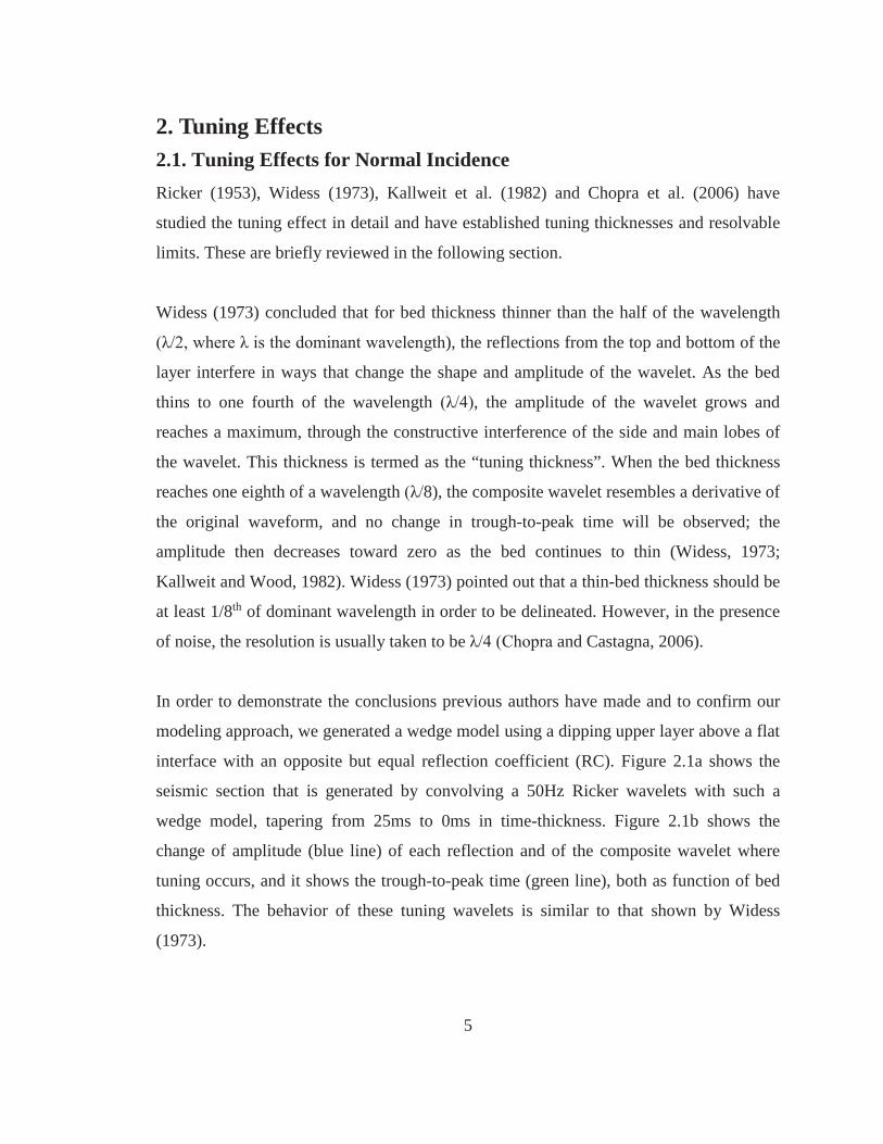
In order to demonstrate the conclusions previous authors have made and to confirm our

modeling approach, we generated a wedge model using a dipping upper layer above a flat

interface with an opposite but equal reflection coefficient (RC). Figure 2.1a shows the

seismic section that is generated by convolving a 50Hz Ricker wavelets with such a

wedge model, tapering from 25ms to 0ms in time-thickness. Figure 2.1b shows the

change of amplitude (blue line) of each reflection and of the composite wavelet where

tuning occurs, and it shows the trough-to-peak time (green line), both as function of bed

thickness. The behavior of these tuning wavelets is similar to that shown by Widess

(1973).

5

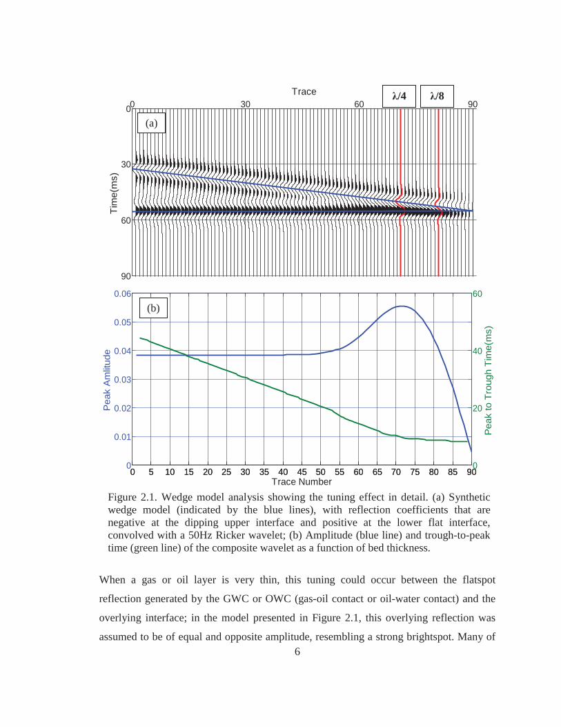
When a gas or oil layer is very thin, this tuning could occur between the flatspot

reflection generated by the GWC or OWC (gas-oil contact or oil-water contact) and the

overlying interface; in the model presented in Figure 2.1, this overlying reflection was

assumed to be of equal and opposite amplitude, resembling a strong brightspot. Many of

0 30 60 900

30

60

90

Trace

Tim

e(m

s)

0 5 10 15 20 25 30 35 40 45 50 55 60 65 70 75 80 85 900

0.01

0.02

0.03

0.04

0.05

0.06

Trace Number

Pea

k A

mlit

ude

0 5 10 15 20 25 30 35 40 45 50 55 60 65 70 75 80 85 900

20

40

60

Pea

k to

Tro

ugh

Tim

e(m

s)

/4 /8

(a)

(b)

Figure 2.1. Wedge model analysis showing the tuning effect in detail. (a) Syntheticwedge model (indicated by the blue lines), with reflection coefficients that are negative at the dipping upper interface and positive at the lower flat interface, convolved with a 50Hz Ricker wavelet; (b) Amplitude (blue line) and trough-to-peaktime (green line) of the composite wavelet as a function of bed thickness.

6

the published examples of tuning employ models in which the overlying and underlying

rocks are identical (and often assumed to be shale), and the wedge in between represents

the potential reservoir rock (often assumed to be a sand).

0 5 10 15 20 25 30 35 40 45 50 55 60 65 70 75 80 85 90-0.03

-0.02

-0.01

0

0.01

0.02

0.03

Trace

Peak

Am

litud

e

0 30 60 9075

100

125

150

175

200

Trace

Tim

e(m

s)

Sealing shale

Water-saturated sand

Hydrocarbon-saturated sand (a)

(b)

Figure 2.2. The model results showing the intriguing reflection-tuning patterns. (a) The normal-incidence responses for the structural model we are interested in, in which awedge of hydrocarbon-saturated rock is overlain by sealing shale and underlain bywater-saturated rock (interfaces are indicated by blue lines). We use a polarity reversal case in this example; (b) Amplitude of the reflection from the dipping interface, where a bright reflection occurs over the hydrocarbon-saturated rock and dim reflections over the water-saturated rock. Notice the change of amplitude due to the tuning and the sign change of the reflection indicating the polarity reversal at the termination of the hydrocarbon wedge.

7

In these cases, the reflection coefficients are identical but have opposite polarity. Some

published examples (e.g., Robertson et al., 1984) use reflection coefficients that are

identical in both amplitude and polarity above and below the wedge. In our case, we are

interested in a wedge of hydrocarbon-saturated rock overlain by a sealing formation and

underlain by a water-saturated rock that is otherwise similar to that in the wedge; in

addition, the flank of the wedge continues to dip as the sealing formation directly overlies

the water-saturated rock. The results of this model are provided in Figure 2.2 showing

some intriguing reflection-tuning patterns. But it is also important to include the effects

of non-normal angles of incidence in order to better understand the stacked response; this

is covered in the following section.

2.2. Tuning Effects for Amplitude Variation with Offset The analysis of amplitude variation with offset (AVO, details presented in Appendix B)

was a significant component in the development of DHIs, and AVO techniques are

identified by Hilterman (2001) as the second era of amplitude interpretation, following

the brightspot era.

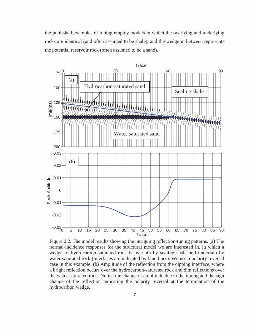
Ostrander (1984) initially established the relationship between AVO characteristics with

lithological identification and verified the use of AVO for seismic interpretation for gas

sands. Rutherford and Williams (1989) grouped AVO responses into three classes based

on normal incident reflection coefficient and AVO behavior. Castagna et al. (1998) added

an additional Class IV. Figure 2.3 shows the four classic AVO classifications for a typical

shale-gas sand interface. Some other authors have identified additional “classes” but most

authors refer only to these four; it should be recognized that AVO behavior can display

other characteristics, but these four classes are the ones generally discussed.

For most brightspots associated with low-impedance sands overlain by high-impedance

shales, Class III AVO behavior is observed; that is, they exhibit a negative reflection at

zero offset (Ro) and with increasing (negative) amplitude with increasing offset. For most

dimspots associated with high-impedance sands overlain by low-impedance shales, Class

8

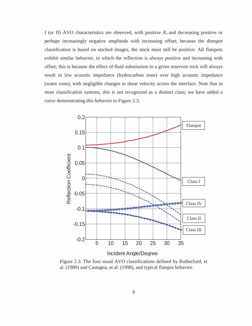
I (or II) AVO characteristics are observed, with positive Ro and decreasing positive or

perhaps increasingly negative amplitude with increasing offset; because the dimspot

classification is based on stacked images, the stack must still be positive. All flatspots

exhibit similar behavior, in which the reflection is always positive and increasing with

offset; this is because the effect of fluid substitution in a given reservoir rock will always

result in low acoustic impedance (hydrocarbon zone) over high acoustic impedance

(water zone), with negligible changes in shear velocity across the interface. Note that in

most classification systems, this is not recognized as a distinct class; we have added a

curve demonstrating this behavior to Figure 2.3.

Figure 2.3. The four usual AVO classifications defined by Rutherford, etal. (1989) and Castagna, et al. (1998), and typical flatspot behavior.

5 10 15 20 25 30 35-0.2

-0.15

-0.1

-0.05

0

0.05

0.1

0.15

0.2

Incident Angle/Degree

Ref

lect

ion

Coe

ffici

ent

Class I

Class II

Class III

Class IV

Flatspot

9

Having established that inclusion of AVO effects is important, even for stacked data (we

will later refer to examples in Figure 3.9, where stacking over different angle ranges

yields different stacked outputs), we also need to consider the effects of normal-moveout

correction and stacking, which tend to distort the wavelet.

2.3. NMO Correction, Stretch and Muting The amount of extra travel time ( tnmo) for reflections observed at non-zero offset, due to

obliquity of path compared to the normal-incidence trace, is called Normal Move-Out

(NMO), and can be readily observed and computed (Buchholtz, 1972). In conventional

processing, CMP gathers are corrected for NMO and stacked into single, stacked, traces

in which multiples and other noise components are greatly reduced. It is commonly,

although incorrectly, assumed that the stacked trace can be treated as if it were a high-

quality normal-incidence trace; the error comes primarily in ignoring the changing

amplitude contributions that come from offset traces.

However, the conventional NMO correction (Appendix C) uses different values of tnmo

at different times, and this can result in different values within the wavelet itself. This is

most pronounced for early times and long offsets, and can lead to a significant reduction

in high frequency content of the wavelet (Andrew et al., 2000). Buchholtz (1972)

analyzed wavelet distortion due to NMO correction and pointed out the most severe

stretching of the wavelet occurs at the intersections of reflection hyperbolae. Dunkin and

Levin (1973) concluded that conventional NMO correction stretches the wavelet such

that its spectrum is linearly compressed and multiplied by a factor defined by offset and

the stacking or NMO velocity used (Vnmo). It can be referred to the example in Figure

3.11, notice that the NMO-corrected wavelets in Figure 3.11b have lower frequency

content than these before correction in Figure 3.11a, and these distortions are pronounced

for shallow and far-offset reflections.

The usual solution for the NMO stretch problem is simply to discard or mute the severely

stretched part of the traces, dependent on time and offset (Buchholtz, 1972). One criterion

10

for offset-and-time-dependent muting is the percent change in frequency caused by the

NMO stretch, given by Equation (2.1) and due to Yilmaz (1987) (derived in Appendix C).

o

NMO

tt

ff

Equation 2.1

Here f f is the change in

frequency after NMO correction, to is the two-way reflection time at zero offset, and

NMO is derived from the Dix equation (Dix, 1955) (see also Appendix C). Usually a

stretch limit of 50% is taken to determine the muting zone of the CMP gather. Sometimes

this limit may extend to 100% based on how much far-offset information is desired in the

stack.

The established industry NMO muting criterion described above will be used to

determine the chance of muting within or without supercritical offset for our dataset,

demonstrating an effect that may or may not contribute to other datasets.

11

3. Methodology and Application to the Dipping-Sand Model 3.1. Rock-Physics Modeling 3.1.1. Rock Properties

The location of the target reservoir is Inline 210-250, Crossline 1050-1200 at a depth of

520-560 ms in the data provided from F3 Block of North Sea. None of the four wells

drilled in the block penetrated the reservoir but a nearby well (F03-4) provides data for

the water-saturated equivalent sand as well as for the overlying shale. Figure 3.1a shows

the well location and water-saturated sand with respect to the reservoir.

This well has only gamma-ray and sonic logs at this depth. The sonic velocities for

overlying shale and wet-sand as noted from the well-logs (Figure 3.1b) are listed in Table

3.1. We also used standard relationships to estimate other important properties (fluid and

grain properties), and the parameters for the upcoming rock-physics modeling are given

in Table 3.1.

12

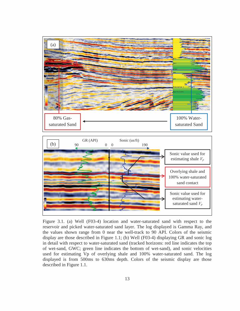
Figure 3.1. (a) Well (F03-4) location and water-saturated sand with respect to thereservoir and picked water-saturated sand layer. The log displayed is Gamma Ray, andthe values shown range from 0 near the well-track to 90 API. Colors of the seismicdisplay are those described in Figure 1.1; (b) Well (F03-4) displaying GR and sonic login detail with respect to water-saturated sand (tracked horizons: red line indicates the topof wet-sand, GWC; green line indicates the bottom of wet-sand), and sonic velocitiesused for estimating Vp of overlying shale and 100% water-saturated sand. The logdisplayed is from 500ms to 630ms depth. Colors of the seismic display are thosedescribed in Figure 1.1.

GR (API) 90 0

Sonic (us/ft) 0 190

Overlying shale and 100% water-saturated

sand contact

Sonic value used for estimating shale Vp

Sonic value used for estimating water-saturated sand Vp

80% Gas-saturated Sand

100% Water-saturated Sand

(a)

(b)

13

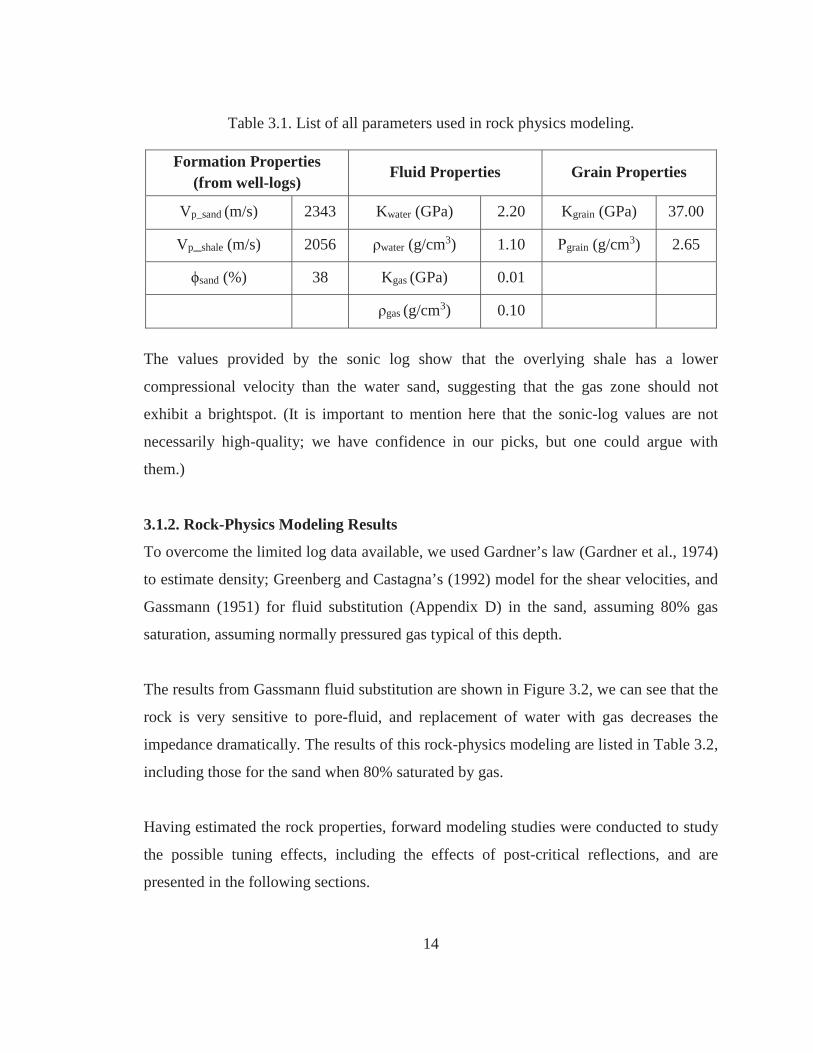
Table 3.1. List of all parameters used in rock physics modeling.

The values provided by the sonic log show that the overlying shale has a lower

compressional velocity than the water sand, suggesting that the gas zone should not

exhibit a brightspot. (It is important to mention here that the sonic-log values are not

necessarily high-quality; we have confidence in our picks, but one could argue with

them.)

3.1.2. Rock-Physics Modeling Results

To overcome the limited log data available, we used Gardner’s law (Gardner et al., 1974)

to estimate density; Greenberg and Castagna’s (1992) model for the shear velocities, and

Gassmann (1951) for fluid substitution (Appendix D) in the sand, assuming 80% gas

saturation, assuming normally pressured gas typical of this depth.

The results from Gassmann fluid substitution are shown in Figure 3.2, we can see that the

rock is very sensitive to pore-fluid, and replacement of water with gas decreases the

impedance dramatically. The results of this rock-physics modeling are listed in Table 3.2,

including those for the sand when 80% saturated by gas.

Having estimated the rock properties, forward modeling studies were conducted to study

the possible tuning effects, including the effects of post-critical reflections, and are

presented in the following sections.

Formation Properties (from well-logs)

Fluid Properties Grain Properties

Vp_sand (m/s) 2343 Kwater (GPa) 2.20 Kgrain (GPa) 37.00

Vp_shale (m/s) 2056 water (g/cm3) 1.10 grain (g/cm3) 2.65

sand (%) 38 Kgas (GPa) 0.01

gas (g/cm3) 0.10

14

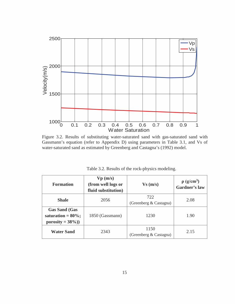
Table 3.2. Results of the rock-physics modeling.

Formation Vp (m/s)

(from well logs or fluid substitution)

Vs (m/s) 3)

Gardner’s law

Shale 2056 722 (Greenberg & Castagna) 2.08

Gas Sand (Gas saturation = 80%; porosity = 38%))

1850 (Gassmann) 1230 1.90

Water Sand 2343 1150 (Greenberg & Castagna) 2.15

Figure 3.2. Results of substituting water-saturated sand with gas-saturated sand withGassmann’s equation (refer to Appendix D) using parameters in Table 3.1, and Vs of water-saturated sand as estimated by Greenberg and Castagna’s (1992) model.

0 0.1 0.2 0.3 0.4 0.5 0.6 0.7 0.8 0.9 11000

1500

2000

2500

Water Saturation

Velo

city(

m/s

)

VpVs

15

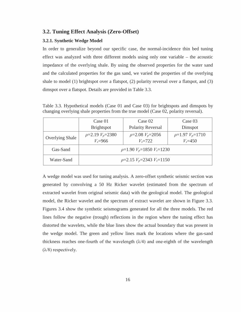
3.2. Tuning Effect Analysis (Zero-Offset) 3.2.1. Synthetic Wedge Model

In order to generalize beyond our specific case, the normal-incidence thin bed tuning

effect was analyzed with three different models using only one variable – the acoustic

impedance of the overlying shale. By using the observed properties for the water sand

and the calculated properties for the gas sand, we varied the properties of the overlying

shale to model (1) brightspot over a flatspot, (2) polarity reversal over a flatspot, and (3)

dimspot over a flatspot. Details are provided in Table 3.3.

Table 3.3. Hypothetical models (Case 01 and Case 03) for brightspots and dimspots by changing overlying shale properties from the true model (Case 02, polarity reversal).

Case 01

Brightspot Case 02

Polarity Reversal Case 03 Dimspot

Overlying Shale =2.19 Vp=2380

Vs=966 =2.08 Vp=2056

Vs=722 =1.97 Vp=1710

Vs=450

Gas-Sand =1.90 Vp=1850 Vs=1230

Water-Sand =2.15 Vp=2343 Vs=1150

A wedge model was used for tuning analysis. A zero-offset synthetic seismic section was

generated by convolving a 50 Hz Ricker wavelet (estimated from the spectrum of

extracted wavelet from original seismic data) with the geological model. The geological

model, the Ricker wavelet and the spectrum of extract wavelet are shown in Figure 3.3.

Figures 3.4 show the synthetic seismograms generated for all the three models. The red

lines follow the negative (trough) reflections in the region where the tuning effect has

distorted the wavelets, while the blue lines show the actual boundary that was present in

the wedge model. The green and yellow lines mark the locations where the gas-sand

thickness reaches one- -eighth of the wavelength

.

16

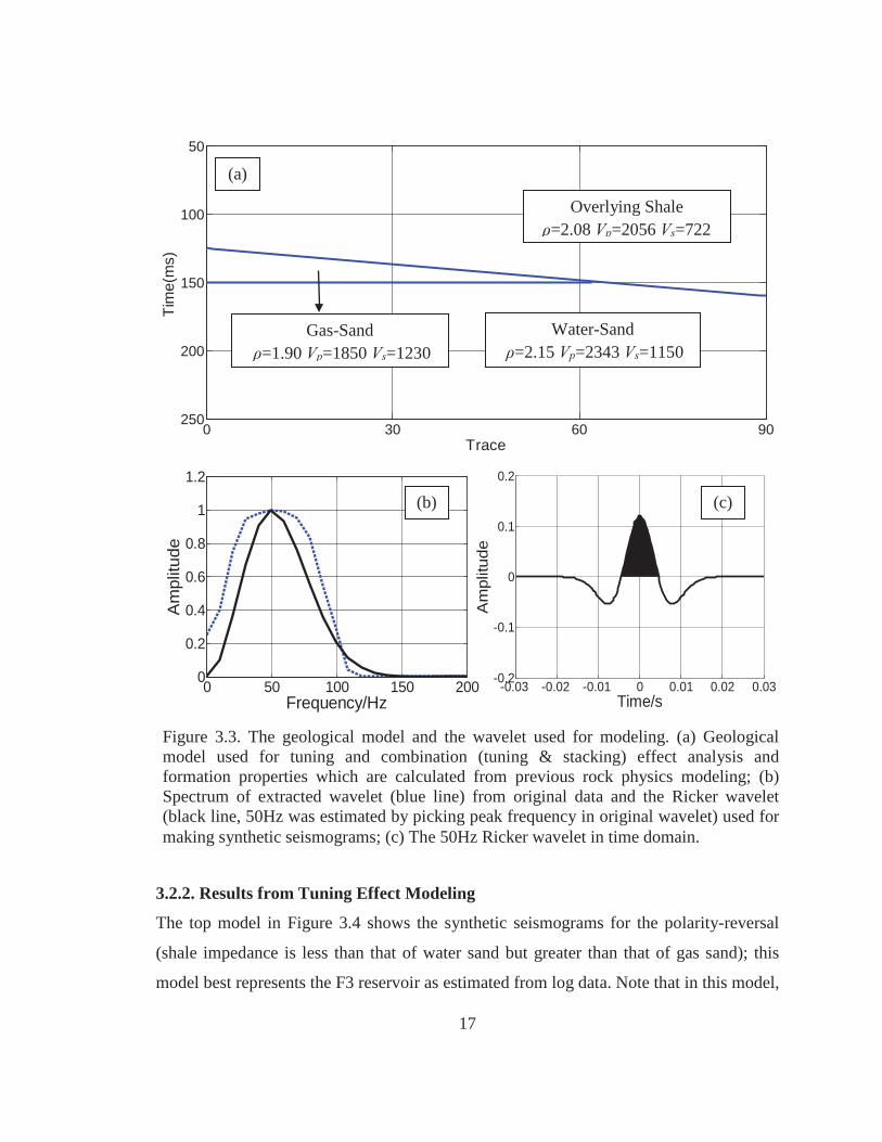
3.2.2. Results from Tuning Effect Modeling

The top model in Figure 3.4 shows the synthetic seismograms for the polarity-reversal

(shale impedance is less than that of water sand but greater than that of gas sand); this

model best represents the F3 reservoir as estimated from log data. Note that in this model,

Figure 3.3. The geological model and the wavelet used for modeling. (a) Geological model used for tuning and combination (tuning & stacking) effect analysis and formation properties which are calculated from previous rock physics modeling; (b) Spectrum of extracted wavelet (blue line) from original data and the Ricker wavelet (black line, 50Hz was estimated by picking peak frequency in original wavelet) used for making synthetic seismograms; (c) The 50Hz Ricker wavelet in time domain.

0 50 100 150 2000

0.2

0.4

0.6

0.8

1

1.2

Frequency/Hz

Am

plitu

de

0 30 60 90

50

100

150

200

250

Trace

Tim

e(m

s)

Overlying Shale =2.08 Vp=2056 Vs=722

Water-Sand =2.15 Vp=2343 Vs=1150

Gas-Sand =1.90 Vp=1850 Vs=1230

(a)

-0.03 -0.02 -0.01 0 0.01 0.02 0.03-0.2

-0.1

0

0.1

0.2

Time/s

Am

plitu

de(b) (c)

17

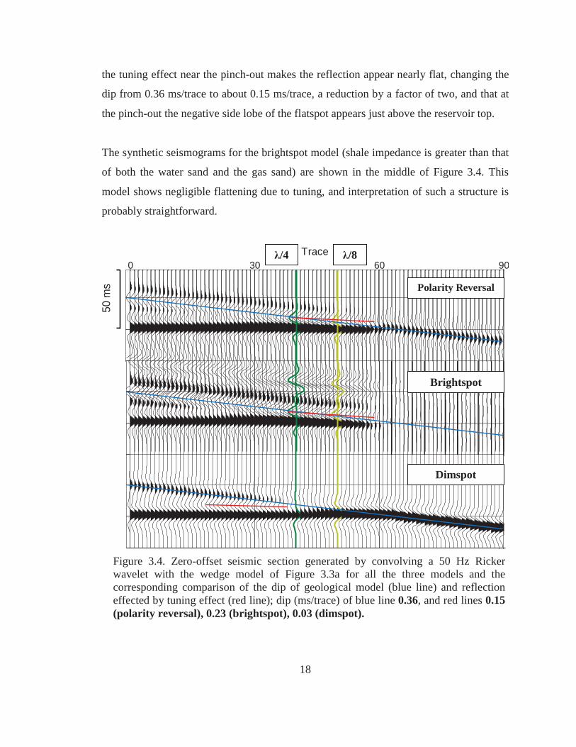
the tuning effect near the pinch-out makes the reflection appear nearly flat, changing the

dip from 0.36 ms/trace to about 0.15 ms/trace, a reduction by a factor of two, and that at

the pinch-out the negative side lobe of the flatspot appears just above the reservoir top.

The synthetic seismograms for the brightspot model (shale impedance is greater than that

of both the water sand and the gas sand) are shown in the middle of Figure 3.4. This

model shows negligible flattening due to tuning, and interpretation of such a structure is

probably straightforward.

/4 /8

Figure 3.4. Zero-offset seismic section generated by convolving a 50 Hz Rickerwavelet with the wedge model of Figure 3.3a for all the three models and thecorresponding comparison of the dip of geological model (blue line) and reflection effected by tuning effect (red line); dip (ms/trace) of blue line 0.36, and red lines 0.15 (polarity reversal), 0.23 (brightspot), 0.03 (dimspot).

50 m

s

0 30 60 90Trace

Polarity Reversal

Brightspot

Dimspot

18

The results from dimspot modeling are remarkable, as shown in the bottom of Figure 3.4.

For a dimspot to occur, the impedance of the shale must be less than that of both the gas

sand and the water sand. Because the dimspot is very low-amplitude, the tuning effect at

pinch-out is not very important. But the side lobes of the dimspot constructively interfere

with the side lobes of the underlying flatspot at thicknesses greater than the tuning

thickness (1/4 of the wavelength), eventually weakening as the hydrocarbon zone

thickens; it is possible that one’s eye, however, would continue to follow the negative

side lobe of the flatspot. The resulting seismic section shows a strong negative flat

reflection over a strong positive flat reflection; this response is similar to that observed in

F3 (Figure 1.1). These reflections exhibit a dip of 0.03 ms/trace rather than the model dip

of 0.36 ms/trace.

We have shown that tuning effects can have significant effects on the flatness of bright

reflections in the case of a dipping interface with a flatspot terminating against it. In the

next section, we analyze and discuss another possible effect: stacking of reflections

beyond the critical offset, and combining that with the tuning effects described here.

3.3. AVO & Stacking Beyond Critical Offset 3.3.1. AVO Analysis

Typically, AVO responses are categorized into four classes as defined by Rutherford and

Williams (1989) and Castagna (1992). In contrast to these, the negligible shear velocity

contrast across any flatspot makes its AVO response distinctive and unique; that is, the

reflection coefficient for any flatspot is always positive and always increases with offset,

as shown in Figure 2.3.

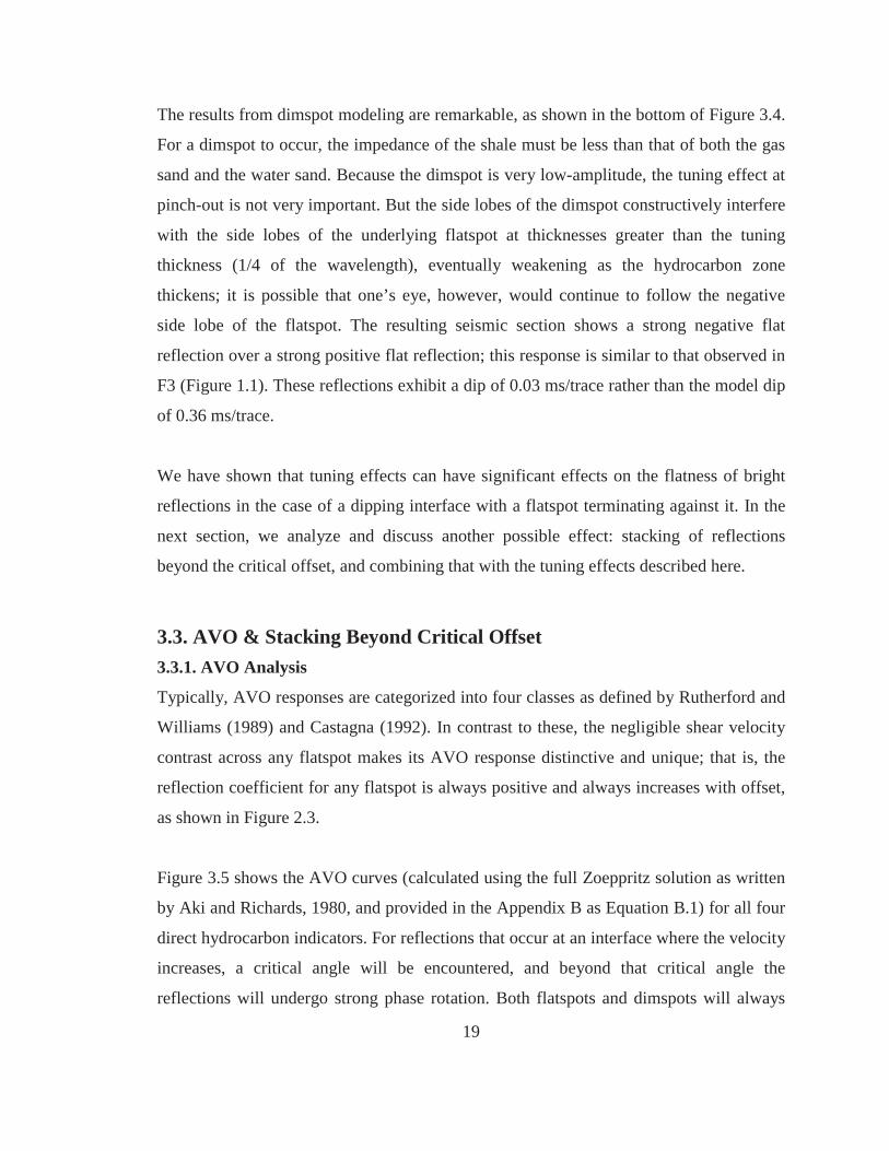
Figure 3.5 shows the AVO curves (calculated using the full Zoeppritz solution as written

by Aki and Richards, 1980, and provided in the Appendix B as Equation B.1) for all four

direct hydrocarbon indicators. For reflections that occur at an interface where the velocity

increases, a critical angle will be encountered, and beyond that critical angle the

reflections will undergo strong phase rotation. Both flatspots and dimspots will always

19

exhibit supercritical phase rotation (see flatspot and dimspot curves in Figure 3.5b,

referring to Equation B.1 and B.2); for flatspots, the critical angle may occur at

surprisingly shallow angles, such as the 52° shown in our example. The velocity increase

across a flatspot can be significant, particularly for shallow sands, the critical angle is

likely to be within the range of recorded data. Because post-critical reflections always

undergo phase rotation, if stacking involves these post-critical reflections then the stacked

output will exhibit large-amplitude non-zero-phase wavelets. This effect may compound

the similar wavelet distortion caused by tuning.

Figure 3.6 shows the result of convolving the AVO response in Figure 3.5 (including

phase shifts for the flatspot and dimspot that extend beyond critical) with a 50Hz Ricker

wavelet. The far-right seismograms show the result of stacking these over different angle

ranges.

0 20 40 60 80-1.5

-1

-0.5

0

0.5

1

1.5

Incident Angle/Degree

Am

plitu

de

FlatspotBrightspotPolarity ReversalDimspot

0 20 40 60 80

-300

-200

-100

0

100

200

300

Incident Angle/Degree

Rot

ated

Ang

le/D

egre

e

FlatspotDimspot

(a) (b)

Figure 3.5. (a) AVO responses for three different models (brightspot, polarity reversal & dimspot) and flatspot (GWC); (b) Rotated phase (beyond critical angle) versus incident angle for flatspot and dimspot, noticing these two are the only ones that will show anynon-zero phase rotation.

20

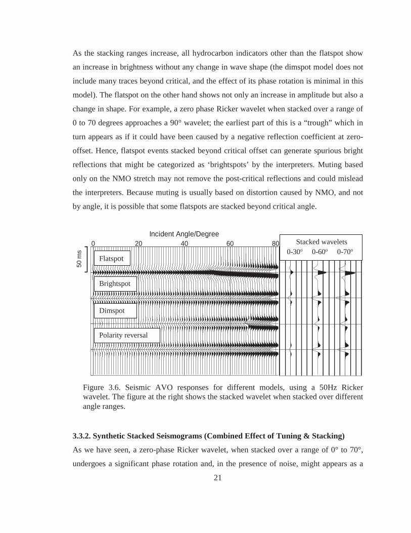
As the stacking ranges increase, all hydrocarbon indicators other than the flatspot show

an increase in brightness without any change in wave shape (the dimspot model does not

include many traces beyond critical, and the effect of its phase rotation is minimal in this

model). The flatspot on the other hand shows not only an increase in amplitude but also a

change in shape. For example, a zero phase Ricker wavelet when stacked over a range of

0 to 70 degrees approaches a 90° wavelet; the earliest part of this is a “trough” which in

turn appears as if it could have been caused by a negative reflection coefficient at zero-

offset. Hence, flatspot events stacked beyond critical offset can generate spurious bright

reflections that might be categorized as ‘brightspots’ by the interpreters. Muting based

only on the NMO stretch may not remove the post-critical reflections and could mislead

the interpreters. Because muting is usually based on distortion caused by NMO, and not

by angle, it is possible that some flatspots are stacked beyond critical angle.

3.3.2. Synthetic Stacked Seismograms (Combined Effect of Tuning & Stacking)

As we have seen, a zero-phase Ricker wavelet, when stacked over a range of 0° to 70°,

undergoes a significant phase rotation and, in the presence of noise, might appears as a

50 m

s

0 20 40 60 80Incident Angle/Degree

Stacked wavelets 0-30o 0-60o 0-70o

Brightspot

Flatspot

Dimspot

Polarity reversal

Figure 3.6. Seismic AVO responses for different models, using a 50Hz Rickerwavelet. The figure at the right shows the stacked wavelet when stacked over differentangle ranges.

21

negative reflection event. Hence, flatspot events stacked beyond critical offset can

generate reflections that might be categorized as ‘brightspot’ by the interpreters.

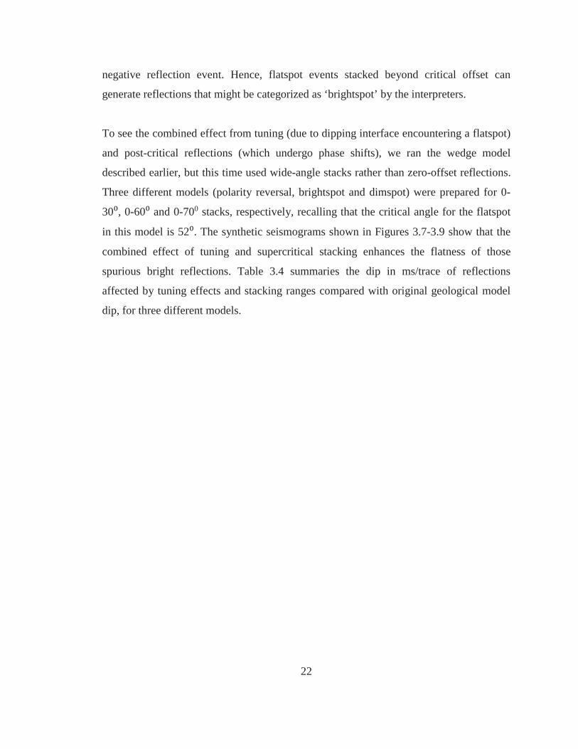
To see the combined effect from tuning (due to dipping interface encountering a flatspot)

and post-critical reflections (which undergo phase shifts), we ran the wedge model

described earlier, but this time used wide-angle stacks rather than zero-offset reflections.

Three different models (polarity reversal, brightspot and dimspot) were prepared for 0-

30 , 0-60 and 0-700 stacks, respectively, recalling that the critical angle for the flatspot

in this model is 52 . The synthetic seismograms shown in Figures 3.7-3.9 show that the

combined effect of tuning and supercritical stacking enhances the flatness of those

spurious bright reflections. Table 3.4 summaries the dip in ms/trace of reflections

affected by tuning effects and stacking ranges compared with original geological model

dip, for three different models.

22

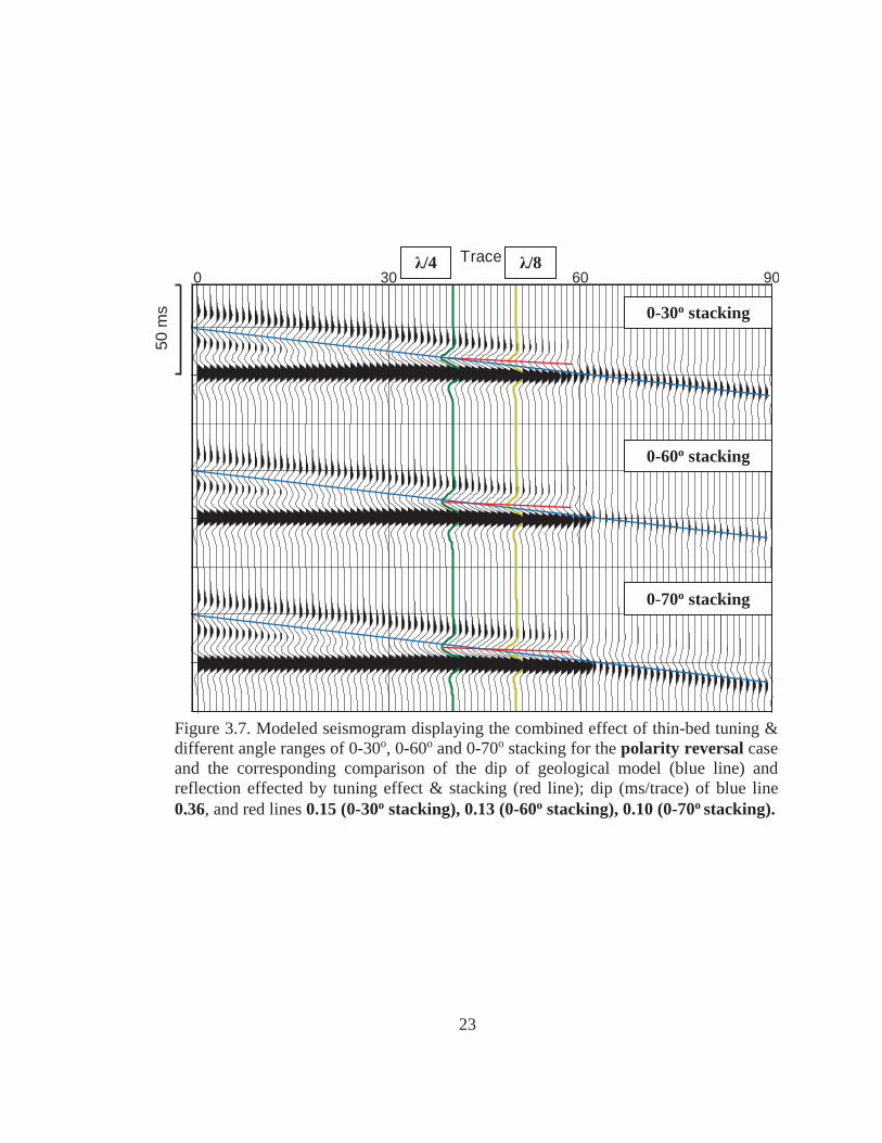
Figure 3.7. Modeled seismogram displaying the combined effect of thin-bed tuning &different angle ranges of 0-30o, 0-60o and 0-70o stacking for the polarity reversal caseand the corresponding comparison of the dip of geological model (blue line) and reflection effected by tuning effect & stacking (red line); dip (ms/trace) of blue line 0.36, and red lines 0.15 (0-30o stacking), 0.13 (0-60o stacking), 0.10 (0-70o stacking).

0 30 60 90Trace

50 m

s 0-30o stacking

0-60o stacking

0-70o stacking

/4 /8

23

Figure 3.8. Modeled seismogram displaying the combined effect of thin-bed tuning &different angle ranges of 0-30o, 0-60o and 0-70o stacking for the brightspot case andthe corresponding comparison of the dip of geological model (blue line) and reflectioneffected by tuning effect & stacking (red line); dip (ms/trace) of blue line 0.36, and redlines 0.23 (0-30o stacking), 0.18 (0-60o stacking), 0.15 (0-70o stacking).

0 30 60 90Trace

50 m

s 0-30o stacking

0-60o stacking

0-70o stacking

/4 /8

24

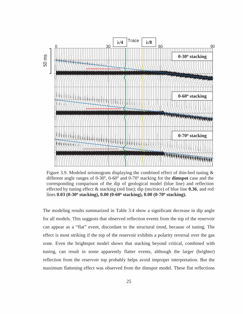
The modeling results summarized in Table 3.4 show a significant decrease in dip angle

for all models. This suggests that observed reflection events from the top of the reservoir

can appear as a “flat” event, discordant to the structural trend, because of tuning. The

effect is most striking if the top of the reservoir exhibits a polarity reversal over the gas

zone. Even the brightspot model shows that stacking beyond critical, combined with

tuning, can result in some apparently flatter events, although the larger (brighter)

reflection from the reservoir top probably helps avoid improper interpretation. But the

maximum flattening effect was observed from the dimspot model. These flat reflections

Figure 3.9. Modeled seismogram displaying the combined effect of thin-bed tuning &different angle ranges of 0-30o, 0-60o and 0-70o stacking for the dimspot case and thecorresponding comparison of the dip of geological model (blue line) and reflection effected by tuning effect & stacking (red line); dip (ms/trace) of blue line 0.36, and red lines 0.03 (0-30o stacking), 0.00 (0-60o stacking), 0.00 (0-70o stacking).

0 30 60 90Trace

50 m

s/4 /8

0-30o stacking

0-60o stacking

0-70o stacking

25

were caused by the tuning effect and are exaggerated when the non-zero-phase wavelet is

stacked in beyond critical. The sonic log from a nearby well suggests that the reservoirs

in the F3 Block most likely exhibit a polarity reversal, but the dimspot model seems to

best match the F3 seismic data, based on visual examination of multiple shallow gas

zones.

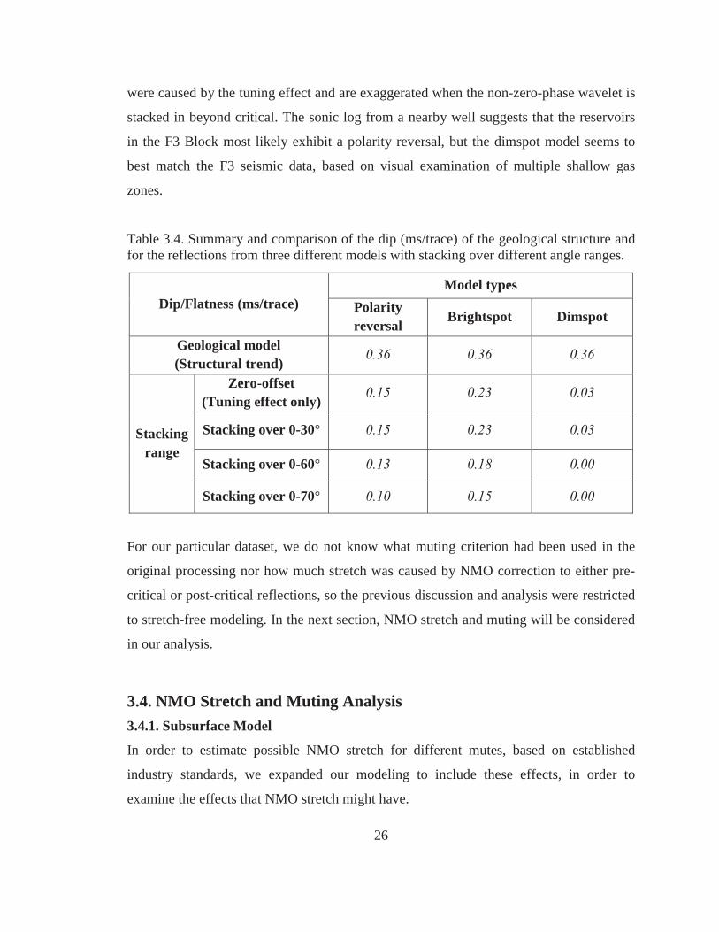
Table 3.4. Summary and comparison of the dip (ms/trace) of the geological structure and for the reflections from three different models with stacking over different angle ranges.

Dip/Flatness (ms/trace) Model types

Polarity reversal

Brightspot Dimspot

Geological model (Structural trend)

0.36 0.36 0.36

Stacking

range

Zero-offset (Tuning effect only)

0.15 0.23 0.03

Stacking over 0-30° 0.15 0.23 0.03

Stacking over 0-60° 0.13 0.18 0.00

Stacking over 0-70° 0.10 0.15 0.00

For our particular dataset, we do not know what muting criterion had been used in the

original processing nor how much stretch was caused by NMO correction to either pre-

critical or post-critical reflections, so the previous discussion and analysis were restricted

to stretch-free modeling. In the next section, NMO stretch and muting will be considered

in our analysis.

3.4. NMO Stretch and Muting Analysis 3.4.1. Subsurface Model

In order to estimate possible NMO stretch for different mutes, based on established

industry standards, we expanded our modeling to include these effects, in order to

examine the effects that NMO stretch might have.

26

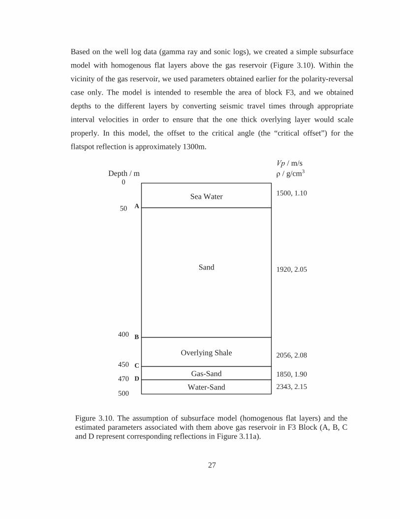
Based on the well log data (gamma ray and sonic logs), we created a simple subsurface

model with homogenous flat layers above the gas reservoir (Figure 3.10). Within the

vicinity of the gas reservoir, we used parameters obtained earlier for the polarity-reversal

case only. The model is intended to resemble the area of block F3, and we obtained

depths to the different layers by converting seismic travel times through appropriate

interval velocities in order to ensure that the one thick overlying layer would scale

properly. In this model, the offset to the critical angle (the “critical offset”) for the

flatspot reflection is approximately 1300m.

Vp / m/s / g/cm3

1500, 1.10 1920, 2.05 2056, 2.08

1850, 1.90

2343, 2.15

Depth / m 0

50

400

450

470

500

Sea Water

Sand

Overlying Shale

Gas-Sand

Water-Sand

A B

C D

Figure 3.10. The assumption of subsurface model (homogenous flat layers) and the estimated parameters associated with them above gas reservoir in F3 Block (A, B, Cand D represent corresponding reflections in Figure 3.11a).

27

3.4.2. NMO Stretch and Muting Analysis

Based on the ‘percent of changing frequency’ criterion (Yilmaz, 1987), our model

suggests that reflections from gas/water contact could be automatically muted. This

criterion yields muting at 1100m offset for the time of the flatspot reflection, and the

critical angle is encountered at around 1300m offset. The details are provided in Figure

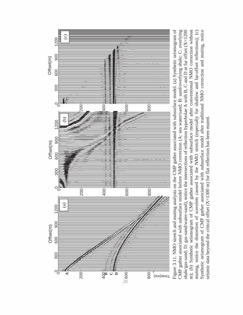
3.11, which show the synthetic CMP gather before NMO correction, after NMO

correction without muting and after muting. Notice the seismic data beyond critical offset

(X=1300m) for the flatspot reflection has been muted.

In addition, the reflection hyperbolae intersection of the seafloor reflection with the

flatspot reflection can be observed at around 1200m. Because the maximum NMO stretch

usually occurs when some of the reflection hyperbolae intersect one another (Buchholtz,

1971; Andrew et al., 1999; Zhang et al., 2011), the traces around that offset are often

muted; in our case, this offset happens to be close to the critical offset for the flatspot

reflections. We conclude that the post-critical seismic data from flatspot reflections in F3

were most likely muted during pre-stacking and excluded from the stacked output.

3.4.3. Results and Comparison with Original Seismic Data

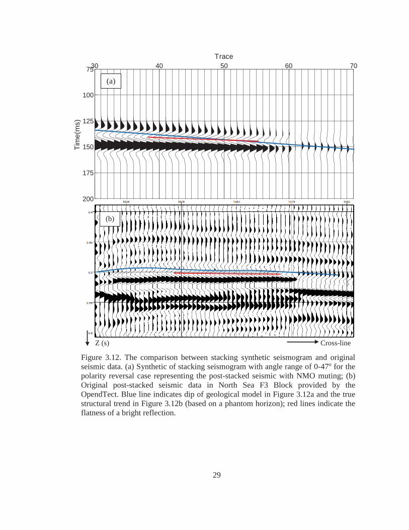
Based on the analyses described above, reflections from gas/water contact are likely to

have been muted beyond 1100 m offset, corresponding to an angle of incidence of 47°.

Figure 3.12a shows the synthetic seismograms that result from stacking over angle range

of 0-47° for the polarity reversal case previously shown for different angle ranges. This

perhaps best represents the case in the dataset we studied in North Sea Block F3. The

synthetic seismograms demonstrate the flat, bright reflections caused by tuning and

stacking. We think that this explains the observations in the seismic data, as shown in

Figure 3.12b.

28

Figu

re 3

.11.

NM

O s

tretc

h an

d m

utin

g an

alys

is o

n th

e C

MP

gath

er a

ssoc

iate

d w

ith s

ubsu

rfac

e m

odel

. (a)

Syn

thet

ic s

eism

ogra

m o

fC

MP

gath

er a

ssoc

iate

d w

ith s

ubsu

rfac

e m

odel

bef

ore

NM

O c

orre

ctio

n (A

: sea

wat

er/s

and;

B: s

and/

over

lyin

g sh

ale;

C: o

verly

ing

shal

e/ga

s-sa

nd; D

: gas

-san

d/w

ater

-san

d), n

otic

e th

e in

ters

ectio

ns o

f ref

lect

ion

hype

rbol

ae A

with

B, C

and

D a

t far

off

set (

X=1

200

m);

(b)

Synt

hetic

sei

smog

ram

of

CM

P ga

ther

ass

ocia

ted

with

sub

surf

ace

mod

el a

fter

conv

entio

nal

NM

O c

orre

ctio

n w

ithou

tm

utin

g, n

otic

e th

e di

stor

tion

of w

avel

ets

caus

ed b

y th

e N

MO

stre

tch

(esp

ecia

lly f

or s

hallo

w a

nd f

ar-o

ffse

t re

flect

ions

); (c

)Sy

nthe

tic s

eism

ogra

m o

f C

MP

gath

er a

ssoc

iate

d w

ith s

ubsu

rfac

e m

odel

afte

r tra

ditio

nal

NM

O c

orre

ctio

n an

d m

utin

g, n

otic

ese

ism

ic d

ata

beyo

nd th

e cr

itica

l off

set (

X=1

300

m) f

or fl

at re

flect

ion

has b

een

mut

ed.

A

B

C

D 0

300

600

900

1200

0

200

400

600

800 4 Time(ms)

Offs

et(m

)0

300

600

900

1200

0

200

400

600

800

Offs

et(m

)0

300

600

900

1200

0

200

400

600

800

Offs

et(m

)

(a)

(b)

(c)

28

Cross-line Z (s)

30 40 50 60 7075

100

125

150

175

200

Trace

Tim

e(m

s)(a)

(b)

Figure 3.12. The comparison between stacking synthetic seismogram and original seismic data. (a) Synthetic of stacking seismogram with angle range of 0-47o for thepolarity reversal case representing the post-stacked seismic with NMO muting; (b)Original post-stacked seismic data in North Sea F3 Block provided by theOpendTect. Blue line indicates dip of geological model in Figure 3.12a and the true structural trend in Figure 3.12b (based on a phantom horizon); red lines indicate theflatness of a bright reflection.

29

4. Results and Discussion Bright reflections in the F3 Block of the North Sea were analyzed for possible sources of

their flatness. Tuning effects and post-critical stacking were evaluated as possible reasons.

For this purpose, zero-offset and wide-angle stacked sections were prepared by forward

modeling, and NMO stretch and muting were investigated in order to evaluate the

possibility that stacking extended beyond the critical offset for our dataset.

The tuning effect results showed significantly decreasing reflection dip for polarity

reversal and dimspot cases: for polarity reversal (the geological model based on well

logs), the synthetic seismograms show that the reflections become very flat due to a

tuning effect for thicknesses under 1/4 wavelength. For the dimspot case, the modeling

results are even more remarkable: because the dimspot event is very low-amplitude, the

tuning effect caused by the underlying flat reflection is very important. As the dimspot

side lobes constructively interfere with the flatspot side lobes at thicknesses greater than

the tuning thickness, and as they destructively interfere (dim reflections are buried in

bright reflections) at thicknesses smaller than the tuning thickness, the trend of the

dimspot reflection is dominated by the flatness of the flatspot reflection. The result for

the dimspot is a strong negative flat reflection over a strong positive flat reflection; this

response is similar to that observed in F3.

If post-critical events were included in the stacking output for our data set, additional

distortion to the event could have resulted, so we studied the AVO response together with

wide-angle stacking. Flatspot events stacked beyond critical offset can generate spurious

bright reflections that might be categorized as ‘brightspots’, and the two phenomena

(tuning effect and supercritical stacking) could act together largely modifying the final

results in actual reservoir. This effect is even more striking if the top of the reservoir

exhibits a polarity reversal over the gas zone. For our particular dataset, the stretching

and muting is unknown, but our simple models suggest that post-critical seismic data was

excluded in stacking output.

30

Based on these analyses, it can be concluded that both tuning effects and post-critical

stacking can make bright reflections in F3 flatter and brighter, but that post-critical

stacking likely did not occur, and the tuning effect is presumed to be the main source of

the bright, flat events in the F3 data. The tuning effects can be significant for both

dimspots or polarity reversals, making these reflections appear as ‘brightspots’. Care

should always be used when interpreting stacked data, with the recognition that it is not

the same as zero-offset data.

31

5. Conclusion The stacking of flatspot reflections beyond critical angle can boost their amplitude

significantly while accompanied by a significant phase shift in the stacked output. Thin-

bed effects can also result in tuning that can change amplitudes and apparent polarity and

phase in cases we examined. Individually, these effects can result in fairly flat, bright

negative events overlying strong positive reflections. The effect can be strong enough

that it can even make a dimspot appear as a (flat) bright spot.

The NMO stretch and muting analysis shows that post-critical seismic data of flat

reflections was most likely excluded in the stacking output from our dataset. We

conclude that the tuning effect is the key reason for the flatness of the bright-reflections

at shallow depths of the North Sea. We further conclude that these bright reflections are

not typical ‘brightspots’ but appear as such because of the tuning effect.

In addition, although for our particular dataset, post-critical offset data were probably

muted based on traditional criteria, we recommend that care should be taken while

dealing with reflection data containing wide range of incidence angles where those

criteria may not be routinely applied (e.g., cross-well seismic data). In addition, muting

applied solely on the basis of NMO stretch might include post-critical reflections and the

stacked output will be significantly altered.

32

References Aki, K., and P. G. Richards, 1980, Quantitative seismology-Theory and Methods, 1: W.H. Freeman and Co. Buchholtz, H., 1972, A note on signal distortion due to dynamic (NMO) corrections: Geophysics Prospecting, 20, 395-402. Brown, A. R., 2010, Dim Spots in Seismic Images as Hydrocarbon Indicators: Search and Discovery Article, American Association of Petroleum Geologists. Brown, A. R., 2012, Dim spots: Opportunity for future hydrocarbon discoveries: The Leading Edge, 31, 682-683. Bortfeld, R., 1961, Approximation to the reflection and transmission coefficients of plane longitudinal and transverse waves: Geophysical Prospecting, 9, 485-503. Castle, R. J., 1994, A theory of normal moveout: Geophysics, 59, 983-999. Castagna, J. P., H. W. Swan, and D. J. Foster, 1998, Framework for AVO gradient and intercept interpretation: Geophysics, 63, 948-956. Chopra, S., J. Castagna, and O. Portniaguine, 2006, Seismic resolution and thin-bed reflectivity inversion: CSEG Recorder, 31, no. 1, 19-25. Dix, C. H., 1955, Seismic velocities from surface measurements: Geophysics, 20, 68-86. Dunkin, J. W., and F. K. Levin, 1973, Effect of normal moveout on a seismic pulse: Geophysics, 38, 635-642. Forrest, M., 2000, Bright ideas still needed persistence: AAPG Explorer, 21, no. 5, 20-21. Gardner, G. H. F., L. W. Gardner, and A. R. Gregory, 1974, Formation velocity and density-the diagnostic basics for stratigraphic traps: Geophysics, 39, 770-780. Gassman, F., 1951, Uber die elastizitat poroser medien: Vierteljahrschrift Der Naturforschenden Gesellschaft in Zurich, 96, 1-21. Greenberg, M. L., and J. P. Castagna, 1992, Shear-wave velocity estimation in porous rocks: theoretical formulation,bpreliminary verification and applications: Geophysical Prospecting, 40, 195-210. Hilterman, F. J., 2001, Seismic amplitude interpretation-distinguished instructor short course: Society of Exploration Geophysicists and European Association of Geoscientists and Engineers.

33

Kallweit, R. S., and L. C. Wood, 1982, The limits of resolution of zero-phase wavelets: Geophysics, 47, 1035-1046. Knott, C. G., 1899, Reflection and refraction of elastic waves with seismological applications: Phil. Mag., 48, 64-97. Koefoed, O., 1955, On the effect of Poisson’s ratios of rock strata on the reflection coefficients of plane waves: Geophysical Prospecting, 3, 381-387. Ostrander, W. J., 1984, Plane wave reflection coefficients for gas sands at non-normal angles of incidence: Geophysics, 49, 1637-1648. Robertson, J. D., and H. H. Nogami, 1984, Complex seismic trace analysis of thin beds: Geophysics, 49, 344–352. Rupert, G. B., and J. H. Chun, 1975, The block move sum normal moveout correction: Geophysics, 40, 17-24. Rutherford, S. R., and R. H. Williams, 1989, Amplitude-versus-offset variations in gas sands: Geophysics, 54, 680-688. Ricker, N., 1953, Wavelet contraction, wavelet expansion and the control of seismic resolution: Geophysics, 18, 769-792. Schroot, B. M., and R. T. E. Schuttenhelm., 2003, Expressions of shallow gas in the Netherlands North Sea: Netherlands Journal of Geosciences, 82(1): 91-106. Shatilo, A., and F. Aminzadeh, 2000, Constant normal-moveout (CNMO) correction: a technique and test results: Geophysical Prospecting, 48, 473-488. Shuey, R. T., 1985, A simplification of the Zoeppritz equations: Geophysics, 50, 609-614. Widess, M. B., 1973, How thin is a thin bed?: Geophysics, 38, 1176-1180. Yilmaz, O., 1987, Seismic Data Processing (Investigations in Geophysics, Vol. 2): Society of Exploration Geophysicists. Zhang, B., K. Zhang, S., Guo and K. J. Marfurt, 2013, Nonstretching NMO correction of prestack time-migrated gathers using a matching-pursuit algorithm: Geophysics, 78, U9-U18. Zoeppritz, K., 1919, Erdbebenwellen VIIIB, On the reflection and propagation of seismic waves: Gottinger Nachrichten, I, 66-84.

34

Shale AIshale

Gas-sand AIgas

Water-sand AIwater

Brightspot

Flatspot

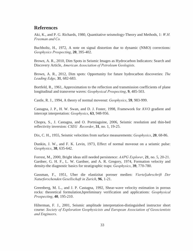
Appendix A: Direct Hydrocarbon Indicators The use of direct hydrocarbon indicators (DHIs) including brightspots, dimspots, and

flatspots, has frequently assisted in the success of exploration projects, since the

widespread application of brightspot technology in the oil industry starting in the late

1960s (Forrest, 2000).

A conventional hydrocarbon reservoir is made up of porous and permeable rock that

contains hydrocarbons which lower the acoustic impedance in contrast to similar rock

saturated entirely with water. If the reservoir rock is overlain by a higher-impedance

formation, there will be larger negative acoustic impedance contrast between the

reservoir and surrounding water-saturated rock, resulting in a high amplitude (negative)

seismic reflection, called a brightspot. By definition, a brightspot is always characterized

by a strong negative reflection coefficient over the reservoir with a weaker negative

reflection event on the sides or edges (Figure A.1).

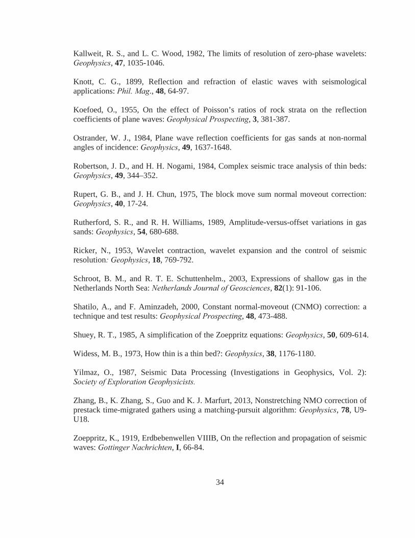
If instead of being overlain by a higher-impedance formation, the reservoir rock is

overlain by a lower-impedance formation, then the replacement of water with

hydrocarbons will cause a decrease in impedance contrast between the reservoir and

surrounding rock frame. The end result is a weaker positive reflection over the reservoir

contrasted with a stronger positive reflection at the water-saturated rock at and beyond

the reservoir edges (Figure A.2). This is called a dimspot. In some cases, the impedance

Figure A.1. Schematic diagrams for brightspot (AIshale > AIwater >AIgas), AIshale AIwater and AIgas represents acoustic impedance of shale,water sand and gas sand respectively. Red indicates a decrease inimpedance; blue an increase.

35

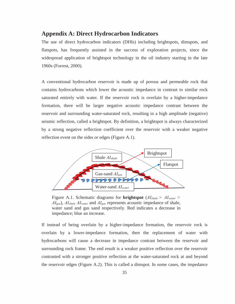
of the overlying formation is only slightly higher than that of the hydrocarbon-saturated

reservoir rock, and slightly lower than similar rock saturated with water; in that case,

there will be a polarity reversal from a weak negative over the reservoir to weak positive

reflections at the edges (Figure A.3). Dimspots are difficult to identify, and one can easily

miss them because of their negligible amplitudes and the tendency to track an associated

flatspot instead (both are positive reflections). But brightspots and dimspots equally

suggest the presence of hydrocarbons, and both are equally abundant (Brown 2012).

Shale AIshale

Gas-sand AIgas

Wate-sand AIwater

Polarity reversal

Flatspot

Shale AIshale

Gas-sand AIgas

Water-sand AIwater

Dimspot

Flatspot

Figure A.2. Schematic diagrams for dimspot (AIwater > AIgas >AIshale), AIshale AIwater and AIgas represents acoustic impedance of shale, watersand and gas sand respectively. Red indicates a decrease in impedance;blue an increase.

Figure A.3. Schematic diagrams for polarity reversal (AIwater >AIshale > AIgas), AIshale AIwater and AIgas represents acoustic impedance ofshale, water sand and gas sand respectively. Red indicates a decrease inimpedance; blue an increase.

36

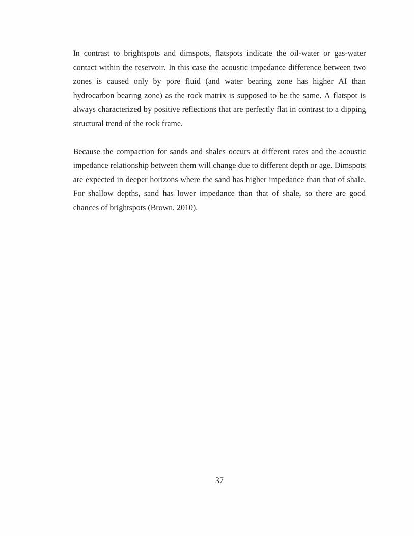
In contrast to brightspots and dimspots, flatspots indicate the oil-water or gas-water

contact within the reservoir. In this case the acoustic impedance difference between two

zones is caused only by pore fluid (and water bearing zone has higher AI than

hydrocarbon bearing zone) as the rock matrix is supposed to be the same. A flatspot is

always characterized by positive reflections that are perfectly flat in contrast to a dipping

structural trend of the rock frame.

Because the compaction for sands and shales occurs at different rates and the acoustic

impedance relationship between them will change due to different depth or age. Dimspots

are expected in deeper horizons where the sand has higher impedance than that of shale.

For shallow depths, sand has lower impedance than that of shale, so there are good

chances of brightspots (Brown, 2010).

37

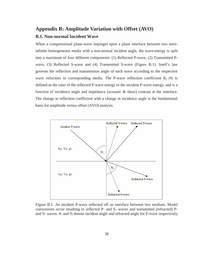
Appendix B: Amplitude Variation with Offset (AVO) B.1. Non-normal Incident Wave When a compressional plane-wave impinges upon a plane interface between two semi-

infinite homogeneous media with a non-normal incident angle, the wave-energy is split

into a maximum of four different components: (1) Reflected P-wave, (2) Transmitted P-

wave, (3) Reflected S-wave and (4) Transmitted S-wave (Figure B.1). Snell’s law

governs the reflection and transmission angle of each wave according to the respective

wave velocities in corresponding media. The P-wave reflection coefficient Rp is

defined as the ratio of the reflected P-wave energy to the incident P-wave energy, and is a

function of incidence angle and impedance (acoustic & shear) contrast at the interface.

The change in reflection coefficient with a change in incidence angle is the fundamental

basis for amplitude versus offset (AVO) analysis.

Figure B.1. An incident P-wave reflected off an interface between two medium. Model conversions occur resulting in reflected P- and S- waves and transmitted (refracted) P- and S- waves. 1 and 2 denote incident angle and refracted angle for P-wave respectively.

38

B.2. Mathematical Expressions of AVO Knott (1899) and Zoeppritz (1919), for the first time, developed the theoretical work and

gave mathematical expressions of the reflection and transmission coefficients as a

function of incidence angle and elastic properties (density, Vp and Vs). However, the exact

mathematical equations are very complex and difficult to understand how reflection

amplitude varies with changing pore properties (Hilterman, 2001). The equations are

modified and approximations to the equations are given by many others e.g., (Koefoed,

1955; Bortfeld, 1961; Aki and Richards, 1980 and Shuey, 1985 etc.).

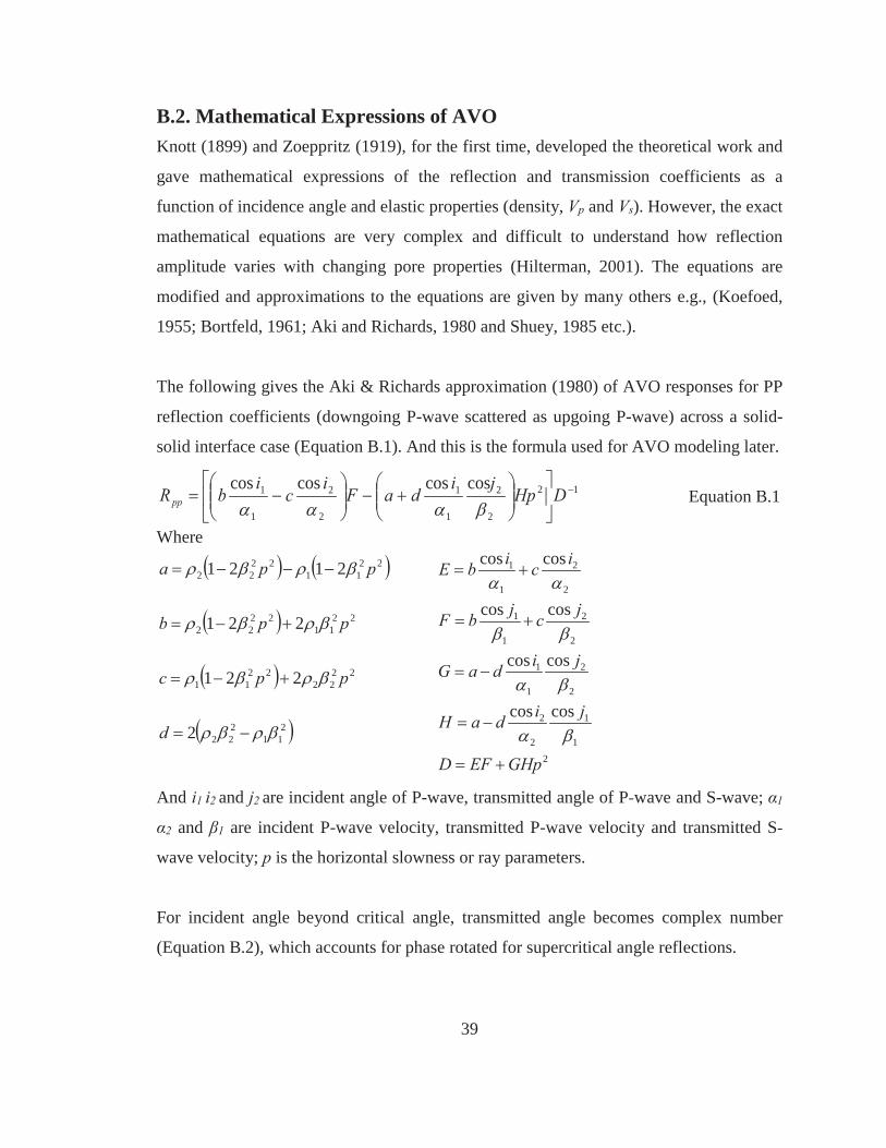
The following gives the Aki & Richards approximation (1980) of AVO responses for PP

reflection coefficients (downgoing P-wave scattered as upgoing P-wave) across a solid-

solid interface case (Equation B.1). And this is the formula used for AVO modeling later.

12

2

2

1

1

2

2

1

1 coscoscoscosDHp

jidaF

ic

ibR pp Equation B.1

Where

And i1 i2 and j2 are incident angle of P-wave, transmitted angle of P-wave and S-wave; 1

2 and 1 are incident P-wave velocity, transmitted P-wave velocity and transmitted S-

wave velocity; p is the horizontal slowness or ray parameters.

For incident angle beyond critical angle, transmitted angle becomes complex number

(Equation B.2), which accounts for phase rotated for supercritical angle reflections.

21

1

2

2

2

2

1

1

2

2

1

1

2

2

1

1

coscos

coscos

coscos

coscos

GHpEFD

jidaH

jidaG

jcjbF

icibE

211

222

2222

2211

2211

2222

2211

2222

2

221

221

2121

d

ppc

ppb

ppa

39

1sin,sincos2 1

1

21

1

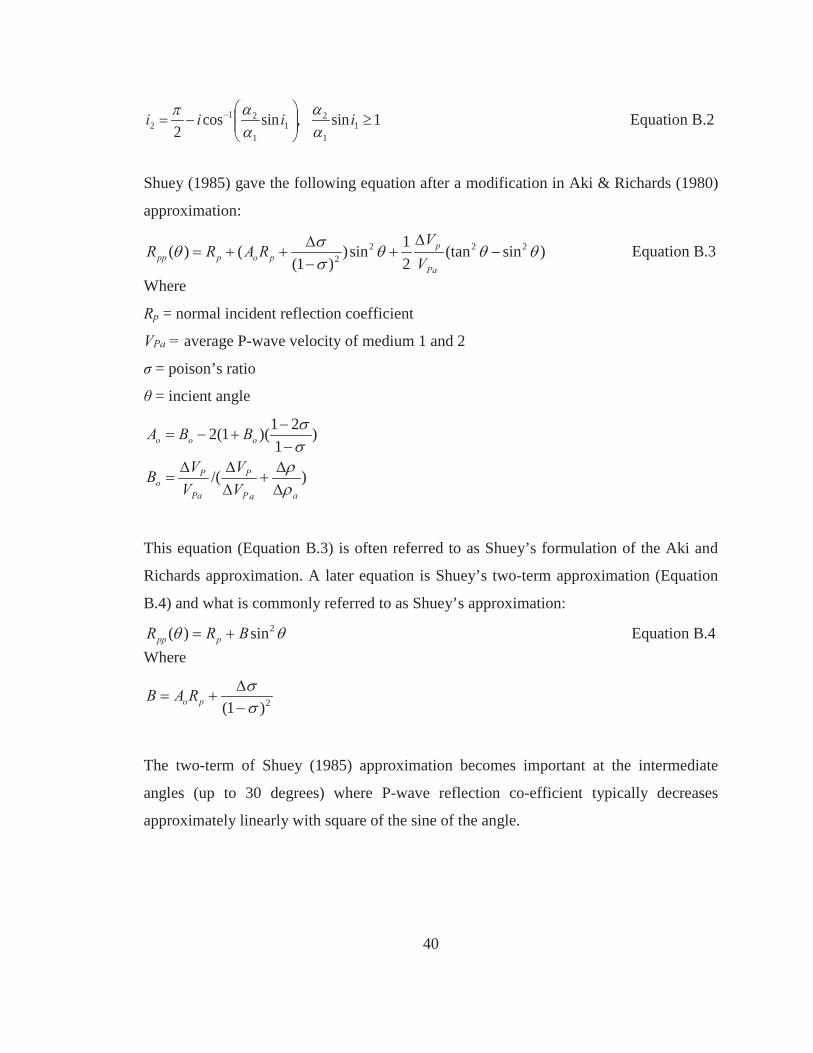
212 iiii Equation B.2

Shuey (1985) gave the following equation after a modification in Aki & Richards (1980)

approximation:

)sin(tan21sin)

)1(()( 222

2Pa

ppoppp V

VRARR Equation B.3

Where

Rp = normal incident reflection coefficient

VPa = average P-wave velocity of medium 1 and 2

= poison’s ratio

= incient angle

)/(

)1

21)(1(2

aaP

P

Pa

Po

ooo

VV

VVB

BBA

This equation (Equation B.3) is often referred to as Shuey’s formulation of the Aki and

Richards approximation. A later equation is Shuey’s two-term approximation (Equation

B.4) and what is commonly referred to as Shuey’s approximation: 2sin)( BRR ppp Equation B.4

Where

2)1(poRAB

The two-term of Shuey (1985) approximation becomes important at the intermediate

angles (up to 30 degrees) where P-wave reflection co-efficient typically decreases

approximately linearly with square of the sine of the angle.

40

Appendix C: NMO Correction and Stretch C.1. NMO Correction Dix (1955) gave the well-known hyperbolic two-way travel time equation as a function

of zero-offset time to and offset x:

)(2

22

oo tV

xtt Equation C.1

Where t is the two-way travel time associated with a source-receiver separation (offset) x,

to is the two-way zero-offset travel time (the time after normal move-out correction).

V(to is the NMO velocity, which can be estimated as the root-mean-square (rms) velocity

for small offset approximation:

N

kk

N

kkk

rms

t

VtV

1

1

2

Equation C.2

And Vk is the interval velocity of the kth layer, k is the vertical two-way travel time to

the kth layer.

For the area where bed are horizontally layered or gentle dipping at small offset, the

expression (Equation C.3) originated with Dix (1955) could give fairly satisfied NMO

correct time:

)(2

22

ooNMO tV

xttttt Equation C.3

C.2. NMO stretch Consider a reflection event represented by a wavelet of dominant period T with an arrival

time t at offset x. After normal-moveout correction, the dominant period becomes To = T

+ T. The moveout Equation C.1 is associated with the onset of the wavelet. Similarly,

the moveout equation with the termination of the wavelet is expressed by

41

2

222 )(

vxTTtTt o Equation C.4

Expand the terms on both sides:

2

22222 )()(22

vxTTTTttTtTt oo Equation C.5

By making the substitution from Equation (C.1), we obtain

22 )()( 2 2 TTTTtTtT o Equation C.6

Simplify and rearrange the terms

2)(2)(2 TTTtTtt oo Equation C.7

Now, ignore the second term on the right-hand side of the equation and observe that

NMO = t - to to obtain

TTtTt oNMO )( Equation C.8

Assume that to >> T and rearrange that terms to obtain a relationship for change in the

period of the wavelet as a result of moveout correction

o

NMO

tt

TT Equation C.9

Express Equation C.9 in terms of dominant frequency f of the wavelet with the relation

fT 1 Equation C.10

And obtain

ff

T 2

1 Equation C.11

Finally, combine Equation C.9 and Equation C.11 and to obtain the equation for the

absolute value of frequency stretching:

o

NMO

tt

ff Equation C.12

This is the same as Equation 2.1 in the main text, and usually 50 percent change of

frequency is taken as threshold to determine the muting zone of the CMP gather.

42

Appendix D: Gassmann Fluid Substitution Density of the water-saturated sand is estimated by Gardner’s law (Gardner et al., 1974):

25.023.0 pV Equation D.1

As no shear velocity available here, Vs is estimated by Greenberg and Castagna (1992) Vp

to Vs transforms (Equation D.2) for wet-sand and shale:

ps

p

VVVV

770.0867.0804.0856.0s Equation D.2

From the Gassmann’s Equation, we can get dry frame moduli of sand Kdry from:

wmamab

wbmabry KKKK

KKKKKK//1

//1 mad Equation D.3

Where bulk modulus Kb is calculated by Vp, Vs and of the water-saturated sand:

22b 3

4sp VVK Equation D.4

Then gas sand properties in the reservoir can be estimated by fluid substitution, the

following Equation (D.5) is used for this purpose:

12

drp //1/1/1

34

flmamadry

madryydry KKKK

KKKV Equation D.5

sV Equation D.6

Here μ is the shear modulus of gas-saturated sand, which will not be changed with fluid content but with density:

2sdry V Equation D.7

And Kdry and Kb are bulk modulus of dry rock frame and bulk rock; Kfl Kma Kw and are

bulk modulus of substitute fluid (gas), matrix grains, original water, bulk rock density

and porosity.

43