petro-physical characterization of shallow aquifers by using avo and theoretical approaches

1

Petro-physical characterization of shallow aquifers by using Avoand theoretical approaches

U. TINIVELLA, F. ACCAINO, M. GIUSTINIANI and S. PICOTTI

Istituto Nazionale di Oceanografia e di Geofisica Sperimentale, Trieste, Italy

(Received:; accepted:)

ABSTRACT We present the results obtained by the Amplitude Versus Offset analysis of 2D and 3Dhigh-resolution seismic data acquired along the resurgence line located in the Friuli-Venezia Giulia plain (Italy), in order to characterize an important multilayered aquifer.The Amplitude Versus Offset analysis was performed to extract the Poisson ratiocontrast, which provides useful information to characterize the aquifers petro-physicalproperties, such as the fluid content.The velocity model, which was obtained from atomographic approach for 2D seismic data and an iterative updating procedureinvolving pre-stack depth migration, residual move-out analysis and seismic reflectiontomography for 3D data, was used to obtain density and porosity maps.

1. Introduction

In the frame of the CAMI project, 2D and 3D seismic data were acquired to characterize theaquifer system located in the Torrate area. During the winter of 2005, three 2D seismic lines wereacquired, as described in Giustiniani et al. (2007). In addition, 3D seismic surveys wereperformed in two different seasons and in two different areas as described in Picotti et al. (2007).

Firstly, we tested the possibility of detecting the pore pressure variation in different seasons,in the acquifer system, by seismic velocity and Amplitude Versus Offset (AVO) analyses. We usedan empirical approach (Prasad et al., 2004) to determine the seismic velocities versus porepressure.

After “true-amplitude” processing of both 2D and 3D seismic data (Giustiniani et al., 2007and Picotti et al., 2007), the AVO was applied to all seismic data sets in order to extract thePoisson ratio contrast that which provides useful information about the petrophysical propertiesof the shallow layers.

The velocity fields were obtained from a tomographic approach for 2D seismic data(Giustiniani et al., 2007) and an iterative procedure for 3D seismic data (Picotti et al., 2007).They were translated, in terms of porosity and density, by using empirical relationships.

2. Velocity and AVO vs pore pressure

Velocities versus pore pressure have been computed in order to verify the possibility ofdetecting overpressures through seismic data analysis for the shallower aquifers, one located atabout a 30 m depth while the second one at about a 180 m depth. The identified physicalproperties of these aquifers are reported in Table 1 (layers 2 and 4). Laboratory measurementsindicate the following relationship between compressional (VP) and shear (VS) wave velocities

Bollettino di Geofisica Teorica ed Applicata Vol. 49, n. x, pp. x-xx; Xxxxxxx 2008

© 2008 – OGS

2

Boll. Geof. Teor. Appl., 49, 000-000 Tinivella et al.

and effective pressure pe (Prasad et al., 2004):

(1)

where the coefficients ai and bi are obtained by fitting the model parameters (Table 1) and ci wasfixed equal to the value proposed by Prasad et al. (2004). The fit gives the results shown in Table2. Considering a 10% increase in hydrostatic pressure of each aquifer obtained from wellmeasurements performed by the waterworks technicians (personal communication, EnricoMarin), we evaluated the compressional and shear velocities and the density values shown inTable 1. The velocity variation caused by conditions of overpressure is not detectable by seismicmethods. On the other hand, the ratio between the VP and VS reflectivity, which can be estimatedby the AVO analysis, can detect the top and the bottom of each layer (Fig. 1), where thereflectivity ( RX) of the X parameter is defined as:

(2)

where ∆X is the variation of the X parameter and⎯X is its average value at the interface, asindicated by the upper bar.

In the case of conditions of overpressure, the VP to VS reflectivity ratio is slightly modified,except at the bottom of the second aquifer (Fig. 1). In fact, in hydrostatic conditions, we assumeda velocity inversion between the second aquifer and the underlying layer (Table 1). In conditions

RX

XX =∆

,

V a b p V a pP ec

S eb= + =1 1 2

1 2,

Layer Medium Mean thickness

VP

(m/s)VS

(m/s)ρρ

(kg/m3)QP QS

1 Clay+gravel 27 1000 300 1700 20 20

2 Saturated gravel 551600

(1564)450

(427)1900

(1890)40

(40)40

(40)

3 Clay 178 1800 600 2000 30 30

4 Saturated gravel 2002200

(2142)800

(767)2100

(2080)50

(50)50

(50)

5 Clay 400 2000 700 2200 40 40

6Gravel+sand+clay (top)

8501800 600 1900 60 60

Gravel+sand+clay (bottom) 2500 1000 2300 60 60

7 Carbonatic basement 3500 1900 2800 100 100

Table 1 - Seismic properties of the aquifer model shown in Fig. 2: compressional-wave (P) and shear-wave (S)velocities, density, and quality factors (Prasad and Meissner, 1992; Bourbié et al., 1987; Schön 1996). The values inbrackets refer to the overpressure condition (see text). The seismic parameters of layer 6 (velocity and density) arelinearly interpolated.

3

Petro-physical characterization of shallow aquifers Boll. Geof. Teor. Appl., 49, 000-000

of overpressure, the velocity contrast reduces itself; consequently, the VP and VS reflectivity ratiodecreases, these masking the bottom of the second aquifer. So, in this case, the AVO analysishighlights possible lithological and saturation changes in porous media.

3. Amplitude Versus Offset

3.1 The analysis

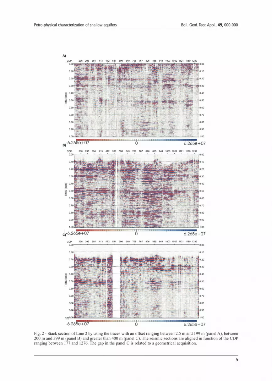
The pre-stack data analysis underlines the presence of AVO effects associated either withlithologic changes or/and the presence of fluids at high pressure. These effects are evident, forexample, in the three stacked sections of Line 2 obtained by using different offset ranges: 0 -199m, 200 – 399 m, and higher than 400 m (Fig. 2). This figure shows that the amplitudes at the twomain shallow aquifers change with offset. In the far-offset section, the amplitude is strongercompared to the others: this is evident for the deeper reflectors, at about 300 m and 500 m. As

Fig. 1 - VP and VS reflectivity ratio versus effective pressure at each modelled layer (see values in Table 1). Circle:hydrostatic condition. Star: overpressure condition.

index a B

1 973.4 985.2

2 662.6 0.349

Table 2 - Fitting parameters of the Eq. (1).

4


expected, the near-offset stacked section provides more information about the shallowest targets.To better discriminate between lithologic and fluid changes at each interface, we performed

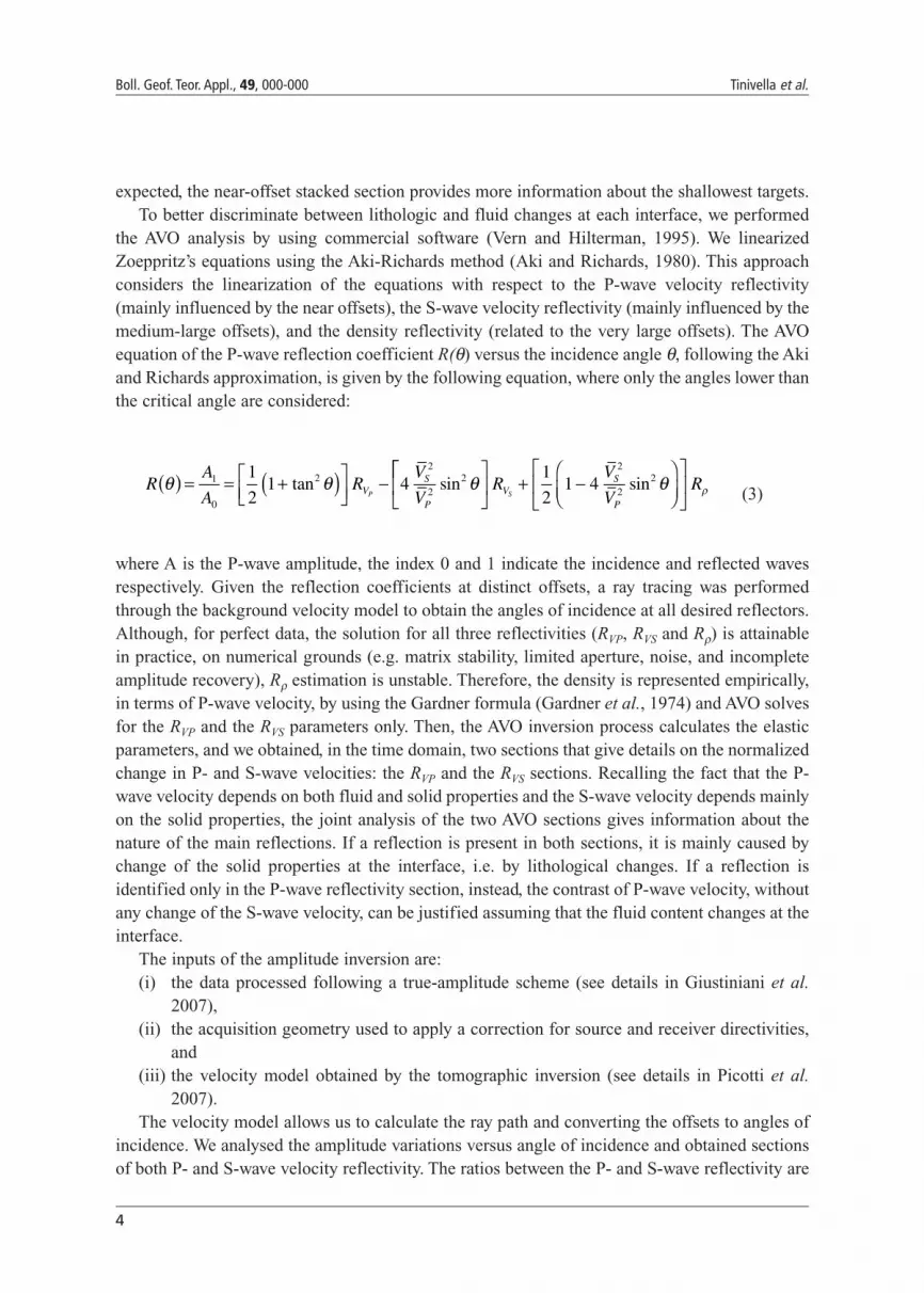
the AVO analysis by using commercial software (Vern and Hilterman, 1995). We linearizedZoeppritz’s equations using the Aki-Richards method (Aki and Richards, 1980). This approachconsiders the linearization of the equations with respect to the P-wave velocity reflectivity(mainly influenced by the near offsets), the S-wave velocity reflectivity (mainly influenced by themedium-large offsets), and the density reflectivity (related to the very large offsets). The AVOequation of the P-wave reflection coefficient R(θ) versus the incidence angle θ, following the Akiand Richards approximation, is given by the following equation, where only the angles lower thanthe critical angle are considered:

(3)

where A is the P-wave amplitude, the index 0 and 1 indicate the incidence and reflected wavesrespectively. Given the reflection coefficients at distinct offsets, a ray tracing was performedthrough the background velocity model to obtain the angles of incidence at all desired reflectors.Although, for perfect data, the solution for all three reflectivities (RVP, RVS and Rρ) is attainablein practice, on numerical grounds (e.g. matrix stability, limited aperture, noise, and incompleteamplitude recovery), Rρ estimation is unstable. Therefore, the density is represented empirically,in terms of P-wave velocity, by using the Gardner formula (Gardner et al., 1974) and AVO solvesfor the RVP and the RVS parameters only. Then, the AVO inversion process calculates the elasticparameters, and we obtained, in the time domain, two sections that give details on the normalizedchange in P- and S-wave velocities: the RVP and the RVS sections. Recalling the fact that the P-wave velocity depends on both fluid and solid properties and the S-wave velocity depends mainlyon the solid properties, the joint analysis of the two AVO sections gives information about thenature of the main reflections. If a reflection is present in both sections, it is mainly caused bychange of the solid properties at the interface, i.e. by lithological changes. If a reflection isidentified only in the P-wave reflectivity section, instead, the contrast of P-wave velocity, withoutany change of the S-wave velocity, can be justified assuming that the fluid content changes at theinterface.

The inputs of the amplitude inversion are: (i) the data processed following a true-amplitude scheme (see details in Giustiniani et al.

2007), (ii) the acquisition geometry used to apply a correction for source and receiver directivities,

and (iii) the velocity model obtained by the tomographic inversion (see details in Picotti et al.

2007). The velocity model allows us to calculate the ray path and converting the offsets to angles of

incidence. We analysed the amplitude variations versus angle of incidence and obtained sectionsof both P- and S-wave velocity reflectivity. The ratios between the P- and S-wave reflectivity are

RA

AR

V

VVS

PP

θ θ θ( ) = = +( )⎡⎣⎢

⎤⎦⎥

−1

0

22

221

21 4tan sin

⎡⎡

⎣⎢

⎤

⎦⎥ + −

⎛⎝⎜

⎞⎠⎟

⎡

⎣⎢

⎤

⎦⎥R

V

VRV

S

PS

1

21 4

2

22sin θ ρ

5


Fig. 2 - Stack section of Line 2 by using the traces with an offset ranging between 2.5 m and 199 m (panel A), between200 m and 399 m (panel B) and greater than 400 m (panel C). The seismic sections are aligned in function of the CDPranging between 177 and 1276. The gap in the panel C is related to a geometrical acquisition.

6


related to Poisson’s ratio and, consequently, to the fluid content. After the visual comparison of the reflectivity sections, we decided to use a quantitative

method to interpret the AVO results. We evaluated the ratio between P and S reflectivity (Accainoet al., 2005).

3.2 The results

The AVO inversion was applied to all 2D and 3D seismic data sets. Note that the reliability ofthe result depends on the data quality and the coverage of the seismic data. Examples of thereflectivity sections obtained are reported in Figs. 3 and 4, which show 2D and 3D, datarespectively. In general, comparing the P and S reflectivity sections, it is possible to discriminatebetween the reflections caused mainly by geological features and the reflections that can beattributed to fluid content variation. In this case, we can identify the same main reflectors in bothP and S reflectivity sections (Figs. 3 and 4), already detected in the stacked sections (Giustinianiet al., 2007), because of the geological characteristics of the aquifer system (Giustiniani et al.,2007). Nevertheless, to avoid a misinterpretation of the results, we have calculated the ratiobetween the P- and S-wave reflectivity sections (Fig. 5).

The comparison of the results shows that the AVO analysis of seismic data acquired indifferent seasons detects the same features. As revealed by the measured and modelled velocities(see section 2), the seismic data cannot detect any changes in the water saturation and porepressure inside the aquifers related to the seasonal change.

In this paper, we show, in detail, the results obtained from the 2D Line 2, for which the AVOanalysis gives the best results because of the quality and the coverage of the data. The two main

Fig. 3 - P- (top) and S-wave (bottom) velocity reflectivity sections along the Line 2 (see text).

7


Fig. 4 - P- (left) and S-wave (right) velocity reflectivity sections along the 3D cube 3 after AVO inversion (see text).

Fig. 5 - Top: P to S wave velocity reflectivity section; the arrowed lines indicate the area where the crossplots areevaluated. The thin lines indicate the main reflectors identified in the staked section and inverted to obtain tomographicvelocity. Bottom: P- versus S-wave velocity reflectivities at selected CDP intervals.

8


aquifers are identified by the strong Poisson ratio variation (Fig. 5). We blanked the area wherethe AVO inversion is not reliable, i.e. the areas where the curve fitting is suspect, due to noise orinsufficient aperture. Note also the high contrast at about 500 m depth, possibly related tolithological changes that may reflect another aquifer.

Finally, we evaluated the cross-plots of P and S velocity versus reflectivity, to verify ifdifferent petrophysical characteristics versus depth can be detected along the seismic profiles. Tothis end, we selected two areas where the coverage is high enough to guarantee a reliable AVOinversion, i.e., between Common Depth Points (CDPs) 200 to 400 and 800 to 1000 (Fig. 5). Todetect different trends, we considered the following depth intervals:

1) shallow part (between 0 and 16 m; in black); 2) first aquifer (between 16 and 40 m; in red); 3) intermediate part between the two main aquifers (between 60 and 140 m; in green); 4) the second aquifer (between 150 and 250 m; in blue); 5) depth greater than 250 m (between 360 and 450 m; in magenta). The two selected zones produce similar results. The two main aquifers have different cross-

plots compared to the other layers. The deepness, i.e. the relationship between P- and S-wavevelocity contrasts, decreases versus depth, even if the characteristics of the layers between the twoaquifers and below the deeper one are similar.

4. The density and porosity maps

The velocity (V) was translated in terms of density (ρ) by using the well-known Gardnerrelationship (Gardner et al., 1974), as used for the AVO analysis (see section 3):

(4)

Supposing that the density of the matrix (ρs) is about 2600 kg/m3 and that one of the waterone (ρw) is about 1000 kg/m3, we obtain the following relationship between density and porosity(Ê), i.e. water saturation:

(5)

The results show that the shallowest confined aquifer is characterized by a density of about1900 kg/m3 and a porosity of about 36-40%. The second aquifer, located at about 180 m depth,is well imaged because it shows a higher porosity (equal to about 32 %) with respect to the upperlayer, characterized by a porosity of about 28%. Note that the deeper aquifer presents a porosityof about 33%. Regarding the density, the deep aquifers are characterized by a density of about2100 kg/m3.

The velocity, density and porosity models are interpolated in order to obtain a complete 3Dmodel of the Torrate area by using a commercial software. We assumed a cell size of

φρ ρ

ρ ρ=

−−

s

s w

ρ = 0 31 0 25. .V

9


Fig. 6 - 3D velocity (m/s) models after the interpolation (see text).

Fig. 7 - 3D density (kg/m3) model after the interpolation (see text).

10


20(x)x20(y)x25(z) m and a number of cells equal to 198, 211, and 23 along the three directionsrespectively.

The data were interpolated by using the inverse distance algorithm (Franke, 1982; Davis,1986). The inverse distance method is a weighted average interpolator that can be either an exactor a smoothing interpolation.

We applied the interpolator module to all data sets obtaining velocity, density and porositydistribution. The results are reported in Figs. 6-8, where the depth ranges from 0 to 550 m. The3D models indicate that the area has variable characteristics, with strong lateral velocityvariations that suggest changes in the interfaces, geometry and the aquifer system thickness. Theanalyses of these data confirm an increase of porosity and the thickness of aquifers north wordsin accordance with the other data acquired in the frame of the CAMI project (see this book).

5. Conclusions

The results obtained from the AVO analysis confirm the presence of a shallow aquifer (atabout 30 m) and a deeper one (at about 180 m). In particular, the cross-plots of the P and Svelocity versus reflectivity show different trends, being related to fluid contents and lithologicchanges. Moreover, seismic data cannot detect the pore pressure condition in this area, butprovided information about the geometrical structures and the petrophysical properties of theaquifers.

The velocity fields, that were obtained as described in Giustiniani et al. (2007) and Picotti etal. (2007), were translated in terms of porosity and density by using empirical relationships. The

Fig. 8 - 3D porosity (%) model after the interpolation (see text).

11


obtained porosity and density maps show the main increase of aquifer thickness versus North anda stronger variability of the petro-physical characteristics of two shallower aquifers than thedeeper ones.

Acknowledgments.We are very grateful to Elvio Del Negro for his contribution and technical support incollecting the field data. We acknowledge the European Community that has supported this project (LIFEProject Number - LIFE04 ENV/IT/000500). We wish to thank the Acquedotto Basso Livenza, and inparticular Enrico Marin, for the logistical support and all the information provided (hydrogeological dataand the stratigraphies of the catchment wells).

REFERENCEAccaino F., Tinivella U., Rossi G. and Nicolich R.; 2005: Geofluid evidence from analysis of deep crustal seismic data

(Southern Tuscany, Italy). Journal of Volcanology and Geothermal Research, 148, 46–59.

Aki K. and Richards P.G.; 1980: Quantitative seismology: Theory and methods. W.H. Freeman, San Francisco, 932 pp.

Bourbié T., Coussy O. and Zinzner B.; 1987: Acoustics of Porous Media. Gulf Publishing, Houston, Texas, 56 pp.

Davis J. C.; 1986: Statistics and Data Analysis in Geology. John Wiley and Sons, New York, NY, 646 pp.

Gardner G.H.F., Gardner L.W. and Gregory A.R.; 1974: Formation velocity and density – The diagnostic basics forstratigraphic traps. Geophysics, 39, 770-780.

Giustiniani M., Accaino F., Del Negro E., Picotti S. and Tinivella U.; 2007: Characterisation of shallow aquifers by 2Dhigh-resolution seismic data analysis. Submitted to this volume.

Picotti S., Giustiniani M., Accaino F. and Tinivella U.; 2007: Depth modelling and imaging of the 4D seismic surveyof Baso Livenza (CAMI project). Submitted to this volume.

Prasad A. and Meissner G.; 1992: Attenuation mechanism in sands: Laboratory versus theoretical (Biot) data.Geophysics, 57, 710-719.

Prasad M., Zimmer M. A., Berge P. A. and Bonner B.P.; 2004: Laboratory measurements of velocity and attenuationin sediments. Lawrence Livermore National Laboratory Report, UCRL-JRNL-205155.

Schön S.; 1996: Physical properties of rocks-Fundamentals and principles of petrophysics. Handbook of GeophysicalExploration: Seismic Exploration, vol. 18, 583 pp., Oxford, UK; Tarrytown, N. Y., Pergamon.

Vern R. and Hilterman F.; 1995: Lithology color-coded seismic sections: The calibration of AVO crossplotting of rockproperties. The Leading Edge, 14, 847-853.

Corresponding author: ?????????????I??????????????????????

petro-physical characterization of shallow aquifers by using avo and theoretical approaches

Documents