shale rock physics and implications for avo analysis: a north sea demonstration

Shales normally constitute more than80% of sediments and sedimentaryrocks in siliciclastic environments.Shales are important both in control-ling the overburden seismic wavepropagation as well as the reflectivitycontrast between cap rocks and reser-voir rocks in prestack seismic data.Therefore, during AVO analysis it iscrucial to understand the seismicproperties of shales as a function ofmineralogy and compaction. In thisstudy, we derive the local shale trendfor a North Sea gas-and-oil field byintegrating rock physics modelingwith well-log and seismic data analy-sis.

Based on the shale trend model-ing, we focus on the following keyissues in this study: 1) What is the seis-mic significance of clay mineral trans-formations occurring at various depths(only smectite-to-illite transition is con-sidered in this paper)? 2) How is theAVO background trend controlled by shale compaction? 3)What are the optimal AVO attributes to be used at variousdepths given the interplay between shale and sand com-paction? 4) What is the effect of shale intrinsic anisotropyas a function of depth, and how will this affect the AVO sig-natures of sandstone reservoirs capped by shale?

We demonstrate that improved understanding of thephysical properties of shales as a function of burial depth,in conjunction with a good understanding of how com-paction affects rock properties of sandstones, will improveour ability to characterize and predict hydrocarbons in sand-stone reservoirs embedded in shales.

Mechanical versus chemical compaction in shales andsandstones. Until recently, shales have often been regardedamong geophysicists as a unique type of lithology, andminor attention has been given to the great variance in min-eralogy, texture, and porosity of shales during seismic dataanalysis. This is partly because the rock properties of clayminerals are difficult to measure in the laboratory, but alsobecause the oil industry has given little priority to the acqui-sition of detailed log data and core samples in shalesequences. Geologists, however, have documented the com-plexity of shales, and there exists a vast amount of publishedliterature on the geochemistry and sedimentology of shales(e.g., Bjørlykke, 1998; Peltonen et al., 2008). With increasedfocus on cross-disciplinary integration, geophysicists arestarting to incorporate this geological knowledge into themodeling and analysis of geophysical data (e.g., Dræge etal., 2006; Brevik et al., 2007; Mondol et al., 2007).

Similar to sandstones, shales can exhibit both deposi-tional and diagenetic trends. Depositional trends in marine

shales are often associated with distance to the coastline andare characterized by variation in silt content and certain typesof clay minerals. However, in this study, we will focus onthe diagenetic trends of marine shales encountered in deep-water sequences of the Tertiary age in the North Sea andhow the chemical compaction of these shales is associatedwith the quartz cementation in embedded turbidite sand-stones.

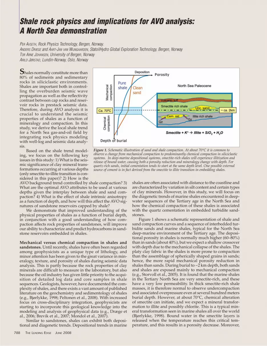
Figure 1 shows a schematic representation of shale andsand compaction curves and a sequence of interbedded tur-bidite sands and marine shales, typical for the North Seadeep-marine environment of the Tertiary age. The deposi-tional porosity in shales is normally much higher (60–80%)than in sands (about 40%), but we expect a shallow crossoverwith depth due to the mechanical collapse of the shales. Theplaty clay fabric in the shales is more prone to compactionthan the assemblage of spherically shaped grains in sands;hence, the more rapid mechanical porosity reduction inshales than sands. During burial to ~2 km depth, both sandsand shales are exposed mainly to mechanical compaction(e.g., Storvoll et al., 2005). It is found that the marine shalesin the Tertiary North Sea are very smectite-rich, and thesehave a very low permeability. In thick smectite-rich shalemasses, it is therefore normal to observe undercompactionand associated overpressure even at several hundred metersburial depth. However, at about 70°C, chemical alterationof smectite can initiate, and we expect a mineral transfor-mation to illite and possibly chlorite. This is a typical min-eral transformation seen in marine shales all over the world(Bjørlykke, 1998). Bound water in the smectite layers isreleased when the temperature reaches this critical tem-perature, and this results in a porosity decrease. Moreover,

Shale rock physics and implications for AVO analysis:A North Sea demonstrationPER AVSETH, Rock Physics Technology, Bergen, Norway.ANDERS DRÆGE and AART-JAN VAN WIJNGAARDEN, StatoilHydro Global Exploration Technology, Bergen, NorwayTOR ARNE JOHANSEN, University of Bergen, NorwayARILD JØRSTAD, Lundin-Norway, Oslo, Norway

788 THE LEADING EDGE JUNE 2008

Figure 1. Schematic illustration of sand and shale compaction. At about 70°C it is common toobserve a change from mechanical compaction to predominantly chemical compaction in siliciclasticsystems. In deep-marine depositional systems, smectite-rich shales will experience illitization andrelease of bound water, causing both a porosity reduction and mineralogy change with depth. Forquartz-rich sands, initial cementation tends to start at the same depth level. One possible externalsource of cement is in fact derived from the smectite to illite transition in embedding shales.

the presence of potassium cations (for instance in feldsparor mica) causes quartz to be produced as a by-product. Thisquartz can precipitate as microcrystalline quartz within theshale matrix, or, if connectivity allows, the quartz may pre-cipitate as cement in adjacent sandstones. The chemical reac-tion can be summarized as follows (Peltonen et al., 2008):

Smectite + K+ fi Illite + SiO2 + H2O (1)

This chemical reaction shows that there can be a link betweenthe quartz cementation of sandstones and illitization ofsmectite-rich shales. It is important to note that the sourceof quartz cement in sandstones is not unique, and can resultfrom a variety of geological processes. Figure 1 also includesa volcanic tuff layer that is typically encountered in theTertiary of the North Sea (i.e., within the Balder Formation).Smectite is often generated from the alteration of volcanictuff, but the tuff also includes amorphous silica that can pre-cipitate as quartz cement, even at temperatures below 70°C.

Amorphous silica can dissolve at tem-peratures lower than crystallinequartz. There are also potential inter-nal sources of quartz cement in thesandstones, either from authigenic ordetrital clays in the sandstone matrix,or from the quartz grains themselves.Moreover, it has been confirmed thatclay minerals can both inhibit the pre-cipitation and catalyze the dissolutionof quartz in sandstones. The presenceof oil has also been shown to inhibitquartz cementation. There are contro-versies among geologists overwhether effective pressure at quartzgrain contacts in sandstones can causequartz dissolution and reprecipitationaround the grain contacts. More likely,time and temperature control thequartz cementation. Regardless of thecomplexity of the clay and quartz dia-genesis, there is empirical evidencethat both smectite-to-illite transfor-mation in shales and quartz cementa-tion of sandstones are geochemicalprocesses that tend to happen con-currently at around 70-80°C. In theNorth Sea, this corresponds to a bur-ial depth of about 2 km, and this isaround the target depth of the prolificPaleocene and Eocene reservoir sandsthat represents major prospects for theoil industry. As geophysicists, wetherefore need to pay attention to thesegeological factors during AVO analy-sis of reservoir sands, because dra-matic changes in the seismicsignatures may reflect not only porefluid changes, but diagenetic alter-ations in the cap rock shales and/orreservoir sandstones.

Rock physics and AVO depth trendmodeling. The primary objective ofthis study is to investigate the rockphysics depth trends of shales, andhow they affect the AVO signatures.However, in order to predict depth-

dependent AVO signatures in siliciclastic environments, wealso need to consider the depth trends of sands.

Figure 2 shows log data from a North Sea well pene-trating siliciclastic sediments and rocks of Tertiary age, jux-taposed with rock physics depth trends for shales andsandstones. The sandstone rock physics models as a func-tion of depth are modeled by combining Hertz-Mindlincontact theory for unconsolidated sands with the Dvorkin-Nur contact cement model for cemented sandstones(Dvorkin and Nur, 1996; Avseth et al., 2003; Avseth et al.,2005). The input porosity-depth trends are calibrated withlocal compaction trends according to empirical relations. Thelight blue model trend curves in Figure 2 show how thevelocities increase drastically for sands as we go from theunconsolidated regime with only mechanical compaction tothe cemented regime with predominantly chemical com-paction. The onset of quartz cement is known to happen atabout 70°C, corresponding to about 2 km burial depth inthe North Sea (Bjørlykke, 1998). The Heimdal Formation

JUNE 2008 THE LEADING EDGE 789

Figure 3. Modeled rock physics depth trends of shales, showing the effect of illitization of marinesmectite-rich shales. The anisotropy parameters derived from the modeling, that are important forAVO studies, include δ in green and ε in red.

Figure 2. Rock physics depth trends for shales (blue) and sandstones (cyan), juxtaposed on NorthSea well-log data penetrating a Tertiary sequence of siliciclastic sediments and rocks. A gas zone isindicated in yellow and an oil zone in red. The remaining interval of the Heimdal Formation is brine-filled. The Heimdal Formation is embedded in the Lista Formation shale.

sandstones in the well shown in Figure 2 appear to becemented as we see a drastic jump in velocities relative tothe overburden, and this is in agreement with earlier regionalstudies of this stratigraphic unit (Avseth et al., 2000).

Shales have different composition and texture than sand-stones. Therefore, the rock physics models applicable forsandstones do not necessary apply for shales. This paperuses the shale compaction model (Dræge et al., 2006; Ruudet al., 2003) to estimate the anisotropic effective propertiesin mechanically compacted shales. The first seismicallyimportant mineral reaction in shales is commonly the smec-tite-to-illite reaction. The reaction has several implicationsfor the shale; the soft smectite is replaced by stiffer illite,which might be distributed differently in the rock, the reac-tion produces water, the amount of solids is decreased (i.e.illite has a denser mineral structure than smectite), quartzis generated as a by-product, and porosity is reduced bychemical compaction. When the shales are moving into thechemical compaction regime, a new set of rock physics mod-els is applied to estimate the seismic properties. Theanisotropic versions of a differential effective medium (DEM)model and self consistent approximation (SCA) are used toapproximate the elongated pores and grains in shales(Hornby et al., 1994).

In this paper, pores in chemically compacted shales areconsidered isolated, while the pores in the mechanical com-paction regime are connected. We define a transition zone,where the properties change from the mechanical to chem-ical regime. In Figure 2, the initial shale (<1500 m) is con-sidered to be smectite-rich, while the deeper (>2200 m)illite-rich shale is somewhat stiffer. The depth trends inFigures 2 and 3 suggest that the background shale proper-ties are neither static nor linear. There are two counteract-ing effects on anisotropy. The initial alignment of grains leadsto more aligned pores and increasing anisotropy. But decreas-ing porosity leads to decreasing anisotropy, culminating in the


Figure 4. Rock physics crossplots of well-log data juxtaposed on depthtrend models for shale (blue), brine sands (cyan), oil sands (red), and gassands (yellow). The data are colored in terms of shale volume (upper) andhydrocarbon saturation (lower) and include both a gas zone and oil zone(see Figure 2).

Figure 5. AVO depth trends, including acoustic impedance, VP/VS, intercept (R(0)) and AVO gradient (G). AVO reflectivity modeling (see Figure 6)is performed at three different depth levels: (1) at 1600 m burial depth where sands are unconsolidated and shales are smectite-rich; (2) at 2000 m burialdepth where initial cementation and associated illitization have started; (3) at 2400 m burial depth where the sandstones are well consolidated. (Thecolor scales of the two right panels are the same as the numerical scales along the x-axes, representing R(0) and G, respectively).

anisotropic properties of the solid material at zero porosity.The pores introduce higher anisotropy than the solid, sincepores commonly are weaker orthogonal to the longest axis,while the solids are less dependent on direction of wave prop-agation. The Thomsen parameters of anisotropy, δ and ε, areimportant for the AVO modeling below, because the transverseisotropy of shales can alter the AVO gradient.

Figure 4 shows rock physics crossplots (acoustic imped-

ance versus VP/VS including the well-log data in Figure 2, aswell as the rock physics depth trends for sandstone and shale.In this crossplot, we also include the depth trends for oil andgas sands; the various fluid scenarios are estimated usingGassmann theory. We see that the modeled shale trend fitsnicely with the shale data from the well logs. The sandstonedata in the target zone are diagnosed as cemented based onthe rock physics models. As expected, the gas and oil filledsandstones, indicated by low water saturation values in Figure4, show low VP/VS values relative to the brine-sand values, inaccordance with the modeled depth trends. The separationand detectability of hydrocarbon-filled sandstones wouldhave been even larger in terms of VP/VS if the sands were shal-lower and not cemented. It is expected that cementation stiff-ens the rock frame and reduces the fluid sensitivity. Acousticimpedance is not a good discriminator of either lithology orfluids for most of the depth range considered in this case. Theserock physics observations indicate that AVO analysis isrequired in order to seismically discriminate hydrocarbonsfrom brine for this North Sea case. By conducting AVO depth-trend modeling, we can verify the feasibility of AVO analysisas a function of burial depth and diagenesis and therebyextrapolate to other burial depths. This can be a useful taskin exploration or appraisal where we want to extend oursearch to slightly deeper or shallower prospects surroundingexisting discoveries.

Figure 5 shows the depth trends of acoustic impedanceand VP/VS superimposed onto the well-log data, together withdepth trends of intercept (R(0)) and AVO gradient (G). Theintercept and gradient curves are estimated on a sample-by-sample basis where the cap rock properties are given by themodeled shale trends, whereas the reservoir properties aregiven by the modeled sandstone trends, for different pore fluidscenarios (brine, oil and gas). Note how the expected seismicreflectivity changes drastically as we go from the mechanicalcompaction domain to the chemical compaction (cementation)domain. Also note how the modeled fluid sensitivity drasti-cally decreases over a range of only a few hundred meters, assandstones become cemented.

Figure 6 includes AVO reflectivity modeling of half-spaceboundaries between cap rock shale and reservoir sandstoneperformed at three different depth levels: (1) at 1600 m whereonly mechanical compaction is occurring (i.e., in the uncon-solidated regime); (2) at 2000 m in a transition zone where ini-tial chemical compaction has taken place (i.e., in the poorlyconsolidated regime); and (3) at 2400 m where the sandstonesare moderately to well cemented (i.e, in the consolidatedregime). In this reflectivity modeling, we include both isotropicand anisotropic AVO modeling. In the latter case we assumethe cap rock shale to be transversely isotropic, with theThomsen parameters estimated from the shale modelingdescribed above. The offset-dependent reflectivity curves forthree-term AVO, including both isotropic and anisotropicterms, are estimated using the following formula (Kim et al.,1993):

RPP(θ)=RIPP(θ)+RAPP(θ) (2)

where the isotropic reflectivity term can be expressed as fol-lows:

RIPP (θ)=R(0) + G . sin2 (θ) + F .[tan2(θ)–sin2 (θ)] (3)

Here, R(0) is the intercept or zero-offset reflectivity, G is theAVO gradient, and F is the third-order curvature term affect-ing far offsets. θ is the average of the angles of incidenceand transmission (normally approximated to be the angle


Figure 6. AVO reflectivity modeling at the three different depth levelsindicated in Figure 5: (1) At 1600 m burial depth we obtain AVO classIV for brine sands and class III for hydrocarbons. Note that the anisotropyeffect (dashed lines) is actually changing the sign of the gradient for brinesands from slightly positive to slightly negative. (2) At 2000 m burialdepth, we observe a weaker fluid sensitivity, and the brine sands havealmost zero near-stack response, but there are significant negative gradi-ents for all fluid scenarios. (3) At 2400 m burial depth, the brine sand-stones show a class I AVO signature, whereas oil- and gas-filledsandstones show a more class II AVO response. For all cases, theanisotropy starts becoming significant beyond about 30° angle ofincidence.

of incidence).Moreover, the anisotropic reflectivity term for the case

where the cap rock is transversely isotropic and the reser-voir is isotropic, is given by:

(4)

As we see from this expression, one of the Thomsen para-meters, δ, is affecting the same offset range as the contrastin VP/VS ratio (i.e., the AVO gradient), whereas ε is affect-ing larger offsets. In the reflectivity modeling in Figure 6,we consider angles of incidence up to 45°. The isotropicreflectivity curves are plotted as continuous lines, whereasthe anisotropic reflectivity curves are plotted as dashedlines. We observe that the anisotropic curves start to devi-ate from the isotropic curves at around 30° for most of thecases. However, for the uppermost case, the brine responseshows a change in gradient from weakly positive to weaklynegative due to the anisotropy. The AVO reflectivity mod-eling at the three different depths and compaction regimesfurthermore show that we go from a AVO class III to classII for hydrocarbon-saturated sandstones within a few hun-dred meters depth.

Using the modeled shale trend as a cap rock analog, thewell-log data in Figure 2 can be crossplotted as AVO inter-cept versus AVO gradient (Figure 7). For each depth sam-ple, we assume a two-layer model, where “layer 1” (i.e., thecap rock) is represented by the modeled shale trend, andthe properties of “layer 2” are given by the well-log data.Hence, this is only showing the expected top “layer 2”responses for simple half-spaces. The plot does not includethe expected base “layer 2” responses, neither does it includeany scale or tuning effects, which is expected in similarcrossplots derived from seismic data. Certainly, this cross-plot representation of the well-log data is simplified, but itgives a qualitative picture of the expected location of thewell-log data at a given depth. We have superimposed theprojections of the modeled sandstone trends for different flu-ids, where we also have used the modeled shale trend asassociated cap rock. These lines show the expected locationof brine, oil and gas sands as a function of the studied depthrange. For the well-log data, the hydrocarbon zone appearsas a class II AVO response, and this matches nicely with the

modeled sandstone trends for oil and gas. However, mostof the reservoir is gas saturated, and the data plots betweenthe oil and the brine trend. It should be mentioned that themodeled sandstone trends represent clean sandstone,whereas the reservoir zone in the well-log data has a vary-ing amount of clay, both pore-filling and laminated. The sha-liness of the sands is expected to bring the hydrocarbonanomaly closer to the brine saturated background trend.

Next, we use the modeled shale and sandstone trends


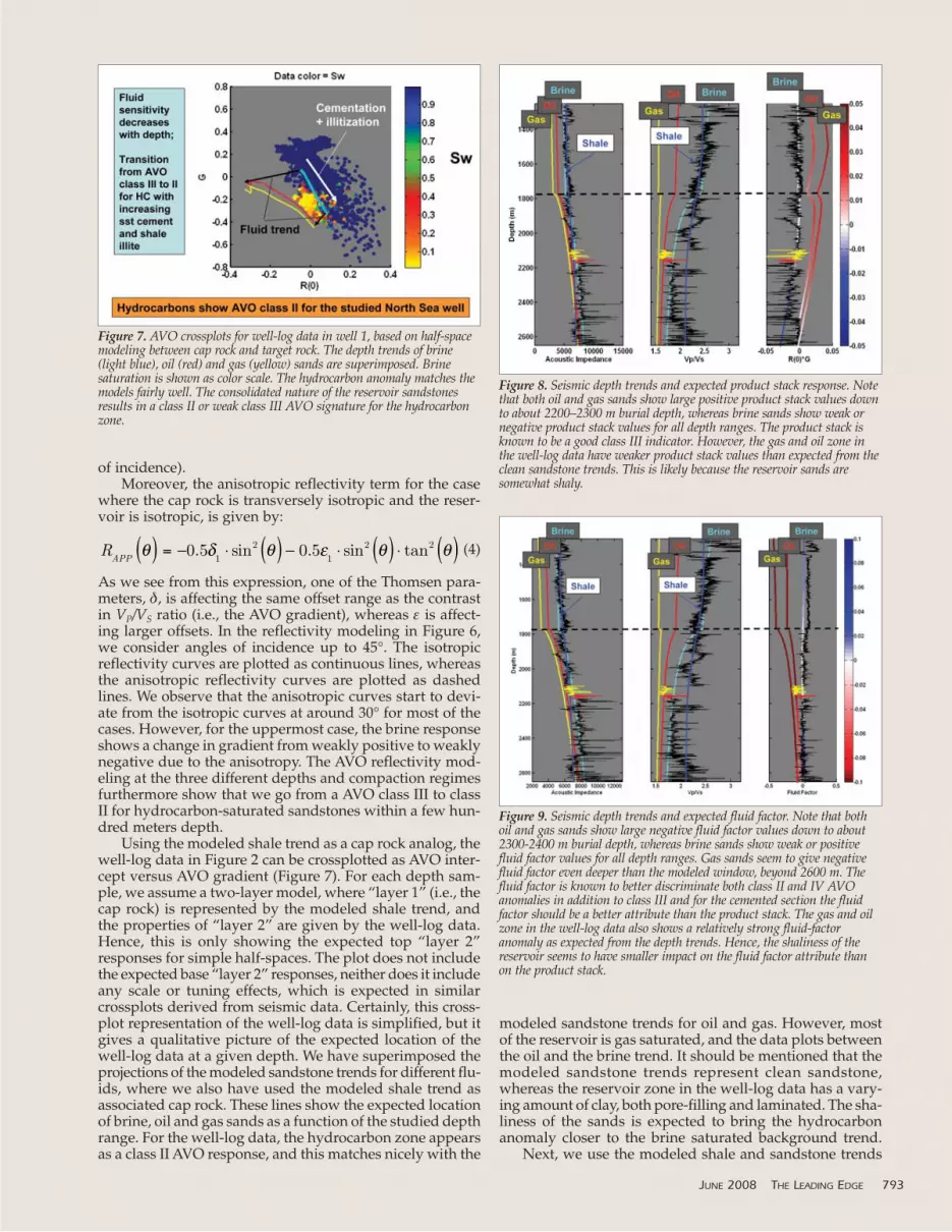
Figure 7. AVO crossplots for well-log data in well 1, based on half-spacemodeling between cap rock and target rock. The depth trends of brine(light blue), oil (red) and gas (yellow) sands are superimposed. Brinesaturation is shown as color scale. The hydrocarbon anomaly matches themodels fairly well. The consolidated nature of the reservoir sandstonesresults in a class II or weak class III AVO signature for the hydrocarbonzone.

Figure 8. Seismic depth trends and expected product stack response. Notethat both oil and gas sands show large positive product stack values downto about 2200–2300 m burial depth, whereas brine sands show weak ornegative product stack values for all depth ranges. The product stack isknown to be a good class III indicator. However, the gas and oil zone inthe well-log data have weaker product stack values than expected from theclean sandstone trends. This is likely because the reservoir sands aresomewhat shaly.

Figure 9. Seismic depth trends and expected fluid factor. Note that bothoil and gas sands show large negative fluid factor values down to about2300-2400 m burial depth, whereas brine sands show weak or positivefluid factor values for all depth ranges. Gas sands seem to give negativefluid factor even deeper than the modeled window, beyond 2600 m. Thefluid factor is known to better discriminate both class II and IV AVOanomalies in addition to class III and for the cemented section the fluidfactor should be a better attribute than the product stack. The gas and oilzone in the well-log data also shows a relatively strong fluid-factor anomaly as expected from the depth trends. Hence, the shaliness of thereservoir seems to have smaller impact on the fluid factor attribute thanon the product stack.

to estimate AVO attributes as a function of depth. Thesedepth trends can be compared with the AVO attributes esti-mated from the well-log data. We do this for two well-known AVO attributes estimated from combinations ofintercept and AVO gradient, the “product-stack” (i.e, R(0)� G) and the “fluid factor,” respectively. The fluid factor,which is defined as the distance from the background trendin an AVO crossplot, can be expressed in terms of interceptand gradient as (Fatti et al., 1994):

(5)

where � is a constant at a given depth, depending on thebackground VP/VS ratio, χ, and the slope of the Vp-Vs rela-tionship of the modeled shale trend, m:

� = m�χ (6)

Commonly, m is selected to be the slope of the mudrock line(Castagna et al., 1985), where m = 1.16. Similarly, the back-ground VP/VS ratio (χ) is often set equal to 2, giving a � valueof .58. However, with our modeled shale trends, we can esti-mate more realistic depth dependent values of � and get abetter control on the expected background trend to be usedin the fluid factor.

Note that the product stack of both oil and gas sands isexpected to give large positive anomalies for depths downto approximately 2200 m, beneath which it gets close tozero, as we go from AVO class III to AVO class II (Figure 8).In contrary to the product stack, the fluid factor is a muchmore robust AVO attribute with respect to hydrocarbondetection (Figure 9). For this attribute, we observe both the

gas sand and the oil sand to cause a negative fluid factoranomaly relative to the background brine trend. The thinoil zone is almost on the brine trend, likely due to relativelyhigh clay content and poor sand quality. However, the chem-ical compaction has a significant impact on the absolutevalue of the fluid factor, which is directly related to the factthat the fluid sensitivity is decreasing with depth and increas-


Figure 10. Seismic sections intersecting the well studied in this case (well 1), including near stack, far stack, and the estimated far-near stack. The bluesquare indicates the window where a background trend is estimated. The yellow ellipse highlights the gradient anomaly of the gas-and-oil discovery ofwell 1. The red ellipse highlights an adjacent oil discovery.

Figure 11. Intercept (near) versus gradient (i.e. far-near) for the seismicstack section in Figure 10. Only data from the selected polygons/ellipsesare included. The blue points represent the background trend right abovethe target; the yellow points represent data from the gas (and oil) discov-ery in well 1, and the red data points represent data from the adjacent oil discovery.

ing rock stiffness. It is well known that the fluid factordetects AVO anomalies of class II, III, and IV, as long as thedeviation from the background trend is sufficient, and, inthis case, we see that the fluid factor will detect the class IIbehavior of the anomaly encountered by the investigatedwell.

Application to real seismic data. Finally, we want to testthe results from the modeling of expected AVO attributesconducted above, on real seismic data from the same area.Figure 10 shows seismic stack sections intersecting the wellstudied above, including a near stack, far stack, and the dif-ference between far and near. The latter is representative ofthe AVO gradient as the near, and the far-stack data havebeen preprocessed for true offset dependent amplitudeanalysis. This line intersects three hydrocarbon discoveriesin Tertiary turbidites in the North Sea; in this study, we willconcentrate on two of these. The one penetrated by themarked well (well 1) is highlighted by a yellow ellipse, andthis is the AVO anomaly caused by the gas and oil zoneshown in the well-log data. Furthermore, the anomaly high-lighted by the red ellipse is a neighboring oil discovery. Itis interesting to note that the oil anomaly to the right of thewell has a strong soft (i.e., negative amplitudes) top on thenear stack, whereas the gas anomaly at the indicated welllocation has a weak, close-to-zero amplitude top on thesame stack. Both anomalies show strong negative far-stackresponses. However, the gas anomaly shows a somewhatstronger gradient anomaly. These observations are evidentin the crossplot in Figure 11. Here we see that the gas (and

thin oil) discovery in well 1 shows a class II AVO anomaly,whereas the neighboring oil discovery shows a class III AVOanomaly. First of all, it is interesting to note that the mod-eled AVO attributes based on the well-log data and a rep-resentative shale trend match very nicely with theobservations in the seismic data (compare Figures 7 and 11).However, at first glance, it is counterintuitive that the adja-cent oil anomaly shows a class III anomaly. This cannot beexplained from the fluid properties, but it has to do withthe sandstone quality. The previous AVO depth-trend mod-eling indicates that we are at a depth level very close to theinitial quartz cementation of sandstones. Going back to theschematic illustration in Figure 1, we can get a clue of whythe oil sands show up as class III while the gas sands showup as class II. There is a good chance that some of the sandsat this depth are not yet cemented. There can be local vari-ations and uncertainties of the onset of chemical compaction.This can be related to many factors: local variations in tem-perature gradient, local variations in clay mineralogy withinthe sands (e.g., clay coating of sand grains inhibit the quartzcementation), or local variation of connectivity for externalsources of quartz, e.g., from illitization of shales or amor-phous silica within the stratigraphically overlying volcanictuffs. Moreover, it has been documented that early migra-tion of oil into reservoir sands can also inhibit quartz cemen-tation.

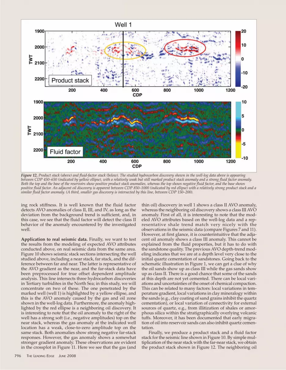
Finally, we produce a product stack and a fluid factorstack for the seismic line shown in Figure 10. By simple mul-tiplication of the near stack with the far-near stack, we obtainthe product stack shown in Figure 12. The neighboring oil


Figure 12. Product stack (above) and fluid-factor stack (below). The studied hydrocarbon discovery shown in the well-log data above is appearingbetween CDP 450–650 (indicated by yellow ellipse), with a relatively weak but still marked product stack anomaly and a strong fluid factor anomaly.Both the top and the base of the reservoirs show positive product stack anomalies, whereas the top shows negative fluid factor, and the base shows positive fluid factor. An adjacent oil discovery is apparent between CDP 850–1000 (indicated by red ellipse) with a relatively strong product stack and asimilar fluid factor anomaly. (A third, smaller gas discovery is intersected by this line, between CDP 150–200).

discovery shows a strong product stack, whereas the gas dis-covery at well 1 shows a much weaker product stack. Thisis expected, as documented in the depth trend modeling (seeFigure 9), where the gas discovery has been confirmed toproduce a class II AVO anomaly. We also produce a fluidfactor stack, which is included in Figure 12. The fluid fac-tor can be derived from near- and far-stack amplitudes usingthe formula:

∆F = Near– η. (Far–Near) (7)

Here, η is not the same as � in the earlier formulation of thefluid factor, since far-near is not exactly the same as the AVOgradient. However, the two-term AVO makes a linear rela-tionship between the far-near and the AVO gradient, andtherefore η and � can also be easily correlated. Assumingthe far stack to be around 30° and the near stack to be at 0°(normally the far stack will be representative for slightlylower angles than 30°, whereas near stack will be repre-sentative for angles slightly higher than 0°), we obtain thefollowing approximate relationship between the gradientand the far-near:

Far–Near = R (30)–R(0) = G . sin (30) = G . 0.25 (8)

Solving for the background trend, that is when ∆F=0, weobtain:

(9)

hence we get:

(10)

The slope of the background trend in the near versus far-near stack is 1/η, and this shows that we can in fact esti-mate the expected background trend for uncalibrated (butoffset balanced) range-limited stacks using the modeledshale trends as illustrated in this study. This can be a use-ful task to verify the correct amplitude balancing betweennear- and far-stack data during AVO crossplot analysis.

Based on the shale model trends, we estimate a value ofη to be of order 2.5. This means the background trend of theshale in the AVO crossplot is relatively flat, equaling -0.4,i.e., far-near = -0.4 near. We observe indeed that the shalebackground trend is relatively flat (blue cloud in Figure 11).Using this background trend, the resulting fluid-factorattribute in Figure 12 shows that both the gas and the oildiscoveries are standing out as strong fluid factor anomalies,whereas the background data are relatively weak. It isexpected from the well-log observations that the brine-sat-urated rocks beneath the hydrocarbon reservoirs will havea steeper negative slope in the near versus far-near cross-plot. This can easily be tested by inputting different valuesfor the background VP-VS relationships.

Conclusions. A rapid transition from predominantlymechanical compaction to predominantly chemical com-paction occurs at around 70°C corresponding to about 2 km

burial depth in the North Sea. Illitization of smectite-richshales and associated quartz cementation of both silty shalesand sandstones cause drastic changes in the elastic proper-ties as this threshold burial temperature is exceeded. Thesediagnetic alterations are important to consider during AVOscreening and quantitative seismic interpretation, especiallywhen the target depth is around this depth. Reservoir sand-stones will obtain a stiffened framework and associateddecrease in fluid sensitivity as cementation occurs. Moreover,the change in shale mineralogy and porosity will determinethe AVO background trend, and an improved understand-ing of rock physics depth trends and anisotropy of shalescan help us to predict expected AVO classes and better con-strain the estimation of optimal fluid-factor attributes.

Suggested reading. “Rock physics modeling of shale diagen-esis” by Dræge et al. (Petroleum Geoscience, 2006). “Clay min-eral diagenesis and quartz cementation in mudstones: Theeffects of smectite to illite transformation on rock properties”by Peltonen et al. (Marine and Petroleum Geology, 2008). “Claymineral diagenesis in sedimentary basins—A key to the pre-diction of rock properties; examples from the North Sea Basin,by Bjørlykke (Clay Minerals, 1998). “Experimental mechanicalcompaction of clay mineral aggregates—Changes in physicalproperties of mudstones during burial” by Mondol et al. (Marineand Petroleum Geology, 2007). “Documentation and quantifica-tion of velocity anisotropy in shales using wireline log mea-surements” by Brevik et al. (TLE, 2007). “Velocity-depth trendsin Mesozoic and Cenozoic sediments from the NorwegianShelf” by Storvoll et al. (AAPG Bulletin, 2005). “Anisotropic effec-tive medium modeling of the elastic properties of shales” byHornby et al. (GEOPHYSICS, 1994). “Seismic properties of shalesduring compaction” by Ruud et al. (SEG Expanded Abstract,2003). “Elasticity of high-porosity sandstones: Theory for twoNorth Sea datasets” by Dvorkin et al. (GEOPHYSICS, 1996). “RockPhysics diagnostics of North Sea sands: The link betweenmicrostructure and seismic properties” by Avseth et al.(Geophysical Research Letters, 2000). “AVO classification of lithol-ogy and pore fluids constrained by rock physics depth trends”by Avseth et al. (TLE, 2003). Quantitative Seismic Interpretation—Applying Rock Physics Tools to Reduce Interpretation Risk by Avsethet al. (Cambridge University Press, 2005). “Detection of gas insandstone reservoirs using AVO-analysis: A3D seismic case his-tory using the Geostack technique” by Fatti et al. (GEOPHYSICS,1994). “Effects of transverse isotropy on P-wave AVO for gassands” by Kim et al. (GEOPHYSICS, 1993). “Relationships betweencompressional-wave and shear-wave velocities in clastic sili-cate rocks” by Castagna et al. (GEOPHYSICS, 1985). TLE

Acknowledgements. We thank Torbjørn Fristad, Erik Ødegaard, CindyGosse, and Trond Seland at StatoilHydro; Ran Bachrach atWesternGeco/Schlumberger; Vigdis Løvø at Lundin-Norway; and KnutBjørlykke at University of Oslo for valuable discussions and input on thetopics of AVO depth trends. Thanks to Lundin-Norway for providing dataused in this study.

Corresponding author: [email protected]


Near =20

8 5(Far Near )

shale rock physics and implications for avo analysis: a north sea demonstration

Documents