GEOPHYSICS, VOL. 65, NO. 1 (JANUARY-FEBRUARY 2000); P. 54–67, 13 FIGS., 3 TABLES.

Bottom-simulating reflectors: Seismic velocities and AVO effects

Jose M. Carcione∗ and Umberta Tinivella∗

ABSTRACT

We obtain the wave velocities of ice- and gas hydrate–bearing sediments as a function of concentration andtemperature. Unlike previous theories based on simpleslowness and/or moduli averaging or two-phase models,we use a Biot-type three-phase theory that considers theexistence of two solids (grain and ice or clathrate) and aliquid (water), and a porous matrix containing gas andwater.For consolidated Berea sandstone, the theory under-

estimates the value of the compressional velocity below0◦C. Including grain-ice interactions and grain cementa-tion yields a good fit to the experimental data. Strictlyspeaking, water proportion and temperature are closelyrelated. Fitting the wave velocity at a given tempera-ture allows the prediction of the velocity throughout therange of temperatures, provided that the average poreradius and its standard deviation are known.

The reflection coefficients are computed with a vis-coelastic single-phase constitutive model. The analysisis carried out for the top and bottom of a free-gas zonebeneath a gas hydrate-bearing sediment and overlyinga sediment fully saturated with water. Assuming thatthe bottom-simulating reflector is caused solely by an in-terface separating cemented gas hydrate– and free gas–bearing sediments, we conclude that (1) for a given gassaturation, it is difficult to evaluate the amount of gashydrate at low concentrations. However, low and highconcentrations of hydrate can be distinguished, sincethey give positive and negative anomalies, respectively.(2) Saturation of free gas can be determined from thereflection amplitude, but not from the type of anomaly.(3) The P to S reflection coefficient is a good indicator ofhigh amounts of free gas and gas hydrate. On the otherhand, the amplitude-variation-with-offset curves are al-ways positive for uncemented sediments.

INTRODUCTIONGashydrate is a clathrate composedofwater andnatural gas,

mainly methane, which forms under conditions of low temper-ature, high pressure, and proper gas concentration. Bottom-simulating reflectors (BSRs) on seismic profiles are interpretedto represent the seismic signature of the base of gas hydrateformation; a free gas zone may be present just below the BSR(e.g., Andreassen et al., 1990).Where nodirectmeasurements are available, detailed know-

ledge of the compressional and/or shearwave velocity distribu-tion in marine sediments is essential for quantitative estimatesof gas hydrate and free gas in the pore space. The discrepan-cies between the inverted velocity profile (from seismic data)and the velocity for water-filled, normally compacted marinesediments are interpreted as caused by the presence of gashydrate (where positive anomalies are present) and free gas(where negative anomalies are present). These anomalies canbe translated in terms of concentration of clathrate and free gasif the velocity trend versus gas hydrate and free gas content is

Manuscript received by the Editor December 04, 1997; revised manuscript received December 15, 1998.∗Osservatorio Geofisico Sperimentale, Borgo Grotta Gigante 42c, 34010 Sgonico, Trieste, Italy. E-mail: jcarcione@ogs.trieste.it; utinivella@ogs.trieste.it.c© 2000 Society of Exploration Geophysicists. All rights reserved.

known. An alternative method for estimating the amount ofhydrate and gas is to analyze the variation of the reflectioncoefficient of the BSR versus offset.

The elastic properties of ice are similar to those of hydrate,so the properties of permafrost are often compared with thoseof hydrated sediments (Sloan, 1990). Timur (1968) proposeda three-phase time-average equation based on slowness av-eraging (Wyllie’s equation) for modeling consolidated per-mafrost sediments. Moreover, he found that as temperatureis decreased below 0◦C, the water contained in the large poresfreezes first, and that the freezing process ends between−21◦Cand −22◦C, in accordance with the phase diagram for thesodium chloride–water system. The problem of transition from“suspension” to “compacted” sediment was treated with com-bined models. For instance, averaging bulk moduli weightedwith the respective porosities [Voigt’s model (Voigt, 1928)]gives a simple model for consolidated sediments, whereas av-eraging the reciprocal of bulk moduli [Reuss’s model (Reuss,1929)] accounts for unconsolidated media. Zimmerman and

54

AVO Effects of BSRs 55

King (1986) used the two-phase theory developed by Kusterand Toksoz (1974), assuming that unconsolidated permafrostcan be approximated by an assemblage of spherical quartzgrains embedded in a matrix composed of spherical inclusionsof water and ice. They first compute the effective elasticmoduliof the ice-water mixture, with water playing the role of inclu-sion. This yields a homogeneousmediumwhere the sand grainsare the inclusion.A three-phase theory based on first principles was proposed

by Leclaire et al. (1994). The theory, hereafter called as theLCA model, assumes that there is no direct contact betweensolid grains and ice since, in principle,water tends to forma thinfilmaround the grains. The theorypredicts three compressionalwaves and two shear waves, and can be applied to unconsoli-dated and consolidated media. Leclaire et al. (1994) also pro-vide a thermodynamic relation between the water proportionand temperature. On the other hand, Santos et al. (1990a, b)presented a theory describing wave propagation in a porousmedium saturated with a mixture of two immiscible, viscous,compressible fluids.We use this theory for calculating the wavevelocities of sediments partially saturated with gas and water.Therefore, the BSR is modeled by a porous medium in whichthere are two solid components (matrix and gas hydrates) over-lying a gas- and water-filled porous medium having the samesolid skeleton as the upper medium.

MODEL FOR GAS HYDRATE-BEARING SEDIMENTS

The theory developed by Leclaire et al. (1994) explicitlytakes into account the presence of the three phases. Here, wehave included the contributions to the potential and kineticenergies due to the contact between the solid grains and thehydrates, and the stiffening of the skeleton due to grain cemen-tation. In fact, samples of gas hydrate recovered in awell (ODPLeg 164 Shipboard Scientific Party, 1996) and a real data study(Ecker et al., 1996) suggest that the hydrates are distributedthrough the pore space and across the grains.The equation of motion of the modified LCA model

(LCAM) can be written in matrix form as

R grad div u − µ curl curl u = ρu + Au,

where u is the displacement field,

R =

R11 R12 R13

R12 R22 R23

R13 R23 R33

and µ =

µ11 0 µ13

0 0 0

µ13 0 µ33

are the stiffness and shear matrices,

ρ =

ρ11 ρ12 ρ13

ρ12 ρ22 ρ23

ρ13 ρ23 ρ33

is the mass density matrix, and

A =

b11 −b11 0

−b11 b11 + b33 −b330 −b33 b33

is the friction matrix, where b13 have been assumed equal tozero (this parameter describes solid-grain/hydrate friction). A

dot above a variable denotes time differentiation. All the pa-rameters with the subindex (13) describe the interaction be-tween the two solid components.

An effective density ρ = ρ − iA/ω can be defined in thefrequency domain.

The three compressional velocities of the three-phase frozenporous medium are given by

VPi = [Re(√

�i )]−1, i = 1, . . . , 3, (1)

where Re takes the real part and �i are obtained from thefollowing characteristic equations:

�3 det(R) − �2a + �b − det(ρ) = 0,

det(R) = R11R22R33 − R223R11 − R2

12R33 − R213R22

+ 2R12R23R13,

a = a1 + a2 + a3,

a1 = ρ11 det(Riw) + ρ22 det(Rsi ) + ρ33 det(Rsw),

a2 = −2(ρ23R23R11 + ρ12R12R33 + ρ13R13R22),

a3 = 2(ρ23R13R12 + ρ13R12R23 + ρ12R23R13),

det(Rsw) = R11R22 − R212,

det(Riw) = R22R33 − R223,

det(Rsi ) = R11R33 − R213,

det(ρ) = ρ11ρ22ρ33 − ρ223ρ11 − ρ2

12ρ33 − ρ213ρ22

+ 2ρ12ρ23ρ13,

det(ρsw) = ρ11ρ22 − ρ212,

det(ρiw) = ρ22ρ33 − ρ223,

det(ρsi ) = ρ11ρ33 − ρ213,

b = b1 + b2 + b3,

b1 = R11 det(ρiw) + R22 det(ρsi ) + R33 det(ρsw),

b2 = −2(R23ρ23ρ11 + R12ρ12ρ33 + R13ρ13ρ22),

b3 = 2(R23ρ13ρ12 + R13ρ12ρ23 + R12ρ23ρ13).

The two shear velocities VSi are given by

VSi = [Re(√

i )]−1, i = 1, 2 (2)

where i are the complex solutions of the equation

2a′ − b′ + det(ρ) = 0,

a′ = ρ22 det(µsi ),

b′ = µ11 det(ρiw) + µ33 det(ρsw)

− 2µ13ρ13ρ22 + 2µ13ρ12ρ23,

det(µsi ) = µ11µ33 − µ213.

Appendix A illustrates the meaning of the different param-eters, and Appendix B the generalization of the potential andkinetic energies. The expressions for Kmax and µmax can befound in Zimmerman and King [1986, equations (1) and (2),respectively], with the subscript m corresponding to ice, i cor-responding to air, and the concentration c equal to φs . Theyare the moduli of the ice matrix, with the water totally frozenand the solid replaced by air. On the other hand, we assumethat the rigidity modulus of the solid matrix µsm is affected bycementation of the sand grains by ice. The equation, indicated

56 Carcione and Tinivella

in Appendix A, follows the same percolation model used forthe ice matrix (Leclaire et al., 1994). The rigidity µsm0 is theshear modulus of the rock at full water saturation. Alterna-tively, the cementation effect can be introduced through thecoupling modulus µsi by means of a similar percolation model.In this work, we assume µsi = 0.The expressions for the density components, given in Ap-

pendix B, include the interaction between the grain and icephases, assuming that the grains flow through the ice matrix(described by the tortuosity a13) and the ice flows throughthe skeleton (described by a31). As is well known, the tortu-osity is related to the difference between the microvelocityand macrovelocity fields. If they are similar (i.e., for relativelyrigidmaterials like solids), the tortuosities equal 1 and the con-tributions vanish. However, we assume that these terms con-tribute to the kinetic energy when the solid and ice matricesare unconsolidated or relatively unconsolidated, for which thetortuosities are greater than 1. As in Biot theory, we neglectthe solid contributions related to the interaction with water.On the other hand, depending on the frequency, a very thin

and viscous water layer may transmit shear deformations fromonematrix to the other. In this case, the coefficientsµ1,µ2, andµ13 become relaxation functions and should be replaced (in thetime domain) by the operators µ1∗, µ2∗, and µ13∗ (∗ denotestime convolution), with µav representing a Maxwell mechani-cal model with two springs, whose stiffnesses are µs/(1− g1)φs

and µi/(1− g3)φi , and a dashpot of viscosity ηw/φw . Note thatLeclaire et al. (1994) neglect the imaginary part of theMaxwellcomplex modulus, and then the related attenuation effects.Assuming a Gaussian porosimetric distribution, the water

proportion φw can be obtained as a function of temperature as

φw = (1− φs)A∫ r0/ln(T0/T )

0exp

[−(r − rav)2/(2 r2)

]dr,

(3)

where rav is the average pore radius, r is the standarddeviation, and the temperature T is given in Kelvins andT0 = 273K (Hudson, 1992; Leclaire et al., 1994). The quantityr0 = 0.228 nm in the ideal case, but here it is used as a parameterin order to take into account the salinity content of the porewater. As stated by Timur (1968), as the ice crystallizes out aspure water, the sodium chloride concentration of the remain-ing solution increases, thereby further lowering the freezingpoint. Hence, ice may be thought of as forming on the walls ofthe larger pores and growing into the pore spaces. This effectis modeled by equation (3).The constant A is obtained after normalization of the

Gaussian probability function from r = 0 to r = ∞. Thus, weobtain

φw = (1 − φs)erf(ζ ) + erf(η)

1 + erf(η), ζ = r0/ln(T0/T )√

2 r− η,

η = rav√2 r

. (4)

MODEL FOR FREE GAS-BEARING SEDIMENTS

The porous media saturated by a mixture of water and freegas can be described by the theory developed by Santos et al.

(1990a, b). The velocity of compressional waves is

VP =[Re

(1V

)]−1

, (5)

where V is the complex velocity satisfying the eigenvalue equa-tion

Mq = V 2(D − iL)q, (6)

with q the eigenvectors,

M =

Kc B1 B2

B1 M1 M3

B2 M3 M2

and D =

ρ ρg Sg ρw Sw

ρg Sg g1 g3ρw Sw g3 g2

the stiffness and density matrices, respectively, and

L = diag

(0,

S2g

ω

ηg

κg,

S2w

ω

ηw

κw

)

the friction matrix. The shear velocity is

VS =[Re

(1V

)]−1

, (7)

where

V = õsm0

[ρm

− ρg Sg(g∗2ρg Sg − g3ρw Sw

) + ρw Sw

(g∗1ρw Sw − g3ρg Sg

)g∗1g∗

2 − g23

]

and

g∗1 = g1 − i

S2g

ω

ηg

κg, and g∗

3 = g3 − iS2

w

ω

ηw

κw

.

The permeabilities can be expressed as

κg = κs0krg and κw = κs0krw,

where krg and krw are the relative permeabilities.For low frequencies (i.e., the seismic case), the compressional

and shear velocities are

VP =√(Kc + 4µsm0/3)/ρm, and VS =

√µsm0/ρm

(8)(see Appendix A for more details).

WAVE VELOCITIES OF BEREA SANDSTONE

The first example (see Figure 1) compares the compressionalvelocity obtained by using the present theory with those of themost commonacousticmodels for permafrost.Adescription ofthesemodels canbe found, for instance, inCarcioneandSeriani(1998). The data (see Table 1) correspond to Berea sandstone,with the properties given by Timur (1968) andWinkler (1985).The Voigt and Wood models provide upper and lower boundsfor the bulk and rigidity moduli. Roughly, the velocities of thedifferent models must lie between the Voigt and Wood ve-locities (note that the bounds refer to the moduli, not to thevelocities). The time average velocity is obtained by averag-ing the slowness of the different phases weighted by the re-spective porosities. Minshull et al. (1994) obtain an effective

AVO Effects of BSRs 57

medium 1 by time averaging the solid and ice (gas-hydrate)phases; then, they obtain a medium 2 for the water-filled sed-iment from Gassmann’s equation; finally, they time averagemediums 1 and 2 to obtain the velocity of the partially sat-urated sediment. On the other hand, Zimmerman and King(1986) use Kuster and Toksoz’s (1974) theory for obtaining theeffective moduli of the ice-water mixture (with water playingthe roleof inclusion), and thenuse thismixture as abackgroundmedium where the sand grains are the inclusion. This gives anunconsolidated model for permafrost, with low velocities forlow ice concentrations.The curves LCA, LCAM and M (Minshull et al., 1994) co-

incide and give Biot’s results at full water saturation, but theygive different values at full ice saturation. Note that the cemen-tation effect is strong for high concentrations of ice (comparethe LCA and LCAM curves). The curve ZK (Zimmerman andKing, 1986) coincides with Wood’s model (W) at full watersaturation, since it assumes an unconsolidated matrix. All thetheories correctly predict the behavior of the fast wave velocityin a partially frozenmedium, i.e., velocity decreases for increas-ingwater saturation. Finally, theV (Voigt’smodel) curve seemsto overestimate the velocity.The next example (Figure 2) analyzes the dependence of

the compressional velocity of permafrost on temperature.The data (see Table 1) correspond to Berea sandstone, withthe properties given by Timur (1968) and Winkler (1985).In order to evaluate the influence of ice-grain interactionsand grain cementation, we represent the compressional andshear velocities versus ice concentration corresponding tofour different models. As can be appreciated, cementation,modeled by the percolation theory, is the most important

FIG. 1. Compressional wave velocity versus water proportionpredicted by the different theories. Themedium is Berea sand-stone, whose properties are given in Table 1. LCAM is themodified theory.

Table 1. Material properties for frozen Berea sandstone.

Grain ρs = 2650 kg/m3 Ks = 38.7 GPa µs = 39.6 GPa κs0 = 1.07 10−13 m2

Ice ρi = 920 kg/m3 Ki = 8.58 GPa µi = 3.7 GPa κi0 = 5 × 10−4 m2

Water ρw = 1000 kg/m3 Kw = 2.25 GPa µw = 0 GPa ηw = 1.798 cP∗Ksm = 14.4 GPa µsm0 = 13.1 GPa rs = 50 µm rav = 10 µm r = 10 µm∗1 cP = 0.001 Pa·s.

factor. However, for low concentrations (less than 30%), allvelocities coincide in practice.

Figure 3a shows thewater proportionφw as a functionof tem-perature computed from equation (4), assuming rav = 10 µm, r = 10 µm, and r0 = 0.04 µm. Figure 3b represents the com-pressionalwavevelocity versus temperature,where the squarescorrespond to the experimental data measured by Timur(1968). The sample was subjected to an uniaxial pressure of313 atm, and the pore fluid was under atmospheric pressure.The sample, with a porosity of 0.2, was first cooled to −23◦C,and then brought back to room temperature. Two curves, com-puted at 200 kHz, are fitted to the experimental points. Thedotted curve strictly corresponds to Leclaire et al.’s (1994) the-ory, i.e., grain-ice interactions and grain cementation with de-creasing temperature are not taken into account, and assum-ing rav = 10 µm, r = 4 µm, and r0 = 0.228 nm (pure water).As can be seen, the velocity is underestimated below 0◦C. Thecontinuous line, which fits the data fairly well, was obtainedfrom the present model.

FIG. 2. Compressional and shear velocities for an ice-bearingsediment (Berea sandstone, see Table 1) versus ice concen-tration, corresponding to the original theory developed byLeclaire et al. (1994) (LCA, dotted line), to the theory includ-ing cementation (broken line), to the theory including grain-icecontact (light broken line), and to the LCAMmodel (continu-ous line). The frequency is 25 Hz.

58 Carcione and Tinivella

REFLECTION AND TRANSMISSION COEFFICIENTS

The properties of the sediment and of its individual con-stituents causing the BSR are given in Table 2. The com-pressional and shear velocities at 25 Hz versus gas hydrateand free-gas saturations are represented in Figures 4a and 4b,respectively. At zero saturation these velocities coincide with

FIG. 3. (a) Water proportion φw as a function of temperature.(b) Compressional wave velocity versus temperature in (con-solidated)Berea sandstoneat 200kHz.The squares correspondto the experimental data measured by Timur (1968), and thedotted curve to the theory developed by Leclaire et al. (1994)(LCA model).

Table 2. Material properties for hydrate- and free gas-bearing sediments.

Grain ρs = 2650 kg/m3 Ks = 38.7 GPa µs = 39.6 GPa κs0 = 1.07 10−13 m2

Gas hydrate ρh = 920 kg/m3 Kh = 8.27 GPa µh = 3.39 GPa κi0 = 5 × 10−4 m2

Water ρw = 1030 kg/m3 Kw = 2.39 GPa µw = 0 GPa ηw = 1.798 cPGas ρg = 116 kg/m3 Kg = 0.0236 GPa µg = 0 GPa ηg = 0.01 cPKsm = 1.095 GPa µsm0 = 1.19 GPa rs = 50 µm 1 − φs = 0.4 r12 = 0.5r13 = 0.5 r23 = 0.5 r31 = 0.5 krw = 0.04 krg = 0.4

FIG. 4. Seismic compressional (a) and shear (b) velocities fora gas hydrate–bearing sediment (see Table 2) as a function ofgas hydrate concentration, corresponding to the LCAMmodel(continuous line),Domenico’s (1977)model (broken line), andMinshull et al.’s (1994) model (dotted line).

AVO Effects of BSRs 59

those of Biot’s theory. On the other hand, Figure 5 displays therespective Poisson ratios. Also illustrated are the velocities andPoisson’s ratios obtained with Domenico’s theory (Domenico,1977) and Minshull et al.’s (1994) model. Actually, Minshull

FIG. 5. Seismic Poisson ratios for a gas hydrate–bearing sedi-ment (a) and a free gas–bearing sediment (b) as a function ofthe respective saturations. They are given for theLCAMmodel(continuous line) andDomenico’s (1977) model (broken line).The dotted line in (a) is the Poisson ratio assumed byMinshullet al. (1994) in their analysis.

et al. assumed a linear decrease of the Poisson ratio from0.41 to 0.28 with increasing hydrate concentration. The modi-fied LCA model gives a nearly constant Poisson’s ratio forlow concentrations and a rapidly decreasing one for highconcentrations.

The BSR is assumed to be a layer partially saturated withfree gas beneath a hydrate-bearing sediment and overlying asediment fully saturatedwithwater.Our objective here is studythe reflection and transmission coefficients of the top and bot-tom of the free gas zone. These are calculated by first com-puting the wave velocities from the three-phase theories andthen using a single phase model that includes attenuation ef-fects (e.g., Carcione, 1997). The anelasticity is described by twostandard linear solid elements associated with dilatational andshear deformations, where the relaxation times are expressedas a function of the respective minimum quality factors Q1

and Q2, and the center frequency f0 of the relaxation peaks.It is important to point out here that by using a single-phasemodel for computing the reflection coefficients, we ignore thepresence of two additional compressional waves and a secondshear wave, whose velocities are represented in Figure 6 (VP2,VP3, and VS2, respectively). Moreover, this approximation ne-glects conversion between the different phases.

Amplitude variation with offset (AVO) variations for vari-ous models corresponding to the top of the BSR are displayedin Figure 7. We assume that the quality factors of the hydrate-bearing sediments are Q1 = Q2 = 30, and those of the free gas-bearing sediments are Q1 = Q2 = 20. The AVO anomalies canbe of type II, III, and IV according to the classification given byCastagna and Swan (1997).We recall that for type II anomaliesthe amplitude may increase or decrease with offset (there is achange of sign in the reflection coefficient), for type III anoma-lies the reflection coefficient is negative and its absolute valueincreases with offset, and for type IV anomalies the coefficientis negative and its absolute value decreases with offset. Here,the anomalies are class IV for very high concentrations of gashydrate, and classes II and III for relatively low concentrations.As stated by Minshull et al. (1994), for low saturations, the be-havior is quite different in the presence and in the absence offree gas. Increasing free gas saturation causes an increase in themagnitude of the reflection coefficient with increasing offset.However, for a given gas saturation, it is difficult to evaluatethe amount of gas hydrate at low saturations.

Ecker et al. (1996) show, from an AVO analysis and a rockphysics model, that gas hydrate–bearing sediments from theBlake Outer Ridge (offshore Florida and Georgia) seem to beuncemented. In order to evaluate the influence of this factor onthe reflection amplitudes, we represent in Figure 8 the curvescorresponding to Figure 7, but without grain cementation.The curves are similar for low concentrations but differ forhigh concentrations. In this case, the AVO anomaly is alwayspositive.

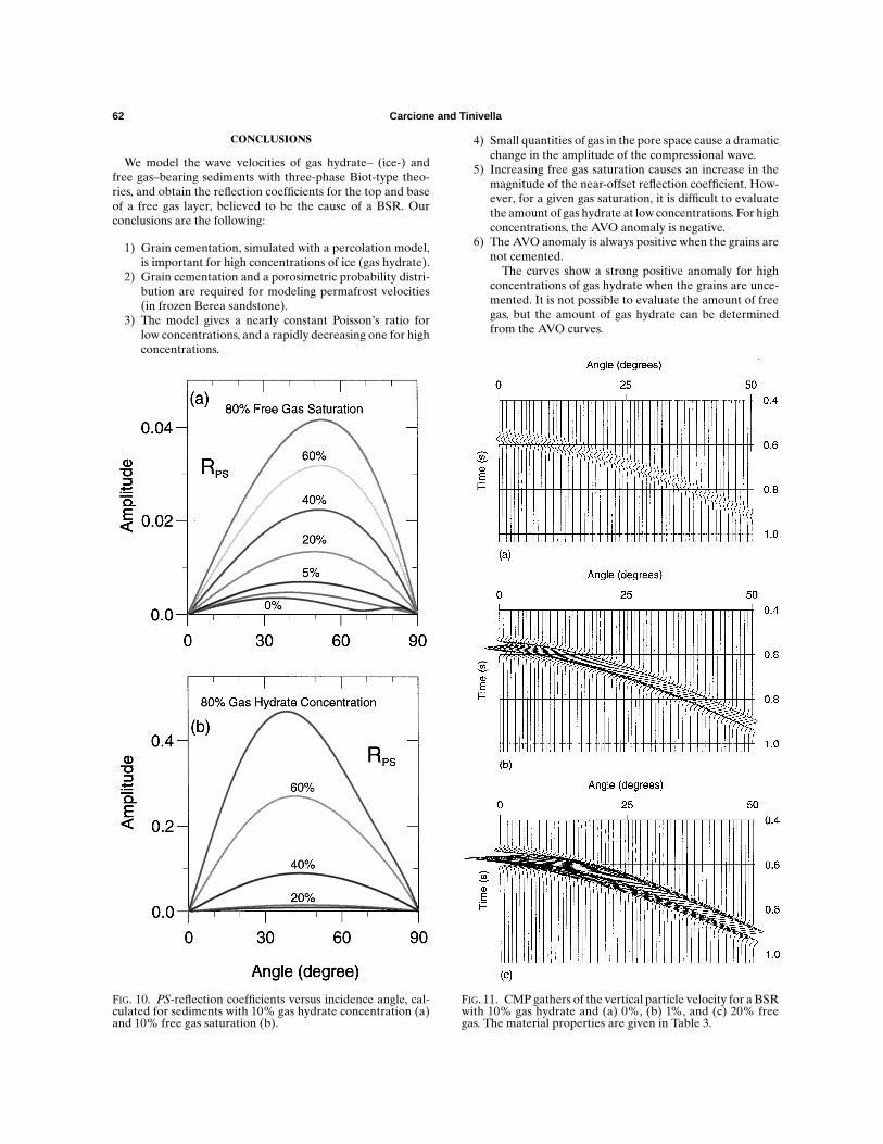
Figures 9 and 10 represent the reflection coefficients RPP andRPS at 25 Hz for various saturations. In part (a) each figure, thehydrate concentration is fixed at 10%, and in part (b) of eachfigure the free gas saturation is fixed at 10%. According to Fig-ure 9, the free gas saturation can be determined from reflectionamplitude but not from the type of anomaly.Moreover, the gashydrate content can be determined when the concentration ishigh.On theotherhand, RPS is a good indicatorofhighamountsof free gas and gas hydrate.

60 Carcione and Tinivella

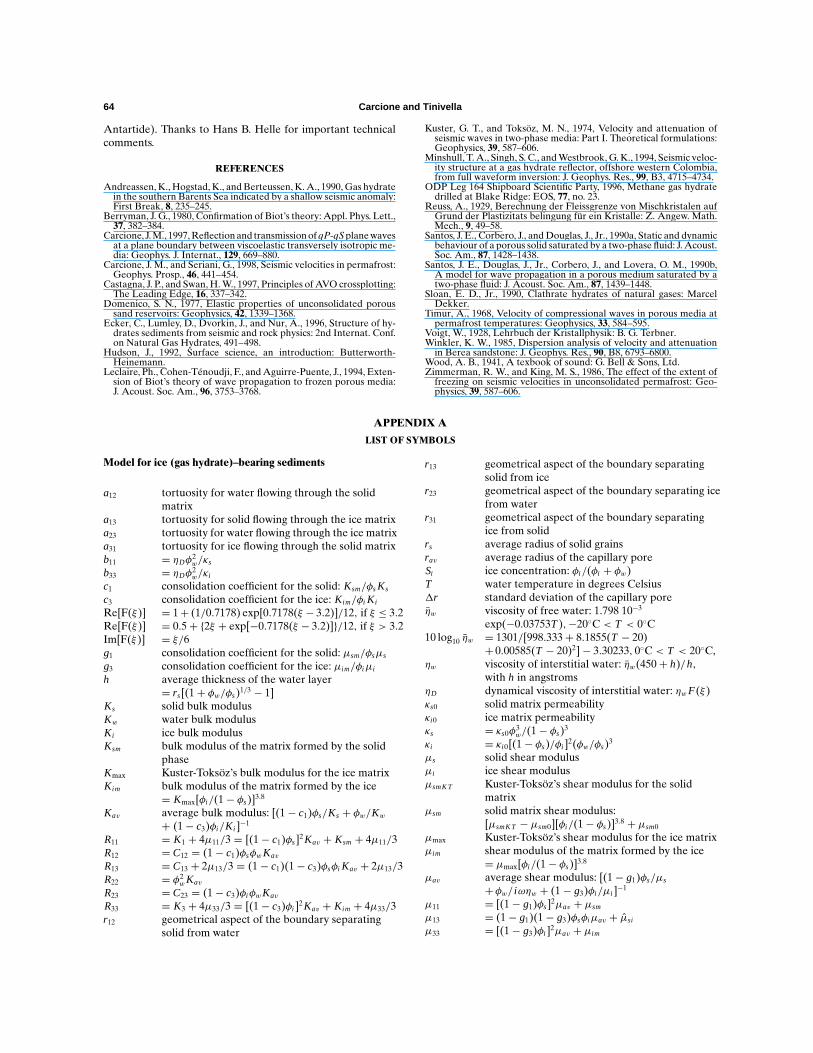
Figure 11 shows common-midpoint (CMP) gathers of thevertical particle velocity corresponding to the top of the BSRwith 10% gas hydrate and 0%, 1%, and 20% free gas. Thematerial properties are given in Table 3, and the previous qual-ity factors are assumed. The source is a 25-Hz Ricker waveletlocated 520 m above the BSR. As predicted by the theoret-ical curves, small quantities of gas in the pore space cause adramatic change in the amplitude of the compressional wave.

Table 3. Material properties.

Medium VP (m/s) VS (m/s) ρ (kg/m3)

10% hydrate 2030 773 19980% free gas 1982 771 20021% free gas 1641 772 199820% free gas 1236 785 1928

FIG. 6. Velocities of the additional compressional waves (a)and second shear wave (b).

FIG. 7. Variations of BSR PP-wave viscoelastic reflectioncoefficient with angle of incidence for different free-gasand gas-hydrate saturations (LCAM model with graincementation).

AVO Effects of BSRs 61

FIG. 8. Computed variations of BSR PP-wave viscoelasticreflection coefficient with angle of incidence for different free-gas and gas-hydrate saturations (LCA model without graincementation).

The propagation effects due to attenuation can be observedin Figure 12, which shows CMP gathers of the vertical particlevelocity for a BSR with 10% gas hydrate and 1% free gas inthe lossy and lossless cases. Attenuation considerably affectsthe far-offset traces.

Finally, Figure 13 represents the reflection coefficients RPP ,phases, and interference coefficients corresponding to the bot-tom of the free gas zone (the frequency is 25 Hz). We as-sume that the quality factors of the free gas–bearing sedimentsare Q1 = Q2 = 20, and those of the water saturated sedimentare Q1 = Q2 = 30. Small amounts of free gas can be deter-mined from theamplitude strength, althoughall the saturationspresent the same type of anomaly. The interference betweenthe incident and reflected P-waves is particularly high for allthe saturations at far offsets. This indicates that much of theenergy is lost by interference.

FIG. 9. PP-reflection coefficients versus incidence angle, cal-culated for sediments with 10% gas hydrate concentration (a)and 10% free-gas saturation (b).

62 Carcione and Tinivella

CONCLUSIONS

We model the wave velocities of gas hydrate– (ice-) andfree gas–bearing sediments with three-phase Biot-type theo-ries, and obtain the reflection coefficients for the top and baseof a free gas layer, believed to be the cause of a BSR. Ourconclusions are the following:

1) Grain cementation, simulated with a percolation model,is important for high concentrations of ice (gas hydrate).

2) Grain cementation and a porosimetric probability distri-bution are required for modeling permafrost velocities(in frozen Berea sandstone).

3) The model gives a nearly constant Poisson’s ratio forlow concentrations, and a rapidly decreasing one for highconcentrations.

FIG. 10. PS-reflection coefficients versus incidence angle, cal-culated for sediments with 10% gas hydrate concentration (a)and 10% free gas saturation (b).

4) Small quantities of gas in the pore space cause a dramaticchange in the amplitude of the compressional wave.

5) Increasing free gas saturation causes an increase in themagnitude of the near-offset reflection coefficient. How-ever, for a given gas saturation, it is difficult to evaluatethe amount of gas hydrate at low concentrations. For highconcentrations, the AVO anomaly is negative.

6) The AVO anomaly is always positive when the grains arenot cemented.

The curves show a strong positive anomaly for highconcentrations of gas hydrate when the grains are unce-mented. It is not possible to evaluate the amount of freegas, but the amount of gas hydrate can be determinedfrom the AVO curves.

FIG. 11. CMP gathers of the vertical particle velocity for a BSRwith 10% gas hydrate and (a) 0%, (b) 1%, and (c) 20% freegas. The material properties are given in Table 3.

AVO Effects of BSRs 63

7) The saturation of free gas can be determined from thereflection amplitude (RPP), but not from the type ofanomaly.

8) The amount of gas hydrate can be determined when theconcentration is high.

9) The P to S reflection coefficient is a good indicator ofhigh amounts of free gas and gas hydrate.

10) Reflections from the base of the free gas zone indicatethat small amounts of free gas can be determined fromthe amplitude strength, although all the saturationspresent the same type of anomaly. Moreover, theinterference between the incident and reflected P-wavesis particularly high for all the saturations at far offsets,indicating that much of the energy is lost by interference.

11) Propagation effects are important, since attenuationconsiderably affects the far-offsets traces.

Unlike in Biot’s two-phase theory, the secondary (slow)waves are propagation modes in the seismic range. In partic-ular, this occurs for high concentrations of gas hydrate. Then,events due to thesewavesmaybepresent in the seismic records.If the free gas zone is thin compared to the dominant wave-length, the analysis requires amore complexAVO study takinginto account the layer thickness. This is currently the subject ofresearch using, for instance, a full wave modeling technique.

ACKNOWLEDGMENTS

This work was supported in part by Norsk Hydro a.s.(Bergen) and PNRA (Programma Nazionale di Ricerca in

FIG. 12. CMP gathers of the vertical particle velocity for a BSRwith 10% gas hydrate and 1% free gas in the lossy (a) andlossless (b) cases.

FIG. 13. PP-reflection coefficients, phases, and interference co-efficients versus incidence angle for various free gas satura-tions. The interface corresponds to the bottom of the free gaszone.

64 Carcione and Tinivella

Antartide). Thanks to Hans B. Helle for important technicalcomments.

REFERENCES

Andreassen, K.,Hogstad,K., andBerteussen, K.A., 1990,Gas hydratein the southern Barents Sea indicated by a shallow seismic anomaly:First Break, 8, 235–245.

Berryman, J. G., 1980, Confirmation of Biot’s theory: Appl. Phys. Lett.,37, 382–384.

Carcione, J.M., 1997,Reflectionand transmissionofqP-qSplanewavesat a plane boundary between viscoelastic transversely isotropic me-dia: Geophys. J. Internat., 129, 669–880.

Carcione, J. M., and Seriani, G., 1998, Seismic velocities in permafrost:Geophys. Prosp., 46, 441–454.

Castagna, J. P., and Swan,H.W., 1997, Principles ofAVO crossplotting:The Leading Edge, 16, 337–342.

Domenico, S. N., 1977, Elastic properties of unconsolidated poroussand reservoirs: Geophysics, 42, 1339–1368.

Ecker, C., Lumley, D., Dvorkin, J., and Nur, A., 1996, Structure of hy-drates sediments from seismic and rock physics: 2nd Internat. Conf.on Natural Gas Hydrates, 491–498.

Hudson, J., 1992, Surface science, an introduction: Butterworth-Heinemann.

Leclaire, Ph., Cohen-Tenoudji, F., andAguirre-Puente, J., 1994, Exten-sion of Biot’s theory of wave propagation to frozen porous media:J. Acoust. Soc. Am., 96, 3753–3768.

Kuster, G. T., and Toksoz, M. N., 1974, Velocity and attenuation ofseismic waves in two-phase media: Part I. Theoretical formulations:Geophysics, 39, 587–606.

Minshull, T.A., Singh, S. C., andWestbrook,G.K., 1994, Seismic veloc-ity structure at a gas hydrate reflector, offshore western Colombia,from full waveform inversion: J. Geophys. Res., 99, B3, 4715–4734.

ODP Leg 164 Shipboard Scientific Party, 1996, Methane gas hydratedrilled at Blake Ridge: EOS, 77, no. 23.

Reuss, A., 1929, Berechnung der Fleissgrenze von Mischkristalen aufGrund der Plastizitats belingung fur ein Kristalle: Z. Angew. Math.Mech., 9, 49–58.

Santos, J. E., Corbero, J., andDouglas, J., Jr., 1990a, Static and dynamicbehaviour of a porous solid saturated by a two-phase fluid: J. Acoust.Soc. Am., 87, 1428–1438.

Santos, J. E., Douglas, J., Jr., Corbero, J., and Lovera, O. M., 1990b,A model for wave propagation in a porous medium saturated by atwo-phase fluid: J. Acoust. Soc. Am., 87, 1439–1448.

Sloan, E. D., Jr., 1990, Clathrate hydrates of natural gases: MarcelDekker.

Timur, A., 1968, Velocity of compressional waves in porous media atpermafrost temperatures: Geophysics, 33, 584–595.

Voigt, W., 1928, Lehrbuch der Kristallphysik: B. G. Terbner.Winkler, K. W., 1985, Dispersion analysis of velocity and attenuationin Berea sandstone: J. Geophys. Res., 90, B8, 6793–6800.

Wood, A. B., 1941, A texbook of sound: G. Bell & Sons, Ltd.Zimmerman, R. W., and King, M. S., 1986, The effect of the extent offreezing on seismic velocities in unconsolidated permafrost: Geo-physics, 39, 587–606.

APPENDIX A

LIST OF SYMBOLS

Model for ice (gas hydrate)–bearing sediments

a12 tortuosity for water flowing through the solidmatrix

a13 tortuosity for solid flowing through the ice matrixa23 tortuosity for water flowing through the ice matrixa31 tortuosity for ice flowing through the solid matrixb11 = ηDφ2

w/κs

b33 = ηDφ2w/κi

c1 consolidation coefficient for the solid: Ksm/φs Ks

c3 consolidation coefficient for the ice: Kim/φi Ki

Re[F(ξ)] = 1+ (1/0.7178) exp[0.7178(ξ − 3.2)]/12, if ξ ≤ 3.2Re[F(ξ)] = 0.5 + {2ξ + exp[−0.7178(ξ − 3.2)]}/12, if ξ > 3.2Im[F(ξ)] = ξ/6g1 consolidation coefficient for the solid: µsm/φsµs

g3 consolidation coefficient for the ice: µim/φiµi

h average thickness of the water layer= rs[(1 + φw/φs)1/3 − 1]

Ks solid bulk modulusKw water bulk modulusKi ice bulk modulusKsm bulk modulus of the matrix formed by the solid

phaseKmax Kuster-Toksoz’s bulk modulus for the ice matrixKim bulk modulus of the matrix formed by the ice

= Kmax[φi/(1 − φs)]3.8

Kav average bulk modulus: [(1 − c1)φs/Ks + φw/Kw

+ (1 − c3)φi/Ki ]−1

R11 = K1 + 4µ11/3 = [(1 − c1)φs]2Kav + Ksm + 4µ11/3R12 = C12 = (1 − c1)φsφw Kav

R13 = C13 + 2µ13/3 = (1 − c1)(1 − c3)φsφi Kav + 2µ13/3R22 = φ2

w Kav

R23 = C23 = (1 − c3)φiφw Kav

R33 = K3 + 4µ33/3 = [(1 − c3)φi ]2Kav + Kim + 4µ33/3r12 geometrical aspect of the boundary separating

solid from water

r13 geometrical aspect of the boundary separatingsolid from ice

r23 geometrical aspect of the boundary separating icefrom water

r31 geometrical aspect of the boundary separatingice from solid

rs average radius of solid grainsrav average radius of the capillary poreSi ice concentration: φi/(φi + φw)T water temperature in degrees Celsius r standard deviation of the capillary poreηw viscosity of free water: 1.798 10−3

exp(−0.03753T ), −20◦C < T < 0◦C10 log10 ηw = 1301/[998.333 + 8.1855(T − 20)

+ 0.00585(T − 20)2] − 3.30233, 0◦C < T < 20◦C,ηw viscosity of interstitial water: ηw(450 + h)/h,

with h in angstromsηD dynamical viscosity of interstitial water: ηw F(ξ)κs0 solid matrix permeabilityκi0 ice matrix permeabilityκs = κs0φ

3w/(1 − φs)3

κi = κi0[(1 − φs)/φi ]2(φw/φs)3

µs solid shear modulusµi ice shear modulusµsmK T Kuster-Toksoz’s shear modulus for the solid

matrixµsm solid matrix shear modulus:

[µsmK T − µsm0][φi/(1 − φs)]3.8 + µsm0

µmax Kuster-Toksoz’s shear modulus for the ice matrixµim shear modulus of the matrix formed by the ice

= µmax[φi/(1 − φs)]3.8

µav average shear modulus: [(1 − g1)φs/µs

+ φw/ iωηw + (1 − g3)φi/µi ]−1

µ11 = [(1 − g1)φs]2µav + µsm

µ13 = (1 − g1)(1 − g3)φsφiµav + µsi

µ33 = [(1 − g3)φi ]2µav + µim

AVO Effects of BSRs 65

µsi coupling shear modulus between the ice and solidphases

ω angular frequency: 2π fφs proportion of solidφw proportion of waterφi proportion of iceρs solid densityρw water densityρi ice densityρ11 = φsρsa13 + (a12 − 1)φwρw + (a31 − 1)φiρi − ib11/ω

ρ12 = −(a12 − 1)φwρw + ib11/ω

ρ13 = −(a13 − 1)φsρs − (a31 − 1)φiρi

ρ22 = (a12 + a23 − 1)φwρw − i(b11 + b33)/ωρ23 = −(a23 − 1)φwρw + ib33/ω

ρ33 = φiρi a31 + (a23 − 1)φwρw + (a13 − 1)φsρs − ib33/ω

ξ = (h/2) (ωρw/ηw)1/2

Model for free gas–bearing sediments

B1 = Kc�[(Sg + β)γ − β]B2 = Kc�Sw

Fs structure factor: 2.8g1 = Sgρg Fs/(φg + φw)

g2 = Swρw Fs/(φg + φw)g3 = 0.1

√g1g2

Ks gas bulk modulusKc = Ks(Ksm + Q)(Ks + Q)K f = α/(γ Sg/Kg + Sw/Kw)M1 = B2r/qM2 = −B1/(Ksmδ) − M3

M3 = −B2[1/(Ksmδ) + r/q]pc capillary pressure: 2650.9e−3.1291(e−6.029158Sg − 1)Q = K f (Ksm − Ks)/[(K f − Ks)(φw + φg)]q = (φg + φw)[1/Kg + 1/(Sg Sw∂pc/∂Sg)]r = (Sg + β)/Ks + χ/Ksm

Sg gas saturation: φg/(φg + φw)Sw water saturation: φw/(φg + φw)α = (γ − 1)(Sg + β) + 1β = pc/(∂pc/∂Sg)δ = 1/Ks − 1/Ksm

γ = [1+ Sg Sw(∂pc/∂Sg)/Kw]/[1+ Sg Sw(∂pc/∂Sg)/Kg]ρg gas densityρm mass density of the bulk material: φsρs + φgρg

+ φwρw

φg proportion of gas� = δ+(φg+φw)(1/Ksm−1/Kc)

α[δ+(φg+φw)(1/Ksm−1/K f )]

APPENDIX B

EXTENSION OF LECLAIRE ET AL.’S THEORY

Leclaire et al. (1994) assume that there is no direct mechan-ical contact between solid and ice. The model is generalizedhere in order to include this interaction. Following Leclaire etal.’s notation, uν , ν = 1, . . . , 3 denote the displacement vectorsof solid, water, and ice, respectively.

Potential energy density

The total potential energy of the system can be expressed as

V = µ11d21 + 1

2K1θ

21 + C12θ1θ2 + 1

2K2θ

22 + C23θ2θ3

+ 12

K3θ23 + µ33d

23 + C13θ1θ3 + µ13D, (B-1)

where θν and dν are the invariants of the strain tensor, calleddeviators and dilatations, D = d(1)

i j d(3)i j , with d(ν)

i j the deviatortensor, Kν and µνν′ are, respectively, the bulk and shear mod-uli of the effective phases. Note that since D is the trace ofthe scalar product between the vectors d(1) and d(3), it is aninvariant quantity.All the parameters except C13 and µ13 are given in Leclaire

et al. (1994). However, they are not modified by solid/ice in-teractions. In order to calculate C13, and µ13, we generalize theelastic moduli obtained for the two-phase Biot’s theory. For amedium with a solid porosity φs and a fluid porosity φ f , theelastic moduli are

K1 = (1 − c1)2φ2s Ka,

C12 = (1 − c1)φsφ f Ka,(B-2)

K2 = φ2f Ka,

Ka =[(1 − c1)

φs

Ks+ φ f

K f

]−1

, c1 = Ksm

φs Ks,

where Ks and K f are the solid and fluid bulk moduli, Ka isthe average bulk modulus, Ksm is the solid matrix bulk mod-ulus, and c1 is the bulk consolidation coefficient such thatc1 = 0 for a suspension of solid grains in a fluid and c1 = 1 fora situation where the grains form a monolithic block. Notethat equations (B-2) correspond to an effective solid porosityφ′

s = (1−c1)φs . If we replace ice by water, the equations shouldread

K1 = φ′s2Ka,

C13 = φ′sφ

′i Ka,

(B-3)K3 = φ′

i2Ka,

Ka =[

φ′s

Ks+ φ′

i

Ki

]−1

, c3 = Kim

φi Ki,

where c3 is the bulk consolidation coefficient of the ice matrixwith bulk modulus Kim . For the three-phase system, general-ization of Ka to

Kav =[

φ′s

Ks+ φ′

i

Ki+ φw

Kw

]−1

gives

K1 = (1 − c1)2φ2s Kav,

C13 = (1 − c1)φs(1 − c3)φi Kav,(B-4)

K3 = (1 − c3)2φ2i Kav,

Kav =[(1 − c1)

φs

Ks+ (1 − c3)

φi

Ki+ φw

Kw

]−1

.

66 Carcione and Tinivella

The shear modulus µ13, given in appendix A, has an analogousexpression to that of C13.

Kinetic energy density

The kinetic energy is a function of the local velocities u1, u2,and u3,where thedotdenotes timedifferentiaton.GeneralizingLeclaire et al.’s kinetic energy, we get

C = 12ρ11u

21 + 1

2ρ22u

22 + 1

2ρ33u

23

+ ρ12u1u2 + ρ23u2u3 + ρ13u1u3, (B-5)

where, for simplicity, we omit the tilde above the density com-ponents.Let us define the macroscopic velocities

w1 = φw(u2 − u1) and w3 = φw(u2 − u3) (B-6)

characterizing water-solid and water-ice flow, and

q = φi (u3 − u1) and r = φs(u1 − u3), (B-7)

the macroscopic velocity characterizing the flow of ice relativeto the solid phase and vice versa, respectively. Since the rel-ative flow is assumed to be of laminar type, the microscopicvelocities can be expressed as

v1 = α(1)i j (w j )1 and v3 = α

(3)i j (w j )3, (B-8)

and

s = β(1)i j q j and t = β

(3)i j r j , (B-9)

where α(1)i j and α

(3)i j are the water/solid and water/ice coeffi-

cients, and β(1)i j and β

(3)i j the ice/solid and solid/ice coefficients,

respectively.The total kinetic energy is given by the expression

C = 12ρw

∫ ∫ ∫w

(u1 + v1)2 d

+ 12ρw

∫ ∫ ∫w

(u3 + v3)2 d − 12ρwφwu2

2

+ 12ρi

∫ ∫ ∫i

(u1 + s)2 d

+ 12ρs

∫ ∫ ∫s

(u3 + t)2 d, (B-10)

where w , i , and s are the volumes of water, ice, and solid,respectively. The term (1/2)ρwφw u2

2 is subtracted since the con-tribution of water must be considered only once in the kineticenergy.Following Leclaire et al. (1994), defining

(mi j )� ≡ ρw

∫ ∫ ∫′

∑k

α(�)ki α

(�)k j d, � = 1, 3 (B-11)

and

(ni j )1 ≡ ρi

∫ ∫ ∫′

∑k

β(1)ki β

(1)k j d,

(B-12)(ni j )3 ≡ ρs

∫ ∫ ∫′

∑k

β(3)ki β

(3)k j d,

where ′ is the volume of the flowing phases, and assumingstatistical isotropy, we obtain

C = 12ρ2u

21 + ρwu1w1 + 1

2m1w

21 + 1

2ρ2u

23 + ρwu3w3

+ 12

m3w23 − 1

2ρwφwu2

2 + 12ρ3u

21 + ρi u1q + 1

2n1q

2

+ 12ρ1u

23 + ρs u3r + 1

2n3r

2, (B-13)

where

ρ1 = ρsφs, ρ2 = ρwφw, ρ3 = ρiφi .

Finally, expressing the kinetic energy as a function of u1, u2,and u3, we get

C = 12

(n3φ

2s − ρ2 + m1φ

2w − ρ3 + n1φ

2i

)u21

+ 12

(m1φ

2w + m3φ

2w − ρ2

)u22

+ 12

(n1φ

2i − ρ2 + m3φ

2w − ρ1 + n3φ

2s

)u23

+ (ρ2 − m1φ

2w

)u1u2 + (

ρ2 − m3φ2w

)u2u3

+ (ρ1 − n3φ

2s + ρ3 − n1φ

2i

)u1u3. (B-14)

The generalizedmass densities ρi j are obtained by equating thecoefficients of expression (B-14) with those of equation (B-5).Thus

ρ11 = ρsφsa13 + (a12 − 1)ρwφw + (a31 − 1)ρiφi ,

ρ22 = (a12 + a23 − 1)ρwφw,

ρ33 = ρiφi a31 + (a23 − 1)ρwφw + (a13 − 1)ρsφs,(B-15)

ρ12 = −(a12 − 1)ρwφw,

ρ23 = −(a23 − 1)ρwφw,

ρ13 = −(a13 − 1)ρsφs − (a31 − 1)ρiφi ,

where

a12 = m1φw

ρw

, a23 = m3φw

ρw

, (B-16)

and

a13 = n3φs

ρs, a31 = n1φi

ρi(B-17)

are the tortuosity parameters.When there is no relative motion between the three phases,

the following relation holds

ρ = ρ11 + ρ22 + ρ33 + 2ρ12 + 2ρ23 + 2ρ13 = ρ1 + ρ2 + ρ3,

(B-18)

corresponding to the effective mass density.

AVO Effects of BSRs 67

Following Berryman (1980) and Leclaire et al. (1994), weexpress the tortuosity parameters as

a12 = φsρ

φwρw

r12 + 1, a23 = φiρ′

φwρw

r23 + 1,

(B-19)

a13 = φiρ′

φsρsr13 + 1, a31 = φsρ

φiρir31 + 1,

where

ρ = φwρw + φiρi

φw + φi, ρ ′ = φwρw + φsρs

φw + φs,

and rνν′ characterize the geometrical features of the pores(r = 1/2 for spheres). This approximation is based on the factthat the three phases are mechanically decoupled. Observethat, for instance, a12 → 1 for φw → 1 and that a12 → ∞ forφw → 0, as expected (Berryman, 1980).