Abstract

This study was conducted to see if current speed enforcement was enough to keep people driving the speed limit.

It was requested by Eng. Dana Abdayyeh , the Supervisor of Traffic laboratory in Al-Ahliyya Amman University (AAU).

It was requested on March / 8 / 2015

The investigation was done by creating a speed trap and recordinghow long it took cars to go through the speed trap. Using some calculations, the times were then converted into speeds and graphed to allow for easier analysis

The main findings were that 40% of the drivers who were timed were driving more than 6 km/h above the 60 km/h limit.

It was concluded that current law enforcement is not enough to get people to obey the speed limit on Yagoz Road.

Even if the experiment yielded some pretty conclusive data, it

should be repeated under different road and weather conditions

using something more accurate than a stop watch and something not

as noticeable as a group of people standing on the sidewalk in

order to get more accurate data.

i

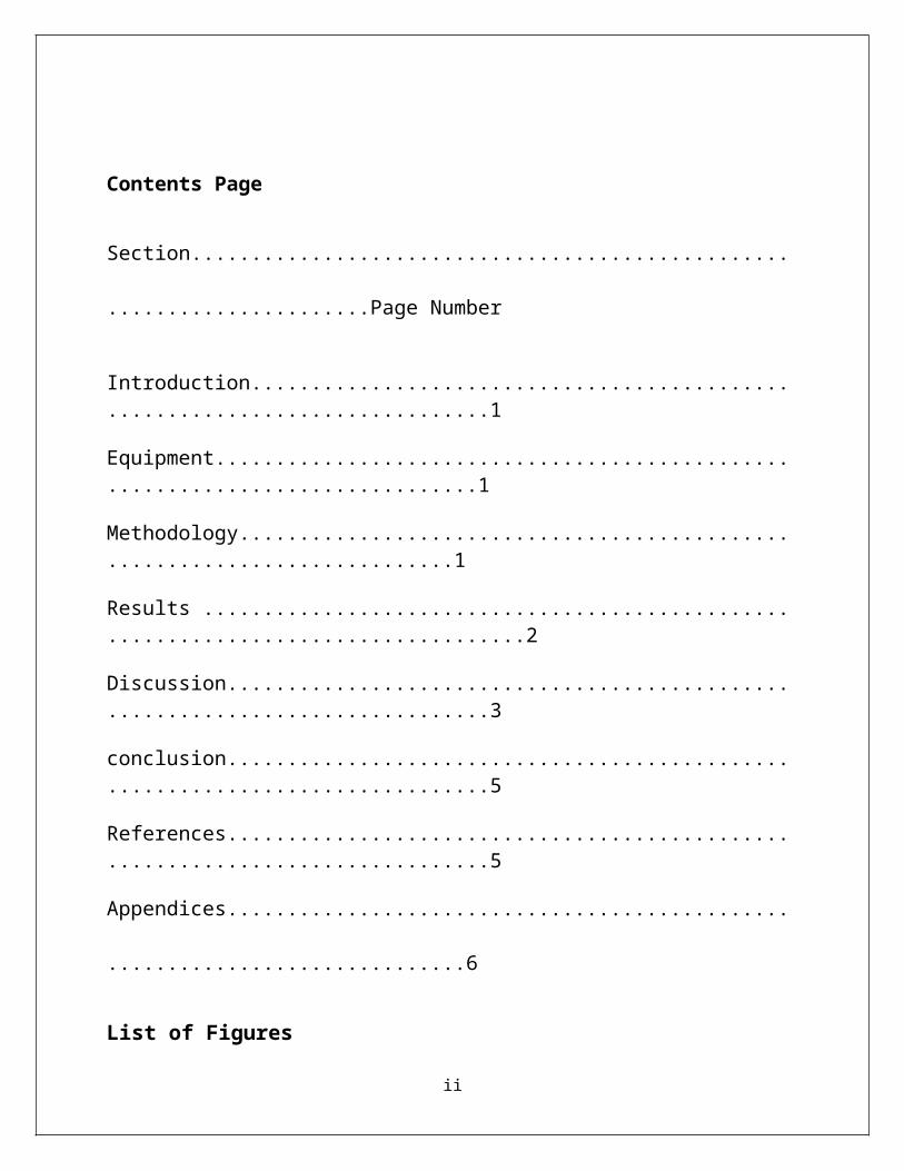
Contents Page

Section..................................................

......................Page Number

Introduction.............................................................................1

Equipment...............................................................................1

Methodology...........................................................................1

Results ....................................................................................2

Discussion...............................................................................3

conclusion...............................................................................5

References...............................................................................5

Appendices...............................................

..............................6

List of Figures

ii

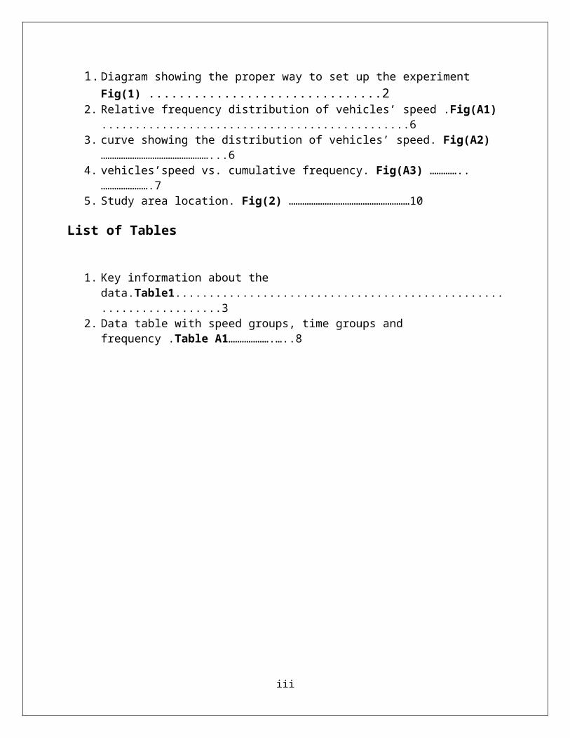
1.Diagram showing the proper way to set up the experiment Fig(1) ...............................2

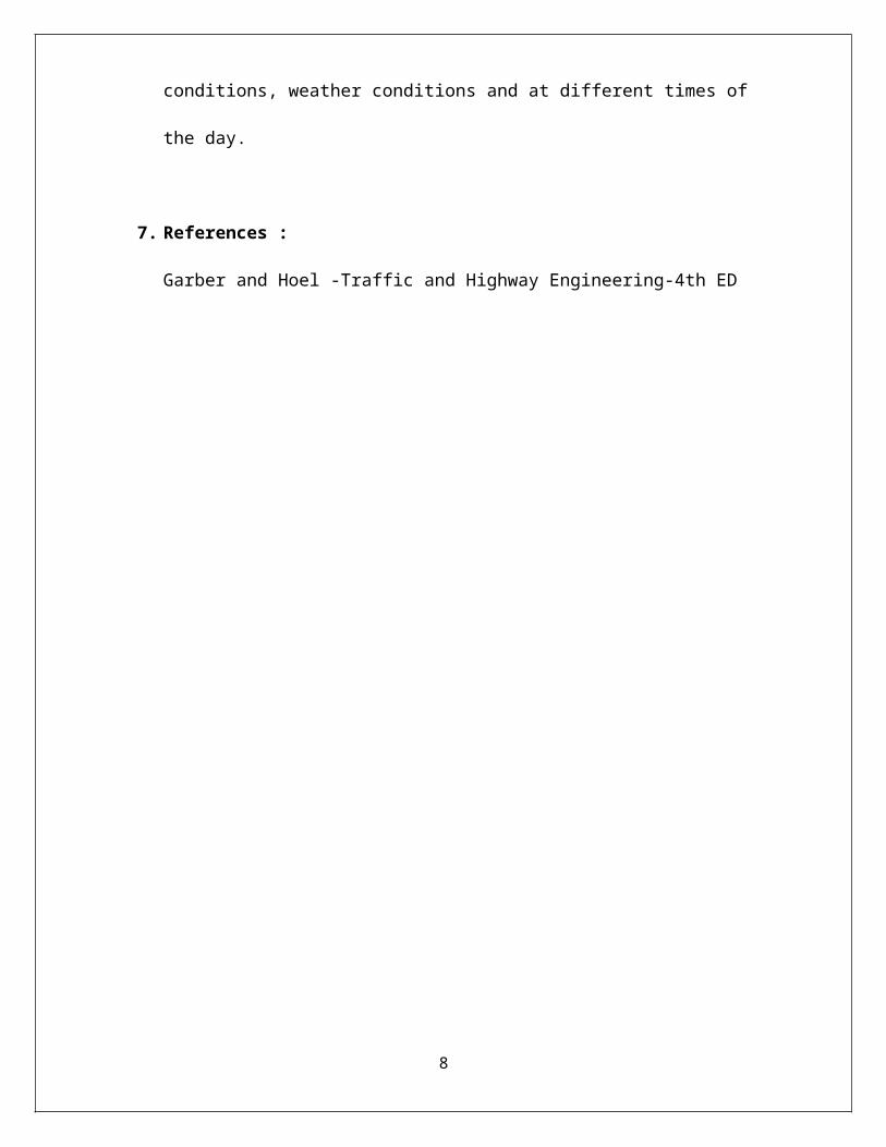
2. Relative frequency distribution of vehicles’ speed .Fig(A1)..............................................6

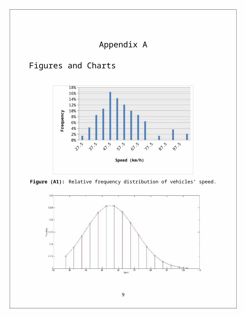
3. curve showing the distribution of vehicles’ speed. Fig(A2) …………………………………………...6

4. vehicles’speed vs. cumulative frequency. Fig(A3) …………..………………….7

5. Study area location. Fig(2) ………………………………………………10

List of Tables

1. Key information about the data.Table1...................................................................3

2. Data table with speed groups, time groups and frequency .Table A1……………….…..8

iii

1.Introduction

The purpose of this lab was to see if current speed limit

enforcement is enough to keep drivers going the speed limit.

To do this, cars were timed going through a 100-m long speed

trap. The resulting times were then used to find the average

speed of cars.

The data was gathered using the experiment described in

Experimental Methodology in Section 3. The data that was

gathered is shown in Results and Description in Section 4 and

discussed in Discussion in Section 5. An overview of the

experiment and a conclusion can be found in the Conclusion in

Section 6.

2.Equipment

This experiment only required a stop watch, a measuring

device, and something used to mark the sidewalk. It also

needed 3 people to run as smoothly as possible: a flagger, a

timer, and a recorder.

1

3.Methodology

First off, a 100 m long speed trap was measured and marked on

the sidewalk. A diagram of the proper setup is shown in Figure

1 at the next page. The flagger stood at the beginning of the

speed trap and signaled to start the stop watch whenever a car

drove by. The timer, who stood at the other end of the speed

trap, had to use the stop watch to time how long it took for

each car to cross the speed trap. The recorder marked all the

times on the field sheet in order to find out the speed. This

process was repeated many times to ensure good data. The

experiment was performed under cloudy weather and dry roads

from roughly 8 PM to 10 PM on March 11th, 2015 along Eastbound

Yagoz Road which is a 60 km/h zone.times

2

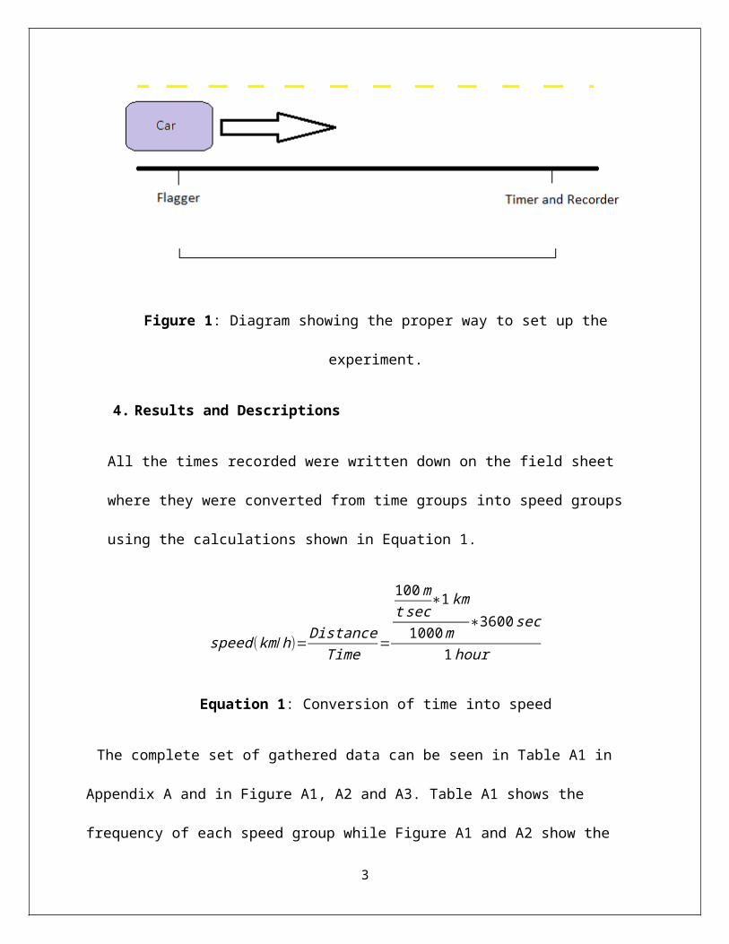
Figure 1: Diagram showing the proper way to set up the

experiment.

4. Results and Descriptions

All the times recorded were written down on the field sheet

where they were converted from time groups into speed groups

using the calculations shown in Equation 1.

speed(km/h)=DistanceTime =

100mtsec

∗1km

1000m ∗3600sec

1hour

Equation 1: Conversion of time into speed

The complete set of gathered data can be seen in Table A1 in

Appendix A and in Figure A1, A2 and A3. Table A1 shows the

frequency of each speed group while Figure A1 and A2 show the

3

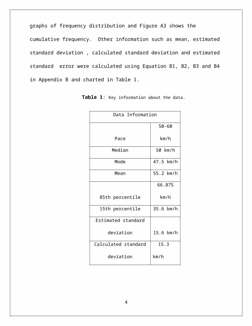
graphs of frequency distribution and Figure A3 shows the

cumulative frequency. Other information such as mean, estimated

standard deviation , calculated standard deviation and estimated

standard error were calculated using Equation B1, B2, B3 and B4

in Appendix B and charted in Table 1.

Table 1: Key information about the data.

Data Information

Pace

50-60

km/h

Median 50 km/h

Mode 47.5 km/h

Mean 55.2 km/h

85th percentile

66.875

km/h

15th percentile 35.6 km/h

Estimated standard

deviation 15.6 km/h

Calculated standard

deviation

15.3

km/h

4

Estimated standard

error

1.14 km/h

5. Discussion

One thing that the data clearly shows is that most drivers

care about the speed limit that evening. This is easily seen when

one looks at the mean, mode and median, all of which are less

than the 60 km/h speed limit. Although the mean of the data was

less than the speed limit, the data still followed a somewhat

normal distribution with a little skew to the left The data

followed a normal pattern with 26% of its points located in the

pace between 50 km/h and 60 km/h. One can also see from the

cumulative frequency graph that about 60% of drivers respected

the 60 km/h speed limit that evening. The data does not show much

dispersion except a few outliers. Although the speeds would be

much higher, meaning that most car speeds would cluster around

the mode of the data with minimal dispersion and few outliers.

This is due to the fact that in both cases there was not anything

near such as traffic, stoplights or pedestrians that would

5

require drivers to stop causing more dispersion. If the same

experiment had been conducted on a random Saturday down High

Street with average traffic, pedestrians and many stop lights,

one could assume that there would be much more dispersion and

inconsistency in the data.

Although the experiment gathered some good data, it could

have been much more accurate if human error would have been taken

out of it. If the experiment had some kind of sensor instead of a

flagger and a timer armed with a stop watch, the data could be

much more accurate and it would rid itself of error due to human

error and reaction time. Another way to get more accurate data

would be to make the data gathering process a little bit more

discreet as to not let the drivers know they are being timed.

Some drivers either accelerated or slowed down when they saw that

they we being timed throwing off our data in the process. One way

to fix this would be once again using small sensor or spreading

out the groups and the group members to make it less obvious to

the driver that they are being timed. The way this experiment was

carried out gave good data but not complete data. Since it was

conducted under cloudy weather and the road was dry when the

6

experiment was done, we only have data for cloudy days with dry

roads. Also, we only have data for the hour between 8 PM and 10

PM. People’s driving tendencies might be affected a lot by

different things such as the road condition, the time of day and

the weather. In order to get a very complete and accurate set of

data, the experiment would need to be carried out a few more

times under different road conditions, weather conditions and at

different times of the day.

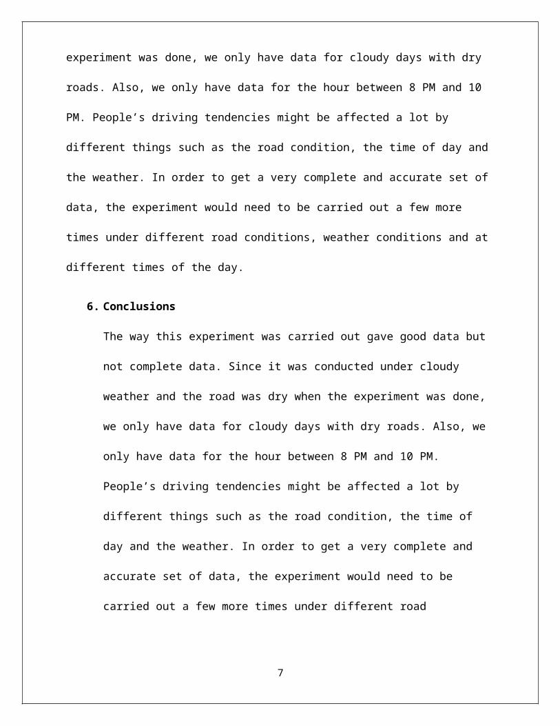
6. Conclusions

The way this experiment was carried out gave good data but

not complete data. Since it was conducted under cloudy

weather and the road was dry when the experiment was done,

we only have data for cloudy days with dry roads. Also, we

only have data for the hour between 8 PM and 10 PM.

People’s driving tendencies might be affected a lot by

different things such as the road condition, the time of

day and the weather. In order to get a very complete and

accurate set of data, the experiment would need to be

carried out a few more times under different road

7

conditions, weather conditions and at different times of

the day.

7. References :

Garber and Hoel -Traffic and Highway Engineering-4th ED

8

Appendix A Figures and Charts

0%2%4%6%8%

10%12%14%16%18%

Speed (km/h)

Freq

uenc

y

Figure (A1): Relative frequency distribution of vehicles’ speed.

9

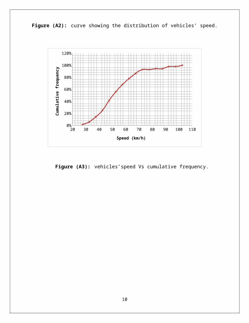
Figure (A2): curve showing the distribution of vehicles’ speed.

20 30 40 50 60 70 80 90 100 1100%

20%

40%

60%

80%

100%

120%

Speed (km/h)

Cumu

lative

frequ

ency

Figure (A3): vehicles’speed Vs cumulative frequency.

10

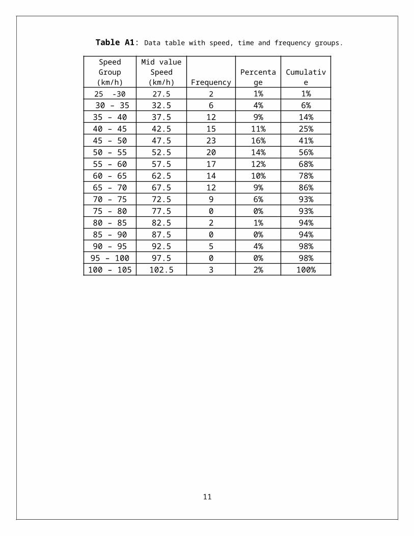
Table A1: Data table with speed, time and frequency groups.

SpeedGroup(km/h)

Mid valueSpeed(km/h) Frequency

Percentage

Cumulative

25 -30 27.5 2 1% 1% 30 – 35 32.5 6 4% 6%35 – 40 37.5 12 9% 14%40 – 45 42.5 15 11% 25%45 – 50 47.5 23 16% 41%50 – 55 52.5 20 14% 56%55 – 60 57.5 17 12% 68%60 – 65 62.5 14 10% 78%65 – 70 67.5 12 9% 86%70 – 75 72.5 9 6% 93%75 – 80 77.5 0 0% 93%80 – 85 82.5 2 1% 94%85 – 90 87.5 0 0% 94%90 – 95 92.5 5 4% 98%95 – 100 97.5 0 0% 98%100 – 105 102.5 3 2% 100%

11

Appendix BEquations and Sample Calculations

Mean Calculation: x=∑ nisi

N(B1)

ni=Frequencyof observations∈groupi

si=Middlespeedofgroupi∈mph

N=Totalnumberofobservations

x=2∗27.5+6∗32.5+12∗37.5+15∗42.5+23∗47.5+20∗52.5+17∗57.5+14∗62.5+12∗67.5+9∗72.5+2∗82.5+5∗92.5+3∗102.5

114

x=55.2km/h

Estimated Standard Deviation: sest=P85−P15

2(B2)

P85=85thpercentile

P15=15thpercentile

Sest=66.875−35.6

2

Sest=15.6km/h

Calculated Standard Deviation: S=√∑ (xi−x)2

N−1(B3)

S=√2(27.5−39.7)2+6(32.5−39.7)2+15 (42.5−39.7)2+23(47.5−39.7)2+20(52.5−39.7)2+17(57.5−39.7)2+ ¿114−1 ¿

12

14(62.5−39.7)2+12(67.5−39.7)2+9(72.5−39.7)2+2(82.5−39.7)2+5(92.5−39.7)2+3(102.5−39.7)2

❑

S=15.3km/h

Estimated error (E): E= S√N

(B4)

E=15.3√140

=1.14km/h

13

Appendix CLocation of study area

Figure (2): Study area location.

14