study of vehicle arrival pattern and free speed
TRANSCRIPT
STUDY OF VEHICLE ARRIVAL PATTERN AND FREE SPEED
CHARACTERISTICS ON SELECTED NATIONAL HIGHWAYS
BYGAZI ARIF IQBAL
A Project thesis submitted to the Department of Civil Engineering of Bangladesh
University of Engineering & Technology, Dhaka in partial fulfilment of the
I requirements for the degree
of
1111111111111111111111111111 1/1111#92771#
MASTER OF ENGINEERING IN CIVIL ENGINEERING
August, 1998
STUDY OF VEHICLE ARRIVAL PATTERN AND FREE SPEED
CHARACTERISTICS ON SELECTED NATIONAL HIGHWAYS
Chairman(Supervisor)
Member
Member
A THESISBY
GAZI ARIF IQBAL
Approved as to the style and content by:
...~ ...DB'9gDr. Moazzem HossainAssistant Professor,Department of Civil EngineeringSUET, Dhaka .
......... . .l1:B"..~~Dr. Md. S msul Ho'ljueAssociate Professor,Department of Civil EngineeringSUET, Dhaka.
Dr. Hasib Mohammed AhsanAssociate Professor,Department of Civil Engineering
• SUET, Dhaka.
11
DECLARATION
I do hereby declare that the work embodied in this thesis is the result of investigation carried
out by me and this has not been submitted in candidature for any degree at any other
university.
August, 1998
III
. ~ .Signature of the student
ACKNOWLEDGEMENT
This work was carried out under the direct supervision of Dr. Moazzem Hossain, Assistant
professor, Department of Civil Engineering of the Bangladesh University of Engineering &
Technology.
The author wishes to express his sincerest debt of gratitude to Dr. Moazzem Hossain for his
continuos guidance and valuable suggestions and affectionate encouragement at all stages of
this study. Without his valuable direction and cordial assistance it would have been
impossible to carry out this study under a number of constrains, time limitation in particular.
The author would like to express his sincere gratitude to Dr. Md. Shamsul Hoque, Associate
professor, Department of Civil Engineering of BUET for his kind help with the operation of
video camera and accessories and also for useful advice regarding field data collection.
The author likes to express his thanks to Mr. Arifur Rahman for his co-operation in traffic
data collection.
IV
ABSTRACT
Analysis and interpretation of traffic Operations on national highways reqUIre a sound
understanding of the traffic flow parameters. Such traffic flow parameters are traffic arrival
headways, free speed of vehicles, operating speed and speed-flow-density relationship. No
significant study has yet been made to investigate these traffic parameters of Bangladeshi
national highways. In this study, effort has been given to investigate the traffic arrival pattern
and free speed characteristics of vehicles on two-lane two-way national highways of
Bangladesh. The research study has been based on field data. Both video and manual data on
the traffic flow of selected national highways have been collected for a net period of
approximately twenty five hours. The analysis of collected data has been made using different
statistical softwares. Analysis of traffic arrival pattern using the vehicular time headway data
has revealed that the pattern follows more than one statistical distribution models for all the
highways. Generally, it has been observed that the vehicles maintain close headways when
they are in following situation. It has been observed that the traffic arrival pattern on selected
Bangladeshi national highways can be described by one or more of the two statistical
distributions, namely, exponential and lognormal. The relevant parameters of the
corresponding arrival headway distributions have been estimated. Analysis of free speed data
of vehicles on a typical section of Dhaka-Aricha highway has revealed that the free speed of
the commonly found vehicles(bus, minibus, truck, passenger-car, nonmotorised vehicles)
follow normal distribution pattern. Corresponding parameters of the normal distribution have
also been estimated. From regression analysis, it has been found that free speed of vehicles
depends on the pavement and shoulder width. In a pavement width range of 5.8m to 7.5m,
free speed of commonly found motorised vehicles increases in a range of 7.25 kmph to 10.29
kmph for each metre of pavement widening for flat, straight and disturbance free highway
section. The analysis has also revealed that free speed of vehicles increases with the increase
in shoulder width except for the case ofbus(the reason of which has been identified as a local
phenomenon on a particular highway).
v

2.1 INTRODUCTION 52.2 DEFINITIONS
52.2.1 Traffic Flow 52.2.2 Headway 62.2.3 Traffic Speed 72.2.4 Traffic Density 8
2.3 HEADWA Y MODELS OF TRAFFIC FLOW 82.4 TRAFFIC ARRIVAL PATTERN 10
2.4.1 Single Distribution Models 102.4.1. J Negative exponential distribution 10
Page111
IV
V
VI
Xli
XIlI
2
3
4
CONTENTS
VI
1.1 BACKGROUND
1.2 OBJECTIVES OF THE RESEARCH
1.3 METHOD OF APPROACH
1.4 SCOPE AND LIMITATIONS OF THE STUDY
1.5 ORGANISA TION OF THESIS
DECLARATIONACKNOWLEDGEMENTABSTRACTCONTENTSLIST OF TABLESLIST OF FIGURES
CHAPTER 1 INTRODUCTION
CHAPTER 2 LITERATURE REVIEW
2.4.1.2 Shifted negative exponential distribution II2.4.1.3 Gamma distribution 122.4.1.4 Log-normal distribution 12
2.4.2 Mixed Distribution Models 132.4.2.1 Composite distribution models 13
2.4.2.1.1 Double exponential model 13
2.4.2.1.2 Hyperlang model 142.4.2.2 Moving queue models 14
2.5 SPEED MODELS 152.5.1 The Indian Speed Model 152.5.2 The Brazilian Speed Models 162.5.3 The Ethiopian Speed Models 182.5.4 The Kenyan Speed Models 182.5.5 The Caribbean Model 202.5.6 RTM 2 Speed Models 212.5.7 HDM-III Speed Models 222.5.8 The Chinese Speed Models 22
2.6 ROADS OF BANGLADESH 262.6.1 Road Classification 262.6.2 Characteristics Of Roads In Bangladesh 28
2.7 COMMENTS 29
CHAPTER 3 DATA COLLECTION
3.1 INTRODUCTION 303.2 REQUIRED DATA ITEMS 303.3 METHODS OF DATA COLLECTION 313.4 VIDEO PHOTOGRAPHY AS TRAFFIC DATA SOURCE 313.5 DESIRED SITE CHARACTERISTICS 323.6 PRELIMINARY SURVEY 33
VII
3.7 PROBLEM IDENTIFIED DURING PRELIMINARY SURVEY 343.8 DESCRIPTION OF THE SELECTED SITES 353.9 PREP ARA TION FOR DATA COLLECTION 373.10 DATA COLLECTION PROCEDURE 383. I I DATA EXTRACTION 39
3.1 I.I Traffic Headway 393.11.2 Free Speed 40
3. 11.3 Traffic Volume And Average Speed 40
3.11.4 Traffic Density And Average Speed 40
CHAPTER 4 DATA ANALYSIS AND INTERPRETATION OF
RESULTS
4.1 GENERAL 444.2 STATISTICAL ANALYSIS 444.3 QUALITATIVE ANALYSIS 454.4 QUANTITATIVE ANALYSIS 46
4.4.1 Traffic Composition 464.4.2 Analysis Of Traffic Arrival Pattern 474.4.3 Free Speed Distribution Pattern 514.4.4 Relationship Of Free Speed With Pavement And 53
Shoulder Width
4.4.5 Speed-Flow Condition At Sites 554.4.6 Speed-Density Condition At Sites 55
CHAPTER 5 CONCLUSIONS AND RECOMMENDATIONS
5.1 INTRODUCTION
5.2 CONCLUSIONS
Vl1l
6262
5.2.1 Traffic Arrival pattern
5.2.2 Free Speed Characteristics
5.2.3 Speed-Flow And Speed-Density Condition
5.2.4 Limitations Of The Study
5.3 RECOMMENDATION FOR FUTURE STUDY
REFERENCES
APPENDIX A DATA TABLES
A.I HEADWAY DATA
A2 FREE SPEED DATA
A.3 FREE SPEED AND WIDTH DATA
A4 FLOW-SPEED
A.4.1 Dhaka-Aricha And Dhaka-Chittagong
A.4.2 Dhaka-Mymensingh And Dhaka-Sylhet
A.4.3 Dhaka-Khulna
A5 SPEED-DENSITY
A5.1 Dhaka-Aricha And Dhaka-Chittagong
A.5.2 Dhaka-Mymensingh And Dhaka-Sylhet
A.5.3 Dhaka-Khulna
APPENDIX B ANALYSIS TABLES
6263
63
6464
66
9
II
13
13
13
14
14
14
15
15
8.1 EXPONENTIAL DISTRIBUTION FOR HEADWAY IDATA OF DHAKA-ARICHA HIGHWAY
8.2 LOGNORMAL DISTRIBUTION FOR HEADWAY 2DATA OF DHAKA-ARICHA HIGHWAY
B.3 EXPONENTIAL DISTRIBUTION FOR HEADWAY 3OATA OF DHAKA-CHITT AGONG HIGHWAY
IX

B.4 LOGNORMAL DISTRIBUTION FOR HEADWAY 4DATA OF DHAKA-CHITTAGONG HIGHWAY
B.5 EXPONENTIAL DISTRIBUTION FOR HEADWAY 5DATA OF DHAKA-MYMENSINGH HIGHWAY
B.6 LOGNORMAL DISTRIBUTION FOR HEADWAY 6DATA OF DHAKA-MYMENSINGH HIGHWAY
8.7 EXPONENTIAL DISTRIBUTION FOR HEADWAY 7DATA OF DHAKA-SYLHET HIGHWAY
B.8 LOGNORMAL DISTRIBUTION FOR HEADWAY 8DATA OF DHAKA-SYLHET HIGHWAY
B.9 EXPONENTIAL DISTRIBUTION FOR HEADWAY 9DATA OF DHAKA-KHULNA HIGHWAY
8.10 LOGNORMAL DISTRIBUTION FOR HEADWAY 10DATA OF DHAKA-KHULNA HIGHWAY
B.11 FREE SPEED ANALYSIS FOR BUSES
8.12 FREE SPEED ANALYSIS FOR CARS
8.13 FREE SPEED ANALYSIS FOR TRUCKS
B.14 FREE SPEED ANALYSIS FOR MINIBUSES
B.15 FREE SPEED ANALYSIS FOR NONMOTORISEDVEHICLES
APPENDIX C SPEED-FLOW-DENSITY OBSERVATION
C.1 SPEED FLOW CONDITION AT DHAKA-ARICHA ANDDHAKA-CHITTAGONG HIGHWAYS
I 1
12
13
14
15
C.2 SPEED FLOW CONDITION AT DHAKA-MYMENSINGH 1AND DHAKA-SYLHET HIGHWAYS
C.3 SPEED FLOW CONDITION AT DHAKA-KHULNA 2HIGHWAY
x
C.4 SPEED DENSITY CONDITION AT DHAKA-ARICHA AND 2DHAKA-CHITTAGONG HIGHWAYS
C.S SPEED DENSITY CONDITION AT DHAKA-MYMENSINGH 3AND DHAKA-SYLHET HIGHWAYS
C.6 SPEED DENSITY CONDITION AT DHAKA-KHULNA 3HIGHWAY
Xl

2.1 Estimates Of Empirical SpeedlFlow Relationships On Typical 25Roads In Plain Terrain In China
2.2 Classification Of Roads Of Bangladesh 283.1 Description Of Data Collection Sites 374.1 Traffic Composition Found In Different Highways 474.2 Results Of Goodness-Of-Fit Test Of Exponential Distribution 49
To Vehicle Arrival Pattern Of Highways
4.3 Results Of Goodness-Of-Fit Test Of Lognormal Distribution 50To Vehicle Arrival Pattern Of Highways
4.4 Results Of The Analysis Of Traffic Arrival Pattern With 51Distribution And Their Parameters
4.5 Results Of Goodness- Of-Fit Test Of Normal Distribution 52To Free Speed Of Vehicles
4.6 Parameters Of Normal Distribution Functions For Free Speed 53Data
4.7 Coefficients Of Linear Regression Analysis 55
Table no. Description
LIST OF TABLES
Xl!
Page
3.1 Arrangement Of Setting The Camera On Pickup Van 423.2 Roadside Arrangements During Video Filming 434.1 Frequency Histogram Of Headway Data Of Dhaka-A rich a 57
Highway
4.2 Frequency Histogram Of Headway Data Of Dhaka-Chittagong 57Highway
4.3 Frequency Histogram Of Headway Data Of Dhaka-My men singh 58Highway
4.4 Frequency Histogram Of Headway Data OfDhaka-Sylhet 58Highway
4.5 Frequency Histogram Of Headway Data OfDhaka-Khu1na 59Highway
4.6 Frequency Histogram Of Free Speed Of Buses On Dhaka-Aricha 59Highway
4.7 Frequency Histogram Of Free Speed Of Minibuses On Dhaka- 60Aricha Highway
4.8 Frequency Histogram Of Free Speed Of Trucks On Dhaka- 60Aricha Highway
4.9 Frequency Histogram Of Free Speed Of Passenger-Cars On 61
Dhaka-Aricha Highway
4.10 Frequency Histogram Of Free Speed OfNon-Motorised Vehicles 61
On Dhaka-Aricha Highway
Figure no. Descriptions
LIST OF FIGURES
xiii
Page
CHAPTER!
INTRODUCTION
1.1 BACKGROUND
Road transportation plays a major role in the land and overall transportation sector of
Bangladesh. With the increased traffic demand roads of Bangladesh are running at or near to
capacity situation. To cater the increased traffic demand each year a significant portion of
national development budget is spent to build and maintain the highway infrastructure.
Analysis and interpretation of traffic operation of inter-city highways require a sound
understanding of the traffic flow parameters. Such traffic flow parameters are traffic arrival
headways, free speed, operating speed and speed-flow-density relationship. In order to make
a mathematical or simulation study of highway traffic operation, these parameters are
required to be estimated first. Till now, no significant effort have been made to establish
these highway traffic parameters. It is, therefore, necessary to make a research study to
investigate these parameters. However, determination of an overall speed-flow-density
relationship for the highways needs huge relevant data over a broad range of traffic flow
condition. Collection of such huge data base is out of the scope of the present research study
considering the time and budget limitations. Therefore, a research study has been undertaken
to investigate the vehicle arrival headway pattern and free speed characteristics of vehicles
on selected national highways of Bangladesh.
1.2 OBJECTIVES OF THE RESEARCH
The objectives of the present research study are as follows:
i) To develop vehicle arrival patterns for the selected national highways of Bangladesh.

ii) To develop spot speed distribution model for the free flowing vehicles along straight
highway sections.
iii) To investigate the speed-flow and speed-density conditions for limited period of time.
1.3METHOD OF APPROACH
Three types of research approach are generally used in the field of traffic engineering. They
are:
(i) Analytical approach
(ii) Simulation approach
(iii) Empirical approach
The analytical modelling approach may be based on macroscopic theories such as fluid flow
analogy, which handles traffic flow as a one dimensional expandable fluid. Although this
approach helps to understand traffic behaviour as a whole, there are underlying assumptions
of homogeneity which are far from the high variations of driver-vehicle characteristics in
mixed traffic conditions of Bangladesh.
The approach of Computer Simulation may be either Macroscopic or Microscopic in nature.
The Macroscopic approach deals with traffic in an aggregate form employing a fluid flow
analogy similar to the analytical approach, and hence, subject to the simplifying assumptions
as the analytical approach. Microscopic simulation approach replicates the individual
vehicle movements along the road system by processing every vehicle with its own
characteristics for each real time interval. However, the basic flow parameters for such a
simulation study of highways are not established yet.
2

Therefore, a study based on real field data remains as the only option for this research study.
Such field is not available from any source. So, a field data collection programme has been
undertaken as a part of the present research study.
1.4 SCOPE AND LIMITATIONS OF THE STUDY
The present research study aims at establishing the highway traffic flow parameters such as
vehicle arrival headway, free speed characteristics of vehicles and speed-flow-density
conditions for the data collection periods. These parameters are the basic elements of the
study and understanding of highway traffic operation. Apart from the use of all these
parameters in analysing highway traffic operation, the free speed data of vehicles can be
used in designing the relevant speed control measures. Also, these parameters can be used in
any future mathematical and simulation modelling of traffic operations on Bangladeshi
national highways.
However, the present study is limited to the flat, horizontal and disturbance free sections on
five selected national highways. And, national highways comprises only eleven percent of
total highway network. Also, as far available information, more than two third (71%) of the
national highways even have pavement width below the prescribed specification limits viz.
5.5 m (Bangladesh Transport Sector Study, 1994). But the pavement width of the five
highway sections in this study are in the range of 5.8m to 7.5m.
3
1.5 ORGANISATION OF THESIS
TIle research work is divided into different topics and presented in five chapters.
Chapter I represents Backgrowld and objectives of the study. A brief review of the traffic
characteristics prevailing in the highway of Bangladesh is presented in the first chapter with
special emphasis placed on the objective of the study.
Chapter 2 incorporates literature review related to different traffic headway anival pattem
and speed models along with the definition of related useful tenns.
Chapter 3 details description of data collection, surveymg, reCOllnalssance survey, data
processing, data extraction, site description etc. are presented.
Chapter 4 deals with the data analysis and interpretatioll of the results.
Chapter 5 includes the conclusions of the entire study and some recommendations for thefullher study.
4
CHAPTER 2
LITERATURE REVIEW
2.1 INTRODUCTION
Transportation service is measured in terms of the ability of a highway to accommodate
vehicular traffic safely and efficiently. Determination of the functional effectiveness of any
highway needs the vehicular analysis of the traffic. In undertaking such an analysis, various
dimension of traffic, such as type, speed, flow, density and arrival pattern must be addressed,
since, they influence analysis, operation and control of highways. A through understanding
of these elements or parameters will provide a valuable foundation for the comprehension
and critical assessment of the various traffic analysis techniques and procedures. This
chapter deals with the review of traffic arrival pattern and free speed characteristics of
vehicles starting with the definition of related useful terms.
2.2 DEFINITIONS
At the beginning of the review definitions of some related useful terms have been presented.
2.2.1 Traffic Flow
Traffic flow, q, is defined as the number of vehicles, n, passing some designated highway
point in a time interval of duration t, or
Ilq=-
I
5
....... ( 2.1)
where q is generally expressed in vehicles per unit time. Normally, vehicleslhour is widely
used as traffic flow unit.
2.2.2 Headway
Aside from knowing the total number of vehicles arriving in some time interval, the amount
of time between the arrival of successive vehicles (or the temporal distribution of traffic
flow) is also of interest. The time between the passing of the front bumpers of two successive
vehicles, past some designated highway point, is known as the time headway, h; This
parameter of time headway h; can be interrelated with Equation (2.1)
....... (2.2)
and
nq=-,-~);;=1
or
1q=-::
h........ (2.3)
where h is the average headway (I h; ). The importance of time headwaysn in traffic
analysis will be extensively demonstrated in forthcoming sections of this chapter.
6
2.2.3 Traffic Speed
The average traffic speed can be defined in two ways. The first is the arithmetic mean of
speeds observed at some point. This is refereed to as the time mean speed, u, and is
expressed as
- 1"u/=-Luj
11 ;=1......... (2.4)
The second measure is more useful in the context of traffic analysis and is defined on the
basis of the time necessary for a vehicle to traverse some known length of roadway. This
measure is known as the space mean speed, u" and is given by,
u =, j=1
t............ (2.5)
where I; is the length of roadway used for the speed measurement of vehicle i, and
with tnO,,)being the time necessary for vehicle n to traverse a section of roadway of length I.
Note that if all vehicle speeds are measured over the same length of roadway (L = I, = 12= I"
),
Us - n
(X,)L [1/(Lit;}]j=1
which is the harmonic mean of speed.
7
.......... (2.7)
2.2.4 Traffic Density
Traffic density, also refers to as traffic concentration is defined as the number of vehicles
occupying a length of a roadway at a specified time. This is stated simply as
where k = traffic density
n = number of vehicles
I = length of roadways
nk= -
I................... (2.8)
2.3 HEADWAY MODELS OF TRAFFIC FLOW
With the basic relationships between traffic flow, speed, and density formalised, attention
can now be directed toward a more microscopic view of traffic flow. That is, instead of
simply modelling the number of vehicles passing a point in some time interval, there is
considerable analytic value in modelling the time between the arrivals of successive vehicles
(i.e., the notion of vehicular headways presented earlier). The most simplistic approach to
vehicle arrival modeling is to assume that all vehicles are equally or uniformly spaced. This
results in what is termed a deterministic and uniform arrival pattern. Under this assumption,
if the flow is 360 veh/hr the number of vehicles arriving in any 5-min time interval is 30 and
the headway between all vehicles in 10 sec (since h will equal to 3600/q). However,
experience tells us that, in many instances, such uniformity of flow may not be an entirely
realistic representation of traffic, since some 5-min intervals are likely to have more or less
flow than other 5-min intervals. Thus a elaborate model of vehicular arrivals is often
warranted.
8
Model that accounts for the nonuniformity of flow are derived by assuming that the pattern
of vehicle arrivals corresponds to some random process. The problem then becomes one of
selecting a probability distribution that is a reasonable representation of observed traffic
arrival patterns. An example of such a distribution is the Poisson distribution which is
expressed as(Mannering and Kilreski 1993)
.................. (2.9)
where t is the duration of the time interval over which vehicles are counted, p(n) is the
probability of having n vehicles arrive in time t, and A. is the average flow or arrival rate in
vehicles per unit time. The assumption of Poisson distributed vehicle arrivals also implies a
distribution of the time intervals between the arrivals of successive vehicles (i.e., time
headway). To show this, let the average arrival rate, A., be in units of vehicles per second, so
that
1...= -q-3600
..................... (2.10)
where q is the flow in vehicles per hour. Substituting Equation (2.10) into Equation. (2.9)
gIves
(qt/3600)" e-qt/3600
pen) = ----- (2.11)n!
It can be noted that the probability of having no vehicles arrive in a time interval of length t (
i.e., p(O) is the equivalent of the probability of a vehicle headway, h, being greater than or
9
equal to the time interval t(Mannering and Kilreski 1993). So from Equation ( 2.11)
p(O) = p( h 2: t )
= e-qt/3600 ....................... (2.12)
This distribution of vehicle headways is known as the negative exponential distribution and
is often simply referred to as an exponential distribution.
Empirical observations shows that the assumption of Poisson-distributed traffic arrivals is
most realistic in lightly congested traffic condition. If traffic flow become heavily congested
other distributions of traffic flow become more appropriate(Mannering and Kilreski 1993).
2.4 TRAFFIC ARRIVAL PATTERN
Adams has reported that [Hossain 1996] free flowing traffic corresponds to a random arrival
pattern, where the arrival of one vehicle is independent of the arrival of any other vehicle.
This means that equal time intervals are equally likely to contain equal number of arrivals.
But at higher flow situation where vehicles are not in a free flow condition, traffic arrival
patterns are not random. This discrepancy led to the formulation of other headway
distribution models. Generally, these may be classified as single distribution models and
mixed distribution models.
2.4.1 Single Distribution Models
2.4.1.1 Negative exponential distribution
If the arrival of traffic is considered to be random then the traffic arrival is described as a
Poisson process. And, under this circumstances, headways are distributed according to the
10
negative exponential distribution [Hossain 1996]. This distribution model is simple as it can
be defined by only one parameter of mean arrival rate and also random variates of this
distribution can be easily generated. But it suffers from serious limitations. It predicts
higher probability density in the range of values very near to zero than those in any other
range. Also, at higher flows the random arrival pattern breaks down. A variable x is said to
be exponentially distributed if its density function is given by ,
.-1e-ltfAt)=lo
-<>0, I~O
otherwise............ (2.1 3)
where, Ie is the rate of arrivals in vehlsec as described earlier.
2.4.1.2 Shifted negative exponential distribution
In the negative exponential distribution the physical finite length of the vehicle is ignored by
taking vehicles as points. But as the vehicles have certain lengths it is obvious that a real
minimum time headway between vehicles exists, and this minimum headway is incorporated
In the negative exponential distribution with a Shifted negative exponential
distribution[Hossain 1996]. As it requires only two parameters to define this model, i.e.
mean headway and a minimum headway, it is a relatively easy model to calibrate; and, its
simple mathematical expression still allows easy generation of random deviates during
simulation. However, this distribution function still assigns a higher probability density to
the smaller headways. The density function for the shifted negative exponential distribution
is given by,
f(t) =
where, ~ = t - r
o t<T
......................... (2.14)
t = the average time spacing between arrivals
t = headway between successive arrival
I I
,= the minimum headway
The corresponding cumulative distribution function is
F (t) = I - e-(I-,)I~
2.4.1.3 Gamma distribution
............. __ (2.15)
In this distribution, a variation of minimum head ways is incorporated. Tolle [Hossain 1996]
fitted a set of observed data to this distribution function and found that the fit was not good
statistically. However, an improved fit was reported when the distribution was shifted by a
minimum headway. The Erlang distribution is the simplified form of the Gamma
distribution. The density function of gamma distribution IS
f(t) =
..tke-.olttk-1
(k -I)!
o
t~O, ..t>0, k=I,2, ..
otherwise
....... __(2.16)
where, k and A are the parameters required to be estimated.
2.4.1.4 Log-normal distribution
This model represents the distribution function of deviates whose natural logarithms follow
the normal distribution. Greenberg [Hossain 1996] proposed this model and suggested its
relation to traffic head ways and car following theory. Two parameters i.e. mean headway
and standard deviation of headways are required to apply this model to traffic headways.
Tolle [Hossain 1996] has tested the distribution model and reported that although the
Kolmogorv-Smimov test produced statistically good fits, the chi-square test did not at higher
flows. A recent study by Bullen and Mei [Hossain 1996] suggested that shifted lognormal
distribution gives better fit at high flow situation. They suggested a shift of 0.3-0.5 second
after their study. This distribution however requires three parameters i.e. mean, standard
deviation and shift of the headways to be defined. A random variable x is said to have a log
12

nom1al distribution if its logarithm is normally distributed. If y is a random variable
representing that normal distribution of natural logarithm then the random variable of
lognormal distribution is given by the following equation.
x = £! (2.17)
2.4.2 Mixed Distribution Models
Mixed distribution models are based on the concept of bunching of vehicles [Hossain 1996]
in a traffic stream. This concept views two distinct categories of vehicles in the traffic
stream: followers and non-followers. The former group consists of the vehicles which are
impeded by front vehicles and are not able to maintain their desired speed for that reason.
The latter group consists of free-flowing vehicles that are able to maintain their desired
speeds. The general form of the probability density function of these models is as follows:
f(t) = tDg(t) + (I -tD)h(t) (2. I 8)
where, tD is the proportion of restrained traffic, and h(t) and get) are the free and restrained
headway distributions respectively. Depending on how the two distributions are specified,
there could be three classes of mixed distribution models which are described below.
2.4.2.1 Composite distribution models
These mixed distribution models treat the distributions of free and restrained headways
independently. Examples of this type of models are the double exponential distribution
model and hyperlang model.
2.4.2.1.1 Double exponential model
This model, proposed by Schull [Hossain 1996] was the first model which classified the
vehicles into free and following groups. He took the headways of both the groups to be
exponentially distributed. Four parameters such as proportion of constrained traffic,
13
minimum headway, mean follower headway and mean non-follower headway are necessary
to define this model.
2.4.2.1.2 Hyperlang model
This mixed distribution model is obtained by linear combination of the Erlang and Negative
exponential functions, for the restrained and free headways function respectively. This
model was reported to conform well with the headway data including high traffic volume,
the only disadvantage being the number of parameters involved.
2.4.2.2 Moving queue models
This mixed distribution model was first introduced by Miller [Hossain 1996] with the basic
assumption that the traffic stream forms a process comprising random bunches and gaps. The
model involves moving randomly placed vehicles backwards in time in order to maintain a
minimum headway. This resembles a Poisson process modified by imposing a classical
queuing system with a single server having finite serving time before entry. The following
headways distribution on the road is analogous to the service time distribution of a queue.
Whereas each non-following headway is made up of a following headway and a gap which is
exponentially distributed. A number of moving queue models have been proposed with
different following headway patterns.
Assuming a constant following headway while the non-following traffic is exponentially
distributed, Tanner [Hossain 1996] proposed a mixed distribution model which is known as
Constant headway queuing model. A generalisation of Tanner's model is the assumption that
following head ways form a distribution instead of having a constant value. The Normal,
Gamma and Lognormal distributions were proposed to represent the following headway
distribution. And, it was claimed that the best fit for a wide range of flows was achieved with
the log-normal distribution [Hossain 1996].
14
Studying the vehicle headways in urban areas, Griffiths and Hunt [Hossain 1996] proposed a
mixed distribution model named DDNED (Double Displaced Negative Exponential
Distribution) which consists of two displaced (shifted) negative exponential distribution.
But again, a number of parameters are involved.
2.5 SPEED MODELS
In this section, highway speed models established in different parts of the world will be
discussed. However, these models represent both free and other operating speed conditions
and are mostly used for evaluation, design and maintenance purpose.
2.5.1 The Indian Speed Model
In India, one of the objectives on speed models and empirical speed/flow relationships in
road user cost study (1982) (Xishi SHI, 1995) was to determine the effect of road width,
surface type, gradient, curvature, road roughness, traffic and environmental conditions on the
vehicle speeds. About 23 sites of different road types were selected, and sample size of speed
/flow and highway data was ranged through 30-200 sets. Traffic flow ranged 0-5000 vehicles
/hr / two-way (the highest hourly flow) on the single and dual carriageways in 1982.
In the analysis of speed/flow experimental data, the most useful tool for multivariate analysis
seems to be the multiple linear regression techniques. Since a large number of road
characteristics were known to influence vehicle speeds, the multiple linear regression
technique assume that the relationship of the dependent variable to the independent variable
was linear. The method provides an overall picture displaying the importance of each
variable and its relationships to the vehicle speed. In the Indian speed models, considering all
the above factors, equations for mean free speed were derived to take account of geometric
effect on low flow roads.
15
Another objective on speed models on road user cost study in India was to develop simple
mathematical relationships between the speeds of different vehicles types in a traffic stream
and the volume with certain vehicle compositions under typical road and traffic conditions.
However, speed/flow relationships were not fully consistent on the free speed items
compared with those from the free speed equations. Adjustment should be made to the
Indian speed models.
The Indian study concluded that the multiple linear regressions equations developed were
not fully satisfactory. The correlation coefficients were not high (R' ranged to 0.16-0.90)
because the speed data were scattered up to 40 km/hr. Enormous error may occur in the
sampling, measurement, and processing. However the total traffic flow can itself be used as
the variable to determine the speed/flow relationships and showed the levels of vehicle
interactions on different road types. The mean speed for cars would decrease some 8.4 km
/hr per 100 total vehicles increased (while only some 1.28 km/hr on two lane roads and
some 0.345 km / hr on four lane carriageways with low curvatures). On two lane roads in
hilly terrain, mean speed will decrease some 2.38 km /hr for cars, 1.78 km/hrs for buses and
1.31 km/hr for trucks per 100 vehicles increased. Speed/flow slopes actually represents the
amount of vehicles interactions to different type of vehicles on roads under the non-free-
flowing condition. One reason for these high reductions of speed with traffic increasing
would be a range of mixed vehicles travelled on the same roads in this developing country.
Another reason for these might be that the lower the class of roads the more vehicles
interactions. This means that speed / flow effects may not be ignored when traffic flows have
frequent interactions under the mixed traffic (low or high flow) conditions in developing
countries.
2.5.2 The Brazilian Speed Models
The Brazilian models conducted between 1975 and 1984 (Xishi sm, 1995), were a major
advance of the development of new model form for the prediction of vehicle speeds. The
method was based on what may be described as an aggregate probabilistic limiting velocity
16
approach to steady state speed prediction, which represented a probabilistic minimum of a
number of constraining speeds. To predict a vehicle mean speed for a round trip, a given
road of various vertical and horizontal alignments consisting of two idealised homogenous
segments of positive grade (uphill) and negative grade (downhill) was considered. The
steady state speed for each type of vehicle can be predicted for each of these road segments
as a function of road and vehicle characteristics.
The Brazilian speed models were derived as the following form :
v"= exp( a.sa') / [( 1/ VDRlVu) lib + (1/ VBRAKu) lib + ( 1/ VCURV) lib
+ ( 1/ VROUG) lib + ( 1/ VDESI ) lib] b
vd= exp( a.Sa') / [( 1/ VDRIVd) lib + (1/ VBRAKd) lib + ( 1/ VCURV) lib
+ ( 1/ VROUG) lib + ( 1/ VDESI ) lib] b
where v"' vd are the vehicle speeds for uphill and downhill ;
exp ( 0.5 a' ) is the bias correction factor of prediction;
a is the standard error of residuals in estimation;
b is the coefficient which determines the speed curve shape for a type of vehicle;
VDRlV is the constraining speed of vertical gradient and engine power;
VBRAK is the constraining speed of vertical gradient and braking capacity;
VCURV is the constraining speed of road curvature;
VROUG is the constraining speed of road roughness and associated ride severity;
VDESI is the desired speed in the absence of other constraints.
Details of the model parameters and constraining speed models were defined in relevant
Brazilian speed studies, which have been adopted as the major speed models in the highway
design and maintenance (HDM-III) model. Obviously, the Brazilian speed models did not
take any account of traffic flow effects and, therefore, the models can only be used for
vehicle speed predictions under the very low flow conditions.
17

From the above uphill and downhill speeds (v" and vd) , the average speed for a round trip
(using both segments) can then be calculated to correspond to the mean space speed over the
two segments, that is, the round trip length divided by the round trip time.
2.5.3 The Ethiopian Speed Models
The Ethiopian traffic speed surveys and studies were reported during 1970s and 1980s
(Xishi SHI, 1995). A total of about 100 traffic counting stations and 7000 km of roads were
used in the studies of vehicle operating characteristics, sizes, weights etc. It was observed
that traffic volume was less than 100 vehicles/day as recorded on 14.4% of the roads, 101-
200 on 23.4% of the roads, 201-300 on 8.5% of the roads, 301-400 on 7.5% of the roads,
401-500 on 23% of the roads and 500-4862 (the highest daily flow) on 23.2%ofthe roads in
1981. Traffic compositions varied from 19-82% of cars, 10-28% of buses, and 8-65% of
trucks on different type of roads. The vehicle mean free speeds were about 110 km/hr for
cars, 90 km /hr for light goods vehicles, and 75 km /hr for trucks and buses on rural paved
roads in plain terrain. However, models of vehicle mean free speeds and speedlflow
relationships were not conducted for each type of vehicle and roads.
2.5.4 The Kenyan Speed Models
Several studies in Kenya were made to relate speed to the type of vehicle and the road
characteristics. Vehicles were classified (Xishi SHI, 1995) in numerous different ways,
normally either light vehicles (cars and light goods vehicles) or heavy vehicles (buses,
medium and heavy goods vehicles).
A total of 880 km of road with different types of surface was initially selected from maps to
provide a representative sample of road geometry under terrain conditions in Kenya
(Abaynayaka etal,1974 ) (Xishi SHI, 1995). It was reduced by field inspection to 598 km
compassing 348 of bitumen (108 sections) and 250 km(78 sections) ofmurram roads. Traffic
18
flow ranged 22-178 vehicles/ hr /two-way with proportion of heavy vehicles varied from 4.3-
57.9%. Road user sample was selected to reflected the complete range of vehicles type,
operation and fleet size on the widest possible range of road types, which consisted of 43
cars, 47 light goods vehicles, 28 medium goods vehicles, 50 heavy goods vehicles and 121
buses (Hide et ai, 1975) (Xishi SHI, 1995).
Abaynayka et al (1974) (Xishi SHI, 1995) found that the speeds of both light And heavy
vehicles were significantly affected by the physical characteristics of roads under low flow
conditions. The most important factors were the type of road surface, the rise and fall of the
road, the horizontal curvature, and the width of roads. They produced a series of regressions
equations by using the following form:
where Y is the dependent variable;
X; is the independent variable;
a , b; are the regression constants.
The multiple regression equations as described can be used to quantify the effect of the
independent variables acting together on the dependent variable. However, in order to
investigate the effect of anyone individual independent variable on the dependent variable,
simple regression analysis must be carried out. Equations derived take the following form:
y= a+bX
where Y, X, a, b, are as above
............ (2.20)
Further studies in Kenya (Xishi SHI, 1995) found that vehicles speeds were not related to
traffic flows under the low flow conditions and the speed models were similar to Caribbean
models. It was concluded from Kenyan studies that it is possible to use the regression models
19
developed above to obtain satisfactory predictions of vehicle speeds in developing countries
where traffic and road conditions are similar (Xishi SRI, 1995).
Meanwhile, Hide et al (1975, TRRL, UK) (Xishi SRI, 1995) also found that, for paved roads
in Kenya, increase in rise, horizontal curvature and altitude reduced speeds for both classes
of vehicles. An increase in fall reduced speeds for light vehicles but increased speeds for
heavy vehicles. For gravel roads they found that altitude had no significant effect but that
increases in surface roughness and the depth ofloose material also had the effect of reducing
speeds.
2.5.5 The Caribbean Model
Morosiuk et al (1983, TRRL, U.K.) (Xishi SRI, 1995) reported an experimental study of
vehicle speed and fuel consumption undertaken in the eastern Caribbean, which was
designed to extend the range of the empirical relations derived in an earlier study in Kenya
(54) and incorporated in the TRRL model ofRTIM2 for developing countries.
The user sample size was 32 cars and light goods vehicles and 36 trucks and buses (hide.
1982) (Xishi SRI, 1995). Both Kenyan and Caribbean studies consisted of vehicles speeds
ranged 5-140 km/hr under the low flow conditions on roads with curvature 0-250 degrees/
km, rise and fall 0-85 m/km, and roughness 2000-14000 mm/km (Xishi SRI, 1995).
Regression coefficients (R') in all empirical models ranged 0.42-0.96 (Xishi SRI, 1995).
Separate analyses were carried out for three classes of vehicles (cars, light vehicles and
trucks). The independent variables considered in these analysis were rise, fall, curvature,
road width and surface roughness. Additionally power-to-weight ratio (PW) and gross
vehicle weight (GVW) were considered in the truck analysis. The final best regression
equations were derived using the statistically significant variables for speed estimation on
normal paved roads under the low flow conditions (Xishi SHI, 1995).
20
In the Caribbean study, the only parameters found to be that were significant for both the
Caribbean vehicle performance study provided a new set of relationships for estimating
vehicle speed and fuel consumption under very low flow conditions. A method of vehicle
operating cost tables has been evolved to make use of these to provide realistic vehicle speed
estimates for intermediate physical and environmental conditions.
2.5.6 RTM 2 Speed Models
In order to estimate vehicles speeds and further user costs in a road project appraisal for
developing countries, speed prediction models under rural low flow conditions were
presented in the form of mathematical relationships and have been incorporated in the RTM2
model (Xishi SHI, 1995) for developing countries by the TRRL of U.K. Details of these
models have been provided to enable users to program them on microcomputers or to
calculate them when required.
The vehicles speed models were set for cars, light vehicles, trucks, and buses on the both
unpaved and paved roads. In these models, it is necessary initially to determine the
environmental free speeds of the different classes of vehicle in the environment under
investigation. Having determined the vehicles speeds on the straight, flat and smooth roads,
these free speeds are adjusted to take into account the effects of highway geometry, such as
the rise, fall, curvature, roughness, road width, moisture content and rut depth for unpaved
roads, which are the speed/highway models rather than speed/flow relationships. No traffic
flows have been taken into account in the speed models. In the case of trucks and buses, this
final estimate is then adjusted according to the power to weight ratio of the vehicle. The
tables of environmental free speeds for cars, light vehicles, trucks and buses against the
reductions in free speeds due to rise, fall, curvature, roughness, road width, moisture content
or rut depth were conducted for estimates.
21
2.5.7 HDM-III Speed Models
Several sets of the above speed models in developing countries were incorporated in the
Highway Design and Maintenance ( HDM-III ) (Watanatada et aI, 1987) (Xishi SHI, 1995)
model by the Transportation Department, World Bank, Which included the following
models:
(1) Brazilian mean speed models;
(2) Indian mean speed models;
(3) Kenyan mean speed models; and
(4) Caribbean mean speed models;
Using the HDM-III, users can specify which set of the above relationships is to be used. In
the consideration of more general form and more extensive empirical validation in the HDM-
III, it was advised to use the Brazilian relationships with as much local calibration as
possible. For applications in India, Kenya, Caribbean countries where the alternative
relationships have been statistically estimated, users are encouraged to use the Brazilian
relationships as parallel analysis of speed effects. However, it seems to be difficult for some
other countries to get enough similar data in the model calibration. It can be seen that all
speeds models incorporated in the HDM-III model can only be applied for the very low flow
( free-flowing) conditions.
2.5.8 The Chinese Speed Models
In China, in order to estimate vehicle mean speed and operating costs on interurban and rural
roads in traffic studies, empirical speed/flow relationships were studied with sample size
varied 10-100 data sets for each type of roads (Xishi SHI, 1995). Traffic flows ranged 100-
10,000 vehicles/ day (the highest daily flow) on the single and dual carriageways in 1985.
Then, models for plain terrain were set up to the specified rural road classes as follows:
22
(I) Motorways (Dual Two-lane carriageway 2 * 7.5 m) :
v'"= 95 km /hr ( when Q, :S 3000 vehs / day / direction)
v",= 337 * ( II QOIS81) (when QI > 3000 vehs / day / direction)
(2) Class I (Dual Two - lane carriageway 2 * 5.5 m ) :
vl=72km/hr ( when QI :S 2000 vehs / day / direction)
VI = 147 * ( II QO.I582) (when QI > 2000 vehs / day / direction)
(3) Class 2 (Single Two - lane Carriageway 7.0 m) :
V2B = 147 ( II Q2 01622)
(4) Class 3 (Single Two - lane Carriageway 6.0 m) :
vJ = 184 ( II Q2 0.2184)
( 5) Class 4 (Single Two - lane Carriageway 5.0 m ) :
v4 = 117 ( II Q,02184 )
( 6) Class 5 (Single Two - lane Carriageway 3.0 m ) :
V, = 117 ( II Q2 02184 )
where Vi is the mean speed of vehicles on road class I ( km / hr) ;
QI is the AADT flow in one - way ( vehicles / day / direction) ;
Q2 is the AADT flow in one - way ( vehicles / day / direction) ;
23
These empirical speed/flow relationships were derived under the Chinese mixed traffic
conditions in plain terrain. Traffic flows on the typical roads, except dual carriageways,
consisted of some 70% of motor vehicles (including tractors) and 30% of non-motorised
vehicles (e.g. bicycles) on the non-motor vehicle lanes. The motor vehicles consisted of
some 20% of cars, 60% oflight and medium goods vehicles (LGVs), and 20% of buses and
heavy goods vehicles (HGVs) on the interurban and rural roads. The Chinese speed/flow
relationship on rural Single carriageways in plain terrain, which represents that as flow
increases the speed decreases. Due to the mixed traffic (the non-free-flowing) conditions and
the higher percentages of LGVs and HGVs on roads, vehicle interactions are frequent and,
hence, vehicle speeds and road capacities are expected to be lower than those in developed
countries.
In order to test speeds/flow effects of highway appraisal in china that above models are
typically represented for the light goods vehicles under the Chinese situation, vehicle speeds
on the single and dual carriageways can be estimated. However, because empirical free speed
models have not been studied in China, the speed for each type of vehicles on the straight,
flat and smooth roads can not be estimated at this stage.
24
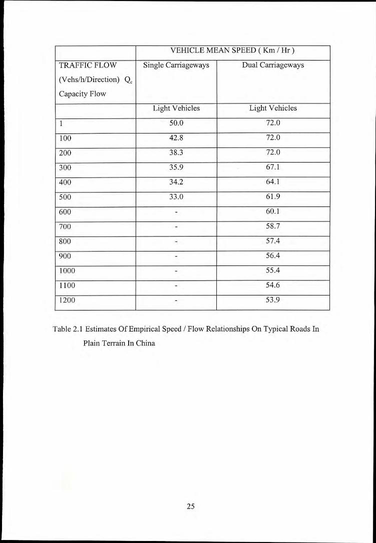
VEHICLE MEAN SPEED ( Km / Hr )
TRAFFIC FLOW Single Carriageways Dual Carriageways
(VehsIhlDirection) Q,Capacity Flow
Light Vehicles Light Vehicles
I 50.0 72.0
100 42.8 72.0
200 38.3 72.0
300 35.9 67.1
400 34.2 64.1
500 33.0 61.9
600 - 60.1
700 - 58.7
800 - 57.4
900 - 56.4
1000 - 55.4
1100 - 54.6
1200 - 53.9
Table 2.1 Estimates Of Empirical Speed / Flow Relationships On Typical Roads In
Plain Terrain In China
25
2.6 ROADS OF BANGLADESH
As it has been intended to conduct the present study on the Bangladeshi highways, it would
be appropriate to discuss about the road networks of Bangladesh. In this section, the
classification and characteristics of the highways of Bangladesh have been discussed.
2.6.1 Road Classification
Bangladesh has two-tier administrative cum functional road classification (Bangladesh
Transport Sector Study 1994). In the first stage road network has two classes: roads under
the jurisdiction of roads and highways department, ministry of communications (RHD,
MOCS) and the rest under local government. In the second stage classification while RHD
network has three functional categories, local government network has five functional
categories. RHD road comprises of:
a) National Highways connecting the nation capital with district (zila) headquarters, port
cities and international highways;
b) Regional Highways connecting the different major regIOn of the country and zila
headquarters not connected by national highways; and
c) Feeder Roads (Type A) connecting sub-district (thana) headquarters to the arterial road
network.
Local government roads consist of
i) Feeder Roads (Type B) connecting growth centres with thana headquarters or to the
Arterial network.
26
ii) Rural Roads (Type I) connecting union headquarters and local markets with centres
or the Road system.
iii) Rural Roads (Type 2) connecting villages and farms with union headquarters and local
markets;
iv) Rural Roads (Type 3) serving villages; and
v) Urban Local Roads: urban local roads are the responsibility of municipalities.
While feeder roads (type b) and rural roads fall in the jurisdiction of local government
engineering department (L G E D). Considering the importance and monetary investment
involved, the national highways should get the priority to be included first. Therefore, five
national highways have been decided to be undertaken for the present research study.
27
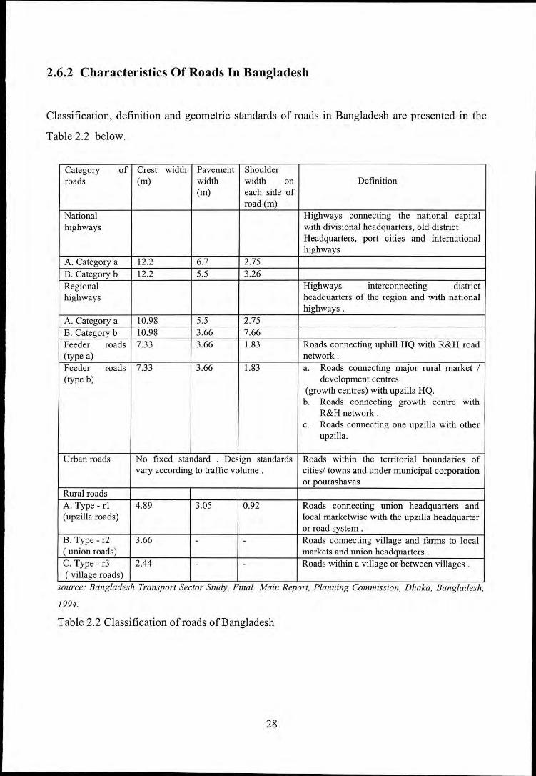
2.6.2 Characteristics Of Roads In Bangladesh
Classification, definition and geometric standards of roads in Bangladesh are presented in the
Table 2.2 below.
Category of Crest width Pavement Shoulderroads (m) width width on Definition
(m) each side ofroad (m)
National Highways connecting the national capitalhighways with divisional headquarters, old district
Headquarters, port cities and internationalhighways
A. Category a 12.2 6.7 2.75B. Category b 12.2 5.5 3.26Regional Highways interconnecting districthighways headquarters of the region and with national
highways.A. Category a to.98 5.5 2.75B. Category b 10.98 3.66 7.66Feeder roads 7.33 3.66 1.83 Roads connecting uphill HQ with R&H road(type a) network.Feeder roads 7.33 3.66 1.83 a. Roads connecting major rural market /(type b) development centres
(growth centres) with upzilla HQ.b. Roads connecting growth centre with
R&H network.c. Roads connecting one upzilla with other
upzilla.
Urban roads No fixed standard . Design standards Roads within the territorial boundaries ofvary according to traffic volume. cities/ towns and under municipal corporation
or pourashavasRural roadsA. Type - r1 4.89 3.05 0.92 Roads connecting union headquarters and(upzilla roads) local marketwise with the upzilla headquarter
or road system.B. Type - r2 3.66 - - Roads connecting village and farms to local( union roads) markets and union headquarters.C. Type - r3 2.44 - - Roads within a village or between villages.( village roads)
source: Bangladesh Transport Sector Study, Final Main Report, Planning Commission, Dhaka, Bangladesh,
/994.
Table 2.2 Classification of roads of Bangladesh
28
2.7 Comments
The literature review of this chapter highlighted the scope of the study of traffic arrival
patterns and free speed of vehicles. No such study for Bangladeshi national highways has
been made to investigate the above topics. It is therefore required to make a study on the
traffic arrival pattern and free speed of vehicles on Bangladeshi national highway.
29
. .
CHAPTER 3
DATA COLLECTION
3.1 INTRODUCTION
Parameters related to traffic flow are useful to the highway engmeers m establishing
geometric design criteria, selecting and implementing traffic control measures and evaluating
the perfonnance of highways. Traffic arrival patterns and their parameters are the basic input
to any of mathematical modelling of highway traffic operations. Driver's free speed denoting
hislher desired speed is a useful parameter considering the traffic safety and relevant control
measures on the highway. Till now, no study has been made for investigating the above cited
parameters for the national highways of Bangladesh. In Bangladesh, most of the national
inter-city highways are two lane two way type with lane width varying from 2.9m-3.75m.
Five national highways of Bangladesh namely Dhaka-Chittangong, Dhaka-Aricha, Dhaka-
Mymensingh, Dhaka-Sylhet and Dhaka-Khulna, are selected for the present study.
3.2 REQUIRED DATA ITEMS
Required data items are as follows:
i) Headways between successive vehicles.
ii) Driver's free speed while he/she is not impeded by the front vehicles.
iii) Speed and flow data at different highway sites.
iv) Speed and density data at different highway sites.
v) Traffic and geometric characteristics of the highway sites.
30

3.3. METHODS OF DATA COLLECTION
The field data has been collected in three ways:
i) Qualitative Observation:
In order to observe the traffic operations in general, field observation of traffic flow has been
made on the national highways of Bangladesh.
ii) Manual measurement:
Physical dimension of the selected sites such as shoulder width and pavement width have
been measured.
iii) Video Recording:
In order to estimate the vehicular time headway data, free speed data and average speed, flow
and density data, video recordings of the traffic flow have been made.
3.4 VIDEO PHOTOGRAPHY AS TRAFFIC DATA SOURCE
In order to be able to analyse the traffic operation, a comprehensive and permanent recording
of the traffic operation is necessary. Video recording is a widely used and cost-effective
means of traffic data collection which can provide a comprehensive and permanent record of
traffic movements (Hossain, 1996). One can obtain many sets of required information
regarding the traffic operation from the same recorded film. Also, recorded video tapes can
readily be used to observe the same traffic scenario repeatedly as many times as required
during analysis. It was, therefore, decided to use video cameras as a main method of
recording highway traffic data.
31
In video filming process the main instrument of data recording is the video camera. For this,
video camera should be placed on a high place to cover a large area of selected section, of
the highway and the camera axis should be parallel with the road alignment.
3.5 DESIRED SITE CHARACTERISTICS
Considering the scope of the study and the limitations of video filming, the selected site of
highway sections should possess following characteristics.
i) The site should be suitable for video data collection.
ii) The site should be chosen free from intersection effect by offsetting a further distance
from intersection and market place.
iii) The site should include the wide variations in traffic conditions in the study area i.e.
with/without non-motorised vehicle.
iv) The site should include vehicle and traffic situation typical of the study area.
v) The site should be free from the disturbances caused by road side access of traffic.
vi) The section should be free from obstruction.
vii) The site should be reasonably flat to eliminate the effect of gradient which is out of the
scope of the present research study.
viii) There should be mInImum disturbances from pedestrian, parked vehicles and
transit/para-transit stops to exclude the effect from these which is again out of the scope of
present study.
32
3.6 PRELIMINARY SURVEY
The preliminary survey has been aimed at identifying sites which satisfy most of the above
set criteria. The preliminary survey has also provided the following useful information for
the successful implementation of final survey.
i) The appropriate time for data collection considering the return journey for data collection,
time of day, sunlight condition and traffic flow conditions. It has been observed that the time
period of 11.00 A.M to 3.00 P.M satisfies most of the considerations cited above.
ii) The proper position for the camera stand considering the visibility of 250-300 meter to be
filmed. It has been found that with the maximum zooming facility the available video
camera can record a distance of around 250m clearly.
iii) The number of surveyors required in the field to install ranging rods with placards &
flags and to record travel time.
iv) For the successful implementation of data collection project training and practical trips
have to be given to the surveyors.
v) The possible the problems which may occur during the final survey work.
33
3.7 PROBLEMS IDENTIFIED DURING PRELIMINARY SURVEY
During preliminary survey, the following problems have been identified:
i) In order to make traffic data measurement, initially, ranging rods have been installed at 50
metre intervals for a distance of 250 metre. But on T.V screen, these ranging rods cannot be
clearly seen. To overcome this problem, placards and flags have been fixed at the upper end
of the ranging rod.
ii) Installation of ranging rod has also been a problem. Because, in most cases road side soil
was not providing enough grip to hold the ranging rod standstill. In order to overcome this
problem ranging rod stands have been used to strengthen the installation ofranging rods.
iii) Another problem identified during preliminary survey is the availability of a suitable
high place from where video recording can be made. In order to be able to see around 300 m
on T.V screen, video recording has to be done from a high place. No one or two storied
building beside the highway has been found at potential sites. Therefore it has been decided
to mount the camera stand on a high wooden table which itself has again been mounted on
the pick-up van parked beside the road.
iv) Parking the pickup van on shoulder has also been a problem, because, the unused
shoulder is not vary wide to accommodate the pickup van. While, parking the vehicle on the
pavement may influence the traffic operations. These has been considered while selecting the
final sites.
v) In order to hold the light camera stand at standstill from the disturbances of wind and
vibration of running vehicles, a skilled person has always been kept available to maintain the
proper alignment of camera.
34
vi) It has been observed that most of the highway sections have been well planted with trees
on both sides. These plantations have created obstructions to sights and sunlight on many
occasions. This has been considered while selecting the site and camera station.
vii) Light weight placards and flags have been observed to change their positions frequently
by wind. Therefore, it has been decided to reinforce the placards and flags to make them as
stable as possible against wind effect. Also two persons have always been available to ensure
their proper orientations.
viii) Availability and direction of sunlight are important for proper video filming. These
considerations have been made while selecting highway section, camera station and time of
video recording.
3.8 DESCRIPTION OF THE SELECTED SITES
Five highway sections have been selected on five national highways for the purpose of data
collection. The characteristics of the sections are as follows:
a) At Savar on Dhaka-Arieha highway: A fairly flat and straight section on Dhaka-Aricha
highway has been selected. At Savar area which is 36 km away from central Dhaka. The
pavement width at this section has been found to be 7.5 m wide and also in good condition
having no potholes and major cracks. The section also has a shoulder of 2.0 m at both side.
b) At Modonpur on Dhaka-Chittagong highway: This fairly straight and flat section has
been selected at Modonpur on Dhaka-Chittagong highway about twenty five km away from
central Dhaka. The pavement width at this section has been found to be 7 m and in good
condition. At both sides of the section, 3.1 m of shoulder has been found.
35
c) At National park on Dhaka-Mymensingh highway: This flat and fairly straight section
has been selected in National Park area on Dhaka-Mymensingh highway. The pavement
width (6 m) here has been found to be narrower than the above sites. But the pavement has
been found to be in similarly good condition as above sections. At both sides of the section
1.4 m of shoulder has been observed.
d) At Bultha on Dhaka-Sylhet highway : This section has been selected at Bultha on
Dhaka-Sylhet highway which is 33 km away from central Dhaka. This is a flat and fairly
straight section having 6.8 m of pavement width and 1.6 m of shoulder at both sides.
Although pavement surface appears to be little older than the above sections, but there is no
potholes or large cracks on the pavement.
e) At Keranigong on Dhaka-Khulna highway: This section has been selected in
Keranigong area which is about 14 km away from central Dhaka. The pavement width has
been found to be 5.8 m here which is the narrowest among the five sections. However, at
both sides of the road 1.6 m wide shoulder has been observed.
All the relevant information of the selected highway sections along with the date of data
collection has been presented Table 3.1.
36

Name of Date Location Pavement Shoulder
highways width width
Dhaka- 11-11-97 National park 6m 104m
Mymensingh
Dhaka- 9-11-97 Karanigong 5.8m 1.6m
Khulna
Dhaka- 13-11-97 BoItha 6.8m 1.6m
Sylhet
Dhaka- 18-11-97 Modonpur 7m 3.1m
Chittagong
Dhaka- 19-11-97 Sayar cantonment 7.5m 2.0m
Aricha
Table 3.1 Description of data collection sites
3.9 PREPARATION FOR DATA COLLECTION
For successful data collection in the field necessary arrangements have been undertaken with
due considerations to the problems identified during the preliminary survey. A check list of
required things has been prepared to check necessary items each day before starting for the
field for data collection.
In order to get the distance mark on the recorded videofilm, placards containing numeric
number I to 10 have been prepared from hard paper board. Numbers on placards have been
written with bright marker paint. Ropes have been collected for hanging the 30inch by
24inch placards from the ranging rod. To make the placards more identifiable, colourful
flags have also been decided to be used along with the placards. To make the flags stable
enough, metal wires have been passed through them.
Twenty rangmg rods, twelve folding chairs, tripod stand with clamp, two odometers,
measuring tapes, two stop watches and eight safety vest are borrowed from the survey store
37
and traffic engineering laboratory of BUET. Spray paint and anamel paint along with brush
have been collected to mark the pavements whenever necessary. A pickup van has been
hired for transport purpose of the whole survey team along with the instruments and
necessary applinaces.
3.10 DATA COLLECTION PROCEDURE
Before starting for data collection, all the instruments and items necessary for data
collection have been loaded on pick up van one by one according to the checklist. Special
attention has been given to the video camera checking whether the battery is fully charged
and whether the video cassettes are blank. Then journey to data collection is started.
At first, the pick up van has been parked on the roadside at a point suitable for cammera
station at the selected site. Then the camera along with its tripod stand has been mounted on
the wooden table which is again mounted on the pick up van(see Fig. 3.1). In the next step,
camera axis and sight have been adjusted for video recording. After that ranging rods have
been installed along with the placards and flags at 50m intervals. At the starting point which
is near to the camera the placard bearing the serial zero(O) has been hung from the ranging
rod. Then placards serial no. 1,2,3 etc. have been hung from the ranging rod at the successive
50m intervaI(see Fig. 3.2).
After checking all the necessary functions of video camera, video recording has been started
at this point. As the 8m.m video cassette can record only for 90 minutes, new blank cassette
has been inserted when 90 minutes recording has been completed. Also battery charged
indicator has been checked at a regular interval. With the diminishing battery charge sign on
the old battery has been replaced by charged battery. About three hours of video filming has
been made at each site. However, including the preliminary survey, a total of 25 hours of
video recording has been made.
38
There is little deviation in the filming process at the field from the standard as cited earlier.
That is, there is an angle of camera axis created with the alignment of highway. This is
because, camera station has to be taken on the side of the road so that there is no interruption
to traffic movement due to the parked vehicle. However, considerations have been given to
this aspect during data collection. It could be avoided by using telescopic tower installing
video camera at vintage point.
3.11 DATA EXTRACTION
As mentioned earlier, the video recording has been made on 8mm video cassette. Recorded
film has then been transferred to standard VHS cassettes. After the transferred, a time base
showing 1/10'" of second has been superimposed on the video film. Because the timer of the
video camera is in second which is not adequate for accurate calculation of speed andheadway data.
Data extraction from the video cassette is a difficult and time consuming task. Data items
have been collected watching the video playback at the laboratory. Speed, density, flow,
headway data have been the main points of interest for this research project. Data items such
as free speed, time headway, flow volume, density and vehicle compositions have been
estimated for the five selected highways.
3.11.1 Traffic Headway
Time headway is the time between the arrival of successive vehicle at a specified point. It is
the reciprocal of volume. Time headway data used for this study has been collected from the
video playback. The superimpose timebase on video film has been very useful in this regard.
39
3.11.2 Free Speed
In this study, driver's are considered to be free or unimpeded when the front vehicle is 80m
away from him/her. At studio, free speed has been measured from video playback. Free
speed is calculated using the travel time required by a vehicle to pass through the 50m
section. The superimpose timebase(accurate up to 1/10th of second) has been utilised for this
purpose.
3.11.3 Traffic Volume and Average Speed
Traffic volume is defined as the number of vehicles that pass a point along a highways per
unit of time. Average speed mentioned here is the average of time mean speed of vehicles
over a 50m section of highway.
Both speed and volume data have been collected from video playback. As the total
videofilming for a site is about three hours, traffic volume per fifteen minutes intervals have
been estimated during this study. However, these speed and volume data has been used only
to illustrate the speed-flow condition during the data collection period
3.11.4 Traffic Density and Average Speed
Traffic density also refereed to as traffic concentration, is defined as the average no. of
vehicles occupying a unit length of road way at a given instant. In this study traffic density
has been measured as vehicles per quarter km as approximately quarter of a km can be
clearly seen on the video playback. This density and speed data have been collected from
video playback. However, these density and speed data have been used only to illustrate the
speed-density condition at site during data collection.
40
The average speed mentioned here is the average of space mean speed of vehicles (distance
travelled divided by average travel time of vehicle) taken over a SOmsection of highway.
The collected data items have been presented in appendix A.
41
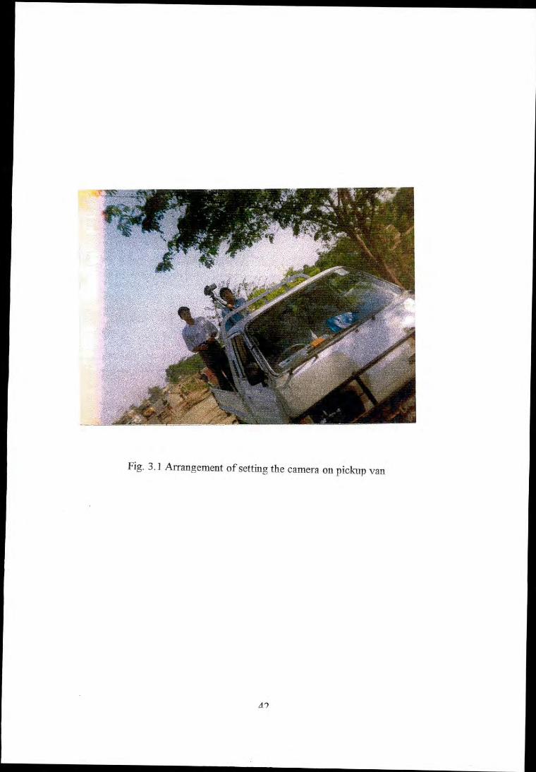
Fig. 3. I Arrangement of setting the camera on pick'up van
d?
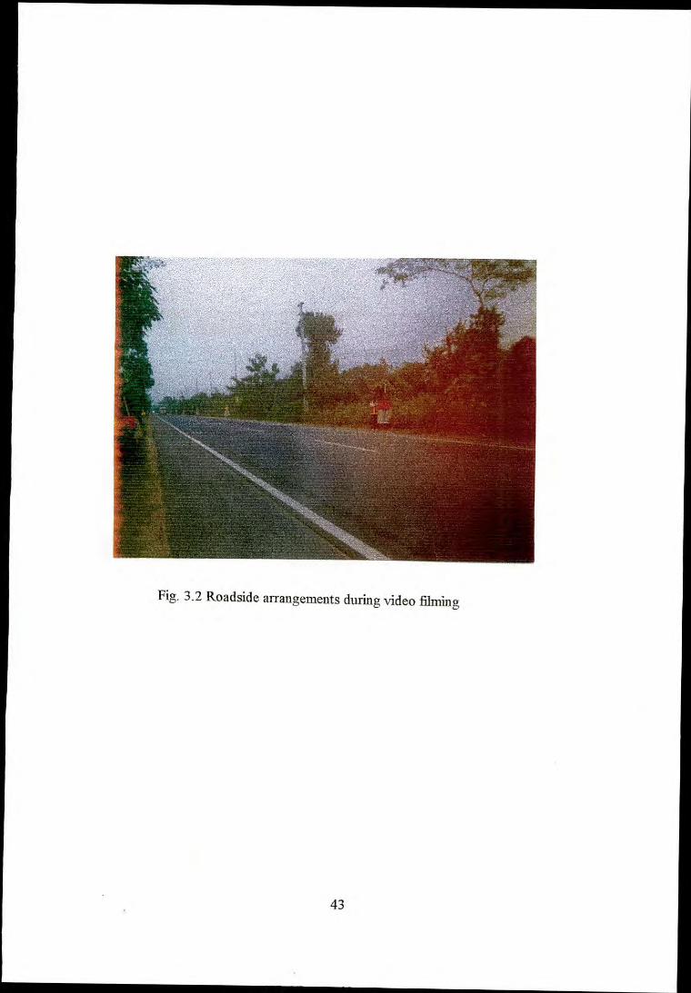
Fig. 3.2 Roadside arrangements during video filming
43
CHAPTER 4
DATA ANALYSIS AND INTERPRETATION OF RESULTS
4.1 GENERAL
In this chapter, both qualitative and quantitative analysis and interpretation of collected
highway traffic data have been made. In the quantitative analysis, a general observation and
analysis of highway traffic stream have been made. While quantitative observation includes
the analysis of traffic arrival pattern data and free speed data along with the presentation of
relevant speed-flow, speed-density situation. Data have been collected from five selected
road sections of five major highways of Bangladesh. In order to achieve the objectives of
this study, data have been collected from different highway sections. Field survey has been
conducted for a period of three weeks during the month of November 97. Efforts have been
given to determine relevant statistics of vehicle arrival pattern, free speed data and to analyse
relationship between speed-flow and speed-density during the period of data collection. It
has been tried to estimate most of the parameters microscopically i.e. at every vehicle level,
rather than macroscopically i.e. at average level of traffic stream characteristics.
4.2 STATISTICAL ANALYSIS
Detailed statistical analysis of the data has been undertaken in order to estimate typical
values of the measured traffic parameters, and to investigate their variability by searching for
mathematical distributions. The statistical packages such as STATGRAPH version 7.0 and
SPSS 6.1 for WINDOWS have been used for general statistical analysis and relevant
graphical output respectively. The most common methods for testing goodness of fit are the
Chi-square test and Kolmogrov-smirnov test(Bullen and Mei 1993). The chi-square test of
goodness-of-fit has been used throughout this study to test the goodness of fit of distribution
function to the observed data. However, the Chi-square test is sensitive to the grouping
44
arrangements of the data. Therefore, the Kolmogorov-Smimov test has also been used as a
tool for checking the goodness-of-fit, especially, when Chi-square test appears to be not
suitable for the respective data set.
The Chi-square test gIves an overall measure of the difference between observed and
predicted frequencies. It provides a comparison of estimated Chi-square values with the
tabulated values for the Chi-square distribution, and thus, enabled the estimation of the
degree of acceptance of a hypothesis. The Kolmogorov-Smimov (K-S) test measures how
much the estimated empirical cumulative distribution function differs from that of the
assumed distribution. The K-S statistics compares the empirical distribution model derived
from observed data with the theoretical one using the maximum absolute differences
between the two. Tolle(l969)(Bullen and Mei 1993) did his analysis with the Kolmogrov-
smimov test because he found that the Chi-square test is not a very forgiving analysis and
may be thrown off by only a few "bad" points. In reality, obtairunent of actual "good" chi-
square fits from data which are influenced by so many unpredictable variables is not fully
expected.
An overall 5% level of significance has been taken as the basis of accepting the statistical
significance. However, in order to be able to make relatively wider basis of acceptance 1%
level of significance has also been checked if the situation demands so. The analysis tables
and graphical outputs regarding the estimation of the parameters have been presented in this
chapter.
4.3 QUALITATIVE ANALYSIS
It has been observed that the traffic stream on the five selected highways comprises of both
motorised and nonmotorised vehicles. Although the proportion of norunotorised vehicles
appears to be much lower than that of motorised portion. Also the pedestrian activities has
been found to be very low on the selected highway sections.
45
On the highway sections with paved shoulder, nonmotorised vehicle normally ply on the
paved portion of the shoulder. But if there is no paved shoulder portion nonmotorised
vehicles normally share the same pavement width with the motorised vehicles. For this
reason, on the highway section without paved shoulder it has been observed that motorised
vehicles have to undertake overtaking manoeuvres frequently to overtake the impeding
nonmotorised vehicles. It has also been observed that in the following situation drivers
maintain close headways and with any opportunity of overtaking he/she avails that readily.
Generally, it has been found that nine types of vehicles i.e., bus, truck, minibus, minitruck,
Autorickshaw, passenger car, pickup van, motorcycle and nonmotorised vehicles. It has also
been observed that a significant portion of the motorised traffic comprises of commercial
buses and trucks. Loaded trucks and short route local buses have been observed to maintain
relatively lower speed. Among the five highways Dhaka-Aricha highway appears to cater
highest proportion of short route local buses(mostly Dhaka-Aricha and Dhaka-Manikgonj
route).
4.4 QUANTITATIVE ANALYSIS
Quantitative analysis regarding traffic composition, vehicle arrival pattern, free speed and
speed-flow-density conditions at different highway sites have been presented in this section.
4.4.1 Traffic Composition
At the first stage of quantitative analysis, the average proportion of different vehicle types in
the traffic mix have been investigated. The typical traffic compositions found in different
highways have been presented in the Table 4.1. From the Table 4.1, it can be observed that
the proportion of nonmotorised vehicles varies in the range of 5.93% to 17.75% with the
lowest and highest percentage being in the Dhaka-Khulna and Dhaka-Mymensingh highway
46
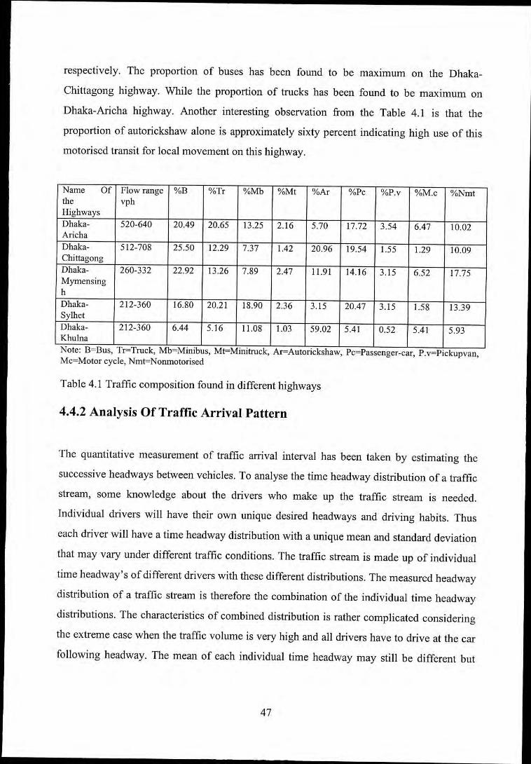
respectively. The proportion of buses has been found to be maxImum on the Dhaka-
Chittagong highway. While the proportion of trucks has been found to be maximum on
Dhaka-Aricha highway. Another interesting observation from the Table 4.1 is that the
proportion of autorickshaw alone is approximately sixty percent indicating high use of this
motorised transit for local movement on this highway.
Name Of Flow range %B %Tr %Mb %Mt %Ar %Pc %P.v %M.c %Nmtthe vphHighwaysDhaka- 520-640 20.49 20.65 13.25 2.16 5.70 17.72 3.54 6.47 10.02ArichaDhaka- 512-708 25.50 12.29 7.37 1.42 20.96 19.54 1.55 1.29 10.09ChillagongDhaka- 260-332 22.92 13.26 7.89 2.47 11.91 14.16 3.15 6.52 17.75MymensinghDhaka- 212-360 16.80 20.21 18.90 2.36 3.15 20.47 3.15 1.58 13.39Sy1hetDhaka- 212-360 6.44 5.16 11.08 1.03 59.02 5.41 0.52 5.41 5.93KhulnaNote: B=Bus, Tr=Truck, Mb~Minibus, MpMinitruck, Ar=Aulorickshaw, Pc=Passenger-car, P.v~Pickupvan,Mc=Molor cycle, Nmt=Nonmolorised
Table 4.1 Traffic composition found in different highways
4.4.2 Analysis Of Traffic Arrival Pattern
The quantitative measurement of traffic arrival interval has been taken by estimating the
successive headways between vehicles. To analyse the time headway distribution of a traffic
stream, some knowledge about the drivers who make up the traffic stream is needed.
Individual drivers will have their own unique desired headways and driving habits. Thus
each driver will have a time headway distribution with a unique mean and standard deviation
that may vary under different traffic conditions. The traffic stream is made up of individual
time headway's of different drivers with these different distributions. The measured headway
distribution of a traffic stream is therefore the combination of the individual time headway
distributions. The characteristics of combined distribution is rather complicated considering
the extreme case when the traffic volume is very high and all drivers have to drive at the car
following headway. The mean of each individual time headway may still be different but
47

they will converge toward a single value because of the close spacing. Traffic arrival pattern
has been analysed by using the statistical software noted above.
All the traffic arrival pattern data have been grouped according to the source highway. A
general statistical analysis of each group has been made and the mean, standard deviation are
shown in table 4.4. Frequency histogram of each group of traffic arrival pattern have been
plotted to get their general distribution pattern. The frequency histograms are shown in Fig.
4.1 to Fig. 4.5. It can be observed from the frequency histograms ( Fig. 4.1 to Fig. 4.5 ) that
vehicular headway distributions have resemble to negative exponential and lognormal pattern
which need to be function fitting. Therefore, distribution functions of negative exponential
and lognormal have been investigated with a view to fit a proper distribution function to the
vehicle arrival pattern.
The statistical analysis results of distribution function fitting are given in Table 4.2 to Table
4.3. The goodness-of-fit test of negative exponential and lognormal distribution functions to
the vehicular headway interval data are discussed below.
i) Negative exponential distribution: The goodness-of-fit test with exponential distribution
function reveals that the traffic arrival patterns on Dhaka-Aricha, Dhaka-Mymensingh and
Dhaka-Khulna highways follow this distribution function (Table 4.2) according to both Chi-
square and K-S test at 5% level of significance. However, at I% level of significance the
headway data of Dhaka-Sylhet and Dhaka-Chittagong show good fit to the exponential
distribution pattern from both the tests.
ii) Log-normal distribution : The Chi-square goodness-of-fit test with lognormal
distribution function reveals that the traffic arrival pattern on none of the five highways
follow this distribution at 5% level of significance. However, the K-S goodness-of-fit test
supports that the traffic arrival pattern on all but Dhaka-Mymensingh highway follow
lognormal distribution at 5% level of significance(Table 4.3).
48
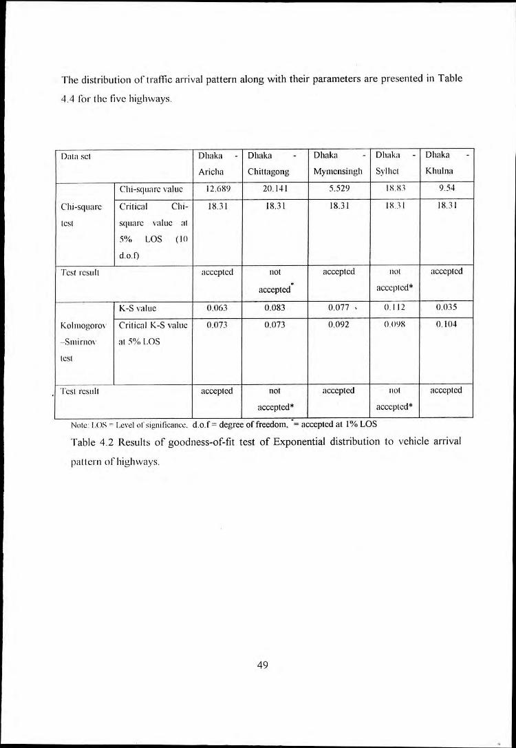
The distribution of tratTic arrival pattern along with their parameters are presented in Table
4.4 li)r the five highways.
Dala sci Dhaka - Dhaka - Dhaka - Dhaka - Dhaka -Aricha Chitlagong Mynlcnsingh Sylhel Khulna
Chi-s(]tlarc value 12.68~ 20.1~1 5.529 IX.Xl 9.54
Chi-square Critical Chi- 18.31 18.31 18.31 18..11 18.31
lest square ,"alnc :II
51% LOS ( 10
d.o.f)
Tcsl result accepted nol accepted not accepted.accepted'accepted
K-S \.alue tU)63 0.083 0.077 , 0.112 tUm
Kolmogorm" Critical K-S value tUm 0.073 tU)92 tl.l)~8 O.IO~
-Snlirno\' :11 5%, LOS
lest
Test result accepted not aecepled 1101 accepted
accepted' acccptcd*
Note: LOS = Lc\"d ofsignilicmll:c. d.o.r= degree offrecdoIn .. = accepted at l% LOS
Table 4.2 Results of goodness-of-tit test of Exponential distribution to vehicle arrival
pallern of highways.
49
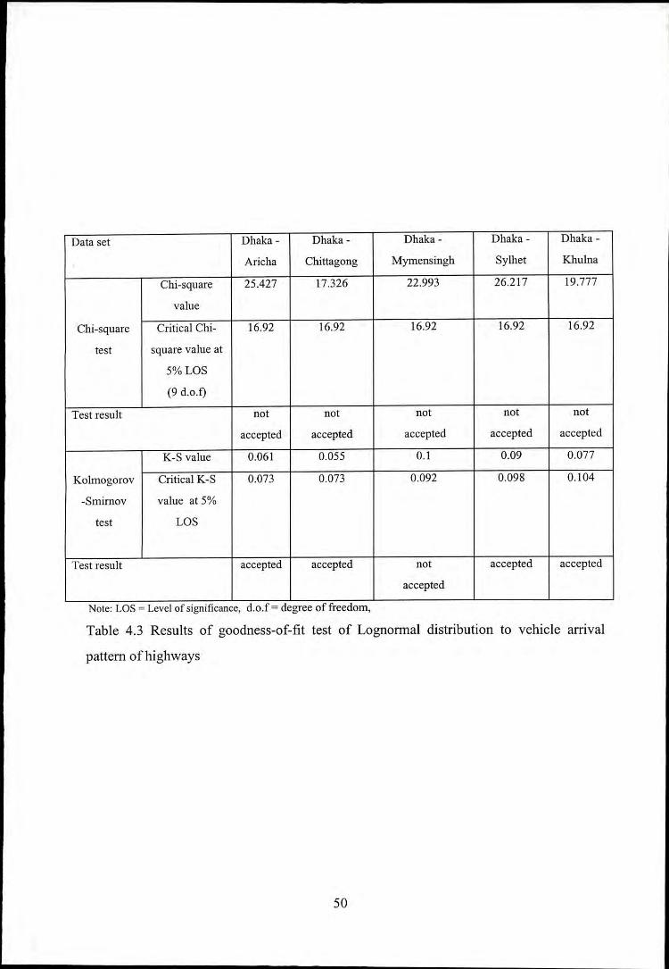
Data set Dhaka - Dhaka - Dhaka - Dhaka - Dhaka -
Aricha Chittagong Mymensingh Sylhet Khulna
Chi-square 25.427 17.326 22.993 26.217 19.777
value
Chi-square Critical Chi- 16.92 16.92 16.92 16.92 16.92
test square value at
5% LOS
(9 d.o.!)
Test result not not not not not
accepted accepted accepted accepted accepted
K-S value 0.061 0.055 0.1 0.09 0.077
Kolmogorov Critical K-S 0.073 0.073 0.092 0.098 0.104
-Smimov value at 5%
test LOS
Test result accepted accepted not accepted accepted
accepted
Note: LOS = Level of significance, d.o.f = degree of freedom,
Table 4.3 Results of goodness-of-fit test of Lognormal distribution to vehicle arrival
pattern of highways
50
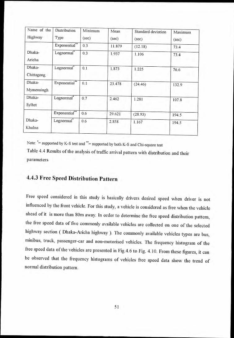
Name of the Distribution Minimum Mean Standard deviation MaximumHighway Type (sec) (sec) (sec) (sec)
Exponential"' 0.3 11.879 (12.18) 73.4Dhaka- Lognormal' 0.3 1.937 l.l06 73.4Aricha
Dhaka- Lognorma( 0.1 1.873 1.225 76.6Chittagong
Dhaka- Exponential" 0.1 23.478 (24.46) 132.9Mymensingh
Dhaka- Lognormal. 0.7 2.462 1.281 107.8Sylhet
Exponential" 0.6 29.621 (28.93) 194.5Dhaka- Lognormal" 0.6 2.858 l.l67 194.5Khulna
Note: '= supported by K-S test and"= supported by both K-S and Chi-square test
Table 4.4 Results of the analysis of traffic anival pattem with disttibutiou and theirparameters
4.4.3 Free Speed Distribution Pattern
Free speed cousidered in this study is basically dtivers desired speed when dtiver is not
influenced by the fi'ont vehicle. For this study, a vehicle is considered as fi'ee when the vehicle
ahead of it is more than 80m away. In order to detennine the fi'ee speed distJibution patten!,
the free speed data of five commonly available vehicles are collected on one of the selected
highway section ( Dhaka-Aticha highway). TIre comlllonly available vehicles types are bus,
minibus, tIUck, passenger-car and non-llIototised vehicles. TIle fi'equency histogram of the
fi'ee speed data of the vehicles are presented in Fig.4.6 to Fig. 4.10. From these figures, it can
be observed that the frequency histograms of vehicles fi'ee speed data show the trend of
nOlmal disttibution pattelll.
51
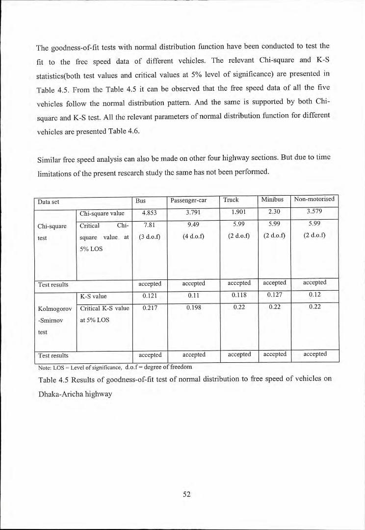
The goodness-of-fit tests with normal distribution function have been conducted to test the
fit to the free speed data of different vehicles. The relevant Chi-square and K-S
statistics(both test values and critical values at 5% level of significance) are presented in
Table 4.5. From the Table 4.5 it can be observed that the free speed data of all the five
vehicles follow the normal distribution pattern. And the same is supported by both Chi-
square and K-S test. All the relevant parameters of nonnal distribution function for different
vehicles are presented Table 4.6.
Similar free speed analysis can also be made on other four highway sections. But due to time
limitations of the present research study the same has not been performed.
Data set Bus Passenger-car Truck Minibus Non-motorised
Chi-square value 4.853 3.791 1.901 2.30 3.579
Chi-square Critical Chi- 7.81 9.49 5.99 5.99 5.99
test square value at (3 d.D.t) (4 d.D.t) (2 d.D.t) (2 d.D.t) (2 d.D.t)
5% LOS
Test results accepted accepted accepted accepted accepted
K-S value 0.121 0.11 0.118 0.127 0.12
Kolmogorov Critical K-S value 0.217 0.198 0.22 0.22 0.22
-Smimov at 5% LOS
test
Test results accepted accepted accepted accepted accepted
Note: LOS = Level of significance, d.o.f= degree of freedom
Table 4.5 Results of goodness-of-fit test of normal distribution to free speed of vehicles on
Dhaka-Aricha highway
52
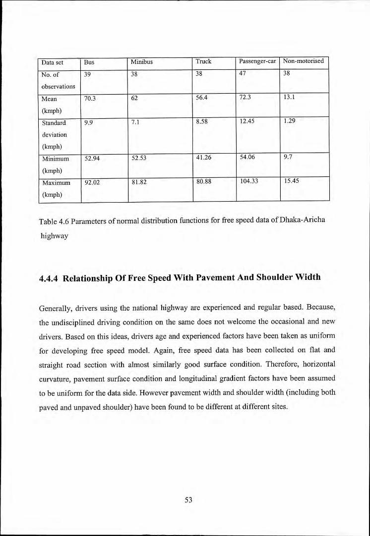
Data set Bus Minibus Truck Passenger-car NOTI-motorised
No. of 39 38 38 47 38
observations
Mean 70.3 62 56.4 72.3 13.1
(kmph)
Standard 9.9 7.1 8.58 12.45 1.29
deviation
(kmph)
Minimum 52.94 52.53 41.26 54.06 9.7
(kmph)
Maximum 92.02 81.82 80.88 104.33 15.45
(kmph)
Table 4.6 Parameters of normal distribution functions for free speed data of Dhaka-Aricha
highway
4.4.4 Relationship Of Free Speed With Pavement And Shoulder Width
Generally, drivers using the national highway are experienced and regular based. Because,
the undisciplined driving condition on the same does not welcome the occasional and new
drivers. Based on this ideas, drivers age and experienced factors have been taken as uniform
for developing free speed model. Again, free speed data has been collected on flat and
straight road section with almost similarly good surface condition. Therefore, horizontal
curvature, pavement surface condition and longitudinal gradient factors have been assumed
to be uniform for the data side. However pavement width and shoulder width (including both
paved and unpaved shoulder) have been found to be different at different sites.
53
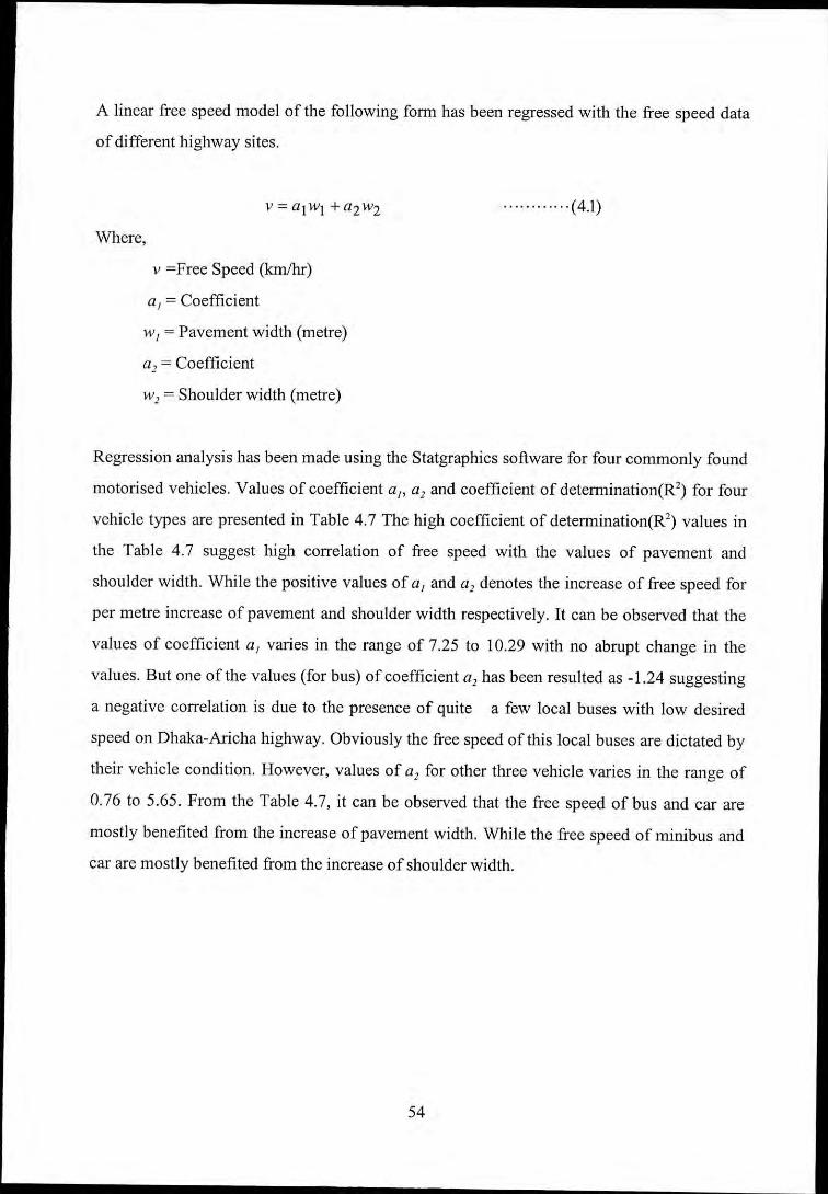
A linear free speed model of the following form has been regressed with the free speed data
of different highway sites.
. (4.1)
Where,
v =Free Speed (km/hr)
a I = Coefficient
WI = Pavement width (metre)
a, = Coefficient
w, = Shoulder width (metre)
Regression analysis has been made using the Statgraphics software for four commonly found
motorised vehicles. Values of coefficient aJ>a, and coefficient of determination(R2) for four
vehicle types are presented in Table 4.7 The high coefficient of determination(R2) values in
the Table 4.7 suggest high correlation of free speed with the values of pavement and
shoulder width. While the positive values of al and a, denotes the increase of free speed for
per metre increase of pavement and shoulder width respectively. It can be observed that the
values of coefficient al varies in the range of 7.25 to 10.29 with no abrupt change in the
values. But one of the values (for bus) of coefficient a, has been resulted as -1.24 suggesting
a negative correlation is due to the presence of quite a few local buses with low desired
speed on Dhaka-Aricha highway. Obviously the free speed of this local buses are dictated by
their vehicle condition. However, values of a, for other three vehicle varies in the range of
0.76 to 5.65. From the Table 4.7, it can be observed that the free speed of bus and car are
mostly benefited from the increase of pavement width. While the free speed of minibus and
car are mostly benefited from the increase of shoulder width.
54
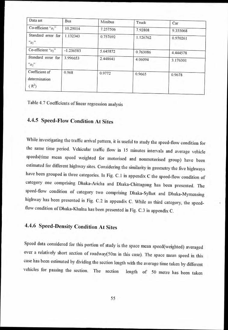
Dataset Bus Minibus Truck CarCo-efficient "al" 10.29014 7.257506 7.92808 9.355068Standard error for 1.132343 0.757692 1.126762 0.970261"'a,"
Co-efficient "al" -1.236583 5.645872 0.763086 4.444578Standard error for 3.996653 2.448641 4.06094 3.176301"a2"
Coefficientof 0.968 0.9772 0.9665 0.9678determination
( R2)
Table 4.7 Coefficients oflinear regression analysis
4.4.5 Speed-Flow Condition At Sites
Wllile investigating the traffic arrival pattelll, it is nsefi,1 to stndy the speed-flow condition for
the same time period. Yelticnlar traffic flow in 15 minntes intervals and average vehjcle
speeds(time mean speed weighted for motmised and nonmotorised gronp) have been
estimated for different highway sites. Consideting the similatity in geometry the five ltighways
have been gronped in three categmies. In Fig. C.I in appendix C the speed-flow condition of
categOlY one comprising Dhaka-Aricha and Dhaka-Chjttagong has been presented. The
speed-flow condition of category two comprising Dhaka-Sylhet and Dhaka-Mymensing
highway has been presented in Fig. C.2 in appendix C. Wllile as third categOlY, the speed-
flow condition ofDhaka-Khnlna has been presented in Fig. C.3 in appendix C.
4.4.6 Speed-Density Condition At Sites
Speed data considered for this portion of study is the space mean speed(weighted) averaged
over a relatively ShOl1section of roadway( 50m in tltis case). TIre space mean speed iu this
case has been estimated by dividing the section length with the average time taken by different
vehicles for passing the section. TIle section length of 50 metre has been taken
55
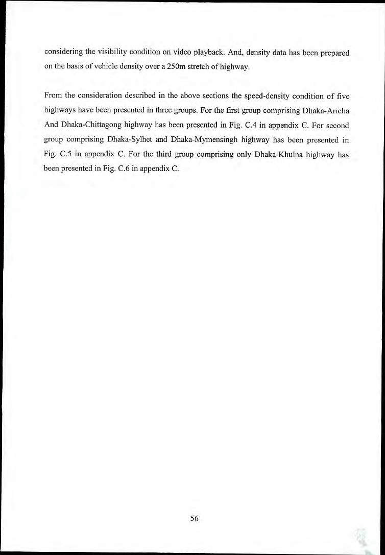
considering the visibility condition on video playback. And, density data has been prepared
on the basis of vehicle density over a 250m stretch of highway.
From the consideration described in the above sections the speed-density condition of five
highways have been presented in three groups. For the first group comprising Dhaka-Aricha
And Dhaka-Chittagong highway has been presented in Fig. C.4 in appendix C. For second
group comprising Dhaka-Sylhet and Dhaka-Mymensingh highway has been presented in
Fig. e.5 in appendix e. For the third group comprising only Dhaka-Khulna highway has
been presented in Fig. e.6 in appendix C.
56
200180160140
>- 1200cQ) 100::J0"Q) 80~IJ...
6040200
39 45 51 57 63 69 75Headway( sec)
Fig. 4.1 Frequency histogram of headway data ofDhaka-Aticha highway
200180160140
>- 1200cQ) 100::J0"Q) 80~IJ...
40
20o
3 9 15 21 27 33 39 45 51 57 63 69 75
Headway( sec)
Fig. 4.2 Frequency histogram of headway data of Dhaka-Chitta gong highway
57
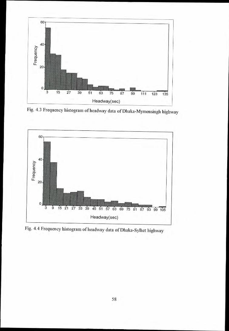
60
40GcID::Jrr~lJ... 20
o3 15 27 39 51 63 75 87 99 111 123 135
Headway(sec)
Fig. 4.3 Frequency histogram of headway data of Dhaka-Mymensingh highway
60
40GcID::Jrr~lJ...
20
o3 9 15 21 27 33 39 45 51 57 63 69 75 81 87 93 99 105
Headway(sec)
Fig. 4.4 Freqnency histogram of headway data ofDhaka-Sylhet highway
58
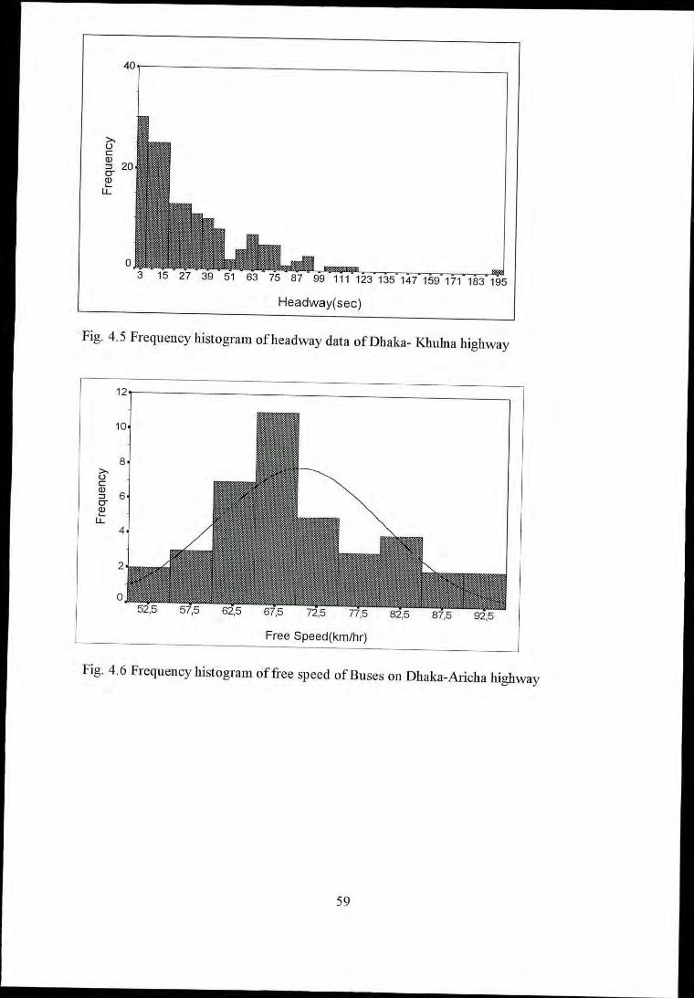
40
>-uc:Q):J 200-
~u..
15 27 39 51 63 75 87 99 111 123135147159171 183195
Headway(sec)
Fig. 4.5 Frequency histogram of headway data of Dhaka- Khulna highway
12
10
8>-uc:~ 60-~u..
4
2
o52,5 57,5 62,5 67,5 72,5 77,5 82,5 87,5 92,5
Free Speed(km/hr)
Fig. 4.6 Frequency histogram offiee speed of Buses on Dhaka-Aricha highway
59
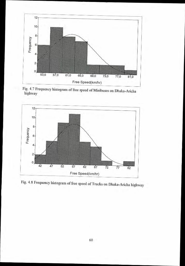
Fig. 4.7 Frequency histogram offiee speed of Minibuses on Dhaka-Arichahighway
Free Speed(km/hr)
81,077,073,069,065,061,057,053,0
12
10
8>.0cQ)
6:Jrr~LL
2
12
2
o
Free Speed(km/hr)
•
Fig. 4.8 Frequency histogram offi-ee speed ofTmcks on Dhaka-Aricha highway
60
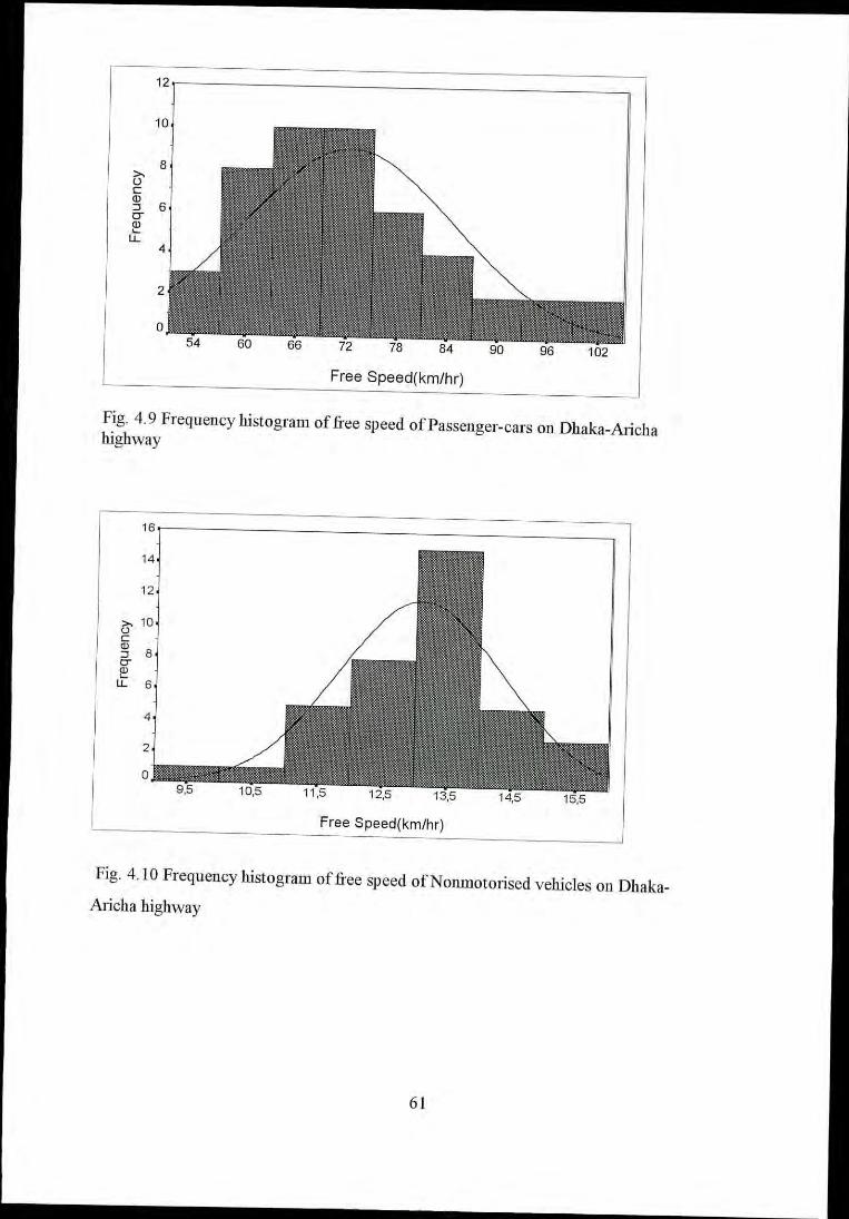
Fig. 4.9 Frequency histogram offi'ee speed of Passenger-cars on Dhaka-Anehahighway
12
10
8>.UcQ)OJ 60-Q)~lL 4
2
054 60 66
16
14
12
>. 10ucQ)
8OJ0-~lL 6
4
2
09,5
Free Speed(km/hr)
96 102
15,5
Free Speed(km/hr)
Fig. 4. IO Frequency histogram of free speed ofNonmotOlised vehicles on Dhaka-Alieha highway
61
CHAPTERS
CONCLUSIONS AND RECOMMENDATIONS
5.1 INTRODUCTION
This chapter presents the conclusions and recommendations of the research study for
estimation of parameters related to traffic flow on the selected national highways of
Bangladesh. In particular, conclusions on different traffic arrival headway patterns and free
speed characteristics of vehicles have been summarised. Recommendations and guide lines
for relevant future study have also been presented.
5.2 CONCLUSIONS
5.2.1 Traffic Arrival pattern
Analysis of traffic arrival pattern using the vehicular time headway data reveals that the
pattern follows more than one distribution models for two highways. Generally, it has been
found that the vehicles maintain close headways when they are in following situation. For
Dhaka-Aricha highway, the goodness-of-fit test suggests that the arrival headway pattern
follows exponential distribution supported by both Chi-square and K-S tests. However, K-S
test suggests that the same headway data also fits to the lognormal distribution. For the
headway data of Dhaka-Chittagong highway, the lognormal distribution gives good fit as
suggested by K-S test only. Analysis of the headway data of Dhaka-Mymensingh highway
reveals that the traffic arrival pattern can be expressed by exponential distribution as
suggested by both Chi-square and K-S test. From Chi-square test, no good fit has been found
for the headway data of Dhaka-Sylhet highway. But K-S test suggests that the traffic arrival
pattern on this highway can be given by lognormal distribution. It has also been observed
62
that exponential distribution gives good fit to the headway data ofDhaka-Khulna highway as
suggested by both Chi-square and K-S test. However, only K-S test suggests that the same
data group also follows lognormal pattern.
5.2.2 Free Speed Characteristics
Analysis of free speed data of vehicles on a typical section of Dhaka-Aricha highway reveals
that free speed of the commonly available vehicles (bus, truck, car, minibus and
nonomotorised vehicles) follow normal distribution models. While the mean free speed of
motorised vehicles ranges from 5604 kmph for truck drivers to 72.3 kmph for passenger car
drivers, the same for non-motorised vehicles is 13.1 kmph. It is also observed that drivers'
free speed depends on the pavement width and shoulder width of the two-lane two-way
highways. From regression analysis, a linear relationship of free speed with pavement and
shoulder width has been developed. The analysis reveals that drivers' free speed increases
with the increase in pavement width. In a pavement width range of 5.8 metre to 7.5 metre,
free speed ofmotorised vehicles' drivers increases in a range of7.25 to 10.29 kmph for each
metre of pavement widening. Similar relationship of free speed with the shoulder width has
also been found except for the case of bus. For the cases of trucks, minibuses and passenger-
cars, it has been observed that in a shoulder width range of IAm to 3.lm, free speed
increases in a range of 0.76 to 5.65 kmph for each metre of shoulder widening at both sides.
However, inclusion of some slow speed local buses in the data group has been resulted
negative correlation ofbus's free speed with the shoulder width.
5.2.3 Speed-Flow And Speed-Density Condition
For the limited period of traffic data collection, the speed-flow and the speed-density
condition have been investigated. However, considering the limited period and traffic flow
range, it is not worthy to go for investigating the overall speed-flow-density relationship.
63
5.2.4 Limitations Of The Study
Present study is limited to the flat, horizontal and disturbance free sections on five selected
national highways. As we did not have any purpose built high platform and also there was no
roadside suitable building to be used as platform, the camera axis could not be fixed
vertically. It is anticipated that this will result some amount of parallax error during data
measurement. We have collected data from video recording with 1/101h of superimpose clock
which was not high precision in counting travel time required by a vehicle to pass through
the Sam section. National highways comprises only eleven percent of total highway network.
More than two third (71%) of the national highways even have pavement width below the
prescribed specification limits viz. 5.5 m (Bangladesh Transport Sector Study, 1994). But the
pavement width of the five highway sections in this study are in the range of5.8m to 7.5m.
5.3 RECOMMENDA nON FOR FUTURE STUDY
Based on the experience gathered from the present study the following recommendations for
future study in this field can be suggested:
i)The same study can be performed with 1/100 seconds time base on the recorded video film.
ii) The large amount of speed-flow data is needed to get a good correlation between speed
and flow.
iii) The large amount of speed-density data is needed to get a good correlation between speed
and density.
64

iv) Video data collection from a further high station is suggested to minimise the relevant
parallax error.
v) The same study can be performed on the national highways with pavement width
narrower than 5.5m.
65
REFERENCES
ADAMS, W.F., Road Traffic considered as random time series, Journal of Ins!. of CivilEngrs., Vol. 4,1936-37, pp.121-130.
ASHTON, W. D. (1966), The theory of road traffic flow. Methuen & Co. Ltd., London.
BANGLDESH TRANSPORT SECTOR STUDY, Final Main Report, PlanningCommission, Dhaka, Bangladesh, 1994
BRANSTON, D. (1976) Models of single lane time headway distribution. TransportationScience, Vol. 10, No.2, pp. 125-148.
BULLEN, A.G.R. AND MEl, M. (1993) Lognormal distribution for high traffic flows,Transportation Research Record, vol. 1398. pp 125-128.
GREENBERG, 1. (1966), The lognormal distribution of headway times, Proc. AustralianRoad Research Board, Vol. 2, NO.7, pp. 14-20.
GREENSHIELD(l975), Transportation Research Board Special Report 165
GRIFFITHS, J. D. and HUNT, J. G. (1991) Vehicle headways in urban areas. TrafficEngineering & Control, Oct '91, pp 458-462.
HOSSAIN M (1996) "Modelling traffic operations in urban networks in developingcountries" Ph.D thesis, Dept of Civil and Environmental Engineering, University ofSouthempton, UK.
MANNERING F.L AND KILARESKI (1993), "Principles of highway engineering andtraffic analysis" John willey & Sons Inc.
MILLER, A. J. (1961) A queuing model for road traffic flow, 1. Royal Stats. Soc. Vol. 23,Series B, No. I, pp. 64-75.
PIPES, L.A. (1967) Car-following models and the fundamental diagram of road traffic.Transportation Research, Vol. I, pp.21-29.
SCHULL A., (1955) The probability theory applied to distribution of vehicles on two-lanehighways. In Poisson and traffic, pp. 59-75, (Eno Foundation)
TANNER, J. C. ( 1961) Delays on a two lane road. 1. Royal Stats. Soc. Vol. 23, Series B,No. I, pp.38-63.
66

TAYLOR, M.A.P and YOUNG, W. (1984) The Distribution of speeds and gaps in trafficsystems. In-Traffic Flow Theory, Dept. of Civil Engr., Monash University, pp. 55-70.
TOLLE, J. E. (1971), The lognormal headway distribution model, Traffic Engineering andControl, Vol. 13, No. I, pp 22-24.
TOLLE, J. E. (1976), Vehicular headways distribution: testing and results. TransportationResearch Board, TRR 567, pp. 56-64.
WRIGHT P.H. AND PAQUETTE R. J. (1979), "HIghway Engineering", 5'h edition, Johnwiley and sons.
XISHI SHI(l995), "Highway Approval in developing countries- A method for determiningthe cost effectiveness of Highway schemes" Ph.D thesis, Dept of Civil and EnvironmentalEngineering, University of Southempton, UK.
67
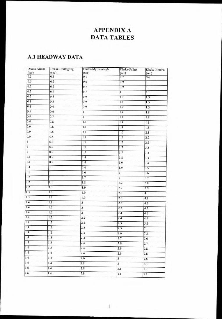
APPENDIX ADATA TABLES
A.I HEADWAY DATA
Dhaka-Arieha Dhaka-Chittagong Dhaka-Mymensingh Dhaka-Sylhet Dhaka-Khulna(sec) (sec) (sec) (sec) (sec)0.3 0.1 0.1 0.7 0.60.6 0.2 0.6 0.9 I0.7 0.2 0.7 0.9 10.7 0.4 0.7 I 1.10.7 0.5 0.9 l.l I.l0.8 0.5 0.9 1.1 I.l0.8 0.6 0.9 1.2 1.50.9 0.6 1 1.4 1.80.9 0.7 I 1.4 1.80.9 0.8 l.l 1.4 1.80.9 0.8 1.1 1.4 1.80.9 0.8 1.1 1.6 2.10.9 0.8 1.1 1.7 2.2I 0.9 1.2 1.7 2.2I 0.9 1.2 1.7 3.3I 0.9 I.l 1.7 3.31.1 0.9 1.4 1.8 3.31.1 0.9 1.4 1.9 3.41.1 I 1.6 1.9 3.51.2 I 1.6 2 3.61.2 I 1.7 2 3.71.2 1.1 1.8 2.2 3.81.2 1.1 1.9 2.2 3.9I.l 1.1 1.9 2.3 41.3 1.1 1.9 2.3 4.11.4 l.l 2 2.3 4.21.4 1.2 2 2.3 4.31.4 1.2 2 2.4 4.61.4 1.2 2.2 2.4 4.91.4 1.2 2.2 2.5 5.21.4 1.2 2.2 2.5 71.4 1.2 2.3 2.6 7.21.4 1.3 2.4 2.7 7.61.4 I.l 2.4 2.9 7.71.6 I.l 2.4 2.9 7.81.6 1.4 2.4 2.9 7.81.6 1.4 2.6 3 7.81.6 1.4 2.8 3 8.31.6 1.4 2.9 3.1 8.71.6 1.4 2.9 3.1 9.1
1
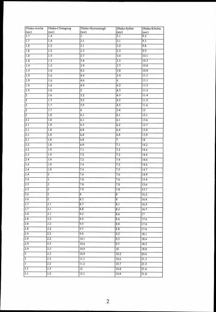
Dhaka-Arieha Dhaka-Chittagong Dhaka-Mymensingh Dhaka-Sylhet Dhaka-Khulna(sec) (sec) (sec) (sec) (sec)J.7 1.4 3 3.1 9.2
1.7 1.4 3.1 3.1 9.3
1.8 1.5 3.1 3.2 9.8
1.8 1.5 3.3 3.3 9.9
1.8 1.5 3.7 3.4 10.1
1.8 1.5 3.8 3.5 10.3
1.9 1.5 3.9 3.7 10.8
1.9 1.6 4.2 3.8 10.8
1.9 1.6 4.4 3.9 11.1
1.9 1.6 4.6 4 11.1
1.9 1.6 4.9 4.2 11.3
1.9 1.6 5 4.3 11.3
2 1.6 5.2 4.5 11.4
2 1.7 5.5 4.5 11.5
2 J.7 5.9 4.5 11.6
2 J.7 6 5.4 13
2 1.8 6.1 6.1 13.1
2.1 1.8 6.1 6.1 13.6
2.1 1.8 6.5 6.2 13.7
2.1 1.8 6.8 6.4 13.8
2.1 1.8 6.8 6.8 13.8
2.1 1.8 6.8 7 14
2.2 1.8 6.9 7.1 14.2
2.2 1.9 7.1 7.2 14.4
2.3 1.9 7.2 7.2 14.4
2.4 1.9 7.2 7.4 14.6
2.4 1.9 7.4 7.5 14.6
2.4 1.9 7.4 7.5 14.7
2.4 2 7.6 7.6 14.9
2.4 2 7.6 7.6 15.4
2.5 2 7.8 7.8 15.6
2.5 2 7.9 7.8 15.7
2.6 2 8 8 16.2
2.6 2 8.7 8 16.4
2.7 2.1 8.7 8.1 16.5
2.7 2.1 8.8 8.3 16.7
2.8 2.1 9.2 8.6 17
2.8 2.2 9.5 8.6 17.6
2.8 2.2 9.5 8.8 17.6
2.8 2.2 9.7 8.8 17.6
2.9 2.2 9.9 9.2 18.1
2.9 2.2 10.1 9.5 18.4
2.9 2.3 10.6 9.7 18.5
2.9 2.3 10.9 10 18.8
3 2.3 10.9 10.2 20.6
3 2.3 11.1 10.6 21.3
3 2.3 11.2 10.7 21.5
3.1 2.5 12 10.8 21.6
3.1 2.5 12.1 10.8 21.8
2

Dhaka-Aricha Dhaka-Chittagong Dhaka-Mymensingh Dhaka-Sylhet Dhaka-Khulna(sec) (sec) (sec) (sec) (sec)3.1 2.5 12.5 10.9 22
3.1 2.6 12.5 10.9 22.7
3.1 2.6 12.7 10.9 22.8
3.2 2.6 12.7 11.4 23.1
3.2 2.7 13.2 11.5 24.2
3.2 2.8 13.2 12.2 24.3
3.3 2.8 13.4 12.6 24.3
3.3 2.8 13.5 12.8 24.7
3.3 2.9 14 13.3 25.9
3.3 3 14.6 13.3 26
3.4 3.1 15 13.7 26
3.4 3.1 15.4 15 26
3.5 3.2 15.5 15.3 26.4
3.5 3.2 15.6 15.7 26.6
3.5 3.2 15.7 15.9 28
3.6 3.3 15.8 16.2 29
3.6 3.3 16.3 16.4 29.3
3.6 3.3 16.3 16.8 30.2
3.7 3.4 16.3 17.3 30.3
3.7 3.4 16.3 17.6 31.5
3.7 3.4 16.3 18.1 31. 7
3.8 3.4 16.5 20.4 33.9
3.8 3.5 16.5 20.8 34.2
3.9 3.5 16.7 20.9 34.8
3.9 3.6 17.5 21.1 34.94 3.7 17.6 22.4 35.2
4 3.8 17.7 22.6 35.6
4 3.8 17.7 23 35.7
4 3.9 17.8 23.2 36.5
4.1 3.9 18.2 23.7 36.8
4.1 4 18.6 23.7 37.1
4.1 4 19.1 24.2 37.5
4.3 4 19.4 24.3 38.24.3 4.3 19.6 24.4 39.14.3 4.3 19.7 24.6 39.84.3 4.3 19.9 25.9 40.64.3 4.3 20.5 26.6 40.64.4 4.5 20.6 27.4 41.84.5 4.5 20.9 28 42
4.5 4.7 21 28.2 42.2
4.6 4.9 21.2 29 43.14.7 4.9 21.5 29.2 43.4
4.9 4.9 21.7 29.4 43.4
4.9 4.9 22 30.9 43.54.9 4.9 22.3 30.9 45.6
4.9 5 22.7 31.3 45.8
5 5.1 23.2 31.8 49.3
5 5.1 24.1 32 50.4
5.1 5.1 25 32.4 54.9
3
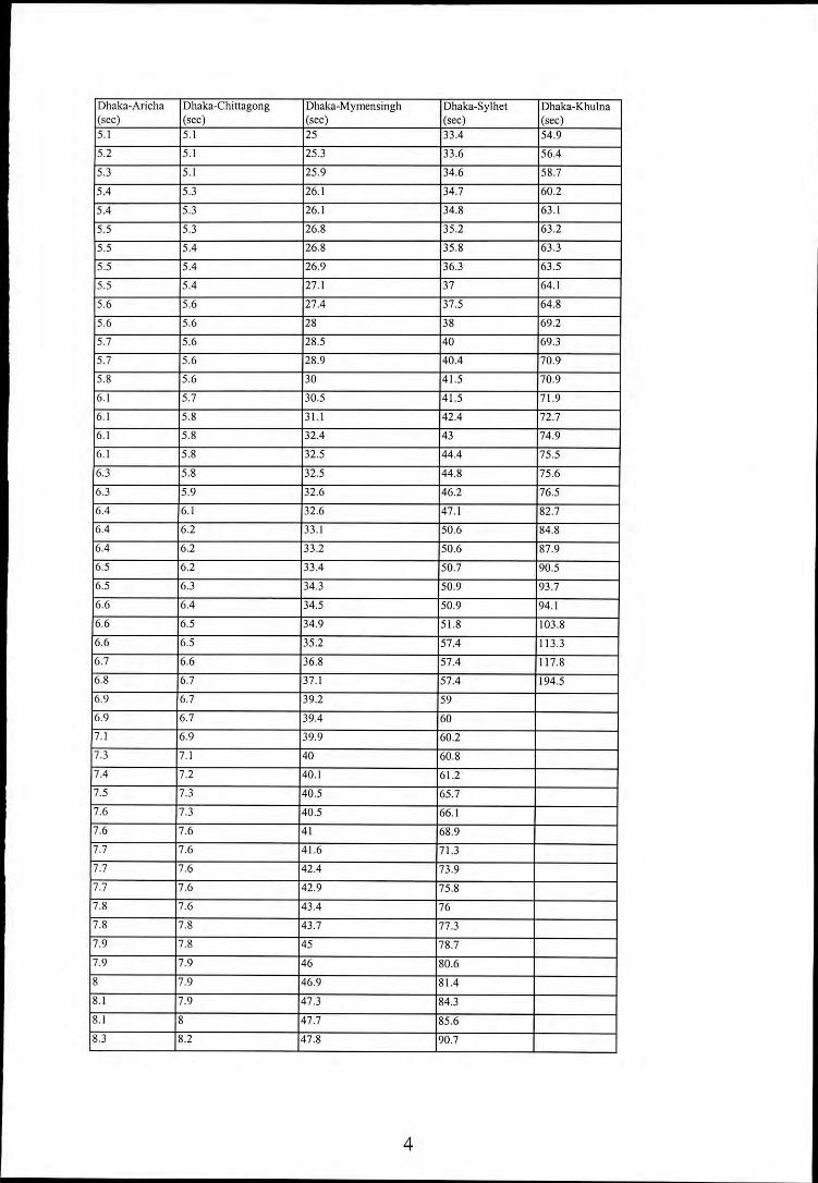
Dhaka-Arieha Dhaka-Chittagong Dhaka-Mymensingh Dhaka-Sylhet Dhaka~Khulna(sec) (sec) (sec) (sec) (sec)5.1 5.1 25 33.4 54.9
5.2 5.1 25.3 33.6 56.4
5.3 5.1 25.9 34.6 58.7
5.4 5.3 26.1 34.7 60.2
5.4 5.3 26.1 34.8 63.1
5.5 5.3 26.8 35.2 63.2
5.5 5.4 26.8 35.8 63.3
5.5 5.4 26.9 36.3 63.5
5.5 5.4 27.1 37 64.1
5.6 5.6 27.4 37.5 64.8
5.6 5.6 28 38 69.2
5.7 5.6 28.5 40 69.3
5.7 5.6 28.9 40.4 70.9
5.8 5.6 30 41.5 70.9
6.1 5.7 30.5 41.5 71.9
6.1 5.8 31.1 42.4 72.7
6.1 5.8 32.4 43 74.9
6.1 5.8 32.5 44.4 75.5
6.3 5.8 32.5 44.8 75.6
6.3 5.9 32.6 46.2 76.5
6.4 6.1 32.6 47.1 82.7
6.4 6.2 33.1 50.6 84.8
6.4 6.2 33.2 50.6 87.9
6.5 6.2 33.4 50.7 90.5
6.5 6.3 34.3 50.9 93.7
6.6 6.4 34.5 50.9 94.1
6.6 6.5 34.9 51.8 103.8
6.6 6.5 35.2 57.4 IIJ.J
6.7 6.6 36.8 57.4 117.8
6.8 6.7 37.1 57.4 194.5
6.9 6.7 39.2 59
6.9 6.7 39.4 60
7.1 6.9 39.9 60.2
7.3 7.1 40 60.8
7.4 7.2 40.1 61.2
7.5 7.3 40.5 65.7
7.6 7.3 40.5 66.1
7.6 7.6 41 68.9
7.7 7.6 41.6 71.3
7.7 7.6 42.4 73.9
7.7 7.6 42.9 75.8
7.8 7.6 43.4 76
7.8 7.8 43.7 77.3
7.9 7.8 45 78.7
7.9 7.9 46 80.6
8 7.9 46.9 81.4
8.1 7.9 47.3 84.3
8.1 8 47.7 85.6
8.3 8.2 47.8 90.7
4

Dhaka-Arlcha Dhaka-Chittagong Dhaka-Mymensingh Dhaka-Sylhet Dhaka-Khulna(sec) (sec) (sec) (sec) (sec)8.3 8.3 48.1 92.6
8.6 8.5 48.9 107.8
8.6 8.5 51.2
8.7 8.5 52.3
9.1 8.5 53.4
9.1 8.7 55.3
9.2 8.8 55.3
9.2 8.8 59
9.4 8.9 61.4
9.4 8.9 62
9.5 9.1 62.4
9.6 9.1 64.9
9.6 9.3 66.7
10 9.3 67.4
10.1 9.3 68
10.2 9.3 69.3
10.3 9.6 72.9
10.3 9.6 73.1
10.3 9.9 83.5
10.3 10.1 84.4
10.4 10.1 87.6
10.4 10.3 96.1
10.6 10.4 99.8
10.7 10.5 100.8
10.8 10.5 104.7
10.8 10.5 126.7
10.9 10.5 132.9
11.2 10.7
11.2 10.9
11.4 11.3
11.4 I 1.4
11.6 11.5
11.6 I 1.6
11.6 11.8
11.7 11.9
12 12
12.3 12
12.4 12.1
12.5 12.2
12.6 12.6
13.1 12.8
13.2 12.9
13.4 12.9
13.7 13
13.7 13.4
13.7 13.4
13.8 13.4
13.8 13.5
14 13.5
5
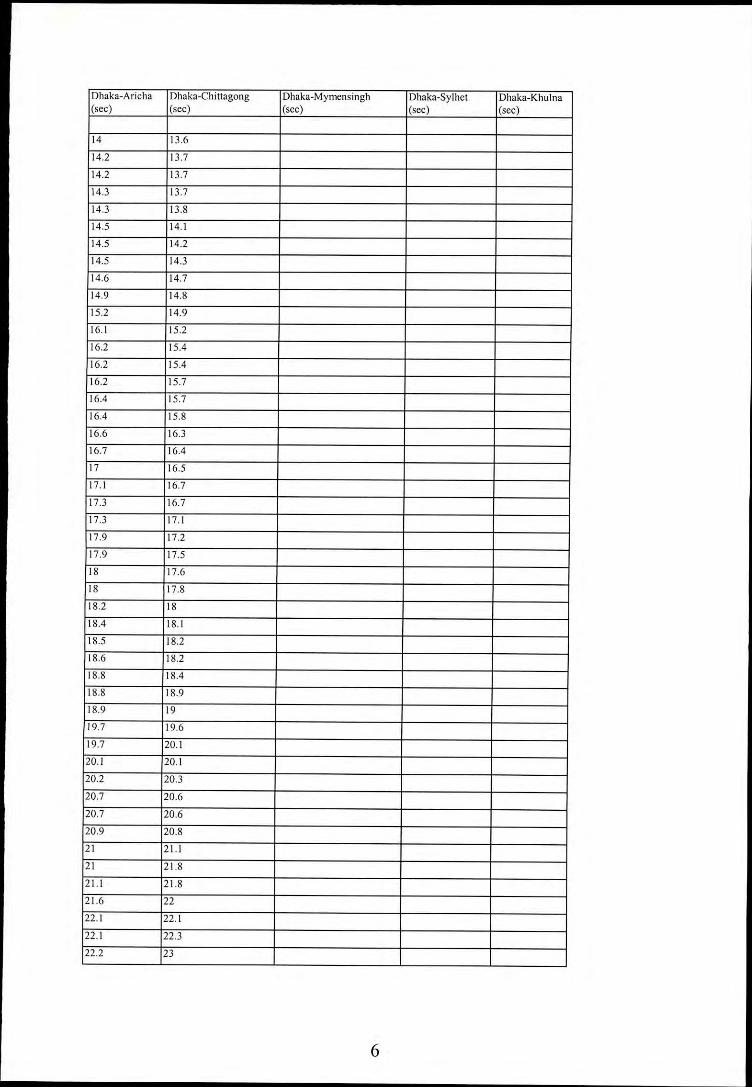
Dhaka.Arieha Dhaka-Chittagong Dhaka-Mymensingh Dhaka-Sylhet Dhaka-Khulna(sec) (sec) (sec) (sec) (sec)
14 13.6
14.2 13.7
14.2 13.7
14.3 13.7
14.3 13.8
14.5 14.1
14.5 14.2
14.5 14.3
14.6 14.7
14.9 14.8
15.2 14.9
16.1 15.2
16.2 15.4
16.2 15.4
16.2 15.7
16.4 15.7
16.4 15.8
16.6 16.3
16.7 16.4
17 16.5
17.1 16.7
17.3 16.7
17.3 17.1
17.9 17.2
17.9 17.5
18 17.6
18 17.8
18.2 18
18.4 18.1
18.5 18.2
18.6 18.2
18.8 18.4
18.8 18.9
18.9 19
19.7 19.6
19.7 20.1
20.1 20.1
20.2 20.3
20.7 20.6
20.7 20.6
20.9 20.8
21 21.1
21 21.8
21.1 21.8
21.6 22
22.1 22.1
22.1 22.3
22.2 23
6
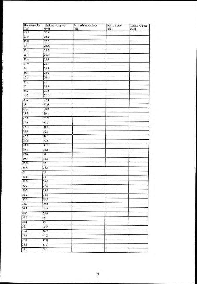
Dhaka-Aricha Dhaka-Chittagong Dhaka-Mymcnsingh Dhaka-Sylhet Dhaka-Khulna(sec) (sec) (sec) (sec) (sec)22.3 23.2
22.5 23.3
22.8 23.3
23.1 23.5
23.1 23.5
23.4 23.6
23.4 23.8
23.9 23.8
24 23.8
24.7 23.9
25.4 24.\
25.7 25
26 25.2
26.2 25.2
26.3 27.1
26.7 27.3
27 27.6
27.2 28.2
27.3 29.\
27.3 29.9
27.4 30.3
27.6 31.2
27.7 32.1
27.8 32.3
28.2 32.9
28.8 33.3
29.1 33.8
29.4 34
29.7 34.\
29.9 35
30.6 35.4
31 36
31.5 36
31.9 36.9
32.3 37.4
32.9 38.3
33.2 38.4
33.6 38.7
33.9 39.2
34.1 41.3
34.5 42.4
34.7 44
35.1 45
36.4 45.5
36.9 46.7
37.1 47.2
37.4 49.8
38.4 51.3
38.6 52.1
7
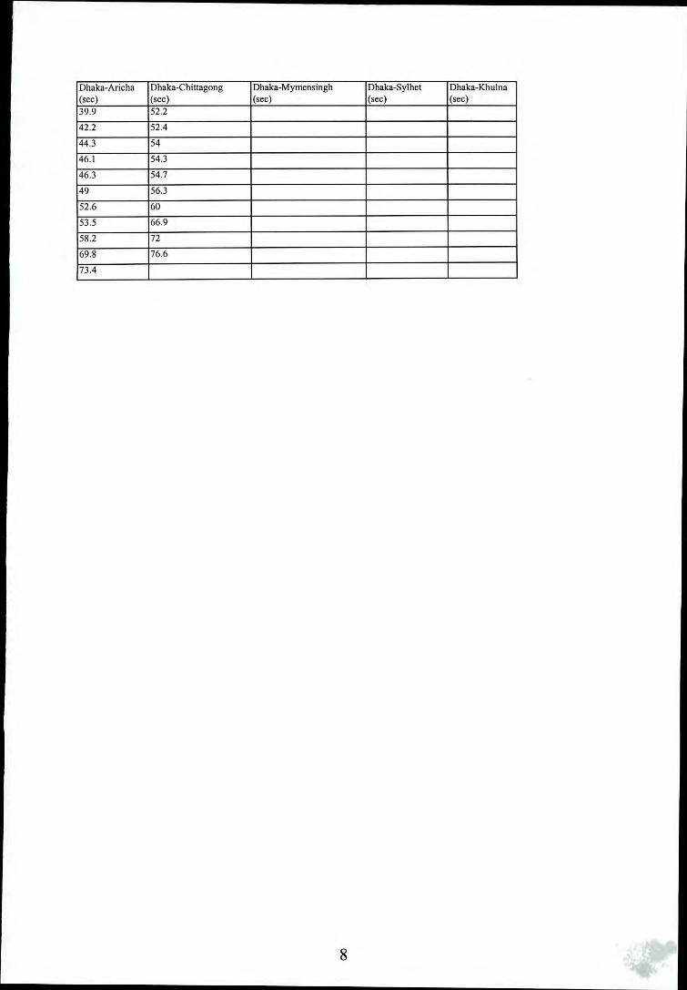
Dhaka-Arieha Dhaka-ehittagong Dhaka-Mymcnsingh Dhaka-Sylhct Dhaka-Khulna(sec) (sec) (sec) (sec) (sec)39.9 52.2
42.2 52.4
44.3 54
46.1 54.3
46.3 54.7
49 56.3
52.6 60
53.5 66.9
58.2 72
69.8 76.6
73.4
8
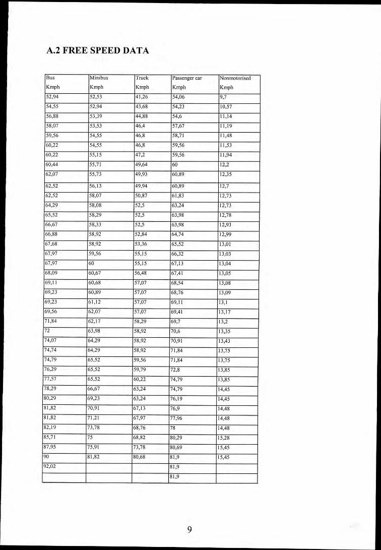
A.2 FREE SPEED DATA
Bus Minibus Truck Passenger car Nonmotorised
Kmph Kmph Kmph Kmph Kmph
52,94 52,53 41,26 54,06 9,7
54,55 52,94 43,68 54,23 10,57
56,88 53,39 44,88 54,6 11,14
58,Q7 53,53 46,4 57,67 11,19
59,56 54,55 46,8 58,71 11,48
60,22 54,55 46,8 59,56 11,53
60,22 55,15 47,2 59,56 11,94
60,44 55,71 49,64 60 12,2
62,07 55,73 49,93 60,89 12,35
62,52 56,13 49.94 60,89 12,7
62,52 58,Q7 50,87 61,83 12,73
64,29 58,08 52,5 63,24 12,73
65,52 58,29 52,5 63,98 12,78
66,67 58,33 52,5 63,98 12,93
66,88 58,92 52,84 64,74 12,99
67,68 58,92 53,36 65,52 13,01
67,97 59,56 55,15 66,32 13,03
67,97 60 55,15 67,13 13,04
68,09 60,67 56,48 67,41 13,05
69,11 60,68 57,07 68,54 13,08
69,23 60,89 57,07 68,76 13,09
69,23 61,12 57,07 69,11 13,1
69,56 62,07 57,07 69,41 13,17
71,84 62,17 58,29 69,7 13,2
72 63,98 58,92 70,6 13,35
74,07 64,29 58,92 70,91 13,43
74,74 64,29 58,92 71,84 13,75
74,79 65,52 59,56 71,84 13,75
76,29 65,52 59,79 72,8 13,85
77,57 65,52 60,22 74,79 13,85
78,29 66,67 63,24 74,79 14,45
80,29 69,23 63,24 76,19 14,45
81,82 70,91 67,13 76,9 14,48
81,82 71,21 67,97 77,96 14,48
82,19 73,78 68,76 78 14,48
85,71 75 68,82 80,29 15,28
87,95 75,91 73,78 80,69 15,45
90 81,82 80,68 81,9 15,45
92,02 81,9
81,9
9
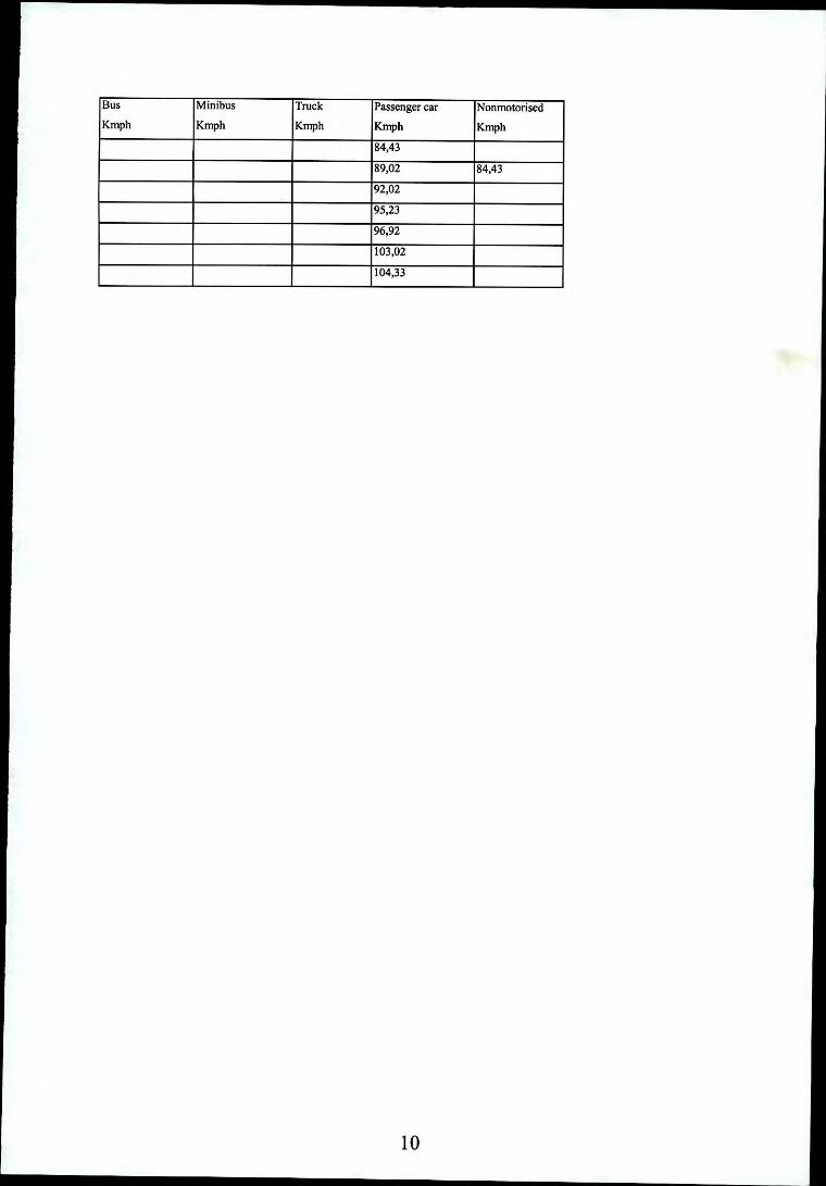
Bus Minibus Truck Passenger car NonmotorisedKrnph Kmph Kmph Kmph Kmph
84,43
89,02 84,43
92,02
95,23
96,92
103,02
104,33
10
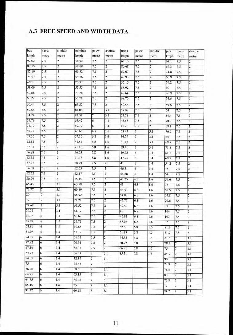
A.3 FREE SPEED AND WIDTH DATA
bus pavw sholdw minibus pavw sholdw truck pavw sholdw p.car pavw sholdwkmph metre metre kmph metre metre kmph metre metre kmph metre metre92.02 7.5 2 58.92 7.5 2 67.13 7.5 2 67.1 7.5 2
87.95 7.5 2 58.08 7.5 2 80.68 7.5 2 66.3 7.5 2
82.19 7.5 2 65.52 7.5 2 57.07 7.5 2 74.8 7.5 2
74.07 7.5 2 59.56 7.5 2 49.93 7.5 2 60.9 7.5 2
69.11 7.5 2 75.91 7.5 2 55.15 7.5 2 76.2 7.5 2
58.09 7.5 2 53.53 7.5 2 58.92 7.5 2 60 7.5 2
57.68 7.5 2 73.78 7.5 2 49.64 7.5 2 96.9 7.5 2
60.22 7.5 2 55.71 7.5 2 68.76 7.5 2 54.6 7.5 2
60.44 7.5 2 65.52 7.5 2 59.56 7.5 2 59.6 7.5 2
59.56 7.5 2 81.08 7 3.1 57.07 7.5 2 64 7.5 2
74.74 7.5 2 82.57 7 3.1 73.78 7.5 2 84.4 7.5 2
74.79 7.5 2 67.42 6 1.4 43.68 7.5 2 70.9 7.5 2
74.79 7.5 2 49.72 6 1.4 47.2 7.5 2 69.1 7.5 2
60.22 7.5 2 46.63 6.8 1.6 58.44 7 3.1 76.9 7.5 2
59.56 7.5 2 67.16 6.8 1.6 56.07 7 3.1 64 7.5 2
62.52 7.5 2 84.51 6.8 1.6 61.43 7 3.1 69.7 7.5 267.97 7.5 2 71.15 6.8 1.6 59.41 7 3.1 71.8 7.5 256.88 7.5 2 46.03 5.8 1.6 49.72 6 1.4 61.8 7.5 262.52 7.5 2 41.47 5.8 1.6 47.75 6 1.4 60.9 7.5 267.97 7.5 2 58.29 7.5 2 41 6 1.4 54.2 7.5 256.88 7.5 2 52.53 7.5 2 46.51 6 1.4 78 7.5 262.52 7.5 2 62.17 7.5 2 54.88 6 1.4 54.1 7.5 280.29 7.5 2 55.15 7.5 2 47.75 6.8 1.6 59.6 7.5 265.45 7 3.1 63.98 7.5 2 41 6.8 1.6 78 7.5 273.77 7 3.1 60.89 7.5 2 46.51 6.8 1.6 68.5 7.5 280 7 3.1 58.92 7.5 2 54.88 6.8 1.6 74.8 7.5 272 7 3.1 71.21 7.5 2 47.75 6.8 1.6 70.6 7.5 274.69 7 3.1 65.52 7.5 2 49.59 6.8 1.6 89 7.5 270.31 7 3.1 61.12 7.5 2 48 6.8 1.6 104 7.5 266.18 6 1.4 60.67 7.5 2 46.88 6.8 1.6 103 7.5 267.92 6 1.4 55.73 7.5 2 58.06 6.8 1.6 92 7.5 253.89 6 1.4 60.68 7.5 2 62.5 6.8 1.6 81.9 7.5 281.08 6 1.4 53.39 7.5 2 51.87 6.8 1.6 81.9 7.5 274.07 6 1.4 56.13 7.5 2 64.52 6.8 1.6 81.5 7 3.177.92 6 1.4 70.91 7.5 2 80.72 6.8 1.6 78.3 7 3.167.16 6 1.4 58.33 7.5 2 66.91 6.8 1.6 75 7 3.164.75 6 1.4 56.07 7 3.1 85.71 6.8 1.6 84.9 7 3.174.07 6 1.4 72.89 7 3.1 90 7 3.175 6 1.4 75.63 7 3.1 74.7 7 3.178.26 6 1.4 68.5 7 3.1 76.6 7 3.164.75 6 1.4 63.15 7 3.1 80 7 3.164.75 6 1.4 65.45 7 3.1 77.9 7 3.165.45 6 1.4 75 7 3.1 72 7 3.191.37 6 1.4 66.18 7 3.1 94.7 7 3.1
I I

bus pavw sholdw minibus pavw sholdw truck pavw sholdw p.car pavw sholdw
kmph metre metre kmph metre metre kmph metre metre kmph metre metre
86.12 6 1.4 65.45 7 3.1 101 7 3.1
52.33 6.8 1.6 69.28 7 3.1 90 7 3.\
58.06 6.8 1.6 55.51 6 1.4 67.2 7 3.1
70.31 6.8 1.6 72.87 6 1.4 57.5 6 1.473.17 6.8 1.6 75.63 6.8 1.6 62.7 6 1.4
68.7 6.8 1.6 74.7 6.8 1.6 78.3 6 1.4
60.61 6.8 1.6 72.83 6.8 1.6 87.4 6 1.4
41.76 5.8 1.6 45.92 5.8 1.6 82.6 6 1.460 5.8 1.6 50.56 5.8 1.6 61.2 6 1.469.23 5.8 1.6 48.03 5.8 1.6 60.6 6 1.4
60.05 5.8 1.6 90.9 6 1.4
96.8 6.8 1.6
76.9 6.8 1.6
87 6.8 1.6
82.2 6.8 1.6
80.7 6.8 1.6
82.2 6.8 1.6
78.9 6.8 1.6
73.5 6.8 1.6
75.6 6.8 1.6
94.2 6.8 1.6
63.4 5.8 1.6
12
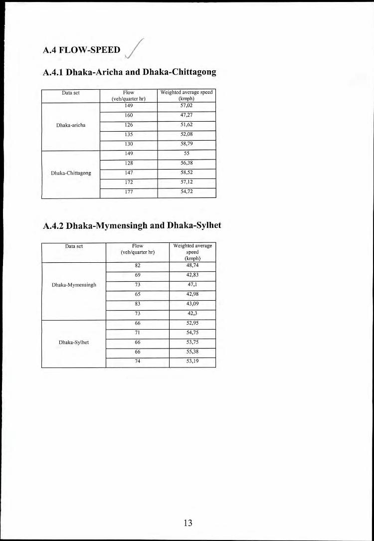
AA FLOW-SPEED /
AA.l Dhaka-Arieha and Dhaka-Chittagong
Data set Flow Weighted average speed(veh/quarter hr) (kmph)
149 57,02
160 47,27
Dhaka-aricha 126 51,62
135 52,08
130 58,79
149 55
128 56,38
Dhaka.Chittagong 147 58,52
172 57,12
177 54,72
AA.2 Dhaka-Mymensingh and Dhaka-Sylhet
Dala set Flow Weighted average(veh/quarter hr) speed
(kmph)82 48,74
69 42,83
Dhaka-Mymcnsingh 73 47,1
65 42,98
83 43,09
73 42,3
66 52,95
71 54,75
Dhaka-Sylhct 66 53,75
66 55,38
74 53,19
13

A.4.3 Dhaka-Khulna
Flow Weighted(vch/quartcr hr) average speed
(kmph)90 43,56
53 47,35
61 49,41
76 50,Q7
64 50,73
77 47,09
56 46,59
63 48,91
76 51,66
64 46,65
A.5 SPEED-DENSITY /
A.5.l Dhaka-Arieha and Dhaka-Chittagong
Data set Density Weighted average(veh/quartcr km) speed
(kmph)11 35,88
2 55,51
Dhaka.arieha 7 51,12
9 53,55
4 49,57
3 51,31
6 42,47
2 76,8
Dhaka.Chittagong 11 49,77
8 51,13
13 56,43
14
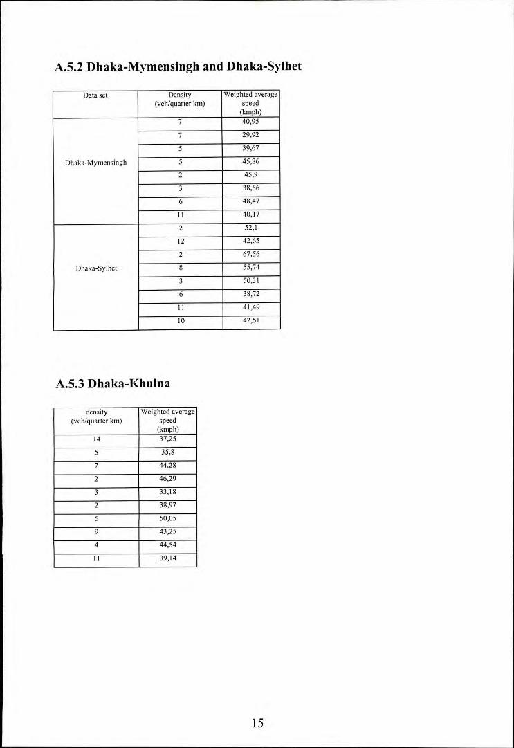
A.S.2 Dhaka-Mymensingh and Dhaka-Sylhet
Data set Density Weighted average(veh/quartcr km) speed
(kmph)7 40,95
7 29,92
5 39,67
Dhaka-Mymcnsingh 5 45,86
2 45,9
3 38,66
6 48,47
11 40,17
2 52,1
12 42,65
2 67,56
Dhaka-Sylhct 8 55,74
3 50,31
6 38,72
11 41,49
10 42,51
A.5.3 Dhaka-Khulna
density Weighted average(vch/quarter km) speed
(kmph)14 37,25
5 35,8
7 44,28
2 46,29
3 33,18
2 38,97
5 50,05
9 43,25
4 44,54
11 39,14
15
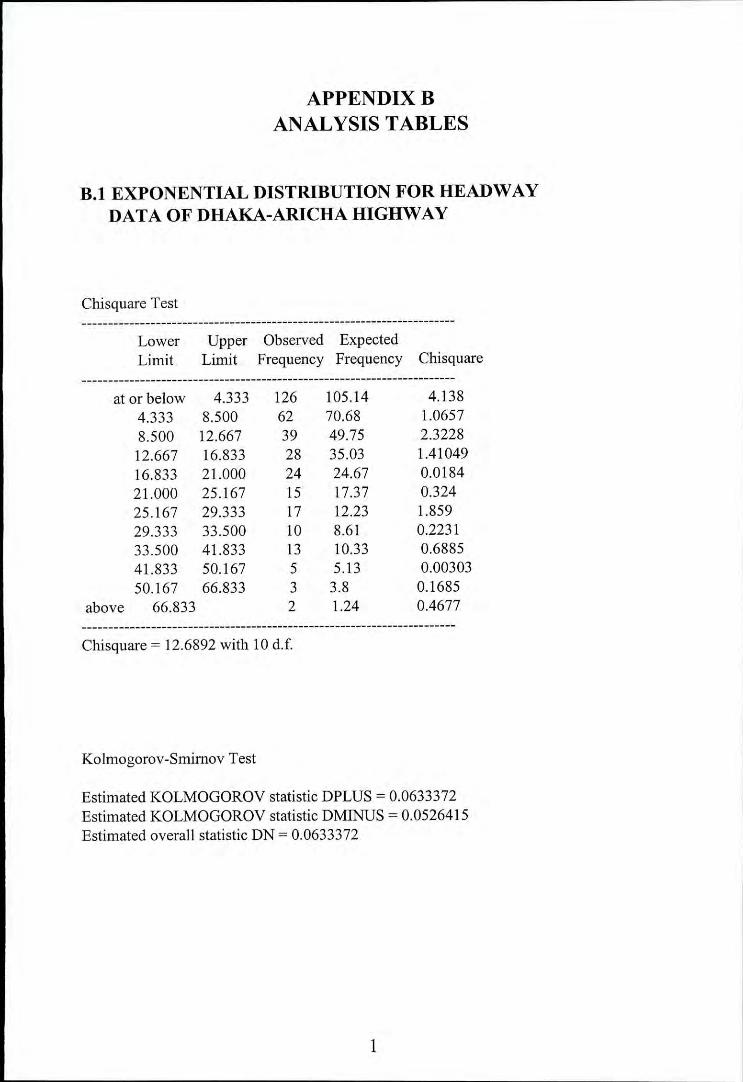
APPENDIXBANALYSIS TABLES
B.1 EXPONENTIAL DISTRIBUTION FOR HEADWAYDATA OF DHAKA-ARICHA HIGHWAY
Chisquare Test-----------------------------------------------------------------------
Lower Upper Observed ExpectedLimit Limit Frequency Frequency Chi square
-----------------------------------------------------------------------at or below 4.333
4.333 8.5008.500 12.66712.667 16.83316.833 21.00021.000 25.16725.167 29.33329.333 33.50033.500 41.83341.833 50.16750.167 66.833
above 66.833
126 105.1462 70.6839 49.7528 35.0324 24.6715 17.3717 12.2310 8.6113 10.335 5.133 3.82 1.24
4.1381.06572.32281.410490.01840.3241.8590.22310.68850.003030.16850.4677
Chisquare = 12.6892 with 10 d.f.
Kolmogorov-Smimov Test
Estimated KOLMOGOROV statistic DPLUS = 0.0633372Estimated KOLMOGOROV statistic DM1NUS = 0.0526415Estimated overall statistic DN = 0.0633372
1

B.2 LOGNORMAL DISTRIBUTION FOR HEADWAYDATA OF DHAKA-ARICHA HIGHWAY
Chisquare Test-----------------------------------------------------------------------
Lower Upper Observed ExpectedLimit Limit Frequency Frequency Chisquare
-----------------------------------------------------------------------at or below 4.333 126 115.3 .993698
4.333 8.500 62 81.7 4.7368018.500 12.667 39 46.1 1.08833912.667 16.833 28 28.1 .00030816.833 21.000 24 18.3 1.78979121.000 25.167 15 12.5 .49895125.167 29.333 17 8.9 7.40254729.333 33.500 10 6.5 1.86082033.500 41.833 13 8.7 2.16840641.833 50.167 5 5.3 .01476450.167 66.833 3 5.7 1.288623
above 66.833 2 7.0 3.584508
Chisquare = 25.4276 with 9 d.f.
Kolmogorov-Smimov Test
Estimated KOLMOGOROV statistic DPLUS = 0.0401802Estimated KOLMOGOROV statistic DMINUS = 0.0618274Estimated overall statistic DN = 0.0618274
2
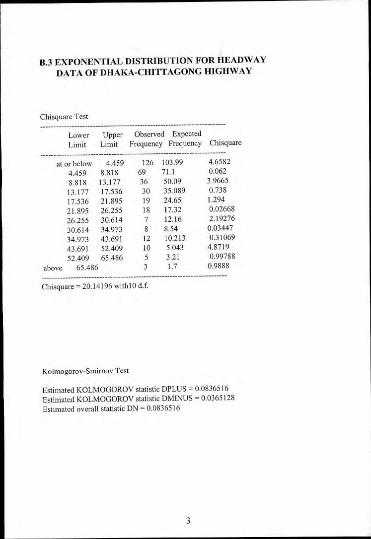
B.3 EXPONENTIAL DISTRIBUTION FOR HEADWAYDATA OF DHAKA-CHITTAGONG HIGHWAY
Chisquare Test-----------------------------------------------------------------------
Lower Upper Observed ExpectedLimit Limit Frequency Frequency Chisquare
-----------------------------------------------------------------------at or below 4.459 126 103.99 4.6582
4.459 8.818 69 71.1 0.0628.818 13.177 36 50.09 3.966513.177 17.536 30 35.089 0.73817.536 21.895 19 24.65 1.29421.895 26.255 18 17.32 0.0266826.255 30.614 7 12.16 2.1927630.614 34.973 8 8.54 0.0344734.973 43.691 12 10.213 0.3106943.691 52.409 10 5.043 4.871952.409 65.486 5 3.21 0.99788
above 65.486 3 1.7 0.9888-----------------------------------------------------------------------Chisquare = 20.14196 with 10 d.f.
Kolmogorov-Smirnov Test
Estimated KOLMOGOROV statistic DPLUS = 0.0836516Estimated KOLMOGOROV statistic DMlNUS = 0.0365128Estimated overall statistic DN = 0.0836516
3
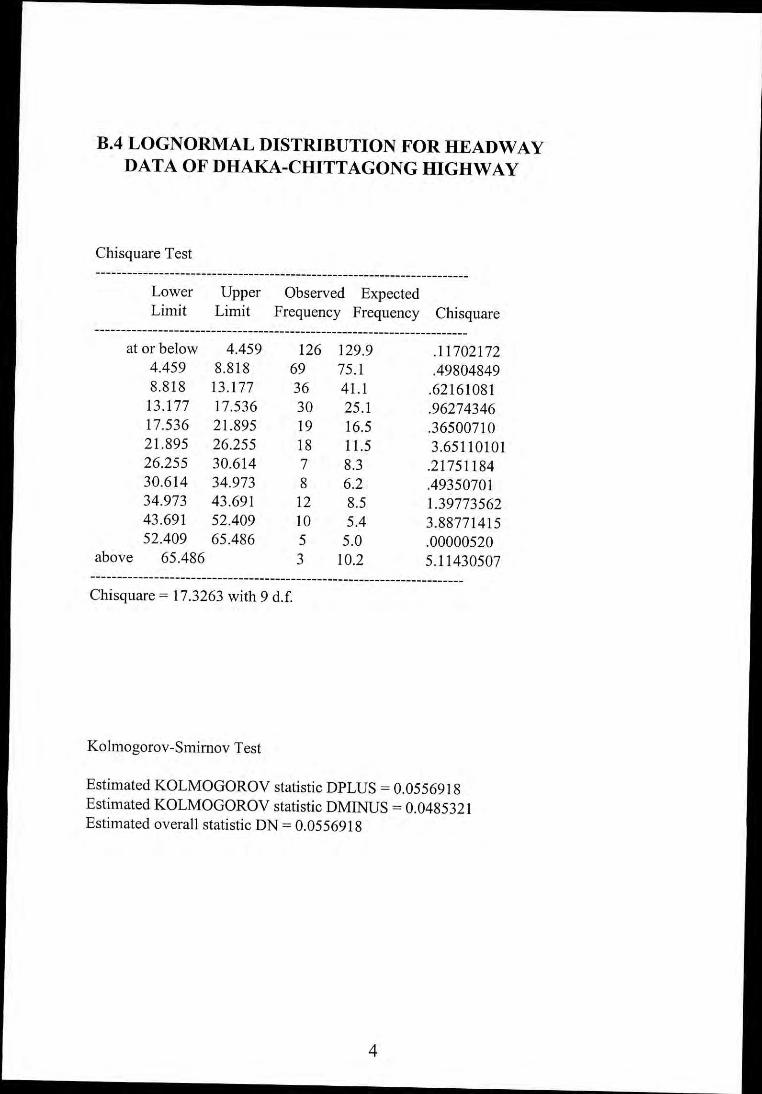
B.4 LOGNORMAL DISTRIBUTION FOR HEADWAYDATA OF DHAKA-CHITTAGONG HIGHWAY
Chisquare Test-----------------------------------------------------------------------
Lower Upper Observed ExpectedLimit Limit Frequency Frequency Chisquare
-----------------------------------------------------------------------at or below 4.459 126 129.9 .11702172
4.459 8.818 69 75.1 .498048498.818 13.177 36 41.1 .6216108113.177 17.536 30 25.1 .9627434617.536 21.895 19 16.5 .3650071021.895 26.255 18 11.5 3.6511010126.255 30.614 7 8.3 .2175118430.614 34.973 8 6.2 .4935070134.973 43.691 12 8.5 1.3977356243.691 52.409 10 5.4 3.8877141552.409 65.486 5 5.0 .00000520
above 65.486 3 10.2 5.11430507-----------------------------------------------------------------------Chisquare = 17.3263 with 9 d.f.
Kolmogorov-Smimov Test
Estimated KOLMOGOROV statistic OPLUS = 0.0556918Estimated KOLMOGOROV statistic OMINUS = 0.0485321Estimated overall statistic ON = 0.0556918
4
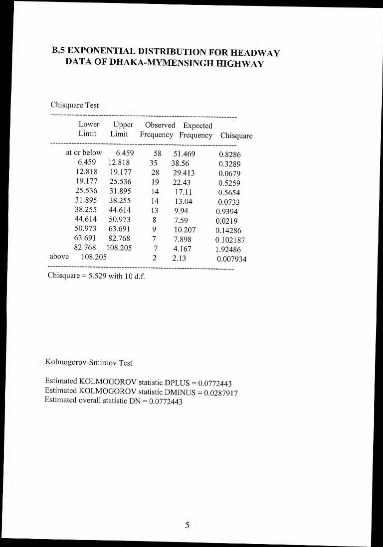
B.5 EXPONENTIAL DISTRIBUTION FOR HEADWAYDATA OF DHAKA-MYMENSINGH HIGHWAY
Chisquare Test-----------------------------------------------------------------------
Lower Upper Observed ExpectedLimit Limit Frequency Frequency Chisquare
-----------------------------------------------------------------------at or below 6.459 58 51.469 0.8286
6.459 12.818 35 38.56 0.328912.818 19.177 28 29.413 0.067919.177 25.536 19 22.43 0.525925.536 31.895 14 17.11 0.565431.895 38.255 14 13.04 0.073338.255 44.614 13 9.94 0.939444.614 50.973 8 7.59 0.021950.973 63.691 9 10.207 0.1428663.691 82.768 7 7.898 0.10218782.768 108.205 7 4.167 1.92486
above 108.205 2 2.13 0.007934-----------------------------------------------------------------------Chisquare = 5.529 with 10 d.f.
Ko1mogorov-Smirnov Test
Estimated KOLMOGOROV statistic DPLUS = 0.0772443Estimated KOLMOGOROV statistic DM1NUS = 0.0287917Estimated overall statistic DN = 0.0772443
5
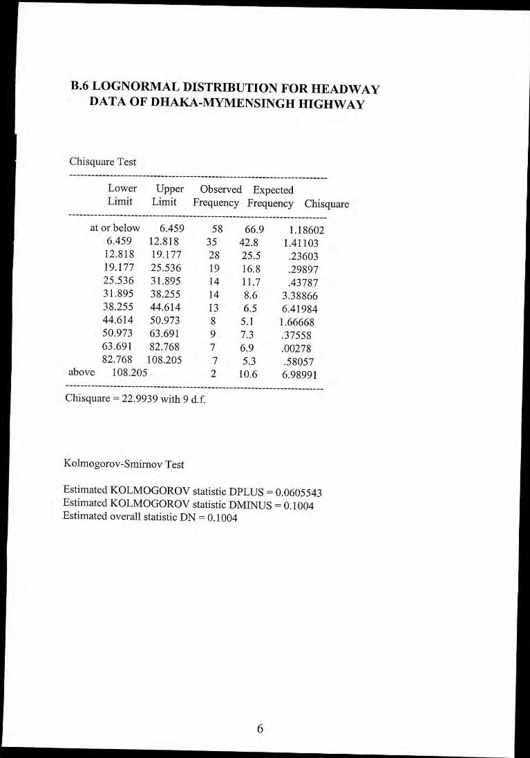
B.6 LOGNORMAL DISTRIBUTION FOR HEADWAYDATA OF DHAKA-MYMENSINGH HIGHWAY
Chi square Test-----------------------------------------------------------------------
Lower Upper Observed ExpectedLimit Limit Frequency Frequency Chisquare
-----------------------------------------------------------------------at or below 6.459 58 66.9 1.18602
6.459 12.818 35 42.8 1.4110312.818 19.177 28 25.5 .2360319.177 25.536 19 16.8 .2989725.536 31.895 14 11.7 .4378731.895 38.255 14 8.6 3.3886638.255 44.614 13 6.5 6.4198444.614 50.973 8 5.1 1.6666850.973 63.691 9 7.3 .3755863.691 82.768 7 6.9 .0027882.768 108.205 7 5.3 .58057
above 108.205 2 10.6 6.98991-----------------------------------------------------------------------Chisquare = 22.9939 with 9 d.f.
Kolmogorov-Smirnov Test
Estimated KOLMOGOROV statistic OPLUS = 0.0605543Estimated KOLMOGOROV statistic OMINUS = 0.1004Estimated overall statistic ON = 0.1004
6
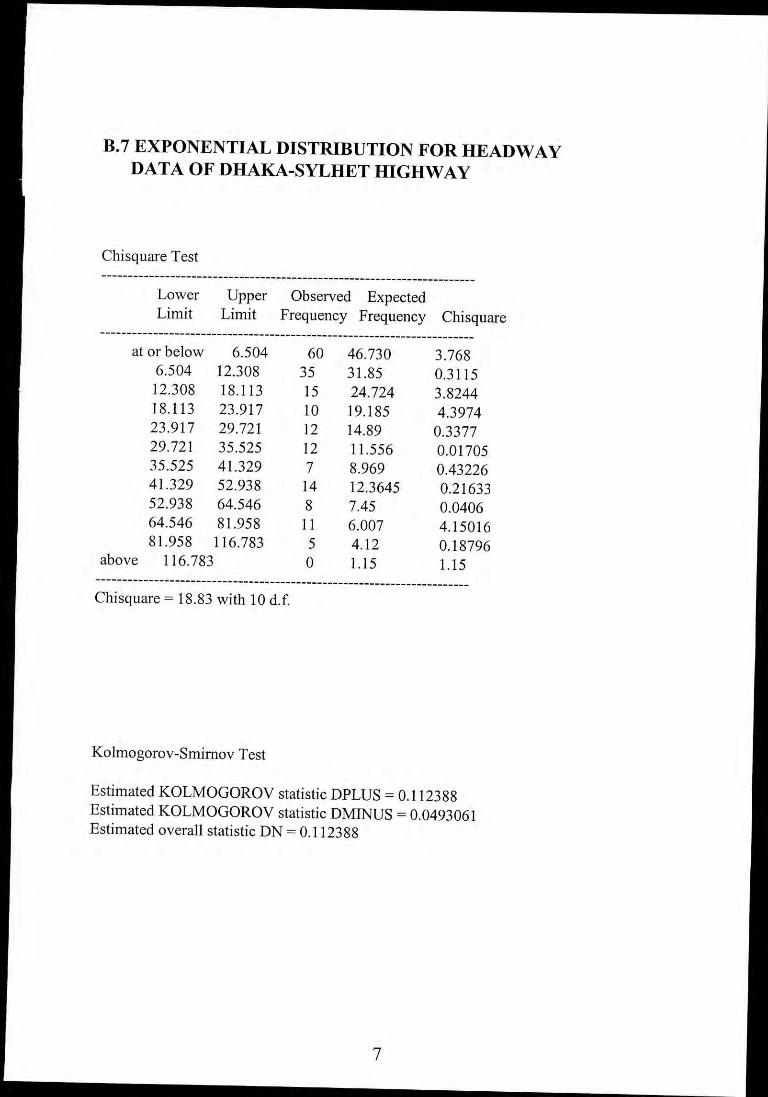
B.7 EXPONENTIAL DISTRIBUTION FOR HEADWAYDATA OF DHAKA-SYLHET HIGHWAY
Chisquare Test-----------------------------------------------------------------------
Lower Upper Observed ExpectedLimit Limit Frequency Frequency Chisquare
-----------------------------------------------------------------------at or below 6.504 60 46.730 3.768
6.504 12.308 35 31.85 0.311512.308 18.113 15 24.724 3.824418.113 23.917 10 19.185 4.397423.917 29.721 12 14.89 0.337729.721 35.525 12 11.556 0.0170535.525 41.329 7 8.969 0.4322641.329 52.938 14 12.3645 0.2163352.938 64.546 8 7.45 0.040664.546 81.958 II 6.007 4.1501681.958 116.783 5 4.12 0.18796
above 116.783 0 l.l5 l.l5-----------------------------------------------------------------------Chisquare = 18.83 with 10 d.f.
Kolmogorov-Smimov Test
Estimated KOLMOGOROV statistic DPLUS = 0.112388Estimated KOLMOGOROV statistic DM1NUS = 0.0493061Estimated overall statistic DN = 0.112388
7
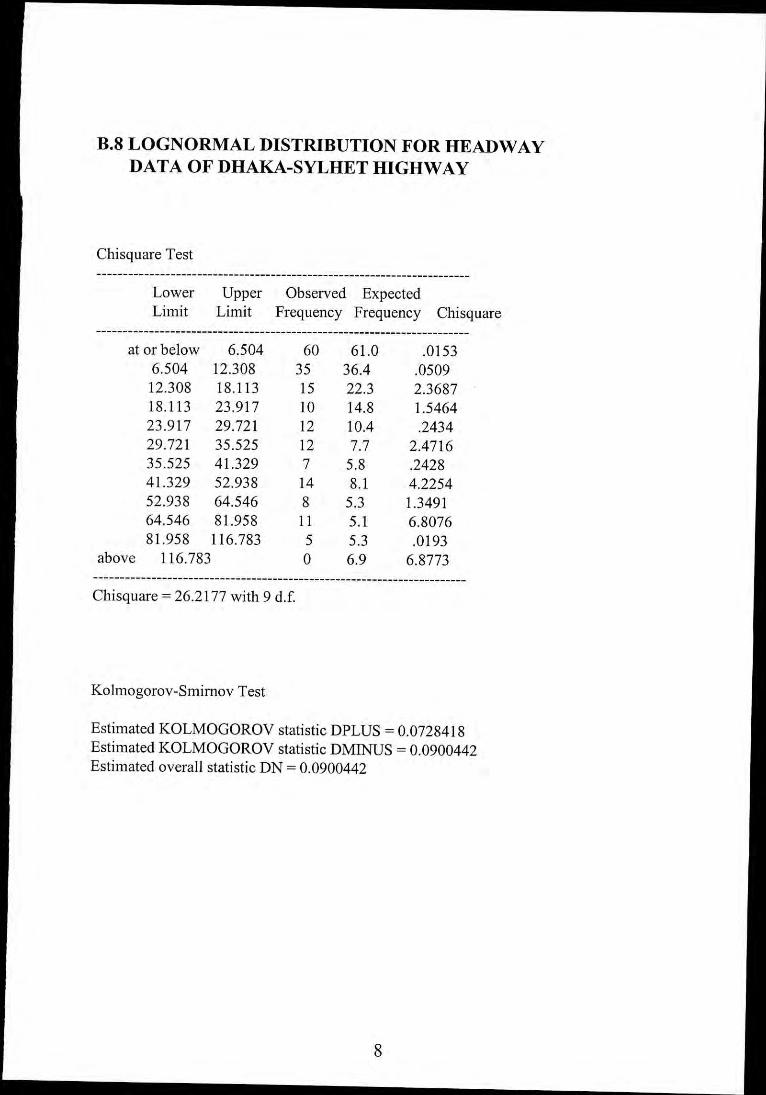
-----------------------------------------------------------------------Chisquare Test
Lower Upper Observed ExpectedLimit Limit Frequency Frequency Chisquare
.0153.05092.36871.5464.24342.4716.24284.22541.34916.8076.01936.8773
60 61.035 36.415 22.310 14.812 10.412 7.77 5.814 8.18 5.311 5.15 5.3o 6.9
B.8 LOGNORMAL DISTRIBUTION FOR HEADWAYDATA OF DHAKA-SYLHET HIGHWAY
at or below 6.5046.504 12.30812.308 18.11318.113 23.91723.917 29.72129.721 35.52535.525 41.32941.329 52.93852.938 64.54664.546 81.95881.958 116.783
above 116.783-----------------------------------------------------------------------Chisquare = 26.2177 with 9 d.f.
Kolmogorov-Smimov Test
Estimated KOLMOGOROV statistic DPLUS = 0.0728418Estimated KOLMOGOROV statistic DMINUS = 0.0900442Estimated overall statistic DN = 0.0900442
8
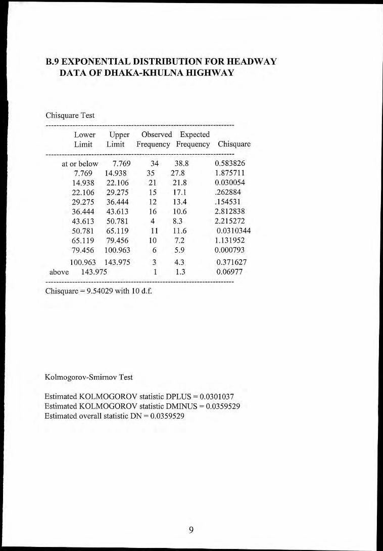
8.9 EXPONENTIAL DISTRIBUTION FOR HEADWAYDATA OF DHAKA-KHULNA HIGHWAY
Chisquare Test
Lower Upper Observed ExpectedLimit Limit Frequency Frequency Chisquare
at or below 7.7697.769 14.93814.938 22.10622.106 29.27529.275 36.44436.444 43.61343.613 50.78150.781 65.11965.119 79.45679.456 100.963100.963 143.975
above 143.975
34 38.835 27.821 21.815 17.112 13.416 10.64 8.3II 11.610 7.26 5.9
3 4.31 1.3
0.5838261.8757110.030054.262884.1545312.8128382.2152720.03103441.1319520.0007930.3716270.06977
Chisquare = 9.54029 with 10 d.f.
Kolmogorov-Smimov Test
Estimated KOLMOGOROV statistic DPLUS = 0.0301037Estimated KOLMOGOROV statistic DMINUS = 0.0359529Estimated overall statistic DN = 0.0359529
9
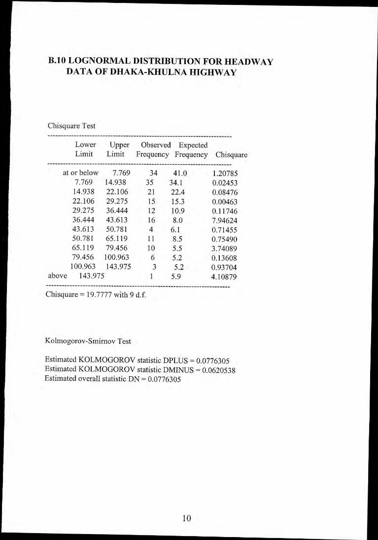
Chisquare Test
Lower Upper Observed ExpectedLimit Limit Frequency Frequency Chisquare
B.10 LOGNORMAL DISTRIBUTION FOR HEADWAYDATA OF DHAKA-KHULNA HIGHWAY
1.207850.024530.084760.004630.117467.946240.714550.754903.740890.136080.937044.10879
34 41.035 34.121 22.415 15.312 10.916 8.04 6.111 8.510 5.56 5.23 5.2I 5.9
at or below 7.7697.769 14.93814.938 22.10622.106 29.27529.275 36.44436.444 43.61343.613 50.78150.781 65.11965.119 79.45679.456 100.963100.963 143.975
above 143.975-----------------------------------------------------------------------Chisquare = 19.7777 with 9 d.f.
Kolmogorov-Smirnov Test
Estimated KOLMOGOROV statistic OPLUS = 0.0776305Estimated KOLMOGOROV statistic OMINUS = 0.0620538Estimated overall statistic ON = 0.0776305
10

-----------------------------------------------------------------------
-----------------------------------------------------------------------
Observed ExpectedFrequency Frequency Chisquare
UpperLimit
LowerLimit
B.II FREE SPEED ANALYSIS FOR BUSES
Chisquare Test
-----------------------------------------------------------------------at or below 60.000 5 5.8 .10260.000 65.000 7 5.7 .28865.000 70.000 11 7.5 1.66970.000 75.000 5 7.6 .89075.000 80.000 3 6.0 1.518
above 80.000 8 6.4 .387
Chisquare = 4.85327 with 3 d.f.
Kolmogorov-Smimov Test
Estimated KOLMOGOROV statistic DPLUS = 0.121487Estimated KOLMOGOROV statistic DMINUS = 0.0562993Estimated overall statistic DN = 0.121487
11
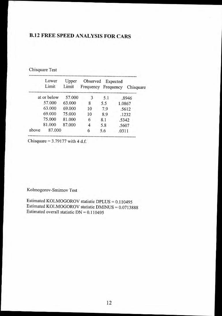
-----------------------------------------------------------------------
----------------------------------------~------------------------------Observed ExpectedFrequency Frequency Chisquare
UpperLimit
LowerLimit
B.12 FREE SPEED ANALYSIS FOR CARS
Chisquare Test
----------------------~------------------------------------------------at or below 57.000 3 5.1 .894657.000 63.000 8 5.5 1.086763.000 69.000 10 7.9 .561269.000 75.000 10 8.9 .123275.000 81.000 6 8.1 .534281.000 87.000 4 5.8 .5607
above 87.000 6 5.6 .0311
Chisquare = 3.79177 with 4 d.f.
Kolmogorov-Smirnov Test
Estimated KOLMOGOROV statistic DPLUS = 0.110495Estimated KOLMOGOROV statistic DMlNUS = 0.0713888Estimated overall statistic DN = 0.110495
12
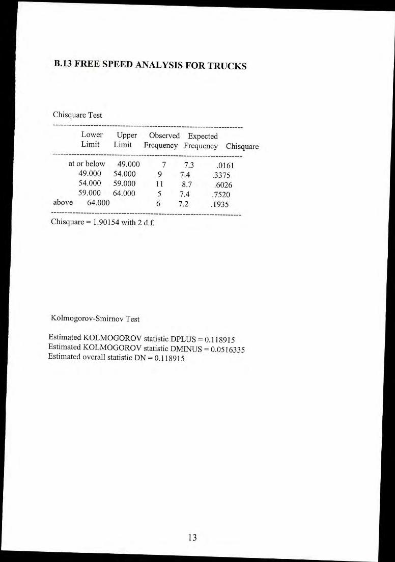
-----------------------------------------------------------------------
-----------------------------------------------------------------------
.0161.3375.6026.7520.1935
7 7.39 7.4I I 8.75 7.46 7.2
Observed ExpectedFrequency Frequency Chisquare
UpperLimit
LowerLimit
13
8.13 FREE SPEED ANALYSIS FOR TRUCKS
at or below 49.00049.000 54.00054.000 59.00059.000 64.000
above 64.000
Chisquare Test-----------------------------------------------------------------------
Kolmogorov-Smirnov Test
Chisquare = 1.90 154 with 2 d.f.
Estimated KOLMOGOROV statistic DPLUS = O. I 18915Estimated KOLMOGOROV statistic DMlNUS = 0.0516335Estimated overall statistic DN = 0.1 18915
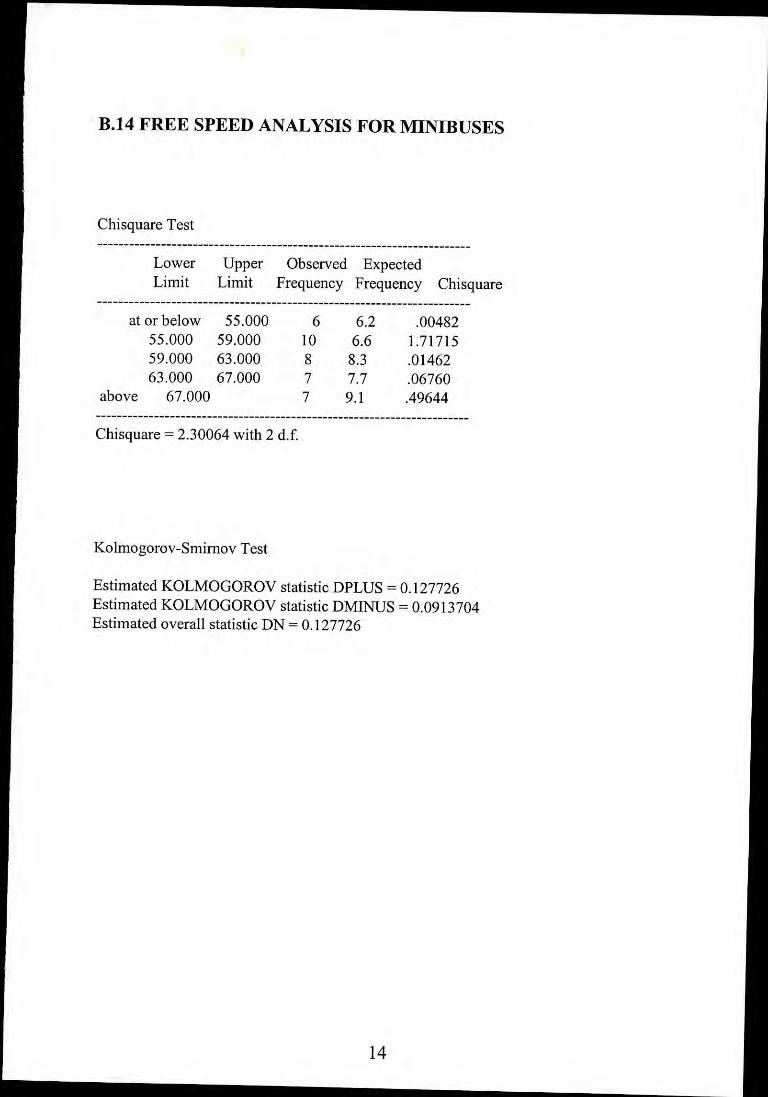
-----------------------------------------------------------------------
-----------------------------------------------------------------------
.004821.71715.01462.06760.49644
6 6.210 6.68 8.37 7.77 9.1
Observed ExpectedFrequency Frequency Chisquare
UpperLimit
LowerLimit
at or below 55.00055.000 59.00059.000 63.00063.000 67.000
above 67.000
B.14 FREE SPEED ANALYSIS FOR MINIBUSES
Chisquare Test
-----------------------------------------------------------------------Chisquare = 2.30064 with 2 d.f.
Kolmogorov-Smimov Test
Estimated KOLMOGOROV statistic DPLUS = 0.127726Estimated KOLMOGOROV statistic DMlNUS = 0.0913704Estimated overall statistic DN = 0.127726
14
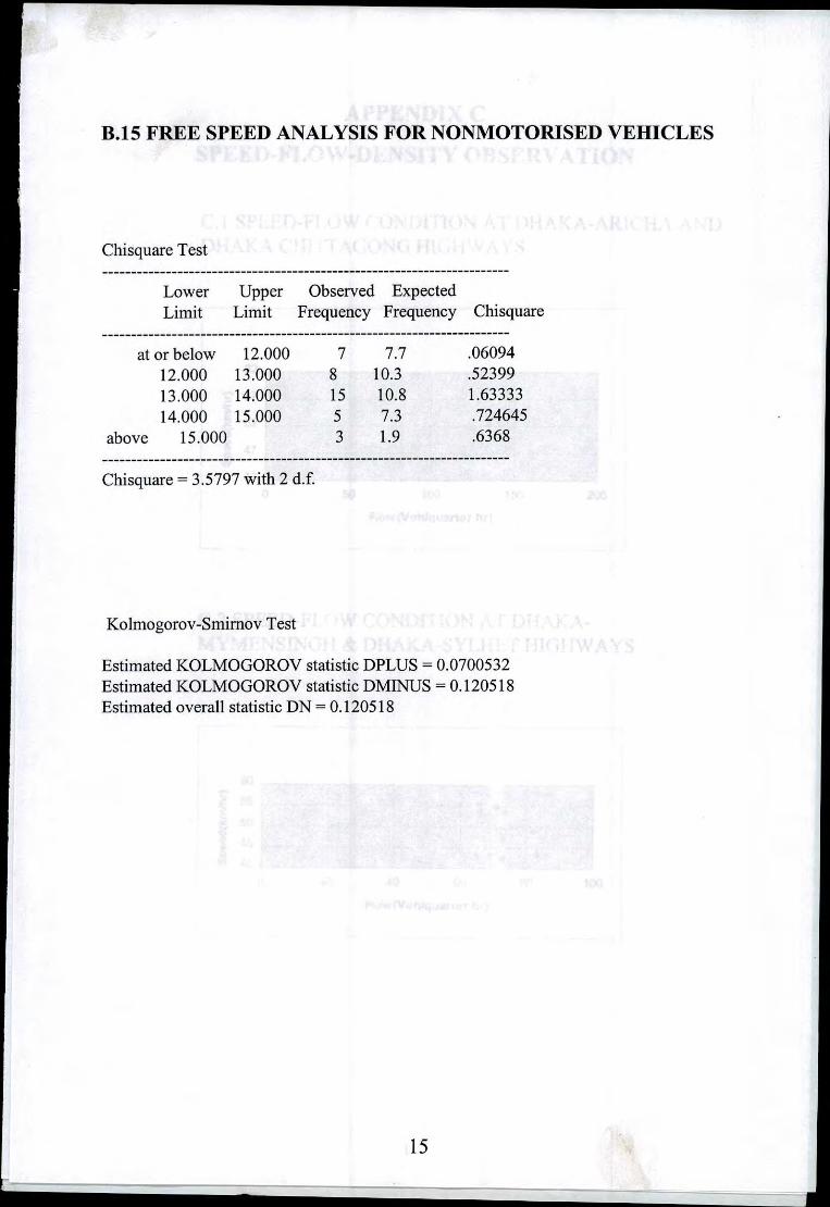
B.IS FREE SPEED ANALYSIS FOR NONMOTORISED VEHICLES
at or below 12.00012.000 13.00013.000 14.00014.000 15.000
above 15.000
Observed ExpectedFrequency Frequency Chisquare
.06094
.523991.63333.724645.6368
7 7.78 10.315 10.85 7.33 1.9
UpperLimit
LowerLimit
Chisquare Test
Chisquare = 3.5797 with 2 d.f.
Kolmogorov-Smimov Test
Estimated KOLMOGOROV statistic DPLUS = 0.0700532Estimated KOLMOGOROV statistic DM1NUS = 0.120518Estimated overall statistic DN = 0.120518
15
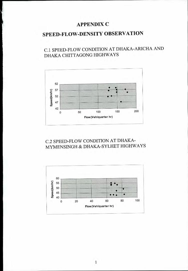
APPENDIXC
SPEED-FLOW-DENSITY OBSERVATION
C.I SPEED-FLOW CONDITION AT DHAKA-A RICH A ANDDHAKA CHITTAGONG HIGHWAYS
• •• ••
•
62-.::- 57.<:
~ 52:c~ 47c.<J)
42a 50 100
Flow(Veh/quarter hr)
150 200
C.2 SPEED-FLOW CONDITION AT DHAKA-MYMENSINGH & DHAKA-SYLHET HIGHWAYS
.~.• I•
••• •
60¥ 55
~ 50:c~ 45c.<J) 40
a 20 40 60 80 100
Flow(Veh/quarter hr)
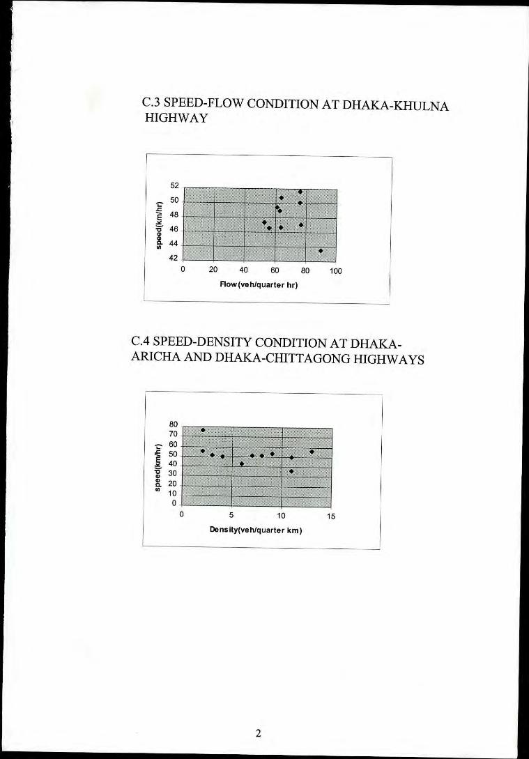
C.3 SPEED-FLOW CONDITION AT DHAKA-KHULNAHIGHWAY
100
•8060
••..'.. .
402042
o
5250~
.l::E 48"":c 46
~ 44;;
Aow(veh/quarler hr)
C.4 SPEED-DENSITY CONDITION AT DHAKA-ARICHA AND DHAKA-CHITTAGONG HIGHWAYS
•
8070.
-.:- 60~ 50..llI: 40_:g 308. 20" 10
oo
••
5 10
••
15
Densily(veh/quarler km)
2

• I-:.-.. ---. I •• • • • ,.-.....- .,--~.
C.6 SPEED-DENSITY CONDITION AT DHAKA-KHULNAHIGHWAY
C.S SPEED-DENSITY CONDITION AT DHAKA-MYMENSINGH AND DHAKA-SYLHET HIGHWAYS
15105
Density{veh/quarter km)
7060
..c: 50E 40'"" 30~ 20Coen 10
oo
• • • •-..-. • ••
6050
I 40E'" 30"" 20~en 10
oo 5 10 15
Densily(veh/quarlerkm)
3