IN DEGREE PROJECT MATHEMATICS,SECOND CYCLE, 30 CREDITS

, STOCKHOLM SWEDEN 2018

Optimal Speed Controller for a Heavy-Duty Vehicle in the Presence of Surrounding Traffic

JAKOB ARNOLDSSON

KTH ROYAL INSTITUTE OF TECHNOLOGYSCHOOL OF ENGINEERING SCIENCES

Optimal Speed Controller for a Heavy-Duty Vehicle in the Presence of Surrounding Traffic

JAKOB ARNOLDSSON Degree Projects in Optimization and Systems Theory (30 ECTS credits) Degree Programme in Applied and Computational Mathematics (120 credits) KTH Royal Institute of Technology year 2018 Supervisors at Scania: Manne Held Supervisor at KTH: Xiaoming Hu Examiner at KTH: Xiaoming Hu

TRITA-SCI-GRU 2018:250 MAT-E 2018:50 Royal Institute of Technology School of Engineering Sciences KTH SCI SE-100 44 Stockholm, Sweden URL: www.kth.se/sci

Abstract

This thesis has explored the concept of an intelligent fuel-efficient speed controller for a

heavy-duty vehicle, given that it is limited by a preceding vehicle. A Model Predictive

Controller (MPC) has been developed together with a PI-controller as a reference con-

troller. The MPC based controller utilizes future information about the traffic conditions

such as the road topography, speed restrictions and velocity of the preceding vehicle to

make fuel-efficient decisions. Simulations have been made for a so called Deterministic

case, meaning that the MPC is given full information about the future traffic conditions,

and a Stochastic case where the future velocity of the preceding vehicle has to be pre-

dicted. For the first case, regenerative braking as well as a simple distance dependent

model for the air drag coefficient are included. For the second case three prediction

models are created: two rule based models (constant velocity, constant acceleration)

and one learning algorithm, a so called Nonlinear Auto Regressive eXogenous (NARX)

network.

Computer simulations have been performed, on both created test cases as well as on

logged data from a Scania vehicle. The developed models are finally evaluated on the

test cases for both varying masses and allowed deviations from the preceding vehicle. The

simulations show on a potential for fuel savings with the MPC based speed controllers

both for the deterministic as well as the stochastic case.

Sammanfattning

Denna avhandling har undersokt intelligenta och bransleeffektiva hastighetsregulator for

tunga fordon, givet ett framforvarande fordon. En modell prediktiv kontroller (MPC),

hastighetsregulator, har utvecklats tillsammans med en PI-regulator som referens. Den

MPC-baserade regulatorn anvander information om framtida trafikforhallanden, sasom

vagtopografi, hastighetsbegransningar och hastighet hos framforvarande fordon for att

ta bransleeffektiva beslut. Simuleringar har gjorts for ett sa kallat Deterministiskt fall,

vilket betyder att MPC regulatorn far fullstandig information om framtida trafikforhalla-

nden, och ett Stokastiskt fall dar den framtida hastigheten hos framforvarande fordon

maste predikteras. For det forsta fallet ingar regenerativ bromsning samt en enkel

distansberoende modell for luftmotstandskoefficienten. For det andra fallet skapas tre

prediktionsmodeller: tva regelbaserade modeller (konstant hastighet, konstant accelera-

tion) och en inlarningsmodell, Nonlinear Auto Regressive eXogenouse model (NARX).

Datorsimuleringar har gjorts, bade pa skapade testfall och pa loggade data fran ett

Scania fordon. De utvecklade modellerna utvarderas slutligen pa testfallen for bade

varierande massor och tillatna avvikelser fran det framforvarande fordonet. Simu-

leringarna visar pa potential for branslebesparingar med MPC-baserade hastighetsreg-

ulatorer bade for det deterministiska och det stokastiska fallet.

Acknowledgements

First and foremost I want to thank my supervisor Manne Held at Scania for his guidance,

knowledge and valuable inputs throughout the work with this thesis. Without the many

fruitful discussions made at critical points in the project many of the developed models

and results seen in the thesis would not have been possible. I would also want to thank

him, Oscar Flardh and Mats Reimark for giving me the great opportunity to do this

project at Scania. The group NECS at Scania should also get a special thanks for the

support and warm welcome given to me during my time there. I would also like to take

the opportunity to thank my supervisor Xiaoming Hu at KTH for his valuable input

and feedback during the project.

At last, I would like to thank Caroline and my family for their support and encourage-

ments throughout the work with this thesis.

iii

Contents

Abstract i

Sammanfattning ii

Acknowledgements iii

List of Figures vii

List of Tables x

Abbreviations xi

1 Introduction 1

1.1 Earlier Work . . . . . . . . . . . . . . . . . . . . . . . . . . . . . . . . . . 3

1.2 Formulation of Main Goals . . . . . . . . . . . . . . . . . . . . . . . . . . 4

1.2.1 Deterministic case . . . . . . . . . . . . . . . . . . . . . . . . . . . 5

1.2.2 Stochastic case . . . . . . . . . . . . . . . . . . . . . . . . . . . . . 6

1.2.3 Delimitations . . . . . . . . . . . . . . . . . . . . . . . . . . . . . . 6

1.3 Outline of the Thesis . . . . . . . . . . . . . . . . . . . . . . . . . . . . . . 8

2 Background 9

2.1 Control and Optimization theory . . . . . . . . . . . . . . . . . . . . . . . 9

2.1.1 Optimal Control . . . . . . . . . . . . . . . . . . . . . . . . . . . . 9

2.1.1.1 General formulation . . . . . . . . . . . . . . . . . . . . . 11

2.1.2 Linear programming . . . . . . . . . . . . . . . . . . . . . . . . . . 12

2.1.2.1 Soft-constraint approach . . . . . . . . . . . . . . . . . . 14

2.1.3 MPC- Model Predictive Control . . . . . . . . . . . . . . . . . . . 15

2.1.4 PI-controller . . . . . . . . . . . . . . . . . . . . . . . . . . . . . . 17

2.1.4.1 Integral Windup . . . . . . . . . . . . . . . . . . . . . . . 18

2.2 FIR-filter . . . . . . . . . . . . . . . . . . . . . . . . . . . . . . . . . . . . 19

2.3 Linear Interpolation and Regression . . . . . . . . . . . . . . . . . . . . . 20

2.3.1 Linear Interpolation . . . . . . . . . . . . . . . . . . . . . . . . . . 20

2.3.2 Linear Regression . . . . . . . . . . . . . . . . . . . . . . . . . . . . 20

2.4 Zero Order Hold . . . . . . . . . . . . . . . . . . . . . . . . . . . . . . . . 21

2.5 Linear and Nonlinear ARX Model . . . . . . . . . . . . . . . . . . . . . . 23

iv

Contents v

2.6 Evaluation of Predictions and Approximations . . . . . . . . . . . . . . . 24

3 Vehicle Models 25

3.1 Vehicle Model . . . . . . . . . . . . . . . . . . . . . . . . . . . . . . . . . . 25

3.1.1 Regenerative Braking Extension . . . . . . . . . . . . . . . . . . . 27

3.1.2 Air drag Model Extension . . . . . . . . . . . . . . . . . . . . . . . 28

3.1.3 States and Disrectized Vehicle model . . . . . . . . . . . . . . . . . 29

3.1.3.1 Model extension considerations . . . . . . . . . . . . . . . 32

3.1.4 Linear Vehicle model . . . . . . . . . . . . . . . . . . . . . . . . . . 33

3.1.4.1 Model extension considerations . . . . . . . . . . . . . . . 34

3.1.5 Limitations on Controllable Forces . . . . . . . . . . . . . . . . . . 36

3.2 Vehicle Parameters . . . . . . . . . . . . . . . . . . . . . . . . . . . . . . . 38

3.3 Preceding Vehicle and Terrain Model . . . . . . . . . . . . . . . . . . . . . 39

4 Methodology 42

4.1 PI-controller . . . . . . . . . . . . . . . . . . . . . . . . . . . . . . . . . . . 43

4.2 Model Predictive Control . . . . . . . . . . . . . . . . . . . . . . . . . . . 46

4.2.1 Optimal Control Problem . . . . . . . . . . . . . . . . . . . . . . . 46

4.2.1.1 Constraints . . . . . . . . . . . . . . . . . . . . . . . . . . 46

4.2.1.2 Regenerative Braking Extension . . . . . . . . . . . . . . 51

4.2.1.3 Air Drag Model Extension . . . . . . . . . . . . . . . . . 52

4.2.2 Objective Function . . . . . . . . . . . . . . . . . . . . . . . . . . . 52

4.2.2.1 Model extension considerations . . . . . . . . . . . . . . . 53

4.2.2.2 Terminal Penalization . . . . . . . . . . . . . . . . . . . . 54

4.2.2.3 Complete Optimization model . . . . . . . . . . . . . . . 55

4.3 Time Linearization . . . . . . . . . . . . . . . . . . . . . . . . . . . . . . . 56

4.4 Air Drag Approximation Update . . . . . . . . . . . . . . . . . . . . . . . 59

4.5 Stochastic Case . . . . . . . . . . . . . . . . . . . . . . . . . . . . . . . . . 60

4.5.1 Rule Based Prediction . . . . . . . . . . . . . . . . . . . . . . . . . 61

4.5.1.1 Constant velocity approach . . . . . . . . . . . . . . . . . 61

4.5.1.2 Constant acceleration approach . . . . . . . . . . . . . . 63

4.5.2 Nonlinear ARX Prediction . . . . . . . . . . . . . . . . . . . . . . 65

5 Results 69

5.1 Simulation . . . . . . . . . . . . . . . . . . . . . . . . . . . . . . . . . . . . 69

5.1.1 Constructed simulation cases . . . . . . . . . . . . . . . . . . . . . 69

5.1.2 Logged Data . . . . . . . . . . . . . . . . . . . . . . . . . . . . . . 72

5.2 Tuning MPC parameters . . . . . . . . . . . . . . . . . . . . . . . . . . . . 74

5.2.1 Slack parameters . . . . . . . . . . . . . . . . . . . . . . . . . . . . 74

5.2.2 Terminal penalization parameters . . . . . . . . . . . . . . . . . . . 78

5.3 PI-controller . . . . . . . . . . . . . . . . . . . . . . . . . . . . . . . . . . . 80

5.3.1 Tuning parameters . . . . . . . . . . . . . . . . . . . . . . . . . . . 80

5.3.2 Anti-Windup . . . . . . . . . . . . . . . . . . . . . . . . . . . . . . 81

5.4 Deterministic case . . . . . . . . . . . . . . . . . . . . . . . . . . . . . . . 82

5.4.1 Basic Simulation Model . . . . . . . . . . . . . . . . . . . . . . . . 82

5.4.1.1 Regenerative braking Model . . . . . . . . . . . . . . . . 90

5.4.1.2 Air Drag coefficient Model . . . . . . . . . . . . . . . . . 94

Contents vi

5.4.2 Evaluation of Time and Distance Approximation . . . . . . . . . . 96

5.4.2.1 Time Approximation in Basic Model . . . . . . . . . . . . 96

5.4.2.2 Time and Distance Approximation in Second model ex-tension . . . . . . . . . . . . . . . . . . . . . . . . . . . . 100

5.4.3 Analysis of the Mass and Maximal Time gap of the Model . . . . . 103

5.5 Stochastic case . . . . . . . . . . . . . . . . . . . . . . . . . . . . . . . . . 105

5.5.1 Performance of Rule Based Prediction . . . . . . . . . . . . . . . . 107

5.5.1.1 Constant Velocity Approach . . . . . . . . . . . . . . . . 107

5.5.1.2 Constant Acceleration Approach . . . . . . . . . . . . . . 108

5.5.2 Performance of NARX Based Prediction . . . . . . . . . . . . . . . 109

5.5.3 Comparison between the Predictive Models . . . . . . . . . . . . . 112

6 Discussion 115

6.1 Models and Simulation cases . . . . . . . . . . . . . . . . . . . . . . . . . 115

6.1.1 PI-controller . . . . . . . . . . . . . . . . . . . . . . . . . . . . . . 116

6.1.2 Deterministic Case . . . . . . . . . . . . . . . . . . . . . . . . . . . 116

6.1.2.1 Model Assumptions . . . . . . . . . . . . . . . . . . . . . 117

6.1.2.2 Basic model . . . . . . . . . . . . . . . . . . . . . . . . . 117

6.1.2.3 Model extensions . . . . . . . . . . . . . . . . . . . . . . . 118

6.1.3 Stochastic Case . . . . . . . . . . . . . . . . . . . . . . . . . . . . . 118

6.1.4 Penalization weights . . . . . . . . . . . . . . . . . . . . . . . . . . 119

6.2 Force peaks - Instability in the model . . . . . . . . . . . . . . . . . . . . 120

6.3 Linearizations and Approximations . . . . . . . . . . . . . . . . . . . . . . 120

6.4 Prediction models . . . . . . . . . . . . . . . . . . . . . . . . . . . . . . . 122

7 Conclusions 124

7.1 Deterministic Case . . . . . . . . . . . . . . . . . . . . . . . . . . . . . . . 124

7.2 Stochastic Case . . . . . . . . . . . . . . . . . . . . . . . . . . . . . . . . . 124

7.3 Future Work . . . . . . . . . . . . . . . . . . . . . . . . . . . . . . . . . . 125

A Appendix A 127

A.1 Yalmip . . . . . . . . . . . . . . . . . . . . . . . . . . . . . . . . . . . . . . 130

A.2 NARX in Matlab . . . . . . . . . . . . . . . . . . . . . . . . . . . . . . . . 131

Bibliography 133

List of Figures

1.1 Statistics over the emissions and cost for road based transportation. . . . 2

1.2 Illustration of the driving scenario. . . . . . . . . . . . . . . . . . . . . . . 4

2.1 Schematic figure over the basic idea behind Model Predictive Control . . . 16

2.2 Schematic figure over the PI controller . . . . . . . . . . . . . . . . . . . . 17

2.3 Describing figure over Windup delay for step response with a PI controllerand desired solution trajectory . . . . . . . . . . . . . . . . . . . . . . . . 18

2.4 Illustrative figure of the NARX model structure . . . . . . . . . . . . . . . 24

3.1 External and Controllable longitudinal forces acting on the HDV . . . . . 26

3.2 Experimental and linear approximation of reduction in air drag coefficient. 28

3.3 Illustration of the approximation of the time update equation. . . . . . . . 31

3.4 Schematic figure over the nonlinear model of the maximal possible tractiveforce as a function of speed. . . . . . . . . . . . . . . . . . . . . . . . . . . 37

3.5 Preceding vehicle with the road topography as well as the velocity trajectory. 39

3.6 An illustrative figure over the topography of the road and how it is createdin the manually created simulations situations. . . . . . . . . . . . . . . . 40

3.7 The trajectory of the preceding vehicle. . . . . . . . . . . . . . . . . . . . 41

4.1 A sketch over the fundamental Methodology of this thesis. . . . . . . . . . 42

4.2 Overview of the MPC implementation. . . . . . . . . . . . . . . . . . . . . 46

4.3 Close up figure over the time gap model. . . . . . . . . . . . . . . . . . . . 47

4.4 Overview of the time gap model. . . . . . . . . . . . . . . . . . . . . . . . 48

4.5 Sketch of the methodology behind the time approximation improvementloop. . . . . . . . . . . . . . . . . . . . . . . . . . . . . . . . . . . . . . . . 56

4.6 Creation of the first reference kinetic trajectory. . . . . . . . . . . . . . . . 57

4.7 Time approximation improvement procedure. . . . . . . . . . . . . . . . . 58

4.8 Time approximation evaluation. . . . . . . . . . . . . . . . . . . . . . . . . 58

4.9 Distance approximation. . . . . . . . . . . . . . . . . . . . . . . . . . . . . 59

4.10 Schematic figure over the stochastic methodology. . . . . . . . . . . . . . . 60

4.11 An illustration over the stochastic scenario. . . . . . . . . . . . . . . . . . 61

4.12 Methodology of the constant velocity approach. . . . . . . . . . . . . . . . 62

4.13 Example of a prediction over a prediction horizon with the constant ve-locity approach. . . . . . . . . . . . . . . . . . . . . . . . . . . . . . . . . . 63

4.14 Methodology of the constant acceleration approach. . . . . . . . . . . . . 64

4.15 Example of a prediction over a prediction horizon of 250m with the con-stant acceleration approach. . . . . . . . . . . . . . . . . . . . . . . . . . . 65

4.16 Methodology of the NARX prediction approach. . . . . . . . . . . . . . . 68

vii

List of Figures viii

5.1 The basic simulation case, Case 1. . . . . . . . . . . . . . . . . . . . . . . 70

5.2 The hill simulation case, Case 2. . . . . . . . . . . . . . . . . . . . . . . . 70

5.3 The oscillating velocity simulation case, Case 3. . . . . . . . . . . . . . . 71

5.4 The catch up simulation case, Case 4. . . . . . . . . . . . . . . . . . . . . 71

5.5 CC-set speed vs. the preceding vehicle speed for the deterministic case. . 72

5.6 Altitude for the logged data case. The logged altitude vs. the filteredaltitude. . . . . . . . . . . . . . . . . . . . . . . . . . . . . . . . . . . . . . 73

5.7 Illustrative figure over the choice of gamma value. . . . . . . . . . . . . . 75

5.8 Illustrative figure over the choice of beta value. . . . . . . . . . . . . . . . 76

5.9 The resulting force for a small value of the jerk penalization parameter. . 77

5.10 Relative time difference between the HDV and the preceding vehicle forthe prediction horizon for different values of δ. . . . . . . . . . . . . . . . 78

5.11 Relative time difference between the HDV and the preceding vehicle forthe prediction horizon for different values of τ . . . . . . . . . . . . . . . . 79

5.12 Solution for the logged data case for the PI-controller. . . . . . . . . . . . 80

5.13 Anti-Windup response to a step in the input signal. . . . . . . . . . . . . 81

5.14 Results of the different Anti-Windup methods for step in input signal. . . 82

5.15 Deterministic case; Case 1 results. . . . . . . . . . . . . . . . . . . . . . . 83

5.16 Deterministic case; Case 1 trajectory. . . . . . . . . . . . . . . . . . . . . . 83

5.17 Deterministic case; Case 2 results. . . . . . . . . . . . . . . . . . . . . . . 84

5.18 Deterministic case; Case 2 trajectory. . . . . . . . . . . . . . . . . . . . . . 85

5.19 Deterministic case; Case 2 force. . . . . . . . . . . . . . . . . . . . . . . . 85

5.20 Deterministic case; Case 3 results. . . . . . . . . . . . . . . . . . . . . . . 86

5.21 Deterministic case; Case 3 trajectories. . . . . . . . . . . . . . . . . . . . . 86

5.22 Deterministic case; Case 3 forces. . . . . . . . . . . . . . . . . . . . . . . . 87

5.23 Deterministic case; Case 4 results. . . . . . . . . . . . . . . . . . . . . . . 88

5.24 Deterministic case; Case 4 trajectory and force. . . . . . . . . . . . . . . . 88

5.25 Deterministic case; Logged data case results. . . . . . . . . . . . . . . . . 89

5.26 Deterministic case; Logged data trajectories. . . . . . . . . . . . . . . . . 90

5.27 Regenerative braking energy consumption versus PI without regenerativebraking, case 2. . . . . . . . . . . . . . . . . . . . . . . . . . . . . . . . . . 91

5.28 Regenerative brake; case 2 trajectories. . . . . . . . . . . . . . . . . . . . . 91

5.29 Regenerative brake; case 2 results vs. PI with regenerative braking. . . . . 92

5.30 Regenerative braking energy consumption versus PI without regenerativebraking, logged data. . . . . . . . . . . . . . . . . . . . . . . . . . . . . . . 93

5.31 Regenerative brake; Logged data case results vs. PI with regenerativebraking. . . . . . . . . . . . . . . . . . . . . . . . . . . . . . . . . . . . . . 93

5.32 Air drag model energy consumption versus PI with constant air dragcoefficient, on logged data. . . . . . . . . . . . . . . . . . . . . . . . . . . . 94

5.33 Air drag coefficient; Logged data case resulting trajectories. . . . . . . . . 95

5.34 Air drag model energy consumption versus PI with distance dependentair drag coefficient. . . . . . . . . . . . . . . . . . . . . . . . . . . . . . . . 96

5.35 Time improvement approximation loop effect for a prediction horizon of250m. . . . . . . . . . . . . . . . . . . . . . . . . . . . . . . . . . . . . . . 97

5.36 The normalized difference between actual and predicted step in the statevariables. . . . . . . . . . . . . . . . . . . . . . . . . . . . . . . . . . . . . 98

5.37 Time difference between the nonlinear and linear models. . . . . . . . . . 99

List of Figures ix

5.38 Comparison of the resulting trajectories between the nonlinear and linearmodel. . . . . . . . . . . . . . . . . . . . . . . . . . . . . . . . . . . . . . . 99

5.39 Difference between predicted and actual step in state variables and intervehicle distance. . . . . . . . . . . . . . . . . . . . . . . . . . . . . . . . . 101

5.40 Time difference between the nonlinear and linear models, second modelextension. . . . . . . . . . . . . . . . . . . . . . . . . . . . . . . . . . . . . 102

5.41 Comparison of the resulting trajectories between the nonlinear and linearmodels, second model extension. . . . . . . . . . . . . . . . . . . . . . . . 102

5.42 Mass evaluation on logged data case. . . . . . . . . . . . . . . . . . . . . . 103

5.43 Mass evaluation, resulting trajectories. . . . . . . . . . . . . . . . . . . . . 104

5.44 Energy consumption for different maximal time gap values. . . . . . . . . 105

5.45 Over take example. . . . . . . . . . . . . . . . . . . . . . . . . . . . . . . . 106

5.46 Logged data case for the stochastic simulations. . . . . . . . . . . . . . . . 106

5.47 Four examples of the constant velocity approach. . . . . . . . . . . . . . . 107

5.48 Total energy consumption for the constant velocity approach. . . . . . . . 108

5.49 Total energy consumption for the constant acceleration approach. . . . . . 108

5.50 Four examples of the constant acceleration approach. . . . . . . . . . . . . 109

5.51 Division of the data set for the NARX approach. . . . . . . . . . . . . . . 110

5.52 Training results of the NARX model. . . . . . . . . . . . . . . . . . . . . . 110

5.53 Four examples of the NARX model approach. . . . . . . . . . . . . . . . . 111

5.54 Total energy consumption for the NARX approach. . . . . . . . . . . . . . 111

5.55 Division of the data set for evaluation of velocity prediction. . . . . . . . . 112

5.56 Two examples where the NARX model prediction is worse than the rulebased models. . . . . . . . . . . . . . . . . . . . . . . . . . . . . . . . . . . 113

5.57 Resulting trajectories for predictive models. . . . . . . . . . . . . . . . . . 114

A.1 Full solution for the force peaks scenario. . . . . . . . . . . . . . . . . . . 127

A.2 Full solution for the force peaks scenario, without force peaks. . . . . . . . 128

A.3 Deterministic case; Logged data forces. . . . . . . . . . . . . . . . . . . . . 129

A.4 Air drag coefficient; Logged data case resulting forces. . . . . . . . . . . . 129

A.5 Resulting controllable forces for the predictive models. . . . . . . . . . . . 130

List of Tables

3.1 Standard vehicle parameters and natural constants. . . . . . . . . . . . . 38

5.1 Results of speed violation penalization for all simulation cases. . . . . . . 76

5.2 Jerk penalization data for deceleration case. . . . . . . . . . . . . . . . . . 77

5.3 Evaluation of terminal penalization parameters. . . . . . . . . . . . . . . . 79

5.4 Tuning parameter values for the PI-controller. . . . . . . . . . . . . . . . . 81

5.5 Data over the time approximation on logged data. . . . . . . . . . . . . . 97

5.6 Time and distance approximation statistics for the logged data case. . . . 100

5.7 Difference in energy consumption between applying the linear or nonlinearmodel as system model, for the second model extension. . . . . . . . . . . 101

5.8 Time gap statistics for the logged data case. . . . . . . . . . . . . . . . . . 104

5.9 Mean deviation of the predictions for the prediction horizons made forthe logged data case. . . . . . . . . . . . . . . . . . . . . . . . . . . . . . . 113

5.10 Energy consumption with the deterministic solution as the reference. . . . 114

x

Abbreviations

GHG Green House Gases

LDV Light Duty Vehicle

HDV Heavy Duty Vehicle

HEV Hybrid Electric Vehicle

ADAS Adaptive Driver Assistance System

CC Cruise Controller

ACC Adaptive Cruise Controller

OCP Optimal Control Problem

LP Linear Program

MPC Model Predtictive Control

V2V Vehicle To Vehicle communication

V2I Vehicle To Infrastructure communication

GPS Global Positioning System

xi

Dedicated to my father

xii

Chapter 1

Introduction

During the past few decades the concerns and attention for the environmental issues

facing the world and civilization have become more prominent in the society. Both

politically and scientifically the issues of reducing the emissions of green house gases

(GHG) as well as emissions of dangerous particles from all parts of the society, but

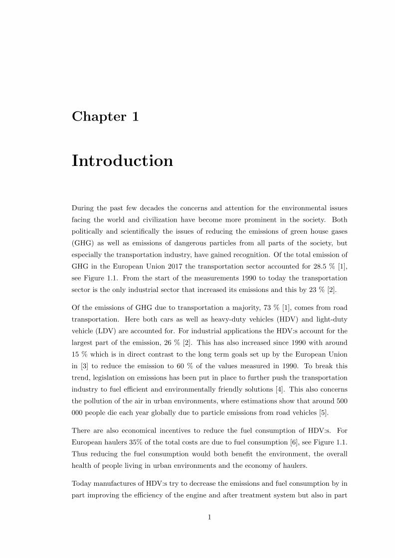
especially the transportation industry, have gained recognition. Of the total emission of

GHG in the European Union 2017 the transportation sector accounted for 28.5 % [1],

see Figure 1.1. From the start of the measurements 1990 to today the transportation

sector is the only industrial sector that increased its emissions and this by 23 % [2].

Of the emissions of GHG due to transportation a majority, 73 % [1], comes from road

transportation. Here both cars as well as heavy-duty vehicles (HDV) and light-duty

vehicle (LDV) are accounted for. For industrial applications the HDV:s account for the

largest part of the emission, 26 % [2]. This has also increased since 1990 with around

15 % which is in direct contrast to the long term goals set up by the European Union

in [3] to reduce the emission to 60 % of the values measured in 1990. To break this

trend, legislation on emissions has been put in place to further push the transportation

industry to fuel efficient and environmentally friendly solutions [4]. This also concerns

the pollution of the air in urban environments, where estimations show that around 500

000 people die each year globally due to particle emissions from road vehicles [5].

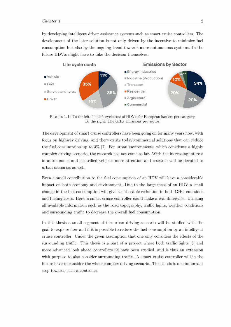
There are also economical incentives to reduce the fuel consumption of HDV:s. For

European haulers 35% of the total costs are due to fuel consumption [6], see Figure 1.1.

Thus reducing the fuel consumption would both benefit the environment, the overall

health of people living in urban environments and the economy of haulers.

Today manufactures of HDV:s try to decrease the emissions and fuel consumption by in

part improving the efficiency of the engine and after treatment system but also in part

1

Chapter 1 2

by developing intelligent driver assistance systems such as smart cruise controllers. The

development of the later solution is not only driven by the incentive to minimize fuel

consumption but also by the ongoing trend towards more autonomous systems. In the

future HDV:s might have to take the decision themselves.

Title and Content

11 April 2018 Info class internal Department / Name / Subject 46

11%

35%

19%

35%

Life cycle costs

Vehicle

Fuel

Service and tyres

Driver

34%

20%

29%

10%

3%4%

Emissions by Sector

Energy Industries

Industrie (Production)

Transport

Residential

Argiculture

Commercial

Figure 1.1: To the left; The life cycle cost of HDV:s for European haulers per category.To the right; The GHG emissions per sector.

The development of smart cruise controllers have been going on for many years now, with

focus on highway driving, and there exists today commercial solutions that can reduce

the fuel consumption up to 3% [7]. For urban environments, which constitute a highly

complex driving scenario, the research has not come as far. With the increasing interest

in autonomous and electrified vehicles more attention and research will be devoted to

urban scenarios as well.

Even a small contribution to the fuel consumption of an HDV will have a considerable

impact on both economy and environment. Due to the large mass of an HDV a small

change in the fuel consumption will give a noticeable reduction in both GHG emissions

and fueling costs. Here, a smart cruise controller could make a real difference. Utilizing

all available information such as the road topography, traffic lights, weather conditions

and surrounding traffic to decrease the overall fuel consumption.

In this thesis a small segment of the urban driving scenario will be studied with the

goal to explore how and if it is possible to reduce the fuel consumption by an intelligent

cruise controller. Under the given assumption that one only considers the effects of the

surrounding traffic. This thesis is a part of a project where both traffic lights [8] and

more advanced look ahead controllers [9] have been studied, and is thus an extension

with purpose to also consider surrounding traffic. A smart cruise controller will in the

future have to consider the whole complex driving scenario. This thesis is one important

step towards such a controller.

Chapter 1 3

1.1 Earlier Work

This thesis is a part of a project where intelligent cruise controllers for urban environ-

ments in HDV:s have been studied. Here, other aspects of the driving scenario as well

as other approaches to the main topic of this thesis has previously been analyzed. In

[10] the optimal control of an HDV in urban environments has been studied using infor-

mation about speed restrictions, intersections as well as vehicle velocity statistics. The

impact of traffic lights have also been studied in [8] and this thesis is a continuation of

both of these.

The automotive industry has the past decades pushed for more fuel efficient as well as

smart cruise controllers. This has led to many studies and implementations for highway

driving [11], [12], [6]. Where fuel savings up to 3% and increased throughput of vehicles

up to 273 % [13] has been recorded. The recent popularity for more autonomous systems

has made the need for urban solutions more prominent.

Today many of the solutions of smart cruise controllers for urban environments are

based on the model predictive controller (MPC) framework. Although the algorithm

itself is similar in many of the studies many different implementations of it exists. In

[14] a hierarchical control architecture is utilized within the MPC structure to both

ensure feasibility and to compensate for the nonlinearities in the vehicle model. Novel

parametric techniques have been developed in [15] to manage real-time computation

of the optimal speed trajectory in an MPC fashion where experiments on urban roads

showed fuel-efficiency improvements up to 2 %. Nonlinear MPC models have been

proven (in simulations) to give promising results in [16] and [17] with savings of up to

11%, although being computationally heavy.

The preceding vehicle model technique is popular and well used approach to model the

surrounding traffic with, e.g. in [18], [19] and [20]. This in order to lower the complexity

and in the end be able to implement the models online. Different strategies exist, where

the time window or distance corridor is the most popular one [21]. Other methods to

incorporate a preceding vehicle to the model is, for example, to model a velocity corridor

after the statistics of how a similar vehicle would drive [22]. Similar research is made in

the case of Platooning [23] where a platoon of HDV:s are controlled fuel-efficiently.

The electrification of the automotive industry is also utilized in the development of smart

cruise controllers. In [24], [25] and [10] electric as well as hybrid vehicles are simulated

and tested with MPC based smart cruise controllers. Regenerative braking and varying

drag coefficient values are studied to give minimum fuel consumption with promising

results.

Chapter 1 4

At last, the above mentioned studies have in large made use of given information of

both future road slope as well as information about the preceding vehicle. When apply-

ing the methods in real life situations prediction models have to be used to predict the

future behavior of the preceding vehicle. Although platooning and improved communica-

tions systems will enable a better flow of information between vehicles, many prediction

models have shown promising results in the MPC framework and thus interesting to

analyze further. In [21] and [26] the future velocity trajectory of the preceding vehicle is

predicted with nonlinear (polynomial) auto regressive exogenous (NARX) models and

Gaussian process’s respectively. Other methods such as ad-hoc grey box models [18]

or combined rule based models [17] have shown to give 1-2% fuel savings. Both rule

based and learning algorithms will be tested in this thesis, but of lower computational

complexity.

1.2 Formulation of Main Goals

In this thesis a cruise controller that minimize the fuel consumption for an HDV will be

developed. This by utilizing future and past information about the road slope, speed

restrictions and surrounding traffic. This kind of controllers will come to use mostly in

urban environments where both surrounding traffic and road slope can have a noticeable

impact on the fuel consumption of the HDV.

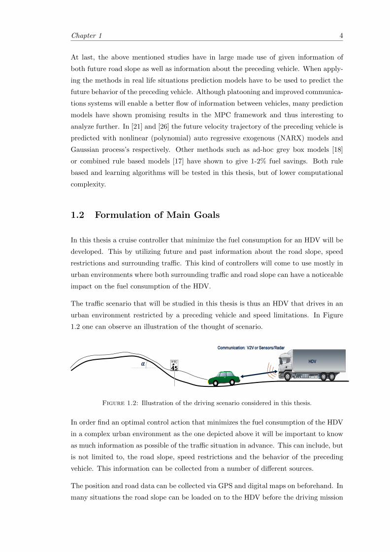
The traffic scenario that will be studied in this thesis is thus an HDV that drives in an

urban environment restricted by a preceding vehicle and speed limitations. In Figure

1.2 one can observe an illustration of the thought of scenario.

Title and Content

11 April 2018 Info class internal Department / Name / Subject 47

𝑺𝒑, 𝑽𝒑 , 𝒂𝒑 𝑺, 𝑽, 𝒂∆𝒕𝒊

𝜶

Communication: V2V or Sensors/Radar

HDV

Figure 1.2: Illustration of the driving scenario considered in this thesis.

In order find an optimal control action that minimizes the fuel consumption of the HDV

in a complex urban environment as the one depicted above it will be important to know

as much information as possible of the traffic situation in advance. This can include, but

is not limited to, the road slope, speed restrictions and the behavior of the preceding

vehicle. This information can be collected from a number of different sources.

The position and road data can be collected via GPS and digital maps on beforehand. In

many situations the road slope can be loaded on to the HDV before the driving mission

Chapter 1 5

thus making it possible to use the future road slope in the developed control algorithm.

The same goes for the speed restrictions of the road. In some cases these are dynamic

and change depending on weather and traffic conditions but today such information is

often available via cloud services or the GPS.

An important factor that can have a significant influence on the fuel consumption of

the HDV is the surrounding traffic. In many situations in urban driving the HDV will

be forced to brake or restrict its velocity because of the surrounding traffic. In other

situation it will have to increase the desired speed to not cause disturbance for other

surrounding traffic participants. One can easily image that the surrounding traffic will

affect the HDV and restrict its driving. Thus information about the preceding vehicle

will be important.

The information about the velocity and driving behavior of the preceding vehicle can

be retrieved via vehicle-to-vehicle communication (V2V). This through some sort of 4G

or 5G connection. Another possibility is to have sensors or radars directly on the HDV

that measure the current position and speed of the preceding vehicle.

In order to analyze how the amount and reliability of the information of the future

velocity trajectory of the preceding vehicle will affect the fuel effective solution of the

developed cruise controller we divide the simulations into two cases: one Deterministic

case and one Stochastic case.

1.2.1 Deterministic case

The Deterministic case will include a cruise controller that minimizes the fuel consump-

tion under the assumption that the full information about the future velocity trajectory

of the preceding vehicle is known. This means that the HDV at every instance know the

full future information about the driving scenario. This is a highly idealized formulation

of the real driving scenario but an interesting formulation from a model point of view.

This will give a measure of how much at most the developed controller can reduced the

fuel consumption for the studied scenarios.

In order to simulate and compare the results, driving scenarios as well as a reference

controller will be created. The created scenarios will both be of specific driving condi-

tions and of more general traffic scenarios collected from logged data given by Scania.

This in order to also include a real driving scenario and see how the model reacts to a

complex situation. The reference will be constructed in the image of a simple cruise con-

troller (CC) or a simple human driver that tries to keep constant headway to a preceding

vehicle.

Chapter 1 6

Here both the amount of future information as well as the restrictions to the preceding

vehicle will be explored. Two model extensions will be made to investigate the effect of

regenerative braking, which may become important for future electrified vehicles, and

inter-vehicle dependent air drag.

1.2.2 Stochastic case

The Stochastic case treats the driving scenario where the HDV will not have full infor-

mation about the future conditions. The speed restrictions as well as road slope will

be known in advance but the future trajectory of the preceding vehicle will not. This

simulation case will come closer to the real driving scenario in urban environments.

In order to build an optimization model and find an energy effective solution, the future

trajectory of the preceding vehicle will be predicted. Three models will be developed for

this purpose to analyze how sensitive the developed cruise controller is to the information

about the future trajectory of the preceding vehicle. Both rule based models as well as

one simple learning algorithm will be explored.

1.2.3 Delimitations

In order to make the project manageable within the time and resources given some

delimitations have to be made. This is both so that reasonable results can be achieved

but also to keep the complexity of the models at a reasonable level for possible future

on-line implementation.

First and foremost the vehicle model will be developed under some strict physical

limitations.

• Longitudinal dynamics: The lateral dynamics of the HDV will not be consid-

ered in this thesis. Only the longitudinal dynamics will be included. Thus only

longitudinal movements will be included in the simulations made.

• No Powertrain model: The powertrain is a term that is used to describe the

components that generate the power and distribute it to the road surface in a

vehicle. The powertrain is an immensely important part of the HDV but will be

neglected in this thesis. Instead a model based purely on the external and the so

called controllable forces will be implemented. One can say that the powertrain is

approximated with two controllable forces, the tractive and the braking force.

Chapter 1 7

• External forces: The external forces such as the rolling resistance and air

resistance will in reality depend on the HDV itself, number of wheels, aerodynamic

properties and condition of the tires. The weather and road conditions will most

probably also affect the external forces on the HDV. This will be approximated by

setting a fix value of the rolling resistance and air drag coefficients. Nevertheless,

the dependency to the preceding vehicle of the air drag coefficient will be explored

in one of the model extensions.

Furthermore, the driving scenario itself will be restricted. This is made in order to have

a reasonable scenario to study. The real driving scenario includes many different traffic

participants which would make the model extremely complex. In order to manage

to develop a model in time the following limitations will be imposed on the driving

scenario itself.

• Only a preceding vehicle: To include all surrounding traffic into the model

would be an extremely hard task. In order to get some results to analyze only the

simplest situation will be studied in this thesis. This by assuming that the only

traffic to consider is a preceding vehicle.

• Not a specific type of vehicle: The preceding vehicle can be any type of

vehicle. This will not be specified in the simulation cases studied. The preceding

vehicle is only seen as a limitation on the HDV and not as a specific type of vehicle.

• No speed violations: The preceding vehicle is assumed to never violate the

speed restrictions.

• Always moving forward: The preceding vehicle will be assumed to always

be in motion, i.e. never be at stand still. Furthermore, we will assume that

the preceding vehicle never drives backwards. This to avoid complications in the

optimization model.

• No traffic lights, pedestrians or stop signs: These factor will not be consid-

ered in this thesis. As is mentioned before only the preceding vehicle, road slope

and speed restrictions will be considered. A future project might be to extend the

developed model to include these factors as well.

At last we will also make limitations and approximations when formulating the system

as an optimization problem. These are made in order to have both a reasonably fast

algorithm but also in order to find the optimal solutions as well as to be able to compare

the results between the developed controller and the reference.

Chapter 1 8

• Linear optimization model: The system itself will become nonlinear. In order

to have a fast and reliable algorithm one can reduce the complexity by reformulat-

ing the system as a linear model. This will also mean that the optimal solution for

the prediction horizon will be found. Thus we will limit the optimization model to

a linear model. The drawback being that approximations have to be made, which

will introduce model errors.

• Piece-wise constant applied force: The control action computed by the

control algorithms will be considered constant in between sample points.

• Constant acceleration: For the update equation of the position in time of the

HDV, constant acceleration in between samples points will be assumed. This will

not be fully correct because the air resistance is proportional to the square of the

velocity. This will not make a big difference for small sample distances and thus

neglected in this thesis. This is also consistent with the assumption of piece-wise

constant control actions.

• Fuel approximated as energy: The fuel consumption will not be available

directly with the delimitations mentioned above. It will although be proportional

to the energy consumption and thus approximated with it.

1.3 Outline of the Thesis

Chapter 2 introduces the basic theory behind the methods used in the developed con-

troller. The mathematically theory behind the controller algorithms as well as the theory

behind the approximations made is given in this chapter. Chapter 3 treats the develop-

ment of the vehicle model. This both for the HDV itself, including the model extensions,

and the preceding vehicle. In Chapter 4 the methodology for both the deterministic and

stochastic case is described in detail. Here the methodology developed in order to deal

with the model errors as well as the approximations made is presented. At last the cho-

sen methodology for the predictive models is described. In Chapter 5 the results of the

developed models on the created simulation cases are showcased. Both the basic models

as well as the model extensions and the predictive model results are shown. Chapter 6

gives a short discussion of the results and methodology of the project. Including unex-

pected behaviors and problems that occurred during the work with the models. At last,

in Chapter 7 the conclusions as well as suggestions on future work can be found.

Chapter 2

Background

In this chapter a theoretical overview of the methods used in this thesis is presented.

First the theory behind optimal control problems and how they in general can be for-

mulated and solved by the MPC algorithm is given. Then, basic control theory such

as the mathematical description of a PI regulator and the theory behind some of the

difficulties that can occur, and their solutions, are also given. At last, the mathematics

behind linear interpolation and regression that is used in the approximations made in

the thesis are briefly mentioned as well as the theory behind the predictive models used

in the stochastic case of this thesis.

2.1 Control and Optimization theory

In this section the control and optimization theory used in this thesis will be presented.

Optimal control as well as the theory behind the well known and well studied PI regulator

will be covered. Furthermore, some important aspects and problems with the algorithms

will be studied more in detail in this section. For a complete and, for this thesis, specific

formulation of the control algorithms and regulators see Chapter 4.

2.1.1 Optimal Control

Nature itself often behaves optimally and it is thus natural to pose many problems, and

specifically control problems in an engineering setting, as optimization problems. Thus

the nowadays important branch of mathematics called Optimal Control has emerged.

Optimal control is the branch of mathematics that deals with algorithms and meth-

ods that solves control problems in a systematic manner whilst optimizing some cost

9

Chapter 2 10

criterion. A control problem has in general many, sometime infinitely many, solutions.

According to some predefined cost criterion, for example to minimize fuel or maximize

profit, the control solutions can be classified as being better or worse. The goal would

then be to find the best control solution for the stated problem. These kind of problems

are usually extremely hard to solve using only engineering intuition or ad-hoc techniques.

Optimal control is the field of control and mathematics that gives a systematic approach

to solve these problems. Reducing the redundancy of control solutions and selecting the

solutions that is best according to the defined cost criterion.

Consider the case when we have a state space realization of a system (2.1), in the time

domain, with states x(t), control u(t) and initial conditions x0 given 1

x(t) = Ax(t) +Bu(t), x(t0) = x0. (2.1)

Here A and B are given matrices. Then we can formulate a control problem as: Find a

control u : [t0, tf ] → R such that the solution to (2.1) satisfies x(tt) = xtf , where

xtf is given and t0 is the initial time and tf is the final time. The solutions to this

control problem can be found by using basic mathematical systems theory. If we define

the state transition matrix Φ(t, s) as the solution to the differential equation

∂Φ(t, s)

∂t= AΦ(t, s), Φ(t, t) = I (2.2)

and the controllability Gramian as

W (tf , t0) =

∫ tf

t0

Φ(tf , s)BBTΦ(tf , s)

Tds (2.3)

then we find the solution to the stated control problem as

u(t) = BTΦ(tf , t)TW (tf , t0)−1[xtf − Φ(tf , t0)x0]. (2.4)

One can now easily see that for many systems (depending on the matrices A and B) this

will yield many, if not infinitely many, solutions. Optimal control can be used to reduce

the set of solutions by introducing a cost criterion. For more details of the derivation of

the solution above see [28].

1This example is taken from [27].

Chapter 2 11

2.1.1.1 General formulation

In this thesis the general formulation for a optimal control problem will consist of four

parts: cost criterion (objective function), the control and state constraints, the boundary

conditions and the system dynamics. Below we will describe each part of the general

formulation of the optimal control problem separately and then define the complete

formulation that will be used in this thesis.

System Dynamics: Here we will define the system dynamics as the update equation

for the states of the system. This means that we define it in terms of a state space

equation of the form (2.1) excluding the initial condition on the states. The system

dynamics is often given by the system itself by expressing the system model in the

introduced states, often as a ordinary first order differential equation. We can in general

formulate the system dynamics as

x(t) = f(t, x, u) (2.5)

where x ∈ Rn are the states, u ∈ Rm are the controls and f ∈ Rn are the functions

describing the dynamics for each state.

Control and State constraints: The states and control variables will usually be

restricted to only take values within a defined set. For the state variables we have that

they are restricted to a certain defined set X ⊂ Rn and for the control variables we have

that they are restricted to U ⊂ Rm. These constraints are set after the limitations the

system already has, for example maximal and minimal control action but also after the

model choices we make. This can for example be to only look at solutions for a certain

subset of values of the states, for example only to look at the solutions where the states

take positive values or only negative values.

Boundary Conditions: The boundary conditions are set on the states at the initial

point and can also be set on the final point. In this thesis we will only look at initial

boundary conditions, where we set the initial point to a given value. Thus we get the

initial boundary condition as stated in (2.1).

Cost function: At last we have the cost function that gives us the cost criterion men-

tioned earlier. This function describes what we are trying to optimize, for example

energy minimization or profit maximization. Generally the cost function can be formu-

lated as in

Chapter 2 12

φ(x(tf ), tf ) +

∫ tf

t0

f0(t, x(t), u(t))dt (2.6)

which consist of two distinctive parts. The first part is the terminal cost φ(x(tf ), tf )

which is there to penalize deviation from some desired final state [27]. The second part,

which is the integral part, is the cumulative cost of the state and control trajectories.

Now we are ready to formulate the complete optimal control problem as we define it in

this thesis, (2.7).

minimizeu

φ(x(tf ), tf ) +

∫ tf

t0

f0(t, x(t), u(t)) dt

subject to x(t) = f(t, x(t), u(t))

x(t) ∈ X, u(t) ∈ U

x(t0) = x0, t0 ≤ t ≤ tf

(2.7)

The optimal control problem is thus to find the control trajectory such that the cost

function is minimized under the given constraints, boundary conditions and system dy-

namics. Generally, as in (2.7), the optimal control problem is formulated as a minimiza-

tion problem. This does not exclude maximization problems from being treated by the

same framework. A maximization problem can easily be reformulated to a minimization

problem by

maximize φ(x(tf ), tf ) +

∫ tf

t0

f0(t, x(t), u(t))dt

= −minimize(−φ(x(tf ), tf )−

∫ tf

t0

f0(t, x(t), u(t))dt

). (2.8)

2.1.2 Linear programming

One part of the subject of optimization is called Linear Programming and involves

the optimization of linear cost functions. This usually involves the minimization (or

maximization) of the cost function under the set F that is describe by linear equality’s

and/or linear inequalities. Thus we have that the function f0 is in this case given by the

linear equation

Chapter 2 13

f0(x) = c1x1 + . . .+ cnxn = cTx (2.9)

where x is the variable, often state variable, and c is the cost vector that is fixed. The

set F is given by a collection of linear equality’s and inequalities on the form of the

following equations

ai,1x1 + . . .+ ai,nxn ≥ bi, i ∈ I, (2.10)

aj,1x1 + . . .+ aj,nxn = bj , j ∈ E. (2.11)

Here we have the fixed coefficients ai,k and aj,k, k = 1 . . . n for the inequalities and

equality’s respectively. Furthermore, b ∈ Rm is also a fixed vector and, I and E corre-

sponds to the set of inequality and equality constraint respectively. Thus the general

linear programming problem can be formulated as (2.12).

minimizex

cTx

subject to AIx ≥ bI

AEx = bE

lb ≤ x ≤ ub

(2.12)

Here we have that the matrices AI and AE consists of the coefficients ai,k and aj,k

respectively for the inequalities and equality’s. We also have constraints on the states

directly with a fixed lower bound lb and upper bound ub [29].

The linear programming formulation will become an important tool in solving optimal

control problems in this thesis. The problems formulated as (2.12) can be solved by

several different optimization methods. The two most common ones are the Simplex

or Dual-Simplex algorithm and Interior-point algorithm. The two methods have their

advantages and disadvantages and the choice between them is done from problem to

problem. Since the solution to a linear programming problem on the form as stated

above, always occurs at a vertex of its polyhedral feasible region [30], the simplex al-

gorithms seems to be a reasonable choice. This under the assumptions that a solution

exists and that the objective function value is bounded from below, assuming a min-

imization formulation. This is due to that the simplex algorithm moves from vertex

to vertex when searching after the optimal solution. This turns out to be efficient for

Chapter 2 14

smaller problems. On the other hand the Interior-point method only moves in the inte-

rior of the feasible region of the problem and converge to the optimal solution when it

is successful. This mean that it do not visit the vertices , nevertheless it turns out that

this method can be more efficient for larger sparse problems than the simplex algorithm.

There are further advantages and disadvantages for both methods and the choice of algo-

rithm highly depends on the problem, mathematical formulation of it and the available

computational power. In this thesis a commercial LP solver will be used, MATLAB’s

linprog [31], which chooses the most appropriate algorithm depending on the formulation

of the problem in the software.

2.1.2.1 Soft-constraint approach

In some cases when one tries to solve an optimization problem on the form of a Linear

programming problem or a general Optimal control problem as in (2.7), the problem can

become in-feasible. The constraints on the states variables or the control variables may

sometimes be to ”hard”, meaning to tight such that the optimization algorithm does not

find any feasible solution, nevertheless an optimal solution. This problem can be solved

in several ways, but one method used in many earlier works [17], [14] is the method

of softening constraints by adding slack variables. In this method the cost function is

modified to include a penalization of the deviation from the original constraint. A new

variable is added to the constraint that causes the problem to become in-feasible. Thus

the solver will be able to violate the original constraint by letting the new slack variable

be equal to the deviation from fulfilling the original constraint. This slack is then added

to the cost function, with a weight parameter, to be minimized. This yields that the

solver will try to find a solution to the original problem when it is possible and otherwise

try to minimize the deviation from it.

Mathematically it can be expressed as in the equations below, where we use the method

of Soft-constraints to the constraint on the upper and lower bounds on the state variables

of the general LP formulated in (2.12).

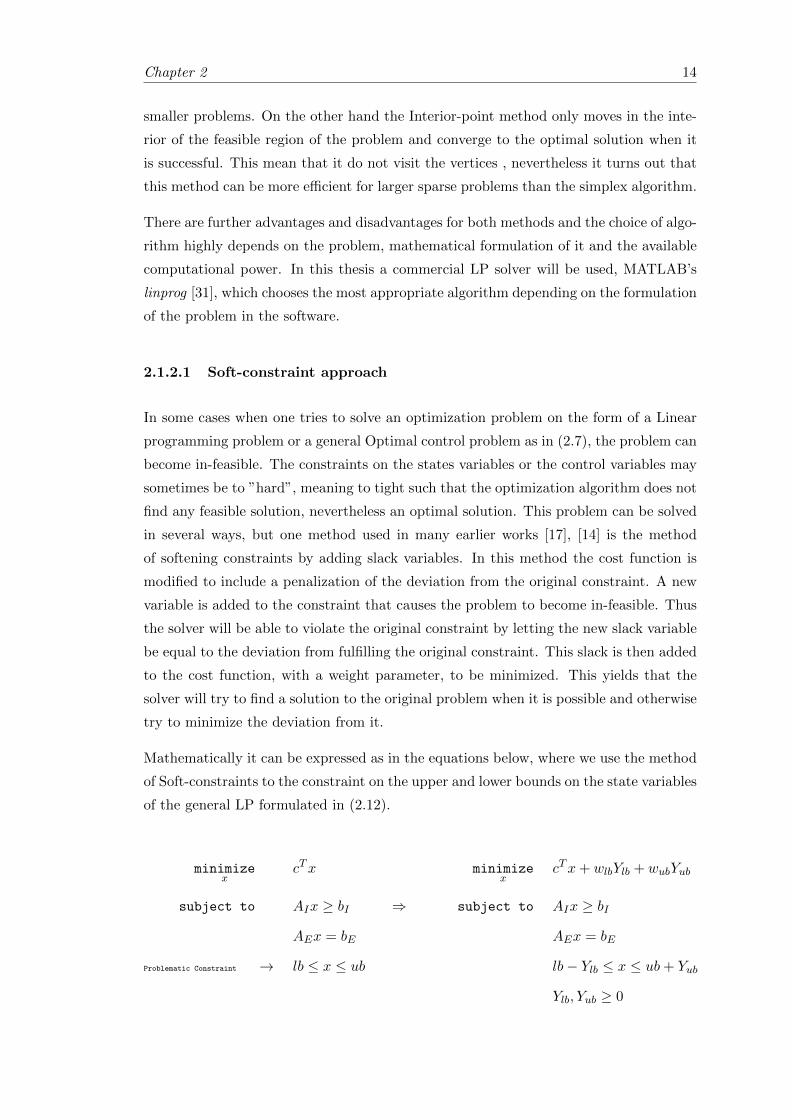
minimizex

cTx minimizex

cTx+ wlbYlb + wubYub

subject to AIx ≥ bI ⇒ subject to AIx ≥ bI

AEx = bE AEx = bE

Problematic Constraint → lb ≤ x ≤ ub lb− Ylb ≤ x ≤ ub+ Yub

Ylb, Yub ≥ 0

Chapter 2 15

In the above equations we have to the left the general LP formulation as stated above.

If we assume that the problematic constraint is the upper and lower bounds on the state

variables we can use the approach of softening the constraint as is shown to the right in

the equations above. We introduce the slack variables Ylb and Yub, and make them non-

negative. These variables are introduced in the concerned constraint as can be see above

to the right. They are also introduced in the cost functions with corresponding weight

parameters wlb and wub, which sets the ”importance” of keeping the original constraint

or not. If these weights have higher values we penalize deviations harder and the solver

will in greater extent avoid deviations from the original constraint. If the weights have

lower values the solver might find optimal solutions where the slack variables are non

zero, thus breaking the original constraint. This is set depending on the problem and

the meaning of the constraint in the model [32].

This method can also be applied as a modelling strategy when modeling systems with

constraints that the solver should be able to break at some point but with a following

cost. For example the speed limit on a road. The constraint could be that the velocity

of a vehicle should be kept under the speed limit but it should also be able to ”break”

the constraint, the speed limit, if necessary. The solver should avoid this, and thus one

includes this violation of the constraint with a corresponding cost in the cost function.

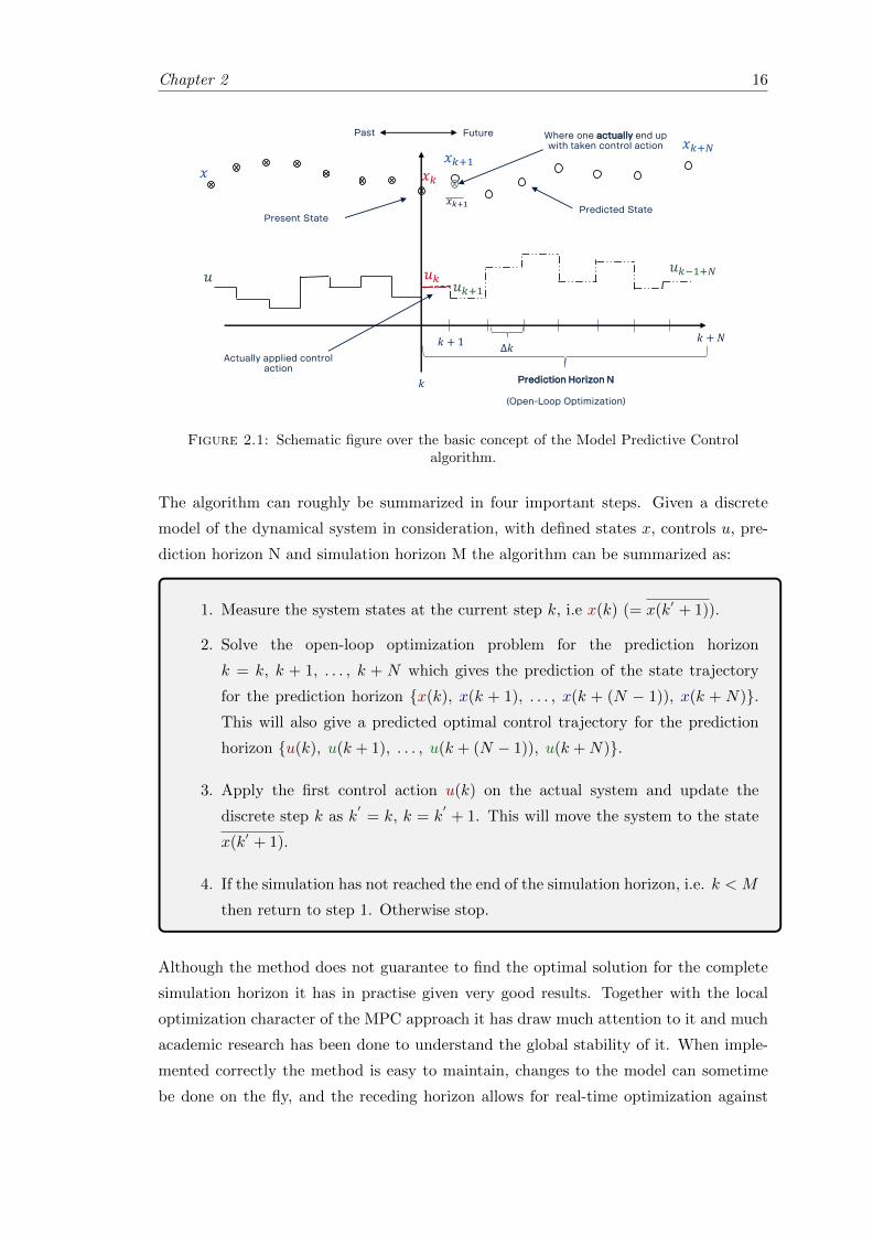
2.1.3 MPC- Model Predictive Control

Model Predictive control (MPC) is an advanced and frequently used optimization method

that is used to solve Optimal control problems in a receding horizon fashion. The method

is based on an iterative process where the system or plant is sampled at each iteration

after which an open loop optimization for a specified prediction horizon is performed.

From this a predicted state trajectory and corresponding optimal control trajectory is

computed using numerical algorithms for the defined prediction horizon. Then the first

control is applied on the system or plant and the process is repeated for the next iteration

step. The prediction horizon keeps on being shifted forward and thus the method also

has the name Receding Horizon Control. In Figure 2.1 below we see the basic concept

of the MPC algorithm.

Chapter 2 16

Title and Content

11 April 2018 Info class internal Department / Name / Subject 2

𝑢

𝑥

𝑥𝑘+𝑁

𝑥𝑘𝑥𝑘+1

𝑢𝑘−1+𝑁𝑢𝑘 𝑢𝑘+1

Prediction Horizon N

(Open-Loop Optimization)

Present StatePredicted State

𝑥𝑘+1

Actually applied control action

Where one actually end up with taken control action

∆𝑘

Past Future

𝑘

𝑘 + 1 𝑘 + 𝑁

Figure 2.1: Schematic figure over the basic concept of the Model Predictive Controlalgorithm.

The algorithm can roughly be summarized in four important steps. Given a discrete

model of the dynamical system in consideration, with defined states x, controls u, pre-

diction horizon N and simulation horizon M the algorithm can be summarized as:

1. Measure the system states at the current step k, i.e x(k) (= x(k′ + 1)).

2. Solve the open-loop optimization problem for the prediction horizon

k = k, k + 1, . . . , k + N which gives the prediction of the state trajectory

for the prediction horizon {x(k), x(k + 1), . . . , x(k + (N − 1)), x(k + N)}.This will also give a predicted optimal control trajectory for the prediction

horizon {u(k), u(k + 1), . . . , u(k + (N − 1)), u(k +N)}.

3. Apply the first control action u(k) on the actual system and update the

discrete step k as k′

= k, k = k′+ 1. This will move the system to the state

x(k′ + 1).

4. If the simulation has not reached the end of the simulation horizon, i.e. k < M

then return to step 1. Otherwise stop.

Although the method does not guarantee to find the optimal solution for the complete

simulation horizon it has in practise given very good results. Together with the local

optimization character of the MPC approach it has draw much attention to it and much

academic research has been done to understand the global stability of it. When imple-

mented correctly the method is easy to maintain, changes to the model can sometime

be done on the fly, and the receding horizon allows for real-time optimization against

Chapter 2 17

hard constraints [33]. Thus, although the sub-optimal character of the algorithm it will

suit the purposes of this thesis.

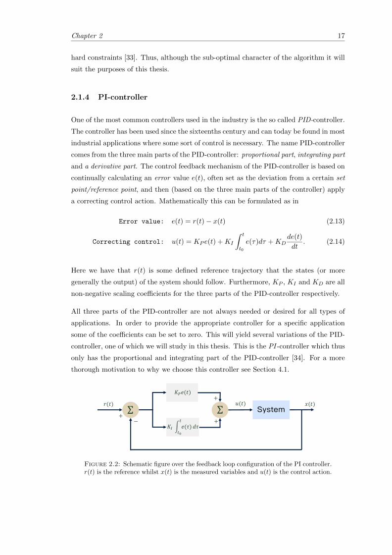
2.1.4 PI-controller

One of the most common controllers used in the industry is the so called PID-controller.

The controller has been used since the sixteenths century and can today be found in most

industrial applications where some sort of control is necessary. The name PID-controller

comes from the three main parts of the PID-controller: proportional part, integrating part

and a derivative part. The control feedback mechanism of the PID-controller is based on

continually calculating an error value e(t), often set as the deviation from a certain set

point/reference point, and then (based on the three main parts of the controller) apply

a correcting control action. Mathematically this can be formulated as in

Error value: e(t) = r(t)− x(t) (2.13)

Correcting control: u(t) = KP e(t) +KI

∫ t

t0

e(τ)dτ +KDde(t)

dt. (2.14)

Here we have that r(t) is some defined reference trajectory that the states (or more

generally the output) of the system should follow. Furthermore, KP , KI and KD are all

non-negative scaling coefficients for the three parts of the PID-controller respectively.

All three parts of the PID-controller are not always needed or desired for all types of

applications. In order to provide the appropriate controller for a specific application

some of the coefficients can be set to zero. This will yield several variations of the PID-

controller, one of which we will study in this thesis. This is the PI -controller which thus

only has the proportional and integrating part of the PID-controller [34]. For a more

thorough motivation to why we choose this controller see Section 4.1.

Title and Content

11 April 2018 Info class internal Department / Name / Subject 3

System𝑟(𝑡) Σ Σ

𝐾𝑃𝑒(𝑡)

𝐾𝐼 න𝑡0

𝑡𝑒(𝜏) 𝑑𝜏

+−

+

+

𝑢(𝑡) 𝑥(𝑡)

Figure 2.2: Schematic figure over the feedback loop configuration of the PI controller.r(t) is the reference whilst x(t) is the measured variables and u(t) is the control action.

Chapter 2 18

The PI-controller will not give or guarantee the optimal control function and often

the tuning of the two parameters KP and KI will mean some work to ensure a stable

and responsive controller. Tuning these coefficients must be done for each application

separately. This because the characteristics of the response from the controller heavily

depends on the response from the system itself and possible signal delays in the feedback

system. Typically, with prior knowledge about the system the controller is applied

to, these coefficient can be given approximate values that give stable results. Further

refinements of the tuning of the parameters, and thus the controller, can often be done

with more advanced tuning methods or by empirically experimenting with the step

response of the feedback system shown in Figure 2.2.

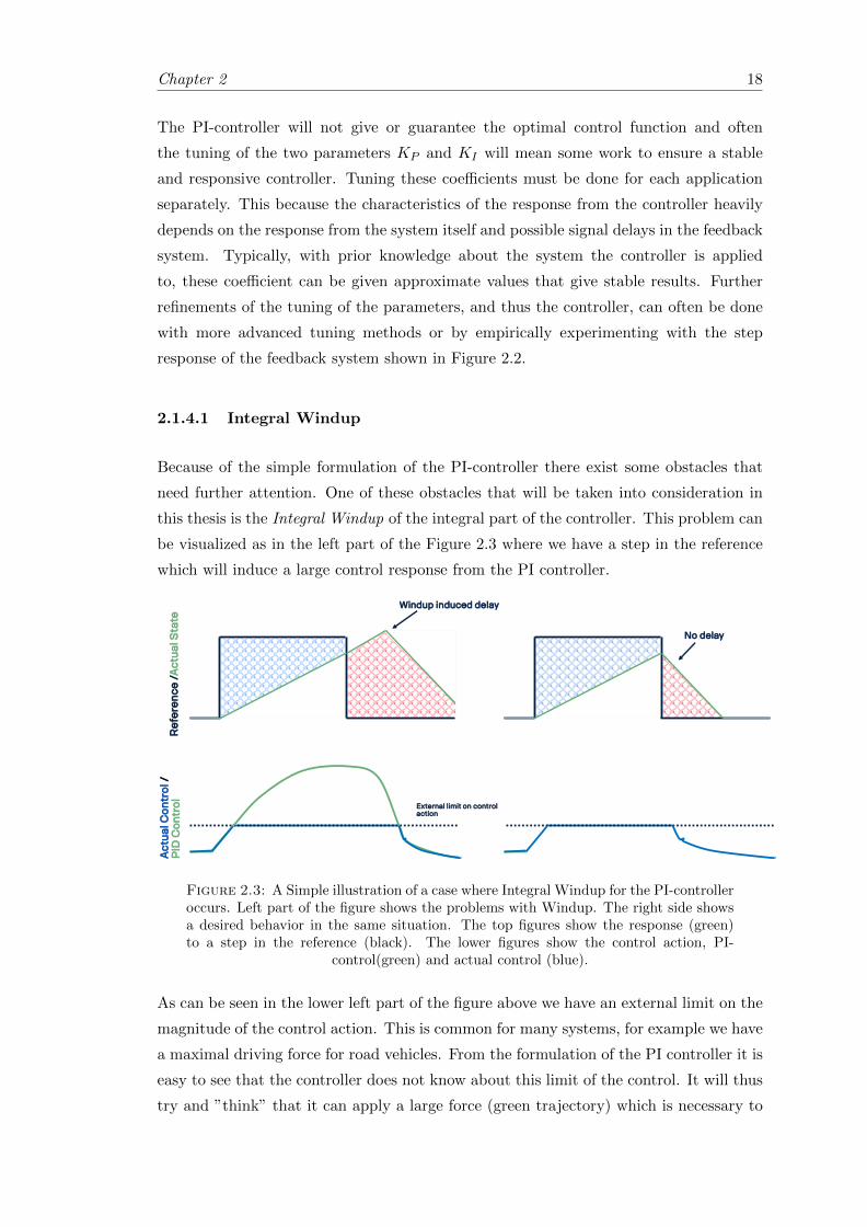
2.1.4.1 Integral Windup

Because of the simple formulation of the PI-controller there exist some obstacles that

need further attention. One of these obstacles that will be taken into consideration in

this thesis is the Integral Windup of the integral part of the controller. This problem can

be visualized as in the left part of the Figure 2.3 where we have a step in the reference

which will induce a large control response from the PI controller.

Windup induced delay

Re

fere

nc

e /

Ac

tua

l Sta

teA

ctu

al C

on

tro

l /P

ID C

on

tro

l

External limit on control action

No delay

Figure 2.3: A Simple illustration of a case where Integral Windup for the PI-controlleroccurs. Left part of the figure shows the problems with Windup. The right side showsa desired behavior in the same situation. The top figures show the response (green)to a step in the reference (black). The lower figures show the control action, PI-

control(green) and actual control (blue).

As can be seen in the lower left part of the figure above we have an external limit on the

magnitude of the control action. This is common for many systems, for example we have

a maximal driving force for road vehicles. From the formulation of the PI controller it is

easy to see that the controller does not know about this limit of the control. It will thus

try and ”think” that it can apply a large force (green trajectory) which is necessary to

Chapter 2 19

follow the reference. In reality the applied force will be clamped by the external limit

(blue trajectory). At the same time the integral part of the controller will accumulate

a large value (see the blue area in the top left part of the figure). This will give rise

to the so called ”Windup” delay and overshoot that can be seen in the figure. Because

the accumulated value of the integral part has grown so large it will induce a delayed

response to the change, step back, of the reference. It has to accumulate some values of

different sign before it gives a response to the step back of the reference.

The desired behavior of the PI-controller in a situation as the one shown in the left part

of Figure 2.3 is the one shown in the right part of the same figure. The actual control

output should follow the external limit and the response of the PI-controller should be

quick and stable for changes in the reference signal. This problem is common for the

PI-controller and there exists many solutions to the problem in the literature [35], [36].

The most common solution is to clamp both the integral part of the PI-controller as

well as the resulting control action. Exactly how this is done is problem specific and an

empirical study will be done to find the best method for our specific problem.

2.2 FIR-filter

In this thesis simple signal processing tools will be implemented, and one of them is the

implementation of a Finite Impulse Response (FIR) filter. FIR-filters, as they also can

be called, are filters that have a finite duration of their impulse response inside a certain

limited interval and zero outside it [37]. If we introduce the interval as M points back

from the current position we can mathematically formulated the filter as in

y(n) =

M−1∑k=0

h(k)x(n− k). (2.15)

Thus we can see that the output y(n) can be formulated as a weighed linear combination

of the past M inputs x(n− k) with weight coefficients h(k), where h(k) = 0 if n− k < 0

or k >= M . One often says that this filter has a memory of M inputs back to generate

the n:th output.

The most basic type of Finite Impulse Response filter is the running average filter. This

is the filter that will be implemented in this thesis and what is referred to as the FIR-

filter. This is simply the above formulation of the FIR-filter, (2.15), where we set all

weights within the interval to h(k) = 1/M where M is the interval length and otherwise

h(k) = 0.

Chapter 2 20

2.3 Linear Interpolation and Regression

In this thesis linear interpolation and regression will be used repeatedly to make the

approximations but also to format the logged data correctly. Because of this we present

the mathematical theory behind the two mathematical tools briefly here.

2.3.1 Linear Interpolation

Linear interpolation is a mathematical tool that uses linear functions to find or construct

new data points within the interval of the known discrete data points. In this way one

can get a linear approximation of the set of data points expressed in a new basis, as long

as it is within the range of the given data.

Given two discrete data points (x1, y1) and (x2, y2) we can geometrically derive a formula

for a new data point ynew at position xnew, x1 ≤ xnew ≤ x2, by a linear function between

the two given data points and the equation for the slope. This will yield us the Linear

Interpolation formula as in

ynew = y1 + (xnew − x1)(y2 − y1)

(x2 − x1). (2.16)

This can easily be extended for a set of given data points by simple concatenation of the

linear interpolations between each pair of points. The result of a linear interpolation of

a set of points will be a new set of points in a predefined new basis. Thus we can use

this mathematical tool to change the basis of the given data points, within the range of

the given data, and thus get an approximation of the values in the new basis [38].

2.3.2 Linear Regression

Given two variables and observed data of them, one sometimes want to find or model the

mathematical relationship between them. One powerful mathematical tool to achieve

this is the tool of mathematical regression. There exists many forms of regression and

one of the simplest ones is the simple Linear regression. This method attempts to find a

linear relationship between the two variables given the observed data, thus estimating the

parameters in the linear model of the mathematical relationship between the variables.

If we call the two variables for y and x, and are given a set of n observed data points for

the two variables {yi, xi}ni=1, we can model the linear relationship between them as in

yi = βxi + εi, i = 1, . . . , n. (2.17)

Chapter 2 21

Here we introduced the estimation parameter β and error term εi. Thus the goal is

to try to find the value of the estimation parameter with the introduced error or noise

term εi describing all other factors that affect yi other than the xi values. This can

be seen as a random variable [38]. To estimate the parameter, and thus the linear

relationship between the variables, one has to implement a separate method. One of the

most common methods is the method of least-squares. The method tries to minimize

the sum of the squared distance to the linear model and leads to a neat closed form

solution shown below as

β =(∑

(xixi)−1)(∑

xiyi

). (2.18)

An important assumption for this method is that we assume that the error term has

finite variance and is uncorrelated to all xi. This can be problematic for experimental

or observed data. In this thesis we will only have two variables and use the simple linear

regression formulation. The details of the parameter estimation will not be studied in

depth and commercial estimation tools will be used for this purpose [39].

2.4 Zero Order Hold

In order to discretize a continuous time-invariant state space realization we will be using

the method of Zero Order Hold. This because it gives us an exact match between

the continuous and discrete time systems for piece-wise constant inputs. For the MPC

algorithm we will get a constant control actions for each discrete step. This will also hold

for the PI approach and thus the zero order hold will suit the purpose of discretizing

our system model well.

Zero order hold is a method for converting a continuous time system into a discrete one.

This by holding the input signal constant over each sample period. If we are given a

continuous state space realization of a system, i.e

x(t) = Acx(t) +Bcu(t) (2.19)

we can derive the general solution to the system as in

x(t) = Φ(t− t0)x(0) +

∫ t

t0

Φ(t− τ)Bcu(τ)dτ. (2.20)

Here we have introduced the state transition matrix Φ as in (2.2). Now, if we apply the

zero order hold on the input signal u(t) with the sample time T , initial time t0 = kT

and final time tf = (k + 1)T we get that

Chapter 2 22

u(t) = u(kT ), kT ≤ t ≤ (k + 1)T

x(t) = Φ(t, kT )x(kT ) +∫ tkT Φ(t, τ)Bcdτ u(kT ), kT ≤ t ≤ (k + 1)T

(2.21)

where we have moved out the control from the integral because we only consider one

sample time above where the control is held constant [40]. From the above formulation,

(2.21), we can now formulate the discrete system as

x[k + 1] = Adx[k] +Bdu[k] (2.22)

where the matrices Ad and Bd are given by

Ad = Φ((k + 1)T, kT ), (2.23)

Bd =

∫ (k+1)T

kTΦ((k + 1)T, τ)Bcdτ. (2.24)

For time-invariant system we can simplify the notation even further and with some basic

mathematical system theory [28] get that the discrete, zero order hold, system can be

expressed according to

x[k + 1] = Adx[k] +Bdu[k] where

Ad = eAcT

Bd =∫ T

0 eAcτdτBc.(2.25)

Where we again have that the sample length is given by T .

Chapter 2 23

2.5 Linear and Nonlinear ARX Model

There exists today numerous methods for predicting, forecasting or estimating the future

behavior of a system. Many of the methods are collected into different subcategories of

system identification methods. These are often called grey box models, black box models

or ad-Hoc/combined models [18]. In this thesis, and under this section specifically,

we will present one black box model called the Nonlinear Auto Regressive eXogenous

(NARX) model.

In a block box model the system is modeled, as the name suggest, as a black box

without any knowledge about the details of the internals but only with knowledge about

the inputs and outputs of the system. One such model is the (linear) Auto Regressive

eXogenous model (ARX), which is given by the following equation

y(k) + a1y(k − 1) + . . .+ anay(k − na) = b1u(k − nk) + . . .+ bnbu(k − nk − nb + 1)

(2.26)

where y and u are the outputs and inputs respectively of the system, k is the discrete time

instance, nk is the delay (in terms of numbers of samples) between input and output,

na is the number of autoregressors and nb is the number of exogenous regressors. The

triplet (na, nb, nk) is often called the model order [41]. From the (2.26) we can derive a

compact formulation of the predicted next output as in

y(k) = zT (k)Θ where

z(k) = [y(k − 1), . . . , y(k − na), u(k − nk), . . . , u(k − nk − nb + 1))]

Θ = [−a1, . . . ,−ana , b1, . . . , bnb].

(2.27)

The goal of the model is thus to find the regressor parameters Θ using the past inputs and

outputs of the system such that the prediction error is minimized. For ARX models this

can for example be done by using the method of least squares which has the advantage

of a closed form solution, as mentioned earlier in Section 2.3.2.

Now if the system itself has a nonlinear behavior one would also want the model to be

able to ”catch” this behavior to make a better prediction. Based on the linear model

presented above a nonlinear ARX model, the NARX model, can be formulated. This

model uses a nonlinear mapping F between the output and inputs of the system. This,

rather than the weighted sum present in the linear ARX model. Mathematically we can

formulate this as in

y(k) = F (z(k)) where F (z(k)) = g(z(k)− r(k)) + LT (z(k)− r(k)) + d. (2.28)

Chapter 2 24

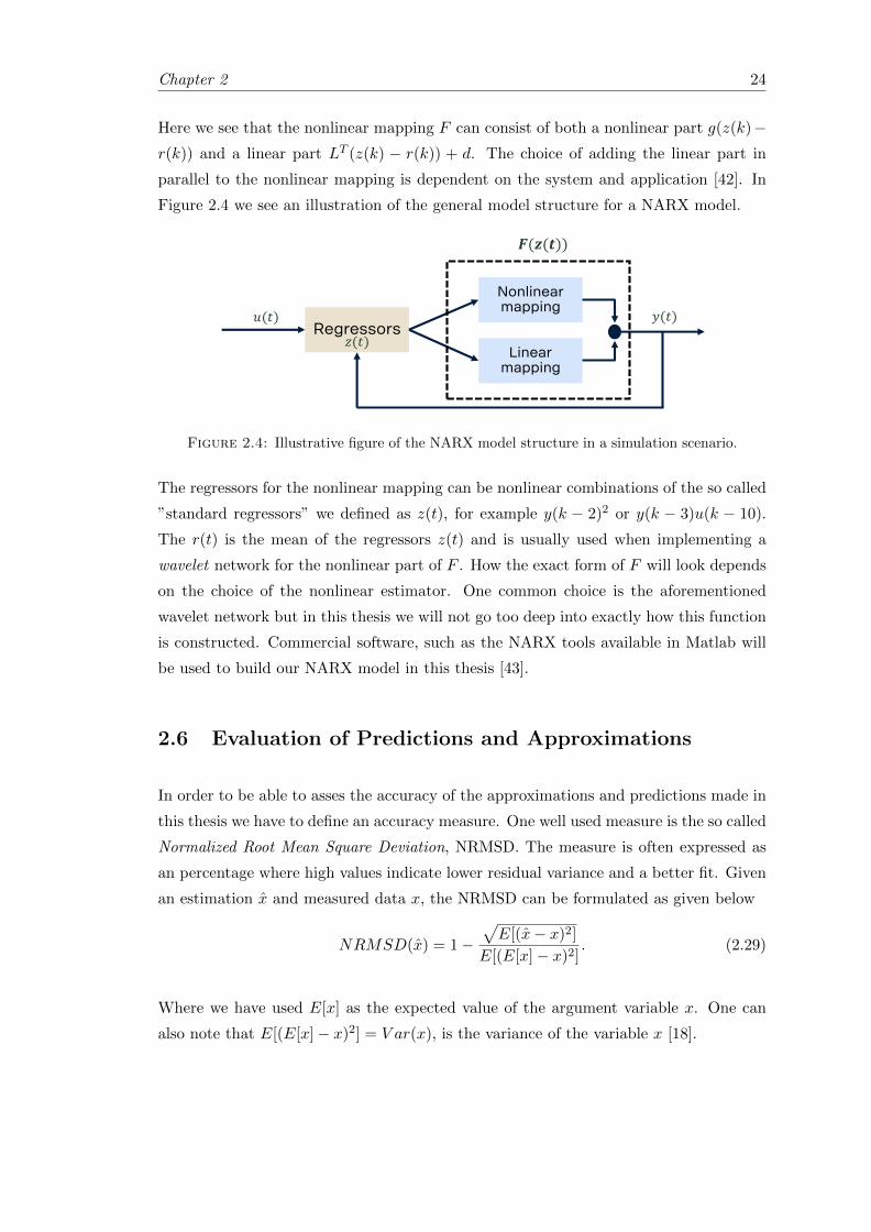
Here we see that the nonlinear mapping F can consist of both a nonlinear part g(z(k)−r(k)) and a linear part LT (z(k) − r(k)) + d. The choice of adding the linear part in

parallel to the nonlinear mapping is dependent on the system and application [42]. In

Figure 2.4 we see an illustration of the general model structure for a NARX model.

Title and Content

11 April 2018 Info class internal Department / Name / Subject 5

Regressors

Nonlinear mapping

Linear mapping

𝑢(𝑡)

𝑧(𝑡)

𝑦(𝑡)

𝑭(𝒛(𝒕))

Figure 2.4: Illustrative figure of the NARX model structure in a simulation scenario.

The regressors for the nonlinear mapping can be nonlinear combinations of the so called

”standard regressors” we defined as z(t), for example y(k − 2)2 or y(k − 3)u(k − 10).

The r(t) is the mean of the regressors z(t) and is usually used when implementing a

wavelet network for the nonlinear part of F . How the exact form of F will look depends

on the choice of the nonlinear estimator. One common choice is the aforementioned

wavelet network but in this thesis we will not go too deep into exactly how this function

is constructed. Commercial software, such as the NARX tools available in Matlab will

be used to build our NARX model in this thesis [43].

2.6 Evaluation of Predictions and Approximations

In order to be able to asses the accuracy of the approximations and predictions made in

this thesis we have to define an accuracy measure. One well used measure is the so called

Normalized Root Mean Square Deviation, NRMSD. The measure is often expressed as

an percentage where high values indicate lower residual variance and a better fit. Given

an estimation x and measured data x, the NRMSD can be formulated as given below

NRMSD(x) = 1−√E[(x− x)2]

E[(E[x]− x)2]. (2.29)

Where we have used E[x] as the expected value of the argument variable x. One can

also note that E[(E[x]− x)2] = V ar(x), is the variance of the variable x [18].

Chapter 3

Vehicle Models

In this chapter we will present the overall system model for both the HDV as well as

for the preceding vehicle. The vehicle model for the HDV is based on Newton’s second

law and do not include any advanced powertrain properties. It takes the external as

well as the controllable forces into consideration and constitutes a simple force based

model for the HDV, which is seen as a point mass. First the basic model for the HDV

is presented followed by the two system extensions, regenerative braking and distance

dependent air drag coefficient. The discretized versions of the models are derived and

lastly some notes on the preceding vehicle are given.

The basic force model of the vehicle dynamics are inspired by [8] and [22]. The regener-

ative braking extension is modeled after the methodology used in [10] and the air drag

coefficient extension is inspired by the works done in [44], [45] and [46].

3.1 Vehicle Model

In this thesis we implement a simple vehicle model for the HDV where we do not take

any advanced powertrain aspects into consideration. The vehicle is seen as a point mass

with external forces acting on it as well as controllable forces, which we are able to

control directly. The forces that we consider in this thesis are only the forces acting

along the longitudinal direction of the vehicle. All lateral forces are ignored, meaning

that the vehicle model developed only describes the longitudinal dynamics of the HDV.

With these assumptions and delimitation’s in mind the next step is to begin to formulate

the vehicle model by considering the well known and well used Newton’s second law,

25

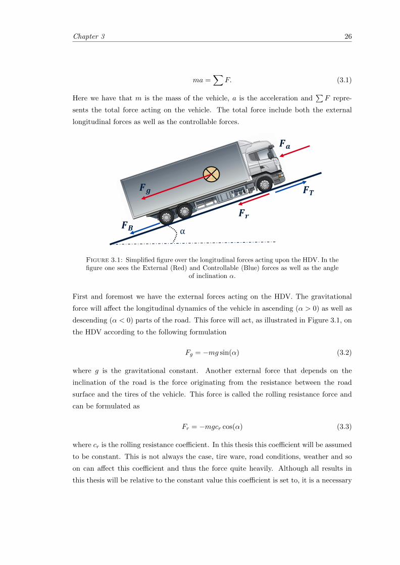
Chapter 3 26

ma =∑

F. (3.1)

Here we have that m is the mass of the vehicle, a is the acceleration and∑F repre-

sents the total force acting on the vehicle. The total force include both the external

longitudinal forces as well as the controllable forces.

Title and Content

11 April 2018 Info class internal Department / Name / Subject 6

α

𝑭𝒈

𝑭𝒂

𝑭𝒓

𝑭𝑻

𝑭𝑩

Figure 3.1: Simplified figure over the longitudinal forces acting upon the HDV. In thefigure one sees the External (Red) and Controllable (Blue) forces as well as the angle

of inclination α.

First and foremost we have the external forces acting on the HDV. The gravitational

force will affect the longitudinal dynamics of the vehicle in ascending (α > 0) as well as

descending (α < 0) parts of the road. This force will act, as illustrated in Figure 3.1, on

the HDV according to the following formulation

Fg = −mg sin(α) (3.2)

where g is the gravitational constant. Another external force that depends on the

inclination of the road is the force originating from the resistance between the road

surface and the tires of the vehicle. This force is called the rolling resistance force and

can be formulated as

Fr = −mgcr cos(α) (3.3)

where cr is the rolling resistance coefficient. In this thesis this coefficient will be assumed

to be constant. This is not always the case, tire ware, road conditions, weather and so

on can affect this coefficient and thus the force quite heavily. Although all results in

this thesis will be relative to the constant value this coefficient is set to, it is a necessary

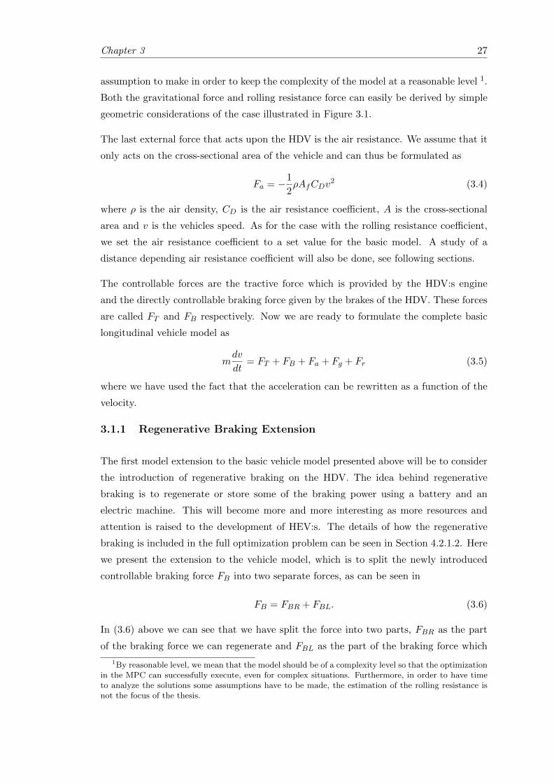
Chapter 3 27

assumption to make in order to keep the complexity of the model at a reasonable level 1.

Both the gravitational force and rolling resistance force can easily be derived by simple

geometric considerations of the case illustrated in Figure 3.1.

The last external force that acts upon the HDV is the air resistance. We assume that it

only acts on the cross-sectional area of the vehicle and can thus be formulated as

Fa = −1

2ρAfCDv

2 (3.4)

where ρ is the air density, CD is the air resistance coefficient, A is the cross-sectional

area and v is the vehicles speed. As for the case with the rolling resistance coefficient,

we set the air resistance coefficient to a set value for the basic model. A study of a

distance depending air resistance coefficient will also be done, see following sections.

The controllable forces are the tractive force which is provided by the HDV:s engine

and the directly controllable braking force given by the brakes of the HDV. These forces

are called FT and FB respectively. Now we are ready to formulate the complete basic

longitudinal vehicle model as

mdv

dt= FT + FB + Fa + Fg + Fr (3.5)

where we have used the fact that the acceleration can be rewritten as a function of the

velocity.

3.1.1 Regenerative Braking Extension

The first model extension to the basic vehicle model presented above will be to consider

the introduction of regenerative braking on the HDV. The idea behind regenerative

braking is to regenerate or store some of the braking power using a battery and an

electric machine. This will become more and more interesting as more resources and

attention is raised to the development of HEV:s. The details of how the regenerative

braking is included in the full optimization problem can be seen in Section 4.2.1.2. Here

we present the extension to the vehicle model, which is to split the newly introduced

controllable braking force FB into two separate forces, as can be seen in

FB = FBR + FBL. (3.6)

In (3.6) above we can see that we have split the force into two parts, FBR as the part

of the braking force we can regenerate and FBL as the part of the braking force which

1By reasonable level, we mean that the model should be of a complexity level so that the optimizationin the MPC can successfully execute, even for complex situations. Furthermore, in order to have timeto analyze the solutions some assumptions have to be made, the estimation of the rolling resistance isnot the focus of the thesis.

Chapter 3 28

we can not regenerate. The reason why we introduce to braking force’s, as done above,

is that all braking power can not be regenerated. The battery has a limitation on how

much power it can regenerate and thus we have to split the force into the part that can

be regenerated and the part that constitute pure braking losses. The motivation behind

this model decision will become clearer as the full optimization model is formulated.

3.1.2 Air drag Model Extension

As mentioned earlier, the air resistance coefficient will be set to a constant value if

nothing else is mentioned. In reality this will not always be the case, for example

weather and distance to the preceding vehicle will affect the air resistance on the HDV

and thus the solution. An attempt to model a varying air resistance coefficient will be

made in this thesis, with respect to the distance to the preceding vehicle.

The intermediate distance between the HDV and the preceding vehicle is denoted as d.

The air drag coefficient can be modeled as a function of this distance, thus we introduce

Cd(d) = CDG(d). Here we model the distance dependent air drag coefficient Cd(d) as the

product of the fixed parameter value CD and the air drag coefficient reduction function

G(d). This function is derived using empirical experiments of the air drag reduction of

HDV:s driving in platoon formation [47].Title and Content

7

20

40

60

10 20 30 40 50 60 70 80

Linear approximation, H(d)

Measured Data

𝑪 𝑫𝑹𝒆𝒅

𝒖𝒄𝒕𝒊𝒐𝒏

[%]

𝑰𝒏𝒕𝒆𝒓 − 𝒗𝒆𝒉𝒊𝒄𝒍𝒆 𝑫𝒊𝒔𝒕𝒂𝒏𝒄𝒆 [𝒎]

Figure 3.2: Experimental data over the reduction of the air drag coefficient for HDV:swhilst driving in a platoon formation based on [47]. Red line is the linear approximation

for the reduction from one preceding HDV.

Chapter 3 29

In Figure 3.2 we see the experimental data along with a linear approximation of the

reduction of the coefficient as a function of the distance to the preceding HDV. This

approximation has been made with linear regression where we have used that G(d) can

be expressed as

G(d) =

(1− H(d)

100

)(3.7)

where H(d) was approximated to

H(d) = Q1d+Q2 = −0.45d+ 43. (3.8)

This will only hold for a maximum inter-vehicle distance of 95m, longer distances will

not be considered in this thesis. In this case we assume that the preceding vehicle is

another HDV. Thus, we can formulate the air resistance for this model extension as

Fa(d) = −1

2ρAfCdv

2 = −1

2ρAf

(1− −0.45d+ 43

100

)v2. (3.9)

Further details on how this will be implemented into the optimization model can be seen

in the following sections and in the next chapter.

3.1.3 States and Disrectized Vehicle model

The vehicle models developed above are all in the continuous time domain. In order

to simulate the system the vehicle models have to be discretized. In this section we

present the nonlinear discretization of the basic vehicle model, which will be used as the

approximation of the real system in the MPC algorithm.

First and foremost we make the model choice to convert the vehicle model from the time

domain (t) to the spatial domain (s) and introduce the state variable K, representing

the kinetic energy of the HDV. We make the quite unusual choice of having the position

s as the independent variable, rather than the usual time variable t, because the road

topography as well as speed limits are given as a function of position and not time. This

information are usually collected from maps where these variables are given in spatial

coordinates. Thus it is natural to convert the system to the position domain where, as

we soon will see, we get additional mathematical advantages by the state choice K(s).

Chapter 3 30

Now, we begin by rewriting the left hand side of (3.5) to the new spatial domain s. We

begin by the well know relationship between the kinetic energy K and the velocity v

which can be written as

K(s) =1

2mv2. (3.10)

Furthermore the transition of the derivative between the spatial and time domain can

be derived as

d

ds=dt

ds

d

dt=

1

v

d

dt(3.11)

which we in combination with (3.10) can rewrite the left hand side of (3.5) as

mdv

dt= mv

dv

ds=

1

2md

dsv2 =

d

ds

(1

2mv2

)=

d

dsK(s). (3.12)

The right hand side of the basic vehicle model can easily be transformed to the spatial

domain as

FT + FB −mgsin(α(s))︸ ︷︷ ︸Fg

−mgcrcos(α(s))︸ ︷︷ ︸Fr

− ρAfCDK(s)

m︸ ︷︷ ︸Fa

(3.13)

where we used (3.10) to rewrite the air resistance. With this in mind we can now for-

mulate the continuous state space realization of the basic vehicle model, the continuous

vehicle model (CVM) as

K(s) =

(−ρAfCDm

)︸ ︷︷ ︸

Ac

K(s) +[

1 1]

︸ ︷︷ ︸Bc

[FT (s)

FB(s)

]︸ ︷︷ ︸

u(s)

−mg(sin(α(s)) + crcos(α(s)))

(CVM)

where we introduced the continuous domain matrices Ac and Bc according to the nota-

tion in Section 2.4. Here we also can observe the additional mathematical advantage of

the spatial domain in combination of the state choice of the kinetic energy. The relation

between the derivative of the kinetic energy with respect to the position and the sum

of the forces becomes linear. This will be advantageous when implementing the MPC

algorithm.

In order to discretize the model we will here use the zero order hold method presented in

the previous chapter. Defining the discrete control vector as the two controllable forces

FT and FB, as seen below

uk =

[FT,k

FB,k

](3.14)

Chapter 3 31

the sample distance as ∆s and using the introduced state variable Kk we can now write

the basic vehicle model as a state space representation on discrete form, the discrete

vehicle model (DVM) as

Kk+1 = AdKk +Bduk + hd,k (DVM)

where Ad, Bd and hd,k have been derived using the continuous (CVM) model and the

theory behind zero order hold approximations. Here we have that

Ad = eAc∆s, (3.15)

Bd =

(eAc∆s − 1

Ac

)Bc, (3.16)

hd,k = −1

2BdB

Tc mg(sin(αk) + crcos(αk)). (3.17)

The kinetic energy of the HDV has been introduced as the only state of the model so

far. It will turn out that it will also be useful to define the time as a state variable. The

choice of time as the additional state variable will become clearer in the Methodology

chapter, but to for now we just accept it as a reasonable model choice.

We introduce the state variable time as t. The update equation for the time variable

will not depend explicitly on the control and we choose to approximate it with Eular

forward. Generally we can write the update equation for the time variable now as

tk+1 = tk + ∆tk. (3.18)

To find ∆tk we assume constant acceleration between sampling points. In Figure 3.3 we

see an illustration of the scenario between two sample points.

Title and Content

11 April 2018 Info class internal Department / Name / Subject 8

K

𝑆𝑘 𝑆𝑘+1

𝐾𝑘

𝐾𝑘+1

𝑡𝑘

𝑡𝑘+1

∆𝑆𝑆

𝑲𝒊𝒏𝒆𝒕𝒊𝒄𝑬𝒏

𝒆𝒓𝒈𝒚

[𝑱]

𝑷𝒐𝒔𝒊𝒕𝒊𝒐𝒏 [𝒎]

Figure 3.3: An illustration of the scenario between two sample points. Given thekinetic energy and the time.

Chapter 3 32

From the figure above we can approximate the constant acceleration between two sample

points as

∆K

m∆s=Kk+1 −Kk

m∆s= ak. (3.19)

Given the assumption of constant acceleration ak between two sample points we can use

the following formula

∆s = vk∆t+1

2ak∆t

2 (3.20)

to derive the following formula for ∆t

∆t = −vkak

+ sign(ak)

√(vkak

)2

+2∆s

ak(3.21)

where vk =√

2Kk/m and sign(ak) is the sign function returning -1 if ak < 0 and 1 if

ak > 0. For the case the approximated value of the acceleration becomes zero we assume

constant velocity between two sample points.

This give us now the complete nonlinear discretized state space realization of the basic

vehicle model (NDBVM) asKk+1 = AdKk +Bduk + hd,k

tk+1 = tk + ∆tk

(NDBVM)

where all matrices and parameters are given according to the above equations.

3.1.3.1 Model extension considerations

In this case the model extension will only have a minor affect on the nonlinear discre-

itization of the state space realization. For the first model extension, the regenerative

braking case, the change consist only of substituting the control vector

uk =

FT,k

FBR,k

FBL,k

, Bc =[

1 1 1]

(3.22)

and the Bc matrix as shown above. For the second model extension, distance dependent

air drag coefficient, the change is to set the Ac matrix to the value shown below

Ac,k = −ρAfCd(dk)

m, where Cd(dk) =

(1− −0.45dk + 43

100

). (3.23)

Chapter 3 33

Where dk is the current distance to the preceding vehicle. This can be computed sep-

arately by using linear interpolation (given that we know the velocity of the preceding

vehicle for some horizon [s, s+ ∆s ·M ], where M is large enough) 2.

3.1.4 Linear Vehicle model

The (NDBVM) model can be used as the state update equation in the optimization

model of the MPC algorithm as well, and not only as the approximative model of the real

system. The disadvantages with this approach are many, for example the computational

complexity of the optimization problem will become higher which will most probably

mean a longer execution time of the MPC algorithm. Since we are trying to achieve

an MPC model that could be solved online on an HDV, with limited computational

resource, a quick and computationally light algorithm is desirable. One way to do this

is to formulate the optimization model as an LP-problem. This in turn means that we

will linearize the discrete vehicle model (NDBVM) above to achieve linear state update

equations.

In the spatial domain we know the sample distance ∆s but need to approximate the

sample time ∆tk. This can be done, assuming a small sample distance and constant

velocity vk between sample points, as

∆tk ≈∆s

vk= ∆s

√m

2K

−1/2k (3.24)

where we used (3.10) to rewrite the velocity vk in terms of the state variable Kk. The

sample time approximation in (3.24) is not linear, thus we have to linearize the approx-

imation with respect to the kinetic energy. This can be done using a first order Taylor

approximation as

∆tk = ∆s

√m

2K

−1/2k

= ∆s

√m

2

(1√Kk

)

= ∆s

√m

2

(K

−1/20,k − 1

2K

−3/20,k (Kk −K0,k)

)

= ∆s

√m

2

(3

2K

−1/20,k − 1

2K

−3/20,k Kk

)

= 3∆s

√m

8K

−1/20,k −∆s

√m

8K

−3/20,k Kk (3.25)

2This will only be considered in the Deterministic case, thus we will have information about thepreceding vehicles trajectory into the future. Furthermore, ”large enough” means that the interval is solarge that it at least reaches the time point of our own vehicle.

Chapter 3 34

where we linearized around a reference trajectory K0,k. The exact choice of this reference

trajectory is explained in the next chapter. This will give us the linear update equation

for the time variable as

tk+1 = tk + 3∆s

√m

8K

−1/20,k −∆s

√m

8K

−3/20,k Kk

= AL,4tk +AL,3,kKk + hL,t,k (3.26)

where we have introduced the parameters

AL,4 = 1, (3.27)

AL,3,k = −∆s

√m

8K

−3/20,k , (3.28)

hL,t,k = 3∆s

√m

8K

−1/20,k . (3.29)

For the update equation for the kinetic energy we already have a linear discrete formu-

lation. This was given by the zero order hold approximation in (DVM).

Now we can formulate the complete linear discretized basic vehicle model (LDBVM)

using the introduced parameters in the equations above as[Kk+1

tk+1

]=

[Ad 0

AL,3,k AL,4

][Kk

tk

]+

[Bd

0

]uk +

[hd,k

hL,t,k

]. (LDBVM)

For notation purposes one can also introduce the state vector as

xk =

[Kk

tk

](3.30)

so as to make the notation cleaner.

3.1.4.1 Model extension considerations

As for the nonlinear disceretization case we will have some adaptations of the LDBVM

for the two model extension. For the case of regenerative braking we will only have a

minor adaption of the basic model. The difference being the control vector and the Bc

vector. These are changed according to

uk =

FT,k

FBR,k

FBL,k

, BL =[

1 1 1]

(3.31)

Chapter 3 35

which is the same change as for the nonlinear vehicle model extension. For the second

model extension, distance dependent air resistance coefficient, there are other required

adaptations of the basic vehicle model LDBVM. In this case we will have a nonlinear

air resistance force as

Fa,k = −ρAfCd(dk)Kk

m

= −ρAfCD(

1− Q1dk +Q2

100

)Kk

m

= −ρAfCD(

1− H(dk)

100

)Kk

m(3.32)

which we have to linearize to get a linear model. We apply the same method as for the

time update equation and use a first order multivariate Taylor expansion of (3.32) to

get the linear expression of the force Fa,k as

Fa,k ≈ ρAfCD(

1−H(d0,k)

100

)K0,k

m− ρAfCD

Q1

100

K0,k

m(dk − d0,k)

+ ρAfCD

(1−

H(d0,k)

100

)Kk −K0,k

m(3.33)

where Q1 is given by the linear regression in (3.8). Here we linearize around both the

reference kinetic trajectory K0,k as in (3.26) and a reference inter vehicle distance d0,k.

Details of how this reference distance is chosen can be seen in Section 4.4, as well as

how the variable distance dk that the optimization in the MPC algorithm should decide

upon is modeled.

Furthermore, with this formulation of the air resistance we choose to reformulate the

discrete form of the update equation of the kinetic energy. This is done because the zero

order hold formulation will become rather complex, and in the end this change will not

affect the results (assuming a small sample distance). Thus we reformulate the update

equation, in order to make the implementation easier, using Eular forward as

Kk ≈Kk+1 −Kk

∆s(3.34)

⇒ Kk+1 = Kk + ∆sKk (3.35)

⇔ Kk+1 = Kk + ∆s (FT,k + FB,k + Fg,k + Fr,k + Fa,k) (3.36)

where we in (3.36) used the right hand side of (CVM). Now, the forces are already on a

linear form and thus we can state the update equation for the kinetic energy as

Kk+1 = AL,1Kk +BLuk + hL,K,k (3.37)

Chapter 3 36

where we have introduced the parameters

AL,1 =

1−ρAf

(1− H(d0,k)

100

)∆s

m

, (3.38)

BL =[

∆s ∆s], (3.39)

hL,K,k = −mg∆s(sin(αk) + cr cos(αk)) + ρ∆sAfCDQ1

100

K0,k

m(dk − d0,k) (3.40)

and the control vector uk on the same form as in (CVM).

3.1.5 Limitations on Controllable Forces

The controllable forces, the tractive force FT and the braking force FB, have their

physical limitation depending on the system. These can be modeled as follows

0 ≤ FT,k ≤ FT,max(Kk), (3.41)

−FB,min ≤ FB,k ≤ 0 (3.42)

where we introduce some maximal tractive force as a function of the kinetic energy

FT,max(Kk) and a constant maximal braking force FB,min. The lower and upper limi-

tations respectively for the two forces are set to 0 for obvious reasons. This to separate

the two forces, a braking force is defined as negative whilst a tractive force is defined as

positive. Thus these limits are enforced on the two model variables FT,k and FB,k.

The upper limit on the tractive force can be modelled as in [10]. Here we on the one

hand have a constant maximal tractive power, PT,max, that the engine and powertrain

of the HDV can deliver. This can be reformulated to a maximal tractive force through

FT,max(Kk) =PT,maxvk

= PT,max

√m

2K

−1/2k (3.43)

where we again used (3.10) to rewrite the relation from a function of the velocity to

a function of the kinetic energy of the HDV. Because these system limitation will also

be used in the linear optimization model the expression above for the maximal tractive

force has to be linearized. A first order Taylor approximation gives that

FT,max,L(Kk) = PT,max

√m

2

(3

2K

−1/20,k − 1

2K

−3/20,k Kk

)

= 3PT,max

√m

8K

−1/20,k − PT,max

√m

8K

−3/20,k Kk

= P1 + P2Kk (3.44)

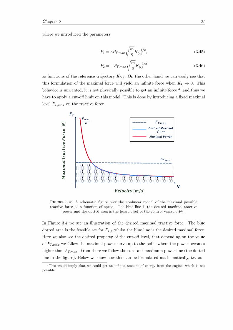
Chapter 3 37

where we introduced the parameters

P1 = 3PT,max

√m

8K

−1/20,k , (3.45)

P2 = −PT,max√m

8K

−3/20,k (3.46)

as functions of the reference trajectory K0,k. On the other hand we can easily see that

this formulation of the maximal force will yield an infinite force when Kk → 0. This

behavior is unwanted, it is not physically possible to get an infinite force 3, and thus we

have to apply a cut-off limit on this model. This is done by introducing a fixed maximal

level FT,max on the tractive force.Title and Content

11 April 2018 Info class internal Department / Name / Subject 9

v

𝑭𝑻,𝒎𝒂𝒙

𝑷𝒎𝒂𝒙𝒗 𝑭𝑻,𝒎𝒂𝒙

𝑫𝒆𝒔𝒊𝒓𝒆𝒅 𝑴𝒂𝒙𝒊𝒎𝒂𝒍𝒇𝒐𝒓𝒄𝒆

𝑴𝒂𝒙𝒊𝒎𝒂𝒍 𝑷𝒐𝒘𝒆𝒓

𝑴𝒂𝒙

𝒊𝒎𝒂𝒍

𝒕𝒓𝒂𝒄𝒕𝒊𝒗𝒆

𝑭𝒐𝒓𝒄𝒆[𝑵]

𝑽𝒆𝒍𝒐𝒄𝒊𝒕𝒚 [𝒎/𝒔]

𝑭𝑻

Figure 3.4: A schematic figure over the nonlinear model of the maximal possibletractive force as a function of speed. The blue line is the desired maximal tractive

power and the dotted area is the feasible set of the control variable FT .

In Figure 3.4 we see an illustration of the desired maximal tractive force. The blue

dotted area is the feasible set for FT,k whilst the blue line is the desired maximal force.

Here we also see the desired property of the cut-off level, that depending on the value

of FT,max we follow the maximal power curve up to the point where the power becomes

higher than FT,max. From there we follow the constant maximum power line (the dotted

line in the figure). Below we show how this can be formulated mathematically, i.e. as

3This would imply that we could get an infinite amount of energy from the engine, which is notpossible.

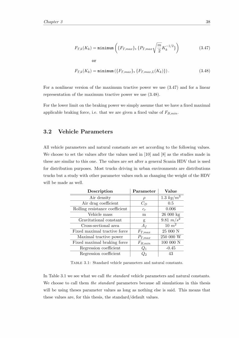
Chapter 3 38

FT,k(Kk) = minimum

({FT,max}, {PT,max

√m

2K

−1/2k }

)(3.47)

or

FT,k(Kk) = minimum ({FT,max}, {FT,max,L(Kk)}) . (3.48)

For a nonlinear version of the maximum tractive power we use (3.47) and for a linear

representation of the maximum tractive power we use (3.48).

For the lower limit on the braking power we simply assume that we have a fixed maximal

applicable braking force, i.e. that we are given a fixed value of FB,min.

3.2 Vehicle Parameters

All vehicle parameters and natural constants are set according to the following values.

We choose to set the values after the values used in [10] and [8] as the studies made in

these are similar to this one. The values are set after a general Scania HDV that is used

for distribution purposes. Most trucks driving in urban environments are distributions

trucks but a study with other parameter values such as changing the weight of the HDV

will be made as well.

Description Parameter Value

Air density ρ 1.3 kg/m3

Air drag coefficient CD 0.5

Rolling resistance coefficient cr 0.006

Vehicle mass m 26 000 kg

Gravitational constant g 9.81 m/s2

Cross-sectional area Af 10 m2

Fixed maximal tractive force FT,max 25 000 N

Maximal tractive power PT,max 250 000 W

Fixed maximal braking force FB,min 100 000 N

Regression coefficient Q1 -0.45

Regression coefficient Q2 43

Table 3.1: Standard vehicle parameters and natural constants.

In Table 3.1 we see what we call the standard vehicle parameters and natural constants.

We choose to call them the standard parameters because all simulations in this thesis

will be using theses parameter values as long as nothing else is said. This means that

these values are, for this thesis, the standard/default values.

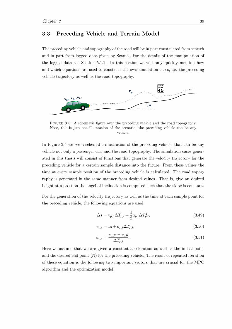
Chapter 3 39

3.3 Preceding Vehicle and Terrain Model

The preceding vehicle and topography of the road will be in part constructed from scratch

and in part from logged data given by Scania. For the details of the manipulation of

the logged data see Section 5.1.2. In this section we will only quickly mention how

and which equations are used to construct the own simulation cases, i.e. the preceding

vehicle trajectory as well as the road topography.

Title and Content

1010

𝜶

𝑽𝒑

Figure 3.5: A schematic figure over the preceding vehicle and the road topography.Note, this is just one illustration of the scenario, the preceding vehicle can be any

vehicle.

In Figure 3.5 we see a schematic illustration of the preceding vehicle, that can be any

vehicle not only a passenger car, and the road topography. The simulation cases gener-

ated in this thesis will consist of functions that generate the velocity trajectory for the

preceding vehicle for a certain sample distance into the future. From these values the

time at every sample position of the preceding vehicle is calculated. The road topog-

raphy is generated in the same manner from desired values. That is, give an desired

height at a position the angel of inclination is computed such that the slope is constant.

For the generation of the velocity trajectory as well as the time at each sample point for

the preceding vehicle, the following equations are used

∆s = vp,0∆Tp,i +1

2ap,i∆T

2p,i, (3.49)

vp,i = v0 + ap,i∆Tp,i, (3.50)

ap,i =vp,N − vp,0

∆Tp,i. (3.51)

Here we assume that we are given a constant acceleration as well as the initial point

and the desired end point (N) for the preceding vehicle. The result of repeated iteration

of these equation is the following two important vectors that are crucial for the MPC

algorithm and the optimization model

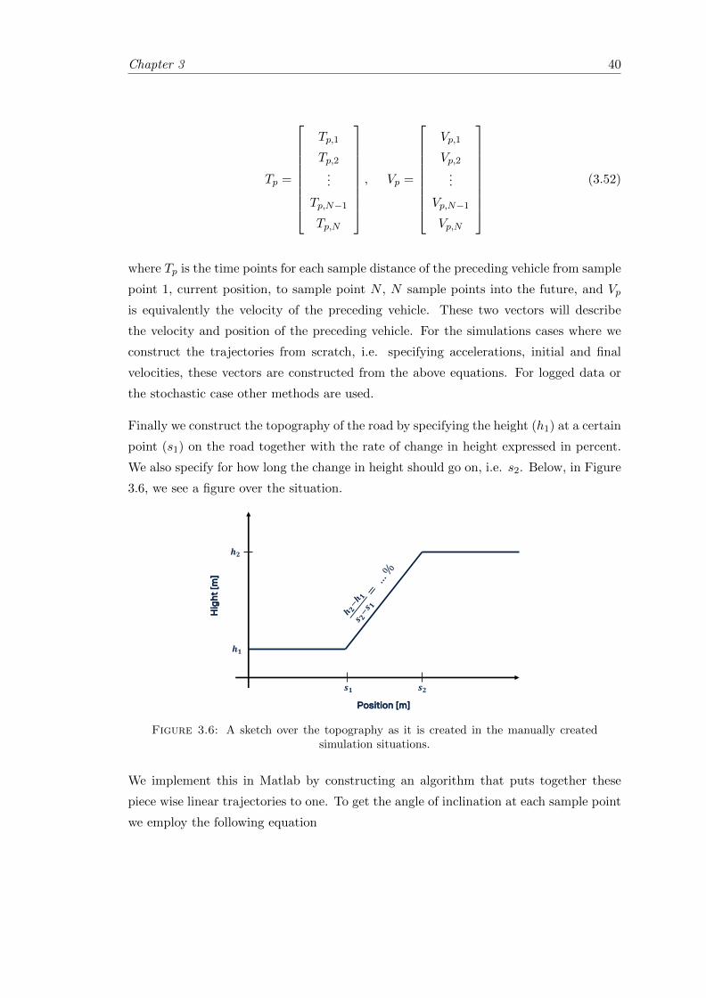
Chapter 3 40

Tp =

Tp,1

Tp,2...

Tp,N−1

Tp,N

, Vp =

Vp,1

Vp,2...

Vp,N−1

Vp,N

(3.52)

where Tp is the time points for each sample distance of the preceding vehicle from sample

point 1, current position, to sample point N , N sample points into the future, and Vp

is equivalently the velocity of the preceding vehicle. These two vectors will describe

the velocity and position of the preceding vehicle. For the simulations cases where we

construct the trajectories from scratch, i.e. specifying accelerations, initial and final

velocities, these vectors are constructed from the above equations. For logged data or

the stochastic case other methods are used.

Finally we construct the topography of the road by specifying the height (h1) at a certain

point (s1) on the road together with the rate of change in height expressed in percent.

We also specify for how long the change in height should go on, i.e. s2. Below, in Figure

3.6, we see a figure over the situation.

Title and Content

11

Hig

ht

[m]

Position [m]

𝒔𝟏 𝒔𝟐

𝒉𝟏

𝒉𝟐

Figure 3.6: A sketch over the topography as it is created in the manually createdsimulation situations.

We implement this in Matlab by constructing an algorithm that puts together these

piece wise linear trajectories to one. To get the angle of inclination at each sample point

we employ the following equation

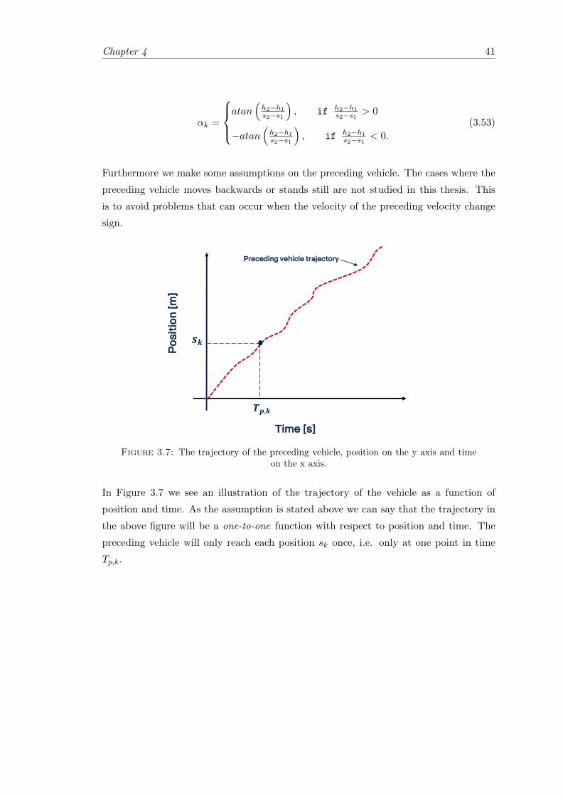
Chapter 4 41

αk =

atan

(h2−h1s2−s1

), if h2−h1

s2−s1 > 0

−atan(h2−h1s2−s1

), if h2−h1

s2−s1 < 0.

(3.53)

Furthermore we make some assumptions on the preceding vehicle. The cases where the

preceding vehicle moves backwards or stands still are not studied in this thesis. This

is to avoid problems that can occur when the velocity of the preceding velocity change

sign.

Title and Content

11 April 2018 Info class internal Department / Name / Subject 13

𝒔𝒌

𝑻𝒑,𝒌

Preceding vehicle trajectory

Po

siti

on

[m

]

Time [s]

Figure 3.7: The trajectory of the preceding vehicle, position on the y axis and timeon the x axis.

In Figure 3.7 we see an illustration of the trajectory of the vehicle as a function of

position and time. As the assumption is stated above we can say that the trajectory in

the above figure will be a one-to-one function with respect to position and time. The

preceding vehicle will only reach each position sk once, i.e. only at one point in time

Tp,k.

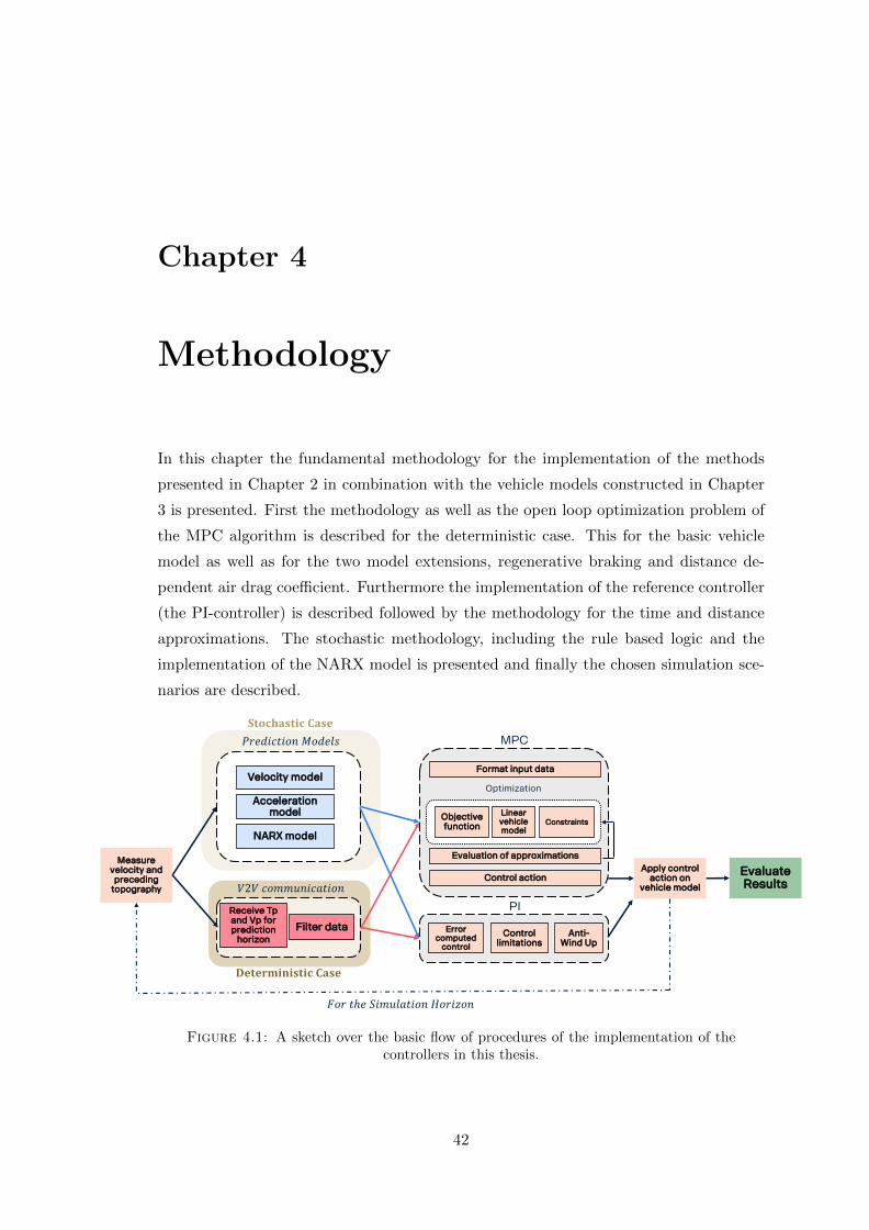
Chapter 4

Methodology

In this chapter the fundamental methodology for the implementation of the methods

presented in Chapter 2 in combination with the vehicle models constructed in Chapter

3 is presented. First the methodology as well as the open loop optimization problem of

the MPC algorithm is described for the deterministic case. This for the basic vehicle

model as well as for the two model extensions, regenerative braking and distance de-

pendent air drag coefficient. Furthermore the implementation of the reference controller

(the PI-controller) is described followed by the methodology for the time and distance

approximations. The stochastic methodology, including the rule based logic and the

implementation of the NARX model is presented and finally the chosen simulation sce-

narios are described.

Title and Content

12

Velocity model

Acceleration model

NARX model

Receive Tpand Vp for prediction

horizon

Measure velocity and preceding

topography

𝑃𝑟𝑒𝑑𝑖𝑐𝑡𝑖𝑜𝑛 𝑀𝑜𝑑𝑒𝑙𝑠

𝑉2𝑉 𝑐𝑜𝑚𝑚𝑢𝑛𝑖𝑐𝑎𝑡𝑖𝑜𝑛

Filter data

MPC

PI

Error computed

control

Control limitations

Anti-Wind Up

Optimization

Objective function

Linear vehicle model

Constraints

Evaluation of approximations

Control action

Format input data

Apply control action on

vehicle model

Evaluate Results

𝐹𝑜𝑟 𝑡ℎ𝑒 𝑆𝑖𝑚𝑢𝑙𝑎𝑡𝑖𝑜𝑛 𝐻𝑜𝑟𝑖𝑧𝑜𝑛

𝐃𝐞𝐭𝐞𝐫𝐦𝐢𝐧𝐢𝐬𝐭𝐢𝐜 𝐂𝐚𝐬𝐞

𝐒𝐭𝐨𝐜𝐡𝐚𝐬𝐭𝐢𝐜 𝐂𝐚𝐬𝐞

Figure 4.1: A sketch over the basic flow of procedures of the implementation of thecontrollers in this thesis.

42

Chapter 4 43

In Figure 4.1 we see a basic sketch over the methodology of the implementation of the

controllers in this thesis. First we measure the current velocity of the preceding vehicle

along with the future topography of the road. The road topography is often given by

maps or other V2I communication. Then, depending if we study the deterministic or

stochastic case, we either receive the future velocity trajectory for the preceding vehicle

via V2V communication for a prediction horizon or predict the same using different

strategies and models. Given the road topography and the velocity/time point trajectory

of the preceding vehicle we apply the MPC and PI controller algorithms. This will give

a control action, one each, which we apply to the current vehicle model. This is repeated

until the simulation horizon is reached. Thereafter the results are evaluated.

4.1 PI-controller

In this section we describe the methodology behind the PI-controller implemented in

this thesis. As stated in (2.13) and (2.14) we will formulate the PI-controller by an error

term and the two parts, the proportional part and the integral part. This will mean

that we can formulate the PI- controller generally as

uk = KP ek +KI

i=k∑i=0

ek, where ek = rk − xk (4.1)

where we have discretized the formulation given in the earlier mentioned equations. Here

we have that rk is the reference trajectory and xk is the state variable. The PI-controller

is implemented as the reference or benchmark controller to enable a comparison with

the developed MPC controller. The purpose of it is to act as a simple CC or as a less

intelligent driver that does not compensate for predicted future actions of the preceding

vehicle1.

Now to keep the controller simple the main goal of the controller will be to track the

preceding vehicle with a set time gap. The time gap is set to the ”three seconds rule”

which is a common rule taught to drivers in Sweden [48]. To achieve this we begin by

constructing the control error ek as can be seen below

ek = [eK,k et,k]. (4.2)

In (4.2) we make the model choice to divide the control error into two parts, one part for

each state variable. In order to get a stable and quickly tuned controller we also set the

controller to track the acceleration of the preceding vehicle. With these model choices

in mind we define the control error as

1Thus we exclude the derivative term in the PID-controller, which gives us the PI-controller.

Chapter 4 44

eK,k =

(mpV

2p,k

2−Kk

), (4.3)

et,k = (tk − Tp,k)−∆Tref (4.4)

where we have the state variables as (tk, Kk), preceding vehicle speed and point of time

at sample k as (vp,k, Tp,k) and the reference time gap the controller should track as

∆Tref . We see in (4.3) that the controller will try to minimize the relative velocity, i.e.

follow the velocity of the preceding vehicle as well as track the time gap ∆Tref to the

preceding vehicle, (4.4). We will also define the tuning parameters after this division of

the control error into two parts, one for each state, as can be seen in

KP =

[KP,1

KP,2

], KI =

[KI,1

KI,2

]. (4.5)

The tuning parameters defined above will be tuned by empirically experimenting with

the values of them until the solution is stable.

The PI-controller will also obey the limitations on the control variable, i.e. follow the

following equations

0 ≤ FT,k ≤ FT,k(Kk), (4.6)

−FB,min ≤ FB,k ≤ 0 (4.7)

where FT,k(Kk) is given by (3.47). An Anti-Windup solution will also be implemented

and derived through simple step response tests on the system. There exists, as earlier

mentioned, several ways to solve the Wind up problem for PI-controllers. To find the

solution that fits these problems and vehicle model best we will try three different

methods. These methods are:

Anti-Windup Method 1: If the PI-controller tries to implement a control action

that violates (4.6) or (4.7) we do the following

1. Cap the control action to the nearest limit, i.e. if uk > FT,k(Kk) then set

uk = FT,k(Kk) or if uk < −FB,min then set uk = −FB,min.

2. Cap the integral part of the PI-controller. This means that we let the integral part

keep the same value, stop integrating the error signal, from the point where the

control violation occurs to the point where the control given by the PI-controller

again becomes feasible.

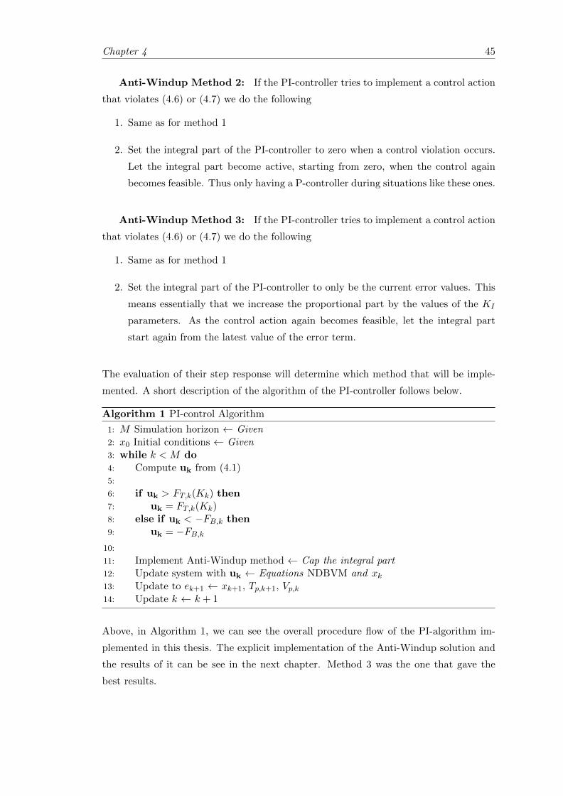
Chapter 4 45

Anti-Windup Method 2: If the PI-controller tries to implement a control action

that violates (4.6) or (4.7) we do the following

1. Same as for method 1

2. Set the integral part of the PI-controller to zero when a control violation occurs.

Let the integral part become active, starting from zero, when the control again

becomes feasible. Thus only having a P-controller during situations like these ones.

Anti-Windup Method 3: If the PI-controller tries to implement a control action

that violates (4.6) or (4.7) we do the following

1. Same as for method 1

2. Set the integral part of the PI-controller to only be the current error values. This

means essentially that we increase the proportional part by the values of the KI

parameters. As the control action again becomes feasible, let the integral part

start again from the latest value of the error term.

The evaluation of their step response will determine which method that will be imple-

mented. A short description of the algorithm of the PI-controller follows below.

Algorithm 1 PI-control Algorithm

1: M Simulation horizon ← Given2: x0 Initial conditions ← Given3: while k < M do4: Compute uk from (4.1)5:

6: if uk > FT,k(Kk) then7: uk = FT,k(Kk)8: else if uk < −FB,k then9: uk = −FB,k

10:

11: Implement Anti-Windup method ← Cap the integral part12: Update system with uk ← Equations NDBVM and xk13: Update to ek+1 ← xk+1, Tp,k+1, Vp,k14: Update k ← k + 1

Above, in Algorithm 1, we can see the overall procedure flow of the PI-algorithm im-

plemented in this thesis. The explicit implementation of the Anti-Windup solution and

the results of it can be see in the next chapter. Method 3 was the one that gave the

best results.

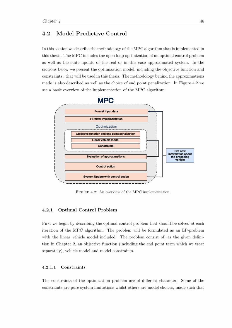
Chapter 4 46

4.2 Model Predictive Control

In this section we describe the methodology of the MPC algorithm that is implemented in

this thesis. The MPC includes the open loop optimization of an optimal control problem

as well as the state update of the real or in this case approximated system. In the

sections below we present the optimization model, including the objective function and

constraints , that will be used in this thesis. The methodology behind the approximations

made is also described as well as the choice of end point penalization. In Figure 4.2 we

see a basic overview of the implementation of the MPC algorithm.

14

MPC

Optimization

Objective function and end point penalization

Linear vehicle model

Constraints

Evaluation of approximations

Control action

Format input data

FIR filter implementation

System Update with control action

Get new information about

the preceding vehicle

Figure 4.2: An overview of the MPC implementation.

4.2.1 Optimal Control Problem

First we begin by describing the optimal control problem that should be solved at each

iteration of the MPC algorithm. The problem will be formulated as an LP-problem

with the linear vehicle model included. The problem consist of, as the given defini-

tion in Chapter 2, an objective function (including the end point term which we treat

separately), vehicle model and model constraints.

4.2.1.1 Constraints

The constraints of the optimization problem are of different character. Some of the

constraints are pure system limitations whilst others are model choices, made such that

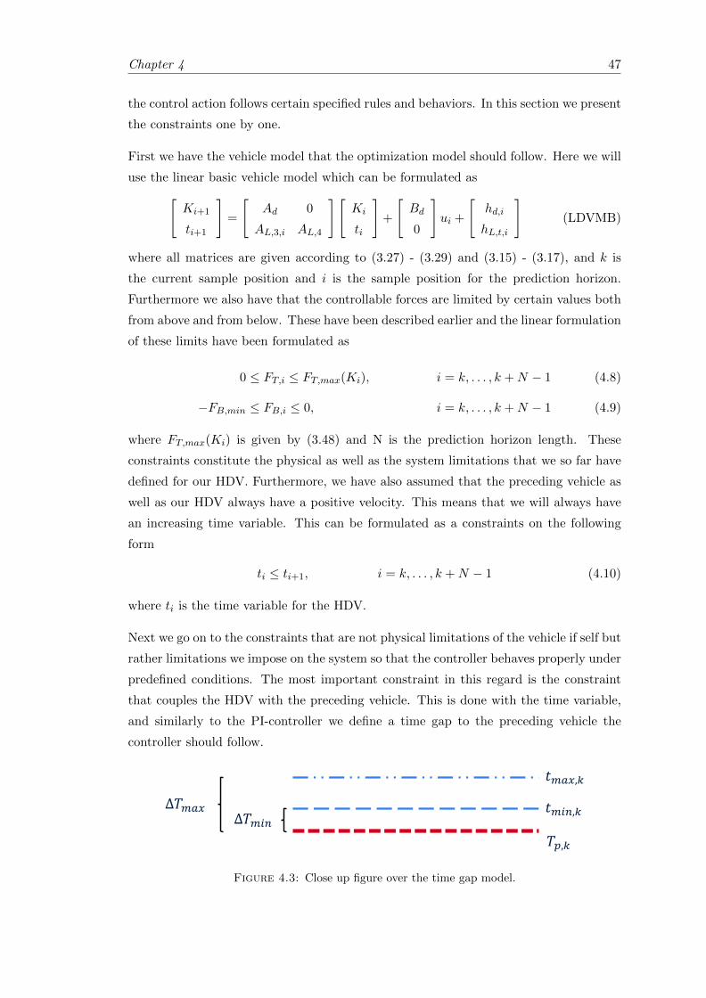
Chapter 4 47

the control action follows certain specified rules and behaviors. In this section we present

the constraints one by one.

First we have the vehicle model that the optimization model should follow. Here we will

use the linear basic vehicle model which can be formulated as[Ki+1

ti+1

]=

[Ad 0

AL,3,i AL,4

][Ki

ti

]+

[Bd

0

]ui +

[hd,i

hL,t,i

](LDVMB)

where all matrices are given according to (3.27) - (3.29) and (3.15) - (3.17), and k is

the current sample position and i is the sample position for the prediction horizon.

Furthermore we also have that the controllable forces are limited by certain values both

from above and from below. These have been described earlier and the linear formulation

of these limits have been formulated as

0 ≤ FT,i ≤ FT,max(Ki), i = k, . . . , k +N − 1 (4.8)

−FB,min ≤ FB,i ≤ 0, i = k, . . . , k +N − 1 (4.9)

where FT,max(Ki) is given by (3.48) and N is the prediction horizon length. These

constraints constitute the physical as well as the system limitations that we so far have

defined for our HDV. Furthermore, we have also assumed that the preceding vehicle as

well as our HDV always have a positive velocity. This means that we will always have

an increasing time variable. This can be formulated as a constraints on the following

form

ti ≤ ti+1, i = k, . . . , k +N − 1 (4.10)

where ti is the time variable for the HDV.

Next we go on to the constraints that are not physical limitations of the vehicle if self but

rather limitations we impose on the system so that the controller behaves properly under

predefined conditions. The most important constraint in this regard is the constraint

that couples the HDV with the preceding vehicle. This is done with the time variable,

and similarly to the PI-controller we define a time gap to the preceding vehicle the

controller should follow.

Title and Content

11 April 2018 Info class internal Department / Name / Subject 16

∆𝑇𝑚𝑎𝑥∆𝑇𝑚𝑖𝑛

𝑇𝑝,𝑘

𝑡𝑚𝑖𝑛,𝑘

𝑡𝑚𝑎𝑥,𝑘

Figure 4.3: Close up figure over the time gap model.

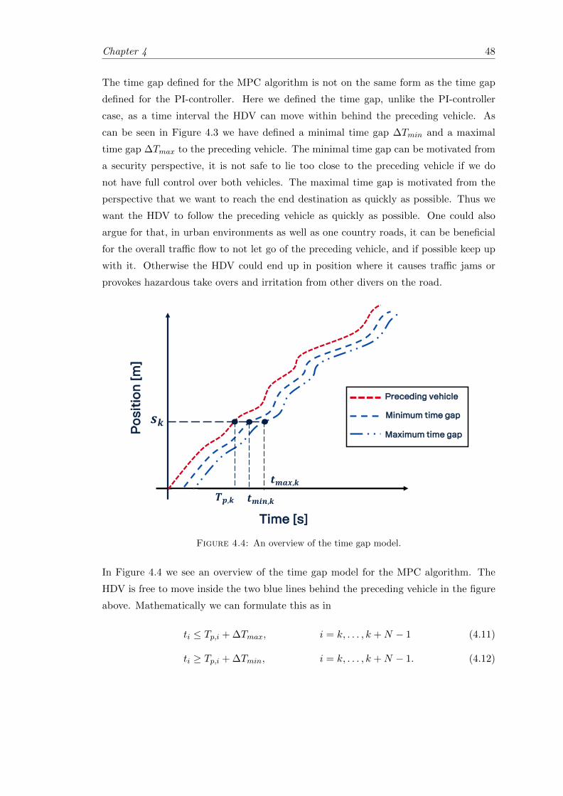
Chapter 4 48

The time gap defined for the MPC algorithm is not on the same form as the time gap

defined for the PI-controller. Here we defined the time gap, unlike the PI-controller

case, as a time interval the HDV can move within behind the preceding vehicle. As

can be seen in Figure 4.3 we have defined a minimal time gap ∆Tmin and a maximal

time gap ∆Tmax to the preceding vehicle. The minimal time gap can be motivated from

a security perspective, it is not safe to lie too close to the preceding vehicle if we do

not have full control over both vehicles. The maximal time gap is motivated from the

perspective that we want to reach the end destination as quickly as possible. Thus we

want the HDV to follow the preceding vehicle as quickly as possible. One could also

argue for that, in urban environments as well as one country roads, it can be beneficial

for the overall traffic flow to not let go of the preceding vehicle, and if possible keep up

with it. Otherwise the HDV could end up in position where it causes traffic jams or

provokes hazardous take overs and irritation from other divers on the road.

Title and Content

11 April 2018 Info class internal Department / Name / Subject 15

𝒔𝒌

𝑻𝒑,𝒌

Po

siti

on

[m

]

Time [s]

𝒕𝒎𝒊𝒏,𝒌

𝒕𝒎𝒂𝒙,𝒌

Preceding vehicle

Minimum time gap

Maximum time gap

Figure 4.4: An overview of the time gap model.

In Figure 4.4 we see an overview of the time gap model for the MPC algorithm. The

HDV is free to move inside the two blue lines behind the preceding vehicle in the figure

above. Mathematically we can formulate this as in

ti ≤ Tp,i + ∆Tmax, i = k, . . . , k +N − 1 (4.11)

ti ≥ Tp,i + ∆Tmin, i = k, . . . , k +N − 1. (4.12)

Chapter 4 49

It is not realistic and mathematically ”flexible”2 to constrain the HDV to only be able

to act in the often small time window behind the preceding vehicle. If the preced-

ing vehicle accelerates or decelerates quickly the solver should still be able to find a

solution although outside this time window. To enable this we use the approach of

Soft-constraints described in Chapter 2, and introduced slack variables RMi and Rmi.

These are introduced to the constraints as in

ti ≤ Tp,i + ∆Tmax +RMi, i = k, . . . , k +N (4.13)

ti ≥ Tp,i + ∆Tmin −Rmi, i = k, . . . , k +N (4.14)

RMi ≥ 0, Rmi ≥ 0, i = k, . . . , k +N. (4.15)

These slack variable will also be introduced in the objective function with corresponding

weight parameters. This in order to penalize deviations from the defined time window

behind the preceding vehicle, but at the same time enabling the solver to find solutions

outside it if necessary.

The road the HDV is travelling on will most probably have speed restrictions which it

has to follow. Here, we will include this in the model as a constraint on the kinetic

energy of the HDV. Given that we get the speed restriction Ki,max of the road as a

function of position, as for the topography of the road, we can formulate the constraint

as

0 ≤ Ki ≤ Ki,max, i = k, . . . , k +N − 1. (4.16)

As for the time gap constraint we will allow the vehicle to exceed the speed restriction

but for a cost. This will be necessary, in part so that the solver finds feasible solutions

and in part so that it in some situations can utilize the terrain more for fuel efficient

driving. Here a balance between fuel efficiency and allowed speed violations have to be

made, see coming sections. By introducing the slack variable KEk we formulate the

speed restriction constraint as

0 ≤ Ki ≤ Ki,max +KEk, i = k, . . . , k +N − 1 (4.17)

KEk ≥ 0, i = k, . . . , k +N − 1. (4.18)

At last we will also take driveability into consideration and enforce limitations on the

jerk of the HDV. This is done inspired by the implementation made in [8]. The optimal

solution to the designed model will not always be a smooth solution, and as will be

mentioned in Chapter 5 there will also be some problems (probably originating in the

2By flexible we mean that with this formulation the solver will have a hard time to find feasiblesolution. If we relax these equation the optimization solver will be able to execute successfully even inthought conditions.

Chapter 4 50

LP-solver) to find the fuel optimal solutions. The control actions, the tractive and

braking forces, will sometimes exhibit spikes or large changes in magnitude over a small

sample distance. These solutions are not always optimal and a discussion of this can be

seen in Section 5.2.1 . To solve this problem as well as ensuring some level of driving

comfort, minimizing the jerk of the solution, we implement the following condition

minimize | ∆FT,k | + | ∆FB,k | . (4.19)

Where we have defined ∆FT,k and ∆FB,k as

∆FT,k =FT,k+1 − FT,k

∆s, (4.20)

∆FB,k =FB,k+1 − FB,k

∆s(4.21)

in order to minimize the rate of change in the controllable forces. This is also often the

reason to what is often called jerk, the rate of change in the acceleration of the HDV.

The condition given in (4.19) is not a constraint but rather an addition to the objective

function. Furthermore, the equation is not linear which means that it has to be refor-

mulated in terms of linear functions. This can be done by introducing the additional

variables RTk and RBk as

RTk =| ∆FT,k |, (4.22)

RBk =| ∆FB,k | (4.23)

and observing that if we introduce the following four linear inequalities

∆s∆FT,k ≤ RTk and −∆s∆FT,k ≤ RTk, (4.24)

∆s∆FB,k ≤ RBk and −∆s∆FB,k ≤ RBk (4.25)

and impose the following condition in the objective function

minimize RTk +RDk (4.26)

it will be mathematically equivalent to imposing only condition (4.19), but on a linear

form. Thus the last constraints added to the model are the four constraints

Chapter 4 51

∆s∆FT,i ≤ RTi, i = k, . . . , k +N − 1 (4.27)

−∆s∆FT,i ≤ RTi, i = k, . . . , k +N − 1 (4.28)

∆s∆FB,i ≤ RBi, i = k, . . . , k +N − 1 (4.29)

−∆s∆FB,i ≤ RBi, i = k, . . . , k +N − 1. (4.30)

4.2.1.2 Regenerative Braking Extension

For the model extension case of regenerative braking the constraints are changed to

the extent that the extended basic vehicle model is used. This means that we apply

the changes described in (3.31) to the basic vehicle model (LDVMB). Furthermore, the

constraints for the limitations on the controllable force will be changed according to

0 ≤ FT,i ≤ FT,max(Ki), i = k, . . . , k +N − 1 (4.31)

−FB,min ≤ FBL,i + FBR,i ≤ 0, i = k, . . . , k +N − 1 (4.32)

where again FT,max is given by (3.48), FBL,i is the braking force corresponding to pure

energy losses and FBR,i is the part of the braking force that can be regenerated.

As for the tractive force, the part of the braking force that can be regenerated will not

only be restricted by the fixed minimum limit in (4.32) but also by the maximal power

that can be regenerated. This is can be formulated analogous to the maximum limit of

the tractive force as

FBR,min(Kk) ≤ FBR,k ≤ 0, (4.33)

FBR,min(Kk) =PBR,max

vk= PBR,max

√m

sKk(4.34)

where we introduced the maximal regenerative power as PBR,max. This value is set to

100 000 W for all simulations in this thesis. As for the tractive power, we linearize (4.34)

and get

FBR,min(Kk) = PBR,max

√m

2

(3

2K

−1/20,k − 1

2K

−3/20,k Kk

)

= 3PBR,max

√m

8K

−1/20,k − PBR,max

√m

8K

−3/20,k Kk

= P1,BR + P2,BRKk (4.35)

where we introduced the parameters

Chapter 4 52

P1,BR = 3PT,max

√m

8K

−1/20,k , (4.36)

P2,BR = −PT,max√m

8K

−3/20,k . (4.37)

This yields that we also ad the following constraint to the model for this model extension

FBR,min(Ki) = P1,BR + P2,BRKi, i = k, . . . , k +N − 1. (4.38)

4.2.1.3 Air Drag Model Extension

For the air drag model extension the basic vehicle model is adapted according to the

adaptations made in Section 3.1.4.1. The constraint found in (4.51) will also be added

to the model so as to define the inter vehicle distance. No further additions are made.

4.2.2 Objective Function

In this section we present the objective function of the optimization model used in the

MPC algorithm.

The objective function determine the criterions that should be optimized, minimized or

maximized, under the constraints given in the sections above. The objective function J

can generally be formulated on discrete form as in Section 2.1.1.1

minimize J = φ(x(sf ), sf ) +

sf∑s=s0

f0(s, x(s), u(s))∆s (4.39)

where φ(x(sf ), sf ) is the terminal condition. Here we will treat the terminal condition

and the rest of the objective function separately.

The main purpose of this thesis is to find a speed controller that minimize the fuel con-

sumption given a preceding vehicle. The fuel consumption will here be approximated

with the energy consumption for the vehicle given that it moves from position sk to po-

sition sk+N . Thus we want to penalize all added energy from the engine and powertrain

of the HDV during its driving mission. In the variables and parameters defined in this

thesis this can be formulated as

k+N−1∑i=k

∆sFT,i. (4.40)

Chapter 4 53

Furthermore, we have also defined a number of slack variables when constructing the

constraints. These variables should all be minimized with corresponding weight param-

eters that decide the importance of the deviations from the original constraints without

slack. First we have the variables RMk and Rmk which are slack variables correspond-

ing to the maximal and minimal time gap respectively. These can be introduced to the

objective function as

k+N−1∑i=k

βRMi + γRmi (4.41)

where we introduced the weight parameters β and γ. These values are set so that the

fuel optimal solution is found in the basic simulation case, case 1. Another constraint

that has been modified with slack variables is the constraint concerning the speed re-

strictions. Here we have introduced the slack variable KEk so as to allow some small

speed violations. This can be added to the objective function as

k+N−1∑i=k

q(Ki,max)KEi (4.42)

where we introduced the weight parameter q(Kk,max) to penalize speed violations. These

values depend on the maximum velocity because we penalize speed violations more at

lower speed restrictions than at higher. From experimental testing the parameter is

given, so that no speed violations occur for speed restrictions below 30 km/h, by

q(Kk,max) = − 3

36Kk,max +

29

17. (4.43)

These values are computed before the optimization and given as a vector of fixed values

to the LP solver. Thus the linear property of the model is preserved.

At last we also introduced the driveability condition to the objective function where

RTk and RBk are to be minimized. This can be added as

k+N−1∑i=k

σ(RTi +RBi) (4.44)

where σ is the penalization parameter for jerk in the system.

4.2.2.1 Model extension considerations

For the model extensions we will have some additions to the above stated terms in the

objective function. For the regenerative case we will introduce the regenerative part into

the objective function. This because we will reuse some of the energy the HDV has used

through regenerative braking. Thus we add

Chapter 4 54

k+N−1∑i=k

−ε∆sFBR,i (4.45)

where ε is the ratio of regeneration, i.e. the amount of FBR,k that actually get regenerated

to tractive power again. There are losses in the process of regeneration as well which

means that ε usually is less than 1. In our simulations we set it to 0.7, i.e. 70 % percent.

For the air drag model extension there are no changes to the objective function.

4.2.2.2 Terminal Penalization

The last part of the objective function that is common for all models used in this thesis

is the terminal penalization term φ(x(sk+N ), sk+N ). This term should account for the

rest of the simulation horizon when optimizing for the prediction horizon. This can be

modeled in several different ways, and a more thorough description of the different ways

to do this can be seen in Chapter 5.

Up to the terminal point of the prediction horizon any acceleration of the HDV has been

penalized through (4.40). Thus it seems reasonable to include the kinetic energy of the

HDV in the terminal point so that the HDV does not lose too much speed during the

last sample points. Another aspect that is reasonable to include in the terminal point is

the deviation to the reference ∆Tref the PI-controller follows. This, so that if the MPC

does not find any other optimal time gap to position the HDV on it should follow the

same trajectory as the PI-controller.

With these considerations in mind we will try to find a good formulation of the terminal

condition by experimenting on the basic simulation case, case 1, with

φ(x(sk+N ), sN ) = δ | KN+k −Kp,N+k | +τ | tN+k − (Tp,N+k + ∆Tref ) | (4.46)

where we have introduced the weight parameters δ and τ . The values of these parameters

will be decide by the experiments made on simulation case 1.

Chapter 4 55

4.2.2.3 Complete Optimization model

In this section we present the complete optimization problem for the basic case, i.e.

excluding the model extension. The extension of this optimization problem to the model

extension cases have been described in the sections above. The complete optimization

problem can be formulated as

minimizeFT,k, FB,k

δ | KN+k −Kp,N+k | +τ | tN+k − (Tp,N+k + ∆Tref ) |

+k+N−1∑i=k

(∆sFT,i + βRMi + γRmi + q(Ki,max)KEi + σ(RTi +RBi))

(4.47)

such that Ki+1 = AL,1Ki +BLui + hL,K,i, i = k, . . . , k +N − 1 (4.48a)

ti+1 = AL,3,iKi +AL,4ti + hL,t,i, i = k, . . . , k +N − 1 (4.48b)

0 ≤ FT,i ≤ FT,max(Ki), i = k, . . . , k +N − 1 (4.48c)

− FB,min ≤ FB,i ≤ 0, i = k, . . . , k +N − 1 (4.48d)

ti ≤ Tp,i + ∆Tmax +RMi, i = k, . . . , k +N (4.48e)

ti ≥ Tp,i + ∆Tmin −Rmi, i = k, . . . , k +N (4.48f)

0 ≤ Ki ≤ Ki,max +KEk, i = k, . . . , k +N − 1 (4.48g)

∆s∆FT,i ≤ RTi, i = k, . . . , k +N − 1 (4.48h)

−∆s∆FT,i ≤ RTi, i = k, . . . , k +N − 1 (4.48i)

∆s∆FB,i ≤ RBi, i = k, . . . , k +N − 1 (4.48j)

−∆s∆FB,i ≤ RBi, i = k, . . . , k +N − 1 (4.48k)

ti ≤ ti+1, i = k, . . . , k +N − 1 (4.48l)

RMi ≥ 0, Rmi ≥ 0, i = k, . . . , k +N (4.48m)

KEk ≥ 0, i = k, . . . , k +N − 1 (4.48n)

Kk, tk given. (4.48o)

The above LP-problem is solved in each iteration of the MPC algorithm with given initial

conditions Kk, tk as well as the trajectory of the preceding vehicle for the prediction

horizon {Tp,i, Vp,i}k+Ni=k . The built in solver Linprog in Matlab is used to solve the

optimization problem along with Yalmip [49], see Appendix A.1 to put the problem on

the correct form.

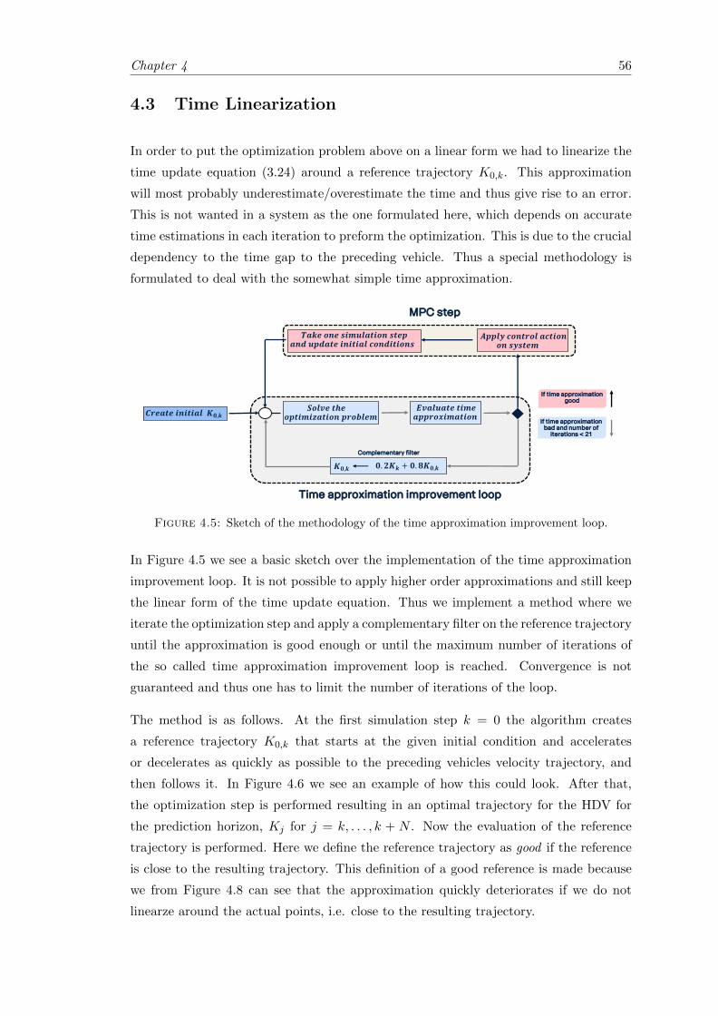
Chapter 4 56

4.3 Time Linearization

In order to put the optimization problem above on a linear form we had to linearize the

time update equation (3.24) around a reference trajectory K0,k. This approximation

will most probably underestimate/overestimate the time and thus give rise to an error.

This is not wanted in a system as the one formulated here, which depends on accurate

time estimations in each iteration to preform the optimization. This is due to the crucial

dependency to the time gap to the preceding vehicle. Thus a special methodology is

formulated to deal with the somewhat simple time approximation.

11 April 2018 Info class internal Department / Name / Subject 17

𝑪𝒓𝒆𝒂𝒕𝒆 𝒊𝒏𝒊𝒕𝒊𝒂𝒍 𝑲𝟎,𝒌𝑺𝒐𝒍𝒗𝒆 𝒕𝒉𝒆

𝒐𝒑𝒕𝒊𝒎𝒊𝒛𝒂𝒕𝒊𝒐𝒏 𝒑𝒓𝒐𝒃𝒍𝒆𝒎𝑬𝒗𝒂𝒍𝒖𝒂𝒕𝒆 𝒕𝒊𝒎𝒆𝒂𝒑𝒑𝒓𝒐𝒙𝒊𝒎𝒂𝒕𝒊𝒐𝒏

𝑨𝒑𝒑𝒍𝒚 𝒄𝒐𝒏𝒕𝒓𝒐𝒍 𝒂𝒄𝒕𝒊𝒐𝒏𝒐𝒏 𝒔𝒚𝒔𝒕𝒆𝒎

𝑻𝒂𝒌𝒆 𝒐𝒏𝒆 𝒔𝒊𝒎𝒖𝒍𝒂𝒕𝒊𝒐𝒏 𝒔𝒕𝒆𝒑𝒂𝒏𝒅 𝒖𝒑𝒅𝒂𝒕𝒆 𝒊𝒏𝒊𝒕𝒊𝒂𝒍 𝒄𝒐𝒏𝒅𝒊𝒕𝒊𝒐𝒏𝒔

𝑲𝟎,𝒌 𝟎. 𝟐𝑲𝒌 + 𝟎. 𝟖𝑲𝟎,𝒌

Complementary filter

If time approximation bad and number of

iterations < 21

If time approximation good

Time approximation improvement loop

MPC step

Figure 4.5: Sketch of the methodology of the time approximation improvement loop.

In Figure 4.5 we see a basic sketch over the implementation of the time approximation

improvement loop. It is not possible to apply higher order approximations and still keep

the linear form of the time update equation. Thus we implement a method where we

iterate the optimization step and apply a complementary filter on the reference trajectory

until the approximation is good enough or until the maximum number of iterations of

the so called time approximation improvement loop is reached. Convergence is not

guaranteed and thus one has to limit the number of iterations of the loop.

The method is as follows. At the first simulation step k = 0 the algorithm creates

a reference trajectory K0,k that starts at the given initial condition and accelerates

or decelerates as quickly as possible to the preceding vehicles velocity trajectory, and

then follows it. In Figure 4.6 we see an example of how this could look. After that,

the optimization step is performed resulting in an optimal trajectory for the HDV for

the prediction horizon, Kj for j = k, . . . , k + N . Now the evaluation of the reference

trajectory is performed. Here we define the reference trajectory as good if the reference

is close to the resulting trajectory. This definition of a good reference is made because

we from Figure 4.8 can see that the approximation quickly deteriorates if we do not

linearze around the actual points, i.e. close to the resulting trajectory.

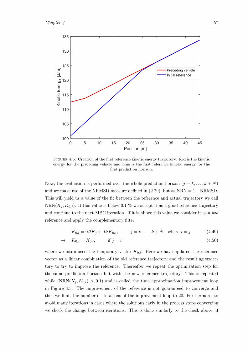
Chapter 4 57

0 5 10 15 20 25 30 35 40 45Position [m]

100

105

110

115

120

125

130

135

Kine

tic E

nerg

y [J

/m] Preceding vehicle

Initial reference

Figure 4.6: Creation of the first reference kinetic energy trajectory. Red is the kineticenergy for the preceding vehicle and blue is the first reference kinetic energy for the

first prediction horizon.

Now, the evaluation is performed over the whole prediction horizon (j = k, . . . , k + N)

and we make use of the NRMSD measure defined in (2.29), but as NRN = 1−NRMSD.

This will yield us a value of the fit between the reference and actual trajectory we call

NRN(Kj ,K0,j). If this value is below 0.1 % we accept it as a good reference trajectory

and continue to the next MPC iteration. If it is above this value we consider it as a bad

reference and apply the complementary filter

K0,i = 0.2Kj + 0.8K0,j , j = k, . . . , k +N, where i = j (4.49)

→ K0,j = K0,i, if j = i (4.50)

where we introduced the temporary vector K0,i. Here we have updated the reference

vector as a linear combination of the old reference trajectory and the resulting trajec-

tory to try to improve the reference. Thereafter we repeat the optimization step for

the same prediction horizon but with the new reference trajectory. This is repeated

while (NRN(Kj ,K0,i) > 0.1) and is called the time approximation improvement loop

in Figure 4.5. The improvement of the reference is not guaranteed to converge and

thus we limit the number of iterations of the improvement loop to 20. Furthermore, to

avoid many iterations in cases where the solutions early in the process stops converging

we check the change between iterations. This is done similarly to the check above, if

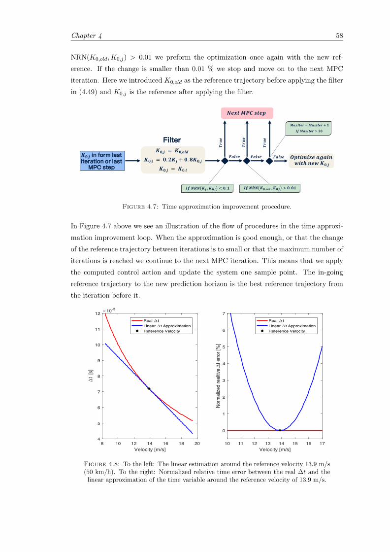
Chapter 4 58

NRN(K0,old,K0,j) > 0.01 we preform the optimization once again with the new ref-

erence. If the change is smaller than 0.01 % we stop and move on to the next MPC

iteration. Here we introduced K0,old as the reference trajectory before applying the filter

in (4.49) and K0,j is the reference after applying the filter.

Title and Content

11 April 2018 Info class internal Department / Name / Subject 18

𝑲𝟎,𝒋 in form last iteration or last

MPC step

𝑲𝟎,𝒋 = 𝑲𝟎,𝒐𝒍𝒅

𝑲𝟎,𝒊 = 𝟎. 𝟐𝑲𝒋 + 𝟎. 𝟖𝑲𝟎,𝒋

𝑲𝟎,𝒋 = 𝑲𝟎,𝒊

Filter

𝑶𝒑𝒕𝒊𝒎𝒊𝒛𝒆 𝒂𝒈𝒂𝒊𝒏𝒘𝒊𝒕𝒉 𝒏𝒆𝒘 𝑲𝟎,𝒋

𝑵𝒆𝒙𝒕 𝑴𝑷𝑪 𝒔𝒕𝒆𝒑

𝑰𝒇 𝑵𝑹𝑵 𝑲𝒋 ,𝑲𝟎,𝒊 < 𝟎. 𝟏 𝑰𝒇 𝑵𝑹𝑵 𝑲𝟎,𝒐𝒍𝒅 ,𝑲𝟎,𝒋 > 𝟎. 𝟎𝟏

𝑻𝒓𝒖𝒆

𝑻𝒓𝒖𝒆

𝑭𝒂𝒍𝒔𝒆𝑭𝒂𝒍𝒔𝒆

𝑴𝒂𝒙𝑰𝒕𝒆𝒓 = 𝑴𝒂𝒙𝑰𝒕𝒆𝒓 + 𝟏

𝑭𝒂𝒍𝒔𝒆

𝑻𝒓𝒖𝒆

𝑰𝒇 𝑴𝒂𝒙𝑰𝒕𝒆𝒓 > 𝟐𝟎

Figure 4.7: Time approximation improvement procedure.

In Figure 4.7 above we see an illustration of the flow of procedures in the time approxi-

mation improvement loop. When the approximation is good enough, or that the change

of the reference trajectory between iterations is to small or that the maximum number of

iterations is reached we continue to the next MPC iteration. This means that we apply

the computed control action and update the system one sample point. The in-going

reference trajectory to the new prediction horizon is the best reference trajectory from

the iteration before it.

8 10 12 14 16 18 20Velocity [m/s]

4

5

6

7

8

9

10

11

12

t [s]

10-3

Real tLinear t ApproximationReference Velocity

10 11 12 13 14 15 16 17Velocity [m/s]

0

1

2

3

4

5

6

7

Norm

alize

d re

altive

t e

rror [

%]

Real tLinear t ApproximationReference Velocity

Figure 4.8: To the left: The linear estimation around the reference velocity 13.9 m/s(50 km/h). To the right: Normalized relative time error between the real ∆t and the

linear approximation of the time variable around the reference velocity of 13.9 m/s.

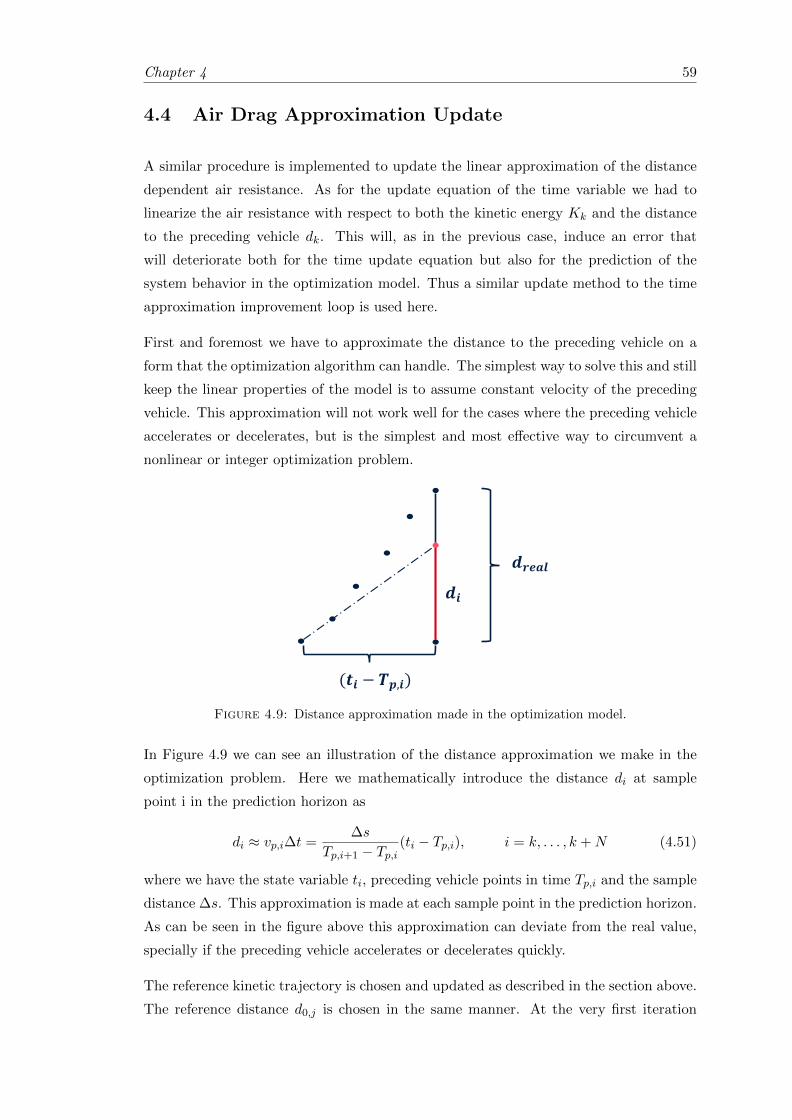
Chapter 4 59

4.4 Air Drag Approximation Update

A similar procedure is implemented to update the linear approximation of the distance

dependent air resistance. As for the update equation of the time variable we had to

linearize the air resistance with respect to both the kinetic energy Kk and the distance

to the preceding vehicle dk. This will, as in the previous case, induce an error that

will deteriorate both for the time update equation but also for the prediction of the

system behavior in the optimization model. Thus a similar update method to the time

approximation improvement loop is used here.

First and foremost we have to approximate the distance to the preceding vehicle on a

form that the optimization algorithm can handle. The simplest way to solve this and still

keep the linear properties of the model is to assume constant velocity of the preceding

vehicle. This approximation will not work well for the cases where the preceding vehicle

accelerates or decelerates, but is the simplest and most effective way to circumvent a

nonlinear or integer optimization problem.

Title and Content

11 April 2018 Info class internal Department / Name / Subject 19

(𝒕𝒊 − 𝑻𝒑,𝒊)

𝒅𝒊

𝒅𝒓𝒆𝒂𝒍

Figure 4.9: Distance approximation made in the optimization model.

In Figure 4.9 we can see an illustration of the distance approximation we make in the

optimization problem. Here we mathematically introduce the distance di at sample

point i in the prediction horizon as

di ≈ vp,i∆t =∆s

Tp,i+1 − Tp,i(ti − Tp,i), i = k, . . . , k +N (4.51)

where we have the state variable ti, preceding vehicle points in time Tp,i and the sample

distance ∆s. This approximation is made at each sample point in the prediction horizon.

As can be seen in the figure above this approximation can deviate from the real value,

specially if the preceding vehicle accelerates or decelerates quickly.

The reference kinetic trajectory is chosen and updated as described in the section above.

The reference distance d0,j is chosen in the same manner. At the very first iteration

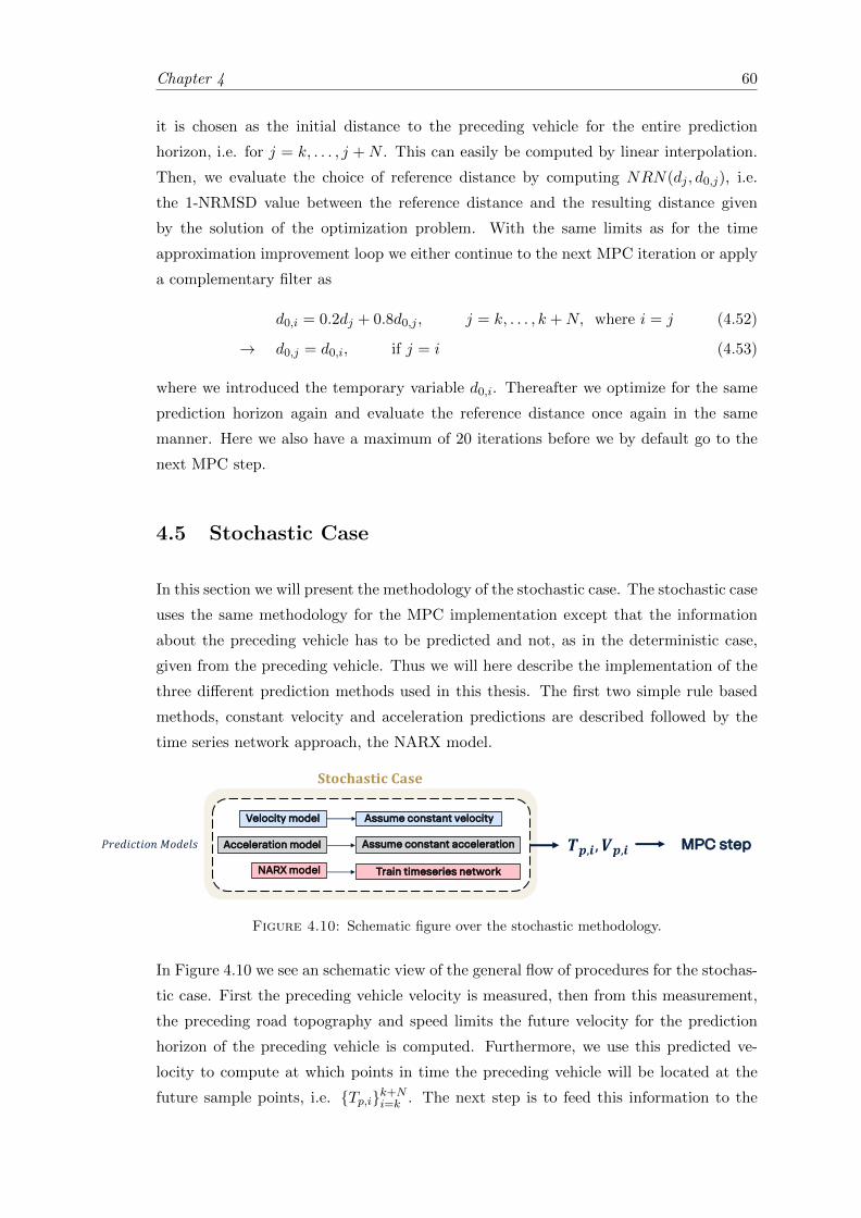
Chapter 4 60

it is chosen as the initial distance to the preceding vehicle for the entire prediction

horizon, i.e. for j = k, . . . , j +N . This can easily be computed by linear interpolation.

Then, we evaluate the choice of reference distance by computing NRN(dj , d0,j), i.e.

the 1-NRMSD value between the reference distance and the resulting distance given

by the solution of the optimization problem. With the same limits as for the time

approximation improvement loop we either continue to the next MPC iteration or apply

a complementary filter as

d0,i = 0.2dj + 0.8d0,j , j = k, . . . , k +N, where i = j (4.52)

→ d0,j = d0,i, if j = i (4.53)

where we introduced the temporary variable d0,i. Thereafter we optimize for the same

prediction horizon again and evaluate the reference distance once again in the same

manner. Here we also have a maximum of 20 iterations before we by default go to the

next MPC step.

4.5 Stochastic Case

In this section we will present the methodology of the stochastic case. The stochastic case

uses the same methodology for the MPC implementation except that the information

about the preceding vehicle has to be predicted and not, as in the deterministic case,

given from the preceding vehicle. Thus we will here describe the implementation of the

three different prediction methods used in this thesis. The first two simple rule based

methods, constant velocity and acceleration predictions are described followed by the

time series network approach, the NARX model.

Title and Content

20

Velocity model

Acceleration model

NARX model

𝑃𝑟𝑒𝑑𝑖𝑐𝑡𝑖𝑜𝑛 𝑀𝑜𝑑𝑒𝑙𝑠

𝐒𝐭𝐨𝐜𝐡𝐚𝐬𝐭𝐢𝐜 𝐂𝐚𝐬𝐞

Assume constant velocity

Assume constant acceleration

Train timeseries network

𝑻𝒑,𝒊, 𝑽𝒑,𝒊 MPC step

Figure 4.10: Schematic figure over the stochastic methodology.

In Figure 4.10 we see an schematic view of the general flow of procedures for the stochas-

tic case. First the preceding vehicle velocity is measured, then from this measurement,

the preceding road topography and speed limits the future velocity for the prediction

horizon of the preceding vehicle is computed. Furthermore, we use this predicted ve-

locity to compute at which points in time the preceding vehicle will be located at the

future sample points, i.e. {Tp,i}k+Ni=k . The next step is to feed this information to the

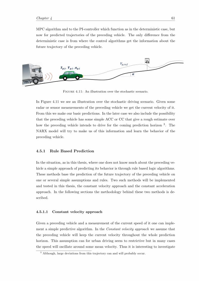
Chapter 4 61

MPC algorithm and to the PI-controller which function as in the deterministic case, but

now for predicted trajectories of the preceding vehicle. The only difference from the

deterministic case is from where the control algorithms get the information about the

future trajectory of the preceding vehicle.

Title and Content

11 April 2018 Info class internal Department / Name / Subject 21

𝑺𝒑,𝒊, 𝑽𝒑,𝒊 , 𝒂𝒑,𝒊

𝜶

𝑉𝑝,𝑟𝑒𝑓

Figure 4.11: An illustration over the stochastic scenario.

In Figure 4.11 we see an illustration over the stochastic driving scenario. Given some

radar or sensor measurements of the preceding vehicle we get the current velocity of it.

From this we make our basic predictions. In the later case we also include the possibility

that the preceding vehicle has some simple ACC or CC that give a rough estimate over

how the preceding vehicle intends to drive for the coming prediction horizon 3. The

NARX model will try to make us of this information and learn the behavior of the

preceding vehicle.

4.5.1 Rule Based Prediction

In the situation, as in this thesis, where one does not know much about the preceding ve-

hicle a simple approach of predicting its behavior is through rule based logic algorithms.

These methods base the prediction of the future trajectory of the preceding vehicle on

one or several simple assumptions and rules. Two such methods will be implemented

and tested in this thesis, the constant velocity approach and the constant acceleration

approach. In the following sections the methodology behind these two methods is de-

scribed.

4.5.1.1 Constant velocity approach

Given a preceding vehicle and a measurement of the current speed of it one can imple-

ment a simple predictive algorithm. In the Constant velocity approach we assume that

the preceding vehicle will keep the current velocity throughout the whole prediction

horizon. This assumption can for urban driving seem to restrictive but in many cases

the speed will oscillate around some mean velocity. Thus it is interesting to investigate

3 Although, large deviations from this trajectory can and will probably occur.

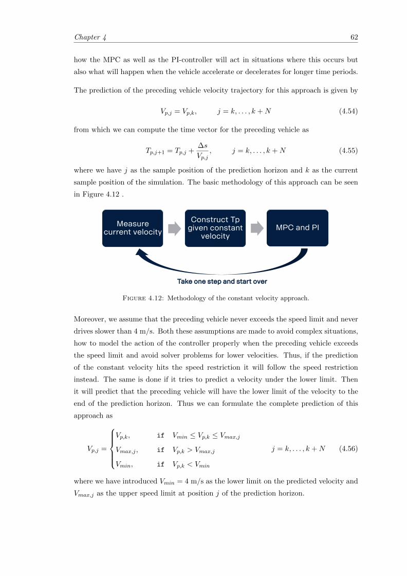
Chapter 4 62

how the MPC as well as the PI-controller will act in situations where this occurs but

also what will happen when the vehicle accelerate or decelerates for longer time periods.

The prediction of the preceding vehicle velocity trajectory for this approach is given by

Vp,j = Vp,k, j = k, . . . , k +N (4.54)

from which we can compute the time vector for the preceding vehicle as

Tp,j+1 = Tp,j +∆s

Vp,j, j = k, . . . , k +N (4.55)

where we have j as the sample position of the prediction horizon and k as the current

sample position of the simulation. The basic methodology of this approach can be seen

in Figure 4.12 .

Title and Content

11 April 2018 Info class internal Department / Name / Subject 22

MPC and PIConstruct Tp

given constant velocity

Measure current velocity

Take one step and start over

Figure 4.12: Methodology of the constant velocity approach.

Moreover, we assume that the preceding vehicle never exceeds the speed limit and never

drives slower than 4 m/s. Both these assumptions are made to avoid complex situations,

how to model the action of the controller properly when the preceding vehicle exceeds

the speed limit and avoid solver problems for lower velocities. Thus, if the prediction

of the constant velocity hits the speed restriction it will follow the speed restriction

instead. The same is done if it tries to predict a velocity under the lower limit. Then

it will predict that the preceding vehicle will have the lower limit of the velocity to the

end of the prediction horizon. Thus we can formulate the complete prediction of this

approach as

Vp,j =

Vp,k, if Vmin ≤ Vp,k ≤ Vmax,j

Vmax,j , if Vp,k > Vmax,j

Vmin, if Vp,k < Vmin

j = k, . . . , k +N (4.56)

where we have introduced Vmin = 4 m/s as the lower limit on the predicted velocity and

Vmax,j as the upper speed limit at position j of the prediction horizon.

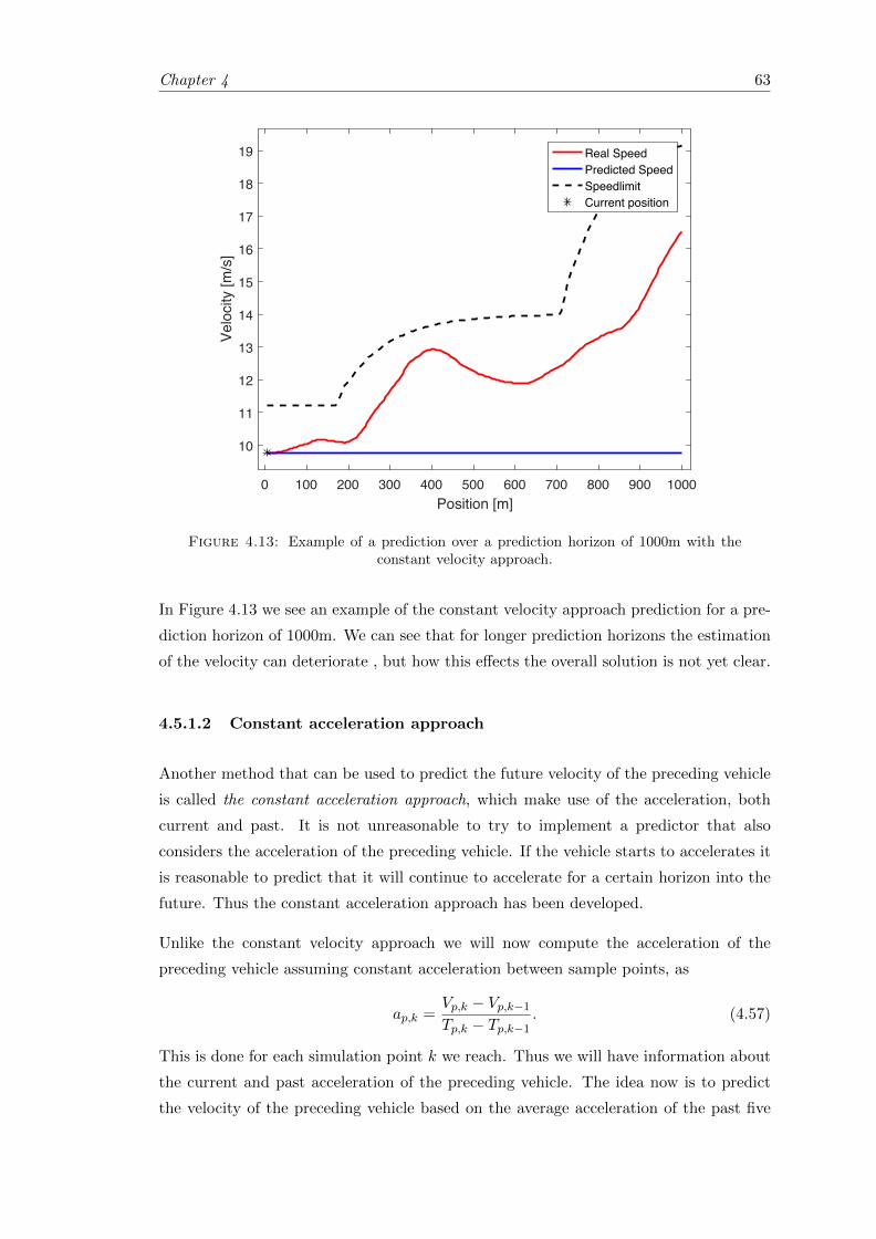
Chapter 4 63

0 100 200 300 400 500 600 700 800 900 1000Position [m]

10

11

12

13

14

15

16

17

18

19

Velo

city

[m/s

]

Real SpeedPredicted SpeedSpeedlimitCurrent position

Figure 4.13: Example of a prediction over a prediction horizon of 1000m with theconstant velocity approach.

In Figure 4.13 we see an example of the constant velocity approach prediction for a pre-

diction horizon of 1000m. We can see that for longer prediction horizons the estimation

of the velocity can deteriorate , but how this effects the overall solution is not yet clear.

4.5.1.2 Constant acceleration approach

Another method that can be used to predict the future velocity of the preceding vehicle

is called the constant acceleration approach, which make use of the acceleration, both

current and past. It is not unreasonable to try to implement a predictor that also

considers the acceleration of the preceding vehicle. If the vehicle starts to accelerates it

is reasonable to predict that it will continue to accelerate for a certain horizon into the

future. Thus the constant acceleration approach has been developed.

Unlike the constant velocity approach we will now compute the acceleration of the

preceding vehicle assuming constant acceleration between sample points, as

ap,k =Vp,k − Vp,k−1

Tp,k − Tp,k−1. (4.57)

This is done for each simulation point k we reach. Thus we will have information about

the current and past acceleration of the preceding vehicle. The idea now is to predict

the velocity of the preceding vehicle based on the average acceleration of the past five

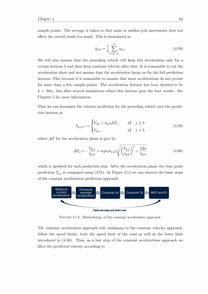
Chapter 4 64

sample points. The average is taken so that noise or sudden jerk movements does not

effect the overall result too much. This is formulated as

ap,k =1

5

k∑i=k−4

ap,i. (4.58)

We will also assume that the preceding vehicle will keep this acceleration only for a

certain horizon h and then keep constant velocity after that. It is reasonable to cut the

acceleration short and not assume that the acceleration keeps on for the full prediction

horizon. This because it is reasonable to assume that most accelerations do not persist

for more than a few sample points. The acceleration horizon has been decided to be

h = 50m, this after several simulations where this horizon gave the best results. See

Chapter 5 for more information.

Thus we can formulate the velocity prediction for the preceding vehicle over the predic-

tion horizon as

Vp,j+1 =

Vp,j + ap,k∆Tj , if j ≤ h

Vp,j , if j > h(4.59)

where ∆T for the acceleration phase is give by

∆Tj = −Vp,jap,k

+ sign(ap,k)

√(Vp,jap,k

)2

+2∆s

ap,k(4.60)

which is updated for each prediction step. After the acceleration phase the time point

prediction Tp,i is computed using (4.55). In Figure 4.14 we can observe the basic steps

of the constant acceleration prediction approach.

Title and Content

11 April 2018 Info class internal Department / Name / Subject 23

MPC and PICompute TpCompute VpCompute average

acceleration

Measure current

acceleration

Take one step and start over

Figure 4.14: Methodology of the constant acceleration approach.

The constant acceleration approach will, analogous to the constant velocity approach,

follow the speed limits, both the speed limit of the road as well as the lower limit

introduced in (4.56). Thus, as a last step of the constant accelerations approach we

filter the predicted velocity according to

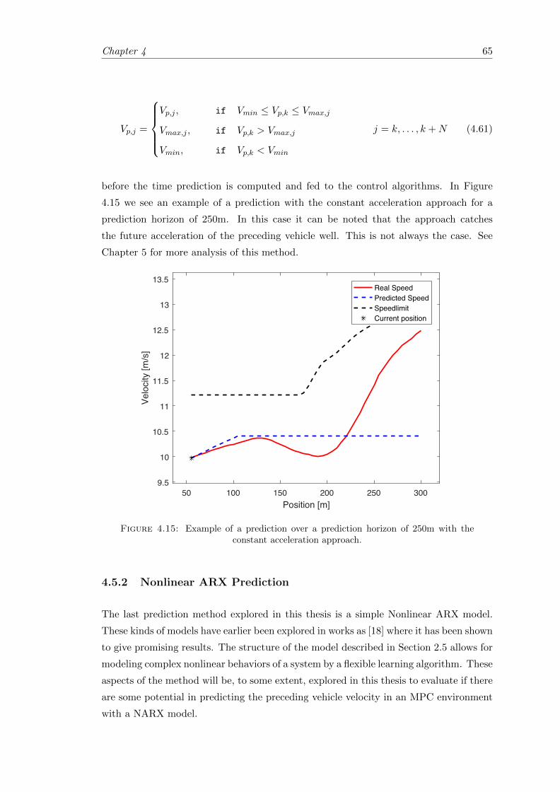
Chapter 4 65

Vp,j =

Vp,j , if Vmin ≤ Vp,k ≤ Vmax,j

Vmax,j , if Vp,k > Vmax,j

Vmin, if Vp,k < Vmin

j = k, . . . , k +N (4.61)

before the time prediction is computed and fed to the control algorithms. In Figure

4.15 we see an example of a prediction with the constant acceleration approach for a

prediction horizon of 250m. In this case it can be noted that the approach catches

the future acceleration of the preceding vehicle well. This is not always the case. See

Chapter 5 for more analysis of this method.

50 100 150 200 250 300Position [m]

9.5

10

10.5

11

11.5

12

12.5

13

13.5

Velo

city

[m/s

]

Real SpeedPredicted SpeedSpeedlimitCurrent position

Figure 4.15: Example of a prediction over a prediction horizon of 250m with theconstant acceleration approach.

4.5.2 Nonlinear ARX Prediction

The last prediction method explored in this thesis is a simple Nonlinear ARX model.

These kinds of models have earlier been explored in works as [18] where it has been shown

to give promising results. The structure of the model described in Section 2.5 allows for

modeling complex nonlinear behaviors of a system by a flexible learning algorithm. These

aspects of the method will be, to some extent, explored in this thesis to evaluate if there

are some potential in predicting the preceding vehicle velocity in an MPC environment

with a NARX model.

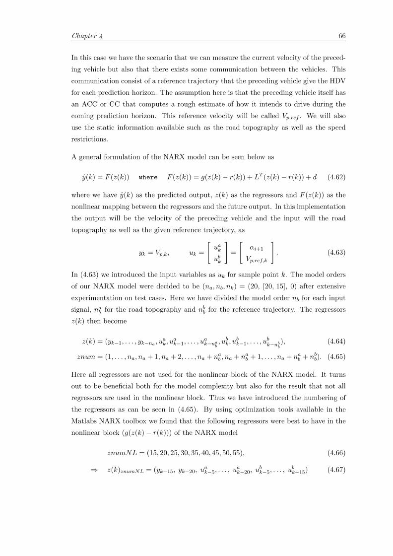
Chapter 4 66

In this case we have the scenario that we can measure the current velocity of the preced-

ing vehicle but also that there exists some communication between the vehicles. This

communication consist of a reference trajectory that the preceding vehicle give the HDV

for each prediction horizon. The assumption here is that the preceding vehicle itself has

an ACC or CC that computes a rough estimate of how it intends to drive during the

coming prediction horizon. This reference velocity will be called Vp,ref . We will also

use the static information available such as the road topography as well as the speed

restrictions.

A general formulation of the NARX model can be seen below as

y(k) = F (z(k)) where F (z(k)) = g(z(k)− r(k)) + LT (z(k)− r(k)) + d (4.62)

where we have y(k) as the predicted output, z(k) as the regressors and F (z(k)) as the

nonlinear mapping between the regressors and the future output. In this implementation

the output will be the velocity of the preceding vehicle and the input will the road

topography as well as the given reference trajectory, as

yk = Vp,k, uk =

[uak

ubk

]=

[αi+1

Vp,ref,k

]. (4.63)

In (4.63) we introduced the input variables as uk for sample point k. The model orders

of our NARX model were decided to be (na, nb, nk) = (20, [20, 15], 0) after extensive

experimentation on test cases. Here we have divided the model order nb for each input

signal, nab for the road topography and nbb for the reference trajectory. The regressors

z(k) then become

z(k) = (yk−1, . . . , yk−na , uak, u

ak−1, . . . , u

ak−na

b, ubk, u

bk−1, . . . , u

bk−nb

b), (4.64)

znum = (1, . . . , na, na + 1, na + 2, . . . , na + nab , na + nab + 1, . . . , na + nab + nbb). (4.65)

Here all regressors are not used for the nonlinear block of the NARX model. It turns

out to be beneficial both for the model complexity but also for the result that not all

regressors are used in the nonlinear block. Thus we have introduced the numbering of

the regressors as can be seen in (4.65). By using optimization tools available in the

Matlabs NARX toolbox we found that the following regressors were best to have in the

nonlinear block (g(z(k)− r(k))) of the NARX model

znumNL = (15, 20, 25, 30, 35, 40, 45, 50, 55), (4.66)

⇒ z(k)znumNL = (yk−15, yk−20, uak−5, . . . , u

ak−20, u

bk−5, . . . , u

bk−15) (4.67)

Chapter 4 67

where we have expressed the regressors by their numbering. All regressors z(k) are used

in the linear block LT (z(k) − r(k)) + d. Here we see that most inputs signals are used

in the nonlinear block. This gives us that our NARX model can be formulated as

y(k) = F (z(k)) where F (z(k)) = g(z(k)znumNL − r(k)znumNL) + LT (z(k)− r(k)) + d

(4.68)

where the notation z(k)znumNL means that we only use regressors with numbers given

in znumNL. The network itself is a wavelet network of 20 units. This is also decided

after simulations on test cases.

The next step is to describe the implementation of the above defined NARX model

structure. The methodology of the NARX model implementation can be divided into

two stages.

1. Training stage, given past and current input data as well as past output

data compute the regressor parameters and form the nonlinear mapping

according to chosen algorithm.

2. Prediction stage, given past data, and possibly future input data, predict

the future output of the system using the nonlinear mapping constructed in

the training stage.

As described above the methodology is divided into a training stage and a prediction

stage. The model is constructed during the training stage where the software finds the

values of the parameters L, r, d and other hidden parameters in the wavelet network

of the nonlinear block of the nonlinear mapping function F (z(k)). This is done for a

training data set, which we will choose as the first couple of kilometers of the driving

scenario. During this phase other prediction algorithms are implemented on the HDV

so that the NARX model learns the behavior of the preceding vehicle. Then, during the

prediction stage, the NARX model is live on the HDV and predicts the future velocity

trajectory of the preceding vehicle for the prediction horizon. This is done using the

past data which we define as

PastData = {yk−1, . . . , y0, uk−1, . . . , u0} (4.69)

where yi, i = k−1, . . . , 0 is the measured speed of the preceding vehicle at each simulation

point up to the current simulation point and similarly for the input data ui. We also

make use of the future input data which we define as

uk, . . . , uk+N (4.70)

Chapter 4 68

for the current prediction horizon. Using the trained NARX model with the past data

and future input data we can predict the future velocity trajectory for the preceding

vehicle over the prediction horizon. This is done by recursively using the one step

prediction made by the NARX model (4.68) and utilizing that we know the past data

as well as the future input data. With the future input data known we do not need

approximations of these variables as well. This can be written as

yK+k = F (z(k))where z(k) = (yK+k−1, . . . , yK+k−na , uK+k, uK+k−1, . . . , uK+k−nb)

(4.71)

for a prediction K steps into the future. In (4.71) we see the recursive aspect of the

prediction step. This is thus made recursively for K = 0, . . . , N , i.e. the prediction

horizon. This will give us the complete prediction of the velocity of the preceding

vehicle Vp,j . The time prediction is given by (4.55). These predictions are fed to the

control algorithms which find a control action. Then the system is updated one step as

well as the past data, future input data and initial conditions (measurement of current

velocity of preceding vehicle). Thereafter a new prediction is made for the new prediction

horizon. This is iterated until the end of the simulation horizon.

Title and Content

11 April 2018 Info class internal Department / Name / Subject 24

Train the model parameters of

the NARX model

Use NARX with past data and

future input data to predict Vp

Construct Tp MPC and PI

Take one step and start over

Update past data with measurement of current velocity Vp and future

input data

Figure 4.16: Methodology of the NARX prediction approach.

In Figure 4.16 above we see an illustration of the basic methodology of the NARX

prediction approach. As for the other prediction methods described in this thesis, the

NARX prediction approach will be limited to the speed restriction as well as the lower

speed limit. As a last step before the time prediction is computed and the information

is fed to the control algorithms, the velocity prediction is filtered as in (4.56).

Chapter 5

Results

In this chapter we present the simulation cases as well as the results of the simulations

with the algorithms and methods developed in the previous chapters. First the differ-

ent simulation cases as well as the logged data manipulations are described before the

parameter and penalization variable analysis is presented. Thereafter the Deterministic

case results are described, both for the basic models as well as the two different model

extensions. The evaluation of the time and distance approximations are presented as

well as further analysis such as the effect of the weight of the HDV and the choice of

the maximal time gap in the MPC algorithm. At last the Stochastic case results are

presented for all three prediction approaches.

5.1 Simulation

Many of the results shown in the sections below will be simulations on several different

cases. These cases have been in part constructed, using the methodology in Section 3.3,

to showcase the optimal trajectory in specific situations and in part taken from logged

data. The later case is included to test the algorithms on a full driving cycle with varying

velocity as well as road topography. This in order to see how the algorithms react to a

scenario close to a real life setting, excluding the hardware limitations and effects that

are not included in the model (for example weather and lateral dynamics).

5.1.1 Constructed simulation cases

In this section we present the main simulations cases that we have constructed from using

the methodology presented in Section 3.3. These cases will be named and tested in the

Deterministic case for all three models, the basic model and the two model extensions.

69

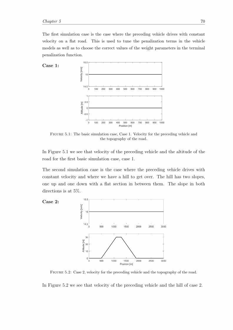
Chapter 5 70

The first simulation case is the case where the preceding vehicle drives with constant

velocity on a flat road. This is used to tune the penalization terms in the vehicle

models as well as to choose the correct values of the weight parameters in the terminal

penalization function.

Case 1:

0 100 200 300 400 500 600 700 800 900 100014.5

15

15.5

Velo

city

[m/s

]

0 100 200 300 400 500 600 700 800 900 1000Position [m]

-1

-0.5

0

0.5

1

Altit

ude

[m]

Figure 5.1: The basic simulation case, Case 1. Velocity for the preceding vehicle andthe topography of the road.

In Figure 5.1 we see that velocity of the preceding vehicle and the altitude of the

road for the first basic simulation case, case 1.

The second simulation case is the case where the preceding vehicle drives with

constant velocity and where we have a hill to get over. The hill has two slopes,

one up and one down with a flat section in between them. The slope in both

directions is at 5%.

Case 2:

Figure 5.2: Case 2, velocity for the preceding vehicle and the topography of the road.

In Figure 5.2 we see that velocity of the preceding vehicle and the hill of case 2.

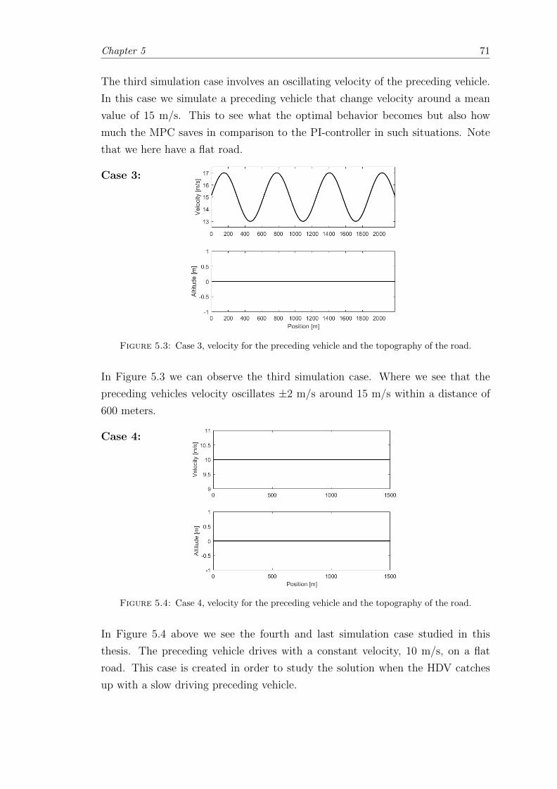
Chapter 5 71

The third simulation case involves an oscillating velocity of the preceding vehicle.

In this case we simulate a preceding vehicle that change velocity around a mean

value of 15 m/s. This to see what the optimal behavior becomes but also how

much the MPC saves in comparison to the PI-controller in such situations. Note

that we here have a flat road.

Case 3:

Figure 5.3: Case 3, velocity for the preceding vehicle and the topography of the road.

In Figure 5.3 we can observe the third simulation case. Where we see that the

preceding vehicles velocity oscillates ±2 m/s around 15 m/s within a distance of

600 meters.

Case 4:

Figure 5.4: Case 4, velocity for the preceding vehicle and the topography of the road.

In Figure 5.4 above we see the fourth and last simulation case studied in this

thesis. The preceding vehicle drives with a constant velocity, 10 m/s, on a flat

road. This case is created in order to study the solution when the HDV catches

up with a slow driving preceding vehicle.

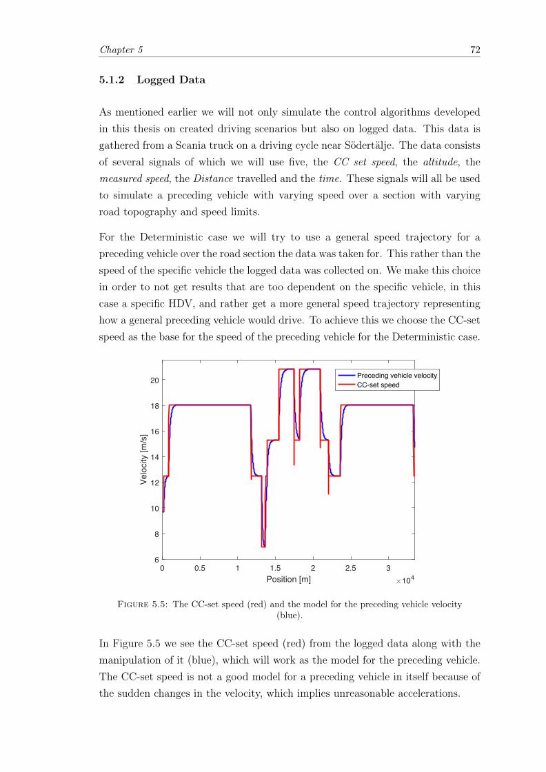
Chapter 5 72

5.1.2 Logged Data

As mentioned earlier we will not only simulate the control algorithms developed

in this thesis on created driving scenarios but also on logged data. This data is

gathered from a Scania truck on a driving cycle near Sodertalje. The data consists

of several signals of which we will use five, the CC set speed, the altitude, the

measured speed, the Distance travelled and the time. These signals will all be used

to simulate a preceding vehicle with varying speed over a section with varying

road topography and speed limits.

For the Deterministic case we will try to use a general speed trajectory for a

preceding vehicle over the road section the data was taken for. This rather than the

speed of the specific vehicle the logged data was collected on. We make this choice

in order to not get results that are too dependent on the specific vehicle, in this

case a specific HDV, and rather get a more general speed trajectory representing

how a general preceding vehicle would drive. To achieve this we choose the CC-set

speed as the base for the speed of the preceding vehicle for the Deterministic case.

0 0.5 1 1.5 2 2.5 3Position [m] 104

6

8

10

12

14

16

18

20

Velo

city

[m/s

]

Preceding vehicle velocityCC-set speed

Figure 5.5: The CC-set speed (red) and the model for the preceding vehicle velocity(blue).

In Figure 5.5 we see the CC-set speed (red) from the logged data along with the

manipulation of it (blue), which will work as the model for the preceding vehicle.

The CC-set speed is not a good model for a preceding vehicle in itself because of

the sudden changes in the velocity, which implies unreasonable accelerations.

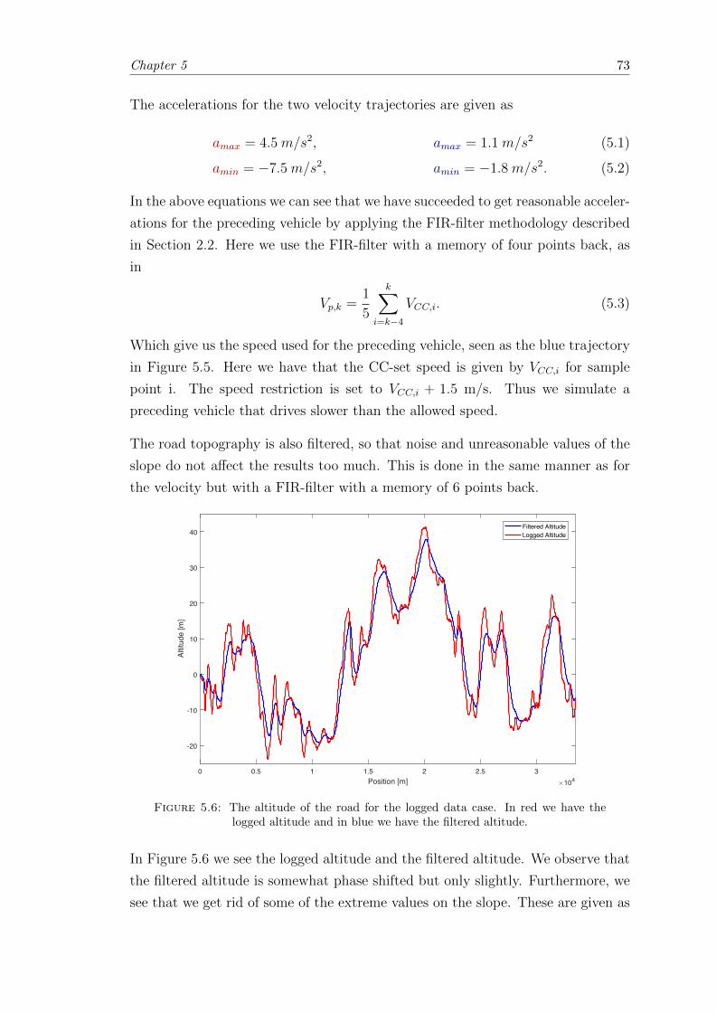
Chapter 5 73

The accelerations for the two velocity trajectories are given as

amax = 4.5 m/s2, amax = 1.1 m/s2 (5.1)

amin = −7.5 m/s2, amin = −1.8 m/s2. (5.2)

In the above equations we can see that we have succeeded to get reasonable acceler-

ations for the preceding vehicle by applying the FIR-filter methodology described

in Section 2.2. Here we use the FIR-filter with a memory of four points back, as

in

Vp,k =1

5

k∑i=k−4

VCC,i. (5.3)

Which give us the speed used for the preceding vehicle, seen as the blue trajectory

in Figure 5.5. Here we have that the CC-set speed is given by VCC,i for sample

point i. The speed restriction is set to VCC,i + 1.5 m/s. Thus we simulate a

preceding vehicle that drives slower than the allowed speed.

The road topography is also filtered, so that noise and unreasonable values of the

slope do not affect the results too much. This is done in the same manner as for

the velocity but with a FIR-filter with a memory of 6 points back.

0 0.5 1 1.5 2 2.5 3Position [m] 104

-20

-10

0

10

20

30

40

Altit

ude

[m]

Filtered AltitudeLogged Altitude

Figure 5.6: The altitude of the road for the logged data case. In red we have thelogged altitude and in blue we have the filtered altitude.

In Figure 5.6 we see the logged altitude and the filtered altitude. We observe that

the filtered altitude is somewhat phase shifted but only slightly. Furthermore, we

see that we get rid of some of the extreme values on the slope. These are given as

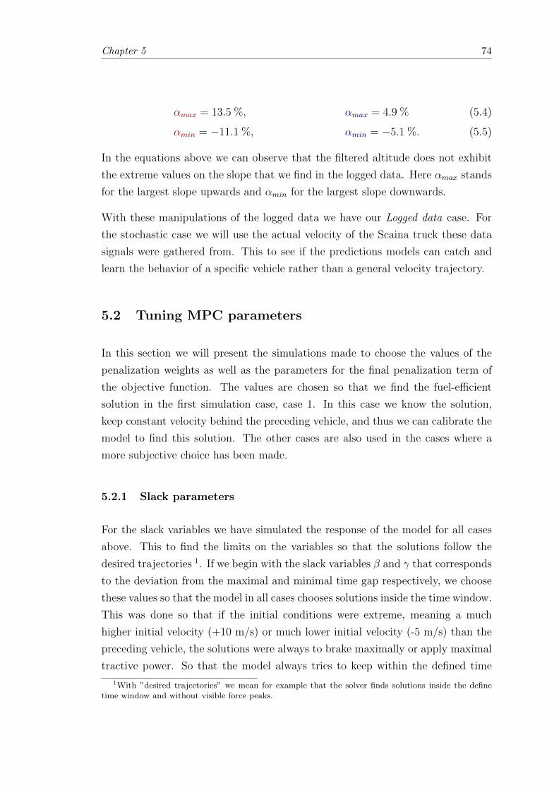
Chapter 5 74

αmax = 13.5 %, αmax = 4.9 % (5.4)

αmin = −11.1 %, αmin = −5.1 %. (5.5)

In the equations above we can observe that the filtered altitude does not exhibit

the extreme values on the slope that we find in the logged data. Here αmax stands

for the largest slope upwards and αmin for the largest slope downwards.

With these manipulations of the logged data we have our Logged data case. For

the stochastic case we will use the actual velocity of the Scaina truck these data

signals were gathered from. This to see if the predictions models can catch and

learn the behavior of a specific vehicle rather than a general velocity trajectory.

5.2 Tuning MPC parameters

In this section we will present the simulations made to choose the values of the

penalization weights as well as the parameters for the final penalization term of

the objective function. The values are chosen so that we find the fuel-efficient

solution in the first simulation case, case 1. In this case we know the solution,

keep constant velocity behind the preceding vehicle, and thus we can calibrate the

model to find this solution. The other cases are also used in the cases where a

more subjective choice has been made.

5.2.1 Slack parameters

For the slack variables we have simulated the response of the model for all cases

above. This to find the limits on the variables so that the solutions follow the

desired trajectories 1. If we begin with the slack variables β and γ that corresponds

to the deviation from the maximal and minimal time gap respectively, we choose

these values so that the model in all cases chooses solutions inside the time window.

This was done so that if the initial conditions were extreme, meaning a much

higher initial velocity (+10 m/s) or much lower initial velocity (-5 m/s) than the

preceding vehicle, the solutions were always to brake maximally or apply maximal

tractive power. So that the model always tries to keep within the defined time

1With ”desired trajcetories” we mean for example that the solver finds solutions inside the definetime window and without visible force peaks.

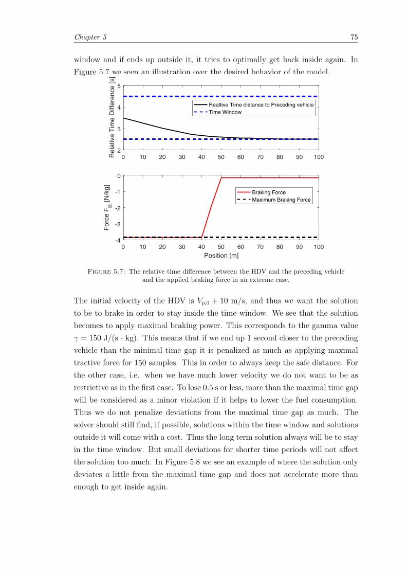
Chapter 5 75

window and if ends up outside it, it tries to optimally get back inside again. In

Figure 5.7 we seen an illustration over the desired behavior of the model.

0 10 20 30 40 50 60 70 80 90 1002

3

4

5

Rel

ativ

e Ti

me

Diff

eren

ce [s

]Realtive Time distance to Preceding vehicleTime Window

0 10 20 30 40 50 60 70 80 90 100Position [m]

-4

-3

-2

-1

0

Forc

e F B

[N/k

g]

Braking ForceMaximum Braking Force

Figure 5.7: The relative time difference between the HDV and the preceding vehicleand the applied braking force in an extreme case.

The initial velocity of the HDV is Vp,0 + 10 m/s, and thus we want the solution

to be to brake in order to stay inside the time window. We see that the solution

becomes to apply maximal braking power. This corresponds to the gamma value

γ = 150 J/(s · kg). This means that if we end up 1 second closer to the preceding

vehicle than the minimal time gap it is penalized as much as applying maximal

tractive force for 150 samples. This in order to always keep the safe distance. For

the other case, i.e. when we have much lower velocity we do not want to be as

restrictive as in the first case. To lose 0.5 s or less, more than the maximal time gap

will be considered as a minor violation if it helps to lower the fuel consumption.

Thus we do not penalize deviations from the maximal time gap as much. The

solver should still find, if possible, solutions within the time window and solutions

outside it will come with a cost. Thus the long term solution always will be to stay

in the time window. But small deviations for shorter time periods will not affect

the solution too much. In Figure 5.8 we see an example of where the solution only

deviates a little from the maximal time gap and does not accelerate more than

enough to get inside again.

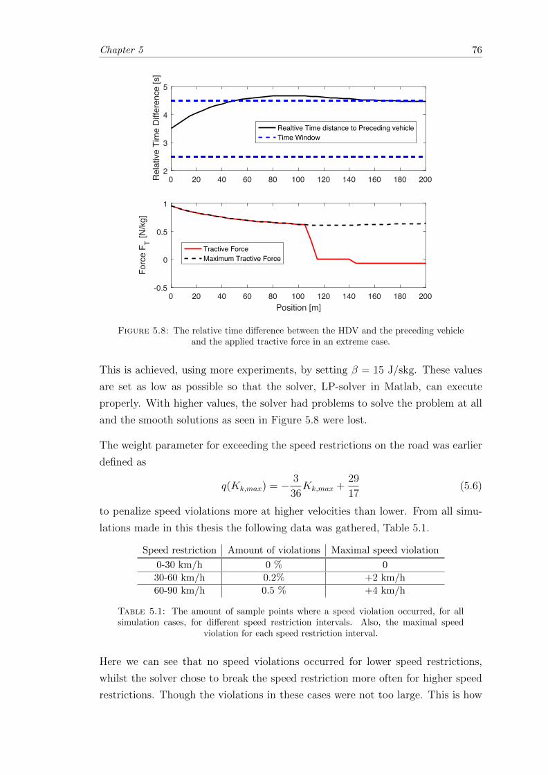
Chapter 5 76

0 20 40 60 80 100 120 140 160 180 2002

3

4

5

Rel

ativ

e Ti

me

Diff

eren

ce [s

]

Realtive Time distance to Preceding vehicleTime Window

0 20 40 60 80 100 120 140 160 180 200Position [m]

-0.5

0

0.5

1

Forc

e F T [N

/kg]

Tractive ForceMaximum Tractive Force

Figure 5.8: The relative time difference between the HDV and the preceding vehicleand the applied tractive force in an extreme case.

This is achieved, using more experiments, by setting β = 15 J/skg. These values

are set as low as possible so that the solver, LP-solver in Matlab, can execute

properly. With higher values, the solver had problems to solve the problem at all

and the smooth solutions as seen in Figure 5.8 were lost.

The weight parameter for exceeding the speed restrictions on the road was earlier

defined as

q(Kk,max) = − 3

36Kk,max +

29

17(5.6)

to penalize speed violations more at higher velocities than lower. From all simu-

lations made in this thesis the following data was gathered, Table 5.1.

Speed restriction Amount of violations Maximal speed violation

0-30 km/h 0 % 0

30-60 km/h 0.2% +2 km/h

60-90 km/h 0.5 % +4 km/h

Table 5.1: The amount of sample points where a speed violation occurred, for allsimulation cases, for different speed restriction intervals. Also, the maximal speed

violation for each speed restriction interval.

Here we can see that no speed violations occurred for lower speed restrictions,

whilst the solver chose to break the speed restriction more often for higher speed

restrictions. Though the violations in these cases were not too large. This is how

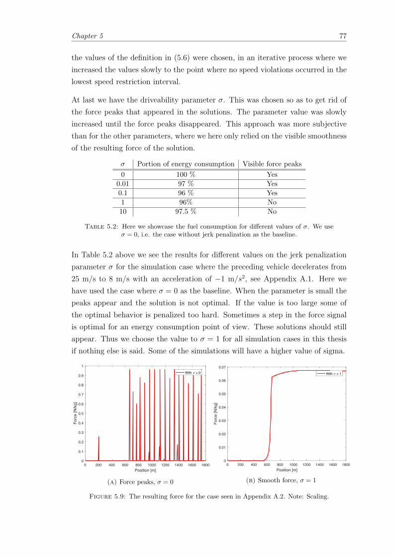
Chapter 5 77

the values of the definition in (5.6) were chosen, in an iterative process where we

increased the values slowly to the point where no speed violations occurred in the

lowest speed restriction interval.

At last we have the driveability parameter σ. This was chosen so as to get rid of

the force peaks that appeared in the solutions. The parameter value was slowly

increased until the force peaks disappeared. This approach was more subjective

than for the other parameters, where we here only relied on the visible smoothness

of the resulting force of the solution.

σ Portion of energy consumption Visible force peaks

0 100 % Yes

0.01 97 % Yes

0.1 96 % Yes

1 96% No

10 97.5 % No

Table 5.2: Here we showcase the fuel consumption for different values of σ. We useσ = 0, i.e. the case without jerk penalization as the baseline.

In Table 5.2 above we see the results for different values on the jerk penalization

parameter σ for the simulation case where the preceding vehicle decelerates from

25 m/s to 8 m/s with an acceleration of −1 m/s2, see Appendix A.1. Here we

have used the case where σ = 0 as the baseline. When the parameter is small the

peaks appear and the solution is not optimal. If the value is too large some of

the optimal behavior is penalized too hard. Sometimes a step in the force signal

is optimal for an energy consumption point of view. These solutions should still

appear. Thus we choose the value to σ = 1 for all simulation cases in this thesis

if nothing else is said. Some of the simulations will have a higher value of sigma.

0 200 400 600 800 1000 1200 1400 1600 1800Position [m]

0

0.1

0.2

0.3

0.4

0.5

0.6

0.7

0.8

0.9

1

Forc

e [N

/kg]

With = 0

(a) Force peaks, σ = 0

0 200 400 600 800 1000 1200 1400 1600 1800Position [m]

0

0.01

0.02

0.03

0.04

0.05

0.06

0.07

Forc

e [N

/kg]

With = 1

(b) Smooth force, σ = 1

Figure 5.9: The resulting force for the case seen in Appendix A.2. Note: Scaling.

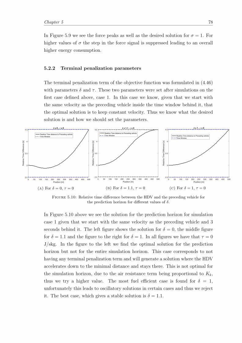
Chapter 5 78

In Figure 5.9 we see the force peaks as well as the desired solution for σ = 1. For

higher values of σ the step in the force signal is suppressed leading to an overall

higher energy consumption.

5.2.2 Terminal penalization parameters

The terminal penalization term of the objective function was formulated in (4.46)

with parameters δ and τ . These two parameters were set after simulations on the

first case defined above, case 1. In this case we know, given that we start with

the same velocity as the preceding vehicle inside the time window behind it, that

the optimal solution is to keep constant velocity. Thus we know what the desired

solution is and how we should set the parameters.

0 50 100 150 200 250 300 350 400 450 500Position [m]

2.5

3

3.5

4

4.5

Rel

ativ

e Ti

me

Diff

eren

ce [s

]

= 0 , = 0

Realtive Time distance to Preceding vehicleTime Window

(a) For δ = 0, τ = 0

0 50 100 150 200 250 300 350 400 450 500Position [m]

2.5

3

3.5

4

4.5

Rel

ativ

e Ti

me

Diff

eren

ce [s

]

= 1.1 , = 0

Realtive Time distance to Preceding vehicleTime Window

(b) For δ = 1.1, τ = 0

0 50 100 150 200 250 300 350 400 450 500Position [m]

2.5

3

3.5

4

4.5

Rel

ativ

e Ti

me

Diff

eren

ce [s

]

= 1 , = 0

Realtive Time distance to Preceding vehicleTime Window

(c) For δ = 1, τ = 0

Figure 5.10: Relative time difference between the HDV and the preceding vehicle forthe prediction horizon for different values of δ.

In Figure 5.10 above we see the solution for the prediction horizon for simulation

case 1 given that we start with the same velocity as the preceding vehicle and 3

seconds behind it. The left figure shows the solution for δ = 0, the middle figure

for δ = 1.1 and the figure to the right for δ = 1. In all figures we have that τ = 0

J/skg. In the figure to the left we find the optimal solution for the prediction

horizon but not for the entire simulation horizon. This case corresponds to not

having any terminal penalization term and will generate a solution where the HDV

accelerates down to the minimal distance and stays there. This is not optimal for

the simulation horizon, due to the air resistance term being proportional to Kk,

thus we try a higher value. The most fuel efficient case is found for δ = 1,

unfortunately this leads to oscillatory solutions in certain cases and thus we reject

it. The best case, which gives a stable solution is δ = 1.1.

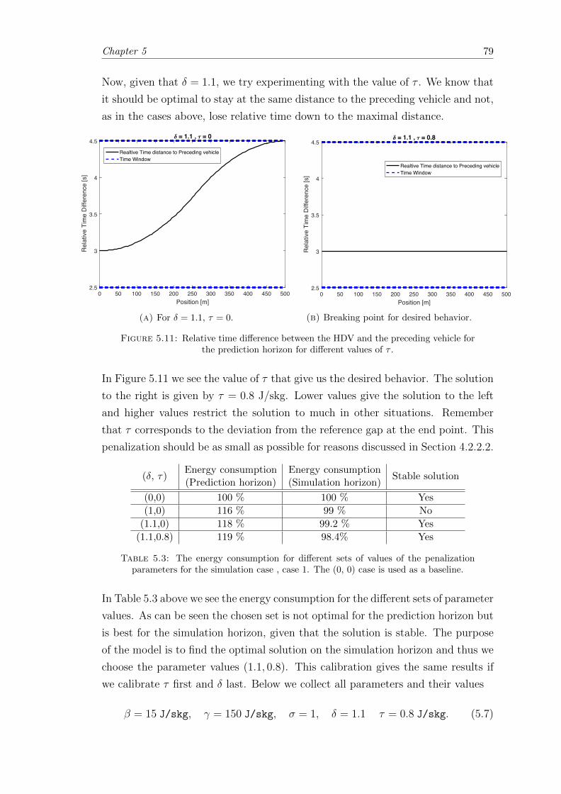
Chapter 5 79

Now, given that δ = 1.1, we try experimenting with the value of τ . We know that

it should be optimal to stay at the same distance to the preceding vehicle and not,

as in the cases above, lose relative time down to the maximal distance.

0 50 100 150 200 250 300 350 400 450 500Position [m]

2.5

3

3.5

4

4.5

Rel

ativ

e Ti

me

Diff

eren

ce [s

]

= 1.1 , = 0

Realtive Time distance to Preceding vehicleTime Window

(a) For δ = 1.1, τ = 0.

0 50 100 150 200 250 300 350 400 450 500Position [m]

2.5

3

3.5

4

4.5

Rel

ativ

e Ti

me

Diff

eren

ce [s

]

= 1.1 , = 0.8

Realtive Time distance to Preceding vehicleTime Window

(b) Breaking point for desired behavior.

Figure 5.11: Relative time difference between the HDV and the preceding vehicle forthe prediction horizon for different values of τ .

In Figure 5.11 we see the value of τ that give us the desired behavior. The solution

to the right is given by τ = 0.8 J/skg. Lower values give the solution to the left

and higher values restrict the solution to much in other situations. Remember

that τ corresponds to the deviation from the reference gap at the end point. This

penalization should be as small as possible for reasons discussed in Section 4.2.2.2.

(δ, τ)Energy consumption(Prediction horizon)

Energy consumption(Simulation horizon)

Stable solution

(0,0) 100 % 100 % Yes

(1,0) 116 % 99 % No

(1.1,0) 118 % 99.2 % Yes

(1.1,0.8) 119 % 98.4% Yes

Table 5.3: The energy consumption for different sets of values of the penalizationparameters for the simulation case , case 1. The (0, 0) case is used as a baseline.

In Table 5.3 above we see the energy consumption for the different sets of parameter

values. As can be seen the chosen set is not optimal for the prediction horizon but

is best for the simulation horizon, given that the solution is stable. The purpose

of the model is to find the optimal solution on the simulation horizon and thus we

choose the parameter values (1.1, 0.8). This calibration gives the same results if

we calibrate τ first and δ last. Below we collect all parameters and their values

β = 15 J/skg, γ = 150 J/skg, σ = 1, δ = 1.1 τ = 0.8 J/skg. (5.7)

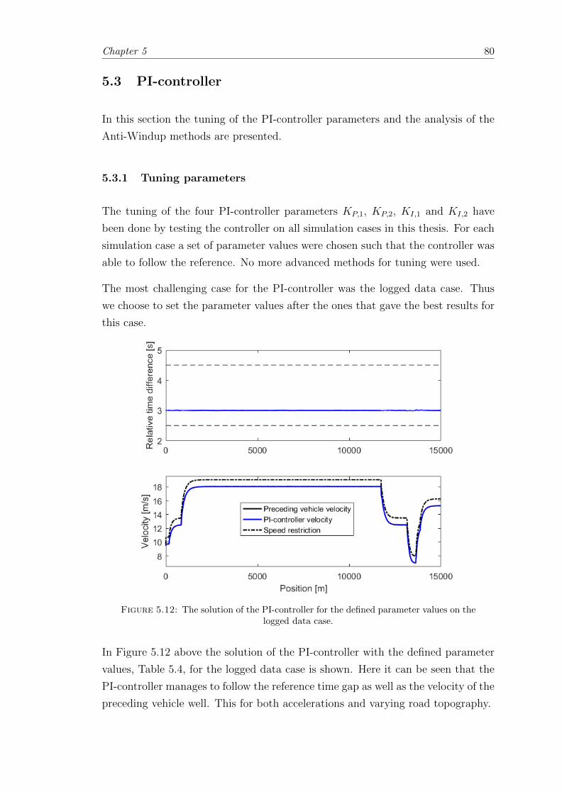
Chapter 5 80

5.3 PI-controller

In this section the tuning of the PI-controller parameters and the analysis of the

Anti-Windup methods are presented.

5.3.1 Tuning parameters

The tuning of the four PI-controller parameters KP,1, KP,2, KI,1 and KI,2 have

been done by testing the controller on all simulation cases in this thesis. For each

simulation case a set of parameter values were chosen such that the controller was

able to follow the reference. No more advanced methods for tuning were used.

The most challenging case for the PI-controller was the logged data case. Thus

we choose to set the parameter values after the ones that gave the best results for

this case.

Figure 5.12: The solution of the PI-controller for the defined parameter values on thelogged data case.

In Figure 5.12 above the solution of the PI-controller with the defined parameter

values, Table 5.4, for the logged data case is shown. Here it can be seen that the

PI-controller manages to follow the reference time gap as well as the velocity of the

preceding vehicle well. This for both accelerations and varying road topography.

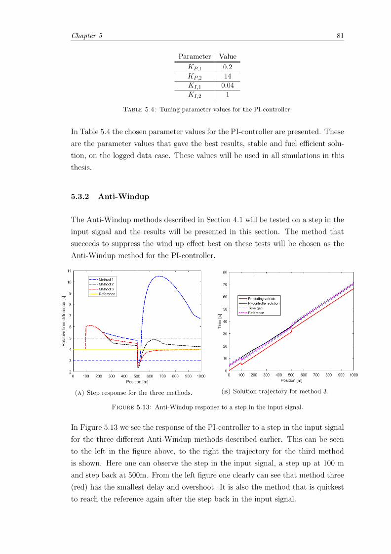
Chapter 5 81

Parameter Value

KP,1 0.2

KP,2 14

KI,1 0.04

KI,2 1

Table 5.4: Tuning parameter values for the PI-controller.

In Table 5.4 the chosen parameter values for the PI-controller are presented. These

are the parameter values that gave the best results, stable and fuel efficient solu-

tion, on the logged data case. These values will be used in all simulations in this

thesis.

5.3.2 Anti-Windup

The Anti-Windup methods described in Section 4.1 will be tested on a step in the

input signal and the results will be presented in this section. The method that

succeeds to suppress the wind up effect best on these tests will be chosen as the

Anti-Windup method for the PI-controller.

(a) Step response for the three methods. (b) Solution trajectory for method 3.

Figure 5.13: Anti-Windup response to a step in the input signal.

In Figure 5.13 we see the response of the PI-controller to a step in the input signal

for the three different Anti-Windup methods described earlier. This can be seen

to the left in the figure above, to the right the trajectory for the third method

is shown. Here one can observe the step in the input signal, a step up at 100 m

and step back at 500m. From the left figure one clearly can see that method three

(red) has the smallest delay and overshoot. It is also the method that is quickest

to reach the reference again after the step back in the input signal.

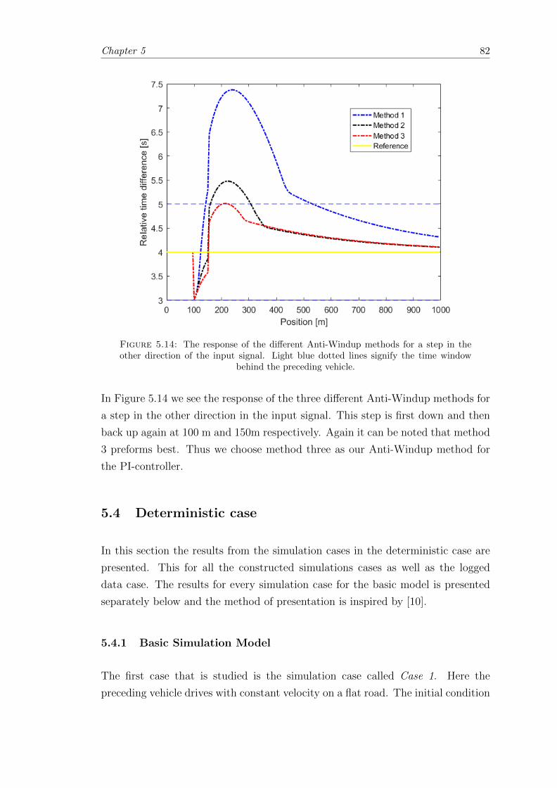
Chapter 5 82

Figure 5.14: The response of the different Anti-Windup methods for a step in theother direction of the input signal. Light blue dotted lines signify the time window

behind the preceding vehicle.

In Figure 5.14 we see the response of the three different Anti-Windup methods for

a step in the other direction in the input signal. This step is first down and then

back up again at 100 m and 150m respectively. Again it can be noted that method

3 preforms best. Thus we choose method three as our Anti-Windup method for

the PI-controller.

5.4 Deterministic case

In this section the results from the simulation cases in the deterministic case are

presented. This for all the constructed simulations cases as well as the logged

data case. The results for every simulation case for the basic model is presented

separately below and the method of presentation is inspired by [10].

5.4.1 Basic Simulation Model

The first case that is studied is the simulation case called Case 1. Here the

preceding vehicle drives with constant velocity on a flat road. The initial condition

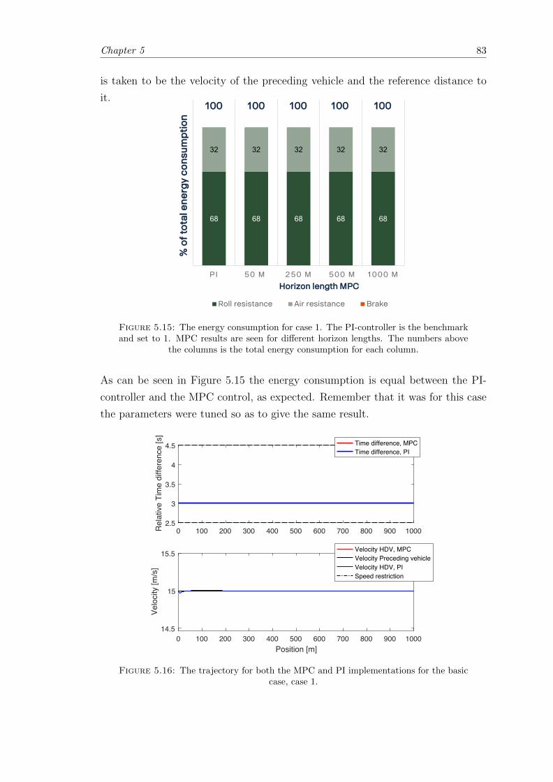
Chapter 5 83

is taken to be the velocity of the preceding vehicle and the reference distance to

it.

Title and Content

11 April 2018 Info class internal Department / Name / Subject 25

68 68 68 68 68

32 32 32 32 32

PI 50 M 250 M 500 M 1000 M

Roll resistance Air resistance Brake

% o

f to

tal e

ne

rgy

co

nsu

mp

tio

n

Horizon length MPC

100 100 100 100 100

Deterministic basic

Figure 5.15: The energy consumption for case 1. The PI-controller is the benchmarkand set to 1. MPC results are seen for different horizon lengths. The numbers above

the columns is the total energy consumption for each column.

As can be seen in Figure 5.15 the energy consumption is equal between the PI-

controller and the MPC control, as expected. Remember that it was for this case

the parameters were tuned so as to give the same result.

0 100 200 300 400 500 600 700 800 900 10002.5

3

3.5

4

4.5

Rel

ativ

e Ti

me

diffe

renc

e [s

]

Time difference, MPCTime difference, PI

0 100 200 300 400 500 600 700 800 900 1000Position [m]

14.5

15

15.5

Velo

city

[m/s

]

Velocity HDV, MPCVelocity Preceding vehicleVelocity HDV, PISpeed restriction

Figure 5.16: The trajectory for both the MPC and PI implementations for the basiccase, case 1.

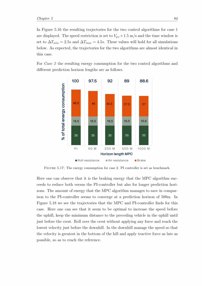
Chapter 5 84

In Figure 5.16 the resulting trajectories for the two control algorithms for case 1

are displayed. The speed restriction is set to Vp,i+1.5 m/s and the time window is

set to ∆Tmin = 2.5s and ∆Tmax = 4.5s. These values will hold for all simulations

below. As expected, the trajectories for the two algorithms are almost identical in

this case.

For Case 2 the resulting energy consumption for the two control algorithms and

different prediction horizon lengths are as follows.

Title and Content

11 April 2018 Info class internal Department / Name / Subject 26

35 35 35 35 35

16,5 16,5 16,5 16,5 16,6

48,5 46 40,5 37,5 37

PI 50 M 250 M 500 M 1000 M

Roll resistance Air resistance Brake

100 97.5 92 89 88.6

% o

f to

tal e

ne

rgy

co

nsu

mp

tio

n

Horizon length MPC

Deterministic hill

Figure 5.17: The energy consumption for case 2. PI controller is set as benchmark.

Here one can observe that it is the braking energy that the MPC algorithm suc-

ceeds to reduce both versus the PI-controller but also for longer prediction hori-

zons. The amount of energy that the MPC algorithm manages to save in compar-

ison to the PI-controller seems to converge at a prediction horizon of 500m. In

Figure 5.18 we see the trajectories that the MPC and PI-controller finds for this

case. Here one can see that it seem to be optimal to increase the speed before

the uphill, keep the minimum distance to the preceding vehicle in the uphill until

just before the crest. Roll over the crest without applying any force and reach the

lowest velocity just before the downhill. In the downhill manage the speed so that

the velocity is greatest in the bottom of the hill and apply tractive force as late as

possible, so as to reach the reference.

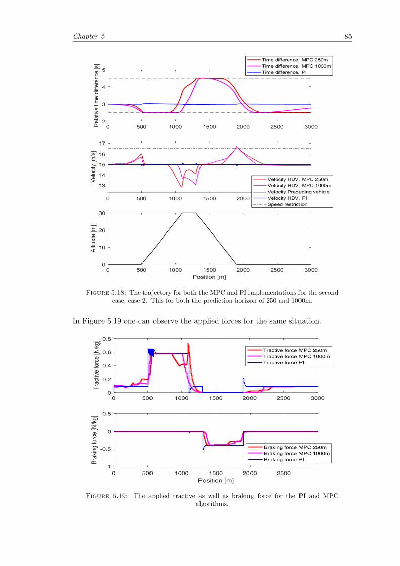
Chapter 5 85

Figure 5.18: The trajectory for both the MPC and PI implementations for the secondcase, case 2. This for both the prediction horizon of 250 and 1000m.

In Figure 5.19 one can observe the applied forces for the same situation.

0 500 1000 1500 2000 2500 30000

0.2

0.4

0.6

0.8

Trac

tive f

orce [

N/kg

]

Tractive force MPC 250mTractive force MPC 1000mTractive force PI

0 500 1000 1500 2000 2500Position [m]

-1

-0.5

0

0.5

Brak

ing fo

rce [N

/kg]

Braking force MPC 250mBraking force MPC 1000mBraking force PI

Figure 5.19: The applied tractive as well as braking force for the PI and MPCalgorithms.

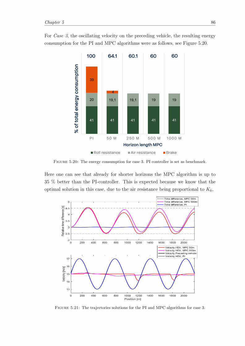
Chapter 5 86

For Case 3, the oscillating velocity on the preceding vehicle, the resulting energy

consumption for the PI and MPC algorithms were as follows, see Figure 5.20.

Title and Content

11 April 2018 Info class internal Department / Name / Subject 27

41 41 41 41 41

20 19,1 19,1 19 19

39

4

PI 50 M 250 M 500 M 1000 M

Roll resistance Air resistance Brake

100 64.1 60.1 60 60

% o

f to

tal e

ne

rgy

co

nsu

mp

tio

n

Horizon length MPC

Deterministic ocillating

Figure 5.20: The energy consumption for case 3. PI controller is set as benchmark.

Here one can see that already for shorter horizons the MPC algorithm is up to

35 % better than the PI-controller. This is expected because we know that the

optimal solution in this case, due to the air resistance being proportional to Kk,

Figure 5.21: The trajectories solutions for the PI and MPC algorithms for case 3.

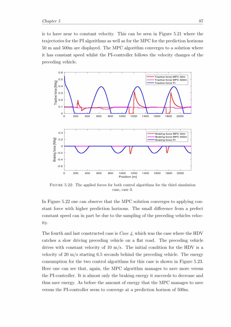
Chapter 5 87

is to have near to constant velocity. This can be seen in Figure 5.21 where the

trajectories for the PI algorithms as well as for the MPC for the prediction horizons

50 m and 500m are displayed. The MPC algorithm converges to a solution where

it has constant speed whilst the PI-controller follows the velocity changes of the

preceding vehicle.

0 200 400 600 800 1000 1200 1400 1600 1800 20000

0.1

0.2

0.3

0.4

0.5

0.6

Trac

tive f

orce [

N/kg

]

Tractive force MPC 50mTractive force MPC 500mTractive force PI

0 200 400 600 800 1000 1200 1400 1600 1800 2000Position [m]

-0.6

-0.4

-0.2

0

0.2

0.4

Brak

ing fo

rce [N

/kg]

Braking force MPC 50mBraking force MPC 500mBraking force PI

Figure 5.22: The applied forces for both control algorithms for the third simulationcase, case 3.

In Figure 5.22 one can observe that the MPC solution converges to applying con-

stant force with higher prediction horizons. The small difference from a prefect

constant speed can in part be due to the sampling of the preceding vehicles veloc-

ity.

The fourth and last constructed case is Case 4, which was the case where the HDV

catches a slow driving preceding vehicle on a flat road. The preceding vehicle

drives with constant velocity of 10 m/s. The initial condition for the HDV is a

velocity of 20 m/s starting 6.5 seconds behind the preceding vehicle. The energy

consumption for the two control algorithms for this case is shown in Figure 5.23.

Here one can see that, again, the MPC algorithm manages to save more versus

the PI-controller. It is almost only the braking energy it succeeds to decrease and

thus save energy. As before the amount of energy that the MPC manages to save

versus the PI-controller seem to converge at a prediction horizon of 500m.

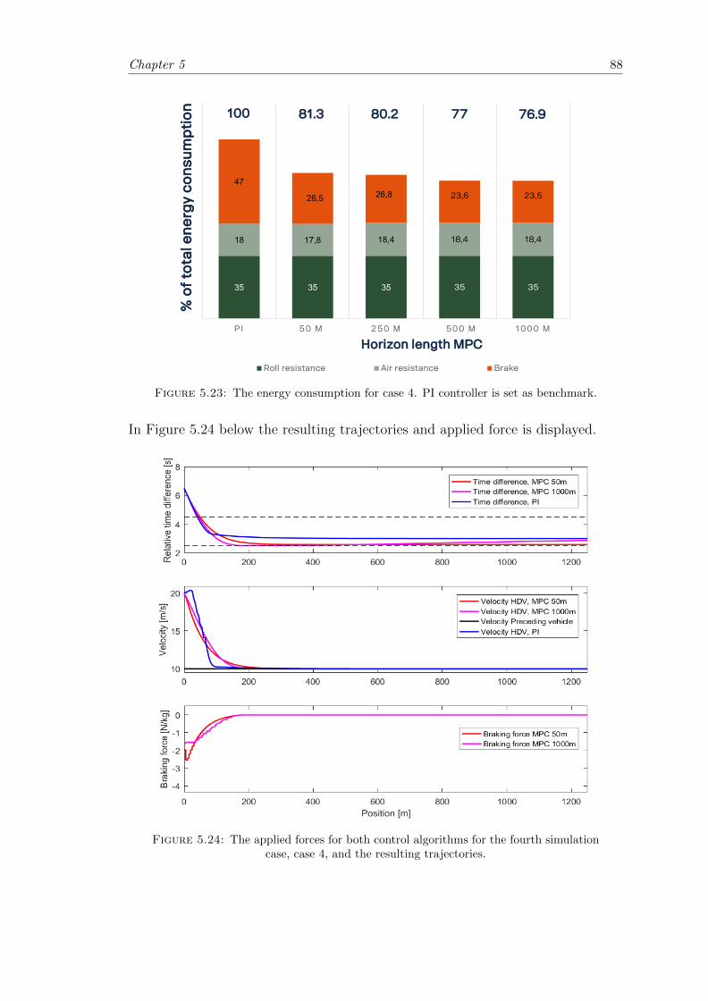
Chapter 5 88

Title and Content

11 April 2018 Info class internal Department / Name / Subject 28

35 35 35 35 35

18 17,8 18,4 18,4 18,4

47

28,5 26,8 23,6 23,5

PI 50 M 250 M 500 M 1000 M

Roll resistance Air resistance Brake

100 81.3 80.2 77 76.9

% o

f to

tal e

ne

rgy

co

nsu

mp

tio

n

Horizon length MPC

Deterministic catch

Figure 5.23: The energy consumption for case 4. PI controller is set as benchmark.

In Figure 5.24 below the resulting trajectories and applied force is displayed.

Figure 5.24: The applied forces for both control algorithms for the fourth simulationcase, case 4, and the resulting trajectories.

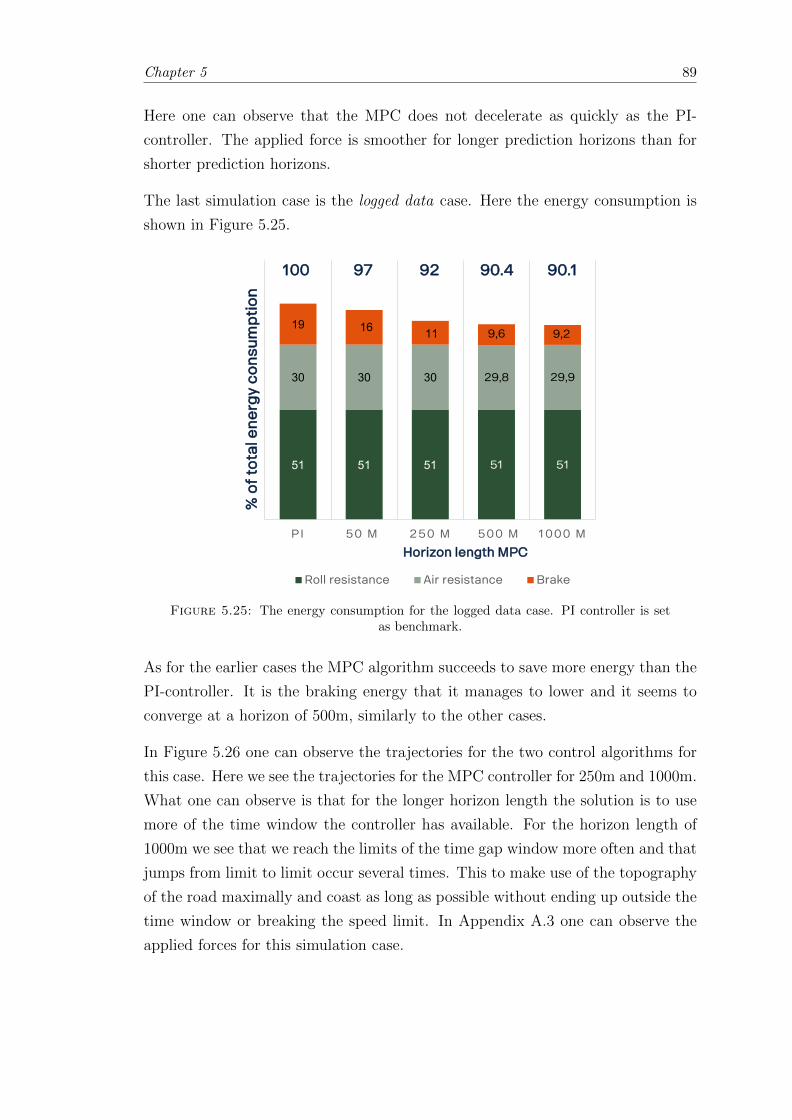
Chapter 5 89

Here one can observe that the MPC does not decelerate as quickly as the PI-

controller. The applied force is smoother for longer prediction horizons than for

shorter prediction horizons.

The last simulation case is the logged data case. Here the energy consumption is

shown in Figure 5.25.

Title and Content

29

Deterministic Logged case

51 51 51 51 51

30 30 30 29,8 29,9

19 16 11 9,6 9,2

PI 50 M 250 M 500 M 1000 M

Roll resistance Air resistance Brake

100 97 92 90.4 90.1

Horizon length MPC

% o

f to

tal e

ne

rgy

co

nsu

mp

tio

n

Figure 5.25: The energy consumption for the logged data case. PI controller is setas benchmark.

As for the earlier cases the MPC algorithm succeeds to save more energy than the

PI-controller. It is the braking energy that it manages to lower and it seems to

converge at a horizon of 500m, similarly to the other cases.

In Figure 5.26 one can observe the trajectories for the two control algorithms for

this case. Here we see the trajectories for the MPC controller for 250m and 1000m.

What one can observe is that for the longer horizon length the solution is to use

more of the time window the controller has available. For the horizon length of

1000m we see that we reach the limits of the time gap window more often and that

jumps from limit to limit occur several times. This to make use of the topography

of the road maximally and coast as long as possible without ending up outside the

time window or breaking the speed limit. In Appendix A.3 one can observe the

applied forces for this simulation case.

Chapter 5 90

Figure 5.26: The resulting trajectories for the PI and MPC algorithms for the loggeddata case.

5.4.1.1 Regenerative braking Model

In this section the results of the simulations with the regenerative brake model are

presented. First the results from the hill case, Case 2, are presented. This both

with respect to a PI-controller with and without regenerative braking. Then, the

results of the simulations made on the Logged data case are presented, again both

with respect to a PI-controller with and without regenerative braking. The results

are presented with respect to two different PI-controller in order to compare the

results to the model without regenerative braking.

The first simulation results are from simulations on the second case, case 2, which

consisted of a hill and a preceding vehicle keeping constant velocity. In Figure

5.27 one can see the energy consumption with respect to a PI-controller without

regenerative braking for both the MPC algorithm with and without regenerative

braking for case 2.

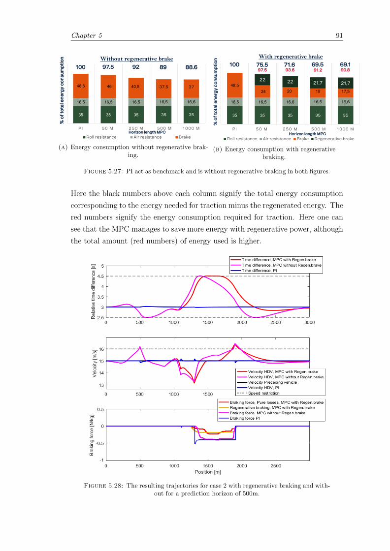
Chapter 5 91

Title and Content

11 April 2018 Info class internal Department / Name / Subject 31

35 35 35 35 35

16,5 16,5 16,5 16,5 16,6

48,5 46 40,5 37,5 37

PI 50 M 250 M 500 M 1000 M

Roll resistance Air resistance Brake

Without regenerative brake100 97.5 92 89 88.6

% o

f to

tal e

ne

rgy

co

nsu

mp

tio

n

Horizon length MPC

Regenerative brake; Hill

(a) Energy consumption without regenerative brak-ing.

Title and Content

11 April 2018 Info class internal Department / Name / Subject 30

35 35 35 35 35

16,5 16,5 16,6 16,5 16,6

48,524 20 18 17,5

22 22 21,7 21,7

PI 50 M 250 M 500 M 1000 M

Roll resistance Air resistance Brake Regenerative brake

With regenerative brake100 75.5 71.6 69.5

97.5 93.6 91.269.190.8

% o

f to

tal e

ne

rgy

co

nsu

mp

tio

n

Horizon length MPC

Regenerative brake; Hill

(b) Energy consumption with regenerativebraking.

Figure 5.27: PI act as benchmark and is without regenerative braking in both figures.

Here the black numbers above each column signify the total energy consumption

corresponding to the energy needed for traction minus the regenerated energy. The

red numbers signify the energy consumption required for traction. Here one can

see that the MPC manages to save more energy with regenerative power, although

the total amount (red numbers) of energy used is higher.

Figure 5.28: The resulting trajectories for case 2 with regenerative braking and with-out for a prediction horizon of 500m.

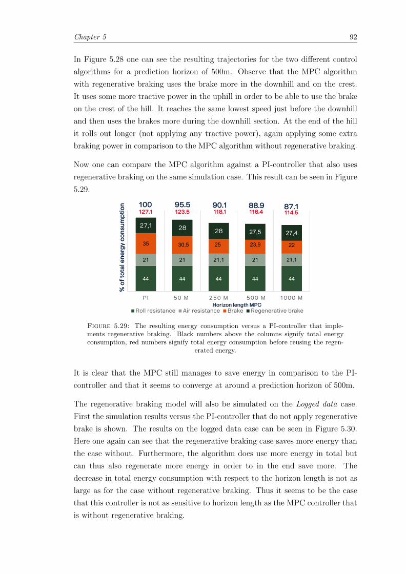
Chapter 5 92

In Figure 5.28 one can see the resulting trajectories for the two different control

algorithms for a prediction horizon of 500m. Observe that the MPC algorithm

with regenerative braking uses the brake more in the downhill and on the crest.

It uses some more tractive power in the uphill in order to be able to use the brake

on the crest of the hill. It reaches the same lowest speed just before the downhill

and then uses the brakes more during the downhill section. At the end of the hill

it rolls out longer (not applying any tractive power), again applying some extra

braking power in comparison to the MPC algorithm without regenerative braking.

Now one can compare the MPC algorithm against a PI-controller that also uses

regenerative braking on the same simulation case. This result can be seen in Figure

5.29.

Title and Content

11 April 2018 Info class internal Department / Name / Subject 32

Regenerative brake; Hill, PI with regenerative brake, skapa data

44 44 44 44 44

21 21 21,1 21 21,1

35 30,5 25 23,9 22

27,1 28 28 27,5 27,4

PI 50 M 250 M 500 M 1000 M

Roll resistance Air resistance Brake Regenerative brake

100 95.5 90.1 88.9 87.1127.1 123.5 118.1 116.4 114.5

% o

f to

tal e

ne

rgy

co

nsu

mp

tio

n

Horizon length MPC

Figure 5.29: The resulting energy consumption versus a PI-controller that imple-ments regenerative braking. Black numbers above the columns signify total energyconsumption, red numbers signify total energy consumption before reusing the regen-

erated energy.

It is clear that the MPC still manages to save energy in comparison to the PI-

controller and that it seems to converge at around a prediction horizon of 500m.

The regenerative braking model will also be simulated on the Logged data case.

First the simulation results versus the PI-controller that do not apply regenerative

brake is shown. The results on the logged data case can be seen in Figure 5.30.

Here one again can see that the regenerative braking case saves more energy than

the case without. Furthermore, the algorithm does use more energy in total but

can thus also regenerate more energy in order to in the end save more. The

decrease in total energy consumption with respect to the horizon length is not as

large as for the case without regenerative braking. Thus it seems to be the case

that this controller is not as sensitive to horizon length as the MPC controller that

is without regenerative braking.

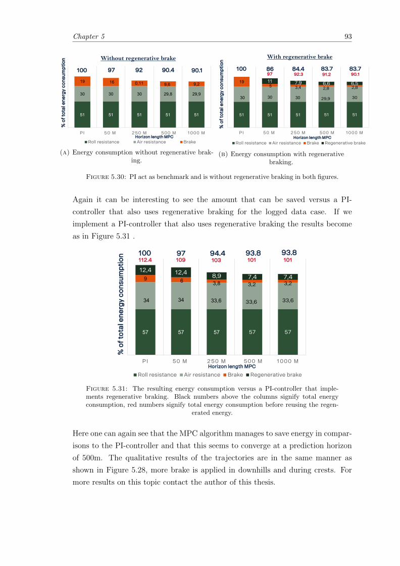
Chapter 5 93

Title and Content

11 April 2018 Info class internal Department / Name / Subject 34

Regenerative brake; Logged data

51 51 51 51 51

30 30 30 29,8 29,9

19 16 0,11 9,6 9,2

PI 50 M 250 M 500 M 1000 M

Roll resistance Air resistance Brake

100 97 92 90.4 90.1

% o

f to

tal e

ne

rgy

co

nsu

mp

tio

n

Horizon length MPC

Without regenerative brake

(a) Energy consumption without regenerative brak-ing.

Title and Content

11 April 2018 Info class internal Department / Name / Subject 33

Regenerative brake; Logged data

51 51 51 51 51

30 30 30 29,9 30

195 3,4 2,8 2,8

11 7,9 6,6 6,5

PI 50 M 250 M 500 M 1000 M

Roll resistance Air resistance Brake Regenerative brake

100 86 84.4 83.797 92.3 91.2

83.790.1

With regenerative brake

% o

f to

tal e

ne

rgy

co

nsu

mp

tio

n

Horizon length MPC

(b) Energy consumption with regenerativebraking.

Figure 5.30: PI act as benchmark and is without regenerative braking in both figures.

Again it can be interesting to see the amount that can be saved versus a PI-

controller that also uses regenerative braking for the logged data case. If we

implement a PI-controller that also uses regenerative braking the results become

as in Figure 5.31 .

Title and Content

11 April 2018 Info class internal Department / Name / Subject 35

Regenerative brake; Logged data, PI with regenerative brake, skapa data

57 57 57 57 57

34 34 33,6 33,6 33,6

9 6 3,8 3,2 3,2

12,4 12,48,9 7,4 7,4

PI 50 M 250 M 500 M 1000 M

Roll resistance Air resistance Brake Regenerative brake

100 97 94.4 93.8109 103 101

93.8101

% o

f to

tal e

ne

rgy

co

nsu

mp

tio

n

Horizon length MPC

112.4

Figure 5.31: The resulting energy consumption versus a PI-controller that imple-ments regenerative braking. Black numbers above the columns signify total energyconsumption, red numbers signify total energy consumption before reusing the regen-

erated energy.

Here one can again see that the MPC algorithm manages to save energy in compar-

isons to the PI-controller and that this seems to converge at a prediction horizon

of 500m. The qualitative results of the trajectories are in the same manner as

shown in Figure 5.28, more brake is applied in downhills and during crests. For

more results on this topic contact the author of this thesis.

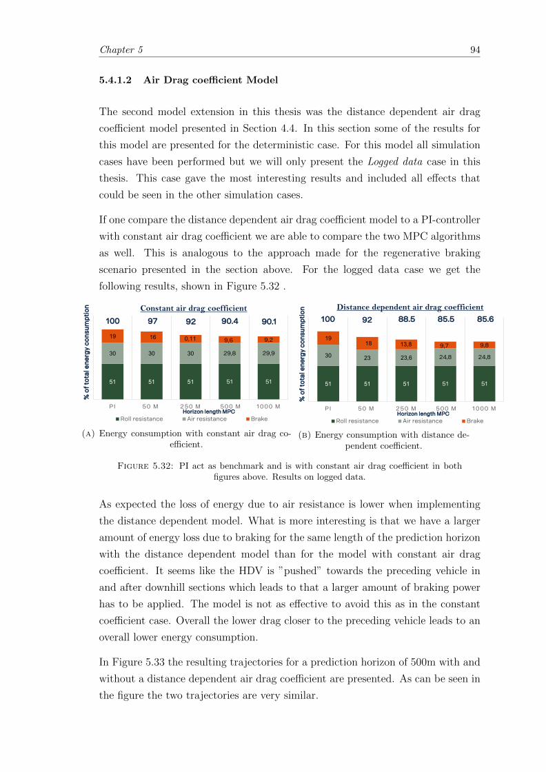
Chapter 5 94

5.4.1.2 Air Drag coefficient Model

The second model extension in this thesis was the distance dependent air drag

coefficient model presented in Section 4.4. In this section some of the results for

this model are presented for the deterministic case. For this model all simulation

cases have been performed but we will only present the Logged data case in this

thesis. This case gave the most interesting results and included all effects that

could be seen in the other simulation cases.

If one compare the distance dependent air drag coefficient model to a PI-controller

with constant air drag coefficient we are able to compare the two MPC algorithms

as well. This is analogous to the approach made for the regenerative braking

scenario presented in the section above. For the logged data case we get the

following results, shown in Figure 5.32 .

Title and Content

11 April 2018 Info class internal Department / Name / Subject 37

51 51 51 51 51

30 30 30 29,8 29,9

19 16 0,11 9,6 9,2

PI 50 M 250 M 500 M 1000 M

Roll resistance Air resistance Brake

100 97 92 90.4 90.1

% o

f to

tal e

ne

rgy

co

nsu

mp

tio

n

Horizon length MPC

Constant air drag coefficient

Air resistance; Logged data

(a) Energy consumption with constant air drag co-efficient.

Title and Content

11 April 2018 Info class internal Department / Name / Subject 36

51 51 51 51 51

30 23 23,6 24,8 24,8

1918 13,8 9,7 9,8

PI 50 M 250 M 500 M 1000 M

Roll resistance Air resistance Brake

100 88.5 85.5 85.692

Air resistance; Logged data

Distance dependent air drag coefficient%

of

tota

l en

erg

y c

on

sum

pti

on

Horizon length MPC

(b) Energy consumption with distance de-pendent coefficient.

Figure 5.32: PI act as benchmark and is with constant air drag coefficient in bothfigures above. Results on logged data.

As expected the loss of energy due to air resistance is lower when implementing

the distance dependent model. What is more interesting is that we have a larger

amount of energy loss due to braking for the same length of the prediction horizon

with the distance dependent model than for the model with constant air drag

coefficient. It seems like the HDV is ”pushed” towards the preceding vehicle in

and after downhill sections which leads to that a larger amount of braking power

has to be applied. The model is not as effective to avoid this as in the constant

coefficient case. Overall the lower drag closer to the preceding vehicle leads to an

overall lower energy consumption.

In Figure 5.33 the resulting trajectories for a prediction horizon of 500m with and

without a distance dependent air drag coefficient are presented. As can be seen in

the figure the two trajectories are very similar.

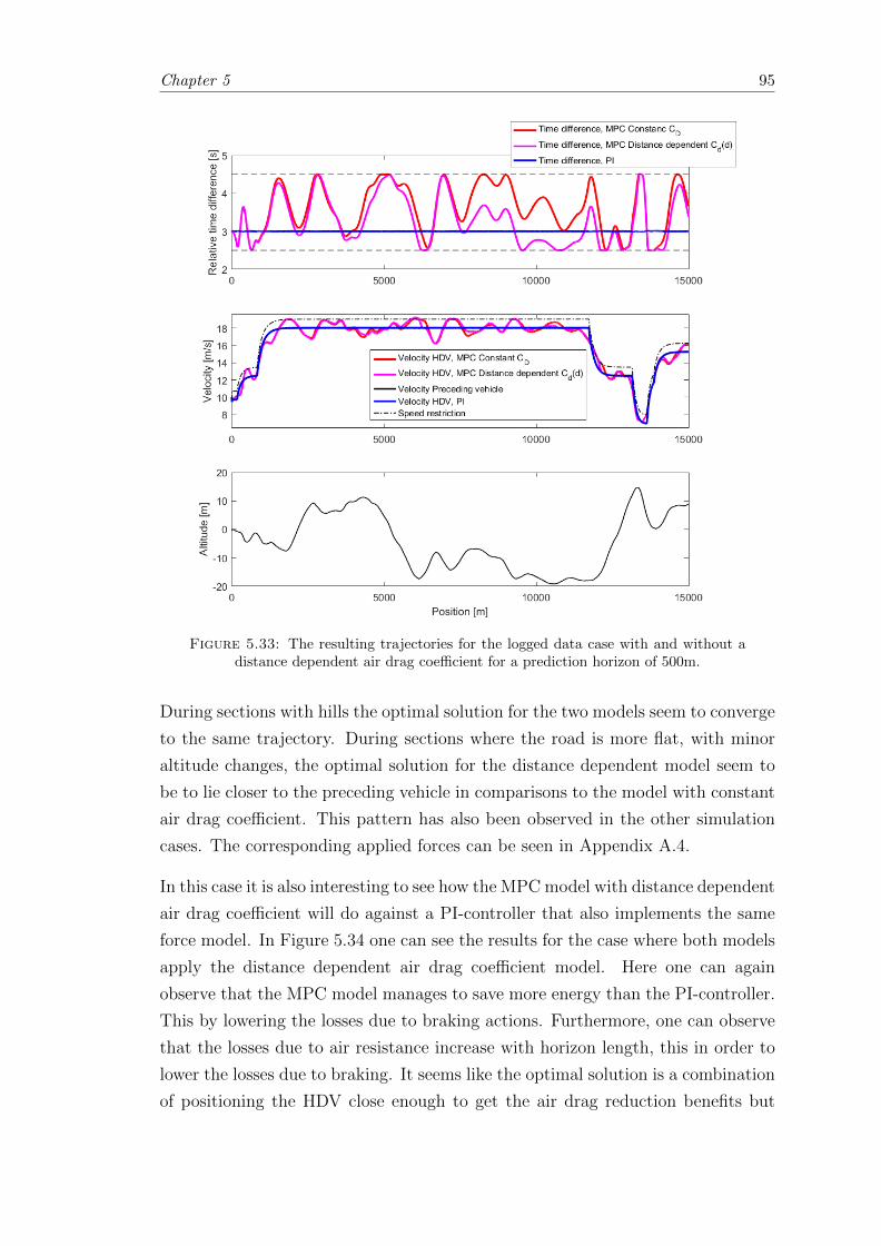
Chapter 5 95

Figure 5.33: The resulting trajectories for the logged data case with and without adistance dependent air drag coefficient for a prediction horizon of 500m.

During sections with hills the optimal solution for the two models seem to converge

to the same trajectory. During sections where the road is more flat, with minor

altitude changes, the optimal solution for the distance dependent model seem to

be to lie closer to the preceding vehicle in comparisons to the model with constant

air drag coefficient. This pattern has also been observed in the other simulation

cases. The corresponding applied forces can be seen in Appendix A.4.

In this case it is also interesting to see how the MPC model with distance dependent

air drag coefficient will do against a PI-controller that also implements the same

force model. In Figure 5.34 one can see the results for the case where both models

apply the distance dependent air drag coefficient model. Here one can again

observe that the MPC model manages to save more energy than the PI-controller.

This by lowering the losses due to braking actions. Furthermore, one can observe

that the losses due to air resistance increase with horizon length, this in order to

lower the losses due to braking. It seems like the optimal solution is a combination

of positioning the HDV close enough to get the air drag reduction benefits but

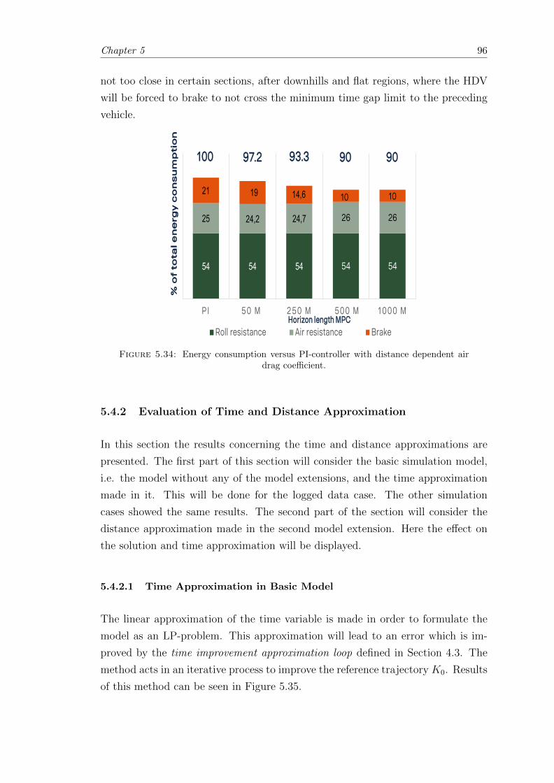
Chapter 5 96

not too close in certain sections, after downhills and flat regions, where the HDV

will be forced to brake to not cross the minimum time gap limit to the preceding

vehicle.

Title and Content

11 April 2018 Info class internal Department / Name / Subject 38

54 54 54 54 54

25 24,2 24,7 26 26

21 19 14,6 10 10

PI 50 M 250 M 500 M 1000 M

Roll resistance Air resistance Brake

100 93.3 90 9097.2

Horizon length MPC

Air resistance; Logged data, PI also distance dependent

% o

f to

tal e

ne

rgy

co

ns

um

pti

on

Figure 5.34: Energy consumption versus PI-controller with distance dependent airdrag coefficient.

5.4.2 Evaluation of Time and Distance Approximation

In this section the results concerning the time and distance approximations are

presented. The first part of this section will consider the basic simulation model,

i.e. the model without any of the model extensions, and the time approximation

made in it. This will be done for the logged data case. The other simulation

cases showed the same results. The second part of the section will consider the

distance approximation made in the second model extension. Here the effect on

the solution and time approximation will be displayed.

5.4.2.1 Time Approximation in Basic Model

The linear approximation of the time variable is made in order to formulate the

model as an LP-problem. This approximation will lead to an error which is im-

proved by the time improvement approximation loop defined in Section 4.3. The

method acts in an iterative process to improve the reference trajectory K0. Results

of this method can be seen in Figure 5.35.

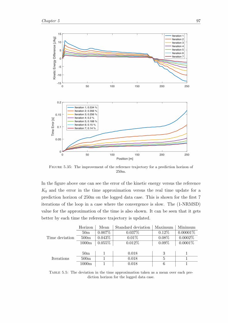
Chapter 5 97

0 50 100 150 200 250-15

-10

-5

0

5

10

15

Kine

tic E

nerg

y Di

ffere

nce

[J/k

g]

Iteration 1Iteration 2Iteration 3Iteration 4Iteration 5Iteration 6Iteration 7

0 50 100 150 200 250Position [m]

0

0.05

0.1

0.15

0.2

Tim

e Er

ror [

s]

Iteration 1; 0.534 %Iteration 2; 0.356 %Iteration 3; 0.256 %Iteration 4; 0.2 %Iteration 5; 0.168 %Iteration 6; 0.15 %Iteration 7; 0.14 %

Figure 5.35: The improvement of the reference trajectory for a prediction horizon of250m.

In the figure above one can see the error of the kinetic energy versus the reference

K0 and the error in the time approximation versus the real time update for a

prediction horizon of 250m on the logged data case. This is shown for the first 7

iterations of the loop in a case where the convergence is slow. The (1-NRMSD)

value for the approximation of the time is also shown. It can be seen that it gets

better by each time the reference trajectory is updated.

Horizon Mean Standard deviation Maximum Minimum50m 0.007% 0.037% 0.12% 0.00001%

Time deviation 500m 0.043% 0.01% 0.08% 0.0002%1000m 0.055% 0.012% 0.09% 0.0001%

50m 1 0.018 3 1Iterations 500m 1 0.018 5 1

1000m 1 0.018 6 1

Table 5.5: The deviation in the time approximation taken as a mean over each pre-diction horizon for the logged data case.

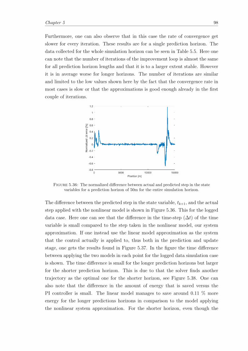
Chapter 5 98

Furthermore, one can also observe that in this case the rate of convergence get

slower for every iteration. These results are for a single prediction horizon. The

data collected for the whole simulation horizon can be seen in Table 5.5. Here one

can note that the number of iterations of the improvement loop is almost the same

for all prediction horizon lengths and that it is to a larger extent stable. However

it is in average worse for longer horizons. The number of iterations are similar

and limited to the low values shown here by the fact that the convergence rate in

most cases is slow or that the approximations is good enough already in the first

couple of iterations.

Figure 5.36: The normalized difference between actual and predicted step in the statevariables for a prediction horizon of 50m for the entire simulation horizon.

The difference between the predicted step in the state variable, tk+1, and the actual

step applied with the nonlinear model is shown in Figure 5.36. This for the logged

data case. Here one can see that the difference in the time-step (∆t) of the time

variable is small compared to the step taken in the nonlinear model, our system

approximation. If one instead use the linear model approximation as the system

that the control actually is applied to, thus both in the prediction and update

stage, one gets the results found in Figure 5.37. In the figure the time difference

between applying the two models in each point for the logged data simulation case

is shown. The time difference is small for the longer prediction horizons but larger

for the shorter prediction horizon. This is due to that the solver finds another

trajectory as the optimal one for the shorter horizon, see Figure 5.38. One can

also note that the difference in the amount of energy that is saved versus the

PI controller is small. The linear model manages to save around 0.11 % more

energy for the longer predictions horizons in comparison to the model applying

the nonlinear system approximation. For the shorter horizon, even though the

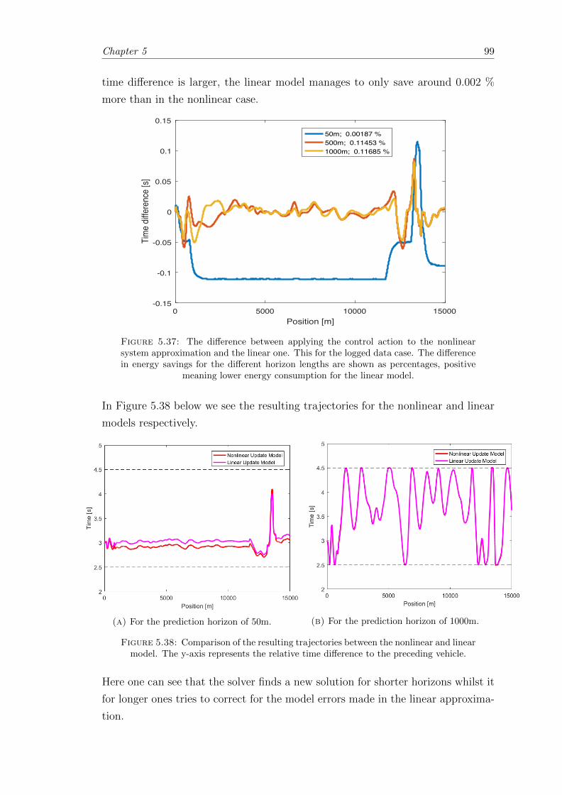
Chapter 5 99

time difference is larger, the linear model manages to only save around 0.002 %

more than in the nonlinear case.

0 5000 10000 15000Position [m]

-0.15

-0.1

-0.05

0

0.05

0.1

0.15

Time

diffe

renc

e [s]

50m; 0.00187 %500m; 0.11453 %1000m; 0.11685 %

Figure 5.37: The difference between applying the control action to the nonlinearsystem approximation and the linear one. This for the logged data case. The differencein energy savings for the different horizon lengths are shown as percentages, positive

meaning lower energy consumption for the linear model.

In Figure 5.38 below we see the resulting trajectories for the nonlinear and linear

models respectively.

(a) For the prediction horizon of 50m. (b) For the prediction horizon of 1000m.

Figure 5.38: Comparison of the resulting trajectories between the nonlinear and linearmodel. The y-axis represents the relative time difference to the preceding vehicle.

Here one can see that the solver finds a new solution for shorter horizons whilst it

for longer ones tries to correct for the model errors made in the linear approxima-

tion.

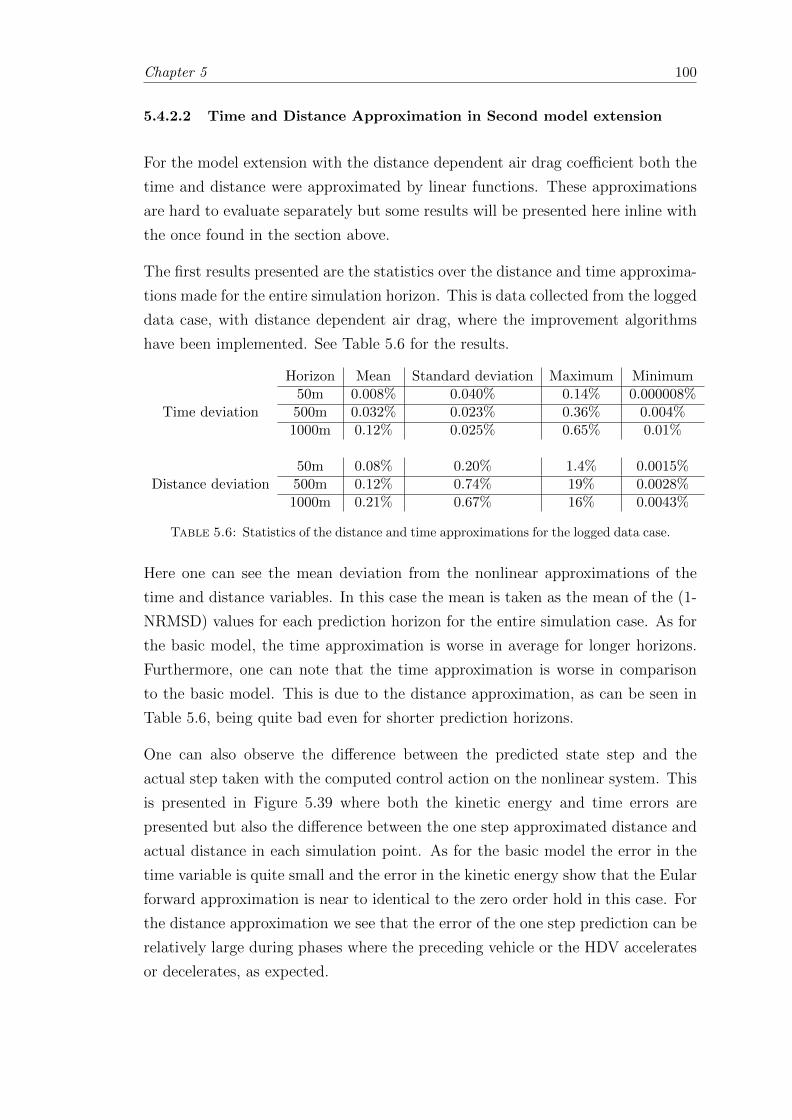
Chapter 5 100

5.4.2.2 Time and Distance Approximation in Second model extension

For the model extension with the distance dependent air drag coefficient both the

time and distance were approximated by linear functions. These approximations

are hard to evaluate separately but some results will be presented here inline with

the once found in the section above.

The first results presented are the statistics over the distance and time approxima-

tions made for the entire simulation horizon. This is data collected from the logged

data case, with distance dependent air drag, where the improvement algorithms

have been implemented. See Table 5.6 for the results.

Horizon Mean Standard deviation Maximum Minimum50m 0.008% 0.040% 0.14% 0.000008%

Time deviation 500m 0.032% 0.023% 0.36% 0.004%1000m 0.12% 0.025% 0.65% 0.01%

50m 0.08% 0.20% 1.4% 0.0015%Distance deviation 500m 0.12% 0.74% 19% 0.0028%

1000m 0.21% 0.67% 16% 0.0043%

Table 5.6: Statistics of the distance and time approximations for the logged data case.

Here one can see the mean deviation from the nonlinear approximations of the

time and distance variables. In this case the mean is taken as the mean of the (1-

NRMSD) values for each prediction horizon for the entire simulation case. As for

the basic model, the time approximation is worse in average for longer horizons.

Furthermore, one can note that the time approximation is worse in comparison

to the basic model. This is due to the distance approximation, as can be seen in

Table 5.6, being quite bad even for shorter prediction horizons.

One can also observe the difference between the predicted state step and the

actual step taken with the computed control action on the nonlinear system. This

is presented in Figure 5.39 where both the kinetic energy and time errors are

presented but also the difference between the one step approximated distance and

actual distance in each simulation point. As for the basic model the error in the

time variable is quite small and the error in the kinetic energy show that the Eular

forward approximation is near to identical to the zero order hold in this case. For

the distance approximation we see that the error of the one step prediction can be

relatively large during phases where the preceding vehicle or the HDV accelerates

or decelerates, as expected.

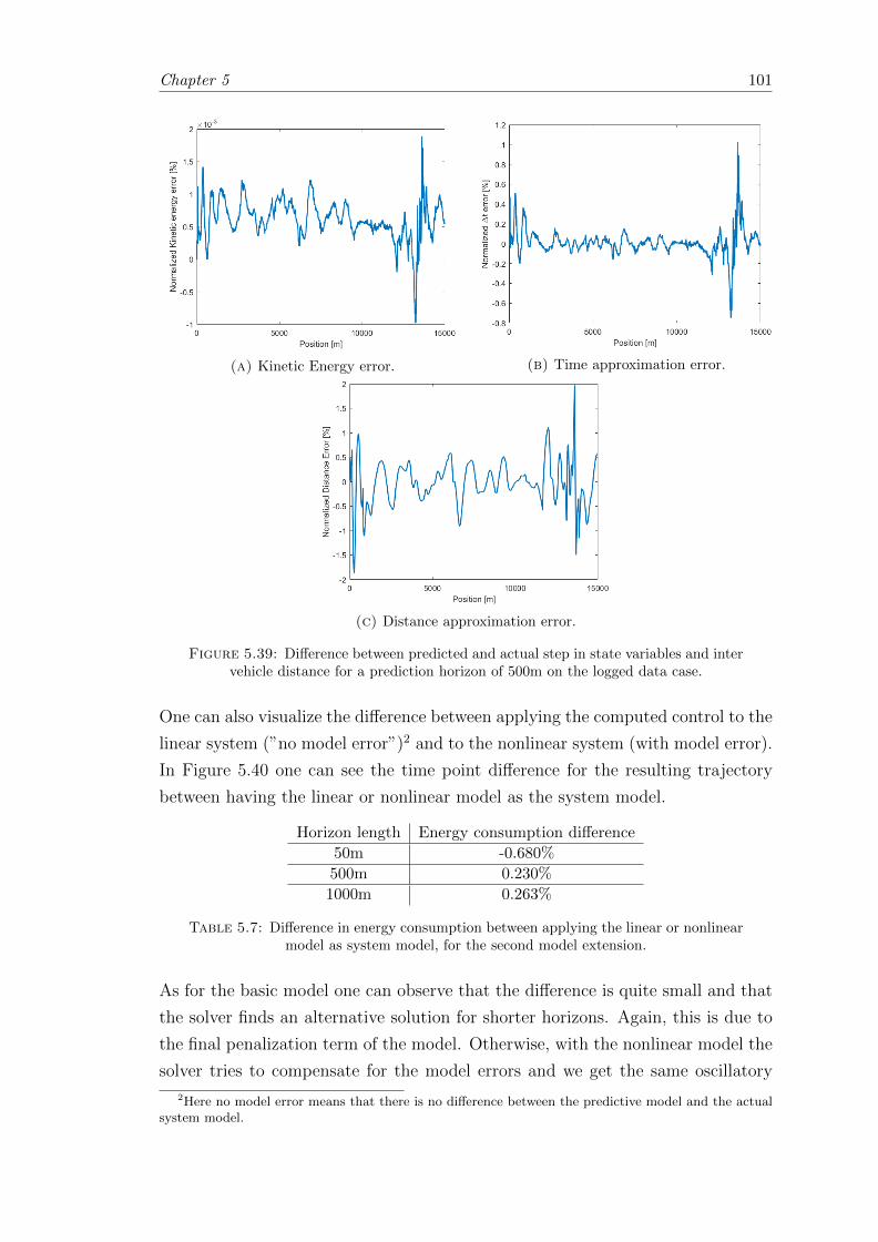
Chapter 5 101

(a) Kinetic Energy error. (b) Time approximation error.

(c) Distance approximation error.

Figure 5.39: Difference between predicted and actual step in state variables and intervehicle distance for a prediction horizon of 500m on the logged data case.

One can also visualize the difference between applying the computed control to the

linear system (”no model error”)2 and to the nonlinear system (with model error).

In Figure 5.40 one can see the time point difference for the resulting trajectory

between having the linear or nonlinear model as the system model.

Horizon length Energy consumption difference

50m -0.680%

500m 0.230%

1000m 0.263%

Table 5.7: Difference in energy consumption between applying the linear or nonlinearmodel as system model, for the second model extension.

As for the basic model one can observe that the difference is quite small and that

the solver finds an alternative solution for shorter horizons. Again, this is due to

the final penalization term of the model. Otherwise, with the nonlinear model the

solver tries to compensate for the model errors and we get the same oscillatory

2Here no model error means that there is no difference between the predictive model and the actualsystem model.

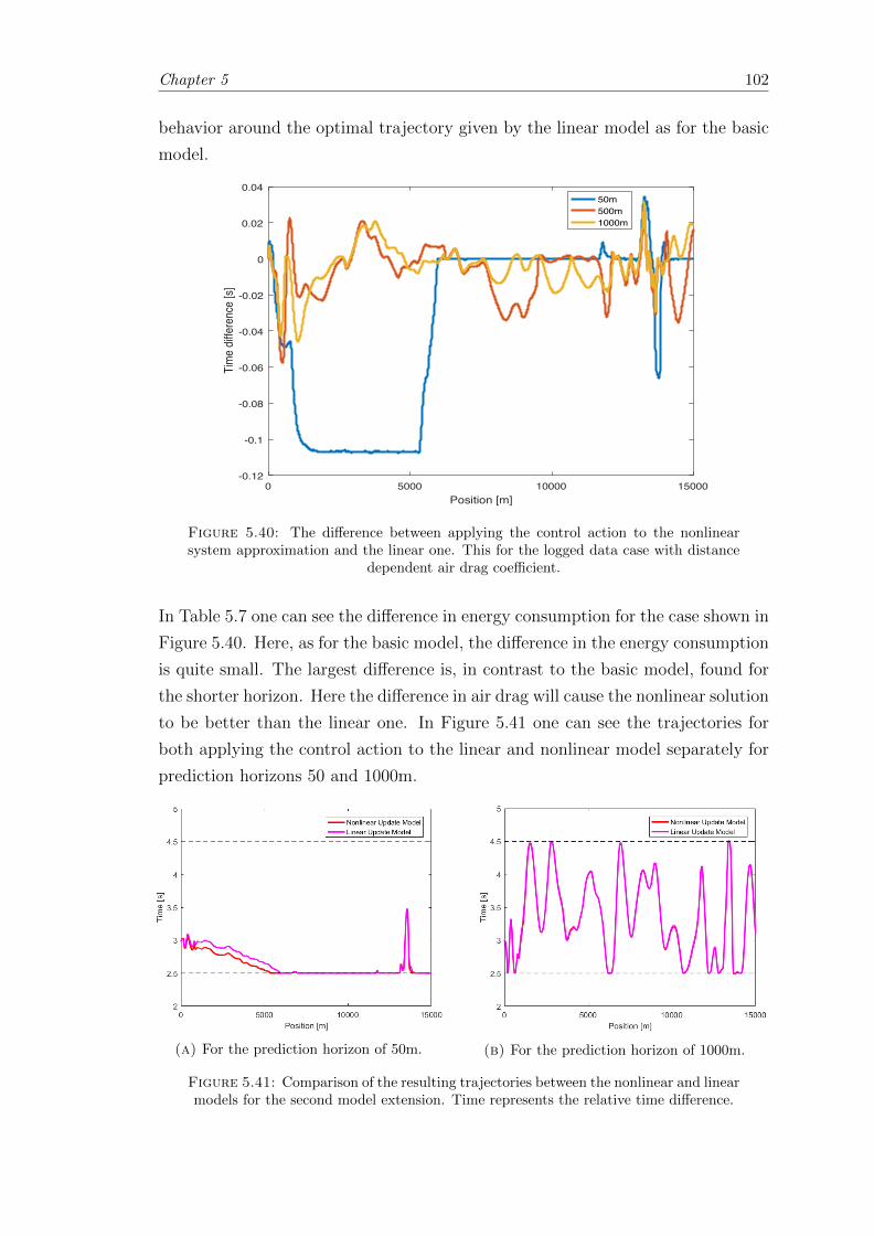
Chapter 5 102

behavior around the optimal trajectory given by the linear model as for the basic

model.

0 5000 10000 15000Position [m]

-0.12

-0.1

-0.08

-0.06

-0.04

-0.02

0

0.02

0.04

Tim

e dif

fere

nce

[s]

50m500m1000m

Figure 5.40: The difference between applying the control action to the nonlinearsystem approximation and the linear one. This for the logged data case with distance

dependent air drag coefficient.

In Table 5.7 one can see the difference in energy consumption for the case shown in

Figure 5.40. Here, as for the basic model, the difference in the energy consumption

is quite small. The largest difference is, in contrast to the basic model, found for

the shorter horizon. Here the difference in air drag will cause the nonlinear solution

to be better than the linear one. In Figure 5.41 one can see the trajectories for

both applying the control action to the linear and nonlinear model separately for

prediction horizons 50 and 1000m.

(a) For the prediction horizon of 50m. (b) For the prediction horizon of 1000m.

Figure 5.41: Comparison of the resulting trajectories between the nonlinear and linearmodels for the second model extension. Time represents the relative time difference.

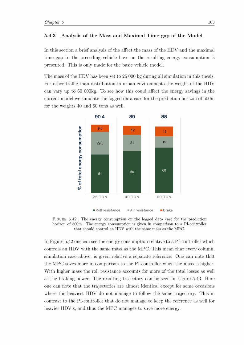
Chapter 5 103

5.4.3 Analysis of the Mass and Maximal Time gap of the Model

In this section a brief analysis of the affect the mass of the HDV and the maximal

time gap to the preceding vehicle have on the resulting energy consumption is

presented. This is only made for the basic vehicle model.

The mass of the HDV has been set to 26 000 kg during all simulation in this thesis.

For other traffic than distribution in urban environments the weight of the HDV

can vary up to 60 000kg. To see how this could affect the energy savings in the

current model we simulate the logged data case for the prediction horizon of 500m

for the weights 40 and 60 tons as well.

Title and Content

11 April 2018 Info class internal Department / Name / Subject 39

51 56 60

29,8 21 15

9,6 12 13

26 TON 40 TON 60 TON

Roll resistance Air resistance Brake

90.4 89 88

% o

f to

tal e

ne

rgy

co

nsu

mp

tio

n

Massa jämförelse 500m loggad data

Figure 5.42: The energy consumption on the logged data case for the predictionhorizon of 500m. The energy consumption is given in comparison to a PI-controller

that should control an HDV with the same mass as the MPC.

In Figure 5.42 one can see the energy consumption relative to a PI-controller which

controls an HDV with the same mass as the MPC. This mean that every column,

simulation case above, is given relative a separate reference. One can note that

the MPC saves more in comparison to the PI-controller when the mass is higher.

With higher mass the roll resistance accounts for more of the total losses as well

as the braking power. The resulting trajectory can be seen in Figure 5.43. Here

one can note that the trajectories are almost identical except for some occasions

where the heaviest HDV do not manage to follow the same trajectory. This in

contrast to the PI-controller that do not manage to keep the reference as well for

heavier HDV:s, and thus the MPC manages to save more energy.

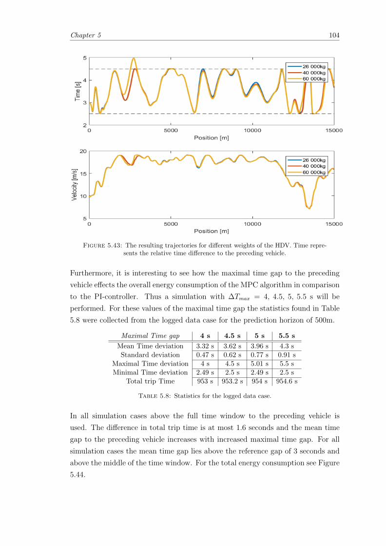
Chapter 5 104

Figure 5.43: The resulting trajectories for different weights of the HDV. Time repre-sents the relative time difference to the preceding vehicle.

Furthermore, it is interesting to see how the maximal time gap to the preceding

vehicle effects the overall energy consumption of the MPC algorithm in comparison

to the PI-controller. Thus a simulation with ∆Tmax = 4, 4.5, 5, 5.5 s will be

performed. For these values of the maximal time gap the statistics found in Table

5.8 were collected from the logged data case for the prediction horizon of 500m.

Maximal Time gap 4 s 4.5 s 5 s 5.5 s

Mean Time deviation 3.32 s 3.62 s 3.96 s 4.3 sStandard deviation 0.47 s 0.62 s 0.77 s 0.91 s

Maximal Time deviation 4 s 4.5 s 5.01 s 5.5 sMinimal Time deviation 2.49 s 2.5 s 2.49 s 2.5 s

Total trip Time 953 s 953.2 s 954 s 954.6 s

Table 5.8: Statistics for the logged data case.

In all simulation cases above the full time window to the preceding vehicle is

used. The difference in total trip time is at most 1.6 seconds and the mean time

gap to the preceding vehicle increases with increased maximal time gap. For all

simulation cases the mean time gap lies above the reference gap of 3 seconds and

above the middle of the time window. For the total energy consumption see Figure

5.44.

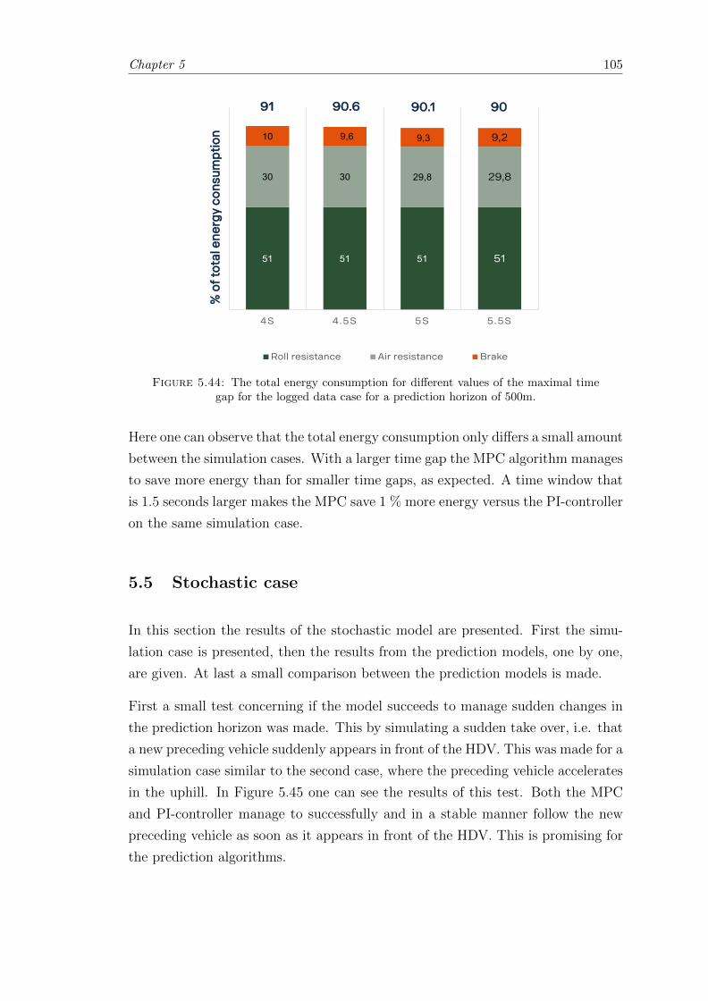
Chapter 5 105

Title and Content

11 April 2018 Info class internal Department / Name / Subject 40

51 51 51 51

30 30 29,8 29,8

10 9,6 9,3 9,2

4S 4.5S 5S 5.5S

Roll resistance Air resistance Brake

91 90.6 90.1

% o

f to

tal e

ner

gy

con

sum

pti

on

90

Figure 5.44: The total energy consumption for different values of the maximal timegap for the logged data case for a prediction horizon of 500m.

Here one can observe that the total energy consumption only differs a small amount

between the simulation cases. With a larger time gap the MPC algorithm manages

to save more energy than for smaller time gaps, as expected. A time window that

is 1.5 seconds larger makes the MPC save 1 % more energy versus the PI-controller

on the same simulation case.

5.5 Stochastic case

In this section the results of the stochastic model are presented. First the simu-

lation case is presented, then the results from the prediction models, one by one,

are given. At last a small comparison between the prediction models is made.

First a small test concerning if the model succeeds to manage sudden changes in

the prediction horizon was made. This by simulating a sudden take over, i.e. that

a new preceding vehicle suddenly appears in front of the HDV. This was made for a

simulation case similar to the second case, where the preceding vehicle accelerates

in the uphill. In Figure 5.45 one can see the results of this test. Both the MPC

and PI-controller manage to successfully and in a stable manner follow the new

preceding vehicle as soon as it appears in front of the HDV. This is promising for

the prediction algorithms.

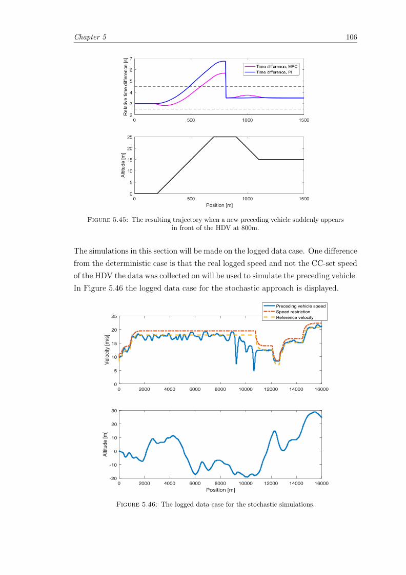
Chapter 5 106

Figure 5.45: The resulting trajectory when a new preceding vehicle suddenly appearsin front of the HDV at 800m.

The simulations in this section will be made on the logged data case. One difference

from the deterministic case is that the real logged speed and not the CC-set speed

of the HDV the data was collected on will be used to simulate the preceding vehicle.

In Figure 5.46 the logged data case for the stochastic approach is displayed.

0 2000 4000 6000 8000 10000 12000 14000 160000

5

10

15

20

25

Veloc

ity [m

/s]

Preceding vehicle speedSpeed restrictionReference velocity

0 2000 4000 6000 8000 10000 12000 14000 16000Position [m]

-20

-10

0

10

20

30

Altitu

de [m

]

Figure 5.46: The logged data case for the stochastic simulations.

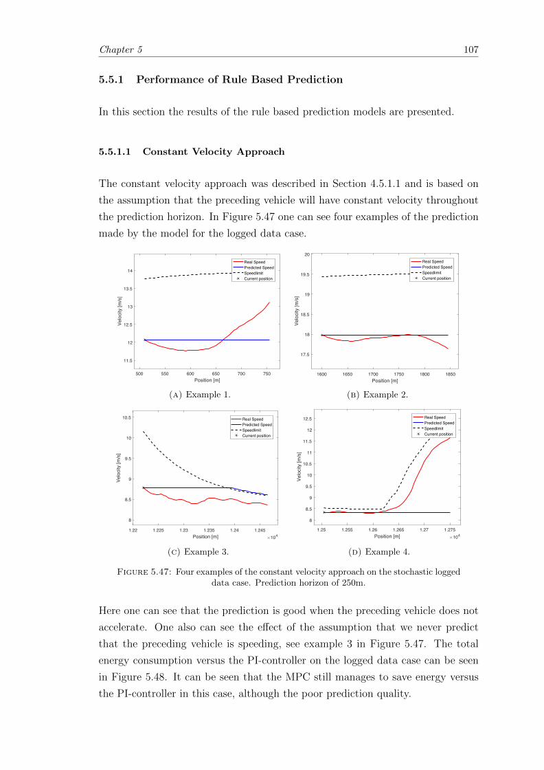
Chapter 5 107

5.5.1 Performance of Rule Based Prediction

In this section the results of the rule based prediction models are presented.

5.5.1.1 Constant Velocity Approach

The constant velocity approach was described in Section 4.5.1.1 and is based on

the assumption that the preceding vehicle will have constant velocity throughout

the prediction horizon. In Figure 5.47 one can see four examples of the prediction

made by the model for the logged data case.

500 550 600 650 700 750Position [m]

11.5

12

12.5

13

13.5

14

Velo

city

[m/s

]

Real SpeedPredicted SpeedSpeedlimitCurrent position

(a) Example 1.

1600 1650 1700 1750 1800 1850Position [m]

17.5

18

18.5

19

19.5

20

Velo

city

[m/s

]

Real SpeedPredicted SpeedSpeedlimitCurrent position

(b) Example 2.

1.22 1.225 1.23 1.235 1.24 1.245Position [m] 104

8

8.5

9

9.5

10

10.5

Velo

city

[m/s

]

Real SpeedPredicted SpeedSpeedlimitCurrent position

(c) Example 3.

1.25 1.255 1.26 1.265 1.27 1.275Position [m] 104

8

8.5

9

9.5

10

10.5

11

11.5

12

12.5

Velo

city

[m/s

]

Real SpeedPredicted SpeedSpeedlimitCurrent position

(d) Example 4.

Figure 5.47: Four examples of the constant velocity approach on the stochastic loggeddata case. Prediction horizon of 250m.

Here one can see that the prediction is good when the preceding vehicle does not

accelerate. One also can see the effect of the assumption that we never predict

that the preceding vehicle is speeding, see example 3 in Figure 5.47. The total

energy consumption versus the PI-controller on the logged data case can be seen

in Figure 5.48. It can be seen that the MPC still manages to save energy versus

the PI-controller in this case, although the poor prediction quality.

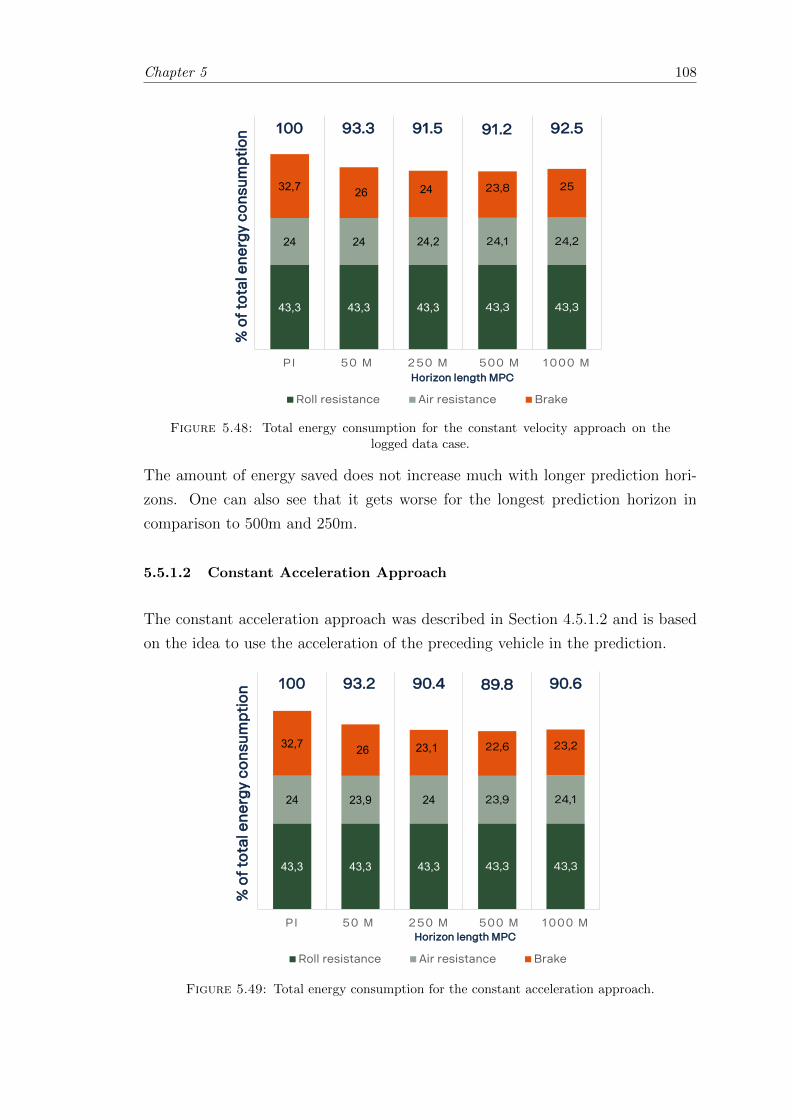
Chapter 5 108

Title and Content

11 April 2018 Info class internal Department / Name / Subject 41

Stochastiska fallet

43,3 43,3 43,3 43,3 43,3

24 24 24,2 24,1 24,2

32,7 26 24 23,8 25

PI 50 M 250 M 500 M 1000 M

Roll resistance Air resistance Brake

100 93.3 91.5 91.2 92.5

% o

f to

tal e

ne

rgy

con

sum

pti

on

Horizon length MPC

Constant velocity

Figure 5.48: Total energy consumption for the constant velocity approach on thelogged data case.

The amount of energy saved does not increase much with longer prediction hori-

zons. One can also see that it gets worse for the longest prediction horizon in

comparison to 500m and 250m.

5.5.1.2 Constant Acceleration Approach

The constant acceleration approach was described in Section 4.5.1.2 and is based

on the idea to use the acceleration of the preceding vehicle in the prediction.

Title and Content

11 April 2018 42

Constant acceleration

43,3 43,3 43,3 43,3 43,3

24 23,9 24 23,9 24,1

32,7 26 23,1 22,6 23,2

PI 50 M 250 M 500 M 1000 M

Roll resistance Air resistance Brake

100 93.2 90.4 89.8 90.6

% o

f to

tal e

ne

rgy

co

nsu

mp

tio

n

Horizon length MPC

Figure 5.49: Total energy consumption for the constant acceleration approach.

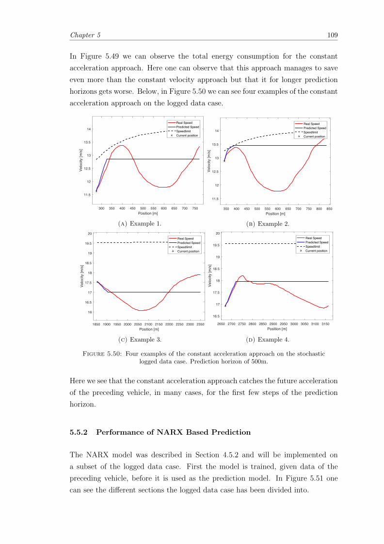
Chapter 5 109

In Figure 5.49 we can observe the total energy consumption for the constant

acceleration approach. Here one can observe that this approach manages to save

even more than the constant velocity approach but that it for longer prediction

horizons gets worse. Below, in Figure 5.50 we can see four examples of the constant

acceleration approach on the logged data case.

300 350 400 450 500 550 600 650 700 750Position [m]

11.5

12

12.5

13

13.5

14

Velo

city

[m/s

]

Real SpeedPredicted SpeedSpeedlimitCurrent position

(a) Example 1.

350 400 450 500 550 600 650 700 750 800 850Position [m]

11.5

12

12.5

13

13.5

14

Velo

city

[m/s

]

Real SpeedPredicted SpeedSpeedlimitCurrent position

(b) Example 2.

1850 1900 1950 2000 2050 2100 2150 2200 2250 2300 2350Position [m]

16

16.5

17

17.5

18

18.5

19

19.5

20

Velo

city

[m/s

]

Real SpeedPredicted SpeedSpeedlimitCurrent position

(c) Example 3.

2650 2700 2750 2800 2850 2900 2950 3000 3050 3100 3150Position [m]

16.5

17

17.5

18

18.5

19

19.5

20

Velo

city

[m/s

]

Real SpeedPredicted SpeedSpeedlimitCurrent position

(d) Example 4.

Figure 5.50: Four examples of the constant acceleration approach on the stochasticlogged data case. Prediction horizon of 500m.

Here we see that the constant acceleration approach catches the future acceleration

of the preceding vehicle, in many cases, for the first few steps of the prediction

horizon.

5.5.2 Performance of NARX Based Prediction

The NARX model was described in Section 4.5.2 and will be implemented on

a subset of the logged data case. First the model is trained, given data of the

preceding vehicle, before it is used as the prediction model. In Figure 5.51 one

can see the different sections the logged data case has been divided into.

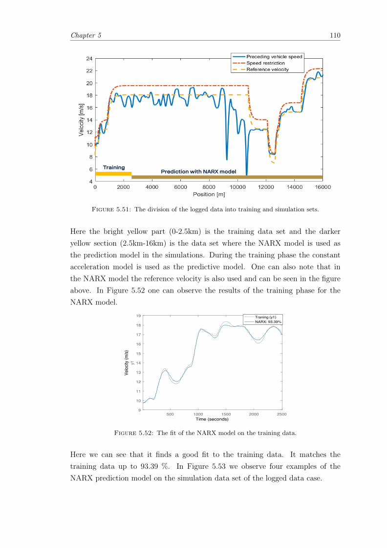
Chapter 5 110

Title and Content

TrainingPrediction with NARX model

Figure 5.51: The division of the logged data into training and simulation sets.

Here the bright yellow part (0-2.5km) is the training data set and the darker

yellow section (2.5km-16km) is the data set where the NARX model is used as

the prediction model in the simulations. During the training phase the constant

acceleration model is used as the predictive model. One can also note that in

the NARX model the reference velocity is also used and can be seen in the figure

above. In Figure 5.52 one can observe the results of the training phase for the

NARX model.

500 1000 1500 2000 25009

10

11

12

13

14

15

16

17

18

19

y1

Traning (y1)NARX: 93.39%

Time (seconds)

Veloc

ity (m

/s)

Figure 5.52: The fit of the NARX model on the training data.

Here we can see that it finds a good fit to the training data. It matches the

training data up to 93.39 %. In Figure 5.53 we observe four examples of the

NARX prediction model on the simulation data set of the logged data case.

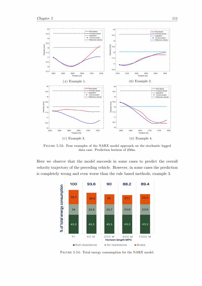
Chapter 5 111

2500 2550 2600 2650 2700 2750Position [m]

15.5

16

16.5

17

17.5

18

18.5

19

19.5

20

Velo

city

[m/s

]

Real SpeedPredicted SpeedSpeedlimitCurrent positionReference velocity

(a) Example 1.

3100 3150 3200 3250 3300 3350Position [m]

16.5

17

17.5

18

18.5

19

19.5

20

Velo

city

[m/s

]

Real SpeedPredicted SpeedSpeedlimitCurrent positionReference velocity

(b) Example 2.

3500 3550 3600 3650 3700 3750Position [m]

16

16.5

17

17.5

18

18.5

19

19.5

20

Velo

city

[m/s

]

Real SpeedPredicted SpeedSpeedlimitCurrent positionReference velocity

(c) Example 3.

3950 4000 4050 4100 4150 4200Position [m]

16

16.5

17

17.5

18

18.5

19

19.5

20

Velo

city

[m/s

]

Real SpeedPredicted SpeedSpeedlimitCurrent positionReference velocity

(d) Example 4.

Figure 5.53: Four examples of the NARX model approach on the stochastic loggeddata case. Prediction horizon of 250m.

Here we observe that the model succeeds in some cases to predict the overall

velocity trajectory of the preceding vehicle. However, in some cases the prediction

is completely wrong and even worse than the rule based methods, example 3.

Title and Content

11 April 2018 44

43,3 43,3 43,3 43,3 43,3

24 23,8 23,7 23,8 23,9

32,7 26,5 23 21,1 23,2

PI 50 M 250 M 500 M 1000 M

Roll resistance Air resistance Brake

100 93.6 90 88.2 89.4

% o

f tot

al e

nerg

y co

nsum

ptio

n

Horizon length MPC

NARX model

Figure 5.54: Total energy consumption for the NARX model.

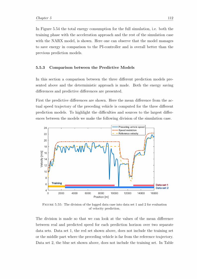
Chapter 5 112

In Figure 5.54 the total energy consumption for the full simulation, i.e. both the

training phase with the acceleration approach and the rest of the simulation case

with the NARX model, is shown. Here one can observe that the model manages

to save energy in comparison to the PI-controller and is overall better than the

previous prediction models.

5.5.3 Comparison between the Predictive Models

In this section a comparison between the three different prediction models pre-

sented above and the deterministic approach is made. Both the energy saving

differences and predictive differences are presented.

First the predictive differences are shown. Here the mean difference from the ac-

tual speed trajectory of the preceding vehicle is computed for the three different

prediction models. To highlight the difficulties and sources to the largest differ-

ences between the models we make the following division of the simulation case.

Title and Content

11 April 2018 Info class internal Department / Name / Subject 45

Training

Data set 2Data set 1

Figure 5.55: The division of the logged data case into data set 1 and 2 for evaluationof velocity prediction.

The division is made so that we can look at the values of the mean difference

between real and predicted speed for each prediction horizon over two separate

data sets. Data set 1, the red set shown above, does not include the training set

or the middle part where the preceding vehicle is far from the reference trajectory.

Data set 2, the blue set shown above, does not include the training set. In Table

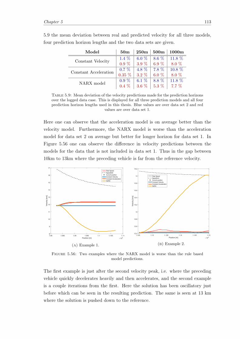
Chapter 5 113

5.9 the mean deviation between real and predicted velocity for all three models,

four prediction horizon lengths and the two data sets are given.

Model 50m 250m 500m 1000m

Constant Velocity1.4 %0.9 %

6.0 %3.9 %

8.6 %6.9 %

11.8 %8.0 %

Constant Acceleration0.7 %0.35 %

4.8 %3.2 %

7.8 %6.0 %

10.8 %8.0 %

NARX model0.9 %0.4 %

6.1 %3.6 %

8.8 %5.3 %

11.8 %7.7 %

Table 5.9: Mean deviation of the velocity predictions made for the prediction horizonsover the logged data case. This is displayed for all three prediction models and all fourprediction horizon lengths used in this thesis. Blue values are over data set 2 and red

values are over data set 1.

Here one can observe that the acceleration model is on average better than the

velocity model. Furthermore, the NARX model is worse than the acceleration

model for data set 2 on average but better for longer horizon for data set 1. In

Figure 5.56 one can observe the difference in velocity predictions between the

models for the data that is not included in data set 1. Thus in the gap between

10km to 13km where the preceding vehicle is far from the reference velocity.

1.08 1.085 1.09 1.095 1.1 1.105 1.11Position [m] 104

8

9

10

11

12

13

14

15

16

17

Velo

city

[m/s

]

Real SpeedSpeedlimitCurrent positionConstant VelocityConstant AccelerationNARX

(a) Example 1.

1.125 1.13 1.135 1.14 1.145 1.15Position [m] 104

12.4

12.6

12.8

13

13.2

13.4

13.6

13.8

14

14.2

Velo

city

[m/s

]

Real SpeedSpeedlimitCurrent positionConstant VelocityConstant AccelerationNARX

(b) Example 2.

Figure 5.56: Two examples where the NARX model is worse than the rule basedmodel predictions.

The first example is just after the second velocity peak, i.e. where the preceding

vehicle quickly decelerates heavily and then accelerates, and the second example

is a couple iterations from the first. Here the solution has been oscillatory just

before which can be seen in the resulting prediction. The same is seen at 13 km

where the solution is pushed down to the reference.

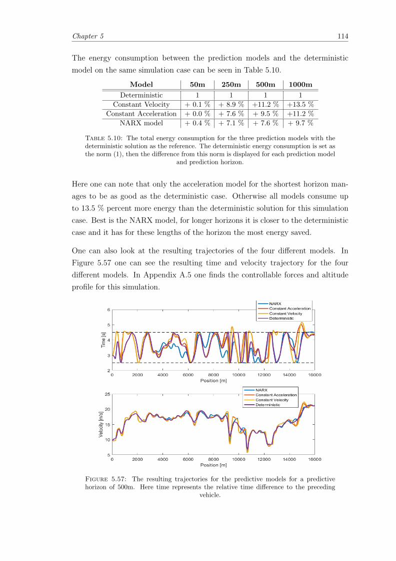
Chapter 5 114

The energy consumption between the prediction models and the deterministic

model on the same simulation case can be seen in Table 5.10.

Model 50m 250m 500m 1000m

Deterministic 1 1 1 1

Constant Velocity + 0.1 % + 8.9 % +11.2 % +13.5 %

Constant Acceleration + 0.0 % + 7.6 % + 9.5 % +11.2 %

NARX model + 0.4 % + 7.1 % + 7.6 % + 9.7 %

Table 5.10: The total energy consumption for the three prediction models with thedeterministic solution as the reference. The deterministic energy consumption is set asthe norm (1), then the difference from this norm is displayed for each prediction model

and prediction horizon.

Here one can note that only the acceleration model for the shortest horizon man-

ages to be as good as the deterministic case. Otherwise all models consume up

to 13.5 % percent more energy than the deterministic solution for this simulation

case. Best is the NARX model, for longer horizons it is closer to the deterministic

case and it has for these lengths of the horizon the most energy saved.

One can also look at the resulting trajectories of the four different models. In

Figure 5.57 one can see the resulting time and velocity trajectory for the four

different models. In Appendix A.5 one finds the controllable forces and altitude

profile for this simulation.

Figure 5.57: The resulting trajectories for the predictive models for a predictivehorizon of 500m. Here time represents the relative time difference to the preceding

vehicle.

Chapter 6

Discussion

In this chapter the results as well as methodology and difficulties of the project

will be discussed. The main focus will be on the results of the deterministic and

stochastic cases which was the main focus of this thesis. The chosen solution to

certain problems and problems that still are left to be solved are brought up as

well as the evaluation of them made in the results chapter. At last the significance

of the results of the predictive models are discussed.

6.1 Models and Simulation cases

During the work with this project many different models were developed in order

to find the energy effective trajectories for an HDV that is limited by a preceding

vehicle. Some of the models were more promising than others and a great effort was

made to get stable and reliable results. Many working hours were spent on tuning

the model parameters, developing methodology to deal with the approximation

errors and constructing good simulation cases. This for many different interesting

topics such as regenerative braking, distance dependent air drag and predictive

algorithms. The results of the models presented in this thesis showed, in large,

that there is a potential to save energy by an MPC based velocity controller on the

HDV in situations where the preceding vehicle limits the HDV. The exact amount

of energy that can be saved, shown in this thesis, is not the most important result

but rather that it shows that there is a potential for energy savings even for tough

situations, such as where the HDV does not have reliable future information about

the velocity of the preceding vehicle.

115

Chapter 6 116

In this section the results of the two main cases study in this thesis will be discussed

in short. The weights of the penalization terms, common for both approaches, will

also be discussed as well as the development of the reference controller, the PI-

controller.

6.1.1 PI-controller

We begin with the developed reference controller, the PI-controller. The main

focus of this thesis was not to develop a prefect reference controller but to study

the potential of the MPC algorithm on the stipulated driving scenario. For this

a good enough and simple reference controller was needed. The choice fell upon

the well studied and well used PI-controller. Some effort has been taken to make

the PI-controller stable and reliable. Many hours have been spent tuning the

parameters of the controller as well as the implementation of the Anti-Windup

methodology. The choice of control error was also carefully chosen after some

experimentation. The goal always being a controller simulating a simple cruise

controller or human driver that tries to keep a certain distance to the preceding

vehicle.

As can be seen in the results given in the previous chapter the developed PI-

controller manages to keep the reference in almost all simulation cases. Thus

achieving its goal. This is not an energy effective controller but, as mentioned

earlier, a controller simulating a human driver or simple CC-controller. In some

simulations the controller was quite poor and used large amounts of energy in order

to keep the reference. This behavior was not desired but was tough to get rid off.

This resulted in quite high values for the amount of energy the MPC managed

to save in comparison to the PI-controller. Which made the MPC algorithm

seem better than it actually was. More time and energy on a better reference

should be made in the future to further evaluate exactly the potential of the MPC

implementation. Nevertheless, the results still shows on the potential for an energy

effective velocity control using the MPC methodology.

6.1.2 Deterministic Case

In this section the results of the deterministic models and simulations are discussed.

The model assumptions as well as the results for each developed model is brought

up. At last the chosen values of the penalization weights are discussed.

Chapter 6 117

6.1.2.1 Model Assumptions

The deterministic case consisted of a basic model and two model extension. In

all of these models the underlying assumption was that there existed a V2V com-

munication between the HDV and the preceding vehicle. Furthermore, that the

preceding vehicle knew its future velocity trajectory for the prediction horizon and

could send this information without delay to the HDV behind it. Both these as-

sumptions, but especially the last, are idealizations of the real driving scenario an

HDV encounters today. To assume that there exists some sort of communication

between the vehicles is today not as extraordinary as before. The development of

V2V communication is on the rise today and many new methods and tools are

implemented each year. Despite this, the amount and delay of the information

that can be sent today is not take into consideration in this case.

The assumption that the preceding vehicle know its future velocity trajectory is

a large deviation from the real driving scenario. In many situations the preceding

vehicle would not know the future trajectory and thus not be able to send this

information to the HDV. To have this information when optimizing the velocity

trajectory of the HDV is an important idealization. In many cases this will put a

lower bound on the amount the MPC can save versus the PI-controller. This is

also why the stochastic case is studied and the results between them are analyzed.

6.1.2.2 Basic model

The basic deterministic model showed that the MPC implementation could save up

to 20% in comparison to the PI-controller. Depending on the mass of the HDV and

the set allowed time window behind the preceding vehicle this could changed±2 %.

The amount of energy saved converged at around a prediction horizon of 500m. For

longer prediction horizons the amount of energy saved increased but only slightly.

Depending on the hardware system on the HDV, an online implementation of

the MPC algorithm would preferably use a shorter prediction horizon. It is not

desirable to have an algorithm with a high computational complexity and thus we

choose to end the analysis at 1000m.

More energy could be saved for certain situation if one tuned the penalization

terms for each situation separately. This would although require an algorithm

that could recognized the correct situation and use the correctly tuned terms.

Furthermore, one would also have to identify all kinds of situations and find an

Chapter 6 118

optimal tuning of the model for each one. This was not made in this thesis, and

may be an improvement one can consider for future studies.

6.1.2.3 Model extensions

The deterministic case had two model extensions, the regenerative braking exten-

sion and distance dependent air drag coefficient extension. Both model extensions

were included to see how the developed MPC framework would manage to solve

the problem given, in the first case regenerative power and in the second case

distance dependent air drag.

For the regenerative braking extension it could be seen that the MPC managed to

save even more energy than the basic model, as expected. During downhills and

shorter crests the solution became to use the brake more in order to regenerate

some of the potential energy the HDV had. Otherwise the trajectory became

almost identical to the basic model case. This is an indication that the basic

model would work as a good reference even for HDV:s with regenerative braking

and electrical vehicles in the future. Furthermore we could see that the model

was not as sensitive to prediction horizon length. This would mean that the

computational complexity could be kept at a lower level by lowering the horizon

length in comparison to the basic case.

At last, the second model extension showed that energy could also be saved with

the distance dependent air drag model in place. Again, versus the model with

constant air drag the model with the extension could save up to 5 % more energy.

This through less air resistance by placing the HDV closer to the preceding vehicle

in flat sections. The comparison versus a PI-controller with the same extension

showed instead that the energy saved was almost the same as for the basic case.

The final trajectory was again similar to the basic model solution but in general

closer to the preceding vehicle. Depending on the reliability of the communication

between the vehicles the minimum time gap could be lowered and even more energy

could possibly be saved.

6.1.3 Stochastic Case

The stochastic case showed that, although predictive models with quite large pre-

dictive error were implemented instead of having full information about the future

velocity of the preceding vehicle, up to 11 % could be saved versus the PI-controller.

Chapter 6 119

This is an unexpected but exciting result. This shows that although the HDV do

not get full information about the preceding vehicle trajectory there is still a

potential to save energy with this approach. This even with simple rule based

algorithms.

As could be seen in the results chapter the trajectories for the three different pre-

diction models were not far from the deterministic solution, that can be regarded

as the optimal trajectory. For the acceleration and NARX models the results seem

really promising and further development and research of them could give good

results. One important fact to have in mind when evaluating the results are that

the NARX model, in contrast to the rule based models, uses some future informa-

tion about the preceding vehicle, Vp,ref . The reference velocity could be considered

to be reasonable information that the HDV could get, but in some cases this may

not be possible. Attempts to design a NARX model without this information was

made without any success. One should also not that all results originate from

one data set, one simulation. This makes these results highly uncertain and for

future studies a larger collection of logged data from different vehicles should be

used. Still, the results show on the potential for both simpler and more advanced

prediction algorithms in the MPC framework.

6.1.4 Penalization weights

In the developed model there are several penalization weights that must be tuned

to get stable and reasonable result from the solver. These included the jerk penal-

ization, final term penalization and speed limit penalization weights. These were

tuned on the first simulation case on the flat road with a preceding vehicle keeping

constant velocity. These values turned out to not always give the desired results.

For the jerk penalization the value of the weight was set so that all visible large

changes in the control vanished. During the development of the model, instabilities

with the control action were encountered. The solution became to limit the jerk.

Unfortunately this will also give a higher energy consumption for certain situations

such as where the preceding vehicle decelerates or accelerates heavily. The value

is, in this thesis, set somewhat ad-hoc after visual results on specific simulation

cases. A better methodology for the value of this parameter would be desirable in

order to get more reliable and stable results.

The final penalization weights turned out to have a significant impact on the

final results of the model. In many cases a small change in the weight would

Chapter 6 120

give a completely different result. The values set in this thesis were again set

on the first simulation case. This because it was the case which we knew on

beforehand what the optimal solution was. As could be seen in the evaluation of

the time approximation the model error itself was enough, for shorter prediction

horizons, to make the solver find another solution. This because of the final

penalization term. Given other values on the penalization weights the solver would

find other solutions, which are not always the desired solutions i.e. energy effective

or following the reference. Here a dynamic methodology for the parameter values,

dependent on horizon length, would be desirable.

At last, one important drawback of the model is that all results given are rela-

tive to the values of these penalization terms and parameter values. A smarter

methodology for these weights and parameters could possibly improve the results

even further, and most of all make for a more stable model.

6.2 Force peaks - Instability in the model

As could be seen in Figure 5.9 a problem with peaks in the applied force was

encountered with the developed model. Given that we only use a linear model in

the optimization and have a model of the HDV purely based on outer forces, these

force peaks are not expected. In fact, they do not constitute an optimal solution

and should not appear in the solution as such. A large effort was made to identify

the source of these force peaks without success. Different approximation methods

and solver algorithms were tested but all with the same results.

During the testing it became clear that the solver quickly encountered problems

with the model and at some occasions threw internal error messages. This leads

me to believe that these force peaks originate from the internals of the solvers used

in Matlab. Although, it can not be excluded that they also can originate from the

implementation of the model itself and not the solvers. The final and conclusive

answer to the origin of these force peaks was not found during the work with this

project.

6.3 Linearizations and Approximations

In order to get a linear optimization problem we had to approximate the time

variable by a first order Taylor approximation. This will give us a model error that

Chapter 6 121

the optimization model continuously will try to correct for. By the results seen

in Section 5.4.2.1 we could see that the time approximation, with the developed

improvement methodology, was quite good. Both the average and maximum time

deviation from the actual time trajectory was small, under 0.055 %. On the other

hand the system is time critical which means that a high accuracy of the time is

needed.

From Figure 5.36 we could see that the difference between predicted step and

taken step in the state variables was small. During phases of acceleration or decel-

eration the error grew but still within the set limits. What was more unexpected

was the results found in Figures 5.37 and 5.38. Here we could see that the largest

deviation was found for the shortest horizon, although the energy consumption

followed the expected pattern. The reason behind these results are the final pe-

nalization weights. For shorter horizons the final point will matter more, under

the assumption that we have constant weight parameters. Thus a small error in

the final point will have a greater impact on the solution for shorter horizons. For

the case shown in Figure 5.38 we see that this leads the solver to find an alter-

native solution and thus a higher time deviation. Nevertheless, we see that there

are more flat regions than for the longer horizons that oscillate around 0. This

means that the solver constantly compensates for the model errors, which in turn

means a higher energy consumption. Overall the difference in energy consumption

is small indicating that the approximation on average is good.

For the final term penalization the weights could depend on the length of the

prediction horizon to overcome this problem for shorter horizons. However, be-

cause the total energy consumption and time approximation on average is good

no further effort was made to implement such weight functions.

For the distance approximation the exact position in time behind the preceding

vehicle matters, how close you are to each other. Thus the separation of the

trajectories for shorter horizon will have a larger impact on the overall energy

consumption and explains the difference we see in Figure 5.40. Otherwise we

could see that the rather simple distance approximation was on average quite

good, but for some cases really bad. This is expected, as is mentioned earlier the

approximation deteriorates when the preceding vehicle accelerates. Fortunately,

the affect of small accelerations seem to not have a significant impact on the results.

For future studies a smarter approximation of the distance would be desirable.

Chapter 6 122

6.4 Prediction models

Three prediction models have been developed and implemented on the logged data

case. As can be seen from the results for the stochastic case the MPC algorithm has

no problems with the predictive models and manages to save energy versus the PI-

algorithm. The amount saved is quite far from the deterministic case, as expected,

that can be regarded as a lower bound for the energy consumption. With full

information about the future the deterministic model should beat the predictive

models every time. What is more unexpected is how well the predictive models,

even the simple rule based models, do in comparison to the PI-controller. This is

an indication on that the PI-controller may not be as good as we thought but also

that there is some potential for predictive algorithms in an MPC framework.

The velocity model is the simplest and worst of the three predictive models. Both

the amount of energy saved and the predictions themselves are the worst of all

three models. Nevertheless it manages to save 8% at most in comparison to the

PI-controller. This is somewhat unexpected because we can see in Figure 5.47

that the predictions can differ much from the actual speed in many cases. Thus

the MPC algorithm seems to not be terribly sensitive for the prediction of the

preceding vehicle. One advantage of the model is its simplicity which makes it

easy to implement online on an HDV.

The second prediction model was the acceleration model. From the results we see

that both the predictions and energy consumption is better than for the velocity

model. The model manages to save up to 10% more energy than the PI-controller.

Furthermore, as can be seen in Figure 5.50 it catches some of the accelerations

the preceding vehicle makes. Here the set acceleration horizon of h = 50 m can

be modified and improved. Attempts of making this horizon length dynamic i.e.

dependent on the confidence (based on variance) of the acceleration and road

topography has been made without success. The best strategy found was to set a

fixed value of 50m. For future work a dynamic methodology for the acceleration

horizon would probably give even better results.

The last and most complex prediction model was the NARX model. The model

had to be trained before it was used and thus the results is a combination between

the NARX and acceleration model. From the results section we can see that this

model had the lowest energy consumption of all three predictive models. Although

this, it had 7.6 % higher energy consumption than the deterministic case. Further-

more it did not have the best predictions on average over the complete simulation

Chapter 6 123

horizon. It had some difficulties, examples shown in Figure 5.56, with the cases

where the preceding vehicle was far from the reference trajectory and had large

oscillations in the velocity. Outside these sections, i.e. where the preceding vehicle

velocity oscillated around the reference the NARX model had the best predictions.

What one has to have in mind is also that the model parameters of the NARX

model has been tuned to give good results on the particular training set. Thus

it will probably not be as good on other data from other vehicles. This is a vast

drawback of the model and one would have to implement a special methodology

to find a good set of parameter values for every new vehicle that comes in front

of the HDV. The complexity of the model might also make it hard to implement

online. Nevertheless, with future developments of connected vehicles and learning

algorithms this could be solved. The potential for smart predictive energy efficient

speed controllers is to good to not be further explored.

At last we will also comment on one unexpected results connected to all three pre-

diction models. For all three models the best results, from an energy perspective,

was found for a prediction horizon of 500m. For both shorter as well as longer

horizon lengths the energy consumption increased. That it would be higher for

short horizons did not come as a surprise, but that it also did that for longer

horizons was more unexpected. This is probably because the model will base the

control action earlier on in the simulation on incorrect predictions of the preceding

vehicle velocity far into the future. It seems to be the case that there is a sweet

spot between giving the MPC algorithm enough information about the future road

topography and too much uncertain velocity predictions. For all three models this

seems to occur at a prediction horizon of 500m.

Chapter 7

Conclusions

In this chapter the overall conclusions for the two main simulation cases, Deter-

ministic and Stochastic case, are presented. Comments about possible future work

are also mentioned.

7.1 Deterministic Case

In the deterministic case it have been shown that there is potential to save up to

20% energy versus the reference and thus both improving the fuel economy for the

haulers but also reducing the emissions from road based vehicles. Although the

V2V communication and assumption of full information of the preceding vehicle

velocity trajectory is somewhat idealistic the results show that much can be done to

reduce the fuel consumption in situations where the HDV is limited by a preceding

vehicle. Furthermore, it also shows that a smart cruise controller with an allowed

time window behind the preceding vehicle can manage to save significant amounts

of energy. Thus we can conclude that the results above speak for the concept

of a smart controller, as the one developed in this thesis, that keep up with the

preceding vehicle but at the same time drives efficiently to save energy.

7.2 Stochastic Case

In the stochastic case we have seen that although the predictive models are quite

poor the MPC algorithm succeeds to reduce the fuel consumption of the HDV com-

pared to the PI-controller. More complex predictive models such as the NARX

124

Chapter7 125

model show that it is possible to reduce the gap between the deterministic and

predictive simulations, but also that there is much to be done. Both the algorithms

themselves and the technology is not yet there today. But with the ongoing de-

velopment of both electrified and more autonomous vehicles these obstacles might

soon be solved. Thus making it possible to implement smart cruise controllers

of the type shown here, that uses the information available such as the road to-

pography and the preceding vehicles speed to drive both smarter and more fuel

efficient.

7.3 Future Work

In this thesis only a small segment of all traffic scenarios have been studied, the

simplified case of a preceding vehicle. To further develop the methodology and

making it ready for implementation in real traffic scenarios further research has to

be done. In this section some possible extensions to the developed methodology

are mentioned.

First and foremost the model also has to consider the lateral resistance and dynam-

ics of the vehicle. There are important limitations and restrictions on the HDV

that are not included in the existing model because they have their origin in the

lateral dynamics of the HDV. This would be one aspect that could be considered

in a future development of the model.

Another possibility is to model the powertrain of the HDV in detail instead of the

pure force model that is used here. This will also account for the specific control

of the different parts as well as energy losses in the powertrain of the HDV. This

will in turn also give a more explicit control of the vehicle rather than the more

abstract tractive and braking power used in the developed model.

Furthermore, the reality of the traffic situation is that there will not only be a

preceding vehicle on the road together with the HDV. Most probably there will be

many other vehicles on the road that our vehicle has to take into consideration.

This will need further analysis and extensions of the existing model. Weather,

stop signs, traffic lights and pedestrians are only a few other aspects that have to

be taken into consideration to get the full traffic situation and a smart and safe

controller.

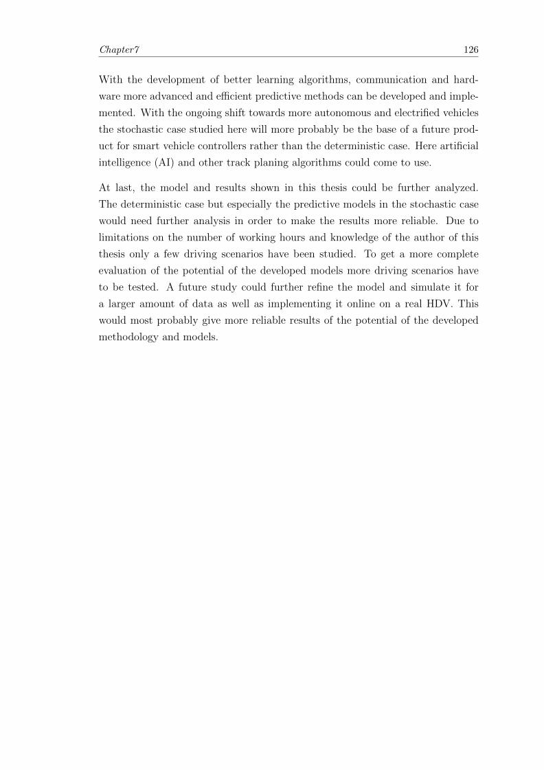
Chapter7 126

With the development of better learning algorithms, communication and hard-

ware more advanced and efficient predictive methods can be developed and imple-

mented. With the ongoing shift towards more autonomous and electrified vehicles

the stochastic case studied here will more probably be the base of a future prod-

uct for smart vehicle controllers rather than the deterministic case. Here artificial

intelligence (AI) and other track planing algorithms could come to use.

At last, the model and results shown in this thesis could be further analyzed.

The deterministic case but especially the predictive models in the stochastic case

would need further analysis in order to make the results more reliable. Due to

limitations on the number of working hours and knowledge of the author of this

thesis only a few driving scenarios have been studied. To get a more complete

evaluation of the potential of the developed models more driving scenarios have

to be tested. A future study could further refine the model and simulate it for

a larger amount of data as well as implementing it online on a real HDV. This

would most probably give more reliable results of the potential of the developed

methodology and models.

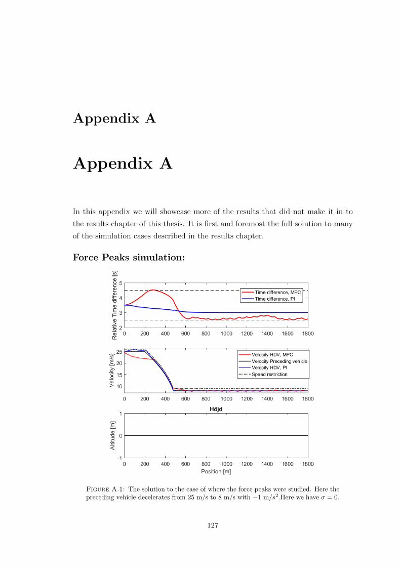
Appendix A

Appendix A

In this appendix we will showcase more of the results that did not make it in to

the results chapter of this thesis. It is first and foremost the full solution to many

of the simulation cases described in the results chapter.

Force Peaks simulation:

Figure A.1: The solution to the case of where the force peaks were studied. Here thepreceding vehicle decelerates from 25 m/s to 8 m/s with −1 m/s2.Here we have σ = 0.

127

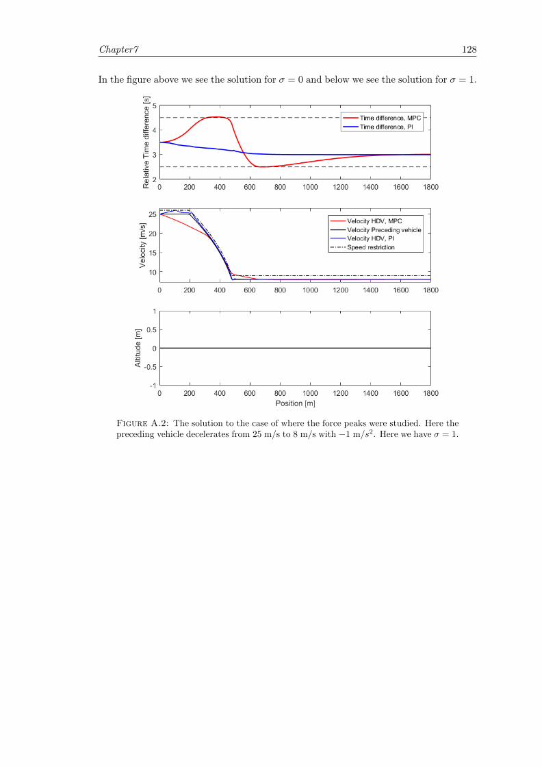
Chapter7 128

In the figure above we see the solution for σ = 0 and below we see the solution for σ = 1.

Figure A.2: The solution to the case of where the force peaks were studied. Here thepreceding vehicle decelerates from 25 m/s to 8 m/s with −1 m/s2. Here we have σ = 1.

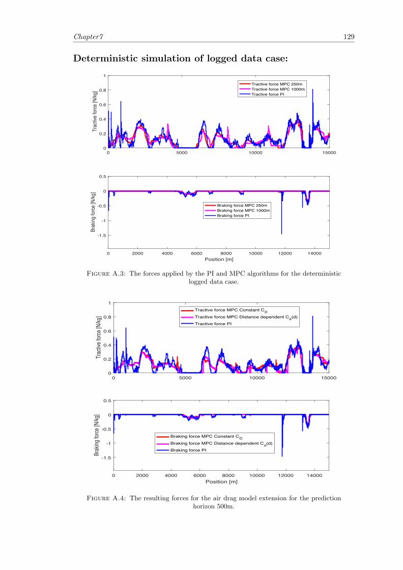
Chapter7 129

Deterministic simulation of logged data case:

0 5000 10000 150000

0.2

0.4

0.6

0.8

1

Trac

tive f

orce

[N/kg

]

Tractive force MPC 250mTractive force MPC 1000mTractive force PI

0 2000 4000 6000 8000 10000 12000 14000Position [m]

-1.5

-1

-0.5

0

0.5

Brak

ing fo

rce [N

/kg]

Braking force MPC 250mBraking force MPC 1000mBraking force PI

Figure A.3: The forces applied by the PI and MPC algorithms for the deterministiclogged data case.

0 5000 10000 150000

0.2

0.4

0.6

0.8

1

Trac

tive f

orce [

N/kg

]

Tractive force MPC Constant CDTractive force MPC Distance dependent Cd(d)Tractive force PI

0 2000 4000 6000 8000 10000 12000 14000Position [m]

-1.5

-1

-0.5

0

0.5

Brak

ing fo

rce [N

/kg]

Braking force MPC Constant CDBraking force MPC Distance dependent Cd(d)Braking force PI

Figure A.4: The resulting forces for the air drag model extension for the predictionhorizon 500m.

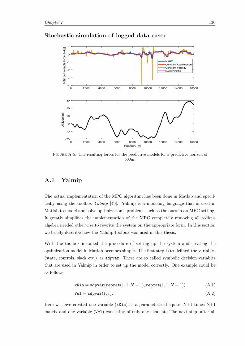
Chapter7 130

Stochastic simulation of logged data case:

0 2000 4000 6000 8000 10000 12000 14000 16000-4

-3

-2

-1

0

1

Tota

l con

trolla

ble fo

rce

[N/kg

]NARXConstant AccelerationConstant VelocityDeterministic

0 2000 4000 6000 8000 10000 12000 14000 16000Position [m]

-20

-10

0

10

20

30

Altitu

de [m

]

Figure A.5: The resulting forces for the predictive models for a predictive horizon of500m.

A.1 Yalmip

The actual implementation of the MPC algorithm has been done in Matlab and specif-

ically using the toolbox Yalmip [49]. Yalmip is a modeling language that is used in

Matlab to model and solve optimization’s problems such as the ones in an MPC setting.

It greatly simplifies the implementation of the MPC completely removing all tedious

algebra needed otherwise to rewrite the system on the appropriate form. In this section

we briefly describe how the Yalmip toolbox was used in this thesis.

With the toolbox installed the procedure of setting up the system and creating the

optimization model in Matlab becomes simple. The first step is to defined the variables

(state, controls, slack etc.) as sdpvar. These are so called symbolic decision variables

that are used in Yalmip in order to set up the model correctly. One example could be

as follows

xKin = sdpvar(repmat(1, 1, N + 1), repmat(1, 1, N + 1)) (A.1)

Vel = sdpvar(1, 1). (A.2)

Here we have created one variable (xKin) as a parameterized square N+1 times N+1

matrix and one variable (Vel) consisting of only one element. The next step, after all

Chapter7 131

variables are created is to instantiate the objective and constraints vectors. These

will hold the objective function and constraints of the optimization model and can

created as

objective = 0 (A.3)

constraints = [ ]. (A.4)

The actual optimization model is defined by a simple for loop over all terms in the

model, i.e. all terms in the objective function and all constraints as

for k = 1 : N

objective = objective + f(xKin, Vel) (A.5)

constraints = [constraints, g(xKin, Vel) ≤ 0] (A.6)

end.

Above we seen an example over how this can be achieved. Here f and g are some

functions, which can be both linear, nonlinear or other Matlab specific functions. The

added constraint here is just one example, equality’s are also possible and defined with

==.

The last step is to define the in-going and the out-going parameters as paramin and

paramout, and call the optimization algorithm. This is done in the following manner

controller = optimizer(constraints, objective, sdpsettings, paramin, paramout).

(A.7)

Where we have that sdpsettings defines the used solver and solver output. This will

be the controller that can be called in every iteration of the simulation horizon, if

implemented in an MPC fashion.

A.2 NARX in Matlab

The implementation of the NARX model in this thesis have been made in Matlab using

the system identification toolbox. The toolbox makes the procedure of creating, training

and simulating with the NARX model simple and quick. By just a few commands a

NARX model is build.

Chapter7 132

First all data is collected as output data and input data separately and defined as iddata

in Matlab as in

data = optimizer(outputdata, inputdata, Steplength) (A.8)

training = data(1 : i) (A.9)

validation = data(i : end). (A.10)

Here we have also split the data into training data and validation or simulation data,

for some specified split point i. The next step is to create and train the NARX model

with the above defined data as

NARX = nlarx(training, [na, nb, nk], wavenet(...), Options). (A.11)

Here we have chosen a wavenet network, other exists such as sigmoid networks, with cer-

tain specification denoted as (...). One example of a specification available is the number

of layers the network should have. In the Option parameter any other specifications of

the model are give, such as which regressors should be included in the nonlinear block

of the NARX model and which method should be used to train the model. With the

compare command one can test the trained model on the training data or validation

data.

To predict the future output values of the system, for example for a prediction horizon

in the MPC algorithm, one can use the forecast command. This is done by defining

the future inputs values and past input and output values as iddata objects and calling

the forecast command as in

prediction = forecast(NARX, PastData, K, FuturInput). (A.12)

Here K is the number of steps into the future the prediction should be made over and,

PastData and FuturInput are the past (input and output) and future (input) data

objects.

For the implementation in the MPC framework the data objects for the past and future

data is constantly updated for each step in the simulation.

Bibliography

[1] European Union. EU Transport in figures, Statistical Pocketbook. EU Mobility and Trans-

port, 2017.

[2] European Environment Agency. Greenhouse gas emissions from transport. EEA Web, 2017.

[3] European Commission. White Paper 2011. Mobility and transport, European strategies,

2011.

[4] European Union. Regulation (EC) No 715/2007 of the European Parliament and of the

council. Official Journal of the European Union, 2011.

[5] Andr Nel. Air Pollution-Related Illness: Effects of Particles. The Department of Medicine,

University of California, Los Angeles, Science, 06 May 2005.

[6] Scania CV AB. Annual report 2012. Technical report, 2012.

[7] Scania CV AB. Scania active prediction. Technical report, 2012.

[8] Kristoffer Thorin. Optimal Speed Controller in the Presence of Traffic Lights. Master

Thesis, 2017. doi: UPTECE17005.

[9] Manne Henriksson, Oscar Flardh, and Jonas Martensson. Optimal Powertrain Control of

a Heavy-Duty Vehicle Under Varying Speed Requirements. 2017 IEEE 20th International

Conference on Intelligent Transportation Systems (ITSC), pages 1922–1927, 2017.

[10] Manne Held. Optimal Speed and Powertrain Control of a Heavy-Duty Vehicle in Urban

Driving. Licentiate Thesis in Electrical Engineering, 1(1), 2017. doi: TRITA-EE2017-141.

[11] Shengbo Li, Keqiang Li, Jianqiang Wang, Lei Zhang, Xiaomin Lian, Hiroshi Ukawa, and

Dongsheng Bai. MPC based vehicular following control considering both fuel economy and

tracking capability. 2008 IEEE Vehicle Power and Propulsion Conference, VPPC 2008,

pages 1–6, 2008. doi: 10.1109/VPPC.2008.4677689.

[12] Feyyaz Emre Sancar, Baris Fidan, Jan P. Huissoon, and Steven L. Waslander. MPC based

collaborative adaptive cruise control with rear end collision avoidance. IEEE Intelligent

Vehicles Symposium, Proceedings, (Iv):516–521, 2014. doi: 10.1109/IVS.2014.6856559.

[13] Carlos M. Massera, Marco H. Terra, and Denis F. Wolf. Safely Optimizing Highway

Traffic with Robust Model Predictive Control-based Cooperative Adaptive Cruise Control.

133

Bibliography 134

IEEE Transactions on Intelligent Transportation Systems, 18(11):3193–3203, 2016. ISSN

15249050. doi: 10.1109/TITS.2017.2679098.

[14] Shengbo Li, Keqiang Li, Rajesh Rajamani, and Jianqiang Wang. Model predictive multi-

objective vehicular adaptive cruise control. IEEE Transactions on Control Systems Tech-

nology, 19(3):556–566, 2011.

[15] Antonio Sciarretta, Giovanni De Nunzio, and Luis Leon Ojeda. Optimal Ecodriving Control:

Energy-Efficient Driving of Road Vehicles as an Optimal Control Problem. IEEE Control

Systems, 35(5):71–90, 2015. ISSN 1066033X. doi: 10.1109/MCS.2015.2449688.

[16] Shengbo Eben Li, Zhenzhong Jia, Keqiang Li, and Bo Cheng. Fast Online Computation of a

Model Predictive Controller and Its Application to Fuel Economy Oriented Adaptive Cruise

Control. IEEE Transactions on Intelligent Transportation Systems, 16(3):1199–1209, 2015.

ISSN 1524-9050. doi: 10.1109/TITS.2014.2354052.

[17] Md Abdus Samad Kamal, Masakazu Mukai, Junichi Murata, and Taketoshi Kawabe. Model

predictive control of vehicles on urban roads for improved fuel economy. IEEE Transactions

on Control Systems Technology, 21(3):831–841, 2013. ISSN 10636536. doi: 10.1109/TCST.

2012.2198478.

[18] Pawel Kupsc. Preceding Vehicle Dynamics Modeling for Fuel Efficient Control Strategies.

Master Thesis, The Royal institute of Technology, 2016.

[19] D. Swaroop and K.R. Rajagopal. A review of constant time headway policy for automatic

vehicle following. ITSC 2001. 2001 IEEE Intelligent Transportation Systems. Proceedings

(Cat. No.01TH8585), pages 65–69, 2001. doi: 10.1109/ITSC.2001.948631.

[20] Jeroen Ploeg, Bart T. M. Scheepers, Ellen van Nunen, Nathan van de Wouw, and Henk

Nijmeijer. Design and experimental evaluation of cooperative adaptive cruise control. 2011

14th International IEEE Conference on Intelligent Transportation Systems (ITSC), pages

260–265, 2011. ISSN 2153-0009. doi: 10.1109/ITSC.2011.6082981.

[21] Roman Schmied, Harald Waschl, and Luigi Del Re. Extension and experimental validation

of fuel efficient predictive adaptive cruise control. Proceedings of the American Control

Conference, 2015-July:4753–4758, 2015. ISSN 07431619. doi: 10.1109/ACC.2015.7172078.

[22] Manne Henriksson, Oscar Flardh, and Jonas Martensson. Optimal speed trajectory for a

heavy duty truck under varying requirements. IEEE Conference on Intelligent Transporta-

tion Systems, Proceedings, ITSC, pages 820–825, 2016. doi: 10.1109/ITSC.2016.7795650.

[23] Valerio Turri, Bart Besselink, and Karl H. Johansson. Cooperative look-ahead control for

fuel-efficient and safe heavy-duty vehicle platooning. 25(1):12–28, 2015. ISSN 10636536.

doi: 10.1109/TCST.2016.2542044.

[24] Bijan Sahkdari, Mahyar Vajedi, and Nasser L.Azad. Ecological Adaptive Cruise Control of

a Plug-in Hybrid Electric Vehicle for Urban Driving. IEEE 19th ITSC, 2016.

Bibliography 135

[25] Kaijiang Yu, Haizhu Yang, Xingguo Tan, Taketoshi Kawabe, Yanan Guo, Qing Liang, Ziyi

Fu, and Zheng Zheng. Model Predictive Control for Hybrid Electric Vehicle Platooning

Using Slope Information. IEEE Transactions on intelligent transportation systems, 2016.

[26] Fernando Henrique Morais Da Rocha, Valdir Grassi, Vitor Campanholo Guizilini, and Fabio

Ramos. Model Predictive Control of a Heavy-Duty Truck Based on Gaussian Process.

Proceedings - 13th Latin American Robotics Symposium and 4th Brazilian Symposium on

Robotics, LARS/SBR 2016, pages 97–102, 2016. doi: 10.1109/LARS-SBR.2016.23.

[27] Ulf Jonsson, Claes Trygger, and Petter ’Ogren. Optimal Control. lecture notes, Royal

Institute of Technology, 2010.

[28] Anders Lindquist and Janne Sand (Revised by Xiaoming Hu). An Introduction to Mathe-

matical Systems Theory. lecture notes, 2012.

[29] Amol Sasane and Krister Svanberg. Optimization. Department of Mathematics, Royal

Institute of Technology, Stockholm, 2015.

[30] I.Griva, S.G.Nash, and A.Sofer. Linear and Nonlinear Optimization. SIAM, 2009.

[31] Mathworks Documentation. Linprog. Mathworks, 2018. URL https://se.mathworks.

com/help/optim/ug/linprog.html.

[32] Rubens Junqueira Magalhes Afonso and Roberto Kawakami Harrop Galvo. Infeasibility

Handling in Constrained MPC, Frontiers of Model Predictive Control. ISBN: 978-953-51-

0119-2, InTech, 2012.

[33] J. B. Rawlings and D. Q. Mayne. Model Predictive Control: Theory and Practice. Nob Hill

Publishing, 2015.

[34] Torkel Glad and Lennart Ljung. Reglerteknik, Grundlaggande teori. Studentlitteratur AB,

Lund, 4:12, 2014.

[35] F. C. Ferreira, T. R. Nascimento, N. F. S. Bem M. F. Santos, and V. C. Reis. Anti

Wind-up Techniques Applied to Real Tank Level System Performed by PI Controllers. 20th

International Conference on System Theory, Control and Computing (ICSTCC), October

13-15, Sinaia, Romania, 2016.

[36] R. Safaric, K. Jezernik, and D. Borojevic. PI controller for avoiding integrator wind-up

in systems with plant input saturation. 6th Mediterranean Electrotechnical Conference,

Ljubljana, 1991, pp. 803-806 vol.2., 1991.

[37] Mathworks Documentation. FIR Filter Design. Mathworks, 2018. URL https://se.

mathworks.com/help/signal/ug/fir-filter-design.html.

[38] Sauer Timothy. Numerical Analysis. Persons New International Edition Limited, Second

Edition, 2013.

[39] Mathworks Documentation. Linear Regression. Mathworks, 2018. URL https://se.

mathworks.com/help/matlab/data_analysis/linear-regression.html.

Bibliography 136

[40] Johansson Mikael. Discrete-time linear systems. KTH- Royal Institute of Technology, Lec-

ture slides 2, 2017.

[41] Yul Y. Nazaruddin and Ferdian Cahyadi. Adaptive Predictive Control Strategy Using

Wavenet Based Plant Modeling. Proceedings of the 17th World Congress The International

Federation of Automatic Control Seoul, Korea,, July 6-11, 2008.

[42] Emanuel Cajueiro, Ricardo Kalid, and Leizer Schnitman. Using NARX model with wavelet

network to inferring the polished rod position. International Journal of Mathematics and

Computers in Simulation, 2011.

[43] Qinghua Zhang and Lennart Ljung. Multiple steps Prediction with Nonlinear ARX Models.

IFAC Nonlinear Control Systems, Stuttgart, Germany, 2004, 2004.

[44] Wu Menfxi and Norman Gustav. Optimal Driving Strategies for Minimizing Fuel Con-

sumption and Travelling Time. Master Thesis, Royal Institute of Technology School of

Engineering Sciences, 2013.

[45] Wahnstrom Johan. Energy Optimization for Platooning through Utilizing the Road Topog-

raphy. Master Thesis, Department of Automatic Control Lund University, 2015.

[46] Kemppainen Josefin. Model Predictive Control for Heavy Duty Vehicle Platooning. Master

Thesis, Department of Automatic Control Linkoping University, 2012.

[47] Assad Al Alam, Ather Gattami, and Karl Henrik Johansson. An experimental study on the

fuel reduction potential of heavy duty vehicle platooning. IEEE Conference on Intelligent

Transportation Systems, Proceedings, ITSC, pages 306–311, 2010. ISSN 2153-0009. doi:

10.1109/ITSC.2010.5625054.

[48] Forsvarets Motorklubb. 65 Plus del 2. Motorvag och Motortrafikled, (1), 2004.

[49] Lofberg Johan. Yalmip: a toolbox for modeling and optimization in matlab. In 2004 IEEE

International Conference on Robotics and Automation, pages 284-289, New Orleans, 2004.

TRITA -SCI-GRU 2018:250

www.kth.se