fuel-effi cient heavy-duty vehicle platooning - diva portal
TRANSCRIPT
ASSAD ALAM
Fuel-Effi cient Heavy-Duty Vehicle Platooning
TRITA-EE 2014:027ISBN 978-91-7595-194-2ISSN 1653-5146
KTH 2014
Fuel-Effi cient Heavy-Duty Vehicle PlatooningASSAD ALAM
DOCTORAL THESIS IN AUTOMATIC CONTROLSTOCKHOLM, SWEDEN 2014
KTH ROYAL INSTITUTE OF TECHNOLOGYSCHOOL OF ELECTRICAL ENGINEERINGwww.kth.se
Fuel-E�cientHeavy-Duty Vehicle Platooning
ASSAD ALAM
Doctoral ThesisStockholm, Sweden 2014
TRITA-EE 2014:027ISSN 1653-5146ISBN 978-91-7595-194-2
KTH School of Electrical EngineeringAutomatic Control Lab
SE-100 44 StockholmSWEDEN
Akademisk avhandling som med tillstånd av Kungliga Tekniska högskolan framläggestill o�entlig granskning för avläggande av teknologie doktorsexamen i Reglerteknikfredagen den 13:e juni 2014 klockan 14.00 i sal F3 Kungliga Tekniska högskolan,Lindstedtsvägen 26, Stockholm.
© Assad Alam, May 2014. All rights reserved.
Tryck: Universitetsservice US AB
Abstract
The freight transport industry faces big challenges as the demand for transportand fuel prices are steadily increasing, whereas the environmental impact needsto be significantly reduced. Heavy-duty vehicle (HDV) platooning is a promisingtechnology for a sustainable transportation system. By semi-autonomously governingeach platooning vehicle at small inter-vehicle spacing, we can e�ectively reducefuel consumption, emissions, and congestion, and relieve driver tension. Yet, it isnot evident how to synthesize such a platoon control system and how constraintsimposed by the road topography a�ect the safety or fuel-saving potential in practice.
This thesis presents contributions to a framework for the design, implementation,and evaluation of HDV platooning. The focus lies mainly on establishing fuel-e�cient platooning control and evaluating the fuel-saving potential in practice. Avehicle platoon model is developed together with a system architecture that dividesthe control problem into manageable subsystems. Presented results show that asignificant fuel reduction potential exists for HDV platooning and it is favorableto operate the vehicles at a small inter-vehicle spacing. We address the problem offinding the minimum distance between HDVs in a platoon without compromisingsafety, by setting up the problem in a game theoretical framework. Thereby, wedetermine criteria for which collisions can be avoided in a worst-case scenarioand establish the minimum safe distance to a vehicle ahead. A systematic designmethodology for decentralized inter-vehicle distance control based on linear quadraticregulators is presented. It takes dynamic coupling and engine response delays intoconsideration, and the structure of the controller feedback matrix can be tailoredto the locally available state information. The results show that a decentralizedcontroller gives good tracking performance and attenuates disturbances downstreamin the platoon for dynamic scenarios that commonly occur on highways. We alsoconsider the problem of finding a fuel-e�cient controller for HDV platooning based onroad grade preview information under road and vehicle parameter uncertainties. Wepresent two model predictive control policies and derive their fuel-saving potential.The thesis finally evaluates the fuel savings in practice. Experimental results showthat a fuel reduction of 3.9–6.5 % can be obtained on average for a heterogenousplatoon of HDVs on a Swedish highway. It is demonstrated how the savings dependon the vehicle position in the platoon, the behavior of the preceding vehicles, andthe road topography. With the results obtained in this thesis, it is argued that asignificant fuel reduction potential exists for HDV platooning.


To my family.

Acknowledgements
There are many who have contributed to the work presented in this thesis. First ofall, I would like to thank my main advisor Karl Henrik Johansson at KTH. Yourguidance, eye for details, and truly inspiring enthusiasm have been invaluable. Ihave learned a lot from you. Then, I would like to thank Tony Sandberg at Scaniafor giving me the opportunity to pursue a Ph.D and for his never-ending support.Many thanks to Magnus Adolfson, my supervisor at Scania, for his support andguidance in all matters. My current and previous co-advisors Jonas Mårtenssonand Ather Gattami, respectively, at KTH deserve many thanks for their insightsand enthusiasm. Henrik Petterson, my advisor at Scania, deserves a lot gratitudefor his unbelievable e�ort and dedication throughout this work. Thank you for allthe knowledge and support that you have given me during the toughest hours. Aheartfelt thanks goes to Per Sahlholm for his mentoring and the fruitful discussionsthroughout the first part of my Ph.D. Many thanks to Kuo-Yun Liang, who hasbeen an ally both as a Master’s student and a fellow Ph.D. candidate at Scaniaand at the Control department, KTH. I have greatly enjoyed our travels togetheralong with a varied range of discussions. My gratitude goes to Claire J. Tomlin forher constructive feedback and interest in my research. I am also grateful for thevaluable insights and advice from Roy Smith after my Licentiate defense.
I am extremely grateful to my colleagues Farhad Farokhi, Bart Besselink, andChithrupa Ramesh for proofreading parts of my thesis and providing valuablecomments. Naturally, you are now to blame for any mistakes in the thesis! Thanksto all my Master’s students for all the nice discussions and inspiring ideas.
I am grateful for all the support and help from my colleagues at Scania. Inparticular, I would like to extend my gratitude to the senior engineers Jan Dellrudand Samuel Wickström, at Scania CV AB, for assisting with the experimental resultsprovided in this thesis. Thank you Tom Nyström, Jon Andersson, Anders Johansson,Carl Svärd, Pär Degerman, Joseph Ah-King, and Jonny Andersson for all the helpand nice discussions that we have had. Thanks to the additional members in mysteering group, Helene Sjöblom and Fredrik Stensson, for keeping this project on astraight path. I am also appreciative for the valuable input given by my referencegroup. A special thanks goes out to the late Rickard Lyberger for providing a lot oftechnical insight into this project. He will be greatly missed.
All my present and former colleagues at KTH deserve thanks for providing suchan inspiring and positive work environment. Specially, I would like to thank Burak
vii
viii Acknowledgements
Demirel, Farhad Farokhi, Euhanna Ghadimi, Chithrupa Ramesh, Arda Aytekin,Valerio Turri, Christian Larsson, Bart Besselink, Demia Della Penda, PG Di Marco,Iman Shames, Themistoklis Charalambous, Jana Tumova, Pablo Soldati, UbaldoTiberi, Torbjörn Nordling, Alireza Ahmadi, José Araujo, and André Teixeira whohave been my brothers and sisters in arms and also become good friends duringmy time as a Ph.D. student. It has been a great pleasure to work, discuss, andspend time with all of you. Conversations with Erik Henriksson, Oscar Flärdh,Tao Yang, Afrooz Ebadat, Hamid Reza Feyzmahdavian, Per Hägg, and MarietteAnnergren were always welcome breaks. I would also like to thank Henrik Sandbergfor providing valuable assistance in certain subject matters in this thesis. Manythanks to Karin, Anneli, Kristina, and Hanna for their great spirit and assistancewith any issue I’ve had.
The research presented in this thesis has been financed by Vinnova (FFI), andby Scania CV AB. Thank you for your faith and bestowing upon me this greatopportunity.
Last, but definitely not the least, I would specially like to thank my family. First,I would like to thank my most beloved Ma and my brother Abbas for their patience,love and endless all-around support. Also, gratitude to my choto Ma Chobi for yourgreat a�ection, encouragement, and inspiration. Mejokhala, Shejokhala, Bachubhaia,and Butkiapa, thanks for all your heartfelt dowas in everything.
Assad AlamStockholm, May 2014.
Contents
Acknowledgements vii
Contents ix
1 Introduction 11.1 Necessity for Future Fuel-E�cient Freight Transports . . . . . . 11.2 Enabling Platooning Technologies . . . . . . . . . . . . . . . . . . 71.3 Problem Formulation . . . . . . . . . . . . . . . . . . . . . . . . . 91.4 Thesis Outline and Contributions . . . . . . . . . . . . . . . . . . 11
2 Background 212.1 Intelligent Transportation Systems . . . . . . . . . . . . . . . . . 222.2 Technology for HDV Platooning . . . . . . . . . . . . . . . . . . 252.3 Cooperative Vehicle Platooning . . . . . . . . . . . . . . . . . . . 302.4 ADAS for HDV Platooning . . . . . . . . . . . . . . . . . . . . . 332.5 Safety in Vehicle Platooning . . . . . . . . . . . . . . . . . . . . . 372.6 Summary . . . . . . . . . . . . . . . . . . . . . . . . . . . . . . . 39
3 Modeling 413.1 Vehicle Models . . . . . . . . . . . . . . . . . . . . . . . . . . . . 413.2 Simulation Model . . . . . . . . . . . . . . . . . . . . . . . . . . . 513.3 Systems Architecture . . . . . . . . . . . . . . . . . . . . . . . . . 533.4 Summary . . . . . . . . . . . . . . . . . . . . . . . . . . . . . . . 59
4 Fuel-Saving Potential of Platooning 614.1 Fuel Consumption for Identical HDVs . . . . . . . . . . . . . . . 624.2 Isolating the Influence from the ACC . . . . . . . . . . . . . . . . 644.3 Mass Variations . . . . . . . . . . . . . . . . . . . . . . . . . . . . 674.4 Experiments . . . . . . . . . . . . . . . . . . . . . . . . . . . . . . 684.5 Summary . . . . . . . . . . . . . . . . . . . . . . . . . . . . . . . 70
5 Platooning under Safety Constraints 735.1 System Model . . . . . . . . . . . . . . . . . . . . . . . . . . . . . 75
ix
x Contents
5.2 Computing Safe Sets . . . . . . . . . . . . . . . . . . . . . . . . . 765.3 Cooperative Braking Experiments . . . . . . . . . . . . . . . . . 845.4 Summary . . . . . . . . . . . . . . . . . . . . . . . . . . . . . . . 91
6 Decentralized Cooperative Control for Platooning 936.1 System Model . . . . . . . . . . . . . . . . . . . . . . . . . . . . . 956.2 Control Design . . . . . . . . . . . . . . . . . . . . . . . . . . . . 986.3 Numerical Evaluations . . . . . . . . . . . . . . . . . . . . . . . . 1056.4 Experimental Evaluations . . . . . . . . . . . . . . . . . . . . . . 1106.5 Summary . . . . . . . . . . . . . . . . . . . . . . . . . . . . . . . 115
7 Look-Ahead Control for Platooning 1177.1 System Model . . . . . . . . . . . . . . . . . . . . . . . . . . . . . 1207.2 Cooperative Look-Ahead Control . . . . . . . . . . . . . . . . . . 1217.3 Evaluation of Platoon Controls Responses . . . . . . . . . . . . . 1257.4 Evaluation of Fuel-Saving Possibilities . . . . . . . . . . . . . . . 1307.5 Influence of System Uncertainties . . . . . . . . . . . . . . . . . . 1357.6 Summary . . . . . . . . . . . . . . . . . . . . . . . . . . . . . . . 140
8 Experimental Evaluation of Platooning 1438.1 Experiment Setup . . . . . . . . . . . . . . . . . . . . . . . . . . 1448.2 Experiment Results . . . . . . . . . . . . . . . . . . . . . . . . . . 1478.3 Discussion . . . . . . . . . . . . . . . . . . . . . . . . . . . . . . . 1588.4 Summary . . . . . . . . . . . . . . . . . . . . . . . . . . . . . . . 159
9 Conclusions and Future Outlook 1619.1 Conclusions . . . . . . . . . . . . . . . . . . . . . . . . . . . . . . 1619.2 Future Outlook . . . . . . . . . . . . . . . . . . . . . . . . . . . . 165
Nomenclature 167
Bibliography 169
Chapter 1
Introduction
“I have been impressed with the urgency of doing. Knowing is not
enough; we must apply. Being willing is not enough; we must do.”Leonardo da Vinci
The tra�c intensity is escalating in most part of the world, making tra�ccongestion a growing issue. In parallel, to facilitate the continuously advanc-ing needs for goods, the demand for transportation services is increasing. In
2010, 58 thousand heavy-duty vehicles (HDVs) were in use in Sweden and 1.8 millionHDVs in the EU-15 countries, with a corresponding growth rate of 2.8 % and 0.5 %,respectively, from the previous year (ACEA, 2012). Congruently, the InternationalTransport Forum (ITF), which is a strategic think tank for the transport sector,predicts that the surface freight transport in OECD countries will increase up to125 % by the year 2050, based on measured levels in 2010 (OECD/ITF, 2013). In linewith this prediction, 2.3 billion tonne1-kilometers of inland freight was transportedin 2010, of which 76.4 % was transported over roads (Eurostat, 2011).
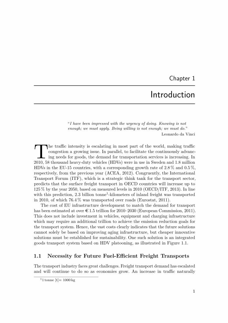
The cost of EU infrastructure development to match the demand for transporthas been estimated at over e 1.5 trillion for 2010–2030 (European Commission, 2011).This does not include investment in vehicles, equipment and charging infrastructurewhich may require an additional trillion to achieve the emission reduction goals forthe transport system. Hence, the vast costs clearly indicates that the future solutionscannot solely be based on improving aging infrastructure, but cheaper innovativesolutions must be established for sustainability. One such solution is an integratedgoods transport system based on HDV platooning, as illustrated in Figure 1.1.
1.1 Necessity for Future Fuel-E�cient Freight Transports
The transport industry faces great challenges. Freight transport demand has escalatedand will continue to do so as economies grow. An increase in tra�c naturally
11 tonne [t]= 1000 kg
1
2 Introduction
Figure 1.1: Future intelligent road transportation systems, where goods transport isintegrated with platooning. Commercial vehicles are governed semi-autonomously atsmall inter-vehicle spacings and thereby e�ectively improve fuel consumption, reduceemissions, reduce congestion, and relieve driver tension without compromising safety.Each vehicle is able to serve as an information node through wireless communication;enabling a cooperative networked transportation system. Instructions, for example,regarding the possibility to platoon with vehicles further ahead and how to mergeto an appropriate platoon position for fuel-optimality can be displayed on advancedhuman to machine interfaces. Furthermore, the infrastructure aids the vehicle platoonsby providing information regarding the upcoming road incidents, tra�c signals, roadconstruction, road tolls, etc. A central o�ce, such as a fleet management system,monitors each vehicle on the road and systematically coordinate scattered vehicles onthe road network to form platoons in order to maximize the benefits of platooning.(Illustration provided courtesy of the Smart Mobility Lab, KTH Royal Institute ofTechnology.)
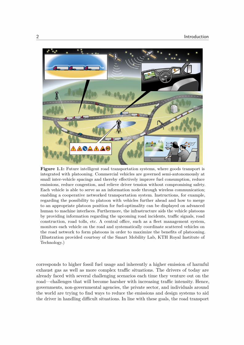
corresponds to higher fossil fuel usage and inherently a higher emission of harmfulexhaust gas as well as more complex tra�c situations. The drivers of today arealready faced with several challenging scenarios each time they venture out on theroad—challenges that will become harsher with increasing tra�c intensity. Hence,governments, non-governmental agencies, the private sector, and individuals aroundthe world are trying to find ways to reduce the emissions and design systems to aidthe driver in handling di�cult situations. In line with these goals, the road transport
1.1. Necessity for Future Fuel-E�cient Freight Transports 3
sector has been targeted as a main policy area where further environmental andoverall e�ciency improvements are critical for a sustainable future of Europeantransport (European Commission, 2014). Furthermore, complex tra�c scenarioscan have a devastating impact: more than 1.3 million people die every year inroad accidents. If nothing is done, this number might rise to 1.9 million deaths peryear according to ITF (2011). Urban transport is responsible for 69 % of accidentsthat occur in cities (European Commission, 2011). In parallel, the growing tra�cintensity have led to that almost every weekday morning and evening, the mainroads saturate throughout the major cities in the world.
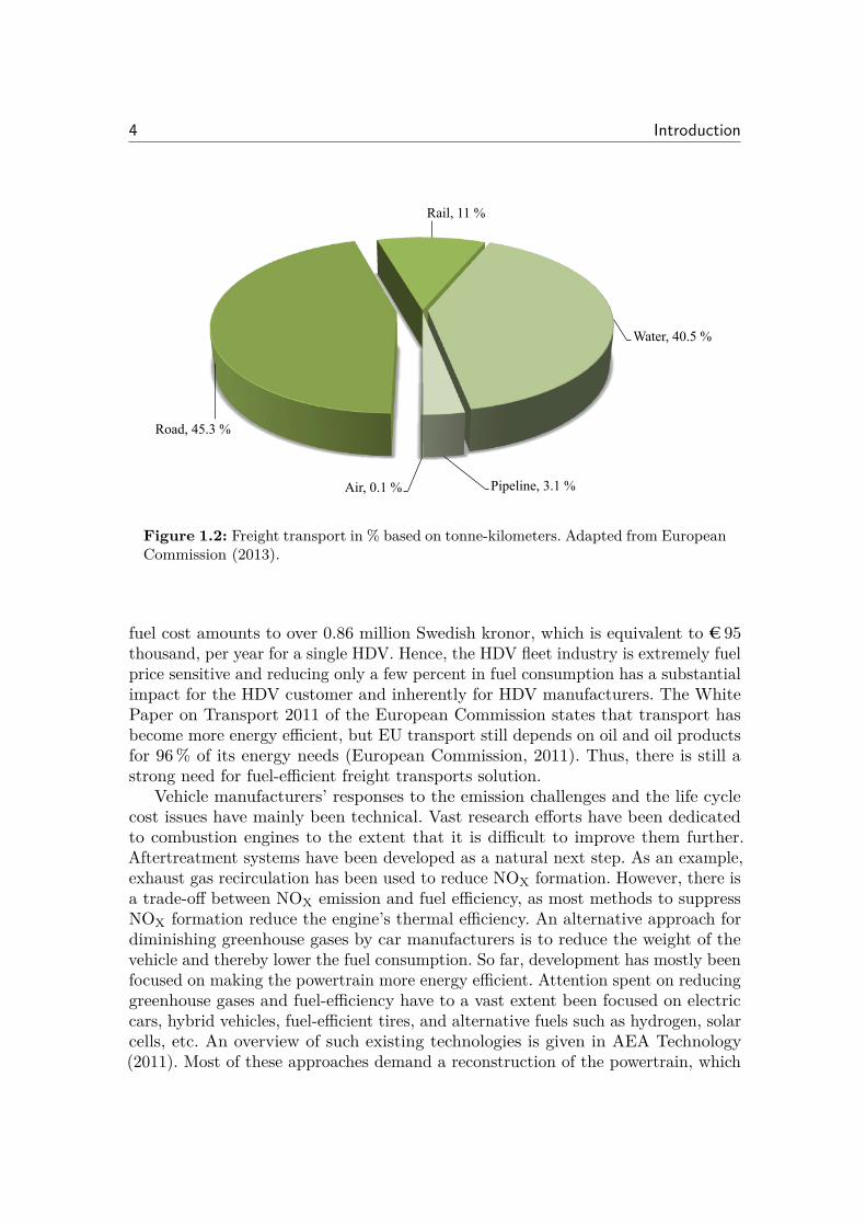
In addition, harmful emissions have proved to result in severe long term con-sequences. Hence, industrialized countries have agreed to reduce greenhouse gasemissions under the Kyoto protocol. Working toward the development of a low-carbon economy is vital for averting climate change. Combating climate changeand rooting out its main causes, a problem due to increase in greenhouse gases,are among the top priorities in Europe. Road transport constitute the dominantmode of transportation, as illustrated in Figure 1.2, and contribute to 72 % of thegreenhouse gas emissions (European Commission, 2013). Overall green house gasemissions were recorded to be reduced by 17 % between 1990 and 2009 (Eurostat,2011). While emissions from other sectors are falling, those from the transport sectorhave increased by 21 %. The road sector emissions dominate transport emissionsglobally. Road transport alone contributes about 20 % of the EU’s total emissionsof CO
2
, the main greenhouse gas, from fossil fuel combustion. Similar results werepresented by the Community Research and Development Service (CORDIS), whichis part of the European Commission. They reported that road freight accounts forapproximately 35 % of transport CO
2
emissions, 75 % of the particulate emissions,and 60 % of nitrogen oxides (NO
X
) emissions. Thus, the European Union have setthe goal to reduce emissions by 80–95 % by 2050 with respect to the levels measuredin 1990, which implies a 60 % reduction in green house gas emissions from thetransport sector. Considering the high emission of greenhouse gases from fossil fuelcombustion, especially in freight transports, legislation and policies have been set.Thus, vehicle manufacturers are facing increasingly di�cult emission challenges.
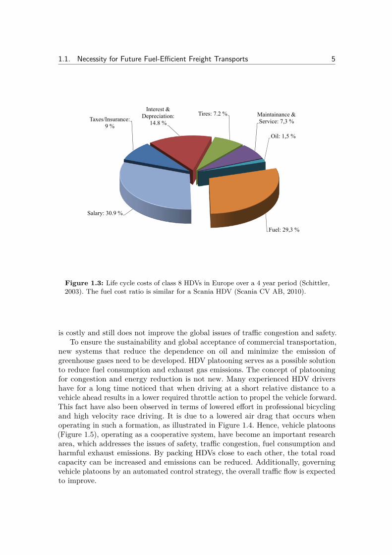
Along with challenges regarding safety and emission policies, the vehicle manufac-turers also experience an increase in fuel prices. The oil price is expected to increaseby 60 % by 2050, compared to the prices in 2010 (OECD/ITF, 2013). Transportationconstitutes the main part of the increase in oil consumption during the last threedecades and the growth is expected to continue. As the fuel price increases, thestrain on operating costs grows for an HDV fleet provider. This issue has a majorimpact within the transport industry. Road transport serves as the backbone ofthe economy in many countries. With the rise in fuel prices, road transportationbecomes less economically viable. Figure 1.3 shows the main operational costs for anHDV in Europe. Fuel cost constitutes approximately one third of the total life cyclecost in European long haulage HDVs. An HDV fleet provider generally owns manyvehicles that travel over 200 000 km per year. With an average fuel consumption of0.3 liter/km and the current diesel fuel price in Sweden being 14.42 kr/liter, only the
4 Introduction
Air, 0.1 %!
Road, 45.3 %!
Rail, 11 %!
Water, 40.5 %!
Pipeline, 3.1 %!
Figure 1.2: Freight transport in % based on tonne-kilometers. Adapted from EuropeanCommission (2013).
fuel cost amounts to over 0.86 million Swedish kronor, which is equivalent to e 95thousand, per year for a single HDV. Hence, the HDV fleet industry is extremely fuelprice sensitive and reducing only a few percent in fuel consumption has a substantialimpact for the HDV customer and inherently for HDV manufacturers. The WhitePaper on Transport 2011 of the European Commission states that transport hasbecome more energy e�cient, but EU transport still depends on oil and oil productsfor 96 % of its energy needs (European Commission, 2011). Thus, there is still astrong need for fuel-e�cient freight transports solution.
Vehicle manufacturers’ responses to the emission challenges and the life cyclecost issues have mainly been technical. Vast research e�orts have been dedicatedto combustion engines to the extent that it is di�cult to improve them further.Aftertreatment systems have been developed as a natural next step. As an example,exhaust gas recirculation has been used to reduce NO
X
formation. However, there isa trade-o� between NO
X
emission and fuel e�ciency, as most methods to suppressNO
X
formation reduce the engine’s thermal e�ciency. An alternative approach fordiminishing greenhouse gases by car manufacturers is to reduce the weight of thevehicle and thereby lower the fuel consumption. So far, development has mostly beenfocused on making the powertrain more energy e�cient. Attention spent on reducinggreenhouse gases and fuel-e�ciency have to a vast extent been focused on electriccars, hybrid vehicles, fuel-e�cient tires, and alternative fuels such as hydrogen, solarcells, etc. An overview of such existing technologies is given in AEA Technology(2011). Most of these approaches demand a reconstruction of the powertrain, which
1.1. Necessity for Future Fuel-E�cient Freight Transports 5
Taxes/Insurance: 9 %
Interest & Depreciation:
14.8 %Tires: 7.2 % Maintainance &
Service: 7,3 %
Oil: 1,5 %
Fuel: 29,3 %
Salary: 30.9 %
Figure 1.3: Life cycle costs of class 8 HDVs in Europe over a 4 year period (Schittler,2003). The fuel cost ratio is similar for a Scania HDV (Scania CV AB, 2010).
is costly and still does not improve the global issues of tra�c congestion and safety.To ensure the sustainability and global acceptance of commercial transportation,
new systems that reduce the dependence on oil and minimize the emission ofgreenhouse gases need to be developed. HDV platooning serves as a possible solutionto reduce fuel consumption and exhaust gas emissions. The concept of platooningfor congestion and energy reduction is not new. Many experienced HDV drivershave for a long time noticed that when driving at a short relative distance to avehicle ahead results in a lower required throttle action to propel the vehicle forward.This fact have also been observed in terms of lowered e�ort in professional bicyclingand high velocity race driving. It is due to a lowered air drag that occurs whenoperating in such a formation, as illustrated in Figure 1.4. Hence, vehicle platoons(Figure 1.5), operating as a cooperative system, have become an important researcharea, which addresses the issues of safety, tra�c congestion, fuel consumption andharmful exhaust emissions. By packing HDVs close to each other, the total roadcapacity can be increased and emissions can be reduced. Additionally, governingvehicle platoons by an automated control strategy, the overall tra�c flow is expectedto improve.
6 Introduction
0 10 20 30 40 50 60 700
10
20
30
40
50
60
70
80
cD
reducti
on
[%]
Re lat ive distance in platoon [m]
HDV 1HDV 2HDV 3
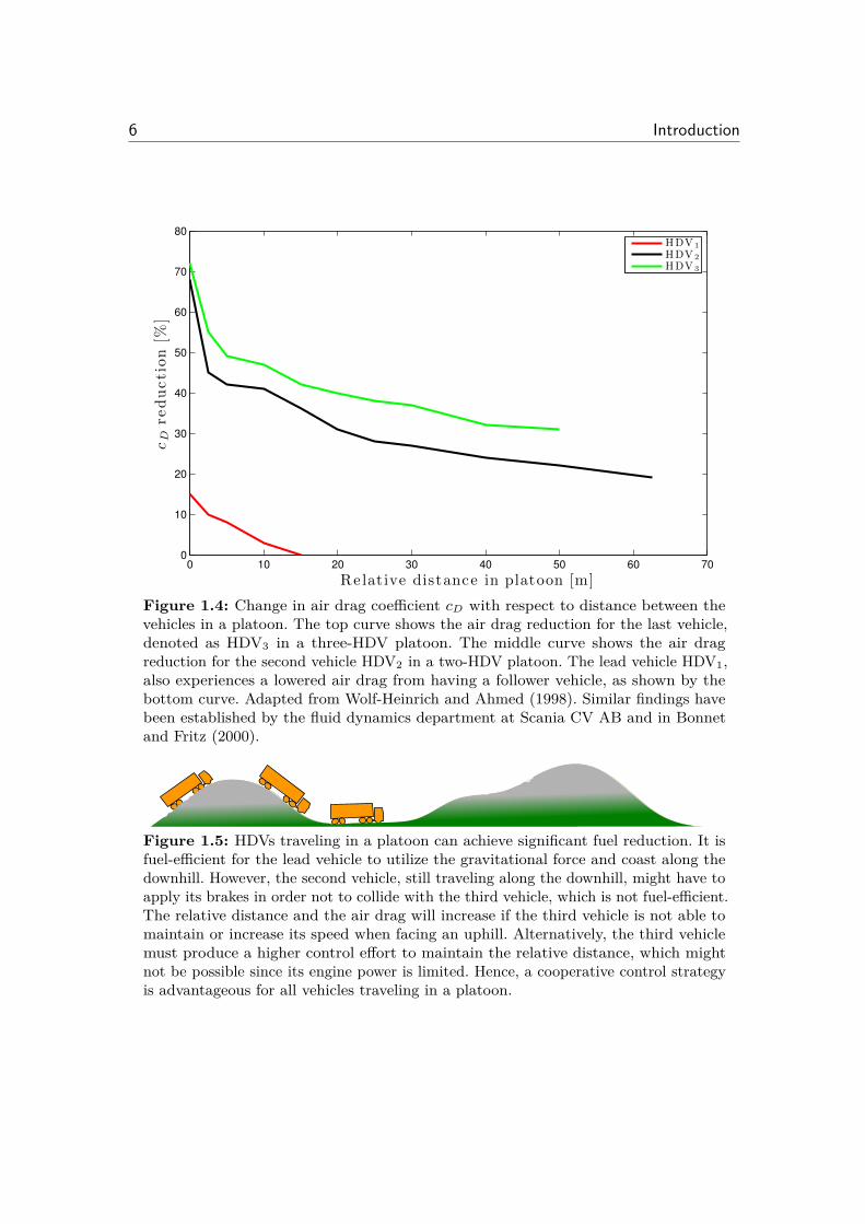
Figure 1.4: Change in air drag coe�cient c
D
with respect to distance between thevehicles in a platoon. The top curve shows the air drag reduction for the last vehicle,denoted as HDV3 in a three-HDV platoon. The middle curve shows the air dragreduction for the second vehicle HDV2 in a two-HDV platoon. The lead vehicle HDV1,also experiences a lowered air drag from having a follower vehicle, as shown by thebottom curve. Adapted from Wolf-Heinrich and Ahmed (1998). Similar findings havebeen established by the fluid dynamics department at Scania CV AB and in Bonnetand Fritz (2000).
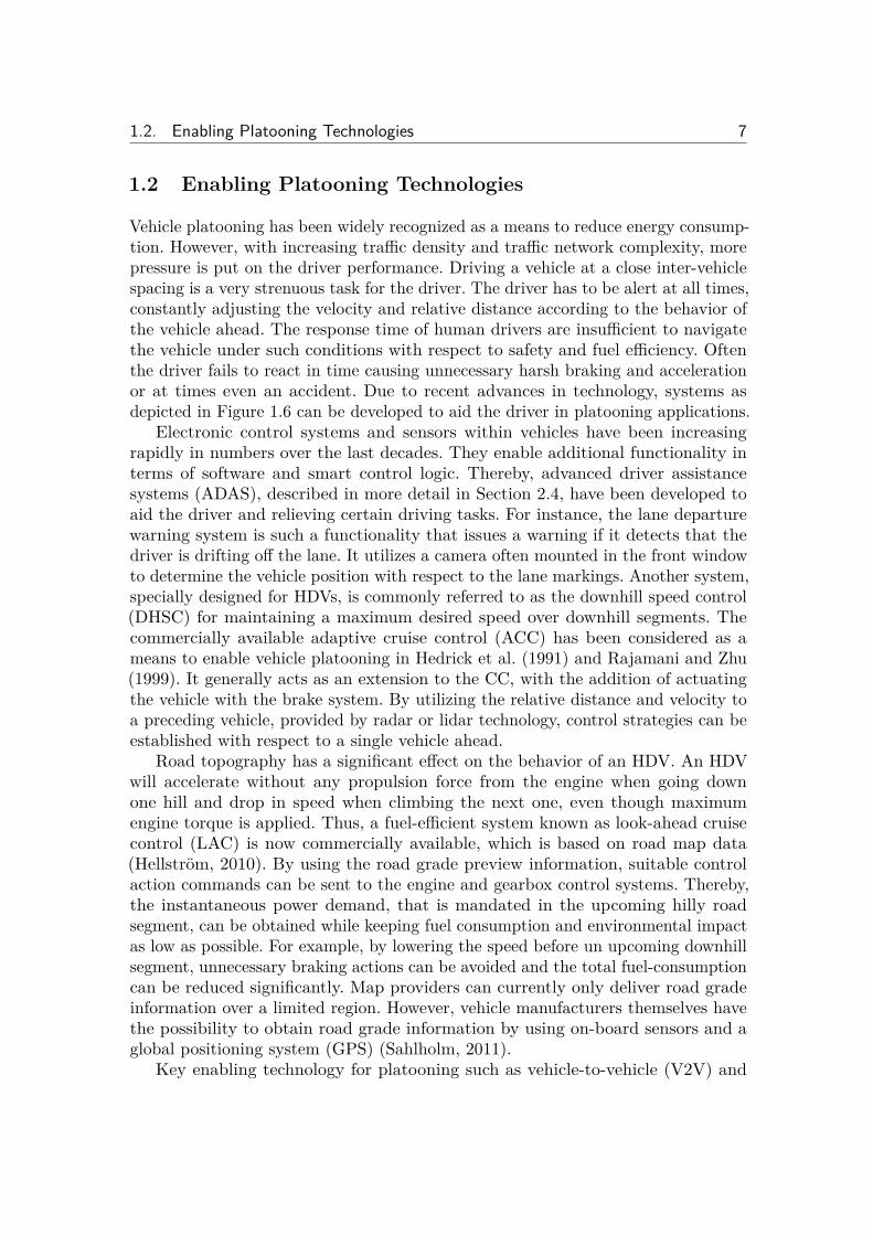
Figure 1.5: HDVs traveling in a platoon can achieve significant fuel reduction. It isfuel-e�cient for the lead vehicle to utilize the gravitational force and coast along thedownhill. However, the second vehicle, still traveling along the downhill, might have toapply its brakes in order not to collide with the third vehicle, which is not fuel-e�cient.The relative distance and the air drag will increase if the third vehicle is not able tomaintain or increase its speed when facing an uphill. Alternatively, the third vehiclemust produce a higher control e�ort to maintain the relative distance, which mightnot be possible since its engine power is limited. Hence, a cooperative control strategyis advantageous for all vehicles traveling in a platoon.
1.2. Enabling Platooning Technologies 7
1.2 Enabling Platooning Technologies
Vehicle platooning has been widely recognized as a means to reduce energy consump-tion. However, with increasing tra�c density and tra�c network complexity, morepressure is put on the driver performance. Driving a vehicle at a close inter-vehiclespacing is a very strenuous task for the driver. The driver has to be alert at all times,constantly adjusting the velocity and relative distance according to the behavior ofthe vehicle ahead. The response time of human drivers are insu�cient to navigatethe vehicle under such conditions with respect to safety and fuel e�ciency. Oftenthe driver fails to react in time causing unnecessary harsh braking and accelerationor at times even an accident. Due to recent advances in technology, systems asdepicted in Figure 1.6 can be developed to aid the driver in platooning applications.
Electronic control systems and sensors within vehicles have been increasingrapidly in numbers over the last decades. They enable additional functionality interms of software and smart control logic. Thereby, advanced driver assistancesystems (ADAS), described in more detail in Section 2.4, have been developed toaid the driver and relieving certain driving tasks. For instance, the lane departurewarning system is such a functionality that issues a warning if it detects that thedriver is drifting o� the lane. It utilizes a camera often mounted in the front windowto determine the vehicle position with respect to the lane markings. Another system,specially designed for HDVs, is commonly referred to as the downhill speed control(DHSC) for maintaining a maximum desired speed over downhill segments. Thecommercially available adaptive cruise control (ACC) has been considered as ameans to enable vehicle platooning in Hedrick et al. (1991) and Rajamani and Zhu(1999). It generally acts as an extension to the CC, with the addition of actuatingthe vehicle with the brake system. By utilizing the relative distance and velocity toa preceding vehicle, provided by radar or lidar technology, control strategies can beestablished with respect to a single vehicle ahead.
Road topography has a significant e�ect on the behavior of an HDV. An HDVwill accelerate without any propulsion force from the engine when going downone hill and drop in speed when climbing the next one, even though maximumengine torque is applied. Thus, a fuel-e�cient system known as look-ahead cruisecontrol (LAC) is now commercially available, which is based on road map data(Hellström, 2010). By using the road grade preview information, suitable controlaction commands can be sent to the engine and gearbox control systems. Thereby,the instantaneous power demand, that is mandated in the upcoming hilly roadsegment, can be obtained while keeping fuel consumption and environmental impactas low as possible. For example, by lowering the speed before un upcoming downhillsegment, unnecessary braking actions can be avoided and the total fuel-consumptioncan be reduced significantly. Map providers can currently only deliver road gradeinformation over a limited region. However, vehicle manufacturers themselves havethe possibility to obtain road grade information by using on-board sensors and aglobal positioning system (GPS) (Sahlholm, 2011).
Key enabling technology for platooning such as vehicle-to-vehicle (V2V) and
8 Introduction
����������
��� �� �����
��� �� ��� ��� ��� ��� ���
��
���
���
���
���
���
���
��
�� � ����
�� � ������
�������
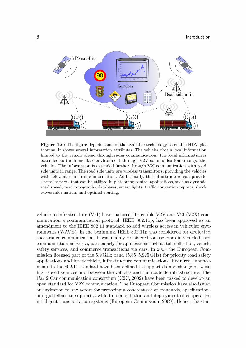
Figure 1.6: The figure depicts some of the available technology to enable HDV pla-tooning. It shows several information attributes. The vehicles obtain local informationlimited to the vehicle ahead through radar communication. The local information isextended to the immediate environment through V2V communication amongst thevehicles. The information is extended further through V2I communication with roadside units in range. The road side units are wireless transmitters, providing the vehicleswith relevant road tra�c information. Additionally, the infrastructure can provideseveral services that can be utilized in platooning control applications, such as dynamicroad speed, road topography databases, smart lights, tra�c congestion reports, shockwaves information, and optimal routing.
vehicle-to-infrastructure (V2I) have matured. To enable V2V and V2I (V2X) com-munication a communication protocol, IEEE 802.11p, has been approved as anamendment to the IEEE 802.11 standard to add wireless access in vehicular envi-ronments (WAVE). In the beginning, IEEE 802.11p was considered for dedicatedshort-range communication. It was mainly considered for use cases in vehicle-basedcommunication networks, particularly for applications such as toll collection, vehiclesafety services, and commerce transactions via cars. In 2008 the European Com-mission licensed part of the 5.9 GHz band (5.85–5.925 GHz) for priority road safetyapplications and inter-vehicle, infrastructure communications. Required enhance-ments to the 802.11 standard have been defined to support data exchange betweenhigh-speed vehicles and between the vehicles and the roadside infrastructure. TheCar 2 Car communication consortium (C2C, 2002) have been tasked to develop anopen standard for V2X communication. The European Commission have also issuedan invitation to key actors for preparing a coherent set of standards, specificationsand guidelines to support a wide implementation and deployment of cooperativeintelligent transportation systems (European Commission, 2009). Hence, the stan-
1.3. Problem Formulation 9
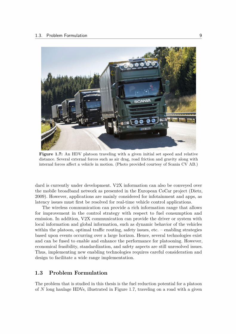
Figure 1.7: An HDV platoon traveling with a given initial set speed and relativedistance. Several external forces such as air drag, road friction and gravity along withinternal forces a�ect a vehicle in motion. (Photo provided courtesy of Scania CV AB.)
dard is currently under development. V2X information can also be conveyed overthe mobile broadband network as presented in the European CoCar project (Dietz,2009). However, applications are mainly considered for infotainment and apps, aslatency issues must first be resolved for real-time vehicle control applications.
The wireless communication can provide a rich information range that allowsfor improvement in the control strategy with respect to fuel consumption andemission. In addition, V2X communication can provide the driver or system withlocal information and global information, such as dynamic behavior of the vehicleswithin the platoon, optimal tra�c routing, safety issues, etc. – enabling strategiesbased upon events occurring over a large horizon. Hence, several technologies existand can be fused to enable and enhance the performance for platooning. However,economical feasibility, standardization, and safety aspects are still unresolved issues.Thus, implementing new enabling technologies requires careful consideration anddesign to facilitate a wide range implementation.
1.3 Problem Formulation
The problem that is studied in this thesis is the fuel reduction potential for a platoonof N long haulage HDVs, illustrated in Figure 1.7, traveling on a road with a given
10 Introduction
initial set speed and relative distance.Each HDV in the platoon can be modeled based upon the road grade –, the
internal forces produced by the powertrain and the main external forces acting uponthe vehicle. A longitudinal dynamics model can be derived for each vehicle in theplatoon based upon their individual vehicle properties. Dynamics of the relativedistance between the vehicles is modeled as the change in velocity between twovehicles in the platoon. The HDV platoon model is
s1
= v1
,
v1
= f1
(v1
, s1
≠ s2
, –(s1
), u1
),s
2
= v2
,
v2
= f2
(v2
, s1
≠ s2
, s2
≠ s3
, –(s2
), u2
),...
sN≠1
= vN≠1
,
vN≠1
= fN≠1
(vN≠1
, sN≠2
≠ sN≠1
, sN≠1
≠ sN , –(sN≠1
), uN≠1
),sN = vN ,
vN = fN (vN , sN≠1
≠ sN , –(sN ), uN ),
(1.1)
where si denotes the absolute traveled distance for the ith HDV from a referencepoint common to all vehicles in the platoon, vi is the velocity for vehicle i, ui denotesthe control input to the vehicle and i = 1, . . . , N denotes the vehicle position indexin the platoon. The maps fi are the longitudinal dynamics. For convenience, let usintroduce di≠1,i = si≠1
≠ si as the relative distance between ith vehicle its precedingvehicle.
A coupling is induced by the variation in aerodynamics between HDVs operatingat a close distance. This is essential in the analysis of fuel reduction potentialfor HDV platooning. The aerodynamic drag decreases as the gap between thevehicles are reduced. However, as the relative distance decreases, it becomes morecostly to maintain the relative distance due to safety aspects. Moreover, additionalconstraints are induced due to physical limitation on the control inputs. An HDVcan generally produce a maximum engine torque of 2000–3000 Nm depending on thespecific diesel engine. Thus, due to its extensive mass, an HDV might not be able tomaintain a constant velocity when traversing steep uphill segments. The maximumbraking torque depends on the vehicle configuration but can be approximated by60 000 Nm/axle. Hence, the physical constraints for an HDV has an influence on theminimum achievable safe relative distance. Also, fuel-optimal control for a singlevehicle on a flat road is to maintain a constant velocity, under the presumption thatthe traveling time is fixed. Any deviations in the form of acceleration and decelerationresult in an increased fuel consumption. An HDV platoon control strategy generallyreceives information regarding the relative velocity and distance to the vehiclesin the platoon and thereby maintains the relative distance by adjusting its speed
1.4. Thesis Outline and Contributions 11
accordingly. The increased control e�ort that the strategy creates, in the sense ofadditional transient engine actions and brake events, produces an increased fuelconsumption.
Hence, the problem that we consider is finding the fuel reduction potentialfor an HDV platoon consisting of N vehicles, traveling without any surroundingtra�c, subject to the HDV vehicle dynamics, the safety constraints, road gradeinfluence, and the physical constraints on the control inputs imposed by the vehicleconfiguration.
1.4 Thesis Outline and Contributions
In this section, we outline the contents of the thesis and the main contributions. InChapter 2, we describe the background for vehicle platooning. A brief descriptionintelligent transportation systems is presented along with a short survey on thecurrent technology development for vehicle platooning. A review of the existingliterature on automated vehicle platooning is given, followed by a description ofcurrent ADAS that can already be used for vehicle platooning or serve as inspirationfor future possible use cases. In Chapter 3, several models are presented, which areutilized to address certain aspects of vehicle platooning. We present an advancedsimulation model that serves as a basis for evaluation and verification throughoutthis thesis. Furthermore, a model for a platoon system architecture is presentedthat divides the large and complex system into smaller manageable subsystems.In Chapter 4, the fuel reduction potential of HDV platooning for a commercialcontroller is evaluated on a measured highway in Sweden. In Chapter 5 we addressthe problem of finding the minimum safety distance between two HDVs traveling ona road without compromising safety, where an experimental setup for evaluating thederived safe sets is given together with experimental evaluations. A methodologyto produce a systematic decentralized LQR control design for HDV platooningis presented in Chapter 6, where simulation and experiment results are given todetermine and evaluate the performance of the proposed controller in practice. InChapter 7, we consider the problem of finding a suitable fuel-e�cient controllerfor HDV platooning under road and vehicle parameter uncertainties, where wepropose two novel model predictive control strategies based on road grade previewinformation. The fuel-saving potential is studied for a three-vehicle platoon inChapter 8, where the follower vehicles are governed by our proposed decentralizedcooperative controllers over a varying topography. Chapter 9 provides concludingremarks and future outlook for HDV platooning. In the following, we discuss thedetails of the contributions.
System Modeling
In Chapter 3, we consider the longitudinal dynamics for a single vehicle and formmodels that serve as a basis for the analysis and control design presented in thefollowing chapters. We present the main components that influence the considered
12 Introduction
dynamics for a single HDV, which is then extended to a linearized platoon model.However, the analytical model does not capture the dynamics that arise from gearchanges, e�ects of switching between the embedded systems, brake blending, etc.,that come into play in practice. A more complex simulation model is thus necessaryto evaluate the fuel reduction potential of the implemented control strategy andplatoon behavior. Hence, we present an advanced simulation model that has beentested and verified to mimic real life behavior for a single vehicle. The simulationmodel serves as a basis for evaluation and validation throughout this thesis. Italso facilitates reproducible data and serves as a necessary precaution measurebefore evaluating safety critical operations in practice. Furthermore, there areseveral technologies and systems that are involved in the process of automatedHDV platooning. Analyzing the entire system is not manageable due to the systemcomplexity. There are no available tools to handle all the aspects of such a largecontrol system. Thus, we propose a suitable system architecture for dividing thecomplex problem into manageable subsystems for optimal control. The materialpresented in this chapter is in part based on the work presented in
A. Alam. Optimally Fuel E�cient Speed Adaptation. Master’s thesis, RoyalInstitute of Technology, Automatic Control (2008)
Part of the proposed architecture in this thesis is based on the journal paper in
A. Alam, J. Mårtensson, and K. H. Johansson. Experimental evaluation ofdecentralized cooperative cruise control for heavy-duty vehicle platooning (2014c).Submitted for journal publication.
Preliminary work, in line with the interests of this chapter, were also conducted asa supervised Master’s thesis project in
H. J. Tehrani. Study of Disturbance Models for Heavy-duty Vehicle Platooning.Master’s thesis, Royal Institute of Technology (KTH) (2010)
D. Norrby. A CFD study of the aerodynamic e�ects of platooning trucks. Master’sthesis, Royal Institute of Technology (2014)
Fuel-Saving Potential of Platooning
In Chapter 4, we investigate the fuel reduction potential of heavy-duty vehicleplatooning, solely with respect to a commercial control strategy. The aim is notto investigate the specifics of the control strategy, but rather the translation fromthe lowered air drag to the fuel reduction potential in HDV platooning based onsimulations and experimental studies. Fuel-optimal control for a single vehicle on aflat road is to maintain a constant velocity, under the presumption that the travelingtime is fixed. Any deviations in the form of acceleration and deceleration result inan increased fuel consumption. The ACC generally receives information regardingthe relative velocity and distance to the vehicle ahead and thereby maintains the
1.4. Thesis Outline and Contributions 13
relative distance by adjusting its speed accordingly. The increased control e�ort thatthe ACC creates, in the sense of additional transient engine actions and brake events,produces an overall increased fuel consumption. Thus, it is interesting to determinewhether the increased control e�ort produced by the ACC possibly cancels thereduction in fuel consumption achieved by decreasing the air drag. Furthermore, weshow that it is beneficial to reduce the inter-vehicle spacing between each vehiclein the platoon and that the conventional control strategy can be improved withrespect to fuel consumption. However, safety becomes an issue when reducing therelative distance. The material presented in this chapter is based on the conferencepublication in
A. Alam, A. Gattami, and K. H. Johansson. An experimental study on the fuelreduction potential of heavy duty vehicle platooning. In 13th International IEEEConference on Intelligent Transportation Systems. Madeira, Portugal (2010)
Safety Constraints
In Chapter 5, we investigate the minimum possible relative distance between pla-tooning HDVs that can be maintained without compromising safety. We primarilyestablish safe sets, which can serve as a reference for HDV platooning in collisionavoidance. We propose a novel approach by setting up a relative coordinate frame-work and thereby computing so called reachable sets to develop safety criteria forHDV platooning. A di�erential game formulation of the problem enables the safeset derivation by capturing the event when the lead vehicle blunders in the worstpossible manner. A collision can occur if the unsafe set is entered. Computing safesets is an e�cient method to capture the behavior of entire sets of trajectories simul-taneously. We establish empiric results for validation of the analytical framework andnumerical safe set computation for collision avoidance in HDV platooning scenarios.We propose an automated and reproducible method to derive empiric results forvalidation of safe sets. We show how the method has been evaluated experimentallyusing real HDVs provided by Scania CV AB on a test site near Stockholm. Basedon the theoretic and empiric results, we determine criteria for which collisions canbe avoided in a worst-case scenario and thereby establish the minimum possiblesafe distance in practice between vehicles in a platoon. We show that the minimumrelative distance with respect to safety depends on the nonlinear behavior of thebrake system and delays in information propagation along with the implementedcontrol actions. By introducing V2V communication, the relative distance betweenthe HDVs can be reduced significantly compared to what is utilized in current ACCs.The material presented in this chapter is based on the conference publication andjournal paper in
A. Alam, A. Gattami, K. H. Johansson, and C. J. Tomlin. Establishing safety forheavy duty vehicle platooning: A game theoretical approach. In 18th IFAC WorldCongress. Milan, Italy (2011b)
14 Introduction
A. Alam, A. Gattami, K. H. Johansson, and C. J. Tomlin. Guaranteeing safety forheavy duty vehicle platooning: Safe set computations and experimental evaluations.Control Engineering Practice, 24: 33 – 41 (2014a)
Decentralized Cooperative Control for HDV Platooning
In Chapter 6, we derive a decentralized controller for HDV platooning and establishempiric performance results for the presented control design. Several studies onvehicle platooning have been based on simplified theoretical models. However,as shown in this chapter, delay and nonlinear dynamics can have a significantinfluence on the closed-loop system. We present a method for designing suboptimaldecentralized feedback controllers, with low computational complexity, that takesdynamic coupling and engine response delays into consideration. The controllerperformance is evaluated through implementation on commercial HDVs. The designmethod is scalable in the sense that an additional vehicle can be added at the tail ofthe platoon without mandating a change in the controllers of the already platooningvehicles. Our proposed vehicle system architecture in Section 3.3.3 is shown to berobust to packet losses or short outages in V2V communication. As modern HDVsin general have two separate low-level control systems for governing the longitudinalpropulsion and deceleration of the vehicle, the engine management system (EMS)and the brake management system (BMS), we present a simple bumpless transferscheme to switch between these systems. The proposed platooning controller canbe easily implemented on modern HDVs, without requiring any changes in thealready existing vehicle architecture. We show that the controller behaves well evenwhen performing outside the linear region of operation. We also show that theproposed controller attenuates the e�ect of disturbances downstream in the platoon,when studying scenarios that commonly occur on highways with dynamic operatingconditions and physical constraints. Experimental results are given to qualitativelyvalidate the proposed control system behavior. The results show that the controllerperformance is improved with increasing position index in the platoon, by utilizingadditional information from preceding vehicles. However, the e�ects of unmodelednonlinearities, such as gear changes, brake blending, and engine dynamics, can causeundesirable behavior in some cases. The experiments were conducted on a test sitesouth of Stockholm, using HDVs provided by Scania CV AB. The material presentedin this chapter is based on the conference publications and journal paper in
A. Alam, A. Gattami, and K. H. Johansson. Suboptimal decentralized controllerdesign for chain structures: Applications to vehicle formations. In 50th IEEEConference on Decision and Control and European Control Conference. Orlando,FL, USA (2011a)
A. Alam, J. Mårtensson, and K. H. Johansson. Experimental evaluation ofdecentralized cooperative cruise control for heavy-duty vehicle platooning (2014c).Submitted for journal publication.
1.4. Thesis Outline and Contributions 15
K.-Y. Liang, A. Alam, and A. Gattami. The impact of heterogeneity and orderin heavy duty vehicle platooning networks. In 3rd IEEE Vehicular NetworkingConference. Amsterdam, Netherlands (2011)
O. Khorsand, A. Alam, and A. Gattami. Optimal distributed controller synthe-sis for chain structures: Applications to vehicle formations. In 9th InternationalConference on Informatics in Control, Automation and Robotics. Rome, Italy (2012)
Preliminary work for this chapter were also conducted as a supervised Master’sthesis projects in
G. Hammar and V. Ovtchinnikov. Structural Intelligent Platooning by a Sys-tematic LQR Algorithm. Master’s thesis, Royal Institute of Technology, AutomaticControl (2010)
K.-Y. Liang. Linear Quadratic Control for Heavy Duty Vehicle Platooning.Master’s thesis, Royal Institue of Technology, Osquldas väg 10, 100 44 Stockholm,Sweden (2011)
J. Kemppainen. Model Predictive Control for Heavy Duty Vehicle Platooning.Master’s thesis, Linköping University, Automatic Control (2012)
Look-Ahead Control for HDV Platooning
In Chapter 7, we propose two novel fuel-e�cient controllers based on road gradepreview information for HDV platooning and determine guidelines for handlingsystem uncertainties to maintain the fuel reduction benefits. The instantaneousfuel consumption can increase by a factor of four over a steep uphill segment whenthe engine is operating at maximum torque. Hence, the air drag reduction has alower e�ect on the total resistive forces that are exerted on an HDV in motion oversteep hills. We focus on establishing fuel-e�cient controllers with low computationalcomplexity, since it is generally not possible to implement complex control algorithmsdue to the limited computational power in the on-board electronic control units. Thefirst proposed controller adapts its velocity solely based on the look-ahead velocityprofile of the vehicle ahead. A more fuel-e�cient strategy is established with thesecond proposed controller, which cooperatively forms a common look-ahead controlstrategy for all platooning vehicles with respect to the most restricted vehicle in theplatoon. The main idea for this control strategy is to initiate the control actions in aplatoon based on a point in the road rather than simultaneously implementing eachHDV’s control action to maintain a fixed spacing. The results for a heterogeneousHDV platoon of nine HDVs traveling over a 2 km road segment show that a fuelreduction of 12 % or 19 % can be achieved with the cooperative look-ahead controllerwhen traversing a typical steep uphill or downhill segment of 240 m, respectively.Thus, the findings show that the fuel-saving potential can be improved significantlyby considering the road grade preview information in control for HDV platooning.
16 Introduction
We also study commercially available controllers that could be utilized for platooning.It is shown that the commercially available ACC is not fuel-e�cient for a varyingtopography and that the LAC for a single HDV is not practical in HDV platooning.Furthermore, we investigate whether it is better to split up or maintain a platoonover steep hills and show that it is most fuel-e�cient to maintain a platoon whentraversing a hill, as opposed to split the platoon and resume it during or after the hill.We study what e�ect a varying road topography and the system uncertainties haveon the fuel consumption for HDV platooning. It is shown that the fuel reductionpotential with the proposed controller can degrade depending on the magnitude ofthe inherent errors. Hence, guidelines are determined for handling common systemuncertainties that occur in practice, to maintain the fuel-saving potential. Thematerial in this chapter is based on the conference publication and journal paper in
A. Alam, J. Mårtensson, and K. H. Johansson. Look-ahead cruise control forheavy duty vehicle platooning. In 16th International IEEE Conference on IntelligentTransportation Systems, 928–935. Hague, The Netherlands (2013a)
A. Alam, J. Mårtensson, and K. H. Johansson. Cooperative control with previewtopography information under system uncertainties for heavy-duty vehicle platooning(2014b). Submitted for journal publication.
Preliminary work, in line with the interests of this chapter, were also conducted asa supervised Master’s thesis projects in
G. J. Babu. Look-Ahead Platooning through Guided Dynamic Programming.Master’s thesis, Royal Institute of Technology, Automatic Control (2013)
L. Bühler. Fuel-E�cient Platooning of Heavy Duty Vehicles through RoadTopography Preview Information. Master’s thesis, Royal Institute of Technology,Automatic Control (2013)
Experimental Evaluation for HDV Platooning
In Chapter 8, we study the possible issues that might arise when governing anHDV platoon in practice with a cooperative adaptive cruise control (CACC) that isbased on simplified linear models. We present an experimental evaluation of the fuelreduction possibilities for a heterogeneous three-vehicle platoon in practice, whereresults are presented based on data recorded over 2700 km per vehicle. The e�ects ofunmodeled nonlinearities, such as gear changes, brake blending between the variousbrake systems in an HDV, and engine dynamics, can have unforeseen consequences.Thus, it is important to understand the issues with implementing a CACC based onlinear models. Hence, we derive empirical results for our proposed CACC throughexperiments conducted over a Swedish highway with varying topography. It can beinferred from the obtained results that linear controllers, which does not accountfor road topography constraints, can reduce the fuel-saving potential significantly.
1.4. Thesis Outline and Contributions 17
However, the results also show that the fuel-saving potential can be lost due tounmodeled engine dynamics for uphill segments and excessive braking over downhillsegments. Nevertheless, a vast fuel savings can be obtained over relatively flat roadsegments. Furthermore, the shape and behavior of the preceding vehicles also havean impact of the fuel-saving potential. This chapter is to be submitted as a journalpaper. Preliminary work for some of the material in this chapter is based on thejournal publication in
J. Mårtensson, A. Alam, S. Behere, M. Khan, J. Kjellberg, K.-Y. Liang, H. Pet-tersson, and D. Sundman. The development of a cooperative heavy-duty vehicle forthe GCDC 2011: Team Scoop. IEEE Transactions on Intelligent TransportationSystems, 13(3): 1033–1049 (2012)
and the supervised Master’s thesis projects in
H. Pettersson. Estimation and Pre-Processing of Sensor Data in Heavy DutyVehicle Platooning. Master’s thesis, Linköping University, Automatic Control (2012)
S. Nilsson. Sensor Fusion for Heavy Duty Vehicle Platooning. Master’s thesis,Linköping University, Automatic Control (2012)
Other Academic Publications
The following publications are not covered in this thesis but they inspired some ofthe contents.
H. Feyzmahdavian, A. Alam, and A. Gattami. Optimal distributed controllerdesign with communication delays: Application to vehicle formations. In IEEE 51stAnnual Conference on Decision and Control, 2232–2237. Maui, HI, USA (2012)
M. Larsson, J. Lindberg, J. Lycke, K. Hansson, E. R. A. Khakulov, F. Svensson,I. Tjernberg, A. Alam, J. Araujo, F. Farokhi, E. Ghadimi, A. Teixeira, D. V.Dimarogonas, and K. H. Johansson. Towards an indoor testbed for mobile networkedcontrol systems. In Proceedings of the 1st Workshop on Research, Development, andEducation on Unmanned Aerial Systems, 51–60 (2011)
Contributions by the Author
The order of the authors’ names reflect the work load of the paper, where themain contribution is attributed to the first author. An exception with the journalpublication in Mårtensson et al. (2012), where the first author was the correspondingauthor. All other authors’ names are given in alphabetical order and the workloadis divided into their respective fields. Several Master’s thesis projects have alsobeen conducted in parallel with this thesis work. Each thesis project have been
18 Introduction
supervised by the author of this thesis, where the author participated activelythrough discussions and derivations of the theories.
Patents
Along with academic publications, two Swedish and nine international patent appli-cations have been published during the course of this work. Two, out of the nineinternational patent applications, have been granted as Swedish patents.
A. Alam, J. Andersson, and P. Sahlholm. A Vehicle Speed Control Method.International patent application number: PCT/SE09/050030 (filed 2009a)
A. Alam, J. Andersson, and P. Sahlholm. Determination of acceleration behavior.International patent application number: PCT/SE09/051299 (filed 2009b)
A. Alam, K.-Y. Liang, and A. Gattami. Metod i samband med fordonståg, ochett fordon som använder metoden [A method in connection to vehicle trains and avehicle that uses that method]. Swedish patent application number: 1150579-9 (filed2011c)
A. Alam, H. Pettersson, T. Sandberg, and J. Dellrud. Method and manage-ment unit pertaining to vehicle trains. International patent application number:PCT/SE12/050066 (filed 2011d)
A. Alam, J. Andersson, H. Gustafsson, H. Pettersson, P. Sahlholm, and H. Schau-man. Metod i samband med trafikövervakning, och ett trafikövervakningssystem[Method in connection with tra�c monitoring and a tra�c monitoring system].Swedish patent application number: 1150073-3 (filed 2011b)
A. Alam, J. Andersson, H. Gustafsson, H. Pettersson, P. Sahlholm, and H. Schau-man. Method and system for speed verification. European patent application number:11193590.4 (filed 2011a)
A. Alam, S. Nilsson, J. Kemppainen, H. Pettersson, and H. Pettersson. Systemand method for assisting a vehicle when overtaking a vehicle train. Internationalpatent application number: PCT/SE13/050674 (filed 2012b)
A. Alam, S. Nilsson, J. Kemppainen, H. Pettersson, and H. Pettersson. Systemoch metod för att assistera ett fordon vid omkörning av fordonståg [System andmethod for assisting a vehicle when overtaking a vehicle train]. Swedish patentnumber: 1250627-5 (Granted 2014a)
A. Alam, S. Nilsson, J. Kemppainen, H. Pettersson, and H. Pettersson. Systemand method for regulating of vehicle pertaining to a vehicle train. Internationalpatent application number: PCT/SE13/050673 (filed 2012c)
1.4. Thesis Outline and Contributions 19
A. Alam, S. Nilsson, J. Kemppainen, H. Pettersson, and H. Pettersson. Systemoch metod för reglering av fordon i ett fordonståg [System and method for regulatingof vehicle pertaining to a vehicle train]. Swedish patent number: 1250628-3 (Granted2014b)
A. Alam, S. Nilsson, J. Kemppainen, H. Pettersson, and H. Pettersson. Sys-tem and method for regulation of vehicles in vehicle trains. International patentapplication number: PCT/SE13/050672 (filed 2012d)
A. Alam, S. Nilsson, J. Kemppainen, H. Pettersson, and H. Pettersson. Systemand method pertaining to vehicle trains. International patent application number:PCT/SE13/050687 (filed 2012e)
A. Alam, A. Johansson, R. Lyberger, and H. Pettersson. Method and systemfor spacing adjustment in a moving vehicle train. International patent applicationnumber: PCT/SE13/050317 (filed 2012a)
In addition, thirteen international patent applications have been filed and arecurrently under examination. Due to the confidential nature of the patents, thefiling numbers are only given as follows:
PCT/SE14/050241, PCT/SE14/050243, 1351125-8, 1351126-6, 1351127-4, 1351128-2,1351129-0, 1351130-8, 1351131-6, PCT/SE13/051382, 1351132-4, 1350891-6, 1350266-1.

Chapter 2
Background
“Learn from yesterday, live for today, hope for tomorrow.”Albert Einstein
Information and communication technology (ICT) is paving its path into trans-portation systems. Many governments spend a countless amount of money onthe infrastructure in restoration and expansion of the road network. However,
the future improvement lies not in increasingly stringent road taxation policies tochange incentives or only in improving aging infrastructure, but also increasing theutilization of information technology and thereby introducing intelligence to roadtra�c networks. The rapid development in ICT presents an excellent opportunity totackle transport issues through novel integrated intelligent transportation systems(ITS) solutions.
In this chapter, we first list a few ITS applications in Section 2.1. Then, inSection 2.2, we present the contemporary technology premise for heavy-duty vehicle(HDV) platooning. Afterward, we give an overview of the related work on vehicleplatooning in Section 2.3. The literature on control of platoons is quite extensive.Therefore, we have not attempted a thorough review of all the proposed controlschemes here, but rather give a review of the general concepts and issues in vehicleplatooning that is addressed in the literature. We then, in Section 2.4, give a briefoverview of commercial advanced driver assistant systems (ADAS) that can be used,or integrated in the future, for control of HDV platoons. In particular, a detaileddescription of the adaptive cruise control (ACC) is given, since it serves as a firststepping stone to practical implementation of HDV platooning. A brief overview oncollision avoidance and safety in vehicle applications is given in Section 2.5. Thechapter is concluded with a short summary in Section 2.6.
21
22 Background
2.1 Intelligent Transportation Systems
Transportation systems can be perceived as large mobile networks. By introducingdecision making based on suitable and accurate ICT, intelligence is induced in thenetwork. ITS, illustrated in Figure 2.1, empower actors in the system with infor-mation based actions. The European Road Transport Telematics ImplementationCo-ordination Organisation (ERTICO) - ITS Europe is the network of intelligenttransport systems and services stakeholders in Europe. It was founded at the initia-tive of leading members of the European Commission, Ministries of Transport andthe European industry. ERTICO’s o�cial definition of ITS “is the integration ofICT with transport infrastructure, vehicles, and users. By sharing vital information,ITS allow people to get more from transport networks, in greater safety and withless impact on the environment” (ERTICO, 2014). ITS have received a great deal ofattention in the transportation community as well as in governments over the lastdecade. The initial e�orts were referred to as intelligent vehicle highway systems(IVHS). However, due to the increasingly intermodal focus, the scope was broadenedto include modes beyond highways. There are numerous agencies working with ITSthroughout the world, such as ITS America (ITSA, 2014) and ITS Japan (ITSJP,2014) amongst others.
ITS include several applications and can be grouped within five main categories(Ezell, 2010):
• Advanced Public Transportation Systems include systems that for exampleallow trains, buses, and boats to report their position so passengers can beinformed of their real-time arrival status and departure information.
• Advanced Traveler Information Systems provide travelers with real-time nav-igation routes, tra�c lights, weather conditions, tra�c construction, delaysand congestion. Accident reports can also be provided.
• Advanced Transportation Management Systems include systems that monitorstra�c flow and provide decision support based upon tra�c control devices,such as tra�c signals, variable message signs, and tra�c operations centers.
• ITS-Enabled Transportation Pricing Systems provide services such as electronictoll collection and congestion pricing.
• Automated Transportation Systems include supporting and replacing humanfunctions in various driving processes. The focus in this category lies on e�ortsfor developing vehicles with automated components. Here, vehicle-to-vehicleand/or infrastructure (V2X) communication serves as a basis to provideinformation and enable communication between all the actors.
Through these categories, ITS aim at enhancing safety, operational performance,mobility, environmental benefits, and productivity by expanding economic andemployment growth. ITS encompass the full scope of information technologies
2.1. Intelligent Transportation Systems 23
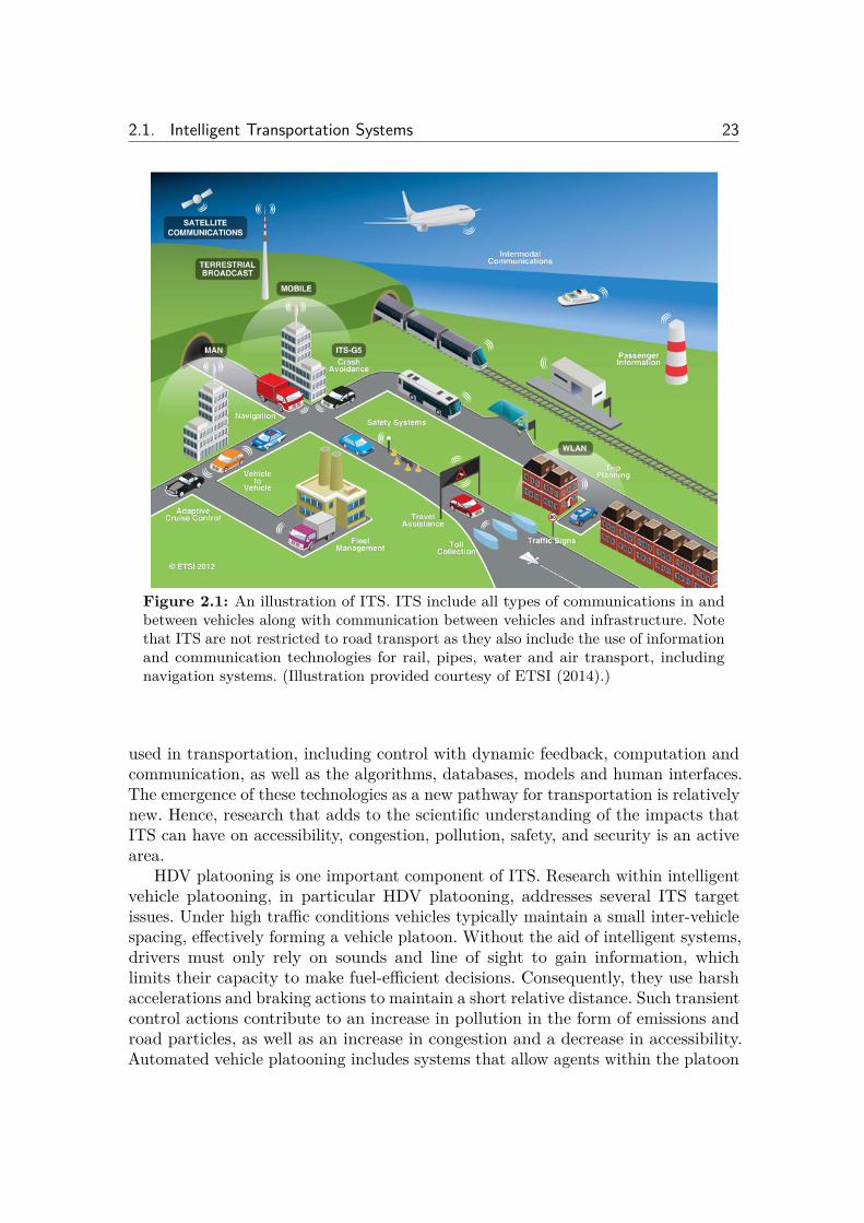
Figure 2.1: An illustration of ITS. ITS include all types of communications in andbetween vehicles along with communication between vehicles and infrastructure. Notethat ITS are not restricted to road transport as they also include the use of informationand communication technologies for rail, pipes, water and air transport, includingnavigation systems. (Illustration provided courtesy of ETSI (2014).)
used in transportation, including control with dynamic feedback, computation andcommunication, as well as the algorithms, databases, models and human interfaces.The emergence of these technologies as a new pathway for transportation is relativelynew. Hence, research that adds to the scientific understanding of the impacts thatITS can have on accessibility, congestion, pollution, safety, and security is an activearea.
HDV platooning is one important component of ITS. Research within intelligentvehicle platooning, in particular HDV platooning, addresses several ITS targetissues. Under high tra�c conditions vehicles typically maintain a small inter-vehiclespacing, e�ectively forming a vehicle platoon. Without the aid of intelligent systems,drivers must only rely on sounds and line of sight to gain information, whichlimits their capacity to make fuel-e�cient decisions. Consequently, they use harshaccelerations and braking actions to maintain a short relative distance. Such transientcontrol actions contribute to an increase in pollution in the form of emissions androad particles, as well as an increase in congestion and a decrease in accessibility.Automated vehicle platooning includes systems that allow agents within the platoon
24 Background
to report their position and velocity in addition to systems that provide navigationroutes, information from tra�c control devices, road construction and congestion.With the aid of V2X communication devices, a cooperative system is formed forsupporting and replacing human functions in various driving processes to enhanceoperational performance, mobility, environmental benefits, safety, and economicgrowth.
In line with the interests of this thesis, the challenges and benefits of HDVplatooning in practice have been studied within several ITS research projectsthroughout the world. In the projects PROMOTE-CHAUFFEUR I & II, needsof intermediate and end users, along with safety and operational requirements,were investigated (Harker, 2001). In KONVOI, experimentally analyzing the useof electronically regulated truck convoys on the road with five vehicles was one ofthe main focuses (Deutschle et al., 2010). The acceptance of automated platoons inmixed tra�c was studied, where it was observed that operating at an inter-vehiclespacing of 10 m seemed to be insignificant for passing vehicle, in comparison to aspacing of 50 m. It was inferred that road users expect automated platoons to behavecooperatively by, for example, open up a gap or change lanes if needed. CaliforniaPartners for Advanced Transportation Technology (PATH), established in 1986, isa vast research project that addresses many tra�c related research aspects (Buet al., 2010). Results in this project have shown that the highway throughput canbe increased three times through platooning by utilizing services provided by theautomated transportation systems. Another research project, Strategic Platform forIntelligent Tra�c Systems (SPITS), shows in addition that potential shock wavesarising in tra�c congestions can be removed through automated platooning (SPITS,2014). Focus has lately been directed towards studying HDV platooning, mainly dueto the fuel and congestion reduction potential. The recently concluded ENERGY ITSproject, evaluated energy-e�ciency for automated HDV platooning and methods fore�ectiveness of ITS on energy saving (Tsugawa, 2013). The results obtained in theproject showed an average fuel-saving potential of 9–16 % for a three-vehicle platoonon a flat test track. In the Safe Road Trains for the Environment (SARTRE) project,the focused lied on mixed tra�c in highway situations, where fuel-e�ciency, safety,and comfort was evaluated, (Robinson et al., 2010). Findings within this projectshowed that a 20 % emission reduction, a 10 % reduction in fatalities, and a smoothertra�c flow with potential increase in tra�c flow can be obtained through automatedvehicle platoons. The findings are based on that a lead vehicle with a professionaldriver will take responsibility and guide the vehicle platoon. Vehicles will join theplatoon and enter an autonomous control mode that will allow the automated systemto fully govern the vehicle while the driver can withdraw his attention from theroad. In addition, experiments conducted on a flat test track in this project showedfuel saving results between 2–16 % depending on the vehicle type and inter-vehiclespacing. The aim of the Grand Cooperative Driving Challenge (GCDC) projectwas to accelerate the deployment of cooperative driving systems (van Nunen et al.,2012). Several, issues, such as communication constraints and erroneous information,were revealed in this project that needs to be solved before platooning can presented
2.2. Technology for HDV Platooning 25
commercially. Finally, in the recent project COMPANION (Adolfson, 2014) a widerperspective is undertaken, where the actual creation, coordination, and operation ofplatoons is studied. The goal is to identify means of applying the platooning conceptin practice for daily transport operations.
2.2 Technology for HDV Platooning
The demand for enhancing vehicle performance has paved the way for several tech-nological developments. On-board sensors have increased in number and accuracy.This has led to the development of on-board networks to share and convey informa-tion between electronic control units (ECUs). Faster and cheaper vehicle computertechnology has been developed to process the growing amount of available informa-tion. With increasing reliability and computational performance, in parallel withdecreasing size and price, new sensors have been implemented to further enhancethe operational performance. However, currently we see a transition, which is notnecessarily induced by the vehicle industry. Technology that was initially developedand intended for entirely di�erent markets is now finding its use and presentinga new scope for enhancing vehicle applications and enabling vehicle platooning.Thus, automated HDV platooning could not be considered in practice until now andthe understanding of the potential benefits is growing rapidly. In this section, wedescribe some of the key components that contribute to and enable HDV platooning,where we use Figure 2.2 to guide our discussion. We begin with the inner most ringand proceed outwards.
A wide range of vehicle specific information is provided through on-board sensorsand ECUs. Traditionally vehicular research focus has been on improving the vehicleperformance. During the last decades on-board sensors have been developed andimplemented to facilitate the overall HDV operational e�ciency. Initially, sensortechnology was introduced to enhance the engine operational performance withrespect to fuel e�ciency and exhaust gasses. Crank-angle, RPM, pressure, andtemperature sensors were implemented to enable better engine control. With thepassage of time, additional sensors were implemented, for example rotational wheelsensors and gear box sensors, to further increase the operational performance.ECUs process the information and in some cases fuse it to create virtual sensors.Today, 30 to 80 ECUs are integrated in an average car, whereas 6 to 17 ECUs areintegrated in an HDV. This substantial di�erence in ECUs is mainly due to that apassenger vehicle and an HDV operate under di�erent premises. An HDV commonlytravels under more strenuous conditions. Introducing more ECUs opens up thepossibility for more system errors, which is less acceptable in the HDV market.Furthermore, underdeveloped countries demand less ECUs due to manageabilityand price sensitivity. Implementing electronic sensors has become a relatively cheapand e�cient way to enable new functionality.
In 1985 Bosch developed the controller area network (CAN) for in-vehiclenetworks (Johansson et al., 2005). Thereby, dedicated wiring was replaced by a
26 Background
������������
� �
��������� �������
����
������
����
�����������������
���
� �
����
���
������������
��
������������
�����������
��������������������
���������
�����
�����
�
!�
"�#�����
$�%
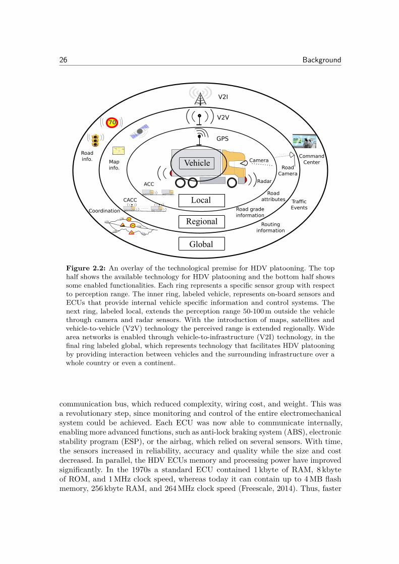
Figure 2.2: An overlay of the technological premise for HDV platooning. The tophalf shows the available technology for HDV platooning and the bottom half showssome enabled functionalities. Each ring represents a specific sensor group with respectto perception range. The inner ring, labeled vehicle, represents on-board sensors andECUs that provide internal vehicle specific information and control systems. Thenext ring, labeled local, extends the perception range 50-100 m outside the vehiclethrough camera and radar sensors. With the introduction of maps, satellites andvehicle-to-vehicle (V2V) technology the perceived range is extended regionally. Widearea networks is enabled through vehicle-to-infrastructure (V2I) technology, in thefinal ring labeled global, which represents technology that facilitates HDV platooningby providing interaction between vehicles and the surrounding infrastructure over awhole country or even a continent.
communication bus, which reduced complexity, wiring cost, and weight. This wasa revolutionary step, since monitoring and control of the entire electromechanicalsystem could be achieved. Each ECU was now able to communicate internally,enabling more advanced functions, such as anti-lock braking system (ABS), electronicstability program (ESP), or the airbag, which relied on several sensors. With time,the sensors increased in reliability, accuracy and quality while the size and costdecreased. In parallel, the HDV ECUs memory and processing power have improvedsignificantly. In the 1970s a standard ECU contained 1 kbyte of RAM, 8 kbyteof ROM, and 1 MHz clock speed, whereas today it can contain up to 4 MB flashmemory, 256 kbyte RAM, and 264 MHz clock speed (Freescale, 2014). Thus, faster
2.2. Technology for HDV Platooning 27
and more computational complex functionalities have been developed over time.A local environment awareness is obtained by monitoring the nearest vicinity.
With the development of vehicle internal sensors for improving operational andsafety performance, the next step in sensor development was to monitor the nearestvicinity. Initially the local environment sensors were costly, large, and therefore notyet suitable for the commercial market. To date, the technology has improved andis becoming fairly inexpensive. Radar or lidar sensors, to detect and monitor objectsmoving in the neighborhood of the subject vehicle, have matured to the extent ofbeing commercially viable. The cost and hardware size have reduced significantly overthe years. Low cost monolithic microwave integrated circuit based millimeter-wavefront end modules, entailing down to a 1 mm2 chip, for automotive radar applicationsare now available (Walden and Garrod, 2003). In-vehicle camera monitoring devicesis another local environment sensor technology that has matured. Initially the sizeof the cameras and the image processing unit were too large to mount in the frontwindow. With the emerging improvement in camera lens technology and signalprocessing capabilities of microprocessors, most vehicle manufacturers are startingto implement camera based monitoring systems. Commonly, such systems involvelane departure warning or steering. More advanced systems involving tra�c signdetection, driver attention, and pedestrian detection are now also being developedand o�ered by some vehicle manufacturers. Furthermore, fused with radar data,a three dimensional environment can be formed, which can be utilized in futurearising safety and navigation systems. Hence, the small hardware size and thecomputation power for performing advanced calculations within milliseconds, haverecently extended the range for the on-board vehicle sensors and their possible usecases.
The regional environment awareness is provided by information from globalpositioning system (GPS) technology, map data, and V2V communication devices.Due to recent advancements in improved map data and GPS accuracy, GPS tech-nology can now deliver centimeter accuracy with the aid of real time kinematicbase stations or di�erential GPS (Kaplan and Hegarthy, 2006). Alternatively, therelative position estimates in each vehicle can cooperatively be fused together withthe estimates of neighboring vehicles that are obtained through V2V communication.Thereby, relative positioning can be made with higher accuracy and precision incomparison to the di�erential GPS (Alam et al., 2013b). Map providers, such asNAVTEQ, are developing methods for acquiring road grade information to obtain athree dimensional topography map and are currently able to deliver such maps overa limited region. Hence, in Sahlholm and Johansson (2010) a road grade estimationalgorithm is presented, based on Kalman filter fusion of vehicle sensor data and GPSpositioning information. Road grade estimation is a vast research area. It is typicallyestimated at the vehicle position, but it can also be estimated over segments. In Baeet al. (2001) one for road grade estimation method based on a GPS receiver with3D velocity output and one using a two-antenna GPS were presented. A recursiveleast squares method with forgetting for online applications was presented in Vahidiet al. (2005). Another recursive least squares method and survey of online road
28 Background
grade estimation without GPS, based on accelerometers and on-board sensors, canbe found in Fathy et al. (2008). Moreover, GPS devices are becoming increasinglycommon among all tra�c agents. Omnipresent mobile phone devices can deliverpositioning, heading and velocity for pedestrians, mopeds, motorcycles and bicycles.Thus, ECUs might now not only be able to monitor and intelligently govern theinternal vehicle systems, but also gather external information regarding the sur-rounding tra�c and topography. Hence, an HDV will be able to react based uponthe internal and external environment influences.
For e�ective and safe platooning additional information is necessary in additionto what is provided by radars and cameras. If vehicles interact through wireless com-munication, an HDV can adjust the velocity and relative distance based upon eventsoccurring further ahead in the platoon. Thus, safety, fuel e�ciency, road capacityand emissions can be improved significantly by enabling a reduced inter-vehiclespacing through preview information. The interaction through V2V communicationcan improve safety by setting for example a deceleration limit for the HDVs in theplatoon or setting a safe distance based upon the vehicle characteristics. Smoothercontrol can also be implemented through prediction based upon information onevents occurring upstream. Hence, V2V communication enables cooperative driv-ing and automated platooning systems. Several di�erent wireless technologies arecurrently under consideration for V2V communication. These technologies includeconventional IEEE 802.11 wireless local area network (LAN), dedicated short rangecommunication, and GPRS/UMTS, amongst others. However, the IEEE 802.11technology family is most likely to be used as the prevailing communication standardfor future V2V communication, due to its success in the area of data communication.In particular, the recent wireless communication protocol IEEE 802.11p (802.11p,2014) has opened up an entire new set of applications for vehicular systems. Thepurpose of this standard is to provide the minimum set of specifications requiredto ensure interoperability between wireless devices. The access layer technologyfor the European protocol stack has been given the name ITS-G5, even though itis purely based on IEEE standards with the addition of decentralized congestioncontrol. For ITS-G5 in Europe this standard is given in ETSI EN 302 571 (2014). Itis meant for devices attempting to communicate in rapidly changing communica-tions environments and in situations where transactions must be completed in timeframes much shorter than what is set for ad hoc 802.11 networks. This is obtainedby splitting the high-rate data stream into a number of lower-rate data streamstransmitted simultaneously over a number of subcarriers, where each subcarrieris narrow banded. The medium access control (MAC) in ITS-G5/802.11, is basedon carrier sense multiple access with collision avoidance (CSMA/CA). The usercan define own message types in the transport layer. However, two standardizedmessage types must be generated, which are called cooperative awareness message(CAM) and decentralized environmental notification message (DENM), see thedocuments ETSI EN 302 637-2 (2014) and ETSI EN 302 637-3 (2014) for details.The DENMs consist of event-driven hazard warnings. CAMs are sent periodically,but not with a fixed frequency. The minimum time between two CAMs are 100 ms
2.2. Technology for HDV Platooning 29
and the maximum time is 1 s. The content of the CAM is divided in a number ofcontainers, with di�erent frequencies. There are currently no general purpose fieldsdefined in any of the containers above, but there are possibilities to extend thenumber of choices in many places.
Vehicular ad hoc networks (VANETs) impose a new set of requirements on thecommunication systems. For example, vehicle communication cannot tolerate longdelays and the moving vehicles form a dynamic ad hoc communication network.Numerous studies and evaluations have been performed on the standard, for ex-ample in Jiang and Delgrossi (2008); Ferreira et al. (2008); Barradi et al. (2010).Scalability and safety are challenging issues, since IEEE 802.11 is designed for datacommunication where reliability is more important than delay (Bilstrup et al., 2010).In dense and high load scenarios the throughput decreases and the delay increasessignificantly. Hence, even though wireless LAN is promising for the exchangingmessages between vehicles in an ad hoc manner, it might not be able to providethe quality or time constraints for large vehicle networks (Gupta and Kumar, 2000).Furthermore, aspects like e�cient message dissemination and information securitymechanisms are still ongoing research areas for VANETs (Eichler et al., 2006). Theseissues must be resolved before full implementation of VANETs. Nevertheless, V2Vcommunication enables a wide range of information to the vicinity. Previously mostinformation has been gathered by direct visual observation and in response to sounds.Now, vehicles traveling in a platoon will be able to act faster with interaction, intentsand events produced by several vehicles in the surrounding environment.
A global awareness is enabled by V2I information. Thereby, for example, co-ordinating and routing vehicles to form platoons for improved fuel-e�ciency isachieved. In combination with GPS-technology, the position and movement of everyconnected vehicle are known to the fleet manager. If coordinated departures arenot feasible, HDVs are typically scattered over the road network (Liang, 2014).Through V2I, a command center or a fleet manager can monitor the vehicles intra�c. For every transport assignment the fleet manager can pre-plan the routesand departures through optimization schemes, such that platoons are formed formaximized fuel-e�ciency and fill rate in each vehicle. In addition, o�ine routeoptimization can be formed at the command center for every vehicle that is alreadyout on the road. Thereby, directives are sent through V2I, instructing a vehicle toeither increase its speed to catch up with an HDV further ahead, or slow down suchthat another HDV might catch up to form a platoon. Obstructing tra�c situationsthat are reported to a tra�c management center is also relayed to vehicles that planto travel on that route. Hence, smart routing is formed by finding an alternativepath to ensure that the transport assignment is on time.
Even though there is an apparent strong need for automated HDV platooningsystems, they have only recently become a possibility. Each tra�c agent will soonbe able to serve as an information node through wireless communication; enablingother agents to interact, as opposed to simply react, to internal and externalinfluences. Thereby, vehicles will be able to travel at small inter-vehicle spacings,e�ectively reducing congestion, relieving driver tension, improving fuel consumption
30 Background
and emissions without compromising safety. There are however many challenges,such as safety, reliability, standards, etc., that must be addressed before HDVplatooning can become commercially feasible. With respect to longitudinal controlof the vehicles, the question of whether to implement a centralized or decentralizedcontrol arises. As depicted in Figure 2.2, there are several technologies and systemsinvolved in the process of HDV platooning. Analyzing the entire system is notmanageable due to the system complexity. There are no available tools to handleall the aspects of such a large control system. Thus, an important challenge is toestablish a suitable system architecture, which is decomposable into manageablesubsystems. In this thesis we present such a system architecture in Chapter 3.Chapter 6 presents a decentralized controller suitable for that architecture.
2.3 Cooperative Vehicle Platooning
The concept of partial automation of highway tra�c is not a new idea. At the1939 World’s Fair in New York, General Motors presented a vision of automaticallycontrolled vehicles on highways, aiming at guaranteeing safety for increased speed(General Motors, 1939). Even before the automatic control of vehicles was considered,studies on the dynamics of a collection of vehicles following each other in a singlelane have been performed since the 1950s. By assuming a simple model of driverbehavior, Pipes (1953) and Chandler et al. (1958) give early results on the dynamicresponse of follower vehicles to the behavior of the leading vehicle, where the latterreference includes experiments using real vehicles.
The first investigations into control for heavy vehicle platooning was in theearly 1960s (Rothery et al., 1964). Vehicle platooning can be described as a chainof vehicles traveling at a given velocity and inter-vehicle spacings. The primaryobjective for each vehicle with respect to safety is to maintain its distance to thepreceding vehicle in the platoon. Even under normal operating conditions there willbe deviations from the desired velocities and desired relative distances. A vehicleplatoon is most commonly modeled in the literature as a set of moving masses
xi + kixi = ui, i = 1, . . . , N (2.1)
where xi represents the position of the i:th vehicle, ki Ø 0 denotes a systemdamping coe�cient, sometimes referred to as the linearized drag coe�cient per unitmass, and ui is the applied control force. Control of vehicular platoons was earlystudied by Levine and Athans (1966) and Melzer and Kuo (1971a). Their workconsidered centralized control design for vehicle platoons, indirectly assuming thatcomputational complexity and V2V communication hardware constraints would notbe an issue. A linear quadratic regulator (LQR) control strategy was developed thatregulates the position and velocity of every vehicle in a densely packed string ofhigh-speed moving vehicles. The presented control methodology involved full stateinformation of each vehicle in the platoon.
2.3. Cooperative Vehicle Platooning 31
An early hope for high-speed vehicle platoons was that centralized automaticcontrol could encompass very large platoons. Thus, control strategies were derivedbased upon a countably infinite number of vehicles in order to understand thefundamentals of the problem (Melzer and Kuo, 1971b). A new structural analysiswas introduced, allowing for a bilateral Z-transform to convert the problem intoa family of finite-dimensional systems. It was found that coupling between thevehicles decreases as the platoon index distance between them increases. It hasbeen hypothesized that the controller gain will decrease with increasing indexdistance, concluding that vehicles far away in a platoon has less controller impacton performance. However, even though infinite platoons capture the essence of largeplatoons, the LQR problem formulation lacks observability and stabilizability in theinfinite case and is therefore ill-posed (JovanoviÊ and Bamieh, 2004).
Governing vehicle platoons by an automated control strategy, the overall tra�cflow is expected to be improved (Ioannou and Chien, 1993). Through short relativedistances down to 2 m, the road capacity is significantly increased. In De Schutter et al.(1999), it is shown that the total road capacity can be increased two to three timescompared to roads with manually operated vehicles and emissions can be reducedthrough an automated controller for platooning. Tra�c flow has been considered as akey performance index in vehicle platooning. In Varaiya (1993) it was shown that byforming platoons, the throughput of a highway can be increased from 2000 vehiclesper lane per hour to more than 6000 vehicles per lane per hour. The findings werebased on an average platoon size of 15 vehicles, with intra-platoon distances of 2 m,inter-platoon distances of 60 m, vehicle length of 5 m, and speed of 20 m/s. However,it was argued that only full automation can achieve significant capacity increaseson highways and thereby reduce the occurrences of tra�c congestion. In Wangand Rajamani (2004b) the e�ects of having a varying spacing policy on the tra�cflow is studied. The research areas coordinating and forming platoons have grownrecently. In Farokhi and Johansson (2013), a game-theoretic approach is undertakenfor evaluating platoon incentives. Local controllers throughout the road network areintroduced in Larson et al. (2013) to facilitate platoon formations with minimalinformation. The paper by Meisen et al. (2008) attempts to increase platooningthroughout a network by using data-mining techniques to identify common routeswhere platoons can be formed. In Liang et al. (2013), the fuel-e�ciency of increasingthe speed to catch-up to a vehicle further ahead on the road is studied. Thereby,distance boundaries are given for when it is beneficial to form a platoon by increasingthe speed temporarily.
Communication constraints is an important issue that can dictate the definingfeature of the problem (Gupta et al., 2004). It is not realistic to assume that anagent in the platoon would know the state of all the other agents in the formationat any given time and be able to use it to calculate the control input due to physicalconstraints in the information flow. Hence, we argue in Chapter 6 that the problemat hand is a decentralized control problem with arbitrary information flow patterns.In general, this is a much harder to solve than the traditional optimal controlproblem.
32 Background
The problem of decentralized control has a long history and much e�ort hasbeen put in the research area. Decision team problems were introduced in Marshak(1955), where each team member is trying to optimize a common cost functionthrough limited information concerning the global state of nature. Witsenhausenshowed that, in general, a linear controller is not optimal for a quadratic performancecriterion with a linear time-invariant system subject to Gaussian noise under thedistributed information constraint and that the cost function is not necessarilyconvex in the controller variables (Witsenhausen, 1968). In Blondel and Tsitsiklis(2000); Papadimitriou and Tsitsiklis (1986) it was established that the discrete-timeversion of the Witsenhausen counter-example is NP-complete. There have beensome e�orts also to identify the cases in which a linear solution is optimal. Forinstance, Witsenhausen identified some cases where the resulting optimal controllersare linear (Witsenhausen, 1971). In Ho and Chu (1972) it was shown that undera partially nested information pattern the optimal controller is a linear controller.It was shown in Sandell and Athans (1974) that the optimal controller is linear ifeach subcontroller has access to all the previously implemented control values andobservations made by any other subsystem in the system before the current time andits own observations including the current time. Decentralized control was studiedthrough a sequential manner by closing one loop at a time in Mayne (1979). InBamieh et al. (2002); D’Andrea (1998) it was studied under the assumption of spatialinvariance. Decentralized controllers, using only relative distance measurements withrespect to nearest neighbors, were first given by Chu (1974) and Peppard (1974).Control for chain structures in the context of platoons has been studied throughvarious perspectives, for example in Dunbar and Murray (2006); Bamieh et al. (2008);Barooah et al. (2009), where it was studied based on following a predecessor in thefirst paper, under certain network topologies in the second paper, and based onbidirectional schemes in the third paper. A survey on platooning and inter-vehiclecontrol can be found in Tsugawa (1999) and more recently in Kavathekar and Chen(2011). It has been shown that control strategies may vary depending on the availableinformation within the platoon. Initially the ACC, not being cooperative in thesense of sharing information with other agents, simply reacted with respect to thebehavior of the preceding vehicle. With the introduction of V2X communication, thequestion arises of what information is relevant, necessary, or critical for platooningapplications. Furthermore, it is of interest to determine which agents should serveas the local information sources. A natural extension to the commercially availableACC is to implement a symmetric bidirectional control architecture, where eachvehicle bases its control action on the error feedback from its predecessor and follower(Barooah and Hespanha, 2005). In Sudin and Cook (2004) a two-vehicle look-aheadinformation structure is proposed, where each vehicle bases its control strategy onlyon information regarding relative velocity and relative distance from two vehiclesahead. A more general approach can be found in Gupta et al. (2004), where theinformation flow is dictated by the constraints of a pre-specified topology. In recentwork (Kianfar et al., 2014), a design procedure is proposed that matches a modelpredictive control (MPC), enforcing constraints satisfaction, with a linear controller
2.4. ADAS for HDV Platooning 33
designed to guarantee string stability.Maintaining a suitable relative distance, stability and robustness of the platoon
have been identified to be amongst the main criteria to be considered. Control designfor platooning applications is still an open problem, despite substantial academicwork. In Levine and Athans (1966); StankoviÊ et al. (2000); Dunbar and Murray(2006), optimized procedures were presented to give a systematic approach to thedesign. However, the vehicle coupling was only introduced through the cost function.To our knowledge, no control algorithm has yet considered decentralized optimalcontrol based upon systems with interconnected dynamics. In HDV platooningapplications the coupling is induced by the variation in aerodynamics, which isessential in the analysis of fuel reduction potential. Such a consideration is presentedin Chapter 6.
For vehicle platooning it is essential to use realistic models (Sahlholm andJohansson, 2010; Guzzella and Sciarretta, 2007) and not just identical low-ordercoupled linear models, as has often been the case in the literature. In HDV platooningmass and road slope has a significant e�ect on the system dynamics. Research intomore implementation-relevant aspects is only recently emerging. For example, inNaus et al. (2009) a setup is presented for the cooperative adaptive cruise control(CACC), where feasibility of the actual implementation is one of the main objectives.Several practical issues such as constrained communication, heterogeneous tra�cand graceful degradation to standard ACC if communication fails, are taken intoconsideration. In Shaw and Hedrick (2007) heterogeneous vehicle strings under simpledecentralized control laws with a constant spacing control policy are analyzed. Theconsidered vehicles do not need to have the same dynamics or the same controllersand can be arranged in any order. It is further argued that centralized formationcontrol is impractical due to the large amount of information that needs to becommunicated. Another design approach for a practical CACC was presented in Buet al. (2010). In Milanes et al. (2014), a control system is designed, which is evaluatedon four production passenger cars and the performance is evaluated in comparisonwith the ACC. Experiments for a platoon of six passenger cars under longitudinalcontrol is presented in Ploeg et al. (2011). Considering nonlinearities and powertrainactuator uncertainties in HDVs, a method for calculating worst-case spacing boundsis given in Rödönyi et al. (2013). In Geiger et al. (2012); Lidström et al. (2012);Mårtensson et al. (2012), system architectures, wireless communication, and controlfor platooning applications were studied and evaluated through experiments inmixed tra�c on a highway. Fuel reduction potentials of 5–20 % was demonstrated inexperiments by Alam et al. (2010); Robinson et al. (2010); Tsugawa (2013). Theseresults indicate that HDV platooning is an attractive concept.
2.4 ADAS for HDV Platooning
One area that shows promise for energy-e�ciency and improved safety is advanceddriver assistant systems (ADAS). The increasing number of on-board sensors and
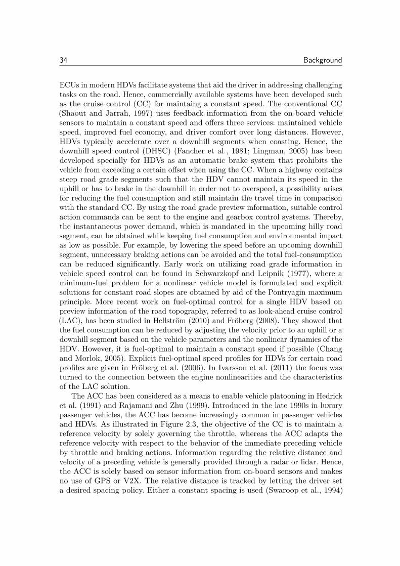
34 Background
ECUs in modern HDVs facilitate systems that aid the driver in addressing challengingtasks on the road. Hence, commercially available systems have been developed suchas the cruise control (CC) for maintaing a constant speed. The conventional CC(Shaout and Jarrah, 1997) uses feedback information from the on-board vehiclesensors to maintain a constant speed and o�ers three services: maintained vehiclespeed, improved fuel economy, and driver comfort over long distances. However,HDVs typically accelerate over a downhill segments when coasting. Hence, thedownhill speed control (DHSC) (Fancher et al., 1981; Lingman, 2005) has beendeveloped specially for HDVs as an automatic brake system that prohibits thevehicle from exceeding a certain o�set when using the CC. When a highway containssteep road grade segments such that the HDV cannot maintain its speed in theuphill or has to brake in the downhill in order not to overspeed, a possibility arisesfor reducing the fuel consumption and still maintain the travel time in comparisonwith the standard CC. By using the road grade preview information, suitable controlaction commands can be sent to the engine and gearbox control systems. Thereby,the instantaneous power demand, which is mandated in the upcoming hilly roadsegment, can be obtained while keeping fuel consumption and environmental impactas low as possible. For example, by lowering the speed before an upcoming downhillsegment, unnecessary braking actions can be avoided and the total fuel-consumptioncan be reduced significantly. Early work on utilizing road grade information invehicle speed control can be found in Schwarzkopf and Leipnik (1977), where aminimum-fuel problem for a nonlinear vehicle model is formulated and explicitsolutions for constant road slopes are obtained by aid of the Pontryagin maximumprinciple. More recent work on fuel-optimal control for a single HDV based onpreview information of the road topography, referred to as look-ahead cruise control(LAC), has been studied in Hellström (2010) and Fröberg (2008). They showed thatthe fuel consumption can be reduced by adjusting the velocity prior to an uphill or adownhill segment based on the vehicle parameters and the nonlinear dynamics of theHDV. However, it is fuel-optimal to maintain a constant speed if possible (Changand Morlok, 2005). Explicit fuel-optimal speed profiles for HDVs for certain roadprofiles are given in Fröberg et al. (2006). In Ivarsson et al. (2011) the focus wasturned to the connection between the engine nonlinearities and the characteristicsof the LAC solution.
The ACC has been considered as a means to enable vehicle platooning in Hedricket al. (1991) and Rajamani and Zhu (1999). Introduced in the late 1990s in luxurypassenger vehicles, the ACC has become increasingly common in passenger vehiclesand HDVs. As illustrated in Figure 2.3, the objective of the CC is to maintain areference velocity by solely governing the throttle, whereas the ACC adapts thereference velocity with respect to the behavior of the immediate preceding vehicleby throttle and braking actions. Information regarding the relative distance andvelocity of a preceding vehicle is generally provided through a radar or lidar. Hence,the ACC is solely based on sensor information from on-board sensors and makesno use of GPS or V2X. The relative distance is tracked by letting the driver seta desired spacing policy. Either a constant spacing is used (Swaroop et al., 1994)
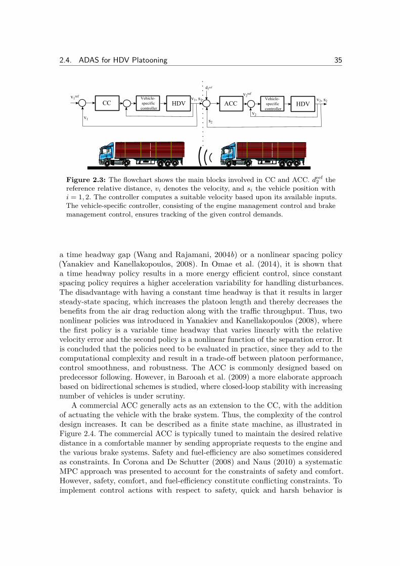
2.4. ADAS for HDV Platooning 35
����������������� �������
�� �������������������� �������
��� ��������
��
����� ����������
�����
���
Figure 2.3: The flowchart shows the main blocks involved in CC and ACC. d
ref2 the
reference relative distance, v
i
denotes the velocity, and s
i
the vehicle position withi = 1, 2. The controller computes a suitable velocity based upon its available inputs.The vehicle-specific controller, consisting of the engine management control and brakemanagement control, ensures tracking of the given control demands.
a time headway gap (Wang and Rajamani, 2004b) or a nonlinear spacing policy(Yanakiev and Kanellakopoulos, 2008). In Omae et al. (2014), it is shown thata time headway policy results in a more energy e�cient control, since constantspacing policy requires a higher acceleration variability for handling disturbances.The disadvantage with having a constant time headway is that it results in largersteady-state spacing, which increases the platoon length and thereby decreases thebenefits from the air drag reduction along with the tra�c throughput. Thus, twononlinear policies was introduced in Yanakiev and Kanellakopoulos (2008), wherethe first policy is a variable time headway that varies linearly with the relativevelocity error and the second policy is a nonlinear function of the separation error. Itis concluded that the policies need to be evaluated in practice, since they add to thecomputational complexity and result in a trade-o� between platoon performance,control smoothness, and robustness. The ACC is commonly designed based onpredecessor following. However, in Barooah et al. (2009) a more elaborate approachbased on bidirectional schemes is studied, where closed-loop stability with increasingnumber of vehicles is under scrutiny.
A commercial ACC generally acts as an extension to the CC, with the additionof actuating the vehicle with the brake system. Thus, the complexity of the controldesign increases. It can be described as a finite state machine, as illustrated inFigure 2.4. The commercial ACC is typically tuned to maintain the desired relativedistance in a comfortable manner by sending appropriate requests to the engine andthe various brake systems. Safety and fuel-e�ciency are also sometimes consideredas constraints. In Corona and De Schutter (2008) and Naus (2010) a systematicMPC approach was presented to account for the constraints of safety and comfort.However, safety, comfort, and fuel-e�ciency constitute conflicting constraints. Toimplement control actions with respect to safety, quick and harsh behavior is
36 Background
Manual CC
LAC
ACC
DHSC
Figure 2.4: Illustration of a finite state machine for the commercially available speedcontrol systems under consideration. If there is no vehicle in front of the subjectvehicle, the ACC acts as an CC or LAC, depending on the driver setting. If the speedis exceeded with a given o�set the DHSC will be activated automatically. The speedactive control strategy is deactivated by pushing the brake pedal or manually switchingo� the system.
required, which in turn mandates a high acceleration or deceleration. Such behavioris neither comfortable nor fuel-e�cient. The ACC accounts for switching betweendi�erent modes, which induces a nonlinear behavior. The switching is generallybased on logic rules and specific tuning parameters for each mode (Moon et al.,2009). Furthermore, it is desirable for the ACC to mimic reasonable human behaviorfor driver acceptance. The requirement of the ACC to mimic driver behavior foracceptance was investigated to some extent in Driel et al. (2007). Studies have shownthat the ACC is most commonly utilized in highway situations. Hence, the impactof the speed controller on the tra�c flow is of interest (Wang and Rajamani, 2004a).The ACC works reasonably well in a two-vehicle platoon. However, a delay arisesfrom measuring the behavior of the preceding vehicle with the radar to producingthe actual brake torque at the wheels. Thus, overshoots commonly occur when facinga velocity disturbance. In addition, the follower vehicle might not be able to reduceits speed in time if the preceding vehicle performs an emergency brake. Therefore, itis not suitable for longer vehicle platoons to operate at a short spacing due to safetyissues. To further understand practical implementation issues and constraints, weconsider the ACC in Chapter 4 and thereby investigate the fuel reduction potentialof HDV platooning, with respect to a commercial control strategy.
2.5. Safety in Vehicle Platooning 37
2.5 Safety in Vehicle Platooning
Safety is of utmost importance in vehicle platooning. It is desirable to reduce theinter-vehicle spacing in an automated platoon to lower the air drag and, thereby,obtain a higher fuel reduction. However, the actions of one vehicle may in turn a�ectall vehicles in the linked chain, which makes ensuring safety an issue.
String stability addresses the property that a disturbance from the lead vehicleshould not be amplified along the platoon (Swaroop and Hedrick, 1996; Shaw andHedrick, 2007). It is related to the ability to suppress a disturbance in position,velocity, or acceleration, as it propagates along the platoon, which in turn might leadto a collision. Focusing on preventing collisions, the errors in spacing between thevehicles in the platoon is often considered. In Pipes (1953) dynamics of a line tra�cwith N vehicles were studied, where a wave phenomena was noticed when vehiclesresumed the road speed after a tra�c light turned green. This observation was laterintroduced as string stability by Peppard (1974). It is also known as the bullwhipe�ect in economic theory (Lee et al., 2004). In Swaroop (1994) and Swaroop andHedrick (1996) a mathematical definition of string stability, in particular lp-stringstability, is presented. A more recent overview is given in Ploeg et al. (2014). Theproperty of lŒ-string stability implies that there exists a bounded set of initialconditions such that the peaks of the spacings errors remain uniformly boundedalong the string of vehicles. A weaker condition is l
2
-string stability, which is morecommonly used as a performance measure. l
2
-string stability implies that the energyof the spacing errors are not amplified downstream in the platoon. It is not possible toachieve longitudinal string stability with a constant spacing policy for a homogeneousstring of vehicles with feedback control based on nearest neighbor communications(Sheikholeslam and Desoer, 1993). In Seiler et al. (2004) it was shown that thislimitation occurs due to a complementary sensitivity integral constraint, which canbe solved by using a time headway policy. Hence, it is preferable to use a timeheadway policy both with respect to string stability and energy e�ciency. Controldi�culties for infinite vehicle platoons were studied in Bamieh and JovanoviÊ (2005).In Middleton and Braslavsky (2010), communication constraints are considered ina chain of linear time-invariant autonomous vehicles with su�cient conditions forstring stability are given. String stability is shown over a ring topology in Rogge andAeyels (2005), where control design for identical vehicles is studied. In Rajamaniand Zhu (2002) practical systems with ACC were considered, where both manuallydriven and automated cars can coexist. It was shown that the inter-vehicle spacingcan be reduced while maintaining string stability through wireless communication.Numerical methods for analyzing robust peak-to-peak performance of heterogeneousvehicle platoons were presented and evaluated in practice on real HDVs in Rödönyiet al. (2014). String stability can also be obtained in some cases through an orderingstrategy with respect to vehicle mass (Liang et al., 2011). In Kianfar et al. (2013)string stability is studied in a lateral direction and in Knorn and Middleton (2013),it is studied in both longitudinal and lateral directions. Note that ensuring stringstability does not imply that safety is guaranteed. String stability only guarantees
38 Background
that a disturbance is is not amplified along the platoon. Thus, if a collision occurs,for example, due to a harsh braking that causes a disturbance such that the errorin spacing becomes equal to the relative distance between two neighboring vehicles,then additional collisions might still occur downstream. Hence, a more rigorousapproach is needed for ensuring safety in vehicle platoons.
A collision avoidance system is designed to enhance safety by providing warn-ings to the driver or, in some cases, automating maneuvering procedures. Collisionavoidance has been studied in many areas of engineering such as maritime trans-portation, unmanned aerial vehicles (UAV), see Ryan et al. (2004), mobile robotics,see Siegwart and Nourbakhsh (2004), and automotive engineering. The literature onsafety strategies for HDVs is scarce, even though collision avoidance for cars is a vastarea. In the car industry, ACC systems with collision avoidance have been studiedextensively and are now commercially available. A review can be found in Vahidi andEskandarian (2003). In Seiler et al. (1998) longitudinal collision avoidance algorithmsby Mazda and Honda were reviewed and human factors were considered. Criticaldistances for a collision avoidance system are derived as a function of velocity andrelative velocity. In Chapter 5, we consider a similar reference framework, but forHDVs. Additionally, we use a dynamical game formulation to capture the worstpossible behavior by a preceding vehicle. In Gustafsson (2009), automotive safetysystems were reviewed. Conditions on safe platooning for passenger vehicles undernormal-mode of operation are investigated in Alvarez and Horowitz (1997). Morerecent work on collision avoidance for cars can be found in the thesis by Ali (2012),where reachability analysis tools were utilized for threat assessment and a novelautomotive safety function was proposed, based on vehicle state and road previewinformation. Zonotopes, a special case of polytopes, is an approach for computingreachable sets by abstracting to di�erential inclusions of simpler dynamics (Girard,2005). An approach to verify maneuvers of an automated car was presented in Altho�and Dolan (2012). Makhlouf and Kowalewski (2012) considered safety verificationof a platoon of vehicles under a varying communication network using zonotopes.
Vehicle platooning can facilitate an improved safety through higher interactivity.We propose a novel approach in Chapter 5, through a game theoretical approach forHDV platooning. The approach is an extension of the work presented in Bayen et al.(2003), where collision avoidance was analyzed with a di�erential game formulation ofan alerting logic for conflicts in high altitude air tra�c. V2X communication enablesnew possibilities and naturally new challenges for safety applications. Safety isincreased through automated functions and close coordination. Through interactioneach agent in the platoon will be able to take precautionary measures, in the senseof adjusting its speed and relative distance, based upon several incidents ahead.However, uncertainties with respect to mixed tra�c, communication failure anddelays must be resolved.
2.6. Summary 39
2.6 Summary
A brief introduction has been given on ITS. ITS aim at enhancing safety, opera-tional performance, mobility, environmental benefits, and productivity by expandingeconomic and employment growth. It covers a broad range of services and focuseson topics that adds understanding of accessibility, congestion, pollution, safety andsecurity in transportation. We have discussed the technology premise for HDVplatooning. On-board sensor technology and ECU functionality have improvedand become increasingly present during the last decades. Sensors and ECUs haveincreased in numbers. ECUs have developed in memory and processing speed. Radarand camera technology have developed to extend the information range to a localenvironment. GPS technology can provide up to centimeter accuracy and mapproviders are focusing on delivering three-dimensional road topography. With theintroduction of wireless communication to vehicle networks, which is the key tech-nology that enables HDV platooning by providing interaction between vehicles andthe surrounding infrastructure, a cooperative control system can be produced toimprove fuel e�ciency, safety and congestion. Several commercially available ADASfunctionalities, such as the ACC, have been mentioned that can already be usedfor vehicle platooning or serve as inspiration for future possible use cases. A briefoverview of the related work within platooning have been presented. String stability,collision avoidance and several control approaches have been mentioned. Despitethe substantial academic work, control design for platooning in practice is still anopen problem. Research into more implementation relevant aspects is only recentlyemerging.

Chapter 3
Modeling
“A mathematical model does not have to be exact; it just has to be close
enough to provide better results than can be obtained by common sense.”Herbert A. Simon
In this chapter we present models that serve as a basis for the analysis andcontrol design presented in the following chapters. First, a general descriptionof the internal and external forces a�ecting a vehicle in motion is given in
Section 3.1, resulting in an analytical model. Then, a more detailed simulationmodel is presented in Section 3.2. Finally, the system architectures, to facilitatethe control applications for heavy-duty vehicle (HDV) platooning developed in thiswork, are given in Section 3.3. A summary of the presented models and the benefitsof the proposed architecture in Section 3.4 concludes this chapter.
3.1 Vehicle Models
Several forces are imposed on a moving vehicle. The main forces are depicted inFigure 3.1 with the arrows indicating the corresponding sign convention, where F
a
,F
r
, and Fg
denote the external air drag, rolling resistance, and gravitational forcesacting upon the vehicle, respectively. The road grade is denoted by –, F
b
denotesthe negative longitudinal force obtained if the brakes are applied and F
p
denotesthe positive longitudinal driving force from the powertrain, which is produced bythe engine through fuel combustion. However, during coasting, i.e. when the fuelinjection is cut-o�, the engine exerts a constant braking force as it is propelled bythe accumulated kinetic energy or potential energy and not by fuel. In our modelthis e�ect is accounted for in inertial force produced by the engine. Therefore, thesign convention indicated by Figure 3.1 is maintained. In this section, we discusseach force of interest and then combine them at the end to provide a completevehicle dynamics model.
41
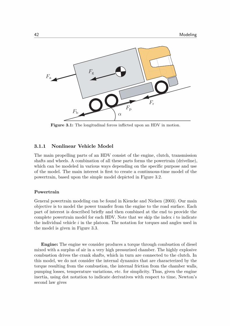
42 Modeling
Fa
Fg
FbFp
Fr
↵
Figure 3.1: The longitudinal forces inflicted upon an HDV in motion.
3.1.1 Nonlinear Vehicle Model
The main propelling parts of an HDV consist of the engine, clutch, transmissionshafts and wheels. A combination of all these parts forms the powertrain (driveline),which can be modeled in various ways depending on the specific purpose and useof the model. The main interest is first to create a continuous-time model of thepowertrain, based upon the simple model depicted in Figure 3.2.
Powertrain
General powertrain modeling can be found in Kiencke and Nielsen (2003). Our mainobjective is to model the power transfer from the engine to the road surface. Eachpart of interest is described briefly and then combined at the end to provide thecomplete powertrain model for each HDV. Note that we skip the index i to indicatethe individual vehicle i in the platoon. The notation for torques and angles used inthe model is given in Figure 3.3.
Engine: The engine we consider produces a torque through combustion of dieselmixed with a surplus of air in a very high pressurized chamber. The highly explosivecombustion drives the crank shafts, which in turn are connected to the clutch. Inthis model, we do not consider the internal dynamics that are characterized by thetorque resulting from the combustion, the internal friction from the chamber walls,pumping losses, temperature variations, etc. for simplicity. Thus, given the engineinertia, using dot notation to indicate derivatives with respect to time, Newton’ssecond law gives
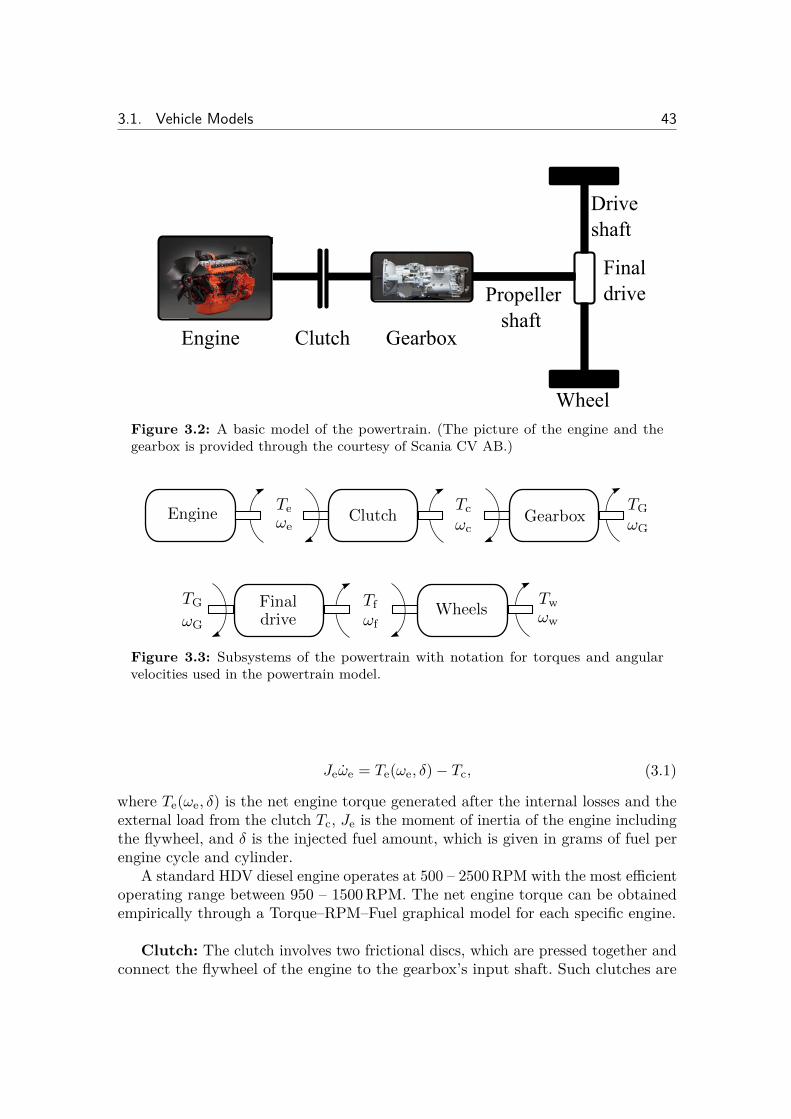
3.1. Vehicle Models 43
������ ���� �� ����
�����
��� ������
������� �
�������������� �
Figure 3.2: A basic model of the powertrain. (The picture of the engine and thegearbox is provided through the courtesy of Scania CV AB.)
Engine Clutch Gearbox!c!e
Te Tc
!G
TG
Finaldrive
Wheels !w!G
TG TwTf
!f
Figure 3.3: Subsystems of the powertrain with notation for torques and angularvelocities used in the powertrain model.
Je
Êe
= Te
(Êe
, ”) ≠ Tc
, (3.1)
where Te
(Êe
, ”) is the net engine torque generated after the internal losses and theexternal load from the clutch T
c
, Je
is the moment of inertia of the engine includingthe flywheel, and ” is the injected fuel amount, which is given in grams of fuel perengine cycle and cylinder.
A standard HDV diesel engine operates at 500 – 2500 RPM with the most e�cientoperating range between 950 – 1500 RPM. The net engine torque can be obtainedempirically through a Torque–RPM–Fuel graphical model for each specific engine.
Clutch: The clutch involves two frictional discs, which are pressed together andconnect the flywheel of the engine to the gearbox’s input shaft. Such clutches are
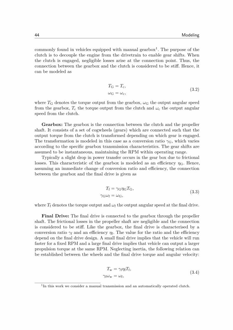
44 Modeling
commonly found in vehicles equipped with manual gearbox1. The purpose of theclutch is to decouple the engine from the drivetrain to enable gear shifts. Whenthe clutch is engaged, negligible losses arise at the connection point. Thus, theconnection between the gearbox and the clutch is considered to be sti�. Hence, itcan be modeled as
TG
= Tc
,
ÊG
= Êc
,(3.2)
where TG
denotes the torque output from the gearbox, ÊG
the output angular speedfrom the gearbox, T
c
the torque output from the clutch and Êc
the output angularspeed from the clutch.
Gearbox: The gearbox is the connection between the clutch and the propellershaft. It consists of a set of cogwheels (gears) which are connected such that theoutput torque from the clutch is transformed depending on which gear is engaged.The transformation is modeled in this case as a conversion ratio “
G
, which variesaccording to the specific gearbox transmission characteristics. The gear shifts areassumed to be instantaneous, maintaining the RPM within operating range.
Typically a slight drop in power transfer occurs in the gear box due to frictionallosses. This characteristic of the gearbox is modeled as an e�ciency ÷
G
. Hence,assuming an immediate change of conversion ratio and e�ciency, the connectionbetween the gearbox and the final drive is given as
Tf
= “G
÷G
TG
,
“G
Êf
= ÊG
,(3.3)
where Tf
denotes the torque output and Êf
the output angular speed at the final drive.
Final Drive: The final drive is connected to the gearbox through the propellershaft. The frictional losses in the propeller shaft are negligible and the connectionis considered to be sti�. Like the gearbox, the final drive is characterised by aconversion ratio “
f
and an e�ciency ÷f
. The value for the ratio and the e�ciencydepend on the final drive design. A small final drive implies that the vehicle will runfaster for a fixed RPM and a large final drive implies that vehicle can output a largerpropulsion torque at the same RPM. Neglecting inertia, the following relation canbe established between the wheels and the final drive torque and angular velocity:
Tw
= “f
÷f
Tf
,
“f
Êw
= Êf
,(3.4)
1In this work we consider a manual transmission and an automatically operated clutch.
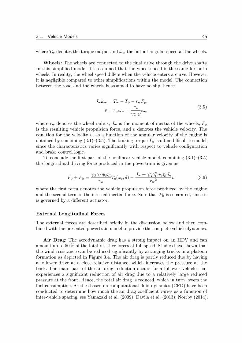
3.1. Vehicle Models 45
where Tw
denotes the torque output and Êw
the output angular speed at the wheels.
Wheels: The wheels are connected to the final drive through the drive shafts.In this simplified model it is assumed that the wheel speed is the same for bothwheels. In reality, the wheel speed di�ers when the vehicle enters a curve. However,it is negligible compared to other simplifications within the model. The connectionbetween the road and the wheels is assumed to have no slip, hence
Jw
Êw
= Tw
≠ Tb
≠ rw
Fp
,
v = rw
Êw
= rw
“G
“f
Êe
,(3.5)
where rw
denotes the wheel radius, Jw
is the moment of inertia of the wheels, Fp
is the resulting vehicle propulsion force, and v denotes the vehicle velocity. Theequation for the velocity v, as a function of the angular velocity of the engine isobtained by combining (3.1)–(3.5). The braking torque T
b
is often di�cult to model,since the characteristics varies significantly with respect to vehicle configurationand brake control logic.
To conclude the first part of the nonlinear vehicle model, combining (3.1)–(3.5)the longitudinal driving force produced in the powertrain is given as
Fp
+ Fb
= “G
“f ÷G
÷f
rw
Te
(Êe
, ”) ≠ Jw
+ “2
G
“2
f
÷G
÷f
Je
rw
2
v, (3.6)
where the first term denotes the vehicle propulsion force produced by the engineand the second term is the internal inertial force. Note that F
b
is separated, since itis governed by a di�erent actuator.
External Longitudinal Forces
The external forces are described briefly in the discussion below and then com-bined with the presented powertrain model to provide the complete vehicle dynamics.
Air Drag: The aerodynamic drag has a strong impact on an HDV and canamount up to 50 % of the total resistive forces at full speed. Studies have shown thatthe wind resistance can be reduced significantly by arranging trucks in a platoonformation as depicted in Figure 3.4. The air drag is partly reduced due by havinga follower drive at a close relative distance, which increases the pressure at theback. The main part of the air drag reduction occurs for a follower vehicle thatexperiences a significant reduction of air drag due to a relatively large reducedpressure at the front. Hence, the total air drag is reduced, which in turn lowers thefuel consumption. Studies based on computational fluid dynamics (CFD) have beenconducted to determine how much the air drag coe�cient varies as a function ofinter-vehicle spacing, see Yamazaki et al. (2009); Davila et al. (2013); Norrby (2014).
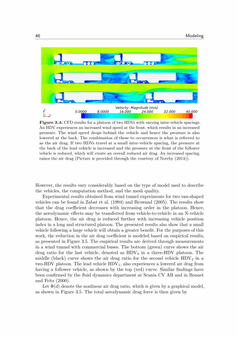
46 Modeling
���������� �����������������������������������������������
�
� �
Figure 3.4: CFD results for a platoon of two HDVs with varying inter-vehicle spacings.An HDV experiences an increased wind speed at the front, which results in an increasedpressure. The wind speed drops behind the vehicle and hence the pressure is alsolowered at the back. The combination of these to occurrences is what is referred toas the air drag. If two HDVs travel at a small inter-vehicle spacing, the pressure atthe back of the lead vehicle is increased and the pressure at the front of the followervehicle is reduced, which will create an overall reduced air drag. An increased spacing,raises the air drag (Picture is provided through the courtesy of Norrby (2014)).
However, the results vary considerably based on the type of model used to describethe vehicles, the computation method, and the mesh quality.
Experimental results obtained from wind tunnel experiments for two van-shapedvehicles can be found in Zabat et al. (1994) and Browand (2005). The results showthat the drag coe�cient decreases with increasing order in the platoon. Hence,the aerodynamic e�ects may be transferred from vehicle-to-vehicle in an N-vehicleplatoon. Hence, the air drag is reduced further with increasing vehicle positionindex in a long and structured platoon. The presented results also show that a smallvehicle following a large vehicle will obtain a greater benefit. For the purposes of thiswork, the reduction in the air drag coe�cient is modeled based on empirical results,as presented in Figure 3.5. The empirical results are derived through measurementsin a wind tunnel with commercial buses. The bottom (green) curve shows the airdrag ratio for the last vehicle, denoted as HDV
3
in a three-HDV platoon. Themiddle (black) curve shows the air drag ratio for the second vehicle HDV
2
in atwo-HDV platoon. The lead vehicle HDV
1
, also experiences a lowered air drag fromhaving a follower vehicle, as shown by the top (red) curve. Similar findings havebeen confirmed by the fluid dynamics department at Scania CV AB and in Bonnetand Fritz (2000).
Let �(d) denote the nonlinear air drag ratio, which is given by a graphical model,as shown in Figure 3.5. The total aerodynamic drag force is then given by
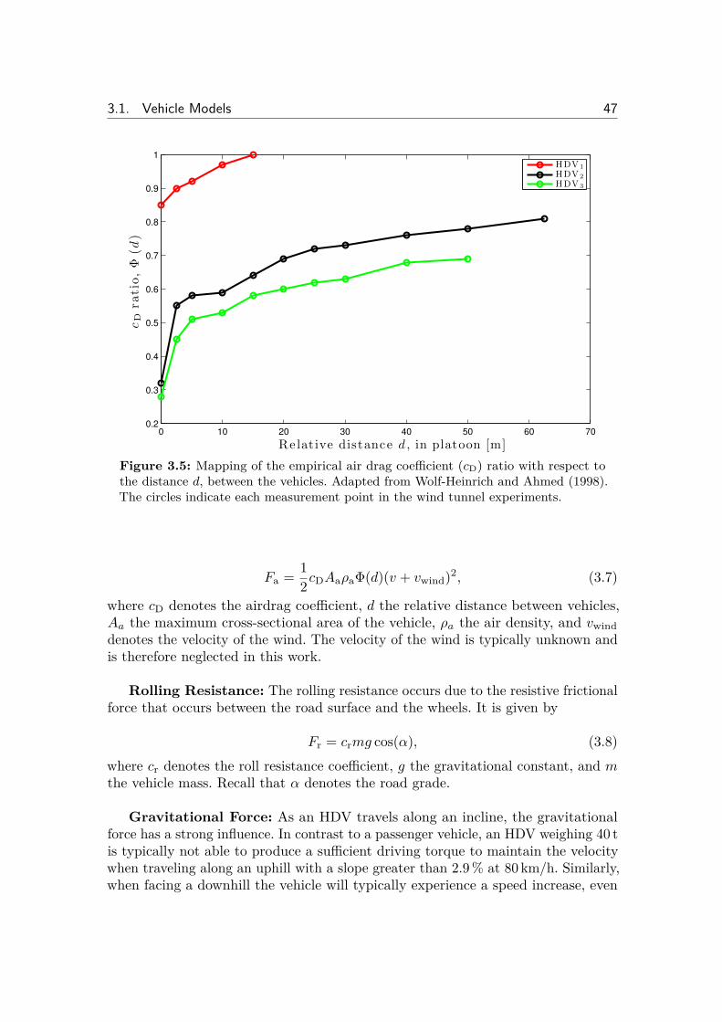
3.1. Vehicle Models 47
0 10 20 30 40 50 60 700.2
0.3
0.4
0.5
0.6
0.7
0.8
0.9
1
cD
rati
o,
�(d
)
Re lat ive distance d , in platoon [m]
HDV 1HDV 2HDV 3
Figure 3.5: Mapping of the empirical air drag coe�cient (cD) ratio with respect tothe distance d, between the vehicles. Adapted from Wolf-Heinrich and Ahmed (1998).The circles indicate each measurement point in the wind tunnel experiments.
Fa
= 12c
D
Aa
fla
�(d)(v + vwind
)2, (3.7)
where cD
denotes the airdrag coe�cient, d the relative distance between vehicles,Aa the maximum cross-sectional area of the vehicle, fla the air density, and v
wind
denotes the velocity of the wind. The velocity of the wind is typically unknown andis therefore neglected in this work.
Rolling Resistance: The rolling resistance occurs due to the resistive frictionalforce that occurs between the road surface and the wheels. It is given by
Fr
= cr
mg cos(–), (3.8)where c
r
denotes the roll resistance coe�cient, g the gravitational constant, and mthe vehicle mass. Recall that – denotes the road grade.
Gravitational Force: As an HDV travels along an incline, the gravitationalforce has a strong influence. In contrast to a passenger vehicle, an HDV weighing 40 tis typically not able to produce a su�cient driving torque to maintain the velocitywhen traveling along an uphill with a slope greater than 2.9 % at 80 km/h. Similarly,when facing a downhill the vehicle will typically experience a speed increase, even
48 Modeling
though no fuel is injected, if the slope is less than -0.9 %. Hence, the inducedgravitational force can act as a positive or negative longitudinal force depending onthe incline of the road. It is given by
Fg
= mg sin(–). (3.9)
Vehicle Model Composition
Applying Newton’s second law of motion along with all the external forces describedabove, a nonlinear continuous mathematical vehicle model is derived as
ds
dt =v
mt
(G)dv
dt =Fe
≠ Fb
≠ Fa
(v, d) ≠ Fr
(–(s)) ≠ Fg
(–(s)),
=“G
“f
÷G
÷f
rw
T (Êe
, ”) ≠ Fb
≠ 12c
D
Aa
fla
�(d)v2
≠ cr
mg cos(–(s)) ≠ mg sin(–(s)),=k
e
T (Êe
, ”) ≠ Fb
≠ kd
v2 ≠ kr
cos(–(s)) ≠ kg
sin(–(s))
(3.10)
where
mt
(G) = Jw
r2
w
+ m + “G
2“f
2÷G
÷f
Je
r2
w
(3.11)
is the total inertial mass, G denotes the active gear number, and s is the absolutetraveled distance from a known point of origin. Note that “
G
and ÷G
varies with theactive gear number G. We omit to express G explicitly in (3.11) in some chapters,unless gear changes are considered in the control design. The model parametersused in this thesis, unless otherwise stated, are given in Table 3.1.
Model Uncertainties
The vehicle model is based upon perfect knowledge of the vehicle parameters. Inpractice, only the gearbox ratio and the final gear ratio is known to be static. Theinertias and e�ciencies vary based upon the temperature and quality of the corre-sponding lubricating oil. The wheel radius also varies based upon the current airpressure and the friction between the road surface and tire is not static. The rollingresistance varies nonlinearly with tire temperature and velocity. However, the domi-nant uncertainty in (3.10) is the vehicle mass. During a freight transport assignmentthe cargo is often unloaded at several points, since it generally encompasses di�erentcontractors. Each time part of the cargo is unloaded there is seldom a measuringdevice to obtain new accurate mass measurements. The mass is generally severalmagnitudes larger than the other parameters. We adopt the common approach thatall the parameter uncertainties can be aggregated as an uncertainty in mass.
3.1. Vehicle Models 49
Table 3.1: Nominal vehicle model parameters.
Parameter Symbol Value UnitRolling resistance coe�cient c
r
1.5 ◊ 10≠3 -Air drag coe�cient c
D
0.56 -Engine inertia J
e
3.5 kg m2
Wheel inertia Jw
32.9 kg m2
Vehicle mass m 40 000 kgFrontal area A
a
10.26 m2
Wheel radius rw
0.5 mFinal drive ratio “
f
3.08 -Final gear e�ciency ÷
e
0.97 -Air density fl
a
1.29 kg m≠3
An accurate model of the powertrain would mandate flexible shafts, where energyis stored when the shafts are twisted. However, the e�ects of such dynamics comeinto play when there are quickly varying changes in the engine torque, which mightcause oscillations in the powertrain or backlash (Lagerberg and Egart, 2007). Thesedynamics mainly impact driveability and not the fuel consumption (Sandberg, 2001).The platooning scenarios we consider does not involve such behavior, since theobjective is fuel e�ciency, which requires only smooth control actions. Therefore,dynamics for backlash and oscillations in the vehicular powertrain are neglected forthe purposes of this model.
3.1.2 Linearized Vehicle ModelWhen studying the behavior of vehicles within a platoon, the velocities are controlledand should not deviate significantly from the lead vehicles velocity trajectory. Thus,a linearized model, used for control design in this thesis, might satisfactorily describevehicle behavior. The nonlinear model (3.10) can be linearized with respect to a setreference velocity vref, a fixed gear number G
0
, an engine torque which maintains thevelocity T
0
, a fixed time headway setting · , and a constant slope –0
. The equilibriaare denoted
v0
= vref
–0
= –ref
d0
= v0
·
T0
= cd
(d0
)v0
2 + cr
cos (–0) + cg
sin (–0)c
e
(3.12)
50 Modeling
where d0
is the equilibrium inter-vehicle spacing for a time headway setting and
ce
= rw
“G
“f
÷G
÷f
Jw
+ mr2
w
+ “2
G
“2
f
÷G
÷f
Je
, cd
(d0
) =1
2
r2
w
cD
Aa
fla
Jw
+ mr2
w
+ “2
G
“2
f
÷G
÷f
Je
�(d0
),
cr
= cr
r2
w
mg
Jw
+ mr2
w
+ “2
G
“2
f
÷G
÷f
Je
, cg = r2
w
mg
Jw
+ mr2
w
+ “2
G
“2
f
÷G
÷f
Je
. (3.13)
To account for the aerodynamics, we approximate the nonlinear air drag function�(d) with a least square approximation. Hence, the approximated a�ne air dragreduction is given as
Ï(d) = alsq
d + blsq
,
where Ï(d) œ [0, 1]. The parameters alsq
and blsq
are determined with respect to therelevant operating range.
Let F (v, T, –, d) denote the function for the nonlinear vehicle dynamics model in(3.10). Applying a first order Taylor approximation to (3.10) around the equilibriumpoints v
0
, T0
, –0
, d0
, the linearized model for a single vehicle is given by
dv
dt¥ F (v
0
, T0
, –0
, d0
) + ˆ
ˆvF (v
0
, T0
, –0
, d0
)�v
+ ˆ
ˆdF (v
0
, T0
, –0
, d0
)�d + ˆ
ˆTF (v
0
, T0
, –0
, d0
)�T
= ce
�T ≠ 2cd
(d0
)v0
�v ≠1
2
alsq
r2
w
Aa
fla
v2
0
Jw
+ mr2
w
+ “2
G
“2
f
÷G
÷f
Je
�d,
(3.14)
where ce
and cd
(d0
) is given in (3.13). Approximately we have
v = ce
T + �v + —d, (3.15)where, with abuse of notation, T and v denote the deviation in control input andthe vehicle velocity from the equilibrium point, respectively. The characteristiccoe�cients � and — are given by
� = ≠ 2cd
(d0
)v0
,
— = ≠1
2
alsq
r2
w
Aa
fla
v2
0
Jw
+ mr2
w
+ “2
G
“2
f
÷G
÷f
Je
.(3.16)
Note that for the lead vehicle we get
v = ce
T ≠ r2
w
cD
Aa
fla
v0
Jw
+ mr2
w
+ “2
G
“2
f
÷G
÷f
Je
v,
since the air drag reduction obtained due to a following vehicle is minor and thereforenot considered.
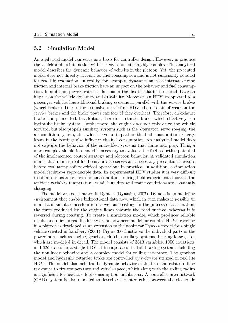
3.2. Simulation Model 51
3.2 Simulation Model
An analytical model can serve as a basis for controller design. However, in practicethe vehicle and its interaction with the environment is highly complex. The analyticalmodel describes the dynamic behavior of vehicles in the platoon. Yet, the presentedmodel does not directly account for fuel consumption and is not su�ciently detailedfor real life evaluation. In reality, for example, dynamics such as internal enginefriction and internal brake friction have an impact on the behavior and fuel consump-tion. In addition, power train oscillations in the flexible shafts, if excited, have animpact on the vehicle dynamics and drivability. Moreover, an HDV, as opposed to apassenger vehicle, has additional braking systems in parallel with the service brakes(wheel brakes). Due to the extensive mass of an HDV, there is lots of wear on theservice brakes and the brake power can fade if they overheat. Therefore, an exhaustbrake is implemented. In addition, there is a retarder brake, which e�ectively is ahydraulic brake system. Furthermore, the engine does not only drive the vehicleforward, but also propels auxiliary systems such as the alternator, servo steering, theair condition system, etc., which have an impact on the fuel consumption. Energylosses in the bearings also influence the fuel consumption. An analytical model doesnot capture the behavior of the embedded systems that come into play. Thus, amore complex simulation model is necessary to evaluate the fuel reduction potentialof the implemented control strategy and platoon behavior. A validated simulationmodel that mimics real life behavior also serves as a necessary precaution measurebefore evaluating safety critical operations in practice. In addition, a simulationmodel facilitates reproducible data. In experimental HDV studies it is very di�cultto obtain repeatable environment conditions during field experiments because theambient variables temperature, wind, humidity and tra�c conditions are constantlychanging.
The model was constructed in Dymola (Dynasim, 2007). Dymola is an modelingenvironment that enables bidirectional data flow, which in turn makes it possible tomodel and simulate acceleration as well as coasting. In the process of acceleration,the force produced by the engine flows towards the road surface, whereas it isreversed during coasting. To create a simulation model, which produces reliableresults and mirrors real-life behavior, an advanced model for coupled HDVs travelingin a platoon is developed as an extension to the nonlinear Dymola model for a singlevehicle created in Sandberg (2001). Figure 3.6 illustrates the individual parts in thepowertrain, such as engine, gearbox, clutch, auxiliary systems, bearing losses, etc.,which are modeled in detail. The model consists of 3313 variables, 1058 equations,and 626 states for a single HDV. It incorporates the full braking system, includingthe nonlinear behavior and a complex model for rolling resistance. The gearboxmodel and hydraulic retarder brake are controlled by software utilized in real lifeHDVs. The model also includes the dynamic behavior of the tires and relates rollingresistance to tire temperature and vehicle speed, which along with the rolling radiusis significant for accurate fuel consumption simulations. A controller area network(CAN) system is also modeled to describe the interaction between the electronic
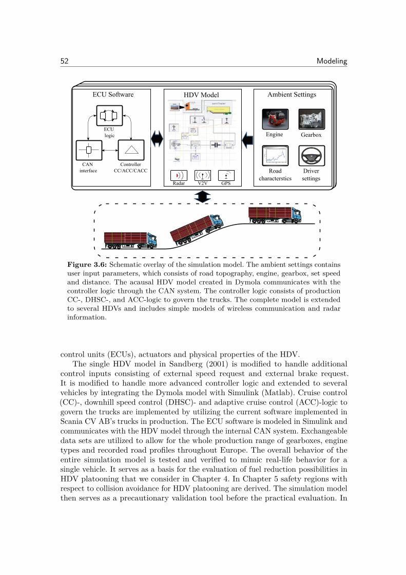
52 Modeling
HDV Model Ambient Settings
Radar V2V GPS
Engine Gearbox
Roadcharacterstics
Driversettings
ECU Software
ECU logic
CAN interface
ControllerCC/ACC/CACC
00 50 100 150 200 250 300
50
100
150
200
250
300
350
[km]
Altitude[m]
Figure 3.6: Schematic overlay of the simulation model. The ambient settings containsuser input parameters, which consists of road topography, engine, gearbox, set speedand distance. The acausal HDV model created in Dymola communicates with thecontroller logic through the CAN system. The controller logic consists of productionCC-, DHSC-, and ACC-logic to govern the trucks. The complete model is extendedto several HDVs and includes simple models of wireless communication and radarinformation.
control units (ECUs), actuators and physical properties of the HDV.The single HDV model in Sandberg (2001) is modified to handle additional
control inputs consisting of external speed request and external brake request.It is modified to handle more advanced controller logic and extended to severalvehicles by integrating the Dymola model with Simulink (Matlab). Cruise control(CC)-, downhill speed control (DHSC)- and adaptive cruise control (ACC)-logic togovern the trucks are implemented by utilizing the current software implemented inScania CV AB’s trucks in production. The ECU software is modeled in Simulink andcommunicates with the HDV model through the internal CAN system. Exchangeabledata sets are utilized to allow for the whole production range of gearboxes, enginetypes and recorded road profiles throughout Europe. The overall behavior of theentire simulation model is tested and verified to mimic real-life behavior for asingle vehicle. It serves as a basis for the evaluation of fuel reduction possibilities inHDV platooning that we consider in Chapter 4. In Chapter 5 safety regions withrespect to collision avoidance for HDV platooning are derived. The simulation modelthen serves as a precautionary validation tool before the practical evaluation. In
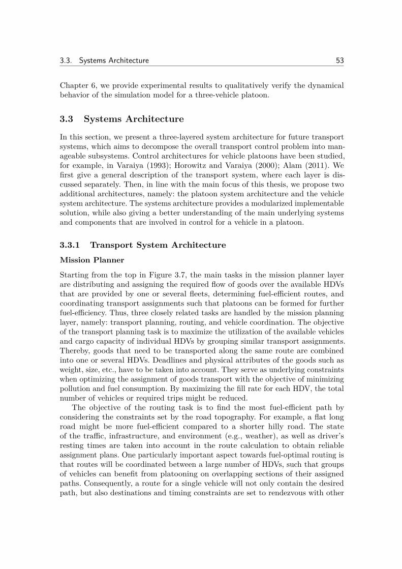
3.3. Systems Architecture 53
Chapter 6, we provide experimental results to qualitatively verify the dynamicalbehavior of the simulation model for a three-vehicle platoon.
3.3 Systems Architecture
In this section, we present a three-layered system architecture for future transportsystems, which aims to decompose the overall transport control problem into man-ageable subsystems. Control architectures for vehicle platoons have been studied,for example, in Varaiya (1993); Horowitz and Varaiya (2000); Alam (2011). Wefirst give a general description of the transport system, where each layer is dis-cussed separately. Then, in line with the main focus of this thesis, we propose twoadditional architectures, namely: the platoon system architecture and the vehiclesystem architecture. The systems architecture provides a modularized implementablesolution, while also giving a better understanding of the main underlying systemsand components that are involved in control for a vehicle in a platoon.
3.3.1 Transport System ArchitectureMission Planner
Starting from the top in Figure 3.7, the main tasks in the mission planner layerare distributing and assigning the required flow of goods over the available HDVsthat are provided by one or several fleets, determining fuel-e�cient routes, andcoordinating transport assignments such that platoons can be formed for furtherfuel-e�ciency. Thus, three closely related tasks are handled by the mission planninglayer, namely: transport planning, routing, and vehicle coordination. The objectiveof the transport planning task is to maximize the utilization of the available vehiclesand cargo capacity of individual HDVs by grouping similar transport assignments.Thereby, goods that need to be transported along the same route are combinedinto one or several HDVs. Deadlines and physical attributes of the goods such asweight, size, etc., have to be taken into account. They serve as underlying constraintswhen optimizing the assignment of goods transport with the objective of minimizingpollution and fuel consumption. By maximizing the fill rate for each HDV, the totalnumber of vehicles or required trips might be reduced.
The objective of the routing task is to find the most fuel-e�cient path byconsidering the constraints set by the road topography. For example, a flat longroad might be more fuel-e�cient compared to a shorter hilly road. The stateof the tra�c, infrastructure, and environment (e.g., weather), as well as driver’sresting times are taken into account in the route calculation to obtain reliableassignment plans. One particularly important aspect towards fuel-optimal routing isthat routes will be coordinated between a large number of HDVs, such that groupsof vehicles can benefit from platooning on overlapping sections of their assignedpaths. Consequently, a route for a single vehicle will not only contain the desiredpath, but also destinations and timing constraints are set to rendezvous with other
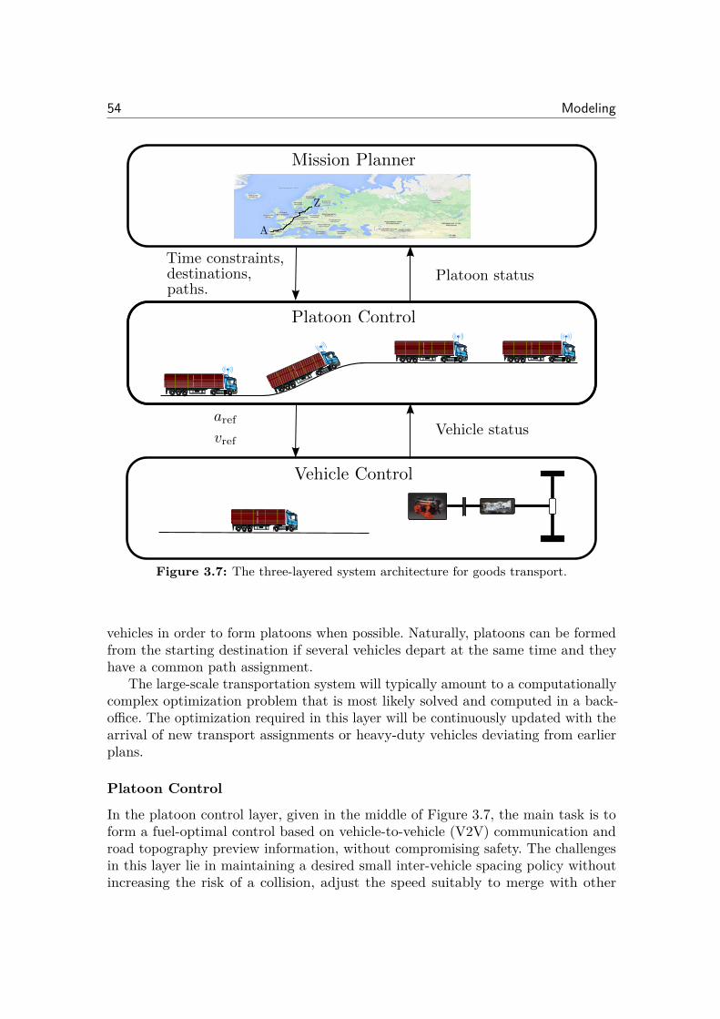
54 Modeling
Time constraints,destinations,paths.
Platoon status
Vehicle statusarefvref
Mission Planner
Platoon Control
Vehicle Control
Z
A
Figure 3.7: The three-layered system architecture for goods transport.
vehicles in order to form platoons when possible. Naturally, platoons can be formedfrom the starting destination if several vehicles depart at the same time and theyhave a common path assignment.
The large-scale transportation system will typically amount to a computationallycomplex optimization problem that is most likely solved and computed in a back-o�ce. The optimization required in this layer will be continuously updated with thearrival of new transport assignments or heavy-duty vehicles deviating from earlierplans.
Platoon Control
In the platoon control layer, given in the middle of Figure 3.7, the main task is toform a fuel-optimal control based on vehicle-to-vehicle (V2V) communication androad topography preview information, without compromising safety. The challengesin this layer lie in maintaining a desired small inter-vehicle spacing policy withoutincreasing the risk of a collision, adjust the speed suitably to merge with other
3.3. Systems Architecture 55
vehicles or platoons, and forming fuel-optimal policies in the presence of uncertaintiesin vehicle parameters, sensor information, and map data. It is fuel-e�cient to drivethe vehicles at a small inter-vehicle spacing to achieve a large reduction in air drag,but, as the number of vehicles in a platoon and the tra�c intensity grows, thecomplexity of the coupled tra�c dynamics increases. The actions of one vehiclemay in turn a�ect all vehicles in a linked chain, where a disturbance in the firstvehicle might propagate and amplify throughout the chain; causing an increasedcontrol e�ort to handle the disturbances or even a collision. V2V communication isintroduced such that interaction is enabled between vehicles within spatial rangeof their wireless transceiver. Thereby, fuel-e�ciency and safety are improved bymaking cooperative control decisions that takes the behavior of surrounding vehiclesinto account. Hence, suitable decentralized controllers are established in this layerfor fuel-e�cient and safe control. We consider a decentralized controller, mainly dueto the communication constraints that occur in practice2. Furthermore, the fuelconsumption of heavy-duty vehicles is strongly dependent on the road grade due totheir extensive mass. However, when the topography of the road ahead is knownthrough map data, this information can be used to optimize a velocity profile, forall the platooning vehicles, that minimizes the fuel consumption with respect to afixed travel time3.
The constraints provided by the top layer are translated into a reference velocityprofile for each HDV, consisting of average velocities over upcoming road segmentsthat need to be maintained in order to merge platoons or to meet the specifiedtime constraints. A platoon status is transmitted suitably often to the top layer,reporting if the constraints can be satisfied. If the constraints are violated for somereason, for example, due to a disturbance in tra�c, the mission planning layer isrequested to provide a new set of feasible directions. The platoon control layer alsoincludes tasks such as the merging of several HDVs, or platoons, or the splitting andreordering of platoons, where fuel-optimal trajectories are derived for every HDV.
Vehicle Control
The main task of the vehicle control layer, shown in the bottom of Figure 3.7, isto ensure tracking of the desired velocities and acceleration requests. In addition,fuel-e�cient control strategies are executed based on on-board sensor informationand the powertrain is optimized for energy e�ciency. A vehicle status is continuouslyprovided to the platoon layer, notifying if the desired velocities and accelerationrequests are not feasible or if a system failure has occurred. Recall that the parts ofthe powertrain are elastic, hence velocities and torque di�er along the powertrain.As a result, resonances may occur. The handling of such resonances for functionality,drivability, and noise reduction are challenges that are addressed in this layer.
2A more detailed motivation for why decentralized controllers are considered in this thesis isgiven in Chapter 6.
3A more detailed discussion regarding how to use road grade preview information in controlfor HDV platooning is given in Chapter 7.
56 Modeling
Tracking of the desired velocities and acceleration requests is obtained through thevehicle’s engine management system (EMS), brake management system (BMS),and gear management system (GMS). Hence, fuel-injection, brake blending, andgear shift strategies are also formed to optimize the response performance in thislayer. Recall that the brake discs are susceptible to brake fade when used overlonger periods, which can degrade the brake performance. Thus, an HDV is typicallycomprised of additional brake systems, such the exhaust brake and the retarder.Hence, the combination and coordination of the various braking systems to avoidbrake performance loss are also handled in this layer. HDVs might drop drasticallyin speed during a gear change, for example, over an uphill segment. Therefore, thetotal driving resistance is estimated in this layer to determine whether a one or twostep change in gear is required. To reduce the drop in velocity, the gear change mustbe quickly executed.
Several vehicle specific control tasks for a single vehicle that is traveling alone andcatching up to form a platoon are also handled in this layer for fuel-e�cient vehiclepropulsion. Fuel-e�cient control strategies such as the economical cruise control isformed by predicting if a hill crest is reached. If so, the torque can be reduced and thespeed is then resumed slightly after the crest is passed for fuel-e�ciency. If map dataare available, road grade preview data are utilized to establish predictive controllers,for a single vehicle, that are typically implemented in a receding horizon fashion,see Hellström (2010). The conventional CC can also be optimized for fuel-e�ciency,by handling disturbances that are induced by external forces in a suitable manner(Shaout and Jarrah, 1997).
3.3.2 Platoon System ArchitectureThe platoon system architecture that we consider is illustrated in Figure 3.8, whichcorresponds to the two lower layers of Figure 3.7. The control systems rely on theunderlying information and their structure will vary with a varying range of inputs,which must be considered. Thus, an understanding of both the control architectureand the underlying sensor and communication systems is important.
The arrows indicate the direction of information flow in the system. Vehicleinformation is obtained through on-board sensors, which is used in feedback control,as illustrated by the arrow from a vehicle to its controllers. The arrow between apreceding vehicle and the ACC shows the information that is obtained through theradar. Here, state information is provided with respect to the preceding vehicle. Thearrows between each cooperative adaptive cruise control (CACC) and the wirelesscommunication network, show the two-way communication between the platooningvehicles. It includes the system state information and vehicle parameter information.
We propose a layered control system architecture, as illustrated in Figure 3.8.Starting from the bottom, the conventional CC o�ers three advantages: maintainedvehicle speed, improved fuel economy, and driver comfort over long distances. Ittypically uses velocity feedback information and acts as a PI- or PID-controller todetermine the required change in velocity, which is then sent as an input to the
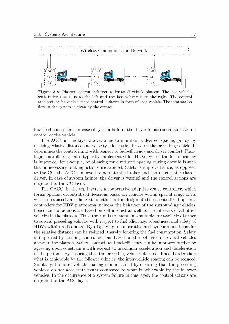
3.3. Systems Architecture 57
Wireless Communication Network
CACC
CC
ACC
CACC
CC
ACC
CACC
CC
ACC
Figure 3.8: Platoon system architecture for an N vehicle platoon. The lead vehicle,with index i = 1, is to the left and the last vehicle is to the right. The controlarchitecture for vehicle speed control is shown in front of each vehicle. The informationflow in the system is given by the arrows.
low-level controllers. In case of system failure, the driver is instructed to take fullcontrol of the vehicle.
The ACC, in the layer above, aims to maintain a desired spacing policy byutilizing relative distance and velocity information based on the preceding vehicle. Itdetermines the control input with respect to fuel-e�ciency and driver comfort. Fuzzylogic controllers are also typically implemented for HDVs, where the fuel-e�ciencyis improved, for example, by allowing for a reduced spacing during downhills suchthat unnecessary braking actions are avoided. Safety is improved since, as opposedto the CC, the ACC is allowed to actuate the brakes and can react faster than adriver. In case of system failure, the driver is warned and the control actions aredegraded to the CC layer.
The CACC, in the top layer, is a cooperative adaptive cruise controller, whichforms optimal decentralized decisions based on vehicles within spatial range of itswireless transceiver. The cost function in the design of the decentralized optimalcontrollers for HDV platooning includes the behavior of the surrounding vehicles,hence control actions are based on self-interest as well as the interests of all othervehicles in the platoon. Thus, the aim is to maintain a suitable inter-vehicle distanceto several preceding vehicles with respect to fuel-e�ciency, robustness, and safety ofHDVs within radio range. By displaying a cooperative and synchronous behaviorthe relative distance can be reduced, thereby lowering the fuel consumption. Safetyis improved by forming control actions based on the behavior of several vehiclesahead in the platoon. Safety, comfort, and fuel-e�ciency can be improved further byagreeing upon constraints with respect to maximum acceleration and decelerationin the platoon. By ensuring that the preceding vehicles does not brake harder thanwhat is achievable by the follower vehicles, the inter-vehicle spacing can be reduced.Similarly, the inter-vehicle spacing is maintained by ensuring that the precedingvehicles do not accelerate faster compared to what is achievable by the followervehicles. In the occurrence of a system failure in this layer, the control actions aredegraded to the ACC layer.
58 Modeling
There are several challenges in this architecture. The low-level controllers handlesome of the nonlinearities in the vehicle and inherently linearize the vehicle behaviorto some extent. However, a drawback is that the model uncertainty increases withincertain dynamic range of operation, since the behavior of the nonlinear low-levelcontrollers might vary in behavior depending on its current state. For example, stepresponses in velocity of the same magnitude might vary depending on the currentgear, if the engine was idling or active, or if the BMS was active just before thestep is requested. Furthermore, radar information can be lost, for example overroad bends, when the preceding vehicle is not directly in front. Delays in wirelesscommunication or in processing of radar information can occur, which must behandled by the active controller.
3.3.3 Vehicle System ArchitectureMany on-board systems are involved in control of a platooning vehicle. An under-standing of the main underlying systems for data processing and control is importantfor implementation purposes. Each HDV that we consider has the system archi-tecture shown in Figure 3.9. Several control units are connected to the controllerarea network (CAN). The wireless sensor unit (WSU), global positioning system(GPS), and radar act as sensor units, providing information about the surroundingenvironment. Even though a wide range of information is available from wirelesscommunication, ECUs, and on-board sensors, it is often noisy and must be processedbefore it can be used as input to the controllers. In the data processing block, thenoisy data from all the transmitting vehicles in the established platoon are processedthrough a Kalman filter and GPS information from the preceding vehicle is fusedtogether with the state information from the radar. In the event of packet losses orshort outages, the Kalman filter acts as a state predictor. Each received messagefrom other platooning vehicles contains GPS information. Based on the positionand heading of each surrounding vehicles, the platooning vehicles are mapped to alocal coordinate system. Filtered information, along with vehicle specific parameters,controller gains, and the current mode of operation for the platooning vehicles, isforwarded to the high-level controllers block. The active controller sends out thereference signal on CAN, which is then carried out by the low-level controllers shownto the right in Figure 3.9.
The low-level control systems consists of the EMS, BMS, and GMS. The EMScontroller receives a velocity request as an input. It then calculates the requiredfueling amount for obtaining the necessary torque to obtain the requested velocity.The EMS also assures that no oscillations arise in the powertrain. It monitors theturbo pressure and limits the fueling in case a su�cient amount of air is not availablefor the combustion process. Hence, the achievable torque might be limited. There areseveral brake systems in a modern HDV, ranging from the weaker exhaust brake tothe strong brake discs. The BMS receives a deceleration request and typically blendsthe brake power from the di�erent systems depending on the magnitude of therequested signal. It also assures that no system overheats. Therefore, the achieved
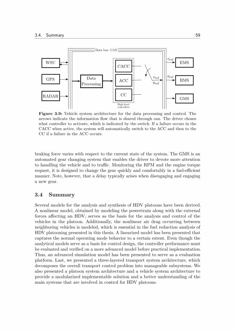
3.4. Summary 59
Data
Processing
GMSRADAR
EMS
BMS
WSU
GPSvrefaref
Data bus: CAN
CACC
ACC
CC
vref
aref
controllersHigh-level
Figure 3.9: Vehicle system architecture for the data processing and control. Thearrows indicate the information flow that is shared through can. The driver choseswhat controller to activate, which is indicated by the switch. If a failure occurs in theCACC when active, the system will automatically switch to the ACC and then to theCC if a failure in the ACC occurs.
braking force varies with respect to the current state of the system. The GMS is anautomated gear changing system that enables the driver to devote more attentionto handling the vehicle and to tra�c. Monitoring the RPM and the engine torquerequest, it is designed to change the gear quickly and comfortably in a fuel-e�cientmanner. Note, however, that a delay typically arises when disengaging and engaginga new gear.
3.4 Summary
Several models for the analysis and synthesis of HDV platoons have been derived.A nonlinear model, obtained by modeling the powertrain along with the externalforces a�ecting an HDV, serves as the basis for the analysis and control of thevehicles in the platoon. Additionally, the nonlinear air drag occurring betweenneighboring vehicles is modeled, which is essential in the fuel reduction analysis ofHDV platooning presented in this thesis. A linearized model has been presented thatcaptures the normal operating mode behavior to a certain extent. Even though theanalytical models serve as a basis for control design, the controller performance mustbe evaluated and verified on a more advanced model before practical implementation.Thus, an advanced simulation model has been presented to serve as a evaluationplatform. Last, we presented a three-layered transport system architecture, whichdecomposes the overall transport control problem into manageable subsystems. Wealso presented a platoon system architecture and a vehicle system architecture toprovide a modularized implementable solution and a better understanding of themain systems that are involved in control for HDV platoons.

Chapter 4
Fuel-Saving Potential of Platooning
“Every great advance in science has issued from a new audacity of
imagination.”John Dewey
Vehicle platooning is important for the automotive industry. The focus lieson the environmental benefits and safety issues but it is of equal importanceto also investigate the economical prospective and feasibility of platooning
for commercial purposes. Recall that the road transport industry is very fuel pricesensitive, since fuel cost constitutes approximately one third of the total operationalcost in European long haulage heavy-duty vehicles (HDVs). Fuel saving potentialsof 5–20 %, was demonstrated for HDV platooning in experiments on flat test tracksby Bonnet and Fritz (2000); Davila et al. (2013); Tsugawa (2013). The saving varieswith set speed, inter-vehicle spacing, and vehicle mass. However, conclusive resultsremain unclear for the fuel-saving potential of platooning on roads with varyingtopography. The focus in this chapter is the fuel reduction that HDV platooningenables over a varying topography and the analysis with respect to the influenceof a commercial adaptive cruise control (ACC) has on the fuel consumption. Weconsider a platoon consisting of N HDVs. The main forces a�ecting a vehicle inmotion is given by
mtdv
dt=F
e
(Êe
, ”) ≠ Fb
≠ Fa
(v, d) ≠ Fr
(–) ≠ Fg
(–)
=“G
“f
÷G
÷f
rw
Te
(Êe
, ”) ≠ Fb
≠ 12c
D
Aa
fla
�(d)v2 ≠ cr
mg cos – ≠ mg sin –,
where Fe
Ø 0 denotes the force produced by the engine through fuel injection,F
b
Ø 0 denotes the braking force, – denotes the slope of the road, cD
and cr
arecharacteristic coe�cients, g denotes the gravitational force, fl
a
the air density, rw
the wheel radius, and “G
, “f
, ÷G
, ÷f
are transmission and gear specific constants.Moreover, F a, F r, and F g denote the external air drag, rolling resistance, and
61
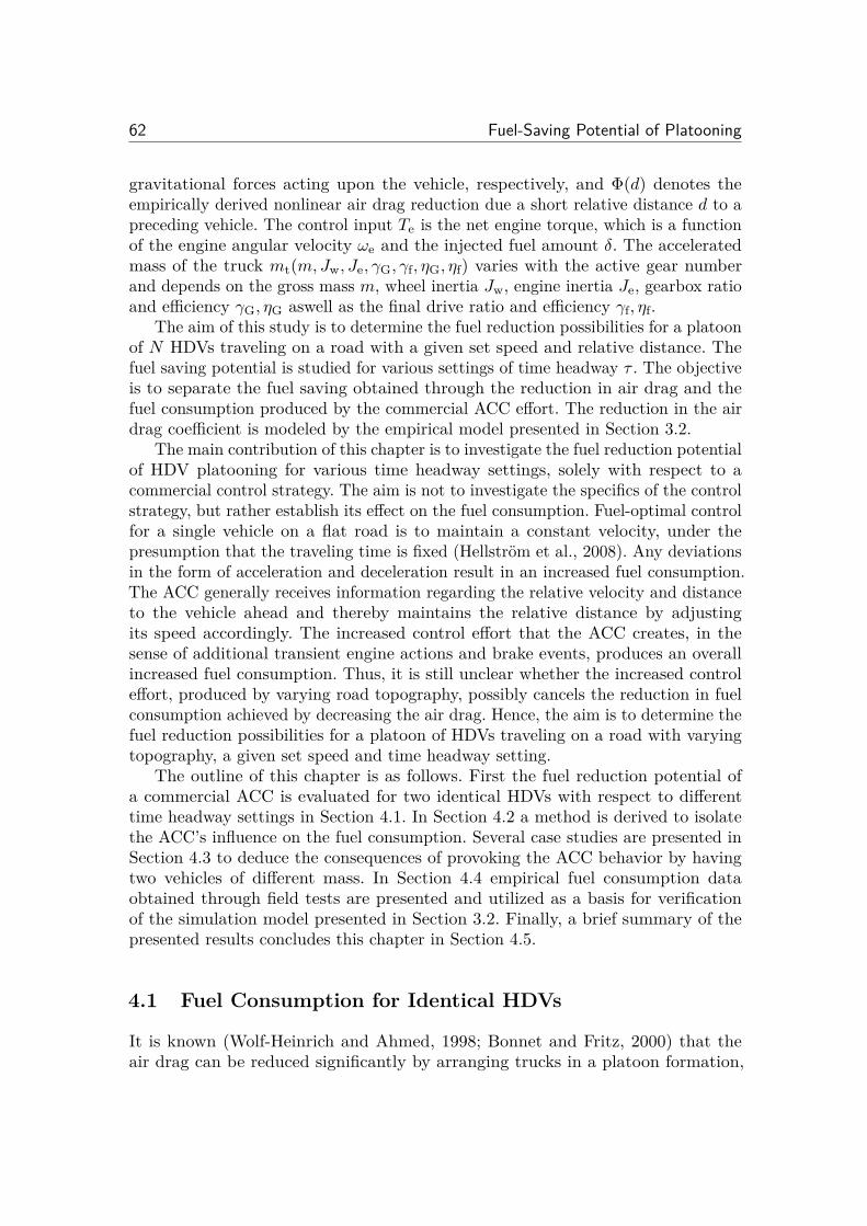
62 Fuel-Saving Potential of Platooning
gravitational forces acting upon the vehicle, respectively, and �(d) denotes theempirically derived nonlinear air drag reduction due a short relative distance d to apreceding vehicle. The control input T
e
is the net engine torque, which is a functionof the engine angular velocity Ê
e
and the injected fuel amount ”. The acceleratedmass of the truck m
t
(m, Jw
, Je
, “G
, “f
, ÷G
, ÷f
) varies with the active gear numberand depends on the gross mass m, wheel inertia J
w
, engine inertia Je
, gearbox ratioand e�ciency “
G
, ÷G
aswell as the final drive ratio and e�ciency “f
, ÷f
.The aim of this study is to determine the fuel reduction possibilities for a platoon
of N HDVs traveling on a road with a given set speed and relative distance. Thefuel saving potential is studied for various settings of time headway · . The objectiveis to separate the fuel saving obtained through the reduction in air drag and thefuel consumption produced by the commercial ACC e�ort. The reduction in the airdrag coe�cient is modeled by the empirical model presented in Section 3.2.
The main contribution of this chapter is to investigate the fuel reduction potentialof HDV platooning for various time headway settings, solely with respect to acommercial control strategy. The aim is not to investigate the specifics of the controlstrategy, but rather establish its e�ect on the fuel consumption. Fuel-optimal controlfor a single vehicle on a flat road is to maintain a constant velocity, under thepresumption that the traveling time is fixed (Hellström et al., 2008). Any deviationsin the form of acceleration and deceleration result in an increased fuel consumption.The ACC generally receives information regarding the relative velocity and distanceto the vehicle ahead and thereby maintains the relative distance by adjustingits speed accordingly. The increased control e�ort that the ACC creates, in thesense of additional transient engine actions and brake events, produces an overallincreased fuel consumption. Thus, it is still unclear whether the increased controle�ort, produced by varying road topography, possibly cancels the reduction in fuelconsumption achieved by decreasing the air drag. Hence, the aim is to determine thefuel reduction possibilities for a platoon of HDVs traveling on a road with varyingtopography, a given set speed and time headway setting.
The outline of this chapter is as follows. First the fuel reduction potential ofa commercial ACC is evaluated for two identical HDVs with respect to di�erenttime headway settings in Section 4.1. In Section 4.2 a method is derived to isolatethe ACC’s influence on the fuel consumption. Several case studies are presented inSection 4.3 to deduce the consequences of provoking the ACC behavior by havingtwo vehicles of di�erent mass. In Section 4.4 empirical fuel consumption dataobtained through field tests are presented and utilized as a basis for verificationof the simulation model presented in Section 3.2. Finally, a brief summary of thepresented results concludes this chapter in Section 4.5.
4.1 Fuel Consumption for Identical HDVs
It is known (Wolf-Heinrich and Ahmed, 1998; Bonnet and Fritz, 2000) that theair drag can be reduced significantly by arranging trucks in a platoon formation,
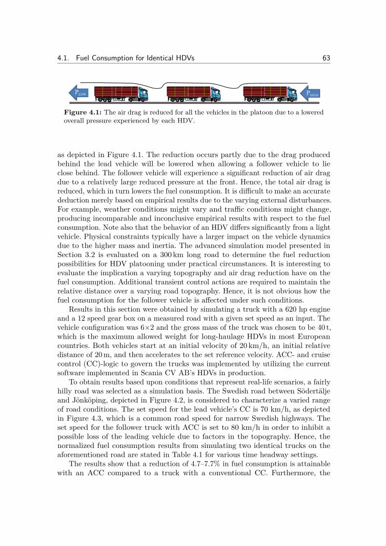
4.1. Fuel Consumption for Identical HDVs 63
���� �����
Figure 4.1: The air drag is reduced for all the vehicles in the platoon due to a loweredoverall pressure experienced by each HDV.
as depicted in Figure 4.1. The reduction occurs partly due to the drag producedbehind the lead vehicle will be lowered when allowing a follower vehicle to lieclose behind. The follower vehicle will experience a significant reduction of air dragdue to a relatively large reduced pressure at the front. Hence, the total air drag isreduced, which in turn lowers the fuel consumption. It is di�cult to make an accuratededuction merely based on empirical results due to the varying external disturbances.For example, weather conditions might vary and tra�c conditions might change,producing incomparable and inconclusive empirical results with respect to the fuelconsumption. Note also that the behavior of an HDV di�ers significantly from a lightvehicle. Physical constraints typically have a larger impact on the vehicle dynamicsdue to the higher mass and inertia. The advanced simulation model presented inSection 3.2 is evaluated on a 300 km long road to determine the fuel reductionpossibilities for HDV platooning under practical circumstances. It is interesting toevaluate the implication a varying topography and air drag reduction have on thefuel consumption. Additional transient control actions are required to maintain therelative distance over a varying road topography. Hence, it is not obvious how thefuel consumption for the follower vehicle is a�ected under such conditions.
Results in this section were obtained by simulating a truck with a 620 hp engineand a 12 speed gear box on a measured road with a given set speed as an input. Thevehicle configuration was 6◊2 and the gross mass of the truck was chosen to be 40 t,which is the maximum allowed weight for long-haulage HDVs in most Europeancountries. Both vehicles start at an initial velocity of 20 km/h, an initial relativedistance of 20 m, and then accelerates to the set reference velocity. ACC- and cruisecontrol (CC)-logic to govern the trucks was implemented by utilizing the currentsoftware implemented in Scania CV AB’s HDVs in production.
To obtain results based upon conditions that represent real-life scenarios, a fairlyhilly road was selected as a simulation basis. The Swedish road between Södertäljeand Jönköping, depicted in Figure 4.2, is considered to characterize a varied rangeof road conditions. The set speed for the lead vehicle’s CC is 70 km/h, as depictedin Figure 4.3, which is a common road speed for narrow Swedish highways. Theset speed for the follower truck with ACC is set to 80 km/h in order to inhibit apossible loss of the leading vehicle due to factors in the topography. Hence, thenormalized fuel consumption results from simulating two identical trucks on theaforementioned road are stated in Table 4.1 for various time headway settings.
The results show that a reduction of 4.7–7.7% in fuel consumption is attainablewith an ACC compared to a truck with a conventional CC. Furthermore, the
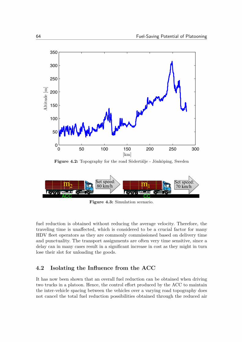
64 Fuel-Saving Potential of Platooning
0 50 100 150 200 250 3000
50
100
150
200
250
300
350
[km]
Alt
itude
[m]
Figure 4.2: Topography for the road Södertälje - Jönköping, Sweden
����� ��
����������� ���
����������� �����
Figure 4.3: Simulation scenario.
fuel reduction is obtained without reducing the average velocity. Therefore, thetraveling time is una�ected, which is considered to be a crucial factor for manyHDV fleet operators as they are commonly commissioned based on delivery timeand punctuality. The transport assignments are often very time sensitive, since adelay can in many cases result in a significant increase in cost as they might in turnlose their slot for unloading the goods.
4.2 Isolating the Influence from the ACC
It has now been shown that an overall fuel reduction can be obtained when drivingtwo trucks in a platoon. Hence, the control e�ort produced by the ACC to maintainthe inter-vehicle spacing between the vehicles over a varying road topography doesnot cancel the total fuel reduction possibilities obtained through the reduced air
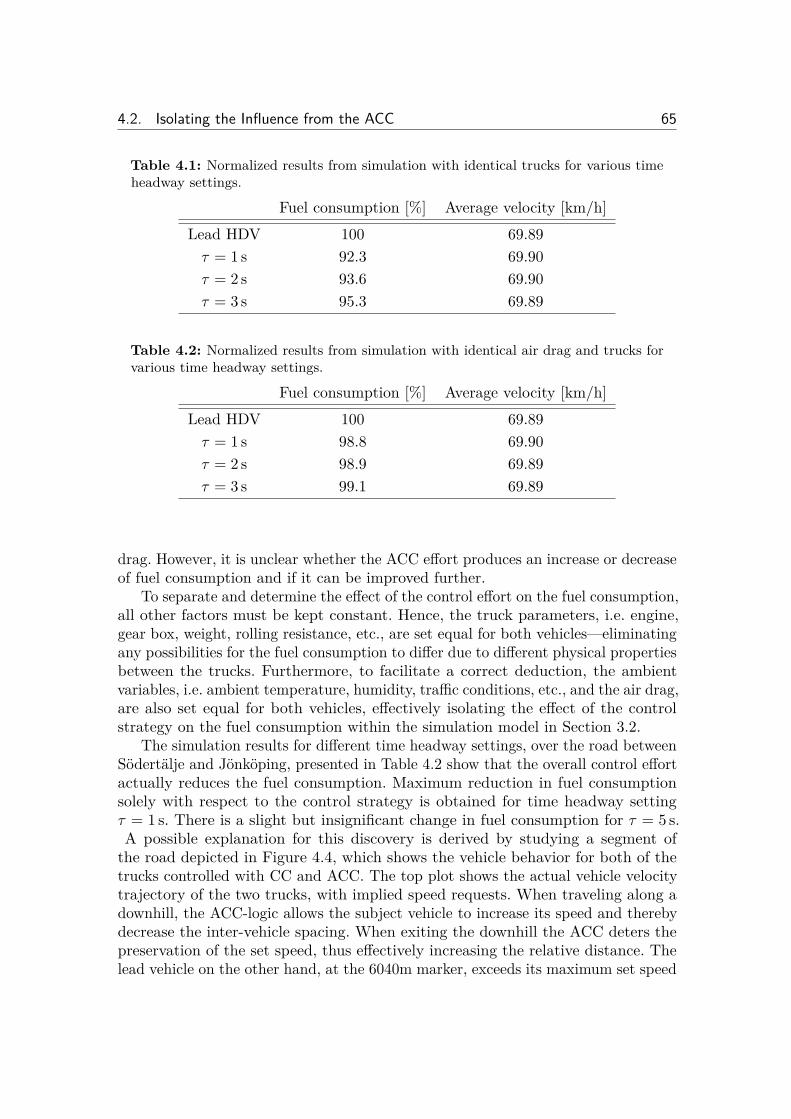
4.2. Isolating the Influence from the ACC 65
Table 4.1: Normalized results from simulation with identical trucks for various timeheadway settings.
Fuel consumption [%] Average velocity [km/h]Lead HDV 100 69.89
· = 1 s 92.3 69.90· = 2 s 93.6 69.90· = 3 s 95.3 69.89
Table 4.2: Normalized results from simulation with identical air drag and trucks forvarious time headway settings.
Fuel consumption [%] Average velocity [km/h]Lead HDV 100 69.89
· = 1 s 98.8 69.90· = 2 s 98.9 69.89· = 3 s 99.1 69.89
drag. However, it is unclear whether the ACC e�ort produces an increase or decreaseof fuel consumption and if it can be improved further.
To separate and determine the e�ect of the control e�ort on the fuel consumption,all other factors must be kept constant. Hence, the truck parameters, i.e. engine,gear box, weight, rolling resistance, etc., are set equal for both vehicles—eliminatingany possibilities for the fuel consumption to di�er due to di�erent physical propertiesbetween the trucks. Furthermore, to facilitate a correct deduction, the ambientvariables, i.e. ambient temperature, humidity, tra�c conditions, etc., and the air drag,are also set equal for both vehicles, e�ectively isolating the e�ect of the controlstrategy on the fuel consumption within the simulation model in Section 3.2.
The simulation results for di�erent time headway settings, over the road betweenSödertälje and Jönköping, presented in Table 4.2 show that the overall control e�ortactually reduces the fuel consumption. Maximum reduction in fuel consumptionsolely with respect to the control strategy is obtained for time headway setting· = 1 s. There is a slight but insignificant change in fuel consumption for · = 5 s.A possible explanation for this discovery is derived by studying a segment of
the road depicted in Figure 4.4, which shows the vehicle behavior for both of thetrucks controlled with CC and ACC. The top plot shows the actual vehicle velocitytrajectory of the two trucks, with implied speed requests. When traveling along adownhill, the ACC-logic allows the subject vehicle to increase its speed and therebydecrease the inter-vehicle spacing. When exiting the downhill the ACC deters thepreservation of the set speed, thus e�ectively increasing the relative distance. Thelead vehicle on the other hand, at the 6040m marker, exceeds its maximum set speed
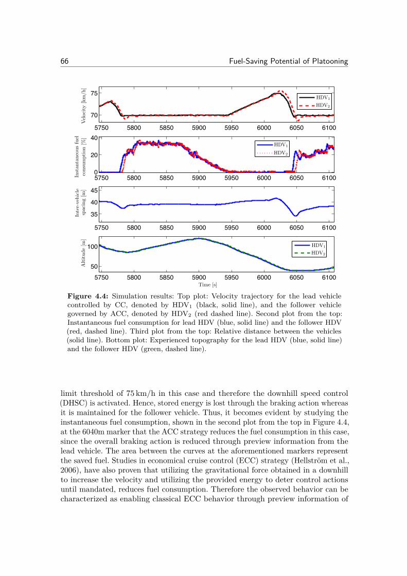
66 Fuel-Saving Potential of Platooning
5750 5800 5850 5900 5950 6000 6050 6100
70
75
5750 5800 5850 5900 5950 6000 6050 61000
20
40
5750 5800 5850 5900 5950 6000 6050 6100
35
40
45
5750 5800 5850 5900 5950 6000 6050 6100
50
100
Vel
oci
ty[k
m/h
]
Inst
anta
neo
us
fuel
consu
mption
[%]
Inte
r-veh
icle
spac
ing
[m]
Altitude
[m]
Time [s]
HDV1
HDV2
HDV2
HDV2
HDV1
HDV1
Figure 4.4: Simulation results: Top plot: Velocity trajectory for the lead vehiclecontrolled by CC, denoted by HDV1 (black, solid line), and the follower vehiclegoverned by ACC, denoted by HDV2 (red dashed line). Second plot from the top:Instantaneous fuel consumption for lead HDV (blue, solid line) and the follower HDV(red, dashed line). Third plot from the top: Relative distance between the vehicles(solid line). Bottom plot: Experienced topography for the lead HDV (blue, solid line)and the follower HDV (green, dashed line).
limit threshold of 75 km/h in this case and therefore the downhill speed control(DHSC) is activated. Hence, stored energy is lost through the braking action whereasit is maintained for the follower vehicle. Thus, it becomes evident by studying theinstantaneous fuel consumption, shown in the second plot from the top in Figure 4.4,at the 6040m marker that the ACC strategy reduces the fuel consumption in this case,since the overall braking action is reduced through preview information from thelead vehicle. The area between the curves at the aforementioned markers representthe saved fuel. Studies in economical cruise control (ECC) strategy (Hellström et al.,2006), have also proven that utilizing the gravitational force obtained in a downhillto increase the velocity and utilizing the provided energy to deter control actionsuntil mandated, reduces fuel consumption. Therefore the observed behavior can becharacterized as enabling classical ECC behavior through preview information of
4.3. Mass Variations 67
the road characteristics ahead from the lead vehicle, which undoubtedly reduces thefuel consumption.
The noted result could also have been a consequence of finding a more fuel-e�cient Fuel–Torque–RPM point for the specific engine due to a small di�erence inactual speed between the two trucks. However, an identical simulation with di�erentengine characteristics resulted in equivalent results concluded from Table 4.2.
4.3 Mass Variations
The aforementioned results indicate that platooning with two identical trucks reducesthe fuel consumption due to both air drag reduction and control strategy. However,two HDVs with di�erent masses could induce a di�erent ACC behavior. In somecases when following a lighter truck over an uphill segment, the lead vehicle willbe able to maintain its velocity, while the follower vehicle will drop in speed, eventhough maximum engine torque is applied, due to its extensive mass. Similarlywhen following a lighter vehicle, the follower vehicle will have to brake in a downhillsegment to maintain the inter-vehicle spacing when the lead vehicle is coasting.Hence, a di�erence in mass between the two trucks will inflict constraints on theACC and alter the controller behavior in comparison with the case of two identicaltrucks. Thus, it is of interest to study the e�ects of provoking the ACC strategy insuch a manner.
Two scenarios are investigated. In the first scenario, the mass of the lead vehicleis set to m
1
= 30 t, whereas the truck governed by ACC is maintained at m2
= 40 t,as illustrated in Figure 4.3. In the second scenario, the leading vehicle’s mass is setto m
1
= 50 t. All other conditions are identical and the simulation is carried out onthe same road as before.
The results displayed in Figure 4.5 were derived by comparing the fuel consump-tion of the follower vehicle, with the fuel consumption of a lead vehicle with the samemass to avoid ambiguity. The results show that a fuel saving of 3.8–7.4% can beobtained when following a lighter lead vehicle and a reduction in fuel consumptionof 4.3–6.9% when following a heavier lead vehicle. Hence, a significant fuel reductioncan still be obtained for various considered time headway settings. However, anoticeable di�erence in fuel consumption is detected due to the physically inducedchange in control. For time headway setting · = 1 s, a 0.5% higher fuel reductioncan be obtained with a lighter lead vehicle in comparison with a heavier lead vehicle.It is probably due to the fact that the vehicle governed by ACC acts as a low passfilter when it is heavier, making it less sensitive to small fluctuations in the leadvehicle’s velocity. Thus, a lower variance in control e�ort is required for the vehicle,resulting in lower fuel consumption. However, · = 3 s a lighter lead vehicle producesan increase of 0.5% in fuel consumption compared to the results from a heavier leadvehicle. A lighter lead vehicle has a lower acceleration when coasting over steepdownhill segments. Thus, the heavier vehicle governed by the ACC has to brake inthose cases in order to maintain the relative distance. Hence, energy produced from
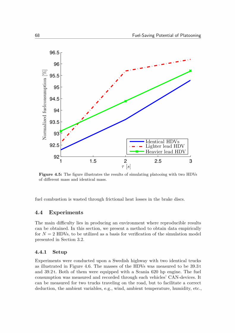
68 Fuel-Saving Potential of Platooning
1 2 392
92.5
93
93.5
94
94.5
95
95.5
96
96.5N
orm
alize
dfu
elco
nsu
mpti
on
[%]
Identical HDVsLighter lead HDVHeavier lead HDV
1.5 2.5⌧ [s]
Figure 4.5: The figure illustrates the results of simulating platooing with two HDVsof di�erent mass and identical mass.
fuel combustion is wasted through frictional heat losses in the brake discs.
4.4 Experiments
The main di�culty lies in producing an environment where reproducible resultscan be obtained. In this section, we present a method to obtain data empiricallyfor N = 2 HDVs, to be utilized as a basis for verification of the simulation modelpresented in Section 3.2.
4.4.1 SetupExperiments were conducted upon a Swedish highway with two identical trucksas illustrated in Figure 4.6. The masses of the HDVs was measured to be 39.3 tand 39.2 t. Both of them were equipped with a Scania 620 hp engine. The fuelconsumption was measured and recorded through each vehicles’ CAN-devices. Itcan be measured for two trucks traveling on the road, but to facilitate a correctdeduction, the ambient variables, e.g., wind, ambient temperature, humidity, etc.,
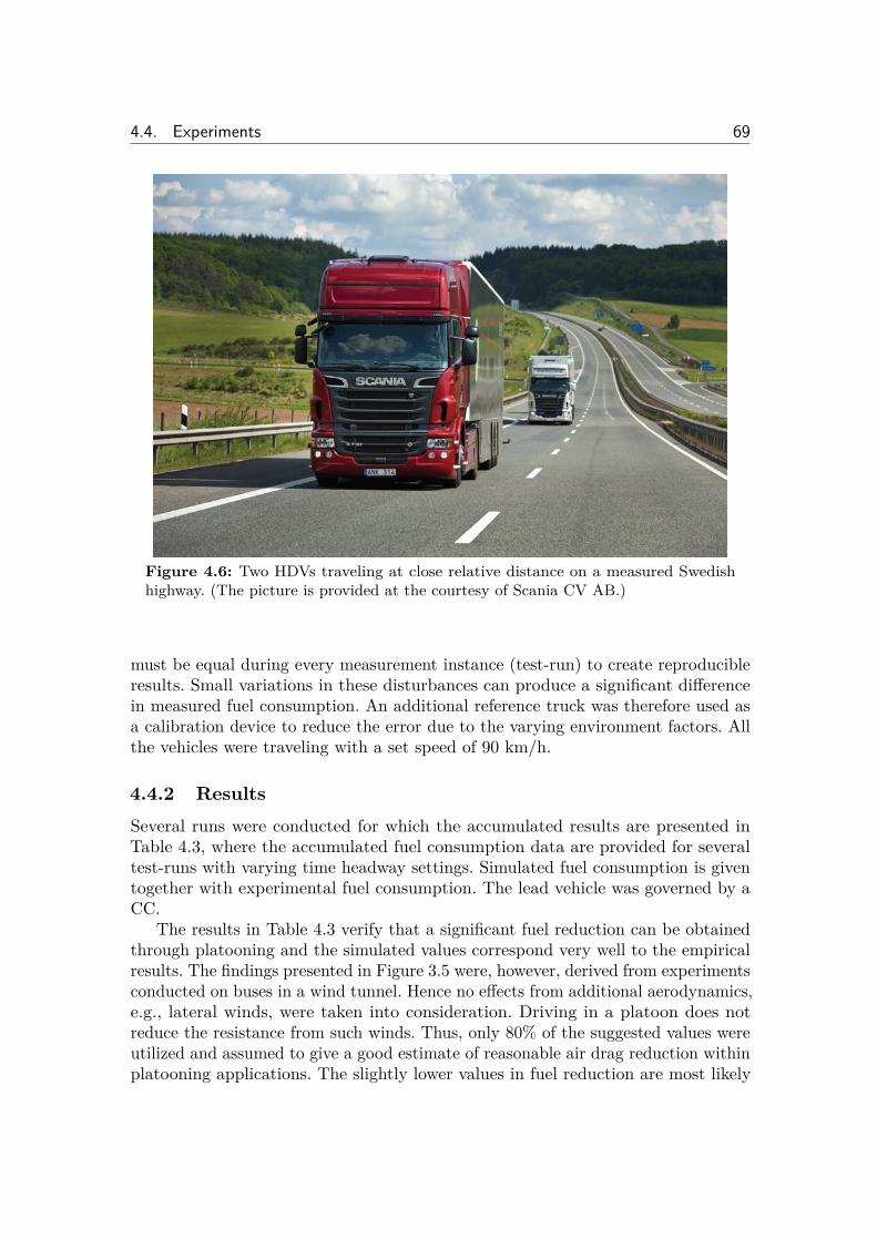
4.4. Experiments 69
Figure 4.6: Two HDVs traveling at close relative distance on a measured Swedishhighway. (The picture is provided at the courtesy of Scania CV AB.)
must be equal during every measurement instance (test-run) to create reproducibleresults. Small variations in these disturbances can produce a significant di�erencein measured fuel consumption. An additional reference truck was therefore used asa calibration device to reduce the error due to the varying environment factors. Allthe vehicles were traveling with a set speed of 90 km/h.
4.4.2 ResultsSeveral runs were conducted for which the accumulated results are presented inTable 4.3, where the accumulated fuel consumption data are provided for severaltest-runs with varying time headway settings. Simulated fuel consumption is giventogether with experimental fuel consumption. The lead vehicle was governed by aCC.
The results in Table 4.3 verify that a significant fuel reduction can be obtainedthrough platooning and the simulated values correspond very well to the empiricalresults. The findings presented in Figure 3.5 were, however, derived from experimentsconducted on buses in a wind tunnel. Hence no e�ects from additional aerodynamics,e.g., lateral winds, were taken into consideration. Driving in a platoon does notreduce the resistance from such winds. Thus, only 80% of the suggested values wereutilized and assumed to give a good estimate of reasonable air drag reduction withinplatooning applications. The slightly lower values in fuel reduction are most likely
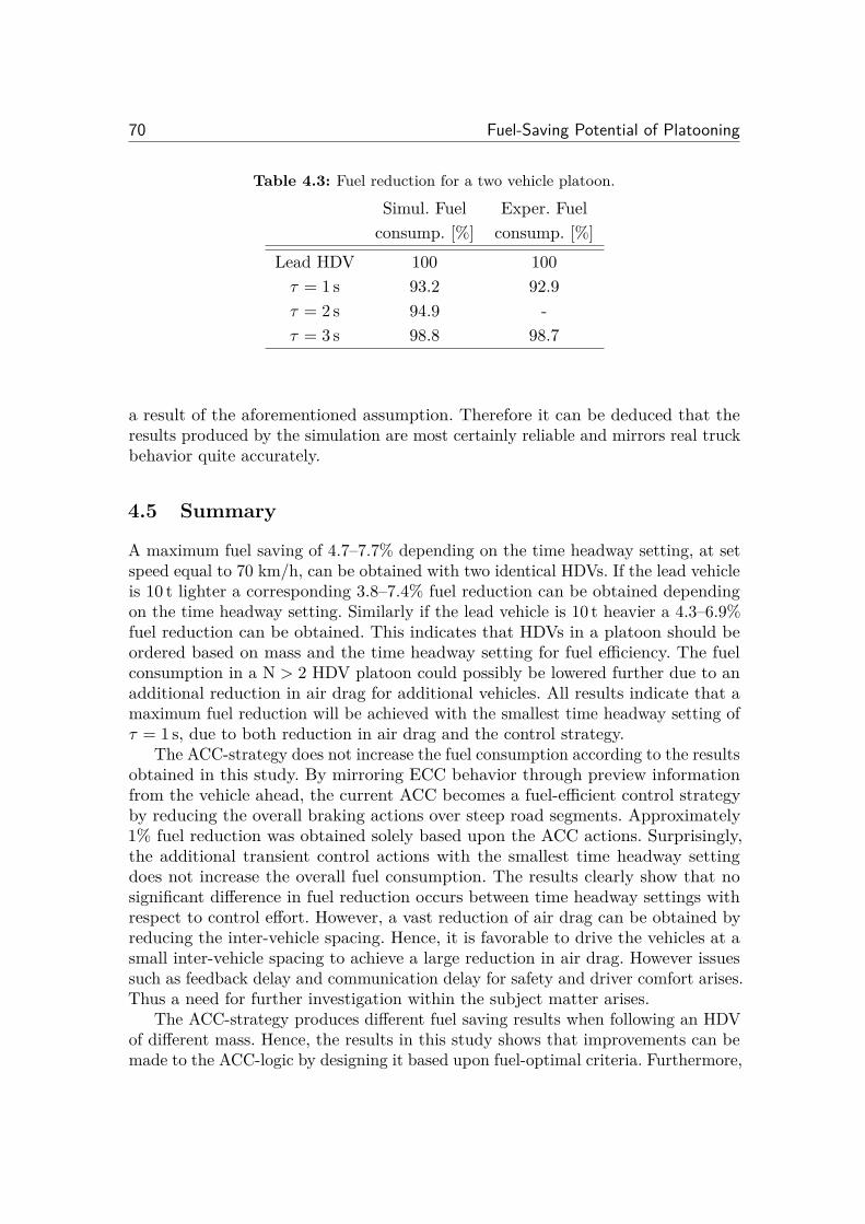
70 Fuel-Saving Potential of Platooning
Table 4.3: Fuel reduction for a two vehicle platoon.
Simul. Fuel Exper. Fuelconsump. [%] consump. [%]
Lead HDV 100 100· = 1 s 93.2 92.9· = 2 s 94.9 -· = 3 s 98.8 98.7
a result of the aforementioned assumption. Therefore it can be deduced that theresults produced by the simulation are most certainly reliable and mirrors real truckbehavior quite accurately.
4.5 Summary
A maximum fuel saving of 4.7–7.7% depending on the time headway setting, at setspeed equal to 70 km/h, can be obtained with two identical HDVs. If the lead vehicleis 10 t lighter a corresponding 3.8–7.4% fuel reduction can be obtained dependingon the time headway setting. Similarly if the lead vehicle is 10 t heavier a 4.3–6.9%fuel reduction can be obtained. This indicates that HDVs in a platoon should beordered based on mass and the time headway setting for fuel e�ciency. The fuelconsumption in a N > 2 HDV platoon could possibly be lowered further due to anadditional reduction in air drag for additional vehicles. All results indicate that amaximum fuel reduction will be achieved with the smallest time headway setting of· = 1 s, due to both reduction in air drag and the control strategy.
The ACC-strategy does not increase the fuel consumption according to the resultsobtained in this study. By mirroring ECC behavior through preview informationfrom the vehicle ahead, the current ACC becomes a fuel-e�cient control strategyby reducing the overall braking actions over steep road segments. Approximately1% fuel reduction was obtained solely based upon the ACC actions. Surprisingly,the additional transient control actions with the smallest time headway settingdoes not increase the overall fuel consumption. The results clearly show that nosignificant di�erence in fuel reduction occurs between time headway settings withrespect to control e�ort. However, a vast reduction of air drag can be obtained byreducing the inter-vehicle spacing. Hence, it is favorable to drive the vehicles at asmall inter-vehicle spacing to achieve a large reduction in air drag. However issuessuch as feedback delay and communication delay for safety and driver comfort arises.Thus a need for further investigation within the subject matter arises.
The ACC-strategy produces di�erent fuel saving results when following an HDVof di�erent mass. Hence, the results in this study shows that improvements can bemade to the ACC-logic by designing it based upon fuel-optimal criteria. Furthermore,
4.5. Summary 71
the isolated strategies within this chapter have shown significant fuel reductionpossibilities in HDV platooning at relatively large inter-vehicle spacings. The fuelsaving can most likely be improved further by reducing the inter-vehicle spacing.However, driver comfort should be taken into consideration for widespread of theplatooning system concept. Safety cannot be compromised, hence the impact of theautomated vehicle control on the safety must be established and verified.

Chapter 5
Platooning under Safety Constraints
“The most exciting phrase to hear in science, the one that heralds new
discoveries, is not ’Eureka!’ but ’That’s funny...’”Isaac Asimov
It is fuel-e�cient to drive at a small inter-vehicle spacing to achieve a highreduction in air drag, but, as tra�c intensity grows, the complexity of thecoupled tra�c dynamics increases. The actions of one vehicle may in turn
a�ect all vehicles in a linked chain. Through improved sensor technology, wirelesscommunication, GPS devices, and digital maps, advanced driver assistance systemsare being developed to aid the driver. Key enabling technologies, such as vehicle-to-vehicle (V2V) and vehicle-to-infrastructure (V2I) communication, have matured.However, they impose constraints in terms of accuracy, reliability, and delays.Therefore, safety constraints with respect to how close we can drive to the vehicleahead without increasing the risk of a collision are a challenge to satisfy. A questionarises of how close the automated vehicles can operate without compromising safety.
Commercially available systems, such as the adaptive cruise control (ACC),in a collision avoidance scenario currently use radar measurements of the relativedistance and velocity to a preceding vehicle and adjust the velocity automatically.A delay arises from measuring the behavior of the preceding vehicle to producingthe actual brake torque at the wheels, since it takes time in determining whetherthe preceding vehicle is braking and then creating the necessary pressure in thebrake cylinders. As an alternative to radar measurements, wireless communicationof the breaking signal may be utilized. However, delays are still imposed due todata processing, retransmissions, etc. Thus, the impact of the vehicle control onthe safety must be established and verified. Rigorous guarantees cannot only beobtained through extensive simulations, but mathematical tools that are verified byexperiments need to be developed.
In this chapter, we consider a heavy-duty vehicle (HDV) platooning scenariowith two vehicles where the follower vehicle receives information regarding the
73
74 Platooning under Safety Constraints
relative position and velocity of the vehicle ahead.1 The objective is to determinethe minimum relative distance between the vehicles that can be maintained withoutcompromising safety. The aim is to find the largest set of initial states, irrespectiveof how the lead vehicle behaves, for which there exists a controller that manages tokeep all executions inside a safe subset of the state space.
The main contribution of this chapter is to primarily establish safe sets, whichcan serve as a reference for HDV platooning in collision avoidance. The aim is toestablish empirical results for validation of the analytical framework and numericalsafe set computation for collision avoidance in HDV platooning scenarios. We proposean automated and reproducible method to derive empirical results for validation ofsafe sets. We show how the method has been evaluated experimentally using realHDVs provided by Scania CV AB on a test site near Stockholm. A di�erential gameformulation of the problem enables the safe set derivation by capturing the eventwhen the lead vehicle blunders in the worst possible manner. We model the game asthe follower vehicle (player u
2
) is trying its best to avoid a collision while the leadvehicle (player u
1
) is trying its best to create a collision. Based on the theoreticaland empirical results, we determine criteria for which collisions can be avoided forthe worst-case scenario and thereby, establish the minimum possible safe distance inpractice between vehicles in a platoon. We show that the minimum relative distancewith respect to safety depends on the nonlinear behavior of the brake system, thedelays in information propagation, and the constraints on the implemented controlactions.
The di�erential game approach based on optimization (Basar and Olsder, 1995,Chapter 5.3), adopted in this chapter has previously been applied to air tra�cmanagement, e.g. Bayen et al. (2003). The computational challenges for our systemare similar, but the implementation aspects are quite di�erent. For example, thedelays imposed by inter-vehicle communication and sensor processing are importantfor platoon safety. Moreover, the braking capability of each vehicle plays a crucial role.Still we are able to use the same mathematical framework, conveniently packagedin the level set Matlab toolbox by Mitchell (2007).
The outline of this chapter is as follows. First the system model for the di�erentialgame formulation is presented in Section 5.1. In Section 5.2 we present the theoreticalpremise for computing safe sets and then apply it to platooning. Safe sets are derivedfor homogeneous and heterogeneous HDV platoons, which are verified through thesimulation model presented in Section 3.2. The experimental setup for evaluatingthe safe sets is given in Section 5.3 together with experimental evaluations. Thechapter concludes with a brief summary in Section 5.4.
1The extension to platoons with N > 2 vehicles is discussed in the chapter. The developedapproach generalizes to this case, but the numerical computation are harder.
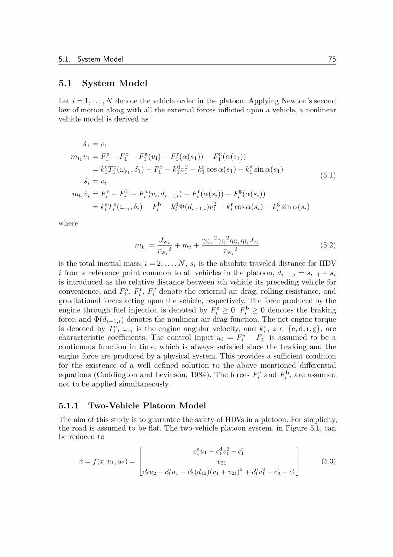
5.1. System Model 75
5.1 System Model
Let i = 1, . . . , N denote the vehicle order in the platoon. Applying Newton’s secondlaw of motion along with all the external forces inflicted upon a vehicle, a nonlinearvehicle model is derived as
s1
= v1
mt1 v
1
= F e
1
≠ F b
1
≠ F a
1
(v1
) ≠ F r
1
(–(s1
)) ≠ F g
1
(–(s1
))= ke
1
T e
1
(Êe1 , ”
1
) ≠ F b
1
≠ kd
1
v2
1
≠ kr
1
cos –(s1
) ≠ kg
1
sin –(s1
)si = vi
mti vi = F e
i ≠ F b
i ≠ F a
i (vi, di≠1,i) ≠ F r
i (–(si)) ≠ F g
i (–(si))= ke
i T e
i (Êei , ”i) ≠ F b
i ≠ kd
i �(di≠1,i)v2
i ≠ kr
i cos –(si) ≠ kg
i sin –(si)
(5.1)
where
mti = J
wi
rwi
2
+ mi + “Gi
2“fi
2÷Gi÷fiJei
rwi
2
(5.2)
is the total inertial mass, i = 2, . . . , N , si is the absolute traveled distance for HDVi from a reference point common to all vehicles in the platoon, di≠1,i = si≠1
≠ si
is introduced as the relative distance between ith vehicle its preceding vehicle forconvenience, and F a
i , F r
i , F g
i denote the external air drag, rolling resistance, andgravitational forces acting upon the vehicle, respectively. The force produced by theengine through fuel injection is denoted by F e
i Ø 0, F b
i Ø 0 denotes the brakingforce, and �(di≠1,i) denotes the nonlinear air drag function. The net engine torqueis denoted by T e
i , Êei is the engine angular velocity, and kz
i , z œ {e, d, r, g}, arecharacteristic coe�cients. The control input ui = F e
i ≠ F b
i is assumed to be acontinuous function in time, which is always satisfied since the braking and theengine force are produced by a physical system. This provides a su�cient conditionfor the existence of a well defined solution to the above mentioned di�erentialequations (Coddington and Levinson, 1984). The forces F e
i and F b
i , are assumednot to be applied simultaneously.
5.1.1 Two-Vehicle Platoon ModelThe aim of this study is to guarantee the safety of HDVs in a platoon. For simplicity,the road is assumed to be flat. The two-vehicle platoon system, in Figure 5.1, canbe reduced to
x = f(x, u1, u2) =
S
Uc
u1u1 ≠ c
d1v
21 ≠ c
r1
≠v21
c
u2u2 ≠ c
u1u1 ≠ c
d2(d12)(v1 + v21)2 + c
d1v
21 ≠ c
r2 + c
r1
T
V (5.3)
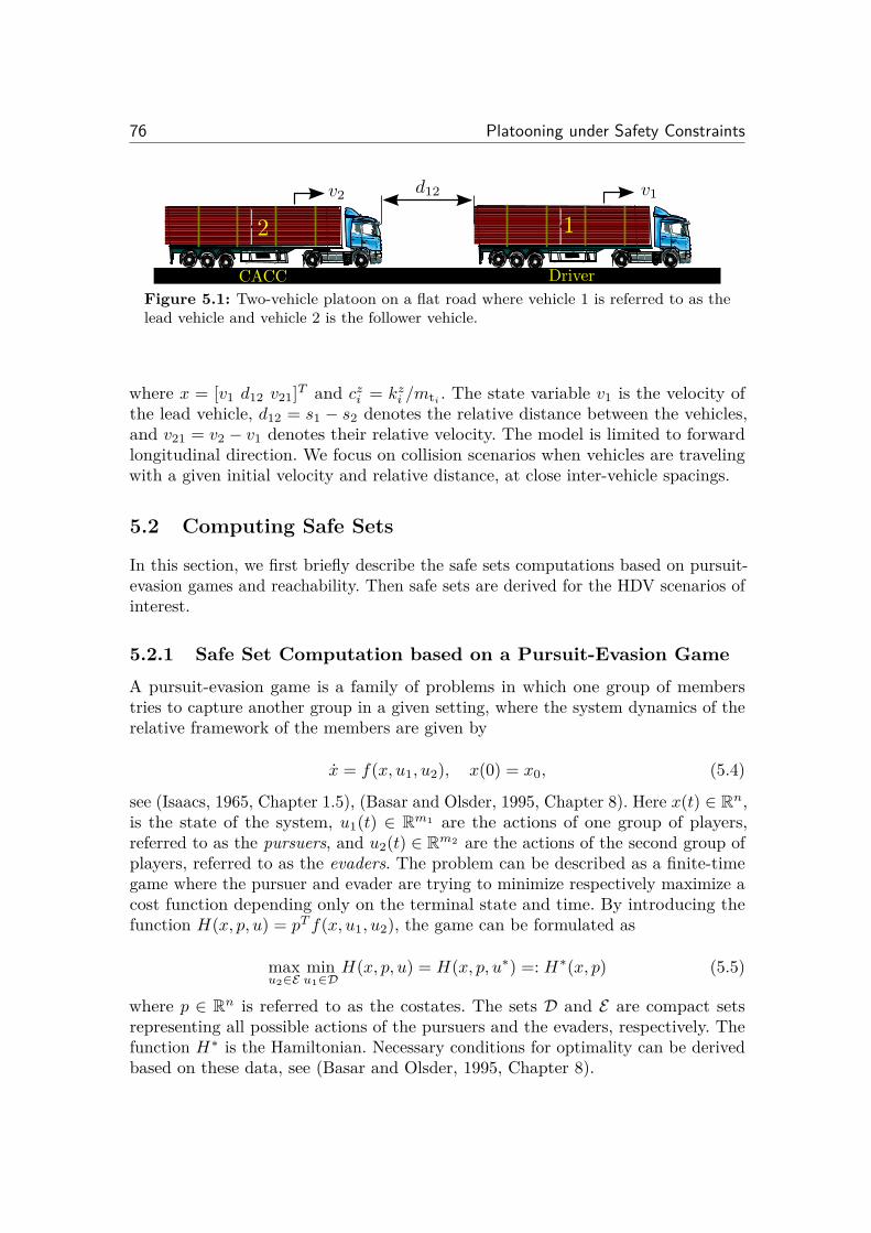
76 Platooning under Safety Constraints
d12 v1v2
12
CACC Driver
Figure 5.1: Two-vehicle platoon on a flat road where vehicle 1 is referred to as thelead vehicle and vehicle 2 is the follower vehicle.
where x = [v1
d12
v21
]T and czi = kz
i /mti . The state variable v
1
is the velocity ofthe lead vehicle, d
12
= s1
≠ s2
denotes the relative distance between the vehicles,and v
21
= v2
≠ v1
denotes their relative velocity. The model is limited to forwardlongitudinal direction. We focus on collision scenarios when vehicles are travelingwith a given initial velocity and relative distance, at close inter-vehicle spacings.
5.2 Computing Safe Sets
In this section, we first briefly describe the safe sets computations based on pursuit-evasion games and reachability. Then safe sets are derived for the HDV scenarios ofinterest.
5.2.1 Safe Set Computation based on a Pursuit-Evasion GameA pursuit-evasion game is a family of problems in which one group of memberstries to capture another group in a given setting, where the system dynamics of therelative framework of the members are given by
x = f(x, u1
, u2
), x(0) = x0
, (5.4)
see (Isaacs, 1965, Chapter 1.5), (Basar and Olsder, 1995, Chapter 8). Here x(t) œ Rn,is the state of the system, u
1
(t) œ Rm1 are the actions of one group of players,referred to as the pursuers, and u
2
(t) œ Rm2 are the actions of the second group ofplayers, referred to as the evaders. The problem can be described as a finite-timegame where the pursuer and evader are trying to minimize respectively maximize acost function depending only on the terminal state and time. By introducing thefunction H(x, p, u) = pT f(x, u
1
, u2
), the game can be formulated as
maxu2œE
minu1œD
H(x, p, u) = H(x, p, uú) =: Hú(x, p) (5.5)
where p œ Rn is referred to as the costates. The sets D and E are compact setsrepresenting all possible actions of the pursuers and the evaders, respectively. Thefunction Hú is the Hamiltonian. Necessary conditions for optimality can be derivedbased on these data, see (Basar and Olsder, 1995, Chapter 8).
5.2. Computing Safe Sets 77
Given actions u1
œ E and u2
œ D, the ability to reach a defined unsafe set froma set of feasible initial states x
0
is of interest for establishing safety criteria. InMitchell et al. (2005), it was shown that the unsafe set U(·) in which the pursuer ina two-person dynamic game can create a collision in the next · time units despitethe best e�ort from the evader, can be computed as U(·) = {xœR3|Ï(x, ≠·) Æ 0},where Ï(· , · ) is the viscosity solution of the (modified) Hamilton-Jacobi-Isaacspartial di�erential equation
ˆÏ(x, t)ˆt
+ min(0, H(x, p, uú)) = 0, t Æ 0, (5.6)
with suitable terminal conditions2 Ï(x, 0) = Ï0
(x). The equation is solved by startingat the boundary of the unsafe set ˆU(·). The set of states under consideration is
‰(·) = {x œ ˆU(·) | pT (0)f(x, uú1
, uú2
) < 0}, (5.7)which denotes all states heading into the unsafe set. The reachable set is calculatedby starting at ˆU(0) and simultaneously solving the equations corresponding to theoptimality conditions. Hence, the trajectories are computed on the boundary of theset ‰(·), from where it is possible to move away from the unsafe set. The proceduregives the surface sets that partitions the safe and unsafe regions.
5.2.2 Safe Set Computation for a Two-Vehicle PlatoonIn the problem at hand, f(x, u
1
, u2
) in (5.4) corresponds to the platoon systemin (5.3) and uú
1
, uú2
are the optimal strategies for the lead vehicle and the followervehicles, respectively. The unsafe set U(·) corresponds to a vehicle collision at time· > 0. Note that the game formulation leads to a conservative estimate of the unsafeset, since the lead vehicle’s optimal control action is based on knowledge of how thefollower vehicle will respond, but not vice versa, see Mitchell et al. (2005). Such aformulation is preferable to ensure safety in practice.
The Hamiltonian function for the two-vehicle platoon is
Hú(x, p) := maxu2œE
minu1œD
pT f(x, u1
, u2
)
= maxu2œE
minu1œD
Ëp
1
p2
p3
ÈS
WUv
1
d12
v21
T
XV
= ≠ p2
v21
≠ (p3
≠ p1
)cu
1
uú1
+ p3
cu
2
uú2
+ (p3
≠ p1
)cd
1
v2
1
≠ p3
cd
2
(d12
)(v1
+ v21
)2 + (p3
≠ p1
)cr
1
+ p3
cr
2
.
(5.8)
With the formulation in (5.8), the lead vehicle determines its optimal controlstrategy based on the information regarding the follower vehicle’s strategy. This is a
2In our case the terminal condition is when a collision has occurred, i.e. when Ï0(x) = d12 = 0.
78 Platooning under Safety Constraints
reasonable assumption as we wish to find a set which guarantees that a collisioncan be avoided despite the worst possible behavior of the lead vehicle. The costatesfulfill
p = ≠ˆHú
ˆx=
S
WU2p
3
cd
2
(d12
)(v1
+ v12
) ≠ 2(p3
≠ p1
)cd
1
v1
p3
1
2
cw
2
A2
flkpw(v1
+ v21
)2
2p3
cd
2
(d12
)(v1
+ v21
)
T
XV . (5.9)
The optimal strategy can easily be computed as
uú1
= F e
1
≠ F b
1
2 + sgn(p3
≠ p1
) F e
1
+ F b
1
2 , uú2
= F e
2
≠ F b
2
2 + sgn(p3
) F e
2
+ F b
2
2 , (5.10)
where F bi > 0 is the maximum brake force and F e
i > 0 is the maximum engine forceof vehicle i = 1, 2.
5.2.3 Safe Set Computation for an N-Vehicle Platoon
The safe set computation approach for a two-vehicle derived in the previous sectioncan be generalized to N > 0 vehicles. First we consider an N = 3 HDV platoon.Two states are added to (5.3) for the three-vehicle platoon system:
x = f(x, u1, u2, u3) =
S
WWWWWU
c
u1u1 ≠ c
d1v
21 ≠ c
r1
≠v21
c
u2u2 ≠ c
u1u1 ≠ c
d2(d12)v2
2 + c
d1(v1 + v21)2 ≠ c
r2 + c
r1
≠v32
c
u3u3 ≠ c
u2u2 ≠ c
d3(d23)(v1 + v21 + v32)2 + c
d2(d12)v2
2 ≠ c
r3 + c
r2
T
XXXXXV,
(5.11)
where x = [v1
d12
v21
d23
v32
]T and we have used vj = v1
+qj≠1
i=1
vi+1,i, for j > 1,in the expression for the third and last state. The costates satisfy p = ≠ ˆHú
ˆx withthe Hamiltonian function
Hú(x, p) := max(u2,u3)œE
minu1œD
pT f(x, u1
, u2
, u3
)
= ≠ (p3
≠ p1
)cu
1
uú1
+ (p3
≠ p5
)cu
2
uú2
+ p5
cu
3
uú3
≠ p2
vr12 ≠ p
4
vr23
≠ p1
(cw
1
v2
1
+ cr
1
) ≠ p3
(cd
2
(d)v2
2
≠ cd
1
(v1
+ vr12)2 + cr
2
≠ cr
1
)≠ p
5
(cd
3
(d23
)(v1
+ vr12 + v
r23)2 ≠ cd
2
(d12
)v2
2
+ cr
3
≠ cr
2
),
(5.12)
where E = E2
◊ E3
is the compact set of controller actions for the two followervehicles. The optimal strategies are given by
5.2. Computing Safe Sets 79
uú1
= F e
1
≠ F b1
2 + sgn(p3
≠ p1
) F e
1
+ F b1
2 ,
uú2
= F e
2
≠ F b2
2 + sgn(p3
≠ p5
) F e
2
+ F b2
2 ,
uú3
= F e
3
≠ F b3
2 + sgn(p5
) F e
3
+ F b3
2 .
(5.13)
Thus, for a three-vehicle platoon the complexity of the pursuit-evasion solutionincreases. Note that the solution has a physical interpretation. For example, both p
3
and p5
appear in the optimal controller for the second vehicle, as shown in (5.13).Hence, the middle vehicle must consider its safety strategy both with respect to itspreceding and following vehicle to avoid a collision with either HDV.
In general, for an N-vehicle platoon the state is given byx = [v
1
d12
v21
d23
. . . vN,N≠1
]T
and its system dynamics corresponding to (5.12) is readily derived. Note thatthe controls u
1
and (u2
, . . . , uN ) enter linearly. Hence, the optimal inputs to theHamiltonian function, Hú(x, p), can again be given analytically, as
uúi =
IF e
i if pT Di > 0, i = 1, . . . , N
F b
i otherwise,(5.14)
where D œ R2N≠1◊N is a matrix, with column vectors Di in the ith column, contain-ing 1 or ≠1 in the appropriate elements, e.g., D
2
= [0 0 1 0 ≠ 1]T for the secondvehicle in the three-vehicle platoon. The unsafe set U(·) is a 2N ≠ 1 dimensionalvector space. Even though analytical expressions for the N -vehicle optimal strategiescan be found through the given framework, the computational cost for solving thepartial di�erential equation to derive the safe sets grows exponentially with thestate dimension. An added HDV to the platoon corresponds to the addition of twonew states. Thus, it is extremely computationally expensive for online applicationsand in general hard to find accurate numerical solutions for the N -vehicle problemwhen N is large.
5.2.4 Numerical EvaluationsTo compute the unsafe set from the solution of (5.6), the level sets methods toolboxof Mitchell (2007) is utilized. In this section, the scenarios are calculated; first weconsider a simple setup with two identical platooning HDV’s and then we studymass heterogeneity and uncertainties in braking capacity.
Identical HDVs
The collision avoidance scenario is first investigated for two identical HDVs. Thevehicles have identical vehicle parameters in (5.1) and the gross mass of each HDV
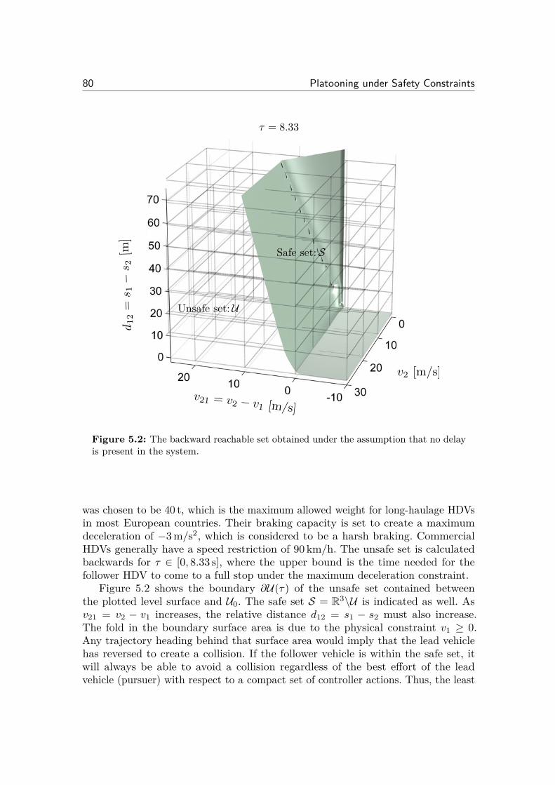
80 Platooning under Safety Constraints
v2 [m/s]
v21 = v2 � v1 [m/s]
d 12
=s 1
�s 2
[m]
Safe set: S
Unsafe set: U
· = 8.33
Figure 5.2: The backward reachable set obtained under the assumption that no delayis present in the system.
was chosen to be 40 t, which is the maximum allowed weight for long-haulage HDVsin most European countries. Their braking capacity is set to create a maximumdeceleration of ≠3 m/s2, which is considered to be a harsh braking. CommercialHDVs generally have a speed restriction of 90 km/h. The unsafe set is calculatedbackwards for · œ [0, 8.33 s], where the upper bound is the time needed for thefollower HDV to come to a full stop under the maximum deceleration constraint.
Figure 5.2 shows the boundary ˆU(·) of the unsafe set contained betweenthe plotted level surface and U
0
. The safe set S = R3\U is indicated as well. Asv
21
= v2
≠ v1
increases, the relative distance d12
= s1
≠ s2
must also increase.The fold in the boundary surface area is due to the physical constraint v
1
Ø 0.Any trajectory heading behind that surface area would imply that the lead vehiclehas reversed to create a collision. If the follower vehicle is within the safe set, itwill always be able to avoid a collision regardless of the best e�ort of the leadvehicle (pursuer) with respect to a compact set of controller actions. Thus, the least
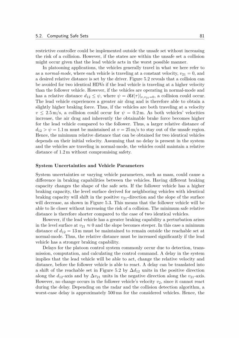
5.2. Computing Safe Sets 81
restrictive controller could be implemented outside the unsafe set without increasingthe risk of a collision. However, if the states are within the unsafe set a collisionmight occur given that the lead vehicle acts in the worst possible manner.
In platooning applications, the vehicles generally travel in what we here refer toas a normal-mode, where each vehicle is traveling at a constant velocity, v
21
= 0, anda desired relative distance is set by the driver. Figure 5.2 reveals that a collision canbe avoided for two identical HDVs if the lead vehicle is traveling at a higher velocitythan the follower vehicle. However, if the vehicles are operating in normal-mode andhas a relative distance d
12
Æ Â, where  = ˆU(·)|v,v21=0
, a collision could occur.The lead vehicle experiences a greater air drag and is therefore able to obtain aslightly higher braking force. Thus, if the vehicles are both traveling at a velocityv Æ 2.5 m/s, a collision could occur for  = 0.2 m. As both vehicles’ velocitiesincrease, the air drag and inherently the obtainable brake force becomes higherfor the lead vehicle compared to the follower. Thus, a larger relative distance ofd
12
> Â = 1.1 m must be maintained at v = 25 m/s to stay out of the unsafe region.Hence, the minimum relative distance that can be obtained for two identical vehiclesdepends on their initial velocity. Assuming that no delay is present in the systemand the vehicles are traveling in normal-mode, the vehicles could maintain a relativedistance of 1.2 m without compromising safety.
System Uncertainties and Vehicle Parameters
System uncertainties or varying vehicle parameters, such as mass, could cause adi�erence in braking capabilities between the vehicles. Having di�erent brakingcapacity changes the shape of the safe sets. If the follower vehicle has a higherbraking capacity, the level surface derived for neighboring vehicles with identicalbraking capacity will shift in the positive v
21
-direction and the slope of the surfacewill decrease, as shown in Figure 5.3. This means that the follower vehicle will beable to lie closer without increasing the risk of a collision. The minimum safe relativedistance is therefore shorter compared to the case of two identical vehicles.
However, if the lead vehicle has a greater braking capability a perturbation arisesin the level surface at v
21
¥ 0 and the slope becomes steeper. In this case a minimumdistance of d
12
= 13 m must be maintained to remain outside the reachable set atnormal-mode. Thus, the relative distance must be increased significantly if the leadvehicle has a stronger braking capability.
Delays for the platoon control system commonly occur due to detection, trans-mission, computation, and calculating the control command. A delay in the systemimplies that the lead vehicle will be able to act, change the relative velocity anddistance, before the follower vehicle is able to react. A delay can be translated intoa shift of the reachable set in Figure 5.2 by �d
12
units in the positive directionalong the d
12
-axis and by �v21
units in the negative direction along the v21
-axis.However, no change occurs in the follower vehicle’s velocity v
2
, since it cannot reactduring the delay. Depending on the radar and the collision detection algorithm, aworst-case delay is approximately 500 ms for the considered vehicles. Hence, the
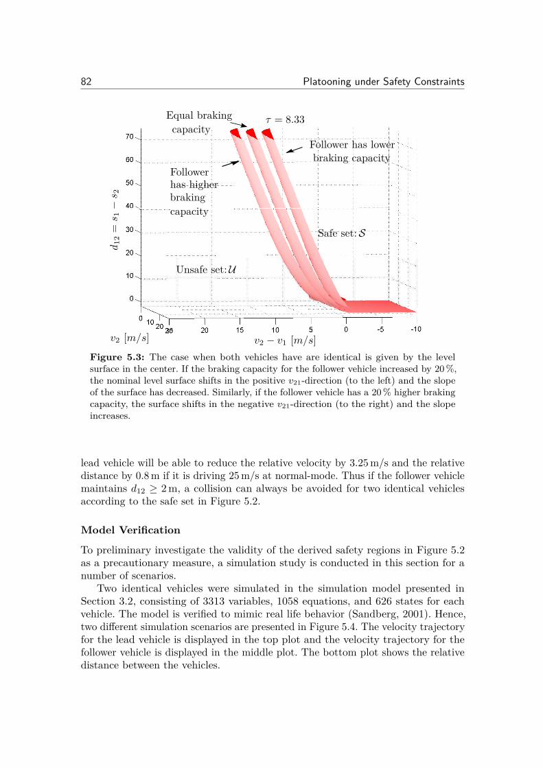
82 Platooning under Safety Constraints
Equal braking
v2
≠ v1
[m/s]v2
[m/s]
d1
2
=s 1
≠s 2
· = 8.33capacity
Follower
braking
Follower has lowerbraking capacity
Unsafe set: U
Safe set: S
has higher
capacity
Figure 5.3: The case when both vehicles have are identical is given by the levelsurface in the center. If the braking capacity for the follower vehicle increased by 20 %,the nominal level surface shifts in the positive v21-direction (to the left) and the slopeof the surface has decreased. Similarly, if the follower vehicle has a 20 % higher brakingcapacity, the surface shifts in the negative v21-direction (to the right) and the slopeincreases.
lead vehicle will be able to reduce the relative velocity by 3.25 m/s and the relativedistance by 0.8 m if it is driving 25 m/s at normal-mode. Thus if the follower vehiclemaintains d
12
Ø 2 m, a collision can always be avoided for two identical vehiclesaccording to the safe set in Figure 5.2.
Model Verification
To preliminary investigate the validity of the derived safety regions in Figure 5.2as a precautionary measure, a simulation study is conducted in this section for anumber of scenarios.
Two identical vehicles were simulated in the simulation model presented inSection 3.2, consisting of 3313 variables, 1058 equations, and 626 states for eachvehicle. The model is verified to mimic real life behavior (Sandberg, 2001). Hence,two di�erent simulation scenarios are presented in Figure 5.4. The velocity trajectoryfor the lead vehicle is displayed in the top plot and the velocity trajectory for thefollower vehicle is displayed in the middle plot. The bottom plot shows the relativedistance between the vehicles.
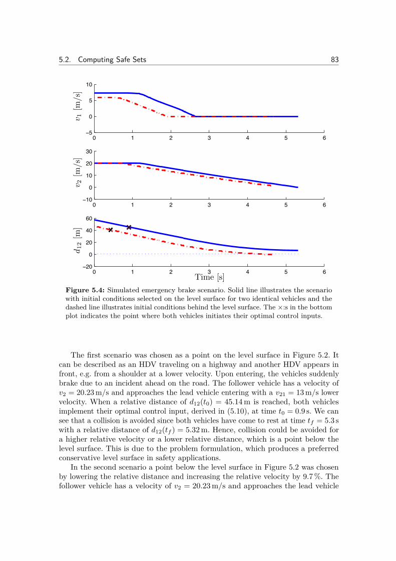
5.2. Computing Safe Sets 83
0 1 2 3 4 5 6ï�
0
5
10
0 1 2 3 4 5 6�
0
10
20
30
0 1 2 3 4 5 6�
0
20
40
60
v 1[m
/s]
v 2[m
/s]
d 12
[m]
Time [s]
Figure 5.4: Simulated emergency brake scenario. Solid line illustrates the scenariowith initial conditions selected on the level surface for two identical vehicles and thedashed line illustrates initial conditions behind the level surface. The ◊:s in the bottomplot indicates the point where both vehicles initiates their optimal control inputs.
The first scenario was chosen as a point on the level surface in Figure 5.2. Itcan be described as an HDV traveling on a highway and another HDV appears infront, e.g. from a shoulder at a lower velocity. Upon entering, the vehicles suddenlybrake due to an incident ahead on the road. The follower vehicle has a velocity ofv
2
= 20.23 m/s and approaches the lead vehicle entering with a v21
= 13 m/s lowervelocity. When a relative distance of d
12
(t0
) = 45.14 m is reached, both vehiclesimplement their optimal control input, derived in (5.10), at time t
0
= 0.9 s. We cansee that a collision is avoided since both vehicles have come to rest at time tf = 5.3 swith a relative distance of d
12
(tf ) = 5.32 m. Hence, collision could be avoided fora higher relative velocity or a lower relative distance, which is a point below thelevel surface. This is due to the problem formulation, which produces a preferredconservative level surface in safety applications.
In the second scenario a point below the level surface in Figure 5.2 was chosenby lowering the relative distance and increasing the relative velocity by 9.7 %. Thefollower vehicle has a velocity of v
2
= 20.23 m/s and approaches the lead vehicle
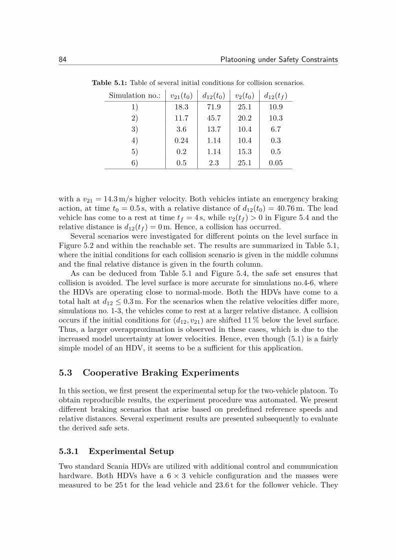
84 Platooning under Safety Constraints
Table 5.1: Table of several initial conditions for collision scenarios.
Simulation no.: v21
(t0
) d12
(t0
) v2
(t0
) d12
(tf )1) 18.3 71.9 25.1 10.92) 11.7 45.7 20.2 10.33) 3.6 13.7 10.4 6.74) 0.24 1.14 10.4 0.35) 0.2 1.14 15.3 0.56) 0.5 2.3 25.1 0.05
with a v21
= 14.3 m/s higher velocity. Both vehicles intiate an emergency brakingaction, at time t
0
= 0.5 s, with a relative distance of d12
(t0
) = 40.76 m. The leadvehicle has come to a rest at time tf = 4 s, while v
2
(tf ) > 0 in Figure 5.4 and therelative distance is d
12
(tf ) = 0 m. Hence, a collision has occurred.Several scenarios were investigated for di�erent points on the level surface in
Figure 5.2 and within the reachable set. The results are summarized in Table 5.1,where the initial conditions for each collision scenario is given in the middle columnsand the final relative distance is given in the fourth column.
As can be deduced from Table 5.1 and Figure 5.4, the safe set ensures thatcollision is avoided. The level surface is more accurate for simulations no.4-6, wherethe HDVs are operating close to normal-mode. Both the HDVs have come to atotal halt at d
12
Æ 0.3 m. For the scenarios when the relative velocities di�er more,simulations no. 1-3, the vehicles come to rest at a larger relative distance. A collisionoccurs if the initial conditions for (d
12
, v21
) are shifted 11 % below the level surface.Thus, a larger overapproximation is observed in these cases, which is due to theincreased model uncertainty at lower velocities. Hence, even though (5.1) is a fairlysimple model of an HDV, it seems to be a su�cient for this application.
5.3 Cooperative Braking Experiments
In this section, we first present the experimental setup for the two-vehicle platoon. Toobtain reproducible results, the experiment procedure was automated. We presentdi�erent braking scenarios that arise based on predefined reference speeds andrelative distances. Several experiment results are presented subsequently to evaluatethe derived safe sets.
5.3.1 Experimental SetupTwo standard Scania HDVs are utilized with additional control and communicationhardware. Both HDVs have a 6 ◊ 3 vehicle configuration and the masses weremeasured to be 25 t for the lead vehicle and 23.6 t for the follower vehicle. They
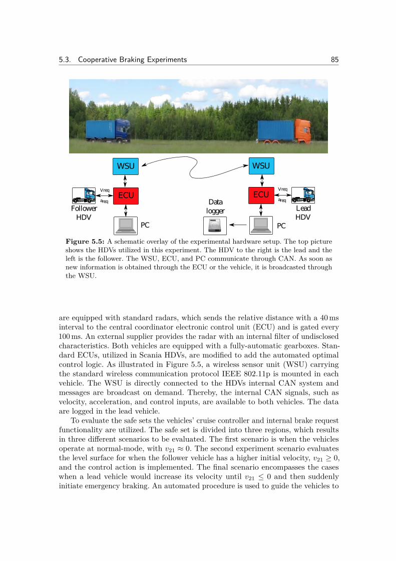
5.3. Cooperative Braking Experiments 85
����
����
���
�����
����
���
����� �����
� �
�� �������
�������
Figure 5.5: A schematic overlay of the experimental hardware setup. The top pictureshows the HDVs utilized in this experiment. The HDV to the right is the lead and theleft is the follower. The WSU, ECU, and PC communicate through CAN. As soon asnew information is obtained through the ECU or the vehicle, it is broadcasted throughthe WSU.
are equipped with standard radars, which sends the relative distance with a 40 msinterval to the central coordinator electronic control unit (ECU) and is gated every100 ms. An external supplier provides the radar with an internal filter of undisclosedcharacteristics. Both vehicles are equipped with a fully-automatic gearboxes. Stan-dard ECUs, utilized in Scania HDVs, are modified to add the automated optimalcontrol logic. As illustrated in Figure 5.5, a wireless sensor unit (WSU) carryingthe standard wireless communication protocol IEEE 802.11p is mounted in eachvehicle. The WSU is directly connected to the HDVs internal CAN system andmessages are broadcast on demand. Thereby, the internal CAN signals, such asvelocity, acceleration, and control inputs, are available to both vehicles. The dataare logged in the lead vehicle.
To evaluate the safe sets the vehicles’ cruise controller and internal brake requestfunctionality are utilized. The safe set is divided into three regions, which resultsin three di�erent scenarios to be evaluated. The first scenario is when the vehiclesoperate at normal-mode, with v
21
¥ 0. The second experiment scenario evaluatesthe level surface for when the follower vehicle has a higher initial velocity, v
21
Ø 0,and the control action is implemented. The final scenario encompasses the caseswhen a lead vehicle would increase its velocity until v
21
Æ 0 and then suddenlyinitiate emergency braking. An automated procedure is used to guide the vehicles to
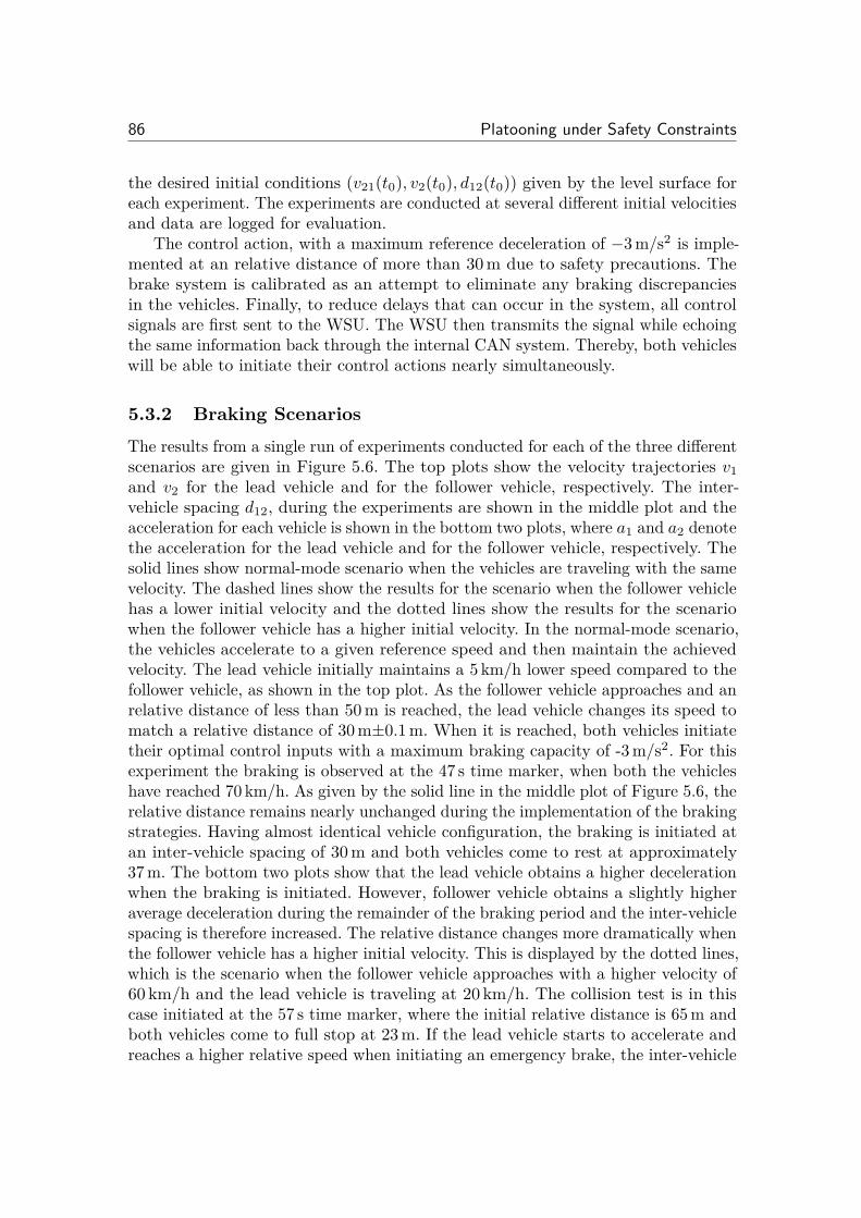
86 Platooning under Safety Constraints
the desired initial conditions (v21
(t0
), v2
(t0
), d12
(t0
)) given by the level surface foreach experiment. The experiments are conducted at several di�erent initial velocitiesand data are logged for evaluation.
The control action, with a maximum reference deceleration of ≠3 m/s2 is imple-mented at an relative distance of more than 30 m due to safety precautions. Thebrake system is calibrated as an attempt to eliminate any braking discrepanciesin the vehicles. Finally, to reduce delays that can occur in the system, all controlsignals are first sent to the WSU. The WSU then transmits the signal while echoingthe same information back through the internal CAN system. Thereby, both vehicleswill be able to initiate their control actions nearly simultaneously.
5.3.2 Braking ScenariosThe results from a single run of experiments conducted for each of the three di�erentscenarios are given in Figure 5.6. The top plots show the velocity trajectories v
1
and v2
for the lead vehicle and for the follower vehicle, respectively. The inter-vehicle spacing d
12
, during the experiments are shown in the middle plot and theacceleration for each vehicle is shown in the bottom two plots, where a
1
and a2
denotethe acceleration for the lead vehicle and for the follower vehicle, respectively. Thesolid lines show normal-mode scenario when the vehicles are traveling with the samevelocity. The dashed lines show the results for the scenario when the follower vehiclehas a lower initial velocity and the dotted lines show the results for the scenariowhen the follower vehicle has a higher initial velocity. In the normal-mode scenario,the vehicles accelerate to a given reference speed and then maintain the achievedvelocity. The lead vehicle initially maintains a 5 km/h lower speed compared to thefollower vehicle, as shown in the top plot. As the follower vehicle approaches and anrelative distance of less than 50 m is reached, the lead vehicle changes its speed tomatch a relative distance of 30 m±0.1 m. When it is reached, both vehicles initiatetheir optimal control inputs with a maximum braking capacity of -3 m/s2. For thisexperiment the braking is observed at the 47 s time marker, when both the vehicleshave reached 70 km/h. As given by the solid line in the middle plot of Figure 5.6, therelative distance remains nearly unchanged during the implementation of the brakingstrategies. Having almost identical vehicle configuration, the braking is initiated atan inter-vehicle spacing of 30 m and both vehicles come to rest at approximately37 m. The bottom two plots show that the lead vehicle obtains a higher decelerationwhen the braking is initiated. However, follower vehicle obtains a slightly higheraverage deceleration during the remainder of the braking period and the inter-vehiclespacing is therefore increased. The relative distance changes more dramatically whenthe follower vehicle has a higher initial velocity. This is displayed by the dotted lines,which is the scenario when the follower vehicle approaches with a higher velocity of60 km/h and the lead vehicle is traveling at 20 km/h. The collision test is in thiscase initiated at the 57 s time marker, where the initial relative distance is 65 m andboth vehicles come to full stop at 23 m. If the lead vehicle starts to accelerate andreaches a higher relative speed when initiating an emergency brake, the inter-vehicle
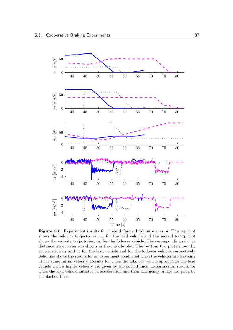
5.3. Cooperative Braking Experiments 87
40 45 50 55 60 65 70 75 800
50
40 45 50 55 60 65 70 75 800
50
40 45 50 55 60 65 70 75 800
50
40 45 50 55 60 65 70 75 80-4
-2
0
40 45 50 55 60 65 70 75 80-4
-2
0
d1
2
[m]
a1
[m/s
2
]a
2
[m/s
2
]
Time [s]
v 2[k
m/h
]v 1
[km
/h
]
Figure 5.6: Experiment results for three di�erent braking scenarios. The top plotshows the velocity trajectories, v1, for the lead vehicle and the second to top plotshows the velocity trajectories, v2, for the follower vehicle. The corresponding relativedistance trajectories are shown in the middle plot. The bottom two plots show theacceleration a1 and a2 for the lead vehicle and for the follower vehicle, respectively.Solid line shows the results for an experiment conducted when the vehicles are travelingat the same initial velocity. Results for when the follower vehicle approaches the leadvehicle with a higher velocity are given by the dotted lines. Experimental results forwhen the lead vehicle initiates an acceleration and then emergency brakes are given bythe dashed lines.
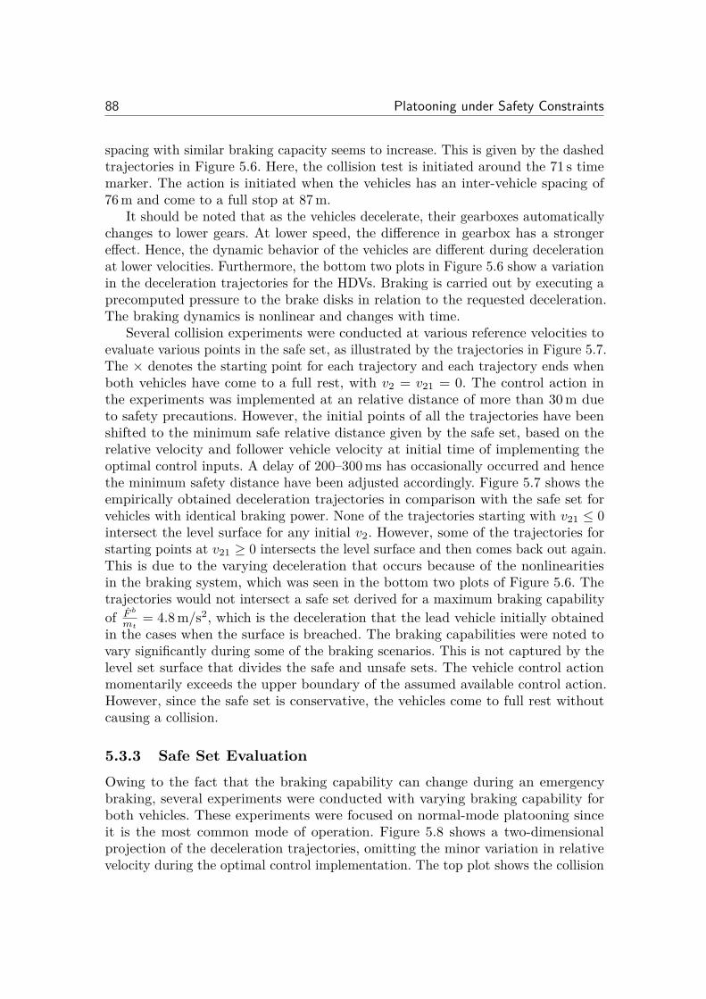
88 Platooning under Safety Constraints
spacing with similar braking capacity seems to increase. This is given by the dashedtrajectories in Figure 5.6. Here, the collision test is initiated around the 71 s timemarker. The action is initiated when the vehicles has an inter-vehicle spacing of76 m and come to a full stop at 87 m.
It should be noted that as the vehicles decelerate, their gearboxes automaticallychanges to lower gears. At lower speed, the di�erence in gearbox has a strongere�ect. Hence, the dynamic behavior of the vehicles are di�erent during decelerationat lower velocities. Furthermore, the bottom two plots in Figure 5.6 show a variationin the deceleration trajectories for the HDVs. Braking is carried out by executing aprecomputed pressure to the brake disks in relation to the requested deceleration.The braking dynamics is nonlinear and changes with time.
Several collision experiments were conducted at various reference velocities toevaluate various points in the safe set, as illustrated by the trajectories in Figure 5.7.The ◊ denotes the starting point for each trajectory and each trajectory ends whenboth vehicles have come to a full rest, with v
2
= v21
= 0. The control action inthe experiments was implemented at an relative distance of more than 30 m dueto safety precautions. However, the initial points of all the trajectories have beenshifted to the minimum safe relative distance given by the safe set, based on therelative velocity and follower vehicle velocity at initial time of implementing theoptimal control inputs. A delay of 200–300 ms has occasionally occurred and hencethe minimum safety distance have been adjusted accordingly. Figure 5.7 shows theempirically obtained deceleration trajectories in comparison with the safe set forvehicles with identical braking power. None of the trajectories starting with v
21
Æ 0intersect the level surface for any initial v
2
. However, some of the trajectories forstarting points at v
21
Ø 0 intersects the level surface and then comes back out again.This is due to the varying deceleration that occurs because of the nonlinearitiesin the braking system, which was seen in the bottom two plots of Figure 5.6. Thetrajectories would not intersect a safe set derived for a maximum braking capabilityof ˆF b
mt= 4.8 m/s2, which is the deceleration that the lead vehicle initially obtained
in the cases when the surface is breached. The braking capabilities were noted tovary significantly during some of the braking scenarios. This is not captured by thelevel set surface that divides the safe and unsafe sets. The vehicle control actionmomentarily exceeds the upper boundary of the assumed available control action.However, since the safe set is conservative, the vehicles come to full rest withoutcausing a collision.
5.3.3 Safe Set EvaluationOwing to the fact that the braking capability can change during an emergencybraking, several experiments were conducted with varying braking capability forboth vehicles. These experiments were focused on normal-mode platooning sinceit is the most common mode of operation. Figure 5.8 shows a two-dimensionalprojection of the deceleration trajectories, omitting the minor variation in relativevelocity during the optimal control implementation. The top plot shows the collision
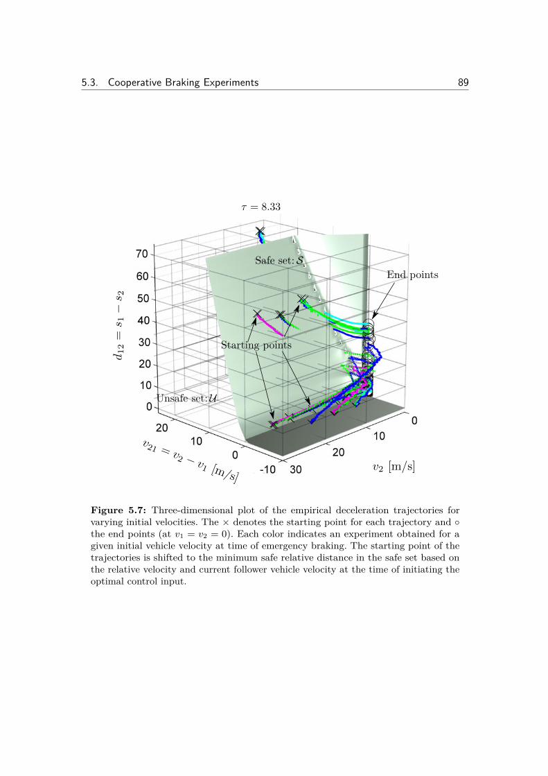
5.3. Cooperative Braking Experiments 89
d 12
=s 1
�s 2
v21 = v2 � v1 [m/s]v2 [m/s]
Safe set: S
Starting points
End points
Unsafe set: U
· = 8.33
Figure 5.7: Three-dimensional plot of the empirical deceleration trajectories forvarying initial velocities. The ◊ denotes the starting point for each trajectory and ¶the end points (at v1 = v2 = 0). Each color indicates an experiment obtained for agiven initial vehicle velocity at time of emergency braking. The starting point of thetrajectories is shifted to the minimum safe relative distance in the safe set based onthe relative velocity and current follower vehicle velocity at the time of initiating theoptimal control input.
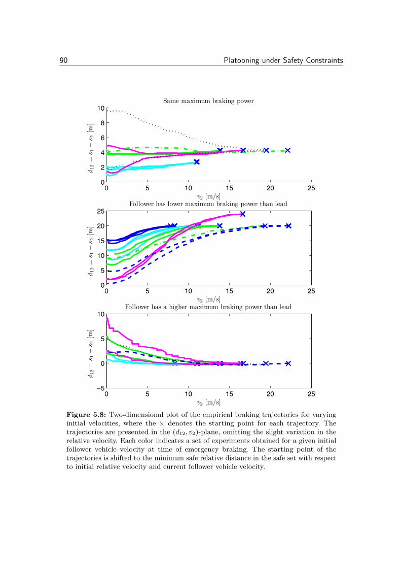
90 Platooning under Safety Constraints
0 5 10 15 20 250
2
4
6
8
10
v2 [m/s]
=s 1
�s 2
[m]
Same maximum braking power
0 5 10 15 20 250
5
10
15
20
25
v2 [m/s]
=s 1
�s 2
[m]
Follower has lower maximum braking power than lead
0 5 10 15 20 25ï�
0
5
10
v2 [m/s]
=s 1
�s 2
[m]
Follower has a higher maximum braking power than lead
d 12
d 12
d 12
Figure 5.8: Two-dimensional plot of the empirical braking trajectories for varyinginitial velocities, where the ◊ denotes the starting point for each trajectory. Thetrajectories are presented in the (d12, v2)-plane, omitting the slight variation in therelative velocity. Each color indicates a set of experiments obtained for a given initialfollower vehicle velocity at time of emergency braking. The starting point of thetrajectories is shifted to the minimum safe relative distance in the safe set with respectto initial relative velocity and current follower vehicle velocity.
5.4. Summary 91
tests for varying initial velocities and similar vehicle braking capacity. It can beseen that the relative distance remains fairly constant throughout the collision tests.However, below a velocity of 5 m/s the vehicles starts changing gears, which has aclear impact on the vehicle dynamics. The model for deriving the safe sets does nottake gear change logic into consideration. Nevertheless, the safe sets are conservativeand a collision is hence still avoided. The middle plot, in Figure 5.8, shows thedeceleration trajectories for when the follower vehicle has a 30–40 % lower brakingcapacity. It can be seen that the relative distance is constantly decreasing. Most ofthe trajectories end with both vehicles at rest and still a few meters to spare. Finally,the bottom plot shows the deceleration trajectories for when the follower vehiclehas a 20–30 % higher braking capacity. It can be seen that the relative distanceremains the same or increases, which is congruent with the results obtained from thecorresponding safe set. Hence, if the follower vehicle has a higher braking capacity, arelative distance within decimeters could have been maintained with the presentedsystem and still no collision would have occurred.
5.4 Summary
It is fuel e�cient to drive vehicles closely spaced to each other due to the inherent airdrag reduction, as was shown in Chapter 4. A minimum distance for two HDVs canbe deduced with respect to a compact set of controller actions without increasingthe the risk of a collision despite the worst possible action by the vehicle ahead.Thus, if the minimum distance is determined for each vehicle pair, a collision canbe avoided throughout the platoon. During normal-mode operation a minimumdistance of 1.2 m should be maintained to ensure that a collision can be avoidedfor two identical vehicles when no delay is present in the system. Delays can beaccounted for in the reachable set formulation through a simple translation. Thederived minimum possible relative distance with a measured worst-case delay of500 ms in this chapter for identical vehicles is 2 m, which is lower compared to whatis utilized in commercial applications today.
A stronger overall braking capability in the follower vehicle creates the possibilityof reducing the relative distance further. Thus, in platooning applications, theresults suggest that HDVs with stronger braking capabilities should always be placedbehind to enable the shortest possible relative distance without compromising safety.However, this might be contrary to fuel-e�cient control criteria, where the followerHDV should have less stringent control actions.
Even though the model and the procedure utilized for deriving the safe setsdo not encompass all nonlinear features of an HDV in motion, the sets serve as areliable reference to ensure that a collision can be avoided. Both theoretical andempirical results show that it is suitable to order HDVs according to increasingbraking capacity. Thereby, the inter-vehicle spacing can be reduced significantlywithout compromising safety. Naturally, it only holds under the assumption thatthe relative distance and velocity is available through reliable V2V communication
92 Platooning under Safety Constraints
or that radar measurements are obtainable.The experimental results presented in this chapter indicates that the derived
safety sets are least conservative for platoons traveling under normal operationalmode. The presented method forms a conservative safety set. Therefore, uncertaintiesfrom unmodeled dynamics do not cause a collision, as was seen in the experimentalresults. Hence, V2V communication enables HDVs to operate at very small inter-vehicle spacing.
Chapter 6
Decentralized Cooperative Control forPlatooning
“It is the weight, not numbers of experiments that is to be regarded.”Isaac Newton
The objective in heavy-duty vehicle (HDV) platooning is to maintain a prede-fined inter-vehicle spacing policy to the surrounding vehicles. With the aid ofvehicle-to-vehicle (V2V) communication, vehicle characteristics and events,
such as emergency braking, can be transmitted within radio range. Therefore, aminimum distance, far less than what is utilized in todays commercial systems,between two HDVs can be calculated with respect to a compact set of controlleractions without increasing the risk of a collision despite the worst possible scenariodisplayed by the vehicle ahead. By traveling at a short relative distance to an HDV,the air drag is reduced substantially. Thus, a significant reduction in fuel consump-tion can be obtained. The e�ort needed to maintain the desired relative velocityvaries with the relative distance. This creates a coupling of the dynamics betweenvehicles throughout the platoon. However, the control becomes increasingly stringentwith shorter relative distance. Thereby, the fuel consumption increases due to theadditional control e�ort, produced by the existing control systems, for maintainingthe relative distance. Hence, it is of considerable interest for the industry to producea new fuel-optimal control. The question of whether to implement a centralized,decentralized, or some combination of the control strategies then naturally arises.
The main motivation for considering a decentralized controller is the limitedcommunication range that can be achieved in practice. It is di�cult to realize acentralized controller under such constraints. Using a centralized controller is onlypossible if all the global states and system parameters are known to every vehicle inthe platoon. In that case, a central unit, for example a vehicle in the platoon or a roadside unit, determines the control actions for all the vehicles in the platoon. Therefore,a centralized control scheme requires an increase in communication with the number
93
94 Decentralized Cooperative Control for Platooning
of vehicles in the platoon. Furthermore, package drops or outages can occur inwireless transmission. A centralized system is more sensitive to communication delaysand physical limitations on the radio range. It is often not realistic to assume thatevery vehicle in the platoon knows the state of every other vehicle instantaneouslydue to physical constraints in the information flow. It is, however, reasonable toassume that a vehicle is able to communicate with some vehicles within a givenrange. Hence, a decentralized strategy is suitable, where every vehicle determinesits own control actions based on local information. Furthermore, a decentralizedlongitudinal control is practical to ensure scalability and robustness. However, othercontrol applications, such as route assigning, coordinating, ordering and mergingseveral platoons, are not time and information critical operations and thus suitableas centralized control strategies.
The main contribution of this chapter is to derive a decentralized controllerfor HDV platooning. We establish empirical performance results for the presentedcontrol design and present a qualitative verification of the transient dynamics inthe simulation model that is presented in Section 3.2. We present a linear quadraticcontrol framework for the design of a high-level cooperative platooning controllersuitable for modern HDVs, which imposes a lower block-diagonal structure on thefeedback gain matrix. We also consider realistic response delays for the low-levelcontroller that governs the engine. The controller performance is evaluated throughnumerical and experimental studies. It is shown that the proposed controller allowsfor short time headways to achieve fuel e�ciency, without compromising safety.
Several studies on vehicle platooning have been based on simplified theoreticalmodels. However, as shown in this chapter, delays and nonlinear dynamics cansignificantly influence the closed-loop system. We present a method for designingsuboptimal decentralized feedback controllers, with low computational complexity,that takes dynamic coupling and engine response delays into consideration. Thecontroller performance is evaluated through implementation on commercial HDVs.The design method is scalable in the sense that an additional vehicle can be added atthe tail of the platoon without mandating a change in the controllers of the alreadyplatooning vehicles. As modern HDVs in general have two separate low-level controlsystems for governing the longitudinal propulsion and deceleration of the vehicle,the engine management system (EMS) and the brake management system (BMS),we present a simple bumpless transfer scheme to switch between these systems.The proposed platooning controller can be easily implemented on modern HDVswithout requiring any changes in the already existing vehicle architecture. We showthat the controller behaves well even when performing outside the linear regionof operation. We also show that the proposed controller attenuates the e�ect ofdisturbances downstream in the platoon, when studying scenarios that commonlyoccur on highways with dynamic operating conditions and physical constraints.Experimental results are given to qualitatively validate the proposed control systembehavior. The experiments have been conducted on a test site south of Stockholm,using HDVs provided by Scania CV AB.
The outline of this chapter is as follows. We start by giving a short summary of
6.1. System Model 95
the system model in Section 6.1 and present a translation of the platoon performancecriteria into quadratic costs. In Section 6.2 we develop a method for deriving theproposed decentralized controllers and then give a simple bumpless transfer scheme,based on performance and driver acceptance, for switching between the low-levelEMS and BMS controllers. We also provide guidelines for how to set the weightparameters for the proposed controller. Simulation results are given in Section 6.3to determine and evaluate the chosen weight parameters for the controller. Theexperimental setup based on three HDVs is presented in Section 6.4 together with theexperimental results. The chapter is concluded with a brief summary in Section 6.5.
6.1 System Model
In this section, we present the models that serve as the basis for the controller designpresented in Section 6.2. First a brief description of the longitudinal model of avehicle traveling in a platoon is given. The longitudinal model is then extended todescribe the dynamics of an HDV platoon. Then, we present a simple model for thevehicle engine system dynamics. Finally, we form the platoon model by combiningand discretizing all the presented models. Recall that details of the vehicle model,the characteristic coe�cients, and its derivation can be found in Chapter 3.
Let i = 1, . . . , N denote the vehicle order in the platoon. Applying Newton’ssecond law of motion along with all the external forces described above, a nonlinearvehicle model is derived as
s1
= v1
mt1 v
1
= F e
1
≠ F b
1
≠ F a
1
(v1
) ≠ F r
1
(–(s1
)) ≠ F g
1
(–(s1
))= ke
1
T e
1
(Êe1 , ”
1
) ≠ F b
1
≠ kd
1
v2
1
≠ kr
1
cos –(s1
) ≠ kg
1
sin –(s1
)si = vi
mti vi = F e
i ≠ F b
i ≠ F a
i (vi, di≠1,i) ≠ F r
i (–(si)) ≠ F g
i (–(si))= ke
i T e
i (Êi, ”i) ≠ F b
i ≠ kd
i �(di≠1,i)v2
i ≠ kr
i cos –(si) ≠ kg
i sin –(si)
(6.1)
where i = 2, . . . , N , si is the absolute traveled distance for HDV i from a referencepoint common to all vehicles in the platoon, di≠1,i = si≠1
≠ si is introduced asthe relative distance between ith vehicle its preceding vehicle for convenience, vi
is the velocity, mti is the total inertial mass, F e
i Ø 0 denotes the force producedby the engine through fuel injection, F b
i Ø 0 denotes the braking force, and kli,
l œ {e, d, r, g}, are characteristic coe�cients. Moreover, F a
i , F r
i , and F g
i denotethe external air drag, rolling resistance, and gravitational forces acting upon thevehicle, respectively, and �(di≠1,i) denotes the empirically derived nonlinear airdrag reduction due to a preceding vehicle. The control input T e
i is the net enginetorque, which is a function of the engine angular velocity Ê
ei and the injected fuelamount ”i. It is determined by the EMS, which receives a velocity request as aninput. Furthermore, the control input F b
i is determined through the BMS, which
96 Decentralized Cooperative Control for Platooning
receives an acceleration demand as an input. The EMS determines the requiredfuel injection to produce the necessary propulsion torque for achieving the velocityinput to the system. Similarly, the BMS determines the required force that needsto be generated to obtain the acceleration input to the system. To account for theadditional system dynamics produced by the EMS, for simplicity, its computedcontrol input is modeled as
Tei = Kc
i (ei + 1T I
i
⁄eidt), (6.2)
where ei = vref
i ≠ vi and Kc
i , T I
i are design parameters that are set according to theengine type. By inserting the model for the EMS into (6.1), the nonlinear systemmodel for a single HDV in a platoon is given as
mti vi =ke
i Kc
i
!ei + 1
T I
i
⁄eidt
"≠ kd
i Ï(di≠1,i)v2
i ≠ kr
i cos –i ≠ kg
i sin –i
=ke
i Kc
i vref
i ≠ ke
i Kc
i v + zv
i ≠ kd
i Ï(di≠1,i)v2 ≠ kr
i cos –i ≠ kg
i sin –i,
zv
i =ke
i Kc
i
T I
i
ei
(6.3)
where vref
i is the control input to the EMS and zv
i is an integral state in the EMSmodel. The vehicle dynamics with the BMS is significantly faster, since a relativelylarge deceleration force can be produced by the brake system. Thus, it is assumedthat the input to the BMS is obtained instantaneously, hence the nonlinear systemmodel during braking is given as
mti vi = maref
i ≠ kd
i �(di≠1,i)v2
i ≠ kr
i cos –i ≠ kg
i sin –i (6.4)
where aref
i is the input signal to the BMS.
6.1.1 Platoon ModelHere, we develop a model to capture the platoon dynamics. We first introduce thediscrete states
zv
i (k + 1) = zv
i (k) + Ts’i(vref
i (k) ≠ vi(k)),di≠1,i(k + 1) = di≠1,i(k) + Ts(vi≠1
(k) ≠ vi(k)),zd
i≠1,i(k + 1) = zd
i≠1,i(k) + Ts(di≠1,i(k) ≠ ·vi(k)),(6.5)
where ’i = keiKci /mtiT
Ii , Ts is the sampling time, · is the time headway constant,
and zd
i≠1,i is the integral action for maintaining the time headway policy. Let thestate vector be partioned as
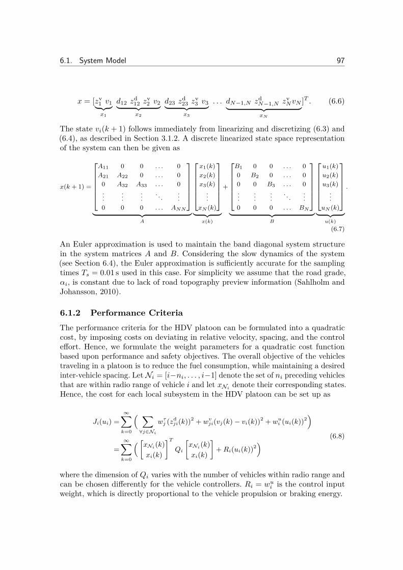
6.1. System Model 97
x = [zv
1
v1¸ ˚˙ ˝
x1
d12
zd
12
zv
2
v2¸ ˚˙ ˝
x2
d23
zd
23
zv
3
v3¸ ˚˙ ˝
x3
. . . dN≠1,N zd
N≠1,N zv
N vN¸ ˚˙ ˝xN
]T . (6.6)
The state vi(k + 1) follows immediately from linearizing and discretizing (6.3) and(6.4), as described in Section 3.1.2. A discrete linearized state space representationof the system can then be given as
x(k + 1) =
S
WWWWU
A11 0 0 . . . 0A21 A22 0 . . . 0
0 A32 A33 . . . 0...
......
. . ....
0 0 0 . . . A
NN
T
XXXXV
¸ ˚˙ ˝A
S
WWWWU
x1(k)x2(k)x3(k)
...x
N
(k)
T
XXXXV
¸ ˚˙ ˝x(k)
+
S
WWWWU
B1 0 0 . . . 00 B2 0 . . . 00 0 B3 . . . 0...
......
. . ....
0 0 0 . . . B
N
T
XXXXV
¸ ˚˙ ˝B
S
WWWWU
u1(k)u2(k)u3(k)
...u
N
(k)
T
XXXXV
¸ ˚˙ ˝u(k)
.
(6.7)
An Euler approximation is used to maintain the band diagonal system structurein the system matrices A and B. Considering the slow dynamics of the system(see Section 6.4), the Euler approximation is su�ciently accurate for the samplingtimes Ts = 0.01 s used in this case. For simplicity we assume that the road grade,–i, is constant due to lack of road topography preview information (Sahlholm andJohansson, 2010).
6.1.2 Performance CriteriaThe performance criteria for the HDV platoon can be formulated into a quadraticcost, by imposing costs on deviating in relative velocity, spacing, and the controle�ort. Hence, we formulate the weight parameters for a quadratic cost functionbased upon performance and safety objectives. The overall objective of the vehiclestraveling in a platoon is to reduce the fuel consumption, while maintaining a desiredinter-vehicle spacing. Let Ni = [i≠ni, . . . , i≠1] denote the set of ni preceding vehiclesthat are within radio range of vehicle i and let xNi denote their corresponding states.Hence, the cost for each local subsystem in the HDV platoon can be set up as
J
i
(ui
) =Œÿ
k=0
1 ÿ
’jœNi
w
·
j
(zdji
(k))2 + w
v
ji
(vj
(k) ≠ v
i
(k))2 + w
u
i
(ui
(k))22
=Œÿ
k=0
1 5xNi (k)x
i
(k)
6T
Q
i
5xNi (k)x
i
(k)
6+ R
i
(ui
(k))22 (6.8)
where the dimension of Qi varies with the number of vehicles within radio range andcan be chosen di�erently for the vehicle controllers. Ri = wu
i is the control inputweight, which is directly proportional to the vehicle propulsion or braking energy.
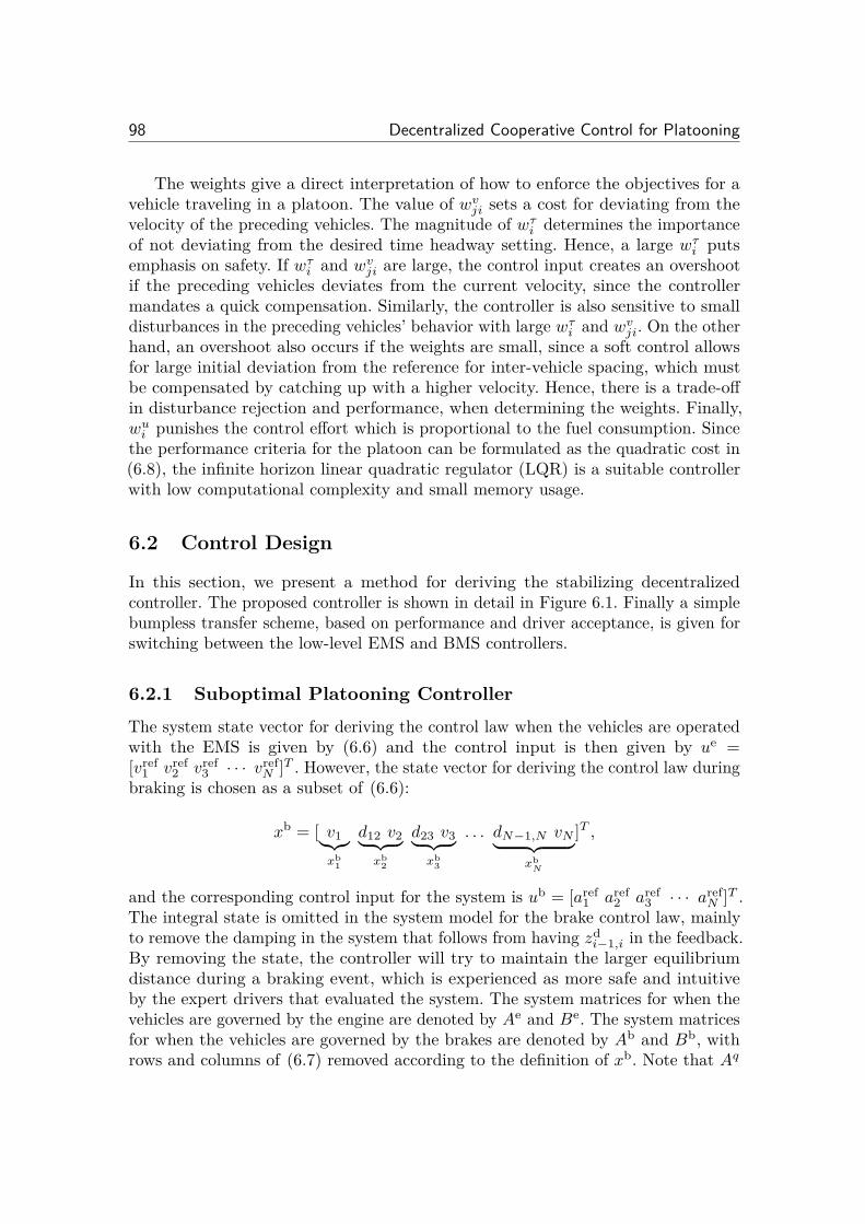
98 Decentralized Cooperative Control for Platooning
The weights give a direct interpretation of how to enforce the objectives for avehicle traveling in a platoon. The value of wv
ji sets a cost for deviating from thevelocity of the preceding vehicles. The magnitude of w·
i determines the importanceof not deviating from the desired time headway setting. Hence, a large w·
i putsemphasis on safety. If w·
i and wvji are large, the control input creates an overshoot
if the preceding vehicles deviates from the current velocity, since the controllermandates a quick compensation. Similarly, the controller is also sensitive to smalldisturbances in the preceding vehicles’ behavior with large w·
i and wvji. On the other
hand, an overshoot also occurs if the weights are small, since a soft control allowsfor large initial deviation from the reference for inter-vehicle spacing, which mustbe compensated by catching up with a higher velocity. Hence, there is a trade-o�in disturbance rejection and performance, when determining the weights. Finally,wu
i punishes the control e�ort which is proportional to the fuel consumption. Sincethe performance criteria for the platoon can be formulated as the quadratic cost in(6.8), the infinite horizon linear quadratic regulator (LQR) is a suitable controllerwith low computational complexity and small memory usage.
6.2 Control Design
In this section, we present a method for deriving the stabilizing decentralizedcontroller. The proposed controller is shown in detail in Figure 6.1. Finally a simplebumpless transfer scheme, based on performance and driver acceptance, is given forswitching between the low-level EMS and BMS controllers.
6.2.1 Suboptimal Platooning ControllerThe system state vector for deriving the control law when the vehicles are operatedwith the EMS is given by (6.6) and the control input is then given by ue =[vref
1
vref
2
vref
3
· · · vref
N ]T . However, the state vector for deriving the control law duringbraking is chosen as a subset of (6.6):
xb = [ v1¸˚˙˝
xb1
d12
v2¸ ˚˙ ˝
xb2
d23
v3¸ ˚˙ ˝
xb3
. . . dN≠1,N vN¸ ˚˙ ˝xb
N
]T ,
and the corresponding control input for the system is ub = [aref
1
aref
2
aref
3
· · · aref
N ]T .The integral state is omitted in the system model for the brake control law, mainlyto remove the damping in the system that follows from having zd
i≠1,i in the feedback.By removing the state, the controller will try to maintain the larger equilibriumdistance during a braking event, which is experienced as more safe and intuitiveby the expert drivers that evaluated the system. The system matrices for when thevehicles are governed by the engine are denoted by Ae and Be. The system matricesfor when the vehicles are governed by the brakes are denoted by Ab and Bb, withrows and columns of (6.7) removed according to the definition of xb. Note that Aq
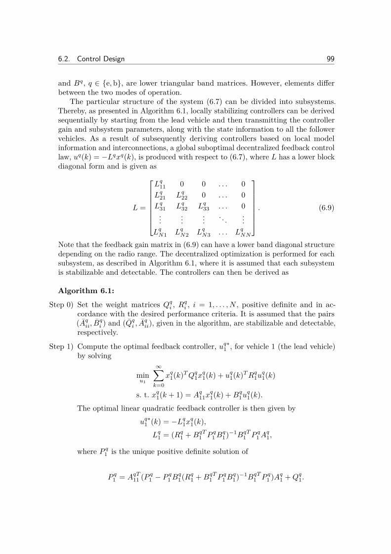
6.2. Control Design 99
and Bq, q œ {e, b}, are lower triangular band matrices. However, elements di�erbetween the two modes of operation.
The particular structure of the system (6.7) can be divided into subsystems.Thereby, as presented in Algorithm 6.1, locally stabilizing controllers can be derivedsequentially by starting from the lead vehicle and then transmitting the controllergain and subsystem parameters, along with the state information to all the followervehicles. As a result of subsequently deriving controllers based on local modelinformation and interconnections, a global suboptimal decentralized feedback controllaw, uq(k) = ≠Lqxq(k), is produced with respect to (6.7), where L has a lower blockdiagonal form and is given as
L =
S
WWWWWWU
Lq11
0 0 . . . 0Lq
21
Lq22
0 . . . 0Lq
31
Lq32
Lq33
. . . 0...
...... . . . ...
LqN1
LqN2
LqN3
. . . LqNN
T
XXXXXXV. (6.9)
Note that the feedback gain matrix in (6.9) can have a lower band diagonal structuredepending on the radio range. The decentralized optimization is performed for eachsubsystem, as described in Algorithm 6.1, where it is assumed that each subsystemis stabilizable and detectable. The controllers can then be derived as
Algorithm 6.1:
Step 0) Set the weight matrices Qqi , Rq
i , i = 1, . . . , N , positive definite and in ac-cordance with the desired performance criteria. It is assumed that the pairs(Aq
ii, Bqi ) and (Qq
i , Aqii), given in the algorithm, are stabilizable and detectable,
respectively.
Step 1) Compute the optimal feedback controller, uqú1
, for vehicle 1 (the lead vehicle)by solving
minu1
Œÿ
k=0
xq1
(k)T Qq1
xq1
(k) + uq1
(k)T Rq1
uq1
(k)
s. t. xq1
(k + 1) = Aq11
xq1
(k) + Bq1
uq1
(k).The optimal linear quadratic feedback controller is then given by
uqú1
(k) = ≠Lq1
xq1
(k),Lq
1
= (Rq1
+ BqT1
P q1
Bq1
)≠1BqT1
P q1
Aq1
,
where P q1
is the unique positive definite solution of
P q1
= AqT11
(P q1
≠ P q1
Bq1
(Rq1
+ BqT1
P q1
Bq1
)≠1BqT1
P q1
)Aq1
+ Qq1
.
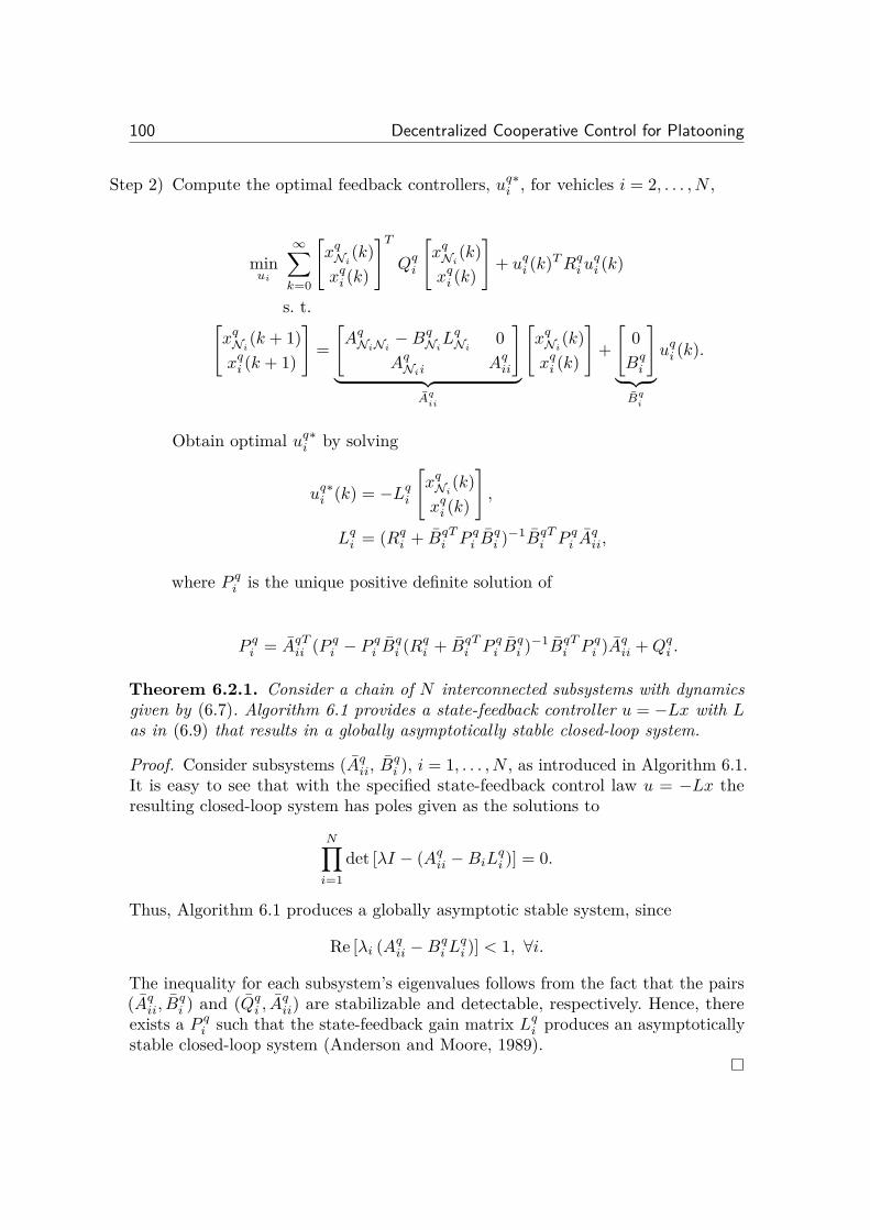
100 Decentralized Cooperative Control for Platooning
Step 2) Compute the optimal feedback controllers, uqúi , for vehicles i = 2, . . . , N ,
minui
Œÿ
k=0
Cxq
Ni(k)
xqi (k)
DT
Qqi
Cxq
Ni(k)
xqi (k)
D+ uq
i (k)T Rqi uq
i (k)
s. t.C
xqNi
(k + 1)xq
i (k + 1)
D=
CAq
NiNi≠ Bq
NiLq
Ni0
AqNii Aq
ii
D
¸ ˚˙ ˝¯Aq
ii
Cxq
Ni(k)
xqi (k)
D+
C0
Bqi
D
¸ ˚˙ ˝¯Bq
i
uqi (k).
Obtain optimal uqúi by solving
uqúi (k) = ≠Lq
i
Cxq
Ni(k)
xqi (k)
D,
Lqi = (Rq
i + BqTi P q
i Bqi )≠1BqT
i P qi Aq
ii,
where P qi is the unique positive definite solution of
P qi = AqT
ii (P qi ≠ P q
i Bqi (Rq
i + BqTi P q
i Bqi )≠1BqT
i P qi )Aq
ii + Qqi .
Theorem 6.2.1. Consider a chain of N interconnected subsystems with dynamicsgiven by (6.7). Algorithm 6.1 provides a state-feedback controller u = ≠Lx with Las in (6.9) that results in a globally asymptotically stable closed-loop system.
Proof. Consider subsystems (Aqii, Bq
i ), i = 1, . . . , N , as introduced in Algorithm 6.1.It is easy to see that with the specified state-feedback control law u = ≠Lx theresulting closed-loop system has poles given as the solutions to
NŸ
i=1
det [⁄I ≠ (Aqii ≠ BiL
qi )] = 0.
Thus, Algorithm 6.1 produces a globally asymptotic stable system, since
Re [⁄i (Aqii ≠ Bq
i Lqi )] < 1, ’i.
The inequality for each subsystem’s eigenvalues follows from the fact that the pairs(Aq
ii, Bqi ) and (Qq
i , Aqii) are stabilizable and detectable, respectively. Hence, there
exists a P qi such that the state-feedback gain matrix Lq
i produces an asymptoticallystable closed-loop system (Anderson and Moore, 1989).
6.2. Control Design 101
Remark 6.2.2. Algorithm 6.1 provides locally optimal state-feedback controllers,given that the linear quadratic controllers for all preceding vehicles are fixed. Thus,the ith vehicle optimizes its controller and obtains the minimum quadratic cost forthe local system under consideration.
Note that even though the spacing states, di≠1,i, between preceding vehicles arenot controllable for an HDV downstream, an LQR solution can still be found sinceit is only required that each vehicle subsystem in Algorithm 6.1 is stabilizable anddetectable. Another advantage of the proposed algorithm is that it is scalable. If anew vehicle would like to join the platoon at the tail, the decentralized platooningcontrollers do not need to be recomputed. Only the joining HDV needs to receiveinformation regarding the parameters, control gains, and states from all the vehicleswithin communication range.
To choose the weights in (6.8), some engineering intuition is needed. One sug-gestion is to choose the weights such that the closed-loop system satisfy a conditionon that disturbances should be attenuated between two neighboring vehicles. Thel2
-condition, a common criterion for string stability (Swaroop, 1994), can be usedas a reference for obtaining a desirable platooning behavior. The l
2
-condition canviewed as a performance measure, which is given as
||Gi(z)||Œ Æ 1, (6.10)
where Gi(z) is the transfer function between two neighboring vehicles, Yi(z) =Gi(z)Yi≠1
(z), || · ||Œ denotes the maximum peak of the frequency response, andYi(z) := Z(yi(k)) is the Z-transform of the discrete-time domain signal yi(k), whichcan either be chosen as the velocity vi(k) or the relative distance di≠1,i(k). Theperformance measure in (6.10) is similar to what was presented by Sheikholeslamand Desoer (1993) and Yamamura and Seto (2006). It states that the energy in thesignal of a disturbance in velocity or relative distance from the preceding vehicleis attenuated by the follower vehicle if satisfied, which is a desirable property forvehicle platoons. It is a weaker condition than the lŒ-string stability condition(Swaroop and Hedrick, 1996), which implies that there exists a bounded set of initialconditions such that the peaks of the spacings errors remain uniformly boundedalong the string of vehicles. If the performance measure in (6.10) is satisfied forall vehicles in the platoon, then it is a su�cient, but not necessary, condition forl2
-string stability.The transfer function between two neighboring vehicles is given as
Gi(z) = eTi
AzI ≠
CAq
i≠1,i≠1
≠ Bqi≠1
Lqi≠1
0Aq
i≠1,i Aqii
D+
C0
Bqi
DLi
B≠1
ei≠1
, (6.11)
where ei is a column vector that extracts the velocity or relative distance of vehiclei, depending on the desired requirements. Hence, after calculating the controller
102 Decentralized Cooperative Control for Platooning
gains Li in Algorithm 6.1, the condition (6.10) can be checked to ensure that thedesired performance is obtained.
Proposition 6.2.3. Consider the transfer function Gi(z) in (6.11). Let {gi(k)}kœNdenote its impulse response. If {gi(k)}kœN does not change sign, then ||Gi(z)||Œ =||Gi(z)||
1
.
Proof. The Z-transform of the impulse response {gi(k)}kœN is given by Gi(z) =qŒk=0
gi(k)z≠k. Considering that Gi(z) is asymptotically stable1, then ||Gi(z)||Œ =supÊœ[0,2fi)
|Gi(ejÊ)|. We have that
||Gi(z)||Œ = supÊ
|Gi(ejÊ)| = supÊ
|Œÿ
k=0
gi(k)e≠jÊk| ÆŒÿ
k=0
|gi(k)| = ||Gi(z)||1
, (6.12)
where the last equality follows from the definition ||Gi||1 =qŒ
k=0
|gi(k)|. Further-more, we have that
||Gi(z)||Œ = supÊ
|Gi(ejÊ)| Ø|Gi(ej0)|
=|Œÿ
k=0
gi(k)| (6.13)
=Œÿ
k=0
|gi(k)| (6.14)
=||Gi(z)||1
, (6.15)
where (6.13) and (6.14) follow from the definition of the Z-transform and the factthat {g(k)}kœN does not change sign, respectively. Combining (6.12) and (6.15)concludes the proof.
Thus, as proved in Proposition 6.2.3, if the sign of the impulse response of thetransfer function (6.11) does not change, the l
2
- and the lŒ-string stability conditionare equivalent, which means that both the maximum peak and the energy of adisturbance in the preceding vehicles’ velocity or relative distance are attenuated.Hence, by satisfying (6.10) in the control design for a single vehicle in the platoon, theerror magnitude can be locally attenuated. Note that if additional HDVs are addedto the tail of the platoon, the transfer function (6.11) will not change and, inherently,the local string stability property is maintained with the proposed decentralizedcontroller design regardless of the number of vehicles that are added.
1All poles are inside the unit circle for a discrete asymptotically stable discrete system
6.2. Control Design 103
6.2.2 Bumpless SwitchingThe objective for introducing bumpless transfer, in addition, is to avoid overshoots,uncomfortable behavior, or even hardware damage, when switching between actua-tion with the EMS and BMS. A rather standard method is followed to do bumplesstransfer as discussed next (Åström and Hägglund, 2006).
It is not fuel-e�cient to brake, since the energy produced through diesel com-bustion is wasted through heat loss produced by the frictional forces in the brakediscs. However, braking must be performed if the preceding vehicle decelerates bybraking or the platooning HDVs are traversing a steep downhill segment withoutany preview information with respect to the upcoming topography (Alam et al.,2013a). Therefore, we propose a control system that switches between engine andbrake control, as illustrated in Figure 6.1.
The decentralized high-level controller, in Figure 6.1, where Le
i and Lb
i areestablished as given in Algorithm 6.1. A maximum velocity is enforced due tolegislation on the speed demand to the EMS, which might saturate the controldemand produced by the Le
i . Hence, an anti-windup filter W , is implemented as
zv
i (k + 1) = zv
i (k) + ’iTs(ei(k) + 1Tt
es(k)) (6.16)
where es = vref
≠ vLQR
and Tt is a design parameter.The switching guards, gi in Figure 6.1, between the three modes of operation
are defined as
g1
: (di≠1,i < —·vi and vi≠1
< vi) or (b = 1 and di≠1,i < ·vi)
g2
: di≠1,i Ø ·vi and vi≠1
Ø vi and b = 0 and ds < di≠1,i
g3
: [vi, di≠1,i, vr]T œ ˆS
g4
: [vi, di≠1,i, vr]T œ S
where b œ {0, 1} is a binary signal that is transmitted if a preceding vehiclebrakes, ds is a minimum allowed spacing for safety, and — œ [0, 1] is a designparameter that determines how much the relative distance is allowed to decreasefrom the reference for inter-vehicle spacing before the brakes should be applied.S = [0, vmax
i ]◊[dmin
i≠1,i, Œ]◊[vmin
r , vmax
r ] denotes a safe set, derived through a gametheoretical formulation for guaranteeing safety in HDV platooning (Alam et al.,2014a), where vr is the relative velocity with respect to the preceding vehicle. Acollision can always be avoided despite the worst-case behavior of the precedingvehicle if the vehicle states are inside the safe set, otherwise, a collision can occur.Hence, if a vehicle reaches the boundary of the safe set, denoted as ˆS, an optimalcollision avoidance brake request, a
s
, is sent to the BMS to guarantee safety with theproposed controller. The collision avoidance is aborted and the less restrictive controlis resumed once the vehicle reaches su�ciently inside the safe set. The controller
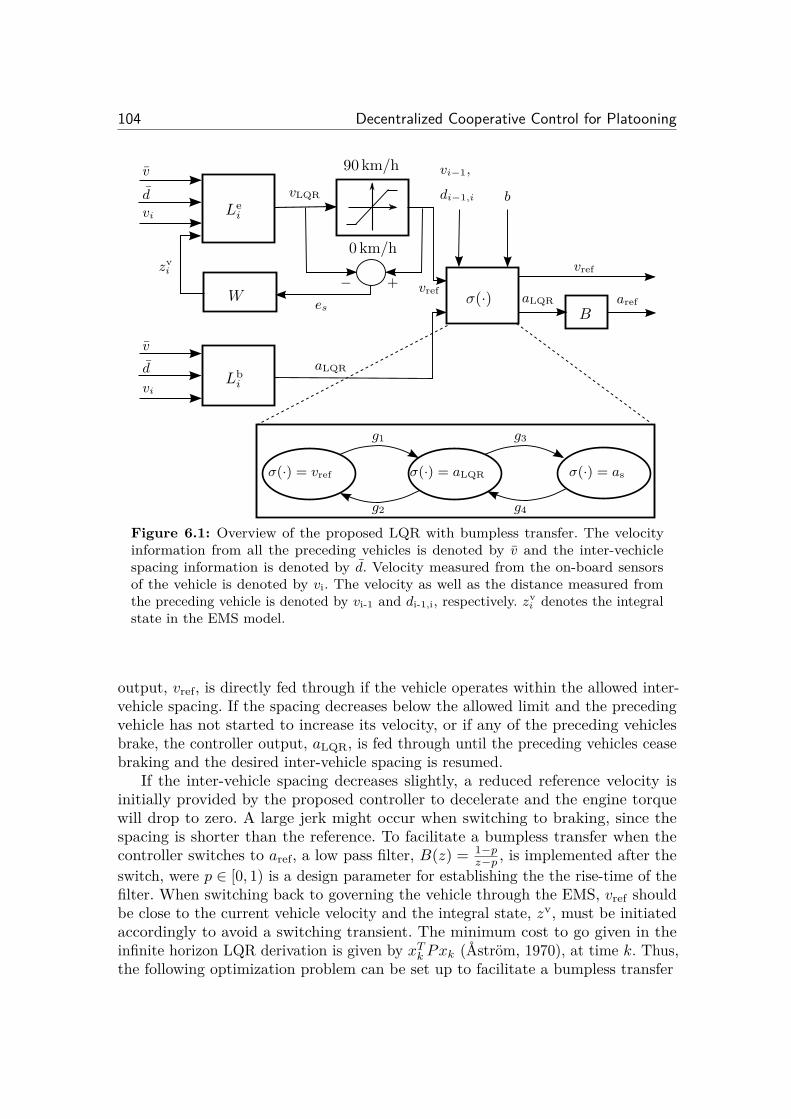
104 Decentralized Cooperative Control for Platooning
v
d
v
i
vref
aref
Le
i
v
d
v
i
Lb
i
90 km/h
0 km/h
vLQR
vref
v
i≠1,
d
i≠1,i
b
W ‡(·)+≠
e
s
z
vi
B
aLQR
aLQR
‡(·) = aLQR‡(·) = vref ‡(·) = as
g1
g2
g3
g4
Figure 6.1: Overview of the proposed LQR with bumpless transfer. The velocityinformation from all the preceding vehicles is denoted by v and the inter-vechiclespacing information is denoted by d. Velocity measured from the on-board sensorsof the vehicle is denoted by vi. The velocity as well as the distance measured fromthe preceding vehicle is denoted by vi-1 and di-1,i, respectively. z
vi
denotes the integralstate in the EMS model.
output, vref
, is directly fed through if the vehicle operates within the allowed inter-vehicle spacing. If the spacing decreases below the allowed limit and the precedingvehicle has not started to increase its velocity, or if any of the preceding vehiclesbrake, the controller output, a
LQR
, is fed through until the preceding vehicles ceasebraking and the desired inter-vehicle spacing is resumed.
If the inter-vehicle spacing decreases slightly, a reduced reference velocity isinitially provided by the proposed controller to decelerate and the engine torquewill drop to zero. A large jerk might occur when switching to braking, since thespacing is shorter than the reference. To facilitate a bumpless transfer when thecontroller switches to a
ref
, a low pass filter, B(z) = 1≠pz≠p , is implemented after the
switch, were p œ [0, 1) is a design parameter for establishing the the rise-time of thefilter. When switching back to governing the vehicle through the EMS, v
ref
shouldbe close to the current vehicle velocity and the integral state, zv, must be initiatedaccordingly to avoid a switching transient. The minimum cost to go given in theinfinite horizon LQR derivation is given by xT
k Pxk (Åström, 1970), at time k. Thus,the following optimization problem can be set up to facilitate a bumpless transfer
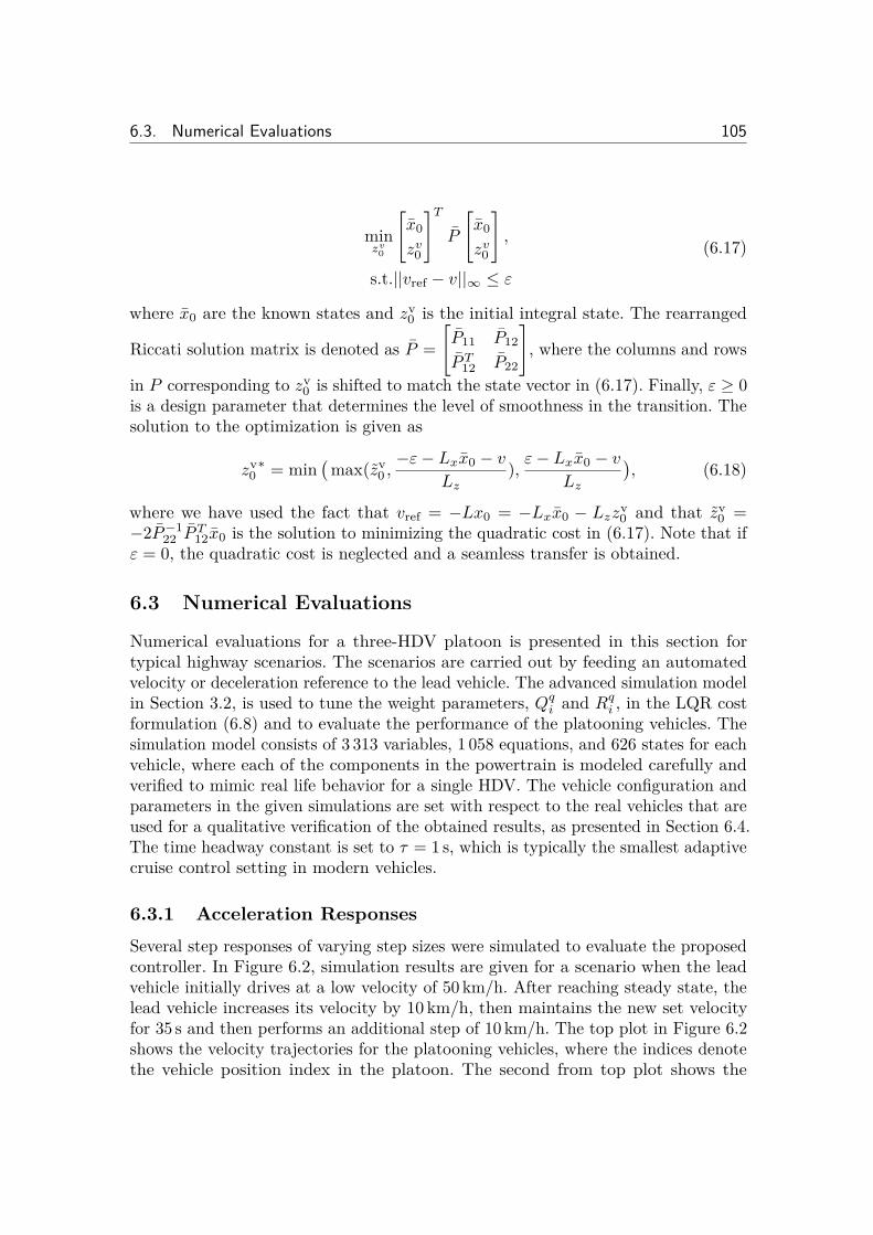
6.3. Numerical Evaluations 105
minzv
0
Cx
0
zv0
DT
P
Cx
0
zv0
D,
s.t.||vref
≠ v||Œ Æ Á
(6.17)
where x0
are the known states and zv
0
is the initial integral state. The rearranged
Riccati solution matrix is denoted as P =C
P11
P12
P T12
P22
D, where the columns and rows
in P corresponding to zv
0
is shifted to match the state vector in (6.17). Finally, Á Ø 0is a design parameter that determines the level of smoothness in the transition. Thesolution to the optimization is given as
zv
0
ú = min!
max(zv
0
,≠Á ≠ Lxx
0
≠ v
Lz), Á ≠ Lxx
0
≠ v
Lz
", (6.18)
where we have used the fact that vref
= ≠Lx0
= ≠Lxx0
≠ Lzzv
0
and that zv
0
=≠2P ≠1
22
P T12
x0
is the solution to minimizing the quadratic cost in (6.17). Note that ifÁ = 0, the quadratic cost is neglected and a seamless transfer is obtained.
6.3 Numerical Evaluations
Numerical evaluations for a three-HDV platoon is presented in this section fortypical highway scenarios. The scenarios are carried out by feeding an automatedvelocity or deceleration reference to the lead vehicle. The advanced simulation modelin Section 3.2, is used to tune the weight parameters, Qq
i and Rqi , in the LQR cost
formulation (6.8) and to evaluate the performance of the platooning vehicles. Thesimulation model consists of 3 313 variables, 1 058 equations, and 626 states for eachvehicle, where each of the components in the powertrain is modeled carefully andverified to mimic real life behavior for a single HDV. The vehicle configuration andparameters in the given simulations are set with respect to the real vehicles that areused for a qualitative verification of the obtained results, as presented in Section 6.4.The time headway constant is set to · = 1 s, which is typically the smallest adaptivecruise control setting in modern vehicles.
6.3.1 Acceleration ResponsesSeveral step responses of varying step sizes were simulated to evaluate the proposedcontroller. In Figure 6.2, simulation results are given for a scenario when the leadvehicle initially drives at a low velocity of 50 km/h. After reaching steady state, thelead vehicle increases its velocity by 10 km/h, then maintains the new set velocityfor 35 s and then performs an additional step of 10 km/h. The top plot in Figure 6.2shows the velocity trajectories for the platooning vehicles, where the indices denotethe vehicle position index in the platoon. The second from top plot shows the
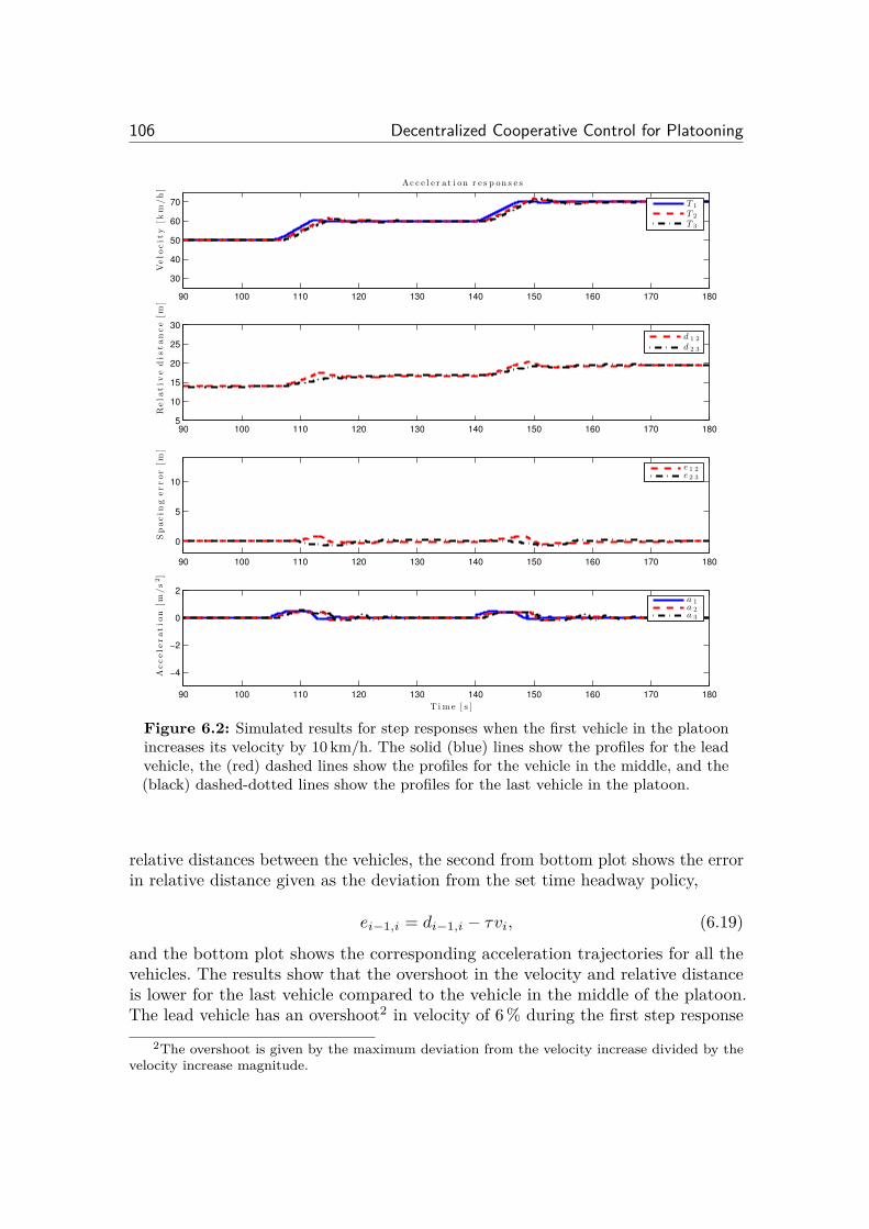
106 Decentralized Cooperative Control for Platooning
90 100 110 120 130 140 150 160 170 180
30
40
50
60
70
Velo
cit
y[k
m/h
]
Ac c e l e r at i on r e s p on s e s
T 1
T 2
T 3
90 100 110 120 130 140 150 160 170 1805
10
15
20
25
30
Rela
tiv
ed
istan
ce
[m]
d 1 2
d 2 3
90 100 110 120 130 140 150 160 170 180
0
5
10
Sp
acin
gerror
[m]
e 1 2e 2 3
90 100 110 120 130 140 150 160 170 180
−4
−2
0
2
Accele
ratio
n[m
/s2]
T i m e [ s ]
a 1a 2a 3
Figure 6.2: Simulated results for step responses when the first vehicle in the platoonincreases its velocity by 10 km/h. The solid (blue) lines show the profiles for the leadvehicle, the (red) dashed lines show the profiles for the vehicle in the middle, and the(black) dashed-dotted lines show the profiles for the last vehicle in the platoon.
relative distances between the vehicles, the second from bottom plot shows the errorin relative distance given as the deviation from the set time headway policy,
ei≠1,i = di≠1,i ≠ ·vi, (6.19)
and the bottom plot shows the corresponding acceleration trajectories for all thevehicles. The results show that the overshoot in the velocity and relative distanceis lower for the last vehicle compared to the vehicle in the middle of the platoon.The lead vehicle has an overshoot2 in velocity of 6 % during the first step response
2The overshoot is given by the maximum deviation from the velocity increase divided by thevelocity increase magnitude.
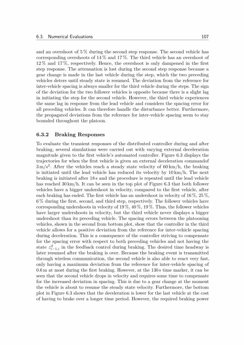
6.3. Numerical Evaluations 107
and an overshoot of 5 % during the second step response. The second vehicle hascorresponding overshoots of 14 % and 17 %. The third vehicle has an overshoot of12 % and 17 %, respectively. Hence, the overshoot is only dampened in the firststep response. The attenuation is lost during the second step response because agear change is made in the last vehicle during the step, which the two precedingvehicles deters until steady state is resumed. The deviation from the reference forinter-vehicle spacing is always smaller for the third vehicle during the steps. The signof the deviation for the two follower vehicles is opposite because there is a slight lagin initiating the step for the second vehicle. However, the third vehicle experiencesthe same lag in response from the lead vehicle and considers the spacing error forall preceding vehicles. It can therefore handle the disturbance better. Furthermore,the propagated deviations from the reference for inter-vehicle spacing seem to staybounded throughout the platoon.
6.3.2 Braking ResponsesTo evaluate the transient responses of the distributed controller during and afterbraking, several simulations were carried out with varying external decelerationmagnitude given to the first vehicle’s automated controller. Figure 6.3 displays thetrajectories for when the first vehicle is given an external deceleration commandof3 m/s2. After the vehicles reach a steady state velocity of 60 km/h, the brakingis initiated until the lead vehicle has reduced its velocity by 10 km/h. The nextbraking is initiated after 18 s and the procedure is repeated until the lead vehiclehas reached 30 km/h. It can be seen in the top plot of Figure 6.3 that both followervehicles have a bigger undershoot in velocity, compared to the first vehicle, aftereach braking has ended. The first vehicle has an undershoot in velocity of 16 %, 25 %,6 % during the first, second, and third step, respectively. The follower vehicles havecorresponding undershoots in velocity of 19 %, 40 %, 19 %. Thus, the follower vehicleshave larger undershoots in velocity, but the third vehicle never displays a biggerundershoot than its preceding vehicle. The spacing errors between the platooningvehicles, shown in the second from bottom plot, show that the controller in the thirdvehicle allows for a positive deviation from the reference for inter-vehicle spacingduring deceleration. This is a consequence of the controller striving to compensatefor the spacing error with respect to both preceding vehicles and not having thestate zd
i≠1,i in the feedback control during braking. The desired time headway islater resumed after the braking is over. Because the braking event is transmittedthrough wireless communication, the second vehicle is also able to react very fast,only having a maximum deviation from the reference for inter-vehicle spacing of0.6 m at most during the first braking. However, at the 130 s time marker, it can beseen that the second vehicle drops in velocity and requires some time to compensatefor the increased deviation in spacing. This is due to a gear change at the momentthe vehicle is about to resume the steady state velocity. Furthermore, the bottomplot in Figure 6.3 shows that the deceleration is lower for the last vehicle at the costof having to brake over a longer time period. However, the required braking power
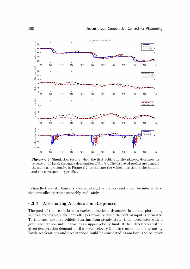
108 Decentralized Cooperative Control for Platooning
100 105 110 115 120 125 130 135 140 145 150 155
30
40
50
60
70
Velo
cit
y[k
m/h
]
B r ak i n g r e s p on s e s
T 1
T 2
T 3
100 105 110 115 120 125 130 135 140 145 150 1555
10
15
20
25
30
Rela
tiv
ed
istan
ce
[m]
d 1 2
d 2 3
100 105 110 115 120 125 130 135 140 145 150 155
0
5
10
Sp
acin
gerror
[m]
e 1 2e 2 3
100 105 110 115 120 125 130 135 140 145 150 155
−4
−2
0
2
Accele
ratio
n[m
/s2]
T i m e [ s ]
a 1a 2a 3
Figure 6.3: Simulation results when the first vehicle in the platoon decreases itsvelocity by 10 km/h through a deceleration of 3 m/s2. The displayed profiles are denotedthe same as previously, in Figure 6.2, to indicate the vehicle position in the platoonand the corresponding profiles.
to handle the disturbance is lowered along the platoon and it can be inferred thatthe controller operates smoothly and safely.
6.3.3 Alternating Acceleration ResponsesThe goal of this scenario is to excite unmodeled dynamics in all the platooningvehicles and evaluate the controller performance when the control input is saturated.To this end, the first vehicle, starting from steady state, then accelerates with agiven acceleration until it reaches an upper velocity limit. It then decelerates with agiven deceleration demand until a lower velocity limit is reached. The alternatingharsh accelerations and decelerations could be considered as analogous to behavior
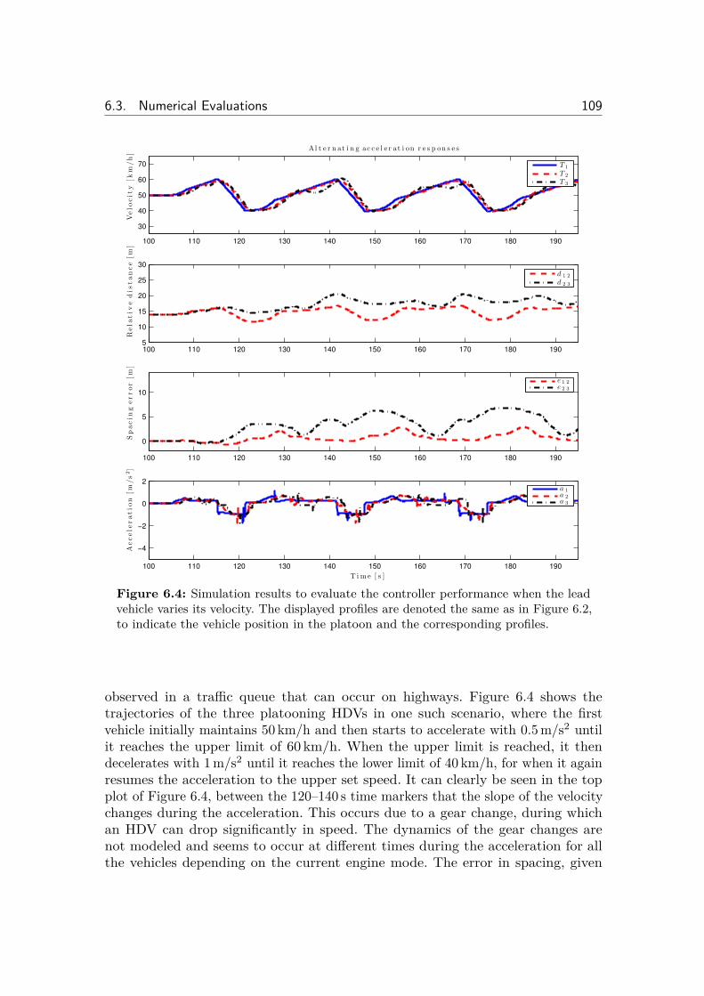
6.3. Numerical Evaluations 109
100 110 120 130 140 150 160 170 180 190
30
40
50
60
70
Velo
cit
y[k
m/h
]
A l t e r n at i n g ac c e l e r at i on r e s p on s e s
T 1
T 2
T 3
100 110 120 130 140 150 160 170 180 1905
10
15
20
25
30
Rela
tiv
ed
istan
ce
[m]
d 1 2
d 2 3
100 110 120 130 140 150 160 170 180 190
0
5
10
Sp
acin
gerror
[m]
e 1 2e 2 3
100 110 120 130 140 150 160 170 180 190
−4
−2
0
2
Accele
ratio
n[m
/s2]
T i m e [ s ]
a 1a 2a 3
Figure 6.4: Simulation results to evaluate the controller performance when the leadvehicle varies its velocity. The displayed profiles are denoted the same as in Figure 6.2,to indicate the vehicle position in the platoon and the corresponding profiles.
observed in a tra�c queue that can occur on highways. Figure 6.4 shows thetrajectories of the three platooning HDVs in one such scenario, where the firstvehicle initially maintains 50 km/h and then starts to accelerate with 0.5 m/s2 untilit reaches the upper limit of 60 km/h. When the upper limit is reached, it thendecelerates with 1 m/s2 until it reaches the lower limit of 40 km/h, for when it againresumes the acceleration to the upper set speed. It can clearly be seen in the topplot of Figure 6.4, between the 120–140 s time markers that the slope of the velocitychanges during the acceleration. This occurs due to a gear change, during whichan HDV can drop significantly in speed. The dynamics of the gear changes arenot modeled and seems to occur at di�erent times during the acceleration for allthe vehicles depending on the current engine mode. The error in spacing, given
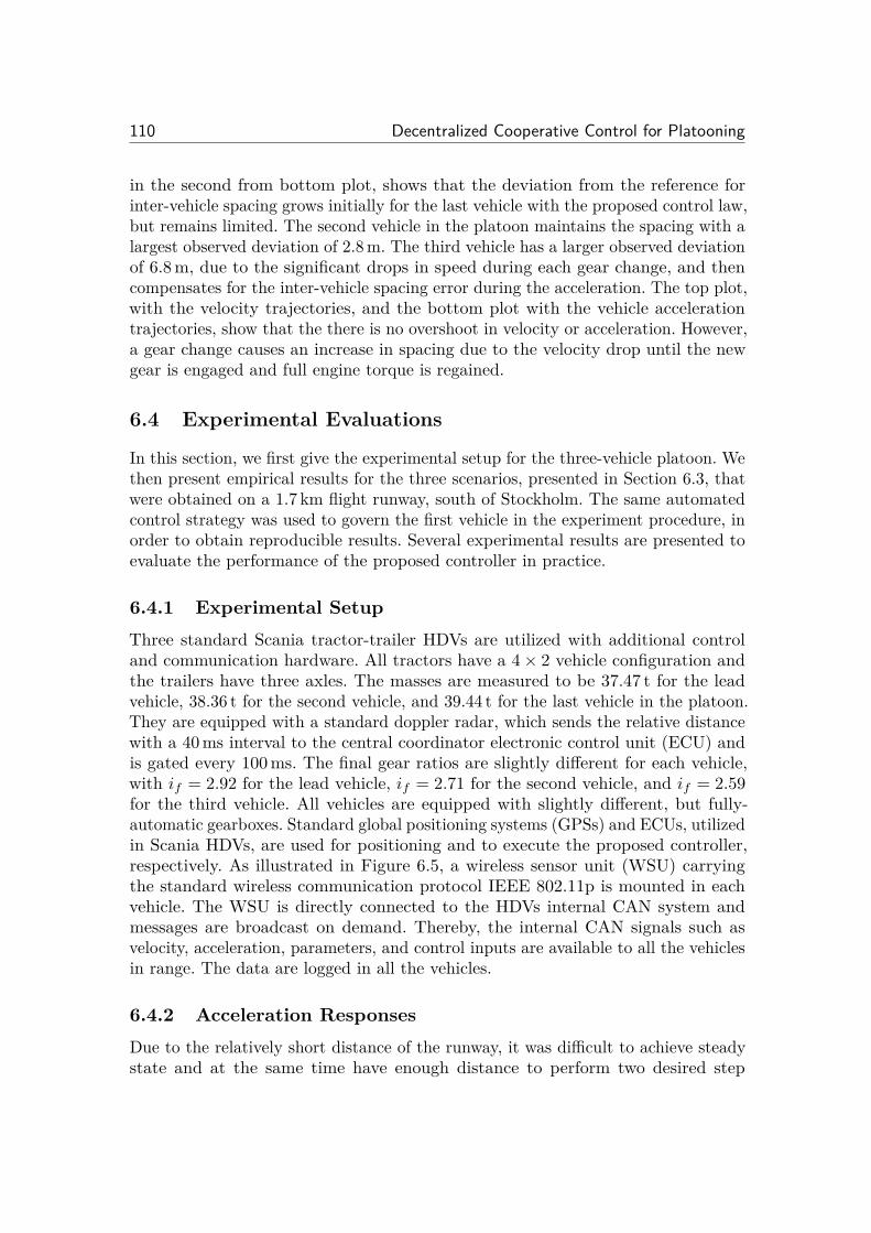
110 Decentralized Cooperative Control for Platooning
in the second from bottom plot, shows that the deviation from the reference forinter-vehicle spacing grows initially for the last vehicle with the proposed control law,but remains limited. The second vehicle in the platoon maintains the spacing with alargest observed deviation of 2.8 m. The third vehicle has a larger observed deviationof 6.8 m, due to the significant drops in speed during each gear change, and thencompensates for the inter-vehicle spacing error during the acceleration. The top plot,with the velocity trajectories, and the bottom plot with the vehicle accelerationtrajectories, show that the there is no overshoot in velocity or acceleration. However,a gear change causes an increase in spacing due to the velocity drop until the newgear is engaged and full engine torque is regained.
6.4 Experimental Evaluations
In this section, we first give the experimental setup for the three-vehicle platoon. Wethen present empirical results for the three scenarios, presented in Section 6.3, thatwere obtained on a 1.7 km flight runway, south of Stockholm. The same automatedcontrol strategy was used to govern the first vehicle in the experiment procedure, inorder to obtain reproducible results. Several experimental results are presented toevaluate the performance of the proposed controller in practice.
6.4.1 Experimental SetupThree standard Scania tractor-trailer HDVs are utilized with additional controland communication hardware. All tractors have a 4 ◊ 2 vehicle configuration andthe trailers have three axles. The masses are measured to be 37.47 t for the leadvehicle, 38.36 t for the second vehicle, and 39.44 t for the last vehicle in the platoon.They are equipped with a standard doppler radar, which sends the relative distancewith a 40 ms interval to the central coordinator electronic control unit (ECU) andis gated every 100 ms. The final gear ratios are slightly di�erent for each vehicle,with if = 2.92 for the lead vehicle, if = 2.71 for the second vehicle, and if = 2.59for the third vehicle. All vehicles are equipped with slightly di�erent, but fully-automatic gearboxes. Standard global positioning systems (GPSs) and ECUs, utilizedin Scania HDVs, are used for positioning and to execute the proposed controller,respectively. As illustrated in Figure 6.5, a wireless sensor unit (WSU) carryingthe standard wireless communication protocol IEEE 802.11p is mounted in eachvehicle. The WSU is directly connected to the HDVs internal CAN system andmessages are broadcast on demand. Thereby, the internal CAN signals such asvelocity, acceleration, parameters, and control inputs are available to all the vehiclesin range. The data are logged in all the vehicles.
6.4.2 Acceleration ResponsesDue to the relatively short distance of the runway, it was di�cult to achieve steadystate and at the same time have enough distance to perform two desired step

6.4. Experimental Evaluations 111
ECUECUECU
WSU WSU WSU
v
req
a
req
v
req
a
req
v
req
a
req
Data logger Data logger Data logger
HDV1 HDV2 HDV3
Figure 6.5: A schematic overlay of the experimental hardware setup. The top pictureshows the HDVs utilized in these experiments. The left HDV is the lead. The WSU,ECU, and data logger communicate through CAN. As soon as new information isobtained through the ECU or the vehicle, it is broadcast through the WSU.
responses. The results for two step responses in the lead vehicle of 10 km/h aregiven in Figure 6.6, where the top plot shows the velocity trajectories for the threeplatooning HDVs. The second from top plot shows the inter-vehicle spacings andthe second from bottom plot shows the deviation from the reference for inter-vehiclespacing, in which it can be seen that the vehicles had not yet been able to reachsteady state at the beginning of the first step response. Finally, the bottom plotshows the vehicle acceleration trajectories. As shown in the second from bottomplot in Figure 6.6, there is a deviation from the reference for inter-vehicle spacingof 1.1 m for the middle vehicle and a deviation of 2.4 m for the third vehicle, whenthe step is initiated. The first vehicle has an overshoot in velocity of 14 % duringthe first step response and an overshoot of 8 % during the second step response.This is higher compared to the numerical results and is due to di�erent cruisecontrol (CC) logic in the first vehicle. However, the overshoots decrease in thesecond step, which is congruent with the simulation model. The second vehicle has
112 Decentralized Cooperative Control for Platooning
80 90 100 110 120 130 140
30
40
50
60
70
Velo
cit
y[k
m/h
]
Ac c e l e r at i on r e s p on s e s
T 1
T 2
T 3
80 90 100 110 120 130 1405
10
15
20
25
30
Rela
tiv
ed
istan
ce
[m]
d 1 2
d 2 3
80 90 100 110 120 130 140
0
5
10
Sp
acin
gerror
[m]
e 1 2e 2 3
80 90 100 110 120 130 140
−4
−2
0
2
Accele
ratio
n[m
/s2]
T i m e [ s ]
a 1a 2a 3
Figure 6.6: Experiment results for step responses when the first vehicle in the platoonincreases its velocity by 10 km/h. The solid (blue) lines show the profiles for the leadvehicle, the (red) dashed lines show the profiles for the vehicle in the middle, and the(black) dashed-dotted lines show the profiles for the last vehicle in the platoon.
corresponding overshoots in velocity of 24 % and 8 %, respectively, and the thirdvehicle has overshoots in velocity of 33 % and 40 %. The variation for the error inrelative distance is also initially smaller for the third vehicle. Then, at the 118 s timemarker, a gear change is performed in the third vehicle just before the step response,which causes the vehicle to fall behind and thereby causing a large overshoot bycatching up. A similar behavior is observed in the simulation model, with a lesssevere overshoot. The additional lag in handling the step response occurs becausethe last vehicle decelerates, i.e. coasts, just before the step is initiated. Hence, theturbo pressure is low, which limits the engine from outputting the desired torqueuntil the turbo pressure is regained. Thus, the preceding vehicles manage to increase
6.4. Experimental Evaluations 113
their velocities before the third vehicle can do so, causing a large overshoot tocompensate for the increased errors in spacing and velocity.
6.4.3 Braking ResponsesThe results obtained when the first vehicle, after reaching a steady state velocityof 60 km/h, brakes with 3 m/s2 until the velocity is reduced by 10 km/h and thenrepeats the procedure after 18 s, is given in Figure 6.7. As can be seen in the secondplot from the bottom, the vehicles had nearly reached steady state when the firstbraking is initiated, with an error in relative distance close to zero. The accelerationtrajectories for all the vehicles, given in the bottom plot, show that the first vehicleperforms the strongest deceleration, whereas the third vehicle has an equal or smallerdeceleration compared to the second vehicle. The first vehicle has undershoots invelocity of 41 % during the first two steps and 47 % in the last. The follower vehiclesboth have undershoots in velocity of 37 %, 45 %, and 48 %, respectively. Hence, thefollower vehicles display a smaller undershoot during the first braking instance. Incontrast to the simulation results, a severe overshoot in relative does not occurdue to a gear change for the second vehicle. The third vehicle does not have abigger undershoot than its preceding vehicle, which is congruent with the simulationmodel. The third vehicle maintains a larger relative distance, compared to thesecond vehicle, during the braking actions and then compensates for the error inrelative distance after the braking is completed. A deviation from the referencefor inter-vehicle spacing of -1.9 m occurs for the second vehicle, whereas the thirdvehicle always manages to maintain a positive deviation. After each braking event,when the proposed high-level controller switches back to the engine control, anunmodeled gear change occurs that results in an overshoot in desired inter-vehiclespacing. Nevertheless, the errors in relative distance stay limited. The controllerperformance is considered safe and the results are congruent with the simulationmodel.
6.4.4 Alternating Acceleration ResponsesThe results for the alternating accelerations and decelerations for the lead vehicle isgiven in Figure 6.8. It can be seen that the maximum deviation from the referencefor inter-vehicle spacing is 7.2 m for the last vehicle, which is nearly the same in thesimulation model. However, the maximum error is larger for the second vehicle incontrast to the simulation results. This is due to a di�erence in gear managementlogic between the real vehicles and the simulation model. A periodic behavior can beobserved in the plot for the relative distances and in the plot for the error in relativedistance. The top plot in Figure 6.8, for the velocity trajectories, reveals that a gearchange occurs every other time an acceleration is performed, for the second vehicle,since there is a significant drop in velocity around the 105 s and 155 s time markers.The gear change results in a velocity decrease that creates an increase in relativedistance. The second vehicle then manages to reduce the error in relative distance
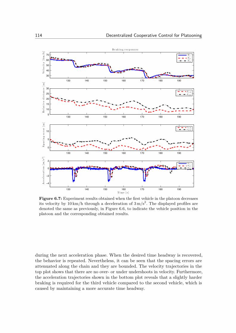
114 Decentralized Cooperative Control for Platooning
130 140 150 160 170 180 190
30
40
50
60
70
Velo
cit
y[k
m/h
]
B r ak i n g r e s p on s e s
T 1
T 2
T 3
130 140 150 160 170 180 1905
10
15
20
25
30
Rela
tiv
ed
istan
ce
[m]
d 1 2
d 2 3
130 140 150 160 170 180 190
0
5
10
Sp
acin
gerror
[m]
e 1 2e 2 3
130 140 150 160 170 180 190
−4
−2
0
2
Accele
ratio
n[m
/s2]
T i m e [ s ]
a 1a 2a 3
Figure 6.7: Experiment results obtained when the first vehicle in the platoon decreasesits velocity by 10 km/h through a deceleration of 3 m/s2. The displayed profiles aredenoted the same as previously, in Figure 6.6, to indicate the vehicle position in theplatoon and the corresponding obtained results.
during the next acceleration phase. When the desired time headway is recovered,the behavior is repeated. Nevertheless, it can be seen that the spacing errors areattenuated along the chain and they are bounded. The velocity trajectories in thetop plot shows that there are no over- or under undershoots in velocity. Furthermore,the acceleration trajectories shown in the bottom plot reveals that a slightly harderbraking is required for the third vehicle compared to the second vehicle, which iscaused by maintaining a more accurate time headway.
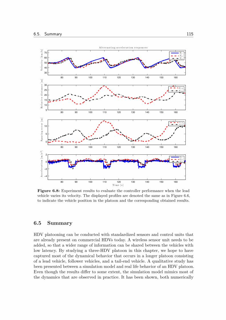
6.5. Summary 115
80 90 100 110 120 130 140 150 160
30
40
50
60
70
Velo
cit
y[k
m/h
]
A l t e r n at i n g ac c e l e r at i on r e s p on s e s
T 1
T 2
T 3
80 90 100 110 120 130 140 150 1605
10
15
20
25
30
Rela
tiv
ed
istan
ce
[m]
d 1 2
d 2 3
80 90 100 110 120 130 140 150 160
0
5
10
Sp
acin
gerror
[m]
e 1 2e 2 3
80 90 100 110 120 130 140 150 160
−4
−2
0
2
Accele
ratio
n[m
/s2]
T i m e [ s ]
a 1a 2a 3
Figure 6.8: Experiment results to evaluate the controller performance when the leadvehicle varies its velocity. The displayed profiles are denoted the same as in Figure 6.6,to indicate the vehicle position in the platoon and the corresponding obtained results.
6.5 Summary
HDV platooning can be conducted with standardized sensors and control units thatare already present on commercial HDVs today. A wireless sensor unit needs to beadded, so that a wider range of information can be shared between the vehicles withlow latency. By studying a three-HDV platoon in this chapter, we hope to havecaptured most of the dynamical behavior that occurs in a longer platoon consistingof a lead vehicle, follower vehicles, and a tail-end vehicle. A qualitative study hasbeen presented between a simulation model and real life behavior of an HDV platoon.Even though the results di�er to some extent, the simulation model mimics most ofthe dynamics that are observed in practice. It has been shown, both numerically
116 Decentralized Cooperative Control for Platooning
and through experiments, that the proposed decentralized high-level controllerattenuates the disturbances produced by the lead vehicle and operates safely. Theexperimental results showed that the deviation from the reference for inter-vehiclespacing during the braking scenarios never decrease more than 1.9 m. Hence, itcan be inferred that the vehicles could have operated at shorter time headways toachieve further air drag reduction, i.e., fuel-e�ciency, without compromising safety.The controller performs well even though the vehicles operate to some extent outsidethe equilibrium points. However, there are still nonlinearities present in the systemthat causes unwanted behavior. In contrast to passenger vehicles, a gear changeproduced in an HDV has a significant impact on the velocity. We presented a simplemodel for the EMS and engine dynamics, which worked su�ciently well in mostof the studied cases. However, there can still arise cases in the nonlinear enginedynamics that can cause unwanted response delays. These situations do not causean issue with respect to safety, but degrade the tracking performance and increasethe control input energy.
Chapter 7
Look-Ahead Control for Platooning
“It is always wise to look ahead, but di�cult to look further than you
can see.”Winston Churchill
The focus within platooning in the current literature has mainly been onestablishing optimal control policies based on linear models for maintaininga given spacing policy without considering the road topography. However,
it is not realistic to assume that a vehicle platoon in practice consists of identicalheavy-duty vehicles (HDVs) with equal cargo weight and thus the road grade mightconstrain an HDV in the platoon such that it cannot maintain the overall desiredvelocity for the platoon. Over steep uphill climb the inter-vehicle spacing is typicallyincreased, when following a vehicle with a stronger engine or a lower mass. Overdownhill segments the heaviest follower vehicle might have to brake to avoid coastinginto the vehicle ahead. This has in particular been reported as an issue by professionalHDV drivers in situations when no overtaking is possible, since constant braking canlead to brake failure due to overheating. Furthermore, braking is never fuel-e�cient,since energy produced by the engine is lost through frictional heating of the brakesduring braking.
Preview road grade information introduces a possibility to address the issuesmentioned above and further improve the fuel-saving potential in HDV platooning.The idea of using preview road grade information for fuel-e�cient control is not newand has been studied for HDVs that are traveling alone. Early work on utilizingroad grade information, for a single vehicle, in vehicle speed control can be foundin Schwarzkopf and Leipnik (1977), where a minimum-fuel problem for a nonlinearvehicle model is presented. More recent work on fuel-optimal control for a singleHDV based on preview information of the road topography, referred to as look-aheadcontrol (LAC), has been studied in Hellström (2010) and Fröberg (2008), wherethe presented controller is derived through dynamic programming. They showedthat the fuel consumption can be reduced by adjusting the velocity prior to anuphill or a downhill segment based on the parameters and the nonlinear dynamics
117
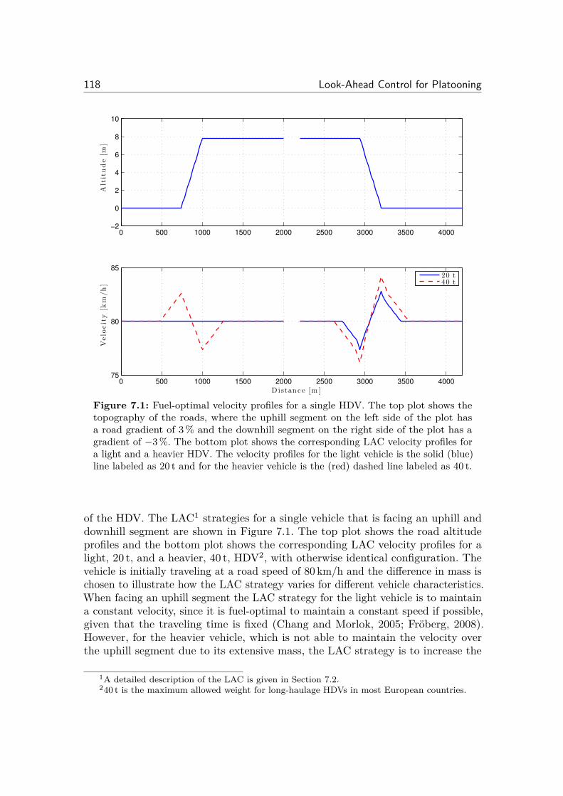
118 Look-Ahead Control for Platooning
0 500 1000 1500 2000 2500 3000 3500 4000−2
0
2
4
6
8
10
Alt
itu
de
[m]
0 500 1000 1500 2000 2500 3000 3500 400075
80
85
Velo
cit
y[k
m/h
]
D i stanc e [m ]
20 t40 t
Figure 7.1: Fuel-optimal velocity profiles for a single HDV. The top plot shows thetopography of the roads, where the uphill segment on the left side of the plot hasa road gradient of 3 % and the downhill segment on the right side of the plot has agradient of ≠3 %. The bottom plot shows the corresponding LAC velocity profiles fora light and a heavier HDV. The velocity profiles for the light vehicle is the solid (blue)line labeled as 20 t and for the heavier vehicle is the (red) dashed line labeled as 40 t.
of the HDV. The LAC1 strategies for a single vehicle that is facing an uphill anddownhill segment are shown in Figure 7.1. The top plot shows the road altitudeprofiles and the bottom plot shows the corresponding LAC velocity profiles for alight, 20 t, and a heavier, 40 t, HDV2, with otherwise identical configuration. Thevehicle is initially traveling at a road speed of 80 km/h and the di�erence in mass ischosen to illustrate how the LAC strategy varies for di�erent vehicle characteristics.When facing an uphill segment the LAC strategy for the light vehicle is to maintaina constant velocity, since it is fuel-optimal to maintain a constant speed if possible,given that the traveling time is fixed (Chang and Morlok, 2005; Fröberg, 2008).However, for the heavier vehicle, which is not able to maintain the velocity overthe uphill segment due to its extensive mass, the LAC strategy is to increase the
1A detailed description of the LAC is given in Section 7.2.240 t is the maximum allowed weight for long-haulage HDVs in most European countries.
Look-Ahead Control for Platooning 119
velocity before the hill to minimize the variation around the road speed. Similarly,when facing a downhill segment, the LAC strategy is to reduce the velocity beforethe downhill segment to avoid excessive braking, which becomes necessary if thevehicle exceeds an acceptable o�set from the road speed limit when coasting alongthe decline.
It is not obvious how to extend LAC for a single vehicle to look-ahead controlfor HDV platooning. The individual optimal LAC strategies are not consistent withmaintaing a constant inter-vehicle spacing for air drag reduction, which is the aim inHDV platooning. The instantaneous fuel consumption of a single HDV can increaseby a factor of four, from 0.3 l/km to 1.2 l/km, over a steep uphill segment whenthe engine is operating at maximum torque. Hence, the air drag reduction has alower e�ect on the total resistive forces that are exerted on an HDV in motion oversteep hills. Furthermore, the individual LAC strategies might not be feasible whentraveling in a platoon, since, for example, increasing the velocity prior to an uphillsegment implies that the minimum safe distance constraint is transgressed if thepreceding vehicle does not adjust its velocity. Hence, it is unclear whether or not itis feasible or fuel-e�cient to utilize preview road gradient information in control forHDV platooning. A question arises of whether it is more fuel-e�cient to maintain theplatoon when traversing a hill or let the HDVs separate and then catch up, during orafter the hill. Thus, it becomes interesting to investigate whether it is fuel-e�cientto utilize a controller based on road preview information for HDV platooning, orif commercial controllers that aim to maintain the inter-vehicle spacing withoutconsidering the road characteristics are su�cient in this regard. Moreover, thecomputational cost for solving the dynamic programming in the LAC is exponentialin the state dimension. Thus, a centralized solution is too computationally expensivefor online applications and in general hard to solve for a large number of vehicles.Hence, the objective for the study in this chapter is to find a computationally feasibleand fuel-e�cient control strategy for HDV platoons when traversing steep uphill ordownhill segments.
The main contribution of this chapter is to determine a fuel-e�cient behavior foran HDV platoon when traversing a hill. We study commercially available controllersthat could be utilized for platooning and propose two novel fuel-e�cient controllersfor HDV platooning based on road grade preview information. The proposed con-trollers are established with low computational complexity, since it is generally notpossible to implement complex control algorithms due to the limited computationalpower in the on-board electronic control units. We study system uncertainties thatcommonly occur in practice, which might cause errors or loss of performance forthe proposed controller. We also study the e�ect of a varying road topography andsystem uncertainties on the fuel consumption for HDV platooning. Hence, guidelinesare determined for handling common system uncertainties that occur in practice,to maintain the fuel reduction potential. Furthermore, we investigate whether it isbetter to split up or maintain a platoon over steep hills and show that it is mostfuel-e�cient to maintain a platoon when traversing a hill as opposed to split theplatoon and resume it during or after the hill. It is shown that the commercially
120 Look-Ahead Control for Platooning
available adaptive cruise control (ACC) is not fuel-e�cient for a varying topographyand that the LAC for a single HDV is not practical in HDV platooning. Hence,we propose a cooperative look-ahead controller for platooning (CLAC), where themain idea is to initiate the control actions in a platoon based on a point in the roadrather than simultaneously implementing each HDV’s control action to maintain afixed spacing.
The outline of this chapter is as follows. First we present the system model inSection 7.1, which serves as the basis for the model predictive controllers that arepresented in Section 7.2. The behavior of the proposed controllers and commerciallyavailable controllers that can be used as an alternative, are evaluated in Section 7.3.Numerical results for the controllers are presented in Section 7.4. The e�ects thatcommon system errors in practice have on the fuel reduction potential of the proposedcontroller is studied in Section 7.5. Finally, in Section 7.6 we present a brief summaryof the results.
7.1 System Model
In this section, we present the vehicle dynamics and fuel consumption models thatserve as a basis for the proposed controllers in Section 7.2. Recall, from Chapter 3,that the state equation of a single HDV in a platoon can be formulated as
ds
i
dt = v
i
dd
i≠1,i
dt = v
i≠1 ≠ v
i
m
ti (G)dv
i
dt = F
ei
(”i
, Êei ) ≠ F
bi
≠ F
ai
(vi
, d
i≠1,i
) ≠ F
ri
(–(si
)) ≠ F
gi
(–(si
))
= k
ei
T
ei
(”i
, Êei ) ≠ F
bi
≠ k
d
i
v
2i
�i
(di≠1,i
) ≠ k
ri
cos –(si
) ≠ k
gi
sin –(si
)
(7.1)
where F e
i , F b
i , F a
i , F r
i , F g
i denote the engine, brake, air drag, rolling resistance,and gravitational forces acting upon the vehicle, respectively. The absolute traveleddistance for the ith HDV from a reference point common to all vehicles in theplatoon is denoted as si, T e
i (”i, Êei) denotes the net engine torque, ”i is grams of fuel
per engine cycle and cylinder, Êei denotes the angular velocity of the engine, mti(G)
denotes the accelerated mass for the current gear G, and i = 1, . . . , N denotes thevehicle position index in the platoon. The constants ke
i , kdi , kr
i , and kg
i denote thecharacteristic vehicle and environment coe�cients for the engine, air drag, roadfriction, and gravitation, respectively. The state variables vi and di≠1,i denote thevelocity for vehicle i and the inter-vehicle spacing with respect to the precedingvehicle, as shown in Figure 7.2. –(si) denotes the road gradient and the function�i(di≠1,i) is a nonlinear mapping of the air drag reduction with respect to theposition in the platoon.
The engine is modeled after a six cylinder 420 hp Scania engine, where the enginetorque during fueling for a single HDV is given as
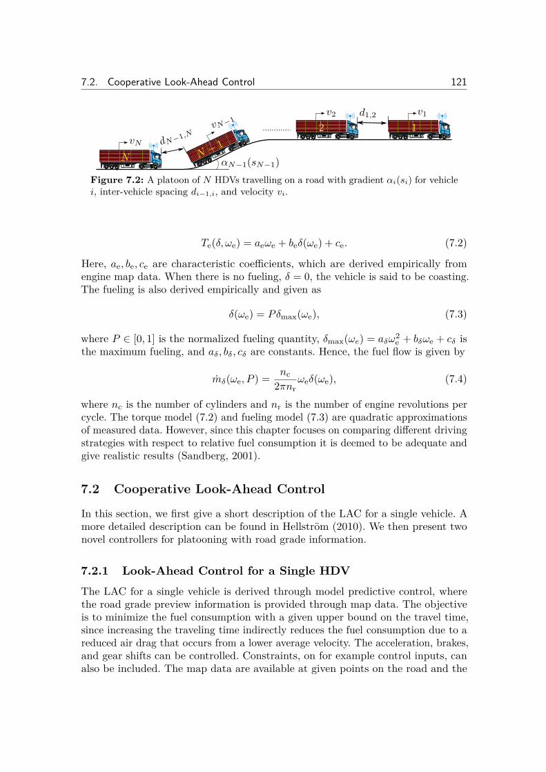
7.2. Cooperative Look-Ahead Control 121
–N≠1
(sN≠1
)
dN≠1
,N
d1,2
N
12
N ≠ 1
v1
vN
vN≠1
v2
Figure 7.2: A platoon of N HDVs travelling on a road with gradient –
i
(si
) for vehiclei, inter-vehicle spacing d
i≠1,i
, and velocity v
i
.
Te
(”, Êe
) = ae
Êe
+ be
”(Êe
) + ce
. (7.2)
Here, ae
, be
, ce
are characteristic coe�cients, which are derived empirically fromengine map data. When there is no fueling, ” = 0, the vehicle is said to be coasting.The fueling is also derived empirically and given as
”(Êe
) = P ”max
(Êe
), (7.3)
where P œ [0, 1] is the normalized fueling quantity, ”max
(Êe) = a”Ê2
e
+ b”Êe
+ c” isthe maximum fueling, and a”, b”, c” are constants. Hence, the fuel flow is given by
m”(Êe
, P ) = nc
2finr
Êe
”(Êe
), (7.4)
where nc
is the number of cylinders and nr
is the number of engine revolutions percycle. The torque model (7.2) and fueling model (7.3) are quadratic approximationsof measured data. However, since this chapter focuses on comparing di�erent drivingstrategies with respect to relative fuel consumption it is deemed to be adequate andgive realistic results (Sandberg, 2001).
7.2 Cooperative Look-Ahead Control
In this section, we first give a short description of the LAC for a single vehicle. Amore detailed description can be found in Hellström (2010). We then present twonovel controllers for platooning with road grade information.
7.2.1 Look-Ahead Control for a Single HDVThe LAC for a single vehicle is derived through model predictive control, wherethe road grade preview information is provided through map data. The objectiveis to minimize the fuel consumption with a given upper bound on the travel time,since increasing the traveling time indirectly reduces the fuel consumption due to areduced air drag that occurs from a lower average velocity. The acceleration, brakes,and gear shifts can be controlled. Constraints, on for example control inputs, canalso be included. The map data are available at given points on the road and the
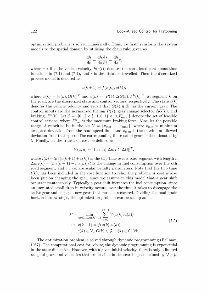
122 Look-Ahead Control for Platooning
optimization problem is solved numerically. Thus, we first transform the systemmodels to the spatial domain by utilizing the chain rule, given as
dh
dt= dh
ds
ds
dt= dh
dsv,
where v > 0 is the vehicle velocity, h(s(t)) denotes the considered continuous timefunctions in (7.1) and (7.4), and s is the distance travelled. Then the discretizedprocess model is denoted as
x(k + 1) = f(x(k), u(k)),
where x(k) = [v(k), G(k)]T and u(k) = [P (k), �G(k), F b(k)]T , at segment k onthe road, are the discretized state and control vectors, respectively. The state v(k)denotes the vehicle velocity and recall that G(k) œ Z+ is the current gear. Thecontrol inputs are the normalized fueling P (k), gear change selector �G(k), andbraking, F b(k). Let C = {[0, 1] ◊ {≠1, 0, 1} ◊ [0, F b
max
]} denote the set of feasiblecontrol actions, where F b
max
is the maximum braking force. Also, let the possiblerange of velocities be in the set V = {v
min
, . . . , vmax
}, where vmin
is minimumaccepted deviation from the road speed limit and v
max
is the maximum alloweddeviation from that speed. The corresponding finite set of gears is then denoted byG. Finally, let the transition cost be defined as
V (x, u) = [1 c1
c2
][�m” t |�G|]T ,
where t(k) = 2l/(v(k + 1) + v(k)) is the trip time over a road segment with length l,�m”(k) = (m”(k + 1) ≠ m”(k))/l is the change in fuel consumption over the kthroad segment, and c
1
, c2
, are scalar penalty parameters. Note that the trip timet(k), has been included in the cost function to relax the problem. A cost is alsobeen put on changing the gear, since we assume in this model that a gear shiftoccurs instantaneously. Typically a gear shift increases the fuel consumption, sincean unwanted small drop in velocity occurs, over the time it takes to disengage theactive gear and engage a new gear, that must be recovered. Dividing the road gradehorizon into M steps, the optimization problem can be set up as
Jú = minu(0),...,u(M≠1)
M≠1ÿ
k=0
V (x(k), u(k))
s.t. x(k + 1) = f(x(k), u(k)),v(k) œ V, G(k) œ G, u(k) œ C, ’k,
(7.5)
The optimization problem is solved through dynamic programming (Bellman,1957). The computational cost for solving the dynamic programming is exponentialin the state dimension. However, with a given initial velocity, there is only a limitedrange of gears and velocities that are feasible in the search space defined by V ◊ G,
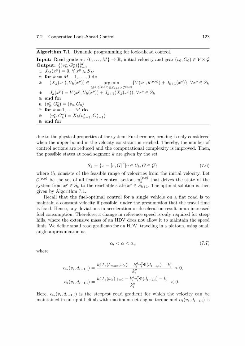
7.2. Cooperative Look-Ahead Control 123
Algorithm 7.1 Dynamic programming for look-ahead control.Input: Road grade – : {0, . . . , M} æ R, initial velocity and gear (v
0
, G0
) œ V ◊ GOutput: {(vú
k, Gúk)}M
k=0
1: JM (xp) = 0, ’ xp œ SM
2: for k := M ≠ 1, . . . , 0 do3: (Xk(xp), Uk(xp)) œ arg min
(xq,u(p,q))œSk+1◊C(p,q)
{V (xp, u(p,q)) + Jk+1
(xq)}, ’xp œ Sk
4: Jk(xp) = V (xp, Uk(xp)) + Jk+1
(Xk(xp)), ’xp œ Sk
5: end for6: (vú
0
, Gú0
) = (v0
, G0
)7: for k = 1, . . . , M do8: (vú
k, Gúk) = Xk(vú
k≠1
, Gúk≠1
)9: end for
due to the physical properties of the system. Furthermore, braking is only consideredwhen the upper bound in the velocity constraint is reached. Thereby, the number ofcontrol actions are reduced and the computational complexity is improved. Then,the possible states at road segment k are given by the set
Sk = {x = [v, G]T |v œ Vk, G œ G}, (7.6)where Vk consists of the feasible range of velocities from the initial velocity. LetC(p,q) be the set of all feasible control actions u
(p,q)
k that drives the state of thesystem from xp œ Sk to the reachable state xq œ Sk+1
. The optimal solution is thengiven by Algorithm 7.1.
Recall that the fuel-optimal control for a single vehicle on a flat road is tomaintain a constant velocity if possible, under the presumption that the travel timeis fixed. Hence, any deviations in acceleration or deceleration result in an increasedfuel consumption. Therefore, a change in reference speed is only required for steephills, where the extensive mass of an HDV does not allow it to maintain the speedlimit. We define small road gradients for an HDV, traveling in a platoon, using smallangle approximation as
–l < – < –u (7.7)where
–u(vi, di≠1,i) = kei Te(”max, Êe) ≠ kd
i v2
i �(di≠1,i) ≠ kri
kgi
> 0,
–l(vi, di≠1,i) = kei Te(Êe)|”=0
≠ kdi v2
i �(di≠1,i) ≠ kri
kgi
< 0.
Here, –u(vi, di≠1,i) is the steepest road gradient for which the velocity can bemaintained in an uphill climb with maximum net engine torque and –l(vi, di≠1,i) is
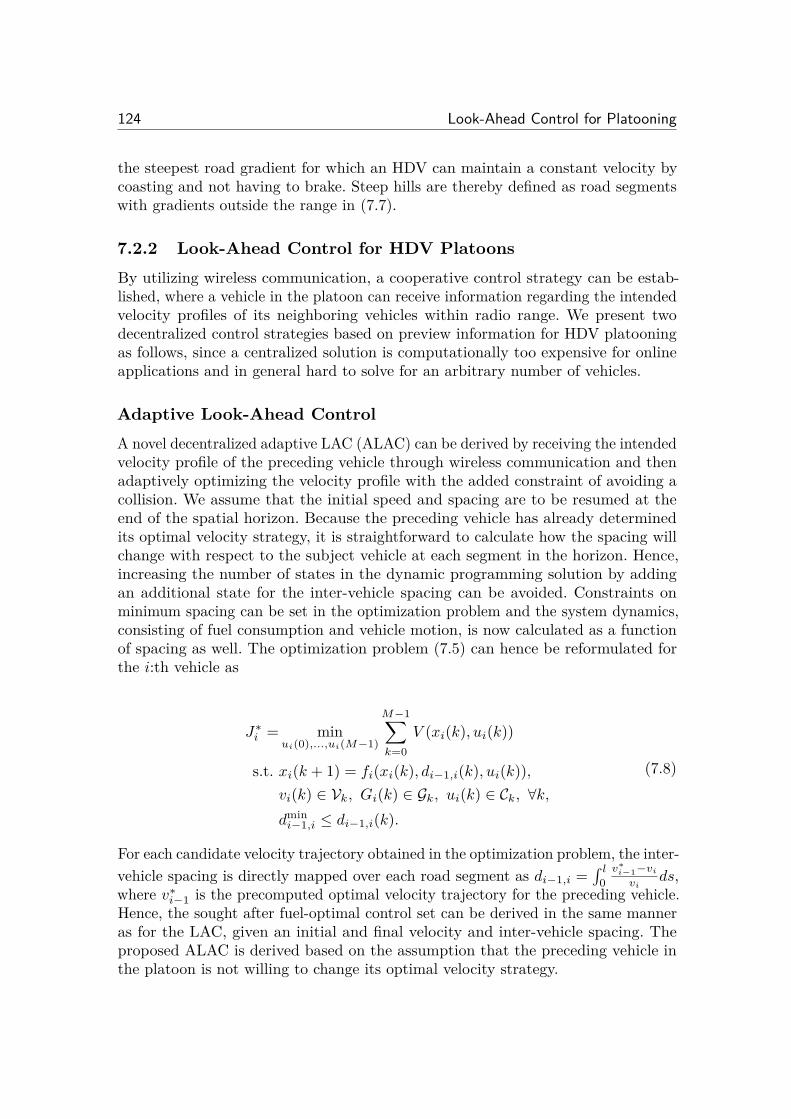
124 Look-Ahead Control for Platooning
the steepest road gradient for which an HDV can maintain a constant velocity bycoasting and not having to brake. Steep hills are thereby defined as road segmentswith gradients outside the range in (7.7).
7.2.2 Look-Ahead Control for HDV PlatoonsBy utilizing wireless communication, a cooperative control strategy can be estab-lished, where a vehicle in the platoon can receive information regarding the intendedvelocity profiles of its neighboring vehicles within radio range. We present twodecentralized control strategies based on preview information for HDV platooningas follows, since a centralized solution is computationally too expensive for onlineapplications and in general hard to solve for an arbitrary number of vehicles.
Adaptive Look-Ahead ControlA novel decentralized adaptive LAC (ALAC) can be derived by receiving the intendedvelocity profile of the preceding vehicle through wireless communication and thenadaptively optimizing the velocity profile with the added constraint of avoiding acollision. We assume that the initial speed and spacing are to be resumed at theend of the spatial horizon. Because the preceding vehicle has already determinedits optimal velocity strategy, it is straightforward to calculate how the spacing willchange with respect to the subject vehicle at each segment in the horizon. Hence,increasing the number of states in the dynamic programming solution by addingan additional state for the inter-vehicle spacing can be avoided. Constraints onminimum spacing can be set in the optimization problem and the system dynamics,consisting of fuel consumption and vehicle motion, is now calculated as a functionof spacing as well. The optimization problem (7.5) can hence be reformulated forthe i:th vehicle as
Júi = min
ui(0),...,ui(M≠1)
M≠1ÿ
k=0
V (xi(k), ui(k))
s.t. xi(k + 1) = fi(xi(k), di≠1,i(k), ui(k)),vi(k) œ Vk, Gi(k) œ Gk, ui(k) œ Ck, ’k,
dmin
i≠1,i Æ di≠1,i(k).
(7.8)
For each candidate velocity trajectory obtained in the optimization problem, the inter-vehicle spacing is directly mapped over each road segment as di≠1,i =
s l
0
vúi≠1≠vi
vids,
where vúi≠1
is the precomputed optimal velocity trajectory for the preceding vehicle.Hence, the sought after fuel-optimal control set can be derived in the same manneras for the LAC, given an initial and final velocity and inter-vehicle spacing. Theproposed ALAC is derived based on the assumption that the preceding vehicle inthe platoon is not willing to change its optimal velocity strategy.
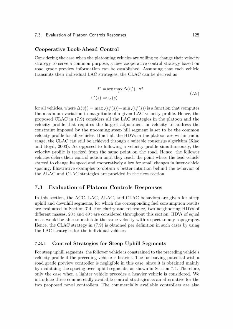
7.3. Evaluation of Platoon Controls Responses 125
Cooperative Look-Ahead ControlConsidering the case when the platooning vehicles are willing to change their velocitystrategy to serve a common purpose, a new cooperative control strategy based onroad grade preview information can be established. Assuming that each vehicletransmits their individual LAC strategies, the CLAC can be derived as
iú = arg maxi
�(vúi ), ’i
vú(s) =viú(s)(7.9)
for all vehicles, where �(vúi ) = maxs(vú
i (s))≠mins(vúi (s)) is a function that computes
the maximum variation in magnitude of a given LAC velocity profile. Hence, theproposed CLAC in (7.9) considers all the LAC strategies in the platoon and thevelocity profile that requires the largest adjustment in velocity to address theconstraint imposed by the upcoming steep hill segment is set to be the commonvelocity profile for all vehicles. If not all the HDVs in the platoon are within radiorange, the CLAC can still be achieved through a suitable consensus algorithm (Xiaoand Boyd, 2003). As opposed to following a velocity profile simultaneously, thevelocity profile is tracked from the same point on the road. Hence, the followervehicles defers their control action until they reach the point where the lead vehiclestarted to change its speed and cooperatively allow for small changes in inter-vehiclespacing. Illustrative examples to obtain a better intuition behind the behavior ofthe ALAC and CLAC strategies are provided in the next section.
7.3 Evaluation of Platoon Controls Responses
In this section, the ACC, LAC, ALAC, and CLAC behaviors are given for steepuphill and downhill segments, for which the corresponding fuel consumption resultsare evaluated in Section 7.4. For clarity and relevance, two neighboring HDVs ofdi�erent masses, 20 t and 40 t are considered throughout this section. HDVs of equalmass would be able to maintain the same velocity with respect to any topography.Hence, the CLAC strategy in (7.9) is obtained per definition in such cases by usingthe LAC strategies for the individual vehicles.
7.3.1 Control Strategies for Steep Uphill SegmentsFor steep uphill segments, the follower vehicle is constrained to the preceding vehicle’svelocity profile if the preceding vehicle is heavier. The fuel-saving potential with aroad grade preview controller is negligible in this case, since it is obtained mainlyby maintaing the spacing over uphill segments, as shown in Section 7.4. Therefore,only the case when a lighter vehicle precedes a heavier vehicle is considered. Weintroduce three commercially available control strategies as an alternative for thetwo proposed novel controllers. The commercially available controllers are also
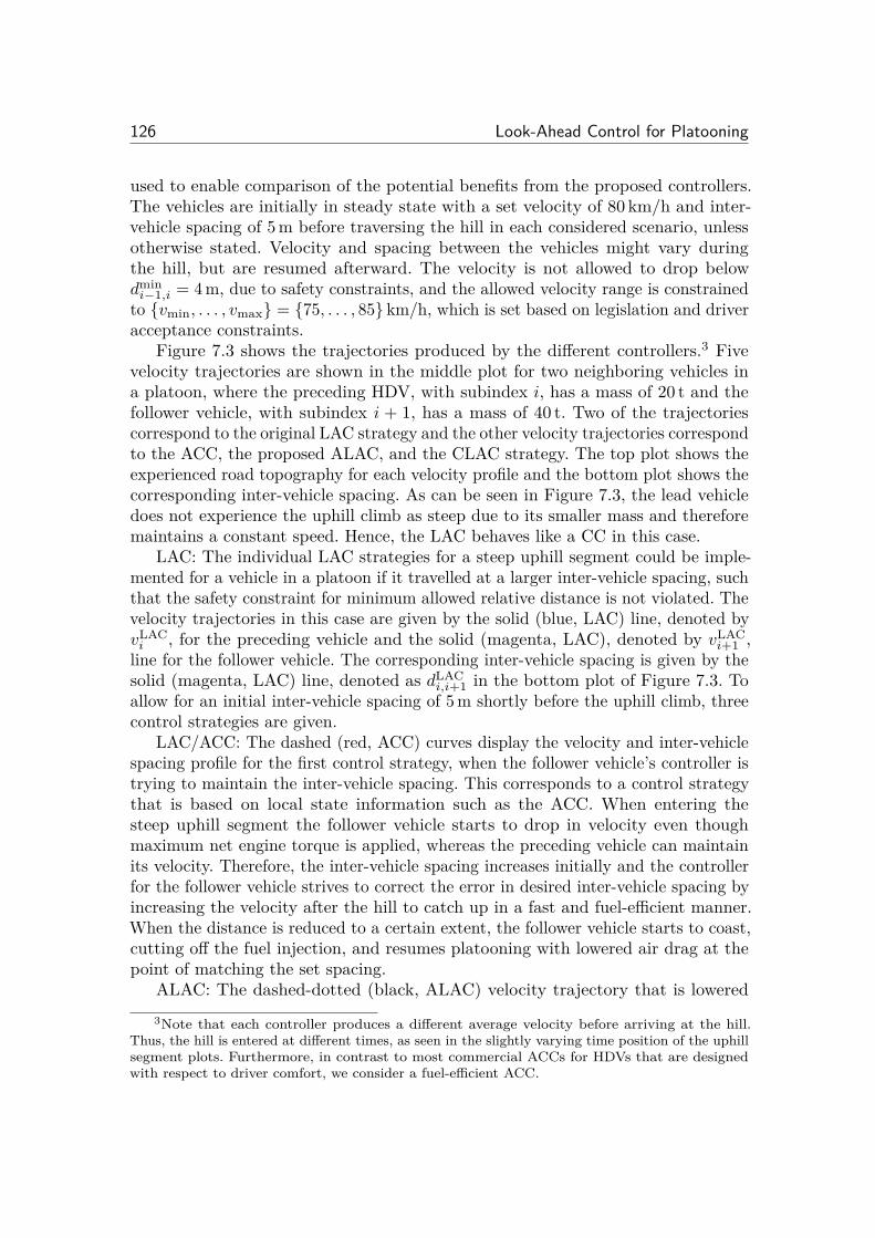
126 Look-Ahead Control for Platooning
used to enable comparison of the potential benefits from the proposed controllers.The vehicles are initially in steady state with a set velocity of 80 km/h and inter-vehicle spacing of 5 m before traversing the hill in each considered scenario, unlessotherwise stated. Velocity and spacing between the vehicles might vary duringthe hill, but are resumed afterward. The velocity is not allowed to drop belowdmin
i≠1,i = 4 m, due to safety constraints, and the allowed velocity range is constrainedto {v
min
, . . . , vmax
} = {75, . . . , 85} km/h, which is set based on legislation and driveracceptance constraints.
Figure 7.3 shows the trajectories produced by the di�erent controllers.3 Fivevelocity trajectories are shown in the middle plot for two neighboring vehicles ina platoon, where the preceding HDV, with subindex i, has a mass of 20 t and thefollower vehicle, with subindex i + 1, has a mass of 40 t. Two of the trajectoriescorrespond to the original LAC strategy and the other velocity trajectories correspondto the ACC, the proposed ALAC, and the CLAC strategy. The top plot shows theexperienced road topography for each velocity profile and the bottom plot shows thecorresponding inter-vehicle spacing. As can be seen in Figure 7.3, the lead vehicledoes not experience the uphill climb as steep due to its smaller mass and thereforemaintains a constant speed. Hence, the LAC behaves like a CC in this case.
LAC: The individual LAC strategies for a steep uphill segment could be imple-mented for a vehicle in a platoon if it travelled at a larger inter-vehicle spacing, suchthat the safety constraint for minimum allowed relative distance is not violated. Thevelocity trajectories in this case are given by the solid (blue, LAC) line, denoted byvLAC
i , for the preceding vehicle and the solid (magenta, LAC), denoted by vLAC
i+1
,line for the follower vehicle. The corresponding inter-vehicle spacing is given by thesolid (magenta, LAC) line, denoted as dLAC
i,i+1
in the bottom plot of Figure 7.3. Toallow for an initial inter-vehicle spacing of 5 m shortly before the uphill climb, threecontrol strategies are given.
LAC/ACC: The dashed (red, ACC) curves display the velocity and inter-vehiclespacing profile for the first control strategy, when the follower vehicle’s controller istrying to maintain the inter-vehicle spacing. This corresponds to a control strategythat is based on local state information such as the ACC. When entering thesteep uphill segment the follower vehicle starts to drop in velocity even thoughmaximum net engine torque is applied, whereas the preceding vehicle can maintainits velocity. Therefore, the inter-vehicle spacing increases initially and the controllerfor the follower vehicle strives to correct the error in desired inter-vehicle spacing byincreasing the velocity after the hill to catch up in a fast and fuel-e�cient manner.When the distance is reduced to a certain extent, the follower vehicle starts to coast,cutting o� the fuel injection, and resumes platooning with lowered air drag at thepoint of matching the set spacing.
ALAC: The dashed-dotted (black, ALAC) velocity trajectory that is lowered3Note that each controller produces a di�erent average velocity before arriving at the hill.
Thus, the hill is entered at di�erent times, as seen in the slightly varying time position of the uphillsegment plots. Furthermore, in contrast to most commercial ACCs for HDVs that are designedwith respect to driver comfort, we consider a fuel-e�cient ACC.
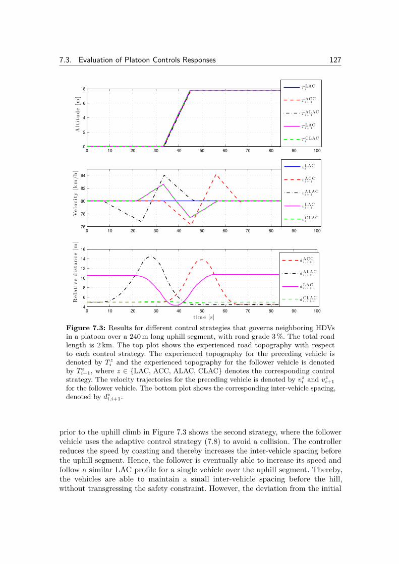
7.3. Evaluation of Platoon Controls Responses 127
0 10 20 30 40 50 60 70 80 90 1000
2
4
6
8
Alt
itu
de
[m]
0 10 20 30 40 50 60 70 80 90 10076
78
80
82
84
Velo
cit
y[k
m/h
]
0 10 20 30 40 50 60 70 80 90 1004
6
8
10
12
14
16
Rela
tive
dis
tan
ce
[m]
t im e [s]
T LACi
T ACCi + 1
T ALACi + 1
T LACi + 1
T CLACi
vLACi
vACCi + 1
vALACi + 1
vLACi + 1
vCLACi
d ACCi , i + 1
d ALACi , i + 1
d LACi , i + 1
d CLACi , i + 1
Figure 7.3: Results for di�erent control strategies that governs neighboring HDVsin a platoon over a 240 m long uphill segment, with road grade 3 %. The total roadlength is 2 km. The top plot shows the experienced road topography with respectto each control strategy. The experienced topography for the preceding vehicle isdenoted by T
z
i
and the experienced topography for the follower vehicle is denotedby T
z
i+1, where z œ {LAC, ACC, ALAC, CLAC} denotes the corresponding controlstrategy. The velocity trajectories for the preceding vehicle is denoted by v
z
i
and v
z
i+1for the follower vehicle. The bottom plot shows the corresponding inter-vehicle spacing,denoted by d
z
i,i+1.
prior to the uphill climb in Figure 7.3 shows the second strategy, where the followervehicle uses the adaptive control strategy (7.8) to avoid a collision. The controllerreduces the speed by coasting and thereby increases the inter-vehicle spacing beforethe uphill segment. Hence, the follower is eventually able to increase its speed andfollow a similar LAC profile for a single vehicle over the uphill segment. Thereby,the vehicles are able to maintain a small inter-vehicle spacing before the hill,without transgressing the safety constraint. However, the deviation from the initial
128 Look-Ahead Control for Platooning
velocity varies similarly compared to the LAC/ACC combination. This could inducedisturbances that are di�cult to handle further downstream in the platoon.
CLAC: The dashed (green, CLAC) trajectories show the velocity profile andslight variation in spacing that occurs with the CLAC. Here, the preceding vehiclecooperatively adjusts its velocity profile to match the constrained LAC profile for thefollower vehicle. Thereby, the deviation in inter-vehicle spacing is reduced comparedto the previous controllers and inherently a lower air drag is achieved throughoutthe hill. Furthermore, if the follower vehicles downstream in the platoon followthe velocity trajectory, from the same point in the road, the heterogenous platoonwill act as a homogenous platoon and reduce the variation in velocity between thevehicles in the platoon.
7.3.2 Control Strategies for Steep Downhill SegmentsFor steep downhill segments, the additional constraint of avoiding braking must betaken into consideration and hence, as opposed to control for steep uphills, bothcases of having a lighter or heavier preceding vehicle compared to the follower vehicleis addressed. The trajectories for facing a downhill segment when the heavier HDVis preceding the lighter HDV are shown in Figure 7.4. They are subindexed by i forthe preceding vehicle and by i + 1 for the follower vehicle. The top plot shows theexperienced road topography, the middle plot shows the velocity trajectories basedon the corresponding control strategy, and the bottom plot shows the inter-vehiclespacing with respect to each velocity profile. Four di�erent control strategies areillustrated in Figure 7.4.
LAC: The trajectories with superindex LAC shows the case when the LACstrategy is utilized by both vehicles and the inter-vehicle spacing is 8.7 m, so thatthe lower boundary of 4 m is not breached.
CC/ACC: The dashed (red, CC) lines display the trajectories for when thepreceding vehicle is governed by the commercial CC and the follower vehicle isgoverned by the ACC. The corresponding relative distance, which is kept constantwith the ACC, is given in the bottom plot. The CC has no information regardingthe oncoming topography. Thus, the velocity increases when entering the downhillsegment and it is forced to brake when it exceeds the allowed velocity limit. Thefollower vehicle tracks the velocity with its ACC and is able to maintain the inter-vehicle spacing throughout the hill to obtain the benefits from a low air drag.However, it is forced to brake eventually and thus reduces the fuel-saving potential.
ALAC: The dashed-dotted (black, ALAC) trajectories display the ALAC strategyfor when the follower vehicle receives information through wireless communicationregarding the preceding HDV’s LAC velocity profile. Thereby, it can adapt and avoida collision by initially reducing its speed to increase the inter-vehicle spacing andthen compensate by maintaining the gained speed over the downhill segment a whileafterward. When the spacing is increased, the follower vehicle finally reduces itsvelocity by coasting to match the desired spacing and speed of the preceding vehicle.Hence, for this case, the ALAC finds a strategy such that the initial inter-vehicle
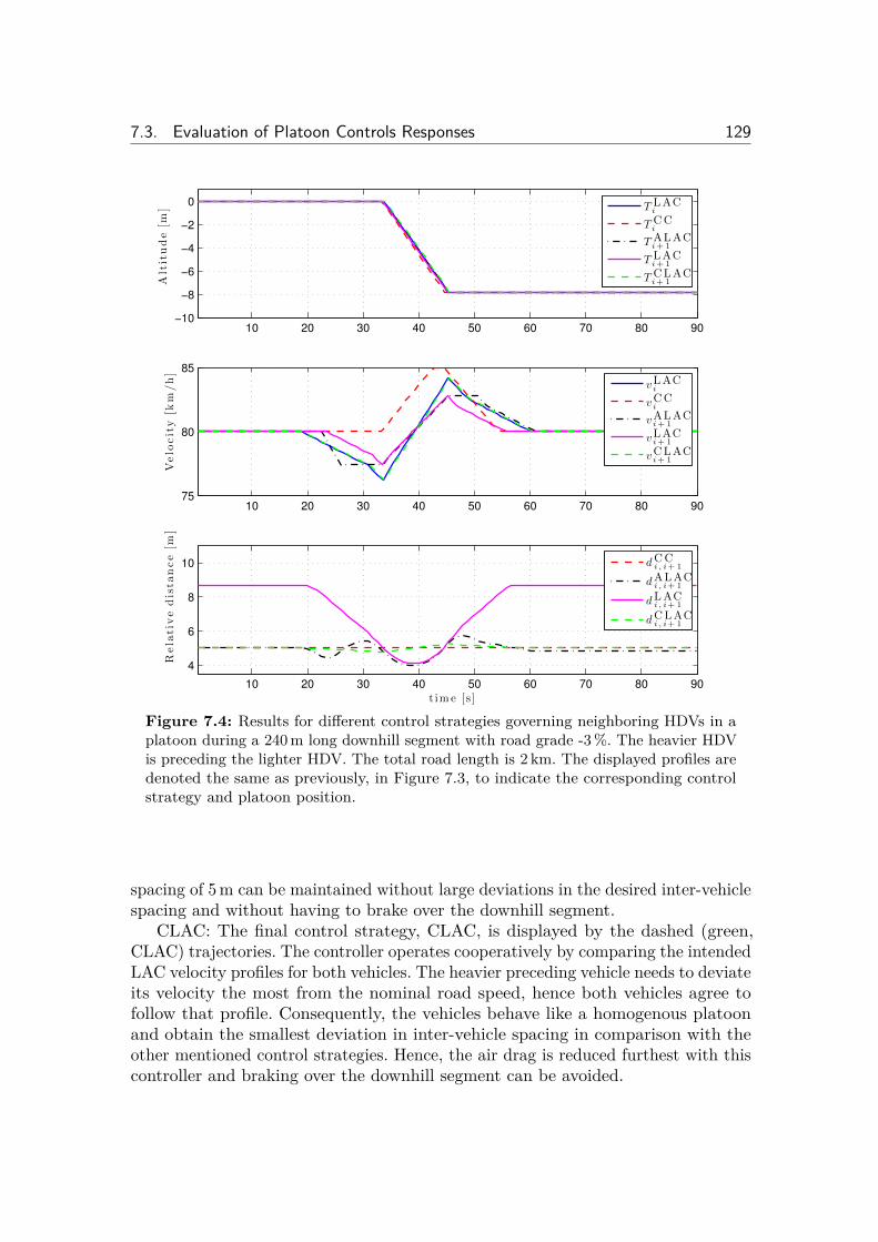
7.3. Evaluation of Platoon Controls Responses 129
10 20 30 40 50 60 70 80 90−10
−8
−6
−4
−2
0
Alt
itu
de
[m]
10 20 30 40 50 60 70 80 9075
80
85
Velo
cit
y[k
m/h
]
10 20 30 40 50 60 70 80 90
4
6
8
10
Rela
tive
dis
tan
ce
[m]
t im e [s]
T L ACi
T C Ci
T AL ACi+ 1
T L ACi+ 1
T C LACi+ 1
vL ACi
vC Ci
vAL ACi+ 1
vL ACi+ 1
vC LACi+ 1
dC Ci , i+ 1
dAL ACi , i+ 1
dL ACi , i+ 1
dC L ACi , i+ 1
Figure 7.4: Results for di�erent control strategies governing neighboring HDVs in aplatoon during a 240 m long downhill segment with road grade -3 %. The heavier HDVis preceding the lighter HDV. The total road length is 2 km. The displayed profiles aredenoted the same as previously, in Figure 7.3, to indicate the corresponding controlstrategy and platoon position.
spacing of 5 m can be maintained without large deviations in the desired inter-vehiclespacing and without having to brake over the downhill segment.
CLAC: The final control strategy, CLAC, is displayed by the dashed (green,CLAC) trajectories. The controller operates cooperatively by comparing the intendedLAC velocity profiles for both vehicles. The heavier preceding vehicle needs to deviateits velocity the most from the nominal road speed, hence both vehicles agree tofollow that profile. Consequently, the vehicles behave like a homogenous platoonand obtain the smallest deviation in inter-vehicle spacing in comparison with theother mentioned control strategies. Hence, the air drag is reduced furthest with thiscontroller and braking over the downhill segment can be avoided.
130 Look-Ahead Control for Platooning
The trajectories for the reverse order, when the preceding HDV weighs 20 t andthe follower HDV weighs 40 t, are given in Figure 7.5.
LAC: For this ordering, both vehicles can use their LAC and maintain the smallinter-vehicle spacing of 5 m before the downhill segment, since the follower willinitiate its speed reduction before the preceding lighter HDV. Hence, there is no needfor an ALAC in this case. The trajectories produced by this controller is displayedby the solid (blue, LAC) trajectory for the preceding vehicle and the solid (magenta,LAC) trajectory for the follower vehicle. The corresponding increase in relativedistance is given in the bottom plot by the solid (magenta, LAC) curve.
CC/ACC: The dashed (red, CC) trajectories display the scenario when thepreceding vehicle is governed by the CC and the follower vehicle is governed bythe ACC. The preceding HDV does not reach the maximum speed constraint andcan resume its set speed by cutting o� the fuel injection throughout the downhillsegment and afterward. However, the follower vehicle must brake all the way duringthat stretch to maintain a constant spacing due to its heavier mass.
LAC/ACC: The dashed-dotted (black, ACC) trajectories display the scenariowhen the preceding vehicle is governed by the LAC and the follower vehicle isgoverned by the ACC. In this case, the ACC must brake over the entire stretchthat the preceding vehicle is adapting its speed through the LAC to address theconstraints imposed by the hill.
CLAC: The trajectories for the cooperative look-ahead controller is given bythe dashed (green, CLAC) curves. In this case the preceding vehicle agrees to trackthe trajectory of the follower vehicle, since it requires the largest velocity changeswhen facing the downhill segment. Thereby, the follower vehicle is able to avoidbraking. The preceding vehicle vehicle has to inject a small amount of fuel to followthe agreed velocity profile. However, the small increase in fuel consumption is lessthan the fuel saved for the subject vehicle and the follower vehicle by allowing for amaintained small inter-vehicle spacing over the entire road stretch.
7.4 Evaluation of Fuel-Saving Possibilities
In this section, we evaluate the fuel-e�ciency of the proposed controller strategies,which are based on preview information of the topography. The hill characteristicschange with the grade or the length of the hill. We study the total fuel consumptionfor two neighboring HDVs that travel over a 2 km long road with a 240 m or 320 msteep hill. The length of the hill is chosen such that it is a significant part of thetotal road stretch and the road grade for the considered uphills and downhills is3 % and -3%, respectively. The most fuel-e�cient controller is determined for theconsidered hills. Finally, we apply the proposed CLAC on an N = 9 HDV platoonof masses ranging between 20 t to 40 t and evaluate the performance for two hills.
The relative fuel consumption for two HDVs of masses 20 t and 40 t traveling asa platoon facing an uphill segment are given in Table 7.1. Table 7.2 lists the relativefuel consumption when facing a downhill segment with the preceding HDV being
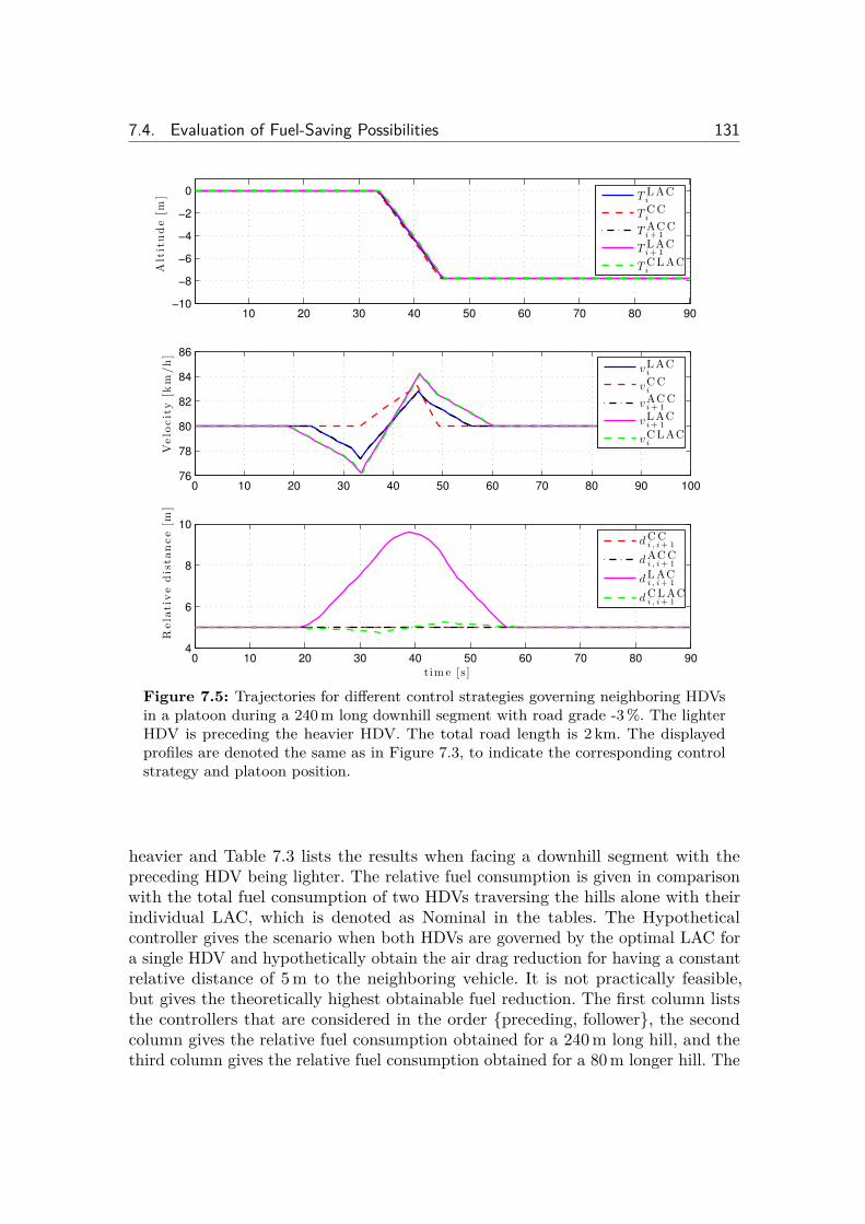
7.4. Evaluation of Fuel-Saving Possibilities 131
10 20 30 40 50 60 70 80 90−10
−8
−6
−4
−2
0
Alt
itu
de
[m]
0 10 20 30 40 50 60 70 80 90 10076
78
80
82
84
86
Velo
cit
y[k
m/h
]
0 10 20 30 40 50 60 70 80 904
6
8
10
Rela
tive
dis
tan
ce
[m]
t im e [s]
T L ACi
T C Ci
T AC Ci+ 1
T L ACi+ 1
T C LACi
vL ACi
vC Ci
vAC Ci+ 1
vL ACi+ 1
vC LACi
dC Ci , i+ 1
dAC Ci , i+ 1
dL ACi , i+ 1
dC LACi , i+ 1
Figure 7.5: Trajectories for di�erent control strategies governing neighboring HDVsin a platoon during a 240 m long downhill segment with road grade -3 %. The lighterHDV is preceding the heavier HDV. The total road length is 2 km. The displayedprofiles are denoted the same as in Figure 7.3, to indicate the corresponding controlstrategy and platoon position.
heavier and Table 7.3 lists the results when facing a downhill segment with thepreceding HDV being lighter. The relative fuel consumption is given in comparisonwith the total fuel consumption of two HDVs traversing the hills alone with theirindividual LAC, which is denoted as Nominal in the tables. The Hypotheticalcontroller gives the scenario when both HDVs are governed by the optimal LAC fora single HDV and hypothetically obtain the air drag reduction for having a constantrelative distance of 5 m to the neighboring vehicle. It is not practically feasible,but gives the theoretically highest obtainable fuel reduction. The first column liststhe controllers that are considered in the order {preceding, follower}, the secondcolumn gives the relative fuel consumption obtained for a 240 m long hill, and thethird column gives the relative fuel consumption obtained for a 80 m longer hill. The
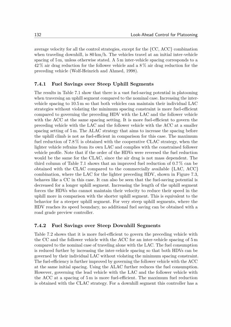
132 Look-Ahead Control for Platooning
average velocity for all the control strategies, except for the {CC, ACC} combinationwhen traveling downhill, is 80 km/h. The vehicles travel at an initial inter-vehiclespacing of 5 m, unless otherwise stated. A 5 m inter-vehicle spacing corresponds to a42 % air drag reduction for the follower vehicle and a 8 % air drag reduction for thepreceding vehicle (Wolf-Heinrich and Ahmed, 1998).
7.4.1 Fuel Savings over Steep Uphill SegmentsThe results in Table 7.1 show that there is a vast fuel-saving potential in platooningwhen traversing an uphill segment compared to the nominal case. Increasing the inter-vehicle spacing to 10.5 m so that both vehicles can maintain their individual LACstrategies without violating the minimum spacing constraint is more fuel-e�cientcompared to governing the preceding HDV with the LAC and the follower vehiclewith the ACC at the same spacing setting. It is more fuel-e�cient to govern thepreceding vehicle with the LAC and the follower vehicle with the ACC at a smallerspacing setting of 5 m. The ALAC strategy that aims to increase the spacing beforethe uphill climb is not as fuel-e�cient in comparison for this case. The maximumfuel reduction of 7.8 % is obtained with the cooperative CLAC strategy, when thelighter vehicle refrains from its own LAC and complies with the constrained followervehicle profile. Note that if the order of the HDVs were reversed the fuel reductionwould be the same for the CLAC, since the air drag is not mass dependent. Thethird column of Table 7.1 shows that an improved fuel reduction of 0.7 % can beobtained with the CLAC compared to the commercially available {LAC, ACC}combination, where the LAC for the lighter preceding HDV, shown in Figure 7.3,behaves like a CC in this case. It can also be seen that the fuel-saving potential isdecreased for a longer uphill segment. Increasing the length of the uphill segmentforces the HDVs who cannot maintain their velocity to reduce their speed in theuphill more in comparison with the shorter uphill segment. This is equivalent to thebehavior for a steeper uphill segment. For very steep uphill segments, where theHDV reaches its speed boundary, no additional fuel saving can be obtained with aroad grade preview controller.
7.4.2 Fuel Savings over Steep Downhill SegmentsTable 7.2 shows that it is more fuel-e�cient to govern the preceding vehicle withthe CC and the follower vehicle with the ACC for an inter-vehicle spacing of 5 mcompared to the nominal case of traveling alone with the LAC. The fuel consumptionis reduced further by increasing the inter-vehicle spacing so that both HDVs can begoverned by their individual LAC without violating the minimum spacing constraint.The fuel-e�ciency is further improved by governing the follower vehicle with the ACCat the same initial spacing. Using the ALAC further reduces the fuel consumption.However, governing the lead vehicle with the LAC and the follower vehicle withthe ACC at a spacing of 5 m is more fuel-e�cient. The maximum fuel reductionis obtained with the CLAC strategy. For a downhill segment this controller has a
7.4. Evaluation of Fuel-Saving Possibilities 133
Table 7.1: Table of relative fuel consumption for di�erent uphill control strategieswith a lighter preceding HDV. The uphill segment has a grade of 3 %.
Controllers: Fuel Consumption [%] Fuel Consumption [%]{HDVi, HDVi+1
} (240 m uphill) (320 m uphill)Nominal 100 100
{LAC, ACC}ú 93.50 95.34{LAC, LAC}ú 93.00 94.29{LAC, ACC} 92.50 93.45
{LAC, ALAC} 92.54 93.20{CLAC, CLAC} 92.24 92.81
Hypothetical 92.23 92.76* Results obtained for initial inter-vehicle spacing of 10.5 m for the240 m segment and 15.5 m for the 320 m segment.
Table 7.2: Table of relative fuel consumption for di�erent downhill control strategieswith a heavier preceding HDV. The downhill segment has a grade of -3 %.
Controllers: Fuel Consumption [%] Fuel Consumption [%]{HDVi, HDVi+1
} (240 m downhill) (320 m downhill)Nominal 100 100
{CC, ACC} 91.97 96.07{LAC, LAC}ú 88.12 87.80{LAC, ACC}ú 88.10 88.47{LAC, ALAC} 87.88 87.04{LAC, ACC} 87.17 86.04
{CLAC, CLAC} 87.15 86.03Hypothetical 87.65 86.76
* Results obtained for initial inter-vehicle spacing of 8.7 m for the240 m segment and 12 m for the 320 m segment.
higher fuel reduction than the hypothetic case. As opposed to traveling in an uphill,when traveling in a downhill the air drag has a larger e�ect on the required enginetorque input to handle the imposed constraints. Therefore, the LAC is no longeroptimal in a downhill due to the lowered air drag. Hence a slightly higher fuel savingis obtained for the CLAC strategy.
Table 7.3 shows it is still more fuel-e�cient to platoon by governing the preceding20 t vehicle with the CC and the follower 40 t vehicle with the ACC in the 240 mlong downhill segment, compared to the nominal case. However, for the 320 m
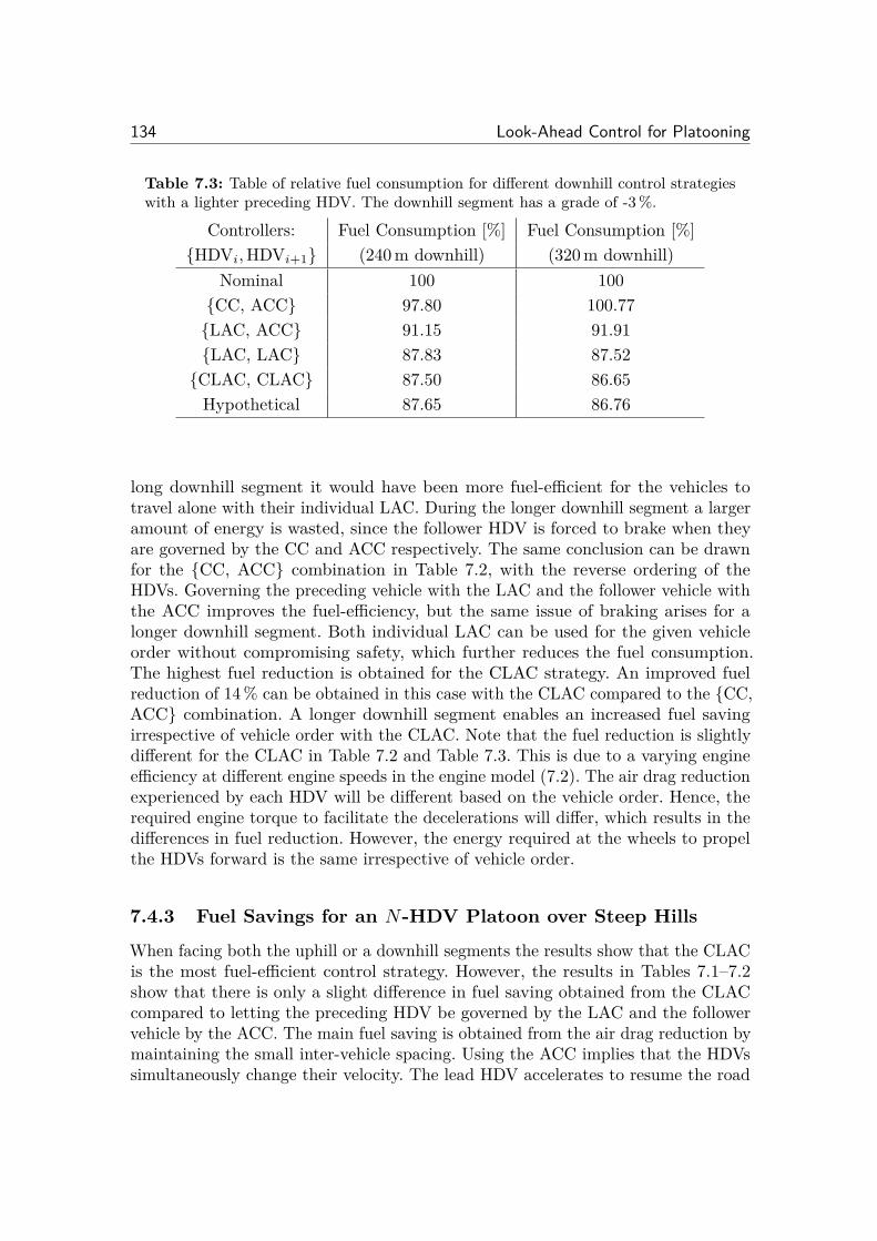
134 Look-Ahead Control for Platooning
Table 7.3: Table of relative fuel consumption for di�erent downhill control strategieswith a lighter preceding HDV. The downhill segment has a grade of -3 %.
Controllers: Fuel Consumption [%] Fuel Consumption [%]{HDVi, HDVi+1
} (240 m downhill) (320 m downhill)Nominal 100 100
{CC, ACC} 97.80 100.77{LAC, ACC} 91.15 91.91{LAC, LAC} 87.83 87.52
{CLAC, CLAC} 87.50 86.65Hypothetical 87.65 86.76
long downhill segment it would have been more fuel-e�cient for the vehicles totravel alone with their individual LAC. During the longer downhill segment a largeramount of energy is wasted, since the follower HDV is forced to brake when theyare governed by the CC and ACC respectively. The same conclusion can be drawnfor the {CC, ACC} combination in Table 7.2, with the reverse ordering of theHDVs. Governing the preceding vehicle with the LAC and the follower vehicle withthe ACC improves the fuel-e�ciency, but the same issue of braking arises for alonger downhill segment. Both individual LAC can be used for the given vehicleorder without compromising safety, which further reduces the fuel consumption.The highest fuel reduction is obtained for the CLAC strategy. An improved fuelreduction of 14 % can be obtained in this case with the CLAC compared to the {CC,ACC} combination. A longer downhill segment enables an increased fuel savingirrespective of vehicle order with the CLAC. Note that the fuel reduction is slightlydi�erent for the CLAC in Table 7.2 and Table 7.3. This is due to a varying enginee�ciency at di�erent engine speeds in the engine model (7.2). The air drag reductionexperienced by each HDV will be di�erent based on the vehicle order. Hence, therequired engine torque to facilitate the decelerations will di�er, which results in thedi�erences in fuel reduction. However, the energy required at the wheels to propelthe HDVs forward is the same irrespective of vehicle order.
7.4.3 Fuel Savings for an N-HDV Platoon over Steep Hills
When facing both the uphill or a downhill segments the results show that the CLACis the most fuel-e�cient control strategy. However, the results in Tables 7.1–7.2show that there is only a slight di�erence in fuel saving obtained from the CLACcompared to letting the preceding HDV be governed by the LAC and the followervehicle by the ACC. The main fuel saving is obtained from the air drag reduction bymaintaining the small inter-vehicle spacing. Using the ACC implies that the HDVssimultaneously change their velocity. The lead HDV accelerates to resume the road
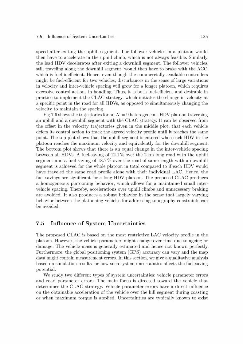
7.5. Influence of System Uncertainties 135
speed after exiting the uphill segment. The follower vehicles in a platoon wouldthen have to accelerate in the uphill climb, which is not always feasible. Similarly,the lead HDV decelerates after exiting a downhill segment. The follower vehicles,still traveling along the downhill segment, would then have to brake with the ACC,which is fuel-ine�cient. Hence, even though the commercially available controllersmight be fuel-e�cient for two vehicles, disturbances in the sense of large variationsin velocity and inter-vehicle spacing will grow for a longer platoon, which requiresexcessive control actions in handling. Thus, it is both fuel-e�cient and desirable inpractice to implement the CLAC strategy, which initiates the change in velocity ata specific point in the road for all HDVs, as opposed to simultaneously changing thevelocity to maintain the spacing.
Fig 7.6 shows the trajectories for an N = 9 heterogeneous HDV platoon traversingan uphill and a downhill segment with the CLAC strategy. It can be observed fromthe o�set in the velocity trajectories given in the middle plot, that each vehicledefers its control action to track the agreed velocity profile until it reaches the samepoint. The top plot shows that the uphill segment is entered when each HDV in theplatoon reaches the maximum velocity and equivalently for the downhill segment.The bottom plot shows that there is an equal change in the inter-vehicle spacingbetween all HDVs. A fuel-saving of 12.1 % over the 2 km long road with the uphillsegment and a fuel-saving of 18.7 % over the road of same length with a downhillsegment is achieved for the whole platoon in total compared to if each HDV wouldhave traveled the same road profile alone with their individual LAC. Hence, thefuel savings are significant for a long HDV platoon. The proposed CLAC producesa homogeneous platooning behavior, which allows for a maintained small inter-vehicle spacing. Thereby, accelerations over uphill climbs and unnecessary brakingare avoided. It also produces a robust behavior in the sense that largely varyingbehavior between the platooning vehicles for addressing topography constraints canbe avoided.
7.5 Influence of System Uncertainties
The proposed CLAC is based on the most restrictive LAC velocity profile in theplatoon. However, the vehicle parameters might change over time due to ageing ordamage. The vehicle mass is generally estimated and hence not known perfectly.Furthermore, the global positioning system (GPS) accuracy can vary and the mapdata might contain measurement errors. In this section, we give a qualitative analysisbased on simulation results for how such system uncertainties a�ects the fuel-savingpotential.
We study two di�erent types of system uncertainties: vehicle parameter errorsand road parameter errors. The main focus is directed toward the vehicle thatdetermines the CLAC strategy. Vehicle parameter errors have a direct influenceon the obtainable acceleration of the vehicle over the hill segment during coastingor when maximum torque is applied. Uncertainties are typically known to exist
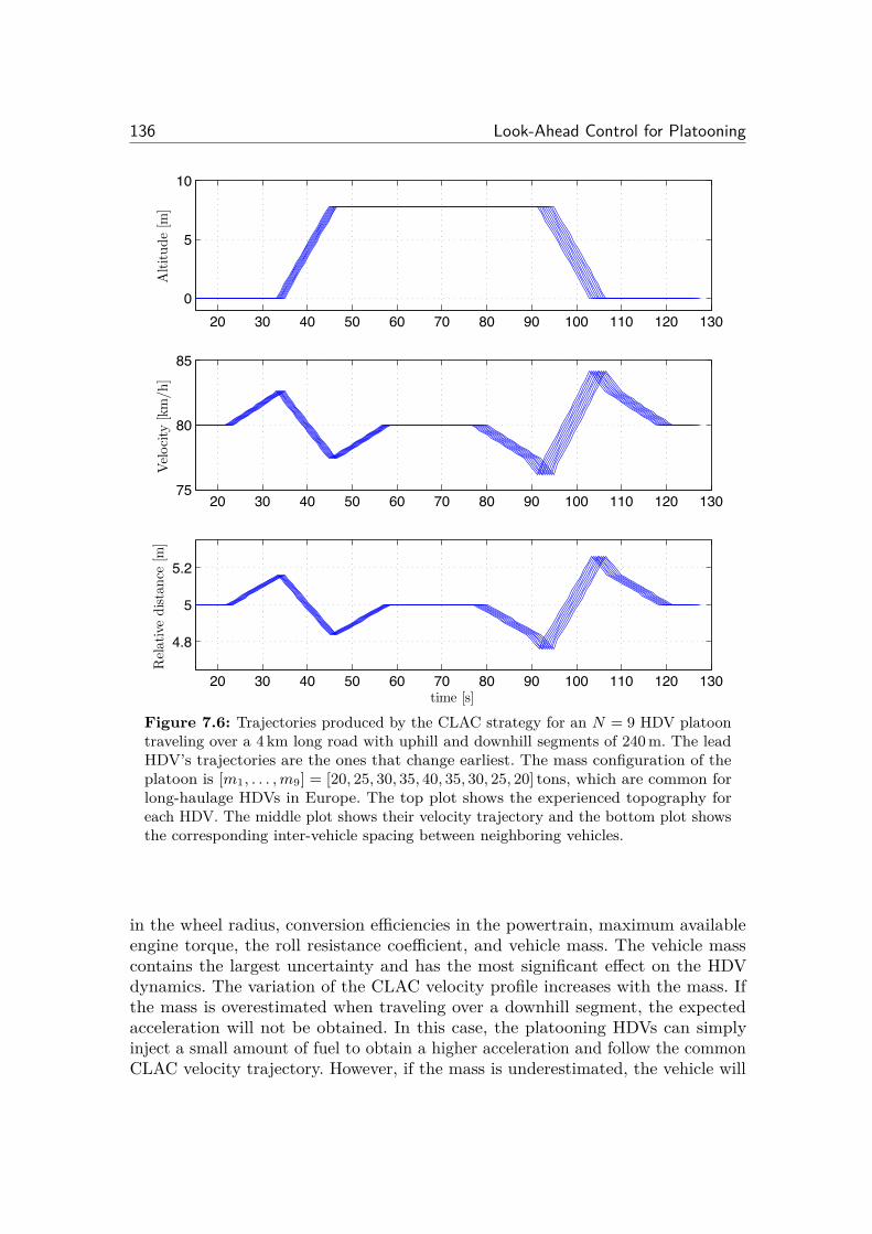
136 Look-Ahead Control for Platooning
20 30 40 50 60 70 80 90 100 110 120 1300
5
10A
ltitude
[m]
20 30 40 50 60 70 80 90 100 110 120 13075
80
85
Vel
oci
ty[k
m/h
]
20 30 40 50 60 70 80 90 100 110 120 130
4.8
5
5.2
Rel
ativ
edista
nce
[m]
time [s]
Figure 7.6: Trajectories produced by the CLAC strategy for an N = 9 HDV platoontraveling over a 4 km long road with uphill and downhill segments of 240 m. The leadHDV’s trajectories are the ones that change earliest. The mass configuration of theplatoon is [m1, . . . , m9] = [20, 25, 30, 35, 40, 35, 30, 25, 20] tons, which are common forlong-haulage HDVs in Europe. The top plot shows the experienced topography foreach HDV. The middle plot shows their velocity trajectory and the bottom plot showsthe corresponding inter-vehicle spacing between neighboring vehicles.
in the wheel radius, conversion e�ciencies in the powertrain, maximum availableengine torque, the roll resistance coe�cient, and vehicle mass. The vehicle masscontains the largest uncertainty and has the most significant e�ect on the HDVdynamics. The variation of the CLAC velocity profile increases with the mass. Ifthe mass is overestimated when traveling over a downhill segment, the expectedacceleration will not be obtained. In this case, the platooning HDVs can simplyinject a small amount of fuel to obtain a higher acceleration and follow the commonCLAC velocity trajectory. However, if the mass is underestimated, the vehicle will
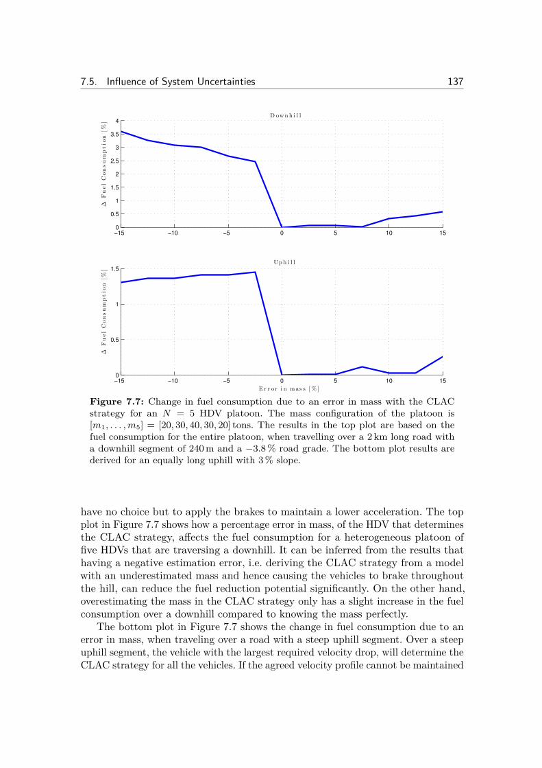
7.5. Influence of System Uncertainties 137
−15 −10 −5 0 5 10 150
0.5
1
1.5
2
2.5
3
3.5
4D own h i l l
�F
uel
Con
su
mp
tio
n[%
]
−15 −10 −5 0 5 10 150
0.5
1
1.5
Up h i l l
�F
uel
Con
su
mp
tio
n[%
]
E r r or i n mas s [ % ]
Figure 7.7: Change in fuel consumption due to an error in mass with the CLACstrategy for an N = 5 HDV platoon. The mass configuration of the platoon is[m1, . . . , m5] = [20, 30, 40, 30, 20] tons. The results in the top plot are based on thefuel consumption for the entire platoon, when travelling over a 2 km long road witha downhill segment of 240 m and a ≠3.8 % road grade. The bottom plot results arederived for an equally long uphill with 3 % slope.
have no choice but to apply the brakes to maintain a lower acceleration. The topplot in Figure 7.7 shows how a percentage error in mass, of the HDV that determinesthe CLAC strategy, a�ects the fuel consumption for a heterogeneous platoon offive HDVs that are traversing a downhill. It can be inferred from the results thathaving a negative estimation error, i.e. deriving the CLAC strategy from a modelwith an underestimated mass and hence causing the vehicles to brake throughoutthe hill, can reduce the fuel reduction potential significantly. On the other hand,overestimating the mass in the CLAC strategy only has a slight increase in the fuelconsumption over a downhill compared to knowing the mass perfectly.
The bottom plot in Figure 7.7 shows the change in fuel consumption due to anerror in mass, when traveling over a road with a steep uphill segment. Over a steepuphill segment, the vehicle with the largest required velocity drop, will determine theCLAC strategy for all the vehicles. If the agreed velocity profile cannot be maintained
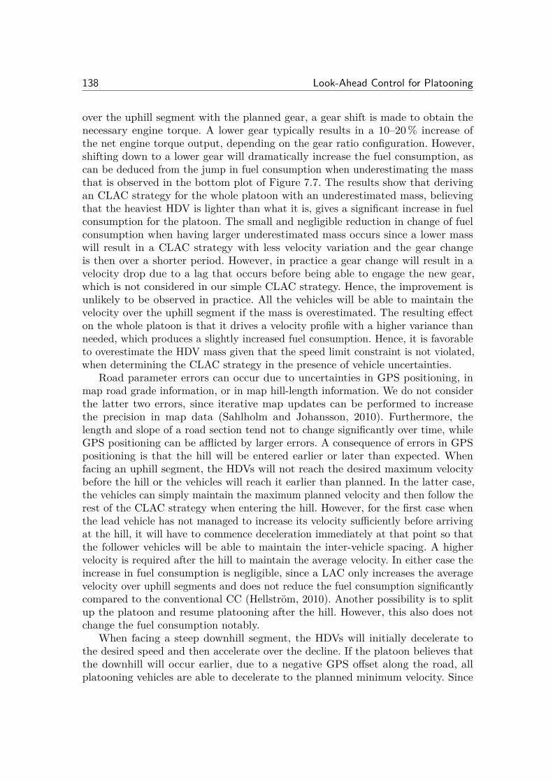
138 Look-Ahead Control for Platooning
over the uphill segment with the planned gear, a gear shift is made to obtain thenecessary engine torque. A lower gear typically results in a 10–20 % increase ofthe net engine torque output, depending on the gear ratio configuration. However,shifting down to a lower gear will dramatically increase the fuel consumption, ascan be deduced from the jump in fuel consumption when underestimating the massthat is observed in the bottom plot of Figure 7.7. The results show that derivingan CLAC strategy for the whole platoon with an underestimated mass, believingthat the heaviest HDV is lighter than what it is, gives a significant increase in fuelconsumption for the platoon. The small and negligible reduction in change of fuelconsumption when having larger underestimated mass occurs since a lower masswill result in a CLAC strategy with less velocity variation and the gear changeis then over a shorter period. However, in practice a gear change will result in avelocity drop due to a lag that occurs before being able to engage the new gear,which is not considered in our simple CLAC strategy. Hence, the improvement isunlikely to be observed in practice. All the vehicles will be able to maintain thevelocity over the uphill segment if the mass is overestimated. The resulting e�ecton the whole platoon is that it drives a velocity profile with a higher variance thanneeded, which produces a slightly increased fuel consumption. Hence, it is favorableto overestimate the HDV mass given that the speed limit constraint is not violated,when determining the CLAC strategy in the presence of vehicle uncertainties.
Road parameter errors can occur due to uncertainties in GPS positioning, inmap road grade information, or in map hill-length information. We do not considerthe latter two errors, since iterative map updates can be performed to increasethe precision in map data (Sahlholm and Johansson, 2010). Furthermore, thelength and slope of a road section tend not to change significantly over time, whileGPS positioning can be a�icted by larger errors. A consequence of errors in GPSpositioning is that the hill will be entered earlier or later than expected. Whenfacing an uphill segment, the HDVs will not reach the desired maximum velocitybefore the hill or the vehicles will reach it earlier than planned. In the latter case,the vehicles can simply maintain the maximum planned velocity and then follow therest of the CLAC strategy when entering the hill. However, for the first case whenthe lead vehicle has not managed to increase its velocity su�ciently before arrivingat the hill, it will have to commence deceleration immediately at that point so thatthe follower vehicles will be able to maintain the inter-vehicle spacing. A highervelocity is required after the hill to maintain the average velocity. In either case theincrease in fuel consumption is negligible, since a LAC only increases the averagevelocity over uphill segments and does not reduce the fuel consumption significantlycompared to the conventional CC (Hellström, 2010). Another possibility is to splitup the platoon and resume platooning after the hill. However, this also does notchange the fuel consumption notably.
When facing a steep downhill segment, the HDVs will initially decelerate tothe desired speed and then accelerate over the decline. If the platoon believes thatthe downhill will occur earlier, due to a negative GPS o�set along the road, allplatooning vehicles are able to decelerate to the planned minimum velocity. Since
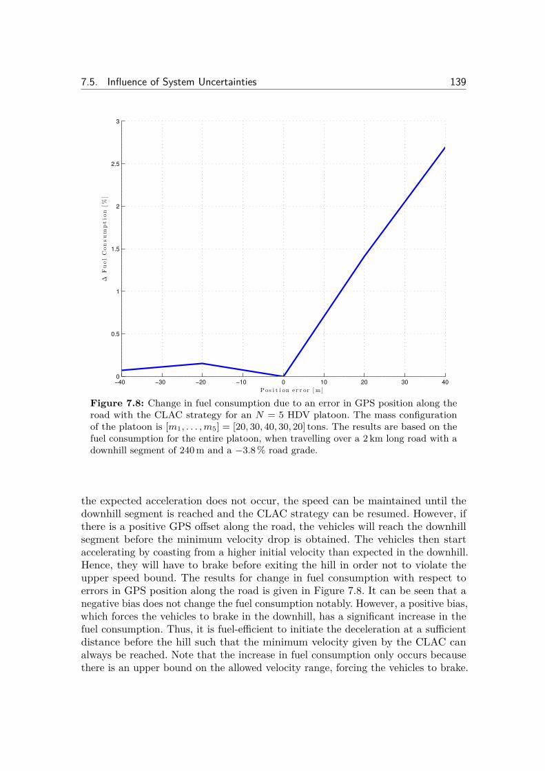
7.5. Influence of System Uncertainties 139
−40 −30 −20 −10 0 10 20 30 400
0.5
1
1.5
2
2.5
3
�F
uel
Con
su
mp
tio
n[%
]
P os i t i on e r r or [ m ]
Figure 7.8: Change in fuel consumption due to an error in GPS position along theroad with the CLAC strategy for an N = 5 HDV platoon. The mass configurationof the platoon is [m1, . . . , m5] = [20, 30, 40, 30, 20] tons. The results are based on thefuel consumption for the entire platoon, when travelling over a 2 km long road with adownhill segment of 240 m and a ≠3.8 % road grade.
the expected acceleration does not occur, the speed can be maintained until thedownhill segment is reached and the CLAC strategy can be resumed. However, ifthere is a positive GPS o�set along the road, the vehicles will reach the downhillsegment before the minimum velocity drop is obtained. The vehicles then startaccelerating by coasting from a higher initial velocity than expected in the downhill.Hence, they will have to brake before exiting the hill in order not to violate theupper speed bound. The results for change in fuel consumption with respect toerrors in GPS position along the road is given in Figure 7.8. It can be seen that anegative bias does not change the fuel consumption notably. However, a positive bias,which forces the vehicles to brake in the downhill, has a significant increase in thefuel consumption. Thus, it is fuel-e�cient to initiate the deceleration at a su�cientdistance before the hill such that the minimum velocity given by the CLAC canalways be reached. Note that the increase in fuel consumption only occurs becausethere is an upper bound on the allowed velocity range, forcing the vehicles to brake.
140 Look-Ahead Control for Platooning
Manual CC
LAC
ACC
DHSC
CACC
ALAC
CLAC
Figure 7.9: Illustration of a finite state machine for the commercially available speedcontrol systems, given in Figure 2.4, in combination with the proposed look-aheadcontroller for HDV platooning. If road grade preview information is available andthe vehicles in the platoon are not willing to cooperate, the ALAC is active. TheCLAC is active if the vehicles are willing to cooperatively form a common look-aheadcontrol strategy for all platooning vehicles with respect to the most restricted vehiclein the platoon. If road grade preview information is not available, the cooperativeadaptive cruise control (CACC) is active. Finally, if V2V communication is lost, theACC becomes active in the vehicle platoon and the relative distance is adjusted forsafety.
7.6 Summary
It is fuel-e�cient to consider the road grade preview information in HDV platooning.A simple cooperative controller for HDV platooning, based on road grade previewinformation and wireless communication, has been proposed that is close to thetheoretically highest obtainable fuel reduction. The controller enables a homogeneousbehavior for a heterogeneous platoon under topography constraints, such that theinter-vehicle spacing can be maintained for fuel-e�ciency. It also produces a robustbehavior in the sense that largely varying behavior between the platooning vehiclesfor addressing topography constraints can be avoided and inter-vehicle spacing canbe maintained throughout a hill. For fuel-e�ciency the platoon should be maintainedwhen traversing a hill, as opposed to letting the HDVs separate due to imposedconstraints and then resume platooning by catching up after the hill. Thus, it isfavorable to have a cooperative LAC strategy, which initiates the change in velocityat a specific point in the road for all HDVs, in contrast with simultaneously changingthe velocity to maintain the spacing. The presented controllers, based on road gradepreview information and wireless communication, fit nicely into the already existingsoftware control architecture in commercial HDVs, as illustrated in Figure 7.9.
The CLAC can reduce the fuel consumption for two neighboring HDVs up to14 % over a road with a downhill segment compared to the commercially availableCC and ACC that could currently be utilized for platooning in practice. For an uphill
7.6. Summary 141
climb, it can be observed that a more subtle benefit of 0.7 % improvement can beobtained with the proposed controller. However, the fuel-saving potential increaseswith the number of vehicles in the platoon. Furthermore, the CLAC is also favorablebecause it does not mandate any accelerations over uphill segments or braking overdownhill segments, which commonly occurs for synchronous control strategies. TheCLAC is also feasible in practice, since each HDV’s intended velocity profile givenby the commercially available LAC system can be transmitted. It is then simple tocompare the profiles such that the profile with the most restrictive LAC velocityprofile can be agreed upon. In the presence of vehicle parameter uncertainties, itis favorable to overestimate the vehicle mass when forming CLAC strategies tomaintain the fuel reduction potential. For GPS positioning uncertainties along theroad, it is fuel-e�cient to assume that the hill starts earlier in the road rather thanlater.

Chapter 8
Experimental Evaluation of Platooning
“The value of an idea lies in the using of it.”Thomas A. Edison
Cooperative control for heavy-duty vehicle (HDV) platooning can already beimplemented with today’s technology. Wireless communication in additionto radar information enables the possibility of forming cooperative decisions
based on actions and information from the neighboring vehicles. Most studies oncontrol for vehicle platoons have been based on simplified theoretical models, see,e.g, the survey (Tsugawa, 1999; Kavathekar and Chen, 2011). It is still unclearhow the unmodeled nonlinearities, such as gear changes, brake dynamics, enginedynamics, and a varying road topography a�ect the control performance in practice.In particular for HDVs, the road grade has a significant e�ect on the vehicledynamics: An HDV can generally not maintain its velocity when traversing steepuphill segments and it typically accelerates when coasting over a steep downhillsegment. The acceleration when coasting1 varies with vehicle mass. Hence, unwantedbehavior for heterogenous platoons, such as braking to avoid coasting into the vehicleahead, might arise over road segments with a varying topography for cooperativeadaptive cruise controllers (CACCs) that are based on linear models. Even undernormal operating conditions, when the platoon is traveling at constant speed,additional control actions for maintaining the desired relative distance are required,since external forces exert unmodeled disturbances on the system dynamics. Thus,it is important to understand the limitations when implementing a CACC basedon simplified models. It is interesting to study the performance and evaluate thefuel-saving potential of these controllers in practice.
In this chapter we evaluate the performance of the decentralized CACC presentedin Chapter 6 for a three-HDV platoon. The objective is to evaluate the performanceof this simple controller and identify possible issues that might arise in a practical
1A vehicle is said to be coasting when it is moving forward even though no fuel is injected andno braking is applied.
143
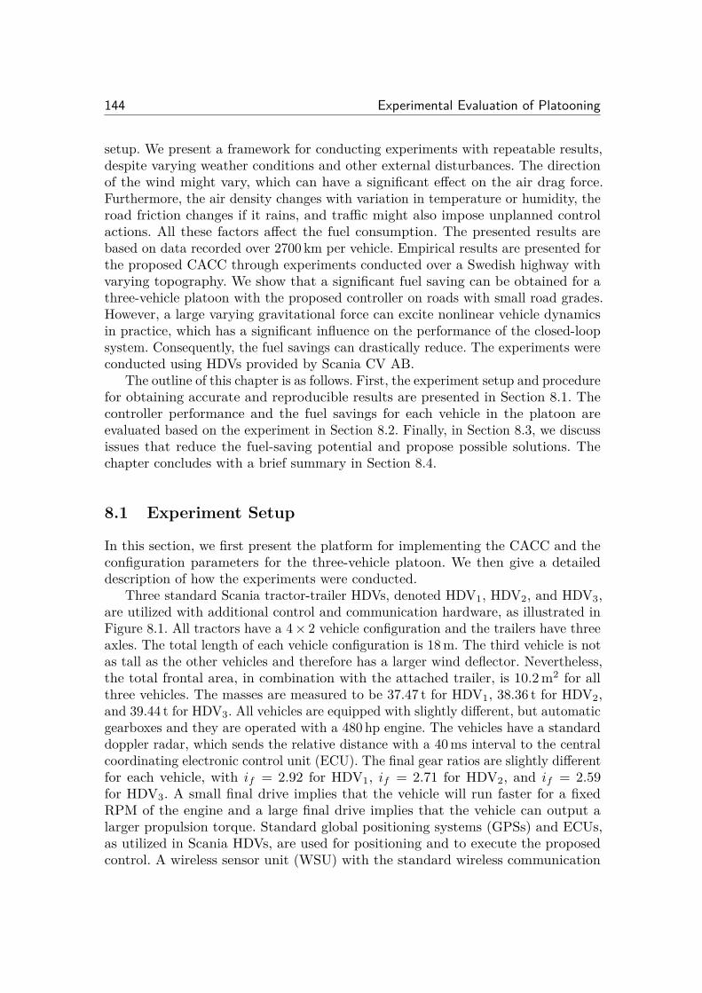
144 Experimental Evaluation of Platooning
setup. We present a framework for conducting experiments with repeatable results,despite varying weather conditions and other external disturbances. The directionof the wind might vary, which can have a significant e�ect on the air drag force.Furthermore, the air density changes with variation in temperature or humidity, theroad friction changes if it rains, and tra�c might also impose unplanned controlactions. All these factors a�ect the fuel consumption. The presented results arebased on data recorded over 2700 km per vehicle. Empirical results are presented forthe proposed CACC through experiments conducted over a Swedish highway withvarying topography. We show that a significant fuel saving can be obtained for athree-vehicle platoon with the proposed controller on roads with small road grades.However, a large varying gravitational force can excite nonlinear vehicle dynamicsin practice, which has a significant influence on the performance of the closed-loopsystem. Consequently, the fuel savings can drastically reduce. The experiments wereconducted using HDVs provided by Scania CV AB.
The outline of this chapter is as follows. First, the experiment setup and procedurefor obtaining accurate and reproducible results are presented in Section 8.1. Thecontroller performance and the fuel savings for each vehicle in the platoon areevaluated based on the experiment in Section 8.2. Finally, in Section 8.3, we discussissues that reduce the fuel-saving potential and propose possible solutions. Thechapter concludes with a brief summary in Section 8.4.
8.1 Experiment Setup
In this section, we first present the platform for implementing the CACC and theconfiguration parameters for the three-vehicle platoon. We then give a detaileddescription of how the experiments were conducted.
Three standard Scania tractor-trailer HDVs, denoted HDV1
, HDV2
, and HDV3
,are utilized with additional control and communication hardware, as illustrated inFigure 8.1. All tractors have a 4 ◊ 2 vehicle configuration and the trailers have threeaxles. The total length of each vehicle configuration is 18 m. The third vehicle is notas tall as the other vehicles and therefore has a larger wind deflector. Nevertheless,the total frontal area, in combination with the attached trailer, is 10.2 m2 for allthree vehicles. The masses are measured to be 37.47 t for HDV
1
, 38.36 t for HDV2
,and 39.44 t for HDV
3
. All vehicles are equipped with slightly di�erent, but automaticgearboxes and they are operated with a 480 hp engine. The vehicles have a standarddoppler radar, which sends the relative distance with a 40 ms interval to the centralcoordinating electronic control unit (ECU). The final gear ratios are slightly di�erentfor each vehicle, with if = 2.92 for HDV
1
, if = 2.71 for HDV2
, and if = 2.59for HDV
3
. A small final drive implies that the vehicle will run faster for a fixedRPM of the engine and a large final drive implies that the vehicle can output alarger propulsion torque. Standard global positioning systems (GPSs) and ECUs,as utilized in Scania HDVs, are used for positioning and to execute the proposedcontrol. A wireless sensor unit (WSU) with the standard wireless communication
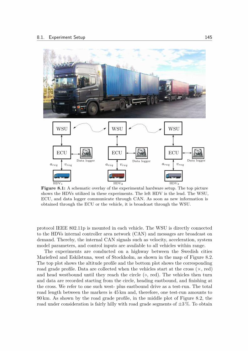
8.1. Experiment Setup 145
ECUECUECU
WSU WSU WSU
v
req
a
req
v
req
a
req
v
req
a
req
Data logger Data logger Data logger
HDV1 HDV2 HDV3
Figure 8.1: A schematic overlay of the experimental hardware setup. The top pictureshows the HDVs utilized in these experiments. The left HDV is the lead. The WSU,ECU, and data logger communicate through CAN. As soon as new information isobtained through the ECU or the vehicle, it is broadcast through the WSU.
protocol IEEE 802.11p is mounted in each vehicle. The WSU is directly connectedto the HDVs internal controller area network (CAN) and messages are broadcast ondemand. Thereby, the internal CAN signals such as velocity, acceleration, systemmodel parameters, and control inputs are available to all vehicles within range.
The experiments are conducted on a highway between the Swedish citiesMariefred and Eskilstuna, west of Stockholm, as shown in the map of Figure 8.2.The top plot shows the altitude profile and the bottom plot shows the correspondingroad grade profile. Data are collected when the vehicles start at the cross (◊, red)and head westbound until they reach the circle (¶, red). The vehicles then turnand data are recorded starting from the circle, heading eastbound, and finishing atthe cross. We refer to one such west- plus eastbound drive as a test-run. The totalroad length between the markers is 45 km and, therefore, one test-run amounts to90 km. As shown by the road grade profile, in the middle plot of Figure 8.2, theroad under consideration is fairly hilly with road grade segments of ±3 %. To obtain
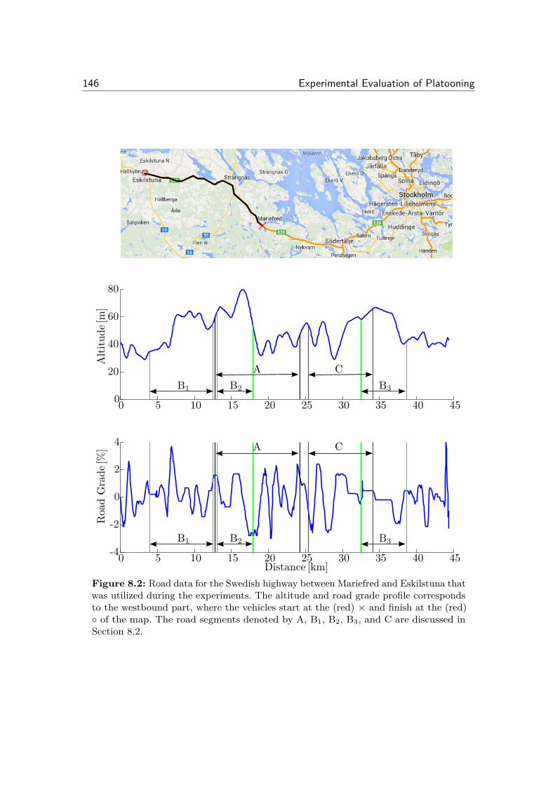
146 Experimental Evaluation of Platooning
0 5 10 15 20 25 30 35 40 450
20
40
60
80
Alti
tude
[m]
0 5 10 15 20 25 30 35 40 45-4
-2
0
2
4
Roa
dG
rade
[%]
Distance [km]
AB
2
B1
B3
C
A C
B2
B1
B3
◊
¶
Figure 8.2: Road data for the Swedish highway between Mariefred and Eskilstuna thatwas utilized during the experiments. The altitude and road grade profile correspondsto the westbound part, where the vehicles start at the (red) ◊ and finish at the (red)¶ of the map. The road segments denoted by A, B1, B2, B3, and C are discussed inSection 8.2.
8.2. Experiment Results 147
normal vehicle operating temperature, the vehicles are driven 35 km before startingthe test-runs, as a large amount of energy from the fueling is initially spent onheating up the various components, such as the oil for lubrication and the cabin. Sixtest-runs are conducted every day, over five days. Consequently, the experiments areconducted and data are collected over a total of 2700 km per vehicle. The aim is todetermine the fuel-saving potential of HDV platooning and evaluate the controllerperformance. Two test-runs are conducted each day when the vehicles operate aloneto determine the average fuel consumption over the road stretch without any air dragreduction from platooning. An additional two test-runs are conducted each day whenthe vehicles are operated as a platoon to investigate the change in fuel consumptionover the same stretch and in similar weather conditions. In the final two test-runs ofthe day, the positions of the two follower vehicles are interchanged to determine ifthe position in the platoon has an e�ect on the fuel-saving potential. HDV
1
is alwayskept in the first platoon position to maintain the overall platoon behavior. HDV
2
and HDV3
are follower vehicles. The vehicle speed sensor in commercial vehiclescan have a slight o�set. Therefore, the vehicle speed for each vehicle is calibratedwith respect to the common GPS speed information before the experiment trials.The maximum allowed road speed in Sweden for HDVs with the configuration athand is 80 km/h. However, the nominal operating speed for all vehicles was set to75 km/h, with a downhill speed control (DHSC) o�set of 10 km/h, to reduce thetra�c interference as much as possible. By operating the vehicles at a lower thanallowed speed, it is expected that surrounding vehicles pass the platoon and do notchange the operating conditions of a test-run by cutting in-between. The CACCs ofthe follower vehicles are set to maintain a time headway gap of · = 1 s. Operatingat closer spacings is currently not allowed in Sweden due to legislation2.
8.2 Experiment Results
In this section, we first investigate the controller performance based on experimentalresults. Then, we evaluate the fuel-saving. The weather conditions change over time,which a�ects the instantaneous fuel consumption for an HDV and can create avariation in fuel consumption from day to day. Hence, in this section, we try toperform the experiments in a way to achieve reproducible and reliable results.
8.2.1 Controller PerformanceSeveral test-runs are conducted. The results for one test-run over the westboundpart is shown in Figure 8.3. Starting from the top, the first plot shows the altitudeprofile with respect to the third vehicle in the platoon. The second plot shows thevelocity profiles for the three-vehicle platoon. The third plot shows the relativedistance between the vehicles, where d
12
denotes the distance between the first2The Swedish law does not directly state that operating at closer spacing is illegal. It falls
under the category of reckless behavior and is therefore subject to penalties.
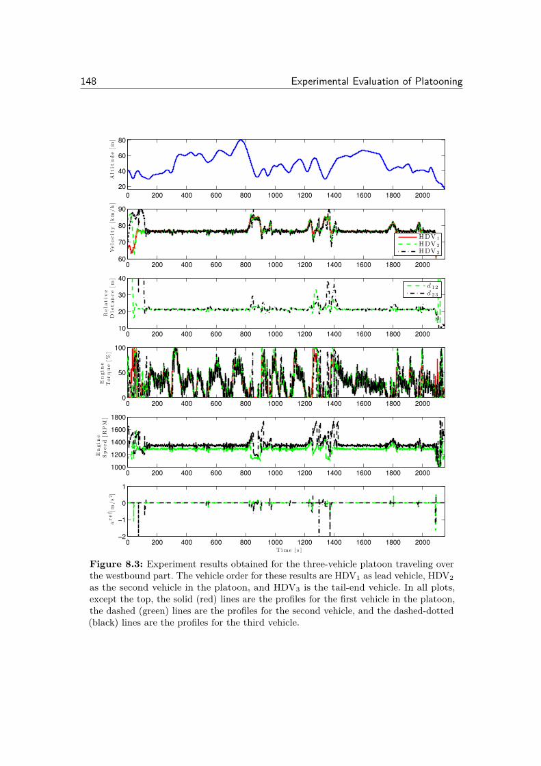
148 Experimental Evaluation of Platooning
0 200 400 600 800 1000 1200 1400 1600 1800 2000
20
40
60
80
Alt
itu
de
[m]
0 200 400 600 800 1000 1200 1400 1600 1800 200060
70
80
90
Velo
cit
y[k
m/h
]
HDV 1HDV 2HDV 3
0 200 400 600 800 1000 1200 1400 1600 1800 200010
20
30
40
Rela
tiv
eD
istan
ce
[m]
d 12
d 23
0 200 400 600 800 1000 1200 1400 1600 1800 20000
50
100
En
gin
eT
orq
ue
[%]
0 200 400 600 800 1000 1200 1400 1600 1800 20001000
1200
1400
1600
1800
En
gin
eS
peed
[RP
M]
0 200 400 600 800 1000 1200 1400 1600 1800 2000−2
−1
0
1
aref [
m/s2]
T i m e [ s ]
Figure 8.3: Experiment results obtained for the three-vehicle platoon traveling overthe westbound part. The vehicle order for these results are HDV1 as lead vehicle, HDV2as the second vehicle in the platoon, and HDV3 is the tail-end vehicle. In all plots,except the top, the solid (red) lines are the profiles for the first vehicle in the platoon,the dashed (green) lines are the profiles for the second vehicle, and the dashed-dotted(black) lines are the profiles for the third vehicle.
8.2. Experiment Results 149
and the second vehicle and d23
denotes the distance between the second and thethird vehicle. The fourth plot shows the normalized engine torque for all vehicles.The fifth plot shows the engine speed for the second and third vehicle, where thesudden jumps in RPM, for example between the 800–900 s time markers, signify gearchanges. Finally, the sixth (bottom) plot shows the corresponding brake requests.Note that a small braking force might be needed to maintain the relative distanceto a lighter preceding vehicle when coasting over a downhill segment. Therefore, apositive braking request, which can be seen in the bottom plot, implies that thebrakes are active to facilitate the desired acceleration.
It can be observed that the CACC works well and is able to maintain the inter-vehicle spacing over most parts of the road. The test-runs are initialized by lettingthe vehicles travel at a large inter-vehicle spacing followed by a merging action,as illustrated between the 0–200 s time markers in Figure 8.3. The lead vehicle isgoverned by a cruise control (CC) that is set at the nominal operating speed of75 km/h. The follower vehicles are governed by the CACC, which acts as a CC if nopreceding vehicle is detected. To catch up with the lead vehicle the set speed for thefollower is higher than the nominal operating speed. When a wireless connectionis established and relevant information is obtained, the CACC reduces the speedreference to merge with the vehicle ahead.
The velocity and relative distance between the vehicles do not vary significantlyover segments with small road grade. For example, the unbiased sample standarddeviations3, over the segment denoted by B
3
in Figure 8.3 for the velocity are‡v
1
= 0.3 km/h, ‡v
2
= 0.4 km/h, and ‡v
3
= 0.4 km/h for the first, second, andthird vehicle, respectively. Small disturbances produced by the varying road gradecreate a variation in velocity for the follower vehicles. This is also confirmed bythe sample standard deviation for the inter-vehicle spacing, given by ‡d
12
= 0.3 mand ‡d
23
= 0.3 m. Thus, it can be inferred that the CACC performs well when thedeviations from steady-state operations are small. Moreover, as indicated by thebrake requests, the follower vehicles seem to brake over steep downhill segments.Braking is required in these cases, since the follower vehicles are heavier than thelead vehicle. Thus, they coast with a higher acceleration over the downhill segmentsand inherently would slide in to the preceding vehicle if braking is not performed.The trajectories for the engine speed show that a braking is often followed by agear change. Hence, a jump occurs in the engine speed as can be seen between the800–1000 s time markers in the fifth plot.
The results in Figure 8.4, corresponding to segment A in Figure 8.2, show thatunwanted braking actions can occur over steep downhill segments with the CACCdue to lack of road grade information. Figure 8.4 zooms in to the interval 600–1150 sof Figure 8.3. Note that a high variation in relative velocity arise over the downhillsegment between 750–950 s. Here, the first vehicle starts to coast when entering the
3We define the unbiased sample standard deviation as ‡
i
=Ò
1n≠1
qn
k=1(yi
(k) ≠ y
i
)2, wherei = 1, 2, 3 denotes the vehicle position index in the platoon, n is the number of samples, y
i
(k) isthe value for the kth sample in platoon position i, and y
i
= 1n
qn
k=1 y
i
(k)
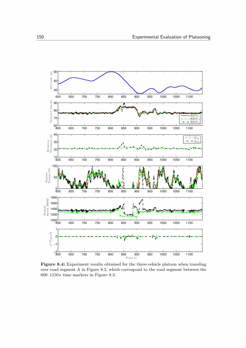
150 Experimental Evaluation of Platooning
600 650 700 750 800 850 900 950 1000 1050 1100
40
60
80
Alt
itu
de
[m]
600 650 700 750 800 850 900 950 1000 1050 110060
70
80
90
Velo
cit
y[k
m/h
]
HDV 1HDV 2HDV 3
600 650 700 750 800 850 900 950 1000 1050 110010
20
30
40
Rela
tiv
eD
istan
ce
[m]
d 12
d 23
600 650 700 750 800 850 900 950 1000 1050 11000
50
100
En
gin
eT
orq
ue
[%]
600 650 700 750 800 850 900 950 1000 1050 11001000
1200
1400
1600
1800
En
gin
eS
peed
[RP
M]
600 650 700 750 800 850 900 950 1000 1050 1100−2
−1
0
1
aref [
m/s2]
T i m e [ s ]
Figure 8.4: Experiment results obtained for the three-vehicle platoon when travelingover road segment A in Figure 8.2, which correspond to the road segment between the600–1150 s time markers in Figure 8.3.
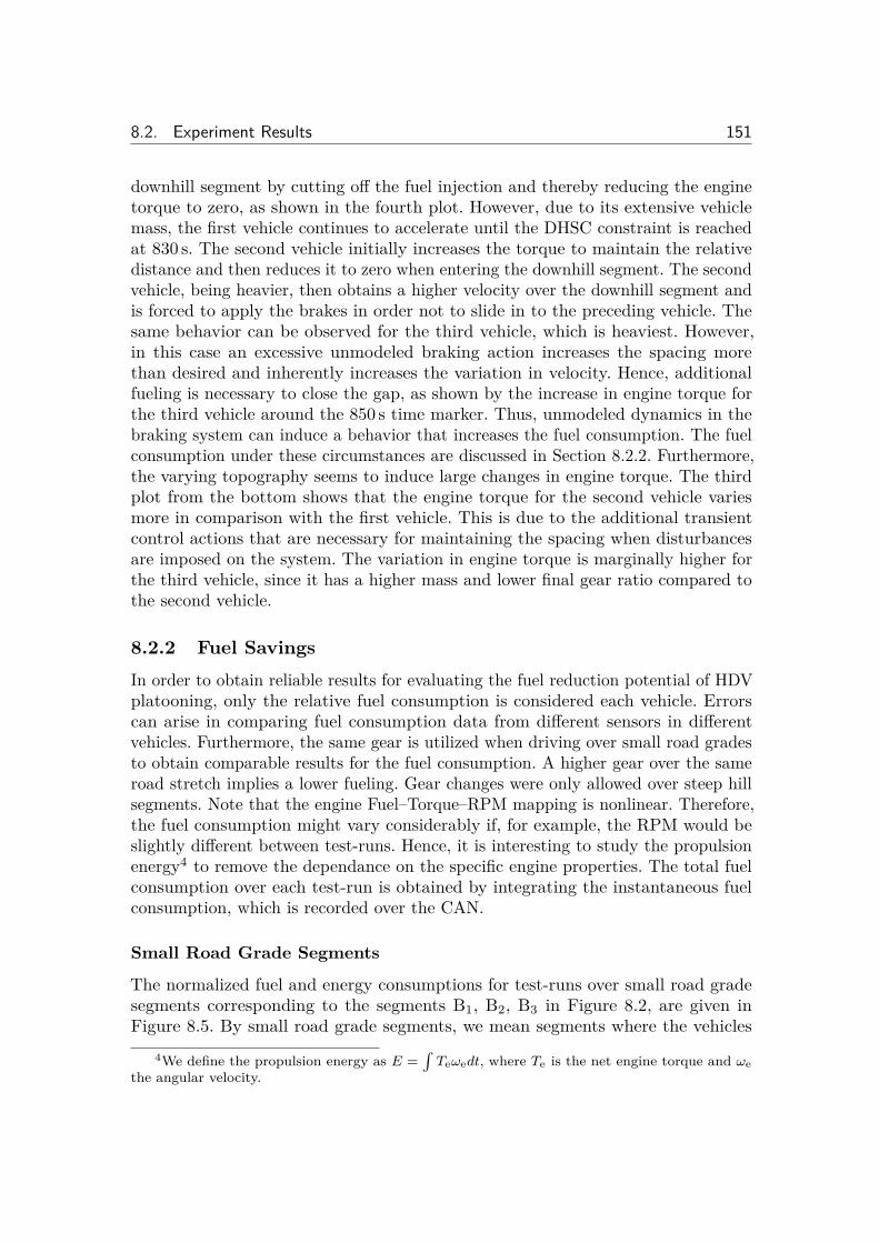
8.2. Experiment Results 151
downhill segment by cutting o� the fuel injection and thereby reducing the enginetorque to zero, as shown in the fourth plot. However, due to its extensive vehiclemass, the first vehicle continues to accelerate until the DHSC constraint is reachedat 830 s. The second vehicle initially increases the torque to maintain the relativedistance and then reduces it to zero when entering the downhill segment. The secondvehicle, being heavier, then obtains a higher velocity over the downhill segment andis forced to apply the brakes in order not to slide in to the preceding vehicle. Thesame behavior can be observed for the third vehicle, which is heaviest. However,in this case an excessive unmodeled braking action increases the spacing morethan desired and inherently increases the variation in velocity. Hence, additionalfueling is necessary to close the gap, as shown by the increase in engine torque forthe third vehicle around the 850 s time marker. Thus, unmodeled dynamics in thebraking system can induce a behavior that increases the fuel consumption. The fuelconsumption under these circumstances are discussed in Section 8.2.2. Furthermore,the varying topography seems to induce large changes in engine torque. The thirdplot from the bottom shows that the engine torque for the second vehicle variesmore in comparison with the first vehicle. This is due to the additional transientcontrol actions that are necessary for maintaining the spacing when disturbancesare imposed on the system. The variation in engine torque is marginally higher forthe third vehicle, since it has a higher mass and lower final gear ratio compared tothe second vehicle.
8.2.2 Fuel SavingsIn order to obtain reliable results for evaluating the fuel reduction potential of HDVplatooning, only the relative fuel consumption is considered each vehicle. Errorscan arise in comparing fuel consumption data from di�erent sensors in di�erentvehicles. Furthermore, the same gear is utilized when driving over small road gradesto obtain comparable results for the fuel consumption. A higher gear over the sameroad stretch implies a lower fueling. Gear changes were only allowed over steep hillsegments. Note that the engine Fuel–Torque–RPM mapping is nonlinear. Therefore,the fuel consumption might vary considerably if, for example, the RPM would beslightly di�erent between test-runs. Hence, it is interesting to study the propulsionenergy4 to remove the dependance on the specific engine properties. The total fuelconsumption over each test-run is obtained by integrating the instantaneous fuelconsumption, which is recorded over the CAN.
Small Road Grade Segments
The normalized fuel and energy consumptions for test-runs over small road gradesegments corresponding to the segments B
1
, B2
, B3
in Figure 8.2, are given inFigure 8.5. By small road grade segments, we mean segments where the vehicles
4We define the propulsion energy as E =s
TeÊedt, where Te is the net engine torque and Êethe angular velocity.
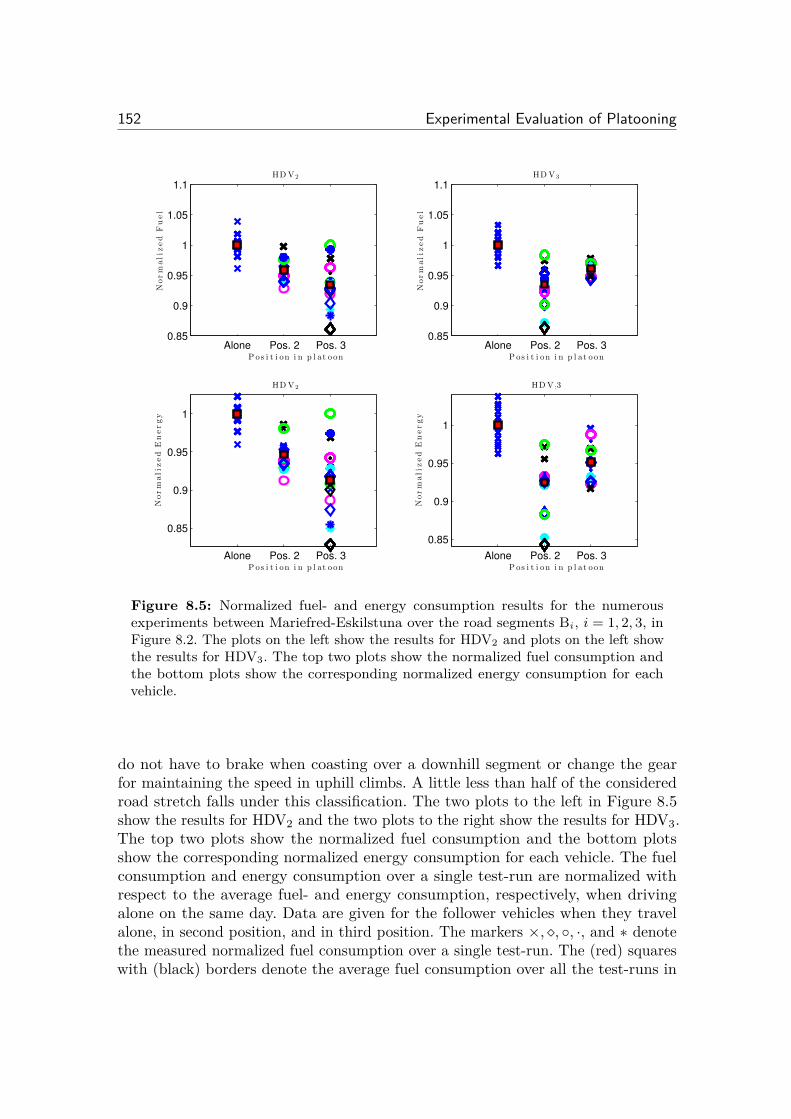
152 Experimental Evaluation of Platooning
Alone Pos. 2 Pos. 30.85
0.9
0.95
1
1.05
1.1
Norm
ali
zed
Fu
el
P os i t i on i n p l at oon
HD V2
Alone Pos. 2 Pos. 30.85
0.9
0.95
1
1.05
1.1
Norm
ali
zed
Fu
el
P os i t i on i n p l at oon
HD V3
Alone Pos. 2 Pos. 3
0.85
0.9
0.95
1
Norm
ali
zed
En
ergy
P os i t i on i n p l at oon
HD V2
Alone Pos. 2 Pos. 3
0.85
0.9
0.95
1N
orm
ali
zed
En
ergy
P os i t i on i n p l at oon
HD V :3
Figure 8.5: Normalized fuel- and energy consumption results for the numerousexperiments between Mariefred-Eskilstuna over the road segments B
i
, i = 1, 2, 3, inFigure 8.2. The plots on the left show the results for HDV2 and plots on the left showthe results for HDV3. The top two plots show the normalized fuel consumption andthe bottom plots show the corresponding normalized energy consumption for eachvehicle.
do not have to brake when coasting over a downhill segment or change the gearfor maintaining the speed in uphill climbs. A little less than half of the consideredroad stretch falls under this classification. The two plots to the left in Figure 8.5show the results for HDV
2
and the two plots to the right show the results for HDV3
.The top two plots show the normalized fuel consumption and the bottom plotsshow the corresponding normalized energy consumption for each vehicle. The fuelconsumption and energy consumption over a single test-run are normalized withrespect to the average fuel- and energy consumption, respectively, when drivingalone on the same day. Data are given for the follower vehicles when they travelalone, in second position, and in third position. The markers ◊, ù, ¶, ·, and ú denotethe measured normalized fuel consumption over a single test-run. The (red) squareswith (black) borders denote the average fuel consumption over all the test-runs in
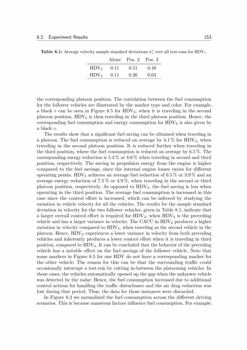
8.2. Experiment Results 153
Table 8.1: Average velocity sample standard deviations ‡
vi
over all test-runs for HDVi
.
Alone Pos. 2 Pos. 3HDV
2
0.11 0.51 0.48HDV
3
0.11 0.26 0.63
the corresponding platoon position. The correlation between the fuel consumptionfor the follower vehicles are illustrated by the marker type and color. For example,a black ù can be seen in Figure 8.5 for HDV
3
, when it is traveling in the secondplatoon position. HDV
2
is then traveling in the third platoon position. Hence, thecorresponding fuel consumption and energy consumption for HDV
2
is also given bya black ù.
The results show that a significant fuel saving can be obtained when traveling ina platoon. The fuel consumption is reduced on average by 4.1 % for HDV
2
, whentraveling in the second platoon position. It is reduced further when traveling inthe third position, where the fuel consumption is reduced on average by 6.5 %. Thecorresponding energy reduction is 5.3 % or 8.6 % when traveling in second and thirdposition, respectively. The saving in propulsion energy from the engine is highercompared to the fuel savings, since the internal engine losses varies for di�erentoperating points. HDV
3
achieves an average fuel reduction of 6.5 % or 3.9 % and anaverage energy reduction of 7.5 % or 4.9 %, when traveling in the second or thirdplatoon position, respectively. As opposed to HDV
2
, the fuel saving is less whenoperating in the third position. The average fuel consumption is increased in thiscase since the control e�ort is increased, which can be inferred by studying thevariation in vehicle velocity for all the vehicles. The results for the sample standarddeviation in velocity for the two follower vehicles, given in Table 8.1, indicate thata larger overall control e�ort is required for HDV
3
, when HDV2
is the precedingvehicle and has a larger variance in velocity. The CACC in HDV
2
produces a highervariation in velocity compared to HDV
3
, when traveling as the second vehicle in theplatoon. Hence, HDV
2
experiences a lower variance in velocity from both precedingvehicles and inherently produces a lower control e�ort when it is traveling in thirdposition, compared to HDV
3
. It can be concluded that the behavior of the precedingvehicle has a notable e�ect on the fuel savings of the follower vehicle. Note thatsome markers in Figure 8.5 for one HDV do not have a corresponding marker forthe other vehicle. The reason for this can be that the surrounding tra�c couldoccasionally interrupt a test-run by cutting in-between the platooning vehicles. Inthose cases, the vehicles automatically opened up the gap when the unknown vehiclewas detected by the radar. Hence, the fuel consumption increased due to additionalcontrol actions for handling the tra�c disturbance and the air drag reduction waslost during that period. Thus, the data for those instances were discarded.
In Figure 8.2 we normalized the fuel consumption across the di�erent drivingscenarios. This is because numerous factors influence fuel consumption. For example,
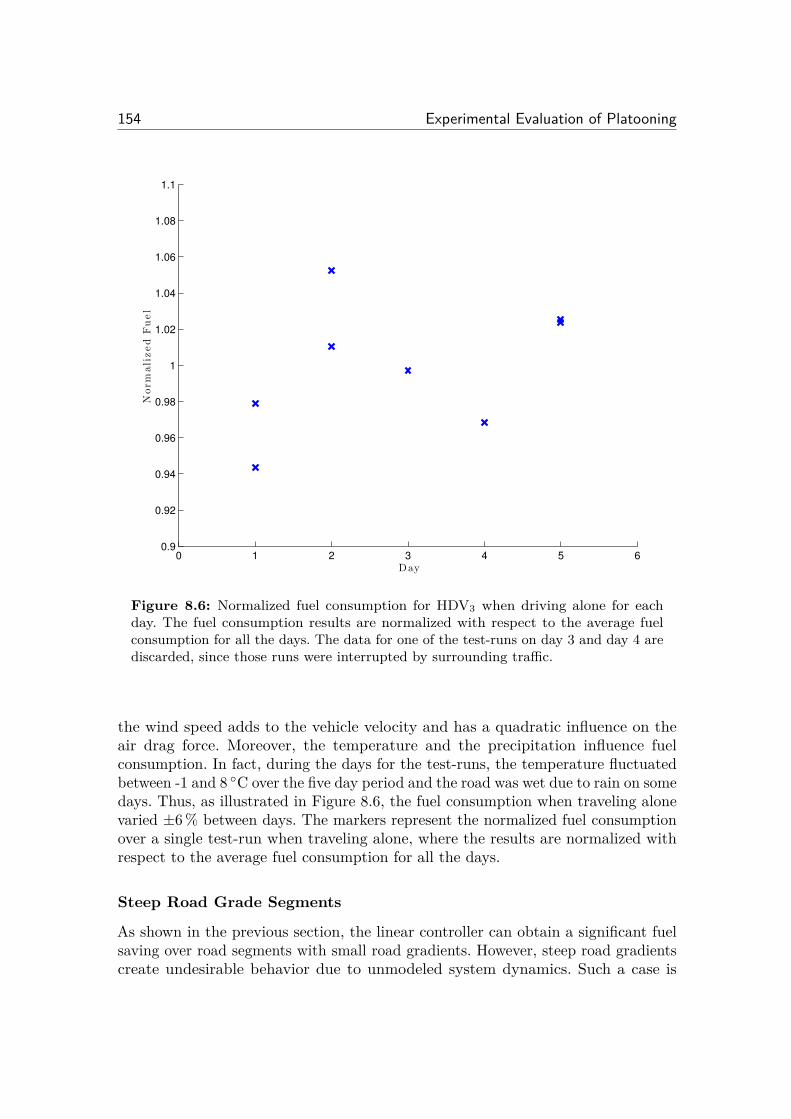
154 Experimental Evaluation of Platooning
0 1 2 3 4 5 60.9
0.92
0.94
0.96
0.98
1
1.02
1.04
1.06
1.08
1.1
Day
Norm
ali
zed
Fu
el
Figure 8.6: Normalized fuel consumption for HDV3 when driving alone for eachday. The fuel consumption results are normalized with respect to the average fuelconsumption for all the days. The data for one of the test-runs on day 3 and day 4 arediscarded, since those runs were interrupted by surrounding tra�c.
the wind speed adds to the vehicle velocity and has a quadratic influence on theair drag force. Moreover, the temperature and the precipitation influence fuelconsumption. In fact, during the days for the test-runs, the temperature fluctuatedbetween -1 and 8 ¶C over the five day period and the road was wet due to rain on somedays. Thus, as illustrated in Figure 8.6, the fuel consumption when traveling alonevaried ±6 % between days. The markers represent the normalized fuel consumptionover a single test-run when traveling alone, where the results are normalized withrespect to the average fuel consumption for all the days.
Steep Road Grade Segments
As shown in the previous section, the linear controller can obtain a significant fuelsaving over road segments with small road gradients. However, steep road gradientscreate undesirable behavior due to unmodeled system dynamics. Such a case is
8.2. Experiment Results 155
illustrated in Figure 8.7, corresponding to road segment C in Figure 8.2. All vehiclesinitially travel at the same velocity and with a constant inter-vehicle spacing. Whenentering the first downhill segment, at the 70 s time marker, the vehicles start tocoast by cutting o� the fuel injection and thereby reducing the engine torque tozero. As the velocity increases, the inter-vehicle spacing remains constant. For atime headway spacing policy, however, the desired relative distance increases withthe velocity. Thus, the follower vehicles eventually have to apply their brakes, as canbe seen right after the 100 s time marker in the bottom plot in Figure 8.7. Hence,the spacing is increased and the engine turbo pressure remains low for both followervehicles. The lead vehicle drops slightly in velocity when it enters the followeduphill segment, but increases the engine torque as soon as possible to maintain theset velocity. The follower vehicles observe that the lead vehicle is initially slowingdown and the CACC thus defers the increase in velocity until the desired relativedistance is resumed. In addition, a delay arises in building up the turbo pressureand, inherently, the engine torque, when entering the uphill segment. Furthermore,the acceleration is constrained due to extensive vehicle masses and engine torquesaturations. Thus, the relative velocity to the preceding vehicle increases and therelative distance grows over the uphill segment. Moreover, HDV
2
changes gear in themiddle of the uphill segment, as indicated by the sudden short drop in velocity, whichfurther increases the relative distance. To regain the desired relative distance afterthe uphill climb, fuel is injected to increase the velocity. However, since a downhillsegment follows, the velocity is increased too much and the follower vehicles mustbrake in the downhill to maintain the desired relative distance. Finally, additionalfuel is injected in the downhill because a higher deceleration than desired was initiallyproduced by the unmodeled dynamics in the braking system. Performing a similaranalysis to what was presented in Figure 8.5, we find that the fuel consumption isactually increased on average by 4 % for HDV
2
compared to driving alone, but isunchanged for HDV
3
, when traveling in the second platoon position over the theentire road segment shown in Figure 8.7. The una�ected fuel consumption for HDV
3
in the second platoon position can be explained by the results given in Figure 8.8.It illustrates the behavior over the same road stretch when the order of the followervehicles is changed, such that HDV
3
is in the second platoon position and HDV2
isin the third position. A similar behavior can be observed for this vehicle ordering,where the inter-vehicle spacing increases over the uphill segment starting at the120 s time marker. However, a gear change does not occur for HDV
3
in this case,which produces a smoother behavior when catching up with the lead vehicle. Thebraking over the following downhill segment is also reduced. HDV
2
, on the otherhand, performs a gear change over the uphill climb, which even for this case causesit to brake over the following downhill segment when it is catching up. A smootheroverall behavior and significantly less braking is achieved over the entire road stretchwith HDV
3
in the second platoon position, in comparison with HDV2
. Thus, thefuel consumption is unchanged for HDV
3
in this case.Recall that HDV
3
is the heaviest vehicle in the platoon. Hence, it has di�cultiesin maintaining the inter-vehicle spacing over uphill segments and has to brake
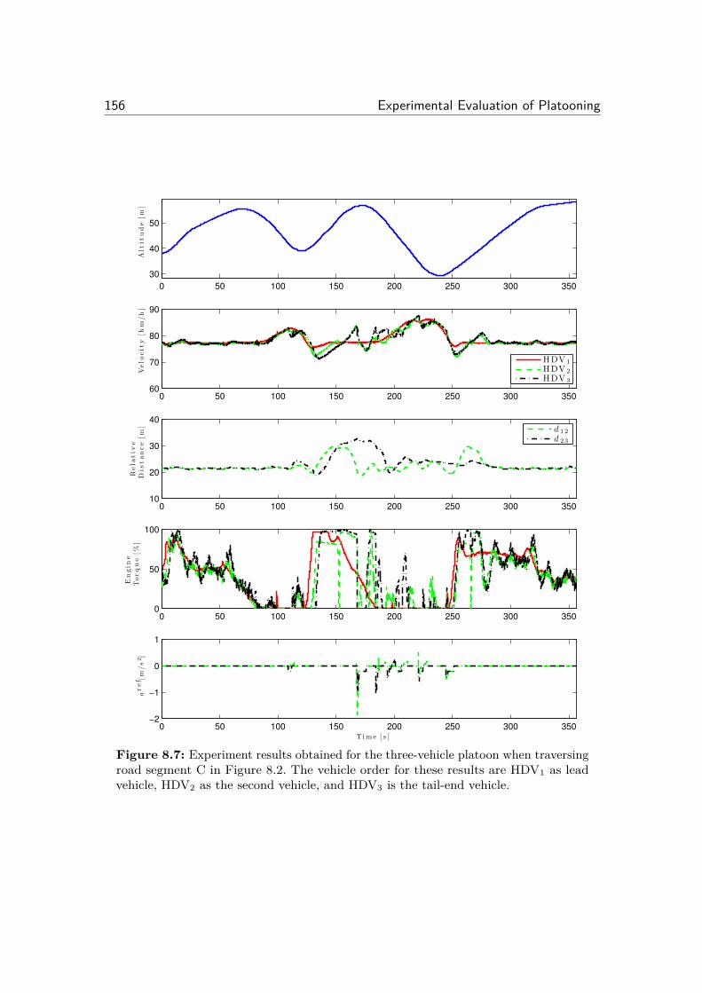
156 Experimental Evaluation of Platooning
0 50 100 150 200 250 300 350
30
40
50
Alt
itu
de
[m]
0 50 100 150 200 250 300 35060
70
80
90
Velo
cit
y[k
m/h
]
HDV 1HDV 2HDV 3
0 50 100 150 200 250 300 35010
20
30
40
Rela
tiv
eD
istan
ce
[m]
d 12
d 23
0 50 100 150 200 250 300 3500
50
100
En
gin
eT
orq
ue
[%]
0 50 100 150 200 250 300 350−2
−1
0
1
aref [
m/s2]
T i m e [ s ]
Figure 8.7: Experiment results obtained for the three-vehicle platoon when traversingroad segment C in Figure 8.2. The vehicle order for these results are HDV1 as leadvehicle, HDV2 as the second vehicle, and HDV3 is the tail-end vehicle.
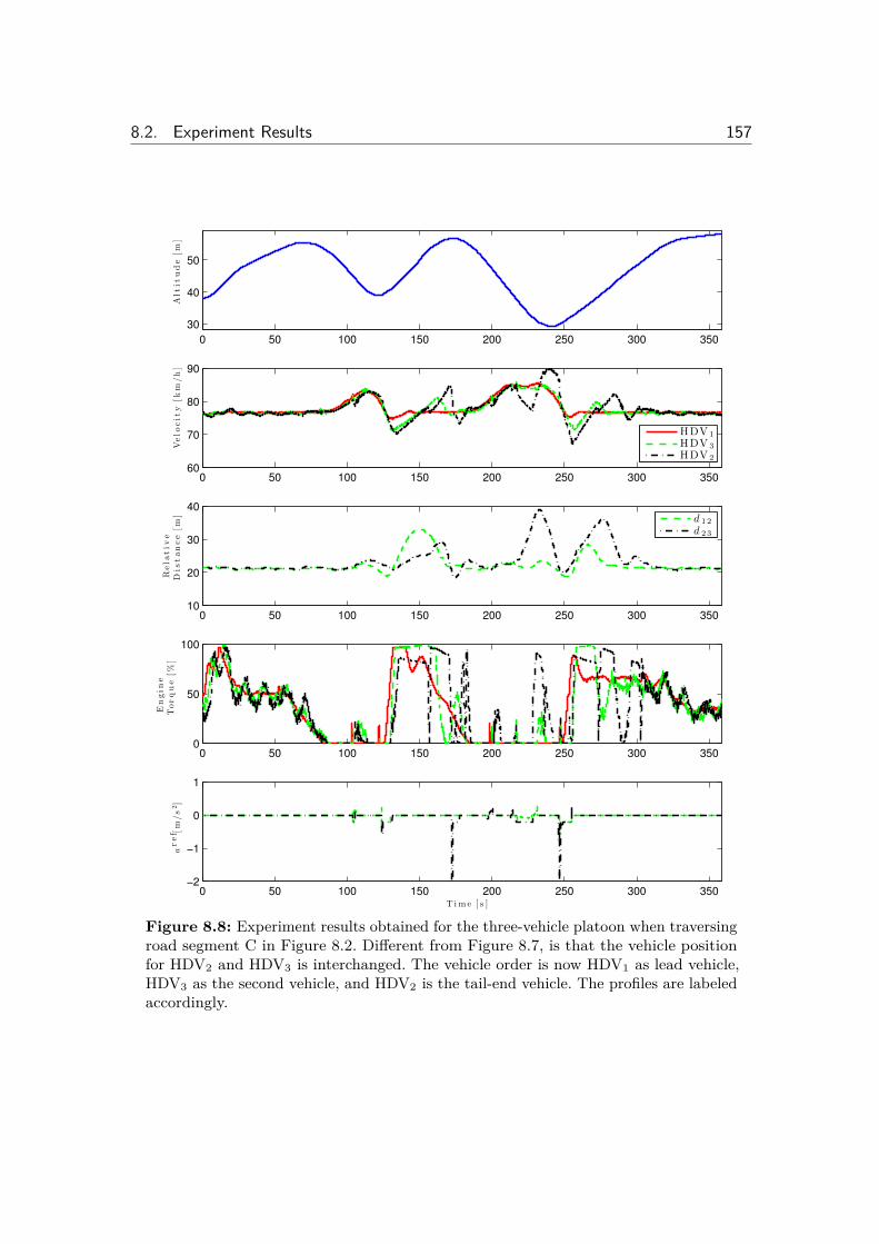
8.2. Experiment Results 157
0 50 100 150 200 250 300 350
30
40
50
Alt
itu
de
[m]
0 50 100 150 200 250 300 35060
70
80
90
Velo
cit
y[k
m/h
]
HDV 1HDV 3HDV 2
0 50 100 150 200 250 300 35010
20
30
40
Rela
tiv
eD
istan
ce
[m]
d 12
d 23
0 50 100 150 200 250 300 3500
50
100
En
gin
eT
orq
ue
[%]
0 50 100 150 200 250 300 350−2
−1
0
1
aref [
m/s2]
T i m e [ s ]
Figure 8.8: Experiment results obtained for the three-vehicle platoon when traversingroad segment C in Figure 8.2. Di�erent from Figure 8.7, is that the vehicle positionfor HDV2 and HDV3 is interchanged. The vehicle order is now HDV1 as lead vehicle,HDV3 as the second vehicle, and HDV2 is the tail-end vehicle. The profiles are labeledaccordingly.
158 Experimental Evaluation of Platooning
slightly over the downhill segments to avoid coasting into the lead vehicle, whentraveling in the second platoon position. The unfavorable gear change performedby HDV
2
in Figure 8.8 over the uphill segment increase the inter-vehicle spacingand creates additional braking. The fuel consumption is increased by 12 % and by9 % in the third platoon position for HDV
2
and HDV3
, respectively. Thus, due tounmodeled road topography and engine dynamics, the fuel-saving potential dueto air drag reduction in platooning can be lost over hilly road segments such asthe ones presented in Figure 8.7. The solution to this problem is to use predictiveinformation in the CACC, as further discussed in the next section.
8.3 Discussion
The CACC is designed to obtain a quick response when deviations in the set velocityand relative distance occurs, as presented in Chapter 6. However, it then becomessensitive to small variations in the preceding vehicles behavior. On the other hand,if the controller response is made slower, i.e., less sensitive to small variations in thepreceding vehicles behavior, large overshoots arise when compensating for largervariations in velocity. Hence, there is a trade-o� between sensitivity to slow varyingdisturbances and maintaining the desired relative distance. Furthermore, the CACCis based on a time headway policy, which induces excessive braking when coastingover downhill segments. A time headway spacing policy, as opposed to a constantspacing policy, typically produces a more fuel-e�cient control behavior (Omae et al.,2014). The results show that a time headway spacing policy is not desirable whencoasting over downhill segments.
The proposed linear CACC is not fuel-e�cient over varying steep road segments.The main losses in fuel saving occur, in particular, when traveling over an uphillsegment that is followed by a downhill segment. The relative distance is increasedover the uphill, which in turn is followed by excessive braking for the consideredheterogenous HDV platoon over the downhill segment. This behavior is caused bydelays in engine dynamics and since the lead vehicle unavoidably drops slightlyin velocity when entering a steep uphill segment. Hence, di�culties arise whenpredictive road grade information is not available. To counteract the performancedeterioration, first the inter-vehicle spacing should be maintained if possible whenentering a steep uphill segment. If it is not possible, e.g., due to a limited enginepower, then the follower vehicles should regain the desired inter-vehicle spacingby avoiding braking. Using feedforward in the controller can compensate for thisunwanted behavior. Information that the lead vehicle has entered a steep uphillsegment can be forwarded to the follower vehicles. Thereby, the turbo pressurecan be increased in time such that su�cient engine torque is obtained and therelative distance is maintained in the uphill. Furthermore, the reference signal forthe velocity, in addition to the state of the preceding vehicles, should be used in thefeedback control. The follower vehicles will then know that the reference velocity ofthe lead vehicle is not reduced when entering the uphill segment. Similarly, if the
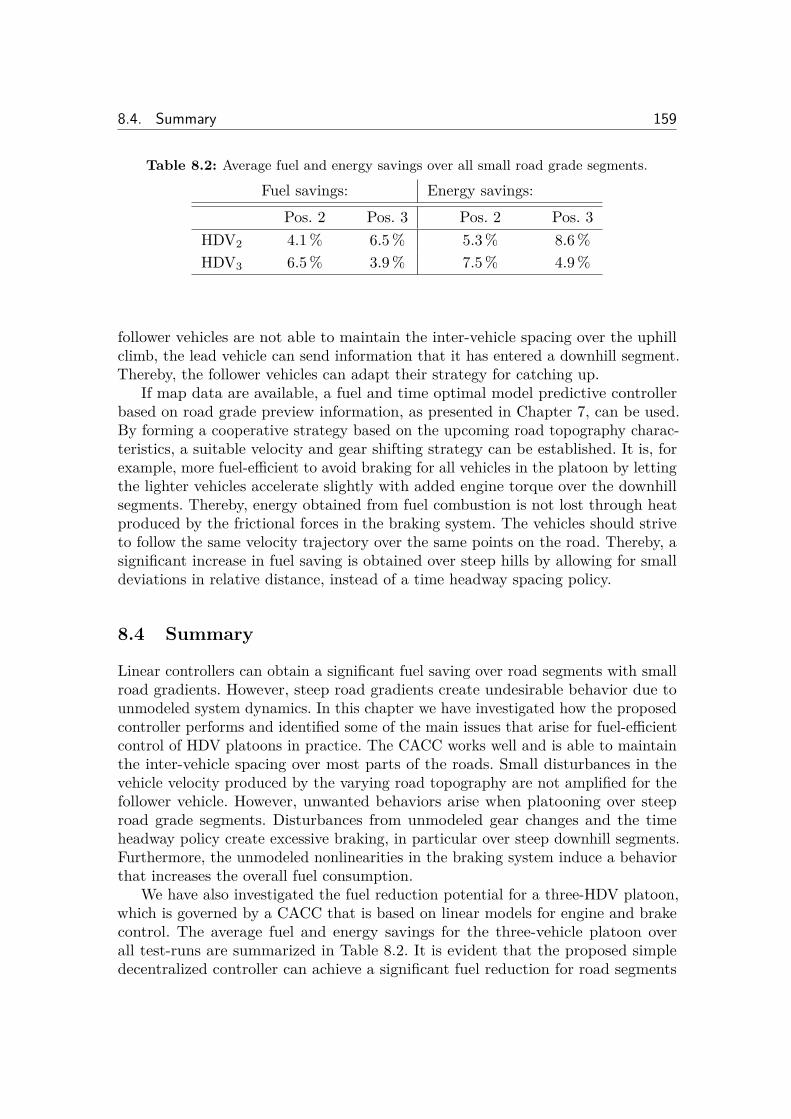
8.4. Summary 159
Table 8.2: Average fuel and energy savings over all small road grade segments.
Fuel savings: Energy savings:Pos. 2 Pos. 3 Pos. 2 Pos. 3
HDV2
4.1 % 6.5 % 5.3 % 8.6 %HDV
3
6.5 % 3.9 % 7.5 % 4.9 %
follower vehicles are not able to maintain the inter-vehicle spacing over the uphillclimb, the lead vehicle can send information that it has entered a downhill segment.Thereby, the follower vehicles can adapt their strategy for catching up.
If map data are available, a fuel and time optimal model predictive controllerbased on road grade preview information, as presented in Chapter 7, can be used.By forming a cooperative strategy based on the upcoming road topography charac-teristics, a suitable velocity and gear shifting strategy can be established. It is, forexample, more fuel-e�cient to avoid braking for all vehicles in the platoon by lettingthe lighter vehicles accelerate slightly with added engine torque over the downhillsegments. Thereby, energy obtained from fuel combustion is not lost through heatproduced by the frictional forces in the braking system. The vehicles should striveto follow the same velocity trajectory over the same points on the road. Thereby, asignificant increase in fuel saving is obtained over steep hills by allowing for smalldeviations in relative distance, instead of a time headway spacing policy.
8.4 Summary
Linear controllers can obtain a significant fuel saving over road segments with smallroad gradients. However, steep road gradients create undesirable behavior due tounmodeled system dynamics. In this chapter we have investigated how the proposedcontroller performs and identified some of the main issues that arise for fuel-e�cientcontrol of HDV platoons in practice. The CACC works well and is able to maintainthe inter-vehicle spacing over most parts of the roads. Small disturbances in thevehicle velocity produced by the varying road topography are not amplified for thefollower vehicle. However, unwanted behaviors arise when platooning over steeproad grade segments. Disturbances from unmodeled gear changes and the timeheadway policy create excessive braking, in particular over steep downhill segments.Furthermore, the unmodeled nonlinearities in the braking system induce a behaviorthat increases the overall fuel consumption.
We have also investigated the fuel reduction potential for a three-HDV platoon,which is governed by a CACC that is based on linear models for engine and brakecontrol. The average fuel and energy savings for the three-vehicle platoon overall test-runs are summarized in Table 8.2. It is evident that the proposed simpledecentralized controller can achieve a significant fuel reduction for road segments
160 Experimental Evaluation of Platooning
with small road grade. Thus, substantial fuel-savings can be obtained from HDVplatooning in practice. However, the fuel savings vary with respect to the behaviorof the preceding vehicles. HDV
2
achieves a fuel reduction in both considered platoonpositions, whereas HDV
3
only saves fuel in the second platoon position due to thecontroller responses to the unfavorable behavior of HDV
2
. The results presentedin this chapter also show that the fuel-saving potential obtained from the air dragreduction in platooning can be lost over steep road segments, due to constraints setby the road topography and the limited engine power.
Chapter 9
Conclusions and Future Outlook
“If we knew what it was we were doing, it would not be called research,
would it?”Albert Einstein
Heavy-duty vehicle (HDV) platooning is a promising means to reduce fuelconsumption, improve safety, reduce congestion, decrease emission of harmfulexhaust gasses, and aid the driver in complex driving situations. In this
thesis, a system for dividing the complex problem into manageable subsystemsfor fuel-e�cient optimal control has been presented. Nonlinear and linear HDVplatooning models have been derived. We have investigated the current fuel reductionpotential of HDV platooning for vehicles governed by a commercial adaptive cruisecontrol. It has been shown through analytical and experimental results that it isboth fuel-e�cient and possible to operate the vehicles at a much shorter inter-vehiclespacing than what is currently done by commercially available systems, withoutcompromising safety. We have also argued why a decentralized control strategy isfavorable and presented an algorithm that produces a simple and energy-e�cientdecentralized controller with good tracking performance, stability, and scalability. Ithas been shown through empirical findings that, even though the proposed controlleris fuel-e�cient over roads with small road gradient, the fuel savings can be lost overcertain steep hill segments in practice. We have presented two model predictivecontrol policies and shown that it is fuel-e�cient to consider the road grade previewinformation. This chapter concludes the thesis by detailing the inferrences that canbe drawn from the obtained results and outlines directions for possible future workin this area.
9.1 Conclusions
Vehicle platooning is becoming increasingly important. Even though platooningo�ers many benefits in tra�c networks, it mostly o�ers functionality to improve
161
162 Conclusions and Future Outlook
driver comfort for passenger vehicles. The ground transportation industry on theother hand has a strong incentive to utilize platooning applications due to the fuel-price sensitive market and long freight transport assignments. Hence, platooningwill most likely find an initial market entry in the transportation industry due tothe high demand and strong business case.
The simulation results in Chapter 4, derived from a validated simulation model,showed that a fuel reduction of 4.7–7.7 % in HDV platooning for identical vehiclescan be obtained depending on the time headway setting in the adaptive cruisecontroller. If the lead vehicle is 10 t lighter a corresponding 3.8–7.4 % fuel reductioncan be obtained. Similarly, if the lead vehicle is 10 t heavier a 4.3–6.9 % fuel reductioncan be obtained. Hence, HDV heterogeneity and order have a significant impact onthe fuel reduction possibilities. Furthermore, reducing the inter-vehicle spacing forHDVs traveling in a platoon yields the highest fuel reduction potential. Thus, itseems most beneficial to reduce the inter-vehicle spacing for HDVs traveling in aplatoon.
The results presented in Chapter 5 showed that the relative distance can bereduced significantly compared to what is utilized in current commercial systems.During normal operation a minimum distance of 1–2 m can be maintained withoutincreasing the risk of a collision despite the worst possible behavior displayed bythe preceding vehicle. The safe relative distance varies with braking capabilityand communication and computation delays within the system. A stronger overallbraking capability in the follower vehicle creates the possibility of reducing therelative distance further. Thus, in platooning applications the results suggested thatvehicles with stronger braking capabilities should always be placed last to enable theshortest possible relative distance without increasing the risk of a collision. This couldeasily be achieved with wireless communication if the braking capabilities and massare transmitted between each vehicle in the platoon. However, rearranging the HDVson a highway is not always feasible. Hence, another approach to ensure safety andobtain a minimum relative distance is to set maximum braking constraints throughwireless communication within the platoon. Producing the maximum brake torquethrough the internal brake system after a request could take up to 0.4 s dependingon the vehicle configuration, which will be propagated downstream through theplatoon. However, if the first vehicle transmits that it is initiating an emergencybrake to all the following vehicles within the platoon, they will be able to commencetheir control actions almost simultaneously and thereby prevent a propagation ofactuation delay. This in turn would enable a shorter inter-vehicle spacing betweenall the follower vehicles.
In Chapter 6, we presented a method for designing suboptimal decentralizedfeedback controllers for HDV platooning that takes dynamic coupling and engineresponse delays into consideration. The aim was to propose a simple and imple-mentable fuel-e�cient cooperative controller that could be utilized for practicalevaluation of the fuel-saving potential of HDV platooning. An interesting observationcan be made with respect to the system behavior due to the time-varying natureof the desired relative distance: As a disturbance is introduced by changing the
9.1. Conclusions 163
velocity of the lead vehicle, the relative distance will initially change between thefirst two vehicles in the platoon. However, as the velocity increases or decreases forthe lead vehicle, so will the desired relative reference distance. Hence, if for examplethe lead vehicle accelerates, the follower vehicles will defer their control actionsaccordingly until the relative distance is increased and produce a smoother controlinput to change their own speed. Thus, a lower control e�ort will be mandatedfrom the follower vehicle. The proposed controller is designed to obtain a quickresponse when a change in the legislated road speed occurs, but without becomingtoo sensitive to small variations in the preceding vehicles behavior. If the controllerresponse is made too slow, i.e., less sensitive to small variations in the precedingvehicles behavior, large overshoots arise when compensating for larger variations invelocity. Hence, there is a trade-o� between sensitivity to slow varying disturbancesand maintaining the desired relative distance. The experimental results showedthat the deviation from the reference for inter-vehicle spacing during the brakingscenarios never decrease more than 1.9 m. Thus, the vehicles could have operatedat a much closer inter-vehicle spacing without increasing the risk of a collision andthus obtained a higher fuel reduction.
In Chapter 7, we presented a method for deriving two fuel-optimal controllersbased on road grade preview information for HDV platooning. A surprising resultwas that the fuel-savings obtained for the proposed cooperative look-ahead controlleris very close to a hypothetically optimal fuel reduction, defined as when each vehicleuses its individual fuel-optimal velocity strategy while hypothetically obtaining theair drag reduction from maintaining a constant relative distance to neighboringvehicles (even if it cannot be constant in practice). Hence, the results suggested thatderiving the globally optimal velocity profile for a centralized solution might onlycreate marginal improvements in fuel savings. Furthermore, the presented resultsshow that it is important to consider the road grade preview information in HDVplatooning. It is fuel-e�cient to maintain the platoon when traversing a hill, asopposed to letting the platoon separate due to imposed constraints and then resumeplatooning by catching up after the hill. In particular, the results showed that it isfuel-e�cient and desirable for heterogenous vehicle platoons, where the vehicles areconstrained by di�erent limitations in maximum engine power, to initiate the controlactions based on a point in the road rather than simultaneously implementing eachHDV’s control action to maintain a fixed spacing. The overall fuel-saving potentialis improved by maintaining the short relative distance to the preceding vehicleover an uphill climb and hence slow down if the follower vehicle is not able tomaintain the nominal road speed. Over a downhill segment, it is fuel-e�cient for apreceding vehicle to inject additional fuel and thereby increase its acceleration ifit causes the follower vehicle to refrain from braking. A fuel reduction of 12 % or19 % can be achieved with a cooperative control policy, when traversing steep uphillor downhill segments, respectively. Furthermore, it was shown that the fuel-savingpotential for the proposed controller is not overly sensitive to errors in vehicle massor positioning, since the main fuel reduction is obtained from the air drag reduction.Thus, significant losses in the fuel-saving potential can be avoided, e.g., due to errors
164 Conclusions and Future Outlook
in the look-ahead control trajectory, as long as the inter-vehicle spacing can bemaintained.
The experimental results in Chapter 8 showed that a fuel reduction of 3.9–6.5 %can be obtained for a heterogenous platoon of HDVs on a Swedish highway. Thesavings depend on the vehicle position in the platoon and the behavior of thepreceding vehicles. The proposed decentralized controller, which is based on simplelinear models and no road topography information, is fuel-e�cient over roads withrelatively small road gradients. Steep hills saturate the low-level engine control inputover uphill climbs and create accelerations when coasting over downhill segments.Thus, if the relative distance cannot be maintained over an uphill segment that isfollowed by a downhill segment, an excessive braking occurs when catching up toregain the relative distance. A consequence of the braking is waste of fuel. Anotherinteresting observation can be made when studying the implications for a timeheadway spacing policy over a steep downhill segment. As the HDVs enter thedownhill segment, each vehicle starts to coast by cutting o� the fuel injection.Hence, the velocities of the vehicles increase and the inter-vehicle spacing remainsconstant or changes very slowly. A time headway policy implies that the desiredrelative distance increases with the vehicle velocity. Therefore, the control strategyexecutes a braking request when coasting over the downhill segment to increasethe spacing, which is not necessary in this case. Moreover, an unexpected gearchange over an uphill segment can give the follower vehicles the impression that itis intentionally slowing down for a short period. Therefore, the follower vehicles willcut o� their fuel injection to match the speed, which also lowers the engine turbopressure. Consequently, the inter-vehicle spacing will increase in this case, since ittakes time to increase the turbo pressure when striving to regain the nominal speed.Such behavior is unwanted and fuel-ine�cient. Thus, the intention of a gear changeshould be communicated to all follower vehicles in order to prevent an increasedfuel consumption over the hill segment.
With the results obtained in this thesis, it is clear that a substantial fuelreduction potential exists for HDV platooning. The results indicate that a maximumfuel reduction can be achieved at a short relative distance due to the air dragreduction and that a relatively small inter-vehicle spacing can be obtained withoutcompromising safety. The results also show that a cooperative control strategy,where the HDVs interact and consider the dynamics of their neighbors, producesa lowered energy consumption downstream. However, safety is an issue as inter-vehicle communication cannot be guaranteed at all time. If communication isavailable, the inter-vehicle spacing can be relatively small without compromisingsafety. When communication is lost, the spacing should be increased. Thus, theavailable information structure dictates the inter-vehicle spacing indirectly, creatinga need for a graceful degradation scheme in the architecture presented in Chapter 3.
9.2. Future Outlook 165
9.2 Future Outlook
“Nothing in life is to be feared, it is only to be understood. Now is the
time to understand more, so that we may fear less.”Marie Curie
The simulation and experimental results in this thesis have mainly been based on 2–3HDVs traveling at the shortest allowed time headway setting on Swedish highways.Studies on the air drag reductions suggest that the wind reduction is additionallylowered for vehicles traveling further down the platoon and at shorter inter-vehiclespacings. Thus, further experiments conducted with respect to the fuel reductionfor several HDVs in a platoon and at smaller inter-vehicle spacing is crucial to get abetter understanding of the real-life fuel reduction potential of HDV platooning.
The safety analysis presented in this thesis has been performed based on certainsimplifications. In realistic scenarios the vehicles commonly travel along a varyingroad topography. Due to the extensive mass of an HDV, the gravitational forcehas a significant impact on the overall braking power. Hence, studying the impactof a varying road incline serves as a natural direction to establish minimum saferelative distances for HDV platooning. Additional factors may also shape thesafety boundary, which was not considered in the presented work. One of thevehicles might be traveling on a wet patch or the tires might be in bad condition,reducing the braking capabilities. Also, unmodeled nonlinearities might arise inthe applied brake force due to temperature variation. Although the experimentalresults confirm the numerical evaluations, the results reveal that the influence of theunmodeled nonlinear braking system and gear changes are important. Furthermore,extending the experimentally evaluated and validated model to both longitudinaland lateral motion is of high relevance. Finally, we believe that finding a novelcomputational method for computing safe sets for more than two HDVs is interesting,since establishing what minimum distance can be maintained between HDVs in aheterogeneous platoon is not evident. Investigating these factors requires a moreadvanced vehicle model and computation method. It is therefore a possible avenuefor continued work in this area.
The results in Chapter 6 showed that the controller performance is improvedwith increasing position index in the platoon. However, the e�ects of unmodelednonlinearities, such as gear changes, brake blending, and engine dynamics, cancause undesirable behavior in some cases. To handle these e�ects the intention ofa necessary gear change could be broadcasted so that the rest of the platooningvehicles will be able to make informed decisions regarding whether to change gearsimultaneously or to deter the action. Thus, a high-level control law for the gearmanagement system might be necessary to further improve the control performance.The main drawback of the proposed controller is that it does not directly accountfor the physical constraints present in the systems. Currently the linear quadraticweights are adjusted in an ad hoc manner until the constraints criteria are met
166 Conclusions and Future Outlook
and the performance criteria are satisfied. A systematic optimal control procedureis preferable, which can directly consider the system constraints when derivingthe fuel-optimal controller. A more sophisticated engine model might possibly berequired to capture the behavior that a�ects the tracking performance. One solutionmight be to not only transmit the actual velocity of the vehicles in the platoonover the communication network, but also the reference velocity. Thereby, eachvehicle would be able to determine when the control action to the engine is resumedand increase the turbo pressure to reduce the response delay. Investigating thesepossibilities require further experiments.
The proposed controller based on road grade preview information in this thesisdoes not require knowledge of the specific vehicle parameters such as mass ormaximum available engine torque, or any information regarding the dynamicsof the surrounding vehicles. We have provided a simple open-loop approach forhow to handle system uncertainties, such that the fuel saving with the proposedcooperative look-ahead cruise control (CLAC) is maintained. However, disturbancesin the form of an unexpected gear change, by for example a preceding vehicle, ornonlinearities in the engine dynamics might cause an HDV to deviate from theCLAC velocity trajectory. A feedback solution for how to handle such deviations,where for example a new locally corrected velocity profile is established, is necessary.Further investigation into this is a natural next step in utilizing road grade previewinformation for HDV platooning control.
Finally, we also believe that a relevant future research direction for HDV platoon-ing is work in the top layer of the architecture presented in Chapter 3. In particularcoordination and routing to create vehicle platoons is an important research area forestablishing vehicle platoons. Several control policies currently exist for control ofvehicle platoons and research projects have recently emerged worldwide to evaluatevarious performance criteria for HDV platoons in practice. However, as goods havedi�erent origins, destinations, and time restrictions, it is not evident how the HDVscan fully utilize the platooning benefits during individual transport missions. Thus,there is a need to systematically coordinate scattered vehicles on the road networkto form platoons in order to maximize the benefits of platooning.
Nomenclature
Acronyms and Abbreviations
ABS Anti-Lock Braking SystemACC Adaptive Cruise ControlADAS Advanced Driver Assistance SystemsALAC Adaptive Look-Ahead Cruise ControlBMS Brake Management SystemCAN Controller Area NetworkCACC Cooperative Adaptive Cruise ControlCAM Cooperative Awareness MessageCC Cruise ControlCFD Computational Fluid DynamicsCLAC Cooperative Look-Ahead Cruise ControlCORDIS Community Research and Development Information ServiceDENM Decentralized Environmental Notification MessageDHSC Down Hill Speed ControlECC Economical Cruise ControlEMS Engine Management SystemERTICO European Road Transport
Telematics Implementation Co-ordination OrganizationESP Electronic Stability ProgramGPS Global Positioning SystemHDV Heavy-Duty VehicleICT Information and Communication TechnologyITF The International Transport ForumITS Intelligent Transportation SystemsLAC Look-Ahead Cruise ControlLAN Local Area Network
167
168 Nomenclature
LQR Linear Quadratic RegulatorMAC Medium Access ControlMPC Model Predictive ControlOECD Organization for Economic Co-operation and DevelopmentPATH Partners for Advanced Transportation TechnologySARTRE Safe Road Trains for the Environment: EU projectUMTS Universal Mobile Telecommunications SystemVANET Vehicular Ad hoc NetworkV2I Vehicle-to-InfrastructureV2V Vehicle-to-VehicleV2X Vehicle-to-Vehicle and/or InfrastructureWSU Wireless Sensor Unit
Bibliography
802.11p. Status of project IEEE 802.11, Task Group p, Wireless Access in VehicularEnvironments (WAVE) (2014). URL http://www.ieee802.org/11/Reports/tgp_update.htm. Accessed: April 9, 2014.
ACEA. European Motor Vehicle PARC 2010, European Automobile Manufacturers’Association (2012). URL http://www.acea.be/uploads/statistic_documents/ANFAC_Report_2010_(2012).pdf. ANFAC Report.
M. Adolfson. Cooperative dynamic formation of platoons for safe and energy-optimized goods transportation. In 93rd Annual Meeting of the TransportationResearch Board. Washington D.C., USA (2014). (Oral presentation).
AEA Technology. Reduction and testing of greenhouse gas (ghg) emissions fromheavy duty vehicles - lot 1: Strategy. Technical report, Ricardo (2011).
A. Alam. Optimally Fuel E�cient Speed Adaptation. Master’s thesis, Royal Instituteof Technology, Automatic Control (2008).
A. Alam. Fuel-E�cient Distributed Control for Heavy Duty Vehicle Platooning.Licentiate thesis, Royal Institute of Technology, SE-100 44 Stockholm, Sweden(2011).
A. Alam, J. Andersson, H. Gustafsson, H. Pettersson, P. Sahlholm, and H. Schauman.Method and system for speed verification. European patent application number:11193590.4 (filed 2011a).
A. Alam, J. Andersson, H. Gustafsson, H. Pettersson, P. Sahlholm, and H. Schauman.Metod i samband med trafikövervakning, och ett trafikövervakningssystem [Methodin connection with tra�c monitoring and a tra�c monitoring system]. Swedishpatent application number: 1150073-3 (filed 2011b).
A. Alam, J. Andersson, and P. Sahlholm. A Vehicle Speed Control Method. Interna-tional patent application number: PCT/SE09/050030 (filed 2009a).
A. Alam, J. Andersson, and P. Sahlholm. Determination of acceleration behavior.International patent application number: PCT/SE09/051299 (filed 2009b).
169
170 Bibliography
A. Alam, A. Gattami, and K. H. Johansson. An experimental study on the fuelreduction potential of heavy duty vehicle platooning. In 13th International IEEEConference on Intelligent Transportation Systems. Madeira, Portugal (2010).
A. Alam, A. Gattami, and K. H. Johansson. Suboptimal decentralized controllerdesign for chain structures: Applications to vehicle formations. In 50th IEEEConference on Decision and Control and European Control Conference. Orlando,FL, USA (2011a).
A. Alam, A. Gattami, K. H. Johansson, and C. J. Tomlin. Establishing safety forheavy duty vehicle platooning: A game theoretical approach. In 18th IFAC WorldCongress. Milan, Italy (2011b).
A. Alam, A. Gattami, K. H. Johansson, and C. J. Tomlin. Guaranteeing safety forheavy duty vehicle platooning: Safe set computations and experimental evaluations.Control Engineering Practice, 24: 33 – 41 (2014a).
A. Alam, A. Johansson, R. Lyberger, and H. Pettersson. Method and system forspacing adjustment in a moving vehicle train. International patent applicationnumber: PCT/SE13/050317 (filed 2012a).
A. Alam, K.-Y. Liang, and A. Gattami. Metod i samband med fordonståg, och ettfordon som använder metoden [A method in connection to vehicle trains and avehicle that uses that method]. Swedish patent application number: 1150579-9(filed 2011c).
A. Alam, J. Mårtensson, and K. H. Johansson. Look-ahead cruise control for heavyduty vehicle platooning. In 16th International IEEE Conference on IntelligentTransportation Systems, 928–935. Hague, The Netherlands (2013a).
A. Alam, J. Mårtensson, and K. H. Johansson. Cooperative control with pre-view topography information under system uncertainties for heavy-duty vehicleplatooning (2014b). Submitted for journal publication.
A. Alam, J. Mårtensson, and K. H. Johansson. Experimental evaluation of de-centralized cooperative cruise control for heavy-duty vehicle platooning (2014c).Submitted for journal publication.
A. Alam, S. Nilsson, J. Kemppainen, H. Pettersson, and H. Pettersson. Systemand method for assisting a vehicle when overtaking a vehicle train. Internationalpatent application number: PCT/SE13/050674 (filed 2012b).
A. Alam, S. Nilsson, J. Kemppainen, H. Pettersson, and H. Pettersson. System andmethod for regulating of vehicle pertaining to a vehicle train. International patentapplication number: PCT/SE13/050673 (filed 2012c).
Bibliography 171
A. Alam, S. Nilsson, J. Kemppainen, H. Pettersson, and H. Pettersson. System andmethod for regulation of vehicles in vehicle trains. International patent applicationnumber: PCT/SE13/050672 (filed 2012d).
A. Alam, S. Nilsson, J. Kemppainen, H. Pettersson, and H. Pettersson. Systemand method pertaining to vehicle trains. International patent application number:PCT/SE13/050687 (filed 2012e).
A. Alam, S. Nilsson, J. Kemppainen, H. Pettersson, and H. Pettersson. Systemoch metod för att assistera ett fordon vid omkörning av fordonståg [System andmethod for assisting a vehicle when overtaking a vehicle train]. Swedish patentnumber: 1250627-5 (Granted 2014a).
A. Alam, S. Nilsson, J. Kemppainen, H. Pettersson, and H. Pettersson. System ochmetod för reglering av fordon i ett fordonståg [System and method for regulating ofvehicle pertaining to a vehicle train]. Swedish patent number: 1250628-3 (Granted2014b).
A. Alam, H. Pettersson, T. Sandberg, and J. Dellrud. Method and manage-ment unit pertaining to vehicle trains. International patent application number:PCT/SE12/050066 (filed 2011d).
N. Alam, A. T. Balaei, and A. Dempster. Relative positioning enhancement in vanets:A tight integration approach. IEEE Transactions on Intelligent TransportationSystems, 14(1): 47–55 (2013b).
M. Ali. Decision Making and Control for Automotive Safety. Ph.D. thesis, De-partment of Signals and Systems, Chalmers University of Technology, Göteborg,Sweden (2012).
M. Altho� and J. M. Dolan. Reachability computation of low-order models forthe safety verification of high-order road vehicle models. In American ControlConference. Montreal, Canada (2012).
L. Alvarez and R. Horowitz. Safe platooning in automated highway systems.Technical report, Safe Platooning in Automated Highway Systems (1997). ResearchReport UCB-ITS-PRR-97-46.
B. D. O. Anderson and J. B. Moore. Optimal Control: Linear Quadratic Methods.Prentice-Hall International, Inc. (1989). ISBN: 0-13-638651-2.
K. J. Åström. Introduction to Stochastic Control Theory. Academic Press, NewYork and London (1970).
K. J. Åström and T. Hägglund. Advanced PID Control. ISA - Instrumentation,Systems, and Automation Society, New York (2006). ISBN: 1-55617-942-1.
172 Bibliography
G. J. Babu. Look-Ahead Platooning through Guided Dynamic Programming. Master’sthesis, Royal Institute of Technology, Automatic Control (2013).
H. S. Bae, J. Ryu, and J. C. Gerdes. Road grade and vehicle parameter estimation forlongitudinal control using gps. In IEEE Conference on Intelligent TransportationSystems, 166–171. Oakland, CA, USA (2001).
B. Bamieh and M. R. JovanoviÊ. On the ill-posedness of certain vehicular platooncontrol problem. IEEE Transactions on Automatic Control, 50(9) (2005).
B. Bamieh, M. R. JovanoviÊ, P. Mitra, and S. Patterson. E�ect of topologicaldimension on rigidity of vehicle formations: Fundamental limitations of localfeedback. In 47th IEEE Conference on Decision and Control, 369–374. Cancun,Mexico (2008).
B. Bamieh, F. Paganini, and M. A. Dahleh. Distributed control of spatially invariantsystems. IEEE Transactions on Automatic Control, 47(7) (2002).
P. Barooah and J. P. Hespanha. Error amplification and disturbance propagationin vehicle strings with decentralized linear control. In 44th IEEE Conference onDecision and Control and the European Control Conference, 1350–1354. Seville,Spain (2005).
P. Barooah, P. G. Mehta, and J. P. Hespanha. Mistuning-based control design toimprove closed-loop stability margin of vehicular platoons. IEEE Transactionson Automatic Control, 54(9): 2100–2113 (2009).
M. Barradi, A. Hafid, and J. Gallardo. Establishing strict priorities in ieee 802.11pwave vehicular networks. In IEEE Global Telecommunications Conference, 1–6.Miami, FL, USA (2010).
T. Basar and G. J. Olsder. Dynamic Noncooperative Game Theory. Academic Press,New York, 2nd edition (1995). ISBN: 978-0-89871-429-6.
A. M. Bayen, S. Shanthanam, I. Mitchell, and C. J. Tomlin. A di�erential gameformulation of alert levels in ETMS data for high altitude tra�c. In GNCConference, volume AIAA, 2003-5341. Austin, Texas (2003).
R. Bellman. Dynamic Programming. Princeton University Press, Princeton, NJ,USA, 1 edition (1957).
K. Bilstrup, E. Uhlemann, and E. Strom. Scalability issues of the mac methodsstdma and csma of ieee 802.11p when used in vanets. In IEEE InternationalConference on Communications Workshops (ICC), 2010, 1–5. Capetown, SouthAfrica (2010).
V. D. Blondel and J. N. Tsitsiklis. A survey of computational complexity results insystems and control. Automatica, 36(9): 1249–1274 (2000).
Bibliography 173
C. Bonnet and H. Fritz. Fuel consumption reduction in a platoon: Experimentalresults with two electronically coupled trucks at close spacing. In Future Trans-portation Technology Conference & Exposition. Costa Mesa, CA, USA (2000).SAE paper 2000 - 01 - 3056.
F. Browand. Reducing aerodynamic drag and fuel consumption. In Global Climateand Energy Project, Workshop on Advanced Transportation. Stanford University,USA (2005). (Oral presentation).
F. Bu, H.-S. Tan, and J. Huang. Design and field testing of a cooperative adap-tive cruise control system. In American Control Conference, 4616–4621 (2010).Developed under the California PATH research project.
L. Bühler. Fuel-E�cient Platooning of Heavy Duty Vehicles through Road TopographyPreview Information. Master’s thesis, Royal Institute of Technology, AutomaticControl (2013).
C2C. CAR 2 CAR Communication Consortium (2002). URL http://www.car-to-car.org/index.php?id=22. Accessed: April 2, 2014.
R. Chandler, R. Herman, and E. Montroll. Tra�c dynamics: Studies in car following.Operations Research, 6: 165–184 (1958).
D. Chang and E. Morlok. Vehicle speed profiles to minimize work and fuel consump-tion. Journal of transportation engineering, 131: 173–185 (2005).
K.-C. Chu. Decentralized control of high-speed vehicular strings. TransportationScience, 8(4): 361–384 (1974).
E. A. Coddington and N. Levinson. Theory of Ordinary Di�erential Equations.Krieger Pub Co, 1st edition (1984). ISBN: 978-0898747553.
D. Corona and B. De Schutter. Adaptive cruise control for a smart car: A comparisonbenchmark for mpc-pwa control methods. IEEE Transactions on Control SystemsTechnology, 16(2): 365–372 (2008).
R. D’Andrea. A linear matrix inequality approach to decentralized control ofdistributed parameter systems. In Proceedings of the American Control Conference,volume 3, 1350–1354. Philadelphia, PA, USA (1998).
A. Davila, E. Aramburu, and A. Freixas. Making the best out of aerodynamics:Platoons. In SAE International. USA (2013). SAE Technical Paper 2013-01-0767.
B. De Schutter, T. Bellemans, S. Logghe, J. Stada, B. De Moor, and B. Immers.Advanced tra�c control on highways. Journal A, 40(4): 42–51 (1999).
S. Deutschle, G. C. Kessler, C. Lank, G. Ho�mann, M. Hakenberg, and M. Brum-mer. Use of electronically linked konvoi truck platoons on motorways. ATZautotechnology Edition: 2010-04 (2010).
174 Bibliography
U. Dietz. Cellular vehicle communications: Preliminary results from the cocarproject. In 1st ETSI TC ITS Workshop. Sophia Antipolis, France (2009).
C. V. Driel, M. Hoedemaeker, and B. V. Arem. Impacts of a congestion assistanton driving behaviour and acceptance using a driving simulator. TransportationResearch Part F Tra�c Psychology and Behaviour, 10(2): 139–152 (2007).
W. B. Dunbar and R. M. Murray. Receding horizon control of multi-vehicle forma-tions: a distributed implementation. Automatica, 42: 549–558 (2006).
Dynasim. User Manual Dymola 6 Additions. Dynasim AB, Research Park Ideon,SE-223 70 Lund, Sweden (2007).
S. Eichler, C. Schroth, and J. Eberspächer. Car-to-car communication. In VDE-Kongress 2006. VDE VERLAG GmbH (2006).
ERTICO. ITS can help improve our daily lives (2014). URL http://www.ertico.com/about-ertico-its/index.html. Accessed: April 2, 2014.
ETSI. Intelligent Transportation Systems (2014). URL http://www.etsi.org/website/Technologies/IntelligentTransportSystems.aspx. Accessed:March 31, 2014 - ©European Telecommunications Standards Institute 2008. Fur-ther use, modification, redistribution is strictly prohibited. ETSI standards areavailable form http://pda.etsi.org/pda/.
ETSI EN 302 571. ETSI EN 302 571 V1.2.0 (2014). URL http://www.etsi.org/deliver/etsi_en/302500_302599/302571/01.02.00_20/en_302571v010200a.pdf. Accessed: April 10, 2014.
ETSI EN 302 637-2. Intelligent Transport Systems (ITS); Vehicular Communica-tions; Basic Set of Applications; Part 2: Specification of Cooperative AwarenessBasic Service (V1.3.0) (2014). URL http://www.etsi.org/deliver/etsi_en/302600_302699/30263702/01.03.00_20/en_30263702v010300a.pdf. Accessed:April 10, 2014.
ETSI EN 302 637-3. Intelligent Transport Systems (ITS); Vehicu-lar Communications; Basic Set of Applications; Part 3: Specification ofDecentralized Environmental Notification Basic Service (V1.2.0) (2014).URL http://www.etsi.org/deliver/etsi_en/302600_302699/30263703/01.02.00_20/en_30263703v010200a.pdf. Accessed: April 10, 2014.
European Commission. Innovation policy: ICT for Competitiveness and Innovation(2009). URL http://ec.europa.eu/enterprise/sectors/ict/files/standardisation_mandate_en.pdf. Mandate M/453 on Cooperative ITS.
European Commission. White paper on transport - Roadmap to a Single EuropeanTransport Area - Towards a competitive and resource e�cient transport sys-tem (2011). URL http://eur-lex.europa.eu/LexUriServ/LexUriServ.do?
Bibliography 175
uri=CELEX:52011DC0144:EN:NOT. European Strategies, Publications O�ce ofthe European Union, Luxembourg.
European Commission. EU transport in figures - Statistical pocketbook. PublicationO�ce of the European Union, Luxembourg, Belgium, (2013).
European Commission. Climate Action (2014). URL http://ec.europa.eu/clima/policies/transport/index_en.htm. Accessed: February 18, 2014.
Eurostat. Energy, transport and environment indicators. European Union, 1stedition (2011). ISBN: 978-92-79-21384-7.
S. Ezell. Intelligent Transportation Systems. The Information Technology & Inno-vation Foundation (2010). URL http://www.itif.org/files/2010-1-27-ITS_Leadership.pdf.
P. S. Fancher, J. O’Day, H. Bunch, M. Sayers, and C. B. Winkler. Retarders forheavy vehicles: Evaluation of performance characteristics and in-service costs.Technical report, Highway Safety Research Institute, The University of Michigan,Ann Arbor, Michigan (1981).
F. Farokhi and K. H. Johansson. A game-theoretic framework for studying truckplatooning incentives. In 16th International IEEE Conference on IntelligentTransportation Systems, 1253–1260. Hague, The Netherlands (2013).
H. Fathy, D. Kang, and J. Stein. Online vehicle mass estimation using recursiveleast squares and supervisory data extraction. In American Control Conference,1842–1848 (2008).
N. Ferreira, J. Fonseca, and J. Gomes. On the adequacy of 802.11p mac protocolsto support safety services in its. In IEEE International Conference on EmergingTechnologies and Factory Automation, ETFA, 1189–1192 (2008).
H. Feyzmahdavian, A. Alam, and A. Gattami. Optimal distributed controller designwith communication delays: Application to vehicle formations. In IEEE 51stAnnual Conference on Decision and Control, 2232–2237. Maui, HI, USA (2012).
Freescale. MPC5674F Microcontroller Data Sheet. Freescale Semiconductor, Inc.(2014). URL {http://cache.freescale.com/files/32bit/doc/data_sheet/MPC5674F.pdf}.
A. Fröberg. E�cient Simulation and Optimal Control for Vehicle Propulsion. Ph.D.thesis, Linköpings universitet (2008).
A. Fröberg, E. Hellström, and L. Nielsen. Explicit fuel optimal speed profiles forheavy trucks on a set of topographic road profiles. In SAE World Congress,2006-01-1071 in SAE Technical Paper Series. Detroit, MI, USA (2006).
176 Bibliography
A. Geiger, M. Lauer, F. Moosmann, B. Ranft, H. Rapp, C. Stiller, and J. Ziegler.Team annieway’s entry to the 2011 grand cooperative driving challenge. IEEETransactions on Intelligent Transportation Systems, 13(3): 1008–1017 (2012).
General Motors. To New Horizons (1939). URL http://www.etsi.org/deliver/etsi_en/302600_302699/30263703/01.02.00_20/en_30263703v010200a.pdf.Accessed: April 10, 2014.
A. Girard. Reachability of uncertain linear systems using zonotopes. In Proceedingsof the 8th international conference on Hybrid Systems: computation and control,HSCC’05, 291–305 (2005).
P. Gupta and P. Kumar. The capacity of wireless networks. IEEE Transactions onInformation Theory, 46(2): 388–404 (2000).
V. Gupta, B. Hassibi, and R. Murray. On the synthesis of control laws for a network ofautonomous agents. In Proceedings of the American Control Conference, volume 6,4927–4932. Boston, MA, USA (2004).
F. Gustafsson. Automotive safety systems. IEEE Signal Processing Magazine, 26(4):32–47 (2009).
L. Guzzella and A. Sciarretta. Vehicle Propulsion Systems. Springer Berlin Heidel-berg New York, 2nd edition (2007). ISBN: 978-3-540-74691-1.
G. Hammar and V. Ovtchinnikov. Structural Intelligent Platooning by a SystematicLQR Algorithm. Master’s thesis, Royal Institute of Technology, Automatic Control(2010).
B. J. Harker. Promote-chau�eur ii & 5.8 ghz vehicle to vehicle communicationssystem. In International Conference on Advanced Driver Assistance Systems,81–85 (2001). (IEE Conf. Publ. No. 483).
J. K. Hedrick, D. McMahon, V. Narendran, and D. Swaroop. Longitudinal vehiclecontroller design for ivhs systems. In Proceedings of American Control Conference,3107–3112 (1991).
E. Hellström. Look-ahead Control of Heavy Vehicles. Ph.D. thesis, LinköpingUniversity (2010).
E. Hellström, J. Åslund, and L. Nielsen. Design of a well-behaved algorithm foron-board look-ahead control. In IFAC World Congress. Seoul, Korea (2008).
E. Hellström, A. Fröberg, and L. Nielsen. A real-time fuel-optimal cruise controllerfor heavy trucks using road topography information. In SAE 2006 World Congress.Detroit, MI, USA (2006). SAE paper 2006-01-0008.
Bibliography 177
Y. Ho and K. Chu. Team decision theory and information structures in optimalcontrol problems-part I. IEEE Transactions on Automatic Control, 17(1): 15–22(1972).
R. Horowitz and P. Varaiya. Control design of an automated highway system.volume 88, 913–925 (2000).
P. Ioannou and C. Chien. Autonomous intelligent cruise control. IEEE Transactionson Vehicular Technology, 42(4): 657–672 (1993).
R. Isaacs. Di�erential Games. Dover Publications, Inc. (John Wiley) (1965).Reprinted 1999.
ITF. Combating road deaths moves up on global policy agenda (2011). URLhttp://www.internationaltransportforum.org/Press/PDFs/2011-05-26Safety.pdf. Press release.
ITSA. Intelligent Transportation Society of America (2014). URL http://www.itsa.org. Accessed: April 2, 2014.
ITSJP. ITS Japan (2014). URL http://www.its-jp.org/english/. Accessed:April 2, 2014.
M. Ivarsson, J. Åslund, and L. Nielsen. Look ahead control - consequences ofa nonlinear fuel map on truck fuel consumption. In Institution of MechanicalEngineers, Part D, Journal of Automobile Engineering. Washington, DC, USA(2011).
D. Jiang and L. Delgrossi. Ieee 802.11p: Towards an international standard for wire-less access in vehicular environments. In IEEE Vehicular Technology Conference,VTC 2008, 2036–2040 (2008).
K. H. Johansson, M. Törngren, and L. Nielsen. Vehicle applications of controllerarea network. In Handbook of networked and embedded control systems, 741–765.Springer (2005).
M. R. JovanoviÊ and B. Bamieh. On the ill-posedness of certain vehicular platooncontrol problems. In 43rd IEEE Conference on Decision and Control. Atlantis,Paradise Island, Bahamas (2004).
E. D. Kaplan and C. J. Hegarthy. Understanding GPS - Principles and Applications.Artech House, Inc., 685 Canton Street, Norwood, MA 02062, 2nd edition (2006).ISBN: 1-58053-894-0.
P. Kavathekar and Y. Chen. Vehicle platooning: A brief survey and categorization.In ASME/IEEE International Conference on Mechatronic and Embedded Systemsand Applications, Parts A and B. Washington, DC, USA (2011).
178 Bibliography
J. Kemppainen. Model Predictive Control for Heavy Duty Vehicle Platooning.Master’s thesis, Linköping University, Automatic Control (2012).
O. Khorsand, A. Alam, and A. Gattami. Optimal distributed controller synthesisfor chain structures: Applications to vehicle formations. In 9th InternationalConference on Informatics in Control, Automation and Robotics. Rome, Italy(2012).
R. Kianfar, P. Falcone, and J. Fredriksson. A distributed model predictive control(mpc) approach to active steering control of string stable cooperative vehicleplatoon. In 7th IFAC Symposium on Advances in Automotive Control. Tokyo,Japan (2013).
R. Kianfar, P. Falcone, and J. Fredriksson. A control matching-based predictiveapproach to string stable vehicle platooning. In 19th World Congress of theInternational Federation of Automatic Control. Cape Town, South Africa (2014).
U. Kiencke and L. Nielsen. Automotive Control Systems. Springer Verlag, Berlin(2003).
S. Knorn and R. H. Middleton. String stability analysis of a vehicle platoon withcommunication range 2 using the two-dimensional induced operator norm. InEuropean Control Conference, 3354–3359. ZŸrich, Switzerland (2013).
A. Lagerberg and B. Egart. Backlash estimation with application to automotivepowertrains. IEEE Transactions on Control Systems Technology, 15(3): 483–493(2007).
J. Larson, C. Kammer, K.-Y. Liang, and K. H. Johansson. Coordinated routeoptimization for heavy-duty vehicle platoons. In 16th International IEEE Confer-ence on Intelligent Transportation Systems, 1196–1202. Hague, The Netherlands(2013).
M. Larsson, J. Lindberg, J. Lycke, K. Hansson, E. R. A. Khakulov, F. Svensson,I. Tjernberg, A. Alam, J. Araujo, F. Farokhi, E. Ghadimi, A. Teixeira, D. V.Dimarogonas, and K. H. Johansson. Towards an indoor testbed for mobilenetworked control systems. In Proceedings of the 1st Workshop on Research,Development, and Education on Unmanned Aerial Systems, 51–60 (2011).
H. L. Lee, V. Padmanabhan, and S. Whang. Information distortion in a supplychain: The bullwhip e�ect. Management Science, 50(12): 1875–1886 (2004).
W. Levine and M. Athans. On the optimal error regulation of a string of movingvehicles. IEEE Transactions on Automatic Control, 11(3): 355–361 (1966).
K.-Y. Liang. Linear Quadratic Control for Heavy Duty Vehicle Platooning. Master’sthesis, Royal Institue of Technology, Osquldas väg 10, 100 44 Stockholm, Sweden(2011).
Bibliography 179
K.-Y. Liang. Coordination and Routing for Fuel-E�cient Heavy-Duty VehiclePlatoon Formation. Licentiate thesis, Royal Institute of Technology, SE-100 44Stockholm, Sweden (2014).
K.-Y. Liang, A. Alam, and A. Gattami. The impact of heterogeneity and orderin heavy duty vehicle platooning networks. In 3rd IEEE Vehicular NetworkingConference. Amsterdam, Netherlands (2011).
K.-Y. Liang, J. Mårtensson, and K. H. Johansson. When is it fuel e�cient fora heavy duty vehicle to catch up with a platoon? In 7th IFAC Symposium onAdvances in Automotive Control. Tokyo, Japan (2013).
K. Lidström, K. Sjöberg, U. Holmberg, J. Andersson, F. Bergh, M. Bjäde, andS. Mak. A modular CACC system integration and design. IEEE Transactions onIntelligent Transportation Systems, 13(3): 1050–1061 (2012).
P. Lingman. Integrated Brake Control: Downhill Driving Strategies. Ph.D. thesis,Chalmers University of Technology, Göteborg, Sweden (2005).
I. B. Makhlouf and H. D. S. Kowalewski. Safety verification of a controlled coopera-tive platoon under loss of communication using zonotopes. In 4th IFAC Conferenceon Analysis and Design of Hybrid Systems. TU Eindhoven, Netherlands (2012).
J. Marshak. Elements for a theory of teams. Management Science, 127–137 (1955).
J. Mårtensson, A. Alam, S. Behere, M. Khan, J. Kjellberg, K.-Y. Liang, H. Pettersson,and D. Sundman. The development of a cooperative heavy-duty vehicle for theGCDC 2011: Team Scoop. IEEE Transactions on Intelligent TransportationSystems, 13(3): 1033–1049 (2012).
D. Q. Mayne. Sequential design of linear multivariable systems. Proceedings of theInstitution of Electrical Engineers, 126(6): 568–572 (1979).
P. Meisen, T. Seidl, and K. Henning. A data-mining technique for the planning andorganization of truck platoons. In International Conference on Heavy Vehicles.Paris, France (2008).
S. Melzer and B. Kuo. A closed-form solution for the optimal error regulation of astring of moving vehicles. IEEE Transactions on Automatic Control, 16(1): 50–52(1971a).
S. M. Melzer and B. C. Kuo. Optimal regulation of systems described by a countablyinfinite number of objects. Automatica, 7: 359–366 (1971b).
R. Middleton and J. Braslavsky. String instability in classes of linear time invariantformation control with limited communication range. IEEE Transactions onAutomatic Control, 55(7): 1519–1530 (2010).
180 Bibliography
V. Milanes, S. Shladover, J. Spring, C. Nowakowski, H. Kawazoe, and M. Nakamura.Cooperative adaptive cruise control in real tra�c situations. IEEE Transactionson Intelligent Transportation Systems, 15(1): 296–305 (2014).
I. Mitchell. A toolbox of level set methods (version 1.1). Vancou-ver, BC, Canada (2007). Tech. Rep. TR-2007-11, [Online]. Available:http://www.cs.ubc.ca/~mitchell/ToolboxLS/toolboxLS-1.1.pdf.
I. Mitchell, A. Bayen, and C. Tomlin. A time-dependent Hamilton-Jacobi formulationof reachable sets for continuous dynamic games. IEEE Transactions on AutomaticControl, 50(7): 947–957 (2005).
S. Moon, I. Moon, and K. Yi. Design, tuning, and evaluation of a full-range adaptivecruise control system with collision avoidance. Control Engineering Practice,17(4): 442–455 (2009).
G. Naus, R. Vugts, J. Ploeg, R. van de Molengraft, and M. Steinbuch. Towardson-the-road implementation of cooperative adaptive cruise control. In 16th WorldCongress on Intelligent Transport Systems and Services, Stockholm, Sweden (2009).
G. J. L. Naus. Model-based control for automotive applications. Ph.D. thesis,Eindhoven University of Technology, Eindhoven, Netherlands (2010).
S. Nilsson. Sensor Fusion for Heavy Duty Vehicle Platooning. Master’s thesis,Linköping University, Automatic Control (2012).
D. Norrby. A CFD study of the aerodynamic e�ects of platooning trucks. Master’sthesis, Royal Institute of Technology (2014).
OECD/ITF. International transport outlook 2013: Funding transport (2013).URL http://www.keepeek.com/Digital-Asset-Management/oecd/transport/itf-transport-outlook-2013_9789282103937-en\#page7. OECD Publish-ing/ITF.
M. Omae, R. Fukuda, T. Ogitsu, and W.-P. Chiang. Spacing control of cooperativeadaptive cruise control for heavy-duty vehicles. In 7th IFAC Symposium onAdvances in Automotive Control. Tokyo, Japan (2014).
C. H. Papadimitriou and J. N. Tsitsiklis. Intractable problems in control theory.SIAM Journal on Control and Optimization, 24(1): 639–654 (1986).
L. Peppard. String stability of relative-motion pid vehicle control systems. IEEETransactions on Automatic Control, 19(5): 579–581 (1974).
H. Pettersson. Estimation and Pre-Processing of Sensor Data in Heavy Duty VehiclePlatooning. Master’s thesis, Linköping University, Automatic Control (2012).
L. Pipes. An operational analysis of tra�c dynamics. Journal of Applied Physics,24: 274–281 (1953).
Bibliography 181
J. Ploeg, B. Scheepers, E. van Nunen, N. V. de Wouw, and H. Nijmeijer. Designand experimental evaluation of cooperative adaptive cruise control. In 14thInternational IEEE Conference on Intelligent Transportation Systems, 260–265.Washington DC, USA (2011).
J. Ploeg, N. van de Wouw, and H. Nijmeijer. lp string stability of cascaded sys-tems: Application to vehicle platooning. IEEE Transactions on Control SystemsTechnology, 22(2): 786–793 (2014).
R. Rajamani and C. Zhu. Semi-autonomous adaptive cruise control systems. InProceedings of the American Control Conference, volume 2, 1491–1495. San Diego,CA, USA (1999).
R. Rajamani and C. Zhu. Semi-autonomous adaptive cruise control systems. IEEETransactions on Vehicular Technology, 51(5): 1186–1192 (2002).
T. Robinson, E. Chan, and E. Coelingh. Operating platoons on public motorways:An introduction to the sartre platooning programme. In 17th World Congress onIntelligent Transport Systems. Busan, Korea (2010).
G. Rödönyi, P. Gáspár, and J. Bokor. Unfalsified uncertainty modeling for computingtight bounds on peak spacing errors in vehicle platoons. In American ControlConference, 3057–3062. Washington, DC, USA (2013).
G. Rödönyi, P. Gáspár, J. Bokor, and L. Palkovics. Experimental verification ofrobustness in a semi-autonomous heavy vehicle platoon. Control EngineeringPractice, 28: 13–25 (2014).
J. Rogge and D. Aeyels. Decentralized control of vehicle platoons with interconnec-tion possessing ring topology. 44th IEEE Conference on Decision and Controland the European Control Conference, 1491–1496 (2005).
R. Rothery, R. Silver, R. Herman, and C. Torner. Analysis of experiments onsingle-lane bus flow. Journal of the Institute for Operations and the ManagementSciences, 12(6): 913–933 (1964).
A. Ryan, M. Zennaro, A. Howell, R. Sengupta, and J. K. Hedrick. An overviewof emerging results in cooperative UAV control. In 43rd IEEE Conference onDecision and Control, volume 1, 602–607 (2004).
P. Sahlholm. Distributed Road Grade Estimation for Heavy Duty Vehicles. Ph.D.thesis, Royal Institute of Technology (KTH) (2011).
P. Sahlholm and K. H. Johansson. Road grade estimation for look-ahead vehiclecontrol using multiple measurement runs. Control Engineering Practice, 18(11):1328–1341 (2010).
182 Bibliography
T. Sandberg. Heavy Truck Modeling for Fuel Consumption, Simulations, andMeasurements. Licentiate thesis LiU-TEK-LIC-2001:61, Linköpings universitet,S-581 83 Linköping, Sweden (2001).
N. R. Sandell and M. Athans. Solution of some nonclassical lqg stochastic decisionproblems. IEEE Transactions on Automatic Control, 19(2): 108–116 (1974).
Scania CV AB. Annual Report. Scania CV AB (2010).
M. Schittler. State-of-the-art and emerging truck engine technologies for optimizedperformance, emissions and life cycle costs. In 9th Diesel Emissions ReductionConference. Rhode Island, USA (2003).
A. Schwarzkopf and R. Leipnik. Control of highway vehicles for minimum fuelconsumption over varying terrain. Transportation Research, 11(4): 279–286 (1977).
P. Seiler, A. Pant, and J. K. Hedrick. Disturbance propagation in vehicle strings.IEEE Transactions on Automatic Control, 49(10): 1835–1842 (2004).
P. Seiler, B. Song, and J. K. Hedrick. Development of a collision avoidance system.In SAE 1998 World Congress. Detroit, MI, USA (1998). SAE paper 980853.
A. Shaout and M. A. Jarrah. Cruise control technology review. Computers &Electrical Engineering, 23(4): 259–271 (1997).
E. Shaw and J. K. Hedrick. String stability analysis for heterogeneous vehicle strings.In American Control Conference, 3118–3125. New York, USA (2007).
S. Sheikholeslam and C. A. Desoer. Longitudinal control of a platoon of vehicleswith no communication of lead vehicle information: A system level study. IEEETransactions on Vehicular Technology, 42(4) (1993).
R. Siegwart and I. R. Nourbakhsh. Introduction to Autonomous Mobile Robots. MITPress (2004).
SPITS. SPITS: the Strategic Platform for Intelligent Tra�c Systems(2014). URL http://www.cvisproject.org/en/news/spits_the_strategic_platform_for_intelligent_traffic_systems.htm. Accessed: April 3, 2014.
S. S. StankoviÊ, M. J. StanojeviÊ, and D. D. Siljak. Decentralized overlapping controlof a platoon of vehicles. IEEE Transactions on Control Systems Technology InControl Systems Technology, 8(5): 816–832 (2000).
S. Sudin and P. A. Cook. Two-vehicle look-ahead convoy control systems. In 59thIEEE Vehicular Technology Conference, VTC. Milan, Italy (2004).
D. Swaroop. String stability of interconnected system: An application to platooningin automated highway systems. Ph.D. thesis, University of California at Berkeley(1994).
Bibliography 183
D. Swaroop and J. K. Hedrick. String stability of interconnected systems. IEEETransactions on Automatic Control, 41(3): 349–357 (1996).
D. Swaroop, J.K., C. C. Chien, and P. Ioannou. A comparision of spacing and head-way control laws for automatically controlled vehicles. Vehicle System Dynamics,23(1) (1994).
H. J. Tehrani. Study of Disturbance Models for Heavy-duty Vehicle Platooning.Master’s thesis, Royal Institute of Technology (KTH) (2010).
S. Tsugawa. An overview on control algorithms for automated highway systems. InIEEE/IEEJ/JSAI International Conference on Intelligent Transportation Systems,234–239. Tokyo, Japan (1999).
S. Tsugawa. An overview on an automated truck platoon within the energy itsproject. In 7th IFAC Symposium on Advances in Automotive Control. Tokyo,Japan (2013).
A. Vahidi and A. Eskandarian. Research advances in intelligent collision avoidanceand adaptive cruise control. IEEE Transactions on Intelligent TransportationSystems, 4(3): 143–153 (2003).
A. Vahidi, A. Stefanopoulou, and H. Peng. Recursive least squares with forgettingfor online estimation of vehicle mass and road grade: Theory and experiments.Vehicle System Dynamics, 43: 31–57 (2005).
E. van Nunen, R. Kwakkernaat, J. Ploeg, and B. D. Netten. Cooperative competitionfor future mobility. IEEE Transactions on Intelligent Transportation Systems,13(3): 1018–1025 (2012).
P. Varaiya. Smart cars on smart roads: Problem of control. IEEE Transactions onAutomatic Control, 38(2) (1993).
M. Walden and A. Garrod. A european low cost mmic based millimetre-wave radarmodule for automotive applications. In 33rd European Microwave Conference,1195–1198 (2003).
J. Wang and R. Rajamani. The impact of adaptive cruise control systems on highwaysafety and tra�c flow. Proceedings of the Institution of Mechanical EngineersPart D: Journal of Automobile Engineering, 218, no. 2: 111–130 (2004a).
J. Wang and R. Rajamani. Should adaptive cruise-control systems be designed tomaintain a constant time gap between vehicles? IEEE Transactions on VehicularTechnology, 53(5): 1480–1490 (2004b).
H. S. Witsenhausen. A counterexample in stochastic optimum control. SIAMJournal on Control and Optimization, 6(1): 131–147 (1968).
184 Bibliography
H. S. Witsenhausen. Separation of estimation and control for discrete time systems.Proceedings of the IEEE, 59(11): 1557–1566 (1971).
H. Wolf-Heinrich and S. R. Ahmed. Aerodynamics of Road Vehicles. Society ofAutomotive Engineers, Inc, Warrendale (1998).
L. Xiao and S. Boyd. Fast linear iterations for distributed averaging. Systems andControl Letters, 53: 65–78 (2003).
Y. Yamamura and Y. Seto. A study of string-stable acc using vehicle-to-vehiclecommunication. In SAE 2006 World Congress. Detroit, Michigan, USA (2006).SAE paper 2006-01-0348.
H. Yamazaki, K. Okamoto, K. Aoki, and Y. Ito. Fuel saving e�ect of single fileplatooning trucks on expressway. In JSAE Annual Congress (Fall) (2009). InJapanese.
D. Yanakiev and I. Kanellakopoulos. Nonlinear spacing policies for automatedheavy-duty vehicles. IEEE Transactions on vehicular technology, 47(4) (2008).
M. Zabat, S. Farascaroli, F. Browand, M. Nestlerode, and J. Baez. Drag measure-ments on a platoon of vehicles. Technical report, California Partners for AdvancedTransit and Highways (PATH), UC Berkeley, USA (1994).
“A scientific truth does not triumph by convincing its opponents and
making them see the light, but rather because its opponents eventually
die and a new generation grows up that is familiar with it.”Max Planck

ASSAD ALAM
Fuel-Effi cient Heavy-Duty Vehicle Platooning
TRITA-EE 2014:027ISBN 978-91-7595-194-2ISSN 1653-5146
KTH 2014
Fuel-Effi cient Heavy-Duty Vehicle PlatooningASSAD ALAM
DOCTORAL THESIS IN AUTOMATIC CONTROLSTOCKHOLM, SWEDEN 2014
KTH ROYAL INSTITUTE OF TECHNOLOGYSCHOOL OF ELECTRICAL ENGINEERINGwww.kth.se