MODELING CARRIER TRUCKLOAD FREIGHT RATES IN SPOT MARKETS

Christopher Lindsey

Andreas Frei

Hamed Alibabai

Hani S. Mahmassani*

Department of Civil & Environmental Engineering, Northwestern University, 2145 Sheridan Road, Evanston, IL 60208

Young-Woong Park

Diego Klabjan

Department of Industrial Engineering and Management Sciences, Northwestern University, 2145 Sheridan Road, Evanston, IL 60208

Michael Reed

Greg Langheim

Todd Keating

Echo Global Logistics, 600 West Chicago Avenue, Ste. 725, Chicago, IL 60654

*Corresponding Author: Hani S. Mahmassani

Phone: 847-491-7287

email: masmah@northwestern.edu

  2

ABSTRACT

Most transportation research related to motor carrier rates has focused on the cost determinants of long-term carrier contracts for specific lanes. However, with the emergence of third-party logistics (3PL) providers in the U.S. following deregulation in the 1980s, a significant amount of capacity for shipments is secured via spot market transactions. Carrier rates for shipments with even the same origin and destination can vary widely between transactions in this scenario. This research investigates the factors behind this occurrence and identifies the major determinants of carrier costs in spot market transactions at both the individual shipment and the more aggregate lane level. Additionally, it also explores a tactical planning scenario in which a 3PL provider addresses chronic fiscal underperformance on certain lanes. The research has found that factors such as distance, characteristics of the shipping lane and the required truck type are among the most important determinants of motor carrier rates at both the shipment and lane level. Also, seasonality and overall market conditions play a major role in determining rates for truckload shipments. The study then goes on to show that the results of the cost determinant analysis may be used to set better baseline prices on underperforming lanes.

  3

INTRODUCTION

Since the deregulation of the U.S. freight and logistics industry in the 1980s, the freight market has experienced the entry of third parties into the logistics process. The Council of Supply Chain Management defines third-party logistics (3PL) providers as “a firm which provides multiple logistics services for use by customers…These firms facilitate the movement of parts and materials from suppliers to manufacturers, and finished products from manufacturers to distributors and retailers (Council of Supply Chain Management, 2012).” Deregulation and the subsequent emergence of 3PL providers allowed the freight and logistics industry to realize the efficiencies gained through specialization and outsourcing that were not previously possible in the regulated environment. By outsourcing the management of the supply chain companies could concentrate on their core business activities. However, deregulation also gave rise to an extremely competitive market in which shippers, carriers and third parties all try to leverage information and technology to their advantage.

Primarily, 3PL providers manage portions, or the entirety of the supply chain on behalf of a shipper; in addition, they may supply capacity over the long-term or in spot markets. 3PL providers supply these services using either their own physical assets or those of others which leads to a distinction among 3PL providers. Besides the breadth of offered services and areas of specialization, 3PL providers are often further distinguished by their ownership, or lack thereof, of transportation and logistics assets (Sheffi, 1990). Asset-based 3PL providers are those that own or control rolling stock, warehouse space, or any other physical assets critical to the movement of goods. Non asset-based 3PL providers are those that do not own any freight assets. Instead, these companies treat their industry knowledge and specialized skills as the primary assets available to shippers. Because non asset-based 3PL providers rely solely on knowledge and skill for survival, the use of information and decision-making tools is especially important in such a competitive and economically significant industry. According to Armstrong and Associates, Inc. (2012), in 2010 the 3PL industry accounted for over a $127 billion in revenue. Of that, non asset-based providers generated the second largest share at $36.8 billion.

This research demonstrates a potential use of historical shipment data by a non asset-based 3PL provider. The first objective of the study is to empirically investigate the determinants of carrier linehaul costs in shipping lanes over time, and also in transactional spot markets. The spatial nature of freight movement gives us a cross-sectional unit, lanes, over which to examine carrier costs over time. We seek to determine which factors most affect these costs.

A common task of 3PL brokers is to source capacity for recently attained loads. These loads are not part of a pre-determined shipping schedule in which a contract is

  4

negotiated. Instead, they are the result of a “cold call” from a shipper to the 3PL provider in which the 3PL provider agrees to find capacity for a negotiated fee: a spot market. Knowing how characteristics of a shipment affect the expected carrier costs would prove useful to the 3PL broker.

The second objective of this study is to demonstrate how this information may be used in a tactical planning situation, specifically the avoidance of habitual non-profitable transactions. The assumption is that while some non-profitable transactions are the result of market conditions or human fallacy, others share common characteristics, namely a shippping lane, which indicates the 3PL provider is habitually “missing” some critical aspect of carrier costs. If identified and addressed, the result would be fewer non-profitable transactions.

In addition to its practicality, this research fills a gap in the freight and logistics literature. There appear to be no studies regarding the factors affecting motor carrier rates for shipments that occur in spot markets. This is extremely useful to 3PL providers who often operate in this type of environment.

BACKGROUND AND LITERATURE REVIEW

Spot Markets in the Procurement of Transportation Services

The Internet and information and communication technologies (ICT) together have played a major role in enabling the direct exchange between shippers and carriers in the procurement of transportation services. In these marketplaces, shippers receive quotes from carriers for the provision of transportation services ranging from one-time shipments to long-term contract services. Online marketplaces such as NTE (www.nte.com), BestTransport (www.BestTransport.com) and LeanLogistics (www.LeanLogistics.com) are examples. Lin et al. (2002) found many shippers to be aware of and willing to utilize the services provided by these marketplaces. Much of the scholarly work regarding the procurement of transportation services in spot markets assumed business models similar to the examples given. An exception is Huang et al. (2011) who used a spot market facilitated by a 3PL provider as done here. However, they examined profitability and broker efficiency as opposed to carrier rates as this work does.

Largely, researchers have employed auctions as the methodological tool for examining the operation and improving the performance of transportation spot markets (Song and Regan, 2003; Sheffi, 2004; Figliozzi, 2004; Garrido, 2007). Though all of these studies center on transportation spot markets, the basic business model is different from the one used in this paper. In this study, the 3PL provider acts as a broker in the spot market and facilitates deals between shippers and carriers. Also, none of these research efforts investigated the determinants of motor carrier rates, the basic goal of this paper.

  5

Motor Carrier Rates

There has not been much research into the factors affecting carrier freight rates in spot markets. Much more attention has been devoted to the determinants of base motor carrier cost structures. The impetus for much of this research was the deregulation of the U.S. freight and logistics industry in the 1980s. Researchers were primarily concerned with identifying economies of scale, economies of specialization (e.g., truckload and less-than-truckload operators versus general carriers), and gaining insights into the possible effects of deregulation on the trucking industry (Christensen et al., 1987; Grimm et al., 1989; Ferguson and Glorfeld, 1981). Research in this vein of the literature largely confirmed that service-quality, the number of shipments, weight of shipments, and the distance shipped are the predominant factors determining carrier rates to shippers. Though these factors are obviously important, they describe rates given for long-term contracts over specific lanes, not spot market transactions.

Other works in the literature focus solely on less-than-truckload operations (Harmatuck, 1992; Thomas and Callan, 1992; Smith et al., 2007; Ozkaya et al., 2010; Baker, 1991). Smith et al. (2007) modeled net freight rates for less-than-truckload (LTL) shipments using data from a nationwide motor carrier. They were primarily interested in ascertaining the determinants of freight rates offered to shippers and also in assessing carrier policy for offering discounts to published freight rates, i.e. net freight rates. Their work confirmed that results of previously conducted work regarding the major determinants of freight rates. They then used insights from their model to describe how the model could be used to reassess rate discount policies for certain shippers or at particular terminals.

Using a regression-based methodology, Ozkaya et al. (2010) estimated LTL market rates using data from a nationwide carrier. Their approach was to combine quantitative data with qualitative market knowledge to improve the predictive ability of their models. Ozkaya et al. found that distance and weight are among the most important determinants of LTL rates. Also, the incorporation of qualitative information into the analysis proved to be useful.

Our research is unique because it examines motor carrier rates within a spot market setting as opposed to long-term contracts as done by all others. Because these rates are determined in spot markers, there is an added dimension to the prediction of and explication of the factors affecting TL rates. Also, this research treats the spatial distribution of shipments differently than other works. Instead of relying on pre-determined carrier regions in ascertaining their effect on market rates, we allow the data to reveal these regions of influence. This research is useful to 3PL providers because it gives them greater insight into the factors affecting carrier rates beyond current market averages and rules of thumb.

  6

DATA

The data for this study comes from a U.S.-based 3PL provider operating in North America. Data is from the year 2011 and contains information denoting the date of the shipment, origin and destination, carrier, equipment type, cost and the number of stops among other information. Over 4,000 carriers, both large firms and owner-operators, are included in the data set. The representativeness among carriers in the data set makes it an excellent source of insight into the determinants of carrier costs.

LANE-LEVEL ANALYSIS

Here, the aggregate effects over time of different variables on carrier prices at the lane level are explored. A panel data set is formed by aggregating individual shipment data at lane-level cross-sections (i) and months longitudinally (t). Observations are measured as their median values in a particular one-month span. With this treatment of the data, we are in a position to explore broad market dynamics.

Data Mining

In order to draw useful inferences from the data, we construct a data mining framework in which several tasks are done. The data mining process described here, and also the alternative process for shipment-level analyses in the following section of the paper, can serve as a framework for dealing with transactional shipment data. Since 3PL providers will likely continue to serve as excellent sources of data to researchers for years to come, this framework provides an excellent method for data treatment. The process, shown in Figure 1, starts with the clustering of data. 

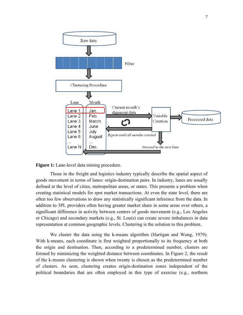
  7

Figure 1: Lane-level data mining procedure.

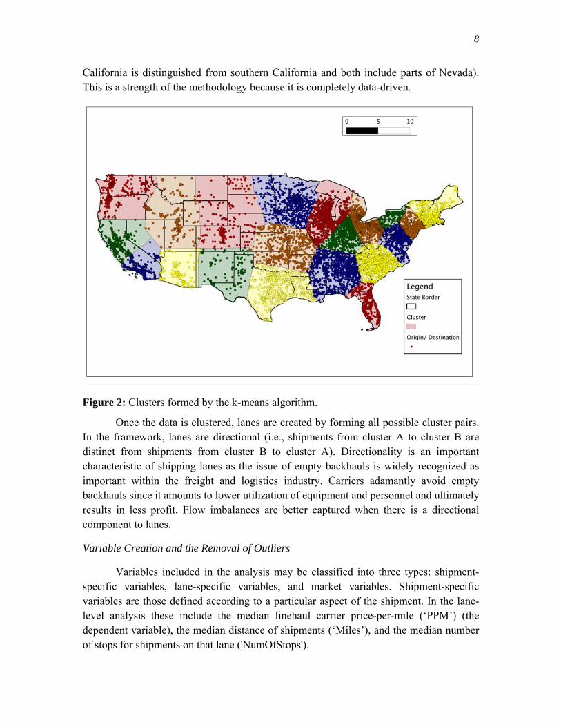
Those in the freight and logistics industry typically describe the spatial aspect of goods movement in terms of lanes: origin-destination pairs. In industry, lanes are usually defined at the level of cities, metropolitan areas, or states. This presents a problem when creating statistical models for spot market transactions. At even the state level, there are often too few observations to draw any statistically significant inference from the data. In addition to 3PL providers often having greater market share in some areas over others, a significant difference in activity between centers of goods movement (e.g., Los Angeles or Chicago) and secondary markets (e.g., St. Louis) can create severe imbalances in data representation at common geographic levels. Clustering is the solution to this problem.

We cluster the data using the k-means algorithm (Hartigan and Wong, 1979). With k-means, each coordinate is first weighted proportionally to its frequency at both the origin and destination. Then, according to a predetermined number, clusters are formed by minimizing the weighted distance between coordinates. In Figure 2, the result of the k-means clustering is shown when twenty is chosen as the predetermined number of clusters. As seen, clustering creates origin-destination zones independent of the political boundaries that are often employed in this type of exercise (e.g., northern

  8

California is distinguished from southern California and both include parts of Nevada). This is a strength of the methodology because it is completely data-driven.

 

Figure 2: Clusters formed by the k-means algorithm.

Once the data is clustered, lanes are created by forming all possible cluster pairs. In the framework, lanes are directional (i.e., shipments from cluster A to cluster B are distinct from shipments from cluster B to cluster A). Directionality is an important characteristic of shipping lanes as the issue of empty backhauls is widely recognized as important within the freight and logistics industry. Carriers adamantly avoid empty backhauls since it amounts to lower utilization of equipment and personnel and ultimately results in less profit. Flow imbalances are better captured when there is a directional component to lanes.

Variable Creation and the Removal of Outliers

Variables included in the analysis may be classified into three types: shipment-specific variables, lane-specific variables, and market variables. Shipment-specific variables are those defined according to a particular aspect of the shipment. In the lane-level analysis these include the median linehaul carrier price-per-mile (‘PPM’) (the dependent variable), the median distance of shipments (‘Miles’), and the median number of stops for shipments on that lane ('NumOfStops').

  9

Lane-specific variables are likewise defined. They include the type of equipment primarily used for transport on that lane (i.e.., Van, Flatbed, Refrigerated, Other, or None). The market variable, ‘Market Index,’ is the Cass Truckload Linehaul Index (Cass Information Systems, 2012). It is an indicator of the per-mile price fluctuations in the truckload market. It is all the more valuable since it is an exogenous source of information for our model.

The analysis is limited to only those shipments within the contiguous U.S. This is because shipments that cross international borders have costs and challenges associated with them that are not common to domestic loads. Prior to estimation, we removed observations in the data set believed to be outliers. These include those with costs that seem unreasonable. Also, only those observations with no accessorial costs are included. Accessorial costs are those that are charged for activities beyond the basic shipping service (e.g., loading/ unloading, etc.).

Twenty clusters are used resulting in 400 unique lanes in our analysis. Twenty clusters were chosen because of diminishing returns in accuracy with an increasing number of clusters. That is, the gains in terms of statistical fit did not continue to increase with the addition of more clusters. There are 38 months in the data set. However, because there is not an observation for every lane in every month, we are left with an unbalanced panel consisting of 10,980 observations.

Model Estimation

The model is estimated using fixed-effects regression. The fixed-effects technique was chosen over the corresponding random-effects method because the results of the Hausman test strongly suggested that the fixed-effects model was more appropriate (Hausman, 1978). The model specification is as follows:

PPMit = β0 + β1*NumOfStopsit + β2* ln(Milesit)+ β3*IndexMonthChanget + β4*Primary Equipmentit + ε.

The number of stops in the lane-level analysis is determined by the most frequently occurring trip type on a lane in the month under consideration. Likewise, the primary equipment type is defined as the most frequently used truck type on a given lane in a given month. In the model, it is treated as a categorical variable indicating one of several equipment types. In this case, those include ‘Van’, ‘Refrigerated’, ‘Flatbed’, ‘Other’, or ‘None’. In the event of a tie, the ‘None’ category is assigned as the primary equipment type. The monthly percent change in the market index (‘IndexMonthChange’) is indexed only by time t since it is the same for all lanes. The results of the analysis are in Table 1.

  10

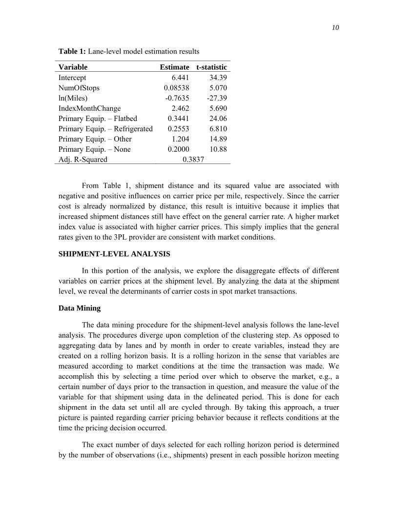
Table 1: Lane-level model estimation results

Variable Estimate t-statisticIntercept 6.441 34.39NumOfStops 0.08538 5.070ln(Miles) -0.7635 -27.39IndexMonthChange 2.462 5.690Primary Equip. – Flatbed 0.3441 24.06Primary Equip. – Refrigerated 0.2553 6.810Primary Equip. – Other 1.204 14.89Primary Equip. – None 0.2000 10.88Adj. R-Squared 0.3837

From Table 1, shipment distance and its squared value are associated with negative and positive influences on carrier price per mile, respectively. Since the carrier cost is already normalized by distance, this result is intuitive because it implies that increased shipment distances still have effect on the general carrier rate. A higher market index value is associated with higher carrier prices. This simply implies that the general rates given to the 3PL provider are consistent with market conditions.

SHIPMENT-LEVEL ANALYSIS

In this portion of the analysis, we explore the disaggregate effects of different variables on carrier prices at the shipment level. By analyzing the data at the shipment level, we reveal the determinants of carrier costs in spot market transactions.

Data Mining

The data mining procedure for the shipment-level analysis follows the lane-level analysis. The procedures diverge upon completion of the clustering step. As opposed to aggregating data by lanes and by month in order to create variables, instead they are created on a rolling horizon basis. It is a rolling horizon in the sense that variables are measured according to market conditions at the time the transaction was made. We accomplish this by selecting a time period over which to observe the market, e.g., a certain number of days prior to the transaction in question, and measure the value of the variable for that shipment using data in the delineated period. This is done for each shipment in the data set until all are cycled through. By taking this approach, a truer picture is painted regarding carrier pricing behavior because it reflects conditions at the time the pricing decision occurred.

The exact number of days selected for each rolling horizon period is determined by the number of observations (i.e., shipments) present in each possible horizon meeting

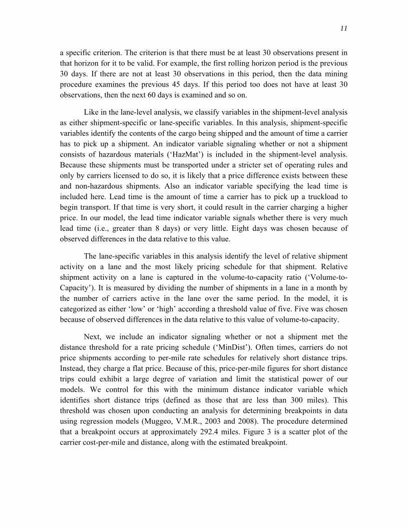
  11

a specific criterion. The criterion is that there must be at least 30 observations present in that horizon for it to be valid. For example, the first rolling horizon period is the previous 30 days. If there are not at least 30 observations in this period, then the data mining procedure examines the previous 45 days. If this period too does not have at least 30 observations, then the next 60 days is examined and so on.

Like in the lane-level analysis, we classify variables in the shipment-level analysis as either shipment-specific or lane-specific variables. In this analysis, shipment-specific variables identify the contents of the cargo being shipped and the amount of time a carrier has to pick up a shipment. An indicator variable signaling whether or not a shipment consists of hazardous materials (‘HazMat’) is included in the shipment-level analysis. Because these shipments must be transported under a stricter set of operating rules and only by carriers licensed to do so, it is likely that a price difference exists between these and non-hazardous shipments. Also an indicator variable specifying the lead time is included here. Lead time is the amount of time a carrier has to pick up a truckload to begin transport. If that time is very short, it could result in the carrier charging a higher price. In our model, the lead time indicator variable signals whether there is very much lead time (i.e., greater than 8 days) or very little. Eight days was chosen because of observed differences in the data relative to this value.

The lane-specific variables in this analysis identify the level of relative shipment activity on a lane and the most likely pricing schedule for that shipment. Relative shipment activity on a lane is captured in the volume-to-capacity ratio (‘Volume-to-Capacity’). It is measured by dividing the number of shipments in a lane in a month by the number of carriers active in the lane over the same period. In the model, it is categorized as either ‘low’ or ‘high’ according a threshold value of five. Five was chosen because of observed differences in the data relative to this value of volume-to-capacity.

Next, we include an indicator signaling whether or not a shipment met the distance threshold for a rate pricing schedule (‘MinDist’). Often times, carriers do not price shipments according to per-mile rate schedules for relatively short distance trips. Instead, they charge a flat price. Because of this, price-per-mile figures for short distance trips could exhibit a large degree of variation and limit the statistical power of our models. We control for this with the minimum distance indicator variable which identifies short distance trips (defined as those that are less than 300 miles). This threshold was chosen upon conducting an analysis for determining breakpoints in data using regression models (Muggeo, V.M.R., 2003 and 2008). The procedure determined that a breakpoint occurs at approximately 292.4 miles. Figure 3 is a scatter plot of the carrier cost-per-mile and distance, along with the estimated breakpoint.

  12

 

Figure 3: The estimated breakpoint for rate scheduling.

The same outlier removal conditions as described in the Lane-level Analysis section are employed for the shipment-level analysis. Figure 4 outlines the entire procedure.

  13

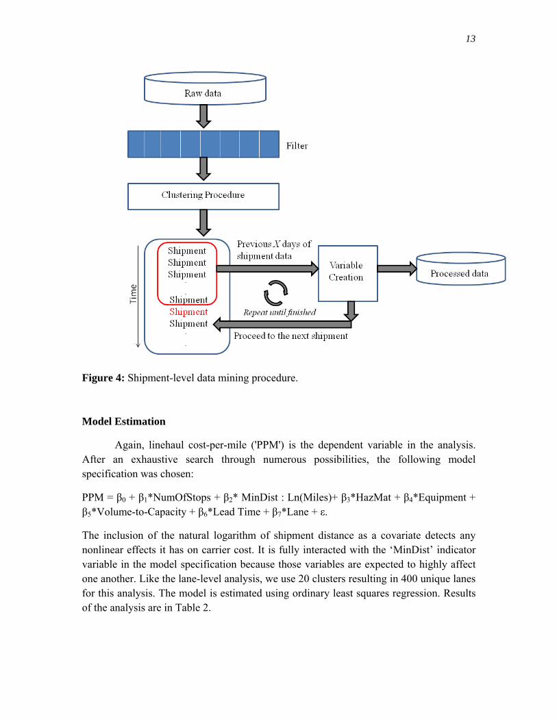
Figure 4: Shipment-level data mining procedure.

Model Estimation

Again, linehaul cost-per-mile ('PPM') is the dependent variable in the analysis. After an exhaustive search through numerous possibilities, the following model specification was chosen:

PPM = β0 + β1*NumOfStops + β2* MinDist : Ln(Miles)+ β3*HazMat + β4*Equipment + β5*Volume-to-Capacity + β6*Lead Time + β7*Lane + ε.

The inclusion of the natural logarithm of shipment distance as a covariate detects any nonlinear effects it has on carrier cost. It is fully interacted with the ‘MinDist’ indicator variable in the model specification because those variables are expected to highly affect one another. Like the lane-level analysis, we use 20 clusters resulting in 400 unique lanes for this analysis. The model is estimated using ordinary least squares regression. Results of the analysis are in Table 2.

  14

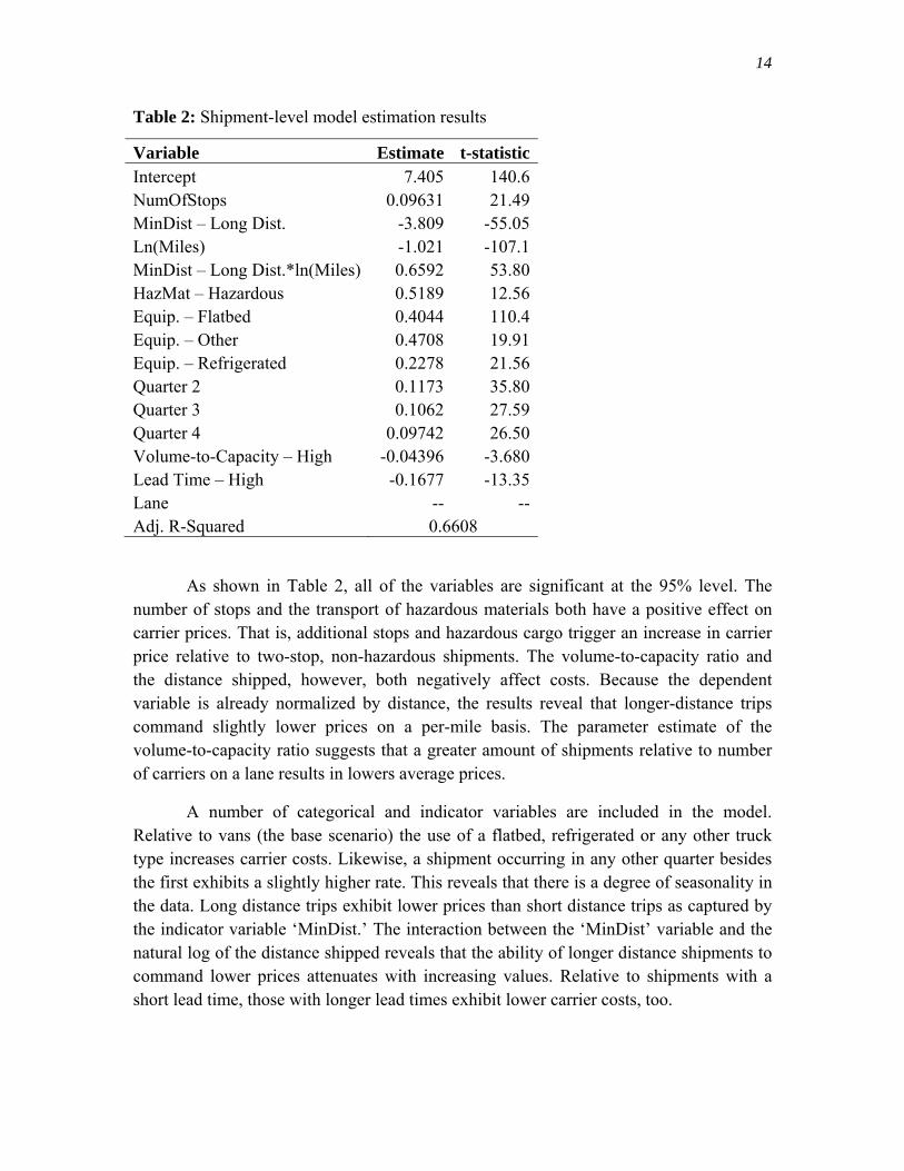
Table 2: Shipment-level model estimation results

Variable Estimate t-statisticIntercept 7.405 140.6NumOfStops 0.09631 21.49MinDist – Long Dist. -3.809 -55.05Ln(Miles) -1.021 -107.1MinDist – Long Dist.*ln(Miles) 0.6592 53.80HazMat – Hazardous 0.5189 12.56Equip. – Flatbed 0.4044 110.4Equip. – Other 0.4708 19.91Equip. – Refrigerated 0.2278 21.56Quarter 2 0.1173 35.80Quarter 3 0.1062 27.59Quarter 4 0.09742 26.50Volume-to-Capacity – High -0.04396 -3.680Lead Time – High -0.1677 -13.35Lane -- --Adj. R-Squared 0.6608

As shown in Table 2, all of the variables are significant at the 95% level. The number of stops and the transport of hazardous materials both have a positive effect on carrier prices. That is, additional stops and hazardous cargo trigger an increase in carrier price relative to two-stop, non-hazardous shipments. The volume-to-capacity ratio and the distance shipped, however, both negatively affect costs. Because the dependent variable is already normalized by distance, the results reveal that longer-distance trips command slightly lower prices on a per-mile basis. The parameter estimate of the volume-to-capacity ratio suggests that a greater amount of shipments relative to number of carriers on a lane results in lowers average prices.

A number of categorical and indicator variables are included in the model. Relative to vans (the base scenario) the use of a flatbed, refrigerated or any other truck type increases carrier costs. Likewise, a shipment occurring in any other quarter besides the first exhibits a slightly higher rate. This reveals that there is a degree of seasonality in the data. Long distance trips exhibit lower prices than short distance trips as captured by the indicator variable ‘MinDist.’ The interaction between the ‘MinDist’ variable and the natural log of the distance shipped reveals that the ability of longer distance shipments to command lower prices attenuates with increasing values. Relative to shipments with a short lead time, those with longer lead times exhibit lower carrier costs, too.

  15

Of the 399 lanes included as dummy variables in the analysis (a single lane is reserved as the base category), at the 95% significance level 284 lanes are statistically significantly different from the reference lane. This result suggests that there are powerful lane effects in the determinants of carrier prices.

DISCUSSION AND COMPARISON OF THE RESULTS

Largely, the shipment-level analysis reflects many of the insights gleaned from the lane-level analysis. The lane on which the shipment occurred and the characteristics of that lane are important determinants of carrier price. Shipment characteristics such as distance, the required equipment type, and whether or not the cargo consists of hazardous materials play major roles in carrier pricing. Also, seasonal effects reflected in the calendar quarter in which the shipment occurs and market conditions as reflected in the index affects carrier prices.

The primary economic implications of the analyses include the role of shipment, lane, and market characteristics in determining carrier rates. A number of these, primarily shipment characteristics (such as equipment type, distance, cargo type, and number of stops), capture what are essentially operating costs to the carrier. These parameter estimates capture the bulk of carrier costs when their magnitude is taken into account. Meanwhile, others, primarily lane and market characteristics (such as lane volume-to-capacity and the time of year), capture aspects of carrier rates not directly related to carrier costs. Considering the scale of these parameter estimates, though they are statistically significant, they contribute very little to overall carrier costs. These are likely the variables that largely determine carrier profit margins, the aspect of cost to 3PL providers that could be negotiable.

In particular, distance-related variables have a huge effect on price-per-mile if all other variables are held constant. As captured by a comparison of the estimates for ‘Intercept’ and ‘MinDist,’ long-distance trip costs are approximately on average half that of short distance trips. This is intuitive as short-distance trips will undoubtedly have a higher per-mile cost than longer trips. Consider the parameter estimate for ‘Miles,’ it suggests that a 1% increase in distance is associated with a $0.01 decrease in carrier price-per-mile. The amount may not be large, but realizing that a 1% increase in distance can easily be as small as 3 or 4 miles, the total change can quickly become significant, especially for short-distance trips. For example, a 240-mile trip would be $0.20 less expensive than a 200-mile trip. This effect is tempered when ‘Miles’ and the ‘MinDist’ indicator are interacted for long-distance trips. In that scenario a 1% increase in distance is associated with only about a $0.003 decrease in carrier price-per-mile.

  16

TACTICAL PLANNING SCENARIO: UNDERPERFORMING LANES

While most non-profitable transactions are sporadic, others are habitual and share common characteristics that suggest the 3PL provider repeatedly overlooks some critical aspect of carrier costs. Otherwise, a sufficient cost would have been charged to the carrier to ensure a profit. The obvious manner in which to investigate this occurrence is by lane. Lanes are the common denominator by which we can identify habitual non-profitable transactions and begin to address the problem.

Identifying Underperforming Lanes

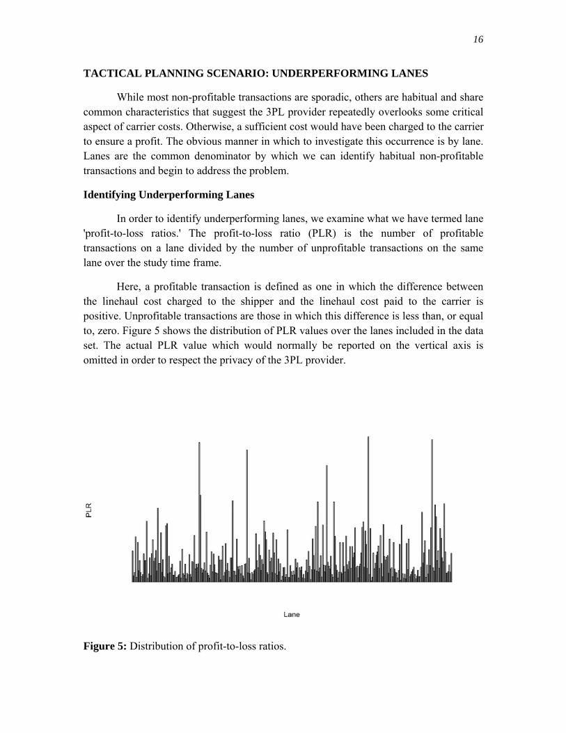
In order to identify underperforming lanes, we examine what we have termed lane 'profit-to-loss ratios.' The profit-to-loss ratio (PLR) is the number of profitable transactions on a lane divided by the number of unprofitable transactions on the same lane over the study time frame.

Here, a profitable transaction is defined as one in which the difference between the linehaul cost charged to the shipper and the linehaul cost paid to the carrier is positive. Unprofitable transactions are those in which this difference is less than, or equal to, zero. Figure 5 shows the distribution of PLR values over the lanes included in the data set. The actual PLR value which would normally be reported on the vertical axis is omitted in order to respect the privacy of the 3PL provider. 

 

Figure 5: Distribution of profit-to-loss ratios.

  17

A relatively low PLR value for a lane indicates poor profit performance while higher PLR values imply good performance. By examining the distribution of PLR values and setting an appropriate base performance level for a lane (e.g., a PLR value less than or equal to 3, or perhaps the 25th percentile for instance), a 3PL provider can identify underperforming lanes. Once those lanes are singled out, the firm can analyze them and then devise strategies to improve their performance.

As an example, using a PLR that is less than or equal to 3 as the criterion, three lanes in the data are identified as underperforming. There are 2,356 combined shipments on these lanes. Of the three lanes, one consists of shipments with origin-destination pairs primarily within the state of Texas and between Texas and Louisiana. It accounts for the vast majority of identified underperforming shipments, 2,271. The other two lanes consist of shipments with origin-destination pairs in sparsely populated states in the Midwestern and Mountain West regions of the U.S. (e.g., Utah to North Dakota, Idaho to Iowa, etc.). Two possible reasons for underperformance become readily apparent, the first is that intrastate shipments, especially in a state as large and diverse as Texas, are difficult to correctly price because of local market dynamics. The standard deviation reveals that carrier price-per-mile can vary by as much as $0.80 for these shipments. Likely, it makes a big difference whether or not a shipment has an origin-destination pair in one of the economic centers (e.g., Houston or Dallas) or a more rural area.

The second possible reason for underperformance is that infrequent shipments to sparsely populated regions, as evidenced by the other two lanes, are difficult to price because of their unfamiliarity to brokers and unattractiveness to carriers. Lanes such as these are not likely to offer many backhaul opportunities. The standard deviation reveals that carrier price-per-mile can vary by as much as $0.34 for these shipments. Though not as much in the case of an intrastate lane, it is still significant.

Thus, the data mining procedure combined with the PLR present a methodology by which 3PL provider performance can be assessed on a lane-by-lane basis. Based on an examination of the data, volatility in price (due to local dynamics on intrastate lanes, and unfamiliarity and unattractiveness on infrequent lanes) is the likely culprit.

Application of the Shipment-Level Model Results to Underperforming Lanes

Once underperforming lanes have been identified according to the pre-defined baseline metric, the question that naturally follows is 'How can they be improved?' We address this issue by again estimating a regression model. However, the primary goal is now prediction instead of explication. In addition, this new model represents a departure from our previous strategies in that now instead of using price-per-mile as the dependent variable we now simply use price. This is done because the authors found the price

  18

models to provide better predictive ability than the rate models. The model specification is as follows:

Carrier linehaul cost = β0 + β1*NumOfStops + β2* MinDist : Ln(Miles)+ β3*HazMat + β4*Equipment + β5*Volume-to-Capacity + β6*Lead Time + β7*Lane + ε.

The model is estimated using the primary set of data and its predictive ability is gauged using a holdout sample (a portion of data over which the models were not calibrated). Results are in Table 3. The metric by which the model is assessed is the mean absolute error (MAE). Absolute error is the absolute difference between the predicted and true value; the MAE is the average value across all observations.

Table 3: Predictive model estimation results

Variable Estimate t-statisticIntercept -752.8 -18.79NumOfStops 139.7 41.31MinDist – Long Dist. -3414 -65.39Ln(Miles) 172.4 23.97MinDist – Long Dist.*ln(Miles) 583.4 63.08HazMat – Hazardous 395.9 12.69Equip. – Flatbed 262.8 94.97Equip. – Refrigerated 274.8 15.39Equip. – Other 184.1 23.09Quarter 2 81.33 32.88Quarter 3 82.00 28.22Quarter 4 71.18 25.66Volume-to-Capacity -14.45 -10.51Lead Time – High -52.03 -5.480Lane -- --Adj. R-Squared 0.8464

With an adjusted R-squared value of 0.8464, much of the variance in carrier costs is explained. The model’s MAE was calculated to be 208.6. Dividing the absolute error by the true linehaul cost for each shipment and then taking the average yields a value equal to 0.2685. This value implies that, on average, the predicted values are within approximately 27% of the true value.

If underperforming lanes are singled out using the previously defined criterion, a PLR less than or equal to 3, it can be judge how well the model estimates carrier prices on those lanes. Using the lanes in the holdout data set that meet the criterion, the predicted values of the linehaul costs are within 21% of their true value. This shows that

  19

the model does a good job of predicting what the actual linehaul costs for a shipment may be. A 3PL broker with this information beforehand could use it to set a baseline price for shipper negotiations.

CONCLUSIONS

This research has investigated the determinants of carrier linehaul costs in spot markets; it has defined a methodology by which historical shipment data may be processed and mined; and lastly it has demonstrated some of the potential uses of historical shipment data by non asset-based 3PL providers. Regarding the determinants of carrier costs, the distance a shipment is transported along with the type of equipment used are among the most important factors.

Also, the study examined the transactional data as a panel data set by aggregating transactions at the lane level and in monthly intervals. In so doing, a broad view of the temporal and spatial dynamics of carrier pricing was taken yielding insights into overall market behavior. Many of the same characteristics identified in the shipment analysis proved to be consistent with the lane-level analysis. However, the direction of influence was sometimes opposite.

Lastly, the research developed a methodology by which underperforming lanes are identified using historical shipment data. Lanes that exhibit below par PLRs can be singled out for improvement by the 3PL provider and efforts can be undertaken to improve performance. As part of those efforts, the regression model used for prediction can suggest to the 3PL broker baseline prices to begin negotiations with a potential shipper.

There are few potential limitations to this work that could be addressed in future studies. In further work, measures other than median values could be tested in the lane-level analysis. The use of a single 3PL provider as the source of data is another potential limitation because, inevitably, there will be more data available in the geographic areas in which that provider is strongest. Pooling data across several 3PL providers would provide a more complete perspective of the market. Other possible limitations include the use of a clustering algorithm for distinguishing lanes. It is possible that political boundaries have a greater influence on carrier rates than assumed, which could potentially bias the results.

REFERENCES

Armstrong & Associates, Inc. “U.S. 3PL/ Contract Logistics Market.” http://www.3plogistics.com/3PLmarket.htm. Accessed July 19, 2012.

Baker, J.A. 1991. “Emergent pricing structures in LTL transportation.” Journal of Business Logistics 12 (1): 191-202.

  20

Cass Information Systems. “Cass Truckload Linehaul Index: April 2010 to April 2012.” www.cassinfo.com/Transportation-Expense-Management/Supply-Chain-Analysis/Transportation-Indexes. Accessed June 12, 2012.

Christensen, L.R. and Huston, J.H. 1987. “A reexamination of the cost structure for specialized motor carriers.” Logistics and Transportation Review 23 (4): 339-351.

Council of Supply Chain Management. “Glossary of Terms and Definitions.” http://cscmp.org/digital/glossary/glossary.asp. Accessed May 23, 2012.

Ferguson, W. and Glorfeld, L. 1981. “Modeling the Present Carrier Rate Structure as a Benchmark for Pricing in the New Competitive Environment.” Transportation Journal 21 (2): 59-66.

Figliozzi, M. 2004. “Performance and Analysis of Spot Truck-Load Procurement Markets using Sequential Auctions.” PhD dissertation, University of Maryland, College Park.

Garrido, R. 2007. “Procurement of transportation services in spot markets under a double-auction scheme with elastic demand.” Transportation Research Part B: Methodological 41 (9): 1067-1078.

Greene, W. 2011. Econometric Analysis. Prentice Hall, 7th ed.

Grimm, C.M., Corsi, T.M. and Jarrel, J.L. 1989. “U.S. motor carrier cost structure under deregulation.” Logistics and Transportation Review 25 (3): 231-249.

Harmatuck, D.J. 1992. “Motor Carrier Cost Function Comparisons.” Transportation Journal 31 (4): 31-46.

Hartigan, J. and Wong. M. 1979. “Algorithm as 136: A k-means clustering algorithm.” Journal of the Royal Statistical Society, Series C 28 (1): 100-108.

Hausman, J. 1978. “Specification Tests in Econometrics.” Econometrica, 41 (4): 733-750.

Huang, M., Homem-de-Mello, T., Smilowitz K. and Driegert, B. 2011. “Supply Chain Broker Operations: Network Perspective.” Transportation Research Record (2224): 1-7.

Lin, I., Mahmassani, H., Jaillet, P. and Walton, C.M. 2002. “Electronic Marketplaces for Transportation Services: Shipper Considerations.” Transportation Research Record (1790): 1-9.

Muggeo, V.M.R. 2003. “Estimating regression models with unknown breakpoints.” Statistics in Medicine 22 (19): 3055-3071.

Muggeo, V.M.R. 2008. “Segmented: An R package to fit regression models with broken-line relationships.” R News 8 (1): 20-25.

Ozkaya, E., Keskinocak, P., Joseph, V.R. and Weight, R. 2010. “Estimating and benchmarking Less-than-Truckload market rates.” Transportation Research Part E 46 (5): 667-682.

Sheffi, Y. 1990. “Third Party Logistics: Present and Future Prospects.” Journal of Business Logistics 11 (2): 27-39.

Sheffi, Y. 2004. “Combinatorial Auctions in the Procurement of Transportation Services.” Interfaces 34 (4): 245-252.

Smith, L., Campbell, J.F. and Mundy, R. 2007. “Modeling Net Rates for Expedited Freight Services.” Transportation Research Part E 43 (2): 192-207.

  21

Song, J. and Regan, A. 2003. “Combinatorial Auctions for Transportation Service Procurement: The Carrier Perspective.” Transportation Research Record (1833): 40-46.

StataCorp. 2011. Stata Statistical Software: Release 12. College Station, TX: StataCorp LP.

Thomas, J.M. and Callan, S.J. 1992. “Cost analysis of specialized motor carriers: an investigation of aggregation and specification bias.” Logistics and Transportation Review 28 (3): 217-230.

Wooldridge, J. 2002. Econometric Analysis of Cross Section and Panel Data. MIT Press, Cambridge, Mass.