Time-Varied Daylighting Performance to Enable aGoal-Driven Design Process

by

Sian Alexandra KleindienstMASSACHUSETTS INSTITUTE

B.A. Physics (2003) OF TECHNOLOGY

Harvard University

M.S. Building Technology (2006)Massachusetts Institute of Technology LIBRARIES

Submitted to the Department of ArchitectureIn Partial Fulfillment of the Requirements for the Degree of

DOCTOR OF PHILOSOPHY IN ARCHITECTURE: BUILDING TECHNOLOGYat the

MASSACHUSETTS INSTITUTE OF TECHNOLOGY

February 2010 ARCHIVES

@ 2010 Sian A. Kleindienst. All rights reserved.

The author hereby grants to MIT permission to reproduceand to distribute publicly paper and electronic

copies of this thesis document on whole or in partin any medium now known or hereafter created.

Author:

Building Technology ProgramJanuary 8th, 2010

Certified by: Mryi AndersenMarilyri ndre

Associate Professor of Building TechnologyThesis Supervisor

Accepted by:

Julian BeinartProfessor of Architecture

Chairman, Committee for Graduate Students

2

Thesis Supervisor....... .. ........ ...............................Marilyne Andersen

Associate Professor of Building TechnologyDepartment of Architecture, MIT

Thesis Reader......... ..........................Leslie K. Norford

Professor of Building TechnologyDepartment of Architecture, MIT

Thesis Reader........Christoph Reinhart

Associate Professor of Architectural TechnologyGraduate School of Design, Harvard

3

4

Time-Varied Daylighting Performance to Enable a Goal-Driven Design Process

by

Sian A. Kleindienst

Submitted to the Department of Architecture on January 8th 2010in Partial Fulfillment of the Requirements of the Degree ofDoctor of Philosophy in Architecture: Building Technology

ABSTRACT

Due to the overwhelming number of decisions to be made during early stage design,there is a need for intuitive methods to communicate data so that it is quickly and easilyunderstood by the designer. In daylighting analysis, research has been moving towardsdynamic daylighting metrics, which include both annual performance indicators and localclimate conditions. Temporally-based graphics are one method of annual data displaywhich shows great promise for use in the early design stage. Not only can temporaldata be easily connected to time-dependent environmental variables like weather andsolar angle, but non-spatial quantities related to solar heat gain can be compared on thesame terms with spatial quantities like illuminance.

This thesis demonstrates methods for quickly calculating annual data sets for whichtemporal maps are the intended display format. Metrics are then developed in order todisplay goal-based performance information for an entire area of interest on a singletemporal map. This process is demonstrated first by reducing the number of simulationsnecessary to produce reliable annual illuminance data, the results of which are compiledinto a metric based on a user-given illuminance range, known as Acceptable IlluminanceExtent (AIE). Similarly, a geometry-based glare approximation method is developed andvalidated for quick annual calculations of Daylight Glare Probability, and the results arecondensed to a single number representative of glare perception within the model,known as Glare Avoidance Extent (GAE). Finally, a simple solar heat gain indicator isdemonstrated using the Balance Point calculation method and the metric Solar HeatScarcity/Surplus (SHS) is used to convey the urgency of allowing more direct solar gainor shading it.

This thesis is part of the Lightsolve project, which aims to specifically address the needsof the architect during early design stages. Specifically, Lightsolve aims to produce fast,unique design analyses, based on local annual climate data with reasonably accurateand intuitive outputs to promote good decision-making. Such resources could enable adesirable shift in schematic stage design practices and move daylighting analysis onestep closer to achieving "best practice" recognition.

Thesis Supervisor: Marilyne AndersenTitle: Associate Professor of Building Technology

Acknowledgements

The work in this thesis was accomplished as all large projects are: by learning fromthose who preceded me and by the unending patience and support of family and friends.

In particular I would like to thank Marilyne Andersen for her excellent advice, guidance,understanding, and sense of humor. I would like to thank Les Norford and ChristophReinhart for their advice (and helpful criticisms), and I would especially like toacknowledge Les Norford for his help in during development of the Solar HeatScarcity/Surplus metric. I would also like to thank Jan Wienold for conversations andadvice regarding his work with evalglare and the Daylight Glare Probability metric.

I would like to thank the MIT Department of Architecture Building Technology Programand the Martin Family fellowship for funding this work, and Google for providing briefeducational SketchUp licenses to those who tested it.

I would like to thank Angela Watson for allowing us to use her studio as the first test ofLightsolve, and all those students who have given us feedback on early versions of thesoftware. I would like to thank Les Norford and John Ochsendorf for allowing me to givea survey in their classes.

Finally, I would like to thank all of my friends and family. I would especially like to thankJaime for her heroic dealings with Lightsolve issues, Stephen and Nick for theirunderstanding, David for enabling an obsession with tea, and everyone else in theBuilding Technology Lab. I would like to thank my Ashdown family - you know who youare - for providing an enjoyable and somewhat balanced social life. Last but far fromleast, I would like to thank my parents, sister, and Evan for their love and support.

Table of Contents

1 Introduction ....................................................................................... 101.1 Motivating Daylight in Design ........................................................... 101.2 Problem Statement ........................................................................... 111.3 The Lightsolve Concept ................................................................... 14

2 State of the Art ................................................................................... 162.1 Lighting M etrics .......................................................................... .. 16

2.1.1 Quantity Metrics ................................................................... 162.1.2 Existing Annual Illuminance Calculations ................................... 182.1.3 Light Contrast Metrics ............................................................ 202.1.4 Daylight Glare Probability ........................................................ 212.1.5 Existing Annual Glare Calculations .......................................... 232 .1.6 S olar H eat G ain ..................................................................... 24

2.2 Graphical Displays of Numerical Information ...................................... 252.3 Existing Solutions for Early-Stage Analysis .......................................... 28

2.3.1 Allowed Model Complexity ..................................................... 282.3.2 Sky Luminance Distribution ................................................... 302.3.3 Calculation and Simulation ..................................................... 312.3.4 Annual Calculations and Metrics .............................................. 332.3.5 Light Quantity, Glare, and Heat Gain ........................................ 332.3.6 Goal-based Performance Metrics ................... ...................... 342.3.7 Visualizations ............................................. ................... 342.3.8 Summary of Existing Solutions ................................................ 35

3 Simulation Reduction for Temporal Graphics ........................................... 383.1 Data Reduction Methodology ........................................................... 39

3.1.1 Representative Annual Periods ................................................ 403.1.2 Sky Models Choice and Discussion ........................................... 42

3.2 Validation of Data Reduction Method ................................................ 443.3 External Sky and Weather Variability Test .......................................... 45

3.3.1 Temporal Map Visual Similarities .............................................. 473.3.2 Numerical Pixel-Based Comparison .......................................... 50

3.4 Interior Illuminance Test for Simple Geometry .................................... 533.4.1 Temporal Map Visual Similarities .............................................. 543.4.2 Numerical Pixel Comparison ................................................... 55

3.5 Interior Illuminance Data for Complex Geometry ................................... 583.6 Summary of Data Reduction Method ........................................................ 62

4 Acceptable Illuminance Extent ............................................................ 634.1 Definition of a Temporal Illuminance Metric ........................................ 644.2 Temporal Map Visual Similarities using Acceptable Illuminance Extent ....... 66

4.2.1 Simple Geometry Case .......................................................... 664.2.2 Classroom Iterations Case ...................................................... 694.2.3 Complex Geometry Case ....................................................... 71

4.3 Summary of New Temporal Illuminance Metric ....................................... 715 Glare Avoidance Extent ........................................................................ 73

5.1 Daylight Glare Probability in Depth ................................................... 735.2 Deriving a Model-Based DGP Approximation ...................................... 765.3 Glare Simulation Parameters ............................................................. 795.4 Validation of Model-Based DPG Approximation ...................................... 81

5.4.1 Vertical Windows Classroom Case ....... ...... ............ 815.4.2 Skylights Classroom Case ...................................................... 835.4.3 Cases Involving Contrast Glare ................................................ 84

5.5 Definition of a Temporal Glare Metric ....................... ....................... 875.6 Visual Comparisons using Glare Avoidance Extent ............................... 88

5.6.1 Classroom Model Comparisons .................................................. 885.6.2 Frame Model Comparisons ..................................................... 90

5.7 Summary of New Temporal Glare Metric ............................................. 906 Solar Heat Surplus and Scarcity .......................................................... 93

6.1 Balance Point Method .................................................................... 936.2 User Inputs and Defaults for Balance Point Analysis ............................. 966.3 Definition of a Temporal Solar Energy Metric ....................................... 976.4 Solar Heat Surplus/Scarcity Feasibility Study ....................................... 100

6.4.1 Comparison of Daily Total Loads ............................................. 1026.4.2 Visualizing Solar Heat Scarcity/Surplus ..................................... 108

6.5 An Alternate Daily Totals Visualization ............................................... 1126.5 Summary of New Solar Energy Metric ................................................. 112

7 Temporal Maps and Design Analysis ................................................... 1147.1 Iterative Example of Improving Illuminance Performance ...................... 114

7.2 Spatial and Temporal Analysis ......................................................... 1187.2.1 Classroom Example ............................................................. 1187.2.2 Hospital Room Example ......................................................... 122

7.2.3 Church of Light Example ........................................................ 124

7.2.4 Combining Temporal Maps with Renderings ............................... 1257.3 Analyzing Options Using All New Metrics ............................................ 1277.4 Daylight Analysis Surveys ............................................................... 130

7.4 .1 S urvey R esults ..................................................................... 13 1

7.4.2 Survey Discussion . ........................... ....... 1327.5 Design Analysis Summary ............................................................... 134

8 Conclusion ...................................................................................... 1358.1 Main Achievements ....................................... 1358 .2 A pplications ..................................................................... 1378 .3 F utu re W o rk ................................................................................. 138

9 References ...................................................................................... 140Appendix A ......................................................................................... 153Appendix B ......................................................................................... 154Appendix C ......................................................................................... 155Appendix D ........................................................................................ 157

9

Chapter 1

Introduction

1.1 Motivating Daylight in Design

Architecture is the learned game, correct and magnificent, of forms assembled in thelight. Le Corbusier

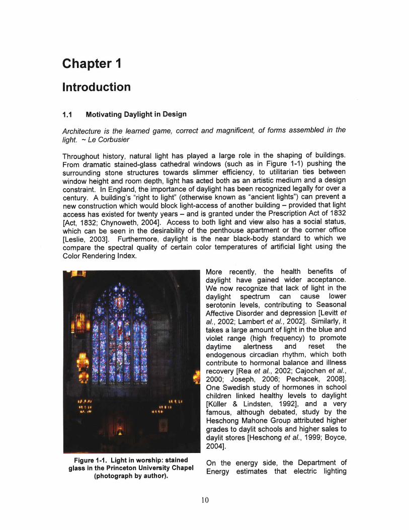
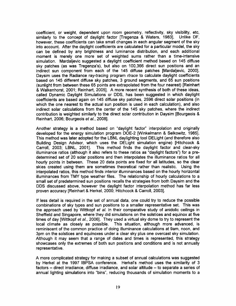
Throughout history, natural light has played a large role in the shaping of buildings.From dramatic stained-glass cathedral windows (such as in Figure 1-1) pushing thesurrounding stone structures towards slimmer efficiency, to utilitarian ties betweenwindow height and room depth, light has acted both as an artistic medium and a designconstraint. In England, the importance of daylight has been recognized legally for over acentury. A building's "right to light" (otherwise known as "ancient lights") can prevent anew construction which would block light-access of another building - provided that lightaccess has existed for twenty years - and is granted under the Prescription Act of 1832[Act, 1832; Chynoweth, 2004]. Access to both light and view also has a social status,which can be seen in the desirability of the penthouse apartment or the corner office[Leslie, 2003]. Furthermore, daylight is the near black-body standard to which wecompare the spectral quality of certain color temperatures of artificial light using theColor Rendering Index.

More recently, the health benefits ofdaylight have gained wider acceptance.We now recognize that lack of light in thedaylight spectrum can cause lowerserotonin levels, contributing to SeasonalAffective Disorder and depression [Levitt etal., 2002; Lambert et al., 2002]. Similarly, ittakes a large amount of light in the blue andviolet range (high frequency) to promotedaytime alertness and reset theendogenous circadian rhythm, which bothcontribute to hormonal balance and illnessrecovery [Rea et al., 2002; Cajochen et al.,2000; Joseph, 2006; Pechacek, 2008].One Swedish study of hormones in schoolchildren linked healthy levels to daylight[Kuller & Lindsten, 1992], and a veryfamous, although debated, study by theHeschong Mahone Group attributed highergrades to daylit schools and higher sales todaylit stores [Heschong et al., 1999; Boyce,2004].

Figure 1-1. Light in worship: stained On the energy side, the Department ofglass in the Princeton University Chapel Energy estimates that electric lighting

(photograph by author).

consumes 38% of electricity used in US commercial buildings [DOE-EIA, 2008], and thatdoesn't account for the cooling load generated by active light bulbs. Proper daylightingcan offset a significant fraction of that energy demand, and well-controlled solar gainscan positively impact the heating and cooling demands [Li & Lam, 2001; Bodart & DeHerde, 2002; Nicklas & Bailey, 1996].

The motivations for good daylighting design are numerous and compelling, ranging fromaesthetics to health to energy, but creating a good daylighting design is not alwaysstraightforward. The quantity, color, diffusivity, and angle of natural light change withlatitude, weather, building orientation, and time of day. Although both old and new rulesof thumb exist for rectangular rooms with windows on one wall [IESNA, 2000; Reinhart,2005a], more complex needs and building forms require more complex modeling.

1.2 Problem Statement

The quality and quantity of daylight available in an architectural space depends on athree part process: collection, transportation, and distribution. These steps arecontained in the simplicity of a window and the complexity of a tracking heliostat system,and every design choice has a different level of impact on these three aspects ofdaylighting. Decisions that impact daylight access and collection are usually veryinfluential because it is, metaphorically, the first link in the chain. These include choicesmade about building orientation, form, and exterior shading, and on a lesser level,window area and complex fagade systems. Decisions impacting daylight transport mightinclude wall thickness, glazing type, complex fagade systems, reflector systems, andlight ducts, and daylight distribution is affected mainly by window positions, interiorgeometry, interior reflectivity, and interior shading. Design features which have thegreatest impact - orientation, form, and space distribution - are all governed by choicesmade in the earliest or schematic stages of design. It may be impractical for an expert tobe called in at this stage, due to tight schedules or financial constraints, and therefore itoften falls to architects to make the decisions that have the greatest effect ondaylighting.

Unfortunately, as several recent surveys have revealed, daylighting design explorationsdo not often happen during schematic design. Two of these surveys were given by theNational Research Council (NRC) of Canada and less comprehensive one by a Harvarddesign student, which was administered a few months after the second NRC survey[Reinhart & Fitz, 2004; Reinhart & Fitz, 2006; Galasiu & Reinhart, 2008; Lawrence,2005]. Although each survey had a different participant group - the NRC queriedmembers of software mailing lists in one survey and practitioners interested insustainable design in the other, while the Harvard survey targeted students andpractitioners in the Boston area who had no obvious bias for or against daylightingsoftware - each survey found similar trends. Although both NRC surveys founddaylighting software use to be around 75% among architects, both also found that toolswere largely used in design development or later stages [Reinhart & Fitz, 2004; Reinhart& Fitz, 2006; Galasiu & Reinhart, 2008]. The earlier NRC survey drew this conclusionbecause the majority of users reported using tools to resize windows and shadingsystems and to prove code compliance. The later survey asked directly and found thatless than 50% of designers who use software tools use it during schematic design. Inthat survey, "prior experience" and "rules of thumb" were the more popular choicesduring schematic design at just under 80% and 60% respectively [Galasiu & Reinhart,

2008]. In Lawrence's less specific group of participants, over one third did not usedaylight design tools of any kind. In fact, only 22% of Lawrence's participants used 3Dmodeling software (not necessarily daylight-specific) in the schematic designexploration, preferring to use hand drawings and physical models [Lawrence, 2005].

There may be many reasons why software tools are not used in the earliest stages ofdesign. Reasons given in the later NRC survey included lack of software experience,client not paying for it, and lack of time, although a conviction that experience and rulesof thumb are sufficient for early decisiond can also be implied [Galasiu & Reinhart,2008]. Another culprit could be the lack of exposure in architectural education. A surveygiven by Sarawgi in 2006 to educators at American accredited architectural schoolsrevealed that "computer software packages" was the least used method for teachinglighting design [Sarawgi, 2006]. The other choices were "rules of thumb", "manualcalculation methods", "manufacturer's literature", and "scale physical models", all ofwhich were more popular. Unfortuantely, simple calculations are inaccurate at best andonly really work with box-like spaces. Physical models can vary widely in accuracy,depending on the care given to detail and the choice of light source [Thanachareonkit etal., 2005], and any model flexibility must be designed in from the start. Furthermore, thelatter NRC survey found most architects' rules of thumb to be non-standard and home-grown [Galasiu & Reinhart, 2008], and while prior experience is useful for developingintuition, it cannot be used as a proof of concept for new designs, and it does not alwaystranslate well between different climates. "Prior experience" is also limited to thecollective lighting experience of the design team, which could be extensive or limiteddepending on those involved. For these reasons, and to meet the growing interest ingood daylighting, there needs to be a shift in the accepted exploration techniques in theearliest stages of design.

Since current popular rules of thumb and simplified analytic methods are of variableaccuracy or are non-transferable to new situations, more useful methods, includingappropriate computer simulation tools, should be given greater prominence in theschematic toolbox. Architects need the resources to produce fast, unique designanalyses, based on local annual climate data with reasonably accurate and intuitiveoutputs to promote good decision-making.

In early-stage daylighting analysis, speed is of the utmost importance, or there is nochance for exploration, iteration, and comparison. This means that defining a model andperforming calculations in any medium should be relatively quick, and that resulting datashould be easily understood by the user. In the case of computer simulation, althoughhardware is constantly improving, making design truly iterative may still requireshortening the computation time. It also makes sense to focus on improvements tomodeling and intuitive data outputs.

The goal of schematic analysis is for the designer to acquire all data necessary to makedecisions. Because this stage is one of seemingly infinite possibility, the amount andbreadth of data involved necessary to understand "the factual constraints, without undulyrestricting the designer's freedom, and without prejudicing the solution" can seemoverwhelming [Koenigsberger et al., 1975]. Koenigsberger et al. state the problem verysuccinctly:

In the synthesis, the designer must consider a wide range of factorssimultaneously. The capacity of his mind is limited. It is therefore

essential to present the information in a readily comprehensible form. Itshould not be excessively detailed, but it should still take into account allthat is relevant [Koenigsberger et al., 1975].

Herbert Simon also describes the limits of memory in the context of pattern recognitionand design process in his book The Sciences of the Artificial. The "bottleneck", as heputs it, is in the short-term memory required to hold all information simultaneously whilea solution can be synthesized from the disparate pieces [Simon, 1969]. Both bookssuggest that mental processing time can be improved if the data is pre-processed orotherwise arranged. Simon points out the benefits of grouping information intoassociative "chunks" while Koenigsberger et al. suggest data can be conveyed in theform of performance specifications [Simon, 1969; Koenigsberger et al., 1975].

The main questions involved in creating a design analysis process for the earliest stageof design are therefore:

1) What daylighting information is necessary for informed design decisions?2) How can that information be calculated quickly, but with reasonable

accuracy?3) How, if at all, should that information be pre-processed for the designer?4) What output formats should be used to convey the information?5) What metrics are appropriate for those output formats?

There is not always a consensus regarding which daylighting information is "necessary"to make informed design decisions, but research has been moving towards dynamicdaylighting metrics which include both annual performance indicators and local climateconditions. Daylight Autonomy (DA) [Reinhart & Walkenhorst, 2001] and Useful DaylightIlluminance (UDI) [Mardaljevic & Nabil, 2006; Mardaljevic, 2009], are existing metricswhich use annual climate data to find the percentage of time that a sensor point is aboveor between given illuminance benchmarks. Another direction research has taken isgraphing data as it changes over time, often together with spatial data. One benefit of atime-based graph is the implicit correlation to solar angle and climate, which, for eachlocation, are dependant on time of day and year. These environmentally basedvariables have a large impact on design orientations, window size, and basic form, whichare all important aspects of daylight access, as discussed above. Mardaljevic andGlaser have separately published papers on temporal and spatial graphics, which will bediscussed at greater length in Chapter 2 [Mardaljevic, 2001; Glaser & Ubbelohde, 2001].

Regarding what kind of information should be given in annual data sets, the performanceof daylight can be quantified in three main ways: the quantity of light on a surface (suchas illuminance), the contrast caused by neighboring luminous sources (of which glare isthe negative result), and the solar heat gain associated with light penetration. Becausethese aspects of performance can often be conflicting, it's essential to convey each kindof information in the same format so that the benefits and tradeoffs are easilycomparable. This can be accomplished using a temporal graphic format so that non-spatial quantities like solar heat gain may be compared with more spatially orientedperformance data like illuminance. The comparability of different data types can also beenhanced by using similar goal-based metrics to convey each quantity.

Goal-based metrics can also help reduce the data interpretation and synthesis requiredby the user. Dynamic data sets involving both temporal and spatial data are by naturevery large. The greatest challenge involved in producing such an immense quantity of

information is the problem of transferring it to designers without overwhelming them, asdiscussed above. Some of this difficulty can be alleviated if the data is given, not aspure numbers, but as a relationship between the calculated data and the user's designgoals. Goal-driven metrics could show the varying success of a certain design ratherthan numerical results, which would reduce the time needed to interpret the data.Furthermore, goal-driven results can be compiled over either time or space to reduce thenumber of graphs required to convey the same results.

This thesis demonstrates methods for quickly calculating annual data sets for whichtemporal maps are the intended display format. Metrics are then developed in order todisplay goal-based performance information for an entire area of interest on a singletemporal map. This process is demonstrated first in Chapter 3 by reducing the numberof simulations necessary to produce reliable annual illuminance data, the results ofwhich are compiled in Chapter 4 into a new metric based on a user-given illuminancerange, known as Acceptable Illuminance Extent (AIE). Similarly, in Chapter 5, ageometry-based glare approximation method is developed and validated for quickannual calculations of Daylight Glare Probability, and the results are condensed to asingle number representative of overall glare perception within the model, introduced asGlare Avoidance Extent (GAE). In Chapter 6, a simple solar heat gain indicator isdemonstrated using the Balance Point calculation method, and a new metric called SolarHeat Scarcity/Surplus (SHS) is used to convey the urgency of allowing more direct solargain or shading it. Finally, in Chapter 7, several examples are used to demonstrate theconclusions which can be drawn from temporal graphics and the new metric formsdescribed above. The chapter concludes with the results of a small user survey given toa group of students in the architecture department of the Massachusetts Institute ofTechnology.

One important note is that the simulations in this thesis do not involve models ofoccupant behavior regarding blinds control. Large energy impacts (and certainly lightingimpacts) can be attributed to the predicted use of blinds [Bourgeois et al., 2006],however there is also a school of thought which suggests "that a design evaluationshould always begin with the intrinsic daylighting performance of the space, and onlythen should the simulations be repeated with behavioral models added" [Mardaljevic etaL, 2009]. In the development of an analysis for the earliest stages of design, this thesisfocuses on the building daylight potential, rather than simulations including probabilisticoccupant behavior models.

1.3 The Lightsolve Concept

This thesis is part of the Lightsolve project, which was initiated with the object of meetingthe needs described in the previous section while promoting a greater understanding ofdaylighting strategies [Andersen et al., 2008]. The current version of Lightsolve acts asa plug-in to SketchUp, receiving geometric and material files from that program andproducing data and renderings with an in-house radiosity engine [Cutler et al., 2007].Annual results - which take local climate conditions into account - are presentedgraphically along side renderings on a highly visual GUI, designed for architects byarchitects [Yi, 2008; Seaton, 2009].

The data outputs of Lightsolve will be graphical in format, due not only to the generalappeal of visual information (and the increased appeal for architects), but becausegraphics can display trends and patterns in data more succinctly and intuitively thannumerical outputs [Tufte, 1983]. Lightsolve aims to produce fast, unique designanalyses, based on local annual climate data with reasonably accurate and intuitiveoutputs to promote good decision-making. Such resources could enable a desirableshift in schematic stage design practices and move daylighting analysis one step closerto achieving "best practice" recognition.

Chapter 2

State of the Art

2.1 Lighting Metrics

Good daylighting is not easily quantifiable. There are too many variables to consider,and judging some of them can be a highly subjective process. However, most lightmeasurements can be considered from one of three perspectives: measurements oflight quantity, measurements of light contrast, and measurements of the heat gainassociated with light.

2.1.1 Quantity Metrics

Light quantity measurements are the most numerically quantifiable ways to judge lightingperformance, which also makes them the most commonly used. Illuminance, a physicalmeasurement of incident luminous flux per area, is the most ubiquitous of these and it isthe metric around which many other quantity metrics are based - for instance, buildingcodes and recommendations are nearly always in terms of illuminance on the workplane or important surfaces [IESNA, 2000]. Luminance, a physical measurement ofluminous flux emitted per area per solid angle, is another common quantitymeasurement, but the metrics based on luminance generally fall into the light contrastcategory. Both illuminance and luminance are photometric measurements, meaning thatthey are energy values that have been weighted according to the spectral sensitivity ofthe eye [CIE, 1926].

Because illuminance is an objective quantity, it can be difficult to use it to judge thearchitectural use of daylight. Sunlight and skylight are highly variable in intensity,diffusivity, color, and direction of incidence, and because our eye is a very adaptivesensor, there is a range of possibilities that could be determined "successful", whichcould adjust according to the situation. Therefore, other metrics have been developedwhich convert illuminance values to something which relates more specifically to thearchitectural use of daylight.

The Daylight Factor (DF) has been in existence through most of the 2 0 th century,although it evolved greatly over time. Its modern form consists of a sum of threecomponents: the direct component, the externally reflected component, and theinternally reflected component. The direct component, originally the only oneconsidered, started purely as a measure of the fraction of the sky vault visible from thewindow. It was also sometimes called "sky factor," and that term is still used today whendescribing this sky vault view [Wu & Ng, 2003]. This direct component went throughseveral iterations of correction factors for CIE overcast sky luminance distribution, glasstransmittance, and other factors [Collins, 1984], until it was put in its final form in 1968 byJ. A. Lynes, who added weighting corrections based on the measurement position in arectangular room [Lynes, 1968]. The externally reflected component, like the directcomponent, was calculated by angular view, and then divided by 5, under theassumption that the ground and all building materials have an average reflectance factorof 20% [Collins, 1984]. For the internally reflection component, there was no good

calculation until Hopkinson, et al., published what they called the "split-flux method" in1954. This method divides the light flux entering a rectangular room into two parts: oneseen by the upper part of the room and affected by the average reflectance factors fromthe higher spaces, and one seen by the lower part of the room and affected by thereflectance factors of the floor and lower walls [Hopkins et al., 1966]. All together, thesethree components add to produce the total daylight factor, which is defined, for any pointin a space, as the fraction of the illuminance that one would receive on a horizontalplane under an unobstructed view of a CIE overcast sky.

The Daylight Factor has been the dominant method of analyzing daylight for the betterpart of a century. It analyzes the geometry of a building without reference to location,orientation, or weather, but these characteristics are seen more as a weakness than astrength. In his 1968 book Principals of Natural Lighting, Lynes notes that DF onlyapplies "when the pattern of sky luminance is static... The use of daylight factors istherefore restricted in practice to solidly overcast weather," [Lynes, 1968]. Then in 1980,Tregenza's study of the internal illuminances of several models found DF to beunreliable under real skies. This was mainly because the CIE overcast sky distribution isidealized and uncommon [Tregenza, 1980]. More recently, Reinhart did a study in whichseveral daylight analysis methods were compared, and his data shows DF often vastlyunderestimated the illuminance values in comparison with other analysis tools [Reinhart& Herkel, 2000]. Mardaljevic also published a paper which compared standard daylightfactors to those measured in life. He found that the standard DF tended tounderestimate the real DF by at least 20% (and in many cases as much as 40-77%)[Mardaljevic, 2004]. One of the primary reasons given for this discrepancy was againthe difference between the CIE overcast sky and real skies. In essence, DF is anidealized worst-case scenario, and its application promotes the design of fully-glazedbuildings [Reinhart et al., 2006]. The use of only overcast skies also precludes anymechanism for studying automatic or occupant shading control.

Because DF represents only one rather uncommon sky possibility, Mardaljevic,Reinhart, and other experts are now advocating metrics which takes into accountweather, statistical realistic skies, location, and building occupancy over the period of afull year. Both men developed similar dynamic metrics at approximately the same timein Europe and North America respectively. Mardaljevic tackled the problem by doing aset of hourly illuminance simulations, and graphing illuminance ranges every 50 luxagainst the frequency of occurance in that range. This approach is called "AnnualDaylight Profiles (ADP), and each graph represents the information from a single sensor[Mardaljevic, 2000]. Reinhart's method involves finding illuminance data at variouspoints hourly, or even sub-hourly, and finding the percent of yearly occupied hours whenthe illuminance is above a user-defined threshold [Reinhart & Walkenhorst, 2001;Walkenhorst et al., 2002]. This became known as Daylight Autonomy (DA), since itrepresented the percent of time when a building was autonomous from electric lighting.A few years later, Nabil and Mardaljevic introduced the idea of Useful DaylightIlluminance (UDI), which is similar to daylight autonomy, except it uses a pre-definedilluminance range of 100 to 2500 lux (the original range was 100 to 2000 lux) to find thepercent autonomy instead of a user-defined lower threshold [Nabil & Mardaljevic, 2005;Nabil & Mardaljevic, 2006; Mardaljevic, 2009]. UDI takes into account the times whenlighting is too high, but lacks the flexibility of DA to conform to a designer's specificgoals.

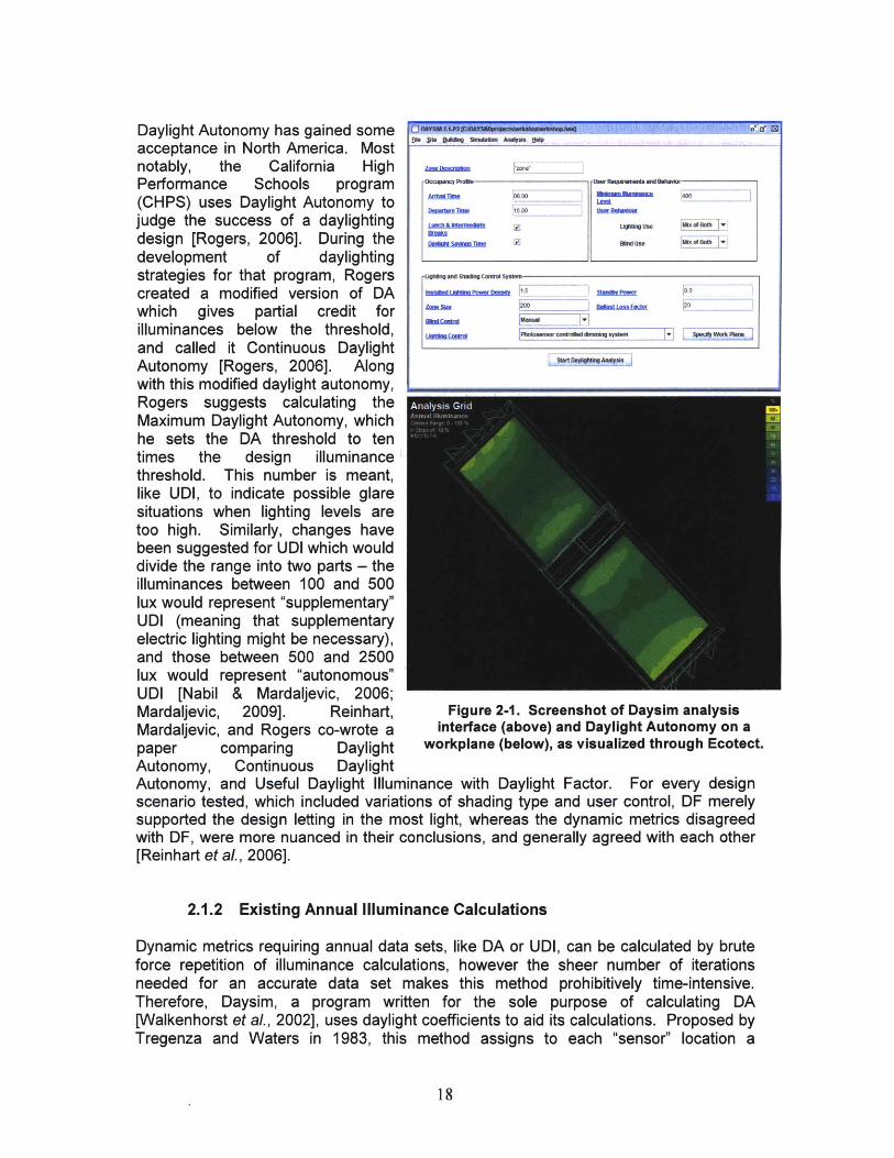
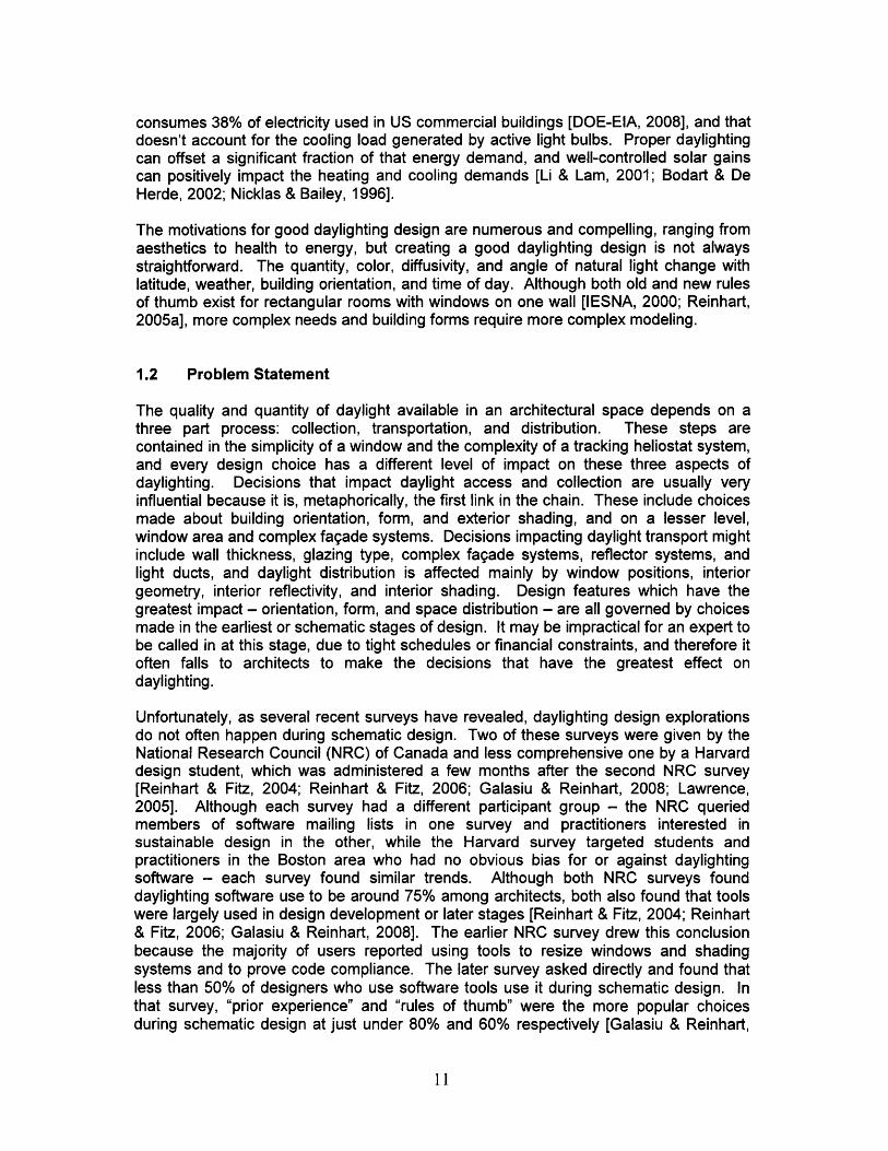
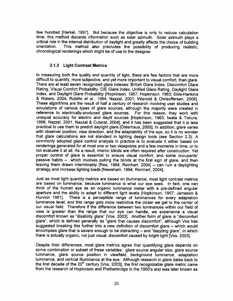
Daylight Autonomy has gained someacceptance in North America. Mostnotably, the California HighPerformance Schools program -McudIa(CHPS) uses Daylight Autonomy to L00judge the success of a daylighting D V Ube

design [Rogers, 2006]. During the 8,dO e aI0Tme OtUs

development of daylightingstrategies for that program, Rogers _MW___st

created a modified version of DA 00

which gives partial credit for ffm 2000r2

illuminances below the threshold,and called it Continuous DaylightAutonomy [Rogers, 2006]. Alongwith this modified daylight autonomy,Rogers suggests calculating theMaximum Daylight Autonomy, whichhe sets the DA threshold to tentimes the design illuminancethreshold. This number is meant,like UDI, to indicate possible glaresituations when lighting levels aretoo high. Similarly, changes havebeen suggested for UDI which woulddivide the range into two parts - theilluminances between 100 and 500lux would represent "supplementary"UDI (meaning that supplementaryelectric lighting might be necessary),and those between 500 and 2500lux would represent "autonomousruUDI [Nabil & Mardaljevic, 2006;Mardaljevic, 2009]. Reinhart, Figure 2-1. Screenshot of Daysim analysisMardaljevic, and Rogers co-wrote a interface (above) and Daylight Autonomy on apaper comparing Daylight workplane (below), as visualized through Ecotect.Autonomy, Continuous DaylightAutonomy, and Useful Daylight Illuminance with Daylight Factor. For every designscenario tested, which included variations of shading type and user control, DF merelysupported the design letting in the most light, whereas the dynamic metrics disagreedwith DF, were more nuanced in their conclusions, and generally agreed with each other[Reinhart et al, 2006].

2.1.2 Existing Annual Illuminance Calculations

Dynamic metrics requiring annual data sets, like DA or UDI, can be calculated by bruteforce repetition of illuminance calculations, however the sheer number of iterationsneeded for an accurate data set makes this method prohibitively time-intensive.Therefore, Daysim, a program written for the sole purpose of calculating DA[Walkenhorst et a, 2002], uses daylight coefficients to aid its calculations. Proposed byTregenza and Waters in 1983, this method assigns to each "rsensor" location a

_.- ---......................................................................... ... .. .................................................... .......................... ................... ........ .............. _ ...... ... .......... .......... ............ .. ........... ............. -- ............ ........ .

coefficient, or weight, dependent upon room geometry, reflectivity, sky visibility, etc,similarly to the concept of daylight factor [Tregenza & Waters, 1983]. Unlike DF,however, these coefficients can take small changes in each angular segment of the skyinto account. After the daylight coefficients are calculated for a particular model, the skycan be defined by any brightness and luminance distribution, and each additionalmoment is merely one more set of weighted sums rather than a time-intensivesimulation. Mardaljevic suggested a daylight coefficient method based on 145 diffusesky patches (as was Tregenza's), but also on 100,366 direct sun positions and anindirect sun component from each of the 145 diffuse patches [Mardaljevic, 2000].Daysim uses the Radiance ray-tracing program rtrace to calculate daylight coefficientsbased on 145 different diffuse sky patches, 3 ground segments, and 65 sun positions(sunlight from between these 65 points are extrapolated from the four nearest) [Reinhart& Walkenhorst, 2001; Reinhart, 2005]. A more recent synthesis of both of these ideas,called Dynamic Daylight Simulations or DDS, has been suggested in which daylightcoefficients are based again on 145 diffuse sky patches, 2596 direct solar positions (inwhich the one nearest to the actual sun position is used in each calculation), and alsoindirect solar calculations from the center of the 145 sky patches, where the indirectcontribution is weighted similarly to the direct solar contribution in Daysim [Bourgeois &Reinhart, 2006; Bourgeois et al., 2008].

Another strategy is a method based on "daylight factor' interpolation and originallydeveloped for the energy simulation program DOE-2 [Winkelmann & Selkowitz, 1985].This method was later adopted for the LBNL daylighting tool DELight (and therefore alsoBuilding Design Advisor, which uses the DELight simulation engine) [Hitchcock &Carroll, 2003; LBNL, 2001]. This method finds the daylight factor and clear-skyilluminance ratios (although it also refers to these ratios as "daylight factors") for a pre-determined set of 20 solar positions and then interpolates the illuminance ratios for allhourly points in between. These 20 data points are fixed for all latitudes, so the clearskies created using them are sometimes theoretical rather than realistic. Using theinterpolated ratios, this method finds interior illuminances based on the hourly horizontalilluminances from TMY type weather files. The relationship of hourly calculations to asmall set of predetermined sun positions recalls the strategies from both Daysim and theDDS discussed above, however the daylight factor interpolation method has far lessproven accuracy [Reinhart & Herkel, 2000; Hitchcock & Carroll, 2003].

If less detail is required in the set of annual data, one could try to reduce the possiblecombinations of sky types and sun positions to a smaller representative set. This wasthe approach used by Wittkopf et al. in their comparative study of anidolic ceilings inSheffield and Singapore, where they did simulations on the solstices and equinox at fivetimes of day [Wittkopf et al., 2006]. They used a virtual sky dome to try to represent thelocal climate as closely as possible. This situation, although more advanced, isreminiscent of the common practice of doing illuminance calculations at 9am, noon, and3pm on the solstices and equinoxes under a clear sky plus one overcast sky simulation.Although it may seem that a range of dates and times is represented, this strategyshowcases only the extremes of both sun positions and conditions and is not annuallyrepresentative.

A more complicated strategy for making a subset of annual calculations was suggestedby Herkel at the 1997 IBPSA conference. Herkel's method uses the similarity of 3factors - direct irradiance, diffuse irradiance, and solar altitude - to separate a series ofannual lighting simulations into "bins", reducing thousands of simulation moments to a

few hundred [Herkel, 1997]. But because the objective is only to reduce calculationtime, this method discards information such as solar azimuth. Solar azimuth plays acritical role in the internal distribution of daylight and greatly affects the choice of buildingorientation. This method also precludes the possibility of producing realistic,chronological renderings which might be of use to the designer.

2.1.3 Light Contrast Metrics

In measuring both the quality and quantity of light, there are few factors that are moredifficult to quantify, more subjective, and yet more important to visual comfort, than glare.There are at least seven recognized glare indexes: British Glare Index, Discomfort GlareRating, Visual Comfort Probability, CIE Glare Index, Unified Glare Rating, Daylight GlareIndex, and Daylight Glare Probability [Hopkinson, 1957; Hopkinson, 1963; Eble-Hankins& Waters, 2004; Rubiho et al., 1994; Nazzal, 2001; Wienold & Chrisoffersen, 2006].These algorithms are the result of half a century of research involving user studies andsimulations of various types of glare sources, although the majority were created inreference to electrically-produced glare sources. For this reason, they work withunequal accuracy for electric and daylit sources [Hopkinson, 1963; Iwata & Tokura,1998; Nazzal, 2001; Nazzal & Cutarat, 2004], and it has been suggested that it is lesspractical to use them to predict daylight glare [Osterhaus, 2005]. In addition, glare varieswith observer position, view direction, and the adaptability of the eye, so it is no wonderthat glare calculations are not standard in lighting design tools (see Section 2.3). Acommonly adopted glare control analysis in practice is to evaluate it either based onrenderings generated for at most one or two viewpoints and a few moments in time, or tonot evaluate it at all. As a result, interior blinds are often required after construction. Yetproper control of glare is essential to ensure visual comfort, and some occupants'passive habits - which involves pulling the blinds at the first sign of glare, and thenleaving them drawn interminably [Rea, 1984; Reinhart, 2004] - can ruin a daylightingstrategy and increase lighting loads [Newsham, 1994; Reinhart, 2004].

Just as most light quantity metrics are based on illuminance, most light contrast metricsare based on luminance, because luminance is what our eye sees. In fact, one canthink of the human eye as an organic luminance meter with a pre-defined angularaperture and the ability to adapt to different light levels [Hopkinson, 1957; Jameson &Hurvich 1961]. There is a perceptible range of luminances for every adaptationluminance level, and this range gets more restrictive the closer we get to the center ofour visual field. Therefore if the difference between two luminances within our field ofview is greater than the range that our eye can handle, we experience a visualdiscomfort known as "disability glare" [Vos, 2003]. Another form of glare is "discomfortglare", which is defined generally as "glare that causes discomfort", although Vos hassuggested breaking this further into a new definition of discomfort glare - which wouldencompass glare that is severe enough to be distracting - and "dazzling glare", in whichthere is actually organic, not just visual, discomfort caused by bright light [Vos, 2003].

Despite their differences, most glare metrics agree that quantifying glare depends onsome combination or subset of these variables: glare source angular size, glare sourceluminance, glare source position in viewfield, background luminance, adaptationluminance, and vertical illuminance at the eye. Although research in glare dates back tothe first decade of the 2 0 th century [Vos, 2003], the first recognizable glare metric camefrom the research of Hopkinson and Pretherbridge in the 1950's and was later known as

the British Glare Index, or BGI [Hopkinson, 1957; Hopkinson, 1972; Rubiho et aL, 1994].The BGI ranges from 0 to above 30, with 10 representing imperceptible glare and 28representing intolerable glare. At around the same time, Lukiesh and Guth beganstudies that would turn into the Discomfort Glare Rating (DGR) and Visual ComfortProbability, or VCP. The DGR was based on Lukiesh's work on glare sensation in the1920's, and it formed the basis of the VCP, which is defined as the probability that aperson will find the visual environment comfortable, and was based on participantstudies [Eble-Hankins & Waters, 2004; Rubiho et al., 1994]. All of these metrics werebased on point-source glare, and are not easily applicable to large-area glare situationscaused by daylight.

The CIE Glare Index, or CGI, was proposed in 1978 by a CIE committee led by Einhorn.It did not attempt to create new human subject studies, but used the current metrics andthe information available to create a synthesized metric which would also account for theeffect of the glare source on the adaptation level (thus making it better suited to largerarea glare sources) [Osterhaus, 2005; Eble-Hankins & Waters, 2004]. The next CIEcommittee decided then to remove the new detailed definition of adaptation level andcreated a compromise rating in 1995, the Unified Glare Rating (UGR), which wassimplified to appeal to a wider audience; it produces results very similar to the BRI[Osterhaus, 2005; Ebel Eble-Hankins & Waters, 2004]. Like the BRI, the UGR has ascale ranging from 0 to 30 with the same thresholds, and each step in the scale is meantto be a uniform change in glare perception. Another attempt to correct the weaknessesof the original glare equations is known as the Cornell equation or the Daylight GlareIndex (DGI). Despite its name, it was formulated with user studies that employed directand diffuse electric light sources, and has been shown less accurate for actual daylightsources [Wienold & Chrisoffersen, 2006]. There have been more recent suggestionsregarding changes to the DGI which involve actual daylight sensor readings, but nofurther human studies [Nazzal, 2001; Nazzal & Chutarat, 2004]. DGI also uses the scalefrom 0 to 30.

2.1.4 Daylight Glare Probability

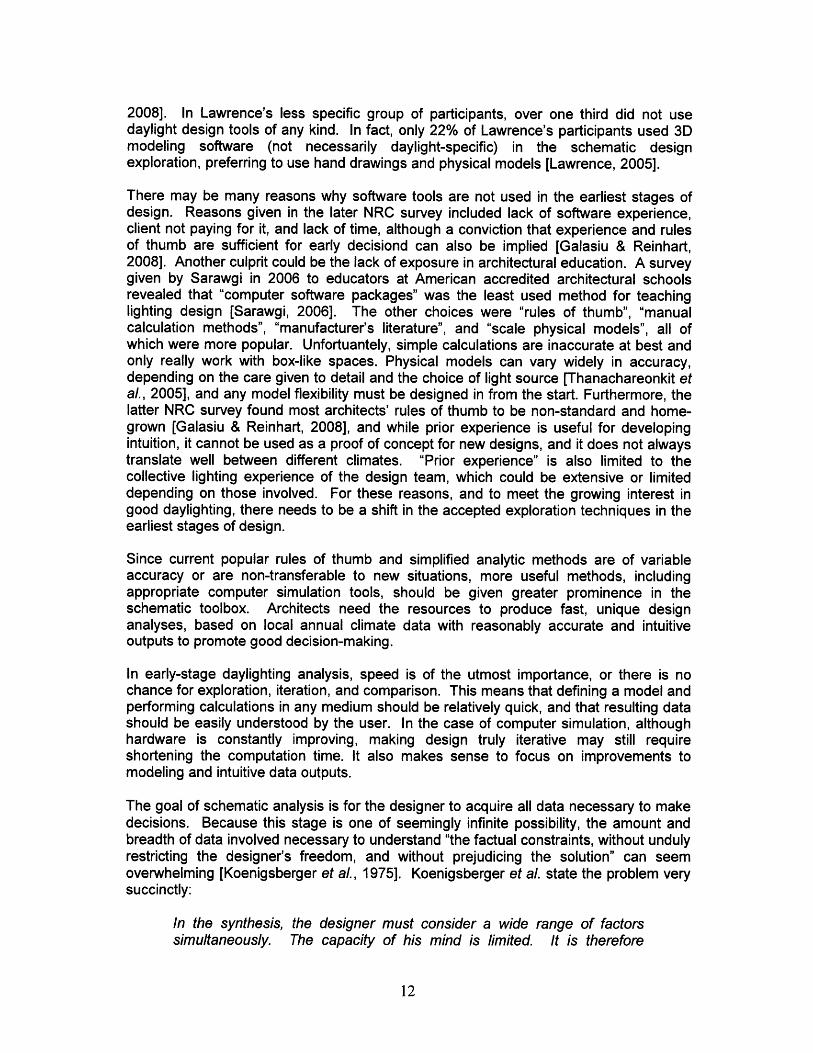
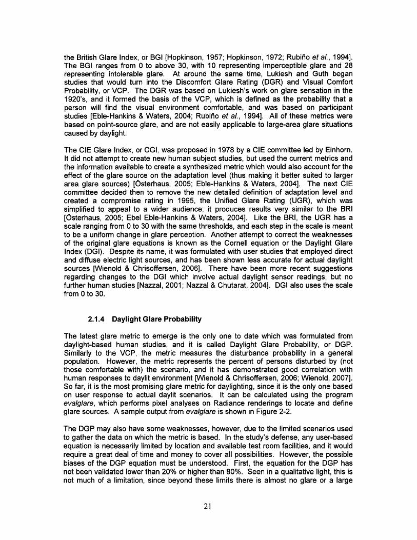
The latest glare metric to emerge is the only one to date which was formulated fromdaylight-based human studies, and it is called Daylight Glare Probability, or DGP.Similarly to the VCP, the metric measures the disturbance probability in a generalpopulation. However, the metric represents the percent of persons disturbed by (notthose comfortable with) the scenario, and it has demonstrated good correlation withhuman responses to daylit environment [Wienold & Chrisoffersen, 2006; Wienold, 2007].So far, it is the most promising glare metric for daylighting, since it is the only one basedon user response to actual daylit scenarios. It can be calculated using the programevalglare, which performs pixel analyses on Radiance renderings to locate and defineglare sources. A sample output from evalglare is shown in Figure 2-2.

The DGP may also have some weaknesses, however, due to the limited scenarios usedto gather the data on which the metric is based. In the study's defense, any user-basedequation is necessarily limited by location and available test room facilities, and it wouldrequire a great deal of time and money to cover all possibilities. However, the possiblebiases of the DGP equation must be understood. First, the equation for the DGP hasnot been validated lower than 20% or higher than 80%. Seen in a qualitative light, this isnot much of a limitation, since beyond these limits there is almost no glare or a large

amount of glare, respectively. Also,although the DGP follows the samebasic format for contrast glare analysis -all the formulas described above havesimilarities to the original Glare Indexwhich became the BGI - the DGP hasonly been validated in moderately sizedrooms with unilateral openings and non-extreme light levels. There is areasonably heavy dependence in theequation on vertical illuminance whichmight cause the metric to recognizehigh-illuminance glare more readily thanlow-illuminance glare caused only bycontrast levels. However, if further datasets were later assimilated, the DGPcould be either validated for low-illuminance glare situations or modifiedto account for them. The circumstances

Figure 2-2. Pixel analysis output of a DGP of the user tests which resulted in thecalculation done in the program evalglare. DGP are listed in Table 2-1, and the

DGP itself is discussed in further detailin Chapter 5.

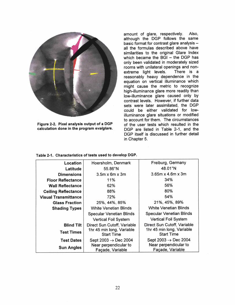
Table 2-1. Characteristics of tests used to develop DGP.

LocationLatitude

DimensionsFloor ReflectanceWall Reflectance

Ceiling ReflectanceVisual Transmittance

Glass FractionShading Types

Blind Tilt

Test Times

Test Dates

Sun Angles

Hoersholm, Denmark55.86*N

3.5m x 6m x 3m11%62%88%72%

25%, 44%, 85%White Venetian Blinds

Specular Venetian BlindsVertical Foil System

Direct Sun Cutoff, Variable1 hr 45 min long, Variable

Start TimeSept 2003 -+ Dec 2004Near perpendicular to

Facade, Variable

Freiburg, Germany48.01*N

3.65m x 4.6m x 3m34%56%80%54%

21%, 45%, 89%White Venetian Blinds

Specular Venetian BlindsVertical Foil System

Direct Sun Cutoff, Variable1 hr 45 min long, Variable

Start TimeSept 2003 -+ Dec 2004Near perpendicular to

FaQade, Variable

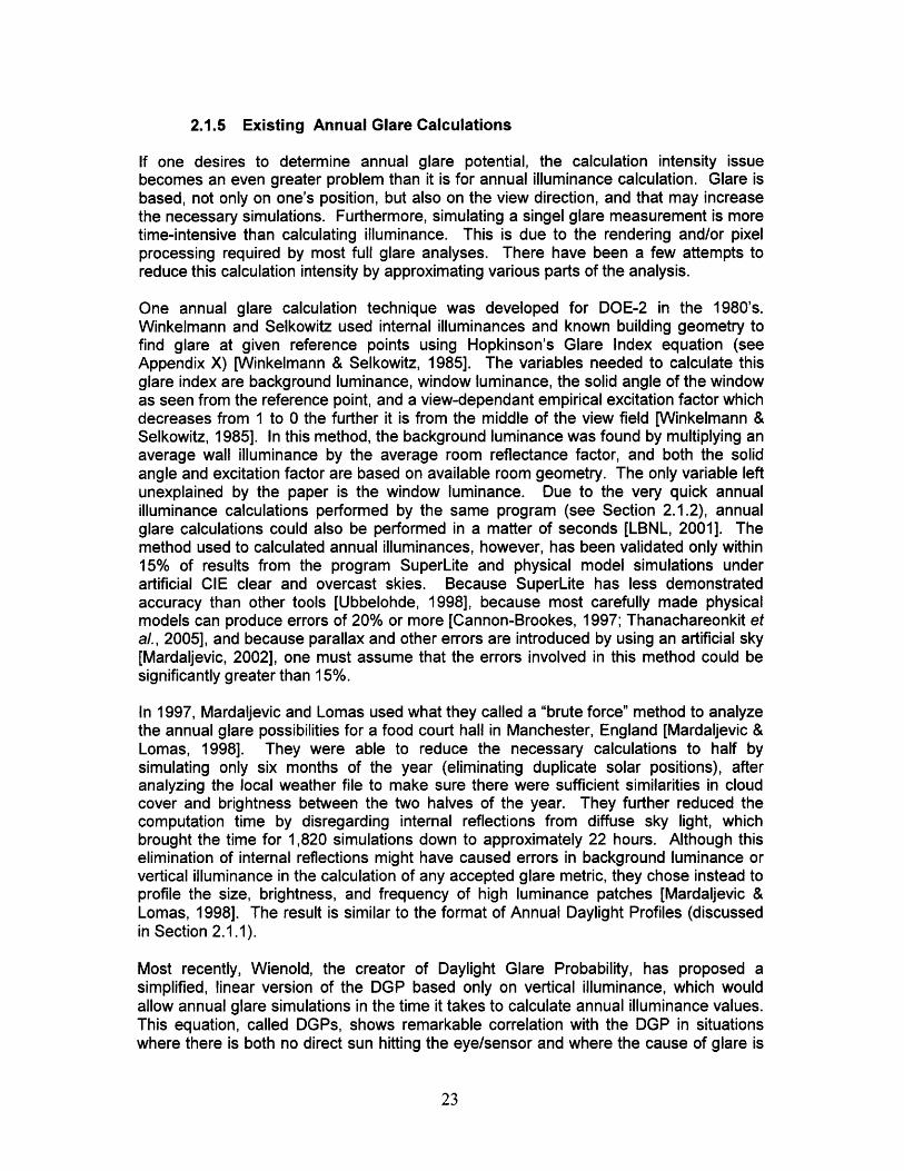
2.1.5 Existing Annual Glare Calculations

If one desires to determine annual glare potential, the calculation intensity issuebecomes an even greater problem than it is for annual illuminance calculation. Glare isbased, not only on one's position, but also on the view direction, and that may increasethe necessary simulations. Furthermore, simulating a singel glare measurement is moretime-intensive than calculating illuminance. This is due to the rendering and/or pixelprocessing required by most full glare analyses. There have been a few attempts toreduce this calculation intensity by approximating various parts of the analysis.

One annual glare calculation technique was developed for DOE-2 in the 1980's.Winkelmann and Selkowitz used internal illuminances and known building geometry tofind glare at given reference points using Hopkinson's Glare Index equation (seeAppendix X) [Winkelmann & Selkowitz, 1985]. The variables needed to calculate thisglare index are background luminance, window luminance, the solid angle of the windowas seen from the reference point, and a view-dependant empirical excitation factor whichdecreases from 1 to 0 the further it is from the middle of the view field [Winkelmann &Selkowitz, 1985]. In this method, the background luminance was found by multiplying anaverage wall illuminance by the average room reflectance factor, and both the solidangle and excitation factor are based on available room geometry. The only variable leftunexplained by the paper is the window luminance. Due to the very quick annualilluminance calculations performed by the same program (see Section 2.1.2), annualglare calculations could also be performed in a matter of seconds [LBNL, 2001]. Themethod used to calculated annual illuminances, however, has been validated only within15% of results from the program SuperLite and physical model simulations underartificial CIE clear and overcast skies. Because SuperLite has less demonstratedaccuracy than other tools [Ubbelohde, 1998], because most carefully made physicalmodels can produce errors of 20% or more [Cannon-Brookes, 1997; Thanachareonkit etal., 2005], and because parallax and other errors are introduced by using an artificial sky[Mardaljevic, 2002], one must assume that the errors involved in this method could besignificantly greater than 15%.

In 1997, Mardaljevic and Lomas used what they called a "brute force" method to analyzethe annual glare possibilities for a food court hall in Manchester, England [Mardaljevic &Lomas, 1998]. They were able to reduce the necessary calculations to half bysimulating only six months of the year (eliminating duplicate solar positions), afteranalyzing the local weather file to make sure there were sufficient similarities in cloudcover and brightness between the two halves of the year. They further reduced thecomputation time by disregarding internal reflections from diffuse sky light, whichbrought the time for 1,820 simulations down to approximately 22 hours. Although thiselimination of internal reflections might have caused errors in background luminance orvertical illuminance in the calculation of any accepted glare metric, they chose instead toprofile the size, brightness, and frequency of high luminance patches [Mardaljevic &Lomas, 1998]. The result is similar to the format of Annual Daylight Profiles (discussedin Section 2.1.1).

Most recently, Wienold, the creator of Daylight Glare Probability, has proposed asimplified, linear version of the DGP based only on vertical illuminance, which wouldallow annual glare simulations in the time it takes to calculate annual illuminance values.This equation, called DGPs, shows remarkable correlation with the DGP in situationswhere there is both no direct sun hitting the eye/sensor and where the cause of glare is

caused by high vertical illuminances [Wienold, 2007; Wienold 2009]. Situations whereglare may be caused by luminance contrasts rather than peak luminances were againless present in the analysis, as the test case was the model of a small office with a largewindow. Within the last year, Wienold has also proposed integrating DGPs with theprogram Daysim (a program discussed in Section 2.3) which would benefit fromDaysim's quick daylight coefficient-based illuminance calculations and improve DGPsaccuracy by adding an analysis of quick and simple renderings [Wienold, 2007; Wienold,2009].

2.1.6 Solar Heat Gain

Solar heat gain is not a measure of "light" as we define it, nor does it have a visualaspect, but light and heat are so tightly tied together that one cannot afford to ignore thethermal consequences of daylighting. Despite the fact that solar gain is an importanttradeoff, few lighting simulation programs even mention it. The problem is one ofpracticality. While it would be reasonably easy to find the energetic solar influx in Wattsusing current lighting simulation techniques, this number alone could not be used tomake design decisions - or even to understand the consequences of the tradeoff. Thesame value in watts could, under different circumstances, have a very different effect onindoor temperature and HVAC loads. For instance, solar gains might be welcome inwinter, but detrimental to the same building in summer. A heavily occupied buildingmight find solar gains harmful during the week, but beneficial when it is empty on theweekend, and the existence of thermal mass only complicates the issue by delaying thethermal effects. The only information suitable for judging the impact of solar gains is theindoor temperature change as a result of those gains. From this value, HVAC loads caneither be calculated or inferred.

Finding the indoor temperature requires an energy simulation. Energy and lightingsimulations require different inputs from the user, which means that a combined modelwould have to include both sets of information. Fortunately, the industry has beenmoving in the direction of combined simulation tools and Building Information Modelsincorporating multiple building characteristics [Ibrahim & Krawczyk, 2003; Papamichaelet al., 1998]. However, few tools focused primarily on lighting include this still importanteffect of using natural light.

A few people have addressed the issue of accounting for solar gains in design withoutthe need for energy models, but these methods tend to be more primitive in scope.Work done by Littlefair in the 1980's and 1990's resulted in a set of recommendations formaximum obstruction angles depending on European latitudes and climates [Littlefair,2001]. The goal of making sure certain solar angles are not masked is to preserve thepsychological and winter heating benefits of direct sun in buildings.

Because it is located in a tropical climate, the government of Hong Kong took theopposite approach. In 1995, they included a maximum Overall Thermal Transfer Value(OTTV) in the building codes which limits the average thermal transfer (including transferthrough the envelope and solar gain) of facades based on height from the ground[Building Authority, 1995]. For building facades within 15m of the ground, the OTTV wascapped at 80 W/m2, while higher facades were capped at 35 W/m2 (changed later to 30W/m 2), since they generally have greater sun exposure. Hong Kong was the fifthSoutheast Asian government to adopt OTTV regulations, which are developed from

detailed energy analysis, specific location climate data, and economic factors [Hui,1997]. However, critics claim that such codes restrict fagade innovation, disregardtradeoffs between higher OTTV and electric lighting savings due to daylight use, andcannot take internal heat gains and building layout into account [Hui, 1997; Li et al.,2002; Yik & Wan, 2005].

Recommendations and regulations regarding solar gain are generally based on previousenergy analyses, and are therefore specific to location and assumptions made aboutbuilding variables. For a simple, yet more general approach, one can use various handcalculations based on tables of sun angles and solar incident radiation, although eventhese require information from the user about the heat transfer of the building envelope[ASHRAE, 2001; Stephenson, 1957; Stephenson, 1965]. Also, since these tables areforced to make assumptions and simplify the building in question, they are less accuratethan the more detailed computer simulations. Some hand calculation methods forthermal assessment include steady-state heat balance equations, the lumpedcapacitance model, radiant time series, and the balance point model, the last of whichwill be discussed at greater length in Chapter 6 [ASHRAE, 2001; McQuiston et al., 2005;LBNL, 2001].

2.2 Graphical Displays of Numerical Information

In the introduction to his book, The Visual Display of Quantitative Information, EdwardTufte observes that "of all methods for analyzing and communicating statisticalinformation, well-designed data graphics are usually the simplest and at the same timethe most powerful," [Tufte, 1983]. Successful graphics take a large data set andcommunicate it in such a way that the patterns and trends in the numbers are instantlyand intuitively understood by the reader. The larger and more complex the data set, thegreater the benefit of communicating via graphics, which makes it a perfect medium forlarge annual daylighting data sets. Unfortunately, it is impossible to put every usefulpiece of information in the same graph. Some choices must be made regarding whichdata to show and how to convey it, or different data trends may devolve into unreadablenoise.

The greatest difficulty with daylighting data is in attempting to simultaneously show howperformance varies over both time and space. To display a four-dimensional data set ina static two-dimensional medium is complicated at best and near impossible at worst, soat least one or two aspects are usually condensed in pre-processing. The most commonway to display quantitative daylighting data is by disregarding the time-variation ofperformance and focusing on the spatial variation. Contour-line renderings or workplaneilluminance plots representing a single moment in time are the only available outputs ofnearly every daylighting tool that supports graphics. Although a few tools will showanimations of sun penetration and shadows [Ecotect web] or renderings tacked togetherto represent time passing [AG132 web], analyzing annual daylight performance usingonly these graphics is computationally intense, time-consuming, and requires expertiseto choose which moments to simulate (and which skies to simulate them under) andmental processing to fill the inevitable information gaps.

A more efficient option for annual analysis is to output data in the form of DaylightAutonomy or Useful Daylight Illuminance, which were both discussed in Section 2.1.1[Reinhart & Walkenhorst, 2001; Nabil & Mardaljevic, 2006]. Both metrics, which

condense temporally-based performance to a single number, are calculated at specificpoints in space and can be displayed in a work plane contour map, as is often done withDaylight Factor or single-moment illuminance measurements.

Knowing the spatial variation of performance data is important, since architecture is, inessence, the shaping of man-made spaces. However, many practical daylightingproblems are caused by not anticipating the effects of changing sun angles and weatherconditions - variables which are largely dependant on time of year and day. To fullyunderstand these factors and to best judge the cause of a design's success or failurerequires lighting data in a "fourth" dimension.

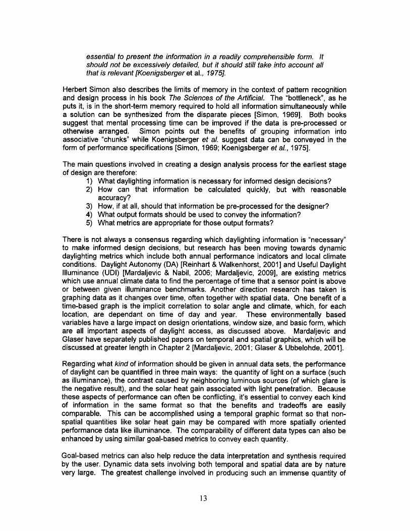
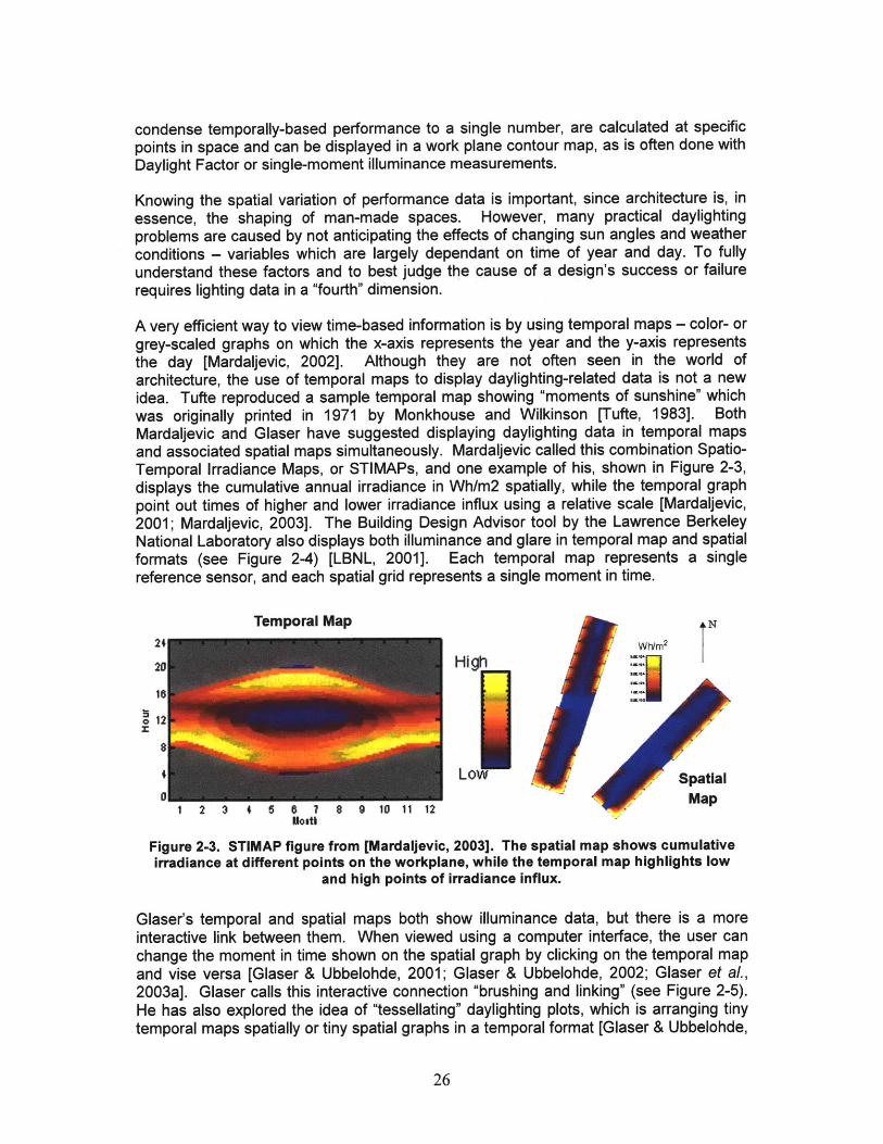
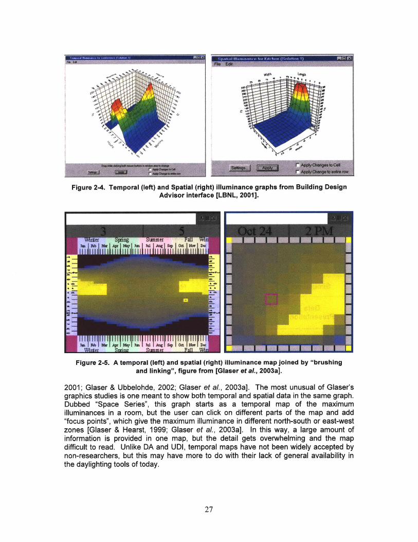
A very efficient way to view time-based information is by using temporal maps - color- orgrey-scaled graphs on which the x-axis represents the year and the y-axis representsthe day [Mardaljevic, 2002]. Although they are not often seen in the world ofarchitecture, the use of temporal maps to display daylighting-related data is not a newidea. Tufte reproduced a sample temporal map showing "moments of sunshine" whichwas originally printed in 1971 by Monkhouse and Wilkinson [Tufte, 1983]. BothMardaljevic and Glaser have suggested displaying daylighting data in temporal mapsand associated spatial maps simultaneously. Mardaljevic called this combination Spatio-Temporal Irradiance Maps, or STIMAPs, and one example of his, shown in Figure 2-3,displays the cumulative annual irradiance in Wh/m2 spatially, while the temporal graphpoint out times of higher and lower irradiance influx using a relative scale [Mardaljevic,2001; Mardaljevic, 2003]. The Building Design Advisor tool by the Lawrence BerkeleyNational Laboratory also displays both illuminance and glare in temporal map and spatialformats (see Figure 2-4) [LBNL, 2001]. Each temporal map represents a singlereference sensor, and each spatial grid represents a single moment in time.

Temporal Map N

24 Wh/m2

20 High I

Low Spatial/ Map1 2 3 4 56 7 8 9 10 11 12Ma

Mouti

Figure 2-3. STIMAP figure from [Mardaljevic, 2003]. The spatial map shows cumulativeirradiance at different points on the workplane, while the temporal map highlights low

and high points of irradiance influx.

Glaser's temporal and spatial maps both show illuminance data, but there is a moreinteractive link between them. When viewed using a computer interface, the user canchange the moment in time shown on the spatial graph by clicking on the temporal mapand vise versa [Glaser & Ubbelohde, 2001; Glaser & Ubbelohde, 2002; Glaser et al.,2003a]. Glaser calls this interactive connection "brushing and linking" (see Figure 2-5).He has also explored the idea of "tessellating" daylighting plots, which is arranging tinytemporal maps spatially or tiny spatial graphs in a temporal format [Glaser & Ubbelohde,

1#0

Figure 2-4 Temporal (left) and Spatial (right) illuminance graphs from Building DesignAdvisor interface [LBNL, 2001].

1ft UK A; lit ?&y Aa g 8q Oad 1w Dec

Figure 2-5. A temporal (left) and spatial (right) illuminance map joined by "brushingand linking", figure from [Glaser et al., 2003a].

2001; Glaser & Ubbelohde, 2002; Glaser et al., 2003a]. The most unusual of Glaser'sgraphics studies is one meant to show both temporal and spatial data in the same graph.Dubbed "Space Series", this graph starts as a temporal map of the maximumilluminances in a room, but the user can click on different parts of the map and add"focus points", which give the maximum illuminance in different north-south or east-westzones [Glaser & Hearst, 1999; Glaser et al., 2003a]. In this way, a large amount ofinformation is provided in one map, but the detail gets overwhelming and the mapdifficult to read. Unlike DA and UDI, temporal maps have not been widely accepted bynon-researchers, but this may have more to do with their lack of general availability inthe daylighting tools of today.

. ..........

M F. F-7771770 V

2.3 Existing Solutions for Early-Stage Analysis

Early-stage daylighting analysis is a balancing act between conflicting agendas. Theanalysis should be fast and easy enough to be used in an iterative process, whichsuggests a need for simplicity. On the other hand, the analysis should be accurateenough to be useful in making decisions for a unique design scenario. This suggestssome level of complexity in the aspects of the model that have the greatest impact ondaylighting simulation (or calculation) accuracy. The analysis should also result in adata set with all necessary information for making informed design decisions. In otherwords, all useful types of lighting data should be calculated at all moments necessary fora complete understanding of design performance. The following sections will exploresome of the current solutions that exist for each analysis feature individually. They willfocus on computer simulation solutions, but similar examples and issues could be foundin the strategies and tools available for physical model simulation. Hand calculations areat least partially represented in the computer tools exploration below, since some toolsuse hand calculations as their primary analysis method.

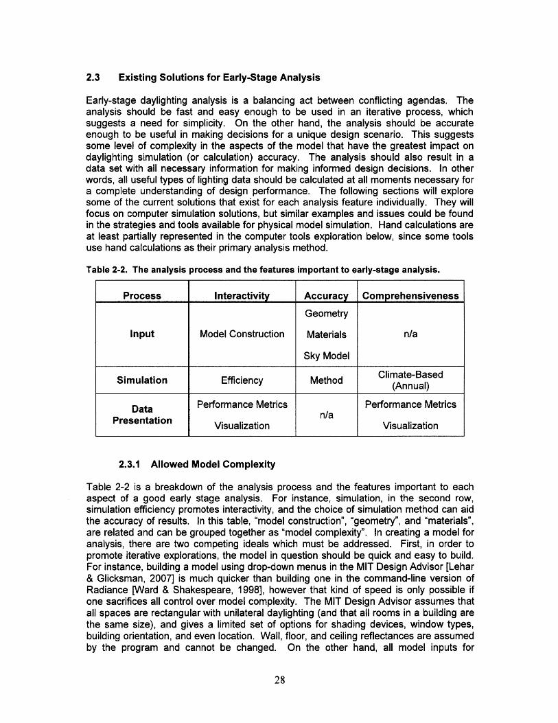
Table 2-2. The analysis process and the features important to early-stage analysis.

Process Interactivity Accuracy Comprehensiveness

Geometry

Input Model Construction Materials n/a

Sky Model

Simulation Efficiency Method Climate-Based

Data Performance Metrics Performance MetricsPresentation Visualization Visualization

2.3.1 Allowed Model Complexity

Table 2-2 is a breakdown of the analysis process and the features important to eachaspect of a good early stage analysis. For instance, simulation, in the second row,simulation efficiency promotes interactivity, and the choice of simulation method can aidthe accuracy of results. In this table, "model construction", "geometry", and "materials",are related and can be grouped together as "model complexity". In creating a model foranalysis, there are two competing ideals which must be addressed. First, in order topromote iterative explorations, the model in question should be quick and easy to build.For instance, building a model using drop-down menus in the MIT Design Advisor [Lehar& Glicksman, 2007] is much quicker than building one in the command-line version ofRadiance [Ward & Shakespeare, 1998], however that kind of speed is only possible ifone sacrifices all control over model complexity. The MIT Design Advisor assumes thatall spaces are rectangular with unilateral daylighting (and that all rooms in a building arethe same size), and gives a limited set of options for shading devices, window types,building orientation, and even location. Wall, floor, and ceiling reflectances are assumedby the program and cannot be changed. On the other hand, all model inputs for

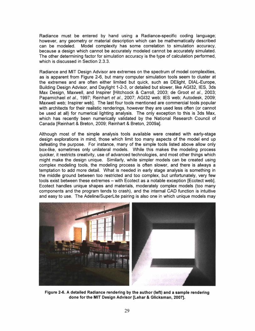
Radiance must be entered by hand using a Radiance-specific coding language;however, any geometry or material description which can be mathematically describedcan be modeled. Model complexity has some correlation to simulation accuracy,because a design which cannot be accurately modeled cannot be accurately simulated.The other determining factor for simulation accuracy is the type of calculation performed,which is discussed in Section 2.3.3.

Radiance and MIT Design Advisor are extremes on the spectrum of model complexities,as is apparent from Figure 2-6, but many computer simulation tools seem to cluster atthe extremes and are often either limited but quick, such as DElight, DIAL-Europe,Building Design Advisor, and Daylight 1-2-3, or detailed but slower, like AG132, IES, 3dsMax Design, Maxwell, and Inspirer [Hitchcock & Carroll, 2003; de Groot et al., 2003;Papamichael et al., 1997; Reinhart et al., 2007; AG132 web; IES web; Autodesk, 2009;Maxwell web; Inspirer web]. The last four tools mentioned are commercial tools popularwith architects for their realistic renderings, however they are used less often (or cannotbe used at all) for numerical lighting analysis. The only exception to this is 3ds Max,which has recently been numerically validated by the National Research Council ofCanada [Reinhart & Breton, 2009; Reinhart & Breton, 2009a].

Although most of the simple analysis tools available were created with early-stagedesign explorations in mind, those which limit too many aspects of the model end updefeating the purpose. For instance, many of the simple tools listed above allow onlybox-like, sometimes only unilateral models. While this makes the modeling processquicker, it restricts creativity, use of advanced technologies, and most other things whichmight make the design unique. Similarly, while simpler models can be created usingcomplex modeling tools, the modeling process is often slower, and there is always atemptation to add more detail. What is needed in early stage analysis is something inthe middle ground between too restricted and too complex, but unfortunately, very fewtools exist between these extremes - with Ecotect as a notable exception [Ecotect web].Ecotect handles unique shapes and materials, moderately complex models (too manycomponents and the program tends to crash), and the internal CAD function is intuitiveand easy to use. The Adeline/SuperLite pairing is also one in which unique models may

Figure 2-6. A detailed Radiance rendering by the author (left) and a sample renderingdone for the MIT Design Advisor [Lehar & Glicksman, 2007].

:: ............................................................. .... ... ... ......... .. ..................................... ............... .... .. . ... .........

be made in the internal Scribe Modeler, but its complexity is stunted by the limitednumber of allowed surfaces and objects [Erhorn et al., 1998; Adeline web ; Ubbelohde,1998]. This strategy is useful for keeping modeling simple, however the limitation onexternal shading objects could be too restrictive for the sake of necessary modelaccuracy [Ubbelohde, 1998].

Although it is limited, the Building Design Adviser approaches moderate modelcomplexity [Papamichael et al., 1997; Papamichael et al., 1998; LBNL, 2001]. While itrestricts the user to rectangular spaces, these can be grouped in any way, and eachspace can be moved to as a unit to a different place in the building plan. The SchematicGraphic Editor makes liberal use of drop-down menus and default values, but allows anydefault to be changed.

Finally, there are a few "sketch" modeling tools which could be considered quick,intuitive, and moderately complex. Space Pen [Jung et al., 2002], which is the modelingtool used in Spot! [Bund & Do, 2005], and LightSketch [Glaser et al., 2003] are both toolsin which the modeling is done by interpolating user sketches using a pre-conceived setof symbols. Both tools came out of the Carnegie Mellon Computational Design Lab andcan handle unique, but not detailed shapes, and at least LightSketch is restricted to adefault diffuse wall material. There is great potential in the possible development oftools such as these, but unfortunately, both projects seem to have halted, or at leastpaused.

2.3.2 Sky Luminance Distribution

Sky luminance distribution is one model input which requires a higher level of necessaryaccuracy for daylight analysis. The sky and sun are the primary sources of light, and ifthe source is modeled incorrectly, the simulated data will probably also be erroneous[Mardaljevic, 2004], and any daylighting tool should be able to model a variety of skies,since every location on earth has a variety of weather. At the very least, one "inbetween" option should be offered apart from overcast and clear sky extremes, so amodel offering the CIE clear, intermediate, and overcast skies should be the minimumacceptable accuracy [CIE, 1973; Nakamura et al., 1985; Moon & Spencer, 1942].Unfortunately, while the CIE clear and overcast skies are ubiquitous in the existingcomputer tools set, the intermediate sky is less so - Radiance, AG132, Ecotect, and IESare some of the tools which can model CIE intermediate skies [Ward & Shakespeare,1998; AG132 web; Ecotect web; IES web].

Because real skies are infinite in variety, it is better to be able to model a spread ofdifferent intermediate skies. Darula and Kittler have defined many individual stepsbetween the CIE clear and overcast skies [Darula & Kittler, 2002] while Igawa et al. havemade a similar set of distinct sky distributions based on their intermediate sky model[Igawa et al., 1999]. Unfortunately, the author knows of no current analysis tool whichcan automatically create either of these sets of sky definitions.

The Perez All-Weather sky distribution uses a single equation which, given brightnessand clearness index inputs, can define any number of realistic sky distributions [Perez etal., 1993]. Although this sky model has been validated to a reasonably high accuracy,only Radiance and 3ds Max Design can easily be used to model a Perez All-Weathersky [Ward & Shakespeare, 1998; Reinhart & Breton, 2009]. This model will be

discussed at greater length in Chapter 3, as will another sky distribution by Perez et al.known as the ASRC-CIE model [Perez et al., 1992].

2.3.3 Calculation and Simulation

Some tools which strive for speed choose to find illuminances and other light quantitiesusing simplified approximate algorithms. Analyses like the lumen method or the split fluxmethod [ASHRAE, 2001; Lynes, 1968] were developed before the widespread use ofcomputer simulations and could be done with a calculator, prepared numerical tables,and view protractors. With the speed of today's computers, any one of these algorithmscan be calculated in under a few seconds, making any computer tool that uses themvery quick. Unfortunately, they are approximations of the way light reacts in specificcommon situations, and many were developed for rectangular rooms with unilateral side-lighting. The further one gets from that geometric base case, the less accurate thecalculation.

The alternate option, available only as faster computers have become ubiquitous, arephysical simulations which attempt to imitate the behavior of light in reality. The twomost common physical light simulation methods are ray-tracing and radiosity, both ofwhich encompass a few different methodologies based on the same idea. The softwarewith best known accuracy is Radiance, which is a Monte Carlo backwards ray-tracingprogram valid to within 5.6% of life measurements [Mardaljevic, 1995]. Each sensor orpixel point sends a user-determined number of light rays in a spread of directionsaccording to a randomized Monte Carlo algorithm, and when these rays hit objects, theybounce and split (again according to user-defined parameters) until some of them havetraced a path backwards from the sensor point to a light source [Ward & Shakespeare,1998]. Ray tracing software can theoretically handle any model geometry and anymaterial definition. Because of its proven robustness, flexibility, and accuracy, Radiancehas gained a great deal of trust from the daylighting simulation world. In fact, in tworecent surveys given by the National Research Council of Canada found that, among aspread of many tools, about 50% of participants chose to use a tool with a Radiancesimulation engine [Reinhart & Fitz, 2006; Galasiu & Reinhart, 2008]. The drawback tothis famous accuracy is that Radiance is one of the slower simulation tools with no userinterface to speak of. Its renderings are also view-dependant, so rendering two differentviews of the same scene would take twice as long. Two ray-tracing tools which producequicker results than Radiance are Daysim [Reinhart & Walkenhorst, 2001], which uses amodified version of Radiance to run annual simulations, and 3ds Max Design [Autodesk,2009], which uses a ray-tracing engine called mental ray. Both tools have beenvalidated by Christoph Reinhart and the National Research Council of Canada [Reinhart& Breton, 2009]. Other tools which include ray-tracing engines are Genelux, FormZ, andInspirer [Mitanchey et al., 1997; FormZ web, Inspirer web].

The other common physical simulation method is radiosity. Radiosity is calculated in asimilar way to radiant heat transfer between surfaces, and because of this, radiosity isrestricted to diffuse materials only. (Although some radiosity programs add a singlebounce ray tracing at the end of rendering simulations [AG132 web] this is merely foraesthetic purposes, and it makes little or no difference to numerical calculations.)However, materials definitions are the only real restriction to radiosity. In a thoroughcomparison between Radiance and Lightscape, the most prominent radiosity tool in2001, Altmann and Apian-Bennewitz found comparable results as long as specular

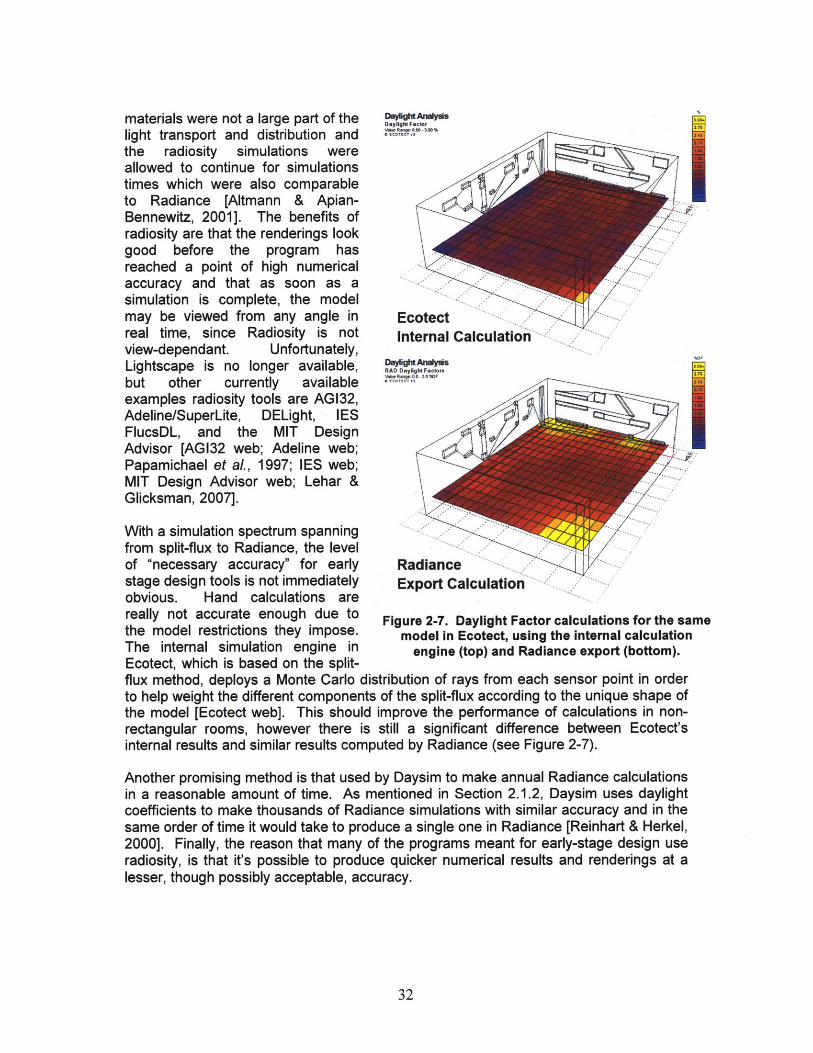
materials were not a large part of the Daniya s

light transport and distribution andthe radiosity simulations wereallowed to continue for simulationstimes which were also comparableto Radiance [Altmann & Apian-Bennewitz, 2001]. The benefits ofradiosity are that the renderings lookgood before the program hasreached a point of high numericalaccuracy and that as soon as asimulation is complete, the modelmay be viewed from any angle in Ecotectreal time, since Radiosity is not Internal Calculationview-dependant. Unfortunately,Lightscape is no longer available, R

but other currently availableexamples radiosity tools are AG132,Adeline/SuperLite, DELight, IESFlucsDL, and the MIT DesignAdvisor [AG132 web; Adeline web;Papamichael et al., 1997; IES web;MIT Design Advisor web; Lehar &Glicksman, 2007].

With a simulation spectrum spanningfrom split-flux to Radiance, the levelof "necessary accuracy" for early Radiancestage design tools is not immediately Export Calculationobvious. Hand calculations arereally not accurate enough due to Figure 2-7. Daylight Factor calculations for the samethe model restrictions they impose. model in Ecotect, using the internal calculationThe internal simulation engine in engine (top) and Radiance export (bottom).Ecotect, which is based on the split-flux method, deploys a Monte Carlo distribution of rays from each sensor point in orderto help weight the different components of the split-flux according to the unique shape ofthe model [Ecotect web]. This should improve the performance of calculations in non-rectangular rooms, however there is still a significant difference between Ecotect'sinternal results and similar results computed by Radiance (see Figure 2-7).

Another promising method is that used by Daysim to make annual Radiance calculationsin a reasonable amount of time. As mentioned in Section 2.1.2, Daysim uses daylightcoefficients to make thousands of Radiance simulations with similar accuracy and in thesame order of time it would take to produce a single one in Radiance [Reinhart & Herkel,2000]. Finally, the reason that many of the programs meant for early-stage design useradiosity, is that it's possible to produce quicker numerical results and renderings at alesser, though possibly acceptable, accuracy.

........................... ...........................

2.3.4 Annual Calculations and Metrics

As discussed in Section 2.1.1, understanding the performance of a space over the fullyear for a correct climatic representation of sky-types is an important part of making aninformed design decisions. Therefore, the ability to automatically perform annualsimulations and convey them to the user using annual metrics is a "necessary accuracy"required in early-stage design tools. Unfortunately, it is also rare in the set of availabletools. MIT Design advisor performs annual calculations using radiosity, and the annual(or monthly) impacts on lighting, heating, and cooling energy are the output [Lehar &Glicksman, 2007, MIT Design Advisor web]. The Building Design Advisor originally usedthe split-flux method and now uses the DELight radiosity engine to produce annual setsof illuminance and glare data [Papamichael et al., 1997; LBNL, 2001; Hitchcock &Carroll, 2003; Winkelmann & Selkowitz, 1985]. It does not output data using any specialannual metrics but rather, keeps it in the form of illuminance or Daylight Glare Index. Asmentioned several times previously, Daysim was written in order to perform annualRadiance calculations using the daylight coefficients method [Reinhart & Herkel, 2000].It outputs data in the form of Daylight Autonomy, as do Daylight 1-2-3 [Reinhart et al.,2003; Reinhart et al., 2007] and the Sensor Placement Optimization Tool (S.P.O.T.)[Rogers, 2006]. LightSketch seems also to have been meant for annual calculations[Glaser et al., 2003], but similarly to Building Design Advisor, only illuminances areoutput.

2.3.5 Light Quantity, Glare, and Heat Gain

When it comes to making informed decisions, especially during schematic design, it isimportant to understand the tradeoffs between light quantity, glare, and solar heat gain.Every software created for the express purpose of light simulation calculates data interms of light quantity, usually as illuminance, although many of these also calculateDaylight Factor. Those which output Daylight Autonomy were listed in the previoussection. Far fewer tools additionally calculate some form of glare; these include Adeline(using the Radiance engine), AG132, Building Design Advisor, DIALux, Genelux, IES,and Radiance [Erhorn et al., 1998; AG132 web; Papamichael et al., 1997; GmbH, 2009;Mitanchey et al., 1997; IES web; Ward & Shakespeare, 1998]. Of these, only Radiancewith the plug-in program evalglare can calculate the Daylight Glare Probability, althoughthere is currently plan for implementing evalglare within Daysim [Wienold &Christoffersen, 2006; Wienold, 2009].

Only those tools which also have some (if simple) thermal modeling abilities (Dial-Europe, MIT Design Advisor, Building Design Advisor, Daylight 1-2-3, Ecotect, and IES)provide any sort of dedicated solar heat gain indicators [de Groot et al., 2003; Urban &Glicksman, 2007; Reinhart et al., 2007; Ecotect web, IES web]. Of these tools, onlyDial-Europe includes the thermal modeling solely for the purposes of assessing solarheat gain rather than energy loads. Both Dial-Europe and MIT Design Advisor predictthe number of days or hours when the space may overheat, and MIT Design Advisorincludes thermal comfort as dependant on proximity to the window. Solar heat gain,though a crucial part of balancing daylight performance, is not included in many lightinganalysis tools, since it takes an energy model to truly find the effects of solar heat gain.

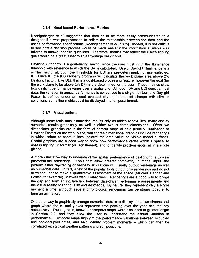
2.3.6 Goal-based Performance Metrics

Koenigsberger et al. suggested that data could be more easily communicated to adesigner if it was preprocessed to reflect the relationship between the data and theuser's performance specifications [Koenigsberger et al., 1975]. Indeed, it is not difficultto see how a decision process would be made easier if the information available wastailored to answer specific questions. Therefore, metrics that reflect the user's lightinggoals would be a great asset to an early-stage design tool.

Daylight Autonomy is a goal-driving metric, since the user must input the illuminancethreshold with reference to which the DA is calculated. Useful Daylight Illuminance is asimilar metric, although the thresholds for UDI are pre-determined, not user-selected.IES FlucsDL (the IES radiosity program) will calculate the work plane area above 2%Daylight Factor. Like UDI, this is a goal-based processing feature, however the goal (forthe work plane to be above 2% DF) is pre-determined for the user. These metrics showhow daylight performance varies over a spatial grid. Although DA and UDI depict annualdata, the variation in annual performance is condensed to a single number, and DaylightFactor is defined under an ideal overcast sky and does not change with climaticconditions, so neither metric could be displayed in a temporal format.

2.3.7 Visualizations

Although some tools output numerical results only as tables or text files, many displaynumerical results graphically as well in either two or three dimensions. Often twodimensional graphics are in the form of contour maps of data (usually illuminance orDaylight Factor) on the work plane, while three dimensional graphics include renderingsin which colors or contour lines indicate the data value on visible model surfaces.Spatial graphics are a good way to show how performance varies within a space, toassess lighting uniformity (or lack thereof), and to identify problem spots, all in a singleglance.

A more qualitative way to understand the spatial performance of daylighting is to viewphotorealistic renderings. Tools that allow greater complexity in model input andperform either ray-tracing or radiosity simulations will usually output renderings as wellas numerical data. In fact, a few of the popular tools output only renderings and do notallow the user to make a quantitative assessment of the space (Maxwell Render andFormZ, for example) [Maxwell web; FormZ web]. Renderings are a good way to bridgethe gap and form an intuitive link between data-driven performance assessments andthe visual reality of light quality and aesthetics. By nature, they represent only a singlemoment in time, although several chronological renderings can be strung together toform an animation.

One other way to graphically arrange numerical data is to display it in a two-dimensionalgraph where the x- and y-axes represent time passing over the year and the dayrespectively. These graphs, known as temporal maps, were discussed at greater lengthin Section 2.2, and they allow the user to understand the annual variation inperformance. Temporal maps highlight the performance variations between occupiedand non-occupied times, and help identify problem moments - which can then becorrelated with typical weather patterns and sun positions.

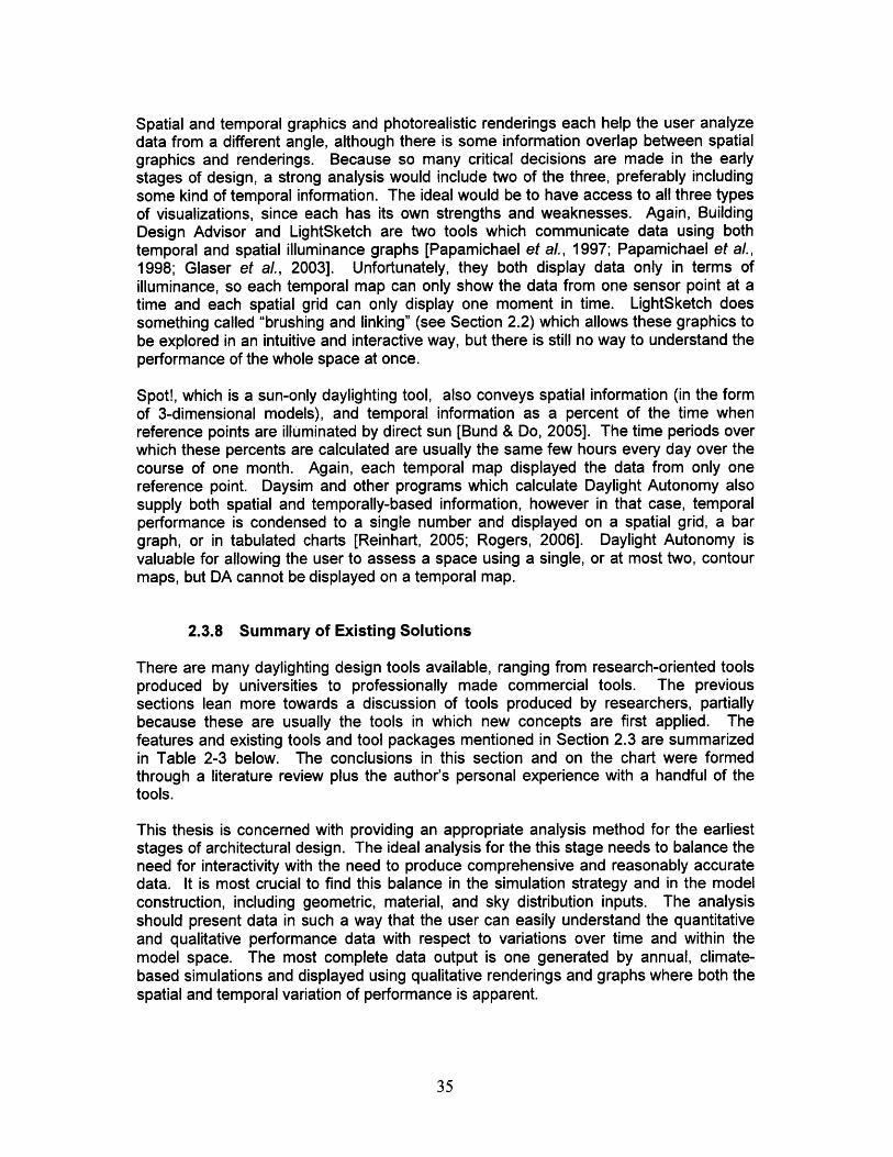
Spatial and temporal graphics and photorealistic renderings each help the user analyzedata from a different angle, although there is some information overlap between spatialgraphics and renderings. Because so many critical decisions are made in the earlystages of design, a strong analysis would include two of the three, preferably includingsome kind of temporal information. The ideal would be to have access to all three typesof visualizations, since each has its own strengths and weaknesses. Again, BuildingDesign Advisor and LightSketch are two tools which communicate data using bothtemporal and spatial illuminance graphs [Papamichael et aL, 1997; Papamichael et al.,1998; Glaser et al., 2003]. Unfortunately, they both display data only in terms ofilluminance, so each temporal map can only show the data from one sensor point at atime and each spatial grid can only display one moment in time. LightSketch doessomething called "brushing and linking" (see Section 2.2) which allows these graphics tobe explored in an intuitive and interactive way, but there is still no way to understand theperformance of the whole space at once.

Spot!, which is a sun-only daylighting tool, also conveys spatial information (in the formof 3-dimensional models), and temporal information as a percent of the time whenreference points are illuminated by direct sun [Bund & Do, 2005]. The time periods overwhich these percents are calculated are usually the same few hours every day over thecourse of one month. Again, each temporal map displayed the data from only onereference point. Daysim and other programs which calculate Daylight Autonomy alsosupply both spatial and temporally-based information, however in that case, temporalperformance is condensed to a single number and displayed on a spatial grid, a bargraph, or in tabulated charts [Reinhart, 2005; Rogers, 2006]. Daylight Autonomy isvaluable for allowing the user to assess a space using a single, or at most two, contourmaps, but DA cannot be displayed on a temporal map.

2.3.8 Summary of Existing Solutions

There are many daylighting design tools available, ranging from research-oriented toolsproduced by universities to professionally made commercial tools. The previoussections lean more towards a discussion of tools produced by researchers, partiallybecause these are usually the tools in which new concepts are first applied. Thefeatures and existing tools and tool packages mentioned in Section 2.3 are summarizedin Table 2-3 below. The conclusions in this section and on the chart were formedthrough a literature review plus the author's personal experience with a handful of thetools.

This thesis is concerned with providing an appropriate analysis method for the earlieststages of architectural design. The ideal analysis for the this stage needs to balance theneed for interactivity with the need to produce comprehensive and reasonably accuratedata. It is most crucial to find this balance in the simulation strategy and in the modelconstruction, including geometric, material, and sky distribution inputs. The analysisshould present data in such a way that the user can easily understand the quantitativeand qualitative performance data with respect to variations over time and within themodel space. The most complete data output is one generated by annual, climate-based simulations and displayed using qualitative renderings and graphs where both thespatial and temporal variation of performance is apparent.

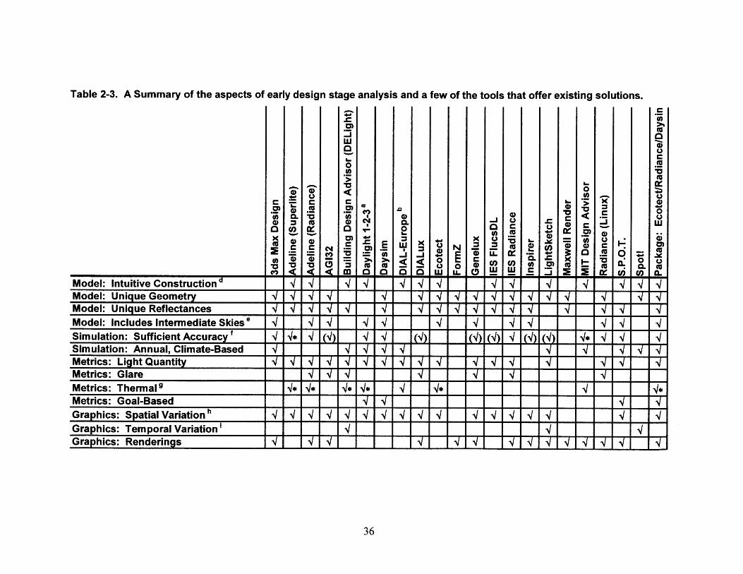
Table 2-3. A Summary of the aspects of early design stage analysis and a few of the tools that offer existing solutions.

(D 0U)U

.5 x

- oU) 0*0 o1... 4

MoeE U G 4) ) C M.2 -- 1 6

Model: Incluies Cntrediat S 4 4 4 4 4 4

Simulation: Sufficient Accuracy f 0 () * ()4 ) 1() 4* 4 4 4Simulation: Annual, Climate-Based -) L U 4

Metrics: Light Quantity --- T T-- 4 -TiiiiMetrics: GlareMetrics: Thermal* * N*

Metrics: Goal-BasedGrahics: Satial Variationd 4 4 4 4 4 4 4 4 4 4 4 4 4 4Graphics: Temporal VariationGraphics: Renderings 7777777 I7i7777 7 "7"7

NOTES:a) The prototype for Daylight 1-2-3 was previously named The Lightswitch Wizard. Thermal, geometric, and other features were added to

Daylight 1-2-3.b) DIAL-Europe was previously named LESO-DIAL.c) Viz is the result of Autdesk purchasing and significantly changing Lightscape.d) For tools with which the author has no pesonal experience, this judgement is based on literature and website reviews.e) This includes CIE Intermediate skies [Nakamura et al., 1985] and Perez All-Weather skies [Perez et al., 1993], but not averaged skies or

user-defined distributions.f) For the most part, any tool using radiosity or ray-tracing is considered sufficient. (4) indicates tools for which the author cannot find a

validation of accuracy, and 4* indicates tools which demonstrate less accuracy in published papers [Ubbelohde; Lehar].g) 4* indicates tools which perfrom energy simulations (which include solar thermal effects) internally or as a convenient export, but do not

have specific solar thermal metrics.h) This includes both 2-dimensional contour maps and falsecolor renderings.i) This does not include the ability to produce animations.

Chapter 3

Simulation Reduction for Temporal GraphicsTemporal and spatial graphics convey different information to the designer, and a furtherexploration of their complementary natures can be found in Chapter 7. However,temporal graphics were chosen as the primary mode of conveying numerical datathroughout this thesis and in the Lightsolve project [Andersen et al., 2008]. This is duein part to the close connection between the passage of time and environmentaldaylighting variables, and in part to the ease by which one can compare spatial and non-spatial quantities using temporal graphics (see Section 1.2).

Because it is important to give the user both temporal and spatial information, acorrelated set of representative renderings provides both spatial information and anopportunity for qualitative assessment (see Section 7.2.4). Spatial renderings, ratherthan spatial numerical graphics, were chosen partially due to the work of Lu Yi, who dida master's thesis for the MIT architecture department. Yi's work was the development ofa user interface design, the idea of which was to strongly link the numerical rigor of theanalysis software preferred by engineers to the highly interactive and visual displayspreferred by architects [Yi, 2008]. The centerpiece of these daylighting visual outputs,and one of the most striking results of any daylighting analysis software, is the realisticrendering.

The relationship between the temporal map and renderings in the proposed Lightsolveinterface is similar to the "brushing and linking" method described in Section 2.2 [Glaser& Ubbelohde, 2001] - as the mouse travels over different points in the temporal map,the nearby renderings update in real time to display the one closest to the time of dayand year indicated by the cursor. In this way, temporal data and spatial renderings areintuitively linked to form a more informative whole. Other features of the interface allowthe user to watch animations of the changing light patterns over a day or over a year fora specific hour. Renderings can also be displayed according to dominant weather type,or as clear, clear-turbid, intermediate, or overcast renderings only, and they can beshown simultaneously in a tiled table rather than as chronologically linked with thetemporal maps. The model's object file can also be viewed and manipulated from theinterface and new views chosen for rendering [Yi, 2008]. Although the aesthetics andnavigation functions have been updated since Yi completed her thesis [Seaton, 2009],the ideas and principals behind it have been preserved in the new incarnation. Figure 3-1 shows a screenshot of both Yi's and Seaton's interface which links the temporalnumerical data to spatial renderings.

This chapter develops and validates a method to reduce the number of simulationsnecessary to produce an annual data set which will be displayed using a temporalgraphic format. The year is first divided into periods of similar seasonal and dailymoments, which are then analyzed for sky type frequency and average brightness ofeach sky type. The choice of sky model, the ASRC-CIE model by Perez et al. [Perez etal., 1992], was influenced by the decision to associate renderings with the numericaldata in the temporal map (see Section 3.1.2). Finally, the data reduction method isvalidated against a far more detailed data set for sensors under unobstructed skies,inside a simple room, and inside more a complex architectural model.

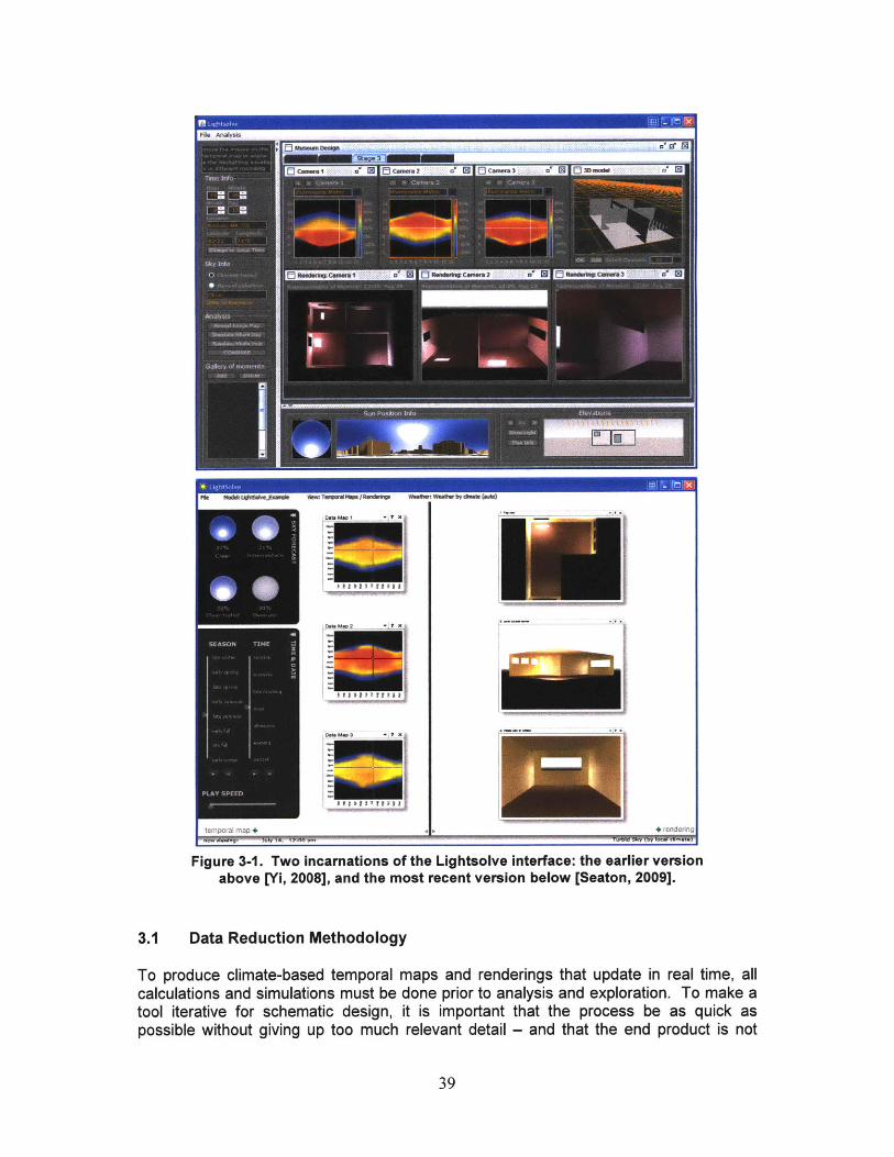
IF4k, i:v- x q~ +w~WfWs~0WV WsO 1 ,twy il ib)l

temporal~~ ma)+ fenderingj

Figure 3-1. Two incarnations of the Lightsolve interface: the earlier versionabove [Yi, 2008], and the most recent version below [Seaton, 2009].

3.1 Data Reduction Methodology

To produce climate-based temporal maps and renderings that update in real time, allcalculations and simulations must be done prior to analysis and exploration. To make atool iterative for schematic design, it is important that the process be as quick aspossible without giving up too much relevant detail - and that the end product is not

......................

1,:k LOIS"JEMMie View TwMaral Mapg I RendvkW WNMIer. WWNW by dkWW Wft)

D.t. MW I -'? X

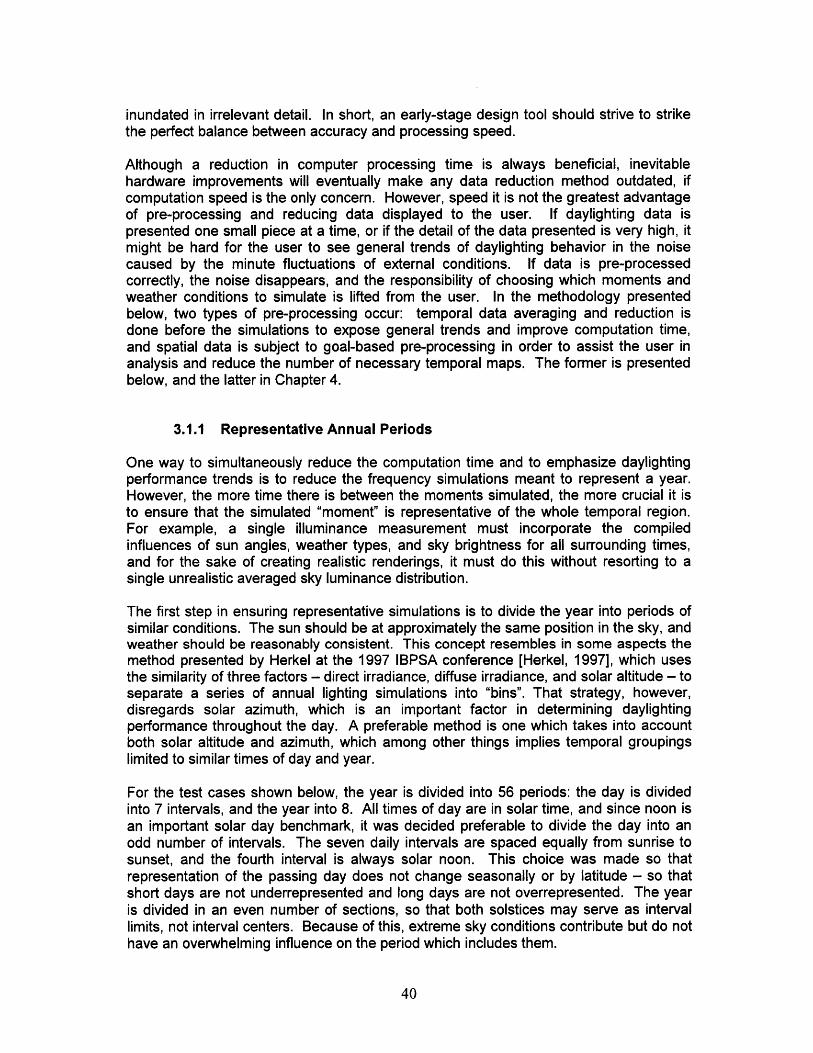
inundated in irrelevant detail. In short, an early-stage design tool should strive to strikethe perfect balance between accuracy and processing speed.

Although a reduction in computer processing time is always beneficial, inevitablehardware improvements will eventually make any data reduction method outdated, ifcomputation speed is the only concern. However, speed it is not the greatest advantageof pre-processing and reducing data displayed to the user. If daylighting data ispresented one small piece at a time, or if the detail of the data presented is very high, itmight be hard for the user to see general trends of daylighting behavior in the noisecaused by the minute fluctuations of external conditions. If data is pre-processedcorrectly, the noise disappears, and the responsibility of choosing which moments andweather conditions to simulate is lifted from the user. In the methodology presentedbelow, two types of pre-processing occur: temporal data averaging and reduction isdone before the simulations to expose general trends and improve computation time,and spatial data is subject to goal-based pre-processing in order to assist the user inanalysis and reduce the number of necessary temporal maps. The former is presentedbelow, and the latter in Chapter 4.

3.1.1 Representative Annual Periods

One way to simultaneously reduce the computation time and to emphasize daylightingperformance trends is to reduce the frequency simulations meant to represent a year.However, the more time there is between the moments simulated, the more crucial it isto ensure that the simulated "moment" is representative of the whole temporal region.For example, a single illuminance measurement must incorporate the compiledinfluences of sun angles, weather types, and sky brightness for all surrounding times,and for the sake of creating realistic renderings, it must do this without resorting to asingle unrealistic averaged sky luminance distribution.

The first step in ensuring representative simulations is to divide the year into periods ofsimilar conditions. The sun should be at approximately the same position in the sky, andweather should be reasonably consistent. This concept resembles in some aspects themethod presented by Herkel at the 1997 IBPSA conference [Herkel, 1997], which usesthe similarity of three factors - direct irradiance, diffuse irradiance, and solar altitude - toseparate a series of annual lighting simulations into "bins". That strategy, however,disregards solar azimuth, which is an important factor in determining daylightingperformance throughout the day. A preferable method is one which takes into accountboth solar altitude and azimuth, which among other things implies temporal groupingslimited to similar times of day and year.

For the test cases shown below, the year is divided into 56 periods: the day is dividedinto 7 intervals, and the year into 8. All times of day are in solar time, and since noon isan important solar day benchmark, it was decided preferable to divide the day into anodd number of intervals. The seven daily intervals are spaced equally from sunrise tosunset, and the fourth interval is always solar noon. This choice was made so thatrepresentation of the passing day does not change seasonally or by latitude - so thatshort days are not underrepresented and long days are not overrepresented. The yearis divided in an even number of sections, so that both solstices may serve as intervallimits, not interval centers. Because of this, extreme sky conditions contribute but do nothave an overwhelming influence on the period which includes them.

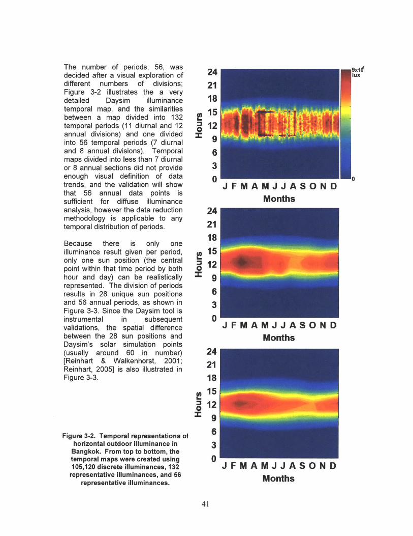
The number of periods, 56, wasdecided after a visual exploration ofdifferent numbers of divisions;Figure 3-2 illustrates the a verydetailed Daysim illuminancetemporal map, and the similaritiesbetween a map divided into 132temporal periods (11 diurnal and 12annual divisions) and one dividedinto 56 temporal periods (7 diurnaland 8 annual divisions). Temporalmaps divided into less than 7 diurnalor 8 annual sections did not provideenough visual definition of datatrends, and the validation will showthat 56 annual data points issufficient for diffuse illuminanceanalysis, however the data reductionmethodology is applicable to anytemporal distribution of periods.

Because there is only oneilluminance result given per period,only one sun position (the centralpoint within that time period by bothhour and day) can be realisticallyrepresented. The division of periodsresults in 28 unique sun positionsand 56 annual periods, as shown inFigure 3-3. Since the Daysim tool isinstrumental in subsequentvalidations, the spatial differencebetween the 28 sun positions andDaysim's solar simulation points(usually around 60 in number)[Reinhart & Walkenhorst, 2001;Reinhart, 2005] is also illustrated inFigure 3-3.

Figure 3-2. Temporal representations olhorizontal outdoor illuminance in

Bangkok. From top to bottom, thetemporal maps were created using105,120 discrete illuminances, 132

representative illuminances, and 56representative illuminances.

24211815129630

24211815129630

24211815129630

JFMAMJJASONDMonths

JFMAMJJASONDMonths

JFMAMJJASONDMonths

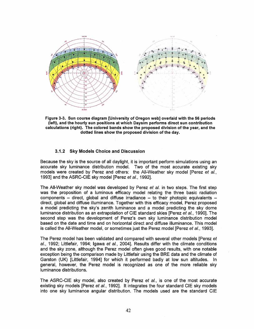
200

Figure 3-3. Sun course diagram [University of Oregon web] overlaid with the 56 periods(left), and the hourly sun positions at which Daysim performs direct sun contribution

calculations (right). The colored bands show the proposed division of the year, and thedotted lines show the proposed division of the day.

3.1.2 Sky Models Choice and Discussion

Because the sky is the source of all daylight, it is important perform simulations using anaccurate sky luminance distribution model. Two of the most accurate existing skymodels were created by Perez and others: the All-Weather sky model [Perez et aL,1993] and the ASRC-CIE sky model [Perez et aL, 1992].

The All-Weather sky model was developed by Perez et al. in two steps. The first stepwas the proposition of a luminous efficacy model relating the three basic radiationcomponents - direct, global and diffuse irradiance - to their photopic equivalents -direct, global and diffuse illuminance. Together with this efficacy model, Perez proposeda model predicting the sky's zenith luminance and a model predicting the sky domeluminance distribution as an extrapolation of CIE standard skies [Perez et al., 1990]. Thesecond step was the development of Perez's own sky luminance distribution modelbased on the date and time and on horizontal direct and diffuse illuminance. This modelis called the All-Weather model, or sometimes just the Perez model [Perez et aL, 1993].

The Perez model has been validated and compared with several other models [Perez etal., 1992; Littlefair, 1994; Igawa et al., 2004]. Results differ with the climate conditionsand the sky zone, although the Perez model often gives good results, with one notableexception being the comparison made by Littlefair using the BRE data and the climate ofGarston (UK) [Littlefair, 1994] for which it performed badly at low sun altitudes. Ingeneral, however, the Perez model is recognized as one of the more reliable skyluminance distributions.

The ASRC-CIE sky model, also created by Perez et al., is one of the most accurateexisting sky models [Perez et al., 1992]. It integrates the four standard CIE sky modelsinto one sky luminance angular distribution. The models used are the standard CIE

overcast sky [Moon & Spencer, 1942], the CIE averaged intermediate sky [Nakamura etal., 1985], the standard CIE clear sky and a high turbidity formulation of the latter (CIEclear sky for polluted atmosphere) [CIE, 1973; Darula & Kittler, 2002].

This sky model has been validated for diverse climate and sky zones (sun proximity)[Perez et aL, 1992; Littlefair, 1994] and compared with several other models.Comparison results vary from one study to another, but the ASRC-CIE model alwaysgives good results (sometimes even better results than the more complex All Weathersky model) and was validated with several other models [Littlefair, 1994]. It wasdeclared most likely to be adaptable to a wide range of climate zones.

The ASRC-CIE model is the one used in simulations populating the 56 periods temporalmaps. The choice was made due not only to the validated accuracy of the model, butmore importantly because the simulation of discrete sky types is inherent in its definition.Ultimately, a temporal map is formed using one data result (one illuminance, forexample) per each of the 56 temporal periods. A sky model which provides the neededability to weight the contributions of different sky types within one period is an asset tothe process.

One change was made to the ASRC-CIE methodology. In order to preserve the realismof renderings under different skies, the weighted sum of weather conditions is performedafter illuminances are calculated rather than applying them to the distribution of skyluminance used in the simulations. Therefore, the governing equation is:

E = bcEc + btEt + b;Ei + b0Eo (3.1)

Where E is the illuminance at the considered point and Ec, Et, E andEo are, respectively,the luminance at the considered point for a standard CIE clear sky, a CIE clear turbidsky, a CIE intermediate sky and a CIE overcast sky. The b; coefficients are found usingequations 3.2-3.6 below.

The luminance definition of each of the four sky types includes a zenithal luminancewhich must be determined before simulation. Representative zenithal luminances foreach of the 56 periods are found by processing a Typical Meteorological Year weatherfile for a given location and finding the average zenithal luminance for each of the foursky types per temporal period. This processing also finds the frequency of occurrence ofthe different sky types during each temporal period.

The frequency of different sky conditions becomes the weighting factors be, bt, b;, bo,which were adapted by Perez in 1992, depend on the sky clearness E and brightness A[Perez et al., 1992]. The sky E and A are calculated using the horizontal diffuseirradiance (Edi;,), the normal incident irradiance (Enorm) and the solar zenith angle (Z)expressed in radians:

(Edi,,+ Enom) +1.041. Z3

E = - ydifff.Z(321+1.041.Z 3

A = m -Ed (3.3)Enorm.ex

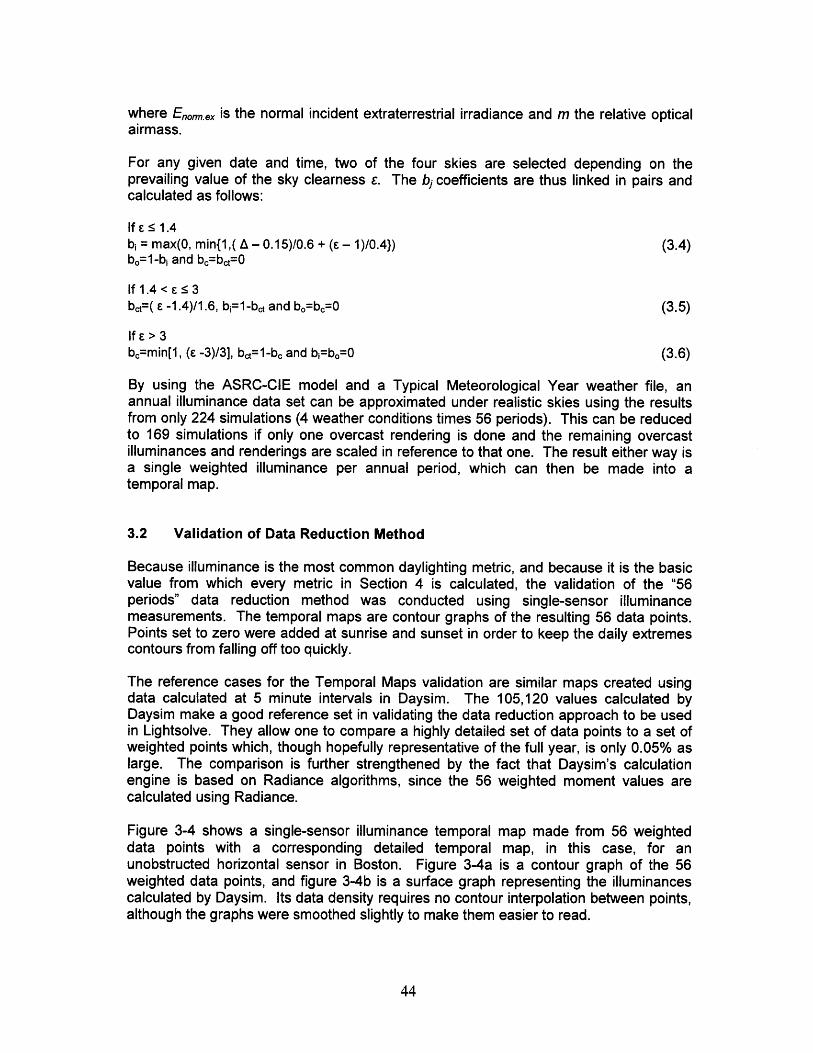
where Eno.e, is the normal incident extraterrestrial irradiance and m the relative opticalairmass.

For any given date and time, two of the four skies are selected depending on theprevailing value of the sky clearness E. The b; coefficients are thus linked in pairs andcalculated as follows:

If E 5 1.4bi = max(O, min{1,( A - 0.15)/0.6 + (E - 1)/0.4}) (3.4)b0=1-bi and bc=bct=0

If 1.4 < E s 3bct=( E -1.4)/1.6, bi=1-bt and bo=bc=0 (3.5)

If E > 3bc=min[1, (E -3)/3], bc=1-bc and bi=bo=0 (3.6)

By using the ASRC-CIE model and a Typical Meteorological Year weather file, anannual illuminance data set can be approximated under realistic skies using the resultsfrom only 224 simulations (4 weather conditions times 56 periods). This can be reducedto 169 simulations if only one overcast rendering is done and the remaining overcastilluminances and renderings are scaled in reference to that one. The result either way isa single weighted illuminance per annual period, which can then be made into atemporal map.

3.2 Validation of Data Reduction Method

Because illuminance is the most common daylighting metric, and because it is the basicvalue from which every metric in Section 4 is calculated, the validation of the "56periods" data reduction method was conducted using single-sensor illuminancemeasurements. The temporal maps are contour graphs of the resulting 56 data points.Points set to zero were added at sunrise and sunset in order to keep the daily extremescontours from falling off too quickly.

The reference cases for the Temporal Maps validation are similar maps created usingdata calculated at 5 minute intervals in Daysim. The 105,120 values calculated byDaysim make a good reference set in validating the data reduction approach to be usedin Lightsolve. They allow one to compare a highly detailed set of data points to a set ofweighted points which, though hopefully representative of the full year, is only 0.05% aslarge. The comparison is further strengthened by the fact that Daysim's calculationengine is based on Radiance algorithms, since the 56 weighted moment values arecalculated using Radiance.

Figure 3-4 shows a single-sensor illuminance temporal map made from 56 weighteddata points with a corresponding detailed temporal map, in this case, for anunobstructed horizontal sensor in Boston. Figure 3-4a is a contour graph of the 56weighted data points, and figure 3-4b is a surface graph representing the illuminancescalculated by Daysim. Its data density requires no contour interpolation between points,although the graphs were smoothed slightly to make them easier to read.

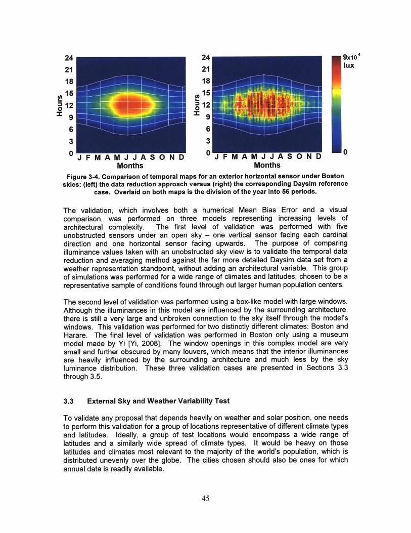
24 24 9x10 4

21 21 lux

18 18

15 15

2 12 Ji,

99

6 6

3 3

0 JFMAMJJASOND 0 JFMAMJJASOND 0Months Months

Figure 3-4. Comparison of temporal maps for an exterior horizontal sensor under Bostonskies: (left) the data reduction approach versus (right) the corresponding Daysim reference

case. Overlaid on both maps is the division of the year into 56 periods.

The validation, which involves both a numerical Mean Bias Error and a visualcomparison, was performed on three models representing increasing levels ofarchitectural complexity. The first level of validation was performed with fiveunobstructed sensors under an open sky - one vertical sensor facing each cardinaldirection and one horizontal sensor facing upwards. The purpose of comparingilluminance values taken with an unobstructed sky view is to validate the temporal datareduction and averaging method against the far more detailed Daysim data set from aweather representation standpoint, without adding an architectural variable. This groupof simulations was performed for a wide range of climates and latitudes, chosen to be arepresentative sample of conditions found through out larger human population centers.

The second level of validation was performed using a box-like model with large windows.Although the illuminances in this model are influenced by the surrounding architecture,there is still a very large and unbroken connection to the sky itself through the model'swindows. This validation was performed for two distinctly different climates: Boston andHarare. The final level of validation was performed in Boston only using a museummodel made by Yi [Yi, 2008]. The window openings in this complex model are verysmall and further obscured by many louvers, which means that the interior illuminancesare heavily influenced by the surrounding architecture and much less by the skyluminance distribution. These three validation cases are presented in Sections 3.3through 3.5.

3.3 External Sky and Weather Variability Test

To validate any proposal that depends heavily on weather and solar position, one needsto perform this validation for a group of locations representative of different climate typesand latitudes. Ideally, a group of test locations would encompass a wide range oflatitudes and a similarly wide spread of climate types. It would be heavy on thoselatitudes and climates most relevant to the majority of the world's population, which isdistributed unevenly over the globe. The cities chosen should also be ones for whichannual data is readily available.

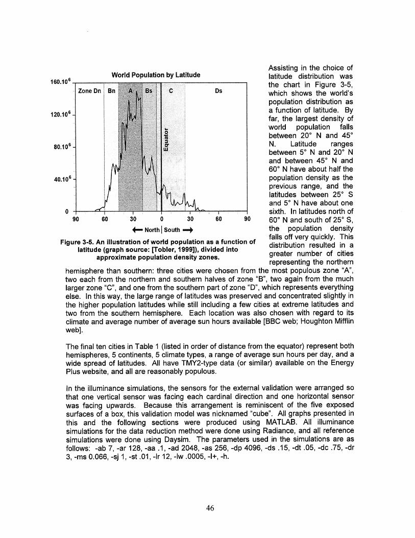
World Population by Latitude

C Ds

04a

C"LU

90 60 30 0 30 604- NorthI South ..

Figure 3-5. An illustration of world population as a functiorlatitude (graph source: [Tobler, 1999]), divided into

approximate population density zones.

hemisphere than southern: three cities were chosen fr

160.106

120.106

80.106

40.106

two each from the northern and southern halves of zone "B", two again from the muchlarger zone "C", and one from the southern part of zone "D", which represents everythingelse. In this way, the large range of latitudes was preserved and concentrated slightly inthe higher population latitudes while still including a few cities at extreme latitudes andtwo from the southern hemisphere. Each location was also chosen with regard to itsclimate and average number of average sun hours available [BBC web; Houghton Mifflinweb].

The final ten cities in Table 1 (listed in order of distance from the equator) represent bothhemispheres, 5 continents, 5 climate types, a range of average sun hours per day, and awide spread of latitudes. All have TMY2-type data (or similar) available on the EnergyPlus website, and all are reasonably populous.

In the illuminance simulations, the sensors for the external validation were arranged sothat one vertical sensor was facing each cardinal direction and one horizontal sensorwas facing upwards. Because this arrangement is reminiscent of the five exposedsurfaces of a box, this validation model was nicknamed "cube". All graphs presented inthis and the following sections were produced using MATLAB. All illuminancesimulations for the data reduction method were done using Radiance, and all referencesimulations were done using Daysim. The parameters used in the simulations are asfollows: -ab 7, -ar 128, -aa .1, -ad 2048, -as 256, -dp 4096, -ds .15, -dt .05, -dc .75, -dr3, -ms 0.066, -sj 1, -st .01, -Ir 12, -lw .0005, -1+, -h.

Assisting in the choice oflatitude distribution wasthe chart in Figure 3-5,which shows the world'spopulation distribution asa function of latitude. Byfar, the largest density ofworld population fallsbetween 20* N and 450N. Latitude rangesbetween 50 N and 20* Nand between 45' N and60' N have about half thepopulation density as theprevious range, and thelatitudes between 250 Sand 50 N have about onesixth. In latitudes north of

90 600 N and south of 250 S,the population densityfalls off very quickly. This

of~ distribution resulted in agreater number of citiesrepresenting the northern

om the most populous zone "A",

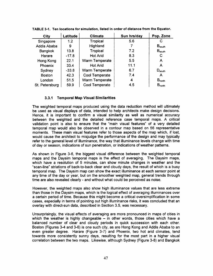
TABLE 3-1. Ten locations for simulation, listed in order of distance from the Equator.

City Latitude Climate Sun hrs/day Pop. ZoneSingapore 1.2 Tropical 5.6 C

Addis Ababa 9 Highland 7 Bsouth

Bangkok 13.8 Tropical 7.2 BsouthHarare -17.8 Hot Arid 8.3 C

Hong Kong 22.1 Warm Temperate 5.5 APhoenix 33.4 Hot Arid 11.1 ASydney -33.8 Warm Temperate 6.7 DsouthBoston 42.3 Cool Temperate 7.4 ALondon 51.5 Warm Temperate 4 Bnori

St. Petersburg 59.9 Cool Temperate 4.5 Bnorih

3.3.1 Temporal Map Visual Similarities

The weighted temporal maps produced using the data reduction method will ultimatelybe used as visual displays of data, intended to help architects make design decisions.Hence, it is important to confirm a visual similarity as well as numerical accuracybetween the weighted and the detailed reference case temporal maps. A criticalvalidation point is also to ensure that the "main visual features" of a very detailedtemporal map would also be observed in a contour map based on 56 representativemoments. These main visual features refer to those aspects of the map which, if lost,would cause the architect to misjudge the performance of the design and may typicallyrefer to the general level of illuminance, the way that illuminance levels change with timeof day or season, indications of sun penetration, or indications of weather patterns.

As shown in Figure 3-6, the biggest visual difference between the weighted temporalmaps and the Daysim temporal maps is the effect of averaging. The Daysim maps,which have a resolution of 5 minutes, can show minute changes in weather and the"scan-line" striations of back-to-back clear and cloudy days, the result of which is a busytemporal map. The Daysim map can show the exact illuminance at each sensor point atany time of the day or year, but on the smoother weighted map, general trends throughtime are also revealed clearly - and without what could be perceived as noise.

However, the weighted maps also show high illuminance values that are less extremethan those in the Daysim maps, which is the logical effect of averaging illuminances overa certain period of time. Because this might become a critical oversimplification in somecases, especially in terms of pointing out high illuminance risks, it was concluded that anoverlay with direct-sun data, described in Section 3.5, was necessary.

Unsurprisingly, the visual effects of averaging are more pronounced in maps of cities inwhich the weather is highly changeable - in other words, those cities which have abalanced number of clear and cloudy periods in quick succession with each other.Boston (Figures 3-4 and 3-6) is one such city, as are Hong Kong and Addis Ababa to aneven greater degree. Harare (Figure 3-7) and Phoenix, two hot arid climates, tendtowards more consistently sunny days, resulting for the most part in a higher visualcorrelation between the two maps. Likewise, although Sydney (Figure 3-8) and Bangkok

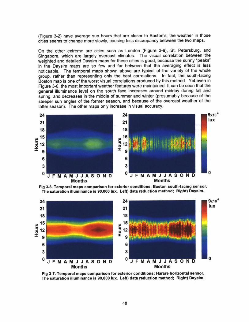
(Figure 3-2) have average sun hours that are closer to Boston's, the weather in thosecities seems to change more slowly, causing less discrepancy between the two maps.

On the other extreme are cities such as London (Figure 3-9), St. Petersburg, andSingapore, which are largely overcast climates. The visual correlation between theweighted and detailed Daysim maps for these cities is good, because the sunny "peaks"in the Daysim maps are so few and far between that the averaging effect is lessnoticeable. The temporal maps shown above are typical of the variety of the wholegroup, rather than representing only the best correlations. In fact, the south-facingBoston map is one of the worst visual correlations produced by this method. Yet even inFigure 3-6, the most important weather features were maintained. It can be seen that thegeneral illuminance level on the south face increases around midday during fall andspring, and decreases in the middle of summer and winter (presumably because of thesteeper sun angles of the former season, and because of the overcast weather of thelatter season). The other maps only increase in visual accuracy.

24 24 9x104

21 21 lux

18 18

15 15

12 12

996 6

3 3

0 JFMAMJJASOND 0 JFMAMJJASOND 0Months Months

Fig 3-6. Temporal maps comparison for exterior conditions: Boston south-facing sensor.The saturation illuminance is 90,000 lux. Left) data reduction method; Right) Daysim.

J FMAMJJASON DMonths

9 J JAMonths

lux

0

Fig 3-7. Temporal maps comparison for exterior conditions: Harare horizontal sensor.The saturation illuminance is 90,000 lux. Left) data reduction method; Right) Daysim.

. ...... .............. W ON

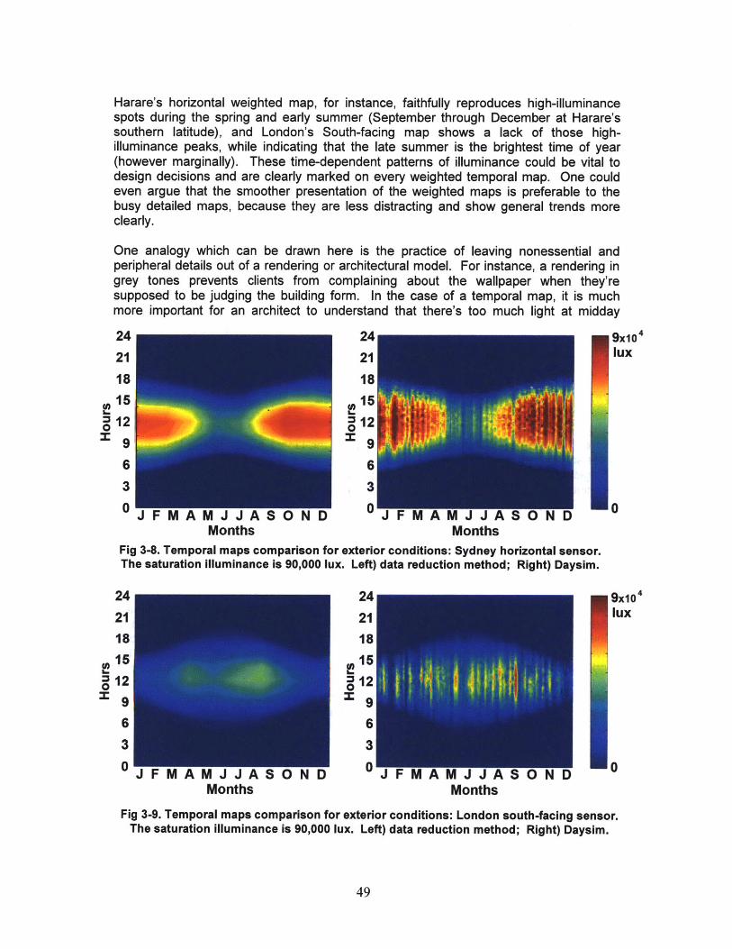
Harare's horizontal weighted map, for instance, faithfully reproduces high-illuminancespots during the spring and early summer (September through December at Harare'ssouthern latitude), and London's South-facing map shows a lack of those high-illuminance peaks, while indicating that the late summer is the brightest time of year(however marginally). These time-dependent patterns of illuminance could be vital todesign decisions and are clearly marked on every weighted temporal map. One couldeven argue that the smoother presentation of the weighted maps is preferable to thebusy detailed maps, because they are less distracting and show general trends moreclearly.

One analogy which can be drawn here is the practice of leaving nonessential andperipheral details out of a rendering or architectural model. For instance, a rendering ingrey tones prevents clients from complaining about the wallpaper when they'resupposed to be judging the building form. In the case of a temporal map, it is muchmore important for an architect to understand that there's too much light at midday

24

21

1815

12

963

0 JFMAMJJ AMonths

J FMAMJJMonths

Fig 3-8. Temporal maps comparison for exterior conditions: Sydney horizontal sensor.The saturation illuminance is 90,000 lux. Left) data reduction method; Right) Daysim.

W JJASONDMonths

24

211815

12

96

3

0 IJJASOMonths

lux

40

0

9x10 4

lux

0

Fig 3-9. Temporal maps comparison for exterior conditions: London south-facing sensor.The saturation illuminance is 90,000 lux. Left) data reduction method; Right) Daysim.

.. .. .................

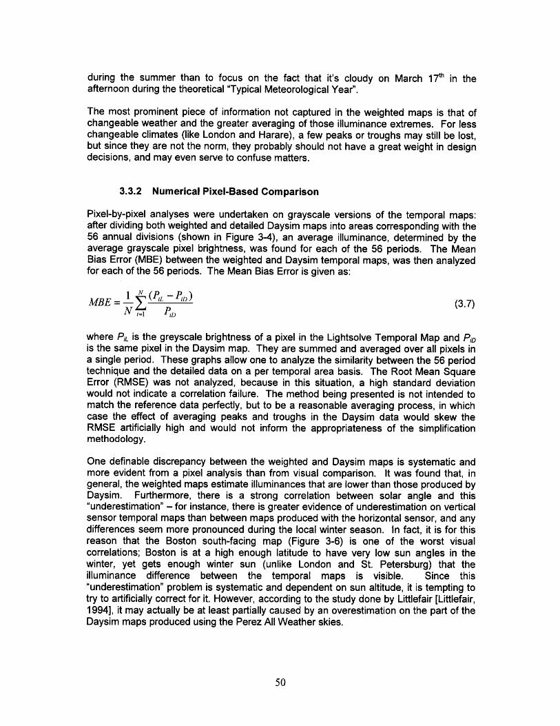
during the summer than to focus on the fact that it's cloudy on March 17th in theafternoon during the theoretical "Typical Meteorological Year".

The most prominent piece of information not captured in the weighted maps is that ofchangeable weather and the greater averaging of those illuminance extremes. For lesschangeable climates (like London and Harare), a few peaks or troughs may still be lost,but since they are not the norm, they probably should not have a great weight in designdecisions, and may even serve to confuse matters.

3.3.2 Numerical Pixel-Based Comparison

Pixel-by-pixel analyses were undertaken on grayscale versions of the temporal maps:after dividing both weighted and detailed Daysim maps into areas corresponding with the56 annual divisions (shown in Figure 3-4), an average illuminance, determined by theaverage grayscale pixel brightness, was found for each of the 56 periods. The MeanBias Error (MBE) between the weighted and Daysim temporal maps, was then analyzedfor each of the 56 periods. The Mean Bias Error is given as:

MBE = 1 IL iD.7N j= PiD

where PiL is the greyscale brightness of a pixel in the Lightsolve Temporal Map and PiDis the same pixel in the Daysim map. They are summed and averaged over all pixels ina single period. These graphs allow one to analyze the similarity between the 56 periodtechnique and the detailed data on a per temporal area basis. The Root Mean SquareError (RMSE) was not analyzed, because in this situation, a high standard deviationwould not indicate a correlation failure. The method being presented is not intended tomatch the reference data perfectly, but to be a reasonable averaging process, in whichcase the effect of averaging peaks and troughs in the Daysim data would skew theRMSE artificially high and would not inform the appropriateness of the simplificationmethodology.

One definable discrepancy between the weighted and Daysim maps is systematic andmore evident from a pixel analysis than from visual comparison. It was found that, ingeneral, the weighted maps estimate illuminances that are lower than those produced byDaysim. Furthermore, there is a strong correlation between solar angle and this"underestimation" - for instance, there is greater evidence of underestimation on verticalsensor temporal maps than between maps produced with the horizontal sensor, and anydifferences seem more pronounced during the local winter season. In fact, it is for thisreason that the Boston south-facing map (Figure 3-6) is one of the worst visualcorrelations; Boston is at a high enough latitude to have very low sun angles in thewinter, yet gets enough winter sun (unlike London and St. Petersburg) that theilluminance difference between the temporal maps is visible. Since this"underestimation" problem is systematic and dependent on sun altitude, it is tempting totry to artificially correct for it. However, according to the study done by Littlefair [Littlefair,1994], it may actually be at least partially caused by an overestimation on the part of theDaysim maps produced using the Perez All Weather skies.

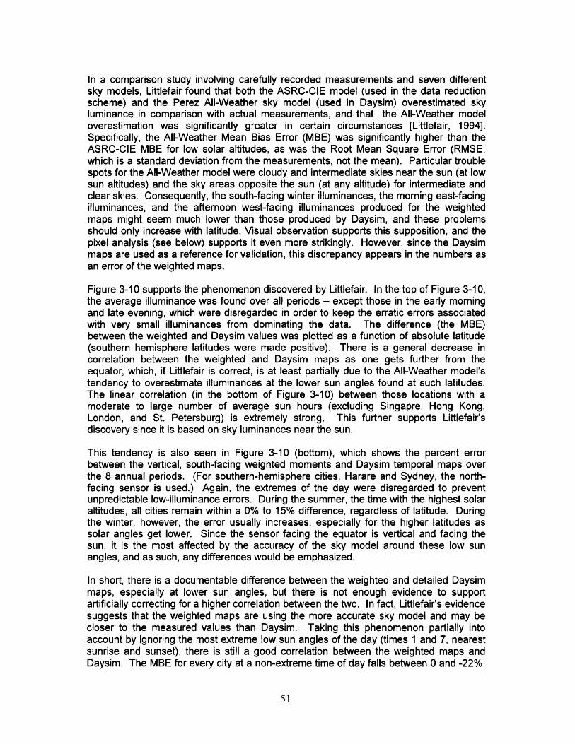
In a comparison study involving carefully recorded measurements and seven differentsky models, Littlefair found that both the ASRC-CIE model (used in the data reductionscheme) and the Perez All-Weather sky model (used in Daysim) overestimated skyluminance in comparison with actual measurements, and that the All-Weather modeloverestimation was significantly greater in certain circumstances [Littlefair, 1994].Specifically, the All-Weather Mean Bias Error (MBE) was significantly higher than theASRC-CIE MBE for low solar altitudes, as was the Root Mean Square Error (RMSE,which is a standard deviation from the measurements, not the mean). Particular troublespots for the All-Weather model were cloudy and intermediate skies near the sun (at lowsun altitudes) and the sky areas opposite the sun (at any altitude) for intermediate andclear skies. Consequently, the south-facing winter illuminances, the morning east-facingilluminances, and the afternoon west-facing illuminances produced for the weightedmaps might seem much lower than those produced by Daysim, and these problemsshould only increase with latitude. Visual observation supports this supposition, and thepixel analysis (see below) supports it even more strikingly. However, since the Daysimmaps are used as a reference for validation, this discrepancy appears in the numbers asan error of the weighted maps.

Figure 3-10 supports the phenomenon discovered by Littlefair. In the top of Figure 3-10,the average illuminance was found over all periods - except those in the early morningand late evening, which were disregarded in order to keep the erratic errors associatedwith very small illuminances from dominating the data. The difference (the MBE)between the weighted and Daysim values was plotted as a function of absolute latitude(southern hemisphere latitudes were made positive). There is a general decrease incorrelation between the weighted and Daysim maps as one gets further from theequator, which, if Littlefair is correct, is at least partially due to the All-Weather model'stendency to overestimate illuminances at the lower sun angles found at such latitudes.The linear correlation (in the bottom of Figure 3-10) between those locations with amoderate to large number of average sun hours (excluding Singapre, Hong Kong,London, and St. Petersburg) is extremely strong. This further supports Littlefair'sdiscovery since it is based on sky luminances near the sun.

This tendency is also seen in Figure 3-10 (bottom), which shows the percent errorbetween the vertical, south-facing weighted moments and Daysim temporal maps overthe 8 annual periods. (For southern-hemisphere cities, Harare and Sydney, the north-facing sensor is used.) Again, the extremes of the day were disregarded to preventunpredictable low-illuminance errors. During the summer, the time with the highest solaraltitudes, all cities remain within a 0% to 15% difference, regardless of latitude. Duringthe winter, however, the error usually increases, especially for the higher latitudes assolar angles get lower. Since the sensor facing the equator is vertical and facing thesun, it is the most affected by the accuracy of the sky model around these low sunangles, and as such, any differences would be emphasized.

In short, there is a documentable difference between the weighted and detailed Daysimmaps, especially at lower sun angles, but there is not enough evidence to supportartificially correcting for a higher correlation between the two. In fact, Littlefair's evidencesuggests that the weighted maps are using the more accurate sky model and may becloser to the measured values than Daysim. Taking this phenomenon partially intoaccount by ignoring the most extreme low sun angles of the day (times 1 and 7, nearestsunrise and sunset), there is still a good correlation between the weighted maps andDaysim. The MBE for every city at a non-extreme time of day falls between 0 and -22%,

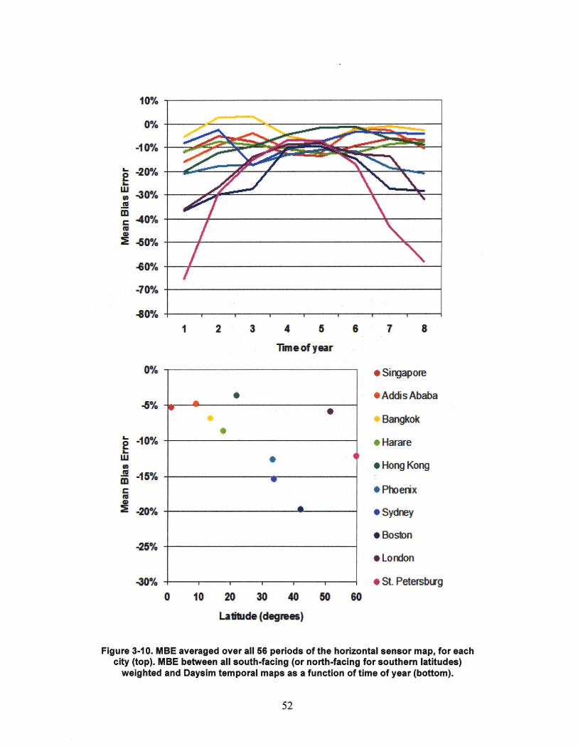
10%

0%

-10%

-20%

40%

.40%

-60%

40%

-70%

80%1 2 3 4 5 6 7 8

Tmeof year

0 Singapore

*AddisAbaba

Bangkok

* Harare

H Hong Kong

* Phoenix

* Sydney

" Bosbn

e Lordon

" St. Petersbiig0 10 20 30 40 50 60

Latitude (degrees)

Figure 3-10. MBE averaged over all 56 periods of the horizontal sensor map, for eachcity (top). MBE between all south-facing (or north-facing for southern latitudes)

weighted and Daysim temporal maps as a function of time of year (bottom).

0%

-6%

-10%

-15%

-20%

-25%

40%

4

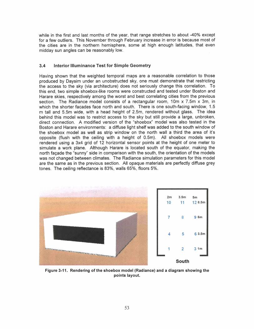
while in the first and last months of the year, that range stretches to about -40% exceptfor a few outliers. This November through February increase in error is because most ofthe cities are in the northern hemisphere, some at high enough latitudes, that evenmidday sun angles can be reasonably low.

3.4 Interior Illuminance Test for Simple Geometry

Having shown that the weighted temporal maps are a reasonable correlation to thoseproduced by Daysim under an unobstructed sky, one must demonstrate that restrictingthe access to the sky (via architecture) does not seriously change this correlation. Tothis end, two simple shoebox-like rooms were constructed and tested under Boston andHarare skies, respectively among the worst and best correlating cities from the previoussection. The Radiance model consists of a rectangular room, 10m x 7.5m x 3m, inwhich the shorter facades face north and south. There is one south-facing window, 1.5m tall and 5.5m wide, with a head height of 2.5m, rendered without glass. The ideabehind this model was to restrict access to the sky but still provide a large, unbroken,direct connection. A modified version of the "shoebox" model was also tested in theBoston and Harare environments: a diffuse light shelf was added to the south window ofthe shoebox model as well as strip window on the north wall a third the area of it'sopposite (flush with the ceiling with a height of 0.5m). All shoebox models wererendered using a 3x4 grid of 12 horizontal sensor points at the height of one meter tosimulate a work plane. Although Harare is located south of the equator, making thenorth fagade the "sunny" side in comparison with the south, the orientation of the modelswas not changed between climates. The Radiance simulation parameters for this modelare the same as in the previous section. All opaque materials are perfectly diffuse greytones. The ceiling reflectance is 83%, walls 65%, floors 5%.

2m 3.5m 5m10 11 12 8.5m

7 8 9 6m

4 5 6 3.5m

1 2 3 1m

South

Figure 3-11. Rendering of the shoebox model (Radiance) and a diagram showing thepoints layout.

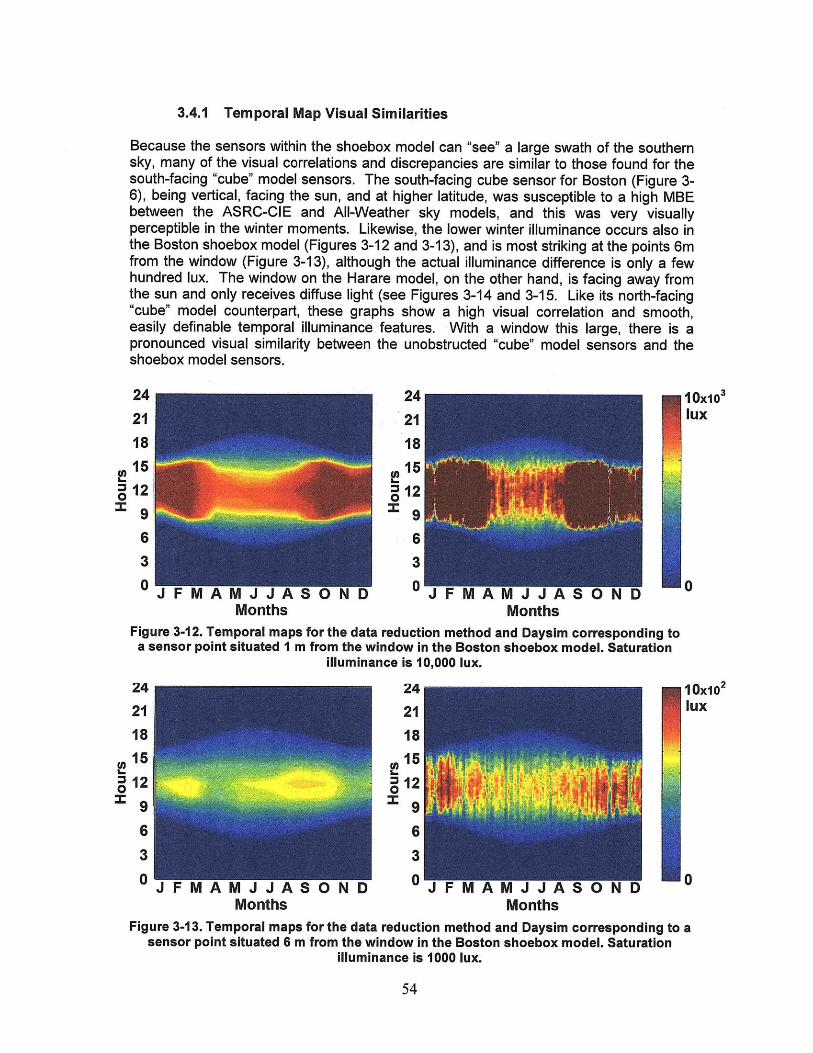
3.4.1 Temporal Map Visual Similarities

Because the sensors within the shoebox model can "see"I a large swath of the southernsky, many of the visual correlations and discrepancies are similar to those found for thesouth-facing "cube" model sensors. The south-facing cube sensor for Boston (Figure 3-6), being vertical, facing the sun, and at higher latitude, was susceptible to a high MBEbetween the ASRC-CIE and All-Weather sky models, and this was very visuallyperceptible in the winter moments. Likewise, the lower winter illuminance occurs also inthe Boston shoebox model (Figures 3-12 and 3-13), and is most striking at the points 6mfrom the window (Figure 3-13), although the actual illuminance difference is only a fewhundred lux. The window on the Harare model, on the other hand, is facing away fromthe sun and only receives diffuse light (see Figures 3-14 and 3-15. Like its north-facing"cube" model counterpart, these graphs show a high visual correlation and smooth,easily definable temporal illuminance features. With a window this large, there is apronounced visual similarity between the unobstructed "cube" model sensors and theshoebox model sensors.

242118151296

30 A J JA

MonthsW JJAMonths

Figure 3-12. Temporal maps for the data reduction method and Daysim corresponding toa sensor point situated I m from the window in the Boston shoebox model. Saturation

illuminance is 10,000 lux.

MAMJJAMonths

MAM J JAMonths

10X103

lux

1010

lux

0

Figure 3-13. Temporal maps for the data reduction method and Daysim corresponding to asensor point situated 6 m from the window in the Boston shoebox model. Saturation

illuminance is 1000 lux.

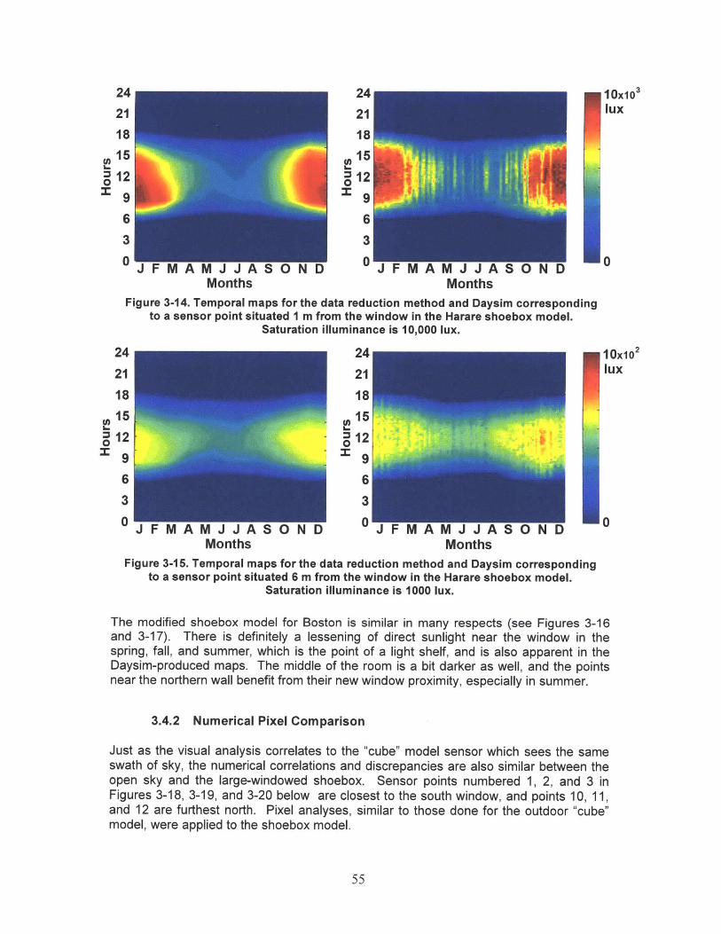
VI J J AMonths

Vi J J AMonths

Figure 3-14. Temporal maps for the data reduction method and Daysim correspondingto a sensor point situated I m from the window in the Harare shoebox model.

Saturation illuminance is 10,000 lux.

16.

0XI

24

21

1815

12

96

3

0

I

MAMJJAbUNU JVMAMJJA

Months MonthsFigure 3-15. Temporal maps for the data reduction method and Daysim corresponding

to a sensor point situated 6 m from the window in the Harare shoebox model.Saturation illuminance is 1000 lux.

The modified shoebox model for Boston is similar in many respects (see Figures 3-16and 3-17). There is definitely a lessening of direct sunlight near the window in thespring, fall, and summer, which is the point of a light shelf, and is also apparent in theDaysim-produced maps. The middle of the room is a bit darker as well, and the pointsnear the northern wall benefit from their new window proximity, especially in summer.

3.4.2 Numerical Pixel Comparison

Just as the visual analysis correlates to the "cube" model sensor which sees the sameswath of sky, the numerical correlations and discrepancies are also similar between theopen sky and the large-windowed shoebox. Sensor points numbered 1, 2, and 3 inFigures 3-18, 3-19, and 3-20 below are closest to the south window, and points 10, 11,and 12 are furthest north. Pixel analyses, similar to those done for the outdoor "cube"model, were applied to the shoebox model.

10x10 3lux

1OxiO 2

lux

10

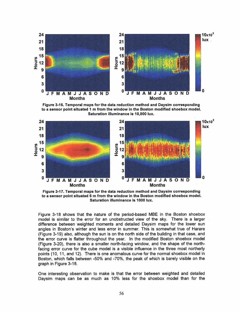
4 24 10x103

21 21 lux

18 18

15 1512 1200

9 9n

6 6

3 3

0 J F M A M J J A S O ND 0 J F M A MJ JAS N D 0Months Months

Figure 3-16. Temporal maps for the data reduction method and Daysim correspondingto a sensor point situated I m from the window in the Boston modified shoebox model.

Saturation illuminance is 10,000 lux.

24 24 10x10 2

21 21 lux

18

10 1512 1

=9 9

6 6

3 3

0 JFMAMJJASOND 0 J F M A M J J A S OND 0Months Months

Figure 3-17. Temporal maps for the data reduction method and Daysim correspondingto a sensor point situated 6 m from the window in the Boston modified shoebox model.

Saturation illuminance is 1000 lux.

Figure 3-18 shows that the nature of the period-based MBE in the Boston shoeboxmodel is similar to the error for an unobstructed view of the sky. There is a largerdifference between weighted moments and detailed Daysim maps for the lower sunangles in Boston's winter and less error in summer. This is somewhat true of Harare(Figure 3-19) also, although the sun is on the north side of the building in that case, andthe error curve is flatter throughout the year. In the modified Boston shoebox model(Figure 3-20), there is also a smaller north-facing window, and the shape of the north-facing error curve for the cube model is a visible influence in the three most northerlypoints (10, 11, and 12). There is one anomalous curve for the normal shoebox model inBoston, which falls between -50% and -70%, the peak of which is barely visible on thegraph in Figure 3-18.

One interesting observation to make is that the error between weighted and detailedDaysim maps can be as much as 10% less for the shoebox model than for the

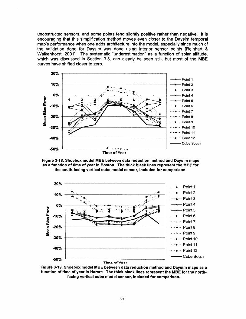
unobstructed sensors, and some points tend slightly positive rather than negative. It isencouraging that this simplification method moves even closer to the Daysim temporalmap's performance when one adds architecture into the model, especially since much ofthe validation done for Daysim was done using interior sensor points [Reinhart &Walkenhorst, 2001]. The systematic "underestimation" as a function of solar altitude,which was discussed in Section 3.3, can clearly be seen still, but most of the MBEcurves have shifted closer to zero.

20%- Point I

10% ---- Point 2U- .- ~

A- -- -. , A Point 3

0% - Point 4

1 2 3 -6 : Point 5

W -10% - Point 6

- --- +--Point 7

-20% Point 8---.--- Point 9

-3C0%/ - Point 10--- Point 11

-40% - --i-- Point 12

- Cube South

-50% - -. -Time of Year

Figure 3-18. Shoebox model MBE between data reduction method and Daysim mapsas a function of time of year in Boston. The thick black lines represent the MBE for

the south-facing vertical cube model sensor, included for comparison.

20%- Point 1

10% ---- Point 2Point 3

0% - - . .x Point 4

--- +-- Point 7

-20% ----- Point 8

Point 9c -30% -. -- .-. Point 10----- Point11

-40% --- Point 12

-50% - Cube South

Timno af Voo.-

Figure 3-19. Shoebox model MBE between data reduction method and Daysim maps as afunction of time of year in Harare. The thick black lines represent the MBE for the north-

facing vertical cube model sensor, included for comparison.

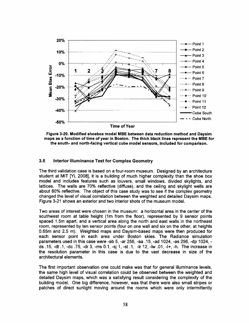
20%10%-''Point -

1Po2n7 810% ~. ~Point 30%Point4-0% A Point 5::Point 4

W -10%+ Point 5

e& Point 6

- - ..- Point 9----- Point 10

--

3-0--%

Point 11

-40--- -- Point 12

4%- Cube South- - - Cube North

-50%Time of Year

Figure 3-20. Modified shoebox model MBE between data reduction method and Daysimmaps as a function of time of year in Boston. The thick black lines represent the MBE for

the south- and north-facing vertical cube model sensors, included for comparison.

3.5 Interior Ililuminance Test for Complex Geometry

The third validation case is based on a four-room museum. Designed by an architecturestudent at MIT [Yi, 2008], it is a building of much higher complexity than the shoe boxmodel and includes features such as louvers, small windows, divided skylights, andlattices. The walls are 70% reflective (diffuse), and the ceiling and skylight wells areabout 80% reflective. The object of this case study was to see if the complex geometrychanged the level of visual correlation between the weighted and detailed Daysim maps.Figure 3-21 shows an exterior and two interior shots of the museum model.

Two areas of interest were chosen in the museum: a horizontal area in the center of thesouthwest room at table height (1m from the floor), represented by 9 sensor pointsspaced 1.5m apart, and a vertical area along the north and east walls in the northeastroom, represented by ten sensor points (four on one wall and six on the other, at heights0.65m and 2.5 m). Weighted maps and Daysim-based maps were then produced foreach sensor point in each area under Boston skies. The Radiance simulationparameters used in this case were -ab 5, -ar 256, -aa .15, -ad 1024, -as 256, -dp 1024, -ds .15, -dt .1, -dc .75, -dr 3, -ms 0.1, -sj 1, -st .1, -Ir 12, -Iw .01, -1+, -h. The increase inthe resolution parameter in this case is due to the vast decrease in size of thearchitectural elements.

The first important observation one could make was that for general illuminance levels,the same high level of visual correlation could be observed between the weighted anddetailed Daysim maps, which was a satisfying result considering the complexity of thebuilding model. One big difference, however, was that there were also small stripes orpatches of direct sunlight moving around the rooms which were only intermittently

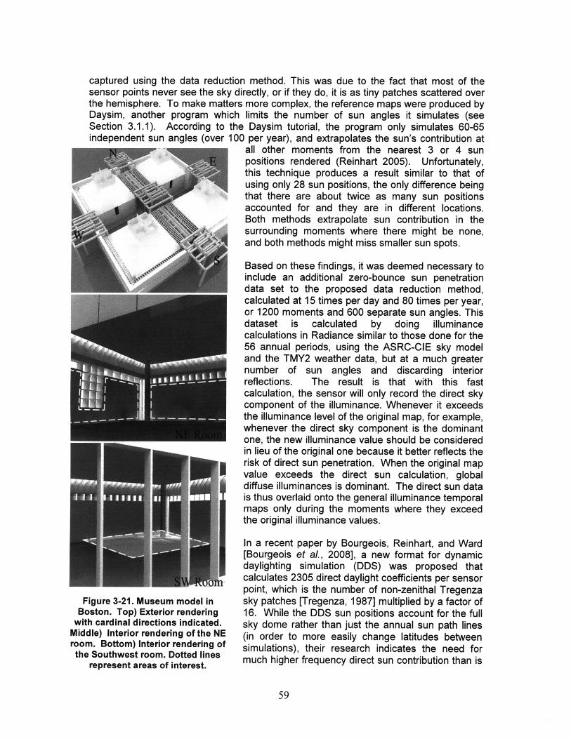
captured using the data reduction method. This was due to the fact that most of thesensor points never see the sky directly, or if they do, it is as tiny patches scattered overthe hemisphere. To make matters more complex, the reference maps were produced byDaysim, another program which limits the number of sun angles it simulates (seeSection 3.1.1). According to the Daysim tutorial, the program only simulates 60-65independent sun angles (over 100 per year), and extrapolates the sun's contribution at

all other moments from the nearest 3 or 4 sunpositions rendered (Reinhart 2005). Unfortunately,this technique produces a result similar to that of

4 using only 28 sun positions, the only difference beingthat there are about twice as many sun positionsaccounted for and they are in different locations.Both methods extrapolate sun contribution in thesurrounding moments where there might be none,and both methods might miss smaller sun spots.

Based on these findings, it was deemed necessary toinclude an additional zero-bounce sun penetrationdata set to the proposed data reduction method,calculated at 15 times per day and 80 times per year,or 1200 moments and 600 separate sun angles. Thisdataset is calculated by doing illuminancecalculations in Radiance similar to those done for the56 annual periods, using the ASRC-CIE sky modeland the TrY2 weather data, but at a much greaternumber of sun angles and discarding interiorreflections. The result is that with this fastcalculation, the sensor will only record the direct skycomponent of the illuminance. Whenever it exceedsthe illuminance level of the original map, for example,whenever the direct sky component is the dominantone, the new illuminance value should be consideredin lieu of the original one because it better reflects therisk of direct sun penetration. When the original mapvalue exceeds the direct sun calculation, globalc ediffuse illuminances is dominant. The direct sun datais thus overlaid onto the general illuminance temporalmaps only during the moments where they exceedthe original illuminance values.

In a recent paper by Bourgeois, Reinhart, and Ward[Bourgeois et al, 2008], a new format for dynamicdaylighting simulation (DDS) was proposed thatcalculates 2305 direct daylight coefficients per sensorpoint, which is the number of non-zenithal Tregenza

Figure 3-21. Museum model in sky patches [Tregenza, 1987] multiplied by a factor ofBoston. Top) Exterior rendering 16. While the DDS sun positions account for the full

with cardinal directions indicated, sky dome rather than just the annual sun path linesMiddle) Interior rendering of the NE (in order to more easily change latitudes betweenroom. Bottom) Interior rendering of simulations), their research indicates the need forthe Southwest room. Dotted lines much higher frequency direct sun contribution than is

represent areas of interest.

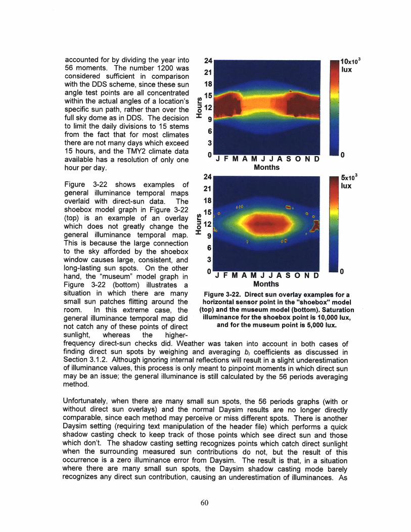
accounted for by dividing the year into 24 1Ox103

56 moments. The number 1200 was 21 luxconsidered sufficient in comparisonwith the DDS scheme, since these sun 18angle test points are all concentrated 15within the actual angles of a location's Ispecific sun path, rather than over the 1full sky dome as in DDS. The decision gto limit the daily divisions to 15 stemsfrom the fact that for most climatesthere are not many days which exceed 315 hours, and the TMY2 climate data 0available has a resolution of only one J F M A M J J A S 0 N Dhour per day. Months

24 5x10 3

Figure 3-22 shows examples of 21 luxgeneral illuminance temporal mapsoverlaid with direct-sun data. The 18shoebox model graph in Figure 3-22(top) is an example of an overlaywhich does not greatly change the 5 12general illuminance temporal map. 9This is because the large connectionto the sky afforded by the shoeboxwindow causes large, consistent, and 3long-lasting sun spots. On the other 0hand, the "museum" model graph in 0 FMAMJJAS0 DFigure 3-22 (bottom) illustrates a Monthssituation in which there are many Figure 3-22. Direct sun overlay examples for asmall sun patches flitting around the horizontal sensor point in the "shoebox" modelroom. In this extreme case, the (top) and the museum model (bottom). Saturationgeneral illuminance temporal map did illuminance for the shoebox point is 10,000 lux,not catch any of these points of direct and for the museum point is 5,000 lux.sunlight, whereas the higher-frequency direct-sun checks did. Weather was taken into account in both cases offinding direct sun spots by weighing and averaging bI, coefficients as discussed inSection 3.1.2. Although ignoring internal reflections will result in a slight underestimationof illuminance values, this process is only meant to pinpoint moments in which direct sunmay be an issue; the general illuminance is still calculated by the 56 periods averagingmethod.

Unfortunately, when there are many small sun spots, the 56 periods graphs (with orwithout direct sun overlays) and the normal Daysim results are no longer directlycomparable, since each method may perceive or miss different spots. There is anotherDaysim setting (requiring text manipulation of the header file) which performs a quickshadow casting check to keep track of those points which see direct sun and thosewhich don't. The shadow casting setting recognizes points which catch direct sunlightwhen the surrounding measured sun contributions do not, but the result of thisoccurrence is a zero illuminance error from Daysim. The result is that, in a situationwhere there are many small sun spots, the Daysim shadow casting mode barelyrecognizes any direct sun contribution, causing an underestimation of illuminances. As

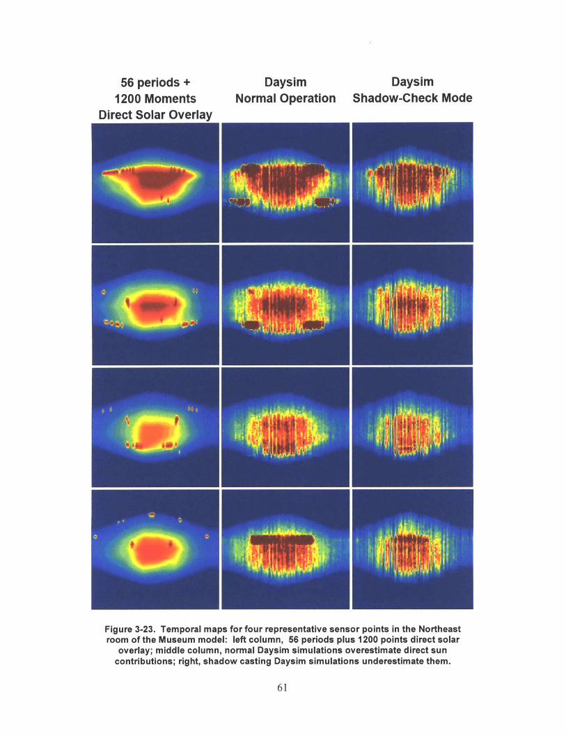
56 periods +1200 Moments

Direct Solar OverlavNormal Operation Shadow-Check Mode

Figure 3-23. Temporal maps for four representative sensor points in the Northeastroom of the Museum model: left column, 56 periods plus 1200 points direct solar

overlay; middle column, normal Daysim simulations overestimate direct suncontributions; right, shadow casting Daysim simulations underestimate them.

DaysimDaysim

this calculation must be performed for one sensor point at a time, only four points in themuseum model were tested using shadow casting. As shown through a sample ofpoints in Figure 3-23 (one point per row), every sensor using the shadow-check methodrecords a drop in direct sun contribution in comparison with conventional Daysimsimulations. However, a visual comparison suffices to show the good correlationbetween the shadow casting Daysim temporal maps and the general illuminances levelsof the weighted temporal maps. The combination of the simplified annual performanceanalysis with this detailed direct sun penetration check allows a designer to grasp, at aglance, how lighting conditions will vary over time for that particular location's climate -and also to point out when there might be comfort or performance issues due to directsunlight.

3.6 Summary of the Data Reduction Method

The overwhelming amount of information possible in an annual data set and thecomputation time of producing large numbers of renderings are arguments in favor ofusing a small number of simulations to represent a full year. However, the skyconditions used in these simulations must be very carefully chosen in order to ensure areasonably accurate representation of the annual weather conditions. TypicalMeteorological Year data was used to define average luminances for four distinct skytypes over each of 56 temporal periods, and these skies became the input for realisticsimulations. The simulated illuminances were then weighted by the frequency ofoccurrence of each type of sky. Results were compared numerically and visually todetailed data for the cube (external), shoebox (simple), and museum (complex) models.

The comparisons show a strong visual and numerical correlation between temporalmaps produced using the data reduction method and those produced using detailedilluminance data extracted from the program Daysim. The result of data reductionmethod is that small details and the sense of immediate weather changeability are lost,while the changeability of performance on an annual scale is retained, and even madeclearer.

However, validation studies found this to be insufficient for accurately depicting the effectof direct sunlight in more complex structures. Therefore, a much greater number ofdirect sun-only simulations are included and the more detailed information overlaid onthe diffuse light-based temporal maps. This extra step is less necessary in cases whereareas of interest are large, as a modest change in sun angle can still be captured by thelarger sensor plane. As areas of interest, or sensor planes, get smaller, there is agreater chance that direct light will miss the sensors if such a limited number of solarpositions are simulated.

Chapter 4

Acceptable Illuminance ExtentThe data reduction method described and validated in Chapter 3 makes it possible toeasily display useful illuminance data as it varies over time. However, there are alsospatial dimensions to consider, since daylighting analysis almost always involves morethan one or two reference sensor points. Because of the physical limitations of the shortterm memory [Simon, 1969], we are only able to imperfectly assimilate a few graphsbefore the amount of data involved becomes overwhelming. Therefore, a single graphicwhich encompasses both spatial and temporal data at once would be a great asset tothe design process - and this is the reason why Daylight Autonomy (DA) (see Section2.1) is such a valuable metric. Unfortunately, although its calculation involves annualdata sets, DA is primarily a spatial metric, whereas this thesis has argued that it isimportant to know the temporal variation in daylighting performance (Chapter 3).

Section 2.2 discussed the existing research on displaying daylighting data usingtemporal maps, which includes work done by Mardaljevic [Mardaljevic, 2003] and thesimulation tools LightSketch and Building Design Advisor [Papamichael, 1998; Glaseret al., 2003]. All use single point illuminance data to populate their spatial and temporalgraphics, and the author has found little precedent for including spatial information in atemporal map format. Glaser's work on "space series" graphs starts in a temporalformat and attempts to overlay instances of spatial data [Glaser & Hearst, 1999],however this method is very limited in the complexity of model it can handle, and theresulting images are very confusing. In fact, the only successful precedents forcombining temporal and spatial information in a single graphic are the spatially-basedDaylight Autonomy and Useful Daylight Illuminance (UDI) [Reinhart & Herkel, 2000;Nabil & Mardaljevic 2005].

DA and UDI sacrifice an understanding of the time-based variability of performance infavor of retaining the spatial variability of performance. In other words, DA can showthat for 70% of annual working hours, a particular point has adequate daylight, but itcannot show whether this point is underperforming in the morning hours, or letting in toomuch light in the summer. Understanding how daylighting data varies over anarchitectural space can help a designer identify problems in light distribution, whichmight relate to wall reflectance or room shape. Understanding how daylighting datavaries over time can help a designer identify problems in light access, such as buildingorientation, building form, and window size. Both temporal and spatial formats arecrucial to an ultimate assessment of daylighting performance, but schematic design isone of easiest times to fix problems with light access, which are more easily linked withtemporal data.

Reversing DA's approach, this chapter describes a metric which condenses the portionof a pre-defined area, in which the illuminance stays within a user-given range, to asingle percent and displays the variation of that percent over time. Because this metricis, in essence, defining the amount of space which stays within acceptable limits, it iscalled the Acceptable Illuminance Extent, or AIE. The first part of this chapter introducesthe concept of AIE, and the second part visually compares temporal graphs of AIE

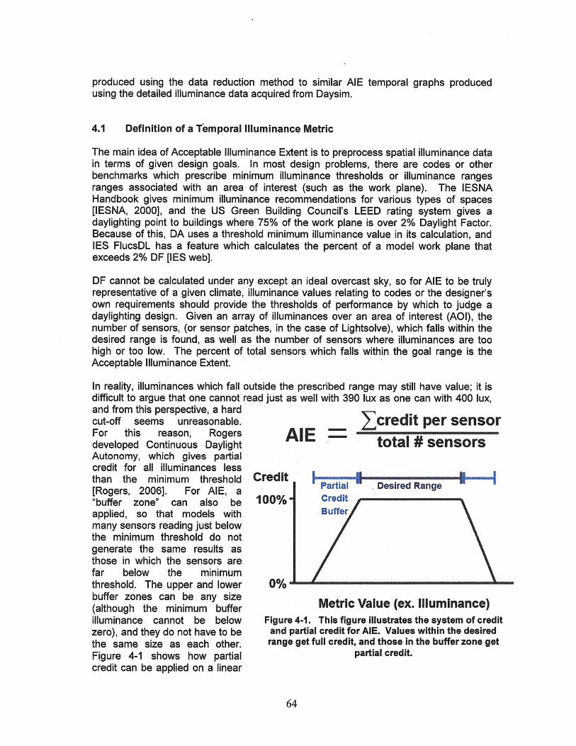
produced using the data reduction method to similar AIE temporal graphs producedusing the detailed illuminance data acquired from Daysim.

4.1 Definition of a T'emporal Illuminance Metric

The main idea of Acceptable Illuminance Extent is to preprocess spatial illuminance datain terms of given design goals. In most design problems, there are codes or otherbenchmarks which prescribe minimum illuminance thresholds or illuminance rangesranges associated with an area of interest (such as the work plane). The IESNAHandbook gives minimum illuminance recommendations for various types of spaces[IESNA, 2000], and the US Green Building Council's LEED rating system gives adaylighting point to buildings where 75% of the work plane is over 2% Daylight Factor.Because of this, DA uses a threshold minimum illuminance value in its calculation, andIES FlucsDL has a feature which calculates the percent of a model work plane thatexceeds 2% DF [IES web].

DF cannot be calculated under any except an ideal overcast sky, so for AIE to be trulyrepresentative of a given climate, illuminance values relating to codes or the designer'sown requirements should provide the thresholds of performance by which to judge adaylighting design. Given an array of illuminances over an area of interest (AOI), thenumber of sensors, (or sensor patches, in the case of Lightsolve), which falls within thedesired range is found, as well as the number of sensors where illuminances are toohigh or too low. The percent of total sensors which falls within the goal range is theAcceptable Illuminance Extent.

In reality, illuminances which fall outside the prescribed range may still have value; it isdifficult to argue that one cannot read just as well with 390 lux as one can with 400 lux,and from this perspective, a hardcut-off seems unreasonable.For this reason, Rogersdeveloped Continuous DaylightAutonomy, which gives partialcredit for all illuminances lessthan the minimum threshold[Rogers, 2006]. For AIE, a"buffer zone" can also beapplied, so that models withmany sensors reading just belowthe minimum threshold do notgenerate the same results asthose in which the sensors arefar below the minimumthreshold. The upper and lowerbuffer zones can be any size(although the minimum bufferilluminance cannot be belowzero), and they do not have to bethe same size as each other.Figure 4-1 shows how partialcredit can be applied on a linear

AIE

Credit

100%

0%

1credit per sensortotal # sensors

I INl

Metric Value (ex. Illuminance)Figure 4-1. This figure illustrates the system of credit

and partial credit for AlE. Values within the desiredrange get full credit, and those in the buffer zone get

partial credit.

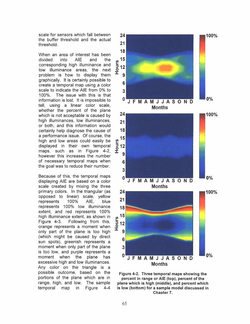
scale for sensors which fall betweenthe buffer threshold and the actualthreshold.

When an area of interest has beendivided into AIE and thecorresponding high illuminance andlow illuminance areas, the nextproblem is how to display themgraphically. It is certainly possible tocreate a temporal map using a colorscale to indicate the AIE from 0% to100%. The issue with this is thatinformation is lost. It is impossible totell, using a linear color scale,whether the percent of the planewhich is not acceptable is caused byhigh illuminances, low illuminances,or both, and this information wouldcertainly help diagnose the cause ofa performance issue. Of course, thehigh and low areas could easily bedisplayed in their own temporalmaps, such as in Figure 4-2,however this increases the numberof necessary temporal maps whenthe goal was to reduce their number.

Because of this, the temporal mapsdisplaying AIE are based on a colorscale created by mixing the threeprimary colors. In the triangular (asopposed to linear) scale, yellowrepresents 100% AIE, bluerepresents 100% low illuminanceextent, and red represents 100%high illuminance extent, as shown inFigure 4-3. Following from this,orange represents a moment whenonly part of the plane is too high(which might be caused by directsun spots), greenish represents amoment when only part of the planeis too low, and purple represents amoment when the plane hasexcessive high and low illuminances.Any color on the triangle is apossible outcome, based on theportions of the plane which are inrange, high, and low. The sampletemporal map in Figure 4-4

VI J JPMonths

J F M A M J J A 5 O N DMonths

24

21

18

12

6

3

0 J F MA M J JA SO NDMonths

Figure 4-2. Three temporal maps showing thepercent in range or AlE (top), percent of the

plane which is high (middle), and percent whichis low (bottom) for a sample model discussed in

Chaoter 7.

100%

0%

100%

0%

100%

0%

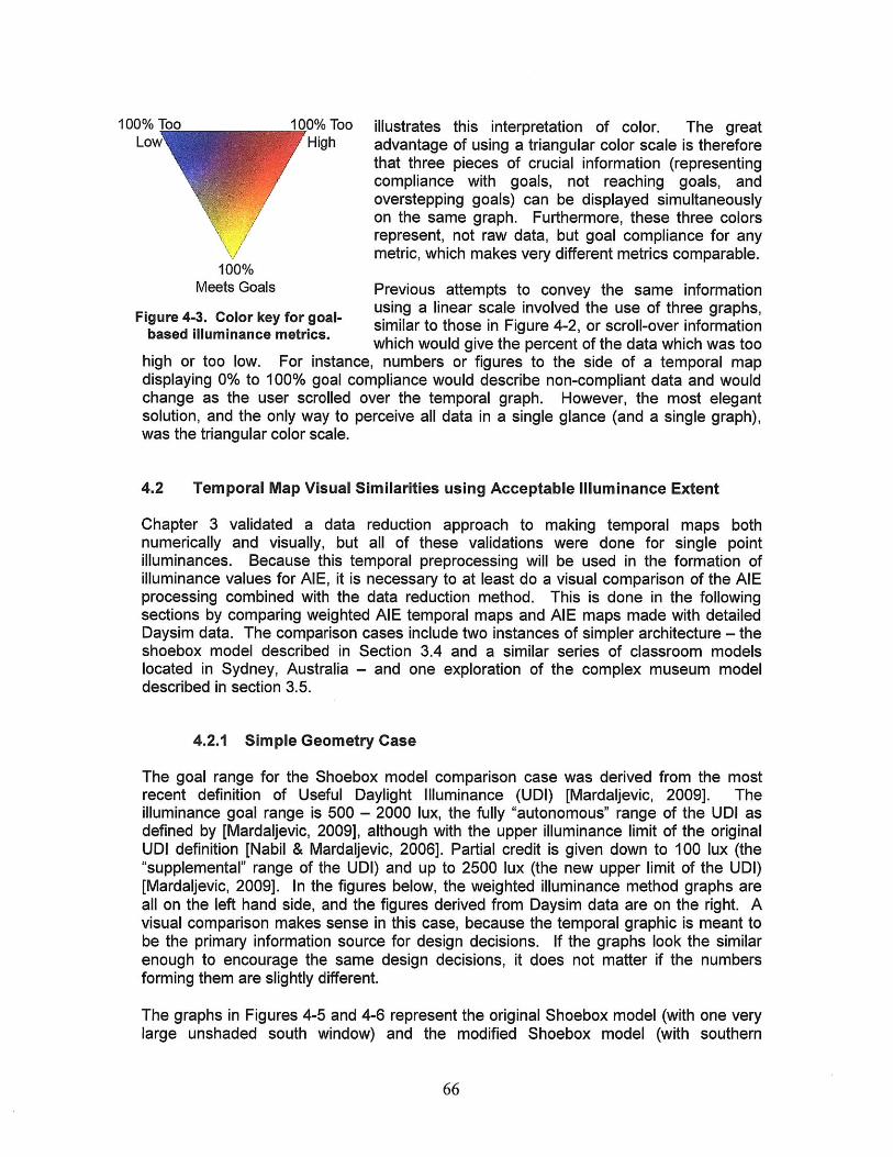
100% Too 100% Too illustrates this interpretation of color. The greatLow High advantage of using a triangular color scale is therefore

that three pieces of crucial information (representingcompliance with goals, not reaching goals, andoverstepping goals) can be displayed simultaneouslyon the same graph. Furthermore, these three colorsrepresent, not raw data, but goal compliance for anymetric, which makes very different metrics comparable.

100%Meets Goals Previous attempts to convey the same information

Figure 4-3. Color key for goal- using a linear scale involved the use of three graphs,based illuminance metrics. similar to those in Figure 4-2, or scroll-over information

which would give the percent of the data which was toohigh or too low. For instance, numbers or figures to the side of a temporal mapdisplaying 0% to 100% goal compliance would describe non-compliant data and wouldchange as the user scrolled over the temporal graph. However, the most elegantsolution, and the only way to perceive all data in a single glance (and a single graph),was the triangular color scale.

4.2 Temporal Map Visual Similarities using Acceptable Illuminance Extent

Chapter 3 validated a data reduction approach to making temporal maps bothnumerically and visually, but all of these validations were done for single pointilluminances. Because this temporal preprocessing will be used in the formation ofilluminance values for AIE, it is necessary to at least do a visual comparison of the AIEprocessing combined with the data reduction method. This is done in the followingsections by comparing weighted AIE temporal maps and AIE maps made with detailedDaysim data. The comparison cases include two instances of simpler architecture - theshoebox model described in Section 3.4 and a similar series of classroom modelslocated in Sydney, Australia - and one exploration of the complex museum modeldescribed in section 3.5.

4.2.1 Simple Geometry Case

The goal range for the Shoebox model comparison case was derived from the mostrecent definition of Useful Daylight Illuminance (UDI) [Mardaljevic, 2009]. Theilluminance goal range is 500 - 2000 lux, the fully "autonomous" range of the UDI asdefined by [Mardaljevic, 2009], although with the upper illuminance limit of the originalUDI definition [Nabil & Mardaljevic, 2006]. Partial credit is given down to 100 lux (the"supplemental" range of the UDI) and up to 2500 lux (the new upper limit of the UDI)[Mardaljevic, 2009]. In the figures below, the weighted illuminance method graphs areall on the left hand side, and the figures derived from Daysim data are on the right. Avisual comparison makes sense in this case, because the temporal graphic is meant tobe the primary information source for design decisions. If the graphs look the similarenough to encourage the same design decisions, it does not matter if the numbersforming them are slightly different.

The graphs in Figures 4-5 and 4-6 represent the original Shoebox model (with one verylarge unshaded south window) and the modified Shoebox model (with southern

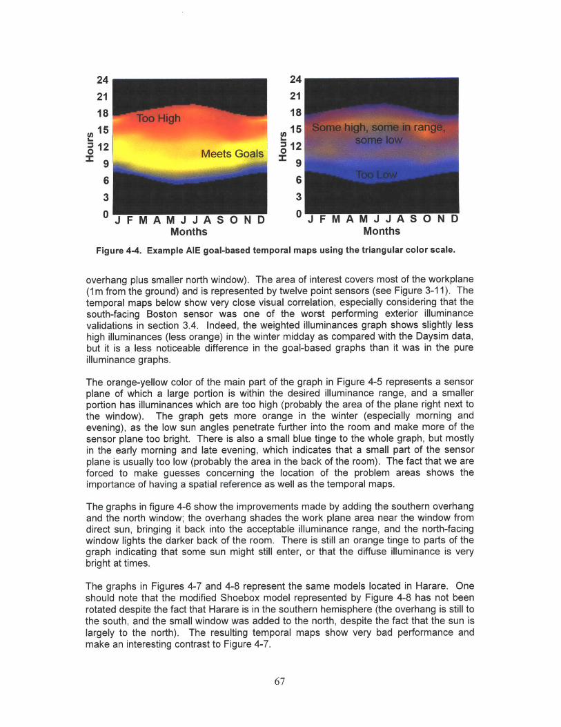
24 24

21 2118 1815 15

12 3 120 Meets Goals 0

9 9

63

Months Months

Figure 4-4. Example AIE goal-based temporal maps using the triangular color scale.

overhang plus smaller north window). The area of interest covers most of the workplane(1 m from the ground) and is represented by twelve point sensors (see Figure 3-11). Thetemporal maps below show very close visual correlation, especially considering that thesouth-facing Boston sensor was one of the worst performing exterior illuminancevalidations in section 3.4. Indeed, the weighted illuminances graph shows slightly lesshigh illuminances (less orange) in the winter midday as compared with the Daysim data,but it is a less noticeable difference in the goal-based graphs than it was in the pureilluminance graphs.

The orange-yellow color of the main part of the graph in Figure 4-5 represents a sensorplane of which a large portion is within the desired illuminance range, and a smallerportion has illuminances which are too high (probably the area of the plane right next tothe window). The graph gets more orange in the winter (especially morning andevening), as the low sun angles penetrate further into the room and make more of thesensor plane too bright. There is also a small blue tinge to the whole graph, but mostlyin the early morning and late evening, which indicates that a small part of the sensorplane is usually too low (probably the area in the back of the room). The fact that we areforced to make guesses concerning the location of the problem areas shows theimportance of having a spatial reference as well as the temporal maps.

The graphs in figure 4-6 show the improvements made by adding the southern overhangand the north window; the overhang shades the work plane area near the window fromdirect sun, bringing it back into the acceptable illuminance range, and the north-facingwindow lights the darker back of the room. There is still an orange tinge to parts of thegraph indicating that some sun might still enter, or that the diffuse illuminance is verybright at times.

The graphs in Figures 4-7 and 4-8 represent the same models located in Harare. Oneshould note that the modified Shoebox model represented by Figure 4-8 has not beenrotated despite the fact that Harare is in the southern hemisphere (the overhang is still tothe south, and the small window was added to the north, despite the fact that the sun islargely to the north). The resulting temporal maps show very bad performance andmake an interesting contrast to Figure 4-7.

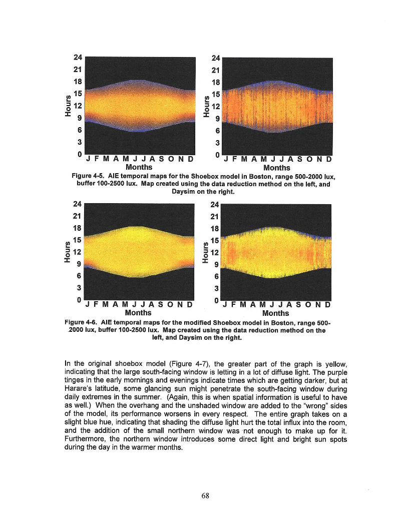
24 2421 2118 1815 15

i 12 120o 129 96 63 30 J F M A M J J A S 0 N D J F M A M J A S 0 N D

Months MonthsFigure 4-5. AlE temporal maps for the Shoebox model in Boston, range 500-2000 lux,

buffer 100-2500 lux. Map created using the data reduction method on the left, andDaysim on the right.

24

21 21

1818

155

12 12

9

6

3

00

Months MonthsFigure 4-6. AlE temporal maps for the modified Shoebox model in Boston, range 500--2000 lux, buffer 100-2500 lux. Map created using the data reduction method on the

left, and Daysim on the right.

In the original shoebox model (Figure 4-7), the greater part of the graph is yellow,indicating that the large south-facing window is letting in a lot of diffuse light. The purpletinges in the early mornings and evenings indicate times which are getting darker, but atHarare's latitude, some glancing sun might penetrate the south-facing window duringdaily extremes in the summer. (Again, this is when spatial information is useful to haveas well.) When the overhang and the unshaded window are added to the "Awrong" sidesof the model, its performance worsens in every respect. The entire graph takes on aslight blue hue, indicating that shading the diffuse light hurt the total influx into the room,and the addition of the small northern window was not enough to make up for it.Furthermore, the northern window introduces some direct light and bright sun spotsduring the day in the warmer months.

.... .... ...... ...... .. --- -------- ---__ ... ..... ... ......

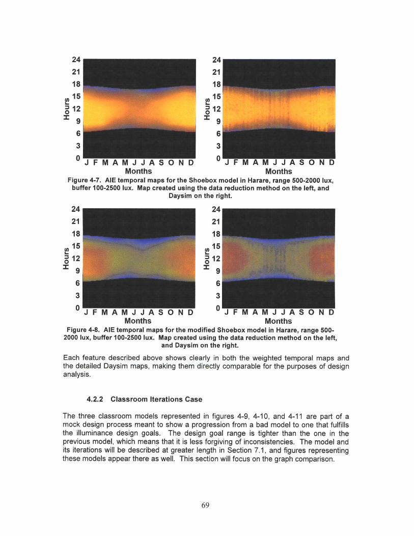
24 24

21 21

18 18

15 15

012 01299

6 6

3 3

0 JFMAMJJAS NID0JFMAMJJASONDMonths Months

Figure 4-7. AlE temporal maps for the Shoebox model in Harare, range 500-2000 lux,buffer 100-2500 lux. Map created using the data reduction method on the left, and

Daysim on the right.

24 24

21 21

18 18

015 01512 12

19 19

6 6

3 3

0 J FM A MJ J ASOND 0J F MA MJJ A SON DMonths Months

Figure 4-8. AlE temporal maps for the modified Shoebox model in Harare, range 500-2000 lux, buffer 100-2500 lux. Map created using the data reduction method on the left,

and Daysim on the right.

Each feature described above shows clearly in both the weighted temporal maps andthe detailed Daysim maps, making them directly comparable for the purposes of designanalysis.

4.2.2 Classroom Iterations Case

The three classroom models represented in figures 4-9, 4-10, and 4-11 are part of amock design process meant to show a progression from a bad model to one that fulfillsthe illuminance design goals. The design goal range is tighter than the one in theprevious model, which means that it is less forgiving of inconsistencies. The model andits iterations will be described at greater length in Section 7.1, and figures representingthese models appear there as well. This section will focus on the graph comparison.

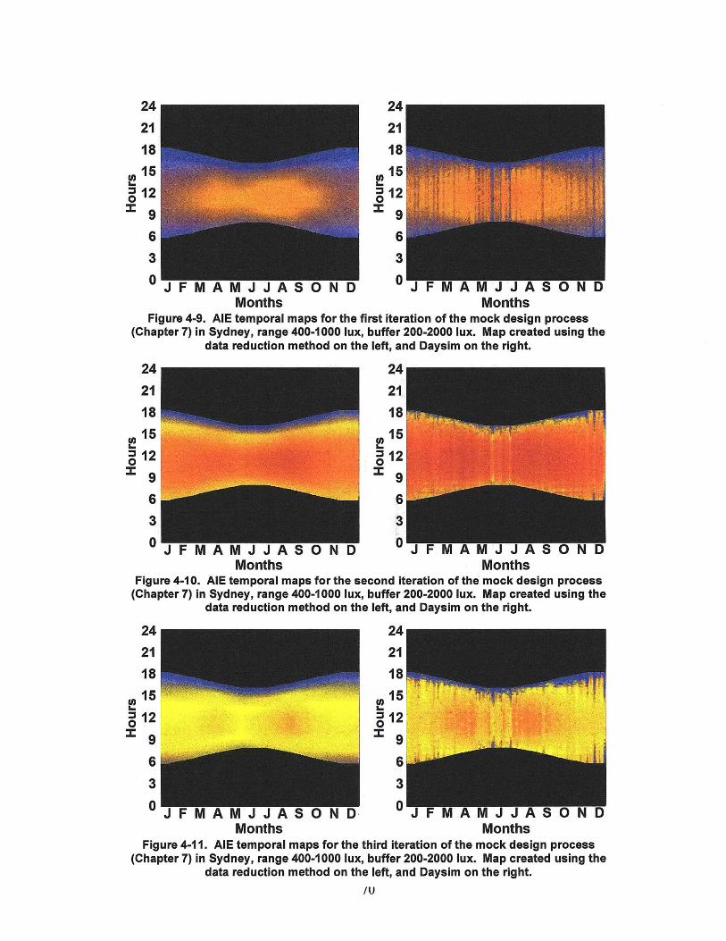
J 1- M AM J J A 5 U N U J 1- M A M J J A b U N UMonths Months

Figure 4-9. AIE temporal maps for the first iteration of the mock design process(Chapter 7) in Sydney, range 400-1000 lux, buffer 200-2000 lux. Map created using the

data reduction method on the left, and Daysim on the right.

J IVI A IM J J A b U N U J r Ivi A IVI J J A a U N UMonths Months

Figure 4-10. AlE temporal maps for the second iteration of the mock design process(Chapter 7) in Sydney, range 400-1000 lux, buffer 200-2000 lux. Map created using the

data reduction method on the left, and Daysim on the right.

J - IVI A M J J A Z U N U j r ivi P ivij j A a u N UMonths Months

Figure 4-11. AlE temporal maps for the third iteration of the mock design process(Chapter 7) in Sydney, range 400-1000 lux, buffer 200-2000 lux. Map created using the

data reduction method on the left, and Daysim on the right.

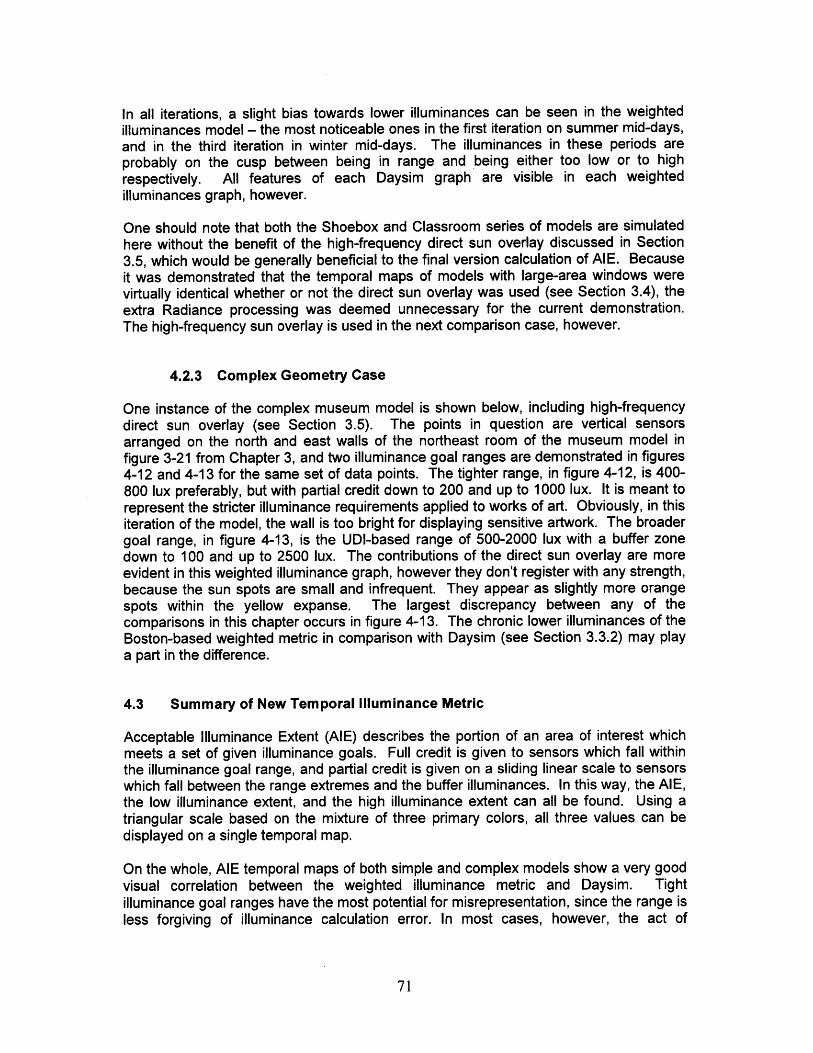
In all iterations, a slight bias towards lower illuminances can be seen in the weightedilluminances model - the most noticeable ones in the first iteration on summer mid-days,and in the third iteration in winter mid-days. The illuminances in these periods areprobably on the cusp between being in range and being either too low or to highrespectively. All features of each Daysim graph are visible in each weightedilluminances graph, however.

One should note that both the Shoebox and Classroom series of models are simulatedhere without the benefit of the high-frequency direct sun overlay discussed in Section3.5, which would be generally beneficial to the final version calculation of AIE. Becauseit was demonstrated that the temporal maps of models with large-area windows werevirtually identical whether or not the direct sun overlay was used (see Section 3.4), theextra Radiance processing was deemed unnecessary for the current demonstration.The high-frequency sun overlay is used in the next comparison case, however.

4.2.3 Complex Geometry Case

One instance of the complex museum model is shown below, including high-frequencydirect sun overlay (see Section 3.5). The points in question are vertical sensorsarranged on the north and east walls of the northeast room of the museum model infigure 3-21 from Chapter 3, and two illuminance goal ranges are demonstrated in figures4-12 and 4-13 for the same set of data points. The tighter range, in figure 4-12, is 400-800 lux preferably, but with partial credit down to 200 and up to 1000 lux. It is meant torepresent the stricter illuminance requirements applied to works of art. Obviously, in thisiteration of the model, the wall is too bright for displaying sensitive artwork. The broadergoal range, in figure 4-13, is the UDI-based range of 500-2000 lux with a buffer zonedown to 100 and up to 2500 lux. The contributions of the direct sun overlay are moreevident in this weighted illuminance graph, however they don't register with any strength,because the sun spots are small and infrequent. They appear as slightly more orangespots within the yellow expanse. The largest discrepancy between any of thecomparisons in this chapter occurs in figure 4-13. The chronic lower illuminances of theBoston-based weighted metric in comparison with Daysim (see Section 3.3.2) may playa part in the difference.

4.3 Summary of New Temporal Illuminance Metric

Acceptable Illuminance Extent (AIE) describes the portion of an area of interest whichmeets a set of given illuminance goals. Full credit is given to sensors which fall withinthe illuminance goal range, and partial credit is given on a sliding linear scale to sensorswhich fall between the range extremes and the buffer illuminances. In this way, the AIE,the low illuminance extent, and the high illuminance extent can all be found. Using atriangular scale based on the mixture of three primary colors, all three values can bedisplayed on a single temporal map.

On the whole, AIE temporal maps of both simple and complex models show a very goodvisual correlation between the weighted illuminance metric and Daysim. Tightilluminance goal ranges have the most potential for misrepresentation, since the range isless forgiving of illuminance calculation error. In most cases, however, the act of

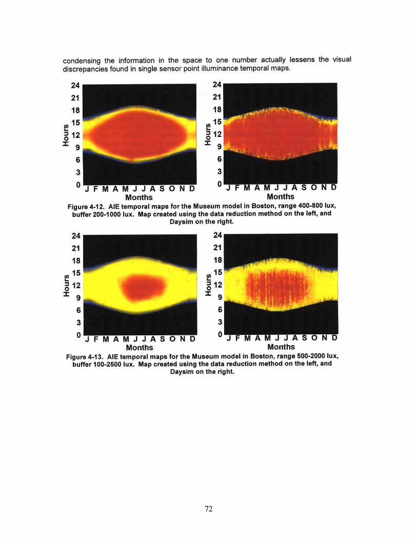
condensing the information in the space to one number actually lessens the visualdiscrepancies found in single sensor point illuminance temporal maps.

24 24

21 21

18 18

1IS 16

=12 1

9 9.

6 6

3 3

0 J F MA MJ J ASOND 0J1 A J so DMonths Months

Figure 4-12. AlE temporal maps for the Museum model in Boston, range 400-800 lux,buffer 200-1000 lux. Map created using the data reduction method on the left, and

Daysim on the right.

24

21

1815

129

6

3n

24

21

18

1512

9

6

3n

JFMAMJJASOND JFMAMJJA ONUMonths Months

Figure 4-13. AlE temporal maps for the Museum model in Boston, range 500-2000 lux,buffer 100-2500 lux. Map created using the data reduction method on the left, and

Daysim on the right.

.... .. ...... ... ... ......

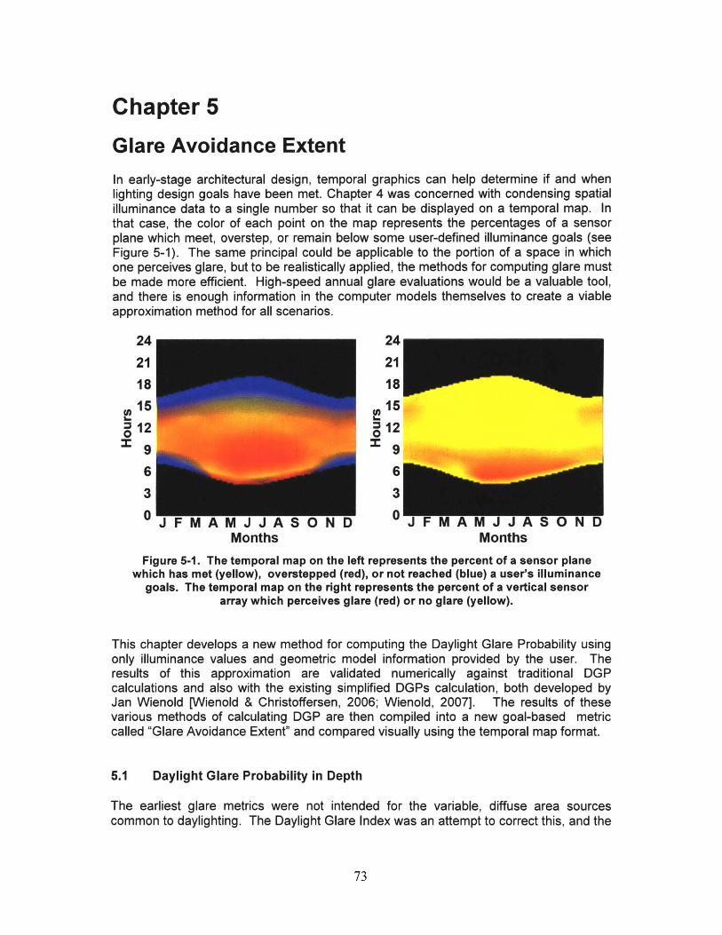
Chapter 5

Glare Avoidance ExtentIn early-stage architectural design, temporal graphics can help determine if and whenlighting design goals have been met. Chapter 4 was concerned with condensing spatialilluminance data to a single number so that it can be displayed on a temporal map. Inthat case, the color of each point on the map represents the percentages of a sensorplane which meet, overstep, or remain below some user-defined illuminance goals (seeFigure 5-1). The same principal could be applicable to the portion of a space in whichone perceives glare, but to be realistically applied, the methods for computing glare mustbe made more efficient. High-speed annual glare evaluations would be a valuable tool,and there is enough information in the computer models themselves to create a viableapproximation method for all scenarios.

24 24

21 21

18 1815 15

~~1212 = 12

6 6

J F M A M J J A S O N D J F M A M J J A S O N DMonths Months

Figure 5-1. The temporal map on the left represents the percent of a sensor planewhich has met (yellow), overstepped (red), or not reached (blue) a user's illuminance

goals. The temporal map on the right represents the percent of a vertical sensorarray which perceives glare (red) or no glare (yellow).

This chapter develops a new method for computing the Daylight Glare Probability usingonly illuminance values and geometric model information provided by the user. Theresults of this approximation are validated numerically against traditional DGPcalculations and also with the existing simplified DGPs calculation, both developed byJan Wienold [Wienold & Christoffersen, 2006; Wienold, 2007]. The results of thesevarious methods of calculating DGP are then compiled into a new goal-based metriccalled "Glare Avoidance Extent" and compared visually using the temporal map format.

5.1 Daylight Glare Probability in Depth

The earliest glare metrics were not intended for the variable, diffuse area sourcescommon to daylighting. The Daylight Glare Index was an attempt to correct this, and the

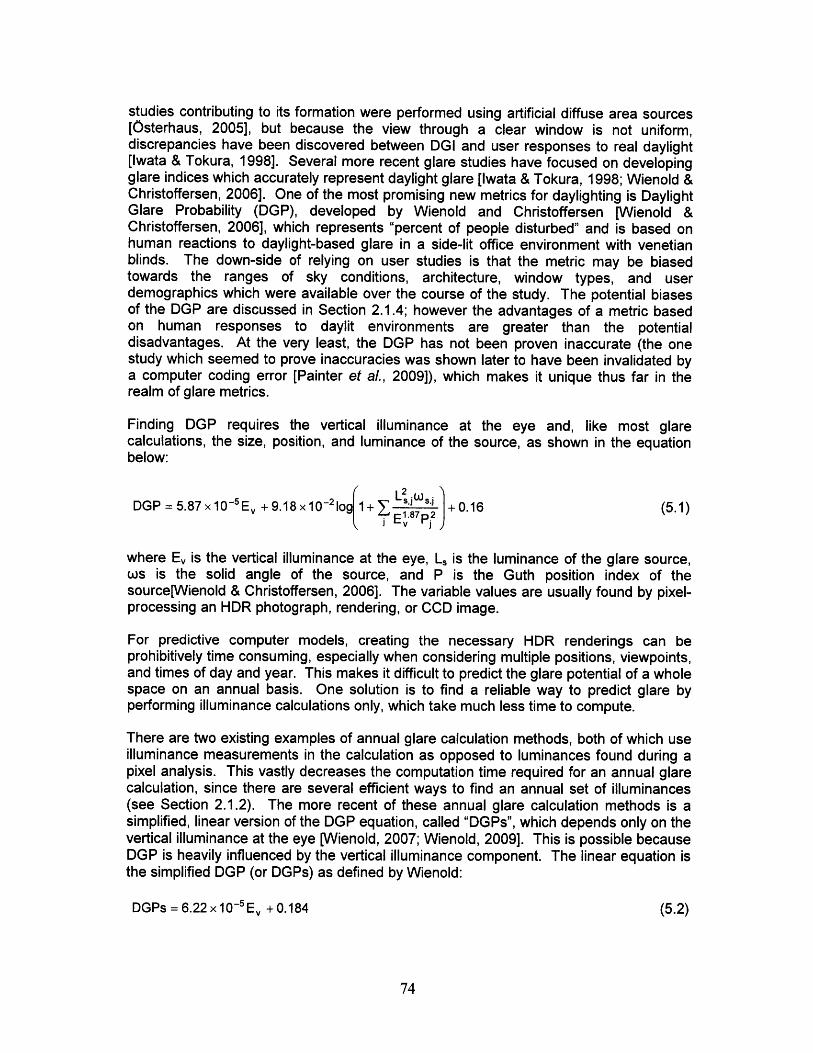
studies contributing to its formation were performed using artificial diffuse area sources[Osterhaus, 2005], but because the view through a clear window is not uniform,discrepancies have been discovered between DGI and user responses to real daylight[Iwata & Tokura, 1998]. Several more recent glare studies have focused on developingglare indices which accurately represent daylight glare [lwata & Tokura, 1998; Wienold &Christoffersen, 2006]. One of the most promising new metrics for daylighting is DaylightGlare Probability (DGP), developed by Wienold and Christoffersen [Wienold &Christoffersen, 2006], which represents "percent of people disturbed" and is based onhuman reactions to daylight-based glare in a side-lit office environment with venetianblinds. The down-side of relying on user studies is that the metric may be biasedtowards the ranges of sky conditions, architecture, window types, and userdemographics which were available over the course of the study. The potential biasesof the DGP are discussed in Section 2.1.4; however the advantages of a metric basedon human responses to daylit environments are greater than the potentialdisadvantages. At the very least, the DGP has not been proven inaccurate (the onestudy which seemed to prove inaccuracies was shown later to have been invalidated bya computer coding error [Painter et al., 2009]), which makes it unique thus far in therealm of glare metrics.

Finding DGP requires the vertical illuminance at the eye and, like most glarecalculations, the size, position, and luminance of the source, as shown in the equationbelow:

DGP = 5.87 x 10~5 E + 9.18 x 102log 1+ E.87' +0.16 (5.1)

where Ev is the vertical illuminance at the eye, Ls is the luminance of the glare source,ws is the solid angle of the source, and P is the Guth position index of thesource[Wienold & Christoffersen, 2006]. The variable values are usually found by pixel-processing an HDR photograph, rendering, or CCD image.

For predictive computer models, creating the necessary HDR renderings can beprohibitively time consuming, especially when considering multiple positions, viewpoints,and times of day and year. This makes it difficult to predict the glare potential of a wholespace on an annual basis. One solution is to find a reliable way to predict glare byperforming illuminance calculations only, which take much less time to compute.

There are two existing examples of annual glare calculation methods, both of which useilluminance measurements in the calculation as opposed to luminances found during apixel analysis. This vastly decreases the computation time required for an annual glarecalculation, since there are several efficient ways to find an annual set of illuminances(see Section 2.1.2). The more recent of these annual glare calculation methods is asimplified, linear version of the DGP equation, called "DGPs", which depends only on thevertical illuminance at the eye [Wienold, 2007; Wienold, 2009]. This is possible becauseDGP is heavily influenced by the vertical illuminance component. The linear equation isthe simplified DGP (or DGPs) as defined by Wienold:

DGPs = 6.22 x 10~5 E + 0.184 (5.2)

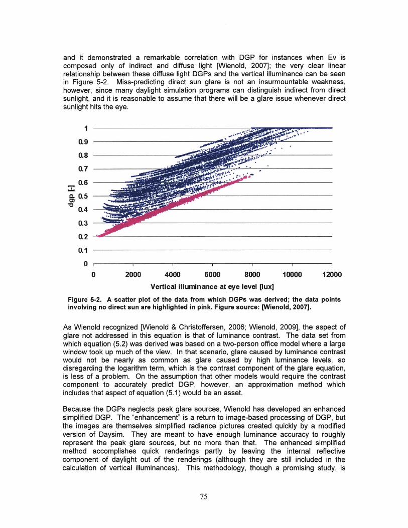
and it demonstrated a remarkable correlation with DGP for instances when Ev iscomposed only of indirect and diffuse light [Wienold, 2007]; the very clear linearrelationship between these diffuse light DGPs and the vertical illuminance can be seenin Figure 5-2. Miss-predicting direct sun glare is not an insurmountable weakness,however, since many daylight simulation programs can distinguish indirect from directsunlight, and it is reasonable to assume that there will be a glare issue whenever directsunlight hits the eye.

1

0.9

0.8

0.7

0.6

0. 5

0.4

0.2-

0.1

00 2000 4000 6000 8000 10000 12000

Vertical illuminance at eye level pux]

Figure 5-2. A scatter plot of the data from which DGPs was derived; the data pointsinvolving no direct sun are highlighted in pink. Figure source: [Wienold, 2007].

As Wienold recognized [Wienold & Christoffersen, 2006; Wienold, 2009], the aspect ofglare not addressed in this equation is that of luminance contrast. The data set fromwhich equation (5.2) was derived was based on a two-person office model where a largewindow took up much of the view. In that scenario, glare caused by luminance contrastwould not be nearly as common as glare caused by high luminance levels, sodisregarding the logarithm term, which is the contrast component of the glare equation,is less of a problem. On the assumption that other models would require the contrastcomponent to accurately predict DGP, however, an approximation method whichincludes that aspect of equation (5.1) would be an asset.

Because the DGPs neglects peak glare sources, Wienold has developed an enhancedsimplified DGP. The "enhancement" is a return to image-based processing of DGP, butthe images are themselves simplified radiance pictures created quickly by a modifiedversion of Daysim. They are meant to have enough luminance accuracy to roughlyrepresent the peak glare sources, but no more than that. The enhanced simplifiedmethod accomplishes quick renderings partly by leaving the internal reflectivecomponent of daylight out of the renderings (although they are still included in thecalculation of vertical illuminances). This methodology, though a promising study, is

................ dim W

currently still a work in progress. It is also limited by its dependence on renderings,however quick. Not only does it still take time to process each image, the renderings arestill position and view dependent, which means that simulating glare over an array ofsensors would somewhat increase the computation involved.

The other annual glare calculation method is the one employed by the Building DesignAdvisor [Papamichael et al., 1998]. Originally developed by Winkelmann and Selkowitzfor use with DOE-2, it computes the Daylight Glare Index (see Section 2.1.3) fromreference points using illuminance values and building geometry to approximate theappropriate variables [Winkelmann & Selkowitz, 1985]. Specifically, the DGI formuladepends on source luminance (Ls), background luminance (Lb), solid angle of the source(w), and the solid angle of the source modified by its deviation from the line of sight (0)(see Appendix A). Building Design Advisor assumes that each full window is a glaresource. f and w are both geometric properties, which can be found using the model'sgeometric data, and the program already calculates annual sets of illuminance values[Hitchcock & Carroll, 2003]. Lb, which is measured in cd/m 2, is found using the equationLb = EbPb, where Eb represents the average illuminance falling on the walls and othersurfaces near the window, and Pb is the average surface reflectance of the whole room[Winkelmann & Selkowitz, 1985]. One inexplicable factor in this approximation is thatthe relationship (in SI units) between luminance and illuminance for a lambertian surfaceusually includes a factor of r in the denominator, or Lsurf = Esurfpsurf/rr. Finally,Winkelmann and Selkowitz do not specify how L. is found.

Although approximation based on illuminance and known geometry is a promising idea,this uncertainty in the definition of luminance values lends some doubt to the accuracy ofthe method, since the luminance values (especially source luminance) have great impacton the outcome of the glare index. Furthermore, the method by which Building DesignAdvisor finds illuminance already includes substantial approximation (see Section 2.1.2).The author was not able to find any validation done for this glare approximation method.

5.2 Deriving a Model-Based DGP Approximation

Any method using pixel analysis to find glare is inevitably still limiting the number of viewpoints and directions which can be processed at each moment, since a separate imagemust be created for each view. On the other hand, any number of reference pointilluminances may be found in a single simulation, and in the case of radiosity, withalmost no impact on computation time. Because of this, and because the geometry andsky distribution are all mathematically defined in the model, there should be areasonably accurate way to calculate the original DGP equation using approximatedvariables. To get any kind of accuracy, however, each variable approximation needs tobe done carefully and as accurately as possible.

The variables that must be found to complete the DGP equation (5.1) are the luminanceof each glare source (Ls), the solid angle of each source (w,), and the position of eachsource (P). Vertical illuminance (Ev) is calculated directly in the simulation. The glaresources must be identified and defined, a task which can be a challenge even fortraditional daylight glare analysis. On the other hand, if one is working inside a daylightmodeling program, there are certain inherent advantages. The approximation methodpresented below is based on variables that are already defined in any daylighting model,so it is called the model-based DGP, or DGPm.

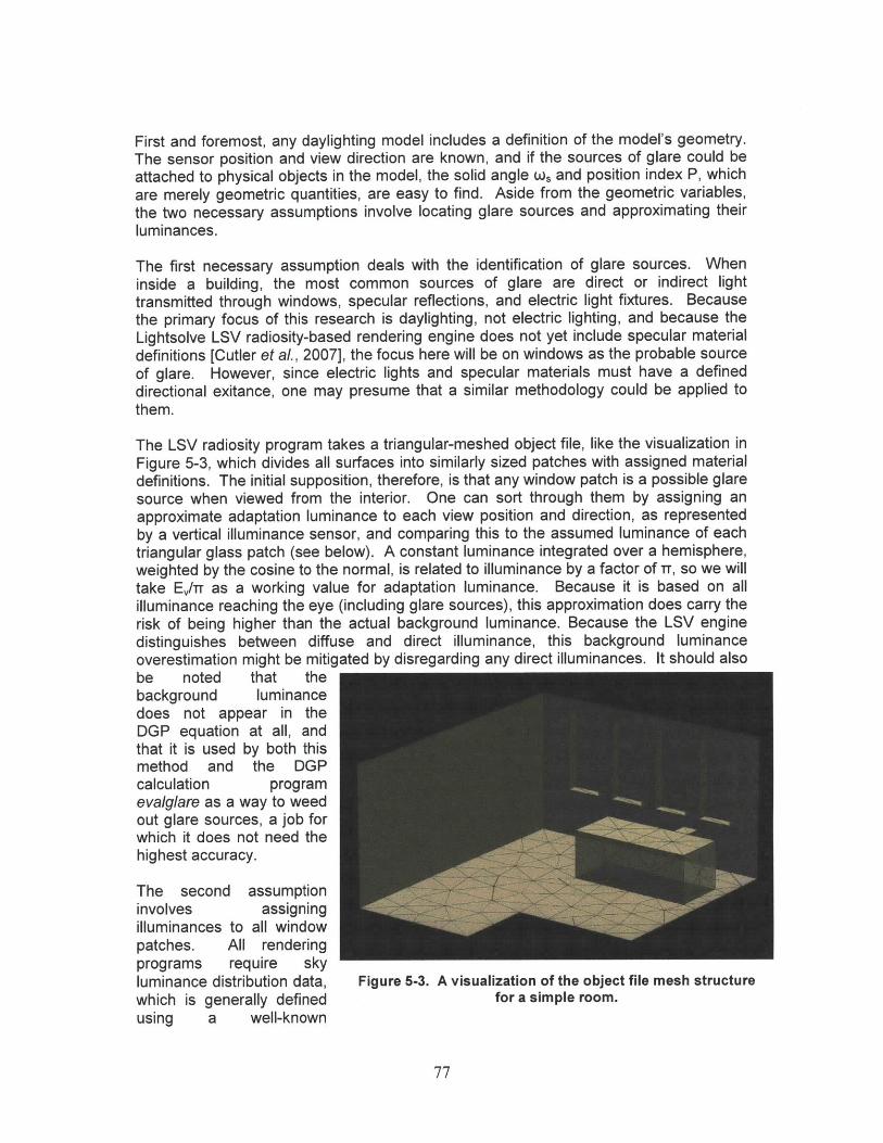
First and foremost, any daylighting model includes a definition of the model's geometry.The sensor position and view direction are known, and if the sources of glare could beattached to physical objects in the model, the solid angle w and position index P, whichare merely geometric quantities, are easy to find. Aside from the geometric variables,the two necessary assumptions involve locating glare sources and approximating theirluminances.

The first necessary assumption deals with the identification of glare sources. Wheninside a building, the most common sources of glare are direct or indirect lighttransmitted through windows, specular reflections, and electric light fixtures. Becausethe primary focus of this research is daylighting, not electric lighting, and because theLightsolve LSV radiosity-based rendering engine does not yet include specular materialdefinitions [Cutler et al., 2007], the focus here will be on windows as the probable sourceof glare. However, since electric lights and specular materials must have a defineddirectional exitance, one may presume that a similar methodology could be applied tothem.

The LSV radiosity program takes a triangular-meshed object file, like the visualization inFigure 5-3, which divides all surfaces into similarly sized patches with assigned materialdefinitions. The initial supposition, therefore, is that any window patch is a possible glaresource when viewed from the interior. One can sort through them by assigning anapproximate adaptation luminance to each view position and direction, as representedby a vertical illuminance sensor, and comparing this to the assumed luminance of eachtriangular glass patch (see below). A constant luminance integrated over a hemisphere,weighted by the cosine to the normal, is related to illuminance by a factor of Tr, so we willtake E/Tr as a working value for adaptation luminance. Because it is based on allilluminance reaching the eye (including glare sources), this approximation does carry therisk of being higher than the actual background luminance. Because the LSV enginedistinguishes between diffuse and direct illuminance, this background luminanceoverestimation might be mitigated by disregarding any direct illuminances. It should alsobe noted that thebackground luminancedoes not appear in theDGP equation at all, andthat it is used by both thismethod and the DGPcalculation programevalglare as a way to weedout glare sources, a job forwhich it does not need thehighest accuracy.

The second assumptioninvolves assigningilluminances to all windowpatches. All renderingprograms require skyluminance distribution data, Figure 5-3. A visualization of the object file mesh structurewhich is generally defined for a simple room.using a well-known

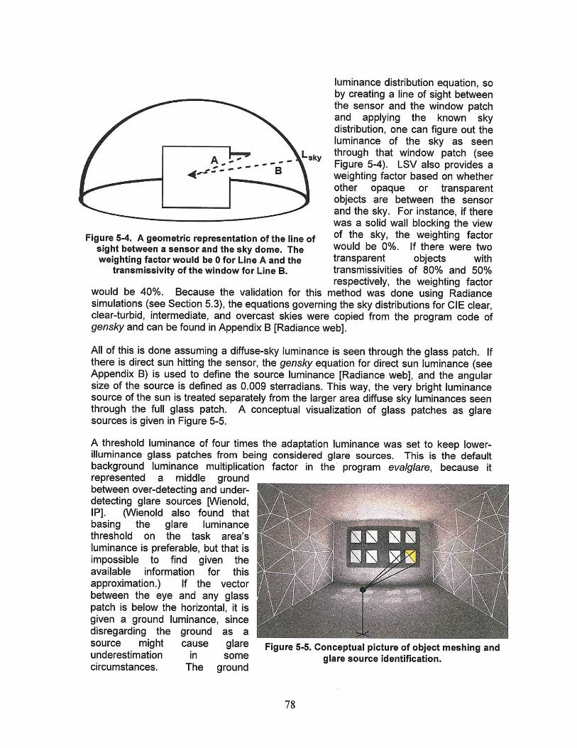
luminance distribution equation, soby creating a line of sight betweenthe sensor and the window patchand applying the known skydistribution, one can figure out theluminance of the sky as seen

A -y through that window patch (seeFigure 5-4). LSV also provides aweighting factor based on whetherother opaque or transparentobjects are between the sensorand the sky. For instance, if therewas a solid wall blocking the view

igure 5-4. A geometric representation of the line of of the sky, the weighting factorsight between a sensor and the sky dome. The would be 0%. If there were twoweighting factor would be 0 for Line A and the transparent objects with

transmissivity of the window for Line B. transmissivities of 80% and 50%respectively, the weighting factor

would be 40%. Because the validation for this method was done using Radiancesimulations (see Section 5.3), the equations governing the sky distributions for CIE clear,clear-turbid, intermediate, and overcast skies were copied from the program code ofgensky and can be found in Appendix B [Radiance web].

All of this is done assuming a diffuse-sky luminance is seen through the glass patch. Ifthere is direct sun hitting the sensor, the gensky equation for direct sun luminance (seeAppendix B) is used to define the source luminance [Radiance web], and the angularsize of the source is defined as 0.009 sterradians. This way, the very bright luminancesource of the sun is treated separately from the larger area diffuse sky luminances seenthrough the full glass patch. A conceptual visualization of glass patches as glaresources is given in Figure 5-5.

A threshold luminance of four times the adaptation luminance was set to keep lower-illuminance glass patches from being considered glare sources. This is the defaultbackground luminance multiplication factor in the program evalg/are, because itrepresented a middle groundbetween over-detecting and under-detecting glare sources [Wienold,IP]. (Wienold also found thatbasing the glare luminancethreshold on the task area'sluminance is preferable, but that isimpossible to find given theavailable information for thisapproximation.) If the vectorbetween the eye and any glasspatch is below the horizontal, it isgiven a ground luminance, sincedisregarding the ground as asource might cause glare Figure 5-5. Conceptual picture of object meshing anunderestimation in some glare source identification.circumstances. The ground

F

d

...... ...... . . .. .... ... .. ......... .. .... .

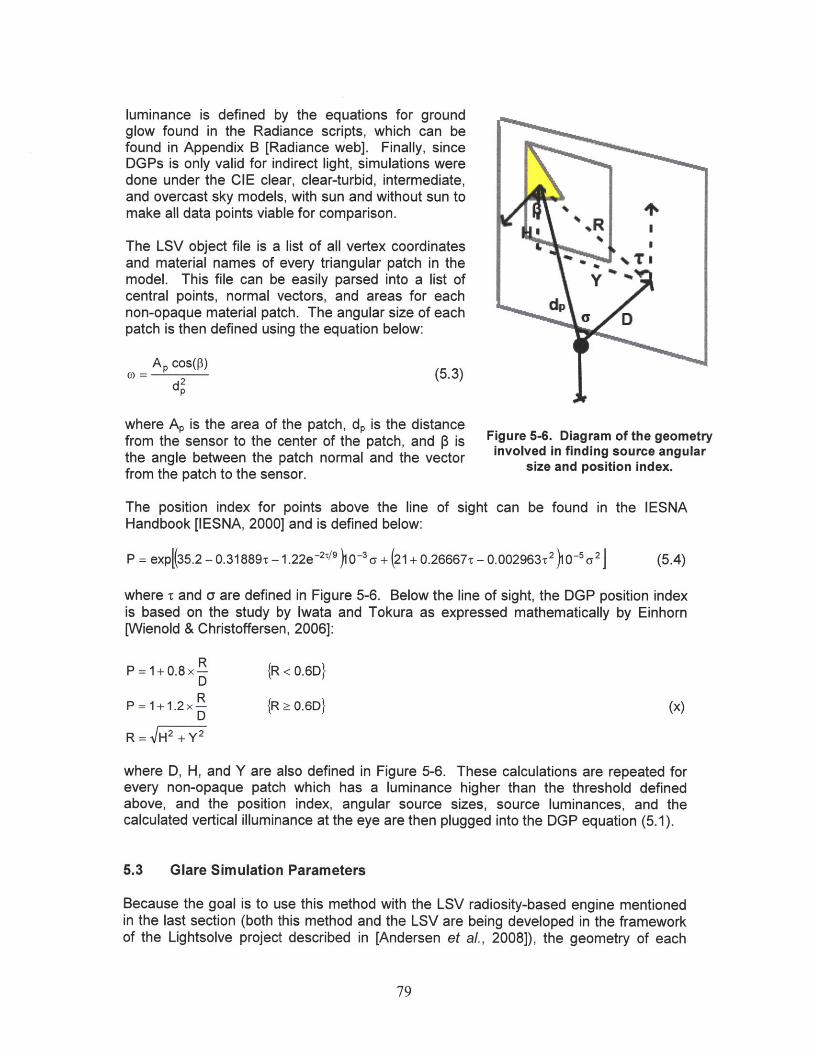
luminance is defined by the equations for groundglow found in the Radiance scripts, which can befound in Appendix B [Radiance web]. Finally, sinceDGPs is only valid for indirect light, simulations weredone under the CIE clear, clear-turbid, intermediate,and overcast sky models, with sun and without sun tomake all data points viable for comparison.

The LSV object file is a list of all vertex coordinatesand material names of every triangular patch in the Tmodel. This file can be easily parsed into a list ofcentral points, normal vectors, and areas for eachnon-opaque material patch. The angular size of eachpatch is then defined using the equation below:

= cos() (5.3)

where AP is the area of the patch, dp is the distancefrom the sensor to the center of the patch, and P is Figure 5-6. Diagram of the geometrythe angle between the patch normal and the vector involved in finding source angularfrom the patch to the sensor. size and position index.

The position index for points above the line of sight can be found in the IESNAHandbook [IESNA, 2000] and is defined below:

P = exp 35.2 - 0.31889t -1.22e2,9 0~3a + (21 + 0.26667c - 0.002963-2)0-5 a2 (5.4)

where T and a are defined in Figure 5-6. Below the line of sight, the DGP position indexis based on the study by Iwata and Tokura as expressed mathematically by Einhorn[Wienold & Christoffersen, 2006]:

P = 1+ 0.8 x {R < 0.6D}D

P = 1+1.2 x RR > 0.6D (x)

R = H2 +Y 2

where D, H, and Y are also defined in Figure 5-6. These calculations are repeated forevery non-opaque patch which has a luminance higher than the threshold definedabove, and the position index, angular source sizes, source luminances, and thecalculated vertical illuminance at the eye are then plugged into the DGP equation (5.1).

5.3 Glare Simulation Parameters

Because the goal is to use this method with the LSV radiosity-based engine mentionedin the last section (both this method and the LSV are being developed in the frameworkof the Lightsolve project described in [Andersen et al., 2008]), the geometry of each

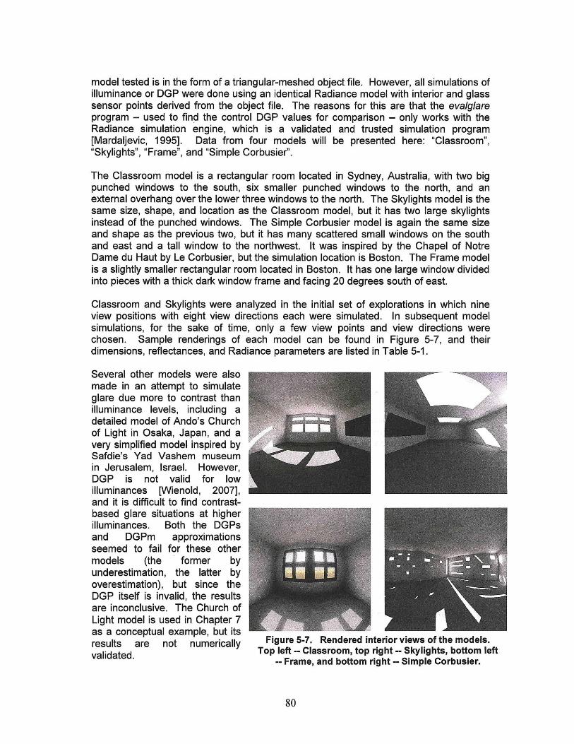
model tested is in the form of a triangular-meshed object file. However, all simulations ofilluminance or DGP were done using an identical Radiance model with interior and glasssensor points derived from the object file. The reasons for this are that the evalglareprogram - used to find the control DGP values for comparison - only works with theRadiance simulation engine, which is a validated and trusted simulation program[Mardaljevic, 1995]. Data from four models will be presented here: "Classroom","Skylights", "Frame", and "Simple Corbusier".

The Classroom model is a rectangular room located in Sydney, Australia, with two bigpunched windows to the south, six smaller punched windows to the north, and anexternal overhang over the lower three windows to the north. The Skylights model is thesame size, shape, and location as the Classroom model, but it has two large skylightsinstead of the punched windows. The Simple Corbusier model is again the same sizeand shape as the previous two, but it has many scattered small windows on the southand east and a tall window to the northwest. It was inspired by the Chapel of NotreDame du Haut by Le Corbusier, but the simulation location is Boston. The Frame modelis a slightly smaller rectangular room located in Boston. It has one large window dividedinto pieces with a thick dark window frame and facing 20 degrees south of east.

Classroom and Skylights were analyzed in the initial set of explorations in which nineview positions with eight view directions each were simulated. In subsequent modelsimulations, for the sake of time, only a few view points and view directions werechosen. Sample renderings of each model can be found in Figure 5-7, and theirdimensions, reflectances, and Radiance parameters are listed in Table 5-1.

Several other models were alsomade in an attempt to simulateglare due more to contrast thanilluminance levels, including adetailed model of Ando's Churchof Light in Osaka, Japan, and avery simplified model inspired bySafdie's Yad Vashem museumin Jerusalem, Israel. However,DGP is not valid for lowilluminances [Wienold, 2007],and it is difficult to find contrast-based glare situations at higherilluminances. Both the DGPsand DGPm approximationsseemed to fail for these othermodels (the former byunderestimation, the latter byoverestimation), but since theDGP itself is invalid, the resultsare inconclusive. The Church ofLight model is used in Chapter 7as a conceptual example, but itsresults are not numerically Figure 5-7. Rendered interior views of the models.validated. Top left -- Classroom, top right -- Skylights, bottom left

- Frame, and bottom right -- Simple Corbusier.

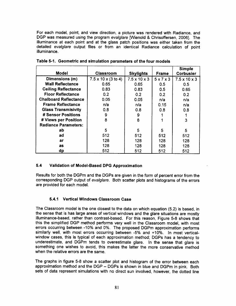
For each model, point, and view direction, a picture was rendered with Radiance, andDGP was measured using the program evalglare [Wienold & Chrisoffersen, 2006]. Theilluminance at each point and at the glass patch positions was either taken from thedetailed evalglare output files or from an identical Radiance calculation of pointilluminance.

Table 5-1. Geometric and simulation parameters of the four models

SimpleModel Classroom Skylights Frame Corbusier

Dimensions (m) 7.5xl0x(3to4) 7.5x10x3 5x7x3 7.5xlOx3Wall Reflectance 0.65 0.65 0.5 0.5

Ceiling Reflectance 0.83 0.83 0.5 0.65Floor Reflectance 0.2 0.2 0.2 0.2

Chalboard Reflectance 0.05 0.05 n/a n/aFrame Reflectance n/a n/a 0.15 n/aGlass Transmisivity 0.8 0.8 0.8 0.8# Sensor Positions 9 9 1 1

# Views per Position 8 8 1 3Radiance Parameters:

ab 5 5 5 5ad 512 512 512 512ar 128 128 128 128as 128 128 128 128dp 512 512 512 512

5.4 Validation of Model-Based DPG Approximation

Results for both the DGPm and the DGPs are given in the form of percent error from thecorresponding DGP output of evalglare. Both scatter plots and histograms of the errorsare provided for each model.

5.4.1 Vertical Windows Classroom Case

The Classroom model is the one closest to the data on which equation (5.2) is based, inthe sense that is has large areas of vertical windows and the glare situations are mostlyilluminance-based, rather than contrast-based. For this reason, Figure 5-8 shows thatthis the simplified DGP method performs very well in the Classroom model, with mosterrors occurring between -10% and 0%. The proposed DGPm approximation performssimilarly well, with most errors occurring between -5% and +10%. In most vertical-window cases, this is typical of each approximation method; DGPs has a tendency tounderestimate, and DGPm tends to overestimate glare. In the sense that glare issomething one wishes to avoid, this makes the latter the more conservative methodwhen the relative errors are the same.

The graphs in figure 5-8 show a scatter plot and histogram of the error between eachapproximation method and the DGP - DGPs is shown in blue and DGPm in pink. Bothsets of data represent simulations with no direct sun involved, however, the dotted line

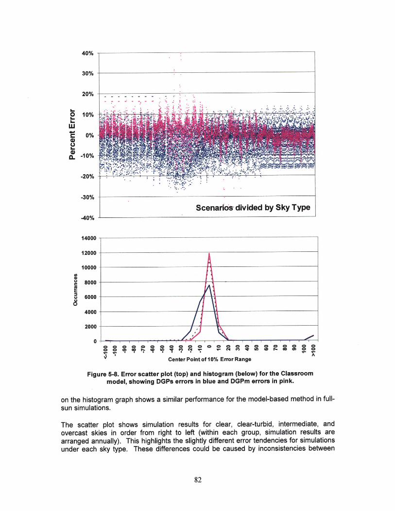
40%

30%

20% - - - ---

0 0.~:~

0%

-10%

-30% -

Scenarios divided by Sky Type-40%

14000

12000 -

10000 -

C 8000 -

U 6000 -

4000

2000

0

1

Center Point of 10% Error Range

Figure 5-8. Error scatter plot (top) and histogram (below) for the Classroommodel, showing DGPs errors in blue and DGPm errors in pink.

on the histogram graph shows a similar performance for the model-based method in full-sun simulations.

The scatter plot shows simulation results for clear, clear-turbid, intermediate, andovercast skies in order from right to left (within each group, simulation results arearranged annually). This highlights the slightly different error tendencies for simulationsunder each sky type. These differences could be caused by inconsistencies between

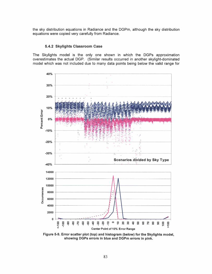
the sky distribution equations in Radiance and the DGPm, although the sky distributionequations were copied very carefully from Radiance.

5.4.2 Skylights Classroom Case

The Skylights model is the only one shown in which the DGPs approximationoverestimates the actual DGP. (Similar results occurred in another skylight-dominatedmodel which was not included due to many data points being below the valid range for

40%

30%

20%

10%

0%

-10%

-20%

-30%

-40%

14000

12000

10000

8000

6000

4000

Center Point of 10% Error Range

00 00

(0 I~- (0 O~ 00

A

Figure 5-9. Error scatter plot (top) and histogram (below) for the Skylights model,showing DGPs errors in blue and DGPm errors in pink.

2000

0

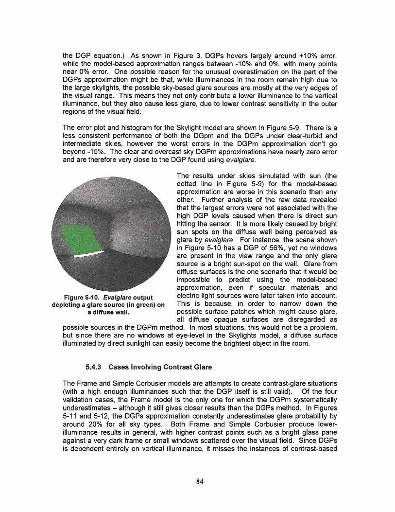
the DGP equation.) As shown in Figure 3, DGPs hovers largely around +10% error,while the model-based approximation ranges between -10% and 0%, with many pointsnear 0% error. One possible reason for the unusual overestimation on the part of theDGPs approximation might be that, while illuminances in the room remain high due tothe large skylights, the possible sky-based glare sources are mostly at the very edges ofthe visual range. This means they not only contribute a lower illuminance to the verticalilluminance, but they also cause less glare, due to lower contrast sensitivity in the outerregions of the visual field.

The error plot and histogram for the Skylight model are shown in Figure 5-9. There is aless consistent performance of both the DGpm and the DGPs under clear-turbid andintermediate skies, however the worst errors in the DGPm approximation don't gobeyond -15%. The clear and overcast sky DGPm approximations have nearly zero errorand are therefore very close to the DGP found using evalglare.

The results under skies simulated with sun (thedotted line in Figure 5-9) for the model-basedapproximation are worse in this scenario than anyother. Further analysis of the raw data revealedthat the largest errors were not associated with thehigh DGP levels caused when there is direct sunhitting the sensor. It is more likely caused by brightsun spots on the diffuse wall being perceived asglare by evalglare. For instance, the scene shownin Figure 5-10 has a DGP of 56%, yet no windowsare present in the view range and the only glaresource is a bright sun-spot on the wall. Glare fromdiffuse surfaces is the one scenario that it would beimpossible to predict using the model-basedapproximation, even if specular materials and

Figure 5-10. Evalglare output electric light sources were later taken into account.depicting a glare source (in green) on This is because, in order to narrow down the

a diffuse wall. possible surface patches which might cause glare,all diffuse opaque surfaces are disregarded as

possible sources in the DGPm method. In most situations, this would not be a problem,but since there are no windows at eye-level in the Skylights model, a diffuse surfaceilluminated by direct sunlight can easily become the brightest object in the room.

5.4.3 Cases Involving Contrast Glare

The Frame and Simple Corbusier models are attempts to create contrast-glare situations(with a high enough illuminances such that the DGP itself is still valid). Of the fourvalidation cases, the Frame model is the only one for which the DGPm systematicallyunderestimates - although it still gives closer results than the DGPs method. In Figures5-11 and 5-12, the DGPs approximation constantly underestimates glare probability byaround 20% for all sky types. Both Frame and Simple Corbusier produce lower-illuminance results in general, with higher contrast points such as a bright glass paneagainst a very dark frame or small windows scattered over the visual field. Since DGPsis dependent entirely on vertical illuminance, it misses the instances of contrast-based

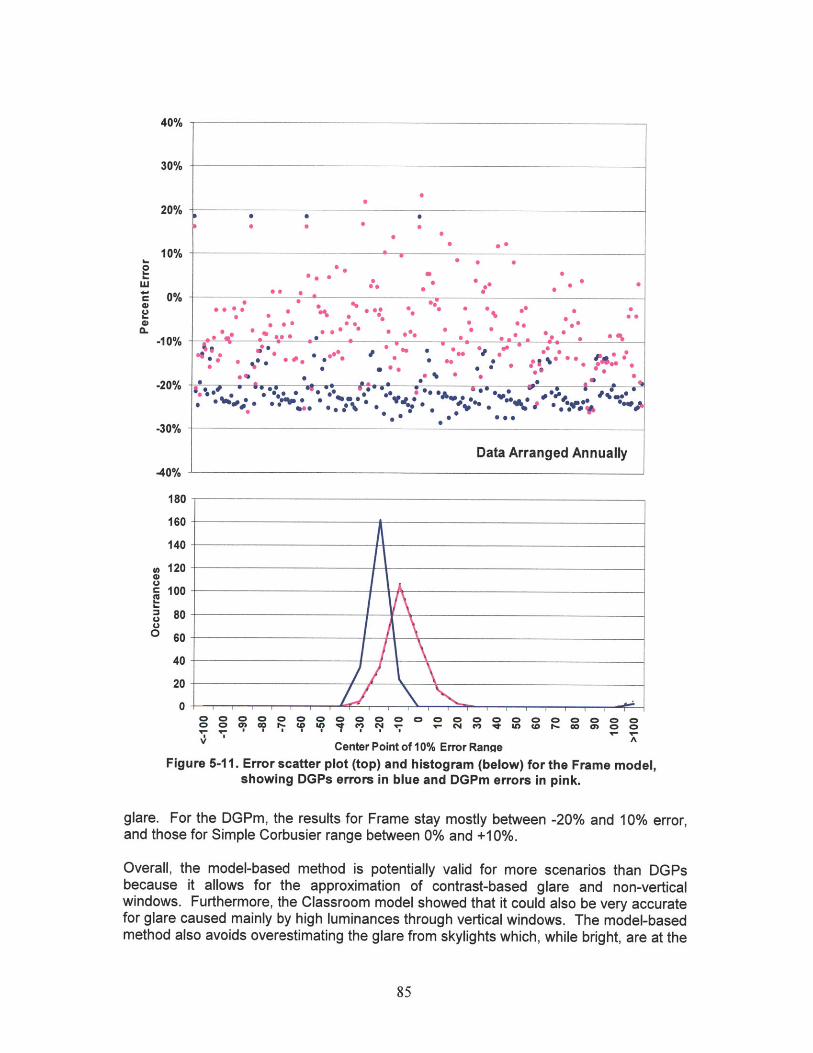
40%

30%

10%.

10%*

20%

-30%-40%0

1800C0. 0 010% So 0 0 W 0* 0

40 0 9 00 0 0 0 * 0 0 go 0.0

00020 go*~ *# *, 000 W * 10.0. 0 00 0 * 000 0

.40%06 *e

1400@

12 - 0

20 center PointAofa10%eErroruRang1801 60140120 -UV

0

Cete 100 o 0 Errag

Figure 5-11. Error scatter plot (top) and histogram (below) for the Frame model,showing DGPs errors in blue and DGPm errors in pink.

glare. For the DGPm, the results for Frame stay mostly between -20% and 10% error,and those for Simple Corbusier range between 0% and +10%.

Overall, the model-based method is potentially valid for more scenarios than DGPsbecause it allows for the approximation of contrast-based glare and non-verticalwindows. Furthermore, the Classroom model showed that it could also be very accuratefor glare caused mainly by high luminances through vertical windows. The model-basedmethod also avoids overestimating the glare from skylights which, while bright, are at the

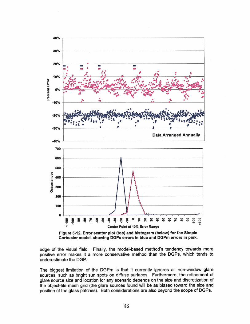
40%

30%

20% *

eS In * ee

100~ P *~--10% *? ** *

0%

-30% s' s

%40%

700

00

500

0 00

o300

200

1000 -

V Center Point of 10% Error Range

Figure 5-12. Error scatter plot (top) and histogram (below) for the SimpleCorbusler rnodel, showing DGPs errors in blue and DGPm errors in pink.

edge of the visual field. Finally, the model-based method's tendency towards morepositive error makes it a more conservative method than the DGPs, which tends tounderestimate the DGP.

The biggest limitation of the DGPm is that it currently ignores all non-window glaresources, such as bright sun spots on diffuse surfaces. Furthermore, the refinement ofglare source size and location for any scenario depends on the size and discretization ofthe object-file mesh grid (the glare sources found will be as biased toward the size andposition of the glass patches). Both considerations are also beyond the scope of DGPs.

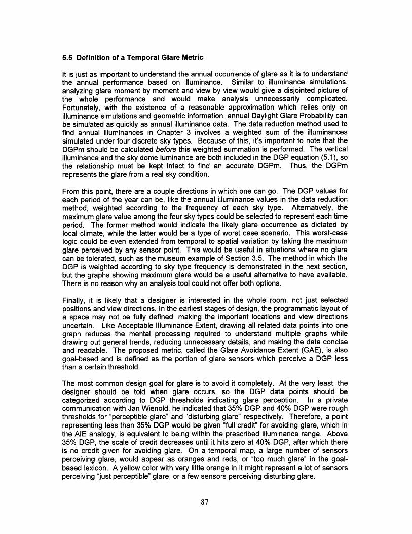
5.5 Definition of a Temporal Glare Metric

It is just as important to understand the annual occurrence of glare as it is to understandthe annual performance based on illuminance. Similar to illuminance simulations,analyzing glare moment by moment and view by view would give a disjointed picture ofthe whole performance and would make analysis unnecessarily complicated.Fortunately, with the existence of a reasonable approximation which relies only onilluminance simulations and geometric information, annual Daylight Glare Probability canbe simulated as quickly as annual illuminance data. The data reduction method used tofind annual illuminances in Chapter 3 involves a weighted sum of the illuminancessimulated under four discrete sky types. Because of this, it's important to note that theDGPm should be calculated before this weighted summation is performed. The verticalilluminance and the sky dome luminance are both included in the DGP equation (5.1), sothe relationship must be kept intact to find an accurate DGPm. Thus, the DGPmrepresents the glare from a real sky condition.

From this point, there are a couple directions in which one can go. The DGP values foreach period of the year can be, like the annual illuminance values in the data reductionmethod, weighted according to the frequency of each sky type. Alternatively, themaximum glare value among the four sky types could be selected to represent each timeperiod. The former method would indicate the likely glare occurrence as dictated bylocal climate, while the latter would be a type of worst case scenario. This worst-caselogic could be even extended from temporal to spatial variation by taking the maximumglare perceived by any sensor point. This would be useful in situations where no glarecan be tolerated, such as the museum example of Section 3.5. The method in which theDGP is weighted according to sky type frequency is demonstrated in the next section,but the graphs showing maximum glare would be a useful alternative to have available.There is no reason why an analysis tool could not offer both options.

Finally, it is likely that a designer is interested in the whole room, not just selectedpositions and view directions. In the earliest stages of design, the programmatic layout ofa space may not be fully defined, making the important locations and view directionsuncertain. Like Acceptable Illuminance Extent, drawing all related data points into onegraph reduces the mental processing required to understand multiple graphs whiledrawing out general trends, reducing unnecessary details, and making the data conciseand readable. The proposed metric, called the Glare Avoidance Extent (GAE), is alsogoal-based and is defined as the portion of glare sensors which perceive a DGP lessthan a certain threshold.

The most common design goal for glare is to avoid it completely. At the very least, thedesigner should be told when glare occurs, so the DGP data points should becategorized according to DGP thresholds indicating glare perception. In a privatecommunication with Jan Wienold, he indicated that 35% DGP and 40% DGP were roughthresholds for "perceptible glare" and "disturbing glare" respectively. Therefore, a pointrepresenting less than 35% DGP would be given "full credit" for avoiding glare, which inthe AIE analogy, is equivalent to being within the prescribed illuminance range. Above35% DGP, the scale of credit decreases until it hits zero at 40% DGP, after which thereis no credit given for avoiding glare. On a temporal map, a large number of sensorsperceiving glare, would appear as oranges and reds, or "too much glare" in the goal-based lexicon. A yellow color with very little orange in it might represent a lot of sensorsperceiving "just perceptible" glare, or a few sensors perceiving disturbing glare.

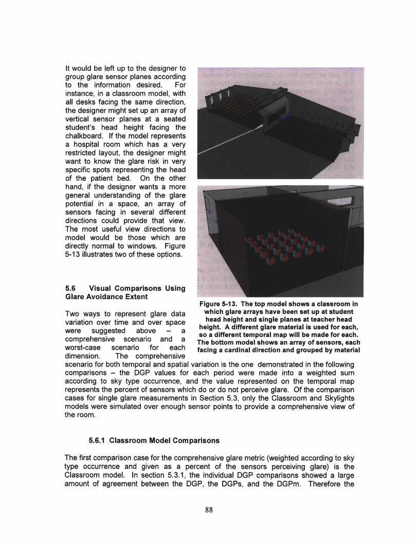
It would be left up to the designer togroup glare sensor planes accordingto the information desired. Forinstance, in a classroom model, withall desks facing the same direction,the designer might set up an array ofvertical sensor planes at a seatedstudent's head height facing thechalkboard. If the model representsa hospital room which has a veryrestricted layout, the designer mightwant to know the glare risk in veryspecific spots representing the headof the patient bed. On the otherhand, if the designer wants a moregeneral understanding of the glarepotential in a space, an array ofsensors facing in several differentdirections could provide that view.The most useful view directions tomodel would be those which aredirectly normal to windows. Figure5-13 illustrates two of these options.

5.6 Visual Comparisons UsingGlare Avoidance Extent

Figure 5-13. The top model shows a classroom inTwo ways to represent glare data which glare arrays have been set up at studentvariation over time and over space head height and single planes at teacher headwere suggested above - a height A different glare material is used for each,comprehensiveso a different temporal map will be made for each.

worst-case scenario and a The bottom model shows an array of sensors, eachwisorcs sceario rfor neach facing a cardinal direction and grouped by material

Figuren-1.oTh.tophedecshowraecassromviscenario for both temporal and spatial variation is the one demonstrated in the followingcomparisons - the DGP values for each period were made into a weighted sumaccording to sky type occurrence, and the value represented on the temporal maprepresents the percent of sensors which do or do not perceive glare. Of the comparisoncases for single glare measurements in Section 5.3, only the Classroom and Skylightsmodels were simulated over enough sensor points to provide a comprehensive view ofthe room.

5.6.1 Classroom Model Comparisons

The first comparison case for the comprehensive glare metric (weighted according to skytype occurrence and given as a percent of the sensors perceiving glare) is theClassroom model. In section 5.3.1, the individual DGP comparisons showed a largeamount of agreement between the DGP, the DGPs, and the DGPm. Therefore the

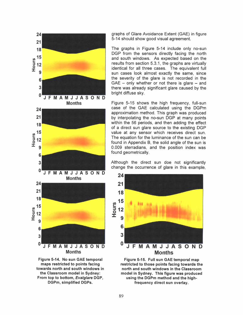
J F M A M J J AMonths

graphs of Glare Avoidance Extent (GAE) in figure5-14 should show good visual agreement.

The graphs in Figure 5-14 include only no-sunDGP from the sensors directly facing the northand south windows. As expected based on theresults from section 5.3.1, the graphs are virtuallyidentical for all three cases. The equivalent fullsun cases look almost exactly the same, sincethe severity of the glare is not recorded in theGAE - only whether or not there is glare - andthere was already significant glare caused by thebright diffuse sky.

Figure 5-15 shows the high frequency, full-suncase of the GAE calculated using the DGPmapproximation method. This graph was producedby interpolating the no-sun DGP at many pointswithin the 56 periods, and then adding the effectof a direct sun glare source to the existing DGPvalue at any sensor which receives direct sun.The equation for the luminance of the sun can befound in Appendix B, the solid angle of the sun is0.009 sterradians, and the position index wasfound geometrically.

Although the direct sunchange the occurrence of

JI MAMJJAMonths

A M J J AMonths

Figure 5-14. No sun GAE temporalmaps restricted to points facing

towards north and south windows inthe Classroom model in Sydney:

From top to bottom, Evalglare DGP,DGPm, simplified DGPs.

doeglare

not significantlyin this example,

24211815129

J I- M A M J J A 5 U N UMonths

Figure 5-15. Full sun GAE temporal maprestricted to those points facing towards thenorth and south windows in the Classroommodel in Sydney. This figure was produced

using the DGPm method and the high-frequency direct sun overlay.

24

21

1815

12

9

6

3

0

24

21

18

1512

9

4

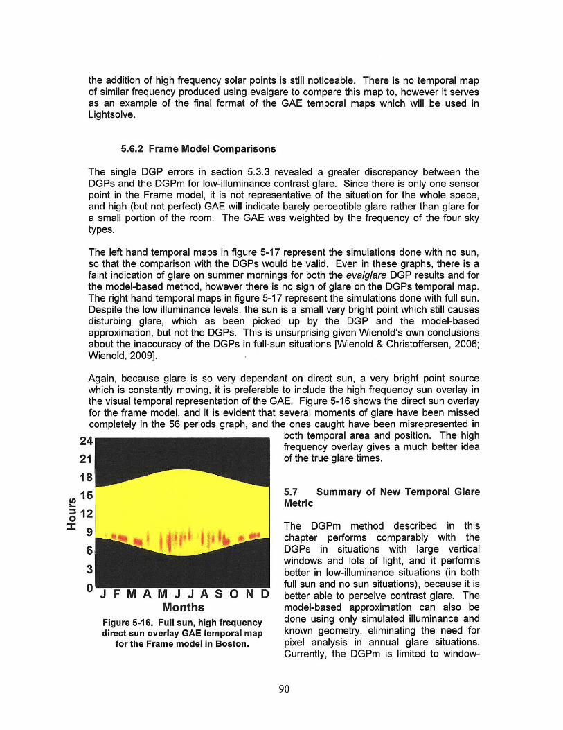
the addition of high frequency solar points is still noticeable. There is no temporal mapof similar frequency produced using evalgare to compare this map to, however it servesas an example of the final format of the GAE temporal maps which will be used inLightsolve.

5.6.2 Frame Model Comparisons

The single DGP errors in section 5.3.3 revealed a greater discrepancy between theDGPs and the DGPm for low-illuminance contrast glare. Since there is only one sensorpoint in the Frame model, it is not representative of the situation for the whole space,and high (but not perfect) GAE will indicate barely perceptible glare rather than glare fora small portion of the room. The GAE was weighted by the frequency of the four skytypes.

The left hand temporal maps in figure 5-17 represent the simulations done with no sun,so that the comparison with the DGPs would be valid. Even in these graphs, there is afaint indication of glare on summer mornings for both the evalglare DGP results and forthe model-based method, however there is no sign of glare on the DGPs temporal map.The right hand temporal maps in figure 5-17 represent the simulations done with full sun.Despite the low illuminance levels, the sun is a small very bright point which still causesdisturbing glare, which as been picked up by the DGP and the model-basedapproximation, but not the DGPs. This is unsurprising given Wienold's own conclusionsabout the inaccuracy of the DGPs in full-sun situations [Wienold & Christoffersen, 2006;Wienold, 2009].

Again, because glare is so very dependant on direct sun, a very bright point sourcewhich is constantly moving, it is preferable to include the high frequency sun overlay inthe visual temporal representation of the GAE. Figure 5-16 shows the direct sun overlayfor the frame model, and it is evident that several moments of glare have been missedcompletely in the 56 periods graph, and the ones caught have been misrepresented in

24 both temporal area and position. The highfrequency overlay gives a much better idea

21 of the true glare times.

185.7 Summary of New Temporal GlareMetric

12'1 The DGPm method described in this

9 9 chapter performs comparably with the6 DGPs in situations with large vertical

3 windows and lots of light, and it performsbetter in low-illuminance situations (in both

0 JFfull sun and no sun situations), because it isJFM A M J J A S 0 N D better able to perceive contrast glare. The

Months model-based approximation can also beFigure 5-16. Full sun, high frequency done using only simulated illuminance anddirect sun overlay GAE temporal map known geometry, eliminating the need for

for the Frame model in Boston. pixel analysis in annual glare situations.Currently, the DGPm is limited to window-

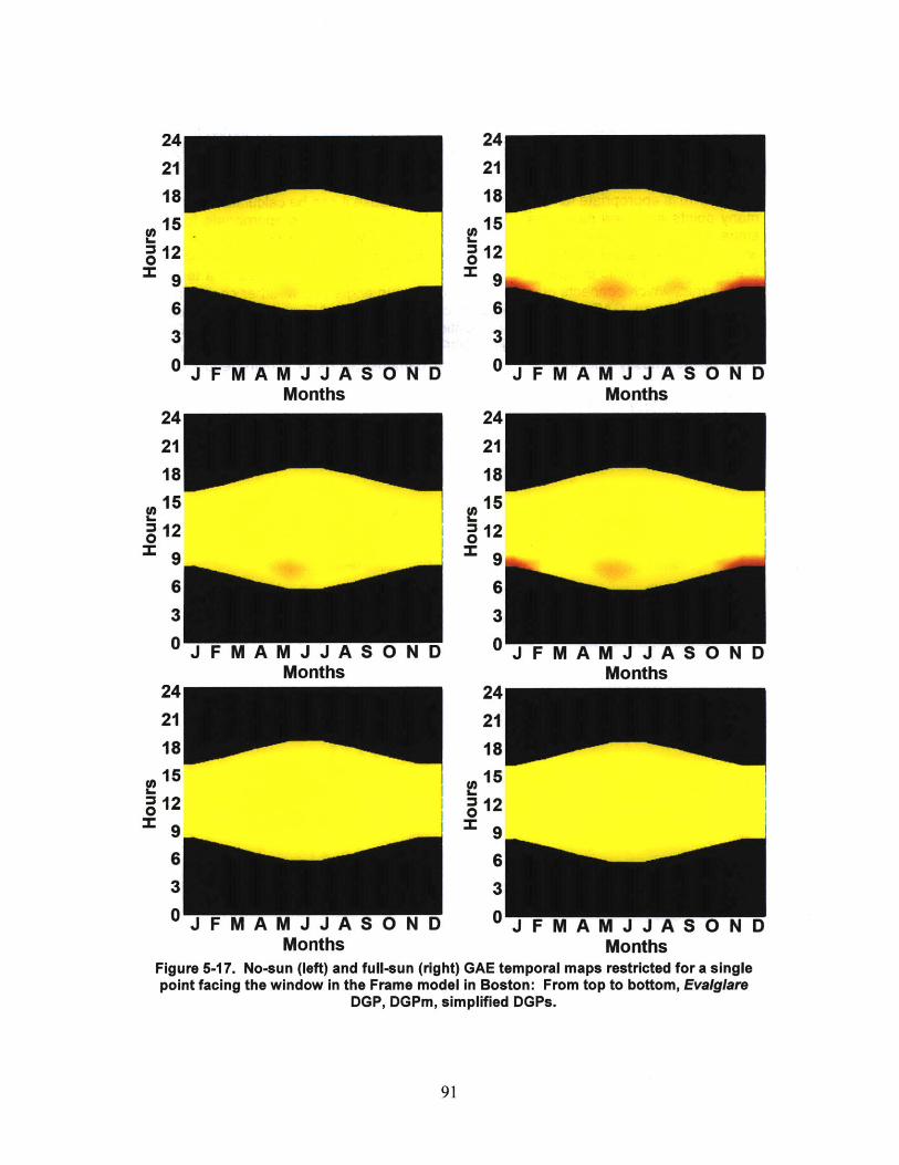
24 24

21 21

18 18

150151212

0 JJ

6 6

Months Months2 124

21 21

18 18so15

1212 00 JFMAMJJA

6 6

J F A MJ J S 0N DJ F M A M J J A S 0 N IMonths Months

24 2421 21

18 poll18

15~12 = 12

9 =96 6

J F A MJ J S 0N DJ F M A M J J A S 0 N IMonths Months

Figure 5-17. No-sun (left) and full-sun (right) GAE temporal maps restricted for a singlepoint facing the window in the Frame model in Boston: From top to bottom, Evalglare

DGP, DGPm, simplified DGPs.

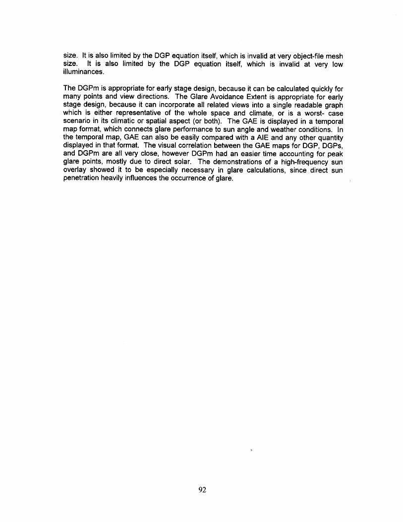
size. It is also limited by the DGP equation itself, which is invalid at very object-file meshsize. It is also limited by the DGP equation itself, which is invalid at very lowilluminances.

The DGPm is appropriate for early stage design, because it can be calculated quickly formany points and view directions. The Glare Avoidance Extent is appropriate for earlystage design, because it can incorporate all related views into a single readable graphwhich is either representative of the whole space and climate, or is a worst- casescenario in its climatic or spatial aspect (or both). The GAE is displayed in a temporalmap format, which connects glare performance to sun angle and weather conditions. Inthe temporal map, GAE can also be easily compared with a AIE and any other quantitydisplayed in that format. The visual correlation between the GAE maps for DGP, DGPs,and DGPm are all very close, however DGPm had an easier time accounting for peakglare points, mostly due to direct solar. The demonstrations of a high-frequency sunoverlay showed it to be especially necessary in glare calculations, since direct sunpenetration heavily influences the occurrence of glare.

Chapter 6

Solar Heat Surplus and ScarcityEven though solar heat gain is not a photometric quantity, it is one of the tradeoffsassociated with daylighting, and therefore it should be considered in any holistic analysisof daylighting. Unfortunately, as discussed in Section 2.1.6, it is difficult to understandthe impact of solar heat gain on a space's temperature difference or HVAC loads withoutdoing some kind of energy analysis. Since energy and daylighting analyses require verydifferent model inputs and types of simulation, most existing daylighting analysissolutions that include solar heat gain are ones which either include or have easy exportsto energy analysis tools [Urban & Glicksman, 2007; Reinhart et al., 2007; Ecotect web;IES web]. The few existing analysis methods that do not require simulation are usuallyonly applicable to certain restricted climate locations and use the existing results fromprevious energy simulations in their application [de Groot et aL, 2003; Hui, 1997]. Veryfew of these methods or tools parse the solar heat gain contribution out from the generalenergy analysis and present it separately as a tradeoff to incoming daylight [Ecotectweb; de Groot et al., 2003].

Like daylighting, the solutions for energy analysis range from algorithms which can becalculated manually to physically based algorithms which require computer simulation. Ifthe energy consequences of solar heat gain are to be portrayed as a daylighting tradeofffor schematic design, it may be possible to use energy simulation results that are onlyaccurate enough to provide a ballpark estimate - an indication of the benefits ordisadvantages. Also, because few building materials are defined in the earliest stagesof design, variable input defaults can be provided based on building type. It is thereforepossible, although not ideal, to use a less accurate calculation of solar heat gain whenmaking decisions in the early design stage.

It is beyond the scope of this thesis to focus on energy simulation techniques, howeversolar heat gain is an important aspect of daylighting. For this reason, a simple existingenergy balance equation, the balance point method, was chosen for solar energycalculation, and the errors that one might expect when employing this method wereanalyzed against energy use data from the program Energy Plus. The data from thebalance point method was then used in a proof of concept for a solar heat gain metricsimilar in form to the AIE and GAE metrics discussed in previous chapters. This metric,named Solar Heat Scarcity/Surplus (SHS) provides an indication of the urgency forshading windows during the cooling season or allowing more solar gain during theheating season. The Energy Plus energy use data, balance point data produced withcomplex equipment and occupancy schedules, and balance point data produced usingsimpler schedules are visually compared as SHS quantities in the temporal map format.

6.1 Balance Point Method

As part of the Vital Signs program run by the University of California - Berkeley, Utzingerand Wasley, of the University of Wisconsin - Milwaukee, produced a very thoroughdocument describing the balance point method of building energy analysis. A building'sbalance point is defined as "the outdoor air temperature required for the indoor

temperature to be comfortable without the use of any mechanical heating or cooling,"[Utzinger & Wasley, 1997]. In essence, when outdoor conditions reach the balancepoint, building heat gains are equal to the heat loss through the fagade, and for thisreason, the balance point temperature is always lower than the target indoortemperature. If the outdoor temperature is higher than the balance point, the buildingwill require cooling, if lower, the building will require heating.

The balance point temperature is found through the application of steady-state energybalance equations. The basic equation for the balance point is as follows:

TBP =Tset SHG + QVHG ' (6.1)t(UALouIdflg + (PCpV tent

where TBP is the balance point temperature (*C), Tset is the thermostat set pointtemperature (*C), QSHG and QIHG are the solar heat gain (from windows) and internalheat gain (W), U is the heat transfer coefficient of the fagade (W/m2*K), A is the area ofthe fagade, p is the density of air (kg/M 3), c, is the heat capacity of air (kJ/kg*K), and V'is the ventilation volume flow rate (m3/s). (Because the balance point equation involvesa temperature difference, rather than an absolute temperature, it is possible to define TBPand Tset in Celsius rather than Kelvin.) The full building product of U and A is defined as:

(UA)building = E (UA), (6.2)

where i represents each building fagade element with a different U-value. QIHG is thesum of heat gain from occupants, equipment, electric lights, and any other heat sourceinternal to the building, and V' includes both infiltration and outdoor air ventilationsupplied either through windows or the HVAC system. Every input given above can alsobe normalized by the total floor area of the building, so that buildings of different sizesmay be compared to each other.

The other useful operation is to turn the balance point into a predicted heat load. Thetemperature difference between the outdoor air and the balance point is not a heat loadin itself, but a load can be found by multiplying by the heat transfer rate of the building:

Load = (Tout - TBP (UA)buiding + cpV )vent Jx t (6.3)

where the load is in Joules (and is positive for cooling, and negative for heating loads),and t represents the appropriate time step in seconds, given the data available.

The balance point and outdoor temperature over the course of a day can be graphed inopposition for an immediate visual representation of heating and cooling load potential.Figure 6-1 a shows a schematic graph of the balance point temperature which assumesa static internal heat gain during occupied hours and no internal heat gain duringunoccupied hours; Figure 6-1 b illustrates a more detailed occupancy and internal gainsschedule. In this simple representation of a single day, the red line is the thermostattemperature, the green line is the balance point temperature due to internal heat gainonly, and the orange line is the balance point temperature due to both internal heat gainand solar heat gain. The temperature differences between the balance point and theoutdoor temperature must be addressed by the heating system (shaded in blue) or the

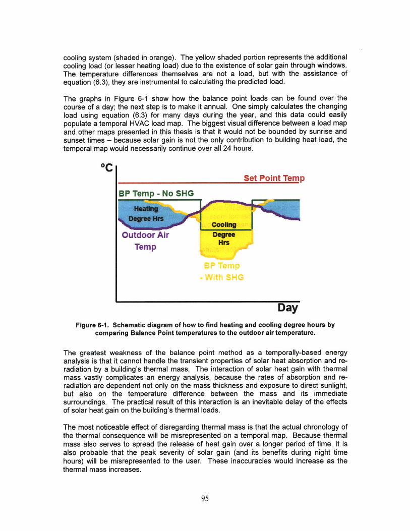
cooling system (shaded in orange). The yellow shaded portion represents the additionalcooling load (or lesser heating load) due to the existence of solar gain through windows.The temperature differences themselves are not a load, but with the assistance ofequation (6.3), they are instrumental to calculating the predicted load.

The graphs in Figure 6-1 show how the balance point loads can be found over thecourse of a day; the next step is to make it annual. One simply calculates the changingload using equation (6.3) for many days during the year, and this data could easilypopulate a temporal HVAC load map. The biggest visual difference between a load mapand other maps presented in this thesis is that it would not be bounded by sunrise andsunset times - because solar gain is not the only contribution to building heat load, thetemporal map would necessarily continue over all 24 hours.

"CSet Point Temp

SP Temp - No SHG

Outdoor Air DegrwTemp Hrs

DayFigure 6-1. Schematic diagram of how to find heating and cooling degree hours by

comparing Balance Point temperatures to the outdoor air temperature.

The greatest weakness of the balance point method as a temporally-based energyanalysis is that it cannot handle the transient properties of solar heat absorption and re-radiation by a building's thermal mass. The interaction of solar heat gain with thermalmass vastly complicates an energy analysis, because the rates of absorption and re-radiation are dependent not only on the mass thickness and exposure to direct sunlight,but also on the temperature difference between the mass and its immediatesurroundings. The practical result of this interaction is an inevitable delay of the effectsof solar heat gain on the building's thermal loads.

The most noticeable effect of disregarding thermal mass is that the actual chronology ofthe thermal consequence will be misrepresented on a temporal map. Because thermalmass also serves to spread the release of heat gain over a longer period of time, it isalso probable that the peak severity of solar gain (and its benefits during night timehours) will be misrepresented to the user. These inaccuracies would increase as thethermal mass increases.

.. ............................................................... ..............

For the particular application of displaying the solar heat gain tradeoffs associated withdaylight, there is one possible advantage to disregarding thermal mass. If all solar gainis treated as if it has immediate consequence, the resulting temporal map wouldaccurately show the chronology and severity of the source of solar gain, which is mostlydue to the amount of direct solar penetration to the building. By understanding the timesof day and year when solar influx is most severe, the designer can better makedecisions to block these solar angles in the summer or preserve them in the winter. Inthis way, the heat influx caused by daylighting is more closely associated with morerelevant illuminance and glare measurements in the mind of the designer.

It is also possible to assess the results of a balance point analysis in terms of whetherthe building would benefit from thermal mass. For instance, if the blue and orangeshaded regions in Figure 6-1 are close in size, we know that the building is a bettercandidate for benefiting from exposed thermal mass, especially if the mass is placedsuch that it absorbs most of the incoming solar gains. Utzinger and Wasley provide amore detailed guide to the basic conclusions one can draw from the relative sizes of thecooling and heating load potentials [Utzinger & Wasley, 1997]. It may also be possible,after some further research, to modify the solar heat gain data in relation to an idealizedeffect of various quantities of thermal mass. This would make it possible for the architectto explore the general massiveness of the building as a design variable.

6.2 User Inputs and Defaults for Balance Point Analysis

Because energy and daylighting simulations require different variable inputs, newinformation will be required from the designer. However, in deference to the need foranalysis interactivity, and because very few specifics are firmly set in early stageanalyses, it is preferable to offer as many variable defaults as possible - although withthe option of editing these defaults. The analysis method presented here will offer thedesigner defaults based on building type and either ASHRAE recommendations[ASHRAE, 2007] or those used in the sixteen benchmark commercial building modelsrecently released by the United States Department of Energy (DOE) [Torcellini et al.,2008; DOE, 2008]. Some defaults suggestions for infiltration are also taken from theVital Signs paper on balance point analysis [Utzinger & Wasley, 1997]. The ASHRAEdefaults are most useful in situations where the designer has modeled a single part ofthe building, while the defaults listed for the sixteen DOE benchmark buildings areaverage values for the full building.

The feasibility study for the metric described in this chapter is done using those DOEbenchmark models (see Section 6.4), and the tables in Appendix C list the suggesteddefault values. The designer will be asked to provide the occupancy hours of the spaceand the building type. The designer is then asked to chose from defaults or assign anew value for occupancy per square meter, ventilation per person, ventilation per squaremeter, infiltration (in terms of air change rate per hour), heat gain due to equipment, andheat gain due to lights, as well as confirming the average room height (with a default setat 3 meters).

Because the required inputs for an energy calculation do not exist in the currentLightsolve modeling process, it is important to know what will be required from the userin the final application. In SketchUp (the CAD program from which one can run

Lightsolve), the model itself will have certain material tags indicating different fagadematerials, which should be only assigned to surfaces with a connection to the exterior.Each unique material with these tags will have its area automatically totaled, and thedesigner will have to enter U-values and Solar Heat Gain Coefficients or choose fromthe defaults listed in Appendix C. The model will also have a material designation for thefloor in order to total the overall area of the space. If any of these material tags do notappear in the model, the designer will be prompted to enter the appropriate surfaceareas.

A few variables are assumed by the balance point calculation without the designer'sinput. Each occupant is assumed to radiate 75 Watts of sensible heat, which is theASHRAE default for an adult doing light office work [ASHRAE, 2001], howeverconvective heat gain should probably be included in similar future calculations. Thedensity of air, p, is assumed to be 1.2 kg/M 3, and the heat capacity of air, cp, is assumedto be 1.005 kJ/kg*K. The exact form of the menus with which this information will begathered from the user is a work in progress.

6.3 Definition of a Temporal Solar Energy Metric

Although it is useful to know the heat loads and the temperature difference between thebalance point and the outdoor air, it is preferable for the solar energy information to bepresented to the designer in the same format as the glare and illuminance information. Ifall three daylighting quantities are in the same format, the designer can more easilyunderstand the heat load consequences of meeting the illuminance goals, or see howmuch illuminance is reduced when all glare is blocked. No single aspect of daylightingcan be changed without affecting the other two, but many existing analyses solutionstreat illuminance as if it occurred in a vacuum (see Section 2.3). For a trulycomprehensive analysis, all three daylighting quantities should be comparable andreadily available to the designer.

In the context of this thesis, that means that solar energy should be presented to thedesigner on a temporal map representative of the whole model and in terms of a goal-oriented metric which highlights the times when there is too much solar gain, when thereis just the right amount of solar heat gain, or when there is not enough solar gain tooffset heating. Using the balance point analysis described above, a building could besaid to have excessive solar gain when the outdoor temperature is greater than thebuilding balance point and be lacking in solar gain when the building balance pointtemperature is greater. The "right" amount of solar gain would be however much isrequired for the outdoor temperature to equal the balance point (or to fall between thetwo building balance points found using the cooling and heating set point respectively).

To apply the above reasoning mathematically, the solar heat gain metric is split into twoparts, called Solar Heat Scarcity and Solar Heat Surplus (SHS), based on whetherheating or cooling is required by the building:

If Tout - TBPS 2 0 - Solar Heat Surplus (cooling)If Tout - TBP,S < 0 - Solar Heat Scarcity (heating) (6.4)

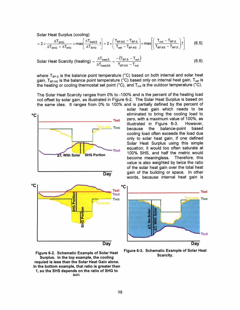
Solar Heat Surplus (cooling)

2 x ATSHG x max Tad,SATSHG + ATIHG SHG

(TBPNS - TBPS out T BPS ,

-set ~ TBPNS ) [C TBP,NS - TBP,S

Solar Heat Scarcity (heating) = ATIoadS - (TBPS -out

ATloadNS TBP,NS ~out

(6.5)

(6.6)

where TBP,S is the balance point temperature (*C) based on both internal and solar heatgain, TBP,NS is the balance point temperature (*C) based only on internal heat gain, Tset isthe heating or cooling thermostat set point (*C), and Tout is the outdoor temperature (*C).

The Solar Heat Scarcity ranges from 0% to -100% and is the percent of the heating loadnot offset by solar gain, as illustrated in Figure 6-2. The Solar Heat Surplus is based onthe same idea. It ranges from 0% to 100% and is partially defined by the percent of

solar heat gain which needs to beeliminated to bring the cooling load to

_ Thet zero, with a maximum value of 100%, asillustrated in Figure 6-3. However,

TIHG because the balance-point basedcooling load often exceeds the load dueonly to solar heat gain, if one definedSolar Heat Surplus using this simple

Tout equation, it would too often saturate at

With Solar SHG Portion 100% SHS, and half the metric wouldbecome meaningless. Therefore, thisvalue is also weighted by twice the ratioof the solar heat gain over the total heat

Day gain of the building or space. In otherwords, because internal heat gain is

*CIC

0

0a.0U)

Tset~ToutTIHG

Tset

TIHG

Tout

Day

Figure 6-2. Schematic Example of Solar HeatSurplus. In the top example, the cooling

requied is less than the Solar Heat Gain alone.In the bottom example, that ratio is greater than1, so the SHS depends on the ratio of SHG to

Iw(

DayFigure 6-3. Schematic Example of Solar Heat

Scarcity.

.................... .. ....................................

=S11.

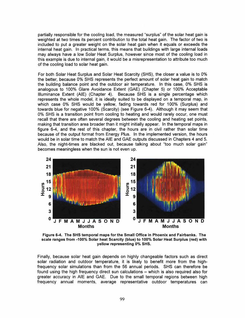
partially responsible for the cooling load, the measured "surplus" of the solar heat gain isweighted at two times its percent contribution to the total heat gain. The factor of two isincluded to put a greater weight on the solar heat gain when it equals or exceeds theinternal heat gain. In practical terms, this means that buildings with large internal loadsmay always have a low Solar Heat Surplus, however since most of the cooling load inthis example is due to internal gain, it would be a misrepresentation to attribute too muchof the cooling load to solar heat gain.

For both Solar Heat Surplus and Solar Heat Scarcity (SHS), the closer a value is to 0%the better, because 0% SHS represents the perfect amount of solar heat gain to matchthe building balance point and the outdoor air temperature. In this case, 0% SHS isanalogous to 100% Glare Avoidance Extent (GAE) (Chapter 5) or 100% AcceptableIlluminance Extent (AIE) (Chapter 4). Because SHS is a single percentage whichrepresents the whole model, it is ideally suited to be displayed on a temporal map, inwhich case 0% SHS would be yellow, fading towards red for 100% (Surplus) andtowards blue for negative 100% (Scarcity) (see Figure 6-4). Although it may seem that0% SHS is a transition point from cooling to heating and would rarely occur, one mustrecall that there are often several degrees between the cooling and heating set points,making that transition area broader than it might initially appear. In the temporal maps infigure 6-4, and the rest of this chapter, the hours are in civil rather than solar timebecause of the output format from Energy Plus. In the implemented version, the hourswould be in solar time to match the AIE and GAE outputs discussed in Chapters 4 and 5.Also, the night-times are blacked out, because talking about "too much solar gain"becomes meaningless when the sun is not even up.

A iJ PMonths

242118

15

129

630 i J P

Months

Figure 6-4. The SHS temporascale ranges from -100% Sola

l maps for the Small Office inir heat Scarcity (blue) to 100%yellow representing 0% SHS.

Phoenix and Fairbanks. TheSolar Heat Surplus (red) with

Finally, because solar heat gain dependssolar radiation and outdoor temperature,frequency solar simulations than from thefound using the high frequency direct sungreater accuracy in AIE and GAE. Due tfrequency annual moments, average

on highly changeable factors such as directit is likely to benefit more from the high-56 annual periods. SHS can therefore be

calculations - which is also required also forto the small temporal regions between highrepresentative outdoor temperatures can

. ....... .... ........... ..... ... ................ #- " -&Ni--

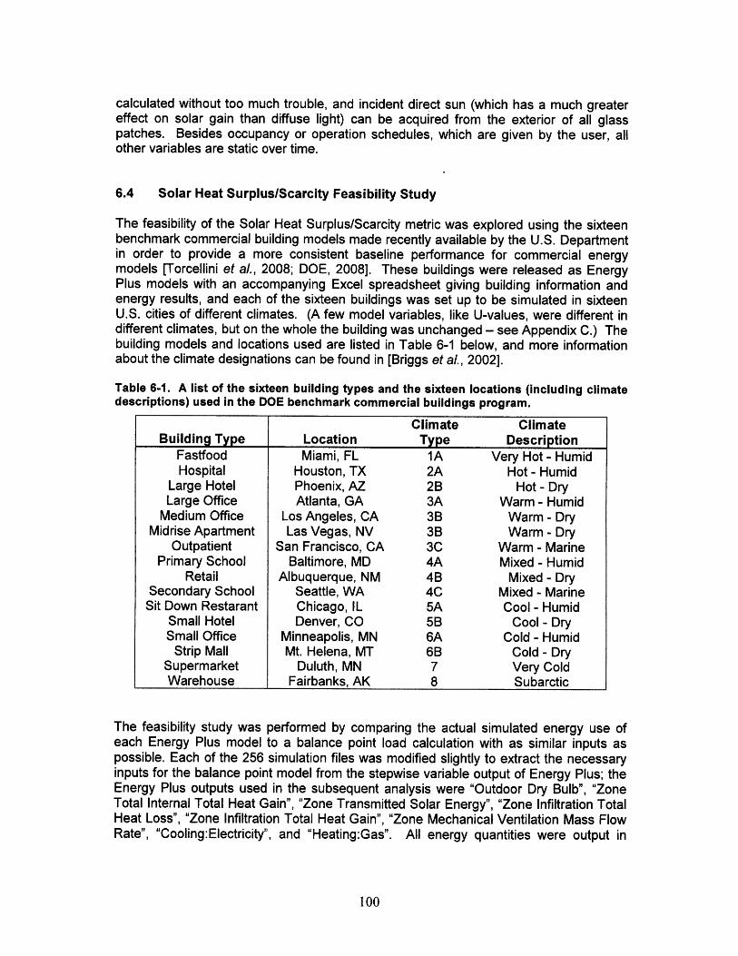
calculated without too much trouble, and incident direct sun (which has a much greatereffect on solar gain than diffuse light) can be acquired from the exterior of all glasspatches. Besides occupancy or operation schedules, which are given by the user, allother variables are static over time.

6.4 Solar Heat Surplus/Scarcity Feasibility Study

The feasibility of the Solar Heat Surplus/Scarcity metric was explored using the sixteenbenchmark commercial building models made recently available by the U.S. Departmentin order to provide a more consistent baseline performance for commercial energymodels [Torcellini et al., 2008; DOE, 2008]. These buildings were released as EnergyPlus models with an accompanying Excel spreadsheet giving building information andenergy results, and each of the sixteen buildings was set up to be simulated in sixteenU.S. cities of different climates. (A few model variables, like U-values, were different indifferent climates, but on the whole the building was unchanged - see Appendix C.) Thebuilding models and locations used are listed in Table 6-1 below, and more informationabout the climate designations can be found in [Briggs et al., 2002].

Table 6-1. A list of the sixteen building types and the sixteen locations (including climatedescriptions) used in the DOE benchmark commercial buildings program.

Climate ClimateBuilding Type Location Type Description

Fastfood Miami, FL 1A Very Hot - HumidHospital Houston, TX 2A Hot - Humid

Large Hotel Phoenix, AZ 2B Hot - DryLarge Office Atlanta, GA 3A Warm - Humid

Medium Office Los Angeles, CA 3B Warm - DryMidrise Apartment Las Vegas, NV 3B Warm - Dry

Outpatient San Francisco, CA 3C Warm - MarinePrimary School Baltimore, MD 4A Mixed - Humid

Retail Albuquerque, NM 4B Mixed - DrySecondary School Seattle, WA 4C Mixed - Marine

Sit Down Restarant Chicago, IL 5A Cool - HumidSmall Hotel Denver, CO 5B Cool - DrySmall Office Minneapolis, MN 6A Cold - Humid

Strip Mall Mt. Helena, MT 6B Cold - DrySupermarket Duluth, MN 7 Very ColdWarehouse Fairbanks, AK 8 Subarctic

The feasibility study waseach Energy Plus modelpossible. Each of the 256

performed by comparing the actual simulated energy use ofto a balance point load calculation with as similar inputs assimulation files was modified slightly to extract the necessary

inputs for the balance point model from the stepwise variable output of Energy Plus; theEnergy Plus outputs used in the subsequent analysis were "Outdoor Dry Bulb", "ZoneTotal Internal Total Heat Gain", "Zone Transmitted Solar Energy", "Zone Infiltration TotalHeat Loss", "Zone Infiltration Total Heat Gain", "Zone Mechanical Ventilation Mass FlowRate", "Cooling:Electricity", and "Heating:Gas". All energy quantities were output in

100

joules and outputs for heating and cooling energy were normalized by the given COP ofthe cooling systems or the given heating efficiency where appropriate.

If the ultimate goal is to compare energy use data with the balance point loadcalculations, the portion of the energy load due to solar heat gain must somehow beparsed from the whole. Therefore, after each building and city combination wassimulated, the window properties of each building were modified so that the visibletransmission and the SHGC were nearly zero (the program wouldn't run with all windowscompletely opaque), while the U-value of the glass was kept intact. The differencebetween the normal building energy use and the opaque building energy use was found,and this difference was attributed to the load effects of solar gain. With this information,the simulated energy use data can be compared with the loads approximated using thebalance point method.

The balance point method was applied to the Energy Plus models in two ways. Themore detailed calculation used the heat gains, ventilation rates, and other variableswhich are output at each time step. In essence, this is purely a test of the heat balanceequation itself, assuming more accurate information than the designer is likely to haveduring schematic design. The most important feature of these inputs is the detailedschedules for occupancy, heat gains, and the ventilation system required by Energy Plus(see Figure 6-6). The second balance point calculation was done using the design

Secondary School

Figure 6-5. Pictures of two of the energy plus building models as they appearin the provided excel workbooks: Top) Small Office, bottom) Secondary School

[DOE, 2008].

101

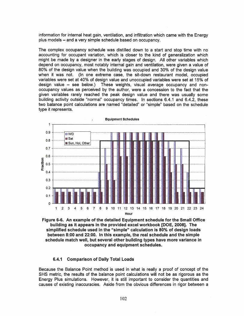
information for internal heat gain, ventilation, and infiltration which came with the Energyplus models - and a very simple schedule based on occupancy.

The complex occupancy schedule was distilled down to a start and stop time with noaccounting for occupant variation, which is closer to the kind of generalization whichmight be made by a designer in the early stages of design. All other variables whichdepend on occupancy, most notably internal gain and ventilation, were given a value of80% of the design value when the building was occupied and 30% of the design valuewhen it was not. (In one extreme case, the sit-down restaurant model, occupiedvariables were set at 40% of design value and unoccupied variables were set at 15% ofdesign value - see below.) These weights, visual average occupancy and non-occupancy values as perceived by the author, were a concession to the fact that thegiven variables rarely reached the peak design value and there was usually somebuilding activity outside "normal" occupancy times. In sections 6.4.1 and 6.4.2, thesetwo balance point calculations are named "detailed" or "simple" based on the scheduletype it represents.

Equipment Schedules1~

0.9 ----------- Il W D - -- -

0.8 ---------- Sat---0 Sun, Hol, Other

0.7 - ---- ------------------------- --- - ---- - - - - L - -

0. -------------------------- - -- - - - - - - - - - - --- - --

0.3 ---------------------------------------------------------

0.2-

0.1 - - - - - - -- - ---m I -

1 2 3 4 5 6 7 8 9 10 11 12 13 14 15 16 17 18 19 20 21 22 23 24

Hour

Figure 6-6. An example of the detailed Equipment schedule for the Small Officebuilding as it appears in the provided excel workbook [DOE, 2008]. The

simplified schedule used in the "simple" calculation is 80% of design loadsbetween 8:00 and 22:00. In this example, the real schedule and the simple

schedule match well, but several other building types have more variance inoccupancy and equipment schedules.

6.4.1 Comparison of Daily Total Loads

Because the Balance Point method is used in what is really a proof of concept of theSHS metric, the results of the balance point calculations will not be as rigorous as theEnergy Plus simulations. However, it is still important to consider the quantities andcauses of existing inaccuracies. Aside from the obvious differences in rigor between a

102

manual calculation and a physically-based simulation, there are at least two reasonswhy the balance point results will not precisely mirror those from Energy Plus.

First, as mentioned earlier, the balance point method disregards thermal mass. Thiscauses all heat gain to have an instantaneous effect on the building loads, whereas inreality, the effects of thermal mass could delay the effects of heat gain for hours(depending on the size and layout of the mass). Second, one should be aware that theoutputs from Energy Plus are in the form of energy use, not energy load. While theenergy load of a building will rise and fall smoothly and sometimes gradually, a realHVAC system does not have infinite settings between on and off. Instead, the energylevels at which it can operate more closely resemble a disjointed stepwise curve, and tomeet energy demands between these levels, the system might cycle on and off. Thiscan cause a realistic system to consume a different amount of instantaneous energy,which can sometimes sum to a different amount of total energy, than an idealizedsystem with an infinite variety of settings. It is still important to keep total energy use asa comparison value, however, because it takes into account the effects of thermal mass.

Both thermal mass and the stepwise behavior of the HVAC system will contribute todiscrepancies between the simulated energy use and the balance point based energyload. Because of both chronological discrepancies, the daily load totals, rather than theinstantaneous cooling and heating loads, will be compared to the daily total simulatedenergy use. The results from both the "detailed" and "simple" balance point calculationswere converted from temperature differences into loads using the equation (6.3) andwere then compared with the simulated energy use from Energy Plus However, thiscomparison is not done in the form of conventional error (the ratio of the difference inresults divided by the control value).

Heating and cooling loads can be considered part of the same spectrum of heat transferconditions, and at the zero point between "positive" cooling and "negative" heatingconditions, any conventional error is blown wildly out of proportion. In the comparisonsshown below, the absolute load difference was more consistent than the conventionalerror. Because of this, the ratio used for comparison is the difference between balancepoint load and simulated energy use, divided by the maximum simulated heating orcooling energy use (whichever is appropriate):

Maximum Load Ratio (MLR) = QBP - Qsim (6.7)Qsim,MAX

where QBP is the daily total balance point load, Qsim is the daily total simulated energyuse, and QsimAx is either the maximum heating or the maximum cooling daily totalenergy use for that particular building and climate. The maximum load was chosen as ameans of error comparison because it is a representative and a recognizable energyquantity associated with each particular building.

The results can be categorized by how closely they agree, using the annual averageMLR - between the balance point daily total loads and the simulated energy use dailytotal - as an indicator. To help give an idea of the overall distribution of results,correlation categories have been assigned based on annual average MLR, as shown inTable 6-2. The thresholds shown in that table were determined after a visual analysis ofmany annual energy use and load graphs (such as the ones in figures 6-8 through 6-12).

103

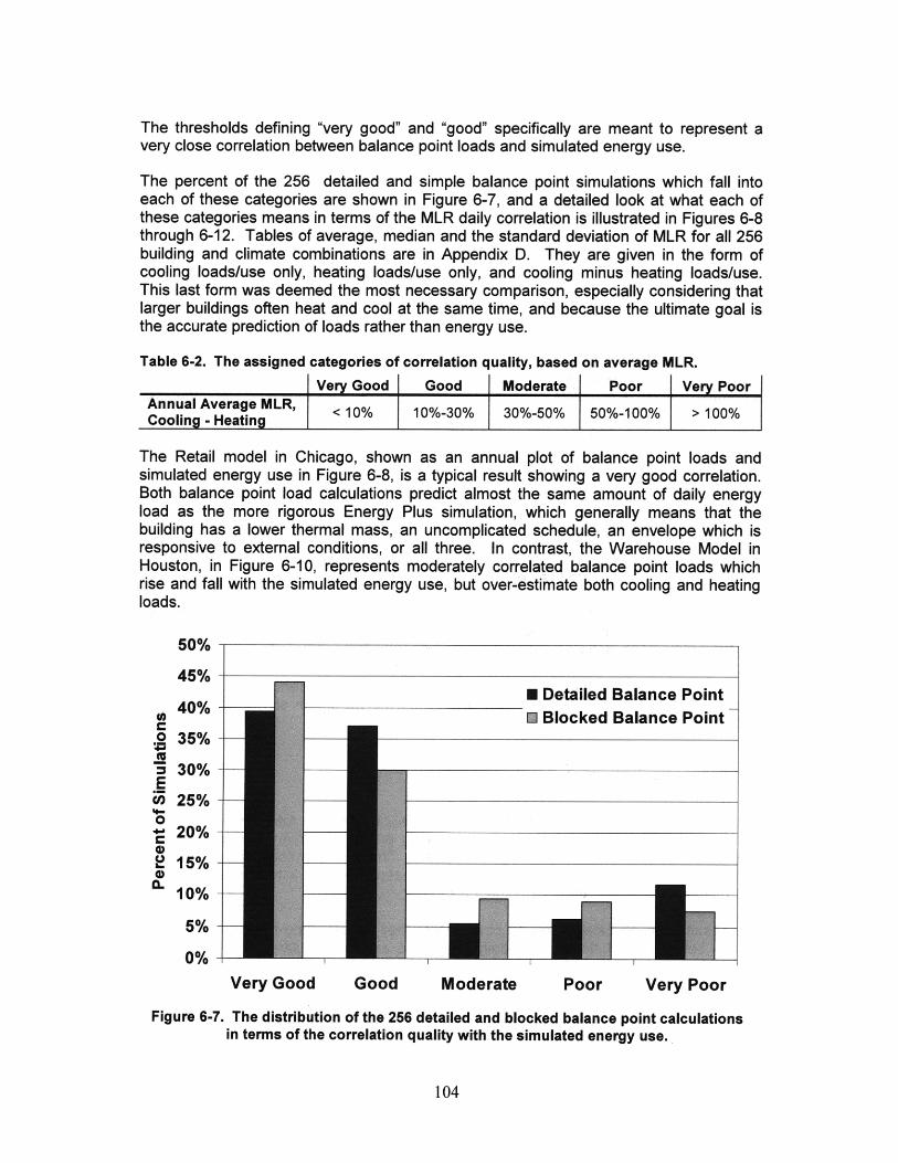
The thresholds defining "very good" and "good" specifically are meant to represent avery close correlation between balance point loads and simulated energy use.

The percent of the 256 detailed and simple balance point simulations which fall intoeach of these categories are shown in Figure 6-7, and a detailed look at what each ofthese categories means in terms of the MLR daily correlation is illustrated in Figures 6-8through 6-12. Tables of average, median and the standard deviation of MLR for all 256building and climate combinations are in Appendix D. They are given in the form ofcooling loads/use only, heating loads/use only, and cooling minus heating loads/use.This last form was deemed the most necessary comparison, especially considering thatlarger buildings often heat and cool at the same time, and because the ultimate goal isthe accurate prediction of loads rather than energy use.

Table 6-2. The assigned categories of correlation quality, based on average MLR.Very Good Good Moderate Poor Very Poor

Annual Average MLR, < 10% 10%-30% 30%-50% 50%-100% > 100%Cooling - Heating

The Retail model in Chicago, shown as an annual plot of balance point loads andsimulated energy use in Figure 6-8, is a typical result showing a very good correlation.Both balance point load calculations predict almost the same amount of daily energyload as the more rigorous Energy Plus simulation, which generally means that thebuilding has a lower thermal mass, an uncomplicated schedule, an envelope which isresponsive to external conditions, or all three. In contrast, the Warehouse Model inHouston, in Figure 6-10, represents moderately correlated balance point loads whichrise and fall with the simulated energy use, but over-estimate both cooling and heatingloads.

50%

45%

40% -

35% -

30% -

25% -

20% -

15%

10%

5% -

* Detailed Balance Point* Blocked Balance Point

0% 4Very Good Good Moderate Poor Very Poor

Figure 6-7. The distribution of the 256 detailed and blocked balance point calculationsin terms of the correlation quality with the simulated energy use.

104

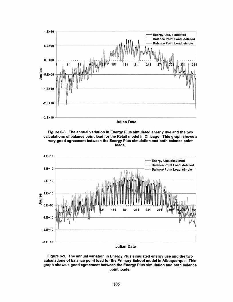
1.E+10

5.E+09 - -

0.E+001 31 81151 181 211 241 2jfr 3 1 36'

-5.E+09-

-1.E11 0

-2.E+10

-2.E-110

Julian Date

Figure 6-8. The annual variation in Energy Plus simulated energy use and the twocalculations of balance point load for the Retail model in Chicago. This graph shows a

very good agreement between the Energy Plus simulation and both balance pointloads.

- Energy Use, simulated- Balance Point Load, detailed

S- Balance Point Load, simple

21 151 181 211 3

Julian Date

Figure 6-9. The annual variation in Energy Plus simulated energy use and the twocalculations of balance point load for the Primary School model in Albuquerque. Thisgraph shows a good agreement between the Energy Plus simulation and both balance

point loads.

105

4.E+10

3.E+10

2.E+10

1.E+10

O.E+00

-1.E+10

-2.E+110

-3.E+10

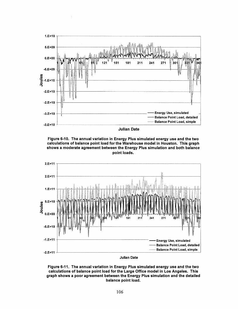
1.E+10

-5.E+09 151 211

O -. E+00

-5.E4-09 f _

-2.E+10

-2.E 110

-3.E+10 -- Energy Use, simulated- Balance Point Load, detailed-- Balance Point Load, simple

-3.E+110Julian Date

Figure 6-10. The annual variation in Energy Plus simulated energy use and the twocalculations of balance point load for the Warehouse model in Houston. This graphshows a moderate agreement between the Energy Plus simulation and both balance

point loads.

2.E+1 I

2.E+11

1.E+1 I

5.E+10

O.E+00

-5.E+1 0

-1.E+11

-2.E+11Julian Date

Figure 6-11. The annual variation in Energy Plus simulated energy use and the twocalculations of balance point load for the Large Office model in Los Angeles. This

graph shows a poor agreement between the Energy Plus simulation and the detailedbalance point load.

106

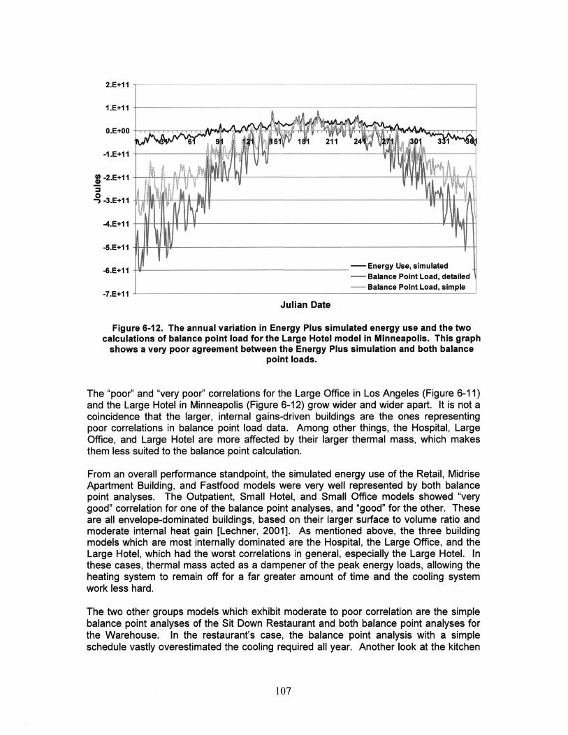
2.E+11

1.E+11

O.E+006 51 1 211 24 3 1 |

-1.E+11 -

-2.E+11

0 N,- -3.E+11

-4.E+11

-5.E+11

-6.E+11 - Energy Use, simulated- Balance Point Load, detailed

-7.E+11 - Balance Point Load, simple

Julian Date

Figure 6-12. The annual variation in Energy Plus simulated energy use and the twocalculations of balance point load for the Large Hotel model in Minneapolis. This graph

shows a very poor agreement between the Energy Plus simulation and both balancepoint loads.

The "poor" and "very poor" correlations for the Large Office in Los Angeles (Figure 6-11)and the Large Hotel in Minneapolis (Figure 6-12) grow wider and wider apart. It is not acoincidence that the larger, internal gains-driven buildings are the ones representingpoor correlations in balance point load data. Among other things, the Hospital, LargeOffice, and Large Hotel are more affected by their larger thermal mass, which makesthem less suited to the balance point calculation.

From an overall performance standpoint, the simulated energy use of the Retail, MidriseApartment Building, and Fastfood models were very well represented by both balancepoint analyses. The Outpatient, Small Hotel, and Small Office models showed "verygood" correlation for one of the balance point analyses, and "good" for the other. Theseare all envelope-dominated buildings, based on their larger surface to volume ratio andmoderate internal heat gain [Lechner, 2001]. As mentioned above, the three buildingmodels which are most internally dominated are the Hospital, the Large Office, and theLarge Hotel, which had the worst correlations in general, especially the Large Hotel. Inthese cases, thermal mass acted as a dampener of the peak energy loads, allowing theheating system to remain off for a far greater amount of time and the cooling systemwork less hard.

The two other groups models which exhibit moderate to poor correlation are the simplebalance point analyses of the Sit Down Restaurant and both balance point analyses forthe Warehouse. In the restaurant's case, the balance point analysis with a simpleschedule vastly overestimated the cooling required all year. Another look at the kitchen

107

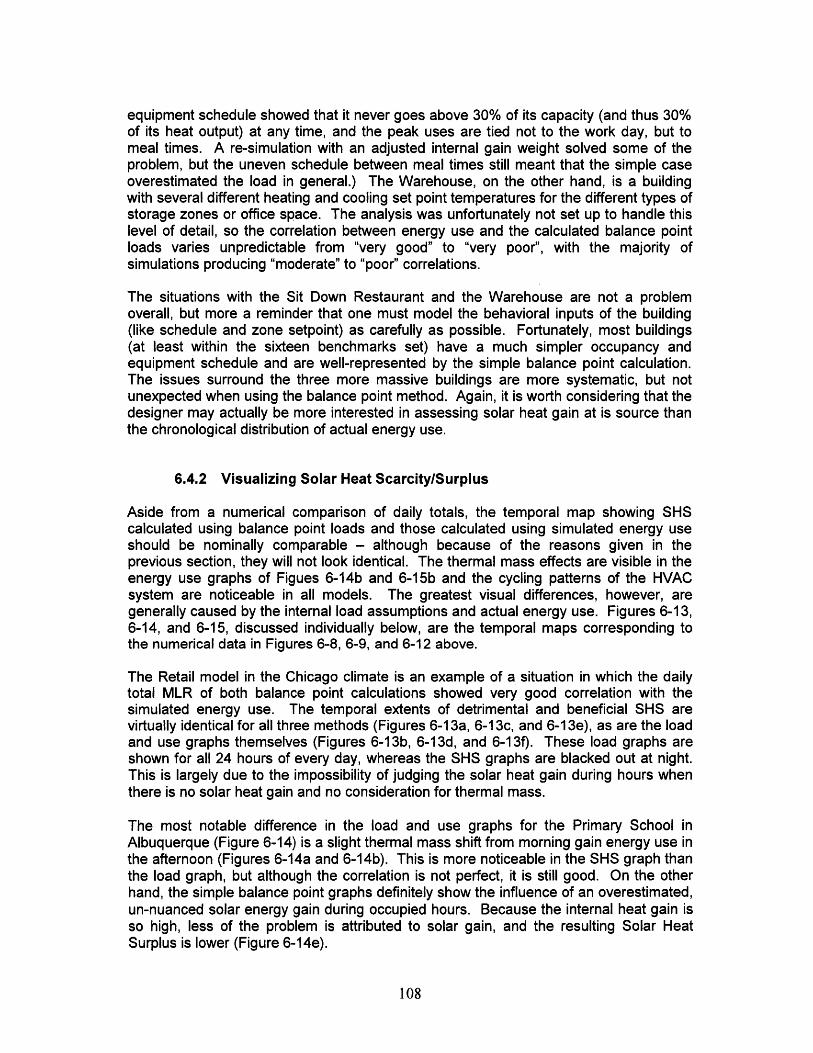
equipment schedule showed that it never goes above 30% of its capacity (and thus 30%of its heat output) at any time, and the peak uses are tied not to the work day, but tomeal times. A re-simulation with an adjusted internal gain weight solved some of theproblem, but the uneven schedule between meal times still meant that the simple caseoverestimated the load in general.) The Warehouse, on the other hand, is a buildingwith several different heating and cooling set point temperatures for the different types ofstorage zones or office space. The analysis was unfortunately not set up to handle thislevel of detail, so the correlation between energy use and the calculated balance pointloads varies unpredictable from "very good" to "very poor", with the majority ofsimulations producing "moderate" to "poor" correlations.

The situations with the Sit Down Restaurant and the Warehouse are not a problemoverall, but more a reminder that one must model the behavioral inputs of the building(like schedule and zone setpoint) as carefully as possible. Fortunately, most buildings(at least within the sixteen benchmarks set) have a much simpler occupancy andequipment schedule and are well-represented by the simple balance point calculation.The issues surround the three more massive buildings are more systematic, but notunexpected when using the balance point method. Again, it is worth considering that thedesigner may actually be more interested in assessing solar heat gain at is source thanthe chronological distribution of actual energy use.

6.4.2 Visualizing Solar Heat Scarcity/Surplus

Aside from a numerical comparison of daily totals, the temporal map showing SHScalculated using balance point loads and those calculated using simulated energy useshould be nominally comparable - although because of the reasons given in theprevious section, they will not look identical. The thermal mass effects are visible in theenergy use graphs of Figues 6-14b and 6-15b and the cycling patterns of the HVACsystem are noticeable in all models. The greatest visual differences, however, aregenerally caused by the internal load assumptions and actual energy use. Figures 6-13,6-14, and 6-15, discussed individually below, are the temporal maps corresponding tothe numerical data in Figures 6-8, 6-9, and 6-12 above.

The Retail model in the Chicago climate is an example of a situation in which the dailytotal MLR of both balance point calculations showed very good correlation with thesimulated energy use. The temporal extents of detrimental and beneficial SHS arevirtually identical for all three methods (Figures 6-13a, 6-13c, and 6-13e), as are the loadand use graphs themselves (Figures 6-13b, 6-13d, and 6-13f). These load graphs areshown for all 24 hours of every day, whereas the SHS graphs are blacked out at night.This is largely due to the impossibility of judging the solar heat gain during hours whenthere is no solar heat gain and no consideration for thermal mass.

The most notable difference in the load and use graphs for the Primary School inAlbuquerque (Figure 6-14) is a slight thermal mass shift from morning gain energy use inthe afternoon (Figures 6-14a and 6-14b). This is more noticeable in the SHS graph thanthe load graph, but although the correlation is not perfect, it is still good. On the otherhand, the simple balance point graphs definitely show the influence of an overestimated,un-nuanced solar energy gain during occupied hours. Because the internal heat gain isso high, less of the problem is attributed to solar gain, and the resulting Solar HeatSurplus is lower (Figure 6-14e).

108

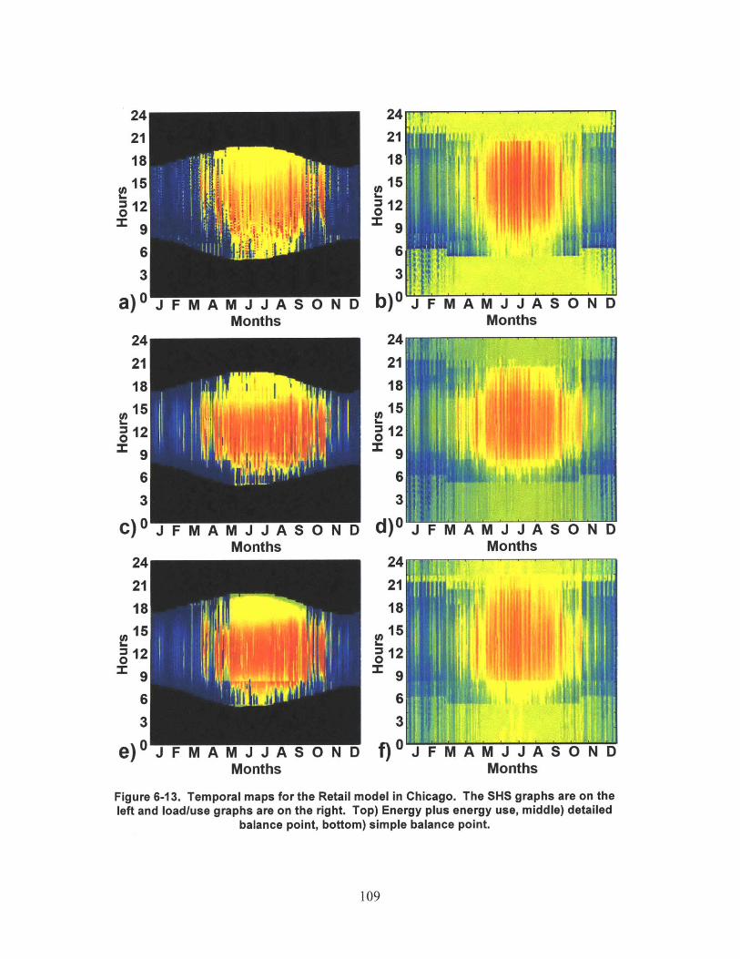
A M J J PMonths

VI J J A U N UMonths

A M J J FMonths

A M J J A SMonths

Figure 6-13. Temporal maps for the Retail model in Chicago. The SHS graphs are on theleft and load/use graphs are on the right. Top) Energy plus energy use, middle) detailed

balance point, bottom) simple balance point.

109

63

a) 0

24i

21

18EM

Is12

9

3.

b)= J F

21

18

15

12

6

3

d)J F

M A M J J AMonths

S O ND

C) AJ J AMonths

3

e) 0

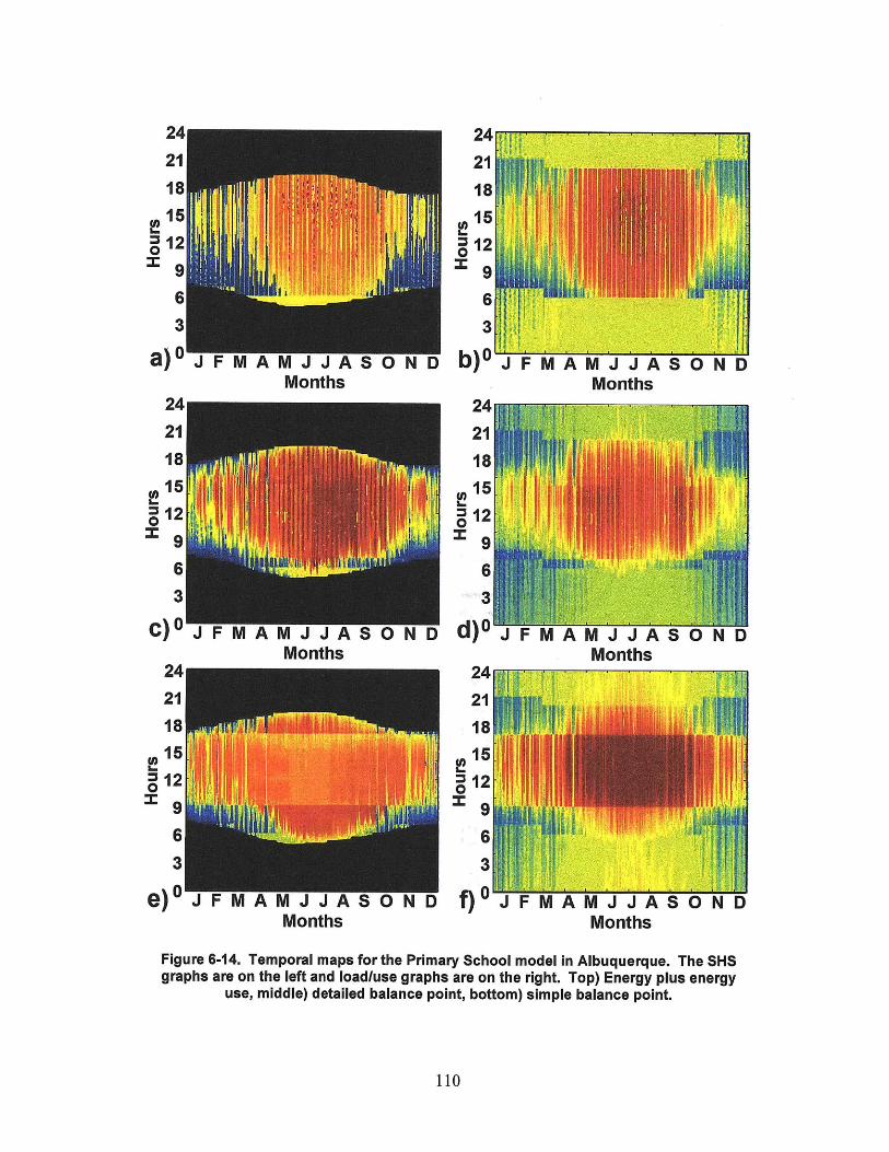
24

21

181512

3b) 0

24

21

1815

12

9

63

d)0 J F M A M J J AMonths

VI J J AMonths

Figure 6-14. Temporal maps for the Primary School model in Albuquerque. The SHSgraphs are on the left and loadluse graphs are on the right. Top) Energy plus energy

use, middle) detailed balance point, bottom) simple balance point.

110

vi 1J I AMonths

A M J J A b U N DMonths

24

21

18

= 12;

96

3

C) 0 J F24

21

1815

12

9

WI J J AMonths

e) J I- M AM J J AMonths

a) O j

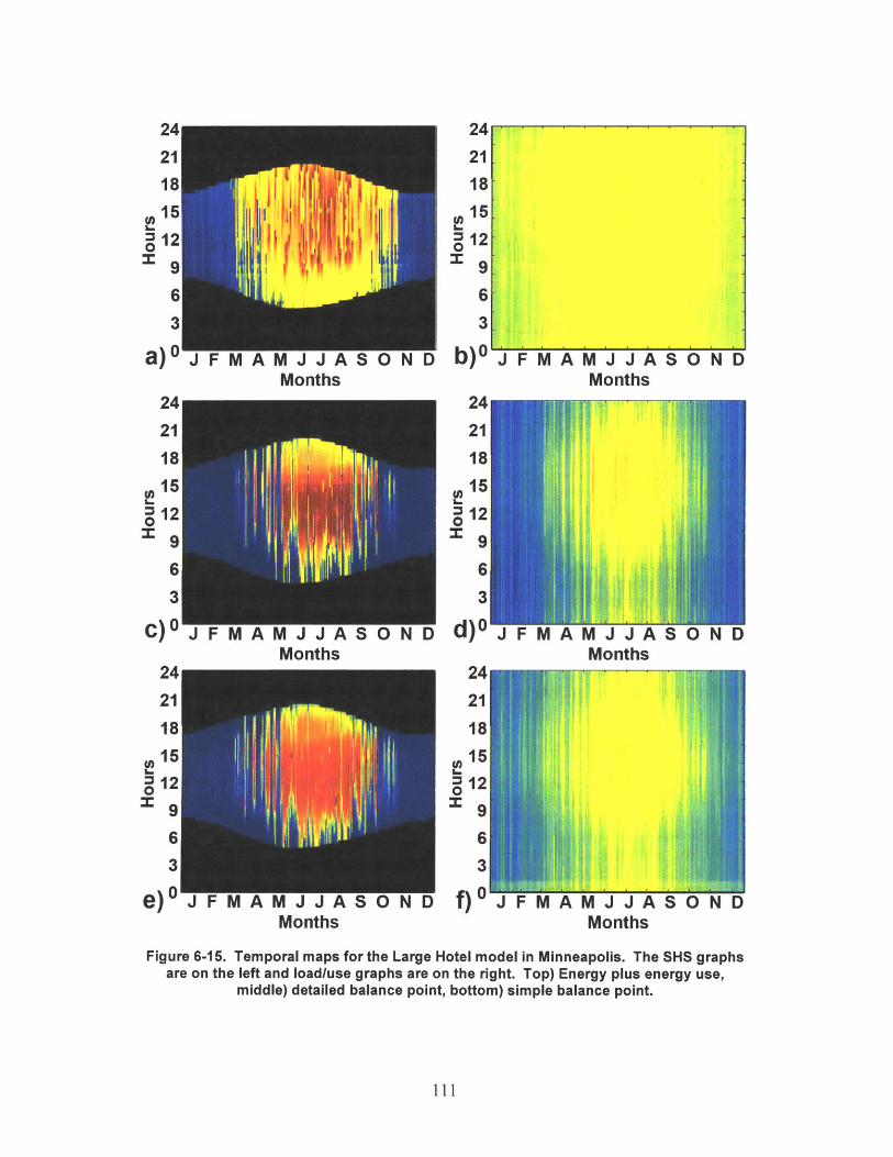
24

211815

12

963

6 J J A S O N DMonths

b) uJ

24

21

1815

812

9

63

d)0A M J J AMonths

M J J PMonths

F M A M J J A S O NMonths

M J J A SMonths

MA M J J A S 0NDMonths

Figure 6-15. Temporal maps for the Large Hotel model in Minneapolis. The SHS graphsare on the left and loadluse graphs are on the right. Top) Energy plus energy use,

middle) detailed balance point, bottom) simple balance point.

111

a)

24

21

1815129

C)

24

21181512

963

e) 0 J F

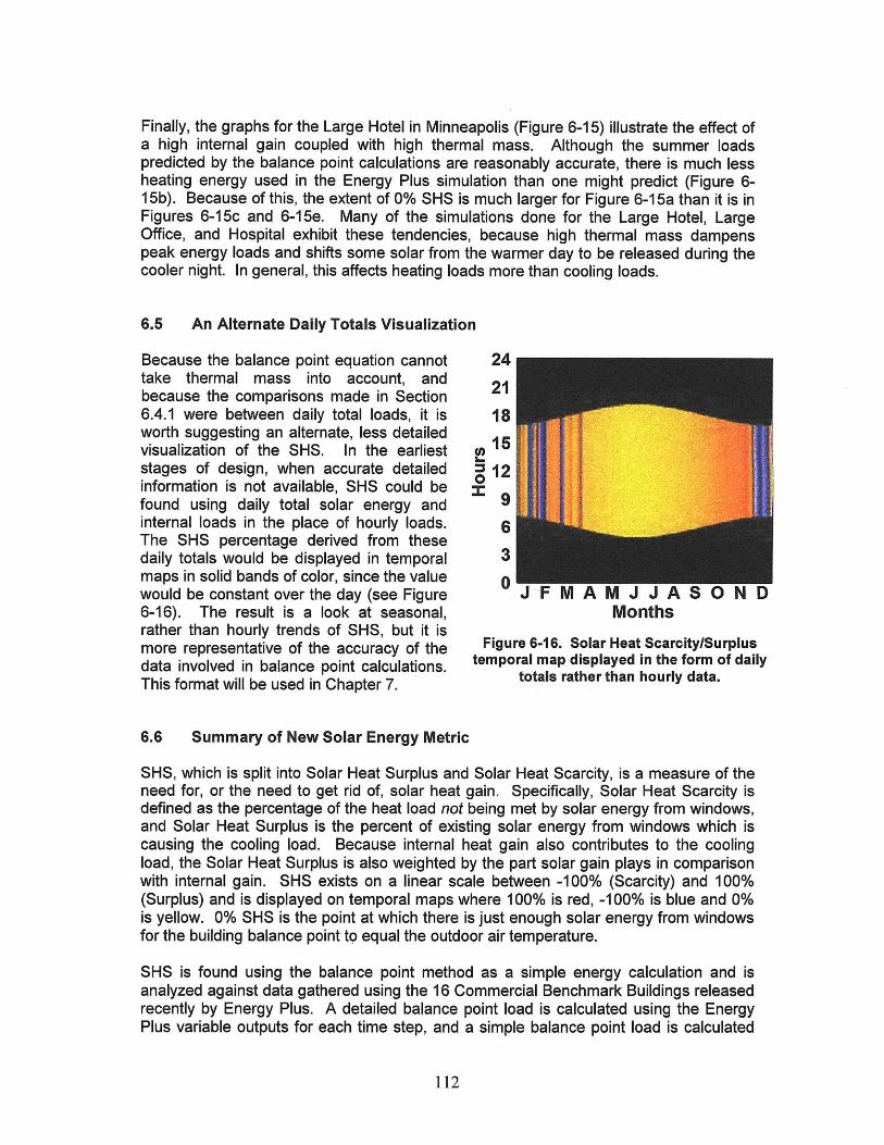
Finally, the graphs for the Large Hotel in Minneapolis (Figure 6-15) illustrate the effect ofa high internal gain coupled with high thermal mass. Although the summer loadspredicted by the balance point calculations are reasonably accurate, there is much lessheating energy used in the Energy Plus simulation than one might predict (Figure 6-15b). Because of this, the extent of 0% SHS is much larger for Figure 6-15a than it is inFigures 6-15c and 6-15e. Many of the simulations done for the Large Hotel, LargeOffice, and Hospital exhibit these tendencies, because high thermal mass dampenspeak energy loads and shifts some solar from the warmer day to be released during thecooler night. In general, this affects heating loads more than cooling loads.

6.5 An Alternate Daily Totals Visualization

Because the balance point equation cannottake thermal mass into account, andbecause the comparisons made in Section6.4.1 were between daily total loads, it isworth suggesting an alternate, less detailedvisualization of the SHS. In the earlieststages of design, when accurate detailedinformation is not available, SHS could befound using daily total solar energy andinternal loads in the place of hourly loads.The SHS percentage derived from thesedaily totals would be displayed in temporalmaps in solid bands of color, since the valuewould be constant over the day (see Figure6-16). The result is a look at seasonal,rather than hourly trends of SHS, but it ismore representative of the accuracy of thedata involved in balance point calculations.This format will be used in Chapter 7.

24

21

1815

12

96

30

W J JPMonths

Figure 6-16. Solar Heat Scarcity/Surplustemporal map displayed in the form of daily

totals rather than hourly data.

6.6 Summary of New Solar Energy Metric

SHS, which is split into Solar Heat Surplus and Solar Heat Scarcity, is a measure of theneed for, or the need to get rid of, solar heat gain. Specifically, Solar Heat Scarcity isdefined as the percentage of the heat load not being met by solar energy from windows,and Solar Heat Surplus is the percent of existing solar energy from windows which iscausing the cooling load. Because internal heat gain also contributes to the coolingload, the Solar Heat Surplus is also weighted by the part solar gain plays in comparisonwith internal gain. SHS exists on a linear scale between -100% (Scarcity) and 100%(Surplus) and is displayed on temporal maps where 100% is red, -100% is blue and 0%is yellow. 0% SHS is the point at which there is just enough solar energy from windowsfor the building balance point to equal the outdoor air temperature.

SHS is found using the balance point method as a simple energy calculation and isanalyzed against data gathered using the 16 Commercial Benchmark Buildings releasedrecently by Energy Plus. A detailed balance point load is calculated using the EnergyPlus variable outputs for each time step, and a simple balance point load is calculated

112

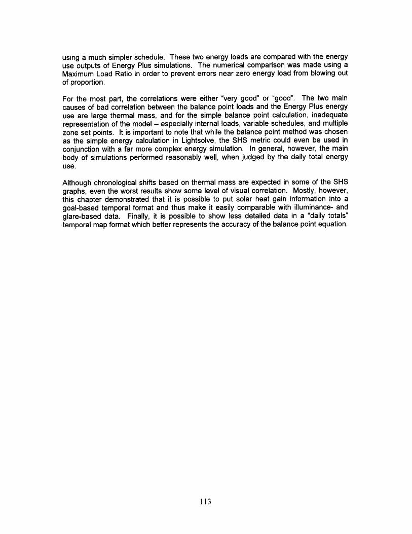
using a much simpler schedule. These two energy loads are compared with the energyuse outputs of Energy Plus simulations. The numerical comparison was made using aMaximum Load Ratio in order to prevent errors near zero energy load from blowing outof proportion.

For the most part, the correlations were either "very good" or "good". The two maincauses of bad correlation between the balance point loads and the Energy Plus energyuse are large thermal mass, and for the simple balance point calculation, inadequaterepresentation of the model - especially internal loads, variable schedules, and multiplezone set points. It is important to note that while the balance point method was chosenas the simple energy calculation in Lightsolve, the SHS metric could even be used inconjunction with a far more complex energy simulation. In general, however, the mainbody of simulations performed reasonably well, when judged by the daily total energyuse.

Although chronological shifts based on thermal mass are expected in some of the SHSgraphs, even the worst results show some level of visual correlation. Mostly, however,this chapter demonstrated that it is possible to put solar heat gain information into agoal-based temporal format and thus make it easily comparable with illuminance- andglare-based data. Finally, it is possible to show less detailed data in a "daily totals"temporal map format which better represents the accuracy of the balance point equation.

113

Chapter 7

Temporal Maps and Design Analysis

Temporal maps have great potential for aiding early-stage design analysis. They havethe ability to convey a full annual data set within a single graphic, which instantlyconnects daylighting performance with important time-based design influences like sunangle, seasonal climate, and occupancy hours. Although they are stronger inpartnership with spatially-based data or renderings, a survey given by the author foundthat architects could answer simple analysis questions based only on AcceptableIlluminance Extent (AIE) temporal maps with no spatial references given at all (seeSection 7.4).

In the following sections, several examples are given which illustrated the analysispotential of the temporal data and metrics described in Chapters 3 through 6: a simplemock design process, a comparison of spatial and temporal information for a classroomand other models, and an options analysis for the orientation and window shades in asingle hospital room. Although this thesis provides a solar heat gain metric andrecommends a comparison of all three aspects of daylighting for a complete analysis(light quantity, glare, and solar heat gain), these examples focus on AIE and GAE (GlareAvoidance Extent), because the solar gain analysis capabilities of Lightsolve have yet tobe implemented.

7.1 Iterative Example of Improving Illuminance Performance

To illustrate a design process of several iterations, a simple box-like room was created inRadiance, located in Sydney, Australia, and given an arbitrary illuminance range goal of400-1000 lux on the work plane (with partial credit given down to 200 and up to 2000lux). This test illuminance range was not chosen for any particular reason, other than tokeep relatively even light appropriate for reading available on the work plane. Nooccupancy hours are given for this model, so we are concerned with all sunlight hours.Radiance was used to perform the rendering rather than the LSV engine so that thesemodels could be used as visual validation models for AIE (see Section 4.2.1), and theparameters used are similar to those considered in the validation of the data reductionmethod in Section 3.x: -ab 5, -ar 128, -aa .1, -ad 2048, -as 256, -dp 1024, -ds .15, -dt.05, -dc .75, -dr 3, -ms 0.066, -sj 1, -st .01, -Ir 12, -1w .0005, -1+, -h.

The model (see Figure 7-1) is not much more complicated than the shoebox model fromChapter 3. It is 7.5m by 1 Om by 3m, with the short fagade on the north and south faces.Two punch windows, each 2m wide by 1.5m tall, are located on the north (sunny) fagadewith 1.5m between them and a sill height of 1m. All objects are grayscale and opaqueobjects are lambertian; the ceiling reflectance is 83%, the wall reflectance is 65%, thefloor reflectance is 20%, and the visible transmittance of the glass is 80%. Becausethere was initially going to be a classroom, there is a 6m by 1.5m chalkboard on the eastwall with a 5% reflectance. The walls have a thickness of 25cm. An array of twelvework plane sensors were placed 1 m from the floor at 2m, 3.5m, and 5m east of the westwall and 1m, 3.5m, 6m, and 8.5m north of the south wall.

114

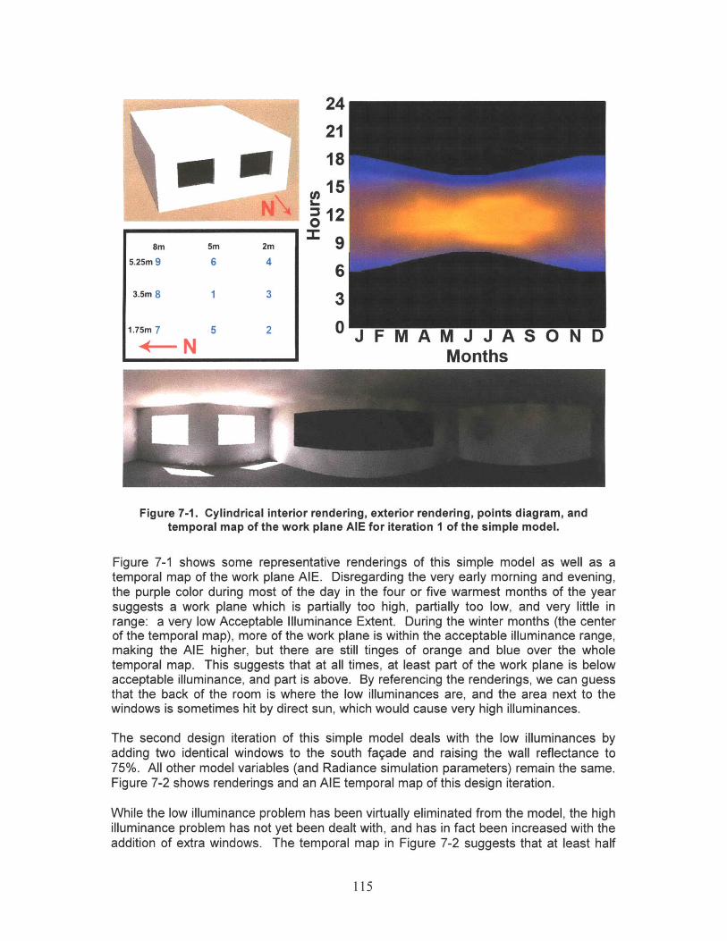
24

21-018____ ___ 12

8m 5m 2m 95.25m 9 6 46

3.5m 8 1 3 3

1.757 5 2 0 FM M AS N15m 7 5 20J F M A M J J A S 0 N DMonths

Figure 7-1. Cylindrical interior rendering, exterior rendering, points diagram, andtemporal map of the work plane AlE for iteration I of the simple model.

Figure 7-1 shows some representative renderings of this simple model as well as atemporal map of the work plane AIE. Disregarding the very early morning and evening,the purple color during most of the day in the four or five warmest months of the yearsuggests a work plane which is partially too high, partially too low, and very little inrange: a very low Acceptable Illuminance Extent. During the winter months (the centerof the temporal map), more of the work plane is within the acceptable illuminance range,making the AIE higher, but there are still tinges of orange and blue over the wholetemporal map. This suggests that at all times, at least part of the work plane is belowacceptable illuminance, and part is above. By referencing the renderings, we can guessthat the back of the room is where the low illuminances are, and the area next to thewindows is sometimes hit by direct sun, which would cause very high illuminances.

The second design iteration of this simple model deals with the low illuminances byadding two identical windows to the south fagade and raising the wall reflectance to75%. All other model variables (and Radiance simulation parameters) remain the same.Figure 7-2 shows renderings and an AIE temporal map of this design iteration.

While the low illuminance problem has been virtually eliminated from the model, the highilluminance problem has not yet been dealt with, and has in fact been increased with theaddition of extra windows. The temporal map in Figure 7-2 suggests that at least half

115

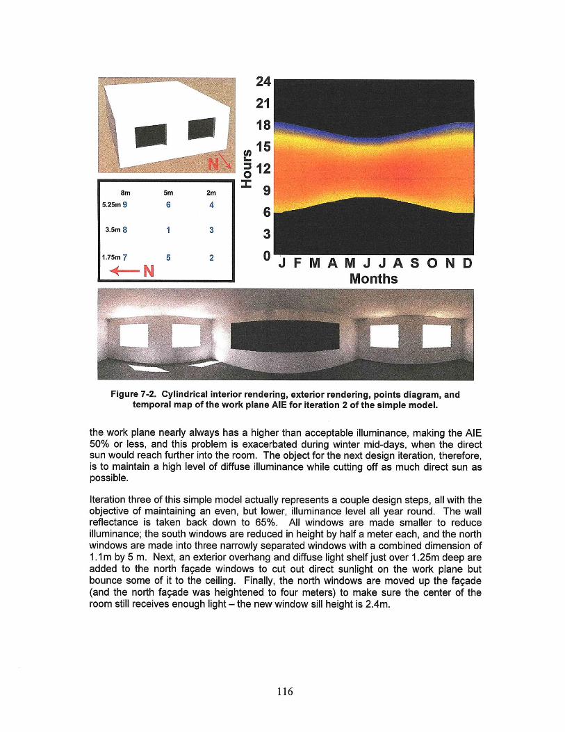
242118

01512

8m 5m 2m5.25m 9 6 4

3.5m 8 1 3 3

1.75m 7 5 20 J F M A M J J A S N D

Months

Figure 7-2. Cylindrical interior rendering, exterior rendering, points diagram, andtemporal map of the work plane AIE for iteration 2 of the simple model.

the work plane nearly always has a higher than acceptable illuminance, making the AIE50% or less, and this problem is exacerbated during winter mid-days, when the directsun would reach further into the room. The object for the next design iteration, therefore,is to maintain a high level of diffuse illuminance while cutting off as much direct sun aspossible.

Iteration three of this simple model actually represents a couple design steps, all with theobjective of maintaining an even, but lower, illuminance level all year round. The wallreflectance is taken back down to 65%. All windows are made smaller to reduceilluminance; the south windows are reduced in height by half a meter each, and the northwindows are made into three narrowly separated windows with a combined dimension of1.1 m by 5 m. Next, an exterior overhang and diffuse light shelf just over 1.25m deep areadded to the north fagade windows to cut out direct sunlight on the work plane butbounce some of it to the ceiling. Finally, the north windows are moved up the fagade(and the north fagade was heightened to four meters) to make sure the center of theroom still receives enough light - the new window sill height is 2.4m.

116

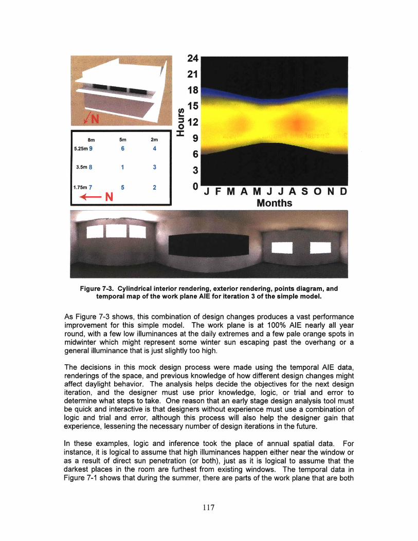
2421

~18I-

12

5 m 5m 2m 95.25m 9 6 6

3.5mB8 1 3 3

1.75m7 5 2 0 J F M A M J J A S O N DMonths

Figure 7-3. Cylindrical interior rendering, exterior rendering, points diagram, andtemporal map of the work plane AlE for iteration 3 of the simple model.

As Figure 7-3 shows, this combination of design changes produces a vast performanceimprovement for this simple model. The work plane is at 100% AIE nearly all yearround, with a few low illuminances at the daily extremes and a few pale orange spots inmidwinter which might represent some winter sun escaping past the overhang or ageneral illuminance that is just slightly too high.

The decisions in this mock design process were made using the temporal AIE data,renderings of the space, and previous knowledge of how different design changes mightaffect daylight behavior. The analysis helps decide the objectives for the next designiteration, and the designer must use prior knowledge, logic, or trial and error todetermine what steps to take. One reason that an early stage design analysis tool mustbe quick and interactive is that designers without experience must use a combination oflogic and trial and error, although this process will also help the designer gain thatexperience, lessening the necessary number of design iterations in the future.

In these examples, logic and inference took the place of annual spatial data. Forinstance, it is logical to assume that high illuminances happen either near the window oras a result of direct sun penetration (or both), just as it is logical to assume that thedarkest places in the room are furthest from existing windows. The temporal data inFigure 7-1 shows that during the summer, there are parts of the work plane that are both

117

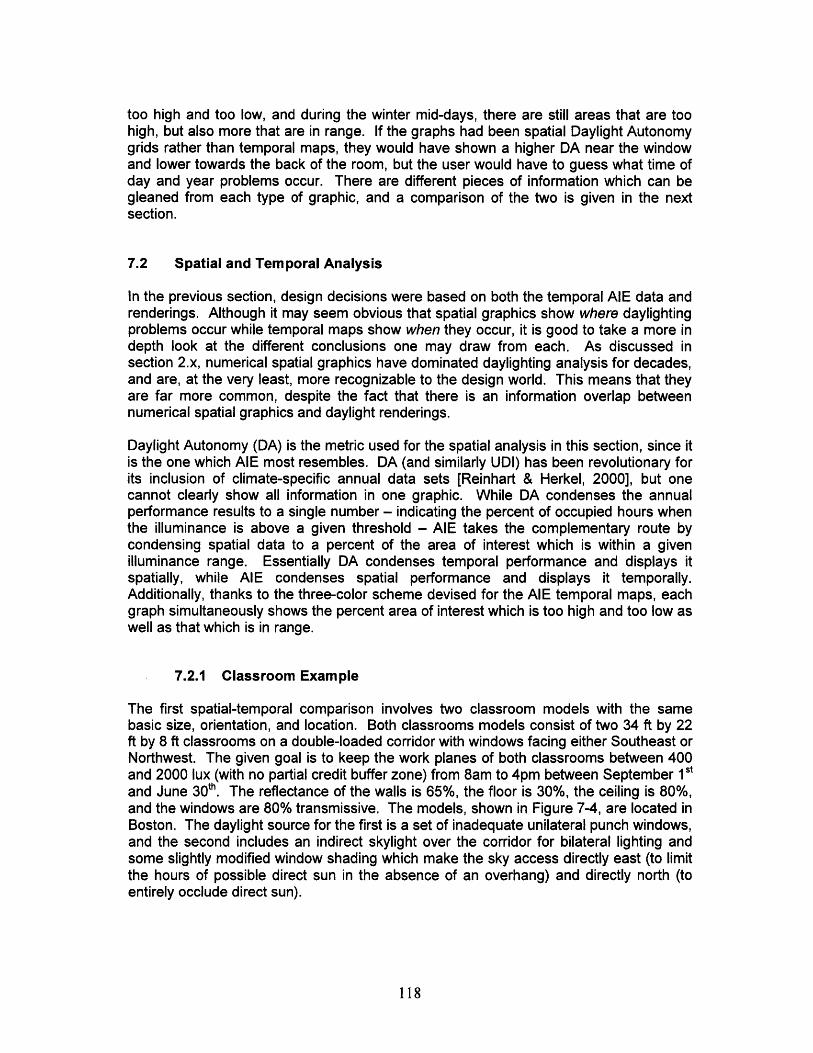
too high and too low, and during the winter mid-days, there are still areas that are toohigh, but also more that are in range. If the graphs had been spatial Daylight Autonomygrids rather than temporal maps, they would have shown a higher DA near the windowand lower towards the back of the room, but the user would have to guess what time ofday and year problems occur. There are different pieces of information which can begleaned from each type of graphic, and a comparison of the two is given in the nextsection.

7.2 Spatial and Temporal Analysis

In the previous section, design decisions were based on both the temporal AIE data andrenderings. Although it may seem obvious that spatial graphics show where daylightingproblems occur while temporal maps show when they occur, it is good to take a more indepth look at the different conclusions one may draw from each. As discussed insection 2.x, numerical spatial graphics have dominated daylighting analysis for decades,and are, at the very least, more recognizable to the design world. This means that theyare far more common, despite the fact that there is an information overlap betweennumerical spatial graphics and daylight renderings.

Daylight Autonomy (DA) is the metric used for the spatial analysis in this section, since itis the one which AIE most resembles. DA (and similarly UDI) has been revolutionary forits inclusion of climate-specific annual data sets [Reinhart & Herkel, 2000], but onecannot clearly show all information in one graphic. While DA condenses the annualperformance results to a single number - indicating the percent of occupied hours whenthe illuminance is above a given threshold - AIE takes the complementary route bycondensing spatial data to a percent of the area of interest which is within a givenilluminance range. Essentially DA condenses temporal performance and displays itspatially, while AIE condenses spatial performance and displays it temporally.Additionally, thanks to the three-color scheme devised for the AIE temporal maps, eachgraph simultaneously shows the percent area of interest which is too high and too low aswell as that which is in range.

7.2.1 Classroom Example

The first spatial-temporal comparison involves two classroom models with the samebasic size, orientation, and location. Both classrooms models consist of two 34 ft by 22ft by 8 ft classrooms on a double-loaded corridor with windows facing either Southeast orNorthwest. The given goal is to keep the work planes of both classrooms between 400and 2000 lux (with no partial credit buffer zone) from 8am to 4pm between September 1stand June 3 0th. The reflectance of the walls is 65%, the floor is 30%, the ceiling is 80%,and the windows are 80% transmissive. The models, shown in Figure 7-4, are located inBoston. The daylight source for the first is a set of inadequate unilateral punch windows,and the second includes an indirect skylight over the corridor for bilateral lighting andsome slightly modified window shading which make the sky access directly east (to limitthe hours of possible direct sun in the absence of an overhang) and directly north (toentirely occlude direct sun).

118

Figure 7-4. Exterior and interior views of SketchUp models (including sensor planes)for classroom I (top) and classroom 2 (bottom).

The classrooms were modeled in SketchUp and the temporal maps were made usingLightsolve. The SketchUp models were then imported into Ecotect and exported intoDaysim to produce the appropriate DA data, which was then imported back into Ecotectwhere it was displayed graphically in two parts, the first showing the DA with a 400 luxthreshold, and the second showing the DA with a 2000 lux threshold. In all instances,the color scheme of the Daylight Autonomy graphics was made to match that of thetemporal maps as closely as possible: The DA graph with a 400 lux threshold fadesfrom blue (0% DA) to yellow (100% DA), and the graph with a 2000 lux threshold fadesfrom yellow (0% DA) to red (100% DA). In each case, yellow is more desirable. Figure7-5. shows all graphics associated with the first basic classroom, and figure 7-6 showsthose relating to the second modified classroom.

The most noticeable feature of the DA graphs is that a large portion of the back of eachroom never reaches 400 lux. They also tell us that a small area near each window issometimes too bright. This in itself is not unexpected; the most interesting informationgiven in the DA graphs is the extent of the space with very low DA, and that the areanearest the window on the southeast side, which is approximately 70-80% DA at 400 luxthreshold, corresponds almost exactly with a similar area between 30% and 60% DA inthe 2000 lux threshold graphs. This suggests that the area near the window actually isonly 20-40% within the prescribed range. The most obvious design decision to makebased on these graphs is to add another light source at the back of the classroom.

The temporal maps give slightly different information. Again the first noticeable featureis that the work plane is always partially too dim - and the whole plane is too dim everyafternoon on the southeast side and nearly all the time on the northwest side. It is alsointeresting to note that the southeastern room receives similarly bright light in themorning regardless of season, and that this light places part of the work plane in rangeand simultaneously makes part too high. This suggests that it is difficult to keep anysignificant percent AIE without also incurring direct sunlight - a circumstance which

119

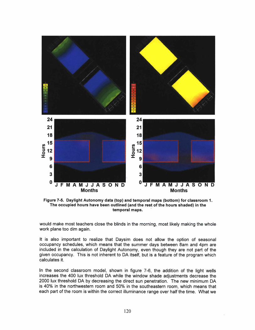
24 24

21 2118 18

015S12 1

9 96 6

3 3

0 J F MA MJ J ASOND 0J FM A MJJ A SON DMonths Months

Figure 7-5. Daylight Autonomy data (top) and temporal maps (bottom) for classroom 1.The occupied hours have been outlined (and the rest of the hours shaded) in the

temporal maps.

would make most teachers close the blinds in the morning, most likely making the wholework plane too dim again.

It is also important to realize that Daysim does not allow the option of seasonaloccupancy schedules, which means that the summer days between 8am and 4pm areincluded in the calculation of Daylight Autonomy, even though they are not part of thegiven occupancy. This is not inherent to DA itself, but is a feature of the program whichcalculates it.

In the second classroom model, shown in figure 7-6, the addition of the light wellsincreases the 400 lux threshold DA while the window shade adjustments decrease the2000 lux threshold DA by decreasing the direct sun penetration. The new minimum DAis 40% in the northwestern room and 50% in the southeastern room, which means thateach part of the room is within the correct illuminance range over half the time. What we

120

............................................................. . .................................................................................................................................................. .............................................................. ........ ............................

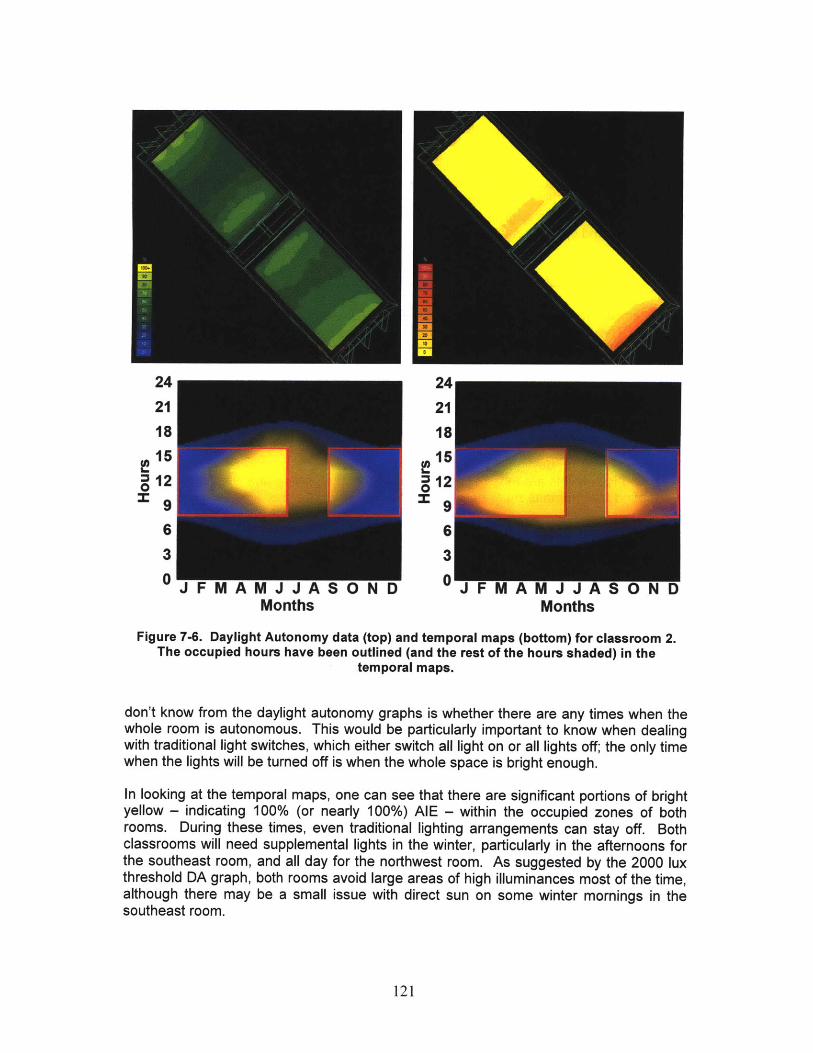
24 2421 2118 18

15 iS12 1=9

6 63 3

0 JFMAMJJASOND 0 JFMAMJ JASONDMonths Months

Figure 7-6. Daylight Autonomy data (top) and temporal maps (bottom) for classroom 2.The occupied hours have been outlined (and the rest of the hours shaded) in the

temporal maps.

don't know from the daylight autonomy graphs is whether there are any times when thewhole room is autonomous. This would be particularly important to know when dealingwith traditional light switches, which either switch all light on or all lights off; the only timewhen the lights will be turned off is when the whole space is bright enough.

In looking at the temporal maps, one can see that there are significant portions of brightyellow - indicating 100% (or nearly 100%) AIE - within the occupied zones of bothrooms. During these times, even traditional lighting arrangements can stay off. Bothclassrooms will need supplemental lights in the winter, particularly in the afternoons forthe southeast room, and all day for the northwest room. As suggested by the 2000 luxthreshold DA graph, both rooms avoid large areas of high illuminances most of the time,although there may be a small issue with direct sun on some winter mornings in thesoutheast room.

121

...... .... .. ..... ........ ........... ...... - ....... - ................................................................................................................................ ::..::..:::::::r ........................ , "" , . ................................. .... ....................

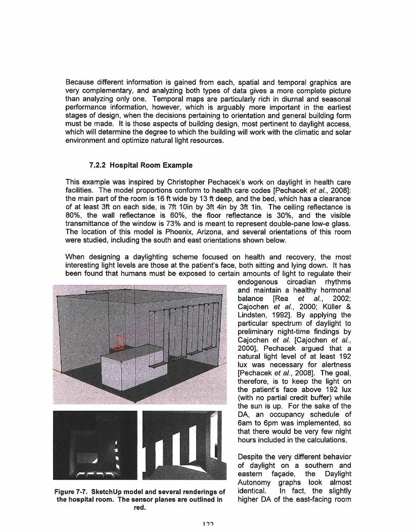
Because different information is gained from each, spatial and temporal graphics arevery complementary, and analyzing both types of data gives a more complete picturethan analyzing only one. Temporal maps are particularly rich in diurnal and seasonalperformance information, however, which is arguably more important in the earlieststages of design, when the decisions pertaining to orientation and general building formmust be made. It is those aspects of building design, most pertinent to daylight access,which will determine the degree to which the building will work with the climatic and solarenvironment and optimize natural light resources.

7.2.2 Hospital Room Example

This example was inspired by Christopher Pechacek's work on daylight in health carefacilities. The model proportions conform to health care codes [Pechacek et aL, 2008]:the main part of the room is 16 ft wide by 13 ft deep, and the bed, which has a clearanceof at least 3ft on each side, is 7ft 1Oin by 3ft 4in by 3ft 1in. The ceiling reflectance is80%, the wall reflectance is 60%, the floor reflectance is 30%, and the visibletransmittance of the window is 73% and is meant to represent double-pane low-e glass.The location of this model is Phoenix, Arizona, and several orientations of this roomwere studied, including the south and east orientations shown below.

When designing a daylighting scheme focused on health and recovery, the mostinteresting light levels are those at the patient's face, both sitting and lying down. It hasbeen found that humans must be exposed to certain amounts of light to regulate their

endogenous circadian rhythmsand maintain a healthy hormonalbalance [Rea et al., 2002;Cajochen et aL, 2000; Koller &Lindsten, 1992]. By applying theparticular spectrum of daylight topreliminary night-time findings byCajochen et al. [Cajochen et aL,2000], Pechacek argued that anatural light level of at least 192lux was necessary for alertness[Pechacek et aL, 2008]. The goal,therefore, is to keep the light onthe patient's face above 192 lux(with no partial credit buffer) whilethe sun is up. For the sake of theDA, an occupancy schedule of6am to 6pm was implemented, sothat there would be very few nighthours included in the calculations.

Despite the very different behaviorof daylight on a southern andeastern fagade, the DaylightAutonomy graphs look almost

Figure 7-7. SketchUp model and several renderings of identical. In fact, the slightlythe hospital room. The sensor planes are outlined in higher DA of the east-facing room

red.

122

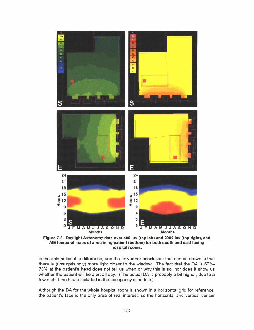
24 2421 2118 18

12 129 IN 9

6 6______________

3 _ _ _ _ _ _ _ 3 _ _ _ _ _

0 JFMAMJJASOND 0 JFMAMJJASONDMonths Months

Figure 7-8. Daylight Autonomy data over 400 lux (top left) and 2000 lux (top right), andAlE temporal maps of a reclining patient (bottom) for both south and east facing

hospital rooms.

is the only noticeable difference, and the only other conclusion that can be drawn is thatthere is (unsurprisingly) more light closer to the window. The fact that the DA is 60%-70% at the patient's head does not tell us when or why this is so, nor does it show uswhether the patient will be alert all day. (The actual DA is probably a bit higher, due to afew night-time hours included in the occupancy schedule.)

Although the DA for the whole hospital room is shown in a horizontal grid for reference,the patient's face is the only area of real interest, so the horizontal and vertical sensor

123

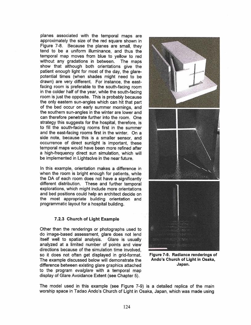
planes associated with the temporal maps areapproximately the size of the red square shown inFigure 7-8. Because the planes are small, theytend to be a uniform illuminance, and thus thetemporal map moves from blue to yellow to redwithout any gradations in between. The mapsshow that although both orientations give thepatient enough light for most of the day, the glare-potential times (when shades might need to bedrawn) are very different. For instance, the east-facing room is preferable to the south-facing roomin the colder half of the year, while the south-facingroom is just the opposite. This is probably becausethe only eastern sun-angles which can hit that partof the bed occur on early summer mornings, andthe southern sun-angles in the winter are lower andcan therefore penetrate further into the room. Onestrategy this suggests for the hospital, therefore, isto fill the south-facing rooms first in the summerand the east-facing rooms first in the winter. On aside note, because this is a smaller sensor, andoccurrence of direct sunlight is important, thesetemporal maps would have been more refined aftera high-frequency direct sun simulation, which willbe implemented in Lightsolve in the near future.

In this example, orientation makes a difference inwhen the room is bright enough for patients, whilethe DA of each room.does not have a significantlydifferent distribution. These and further temporalexplorations, which might include more orientationsand bed positions could help an architect decide onthe most appropriate building orientation andprogrammatic layout for a hospital building.

7.2.3 Church of Light Example

Other than the renderings or photographs used todo image-based assessment, glare does not lenditself well to spatial analysis. Glare is usuallyanalyzed at a limited number of points and viewdirections because of the simulation time involved,so it does not often get displayed in grid-format. Figure 7-9. Radiance renderings ofThe example discussed below will demonstrate the Ando's Church of Light in Osaka,difference between existing glare graphics attached Japan.to the program evalglare with a temporal mapdisplay of Glare Avoidance Extent (see Chapter 5).

The model used in this example (see Figure 7-9) is a detailed replica of the mainworship space in Tadao Ando's Church of Light in Osaka, Japan, which was made using

124

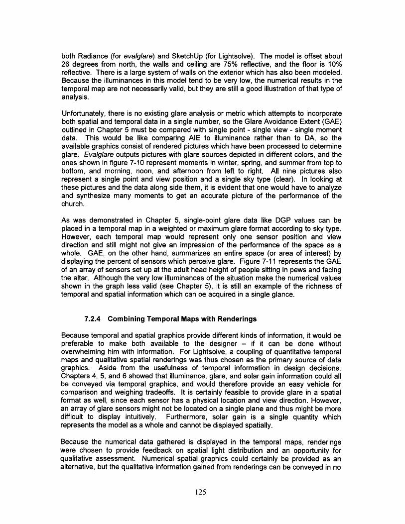
both Radiance (for evalglare) and SketchUp (for Lightsolve). The model is offset about26 degrees from north, the walls and ceiling are 75% reflective, and the floor is 10%reflective. There is a large system of walls on the exterior which has also been modeled.Because the illuminances in this model tend to be very low, the numerical results in thetemporal map are not necessarily valid, but they are still a good illustration of that type ofanalysis.

Unfortunately, there is no existing glare analysis or metric which attempts to incorporateboth spatial and temporal data in a single number, so the Glare Avoidance Extent (GAE)outlined in Chapter 5 must be compared with single point - single view - single momentdata. This would be like comparing AIE to illuminance rather than to DA, so theavailable graphics consist of rendered pictures which have been processed to determineglare. Evalglare outputs pictures with glare sources depicted in different colors, and theones shown in figure 7-10 represent moments in winter, spring, and summer from top tobottom, and morning, noon, and afternoon from left to right. All nine pictures alsorepresent a single point and view position and a single sky type (clear). In looking atthese pictures and the data along side them, it is evident that one would have to analyzeand synthesize many moments to get an accurate picture of the performance of thechurch.

As was demonstrated in Chapter 5, single-point glare data like DGP values can beplaced in a temporal map in a weighted or maximum glare format according to sky type.However, each temporal map would represent only one sensor position and viewdirection and still might not give an impression of the performance of the space as awhole. GAE, on the other hand, summarizes an entire space (or area of interest) bydisplaying the percent of sensors which perceive glare. Figure 7-11 represents the GAEof an array of sensors set up at the adult head height of people sifting in pews and facingthe altar. Although the very low illuminances of the situation make the numerical valuesshown in the graph less valid (see Chapter 5), it is still an example of the richness oftemporal and spatial information which can be acquired in a single glance.

7.2.4 Combining Temporal Maps with Renderings

Because temporal and spatial graphics provide different kinds of information, it would bepreferable to make both available to the designer - if it can be done withoutoverwhelming him with information. For Lightsolve, a coupling of quantitative temporalmaps and qualitative spatial renderings was thus chosen as the primary source of datagraphics. Aside from the usefulness of temporal information in design decisions,Chapters 4, 5, and 6 showed that illuminance, glare, and solar gain information could allbe conveyed via temporal graphics, and would therefore provide an easy vehicle forcomparison and weighing tradeoffs. It is certainly feasible to provide glare in a spatialformat as well, since each sensor has a physical location and view direction. However,an array of glare sensors might not be located on a single plane and thus might be moredifficult to display intuitively. Furthermore, solar gain is a single quantity whichrepresents the model as a whole and cannot be displayed spatially.

Because the numerical data gathered is displayed in the temporal maps, renderingswere chosen to provide feedback on spatial light distribution and an opportunity forqualitative assessment. Numerical spatial graphics could certainly be provided as analternative, but the qualitative information gained from renderings can be conveyed in no

125

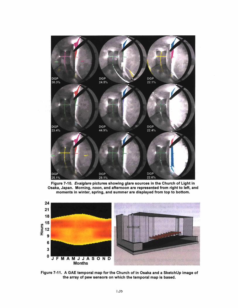
Figure 7-10. Evalglare pictures showing glare sources in the Church of Light inOsaka, Japan. Morning, noon, and afternoon are represented from right to left, and

moments in winter, spring, and summer are displayed from top to bottom.

12196

3

0J F

Figure 7-11. A GAE temporal map for the Church of in Osaka and a SketchUp image ofthe array of pew sensors on which the temporal map is based.

I /-(

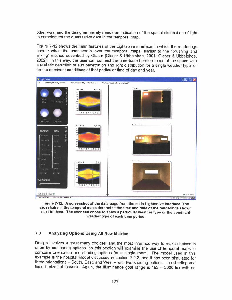
other way, and the designer merely needs an indication of the spatial distribution of lightto complement the quantitative data in the temporal map.

Figure 7-12 shows the main features of the Lightsolve interface, in which the renderingsupdate when the user scrolls over the temporal maps, similar to the "brushing andlinking" method described by Glaser [Glaser & Ubbelohde, 2001; Glaser & Ubbelohde,2002]. In this way, the user can connect the time-based performance of the space witha realistic depiction of sun penetration and light distribution for a single weather type, orfor the dominant conditions at that particular time of day and year.

F*e Model: UgitSolveExample Vw: Temporal Mops /Redeigs Weather: Weather by dkmate (auto)

Dat Mao 3 ? X

temporal map +

Figure 7-12. A screenshot of the data page from the main Lightsolve interface. Thecrosshairs in the temporal maps determine the time and date of the renderings shownnext to them. The user can chose to show a particular weather type or the dominant

weather type of each time period

7.3 Analyzing Options Using All New Metrics

Design involves a great many choices, and the most informed way to make choices isoften by comparing options, so this section will examine the use of temporal maps tocompare orientation and shading options for a single room. The model used in thisexample is the hospital model discussed in section 7.2.2, and it has been simulated forthree orientations - South, East, and West - with two shading options - no shading andfixed horizontal louvers. Again, the illuminance goal range is 192 - 2000 lux with no

127

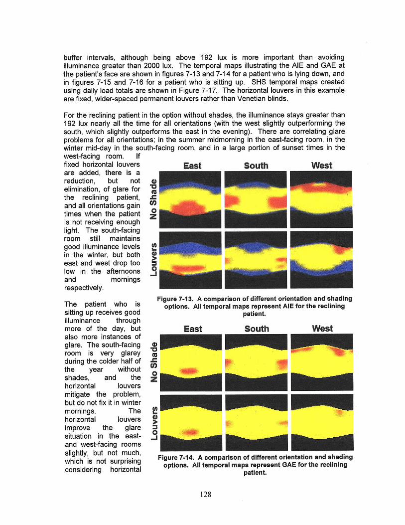
buffer intervals, although being above 192 lux is more important than avoidingilluminance greater than 2000 lux. The temporal maps illustrating the AIE and GAE atthe patient's face are shown in figures 7-13 and 7-14 for a patient who is lying down, andin figures 7-15 and 7-16 for a patient who is sitting up. SHS temporal maps createdusing daily load totals are shown in Figure 7-17. The horizontal louvers in this exampleare fixed, wider-spaced permanent louvers rather than Venetian blinds.

For the reclining patient in the option without shades, the illuminance stays greater than192 lux nearly all the time for all orientations (with the west slightly outperforming thesouth, which slightly outperforms the east in the evening). There are correlating glareproblems for all orientations; in the summer midmorning in the east-facing room, in thewinter mid-day in the south-facing room, and in a large portion of sunset times in thewest-facing room. Iffixed horizontal louvers East South Westare added, there is areduction, but notelimination, of glare for .the reclining patient,and all orientations gaintimes when the patient 0is not receiving enoughlight. The south-facingroom still maintainsgood illuminance levelsin the winter, but botheast and west drop toolow in the afternoons 0and morningsrespectively.

The patient who issitting up receives goodilluminance throughmore of the day, butalso more instances ofglare. The south-facingroom is very glareyduring the colder half ofthe year withoutshades, and thehorizontal louversmitigate the problem,but do not fix it in wintermornings. Thehorizontal louversimprove the glaresituation in the east-and west-facing roomsslightly, but not much,which is not surprisingconsidering horizontal

Figure 7-13. A comparison of different orientation and shadingoptions. All temporal maps represent AlE for the reclining

patient.

East South West

PI

Figure 7-14. A comparison of different orientation and shadingoptions. All temporal maps represent GAE for the reclining

patient.

128

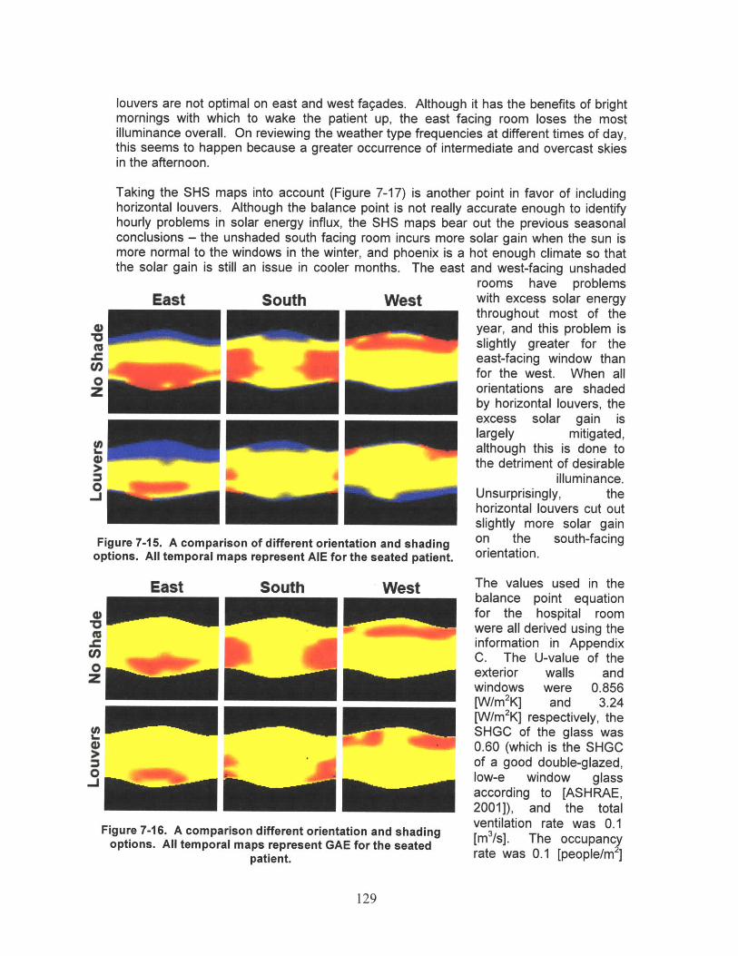
louvers are not optimal on east and west fagades. Although it has the benefits of brightmornings with which to wake the patient up, the east facing room loses the mostilluminance overall. On reviewing the weather type frequencies at different times of day,this seems to happen because a greater occurrence of intermediate and overcast skiesin the afternoon.

Taking the SHS maps into account (Figure 7-17) is another point in favor of includinghorizontal louvers. Although the balance point is not really accurate enough to identifyhourly problems in solar energy influx, the SHS maps bear out the previous seasonalconclusions - the unshaded south facing room incurs more solar gain when the sun ismore normal to the windows in the winter, and phoenix is a hot enough climate so thatthe solar gain is still an issue in cooler months. The east and west-facing unshaded

rooms have problemsEast South West with excess solar energy

throughout most of the0 year, and this problem is

slightly greater for theeast-facing window thanfor the west. When allorientations are shadedby horizontal louvers, theexcess solar gain islargely mitigated,

1 M %_ although this is done tothe detriment of desirable

illuminance.0 Unsurprisingly, the

horizontal louvers cut outslightly more solar gain

Figure 7-15. A comparison of different orientation and shading on the south-facingoptions. All temporal maps represent AlE for the seated patient. orientation.

East South West

Figure 7-16. A comparison different orientation and shadingoptions. All temporal maps represent GAE for the seated

patient.

The values used in thebalance point equationfor the hospital roomwere all derived using theinformation in AppendixC. The U-value of theexterior walls andwindows were 0.856[W/m2K] and 3.24[W/m 2K] respectively, theSHGC of the glass was0.60 (which is the SHGCof a good double-glazed,low-e window glassaccording to [ASHRAE,2001]), and the totalventilation rate was 0.1[m3/s]. The occupancyrate was 0.1 [people/m2]

129

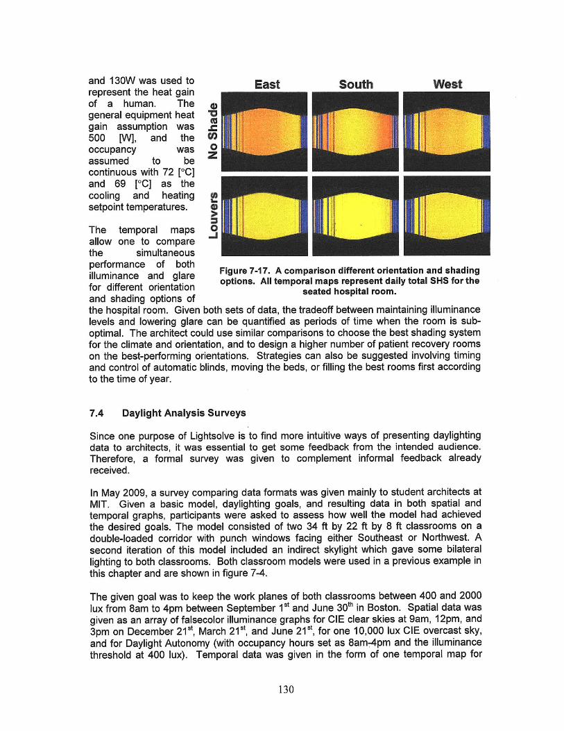
and 130W was used to East South Westrepresent the heat gainof a human. The 0general equipment heat 0gain assumption was .c

500 [W], and the COoccupancy wasassumed to be 2continuous with 72 [OC]and 69 [OC] as thecooling and heating 1setpoint temperatures. 4)

The temporal mapsallow one to comparethe simultaneousperformance of both Figure 7-17. A comparison different orientation and shadingilluminance and glare options. All temporal maps represent daily total SHS for thefor different orientation seated hospital room.and shading options ofthe hospital room. Given both sets of data, the tradeoff between maintaining illuminancelevels and lowering glare can be quantified as periods of time when the room is sub-optimal. The architect could use similar comparisons to choose the best shading systemfor the climate and orientation, and to design a higher number of patient recovery roomson the best-performing orientations. Strategies can also be suggested involving timingand control of automatic blinds, moving the beds, or filling the best rooms first accordingto the time of year.

7.4 Daylight Analysis Surveys

Since one purpose of Lightsolve is to find more intuitive ways of presenting daylightingdata to architects, it was essential to get some feedback from the intended audience.Therefore, a formal survey was given to complement informal feedback alreadyreceived.

In May 2009, a survey comparing data formats was given mainly to student architects atMIT. Given a basic model, daylighting goals, and resulting data in both spatial andtemporal graphs, participants were asked to assess how well the model had achievedthe desired goals. The model consisted of two 34 ft by 22 ft by 8 ft classrooms on adouble-loaded corridor with punch windows facing either Southeast or Northwest. Asecond iteration of this model included an indirect skylight which gave some bilaterallighting to both classrooms. Both classroom models were used in a previous example inthis chapter and are shown in figure 7-4.

The given goal was to keep the work planes of both classrooms between 400 and 2000lux from 8am to 4pm between September 1st and June 3 0 th in Boston. Spatial data wasgiven as an array of falsecolor illuminance graphs for CIE clear skies at 9am, 12pm, and3pm on December 2 1st, March 2 1 't, and June 2 1st, for one 10,000 lux CIE overcast sky,and for Daylight Autonomy (with occupancy hours set as 8am-4pm and the illuminancethreshold at 400 lux). Temporal data was given in the form of one temporal map for

130

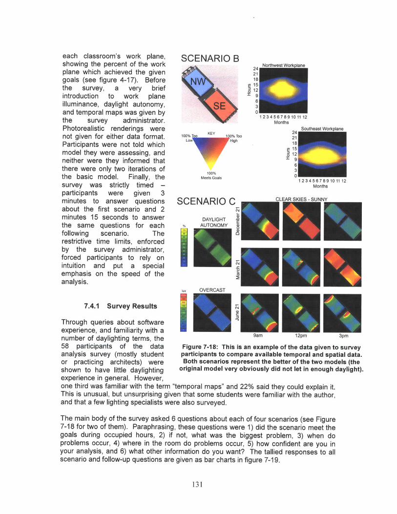
each classroom's work plane,showing the percent of the workplane which achieved the givengoals (see figure 4-17). Beforethe survey, a very briefintroduction to work planeilluminance, daylight autonomy,and temporal maps was given bythe survey administrator.Photorealistic renderings werenot given for either data format.Participants were not told whichmodel they were assessing, andneither were they informed thatthere were only two iterations ofthe basic model. Finally, thesurvey was strictly timed -participants were given 3minutes to answer questionsabout the first scenario and 2minutes 15 seconds to answerthe same questions for eachfollowing scenario. Therestrictive time limits, enforcedby the survey administrator,forced participants to rely onintuition and put a specialemphasis on the speed of theanalysis.

7.4.1 Survey Results

SCENARIO B

)% TooHigh

100%Meets Goals

1 23' 4 b 67 1 U9 10 1112

Months

24 Southeast Workplane2118

n 150 12

963012 3 4 5 6 7 89 10 1112

Months

SCENARIO C

DAYLIGHT% AUTONOMYW~8

OVERCAST

Through queries about softwareexperience, and familiarity with anumber of daylighting terms, the 9am 12pm

58 participants of the data Figure 7-18: This is an example of the data given tanalysis survey (mostly student participants to compare available temporal and spaor practicing architects) were Both scenarios represent the better of the two mocshown to have little daylighting original model very obviously did not let in enoughexperience in general. However,one third was familiar with the term "temporal maps" and 22% said they could explain it.This is unusual, but unsurprising given that some students were familiar with the author,and that a few lighting specialists were also surveyed.

spm

o surveytial data.els (the

daylight).

The main body of the survey asked 6 questions about each of four scenarios (see Figure7-18 for two of them). Paraphrasing, these questions were 1) did the scenario meet thegoals during occupied hours, 2) if not, what was the biggest problem, 3) when doproblems occur, 4) where in the room do problems occur, 5) how confident are you inyour analysis, and 6) what other information do you want? The tallied responses to allscenario and follow-up questions are given as bar charts in figure 7-19.

131

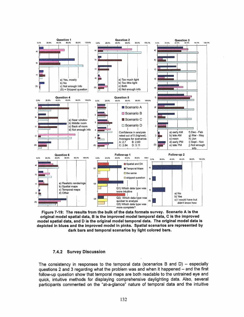
Question I Question 20.0% 20.0% 40.0% 60.0% 80.0% 100.0% 0.0% 20.0% 40.0% 60.0% 80.0% 100)%

a)

b)

)

a) Yes, mostly d a) Too much tightb) No b) Too little light

sc) Not enough Info c) Both(S) = Skipped question d) Not enough info

Question 40.0% 20.0% 40.0% 60.0%

Question 580.0% 100.0% 0.0% 20.0% 40.0% 60.0% 80.0% 100.0%

Question 3n% 70n% 400% inn% Ann% i0

Question 60.0% 20.0% 40.0% 60.0% 80.0% 100.0% 0.0%

Follow-up 120.0% 40.0% 60.0% 80.0% 100.C

U Spatial and DA01 E Temporal Maps a)

D the same

1 skipped question b)

a) Realistic renderings 02

c) Teporal maps Q1) Which data type wasc) Teporalmapsmore intuitive

d) Other a) No

03 Q2) Which data type was b) Yes.qickrtanlz c) I would have but;quicker to analyze (s) ntko o

Q3) Which data type was didn't know howmore complete?

Figure 7-19: The results from the bulk of the data formats survey. Scenario A is theoriginal model spatial data, B is the improved model temporal data, C is the improved

model spatial data, and D is the original model temporal data. The original model data isdepicted in blues and the improved model in pinks. Spatial scenarios are represented by

dark bars and temporal scenarios by light colored bars.

7.4.2 Survey Discussion

The consistency in responses to the temporal data (scenarios B and D) - especiallyquestions 2 and 3 regarding what the problem was and when it happened - and the firstfollow-up question show that temporal maps are both readable to the untrained eye andquick, intuitive methods for displaying comprehensive daylighting data. Also, severalparticipants commented on the "at-a-glance" nature of temporal data and the intuitive

132

Follow-up 2800% 100.0%

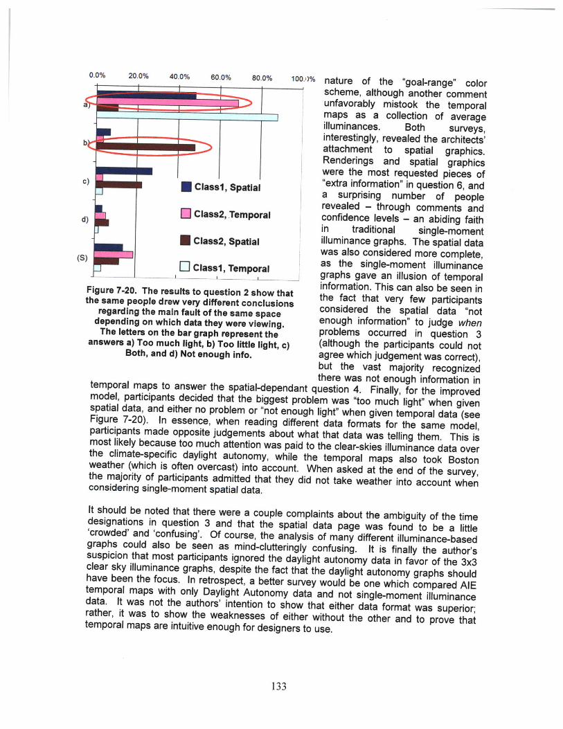
0.0% 20.0% 40.0% 60.0% 80.0% 100.0% nature of the "goal-range" colorscheme, although another comment

sunfavorably mistook the temporal______ _____ _____ ______maps as a collection of average

illuminances. Both surveys,interestingly, revealed the architects'

b attachment to spatial graphics.Renderings and spatial graphicswere the most requested pieces of

C) extra information" in question 6, and

Class2, Spatial* Sptiala surprising number of peoplerevealed - through comments andClass2, Temporal confidence levels - an abiding faithin traditional single-momentSClass2, Spatial illuminance graphs. The spatial datawas also considered more complete,(S) as the single-moment illuminanceEli Cassi Temoralgraphs gave an illusion of temporal

information. This can also be seen inFigure 7-20. The results to question 2 show that the fact that very few participantsthe same people drew very different conclusions considered the spatial data "notregarding the main fault of the same spacedepending on which data they were viewing. enough ora tion The letters on the bar graph represent theanswers a) Too much light, b) Too little light, c) (although the participants could notBoth, and d) Not enough info, agree which judgement was correct),

but the vast majority recognizedthere was not enough information intemporal maps to answer the spatial-dependant question 4. Finally, for the improvedmodel, participants decided that the biggest problem was "too much light" when givenspatial data, and either no problem or "not enough light" when given temporal data (seeFigure 7-20). In essence, when reading different data formats for the same model,participants made opposite judgements about what that data was telling them. This ismost likely because too much attention was paid to the clear-skies illuminance data overthe climate-specific daylight autonomy, while the temporal maps also took Bostonweather (which is often overcast) into account. When asked at the end of the survey,the majority of participants admitted that they did not take weather into account whenconsidering single-moment spatial data.

It should be noted that there were a couple complaints about the ambiguity of the timedesignations in question 3 and that the spatial data page was found to be a little'crowded' and 'confusing. Of course, the analysis of many different illuminance-basedgraphs could also be seen as mind-clutteringly confusing. It is finally the author'ssuspicion that most participants ignored the daylight autonomy data in favor of the 3x3clear sky illuminance graphs, despite the fact that the daylight autonomy graphs shouldhave been the focus. In retrospect, a better survey would be one which compared AlEtemporal maps with only Daylight Autonomy data and not single-moment illuminancedata. It was not the authors' intention to show that either data format was superior;rather, it was to show the weaknesses of either without the other and to prove thattemporal maps are intuitive enough for designers to use.

133

...... ............ .. - - ::- .. .......................... : : r ..! ..................... ................ : : ..: r _ ................... ... ::.- - .. . ............................................... . - , ............................ : ...........

7.5 Design Analysis Summary

In this chapter, examples were shown highlighting the benefits of displaying data in atemporal format. The simple mock design process demonstrated the ability of goal-based temporal maps to convey the degree of design-goal success and the degree andtype of failure to meet goals. The classroom and hospital room comparisons betweengoal-based temporal maps and DA spatial graphs emphasized the different types ofinformation which could be gathered from each. In the temporal maps, the effects ofbuilding orientation and general light access were more pronounced than in the spatialgraphs, as was information pertaining to the instantaneous performance of the wholespace (in other words, whether there are simultaneous highs and lows or if the wholespace is in range at once). The hospital room was also employed in a demonstrationusing temporal maps to compare orientation and window shading options; both AIE andGAE metrics were involved in the comparison, giving more than one dimension to theresults.

Finally, a small-scale survey about reading daylighting data was given to architecturalstudents at MIT. The goal of the survey was to prove the usability and usefulness oftemporal daylighting graphs and to show that they improve an architect's understandingof daylighting performance. While the former claim is well supported by the resultsabove, this section has relied on examples rather than surveys to show the latter.

This chapter included a discussion on the merits of coupling qualitative spatialrenderings with quantitative temporal maps, given that this is the chosen informationpairing in the Lightsolve interface. Since there is a slight redundancy betweenrenderings and spatial graphs, temporal maps could give daylighting data new depth.However, the choice should not be spatial versus temporal data - both should be usedto create the greatest understanding of daylight performance.

134

Chapter 8

Conclusion

Daylighting analysis is under-used in the earliest stages of design, but unfortunately, thatis precisely the time at which it could do the most good. There may be several reasonsfor this, including the current design culture and educational practices, but there is also alack of interactive yet accurate design analysis methods which give the architect allnecessary information in a form that is clear and concise. This thesis has focused onthe simulation, pre-processing, and presentation of light quantity, glare, and solar heatgain data for the purpose of making good design decisions in the earliest stage ofdaylighting design.

8.1 Main Achievements

The overarching objective for the research presented here was to forge a daylightinganalysis process for early stage design which interactively and effectively communicatescomplete and accurate information to the designer. This process has incorporatedexisting research when it fits the agenda, however new work has also been done,especially in the design of goal-based dynamic metrics suitable for temporal graphics.

To achieve this goal, five questions were asked in the introduction:1) What daylighting information is necessary for informed design decisions?2) How can that information be calculated quickly, but with reasonable

accuracy?3) How, if at all, should that information be pre-processed for the designer?4) What output formats should be used to convey the information?5) What metrics are appropriate for those output formats?

First, based on the research of others it was determined that designers require dynamic,climate-inclusive information to fully understand the daylighting performance of a space.Arguments were also made in the introduction and in Chapter 3 for using a format whichpreserves the performance variation over time (a choice which also address question 4).The temporal map was thus chosen to be the basic vehicle for communicatingdaylighting information of all sorts. As a graphic, it emphasizes the time-based variationof daylighting performance, which automatically ties this performance to many of thegreatest influences on daylighting collection, transmission, and distribution - inparticular, to climate considerations and weather type and to solar angles.

Because interactivity is important, and because it reduces the "clutter" of highly detailedannual information, a method was developed to reduce the necessary simulations whilestill keeping the authenticity of realistic sky conditions. The ASRC-CIE sky model wasused to calculate illuminances under four different sky conditions for each of 56 periodsof the year. The sum of these illuminances, weighted by the occurrence of each skytype during the period in question, becomes the single illuminance which represents thewhole period. These illuminances were used to populate temporal maps, which inChapter 3 were then compared to temporal maps made using detailed illuminance data

135

extracted from the program Daysim. The numerical and pixel comparison results weregenerally good and the data reduction method aided the emphasis of generalilluminance trends and patterns. Furthermore, the overlay of high-frequency direct solardata compensated for the inability of a more complex model to capture the highlydynamic nature of direct solar irradiance. This method addresses the questionsconcerning quick, accurate calculation, as does the subsequent development of theDGPm approximation (Chapter 5). The question of pre-processing is handled as part ofthe development of appropriate metrics. Three metrics for communicating three mainaspects of daylight design, light quantity, glare, and solar heat gain, were introduced andvalidated against existing data and processes.

In order to more easily understand the performance of an entire area of interest - be it awork plane in a single or multiple zones, a museum wall, a chalkboard, or other self-contained area to which the same design goals apply - a method was devised forreducing each area to a single temporal map. This metric, called the AcceptableIlluminance Extent (AIE), gives the percent of the area of interest which is within a user-defined illuminance goal range. Thanks to a triangular temporal map color scale whichuses and mixes the three primary colors, the areas of low AIE can be visually dividedinto those areas which are too high and those which are too low. Thus, problem timescan not only be identified but understood as a certain type of issue. Chapter 4 providesa comparison between AIE temporal maps created using the above data reductionmethod and those created using very high frequency Daysim data. The visualcorrelation between these temporal maps is stronger in general even than the singlepoint illuminance comparisons in Chapter 3. The only circumstance under which thevisual correlation is less strong is when the desired illuminance range is very tight andthe model complex.

Chapter 5 examined Daylight Glare Probability (DGP) as a promising glare metric andlooked at the available simplified DGP method (DGPs) for the purpose of annualcalculations. The results show that, while DGPs is a great approximation method forhigh luminance glare, it does not adequately represent contrast-based glare. Analternate model-based DGP approximation method (DGPm) was proposed which usessimulated illuminances, sky distribution equations, and geometric model information tofind the DGP. Both DGPs and DGPm performed very well in the Classroom model,which has large vertical windows and glare caused mostly by the quantity of light hittingthe eye. In the Skylights model, DGPs overestimated the glare a little, probably due tothe bright space combined with the position of the glare sources. In the Frame modeland the Simple Corbusier model, the DGPs approximation underestimated the DGP tonearly the greatest extent allowed by the DGPs equation. This is likely due to the lower-illuminance situations in which glare was largely due to luminance contrast. Conversely,the DGPm method performed within 10% of the DGP nearly all the time, and within 5%of the DGP most of the time. The only model in which this is not true is the Framemodel, where some of the error extended past -10%.

Again, in order to present all available information in as few temporal maps as possible,the glare information at separate sensors was compiled into a single metric, called GlareAvoidance Extent (GAE), which indicates the percent of a group of glare sensors(usually a vertical array) that does not perceive glare - in other words, the portion of thespace at which glare is avoided. In visual comparisons between GAE temporal mapsshowing the true DGP, DGPs, and DGPm, the two approximations performed similarlywell for the Classroom model, and DGPm outperformed DGPs for the Frame model.

136

Chapter 6 discussed the application of the Balance Point load calculation method to asolar heat gain metric called Solar Heat Surplus or Solar Heat Scarcity (SHS). Theintention of SHS is to give a ballpark indication whether the current solar gain isacceptable, or whether it should be decreased or increased. Because SHS or any solarheat gain metric must involve some kind of energy analysis, and because the balancepoint was chosen for its simplicity, not its rigor, the resulting comparison between EnergyPlus and the balance point calculated SHS is not expected to be as close as thevalidations required for AIE and GAE. However, when examined in terms of the ratio ofthe difference between methods and the maximum seasonal energy load, the daily totalenergy use calculated by the balance point method was reasonably correlated to theactual simulated energy use. In some cases, the balance point method with a blockedoccupancy schedule, thought to be closer to the information the designer could supplyduring schematic design, performed better than the detailed balance point method. TheSHS calculated using the balance point method was less accurate when the building hadeither a lot of thermal mass, or a complex occupancy, equipment, or zoning schedule.

The most important goal is not the understanding of each metric separately, but to beable to understand at a glance how they complement and contradict each other - and tobe able to use that knowledge in the design process. This ability is especially usefulwhen choices and tradeoffs must be made between fulfilling conflicting objectives. Forthis purpose, the metrics based on the temporal map format are ideally suited. Someexamples emphasizing the type of data one can gather from sets of complementarytemporal graphics were presented in Chapter 7, along with the results of a small-scalesurvey. The survey was given largely to architecture students at MIT and was anattempt to gauge their intuitive understanding of temporal graphics. The results of thatsurvey indicated that temporal maps were indeed intuitive enough for architects, many ofwhom had never seen them before. The survey also found that architects areuncomfortable without a connection between temporal graphics and some kind of spatialanchor like renderings or spatial data. This further strengthens the claim that bothtemporal and spatial information should be used in design analysis. The survey alsoconcluded that designers will not generally take the variation of climate and sky type intoaccount unless this is done already for them by the preprocessing of data.

8.2 Applications

While some of the components of these data processing and display methodologieshave been in existence for years, it is their unique combination that holds great promisein the capacity of helping architects to make design decisions. The ability to see - inone glance - the variation in annual performance of a building design via temporal mapsadds an extra and important dimension to the design process. With this information, onecould modify a design according to seasonal or daily trends without drowning in datanoise, and without having to rely on single renderings representing only a few somewhatarbitrary moments during the year. This pre-processing of annual data and its linking toboth temporal maps and spatial renderings, an approach designed for a program namedLightsolve, is what the author sees as the next development phase of a research effortmeant to help architects make the correct daylighting design decisions early in theprocess.

137

Lightsolve, is a work in progress which has already involved a diverse group ofresearchers and projects [Andersen et al., 2008; Cutler et al., 2007; Yi, 2008; Seaton,2009]. Aside from the current rendering engine and interface, there are also plans toinclude an interactive design optimization consultant [Lee et al., 2009], and the ultimategoal is for Lightsolve to become an early-stage design analysis tool which exemplifiesthe interactivity, accuracy, communication, and intuition discussed in Section 8.1.

Beyond Lightsolve, the author hopes that this research has an impact on the waydaylighting data is analyzed and communicated. Temporal maps are a valuable designtool and are underused in the daylighting analysis process, however, with thedevelopment of goal based illuminance, glare, and solar gain metrics suitable for them,perhaps they will not be underused for long. In the end, a successful analysis dependson how effectively data is communicated to the designer or whomever makes decisions.

8.3 Future Work

Although the theory of every part of this thesis has been tested and verified, there arecertain aspects which have not yet been implemented in Lightsolve. The high-frequencydirect sun overlay for all metrics is one which will be incorporated in the near future.Similarly, the author would like to include HDR rendering capability and the option fordisplaying numerical spatial graphics as well as renderings.

For the GAE metric, Chapter 5 was generally rectangular in nature. To use this methodfor any situation in which the view of the sky or the window may be masked from thesensor point, such as in "L" or "E" shaped buildings, the rendering engine would need toindicate that the line of sight to the sky is blocked. While this is not yet implemented inthe Lightsolve program, it will be in the near future. The real test of the model-basedapproximation method would be very low illuminance situations with high luminancecontrasts. These scenarios are common in religious architecture and in rooms withlower-reflectance walls (such as dark wood panelling) and can't be ignored.Unfortunately, they cannot be rigorously tested until the DGP equation is modified toinclude lower illuminance situations. Also, the SHS metric is not yet implemented inLightsolve.

The simulations in this thesis have not involved models representing occupant behaviorin the form of predicted blind use, citing the argument that it is important to explore thefull daylighting potential of the design in question [Mardaljevic et al., 2009]. While thismay be a reasonable position, it does not preclude the future incorporation of apredictive blinds model into this method or the Lightsolve program. Research onintegrating blinds control into daylight simulation programs has been done [Reinhart,2004; Bourgeois et al., 2006] and could be included in this case. Similarly, algorithms topredict and account for the use of operable windows and natural ventilation could beincorporated into the balance point calculation. In this vein, Lightsolve could eventuallybecome part of a suite of tools which might include a dedicated, early stage energysimulation tool. One such tool is the MIT Design Advisor mentioned in Chapter 2 [Lehar& Glicksman, 2007].

Beyond the quantitative aspects of daylighting, there are aesthetic and psychologicalgoals that need to be met by the designer. Theses things, by their nature, defyquantification, and it was partially for this reason that so much thought was given to

138

associating realistic renderings with quantitative metrics. However, there are moreperipheral things related to aesthetics which could be quantified, such as the amount ofoutdoor views long lines of sight available in the space. Long lines of sight allow theeyes to relax, and outdoor views give occupants a psychological connection to theoutdoors and the passing of the day. Quantities such as the gradient of light levels couldalso be measured and related in some way to an aesthetic goal.

Climate-based, time-variable data are very valuable to the design process because theyare able to reveal the nature of the environmental conditions in which a design performswell or poorly, to make visual comfort predictions, and because they encourage thedesigner to address the most important issues in daylighting with an annual perspective,such as building orientation, position and size of openings, and shading strategies. It iscritical for an architect to have such data in hand early in the design process, before theoverarching design strategies have been solidified. Ultimately, it is also critical for anarchitect to connect such numerical data to visualizations of a space so as to reconcileperformance criteria with aesthetic considerations. These concerns are the motivationbehind the Lightsolve project and this thesis, and the author hopes that the researchpresented here will go some way towards addressing them.

139

References

[Adeline web] Adeline website: http://www.ibp.fraunhofer.de/wt/adeline/,last accessed October 2009.

[Altmann & Apian-Bennewitz, 2001] Altmann K, Apian-Bennewitz P. "Report on anInvestigation of the Application and Limits of CurrentlyAvailable Programme types for Photorealistic Rendering ofLight and Lighting in Architecture." 2001. Online source:http://www.pab-opto.de/radiance/render verqleich/, lastaccessed November 2009.

[AG132 web]

[Andersen et al., 2008]

[ASHRAE, 2001]

[ASHRAE, 2007]

[Autodesk, 2009]

[BBC web]

[Bodart & De Herde, 2002]

[Bourgeois & Reinhart, 2006]

[Bourgeois et al., 2008]

AG132 website: http://www.aqi32.com/, Data sheet:http://www.aqi32.com/Products/AGI32/AGi32 brief datasheet.pdf, last accessed October 2009.

Andersen M, Kleindienst S, Yi L, Lee J, Bodart M, Cutler B."An intuitive daylighting performance analysis andoptimization approach." Building Research andInformation, Vol 36 (6), pp 593-607, 2008.

ASHRAE Handbook, Fundamentals, ASHRAE, Atlanta,GA, 2001.

ANS/ASHRAE Standard 62.1.2007, Ventilation forAcceptable Indoor Air Quality, ASHRAE, Atlanta, GA,2007.

Autodesk. "Daylight Simulation in 3ds Max Design 2009 -Getting Started." Online source:http://resources.autodesk.com/Architecture/3ds Max Desiqn/White Papers, last accessed October 2009.

BBC World Weather city guides. Online source:http://www.bbc.co.uk/weather/world/city quides/, lastaccessed November 2009.

Bodart M, De Herde A. "Global energy savings in officesbuildings by the use of daylighting." Energy and Buildings,Vol 34, pp 421-429, 2002.

Bourgeois D, Reinhart CF. "An intermodelcomparison of DDS and Daysim daylight coefficientmodels." Proceedings of the 4 th European Conference onEnergy Performance & Indoor Climate in Buildings, Lyons,November 20-22, pp 1-6, 2006.

Bourgeois D, Reinhart CF, Ward G. "A standard daylightcoefficient model for dynamic daylighting simulations."Building Research and Information, Vol 36 (1), pp 68-82,2008.

140

[Boyce, 2004]

[Briggs et al., 2002]

[Building Authority, 1995]

[Bund & Do, 2005]

[Cannon-Brookes, 1997]

[Carroll & Hitchcock, 2005]

[Cajochen et al., 2000]

[CIE, 1926]

[CIE, 1973]

[Collins, 1984]

[Cutler et al., 2007]

Boyce P. "Reviews of Technical Reports on Daylight andProductivity." Daylight Dividends Program. 2004. Onlinesource:http://www.Irc.rpi.edu/programs/daylighting/pdf/BoyceHMGReview.pdf, last accessed: October 2009.

Briggs R, Lucas R, Taylor ZT. "Climate Classification forBuilding Energy Codes and Standards." Technical paperfinal review draft, Pacific Northwest National Laboratory,March 26, 2002. Online Source:http://www.enerqycodes.qov/implement/pdfs/climate paper

review draft rev.pdf, last accessed, October 2009.

Code of Practice for Over-all Thermal Transfer Value inBuildings, Building Authority, Hong Kong, 1995.

Bund S, & Do EYL. "Spot! Fetch Light Interactive navigable3D visualization of direct sunlight." Automation inConstruction, Vol 14 (2), pp 181-188, 2005.

Cannon-Brookes SWA. "Simple scale models fordaylighting design: Analysis of sources of error inilluminance prediction." Lighting Research andTechnology, Vol 29 (3), pp 135-142, 1997.

Carroll WL, Hitchcock RJ. "DElight2 daylighting analysis inenergy plus: integration and preliminary user results."Proceedings of the 9 th International IBPSA Conference,Montreal, August 15-18, pp 139-144, 2005.

Cajochen C, Zeitzer JM, Czeisler CA, Dijk DJ. "Dose-response relationship for light intensity and ocular andelectroncephalographic correlates of human alertness."Behavioral Brain Research, Vol 115, pp 75-83, 2000.

Commission internationale de l'Eclairage. Commissioninternationale de l'Eclairage proceedings, 1924.Cambridge University Press, Cambridge, 1926.

Commission internationale de I'Eclairage. Standardizationof luminous distribution on clear skies. CIE Publication 22,Paris, 1973.

Collins, JB., "The development of daylighting - a Britishview." Lighting Research and Technology, Vol 16 (4), pp155-170, 1984.

Cutler B, Sheng Y, Martin S, Glaser D, Andersen M."Interactive Selection of Optimal Fenestration Materials forSchematic Architectural Daylighting Design." Automationin Construction, Vol 17 (7), pp 809-823, 2008.

141

[Chynoweth, 2004]

[Darula & Kittle

[DOE, 2008]

[DOE-EIA, 200

[Eble-Hankins

[Ecotect web]

[Erhorn et al.,

[Erhorn et al.,

[FormZ web]

[Galasiu & Rei

[Glaser & Hear

[Glaser & Ubbe

r, 2002]

8]

Chynoweth P. "Progressing the rights to light debate -Part 1: a review of current practice." Structural Survey,Vol 22 (3), pp 131-137, 2004.

Darula S, Kittler R. "CIE general sky standard definingluminance distributions." Proceedings of eSim 2002Conference, Montreal, Canada, 2002.

"Net Zero Energy Commercial Buildings Initiative." UnitedStates Department of Energy website:http://wwwl.eere.energy.qov/buildings/commercial initiative/benchmark models.html, last accessed, October 2009.

"Table E5. Electricity Consumption (kWh) by End Use forNon-Mall Buildings." United States Department of Energy,Energy Information Administration website:http://www.eia.doe.qov/emeu/cbecs/cbecs2003/detailed tables 2003/detailed tables 2003.html, last accessed,November 2009.

& Waters, 2004] Eble-Hankins ML, Waters CE. "VCP and UGRGlare Evaluation Systems: A Look Back and A WayForward." LEUKOS, Vol 1 (2), pp 7-38, 2004.

Ecotect website:http://ecotect.com/products/ecotect/features/, lastaccessed: October 2009.

997] Erhorn H, Stoffel J, Szerman M. "Adeline 2.0 - UsingComputer Tools to Evaluate Daylighting and ElectricLighting Applications in Buildings." Proceedings of theRight-Light 4 Conference Copenhagen, Denmark, 1997.

998] Erhorn H, de Boer J, Dirksmoller M. "Adeline - Anintegrated approach to lighting simulation." Proceedings ofDaylighting '98, Ottawa, Canada, pp 21-28, 1998.

FormZ website: http://www.formz.com/, last accessedOctober 2009.

nhart, 2008] Galasiu AD, Reinhart CF. "Current daylighting desingpractice: a survey." Building Research & Information, Vol36 (2), pp 159-174, 2008.

st, 1999] Glaser DC, Hearst MA. "Space Series: simultaneousdisplay of spatial and temporal data." Proceedings of IEEESymposium on Information Visualization 1999, SanFrancisco, October 24-26, 1999.

lohde, 2001] Glaser DC, Ubbelohde MS. "Visualization for timedependent building simulation." Proceedings of the 7thInternational IBPSA Conference, Rio de Janeiro, August13-15, 2001.

142

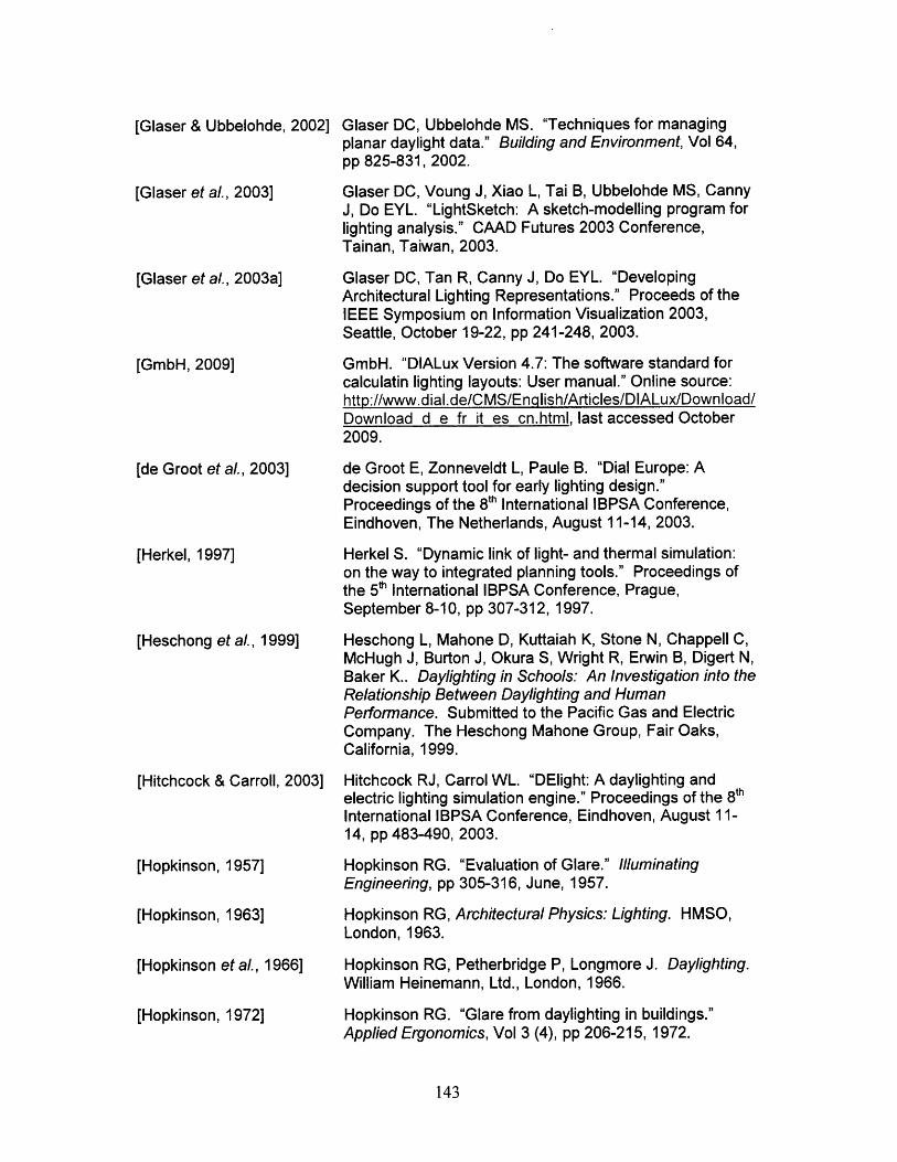
[Glaser & Ubbelohde, 2002]

[Glaser et al., 2003]

[Glaser et al., 2003a]

[GmbH, 2009]

[de Groot et al., 2003]

[Herkel, 1997]

[Heschong et al., 1999]

[Hitchcock & Carroll, 2003]

[Hopkinson, 1957]

[Hopkinson, 1963]

[Hopkinson et al., 1966]

[Hopkinson, 1972]

Glaser DC, Ubbelohde MS. "Techniques for managingplanar daylight data." Building and Environment, Vol 64,pp 825-831, 2002.

Glaser DC, Voung J, Xiao L, Tai B, Ubbelohde MS, CannyJ, Do EYL. "LightSketch: A sketch-modelling program forlighting analysis." CAAD Futures 2003 Conference,Tainan, Taiwan, 2003.

Glaser DC, Tan R, Canny J, Do EYL. "DevelopingArchitectural Lighting Representations." Proceeds of theIEEE Symposium on Information Visualization 2003,Seattle, October 19-22, pp 241-248, 2003.

GmbH. "DIALux Version 4.7: The software standard forcalculatin lighting layouts: User manual." Online source:http://www.dial.de/CMS/English/Articles/DIALux/Download/Download d e fr it es cn.html, last accessed October2009.

de Groot E, Zonneveldt L, Paule B. "Dial Europe: Adecision support tool for early lighting design."Proceedings of the 8th International IBPSA Conference,Eindhoven, The Netherlands, August 11-14, 2003.

Herkel S. "Dynamic link of light- and thermal simulation:on the way to integrated planning tools." Proceedings ofthe 5t' International IBPSA Conference, Prague,September 8-10, pp 307-312, 1997.

Heschong L, Mahone D, Kuttaiah K, Stone N, Chappell C,McHugh J, Burton J, Okura S, Wright R, Erwin B, Digert N,Baker K.. Daylighting in Schools: An Investigation into theRelationship Between Daylighting and HumanPerformance. Submitted to the Pacific Gas and ElectricCompany. The Heschong Mahone Group, Fair Oaks,California, 1999.

Hitchcock RJ, Carrol WL. "DElight: A daylighting andelectric lighting simulation engine." Proceedings of the 8h

International IBPSA Conference, Eindhoven, August 11-14, pp 483-490, 2003.

Hopkinson RG. "Evaluation of Glare." IlluminatingEngineering, pp 305-316, June, 1957.

Hopkinson RG, Architectural Physics: Lighting. HMSO,London, 1963.

Hopkinson RG, Petherbridge P, Longmore J. Daylighting.William Heinemann, Ltd., London, 1966.

Hopkinson RG. "Glare from daylighting in buildings."Applied Ergonomics, Vol 3 (4), pp 206-215, 1972.

143

[Houghton Mifflin web]

[Hui, 1997]

[Ibrahim & Krawczyk, 2003]

[IES web]

[IESNA, 2000]

[Igawa et al., 1999]

[Igawa et al., 2004]

[Inspirer web]

[Iwata & Tokura, 1998]

[Jameson & Hurvich 1961]

[Joseph, 2006]

Houghton Mifflin Company. World Climate. An outline mapof world climates. Online source:http://www.eduplace.com/ss/maps/pdf/world clim.pdf, lastaccessed November 2009.

Hui SCM. "Overall Thermal Transfer Value (OTTV): Howto Improve Its Control in Hong Kong." Proceedings of theOne-day Symposium on Building, Energy, andEnvironment, Hong Kong, October 16, pp12-1 - 12-11,1997.

Ibrahim M, and Robert Krawczyk. "The Level of Knowledgeof CAD Objects within the Building Information Model."Connecting: Crossroads of Digital Discourse, Proceedingsof the 2003 Annual Conference of the Association forComputer Aided Design In Architecture, IndianapolisIndiana, October 24-27, pp 173-177, 2003.

IES Virtual Environment website: http://www.iesve.com/,last accessed October 2009.

Illuminating Engineering Society of North America. TheIESNA Lighting Handbook: reference and application. 9thedition. Edited Mark S. Rea. Pub: IESNA, New York,2000.

Igawa N, Nakamura H, Matsuura K. "Sky luminancedistribution model for simulation of daylit environment."Proceedings of the 6th International IBPSA Conference,Kyoto, Japan, Vol 2, pp 969- 975, 1999.

Igawa N, Koga Y, Matsuzawa T, Nakamura H. "Models ofsky radiance distribution and sky luminance distribution."Solar Energy, Vol 77 (2), pp 137-157, 2004.

Inspirer website:http://www.inteqra.ip/en/inspirer/index.html, last accessedOctober 2009.

Iwata T, Tokura M. "Examination of the limitations ofpredicted glare sensation vote (PGSV) as a glare index fora large source: Towards a comprehensive development ofdiscomfort glare evaluation." Lighting Research andTechnology, Vol 30 (2), pp 81-88, 1998.

Jameson D, Hurvich LM. "Complexities of PerceivedBrightness." Science, Vol 133 (3447), ppl 74-179, 1961.

Joseph A. "The Impact of Light on Outcomes in HealthcareSettings." The Center for Health Design, Concord, CA,Issue Paper #2, August 2006.

144

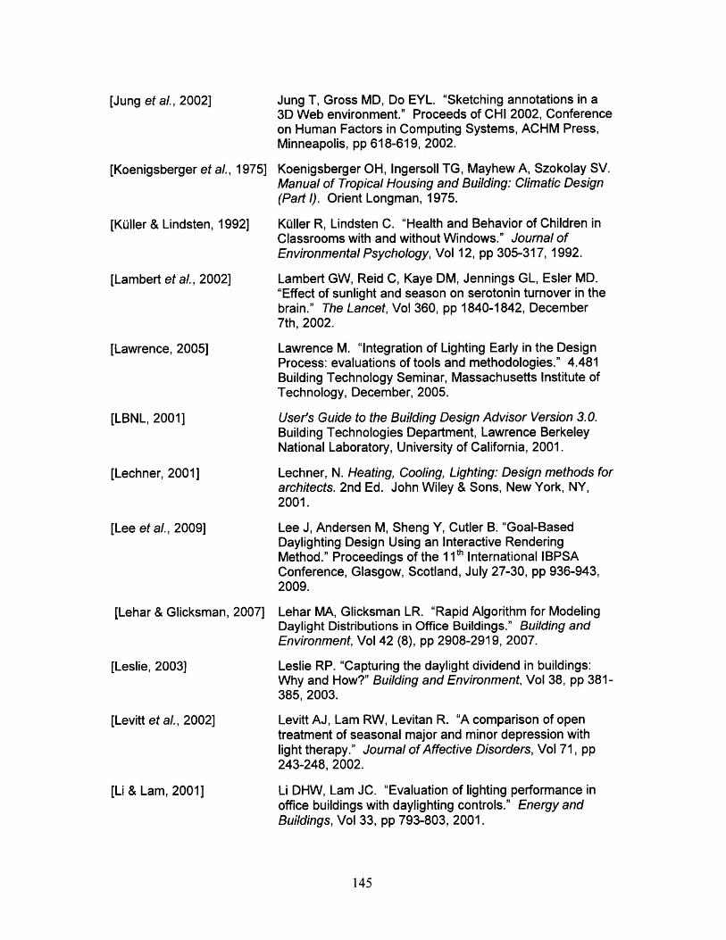
[Jung et al., 2002]

[Koenigsberger et al., 1975]

[Kuller & Lindsten, 1992]

[Lambert et al., 2002]

[Lawrence, 2005]

[LBNL, 2001]

[Lechner, 2001]

[Lee et al., 2009]

[Lehar & Glicksman, 2007]

[Leslie, 2003]

[Levitt et al., 2002]

[Li & Lam, 2001]

Jung T, Gross MD, Do EYL. "Sketching annotations in a3D Web environment." Proceeds of CHI 2002, Conferenceon Human Factors in Computing Systems, ACHM Press,Minneapolis, pp 618-619, 2002.

Koenigsberger OH, Ingersoll TG, Mayhew A, Szokolay SV.Manual of Tropical Housing and Building: Climatic Design(Part /). Orient Longman, 1975.

Kuller R, Lindsten C. "Health and Behavior of Children inClassrooms with and without Windows." Journal ofEnvironmental Psychology, Vol 12, pp 305-317, 1992.

Lambert GW, Reid C, Kaye DM, Jennings GL, Esler MD."Effect of sunlight and season on serotonin turnover in thebrain." The Lancet, Vol 360, pp 1840-1842, December7th, 2002.

Lawrence M. "Integration of Lighting Early in the DesignProcess: evaluations of tools and methodologies." 4.481Building Technology Seminar, Massachusetts Institute ofTechnology, December, 2005.

User's Guide to the Building Design Advisor Version 3.0.Building Technologies Department, Lawrence BerkeleyNational Laboratory, University of California, 2001.

Lechner, N. Heating, Cooling, Lighting: Design methods forarchitects. 2nd Ed. John Wiley & Sons, New York, NY,2001.

Lee J, Andersen M, Sheng Y, Cutler B. "Goal-BasedDaylighting Design Using an Interactive RenderingMethod." Proceedings of the 11* International IBPSAConference, Glasgow, Scotland, July 27-30, pp 936-943,2009.

Lehar MA, Glicksman LR. "Rapid Algorithm for ModelingDaylight Distributions in Office Buildings." Building andEnvironment, Vol 42 (8), pp 2908-2919, 2007.

Leslie RP. "Capturing the daylight dividend in buildings:Why and How?" Building and Environment, Vol 38, pp 381-385, 2003.

Levitt AJ, Lam RW, Levitan R. "A comparison of opentreatment of seasonal major and minor depression withlight therapy." Journal of Affective Disorders, Vol 71, pp243-248, 2002.

Li DHW, Lam JC. "Evaluation of lighting performance inoffice buildings with daylighting controls." Energy andBuildings, Vol 33, pp 793-803, 2001.

145

[Li et al., 2002]

[Littlefair, 2001]

[Lynes, 1968]

[Mardaljevic, 1995]

[Mardaljevic & Lomas, 1998]

[Mardaljevic, 2000]

[Mardaljevic, 2001]

[Mardaljevic, 2002]

[Mardaljevic, 2003]

[Mardaljevic, 2004]

[Mardaljevic, 2009]

[Mardaljevic et al., 2009]

[Maxwell web]

Li DHW, Lam JC, Wong SL. "Daylighting and itsimplications to overall thermal transfer value (OTTV)determinations." Energy, Vol 27, pp 991-1008, 2002.

Littlefair PJ. "Daylight, sunlight, and solar gain in the urbanenvironment." Solar Energy, Vol 70 (3), pp 177-185, 2001.

Lynes, JA. Principals of Natural Lighting. Applied SciencePublishers, Ltd., London, 1968.

Mardaljevic, J. "Validation of a lighting simulation programunder real sky conditions." Lighting Research andTechnology, Vol 27 (4), pp 181-188, 1995.

Mardaljevic J, Lomas KJ. "A Simulation Based Method toEvaluate the Probability of Daylight Glare Over Long TimePeriods and its Application." CIBSE National LightingConference, Lancaster University, April 5-8, pp 282-291,1998.

Mardaljevic J. "Simulation of annual daylighting profiles forinternal illuminance." Lighting Research and Technology,Vol 32 (3), pp 111-118, 2000.

Mardaljevic J. "Taking daylight modeling out of the darkages." International Daylighting RD&A #2, 2001.

Mardaljevic J. "Quantification of parallax errors in skysimulator domes for clear sky conditions." LightingResearch and Technology, Vol 34 (4), pp 313-332, 2002.

Mardaljevic J. "Precision modeling of parametricallydefined solar shading sytems: pseudo-changi." Proceedsof the 8th International IBPSA Conference, Eindhoven,August 11-14, 2003.

Mardaljevic, J. "Verification of program accuracy forilluminance modeling: assumptions, methodology and anexamination of conflicting findings." Lighting Research andTechnology, Vol 36 (3), pp 217-242, 2004.

Mardaljevic J. "Applicaation of the Useful DaylightIlluminance Metric: A Parametric Evaluation Covering 480Combinations of Building Type, Climate and Orientation."Proceedings of Lux Europa 2009, Istanbul, Sept 9-11,2009.

Mardaljevic J, Heschong L, Lee E. "Daylight metrics andenergy savings." Lighting Research and Technology, Vol41 (3), pp 261-283, 2009.

Maxwell Render website: http://www.maxwellrender.com/,last accessed October 2009.

146

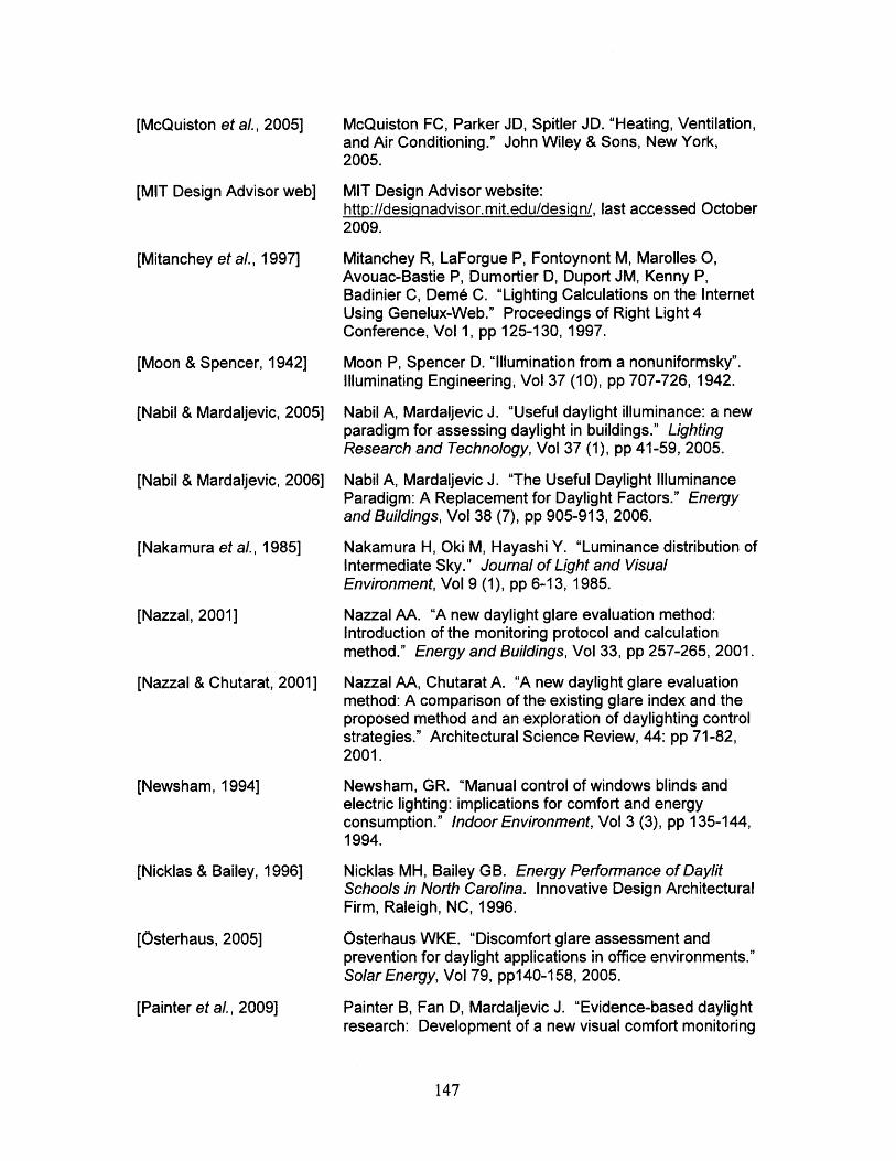
[McQuiston et al., 2005]

[MIT Design Advisor web]

[Mitanchey et al., 1997]

[Moon & Spencer, 1942]

[Nabil & Mardaljevic, 2005]

[Nabil & Mardaljevic, 2006]

[Nakamura et al., 1985]

[Nazzal, 2001]

[Nazzal & Chutarat, 2001]

[Newsham, 1994]

[Nicklas & Bailey, 1996]

[Osterhaus, 2005]

[Painter et al., 2009]

McQuiston FC, Parker JD, Spitler JD. "Heating, Ventilation,and Air Conditioning." John Wiley & Sons, New York,2005.

MIT Design Advisor website:http://designadvisor.mit.edu/design/, last accessed October2009.

Mitanchey R, LaForgue P, Fontoynont M, Marolles 0,Avouac-Bastie P, Dumortier D, Duport JM, Kenny P,Badinier C, Deme C. "Lighting Calculations on the InternetUsing Genelux-Web." Proceedings of Right Light 4Conference, Vol 1, pp 125-130, 1997.

Moon P, Spencer D. "Illumination from a nonuniformsky".Illuminating Engineering, Vol 37 (10), pp 707-726, 1942.

Nabil A, Mardaljevic J. "Useful daylight illuminance: a newparadigm for assessing daylight in buildings." LightingResearch and Technology, Vol 37 (1), pp 41-59, 2005.

Nabil A, Mardaljevic J. "The Useful Daylight IlluminanceParadigm: A Replacement for Daylight Factors." Energyand Buildings, Vol 38 (7), pp 905-913, 2006.

Nakamura H, Oki M, Hayashi Y. "Luminance distribution ofIntermediate Sky." Journal of Light and VisualEnvironment, Vol 9 (1), pp 6-13, 1985.

Nazzal AA. "A new daylight glare evaluation method:Introduction of the monitoring protocol and calculationmethod." Energy and Buildings, Vol 33, pp 257-265, 2001.

Nazzal AA, Chutarat A. "A new daylight glare evaluationmethod: A comparison of the existing glare index and theproposed method and an exploration of daylighting controlstrategies." Architectural Science Review, 44: pp 71-82,2001.

Newsham, GR. "Manual control of windows blinds andelectric lighting: implications for comfort and energyconsumption." Indoor Environment, Vol 3 (3), pp 135-144,1994.

Nicklas MH, Bailey GB. Energy Performance of DaylitSchools in North Carolina. Innovative Design ArchitecturalFirm, Raleigh, NC, 1996.

Osterhaus WKE. "Discomfort glare assessment andprevention for daylight applications in office environments."Solar Energy, Vol 79, ppl40-158, 2005.

Painter B, Fan D, Mardaljevic J. "Evidence-based daylightresearch: Development of a new visual comfort monitoring

147

[Papamichael et al., 1997]

[Papamichael et al., 1998]

[Paule & Scartezzini, 1997]

[Pechacek, 2008]

[Pechacek et al., 2008]

[Perez et al., 1990]

[Perez et al., 1992]

[Perez et al., 1993]

[Prescription Act, 1832]

[Radiance web]

[Rea, 1984]

[Rea et al., 2002]

method." Proceedings of Lux Europa 2009, Istanbul, Sept9-11, 2009.

Papamichael K, La Porta J, Chauvert H. "Decision Makingthrough Use of Interoperable Simulation Software."Proceedings of the 5 th International IBPSA Conference, Vol1l, Prague, Czech Republic, September 8-10, 1997.

Papamichael K, La Porta J, Chauvert H. "Building DesignAdvisor: automated integration of multiple simulation tools."Automation in Construction, Vol 6 (4), pp 341-352, 1998.

Paule B, Scartezzini JJ. "'Leso-DIAL', a new computer-based daylighting design tool." Right Light, Vol 4 (1), pp93-97, 1997.

Pechacek CS. Space, Light, and Time: ProspectiveAnalysis of Circadian Illumination for Health-BasedDaylighting with Applications to Healthcare Architecture.Masters Thesis, Massachusetts Institute of Technology,2008.

Pechacek CS, Andersen M, Lockley SW. PreliminaryMethod for Prospective Analysis of the Circadian Efficacyof (Day)Light with Applications to Healthcare Architecture.LEUKOS, Vol 5 (1), pp 1-26, 2008.

Perez R, Ineichen P, Seals R. "Modeling daylightavailability and irradiance components from direct andglobal irradiance." Solar Energy, Vol 44 (5), pp 271-289,1990.

Perez R, Michalsky J, Seals R. "Modeling Sky LuminanceAngular Distribution for Real Sky Conditions: ExperimentalEvaluation of Existing Algorithms." Journal of theIlluminating Engineering Society, Vol 21 (2), pp 84-92,1992.

Perez R, Seals R, Michalsky J. "All-Weather model for skyluminance distribution - preliminary configuration andvalidation." Solar Energy, Vol 50 (3), pp 235-245, 1993.

Prescription Act 1832. Imperial Act 71, 1 August, 1832.

gensky.c. C code for Radiance simulation program skygeneration. Online source: http://radsite.ibl.qov/radiance/,last accessed November 2009.

Rea MS. "Window Blind Occlusion: a Pilot Study."Building & Environment, Vol 19 (2), pp 133-137, 1984.

Rea MS, Figueiro MG, Bullough JD. "Circadianphotobiology: an emerging framework for lighting practice

148

and research." Lighting Research and Technology, Vol 34(3), pp 177-190, 2002.

[Reinhart & Herkel, 2000] Reinhart CF, Herkel S. "The simulation of annual daylightilluminance distributaions - a state-of-the-art comparisonof six RADIANCE-based methods." Energy and Buildings,Vol 32, pp 167-187, 2000.

[Reinhart & Walkenhorst, 2001] Reinhart CF, Walkenhorst 0. "Validation ofdynamic RADIANCE-based daylight simulations for a testoffice with external blinds." Energy and Buildings, Vol 33,pp 683-697, 2001.

[Reinhart et al., 2003] Reinhart CF, Morrison M, Dubrous F. "The LightswtichWizard - Reliabile daylight simulations for initial designinvestigation." Proceedings of the 8th International IBPSAConference, Eindhoven, The Netherlands, August 11-14,ppl 093-1100, 2003.

[Reinhart, 2004] Reinhart CF. "Lightswitch-2002: a model for manual andautomated control of electric lighting and blinds." SolarEnergy, Vol 77 (1), pp 15-28, 2004.

[Reinhart & Fitz, 2004] Reinhart CF, Fitz A. "Key findings from an online survey inthe use of daylight simulation programs." Proceedings ofeSim 2004, Vancouver, June 10-11, pp 1-8, 2004.

[Reinhart, 2005] Reinhart CF. "Tutorial on the Use of Daysim/RadianceSimulations for Sustainable Design." National ResearchCouncil of Canada, Institute for Research in Construction.Ottawa, February 8, 2005.

[Reinhart, 2005a] Reinhart CF. "A Simulation-based review of the ubiquitouswindow-head-height to daylit zone depth rule-of-thumb."Proceedings of Building Simulation 2005, Montreal,Canada, August 15-18, pp 1-8, 2005.

[Reinhart & Fitz, 2006] Reinhart CF, Fitz A. "Findings from a survey on thecurrent use of daylight simulations in building design."Energy and Buildings, Vol 38 (7), pp 824-835, 2006.

[Reinhart et al., 2006] Reinhart CF, Mardaljevic J, Rogers Z. "Dynamic daylightperformance metrics for sustainable building design."Leukos, Vol 3 (1), pp 1-25, 2006.

[Reinhart et al., 2007] Reinhart CR, Bourgeois D, Dubrous F, Laouadi A, LopezP, Stelescu 0. "Daylight 1-2-3 - A state-of-the-artdaylighting/energy analysis software for initial designinvestigations." Proceedings of the 1 0 th InternationalIBPSA Conference, Beijing, September 3-6, pp 1669-1676,2007.

149

[Reinhart & Breton, 2009]

[Reinhart & Breton, 2009a]

[Rogers, 2006]

[Rubiho et al., 1994]

[Sarawgi, 2006]

[Simon, 1969]

[Stephenson, 1957]

[Stephenson, 1965]

Reinhart CF, Breton PF. "Experimental Validation of 3dsMax@ Design 2009 and Daysim 3.0." Proceedings of the11th International IBPSA Conference, Glasgow, Scotland,July 27-30, pp 1514-1521, 2009.

Reinhart CF, Breton PF. "Experimental Validation of'Autodesk@ 3ds Max@ Design' 2009 and Daysim 3.0."NRC Project #B3241 Report. January 29, 2009

Rogers Z. "Daylighting Metric Development Using DaylightAutonomy Calculations In the Sensor PlacementOptimization Tool: Development Report and CaseStudies." Boulder, Colorado, USA: Architectural EnergyCorporation, March 17, 2006. Online source:http://www.archenerqy.com/SPOT/download.html

Rubiho M, Curz A, Garcia JA, Hita E. "Discomfort glareindices: a comparative study." Applied Optics, Vol 33 (34),pp 8001-8008, 1994.

Sarawgi, T. "Survey on the Use of Lighting DesignSoftware in Architecture and Interior DesignUndergraduate Education." International Journal ofArchitectural Computing, Vol 4 (4), pp 91-108, 2006.

Simon H. The Sciences of the Artificial. MIT Press,Cambridge, Massachusetts, 1st edition, 1969.

Stephenson DG. "Thermal radiation and its effect on theheating and cooling of buildings." National ResearchCouncil of Canada, Division of Building Research, ReportNo. 121, Ottawa, 1957.

Stephenson DG. "Equations for solar heat gain throughwindows." Solar Energy, Vol 9 (2), pp 81-86, 1965.

[Thanachareonkit et al., 2005] Thanachareonkit A, Scartezzini JL, Andersen M."Comparing daylighting performance assessment ofbuildings in scale models and test modules." Solar EnergyVol 79, pp 168-182, 2005.

[Tobler, 1999]

[Torcellini et al., 2008]

Tobler W. "World population by latitude." Slide in UnusualMap Projections slideshow. UC Santa Barbara. Used withpermission, stylistically reformatted. 1999. Online source:http://www.ncqia.ucsb.edu/proiects/tobler/Projections/sld075.htm, last accessed November 2009.

Torcellini P, Deru M, Griffith B, Benne K, Halverson M,Winiarski D, Crawley DB. "DOE Commercial BuildingBenchmark Models." Proceedings of the 2008 ACEEESummer Study on Energy Efficiency in Buildings, PacifcGrove, California, August 17-22, 2008. Online source:http://www.nrel.qov/docs/fy08osti/43291.pdf, last accessedOctober 2009.

150

[Tregenza, 1980]

[Tregenza & Waters, 1983]

[Tregenza, 1987]

[Tufte, 1983]

[Ubbelohde, 1998]

[University of Oregon web]

[Urban & Glicksman, 2007]

[Utzinger & Wasley, 1997]

[Vine, 1998]

[Vos, 2003]

[Walkenhorst et al., 2002]

[Ward & Shakespeare, 1998]

Tregenza PR. "The daylight factor and actual illuminanceratios." Lighting Research and Technology, Vol 12 (2), pp64-68, 1980.

Tregenza PR, Waters IM. "Daylight coefficients." LightingResearch and Technology, Vol 15 (2), pp 65-71, 1983.

Tregenza PR. "Subdivision of the sky hemisphere forluminance measurements." Lighting Research andTechnology, Vol 19 (1), pp 13-14, 1987.

Tufte E. The Visual Display of Quantitative Information.Graphics Press, Cheshire, Connecticut, 1983.

Ubbelohde MS. "Comparative Evaluation of FourDaylighting Software Programs." Proceedings of ACEESummer Study on Energy Efficiency in Buildings, 1998.

University of Oregon. Solar Radiation MonitoringLaboratory. Sun path chart program online source:http://solardat.uoreqon.edu/SunChartProgram.html, lastaccessed November 2009.

Urban BJ, Glicksman LR. "A Simplified Rapid EnergyModel and Interface for Nontechnical Users." Proceedingsof Oak Ridge National Laboratory, Buildings Conference X,2007.

Utzinger M, Wasley JH. "Building Balance Point." VitalSigns Curriculum Materials Project, University of California- Berkeley, and University of Wisconsin - Milwaukee.August, 1997. Online source:http://arch.ced.berkeley.edu/vitalsiqns/res/rps.html, lastaccessed October, 2009.

Vine E, Lee E, Clear R, DiBartolomeo D, Selkowitz S."Office worker response to an automated venetian blindand electric lighting system: a pilot study." Energy andBuildings, Vol 28, pp 205-218,1998.

Vos JJ. "Reflections on glare." Lighting Research andTechnology, Vol 35 (2), pp163-176, 2003.

Walkenhorst 0, Luther J, Reinhart C, Timmer J. "Dynamicannual daylight simulations based on one-hour and one-minute means of irradiance data." Solar Energy, Vol 72(5), pp 385-395, 2002.

Ward G, Shakespeare RA. Rendering with Radiance.Morgan Kaufmann Publishers, 1998.

[Wienold & Chrisoffersen, 2006] Wienold J, Christoffersen J. "Evaluation methodsand development of a new glare prediction model for

151

[Wienold, 2007]

[Wienold, 2009]

[Wienold, IP]

[Winkelmann & Selkowitz,

[Wittkopf et al., 2006]

[Wu & Ng, 2003]

[Yi, 2008]

[Yik & Wan, 2005]

daylight environments with the use of CCD cameras."Energy and Buildings, Vol 38, pp743-757, 2006.

Wienold J. "Dynamic simulation of blind control strategiesfor visual comfort and energy balance analysis."Proceedings of the 1 0th International IBPSA Conference,Beijing, September 3-6, pp 1197-1204, 2007.

Wienold J. "Dynamic daylight glare evaluation."Proceedings of the 1 1 th International IBPSA Conference,Glasgow, July 27-30, pp 944-951, 2009.

Wienold J. Daylight Glare in Offices. Ph.D. Thesis,Fraunhofer Institute for Solar Energy Systems, InProgress.

1985] Winkelmann F, Selkowitz S. "Daylightingsimulation in the DOE-2 building energy analysis program."Energy and Buildings, Vol 8, pp 271-286, 1985.

Wittkopf SK, Yuniarti E, Soon LK. "Prediction of energysavings with anidolic integrated ceiling across differentdaylight climates." Energy and Buildings, Vol 38, ppl 120-1129, 2006.

Wu W, Ng E. "A review of the development of daylightingin schools." Lighting Research and Technology, Vol 35(2), pp 111-125, 2003.

Yi L. A New Approach in Data Visualization to IntegrateTime and Space Variability of Daylighting in the DesignProcess. Masters Thesis, Massachusetts Institute ofTechnology, 2008.

Yik FWH, Wan KSY. "An evaluation of theappropriateness of using overall thermal transfer value(OTTV) to regulate envelope energy performance of air-conditioned buildings." Energy, Vol 30, pp 41-71, 2005.

152

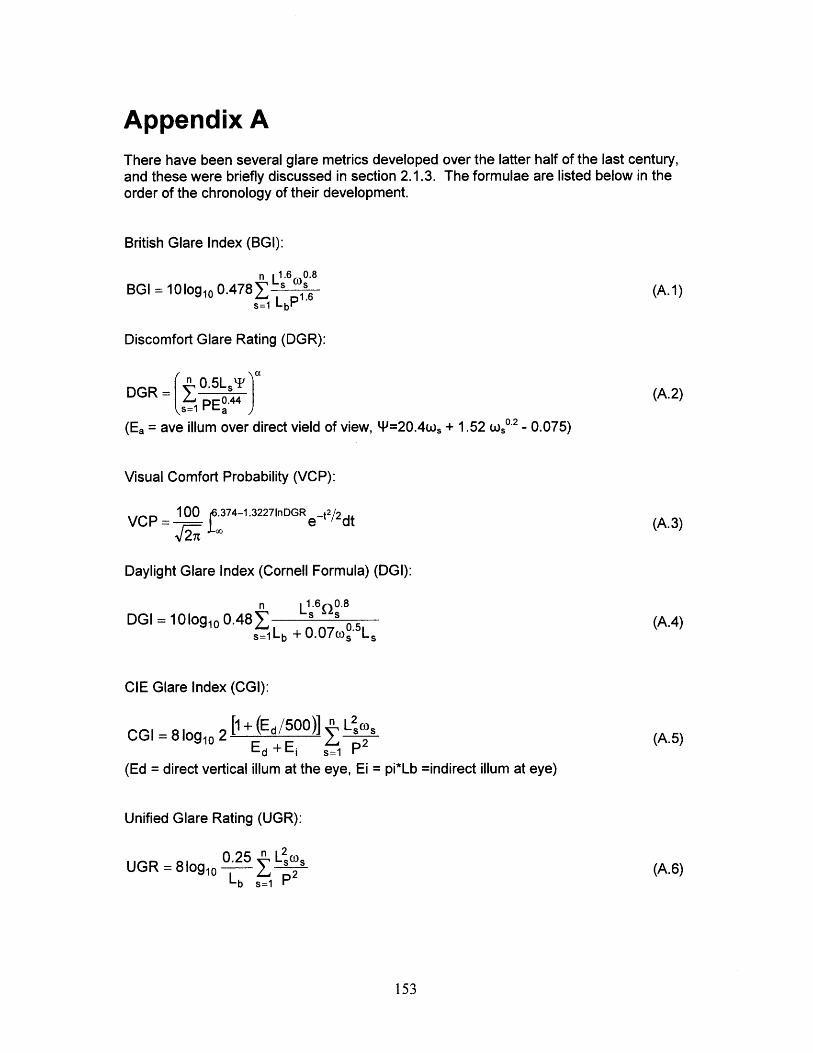
Appendix AThere have been several glare metrics developed over the latter half of the last century,and these were briefly discussed in section 2.1.3. The formulae are listed below in theorder of the chronology of their development.

British Glare Index (BGI):

BGI = 10log10 0.478E S S 6 (A.1)s=1 LbP

Discomfort Glare Rating (DGR):

n0. 5L- t )aDGR = S (A.2)

(Ea = ave ilium over direct vield of view, Y=20.4w, + 1.52 w. 0 2 - 0.075)

Visual Comfort Probability (VCP):

VCP = 100 r.374-1.3227inDGR e -t2/2dt (A.3)

Daylight Glare Index (Cornell Formula) (DGI):

DGI = 10log 1 0.481 S S (A.4)s=1Lb + 0.07oso.5 LS

CIE Glare Index (CGI):

[1 + (Ed /500)] " LseCGI = 8 log10 2 2)(A.5)

Ed +Ei s=1 P(Ed = direct vertical ilium at the eye, Ei = pi*Lb =indirect ilium at eye)

Unified Glare Rating (UGR):

0.25 n (UGR = 8log1 0 LIS " (A.6)

b s=1

153

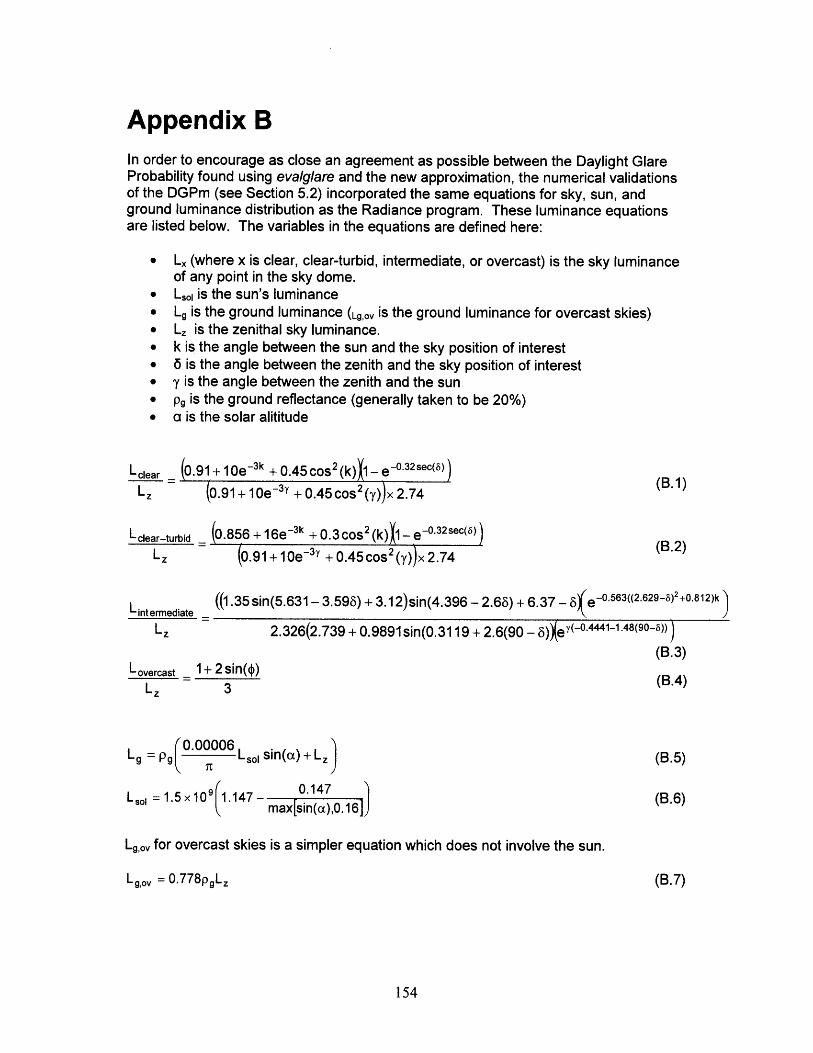
Appendix BIn order to encourage as close an agreement as possible between the Daylight GlareProbability found using evalglare and the new approximation, the numerical validationsof the DGPm (see Section 5.2) incorporated the same equations for sky, sun, andground luminance distribution as the Radiance program. These luminance equationsare listed below. The variables in the equations are defined here:

0 Lx (where x is clear, clear-turbid, intermediate, or overcast) is the sky luminanceof any point in the sky dome.

* Lso0 is the sun's luminance* Lg is the ground luminance (Lg,ov is the ground luminance for overcast skies)* Lz is the zenithal sky luminance.* k is the angle between the sun and the sky position of interest* 6 is the angle between the zenith and the sky position of interest* y is the angle between the zenith and the sun* pg is the ground reflectance (generally taken to be 20%)* a is the solar alititude

L clear (0.91+ 10e-3k + 0.45 cos 2 (k) - e-0.32sec(t))

L z (0.91+10e-3y +0.45 cos2(y))x 2.74

L clear-turbid (0.856 + 16e-3k + 0.3 cos 2 (k) X, - e-0.32sec(8)) (B.2)L z (0.91 + 10e3y + 0.45 cos2(y))x 2.74

Lintermediate ((1.35 sin(5.631 - 3.598) + 3.12)sin(4.396 - 2.68) + 6.37 - e-o.563((2.6295)2 +O.812)k

L z 2.326(2.739 + 0.9891sin(0.3119 + 2.6(90 - )Xe 1(-0.4441-1.48(90-)))

(B.3)Lovercast 1+ 2 sin(()

L z 3

Lg =p (0.00006 Lsi sin(a) + L (B.5)

L so = 1.5 x 109 1.147 - 0.1476 (B.6)max[sin(a),0.16])

Lg,ov for overcast skies is a simpler equation which does not involve the sun.

Lg,ov = 0 .778 pgLz (B.7)

154

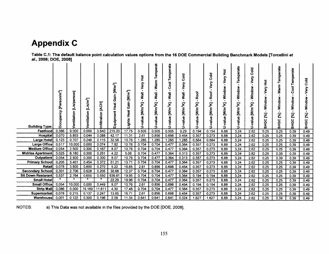
Appendix CTable C.1: The default balance point calculation values options from the 16 DOE Commercial Building Benchmark Models [Torcellini eta., 2008; DOE, 2008]

Building Type:

0

0

0

0

0

C-)

C0

(U

C

(U

E0.

W

0

IM

(UE0.

E

0

E

'0

E

00

E

0

;r

'a0

(D

00

EL

EI-0

Fastfood 0.386 9.000 0.000 0.640 215.20 17.75 0.505 0.505 0.505 0.29 0.194 0.154 6.88 3.24 2.62 0.25 0.25 0.39 0.49Hospital 0.070 5.853 0.044 0.088 42.17 11.31 2.61 0.856 0.698 0.454 0.357 0.273 6.88 3.24 2.62 0.25 0.25 0.39 0.49

Large Hotel 0.123 0.707 0.248 0.115 32.58 10.76 1.285 1.285 1.285 1.285 0.564 0.564 6.88 3.24 2.62 0.25 0.25 0.39 0.49Large Office 0.517 10.000 0.000 0.074 7.82 10.76 0.704 0.704 0.477 0.364 0.357 0.273 6.88 3.24 2.62 0.25 0.25 0.39 0.49

Medium Office 0.054 2.500 0.300 0.167 8.07 10.76 0.704 0.704 0.477 0.364 0.357 0.273 6.88 3.24 2.62 0.25 0.25 0.39 0.49Midrise Apartment 0.025 6.180 0.300 0.251 4.22 5.06 0.704 0.477 0.364 0.313 0.357 0.273 6.88 3.24 2.62 0.25 0.39 0.39 0.49

Outpatient 0.054 2.500 0.300 0.300 8.07 10.76 0.704 0.477 0.364 0.313 0.357 0.273 6.88 3.24 2.62 0.25 0.39 0.39 0.49Primary School 0.205 3.401 0.454 0.372 51.21 13.71 0.704 0.704 0.477 0.364 0.357 0.273 6.88 3.24 2.62 0.25 0.25 0.39 0.49

Retail 0.078 3.800 0.600 0.270 5.22 16.65 2.61 0.856 0.698 0.454 0.357 0.273 6.88 3.24 2.62 0.25 0.25 0.39 0.49Secondary School 0.301 2.706 0.628 0.205 30.68 12.37 0.704 0.704 0.477 0.364 0.357 0.273 6.88 3.24 2.62 0.25 0.25 0.39 0.49

Sit Down Restarant 0.537 2.764 0.655 0.550 636.61 19.95 0.704 0.704 0.477 0.364 0.194 0.154 6.88 3.24 2.62 0.25 0.25 0.39 0.49Small Hotel a a a a 22.29 19.96 0.704 0.704 0.477 0.364 0.357 0.273 6.88 3.24 2.62 0.25 0.25 0.39 0.49Small Office 0.054 10.000 0.000 0.449 8.07 10.76 2.61 0.856 0.698 0.454 0.194 0.154 6.88 3.24 2.62 0.25 0.25 0.39 0.49

Strip Mall 0.086 0.000 15.169 11.611 4.30 17.46 0.704 0.704 0.477 0.364 0.357 0.273 6.88 3.24 2.62 0.25 0.25 0.39 0.49Supermarket 0.078 0.215 0.137 0.247 13.65 16.71 2.61 0.856 0.698 0.454 0.357 0.273 6.88 3.24 2.62 0.25 0.25 0.39 0.49

Warehouse 0.001 0.122 0.300 0.196 2.09 11.34 0.641 0.641 0.641 0.324 1.627 1.627 6.88 3.24 2.62 0.25 0.39 0.39 0.49

a) This Data was not available in the files provided by the DOE [DOE, 2008].

155

NOTES:

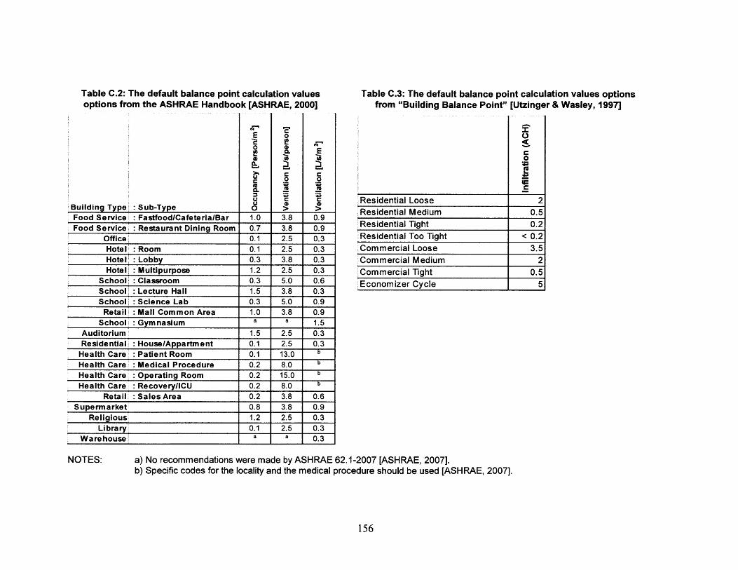
Table C.2: The default balance point calculation valuesoptions from the ASHRAE Handbook [ASHRAE, 2000]

Building Type Sub-Type 6 5 >Food Service Fastfood/Cafeteria/Bar 1.0 3.8 0.9Food Service Restaurant Dining Room 0.7 3.8 0.9

Office 0.1 2.5 0.3Hotel Room 0.1 2.5 0.3Hotel : Lobby 0.3 3.8 0.3Hotel : Multipurpose 1.2 2.5 0.3

School : Classroom 0.3 5.0 0.6School Lecture Hall 1.5 3.8 0.3School Science Lab 0.3 5.0 0.9Retail : Mall Common Area 1.0 3.8 0.9

School : Gymnasium a a 1.5Auditorium 1.5 2.5 0.3Residential : House/Appartment 0.1 2.5 0.3

Health Care : Patient Room 0.1 13.0 b

Health Care : Medical Procedure 0.2 8.0 b

Health Care : Operating Room 0.2 15.0 b

Health Care : Recovery/ICU 0.2 8.0 bRetail : Sales Area 0.2 3.8 0.6

Supermarket 0.8 3.8 0.9Religious 1.2 2.5 0.3

Library 0.1 2.5 0.3Warehouse a a 0.3

Table C.3: The default balance point calculation values optionsfrom "Building Balance Point" [Utzinger & Wasley, 1997]

Residential Loose 2Residential Medium 0.5Residential Tight 0.2Residential Too Tight < 0.2Commercial Loose 3.5Commercial Medium 2Commercial Tight 0.5E conomizer Cy cle 5

a) No recommendations were made by ASHRAE 62.1-2007 [ASHRAE, 2007].b) Specific codes for the locality and the medical procedure should be used [ASHRAE, 2007].

156

NOTES:

Appendix DThe tables in this appendix represent the Maximum Load Ratio (MLR, as defined in Section X) between the measured energy usefrom Energy Plus and the detailed balance point load (white) or the blocked balance point load (gray). A positive MLR means thatbalance point load exceeds the measured energy use, and a negative MLR means that it is less than the measured energy use.Average, median, and standard deviations are presented for annual data sets of cooling energy, heating energy, and cooling energy-heating energy (since realistic HVAC systems sometimes cool and heat at the same time). Al values are displayed in the tables aspercents, rather than decimals, for ease of reading.

157

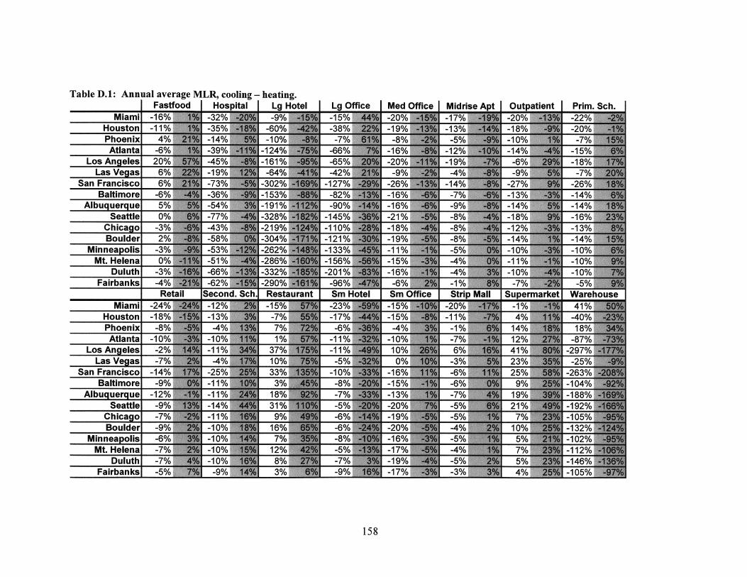
Table D.1: Annual average MLR, cooling - heating.

Lo

San

Alb:

Mi

Lo

San

Alb

Mi

158

Fas od |Hospia | Lg Htl|Lg Offic | Med Offic Midrise At|Outpatient |Prim. Sch.Miamil -16% --2% -% -15%= -20%= -17% -20%0 -22%

Houston| -11% --5%= -60%= -38% -19%= -13% -18% -20%Phoenix 4%= -14%= -10%= -7%= -8%= -50% -10%M -7%Atlantal -6% -39% -124% -66%= -16%= -12% -14% -15%

s Angelesi 20%= -5% -161%= -65% -20%= -19% -6% -18%Las Veg asi 6% -19% -64% -42%= -9% -4% -9% -7%Franciscol 6%= -73% -302% -127% -26%= -14% M 2%M -26%Baltimore| -6%= -36% -153%= -82%= -16%= -7% -3' -uquerque| 5%= -54% -191%= -90%= -16% -9% -14% -14%

Seattle|0 -77%= -328%= -145%= -21% -8% -18% -16%Chicagol -3%= -43% -219% -110% -18%W -8% -12% -13%Boulderl 2%= -58% o 34 =-121% M 19% -8%= -14%= -14%

nneapolisi -3%= 5% -262% -133%= -11%= -5% -10% -10%Mt. Helenal 0%= -51% -286%- -156%= -15%o -4%= -11%= -10%

Duluth| -3% -66% -332%= -201%= -16% -4% -10% -10%

Reti lSecond. Sch. Restaurn Sm Htl|Sm Ofic0 StripMl| Supermarkt WarehousMiamil -24%= -12%= -15%= -23%= -15%= -20%E -1%41

Houstoni -18%E -13% -7%E -17%E -15%E 1% 4%Phoenix| -8%E -% 7% -6%E -4%E -1414 1Atlantal -10% -10% 1 1% -11% -10% -7% 12% -87%

s Angelesi -2% -11% 37% -11% 10% 6% 41% -297%Las Veg asi -7% -4% 10% -5 , 0% -3% 23% -25%Franciscol -14% -25% 33%E -10% -16% -6% 25% -263%Baltimore| -9%= -11%= 3%= -8%= -15% -6% 9% -104%uquerquel -12% --1% 18% -7% M 1%M -7% 19% -188%

Seattlel -9% -14%= 31%= -5%= -20% -5%= 21%= -192%Chicagol -7%0 -11%= 9%= -6% -19% -% 7% -105%Boulderl -9%= -10%= 16%= -6% -0 -4% 10% -132%

nneapolisi -6%6 -10%E 7%E -8%E -16%E -5%E 5%E -102%Mt. Helenal -7%0 -10%E 12%E -5% -17%E -4%E 7%E -112%

Duluthi -7%E -10%E 8%= -7%= -19%= -5%E 5%E -146%

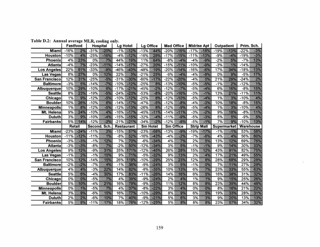
Table D.2: Annual average MLR, cooling only.

S

S

Fastfo Hospta Lg Htl Lg Office Med Offic Midrise AtOutpatien Prim. SchMiami -16% -31% -1% -13% -20% -17% -19%2'o

Houston -10% -25% -4%/ -16% -17% -11% -9% -9Phoenix 4% 0% 44% 11% -8% -4% -2% -7%Atlanta -4% -23% -14% -27% -15% -10% -3% -14%

Los Ang-eles 22% -33% -46% -48% -20% -16% 17% T 18%Las Ve.gas 8% 0% 22% -21% -%-4% 0 5

an Francisco 12% -25% -31 % -60% -22 -4O1%-4Baltimore -3% -14% -10%- -1%-5 1%-2

Albu. uer. ue 10% -10% -17%/ -45% -12% -5% 6% -8%Seattle 8% 6 -19% -24% -53% -20% -3% 1E% -11%

Chica.go 1%0 -12% -10% -25% -12% -5% 1 % -10%Boulder 10% -10% -14% -47% -12% -4% 10% -8%

Minneap.olis 1% -12% -12% -26% -12% -5% 1 % -10%,Mt. Helena 9% -10% -16% -45% -14% -3% 9% -8%

Duluth 3% -10% -15% -32% -11% -5% 5% -9%Fairbanks 5% -1%-21 % -34% -12% -5% 7% -10%

Reti Second. Sch Restarn Sm Hoe Sm Offic Strip Mall Supermarke WarehouseMiami -23% -11% -15% -23% -13% -19%, -1%1 53%

Houston -11% -11% -%-16%/ -4% -7%/4 56%Phoenix -3% -1% 7%-%4% 2%1%69%Atlanta -3% -8%/( -2 12 % 1 9 30%/

Los Ang-eles 9% -9% 35% -12% 26% 15% 43% 82%Las Ve.gas -1% -1% 9% -5% 9% .2% 17% 49%

an Francisco 10% -14% 26% -10% 25% 12% 28% 29%Baltimore -2% -7% -1% -9% 3% -1% M 7%27

Albu. uer. ue 4% -3% 14% -8% 10% 6% 235%Seattle 5% -4% 17% -11% 1%6 6 1

Chicag-o 0% -5% 4% -9% 2% 1% 9% 25%Boulder 5% -4% 16% -9% 11% 8% 23% 44%

Min neap.olis 0% -5% 4% -8% 3% 0% 8% 21%Mt. Helena 3% -- 6% 16% -10% 8% 6%1928

Duluth 2% -6% 7% -9% 5% 3%9% 13%Fairbanks, 5% -11% 1%-12% 5% 34%23

159

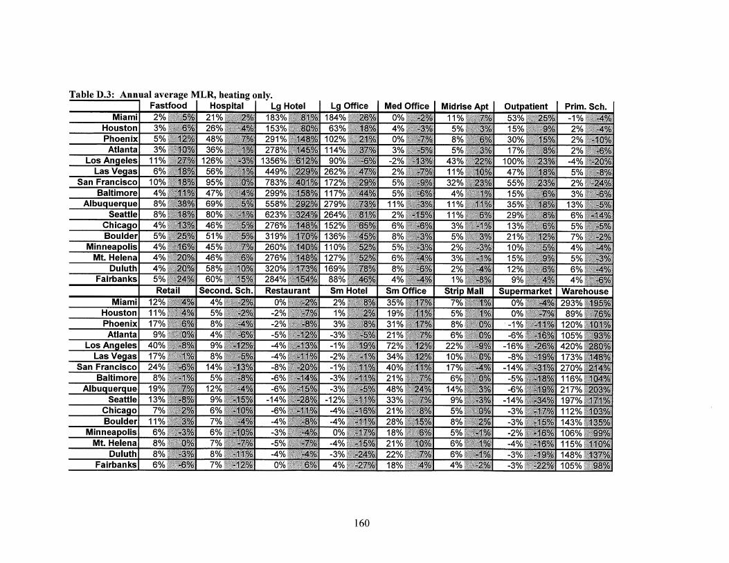
Table D.3: Annual average MLR, heating only.Fastfood Hospital Lg Hotel

Miami 2% , 5 21% 2i(6 183% 81%Houston 3% % d 26% 4% 153% 80%[MPhoenix 5%i 12 48%' 7 291% 148%:Atlanta 3% 1()/o 36% 1% 278%, 1450%

Los Angeles 11% 2%126% -%1356% 612%HLas Vegas 6% 18% 56% 1 449% 9%

San Francisco 10% 18%,/ 95% 00/6- 783% 401%Baltimore 4% 11% 47% 4 299% 158%

Albuquerque 8% 3 8% 69% 5% 558% 292%Seattle 8% 18% 80% -1 623% 32

Chicago 4%, 13% 46% 5 276% 148%Boulder 5% 25 51% /q 319% 170%

Minneapolis 4% 1 45% 4 7 260% 140%Mt. Helena 4%,20% 46% 6% 276% 4 %

Duluth 4% g_24 58% 10)o-320% {73Fairbanks 5% 69>'4 0% 284% 1

Retai Second.Sch. RestaurantMiami 12%, 46 4% 2% 6/0 -2%

Houston 11% 4% 5% -2% -2% 70YPhoenix 17% ea 8% -4 -2% -Atlanta 9% 0% 4% -6|||7 -5% 1/%

Los Angeles 40% -% 9% 2%,| -4%613%Las Vegas 17%, 1% 8% -5% |||| -1-4

San Francisco 24% -6, 14% -13% -8% -0Baltimore 8%,1% 5% 8%|| -6% 4

Albuquerque 19% 7 0/ 12% -||| -6% -Seattle 13% -% 9% -15j% -14% -8

Chicago 7% [% 6% -10% -6% -1Boulder 11% 3% 7% |-|4% -4% -%

Minneapolis 6% - /80 6% -10%. -3% -0SMt. Helena 8% 0% -7% -7 /q. -5% -0o

Duluth 8% i-3%i 8% -11% -4% -%.Fairbanks, 6% -6%1 7% -1% 0% || %1

Med Office Mid rise A0% 2W 11%4% 53%| 5 |

0% 87 8/3% ]5% 5%

-2% 13% 43%22% -7% 11%5% 4-9% 32%||25% 4%% 14%

11% -3% 11% ||||2% -15 11%6% % 3%8% 5%3|||5 |5%-3% 2%6% 4% 38%[-6% 2%||4% -4% 1%|||

Sm Office Strip Ma35% 17% 7%ill19%: 1 5%31%17%] 8%|'M91 N 0/R70_1 A ,(

Outpatient Prim.53% 25 -1%15% 9%12%)

160

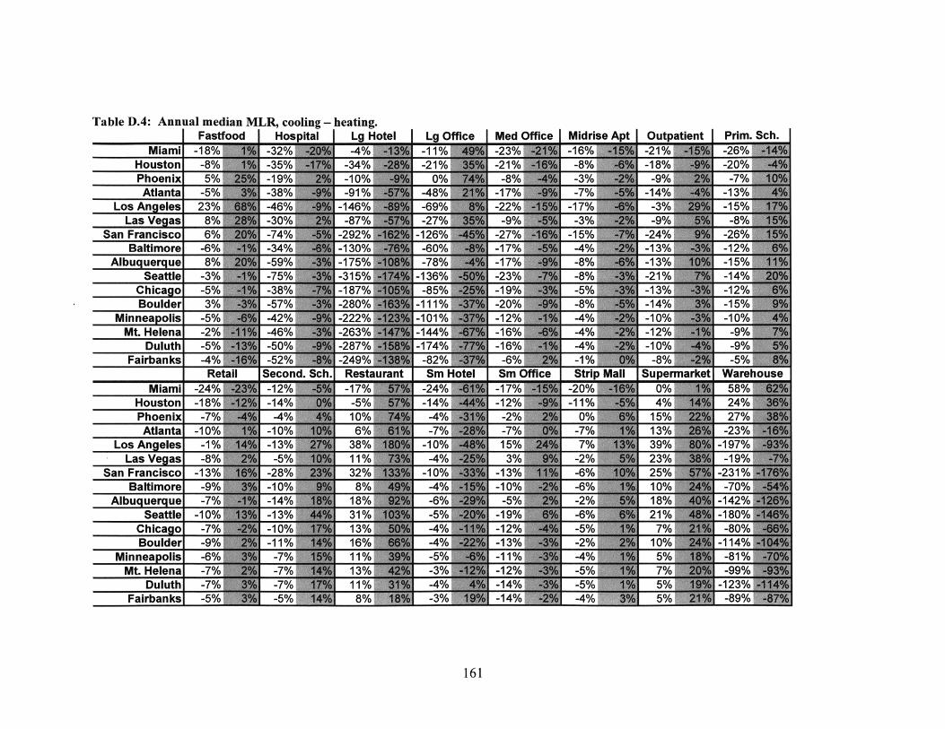
Table D.4: Annual median MLR, cooling - heating.

LosLa

San FB

Albu

MinMt

LosLa

San FB

Albu

MinM

F

Fastfo Hospital | Lg Htl|Lg Office Med Offic Midrise At|Outpatien| Prim. SchMiamil -18%0 -32% -4% -11% -23% = -16% = -21%0 -26%

Houston i-8% -35%= -34%= -21%= -21% _ 8%= -18%= -20%Phoenixl 5%= -19%= -10%= 0%= -8%o -3%i -9% -7Atlantal -5%0 -38%= -91%= -48%= -17%= -7%= -14% -3

Angelesl 23%o -46%= -146%= -69% -22% -17%= -3%= -15%s Vegasi 8%= -30%= -87%= -27%= -9%= -3%= -9r8%ranciscol 6%= -74%= -292% -126%= -27%= -15%= -24%= -26altimorel -6% -34%= -130%= -60%= -17%= -4%= -13%= -12%querauel 8%= -59%= -175%= -78%= -17%= -8%= -13%= -15

Seattlel -3%o -75%= -315% -136%= -23%= -8%= -21%= -14%Chicagol -5%= -38%= -187%= -85%= -19%= -5%= -13%= -12%Boulderl 3% = -57% = -280% -111% = -20% = -8% = -14% = -15neapolisi -5% -42% = 22 -101% -12% = -4% = -10% = -10%

Helenal -2% = -46% = -263% = -4% -16% -%-1% -9%0/Duluthi -5%= -50%= -287% -174%= -16%= -4%= -1%_9%

Reti |Second. Sch. Restarn Sm Hote Sm Ofie|Strip Mall Superakt WarehouseMiamil -24% -12%= -17%= -24%= -17%= -20%= 0%= 58%

Houstoni -18%= -14%= -5%= -14%= -12%o -11%= 4%= 24%Phoenixl -7%= -4%= 10%= -4%= -2%= 0%= 15%= 27%=Atlantal -10%= -10%= 6%= -7%= -7%= -7%= 13%= -23%=

Angelesl -1%= -13%= 38%= -10%= 15%= 7%= 39%= -197%=s Vegasi -8%o -5%= 11%= -4%= 3%= -2%= 23%= -19%Mrancis col -13% -28% 32% -10% -13% -6% 25% -231%altimorel -9% -10% 8% -4% -10% -6% 10% = -70%querauel -7%= -14%= 18%= -6%= -5%= -2%= 18% -142%M

Seattlel -10%= -13%= 31%= -5%= -19% -6%= 21%= -180%=Chicagol -7%= -10%= 13%= -4%= -12% -5%= 7%= -80%Boulderl -9% -11% 16%= -4%= -13%= -2%= 10%= -114%neapolisl -6% -7% (o 11% -5% --11% 0 -4% 6 50% -81%t. Helenal -7% -7% 13%= -3%= -12%= -5%= 7% -99%

Duluth i-7% = -7% = 11% -4% -14% -5% 5%-13

161

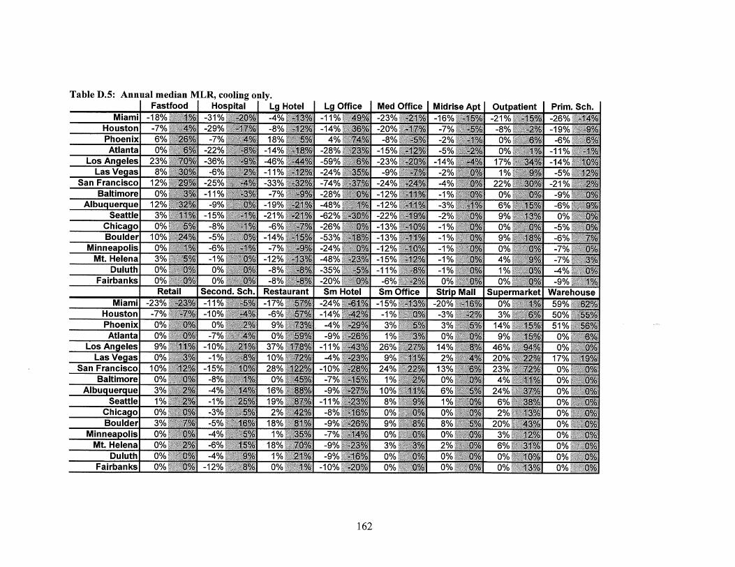
Table D.5: Annual median MLR, cooling only.Fastfood Hospital Lg Hotel

Miami -18% " 1% -31% 2o -4% -13%Houston -7% 4% -29% -17% -8% -1]%Phoenix 6%' 26% -7% 406 18% 5% 0

Atlanta 0% 6 E% -22% -%[ -14% - 1Los Angeles 23% 70j% -36% 9%, -46% -44%

Las Vegas 8% 300 -6% % -11% [10San Francisco 12% 29/ -25% -4% -33% 2 1%

Baltimore 0%,3M -11% [ -7%: -9%Albuquerque 12% 2) -9% 0% -19% 2 [

Seattle 3% 11%; -15% 1% -21W %-21d%Chicago 0% 5 -8% ]1% -6% -7%Boulder 10% 2[,/ -5% 0 % -14% 15%

Minneapolis 0% 11% -6% -10/o -7% [ $Mt. Helena 3% 5% -1% 0 -12% - 0%

Duluth 0%, 0% 0% 0 -8%; -8'Fairbanks 0%M 0 0,% W

Retail Second. Sch. RestaurantMiami -23% -2, -11% -5 0 -17%lir 57

Houston -7% -7% -10% -4 -6% % ,Phoenix 0% 0%$ 0% 2% 9% 73%Atlanta 0%--- 0% -7% 4%@ 0% '59%,

Los Angeles 9% 1% -10%, 2% 37%11178Las Vegas 0% 3 c/ -1% 0/ 10% 20/6

San Francisco 10% 12% -15%i 1 fl1 28% 122Baltimore 0% 0[% -8%' 1 /; 0%2 4%

Albuquerque 3% 27% -4%1 14 16% 88%Seattle 1 % 2%[ -1% 25% 19% [7%

Chicago 0% % -3% 5% 2%1 420/,Boulder 3% 70( -5% 1$ 18% 81[4

Minneapolis 0% 0% -4% [ 1 % 3 50%Mt. Helena 0% 2%, -6% 15%; 18% 7 0 %

Duluth 0% 0%2 -4% 9%| 1 % 21%Fairbanks 0% 0% -12% % 0% M 1

t OutpatientVo, -21% -15%Yo -8% -2M

Il 0% 6%

Vo 17% 34%1f

Lg Office-11%37, 4%-14% j36-r

4% 74l/1o-28% 23jP/o-59% 6 C5-24% 3 5 0-74% -7-28%-48% 1 %-62% -S 3 /-26% 0%-53% -18-24% 0%-48% -23%-35% -5-20% 0%Sm Hotel

-24%1 612 %-14%' -42%

-4% -29%

162

Med Office Midrise)/-23% -201 -16%"7-20% -17% -7%

-8% 5 0o.- -2% W-15% -1I 0 -5%-23%' -20 -14% M

-9% -7%@ -2%-24%! -24/o -4% M-12% -11 -1%K-1 2% -. 1 -3%-22% Eg1]% -2% j-13% -10 -1%-13% , -1[ -1%-12%'-0 -1%-15%'12 -1 % '-11% 8% -1 %,

-6%' -%- 0%MSm Office Strip Me

-15% '13E/ -20%1- -1-1 % 0%S -3%3% 5%' 3%1% 3%g 0% K

26% 27% 14%@9% 11 % 2%@

24% 2 9oR 13%E1 % [2%/ 0%M~

10% 11%i 6%E8% 9[% 1%%0% 0%@[ 0%59% qOl,, 8%'$0%, 0T& 0%El3% 3%M 2%%0% 0%@ 0%,@0% 0%] 0%"g

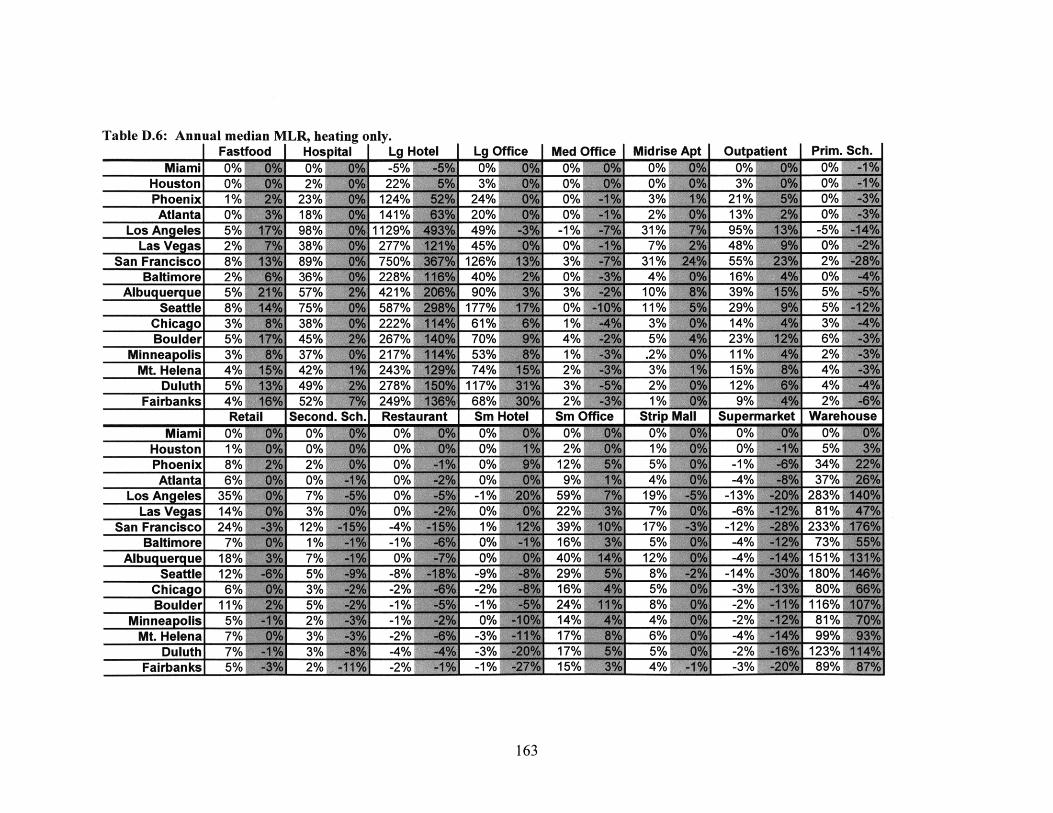
Table D.6: Annual median MLR, heating only.

LosL

San F

AlbI

MinM

F

LosL

San F

Alb

MirM

F

Fastfo Hospita Lg Hotel Lg Ofie Med Offic Midrise At Outpatien Prim. SchMiami 0% 0% -5% 0% 0% 0% 0% 0% G

Houston 0%0 2% 22% 0% 0% 3% 0Phoenix 1 % 23% 124% 24% 0% 3% 21% 0%Atlanta 0% 18% 141% 20% 0% 2% 13% 0%

Ang-eles 5% 98% 1129% 49% -1% 31% 95% -5%as Ve.gas 2% 38% 277% 45% 0% 7% 48% 0%rancisco 8% 89% 750% 126% 3% 31% 55% 2%altimore 2% 36% 28400%4% 16% 0%. uer. ue 5% 57% 421% 90% 3%10% 39% 5%Seattle 8% 75% 587% 177% 0% 11% 29% 5%

Chicag-o 3% 38% 222% 61% 1 % 3% 14% 3%Boulder 5% 45% 267% 70 46 5% 23% 6%

neapolis 3% 37%. 217% 53% 1 % .2% 11% 2%6t. Helena 4% 42% 243% 74% 2% 3% 15% 4%

Duluth 5% 49% 278% 117% 3% 2% 12% 4%airbanks 4% 52% 249% 68% 2% 1% 9% 2%

Real SecondS. Restaurn Sm Htl Sm Ofie Strip Mal Supermarke WarehosMiami 0% 0% 0% 0% 0% 0% 0% 0%/

Houston 1% 0% 0% 0% 2% 1% 0% 5%Phoenix 8% 2% 0% 0% 12% 5% -1% 34%Atlanta 6% 0% 0% 0% 9% 4% -4% 37%

Ang-eles 35% 7% 0% -1% 59% 19% -13% 283%as Ve.gas 14% 3% 0% 0% 22% 7% -6% 81%rancisco 24% 12% -4% 1 % 39% 17% -12% 233%Baltimore 7% 1 % -1% 0% 16% 5% -4% 73%u. uer. ue 18% 7% 0% 0% 40% 12% -4% 151%

Seattle 12% 5% -8% -9% 29% 8% -14% 180%Chicag-o 6% 3% -2% -2% 16% 5% -3% 80%Boulder 11% 5% -1% -1% 24% 8% -2% 116%neap.olis 5% 2% -1% 0% 14% 4% -2% 81%t. Helena 7% 3% -2% -3% 17% 6% -4% 99%

Duluth 7% 3% -4% -3% 17% 5% -2% 123%airbanksl 5%9 2% -2% 4 -1% 15% , 4 -3% 89

163

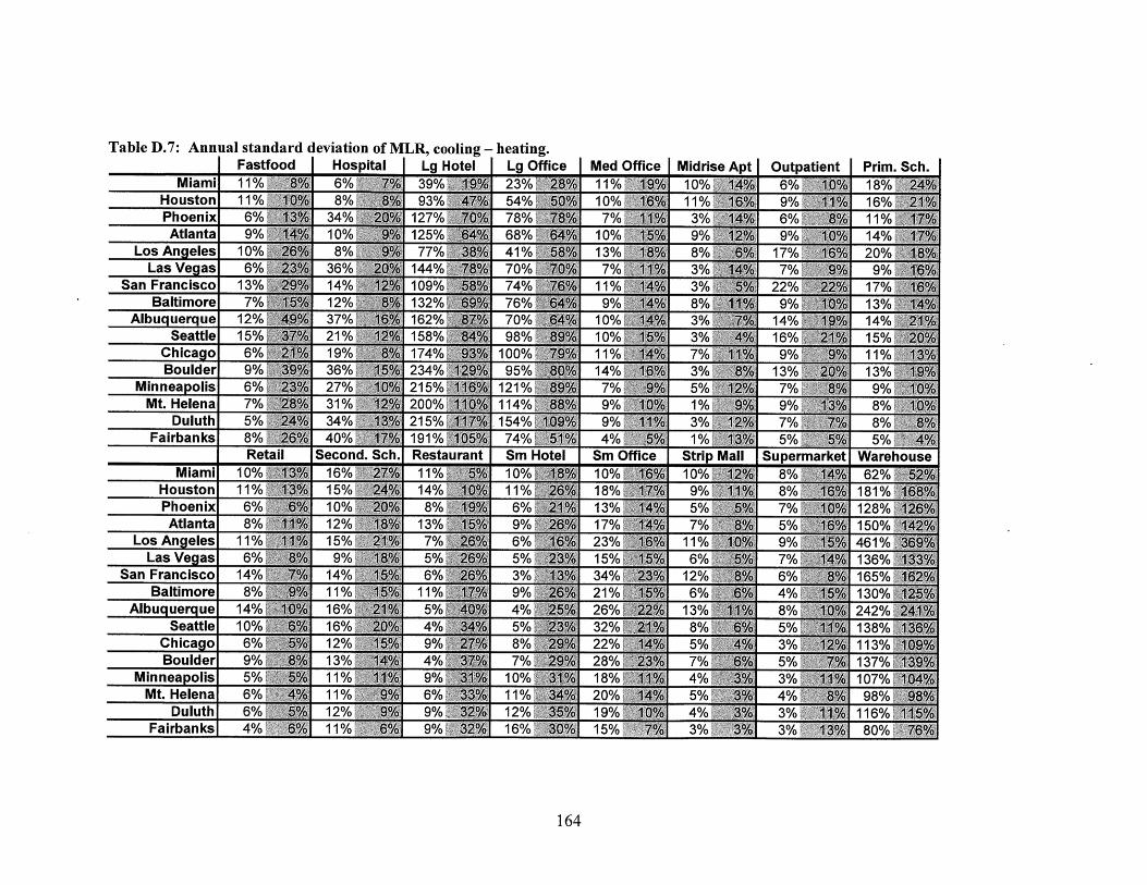
Table D.7: Annutal standard d eviation of M LR, cooling heating.Fastfood Hospital Lg Hotel L fi

Miami 11% 8% 6% 7%39%'.19o 23%Houston 11%1 10 8% 8% 93% 47% 54%Phoenix 6%' 3 34% 2%127% 7%78%1Atlanta 9% 1%10%19 125% [4 68%

Lo Agees10 2% 8% 9%77% 3%41%La Vg 106 % 36% 2%144% 7%70%

Sa Faniso13*/29 14% 1%109%, 8 74%-Batmoe 7%, 106 12% 8%132% 6%76%/6

Minneapolis 6% 2%27% 1%215% 11%121%Mt. Helena 7% 28/ 31% % 200% 00114%

Duluth 5%1.4 34% 1% 215% 11%154% 1Fairbanks 8% 2%40% 7 /,191% 10%74%

Retail Second. Sch. Restaurant Sm Hc

Phoenix 6% 6%10% 2% 8%- [9 61%Atlanta 8% 1%12% 1%13% 1% 9%

Los Angeles 11% 1%15% 2% 7%:26 6% .Las Vegas 6% [ 9% % 5%

San Francisco 14% 7% 14% 1% 6% 26% 3%EBaltimore 8% 9% 11% 1%11% 1% 9%

Albuquerque 14% 1%16% 21-5%'40 4%Seattle 10%, % 16% 20,4% 34% 5%

Chicago 6%1 % 12%, 5 9% 8%% 8Boulder 9% 8,13% 1% 4% 37% 7%Y6

Minneapolis 5W %:1 11% 11% 9% 31% 10%RMt. Helena 6% 4,11% 9,6%@$ 1% $ M

Duluth 6% 5%12% 9% 9% 32% 12%Fairbanksl 4% 6111% % 9%$@ 16

Med Office MidrisE11% 19% 10%-$10% | 16% 11%7% 11 3%

10% 15% 9%13% 18/ 8/7% 11% 3%,,

11%1 3%% 39% 4% 8%

10% 14 3%17% 15% 3%11% 14% 7/

7%_ 9%o 5/

9% [1% 3%4% 5% 1%1

Sm Office Strip10% 10/1718% 7 1; %,~ 9%'13% 14% 5%17% 14% 7%23% 1% 11%15% 15% 6%134% 235% 12%21% 1,0,6%26% 22W 13%32% [1% 8%

i 22% % , 5%| 28%4 23% 7%

18% 1 4%20% 14% 5%19% 17P 4%i15% 7 3%

164

t Outpa6%

YO 9%iA 6%%1/, 9%$

/ 17%%1/ 7% i/ 22%% 9%i

% 16%~17*/

% 13%%o 7%1

/ 9%|

,o 7%|/0 5%|

I Superi

8%19 8%~

% 7%.N 5%M~ 9%-M 7%M' 6%3%Q 4%

o % 8%3% 5%4% 3%3% 5%30/ 3%

3% 4%

3%1 3%TO/. 3%

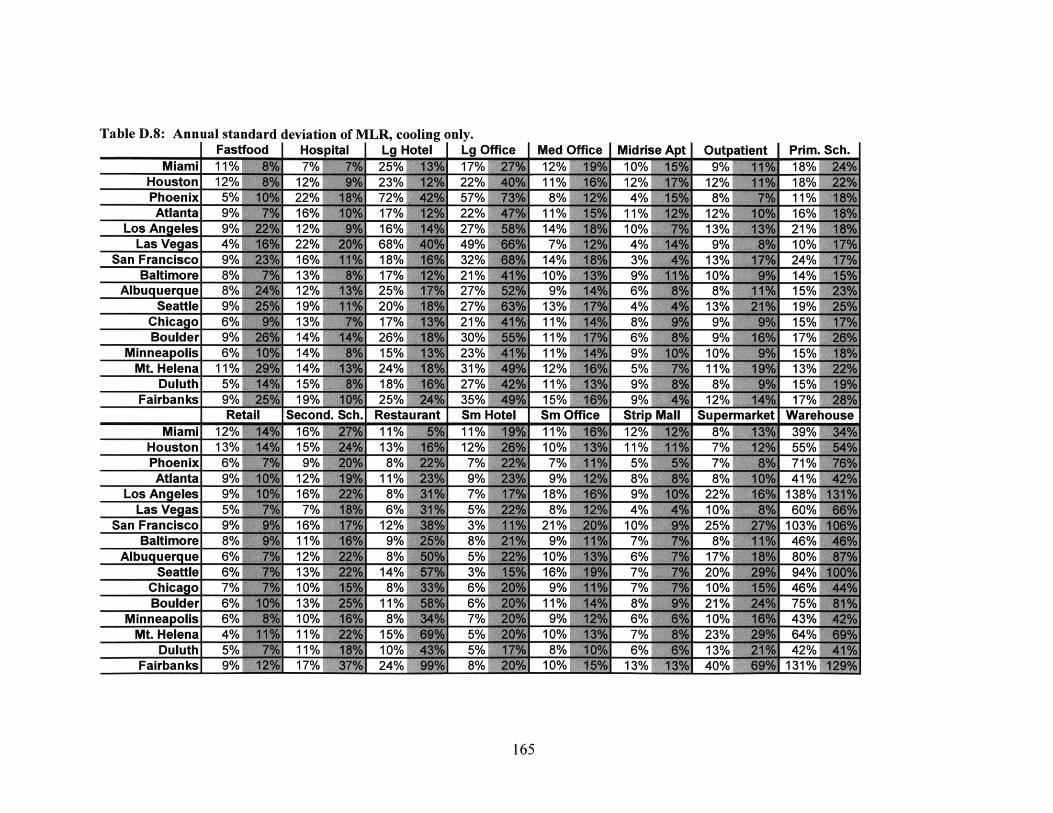
Table D.8: Annual standard deviation of MLR, cooling only.

LosL

San FE

Albu

MinM

F

LosL

San FE

AlbL

MinM

F

Fastfo Hospita Lg Hote Lg Office Med Offic Midrise At Outpatien Prim. SchMiami 11% 7% 25% 17% 12% 10% 9% 18%

Houston 12%6 12% 23% 22% 11% 121% 12%Phoenix 5% 22% 72% 57% 8% 4% 8% 11%Atlanta 9% 16% 17% 22% 11% 11% 12% 16%

Angeles 9% 12% 16% 27% 14% 10% 13%21as Ve.gas 4% 22% 68% 49% 7% 4% 9%10rancisco 9% 16% 18% 32% 14% 3% 13% 24%altimore 8% 13% 17%0c 21% 10% 9% 1%14%/. uer. ue 8% 12% 25% 27% 9% 6% 8%15

Seattle 9% 19% 20% 27% 13% 4 3 9Chica.go 6% 13% 17% 21% 11 %N 9 5Boulder 9% 14% 26% 30% 11% 6% 9% 17%

neapolis 6% 14% 15% 23% 11% 9% 10% 15%t. Helena 11% 14% 24% 31% 12% 5% 11% 13%

Duluth 5% 15% 18% 27% 11% 9% 8% 15%airbanks 9% 19% 25% 35% 15% 9% 12% 17%

Reti Second. Sch. Restarn Sm Hotel Sm Office Strip MalSupermre WarehouseMiami 12% 1%1% 1% 1%1%8 9

Houston 13% 5 3 2 1%1%7 5Phoenix 6%9%87%75%%71Atlanta 9% 1 9 %8%8 1

An.geles 9%%8%7189% 2%%as Vegeas 5% %6 %8 0rancisco 9% 6 2 % 1 0 5altimore 8%1%9%8. uer. ue 6% 1%8Seattle 6%'1%10n111

Chicag 70 o0/( 7%*1 7Boulder 6% 1%1; % 1%8neapolis 6%0%87%9

t. Helena 4% %1% % 10Duluh2% 11% 9%% % 86% 83% 41%

aibakl % 7% 6%4 % 8% 4 1% 1 0% 601%

165

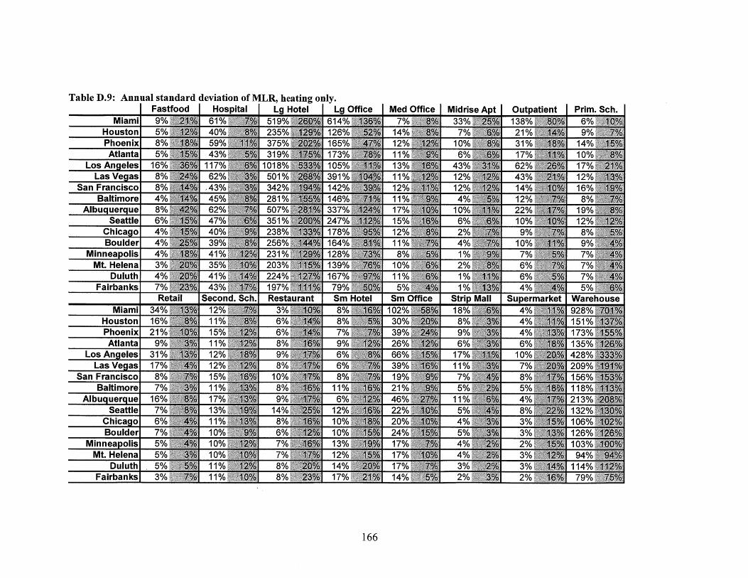
Table D.9: Annual standard deviation of MLR, heating onI Fastfood I Hospital I La Hotel I

MiamiHoustonPhoenixAtlanta

Los AngelesLas Vegas

San FranciscoBaltimore

AlbuquerqueSeattle

Chicago

9%5%8%"5%

16%8%8%4%8%6%4%

Boulder 40/Minneapolis 40/

Mt. Helena 30/Duluth 40/

Fairbanks 70/Ro

Miami 340/Houston 160/Phoenix 210MAtlanta 90M

Los Angeles 310/Las Vegas 170M

San Francisco 80/Baltimore 70/

Albuquerque 160Seattle 70/

Chicago 60MBoulder 70/

Minneapolis 50/Mt. Helena 50/

Duluth . 50/Fairbanks 30%

ly.Lg

614%126%165%173%105%391%142%146%337%247%178%164%128%139%167%79%Sm8%8%7%9%6%6%8%

11%6%

12%10%10%13%12%14%17%

Office I Med Office I7%

14%12%11%13%11%12%11%17%15%12%11%8%

10%11%

5%Sm(

102%30%39%26%66%39%19%21%46%22%20%24%17%17%17%14%

166

Midrise Apt 03 3 % -M5E/M 1 "7%

10%6%

43%12%12%

4%10%

6%2%4%1%2%1%1%

Strip18%

8%9%6%

17%11%7%5%

11%5%4%5%4%4%3%2%

21%31%17%62%43%14%12%22%10%9%

10%7%6%6%4%

Supe4%

4%6%

10%7%8%5%14%8%3%3%2%'3%3%j2%