what fuel properties enable higher thermal efficiency in spark
TRANSCRIPT
Progress in Energy and Combustion Science 82 (2021) 100876
Contents lists available at ScienceDirect
Progress in Energy and Combustion Science
journal homepage: www.elsevier.com/locate/pecs
What fuel properties enable higher thermal efficiency in spark-ignited
engines?
✩
James P. Szybist a , ∗, Stephen Busch
b , Robert L. McCormick
c , Josh A. Pihl a , Derek A. Splitter a , Matthew A. Ratcliff c , Christopher P. Kolodziej d , John M.E. Storey
a , Melanie Moses-DeBusk
a , David Vuilleumier b , Magnus Sjöberg
b , C. Scott Sluder a , Toby Rockstroh
d , Paul Miles b
a Oak Ridge National Laboratory, 2360 Cherahala Blvd, Knoxville, TN 37932, United States b Sandia National Laboratories, United States c National Renewable Energy Laboratory, United States d Argonne National Laboratory, United States
a r t i c l e i n f o
Article history:
Received 10 July 2019
Accepted 30 July 2020
Available online 20 August 2020
Keywords:
Octane
Knock
Spark ignition
Flame speed
Heat of vaporization
Particulate matter
Efficiency
Alternative fuels
a b s t r a c t
The Co-Optimization of Fuels and Engines (Co-Optima) initiative from the US Department of Energy aims
to co-develop fuels and engines in an effort to maximize energy efficiency and the utilization of renew-
able fuels. Many of these renewable fuel options have fuel chemistries that are different from those of
petroleum-derived fuels. Because practical market fuels need to meet specific fuel-property requirements,
a chemistry-agnostic approach to assessing the potential benefits of candidate fuels was developed using
the Central Fuel Property Hypothesis (CFPH). The CFPH states that fuel properties are predictive of the
performance of the fuel, regardless of the fuel’s chemical composition. In order to use this hypothesis
to assess the potential of fuel candidates to increase efficiency in spark-ignition (SI) engines, the indi-
vidual contributions towards efficiency potential in an optimized engine must be quantified in a way
that allows the individual fuel properties to be traded off for one another. This review article begins by
providing an overview of the historical linkages between fuel properties and engine efficiency, including
the two dominant pathways currently being used by vehicle manufacturers to reduce fuel consumption.
Then, a thermodynamic-based assessment to quantify how six individual fuel properties can affect effi-
ciency in SI engines is performed: research octane number, octane sensitivity, latent heat of vaporization,
laminar flame speed, particulate matter index, and catalyst light-off temperature. The relative effects of
each of these fuel properties is combined into a unified merit function that is capable of assessing the
fuel property-based efficiency potential of fuels with conventional and unconventional compositions.
© 2020 The Authors. Published by Elsevier Ltd.
This is an open access article under the CC BY license. ( http://creativecommons.org/licenses/by/4.0/ )
Contents
1. Efficiency trends in spark ignition engines . . . . . . . . . . . . . . . . . . . . . . . . . . . . . . . . . . . . . . . . . . . . . . . . . . . . . . . . . . . . . . . . . . . . . . . . 4
1.1. Historical trends in spark ignition engines (190 0–20 0 0). . . . . . . . . . . . . . . . . . . . . . . . . . . . . . . . . . . . . . . . . . . . . . . . . . . . . . . . 4
✩ This manuscript has been authored by four National Laboratories under contract with the US Department of Energy (DOE): Oak Ridge National Laboratory managed
by UT-Battelle, LLC, under contract DE-AC05-00OR22725; National Renewable Energy Laboratory managed by Alliance for Sustainable Energy, LLC, under contract No. DE-
AC36-08GO28308; Argonne National Laboratory managed by UChicago Argonne, LLC, under contract DE-AC02-06CH11357; and Sandia National Laboratories managed and
operated by National Technology and Engineering Solutions of Sandia, LLC., a wholly owned subsidiary of Honeywell International, Inc, for DOE’s National Nuclear Security
Administration under contract DE-NA0 0 03525. The US government retains and the publisher, by accepting the article for publication, acknowledges that the US government
retains a nonexclusive, paid-up, irrevocable, worldwide license to publish or reproduce the published form of this manuscript, or allow others to do so, for US government
purposes. DOE will provide public access to these results of federally sponsored research in accordance with the DOE Public Access Plan ( http://energy.gov/downloads/
doe-public-access-plan). ∗ Corresponding author.
E-mail address: [email protected] (J.P. Szybist).
https://doi.org/10.1016/j.pecs.2020.100876
0360-1285/© 2020 The Authors. Published by Elsevier Ltd. This is an open access article under the CC BY license. ( http://creativecommons.org/licenses/by/4.0/ )
2 J.P. Szybist, S. Busch and R.L. McCormick et al. / Progress in Energy and Combustion Science 82 (2021) 100876
1.2. Recent trends in SI engines (20 0 0–Present). . . . . . . . . . . . . . . . . . . . . . . . . . . . . . . . . . . . . . . . . . . . . . . . . . . . . . . . . . . . . . . . . . 5
1.2.1. High vehicle efficiency pathway 1. engine downsizing through high power density . . . . . . . . . . . . . . . . . . . . . . . . . . . 6
1.2.2. High vehicle efficiency pathway 2. Low power density . . . . . . . . . . . . . . . . . . . . . . . . . . . . . . . . . . . . . . . . . . . . . . . . . . 7
1.2.3. Comparison of the high vehicle efficiency pathways . . . . . . . . . . . . . . . . . . . . . . . . . . . . . . . . . . . . . . . . . . . . . . . . . . . . 8
2. Factors that increase efficiency in SI engines . . . . . . . . . . . . . . . . . . . . . . . . . . . . . . . . . . . . . . . . . . . . . . . . . . . . . . . . . . . . . . . . . . . . . . 9
2.1. Thermodynamic expressions for efficiency in an SI engine. . . . . . . . . . . . . . . . . . . . . . . . . . . . . . . . . . . . . . . . . . . . . . . . . . . . . . 9
2.2. High-Efficiency Engine Technologies . . . . . . . . . . . . . . . . . . . . . . . . . . . . . . . . . . . . . . . . . . . . . . . . . . . . . . . . . . . . . . . . . . . . . . . 9
2.2.1. Boosted engine operation . . . . . . . . . . . . . . . . . . . . . . . . . . . . . . . . . . . . . . . . . . . . . . . . . . . . . . . . . . . . . . . . . . . . . . . . . . 11
2.2.2. Direct injection fueling. . . . . . . . . . . . . . . . . . . . . . . . . . . . . . . . . . . . . . . . . . . . . . . . . . . . . . . . . . . . . . . . . . . . . . . . . . . . 11
2.2.3. Overexpanded engine cycles . . . . . . . . . . . . . . . . . . . . . . . . . . . . . . . . . . . . . . . . . . . . . . . . . . . . . . . . . . . . . . . . . . . . . . . 11
2.2.4. Exhaust gas recirculation . . . . . . . . . . . . . . . . . . . . . . . . . . . . . . . . . . . . . . . . . . . . . . . . . . . . . . . . . . . . . . . . . . . . . . . . . . 12
2.2.5. Advanced Ignition Systems . . . . . . . . . . . . . . . . . . . . . . . . . . . . . . . . . . . . . . . . . . . . . . . . . . . . . . . . . . . . . . . . . . . . . . . . 12
2.2.6. Variable compression ratio . . . . . . . . . . . . . . . . . . . . . . . . . . . . . . . . . . . . . . . . . . . . . . . . . . . . . . . . . . . . . . . . . . . . . . . . 12
2.2.7. Cylinder deactivation . . . . . . . . . . . . . . . . . . . . . . . . . . . . . . . . . . . . . . . . . . . . . . . . . . . . . . . . . . . . . . . . . . . . . . . . . . . . . 13
2.3. Fuel Property Impacts on SI Engine Efficiency. . . . . . . . . . . . . . . . . . . . . . . . . . . . . . . . . . . . . . . . . . . . . . . . . . . . . . . . . . . . . . . . 13
3. How fuels affect in-cylinder efficiency . . . . . . . . . . . . . . . . . . . . . . . . . . . . . . . . . . . . . . . . . . . . . . . . . . . . . . . . . . . . . . . . . . . . . . . . . . . 13
3.1. Knock resistance . . . . . . . . . . . . . . . . . . . . . . . . . . . . . . . . . . . . . . . . . . . . . . . . . . . . . . . . . . . . . . . . . . . . . . . . . . . . . . . . . . . . . . . . 14
3.1.1. Historical antiknock metrics . . . . . . . . . . . . . . . . . . . . . . . . . . . . . . . . . . . . . . . . . . . . . . . . . . . . . . . . . . . . . . . . . . . . . . . . 14
3.1.2. Octane index and the importance of octane sensitivity . . . . . . . . . . . . . . . . . . . . . . . . . . . . . . . . . . . . . . . . . . . . . . . . . . 15
3.1.3. Accuracy and limitations of octane index . . . . . . . . . . . . . . . . . . . . . . . . . . . . . . . . . . . . . . . . . . . . . . . . . . . . . . . . . . . . . 18
3.1.4. The impact of knock resistance on efficiency . . . . . . . . . . . . . . . . . . . . . . . . . . . . . . . . . . . . . . . . . . . . . . . . . . . . . . . . . . 20
3.1.5. Estimating the Impact of Knock Resistance on Efficiency from Literature . . . . . . . . . . . . . . . . . . . . . . . . . . . . . . . . . . . 21
3.1.6. Estimating the impact of knock resistance through simulation and analysis . . . . . . . . . . . . . . . . . . . . . . . . . . . . . . . . . 21
3.2. Heat of vaporization . . . . . . . . . . . . . . . . . . . . . . . . . . . . . . . . . . . . . . . . . . . . . . . . . . . . . . . . . . . . . . . . . . . . . . . . . . . . . . . . . . . . 23
3.2.1. Thermodynamic impacts of HoV on engine efficiency . . . . . . . . . . . . . . . . . . . . . . . . . . . . . . . . . . . . . . . . . . . . . . . . . . . 23
3.3. The effects of flame speed . . . . . . . . . . . . . . . . . . . . . . . . . . . . . . . . . . . . . . . . . . . . . . . . . . . . . . . . . . . . . . . . . . . . . . . . . . . . . . . 27
3.3.1. Thermodynamic effects of flame speed on engine efficiency . . . . . . . . . . . . . . . . . . . . . . . . . . . . . . . . . . . . . . . . . . . . . 27
3.3.2. Determination of laminar flame speed . . . . . . . . . . . . . . . . . . . . . . . . . . . . . . . . . . . . . . . . . . . . . . . . . . . . . . . . . . . . . . . 28
3.3.3. Quantifying the effect of flame speed. . . . . . . . . . . . . . . . . . . . . . . . . . . . . . . . . . . . . . . . . . . . . . . . . . . . . . . . . . . . . . . . 28
3.3.4. Additional laminar flame speed effects. . . . . . . . . . . . . . . . . . . . . . . . . . . . . . . . . . . . . . . . . . . . . . . . . . . . . . . . . . . . . . . 29
3.4. Low-speed preignition . . . . . . . . . . . . . . . . . . . . . . . . . . . . . . . . . . . . . . . . . . . . . . . . . . . . . . . . . . . . . . . . . . . . . . . . . . . . . . . . . . . 30
3.4.1. Causes of low speed preignition . . . . . . . . . . . . . . . . . . . . . . . . . . . . . . . . . . . . . . . . . . . . . . . . . . . . . . . . . . . . . . . . . . . . 30
3.4.2. Fuel-related causes of LSPI initiation . . . . . . . . . . . . . . . . . . . . . . . . . . . . . . . . . . . . . . . . . . . . . . . . . . . . . . . . . . . . . . . . 31
3.4.3. Additional LSPI fuel-effects . . . . . . . . . . . . . . . . . . . . . . . . . . . . . . . . . . . . . . . . . . . . . . . . . . . . . . . . . . . . . . . . . . . . . . . . 31
3.4.4. Quantification of the fuel-related causes of low-speed preignition . . . . . . . . . . . . . . . . . . . . . . . . . . . . . . . . . . . . . . . . 32
4. How fuels influence efficiency through emission controls . . . . . . . . . . . . . . . . . . . . . . . . . . . . . . . . . . . . . . . . . . . . . . . . . . . . . . . . . . . 34
4.1. Gaseous emissions . . . . . . . . . . . . . . . . . . . . . . . . . . . . . . . . . . . . . . . . . . . . . . . . . . . . . . . . . . . . . . . . . . . . . . . . . . . . . . . . . . . . . . 34
4.1.1. Derivation of the gaseous emissions merit function term . . . . . . . . . . . . . . . . . . . . . . . . . . . . . . . . . . . . . . . . . . . . . . . . 34
4.1.2. Evaluation of the gaseous emissions merit function term . . . . . . . . . . . . . . . . . . . . . . . . . . . . . . . . . . . . . . . . . . . . . . . . 35
4.2. Particulate Emissions . . . . . . . . . . . . . . . . . . . . . . . . . . . . . . . . . . . . . . . . . . . . . . . . . . . . . . . . . . . . . . . . . . . . . . . . . . . . . . . . . . . . 36
4.2.1. PM emissions regulations . . . . . . . . . . . . . . . . . . . . . . . . . . . . . . . . . . . . . . . . . . . . . . . . . . . . . . . . . . . . . . . . . . . . . . . . . . 36
4.2.2. Methods for controlling PM Emissions from gasoline DI Engines. . . . . . . . . . . . . . . . . . . . . . . . . . . . . . . . . . . . . . . . . . 38
4.2.3. Fuel effects on PM emissions. . . . . . . . . . . . . . . . . . . . . . . . . . . . . . . . . . . . . . . . . . . . . . . . . . . . . . . . . . . . . . . . . . . . . . . 38
4.2.4. Particulate matter impact on engine thermodynamics . . . . . . . . . . . . . . . . . . . . . . . . . . . . . . . . . . . . . . . . . . . . . . . . . . 40
5. The merit function . . . . . . . . . . . . . . . . . . . . . . . . . . . . . . . . . . . . . . . . . . . . . . . . . . . . . . . . . . . . . . . . . . . . . . . . . . . . . . . . . . . . . . . . . . . 41
5.1. Realistic fuel property ranges for the sensitivity analysis . . . . . . . . . . . . . . . . . . . . . . . . . . . . . . . . . . . . . . . . . . . . . . . . . . . . . . . 42
5.1.1. Realistic range of RON. . . . . . . . . . . . . . . . . . . . . . . . . . . . . . . . . . . . . . . . . . . . . . . . . . . . . . . . . . . . . . . . . . . . . . . . . . . . . 42
5.1.2. Realistic range of S octane . . . . . . . . . . . . . . . . . . . . . . . . . . . . . . . . . . . . . . . . . . . . . . . . . . . . . . . . . . . . . . . . . . . . . . . . . . . 43
5.1.3. Realistic range of HoV. . . . . . . . . . . . . . . . . . . . . . . . . . . . . . . . . . . . . . . . . . . . . . . . . . . . . . . . . . . . . . . . . . . . . . . . . . . . . 43
5.1.4. Realistic range of flame speed . . . . . . . . . . . . . . . . . . . . . . . . . . . . . . . . . . . . . . . . . . . . . . . . . . . . . . . . . . . . . . . . . . . . . . 43
5.1.5. Realistic range of PMI . . . . . . . . . . . . . . . . . . . . . . . . . . . . . . . . . . . . . . . . . . . . . . . . . . . . . . . . . . . . . . . . . . . . . . . . . . . . . 43
5.1.6. Realistic range of Tc,90 . . . . . . . . . . . . . . . . . . . . . . . . . . . . . . . . . . . . . . . . . . . . . . . . . . . . . . . . . . . . . . . . . . . . . . . . . . . . 43
5.2. Merit function sensitivity analysis . . . . . . . . . . . . . . . . . . . . . . . . . . . . . . . . . . . . . . . . . . . . . . . . . . . . . . . . . . . . . . . . . . . . . . . . . 43
5.2.1. RON impact on merit function. . . . . . . . . . . . . . . . . . . . . . . . . . . . . . . . . . . . . . . . . . . . . . . . . . . . . . . . . . . . . . . . . . . . . . 43
5.2.2. S octane impact on merit function . . . . . . . . . . . . . . . . . . . . . . . . . . . . . . . . . . . . . . . . . . . . . . . . . . . . . . . . . . . . . . . . . . . . 43
5.2.3. HoV impact on merit function. . . . . . . . . . . . . . . . . . . . . . . . . . . . . . . . . . . . . . . . . . . . . . . . . . . . . . . . . . . . . . . . . . . . . . 44
5.2.4. Flame speed impact on merit function. . . . . . . . . . . . . . . . . . . . . . . . . . . . . . . . . . . . . . . . . . . . . . . . . . . . . . . . . . . . . . . 44
5.2.5. PMI impact on merit function . . . . . . . . . . . . . . . . . . . . . . . . . . . . . . . . . . . . . . . . . . . . . . . . . . . . . . . . . . . . . . . . . . . . . . 44
5.2.6. Catalyst light-off temperature impact on merit function. . . . . . . . . . . . . . . . . . . . . . . . . . . . . . . . . . . . . . . . . . . . . . . . . 44
5.3. Exercising the merit function . . . . . . . . . . . . . . . . . . . . . . . . . . . . . . . . . . . . . . . . . . . . . . . . . . . . . . . . . . . . . . . . . . . . . . . . . . . . . 44
6. Future prospects . . . . . . . . . . . . . . . . . . . . . . . . . . . . . . . . . . . . . . . . . . . . . . . . . . . . . . . . . . . . . . . . . . . . . . . . . . . . . . . . . . . . . . . . . . . . . 46
6.1. Improvements to antiknock properties . . . . . . . . . . . . . . . . . . . . . . . . . . . . . . . . . . . . . . . . . . . . . . . . . . . . . . . . . . . . . . . . . . . . . . 46
6.2. Improvements to heat of vaporization impact. . . . . . . . . . . . . . . . . . . . . . . . . . . . . . . . . . . . . . . . . . . . . . . . . . . . . . . . . . . . . . . . 46
6.3. Improvements to flame speed impact . . . . . . . . . . . . . . . . . . . . . . . . . . . . . . . . . . . . . . . . . . . . . . . . . . . . . . . . . . . . . . . . . . . . . . 46
6.4. Improved quantification of LSPI fuel impacts . . . . . . . . . . . . . . . . . . . . . . . . . . . . . . . . . . . . . . . . . . . . . . . . . . . . . . . . . . . . . . . . 47
6.5. Improved particulate matter impacts . . . . . . . . . . . . . . . . . . . . . . . . . . . . . . . . . . . . . . . . . . . . . . . . . . . . . . . . . . . . . . . . . . . . . . . 47
J.P. Szybist, S. Busch and R.L. McCormick et al. / Progress in Energy and Combustion Science 82 (2021) 100876 3
6.6. Improved understanding of catalyst light-off. . . . . . . . . . . . . . . . . . . . . . . . . . . . . . . . . . . . . . . . . . . . . . . . . . . . . . . . . . . . . . . . . 47
7. Summary/conclusions. . . . . . . . . . . . . . . . . . . . . . . . . . . . . . . . . . . . . . . . . . . . . . . . . . . . . . . . . . . . . . . . . . . . . . . . . . . . . . . . . . . . . . . . . 47
Declaration of Competing Interest . . . . . . . . . . . . . . . . . . . . . . . . . . . . . . . . . . . . . . . . . . . . . . . . . . . . . . . . . . . . . . . . . . . . . . . . . . . . . . . . . . 47
Acknowledgements . . . . . . . . . . . . . . . . . . . . . . . . . . . . . . . . . . . . . . . . . . . . . . . . . . . . . . . . . . . . . . . . . . . . . . . . . . . . . . . . . . . . . . . . . . . . . . 47
Supplementary materials. . . . . . . . . . . . . . . . . . . . . . . . . . . . . . . . . . . . . . . . . . . . . . . . . . . . . . . . . . . . . . . . . . . . . . . . . . . . . . . . . . . . . . . . . . 48
References . . . . . . . . . . . . . . . . . . . . . . . . . . . . . . . . . . . . . . . . . . . . . . . . . . . . . . . . . . . . . . . . . . . . . . . . . . . . . . . . . . . . . . . . . . . . . . . . . . . . . 48
αA
A
A
A
B
B
C
C
C
C
C
C
C
C
c
D
D
�
�
D
E
E
E
E
E
f
F
f
F
F
γG
g
ηH
H
H
ηηηηηηH
H
I
I
I
I
K
K
K
L
L
L
L
L
M
M
M
N
N
N
N
N
O
P
p
p
P
P
P
P
P
P
P
P
P
P
θQ
Q
Q
r
R
R
S
σS
σ
S
S
T
T
T
T
T
T
t
T
T
U
V
V
V
V
V
V
W
W
Y
Average catalyst heating rate
FM Air-fuel mixture
FR Mass air-to-fuel ratio
KI Antiknock index
TDC After top dead center
MEP Brake mean effective pressure
OB Blendstock for oxygenate blending
AD Crank-angle degree
AFE Corporate Average Fuel Economy
ARB California air resources board
FPH Central fuel property hypothesis
FR Cooperative fuels research
O Carbon monoxide
O 2 Carbon dioxide
OV Coefficient of variation
v Heat capacity at a constant volume
BE Double bond equivalent
F Downsize factor
F LO Fuel penalty during cold start
f LO Instantaneous difference between the cold and hot fuel
consumption rates
I Direct injection
85 Fuel mixture containing nominally 85 vol % ethanol
GR Exhaust gas recirculation
ISA Energy Independence and Security Act
IVC Early intake valve closing
PA Environmental Protection Agency
C Fuel consumption rate during cold start
FTP Total fuel consumed during the FTP cycle
H Fuel consumption rate during hot start
SN Filter smoke number
TP EPA Federal Test Procedure for the city driving cycle
Ratio of specific heats of a working fluid
PF Gasoline particulate filter
/mi Gram per mile
b Brake efficiency
C Hydrocarbon
CCI Homogeneous charge compression ignition
PD High power density
comb Combustion efficiency
GE Gas exchange efficiency
ideal Ideal efficiency
mech Mechanical efficiency
OE Overexpanded cycle efficiency
Otto Otto cycle efficiency
Heaviside function
oV Heat of vaporization
AT Intake air temperature
MEP g Gross indicated mean effective pressure
MEP n Net indicated mean effective pressure
TE Indicated thermal efficiency
Engine operating variable in OI
LSA Knock limited spark advance
P Knock point
HV Lower heating value
IVC Late intake valve closing
PD Low power density
SPI Low speed preignition
THR Low temperature heat release
AT Mixture air temperature
ON Motor octane number
SS Microsoot sensor
A Naturally aspirated
MOG Non methane organic gases
Ox Oxides of nitrogen
TC Negative temperature coefficient
VH Noise, vibration and harshness
I Octane index
FI Port fuel injection
i Example fuel property
i,ref Reference example fuel property
M Particulate matter
MEP Pumping mean effective pressure
MI Particulate matter index
M soot Soot or solid carbon portion of the particulate matter
N Particle number
PR Peak pressure rise
R Preignition rating
RF Primary reference fuel
RR pressure rise rate
ST Cylinder pressure at spark timing
Crank angle
fuel total Total fuel energy
HR Total energy release through combustion of the fuel
HT Total energy lost via wall heat transfer
c Compression ratio
ON Research octane number
PM Revolutions per minute
octane Octane sensitivity
HT Proportion of energy remaining after wall heat transfer
I Spark ignition
ideal The degree to which the actual heat release profile re-
sembles the ideal profile
L Laminar flame speed
OC Start of combustion
Temperature
50 Temperature at which 50% of the fuel is evaporated
70 Temperature at which 70% of the fuel is evaporated
amb Ambient temperature
c,90 TWC light-off temperature
EL Tetraethyl lead
LO Time required for TWC light-off for 90% conversion
SF Toluene standardization fuels
WC Three-way catalyst
DDS Urban dynamometer driving schedule
Volume
c Clearance volume
CR Variable compression ratio
d Displacement volume
OC Volatile organic compound
P Vapor pressure
Work per cycle
OT Wide open throttle
SI Yield sooting index
4 J.P. Szybist, S. Busch and R.L. McCormick et al. / Progress in Energy and Combustion Science 82 (2021) 100876
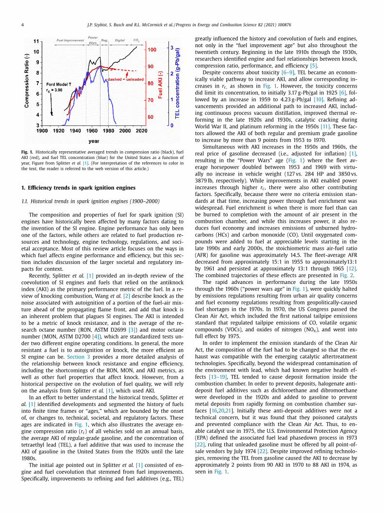
Fig. 1. Historically representative averaged trends in compression ratio (black), fuel
AKI (red), and fuel TEL concentration (blue) for the United States as a function of
year, Figure from Splitter et al. [1] . (For interpretation of the references to color in
the text, the reader is referred to the web version of this article.)
g
n
t
r
c
i
c
d
l
v
i
f
W
t
t
r
r
e
a
3
i
f
d
w
b
c
d
c
p
l
(
d
b
T
t
b
a
f
C
s
c
f
A
h
t
t
f
c
d
w
m
f
t
a
a
(
[
s
g
a
s
1. Efficiency trends in spark ignition engines
1.1. Historical trends in spark ignition engines (190 0–20 0 0)
The composition and properties of fuel for spark ignition (SI)
engines have historically been affected by many factors dating to
the invention of the SI engine. Engine performance has only been
one of the factors, while others are related to fuel production re-
sources and technology, engine technology, regulations, and soci-
etal acceptance. Most of this review article focuses on the ways in
which fuel affects engine performance and efficiency, but this sec-
tion includes discussion of the larger societal and regulatory im-
pacts for context.
Recently, Splitter et al. [1] provided an in-depth review of the
coevolution of SI engines and fuels that relied on the antiknock
index (AKI) as the primary performance metric of the fuel. In a re-
view of knocking combustion, Wang et al. [2] describe knock as the
noise associated with autoignition of a portion of the fuel-air mix-
ture ahead of the propagating flame front, and add that knock is
an inherent problem that plagues SI engines. The AKI is intended
to be a metric of knock resistance, and is the average of the re-
search octane number (RON, ASTM D2699 [3] ) and motor octane
number (MON, ASTM D2700 [4] ), which are standardized tests un-
der two different engine operating conditions. In general, the more
resistant a fuel is to autoignition or knock, the more efficient an
SI engine can be. Section 3 provides a more detailed analysis of
the relationship between knock resistance and engine efficiency,
including the shortcomings of the RON, MON, and AKI metrics, as
well as other fuel properties that affect knock. However, from a
historical perspective on the evolution of fuel quality, we will rely
on the analysis from Splitter et al. [1] , which used AKI.
In an effort to better understand the historical trends, Splitter et
al. [1] identified developments and segmented the history of fuels
into finite time frames or “ages,” which are bounded by the onset
of, or changes to, technical, societal, and regulatory factors. These
ages are indicated in Fig. 1 , which also illustrates the average en-
gine compression ratio ( r c ) of all vehicles sold on an annual basis,
the average AKI of regular-grade gasoline, and the concentration of
tetraethyl lead (TEL), a fuel additive that was used to increase the
AKI of gasoline in the United States from the 1920s until the late
1980s.
The initial age pointed out in Splitter et al. [1] consisted of en-
gine and fuel coevolution that stemmed from fuel improvements.
Specifically, improvements to refining and fuel additives (e.g., TEL)
reatly influenced the history and coevolution of fuels and engines,
ot only in the “fuel improvement age” but also throughout the
wentieth century. Beginning in the late 1910s through the 1930s,
esearchers identified engine and fuel relationships between knock,
ompression ratio, performance, and efficiency [5] .
Despite concerns about toxicity [6–9] , TEL became an econom-
cally viable pathway to increase AKI, and allow corresponding in-
reases in r c , as shown in Fig. 1 . However, the toxicity concerns
id limit its concentration, to initially 3.17 g-Pb/gal in 1925 [6] , fol-
owed by an increase in 1959 to 4.23 g-Pb/gal [10] . Refining ad-
ancements provided an additional path to increased AKI, includ-
ng continuous process vacuum distillation, improved thermal re-
orming in the late 1920s and 1930s, catalytic cracking during
orld War II, and platinum reforming in the 1950s [11] . These fac-
ors allowed the AKI of both regular and premium grade gasoline
o increase by more than 9 points from 1953 to 1970.
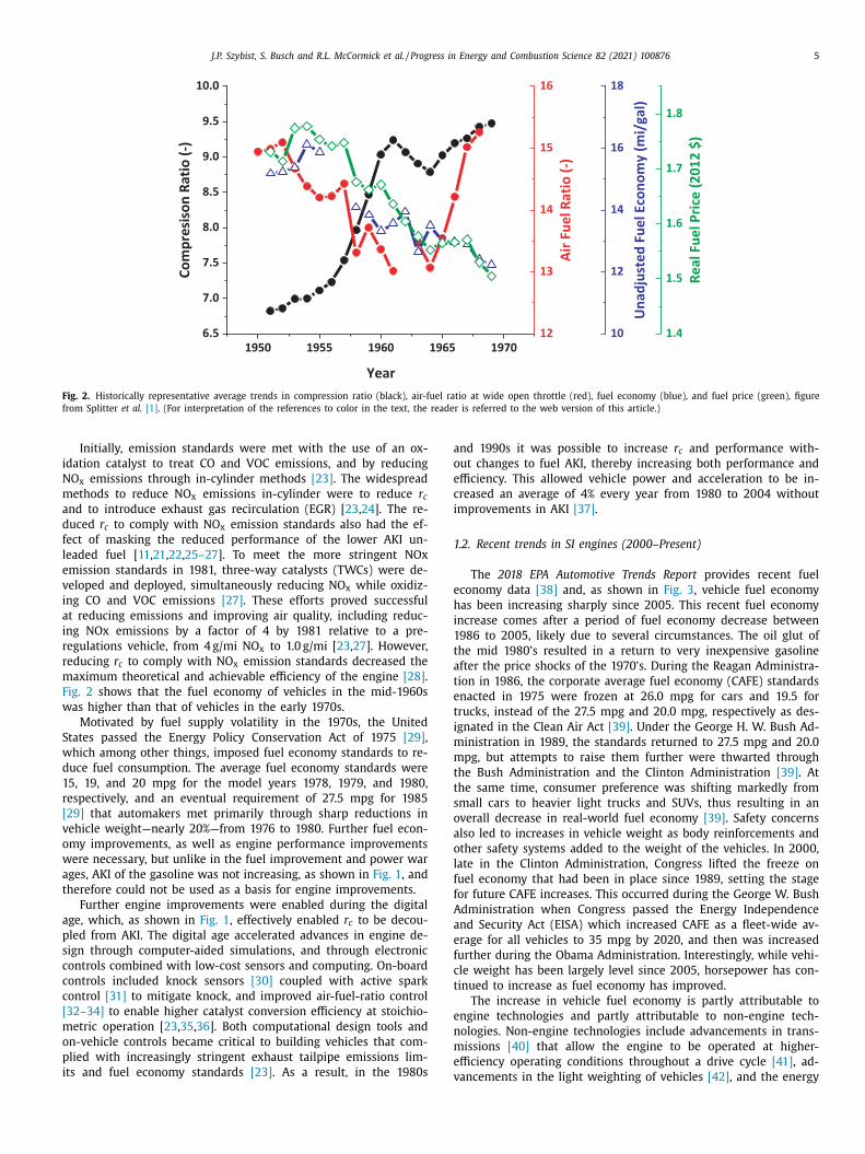
Simultaneous with AKI increases in the 1950s and 1960s, the
eal price of gasoline decreased (i.e., adjusted for inflation) [1] ,
esulting in the “Power Wars” age ( Fig. 1 ) where the fleet av-
rage horsepower doubled between 1953 and 1969 with virtu-
lly no increase in vehicle weight (127 vs. 284 HP and 3850 vs.
879 lb, respectively). While improvements in AKI enabled power
ncreases through higher r c , there were also other contributing
actors. Specifically, because there were no criteria emission stan-
ards at that time, increasing power through fuel enrichment was
idespread. Fuel enrichment is when there is more fuel than can
e burned to completion with the amount of air present in the
ombustion chamber, and while this increases power, it also re-
uces fuel economy and increases emissions of unburned hydro-
arbons (HCs) and carbon monoxide (CO). Until oxygenated com-
ounds were added to fuel at appreciable levels starting in the
ate 1990s and early 20 0 0s, the stoichiometric mass air-fuel ratio
AFR) for gasoline was approximately 14.5. The fleet-average AFR
ecreased from approximately 15:1 in 1955 to approximately13:1
y 1961 and persisted at approximately 13:1 through 1965 [12] .
he combined trajectories of these effects are presented in Fig. 2 .
The rapid advances in performance during the late 1950s
hrough the 1960s (“power wars age” in Fig. 1 ), were quickly halted
y emissions regulations resulting from urban air quality concerns
nd fuel economy regulations resulting from geopolitically-caused
uel shortages in the 1970s. In 1970, the US Congress passed the
lean Air Act, which included the first national tailpipe emissions
tandard that regulated tailpipe emissions of CO, volatile organic
ompounds (VOCs), and oxides of nitrogen (NO x ), and went into
ull effect by 1975.
In order to implement the emission standards of the Clean Air
ct, the composition of the fuel had to be changed so that the ex-
aust was compatible with the emerging catalytic aftertreatment
echnologies. Specifically, beyond the widespread contamination of
he environment with lead, which had known negative health ef-
ects [13–19] , TEL tended to cause deposit formation inside the
ombustion chamber. In order to prevent deposits, halogenate anti-
eposit fuel additives such as dichloroethane and dibromoethane
ere developed in the 1920s and added to gasoline to prevent
etal deposits from rapidly forming on combustion chamber sur-
aces [ 16 , 20 , 21 ]. Initially these anti-deposit additives were not a
echnical concern, but it was found that they poisoned catalysts
nd prevented compliance with the Clean Air Act. Thus, to en-
ble catalyst use in 1975, the U.S. Environmental Protection Agency
EPA) defined the associated fuel lead phasedown process in 1973
22] , ruling that unleaded gasoline must be offered by all point-of-
ale vendors by July 1974 [22] . Despite improved refining technolo-
ies, removing the TEL from gasoline caused the AKI to decrease by
pproximately 2 points from 90 AKI in 1970 to 88 AKI in 1974, as
een in Fig. 1 .
J.P. Szybist, S. Busch and R.L. McCormick et al. / Progress in Energy and Combustion Science 82 (2021) 100876 5
Fig. 2. Historically representative average trends in compression ratio (black), air-fuel ratio at wide open throttle (red), fuel economy (blue), and fuel price (green), figure
from Splitter et al. [1] . (For interpretation of the references to color in the text, the reader is referred to the web version of this article.)
i
N
m
a
d
f
l
e
v
i
a
i
r
r
m
F
w
S
w
d
1
r
[
v
o
w
a
t
a
p
s
c
c
c
[
m
o
p
i
a
o
e
c
i
1
e
h
i
1
t
a
t
e
t
i
m
m
t
t
s
o
a
o
l
f
f
A
a
e
f
c
t
e
n
m
e
Initially, emission standards were met with the use of an ox-
dation catalyst to treat CO and VOC emissions, and by reducing
O x emissions through in-cylinder methods [23] . The widespread
ethods to reduce NO x emissions in-cylinder were to reduce r c nd to introduce exhaust gas recirculation (EGR) [ 23 , 24 ]. The re-
uced r c to comply with NO x emission standards also had the ef-
ect of masking the reduced performance of the lower AKI un-
eaded fuel [ 11 , 21 , 22 , 25–27 ]. To meet the more stringent NOx
mission standards in 1981, three-way catalysts (TWCs) were de-
eloped and deployed, simultaneously reducing NO x while oxidiz-
ng CO and VOC emissions [27] . These effort s proved successful
t reducing emissions and improving air quality, including reduc-
ng NOx emissions by a factor of 4 by 1981 relative to a pre-
egulations vehicle, from 4 g/mi NO x to 1.0 g/mi [ 23 , 27 ]. However,
educing r c to comply with NO x emission standards decreased the
aximum theoretical and achievable efficiency of the engine [28] .
ig. 2 shows that the fuel economy of vehicles in the mid-1960s
as higher than that of vehicles in the early 1970s.
Motivated by fuel supply volatility in the 1970s, the United
tates passed the Energy Policy Conservation Act of 1975 [29] ,
hich among other things, imposed fuel economy standards to re-
uce fuel consumption. The average fuel economy standards were
5, 19, and 20 mpg for the model years 1978, 1979, and 1980,
espectively, and an eventual requirement of 27.5 mpg for 1985
29] that automakers met primarily through sharp reductions in
ehicle weight—nearly 20%—from 1976 to 1980. Further fuel econ-
my improvements, as well as engine performance improvements
ere necessary, but unlike in the fuel improvement and power war
ges, AKI of the gasoline was not increasing, as shown in Fig. 1 , and
herefore could not be used as a basis for engine improvements.
Further engine improvements were enabled during the digital
ge, which, as shown in Fig. 1 , effectively enabled r c to be decou-
led from AKI. The digital age accelerated advances in engine de-
ign through computer-aided simulations, and through electronic
ontrols combined with low-cost sensors and computing. On-board
ontrols included knock sensors [30] coupled with active spark
ontrol [31] to mitigate knock, and improved air-fuel-ratio control
32–34] to enable higher catalyst conversion efficiency at stoichio-
etric operation [ 23 , 35 , 36 ]. Both computational design tools and
n-vehicle controls became critical to building vehicles that com-
lied with increasingly stringent exhaust tailpipe emissions lim-
ts and fuel economy standards [23] . As a result, in the 1980s
vnd 1990s it was possible to increase r c and performance with-
ut changes to fuel AKI, thereby increasing both performance and
fficiency. This allowed vehicle power and acceleration to be in-
reased an average of 4% every year from 1980 to 2004 without
mprovements in AKI [37] .
.2. Recent trends in SI engines (20 0 0–Present)
The 2018 EPA Automotive Trends Report provides recent fuel
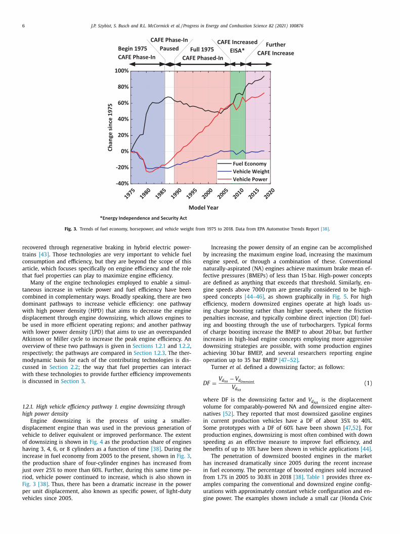
conomy data [38] and, as shown in Fig. 3 , vehicle fuel economy
as been increasing sharply since 2005. This recent fuel economy
ncrease comes after a period of fuel economy decrease between
986 to 2005, likely due to several circumstances. The oil glut of
he mid 1980’s resulted in a return to very inexpensive gasoline
fter the price shocks of the 1970’s. During the Reagan Administra-
ion in 1986, the corporate average fuel economy (CAFE) standards
nacted in 1975 were frozen at 26.0 mpg for cars and 19.5 for
rucks, instead of the 27.5 mpg and 20.0 mpg, respectively as des-
gnated in the Clean Air Act [39] . Under the George H. W. Bush Ad-
inistration in 1989, the standards returned to 27.5 mpg and 20.0
pg, but attempts to raise them further were thwarted through
he Bush Administration and the Clinton Administration [39] . At
he same time, consumer preference was shifting markedly from
mall cars to heavier light trucks and SUVs, thus resulting in an
verall decrease in real-world fuel economy [39] . Safety concerns
lso led to increases in vehicle weight as body reinforcements and
ther safety systems added to the weight of the vehicles. In 20 0 0,
ate in the Clinton Administration, Congress lifted the freeze on
uel economy that had been in place since 1989, setting the stage
or future CAFE increases. This occurred during the George W. Bush
dministration when Congress passed the Energy Independence
nd Security Act (EISA) which increased CAFE as a fleet-wide av-
rage for all vehicles to 35 mpg by 2020, and then was increased
urther during the Obama Administration. Interestingly, while vehi-
le weight has been largely level since 2005, horsepower has con-
inued to increase as fuel economy has improved.
The increase in vehicle fuel economy is partly attributable to
ngine technologies and partly attributable to non-engine tech-
ologies. Non-engine technologies include advancements in trans-
issions [40] that allow the engine to be operated at higher-
fficiency operating conditions throughout a drive cycle [41] , ad-
ancements in the light weighting of vehicles [42] , and the energy
6 J.P. Szybist, S. Busch and R.L. McCormick et al. / Progress in Energy and Combustion Science 82 (2021) 100876
Fig. 3. Trends of fuel economy, horsepower, and vehicle weight from 1975 to 2018. Data from EPA Automotive Trends Report [38] .
b
e
n
f
a
g
s
e
i
p
i
o
i
d
a
o
D
w
v
n
i
S
p
s
b
h
i
f
a
u
g
recovered through regenerative braking in hybrid electric power-
trains [43] . Those technologies are very important to vehicle fuel
consumption and efficiency, but they are beyond the scope of this
article, which focuses specifically on engine efficiency and the role
that fuel properties can play to maximize engine efficiency.
Many of the engine technologies employed to enable a simul-
taneous increase in vehicle power and fuel efficiency have been
combined in complementary ways. Broadly speaking, there are two
dominant pathways to increase vehicle efficiency: one pathway
with high power density (HPD) that aims to decrease the engine
displacement through engine downsizing, which allows engines to
be used in more efficient operating regions; and another pathway
with lower power density (LPD) that aims to use an overexpanded
Atkinson or Miller cycle to increase the peak engine efficiency. An
overview of these two pathways is given in Sections 1.2.1 and 1.2.2 ,
respectively; the pathways are compared in Section 1.2.3 . The ther-
modynamic basis for each of the contributing technologies is dis-
cussed in Section 2.2 ; the way that fuel properties can interact
with these technologies to provide further efficiency improvements
is discussed in Section 3 .
1.2.1. High vehicle efficiency pathway 1. engine downsizing through
high power density
Engine downsizing is the process of using a smaller-
displacement engine than was used in the previous generation of
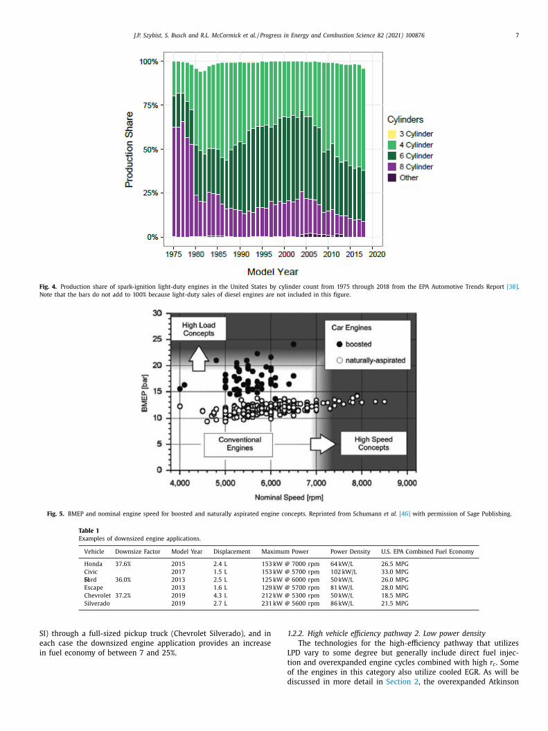
vehicle to deliver equivalent or improved performance. The extent
of downsizing is shown in Fig. 4 as the production share of engines
having 3, 4, 6, or 8 cylinders as a function of time [38] . During the
increase in fuel economy from 2005 to the present, shown in Fig. 3 ,
the production share of four-cylinder engines has increased from
just over 25% to more than 60%. Further, during this same time pe-
riod, vehicle power continued to increase, which is also shown in
Fig. 3 [38] . Thus, there has been a dramatic increase in the power
per unit displacement, also known as specific power, of light-duty
vehicles since 2005.
Increasing the power density of an engine can be accomplished
y increasing the maximum engine load, increasing the maximum
ngine speed, or through a combination of these. Conventional
aturally-aspirated (NA) engines achieve maximum brake mean ef-
ective pressures (BMEPs) of less than 15 bar. High-power concepts
re defined as anything that exceeds that threshold. Similarly, en-
ine speeds above 70 0 0 rpm are generally considered to be high-
peed concepts [44–46] , as shown graphically in Fig. 5 . For high
fficiency, modern downsized engines operate at high loads us-
ng charge boosting rather than higher speeds, where the friction
enalties increase, and typically combine direct injection (DI) fuel-
ng and boosting through the use of turbochargers. Typical forms
f charge boosting increase the BMEP to about 20 bar, but further
ncreases in high-load engine concepts employing more aggressive
ownsizing strategies are possible, with some production engines
chieving 30 bar BMEP, and several researchers reporting engine
peration up to 35 bar BMEP [47–52] .
Turner et al. defined a downsizing factor; as follows:
F =
V d NA − V d Downsized
V d NA
(1)
here DF is the downsizing factor and V d NA is the displacement
olume for comparably-powered NA and downsized engine alter-
atives [52] . They reported that most downsized gasoline engines
n current production vehicles have a DF of about 35% to 40%.
ome prototypes with a DF of 60% have been shown [ 47 , 52 ]. For
roduction engines, downsizing is most often combined with down
peeding as an effective measure to improve fuel efficiency, and
enefits of up to 10% have been shown in vehicle applications [44] .
The penetration of downsized boosted engines in the market
as increased dramatically since 2005 during the recent increase
n fuel economy. The percentage of boosted engines sold increased
rom 1.7% in 2005 to 30.8% in 2018 [38] . Table 1 provides three ex-
mples comparing the conventional and downsized engine config-
rations with approximately constant vehicle configuration and en-
ine power. The examples shown include a small car (Honda Civic
J.P. Szybist, S. Busch and R.L. McCormick et al. / Progress in Energy and Combustion Science 82 (2021) 100876 7
Fig. 4. Production share of spark-ignition light-duty engines in the United States by cylinder count from 1975 through 2018 from the EPA Automotive Trends Report [38] .
Note that the bars do not add to 100% because light-duty sales of diesel engines are not included in this figure.
Fig. 5. BMEP and nominal engine speed for boosted and naturally aspirated engine concepts. Reprinted from Schumann et al. [46] with permission of Sage Publishing.
Table 1
Examples of downsized engine applications.
Vehicle Downsize Factor Model Year Displacement Maximum Power Power Density U.S. EPA Combined Fuel Economy
Honda
Civic
SI
37.6% 2015 2.4 L 153 kW @ 7000 rpm 64 kW/L 26.5 MPG
2017 1.5 L 153 kW @ 5700 rpm 102 kW/L 33.0 MPG
Ford
Escape
36.0% 2013 2.5 L 125 kW @ 6000 rpm 50 kW/L 26.0 MPG
2013 1.6 L 129 kW @ 5700 rpm 81 kW/L 28.0 MPG
Chevrolet
Silverado
37.2% 2019 4.3 L 212 kW @ 5300 rpm 50 kW/L 18.5 MPG
2019 2.7 L 231 kW @ 5600 rpm 86 kW/L 21.5 MPG
S
e
i
1
L
I) through a full-sized pickup truck (Chevrolet Silverado), and in
ach case the downsized engine application provides an increase
n fuel economy of between 7 and 25%.
t
o
d
.2.2. High vehicle efficiency pathway 2. Low power density
The technologies for the high-efficiency pathway that utilizes
PD vary to some degree but generally include direct fuel injec-
ion and overexpanded engine cycles combined with high r c . Some
f the engines in this category also utilize cooled EGR. As will be
iscussed in more detail in Section 2 , the overexpanded Atkinson
8 J.P. Szybist, S. Busch and R.L. McCormick et al. / Progress in Energy and Combustion Science 82 (2021) 100876
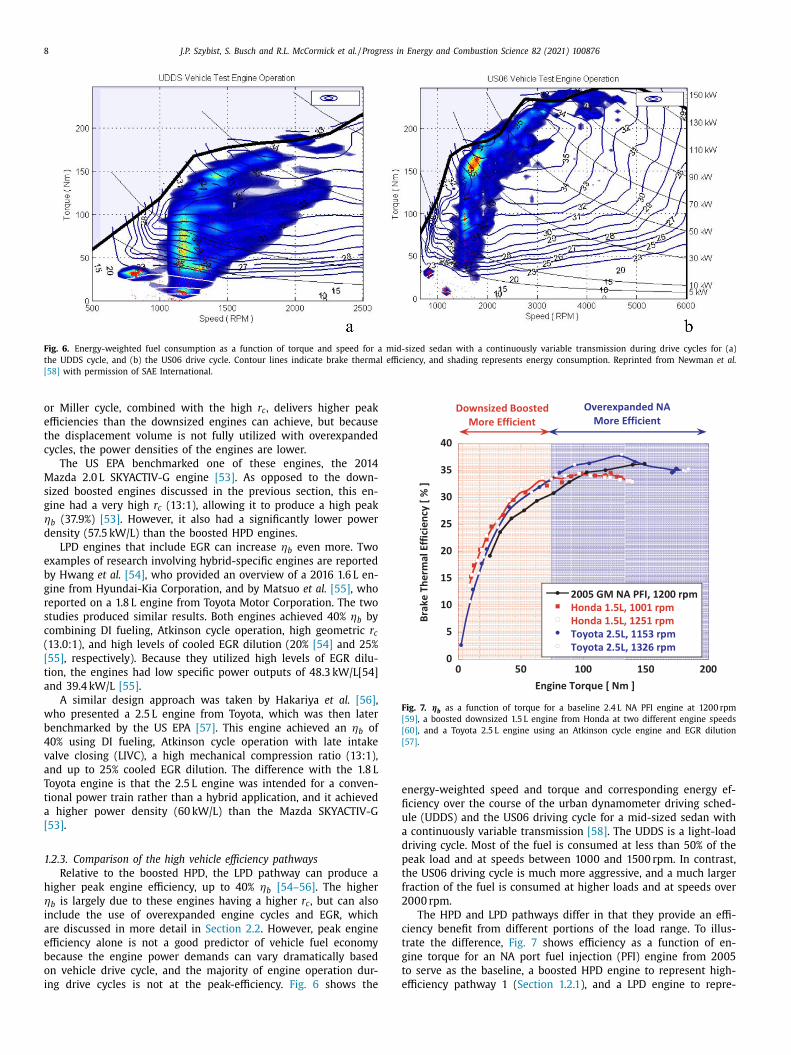
Fig. 6. Energy-weighted fuel consumption as a function of torque and speed for a mid-sized sedan with a continuously variable transmission during drive cycles for (a)
the UDDS cycle, and (b) the US06 drive cycle. Contour lines indicate brake thermal efficiency, and shading represents energy consumption. Reprinted from Newman et al.
[58] with permission of SAE International.
Fig. 7. ηb as a function of torque for a baseline 2.4 L NA PFI engine at 1200 rpm
[59] , a boosted downsized 1.5 L engine from Honda at two different engine speeds
[60] , and a Toyota 2.5 L engine using an Atkinson cycle engine and EGR dilution
[57] .
e
fi
u
a
d
p
t
f
2
c
t
g
t
e
or Miller cycle, combined with the high r c , delivers higher peak
efficiencies than the downsized engines can achieve, but because
the displacement volume is not fully utilized with overexpanded
cycles, the power densities of the engines are lower.
The US EPA benchmarked one of these engines, the 2014
Mazda 2.0 L SKYACTIV-G engine [53] . As opposed to the down-
sized boosted engines discussed in the previous section, this en-
gine had a very high r c (13:1), allowing it to produce a high peak
ηb (37.9%) [53] . However, it also had a significantly lower power
density (57.5 kW/L) than the boosted HPD engines.
LPD engines that include EGR can increase ηb even more. Two
examples of research involving hybrid-specific engines are reported
by Hwang et al. [54] , who provided an overview of a 2016 1.6 L en-
gine from Hyundai-Kia Corporation, and by Matsuo et al. [55] , who
reported on a 1.8 L engine from Toyota Motor Corporation. The two
studies produced similar results. Both engines achieved 40% ηb by
combining DI fueling, Atkinson cycle operation, high geometric r c (13.0:1), and high levels of cooled EGR dilution (20% [54] and 25%
[55] , respectively). Because they utilized high levels of EGR dilu-
tion, the engines had low specific power outputs of 48.3 kW/L[54]
and 39.4 kW/L [55] .
A similar design approach was taken by Hakariya et al. [56] ,
who presented a 2.5 L engine from Toyota, which was then later
benchmarked by the US EPA [57] . This engine achieved an ηb of
40% using DI fueling, Atkinson cycle operation with late intake
valve closing (LIVC), a high mechanical compression ratio (13:1),
and up to 25% cooled EGR dilution. The difference with the 1.8 L
Toyota engine is that the 2.5 L engine was intended for a conven-
tional power train rather than a hybrid application, and it achieved
a higher power density (60 kW/L) than the Mazda SKYACTIV-G
[53] .
1.2.3. Comparison of the high vehicle efficiency pathways
Relative to the boosted HPD, the LPD pathway can produce a
higher peak engine efficiency, up to 40% ηb [54–56] . The higher
ηb is largely due to these engines having a higher r c , but can also
include the use of overexpanded engine cycles and EGR, which
are discussed in more detail in Section 2.2 . However, peak engine
efficiency alone is not a good predictor of vehicle fuel economy
because the engine power demands can vary dramatically based
on vehicle drive cycle, and the majority of engine operation dur-
ing drive cycles is not at the peak-efficiency. Fig. 6 shows the
nergy-weighted speed and torque and corresponding energy ef-
ciency over the course of the urban dynamometer driving sched-
le (UDDS) and the US06 driving cycle for a mid-sized sedan with
continuously variable transmission [58] . The UDDS is a light-load
riving cycle. Most of the fuel is consumed at less than 50% of the
eak load and at speeds between 10 0 0 and 150 0 rpm. In contrast,
he US06 driving cycle is much more aggressive, and a much larger
raction of the fuel is consumed at higher loads and at speeds over
0 0 0 rpm.
The HPD and LPD pathways differ in that they provide an effi-
iency benefit from different portions of the load range. To illus-
rate the difference, Fig. 7 shows efficiency as a function of en-
ine torque for an NA port fuel injection (PFI) engine from 2005
o serve as the baseline, a boosted HPD engine to represent high-
fficiency pathway 1 ( Section 1.2.1 ), and a LPD engine to repre-
J.P. Szybist, S. Busch and R.L. McCormick et al. / Progress in Energy and Combustion Science 82 (2021) 100876 9
s
l
m
w
d
v
H
w
w
a
a
L
i
[
f
a
w
p
A
e
g
w
s
g
v
2
e
s
i
S
e
g
v
s
t
t
h
2
p
η
n
η
w
p
u
i
p
b
l
η
w
t
s
a
L
p
η
w
a
v
P
u
m
p
p
b
h
σ
w
e
q
c
c
η
w
r
b
σ
w
i
p
t
b
2
c
t
t
i
m
w
m
c
ent high-efficiency engine pathway 2 ( Section 1.2.2 ). The base-
ine engine data are from a GM 2.4 L 2005 NA PFI engine with a
aximum power of 132 kW presented by Dugdale et al. [59] , from
hich a plot of brake specific fuel consumption at 1200 rpm was
igitized and then converted to ηb assuming a fuel lower heating
alue (LHV) of 43.5 kJ/g. The downsized boosted data are from a
onda 1.5 L engine with a maximum power output of 130 kW that
as benchmarked by Stuhldreher [60] . The ηb data for this engine
ere not available at 1200 rpm. Thus, the ηb s at both 1001 rpm
nd 1251 rpm are plotted to illustrate that ηb changes very little
s a function of speed within that speed range. The overexpanded
PD Atkinson cycle engine of a Toyota 2.5 L engine with a max-
mum power output of 150 kW was presented by Hakariya et al.
56] and was later benchmarked by Kargul et al. [57] . The ηb data
rom Kargul et al. [57] were available at 1153 and 1326 rpm.
Fig. 7 shows that, relative to the 2005 GM NA PFI engine, there
re efficiency advantages for both the high-power-density path-
ay using a downsized boosted engine and the low-power-density
athway using an overexpanded Atkinson cycle and EGR dilution.
t the lightest engine loads, the HPD pathway provides more of an
fficiency benefit than the overexpanded cycle, but at higher en-
ine loads, the LPD pathway provides more of a benefit. Thus, the
ay that the engines are used in a vehicle, in terms of transmis-
ion pairing and vehicle duty cycle, determines which of the en-
ines can provide the most efficient vehicle. As a result, both are
iable pathways moving forward.
. Factors that increase efficiency in SI engines
Prior to understanding how fuels can improve efficiency in SI
ngines, it is important to understand the thermodynamic ba-
is for efficiency, as well as the engine technologies that are be-
ng deployed by engine manufacturers to improve efficiency. Thus,
ection 2.1 provides a thermodynamic framework by which to
valuate the ways that higher efficiency can be attained in an en-
ine and Section 2.2 provides a discussion of the effect that indi-
idual technologies can have on efficiency from a thermodynamic
tandpoint. Section 2.3 then introduces the role of fuel proper-
ies on increasing engine efficiency in the context of the engine
hermodynamics and other engine technologies being deployed for
igh efficiency.
.1. Thermodynamic expressions for efficiency in an SI engine
Brake thermal efficiency may be expressed as the following
roduct of component efficiencies:
b = ηmech ηcomb ηGE σHT σideal ηideal (2)
These component efficiencies are defined below.
ηmech is the mechanical efficiency, the ratio of brake work to
et indicated work:
mech =
BMEP
IME P n (3)
here BMEP is the brake mean effective pressure (the shaft work
erformed in one cycle divided by the engine’s displacement vol-
me) and IMEP n is the net indicated mean effective pressure (the
ndicated work performed in one cycle divided by the engine’s dis-
lacement volume). The main difference between indicated and
rake work can be attributed to engine friction.
ηcomb is the combustion efficiency (the ratio of total heat re-
eased by combustion to the amount of available fuel energy):
comb =
Q HR
Q f uel, total
(4)
here Q HR is the total amount of energy released through combus-
ion of the fuel and Q fuel , total is the amount of useful fuel energy
upplied or the theoretical maximum amount of fuel energy avail-
ble to perform work (typically assumed to be equal to the fuel’s
HV).
ηGE is the gas exchange efficiency (representing the work
enalty required to move air into the engine):
GE = 1 +
P MEP
IME P g (5)
here PMEP is the pumping mean effective pressure (the net
mount of work performed during the gas exchange process di-
ided by the engine’s displacement volume; for boosted operation,
MEP can be positive, so it is possible for ηGE to be larger than
nity). For reference, Section 2.2.3 includes a discussion of mini-
izing PMEP , including a visualization of the pumping work on a
ressure-volume diagram in Fig. 10 .
IMEP g is the gross mean effective pressure (the amount of work
erformed during the compression and expansion strokes divided
y the engine’s displacement volume).
σ HT is the proportion of total heat release available after wall
eat losses have removed energy from the system:
HT = 1 − Q HT
Q HR
(6)
here Q HT is the total energy lost via wall heat transfer during one
ngine cycle.
ηideal is the efficiency of the ideal working cycle, which is fre-
uently represented as the ideal Otto cycle ( ηOtto ), Eq. 7 . As is dis-
ussed in Section 2.2.3 , however, ηideal can be represented by other
ycles as well.
Otto = 1 − r c 1 −γ (7)
here r c is the geometric compression ratio of the engine, γ is the
atio of specific heats for the working fluid.
σ ideal is degree to which the actual heat release profile resem-
les the ideal profile.
In this case, σ ideal is the degree of constant volume combustion:
ideal =
1
ηOtto Q HR
EOC
∫ SOC
(
1 −(
V d + V c
V ( θ )
)1 −γ)
d Q HR
dθdθ (8)
here
SOC is the start of combustion,
EOC is the end of combustion,
V d is the displacement volume of one cylinder,
V c is the clearance volume of one cylinder,
V ( θ ) is the crank angle dependent volume of one cylinder,
θ is the crank angle.
The impact of changes in friction, combustion efficiency, pump-
ng losses, heat transfer, and combustion speed/phasing may be ex-
ressed in terms of their contributions to relative changes in brake
hermal efficiency. To this end, the total differential of ηb is divided
y ηb :
d ηb
ηb
=
d ηmech
ηmech
+
d ηcomb
ηcomb
+
d ηGE
ηGE
+
d σHT
σHT
+
d ηideal
ηideal
+
d σideal
σideal
(9)
.2. High-Efficiency Engine Technologies
For engine technologies to increase ηb and ultimately to de-
rease vehicle fuel consumption, they must affect one or more of
he terms on the right-hand side of equation 9 . The individual
echnologies that enable these efficiency increases are discussed
n Sections 2.2.1 through 2.2.7. Many of the technologies are ulti-
ately used to increase r c within the acceptable knock limitations,
hich maximizes ηideal , as described by Eq. 7 , or they are used to
inimize pumping, maximizing ηGE . Thus, these two goals are dis-
ussed before the individual technologies.
10 J.P. Szybist, S. Busch and R.L. McCormick et al. / Progress in Energy and Combustion Science 82 (2021) 100876
Fig. 8. Engine operating conditions predicted by vehicle system modeling for a mid-size sedan on the UDDS and city portion of the US06 driving cycles. Reprinted from
Sluder et al. [61] with permission of CRC.
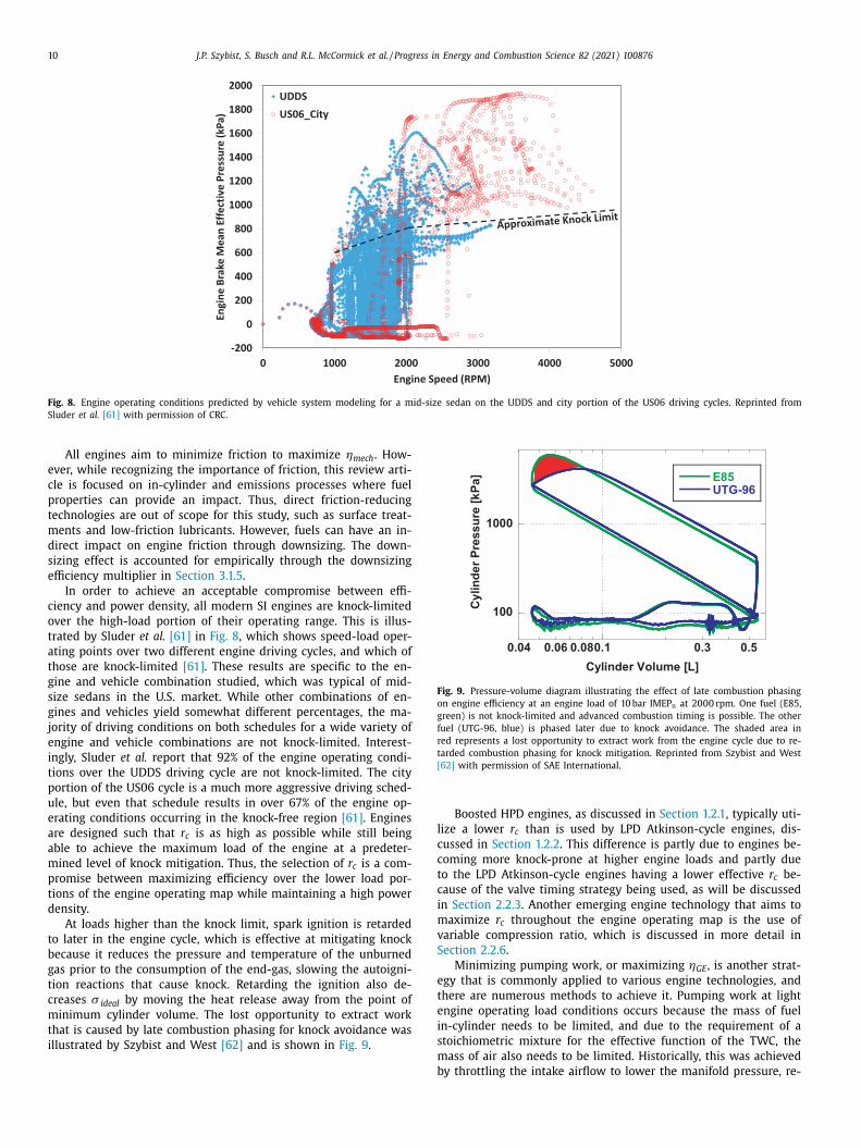
Fig. 9. Pressure-volume diagram illustrating the effect of late combustion phasing
on engine efficiency at an engine load of 10 bar IMEP n at 20 0 0 rpm. One fuel (E85,
green) is not knock-limited and advanced combustion timing is possible. The other
fuel (UTG-96, blue) is phased later due to knock avoidance. The shaded area in
red represents a lost opportunity to extract work from the engine cycle due to re-
tarded combustion phasing for knock mitigation. Reprinted from Szybist and West
[62] with permission of SAE International.
l
c
c
t
c
i
m
v
S
e
t
e
i
s
All engines aim to minimize friction to maximize ηmech . How-
ever, while recognizing the importance of friction, this review arti-
cle is focused on in-cylinder and emissions processes where fuel
properties can provide an impact. Thus, direct friction-reducing
technologies are out of scope for this study, such as surface treat-
ments and low-friction lubricants. However, fuels can have an in-
direct impact on engine friction through downsizing. The down-
sizing effect is accounted for empirically through the downsizing
efficiency multiplier in Section 3.1.5 .
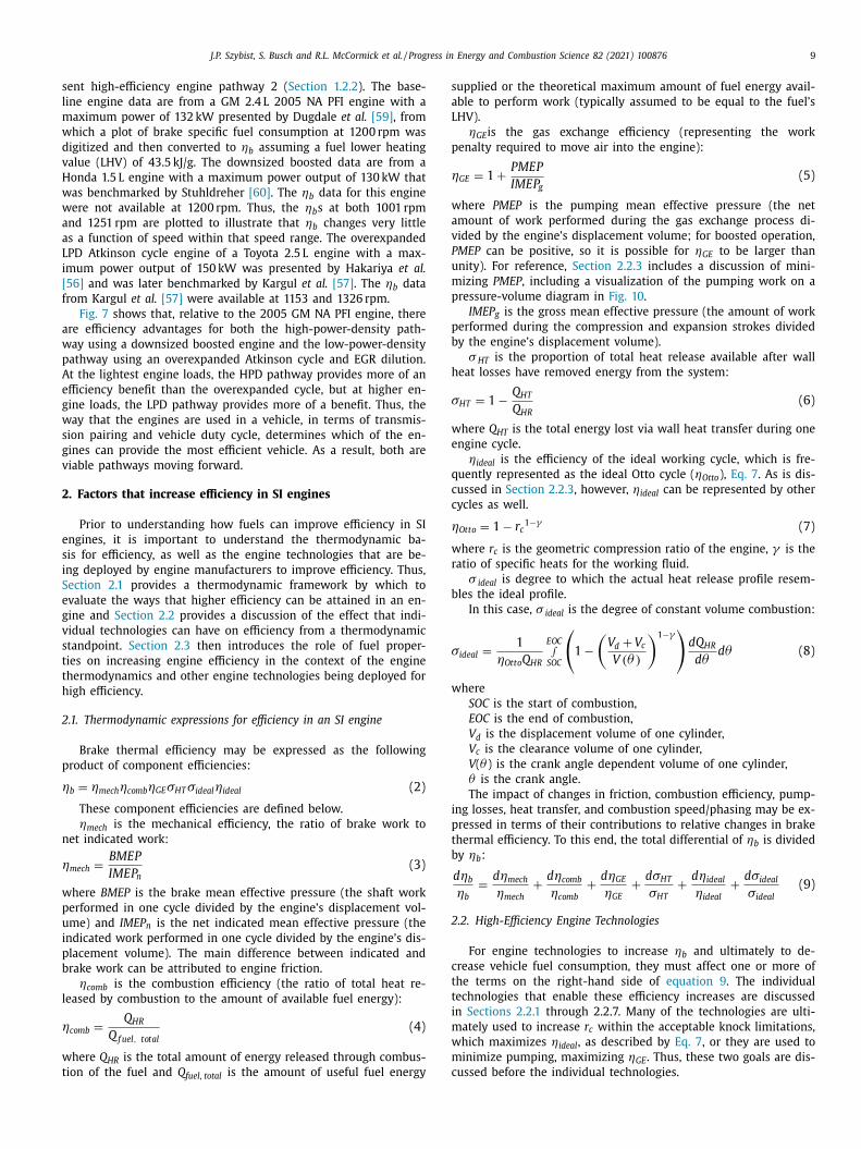
In order to achieve an acceptable compromise between effi-
ciency and power density, all modern SI engines are knock-limited
over the high-load portion of their operating range. This is illus-
trated by Sluder et al. [61] in Fig. 8 , which shows speed-load oper-
ating points over two different engine driving cycles, and which of
those are knock-limited [61] . These results are specific to the en-
gine and vehicle combination studied, which was typical of mid-
size sedans in the U.S. market. While other combinations of en-
gines and vehicles yield somewhat different percentages, the ma-
jority of driving conditions on both schedules for a wide variety of
engine and vehicle combinations are not knock-limited. Interest-
ingly, Sluder et al. report that 92% of the engine operating condi-
tions over the UDDS driving cycle are not knock-limited. The city
portion of the US06 cycle is a much more aggressive driving sched-
ule, but even that schedule results in over 67% of the engine op-
erating conditions occurring in the knock-free region [61] . Engines
are designed such that r c is as high as possible while still being
able to achieve the maximum load of the engine at a predeter-
mined level of knock mitigation. Thus, the selection of r c is a com-
promise between maximizing efficiency over the lower load por-
tions of the engine operating map while maintaining a high power
density.
At loads higher than the knock limit, spark ignition is retarded
to later in the engine cycle, which is effective at mitigating knock
because it reduces the pressure and temperature of the unburned
gas prior to the consumption of the end-gas, slowing the autoigni-
tion reactions that cause knock. Retarding the ignition also de-
creases σ ideal by moving the heat release away from the point of
minimum cylinder volume. The lost opportunity to extract work
that is caused by late combustion phasing for knock avoidance was
illustrated by Szybist and West [62] and is shown in Fig. 9 .
mb
Boosted HPD engines, as discussed in Section 1.2.1 , typically uti-
ize a lower r c than is used by LPD Atkinson-cycle engines, dis-
ussed in Section 1.2.2 . This difference is partly due to engines be-
oming more knock-prone at higher engine loads and partly due
o the LPD Atkinson-cycle engines having a lower effective r c be-
ause of the valve timing strategy being used, as will be discussed
n Section 2.2.3 . Another emerging engine technology that aims to
aximize r c throughout the engine operating map is the use of
ariable compression ratio, which is discussed in more detail in
ection 2.2.6 .
Minimizing pumping work, or maximizing ηGE , is another strat-
gy that is commonly applied to various engine technologies, and
here are numerous methods to achieve it. Pumping work at light
ngine operating load conditions occurs because the mass of fuel
n-cylinder needs to be limited, and due to the requirement of a
toichiometric mixture for the effective function of the TWC, the
ass of air also needs to be limited. Historically, this was achieved
y throttling the intake airflow to lower the manifold pressure, re-
J.P. Szybist, S. Busch and R.L. McCormick et al. / Progress in Energy and Combustion Science 82 (2021) 100876 11
s
H
c
p
t
o
t
e
l
o
i
(
w
l
t
g
t
c
r
l
c
b
e
2
g
b
b
C
c
l
i
e
t
s
a
f
I
w
b
H
m
s
r
c
t
i
m
t
2
t
d
f
g
t
a
t
o
c
w
s
T
a
b
w
e
c
l
c
t
t
l
w
c
e
m
t
m
i
e
t
g
t
k
c
t
t
2
f
a
t
l
f
o
s
f
p
i
c
u
e
t
s
b
p
f
t
t
m
v
i
E
p
a
h
e
S
t
u
N
ulting in the primary source of pumping losses. Using boosted
PD engines is itself a strategy to minimize pumping work be-
ause, relative to a naturally aspirated engine, the intake manifold
ressure only needs to be maintained below ambient pressure for
he lightest loads and is above ambient pressure for much of the
perable load range. Such a situation reduces the use of intake
hrottling. This de-throttling effect is what makes HPD boosted
ngines more efficient than LPD engines at the lightest operating
oads, as shown in Fig. 7 .
LPD engines, and to a lesser extent HPD engines, utilize a host
f additional technologies to maximize ηGE by reducing pump-
ng work. The technologies include overexpanded engine cycles
Section 2.2.3 ) and cylinder deactivation ( Section 2.2.7 ), both of
hich reduce the effective displacement of the engine under part-
oad conditions. They also include utilization of cooled EGR dilu-
ion ( Section 2.2.4 ), which maximizes the in-cylinder mass for a
iven load condition without increasing the air or fuel mass. Some
echnologies provide additive or even synergistic benefits in fuel
onsumption; others may compete with one another because they
epresent different approaches to addressing the same efficiency
osses. For example, combining overexpanded engine cycles and
ylinder deactivation technologies has diminishing returns because
oth attempt to reduce pumping work by decreasing the effective
ngine displacement.
.2.1. Boosted engine operation
As Heywood [63] explains, the maximum load that a given en-
ine can deliver is limited by the amount of fuel that can be
urned inside the engine cylinder, and the amount of fuel that can
e burned is limited by the amount of air that can be inducted.
ompressing the air to a higher density increases the air mass that
an be inducted, which enables the engine to operate at higher
oad operation relative to a naturally aspirated engine. Thus, boost-
ng the air system is a key enabling technology for HPD downsized
ngines.
Boosting the intake manifold pressure can be done through ei-
her turbocharging, which uses exhaust gases to drive a compres-
or, or through supercharging. While superchargers are effective
t increasing engine power, they typically use mechanical power
rom the engine to drive a compressor, leading to efficiency loss.
t is worth pointing out that electric superchargers can be paired
ith electricity recovered from regenerative braking in a mild hy-
rid configuration, resulting in some high efficiency synergies [64] .
owever, such use of electric superchargers is still under develop-
ent and further consideration of this configuration is outside the
cope of this review. Turbochargers, on the other hand, are energy
ecovery devices that use waste heat in the exhaust to perform
ompression work on the intake air, making them a more efficient
echnology than superchargers. With the trend of engine downsiz-
ng, the use of turbochargers in gasoline engines has become com-
on, and the sale of boosted engines has risen from 1.7% in 2005
o 30.8% in 2018 [38] .
.2.2. Direct injection fueling
DI fueling uses either central-mount or side-mount fuel injec-
ors to deliver fuel directly into the combustion chamber and is
ifferentiated from PFI or carbureted fueling, which introduce the
uel upstream of the combustion chamber. DI fueling is advanta-
eous for knock mitigation relative to PFI fueling because more of
he heat of vaporization (HoV) of the fuel comes from the charge
ir itself rather than the metal surfaces of the engine [65] . Addi-
ionally, a combination of DI fueling with variable valve phasing,
ver-scavenging, or some fresh air blowing directly through the
ylinder during gas exchange can be used to remove all burnt gases
ithout introducing un-burnt air-fuel mixture into the exhaust gas
tream because of the flexibility in timing the injection [66–68] .
ogether, these technologies act to reduce the in-cylinder temper-
ture with DI fueling, thereby mitigating knock and allowing r c to
e increased. DI fueling also increases the in-cylinder turbulence,
hich serves to shorten the combustion duration [69] , which ben-
fits σ ideal . Using modern injection hardware and advanced engine
alibration, DI fueling can also reduce fuel-wall interactions by tai-
oring spray patterns and injection durations to the combustion
hamber and the intake-generated flow [70] . This makes more of
he fuel available to the combustion event and increases combus-
ion efficiency ( ηcomb in Eq. 9 ).
When the first generation of modern gasoline DI engines was
aunched, in the late 1990s, the emphasis of improved efficiency
as squarely placed on the ability to run fuel-lean in stratified
harge mode [ 44 , 67 , 68 ]. Due to the need for complicated NOx
mission controls systems and the restricted fuel efficiency gains
ade as a result of the limited operating range in that mode, au-
omotive manufacturers soon switched to a homogeneous stoichio-
etric charge mode while utilizing the benefits of DI, thus achiev-
ng an increase in power density [ 45 , 66 , 71 , 72 ], thereby enabling
ngine downsizing.
Thus, DI fueling combined with turbocharging are the essen-
ial technologies for the HPD engine pathway with downsized en-
ines discussed in Section 1.2.1 . Additionally, DI fueling is a key
echnology enabler to LPD engines. Because LPD engines are also
nock-limited, they can take advantage of the HoV of the fuel for
harge-cooling, which helps to mitigate knock. Further, the addi-
ional turbulence from the DI fuel injection is useful for extending
he EGR dilution tolerance, which is discussed in Section 2.2.4 .
.2.3. Overexpanded engine cycles
The Otto cycle gives up potential for additional work extraction
rom exhaust gasses which are at higher than ambient pressure
t the end of the expansion event. Over-expanded cycles, namely
he Atkinson and Miller cycles, utilize expansion ratios which are
arger than the r c to allow further expansion of the exhaust gases
or additional work extraction [73] . Thus, the ideal efficiency for an
verexpanded cycle, ηOE , is higher than ηOtto for a given compres-
ion ratio.
Over-expanded engine cycles can also have a second major ef-
ect of increasing the gas exchange efficiency ( ηGE ) by decreasing
umping work when the over-expansion ratio is continuously var-
ed to act as a form of variable displacement. Most overexpanded
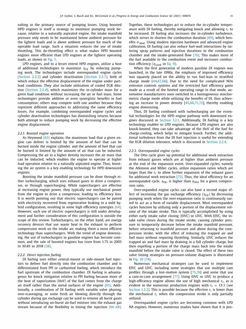
ycles function by utilizing only a portion of the displacement vol-
me of the intake stroke. This is typically accomplished by using
ither early intake valve closing (EIVC) or LIVC. With EIVC, the in-
ake valve closes during the intake stroke, causing cylinder pres-
ure to temporarily decrease below the intake manifold pressure,
efore returning to manifold pressure and above during the com-
ression stroke, with the effect of reducing the trapped air and
uel mass without requiring throttling. Similarly, LIVC reduces the
rapped air and fuel mass by drawing in a full cylinder charge, but
hen expelling a portion of the charge mass back into the intake
anifold before the intake valve is closed. The effect of these two
alve timing strategies on pressure-volume diagrams is illustrated
n Fig. 10 [74] .
Numerous mechanical strategies can be used to implement
IVC and LIVC, including some strategies that use multiple cam
rofiles through a lost-motion system [ 75 , 76 ] and some that use
cam-in-cam arrangement [77] . Using EIVC or LIVC to produce a
igh-efficiency engine allows the use of high mechanical r c , as is
vident in the numerous production engines with r c = 13:1 (see
ection 1.2.2 ). This is possible because the effective r c is lower than
he mechanical r c when the compression stroke is only partially
tilized.
Overexpanded engine cycles are becoming common with LPD
A engines. However, numerous studies have shown that it is pos-
12 J.P. Szybist, S. Busch and R.L. McCormick et al. / Progress in Energy and Combustion Science 82 (2021) 100876
Fig. 10. Pressure-volume diagrams of engine operation at 1500 rpm, 8 bar BMEP with conventional throttled operation, an EIVC valve strategy, and an LIVC valve strategy.
Reprinted from Szybist et al. [74] with permission of American Chemical Society.
i
[
p
m
s
i
e
w
a
v
i
2
o
m
a
n
m
a
c
q
a
t
a
sible to combine the downsized boosted pathway with overex-
panded technologies for further efficiency gains (for example, see
Osborne et al. [78] ).
2.2.4. Exhaust gas recirculation
Cooled EGR is an engine technology that is being deployed as
a method to increase engine efficiency. When cooled external EGR
is used, a fraction of the exhaust is cooled and mixed with the
incoming fresh air. This technology benefits the ηGE , σ HT , and ηideal
terms, but it can adversely impact the ηcomb and σ ideal terms.
The overall efficiency advantages for high-EGR conditions are
summarized in a thermodynamic modeling study by Caton [79] .
The additional mass added by the EGR causes the manifold
pressure to increase without increasing the intake oxygen flow,
thereby maintaining a stoichiometric charge while decreasing en-
gine pumping and increasing engine efficiency at part-load condi-
tions, benefiting the ηGE term in Eq. 9 . Additionally, the adiabatic
flame temperature decreases with EGR dilution, typically causing
the heat transfer to decrease, benefiting the σ HT term in Eq. 9 .
Also, due to a combined thermal and composition effect, the ra-
tio of specific heats ( γ ) of the working fluid increases with EGR,
benefiting the ηideal term in Eq. 9 , as described by Eq. 7 .
In addition to the γ benefit for ηideal , Alger et al. [80] showed
that EGR also reduces the knock propensity, through the reduced
in-cylinder temperature, which could allow r c to be increased. Al-
ger et al. [80] also concluded that every one percent increase of
EGR was equivalent to a 0.5 octane number increase. Splitter et al.
[ 81 , 82 ] confirmed the reduced knock propensity effect using 15%
EGR, which allowed the maximum load limit to be increased by
more than 10% in a single-cylinder engine experiment.
EGR can also alter the combustion process in ways that have
adverse impacts on the terms in Eq. 9 . Specifically, EGR decreases
the laminar flame speed ( S L ) of the fuel, resulting in a longer com-
bustion duration [ 83 , 84 ], adversely impacting the σ ideal term in
Eq. 9 . In addition to a decrease in σ ideal , the use of EGR dilu-
tion is limited because of increased cycle to cycle combustion vari-
ability, as measured by the coefficient of variation (COV) of IMEP g [ 73 , 85 , 86 ]. Ozdor et al. showed that the increase in COV of IMEP gwas directly attributable to the decrease in S L and, in particular,
the increased duration of the initial flame kernel development [86] .
Additionally, Szybist and Splitter [84] showed that EGR decreases
the combustion efficiency, adversely affecting the ηcomb in Eq. 9 .
2.2.5. Advanced Ignition Systems
Conventional electrical ignition systems are comprised of ei-
ther inductive coils or capacitor discharge units, and the underly-
ng physics of these spark ignition processes are well-understood
63 , 87 ]. The total spark energy delivered to the gas in the spark
lug is generally around 30 mJ [88] , which is one to two orders of
agnitude greater than the minimum ignition energy required for
toichiometric combustion with low dilution. Using an advanced
gnition system can impact the terms in Eq. 9 to provide improved
fficiency: decreased combustion duration for a higher σ ideal as
ell as higher ηcomb . Further, advanced ignition systems can en-
ble higher levels of EGR dilution, which is thermodynamically ad-
antageous as discussed in Section 2.2.4 . Several types of advanced
gnition systems are listed below:
• Multiple spark plugs [ 88 , 89 ]
• Discharging multiple ignition events in a single cycle [ 90 , 91 ]
• An extended spark discharge ignition event [92]
• Breakdown or blast wave ignition units [93–96]
• Laser ignition systems [97]
• Corona discharge ignition systems [96–99]
• Plasma jet and rail plug ignition systems [100–106]
• Low temperature plasma ignition systems [107–110]
• Pre-chamber ignition systems [111–118]
.2.6. Variable compression ratio
Variable compression ratio (VCR) technologies enable the use
f increased mechanical r c in the region of the engine operating
ap that is not knock-limited. This is done by varying the clear-
nce volume at top dead center through four categories of mecha-
isms that do not involve varying the stroke of the engine:
• vary the position of the crankshaft relative to the engine head
(e.g., install the crankshaft in an eccentric cradle) [119] ;
• vary the effective linkage distance between the crankshaft and
piston, which can include using a variable-length connecting
rod [120–122] or an intermediate linkage between the crank
throw and connecting rod [123–125] ;
• move the head relative to the crankshaft [ 126 , 127 ]; or
• use movable elements in the head as well as within the piston
to contract or enlarge the clearance volume [128–133] .
VCR strategies can be implemented in a continuously variable
anner within a range of authority or can instead be designed in
two-step manner, where the system can vary between two dis-
rete values of r c . The benefits of both types of systems have been
uantified. Shelby et al. estimated the benefits of both continuous
nd two-step VCR for an r c range of 10:1 to 13:1 and found that a
wo-step implementation reduced fuel consumption 2.5% to 3.6%
nd that a continuously variable strategy was similar, offering a
J.P. Szybist, S. Busch and R.L. McCormick et al. / Progress in Energy and Combustion Science 82 (2021) 100876 13
2
a
a
2
b
m
s
s
n
c
s
s
h
c
b
h
q
a
t
s
[
b
d
t
t
c
o
a
t
1
c
t
2
e
m
t
i
a
f
k
t
t
o
t
e
r
e
t
f
M
w
m
t
t
fi
t
c
t
a
s
i
a
h
l
s
3
f
p
r
g
a
n
t
m
f
s
q
a
b
s
i
c
a
t
p
c
a
p
fi
t
S
p
o
o
t
l
m
f
c
i
S
c
s
e
s
o
c
.7% to 3.7% improvement [134] . Wolfgang et al. [122] estimated
larger fuel consumption decrease of 8.5% by combining VCR with
n overexpanded engine cycle.
.2.7. Cylinder deactivation
One early application of cylinder deactivation occurred in 1916,
ut it was not until the 1980s that several more attempts were
ade. In recent years, cylinder deactivation has become a main-
tream technology that is being used to reduce vehicle fuel con-
umption, and in 2018, 12% of vehicle sales incorporated this tech-
ology [38] .
Cylinder deactivation is a technology that can be employed to
hange the effective displacement of the engine. In addition to
topping the fuel injection, both the intake and exhaust valves
top actuating so that there is no excess air present in the ex-
aust, allowing the TWC to maintain high NO x conversion effi-
iency. Cylinder deactivation increases engine efficiency primarily
y decreasing pumping work, or increasing ηGE . For example, if
alf the cylinders are deactivated, the remaining cylinders are re-
uired to double their net power to maintain demanded power,
llowing those cylinders to operate more efficiently at conditions
hat reduce throttling losses [135] .
Cylinder deactivation has historically been limited by tran-
ient control and noise, vibration, and harshness (NVH) constraints
135] . In recent years, however, many of those constraints have
een overcome. NVH constraints have been overcome with cylin-
er deactivation largely due to improved control technologies, and
he next generation of advanced control for cylinder deactiva-
ion, Dynamic Skip Fire technology [ 136 , 137 ], has recently been
ommercialized and promises to extend the market penetration
f cylinder deactivation even further. Struhldreher [138] baselined
4.3 L six-cylinder engine with and without cylinder deactiva-
ion and found that, at conditions between 1 and 4 bar BMEP at
250 rpm, deactivation can increase ηb by more than three per-
entage points, which is more than a 20% relative improvement at
he lightest loads.
.3. Fuel Property Impacts on SI Engine Efficiency
Like the engine technologies discussed in Section 2.2 , fuel prop-
rties that enable increases in ηb do so through changes to one or
ore of the terms on the right-hand side of Eq. 9 . Changes to the
erms may be the direct result of the fuel property, or they may be
ndirect effects resulting from changes in engine design and oper-
tion enabled by the fuel or required to mitigate undesirable ef-
ects of a fuel property. These effects may be analyzed through
nowledge of the impact of each fuel property on each term on
he right-hand side of Eq. 9 .
To evaluate the merits of new fuel formulations in terms of
heir expected impact on engine efficiency, the combined impact
f the fuel’s properties on brake thermal efficiency must be quan-
ified. It is useful to compare the merits of a new fuel with a refer-
nce fuel, such that the relative improvement in thermal efficiency
esulting from the use of the new fuel may be estimated. To this
nd, the merit function is defined as the relative change in brake
hermal efficiency computed as a linear combination of the new
uel’s properties:
erit =
�ηb
ηb
=
∑
i
1
ηb
∂ ηb
∂ p i
(p i − p i,re f
)(10)
here p i stands for the fuel properties that influence brake ther-
al efficiency and p i,ref stands for the corresponding properties of
he reference fuel.
This Eq. is the basis for the Co-Optima SI efficiency merit func-
ion [139] , the definition of which depends on
• the identification of the fuel properties p i ,
• an established set of reference properties p i,ref , and
• knowledge of the sensitivity of brake thermal efficiency to each
property ( ∂ ηb ∂ p i
) .
Identifying the fuel properties that can enable increases in ef-
ciency, and subsequently quantifying the potential efficiency con-
ribution of each individual fuel property in an optimized engine
onfiguration, is not straight-forward. Performing these tasks was
he major focus of the Co-Optima initiative’s effort s on SI engines
s well as the focus of the remainder of this article. Section 3 de-
cribes the fuel properties that have an efficiency impact through
n-cylinder processes affected by knock-resistance metrics, HoV, S L ,
nd PMI. Section 4 describes how fuel properties can impact ve-
icle efficiency due to the emissions controls required. In particu-
ar, Section 4 focuses on the catalyst light-off temperature and the
ooting tendency of the fuel.
. How fuels affect in-cylinder efficiency
A guiding principle of the Co-Optima initiative is the central
uel properties hypothesis (CFPH), which states that fuel properties
rovide an indication of the performance and emissions of the fuel,
egardless of the fuel’s chemical composition. Historically, some
asoline standards have been performance-based, which implicitly
lign with the CFPH. For instance, the composition of the fuel is
ot considered for the distillation and volatility specifications in
he ASTM standard for gasoline [140] or in the octane number
easurements. Rather, they are performance-based indicators of
uel quality. However, other fuel standards are composition-based,
uch as the sulfur content of gasoline [140] and the California re-
uirement to limit the aromatic content of the gasoline to 35 vol %
nd the olefin content to 10 vol % [141] .
Within the Co-Optima initiative, fuel components derived from
iomass are being considered for blending with gasoline feed-
tocks, and the evaluation criteria extend beyond fuel performance
n an engine. The Co-Optima initiative is also evaluating the life-
ycle environmental and economic impacts of bio-derived fuels
nd the technology readiness and scalability of the fuel production
echnology [142] . The combined analysis of engine performance as-
ects with environmental, economic, and scalability considerations
an be found in a report by Farrell et al. [143] . The present study
ims to provide an in-depth review of the engine performance as-
ects of the Co-Optima initiative.
A number of the fuel components and blending streams identi-
ed within the Co-Optima initiative have oxygen-containing func-
ional groups that are not conventionally associated with fuels for
I engines. Historically, fuel for SI engines has been limited to
etroleum-derived hydrocarbon streams from refineries (alkanes,
lefins, aromatics, and naphthenes), along with a small number
f oxygenated compounds, namely ethanol, methanol, and methyl
ertiary butyl ether. The potential for significant changes in gaso-
ine composition calls into question whether performance-based
etrics that align with the CFPH are accurate indicators of per-
ormance across the full engine operating map with changing fuel
hemistry.
To develop a better understanding of the contributions of
ndividual fuel properties and their adherence to the CFPH,
ection 3 focuses on the role that fuel properties have on in-
ylinder processes that can impact efficiency. Subsection 3.1 con-
iders the various ways to measure and quantify antiknock prop-
rties as well as their ability to accurately predict knock propen-
ity under different operating conditions. Subsection 3.2 focuses
n the impact of the various ways that HoV affects engine effi-
iency, after which the role of S is considered in Subsection 3.3 .
L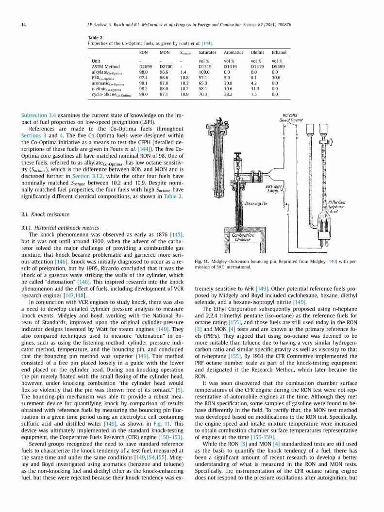
14 J.P. Szybist, S. Busch and R.L. McCormick et al. / Progress in Energy and Combustion Science 82 (2021) 100876
Table 2
Properties of the Co-Optima fuels, as given by Fouts et al. [144] .
RON MON S octane Saturates Aromatics Olefins Ethanol
Unit - - - vol % vol % vol % vol %
ASTM Method D2699 D2700 - D1319 D1319 D1319 D5599
alkylate Co-Optima 98.0 96.6 1.4 100.0 0.0 0.0 0.0
E30 Co-Optima 97.4 86.6 10.8 57.1 5.0 8.1 30.6
aromatic Co-Optima 98.1 87.8 10.3 65.0 30.8 4.2 0.0
olefinic Co-Optima 98.2 88.0 10.2 58.1 10.6 31.3 0.0
cyclo-alkane Co-Optima 98.0 87.1 10.9 70.3 28.2 1.5 0.0
Fig. 11. Midgley–Dickenson bouncing pin. Reprinted from Midgley [149] with per-
mission of SAE International.
t
p
s
a
o
[
e
m
c
o
P
a
R
t
r
t
h
w
t
t
o
a
b
u
S
d
Subsection 3.4 examines the current state of knowledge on the im-
pact of fuel properties on low-speed preignition (LSPI).
References are made to the Co-Optima fuels throughout
Sections 3 and 4 . The five Co-Optima fuels were designed within
the Co-Optima initiative as a means to test the CFPH (detailed de-
scriptions of these fuels are given in Fouts et al. [144] ). The five Co-
Optima core gasolines all have matched nominal RON of 98. One of
these fuels, referred to as alkylate Co-Optima , has low octane sensitiv-
ity ( S octane ), which is the difference between RON and MON and is
discussed further in Section 3.1.2 , while the other four fuels have
nominally matched S octane between 10.2 and 10.9. Despite nomi-
nally matched fuel properties, the four fuels with high S octane have
significantly different chemical compositions, as shown in Table 2 .
3.1. Knock resistance
3.1.1. Historical antiknock metrics
The knock phenomenon was observed as early as 1876 [145] ,
but it was not until around 1900, when the advent of the carbu-
retor solved the major challenge of providing a combustible gas
mixture, that knock became problematic and garnered more seri-
ous attention [146] . Knock was initially diagnosed to occur as a re-
sult of preignition, but by 1905, Ricardo concluded that it was the
shock of a gaseous wave striking the walls of the cylinder, which
he called “detonation” [146] . This inspired research into the knock
phenomenon and the effect of fuels, including development of VCR
research engines [ 147 , 148 ].
In conjunction with VCR engines to study knock, there was also
a need to develop detailed cylinder pressure analysis to measure
knock events. Midgley and Boyd, working with the National Bu-
reau of Standards, improved upon the original cylinder-pressure
indicator designs invented by Watt for steam engines [149] . They
also compared techniques used to measure “detonation” in en-
gines, such as using the listening method, cylinder pressure indi-
cator method, temperature, and the bouncing pin, and concluded
that the bouncing pin method was superior [149] . This method
consisted of a free pin placed loosely in a guide with the lower
end placed on the cylinder head. During non-knocking operation
the pin merely floated with the small flexing of the cylinder head,
however, under knocking combustion “the cylinder head would
flex so violently that the pin was thrown free of its contact . ” [5] .
The bouncing-pin mechanism was able to provide a robust mea-
surement device for quantifying knock by comparison of results
obtained with reference fuels by measuring the bouncing pin fluc-
tuation in a given time period using an electrolytic cell containing
sulfuric acid and distilled water [149] , as shown in Fig. 11 . This
device was ultimately implemented in the standard knock-testing
equipment, the Cooperative Fuels Research (CFR) engine [150–153] .
Several groups recognized the need to have standard reference
fuels to characterize the knock tendency of a test fuel, measured at
the same time and under the same conditions [ 149 , 154 , 155 ]. Midg-
ley and Boyd investigated using aromatics (benzene and toluene)
as the non-knocking fuel and diethyl ether as the knock-enhancing
fuel, but these were rejected because their knock tendency was ex-
remely sensitive to AFR [149] . Other potential reference fuels pro-
osed by Midgely and Boyd included cyclohexane, hexane, diethyl
elenide, and a hexane-isopropyl nitrite [149] .
The Ethyl Corporation subsequently proposed using n-heptane
nd 2,2,4 trimethyl pentane (iso-octane) as the reference fuels for
ctane rating [155] , and those fuels are still used today in the RON
3] and MON [4] tests and are known as the primary reference fu-
ls (PRFs). They argued that using iso-octane was deemed to be
ore suitable than toluene due to having a very similar hydrogen-
arbon ratio and similar specific gravity as well as viscosity to that
f n-heptane [155] . By 1931 the CFR Committee implemented the
RF octane number scale as part of the knock-testing equipment
nd designated it the Research Method, which later became the
ON.
It was soon discovered that the combustion chamber surface
emperatures of the CFR engine during the RON test were not rep-
esentative of automobile engines at the time. Although they met
he RON specification, some samples of gasoline were found to be-
ave differently in the field. To rectify that, the MON test method
as developed based on modifications to the RON test. Specifically,
he engine speed and intake mixture temperature were increased
o obtain combustion chamber surface temperatures representative
f engines at the time [156-159] .
While the RON [3] and MON [4] standardized tests are still used
s the basis to quantify the knock tendency of a fuel, there has
een a significant amount of recent research to develop a better
nderstanding of what is measured in the RON and MON tests.
pecifically, the instrumentation of the CFR octane rating engine
oes not respond to the pressure oscillations after autoignition, but
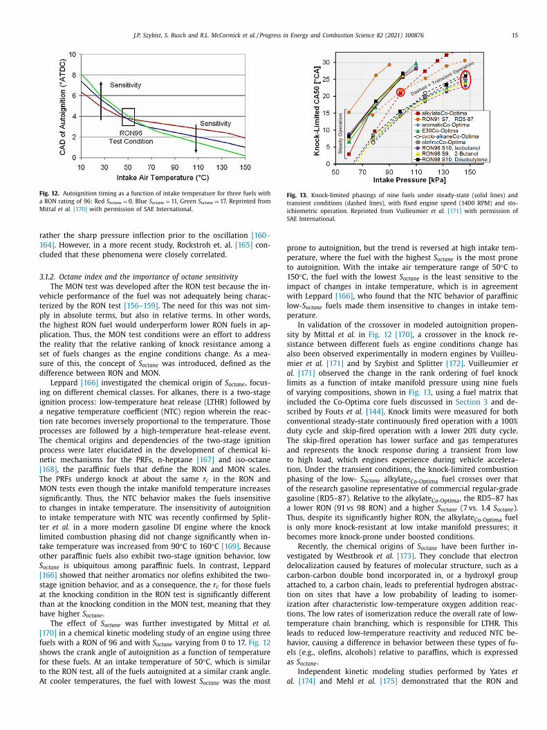
J.P. Szybist, S. Busch and R.L. McCormick et al. / Progress in Energy and Combustion Science 82 (2021) 100876 15
Fig. 12. Autoignition timing as a function of intake temperature for three fuels with
a RON rating of 96: Red S octane = 0, Blue S octane = 11, Green S octane = 17. Reprinted from
Mittal et al. [170] with permission of SAE International.
r
1
c
3
v
t
p
t
p
t
s
s
d
i
i
a
t
p
T
p
n
[
T
M
s
t
t
t
l
t
o
S
[
s
a
t
h
[
f
s
f
t
A
Fig. 13. Knock-limited phasings of nine fuels under steady-state (solid lines) and
transient conditions (dashed lines), with fixed engine speed (1400 RPM) and sto-
ichiometric operation. Reprinted from Vuilleumier et al. [171] with permission of
SAE International.
p
p
t
1
i
w
l
p
s
s
a
m
a
l
o
i
s
c
d
T
a
t
t
p
o
g
a
T
i
b
v
d
c
a
t
i
t
t
l
h
e
a
a
ather the sharp pressure inflection prior to the oscillation [160–
64] . However, in a more recent study, Rockstroh et. al. [165] con-
luded that these phenomena were closely correlated.
.1.2. Octane index and the importance of octane sensitivity
The MON test was developed after the RON test because the in-
ehicle performance of the fuel was not adequately being charac-
erized by the RON test [156–159] . The need for this was not sim-
ly in absolute terms, but also in relative terms. In other words,
he highest RON fuel would underperform lower RON fuels in ap-
lication. Thus, the MON test conditions were an effort to address
he reality that the relative ranking of knock resistance among a
et of fuels changes as the engine conditions change. As a mea-
ure of this, the concept of S octane was introduced, defined as the
ifference between RON and MON.
Leppard [166] investigated the chemical origin of S octane , focus-
ng on different chemical classes. For alkanes, there is a two-stage
gnition process: low-temperature heat release (LTHR) followed by
negative temperature coefficient (NTC) region wherein the reac-
ion rate becomes inversely proportional to the temperature. Those
rocesses are followed by a high-temperature heat-release event.
he chemical origins and dependencies of the two-stage ignition
rocess were later elucidated in the development of chemical ki-
etic mechanisms for the PRFs, n-heptane [167] and iso-octane
168] , the paraffinic fuels that define the RON and MON scales.
he PRFs undergo knock at about the same r c in the RON and
ON tests even though the intake manifold temperature increases
ignificantly. Thus, the NTC behavior makes the fuels insensitive
o changes in intake temperature. The insensitivity of autoignition
o intake temperature with NTC was recently confirmed by Split-
er et al. in a more modern gasoline DI engine where the knock
imited combustion phasing did not change significantly when in-
ake temperature was increased from 90 °C to 160 °C [169] . Because
ther paraffinic fuels also exhibit two-stage ignition behavior, low
octane is ubiquitous among paraffinic fuels. In contrast, Leppard
166] showed that neither aromatics nor olefins exhibited the two-
tage ignition behavior, and as a consequence, the r c for those fuels
t the knocking condition in the RON test is significantly different
han at the knocking condition in the MON test, meaning that they
ave higher S octane .
The effect of S octane was further investigated by Mittal et al.
170] in a chemical kinetic modeling study of an engine using three
uels with a RON of 96 and with S octane varying from 0 to 17. Fig. 12
hows the crank angle of autoignition as a function of temperature
or these fuels. At an intake temperature of 50 °C, which is similar
o the RON test, all of the fuels autoignited at a similar crank angle.
t cooler temperatures, the fuel with lowest S octane was the most
rone to autoignition, but the trend is reversed at high intake tem-
erature, where the fuel with the highest S octane is the most prone
o autoignition. With the intake air temperature range of 50 °C to
50 °C, the fuel with the lowest S octane is the least sensitive to the
mpact of changes in intake temperature, which is in agreement
ith Leppard [166] , who found that the NTC behavior of paraffinic
ow- S octane fuels made them insensitive to changes in intake tem-
erature.
In validation of the crossover in modeled autoignition propen-
ity by Mittal et al. in Fig. 12 [170] , a crossover in the knock re-
istance between different fuels as engine conditions change has
lso been observed experimentally in modern engines by Vuilleu-
ier et al. [171] and by Szybist and Splitter [172] . Vuilleumier et
l. [171] observed the change in the rank ordering of fuel knock
imits as a function of intake manifold pressure using nine fuels
f varying compositions, shown in Fig. 13 , using a fuel matrix that
ncluded the Co-Optima core fuels discussed in Section 3 and de-
cribed by Fouts et al. [144] . Knock limits were measured for both
onventional steady-state continuously fired operation with a 100%
uty cycle and skip-fired operation with a lower 20% duty cycle.
he skip-fired operation has lower surface and gas temperatures
nd represents the knock response during a transient from low
o high load, which engines experience during vehicle accelera-
ion. Under the transient conditions, the knock-limited combustion
hasing of the low- S octane alkylate Co-Optima fuel crosses over that
f the research gasoline representative of commercial regular-grade
asoline (RD5–87). Relative to the alkylate Co-Optima , the RD5–87 has
lower RON (91 vs 98 RON) and a higher S octane (7 vs. 1.4 S octane ).
hus, despite its significantly higher RON, the alkylate Co-Optima fuel
s only more knock-resistant at low intake manifold pressures; it
ecomes more knock-prone under boosted conditions.
Recently, the chemical origins of S octane have been further in-
estigated by Westbrook et al. [173] . They conclude that electron
elocalization caused by features of molecular structure, such as a
arbon-carbon double bond incorporated in, or a hydroxyl group
ttached to, a carbon chain, leads to preferential hydrogen abstrac-
ion on sites that have a low probability of leading to isomer-
zation after characteristic low-temperature oxygen addition reac-
ions. The low rates of isomerization reduce the overall rate of low-
emperature chain branching, which is responsible for LTHR. This
eads to reduced low-temperature reactivity and reduced NTC be-
avior, causing a difference in behavior between these types of fu-
ls (e.g., olefins, alcohols) relative to paraffins, which is expressed
s S octane .
Independent kinetic modeling studies performed by Yates et
l. [174] and Mehl et al. [175] demonstrated that the RON and
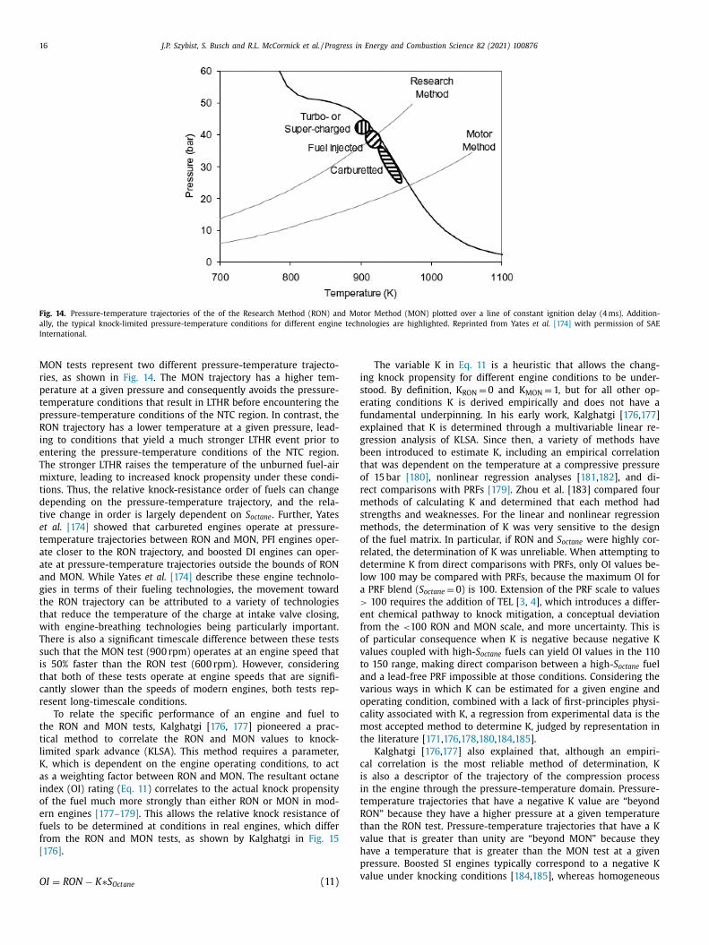
16 J.P. Szybist, S. Busch and R.L. McCormick et al. / Progress in Energy and Combustion Science 82 (2021) 100876
Fig. 14. Pressure-temperature trajectories of the of the Research Method (RON) and Motor Method (MON) plotted over a line of constant ignition delay (4 ms). Addition-
ally, the typical knock-limited pressure-temperature conditions for different engine technologies are highlighted. Reprinted from Yates et al. [174] with permission of SAE
International.
i
s
e
f
e
g
b
t
o
r
m
s
m
o
r
d
l
a
>
e
f
o
v
t
a
v
o
c
m
t
c
i
i
t
R
t
v
h
p
v
MON tests represent two different pressure-temperature trajecto-
ries, as shown in Fig. 14 . The MON trajectory has a higher tem-
perature at a given pressure and consequently avoids the pressure-
temperature conditions that result in LTHR before encountering the
pressure-temperature conditions of the NTC region. In contrast, the
RON trajectory has a lower temperature at a given pressure, lead-
ing to conditions that yield a much stronger LTHR event prior to
entering the pressure-temperature conditions of the NTC region.
The stronger LTHR raises the temperature of the unburned fuel-air
mixture, leading to increased knock propensity under these condi-
tions. Thus, the relative knock-resistance order of fuels can change
depending on the pressure-temperature trajectory, and the rela-
tive change in order is largely dependent on S octane . Further, Yates
et al. [174] showed that carbureted engines operate at pressure-
temperature trajectories between RON and MON, PFI engines oper-
ate closer to the RON trajectory, and boosted DI engines can oper-
ate at pressure-temperature trajectories outside the bounds of RON
and MON. While Yates et al. [174] describe these engine technolo-
gies in terms of their fueling technologies, the movement toward
the RON trajectory can be attributed to a variety of technologies
that reduce the temperature of the charge at intake valve closing,
with engine-breathing technologies being particularly important.
There is also a significant timescale difference between these tests
such that the MON test (900 rpm) operates at an engine speed that
is 50% faster than the RON test (600 rpm). However, considering
that both of these tests operate at engine speeds that are signifi-
cantly slower than the speeds of modern engines, both tests rep-
resent long-timescale conditions.
To relate the specific performance of an engine and fuel to
the RON and MON tests, Kalghatgi [ 176 , 177 ] pioneered a prac-
tical method to correlate the RON and MON values to knock-
limited spark advance (KLSA). This method requires a parameter,
K, which is dependent on the engine operating conditions, to act
as a weighting factor between RON and MON. The resultant octane
index (OI) rating ( Eq. 11 ) correlates to the actual knock propensity
of the fuel much more strongly than either RON or MON in mod-
ern engines [177–179] . This allows the relative knock resistance of
fuels to be determined at conditions in real engines, which differ
from the RON and MON tests, as shown by Kalghatgi in Fig. 15
[176] .
OI = RON − K ∗S Octane (11)
The variable K in Eq. 11 is a heuristic that allows the chang-
ng knock propensity for different engine conditions to be under-
tood. By definition, K RON = 0 and K MON = 1, but for all other op-
rating conditions K is derived empirically and does not have a
undamental underpinning. In his early work, Kalghatgi [ 176 , 177 ]
xplained that K is determined through a multivariable linear re-
ression analysis of KLSA. Since then, a variety of methods have
een introduced to estimate K, including an empirical correlation
hat was dependent on the temperature at a compressive pressure
f 15 bar [180] , nonlinear regression analyses [ 181 , 182 ], and di-
ect comparisons with PRFs [179] . Zhou et al. [183] compared four
ethods of calculating K and determined that each method had
trengths and weaknesses. For the linear and nonlinear regression
ethods, the determination of K was very sensitive to the design
f the fuel matrix. In particular, if RON and S octane were highly cor-
elated, the determination of K was unreliable. When attempting to
etermine K from direct comparisons with PRFs, only OI values be-
ow 100 may be compared with PRFs, because the maximum OI for
PRF blend ( S octane = 0) is 100. Extension of the PRF scale to values
100 requires the addition of TEL [ 3 , 4 ], which introduces a differ-
nt chemical pathway to knock mitigation, a conceptual deviation
rom the < 100 RON and MON scale, and more uncertainty. This is
f particular consequence when K is negative because negative K
alues coupled with high- S octane fuels can yield OI values in the 110
o 150 range, making direct comparison between a high- S octane fuel
nd a lead-free PRF impossible at those conditions. Considering the
arious ways in which K can be estimated for a given engine and
perating condition, combined with a lack of first-principles physi-
ality associated with K, a regression from experimental data is the
ost accepted method to determine K, judged by representation in
he literature [ 171 , 176 , 178 , 180 , 184 , 185 ].
Kalghatgi [ 176 , 177 ] also explained that, although an empiri-
al correlation is the most reliable method of determination, K
s also a descriptor of the trajectory of the compression process
n the engine through the pressure-temperature domain. Pressure-
emperature trajectories that have a negative K value are “beyond
ON” because they have a higher pressure at a given temperature
han the RON test. Pressure-temperature trajectories that have a K
alue that is greater than unity are “beyond MON” because they
ave a temperature that is greater than the MON test at a given
ressure. Boosted SI engines typically correspond to a negative K
alue under knocking conditions [ 184 , 185 ], whereas homogeneous
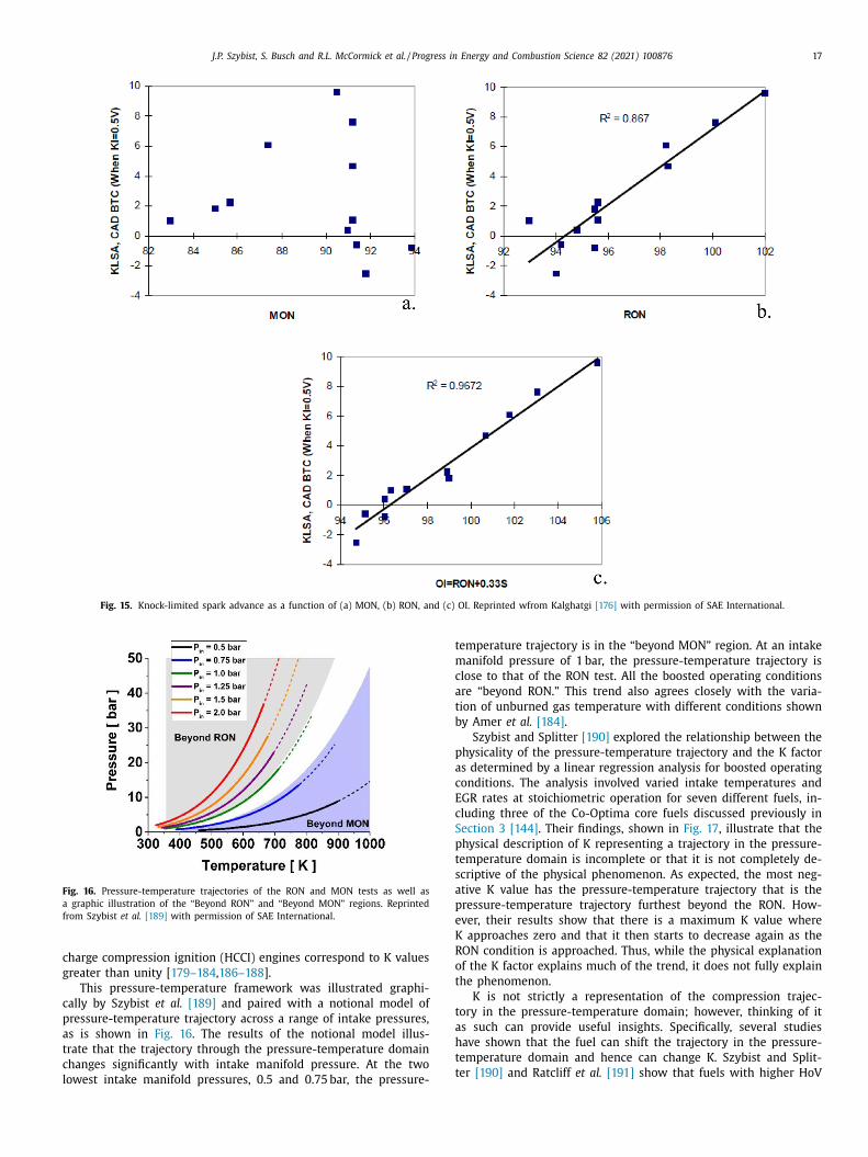
J.P. Szybist, S. Busch and R.L. McCormick et al. / Progress in Energy and Combustion Science 82 (2021) 100876 17
Fig. 15. Knock-limited spark advance as a function of (a) MON, (b) RON, and (c) OI. Reprinted wfrom Kalghatgi [176] with permission of SAE International.
Fig. 16. Pressure-temperature trajectories of the RON and MON tests as well as
a graphic illustration of the “Beyond RON” and “Beyond MON” regions. Reprinted
from Szybist et al. [189] with permission of SAE International.
c
g
c
p
a
t
c
l
t
m
c
a
t
b
p
a
c
E
c
S
p
t
s
a
p
e
K
R
o
t
t
a
h
t
t
harge compression ignition (HCCI) engines correspond to K values
reater than unity [ 179–184 , 186–188 ].
This pressure-temperature framework was illustrated graphi-
ally by Szybist et al. [189] and paired with a notional model of
ressure-temperature trajectory across a range of intake pressures,
s is shown in Fig. 16 . The results of the notional model illus-
rate that the trajectory through the pressure-temperature domain
hanges significantly with intake manifold pressure. At the two
owest intake manifold pressures, 0.5 and 0.75 bar, the pressure-
emperature trajectory is in the “beyond MON” region. At an intake
anifold pressure of 1 bar, the pressure-temperature trajectory is
lose to that of the RON test. All the boosted operating conditions
re “beyond RON.” This trend also agrees closely with the varia-
ion of unburned gas temperature with different conditions shown
y Amer et al. [184] .
Szybist and Splitter [190] explored the relationship between the
hysicality of the pressure-temperature trajectory and the K factor
s determined by a linear regression analysis for boosted operating
onditions. The analysis involved varied intake temperatures and
GR rates at stoichiometric operation for seven different fuels, in-
luding three of the Co-Optima core fuels discussed previously in
ection 3 [144] . Their findings, shown in Fig. 17 , illustrate that the
hysical description of K representing a trajectory in the pressure-
emperature domain is incomplete or that it is not completely de-
criptive of the physical phenomenon. As expected, the most neg-
tive K value has the pressure-temperature trajectory that is the
ressure-temperature trajectory furthest beyond the RON. How-
ver, their results show that there is a maximum K value where
approaches zero and that it then starts to decrease again as the
ON condition is approached. Thus, while the physical explanation
f the K factor explains much of the trend, it does not fully explain
he phenomenon.
K is not strictly a representation of the compression trajec-
ory in the pressure-temperature domain; however, thinking of it
s such can provide useful insights. Specifically, several studies
ave shown that the fuel can shift the trajectory in the pressure-
emperature domain and hence can change K. Szybist and Split-
er [190] and Ratcliff et al. [191] show that fuels with higher HoV
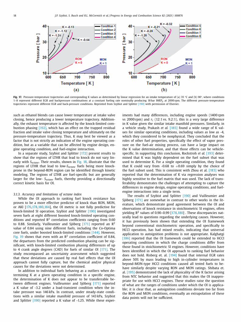
18 J.P. Szybist, S. Busch and R.L. McCormick et al. / Progress in Energy and Combustion Science 82 (2021) 100876
Fig. 17. Pressure-temperature trajectories and corresponding K values as determined by linear regression for an intake temperature of (a) 35 °C and (b) 90 °, where conditions
1–8 represent different EGR and backpressure combinations at a constant fueling rate nominally producing 18 bar IMEP g at 20 0 0 rpm. The different pressure-temperature
trajectories represent different EGR and back-pressure conditions. Reprinted from Szybist and Splitter [190] with permission of Elsevier.
i
v
i
a
u
w
r
s
t
s
m
u
t
t
r
h
f
d
e
S
e
o
y
u
i
b
H
a
[
o
t
b
d
a
b
h
a
f
p
o
b
t
d
such as ethanol blends can cause lower temperature at intake valve
closing, hence producing a lower temperature trajectory. Addition-
ally, the exhaust temperature is affected by the knock-limited com-
bustion phasing [192] , which has an effect on the trapped residual
fraction and intake valve closing temperature and ultimately on the
pressure-temperature trajectory. Thus, K may best be viewed as a
factor that is not strictly an indication of the engine operating con-
dition, but as a variable that can be affected by engine design, en-
gine operating condition, and fuel-engine interaction.
In a separate study, Szybist and Splitter [172] present results to
show that the regions of LTHR that lead to knock do not vary lin-
early with S octane . Their results, shown in Fig. 18 , illustrate that the
regions of LTHR that lead to low- S octane fuels being more knock-
prone in the beyond-RON region can be identified through kinetic
modeling. The regions of LTHR are fuel-specific but are generally
larger for the low- S octane fuels, thereby providing a directionally
correct kinetic basis for OI.
3.1.3. Accuracy and limitations of octane index
While the OI approach to ranking fuel knock resistance has
proven to be a more effective predictor of knock than RON, MON,
or AKI [ 176 , 178 , 180 , 184 ], the OI metric is not fully predictive for
knock-limited SI operation. Szybist and Splitter [190] investigated
seven fuels at eight different boosted knock-limited operating con-
ditions and reported R
2 correlation coefficients ranging from 0.60
to 0.88. Similarly, Vuilleumier and Sjöberg [171] reported an R
2
value of 0.84 using nine different fuels, including the Co-Optima
core fuels, under boosted knock-limited conditions [144] . However,
Fig. 19 shows that even with an R
2 correlation coefficient of 0.84,
the departures from the predicted combustion phasing can be sig-
nificant, with knock-limited combustion phasing differences of up
to 4 crank angle degrees (CAD) for fuels of similar OI [171] . The
study encompassed an uncertainty assessment which suggested
that these deviations are caused by real fuel effects that the OI
approach cannot fully capture, but the chemical and/or physical
causes for the deviations were not determined.
In addition to individual fuels behaving as a outliers when de-
termining K at a given operating condition in a specific engine,
the determination of K does not appear to be transferrable be-
tween different engines. Vuilleumier and Sjöberg [171] reported
a K value of -3.2 under a load-transient condition when the in-
take pressure was 146 kPa. In contrast, under steady-state condi-
tions with a similar intake manifold pressure of 143 kPa, Szybist
and Splitter [190] reported a K value of -1.25. While these exper-
ments had many differences, including engine speeds (1400 rpm
s 20 0 0 rpm) and r c (12:1 vs. 9.2:1), this is a very large difference
n K value given the similar intake manifold pressures. Similarly, in
vehicle study, Prakash et al. [185] found a wide range of K val-
es for similar operating conditions, including values as low as -4,
hich they considered to be nonphysical. They concluded that the
oles of other fuel properties, specifically the effect of vapor pres-
ure on the fuel-air mixing process, can have a large impact on
he K value determination, and that those effects can be vehicle-
pecific. In supporting this conclusion, Rockstroh et al. [193] deter-
ined that K was highly dependent on the fuel subset that was
sed to determine K. For a single operating condition, they found
hat K could vary from -0.68 to + 0.69 simply by the choice of
he fuel subset used. This is consistent with Zhou et al. [183] who
eported that the determination of K via regression analyses was
ighly sensitive to the fuel matrix that was used. The lack of trans-
erability demonstrates the challenges of attempting to capture the
ifferences in engine design, engine operating conditions, and fuel-
ngine interactions into a single term.
The results of Szybist and Splitter [190] and Vuilleumier and
jöberg [171] are somewhat in contrast to other works in the lit-
rature, which demonstrate good agreement between the OI and
bservations of knock resistance in stoichiometric SI engines, often
ielding R
2 values of 0.90–0.99 [ 178 , 180 ] . These discrepancies nat-
rally lead to questions regarding the underlying causes. However,
t has previously been shown that extending the OI framework
eyond conventional stoichiometric operation, and specifically to
CCI operation, has had mixed results, indicating that universal
pplication to autoignition problems is not appropriate. Kalghatgi
186] reported that the OI framework could be extended to HCCI
perating conditions in which the charge conditions differ from
hose found in stoichiometric SI engines. However, conditions have
een identified in which the OI approach to ranking fuel behavior
oes not hold. Risberg et. al. [194] found that internal EGR rates
bove 50% by mass leading to high in-cylinder temperatures in
eyond-MON-type HCCI conditions caused all tested fuels to be-
ave similarly despite varying RON and MON ratings. Shibata et.
l. [195] demonstrated the lack of physicality of the K factor arising
rom NTC behavior and suggested that this makes the OI inappro-
riate for use with HCCI engines. These studies raise the question
f what are the ranges of conditions under which the OI is applica-
le; it is clear that, as autoignition conditions deviate too far from
he RON and MON conditions, eventually an extrapolation of these
ata points will not be sufficient.
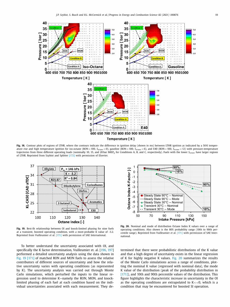
J.P. Szybist, S. Busch and R.L. McCormick et al. / Progress in Energy and Combustion Science 82 (2021) 100876 19
Fig. 18. Contour plots of regions of LTHR, where the contours indicate the difference in ignition delay (shown in ms) between LTHR ignition as indicated by a 50 K temper-
ature rise and high temperature ignition for iso-octane (RON = 100, S octane = 0), gasoline (RON = 100, S octane = 6), and E40 (RON = 100, S octane = 12) with pressure-temperature
trajectories from three different operating loads (nominally 10, 15, and 20 bar IMEP g for Conditions A, B, and C, respectively). Fuels with the lower S octane have larger regions
of LTHR. Reprinted from Szybist and Splitter [172] with permission of Elsevier.
Fig. 19. Best-fit relationship between OI and knock-limited phasing for nine fuels
at a transient, boosted operating condition, with a most-probable K value of -3.2.
Reprinted from Vuilleumier et al. [171] with permission of SAE International.
s
p
F
c
t
b
C
g
l
v
Fig. 20. Nominal and mode of distribution Octane Index K values over a range of
operating conditions. Also shown is the 80% probability range (10th to 90th per-
centile range). Reprinted from Vuilleumier et al. [171] with permission of SAE Inter-
national.
t
a
o
o
t
K
[
fi
a
c
To better understand the uncertainty associated with OI, and
pecifically the K factor determination, Vuilleumier et. al. [ 196 , 197 ]
erformed a detailed uncertainty analysis using the data shown in
ig. 19 [171] of matched RON and MON fuels to assess the relative
ontributors of different sources of uncertainty and how the rela-
ive uncertainty varies with operating conditions (as represented
y K). The uncertainty analysis was carried out through Monte
arlo simulations, which perturbed the inputs to the linear re-
ression used to determine K—namely the RON, MON, and knock-
imited phasing of each fuel at each condition based on the indi-
idual uncertainties associated with each measurement. They de-
ermined that there were probabilistic distributions of the K value
nd that a high degree of uncertainty exists in the linear regression
f K for highly negative K values. Fig. 20 summarizes the results
f the Monte Carlo simulations across a range of conditions, plot-
ing the nominal K value (regressed with nominal data), the mode
value of the distribution (peak of the probability distribution in
171] ), and 10th and 90th percentile values of the distribution. This
gure highlights the characteristic increase in uncertainty in the OI
s the operating conditions are extrapolated to K << 0, which is a
ondition that may be encountered for boosted SI operation.
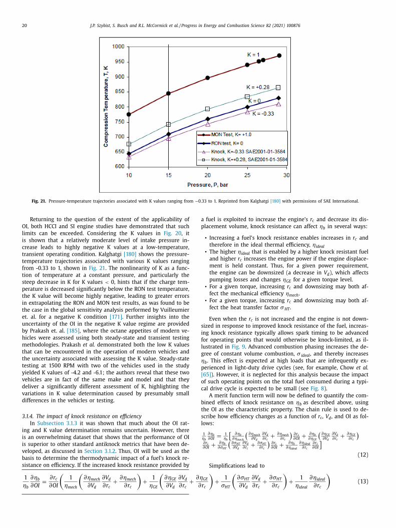
20 J.P. Szybist, S. Busch and R.L. McCormick et al. / Progress in Energy and Combustion Science 82 (2021) 100876
Fig. 21. Pressure-temperature trajectories associated with K values ranging from −0.33 to 1. Reprinted from Kalghatgi [180] with permissions of SAE International.
a
p
s
i
f
l
g
η
p
[
o
c
b
t
s
l
+
∂ η
∂
Returning to the question of the extent of the applicability of
OI, both HCCI and SI engine studies have demonstrated that such
limits can be exceeded. Considering the K values in Fig. 20 , it
is shown that a relatively moderate level of intake pressure in-
crease leads to highly negative K values at a low-temperature,
transient operating condition. Kalghatgi [180] shows the pressure-
temperature trajectories associated with various K values ranging
from -0.33 to 1, shown in Fig. 21 . The nonlinearity of K as a func-
tion of temperature at a constant pressure, and particularly the
steep decrease in K for K values < 0, hints that if the charge tem-
perature is decreased significantly below the RON test temperature,
the K value will become highly negative, leading to greater errors
in extrapolating the RON and MON test results, as was found to be
the case in the global sensitivity analysis performed by Vuilleumier
et. al. for a negative K condition [171] . Further insights into the
uncertainty of the OI in the negative K value regime are provided
by Prakash et. al. [185] , where the octane appetites of modern ve-
hicles were assessed using both steady-state and transient testing
methodologies. Prakash et al. demonstrated both the low K values
that can be encountered in the operation of modern vehicles and
the uncertainty associated with assessing the K value. Steady-state
testing at 1500 RPM with two of the vehicles used in the study
yielded K values of -4.2 and -6.1; the authors reveal that these two
vehicles are in fact of the same make and model and that they
deliver a significantly different assessment of K, highlighting the
variations in K value determination caused by presumably small
differences in the vehicles or testing.
3.1.4. The impact of knock resistance on efficiency
In Subsection 3.1.3 it was shown that much about the OI rat-
ing and K value determination remains uncertain. However, there
is an overwhelming dataset that shows that the performance of OI
is superior to other standard antiknock metrics that have been de-
veloped, as discussed in Section 3.1.2 . Thus, OI will be used as the
basis to determine the thermodynamic impact of a fuel’s knock re-
sistance on efficiency. If the increased knock resistance provided by
1
ηb
∂ ηb
∂OI =
∂ r c ∂OI
(1
ηmech
(∂ ηmech
∂ V d
∂ V d
∂ r c +
∂ ηmech
∂ r c
)+
1
ηGE
(∂ ηGE
∂ V d
∂ V d
∂ r c
fuel is exploited to increase the engine’s r c and decrease its dis-
lacement volume, knock resistance can affect ηb in several ways:
• Increasing a fuel’s knock resistance enables increases in r c and
therefore in the ideal thermal efficiency, ηideal
• The higher ηideal that is enabled by a higher knock resistant fuel
and higher r c increases the engine power if the engine displace-
ment is held constant. Thus, for a given power requirement,
the engine can be downsized (a decrease in V d ), which affects
pumping losses and changes ηGE for a given torque level.
• For a given torque, increasing r c and downsizing may both af-
fect the mechanical efficiency ηmech .
• For a given torque, increasing r c and downsizing may both af-
fect the heat transfer factor σ HT .
Even when the r c is not increased and the engine is not down-
ized in response to improved knock resistance of the fuel, increas-
ng knock resistance typically allows spark timing to be advanced
or operating points that would otherwise be knock-limited, as il-
ustrated in Fig. 9 . Advanced combustion phasing increases the de-
ree of constant volume combustion, σ ideal , and thereby increases
b . This effect is expected at high loads that are infrequently ex-
erienced in light-duty drive cycles (see, for example, Chow et al.
65] ). However, it is neglected for this analysis because the impact
f such operating points on the total fuel consumed during a typi-
al drive cycle is expected to be small (see Fig. 8 ).
A merit function term will now be defined to quantify the com-
ined effects of knock resistance on ηb as described above, using
he OI as the characteristic property. The chain rule is used to de-
cribe how efficiency changes as a function of r c , V d , and OI as fol-
ows:
1 ηb
∂ ηb
∂OI =
1 ηb
[∂ ηb
∂ ηmech
(∂ ηmech
∂ V d
∂ V d ∂ r c
+
∂ ηmech
∂ r c
)∂ r c ∂OI
+
∂ ηb
∂ ηGE
(∂ ηGE
∂ V d
∂ V d ∂ r c
+
∂ ηGE
∂ r c
)∂ r c ∂OI
+
∂ ηb
∂ σHT
(∂ σHT
∂ V d
∂ V d ∂ r c
+
∂ σHT
∂ r c
)∂ r c ∂OI
+
∂ ηb
∂ ηideal
∂ ηideal
∂ r c ∂ r c ∂OI
](12)
Simplifications lead to
GE
r c
)+
1
σHT
(∂ σHT
∂ V d
∂ V d
∂ r c +
∂ σHT
∂ r c
)+
1
ηideal
∂ ηideal
∂ r c
)(13)
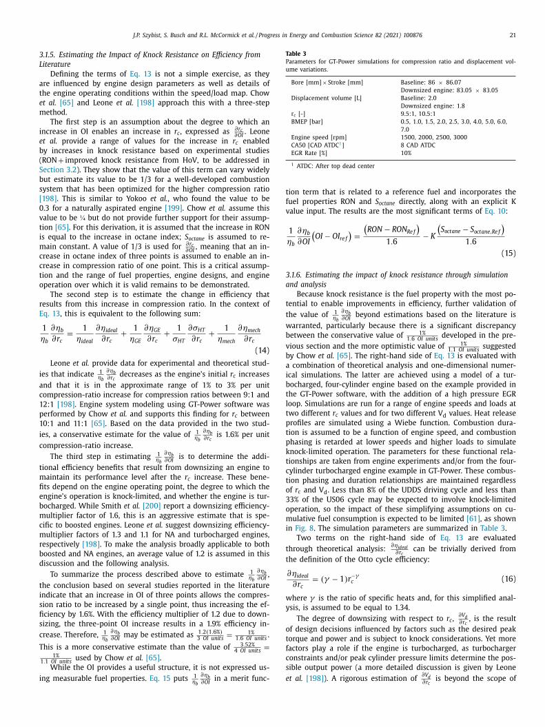
J.P. Szybist, S. Busch and R.L. McCormick et al. / Progress in Energy and Combustion Science 82 (2021) 100876 21
3
L
a
t
e
m
i
e
b
(
S
b
s
[
0
v
t
i
m
c
c
t
o
r
E
i
a
c
1
p
1
i
c
t
m
fi
e
b
m
c
m
r
b
d
t
i
s
fi
s
c
T
i
Table 3
Parameters for GT-Power simulations for compression ratio and displacement vol-
ume variations.
Bore [mm] × Stroke [mm] Baseline: 86 × 86.07
Downsized engine: 83.05 × 83.05
Displacement volume [L] Baseline: 2.0
Downsized engine: 1.8
r c [-] 9.5:1, 10.5:1
BMEP [bar] 0.5, 1.0, 1.5, 2.0, 2.5, 3.0, 4.0, 5.0, 6.0,
7.0
Engine speed [rpm] 1500, 2000, 2500, 3000
CA50 [CAD ATDC 1 ] 8 CAD ATDC
EGR Rate [%] 10%
1 ATDC: After top dead center
t
f
v
3
a
t
t
w
b
v
b
a
i
b
t
l
t
p
t
p
k
t
c
t
o
3
o
m
i
t
t
w
y
o
t
f
c
s
e
.1.5. Estimating the Impact of Knock Resistance on Efficiency from
iterature
Defining the terms of Eq. 13 is not a simple exercise, as they
re influenced by engine design parameters as well as details of
he engine operating conditions within the speed/load map. Chow
t al. [65] and Leone et al. [198] approach this with a three-step
ethod.
The first step is an assumption about the degree to which an
ncrease in OI enables an increase in r c , expressed as ∂ r c ∂OI
. Leone
t al. provide a range of values for the increase in r c enabled
y increases in knock resistance based on experimental studies
RON + improved knock resistance from HoV, to be addressed in
ection 3.2 ). They show that the value of this term can vary widely
ut estimate its value to be 1/3 for a well-developed combustion
ystem that has been optimized for the higher compression ratio
198] . This is similar to Yokoo et al. , who found the value to be
.3 for a naturally aspirated engine [199] . Chow et al. assume this
alue to be ¼ but do not provide further support for their assump-
ion [65] . For this derivation, it is assumed that the increase in RON
s equal to the increase in octane index; S octane is assumed to re-
ain constant. A value of 1/3 is used for ∂ r c ∂OI
, meaning that an in-
rease in octane index of three points is assumed to enable an in-
rease in compression ratio of one point. This is a critical assump-
ion and the range of fuel properties, engine designs, and engine
peration over which it is valid remains to be demonstrated.
The second step is to estimate the change in efficiency that
esults from this increase in compression ratio. In the context of
q. 13 , this is equivalent to the following sum:
1
ηb
∂ ηb
∂ r c =
1
ηideal
∂ ηideal
∂ r c +
1
ηGE
∂ ηGE
∂ r c +
1
σHT
∂ σHT
∂ r c +
1
ηmech
∂ ηmech
∂ r c
(14)
Leone et al. provide data for experimental and theoretical stud-
es that indicate 1 ηb
∂ ηb ∂ r c
decreases as the engine’s initial r c increases
nd that it is in the approximate range of 1% to 3% per unit
ompression-ratio increase for compression ratios between 9:1 and
2:1 [198] . Engine system modeling using GT-Power software was
erformed by Chow et al. and supports this finding for r c between
0:1 and 11:1 [65] . Based on the data provided in the two stud-
es, a conservative estimate for the value of 1 ηb
∂ ηb ∂ r c
is 1.6% per unit
ompression-ratio increase.
The third step in estimating 1 ηb
∂ ηb ∂OI
is to determine the addi-
ional efficiency benefits that result from downsizing an engine to
aintain its performance level after the r c increase. These bene-
ts depend on the engine operating point, the degree to which the
ngine’s operation is knock-limited, and whether the engine is tur-
ocharged. While Smith et al. [200] report a downsizing efficiency-
ultiplier factor of 1.6, this is an aggressive estimate that is spe-
ific to boosted engines. Leone et al. suggest downsizing efficiency-
ultiplier factors of 1.3 and 1.1 for NA and turbocharged engines,
espectively [198] . To make the analysis broadly applicable to both
oosted and NA engines, an average value of 1.2 is assumed in this
iscussion and the following analysis.
To summarize the process described above to estimate 1 ηb
∂ ηb ∂OI
,
he conclusion based on several studies reported in the literature
ndicate that an increase in OI of three points allows the compres-
ion ratio to be increased by a single point, thus increasing the ef-
ciency by 1.6%. With the efficiency multiplier of 1.2 due to down-
izing, the three-point OI increase results in a 1.9% efficiency in-
rease. Therefore, 1 ηb
∂ ηb ∂OI
may be estimated as 1 . 2( 1 . 6% ) 3 OI units
=
1% 1 . 6 OI units
.
his is a more conservative estimate than the value of 3 . 52% 4 OI units
=1%
1 . 1 OI units used by Chow et al. [65] .
While the OI provides a useful structure, it is not expressed us-
ng measurable fuel properties. Eq. 15 puts 1 η
∂ ηb ∂OI
in a merit func-
bion term that is related to a reference fuel and incorporates the
uel properties RON and S octane directly, along with an explicit K
alue input. The results are the most significant terms of Eq. 10 :
1
ηb
∂ ηb
∂OI
(OI − O I re f
)=
(RON − RO N Re f
)1 . 6
− K
(S octane − S octane,Re f
)1 . 6
(15)
.1.6. Estimating the impact of knock resistance through simulation
nd analysis
Because knock resistance is the fuel property with the most po-
ential to enable improvements in efficiency, further validation of
he value of 1 ηb
∂ ηb ∂OI
beyond estimations based on the literature is
arranted, particularly because there is a significant discrepancy
etween the conservative value of 1% 1 . 6 OI units
developed in the pre-
ious section and the more optimistic value of 1% 1 . 1 OI units
suggested
y Chow et al. [65] . The right-hand side of Eq. 13 is evaluated with
combination of theoretical analysis and one-dimensional numer-
cal simulations. The latter are achieved using a model of a tur-
ocharged, four-cylinder engine based on the example provided in
he GT-Power software, with the addition of a high pressure EGR
oop. Simulations are run for a range of engine speeds and loads at
wo different r c values and for two different V d values. Heat release
rofiles are simulated using a Wiebe function. Combustion dura-
ion is assumed to be a function of engine speed, and combustion
hasing is retarded at lower speeds and higher loads to simulate
nock-limited operation. The parameters for these functional rela-
ionships are taken from engine experiments and/or from the four-
ylinder turbocharged engine example in GT-Power. These combus-
ion phasing and duration relationships are maintained regardless
f r c and V d . Less than 8% of the UDDS driving cycle and less than
3% of the US06 cycle may be expected to involve knock-limited
peration, so the impact of these simplifying assumptions on cu-
ulative fuel consumption is expected to be limited [61] , as shown
n Fig. 8 . The simulation parameters are summarized in Table 3 .
Two terms on the right-hand side of Eq. 13 are evaluated
hrough theoretical analysis: ∂ ηideal
∂ r c can be trivially derived from
he definition of the Otto cycle efficiency:
∂ ηideal
∂ r c = ( γ − 1 ) r
−γc (16)
here γ is the ratio of specific heats and, for this simplified anal-
sis, is assumed to be equal to 1.34.
The degree of downsizing with respect to r c , ∂ V d ∂ r c
, is the result
f design decisions influenced by factors such as the desired peak
orque and power and is subject to knock considerations. Yet more
actors play a role if the engine is turbocharged, as turbocharger
onstraints and/or peak cylinder pressure limits determine the pos-
ible output power (a more detailed discussion is given by Leone
t al. [198] ). A rigorous estimation of ∂ V d ∂ r c
is beyond the scope of
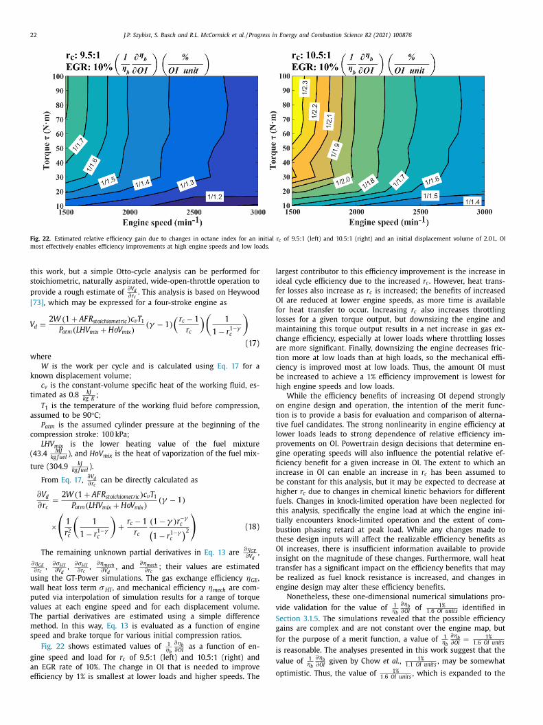
22 J.P. Szybist, S. Busch and R.L. McCormick et al. / Progress in Energy and Combustion Science 82 (2021) 100876
Fig. 22. Estimated relative efficiency gain due to changes in octane index for an initial r c of 9.5:1 (left) and 10.5:1 (right) and an initial displacement volume of 2.0 L. OI
most effectively enables efficiency improvements at high engine speeds and low loads.
V
l
i
f
O
f
l
m
c
a
t
c
b
h
o
t
t
l
p
g
fi
i
b
h
f
t
t
b
t
O
i
t
b
e
v
S
g
f
i
v
o1 . 6 OI units
this work, but a simple Otto-cycle analysis can be performed for
stoichiometric, naturally aspirated, wide-open-throttle operation to
provide a rough estimate of ∂ V d ∂ r c
. This analysis is based on Heywood
[73] , which may be expressed for a four-stroke engine as
d =
2 W ( 1 + AF R stoichiometric ) c v T 1 P atm
( LH V mix + Ho V mix ) ( γ − 1 )
(r c − 1
r c
)(1
1 − r 1 −γc
)(17)
where
W is the work per cycle and is calculated using Eq. 17 for a
known displacement volume;
c v is the constant-volume specific heat of the working fluid, es-
timated as 0.8 kJ kg K
;
T 1 is the temperature of the working fluid before compression,
assumed to be 90 °C;
P atm
is the assumed cylinder pressure at the beginning of the
compression stroke: 100 kPa;
LHV mix is the lower heating value of the fuel mixture
(43.4 MJ kg f uel
), and HoV mix is the heat of vaporization of the fuel mix-
ture (304.9 kJ kg f uel
).
From Eq. 17 , ∂ V d ∂ r c
can be directly calculated as
∂ V d
∂ r c =
2 W ( 1 + AF R stoichiometric ) c v T 1 P atm
( LH V mix + Ho V mix ) ( γ − 1 )
×(
1
r 2 c
(1
1 − r 1 −γc
)+
r c − 1
r c
( 1 − γ ) r −γc (
1 − r 1 −γc
)2
)
(18)
The remaining unknown partial derivatives in Eq. 13 are ∂ ηGE ∂ V d
,
∂ ηGE ∂ r c
, ∂ σHT ∂ V d
, ∂ σHT ∂ r c
, ∂ ηmech ∂ V d
, and
∂ ηmech ∂ r c
; their values are estimated
using the GT-Power simulations. The gas exchange efficiency ηGE ,
wall heat loss term σ HT , and mechanical efficiency ηmech are com-
puted via interpolation of simulation results for a range of torque
values at each engine speed and for each displacement volume.
The partial derivatives are estimated using a simple difference
method. In this way, Eq. 13 is evaluated as a function of engine
speed and brake torque for various initial compression ratios.
Fig. 22 shows estimated values of 1 ηb
∂ ηb ∂OI
as a function of en-
gine speed and load for r c of 9.5:1 (left) and 10.5:1 (right) and
an EGR rate of 10%. The change in OI that is needed to improve
efficiency by 1% is smallest at lower loads and higher speeds. The
argest contributor to this efficiency improvement is the increase in
deal cycle efficiency due to the increased r c . However, heat trans-
er losses also increase as r c is increased; the benefits of increased
I are reduced at lower engine speeds, as more time is available
or heat transfer to occur. Increasing r c also increases throttling
osses for a given torque output, but downsizing the engine and
aintaining this torque output results in a net increase in gas ex-
hange efficiency, especially at lower loads where throttling losses
re more significant. Finally, downsizing the engine decreases fric-
ion more at low loads than at high loads, so the mechanical effi-
iency is improved most at low loads. Thus, the amount OI must
e increased to achieve a 1% efficiency improvement is lowest for
igh engine speeds and low loads.
While the efficiency benefits of increasing OI depend strongly
n engine design and operation, the intention of the merit func-
ion is to provide a basis for evaluation and comparison of alterna-
ive fuel candidates. The strong nonlinearity in engine efficiency at
ower loads leads to strong dependence of relative efficiency im-
rovements on OI. Powertrain design decisions that determine en-
ine operating speeds will also influence the potential relative ef-
ciency benefit for a given increase in OI. The extent to which an
ncrease in OI can enable an increase in r c has been assumed to
e constant for this analysis, but it may be expected to decrease at
igher r c due to changes in chemical kinetic behaviors for different
uels. Changes in knock-limited operation have been neglected for
his analysis, specifically the engine load at which the engine ini-
ially encounters knock-limited operation and the extent of com-
ustion phasing retard at peak load. While any changes made to
hese design inputs will affect the realizable efficiency benefits as
I increases, there is insufficient information available to provide
nsight on the magnitude of these changes. Furthermore, wall heat
ransfer has a significant impact on the efficiency benefits that may
e realized as fuel knock resistance is increased, and changes in
ngine design may alter these efficiency benefits.
Nonetheless, these one-dimensional numerical simulations pro-
ide validation for the value of 1 ηb
∂ ηb ∂OI
of 1% 1 . 6 OI units
identified in
ection 3.1.5 . The simulations revealed that the possible efficiency
ains are complex and are not constant over the engine map, but
or the purpose of a merit function, a value of 1 ηb
∂ ηb ∂OI
=
1% 1 . 6 OI units
s reasonable. The analyses presented in this work suggest that the
alue of 1 ηb
∂ ηb ∂OI
given by Chow et al. , 1% 1 . 1 OI units
, may be somewhat
ptimistic. Thus, the value of 1% , which is expanded to the
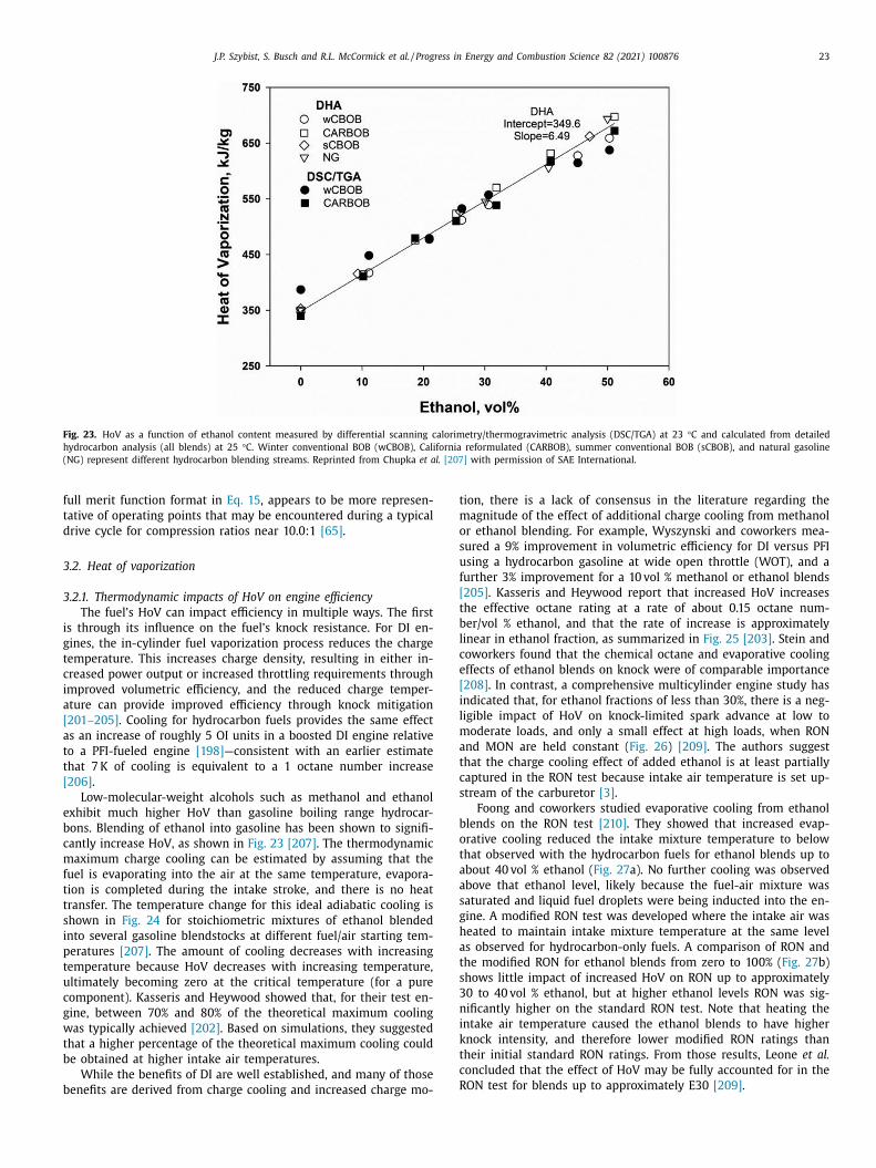
J.P. Szybist, S. Busch and R.L. McCormick et al. / Progress in Energy and Combustion Science 82 (2021) 100876 23
Fig. 23. HoV as a function of ethanol content measured by differential scanning calorimetry/thermogravimetric analysis (DSC/TGA) at 23 °C and calculated from detailed
hydrocarbon analysis (all blends) at 25 °C. Winter conventional BOB (wCBOB), California reformulated (CARBOB), summer conventional BOB (sCBOB), and natural gasoline
(NG) represent different hydrocarbon blending streams. Reprinted from Chupka et al. [207] with permission of SAE International.
f
t
d
3
3
i
g
t
c
i
a
[
a
t
t
[
e
b
c
m
f
t
t
s
i
p
t
u
c
g
w
t
b
b
t
m
o
s
u
f
[
t
b
l
c
e
[
i
l
m
a
t
c
s
b
o
t
a
a
s
g
h
a
t
s
3
n
i
k
t
c
R
ull merit function format in Eq. 15 , appears to be more represen-
ative of operating points that may be encountered during a typical
rive cycle for compression ratios near 10.0:1 [65] .
.2. Heat of vaporization
.2.1. Thermodynamic impacts of HoV on engine efficiency
The fuel’s HoV can impact efficiency in multiple ways. The first
s through its influence on the fuel’s knock resistance. For DI en-
ines, the in-cylinder fuel vaporization process reduces the charge
emperature. This increases charge density, resulting in either in-
reased power output or increased throttling requirements through
mproved volumetric efficiency, and the reduced charge temper-
ture can provide improved efficiency through knock mitigation
201–205] . Cooling for hydrocarbon fuels provides the same effect
s an increase of roughly 5 OI units in a boosted DI engine relative
o a PFI-fueled engine [198] —consistent with an earlier estimate
hat 7 K of cooling is equivalent to a 1 octane number increase
206] .
Low-molecular-weight alcohols such as methanol and ethanol
xhibit much higher HoV than gasoline boiling range hydrocar-
ons. Blending of ethanol into gasoline has been shown to signifi-
antly increase HoV, as shown in Fig. 23 [207] . The thermodynamic
aximum charge cooling can be estimated by assuming that the
uel is evaporating into the air at the same temperature, evapora-
ion is completed during the intake stroke, and there is no heat
ransfer. The temperature change for this ideal adiabatic cooling is
hown in Fig. 24 for stoichiometric mixtures of ethanol blended
nto several gasoline blendstocks at different fuel/air starting tem-
eratures [207] . The amount of cooling decreases with increasing
emperature because HoV decreases with increasing temperature,
ltimately becoming zero at the critical temperature (for a pure
omponent). Kasseris and Heywood showed that, for their test en-
ine, between 70% and 80% of the theoretical maximum cooling
as typically achieved [202] . Based on simulations, they suggested
hat a higher percentage of the theoretical maximum cooling could
e obtained at higher intake air temperatures.
While the benefits of DI are well established, and many of those
enefits are derived from charge cooling and increased charge mo-
ion, there is a lack of consensus in the literature regarding the
agnitude of the effect of additional charge cooling from methanol
r ethanol blending. For example, Wyszynski and coworkers mea-
ured a 9% improvement in volumetric efficiency for DI versus PFI
sing a hydrocarbon gasoline at wide open throttle (WOT), and a
urther 3% improvement for a 10 vol % methanol or ethanol blends
205] . Kasseris and Heywood report that increased HoV increases
he effective octane rating at a rate of about 0.15 octane num-
er/vol % ethanol, and that the rate of increase is approximately
inear in ethanol fraction, as summarized in Fig. 25 [203] . Stein and
oworkers found that the chemical octane and evaporative cooling
ffects of ethanol blends on knock were of comparable importance
208] . In contrast, a comprehensive multicylinder engine study has
ndicated that, for ethanol fractions of less than 30%, there is a neg-
igible impact of HoV on knock-limited spark advance at low to
oderate loads, and only a small effect at high loads, when RON
nd MON are held constant ( Fig. 26 ) [209] . The authors suggest
hat the charge cooling effect of added ethanol is at least partially
aptured in the RON test because intake air temperature is set up-
tream of the carburetor [3] .
Foong and coworkers studied evaporative cooling from ethanol
lends on the RON test [210] . They showed that increased evap-
rative cooling reduced the intake mixture temperature to below
hat observed with the hydrocarbon fuels for ethanol blends up to
bout 40 vol % ethanol ( Fig. 27 a). No further cooling was observed
bove that ethanol level, likely because the fuel-air mixture was
aturated and liquid fuel droplets were being inducted into the en-
ine. A modified RON test was developed where the intake air was
eated to maintain intake mixture temperature at the same level
s observed for hydrocarbon-only fuels. A comparison of RON and
he modified RON for ethanol blends from zero to 100% ( Fig. 27 b)
hows little impact of increased HoV on RON up to approximately
0 to 40 vol % ethanol, but at higher ethanol levels RON was sig-
ificantly higher on the standard RON test. Note that heating the
ntake air temperature caused the ethanol blends to have higher
nock intensity, and therefore lower modified RON ratings than
heir initial standard RON ratings. From those results, Leone et al.
oncluded that the effect of HoV may be fully accounted for in the
ON test for blends up to approximately E30 [209] .
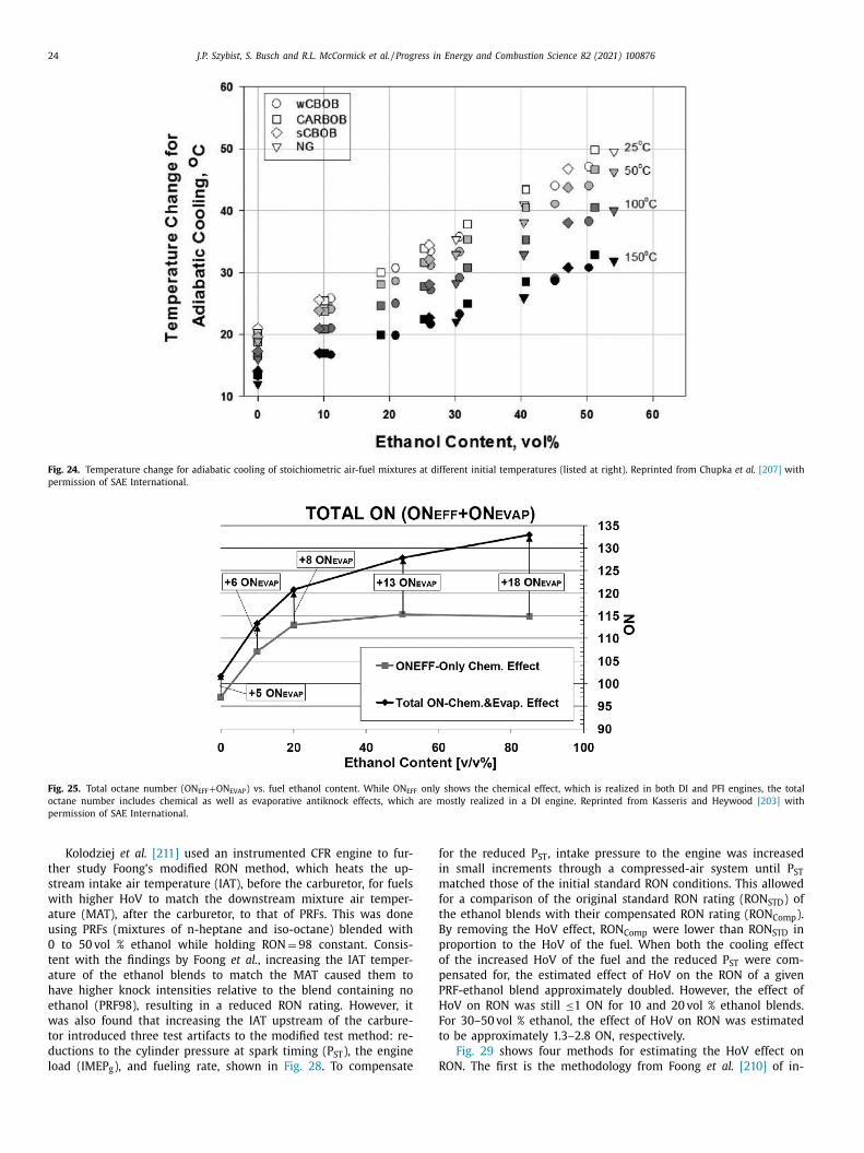
24 J.P. Szybist, S. Busch and R.L. McCormick et al. / Progress in Energy and Combustion Science 82 (2021) 100876
Fig. 24. Temperature change for adiabatic cooling of stoichiometric air-fuel mixtures at different initial temperatures (listed at right). Reprinted from Chupka et al. [207] with
permission of SAE International.
Fig. 25. Total octane number (ON EFF + ON EVAP ) vs. fuel ethanol content. While ON EFF only shows the chemical effect, which is realized in both DI and PFI engines, the total
octane number includes chemical as well as evaporative antiknock effects, which are mostly realized in a DI engine. Reprinted from Kasseris and Heywood [203] with
permission of SAE International.
f
i
m
f
t
B
p
o
p
P
H
F
t
R
Kolodziej et al. [211] used an instrumented CFR engine to fur-
ther study Foong’s modified RON method, which heats the up-
stream intake air temperature (IAT), before the carburetor, for fuels
with higher HoV to match the downstream mixture air temper-
ature (MAT), after the carburetor, to that of PRFs. This was done
using PRFs (mixtures of n-heptane and iso-octane) blended with
0 to 50 vol % ethanol while holding RON = 98 constant. Consis-
tent with the findings by Foong et al. , increasing the IAT temper-
ature of the ethanol blends to match the MAT caused them to
have higher knock intensities relative to the blend containing no
ethanol (PRF98), resulting in a reduced RON rating. However, it
was also found that increasing the IAT upstream of the carbure-
tor introduced three test artifacts to the modified test method: re-
ductions to the cylinder pressure at spark timing (P ST ), the engine
load (IMEP g ), and fueling rate, shown in Fig. 28 . To compensate
or the reduced P ST , intake pressure to the engine was increased
n small increments through a compressed-air system until P ST
atched those of the initial standard RON conditions. This allowed
or a comparison of the original standard RON rating (RON STD ) of
he ethanol blends with their compensated RON rating (RON Comp ).
y removing the HoV effect, RON Comp were lower than RON STD in
roportion to the HoV of the fuel. When both the cooling effect
f the increased HoV of the fuel and the reduced P ST were com-
ensated for, the estimated effect of HoV on the RON of a given
RF-ethanol blend approximately doubled. However, the effect of
oV on RON was still ≤1 ON for 10 and 20 vol % ethanol blends.
or 30–50 vol % ethanol, the effect of HoV on RON was estimated
o be approximately 1.3–2.8 ON, respectively.
Fig. 29 shows four methods for estimating the HoV effect on
ON. The first is the methodology from Foong et al. [210] of in-
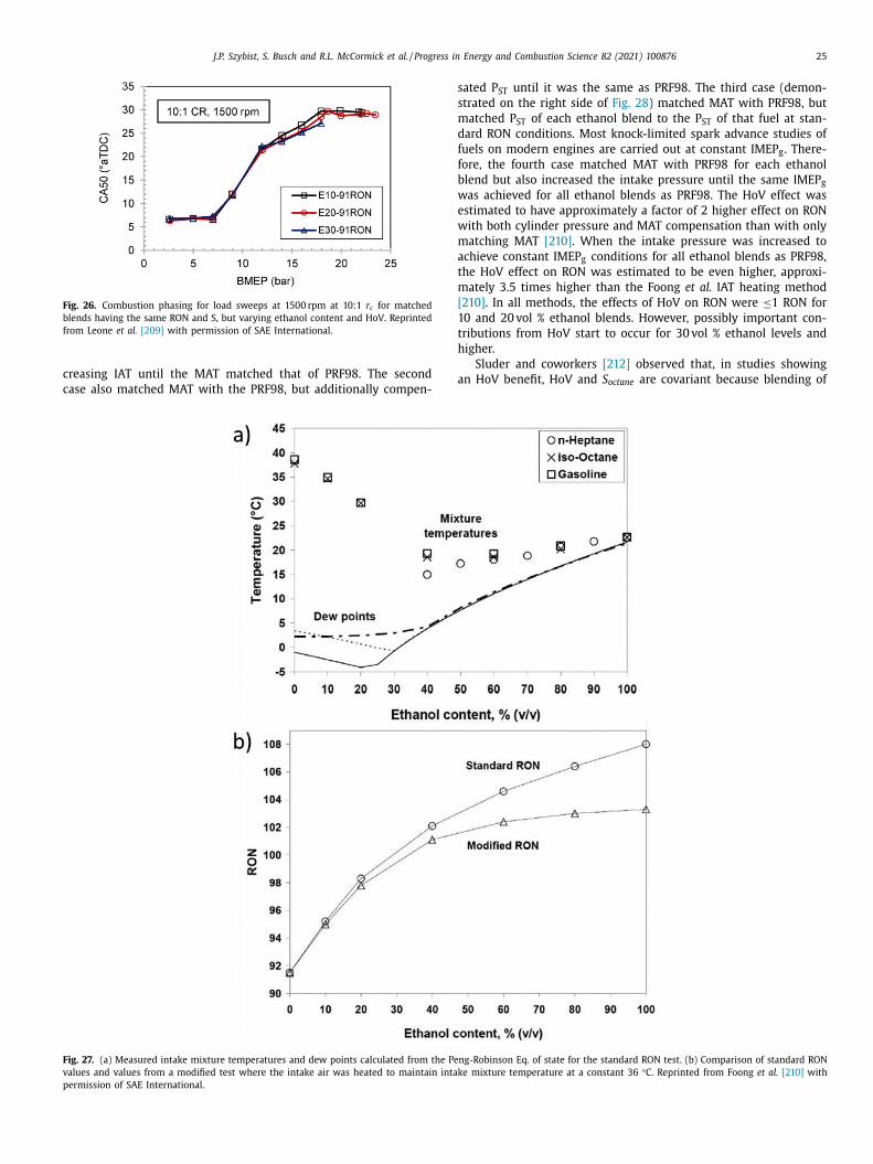
J.P. Szybist, S. Busch and R.L. McCormick et al. / Progress in Energy and Combustion Science 82 (2021) 100876 25
Fig. 26. Combustion phasing for load sweeps at 1500 rpm at 10:1 r c for matched
blends having the same RON and S, but varying ethanol content and HoV. Reprinted
from Leone et al. [209] with permission of SAE International.
c
c
s
s
m
d
f
f
b
w
e
w
m
a
t
m
[
1
t
h
a
F
v
p
reasing IAT until the MAT matched that of PRF98. The second
ase also matched MAT with the PRF98, but additionally compen-
ig. 27. (a) Measured intake mixture temperatures and dew points calculated from the Pe
alues and values from a modified test where the intake air was heated to maintain intak
ermission of SAE International.
ated P ST until it was the same as PRF98. The third case (demon-
trated on the right side of Fig. 28 ) matched MAT with PRF98, but
atched P ST of each ethanol blend to the P ST of that fuel at stan-
ard RON conditions. Most knock-limited spark advance studies of
uels on modern engines are carried out at constant IMEP g . There-
ore, the fourth case matched MAT with PRF98 for each ethanol
lend but also increased the intake pressure until the same IMEP g as achieved for all ethanol blends as PRF98. The HoV effect was
stimated to have approximately a factor of 2 higher effect on RON
ith both cylinder pressure and MAT compensation than with only
atching MAT [210] . When the intake pressure was increased to
chieve constant IMEP g conditions for all ethanol blends as PRF98,
he HoV effect on RON was estimated to be even higher, approxi-
ately 3.5 times higher than the Foong et al. IAT heating method
210] . In all methods, the effects of HoV on RON were ≤1 RON for
0 and 20 vol % ethanol blends. However, possibly important con-
ributions from HoV start to occur for 30 vol % ethanol levels and
igher.
Sluder and coworkers [212] observed that, in studies showing
n HoV benefit, HoV and S octane are covariant because blending of
ng-Robinson Eq. of state for the standard RON test. (b) Comparison of standard RON
e mixture temperature at a constant 36 °C. Reprinted from Foong et al. [210] with
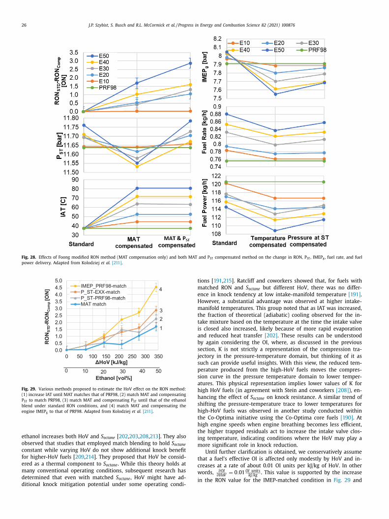
26 J.P. Szybist, S. Busch and R.L. McCormick et al. / Progress in Energy and Combustion Science 82 (2021) 100876
Fig. 28. Effects of Foong modified RON method (MAT compensation only) and both MAT and P ST compensated method on the change in RON, P ST , IMEP g , fuel rate, and fuel
power delivery. Adapted from Kolodziej et al. [211] .
Fig. 29. Various methods proposed to estimate the HoV effect on the RON method:
(1) increase IAT until MAT matches that of PRF98, (2) match MAT and compensating
P ST to match PRF98, (3) match MAT and compensating P ST until that of the ethanol
blend under standard RON conditions, and (4) match MAT and compensating the
engine IMEP g to that of PRF98. Adapted from Kolodziej et al. [211] .
t
m
e
H
m
t
t
i
a
b
s
j
s
p
s
a
h
h
s
h
t
h
t
i
m
t
c
w
i
ethanol increases both HoV and S octane [ 202 , 203 , 208 , 213 ]. They also
observed that studies that employed match blending to hold S octane
constant while varying HoV do not show additional knock benefit
for higher-HoV fuels [ 209 , 214 ]. They proposed that HoV be consid-
ered as a thermal component to S octane . While this theory holds at
many conventional operating conditions, subsequent research has
determined that even with matched S octane , HoV might have ad-
ditional knock mitigation potential under some operating condi-
ions [ 191 , 215 ]. Ratcliff and coworkers showed that, for fuels with
atched RON and S octane but different HoV, there was no differ-
nce in knock tendency at low intake-manifold temperature [191] .
owever, a substantial advantage was observed at higher intake-
anifold temperatures. This group noted that as IAT was increased,
he fraction of theoretical (adiabatic) cooling observed for the in-
ake mixture based on the temperature at the time the intake valve
s closed also increased, likely because of more rapid evaporation
nd reduced heat transfer [202] . These results can be understood
y again considering the OI, where, as discussed in the previous
ection, K is not strictly a representation of the compression tra-
ectory in the pressure-temperature domain, but thinking of it as
uch can provide useful insights. With this view, the reduced tem-
erature produced from the high-HoV fuels moves the compres-
ion curve in the pressure temperature domain to lower temper-
tures. This physical representation implies lower values of K for
igh HoV fuels (in agreement with Stein and coworkers [208] ), en-
ancing the effect of S octane on knock resistance. A similar trend of
hifting the pressure-temperature trace to lower temperatures for
igh-HoV fuels was observed in another study conducted within
he Co-Optima initiative using the Co-Optima core fuels [190] . At
igh engine speeds when engine breathing becomes less efficient,
he higher trapped residuals act to increase the intake valve clos-
ng temperature, indicating conditions where the HoV may play a
ore significant role in knock reduction.
Until further clarification is obtained, we conservatively assume
hat a fuel’s effective OI is affected only modestly by HoV and in-
reases at a rate of about 0.01 OI units per kJ/kg of HoV. In other
ords, ∂OI ∂HoV
= 0 . 01 OI units kJ/kg
. This value is supported by the increase
n the RON value for the IMEP-matched condition in Fig. 29 and
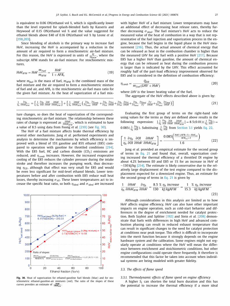
J.P. Szybist, S. Busch and R.L. McCormick et al. / Progress in Energy and Combustion Science 82 (2021) 100876 27
i
t
H
e
[
H
a
F
s
t
H
w
f
o
t
t
i
r
a
s
a
p
p
W
r
c
s
i
b
p
l
c
F
i
c
w
a
t
m
r
g
s
c
t
E
e
i
r
E
η
w
+
∂ ηb
∂ σH
u
f
0
[
o
i
a
∼
a
p
t
s equivalent to 0.06 ON/ethanol vol %, which is significantly lower
han the level reported for splash-blended fuels by Kasseris and
eywood of 0.15 ON/ethanol vol % and the value suggested for
thanol blends above E40 of 0.16 ON/ethanol vol % by Leone et al.
198 , 203 ].
Since blending of alcohols is the primary way to increase fuel
oV, increasing the HoV is accompanied by a reduction in the
mount of air required to form a stoichiometric air-fuel mixture.
or this reason, the HoV is expressed in units of kJ k g AF M
, where the
ubscript AFM stands for air-fuel mixture. For stoichiometric mix-
ures,
o V AF M
= H oV
m f uel
m AF M
=
H oV
1 + AF R s (19)
here m fuel is the mass of fuel, m AFM
is the combined mass of the
uel mixture and the air required to form a stoichiometric mixture
f fuel and air, and AFR s is the stoichiometric air-fuel mass ratio for
he given fuel mixture. As the heat of vaporization of a fuel mix-
ure changes, so does the heat of vaporization of the correspond-
ng stoichiometric air-fuel mixture. The relationship between these
ates of change is expressed as ∂HoV ∂Ho V AF M
, which is estimated to have
value of 8.5 using data from Foong et al. [210] (see Fig. 30 ).
The HoV of a fuel mixture affects brake thermal efficiency by
everal other mechanisms. Jung et al. performed experiments and
nalysis to determine the mechanisms by which efficiency is im-
roved with a blend of 15% gasoline and 85% ethanol (E85) com-
ared to operation with gasoline for throttled conditions [214] .
ith the E85 fuel, HC and carbon dioxide (CO 2 ) emissions are
educed, and ηcomb increases. However, the increased evaporative
ooling of the E85 reduces the cylinder pressure during the intake
troke and therefore increases the pumping work, thus decreas-
ng ηGE , although that effect was very small for E85 and would
e even less significant for mid-level ethanol blends. Lower tem-
eratures before and after combustion with E85 reduce wall heat
osses, thereby increasing σ HT . These lower temperatures act to in-
rease the specific heat ratio, so both ηideal and σ ideal are increased
1 ηb
∂ ηb
∂Ho V AFM =
[1 ηb
∂ ηb
∂OI ∂OI
∂HoV ∂HoV
∂Ho V AFM
]+
[1 ηb
∂HoV ∂Ho V AFM
(∂ ηb
∂ ηcomb
∂ ηcomb
∂HoV +
∂ ηb
∂ ηGE
∂ ηGE
∂HoV
ig. 30. Heat of vaporization for ethanol-gasoline fuel blends (blue) and for sto-
chiometric ethanol-gasoline-air mixtures (red). The ratio of the slopes of these
urves provides an estimate of ∂ HoV ∂ Ho V AFM
.
H
i
f
t
s
b
c
a
i
h
u
e
e
r
u
3
3
t
ith higher HoV of a fuel mixture. Lower temperatures may have
n additional effect of decreasing heat release rates, thereby fur-
her decreasing σ ideal . The fuel mixture’s HoV acts to reduce the
easured value of the heat of combustion in a way that is not rep-
esentative of the fuel injection and vaporization process in the en-
ine, because the fuel begins in the liquid phase in the HoV mea-
urement [216] . Thus, the actual amount of chemical energy that
an be released as heat in the combustion chamber is higher than
he measured LHV for any fuel with a positive HoV [217] . Because
85 has a higher HoV than gasoline, the amount of chemical en-
rgy that can be released as heat during the combustion process
s larger than is indicated by the LHV. This effect accounted for
oughly half of the part-load efficiency improvement observed for
85 and is considered in the definition of combustion efficiency:
comb =
Q HR
m f uel ( LH V + H oV ) (20)
here LHV is the lower heating value of the fuel.
The aggregate of the HoV effects described above is given by:
T
∂ σHT
∂HoV +
∂ ηb
∂ ηideal
∂ ηideal
∂γ∂γ
∂HoV +
∂ ηb
∂ σideal
∂ σideal
∂HoV
)](21)
Evaluating the first group of terms on the right-hand side
sing values for the terms as they are defined above results in the
ollowing expression: [ 1 ηb
∂ ηb ∂OI
∂OI ∂HoV
∂HoV ∂Ho V AF M
] = 8 . 5( 0 . 01 )( 1 ηb
∂ ηb ∂OI
) = . 085( 1
ηb
∂ ηb ∂OI
) . Substituing 1 ηb
∂ ηb ∂OI
from Section 3.1 yields Eq. 22 .
1
ηb
∂ ηb
∂OI
∂OI
∂HoV
∂HoV
∂Ho V AF M
]=
0 . 085
(H oV/ ( AF R +1 ) −H o V re f
AF R re f +1
)1 . 6
(22)
Jung et al. provided an empirical estimate for the second group
f terms in Eq. 21 and found that, overall, vaporization cool-
ng increased the thermal efficiency of a throttled DI engine by
bout 4.2% between E0 and E85 or 1% for an increase in HoV of
130 kJ/kg [214] . The estimate is likely conservative due to the rel-
tively large displacement of the test engine compared to the dis-
lacement expected for a downsized engine. Thus, an estimate for
he second group of terms in Eq. 21 is given by
1
ηb
∂HoV
∂Ho V AF M
∂ ηb
∂HoV
=
8 . 5
130
% ηb increase
kJ/kgAF M
=
1
15 . 3
% ηb increase
kJ/kgAF M
(23)
Although considerations in this analysis are limited as to how
oV affects engine efficiency, HoV can also have other important
mpacts on engine operation, such as cold-start behavior and dif-
erences in the degree of enrichment needed for catalyst protec-
ion. Both Szybist and Splitter [192] and Stein et al. [208] demon-
trate that fuels with differences in high HoV and advanced com-
ustion phasing can result in reduced exhaust temperature that
an result in significant changes to the need for catalyst protection
t conditions near peak torque. This effect is difficult to incorporate
nto the merit function because it strongly depends on the engine
ardware system and the calibration. Some engines might not reg-
larly operate at conditions where the HoV will mean the differ-
nce between enrichment and stoichiometric conditions, but other
ngine configurations could operate there frequently. It therefore is
ecommended that this factor be taken into account when individ-
al systems are being modeled with greater fidelity.
.3. The effects of flame speed
.3.1. Thermodynamic effects of flame speed on engine efficiency
A higher S L can shorten the total burn duration and this has
he potential to increase the thermal efficiency if a more ideal
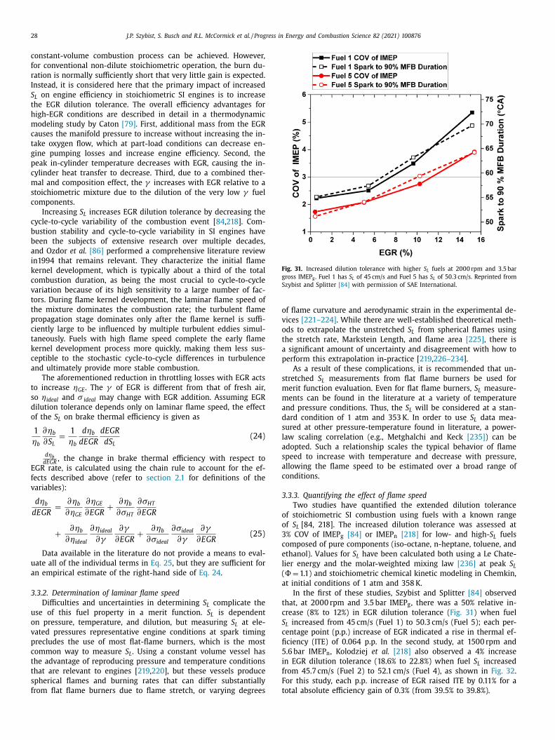
28 J.P. Szybist, S. Busch and R.L. McCormick et al. / Progress in Energy and Combustion Science 82 (2021) 100876
Fig. 31. Increased dilution tolerance with higher S L fuels at 20 0 0 rpm and 3.5 bar
gross IMEP g . Fuel 1 has S L of 45 cm/s and Fuel 5 has S L of 50.3 cm/s. Reprinted from
Szybist and Splitter [84] with permission of SAE International.
o
v
o
t
a
p
s
m
m
a
d
s
l
a
s
a
c
3
o
o
3
c
e
l
(
a
t
c
S
c
fi
5
i
f
F
t
constant-volume combustion process can be achieved. However,
for conventional non-dilute stoichiometric operation, the burn du-
ration is normally sufficiently short that very little gain is expected.
Instead, it is considered here that the primary impact of increased
S L on engine efficiency in stoichiometric SI engines is to increase
the EGR dilution tolerance. The overall efficiency advantages for
high-EGR conditions are described in detail in a thermodynamic
modeling study by Caton [79] . First, additional mass from the EGR
causes the manifold pressure to increase without increasing the in-
take oxygen flow, which at part-load conditions can decrease en-
gine pumping losses and increase engine efficiency. Second, the
peak in-cylinder temperature decreases with EGR, causing the in-
cylinder heat transfer to decrease. Third, due to a combined ther-
mal and composition effect, the γ increases with EGR relative to a
stoichiometric mixture due to the dilution of the very low γ fuel
components.
Increasing S L increases EGR dilution tolerance by decreasing the
cycle-to-cycle variability of the combustion event [ 84 , 218 ]. Com-
bustion stability and cycle-to-cycle variability in SI engines have
been the subjects of extensive research over multiple decades,
and Ozdor et al. [86] performed a comprehensive literature review
in1994 that remains relevant. They characterize the initial flame
kernel development, which is typically about a third of the total
combustion duration, as being the most crucial to cycle-to-cycle
variation because of its high sensitivity to a large number of fac-
tors. During flame kernel development, the laminar flame speed of
the mixture dominates the combustion rate; the turbulent flame
propagation stage dominates only after the flame kernel is suffi-
ciently large to be influenced by multiple turbulent eddies simul-
taneously. Fuels with high flame speed complete the early flame
kernel development process more quickly, making them less sus-
ceptible to the stochastic cycle-to-cycle differences in turbulence
and ultimately provide more stable combustion.
The aforementioned reduction in throttling losses with EGR acts
to increase ηGE . The γ of EGR is different from that of fresh air,
so ηideal and σ ideal may change with EGR addition. Assuming EGR
dilution tolerance depends only on laminar flame speed, the effect
of the S L on brake thermal efficiency is given as
1
ηb
∂ ηb
∂ S L =
1
ηb
d ηb
dEGR
dEGR
d S L (24)
d ηb dEGR
, the change in brake thermal efficiency with respect to
EGR rate, is calculated using the chain rule to account for the ef-
fects described above (refer to section 2.1 for definitions of the
variables):
d ηb
dEGR
=
∂ ηb
∂ ηGE
∂ ηGE
∂EGR
+
∂ ηb
∂ σHT
∂ σHT
∂EGR
+
∂ ηb
∂ ηideal
∂ ηideal
∂γ
∂γ
∂EGR
+
∂ ηb
∂ σideal
∂ σideal
∂γ
∂γ
∂EGR
(25)
Data available in the literature do not provide a means to eval-
uate all of the individual terms in Eq. 25 , but they are sufficient for
an empirical estimate of the right-hand side of Eq. 24 .
3.3.2. Determination of laminar flame speed
Difficulties and uncertainties in determining S L complicate the
use of this fuel property in a merit function. S L is dependent
on pressure, temperature, and dilution, but measuring S L at ele-
vated pressures representative engine conditions at spark timing
precludes the use of most flat-flame burners, which is the most
common way to measure S L . Using a constant volume vessel has
the advantage of reproducing pressure and temperature conditions
that are relevant to engines [ 219 , 220 ], but these vessels produce
spherical flames and burning rates that can differ substantially
from flat flame burners due to flame stretch, or varying degrees
f flame curvature and aerodynamic strain in the experimental de-
ices [221–224] . While there are well-established theoretical meth-
ds to extrapolate the unstretched S L from spherical flames using
he stretch rate, Markstein Length, and flame area [225] , there is
significant amount of uncertainty and disagreement with how to
erform this extrapolation in-practice [ 219 , 226–234 ].
As a result of these complications, it is recommended that un-
tretched S L measurements from flat flame burners be used for
erit function evaluation. Even for flat flame burners, S L measure-
ents can be found in the literature at a variety of temperature
nd pressure conditions. Thus, the S L will be considered at a stan-
ard condition of 1 atm and 353 K. In order to use S L data mea-
ured at other pressure-temperature found in literature, a power-
aw scaling correlation (e.g., Metghalchi and Keck [235] ) can be
dopted. Such a relationship scales the typical behavior of flame
peed to increase with temperature and decrease with pressure,
llowing the flame speed to be estimated over a broad range of
onditions.
.3.3. Quantifying the effect of flame speed
Two studies have quantified the extended dilution tolerance
f stoichiometric SI combustion using fuels with a known range
f S L [84, 218]. The increased dilution tolerance was assessed at
% COV of IMEP g [84] or IMEP n [218] for low- and high- S L fuels
omposed of pure components (iso-octane, n-heptane, toluene, and
thanol). Values for S L have been calculated both using a Le Chate-
ier energy and the molar-weighted mixing law [236] at peak S L = 1.1) and stoichiometric chemical kinetic modeling in Chemkin,
t initial conditions of 1 atm and 358 K.
In the first of these studies, Szybist and Splitter [84] observed
hat, at 20 0 0 rpm and 3.5 bar IMEP g , there was a 50% relative in-
rease (8% to 12%) in EGR dilution tolerance ( Fig. 31 ) when fuel
L increased from 45 cm/s (Fuel 1) to 50.3 cm/s (Fuel 5); each per-
entage point (p.p.) increase of EGR indicated a rise in thermal ef-
ciency (ITE) of 0.064 p.p. In the second study, at 1500 rpm and
.6 bar IMEP n , Kolodziej et al. [218] also observed a 4% increase
n EGR dilution tolerance (18.6% to 22.8%) when fuel S L increased
rom 45.7 cm/s (Fuel 2) to 52.1 cm/s (Fuel 4), as shown in Fig. 32 .
or this study, each p.p. increase of EGR raised ITE by 0.11% for a
otal absolute efficiency gain of 0.3% (from 39.5% to 39.8%).
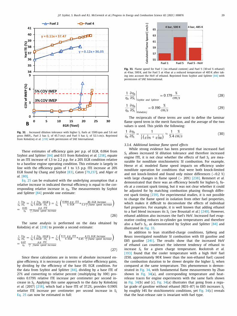
J.P. Szybist, S. Busch and R.L. McCormick et al. / Progress in Energy and Combustion Science 82 (2021) 100876 29
Fig. 32. . Increased dilution tolerance with higher S L fuels at 1500 rpm and 5.6 net
gross IMEP n . Fuel 2 has S L of 45.7 cm/s and Fuel 5 has S L of 52.1 cm/s. Reprinted
from Kolodziej et al. [218] with permission of SAE International.
S
t
t
l
E
a
r
r
a
=
K
=
g
b
t
2
v
c
e
r
E
Fig. 33. Flame speed for Fuel 1 (no ethanol content) and Fuel 5 (30 vol % ethanol)
at 4 bar, 500 K, and for Fuel 5 at 4 bar at a reduced temperature of 485 K after tak-
ing into account the HoV of ethanol. Reprinted from Szybist and Splitter [84] with
permission of SAE International.
fl
v
3
S
e
s
H
n
a
w
d
e
b
e
t
w
f
t
e
o
a
i
R
E
o
i
[
(
t
c
s
s
r
i
l
b
t
These estimates of efficiency gain per p.p. of EGR, 0.064 from
zybist and Splitter [84] and 0.11 from Kolodziej et al. [218] , equate
o an ITE increase of 1.3 to 2.2 p.p. for a 20% EGR condition relative
o a baseline engine operating condition. This estimate is largely in
ine with the efficiency gains of 1 to 1.5 p.p. ITE increase at 20%
GR found by Chang and Szybist [83] , Caton [ 79 , 237 ], and Alger et
l. [80] .
Eq. 25 can be evaluated with the underlying assumption that a
elative increase in indicated thermal efficiency is equal to the cor-
esponding relative increase in ηb . The measurements by Szybist
nd Splitter [84] provide one estimate:
1 ηb
∂ ηb
∂ S L =
1 ηb
(∂ ηb
∂EGR ∂EGR ∂ S L
)=
1 ηb
(0 . 064 p.p. IT E
% EGR ∗ 4 % EGR Increase
5 . 3 cm s f lame speed increase
)
0 . 05 ηb
p.p. IT E cm s f lame speed increase
(26)
The same analysis is performed on the data obtained by
olodziej et al. [218] to provide a second estimate:
1 ηb
∂ ηb
∂ S L =
1 ηb
(∂ ηb
∂EGR ∂EGR ∂ S L
)=
1 ηb
(0 . 11 p.p. IT E
% EGR ∗ 4 . 1 % EGR Increase
6 . 45 cm s f lame speed increase
)
0 . 07 ηb
p.p. IT E cm s f lame speed increase
(27)
Since these calculations are in terms of absolute increased en-
ine efficiency, it is necessary to convert to relative efficiency gains,
y dividing by the efficiency of the base 0% EGR condition. For
he data from Szybist and Splitter [84] , dividing by a base ITE of
7% and converting to relative percent (multiplying by 100) pro-
ides 0.179% relative ITE increase per centimeter per second in-
rease in S L . Applying this same approach to the data by Kolodziej
t al. (2017) [218] , which had a base ITE of 37.2%, provides 0.190%
elative ITE increase per centimeter per second increase in S L q. 25 can now be estimated in full:
1
ηb
∂ ηb
∂ S L
∣∣∣∣Szybist and Splitter
= 0 . 179
%
cm/s (28)
1
ηb
∂ ηb
∂ S L
∣∣∣∣Kolodzie j
= 0 . 190
%
cm/s (29)
The reciprocals of these terms are used to define the laminar
ame speed term in the merit function, and the average of the two
alues is used. This yields the following:
1
ηb
∂ ηb
∂ S L =
1
1 2
(1
0 . 179 +
1 0 . 190
) ≈ 1
5 . 4
%
cm/s (30)
.3.4. Additional laminar flame speed effects
While strong evidence has been presented that increased fuel
L allows increased SI dilution tolerance and therefore increased
ngine ITE, it is not clear whether the effects of fuel S L are mea-
urable for nondilute stoichiometric SI combustion. For example,
eese et al. modeled flame speed impacts on efficiency under
ondilute operation for conditions that were both knock-limited
nd not knock-limited and found only minor differences ( < 0.2 %)
ith large changes in flame speed ( > 20%) [238] . Remmert et al.
emonstrated that there was an efficiency benefit for higher- S L fu-
ls at a constant spark timing, but it was not clear whether it could
e adjusted for by matching combustion phasing through differ-
nt spark timing [239] . For experimental studies, it is not possible
o change the flame speed in isolation from other fuel properties,
hich makes it difficult to deconvolute the effects of individual
uel properties. For example, it is well known that adding ethanol
o a fuel blend increases its S L (see Broustail et al. ) [240] . However,
thanol addition also increases the fuel’s HoV. Increased fuel evap-
rative cooling reduces in-cylinder gas temperatures and therefore
lso a fuel’s S L , as demonstrated by Szybist and Splitter [84] and
llustrated in Fig. 33 .
In addition to lean stratified-charge conditions, Sjöberg and
euss investigated nondilute SI combustion with E0 gasoline and
85 gasoline [241] . The results show that the increased HoV
f ethanol can counteract the inherent tendency of ethanol to
ncrease S L for a given charge temperature. Rockstroh et al.
193] found that the cooler temperature with a high HoV fuel
E50, approximately 90 K lower than the non-ethanol fuel) caused
he combustion duration to be slower despite the higher S L when
ompared at the same temperature. This phenomenon is demon-
trated in Fig. 34 , with fundamental flame measurements by Zhao
hown in Fig. 34 (a), and corresponding temperature and heat-
elease traces for engine experiments with the same fuels shown
n Fig. 34 (b) and (c). Fig. 34 (a) illustrates that going from a regu-
ar grade of gasoline without ethanol (RD3–87) to E85 increases S L y roughly 14% for stoichiometric conditions, yet Fig. 34 (c) reveals
hat the heat-release rate is invariant with fuel type.
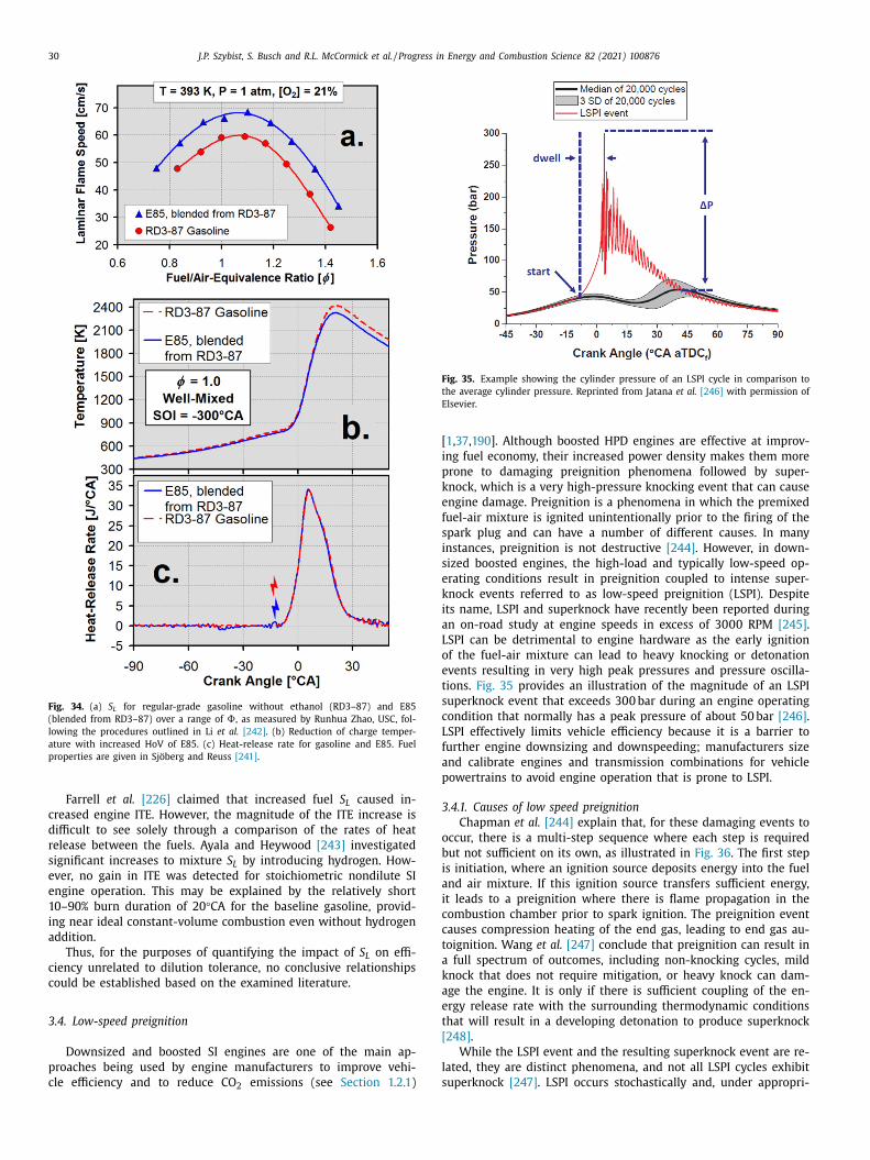
30 J.P. Szybist, S. Busch and R.L. McCormick et al. / Progress in Energy and Combustion Science 82 (2021) 100876
Fig. 34. (a) S L for regular-grade gasoline without ethanol (RD3–87) and E85
(blended from RD3–87) over a range of , as measured by Runhua Zhao, USC, fol-
lowing the procedures outlined in Li et al. [242] . (b) Reduction of charge temper-
ature with increased HoV of E85. (c) Heat-release rate for gasoline and E85. Fuel
properties are given in Sjöberg and Reuss [241] .
Fig. 35. Example showing the cylinder pressure of an LSPI cycle in comparison to
the average cylinder pressure. Reprinted from Jatana et al. [246] with permission of
Elsevier.
[
i
p
k
e
f
s
i
s
e
k
i
a
L
o
e
t
s
c
L
f
a
p
3
o
b
i
a
i
c
c
t
a
k
a
e
t
[
l
s
Farrell et al. [226] claimed that increased fuel S L caused in-
creased engine ITE. However, the magnitude of the ITE increase is
difficult to see solely through a comparison of the rates of heat
release between the fuels. Ayala and Heywood [243] investigated
significant increases to mixture S L by introducing hydrogen. How-
ever, no gain in ITE was detected for stoichiometric nondilute SI
engine operation. This may be explained by the relatively short
10–90% burn duration of 20 °CA for the baseline gasoline, provid-
ing near ideal constant-volume combustion even without hydrogen
addition.
Thus, for the purposes of quantifying the impact of S L on effi-
ciency unrelated to dilution tolerance, no conclusive relationships
could be established based on the examined literature.
3.4. Low-speed preignition
Downsized and boosted SI engines are one of the main ap-
proaches being used by engine manufacturers to improve vehi-
cle efficiency and to reduce CO emissions (see Section 1.2.1 )
21 , 37 , 190 ]. Although boosted HPD engines are effective at improv-
ng fuel economy, their increased power density makes them more
rone to damaging preignition phenomena followed by super-
nock, which is a very high-pressure knocking event that can cause
ngine damage. Preignition is a phenomena in which the premixed
uel-air mixture is ignited unintentionally prior to the firing of the
park plug and can have a number of different causes. In many
nstances, preignition is not destructive [244] . However, in down-
ized boosted engines, the high-load and typically low-speed op-
rating conditions result in preignition coupled to intense super-
nock events referred to as low-speed preignition (LSPI). Despite
ts name, LSPI and superknock have recently been reported during
n on-road study at engine speeds in excess of 30 0 0 RPM [245] .
SPI can be detrimental to engine hardware as the early ignition
f the fuel-air mixture can lead to heavy knocking or detonation
vents resulting in very high peak pressures and pressure oscilla-
ions. Fig. 35 provides an illustration of the magnitude of an LSPI
uperknock event that exceeds 300 bar during an engine operating
ondition that normally has a peak pressure of about 50 bar [246] .
SPI effectively limits vehicle efficiency because it is a barrier to
urther engine downsizing and downspeeding; manufacturers size
nd calibrate engines and transmission combinations for vehicle
owertrains to avoid engine operation that is prone to LSPI.
.4.1. Causes of low speed preignition
Chapman et al. [244] explain that, for these damaging events to
ccur, there is a multi-step sequence where each step is required
ut not sufficient on its own, as illustrated in Fig. 36 . The first step
s initiation, where an ignition source deposits energy into the fuel
nd air mixture. If this ignition source transfers sufficient energy,
t leads to a preignition where there is flame propagation in the
ombustion chamber prior to spark ignition. The preignition event
auses compression heating of the end gas, leading to end gas au-
oignition. Wang et al. [247] conclude that preignition can result in
full spectrum of outcomes, including non-knocking cycles, mild
nock that does not require mitigation, or heavy knock can dam-
ge the engine. It is only if there is sufficient coupling of the en-
rgy release rate with the surrounding thermodynamic conditions
hat will result in a developing detonation to produce superknock
248] .
While the LSPI event and the resulting superknock event are re-
ated, they are distinct phenomena, and not all LSPI cycles exhibit
uperknock [247] . LSPI occurs stochastically and, under appropri-
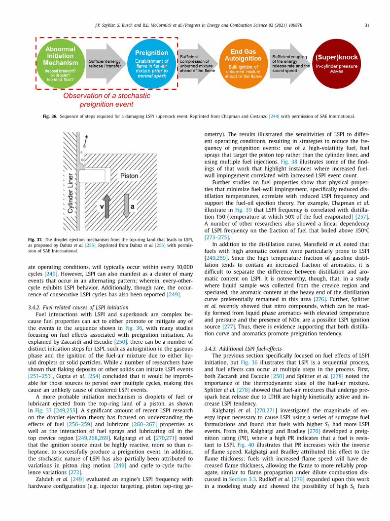
J.P. Szybist, S. Busch and R.L. McCormick et al. / Progress in Energy and Combustion Science 82 (2021) 100876 31
Fig. 36. Sequence of steps required for a damaging LSPI superkock event. Reprinted from Chapman and Costanzo [244] with permission of SAE International.
Fig. 37. The droplet ejection mechanism from the top-ring land that leads to LSPI,
as proposed by Dahnz et al. [255] . Reprinted from Dahnz et al. [255] with permis-
sion of SAE International.
a
c
e
c
r
3
c
t
f
e
d
p
u
s
[
a
c
l
i
o
e
w
t
t
h
t
v
l
h
o
e
q
s
u
i
w
t
t
s
i
t
A
o
[
f
[
l
d
m
w
s
c
e
i
a
s
t
3
i
a
b
i
S
s
c
e
f
e
n
t
o
fl
c
a
c
i
te operating conditions, will typically occur within every 10,0 0 0
ycles [249] . However, LSPI can also manifest as a cluster of many
vents that occur in an alternating pattern; wherein, every-other-
ycle exhibits LSPI behavior. Additionally, though rare, the occur-
ence of consecutive LSPI cycles has also been reported [249] .
.4.2. Fuel-related causes of LSPI initiation
Fuel interactions with LSPI and superknock are complex be-
ause fuel properties can act to either promote or mitigate any of
he events in the sequence shown in Fig. 36 , with many studies
ocusing on fuel effects associated with preignition initiation. As
xplained by Zaccardi and Escudie [250] , there can be a number of
istinct initiation steps for LSPI, such as autoignition in the gaseous
hase and the ignition of the fuel-air mixture due to either liq-
id droplets or solid particles. While a number of researchers have
hown that flaking deposits or other solids can initiate LSPI events
251–253] , Gupta et al. [254] concluded that it would be improb-
ble for those sources to persist over multiple cycles, making this
ause an unlikely cause of clustered LSPI events.
A more probable initiation mechanism is droplets of fuel or
ubricant ejected from the top-ring land of a piston, as shown
n Fig. 37 [ 249 , 255 ]. A significant amount of recent LSPI research
n the droplet ejection theory has focused on understanding the
ffects of fuel [256–259] and lubricant [260–267] properties as
ell as the interaction of fuel sprays and lubricating oil in the
op crevice region [ 24 9 , 26 8 , 269 ]. Kalghatgi et al. [ 270 , 271 ] noted
hat the ignition source must be highly reactive, more so than n-
eptane, to successfully produce a preignition event. In addition,
he stochastic nature of LSPI has also partially been attributed to
ariations in piston ring motion [249] and cycle-to-cycle turbu-
ence variations [272] .
Zahdeh et al. [249] evaluated an engine’s LSPI frequency with
ardware configuration (e.g. injector targeting, piston top-ring ge-
metry). The results illustrated the sensitivities of LSPI to differ-
nt operating conditions, resulting in strategies to reduce the fre-
uency of preignition events: use of a high-volatility fuel, fuel
prays that target the piston top rather than the cylinder liner, and
sing multiple fuel injections. Fig. 38 illustrates some of the find-
ngs of that work that highlight instances where increased fuel-
all impingement correlated with increased LSPI event count.
Further studies on fuel properties show that physical proper-
ies that minimize fuel-wall impingement, specifically reduced dis-
illation temperatures, correlate with reduced LSPI frequency and
upport the fuel-oil ejection theory. For example, Chapman et al.
llustrate in Fig. 39 that LSPI frequency is correlated with distilla-
ion T50 (temperature at which 50% of the fuel evaporated) [257] .
number of other researchers also showed a linear dependency
f LSPI frequency on the fraction of fuel that boiled above 150 °C273–275] .
In addition to the distillation curve, Mansfield et al. noted that
uels with high aromatic content were particularly prone to LSPI
249 , 259 ]. Since the high temperature fraction of gasoline distil-
ation tends to contain an increased fraction of aromatics, it is
ifficult to separate the difference between distillation and aro-
atic content on LSPI. It is noteworthy, though, that, in a study
here liquid sample was collected from the crevice region and
peciated, the aromatic content at the heavy end of the distillation
urve preferentially remained in this area [276] . Further, Splitter
t al. recently showed that nitro compounds, which can be read-
ly formed from liquid phase aromatics with elevated temperature
nd pressure and the presence of NOx, are a possible LSPI ignition
ource [277] . Thus, there is evidence supporting that both distilla-
ion curve and aromatics promote preignition tendency.
.4.3. Additional LSPI fuel-effects
The previous section specifically focused on fuel effects of LSPI
nitiation, but Fig. 36 illustrates that LSPI is a sequential process,
nd fuel effects can occur at multiple steps in the process. First,
oth Zaccardi and Escudie [250] and Splitter et al. [278] noted the
mportance of the thermodynamic state of the fuel-air mixture.
plitter et al. [278] showed that fuel-air mixtures that undergo pre-
park heat release due to LTHR are highly kinetically active and in-
rease LSPI tendency.
Kalghatgi et al. [ 270 , 271 ] investigated the magnitude of en-
rgy input necessary to cause LSPI using a series of surrogate fuel
ormulations and found that fuels with higher S L had more LSPI
vents. From this, Kalghatgi and Bradley [270] developed a preig-
ition rating (PR), where a high PR indicates that a fuel is resis-
ant to LSPI. Fig. 40 illustrates that PR increases with the inverse
f flame speed. Kalghatgi and Bradley attributed this effect to the
ame thickness: fuels with increased flame speed will have de-
reased flame thickness, allowing the flame to more reliably prop-
gate, similar to flame propagation under dilute combustion dis-
ussed in Section 3.3 . Rudloff et al. [279] expanded upon this work
n a modeling study and showed the possibility of high S fuels
L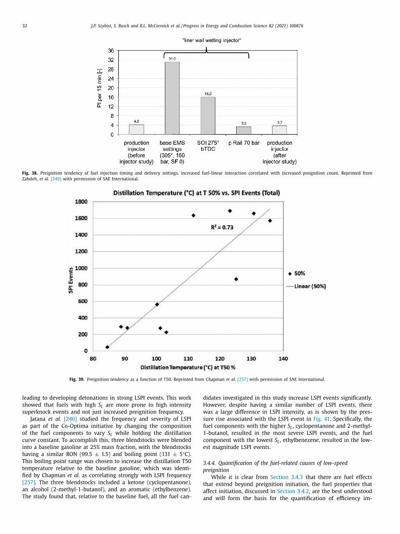
32 J.P. Szybist, S. Busch and R.L. McCormick et al. / Progress in Energy and Combustion Science 82 (2021) 100876
Fig. 38. Preignition tendency of fuel injection timing and delivery settings, increased fuel-linear interaction correlated with increased preignition count. Reprinted from
Zahdeh, et al. [249] with permission of SAE International.
Fig. 39. Preignition tendency as a function of T50. Reprinted from Chapman et al. [257] with permission of SAE International.
d
H
w
s
f
1
c
e
3
p
t
a
leading to developing detonations in strong LSPI events. This work
showed that fuels with high S L are more prone to high intensity
superknock events and not just increased preignition frequency.
Jatana et al. [246] studied the frequency and severity of LSPI
as part of the Co-Optima initiative by changing the composition
of the fuel components to vary S L while holding the distillation
curve constant. To accomplish this, three blendstocks were blended
into a baseline gasoline at 25% mass fraction, with the blendstocks
having a similar RON (99.5 ± 1.5) and boiling point (131 ± 5 °C).
This boiling point range was chosen to increase the distillation T50
temperature relative to the baseline gasoline, which was identi-
fied by Chapman et al. as correlating strongly with LSPI frequency
[257] . The three blendstocks included a ketone (cyclopentanone),
an alcohol (2-methyl-1-butanol), and an aromatic (ethylbenzene).
The study found that, relative to the baseline fuel, all the fuel can-
aidates investigated in this study increase LSPI events significantly.
owever, despite having a similar number of LSPI events, there
as a large difference in LSPI intensity, as is shown by the pres-
ure rise associated with the LSPI event in Fig. 41 . Specifically, the
uel components with the higher S L , cyclopentanone and 2-methyl-
-butanol, resulted in the most severe LSPI events, and the fuel
omponent with the lowest S L , ethylbenezene, resulted in the low-
st magnitude LSPI events.
.4.4. Quantification of the fuel-related causes of low-speed
reignition
While it is clear from Section 3.4.3 that there are fuel effects
hat extend beyond preignition initiation, the fuel properties that
ffect initiation, discussed in Section 3.4.2 , are the best understood
nd will form the basis for the quantification of efficiency im-
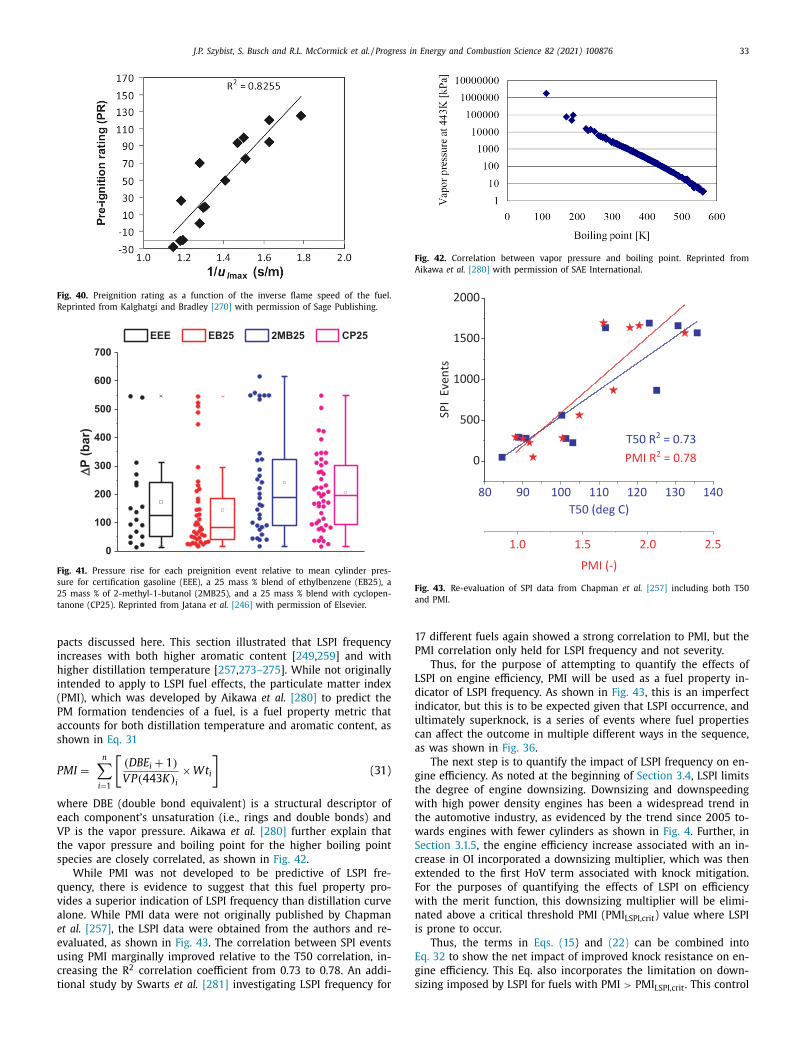
J.P. Szybist, S. Busch and R.L. McCormick et al. / Progress in Energy and Combustion Science 82 (2021) 100876 33
Fig. 40. Preignition rating as a function of the inverse flame speed of the fuel.
Reprinted from Kalghatgi and Bradley [270] with permission of Sage Publishing.
Fig. 41. Pressure rise for each preignition event relative to mean cylinder pres-
sure for certification gasoline (EEE), a 25 mass % blend of ethylbenzene (EB25), a
25 mass % of 2-methyl-1-butanol (2MB25), and a 25 mass % blend with cyclopen-
tanone (CP25). Reprinted from Jatana et al. [246] with permission of Elsevier.
p
i
h
i
(
P
a
s
P
w
e
V
t
s
q
v
a
e
e
u
c
t
Fig. 42. Correlation between vapor pressure and boiling point. Reprinted from
Aikawa et al. [280] with permission of SAE International.
Fig. 43. Re-evaluation of SPI data from Chapman et al. [257] including both T50
and PMI.
1
P
L
d
i
u
c
a
g
t
w
t
w
S
c
e
F
w
n
i
E
g
s
acts discussed here. This section illustrated that LSPI frequency
ncreases with both higher aromatic content [ 249 , 259 ] and with
igher distillation temperature [ 257 , 273–275 ]. While not originally
ntended to apply to LSPI fuel effects, the particulate matter index
PMI), which was developed by Aikawa et al. [280] to predict the
M formation tendencies of a fuel, is a fuel property metric that
ccounts for both distillation temperature and aromatic content, as
hown in Eq. 31
MI =
n ∑
i =1
[( DB E i + 1 )
V P ( 443 K ) i × W t i
](31)
here DBE (double bond equivalent) is a structural descriptor of
ach component’s unsaturation (i.e., rings and double bonds) and
P is the vapor pressure. Aikawa et al. [280] further explain that
he vapor pressure and boiling point for the higher boiling point
pecies are closely correlated, as shown in Fig. 42 .
While PMI was not developed to be predictive of LSPI fre-
uency, there is evidence to suggest that this fuel property pro-
ides a superior indication of LSPI frequency than distillation curve
lone. While PMI data were not originally published by Chapman
t al. [257] , the LSPI data were obtained from the authors and re-
valuated, as shown in Fig. 43 . The correlation between SPI events
sing PMI marginally improved relative to the T50 correlation, in-
reasing the R
2 correlation coefficient from 0.73 to 0.78. An addi-
ional study by Swarts et al. [281] investigating LSPI frequency for
7 different fuels again showed a strong correlation to PMI, but the
MI correlation only held for LSPI frequency and not severity.
Thus, for the purpose of attempting to quantify the effects of
SPI on engine efficiency, PMI will be used as a fuel property in-
icator of LSPI frequency. As shown in Fig. 43 , this is an imperfect
ndicator, but this is to be expected given that LSPI occurrence, and
ltimately superknock, is a series of events where fuel properties
an affect the outcome in multiple different ways in the sequence,
s was shown in Fig. 36 .
The next step is to quantify the impact of LSPI frequency on en-
ine efficiency. As noted at the beginning of Section 3.4 , LSPI limits
he degree of engine downsizing. Downsizing and downspeeding
ith high power density engines has been a widespread trend in
he automotive industry, as evidenced by the trend since 2005 to-
ards engines with fewer cylinders as shown in Fig. 4 . Further, in
ection 3.1.5 , the engine efficiency increase associated with an in-
rease in OI incorporated a downsizing multiplier, which was then
xtended to the first HoV term associated with knock mitigation.
or the purposes of quantifying the effects of LSPI on efficiency
ith the merit function, this downsizing multiplier will be elimi-
ated above a critical threshold PMI (PMI LSPI,crit ) value where LSPI
s prone to occur.
Thus, the terms in Eqs. (15 ) and (22) can be combined into
q. 32 to show the net impact of improved knock resistance on en-
ine efficiency. This Eq. also incorporates the limitation on down-
izing imposed by LSPI for fuels with PMI > PMI LSPI,crit . This control
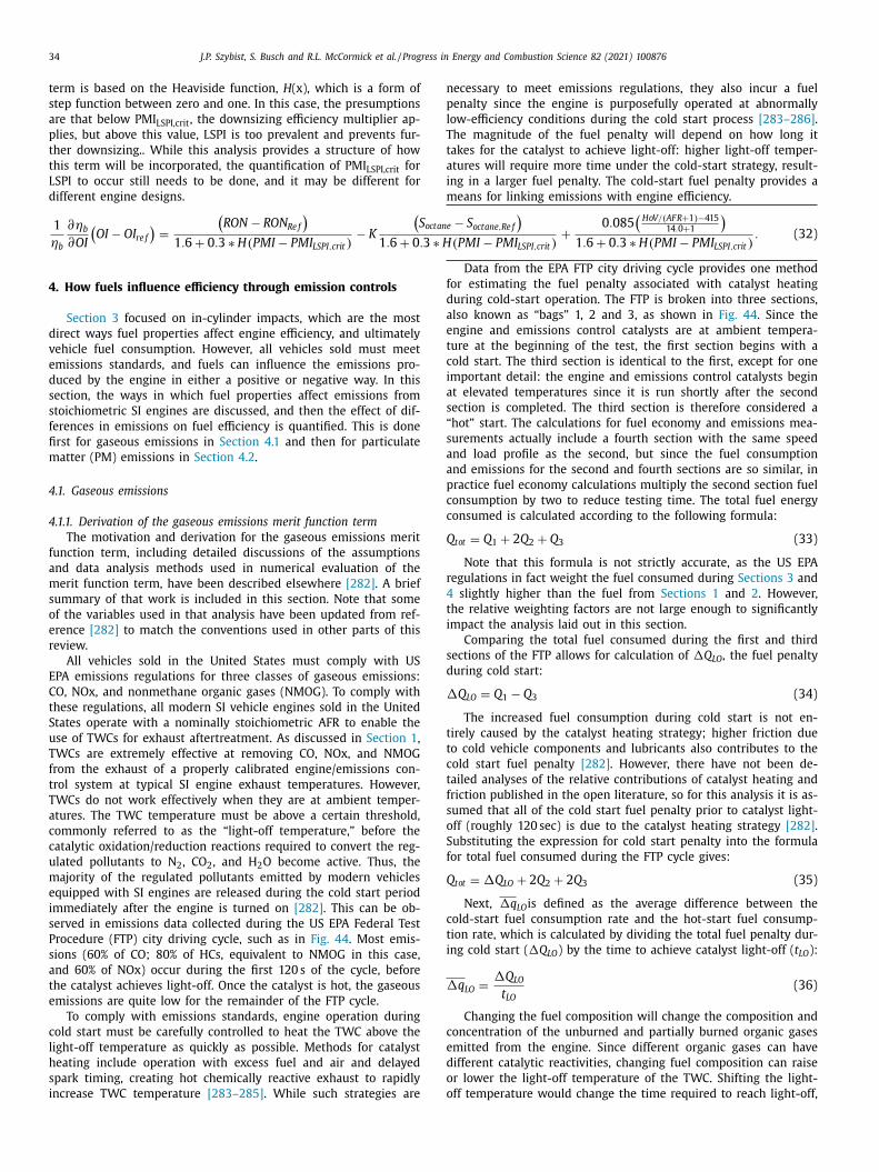
34 J.P. Szybist, S. Busch and R.L. McCormick et al. / Progress in Energy and Combustion Science 82 (2021) 100876
octan
3 ∗ H
n
p
l
T
t
a
i
m
f
d
a
e
t
c
i
a
s
“
s
a
a
p
c
c
Q
r
4
t
i
s
d
�
t
t
c
t
f
s
o
S
f
Q
c
t
i
�
c
e
d
o
o
term is based on the Heaviside function, H (x), which is a form of
step function between zero and one. In this case, the presumptions
are that below PMI LSPI,crit , the downsizing efficiency multiplier ap-
plies, but above this value, LSPI is too prevalent and prevents fur-
ther downsizing.. While this analysis provides a structure of how
this term will be incorporated, the quantification of PMI LSPI,crit for
LSPI to occur still needs to be done, and it may be different for
different engine designs.
1
ηb
∂ ηb
∂OI
(OI − O I re f
)=
(RON − RO N Re f
)1 . 6 + 0 . 3 ∗ H ( P MI − P M I LSPI,crit )
− K
(S
1 . 6 + 0 .
4. How fuels influence efficiency through emission controls
Section 3 focused on in-cylinder impacts, which are the most
direct ways fuel properties affect engine efficiency, and ultimately
vehicle fuel consumption. However, all vehicles sold must meet
emissions standards, and fuels can influence the emissions pro-
duced by the engine in either a positive or negative way. In this
section, the ways in which fuel properties affect emissions from
stoichiometric SI engines are discussed, and then the effect of dif-
ferences in emissions on fuel efficiency is quantified. This is done
first for gaseous emissions in Section 4.1 and then for particulate
matter (PM) emissions in Section 4.2 .
4.1. Gaseous emissions
4.1.1. Derivation of the gaseous emissions merit function term
The motivation and derivation for the gaseous emissions merit
function term, including detailed discussions of the assumptions
and data analysis methods used in numerical evaluation of the
merit function term, have been described elsewhere [282] . A brief
summary of that work is included in this section. Note that some
of the variables used in that analysis have been updated from ref-
erence [282] to match the conventions used in other parts of this
review.
All vehicles sold in the United States must comply with US
EPA emissions regulations for three classes of gaseous emissions:
CO, NOx, and nonmethane organic gases (NMOG). To comply with
these regulations, all modern SI vehicle engines sold in the United
States operate with a nominally stoichiometric AFR to enable the
use of TWCs for exhaust aftertreatment. As discussed in Section 1 ,
TWCs are extremely effective at removing CO, NOx, and NMOG
from the exhaust of a properly calibrated engine/emissions con-
trol system at typical SI engine exhaust temperatures. However,
TWCs do not work effectively when they are at ambient temper-
atures. The TWC temperature must be above a certain threshold,
commonly referred to as the “light-off temperature,” before the
catalytic oxidation/reduction reactions required to convert the reg-
ulated pollutants to N 2 , CO 2 , and H 2 O become active. Thus, the
majority of the regulated pollutants emitted by modern vehicles
equipped with SI engines are released during the cold start period
immediately after the engine is turned on [282] . This can be ob-
served in emissions data collected during the US EPA Federal Test
Procedure (FTP) city driving cycle, such as in Fig. 44 . Most emis-
sions (60% of CO; 80% of HCs, equivalent to NMOG in this case,
and 60% of NOx) occur during the first 120 s of the cycle, before
the catalyst achieves light-off. Once the catalyst is hot, the gaseous
emissions are quite low for the remainder of the FTP cycle.
To comply with emissions standards, engine operation during
cold start must be carefully controlled to heat the TWC above the
light-off temperature as quickly as possible. Methods for catalyst
heating include operation with excess fuel and air and delayed
spark timing, creating hot chemically reactive exhaust to rapidly
increase TWC temperature [283–285] . While such strategies are
e − S octane,Re f
) ( P MI − P M I LSPI,crit )
+
0 . 085
(HoV/ ( AF R +1 ) −415
14 . 0+1
)1 . 6 + 0 . 3 ∗ H ( P MI − P M I LSPI,crit )
. (32)
ecessary to meet emissions regulations, they also incur a fuel
enalty since the engine is purposefully operated at abnormally
ow-efficiency conditions during the cold start process [283–286] .
he magnitude of the fuel penalty will depend on how long it
akes for the catalyst to achieve light-off: higher light-off temper-
tures will require more time under the cold-start strategy, result-
ng in a larger fuel penalty. The cold-start fuel penalty provides a
eans for linking emissions with engine efficiency.
Data from the EPA FTP city driving cycle provides one method
or estimating the fuel penalty associated with catalyst heating
uring cold-start operation. The FTP is broken into three sections,
lso known as “bags” 1, 2 and 3, as shown in Fig. 44 . Since the
ngine and emissions control catalysts are at ambient tempera-
ure at the beginning of the test, the first section begins with a
old start. The third section is identical to the first, except for one
mportant detail: the engine and emissions control catalysts begin
t elevated temperatures since it is run shortly after the second
ection is completed. The third section is therefore considered a
hot” start. The calculations for fuel economy and emissions mea-
urements actually include a fourth section with the same speed
nd load profile as the second, but since the fuel consumption
nd emissions for the second and fourth sections are so similar, in
ractice fuel economy calculations multiply the second section fuel
onsumption by two to reduce testing time. The total fuel energy
onsumed is calculated according to the following formula:
tot = Q 1 + 2 Q 2 + Q 3 (33)
Note that this formula is not strictly accurate, as the US EPA
egulations in fact weight the fuel consumed during Sections 3 and
slightly higher than the fuel from Sections 1 and 2 . However,
he relative weighting factors are not large enough to significantly
mpact the analysis laid out in this section.
Comparing the total fuel consumed during the first and third
ections of the FTP allows for calculation of �Q LO , the fuel penalty
uring cold start:
Q LO = Q 1 − Q 3 (34)
The increased fuel consumption during cold start is not en-
irely caused by the catalyst heating strategy; higher friction due
o cold vehicle components and lubricants also contributes to the
old start fuel penalty [282] . However, there have not been de-
ailed analyses of the relative contributions of catalyst heating and
riction published in the open literature, so for this analysis it is as-
umed that all of the cold start fuel penalty prior to catalyst light-
ff (roughly 120 sec) is due to the catalyst heating strategy [282] .
ubstituting the expression for cold start penalty into the formula
or total fuel consumed during the FTP cycle gives:
tot = �Q LO + 2 Q 2 + 2 Q 3 (35)
Next, �q LO is defined as the average difference between the
old-start fuel consumption rate and the hot-start fuel consump-
ion rate, which is calculated by dividing the total fuel penalty dur-
ng cold start ( �Q LO ) by the time to achieve catalyst light-off ( t LO ):
q LO =
�Q LO
t LO
(36)
Changing the fuel composition will change the composition and
oncentration of the unburned and partially burned organic gases
mitted from the engine. Since different organic gases can have
ifferent catalytic reactivities, changing fuel composition can raise
r lower the light-off temperature of the TWC. Shifting the light-
ff temperature would change the time required to reach light-off,
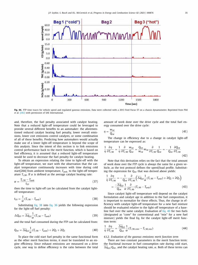
J.P. Szybist, S. Busch and R.L. McCormick et al. / Progress in Energy and Combustion Science 82 (2021) 100876 35
Fig. 44. FTP time traces for vehicle speed and regulated gaseous emissions. Data were collected with a 2013 Ford Focus ST on a chassis dynamometer. Reprinted from Pihl
et al. [282] with permission of SAE International.
a
N
p
t
s
o
m
t
c
f
w
l
a
s
a
α
t
o
t
f
�
a
Q
a
g
c
a
e
η
t
o
h
i
f
i
fi
s
l
(
m
t
4
t
�
nd, therefore, the fuel penalty associated with catalyst heating.
ote that a reduced light-off temperature could be leveraged to
rovide several different benefits to an automaker: the aforemen-
ioned reduced catalyst heating fuel penalty, lower overall emis-
ions, lower cost emissions control catalysts, or some combination
f all of these benefits. Predicting how automakers would actually
ake use of a lower light-off temperature is beyond the scope of
his analysis. Since the intent of this section is to link emissions
ontrol performance back to the merit function, which is based on
uel efficiency, it is assumed that a reduced light-off temperature
ould be used to decrease the fuel penalty for catalyst heating.
To obtain an expression relating the time to light-off with the
ight-off temperature, we start with the observation that the cat-
lyst temperature continuously increases with time during cold
tart[284] from ambient temperature, T amb , to the light-off temper-
ture T c,90 . If α is defined as the average catalyst heating rate:
=
T c, 90 − T amb
t LO
(37)
hen the time to light-off can be calculated from the catalyst light-
ff temperature:
LO =
1
α( T c, 90 − T amb ) (38)
Substituting Eq. 38 into Eq. 36 yields the following expression
or the light-off fuel penalty:
Q LO = �q LO
1
α( T c, 90 − T amb ) (39)
nd the total fuel consumed during the FTP can be calculated from:
tot = �q LO
1
α( T c, 90 − T amb ) + 2 Q 2 + 2 Q 3 (40)
To place the cold start fuel penalty in the same functional form
s the other merit function terms, it must be translated to an en-
ine efficiency. Since exhaust emissions are measured on a drive
ycle, one way to define efficiency is the ratio between the total
mount of work done over the drive cycle and the total fuel en-
rgy consumed over the drive cycle:
=
w tot
Q tot (41)
The change in efficiency due to a change in catalyst light-off
emperature can be expressed as:
1
η
∂η
∂ T c, 90
=
1
η
∂
∂ T c, 90
w tot
Q tot =
Q tot
w tot w tot
∂
∂ T c, 90
1
Q tot = − 1
Q tot
∂ Q tot
∂ T c, 90
(42)
Note that this derivation relies on the fact that the total amount
f work done over the FTP cycle is always the same for a given ve-
icle, as the test protocol defines the speed/load profile. Substitut-
ng the expression for Q tot that was derived above yields:
1
η
∂η
∂ T c, 90
= − 1
Q tot
∂
∂ T c, 90
(�q LO
1
α( T c, 90 − T amb ) + 2 Q 2 + 2 Q 3
)=
−�q LO
Q tot
1
α
∂
∂ T c, 90 ( T c, 90 − T amb ) (43)
Since catalyst light-off temperature will depend on the catalyst
ormulation and catalyst age in addition to the fuel composition, it
s important to normalize for these effects. Thus, the change in ef-
ciency with catalyst light-off temperature for a new fuel mixture
hould be evaluated relative to the light-off temperature of a base-
ine fuel over the same catalyst. Evaluation of Eq. 43 for two fuels
designated as “conv” for conventional and “mix” for a new fuel
ixture) yields the final Eq. for the catalyst light-off merit func-
ion term:
1
η
∂η
∂ T c, 90
=
�q LO
Q tot
1
α( T c, 90 ,con v − T c, 90 ,mix ) (44)
.1.2. Evaluation of the gaseous emissions merit function term
There are two constant parameters in the merit function term:
he fractional increase in fuel consumption rate during cold start,
q LO / Q tot , and the catalyst heating rate, α. Both of these terms can
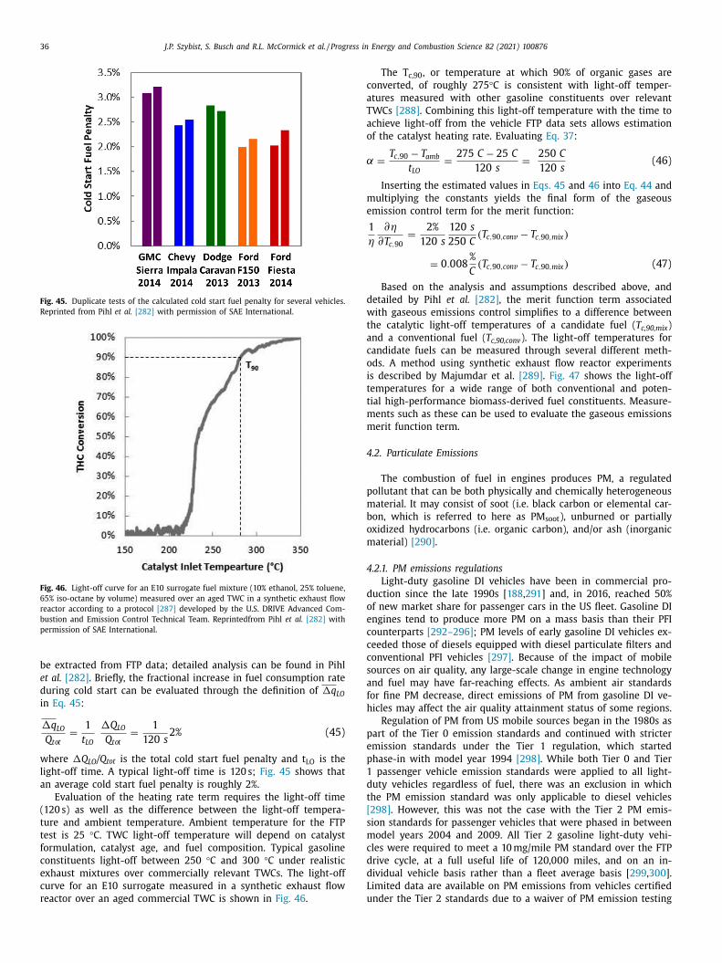
36 J.P. Szybist, S. Busch and R.L. McCormick et al. / Progress in Energy and Combustion Science 82 (2021) 100876
Fig. 45. Duplicate tests of the calculated cold start fuel penalty for several vehicles.
Reprinted from Pihl et al. [282] with permission of SAE International.
Fig. 46. Light-off curve for an E10 surrogate fuel mixture (10% ethanol, 25% toluene,
65% iso-octane by volume) measured over an aged TWC in a synthetic exhaust flow
reactor according to a protocol [287] developed by the U.S. DRIVE Advanced Com-
bustion and Emission Control Technical Team. Reprintedfrom Pihl et al. [282] with
permission of SAE International.
c
a
T
a
o
α
m
e
d
w
t
a
c
o
i
t
t
m
m
4
p
m
b
o
m
4
d
o
e
c
c
c
s
a
f
h
p
e
p
1
d
t
[
s
m
c
d
d
L
u
be extracted from FTP data; detailed analysis can be found in Pihl
et al. [282] . Briefly, the fractional increase in fuel consumption rate
during cold start can be evaluated through the definition of �q LO
in Eq. 45 :
�q LO
Q tot =
1
t LO
�Q LO
Q tot =
1
120 s 2% (45)
where �Q LO /Q tot is the total cold start fuel penalty and t LO is the
light-off time. A typical light-off time is 120 s; Fig. 45 shows that
an average cold start fuel penalty is roughly 2%.
Evaluation of the heating rate term requires the light-off time
(120 s) as well as the difference between the light-off tempera-
ture and ambient temperature. Ambient temperature for the FTP
test is 25 °C. TWC light-off temperature will depend on catalyst
formulation, catalyst age, and fuel composition. Typical gasoline
constituents light-off between 250 °C and 300 °C under realistic
exhaust mixtures over commercially relevant TWCs. The light-off
curve for an E10 surrogate measured in a synthetic exhaust flow
reactor over an aged commercial TWC is shown in Fig. 46 .
The T c,90 , or temperature at which 90% of organic gases are
onverted, of roughly 275 °C is consistent with light-off temper-
tures measured with other gasoline constituents over relevant
WCs [288] . Combining this light-off temperature with the time to
chieve light-off from the vehicle FTP data sets allows estimation
f the catalyst heating rate. Evaluating Eq. 37 :
=
T c, 90 − T amb
t LO
=
275 C − 25 C
120 s =
250 C
120 s (46)
Inserting the estimated values in Eqs. 45 and 46 into Eq. 44 and
ultiplying the constants yields the final form of the gaseous
mission control term for the merit function:
1
η
∂η
∂ T c, 90
=
2%
120 s
120 s
250 C ( T c, 90 ,con v − T c, 90 ,mix )
= 0 . 008
%
C ( T c, 90 ,con v − T c, 90 ,mix ) (47)
Based on the analysis and assumptions described above, and
etailed by Pihl et al. [282] , the merit function term associated
ith gaseous emissions control simplifies to a difference between
he catalytic light-off temperatures of a candidate fuel ( T c,90,mix )
nd a conventional fuel ( T c,90,conv ). The light-off temperatures for
andidate fuels can be measured through several different meth-
ds. A method using synthetic exhaust flow reactor experiments
s described by Majumdar et al. [289] . Fig. 47 shows the light-off
emperatures for a wide range of both conventional and poten-
ial high-performance biomass-derived fuel constituents. Measure-
ents such as these can be used to evaluate the gaseous emissions
erit function term.
.2. Particulate Emissions
The combustion of fuel in engines produces PM, a regulated
ollutant that can be both physically and chemically heterogeneous
aterial. It may consist of soot (i.e. black carbon or elemental car-
on, which is referred to here as PM soot ), unburned or partially
xidized hydrocarbons (i.e. organic carbon), and/or ash (inorganic
aterial) [290] .
.2.1. PM emissions regulations
Light-duty gasoline DI vehicles have been in commercial pro-
uction since the late 1990s [ 188 , 291 ] and, in 2016, reached 50%
f new market share for passenger cars in the US fleet. Gasoline DI
ngines tend to produce more PM on a mass basis than their PFI
ounterparts [292–296] ; PM levels of early gasoline DI vehicles ex-
eeded those of diesels equipped with diesel particulate filters and
onventional PFI vehicles [297] . Because of the impact of mobile
ources on air quality, any large-scale change in engine technology
nd fuel may have far-reaching effects. As ambient air standards
or fine PM decrease, direct emissions of PM from gasoline DI ve-
icles may affect the air quality attainment status of some regions.
Regulation of PM from US mobile sources began in the 1980s as
art of the Tier 0 emission standards and continued with stricter
mission standards under the Tier 1 regulation, which started
hase-in with model year 1994 [298] . While both Tier 0 and Tier
passenger vehicle emission standards were applied to all light-
uty vehicles regardless of fuel, there was an exclusion in which
he PM emission standard was only applicable to diesel vehicles
298] . However, this was not the case with the Tier 2 PM emis-
ion standards for passenger vehicles that were phased in between
odel years 2004 and 2009. All Tier 2 gasoline light-duty vehi-
les were required to meet a 10 mg/mile PM standard over the FTP
rive cycle, at a full useful life of 120,0 0 0 miles, and on an in-
ividual vehicle basis rather than a fleet average basis [ 299 , 300 ].
imited data are available on PM emissions from vehicles certified
nder the Tier 2 standards due to a waiver of PM emission testing
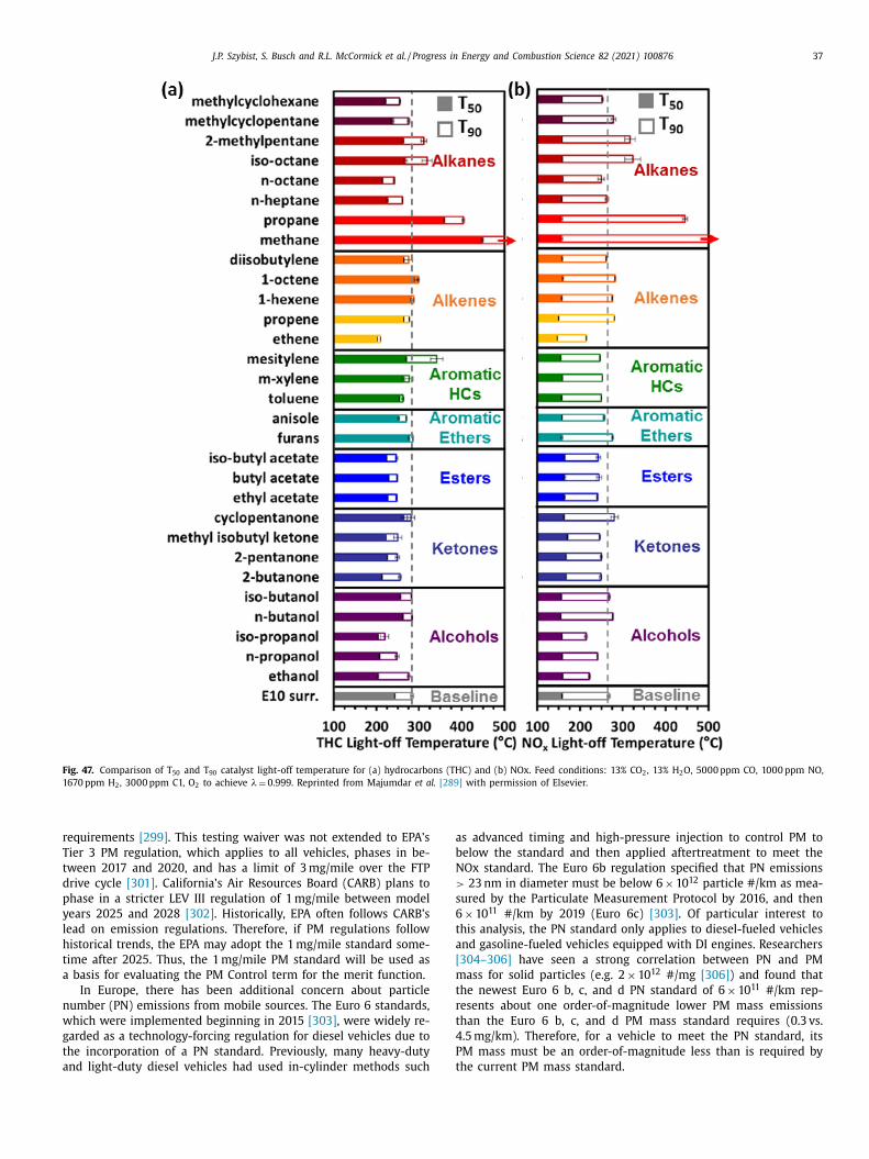
J.P. Szybist, S. Busch and R.L. McCormick et al. / Progress in Energy and Combustion Science 82 (2021) 100876 37
Fig. 47. Comparison of T 50 and T 90 catalyst light-off temperature for (a) hydrocarbons (THC) and (b) NOx. Feed conditions: 13% CO 2 , 13% H 2 O, 50 0 0 ppm CO, 10 0 0 ppm NO,
1670 ppm H 2 , 30 0 0 ppm C1, O 2 to achieve λ= 0.999. Reprinted from Majumdar et al. [289] with permission of Elsevier.
r
T
t
d
p
y
l
h
t
a
n
w
g
t
a
a
b
N
>
s
6
t
a
[
m
t
r
t
4
P
the current PM mass standard.
equirements [299] . This testing waiver was not extended to EPA’s
ier 3 PM regulation, which applies to all vehicles, phases in be-
ween 2017 and 2020, and has a limit of 3 mg/mile over the FTP
rive cycle [301] . California’s Air Resources Board (CARB) plans to
hase in a stricter LEV III regulation of 1 mg/mile between model
ears 2025 and 2028 [302] . Historically, EPA often follows CARB’s
ead on emission regulations. Therefore, if PM regulations follow
istorical trends, the EPA may adopt the 1 mg/mile standard some-
ime after 2025. Thus, the 1 mg/mile PM standard will be used as
basis for evaluating the PM Control term for the merit function.
In Europe, there has been additional concern about particle
umber (PN) emissions from mobile sources. The Euro 6 standards,
hich were implemented beginning in 2015 [303] , were widely re-
arded as a technology-forcing regulation for diesel vehicles due to
he incorporation of a PN standard. Previously, many heavy-duty
nd light-duty diesel vehicles had used in-cylinder methods such
s advanced timing and high-pressure injection to control PM to
elow the standard and then applied aftertreatment to meet the
Ox standard. The Euro 6b regulation specified that PN emissions
23 nm in diameter must be below 6 × 10 12 particle #/km as mea-
ured by the Particulate Measurement Protocol by 2016, and then
× 10 11 #/km by 2019 (Euro 6c) [303] . Of particular interest to
his analysis, the PN standard only applies to diesel-fueled vehicles
nd gasoline-fueled vehicles equipped with DI engines. Researchers
304–306] have seen a strong correlation between PN and PM
ass for solid particles (e.g. 2 × 10 12 #/mg [306] ) and found that
he newest Euro 6 b, c, and d PN standard of 6 × 10 11 #/km rep-
esents about one order-of-magnitude lower PM mass emissions
han the Euro 6 b, c, and d PM mass standard requires (0.3 vs.
.5 mg/km). Therefore, for a vehicle to meet the PN standard, its
M mass must be an order-of-magnitude less than is required by
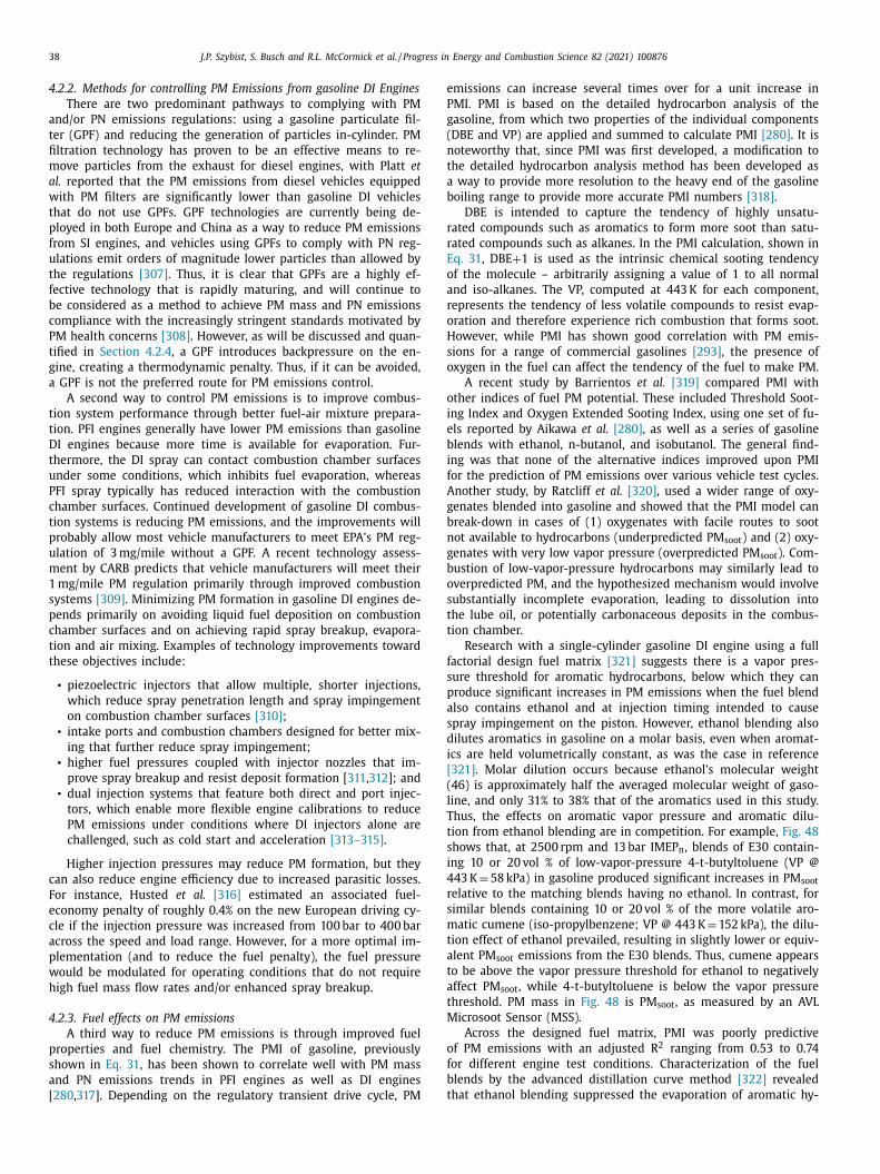
38 J.P. Szybist, S. Busch and R.L. McCormick et al. / Progress in Energy and Combustion Science 82 (2021) 100876
e
P
g
(
n
t
a
b
r
r
E
o
a
r
o
H
s
o
o
i
e
b
i
f
A
g
b
n
g
b
o
s
t
t
f
s
p
a
s
d
i
[
(
l
T
t
s
i
4
r
s
m
t
a
t
a
t
M
o
f
b
t
4.2.2. Methods for controlling PM Emissions from gasoline DI Engines
There are two predominant pathways to complying with PM
and/or PN emissions regulations: using a gasoline particulate fil-
ter (GPF) and reducing the generation of particles in-cylinder. PM
filtration technology has proven to be an effective means to re-
move particles from the exhaust for diesel engines, with Platt et
al. reported that the PM emissions from diesel vehicles equipped
with PM filters are significantly lower than gasoline DI vehicles
that do not use GPFs. GPF technologies are currently being de-
ployed in both Europe and China as a way to reduce PM emissions
from SI engines, and vehicles using GPFs to comply with PN reg-
ulations emit orders of magnitude lower particles than allowed by
the regulations [307] . Thus, it is clear that GPFs are a highly ef-
fective technology that is rapidly maturing, and will continue to
be considered as a method to achieve PM mass and PN emissions
compliance with the increasingly stringent standards motivated by
PM health concerns [308] . However, as will be discussed and quan-
tified in Section 4.2.4 , a GPF introduces backpressure on the en-
gine, creating a thermodynamic penalty. Thus, if it can be avoided,
a GPF is not the preferred route for PM emissions control.
A second way to control PM emissions is to improve combus-
tion system performance through better fuel-air mixture prepara-
tion. PFI engines generally have lower PM emissions than gasoline
DI engines because more time is available for evaporation. Fur-
thermore, the DI spray can contact combustion chamber surfaces
under some conditions, which inhibits fuel evaporation, whereas
PFI spray typically has reduced interaction with the combustion
chamber surfaces. Continued development of gasoline DI combus-
tion systems is reducing PM emissions, and the improvements will
probably allow most vehicle manufacturers to meet EPA’s PM reg-
ulation of 3 mg/mile without a GPF. A recent technology assess-
ment by CARB predicts that vehicle manufacturers will meet their
1 mg/mile PM regulation primarily through improved combustion
systems [309] . Minimizing PM formation in gasoline DI engines de-
pends primarily on avoiding liquid fuel deposition on combustion
chamber surfaces and on achieving rapid spray breakup, evapora-
tion and air mixing. Examples of technology improvements toward
these objectives include:
• piezoelectric injectors that allow multiple, shorter injections,
which reduce spray penetration length and spray impingement
on combustion chamber surfaces [310] ;
• intake ports and combustion chambers designed for better mix-
ing that further reduce spray impingement;
• higher fuel pressures coupled with injector nozzles that im-
prove spray breakup and resist deposit formation [ 311 , 312 ]; and
• dual injection systems that feature both direct and port injec-
tors, which enable more flexible engine calibrations to reduce
PM emissions under conditions where DI injectors alone are
challenged, such as cold start and acceleration [313–315] .
Higher injection pressures may reduce PM formation, but they
can also reduce engine efficiency due to increased parasitic losses.
For instance, Husted et al. [316] estimated an associated fuel-
economy penalty of roughly 0.4% on the new European driving cy-
cle if the injection pressure was increased from 100 bar to 400 bar
across the speed and load range. However, for a more optimal im-
plementation (and to reduce the fuel penalty), the fuel pressure
would be modulated for operating conditions that do not require
high fuel mass flow rates and/or enhanced spray breakup.
4.2.3. Fuel effects on PM emissions
A third way to reduce PM emissions is through improved fuel
properties and fuel chemistry. The PMI of gasoline, previously
shown in Eq. 31 , has been shown to correlate well with PM mass
and PN emissions trends in PFI engines as well as DI engines
[ 280 , 317 ]. Depending on the regulatory transient drive cycle, PM
missions can increase several times over for a unit increase in
MI. PMI is based on the detailed hydrocarbon analysis of the
asoline, from which two properties of the individual components
DBE and VP) are applied and summed to calculate PMI [280] . It is
oteworthy that, since PMI was first developed, a modification to
he detailed hydrocarbon analysis method has been developed as
way to provide more resolution to the heavy end of the gasoline
oiling range to provide more accurate PMI numbers [318] .
DBE is intended to capture the tendency of highly unsatu-
ated compounds such as aromatics to form more soot than satu-
ated compounds such as alkanes. In the PMI calculation, shown in
q. 31 , DBE + 1 is used as the intrinsic chemical sooting tendency
f the molecule – arbitrarily assigning a value of 1 to all normal
nd iso-alkanes. The VP, computed at 443 K for each component,
epresents the tendency of less volatile compounds to resist evap-
ration and therefore experience rich combustion that forms soot.
owever, while PMI has shown good correlation with PM emis-
ions for a range of commercial gasolines [293] , the presence of
xygen in the fuel can affect the tendency of the fuel to make PM.
A recent study by Barrientos et al. [319] compared PMI with
ther indices of fuel PM potential. These included Threshold Soot-
ng Index and Oxygen Extended Sooting Index, using one set of fu-
ls reported by Aikawa et al. [280] , as well as a series of gasoline
lends with ethanol, n-butanol, and isobutanol. The general find-
ng was that none of the alternative indices improved upon PMI
or the prediction of PM emissions over various vehicle test cycles.
nother study, by Ratcliff et al. [320] , used a wider range of oxy-
enates blended into gasoline and showed that the PMI model can
reak-down in cases of (1) oxygenates with facile routes to soot
ot available to hydrocarbons (underpredicted PM soot ) and (2) oxy-
enates with very low vapor pressure (overpredicted PM soot ). Com-
ustion of low-vapor-pressure hydrocarbons may similarly lead to
verpredicted PM, and the hypothesized mechanism would involve
ubstantially incomplete evaporation, leading to dissolution into
he lube oil, or potentially carbonaceous deposits in the combus-
ion chamber.
Research with a single-cylinder gasoline DI engine using a full
actorial design fuel matrix [321] suggests there is a vapor pres-
ure threshold for aromatic hydrocarbons, below which they can
roduce significant increases in PM emissions when the fuel blend
lso contains ethanol and at injection timing intended to cause
pray impingement on the piston. However, ethanol blending also
ilutes aromatics in gasoline on a molar basis, even when aromat-
cs are held volumetrically constant, as was the case in reference
321] . Molar dilution occurs because ethanol’s molecular weight
46) is approximately half the averaged molecular weight of gaso-
ine, and only 31% to 38% that of the aromatics used in this study.
hus, the effects on aromatic vapor pressure and aromatic dilu-
ion from ethanol blending are in competition. For example, Fig. 48
hows that, at 2500 rpm and 13 bar IMEP n , blends of E30 contain-
ng 10 or 20 vol % of low-vapor-pressure 4-t-butyltoluene (VP @
43 K = 58 kPa) in gasoline produced significant increases in PM soot
elative to the matching blends having no ethanol. In contrast, for
imilar blends containing 10 or 20 vol % of the more volatile aro-
atic cumene (iso-propylbenzene; VP @ 443 K = 152 kPa), the dilu-
ion effect of ethanol prevailed, resulting in slightly lower or equiv-
lent PM soot emissions from the E30 blends. Thus, cumene appears
o be above the vapor pressure threshold for ethanol to negatively
ffect PM soot , while 4-t-butyltoluene is below the vapor pressure
hreshold. PM mass in Fig. 48 is PM soot , as measured by an AVL
icrosoot Sensor (MSS).
Across the designed fuel matrix, PMI was poorly predictive
f PM emissions with an adjusted R
2 ranging from 0.53 to 0.74
or different engine test conditions. Characterization of the fuel
lends by the advanced distillation curve method [322] revealed
hat ethanol blending suppressed the evaporation of aromatic hy-
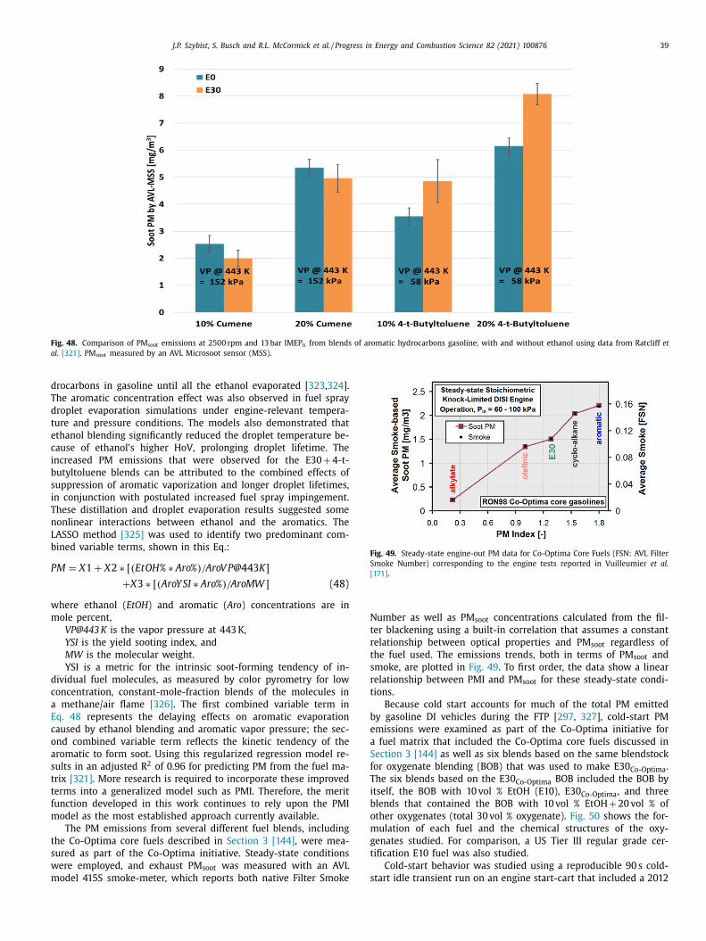
J.P. Szybist, S. Busch and R.L. McCormick et al. / Progress in Energy and Combustion Science 82 (2021) 100876 39
Fig. 48. Comparison of PM soot emissions at 2500 rpm and 13 bar IMEP n from blends of aromatic hydrocarbons gasoline, with and without ethanol using data from Ratcliff et
al. [321] . PM soot measured by an AVL Microsoot sensor (MSS).
d
T
d
t
e
c
i
b
s
i
T
n
L
b
P
w
m
d
c
a
E
c
o
a
s
t
t
f
m
t
s
w
m
Fig. 49. Steady-state engine-out PM data for Co-Optima Core Fuels (FSN: AVL Filter
Smoke Number) corresponding to the engine tests reported in Vuilleumier et al.
[171] .
N
t
r
t
s
r
t
b
e
a
S
f
T
i
b
o
m
g
t
s
rocarbons in gasoline until all the ethanol evaporated [ 323 , 324 ].
he aromatic concentration effect was also observed in fuel spray
roplet evaporation simulations under engine-relevant tempera-
ure and pressure conditions. The models also demonstrated that
thanol blending significantly reduced the droplet temperature be-
ause of ethanol’s higher HoV, prolonging droplet lifetime. The
ncreased PM emissions that were observed for the E30 + 4-t-
utyltoluene blends can be attributed to the combined effects of
uppression of aromatic vaporization and longer droplet lifetimes,
n conjunction with postulated increased fuel spray impingement.
hese distillation and droplet evaporation results suggested some
onlinear interactions between ethanol and the aromatics. The
ASSO method [325] was used to identify two predominant com-
ined variable terms, shown in this Eq.:
M = X 1 + X 2 ∗ [ ( EtOH% ∗ Aro% ) /AroV P @443 K ]
+ X 3 ∗ [ ( AroY SI ∗ Aro% ) /AroMW ] (48)
here ethanol ( EtOH ) and aromatic ( Aro ) concentrations are in
ole percent,
VP@443 K is the vapor pressure at 443 K,
YSI is the yield sooting index, and
MW is the molecular weight.
YSI is a metric for the intrinsic soot-forming tendency of in-
ividual fuel molecules, as measured by color pyrometry for low
oncentration, constant-mole-fraction blends of the molecules in
methane/air flame [326] . The first combined variable term in
q. 48 represents the delaying effects on aromatic evaporation
aused by ethanol blending and aromatic vapor pressure; the sec-
nd combined variable term reflects the kinetic tendency of the
romatic to form soot. Using this regularized regression model re-
ults in an adjusted R
2 of 0.96 for predicting PM from the fuel ma-
rix [321] . More research is required to incorporate these improved
erms into a generalized model such as PMI. Therefore, the merit
unction developed in this work continues to rely upon the PMI
odel as the most established approach currently available.
The PM emissions from several different fuel blends, including
he Co-Optima core fuels described in Section 3 [144] , were mea-
ured as part of the Co-Optima initiative. Steady-state conditions
ere employed, and exhaust PM soot was measured with an AVL
odel 415S smoke-meter, which reports both native Filter Smoke
umber as well as PM soot concentrations calculated from the fil-
er blackening using a built-in correlation that assumes a constant
elationship between optical properties and PM soot regardless of
he fuel used. The emissions trends, both in terms of PM soot and
moke, are plotted in Fig. 49 . To first order, the data show a linear
elationship between PMI and PM soot for these steady-state condi-
ions.
Because cold start accounts for much of the total PM emitted
y gasoline DI vehicles during the FTP [ 297 , 327 ], cold-start PM
missions were examined as part of the Co-Optima initiative for
fuel matrix that included the Co-Optima core fuels discussed in
ection 3 [144] as well as six blends based on the same blendstock
or oxygenate blending (BOB) that was used to make E30 Co-Optima .
he six blends based on the E30 Co-Optima BOB included the BOB by
tself, the BOB with 10 vol % EtOH (E10), E30 Co-Optima , and three
lends that contained the BOB with 10 vol % EtOH + 20 vol % of
ther oxygenates (total 30 vol % oxygenate). Fig. 50 shows the for-
ulation of each fuel and the chemical structures of the oxy-
enates studied. For comparison, a US Tier III regular grade cer-
ification E10 fuel was also studied.
Cold-start behavior was studied using a reproducible 90 s cold-
tart idle transient run on an engine start-cart that included a 2012
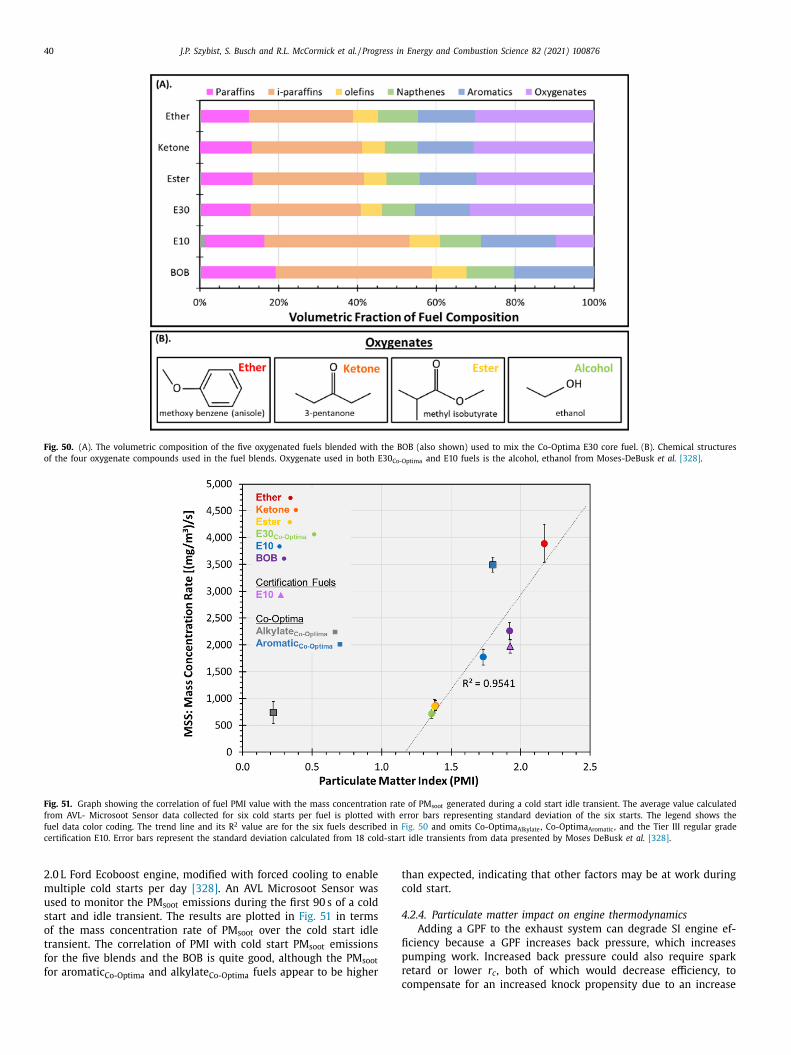
40 J.P. Szybist, S. Busch and R.L. McCormick et al. / Progress in Energy and Combustion Science 82 (2021) 100876
Fig. 50. (A). The volumetric composition of the five oxygenated fuels blended with the BOB (also shown) used to mix the Co-Optima E30 core fuel. (B). Chemical structures
of the four oxygenate compounds used in the fuel blends. Oxygenate used in both E30 Co-Optima and E10 fuels is the alcohol, ethanol from Moses-DeBusk et al. [328] .
Fig. 51. Graph showing the correlation of fuel PMI value with the mass concentration rate of PM soot generated during a cold start idle transient. The average value calculated
from AVL- Microsoot Sensor data collected for six cold starts per fuel is plotted with error bars representing standard deviation of the six starts. The legend shows the
fuel data color coding. The trend line and its R 2 value are for the six fuels described in Fig. 50 and omits Co-Optima Alkylate , Co-Optima Aromatic , and the Tier III regular grade
certification E10. Error bars represent the standard deviation calculated from 18 cold-start idle transients from data presented by Moses DeBusk et al. [328] .
t
c
4
fi
p
r
2.0 L Ford Ecoboost engine, modified with forced cooling to enable
multiple cold starts per day [328] . An AVL Microsoot Sensor was
used to monitor the PM soot emissions during the first 90 s of a cold
start and idle transient. The results are plotted in Fig. 51 in terms
of the mass concentration rate of PM soot over the cold start idle
transient. The correlation of PMI with cold start PM soot emissions
for the five blends and the BOB is quite good, although the PM soot
for aromatic Co-Optima and alkylate Co-Optima fuels appear to be higher
chan expected, indicating that other factors may be at work during
old start.
.2.4. Particulate matter impact on engine thermodynamics
Adding a GPF to the exhaust system can degrade SI engine ef-
ciency because a GPF increases back pressure, which increases
umping work. Increased back pressure could also require spark
etard or lower r c , both of which would decrease efficiency, to
ompensate for an increased knock propensity due to an increase
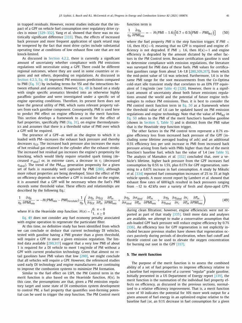
J.P. Szybist, S. Busch and R.L. McCormick et al. / Progress in Energy and Combustion Science 82 (2021) 100876 41
i
p
c
t
b
b
o
k
a
r
r
g
S
t
t
w
p
e
h
u
t
T
f
i
a
l
d
o
T
k
c
η
s
m
o
i
e
d
∂ η
∂ σid
w
w
w
t
w
i
1
G
t
t
u
t
m
t
t
t
t
f
w
1
fi
e
t
t
w
t
t
s
c
a
i
t
n
P
t
r
E
(
t
g
c
0
p
f
T
h
c
m
e
v
e
f
d
p
a
a
[
c
c
t
f
5
a
a
I
m
f
i
s
n trapped residuals. However, recent studies indicate that the im-
act of a GPF on vehicle fuel consumption over regulatory drive cy-
les is minor [329–332] . Yang et al. showed that there was no sta-
istically significant difference [333] . Thus, the effects of increased
ack pressure and more frequent application of spark retard may
e tempered by the fact that most drive cycles include substantial
perating time at conditions of low exhaust flow rate that are not
nock-limited.
As discussed in Section 4.2.2 , there is currently a significant
mount of uncertainty whether compliance with PM emissions
egulations will necessitate using a GPF. There could be different
egional outcomes, where they are used in some countries or re-
ions and not others, depending on regulations. As discussed in
ection 4.2.3 , Eq. 48 improved PM emissions predictions compared
o PMI ( Eq. 31 ) by including terms for YSI and the interactions be-
ween ethanol and aromatics. However, Eq. 48 is based on a study
ith single specific aromatics blended into an otherwise highly
araffinic gasoline and were investigated under a specific set of
ngine operating conditions. Therefore, its present form does not
ave the general utility of PMI, which sums relevant property val-
es from each gasoline component. Consequently, PMI is used here
o predict PM effect on engine efficiency in the merit function.
his section develops a framework to account for the effect of
uel properties, specifically PMI ( Eq. 31 ), on engine thermodynam-
cs and assumes that there is a threshold value of PMI over which
GPF will be required.
The presence of a GPF—as well as the degree to which it is
oaded with PM—increases the exhaust back pressure and thereby
ecreases ηGE . The increased back pressure also increases the mass
f hot residual gas retained in the cylinder after the exhaust stroke.
he increased hot residual gas increases the engine’s propensity for
nocking, which would likely require retarded spark timing (de-
reased σ ideal ) or, in extreme cases, a decrease in r c (decreased
ideal ). The trend of the PM soot generation propensity for a given
et of fuels is reasonably well captured by PMI [280] , although
ore robust properties are being developed. Since the effect of PM
n efficiency depends on whether a GPF is installed on the engine,
t is assumed that a GPF will be necessary when the fuel’s PMI
xceeds some threshold value. These effects and relationships are
escribed by the following Eq.:
1
ηb
∂ ηb
∂P M I mix
= −H ( P M I mix − P M I threshold ) 1
ηb
(∂ ηb
∂ ηGE
∂ ηGE
∂ P ex
∂ P ex
∂P M I mix
+
here H is the Heaviside step function: H(x ) = { 0 , x < 0
1 , x ≥ 0
Eq. 49 does not consider any fuel economy penalty associated
ith engine operation to regenerate the particulate filter.
At this time, no definitive study has been identified from which
e can conclude or deduce that current technology DI vehicles,
ested with gasoline having a PMI greater than a given threshold,
ill require a GPF to meet a given emission regulation. The lim-
ted data available [ 280 , 317 ] suggest that a very low PMI of about
is required for a DI vehicle to meet 1 mg/mile of PM without a
PF with current production technology. Given that almost no re-
ail gasolines have PMI values that low [280] , we might conclude
hat all vehicles will require a GPF. However, the referenced studies
sed early DI technology and engine manufacturers are continuing
o improve the combustion systems to minimize PM formation.
Similar to the fuel effect on LSPI, the PM Control term in the
erit function is also based on the Heaviside function, H (x). In
his case, the presumptions are that, given a PM emission regula-
ory target and some state of DI combustion system development
o control PM, a fuel property that quantifies soot-forming poten-
ial can be used to trigger the step function. The PM Control merit
gb
b
eal
∂ σideal
∂ P ex
∂ P ex
∂P M I mix
+
∂ ηb
∂ ηideal
∂ ηideal
∂ r c
∂ r c ∂ P ex
∂ P ex
∂P M I mix
)(49)
unction term is
1
ηb
∂ ηb
∂P M I mix
= − H ( P MI − 1 . 6 ) [0 . 7 + 0 . 5
(P MI − P M I Re f
)](50)
here the fuel property PMI is the step function trigger. If PMI <
.6, then H (x) = 0, meaning that no GPF is required and engine ef-
ciency is not degraded. If PMI ≥ 1.6, then H (x) = 1 and engine
fficiency is degraded by the amount dictated by the other fac-
ors in the PM Control term. Because certification gasoline is used
o determine compliance with emission regulations, the literature
as surveyed for PMI data of these fuels. PMI values for certifica-
ion gasolines range from about 1.4–1.8 [ 280 , 309 , 317 ], from which
he mid-point value of 1.6 was selected. Furthermore, 1.6 is in the
ame PMI range for the soot measurements from the Co-Optima
old-start idle transient study that correlates to an EPA FTP equiv-
lent of 1 mg/mile (see Table 4 ) [328] . However, there is a signif-
cant amount of uncertainty about both future emissions regula-
ions around the world and the potential of future engine tech-
ologies to reduce PM emissions. Thus, it is best to consider the
M control merit function term in Eq. 50 as a framework where
he threshold value of 1.6 can be updated based on PM emission
egulations and engine technology. Note that the value of PMI Ref in
q. 50 refers to the PMI of the merit function’s baseline gasoline
shown in Section 5 , Table 5 ) and is distinct from the PMI value
hat is the Heaviside step function trigger.
The other factors in the PM control term represent a 0.7% en-
ine efficiency loss from increased back pressure of the GPF (in-
luding some lifetime averaged loading of ash) and an additional
.5% efficiency loss per unit increase in PMI from increased back
ressure arising from fuels with PMIs higher than that of the merit
unction’s baseline fuel, which has the value of 1.4 (see Table 5 ).
he analysis of Mamakos et al. [332] concluded that, over a ve-
icle’s lifetime, higher back pressure from the GPF increases fuel
onsumption by 0.5% to 1.5%, plus 0.17% for GPF regeneration, sum-
ing to a 0.67% increase in fuel consumption. A study by Mikulic
t al. [334] reported fuel consumption increases of 2% to 3% at high
ehicle speeds. A more recent report by Lambert et al. showed that
xhaust flow rates of 600 kg/h resulted in back pressures ranging
rom ∼12 to 42 kPa over a variety of fresh and dyno-aged GPFs
uring clean filtration; however, engine efficiencies were not re-
orted as part of that study [335] . Until more data and analyses
re available, we attempt to make a conservative assumption that
sh-loaded GPF back pressure will reduce engine efficiency by 0.7%
336] . An efficiency loss for GPF regeneration is not explicitly in-
luded because previous studies have shown that regeneration oc-
urs passively during periods of deceleration, when fuel cutoff and
hrottle control can be used to elevate the oxygen concentration
or burning out soot in the GPF [337] .
. The merit function
The purpose of the merit function is to assess the combined
bility of a set of fuel properties to improve efficiency relative to
baseline fuel representative of a current “regular” grade gasoline.
nitially presented in a US Department of Energy report [139] , the
erit function is the summation of the individual fuel property ef-
ects on efficiency, as discussed in the previous sections, normal-
zed to a relative efficiency improvement. That is, a merit function
core of 10 indicates the potential for 10% more work output for a
iven amount of fuel energy in an optimized engine relative to the
aseline fuel (or, an 9.1% decrease in fuel consumption for a given
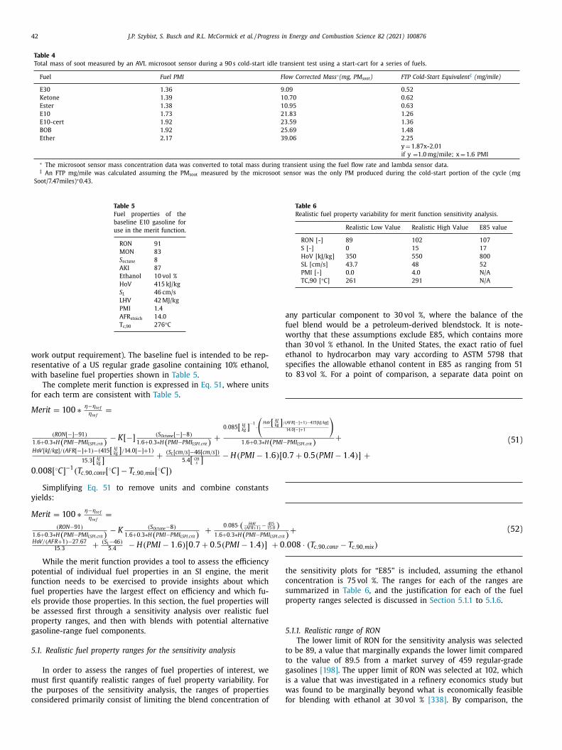
42 J.P. Szybist, S. Busch and R.L. McCormick et al. / Progress in Energy and Combustion Science 82 (2021) 100876
Table 4
Total mass of soot measured by an AVL microsoot sensor during a 90 s cold-start idle transient test using a start-cart for a series of fuels.
Fuel Fuel PMI Flow Corrected Mass ∗(mg, PM soot ) FTP Cold-Start Equivalent ‡ (mg/mile)
E30 1.36 9.09 0.52
Ketone 1.39 10.70 0.62
Ester 1.38 10.95 0.63
E10 1.73 21.83 1.26
E10-cert 1.92 23.59 1.36
BOB 1.92 25.69 1.48
Ether 2.17 39.06 2.25
y = 1.87x-2.01
if y = 1.0 mg/mile; x = 1.6 PMI
∗ The microsoot sensor mass concentration data was converted to total mass during transient using the fuel flow rate and lambda sensor data. ‡ An FTP mg/mile was calculated assuming the PM soot measured by the microsoot sensor was the only PM produced during the cold-start portion of the cycle (mg
Soot/7.47miles) ∗0.43.
Table 5
Fuel properties of the
baseline E10 gasoline for
use in the merit function.
RON 91
MON 83
S octane 8
AKI 87
Ethanol 10 vol %
HoV 415 kJ/kg
S L 46 cm/s
LHV 42 MJ/kg
PMI 1.4
AFR stoich 14.0
T c,90 276 °C
[ kJ kg ] / (
( P MI−
. 6 ) [ 0
15 5 . 0 ) LSPI,crit
+ 0 .
Table 6
Realistic fuel property variability for merit function sensitivity analysis.
Realistic Low Value Realistic High Value E85 value
RON [-] 89 102 107
S [-] 0 15 17
HoV [kJ/kg] 350 550 800
SL [cm/s] 43.7 48 52
PMI [-] 0.0 4.0 N/A
TC,90 [ °C] 261 291 N/A
a
f
w
t
e
s
t
t
c
s
p
5
t
t
g
i
w
f
work output requirement). The baseline fuel is intended to be rep-
resentative of a US regular grade gasoline containing 10% ethanol,
with baseline fuel properties shown in Table 5 .
The complete merit function is expressed in Eq. 51 , where units
for each term are consistent with Table 5 .
Merit = 100 ∗ η−ηre f
ηre f =
( RON [ −] −91 )
1 . 6+0 . 3 ∗H ( P MI−P M I LSPI,crit ) − K [ −]
( S Octane [ −] −8 )
1 . 6+0 . 3 ∗H ( P MI−P M I LSPI,crit ) +
0 . 085 [ kJ kg ]
−1 ·(
HoV
1 . 6+0 . 3 ∗H
HoV [ kJ/kg ] / ( AF R [ −] +1 ) −(415 [ kJ kg ] / 14 . 0 [ −] +1)
15 . 3 [ kJ kg ]
+
( S L [ cm/s ] −46 [ cm/s ] )
5 . 4 [ cm s ]
− H ( P MI − 1
0 . 008 [ ◦C ] −1 ( T c, 90 ,con v [
◦C ] − T c, 90 ,mix [ ◦C ] )
Simplifying Eq. 51 to remove units and combine constants
yields:
Merit = 100 ∗ η−ηre f
ηre f =
( RON−91 )
1 . 6+0 . 3 ∗H ( P MI−P M I LSPI,crit ) − K
( S Octane −8 )
1 . 6+0 . 3 ∗H ( P MI−P M I LSPI,crit ) +
0 . 085 ·( HoV ( AFR +1 )
− 41
1 . 6+0 . 3 ∗H ( P MI−P M IHoV/ ( AF R +1 ) −27 . 67
15 . 3 +
( S L −46) 5 . 4
− H ( P MI − 1 . 6 ) [ 0 . 7 + 0 . 5 ( P MI − 1 . 4 ) ]
While the merit function provides a tool to assess the efficiency
potential of individual fuel properties in an SI engine, the merit
function needs to be exercised to provide insights about which
fuel properties have the largest effect on efficiency and which fu-
els provide those properties. In this section, the fuel properties will
be assessed first through a sensitivity analysis over realistic fuel
property ranges, and then with blends with potential alternative
gasoline-range fuel components.
5.1. Realistic fuel property ranges for the sensitivity analysis
In order to assess the ranges of fuel properties of interest, we
must first quantify realistic ranges of fuel property variability. For
the purposes of the sensitivity analysis, the ranges of properties
considered primarily consist of limiting the blend concentration of
AFR [ −] +1 ) −415 [ kJ/kg ]
14 . 0 [ −] +1
)
P M I LSPI,crit ) +
. 7 + 0 . 5 ( P MI − 1 . 4 ) ] +
(51)
) +
008 · ( T c, 90 ,con v − T c, 90 ,mix )
(52)
ny particular component to 30 vol %, where the balance of the
uel blend would be a petroleum-derived blendstock. It is note-
orthy that these assumptions exclude E85, which contains more
han 30 vol % ethanol. In the United States, the exact ratio of fuel
thanol to hydrocarbon may vary according to ASTM 5798 that
pecifies the allowable ethanol content in E85 as ranging from 51
o 83 vol %. For a point of comparison, a separate data point on
he sensitivity plots for “E85” is included, assuming the ethanol
oncentration is 75 vol %. The ranges for each of the ranges are
ummarized in Table 6 , and the justification for each of the fuel
roperty ranges selected is discussed in Section 5.1.1 to 5.1.6 .
.1.1. Realistic range of RON
The lower limit of RON for the sensitivity analysis was selected
o be 89, a value that marginally expands the lower limit compared
o the value of 89.5 from a market survey of 459 regular-grade
asolines [198] . The upper limit of RON was selected at 102, which
s a value that was investigated in a refinery economics study but
as found to be marginally beyond what is economically feasible
or blending with ethanol at 30 vol % [338] . By comparison, the
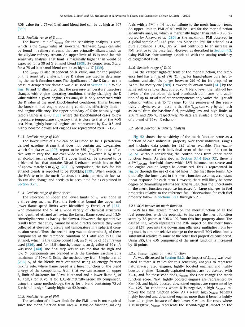
J.P. Szybist, S. Busch and R.L. McCormick et al. / Progress in Energy and Combustion Science 82 (2021) 100876 43
R
[
5
w
b
t
s
e
f
o
i
p
F
c
v
t
t
a
r
a
t
h
5
d
w
t
a
a
o
e
t
t
S
5
a
l
w
a
t
r
c
b
c
e
u
w
l
m
[
m
e
S
4
u
%
5
s
f
A
s
p
a
p
P
u
o
5
e
c
3
s
h
t
b
t
a
2
o
5
f
a
i
E
f
a
t
F
d
l
d
i
p
p
5
f
s
d
t
i
s
U
b
5
u
n
b
K
f
K
K
p
h
b
K
ON value for a 75 vol % ethanol blend fuel can be as high as 107
339] .
.1.2. Realistic range of S octane
The lower limit of S octane for the sensitivity analysis is zero,
hich is the S octane value of iso-octane. Near-zero S octane can also
e found in refinery streams that are primarily alkanes, such as
he alkylate refinery stream. An upper limit of 15 is used for this
ensitivity analysis. That limit is marginally higher than would be
xpected for a 30 vol % ethanol blend [208] . By comparison, S octane
or a 75 vol % ethanol blend can be as high as 17 [339] .
The S octane is also dependent on K value, and for the purpose
f this sensitivity analysis, three K values are used in determin-
ng the merit function score. The significance of the K factor to the
ressure-temperature domain was discussed in Section 3.1.2 . While
igs. 16 and 17 illustrated that the pressure-temperature trajectory
hanges with engine operating condition, thereby changing the K
alue within a given engine, this analysis is only concerned with
he K value at the most knock-limited conditions. This is because
he knock-limited engine operating conditions effectively limit r c nd engine efficiency. The upper boundary of K for naturally aspi-
ated engines is K = 0 [185] , where the knock-limited cases follow
pressure-temperature trajectory that is close to that of the RON
est. Next, lightly boosted engines are represented by K = -0.5, and
ighly boosted downsized engines are represented by K = -1.25.
.1.3. Realistic range of HoV
The lower limit of HoV can be assumed to be a petroleum-
erived gasoline stream that does not contain any oxygenates,
hich Chupka et al. [207] report to be 350 kJ/kg. The most effec-
ive way to vary the HoV over wide ranges, however, is by using
n alcohol, such as ethanol. The upper limit can be assumed to be
blended fuel that contains 30 vol % ethanol, which has an HoV
f approximately 530 kJ/kg [207] . By comparison, the HoV for 75%
thanol blends is reported to be 800 kJ/kg [339] . When exercising
he HoV term in the merit function, the stoichiometric air-fuel ra-
io can also change and needs to be accounted for, as explained in
ection 3.2.1 .
.1.4. Realistic range of flame speed
The selection of upper and lower limits of S L was done in
three-step manner. First, the fuels that bound the upper and
ower flame speed limits were identified by Farrell et al. [234] ,
ho measured the S L of a wide variety of chemical structures
nd identified ethanol as having the fastest flame speed and 1,3,5-
rimethylbenzene as having the slowest. However, the quantitative
esults from that study cannot be used directly because they were
ollected at elevated pressure and temperature in a spherical com-
ustion vessel. Thus, the second step was to determine S L of these
omponents at the reference condition of 1 atm and 353 K. For
thanol, which is the upper-bound fuel, an S L value of 55 cm/s was
sed [236] , and for 1,3,5-trimethylbenzene, an S L value of 39 cm/s
as used [340] . The final step was to assume that the high and
ow S L components are blended with the baseline gasoline at a
aximum of 30 vol %. Using the methodology from Sileghem et al.
236] , S L of the blends were estimated using an energy fraction
ixing rule, where flame speed is a linear function of the blend
nergy of the components. From that we can assume an upper
L limit of 48.0 cm/s for 30 vol % ethanol and a lower flame S L of
3.7 cm/s for 30 vol % for 1,3,5-trimethylbenzene. By comparison,
sing the same methodology, the S L for a blend containing 75 vol
ethanol is significantly higher at 52.0 cm/s.
.1.5. Realistic range of PMI
The selection of a lower limit for the PMI term is not required
ince the merit function term uses a Heaviside function, making
uels with a PMI < 1.6 not contribute to the merit function term.
n upper limit to PMI of 4.0 will be used for the merit function
ensitivity analysis, which is marginally higher than PMI = 3.86 re-
orted by Aikawa et al. [280] as the maximum PMI observed in
global sample of 1445 gasolines. Since the PMI for ethanol as a
ure substance is 0.06, E85 will not contribute to an increase in
MI relative to the base fuel. However, as described in Section 4.2 ,
sing PMI has shortcomings associated with the sooting tendency
f oxygenated fuels.
.1.6. Realistic range of Tc,90
For the catalyst light-off term of the merit function, the refer-
nce fuel has a T c,90 of 276 °C. T c,90 for liquid-phase pure hydro-
arbons and alcohols ranges between 219 °C for iso-propanol to
42 °C for mesitylene [289] . However, follow-on work [341] by the
ame authors shows that, at a 30 vol % blend level, the light-off be-
avior of the petroleum-derived blendstock dominates, and addi-
ion of up to 30 vol % of other components only varies the light-off
ehavior within a ± 15 °C range. For the purposes of this sensi-
ivity analysis, we will assume that the T c,90 can vary by as much
s 20 °C from the baseline fuel, providing low and high limits of
56 °C and 296 °C, respectively. No data are available for the T c,90
f a blend of 75 vol % ethanol.
.2. Merit function sensitivity analysis
Fig. 52 shows the sensitivity of the merit function score as a
unction of each individual property over their individual ranges
nd includes data points for E85 when available. This exam-
nes variations of each individual term of the merit function in
q. 51 without considering the contributions from other merit
unction terms. As described in Section 3.4.4 ( Eq.s 32 ), there is
PMI LSPI,crit threshold above which LSPI becomes too severe and
he engine can no longer be downsized. This is represented in
ig. 52 through the use of dashed lines in the first three terms. Ad-
itionally, the form used in the merit function assumes a constant
inear response for each term. However, there will likely be some
egree of diminishing returns for large values, thus the uncertainty
n the merit function response increases for large changes in fuel
roperties relative to the reference fuel. Observations for each fuel
roperty follow in Sections 5.2.1 through 5.2.6.
.2.1. RON impact on merit function
RON has the largest impact on the merit function of all the
uel properties, with the potential to increase the merit function
core by 7.5 points at RON = 102 from this fuel property alone. The
ashed line, which represents the RON impact on the merit func-
ion if LSPI prevents the downsizing efficiency multiplier from be-
ng used, is a minor relative change to the overall RON effect, but is
ubstantial relative to some of the other fuel properties considered.
sing E85, the RON component of the merit function is increased
y 10 points.
.2.2. S octane impact on merit function
As was discussed in Section 5.1.2 , the impact of S octane was eval-
ated at three K values for this sensitivity analysis to represent
aturally-aspirated engines, lightly boosted engines, and highly
oosted engines. Naturally-aspirated engines are represented with
= 0, and for these conditions, S octane does not change the merit
unction score. Next, lightly boosted engines are represented by
= -0.5, and highly boosted downsized engines are represented by
= -1.25. For conditions where K is negative, a high S octane im-
roves the merit function score. As a result, high S octane benefits
ighly boosted and downsized engines more than it benefits lightly
oosted engines because of their lower K values. For cases where
is negative, S octane represents the second-biggest impact on the
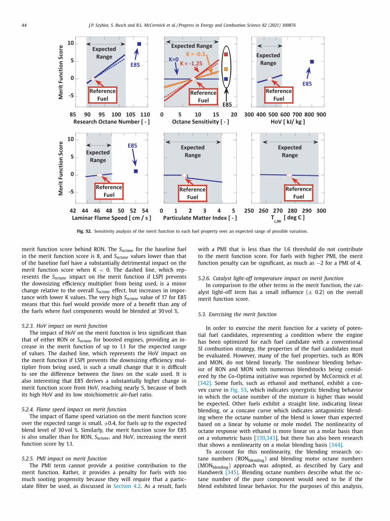
44 J.P. Szybist, S. Busch and R.L. McCormick et al. / Progress in Energy and Combustion Science 82 (2021) 100876
Fig. 52. Sensitivity analysis of the merit function to each fuel property over an expected range of possible variation.
w
t
f
5
a
m
5
t
h
S
b
a
i
e
[
v
i
b
b
i
b
o
o
t
t
(
H
t
b
merit function score behind RON. The S octane for the baseline fuel
in the merit function score is 8, and S octane values lower than that
of the baseline fuel have a substantially detrimental impact on the
merit function score when K < 0. The dashed line, which rep-
resents the S octane impact on the merit function if LSPI prevents
the downsizing efficiency multiplier from being used, is a minor
change relative to the overall S octane effect, but increases in impor-
tance with lower K values. The very high S octane value of 17 for E85
means that this fuel would provide more of a benefit than any of
the fuels where fuel components would be blended at 30 vol %.
5.2.3. HoV impact on merit function
The impact of HoV on the merit function is less significant than
that of either RON or S octane for boosted engines, providing an in-
crease in the merit function of up to 1.1 for the expected range
of values. The dashed line, which represents the HoV impact on
the merit function if LSPI prevents the downsizing efficiency mul-
tiplier from being used, is such a small change that it is difficult
to see the difference between the lines on the scale used. It is
also interesting that E85 derives a substantially higher change in
merit function score from HoV, reaching nearly 5, because of both
its high HoV and its low stoichiometric air-fuel ratio.
5.2.4. Flame speed impact on merit function
The impact of flame speed variation on the merit function score
over the expected range is small, ±0.4, for fuels up to the expected
blend level of 30 vol %. Similarly, the merit function score for E85
is also smaller than for RON, S octane , and HoV, increasing the merit
function score by 1.1.
5.2.5. PMI impact on merit function
The PMI term cannot provide a positive contribution to the
merit function. Rather, it provides a penalty for fuels with too
much sooting propensity because they will require that a partic-
ulate filter be used, as discussed in Section 4.2 . As a result, fuels
ith a PMI that is less than the 1.6 threshold do not contribute
o the merit function score. For fuels with higher PMI, the merit
unction penalty can be significant, as much as −2 for a PMI of 4.
.2.6. Catalyst light-off temperature impact on merit function
In comparison to the other terms in the merit function, the cat-
lyst light-off term has a small influence ( ± 0.2) on the overall
erit function score.
.3. Exercising the merit function
In order to exercise the merit function for a variety of poten-
ial fuel candidates, representing a condition where the engine
as been optimized for each fuel candidate with a conventional
I combustion strategy, the properties of the fuel candidates must
e evaluated. However, many of the fuel properties, such as RON
nd MON, do not blend linearly. The nonlinear blending behav-
or of RON and MON with numerous blendstocks being consid-
red by the Co-Optima initiative was reported by McCormick et al.
342] . Some fuels, such as ethanol and methanol, exhibit a con-
ex curve in Fig. 53 , which indicates synergistic blending behavior
n which the octane number of the mixture is higher than would
e expected. Other fuels exhibit a straight line, indicating linear
lending, or a concave curve which indicates antagonistic blend-
ng where the octane number of the blend is lower than expected
ased on a linear by volume or mole model. The nonlinearity of
ctane response with ethanol is more linear on a molar basis than
n a volumetric basis [ 339 , 343 ], but there has also been research
hat shows a nonlinearity on a molar blending basis [344] .
To account for this nonlinearity, the blending research oc-
ane numbers (RON blending ) and blending motor octane numbers
MON blending ) approach was adopted, as described by Gary and
andwerk [345] . Blending octane numbers describe what the oc-
ane number of the pure component would need to be if the
lend exhibited linear behavior. For the purposes of this analysis,
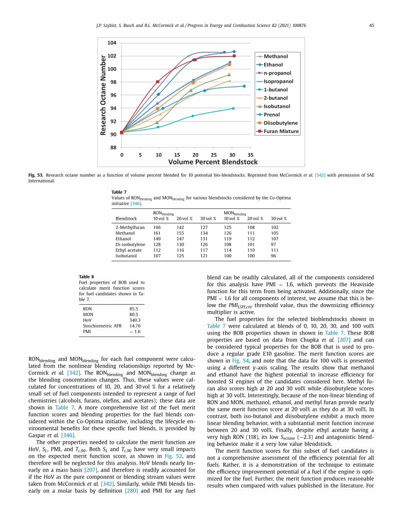
J.P. Szybist, S. Busch and R.L. McCormick et al. / Progress in Energy and Combustion Science 82 (2021) 100876 45
Fig. 53. Research octane number as a function of volume percent blended for 10 potential bio-blendstocks. Reprinted from McCormick et al. [342] with permission of SAE
International.
Table 7
Values of RON blending and MON blending for various blendstocks considered by the Co-Optima
initiative [346] .
Blendstock
RON blending MON blending
10 vol % 20 vol % 30 vol % 10 vol % 20 vol % 30 vol %
2-Methylfuran 166 142 127 125 108 102
Methanol 161 155 134 126 111 105
Ethanol 149 147 131 119 112 107
Di-isobutylene 128 130 126 108 101 97
Ethyl acetate 112 116 117 114 110 111
Isobutanol 107 125 121 100 100 96
Table 8
Fuel properties of BOB used to
calculate merit function scores
for fuel candidates shown in Ta-
ble 7.
RON 85.5
MON 80.5
HoV 340.3
Stoichiometric AFR 14.76
PMI < 1.6
R
l
C
t
c
s
c
s
f
s
v
G
H
o
t
e
i
t
e
b
f
f
P
l
m
T
u
p
b
d
s
u
a
b
r
h
R
t
c
l
b
v
i
n
f
t
m
r
ON blending and MON blending for each fuel component were calcu-
ated from the nonlinear blending relationships reported by Mc-
ormick et al. [342] . The RON blending and MON blending change as
he blending concentration changes. Thus, these values were cal-
ulated for concentrations of 10, 20, and 30 vol % for a relatively
mall set of fuel components intended to represent a range of fuel
hemistries (alcohols, furans, olefins, and acetates); these data are
hown in Table 7 . A more comprehensive list of the fuel merit
unction scores and blending properties for the fuel blends con-
idered within the Co-Optima initiative, including the lifecycle en-
ironmental benefits for these specific fuel blends, is provided by
aspar et al. [346] .
The other properties needed to calculate the merit function are
oV, S L , PMI, and T c,90 . Both S L and T c,90 have very small impacts
n the expected merit function score, as shown in Fig. 52 , and
herefore will be neglected for this analysis. HoV blends nearly lin-
arly on a mass basis [207] , and therefore is readily accounted for
f the HoV as the pure component or blending stream values were
aken from McCormick et al. [342] . Similarly, while PMI blends lin-
arly on a molar basis by definition [280] and PMI for any fuel
lend can be readily calculated, all of the components considered
or this analysis have PMI < 1.6, which prevents the Heaviside
unction for this term from being activated. Additionally, since the
MI < 1.6 for all components of interest, we assume that this is be-
ow the PMI LSPI,crit threshold value, thus the downsizing efficiency
ultiplier is active.
The fuel properties for the selected bioblendstocks shown in
able 7 were calculated at blends of 0, 10, 20, 30, and 100 vol%
sing the BOB properties shown in shown in Table 7 . These BOB
roperties are based on data from Chupka et al. [207] and can
e considered typical properties for the BOB that is used to pro-
uce a regular grade E10 gasoline. The merit function scores are
hown in Fig. 54 , and note that the data for 100 vol% is presented
sing a different y-axis scaling. The results show that methanol
nd ethanol have the highest potential to increase efficiency for
oosted SI engines of the candidates considered here. Methyl fu-
an also scores high at 20 and 30 vol% while diisobutylene scores
igh at 30 vol%. Interestingly, because of the non-linear blending of
ON and MON, methanol, ethanol, and methyl furan provide nearly
he same merit function score at 20 vol% as they do at 30 vol%. In
ontrast, both iso-butanol and diisobutylene exhibit a much more
inear blending behavior, with a substantial merit function increase
etween 20 and 30 vol%. Finally, despite ethyl acetate having a
ery high RON (118), its low S octane ( −2.3) and antagonistic blend-
ng behavior make it a very low value blendstock.
The merit function scores for this subset of fuel candidates is
ot a comprehensive assessment of the efficiency potential for all
uels. Rather, it is a demonstration of the technique to estimate
he efficiency improvement potential of a fuel if the engine is opti-
ized for the fuel. Further, the merit function produces reasonable
esults when compared with values published in the literature. For
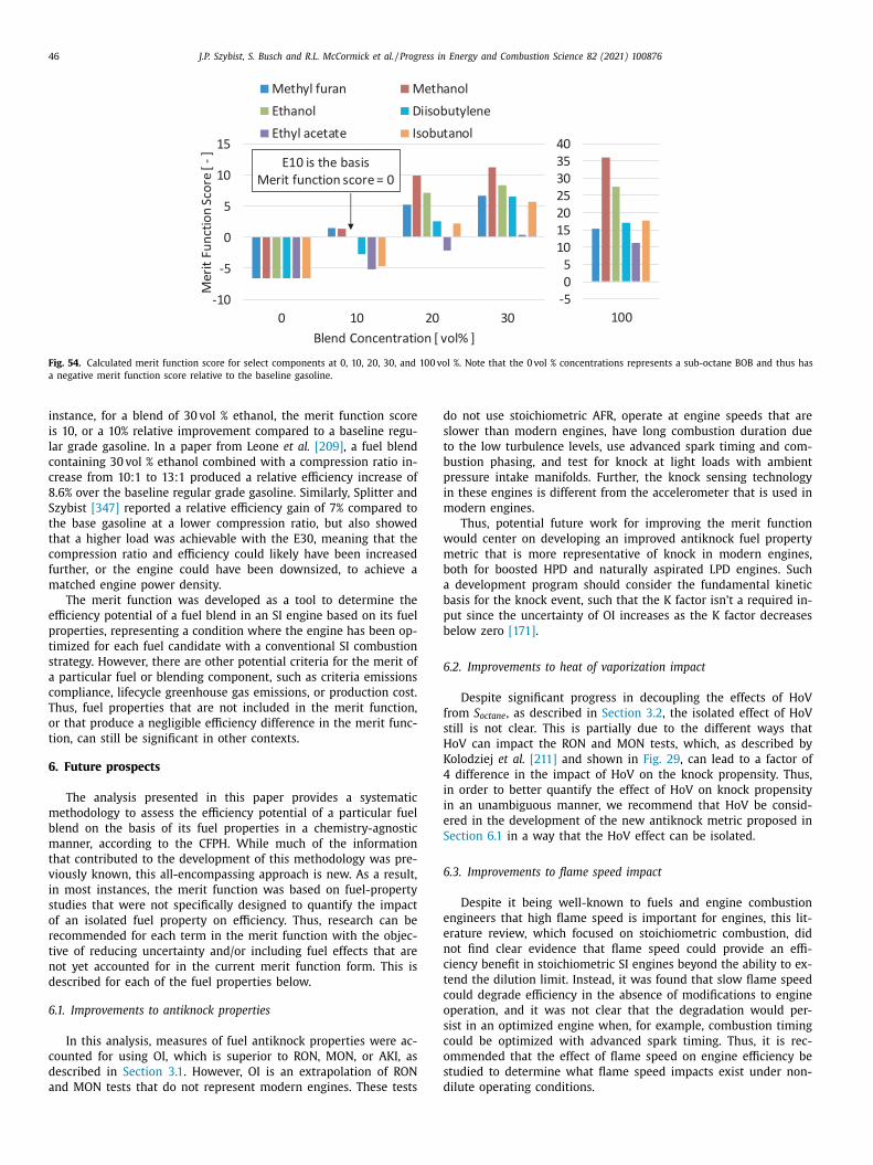
46 J.P. Szybist, S. Busch and R.L. McCormick et al. / Progress in Energy and Combustion Science 82 (2021) 100876
Fig. 54. Calculated merit function score for select components at 0, 10, 20, 30, and 100 vol %. Note that the 0 vol % concentrations represents a sub-octane BOB and thus has
a negative merit function score relative to the baseline gasoline.
d
s
t
b
p
i
m
w
m
b
a
b
p
b
6
f
s
H
K
4
i
i
e
S
6
e
e
n
c
t
c
o
s
c
o
s
d
instance, for a blend of 30 vol % ethanol, the merit function score
is 10, or a 10% relative improvement compared to a baseline regu-
lar grade gasoline. In a paper from Leone et al. [209] , a fuel blend
containing 30 vol % ethanol combined with a compression ratio in-
crease from 10:1 to 13:1 produced a relative efficiency increase of
8.6% over the baseline regular grade gasoline. Similarly, Splitter and
Szybist [347] reported a relative efficiency gain of 7% compared to
the base gasoline at a lower compression ratio, but also showed
that a higher load was achievable with the E30, meaning that the
compression ratio and efficiency could likely have been increased
further, or the engine could have been downsized, to achieve a
matched engine power density.
The merit function was developed as a tool to determine the
efficiency potential of a fuel blend in an SI engine based on its fuel
properties, representing a condition where the engine has been op-
timized for each fuel candidate with a conventional SI combustion
strategy. However, there are other potential criteria for the merit of
a particular fuel or blending component, such as criteria emissions
compliance, lifecycle greenhouse gas emissions, or production cost.
Thus, fuel properties that are not included in the merit function,
or that produce a negligible efficiency difference in the merit func-
tion, can still be significant in other contexts.
6. Future prospects
The analysis presented in this paper provides a systematic
methodology to assess the efficiency potential of a particular fuel
blend on the basis of its fuel properties in a chemistry-agnostic
manner, according to the CFPH. While much of the information
that contributed to the development of this methodology was pre-
viously known, this all-encompassing approach is new. As a result,
in most instances, the merit function was based on fuel-property
studies that were not specifically designed to quantify the impact
of an isolated fuel property on efficiency. Thus, research can be
recommended for each term in the merit function with the objec-
tive of reducing uncertainty and/or including fuel effects that are
not yet accounted for in the current merit function form. This is
described for each of the fuel properties below.
6.1. Improvements to antiknock properties
In this analysis, measures of fuel antiknock properties were ac-
counted for using OI, which is superior to RON, MON, or AKI, as
described in Section 3.1 . However, OI is an extrapolation of RON
and MON tests that do not represent modern engines. These tests
o not use stoichiometric AFR, operate at engine speeds that are
lower than modern engines, have long combustion duration due
o the low turbulence levels, use advanced spark timing and com-
ustion phasing, and test for knock at light loads with ambient
ressure intake manifolds. Further, the knock sensing technology
n these engines is different from the accelerometer that is used in
odern engines.
Thus, potential future work for improving the merit function
ould center on developing an improved antiknock fuel property
etric that is more representative of knock in modern engines,
oth for boosted HPD and naturally aspirated LPD engines. Such
development program should consider the fundamental kinetic
asis for the knock event, such that the K factor isn’t a required in-
ut since the uncertainty of OI increases as the K factor decreases
elow zero [171] .
.2. Improvements to heat of vaporization impact
Despite significant progress in decoupling the effects of HoV
rom S octane , as described in Section 3.2 , the isolated effect of HoV
till is not clear. This is partially due to the different ways that
oV can impact the RON and MON tests, which, as described by
olodziej et al. [211] and shown in Fig. 29 , can lead to a factor of
difference in the impact of HoV on the knock propensity. Thus,
n order to better quantify the effect of HoV on knock propensity
n an unambiguous manner, we recommend that HoV be consid-
red in the development of the new antiknock metric proposed in
ection 6.1 in a way that the HoV effect can be isolated.
.3. Improvements to flame speed impact
Despite it being well-known to fuels and engine combustion
ngineers that high flame speed is important for engines, this lit-
rature review, which focused on stoichiometric combustion, did
ot find clear evidence that flame speed could provide an effi-
iency benefit in stoichiometric SI engines beyond the ability to ex-
end the dilution limit. Instead, it was found that slow flame speed
ould degrade efficiency in the absence of modifications to engine
peration, and it was not clear that the degradation would per-
ist in an optimized engine when, for example, combustion timing
ould be optimized with advanced spark timing. Thus, it is rec-
mmended that the effect of flame speed on engine efficiency be
tudied to determine what flame speed impacts exist under non-
ilute operating conditions.
J.P. Szybist, S. Busch and R.L. McCormick et al. / Progress in Energy and Combustion Science 82 (2021) 100876 47
6
u
L
c
m
T
L
a
c
r
i
fi
r
e
i
w
d
6
a
s
i
f
e
g
t
a
n
fi
fi
n
a
g
o
c
P
F
w
6
e
e
s
p
s
c
t
i
7
w
d
c
i
g
i
p
i
m
i
c
t
S
E
c
p
e
n
o
p
a
o
e
q
l
p
e
t
t
fi
p
a
t
t
S
c
c
e
p
e
m
p
t
g
n
u
t
D
A
o
D
E
fi
.4. Improved quantification of LSPI fuel impacts
Our understanding of fuel impacts on LSPI is still very much
nder development. In order to attempt to quantify the effects of
SPI on engine efficiency, PMI was used as a fuel property basis be-
ause is increases with high distillation temperatures and with aro-
atics. However, linking PMI with LSPI is a relatively new concept.
hus, it is recommended that this proposed fuel property basis for
SPI be validated across several different engine platforms and for
wide range of fuels. Further, it is recommended that the effi-
iency penalty associated with LSPI be further developed. In this
eview, it was hypothesized that LSPI prevented further downsiz-
ng of the engine, thereby precluding the use of the downsizing ef-
ciency multiplier, but this hypothesis has not yet been validated.
Lastly, because LSPI is a multi-step sequence where each step is
equired but not sufficient on its own, as described by Chapman
t al. [247] and shown in Fig. 36 , it is recommended that non-
nitiation LSPI fuel effects be further developed. A number of these
ere described in Section 3.4.3 , but they are at an early stage of
evelopment and cannot yet be quanified in the merit function.
.5. Improved particulate matter impacts
Although presently PMI (a fuel property) appears to be the best
vailable model for predicting PM emissions from gasoline compo-
ition, the literature has demonstrated PMI’s shortcomings regard-
ng effects on PM from blending oxygenates into gasoline. There-
ore, continued development of better models is warranted. How-
ver, because ethanol is the dominant oxygenate currently in the
asoline market, and C3-C4 alcohols appear to have similar poten-
ial, near term PM model improvements might be constrained to
ccount for alcohol-aromatic interaction effects.
In addition to being able to predict PM in a more accurate man-
er, developing a better understanding of how PM can affect ef-
ciency is necessary. Specifically, the impact of PMI was quanti-
ed with a Heaviside function that assumed that a GPF would be
ecessary above a certain threshold value. There is a significant
mount of uncertainty about the development of engine technolo-
ies and emissions standards, such that identifying such a thresh-
ld value is challenging. Thus, it is recommended that studies be
onducted to quantify the threshold value of PMI (or an improved
MI replacement) such that the threshold value can be identified.
urther investigations into the efficiency impacts of GPFs are also
arranted.
.6. Improved understanding of catalyst light-off
Section 5.2 illustrated that the catalyst light-off temperature is
xpected to only have a minor impact on engine efficiency. How-
ver, it remains true that all engines must meet applicable emis-
ions standards to be sold. Further, allowable emissions of criteria
ollutants continue to decrease such that meeting these emissions
tandards at the full useful life of the engine is becoming more
hallenging. Thus, it is recommended that a different merit func-
ion be developed that quantifies how fuel properties and chem-
stry impact the ability to achieve criteria emissions.
. Summary/conclusions
As a part of the US Department of Energy Co-Optima initiative,
hich aims to provide the fundamental knowledge needed to co-
evelop fuels and engines to simultaneously maximize energy effi-
iency and maximize the utilization of renewable fuels, this review
dentified and quantified the efficiency potential of fuels in SI en-
ines based on their fuel properties. This effort started by adopt-
ng a thermodynamic expression of brake engine efficiency as the
roduct of several component efficiencies that include:
• mechanical efficiency
• combustion efficiency
• gas exchange efficiency
• proportion of total heat release available after wall heat losses
• ideal cycle efficiency
• degree to which the actual heat release profile resembles the
ideal profile.
Using this framework, the incremental efficiency potentials of
ndividual fuel properties were quantified by their ability to incre-
entally change one or more of the component efficiency terms
dentified in the thermodynamic analysis through in-cylinder pro-
esses. Specifically, the fuel properties quantified were: the ability
o resist knock, as described by OI which includes both RON and
octane ; the combined effects of HoV; and the effect of S L on the
GR dilution tolerance. Note that the efficiency improvements were
onsidered for an optimized engine where, for instance, if a fuel
roperty enhanced the knock resistance of the fuel, the quantified
fficiency improvement considers a corresponding r c increase. Sig-
ificant fuel effects on LSPI were also reviewed, and a framework
n how fuel properties affecting LSPI can limit engine efficiency by
reventing downsizing was proposed. The fuel property threshold
t which this downsizing limit is met has yet to be quantified.
Additionally, this study considered the effect of fuel properties
n the use of exhaust aftertreatment, which is needed to meet
mission standards. For gaseous emissions, this was done through
uantifying the difference in fuel consumption, relative to a base-
ine fuel, to achieve three-way catalyst light-off, where the tem-
erature at which light-off occurred was fuel-specific. For particle
missions, it was done by assuming there was a threshold sooting
endency, quantified by PMI, over which a GPF would be required
o achieve emissions compliance. Under this PMI threshold, no ef-
ciency penalty would be incurred, but above the threshold the
enalty would continuously increase.
Each of these individual terms was normalized on the basis of
relative efficiency improvement and combined into a merit func-
ion. Performing a sensitivity analysis of the merit function over
he expected ranges of fuel properties, it is apparent that RON and
octane have the most potential to improve efficiency, and that HoV
an also provide a significant benefit. However, S L , PMI, and the
atalyst light-off temperature were found to have small effects on
fficiency.
As constructed, the merit function provides a tool for com-
aring the advantages and disadvantages of different fuel prop-
rties as they relate to efficiency for different fuel blends. The
erit function is applicable, to the first order, to both conventional
etroleum-derived fuels, bio-based fuels, or blends of the two. Fur-
her, the merit function applies to all types of stoichiometric SI en-
ine architectures that use a fixed r c , including both boosted and
aturally aspirated engines. As a result, this is a tool that can be
sed to guide producers of alternative fuels towards formulations
hat can enable the highest efficiency engine operation.
eclaration of Competing Interest
None.
cknowledgements
This research was conducted as part of the Co-Optimization
f Fuels and Engines (Co-Optima) initiative sponsored by the US
epartment of Energy Office of Energy Efficiency and Renewable
nergy and Bioenergy Technologies and Vehicle Technologies Of-
ces. Co-Optima is a collaborative project of multiple national lab-
48 J.P. Szybist, S. Busch and R.L. McCormick et al. / Progress in Energy and Combustion Science 82 (2021) 100876
oratories initiated to simultaneously accelerate the introduction of
affordable, scalable, and sustainable biofuels and high-efficiency,
low-emission vehicle engines. Special thanks to the Vehicle Tech-
nologies Office program managers Kevin Stork, Gurpreet Singh, Leo
Breton, and Mike Weismiller, as well as the Bioenergy Technology
Office Program manager Alicia Lindauer.
We would also like to thank the Co-Optima Leadership Team
comprised of John Farrell, Robert Wagner, John Holladay, Art Pon-
tau, Dan Gaspar, Chris Moen, Bob McCormick, and Paul Bryan. We
would also like to thank the entire Co-Optima team.
Finally, we would like to thank Runhua Zhao of USC for allow-
ing us to include unpublished flame speed measurements ( Fig. 34 )
that were made as part of a collaboration between Sandia National
Laboratories and USC, as well as Darko Kozarac of the University of
Zagreb for providing assistance calibrating the friction model used
in the assessment of factors which increase SI engine efficiency
( Section 2 ).
Supplementary materials
Supplementary material associated with this article can be
found, in the online version, at doi:10.1016/j.pecs.2020.100876 .
References
[1] Splitter DA , Pawlowski AE , Wagner RM . A historical analysis of the co-evo-
lution of gasoline octane number and spark-ignition engines. Front Mech Eng2016; 1 :1–22 .
[2] Wang Z , Liu H , Reitz RD . Knocking combustion in spark-ignition engines. Prog
Energ Combust 2017; 61 :78–112 . [3] ASTM D2699-18a Standard test method for research octane number of spark-ig-
nition engine fuel . West Conshohocken, PA: ASTM International; 2018 . [4] ASTM D2700-18a Standard test method for motor octane number of spark-igni-
tion engine fuel . West Conshohocken, PA: ASTM International; 2018 . [5] Boyd TA . Pathfinding in fuels and engines. SAE Techn Paper 500175 1950 .
[6] Leake JP , Kolb L , Howell WH , Chesley AJ , Edsall DL , Hunt R , et al. The use
of tetraethyl lead gasoline in its relation to public health . Government ReportOCLC 37184326, G.P.O.; 1926 .
[7] Needleman HL . Childhood lead poisoning: The promise and abandonment ofprimary prevention. Am J Public Health 1998; 88 :1871–7 .
[8] Nevin R . How lead exposure relates to temporal changes in IQ, violent crime,and unwed pregnancy. Environ Res 20 0 0; 83 :1–22 .
[9] United States Public Health Service Proceedings of a conference to determine
whether or not there is a public health question in the manufacture, distribution,or use of tetraethyl lead gasoline . Government Report OCLC 18596366, G.P.O.;
1925 . [10] United States Public Health Service. Public health aspects of increasing
tetraethyl lead content in motor fuel. a report [of the] advisory committeeon tetrathyl lead to surgeon general of public health service, U.S. dept. of
health, education, and welfare, public health service, bureau of state services,
division of special health services, occupational health program; 1959. [11] Shelton EM , Whisman ML , Woodward PW . Trends in motor gasolines:
1942-1981 ; 1982. DOE Report DOE/BETC/RI-82/4 . [12] Kohl GA . Passenger car performance trends. SAE Tech Paper 690211 1969 .
[13] Balouet JC , Oudijk G , Smith KT , Petrisor L , Grudd H , Stocklassa B . Applieddendroecology and environmental forensics. Characterizing and age dating
environmental releases: fundamentals and case studies. Environ Forensics
2007; 8 :1–17 . [14] Canfield RL , Henderson CR , Cory-Slechta DA , Cox C , Jusko TA , Lanphear BP .
Intellectual impairment in children with blood lead concentrations below 10mu g per deciliter. New Engl J Med 2003; 348 :1517–26 .
[15] Needleman HL . The removal of lead from gasoline: historical and personalreflections. Environ Res 20 0 0; 84 :20–35 .
[16] Nriagu JO . The rise and fall of leaded gasoline. Sci Total Environ
1990; 92 :13–28 . [17] Oudijk G . Fingerprinting and age-dating of gasoline releases - a case study.
Environ Forensics 2005; 6 :91–9 . [18] Patterson C . Age of meteorites and the Earth. Geochim Cosmochim Ac
1956; 10 :230–7 . [19] Patterson CC . Contaminated and natural lead environments of man. Arch En-
viron Health 1965; 11 :344–60 . [20] Gibbs LM . Gasoline additives - when and why. SAE Tech Paper 902104 1990 .
[21] Gibbs LM . How gasoline has changed. SAE Tech Paper 932828 1993 .
[22] US EPA.Regulation of fuels and fuel additives: notice of proposed rule making.Fed. Reg. Session 1973; 38 :1258–61 .
[23] Kummer JT . Catalysts for automobile emission control. Prog Energ Combust1980; 6 :177–99 .
[24] Campau RM . Low emission concept vehicles. SAE Tech Paper 710294 1971 .
[25] Dickson CL , Woodward PW , Bjugstad PL . Trends of petroleum fuels. Nationalinstitute for petroleum and energy research technical report NIPER-224 ; 1987.
ON:DE87001237 . [26] Neligan RE , Mader PP , Chambers LA . Exhaust composition in relation to fuel
composition. J. Air Pollution Control Ass. 1961; 11 :178–86 . [27] US EPA: Office of Mobile SourcesAir and radiation. History Reducing Tailpipe
Emissions 1999. http://www3.epa.gov/otaq/consumer/f99017.pdf . [28] Caris DF , Nelson EE . a new look at high compression engines. SAE Tech Paper
590019 1959 .
[29] Energy Policy and Conservation Act 42 USC 6201, Public law 94-163. 1975. [30] Dahl D , Andersson M , Denbratt I . The origin of pressure waves in high
load hcci combustion: a high-speed video analysis. Combust. Sci. Technol.2011; 183 :1266–81 .
[31] Kraus BJ , Godici PE , King WH . Reduction of octane requirement by knock sen-sor spark retard system. SAE Tech Paper 780155 1978 .
[32] Holl WH . Air-fuel control to reduce emissions i. engine-emissions relation-
ships. SAE Tech Paper 80 0 051 1980 . [33] Rivard JG . Closed-loop electronic fuel injection control of the internal com-
bustion engine. SAE Tech Paper 730 0 05 1973 . [34] Zechnall R , Baumann G , Eisele H . Closed-loop exhaust emission control sys-
tem with electronic fuel injection. SAE Tech Paper 730566 1973 . [35] Hegedus LL , Summers JC , Schlatter JC , Baron K . Poison-resistant catalysts for
the simultaneous control of hydrocarbon, carbon monoxide, and nitrogen ox-
ide emissions. J. Catalysis 1979; 56 :321–35 . [36] Kaneko Y , Kobayashi H , Komagome R , Hirako O , Nakayama O . Effect of air-fuel
ratio modulation on conversion efficiency of three-way catalysts. SAE Tech Pa-per 780607 1978 .
[37] Pawlowski A , Splitter D . SI engine trends: a historical analysis with futureprojections. SAE Tech Paper 2015-01-0972 2015 .
[38] US EPA US EPA Report EPA-420-R-19-002 ; 2019 .
[39] Lubetsky J. History of fuel economy: one decade of innovation, two decadesof inaction . The Pew Environmental Group; 2011 https:// www.pewtrusts.org/ ∼/media/ assets/ 2011/ 04/ history- of- fuel- economy- clean- energy- factsheet.pdf .
[40] Xu X , Dong P , Liu Y , Zhang H . Progress in automotive transmission technol-
ogy. Automotive Innovation 2018; 1 :187–210 . [41] Virzi Mariotti G . Engine/transmission matching: encyclopedia of automotive en-
gineering . Wiley & Sons; 2014 .
[42] Tucker R . Trends in automotive lightweighting. Metal Finishing 2013; 111 :23–5 .[43] Thomas J . Vehicle efficiency and tractive work: rate of change for the past
decade and accelerated progress required for U.S. fuel economy and CO2 reg-ulations. SAE Int J Fuels Lubr 2016; 9 :290–305 .
[44] Basshuysen V . Ottomotor mit Direkteinspritzung Verfahren, Systeme, En-twicklung. Potenzial 2007 .
[45] Golloch R, P , Merker G . Downsizing bei verbrennungsmotoren. MTZ – Mo-
tortechnische Zeitschrift 2005; 66 :126–34 . [46] Schumann F , Sarikoc F , Buri S , Kubach H , Spicher U . Potential of spray-guided
gasoline direct injection for reduction of fuel consumption and simul-taneous compliance with stricter emissions regulations. Int J Engine Res
2013; 14 :80–91 . [47] Attard WP , Toulson E , Watson H , Hamori F . Abnormal combustion including
mega knock in a 60% downsized highly turbocharged PFI engine. SAE TechPaper 2010-01-1456 2010 .
[48] Boretti A . Towards 40% efficiency with BMEP exceeding 30bar in directly in-
jected, turbocharged, spark ignition ethanol engines. Energ Convers Manage2012; 57 :154–66 .
[49] Cruff L , Kaiser M , Krause S , Harris R , Krueger U , Williams M . EBDI® - appli-cation of a fully flexible high BMEP downsized spark ignited engine. SAE Tech
Paper 2010-01-0587 2010 . [50] Hancock D , Fraser N , Jeremy M , Sykes R , Blaxill H . A new 3 cylinder
1.2l advanced downsizing technology demonstrator engine. SAE Tech Paper
2008-01-0611 2008 . [51] Martin S , Beidl C , Mueller R . Responsiveness of a 30 Bar BMEP 3-cylinder
engine: opportunities and limits of turbocharged downsizing. SAE Tech Paper2014-01-1646 2014 .
[52] Turner JWG , Popplewell A , Patel R , Johnson TR , Darnton NJ , Richardson S ,et al. Ultra boost for economy: extending the limits of extreme engine down-
sizing. SAE Tech Paper 2014-01-1185 2014 .
[53] Schenk C , Butters K . 2014 Mazda 2.0L SKYACTIV-G Engine Tested with Tier 2Test Fuel – Test Data Package . U.S. Environmental Protection Agency: National
Vehicle and Fuel Emissions Laboratory; 2018. Version 2018-02 . [54] Hwang K , Hwang I , Lee H , Park H , Choi H , Lee K , et al. Development of new
high-efficiency kappa 1.6L GDI engine. SAE Tech Paper 2016-01-0667 2016 . [55] Matsuo S , Ikeda E , Ito Y , Nishiura H . The new Toyota inline 4 cylinder 1.8L
ESTEC 2ZR-FXE gasoline engine for hybrid car. SAE Tech Paper 2016-01-0684
2016 . [56] Hakariya M , Toda T , Sakai M . The new Toyota inline 4-cylinder 2.5l gasoline
engine. SAE Tech Paper 2017-01-1021 2017 . [57] Kargul J , Stuhldreher M , Barba D , Schenk C , Bohac S , McDonald J ,
et al. Benchmarking a 2018 Toyota Camry 2.5-liter atkinson cycle engine withcooled-EGR. SAE Tech Paper 2019-01-0249 2019 .
[58] Newman KA , Doorlag M , Barba D . Modeling of a conventional mid-size car
with CVT using ALPHA and comparable powertrain technologies. SAE Tech Pa-per 2016-01-1141 2016 .
[59] Dugdale PH , Rademacher RJ , Price BR , Subhedar JW , Duguay RL . Ecotec 2.4LVVT: A variant of GM’s global 4-cylinder engine. SAE Tech Paper 2005-01-1942
2005 .
J.P. Szybist, S. Busch and R.L. McCormick et al. / Progress in Energy and Combustion Science 82 (2021) 100876 49
[60] Stuhldreher M . 2016 Honda 1.5L L15B7 Engine Tested with Tier 2 Fuel – NCATTest Report . US EPA, National Vehicle and Fuel Emissions Laboratory, National
Center for Advanced Technology: US EPA, National Vehicle and Fuel EmissionsLaboratory, National Center for Advanced Technology; 2018. Version 2018-05 .
[61] Sluder CS , Smith DE , Wissink ML , Anderson JE , Leone TG , Shelby MH . Effectsof octane number, sensitivity, ethanol content, and engine compression ra-
tio on GTDI engine efficiency, fuel economy, and CO2 emissions. CRC AVFL-202017:1–117 .
[62] Szybist JP , West BH . The impact of low octane hydrocarbon blending streams
on the knock limit of “E85”. SAE Int J Fuels Lubricants 2013; 6 :44–54 . [63] Heywood J . Internal Combustion Engine Fundamentals 2E . McGraw-Hill Educa-
tion; 2018 . [64] King J , Barker L , Turner J , Martin J . SuperGen - a novel low costs electro-me-
chanical mild hybrid and boosting system for engine efficiency enhance-ments. SAE Tech Paper 2016-01-0682 2016 .
[65] Chow EW , Heywood JB , Speth RL . Benefits of a higher octane standard gaso-
line for the U.S. light-duty vehicle fleet. SAE Tech Paper 2014-01-1961 2014 . [66] Wirth M , Mayerhofer U , Piock WF , Fraidl GK . Turbocharging the DI Gasoline
Engine. SAE Tech Paper 20 0 0-01-0251 20 0 0 . [67] Zhao F , Lai MC , Harrington DL . Automotive spark-ignited direct-injection
gasoline engines. Prog Energ Combust 1999; 25 :437–562 . [68] Zhao H . Advanced direct injection combustion engine technologies and develop-
ment: gasoline and gas engines . Woodhead Publishing; 2009 .
[69] Spicher U , Reissing J , Kech JM , Gindele J . Gasoline direct injection (GDI) en-gines - development potentialities. SAE Tech Paper 1999-01-2938 1999 .
[70] Iyer CO , Yi J . Spray pattern optimization for the duratec 3.5L ecoboost engine.SAE Int J Engines 2009; 2 :1679–89 .
[71] Bandel W , Fraidl GK , Kapus PE , Sikinger H , Cowland CN . The turbochargedGDI engine: boosted synergies for high fuel economy plus ultra-low emission.
SAE Tech Paper 2006-01-1266 2006 .
[72] Ranini A , Monnier G . Turbocharging a gasoline direct injection engine. SAETech Paper 2001-01-0736 2001 .
[73] Heywood JB . Internal Combustion Engine Fundamentals . New York: New York:McGraw-Hill; 1988 .
[74] Szybist JP , Youngquist AD , Barone TL , Storey JM , Moore WR , Foster M ,et al. Ethanol blends and engine operating strategy effects on light-duty
spark-ignition engine particle emissions. Energ Fuel 2011; 25 :4977–85 .
[75] Sellnau M , Rask E . Two-step variable valve actuation for fuel economy, emis-sions, and performance. SAE Tech Paper 20 03-01-0 029 2003 .
[76] Sellnau M , Kunz T , Sinnamon J , Burkhard J . 2-step variable valve actua-tion: system optimization and integration on an SI engine. SAE Tech Paper
20 06-01-0 040 2006 . [77] Taylor J , Fraser N , Dingelstadt R , Hoffmann H . Benefits of late inlet valve tim-
ing strategies afforded through the use of intake cam in cam applied to a
gasoline turbocharged downsized engine. SAE Tech Paper 2011-01-0360 2011 . [78] Osborne R , Downes T , O’Brien S , Pendlebury K , Christie M . A miller cycle en-
gine without compromise - the magma concept. SAE Tech Paper 2017-01-06422017 .
[79] Caton JA . A Comparison of lean operation and exhaust gas recirculation:thermodynamic reasons for the increases of efficiency. SAE Tech Paper
2013-01-0266 2013 . [80] Alger T , Mangold B , Roberts C , Gingrich J . The interaction of fuel anti-knock
index and cooled egr on engine performance and efficiency. SAE Int J Eng
2012; 5 :1229–41 . [81] Splitter DA , Szybist JP . Experimental Investigation of spark-ignited combus-
tion with high-octane biofuels and EGR. 2. Fuel and EGR effects on knock--limited load and speed. Energ Fuel 2014; 28 :1432–45 .
[82] Splitter DA , Szybist JP . Experimental investigation of spark-ignited combus-tion with high-octane biofuels and EGR. 1. engine load range and downsize
downspeed opportunity. Energ Fuel 2014; 28 :1418–31 .
[83] Chang Y , Szybist JP . Fuel effects on combustion with EGR dilution in sparkignited engines. The 2016 spring technical meeting of the central states section
of the combustion institute (CSSCI 2016) Technical Paper 145IC-0082 ; 2016 . [84] Szybist JP , Splitter D . Effects of fuel composition on EGR dilution tolerance in
spark ignited engines. Sae Int J Eng. 2016; 9 :819–31 . [85] Alger T , Chauvet T , Dimitrova Z . Synergies between High EGR operation and
GDI systems. SAE Int. J. Eng. 2008; 1 :101–14 .
[86] Ozdor N , Dulger M , Sher E . Cyclic variability in spark ignition engines a liter-ature survey. SAE Tech Paper 940987 1994 .
[87] Van Basshuysen R , Schaefer F . Internal Combustion Engine Handbook . 2nd En-glish Edition. SAE International; 2016 .
[88] Dale JD , Checkel MD , Smy PR . Application of high energy ignition systems toengines. Prog Energ Combust 1997; 23 :379–98 .
[89] Lee B , Oh H , Han S , Woo S , Son J . Development of high efficiency gasoline
engine with thermal efficiency over 42%. SAE Tech Paper 2017-01-2229 2017 . [90] Harrington JA , Shishu RC , Asik JR . A study of ignition system effects on
power, emissions, lean misfire limit, and EGR tolerance of a single-cylinderengine-multiple spark versus conventional single spark ignition. SAE Tech Pa-
per 740188 1974 . [91] Asik JR , Bates B . The ferroresonant capacitor discharge ignition (FCDI) system:
a multiple firing CD ignition with spark discharge sustaining between firings.
SAE Tech Paper 760266 1976 . [92] Alger T , Gingrich J , Mangold B , Roberts C . A continuous discharge ignition
system for EGR limit extension in SI engines. SAE Tech Paper 2011-01-06612011 .
[93] Modien RM , Checkel MD , Dale JD . The effect of enhanced ignition systems
on early flame development in quiescent and turbulent conditions. SAE TechPaper 910564 1991 .
[94] Cho YS , Santavicca DA , Sonntag RM . The effect of spark power on spark-ig-nited flame kernel growth. SAE Tech Paper 922168 1992 .
[95] Nakai M , Nakagawa Y , Hamai K , Sone M . Stabilized combustion in a sparkignited engine through a long spark duration. SAE Tech Paper 850075 1985 .
[96] Pischinger S , Heywood JB . A study of flame development and engine perfor-mance with breakdown ignition systems in a visualization engine. SAE Tech
Paper 880518 1988 .
[97] Dale JD , Smy PR , Clements RM . Laser ignited internal combustion engine - anexperimental study. SAE Tech Paper 780329 1978 .
[98] Cimarello A , Grimaldi CN , Mariani F , Battistoni M , Dal Re M . Analysis of RFcorona ignition in lean operating conditions using an optical access engine.
SAE Tech Paper 2017-01-0673 2017 . [99] Burrows J , Lykowski J , Mixell K . Corona ignition system for highly efficient
gasoline engines. MTZ worldwide 2013; 74 :38–41 .
[100] Oppenheim AK , Teichman K , Hom K , Stewart HE . Jet Ignition of an ultra-leanmixture. SAE Tech Paper 780637 1978 .
[101] Cetegen B , Teichman KY , Weinberg FJ , Oppenheim AK . Performance of aplasma jet igniter. SAE Tech Paper 80 0 042 1980 .
[102] Murase E , Ono S , Hanada K , Nakahara S . Plasma jet ignition in turbulent leanmixtures. SAE Tech Paper 890155 1989 .
[103] Asik JR , Piatkowski P , Foucher MJ , Rado WG . Design of a plasma jet ignition
system for automotive application. SAE Tech Paper 770355 1977 . [104] Edwards CF , Oppenheim AK , Dale JD . A comparative study of plasma lgnition
systems. SAE Tech Paper 830479 1983 . [105] Karim GA , Al-Himyary TJ , Dale JD . An examination of the combustion pro-
cesses of a methane fuelled engine when employing plasma jet ignition. SAETech Paper 891639 1989 .
[106] Kupe J , Wilhelmi H , Adams W . Operational characteristics of a lean burn
Sl-engine: comparison between plasma-jet and conventional ignition system.SAE Tech Paper 870608 1987 .
[107] Sevik J , Wallner T , Pamminger M , Scarcelli R , Singleton D , Sanders J . Extend-ing Lean and EGR-dilute operating limits of a modern GDI engine using a
low-energy transient plasma ignition system. ASME ICEF2015-1048 2015 . [108] Wolk BM , Ekoto I . Calorimetry and imaging of plasma produced by a pulsed
nanosecond discharge igniter in EGR gases at engine-relevant densities. SAE
Tech Paper 2017-01-0674 2017 . [109] Shiraishi T , Urushihara T . Fundamental analysis of combustion initiation char-
acteristics of low temperature plasma ignition for internal combustion gaso-line engine. SAE Tech Paper 2011-01-0660 2011 .
[110] Sjöberg M , Zeng W , Singleton D , Sanders JM , Gundersen MA . Combined ef-fects of multi-pulse transient plasma ignition and intake heating on lean
limits of well-mixed E85 DISI engine operation. SAE Tech Paper 2014-01-2615
2014 . [111] Gussak LA , Karpov VP , Tikhonov YV . The application of lag-process in
prechamber engines. SAE Tech Paper 790692 1979 . [112] Gussak LA , Turkish MC , Siegla DC . High chemical activity of incomplete com-
bustion products and a method of prechamber torch ignition for avalancheactivation of combustion in internal combustion engines. SAE Tech Paper
750890 1975 . [113] Oppenheim AK , Beltramo J , Faris DW , Maxson JA , Hom K , Stewart HE . Com-
bustion by pulsed jet plumes - key to controlled combustion engines. SAE
Tech Paper 890153 1989 . [114] Maxson JA , Hensinger DM , Hom K , Oppenheim AK . Performance of multiple
stream pulsed jet combustion systems. SAE Tech Paper 910565 1991 . [115] Hensinger DM , Maxson JA , Hom K , Oppenheim AK . Jet plume injection and
combustion. SAE Tech Paper 920414 1992 . [116] Attard WP , Fraser N , Parsons P , Toulson E . A turbulent jet ignition pre-cham-
ber combustion system for large fuel economy improvements in a modern
vehicle powertrain. SAE Tech Paper 2010-01-1457 2010 . [117] Bunce M , Blaxill H . Sub-200g/kWh BSFC on a light duty gasoline engine. SAE
Tech Paper 2016-01-0709 2016 . [118] Benajes J , Novella R , Gomez-Soriano J , Martinez-Hernandiz PJ , Libert C ,
Dabiri M . Evaluation of the passive pre-chamber ignition concept for fu-ture high compression ratio turbocharged spark-ignition engines. Appl Energy
2019; 248 :576–88 .
[119] Mendler C , Gravel R . Variable compression ratio engine. SAE Tech Paper2002-01-1940 2002 .
[120] Kleeberg H , Tomazic D , Dohmen J , Wittek K , Balazs A . Increasing efficiencyin gasoline powertrains with a two-stage variable compression ratio (VCR)
system. SAE Tech Paper 2013-01-0288 2013 . [121] Wittek K , Tiemann C , Pischinger S . Two-stage variable compression ratio with
eccentric piston pin and exploitation of crank train forces. SAE Int J Eng
2009; 2 :1304–13 . [122] Wolfgang S , Sorger H , Loesch S , Unzeitig W , Huettner T , Fuerhapter A . The
2-step VCR conrod system - modular system for high efficiency and reducedCO2. SAE Tech Paper 2017-01-0634 2017 .
[123] Kojima S , Kiga S , Moteki K , Takahashi E , Matsuoka K . Development of a new2L gasoline VC-turbo engine with the world’s first variable compression ratio
technology. SAE Tech Paper 2018-01-0371 2018 .
[124] Sugiyama T , Hiyoshi R , Takemura S , Aoyama S . Technology for improving en-gine performance using variable mechanisms. SAE Tech Paper 2007-01-1290
2007 . [125] Tanaka Y , Hiyoshi R , Takemura S , Ikeda Y , Sugawara M . A study of a compres-
50 J.P. Szybist, S. Busch and R.L. McCormick et al. / Progress in Energy and Combustion Science 82 (2021) 100876
sion ratio control mechanism for a multiple-link variable compression ratioengine. SAE Tech Paper 2007-01-3547 2007 .
[126] IAV EngineeringVariable compression ratio for reduced fuel consumption andlower emissions. Automotion 2015 .
[127] Drangel H , Olofsson E , Reinmann R . The variable compression (SVC) and thecombustion control (SCC) - two ways to improve fuel economy and still com-
ply with world-wide emission requirements. SAE Tech Paper 2002-01-09962002 .
[128] Christensen M , Hultqvist A , Johansson B . Demonstrating the multi fuel ca-
pability of a homogeneous charge compression ignition engine with variablecompression ratio. SAE Tech Paper 1999-01-3679 1999 .
[129] Harne V , Marathe SR . Variable compression ratio two-stroke engine. SAE TechPaper 891750 1989 .
[130] Ishikawa S , Kadota M , Yoshida K , Takahashi K , Kawajiri S . Advanced design ofvariable compression ratio engine with dual piston mechanism. SAE Int J Eng
2009; 2 :982–90 .
[131] Kadota M , Ishikawa S , Yamamoto K , Kato M , Kawajiri S . Advanced control sys-tem of variable compression ratio (VCR) engine with dual piston mechanism.
SAE Int J Eng 20 09; 2 :10 09–18 . [132] Turner JWG , Blundell DW , Pearson RJ , Patel R , Larkman DB , Burke P ,
et al. Project omnivore: a variable compression ratio ATAC 2-stroke enginefor ultra-wide-range HCCI operation on a variety of fuels. SAE Int J Eng
2010; 3 :938–55 .
[133] Wirbeleit FG , Binder K , Gwinner D . Development of pistons with variablecompression height for increasing efficiency and specific power output of
combustion engines. SAE Tech Paper 900229 1990 . [134] Shelby MH , Leone TG , Byrd KD , Wong FK . Fuel economy potential of variable
compression ratio for light duty vehicles. SAE Int J Eng 2017; 10 :817–31 . [135] Leone TG , Pozar M . Fuel economy benefit of cylinder deactivation - sensitivity
to vehicle application and operating constraints. SAE Tech Paper 2001-01-3591
2001 . [136] Wilcutts M , Switkes J , Shost M , Tripathi A . Design and benefits of dy-
namic skip fire strategies for cylinder deactivated engines. SAE Tech Paper2013-01-0359 2013 .
[137] Serrano J , Routledge G , Lo N , Shost M , Srinivasan V , Ghosh B . Methods ofevaluating and mitigating nvh when operating an engine in dynamic skip fire.
SAE Tech Paper 2014-01-1675 2014 .
[138] Stuhldreher M . Fuel efficiency mapping of a 2014 6-cylinder GM EcoTec 4.3Lengine with cylinder deactivation. SAE Tech Paper 2016-01-0662 2016 .
[139] Miles P . U.S. Department of Energy Technical Report ; 2018.DOE/GO-102018-5041 .
[140] ASTM D4814-19 Standard specification for automotive spark-ignition engine fuel .West Conshohocken, PA: ASTM International; 2019 .
[141] CARB. The California reformulated gasoline regulations California Code of Reg-
ulations Title 13,; 2014. Sections 2250-2273.5 . [142] Dunn JB , Biddy M , Jones S , Cai H , Benavides PT , Markham J , et al. Envi-
ronmental, economic, and scalability considerations and trends of selectedfuel economy-enhancing biomass-derived blendstocks. ACS Sustain Chem Eng
2018; 6 :561–9 . [143] Farrell JT , Holladay J , Wagner RM . Fuel Blendstocks with the Potential to Op-
timize Future Gasoline Engine Performance. Identification of five chemical fam-ilies for detailed evaluation ; 2018. DOE/GO-102018-4970 .
[144] Fouts L , Fioroni G , Christensen E , Ratcliff MA , McCormick R ,
Zigler BT , et al. National renewable energy laboratory technical reportNREL/TP-5400-71341 ; 2018 .
[145] Nicolaus Langen A . August Otto: der Schöpfer des Verbrennungsmotors.Stuttgart: Franksche Verlagshandlung 1949 .
[146] Ricardo H . The Progress of the internal combustion engine and its fuel. Engi-neer 1935 .
[147] ] Clerk D . Investigations on gaseous explosions. Part 2. Explosive reactions
considered in reference to internal combustion engines. Introductory survey.Trans. Farady Soc 1926; 22 :338–40 .
[148] Ricardo H . Recent research work on the internal-combustion engine. SAE TechPaper 220 0 01 1922 .
[149] Midgley T , Boyd TA . Methods of measuring detonation in engines. SAE TechPaper 220 0 04 1922 .
[150] Coull NM . Methods of measuring detonation. SAE Tech Paper 280 0 07 1928 .
[151] Cummings HK . Methods of measuring the antiknock value of fuels. SAE TechPaper 270 0 03 1927 .
[152] Graham E . Detonation specifications for automotive fuels. SAE Tech Paper270 0 06 1927 .
[153] Horning HL . Effect of compression on detonation and its control. SAE TechPaper 230033 1923 .
[154] Campbell JM , Lovell WG , Boyd TA . Detonation characteristics of some of the
fuels suggested as standards of antiknock quality. SAE Tech Paper 30 0 018 1930 .[155] Graham E . Comparison of methods of measuring knock characteristics of fu-
els. SAE Tech Paper 280 0 08 1928 . [156] Boyd TA . 1937 road knock tests. SAE Tech Paper 380145 1938 .
[157] Campbell JM , Greenshields RJ , Holaday WM . 1940 road detonation tests -(compiled from report1 of the cooperative fuel research committee). SAE Tech
Paper 410107 1941 .
[158] Veal CB . C.F.R. committee report on 1934 detonation road tests. SAE Tech Pa-per 350094 1935 .
[159] Veal CB , Best HW , Campbell JM , Holaday WM . Antiknock research coordinateslaboratory and road tests. SAE Tech Paper 330015 1933 .
[160] Swarts A , Yates A , Viljoen C , Coetzer R . Standard knock intensity revisited:
atypical burn rate characteristics identified in the CFR octane rating engine.SAE Tech Paper 2004-01-1850 2004 .
[161] Swarts A , Yates A , Viljoen C , Coetzer R . A further study of inconsistenciesbetween autoignition and knock intensity in the CFR octane rating engine.
SAE Tech Paper 2005-01-2081 2005 . [162] Arrigoni V , Cornetti GM , Spallanzani G , Calvi F , Tontodonati A . High speed
knock in S.I. engines. SAE Tech Paper 741056 1974 . [163] Broeze JJ . Combustion in piston engines: spark-ignition and compression-ig-
nition: H. Stam 1963 .
[164] Taylor CF . The internal combustion engine in theory and practice Volume 2:Combustion, fuels, materials, design . The MIT press; 1985 .
[165] Rockstroh T , Kolodziej CP , Jespersen MC , Goldsborough SS , Wallner T . Insightsinto engine knock: comparison of knock metrics across ranges of intake tem-
perature and pressure in the CFR engine. SAE Tech Paper 2018-01-0210 2018 . [166] Leppard WR . The chemical origin of fuel octane sensitivity. SAE Tech Paper
902137 1990 .
[167] Curran HJ , Gaffuri P , Pitz WJ , Westbrook CK . A comprehensive modeling studyof n-heptane oxidation. Combust Flame 1998; 114 :149–77 .
[168] Curran HJ , Gaffuri P , Pitz WJ , Westbrook CK . A comprehensive modeling studyof iso-octane oxidation. Combust Flame 2002; 129 :253–80 .
[169] Splitter DA , Gilliam A , Szybist J , Ghandhi J . Effects of pre-spark heat releaseon engine knock limit. P Combust Inst 2019; 37 :4893–900 .
[170] Mittal V , Heywood JB , Green WH . The underlying physics and chemistry be-
hind fuel sensitivity. SAE Int J Fuels Lubricants 2010; 3 :256–65 . [171] Vuilleumier D , Huan X , Casey T , Sjöberg M . Uncertainty assessment of octane
index framework for stoichiometric knock limits of co-optima gasoline fuelblends. SAE Int J Fuels Lubr 2018; 11 :247–69 .
[172] Szybist JP , Splitter DA . Pressure and temperature effects on fuels with varyingoctane sensitivity at high load in SI engines. Combust Flame 2017; 177 :49–66 .
[173] Westbrook CK , Mehl M , Pitz WJ , Sjöberg M . Chemical kinetics of octane sen-
sitivity in a spark-ignition engine. Combust Flame 2017; 175 :2–15 . [174] Yates ADB , Swarts A , Viljoen CL . Correlating auto-ignition delays and knock-
-limited spark-advance data for different types of fuel. SAE Tech Paper2005-01-2083 2005 .
[175] Mehl M , Faravelli T , Giavazzi F , Ranzi E , Scorletti P , Tardani A , et al. Detailedchemistry promotes understanding of octane numbers and gasoline sensitiv-
ity. Energ Fuel 2006; 20 :2391–8 .
[176] Kalghatgi GT . Fuel anti-knock quality - part I. engine studies. SAE Tech Paper2001-01-3584 2001 .
[177] Kalghatgi GT . Fuel anti-knock quality- part II. vehicle studies - how rele-vant is motor octane number (MON) in modern engines? SAE Tech Paper
2001-01-3585 2001 v . [178] Kalghatgi GT , Nakata K , Mogi K . Octane appetite studies in direct injection
spark ignition (DISI) engines. SAE Tech Paper 2005-01-0244 2005 .
[179] Mittal V , Heywood JB . The relevance of fuel RON and MON to knock onset inmodern SI engines. SAE Tech Paper 2008-01-2414 2008 .
[180] Kalghatgi GT . Auto-ignition quality of practical fuels and implications for fuelrequirements of future SI and HCCI engines. SAE Tech Paper 2005-01-0239
2005 . [181] Davies T , Cracknell R , Lovett G , Cruff L , Fowler J . Fuel effects in a boosted DISI
engine. SAE Tech Paper 2011-01-1985 2011 . [182] Remmert S , Campbell S , Cracknell R , Schuetze A , Lewis A , Giles K , et al. Oc-
tane appetite: the relevance of a lower limit to the MON specification
in a downsized, highly boosted DISI engine. SAE Int J Fuels Lubricants2014; 7 :743–55 .
[183] Zhou Z , Yang Y , Brear M , Lacey J , Leone TG , Anderson JE , et al. A comparisonof four methods for determining the octane index and K on a modern engine
with upstream, port or direct injection. SAE Tech Paper 2017-01-0666 2017 . [184] Amer A , Babiker H , Chang J , Kalghatgi G , Adomeit P , Brassat A , et al. Fuel
effects on knock in a highly boosted direct injection spark ignition engine.
SAE Int J Fuels Lubricants 2012; 5 :1048–65 . [185] Prakash A , Cracknell R , Natarajan V , Doyle D , Jones A , Jo YS , et al. Under-
standing the octane appetite of modern vehicles. SAE Int J Fuels Lubricants2016; 9 :345–57 .
[186] Kalghatgi G , Risberg P , Angstrom H-E . A method of defining ignition qualityof fuels in HCCI engines. SAE Tech Paper 2003-01-1816 2003 .
[187] Kalghatgi GT , Head RA . The available and required autoignition quality of
gasoline - like fuels in HCCI engines at high temperatures. SAE Tech Paper2004-01-1969 2004 .
[188] Risberg P , Kalghatgi G , Angstrom H-E . Auto-ignition quality of gasoline-likefuels in HCCI engines. SAE Tech Paper 2003-01-3215 2003 .
[189] Szybist JP , Wagnon SW , Splitter D , Pitz WJ , Mehl M . The reduced effective-ness of EGR to mitigate knock at high loads in boosted SI engines. SAE Int J
Eng 2017; 10 :2305–18 .
[190] Szybist JP , Splitter DA . Understanding chemistry-specific fuel differences at aconstant RON in a boosted SI engine. Fuel 2018; 217 :370–81 .
[191] Ratcliff MA , Burton J , Sindler P , Christensen E , Fouts L , McCormick RL . Effectsof heat of vaporization and octane sensitivity on knock-limited spark ignition
engine performance. SAE Tech Paper 2018-01-0218 2018 . [192] Szybist J , Foster M , Moore WR , Confer K , Youngquist A , Wagner R . Investiga-
tion of knock limited compression ratio of ethanol gasoline blends. SAE Tech
Paper 2010-01-0619 2010 . [193] Rockstroh T , Floweday G , Yates A . Optimisation of synthetic gasoline blend
recipes for use in modern charge boosted GDI engines. Fuel 2016; 186 :800–20 .[194] Risberg P , Kalghatgi G , Angstrom H-E . The influence of EGR on auto-ignition
J.P. Szybist, S. Busch and R.L. McCormick et al. / Progress in Energy and Combustion Science 82 (2021) 100876 51
[
[
[
[
[
[
[
quality of gasoline-like fuels in HCCI engines. SAE Tech Paper 2004-01-29522004 .
[195] Shibata G , Urushihara T . Auto-ignition characteristics of hydrocarbons and de-velopment of HCCI fuel index. SAE Tech Paper 2007-01-0220 2007 .
[196] Vuilleumier D , Sjöberg M . Significance of RON, MON, and LTHR for knock lim-its of compositionally dissimilar gasoline fuels in a DISI engine. SAE Int J Eng
2017; 10 :938–50 . [197] Vuilleumier D , Sjöberg M . The use of transient operation to evaluate fuel ef-
fects on knock limits well beyond RON conditions in spark-ignition engines.
SAE Tech Paper 2017-01-2234 2017 . [198] Leone TG , Anderson JE , Davis RS , Iqbal A , Reese RA , Shelby MH , et al. The ef-
fect of compression ratio, fuel octane rating, and ethanol content on spark-ig-nition engine efficiency. Environ Sci Technol 2015; 49 :10778–89 .
[199] Yokoo N , Nakata K , Chapman B , Joseph D , Sabio N , Farenback-Brateman J ,et al. Effect of high RON fuels on engine thermal efficiency and greenhouse
gas emissions. SAE Tech Paper 2019-01-0629 2019 .
200] Smith P , Heywood J , Cheng W . Effects of compression ratio on spark-ignitedengine efficiency. SAE Tech Paper 2014-01-2599 2014 .
[201] Anderson W , Yang J , Brehob DD , Vallance JK , Whiteaker RM . Understandingthe thermodynamics of direct injection spark ignition (DISI) combustion sys-
tems: an analytical and experimental investigation. SAE Tech Paper 9620181996 .
[202] Kasseris E , Heywood JB . Charge cooling effects on knock limits in SI DI en-
gines using gasoline/ethanol blends: part 1-quantifying charge cooling. SAETech Paper 2012-01-1275 2012 .
[203] Kasseris E , Heywood JB . Charge cooling effects on knock limits in SI DI en-gines using gasoline/ethanol blends: part 2-effective octane numbers. SAE Int
J Fuels Lubricants 2012; 5 :844–54 . 204] Okamoto K , Ichikawa T , Saitoh K , Oyama K , Hiraya K , Urushihara T . Study
of antiknock performance under various octane numbers and compression
ratios in a DISI engine. SAE Tech Paper 2003-01-1804 2003 . [205] Wyszynski LP , Stone CR , Kalghatgi GT . The volumetric efficiency of direct
and port injection gasoline engines with different fuels. SAE Tech Paper2002-01-0839 2002 .
206] Russ S . A review of the effect of engine operating conditions on borderlineknock. SAE Tech Paper 1996; 960497 .
[207] Chupka GM , Christensen E , Fouts L , Alleman TL , Ratcliff MA , McCormick RL .
Heat of vaporization measurements for ethanol blends up to 50 volume per-cent in several hydrocarbon blendstocks and implications for knock in SI en-
gines. SAE Int J Fuels Lubricants 2015; 8 :251–63 . [208] Stein RA , Polovina D , Roth K , Foster M , Lynskey M , Whiting T , et al. Effect
of heat of vaporization, chemical octane, and sensitivity on knock limit forethanol - gasoline blends. SAE Int J Fuels Lubricants 2012; 5 :823–43 .
[209] Leone TG , Olin ED , Anderson JE , Jung HH , Shelby MH , Stein RA . Effects of fuel
octane rating and ethanol content on knock, fuel economy, and CO2 for aturbocharged DI engine. SAE Int J Fuels Lubricants 2014; 7 :9–28 .
[210] Foong TM , Morganti KJ , Brear MJ , da Silva G , Yang Y , Dryer FL . The effect ofcharge cooling on the RON of ethanol/gasoline blends. SAE Int J Fuels Lubri-
cants 2013; 6 :34–43 . [211] U.S. Department of Energy. Office of EERE Vehicle Technologies Office: Ad-
vanced Combustion Systems and Fuels 2017 Annual Progress Report. 2017. [212] Sluder CS , Szybist JP , McCormick RL , Ratcliff MA , Zigler BT . Exploring the re-
lationship between octane sensitivity and heat-of-vaporization. SAE Int J Fuels
Lubricants 2016; 9 :80–90 . [213] Thewes M , Kupper C , Rezaei R , Pischinger S . Future fuels for modern DISI en-
gines. 19th Aachen colloquium automobile and engine technology Aachen, Ger-many ; 2010 .
[214] Jung HH , Leone TG , Shelby MH , Anderson JE , Collings T . Fuel economy andCO2 emissions of ethanol-gasoline blends in a turbocharged DI engine. SAE
Int J Eng 2013; 6 :422–34 .
[215] Janssen A , Balthasar F , Balzer C , Wang C , Wilbrand K , Warnecke W , et al. Therole of high octane fuels in future mobility - a technical review 25th Aachen
colloquium on outomobile and engine technology Aachen, Germany ; 2016 . [216] ASTM D4809-18 Standard Test Method for Heat of Combustion of Liquid Hydro-
carbon Fuels by Bomb Calorimeter (Precision Method) . West Conshohocken, PA:ASTM International; 2018 .
[217] Jung HH , Shelby MH , Newman CE , Stein RA . Effect of ethanol on part
load thermal efficiency and CO2 emissions of SI engines. SAE Tech Paper2013-01-1634 2013 .
[218] Kolodziej CP , Pamminger M , Sevik J , Wallner T , Wagnon SW , Pitz WJ . Effectsof fuel laminar flame speed compared to engine tumble ratio, ignition energy,
and injection strategy on lean and EGR dilute spark ignition combustion. SAEInt J Fuels Lubricants 2017; 10 :82–94 .
[219] Marshall SP , Taylor S , Stone CR , Davies TJ , Cracknell RF . Laminar burning ve-
locity measurements of liquid fuels at elevated pressures and temperatureswith combustion residuals. Combust Flame 2011; 158 :1920–32 .
[220] Rallis CJ , Garforth AM . The determination of laminar burning velocity. ProgEnerg Combust 1980; 6 :303–29 .
[221] Andrews GE , Bradley D . Determination of burning velocities - critical review.Combust Flame 1972; 18 :133–53 .
[222] Bradley D , Gaskell PH , Gu XJ . Burning velocities, markstein lengths, and flame
quenching for spherical methane-air flames: a computational study. CombustFlame 1996; 104 :176–98 .
[223] Law CK . Dynamics of stretched flames. Symposium (Int) Combust1989; 22 :1381–402 .
[224] Egolfopoulos FN , Hansen N , Ju Y , Kohse-Höinghaus K , Law CK , Qi F . Advances
and challenges in laminar flame experiments and implications for combus-tion chemistry. Prog Energ Combust 2014; 43 :36–67 .
[225] Williams FA . Combustion Theory . Menlo Park, CA: The Benjamin/CummingsPublishing Company, Inc.; 1985 .
[226] Farrell JT , Weissman W , Johnston RJ , Nishimura J , Ueda T , Iwashita Y . Fueleffects on SIDI efficiency and emissions. SAE Tech Paper 2003-01-3186 2003 .
[227] Hinton N , Stone R , Cracknell R . Laminar burning velocity measurements inconstant volume vessels - Reconciliation of flame front imaging and pressure
rise methods. Fuel 2018; 211 :446–57 .
[228] Rahim F , Elia M , Ulinski M , Metghalchi M . Burning velocity measurements ofmethane-oxygen-argon mixtures and an application to extend methane-air
burning velocity measurements. Int J Engine Res 2002; 3 :81–92 . [229] Rockstroh T , Burger V , Yates A , Smit D . Laminar flame speed characterization
of synthetic gasoline components. SAE Tech Paper 2014-01-2616 2014 . [230] Gu XJ , Haq MZ , Lawes M , Woolley R . Laminar burning velocity and Markstein
lengths of methane-air mixtures. Combust Flame 20 0 0; 121 :41–58 .
[231] Jerzembeck S , Sharma A , Peters N . Laminar burning velocities of nitrogen di-luted standard gasoline-air mixture. SAE Tech Paper 2008-01-1075 2008 .
[232] Johnston RJ , Farrell JT . Laminar burning velocities and Markstein lengthsof aromatics at elevated temperature and pressure. P Combust Inst
2005; 30 :217–24 . [233] Kelley AP , Law CK . Nonlinear effects in the extraction of laminar flame speeds
from expanding spherical flames. Combust Flame 2009; 156 :1844–51 .
[234] Farrell JT , Johnston RJ , Androulakis IP . Molecular structure effects on lami-nar burning velocities at elevated temperature and pressure. SAE Tech Paper
2004-01-2936 2004 . [235] Metghalchi M , Keck JC . Burning velocities of mixtures of air with methanol,
isooctane, and indolene at high-pressure and temperature. Combust Flame1982; 48 :191–210 .
[236] Sileghem L , Vancoillie J , Demuynck J , Galle J , Verhelst S . Alternative fuels for
spark-ignition engines: mixing rules for the laminar burning velocity of gaso-line-alcohol blends. Energ Fuel 2012; 26 :4721–7 .
[237] Caton JA . Thermodynamic considerations regarding the use of EGR for con-ventional and high efficiency engines. In: Proceedings of the ASME ICEF tech-
nical paper WOS:0 0 039246410 0 023; 2016 . [238] Hesse R , Beeckmann J , Wantz K , Pitsch H . Laminar burning velocity of market
type gasoline surrogates as a performance indicator in internal combustion
engines. SAE Tech Paper 2018-01-1667 2018 . [239] Remmert SM , Campbell S , Cracknell R , Schuetze A , Warnecke W , lewis AGJ ,
et al. Fuel effects in a downsized, highly boosted direct injection spark igni-tion engine 23rd Aachen colloquium automobile and engine technology Aachen,
Germany ; 2014 . [240] Broustail G , Halter F , Seers P , Moréac G , Mounaïm-Rousselle C . Experi-
mental determination of laminar burning velocity for butanol/iso-octane
and ethanol/iso-octane blends for different initial pressures. Fuel2013; 106 :310–17 .
[241] Sjöberg M , Reuss D . NOx-reduction by injection-timing retard in a strati-fied-charge DISI engine using gasoline and E85. SAE Tech Paper 2012-01-1643
2012 . [242] Li B , Liu N , Zhao RH , Zhang H , Egolfopoulos FN . Flame propagation of mix-
tures of air with high molecular weight neat hydrocarbons and practical jetand diesel fuels. P Combust Inst 2013; 34 :727–33 .
[243] Ayala FA , Engines Heywood JBLean SI . The role of combustion variability in
defining lean limits. SAE Tech Paper 20 07-24-0 030 2007 . 244] Chapman EM , Costanzo VS . A literature review of abnormal ignition by fuel
and lubricant derivatives. SAE Tech Paper 2015-01-1869 2015 . [245] Michlberger A , Sutton M , Kocsis M , Anderson G , Van Horn A . On-road moni-
toring of low speed pre-ignition. SAE Tech Paper 2018-01-1676 2018 . [246] Jatana GS , Splitter DA , Kaul B , Szybist JP . Fuel property effects on low-speed
pre-ignition. Fuel 2018; 230 :474–82 .
[247] Wang Z , Liu H , Song T , Qi YL , He X , Shuai SJ , et al. Relationship betweensuper-knock and pre-ignition. Int J Engine Res 2015; 16 :166–80 .
248] Wang Z , Qi YL , He X , Wang JX , Shuai SJ , Law CK . Analysis of pre-ig-nition to super-knock: Hotspot-induced deflagration to detonation. Fuel
2015; 144 :222–7 . 249] Zahdeh A , Rothenberger P , Nguyen W , Anbarasu M , Schmuck-Soldan S , Schae-
fer J , et al. Fundamental approach to investigate pre-ignition in boosted SI
engines. SAE Tech Paper 2011-01-0340 2011 . [250] Zaccardi JM , Escudie D . Overview of the main mechanisms trigger-
ing low-speed pre-ignition in spark-ignition engines. Int J Engine Res2015; 16 :152–65 .
[251] Haenel P , Seyfried P , Kleeberg H , Tomazic D . Systematic approach to analyzeand characterize pre-ignition events in turbocharged direct-injected gasoline
engines. SAE Tech Paper 2011-01-0343 2011 .
[252] Okada Y , Miyashita S , Izumi Y , Hayakawa Y . Study of low-speed pre-ignitionin boosted spark ignition engine. SAE Tech Paper 2014-01-1218 2014 .
[253] Wang Z , Qi Y , Liu H , Long Y , Wang J-X . Experimental study on pre-ignitionand super-knock in gasoline engine combustion with carbon particle at ele-
vated temperatures and pressures. SAE Tech Paper 2015-01-0752 2015 . 254] Gupta A , Seeley R , Shao H , Remias J , Roos J , Wang Z , et al. Impact of parti-
cle characteristics and engine conditions on deposit-induced pre-ignition and
superknock in turbocharged gasoline engines. SAE Tech Paper 2017-01-23452017 .
[255] Dahnz C , Han K-M , Spicher U , Magar M , Schiessl R , Maas U . Investigations onpre-ignition in highly supercharged SI engines. SAE Tech Paper 2010-01-0355
2010 .
52 J.P. Szybist, S. Busch and R.L. McCormick et al. / Progress in Energy and Combustion Science 82 (2021) 100876
[
[256] Amann M , Mehta D , Alger T . Engine operating condition and gasoline fuelcomposition effects on low-speed pre-ignition in high-performance spark ig-
nited gasoline engines. SAE Tech Paper 2011-01-0342 2011 . [257] Chapman E , Davis RS , Studzinski W , Geng P . Fuel octane and volatility effects
on the stochastic pre-ignition behavior of a 2.0L gasoline turbocharged DIengine. SAE Tech Paper 2014-01-1226 2014 .
[258] Mansfield AB , Chapman E , Briscoe K . Effect of market variations in gasolinecomposition on aspects of stochastic pre-ignition. Fuel 2016; 184 :390–400 .
[259] Mansfield AB , Chapman E , Briscoe K . Impact of fuel octane rating and aro-
matic content on stochastic pre-ignition. SAE Tech Paper 2016-01-0721 2016 . [260] Dingle SF , Cairns A , Zhao H , Williams J , Williams O , Ali R . Lubricant induced
pre-ignition in an optical SI engine. SAE Tech Paper 2014-01-1222 2014 . [261] Fletcher KA , Dingwell L , Yang K , Lam WY , Styer JP . Engine oil additive impacts
on low speed pre-ignition. SAE Tech Paper 2016-01-2277 2016 . [262] Mayer M , Hofmann P , Geringer B , Williams J , Moss J , Kapus P . Influence of
different oil properties on low-speed pre-ignition in turbocharged direct in-
jection spark ignition engines. SAE Tech Paper 2016-01-0718 2016 . [263] Qi Y , Xu Y , Wang Z , Wang J . The effect of oil intrusion on super knock in
gasoline engine. SAE Tech Paper 2014-01-1224 2014 . [264] Ritchie A , Boese D , Young AW . Controlling low-speed pre-ignition in modern
automotive equipment part 3: identification of key additive component typesand other lubricant composition effects on low-speed pre-ignition. SAE Tech
Paper 2016-01-0717 2016 .
[265] Welling O , Collings N , Williams J , Moss J . Impact of lubricant composition onlow-speed pre-ignition. SAE Tech Paper 2014-01-1213 2014 .
[266] Welling O , Moss J , Williams J , Collings N . Measuring the impact of engineoils and fuels on low-speed pre-ignition in downsized engines. SAE Tech Paper
2014-01-1219 2014 . [267] Whitby RD . Engine oils and low-speed pre-ignition. Tribol Lubr Technol
2015; 71 :88 .
[268] Amann M , Alger T , Westmoreland B , Rothmaier A . The effects of pistoncrevices and injection strategy on low-speed pre-ignition in boosted SI en-
gines. SAE Tech Paper 2012-01-1148 2012 . [269] Dahnz C , Spicher U . Irregular combustion in supercharged spark ignition en-
gines - pre-ignition and other phenomena. Int J Engine Res 2010; 11 :485–98 . [270] Kalghatgi GT , Bradley D . Pre-ignition and ’super-knock’ in turbo-charged
spark-ignition engines. Int J Engine Res 2012; 13 :399–414 .
[271] Kalghatgi GT , Bradley D , Andrae J , Harrison AJ . The nature of "superknock"and its origins in SI engines. Institution of mechanical engineers - internal
combustion engines: performance. Fuel Economy and Emissions 2009:259–69 .[272] Peters N , Kerschgens B , Paczko G . Super-knock prediction using a refined the-
ory of turbulence. SAE Tech Paper 2013-01-1109 2013 . [273] Mayer M , Hofmann P , Geringer B , Williams J , Moss J . Influence of differ-
ent fuel properties and gasoline - ethanol blends on low-speed pre-igni-
tion in turbocharged direct injection spark ignition engines. SAE Tech Paper2016-01-0719 2016 .
[274] Nomura T , Ueura H , Tanaka Y , da Y II , Yuan Z , Ando A . The effect of gasolinemetallic additives on low speed pre-ignition. SAE Tech Paper 2018-01-0936
2018 . [275] Kassai M , Torii K , Shiraishi T , Noda T , Goh TK , Wilbrand K , et al. Research on
the effect of lubricant oil and fuel properties on LSPI Occurrence in boostedS.I. engines. SAE Tech Paper 2016-01-2292 2016 .
[276] Splitter D , Burrows B , Lewis S . Direct measurement and chemical speciation
of top ring zone liquid during engine operation. SAE Tech Paper 2015-01-07412015 .
[277] Splitter D , Kaul B , Szybist J , Speed L , Zigler B , Luecke J . Fuel-LubricantInteractions on the Propensity for Stochastic Pre-Ignition. SAE Tech Paper
2019-24-0103 2019 . [278] Splitter D , Kaul B , Szybist J , Jatana G . Engine operating conditions and fuel
properties on pre-spark heat release and SPI promotion in SI engines. SAE Int
J Eng 2017; 10 :1036–50 . [279] Rudloff J , Zaccardi JM , Richard S , Anderlohr JM . Analysis of pre-ignition in
highly charged SI engines: emphasis on the auto-ignition mode. P CombustInst 2013; 34 :2959–67 .
[280] Aikawa K , Sakurai T , Jetter JJ . Development of a predictive model for gasolinevehicle particulate matter emissions. SAE Int J Fuels Lubricants 2010; 3 :610–22 .
[281] Swarts A , Chapman E , Costanzo VS . Detailed analyses and correlation of fuel
effects on stochasti preignition. SAE Tech Paper, 2020-01-0612 2020 . [282] Pihl J , Thomas J , Sinha Majumdar S , Huff S , West B , Toops T . Development of
a cold start fuel penalty metric for evaluating the impact of fuel compositionchanges on si engine emissions control. SAE Tech Paper 2018-01-1264 2018 .
[283] Anderson J , Rask E , Lohse-Busch H , Miers S . A comparison of cold-start be-havior and its impact on fuel economy for advanced technology vehicles. SAE
Int J Fuels Lubricants 2014; 7 :427–35 .
[284] Kessels JTBA , Foster DL , Bleuanus WAJ . Fuel penalty comparison for (Electri-cally) heated catalyst technology. Oil Gas Sci Technol 2010; 65 :47–54 .
[285] Rodriguez JF , Cheng WK . Reduction of cold-start emissions through valve tim-ing in a GDI engine. SAE Int J Eng 2016; 9 :1220–9 .
[286] Rodriguez JF , Cheng WK . Cycle-by-cycle analysis of cold crank-start in a GDIengine. SAE Int J Eng 2016; 9 :1210–19 .
[287] USDRIVE ACEC Tech Team Working Group on Low Temperature Aftertreat-
ment. Aftertreatment protocols for catalyst characterization and performanceevaluation: low temperature oxidation catalyst test protocol. 2017.
[288] Kang SB , Nam SB , Cho BK , Nam IS , Kim CH , Oh SH . Effect of speciated HCs onthe performance of modern commercial TWCs. Catal Today 2014; 231 :3–14 .
[289] Majumdar SS , Pihl J , Toops T . Reactivity of novel high-performance fuels on
commercial three-way catalysts for control of emissions from spark-ignitionengines. Applied Energy 2019; 255 :13640 .
[290] Maricq MM , Szente JJ , Harwell AL , Loos MJ . How well can aerosol instru-ments measure particulate mass and solid particle number in engine ex-
haust? Aerosol Sci Tech 2016; 50 :605–14 . [291] Cole RL , Poola RB , Sekar R . Exhaust emissions of a vehicle with a gasoline
direct-injection engine. SAE Tech Paper 982605 1998 . [292] He X , Ireland JC , Zigler BT , Ratcliff MA , Knoll KE , Alleman TL , et al. The im-
pacts of mid-level biofuel content in gasoline on SIDI engine-out and tailpipe
particulate matter emissions. SAE Tech Paper 2010-01-2125 2010 . [293] Khalek IA , Bougher T , Jetter JJ . Particle emissions from a 2009 gasoline direct
injection engine using different commercially available fuels. SAE Int J FuelsLubricants 2010; 3 :623–37 .
[294] Maricq MM , Podsiadlik DH , Chase RE . Examination of the size-resolved andtransient nature of motor vehicle particle emissions. Environ Sci Technol
1999; 33 :1618–26 .
[295] Storey JM , Barone T , Norman K , Lewis S . Ethanol blend effects on direct in-jection spark-ignition gasoline vehicle particulate matter emissions. SAE Int J
Fuels Lubricants 2010; 3 :650–9 . [296] Storey JME , Barone TL , Thomas JF , Huff SP . Exhaust particle characterization
for lean and stoichiometric DI vehicles operating on ethanol-gasoline blends.SAE Tech Paper 2012-01-0437 2012 .
[297] Zhang S , McMahon W . Particulate emissions for LEV II light-duty gasoline
direct injection vehicles. SAE Int J Fuels Lubricants 2012; 5 :637–46 . [298] US EPA. Light-Duty Trucks: Tier 0, Tier 1, and Clean Fuel Vehicle (CFV) Ex-
haust Emission Standards. Report US EPA Report EPA-420-B-16-008, 2016. [299] US EPAPart II: environmental protection agency: 40 CFR Parts 80, 85, and 86:
control of air pollution from new motor vehicles: tier 2 motor vehicle emis-sions standards and gasoline sulfur control requirements; final rule. Federal
Register 2010; 65 (28) .
300] US EPA Light-duty vehicles, light-duty trucks, and medium-duty passenger ve-hicles: tier 2 exhaust emission standards and implementation schedule. US EPA
Report EPA-420-B-17-028 ; 2017 . [301] US EPA Control of air pollution from motor vehicles: tier 3 motor vehicle emis-
sion and fuel standards final rule. US EPA Report EPA-420-R-14-005 ; 2014 . [302] . California’s advanced clean cars midterm review: appendix J: vehicle PM
emission control technology assessment. California Environmental Protection
Agency, California Air Resources Board; 2017. p. 1–34 . [303] Delphi Technologies. Delphi technologies worldwide emissions standards:
passenger cars and ligh duty vehicles 2018-2019. Delphi Technologies. p. 1–128.
[304] Giechaskiel B , Arndt M , Schindler W , Bergmann A , Silvis W , Drossinos Y . Sam-pling of non-volatile vehicle exhaust particles: a simplified guide. SAE Int J
Eng 2012; 5 :379–99 .
[305] Giechaskiel B , Mamakos A , Andersson J , Dilara P , Martini G , Schindler W ,et al. Measurement of automotive nonvolatile particle number emissions
within the european legislative framework: a review. Aerosol Sci Tech2012; 46 :719–49 .
[306] Maricq MM , Szente J , Loos M , Vogt R . Motor vehicle PM emissions measure-ment at LEV III levels. SAE Int J Eng 2011; 4 :597–609 .
[307] Joshi A . Review of vehicle engine efficiency and emissions. SAE Tech Paper2019-01-0314 2019 .
[308] Joshi A , Johnson TV . Gasoline particulate filters—a review, 4. Emission Control
Science and Technology; 2018. p. 219–39 . [309] . California’s advanced clean cars midterm review: appendix j: vehicle pm
emission control technology assessment. California Environmental ProtectionAgency, California Air Resources Board; 2017. p. 1–34 .
[310] Stach T , Schlerfer J , Vorbach M . New generation multi-hole fuel injector fordirect-injection si engines - optimization of spray characteristics by means of
adapted injector layout and multiple injection. SAE Tech Paper 2007-01-1404
2007 . [311] He X , Ratcliff MA , Zig BT . Effects of gasoline direct injection engine operating
parameters on particle number emissions. Energ Fuel 2012; 26 :2014–27 . [312] Hoffmann G , Befrui B , Berndorfer A , Piock WF , Varble DL . Fuel system pres-
sure increase for enhanced performance of GDi multi-hole injection systems.SAE Int J Eng 2014; 7 :519–27 .
[313] Bromberg L , Cohn D . Optimized PFI + DI operation for minimizing DI gasoline
engine particulates. SAE Tech Paper 2018-01-1415 2018 . [314] Chen W , Xia C , Mao K , Tao J , Fang J , Huang Z . The effects of injection strate-
gies on particulate emissions from a dual-injection gasoline engine. SAE TechPaper 2019-01-0055 2019 .
[315] Ikoma T , Abe S , Sonoda Y , Suzuki H , Suzuki Y , Basaki M . Development ofV-6 3.5-liter engine adopting new direct injection system. SAE Tech Paper
2006-01-1259 2006 .
[316] Husted H , Spegar TD , Spakowski J . The effects of GDi fuel pressure on fueleconomy. SAE Tech Paper 2014-01-1438 2014 .
[317] Sobotowski RA , Butler AD , Guerra Z . A pilot study of fuel impacts onpm emissions from light-duty gasoline vehicles. SAE Int J Fuels Lubricants
2015; 8 :214–33 . [318] Coordinating Research CouncilEnhanced speciation of gasoline. CRC Report
AVFL-29 2019 .
[319] Barrientos EJ , Anderson JE , Maricq MM , Boehman AL . Particulate matter in-dices using fuel smoke point for vehicle emissions with gasoline, ethanol
blends, and butanol blends. Combust Flame 2016; 167 :308–19 . [320] Ratcliff MA , Burton J , Sindler P , Christensen E , Fouts L , Chupka GM ,
et al. Knock resistance and fine particle emissions for several biomass-derived
J.P. Szybist, S. Busch and R.L. McCormick et al. / Progress in Energy and Combustion Science 82 (2021) 100876 53
[
R
s
o
v
n
f
an active member in SAE and the Combustion Institute.
oxygenates in a direct-injection spark-ignition engine. SAE Int J Fuels Lubri-cants 2016; 9 :59–70 .
[321] Ratcliff MA , Windom B , Fioroni GM , John P St , Burke S , Burton J , et al. Im-pact of ethanol blending into gasoline on aromatic compound evaporation
and particle emissions from a gasoline direct injection engine. Appl Energy2019; 250 :1618–31 .
[322] Smith BL , Bruno TJ . Improvements in the measurement of distillation curves.3. Application to gasoline and gasoline plus methanol mixtures. Ind Eng Chem
Res 2007; 46 :297–309 .
[323] Burke S , Rhoads R , Ratcliff M , McCormick R , Windom B . Measured andpredicted vapor liquid equilibrium of ethanol-gasoline fuels with insight
on the influence of azeotrope interactions on aromatic species enrichmentand particulate matter formation in spark ignition engines. SAE Tech Paper
2018-01-0361 2018 . [324] Burke SC , Ratcliff M , McCormick R , Rhoads R , Windom B . Distillation-based
droplet modeling of non-ideal oxygenated gasoline blends: investigating the
role of droplet evaporation on PM emissions. SAE Int J Fuels Lubricants2017; 10 :69–81 .
[325] Tibshirani R . Regression shrinkage and selection via the Lasso. J Roy Stat SocB Met 1996; 58 :267–88 .
[326] Das DD , John PCS , McEnally CS , Kim S , Pfefferle LD . Measuring and predictingsooting tendencies of oxygenates, alkanes, alkenes, cycloalkanes, and aromat-
ics on a unified scale. Combust Flame 2018; 190 :349–64 .
[327] Storey JM , Moses-DeBusk M , Huff S , Lewis S , Li F , Thomas J , et al. Character-ization of GDI PM during start-stop operation with alcohol fuel blends 2016
heal effects institute workshop on the effects of fuel composition on PM Chicago,IL ; 2016 .
[328] Pihl JA , Ratcliff MA , Kim S , St John P , Moses-Debusk M , Storey JM ,et al. Co-optima emissions, emissions control, and merit function development ,
Washington, D.C.: US Departmment of Energy Vehicle Technologies; 2018. Of-
fice Annual Merit Review FT057 . [329] Chan TW , Meloche E , Kubsh J , Brezny R , Rosenblatt D , Rideout G . Impact of
ambient temperature on gaseous and particle emissions from a direct injec-tion gasoline vehicle and its implications on particle filtration. SAE Int J Fuels
Lubricants 2013; 6 :350–71 . [330] Kern B , Spiess S , Richter JM . Comprehensive gasoline exhaust gas aftertreat-
ment, an effective measure to minimize the contribution of modern direct in-
jection engines to fine dust and soot emissions? SAE Tech Paper 2014-01-15132014 .
[331] Mamakos A . Joint research centre scientific and policy reports EUR 25297 EN ;2011 .
[332] Mamakos A , Steininger N , Martini G , Dilara P , Drossinos Y . Cost effectivenessof particulate filter installation on direct injection gasoline vehicles. Atmos
Environ 2013; 77 :16–23 .
[333] Yang J , Roth P , Durbin TD , Johnson KC , Cocker DR , Asa-Awuku A , et al. Gaso-line particulate filters as an effective tool to reduce particulate and polycyclic
aromatic hydrocarbon emissions from gasoline direct injection (GDI) vehicles:a case study with two GDI vehicles. Environ Sci Technol 2018; 52 :3275–84 .
[334] Milkulic I , Koelman H , Majkowski S , Vosejpka P . A study about particulate fil-ter application on a state-of-the-art homogeneous turbocharged 2L DI gaso-
line engine. Aachener Kolloquium Fahrzeug und Motorentechnik 2010 . [335] Lambert CK , Chanko T , Dobson D , Liu X , Pakko J . Gasoline particle filter de-
velopment. Emission Control Sci Technol 2017; 3 :105–11 .
[336] Lambert CK , Chanko T , Jagner M , Hangas J , Liu X , Pakko J , et al. Analysis ofash in low mileage, rapid aged, and high mileage gasoline exhaust particle
filters. SAE Int J Eng 2017; 10 :1595–603 . [337] Liu X , Chanko T , Lambert C , Maricq M . Gasoline particulate filter efficiency
and backpressure at very low mileage. SAE Tech Paper 2018-01-1259 2018 . [338] Hirshfeld DS , Kolb JA , Anderson JE , Studzinski W , Frusti J . Refining eco-
nomics of U.S. gasoline: octane ratings and ethanol content. Environ Sci Tech-
nol 2014; 48 :11064–71 . [339] Anderson JE , Leone TG , Shelby MH , Wallington TJ , Bizub JJ , Foster M , et al. Oc-
tane numbers of ethanol-gasoline blends: measurements and novel estima-tion method from molar composition. SAE Tech Paper 2012-01-1274 2012 .
[340] Ji CS , Dames E , Wang H , Egolfopoulos FN . Propagation and extinction of ben-zene and alkylated benzene flames. Combust Flame 2012; 159 :1070–81 .
[341] Moses-Debusk M, Pihl JA, Storey JM, Lewis S, Sinha Majumdar S. Co-optima
emissions and emissions control for SI/ACI multimode combustion. US De-partment of Energy Vehicle Technologies Office Annual Merit Review FT073.
Washington, D.C. 2019. [342] McCormick RL , Fioroni G , Fouts L , Christensen E , Yanowitz J , Polikarpov E ,
et al. Selection criteria and screening of potential biomass-derived streams asfuel blendstocks for advanced spark-ignition engines. SAE Int J Fuels Lubricants
2017; 10 :442–60 .
[343] Anderson JE , Kramer U , Mueller SA , Wallington TJ . Octane numbers ofethanol- and methanol-gasoline blends estimated from molar concentrations.
Energ Fuel 2010; 24 :6576–85 . 344] Foong TM . On the autoignition of ethanol/gasoline blends in spark-ignition en-
gines . University of Melborne; 2013 . [345] Gary JH , Handwerk GE . Petroleum refining: technology and economics . 4 ed.
New York, NY: Marcel Decker, Inc.; 2001 .
[346] Gaspar DJ . Top ten blendstocks derived from biomass for turbocharged spark ig-nition engines: bioblendstocks with potential for highest engine efficiency . Pacific
Northwest National Laboratory; 2019. PNNL-28713 . [347] Splitter D , Szybist J . Intermediate alcohol-gasoline blends, fuels for en-
abling increased engine efficiency and powertrain possibilities. SAE Tech Paper2014-01-1231 2014 .
James P. Szybist: Dr. Szybist leads the Fuel Property tech-nical team within the Co-Optima initiative and is a prin-
ciple investigator at Oak Ridge National Laboratory wherehe leads studies to better develop a better understand-
ing of engine and fuel interactions. His current researchinterests include the autoignition processes that result in
knock in spark ignited engines and autoignition in low
temperature combustion engines and using kinetics to de-velop an improved conceptual understanding of the phe-
nomenon. He is a Fellow of the Society of AutomotiveEngineers (SAE) and the 2015 recipient of the SAE Harry
L. Horning Award. He received his Ph.D. from Penn StateUniversity in Fuel Science in in 2005 and then joined Oak
idge National Laboratory as a post-doc, where he is currently a Distinguished Re-
earch Scientist.
Stephen Busch: Stephen Busch is a Principal Member of
the Technical Staff at Sandia National Laboratories, wherehe is responsible for medium-duty diesel combustion re-
search. His research interests include laser-based opti-
cal combustion diagnostics and high-speed imaging; 0D,1D, and 3D fluid- and thermodynamic process analyses;
science-driven approaches to diesel combustion system
design, catalyst heating operation, and heat transfer mea-
surements. He is a member of the Society of AutomotiveEngineers (SAE). He received his doctorate degree from
the Karlsruhe Institute of Technology in 2013 and started
his career as a postdoc at Sandia.
Robert L. McCormick: Dr. Robert L. McCormick is a Se-
nior Research Fellow in the Fuels and Combustion Sci-ence group at the National Renewable Energy Laboratory.
This group’s research is focused on biofuels propertiesand fuel-engine interactions including biofuel quality and
quality specifications, compatibility with modern engines, combustion, pollutant emissions effects, and leveraging
fuel properties for design of more efficient engines. He
has worked extensively on ethanol and biodiesel, as wellas next generation and futuristic fuels. Bob has a PhD in
chemical engineering. Before joining the National Renew-able Energy Laboratory in 2001 he was a research profes-
sor at the Colorado School of Mines. He has coauthoredver 120 peer reviewed technical articles and is a Fellow of SAE International.
Josh A. Pihl: Josh Pihl is the Group Leader for the Applied
Catalysis and Emissions Research Group at Oak Ridge Na-tional Laboratory. His work focuses on developing emis-
sions control solutions that enable high efficiency enginesand alternative fuels to achieve emissions compliance.
He relies on his background in chemical engineering andchemistry to identify the underlying chemical processes
that control the performance of emissions control devices,
and uses that information to develop improved catalystformulations, aftertreatment system architectures, control
strategies, and component models. He chairs the CLEERS(Crosscut Lean Exhaust Emissions Reduction Simulations)
coordinating committee and serves as the Co-Optima Ad-anced Engine Development deputy team lead. He received a M.S. in Chemical Engi-
eering from the University of Wisconsin, Madison in 2005 and a B.S. in Chemistry
rom the University of California, San Diego in 1999.
Derek A. Splitter: Derek Splitter holds a PhD in Mechan-
ical Engineering from the University of Wisconsin EngineResearch Center. He currently is a staff researcher at Oak
Ridge National Laboratory, where he studies stoichiomet-ric, dilute, and abnormal combustion processes including
stochastic pre ignition. He is active in the engine combus-tion community and has authored over 60 publications
in fuels and combustion processes ranging conventional
spark and compression ignition processes to advancedcombustion processes including HCCI, RCCI, PPC, SA-HCCI,
and RCCI. Some of his work has been distinguished withthe SAE Horning Memorial, and Myers Awards, and he is
54 J.P. Szybist, S. Busch and R.L. McCormick et al. / Progress in Energy and Combustion Science 82 (2021) 100876
s
i
n
o
G
c
m
o
a
t
H
s
t
J
f
Matthew A. Ratcliff: Matt is a senior Chemist with NREL’s
Transportation and Hydrogen Systems Center where hisresearch focuses on the intersection of fuel chemistry,
internal combustion engine performance, and exhaust
emissions. On-going investigations involve the use of nextgeneration biofuels in direct injection spark ignition and
advanced compression ignition engines, as part of theUS Department of Energy’s initiative Co-Optimization of
Fuels and Engines. Previously Matt worked in NREL’sNational Bioenergy Center (NBC) integrating an indirect
biomass gasifier with spark-ignition and microturbine en-
gines for electric power generation. While at NBC he alsocollaborated with industry for several years developing
biomass gasification systems with syngas tar reforming catalysts for power gener-ation and liquid fuels synthesis. Matt received a B.S. in Chemistry from Colorado
State University and a M.S. in Analytical Chemistry from Colorado School of Mines.
Christopher P. Kolodziej: Christopher P. Kolodziej has been
a research engineer at Argonne National Laboratory, in
the Center for Transportation Research, for three years.He previously worked at Delphi as a Senior Engineer
and a postdoctoral appointee at Argonne National Labo-ratory. He conducts research in the areas of fuel compo-
sition effects on autoignition reactivity, fuel reactivity rat-ing methods, and gasoline compression ignition (GCI) en-
gine combustion. Christopher holds bachelor and masterdegrees in Mechanical Engineering from the University of
Wisconsin-Madison and a doctoral degree from the CMT-
Motores Termicos, an engine research department withinthe Universidad Politecnica de Valencia in Valencia, Spain.
John M.E. Storey: Dr. Storey retired in 2020 as a distin-guished research staff member from the Oak Ridge Na-
tional Laboratory where he led the emissions character-ization effort s at the Fuels, Engines, and Emissions Re-
search Center. Storey joined Oak Ridge in 1992. His re-
search was focused on engine particulate emissions, in-cluding real-world mobile source emissions. His research
also emphasized air toxics and particulate characteriza-tion. His other areas of interest included health effects
of exhaust nanoparticles, decomposition products in urea-Selective Catalytic Reduction (SCR) systems, and real-time
exhaust composition measurement. Storey’s research has
led to more than 75 publications and three patents. Hehas served on the Transportation and Air Quality Committee of the Transportation
Research Board, and has co-chaired the Department of Energy committees on emis-ions from advanced petroleum-based fuels. Storey is a Fellow of the Society of
Automotive Engineers (SAE) and a 30 year member of the American Chemical So-ciety. During his career, he received three R&D 100 Awards, the Partnership for a
New Generation of Vehicles Award for Technical Accomplishment, and six Signifi-
cant Event Awards from Oak Ridge National Laboratory. Storey earned his bache-lor’s in chemistry at Harvard University, his master’s in environmental engineering
from Duke University and his doctorate in environmental chemistry from the Ore-gon Graduate Institute of Oregon Health Sciences University.
Melanie Moses-Debusk: Dr. Melanie Moses-DeBusk is aStaff R&D Scientist at Oak Ridge National Laboratory
(ORNL) and leads projects at the National Transportation
Research Center in emissions characterization, catalystdevelopment and aftertreatment control. Moses-DeBusk
joined ORNL 2004 as a Post-Doctoral Associate beforetransition to staff. Her current research focuses are in en-
gine particulate and gaseous hydrocarbon emissions andnatural gas aftertreatment development. Other areas she
has worked in at ORNL have ranged from single atomcatalysis to inorganic membrane separation. She has au-
thored over 34 publications, 3 book chapters and holds
4 patents. Moses-DeBusk earned her bachelor’s in chem-stry from Bellarmine University (formerly Bellarmine College) and her PhD in
chemistry from the University of Maryland, College Park.
David Vuilleumier: Dr. David Vuilleumier studies the in-
teractions between internal combustion engines and thefuels they consume, with the goal of elucidating the re-
lationships between fuel composition and engine per-
formance, in order to improve our utilization of en-ergy in the transportation system. Dr. Vuilleumier has
investigated fuel – engine interactions in a variety ofdifferent combustion systems, including stoichiometric
spark-ignition engines, lean-burn spark-ignition engines,stratified-charge engines, homogeneous charge compres-
sion ignition engines, and gasoline compression ignition
engines, using a variety of techniques, including metal-engine performance testing, engine and benchtop optical-
diagnostics, 1-D engine modeling, and detailed kinetic simulations. Dr. Vuilleu-mier received his Ph.D. in Mechanical Engineering from the University of Califor-
ia at Berkeley where he investigated the low-temperature autoignition behaviorf gasoline-ethanol blends under Homogeneous Charge Compression Ignition and
asoline Compression Ignition type conditions.
Magnus Sjöberg: Dr. Magnus Sjöberg is a Principal Mem-
ber of Technical Staff in the Engine Combustion De-partment at Sandia National Laboratories. He is also the
AED Team Lead in DOE’s Co-Optima initiative. Magnus isPrincipal Investigator in Sandia’s Alternative Fuels Direct-
Injection Spark-Ignition (DISI) Engine Lab, where he leads
research on fuel effects on advanced SI engine combus-tion. This research spans from performance testing and
exhaust-emissions measurements to detailed optical mea-surements of in-cylinder processes. One focus area is fuel-
spray mixture formation and emissions-formation pro-cesses in stratified-charge SI combustion. Another focus
area include end-gas autoignition phenomena in both
onventional stoichiometric combustion as well as in lean spark-assisted mixed-ode combustion. Prior research at Sandia involved fundamental research on fuel
effects for Homogeneous Charge Compression Ignition (HCCI) engine combustion.Magnus holds a PhD in Mechanical Engineering from the Royal Institute of Technol-
gy in Stockholm, Sweden, where his studies focused on diesel-engine combustionnd emissions-formation processes.
C. Scott Sluder: Scott Sluder is a Senior Research Engineer
at Oak Ridge National Laboratory’s Fuels, Engines, andEmissions Research Center. He received a B.S. in 1994 and
an M.S. degree in 1995 in Mechanical engineering fromthe University of Tennessee. He joined the staff of Oak
Ridge National Laboratory in 1998. Scott is actively in-volved in SAE International, having organized and chaired
numerous technical sessions and symposia and authored
more than 30 SAE technical paper. Scott received SAE’sForest R. McFarland Award in 2008 and has also twice re-
ceived SAE’s Excellence in Oral Presentation Award. Scottis currently serving as the Chairman of SAE’s Land & Sea
Operating Group and as an Associate editor of the SAE In-ernational Journal of Fuels and Lubricants.
Toby Rockstroh: Toby Rockstroh is a staff research engi-neer in the Energy Systems Division at Argonne National
Laboratory (ANL). His experience in the field of inter-
nal combustion engines ranges from work in the SouthAfrican automotive industry (Volkswagen), synthetic fu-
els research in academia (Sasol) and engine combustionresearch at a US national laboratory. At ANL he is the
principle investigator for light duty engine research, fo-cusing on studying fuel effects on the combustion behav-
ior in spark as well as compression ignition gasoline en-
gines. He holds a PhD in mechanical engineering from theSasol Advanced Fuels Laboratory at the University of Cape
Town.
Paul Miles: Paul Miles manages the Engine CombustionResearch department at Sandia National Laboratories and
has actively researched or guided research in engine com-bustion processes since 1984. Dr. Miles joined Sandia in
1992, and transitioned from his technical work as a Dis-tinguished Member of the Technical Staff into a manage-
ment role in 2014, where he works closely with the U.S.Department of Energy and other government-industry
partnership organizations to define research roadmaps for
advanced engine combustion. Dr. Miles is a Fellow of theSociety of Automotive Engineers (SAE), and has been rec-
ognized with several awards for technical and program-matic accomplishments by the SAE, ASME, and USDRIVE.
e is a past co-chair of the SAE Powertrain, Fuels and Lubricants activities anderves as the Operating Agent for the International Energy Agency Combustion
Technology Collaboration Programme. Dr. Miles also serves as an associate editor of
he SAE Journal of Engines, is a member of the editorial board of the Internationalournal of Engine Research, and serves on the advisory or organizing committees
of several international conferences. He received his PhD in Mechanical Engineeringrom Cornell University, following a BSME from the Georgia Institute of Technology.