the optimization of geotechnical site investigations for pile
TRANSCRIPT
The Optimization of Geotechnical Site Investigations
for Pile Design in Multiple Layer Soil Profiles Using a
Risk-Based Approach
By
Michael Perry Crisp
Thesis submitted in fulfilment of the requirements for the
degree of Doctor of Philosophy (Ph.D)
The University of Adelaide
Faculty of Engineering, Computer and Mathematical Sciences
School of Civil, Environmental and Mining Engineering
Copyright © July 2020


This thesis is dedicated to my mother, Katerene.

i
Table of Contents
CONTENTS .............................................................................................................. I
LIST OF FIGURES .................................................................................................. VIII
LIST OF TABLES .................................................................................................... XIII
PREFACE ......................................................................................................... XIV
ABSTRACT ......................................................................................................... XVI
STATEMENT OF ORIGINALITY ......................................................................XVIII
ACKNOWLEDGEMENTS ...................................................................................... XIX
NOTATION ....................................................................................................... XXII
CHAPTER 1: INTRODUCTION .................................................................................. 1
1.1 INTRODUCTION ..................................................................................................... 3
1.2 LITERATURE REVIEW ........................................................................................... 4
1.2.1 Background ................................................................................................ 4
1.2.2 Site Investigation Optimization Frameworks ............................................ 6
1.2.3 Research Gaps ........................................................................................... 8
1.3 AIMS AND SCOPE OF THESIS ............................................................................... 10
1.4 METHOD ............................................................................................................. 10
1.5 LAYOUT OF THESIS ............................................................................................. 12
1.5.1 Chapter Description ................................................................................ 12
1.5.2 Appendices Description ........................................................................... 15
1.6 REFERENCES ....................................................................................................... 15
CHAPTER 2: SINGLE LAYER ANALYSIS ............................................................ 21
ii
2.1 INTRODUCTION ................................................................................................... 26
2.2 METHODOLOGY .................................................................................................. 29
2.2.1 Overview .................................................................................................. 29
2.2.2 Generation of Virtual Soil Profile ........................................................... 31
2.2.3 Site Investigation ..................................................................................... 33
2.2.4 Foundation and Structure ........................................................................ 34
2.2.5 Determination of Pile Design and Differential Settlement ...................... 35
2.2.6 Cost Calculations .................................................................................... 37
2.3 RESULTS AND DISCUSSION ................................................................................. 38
2.3.1 Comparison of Reduction Methods ......................................................... 38
2.3.2 Comparison of Test Type ......................................................................... 41
2.3.3 Worst Case SOF Analysis ........................................................................ 45
2.3.4 Effect of Structural Configuration ........................................................... 48
2.4 CONCLUSION ...................................................................................................... 50
2.5 REFERENCES ....................................................................................................... 51
CHAPTER 3: STRUCTURE GENERALISATION ................................................. 55
3.1 INTRODUCTION ................................................................................................... 60
3.2 METHODOLOGY .................................................................................................. 61
3.2.1 Framework Overview .............................................................................. 61
3.2.2 Virtual Soils ............................................................................................. 63
3.2.3 Site Description and Soil Investigation ................................................... 63
3.3 RESULTS AND DISCUSSION ................................................................................. 65
iii
3.3.1 Analysis of Site Investigation Performance ............................................. 65
3.3.2 Determination of Optimal Investigation Relationship ............................ 66
3.4 CONCLUSION ...................................................................................................... 69
3.5 ACKNOWLEDGEMENTS ....................................................................................... 70
3.6 REFERENCES ....................................................................................................... 70
CHAPTER 4: GENERATION OF MULTI-LAYER SOILS ................................... 73
4.1 INTRODUCTION ................................................................................................... 78
4.2 METHODOLOGY .................................................................................................. 81
4.2.1 Description of Overall Procedure ........................................................... 81
4.2.1 Description of Software ........................................................................... 82
4.2.2 Generation of Soil by Local Average Subdivision ................................... 84
4.2.3 Definition of Stratigraphy ........................................................................ 86
4.2.4 Mean Layer Geometry Component ......................................................... 90
4.2.5 Layer Roughness Component .................................................................. 90
4.2.6 Optional Boundary Blending and Soil Trends ........................................ 91
4.3 RESULTS ............................................................................................................. 92
4.4 CONCLUSION ...................................................................................................... 94
4.5 REFERENCES ....................................................................................................... 95
CHAPTER 5: TWO-LAYER ANALYSIS ................................................................. 99
5.1 INTRODUCTION ................................................................................................. 104
5.2 METHODOLOGY ................................................................................................ 105
5.2.1 Overview ................................................................................................ 105
iv
5.2.2 Generation of Virtual Soil Profile ......................................................... 107
5.2.3 Site Description ..................................................................................... 108
5.2.4 Cost Calculations .................................................................................. 109
5.2.5 Site Investigation ................................................................................... 110
5.2.6 Settlement Model ................................................................................... 112
5.3 RESULTS AND DISCUSSION ............................................................................... 113
5.3.1 Comparison of Layer Boundaries and Number of Piles........................ 113
5.3.2 Comparison of Test Type and Degree of Layer Boundary Variability.. 115
5.3.3 Scale of Fluctuation, COV and Pile Length Comparisons .................... 117
5.3.4 Layer Stiffness Ratio Comparison ......................................................... 120
5.4 CONCLUSION .................................................................................................... 122
5.5 REFERENCES ..................................................................................................... 124
CHAPTER 6: MULTIPLE LAYER AND LENS ANALYSIS ............................... 127
6.1 INTRODUCTION ................................................................................................. 132
6.2 METHODOLOGY ................................................................................................ 134
6.2.1 Overview ................................................................................................ 134
6.2.2 Soil Generation and Site Conditions ..................................................... 136
6.2.1 Modelling of Structure and Foundation ................................................ 138
6.2.2 Site Investigation ................................................................................... 141
6.3 RESULTS AND DISCUSSION ............................................................................... 142
6.3.1 Boundary SOF Comparison .................................................................. 142
6.3.2 Test Type Comparison ........................................................................... 145
v
6.3.3 Lens Size Comparison ........................................................................... 147
6.3.4 COV and Lens Stiffness Ratio Comparison ........................................... 148
6.3.5 Number of Layers Comparison ............................................................. 150
6.4 CONCLUSION .................................................................................................... 152
6.5 REFERENCES ..................................................................................................... 154
CHAPTER 7: EFFECT OF BOREHOLE LOCATION IN SINGLE LAYER SOILS
.......................................................................................................... 157
7.1 INTRODUCTION ................................................................................................. 162
7.2 METHODOLOGY ................................................................................................ 164
7.2.1 Overview ................................................................................................ 164
7.2.2 Virtual soils ........................................................................................... 166
7.2.3 Site Investigations .................................................................................. 168
7.2.4 Structural Configuration and Foundation Assessment ......................... 169
7.2.5 Performance Metrics ............................................................................. 171
7.2.6 Site Description ..................................................................................... 174
7.3 RESULTS AND DISCUSSION ............................................................................... 175
7.3.1 Performance Metric Comparison .......................................................... 175
7.3.2 Test Type and Reduction Method Comparison ..................................... 178
7.3.3 Soil Comparison .................................................................................... 182
7.3.4 Structural Configuration Comparison .................................................. 184
7.4 CONCLUSION .................................................................................................... 186
7.5 REFERENCES ..................................................................................................... 188
vi
CHAPTER 8: OPTIMIZATION OF BOREHOLE LOCATIONS IN ALL SOILS
.......................................................................................................... 191
8.1 INTRODUCTION ................................................................................................. 196
8.2 METHODOLOGY ................................................................................................ 199
8.2.1 Overview ................................................................................................ 199
8.2.2 Genetic Algorithm.................................................................................. 200
8.2.3 Virtual Soils and Site Description ......................................................... 201
8.2.4 Site Investigation ................................................................................... 204
8.2.5 Pile settlement........................................................................................ 206
8.2.6 Differential Settlement and Failure Cost ............................................... 209
8.3 RESULTS ........................................................................................................... 210
8.3.1 Analysis of GA Parameters.................................................................... 210
8.3.2 Single-layer Analysis ............................................................................. 212
8.3.3 Multiple-layer Analysis.......................................................................... 216
8.4 CONCLUSIONS .................................................................................................. 220
8.5 REFERENCES ..................................................................................................... 221
CHAPTER 9: CONCLUSION................................................................................... 225
9.1 RESEARCH CONTRIBUTIONS ............................................................................. 227
9.1.1 Summary ................................................................................................ 227
9.1.2 Framework Restructuring for Computational Speed ............................ 228
9.1.3 Multiple-Layer Soil Profile Generation ................................................ 232
9.1.4 Recommendations and Findings ............................................................ 233
vii
9.1.5 Tools for Site Investigation Optimization .............................................. 240
9.2 LIMITATIONS AND FUTURE WORK .................................................................... 246
9.2.1 Framework Validation ........................................................................... 246
9.2.2 Elasto-plastic FEA for Pile Analysis ..................................................... 246
9.2.3 Advanced Soil Models ........................................................................... 247
9.2.4 Site Investigations .................................................................................. 247
9.2.5 Failure Cost ........................................................................................... 248
9.2.6 Additional Soil Parameters ................................................................... 248
9.2.7 Additional Optimization Guidelines ...................................................... 249
9.2.8 SIOPS Enhancements ............................................................................ 249
9.3 CONCLUSION .................................................................................................... 251
9.4 REFERENCES ..................................................................................................... 251
APPENDIX A : TWO-LAYER, 2D ANALYSIS WITH SIMPLIFIED
FRAMEWORK .......................................................................................................... 253
APPENDIX B : ANALYSIS OF BOREHOLE PATTERN AND AREA IN A
SINGLE LAYER SOIL .............................................................................................. 271
APPENDIX C : EXAMINATION OF DISTANCE-WEIGHTED SAMPLES .. 297
APPENDIX D : METHODOLOGY REPORT ..................................................... 315
APPENDIX E : SIOPS USER MANUAL ............................................................. 481
APPENDIX F : JFIP LIMITATIONS................................................................... 569
viii
List of Figures
Figure 1.1: Identification of the optimal testing amount through a superposition of the
two main competing cost sources; testing and failure. .......................................... 12
Figure 2.1: Flow chart of cost calculation procedure. .................................................... 30
Figure 2.2: Example soils generated using LAS, with parameters (a) COV 80%, SOF 1
m; (b) COV 80%, SOF 16 m; (c) COV 40%, SOF 16 m. ..................................... 32
Figure 2.3: Standard structural configuration. ................................................................ 35
Figure 2.4: Example pile design (solid green arrows) and performance assessment
(dashed yellow arrows) process, using normalized pile settlement functions
interpolated from settlement associated with a series of pile lengths. ................... 37
Figure 2.5: Comparison of total cost for each reduction method across a range of
boreholes, for a soil with low COV and (a) low SOF; (b) medium SOF; (c) high
SOF; and high COV with (d) low SOF; (e) medium SOF; (f) high SOF. ............. 39
Figure 2.6: Comparison of total cost for each test type across a range of boreholes, for a
soil with low COV and (a) low SOF; (b) medium SOF; (c) high SOF; and high
COV with (d) low SOF; (e) medium SOF; (f) high SOF. ..................................... 42
Figure 2.7: Demonstration of worst case SOF for different pile spacings, in the case of
(a) 1 borehole; (b) 4 boreholes (20 m spacing); (c) 25 boreholes (5 m spacing). . 47
Figure 2.8: Effect of structural configuration and number of boreholes on site
investigation performance, comparing (a) building width; (b) number of footings;
(c) number of floors. .............................................................................................. 49
Figure 3.1: Structure footprints for 10 × 10 m, 20 × 20 m, 30 × 30 m, 40 × 40 m buildings
shown upon the soil. .............................................................................................. 64
Figure 3.2: A series of CPT layouts for different numbers of tests over the structure
footprint. ................................................................................................................ 64
Figure 3.3. Site investigation performance across a range of CPTs for (a) 4 sets of floors
with a 40 × 40m area, and; (b) 4 sets of areas with 5 floors. ................................. 66
ix
Figure 3.4: Fitted functions vs original data for normalized cost as (a) area varies, for a
set of CPTs, and; (b) the number of CPTs varies for a 40m × 40m area. ............. 67
Figure 3.5. Recommendation based on building area and number of floors for (a) the
optimal number of CPTs, and; (b) average CPT spacing. ..................................... 69
Figure 4.1: Evolution process of a 4-layer soil profile, in cross section, as each soil layer
is added to the profile by erosion and deposition. ................................................. 82
Figure 4.2: Cross-sectional view of the steps involved [Steps 1–5 (a-e), respectively] of
the generation of soil layers and their boundaries. ................................................ 82
Figure 4.3: Flowchart describing the process of layer generation, including stratigraphic
definition and interpolation. .................................................................................. 83
Figure 4.4: Demonstration of several stages of soil generation by local average
subdivision. ............................................................................................................ 85
Figure 4.5: Plan view of feasible regions defined by 2 segments in the y-direction, and 3
segments in the x-direction. A randomly generated realization of points is
superimposed, as well as the boundaries defined by these points. ........................ 88
Figure 4.6: 3D view of the segments shown in Figure 2. In this example, the points are
specified to appear vertically between 40% and 60% of the depth of the profile. 88
Figure 4.7: Plan view of the various stages of interpolation of a layer boundary in the: (a)
x-direction, (b) y-direction, (c) average of the x and y interpolations, (d) average
boundary with random noise, (e) random noise component of the boundary. ...... 93
Figure 4.8: Isometric projection of the (a) mean interpolated layer boundary, (b) final
layer boundary incorporating random noise. ......................................................... 93
Figure 4.9: Final virtual soil profile, comprised of 2 layers separated by the generated
boundary. ............................................................................................................... 94
Figure 5.1: Methodology flowchart for calculating total costs. .................................... 106
x
Figure 5.2: Example soils generated using LAS with a mean layer depth of 10 m and
stiffness ratio of 1:9, with parameters (a) COV 80%, SOF 1 m, bSD 0 m; (b) COV
80%, SOF 8 m, bSD 2 m; (c) COV 40%, SOF 8 m, bSD 4 m. ........................... 108
Figure 5.3: Standard structural configuration. .............................................................. 109
Figure 5.4: Comparison of full interpolation (F.I.), weighted horizontal (W.H.) and
horizontal average (H.A.) soil model layer representations for (a) 9 piles and (b) 4
piles. ..................................................................................................................... 113
Figure 5.5: Comparison of various test types in a soil with layer depth standard deviation
of (a) 0 m; (b) 2 m and (c) 4 m. ........................................................................... 115
Figure 5.6: Comparison of various test types in a soil with layer depth standard deviation
of 4 m, a soil COV and SOF of 80% and 8 m. .................................................... 117
Figure 5.7: Comparison of scales of fluctuation for an average pile length of (a) 5 m; (b)
10 m and (c) 15 m. ............................................................................................... 118
Figure 5.8: Comparison of different stiffness ratios and (a) two layers with 0% COV and
(b) two layers with 80% COV, one layer with 80% COV. ................................. 121
Figure 6.1: Methodology flowchart for calculating total costs. .................................... 135
Figure 6.2: Evolution process of a 4-layer soil profile, in cross section, as each soil layer
is added to the profile by erosion and deposition, after (Crisp et al. 2019d) (Chapter
4). ......................................................................................................................... 137
Figure 6.3: A 3-layer profile with resultant lens. Soil COV is 80%, boundary SD is 4 m,
layer offset is 6 m. ............................................................................................... 139
Figure 6.4: A 6-layer profile with 4 m spacing between boundaries. Soil COV is 0%,
boundary SD is 2 m. ............................................................................................ 139
Figure 6.5: 9-pile, 6-storey structure used for each analysis. ....................................... 140
Figure 6.6: Borehole locations relative to the pile for (a) 1, (b) 4, (c) 9, (d) 16, (e) 25
boreholes. ............................................................................................................. 141
xi
Figure 6.7: Layer boundary SOF comparison in terms of failure cost for a range of
boreholes. ............................................................................................................. 143
Figure 6.8: A comparison of different test types in a soil with a COV of (a) 0% and (b)
80%. ..................................................................................................................... 146
Figure 6.9: Total cost comparison for 1-25 CPTs with a 1:9:1 lens stiffness and 80% soil
COV for (a) 2 m and (b) 4 m boundary standard deviation. ............................... 147
Figure 6.10: Total cost comparison for 1-25 CPTs with a 6 m layer offset, COV of 0%
with a boundary standard deviation of (a) 2 m, (b) 4 m, and a COV of 80% with a
boundary standard deviation of (c) 2 m; and (d) 4 m. ......................................... 149
Figure 6.11: Total cost comparison for 1-25 test locations for 2-6 undulating layers and a
COV of (a) 0% and (b) 80%. ............................................................................... 152
Figure 7.1: Flow chart for performance metric calculation procedure. ........................ 165
Figure 7.2: Example soils generated using LAS, with parameters (a) COV 80%, SOF 1
m; (b) COV 80%, SOF 16 m; (c) COV 40%, SOF 16 m, after Crisp et al. (2019b)
(Chapter 2). .......................................................................................................... 167
Figure 7.3: Pile design process using site investigation (SI) settlement data, and true
settlement determination from complete knowledge (CK) settlement data, after
Crisp et al. (2019b) (Chapter 2). .......................................................................... 171
Figure 7.4: Comparison of performance metrics: (a) Failure cost, (b) Probability of
failure, (c) geometric product. ............................................................................. 176
Figure 7.5: (a) Pile length, averaged across all Monte Carlo realisations, (b) Failure cost
for a 20% COV soil. ............................................................................................ 177
Figure 7.6: Heat map comparison with different test types: (a) discrete, (b) continuous,
(c) SPT, (d) CPT, (e) Triaxial, (f) DMT. ............................................................. 179
Figure 7.7: Reduction method comparison: (a) arithmetic average, (b) geometric average,
(c) harmonic average, (d) 1st quartile, (e) standard deviation. ............................ 180
Figure 7.8: Comparison of borehole lengths of (a) 5 m, (b) 20 m, (c) 40 m. ............... 181
xii
Figure 7.9: COV comparison: (a) COV 40%, (b) COV 80%, (c) ratio of 80% to 40%182
Figure 7.10: Mean-normalised heatmaps for a SOF of (a) 1 m, (b), 5 m, (c) 10 m, (d) 20
m, (e) 30 m........................................................................................................... 184
Figure 7.11: Comparison of number of piles, with a 40 X 40 m building, showing (a) 25
piles, (b) 9 piles, (c) 4 piles. ................................................................................ 185
Figure 7.12: Comparison of building area with 4 piles and a pile spacing of (a) 40 m, (b)
20 m, (c) 10 m, using the geometric product metric, and (a) 40 m, (b) 20 m, (c) 10
m using the failure cost metric.. .......................................................................... 186
Figure 8.1: Flow chart for the process of optimising an investigation's borehole locations.
............................................................................................................................. 200
Figure 8.2: Example virtual soils; (a) a single layer profile with a COV of 80% and SOF
of 15 m, (b) A two-layer soil with a stiffness ratio of 1:9, boundary depth of 10 m,
and a boundary standard deviation of 4 m. .......................................................... 202
Figure 8.3: Examples of boreholes arranged in regular grids over the building footprint,
in the case of 4 piles. ........................................................................................... 204
Figure 8.4: Evolution plots for a 9 pile, 40 × 40m building and (a) 1 borehole, (b) 5
boreholes and (c) 25 boreholes. ........................................................................... 212
Figure 8.5: Optimal testing locations for different numbers of piles and boreholes for a
soil with a COV of 80% and SOF of 20 m. ......................................................... 215
Figure 8.6: Failure cost comparison between a regular grid of boreholes (Grid) and
optimal locations (Opt.) for different numbers of piles and a SOF of (a) 10 m, (b)
15 m and (c), 20 m. .............................................................................................. 215
Figure 8.7: Comparison of borehole spacing for a 25 pile building with a soil SOF of (a)
10 m, (b) 15 m, (c) 25 m. ..................................................................................... 216
Figure 8.8: Optimal testing locations for different numbers of piles and boreholes for a
two layer soil with stiffness ratio 1:9 and boundary standard deviation of 2 m. . 218
xiii
Figure 8.9: Failure cost comparison between a regular grid of boreholes (Grid) and
optimal locations (Opt.) in a two layer soil with boundary standard deviation of 4
m and (a) 25 piles, (b) 9 piles, (c) 4 piles. ........................................................... 219
Figure 9.1: Normalised failure cost for each test and a range of different borehole
numbers. .............................................................................................................. 243
List of Tables
Table 2.1: Test type information. .................................................................................... 33
Table 2.2: Linear equation coefficients for failure cost calculation. .............................. 38
Table 4.1: Ranges for input parameters for the generation of soil, as used by the 3D LAS
algorithm. ............................................................................................................... 86
Table 4.2: Parameters for the 2-layer example soil. ....................................................... 89
Table 5.1: Test type information. .................................................................................. 110
Table 6.1: Test type information. .................................................................................. 142
Table 7.1: Test type sampling interval and uncertainties, after Goldsworthy (2006). . 168
Table 7.2: Performance metric relationships ................................................................ 173
Table 9.1: Equations for each test's borehole factor and area factor. ........................... 243
xiv
Preface
List of publications:
The following is a list of journal papers that have resulted from work in this thesis. It is
given in order of placement within this document. All journal and conference papers have
been published, either in their final form or otherwise online in an early-access capacity.
Crisp, M. P., Jaksa, M. B., and Kuo, Y. L. 2019. Toward a generalised guideline to inform
optimal site investigations for pile design. Canadian Geotechnical Journal, 57(8),
doi: 10.1139/cgj-2019-0111
Crisp, M. P., Jaksa, M. B., Kuo, Y. L., Fenton, G. A., and Griffiths, D. V. 2019. A method
for generating virtual soil profiles with complex, multi-layer stratigraphy.
Georisk: Assessment and Management of Risk for Engineered Systems and
Geohazards, 13(2), 154-163, doi: 10.1080/17499518.2018.1554817
Crisp, M. P., Jaksa, M. B., Kuo, Y. L., Fenton, G. A., and Griffiths, D. V. 2020.
Characterising Site Investigation Performance in a Two Layer Soil Profile.
Canadian Journal of Civil Engineering, doi: 10.1139/cjce-2019-0416
Crisp, M. P., Jaksa, M. B., and Kuo, Y. L. 2020. Characterising Site Investigation
Performance in Multiple-Layer Soils and Soil Lenses. Georisk: Assessment and
Management of Risk for Engineered Systems and Geohazards, doi:
10.1080/17499518.2020.1806332
Crisp, M. P., Jaksa, M. B., and Kuo, Y. L. 2020. Effect of borehole location on pile
performance. Georisk: Assessment and Management of Risk for Engineered
Systems and Geohazards, doi: 10.1080/17499518.2020.1757721
Crisp, M. P., Jaksa, M. B., and Kuo, Y. L. 2020. Optimal Testing Locations in
Geotechnical Site Investigations through the Application of a Genetic Algorithm.
Geosciences, 10(7), 265. doi: 10.3390/geosciences10070265
The following is a list of conference papers that have resulted from work in this thesis.
Crisp, M. P., Jaksa, M. B., and Kuo, Y. L. 2019. Towards Optimal Site Investigations for
Generalised Structural Configurations. In Proceedings of the 7th International
Symposium on Geotechnical Safety and Risk, Taipei.
Crisp, M. P., Jaksa, M. B., and Kuo, Y. L. 2017. The influence of Site Investigation Scope
on Pile Design in Multi-layered, 2D Variable Ground. In Proceedings of the Geo-
Risk 2017, Denver, Colorado, USA.
Crisp, M. P., Jaksa, M. B., and Kuo, Y. L. 2018. Influence of Site Investigation Borehole
Pattern and Area on Pile Foundation Performance. In Proceedings of the 12th
ANZ Young Geotechnical Professionals Conference, Hobart.
xv
Crisp, M. P., Jaksa, M. B., and Kuo, Y. L. 2019. Influence of distance-weighted averaging
of site investigation samples on foundation performance. In Proceedings of the
13th Australia New Zealand Conference on Geomechanics, Perth.
List of Software
The following is a list of software that has been developed as a result of this thesis:
Crisp, M. P. (2020). SIOPS (Site Investigation Optimization for Piles using Statistics).
Retrieved from https://github.com/Michael-P-Crisp/SIOPS/releases/latest
Crisp, M. P. (2018). JFIP (Jaksa Framework Implementation in Python). Unpublished
software.
List of Awards and Honours
The following is a list of awards that have been received through work done in this thesis:
Richard Cavagnaro Award, 2017. Awarded by the Australian Geomechanics Society.
It is given to the best research presentation by a young geotechnical engineer in
the state of South Australia and the Northern Territory. The judging criteria included
research relevance, practicality and innovation, as well as audience engagement.
Peter Brooker Travel Prize in Mathematical Geology, 2019. Awarded by the University
of Adelaide.
It recognises excellence in geostatistics and mathematical geology. It is awarded
to a postgraduate research student with the best overall paper for presentation at an
international conference, using significant mathematical techniques to address a problem
in the earth sciences. Specifically, it was awarded based on the content of Chapter 3.
Editor’s Choice, 2020. Awarded by the Canadian Geotechnical Journal.
The journal paper, that is aligned with Chapter 2, was selected by the Editor-in-Chief
as being of particularly high calibre and topical importance. It was then subsequently
made available online for free in perpetuity along with a short list of similarly chosen
papers from the year.
xvi
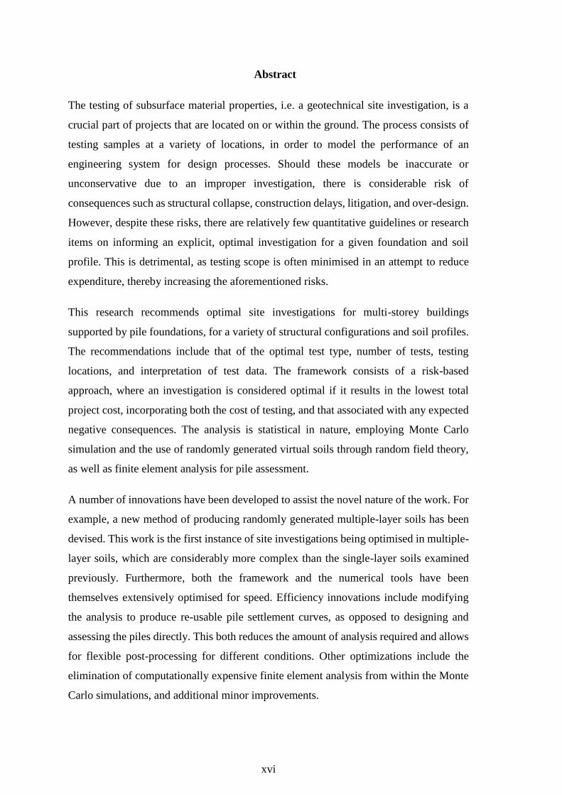
Abstract
The testing of subsurface material properties, i.e. a geotechnical site investigation, is a
crucial part of projects that are located on or within the ground. The process consists of
testing samples at a variety of locations, in order to model the performance of an
engineering system for design processes. Should these models be inaccurate or
unconservative due to an improper investigation, there is considerable risk of
consequences such as structural collapse, construction delays, litigation, and over-design.
However, despite these risks, there are relatively few quantitative guidelines or research
items on informing an explicit, optimal investigation for a given foundation and soil
profile. This is detrimental, as testing scope is often minimised in an attempt to reduce
expenditure, thereby increasing the aforementioned risks.
This research recommends optimal site investigations for multi-storey buildings
supported by pile foundations, for a variety of structural configurations and soil profiles.
The recommendations include that of the optimal test type, number of tests, testing
locations, and interpretation of test data. The framework consists of a risk-based
approach, where an investigation is considered optimal if it results in the lowest total
project cost, incorporating both the cost of testing, and that associated with any expected
negative consequences. The analysis is statistical in nature, employing Monte Carlo
simulation and the use of randomly generated virtual soils through random field theory,
as well as finite element analysis for pile assessment.
A number of innovations have been developed to assist the novel nature of the work. For
example, a new method of producing randomly generated multiple-layer soils has been
devised. This work is the first instance of site investigations being optimised in multiple-
layer soils, which are considerably more complex than the single-layer soils examined
previously. Furthermore, both the framework and the numerical tools have been
themselves extensively optimised for speed. Efficiency innovations include modifying
the analysis to produce re-usable pile settlement curves, as opposed to designing and
assessing the piles directly. This both reduces the amount of analysis required and allows
for flexible post-processing for different conditions. Other optimizations include the
elimination of computationally expensive finite element analysis from within the Monte
Carlo simulations, and additional minor improvements.
xvii
Practicing engineers can optimise their site investigations through three outcomes of this
research. Firstly, optimal site investigation scopes are known for the numerous specific
cases examined throughout this document, and the resulting inferred recommendations.
Secondly, a rule-of-thumb guideline has been produced, suggesting the optimal number
of tests for buildings of all sizes in a single soil case of intermediate variability. Thirdly,
a highly efficient and versatile software tool, SIOPS, has been produced, allowing
engineers to run a simplified version of the analysis for custom soils and buildings. The
tool can do almost all the analysis shown throughout the thesis, including the use of a
genetic algorithm to optimise testing locations. However, it is approximately 10 million
times faster than analysis using the original framework, running on a single-core
computer within minutes.

xviii
Statement of Originality
I certify that this work contains no material which has been accepted for the award of any
other degree or diploma in my name, in any university or other tertiary institution and, to
the best of my knowledge and belief, contains no material previously published or written
by another person, except where due reference has been made in the text. In addition, I
certify that no part of this work will, in the future, be used in a submission in my name,
for any other degree or diploma in any university or other tertiary institution without the
prior approval of the University of Adelaide and where applicable, any partner institution
responsible for the joint-award of this degree.
I acknowledge that copyright of published works contained within this thesis resides with
the copyright holder(s) of those works.
I also give permission for the digital version of my thesis to be made available on the
web, via the University’s digital research repository, the Library Search and also through
web search engines, unless permission has been granted by the University to restrict
access for a period of time.
I acknowledge the support I have received for my research through the provision of an
Australian Government Research Training Program Scholarship (Australian
Postgraduate Award).
Signed: ____ _____ Date: _____19 August 2020___________
xix
Acknowledgements
There are a number of people who I would like to thank as they, through their direct or
indirect support, contributed to the work in this thesis. This starts with my undergraduate
days at the University of Adelaide. Firstly, my interest and ability in geotechnical
engineering was consolidated through the courses taught by An Deng and Brendan Scott,
who set me on this path. Secondly, my work on this topic was also made possible through
a foundation in computer programming in the Fortran courses taught by Nicole Arbon
and Dmitri Kavetski. This base allowed me to learn a variety of programming languages,
which are becoming increasingly important in the modern world. Finally, I would like to
thank my Honours project supervisors Mark Thyer and David McInerny for their
guidance. They helped provide me with the full set of research skills, from writing to
technical analysis, which have served me well throughout my PhD.
There were several people who provided general support throughout my candidature.
This includes Mark Innes, the civil engineering school’s specialist IT officer, who helped
set up my software and instructed use of the school’s cloud server for my early work.
There is also the team behind the University’s Phoenix supercomputer, without which the
majority of this work would not have been possible. In particular I would like to thank
Exequiel Sepúleveda, who is a fellow civil researcher and my most frequent contact on
the Phoenix team. He provided guidance on how to use the system and advice on how to
parallelise the code to run quickly. Exequiel also introduced me to the Python
programming language which I enjoy using, and my knowledge of it has led directly to
my first engineering job.
There are many people who contributed in a non-technical capacity as well. This includes
the civil engineering administrative team, in particular Julie Ligertwood, who has worked
with me many times in postgraduate student matters. This includes both problem-solving
and the running of social events, in collaboration with the Civil Postgrad Liaison
committee which I chaired for two years. I also wish to thank the members of that
committee, and also the more general Adelaide University Postgraduate Society
committee, which I was president of for one year, for improving work-life balance for
students. There can be high levels of stress and pressure at times during a PhD, due to the
large pile of work involved, and having a good support network has been invaluable. I
have also been involved with the Australian Geomechanics Society, which I’m currently

xx
chairing, and am grateful for the opportunity the AGS has given me to learn new skills
and expand my geotechnical engineering network, leading to my first engineering job.
Of those on the AGS committee, I would like to thank Richard Herraman for his
mentoring support.
There are researchers who have contributed in a direct fashion to the technical work in
this thesis. I also wish to thank Gordon Fenton and Vaughan Griffiths for their roles in
developing the powerful Random Finite Element Method which this framework was
originally based on. They also developed the virtual soil generation and finite element
analysis subroutines, which are incorporated in the SIOPS program. Gordon and Vaughan
served as co-authors on two of my journal papers. I am grateful to Jianye Ching, who
provided early access to the Pseudo Incremental Energy method that he developed, which
I’ve implemented as a key optimization in SIOPS’ single layer analysis mode. I also wish
to thank Jason Goldsworthy and Ardy Arsyad for the large raft of studies they’ve done
on an early version of this framework, which have served as a valuable resource and
helped provide a great deal of direction.
I would like to thank my family, in particular my parents Neil and Katerene, for providing
their unending and unwavering support throughout the challenges and obstacles that arose
over the years of PhD candidature. They have also worked hard to provide me with a
good education, and helped shape my dedication and work ethic.
Last, but not least, I would like to thank my PhD supervisors Mark Jaksa and Yien Lik
Kuo for their countless hours of guidance and support towards my PhD. They always
made time for a discussion when I needed advice. Yien Lik provided critical assistance
in helping me understand and set up early software implementations of the virtual soil
generation and finite element analysis algorithms. His suggestions on applying
evolutionary algorithms to this research shaped the direction of final third of my
candidature. This not only resulted in the last two papers on optimising testing locations,
but in SIOPS itself, as I would not have started coding the program without the need for
extreme efficiency that a genetic algorithm requires. As SIOPS is a key outcome of this
research for both practicing engineers and other researchers, this contribution cannot be
understated.

xxi
I am deeply grateful to Mark Jaksa, without whom this PhD would not be possible. Mark
helped me choose this topic based on my strengths, and of course he had authored the
original version of the framework on which this research is based. I am appreciative of
Mark’s hands-off supervising style which gave me the freedom to solve the problems I
wanted to address. He was always supportive of the directions and methods I used,
although wasn’t afraid to give a push when rare tangents occurred. In addition to the
technical support and writing support, Mark has been a mentor to me over many years,
providing valuable advice for my work with the AGS and other extra-curricular activities
such as research presentation competitions. I have enjoyed working with Mark
immensely, and it is unsurprising that he has won many comedy awards. I could not have
hoped for a better supervisor.
xxii
Notation
1Q = 1st quartile (reduction method);
ANN = artificial neural network;
BH = borehole;
C = centre-to-centre pile spacing;
CK = complete knowledge pile case;
CMD = covariance matrix decomposition;
COV = coefficient of variation;
CPT = cone penetration test;
D = pile diameter;
DMT = flatplate dilatometer test;
E = Young’s modulus;
Eeff = effective Young’s modulus;
EA = evolutionary algorithm;
FEA = finite element analysis;
FEM = finite element method;
G = shear modulus
GA = geometric average;
HA = harmonic average;
I2 = inverse-distance squared (reduction method);
ID = inverse-distance (reduction method);
xxiii
JFIP = Jaksa Framework Implementation in Python (software);
L = pile embedment length;
LAS = local average subdivision;
LCPC = Laboratoire Central des Ponts et Chaussées;
MAE = mean absolute error;
MCA = Monte Carlo analysis;
MN = minimum reduction method;
MPI = message passing interface;
MSE = mean square error;
n = number of data points;
PIE = pseudo-incremental energy (method);
qc = cone tip resistance;
r = coefficient of correlation;
RE = relative error;
RFT = random field theory;
RG = regular grid (sampling pattern);
RMSE = root mean square error;
S = settlement;
su = undrained shear strength of soil;
SA = standard arithmetic average;
SI = site investigation;
xxiv
SIOPS = Site Investigation Optimization for Piles using Statistics (software);
SOF = scale of fluctuation;
SPT = standard penetration test;
SR = stratified random (sampling pattern);
SSU = stratified systematic unaligned (sampling pattern);
t = thickness of soil layer;
TT = triaxial test;
μ = average;
μcum = cumulative average;
= Poisson’s ratio;
θj = correlation length in dimension j;
g = geometric standard deviation;

Chapter 1: Introduction
1
1 Chapter 1: Introduction

Chapter 1: Introduction
2
Chapter 1: Introduction
3
1.1 Introduction
The largest aspect of technical and financial risk, in civil engineering projects, lies in the
ground as subsurface material properties are largely unknown (Jaksa et al. 2003).
Therefore, it is necessary to estimate these properties through testing the soil at a subset
of locations; a practice known as a geotechnical site investigation (Bowles 1997; Wiesner
1999). Unfortunately, soil is spatially variable, with properties potentially changing
drastically within a given site, and between different sites (Jaksa 1995). As such, it is
important to test at multiple locations, to a degree that provides adequate knowledge of
the site of interest, as dictated by the variability of the site and the nature of the civil
engineering works (Littlejohn et al. 1994).
Understandably, the use of targeted, robust investigations is likely to decrease total
project cost (Site Investigation Steering Group 1993; Clayton 2001; Van Staveren and
van Seters 2004; Goldsworthy 2006; Goldsworthy et al. 2007a; Albatal 2013). On the
other hand, insufficient or inappropriate investigations can result in an array of
undesirable consequences. These include construction delays as unexpected problems are
discovered (National Research Council 1984; Institution of Civil Engineers 1991;
Littlejohn et al. 1994; Whyte 1995; Albatal 2013; Zumrawi 2014; Boeckmann and Loehr
2016), foundation failure and structural collapse (Nordlund and Deere 1970; Association
of Soil Foundation Engineers 1996; Moh 2004), legal disputes and change orders
(Boeckmann and Loehr 2016), and finally but most difficult to quantify, expensive
foundation overdesign (Collingwood 2003; Andrews 2006). There is evidence to suggest
that over 50% of construction contracts experience major difficulties when carrying out
sub-structure works due to inadequate site investigations (Ashton and Gidado 2002).
Clearly, there is a need to undertake high quality investigations.
Despite this, there is little quantitative guidance on the planning of optimal investigations
for specific projects. Rather, there are non-site specific rules-of-thumb (Lowe III and
Zaccheo 1991; Bowles 1997). There are various standards available in different
jurisdictions, however these are typically quite limited. For example, the Australian and
European standards on site investigations provide vague, open-ended and qualitative
recommendations (European Standards 2006a; Australian Standards 2016). Other
standards provide a range of recommended sample spacings without regard for soil
variability (British Standards 1999; European Standards 2006b). Other standards provide
Chapter 1: Introduction
4
a strict minimum and suggest that additional sampling is required for highly variable
soils, without elaboration (Australian Standards 2017). None of these guidelines provide
explicit, site-specific recommendations. To some extent, this ambiguity is intentional as
it provides engineers with full flexibility to use their engineering judgement and
experience.
However, in reality this ambiguity results in a tendency for investigations to be minimised
in an effort to reduce budget, opening projects up to the risks discussed above and so,
ironically, far greater expenses. Indeed, some investigations cost as little as 0.025-0.03%
of the total budget (National Research Council 1984; Jaksa 2000). It is clear that there’s
a need to inform optimal investigations in a way that balances cost and risk.
Therefore, this thesis presents a risk-based approach that makes site-specific, project-
specific recommendations of optimal investigations, with the intention of minimising
total project cost.
1.2 Literature Review
In addition to the existing site investigation guidelines and standards given in §1.1, there
are a variety of frameworks and studies in existence which aim to inform optimal site
investigations. There is a degree of literature review provided throughout the thesis in
individual papers for their respective individual problems. However, a brief self-
contained literature discussion is provided here, in the context of this research as a whole.
As such, an overview of these frameworks is given below, along with background
information.
1.2.1 Background
Before discussing the specific frameworks, it is worth mentioning some similarities in
order to better understand their justification. Firstly, each framework is statistical in
nature, owing to the fact that soil profiles can vary greatly between different sites, and
even over distance within a single site, as previously mentioned. This variability means
it is very difficult to determine which investigation is truly optimal for a given site without
already knowing the material properties at all locations within the soil. Instead, the
frameworks address this problem by determining what is most likely to the best
investigation for a soil of a given statistical description, as opposed to what is guaranteed
Chapter 1: Introduction
5
to be best. Secondly, it is notable that each of these frameworks involves numerical
simulation as opposed to laboratory or field-based work. Simulation is required as the
full set of material properties of a site must be known at all locations, or otherwise at a
large proportion of locations. Such extensive testing is not feasible from both a practical
and financial perspective.
A common component of the frameworks’ methodology, that solves the problem of
knowing a site’s properties, is that of virtual soil profiles. Specifically, randomly
generated virtual soils, produced through random field theory (Vanmarcke 1983) are
volumes of correlated soil properties that vary over distance. As the name suggests, these
properties are randomly generated according to rules, such that different types of soil
profiles can be achieved by varying these rules and input parameters. Numerous graphical
representations of random fields are given throughout this thesis, starting from Chapter
2.
Furthermore, several of these approaches use a powerful statistical technique called
Monte Carlo analysis (Ang 2007). It solves complex problems through the repetition of
a principally deterministic analysis with random attributes in each run. The resulting
aggregate of outputs forms a statistical distribution of desired data. The random attribute
in this context is the random virtual soil. Note that individual runs are referred to as Monte
Carlo realisations.
To determine the appropriateness of each investigation, it is necessary to have an
understanding of the basic site investigation and design process. When a geotechnical
structure such as a foundation is to be built at a particular location (site), the following
broad steps are undertaken:
1. A site investigation takes place, consisting of drilling into the ground at various
locations and testing the resulting samples. These drilled locations are referred to
as boreholes. There are two general types of tests; in situ, which take place directly
in the field on the original soil, and laboratory, in which samples are transported
to a dedicated facility for testing. The nature of the soil testing is such that some
degree of random error is present in the results (Phoon and Kulhawy 1999).
Laboratory tests are generally more accurate, although errors can occur due to the
collection and transportation processes.
Chapter 1: Introduction
6
2. The results of the investigation are used to build a soil model; a representation of
what engineers expect the subsurface profile to look like based on the available
data. Typically, when there is a greater quantity and quality of data, the soil model
is more accurate and reliable.
3. The soil model is used to design the foundation according to various criteria, for
example; a limit of excessive deformation under load. Models allow the engineer
to trial a range of designs in order to find one that meets the design criteria while
ideally being as inexpensive to build as possible.
4. The foundation and its associated structure are built. If the soil model is incorrect
or inaccurate, or the design is insufficiently conservative, excessive deformation
will occur, leading to structural damage.
1.2.2 Site Investigation Optimization Frameworks
There are three broad families of frameworks that can be used for optimising
investigations. The first consists of frameworks which generate a random virtual soil,
conduct a site investigation, and then analyse the performance of the resulting soil model.
The soil model is assessed either in comparison to the true, original generated soil (Guan
and Wang 2019; Wang et al. 2019), or with regards to some level of soil model
uncertainty (Parsons and Frost 2002; Gong et al. 2014; Gong et al. 2016; Huang et al.
2020). An advantage of this general approach is that, as it assesses the accuracy of the
soil model itself, it is agnostic as to the type of geotechnical structure. As such, it is
theoretically widely applicable. However, this advantage is simultaneously a trade-off;
because it is structure-agnostic, it cannot inform the specific effects on a structure. In
other words, there is no direct relationship given between the accuracy of the soil model
and the performance of a foundation, such as with respect to the degree of structural
damage. Therefore, it is difficult to determine what scope of investigation is sufficient
for a particular case. Furthermore, as soil model accuracy increases with additional
investigation, the performance metric improves asymptotically. This means that while it
informs the ideal attributes of an investigation for a given investigation effort, it cannot
inform a single investigation that is objectively the best.
Another line of study involves the field of reliability-based design (RBD). This approach
relates the nature of an investigation to various probabilities of failure (Ching and Phoon
2012; Ching et al. 2013). The advantage here is that engineers can tailor the scope of a
Chapter 1: Introduction
7
site investigation to the importance of a structure. For instance, a hospital would involve
a higher reliability than a residential house, and would therefore require a more thorough
investigation. However, the aforementioned studies obtained site investigation samples
from a random number generator, which is not representative of a realistic soil profile,
unlike the previously discussed virtual soils. It is possible to use virtual soils in a RBD
and site investigation methodology, e.g. Naghibi et al. (2014), however the precision is
typically insufficient given the large number of Monte Carlo realisations required.
The third general framework is that of Jaksa et al. (2003), which informs an optimal
investigation by suggesting one that is most likely to result in the lowest total project cost,
for a specific foundation type and configuration. The approach is derived from the
Random Finite Element Method (RFEM), detailed by Fenton and Griffiths (2008) and
first used by Fenton and Griffiths (1993); Griffiths and Fenton (1993). RFEM is a
statistical technique combining randomly generated virtual soils with finite element
analysis (FEA) and Monte Carlo simulation. FEA is a mathematical technique used here
to determine the deformation of a foundation and soil according to an applied load (Smith
et al. 2014). The key difference between this framework and the first one described, is
that here, the foundation response is assessed directly, as opposed to indirectly through
the soil model.
This methodology has the advantage that an explicit, objectively optimal investigation
can be identified for a specific project. This is in contrast to the other frameworks where
additional investigation continually results in superior performance, albeit at a
diminishing rate. Furthermore, the performance metric of total cost is relatable and easy
to understand, and the benefit from undertaking the optimal investigation, over a less
thorough one, is explicitly quantified. Quantifying the improvement provides engineers,
and more importantly the clients, with the necessary motivation to choose the optimal
investigation. The procedure associated with this method is elaborated further in §1.4.
It should be noted that several variants of this framework exist, featuring differences such
as the choice of investigation performance metric, or the presence or otherwise of a true
optimal foundation for comparison. This general framework family has been used to
assess site investigation performance for pad footings and piles, with the most extensive
examples given by Goldsworthy (2006) and Arsyad (2009) for those foundation types
respectively.
Chapter 1: Introduction
8
The clear advantages of the Jaksa et al. (2003) framework are what led to its use in this
thesis, and why it has been used in a wide range of studies. The description of this
framework is given in §1.4.
For the sake of completeness, it is worth mentioning some studies which are tangentially
related to the topic of optimising site investigations for foundations. This includes the
optimization of site investigations for slopes, e.g. (Li et al. 2016b; Li et al. 2019b; Yang
et al. 2019a; Yang et al. 2019b), and advanced characterisation of ground profiles based
on site investigation results, e.g. (Li et al. 2016a; Li et al. 2019a; Sastre Jurado et al.
2020). Similarly, two theses involving site investigations are briefly discussed here. Kim
(2011) undertook some general work on soil simulation and site investigations, although
this was largely in the context of classroom education. Halim (1991) undertook statistical
analysis of site investigations for detecting a geological anomaly in a layered soil.
However, the soil properties within each layer were uniform, and the layer boundaries
were flat and horizontal. These limitations, likely resulting from the lack of computing
power at the time of writing, are deemed excessive.
1.2.3 Research Gaps
The full suite of works using the adopted framework include: (Goldsworthy et al. 2004a;
Goldsworthy et al. 2004b; Goldsworthy et al. 2005; Jaksa et al. 2005; Goldsworthy 2006;
Goldsworthy et al. 2007a; Goldsworthy et al. 2007b) for pad footings, and (Arsyad 2009;
Arsyad et al. 2009; Arsyad et al. 2010) for pile foundations. Despite the number of studies
using this framework, there are significant and consistent gaps and limitations present
throughout.
Firstly, to date, all instances have involved the use of single-layer soils. This is
unconservative and unrealistic, as soils typically consist of multiple layers separated by
complex, undulating boundaries which add another source of uncertainty. Furthermore,
as elaborated in Chapter 4, there is currently no method of generating multiple-layer soil
profiles that is suitable for use in this framework. Some work has been undertaken in
predicting pad foundation settlement in multi-layered random fields, e.g Kuo et al.
(2004); Kuo (2009); Kuo et al. (2009); Ghalba et al. (2012). However, limitations exist
in that the layer boundaries were horizontal, which is an unrealistic simplification, and
the works did not incorporate site investigations.
Chapter 1: Introduction
9
Secondly, the framework is extremely computationally intensive due to its extensive use
of finite element analysis, which is the recommended method of foundation assessment
(Goldsworthy 2006). A supercomputer is required to obtain results in a realistic
timeframe; however, innovations could be employed to make the method more accessible
to researchers.
Thirdly, while significant focus was placed on optimising investigation attributes such as
the number of boreholes, little attention was given to optimising borehole locations,
particularly for more than a single borehole. Finally, the studies have not formed a guide
or tool to allow engineers to optimise site investigations. Rather, they have assessed the
performance of a small number of investigations in relation to a limited number of soils
and structural configurations. While these assessments are informative, they are not
comprehensive, nor structured in an applicable, user-ready manner.
A further gap involves pile foundation assessment, owing to two observations. Firstly,
relatively little work in this field has been carried out on piles compared to pads.
Secondly, the existing studies on pile foundations, which were produced from a Masters
thesis, used a highly simplified version of the framework, subject to numerous technical
simplifications that diminish the robustness of the results. These simplifications include
a crude and arbitrary approximation of pile performance, as opposed to the accuracy and
reliability of FEA. There was no pile design process; instead, the capacity of a fixed pile
length was assessed. While several test types are commonly used by practicing engineers,
this research had only focused on a single type, the cone penetration test. Furthermore,
the optimization metrics of probability of failure and over-design were employed, as
opposed to that of total project cost. These simplifications and limitations mean that
existing studies featuring pile foundations are not comparable with the current
framework.
Recent studies, which are similar in methodology to this framework, include
Christodoulou and Pantelidis (2020); Christodoulou et al. (2020a, 2020b) which each
study the case of a pad foundation, pile foundation and retaining wall, respectively.
However, the metric used is the probability of failure. Perhaps more importantly, the
analyses were limited to 2D, variable, single-layer soils, while soils in nature vary in 3D.
Chapter 1: Introduction
10
A more specific, technical and in-depth literature review of all studies using the Jaksa et
al. (2003) framework are given throughout Sections 3 and 4 of Appendix D, in addition
to discussion throughout this thesis.
1.3 Aims and Scope of Thesis
Based on the discussion in the previous section, the most prominent gaps and limitations
are:
• The existing methodology is extremely computationally intensive.
• Studies using the nominated framework have been limited to single-layer soils,
which is an overly simplified case.
• No ideal means of generating multiple-layer soils is available.
• Existing studies on optimising site investigations for pile design have been
flawed.
• Perhaps most importantly, existing studies in general have yet to produce a tool
or guideline that can universally optimise investigations on a case-specific basis.
As such, the aims of this thesis are therefore:
1. To optimise the site investigation framework with regards to computational speed.
2. To devise a method of simulating multi-layer site investigation soils that is
random yet customisable.
3. To use (1) and (2) to assess site investigation performance in a variety of 3D soil
profiles, including those with multiple layers and soil lenses, and with a range of
site investigation attributes. The results will determine the impact of these
conditions and inform engineers of good site investigation practice.
4. To create versatile tools to allow engineers to optimise a wide variety of site
investigations in a range of soils and for all structural configurations.
1.4 Method
As with the literature review, there is description of specific methodology in each paper
contained in this thesis. However, a high-level overview is given here to describe the
general framework used.
The present framework uses the RFEM method, described in §1.2.2, to calculate the
expected total project cost for a wide range of different site investigations. As such,
Chapter 1: Introduction
11
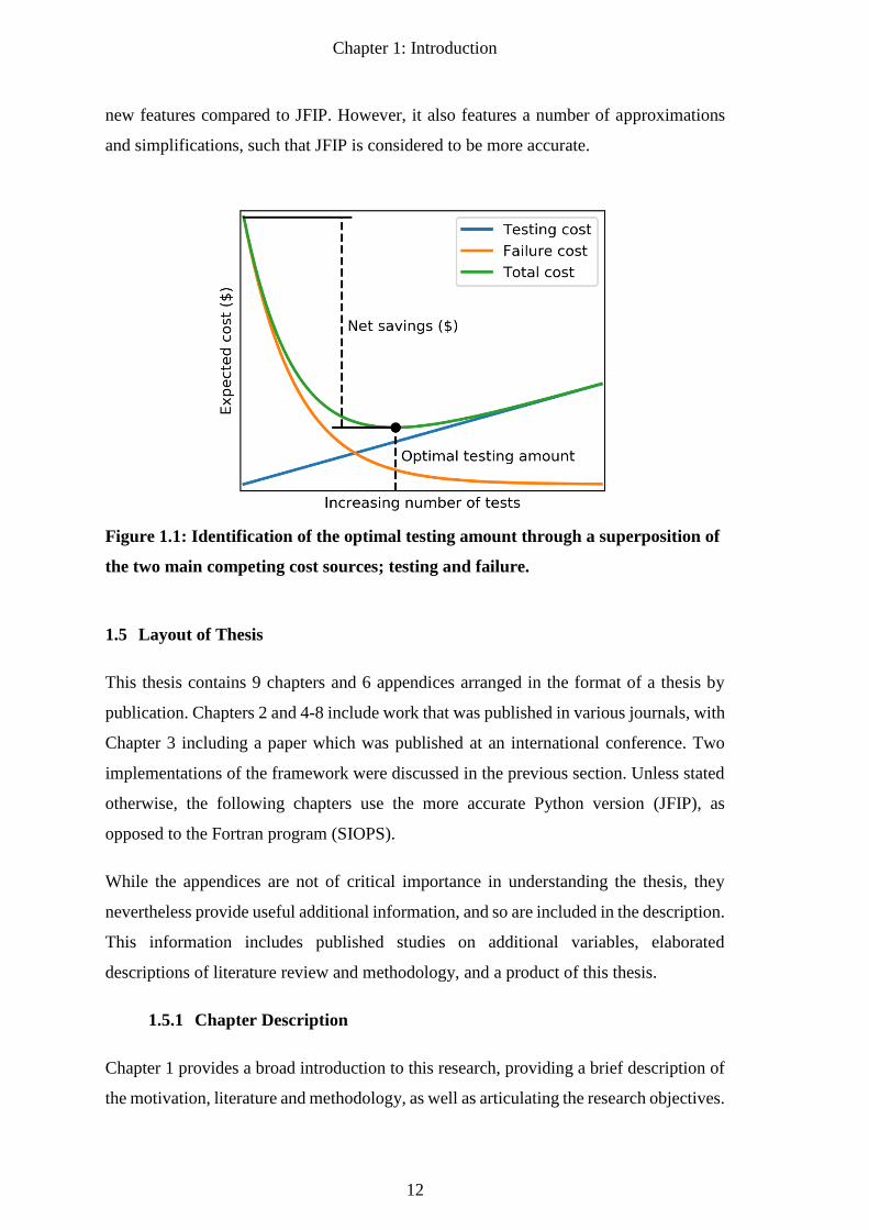
optimal investigation is simply that associated with the lowest cost. The cost is primarily
a trade-off between two competing sources, that of the investigation, and of undesirable
consequences, as shown in Figure 1.1. These costs increase and decrease with further
testing, respectively. It should be noted that the undesirable consequences are modelled
exclusively as the cost of repairing structural damage that results from excessive
foundation deformation. Other consequences such as construction delays and litigation
are not considered.
The total expected cost is calculated through a multi-step process. Detailed flow charts
of the procedure are given throughout this thesis, however a brief summary is given
below:
1. A 3D virtual soil with the desired statistics is generated using random field theory.
2. A virtual site investigation is conducted, consisting of extracting samples from
the soil at respective testing locations.
3. A soil model is devised, and the foundation is designed from it.
4. The deformation of the foundation is determined with respect to the true virtual
soil.
5. A failure cost is calculated as a function of the deformation, and the cost
associated with the investigation is given.
6. Steps 2-5 are repeated for a variety of investigations.
7. Steps 1-6 are repeated multiple times in a Monte Carlo simulation.
8. The average (expected) total cost is calculated, and the investigation with the
lowest cost is recommended.
The research report given in Appendix D was written for the purpose of describing and
validating this framework. As such, the author directs the reader to that section for the
most extensive methodology description. Alternatively, the software manual given in
Appendix E contains an arguably more concise description of the steps given above.
The majority of the analysis has been conducted through the unreleased JFIP (Jaksa
Framework Implementation in Python) software created by the author in the Python
programming language. JFIP is not intended for public use owing to reasons discussed in
Appendix F. Later analysis was carried out through a reimplementation in the Fortran
programming language. The Fortran program, termed SIOPS (Site Investigation
Optimization of Piles using Statistics), features extensive optimizations, innovations and
Chapter 1: Introduction
12
new features compared to JFIP. However, it also features a number of approximations
and simplifications, such that JFIP is considered to be more accurate.
Figure 1.1: Identification of the optimal testing amount through a superposition of
the two main competing cost sources; testing and failure.
1.5 Layout of Thesis
This thesis contains 9 chapters and 6 appendices arranged in the format of a thesis by
publication. Chapters 2 and 4-8 include work that was published in various journals, with
Chapter 3 including a paper which was published at an international conference. Two
implementations of the framework were discussed in the previous section. Unless stated
otherwise, the following chapters use the more accurate Python version (JFIP), as
opposed to the Fortran program (SIOPS).
While the appendices are not of critical importance in understanding the thesis, they
nevertheless provide useful additional information, and so are included in the description.
This information includes published studies on additional variables, elaborated
descriptions of literature review and methodology, and a product of this thesis.
1.5.1 Chapter Description
Chapter 1 provides a broad introduction to this research, providing a brief description of
the motivation, literature and methodology, as well as articulating the research objectives.
Chapter 1: Introduction
13
Chapter 2 assesses site investigation performance in a single layer soil scenario using an
updated version of the optimization framework. Some early, albeit critical speed
optimizations are introduced and described. The test type, means of data interpretation,
and number of boreholes was optimised for a range of soil conditions. A sensitivity
analysis of these parameters, along with that of building size, is discussed to inform areas
of focus for subsequent multi-layer analysis. The study also presents an argument for
components that should be included in a universal site investigation optimization
guideline. The paper was published in the Canadian Geotechnical Journal.
Chapter 3 presents an approach that generalises site investigation optimization results to
all building sizes. This chapter serves as an explanation and proof-of-concept, using
results generated from the SIOPS program. An example is given for a highly variable
single-layer soil and the CPT test, where the number of boreholes is optimised for a
variety of building sizes. The approach can be extended to other soils and test types,
although the results will need to be processed for each new case. An additional set of test
types have been assessed in §9.1.5.1. The study was published in the Proceedings of the
7th International Symposium on Geotechnical Safety and Risk, in Taipei, Taiwan.
Chapter 4 provides a new method of generating complex, multi-layered soils. This
research required a method that produces soils that are random, yet have attributes that
are easy to control. The approach is loosely inspired by the processes of erosion and
deposition, producing plausibly realistic profiles that may potentially contain lenses; a
geological feature that may be particularly detrimental to site investigations. Inputs to
this method include the number of layers, their variability and approximate location, in
addition to single-layer soil parameters. This method can be used in other fields of
probabilistic geotechnical analysis, augmenting existing single-layer generation routines.
This work was published as a technical note in Georisk.
Chapter 5 contains the first study that examines site investigation performance in a multi-
layer system, examining the relatively simple case of a two-layer soil scenario. It
examined the effect of the presence of a layer boundary on investigation performance
compared to a single layer scenario. This demonstrated the relative importance of soil
parameters regarding their contribution to site investigation uncertainty. This
disambiguation of performance both informs what to focus on in subsequent analysis,
and is of use to practicing engineers. The study also introduced an important speed
Chapter 1: Introduction
14
optimization of multi-layer pile settlement analysis, allowing 3D scenarios to be
represented as the exponentially faster 2D. The number of boreholes was optimised for
each case examined. This work was published in the Canadian Journal of Civil
Engineering.
Chapter 6 greatly increased the complexity of soils, featuring various numbers of layers,
and the possibility of soil lenses. It examined what effect these features had on site
investigation performance and optimised the number of boreholes for those cases. It also
provides a sensitivity analysis of the horizontal variability of layer boundaries. This study
was published in Georisk.
The remaining studies changed the focus from optimising the number of boreholes to
optimising borehole locations. Furthermore, they used the more efficient SIOPS program
to generate results, due to the quantity of data required.
Chapter 7 optimised the location of a single borehole in a single-layer soil through
assessing heatmaps of borehole performance across a site. Inspection of the heatmaps
also conveyed the relative performance between different testing locations. This chapter
examined many of the variables seen in Chapter 1, albeit with respect to testing location.
These variables include test type, method of data interpretation and aspects of soil
variability. Additionally, different foundation configurations and performance metrics
were assessed. The results informed which variables were sensitive and required further
analysis with additional boreholes. The study was published in Georisk.
Chapter 8 implemented a genetic algorithm to optimise the location of different numbers
of boreholes in both single- and multi-layered soils. This is the first study to use such an
algorithm to find globally optimal testing locations with respect to foundation
performance. As such, it serves as a proof-of-concept. A comparison of optimal testing
locations for single and multiple-layer soils is given. Through inference of trends across
the results, a set of suggested rules is provided for ideal testing locations. This paper has
been submitted to the Journal of Geosciences.
Chapter 9 summarises conclusions and useful insights that have resulted from work in
this thesis, along with providing recommendations for future work.
Chapter 1: Introduction
15
1.5.2 Appendices Description
Appendices A-C contain work published in conference papers relatively early in the PhD.
The first study published in relation to this thesis is given in Appendix A, which consists
of a simplified analysis of a 2D multi-layered soil profile. It examined the effect of
different testing location patterns and performance metrics, using a now-obsolete early
Fortran program. Appendix B complements Chapter 2 in that a variety of sampling
location patterns and areas were assessed in a 3D single-layer soil using the Python
implementation (JFIP). Similarly, Appendix C complements Chapter 2 in that it
investigated possible benefits to weighting samples according to their distance from a
pile when interpreting the data.
Appendix D contains a detailed report describing the development, justification and
verification of the current version of the site investigation optimization framework.
Specifically, it was written in respect to the methodology used in JFIP. The report also
includes a literature review of the studies that used earlier versions of this thesis’
framework.
Appendix E contains the SIOPS software manual, describing the general theory and user
inputs for the program developed by the author. This manual was created to instruct
engineers how to use SIOPS so that they may optimise their investigations for their
respective projects and sites. SIOPS is highly efficient, running in less than one minute
under some circumstances on a single-core computer. It can be used to optimise the
number of boreholes, test type and interpretation of sample data through comparative
analysis. It can also optimise borehole locations through heatmap analysis or use of the
genetic algorithm. Other researchers can use SIOPS for future studies. The software, and
by extension the user manual, is a key product of this thesis. Appendix F discusses why
the JFIP software is not supported or publicly released, with SIOPS being favoured for
future work.
1.6 References
Albatal, A. 2013. Effect of inadequate site investigation on the cost and time of a
construction project. Masters Thesis, Construction and Building Engineering
Department, Arab Academy for Science, Technology and Maritime Transport,
Cairo.
Chapter 1: Introduction
16
Andrews, P. V. 2006. The Hidden Cost of Geotechnical Investigations. Australian
Geomechanics, 41(4), 35-46.
Ang, A. H.-S. 2007. Probability concepts in engineering : emphasis on applications in
civil & environmental engineering (2nd ed. ed.). Hoboken, N.J: John Wiley &
Sons.
Arsyad, A. 2009. The effect of limited site investigations on the design and performance
of pile foundations. Masters Thesis, School of Civil, Environmental and Mining
Engineering, University of Adelaide, Adelaide.
Arsyad, A., Jaksa, M., Fenton, G., and Kaggwa, W. 2009. The effect of limited site
investigations on the design of pile foundations. In Proceedings of the
International Conference on Soil Mechanics and Geotechnical Engineering (17th:
2009: Egypt).
Arsyad, A., Jaksa, M. B., Kaggwa, W., and Mitani, Y. 2010. Effect of radial distance of
a single CPT sounding on the probability of over-and under-design of pile
foundation. In Proceedings of the tthe First Makassar International Conference on
Civil Engineering, Makassar, Indonesia.
Ashton, P., and Gidado, K. 2002. The identification of uncertainty and risk associated
with inadequate site investigation procedures relative to project complexity.
Association of Soil Foundation Engineers. 1996. Case Histories of Professional Liability
Losses: ASFE Case Histories 1-65: Association of Soil and Foundation
Engineers.
Australian Standards. (2016). Geotechnical Site Investigations AS 1726.
Australian Standards. (2017). Bridge Design Part 3: Foundation and soil-sampling
structures AS 5100.3.
Boeckmann, A. Z., and Loehr, J. E. 2016. Influence of Geotechnical Investigation and
Subsurface Conditions on Claims, Change Orders, and Overruns.
Bowles, J. E. 1997. Foundation analysis and design (5 ed.): McGraw-Hill.
British Standards. (1999). Code of practice for site investigations BS 5930.
Ching, J., and Phoon, K.-K. 2012. Value of geotechnical site investigation in reliability-
based design. Advances in Structural Engineering, 15(11), 1935-1945.
Ching, J., Phoon, K.-K., and Yu, J.-W. 2013. Linking site investigation efforts to final
design savings with simplified reliability-based design methods. Journal of
Geotechnical and Geoenvironmental Engineering, 140(3), 04013032.
Christodoulou, P., and Pantelidis, L. 2020. Reducing Statistical Uncertainty in Elastic
Settlement Analysis of Shallow Foundations Relying on Targeted Field
Investigation: A Random Field Approach. Geosciences, 10(1), 20.
Chapter 1: Introduction
17
Christodoulou, P., Pantelidis, L., and Gravanis, E. 2020a. The Effect of Targeted Field
Investigation on the Reliability of Axially Loaded Piles: A Random Field
Approach. Geosciences, 10(5), 160.
Christodoulou, P., Pantelidis, L., and Gravanis, E. 2020b. The Effect of Targeted Field
Investigation on the Reliability of Earth-Retaining Structures in Passive State: A
Random Field Approach. Geosciences, 10(3), 110.
Clayton, C. 2001. Managing geotechnical risk: time for change? Proceedings of the
Institution of Civil Engineers-Geotechnical Engineering, 149(1), 3-11.
Collingwood, B. 2003. Geotechnical Investigations for Piling Projects: The False
Economy of a Cheap Site Investigation. Australian Geomechanics, 38(1), 41-48.
European Standards. (2006a). Eurocode 7 - Geotechnical desigh - Part 2: Ground
investigation and testing EN 1997-2.
European Standards. (2006b). Eurocode 7 - Geotechnical design - Part2: Ground
investigation and testing (Annex B.3) EN 1997-2.
Fenton, G. A., and Griffiths, D. 1993. Statistics of block conductivity through a simple
bounded stochastic medium. Water Resources Research, 29(6), 1825-1830.
Fenton, G. A., and Griffiths, D. V. 2008. Risk assessment in geotechnical engineering:
Wiley.
Ghalba, A., Jaksa, M. B., Kaggwa, W. S., Fenton, G. A., and Griffiths, V. G. 2012, 15-
18 July. Probabilistic analysis of foundation settlement on multilayered soil with
a complex layer-boundary. In Proceedings of the 11th Australia New Zealand
Conference on Geomechanics, Melbourne, Australia.
Goldsworthy, J., Jaksa, M., Fenton, G., Kaggwa, G., Griffiths, D., Poulos, H., and Kuo,
Y. 2004a. Influence of site investigations on the design of pad footings. In
Proceedings of the Australia-New Zealand Conference on Geomechanics (9th:
2004: Auckland, NZ).
Goldsworthy, J., Jaksa, M., Kaggwa, G., Fenton, G., Griffiths, D., and Poulos, H. 2005.
Reliability of site investigations using different reduction techniques for
foundation design. 9th International Conference on Structural Safety and
Reliability, 901-908.
Goldsworthy, J., Jaksa, M., Kaggwa, W., Fenton, G., Griffiths, D., and Poulos, H. 2004b.
Cost of foundation failures due to limited site investigations. In Proceedings of
the International Conference on Structural and Foundation Failures, Singapore.
Goldsworthy, J. S. 2006. Quantifying the risk of geotechnical site investigations. Ph.D
Thesis, School of Civil, Environmental and Mining Engineering, University of
Adelaide, Adelaide.
Goldsworthy, J. S., Jaksa, M. B., Fenton, G. A., Griffiths, D. V., Kaggwa, W. S., and
Poulos, H. G. 2007a. Measuring the risk of geotechnical site investigations. In
Proceedings of the Proc., Geo-Denver 2007.
Chapter 1: Introduction
18
Goldsworthy, J. S., Jaksa, M. B., Fenton, G. A., Kaggwa, W. S., Griffiths, V., and Poulos,
H. G. 2007b. Effect of sample location on the reliability based design of pad
foundations. Georisk, 1(3), 155-166.
Gong, W., Luo, Z., Juang, C. H., Huang, H., Zhang, J., and Wang, L. 2014. Optimization
of site exploration program for improved prediction of tunneling-induced ground
settlement in clays. Computers and Geotechnics, 56, 69-79. doi:
http://dx.doi.org/10.1016/j.compgeo.2013.10.008
Gong, W., Tien, Y.-M., Juang, C. H., Martin, J. R., and Luo, Z. 2016. Optimization of
site investigation program for improved statistical characterization of
geotechnical property based on random field theory. [journal article]. Bulletin of
Engineering Geology and the Environment, 1-15. doi: 10.1007/s10064-016-0869-
3
Griffiths, D., and Fenton, G. A. 1993. Seepage beneath water retaining structures founded
on spatially random soil. Géotechnique, 43(4), 577-587.
Guan, Z., and Wang, Y. 2019. Statistical charts for determining sample size at various
levels of accuracy and confidence in geotechnical site investigation.
Géotechnique, 1-15.
Halim, I. 1991. Reliability of geotechnical systems considering geological anomaly Ph.D
Thesis, Graduate College, University of Illinois, Urbana–Champaign, USA.
Huang, L., Huang, S., and Lai, Z. 2020. On the optimization of site investigation
programs using centroidal Voronoi tessellation and random field theory.
Computers and Geotechnics, 118, 103331.
Institution of Civil Engineers. 1991. Inadequate Site Investigation. London: Thomal
Telford.
Jaksa, M., Goldsworthy, J., Fenton, G., Kaggwa, W., Griffiths, D., Kuo, Y., and Poulos,
H. 2005. Towards reliable and effective site investigations. Géotechnique, 55(2),
109-121.
Jaksa, M., Kaggwa, W., Fenton, G., and Poulos, H. 2003. A framework for quantifying
the reliability of geotechnical investigations. In Proceedings of the 9th
International Conference on the Application of Statistics and Probability in Civil
Engineering.
Jaksa, M. B. 1995. The influence of spatial variability on the geotechnical design
properties of a stiff, overconsolidated clay. Ph.D Thesis, School of Civil,
Environmental and Mining Engineering, University of Adelaide, Adelaide.
Jaksa, M. B. 2000. Geotechnical risk and inadequate site investigations: a case study.
Australian Geomechanics, 35(2), 39-46.
Kim, J. H. 2011. Improvement of geotechnical site investigations via statistical analyses
and simulation. Ph.D Thesis, School of Civil & Environmental Engineering,
Georgia Institute of Technology, Atlanta.
Chapter 1: Introduction
19
Kuo, Y. L. 2009. Effect of soil variability on the bearing capacity of footings on multi-
layered soil. Ph.D Thesis, School of Civil, Environmental and Mining
Engineering, University of Adelaide, Adelaide.
Kuo, Y. L., Jaksa, M. B., Kaggwa, G. S., Fenton, G. A., Griffiths, D. V., and
Goldsworthy, J. S. 2004. Probabilistic analysis of multi-layered soil effects on
shallow foundation settlement. In Proceedings of the 9th Australia-New Zealand
Conference on Geomechanics, Auckland, NZ.
Kuo, Y. L., Jaksa, M. B., Lyamin, A. V., and Kaggwa, W. S. 2009. ANN-based model
for predicting the bearing capacity of strip footing on multi-layered cohesive soil.
Computers and Geotechnics, 36(3), 503-516. doi:
10.1016/j.compgeo.2008.07.002
Li, A., Jafari, N. H., and Tsai, F. T. C. 2019a. Modelling and comparing 3-D soil
stratigraphy using subsurface borings and cone penetrometer tests in coastal
Louisiana, USA. Georisk: Assessment and Management of Risk for Engineered
Systems and Geohazards, 1-19. doi: 10.1080/17499518.2019.1637528
Li, J., Cassidy, M. J., Huang, J., Zhang, L., and Kelly, R. 2016a. Probabilistic
identification of soil stratification. Géotechnique, 66(1), 16-26.
Li, Y., Hicks, M., and Vardon, P. 2016b. Uncertainty reduction and sampling efficiency
in slope designs using 3D conditional random fields. Computers and Geotechnics,
79, 159-172.
Li, Y., Qian, C., and Liu, K. 2019b. Sampling Efficiency in Spatially Varying Soils for
Slope Stability Assessment. Advances in Civil Engineering, 2019.
Littlejohn, G., MELLORS, T., and COLE, K. 1994. Without site investigation ground is
a hazard. In Proceedings of the Institution of Civil Engineers - Civil Engineering.
Lowe III, J., and Zaccheo, P. F. 1991. Subsurface explorations and sampling. In
Foundation Engineering Handbook (pp. 1-71): Springer.
Moh, Z. C. 2004. Site investigation and geotechnical failures. In Proceedings of the
Proceeding of International Conference on Structural and Foundation Failures.
Naghibi, F., Fenton, G., and Griffiths, D. 2014. Serviceability limit state design of deep
foundations. Géotechnique, 64(10), 787-799.
National Research Council. 1984. Geotechnical Site Investigations for Underground
Projects (Vol. 1). Washington.
Nordlund, R. L., and Deere, D. U. 1970. Collapse of Fargo grain elevator. Journal of Soil
Mechanics & Foundations Div.
Parsons, R., and Frost, J. 2002. Evaluating site investigation quality using GIS and
geostatistics. Journal of Geotechnical and Geoenvironmental Engineering,
128(6), 451-461.
Chapter 1: Introduction
20
Phoon, K.-K., and Kulhawy, F. H. 1999. Characterization of geotechnical variability.
Canadian Geotechnical Journal, 36(4), 612-624.
Sastre Jurado, C., Breul, P., Bacconnet, C., and Benz-Navarrete, M. 2020. Probabilistic
3D modelling of shallow soil spatial variability using dynamic cone penetrometer
results and a geostatistical method. Georisk: Assessment and Management of Risk
for Engineered Systems and Geohazards, 1-13. doi:
10.1080/17499518.2020.1728558
Site Investigation Steering Group. 1993. Specification for ground investigation: Thomas
Telford.
Smith, I. M., Griffiths, D. V., and Margetts, L. 2014. Programming the finite element
method (5th ed.): John Wiley & Sons.
Van Staveren, M. T., and van Seters, A. J. 2004. Smart Site Investigations Save Money!
In Engineering Geology for Infrastructure Planning in Europe (pp. 792-800):
Springer.
Vanmarcke, E. 1983. Random Fields: Analysis and Synthesis. London: MIT Press.
Wang, Y., Guan, Z., and Zhao, T. 2019. Sample size determination in geotechnical site
investigation considering spatial variation and correlation. Canadian
Geotechnical Journal, 56(7), 992-1002.
Whyte, I. 1995. The financial benefit from a site investigation strategy. Ground
engineering, 28(8), 33-36.
Wiesner, T. 1999. Site Characterisation. Australian Geomechanics, 34(4), 41-57.
Yang, R., Huang, J., Griffiths, D., Li, J., and Sheng, D. 2019a. Importance of soil property
sampling location in slope stability assessment. Canadian Geotechnical Journal,
56(3), 335-346.
Yang, R., Huang, J., Griffiths, D., Meng, J., and Fenton, G. A. 2019b. Optimal
geotechnical site investigations for slope design. Computers and Geotechnics,
114, 103111.
Zumrawi, M. 2014. Effects of Inadequate Geotechnical Investigation on Civil
Engineering Projects. International Journal of Science and Research, 3(6), 927-
931.
Chapter 2: Single Layer Analysis
21
2 Chapter 2: Single Layer
Analysis
Paper Title:
Toward a Generalised Guideline to Inform Optimal
Site Investigations for Pile Design

Chapter 2: Single Layer Analysis
22

Statement of AuthorshipTitle of Paper Toward a generalized guideline to inform optimal site investigations for pile design.
Publication Status
Publication Details Crisp, M. P., Jaksa, M. B., and Kuo, Y. L. 2019. Toward a generalized guideline to inform optimal
site investigations for pile design. Canadian Geotechnical Journal, 57(8), doi:
https://doi.org/10.1139/cgj-2019-0111
Principal Author
Name of Principal Author (Candidate) Michael Perry Crisp
Contribution to the Paper
Modified the software and methodology, generated and analysed the data, wrote the
manuscript.
Overall percentage (%) 80%
Certification: This paper reports on original research I conducted during the period of my Higher Degree by
Research candidature and is not subject to any obligations or contractual agreements with a
third party that would constrain its inclusion in this thesis. I am the primary author of this paper.
Signature Date
Co-Author Contributions
By signing the Statement of Authorship, each author certifies that:
i. the candidate’s stated contribution to the publication is accurate (as detailed above);
ii. permission is granted for the candidate in include the publication in the thesis; and
iii. the sum of all co-author contributions is equal to 100% less the candidate’s stated contribution.
Name of Co-Author Mark Jaksa
Contribution to the Paper Provided primary supervision of work, contributed to the methodology, helped evaluate and edit
the manuscript.
Signature
Date
Name of Co-Author Yien Lik Kuo
Contribution to the Paper Provided secondary supervision of work, contributed to the methodology, provided support with
software development, helped edit the manuscript.
Signature Date
Please cut and paste additional co-author panels here as required.
Published Accepted for Publication
Submitted for PublicationUnpublished and Unsubmitted work written in manuscript style
24 October 2020
24 October 2020
24 October 2020

Chapter 2: Single Layer Analysis
24
Chapter 2: Single Layer Analysis
25
Abstract
Insufficient or inappropriate soil testing can lead to a range of undesirable consequences,
and yet there is no guideline for optimal investigation. This study analyses the influence
of test type, number of boreholes, data interpretation, soil conditions, and structural
configuration on site investigation performance. In addition to providing general
recommendations, the relative sensitivity of these variables on performance is
determined. Performance is assessed in terms of total expected project cost, while
implicitly incorporating the risk of damage from poor investigation. The framework for
this study involves the use of randomly-generated, variable, single layer virtual soils in a
Monte Carlo analysis. It was found that optimal investigations can produce net savings
in the order of several hundreds of thousands of Australian dollars, and key features of a
future site investigation guideline are identified.
Keywords: site investigation, virtual soil, pile design, Monte Carlo analysis, optimization
Chapter 2: Single Layer Analysis
26
2.1 Introduction
The aim of a site investigation is to characterize a site to a sufficient degree of accuracy
(Bowles 1997). It therefore stands to reason that a site investigation scope should be
dictated by the spatial variability of the soil exhibited at the site. However, in practice,
scopes are often dictated by cost. Site investigations typically account for as little as
0.025-0.03% of the total budget (National Research Council 1984; Jaksa 2000), despite
being the largest element of technical and financial risk in a civil engineering project.
This cost constraint often results in the execution of poor quality site investigations,
which can result in millions of dollars wasted per company annually. This wastage is due
to a combination of foundation failure (Moh 2004), change orders (Loehr et al. 2015),
delays of up to 33% of the total project duration (Jaksa 2000) and; most commonly but
difficult to quantify, over-design (Clayton 2001; Albatal 2013). In contrast, studies have
shown that there can be considerable financial benefits by conducting investigations
beyond the minimal scope (Goldsworthy 2006; Crisp et al. 2018) (Appendix B). Clearly,
there is a need to develop a site investigation optimization guideline.
This study aims to determine the influence of site investigation attributes on the
performance of various types of structures. The method used to determine site
investigation quality is based on a framework described by Crisp et al. (2019a) (Appendix
D) and originally proposed by Jaksa et al. (2003). The framework conducts a statistical
analysis known as the Random Finite Element Method (Fenton and Griffiths 2008),
involving Monte Carlo simulation, virtual soils represented by random fields (Vanmarcke
1983), and finite element analysis (Smith et al. 2013) to determine total project cost for a
given site investigation. By comparing costs, including those relating to construction, soil
testing and failure resulting from poor investigation, it is possible to find an optimal
investigation for a given soil, where total cost is minimised.
There are many different components of a site investigation that can be individually
optimised, including the number of boreholes, borehole depth, borehole location, test type
and reduction method. It is important to consider all factors, as it is possible to specify an
expensive yet inappropriate investigation, resulting in poor performance (Albatal 2013).
The reduction method is the transformation used to reduce the numerous test results into
an equivalent, single representative value which, in the present paper, is referred to as the
effective modulus. Typical reduction methods include various types of averages, such as
Chapter 2: Single Layer Analysis
27
the standard arithmetic average (SA), geometric average (GA) and harmonic average
(HA), in increasing order of conservatism. Use of the more conservative GA and HA
techniques, which are low-value dominated, may be more accurate when compared to the
SA for a variety of reasons. Firstly, it has been shown that soil settlement itself is low-
value dominated, with less-stiff regions providing a greater influence than the stiffer ones
with respect to overall response (Griffiths and Fenton 2009). Secondly, geometric
averaging preserves the median of the lognormal distribution; the distribution used in the
present study and several others (Fenton and Griffiths 2008). Thirdly, the soil below an
infinitely-wide shallow foundation is represented perfectly by the arithmetic or harmonic
averages, assuming that the soil properties are constant in the vertical or horizontal
directions, respectively (Fenton and Griffiths 2005). As the geometric average lies
between these two values, and that soil typically varies in all directions, this average is
theoretically the ideal reduction method, assuming that the soil properties of the full
profile are known. Furthermore, a weighted geometric average of the full soil profile is
an excellent approximation of the effective modulus (Ching et al. 2018). However,
weighted samples have proved ineffective in the context of real-word site investigations,
and so weights are not considered in the present study (Crisp et al. 2019b) (Appendix C).
There have been several studies that have examined the influence of site investigation
options on total cost, including (Goldsworthy 2006); Arsyad (2009) and derivative works
given below. Of the more recent and sophisticated studies, Goldsworthy et al. (2007a)
examined the case of pad footings. It was found that the first quartile (1Q) reduction
method, which is more conservative than the averages described above, consistently
yielded the lowest total cost. This finding is supported by Crisp et al. (2019b) (Appendix
C) who found that more conservative reduction methods performed better overall, and
were superior to the averages, in the context of pile design. It was noted that the
performance of the averaging methods deteriorated considerably in the presence of
inherent testing errors, implying that regardless of their theoretical accuracy, pure
averages are unreliable in real-world situations. The benefit of more conservative
reduction methods is partly due to the low-strength dominated nature of soils, as
mentioned above. Perhaps more importantly, conservative methods compensate for the
statistical uncertainty due to lack of sampling. In other words, within a statistical context,
there is a non-zero probability that tests would be conducted on uncharacteristically
strong soil samples, resulting in an unconservative soil model. The greater the soil
Chapter 2: Single Layer Analysis
28
variability, the greater the potential magnitude of error. As such, it is important to
implement a degree of redundancy into the reduced soil properties that directly reflects
the variability of the soil. The ideal reduction method for site investigations would
therefore reflect both the low-strength dominance and the degree of soil variability.
Several studies have also examined the influence of test type and borehole location on
site investigation performance. It was found that the cone penetration test (CPT) was the
best performing test compared to the standard penetration test (SPT), Marchetti flat
dilatometer test (DMT) and triaxial test (TT), with regards to pad footings (Goldsworthy
et al. 2007a). The CPT’s performance is explained by its relatively low cost and high
accuracy, as noted by Crisp et al. (2018) (Appendix B), who compared it to the SPT in
the context of pile design. These latter two studies also concluded that boreholes arranged
in a regular grid pattern yielded the best performance in comparison to the more
randomized schemes suggested by Ferguson (1992). With regards to potential cost
savings, it was found that an increased amount of sampling can produce a net saving up
to the order of $2 million for a similar structure to that examined in the present study
(Goldsworthy et al. 2007a; Crisp et al. 2019b) (Appendix C). These savings are primarily
due to the reduced risk of failure, and case studies have shown that insufficient
investigation can lead to a cost increase of 8,500% over a minimal investigation for this
reason (Albatal 2013). The optimal site investigation cost has been suggested as 0.2–
0.3% of construction cost for a 5 storey 20 m 20 m building Goldsworthy et al. (2007a),
although it is not known whether this recommendation is universally-applicable. The
framework also extends to optimizing site investigations for slope design, where it is
shown that optimal investigation can minimise cost (Yang et al. 2019).
An alternative framework for optimising site investigations exists, as proposed by Gong
et al. (2016), which works by maximizing the statistical robustness of the estimated
geotechnical properties for a given investigation effort. However, this framework does
not explicitly quantify investigation performance in terms of the foundation and
superstructure performance. Furthermore, while it can produce a set of optimal,
nondominated solutions in the trade-off between investigation effort and robustness, it
cannot quantitatively suggest a single ideal investigation where all parameters are
globally optimised. For these reasons, the aforementioned framework and associated
studies are not considered.
Chapter 2: Single Layer Analysis
29
Examination of the literature reveals that no study has yet examined the influence of the
structure’s layout on site investigation performance, which is a critical consideration for
a site investigation planning guideline that is to be applicable to a wide range of
structures. For example, the recommendation by Goldsworthy et al. (2007a) is specific to
the structural configuration relevant to pad footings. It is likely that buildings of different
sizes or numbers of footings require different site investigation scopes and investments
as a proportion of construction cost. Furthermore, while there have been some studies
examining the optimization of site investigations for pile design, these have either
focused on a subset of reduction methods (Crisp et al. 2019b) (Appendix C) or a subset
of test types (Crisp et al. 2018) (Appendix B). No study has yet explored the full range
of site investigation options for piles under the same conditions.
As such, the aims of the present study are to determine the optimal site investigation
options for pile design in variable, single-layer soils; specifically:
1. To examine a wide range of reduction methods using the CPT, under constant soil
and structural conditions.
2. To implement the most effective reduction method from (1) and compare the
effectiveness of the CPT, SPT, DMT and TT.
3. To determine the influence of structural configuration on site investigation
performance, in terms of number of footings, footing spacing and number of
floors, using the worst case scale of fluctuation (SOF).
2.2 Methodology
2.2.1 Overview
The analysis in the present study is itself insufficient to compile a complete site
investigation optimization guideline. However, it serves to illustrate the relative
importance of different variables, as well as any trends and influences of those variables
on investigation performance. As such, in addition to optimising site investigations for
the specific cases detailed in this study, there are implicit conclusions for what such a
guideline must contain in order to be universally applicable for practising engineers.
The framework for determining this cost is described by Crisp et al. (2019a) (Appendix
D), and the authors refer readers to that report for verification, justification, and
background information relevant to the procedures adopted in the present paper. For
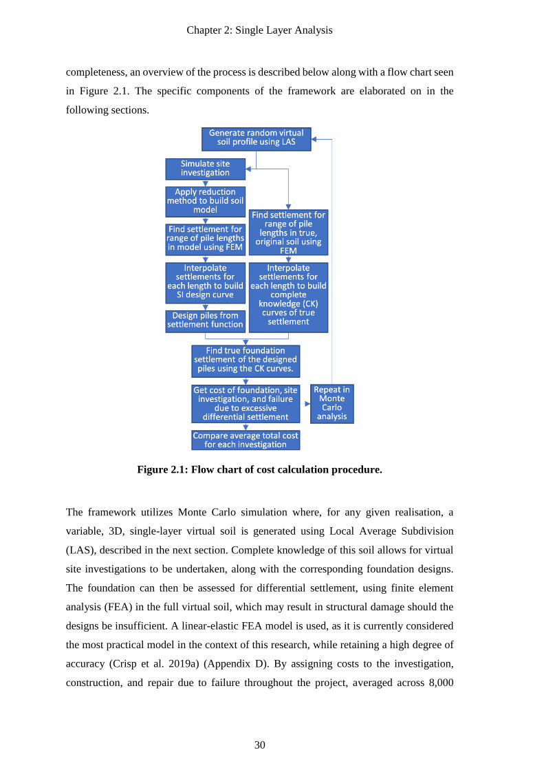
Chapter 2: Single Layer Analysis
30
completeness, an overview of the process is described below along with a flow chart seen
in Figure 2.1. The specific components of the framework are elaborated on in the
following sections.
Figure 2.1: Flow chart of cost calculation procedure.
The framework utilizes Monte Carlo simulation where, for any given realisation, a
variable, 3D, single-layer virtual soil is generated using Local Average Subdivision
(LAS), described in the next section. Complete knowledge of this soil allows for virtual
site investigations to be undertaken, along with the corresponding foundation designs.
The foundation can then be assessed for differential settlement, using finite element
analysis (FEA) in the full virtual soil, which may result in structural damage should the
designs be insufficient. A linear-elastic FEA model is used, as it is currently considered
the most practical model in the context of this research, while retaining a high degree of
accuracy (Crisp et al. 2019a) (Appendix D). By assigning costs to the investigation,
construction, and repair due to failure throughout the project, averaged across 8,000
Chapter 2: Single Layer Analysis
31
Monte Carlo realisations, it is possible to represent the quality of a site investigation by
its expected total project cost. The optimal investigation is therefore identified by
minimising the total cost objective function. As this metric incorporates both economic
and risk-based factors, it is considered an ideal objective function for practising
engineers. The relationship between total cost and site investigation effort can be
determined through plots of the two variables, as presented later in the paper.
2.2.2 Generation of Virtual Soil Profile
The randomly-generated virtual soil profiles, or random fields, are volumes of soil
properties represented by a 3D grid of discrete elements. As linear-elastic FEA is used,
the required properties are Young’s modulus (E), which is randomly generated and
Poisson’s ratio (v), which is constant at 0.3, which represents a wide range of soils. The
deterministic treatment of v is due to this parameter’s spatial variability having a
relatively insignificant effect on settlement (Fenton and Griffiths 2005; Naghibi et al.
2014a). The random field used in this study consists of 240 240 160 elements, where
the elements are 0.25 m cubes. Therefore, the physical dimensions of the field are 60
60 40 m in the x, y and z directions, respectively.
The soil properties within these random fields can be statistically described by three
parameters; the mean, standard deviation, and the scale of fluctuation (SOF) (Vanmarcke
1983). The SOF is analogous to the range parameter in geostatistics (Jaksa et al. 1997),
and is defined as the distance over which soil properties exhibit strong similarity. In other
words, high SOF values correspond to large pockets of similar material. Within this
study, the standard deviation is normalized by the mean to produce the coefficient of
variation (COV), which is more useful as the results can be applied to any mean parameter
value. The soil properties themselves are generated according to the lognormal
distribution, which has been found to be appropriate for geotechnical engineering
probabilistic studies (Fenton and Griffiths 2008), and ensures that stiffness values are
strictly non-negative.
SOFs of 1 (low), 8 (medium) and 24 m (high) are assessed, along with COVs of 20, 40
and 80%. Isotropic soils, where the SOF is constant in all directions, are considered in
this analysis, as they are the worst case when compared to anisotropic soils which have a
higher SOF in the horizontal direction (Naghibi et al. 2014b). Isotropic soils exhibit
inferior performance because a larger correlation length in the vertical direction leads to
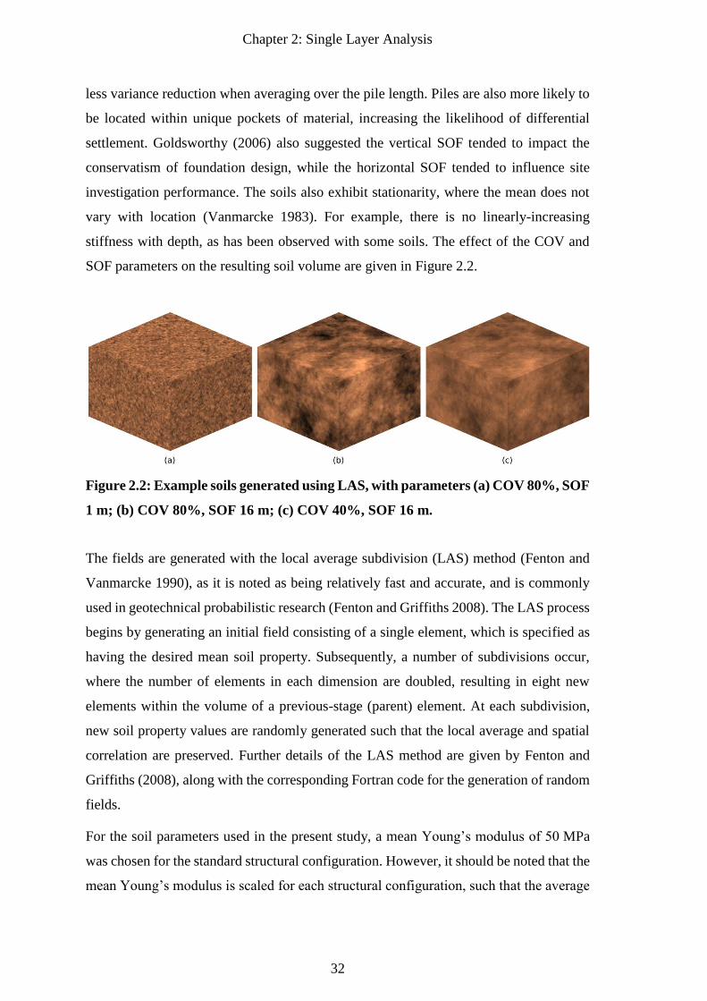
Chapter 2: Single Layer Analysis
32
less variance reduction when averaging over the pile length. Piles are also more likely to
be located within unique pockets of material, increasing the likelihood of differential
settlement. Goldsworthy (2006) also suggested the vertical SOF tended to impact the
conservatism of foundation design, while the horizontal SOF tended to influence site
investigation performance. The soils also exhibit stationarity, where the mean does not
vary with location (Vanmarcke 1983). For example, there is no linearly-increasing
stiffness with depth, as has been observed with some soils. The effect of the COV and
SOF parameters on the resulting soil volume are given in Figure 2.2.
Figure 2.2: Example soils generated using LAS, with parameters (a) COV 80%, SOF
1 m; (b) COV 80%, SOF 16 m; (c) COV 40%, SOF 16 m.
The fields are generated with the local average subdivision (LAS) method (Fenton and
Vanmarcke 1990), as it is noted as being relatively fast and accurate, and is commonly
used in geotechnical probabilistic research (Fenton and Griffiths 2008). The LAS process
begins by generating an initial field consisting of a single element, which is specified as
having the desired mean soil property. Subsequently, a number of subdivisions occur,
where the number of elements in each dimension are doubled, resulting in eight new
elements within the volume of a previous-stage (parent) element. At each subdivision,
new soil property values are randomly generated such that the local average and spatial
correlation are preserved. Further details of the LAS method are given by Fenton and
Griffiths (2008), along with the corresponding Fortran code for the generation of random
fields.
For the soil parameters used in the present study, a mean Young’s modulus of 50 MPa
was chosen for the standard structural configuration. However, it should be noted that the
mean Young’s modulus is scaled for each structural configuration, such that the average
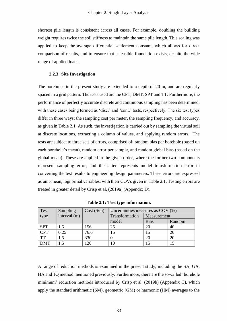
Chapter 2: Single Layer Analysis
33
shortest pile length is consistent across all cases. For example, doubling the building
weight requires twice the soil stiffness to maintain the same pile length. This scaling was
applied to keep the average differential settlement constant, which allows for direct
comparison of results, and to ensure that a feasible foundation exists, despite the wide
range of applied loads.
2.2.3 Site Investigation
The boreholes in the present study are extended to a depth of 20 m, and are regularly
spaced in a grid pattern. The tests used are the CPT, DMT, SPT and TT. Furthermore, the
performance of perfectly accurate discrete and continuous sampling has been determined,
with these cases being termed as ‘disc.’ and ‘cont.’ tests, respectively. The six test types
differ in three ways: the sampling cost per meter, the sampling frequency, and accuracy,
as given in Table 2.1. As such, the investigation is carried out by sampling the virtual soil
at discrete locations, extracting a column of values, and applying random errors. The
tests are subject to three sets of errors, comprised of: random bias per borehole (based on
each borehole’s mean), random error per sample, and random global bias (based on the
global mean). These are applied in the given order, where the former two components
represent sampling error, and the latter represents model transformation error in
converting the test results to engineering design parameters. These errors are expressed
as unit-mean, lognormal variables, with their COVs given in Table 2.1. Testing errors are
treated in greater detail by Crisp et al. (2019a) (Appendix D).
Table 2.1: Test type information.
Test
type
Sampling
interval (m)
Cost ($/m) Uncertainties measures as COV (%)
Transformation
model
Measurement
Bias Random
SPT 1.5 156 25 20 40
CPT 0.25 76.6 15 15 20
TT 1.5 330 0 20 20
DMT 1.5 120 10 15 15
A range of reduction methods is examined in the present study, including the SA, GA,
HA and 1Q method mentioned previously. Furthermore, there are the so-called ‘borehole
minimum’ reduction methods introduced by Crisp et al. (2019b) (Appendix C), which
apply the standard arithmetic (SM), geometric (GM) or harmonic (HM) averages to the
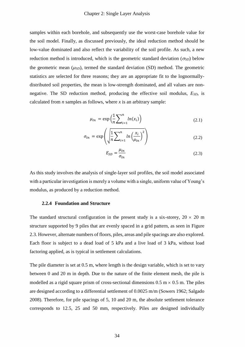
Chapter 2: Single Layer Analysis
34
samples within each borehole, and subsequently use the worst-case borehole value for
the soil model. Finally, as discussed previously, the ideal reduction method should be
low-value dominated and also reflect the variability of the soil profile. As such, a new
reduction method is introduced, which is the geometric standard deviation (SD) below
the geometric mean (SD), termed the standard deviation (SD) method. The geometric
statistics are selected for three reasons; they are an appropriate fit to the lognormally-
distributed soil properties, the mean is low-strength dominated, and all values are non-
negative. The SD reduction method, producing the effective soil modulus, ESD, is
calculated from n samples as follows, where x is an arbitrary sample:
𝜇𝑙𝑛 = exp (1
𝑛∑ 𝑙𝑛(𝑥𝑖)
𝑛
𝑖=1) (2.1)
𝜎𝑙𝑛 = exp(√1
𝑛∑ 𝑙𝑛 (
𝑥𝑖𝜇𝑙𝑛 )2𝑛
𝑖=1) (2.2)
𝐸𝑆𝐷 =𝜇𝑙𝑛 𝜎𝑙𝑛
(2.3)
As this study involves the analysis of single-layer soil profiles, the soil model associated
with a particular investigation is merely a volume with a single, uniform value of Young’s
modulus, as produced by a reduction method.
2.2.4 Foundation and Structure
The standard structural configuration in the present study is a six-storey, 20 20 m
structure supported by 9 piles that are evenly spaced in a grid pattern, as seen in Figure
2.3. However, alternate numbers of floors, piles, areas and pile spacings are also explored.
Each floor is subject to a dead load of 5 kPa and a live load of 3 kPa, without load
factoring applied, as is typical in settlement calculations.
The pile diameter is set at 0.5 m, where length is the design variable, which is set to vary
between 0 and 20 m in depth. Due to the nature of the finite element mesh, the pile is
modelled as a rigid square prism of cross-sectional dimensions 0.5 m 0.5 m. The piles
are designed according to a differential settlement of 0.0025 m/m (Sowers 1962; Salgado
2008). Therefore, for pile spacings of 5, 10 and 20 m, the absolute settlement tolerance
corresponds to 12.5, 25 and 50 mm, respectively. Piles are designed individually
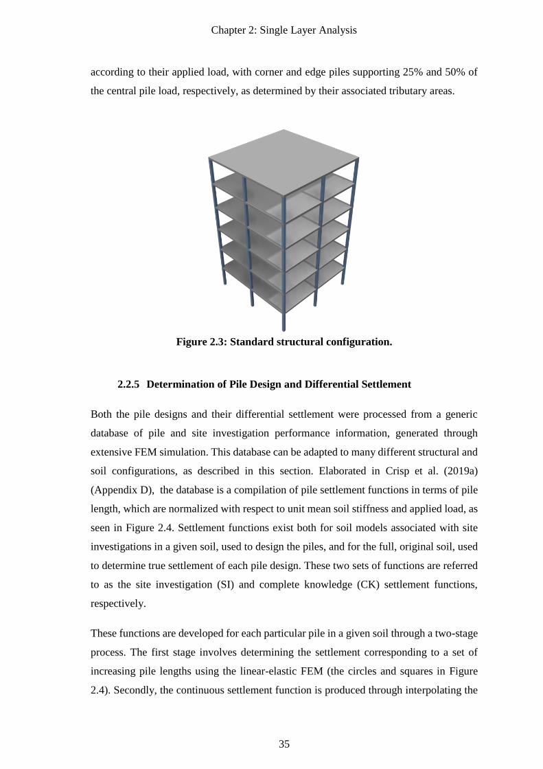
Chapter 2: Single Layer Analysis
35
according to their applied load, with corner and edge piles supporting 25% and 50% of
the central pile load, respectively, as determined by their associated tributary areas.
Figure 2.3: Standard structural configuration.
2.2.5 Determination of Pile Design and Differential Settlement
Both the pile designs and their differential settlement were processed from a generic
database of pile and site investigation performance information, generated through
extensive FEM simulation. This database can be adapted to many different structural and
soil configurations, as described in this section. Elaborated in Crisp et al. (2019a)
(Appendix D), the database is a compilation of pile settlement functions in terms of pile
length, which are normalized with respect to unit mean soil stiffness and applied load, as
seen in Figure 2.4. Settlement functions exist both for soil models associated with site
investigations in a given soil, used to design the piles, and for the full, original soil, used
to determine true settlement of each pile design. These two sets of functions are referred
to as the site investigation (SI) and complete knowledge (CK) settlement functions,
respectively.
These functions are developed for each particular pile in a given soil through a two-stage
process. The first stage involves determining the settlement corresponding to a set of
increasing pile lengths using the linear-elastic FEM (the circles and squares in Figure
2.4). Secondly, the continuous settlement function is produced through interpolating the
Chapter 2: Single Layer Analysis
36
discrete FEM settlement data using piecewise cubic splines built with the Akima method
(Akima 1970), which has been found to be the most appropriate interpolation method for
this case. In essence, each pile has been analysed extensively enough through the use of
FEM that design can be undertaken by scaling and interpolating the FEM results, through
the use of the settlement functions.
Due to the linear-elastic nature of the analysis, the normalized functions can be scaled
linearly with respect to load and soil stiffness, as well as the piles being designed to an
arbitrary settlement tolerance, hence its generic, and therefore adaptable, nature. As such,
this pile function database may be used by other researchers for a wide variety of
structural and foundation configurations, as well as soil stiffness and design redundancy.
The latter functionality facilitates extensive reliability-based design research to be
conducted, in a similar manner to that of (Naghibi et al. 2014b). Note that this pile
performance database was generated using the Phoenix supercomputer (University of
Adelaide 2018). The database itself would, under normal circumstances, have taken 30
years to generate, despite the heavy software optimization implemented, had Phoenix’s
parallel computing capabilities not been utilized.
It is important to clarify the number of settlement functions required. For a given soil, a
single SI function is required for every site investigation and Monte Carlo realization, as
each pile supporting a structure can be designed from a single curve. Regarding true
settlement, a unique CK function is needed for every pile and every Monte Carlo
realization, as each pile under the structure may behave differently as a result of natural
soil variability.
Designing piles from a given investigation involves generating SI settlement curves using
the soil model associated with that investigation. In other words, the FEM is applied in a
mesh with uniform soil properties; that of the effective modulus, as discussed in the
previous section. The design process itself involves iteratively increasing the pile length
until its settlement is less than or equal to the settlement tolerance, as described by the
settlement function. The tolerances were given in the previous section.
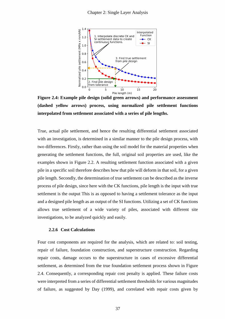
Chapter 2: Single Layer Analysis
37
Figure 2.4: Example pile design (solid green arrows) and performance assessment
(dashed yellow arrows) process, using normalized pile settlement functions
interpolated from settlement associated with a series of pile lengths.
True, actual pile settlement, and hence the resulting differential settlement associated
with an investigation, is determined in a similar manner to the pile design process, with
two differences. Firstly, rather than using the soil model for the material properties when
generating the settlement functions, the full, original soil properties are used, like the
examples shown in Figure 2.2. A resulting settlement function associated with a given
pile in a specific soil therefore describes how that pile will deform in that soil, for a given
pile length. Secondly, the determination of true settlement can be described as the inverse
process of pile design, since here with the CK functions, pile length is the input with true
settlement is the output This is as opposed to having a settlement tolerance as the input
and a designed pile length as an output of the SI functions. Utilizing a set of CK functions
allows true settlement of a wide variety of piles, associated with different site
investigations, to be analyzed quickly and easily.
2.2.6 Cost Calculations
Four cost components are required for the analysis, which are related to: soil testing,
repair of failure, foundation construction, and superstructure construction. Regarding
repair costs, damage occurs to the superstructure in cases of excessive differential
settlement, as determined from the true foundation settlement process shown in Figure
2.4. Consequently, a corresponding repair cost penalty is applied. These failure costs
were interpreted from a series of differential settlement thresholds for various magnitudes
of failure, as suggested by Day (1999), and correlated with repair costs given by
Chapter 2: Single Layer Analysis
38
Rawlinsons (2016). The remaining costs for construction and soil testing were derived
through a combination of Rawlinsons (2016) and personal correspondences with
practising engineers (Crisp et al. 2019a) (Appendix D).
The normalized construction cost of the structure per square meter is Cc = 1,540 n1.29,
where n is the number of floors. The pile construction cost is $200 per meter, per pile.
While bored piles are assumed, the settlement model does not distinguish between
installation methods. The repair cost for foundation failure per square meter (Cf) is more
complex, and is determined as a continuous relationship with differential settlement (δ).
Specifically, it is a bounded linear function of the form Cf = A δ + B, where A and B are
related to the number of floors, as given in Table 2.2. The bounds are such that Cf is
constrained to a minimum of $0, where no damage occurs, and a maximum of Cmax,
approximating the process of demolishing and rebuilding the superstructure. These
bounding costs correspond to differential settlements of roughly 0.003 and 0.0096 m/m
respectively.
The site investigation costs are specified later in the paper and increase as the scope of
the investigation increases, as one would expect. The resulting problem then becomes
that of optimization, where total cost is to be minimised. This is a trade-off, as foundation
failure decreases as the investigation effort increases, and failure cost is known to be the
most prominent component of the total (Goldsworthy et al. 2007a).
Table 2.2: Linear equation coefficients for failure cost calculation.
A B Cmax
3 floors 1,006,680 –3,030 6,520
6 floors 2,560,230 –7,640 16,340
9 floors 4,416,470 –13,100 28,000
2.3 Results and Discussion
2.3.1 Comparison of Reduction Methods
This section examines the influence of choice of reduction method using the CPT. The
results given in Figure 2.5 are for a soil COV of 40% (low) and 80% (high). While COVs
of less than 40% are also common, such results are not included as the corresponding
plots are similar in appearance to Figure 2.5(a), and therefore redundant. The
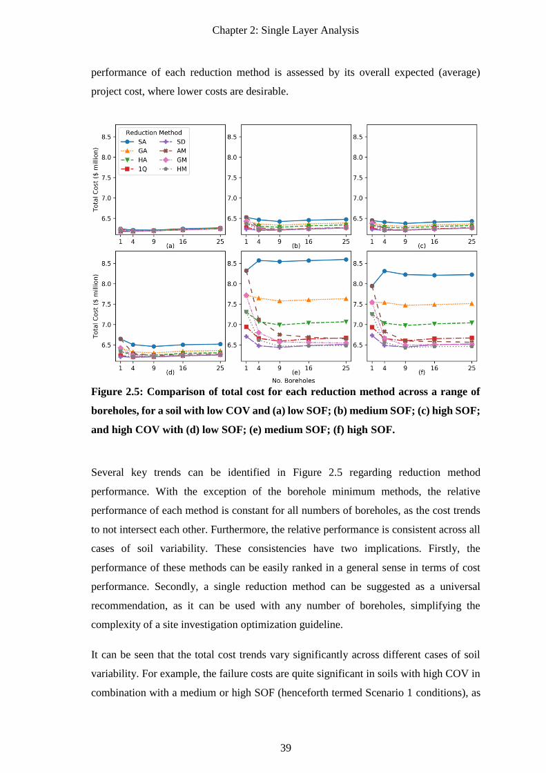
Chapter 2: Single Layer Analysis
39
performance of each reduction method is assessed by its overall expected (average)
project cost, where lower costs are desirable.
Figure 2.5: Comparison of total cost for each reduction method across a range of
boreholes, for a soil with low COV and (a) low SOF; (b) medium SOF; (c) high SOF;
and high COV with (d) low SOF; (e) medium SOF; (f) high SOF.
Several key trends can be identified in Figure 2.5 regarding reduction method
performance. With the exception of the borehole minimum methods, the relative
performance of each method is constant for all numbers of boreholes, as the cost trends
to not intersect each other. Furthermore, the relative performance is consistent across all
cases of soil variability. These consistencies have two implications. Firstly, the
performance of these methods can be easily ranked in a general sense in terms of cost
performance. Secondly, a single reduction method can be suggested as a universal
recommendation, as it can be used with any number of boreholes, simplifying the
complexity of a site investigation optimization guideline.
It can be seen that the total cost trends vary significantly across different cases of soil
variability. For example, the failure costs are quite significant in soils with high COV in
combination with a medium or high SOF (henceforth termed Scenario 1 conditions), as
Chapter 2: Single Layer Analysis
40
seen in Figure 2.5(e, f). However, they are relatively minor in all other soil variability
cases (termed Scenario 2), such that minimal investigation of one or four boreholes is
required, as seen in Figure 2.5(a-d).
In the low variability situation of Scenario 2, rather than the moderate costs being a
reflection of the investigation quality, it is instead indicative of the foundation
performance. Foundations are unlikely to fail when the soil exhibits modest variability.
In the case of a low COV, this soil variability is not excessive, as seen in Figure 2.2(c).
In the case of a low SOF, the soil properties fluctuate rapidly over short distances, as seen
in Figure 2.2(a), meaning that the soil appears to be largely uniform at a macro scale
when locally-averaged, precluding differential settlement. Therefore, the foundation
performance is largely independent of site investigation scope in such cases, resulting in
minimal testing being sufficient. However, it can be seen that, even in the relatively
homogenous soil case in Figure 2.5(a), the added cost of conducting 25 boreholes
compared to one is negligible in comparison to the potential failure costs in the more
variable soils. This reinforces the belief that clients should invest in more thorough
investigations if the ground conditions are unknown at a given site.
Comparing the reduction methods in Scenario 1, as seen in Figure 2.5(e,f), it can be seen
that the more conservative reduction methods, such as 1Q, SD and HM, perform better
overall across all soil cases. Ignoring the borehole minimum methods, such as the HM,
the reduction method ranking from worst to best performance is SA, GA, HA, 1Q and
SD. Comparing the two extremes, the improvement of the SD method over SA is in the
order of $2 million. This difference illustrates how the manner of transforming site
investigation samples into a soil model, as opposed to the investigation itself, is a highly
significant factor in the investigation’s performance.
These conservative reduction methods perform well even in relatively homogenous soils,
as seen in Figure 2.5(a), as the cost trends have converged. This convergence is logical,
as a relatively uniform soil should produce a largely constant effective modulus,
regardless of interpretation. However, it is worth noting that the conservative methods’
performance is excellent even in the case of high COV and low SOF, where the borehole
samples would be highly variable, yet the foundation would be unlikely to fail due to the
previously-discussed macro-similarity. This suggests that the conservative methods
assessed here do not result in excessively over-designed foundations, which is the
Chapter 2: Single Layer Analysis
41
primary concern regarding conservatism. As such, the SD method can be recommended
as a largely universal means of reduction.
A case could also be made that the HM method is the true global optimum, as it has the
lowest total cost, corresponding to a high number of boreholes. Furthermore, contrary to
showing a clear global optimum in the data, the cost generally continues to decrease as
the number of boreholes increases, implying that savings from further testing is sufficient
to offset the additional costs. However, the improvement over the SD method is modest,
in the order of $40,000. Perhaps more importantly, it is likely that the borehole depth has
a notable impact on the performance of the borehole minimum methods, such as the HM.
This influence is due to the reliance on the averaging within each borehole to eliminate
excessively low sample values, the inclusion of which would otherwise result in an
excessively conservative soil model, and foundation over-design. For example, the
method is low value-weighted to such a degree that a single near-zero sample would
result in the effective modulus being near-zero. For this reason, the SD method remains
the most appropriate reduction technique.
The optimal number of boreholes varies depending on the reduction method used and is
defined as the number of boreholes which results in the minimum total cost, or by which
the cost has plateaued. In the case of the HM method, this is approximately 16 boreholes,
although given that the optimal case for the SD method is 4 boreholes, it is unlikely that
engineering clients would be compelled to invest in the higher number given the modest
level of improvement. In contrast, the expected total cost for the SA reduction method
typically increases as the number of boreholes increases. This is counter-intuitive,
although it occurs because the average soil model from this method results in foundation
failure. Therefore, as the number of boreholes increases and the variability of
investigation performance decreases across Monte Carlo realisations, the proportion of
safe foundations also decreases. As such, the SD method is largely both a global optimum
in terms of minimum cost, and results in a minimal number of boreholes.
2.3.2 Comparison of Test Type
This section compares the total expected costs for different test types, across different
numbers of boreholes using the SD reduction method. For simplicity, a borehole here
refers to any vertical set of samples taken at a given location, regardless of test type. The
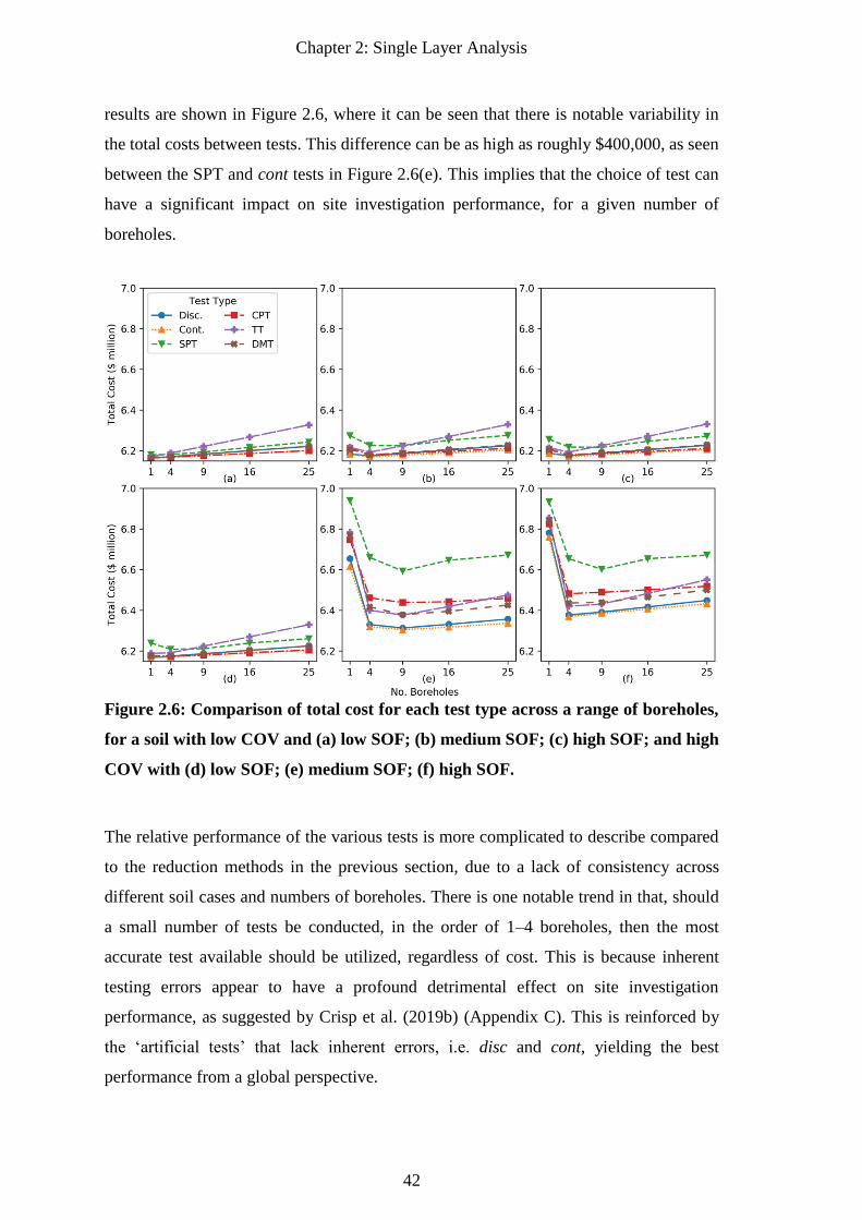
Chapter 2: Single Layer Analysis
42
results are shown in Figure 2.6, where it can be seen that there is notable variability in
the total costs between tests. This difference can be as high as roughly $400,000, as seen
between the SPT and cont tests in Figure 2.6(e). This implies that the choice of test can
have a significant impact on site investigation performance, for a given number of
boreholes.
Figure 2.6: Comparison of total cost for each test type across a range of boreholes,
for a soil with low COV and (a) low SOF; (b) medium SOF; (c) high SOF; and high
COV with (d) low SOF; (e) medium SOF; (f) high SOF.
The relative performance of the various tests is more complicated to describe compared
to the reduction methods in the previous section, due to a lack of consistency across
different soil cases and numbers of boreholes. There is one notable trend in that, should
a small number of tests be conducted, in the order of 1–4 boreholes, then the most
accurate test available should be utilized, regardless of cost. This is because inherent
testing errors appear to have a profound detrimental effect on site investigation
performance, as suggested by Crisp et al. (2019b) (Appendix C). This is reinforced by
the ‘artificial tests’ that lack inherent errors, i.e. disc and cont, yielding the best
performance from a global perspective.
Chapter 2: Single Layer Analysis
43
In highly variable soils, i.e. Scenario 1 from the previous section, the relative test
performance remains largely consistent across different numbers of boreholes, and is
dictated by test accuracy, as discussed previously. In this context, the tests can generally
be ranked from worst to best performance as follows: SPT, CPT, DMT, TT, with the
latter two being largely similar for the cases shown.
The differences in test performance are such that there is clear benefit to conducting a
smaller number of more accurate tests, as opposed to a higher number of inaccurate tests.
For example, based on Figure 2.6(e,f), it is cheaper to drill or conduct 4 boreholes with
the CPT, DMT or TT than 9 boreholes with the SPT. Similarly, it is cheaper to drill 4
boreholes with the DMT or TT compared to 9 CPTs. These results reinforce the
conclusion that a recommended fixed number of boreholes or fixed site investigation cost
is not in itself a sufficiently optimal guideline. Rather, the manner and configuration of
the investigation is of paramount importance and must also be appropriately considered.
In the case of soils with low variability, as with Scenario 2, site investigation performance
becomes dominated by the sampling cost as the number of tests increases. This is because
foundation failure is unlikely to occur for reasons discussed previously, and so failure
costs become negligible. Therefore, it can be argued that the better performing tests in
this context are those that are cheapest to conduct, while still maintaining a reasonable
degree of accuracy. Sampling cost is largely driven by the rate at which sampling occurs.
In these soil cases, the CPT consistently yields the lowest cost, with the triaxial test being
the most expensive for the majority of boreholes. The higher expense of the TT is due to
it being a laboratory test, which requires an explicit testing procedure, in addition to that
of drilling the boreholes. However, it should be noted that, if a single borehole is to be
drilled, then the TT is among the test methods yielding the most favourable results, due
to it being a highly accurate test that determines Young’s modulus directly, rather than
through a transformation of parameters.
The optimal number of boreholes varies considerably with test type and soil variability,
as expected. For the SPT, 9 boreholes are required almost universally in order to achieve
minimum cost for that particular test. This is generally a larger number of recommended
boreholes than the other, more accurate tests, implying that the additional sampling is
required specifically to overcome the high degree of errors associated with the SPT; a
conclusion in agreement with Crisp et al. (2018) (Appendix B). For the remaining three
Chapter 2: Single Layer Analysis
44
tests, 4 boreholes are generally recommended as optimal, or are otherwise generally
consistent with the cost of a single borehole. The exception to this is the case of high
COV and medium SOF as seen in Figure 2.6(e), where 9 boreholes is optimal for all tests,
implying this soil variability to be the worst case; a concept discussed later in the study.
In other words, high COV and medium SOF could be assumed in the complete absence
of soil information, for the structural configuration examined. In contrast, the best case is
low COV and low SOF, as expected, where one borehole is optimal. As the technically-
optimal number of boreholes varies from one to nine depending on soil type, the results
reinforce that a site investigation optimization guideline should consider multiple types
of soil variability, as opposed to providing indiscriminate recommendations regardless of
site conditions. On the other hand, if a single recommendation were to be given, then four
boreholes would be considered optimal, as there is significant improvement over a single
borehole; up to $400,000. In contrast, there is relatively modest improvement from
additional sampling over four boreholes, in the case of most test types.
It is worth exploring the influence of continuous vs discrete sampling in the context of
highly variable soils. The CPT is the only real continuous test examined, with the SPT,
DMT and TT being discrete. As such, the CPT collects considerably more information
for a given number of boreholes (i.e. soundings), and so would theoretically be more
accurate overall. However, by comparing the theoretical discrete and continuous test
cases, disc and cont, it appears that there is negligible difference between them in terms
of cost. This similarity implies that the number of samples in and of itself is not a
significant factor. Note that the number of samples does not necessarily correspond to the
proportion of the soil profile represented by the samples, which is more a function of
sample location, testing procedure, and scale of fluctuation. In other words, soil in close
proximity to a sample is likely to be similar to the sample, within a certain distance.
Conducting additional samples within this distance merely provides duplicates of existing
information as opposed to producing new data, meaning the additional samples are
largely redundant. The sampling frequency of the discrete tests (1.5 m intervals) appears
to be sufficient, given that the smallest SOF is 1 m, although it is likely that site
investigation performance will decrease should this interval be increased.
There is also the consideration of the CPT’s additional sampling frequency theoretically
helping to offset testing error. While it is true that the per-sample error can be largely
Chapter 2: Single Layer Analysis
45
overcome with a sufficient quantity, the borehole bias and global transformation error
components are consistent regardless of the number of samples obtained from each
borehole. For these two reasons, it can be concluded that there is negligible benefit from
continuous sampling over sufficiently-spaced discrete sampling in single-layer soils.
Based on the results, the DMT could be considered the optimal test, as it typically
produces the best, or comparable, performance across different numbers of boreholes and
soil cases. There is some minor improvement with the CPT compared to the DMT in soils
with low variability, particularly in the case with a high number of boreholes. However,
the DMT can produce a net saving of up to $50,000 compared with the CPT in more
variable soils, as seen in Figure 2.6(e). Although, it should be noted that this analysis only
considers site investigations for the property of Young’s modulus. It may be the case that,
if multiple soil properties from a single test are desired, then a test should be selected that
can measure a more complete range of properties with appropriate accuracy. Indeed,
although it is not shown here, the TT provides a lower global cost for larger buildings
due to its higher accuracy, as larger failure costs offset its high testing cost, and this test
is accurate for many soil properties. At the other end of the testing spectrum, the SPT can
produce a total cost that is up to $200,000 higher than the DMT due to an increased risk
of failure. It is therefore suggested that the SPT is avoided if possible.
2.3.3 Worst Case SOF Analysis
As suggested in the previous section, there appears to be a specific worst-case SOF. It is
useful to identify these worst cases, as this provides engineers with some default guidance
in the absence of specific geotechnical information. However, the relationship between
site investigation performance and SOF is relatively complex compared to the variable
of COV, where performance monotonically decreases as COV increases. The concept of
a SOF worst-case can be explained by the previously-discussed notion of soil appearing
uniform at a macro scale. Soil situations where properties fluctuate very rapidly or very
slowly with distance tend to exhibit the overall behaviour of a uniform soil profile, as is
the case with low or high SOF, regardless of COV. As such, conducting additional
boreholes does not provide new soil property values that have not already been collected.
Furthermore, a largely uniform soil precludes the possibility of damage through excessive
differential settlement. In contrast to these two extremes, a moderate SOF is more likely
to incorporate distinct pockets of different soil stiffness. Whether each footing lies in a
Chapter 2: Single Layer Analysis
46
different pocket, and whether or not the relevant pockets are sufficiently sampled, has a
notable impact on site investigation performance.
The notion of a moderate SOF being the worst case is supported by Figure 2.6(e), where
the medium SOF of 8 m requires the most extensive investigations, and is associated with
a high degree of savings with additional sampling. It is possible that the true worst case
appears between the discrete SOF values assessed here of 1, 8 and 24 m, and is likely to
be at the lower end of the range of 8 – 24 m, judging from the similar magnitude of cost
savings in Figure 2.6(f). This observation is consistent with previous studies which
implied that a worst-case SOF is in the order of 8 – 16 m, (Jaksa et al. 2005; Goldsworthy
et al. 2007a; Goldsworthy et al. 2007b; Arsyad et al. 2009). However, there has been
some speculation that this worst case is a function of the centre-to-centre spacing of the
footings (Jaksa et al. 2005), which is certainly true for worst-case foundation settlement
when disregarding site investigations (Fenton and Griffiths 2005). However, a worst-case
SOF, with regards to site investigations, has yet to be conclusively demonstrated in a
generalised manner.
An analysis is conducted to determine the worst-case SOF in relation to footing and
borehole spacings, by varying both variables. To examine this relationship, a 4-pile
building is assessed, with footing spacings of 5, 10 and 20 m. Furthermore, for each of
these cases, a variety of site investigations are conducted with the CPT and SD reduction
method, including a single, centrally-located borehole, 4 boreholes located at the corners,
and 25 boreholes evenly spaced across the building footprint. These latter two
investigations correspond to borehole spacings of 20 and 5 m, respectively, with the
former being independent of borehole spacing. The results are presented in Figure 2.7 for
SOFs ranging from 1 to 24 m, where the cost curves are interpolated using splines.
Contrary to previous sections, the failure cost is shown, normalized per square meter, per
floor in order to better examine the corresponding reliability. The apparent maximum
cost is highlighted with a cross symbol.
As seen in Figure 2.7(b) and Figure 2.7(c), there is negligible difference between the 4
borehole and 25 borehole cases when comparing the same pile spacing. This similarity
implies that borehole density, and therefore spacing, has no notable relationship with
SOF. The roughly 5% difference between the two cases is within the Monte Carlo error
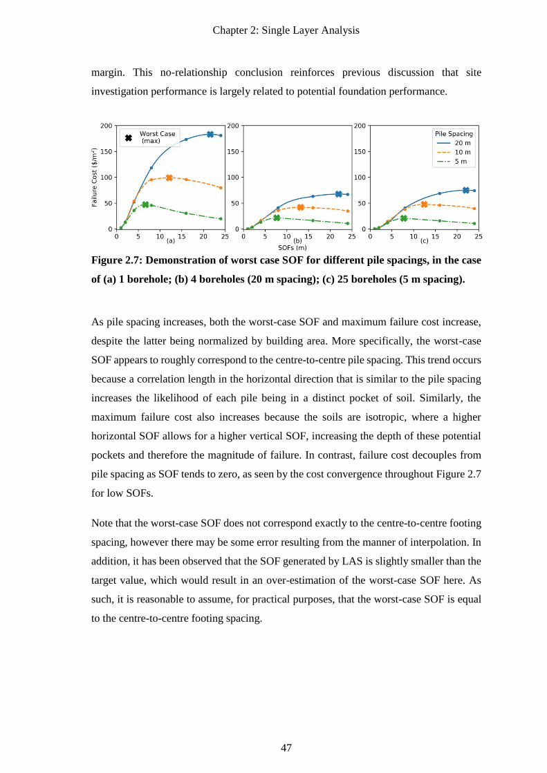
Chapter 2: Single Layer Analysis
47
margin. This no-relationship conclusion reinforces previous discussion that site
investigation performance is largely related to potential foundation performance.
Figure 2.7: Demonstration of worst case SOF for different pile spacings, in the case
of (a) 1 borehole; (b) 4 boreholes (20 m spacing); (c) 25 boreholes (5 m spacing).
As pile spacing increases, both the worst-case SOF and maximum failure cost increase,
despite the latter being normalized by building area. More specifically, the worst-case
SOF appears to roughly correspond to the centre-to-centre pile spacing. This trend occurs
because a correlation length in the horizontal direction that is similar to the pile spacing
increases the likelihood of each pile being in a distinct pocket of soil. Similarly, the
maximum failure cost also increases because the soils are isotropic, where a higher
horizontal SOF allows for a higher vertical SOF, increasing the depth of these potential
pockets and therefore the magnitude of failure. In contrast, failure cost decouples from
pile spacing as SOF tends to zero, as seen by the cost convergence throughout Figure 2.7
for low SOFs.
Note that the worst-case SOF does not correspond exactly to the centre-to-centre footing
spacing, however there may be some error resulting from the manner of interpolation. In
addition, it has been observed that the SOF generated by LAS is slightly smaller than the
target value, which would result in an over-estimation of the worst-case SOF here. As
such, it is reasonable to assume, for practical purposes, that the worst-case SOF is equal
to the centre-to-centre footing spacing.
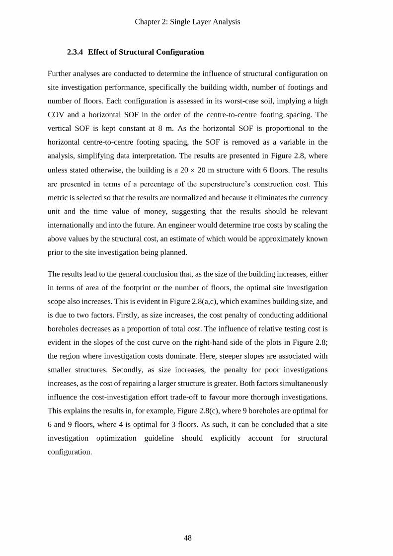
Chapter 2: Single Layer Analysis
48
2.3.4 Effect of Structural Configuration
Further analyses are conducted to determine the influence of structural configuration on
site investigation performance, specifically the building width, number of footings and
number of floors. Each configuration is assessed in its worst-case soil, implying a high
COV and a horizontal SOF in the order of the centre-to-centre footing spacing. The
vertical SOF is kept constant at 8 m. As the horizontal SOF is proportional to the
horizontal centre-to-centre footing spacing, the SOF is removed as a variable in the
analysis, simplifying data interpretation. The results are presented in Figure 2.8, where
unless stated otherwise, the building is a 20 20 m structure with 6 floors. The results
are presented in terms of a percentage of the superstructure’s construction cost. This
metric is selected so that the results are normalized and because it eliminates the currency
unit and the time value of money, suggesting that the results should be relevant
internationally and into the future. An engineer would determine true costs by scaling the
above values by the structural cost, an estimate of which would be approximately known
prior to the site investigation being planned.
The results lead to the general conclusion that, as the size of the building increases, either
in terms of area of the footprint or the number of floors, the optimal site investigation
scope also increases. This is evident in Figure 2.8(a,c), which examines building size, and
is due to two factors. Firstly, as size increases, the cost penalty of conducting additional
boreholes decreases as a proportion of total cost. The influence of relative testing cost is
evident in the slopes of the cost curve on the right-hand side of the plots in Figure 2.8;
the region where investigation costs dominate. Here, steeper slopes are associated with
smaller structures. Secondly, as size increases, the penalty for poor investigations
increases, as the cost of repairing a larger structure is greater. Both factors simultaneously
influence the cost-investigation effort trade-off to favour more thorough investigations.
This explains the results in, for example, Figure 2.8(c), where 9 boreholes are optimal for
6 and 9 floors, where 4 is optimal for 3 floors. As such, it can be concluded that a site
investigation optimization guideline should explicitly account for structural
configuration.
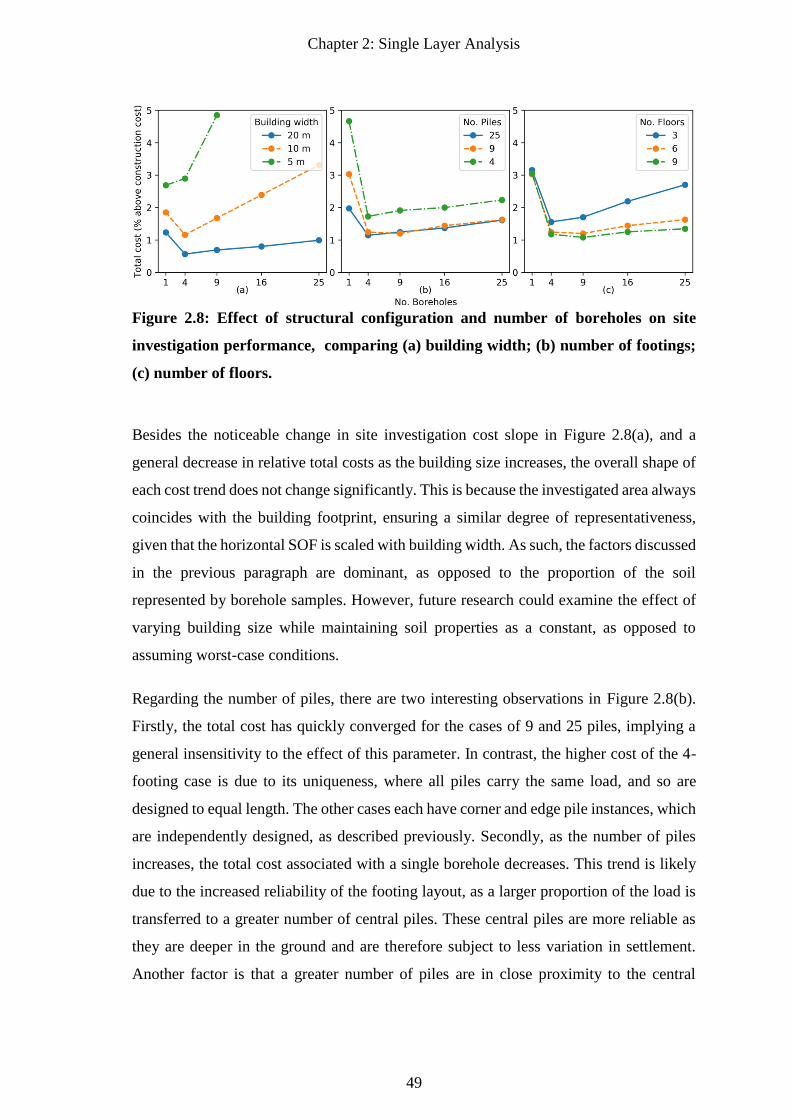
Chapter 2: Single Layer Analysis
49
Figure 2.8: Effect of structural configuration and number of boreholes on site
investigation performance, comparing (a) building width; (b) number of footings;
(c) number of floors.
Besides the noticeable change in site investigation cost slope in Figure 2.8(a), and a
general decrease in relative total costs as the building size increases, the overall shape of
each cost trend does not change significantly. This is because the investigated area always
coincides with the building footprint, ensuring a similar degree of representativeness,
given that the horizontal SOF is scaled with building width. As such, the factors discussed
in the previous paragraph are dominant, as opposed to the proportion of the soil
represented by borehole samples. However, future research could examine the effect of
varying building size while maintaining soil properties as a constant, as opposed to
assuming worst-case conditions.
Regarding the number of piles, there are two interesting observations in Figure 2.8(b).
Firstly, the total cost has quickly converged for the cases of 9 and 25 piles, implying a
general insensitivity to the effect of this parameter. In contrast, the higher cost of the 4-
footing case is due to its uniqueness, where all piles carry the same load, and so are
designed to equal length. The other cases each have corner and edge pile instances, which
are independently designed, as described previously. Secondly, as the number of piles
increases, the total cost associated with a single borehole decreases. This trend is likely
due to the increased reliability of the footing layout, as a larger proportion of the load is
transferred to a greater number of central piles. These central piles are more reliable as
they are deeper in the ground and are therefore subject to less variation in settlement.
Another factor is that a greater number of piles are in close proximity to the central
Chapter 2: Single Layer Analysis
50
borehole. Still, compared to the other variables of building size and height, site
investigation performance is relatively insensitive to the number of footings.
Inspection of the optimal site investigation cost, as a proportion of the construction cost,
suggests a value of 0.2% for a 6-storey structure supported by 9 footings. This result is
in general agreement with Goldsworthy et al. (2007a), who suggested a range of 0.2 –
0.3% for a similar structure with pad footings, suggesting that the recommended testing
investment may be independent of the foundation type. While the 0.2% recommendation
above is at the lower end of the suggested spectrum, it should be noted that the SD
reduction method used here is more efficient than the 1Q method suggested in
Goldsworthy et al. (2007a), explaining the discrepancy.
2.4 Conclusion
Analyses have shown that a site investigation optimization guideline, that informs truly
optimal recommendations, should incorporate: the optimal number of boreholes for a
range of different soil variability scenarios, and a reflection of various structural sizes,
such as building width and number of storeys. This latter point is due to the trend that
larger structures require more extensive investigation to achieve minimum expected cost.
However, further analysis with additional areas and scopes of investigation is needed to
accurately quantify the explicit relationship between building size and required
investigation effort. Finally, a guideline should include recommendations for different
test types so that it can be used regardless of available apparatus. With all these features,
the guideline would inform the relative cost of different boreholes for the purpose of
convincing engineering clients to invest in the ideal investigation. This cost should be
agnostic in terms of currency units such that it can be applied to many countries at any
point in time.
Furthermore, suggested worst-case soil conditions should be highlighted for use on sites
where conditions are not known in advance. It has been demonstrated that assuming a
scale of fluctuation (SOF) that is equal to the centre-to-centre footing spacing is a
reasonable and practical consideration.
When interpreting investigation data for a soil model, more conservative reduction
methods generally perform better. The standard deviation (SD) reduction method has
been found to provide minimal costs for the vast majority of cases. This is because it
Chapter 2: Single Layer Analysis
51
reflects the low-strength dominance of soils as well as the statistical uncertainty inherent
from soil variability. It is suggested that further research be undertaken on this method
exploring the number of standard deviations below the mean that yields optimal results.
It has been shown that a smaller number of more accurate tests, such as the CPT and
DMT, is superior to a larger amount of less accurate tests, such as the SPT, which
exhibited consistently poor performance and should therefore be avoided, if possible. It
was also found that there is negligible difference between continuous and discrete soil
testing. However, it should be emphasized that these results are only applicable to single-
layer soil profiles, which is a notable simplification of soils found in reality.
It is anticipated that analysis of multi-layered soil profiles, with complex geology, will
require a greater number of boreholes than those recommended in this study in order to
help delineate layer boundaries and compensate for the reduced number of samples
representing each layer on a per-borehole basis. Similarly, continuous sampling is likely
to show increased benefit compared to discrete sampling for the purpose of delineating
layer boundaries. For these reasons, despite the general recommendation of 4-9 boreholes
per site, this should be taken as a minimum if reliability and cost effectiveness are to be
achieved in practice.
2.5 References
Akima, H. 1970. A new method of interpolation and smooth curve fitting based on local
procedures. Journal of the ACM (JACM), 17(4), 589-602.
Albatal, A. 2013. Effect of inadequate site investigation on the cost and time of a
construction project. Masters Thesis, Construction and Building Engineering
Department, Arab Academy for Science, Technology and Maritime Transport,
Cairo.
Arsyad, A. 2009. The effect of limited site investigations on the design and performance
of pile foundations. M.Sc. thesis, School of Civil, Environmental and Mining
Engineering, The University of Adelaide, Adelaide, S.A.
Arsyad, A., Jaksa, M. B., Fenton, G. A., and Kaggwa, W. S. 2009. The effect of limited
site investigations on the design of pile foundations. In Proceedings of the
International Conference on Soil Mechanics and Geotechnical Engineering (17th:
2009: Egypt).
Bowles, J. E. 1997. Foundation analysis and design (5 ed.): McGraw-Hill.
Chapter 2: Single Layer Analysis
52
Ching, J., Hu, Y. G., and Phoon, K. K. 2018. Effective Young’s modulus of a spatially
variable soil mass under a footing. Structural Safety, 73, 99-113.
Clayton, C. 2001. Managing geotechnical risk: time for change? In Proceedings of the
Institution of Civil Engineers-Geotechnical Engineering.
Crisp, M. P., Jaksa, M. B., and Kuo, Y. L. 2018. Influence of Site Investigation Borehole
Pattern and Area on Pile Foundation Performance. In Proceedings of the 12th
ANZ Young Geotechnical Professionals Conference, Hobart.
Crisp, M. P., Jaksa, M. B., and Kuo, Y. L. 2019a. Framework for the Optimisation of Site
Investigations for Pile Designs in Complex Multi-Layered Soil, Research Report,
School of Civil, Environmental and Mining Engineering. doi:
10.13140/RG.2.2.23536.71685
Crisp, M. P., Jaksa, M. B., and Kuo, Y. L. 2019b. Influence of distance-weighted
averaging of site investigation samples on foundation performance. In
Proceedings of the 13th Australia New Zealand Conference on Geomechanics,
Perth.
Day, R. W. 1999. Forensic geotechnical and foundation engineering: McGraw-Hill New
York.
Fenton, G. A., and Griffiths, D. V. 2005. Three-dimensional probabilistic foundation
settlement. Journal of Geotechnical and Geoenvironmental Engineering, 131(2),
232-239.
Fenton, G. A., and Griffiths, D. V. 2008. Risk assessment in geotechnical engineering.
Hoboken: Wiley.
Fenton, G. A., and Vanmarcke, E. H. 1990. Simulation of random fields via local average
subdivision. Journal of Engineering Mechanics, 116(8), 1733-1749.
Ferguson, C. 1992. The statistical basis for spatial sampling of contaminated land.
Ground engineering, 25, 34-34.
Goldsworthy, J. S. 2006. Quantifying the risk of geotechnical site investigations. Ph.D
Thesis, School of Civil, Environmental and Mining Engineering, University of
Adelaide, Adelaide.
Goldsworthy, J. S., Jaksa, M. B., Fenton, G. A., Griffiths, D. V., Kaggwa, W. S., and
Poulos, H. G. 2007a. Measuring the risk of geotechnical site investigations. In
Proceedings of the Proc., Geo-Denver 2007.
Goldsworthy, J. S., Jaksa, M. B., Fenton, G. A., Kaggwa, W. S., Griffiths, D. V., and
Poulos, H. G. 2007b. Effect of sample location on the reliability based design of
pad foundations. Georisk, 1(3), 155-166.
Gong, W., Tien, Y. M., Juang, C. H., Martin, J. R., and Luo, Z. 2016. Optimization of
site investigation program for improved statistical characterization of
geotechnical property based on random field theory. Bulletin of Engineering
Geology and the Environment, 1-15. doi: 10.1007/s10064-016-0869-3
Chapter 2: Single Layer Analysis
53
Griffiths, D. V., and Fenton, G. A. 2009. Probabilistic settlement analysis by stochastic
and random finite-element methods. Journal of Geotechnical and
Geoenvironmental Engineering, 135(11), 1629-1637.
Jaksa, M. B. 2000. Geotechnical risk and inadequate site investigations: a case study.
Australian Geomechanics, 35(2), 39-46.
Jaksa, M. B., Brooker, P. I., and Kaggwa, W. S. 1997. Modelling the spatial variability
of the undrained shear strength of clay soils using geostatistics. In Proceedings of
the Proc. of 5th Int. Geostatistics Congress, Wollongong.
Jaksa, M. B., Goldsworthy, J. S., Fenton, G. A., Kaggwa, W. S., Griffiths, D. V., Kuo,
Y. L., and Poulos, H. G. 2005. Towards reliable and effective site investigations.
Géotechnique, 55(2), 109-121.
Jaksa, M. B., Kaggwa, W. S., Fenton, G. A., and Poulos, H. G. 2003. A framework for
quantifying the reliability of geotechnical investigations. In Proceedings of the
9th International Conference on the Application of Statistics and Probability in
Civil Engineering.
Loehr, J. E., Ding, D., and Likos, W. J. 2015. Effect of Number of Soil Strength
Measurements on Reliability of Spread Footing Designs. Transportation Research
Record: Journal of the Transportation Research Board, (2511), 37-44.
Moh, Z. C. 2004. Site investigation and geotechnical failures. In Proceedings of the
Proceeding of International Conference on Structural and Foundation Failures.
Naghibi, F., Fenton, G. A., and Griffiths, D. V. 2014a. Prediction of pile settlement in an
elastic soil. Computers and Geotechnics, 60, 29-32.
Naghibi, F., Fenton, G. A., and Griffiths, D. V. 2014b. Serviceability limit state design
of deep foundations. Géotechnique, 64(10), 787-799.
National Research Council. 1984. Geotechnical Site Investigations for Underground
Projects (Vol. 1). Washington.
Rawlinsons, A. (2016). Australian Construction Handbook (34 ed., pp. 1005). Perth,
Australia: Rawlhouse Publishing Pty. Ltd.
Salgado, R. 2008. The engineering of foundations (Vol. 888): McGraw-Hill New York.
Smith, I. M., Griffiths, D. V., and Margetts, L. 2013. Programming the finite element
method: John Wiley & Sons.
Sowers, G. (1962). Shallow foundations (Vol. 569): McGraw-Hill, New York, NY.
University of Adelaide. 2018. Phoenix High Performance Computing Technical
Information. Retrieved from
https://www.adelaide.edu.au/phoenix/training/technical/
Vanmarcke, E. H. 1983. Random Fields: Analysis and Synthesis. London: MIT Press.

Chapter 2: Single Layer Analysis
54
Yang, R., Huang, J., Griffiths, D., Meng, J., and Fenton, G. A. 2019. Optimal
geotechnical site investigations for slope design. Computers and Geotechnics,
114, 103-111.
Chapter 3: Structure Generalisation
55
3 Chapter 3: Structure
Generalisation
Paper Title:
Towards Optimal Site Investigations for Generalised
Structural Configurations

Chapter 3: Structure Generalisation
56


Chapter 3: Structure Generalisation
58
Chapter 3: Structure Generalisation
59
Abstract
This paper demonstrates the possibility of producing a site investigation optimization
guideline that is generalised with respect to building area and height. This has been
achieved by considering the case of a single layer soil profile with worst-case variability
conditions. The optimization itself was undertaken with a statistical framework that
determines the total expected cost associated with a given investigation, within a Monte
Carlo analysis. By comparing testing and expected failure costs, the optimal investigation
is that found to be the cheapest overall. The results have been generalised for structures
by examining a range of structural configurations and identifying relationships that can
be described mathematically. Practicing engineers can use this information as a rough
guide for planning their investigations with cone penetration tests (CPTs), regardless of
the size of the structure. Furthermore, they can inform clients of the relative cost savings
by incorporating additional CPTs. All of this can be achieved using the provided
investigation performance equation. An inspection of relative investigation performance
has shown that one can save over AUD$4 million for a moderately large structure.
Keywords: virtual soils, site investigations, Monte Carlo analysis, pile design,
optimization.
Chapter 3: Structure Generalisation
60
3.1 Introduction
Geotechnical site investigations are an essential part of civil engineering works, as they
help characterize the subsurface profile, and remove uncertainty inherent to the ground.
In fact, site investigations are arguably the highest element of technical and financial risk,
with insufficient or inappropriate investigations resulting in construction delays (Jaksa
2000; Albatal 2013), change orders (Loehr et al. 2015), foundation failure (Moh 2004),
and overdesign (Clayton 2001). Despite these risks, there is no quantitative guideline to
help engineers plan their investigations with regards to their particular soil and structure.
Rather, investigation scopes are often dictated by budgetary constraints (National
Research Council 1984; Jaksa 2000).
This paper presents an analysis of site investigation performance with regards to
structural configuration, specifically the building plan area and number of floors. The
analysis was undertaken using a statistical framework derived from Jaksa et al. (2003),
and more recently refined and elaborated by Crisp et al. (2019a) (Appendix D). The
framework allows for the risk of site investigations to be financially quantified for a given
structure, by assigning structural repair costs corresponding to damage, should the
investigation be insufficient. These costs typically decrease as site investigation scope
increases, however at the same time, the cost of the investigation increases. The
combination of these competing costs presents a trade-off, whereby the investigation
corresponding to the lowest total cost is optimal. As this is a statistical framework, it is
the average failure cost that is considered; in other words, both the likelihood and
consequences are reflected in the failure cost function. As such, this framework
recommends investigations that are most likely to result in the lowest total cost for a given
structure and set of soil conditions.
There have been a number of studies examining the influence of site investigation scope
on total cost, including Jaksa et al. (2005); (Goldsworthy 2006); Goldsworthy et al.
(2007) in the context of pad footings, and Arsyad (2009); Crisp et al. (2018, 2019b) (0,
0) with regards to piles. However, a key limitation across the literature is that, within each
study, a single structural configuration was examined. Typically, these structures have
been 20m × 20m in plan, and consisting of roughly 5 floors. While optimal investigations
were identified in terms of an absolute number of boreholes, it is likely that this borehole
number will vary along with the structure size. Unfortunately, there is no information on
Chapter 3: Structure Generalisation
61
whether the recommendations within the aforementioned studies are applicable to
structures with alternate configurations to that described above. On the other hand,
Eurocode 7 recommends borehole spacing in the order of 15-40 m arranged in a grid
pattern for high-rise and industrial buildings (European Standards 2006). This
recommendation format does scale with plan area; however, it remains a somewhat vague
and broad guide that does not relate to the height of the buildings or soil variability.
Using the aforementioned framework to address the gaps detailed above, the aims of this
study are:
1. To determine whether it is possible to capture and identify a generalised
relationship between optimal investigations and building size, by doing so for a
single soil case.
2. To define optimal investigations for a variety of structural configurations.
3. To provide a tool for practicing engineers to plan optimal site investigations, in
an approximate manner.
3.2 Methodology
3.2.1 Framework Overview
The aforementioned framework is described in detail and validated by Crisp et al. (2019a)
(Appendix D), and the authors refer readers to this document for further details. Briefly,
site investigation performance, given as total expected project cost, is determined through
the use of Monte Carlo analysis with 8,000 realizations. Within each realization, a
random, variable, single layer virtual soil profile is generated. These profiles consist of a
volume of soil properties over a 3D grid of discrete elements, elaborated upon in the next
section. As the properties within these soils are known, it is possible to conduct a wide
variety of virtual site investigations by extracting columns of soil samples at their
respective physical locations. The properties of these samples, are used to construct an
idealized soil model from which the pile foundations are designed using a settlement
model, detailed below.
As the properties within the soil are fully known, the true performance of these
foundations, in terms of differential settlement, can be identified. The true foundation
performance is obtained using the aforementioned settlement model, where the original,
variable virtual soil is used as input for the material properties. Differential settlement
Chapter 3: Structure Generalisation
62
has a well-defined relationship to structural damage, described below. Therefore, by
assigning repair costs to this damage, costs can be associated with foundation failure and
by extension, with various magnitudes of site investigation inadequacy. These failure
costs are derived from various magnitudes of damage defined by Day (1999) and repair
costs defined by Rawlinsons (2016), whereby the ultimate failure requires demolition and
rebuilding, approximated by the building’s total construction cost (CC). The normalized
failure cost (CF) is the expected failure cost as a proportion of construction cost per square
meter, per floor.
For a given differential settlement (δ), CF is linearly interpolated between $0 at 0.003
m/m, and $1 at 0.009 m/m, resulting in a value between 0-1. The total failure cost can
then be obtained by scaling this value with by CC. Practicing engineers can substitute
their own estimate of the construction cost. However, in the present study, CC is
calculated for n floors and area A as seen in Eq. (3.1), derived by Crisp et al. (2019a)
(Appendix D). Note that construction costs for the superstructure and foundation are not
considered, as they were found to have a negligible impact on the average results. The
currency is Australian dollars.
𝐶𝐶 = 1540𝐴𝑛1.286 (3.1)
Pile design is undertaken using the pseudo-incremental energy (PIE) method (Ching et
al. 2018). The PIE method approximates a linear-elastic finite element (FE) model, which
has been deemed to be the most suitable within the context of this research, as described
by Crisp et al. (2019a) (Appendix D). The model consists of 0.5 m cubic elements and a
rigid pile with a vertical applied load. The width of the mesh around the pile is 20 m, with
the depth of the mesh being 40 m. The method scales the deterministic pile settlement
according to a distance-weighted average of soil properties around the pile. The weight
for a given soil/mesh element (W) is determined from the associated FE model, using a
combination of stress (σ) and strain (ε), both normal and shear, as given in Eq. (3.2).
𝑊 = ∆𝜎𝑥∆휀𝑥 + ∆𝜎𝑦∆휀𝑦 + ∆𝜎𝑧∆휀𝑧 + ∆𝜏𝑥𝑦∆휀𝑥𝑦 + ∆𝜏𝑦𝑧∆휀𝑦𝑧 + ∆𝜏𝑥𝑧∆휀𝑥𝑧 (3.2)
Chapter 3: Structure Generalisation
63
3.2.2 Virtual Soils
Within this study, the virtual soils are random fields (Vanmarcke 1983), which are
generated with the local average subdivision (LAS) algorithm (Fenton and Vanmarcke
1990). LAS is widely used throughout the literature, has been described in extensive
detail, and Fortran open source code is available (Fenton and Griffiths 2008). As such,
the algorithm will not be described here due to space constraints. The soil properties are
randomly generated according to a lognormal distribution, and correlated with an
exponential Markov correlation model, as is typical in the literature. As a linear-elastic
FE model is used, the two required properties are: Young’s modulus (E), which is
represented by the random field, and Poisson’s ratio (v), which is held constant at 0.3, as
the results are not sensitive to the variability of this parameter (Naghibi et al. 2014).
In terms of the resulting virtual soils, the properties of random fields are described by
three parameters; the mean, standard deviation (typically normalized by the mean to
produce the more widely applicable coefficient of variation, or COV), and the scale of
fluctuation (SOF) (Vanmarcke 1983). The latter two parameters specify spatial
variability, with COV determining its magnitude, and the SOF its spatial distribution, as
it defines the distance over which soil properties are correlated. In effect, small SOF
values result in rapid variation of properties over distance, while higher values produce
more continuous soil with larger pockets.
3.2.3 Site Description and Soil Investigation
As the building size is variable within this study, the analysis will involve the use of a
single soil case. Worst case soil properties are used; i.e. COV = 80% and SOF = 16 m,
where the latter is speculated to correspond to a 10m pile spacing (Fenton and Griffiths
2005). The soil consists of 0.5 m cubic elements covering a site 80 × 80 × 40 m in the x,
y, z dimensions. The mean soil stiffness is 10n MPa, where n is the number of floors. In
other words, stiffness is proportional to building weight, so that the piles are an identical
length regardless of the building height.
Four square building areas are considered, with lengths of 10, 20, 30 and 40 m as shown
in Figure 3.1, with new piles added at 10 m spacings, as needed. The piles are rigid, and
are designed to a 25 mm settlement tolerance, with the resulting piles being between 0
and 20 m in length, and a 0.5 m square in plan. The investigation area always corresponds
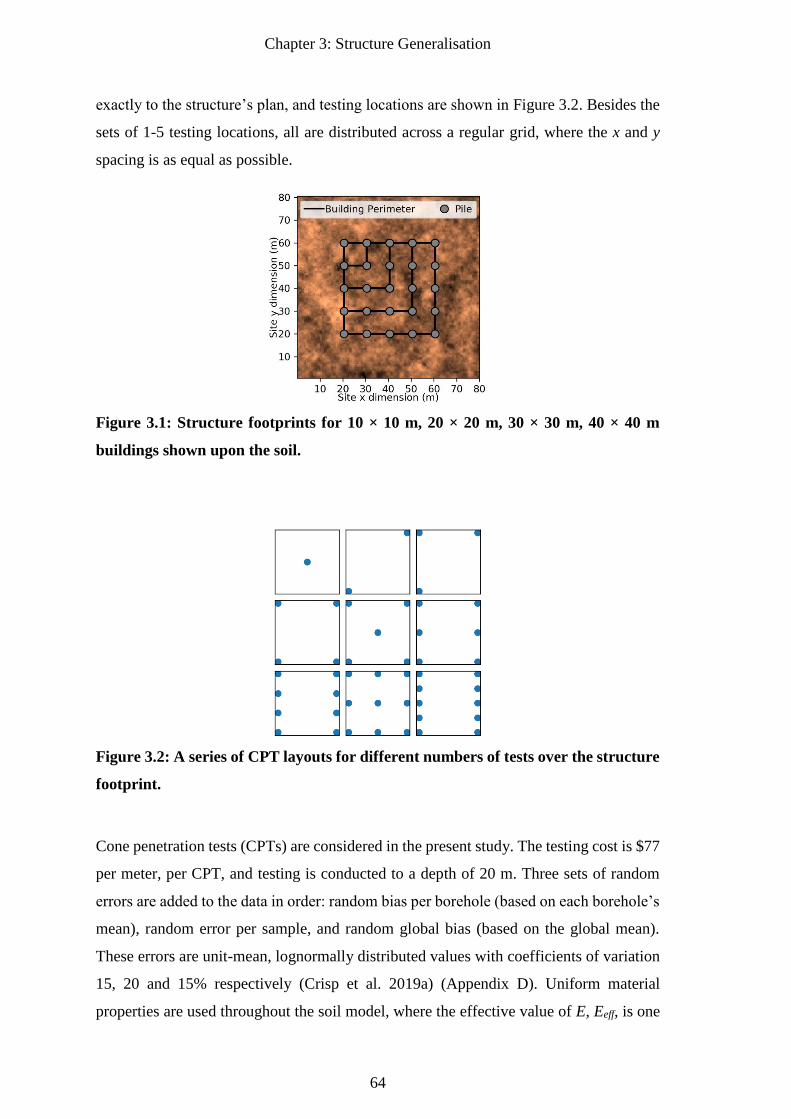
Chapter 3: Structure Generalisation
64
exactly to the structure’s plan, and testing locations are shown in Figure 3.2. Besides the
sets of 1-5 testing locations, all are distributed across a regular grid, where the x and y
spacing is as equal as possible.
Figure 3.1: Structure footprints for 10 × 10 m, 20 × 20 m, 30 × 30 m, 40 × 40 m
buildings shown upon the soil.
Figure 3.2: A series of CPT layouts for different numbers of tests over the structure
footprint.
Cone penetration tests (CPTs) are considered in the present study. The testing cost is $77
per meter, per CPT, and testing is conducted to a depth of 20 m. Three sets of random
errors are added to the data in order: random bias per borehole (based on each borehole’s
mean), random error per sample, and random global bias (based on the global mean).
These errors are unit-mean, lognormally distributed values with coefficients of variation
15, 20 and 15% respectively (Crisp et al. 2019a) (Appendix D). Uniform material
properties are used throughout the soil model, where the effective value of E, Eeff, is one
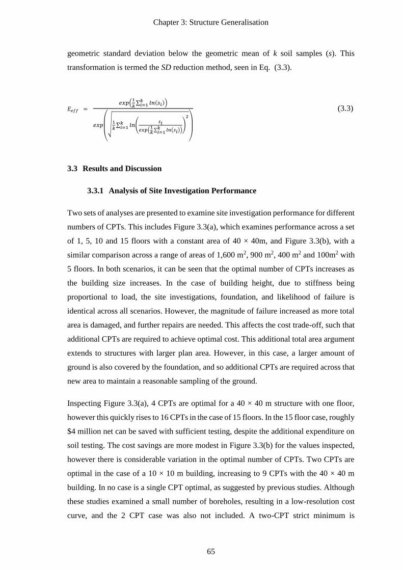
Chapter 3: Structure Generalisation
65
geometric standard deviation below the geometric mean of k soil samples (s). This
transformation is termed the SD reduction method, seen in Eq. (3.3).
𝐸𝑒𝑓𝑓 = 𝑒𝑥𝑝(
1
𝑘∑ 𝑙𝑛(𝑠𝑖)𝑘𝑖=1 )
𝑒𝑥𝑝
(
√1𝑘∑ 𝑙𝑛(
𝑠𝑖
𝑒𝑥𝑝(1𝑘∑ 𝑙𝑛(𝑠𝑖)𝑘𝑖=1 )
)
2
𝑘𝑖=1
)
(3.3)
3.3 Results and Discussion
3.3.1 Analysis of Site Investigation Performance
Two sets of analyses are presented to examine site investigation performance for different
numbers of CPTs. This includes Figure 3.3(a), which examines performance across a set
of 1, 5, 10 and 15 floors with a constant area of 40 × 40m, and Figure 3.3(b), with a
similar comparison across a range of areas of 1,600 m2, 900 m2, 400 m2 and 100m2 with
5 floors. In both scenarios, it can be seen that the optimal number of CPTs increases as
the building size increases. In the case of building height, due to stiffness being
proportional to load, the site investigations, foundation, and likelihood of failure is
identical across all scenarios. However, the magnitude of failure increased as more total
area is damaged, and further repairs are needed. This affects the cost trade-off, such that
additional CPTs are required to achieve optimal cost. This additional total area argument
extends to structures with larger plan area. However, in this case, a larger amount of
ground is also covered by the foundation, and so additional CPTs are required across that
new area to maintain a reasonable sampling of the ground.
Inspecting Figure 3.3(a), 4 CPTs are optimal for a 40 × 40 m structure with one floor,
however this quickly rises to 16 CPTs in the case of 15 floors. In the 15 floor case, roughly
$4 million net can be saved with sufficient testing, despite the additional expenditure on
soil testing. The cost savings are more modest in Figure 3.3(b) for the values inspected,
however there is considerable variation in the optimal number of CPTs. Two CPTs are
optimal in the case of a 10 × 10 m building, increasing to 9 CPTs with the 40 × 40 m
building. In no case is a single CPT optimal, as suggested by previous studies. Although
these studies examined a small number of boreholes, resulting in a low-resolution cost
curve, and the 2 CPT case was also not included. A two-CPT strict minimum is
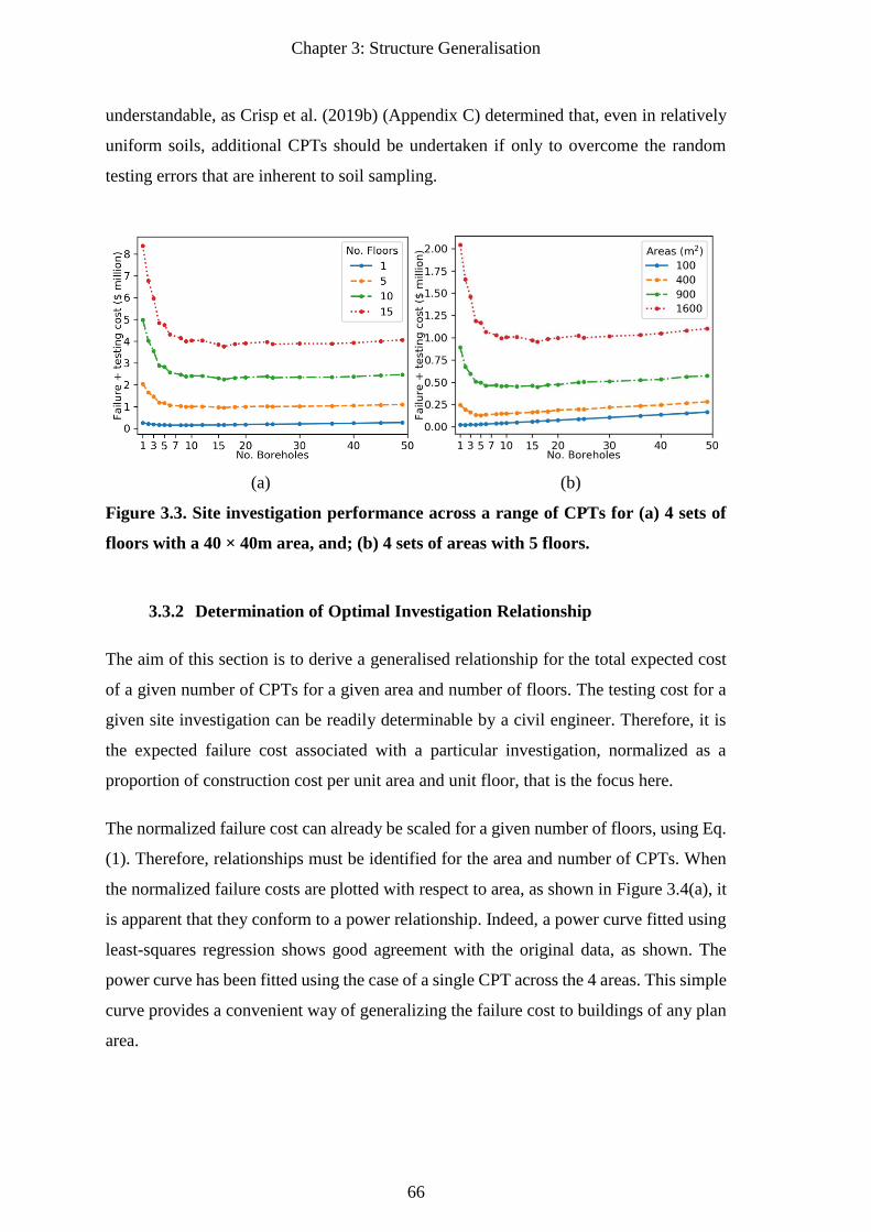
Chapter 3: Structure Generalisation
66
understandable, as Crisp et al. (2019b) (Appendix C) determined that, even in relatively
uniform soils, additional CPTs should be undertaken if only to overcome the random
testing errors that are inherent to soil sampling.
(a) (b)
Figure 3.3. Site investigation performance across a range of CPTs for (a) 4 sets of
floors with a 40 × 40m area, and; (b) 4 sets of areas with 5 floors.
3.3.2 Determination of Optimal Investigation Relationship
The aim of this section is to derive a generalised relationship for the total expected cost
of a given number of CPTs for a given area and number of floors. The testing cost for a
given site investigation can be readily determinable by a civil engineer. Therefore, it is
the expected failure cost associated with a particular investigation, normalized as a
proportion of construction cost per unit area and unit floor, that is the focus here.
The normalized failure cost can already be scaled for a given number of floors, using Eq.
(1). Therefore, relationships must be identified for the area and number of CPTs. When
the normalized failure costs are plotted with respect to area, as shown in Figure 3.4(a), it
is apparent that they conform to a power relationship. Indeed, a power curve fitted using
least-squares regression shows good agreement with the original data, as shown. The
power curve has been fitted using the case of a single CPT across the 4 areas. This simple
curve provides a convenient way of generalizing the failure cost to buildings of any plan
area.
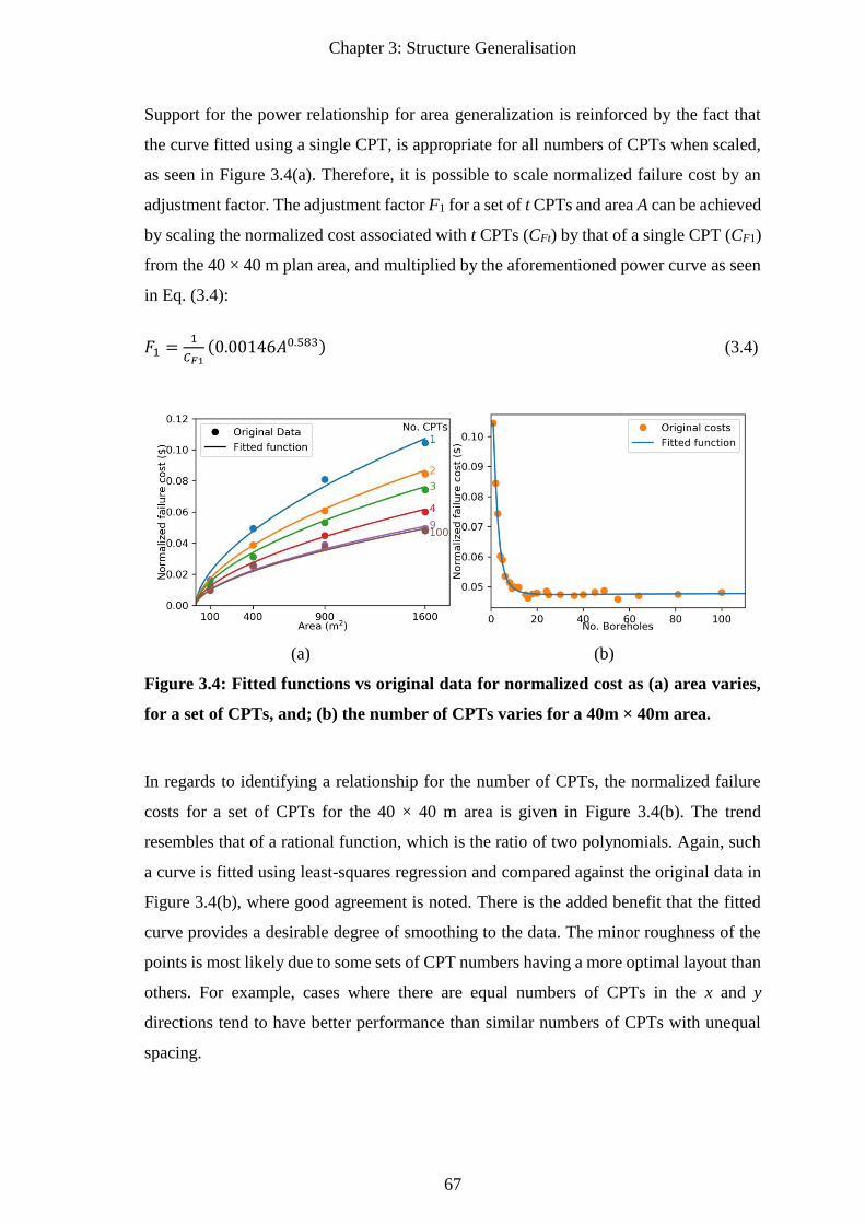
Chapter 3: Structure Generalisation
67
Support for the power relationship for area generalization is reinforced by the fact that
the curve fitted using a single CPT, is appropriate for all numbers of CPTs when scaled,
as seen in Figure 3.4(a). Therefore, it is possible to scale normalized failure cost by an
adjustment factor. The adjustment factor F1 for a set of t CPTs and area A can be achieved
by scaling the normalized cost associated with t CPTs (CFt) by that of a single CPT (CF1)
from the 40 × 40 m plan area, and multiplied by the aforementioned power curve as seen
in Eq. (3.4):
𝐹1 =1
𝐶𝐹1(0.00146𝐴0.583) (3.4)
(a) (b)
Figure 3.4: Fitted functions vs original data for normalized cost as (a) area varies,
for a set of CPTs, and; (b) the number of CPTs varies for a 40m × 40m area.
In regards to identifying a relationship for the number of CPTs, the normalized failure
costs for a set of CPTs for the 40 × 40 m area is given in Figure 3.4(b). The trend
resembles that of a rational function, which is the ratio of two polynomials. Again, such
a curve is fitted using least-squares regression and compared against the original data in
Figure 3.4(b), where good agreement is noted. There is the added benefit that the fitted
curve provides a desirable degree of smoothing to the data. The minor roughness of the
points is most likely due to some sets of CPT numbers having a more optimal layout than
others. For example, cases where there are equal numbers of CPTs in the x and y
directions tend to have better performance than similar numbers of CPTs with unequal
spacing.
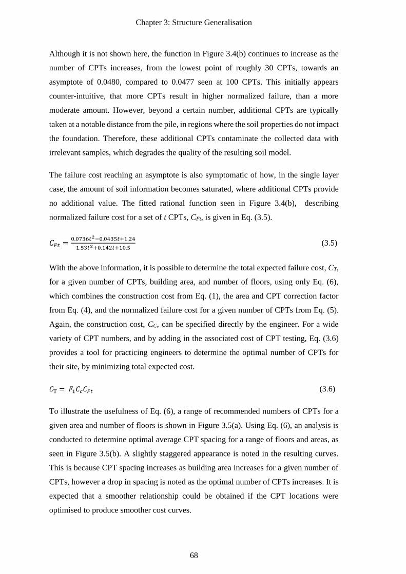
Chapter 3: Structure Generalisation
68
Although it is not shown here, the function in Figure 3.4(b) continues to increase as the
number of CPTs increases, from the lowest point of roughly 30 CPTs, towards an
asymptote of 0.0480, compared to 0.0477 seen at 100 CPTs. This initially appears
counter-intuitive, that more CPTs result in higher normalized failure, than a more
moderate amount. However, beyond a certain number, additional CPTs are typically
taken at a notable distance from the pile, in regions where the soil properties do not impact
the foundation. Therefore, these additional CPTs contaminate the collected data with
irrelevant samples, which degrades the quality of the resulting soil model.
The failure cost reaching an asymptote is also symptomatic of how, in the single layer
case, the amount of soil information becomes saturated, where additional CPTs provide
no additional value. The fitted rational function seen in Figure 3.4(b), describing
normalized failure cost for a set of t CPTs, CFt, is given in Eq. (3.5).
𝐶𝐹𝑡 =0.0736𝑡2−0.0435𝑡+1.24
1.53𝑡2+0.142𝑡+10.5 (3.5)
With the above information, it is possible to determine the total expected failure cost, CT,
for a given number of CPTs, building area, and number of floors, using only Eq. (6),
which combines the construction cost from Eq. (1), the area and CPT correction factor
from Eq. (4), and the normalized failure cost for a given number of CPTs from Eq. (5).
Again, the construction cost, CC, can be specified directly by the engineer. For a wide
variety of CPT numbers, and by adding in the associated cost of CPT testing, Eq. (3.6)
provides a tool for practicing engineers to determine the optimal number of CPTs for
their site, by minimizing total expected cost.
𝐶T = 𝐹1𝐶𝑐𝐶𝐹𝑡 (3.6)
To illustrate the usefulness of Eq. (6), a range of recommended numbers of CPTs for a
given area and number of floors is shown in Figure 3.5(a). Using Eq. (6), an analysis is
conducted to determine optimal average CPT spacing for a range of floors and areas, as
seen in Figure 3.5(b). A slightly staggered appearance is noted in the resulting curves.
This is because CPT spacing increases as building area increases for a given number of
CPTs, however a drop in spacing is noted as the optimal number of CPTs increases. It is
expected that a smoother relationship could be obtained if the CPT locations were
optimised to produce smoother cost curves.
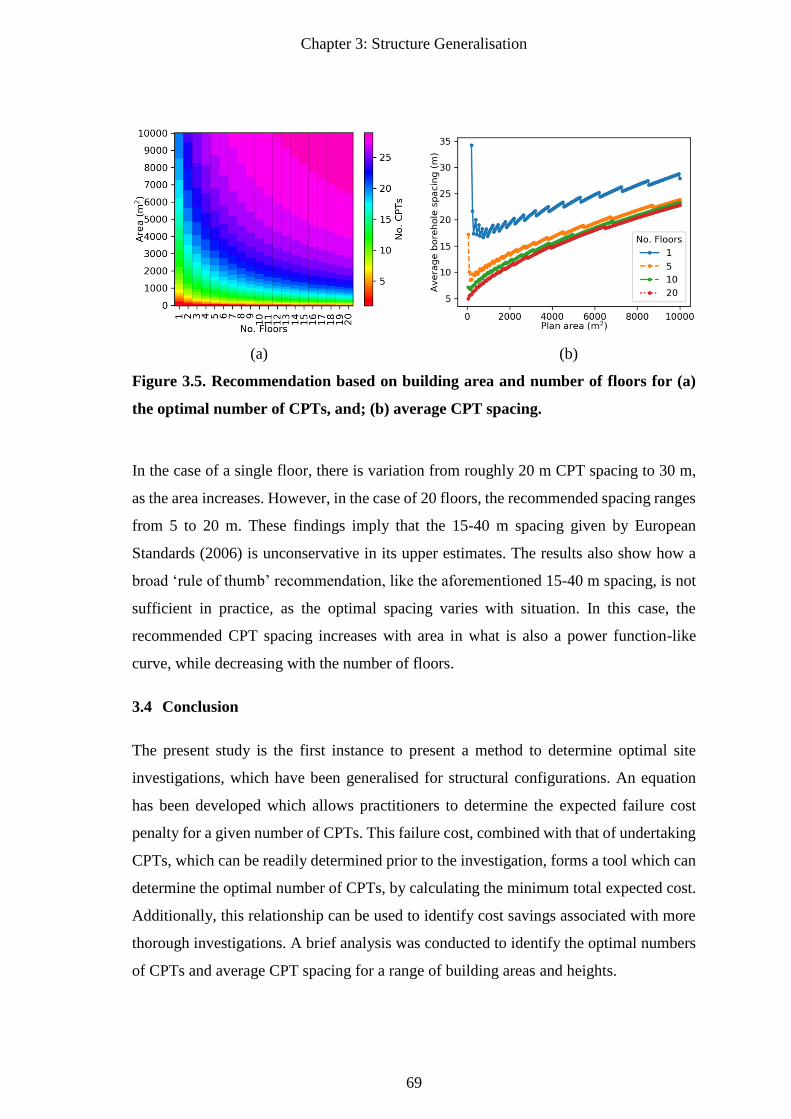
Chapter 3: Structure Generalisation
69
(a) (b)
Figure 3.5. Recommendation based on building area and number of floors for (a)
the optimal number of CPTs, and; (b) average CPT spacing.
In the case of a single floor, there is variation from roughly 20 m CPT spacing to 30 m,
as the area increases. However, in the case of 20 floors, the recommended spacing ranges
from 5 to 20 m. These findings imply that the 15-40 m spacing given by European
Standards (2006) is unconservative in its upper estimates. The results also show how a
broad ‘rule of thumb’ recommendation, like the aforementioned 15-40 m spacing, is not
sufficient in practice, as the optimal spacing varies with situation. In this case, the
recommended CPT spacing increases with area in what is also a power function-like
curve, while decreasing with the number of floors.
3.4 Conclusion
The present study is the first instance to present a method to determine optimal site
investigations, which have been generalised for structural configurations. An equation
has been developed which allows practitioners to determine the expected failure cost
penalty for a given number of CPTs. This failure cost, combined with that of undertaking
CPTs, which can be readily determined prior to the investigation, forms a tool which can
determine the optimal number of CPTs, by calculating the minimum total expected cost.
Additionally, this relationship can be used to identify cost savings associated with more
thorough investigations. A brief analysis was conducted to identify the optimal numbers
of CPTs and average CPT spacing for a range of building areas and heights.
Chapter 3: Structure Generalisation
70
It should be noted that the single layer assumption considered in this paper is a
simplification of reality, as many layers are typically found in practice. Therefore, these
recommendations should be taken as a minimum. However, as the soil investigated is a
worst-case of this simplified single layer scenario, the authors consider the given method
and associated recommendations a reasonable trade-off with respect to soil complexity,
whereby the recommendations can be used as a generalised minimum number of CPTs
for all soil cases.
Further work could involve optimizing the CPT locations with respect to the foundations,
as well as extending the analysis to additional tests. A wider range of soil cases might be
investigated, including alternate combinations of coefficient of variation and scale of
fluctuation, as well as multiple-layer scenarios. However, simpler soil cases, such as that
considered in this study, are typically easier to generalise to a wider range of soils.
3.5 Acknowledgements
This paper was supported by the Peter Brooker Conference Travel Prize in Mathematical
Geology.
3.6 References
Albatal, A. 2013. Effect of inadequate site investigation on the cost and time of a
construction project. Masters Thesis, Construction and Building Engineering
Department, Arab Academy for Science, Technology and Maritime Transport,
Cairo.
Arsyad, A. 2009. The effect of limited site investigations on the design and performance
of pile foundations. Masters Thesis, School of Civil, Environmental and Mining
Engineering, University of Adelaide, Adelaide.
Ching, J., Hu, Y. G., and Phoon, K. K. 2018. Effective Young’s modulus of a spatially
variable soil mass under a footing. Structural Safety, 73, 99-113.
Clayton, C. 2001. Managing geotechnical risk: time for change? Proceedings of the
Institution of Civil Engineers-Geotechnical Engineering, 149(1), 3-11.
Crisp, M. P., Jaksa, M. B., and Kuo, Y. L. 2018. Influence of Site Investigation Borehole
Pattern and Area on Pile Foundation Performance. In Proceedings of the 12th
ANZ Young Geotechnical Professionals Conference, Hobart.
Crisp, M. P., Jaksa, M. B., and Kuo, Y. L. 2019a. Framework for the Optimisation of Site
Investigations for Pile Designs in Complex Multi-Layered Soil. , University of
Adelaide, Adelaide, Australia. doi: 10.13140/RG.2.2.23536.71685
Chapter 3: Structure Generalisation
71
Crisp, M. P., Jaksa, M. B., and Kuo, Y. L. 2019b. Influence of distance-weighted
averaging of site investigation samples on foundation performance. In
Proceedings of the 13th Australia New Zealand Conference on Geomechanics,
Perth.
Day, R. W. 1999. Forensic geotechnical and foundation engineering: McGraw-Hill New
York.
European Standards. (2006). Eurocode 7 - Geotechnical design - Part2: Ground
investigation and testing (Annex B.3) EN 1997-2.
Fenton, G. A., and Griffiths, D. V. 2005. Three-dimensional probabilistic foundation
settlement. Journal of Geotechnical and Geoenvironmental Engineering, 131(2),
232-239.
Fenton, G. A., and Griffiths, D. V. 2008. Risk assessment in geotechnical engineering.
Hoboken: Wiley.
Fenton, G. A., and Vanmarcke, E. H. 1990. Simulation of random fields via local average
subdivision. Journal of Engineering Mechanics, 116(8), 1733-1749.
Goldsworthy, J. S. 2006. Quantifying the risk of geotechnical site investigations. Ph.D
Thesis, School of Civil, Environmental and Mining Engineering, University of
Adelaide, Adelaide.
Goldsworthy, J. S., Jaksa, M. B., Fenton, G. A., Kaggwa, W. S., Griffiths, D. V., and
Poulos, H. G. 2007. Effect of sample location on the reliability based design of
pad foundations. Georisk, 1(3), 155-166.
Jaksa, M. B. 2000. Geotechnical risk and inadequate site investigations: a case study.
Australian Geomechanics, 35(2), 39-46.
Jaksa, M. B., Goldsworthy, J. S., Fenton, G. A., Kaggwa, W. S., Griffiths, D. V., Kuo,
Y. L., and Poulos, H. G. 2005. Towards reliable and effective site investigations.
Géotechnique, 55(2), 109-121.
Jaksa, M. B., Kaggwa, W. S., Fenton, G. A., and Poulos, H. G. 2003. A framework for
quantifying the reliability of geotechnical investigations. In Proceedings of the
9th International Conference on the Application of Statistics and Probability in
Civil Engineering.
Loehr, J. E., Ding, D., and Likos, W. J. 2015. Effect of Number of Soil Strength
Measurements on Reliability of Spread Footing Designs. Transportation Research
Record: Journal of the Transportation Research Board, (2511), 37-44.
Moh, Z. C. 2004. Site investigation and geotechnical failures. In Proceedings of the
Proceeding of International Conference on Structural and Foundation Failures.
Naghibi, F., Fenton, G. A., and Griffiths, D. V. 2014. Serviceability limit state design of
deep foundations. Géotechnique, 64(10), 787-799.

Chapter 3: Structure Generalisation
72
National Research Council. 1984. Geotechnical Site Investigations for Underground
Projects (Vol. 1). Washington.
Rawlinsons, A. (2016). Australian Construction Handbook (34 ed., pp. 1005). Perth,
Australia: Rawlhouse Publishing Pty. Ltd.
Vanmarcke, E. H. 1983. Random Fields: Analysis and Synthesis. London: MIT Press.
Chapter 4: Generation of Multi-Layer Soils
73
4 Chapter 4: Generation of Multi-
Layer Soils
Paper Title:
A Method for Generating Virtual Soil Profiles with
Complex, Multi-Layer Stratigraphy

Chapter 4: Generation of Multi-Layer Soils
74


Chapter 4: Generation of Multi-Layer Soils
77
Abstract
This paper presents a framework for generating multi-layer, unconditional soil profiles
with complex stratigraphy, which simulates the effects of natural erosion and
sedimentation processes. The stratigraphy can have varying degrees of randomness and
can include features such as lenses, as well as sloped and undulating layers. The method
generates the soil comprising the layers using local average subdivision (LAS), and a
random noise component that is added to the layer boundaries. The layers are created by
generating coordinates of key points in the simulated ground profile, which are then
interpolated with a customized, 2D, linear interpolation algorithm. The resulting
simulations facilitate more accurate probabilistic modelling of geotechnical engineering
systems because they provide more realistic geologies, such as those usually encountered
in the ground. Fortran code implementing this framework is included as supplementary
material.
Keywords: spatial variability, layer generation, random field theory
Chapter 4: Generation of Multi-Layer Soils
78
4.1 Introduction
This paper presents a framework for generating virtual, random, three-dimensional (3D),
complex soil profiles by merging multiple, homogenous soils in a process that broadly
emulates erosion and deposition. Here, virtual soil profiles are computer-generated
representations of a volume of soil property values. The framework focuses on the
generation of random stratigraphies, of arbitrary complexity, that define the boundaries
between soil layers. While one method of defining layer geology is presented here as an
example, a program, in the form of Fortran source files, is provided as supplementary
material, and users may modify the layer generation parameters to suit their own
particular circumstances. The code may be added to any number of existing frameworks
and software packages that currently work with single-layer soil profiles, as discussed
later in this section.
For the purpose of clarity, it is important to note the objectives of the proposed
framework, and highlight what it is not intended to achieve. Firstly, the method was
designed to model plausible geology, and allow users to investigate the impact of specific
geological features. It was not designed as a soil genesis model, which attempts to model
physical processes directly, e.g. (Opolot et al. 2015). Secondly, the proposed method
cannot currently be used to replicate existing physical soil profiles found in practice. Such
simulations are known as conditional, as they are constrained to match the soil properties
at their respective physical locations as encountered by soil testing. In contrast, the
proposed method involves unconditional simulation, which generates virtual and
fictitious soils as specified predominantly by statistical parameters. As such, conditional,
multi-layer generation techniques, such as sequential indicator simulation (Bierkens and
Weerts 1994) and coupled Markov chain models (Elfeki and Dekking 2001) are not
relevant to this work. While it is possible to modify the software accompanying this paper
to allow for conditional simulation, it is not the focus of this study.
Virtual soil generation and its use has applications in a range of areas which have pre-
existing Fortran software, including settlement modelling (Kuo et al. 2004), optimization
of site investigations (Jaksa et al. 2005), slope stability analysis (Griffiths and Fenton
2004), calibration of reliability-based design (Fenton and Naghibi 2011), modelling
groundwater flow (Schlüter et al. 2012), and demonstration in teaching (Kim 2011).
Random soils can provide a wealth of statistical information when used within a Monte
Chapter 4: Generation of Multi-Layer Soils
79
Carlo (MC) analysis framework (Ang 2007), where each MC realization uses an
independent random soil. In particular, random soils are often paired with finite element
analysis; a combination referred to as the random finite element method (RFEM) (Fenton
and Griffiths 2008b).
While many studies have used various types of virtual soil generating algorithms, they
are typically only used to produce profiles that are homogenous or otherwise of simple
stratigraphy. Here, homogeneity refers to soils with variable properties that represent a
single soil type. In reality, soils contain complex geological features such as faults, lenses
and layers of arbitrary boundaries. This complexity is due to the wide variety of natural
processes that form and influence the ground and that occur over long periods of time
(Skinner and Porter 1987). Soils have a tendency to be eroded and deposited by water,
wind or ice. These processes can significantly influence the nature, shape and orientation
of soil layers, or even remove them completely. Given the prevalence of these processes
and geological features, it is important to have a model that can represent plausible,
naturally-occurring soils with this geology.
Virtual soils are generated using random field theory (RFT); a means of creating
correlated random values that are representative of realistic geotechnical property spatial
variability (Vanmarcke 1983). The product is a random field; a volume of discrete
elements, where each element represents a soil property value. In practice, RFT is
commonly implemented to generate fields that exhibit second order stationarity (weak
stationarity). The soil is described in its entirety by the first and second order moments:
The mean () and the standard deviation (SD), as well as the correlation structure. The
standard deviation is often standardized by the mean to express the coefficient of
variation (COV) where COV = SD/. The aforementioned soil correlation structure is
needed because soil elements that are in close spatial proximity are expected to have
similar properties. This structure is represented by a scale of fluctuation (SOF), which
describes the distance over which properties are expected to be correlated. A SOF can be
specified for each dimension, and it is often the case that horizontal values are higher
than the vertical. The horizontal-vertical SOF ratio is termed anisotropy, and occurs
because the effects of gravity and sedimentation frequently result in soil deposits being
formed in a series of relatively thin layers, where properties fluctuate more rapidly with
depth (Jaksa 1995).
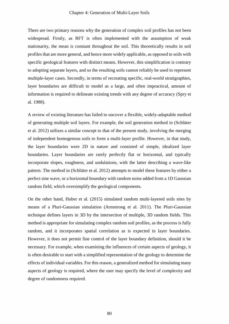
Chapter 4: Generation of Multi-Layer Soils
80
There are two primary reasons why the generation of complex soil profiles has not been
widespread. Firstly, as RFT is often implemented with the assumption of weak
stationarity, the mean is constant throughout the soil. This theoretically results in soil
profiles that are more general, and hence more widely applicable, as opposed to soils with
specific geological features with distinct means. However, this simplification is contrary
to adopting separate layers, and so the resulting soils cannot reliably be used to represent
multiple-layer cases. Secondly, in terms of recreating specific, real-world stratigraphies,
layer boundaries are difficult to model as a large, and often impractical, amount of
information is required to delineate existing trends with any degree of accuracy (Spry et
al. 1988).
A review of existing literature has failed to uncover a flexible, widely-adaptable method
of generating multiple soil layers. For example, the soil generation method in (Schlüter
et al. 2012) utilizes a similar concept to that of the present study, involving the merging
of independent homogenous soils to form a multi-layer profile. However, in that study,
the layer boundaries were 2D in nature and consisted of simple, idealized layer
boundaries. Layer boundaries are rarely perfectly flat or horizontal, and typically
incorporate slopes, roughness, and undulations, with the latter describing a wave-like
pattern. The method in (Schlüter et al. 2012) attempts to model these features by either a
perfect sine wave, or a horizontal boundary with random noise added from a 1D Gaussian
random field, which oversimplify the geological components.
On the other hand, Huber et al. (2015) simulated random multi-layered soils sites by
means of a Pluri-Gaussian simulation (Armstrong et al. 2011). The Pluri-Gaussian
technique defines layers in 3D by the intersection of multiple, 3D random fields. This
method is appropriate for simulating complex random soil profiles, as the process is fully
random, and it incorporates spatial correlation as is expected in layer boundaries.
However, it does not permit fine control of the layer boundary definition, should it be
necessary. For example, when examining the influences of certain aspects of geology, it
is often desirable to start with a simplified representation of the geology to determine the
effects of individual variables. For this reason, a generalized method for simulating many
aspects of geology is required, where the user may specify the level of complexity and
degree of randomness required.
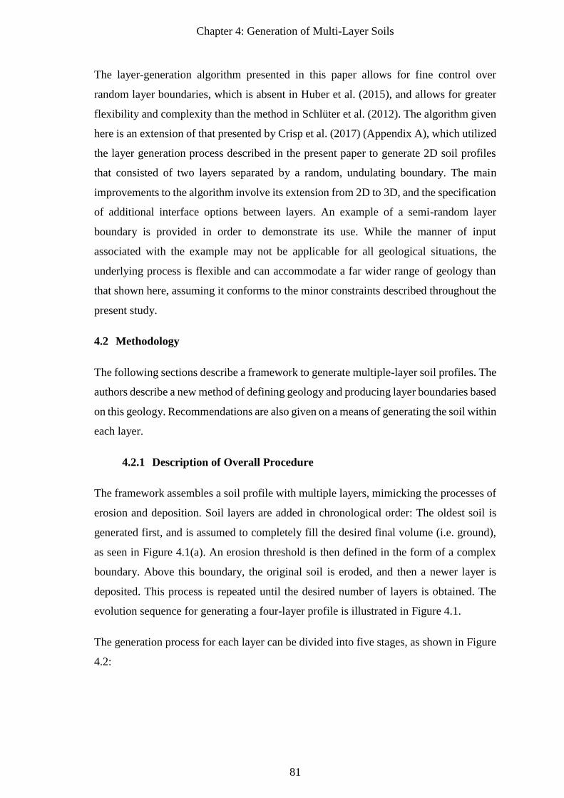
Chapter 4: Generation of Multi-Layer Soils
81
The layer-generation algorithm presented in this paper allows for fine control over
random layer boundaries, which is absent in Huber et al. (2015), and allows for greater
flexibility and complexity than the method in Schlüter et al. (2012). The algorithm given
here is an extension of that presented by Crisp et al. (2017) (Appendix A), which utilized
the layer generation process described in the present paper to generate 2D soil profiles
that consisted of two layers separated by a random, undulating boundary. The main
improvements to the algorithm involve its extension from 2D to 3D, and the specification
of additional interface options between layers. An example of a semi-random layer
boundary is provided in order to demonstrate its use. While the manner of input
associated with the example may not be applicable for all geological situations, the
underlying process is flexible and can accommodate a far wider range of geology than
that shown here, assuming it conforms to the minor constraints described throughout the
present study.
4.2 Methodology
The following sections describe a framework to generate multiple-layer soil profiles. The
authors describe a new method of defining geology and producing layer boundaries based
on this geology. Recommendations are also given on a means of generating the soil within
each layer.
4.2.1 Description of Overall Procedure
The framework assembles a soil profile with multiple layers, mimicking the processes of
erosion and deposition. Soil layers are added in chronological order: The oldest soil is
generated first, and is assumed to completely fill the desired final volume (i.e. ground),
as seen in Figure 4.1(a). An erosion threshold is then defined in the form of a complex
boundary. Above this boundary, the original soil is eroded, and then a newer layer is
deposited. This process is repeated until the desired number of layers is obtained. The
evolution sequence for generating a four-layer profile is illustrated in Figure 4.1.
The generation process for each layer can be divided into five stages, as shown in Figure
4.2:
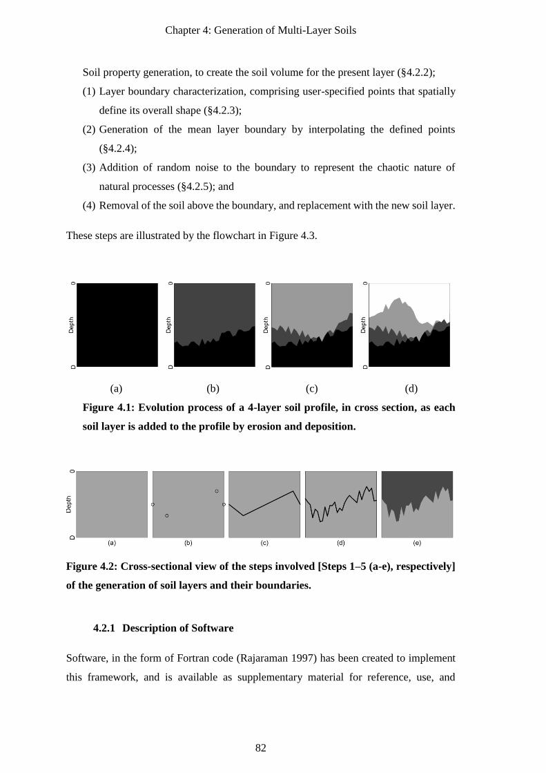
Chapter 4: Generation of Multi-Layer Soils
82
Soil property generation, to create the soil volume for the present layer (§4.2.2);
(1) Layer boundary characterization, comprising user-specified points that spatially
define its overall shape (§4.2.3);
(2) Generation of the mean layer boundary by interpolating the defined points
(§4.2.4);
(3) Addition of random noise to the boundary to represent the chaotic nature of
natural processes (§4.2.5); and
(4) Removal of the soil above the boundary, and replacement with the new soil layer.
These steps are illustrated by the flowchart in Figure 4.3.
(a) (b) (c) (d)
Figure 4.1: Evolution process of a 4-layer soil profile, in cross section, as each
soil layer is added to the profile by erosion and deposition.
Figure 4.2: Cross-sectional view of the steps involved [Steps 1–5 (a-e), respectively]
of the generation of soil layers and their boundaries.
4.2.1 Description of Software
Software, in the form of Fortran code (Rajaraman 1997) has been created to implement
this framework, and is available as supplementary material for reference, use, and
Chapter 4: Generation of Multi-Layer Soils
83
modification. The code is based on subroutines provided by Fenton and Griffiths (2008a),
largely updated to Fortran 95 standard, and with new subroutines added to provide
Figure 4.3: Flowchart describing the process of layer generation, including
stratigraphic definition and interpolation.
Define feasible regions for points and soil layer
properties
Generate random coordinates
in the horizontal plane along
the soil boundary and within
the regions
Generate random
depths for all points
Subdivide area into a
series of quadrilaterals
defined by the points
Interpolate each
segment of the
quadrilateral in x
direction
Interpolate each
segment of the
quadrilateral in y
direction
Generate zero-mean
2D normal Gaussian
random field for
boundary roughness
Average the above
interpolations to form
mean layer geometry
Add the 2D Gaussian field to produce final layer
geometry
Generate log-normal
random field for
time-zero bottom
layer
Generate log-normal
random field for
upper layer
Replace material
above boundary with
that of the upper-
layer field
Repeat for
additional
layers
Interpolation Point definition Field generation Replacement action
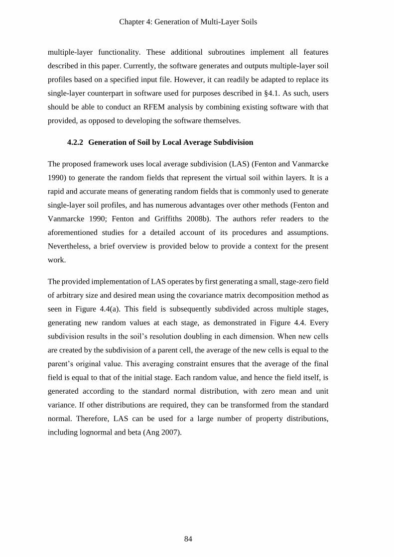
Chapter 4: Generation of Multi-Layer Soils
84
multiple-layer functionality. These additional subroutines implement all features
described in this paper. Currently, the software generates and outputs multiple-layer soil
profiles based on a specified input file. However, it can readily be adapted to replace its
single-layer counterpart in software used for purposes described in §4.1. As such, users
should be able to conduct an RFEM analysis by combining existing software with that
provided, as opposed to developing the software themselves.
4.2.2 Generation of Soil by Local Average Subdivision
The proposed framework uses local average subdivision (LAS) (Fenton and Vanmarcke
1990) to generate the random fields that represent the virtual soil within layers. It is a
rapid and accurate means of generating random fields that is commonly used to generate
single-layer soil profiles, and has numerous advantages over other methods (Fenton and
Vanmarcke 1990; Fenton and Griffiths 2008b). The authors refer readers to the
aforementioned studies for a detailed account of its procedures and assumptions.
Nevertheless, a brief overview is provided below to provide a context for the present
work.
The provided implementation of LAS operates by first generating a small, stage-zero field
of arbitrary size and desired mean using the covariance matrix decomposition method as
seen in Figure 4.4(a). This field is subsequently subdivided across multiple stages,
generating new random values at each stage, as demonstrated in Figure 4.4. Every
subdivision results in the soil’s resolution doubling in each dimension. When new cells
are created by the subdivision of a parent cell, the average of the new cells is equal to the
parent’s original value. This averaging constraint ensures that the average of the final
field is equal to that of the initial stage. Each random value, and hence the field itself, is
generated according to the standard normal distribution, with zero mean and unit
variance. If other distributions are required, they can be transformed from the standard
normal. Therefore, LAS can be used for a large number of property distributions,
including lognormal and beta (Ang 2007).
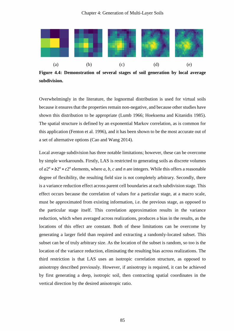
Chapter 4: Generation of Multi-Layer Soils
85
(a) (b) (c) (d) (e)
Figure 4.4: Demonstration of several stages of soil generation by local average
subdivision.
Overwhelmingly in the literature, the lognormal distribution is used for virtual soils
because it ensures that the properties remain non-negative, and because other studies have
shown this distribution to be appropriate (Lumb 1966; Hoeksema and Kitanidis 1985).
The spatial structure is defined by an exponential Markov correlation, as is common for
this application (Fenton et al. 1996), and it has been shown to be the most accurate out of
a set of alternative options (Cao and Wang 2014).
Local average subdivision has three notable limitations; however, these can be overcome
by simple workarounds. Firstly, LAS is restricted to generating soils as discrete volumes
of a2n × b2n × c2n elements, where a, b, c and n are integers. While this offers a reasonable
degree of flexibility, the resulting field size is not completely arbitrary. Secondly, there
is a variance reduction effect across parent cell boundaries at each subdivision stage. This
effect occurs because the correlation of values for a particular stage, at a macro scale,
must be approximated from existing information, i.e. the previous stage, as opposed to
the particular stage itself. This correlation approximation results in the variance
reduction, which when averaged across realizations, produces a bias in the results, as the
locations of this effect are constant. Both of these limitations can be overcome by
generating a larger field than required and extracting a randomly-located subset. This
subset can be of truly arbitrary size. As the location of the subset is random, so too is the
location of the variance reduction, eliminating the resulting bias across realizations. The
third restriction is that LAS uses an isotropic correlation structure, as opposed to
anisotropy described previously. However, if anisotropy is required, it can be achieved
by first generating a deep, isotropic soil, then contracting spatial coordinates in the
vertical direction by the desired anisotropic ratio.
Chapter 4: Generation of Multi-Layer Soils
86
The three parameters required for the generation of the soil volume within each layer are
the mean, COV and SOF. It is important to choose appropriate values for these properties
that correspond to real soils. Several studies have compiled databases of soil properties,
including the mean, SOF and COV for various types of soils. These values can be used
as guidelines for possible inputs to use in unconditional simulation. A comprehensive
investigation of soil property variability was summarized by Phoon (1995). The results
are based on the outcome of many years of research on reliability-based design of
transmission towers at Cornell University (Filippas et al. 1988; Orchant et al. 1988; Spry
et al. 1988; Kulhawy et al. 1992). Further information on soil properties are provided by
(Soulie et al. 1990; Jaksa 1995; Phoon and Kulhawy 1999; Akkaya and Vanmarcke 2003;
Kulatilake and Um 2003). An over-arching review of these studies, in the context of
practical simulation of Young’s modulus, was given by Goldsworthy (2006). Suggested
ranges for input values for soil generation by LAS is provided in Table 4.1 for COV,
horizontal and vertical SOFs, mean stiffness, and anisotropy, which is defined as the ratio
of the horizontal to vertical SOF in any given soil. Other inputs include the element size,
as well as the size of the soil volume in terms of the number of elements in each direction,
which may be specified by the user depending on the size of the problem domain.
Table 4.1: Ranges for input parameters for the generation of soil, as used by the 3D
LAS algorithm.
Variable Lower bound Upper bound
COV (%) 2% 80%
Horizontal SOF (m) 1.5 m 80 m
Vertical SOF (m) 0.1 m 12.7 m
Anisotropy 1 10
Mean (MPa) 5 170
4.2.3 Definition of Stratigraphy
Our aim with the framework presented here is to be as general and as flexible as possible.
This allows one to generate stratigraphies that mimic those observed in nature. In its most
general form, the framework defines a boundary by an arbitrary series of points. The
point coordinates can be specified exactly or generated randomly in the horizontal and
vertical directions. Achieving the desired geological structure then becomes a matter of
simply specifying the positions of these points, or the conditions in which the points may
randomly occur.
Chapter 4: Generation of Multi-Layer Soils
87
It should be noted that any geology generated by this method must conform to two
constraints. Firstly, each layer boundary is defined entirely be a 2D surface of height
information. As such, the boundary cannot fold back over itself in the third dimension.
Secondly, the overall geology must be defined by a series of points arranged in an
arbitrary, and potentially irregular, grid pattern. However, this second constraint may
potentially be removed with the implementation of a more sophisticated interpolation
algorithm than the one described in the present study.
Admittedly, the current input system is not suitable for all cases of layer boundary
definition, as it is deemed impossible to design such a system that satisfies the needs of
all users, while maintaining an arbitrary mix of control and randomness. However,
besides the input system, the core algorithm is capable of flexible geology definition,
subject to the two aforementioned constraints. As such, the user is encouraged to modify
the code to extend or replace this input system as desired. For example, 4 points could be
defined on an inclined plane, if such an inclined layer is desired. Alternatively, the points
may be specified to appear according to a normal distribution to a specified mean and
variance in each dimension. However, while the software can be modified to allow this,
these examples are not explored in the present study.
For the simplicity of visualization and definition, the software input is currently coded to
produce random, multi-segmented boundaries that are likely to result in an undulating
pattern, which in the case of 3 or more layers, may result in the formation of lenses if the
layers are allowed to overlap. Such behavior is desirable, as lenses are a geological feature
that may be especially detrimental to the satisfactory performance of foundations (Halim
1991) and so should be present in the analysis of realistic soil profiles.
The segmentation system described above is sufficient for an example of the framework,
and functions as follows. The layer boundary is subdivided into a grid of arbitrary
quadrilaterals, forming a series of segments in the x- and y- directions. In this case, there
are 3 segments in the x-direction and 4 in the y-direction, as illustrated by the black lines
in the example in Figure 4.5. These quadrilaterals are defined by points that are randomly
located to appear within certain regions. These feasible regions are defined by the colored
hashed boxes in Figure 4.5, where each contains one internal point that is randomly
located according to a uniform distribution. Where the edges of the box coincide with the
edge of the soil, an additional point is created and constrained to that edge, in order to
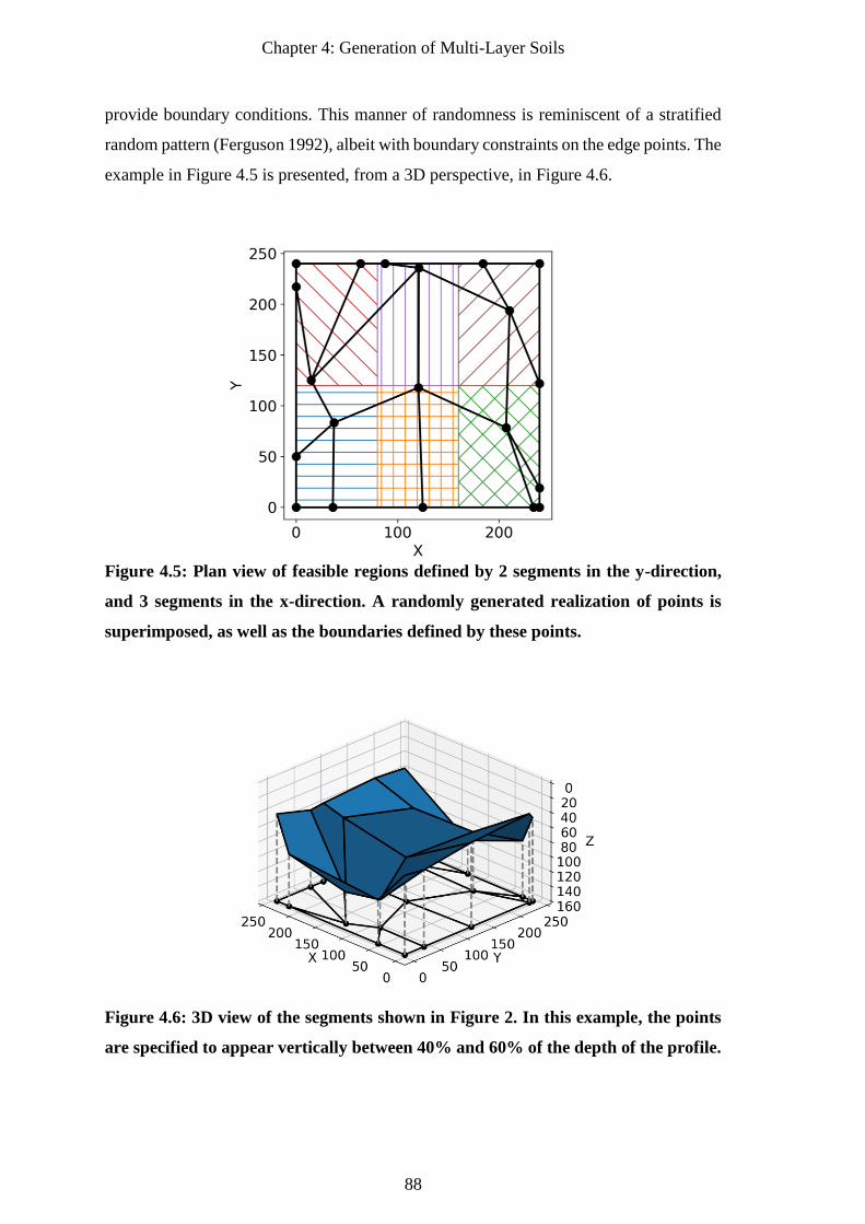
Chapter 4: Generation of Multi-Layer Soils
88
provide boundary conditions. This manner of randomness is reminiscent of a stratified
random pattern (Ferguson 1992), albeit with boundary constraints on the edge points. The
example in Figure 4.5 is presented, from a 3D perspective, in Figure 4.6.
Figure 4.5: Plan view of feasible regions defined by 2 segments in the y-direction,
and 3 segments in the x-direction. A randomly generated realization of points is
superimposed, as well as the boundaries defined by these points.
Figure 4.6: 3D view of the segments shown in Figure 2. In this example, the points
are specified to appear vertically between 40% and 60% of the depth of the profile.
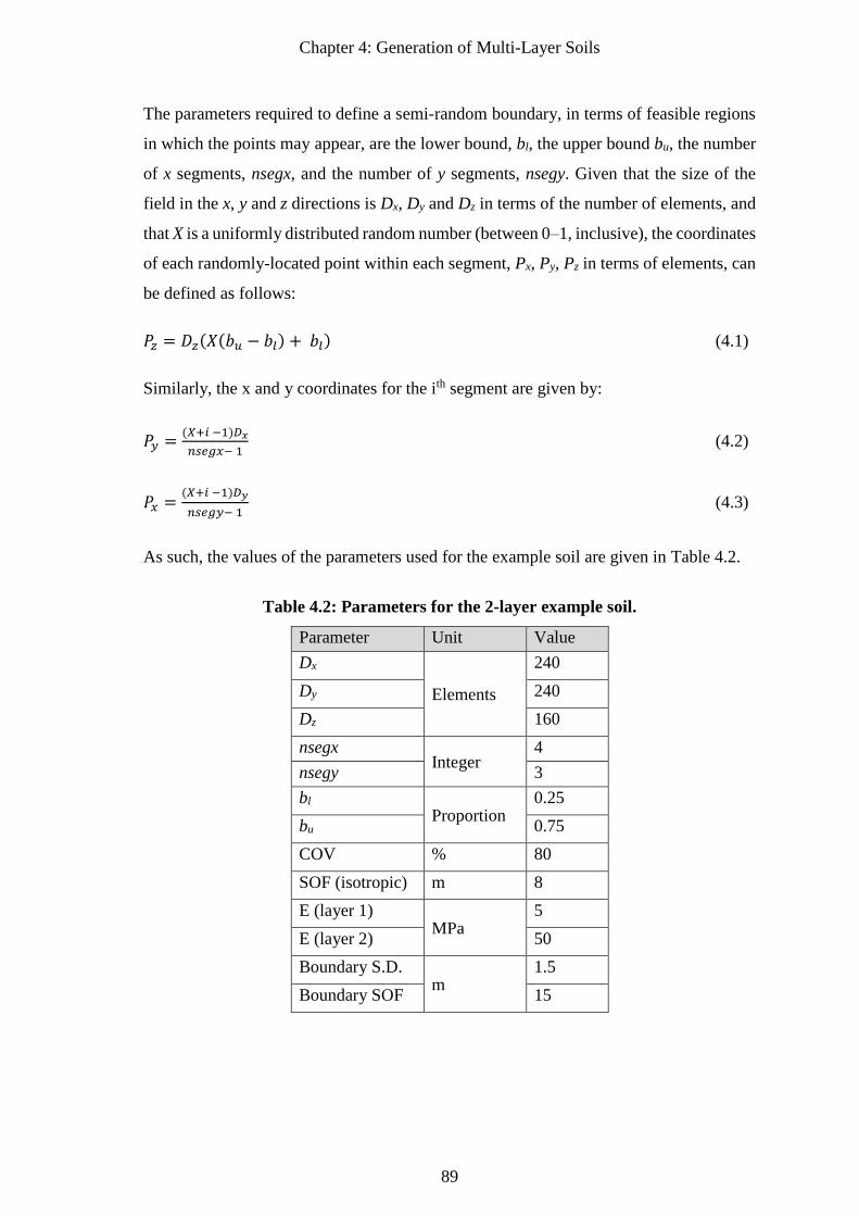
Chapter 4: Generation of Multi-Layer Soils
89
The parameters required to define a semi-random boundary, in terms of feasible regions
in which the points may appear, are the lower bound, bl, the upper bound bu, the number
of x segments, nsegx, and the number of y segments, nsegy. Given that the size of the
field in the x, y and z directions is Dx, Dy and Dz in terms of the number of elements, and
that X is a uniformly distributed random number (between 0–1, inclusive), the coordinates
of each randomly-located point within each segment, Px, Py, Pz in terms of elements, can
be defined as follows:
𝑃𝑧 = 𝐷𝑧(𝑋(𝑏𝑢 − 𝑏𝑙) + 𝑏𝑙) (4.1)
Similarly, the x and y coordinates for the ith segment are given by:
𝑃𝑦 =(𝑋+𝑖 −1)𝐷𝑥
𝑛𝑠𝑒𝑔𝑥− 1 (4.2)
𝑃𝑥 =(𝑋+𝑖 −1)𝐷𝑦
𝑛𝑠𝑒𝑔𝑦− 1 (4.3)
As such, the values of the parameters used for the example soil are given in Table 4.2.
Table 4.2: Parameters for the 2-layer example soil.
Parameter Unit Value
Dx
Elements
240
Dy 240
Dz 160
nsegx Integer
4
nsegy 3
bl Proportion
0.25
bu 0.75
COV % 80
SOF (isotropic) m 8
E (layer 1) MPa
5
E (layer 2) 50
Boundary S.D. m
1.5
Boundary SOF 15
Chapter 4: Generation of Multi-Layer Soils
90
4.2.4 Mean Layer Geometry Component
While the overall geometry of a layer boundary is defined by a series of points, the
boundary itself must be continuous over the horizontal extent of the soil. Interpolation is
used to obtain this continuous profile. As mentioned previously, the soil is represented
by a series of discrete elements. As such, the boundary can be considered as a 2D grid,
where each grid value represents the height of the boundary at that location.
Linear interpolation was selected, as it is the most fundamental form of interpolation
available. This is due to the fact that, with sufficient data resolution, linear interpolation
can produce smooth curves. In contrast, smoother interpolation techniques cannot
produce sharp edges, which may be desirable. Simple interpolation methods are also
frequently used by practicing engineers when attempting to recreate specific geologies
found in nature. This simplification is used because there is typically insufficient
information available to employ more sophisticated interpolation methods (Baecher and
Christian 2005). Instead, the simplest relationship between known layer depths is
assumed. The authors designed a piece-wise, bilinear algorithm to interpolate a series of
arbitrary quadrilaterals, in a domain of discrete elements, as the process involves linearly
interpolating across each quadrilateral in the x-direction, then in the y-direction, followed
by averaging the two interpolated planes. It is worth noting that a user may wish to adopt
their own interpolation algorithm, if desired.
4.2.5 Layer Roughness Component
The final stage of the boundary definition process involves the generation and
superposition of a continuous, zero-mean, normally distributed, 2D random field. This
provides the layer boundaries with a degree of roughness, for reasons discussed
previously in §4.1. The authors selected the normal distribution for this noise, because it
has been shown to provide a reasonable representation of boundary depth variation in
(Vanwalleghem et al. 2010). This is likely due to the central limit theorem, which states
that Gaussian distributions arise naturally when resulting from the mean of several
independent, random variables of arbitrary distribution. In a geotechnical context, the
independent, random variables represent the many geological processes involved in soil
formation. Furthermore, there is precedent, in that studies by Schlüter et al. (2012) and
Crisp et al. (2017) both utilized the Gaussian distribution for random noise. As such, the
Chapter 4: Generation of Multi-Layer Soils
91
parameters for the layer roughness component are the standard deviation and SOF of the
random noise (m).
Regarding statistical properties of layer boundaries, the variation is poorly documented
and even less well understood, with focus given to shallow horizons in agricultural areas
(Vanwalleghem et al. 2010). While some studies have attempted to determine layer depth
parameters, such as standard deviation and SOF, results must be taken with skepticism
as the apparent SOF is heavily influenced by sample spacing (Jaksa et al. 1997a). For
example, (Kempen et al. 2011; Sarkar et al. 2013) obtained samples at an approximate,
average spacing of 1 km, and determined the SOF to generally be in the order of 1 – 2
km, although the latter found the SOF to be as low as 140 m. On the other hand,
(Vanwalleghem et al. 2010) sampled with a separation distance of 30 – 900 m. Besides
one case of an apparent SOF of 100 m, it was generally found that there is no detectable
SOF, implying that the SOF is small, in the order of less than 15 m. Note that the studies
listed here used geostatistical modelling, where the cited range parameter, a, the range of
influence of a spherical semivariogram, is roughly double the SOF parameter in the
exponential Markov model used in the present study (Jaksa et al. 1997b). It is likely that
these large SOF values are resulting from variation in the mean soil geology, as opposed
to random noise. Therefore, a small SOF of 1 – 15 m is tentatively recommended.
In terms of standard deviation of layer depth, Vanwalleghem et al. (2010) examined the
influence of soil horizon depth in natural loess-derived soils, and found the parameter to
range from 0.05 – 2.21 m. It was noted that there was a strong, nearly linear (r2 = 0.98)
increase in standard deviation with depth. This is understandable, as deeper soils are
older, and are therefore likely to have been exposed to a greater number of random
processes, hence the increased variation.
4.2.6 Optional Boundary Blending and Soil Trends
There are several additional, optional features available to increase the realism of the
virtual soil profiles generated. The first is an option for blending at the layer boundary,
to account for cases of two soil layers mixing during the erosion and deposition process.
In this study, the simplest form of blending was selected: A linear transition from one
layer to the next. This variable is controlled by a smoothing distance parameter between
the mean layer boundary (b) and the edge of the linear blending zone. The equation
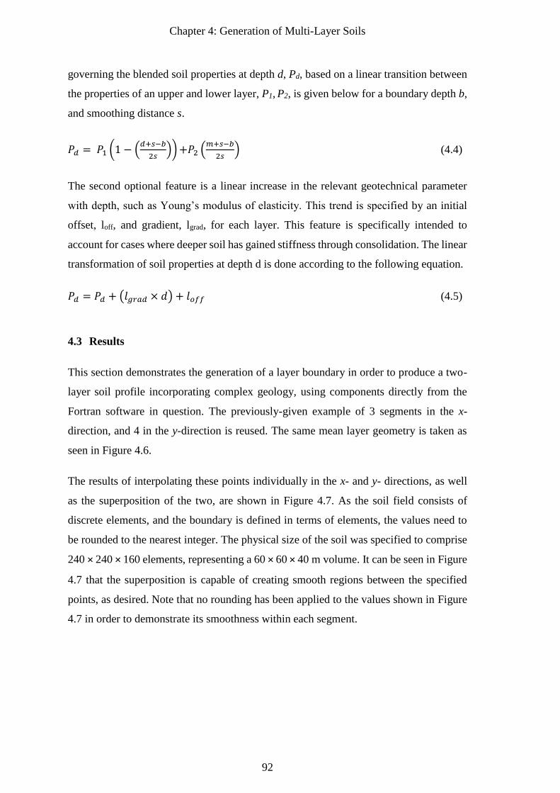
Chapter 4: Generation of Multi-Layer Soils
92
governing the blended soil properties at depth d, Pd, based on a linear transition between
the properties of an upper and lower layer, P1, P2, is given below for a boundary depth b,
and smoothing distance s.
𝑃𝑑 = 𝑃1 (1 − (𝑑+𝑠−𝑏
2𝑠))+𝑃2 (
𝑚+𝑠−𝑏
2𝑠) (4.4)
The second optional feature is a linear increase in the relevant geotechnical parameter
with depth, such as Young’s modulus of elasticity. This trend is specified by an initial
offset, loff, and gradient, lgrad, for each layer. This feature is specifically intended to
account for cases where deeper soil has gained stiffness through consolidation. The linear
transformation of soil properties at depth d is done according to the following equation.
𝑃𝑑 = 𝑃𝑑 + (𝑙𝑔𝑟𝑎𝑑 × 𝑑) + 𝑙𝑜𝑓𝑓 (4.5)
4.3 Results
This section demonstrates the generation of a layer boundary in order to produce a two-
layer soil profile incorporating complex geology, using components directly from the
Fortran software in question. The previously-given example of 3 segments in the x-
direction, and 4 in the y-direction is reused. The same mean layer geometry is taken as
seen in Figure 4.6.
The results of interpolating these points individually in the x- and y- directions, as well
as the superposition of the two, are shown in Figure 4.7. As the soil field consists of
discrete elements, and the boundary is defined in terms of elements, the values need to
be rounded to the nearest integer. The physical size of the soil was specified to comprise
240 × 240 × 160 elements, representing a 60 × 60 × 40 m volume. It can be seen in Figure
4.7 that the superposition is capable of creating smooth regions between the specified
points, as desired. Note that no rounding has been applied to the values shown in Figure
4.7 in order to demonstrate its smoothness within each segment.
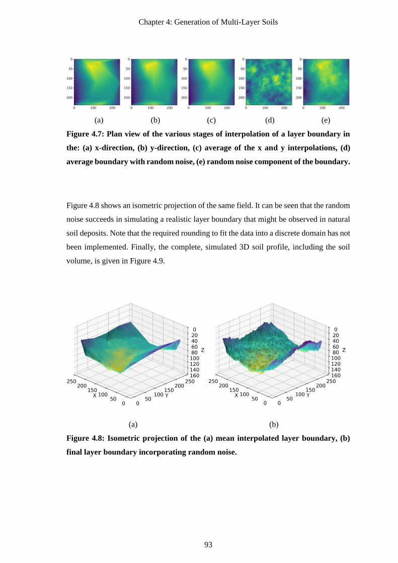
Chapter 4: Generation of Multi-Layer Soils
93
(a) (b) (c) (d) (e)
Figure 4.7: Plan view of the various stages of interpolation of a layer boundary in
the: (a) x-direction, (b) y-direction, (c) average of the x and y interpolations, (d)
average boundary with random noise, (e) random noise component of the boundary.
Figure 4.8 shows an isometric projection of the same field. It can be seen that the random
noise succeeds in simulating a realistic layer boundary that might be observed in natural
soil deposits. Note that the required rounding to fit the data into a discrete domain has not
been implemented. Finally, the complete, simulated 3D soil profile, including the soil
volume, is given in Figure 4.9.
(a) (b)
Figure 4.8: Isometric projection of the (a) mean interpolated layer boundary, (b)
final layer boundary incorporating random noise.
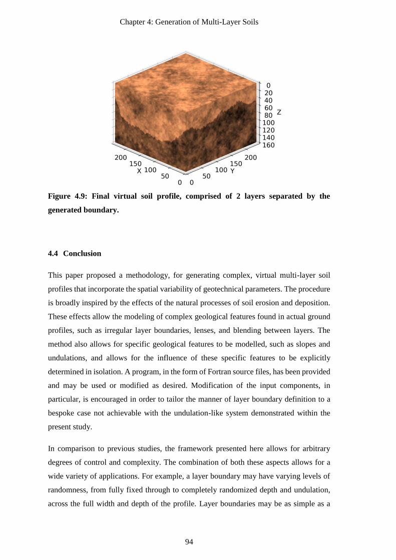
Chapter 4: Generation of Multi-Layer Soils
94
Figure 4.9: Final virtual soil profile, comprised of 2 layers separated by the
generated boundary.
4.4 Conclusion
This paper proposed a methodology, for generating complex, virtual multi-layer soil
profiles that incorporate the spatial variability of geotechnical parameters. The procedure
is broadly inspired by the effects of the natural processes of soil erosion and deposition.
These effects allow the modeling of complex geological features found in actual ground
profiles, such as irregular layer boundaries, lenses, and blending between layers. The
method also allows for specific geological features to be modelled, such as slopes and
undulations, and allows for the influence of these specific features to be explicitly
determined in isolation. A program, in the form of Fortran source files, has been provided
and may be used or modified as desired. Modification of the input components, in
particular, is encouraged in order to tailor the manner of layer boundary definition to a
bespoke case not achievable with the undulation-like system demonstrated within the
present study.
In comparison to previous studies, the framework presented here allows for arbitrary
degrees of control and complexity. The combination of both these aspects allows for a
wide variety of applications. For example, a layer boundary may have varying levels of
randomness, from fully fixed through to completely randomized depth and undulation,
across the full width and depth of the profile. Layer boundaries may be as simple as a
Chapter 4: Generation of Multi-Layer Soils
95
smooth horizontal plane, or as complex as multi-segmented, rough surfaces. It has been
demonstrated that the specification of semi-random conditions allows for the formation
of desirable complex geological features, such as lenses. Within a Monte Carlo
framework, a boundary may be held constant across the full simulation or randomized on
a per-realization basis.
The method is currently being employed to generate complex soil profiles in a Monte
Carlo framework to examine optimal site investigation campaigns. However, the
framework and software can equally be adopted to generate complex, multi-layer profiles
with which to assess many different aspects of geotechnical engineering design and
performance.
4.5 References
Akkaya, A. D., and Vanmarcke, E. H. 2003. Estimation of spatial correlation of soil
parameters based on data from the Texas A&M University NGES. Probabilistic
site characterization at the National Geotechnical Experimentation Sites (eds GA
Fenton and EH Vanmarcke), 29-40.
Ang, A. H.-S. 2007. Probability concepts in engineering : emphasis on applications in
civil & environmental engineering (2nd ed. ed.). Hoboken, N.J: John Wiley &
Sons.
Armstrong, M., Galli, A., Beucher, H., Loc'h, G., Renard, D., Doligez, B., Eschard, R.,
and Geffroy, F. 2011. Plurigaussian simulations in geosciences: Springer Science
& Business Media.
Baecher, G. B., and Christian, J. T. 2005. Reliability and statistics in geotechnical
engineering: John Wiley & Sons.
Bierkens, M. F., and Weerts, H. J. 1994. Application of indicator simulation to modelling
the lithological properties of a complex confining layer. Geoderma, 62(1-3), 265-
284.
Cao, Z., and Wang, Y. 2014. Bayesian model comparison and selection of spatial
correlation functions for soil parameters. Structural Safety, 49, 10-17. doi:
http://dx.doi.org/10.1016/j.strusafe.2013.06.003
Crisp, M. P., Jaksa, M. B., and Kuo, Y. L. 2017. The influence of Site Investigation Scope
on Pile Design in Multi-layered, 2D Variable Ground. In Proceedings of the Geo-
Risk 2017, Denver, Colorado, USA.
Elfeki, A., and Dekking, M. 2001. A Markov chain model for subsurface
characterization: theory and applications. Mathematical geology, 33(5), 569-589.
Fenton, G., and Griffiths, D. 2008a. Risk assessment in geotechnical engineering: Wiley.
Chapter 4: Generation of Multi-Layer Soils
96
Fenton, G., and Vanmarcke, E. H. 1990. Simulation of random fields via local average
subdivision. Journal of Engineering Mechanics, 116(8), 1733-1749.
Fenton, G. A., and Griffiths, D. V. 2008b. Risk assessment in geotechnical engineering:
Wiley.
Fenton, G. A., and Naghibi, M. 2011. Geotechnical resistance factors for ultimate limit
state design of deep foundations in frictional soils. Canadian Geotechnical
Journal, 48(11), 1742-1756.
Fenton, G. A., Paice, G., and Griffiths, D. 1996. Probabilistic analysis of foundation
settlement: Geomechanics Research Center, Colorado School of Mines.
Ferguson, C. 1992. The statistical basis for spatial sampling of contaminated land.
Ground engineering, 25, 34-34.
Filippas, O., Kulhawy, F., and Grigoriu, M. 1988. Reliability-based foundation design
for transmission line structures: Uncertainties in soil property measurement.
Report EL-5507 (3).
Goldsworthy, J. S. 2006. Quantifying the risk of geotechnical site investigations. Ph.D
Thesis, School of Civil, Environmental and Mining Engineering, University of
Adelaide, Adelaide.
Griffiths, D., and Fenton, G. A. 2004. Probabilistic slope stability analysis by finite
elements. Journal of Geotechnical and Geoenvironmental Engineering, 130(5),
507-518.
Halim, I. 1991. Reliability of geotechnical systems considering geological anomaly Ph.D
Thesis, Graduate College, University of Illinois, Urbana–Champaign, USA.
Hoeksema, R. J., and Kitanidis, P. K. 1985. Analysis of the spatial structure of properties
of selected aquifers. Water Resources Research, 21(4), 563-572.
Huber, M., Marconi, F., and Moscatelli, M. 2015. Risk-based characterisation of an urban
building site. Georisk: Assessment and Management of Risk for Engineered
Systems and Geohazards, 9(1), 49-56.
Jaksa, M., Brooker, P., and Kaggwa, W. 1997a. Inaccuracies associated with estimating
random measurement errors. Journal of Geotechnical and Geoenvironmental
Engineering, ASCE, 123(5), 393-401.
Jaksa, M., Brooker, P., and Kaggwa, W. 1997b. Modelling the spatial variability of the
undrained shear strength of clay soils using geostatistics. In Proceedings of the
Proc. of 5th Int. Geostatistics Congress, Wollongong.
Jaksa, M., Goldsworthy, J., Fenton, G., Kaggwa, W., Griffiths, D., Kuo, Y., and Poulos,
H. 2005. Towards reliable and effective site investigations. Géotechnique, 55(2),
109-121.
Chapter 4: Generation of Multi-Layer Soils
97
Jaksa, M. B. 1995. The influence of spatial variability on the geotechnical design
properties of a stiff, overconsolidated clay. Ph.D Thesis, School of Civil,
Environmental and Mining Engineering, University of Adelaide, Adelaide.
Kempen, B., Brus, D., and Stoorvogel, J. 2011. Three-dimensional mapping of soil
organic matter content using soil type–specific depth functions. Geoderma,
162(1-2), 107-123.
Kim, J. H. 2011. Improvement of geotechnical site investigations via statistical analyses
and simulation. Ph.D Thesis, School of Civil & Environmental Engineering,
Georgia Institute of Technology, Atlanta.
Kulatilake, P. H., and Um, J.-G. 2003. Spatial variation of cone tip resistance for the clay
site at Texas A&M University. Geotechnical & Geological Engineering, 21(2),
149-165.
Kulhawy, F. H., Birgisson, B., and Grigoriu, M. 1992. Reliability-based foundation
design for transmission line structures, Electric Power Research Inst., Palo Alto,
CA (United States); Cornell Univ., Ithaca, NY (United States). Geotechnical
Engineering Group.
Kuo, Y. L., Jaksa, M. B., Kaggwa, G. S., Fenton, G. A., Griffiths, D. V., and
Goldsworthy, J. S. 2004. Probabilistic analysis of multi-layered soil effects on
shallow foundation settlement. In Proceedings of the 9th Australia-New Zealand
Conference on Geomechanics, Auckland, NZ.
Lumb, P. 1966. The variability of natural soils. Canadian Geotechnical Journal, 3(2), 74-
97.
Opolot, E., Yu, Y., and Finke, P. 2015. Modeling soil genesis at pedon and landscape
scales: Achievements and problems. Quaternary International, 376, 34-46.
Orchant, C., Kulhawy, F., and Trautmann, C. 1988. Reliability-based foundation design
for transmission line structures: Volume 2, Critical evaluation of in situ test
methods: Final report, Electric Power Research Inst., Palo Alto, CA (USA);
Cornell Univ., Ithaca, NY (USA). Geotechnial Engineering Group.
Phoon, K.-K. 1995. Reliability-based design of foundations for transmission line
structures. Ph.D Thesis, School of Civil and Environmental Engineering, Cornell
University, Ithaca.
Phoon, K.-K., and Kulhawy, F. H. 1999. Evaluation of geotechnical property variability.
Canadian Geotechnical Journal, 36(4), 625-639.
Rajaraman, V. 1997. Computer Programming in FORTRAN 90 and 95: PHI Learning
Pvt. Ltd.
Sarkar, S., Roy, A. K., and Martha, T. R. 2013. Soil depth estimation through soil-
landscape modelling using regression kriging in a Himalayan terrain.
International Journal of Geographical Information Science, 27(12), 2436-2454.
Chapter 4: Generation of Multi-Layer Soils
98
Schlüter, S., Vogel, H.-J., Ippisch, O., Bastian, P., Roth, K., Schelle, H., Durner, W.,
Kasteel, R., and Vanderborght, J. 2012. Virtual soils: Assessment of the effects
of soil structure on the hydraulic behavior of cultivated soils. Vadose Zone
Journal, 11(4).
Skinner, B., and Porter, S. 1987. Physical geology.
Soulie, M., Montes, P., and Silvestri, V. 1990. Modelling spatial variability of soil
parameters. Canadian Geotechnical Journal, 27(5), 617-630.
Spry, M., Kulhawy, F., and Grigoriu, M. 1988. Reliability-based foundation design for
transmission line structures: Geotechnical site characterization strategy. Report
EL-5507 (1).
Vanmarcke, E. 1983. Random Fields: Analysis and Synthesis. London: MIT Press.
Vanwalleghem, T., Poesen, J., McBratney, A., and Deckers, J. 2010. Spatial variability
of soil horizon depth in natural loess-derived soils. Geoderma, 157(1-2), 37-45.
Chapter 5: Two-Layer Analysis
99
5 Chapter 5: Two-Layer Analysis
Paper Title:
Characterising Site Investigation Performance in a
Two Layer Soil Profile

Chapter 5: Two-Layer Analysis
100


Chapter 5: Two-Layer Analysis
103
Abstract
Insufficient or inappropriate soil testing can lead to a range of undesirable consequences,
and yet there is no guideline for optimal investigation. This study analyses the influence
of a two layer, virtual soil profile with an undulating boundary on site investigation
performance. Factors investigated include the method of representing the boundary
within the soil model, the stiffness ratio of the two layers, choice of test type, the pile
length relative to the boundary length, and the number of boreholes and piles. The relative
error contribution from the uncertainty sources of layer geology and soil variability is
also examined. Investigation performance is assessed through Monte Carlo analysis in
terms of total expected project cost, while implicitly incorporating the risk of damage
from poor investigation. It has been shown that the optimal investigation can save in the
order of AUD$ 1.5 million and that 2D soil models can represent 3D soils.
Keywords: pile design, Monte Carlo analysis, optimization, virtual soils, site
investigation
Chapter 5: Two-Layer Analysis
104
5.1 Introduction
Subsurface ground conditions can change drastically from site to site, implying two
considerations. Firstly, one should examine the ground by means of a geotechnical site
investigation to adequately characterise it. Secondly, optimal investigations are site
specific, with the extent dependant on subsurface conditions. However, despite these
points, there is no optimal site investigation guideline relating testing to soil variability.
Rather, investigations are planned by civil engineers through subjective reasoning
(Baecher and Christian 2005), vague or broad rules of thumb (European Standards 2006),
or are otherwise dictated by cost, comprising as little as 0.025–0.03% of the total budget
(National Research Council 1984; Jaksa 2000). It is therefore not surprising that
insufficient investigations regularly occur, resulting in one or more of the following
outcomes: foundation failure (Moh 2004), change orders (Loehr et al. 2015), delays of
up to 33% of the total project duration (Jaksa 2000; Albatal 2013) and; most commonly
but difficult to quantify, over-design (Clayton 2001). In contrast, studies have shown that
there can be considerable financial benefits by conducting investigations beyond the
minimal scope, and that the optimal investigation depends on the nature of the soil
(Goldsworthy 2006; Crisp et al. 2018) (Appendix B). Clearly, there is a need to develop
a site investigation optimization guideline for a range of soil conditions.
The method used to determine site investigation quality is based on a framework
described by Crisp et al. (2019a) (Appendix D) and originally proposed by Jaksa et al.
(2003). The framework is based on the random finite element method (RFEM), which is
a powerful statistical technique that can generate a wide range of soil-related information
(Fenton and Griffiths 1993; Griffiths and Fenton 1993). RFEM involves the use of
random virtual soils combined with finite element analysis within a Monte Carlo
simulation (Fenton and Griffiths 2008). In the context of the present study, RFEM is used
to assess the accuracy of site investigations with regards to a set of given structures and
soil conditions. The wealth of information provided by RFEM allows costs to be assigned
to the soil testing and construction of each investigation. Furthermore, cost penalties are
associated to various degrees of structural failure resulting from inadequate investigation,
and are defined as the cost of repairing the structure to its original condition. By
examining the trade-off between these costs, it is possible to recommend an optimal
investigation strategy corresponding to the lowest expected total project cost.
Chapter 5: Two-Layer Analysis
105
There have been several studies that have examined the influence of site investigation
options on total cost, including Jaksa et al. (2005); (Goldsworthy 2006); Goldsworthy et
al. (2007) in the context of pad footings, and Arsyad (2009); Crisp et al. (2018, 2019b)
(0, 0) with regards to piles. However, the literature almost exclusively focuses on variable
single-layer soil profiles. The exception is Crisp et al. (2017) (Appendix A) which
examined a simplified 2D, 2 layer case without considering costs. This single layer
assumption is generally unrealistic and unconservative, as the uncertainty of layer
boundary locations is expected to contribute considerably to inadequate site investigation
performance, as opposed to the uncertainty of the engineering properties within those
layers. As such, the impact of layer boundary uncertainty on investigation performance
is poorly understood.
As the present study is among the first to examine site investigations in multi-layer soils
in detail, a wide range of factors are analysed for their impact on investigation
performance. These factors include engineering considerations such as the number of
boreholes, the pile embedment depth relative to the pile layer, the selection of soil test
type, and the manner in which the layer boundary is represented within the soil model.
Furthermore, variables related to soil variability are assessed, such as the degree of layer
undulation, the stiffness ratio of the two layers, as well as the magnitude and spatial
distribution of variability within each layer. The conclusions drawn from this endeavour
will serve as the basis for a future site investigation optimization guideline.
5.2 Methodology
5.2.1 Overview
The framework for determining site investigation performance is described by Crisp et
al. (2019a) (Appendix D), and the authors refer readers to that report for verification and
a detailed account of the procedures adopted in the present study. Such verification
includes sensitivity analyses for values of many parameters stated throughout the paper.
For completeness, an overview is given here, with the overall process summarized in
Figure 5.1.
Briefly, site investigation performance, given as total expected project cost, is determined
through the use of Monte Carlo analysis using 8,000 realizations. Within each realization,
a random, variable, two layer virtual soil profile is generated. These profiles consist of a
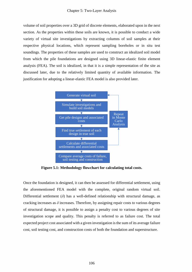
Chapter 5: Two-Layer Analysis
106
volume of soil properties over a 3D grid of discrete elements, elaborated upon in the next
section. As the properties within these soils are known, it is possible to conduct a wide
variety of virtual site investigations by extracting columns of soil samples at their
respective physical locations, which represent sampling boreholes or in situ test
soundings. The properties of these samples are used to construct an idealized soil model
from which the pile foundations are designed using 3D linear-elastic finite element
analysis (FEA). The soil is idealized, in that it is a simple representation of the site as
discussed later, due to the relatively limited quantity of available information. The
justification for adopting a linear-elastic FEA model is also provided later.
Figure 5.1: Methodology flowchart for calculating total costs.
Once the foundation is designed, it can then be assessed for differential settlement, using
the aforementioned FEA model with the complete, original random virtual soil.
Differential settlement (δ) has a well-defined relationship with structural damage, as
cracking increases as δ increases. Therefore, by assigning repair costs to various degrees
of structural damage, it is possible to assign a penalty cost to various degrees of site
investigation scope and quality. This penalty is referred to as failure cost. The total
expected project cost associated with a given investigation is the sum of its average failure
cost, soil testing cost, and construction costs of both the foundation and superstructure.
Generate virtual soil
Simulate investigations and build soil models
Get pile designs and associated costs
Find true settlement of each design in true soil
Compare average costs of failure, soil testing and construction
Repeat in Monte
Carlo Analysis
Calculate differential settlements and associated costs
Chapter 5: Two-Layer Analysis
107
5.2.2 Generation of Virtual Soil Profile
The randomly-generated virtual soil profiles, or random fields, are volumes of soil
properties represented by a 3D grid of discrete elements. The fields are generated by local
average subdivision (LAS) (Fenton and Vanmarcke 1990). This algorithm is commonly
used in geotechnical research, is well-documented, and Fortran open source code is freely
available (Fenton and Griffiths 2008). The authors refer the reader to Crisp et al. (2019d)
(Chapter 4) for a multiple-layer implementation of the algorithm, with associated
descriptions of its use. Due to space constraints and the abundance of available resources,
LAS will not be described here in detail.
In practice, LAS produces fields of soil properties with a desired size and spatial
variability, where the latter is statistically described by three parameters supplied as
inputs; the mean, standard deviation, and the scale of fluctuation (SOF) (Vanmarcke
1983). The SOF is analogous to the range parameter in geostatistics (Jaksa et al. 1997),
and is defined as the distance over which soil properties exhibit a degree of similarity. In
other words, high SOF values correspond to large pockets of similar material.
Mathematically, the SOF is defined by autocorrelation using an exponential Markov
model (Fenton and Vanmarcke 1990). Isotropic soils, where the SOF is constant in all
directions, are considered in this analysis, as they are the worst case when compared to
anisotropic soils, which have a higher SOF in the horizontal direction (Naghibi et al.
2014b). Within this study, the standard deviation is normalised by the mean to produce
the coefficient of variation (COV), which is more useful as the results can be applied to
any mean parameter value.
As linear-elastic FEA is used, two soil properties are required. This includes Young’s
modulus (E), which is randomly generated by LAS, and Poisson’s ratio (v), which is
constant at 0.3. The deterministic treatment of v is due to this parameter’s spatial
variability having a relatively insignificant effect on settlement (Paice et al. 1996;
Naghibi et al. 2014a). The soil properties themselves are generated according to the
lognormal distribution, which has been found to be appropriate for geotechnical
engineering probabilistic studies (Fenton and Griffiths 1993; Griffiths and Fenton 1993),
and ensures that stiffness values are strictly non-negative.
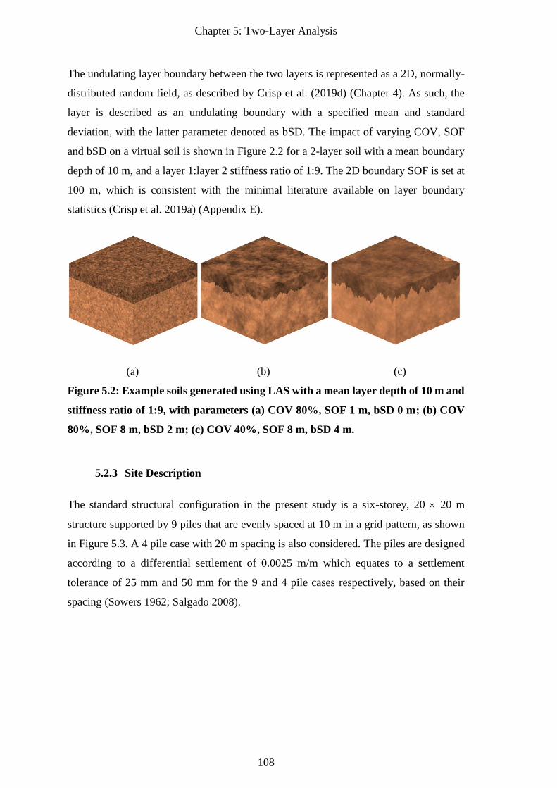
Chapter 5: Two-Layer Analysis
108
The undulating layer boundary between the two layers is represented as a 2D, normally-
distributed random field, as described by Crisp et al. (2019d) (Chapter 4). As such, the
layer is described as an undulating boundary with a specified mean and standard
deviation, with the latter parameter denoted as bSD. The impact of varying COV, SOF
and bSD on a virtual soil is shown in Figure 2.2 for a 2-layer soil with a mean boundary
depth of 10 m, and a layer 1:layer 2 stiffness ratio of 1:9. The 2D boundary SOF is set at
100 m, which is consistent with the minimal literature available on layer boundary
statistics (Crisp et al. 2019a) (Appendix E).
(a) (b) (c)
Figure 5.2: Example soils generated using LAS with a mean layer depth of 10 m and
stiffness ratio of 1:9, with parameters (a) COV 80%, SOF 1 m, bSD 0 m; (b) COV
80%, SOF 8 m, bSD 2 m; (c) COV 40%, SOF 8 m, bSD 4 m.
5.2.3 Site Description
The standard structural configuration in the present study is a six-storey, 20 20 m
structure supported by 9 piles that are evenly spaced at 10 m in a grid pattern, as shown
in Figure 5.3. A 4 pile case with 20 m spacing is also considered. The piles are designed
according to a differential settlement of 0.0025 m/m which equates to a settlement
tolerance of 25 mm and 50 mm for the 9 and 4 pile cases respectively, based on their
spacing (Sowers 1962; Salgado 2008).
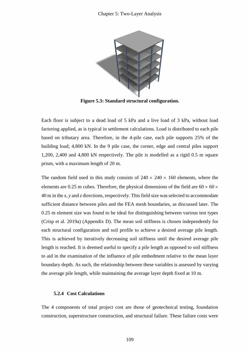
Chapter 5: Two-Layer Analysis
109
Figure 5.3: Standard structural configuration.
Each floor is subject to a dead load of 5 kPa and a live load of 3 kPa, without load
factoring applied, as is typical in settlement calculations. Load is distributed to each pile
based on tributary area. Therefore, in the 4-pile case, each pile supports 25% of the
building load; 4,800 kN. In the 9 pile case, the corner, edge and central piles support
1,200, 2,400 and 4,800 kN respectively. The pile is modelled as a rigid 0.5 m square
prism, with a maximum length of 20 m.
The random field used in this study consists of 240 240 160 elements, where the
elements are 0.25 m cubes. Therefore, the physical dimensions of the field are 60 60
40 m in the x, y and z directions, respectively. This field size was selected to accommodate
sufficient distance between piles and the FEA mesh boundaries, as discussed later. The
0.25 m element size was found to be ideal for distinguishing between various test types
(Crisp et al. 2019a) (Appendix D). The mean soil stiffness is chosen independently for
each structural configuration and soil profile to achieve a desired average pile length.
This is achieved by iteratively decreasing soil stiffness until the desired average pile
length is reached. It is deemed useful to specify a pile length as opposed to soil stiffness
to aid in the examination of the influence of pile embedment relative to the mean layer
boundary depth. As such, the relationship between these variables is assessed by varying
the average pile length, while maintaining the average layer depth fixed at 10 m.
5.2.4 Cost Calculations
The 4 components of total project cost are those of geotechnical testing, foundation
construction, superstructure construction, and structural failure. These failure costs were
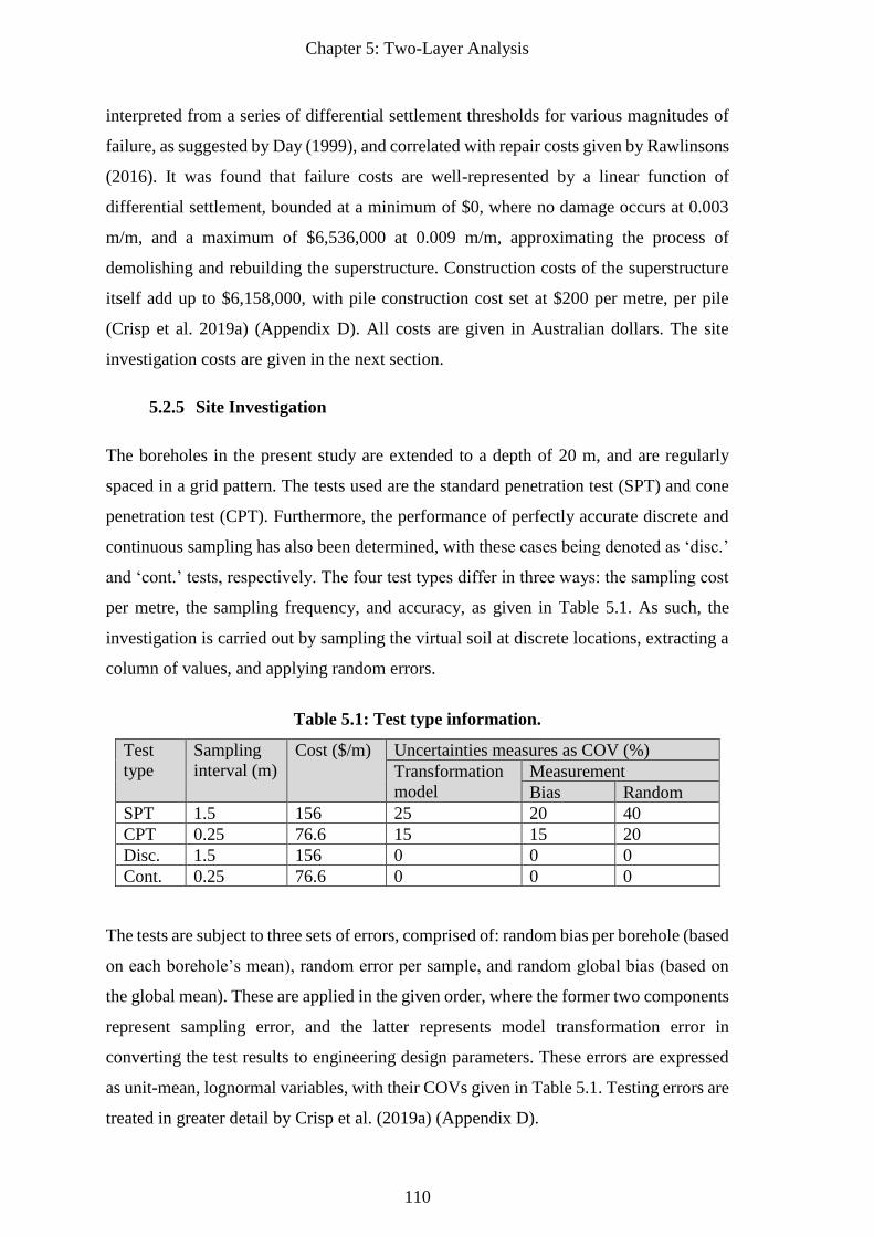
Chapter 5: Two-Layer Analysis
110
interpreted from a series of differential settlement thresholds for various magnitudes of
failure, as suggested by Day (1999), and correlated with repair costs given by Rawlinsons
(2016). It was found that failure costs are well-represented by a linear function of
differential settlement, bounded at a minimum of $0, where no damage occurs at 0.003
m/m, and a maximum of $6,536,000 at 0.009 m/m, approximating the process of
demolishing and rebuilding the superstructure. Construction costs of the superstructure
itself add up to $6,158,000, with pile construction cost set at $200 per metre, per pile
(Crisp et al. 2019a) (Appendix D). All costs are given in Australian dollars. The site
investigation costs are given in the next section.
5.2.5 Site Investigation
The boreholes in the present study are extended to a depth of 20 m, and are regularly
spaced in a grid pattern. The tests used are the standard penetration test (SPT) and cone
penetration test (CPT). Furthermore, the performance of perfectly accurate discrete and
continuous sampling has also been determined, with these cases being denoted as ‘disc.’
and ‘cont.’ tests, respectively. The four test types differ in three ways: the sampling cost
per metre, the sampling frequency, and accuracy, as given in Table 5.1. As such, the
investigation is carried out by sampling the virtual soil at discrete locations, extracting a
column of values, and applying random errors.
Table 5.1: Test type information.
Test
type
Sampling
interval (m)
Cost ($/m) Uncertainties measures as COV (%)
Transformation
model
Measurement
Bias Random
SPT 1.5 156 25 20 40
CPT 0.25 76.6 15 15 20
Disc. 1.5 156 0 0 0
Cont. 0.25 76.6 0 0 0
The tests are subject to three sets of errors, comprised of: random bias per borehole (based
on each borehole’s mean), random error per sample, and random global bias (based on
the global mean). These are applied in the given order, where the former two components
represent sampling error, and the latter represents model transformation error in
converting the test results to engineering design parameters. These errors are expressed
as unit-mean, lognormal variables, with their COVs given in Table 5.1. Testing errors are
treated in greater detail by Crisp et al. (2019a) (Appendix D).
Chapter 5: Two-Layer Analysis
111
There are two main steps in constructing a soil model from site investigation results. First
is interpreting the aggregate of soil testing data from each layer into a single set of
representative material properties. The interpretation used in the present study is the
method of taking one geometric standard deviation (ln) below the geometric mean (ln),
which consistently produced the optimal results. The reduced representation of Young’s
modulus (ESD) from n soil samples in a given layer is defined as follows, where x is an
arbitrary sample:
𝜇𝑙𝑛 = exp (1
𝑛∑ 𝑙𝑛(𝑥𝑖)𝑛𝑖=1 ) (5.1)
𝜎𝑙𝑛 = exp(√1
𝑛∑ 𝑙𝑛 (
𝑥𝑖
𝜇𝑙𝑛 )2
𝑛𝑖=1 ) (5.2)
𝐸𝑆𝐷 =𝜇𝑙𝑛
𝜎𝑙𝑛 (5.3)
The second consideration is the manner by which layer boundaries are represented in the
soil models. Historically, practicing engineers have represented these boundaries as an
idealized horizontal interface, at a depth equal to the average of the layer depths
encountered by each borehole. More recently, with the increases in computing power and
the improved usability and feature sets of FEM software such as Plaxis, it is becoming
increasingly common to linearly interpolate layer boundaries between boreholes (Plaxis
2018). Both the horizontal average (H.A.) and full interpolation (F.I.) layer
representations are analysed to determine if there is a notable advantage with the latter,
more sophisticated technique.
It should be noted that, in the context of this research, analysis of a horizontal boundary,
such as in the H.A. case, requires significantly less time to process. This is because, if the
soil properties within each layer are uniform, as is the case with the soil model, and if the
layer boundary is perfectly horizontal, the 3D FEM mesh can be replaced with a 2D
axisymmetric mesh without loss of accuracy (Crisp et al. 2019a) (Appendix D). As such,
a third interpretation is considered, the weighted horizontal (W.H.) case, which for a
given pile, uses a constant layer depth taken as a weighted average of the fully-
interpolated layer. The weights are calculated using the inverse square of the distance
between the pile and a given depth value. Essentially, this W.H. method reflects the
Chapter 5: Two-Layer Analysis
112
behaviour that soil that is closer to a pile has more impact on its performance than soil
that is further away (Crisp et al. 2019b) (Appendix C).
The layer boundary depths, as encountered by the boreholes, are known exactly. Depth
uncertainty, due to soil material ambiguity, is not incorporated in the analysis. As such,
if the soil was consistently sampled with a continuous test type, then the layer would be
recreated exactly in the 3D soil model. In the case of discrete tests, such as the SPT, when
the borehole encounters the 2nd layer, the layer depth is interpreted as being mid-way
between the first sample taken from that layer, and the previous, higher-up sample. In
other words, when a change of layer is detected, it is assumed to be at the average distance
between samples where the change occurred. As such, the maximum deviation the true
layer can have from the interpreted depth is 0.75 m.
5.2.6 Settlement Model
The 3D and 2D linear-elastic settlement models used were adapted from Programs 5.6
and 5.1 by Smith et al. (2014) respectively. The respective element types are hexahedral
and quadrilateral with a length of 0.25 m, increasing in width with distance from the pile
as a performance measure (Crisp et al. 2019a) (Appendix D). The mesh boundaries are a
minimum of 20 m from the pile in order to minimise boundary effects.
A linear-elastic FEA model is used, as it is currently considered the most practical model
in the context of this research, while retaining an appropriate degree of accuracy (Crisp
et al. 2019a) (Appendix D). As millions of FEA simulations are required, it is not feasible,
from a computational time perspective, to use more sophisticated models, such as elastic-
plastic, at this time. Goldsworthy (2006) compared a range of pad footing settlement
models and found there to be little difference in terms of relative site investigation
performance. Indeed, Naghibi et al. (2014b) stated that the settlement model only changes
the pile design, not the probability of failure, and that the Smith et al. (2014) models are
the best available to capture the effects of soil spatial variability in the context of this
research. In other words, since the same settlement model is being compared, with both
the true soil and the soil model, any settlement model inaccuracy largely cancels itself
out, leaving soil variability as the sole source of error. Furthermore, Leung et al. (2010)
investigated the choice of linear versus non-linear models with respect to the settlement
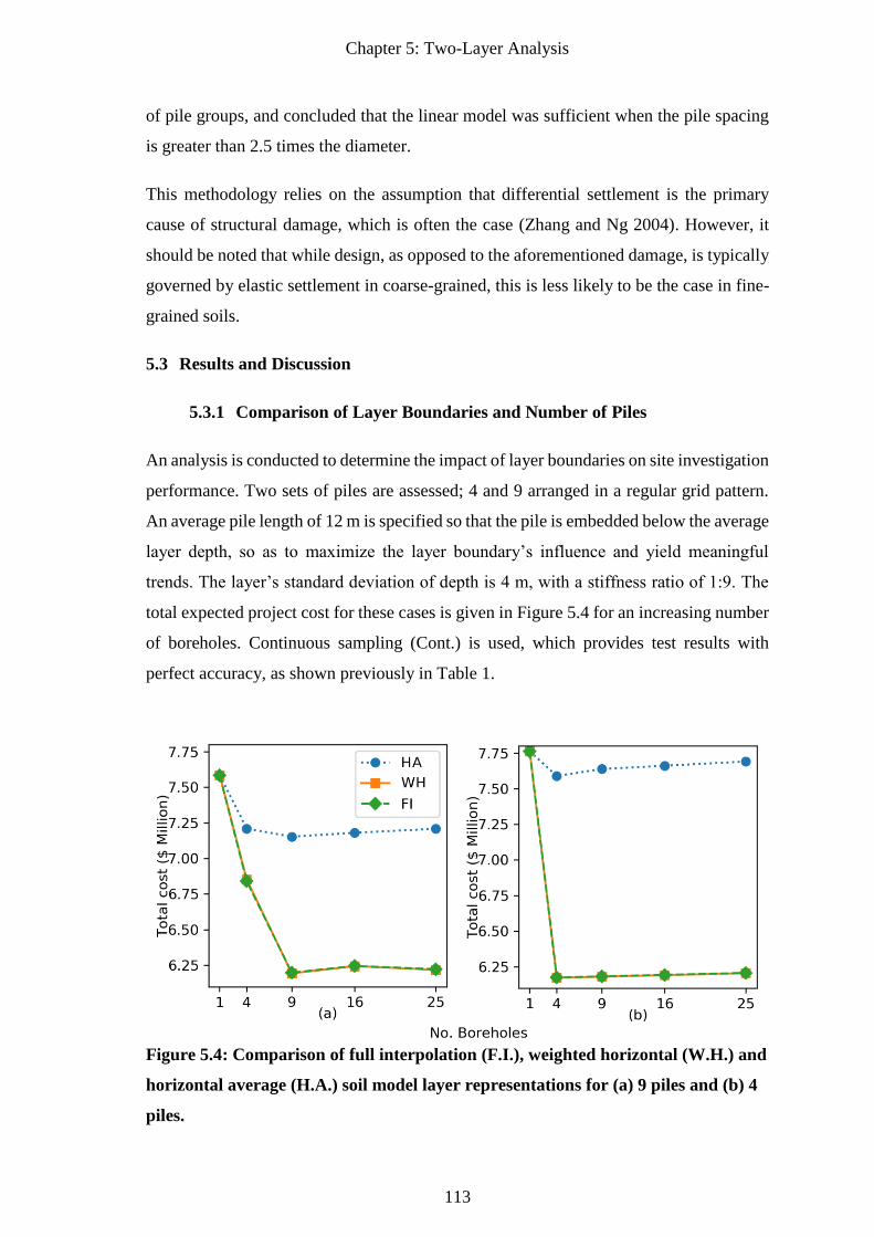
Chapter 5: Two-Layer Analysis
113
of pile groups, and concluded that the linear model was sufficient when the pile spacing
is greater than 2.5 times the diameter.
This methodology relies on the assumption that differential settlement is the primary
cause of structural damage, which is often the case (Zhang and Ng 2004). However, it
should be noted that while design, as opposed to the aforementioned damage, is typically
governed by elastic settlement in coarse-grained, this is less likely to be the case in fine-
grained soils.
5.3 Results and Discussion
5.3.1 Comparison of Layer Boundaries and Number of Piles
An analysis is conducted to determine the impact of layer boundaries on site investigation
performance. Two sets of piles are assessed; 4 and 9 arranged in a regular grid pattern.
An average pile length of 12 m is specified so that the pile is embedded below the average
layer depth, so as to maximize the layer boundary’s influence and yield meaningful
trends. The layer’s standard deviation of depth is 4 m, with a stiffness ratio of 1:9. The
total expected project cost for these cases is given in Figure 5.4 for an increasing number
of boreholes. Continuous sampling (Cont.) is used, which provides test results with
perfect accuracy, as shown previously in Table 1.
Figure 5.4: Comparison of full interpolation (F.I.), weighted horizontal (W.H.) and
horizontal average (H.A.) soil model layer representations for (a) 9 piles and (b) 4
piles.
Chapter 5: Two-Layer Analysis
114
Upon inspection of Figure 5.4, it is clear that in all cases the optimal investigation is one
where there is a borehole located at each pile. This conclusion applies to both 4 and 9
piles, which require 4 and 9 boreholes respectively, and applies across the layer
generation methods. This is because, as mentioned previously, soil that is in close
proximity to a pile has the greatest impact on its performance. Therefore, if the layer
depths at each pile are known, there is little benefit in increasing layer accuracy
elsewhere, and so additional boreholes do not provide notable improvement. The
recommendation of placing boreholes specifically at the pile centres is reinforced by the
case of 9 piles using the F.I. method. Here, 16 boreholes provide a notably higher failure
cost when compared with 9 boreholes, despite providing additional boundary
information. However, the majority of the 16 boreholes do not coincide with piles, and
the boundary is interpolated at the pile locations which results in errors, and an increased
probability of failure.
Comparing the H.A. and F.I. methods, the latter provides significantly better site
investigation performance, saving roughly $1.5 million and $1 million in the cases of 4
and 9 piles respectively. This is because with the F.I. method, adding additional boreholes
to an existing set always results in increased layer accuracy. However, in the case of the
H.A. method, while averaging the depths encountered at each pile improves the method’s
performance as a whole, it reduces the piles’ individual accuracy. When additional
sampling away from the piles is undertaken, as in the case of 16 and 25 boreholes, the
failure cost increases due to this incorporation of insignificant data.
Comparing the W.H. and F.I. methods, which should theoretically be near-identical, there
is indeed a negligible discrepancy between the cost curves seen in Figure 5.4. Upon visual
inspection, the curves appear to overlap almost exactly. Given that the W.H. method is
very accurate with respect to full interpolation, and that it is two orders of magnitude
faster to compute, the W.H. method is used for the remaining analyses in the present
paper.
Lastly, comparing the case of 4 and 9 piles directly, the 9-pile foundation has significantly
better performance in terms of total cost. This is because, while the average pile length is
identical in both cases, the individual bases of the piles are offset from the boundary depth
of 10 m due to the variation in applied loads. By comparison, each pile is subject to the
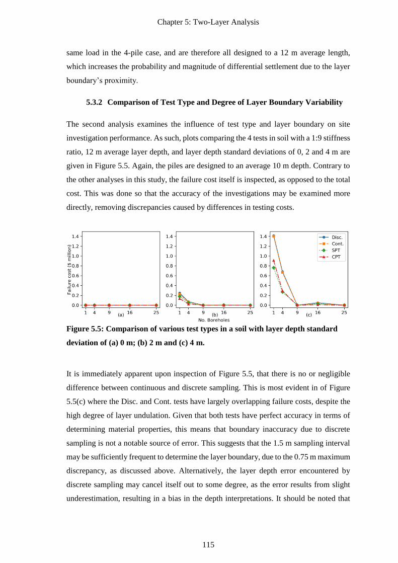
Chapter 5: Two-Layer Analysis
115
same load in the 4-pile case, and are therefore all designed to a 12 m average length,
which increases the probability and magnitude of differential settlement due to the layer
boundary’s proximity.
5.3.2 Comparison of Test Type and Degree of Layer Boundary Variability
The second analysis examines the influence of test type and layer boundary on site
investigation performance. As such, plots comparing the 4 tests in soil with a 1:9 stiffness
ratio, 12 m average layer depth, and layer depth standard deviations of 0, 2 and 4 m are
given in Figure 5.5. Again, the piles are designed to an average 10 m depth. Contrary to
the other analyses in this study, the failure cost itself is inspected, as opposed to the total
cost. This was done so that the accuracy of the investigations may be examined more
directly, removing discrepancies caused by differences in testing costs.
Figure 5.5: Comparison of various test types in a soil with layer depth standard
deviation of (a) 0 m; (b) 2 m and (c) 4 m.
It is immediately apparent upon inspection of Figure 5.5, that there is no or negligible
difference between continuous and discrete sampling. This is most evident in of Figure
5.5(c) where the Disc. and Cont. tests have largely overlapping failure costs, despite the
high degree of layer undulation. Given that both tests have perfect accuracy in terms of
determining material properties, this means that boundary inaccuracy due to discrete
sampling is not a notable source of error. This suggests that the 1.5 m sampling interval
may be sufficiently frequent to determine the layer boundary, due to the 0.75 m maximum
discrepancy, as discussed above. Alternatively, the layer depth error encountered by
discrete sampling may cancel itself out to some degree, as the error results from slight
underestimation, resulting in a bias in the depth interpretations. It should be noted that
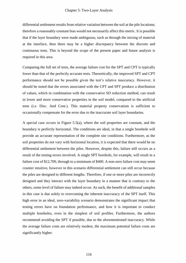
Chapter 5: Two-Layer Analysis
116
differential settlement results from relative variation between the soil at the pile locations;
therefore a reasonably constant bias would not necessarily affect this metric. It is possible
that if the layer boundary were made ambiguous, such as through the mixing of material
at the interface, then there may be a higher discrepancy between the discrete and
continuous tests. This is beyond the scope of the present paper and future analysis is
required in this area.
Comparing the full set of tests, the average failure cost for the SPT and CPT is typically
lower than that of the perfectly accurate tests. Theoretically, the improved SPT and CPT
performance should not be possible given the test’s relative inaccuracy. However, it
should be noted that the errors associated with the CPT and SPT produce a distribution
of values, which in combination with the conservative SD reduction method, can result
in lower and more conservative properties in the soil model, compared to the artificial
tests (i.e. Disc. And Cont.). This material property conservatism is sufficient to
occasionally compensate for the error due to the inaccurate soil layer boundaries.
A special case occurs in Figure 5.5(a), where the soil properties are constant, and the
boundary is perfectly horizontal. The conditions are ideal, in that a single borehole will
provide an accurate representation of the complete site conditions. Furthermore, as the
soil properties do not vary with horizontal location, it is expected that there would be no
differential settlement between the piles. However, despite this, failure still occurs as a
result of the testing errors involved. A single SPT borehole, for example, will result in a
failure cost of $12,700, through to a minimum of $400. A non-zero failure cost may seem
counter intuitive, however in this scenario differential settlement can still occur because
the piles are designed to different lengths. Therefore, if one or more piles are incorrectly
designed and they interact with the layer boundary in a manner that is contrary to the
others, some level of failure may indeed occur. As such, the benefit of additional samples
in this case is due solely to overcoming the inherent inaccuracy of the SPT itself. This
high error in an ideal, zero-variability scenario demonstrates the significant impact that
testing errors have on foundation performance, and how it is important to conduct
multiple boreholes, even in the simplest of soil profiles. Furthermore, the authors
recommend avoiding the SPT if possible, due to the aforementioned inaccuracy. While
the average failure costs are relatively modest, the maximum potential failure costs are
significantly higher.
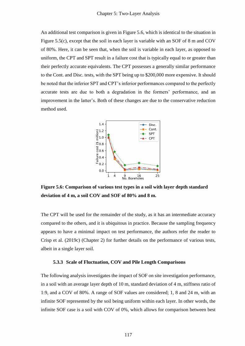
Chapter 5: Two-Layer Analysis
117
An additional test comparison is given in Figure 5.6, which is identical to the situation in
Figure 5.5(c), except that the soil in each layer is variable with an SOF of 8 m and COV
of 80%. Here, it can be seen that, when the soil is variable in each layer, as opposed to
uniform, the CPT and SPT result in a failure cost that is typically equal to or greater than
their perfectly accurate equivalents. The CPT possesses a generally similar performance
to the Cont. and Disc. tests, with the SPT being up to $200,000 more expensive. It should
be noted that the inferior SPT and CPT’s inferior performances compared to the perfectly
accurate tests are due to both a degradation in the formers’ performance, and an
improvement in the latter’s. Both of these changes are due to the conservative reduction
method used.
Figure 5.6: Comparison of various test types in a soil with layer depth standard
deviation of 4 m, a soil COV and SOF of 80% and 8 m.
The CPT will be used for the remainder of the study, as it has an intermediate accuracy
compared to the others, and it is ubiquitous in practice. Because the sampling frequency
appears to have a minimal impact on test performance, the authors refer the reader to
Crisp et al. (2019c) (Chapter 2) for further details on the performance of various tests,
albeit in a single layer soil.
5.3.3 Scale of Fluctuation, COV and Pile Length Comparisons
The following analysis investigates the impact of SOF on site investigation performance,
in a soil with an average layer depth of 10 m, standard deviation of 4 m, stiffness ratio of
1:9, and a COV of 80%. A range of SOF values are considered; 1, 8 and 24 m, with an
infinite SOF represented by the soil being uniform within each layer. In other words, the
infinite SOF case is a soil with COV of 0%, which allows for comparison between best
Chapter 5: Two-Layer Analysis
118
and worst case COV conditions. The results are given in Figure 5.7 for average pile
lengths of 5, 10 and 15 m.
It is immediately obvious in Figure 5.7 that the more intermediate SOFs of 8 m and 24 m
have considerably higher failure costs than the others. This is because of the presence of
moderately-sized pockets of distinct soil properties that are detrimental to both site
investigation performance, and differential settlement of piles. Of the cases examined,
the 24 m SOF appears to be the worst case, as it has a consistently higher failure cost of
up to $250,000 over the 8 m case, and has a nominally better relative cost saving of
drilling 9 boreholes over one. This result is contrary to previous studies which suggest
the worst case SOF of a similar order of magnitude to the centre-to-centre pile spacing
(Fenton and Griffiths 2005; Goldsworthy 2006; Crisp et al. 2019c) (Chapter 2). The
discrepancy is likely due to the higher SOF providing a stronger distinction between the
two layers, as a high COV increases the overlap of soil properties between the two layers,
therefore resulting in them being more similar overall.
Figure 5.7: Comparison of scales of fluctuation for an average pile length of (a) 5
m; (b) 10 m and (c) 15 m.
An important observation is that three distinct categories of SOF can be defined based on
the overall trend of the cost curves seen in Figure 5.7; low, intermediate, and infinite. The
cost trend of low (1 m) and infinite SOFs are relatively unique. For the more intermediate
SOFs, such as 8 m and 24 m, however, the results are quite similar, showing the same
overall trend within each pile length case. Since this framework optimises investigations
according to relative performance, it is the cost trend, as opposed to the absolute total
cost, that is important. Therefore, a wide range of SOF values can be represented by
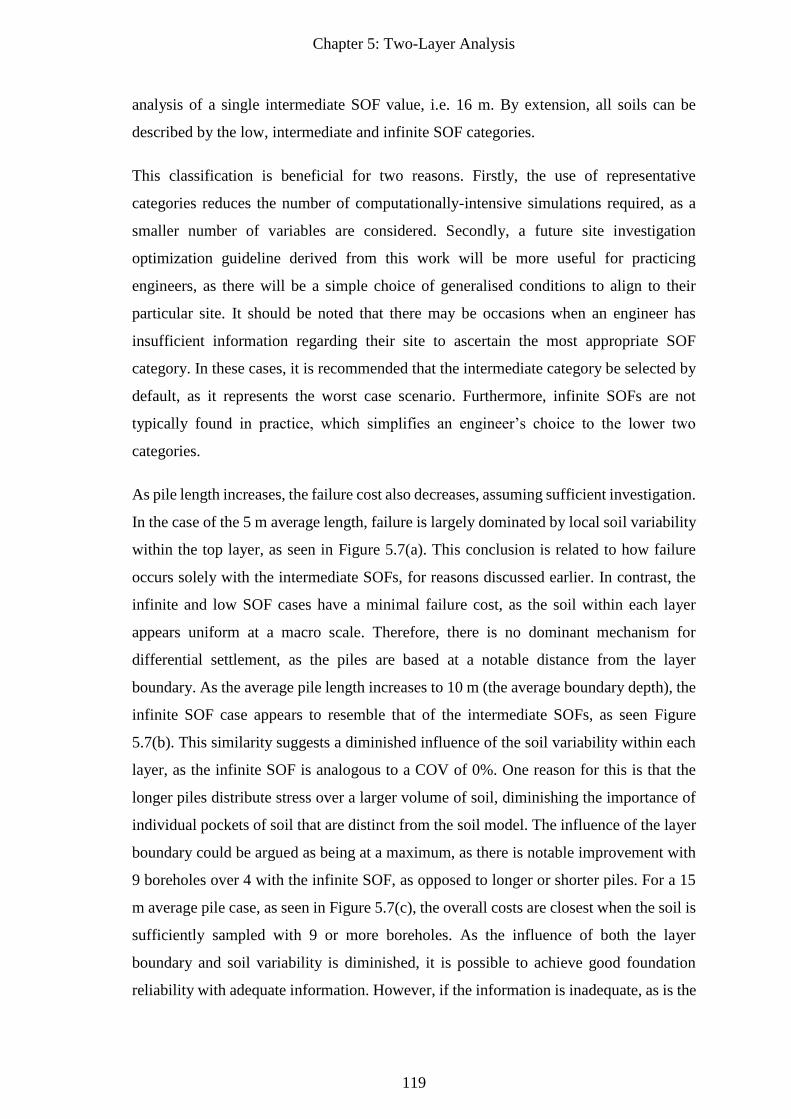
Chapter 5: Two-Layer Analysis
119
analysis of a single intermediate SOF value, i.e. 16 m. By extension, all soils can be
described by the low, intermediate and infinite SOF categories.
This classification is beneficial for two reasons. Firstly, the use of representative
categories reduces the number of computationally-intensive simulations required, as a
smaller number of variables are considered. Secondly, a future site investigation
optimization guideline derived from this work will be more useful for practicing
engineers, as there will be a simple choice of generalised conditions to align to their
particular site. It should be noted that there may be occasions when an engineer has
insufficient information regarding their site to ascertain the most appropriate SOF
category. In these cases, it is recommended that the intermediate category be selected by
default, as it represents the worst case scenario. Furthermore, infinite SOFs are not
typically found in practice, which simplifies an engineer’s choice to the lower two
categories.
As pile length increases, the failure cost also decreases, assuming sufficient investigation.
In the case of the 5 m average length, failure is largely dominated by local soil variability
within the top layer, as seen in Figure 5.7(a). This conclusion is related to how failure
occurs solely with the intermediate SOFs, for reasons discussed earlier. In contrast, the
infinite and low SOF cases have a minimal failure cost, as the soil within each layer
appears uniform at a macro scale. Therefore, there is no dominant mechanism for
differential settlement, as the piles are based at a notable distance from the layer
boundary. As the average pile length increases to 10 m (the average boundary depth), the
infinite SOF case appears to resemble that of the intermediate SOFs, as seen Figure
5.7(b). This similarity suggests a diminished influence of the soil variability within each
layer, as the infinite SOF is analogous to a COV of 0%. One reason for this is that the
longer piles distribute stress over a larger volume of soil, diminishing the importance of
individual pockets of soil that are distinct from the soil model. The influence of the layer
boundary could be argued as being at a maximum, as there is notable improvement with
9 boreholes over 4 with the infinite SOF, as opposed to longer or shorter piles. For a 15
m average pile case, as seen in Figure 5.7(c), the overall costs are closest when the soil is
sufficiently sampled with 9 or more boreholes. As the influence of both the layer
boundary and soil variability is diminished, it is possible to achieve good foundation
reliability with adequate information. However, if the information is inadequate, as is the
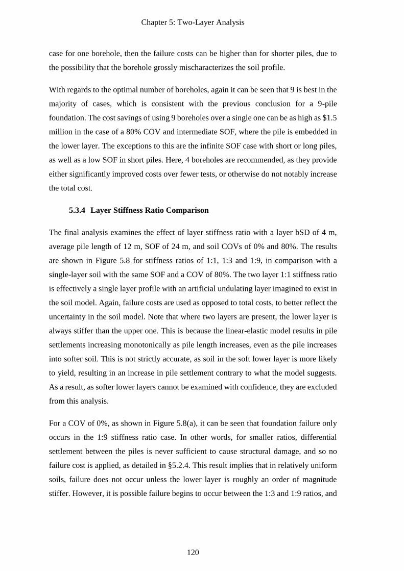
Chapter 5: Two-Layer Analysis
120
case for one borehole, then the failure costs can be higher than for shorter piles, due to
the possibility that the borehole grossly mischaracterizes the soil profile.
With regards to the optimal number of boreholes, again it can be seen that 9 is best in the
majority of cases, which is consistent with the previous conclusion for a 9-pile
foundation. The cost savings of using 9 boreholes over a single one can be as high as $1.5
million in the case of a 80% COV and intermediate SOF, where the pile is embedded in
the lower layer. The exceptions to this are the infinite SOF case with short or long piles,
as well as a low SOF in short piles. Here, 4 boreholes are recommended, as they provide
either significantly improved costs over fewer tests, or otherwise do not notably increase
the total cost.
5.3.4 Layer Stiffness Ratio Comparison
The final analysis examines the effect of layer stiffness ratio with a layer bSD of 4 m,
average pile length of 12 m, SOF of 24 m, and soil COVs of 0% and 80%. The results
are shown in Figure 5.8 for stiffness ratios of 1:1, 1:3 and 1:9, in comparison with a
single-layer soil with the same SOF and a COV of 80%. The two layer 1:1 stiffness ratio
is effectively a single layer profile with an artificial undulating layer imagined to exist in
the soil model. Again, failure costs are used as opposed to total costs, to better reflect the
uncertainty in the soil model. Note that where two layers are present, the lower layer is
always stiffer than the upper one. This is because the linear-elastic model results in pile
settlements increasing monotonically as pile length increases, even as the pile increases
into softer soil. This is not strictly accurate, as soil in the soft lower layer is more likely
to yield, resulting in an increase in pile settlement contrary to what the model suggests.
As a result, as softer lower layers cannot be examined with confidence, they are excluded
from this analysis.
For a COV of 0%, as shown in Figure 5.8(a), it can be seen that foundation failure only
occurs in the 1:9 stiffness ratio case. In other words, for smaller ratios, differential
settlement between the piles is never sufficient to cause structural damage, and so no
failure cost is applied, as detailed in §5.2.4. This result implies that in relatively uniform
soils, failure does not occur unless the lower layer is roughly an order of magnitude
stiffer. However, it is possible failure begins to occur between the 1:3 and 1:9 ratios, and
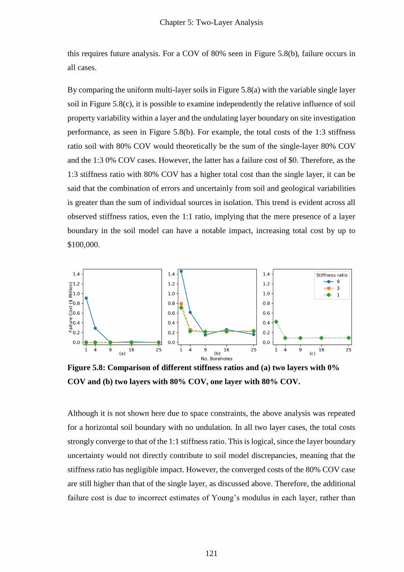
Chapter 5: Two-Layer Analysis
121
this requires future analysis. For a COV of 80% seen in Figure 5.8(b), failure occurs in
all cases.
By comparing the uniform multi-layer soils in Figure 5.8(a) with the variable single layer
soil in Figure 5.8(c), it is possible to examine independently the relative influence of soil
property variability within a layer and the undulating layer boundary on site investigation
performance, as seen in Figure 5.8(b). For example, the total costs of the 1:3 stiffness
ratio soil with 80% COV would theoretically be the sum of the single-layer 80% COV
and the 1:3 0% COV cases. However, the latter has a failure cost of $0. Therefore, as the
1:3 stiffness ratio with 80% COV has a higher total cost than the single layer, it can be
said that the combination of errors and uncertainly from soil and geological variabilities
is greater than the sum of individual sources in isolation. This trend is evident across all
observed stiffness ratios, even the 1:1 ratio, implying that the mere presence of a layer
boundary in the soil model can have a notable impact, increasing total cost by up to
$100,000.
Figure 5.8: Comparison of different stiffness ratios and (a) two layers with 0%
COV and (b) two layers with 80% COV, one layer with 80% COV.
Although it is not shown here due to space constraints, the above analysis was repeated
for a horizontal soil boundary with no undulation. In all two layer cases, the total costs
strongly converge to that of the 1:1 stiffness ratio. This is logical, since the layer boundary
uncertainty would not directly contribute to soil model discrepancies, meaning that the
stiffness ratio has negligible impact. However, the converged costs of the 80% COV case
are still higher than that of the single layer, as discussed above. Therefore, the additional
failure cost is due to incorrect estimates of Young’s modulus in each layer, rather than
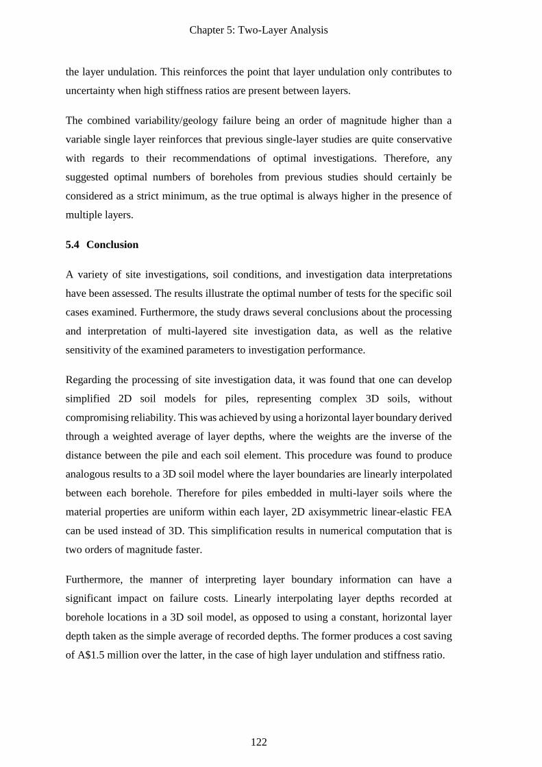
Chapter 5: Two-Layer Analysis
122
the layer undulation. This reinforces the point that layer undulation only contributes to
uncertainty when high stiffness ratios are present between layers.
The combined variability/geology failure being an order of magnitude higher than a
variable single layer reinforces that previous single-layer studies are quite conservative
with regards to their recommendations of optimal investigations. Therefore, any
suggested optimal numbers of boreholes from previous studies should certainly be
considered as a strict minimum, as the true optimal is always higher in the presence of
multiple layers.
5.4 Conclusion
A variety of site investigations, soil conditions, and investigation data interpretations
have been assessed. The results illustrate the optimal number of tests for the specific soil
cases examined. Furthermore, the study draws several conclusions about the processing
and interpretation of multi-layered site investigation data, as well as the relative
sensitivity of the examined parameters to investigation performance.
Regarding the processing of site investigation data, it was found that one can develop
simplified 2D soil models for piles, representing complex 3D soils, without
compromising reliability. This was achieved by using a horizontal layer boundary derived
through a weighted average of layer depths, where the weights are the inverse of the
distance between the pile and each soil element. This procedure was found to produce
analogous results to a 3D soil model where the layer boundaries are linearly interpolated
between each borehole. Therefore for piles embedded in multi-layer soils where the
material properties are uniform within each layer, 2D axisymmetric linear-elastic FEA
can be used instead of 3D. This simplification results in numerical computation that is
two orders of magnitude faster.
Furthermore, the manner of interpreting layer boundary information can have a
significant impact on failure costs. Linearly interpolating layer depths recorded at
borehole locations in a 3D soil model, as opposed to using a constant, horizontal layer
depth taken as the simple average of recorded depths. The former produces a cost saving
of A$1.5 million over the latter, in the case of high layer undulation and stiffness ratio.
Chapter 5: Two-Layer Analysis
123
The optimal number of boreholes was observed to be affected by many factors,
particularly the number of piles, the stiffness ratio between layers, and the degree of layer
undulation. To a lesser extent, the pile length, the soil’s coefficient of variation and scale
of fluctuation also demonstrated some influence. The interaction between these variables,
in terms of recommended investigations, is complex, with some variables only having an
influence under certain conditions. Future work can investigate these variables, with more
extensive combinations, in order to create a site investigation optimization guideline for
use by practicing engineers. Further work could also incorporate varying structural
configurations, as well as the impact of additional layers and soil lenses.
In general, it can be concluded that the greatest reliability, if not lowest cost, can be
achieved by drilling a borehole at each pile location. In the majority of cases with a layer
stiffness ratio of 1:9, 9 boreholes is optimal for 9 piles. For other soil cases, and for 4
piles, 4 boreholes or less is optimal. The savings, in terms of total expected project cost,
can be as high as A$ 1.5 million. The SPT performed consistently worse than the CPT,
potentially by up to A$ 150,000 in failure costs. It has been demonstrated that this is due
to the SPT’s inherent inaccuracy, as opposed to the discrete nature of the test. When
discrete and continuous tests with perfect accuracy are compared, the differences in
failure costs, due to the layer boundary uncertainty, is negligible. The SPT’s inaccuracy
is such that an average failure cost of A$12,700 is possible in a uniform soil with a
perfectly horizontal layer; a simple case where a single borehole should provide complete
site characterization. As such, the authors recommend avoiding use of the SPT, if
possible.
A comparison has shown that the expected failure cost for a two layer profile with
undulating boundary and variable soil, is greater than the sum of these two individual
sources. Again, the interaction between these parameters is complex, with the undulating
layer having a greater influence in the case of high layer stiffness ratios. This reinforces
the point that a site investigation optimization guideline must incorporate both sources.
Treating them individually, as has been the case with the various single-layer studies in
this field to date, has been insufficient. Therefore, all recommended numbers of boreholes
from such studies should be taken as a minimum, as the true optimal number is always
higher.
Chapter 5: Two-Layer Analysis
124
5.5 References
Albatal, A. 2013. Effect of inadequate site investigation on the cost and time of a
construction project. Masters Thesis, Construction and Building Engineering
Department, Arab Academy for Science, Technology and Maritime Transport,
Cairo.
Arsyad, A. 2009. The effect of limited site investigations on the design and performance
of pile foundations. M.Sc. thesis, School of Civil, Environmental and Mining
Engineering, The University of Adelaide, Adelaide, S.A.
Baecher, G. B., and Christian, J. T. 2005. Reliability and statistics in geotechnical
engineering: John Wiley & Sons.
Clayton, C. 2001. Managing geotechnical risk: time for change? In Proceedings of the
Institution of Civil Engineers-Geotechnical Engineering.
Crisp, M. P., Jaksa, M. B., and Kuo, Y. L. 2017. The influence of Site Investigation Scope
on Pile Design in Multi-layered, 2D Variable Ground. In Proceedings of the Geo-
Risk 2017, Denver, Colorado, USA.
Crisp, M. P., Jaksa, M. B., and Kuo, Y. L. 2018. Influence of Site Investigation Borehole
Pattern and Area on Pile Foundation Performance. In Proceedings of the 12th
ANZ Young Geotechnical Professionals Conference, Hobart.
Crisp, M. P., Jaksa, M. B., and Kuo, Y. L. 2019a. Framework for the Optimisation of Site
Investigations for Pile Designs in Complex Multi-Layered Soil, Research Report,
School of Civil, Environmental and Mining Engineering. doi:
10.13140/RG.2.2.23536.71685
Crisp, M. P., Jaksa, M. B., and Kuo, Y. L. 2019b. Influence of distance-weighted
averaging of site investigation samples on foundation performance. In
Proceedings of the 13th Australia New Zealand Conference on Geomechanics,
Perth.
Crisp, M. P., Jaksa, M. B., and Kuo, Y. L. 2019c. Toward a generalized guideline to
inform optimal site investigations for pile design. Canadian Geotechnical Journal.
Crisp, M. P., Jaksa, M. B., Kuo, Y. L., Fenton, G. A., and Griffiths, D. V. 2019d. A
method for generating virtual soil profiles with complex, multi-layer stratigraphy.
Georisk, 13(2), 154-163.
Day, R. W. 1999. Forensic geotechnical and foundation engineering: McGraw-Hill New
York.
European Standards. (2006). Eurocode 7 - Geotechnical desigh - Part 2: Ground
investigation and testing EN 1997-2.
Fenton, G. A., and Griffiths, D. 1993. Statistics of block conductivity through a simple
bounded stochastic medium. Water Resources Research, 29(6), 1825-1830.
Chapter 5: Two-Layer Analysis
125
Fenton, G. A., and Griffiths, D. V. 2005. Three-dimensional probabilistic foundation
settlement. Journal of Geotechnical and Geoenvironmental Engineering, 131(2),
232-239.
Fenton, G. A., and Griffiths, D. V. 2008. Risk assessment in geotechnical engineering.
Hoboken: Wiley.
Fenton, G. A., and Vanmarcke, E. H. 1990. Simulation of random fields via local average
subdivision. Journal of Engineering Mechanics, 116(8), 1733-1749.
Goldsworthy, J. S. 2006. Quantifying the risk of geotechnical site investigations. Ph.D
Thesis, School of Civil, Environmental and Mining Engineering, University of
Adelaide, Adelaide.
Goldsworthy, J. S., Jaksa, M. B., Fenton, G. A., Kaggwa, W. S., Griffiths, D. V., and
Poulos, H. G. 2007. Effect of sample location on the reliability based design of
pad foundations. Georisk, 1(3), 155-166.
Griffiths, D., and Fenton, G. A. 1993. Seepage beneath water retaining structures founded
on spatially random soil. Géotechnique, 43(4), 577-587.
Jaksa, M. B. 2000. Geotechnical risk and inadequate site investigations: a case study.
Australian Geomechanics, 35(2), 39-46.
Jaksa, M. B., Brooker, P. I., and Kaggwa, W. S. 1997. Modelling the spatial variability
of the undrained shear strength of clay soils using geostatistics. In Proceedings of
the Proc. of 5th Int. Geostatistics Congress, Wollongong.
Jaksa, M. B., Goldsworthy, J. S., Fenton, G. A., Kaggwa, W. S., Griffiths, D. V., Kuo,
Y. L., and Poulos, H. G. 2005. Towards reliable and effective site investigations.
Géotechnique, 55(2), 109-121.
Jaksa, M. B., Kaggwa, W. S., Fenton, G. A., and Poulos, H. G. 2003. A framework for
quantifying the reliability of geotechnical investigations. In Proceedings of the
9th International Conference on the Application of Statistics and Probability in
Civil Engineering.
Leung, Y., Soga, K., Lehane, B., and Klar, A. 2010. Role of linear elasticity in pile group
analysis and load test interpretation. Journal of Geotechnical and
Geoenvironmental Engineering, 136(12), 1686-1694.
Loehr, J. E., Ding, D., and Likos, W. J. 2015. Effect of Number of Soil Strength
Measurements on Reliability of Spread Footing Designs. Transportation Research
Record: Journal of the Transportation Research Board, (2511), 37-44.
Moh, Z. C. 2004. Site investigation and geotechnical failures. In Proceedings of the
Proceeding of International Conference on Structural and Foundation Failures.
Naghibi, F., Fenton, G. A., and Griffiths, D. V. 2014a. Prediction of pile settlement in an
elastic soil. Computers and Geotechnics, 60, 29-32.
Chapter 5: Two-Layer Analysis
126
Naghibi, F., Fenton, G. A., and Griffiths, D. V. 2014b. Serviceability limit state design
of deep foundations. Géotechnique, 64(10), 787-799.
National Research Council. 1984. Geotechnical Site Investigations for Underground
Projects (Vol. 1). Washington.
Paice, G., Griffiths, D., and Fenton, G. A. 1996. Finite element modeling of settlements
on spatially random soil. Journal of Geotechnical Engineering, 122(9), 777-779.
Plaxis. 2018. Plaxis 3D Reference Manual.
Rawlinsons, A. (2016). Australian Construction Handbook (34 ed., pp. 1005). Perth,
Australia: Rawlhouse Publishing Pty. Ltd.
Salgado, R. 2008. The engineering of foundations (Vol. 888): McGraw-Hill New York.
Smith, I. M., Griffiths, D. V., and Margetts, L. 2014. Programming the finite element
method (5th ed.): John Wiley & Sons.
Sowers, G. (1962). Shallow foundations (Vol. 569): McGraw-Hill, New York, NY.
Vanmarcke, E. H. 1983. Random Fields: Analysis and Synthesis. London: MIT Press.
Zhang, L., and Ng, A. 2004. Probabilistic limiting tolerable displacements for
serviceability limit state design of foundations.
Chapter 6: Multiple Layer and Lens Analysis
127
6 Chapter 6: Multiple Layer and
Lens Analysis
Paper Title:
Characterising Site Investigation Performance in
Multiple-Layer Soils and Soil Lenses

Chapter 6: Multiple Layer and Lens Analysis
128


Chapter 6: Multiple Layer and Lens Analysis
130
Chapter 6: Multiple Layer and Lens Analysis
131
Abstract
Insufficient or inappropriate soil testing can lead to a range of undesirable consequences,
however there is little research available on site investigation performance in complex
soils. The present study analyses the relationship between investigation quality and
various soil conditions, such as the number of layers and the presence of lenses.
Investigation performance is assessed through the use of random, virtual soils in a Monte
Carlo analysis context. The assessment metric is total expected project cost, which
implicitly incorporates the risk of damage from poor investigation. It is shown that the
optimal investigation can save in the order of up to AUD$ 2 million (£1.1 million), for a
6-storey, 400 m2 building supported by 9 piles, or 30% of its construction cost. The
optimal number of boreholes was found to vary with the lens stiffness ratio, lens
thickness, and the magnitude of variability of both the layer boundaries and soil
properties.
Keywords: Monte Carlo simulation, probabilistic site characterization and modelling,
foundations, random finite element methods, risk analysis
Chapter 6: Multiple Layer and Lens Analysis
132
6.1 Introduction
Unexpected subsurface conditions, caused by inherent soil variability, can be highly
detrimental to civil engineering projects. If the ground’s material properties are
sufficiently different to those expected from initial soil testing, the results can be highly
unfavourable. Such outcomes include delays of up to 33% of project duration (Jaksa
2000; Albatal 2013), change orders (Loehr et al. 2015), foundation failure (Moh 2004)
and overdesign (Clayton 2001). Arguably, the worst-case soil conditions are that of a soil
lens, which is defined as a discontinuous layer or a pocket of soil, that is distinct in
composition and material properties compared to surrounding layers. Here, if the lens is
detected through testing and assumed to be laterally continuous, or if the lens is not
detected, then it will result in a large discrepancy between assumed and actual soil
conditions. As such, this study analyses the impact of soil lenses, as well as the number
of layers, on site investigation (SI) performance.
The framework is based on Jaksa et al. (2003), and later refined and elaborated by Crisp
et al. (2019b) (Appendix D). It works by combining random virtual soils (Vanmarcke
1983) and linear-elastic finite element analysis (Smith et al. 2014) used within a Monte
Carlo simulation context. Together, these components form a broad technique known as
the random finite element method (Fenton and Griffiths 1993; Griffiths and Fenton 1993),
which is capable of providing a wealth of statistical information (Fenton and Griffiths
2008). In this study, the framework is used to determine the total expected project cost
associated with a set of investigations. Generally speaking, as the number of
investigations increases, so too does the cost of testing. On the other hand, the resulting
failure cost typically decreases with additional testing. An optimal investigation can be
found by assessing the trade-off between these two cost components and minimising the
total cost metric. Furthermore, it is possible to examine the effect of various soil
conditions on investigation performance by comparing relative costs.
While a moderate number of studies have used various versions of this framework, they
have typically analysed SI performance in a variable, single-layer soil profile. An early
example is Jaksa et al. (2005b) which examined probabilities of under- and over-design
with respect to pad footings, followed by (Goldsworthy 2006); Goldsworthy et al. (2007)
which examined total costs. A simplified analysis was also conducted for piles by Arsyad
et al. (2009) which again examined probabilities of under- and over-design.
Chapter 6: Multiple Layer and Lens Analysis
133
More recently Crisp et al. (2019c) (Chapter 2) and Crisp et al. (2019a) (Chapter 5) who
analysed the performance of pile foundations in a single layer and 2-layer profile
respectively. Both studies used the updated and optimised methodology given by Crisp
et al. (2019b) (Appendix D) to calculate total project cost, as is adopted in the present
study. Crisp et al. (2019a) (Chapter 5) concluded that the presence of multiple layers
significantly increased the expected failure cost compared to single-layer analyses
reported by Crisp et al. (2019c) (Chapter 2) and earlier works. This increase is due to the
introduced uncertainty of layer boundary location in addition to the two uncertainties in
single layers of material property variability within the layer, and test apparatus
inaccuracy implemented as random errors. It is worth noting that Crisp et al. (2019a)
(Chapter 5) did not explore the undulation frequency or smoothness of the boundary
separating the two layers, so the effect of this parameter is unknown.
Comparing the worst cases of Crisp et al. (2019c) (Chapter 2) and Crisp et al. (2019a)
(Chapter 5), with a 6-storey structure with 9 piles, yields net cost savings of
AUD$200,000 and AUD$1,500,000 respectively, when using conservative material
property estimates. (Note that Australian dollars are used throughout this paper.) The
latter also determined that maximum reliability could be achieved by testing at every pile
location. This suggests that an increased number of footings, which covers a greater
volume of soil, requires a higher amount of testing to maintain a good degree of site
knowledge.
While there have been further studies involving site investigations in multi-layered soil
profiles, such as Li et al. (2016); Li et al. (2019); Sastre Jurado et al. (2020), these studies
have focused on stratification identification and characterising soils from limited site
investigation through techniques such as Kriging. They do not compare the effects of a
wide range of geological features, nor compare site investigation performance in these
features with the aim of optimising the number of tests. In contrast, the present study and
Crisp et al. (2019a) (Chapter 5) performs the above analysis through the use of a simple
site characterisation approach, inspired by current industry practice.
As discussed above, the majority of studies, which examined the impact of soil features
on site investigation performance, have consisted of single-layer soil profiles with one
instance of a two-layer analysis. Both of these cases are simplified and represent idealised
conditions compared to soils found in practice, which can contain numerous layers or
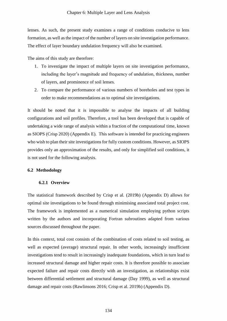
Chapter 6: Multiple Layer and Lens Analysis
134
lenses. As such, the present study examines a range of conditions conducive to lens
formation, as well as the impact of the number of layers on site investigation performance.
The effect of layer boundary undulation frequency will also be examined.
The aims of this study are therefore:
1. To investigate the impact of multiple layers on site investigation performance,
including the layer’s magnitude and frequency of undulation, thickness, number
of layers, and prominence of soil lenses.
2. To compare the performance of various numbers of boreholes and test types in
order to make recommendations as to optimal site investigations.
It should be noted that it is impossible to analyse the impacts of all building
configurations and soil profiles. Therefore, a tool has been developed that is capable of
undertaking a wide range of analysis within a fraction of the computational time, known
as SIOPS (Crisp 2020) (Appendix E). This software is intended for practicing engineers
who wish to plan their site investigations for fully custom conditions. However, as SIOPS
provides only an approximation of the results, and only for simplified soil conditions, it
is not used for the following analysis.
6.2 Methodology
6.2.1 Overview
The statistical framework described by Crisp et al. (2019b) (Appendix D) allows for
optimal site investigations to be found through minimising associated total project cost.
The framework is implemented as a numerical simulation employing python scripts
written by the authors and incorporating Fortran subroutines adapted from various
sources discussed throughout the paper.
In this context, total cost consists of the combination of costs related to soil testing, as
well as expected (average) structural repair. In other words, increasingly insufficient
investigations tend to result in increasingly inadequate foundations, which in turn lead to
increased structural damage and higher repair costs. It is therefore possible to associate
expected failure and repair costs directly with an investigation, as relationships exist
between differential settlement and structural damage (Day 1999), as well as structural
damage and repair costs (Rawlinsons 2016; Crisp et al. 2019b) (Appendix D).
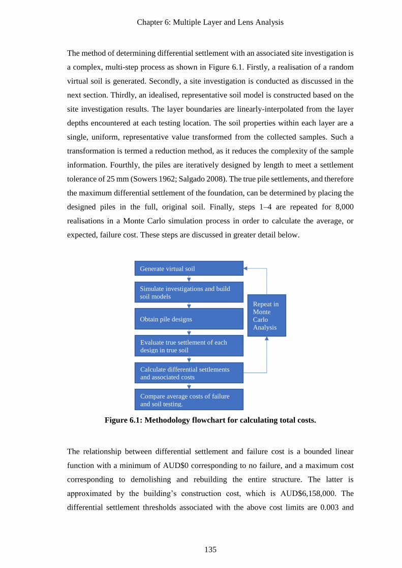
Chapter 6: Multiple Layer and Lens Analysis
135
The method of determining differential settlement with an associated site investigation is
a complex, multi-step process as shown in Figure 6.1. Firstly, a realisation of a random
virtual soil is generated. Secondly, a site investigation is conducted as discussed in the
next section. Thirdly, an idealised, representative soil model is constructed based on the
site investigation results. The layer boundaries are linearly-interpolated from the layer
depths encountered at each testing location. The soil properties within each layer are a
single, uniform, representative value transformed from the collected samples. Such a
transformation is termed a reduction method, as it reduces the complexity of the sample
information. Fourthly, the piles are iteratively designed by length to meet a settlement
tolerance of 25 mm (Sowers 1962; Salgado 2008). The true pile settlements, and therefore
the maximum differential settlement of the foundation, can be determined by placing the
designed piles in the full, original soil. Finally, steps 1–4 are repeated for 8,000
realisations in a Monte Carlo simulation process in order to calculate the average, or
expected, failure cost. These steps are discussed in greater detail below.
Figure 6.1: Methodology flowchart for calculating total costs.
The relationship between differential settlement and failure cost is a bounded linear
function with a minimum of AUD$0 corresponding to no failure, and a maximum cost
corresponding to demolishing and rebuilding the entire structure. The latter is
approximated by the building’s construction cost, which is AUD$6,158,000. The
differential settlement thresholds associated with the above cost limits are 0.003 and
Generate virtual soil
Simulate investigations and build
soil models
Obtain pile designs
Evaluate true settlement of each
design in true soil
Compare average costs of failure
and soil testing.
Repeat in
Monte
Carlo
Analysis
Calculate differential settlements
and associated costs
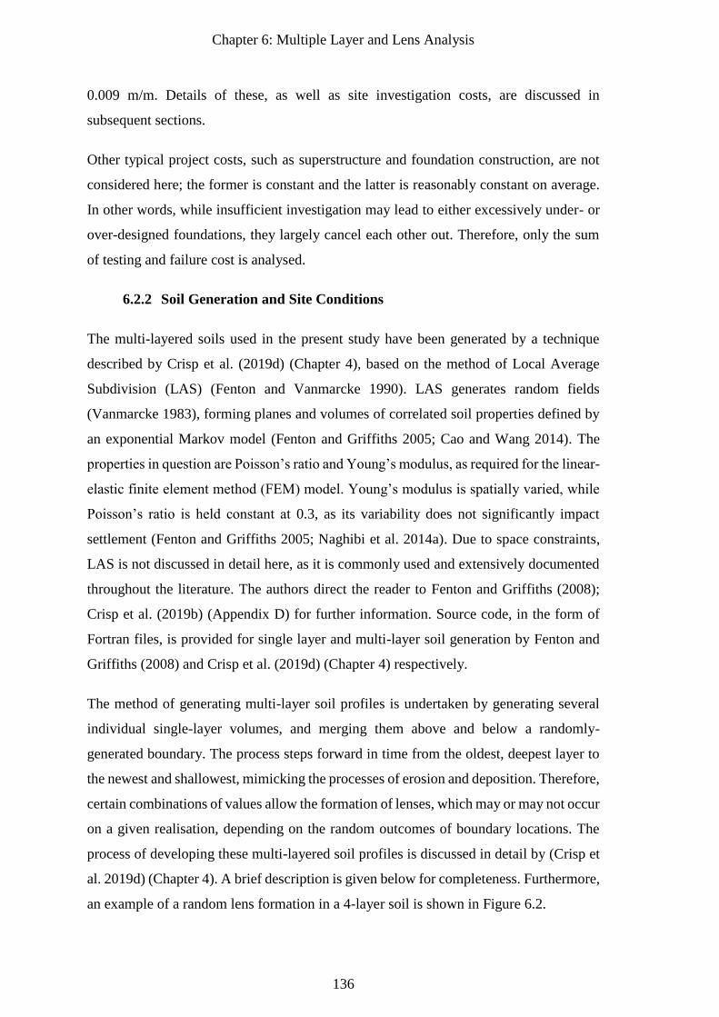
Chapter 6: Multiple Layer and Lens Analysis
136
0.009 m/m. Details of these, as well as site investigation costs, are discussed in
subsequent sections.
Other typical project costs, such as superstructure and foundation construction, are not
considered here; the former is constant and the latter is reasonably constant on average.
In other words, while insufficient investigation may lead to either excessively under- or
over-designed foundations, they largely cancel each other out. Therefore, only the sum
of testing and failure cost is analysed.
6.2.2 Soil Generation and Site Conditions
The multi-layered soils used in the present study have been generated by a technique
described by Crisp et al. (2019d) (Chapter 4), based on the method of Local Average
Subdivision (LAS) (Fenton and Vanmarcke 1990). LAS generates random fields
(Vanmarcke 1983), forming planes and volumes of correlated soil properties defined by
an exponential Markov model (Fenton and Griffiths 2005; Cao and Wang 2014). The
properties in question are Poisson’s ratio and Young’s modulus, as required for the linear-
elastic finite element method (FEM) model. Young’s modulus is spatially varied, while
Poisson’s ratio is held constant at 0.3, as its variability does not significantly impact
settlement (Fenton and Griffiths 2005; Naghibi et al. 2014a). Due to space constraints,
LAS is not discussed in detail here, as it is commonly used and extensively documented
throughout the literature. The authors direct the reader to Fenton and Griffiths (2008);
Crisp et al. (2019b) (Appendix D) for further information. Source code, in the form of
Fortran files, is provided for single layer and multi-layer soil generation by Fenton and
Griffiths (2008) and Crisp et al. (2019d) (Chapter 4) respectively.
The method of generating multi-layer soil profiles is undertaken by generating several
individual single-layer volumes, and merging them above and below a randomly-
generated boundary. The process steps forward in time from the oldest, deepest layer to
the newest and shallowest, mimicking the processes of erosion and deposition. Therefore,
certain combinations of values allow the formation of lenses, which may or may not occur
on a given realisation, depending on the random outcomes of boundary locations. The
process of developing these multi-layered soil profiles is discussed in detail by (Crisp et
al. 2019d) (Chapter 4). A brief description is given below for completeness. Furthermore,
an example of a random lens formation in a 4-layer soil is shown in Figure 6.2.
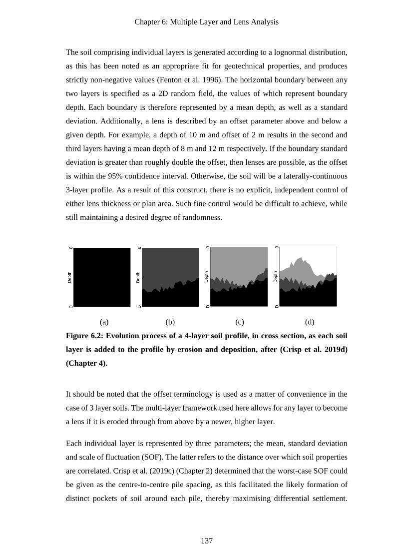
Chapter 6: Multiple Layer and Lens Analysis
137
The soil comprising individual layers is generated according to a lognormal distribution,
as this has been noted as an appropriate fit for geotechnical properties, and produces
strictly non-negative values (Fenton et al. 1996). The horizontal boundary between any
two layers is specified as a 2D random field, the values of which represent boundary
depth. Each boundary is therefore represented by a mean depth, as well as a standard
deviation. Additionally, a lens is described by an offset parameter above and below a
given depth. For example, a depth of 10 m and offset of 2 m results in the second and
third layers having a mean depth of 8 m and 12 m respectively. If the boundary standard
deviation is greater than roughly double the offset, then lenses are possible, as the offset
is within the 95% confidence interval. Otherwise, the soil will be a laterally-continuous
3-layer profile. As a result of this construct, there is no explicit, independent control of
either lens thickness or plan area. Such fine control would be difficult to achieve, while
still maintaining a desired degree of randomness.
(a) (b) (c) (d)
Figure 6.2: Evolution process of a 4-layer soil profile, in cross section, as each soil
layer is added to the profile by erosion and deposition, after (Crisp et al. 2019d)
(Chapter 4).
It should be noted that the offset terminology is used as a matter of convenience in the
case of 3 layer soils. The multi-layer framework used here allows for any layer to become
a lens if it is eroded through from above by a newer, higher layer.
Each individual layer is represented by three parameters; the mean, standard deviation
and scale of fluctuation (SOF). The latter refers to the distance over which soil properties
are correlated. Crisp et al. (2019c) (Chapter 2) determined that the worst-case SOF could
be given as the centre-to-centre pile spacing, as this facilitated the likely formation of
distinct pockets of soil around each pile, thereby maximising differential settlement.
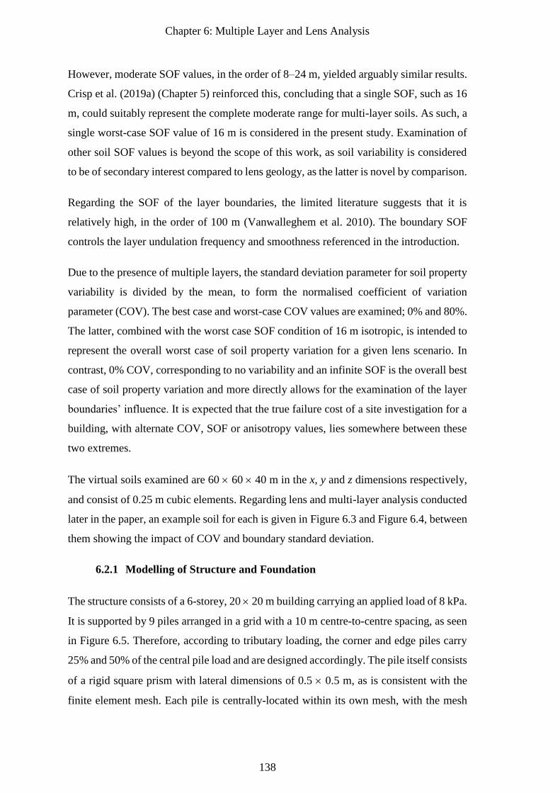
Chapter 6: Multiple Layer and Lens Analysis
138
However, moderate SOF values, in the order of 8–24 m, yielded arguably similar results.
Crisp et al. (2019a) (Chapter 5) reinforced this, concluding that a single SOF, such as 16
m, could suitably represent the complete moderate range for multi-layer soils. As such, a
single worst-case SOF value of 16 m is considered in the present study. Examination of
other soil SOF values is beyond the scope of this work, as soil variability is considered
to be of secondary interest compared to lens geology, as the latter is novel by comparison.
Regarding the SOF of the layer boundaries, the limited literature suggests that it is
relatively high, in the order of 100 m (Vanwalleghem et al. 2010). The boundary SOF
controls the layer undulation frequency and smoothness referenced in the introduction.
Due to the presence of multiple layers, the standard deviation parameter for soil property
variability is divided by the mean, to form the normalised coefficient of variation
parameter (COV). The best case and worst-case COV values are examined; 0% and 80%.
The latter, combined with the worst case SOF condition of 16 m isotropic, is intended to
represent the overall worst case of soil property variation for a given lens scenario. In
contrast, 0% COV, corresponding to no variability and an infinite SOF is the overall best
case of soil property variation and more directly allows for the examination of the layer
boundaries’ influence. It is expected that the true failure cost of a site investigation for a
building, with alternate COV, SOF or anisotropy values, lies somewhere between these
two extremes.
The virtual soils examined are 60 60 40 m in the x, y and z dimensions respectively,
and consist of 0.25 m cubic elements. Regarding lens and multi-layer analysis conducted
later in the paper, an example soil for each is given in Figure 6.3 and Figure 6.4, between
them showing the impact of COV and boundary standard deviation.
6.2.1 Modelling of Structure and Foundation
The structure consists of a 6-storey, 20 20 m building carrying an applied load of 8 kPa.
It is supported by 9 piles arranged in a grid with a 10 m centre-to-centre spacing, as seen
in Figure 6.5. Therefore, according to tributary loading, the corner and edge piles carry
25% and 50% of the central pile load and are designed accordingly. The pile itself consists
of a rigid square prism with lateral dimensions of 0.5 0.5 m, as is consistent with the
finite element mesh. Each pile is centrally-located within its own mesh, with the mesh
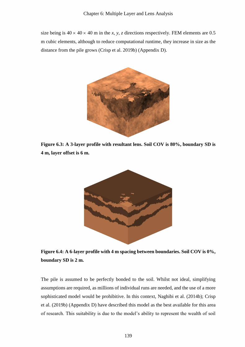
Chapter 6: Multiple Layer and Lens Analysis
139
size being is 40 40 40 m in the x, y, z directions respectively. FEM elements are 0.5
m cubic elements, although to reduce computational runtime, they increase in size as the
distance from the pile grows (Crisp et al. 2019b) (Appendix D).
Figure 6.3: A 3-layer profile with resultant lens. Soil COV is 80%, boundary SD is
4 m, layer offset is 6 m.
Figure 6.4: A 6-layer profile with 4 m spacing between boundaries. Soil COV is 0%,
boundary SD is 2 m.
The pile is assumed to be perfectly bonded to the soil. Whilst not ideal, simplifying
assumptions are required, as millions of individual runs are needed, and the use of a more
sophisticated model would be prohibitive. In this context, Naghibi et al. (2014b); Crisp
et al. (2019b) (Appendix D) have described this model as the best available for this area
of research. This suitability is due to the model’s ability to represent the wealth of soil
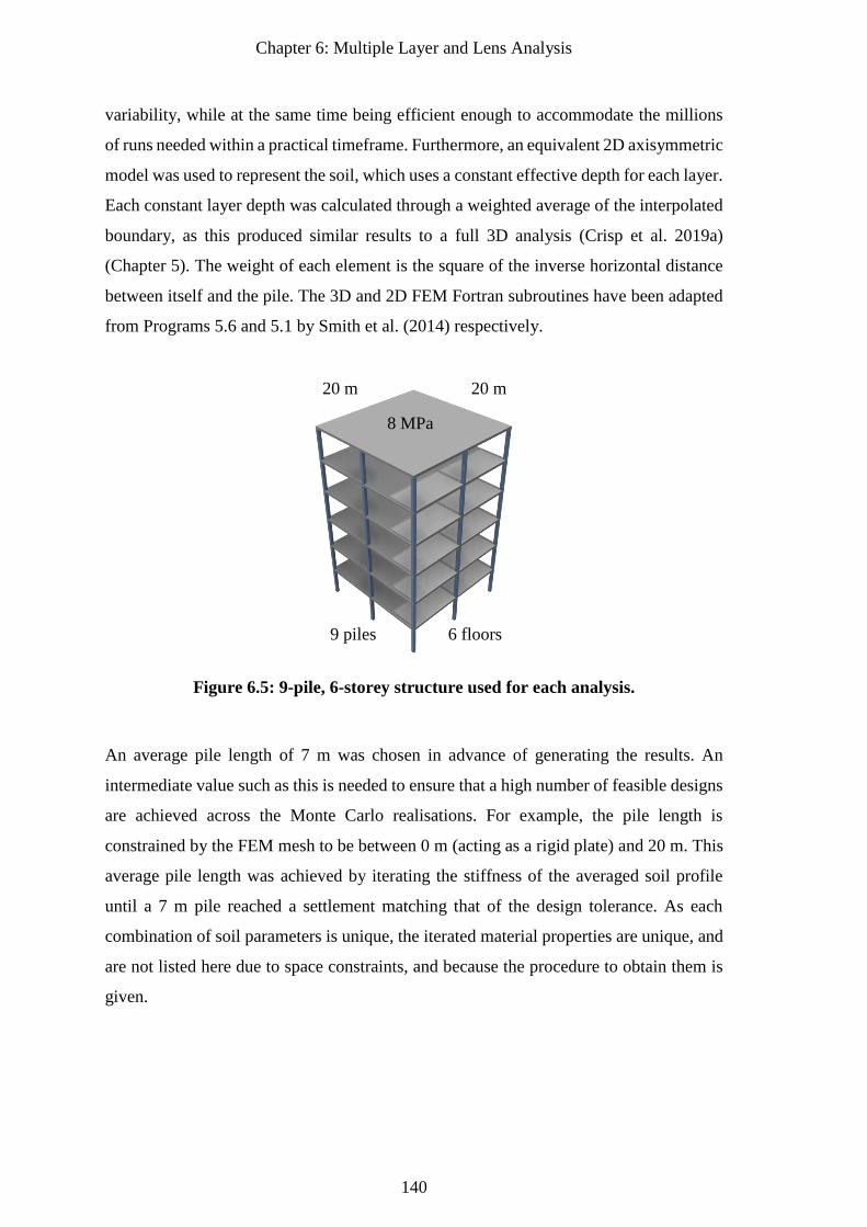
Chapter 6: Multiple Layer and Lens Analysis
140
variability, while at the same time being efficient enough to accommodate the millions
of runs needed within a practical timeframe. Furthermore, an equivalent 2D axisymmetric
model was used to represent the soil, which uses a constant effective depth for each layer.
Each constant layer depth was calculated through a weighted average of the interpolated
boundary, as this produced similar results to a full 3D analysis (Crisp et al. 2019a)
(Chapter 5). The weight of each element is the square of the inverse horizontal distance
between itself and the pile. The 3D and 2D FEM Fortran subroutines have been adapted
from Programs 5.6 and 5.1 by Smith et al. (2014) respectively.
Figure 6.5: 9-pile, 6-storey structure used for each analysis.
An average pile length of 7 m was chosen in advance of generating the results. An
intermediate value such as this is needed to ensure that a high number of feasible designs
are achieved across the Monte Carlo realisations. For example, the pile length is
constrained by the FEM mesh to be between 0 m (acting as a rigid plate) and 20 m. This
average pile length was achieved by iterating the stiffness of the averaged soil profile
until a 7 m pile reached a settlement matching that of the design tolerance. As each
combination of soil parameters is unique, the iterated material properties are unique, and
are not listed here due to space constraints, and because the procedure to obtain them is
given.
6 floors 9 piles
8 MPa
20 m 20 m
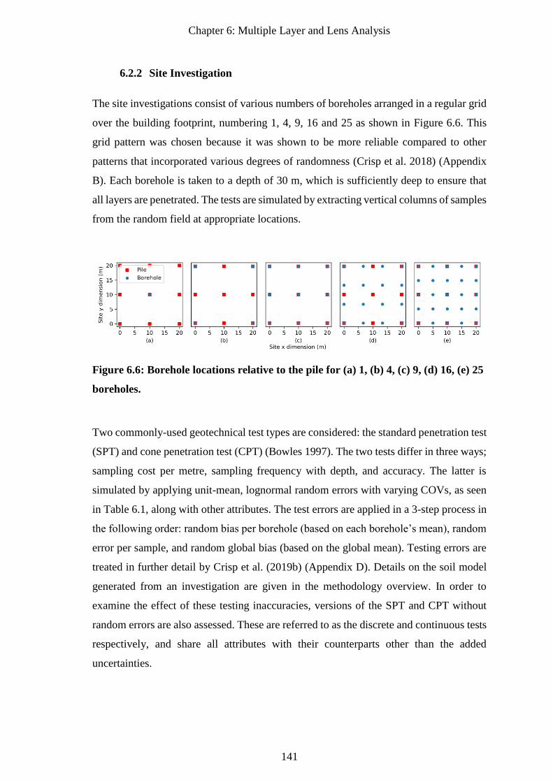
Chapter 6: Multiple Layer and Lens Analysis
141
6.2.2 Site Investigation
The site investigations consist of various numbers of boreholes arranged in a regular grid
over the building footprint, numbering 1, 4, 9, 16 and 25 as shown in Figure 6.6. This
grid pattern was chosen because it was shown to be more reliable compared to other
patterns that incorporated various degrees of randomness (Crisp et al. 2018) (Appendix
B). Each borehole is taken to a depth of 30 m, which is sufficiently deep to ensure that
all layers are penetrated. The tests are simulated by extracting vertical columns of samples
from the random field at appropriate locations.
Figure 6.6: Borehole locations relative to the pile for (a) 1, (b) 4, (c) 9, (d) 16, (e) 25
boreholes.
Two commonly-used geotechnical test types are considered: the standard penetration test
(SPT) and cone penetration test (CPT) (Bowles 1997). The two tests differ in three ways;
sampling cost per metre, sampling frequency with depth, and accuracy. The latter is
simulated by applying unit-mean, lognormal random errors with varying COVs, as seen
in Table 6.1, along with other attributes. The test errors are applied in a 3-step process in
the following order: random bias per borehole (based on each borehole’s mean), random
error per sample, and random global bias (based on the global mean). Testing errors are
treated in further detail by Crisp et al. (2019b) (Appendix D). Details on the soil model
generated from an investigation are given in the methodology overview. In order to
examine the effect of these testing inaccuracies, versions of the SPT and CPT without
random errors are also assessed. These are referred to as the discrete and continuous tests
respectively, and share all attributes with their counterparts other than the added
uncertainties.
Chapter 6: Multiple Layer and Lens Analysis
142
Table 6.1: Test type information.
Test
type
Sampling
interval (m)
Cost
(AUD$/m)
Uncertainties measures as COV (%)
Transformation
model
Measurement
Bias Random
SPT 1.5 156 25 20 40
CPT 0.25 76.6 15 15 20
The reduction method for transforming the many soil samples into a single representative
value is that of subtracting the samples’ geometric standard deviation from its geometric
mean. This technique is henceforth referred to as the standard deviation (SD) reduction
method. This particular method is chosen as it consistently provided the lowest total cost
in the single layer analysis by Crisp et al. (2019c) (Chapter 2), and was used in the two-
layer analysis by Crisp et al. (2019a) (Chapter 5). When applied to lognormally-
distributed values, as is the case here, the standard deviation method can be made
analogous to taking percentiles, as both approaches can be interpreted as probabilities of
exceedance, depending on the number of standard deviations and choice of percentile
used. One geometric standard deviation below the geometric mean provides results that
are similar to, but slightly more conservative than, the 25th percentile, which is one
reduction method in use by practising engineers. It should be noted that the choice of
reduction method has no impact on interpretation of the layer boundaries, and has no
impact on the results when a COV of 0% is used and no random testing errors are applied.
6.3 Results and Discussion
6.3.1 Boundary SOF Comparison
This section examines the effect of a layer boundary’s scale of fluctuation on site
investigation and foundation performance. This boundary SOF variable is assessed first
as it has not been analysed in the literature. As such, its influence must be known prior to
the detailed analysis in the following sections.
A set of 6 boundary SOFs are investigated; 5, 10, 25, 50, 100 and 200 m. The results are
shown in Figure 6.7 in terms of failure cost and for the perfectly accurate continuous test.
This metric and test type were chosen, along with a soil COV of 0%, in order to measure
the reliability of the different SOFs as directly as possible, minimising the impact of other
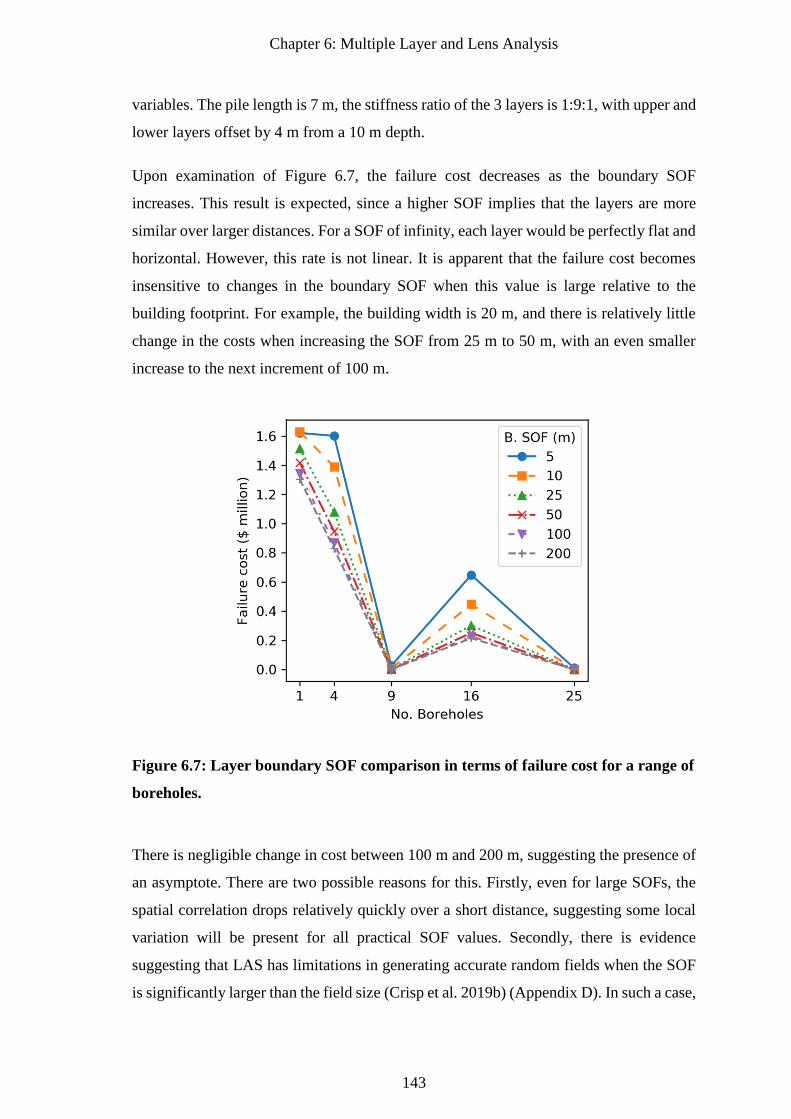
Chapter 6: Multiple Layer and Lens Analysis
143
variables. The pile length is 7 m, the stiffness ratio of the 3 layers is 1:9:1, with upper and
lower layers offset by 4 m from a 10 m depth.
Upon examination of Figure 6.7, the failure cost decreases as the boundary SOF
increases. This result is expected, since a higher SOF implies that the layers are more
similar over larger distances. For a SOF of infinity, each layer would be perfectly flat and
horizontal. However, this rate is not linear. It is apparent that the failure cost becomes
insensitive to changes in the boundary SOF when this value is large relative to the
building footprint. For example, the building width is 20 m, and there is relatively little
change in the costs when increasing the SOF from 25 m to 50 m, with an even smaller
increase to the next increment of 100 m.
Figure 6.7: Layer boundary SOF comparison in terms of failure cost for a range of
boreholes.
There is negligible change in cost between 100 m and 200 m, suggesting the presence of
an asymptote. There are two possible reasons for this. Firstly, even for large SOFs, the
spatial correlation drops relatively quickly over a short distance, suggesting some local
variation will be present for all practical SOF values. Secondly, there is evidence
suggesting that LAS has limitations in generating accurate random fields when the SOF
is significantly larger than the field size (Crisp et al. 2019b) (Appendix D). In such a case,
Chapter 6: Multiple Layer and Lens Analysis
144
the high SOF imposes strong continuity and consistency across the boundary, while the
standard deviation imposes variation. The conflict between these two parameters tends
to result in a decreased apparent SOF, which is contributing to the results seen here.
A small SOF is deemed the worst case for layer boundaries. This conclusion is in contrast
to several studies on the impact of SOF in variable, single layer soils. For example Fenton
and Griffiths (2002); Jaksa et al. (2005a); Crisp et al. (2019c) (Chapter 2) suggested that
the worst case is approximately equal to the centre-to-centre spacing of the individual
footings. In the single layer case with a small SOF, the rapidly fluctuating properties are
locally-averaged, such that the soil around each pile is similar at a macro scale,
minimising differential settlement.
However, with the layer boundary, any local averaging mechanism that exists is greatly
reduced. As discussed in the section describing the pile settlement model, the contribution
of the layer boundary to pile settlement decreases by the square of the inverse distance;
i.e. a rapid rate. As such, small boundary SOFs result in layer depths that are purely
random at each pile, increasing the probability of differential settlement, and hence
failure cost. This randomness explains why there is little improvement from 4 boreholes
when compared to a single one, in the 5 m SOF case; while the 4 piles at the building
corners are accurately modelled, the remaining 5 piles without a borehole are not well
accounted for.
Another finding from Figure 6.7 is that the failure cost for 16 boreholes is considerably
greater than that for 9. This is counterintuitive, as the former, more thorough investigation
provides more soil information. The low cost for both the 9 and 25 borehole cases is
explained by the fact that a borehole is located at each pile, resulting in a highly accurate
soil model at the pile locations, where accuracy is most critical. In contrast, other than at
the 4 piles at the building corners, the remaining 12 boreholes are placed at a notable
distance from the piles, as shown in Figure 6.6(d). This difference in failure cost between
9 and 16 boreholes is in excess of AUD$200,000, compared to the roughly AUD$100,000
under similar circumstances in the 2-layer case described by Crisp et al. (2019a) (Chapter
5). That study also found that 4 boreholes was optimal when only 4 piles were present.
The aforementioned decreases in reliability with additional testing reinforce that testing
location is an important consideration in site investigation planning.
Chapter 6: Multiple Layer and Lens Analysis
145
An important point is that the recommended number of boreholes does not change with
the boundary SOF, as failure cost is anchored at near-zero when a borehole is located at
each pile. Since the failure cost is insensitive to the choice of SOF when this value is
high, and that high values are the realistic expectation (Crisp et al. 2019d) (Chapter 4),
this parameter will be set at 100 m for the remainder of this study. This value is consistent
with that used by Crisp et al. (2019a) (Chapter 5) which allows for direct comparison
with that study.
6.3.2 Test Type Comparison
A brief analysis is conducted comparing the four test types of accurate discrete, accurate
continuous, CPT and SPT. The results are shown in Figure 6.8 for a COV of 0% and
80%. As with the previous section, the layer stiffness ratio is 1:9:1 with boundary depth
standard deviation of 4 m. The two layer boundaries are at a 6 m offset from a 10 m depth.
One would assume that testing errors, such as those present with the SPT and CPT, would
result in inferior performance, as the soil model’s material properties are inaccurate.
However, in the case of the 0% COV as seen in Figure 6.8(a), the CPT and SPT
considerably outperform the accurate tests in terms of failure cost. This improvement is
in the order of AUD$0.7 million and AUD$1 million respectively, with both tests
outperforming their accurate counterparts in roughly 90% of Monte Carlo realisations.
This behaviour was observed to a lesser extent in Crisp et al. (2019a) (Chapter 5) under
similar circumstances for a two-layer soil, where it was explained that the improvement
is due to use of the conservative standard deviation reduction method. This method yields
increasingly conservative results for more variable soils. Therefore, for the perfectly
accurate tests and a COV of 0%, there is no variation and so no conservatism. On the
other hand, the random errors introduced by the SPT and CPT provide artificial variation
that does allow a soil model with safer estimates of material properties which compensate
for the uncertainty caused by the layer boundaries. This effect is particularly prominent
for small numbers of boreholes where the added conservativism is most beneficial due to
the lack of soil knowledge.
The case of an 80% COV, as seen in Figure 6.8(b), shows more consistent results across
all test types. While there is reduction in failure cost of roughly AUD$200,000 for a single
borehole with the SPT or CPT for the reasons discussed previously, these tests otherwise
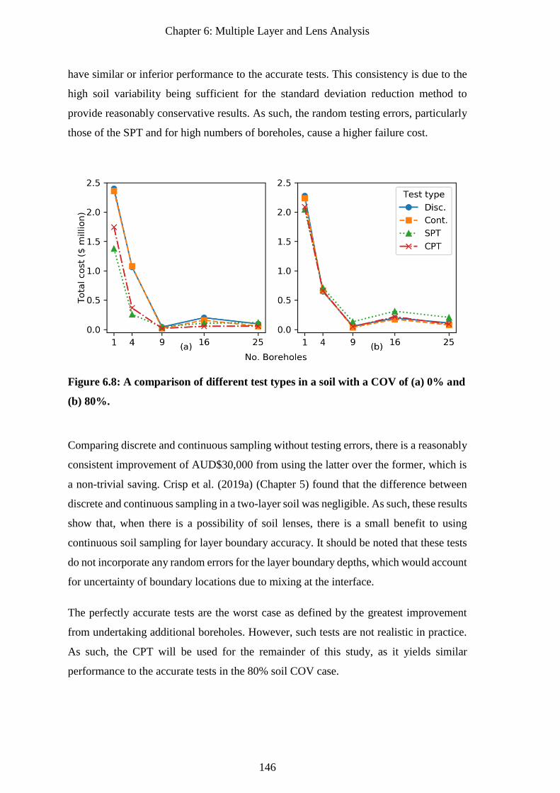
Chapter 6: Multiple Layer and Lens Analysis
146
have similar or inferior performance to the accurate tests. This consistency is due to the
high soil variability being sufficient for the standard deviation reduction method to
provide reasonably conservative results. As such, the random testing errors, particularly
those of the SPT and for high numbers of boreholes, cause a higher failure cost.
Figure 6.8: A comparison of different test types in a soil with a COV of (a) 0% and
(b) 80%.
Comparing discrete and continuous sampling without testing errors, there is a reasonably
consistent improvement of AUD$30,000 from using the latter over the former, which is
a non-trivial saving. Crisp et al. (2019a) (Chapter 5) found that the difference between
discrete and continuous sampling in a two-layer soil was negligible. As such, these results
show that, when there is a possibility of soil lenses, there is a small benefit to using
continuous soil sampling for layer boundary accuracy. It should be noted that these tests
do not incorporate any random errors for the layer boundary depths, which would account
for uncertainty of boundary locations due to mixing at the interface.
The perfectly accurate tests are the worst case as defined by the greatest improvement
from undertaking additional boreholes. However, such tests are not realistic in practice.
As such, the CPT will be used for the remainder of this study, as it yields similar
performance to the accurate tests in the 80% soil COV case.
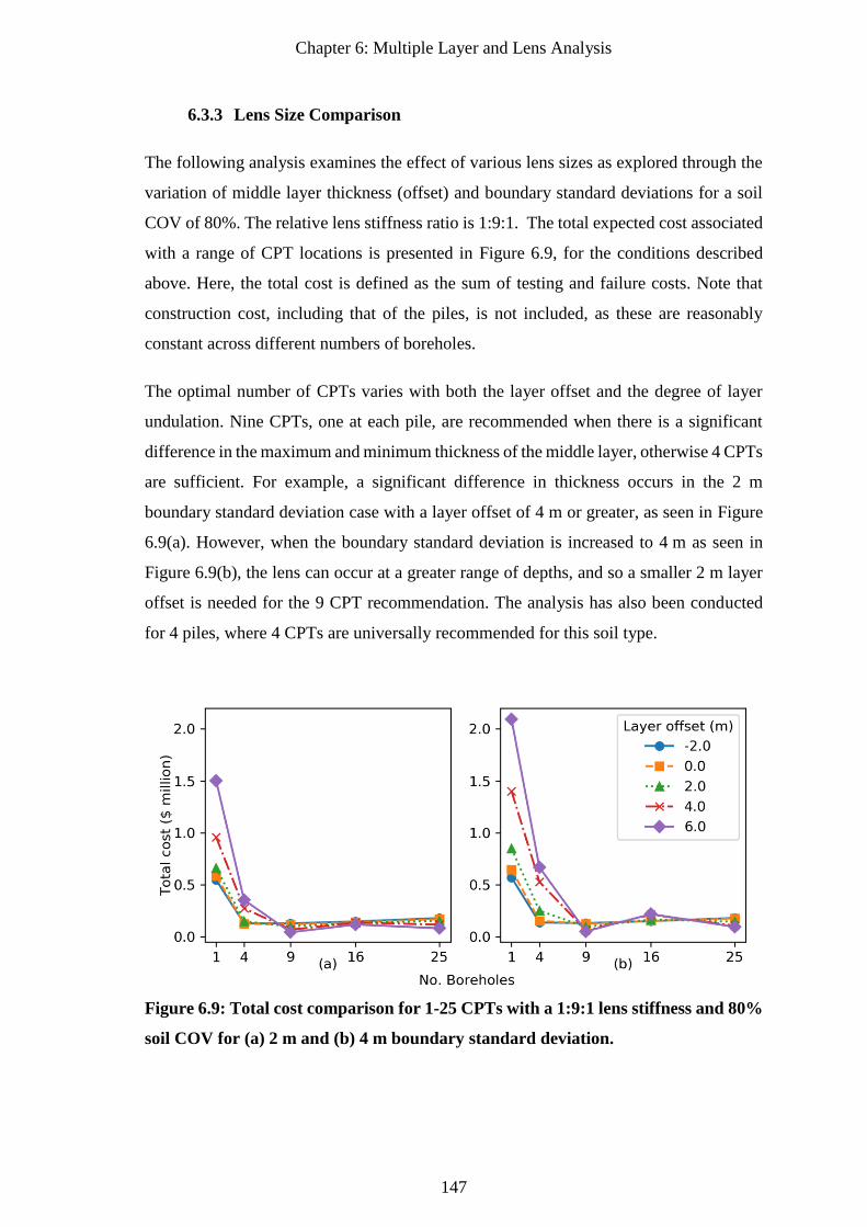
Chapter 6: Multiple Layer and Lens Analysis
147
6.3.3 Lens Size Comparison
The following analysis examines the effect of various lens sizes as explored through the
variation of middle layer thickness (offset) and boundary standard deviations for a soil
COV of 80%. The relative lens stiffness ratio is 1:9:1. The total expected cost associated
with a range of CPT locations is presented in Figure 6.9, for the conditions described
above. Here, the total cost is defined as the sum of testing and failure costs. Note that
construction cost, including that of the piles, is not included, as these are reasonably
constant across different numbers of boreholes.
The optimal number of CPTs varies with both the layer offset and the degree of layer
undulation. Nine CPTs, one at each pile, are recommended when there is a significant
difference in the maximum and minimum thickness of the middle layer, otherwise 4 CPTs
are sufficient. For example, a significant difference in thickness occurs in the 2 m
boundary standard deviation case with a layer offset of 4 m or greater, as seen in Figure
6.9(a). However, when the boundary standard deviation is increased to 4 m as seen in
Figure 6.9(b), the lens can occur at a greater range of depths, and so a smaller 2 m layer
offset is needed for the 9 CPT recommendation. The analysis has also been conducted
for 4 piles, where 4 CPTs are universally recommended for this soil type.
Figure 6.9: Total cost comparison for 1-25 CPTs with a 1:9:1 lens stiffness and 80%
soil COV for (a) 2 m and (b) 4 m boundary standard deviation.
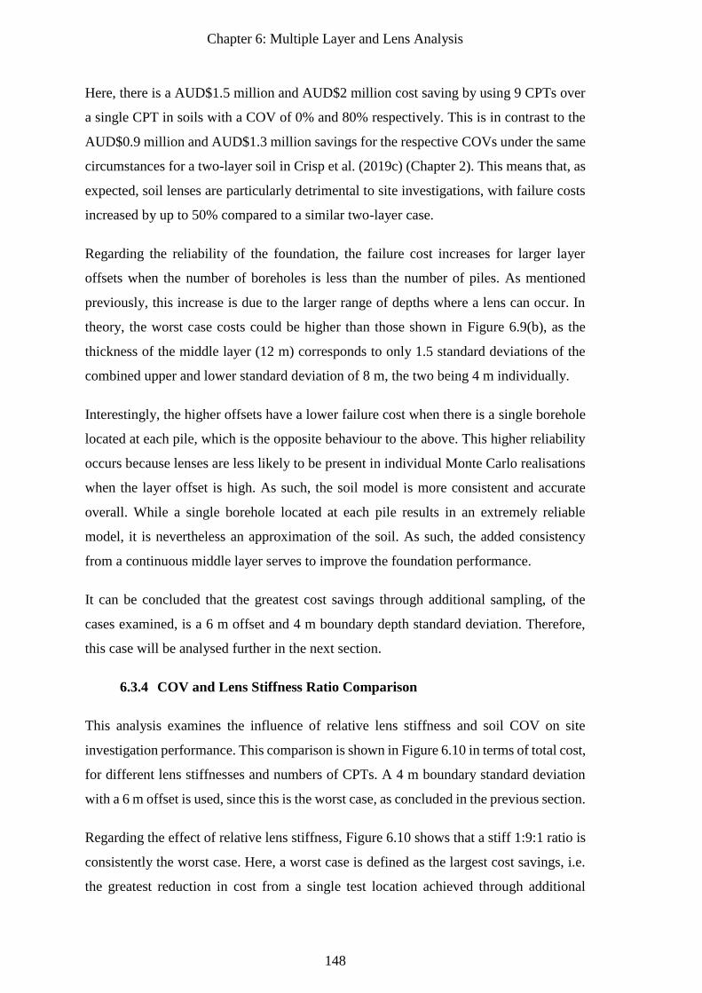
Chapter 6: Multiple Layer and Lens Analysis
148
Here, there is a AUD$1.5 million and AUD$2 million cost saving by using 9 CPTs over
a single CPT in soils with a COV of 0% and 80% respectively. This is in contrast to the
AUD$0.9 million and AUD$1.3 million savings for the respective COVs under the same
circumstances for a two-layer soil in Crisp et al. (2019c) (Chapter 2). This means that, as
expected, soil lenses are particularly detrimental to site investigations, with failure costs
increased by up to 50% compared to a similar two-layer case.
Regarding the reliability of the foundation, the failure cost increases for larger layer
offsets when the number of boreholes is less than the number of piles. As mentioned
previously, this increase is due to the larger range of depths where a lens can occur. In
theory, the worst case costs could be higher than those shown in Figure 6.9(b), as the
thickness of the middle layer (12 m) corresponds to only 1.5 standard deviations of the
combined upper and lower standard deviation of 8 m, the two being 4 m individually.
Interestingly, the higher offsets have a lower failure cost when there is a single borehole
located at each pile, which is the opposite behaviour to the above. This higher reliability
occurs because lenses are less likely to be present in individual Monte Carlo realisations
when the layer offset is high. As such, the soil model is more consistent and accurate
overall. While a single borehole located at each pile results in an extremely reliable
model, it is nevertheless an approximation of the soil. As such, the added consistency
from a continuous middle layer serves to improve the foundation performance.
It can be concluded that the greatest cost savings through additional sampling, of the
cases examined, is a 6 m offset and 4 m boundary depth standard deviation. Therefore,
this case will be analysed further in the next section.
6.3.4 COV and Lens Stiffness Ratio Comparison
This analysis examines the influence of relative lens stiffness and soil COV on site
investigation performance. This comparison is shown in Figure 6.10 in terms of total cost,
for different lens stiffnesses and numbers of CPTs. A 4 m boundary standard deviation
with a 6 m offset is used, since this is the worst case, as concluded in the previous section.
Regarding the effect of relative lens stiffness, Figure 6.10 shows that a stiff 1:9:1 ratio is
consistently the worst case. Here, a worst case is defined as the largest cost savings, i.e.
the greatest reduction in cost from a single test location achieved through additional
Chapter 6: Multiple Layer and Lens Analysis
149
sampling. A weak 9:1:9 ratio at the other end of the stiffness spectrum does provide
similar savings, at least for the 4 m layer standard deviation, however the failure costs are
consistently lower overall.
Figure 6.10: Total cost comparison for 1-25 CPTs with a 6 m layer offset, COV of
0% with a boundary standard deviation of (a) 2 m, (b) 4 m, and a COV of 80% with
a boundary standard deviation of (c) 2 m; and (d) 4 m.
In the case of a stiff lens, stresses will be distributed more widely throughout this layer,
providing higher resistance to pile settlement. Therefore, if a stiff lens is inappropriately
accounted for in the soil model, a high differential settlement could be observed, resulting
in significant failure. Conversely, if a weak lens is present along the length of a pile,
additional settlement will occur; however, the stresses will instead be distributed to the
stiff upper and lower soil layers. This transfer mechanism implies that a weak lens would
not contribute as strongly to differential settlement as a stiff one. However, the perfect
bonding nature of the pile-soil interface inherent in the numerical model should be noted.
It is possible that pile settlement associated with lenses may increase if a more
sophisticated interface were accommodated, as stiff soil is less likely to remain bonded
Chapter 6: Multiple Layer and Lens Analysis
150
to the pile under high strains. As the 1:3:1 and 3:1:3 layer stiffness ratios have similar
failure costs to each other, there is an argument that this consistency may also apply to
their more extreme 9:1:9 and 1:9:1 counterparts, if they didn’t stretch the assumptions of
the pile settlement model used in this analysis.
Examination of the pile settlement curves with increasing pile length reveals that there is
a sharp decrease in settlement once the pile encounters a stiff lens. In contrast, there is a
smooth, gradual flattening of the slope when the pile approaches a soft lens. This
behaviour reflects the aforementioned load transfer discussion.
The optimal number of CPTs varies according to the combination of soil COV, layer
stiffness ratio and boundary standard deviation. Nine CPTs, one at each pile, are
recommended for the large ratios of 9:1:9 and 1:9:1 when there is a large boundary depth
standard deviation or high soil COV. In this case, these parameters are between 2-4 m or
0-80% respectively. Furthermore, 9 CPTs are recommended for the intermediate layer
stiffnesses of 1:3:1 and 3:1:3, when there is a high soil COV and large boundary depth
standard deviation. In all other cases, 4 CPTs at the building corners are optimal, or near-
optimal, as the soil variability is sufficiently low that fewer CPTs provide adequate
information.
As this is an initial study examining the impact of lenses on site investigations, and the
procedure is computationally intensive, a limited set of these parameters is assessed, and
a more precise recommendation cannot be given. However, the thresholds separating the
4 and 9 borehole recommendations are likely to be at the higher end of the stated ranges,
i.e. a COV of closer to 80% and boundary depth standard deviation closer to 4 m.
Although not shown here, these overall trends and recommended numbers of boreholes
are consistent with the SPT.
6.3.5 Number of Layers Comparison
This section discusses the influence of test type and the number of layers on site
investigation performance, for 0% and 80% soil COV as shown in Figure 6.11. As
discussed in the previous section, the stiffnesses for each soil case and layer are adjusted
such that the average pile length is 7 m. A set of 2 to 6 layers is examined, with alternating
mean stiffness ratios of 1:9:1:9:1:9, for the first, through to last layers, respectively. The
layer boundaries have a standard deviation of 2 m, with the average depths set at 4 m
Chapter 6: Multiple Layer and Lens Analysis
151
apart, meaning that it is possible for lenses to form. As such, the layer depths are 4, 8, 12,
16 and 20 m, where each case of n layers refers to the uppermost set. In other words, as
the number of layers increases, an additional 4 m layer with contrasting stiffness is added
below the previous lowest boundary. The CPT is used.
Upon inspection of Figure 6.11, examining the case of a single borehole in both subplots,
it can be seen that there is a complex relationship between the failure cost and the number
of layers. One would expect that the failure cost increases with the number of layers, as
the soil complexity is greater. Indeed, the 4-layer soil has a higher cost than the two-layer
soil. Similarly, 5 layers results a higher cost than 3. These aforementioned two
comparisons are consistent with each other in that the former, with an even number of
layers, has a stiff bottom layer. In comparison, the latter comparison, with an odd number
of layers, has a soft lower layer. However, the cases with a soft lower layer tend to have
a lower failure cost overall for the reasons described in the previous section.
The description implies that failure cost generally increases with the number of layers
given that the stiffness of the bottom layer remains consistent. However, this rule is
invalidated in the case of 6 layers, which has a lower failure cost than that of 4. The
authors speculate that there is a theoretical upper limit to the practical uncertainty
introduced by increasing the number of layers. Furthermore, as additional layers are
added with increasing depth into the soil, the soil as a whole becomes more effectively
homogenous. For example, in the two-layer case there is a strong contrast in stiffness
between the upper and lower layer, and so the uncertainty of the layer boundary has a
large impact on pile performance. However, with rapidly fluctuating layers of alternating
stiffness, the upper and lower regions of soil would be more likely to contain a similar
mix of stiffness values. As the pile acts as a spatial averaging mechanism, the resulting
settlement error between the soil model and true model would be reduced, likely
contributing to the reduced failure cost of the 6-layer scenario.
Inspecting other numbers of boreholes in Figure 6.11, the failure costs have largely
converged by 4 boreholes, and particularly by 9, where a borehole is located at each pile.
A notable discrepancy is the two-layer soil with an 80% COV in Figure 6.11(b) with a
reduced failure cost with 4 boreholes. It is worth remembering that the two-layer soil is
unique in that no lenses are possible. This uniquely lower uncertainty means that, when
a reasonable number of boreholes are drilled, such as 4, a much more accurate soil model
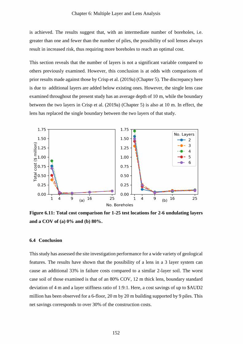
Chapter 6: Multiple Layer and Lens Analysis
152
is achieved. The results suggest that, with an intermediate number of boreholes, i.e.
greater than one and fewer than the number of piles, the possibility of soil lenses always
result in increased risk, thus requiring more boreholes to reach an optimal cost.
This section reveals that the number of layers is not a significant variable compared to
others previously examined. However, this conclusion is at odds with comparisons of
prior results made against those by Crisp et al. (2019a) (Chapter 5). The discrepancy here
is due to additional layers are added below existing ones. However, the single lens case
examined throughout the present study has an average depth of 10 m, while the boundary
between the two layers in Crisp et al. (2019a) (Chapter 5) is also at 10 m. In effect, the
lens has replaced the single boundary between the two layers of that study.
Figure 6.11: Total cost comparison for 1-25 test locations for 2-6 undulating layers
and a COV of (a) 0% and (b) 80%.
6.4 Conclusion
This study has assessed the site investigation performance for a wide variety of geological
features. The results have shown that the possibility of a lens in a 3 layer system can
cause an additional 33% in failure costs compared to a similar 2-layer soil. The worst
case soil of those examined is that of an 80% COV, 12 m thick lens, boundary standard
deviation of 4 m and a layer stiffness ratio of 1:9:1. Here, a cost savings of up to $AUD2
million has been observed for a 6-floor, 20 m by 20 m building supported by 9 piles. This
net savings corresponds to over 30% of the construction costs.
Chapter 6: Multiple Layer and Lens Analysis
153
A comparison of different layer boundary scales of fluctuations has shown that low values
are the worst case. However, performance becomes relatively insensitive to this
parameter for values that are larger than the structure’s footprint dimensions. The
discrepancy with the worst-case scale of fluctuation for within-layer soil property
variability is due to the local-averaging effect of the pile, which is largely absent with
respect to layer boundaries.
The optimal number of boreholes is affected by the layer stiffness ratio, standard
deviation of layer boundary depths, soil coefficient of variation (COV), and thickness of
the middle layer or lens. As the resolution of the parameters is modest, owing to the
number of parameters investigated, it is difficult to make generalised recommendations
that extrapolate beyond the soil cases examined. However, a borehole at every pile is
advised when the soil COV or the layer boundary standard deviation is high, at values
such as 80% and 4 m respectively, when the average lens thickness is at least 2 m. This
recommendation also applies for lower variability soils when the lens is more or less stiff
than the surrounding soil by an order of magnitude. In other cases, assuming the presence
of lenses is a possibility, then 4 boreholes are suggested.
The number of layers was found to have a modest impact on site investigation
performance compared to the above factors. In general, higher numbers of layers are
associated with a greater degree of failure when new layers are added below existing
ones. However, the relative stiffness of the bottom soil layer is equally relevant, where
stiff bottom layers result in lower failure costs. The results also show that failure costs
begin to decrease beyond a certain number of layers, at least for the scenario examined.
The rapid alternating of soil stiffness across multiple layers with depth results in a
relatively homogenous soil at the macro scale owning the local-averaging effect of the
pile.
A comparison of the SPT and CPT, as well as perfectly accurate versions of these tests,
show that the lack of precision from the SPT’s discrete sampling causes a failure cost
increase of AUD$30,000 over the CPT in the worst case soil conditions. When random
testing errors are introduced, the increased apparent soil variability results in more
conservative estimates of soil properties owing to the conservative reduction method
used. Specifically, this occurs in soil with very low COV as well as in highly variable
soil in the case of a single borehole. In other cases, the CPT performance does not
Chapter 6: Multiple Layer and Lens Analysis
154
significantly change due to its inaccuracy. However, the SPT failure cost increases by
AUD$60,000-AUD$120,000.
Future analyses can involve a wider variety of soil, structural and site investigation
parameter values, allowing for more specific recommendations. Furthermore, future
analysis could involve the use of a more complex and accurate pile settlement model,
which incorporates bearing failure and slip at the pile-soil interface, as lenses may exhibit
more detrimental performance under these conditions.
6.5 References
Albatal, A. 2013. Effect of inadequate site investigation on the cost and time of a
construction project. Masters Thesis, Construction and Building Engineering
Department, Arab Academy for Science, Technology and Maritime Transport,
Cairo.
Arsyad, A., Jaksa, M. B., Fenton, G. A., and Kaggwa, W. S. 2009. The effect of limited
site investigations on the design of pile foundations. In Proceedings of the
International Conference on Soil Mechanics and Geotechnical Engineering (17th:
2009: Egypt).
Bowles, J. E. 1997. Foundation analysis and design (5 ed.): McGraw-Hill.
Cao, Z., and Wang, Y. 2014. Bayesian model comparison and selection of spatial
correlation functions for soil parameters. Structural Safety, 49, 10-17. doi:
http://dx.doi.org/10.1016/j.strusafe.2013.06.003
Clayton, C. 2001. Managing geotechnical risk: time for change? In Proceedings of the
Institution of Civil Engineers-Geotechnical Engineering.
Crisp, M. P. 2020. SIOPS User Manual (Site investigation optimisation for piles using
statistics). doi: 10.13140/RG.2.2.33644.92807
Crisp, M. P., Jaksa, M. B., and Kuo, Y. L. 2018. Influence of Site Investigation Borehole
Pattern and Area on Pile Foundation Performance. In Proceedings of the 12th
ANZ Young Geotechnical Professionals Conference, Hobart.
Crisp, M. P., Jaksa, M. B., and Kuo, Y. L. 2019a. Characterising Site Investigation
Performance in a Two Layer Soil Profile. Canadian Journal of Civil Engineering.
Crisp, M. P., Jaksa, M. B., and Kuo, Y. L. 2019b. Framework for the Optimisation of Site
Investigations for Pile Designs in Complex Multi-Layered Soil, Research Report,
School of Civil, Environmental and Mining Engineering. doi:
10.13140/RG.2.2.23536.71685
Crisp, M. P., Jaksa, M. B., and Kuo, Y. L. 2019c. Toward a generalized guideline to
inform optimal site investigations for pile design. Canadian Geotechnical Journal.
Chapter 6: Multiple Layer and Lens Analysis
155
Crisp, M. P., Jaksa, M. B., Kuo, Y. L., Fenton, G. A., and Griffiths, D. V. 2019d. A
method for generating virtual soil profiles with complex, multi-layer stratigraphy.
Georisk, 13(2), 154-163.
Day, R. W. 1999. Forensic geotechnical and foundation engineering: McGraw-Hill New
York.
Fenton, G. A., and Griffiths, D. 1993. Statistics of block conductivity through a simple
bounded stochastic medium. Water Resources Research, 29(6), 1825-1830.
Fenton, G. A., and Griffiths, D. 2002. Probabilistic foundation settlement on spatially
random soil. Journal of Geotechnical and Geoenvironmental Engineering, 128(5),
381-390.
Fenton, G. A., and Griffiths, D. V. 2005. Three-dimensional probabilistic foundation
settlement. Journal of Geotechnical and Geoenvironmental Engineering, 131(2),
232-239.
Fenton, G. A., and Griffiths, D. V. 2008. Risk assessment in geotechnical engineering.
Hoboken: Wiley.
Fenton, G. A., Paice, G. M., and Griffiths, D. V. 1996. Probabilistic analysis of
foundation settlement. Golden: Geomechanics Research Center, Colorado School
of Mines.
Fenton, G. A., and Vanmarcke, E. H. 1990. Simulation of random fields via local average
subdivision. Journal of Engineering Mechanics, 116(8), 1733-1749.
Goldsworthy, J. S. 2006. Quantifying the risk of geotechnical site investigations. Ph.D
Thesis, School of Civil, Environmental and Mining Engineering, University of
Adelaide, Adelaide.
Goldsworthy, J. S., Jaksa, M. B., Fenton, G. A., Kaggwa, W. S., Griffiths, D. V., and
Poulos, H. G. 2007. Effect of sample location on the reliability based design of
pad foundations. Georisk, 1(3), 155-166.
Griffiths, D., and Fenton, G. A. 1993. Seepage beneath water retaining structures founded
on spatially random soil. Géotechnique, 43(4), 577-587.
Jaksa, M., Goldsworthy, J., Fenton, G., Kaggwa, W., Griffiths, D., Kuo, Y., and Poulos,
H. 2005a. Towards reliable and effective site investigations. Géotechnique, 55(2),
109-121.
Jaksa, M. B. 2000. Geotechnical risk and inadequate site investigations: a case study.
Australian Geomechanics, 35(2), 39-46.
Jaksa, M. B., Goldsworthy, J. S., Fenton, G. A., Kaggwa, W. S., Griffiths, D. V., Kuo,
Y. L., and Poulos, H. G. 2005b. Towards reliable and effective site investigations.
Géotechnique, 55(2), 109-121.
Jaksa, M. B., Kaggwa, W. S., Fenton, G. A., and Poulos, H. G. 2003. A framework for
quantifying the reliability of geotechnical investigations. In Proceedings of the
Chapter 6: Multiple Layer and Lens Analysis
156
9th International Conference on the Application of Statistics and Probability in
Civil Engineering.
Li, A., Jafari, N. H., and Tsai, F. T. C. 2019. Modelling and comparing 3-D soil
stratigraphy using subsurface borings and cone penetrometer tests in coastal
Louisiana, USA. Georisk: Assessment and Management of Risk for Engineered
Systems and Geohazards, 1-19. doi: 10.1080/17499518.2019.1637528
Li, J., Cassidy, M. J., Huang, J., Zhang, L., and Kelly, R. 2016. Probabilistic identification
of soil stratification. Géotechnique, 66(1), 16-26.
Loehr, J. E., Ding, D., and Likos, W. J. 2015. Effect of Number of Soil Strength
Measurements on Reliability of Spread Footing Designs. Transportation Research
Record: Journal of the Transportation Research Board, (2511), 37-44.
Moh, Z. C. 2004. Site investigation and geotechnical failures. In Proceedings of the
Proceeding of International Conference on Structural and Foundation Failures.
Naghibi, F., Fenton, G. A., and Griffiths, D. V. 2014a. Prediction of pile settlement in an
elastic soil. Computers and Geotechnics, 60, 29-32.
Naghibi, F., Fenton, G. A., and Griffiths, D. V. 2014b. Serviceability limit state design
of deep foundations. Géotechnique, 64(10), 787-799.
Rawlinsons, A. (2016). Australian Construction Handbook (34 ed., pp. 1005). Perth,
Australia: Rawlhouse Publishing Pty. Ltd.
Salgado, R. 2008. The engineering of foundations (Vol. 888): McGraw-Hill New York.
Sastre Jurado, C., Breul, P., Bacconnet, C., and Benz-Navarrete, M. 2020. Probabilistic
3D modelling of shallow soil spatial variability using dynamic cone penetrometer
results and a geostatistical method. Georisk: Assessment and Management of Risk
for Engineered Systems and Geohazards, 1-13. doi:
10.1080/17499518.2020.1728558
Smith, I. M., Griffiths, D. V., and Margetts, L. 2014. Programming the finite element
method (5th ed.): John Wiley & Sons.
Sowers, G. (1962). Shallow foundations (Vol. 569): McGraw-Hill, New York, NY.
Vanmarcke, E. H. 1983. Random Fields: Analysis and Synthesis. London: MIT Press.
Vanwalleghem, T., Poesen, J., McBratney, A., and Deckers, J. 2010. Spatial variability
of soil horizon depth in natural loess-derived soils. Geoderma, 157(1-2), 37-45.
Chapter 7: Effect of Borehole Location in Single Layer Soils
157
7 Chapter 7: Effect of Borehole
Location in Single Layer Soils
Paper Title:
Effect of Borehole Location on Pile Performance

Chapter 7: Effect of Borehole Location in Single Layer Soils
158


Chapter 7: Effect of Borehole Location in Single Layer Soils
160
Chapter 7: Effect of Borehole Location in Single Layer Soils
161
Abstract
Insufficient or inappropriate soil testing can lead to a range of undesirable consequences,
however there is little research available on site investigation performance in complex
soils. This study investigates site investigation scope in terms of a single borehole and its
location relative to the foundation. The results are given in the form of heatmaps showing
favourable sampling locations, whereby the optimal location can be found. The method
used is statistical in nature, employing Monte Carlo analysis with randomly-generated,
variable, single layer soils. These soils allow both site investigations and true foundation
performance to be conducted, with the resulting statistics analysed. Several site
investigation, structural configuration, and soil variability factors are examined,
including test type, borehole depth, reduction method, number of piles, building size and
investigation performance metric. The results show that investigation quality is
maximised by drilling the borehole in proximity to any pile in the foundation, and that
failure costs can vary with location by up to 8% of the construction cost.
Keywords: Probabilistic site characterisation and modelling, Monte Carlo simulation,
reliability-based optimization, pile foundation, site investigation optimization
Chapter 7: Effect of Borehole Location in Single Layer Soils
162
7.1 Introduction
Site investigations are an essential component of civil engineering projects, as they
identify the subsurface material properties relevant to a foundation, which would
otherwise be unknown. It is possible to undertake a thorough, expensive investigation
with poorly-chosen drilling locations, that proves less effective than cheaper, well-placed
ones (Albatal 2013; Crisp et al. 2020) (Chapter 5). Despite this, there is little guidance in
the literature on where boreholes should be located.
This study presents an analysis of site investigation performance regarding a single
borehole and its location relative to the foundation. The framework is statistical in nature,
and is derived from Jaksa et al. (2003), later refined and elaborated by Crisp et al. (2019a)
(Appendix D). The procedure involves the use of virtual, variable, randomly-generated
soils (Vanmarcke 1983) in a Monte Carlo analysis. When combined with a physical
simulation model, such as finite element analysis (FEA), the method forms a powerful
statistical tool known as the random finite element method (RFEM) (Fenton and Griffiths
1993; Griffiths and Fenton 1993). In the present analysis, RFEM’s virtual soils allow for
a virtual borehole to be conducted, with a foundation designed from the investigation
results. This foundation can then be assessed in the full, original soil for undesirable
consequences, such as differential settlement (Δ). By conducting independent
investigations, consisting of a single borehole at regular intervals over the full site, it is
possible to generate a heatmap of borehole location quality. A heatmap is a 2D gridded
image representing a matrix, whereby the colour of each pixel represents a value of that
matrix.
In terms of existing literature, the most closely related study is that of Goldsworthy et al.
(2007b), who generated heatmaps for pad footings, and to a lesser extent Arsyad et al.
(2010), who examined the effect of radial distance between a borehole and pile. In
general, both recommended drilling near any individual footing. However, a number of
limitations were also present. Firstly, simplified performance metrics were chosen; that
of average design error, and the probability of failure and over-design respectively. Crisp
et al. (2017) (Appendix A) demonstrated that average design error is a poor metric, as
high and low values tend to cancel-each other out, reducing the sensitivity of this result.
On the other hand, while probabilities, such as that of failure, can inform the likelihood
Chapter 7: Effect of Borehole Location in Single Layer Soils
163
of negative consequences, they do not distinguish between different magnitudes of
failure.
Furthermore, these two studies used simplified methods for determining true foundation
performance, i.e. that of Schmertmann (1970) and Bustamante and Gianeselli (1982)
respectively. These methods are not designed to account for the horizontal variation of
soil properties, and so cannot properly account for the full soil variability, leading to
inaccuracies. Additionally, neither study examined the impact of different test types or
the influence of inherent testing inaccuracies, each analysing a single, perfectly accurate
test. Finally, the examination of structural configurations was limited, with Arsyad et al.
(2010) assessing a single pile, and Goldsworthy et al. (2007b) exploring different
numbers of pad footings, but not building size or footing spacing.
Although less relevant to the present study, other examples from the literature have
examined small subsets of investigation locations, given here as further reading.
Goldsworthy et al. (2004) assessed the impact of moving a site investigation area relative
to the foundation, and Goldsworthy et al. (2007a) and Crisp et al. (2018) (Appendix B)
examined the effect of randomizing borehole locations, with the latter also examining the
investigation area size. Crisp et al. (2019b) (Chapter 2) conducted a thorough analysis of
the impact of test type, number of boreholes, structural configuration, and the manner of
interpreting site investigation data; however borehole location was not considered as a
variable.
It can be seen that no study discussed has generated heatmaps for borehole location
quality with regards to pile design. Furthermore, these studies have not thoroughly
explored the impact of test type, structural configuration, borehole depth or data
interpretation on optimal borehole locations. As such, while there have been several
recent studies in this field by the authors, those studies have focused on the impact of
various parameters with regards to the number of boreholes. In contrast, the present study
exclusively examines the effects of various parameters on the location of a single
borehole.
Therefore, with the aid of heatmaps, the aims of this study are to:
Chapter 7: Effect of Borehole Location in Single Layer Soils
164
1. Examine the influence of performance metric on heatmap shape and quality
(smoothness, symmetry), in order to determine its sensitivity and an ideal metric
for subsequent analysis;
2. Determine the sensitivity of a single borehole’s performance with location, to
various parameters, including different single-layer soil types, structural
configurations, testing options, and data interpretations; and
3. From aim (2), inform the optimal testing location for a single borehole for the
above conditions.
It should be noted that heatmaps of test location performance are only possible for the
case of a single borehole, as each investigation has a single associated performance value
and the borehole’s location represents its performance on the 2D map. In other words, a
single borehole has a 2D solution space comprising all combinations of x and y
coordinates. The solution space increases exponentially in dimensionality with the
number of boreholes, such that it is not feasible to visualise multiple borehole situations
in a simple figure.
7.2 Methodology
7.2.1 Overview
The framework used throughout the study is elaborated by Crisp et al. (2019a) (Appendix
D), and the authors refer the reader to this document for a detailed description and
validation of the procedures. However, an overview will be provided here for
completeness. As described in the previous section, RFEM is a powerful tool capable of
generating rich statistical information. In the context of the present study, this includes a
range of performance metrics that measure the quality of a given investigation, largely
derived through an associated foundation differential settlement. This process is outlined
graphically in
Figure 7.1, and will be elaborated upon in the following sections. However, the key steps
involve generating a random soil, simulating an investigation, designing a foundation
based on that investigation, and determining the differential settlement of that foundation
in the original, full soil. As each step of the process is linked in a linear manner, the
differential settlement can be associated directly with the investigation.
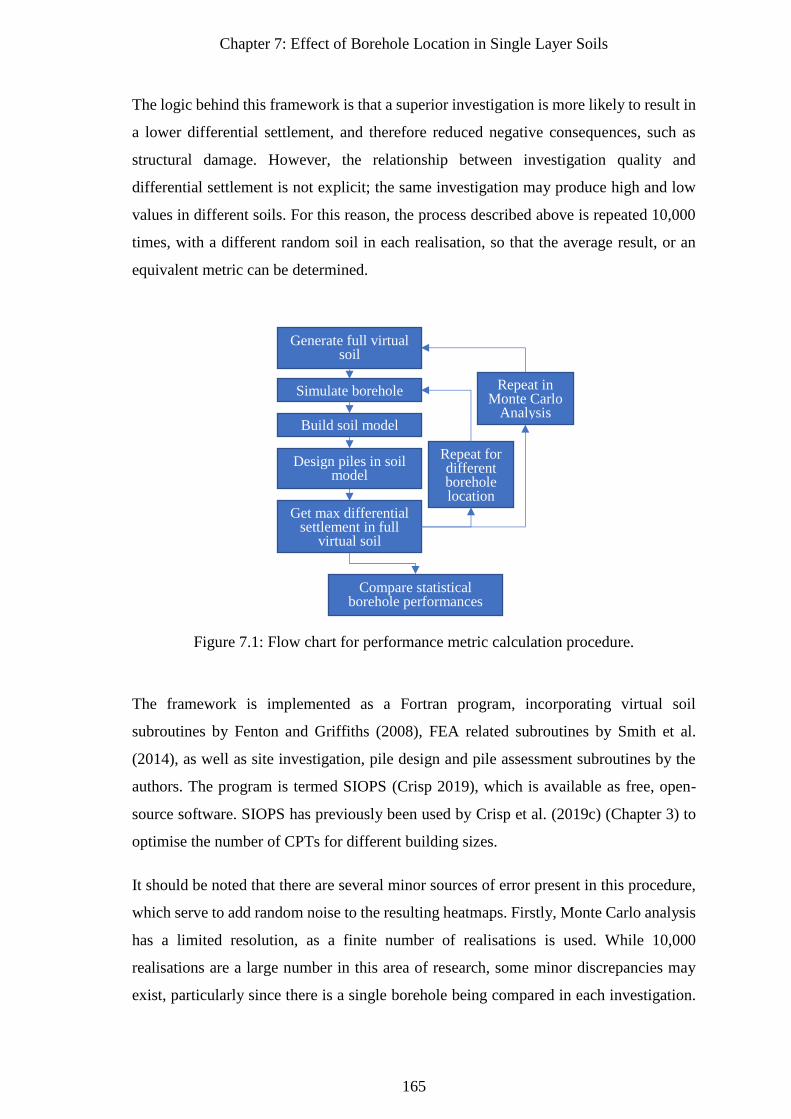
Chapter 7: Effect of Borehole Location in Single Layer Soils
165
The logic behind this framework is that a superior investigation is more likely to result in
a lower differential settlement, and therefore reduced negative consequences, such as
structural damage. However, the relationship between investigation quality and
differential settlement is not explicit; the same investigation may produce high and low
values in different soils. For this reason, the process described above is repeated 10,000
times, with a different random soil in each realisation, so that the average result, or an
equivalent metric can be determined.
Figure 7.1: Flow chart for performance metric calculation procedure.
The framework is implemented as a Fortran program, incorporating virtual soil
subroutines by Fenton and Griffiths (2008), FEA related subroutines by Smith et al.
(2014), as well as site investigation, pile design and pile assessment subroutines by the
authors. The program is termed SIOPS (Crisp 2019), which is available as free, open-
source software. SIOPS has previously been used by Crisp et al. (2019c) (Chapter 3) to
optimise the number of CPTs for different building sizes.
It should be noted that there are several minor sources of error present in this procedure,
which serve to add random noise to the resulting heatmaps. Firstly, Monte Carlo analysis
has a limited resolution, as a finite number of realisations is used. While 10,000
realisations are a large number in this area of research, some minor discrepancies may
exist, particularly since there is a single borehole being compared in each investigation.
Generate full virtual soil
Simulate borehole
Build soil model
Design piles in soil model
Compare statistical borehole performances
Repeat in Monte Carlo
Analysis
Get max differential settlement in full
virtual soil
Repeat for different borehole location
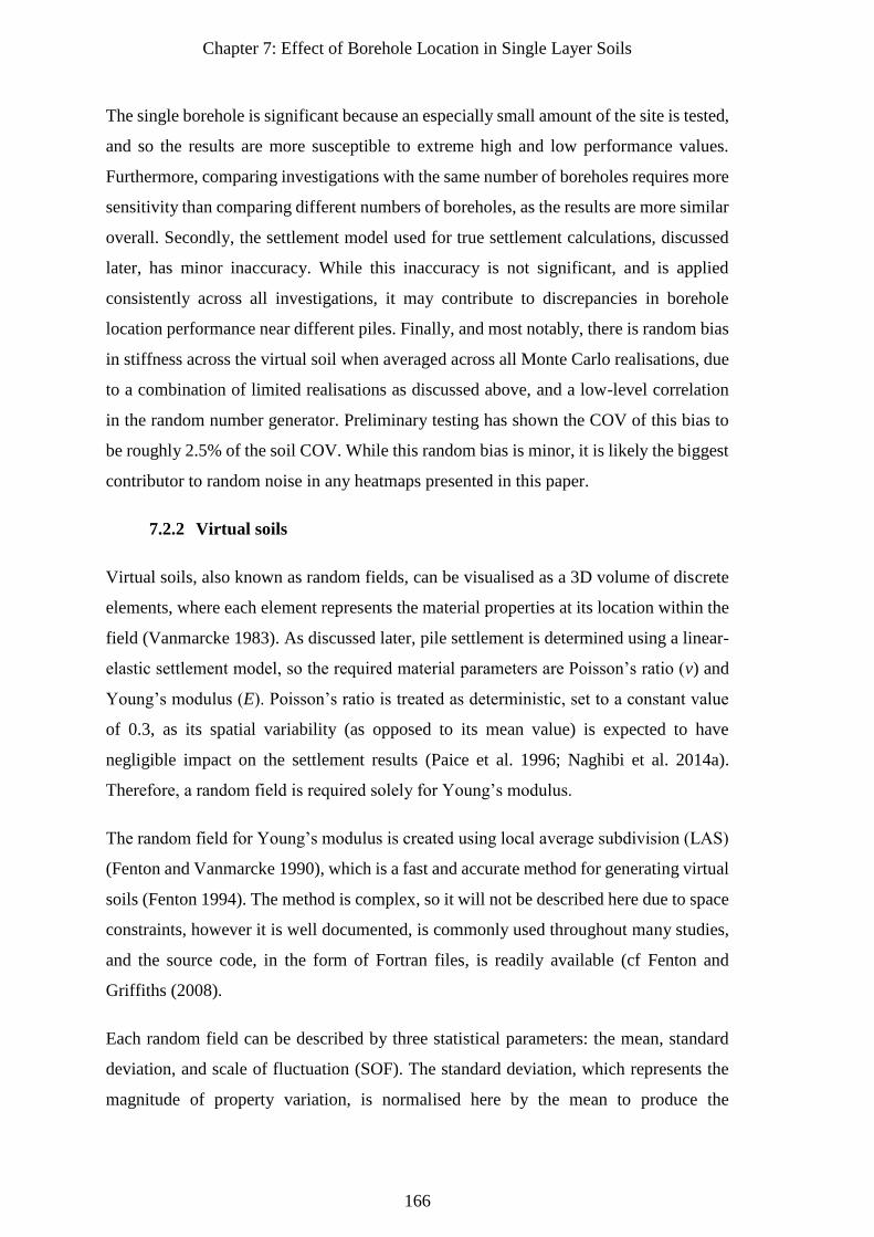
Chapter 7: Effect of Borehole Location in Single Layer Soils
166
The single borehole is significant because an especially small amount of the site is tested,
and so the results are more susceptible to extreme high and low performance values.
Furthermore, comparing investigations with the same number of boreholes requires more
sensitivity than comparing different numbers of boreholes, as the results are more similar
overall. Secondly, the settlement model used for true settlement calculations, discussed
later, has minor inaccuracy. While this inaccuracy is not significant, and is applied
consistently across all investigations, it may contribute to discrepancies in borehole
location performance near different piles. Finally, and most notably, there is random bias
in stiffness across the virtual soil when averaged across all Monte Carlo realisations, due
to a combination of limited realisations as discussed above, and a low-level correlation
in the random number generator. Preliminary testing has shown the COV of this bias to
be roughly 2.5% of the soil COV. While this random bias is minor, it is likely the biggest
contributor to random noise in any heatmaps presented in this paper.
7.2.2 Virtual soils
Virtual soils, also known as random fields, can be visualised as a 3D volume of discrete
elements, where each element represents the material properties at its location within the
field (Vanmarcke 1983). As discussed later, pile settlement is determined using a linear-
elastic settlement model, so the required material parameters are Poisson’s ratio (v) and
Young’s modulus (E). Poisson’s ratio is treated as deterministic, set to a constant value
of 0.3, as its spatial variability (as opposed to its mean value) is expected to have
negligible impact on the settlement results (Paice et al. 1996; Naghibi et al. 2014a).
Therefore, a random field is required solely for Young’s modulus.
The random field for Young’s modulus is created using local average subdivision (LAS)
(Fenton and Vanmarcke 1990), which is a fast and accurate method for generating virtual
soils (Fenton 1994). The method is complex, so it will not be described here due to space
constraints, however it is well documented, is commonly used throughout many studies,
and the source code, in the form of Fortran files, is readily available (cf Fenton and
Griffiths (2008).
Each random field can be described by three statistical parameters: the mean, standard
deviation, and scale of fluctuation (SOF). The standard deviation, which represents the
magnitude of property variation, is normalised here by the mean to produce the
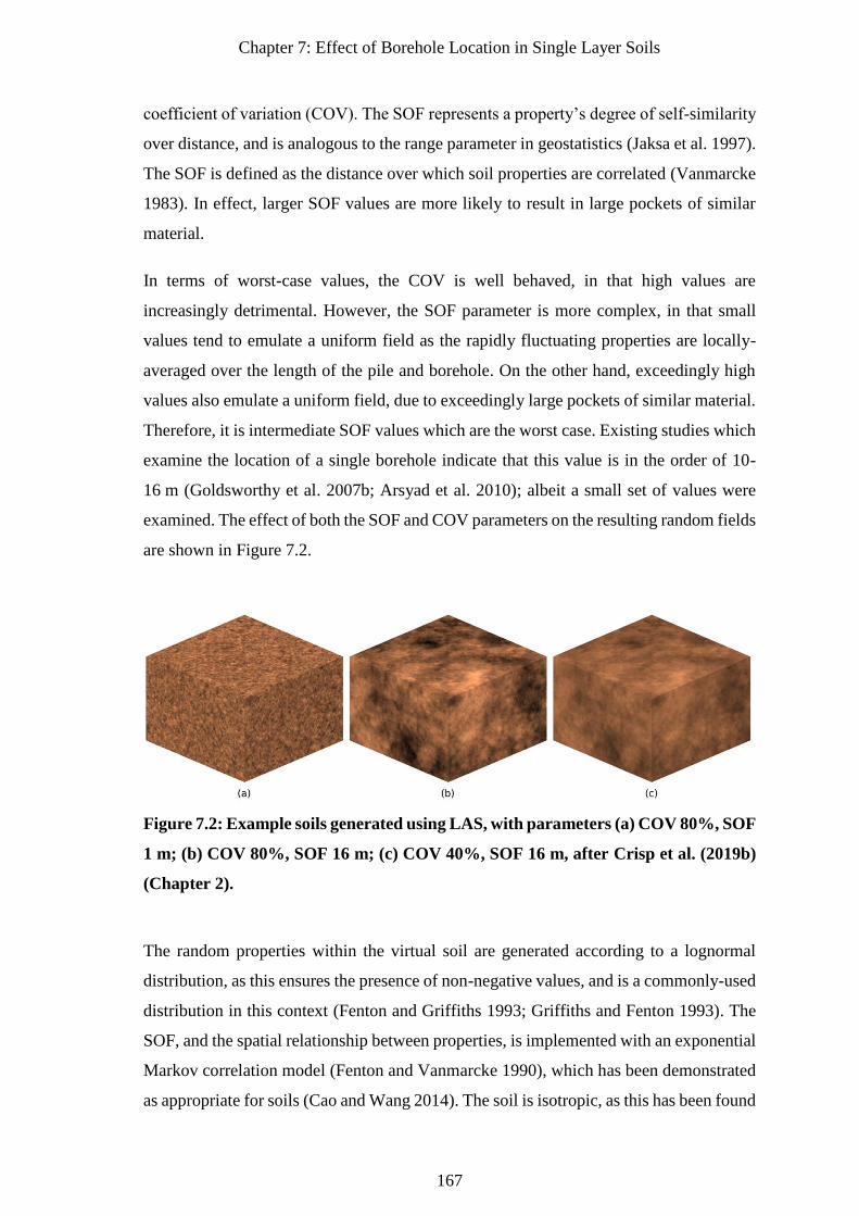
Chapter 7: Effect of Borehole Location in Single Layer Soils
167
coefficient of variation (COV). The SOF represents a property’s degree of self-similarity
over distance, and is analogous to the range parameter in geostatistics (Jaksa et al. 1997).
The SOF is defined as the distance over which soil properties are correlated (Vanmarcke
1983). In effect, larger SOF values are more likely to result in large pockets of similar
material.
In terms of worst-case values, the COV is well behaved, in that high values are
increasingly detrimental. However, the SOF parameter is more complex, in that small
values tend to emulate a uniform field as the rapidly fluctuating properties are locally-
averaged over the length of the pile and borehole. On the other hand, exceedingly high
values also emulate a uniform field, due to exceedingly large pockets of similar material.
Therefore, it is intermediate SOF values which are the worst case. Existing studies which
examine the location of a single borehole indicate that this value is in the order of 10-
16 m (Goldsworthy et al. 2007b; Arsyad et al. 2010); albeit a small set of values were
examined. The effect of both the SOF and COV parameters on the resulting random fields
are shown in Figure 7.2.
Figure 7.2: Example soils generated using LAS, with parameters (a) COV 80%, SOF
1 m; (b) COV 80%, SOF 16 m; (c) COV 40%, SOF 16 m, after Crisp et al. (2019b)
(Chapter 2).
The random properties within the virtual soil are generated according to a lognormal
distribution, as this ensures the presence of non-negative values, and is a commonly-used
distribution in this context (Fenton and Griffiths 1993; Griffiths and Fenton 1993). The
SOF, and the spatial relationship between properties, is implemented with an exponential
Markov correlation model (Fenton and Vanmarcke 1990), which has been demonstrated
as appropriate for soils (Cao and Wang 2014). The soil is isotropic, as this has been found
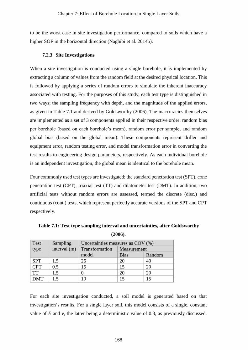
Chapter 7: Effect of Borehole Location in Single Layer Soils
168
to be the worst case in site investigation performance, compared to soils which have a
higher SOF in the horizontal direction (Naghibi et al. 2014b).
7.2.3 Site Investigations
When a site investigation is conducted using a single borehole, it is implemented by
extracting a column of values from the random field at the desired physical location. This
is followed by applying a series of random errors to simulate the inherent inaccuracy
associated with testing. For the purposes of this study, each test type is distinguished in
two ways; the sampling frequency with depth, and the magnitude of the applied errors,
as given in Table 7.1 and derived by Goldsworthy (2006). The inaccuracies themselves
are implemented as a set of 3 components applied in their respective order; random bias
per borehole (based on each borehole’s mean), random error per sample, and random
global bias (based on the global mean). These components represent driller and
equipment error, random testing error, and model transformation error in converting the
test results to engineering design parameters, respectively. As each individual borehole
is an independent investigation, the global mean is identical to the borehole mean.
Four commonly used test types are investigated; the standard penetration test (SPT), cone
penetration test (CPT), triaxial test (TT) and dilatometer test (DMT). In addition, two
artificial tests without random errors are assessed, termed the discrete (disc.) and
continuous (cont.) tests, which represent perfectly accurate versions of the SPT and CPT
respectively.
Table 7.1: Test type sampling interval and uncertainties, after Goldsworthy
(2006).
Test
type
Sampling
interval (m)
Uncertainties measures as COV (%)
Transformation
model
Measurement
Bias Random
SPT 1.5 25 20 40
CPT 0.5 15 15 20
TT 1.5 0 20 20
DMT 1.5 10 15 15
For each site investigation conducted, a soil model is generated based on that
investigation’s results. For a single layer soil, this model consists of a single, constant
value of E and v, the latter being a deterministic value of 0.3, as previously discussed.
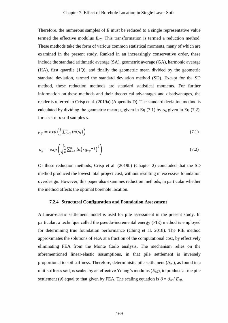
Chapter 7: Effect of Borehole Location in Single Layer Soils
169
Therefore, the numerous samples of E must be reduced to a single representative value
termed the effective modulus Eeff. This transformation is termed a reduction method.
These methods take the form of various common statistical moments, many of which are
examined in the present study. Ranked in an increasingly conservative order, these
include the standard arithmetic average (SA), geometric average (GA), harmonic average
(HA), first quartile (1Q), and finally the geometric mean divided by the geometric
standard deviation, termed the standard deviation method (SD). Except for the SD
method, these reduction methods are standard statistical moments. For further
information on these methods and their theoretical advantages and disadvantages, the
reader is referred to Crisp et al. (2019a) (Appendix D). The standard deviation method is
calculated by dividing the geometric mean μg given in Eq (7.1) by σg given in Eq (7.2),
for a set of n soil samples s.
𝜇𝑔 = 𝑒𝑥𝑝 (1
𝑛∑ 𝑙𝑛(𝑠𝑖)𝑛𝑖=1 ) (7.1)
𝜎𝑔 = 𝑒𝑥𝑝(√1
𝑛∑ 𝑙𝑛(𝑠𝑖𝜇𝑔−1)
2𝑛𝑖=1 ) (7.2)
Of these reduction methods, Crisp et al. (2019b) (Chapter 2) concluded that the SD
method produced the lowest total project cost, without resulting in excessive foundation
overdesign. However, this paper also examines reduction methods, in particular whether
the method affects the optimal borehole location.
7.2.4 Structural Configuration and Foundation Assessment
A linear-elastic settlement model is used for pile assessment in the present study. In
particular, a technique called the pseudo-incremental energy (PIE) method is employed
for determining true foundation performance (Ching et al. 2018). The PIE method
approximates the solutions of FEA at a fraction of the computational cost, by effectively
eliminating FEA from the Monte Carlo analysis. The mechanism relies on the
aforementioned linear-elastic assumptions, in that pile settlement is inversely
proportional to soil stiffness. Therefore, deterministic pile settlement (det), as found in a
unit-stiffness soil, is scaled by an effective Young’s modulus (Eeff), to produce a true pile
settlement () equal to that given by FEA. The scaling equation is = det/ Eeff.
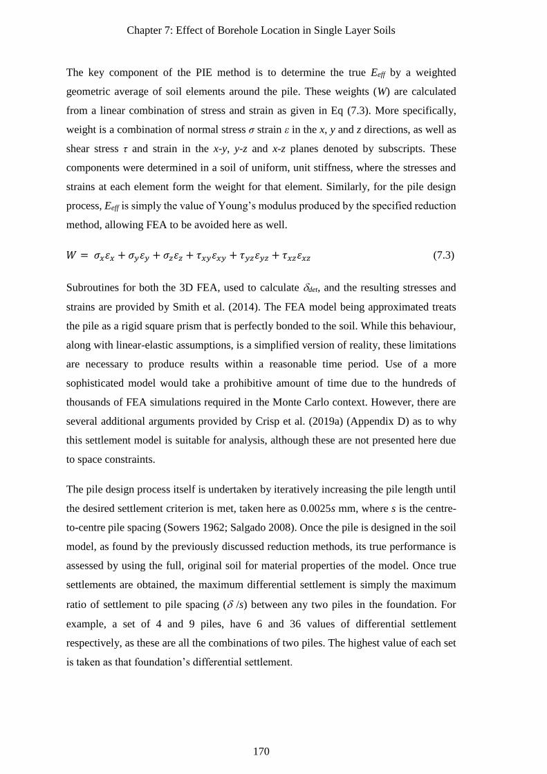
Chapter 7: Effect of Borehole Location in Single Layer Soils
170
The key component of the PIE method is to determine the true Eeff by a weighted
geometric average of soil elements around the pile. These weights (W) are calculated
from a linear combination of stress and strain as given in Eq (7.3). More specifically,
weight is a combination of normal stress σ strain ε in the x, y and z directions, as well as
shear stress τ and strain in the x-y, y-z and x-z planes denoted by subscripts. These
components were determined in a soil of uniform, unit stiffness, where the stresses and
strains at each element form the weight for that element. Similarly, for the pile design
process, Eeff is simply the value of Young’s modulus produced by the specified reduction
method, allowing FEA to be avoided here as well.
𝑊 = 𝜎𝑥휀𝑥 + 𝜎𝑦휀𝑦 + 𝜎𝑧휀𝑧 + 𝜏𝑥𝑦휀𝑥𝑦 + 𝜏𝑦𝑧휀𝑦𝑧 + 𝜏𝑥𝑧휀𝑥𝑧 (7.3)
Subroutines for both the 3D FEA, used to calculate det, and the resulting stresses and
strains are provided by Smith et al. (2014). The FEA model being approximated treats
the pile as a rigid square prism that is perfectly bonded to the soil. While this behaviour,
along with linear-elastic assumptions, is a simplified version of reality, these limitations
are necessary to produce results within a reasonable time period. Use of a more
sophisticated model would take a prohibitive amount of time due to the hundreds of
thousands of FEA simulations required in the Monte Carlo context. However, there are
several additional arguments provided by Crisp et al. (2019a) (Appendix D) as to why
this settlement model is suitable for analysis, although these are not presented here due
to space constraints.
The pile design process itself is undertaken by iteratively increasing the pile length until
the desired settlement criterion is met, taken here as 0.0025s mm, where s is the centre-
to-centre pile spacing (Sowers 1962; Salgado 2008). Once the pile is designed in the soil
model, as found by the previously discussed reduction methods, its true performance is
assessed by using the full, original soil for material properties of the model. Once true
settlements are obtained, the maximum differential settlement is simply the maximum
ratio of settlement to pile spacing ( /s) between any two piles in the foundation. For
example, a set of 4 and 9 piles, have 6 and 36 values of differential settlement
respectively, as these are all the combinations of two piles. The highest value of each set
is taken as that foundation’s differential settlement.
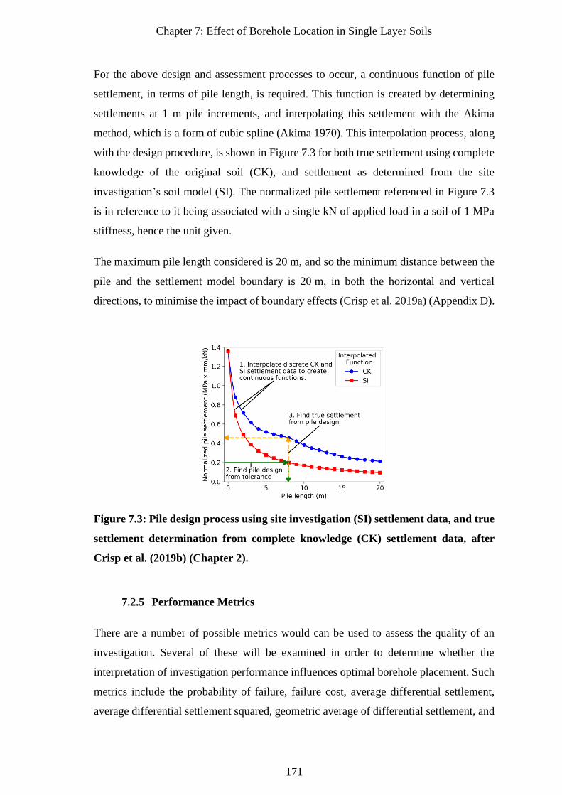
Chapter 7: Effect of Borehole Location in Single Layer Soils
171
For the above design and assessment processes to occur, a continuous function of pile
settlement, in terms of pile length, is required. This function is created by determining
settlements at 1 m pile increments, and interpolating this settlement with the Akima
method, which is a form of cubic spline (Akima 1970). This interpolation process, along
with the design procedure, is shown in Figure 7.3 for both true settlement using complete
knowledge of the original soil (CK), and settlement as determined from the site
investigation’s soil model (SI). The normalized pile settlement referenced in Figure 7.3
is in reference to it being associated with a single kN of applied load in a soil of 1 MPa
stiffness, hence the unit given.
The maximum pile length considered is 20 m, and so the minimum distance between the
pile and the settlement model boundary is 20 m, in both the horizontal and vertical
directions, to minimise the impact of boundary effects (Crisp et al. 2019a) (Appendix D).
Figure 7.3: Pile design process using site investigation (SI) settlement data, and true
settlement determination from complete knowledge (CK) settlement data, after
Crisp et al. (2019b) (Chapter 2).
7.2.5 Performance Metrics
There are a number of possible metrics would can be used to assess the quality of an
investigation. Several of these will be examined in order to determine whether the
interpretation of investigation performance influences optimal borehole placement. Such
metrics include the probability of failure, failure cost, average differential settlement,
average differential settlement squared, geometric average of differential settlement, and
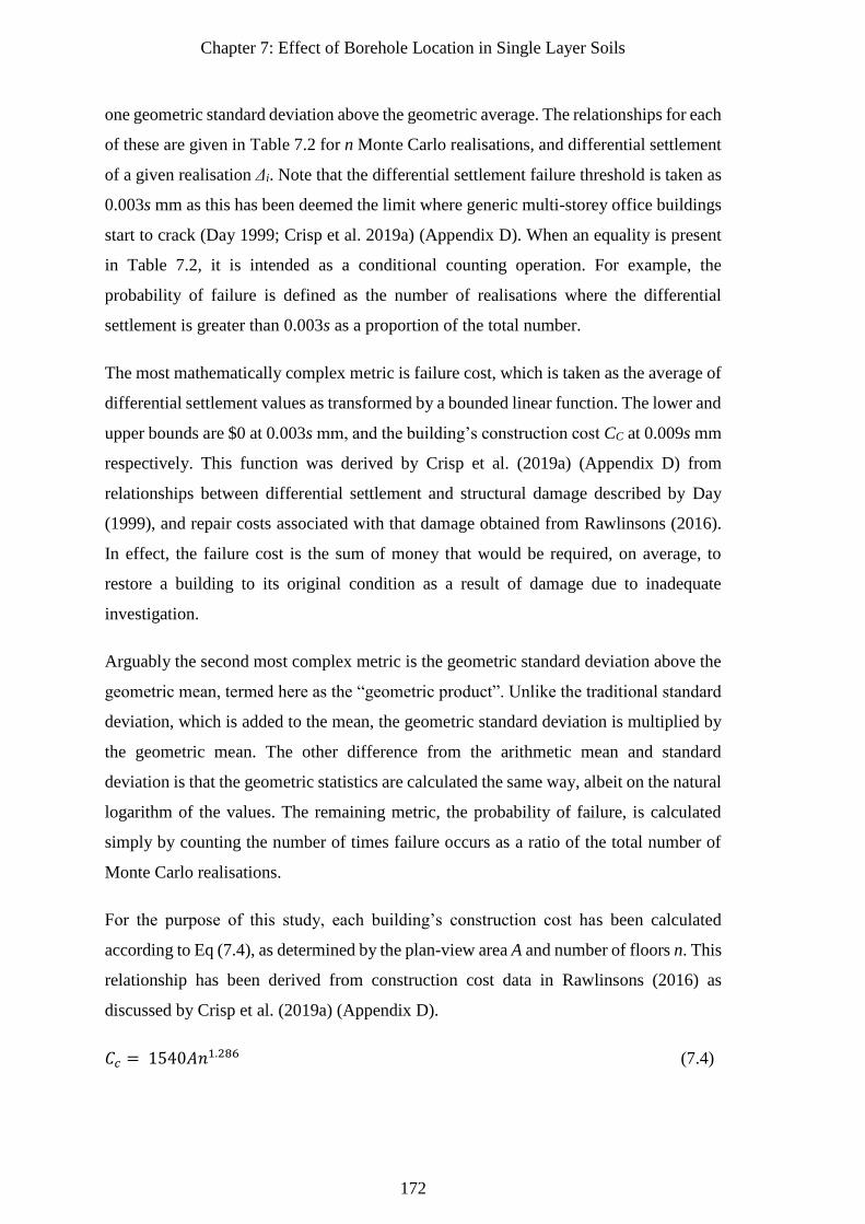
Chapter 7: Effect of Borehole Location in Single Layer Soils
172
one geometric standard deviation above the geometric average. The relationships for each
of these are given in Table 7.2 for n Monte Carlo realisations, and differential settlement
of a given realisation Δi. Note that the differential settlement failure threshold is taken as
0.003s mm as this has been deemed the limit where generic multi-storey office buildings
start to crack (Day 1999; Crisp et al. 2019a) (Appendix D). When an equality is present
in Table 7.2, it is intended as a conditional counting operation. For example, the
probability of failure is defined as the number of realisations where the differential
settlement is greater than 0.003s as a proportion of the total number.
The most mathematically complex metric is failure cost, which is taken as the average of
differential settlement values as transformed by a bounded linear function. The lower and
upper bounds are $0 at 0.003s mm, and the building’s construction cost CC at 0.009s mm
respectively. This function was derived by Crisp et al. (2019a) (Appendix D) from
relationships between differential settlement and structural damage described by Day
(1999), and repair costs associated with that damage obtained from Rawlinsons (2016).
In effect, the failure cost is the sum of money that would be required, on average, to
restore a building to its original condition as a result of damage due to inadequate
investigation.
Arguably the second most complex metric is the geometric standard deviation above the
geometric mean, termed here as the “geometric product”. Unlike the traditional standard
deviation, which is added to the mean, the geometric standard deviation is multiplied by
the geometric mean. The other difference from the arithmetic mean and standard
deviation is that the geometric statistics are calculated the same way, albeit on the natural
logarithm of the values. The remaining metric, the probability of failure, is calculated
simply by counting the number of times failure occurs as a ratio of the total number of
Monte Carlo realisations.
For the purpose of this study, each building’s construction cost has been calculated
according to Eq (7.4), as determined by the plan-view area A and number of floors n. This
relationship has been derived from construction cost data in Rawlinsons (2016) as
discussed by Crisp et al. (2019a) (Appendix D).
𝐶𝑐 = 1540𝐴𝑛1.286 (7.4)
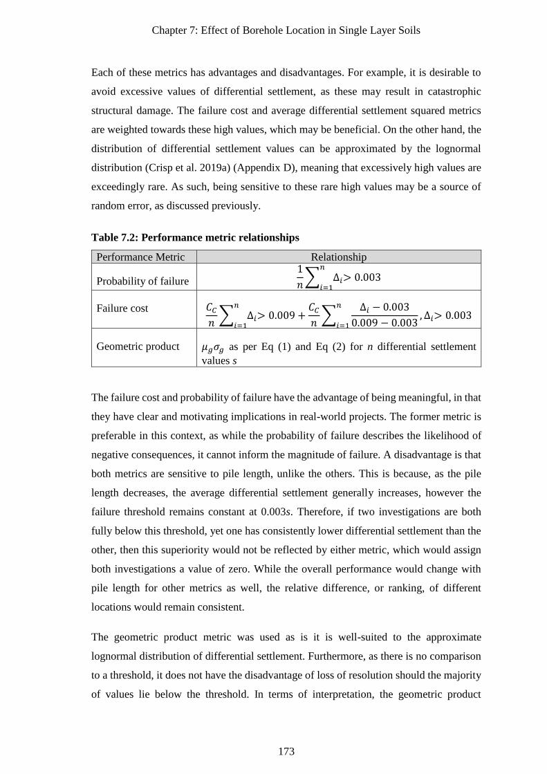
Chapter 7: Effect of Borehole Location in Single Layer Soils
173
Each of these metrics has advantages and disadvantages. For example, it is desirable to
avoid excessive values of differential settlement, as these may result in catastrophic
structural damage. The failure cost and average differential settlement squared metrics
are weighted towards these high values, which may be beneficial. On the other hand, the
distribution of differential settlement values can be approximated by the lognormal
distribution (Crisp et al. 2019a) (Appendix D), meaning that excessively high values are
exceedingly rare. As such, being sensitive to these rare high values may be a source of
random error, as discussed previously.
Table 7.2: Performance metric relationships
Performance Metric Relationship
Probability of failure 1
𝑛∑ ∆𝑖> 0.003
𝑛
𝑖=1
Failure cost 𝐶𝐶𝑛∑ ∆𝑖> 0.009
𝑛
𝑖=1+𝐶𝐶𝑛∑
∆𝑖 − 0.003
0.009 − 0.003, ∆𝑖> 0.003
𝑛
𝑖=1
Geometric product 𝜇𝑔𝜎𝑔 as per Eq (1) and Eq (2) for n differential settlement
values s
The failure cost and probability of failure have the advantage of being meaningful, in that
they have clear and motivating implications in real-world projects. The former metric is
preferable in this context, as while the probability of failure describes the likelihood of
negative consequences, it cannot inform the magnitude of failure. A disadvantage is that
both metrics are sensitive to pile length, unlike the others. This is because, as the pile
length decreases, the average differential settlement generally increases, however the
failure threshold remains constant at 0.003s. Therefore, if two investigations are both
fully below this threshold, yet one has consistently lower differential settlement than the
other, then this superiority would not be reflected by either metric, which would assign
both investigations a value of zero. While the overall performance would change with
pile length for other metrics as well, the relative difference, or ranking, of different
locations would remain consistent.
The geometric product metric was used as is it is well-suited to the approximate
lognormal distribution of differential settlement. Furthermore, as there is no comparison
to a threshold, it does not have the disadvantage of loss of resolution should the majority
of values lie below the threshold. In terms of interpretation, the geometric product
Chapter 7: Effect of Borehole Location in Single Layer Soils
174
approximates the 85th percentile, meaning there is an 85% probability that a differential
settlement value is lower than that given by the metric. More generally, lower values can
be interpreted as being less likely to result in failure.
7.2.6 Site Description
The virtual soil consists of a grid of 0.5 m cubic elements, as is commonly used in studies
in this field (Goldsworthy 2006), and due to computational constraints on RAM usage.
A single soil of 896 896 448 elements is generated, from which a random subset of
160 160 80 elements is extracted in a given Monte Carlo realisation, forming a soil
of equivalent size 80 80 40 m. Taking random subsets of a large field reduces the
computational run time by an order of magnitude, as opposed to regenerating the field
for each realisation. The aforementioned 2.5% averaged bias includes the bias from this
subdivision process, meaning that each subset is independent.
The above soil size allows for a variety of building sizes, up to 40 40 m, while still
allowing 20 m between the building and edge of the soil, as required for the settlement
model discussed previously. A pile spacing of 10 m is implemented, allowing for a
maximum of 25 piles arranged in a grid pattern over the building area. However, any
subset of this pile arrangement can also be investigated without having to re-process true
settlement. This optimization is possible because load can be distributed between the
piles, since settlement is linearly proportional to applied loads, and so the true settlement
curves can be scaled accordingly. As a result, heatmaps have been efficiently generated
for different numbers of piles, pile spacings, and building sizes, as given in later sections.
A 6-storey building is considered, as was the case by Crisp et al. (2019b) (Chapter 2) and
Crisp et al. (2020) (Chapter 5). In terms of loading, a 5 kPa dead load and 3 kPa live load
is applied. Each pile is assumed to carry an equal load and is therefore designed to the
same length. Due to the large variation of loading with different structural configurations,
as well as the variation of pile lengths with different reduction methods, the authors have
implemented an average pile length of roughly 6 m across all cases. This is achieved by
scaling the mean soil stiffness until the desired average length is reached. The process
involves beginning with a highly stiff soil, then iteratively decreasing this stiffness until
the pile length as increased to the desired value. The use of a constant pile length
Chapter 7: Effect of Borehole Location in Single Layer Soils
175
facilitates direct comparison between different cases, while at the same time ensuring that
a valid pile length can be found, between the aforementioned minimum and maximum.
7.3 Results and Discussion
A wide variety of analysis is considered in the present paper. Firstly, a comparison of
different performance metrics is conducted in order to find one that is easy to interpret.
Furthermore, this determines whether the definition of investigation quality has an impact
on optimal testing location. Similarly, comparisons of different test types, reduction
methods, and borehole depths are given to show if test inaccuracy, interpretation of
sample data, or quantity of information has an impact on sensitivity or optimal location.
Finally, the results are generalised to a variety of different soil conditions and structural
configurations so that they are widely applicable. As such, a range of different COVs and
SOFs are analysed, as well as different numbers of piles and pile spacings, to see the
effect on investigation performance with location.
In heatmaps throughout this paper, darker heatmap colours correspond to lower values,
which indicate more optimal placement, while the red squares show pile locations.
7.3.1 Performance Metric Comparison
This section is predominantly for the purpose of choosing an ideal performance metric
for subsequent analysis. An examination of the literature and preliminary analysis has
revealed that random noise is a problematic factor in heatmap interpretation. As such, an
ideal metric would be symmetric for a symmetric foundation, given that the soil is
stationary with a constant mean. Furthermore, ideal heatmaps have smooth contours, as
random noise is minimised.
A comparison of the six metrics has been conducted for a case of 4 piles supporting a 40
40 m, 6-storey building on a soil with COV 80% and SOF 20 m. The results are
presented in Figure 7.4 for a continuous borehole with no random errors applied and a
soil model derived from the standard deviation reduction method. Additional insight into
Figure 7.4 is given in Figure 7.5, which shows the average pile length, as well as the
failure cost in a soil with COV of 20%. This large 40 m pile spacing was chosen as it is
the clearest example of discrepancies across the various metrics examined. Furthermore,
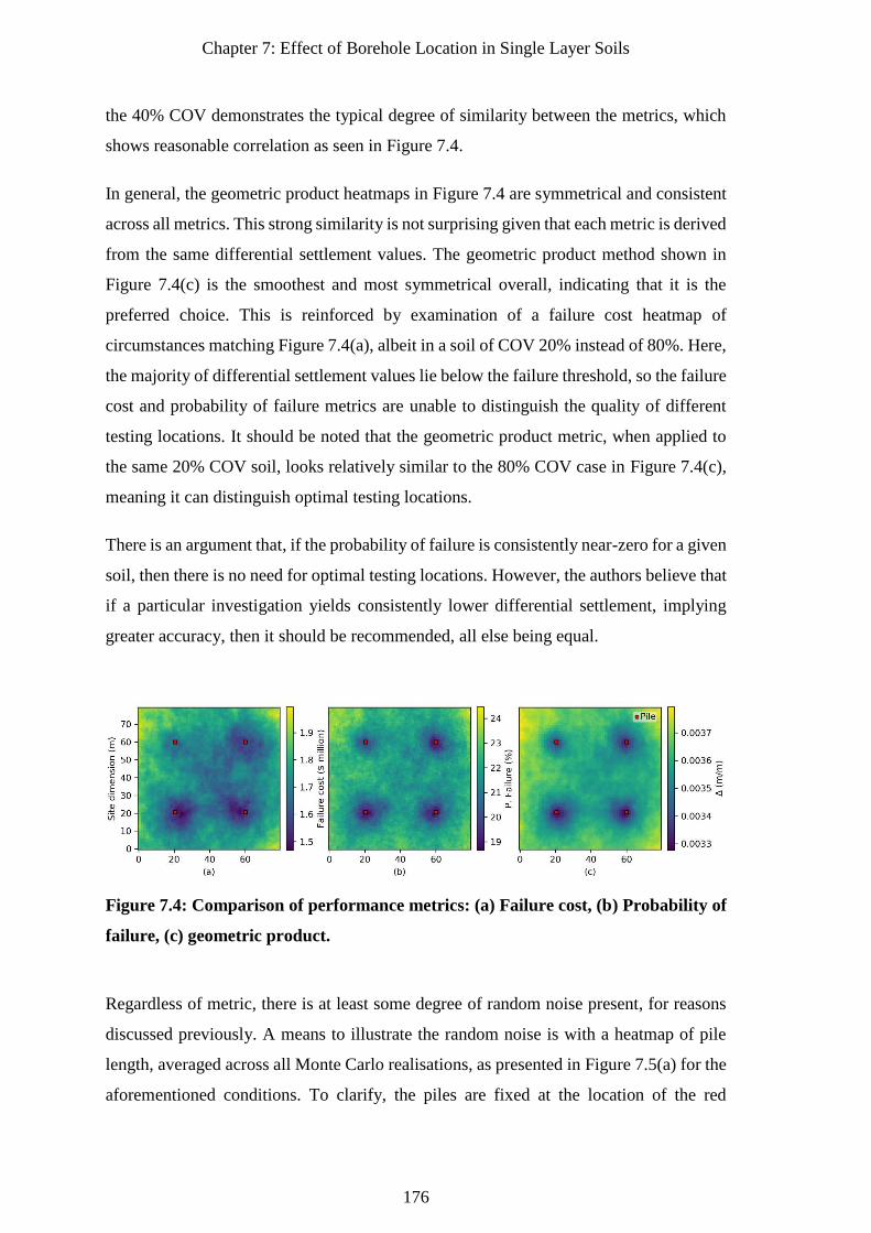
Chapter 7: Effect of Borehole Location in Single Layer Soils
176
the 40% COV demonstrates the typical degree of similarity between the metrics, which
shows reasonable correlation as seen in Figure 7.4.
In general, the geometric product heatmaps in Figure 7.4 are symmetrical and consistent
across all metrics. This strong similarity is not surprising given that each metric is derived
from the same differential settlement values. The geometric product method shown in
Figure 7.4(c) is the smoothest and most symmetrical overall, indicating that it is the
preferred choice. This is reinforced by examination of a failure cost heatmap of
circumstances matching Figure 7.4(a), albeit in a soil of COV 20% instead of 80%. Here,
the majority of differential settlement values lie below the failure threshold, so the failure
cost and probability of failure metrics are unable to distinguish the quality of different
testing locations. It should be noted that the geometric product metric, when applied to
the same 20% COV soil, looks relatively similar to the 80% COV case in Figure 7.4(c),
meaning it can distinguish optimal testing locations.
There is an argument that, if the probability of failure is consistently near-zero for a given
soil, then there is no need for optimal testing locations. However, the authors believe that
if a particular investigation yields consistently lower differential settlement, implying
greater accuracy, then it should be recommended, all else being equal.
Figure 7.4: Comparison of performance metrics: (a) Failure cost, (b) Probability of
failure, (c) geometric product.
Regardless of metric, there is at least some degree of random noise present, for reasons
discussed previously. A means to illustrate the random noise is with a heatmap of pile
length, averaged across all Monte Carlo realisations, as presented in Figure 7.5(a) for the
aforementioned conditions. To clarify, the piles are fixed at the location of the red
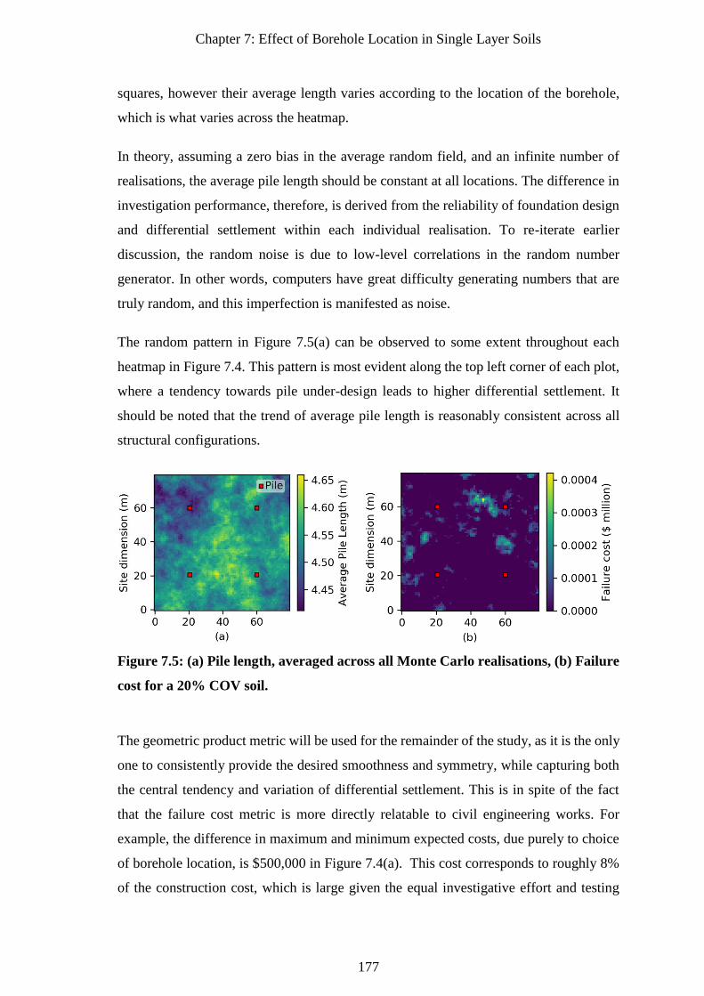
Chapter 7: Effect of Borehole Location in Single Layer Soils
177
squares, however their average length varies according to the location of the borehole,
which is what varies across the heatmap.
In theory, assuming a zero bias in the average random field, and an infinite number of
realisations, the average pile length should be constant at all locations. The difference in
investigation performance, therefore, is derived from the reliability of foundation design
and differential settlement within each individual realisation. To re-iterate earlier
discussion, the random noise is due to low-level correlations in the random number
generator. In other words, computers have great difficulty generating numbers that are
truly random, and this imperfection is manifested as noise.
The random pattern in Figure 7.5(a) can be observed to some extent throughout each
heatmap in Figure 7.4. This pattern is most evident along the top left corner of each plot,
where a tendency towards pile under-design leads to higher differential settlement. It
should be noted that the trend of average pile length is reasonably consistent across all
structural configurations.
Figure 7.5: (a) Pile length, averaged across all Monte Carlo realisations, (b) Failure
cost for a 20% COV soil.
The geometric product metric will be used for the remainder of the study, as it is the only
one to consistently provide the desired smoothness and symmetry, while capturing both
the central tendency and variation of differential settlement. This is in spite of the fact
that the failure cost metric is more directly relatable to civil engineering works. For
example, the difference in maximum and minimum expected costs, due purely to choice
of borehole location, is $500,000 in Figure 7.4(a). This cost corresponds to roughly 8%
of the construction cost, which is large given the equal investigative effort and testing
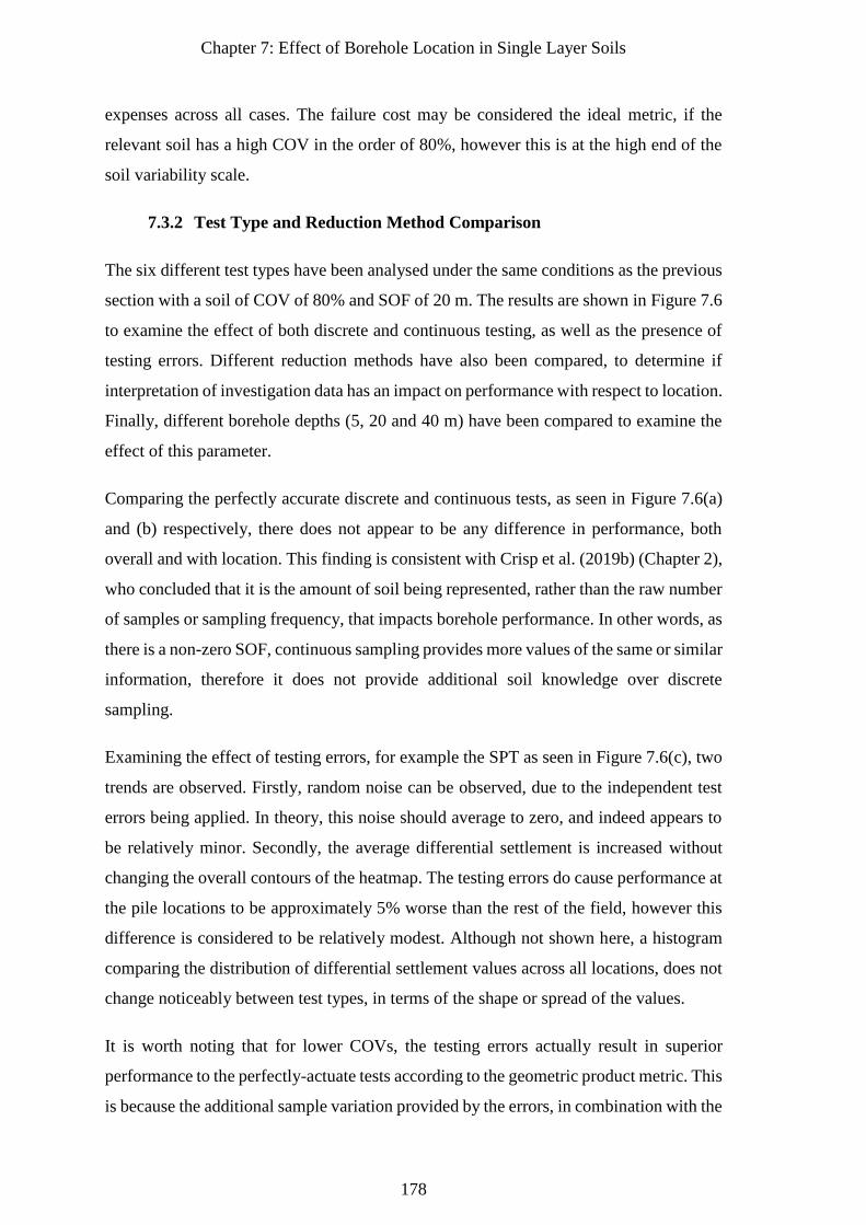
Chapter 7: Effect of Borehole Location in Single Layer Soils
178
expenses across all cases. The failure cost may be considered the ideal metric, if the
relevant soil has a high COV in the order of 80%, however this is at the high end of the
soil variability scale.
7.3.2 Test Type and Reduction Method Comparison
The six different test types have been analysed under the same conditions as the previous
section with a soil of COV of 80% and SOF of 20 m. The results are shown in Figure 7.6
to examine the effect of both discrete and continuous testing, as well as the presence of
testing errors. Different reduction methods have also been compared, to determine if
interpretation of investigation data has an impact on performance with respect to location.
Finally, different borehole depths (5, 20 and 40 m) have been compared to examine the
effect of this parameter.
Comparing the perfectly accurate discrete and continuous tests, as seen in Figure 7.6(a)
and (b) respectively, there does not appear to be any difference in performance, both
overall and with location. This finding is consistent with Crisp et al. (2019b) (Chapter 2),
who concluded that it is the amount of soil being represented, rather than the raw number
of samples or sampling frequency, that impacts borehole performance. In other words, as
there is a non-zero SOF, continuous sampling provides more values of the same or similar
information, therefore it does not provide additional soil knowledge over discrete
sampling.
Examining the effect of testing errors, for example the SPT as seen in Figure 7.6(c), two
trends are observed. Firstly, random noise can be observed, due to the independent test
errors being applied. In theory, this noise should average to zero, and indeed appears to
be relatively minor. Secondly, the average differential settlement is increased without
changing the overall contours of the heatmap. The testing errors do cause performance at
the pile locations to be approximately 5% worse than the rest of the field, however this
difference is considered to be relatively modest. Although not shown here, a histogram
comparing the distribution of differential settlement values across all locations, does not
change noticeably between test types, in terms of the shape or spread of the values.
It is worth noting that for lower COVs, the testing errors actually result in superior
performance to the perfectly-actuate tests according to the geometric product metric. This
is because the additional sample variation provided by the errors, in combination with the
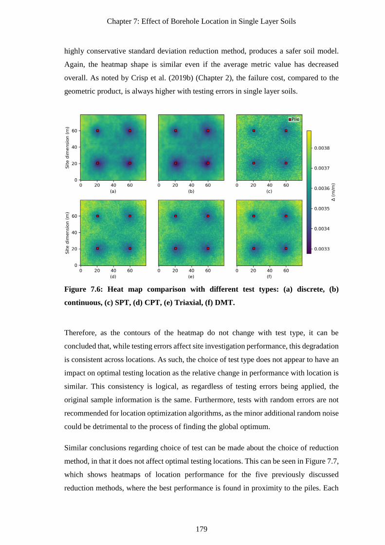
Chapter 7: Effect of Borehole Location in Single Layer Soils
179
highly conservative standard deviation reduction method, produces a safer soil model.
Again, the heatmap shape is similar even if the average metric value has decreased
overall. As noted by Crisp et al. (2019b) (Chapter 2), the failure cost, compared to the
geometric product, is always higher with testing errors in single layer soils.
Figure 7.6: Heat map comparison with different test types: (a) discrete, (b)
continuous, (c) SPT, (d) CPT, (e) Triaxial, (f) DMT.
Therefore, as the contours of the heatmap do not change with test type, it can be
concluded that, while testing errors affect site investigation performance, this degradation
is consistent across locations. As such, the choice of test type does not appear to have an
impact on optimal testing location as the relative change in performance with location is
similar. This consistency is logical, as regardless of testing errors being applied, the
original sample information is the same. Furthermore, tests with random errors are not
recommended for location optimization algorithms, as the minor additional random noise
could be detrimental to the process of finding the global optimum.
Similar conclusions regarding choice of test can be made about the choice of reduction
method, in that it does not affect optimal testing locations. This can be seen in Figure 7.7,
which shows heatmaps of location performance for the five previously discussed
reduction methods, where the best performance is found in proximity to the piles. Each
Chapter 7: Effect of Borehole Location in Single Layer Soils
180
heatmap has been normalised to have a zero-mean so that the variability of borehole
performance with location can be better compared. As such, Figure 7.7 does not convey
the reality that increasingly conservative reduction methods result in consistently
decreased average differential settlement. However, this behaviour has been previously
explored by Crisp et al. (2019b) (Chapter 2).
Figure 7.7: Reduction method comparison: (a) arithmetic average, (b) geometric
average, (c) harmonic average, (d) 1st quartile, (e) standard deviation.
Furthermore, two key conclusions can be drawn from Figure 7.7. Firstly, the more
conservative reduction methods, which also reflect sample variability, such as the first
quartile and standard deviation methods, appear to be less sensitive to borehole location
than the three averages. This conclusion is drawn from Figure 7.7(d, e) lacking values at
the extreme high and low ends of the spectrum compared to Figure 7.7(a-c). Therefore,
in addition to producing overall safer soil models, they infer a reduced penalty from
sampling at suboptimal locations, which is highly desirable.
Secondly, the aforementioned two reduction methods appear to be more immune to
random noise, which aids in the clarity of their interpretation. This immunity is at least
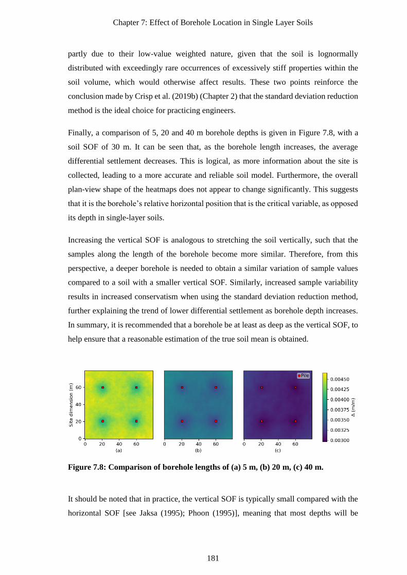
Chapter 7: Effect of Borehole Location in Single Layer Soils
181
partly due to their low-value weighted nature, given that the soil is lognormally
distributed with exceedingly rare occurrences of excessively stiff properties within the
soil volume, which would otherwise affect results. These two points reinforce the
conclusion made by Crisp et al. (2019b) (Chapter 2) that the standard deviation reduction
method is the ideal choice for practicing engineers.
Finally, a comparison of 5, 20 and 40 m borehole depths is given in Figure 7.8, with a
soil SOF of 30 m. It can be seen that, as the borehole length increases, the average
differential settlement decreases. This is logical, as more information about the site is
collected, leading to a more accurate and reliable soil model. Furthermore, the overall
plan-view shape of the heatmaps does not appear to change significantly. This suggests
that it is the borehole’s relative horizontal position that is the critical variable, as opposed
its depth in single-layer soils.
Increasing the vertical SOF is analogous to stretching the soil vertically, such that the
samples along the length of the borehole become more similar. Therefore, from this
perspective, a deeper borehole is needed to obtain a similar variation of sample values
compared to a soil with a smaller vertical SOF. Similarly, increased sample variability
results in increased conservatism when using the standard deviation reduction method,
further explaining the trend of lower differential settlement as borehole depth increases.
In summary, it is recommended that a borehole be at least as deep as the vertical SOF, to
help ensure that a reasonable estimation of the true soil mean is obtained.
Figure 7.8: Comparison of borehole lengths of (a) 5 m, (b) 20 m, (c) 40 m.
It should be noted that in practice, the vertical SOF is typically small compared with the
horizontal SOF [see Jaksa (1995); Phoon (1995)], meaning that most depths will be
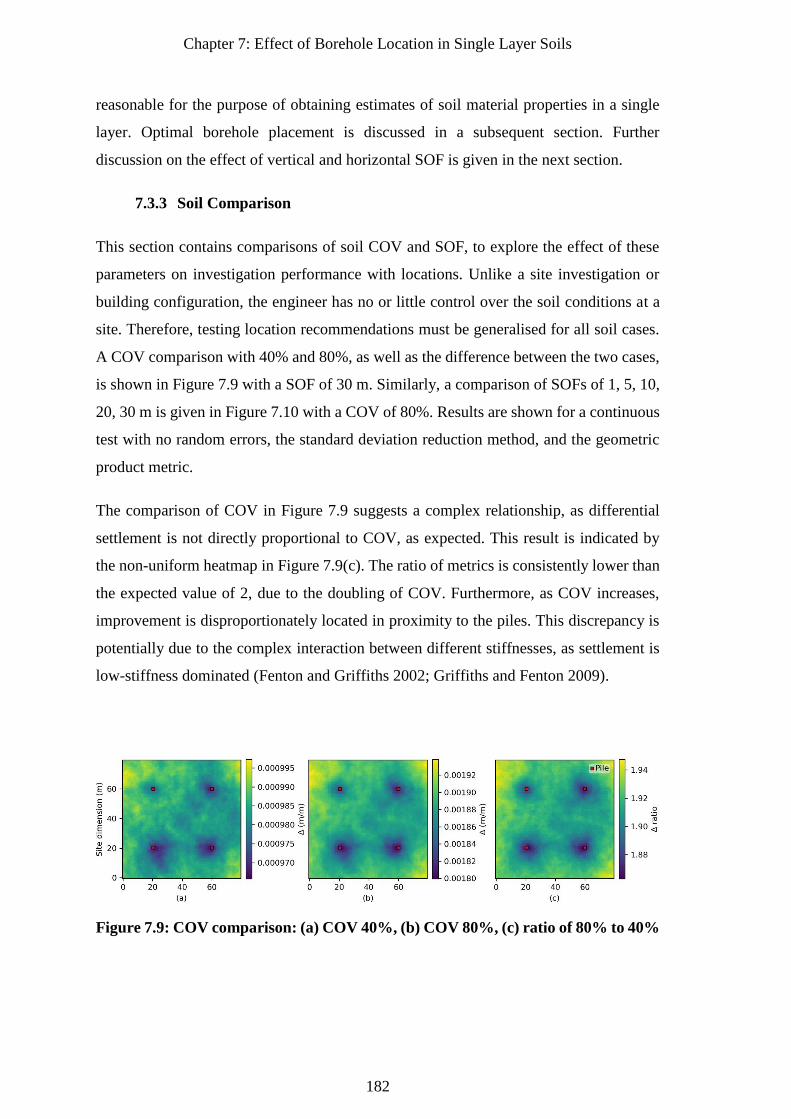
Chapter 7: Effect of Borehole Location in Single Layer Soils
182
reasonable for the purpose of obtaining estimates of soil material properties in a single
layer. Optimal borehole placement is discussed in a subsequent section. Further
discussion on the effect of vertical and horizontal SOF is given in the next section.
7.3.3 Soil Comparison
This section contains comparisons of soil COV and SOF, to explore the effect of these
parameters on investigation performance with locations. Unlike a site investigation or
building configuration, the engineer has no or little control over the soil conditions at a
site. Therefore, testing location recommendations must be generalised for all soil cases.
A COV comparison with 40% and 80%, as well as the difference between the two cases,
is shown in Figure 7.9 with a SOF of 30 m. Similarly, a comparison of SOFs of 1, 5, 10,
20, 30 m is given in Figure 7.10 with a COV of 80%. Results are shown for a continuous
test with no random errors, the standard deviation reduction method, and the geometric
product metric.
The comparison of COV in Figure 7.9 suggests a complex relationship, as differential
settlement is not directly proportional to COV, as expected. This result is indicated by
the non-uniform heatmap in Figure 7.9(c). The ratio of metrics is consistently lower than
the expected value of 2, due to the doubling of COV. Furthermore, as COV increases,
improvement is disproportionately located in proximity to the piles. This discrepancy is
potentially due to the complex interaction between different stiffnesses, as settlement is
low-stiffness dominated (Fenton and Griffiths 2002; Griffiths and Fenton 2009).
Figure 7.9: COV comparison: (a) COV 40%, (b) COV 80%, (c) ratio of 80% to 40%
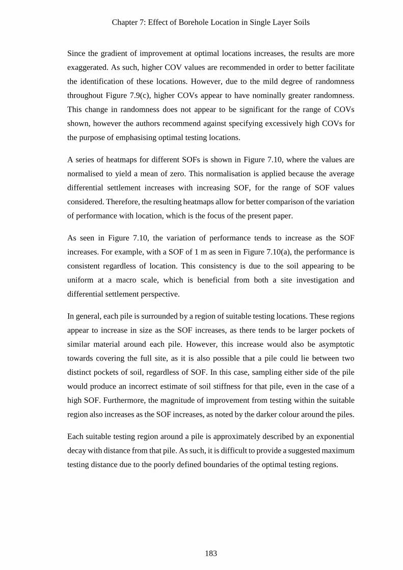
Chapter 7: Effect of Borehole Location in Single Layer Soils
183
Since the gradient of improvement at optimal locations increases, the results are more
exaggerated. As such, higher COV values are recommended in order to better facilitate
the identification of these locations. However, due to the mild degree of randomness
throughout Figure 7.9(c), higher COVs appear to have nominally greater randomness.
This change in randomness does not appear to be significant for the range of COVs
shown, however the authors recommend against specifying excessively high COVs for
the purpose of emphasising optimal testing locations.
A series of heatmaps for different SOFs is shown in Figure 7.10, where the values are
normalised to yield a mean of zero. This normalisation is applied because the average
differential settlement increases with increasing SOF, for the range of SOF values
considered. Therefore, the resulting heatmaps allow for better comparison of the variation
of performance with location, which is the focus of the present paper.
As seen in Figure 7.10, the variation of performance tends to increase as the SOF
increases. For example, with a SOF of 1 m as seen in Figure 7.10(a), the performance is
consistent regardless of location. This consistency is due to the soil appearing to be
uniform at a macro scale, which is beneficial from both a site investigation and
differential settlement perspective.
In general, each pile is surrounded by a region of suitable testing locations. These regions
appear to increase in size as the SOF increases, as there tends to be larger pockets of
similar material around each pile. However, this increase would also be asymptotic
towards covering the full site, as it is also possible that a pile could lie between two
distinct pockets of soil, regardless of SOF. In this case, sampling either side of the pile
would produce an incorrect estimate of soil stiffness for that pile, even in the case of a
high SOF. Furthermore, the magnitude of improvement from testing within the suitable
region also increases as the SOF increases, as noted by the darker colour around the piles.
Each suitable testing region around a pile is approximately described by an exponential
decay with distance from that pile. As such, it is difficult to provide a suggested maximum
testing distance due to the poorly defined boundaries of the optimal testing regions.
Chapter 7: Effect of Borehole Location in Single Layer Soils
184
Figure 7.10: Mean-normalised heatmaps for a SOF of (a) 1 m, (b), 5 m, (c) 10 m, (d)
20 m, (e) 30 m.
Regarding the impact of horizontal vs vertical SOF, the authors speculate that the
horizontal SOF affects the size of the suitable testing region around a pile. This is because
the correlation between the soil properties at the pile and at a borehole are purely
horizontal in nature. In contrast, the vertical SOF would impact the magnitude of
improvement from testing within the suitable region. For example, regardless of the
horizontal SOF, if the vertical SOF is low, then the collection of samples from a borehole
would be similar at any location. In summary, horizontal SOF affects the shape of the
heatmap, while vertical SOF affects the magnitude of improvement or the colour.
7.3.4 Structural Configuration Comparison
Building configuration has been explored through two separate analyses; that of varying
the number of piles with a constant area, and of varying the building area and pile spacing
with 4 piles. These results are presented in Figure 7.11 and Figure 7.12, respectively, with
a SOF of 20 m and COV of 80%. The former figure has been normalised to provide a
zero-mean, while the latter uses the original values.
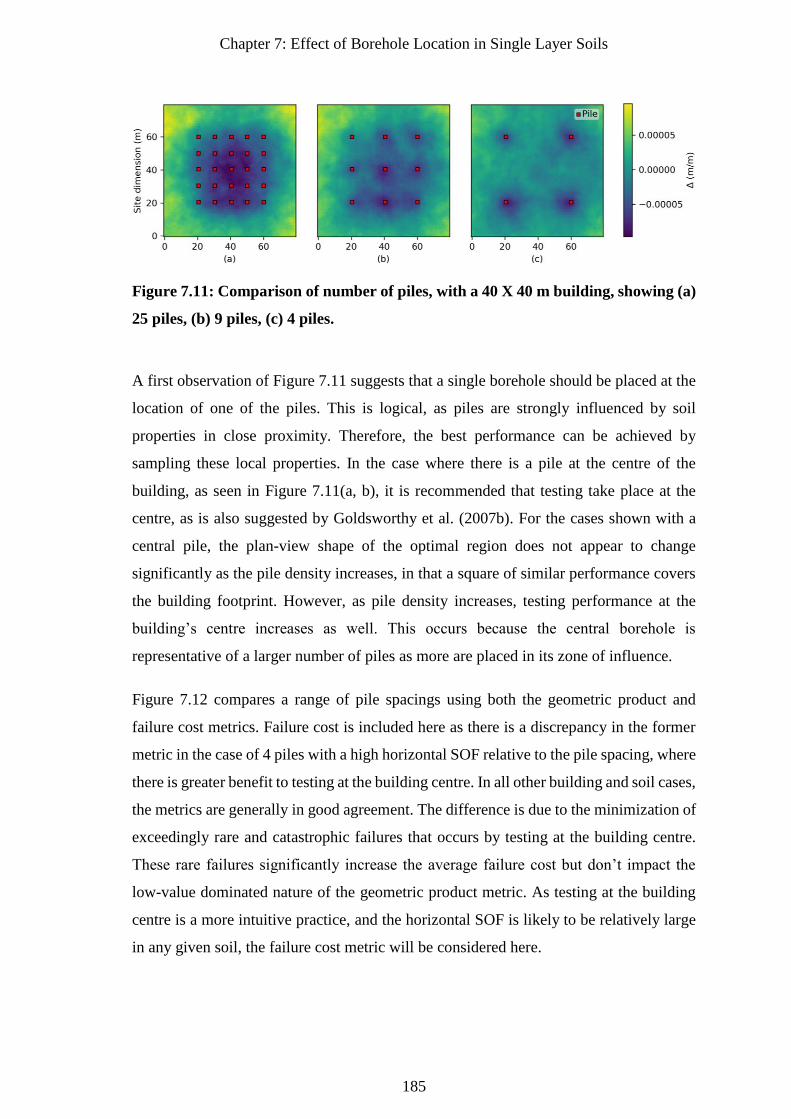
Chapter 7: Effect of Borehole Location in Single Layer Soils
185
Figure 7.11: Comparison of number of piles, with a 40 X 40 m building, showing (a)
25 piles, (b) 9 piles, (c) 4 piles.
A first observation of Figure 7.11 suggests that a single borehole should be placed at the
location of one of the piles. This is logical, as piles are strongly influenced by soil
properties in close proximity. Therefore, the best performance can be achieved by
sampling these local properties. In the case where there is a pile at the centre of the
building, as seen in Figure 7.11(a, b), it is recommended that testing take place at the
centre, as is also suggested by Goldsworthy et al. (2007b). For the cases shown with a
central pile, the plan-view shape of the optimal region does not appear to change
significantly as the pile density increases, in that a square of similar performance covers
the building footprint. However, as pile density increases, testing performance at the
building’s centre increases as well. This occurs because the central borehole is
representative of a larger number of piles as more are placed in its zone of influence.
Figure 7.12 compares a range of pile spacings using both the geometric product and
failure cost metrics. Failure cost is included here as there is a discrepancy in the former
metric in the case of 4 piles with a high horizontal SOF relative to the pile spacing, where
there is greater benefit to testing at the building centre. In all other building and soil cases,
the metrics are generally in good agreement. The difference is due to the minimization of
exceedingly rare and catastrophic failures that occurs by testing at the building centre.
These rare failures significantly increase the average failure cost but don’t impact the
low-value dominated nature of the geometric product metric. As testing at the building
centre is a more intuitive practice, and the horizontal SOF is likely to be relatively large
in any given soil, the failure cost metric will be considered here.
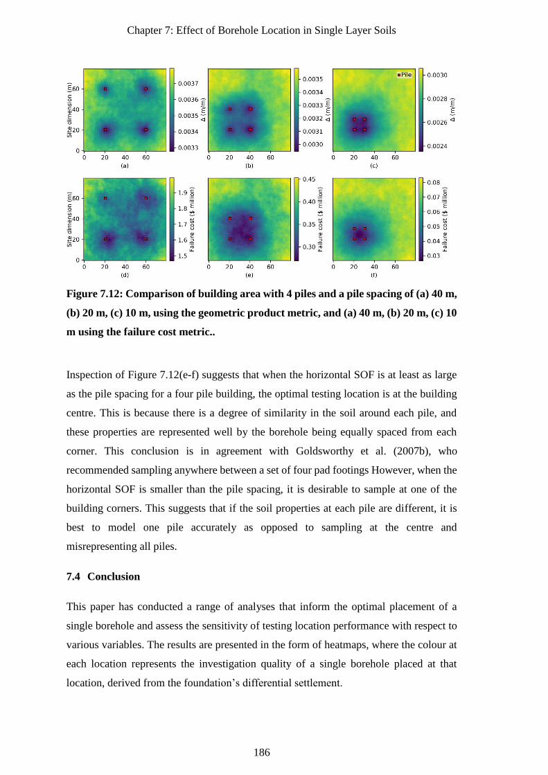
Chapter 7: Effect of Borehole Location in Single Layer Soils
186
Figure 7.12: Comparison of building area with 4 piles and a pile spacing of (a) 40 m,
(b) 20 m, (c) 10 m, using the geometric product metric, and (a) 40 m, (b) 20 m, (c) 10
m using the failure cost metric..
Inspection of Figure 7.12(e-f) suggests that when the horizontal SOF is at least as large
as the pile spacing for a four pile building, the optimal testing location is at the building
centre. This is because there is a degree of similarity in the soil around each pile, and
these properties are represented well by the borehole being equally spaced from each
corner. This conclusion is in agreement with Goldsworthy et al. (2007b), who
recommended sampling anywhere between a set of four pad footings However, when the
horizontal SOF is smaller than the pile spacing, it is desirable to sample at one of the
building corners. This suggests that if the soil properties at each pile are different, it is
best to model one pile accurately as opposed to sampling at the centre and
misrepresenting all piles.
7.4 Conclusion
This paper has conducted a range of analyses that inform the optimal placement of a
single borehole and assess the sensitivity of testing location performance with respect to
various variables. The results are presented in the form of heatmaps, where the colour at
each location represents the investigation quality of a single borehole placed at that
location, derived from the foundation’s differential settlement.
Chapter 7: Effect of Borehole Location in Single Layer Soils
187
It was found that for all building sizes and soil conditions, a single borehole is best placed
at the building’s centre when a central pile is present. A central borehole is also ideal for
buildings with four piles where the horizontal scale of fluctuation is at least as high as the
pile spacing. Otherwise, the borehole is best placed at a corner of the building at one of
the four piles. These results are related purely to the determination of the soil’s material
properties, and do not consider the presence of multiple layers with undulating
boundaries. Analysis of such a multi-layer soil is a candidate for future work. Failure cost
analysis has shown that the difference between optimal and suboptimal placement can be
over 8% of the building’s construction cost for a single borehole.
It should be noted that the heatmaps throughout the paper are only valid for the case of a
single borehole, and do not necessarily indicate optimal placement for two or more.
Optimising the location of multiple boreholes is an area for future study, potentially
through the use of a multi-dimensional optimization algorithm.
While many of the variables were found to affect the relative performance of different
testing locations, the impact has been shown to be minor or negligible. In particular, the
test type and coefficient of variation (COV) have no notable impact on the shape of the
investigation quality heatmaps. More conservative reduction methods, which also reflect
the variability of site investigation samples, are moderately less sensitive to borehole
location, meaning that there is a reduced penalty from testing at suboptimal locations.
The standard deviation reduction method is highly recommended for use by practicing
engineers due to this relative insensitivity to location, and because it has been previously
shown to minimise total project cost and differential settlement.
Regarding the clarity of heat maps, a set of parameter choices are specifically
recommended to minimise random noise and improve interpretation. The objective
function to be minimised is that of taking a geometric standard deviation of differential
settlement above the geometric mean. This metric was found to be relatively insensitive
to random noise in the fitness landscape, without affecting the underlying results.
Furthermore, this function has other advantages, including being interpreted as
minimising the probability of excessive values of differential settlement, which may lead
to catastrophic failure. The metric agrees with heatmaps of failure cost in the vast
majority of cases. Similarly, the standard deviation reduction method is recommended
for reasons given above. As the presence of testing errors add randomness to the fitness
Chapter 7: Effect of Borehole Location in Single Layer Soils
188
landscape, but do not change the shape of its surface, they should not be considered when
producing heatmaps. Finally, it is recommended to use a relatively low COV, as this has
also been shown to minimise random noise, as well as a moderately high SOF to make
the fitness landscape more defined.
7.5 References
Akima, H. 1970. A new method of interpolation and smooth curve fitting based on local
procedures. Journal of the ACM (JACM), 17(4), 589-602.
Albatal, A. 2013. Effect of inadequate site investigation on the cost and time of a
construction project. Masters Thesis, Construction and Building Engineering
Department, Arab Academy for Science, Technology and Maritime Transport,
Cairo.
Arsyad, A., Jaksa, M. B., Kaggwa, W., and Mitani, Y. 2010. Effect of radial distance of
a single CPT sounding on the probability of over-and under-design of pile
foundation. In Proceedings of the tthe First Makassar International Conference on
Civil Engineering, Makassar, Indonesia.
Bustamante, M., and Gianeselli, L. 1982. Pile bearing capacity prediction by means of
static penetrometer CPT. In Proceedings of the 2-nd European Symposium on
Penetration Testing.
Cao, Z., and Wang, Y. 2014. Bayesian model comparison and selection of spatial
correlation functions for soil parameters. Structural Safety, 49, 10-17. doi:
http://dx.doi.org/10.1016/j.strusafe.2013.06.003
Ching, J., Hu, Y. G., and Phoon, K. K. 2018. Effective Young’s modulus of a spatially
variable soil mass under a footing. Structural Safety, 73, 99-113.
Crisp, M. P. (2019). Site Investigation Optimisation for Piles using Statistics (SIOPS).
Crisp, M. P., Jaksa, M. B., and Kuo, Y. L. 2017. The influence of Site Investigation Scope
on Pile Design in Multi-layered, 2D Variable Ground. In Proceedings of the Geo-
Risk 2017, Denver, Colorado, USA.
Crisp, M. P., Jaksa, M. B., and Kuo, Y. L. 2018. Influence of Site Investigation Borehole
Pattern and Area on Pile Foundation Performance. In Proceedings of the 12th
ANZ Young Geotechnical Professionals Conference, Hobart.
Crisp, M. P., Jaksa, M. B., and Kuo, Y. L. 2019a. Framework for the Optimisation of Site
Investigations for Pile Designs in Complex Multi-Layered Soil, Research Report,
School of Civil, Environmental and Mining Engineering. doi:
10.13140/RG.2.2.23536.71685
Crisp, M. P., Jaksa, M. B., and Kuo, Y. L. 2019b. Toward a generalized guideline to
inform optimal site investigations for pile design. Canadian Geotechnical Journal.
Chapter 7: Effect of Borehole Location in Single Layer Soils
189
Crisp, M. P., Jaksa, M. B., and Kuo, Y. L. 2019c. Towards Optimal Site Investigations
for Generalized Structural Configurations. In Proceedings of the 7th International
Symposium on Geotechnical Safety and Risk, Taipei.
Crisp, M. P., Jaksa, M. B., and Kuo, Y. L. 2020. Characterising Site Investigation
Performance in a Two Layer Soil Profile. Canadian Journal of Civil Engineering.
Day, R. W. 1999. Forensic geotechnical and foundation engineering: McGraw-Hill New
York.
Fenton, G. A. 1994. Error evaluation of three random-field generators. Journal of
Engineering Mechanics, 120(12), 2478-2497.
Fenton, G. A., and Griffiths, D. 1993. Statistics of block conductivity through a simple
bounded stochastic medium. Water Resources Research, 29(6), 1825-1830.
Fenton, G. A., and Griffiths, D. V. 2002. Probabilistic foundation settlement on spatially
random soil. Journal of Geotechnical and Geoenvironmental Engineering, 128(5),
381-390.
Fenton, G. A., and Griffiths, D. V. 2008. Risk assessment in geotechnical engineering.
Hoboken: Wiley.
Fenton, G. A., and Vanmarcke, E. H. 1990. Simulation of random fields via local average
subdivision. Journal of Engineering Mechanics, 116(8), 1733-1749.
Goldsworthy, J. S. 2006. Quantifying the risk of geotechnical site investigations. Ph.D
Thesis, School of Civil, Environmental and Mining Engineering, University of
Adelaide, Adelaide.
Goldsworthy, J. S., Jaksa, M. B., Fenton, G. A., Griffiths, D. V., Kaggwa, W. S., and
Poulos, H. G. 2007a. Measuring the risk of geotechnical site investigations. In
Proceedings of the Proc., Geo-Denver 2007.
Goldsworthy, J. S., Jaksa, M. B., Fenton, G. A., Kaggwa, G. S., Griffiths, D. V., Poulos,
H. G., and Kuo, Y. L. 2004. Influence of site investigations on the design of pad
footings. In Proceedings of the Australia-New Zealand Conference on
Geomechanics (9th: 2004: Auckland, NZ).
Goldsworthy, J. S., Jaksa, M. B., Fenton, G. A., Kaggwa, W. S., Griffiths, D. V., and
Poulos, H. G. 2007b. Effect of sample location on the reliability based design of
pad foundations. Georisk, 1(3), 155-166.
Griffiths, D., and Fenton, G. A. 1993. Seepage beneath water retaining structures founded
on spatially random soil. Géotechnique, 43(4), 577-587.
Griffiths, D. V., and Fenton, G. A. 2009. Probabilistic settlement analysis by stochastic
and random finite-element methods. Journal of Geotechnical and
Geoenvironmental Engineering, 135(11), 1629-1637.
Chapter 7: Effect of Borehole Location in Single Layer Soils
190
Jaksa, M. B. 1995. The influence of spatial variability on the geotechnical design
properties of a stiff, overconsolidated clay. Ph.D Thesis, School of Civil,
Environmental and Mining Engineering, University of Adelaide, Adelaide.
Jaksa, M. B., Brooker, P. I., and Kaggwa, W. S. 1997. Modelling the spatial variability
of the undrained shear strength of clay soils using geostatistics. In Proceedings of
the Proc. of 5th Int. Geostatistics Congress, Wollongong.
Jaksa, M. B., Kaggwa, W. S., Fenton, G. A., and Poulos, H. G. 2003. A framework for
quantifying the reliability of geotechnical investigations. In Proceedings of the
9th International Conference on the Application of Statistics and Probability in
Civil Engineering.
Naghibi, F., Fenton, G. A., and Griffiths, D. V. 2014a. Prediction of pile settlement in an
elastic soil. Computers and Geotechnics, 60, 29-32.
Naghibi, F., Fenton, G. A., and Griffiths, D. V. 2014b. Serviceability limit state design
of deep foundations. Géotechnique, 64(10), 787-799.
Paice, G., Griffiths, D., and Fenton, G. A. 1996. Finite element modeling of settlements
on spatially random soil. Journal of Geotechnical Engineering, 122(9), 777-779.
Phoon, K.-K. 1995. Reliability-based design of foundations for transmission line
structures. Ph.D Thesis, School of Civil and Environmental Engineering, Cornell
University, Ithaca.
Rawlinsons, A. (2016). Australian Construction Handbook (34 ed., pp. 1005). Perth,
Australia: Rawlhouse Publishing Pty. Ltd.
Salgado, R. 2008. The engineering of foundations (Vol. 888): McGraw-Hill New York.
Schmertmann, J. H. 1970. Static cone to compute static settlement over sand. Journal of
Soil Mechanics & Foundations Div.
Smith, I. M., Griffiths, D. V., and Margetts, L. 2014. Programming the finite element
method (5th ed.): John Wiley & Sons.
Sowers, G. (1962). Shallow foundations (Vol. 569): McGraw-Hill, New York, NY.
Vanmarcke, E. H. 1983. Random Fields: Analysis and Synthesis. London: MIT Press.
Chapter 8: Optimization of Borehole Locations in All Soils
191
8 Chapter 8: Optimization of
Borehole Locations in All Soils
Paper Title:
Optimal Testing Locations in Geotechnical Site
Investigations through the Application of a Genetic
Algorithm

Chapter 8: Optimization of Borehole Locations in All Soils
192

Statement of AuthorshipTitle of Paper Optimal Testing Locations in Geotechnical Site Investigations through the Application of a
Genetic Algorithm.
Publication Status
Publication Details Crisp, M. P., Jaksa, M. B., and Kuo, Y. L. 2020. Optimal Testing Locations in Geotechnical Site
Investigations through the Application of a Genetic Algorithm. Geosciences, 10(7), 265. doi:
10.3390/geosciences10070265
Principal Author
Name of Principal Author (Candidate) Michael Perry Crisp
Contribution to the Paper
Modified the software and methodology, generated and visualized the data, wrote the
manuscript.
Overall percentage (%) 80%
Certification: This paper reports on original research I conducted during the period of my Higher Degree by
Research candidature and is not subject to any obligations or contractual agreements with a
third party that would constrain its inclusion in this thesis. I am the primary author of this paper.
Signature Date
Co-Author Contributions
By signing the Statement of Authorship, each author certifies that:
i. the candidate’s stated contribution to the publication is accurate (as detailed above);
ii. permission is granted for the candidate in include the publication in the thesis; and
iii. the sum of all co-author contributions is equal to 100% less the candidate’s stated contribution.
Name of Co-Author Mark Jaksa
Contribution to the Paper Provided primary supervision of work, contributed to the methodology, helped evaluate and edit
the manuscript.
Signature
Date
Name of Co-Author Yien Lik Kuo
Contribution to the Paper Provided secondary supervision of work, contributed to the methodology, provided support with
software development.
Signature Date
Please cut and paste additional co-author panels here as required.
Published Accepted for Publication
Submitted for PublicationUnpublished and Unsubmitted work written in manuscript style
24 October 2020
24 October 2020
24 October 2020

Chapter 8: Optimization of Borehole Locations in All Soils
194
Chapter 8: Optimization of Borehole Locations in All Soils
195
Abstract
Geotechnical site investigations are an essential prerequisite for reliable foundation
designs. However, there is relatively little quantitative guidance for planning optimal
investigations, including the choice of testing location. This study uses a genetic
algorithm to find the ideal testing locations of various numbers of boreholes with respect
to pile foundation performance. The optimization has been done separately for single-
layer and multi-layer soils, which infer what is best for obtaining soil material properties,
and delineating layer boundaries respectively. A sensitivity analysis was conducted to
find the genetic algorithm parameters that result in high quality solutions within a
reasonable timeframe. While boreholes arranged in a regular grid pattern provide good
performance in many cases, there are instances where optimised locations provide a cost
saving of A$2 million, or 4.2% of the construction cost. A set of recommended testing
guidelines are provided.
Keywords: Monte Carlo analysis, genetic algorithm, site investigations, optimization
Chapter 8: Optimization of Borehole Locations in All Soils
196
8.1 Introduction
Site investigations, consisting of soil testing, are essential for determining subsurface
material properties relevant to geotechnical engineering works, such as foundations. It
has been shown that variation in placement of a single borehole can impact total project
cost in excess of A$500,000, or 25% of the building’s construction cost (Crisp et al.
2020b) (Chapter 7). Furthermore, optimal placement of a small number of boreholes has
been shown to outperform suboptimal placement of a larger number (Crisp et al. 2020c)
(Chapter 5). As such, testing location has a significant impact on foundation performance.
However, despite this, there is little research regarding optimal test placement relative to
a foundation. There are various standards and suggestions currently available, however
these are not soil-specific nor project-specific. For example, (British Standards 1999;
Shukla and Sivakugan 2011) suggest a borehole spacing of 10-30 m for multi-story
structures, regardless of the soil complexity. Furthermore, the suggested range of
borehole spacing is quite broad, and does not inform specific testing locations.
This study addresses this gap by applying a genetic algorithm (GA) to optimise borehole
locations and make generalised recommendations. Specifically, these subsurface
investigations are for determining ground deformation properties with respect to pile
design. A GA is a metaheuristic, iterative algorithm that uses a population to search a
solution space or fitness landscape. It works through applying the evolutionary processes
of mating, mutation, and survival-of-the fittest. Further information on GAs is provided
by Haupt and Haupt (2004), along with code used as a basis for the present study. The
objective function to be minimised is a representative value of the foundation’s
differential settlement. This information is generated through a Monte Carlo (Ang 2007)
procedure introduced by Jaksa et al. (2003) and refined by Crisp et al. (2019a) (Appendix
D). This framework is in turn based on the random finite element method (RFEM) first
used by Fenton and Griffiths (1993); Griffiths and Fenton (1993), with additional
information given by Fenton and Griffiths (2008).
The present procedure is comprised of multiple steps; generating a virtual soil,
conducting a site investigation, designing a foundation based on the investigation results,
and calculating differential settlement of the designed foundation in the original virtual
soil. These steps are applied independently within each Monte Carlo realisation, such that
a single investigation is associated with a range of differential settlement values across
Chapter 8: Optimization of Borehole Locations in All Soils
197
the realisation set. The advantage of this statistical method is that it provides optimal
locations that are based on a soil of a given type, as opposed to being ideal for a single
soil realisation, to the detriment of similar soils. In other words, if the soil at a site has
similar attributes and statistical descriptions to the soil case being optimised, the results
should be applicable to that site. Furthermore, the GA does not require a pre-existing
notion of an optimal solution. Rather, in theory, it can find a true global solution from an
arbitrary initial condition. The program used in the present study is the bespoke Site
Investigation Optimization of Piles using Statistics (SIOPS), which is open source and
free to use by researchers and practicing engineers (Crisp 2020a).
Existing research studying the comparison of testing locations includes Crisp et al.
(2020b) (Chapter 7), who optimised the location of a single borehole for a range of pile
configurations in a single layer soil. It was concluded that a single borehole should be
placed at a building’s centre, except in the case of 4 piles, where it should be located at a
building corner. Similar conclusions were made by Goldsworthy et al. (2007b) in the
context of pad footings. Crisp et al. (2018) (Appendix B) and Goldsworthy et al. (2007a)
examined the effect of applying boreholes in a regular grid compared to other spatial
patterns and varying degrees of location randomness, and found that the regular grid
resulted in the lowest average project cost. Similarly, Crisp et al. (2017) (Appendix A)
compared regular grid and random sampling using a simplified 2D analysis of a two layer
system, and found the former to increase the probability of optimal design. However,
these studies only explored a fixed set of investigations, which cannot guarantee a global
optimum if it lies outside this set.
An alternative framework for optimising locations was presented by Gong et al. (2016),
who used a bi-objective GA to optimise the statistical robustness of a characterised site
for a given level of site investigation effort. This is presumably achieved through
optimising borehole locations in a single-layer soil. However, optimal borehole locations
were not discussed, and the framework has not been used to this end in subsequent
studies. A limitation of this approach is that the metric of a characterised site’s statistical
robustness is difficult to interpret in a meaningful way by practicing engineers, as it
cannot be directly related to foundation performance. While it demonstrates that more
thorough investigation provides a more accurate soil model, it does not inform what level
of accuracy is sufficient, and so cannot recommend a specific investigation. This is
Chapter 8: Optimization of Borehole Locations in All Soils
198
especially true, given that different investigations may be optimal for different
foundations, as their performance is often dominated by local soil properties rather than
the site as a whole. As such, it can be argued that this framework does not optimise site
investigation performance with respect to foundation performance. Similarly, Huang et
al. (2020) employed Voronoi tessellation to spread an arbitrary number of boreholes
evenly over a potentially irregular area, showing that these testing locations can improve
statistical robustness. However, this approach is subject to the same limitations as those
of Gong et al. (2016).
Crisp et al. (2020b) (Chapter 7) investigated a range of performance metrics for
optimising borehole locations, including failure cost, probability of failure, average
differential settlement, and a geometric standard deviation above the geometric mean of
differential settlement. The latter, termed the geometric product, was suggested as the
best metric for optimising locations, due to the smoothness of the fitness landscape,
consistency across different magnitudes of differential settlement, and ease of
interpretation due to its relationship with excessive differential settlement. Finally, Crisp
et al. (2020b) (Chapter 7) concluded that optimal testing, of a single borehole location,
was relatively insensitive to the choice of test type, magnitude of soil variability, and
degree of conservatism in the interpretation of soil samples. These conclusions are
valuable, as the insensitivity of many parameters allows them to be eliminated from the
present analysis, greatly simplifying the recommendations.
Additional research in optimising site investigations has been undertaken by Crisp et al.
(2019c, 2019d, 2019b) (Chapter 2, Chapter 3, Appendix C) in regards to single layer soils
and Crisp et al. (2020a); Crisp et al. (2020c) (Chapter 5, Chapter 6) in regards to multiple-
layer soils. However, all of these studies focused on optimising the number of boreholes
in an investigation and other attributes not related to sample locations, such as test type
and manner of sample interpretation. These studies assumed that the boreholes were
arranged over a regular grid.
A number of limitations are present across the aforementioned studies which examine
testing location performance with respect to foundation performance. Firstly, location
optimization has only been explored for a single borehole location or otherwise out of a
small, fixed set of locations. Furthermore, these location studies have examined single-
layer soil profiles, which do not account for the additional uncertainty introduced by the
Chapter 8: Optimization of Borehole Locations in All Soils
199
presence of unknown layer boundaries. Finally, no studies were found that optimise site
investigations, specifically for foundation performance, through the use of evolutionary
algorithms such as the genetic algorithm. The specific aims of this paper are therefore to:
1. Demonstrate that a GA can be used to solve the problem of optimal testing
locations and to optimise the GA parameters for speed of convergence.
2. Apply a GA to truly optimise locations of different numbers of boreholes with
regards to various pile configurations in both variable, single-layer soils and
multiple layer soils.
3. Based on the above results, make generalised recommendations for ideal testing
locations independently for estimating material properties and layer boundaries
respectively.
It should be noted that this paper is not intended to inform the optimal number of
boreholes nor borehole spacing. Rather, it is to suggest ideal sampling patterns or layouts
for given numbers of boreholes, and for varying pile configurations. The resulting
recommendations are for plan-view locations in the horizontal plane. In contrast, the
optimization of borehole depth is beyond the scope of this study.
8.2 Methodology
8.2.1 Overview
An overview of the procedures is given in the following sections. Where additional
background or verification is needed, the authors refer the reader to Crisp et al. (2019a)
(Appendix D) for general information, and Crisp (2020b) (Appendix E) for information
specific to the genetic algorithm or software involved. The latter document also acts as a
succinct version of the essential information from the former. A flow chart showing the
location optimization process is shown in Figure 8.1, which summarises steps associated
with the GA and the core investigation assessment components.
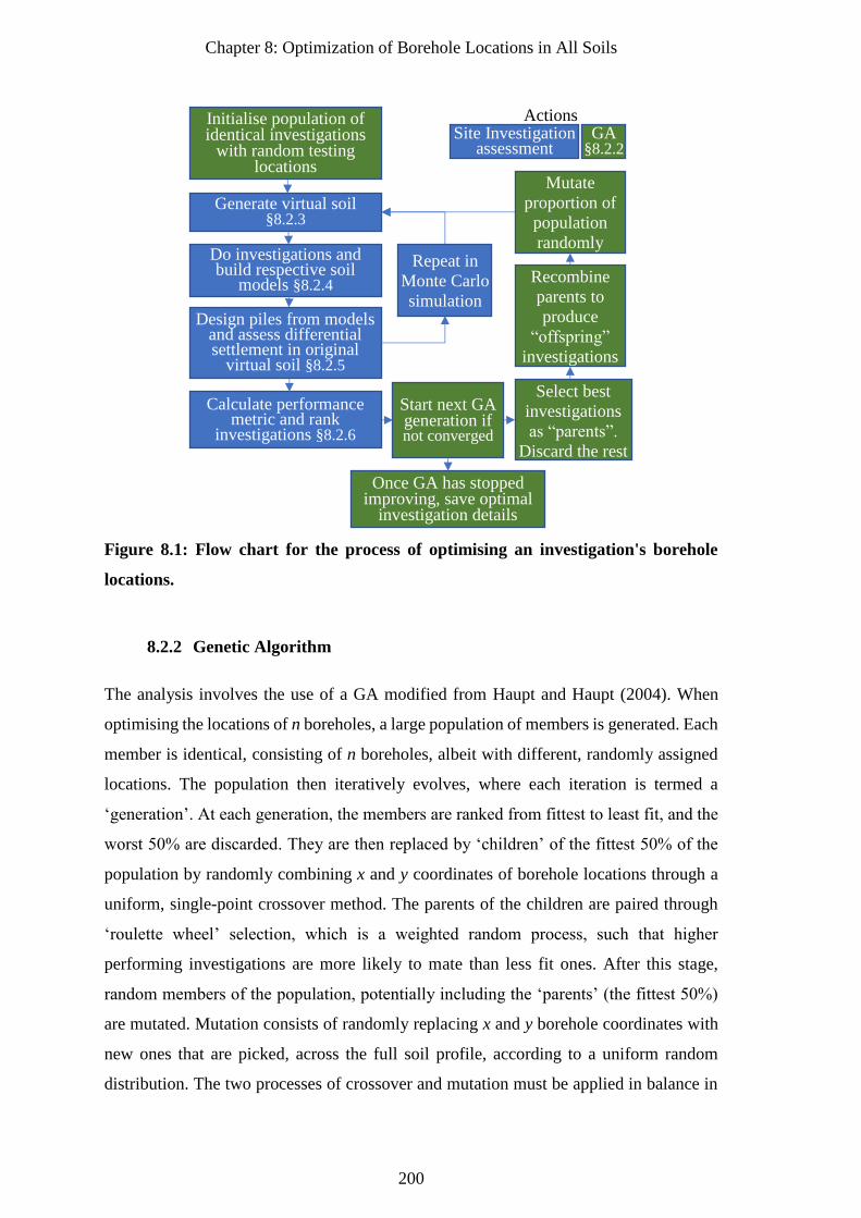
Chapter 8: Optimization of Borehole Locations in All Soils
200
Figure 8.1: Flow chart for the process of optimising an investigation's borehole
locations.
8.2.2 Genetic Algorithm
The analysis involves the use of a GA modified from Haupt and Haupt (2004). When
optimising the locations of n boreholes, a large population of members is generated. Each
member is identical, consisting of n boreholes, albeit with different, randomly assigned
locations. The population then iteratively evolves, where each iteration is termed a
‘generation’. At each generation, the members are ranked from fittest to least fit, and the
worst 50% are discarded. They are then replaced by ‘children’ of the fittest 50% of the
population by randomly combining x and y coordinates of borehole locations through a
uniform, single-point crossover method. The parents of the children are paired through
‘roulette wheel’ selection, which is a weighted random process, such that higher
performing investigations are more likely to mate than less fit ones. After this stage,
random members of the population, potentially including the ‘parents’ (the fittest 50%)
are mutated. Mutation consists of randomly replacing x and y borehole coordinates with
new ones that are picked, across the full soil profile, according to a uniform random
distribution. The two processes of crossover and mutation must be applied in balance in
Initialise population of identical investigations
with random testing locations
Generate virtual soil §8.2.3
Do investigations and build respective soil
models §8.2.4
Design piles from models and assess differential settlement in original
virtual soil §8.2.5
Once GA has stopped improving, save optimal
investigation details
Start next GA generation if not converged
Calculate performance metric and rank
investigations §8.2.6
Repeat in
Monte Carlo
simulation
Select best
investigations
as “parents”.
Discard the rest
Recombine
parents to
produce
“offspring”
investigations
Mutate
proportion of
population
randomly
GA §8.2.2
Site Investigation assessment
Actions
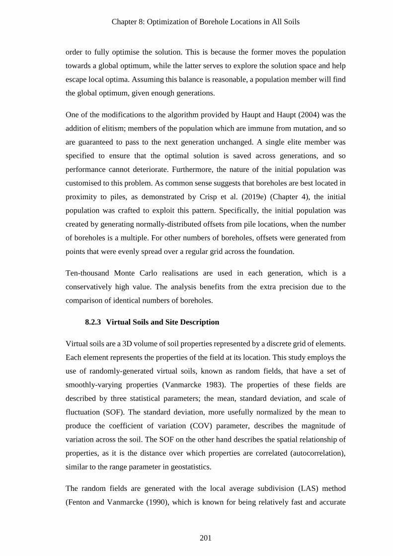
Chapter 8: Optimization of Borehole Locations in All Soils
201
order to fully optimise the solution. This is because the former moves the population
towards a global optimum, while the latter serves to explore the solution space and help
escape local optima. Assuming this balance is reasonable, a population member will find
the global optimum, given enough generations.
One of the modifications to the algorithm provided by Haupt and Haupt (2004) was the
addition of elitism; members of the population which are immune from mutation, and so
are guaranteed to pass to the next generation unchanged. A single elite member was
specified to ensure that the optimal solution is saved across generations, and so
performance cannot deteriorate. Furthermore, the nature of the initial population was
customised to this problem. As common sense suggests that boreholes are best located in
proximity to piles, as demonstrated by Crisp et al. (2019e) (Chapter 4), the initial
population was crafted to exploit this pattern. Specifically, the initial population was
created by generating normally-distributed offsets from pile locations, when the number
of boreholes is a multiple. For other numbers of boreholes, offsets were generated from
points that were evenly spread over a regular grid across the foundation.
Ten-thousand Monte Carlo realisations are used in each generation, which is a
conservatively high value. The analysis benefits from the extra precision due to the
comparison of identical numbers of boreholes.
8.2.3 Virtual Soils and Site Description
Virtual soils are a 3D volume of soil properties represented by a discrete grid of elements.
Each element represents the properties of the field at its location. This study employs the
use of randomly-generated virtual soils, known as random fields, that have a set of
smoothly-varying properties (Vanmarcke 1983). The properties of these fields are
described by three statistical parameters; the mean, standard deviation, and scale of
fluctuation (SOF). The standard deviation, more usefully normalized by the mean to
produce the coefficient of variation (COV) parameter, describes the magnitude of
variation across the soil. The SOF on the other hand describes the spatial relationship of
properties, as it is the distance over which properties are correlated (autocorrelation),
similar to the range parameter in geostatistics.
The random fields are generated with the local average subdivision (LAS) method
(Fenton and Vanmarcke (1990), which is known for being relatively fast and accurate
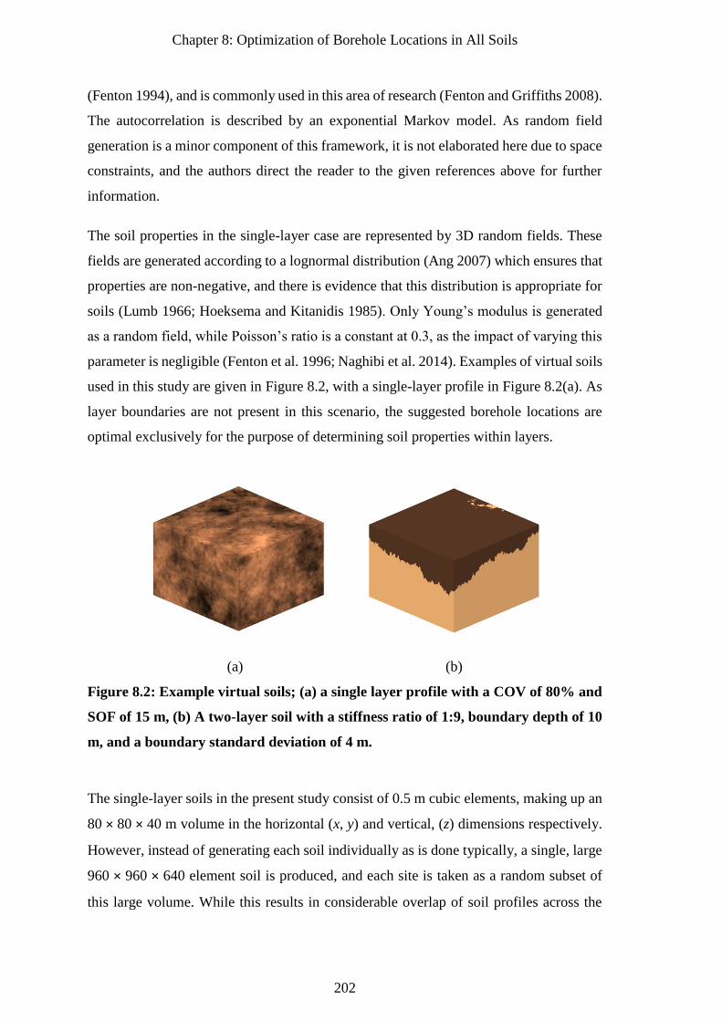
Chapter 8: Optimization of Borehole Locations in All Soils
202
(Fenton 1994), and is commonly used in this area of research (Fenton and Griffiths 2008).
The autocorrelation is described by an exponential Markov model. As random field
generation is a minor component of this framework, it is not elaborated here due to space
constraints, and the authors direct the reader to the given references above for further
information.
The soil properties in the single-layer case are represented by 3D random fields. These
fields are generated according to a lognormal distribution (Ang 2007) which ensures that
properties are non-negative, and there is evidence that this distribution is appropriate for
soils (Lumb 1966; Hoeksema and Kitanidis 1985). Only Young’s modulus is generated
as a random field, while Poisson’s ratio is a constant at 0.3, as the impact of varying this
parameter is negligible (Fenton et al. 1996; Naghibi et al. 2014). Examples of virtual soils
used in this study are given in Figure 8.2, with a single-layer profile in Figure 8.2(a). As
layer boundaries are not present in this scenario, the suggested borehole locations are
optimal exclusively for the purpose of determining soil properties within layers.
(a) (b)
Figure 8.2: Example virtual soils; (a) a single layer profile with a COV of 80% and
SOF of 15 m, (b) A two-layer soil with a stiffness ratio of 1:9, boundary depth of 10
m, and a boundary standard deviation of 4 m.
The single-layer soils in the present study consist of 0.5 m cubic elements, making up an
80 × 80 × 40 m volume in the horizontal (x, y) and vertical, (z) dimensions respectively.
However, instead of generating each soil individually as is done typically, a single, large
960 × 960 × 640 element soil is produced, and each site is taken as a random subset of
this large volume. While this results in considerable overlap of soil profiles across the
Chapter 8: Optimization of Borehole Locations in All Soils
203
Monte Carlo realisations, this has a negligible impact on the average field statistics, as
even a small offset in 3 dimensions can produce an effectively different soil in regards to
the foundation response.
There are two benefits to this soil subset method. Firstly, the random field is only
generated once, instead of being regenerated in each GA generation. Secondly, a single
larger field is generated far more quickly than numerous small fields, as there is a much
smaller total volume being generated. Between these two factors, computation time is
notably reduced by approximately 40 minutes per generation. The analysis of small
numbers of borehole can then be done in under one minute.
Multi-layered soils are treated separately from the single-layer case. Rather than having
material properties that smoothly vary with distance, the properties within each layer are
uniform and constant. However, each layer is separated by a boundary that undulates
randomly with depth as seen in Figure 8.2(b). As a result of this treatment, any soil
uncertainty is explicitly due to the layer boundary. The boundaries themselves are
represented by 2D random fields, where elements of the 2D field represents the layer’s
depth at its location. Similar to the single-layer soils, the 2D fields are generated using
LAS, where the depths are normally-distributed as opposed to lognormal. Further
information about random fields for building multi-layered virtual soils are detailed by
Crisp et al. (2019e) (Chapter 4).
Due to the wide variety of foundations and soil types examined in this study, it is
impossible to specify a single mean Young’s modulus (E) for each layer while having
similar pile lengths. Therefore, to facilitate relatively straightforward comparison of
results, each layer’s E value is customised to achieve a consistent average pile length. In
the single-layer scenario, the target average length is 5 m, as this maximises the number
of Monte Carlo realisations where valid pile designs are achieved. Invalid designs occur
when the required pile length is larger than the allowable maximum of 20 m. For the
multi-layer scenario, the target average pile length is 15 m to ensure that the base is
embedded within the lower layer. In both scenarios, the custom E values are found by
iteratively decreasing the overall soil stiffness, which in turn increases the pile length,
until the target length is achieved.
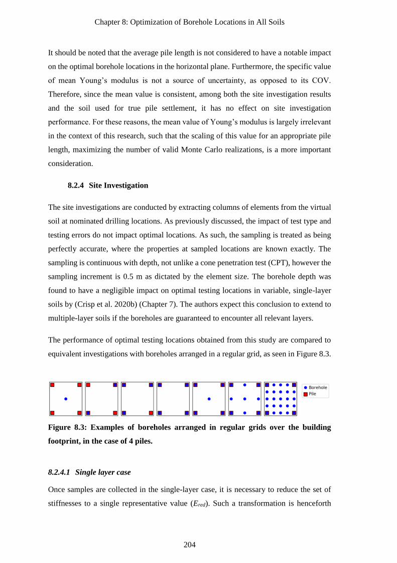
Chapter 8: Optimization of Borehole Locations in All Soils
204
It should be noted that the average pile length is not considered to have a notable impact
on the optimal borehole locations in the horizontal plane. Furthermore, the specific value
of mean Young’s modulus is not a source of uncertainty, as opposed to its COV.
Therefore, since the mean value is consistent, among both the site investigation results
and the soil used for true pile settlement, it has no effect on site investigation
performance. For these reasons, the mean value of Young’s modulus is largely irrelevant
in the context of this research, such that the scaling of this value for an appropriate pile
length, maximizing the number of valid Monte Carlo realizations, is a more important
consideration.
8.2.4 Site Investigation
The site investigations are conducted by extracting columns of elements from the virtual
soil at nominated drilling locations. As previously discussed, the impact of test type and
testing errors do not impact optimal locations. As such, the sampling is treated as being
perfectly accurate, where the properties at sampled locations are known exactly. The
sampling is continuous with depth, not unlike a cone penetration test (CPT), however the
sampling increment is 0.5 m as dictated by the element size. The borehole depth was
found to have a negligible impact on optimal testing locations in variable, single-layer
soils by (Crisp et al. 2020b) (Chapter 7). The authors expect this conclusion to extend to
multiple-layer soils if the boreholes are guaranteed to encounter all relevant layers.
The performance of optimal testing locations obtained from this study are compared to
equivalent investigations with boreholes arranged in a regular grid, as seen in Figure 8.3.
Figure 8.3: Examples of boreholes arranged in regular grids over the building
footprint, in the case of 4 piles.
8.2.4.1 Single layer case
Once samples are collected in the single-layer case, it is necessary to reduce the set of
stiffnesses to a single representative value (Ered). Such a transformation is henceforth
Chapter 8: Optimization of Borehole Locations in All Soils
205
referred to as a reduction method. The so-called ‘standard deviation’ (SD) reduction
method is used in the present study, which involves taking one geometric standard
deviation below the geometric mean of stiffness values. In other words, Ered = μln/ σln,
where μln and σln are the mean and standard deviation of the natural logarithm of sample
values. Sampling is taken to a depth of 20 m; the maximum allowable length of pile.
The SD method was recommended by Crisp et al. (2020b) (Chapter 7) with regards to
optimising a single borehole’s location, as it was found to produce a smoother fitness
landscape than less conservative recommendations. Furthermore, the resulting
performance was less sensitive to borehole location which is desirable in practice. The
standard deviation method was used by Crisp et al. (2018, 2019c, 2019d, 2020a); Crisp
et al. (2020c), (Chapter 2, Chapter , Appendix B, Chapter 5, Chapter 6) with Crisp et al.
(2019c) (Chapter 2) concluding that it provided the lowest expected total project cost
when compared to a variety of reduction methods.
It is important to note that the soil model, being a uniform value, is a simplified
interpretation of investigation data, compared to the full variation of the true soil. This
simplification has two implications. Firstly, if all elements of the soil were tested such
that the site is fully known, the foundation will still experience differential settlement due
to local discrepancies between the site and model. Secondly, and perhaps more
importantly, there is no explicit relationship between the sample locations and foundation
performance; it is the collection of sample values that is relevant, as opposed to their
order. In other words, the sample location is not considered in the soil model. As such,
the relationship between testing locations and foundation performance is implicit and is
derived from the autocorrelation between the sampled soil and the soil at each pile
location. On average, samples within the autocorrelation distance from the pile should be
similar. However, the sample values may still be different in a given Monte Carlo
realisation due to the random nature of the soil, illustrating the importance of the Monte
Carlo framework.
8.2.4.2 Multiple layer case
A number of idealisations are applied to the site investigation process for the purpose of
computational efficiency, due to multi-layer soils having uniform properties in each layer.
Firstly, the soil properties within each layer are known exactly, regardless of the number
of samples. Secondly, the layer boundaries at borehole locations are known exactly. Any
Chapter 8: Optimization of Borehole Locations in All Soils
206
errors in depth estimation due to subjectivity or ambiguity from soil mixing at the
interface are not considered.
Despite the discrete 0.5 m element size, the layer boundaries are continuous in that depths
are not rounded to 0.5 m increments. Sampling is taken continuously to a total depth of
40 m, which is consistent with the bottom of the soil profile. As such, it is impossible for
layer boundaries to pass underneath the bottom of the sampling.
Once the virtual investigation is conducted, a soil model is created based on the known
depths of layer boundaries at borehole locations. In this model, the boundaries are
interpolated from boreholes through Delaunay triangulation (Delaunay 1934).
Extrapolation is achieved with a convex-hull expansion that approximates the layer
extending outwards horizontally from the outer-most points (Crisp 2020b) (Appendix E).
Unlike the single-layer case, there is an explicit relationship between the soil model and
the true soil. If the full surface were sampled then the layer boundaries, and therefore the
full soil, would be known exactly. However, unlike that study, only local information is
used; i.e. the three nearest boreholes which form a triangle around the pile of interest.
This is elaborated on in the next section.
8.2.5 Pile settlement
Two models are needed for determining pile settlement, for single-layer and multi-layer
soils respectively. Between the 10,000 Monte Carlo realisations, and the iterative nature
of the GA, billions of piles must be designed and assessed, necessitating an efficient
settlement model and calculation procedure that is tailored to each soil case.
The building’s weight is equally distributed among the piles. A combined dead and live
loading of 8 kPa is applied to each floor of the structure. Therefore, for the 10 storey, 40
× 40 m building examined in this study, there is a total weight of 128,000 kN. All piles
are designed to a differential settlement tolerance of 0.0025 (Sowers 1962; Salgado
2008).
8.2.5.1 Single layer case
One important optimization for single-layer soils is that the true settlement of each pile,
used in the differential settlement calculations, is pre-processed prior to use of the GA.
Chapter 8: Optimization of Borehole Locations in All Soils
207
This processing produces a continuous function of settlement in terms of pile length. Due
to the assumed linear-elastic mechanics, these functions can be scaled linearly with
applied load and soil stiffness. As such, since applied load, soil stiffness and designed
pile length are known, so too is the true settlement.
These settlement functions are generated for a given pile in a given Monte Carlo
realisation by determining the settlement at discrete 1 m intervals in the variable, virtual
soil. These data are then made continuous through Akima interpolation (Akima 1970).
The settlement at the 1 m intervals themselves are evaluated through an efficient analogy
to finite element analysis (FEA) which serves as the second optimization.
This FEA equivalent, called the Pseudo-Incremental Energy (PIE) method (Ching et al.
2018), approximates FEA results within a Monte Carlo framework within a fraction of
the computational time. Elimination of FEA, the main computational bottleneck, saves
several months of simulation per soil case in the single-layer scenario. It works by
removing the need for FEA within the Monte Carlo simulations. Instead, only a single
instance of the FEA model is needed prior to commencement. For each 1 m pile
increment, a deterministic settlement value (Sdet) is found through FEA in a mesh with
uniform properties, for an applied unit load of 1 kN. This mesh is also used to obtain a
weight (W) for each soil element. Each weight is calculated from the stress (σ, τ) and
strain (ε) components in the corresponding FEA mesh element as given in the following
equation:
𝑊 = 𝜎𝑥휀𝑥 + 𝜎𝑦휀𝑦 + 𝜎𝑧휀𝑧 + 𝜏𝑥𝑦휀𝑥𝑦 + 𝜏𝑦𝑧휀𝑦𝑧 + 𝜏𝑥𝑧휀𝑥𝑧 (8.1)
To determine the true settlement (S) of that length of pile in a given virtual soil, the
deterministic settlement (Sdet) is scaled by the weighted geometric average of soil
surrounding that pile (Eeff). S = Sdet/Eeff. The soil weights reflect the premise that soil
properties closer to the pile have a greater influence on its settlement. Therefore, as the
soil’s distribution of stresses and strains vary with the length of the pile, the weights and
therefore Eeff must be determined for each pile length individually.
The final optimization involves the design of piles from the soil model. The process is
almost identical to that of finding the true pile settlement discussed above. However,
instead of scaling each increment of the settlement curve by Eeff, the whole curve is scaled
by the reduced Ered from the site investigation. Therefore, as the applied load, soil model
Chapter 8: Optimization of Borehole Locations in All Soils
208
stiffness, and settlement design tolerance are known for a given investigation, so too is
the pile design.
8.2.5.2 Multiple layer case
All pile settlement analysis is undertaken using a load transfer technique modified from
Mylonakis and Gazetas (1998). The shaft stiffness is represented as a series of distributed
springs (Winkler assumption). The base resistance is calculated separately, and originally
by using the stiffness of the layer that the pile is based in. The modification here consists
of calculating the base stiffness as a weighted harmonic average of soil stiffness below
the pile base. The weights are determined by integrating an exponential decay of
importance with depth below the pile, and the half-life of this decay is 3 m. The advantage
here is that pile behaviour can account for deeper soil layers, which more accurately
matches results from FEA (Crisp 2020b) (Appendix E). Each pile’s settlement is
calculated individually, using local layer boundary depths. The elimination of FEA from
this scenario reduces the length of the simulation from several years to several hours.
Once the soil model is generated, as described in the previous section, it is used for pile
design. This design process is undertaken by iteratively increasing the pile length until
the settlement criteria is satisfied. True pile settlement is then found by taking the final
design and applying the settlement model using the original, full, variable layer
boundaries as generated by the 2D random fields.
It should be noted that the settlement model is designed for 1D soil profiles, where the
soil properties within each layer are uniform. While the latter constraint is valid here, the
former assumes that the layer boundaries are flat and horizontal, which is not the case.
However, Crisp et al. (2020c) (Chapter 5) found that undulating 2D layer boundaries can
be represented by a single, effective depth by taking an inverse-distance-squared
weighted average of layer depths around the pile, thereby reducing the soil to a 1D
equivalent. This technique is used for calculating true pile settlement.
However, to reduce computational time, the layer depths are taken directly from the
interpolated surface at the pile’s location. In other words, a single depth value is used as
opposed to a local average. This approximation is reasonable for the soil model, as
opposed to the random fields, as there is far less local variation due to the linear
interpolation of scattered data. Furthermore, as the interpolated surface consists of
Chapter 8: Optimization of Borehole Locations in All Soils
209
triangular planes with vertices defined by borehole locations, a point inside each triangle
is also a weighted average of the layer’s depth at each borehole. A comparison has found
that this optimization has negligible impact on the optimal locations in this study, while
further reducing computational time by an order of magnitude. This reduction, from
roughly an hour to several minutes, is due to the significantly reduced amount of 2D
interpolation required for a series of discrete points vs. an entire plane.
8.2.6 Differential Settlement and Failure Cost
Once the true settlement for each pile is obtained in a Monte Carlo realisation for an
investigation, the differential settlement can be determined. This involves finding the
difference in settlement between all combinations of two piles in the foundation as a
proportion of the distance between the piles. The final differential settlement for that
foundation is taken as the maximum value of all combinations.
While the geometric product metric is used by the GA for optimization, the failure costs
associated with the recommendations are also calculated. Comparison of these costs gives
a more meaningful representation of the benefit of using optimal testing locations over a
regular grid.
Previously, a relationship has been derived for failure cost in terms of differential
settlement by Crisp et al. (2019a) (Appendix D). The relationship is based on levels of
structural cracking associated with magnitudes of differential settlement by Day (1999),
and the cost of repairing that cracking Rawlinsons (2016). In essence, an insufficient
investigation is likely to result in higher differential settlement on average, requiring a
larger repair cost.
This relationship itself is represented by a linear function, such that a differential
settlement value of 0.003 results in A$0 of failure, and 0.009 results in a failure cost equal
to the building’s construction cost (Cc). The construction cost, in this case A$47,600,000
(Rawlinsons 2016), is analogous to demolishing and rebuilding the structure due to
excessive cracking. As such, this linear function is bounded by a minimum of $0 and a
maximum of Cc. The costs are calculated individually for each Monte Carlo realisation,
which are subsequently averaged to form the expected failure cost.
Chapter 8: Optimization of Borehole Locations in All Soils
210
8.3 Results
Prior to analysing the results in the following sections, it should be noted that, while
properly configured GAs perform well at finding solutions that are near a global
optimum, they are quite inefficient at finding the exact solution. Therefore, rather than
taking the results as absolute recommendations, a degree of subjective interpretation is
required. One example of subjective interpretation is the consideration of symmetry. If
the pile configuration is symmetrical in one or more axes, and if the number of boreholes
allows for a symmetrical solution, the true optimal locations should be re-interpreted as
such.
8.3.1 Analysis of GA Parameters
The choice of optimal GA parameters is known to be problem-specific (Haupt and Haupt
2004). Therefore, when a GA is introduced to a new problem, as in the present situation,
it is necessary to analyse the parameters that produce the best results in terms of quality
and processing time.
This analysis is undertaken here with a single-layer soil of COV 80% and SOF of 10 m.
The single-layer scenario is considered, as the overall analysis is faster and more efficient
than that of the multi-layer, allowing for a wider range of parameters to be assessed. It
should be noted that the solution space is slightly different between the two soil scenarios
due to the manner the soil models are constructed, as described previously. However, the
nature of the problem is similar, and so the results are expected to be transferable.
Two GA parameters are investigated with regards to the solution evolution; the
population size and mutation rate. Between them, the values are 250 and 500, as well as
1%, 2%, 5% and 10% respectively, resulting in 8 combinations being assessed.
Furthermore, it is important to specify a stopping criterion so that the algorithm concludes
after an appropriate number of generations, beyond which there is little improvement.
The criterion is needed because it is impossible to know in advance when the GA has
found an optimal solution. As such, it must instead detect if the solution has remained
relatively unchanged for a specified number of generations, implying convergence. The
two additional parameters are the performance tolerance, such that improvement below
Chapter 8: Optimization of Borehole Locations in All Soils
211
this threshold is considered negligible, and the number of consecutive generations, which
must have negligible improvement.
For each case, a tolerance of 0% is used along with 20 generations of consecutive values,
meaning that the solution must be unchanged over this time. Furthermore, once the GA
has converged, it is restarted with a new population created from randomly generated
offsets from the optimal solution, in an attempt to find a nearby optimum. This second
stage is set to have 0% improvement for 10 consecutive generations before stopping. Use
of such a conservative, strict stopping criterion allows for the evolution curves to be
analysed for alternative, less strict criteria, without having to re-run the GA.
Plots showing the evolution of performance are given in Figure 8.4 for the cases of 1, 5
and 25 boreholes with a 9 pile, 40 × 40 m building, comparing the aforementioned
mutation rates and population sizes. Other building cases not shown here include
buildings of 10 × 10 m, 20 × 20 m and 30 × 30 m with a variety of numbers of piles and
pile spacings. It should be noted that there are no clear tends across the different building
cases, and the plots in Figure 8.4 shouldn’t necessarily be taken as expected trajectories.
Nevertheless, some general conclusions can be made.
The interpretation of Figure 8.4 is that as the performance value decreases over successive
iterations, the boreholes physically move to more optimal locations. Although counter-
intuitive, lower performance values are more desirable, as there is a reduced likelihood
of excessive differential settlement. The changes between iterations can vary greatly,
from one borehole moving a small distance due to the best solution being improved, to
all boreholes being moved extensively when an entirely new optimal solution is found.
This latter case results in the sudden large drops in performance value while the former
is typically responsible for the segments of gradual, smooth improvement.
For small numbers of boreholes, in the order of 1-2, the solution converges quickly,
regardless of parameter choices. For intermediate numbers, from 3-8, the progression is
stepped (staggered) with several generations in a row stalling with no improvement. For
9 and more boreholes, improvement tends to be relatively smooth and continuous.
Upon inspection of various sets of building sizes and numbers of piles, not shown here
due to space constraints, the authors conclude that a population size of 500 and a mutation
rate of 1% is the single best choice towards finding the optimal locations in all cases.
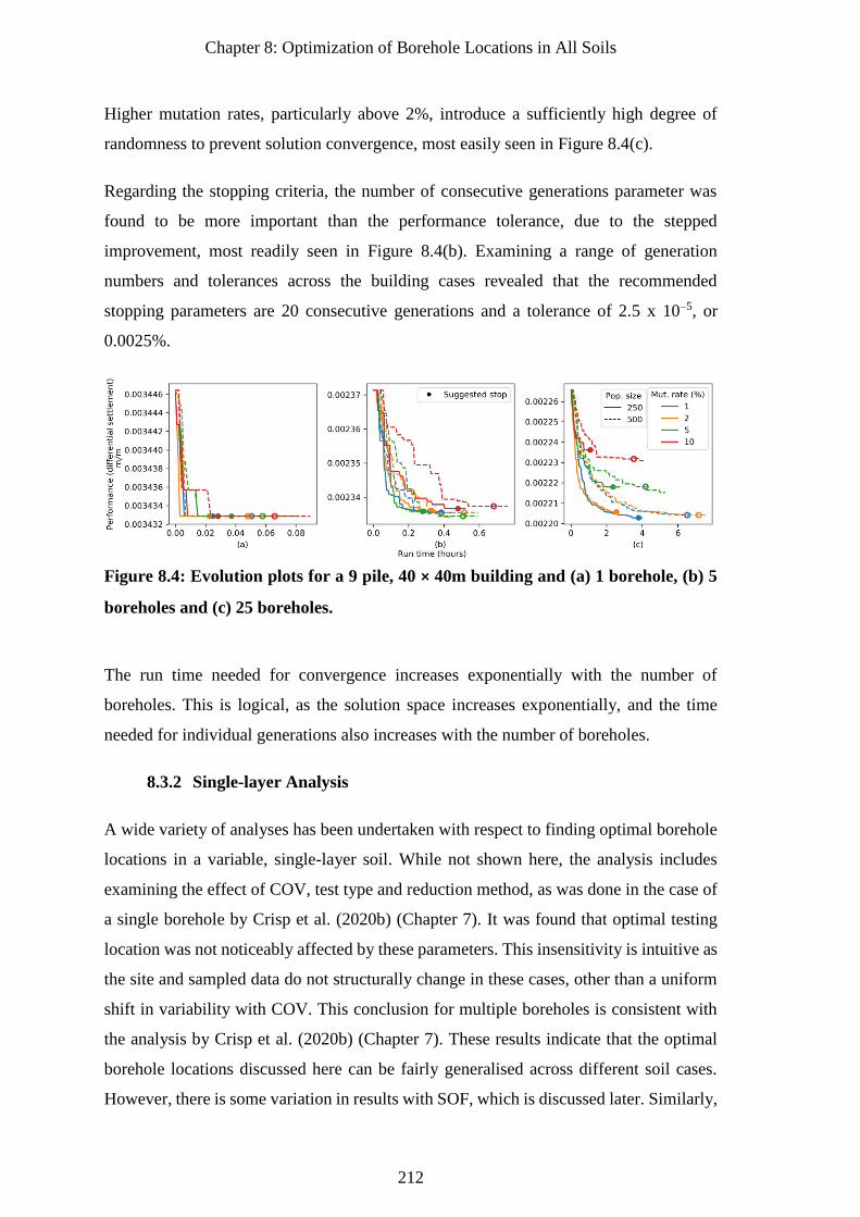
Chapter 8: Optimization of Borehole Locations in All Soils
212
Higher mutation rates, particularly above 2%, introduce a sufficiently high degree of
randomness to prevent solution convergence, most easily seen in Figure 8.4(c).
Regarding the stopping criteria, the number of consecutive generations parameter was
found to be more important than the performance tolerance, due to the stepped
improvement, most readily seen in Figure 8.4(b). Examining a range of generation
numbers and tolerances across the building cases revealed that the recommended
stopping parameters are 20 consecutive generations and a tolerance of 2.5 x 10⁻⁵, or
0.0025%.
Figure 8.4: Evolution plots for a 9 pile, 40 × 40m building and (a) 1 borehole, (b) 5
boreholes and (c) 25 boreholes.
The run time needed for convergence increases exponentially with the number of
boreholes. This is logical, as the solution space increases exponentially, and the time
needed for individual generations also increases with the number of boreholes.
8.3.2 Single-layer Analysis
A wide variety of analyses has been undertaken with respect to finding optimal borehole
locations in a variable, single-layer soil. While not shown here, the analysis includes
examining the effect of COV, test type and reduction method, as was done in the case of
a single borehole by Crisp et al. (2020b) (Chapter 7). It was found that optimal testing
location was not noticeably affected by these parameters. This insensitivity is intuitive as
the site and sampled data do not structurally change in these cases, other than a uniform
shift in variability with COV. This conclusion for multiple boreholes is consistent with
the analysis by Crisp et al. (2020b) (Chapter 7). These results indicate that the optimal
borehole locations discussed here can be fairly generalised across different soil cases.
However, there is some variation in results with SOF, which is discussed later. Similarly,
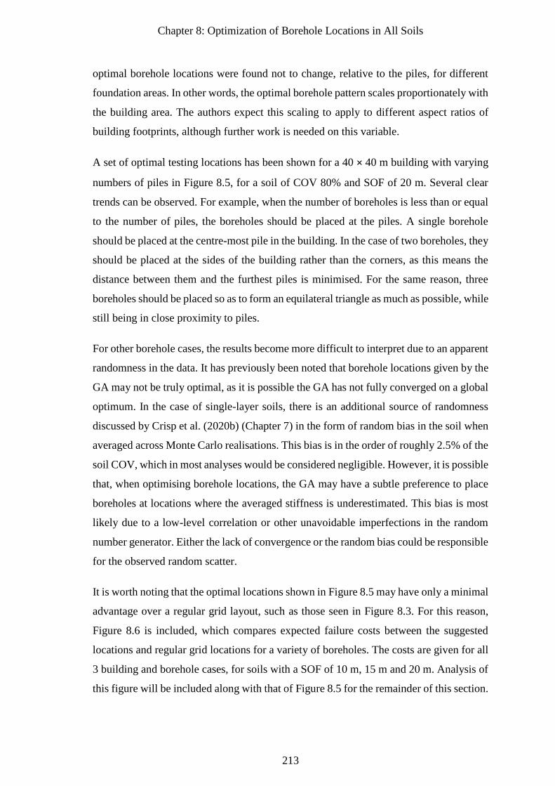
Chapter 8: Optimization of Borehole Locations in All Soils
213
optimal borehole locations were found not to change, relative to the piles, for different
foundation areas. In other words, the optimal borehole pattern scales proportionately with
the building area. The authors expect this scaling to apply to different aspect ratios of
building footprints, although further work is needed on this variable.
A set of optimal testing locations has been shown for a 40 × 40 m building with varying
numbers of piles in Figure 8.5, for a soil of COV 80% and SOF of 20 m. Several clear
trends can be observed. For example, when the number of boreholes is less than or equal
to the number of piles, the boreholes should be placed at the piles. A single borehole
should be placed at the centre-most pile in the building. In the case of two boreholes, they
should be placed at the sides of the building rather than the corners, as this means the
distance between them and the furthest piles is minimised. For the same reason, three
boreholes should be placed so as to form an equilateral triangle as much as possible, while
still being in close proximity to piles.
For other borehole cases, the results become more difficult to interpret due to an apparent
randomness in the data. It has previously been noted that borehole locations given by the
GA may not be truly optimal, as it is possible the GA has not fully converged on a global
optimum. In the case of single-layer soils, there is an additional source of randomness
discussed by Crisp et al. (2020b) (Chapter 7) in the form of random bias in the soil when
averaged across Monte Carlo realisations. This bias is in the order of roughly 2.5% of the
soil COV, which in most analyses would be considered negligible. However, it is possible
that, when optimising borehole locations, the GA may have a subtle preference to place
boreholes at locations where the averaged stiffness is underestimated. This bias is most
likely due to a low-level correlation or other unavoidable imperfections in the random
number generator. Either the lack of convergence or the random bias could be responsible
for the observed random scatter.
It is worth noting that the optimal locations shown in Figure 8.5 may have only a minimal
advantage over a regular grid layout, such as those seen in Figure 8.3. For this reason,
Figure 8.6 is included, which compares expected failure costs between the suggested
locations and regular grid locations for a variety of boreholes. The costs are given for all
3 building and borehole cases, for soils with a SOF of 10 m, 15 m and 20 m. Analysis of
this figure will be included along with that of Figure 8.5 for the remainder of this section.
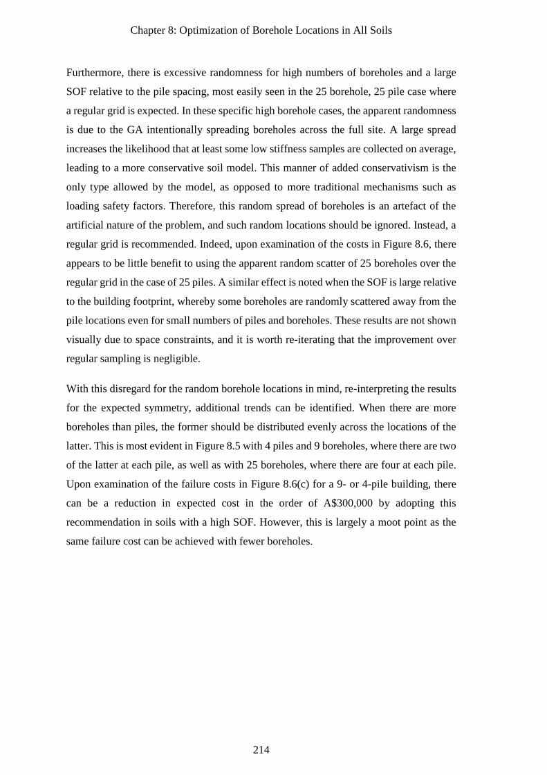
Chapter 8: Optimization of Borehole Locations in All Soils
214
Furthermore, there is excessive randomness for high numbers of boreholes and a large
SOF relative to the pile spacing, most easily seen in the 25 borehole, 25 pile case where
a regular grid is expected. In these specific high borehole cases, the apparent randomness
is due to the GA intentionally spreading boreholes across the full site. A large spread
increases the likelihood that at least some low stiffness samples are collected on average,
leading to a more conservative soil model. This manner of added conservativism is the
only type allowed by the model, as opposed to more traditional mechanisms such as
loading safety factors. Therefore, this random spread of boreholes is an artefact of the
artificial nature of the problem, and such random locations should be ignored. Instead, a
regular grid is recommended. Indeed, upon examination of the costs in Figure 8.6, there
appears to be little benefit to using the apparent random scatter of 25 boreholes over the
regular grid in the case of 25 piles. A similar effect is noted when the SOF is large relative
to the building footprint, whereby some boreholes are randomly scattered away from the
pile locations even for small numbers of piles and boreholes. These results are not shown
visually due to space constraints, and it is worth re-iterating that the improvement over
regular sampling is negligible.
With this disregard for the random borehole locations in mind, re-interpreting the results
for the expected symmetry, additional trends can be identified. When there are more
boreholes than piles, the former should be distributed evenly across the locations of the
latter. This is most evident in Figure 8.5 with 4 piles and 9 boreholes, where there are two
of the latter at each pile, as well as with 25 boreholes, where there are four at each pile.
Upon examination of the failure costs in Figure 8.6(c) for a 9- or 4-pile building, there
can be a reduction in expected cost in the order of A$300,000 by adopting this
recommendation in soils with a high SOF. However, this is largely a moot point as the
same failure cost can be achieved with fewer boreholes.
Chapter 8: Optimization of Borehole Locations in All Soils
215
Figure 8.5: Optimal testing locations for different numbers of piles and boreholes
for a soil with a COV of 80% and SOF of 20 m.
Figure 8.6: Failure cost comparison between a regular grid of boreholes (Grid) and
optimal locations (Opt.) for different numbers of piles and a SOF of (a) 10 m, (b) 15
m and (c), 20 m.
As mentioned earlier, there is a variation in optimal testing locations as the SOF changes.
This is most apparent in the case of 2 or 3 boreholes and 25 piles. The large number of
piles facilitates flexibility in borehole locations since they should be drilled at a pile,
allowing the effects of SOF to be highlighted. The above case is shown for a SOF of 10
m, 15 m and 25 m in Figure 8.7. It can be seen that as the SOF increases, so does the
recommended borehole spacing. While this spacing appears to be approximately double
that of the SOF, it is difficult to define an explicit relationship due to the possibility of
the randomness discussed previously. Therefore, optimal borehole spacing with regards
to SOF is an area for future research. The relationship does not apply for small or large
SOFs. In the former case, a wide variety of sample values is encountered by each borehole
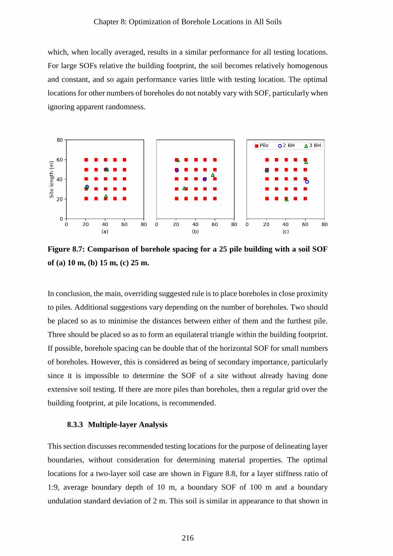
Chapter 8: Optimization of Borehole Locations in All Soils
216
which, when locally averaged, results in a similar performance for all testing locations.
For large SOFs relative the building footprint, the soil becomes relatively homogenous
and constant, and so again performance varies little with testing location. The optimal
locations for other numbers of boreholes do not notably vary with SOF, particularly when
ignoring apparent randomness.
Figure 8.7: Comparison of borehole spacing for a 25 pile building with a soil SOF
of (a) 10 m, (b) 15 m, (c) 25 m.
In conclusion, the main, overriding suggested rule is to place boreholes in close proximity
to piles. Additional suggestions vary depending on the number of boreholes. Two should
be placed so as to minimise the distances between either of them and the furthest pile.
Three should be placed so as to form an equilateral triangle within the building footprint.
If possible, borehole spacing can be double that of the horizontal SOF for small numbers
of boreholes. However, this is considered as being of secondary importance, particularly
since it is impossible to determine the SOF of a site without already having done
extensive soil testing. If there are more piles than boreholes, then a regular grid over the
building footprint, at pile locations, is recommended.
8.3.3 Multiple-layer Analysis
This section discusses recommended testing locations for the purpose of delineating layer
boundaries, without consideration for determining material properties. The optimal
locations for a two-layer soil case are shown in Figure 8.8, for a layer stiffness ratio of
1:9, average boundary depth of 10 m, a boundary SOF of 100 m and a boundary
undulation standard deviation of 2 m. This soil is similar in appearance to that shown in
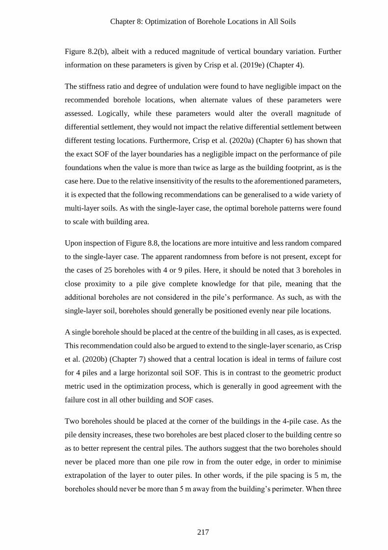
Chapter 8: Optimization of Borehole Locations in All Soils
217
Figure 8.2(b), albeit with a reduced magnitude of vertical boundary variation. Further
information on these parameters is given by Crisp et al. (2019e) (Chapter 4).
The stiffness ratio and degree of undulation were found to have negligible impact on the
recommended borehole locations, when alternate values of these parameters were
assessed. Logically, while these parameters would alter the overall magnitude of
differential settlement, they would not impact the relative differential settlement between
different testing locations. Furthermore, Crisp et al. (2020a) (Chapter 6) has shown that
the exact SOF of the layer boundaries has a negligible impact on the performance of pile
foundations when the value is more than twice as large as the building footprint, as is the
case here. Due to the relative insensitivity of the results to the aforementioned parameters,
it is expected that the following recommendations can be generalised to a wide variety of
multi-layer soils. As with the single-layer case, the optimal borehole patterns were found
to scale with building area.
Upon inspection of Figure 8.8, the locations are more intuitive and less random compared
to the single-layer case. The apparent randomness from before is not present, except for
the cases of 25 boreholes with 4 or 9 piles. Here, it should be noted that 3 boreholes in
close proximity to a pile give complete knowledge for that pile, meaning that the
additional boreholes are not considered in the pile’s performance. As such, as with the
single-layer soil, boreholes should generally be positioned evenly near pile locations.
A single borehole should be placed at the centre of the building in all cases, as is expected.
This recommendation could also be argued to extend to the single-layer scenario, as Crisp
et al. (2020b) (Chapter 7) showed that a central location is ideal in terms of failure cost
for 4 piles and a large horizontal soil SOF. This is in contrast to the geometric product
metric used in the optimization process, which is generally in good agreement with the
failure cost in all other building and SOF cases.
Two boreholes should be placed at the corner of the buildings in the 4-pile case. As the
pile density increases, these two boreholes are best placed closer to the building centre so
as to better represent the central piles. The authors suggest that the two boreholes should
never be placed more than one pile row in from the outer edge, in order to minimise
extrapolation of the layer to outer piles. In other words, if the pile spacing is 5 m, the
boreholes should never be more than 5 m away from the building’s perimeter. When three
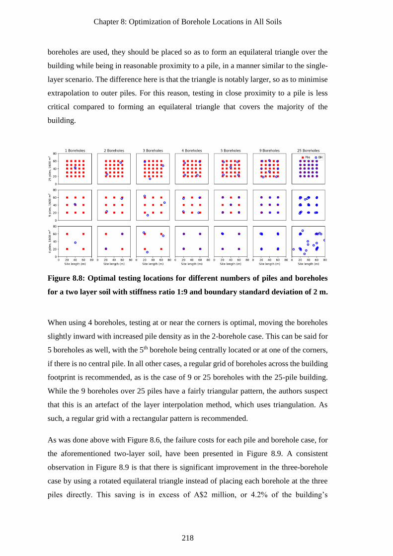
Chapter 8: Optimization of Borehole Locations in All Soils
218
boreholes are used, they should be placed so as to form an equilateral triangle over the
building while being in reasonable proximity to a pile, in a manner similar to the single-
layer scenario. The difference here is that the triangle is notably larger, so as to minimise
extrapolation to outer piles. For this reason, testing in close proximity to a pile is less
critical compared to forming an equilateral triangle that covers the majority of the
building.
Figure 8.8: Optimal testing locations for different numbers of piles and boreholes
for a two layer soil with stiffness ratio 1:9 and boundary standard deviation of 2 m.
When using 4 boreholes, testing at or near the corners is optimal, moving the boreholes
slightly inward with increased pile density as in the 2-borehole case. This can be said for
5 boreholes as well, with the 5th borehole being centrally located or at one of the corners,
if there is no central pile. In all other cases, a regular grid of boreholes across the building
footprint is recommended, as is the case of 9 or 25 boreholes with the 25-pile building.
While the 9 boreholes over 25 piles have a fairly triangular pattern, the authors suspect
that this is an artefact of the layer interpolation method, which uses triangulation. As
such, a regular grid with a rectangular pattern is recommended.
As was done above with Figure 8.6, the failure costs for each pile and borehole case, for
the aforementioned two-layer soil, have been presented in Figure 8.9. A consistent
observation in Figure 8.9 is that there is significant improvement in the three-borehole
case by using a rotated equilateral triangle instead of placing each borehole at the three
piles directly. This saving is in excess of A$2 million, or 4.2% of the building’s
Chapter 8: Optimization of Borehole Locations in All Soils
219
construction cost. Interestingly, three boreholes placed in the regular grid pattern have
considerably worse performance than two boreholes, despite the additional soil
information. This degradation is due to the layer boundary being extrapolated outside of
the triangle formed by the three boreholes. As such, the 4th pile, without an associated
borehole, is likely to be misrepresented in the soil model. It must be remembered that the
addition of a third borehole significantly reduces the failure cost compared to two in the
single-layer scenario.
For all other cases, the improvement from optimal sampling over the regular grid
increases with the number of piles. Other than with three boreholes, there is negligible
difference between the optimal and grid placement in the case of four piles. There is
moderate improvement in the 9-pile case for less than five boreholes. Similarly, there is
greater improvement for 25 piles and less than 9 boreholes, in the order of A$500,000.
Figure 8.9: Failure cost comparison between a regular grid of boreholes (Grid) and
optimal locations (Opt.) in a two layer soil with boundary standard deviation of 4 m
and (a) 25 piles, (b) 9 piles, (c) 4 piles.
Further analysis was conducted on multi-layer soil profiles, including those featuring the
possible formation of soil lenses. A lens is a soil layer is that is laterally discontinuous,
such that it can be present at one borehole or pile location and absent from another.
Understandably, this circumstance is particularly detrimental to foundation performance.
However, optimal testing locations do not notably change from that seen in Figure 8.8.
As such, those locations are also recommended in soils with 3 or more layers.
Comparing the improvement between the single-layer and multi-layer scenarios, the cost
savings are noticeably higher in the latter case. This improvement is due to the more
Chapter 8: Optimization of Borehole Locations in All Soils
220
explicit relationship between borehole locations and the soil model for the layer
boundaries. Therefore, as the foundation performance is less sensitive to the exact
borehole locations in the single-layer case, the authors suggest using the multi-layer
recommendations in practice. This suggestion is reinforced by the overall similarity of
recommendations between the two soil scenarios, and that the multi-layer
recommendations are less random.
8.4 Conclusions
This study has demonstrated that a genetic algorithm (GA) can be used to optimise
borehole locations with respect to improving foundation performance. An analysis of GA
parameters reveals that the best overall configuration is a low mutation rate in the order
of 1-2% and a large population such as 500 members. The recommended stopping
criterion, used to assess when the GA has converged on a global solution, is when there
has been less than a 0.0025% improvement on the previous generation for 20 consecutive
generations.
Optimal borehole locations have been derived independently for a single-layer soil and
multi-layer soils. These scenarios examine what is optimal for determining the material
properties of layers and layer boundaries respectively. The recommended testing
locations were generally similar across the two scenarios. However, locations appeared
somewhat random in the single-layer soil due to an implicit relationship between the
sample locations and soil model. Since this relationship is explicit in the multi-layer case,
and because the cost savings were greater, the optimal multi-layer locations are
recommended for general use. The difference in failure cost between the optimal and
regular grid patterns varied greatly, from being negligible through to over A$2 million,
or 4.2% of the building’s construction cost in the case of three boreholes.
A large number of variables were identified as having no or negligible effect on optimal
borehole locations. In the single-layer scenario, this includes the coefficient of variation,
test type and reduction method. The optimal borehole spacing appeared to increase with
scale of fluctuation (SOF) in the case of two or three boreholes. However, the relationship
between borehole spacing and SOF requires further analysis, ideally with anisotropic
soils where the vertical SOF is held constant. A high SOF relative to either the borehole
spacing or building footprint results in increasingly random borehole locations being
Chapter 8: Optimization of Borehole Locations in All Soils
221
preferred. However, the improvement due to this random sampling is negligible, such
that the final stated guidelines are recommended. In the multi-layer scenario, the degree
of layer undulation, layer stiffness ratio and number of layers appear to have little effect
on the results. Similarly, the building area has little impact on the optimal borehole
pattern, as locations scale linearly with footprint size.
The recommended testing locations for all soil conditions is as follows:
• The general rule is that boreholes should be placed in close proximity to piles,
unless stated otherwise.
• A single borehole should be located in the centre of the building.
• Two boreholes should be placed at the building corners.
• Three boreholes should be arranged as an equilateral triangle, rotated to be in
proximity to piles and containing the majority of the building within its area.
• With four or five boreholes, the outer-most ones should be moved closer to the
centre as pile density increases, however should not be further inward than one
row of piles.
Some recommendations for future research have been given within this section. Further
suggestions include the use of a more advanced GA or evolutionary algorithm. For
example, exploring the use of alternate selection, crossover and mutation mechanisms
that are more sophisticated than the simple implementations used in the present study,
such as normally-distributed mutation. The GA could also be adapted to optimise
additional site investigation parameters, such as borehole depth and test type within the
same investigation. It should be noted that the results are only applicable to the design of
pile foundations. Future research could analyse alternate foundations types, as well as
investigations for retaining structures and tension piles for building basements, and
dewatering plans. The software and source code used in this study is open source and
available for use by researchers and practicing engineers.
8.5 References
Akima, H. 1970. A new method of interpolation and smooth curve fitting based on local
procedures. Journal of the ACM (JACM), 17(4), 589-602.
Ang, A. H.-S. 2007. Probability concepts in engineering : emphasis on applications in
civil & environmental engineering (2nd ed. ed.). Hoboken, N.J: John Wiley &
Sons.
Chapter 8: Optimization of Borehole Locations in All Soils
222
British Standards. (1999). Code of practice for site investigations BS 5930.
Ching, J., Hu, Y.-G., and Phoon, K.-K. 2018. Effective Young’s modulus of a spatially
variable soil mass under a footing. Structural Safety, 73, 99-113.
Crisp, M. P. (2020a). SIOPS (Site Investigation Optimisation for Piles using Statistics).
Retrieved from https://github.com/Michael-P-Crisp/SIOPS/releases/latest
Crisp, M. P. 2020b. SIOPS User Manual (Site investigation optimisation for piles using
statistics). doi: 10.13140/RG.2.2.33644.92807
Crisp, M. P., Jaksa, M. B., and Kuo, Y. L. 2017. The influence of Site Investigation Scope
on Pile Design in Multi-layered, 2D Variable Ground. In Proceedings of the Geo-
Risk 2017, Denver, Colorado, USA.
Crisp, M. P., Jaksa, M. B., and Kuo, Y. L. 2018. Influence of Site Investigation Borehole
Pattern and Area on Pile Foundation Performance. In Proceedings of the 12th
ANZ Young Geotechnical Professionals Conference, Hobart.
Crisp, M. P., Jaksa, M. B., and Kuo, Y. L. 2019a. Framework for the Optimisation of Site
Investigations for Pile Designs in Complex Multi-Layered Soil, Research Report,
School of Civil, Environmental and Mining Engineering. doi:
10.13140/RG.2.2.23536.71685
Crisp, M. P., Jaksa, M. B., and Kuo, Y. L. 2019b. Influence of distance-weighted
averaging of site investigation samples on foundation performance. In
Proceedings of the 13th Australia New Zealand Conference on Geomechanics,
Perth.
Crisp, M. P., Jaksa, M. B., and Kuo, Y. L. 2019c. Toward a generalized guideline to
inform optimal site investigations for pile design. Canadian Geotechnical Journal.
Crisp, M. P., Jaksa, M. B., and Kuo, Y. L. 2019d. Towards Optimal Site Investigations
for Generalized Structural Configurations. In Proceedings of the 7th International
Symposium on Geotechnical Safety and Risk, Taipei.
Crisp, M. P., Jaksa, M. B., and Kuo, Y. L. 2020a. Characterising Site Investigation
Performance in Multiple-Layer Soils and Soil Lenses. Georisk, (ja). doi:
10.1080/17499518.2020.1806332
Crisp, M. P., Jaksa, M. B., and Kuo, Y. L. 2020b. Effect of borehole location on pile
performance. Georisk: Assessment and Management of Risk for Engineered
Systems and Geohazards, 1-16. doi: 10.1080/17499518.2020.1757721
Crisp, M. P., Jaksa, M. B., Kuo, Y. L., Fenton, G. A., and Griffiths, D. V. 2019e. A
method for generating virtual soil profiles with complex, multi-layer stratigraphy.
Georisk: Assessment and Management of Risk for Engineered Systems and
Geohazards, 13(2), 154-163. doi: 10.1080/17499518.2018.1554817
Crisp, M. P., Jaksa, M. B., Kuo, Y. L., Fenton, G. A., and Griffiths, D. V. 2020c.
Characterising Site Investigation Performance in a Two Layer Soil Profile.
Canadian Journal of Civil Engineering, (ja). doi: 10.1139/cjce-2019-0416
Chapter 8: Optimization of Borehole Locations in All Soils
223
Day, R. W. 1999. Forensic geotechnical and foundation engineering: McGraw-Hill New
York.
Delaunay, B. 1934. Sur la sphere vide. Izv. Akad. Nauk SSSR, Otdelenie
Matematicheskii i Estestvennyka Nauk, 7(793-800), 1-2.
Fenton, G. A. 1994. Error evaluation of three random-field generators. Journal of
Engineering Mechanics, 120(12), 2478-2497.
Fenton, G. A., and Griffiths, D. 1993. Statistics of block conductivity through a simple
bounded stochastic medium. Water Resources Research, 29(6), 1825-1830.
Fenton, G. A., and Griffiths, D. V. 2008. Risk assessment in geotechnical engineering:
Wiley.
Fenton, G. A., Paice, G., and Griffiths, D. 1996. Probabilistic analysis of foundation
settlement: Geomechanics Research Center, Colorado School of Mines.
Fenton, G. A., and Vanmarcke, E. H. 1990. Simulation of random fields via local average
subdivision. Journal of Engineering Mechanics, 116(8), 1733-1749.
Goldsworthy, J. S., Jaksa, M. B., Fenton, G. A., Griffiths, D. V., Kaggwa, W. S., and
Poulos, H. G. 2007a. Measuring the risk of geotechnical site investigations. In
Proceedings of the Proc., Geo-Denver 2007.
Goldsworthy, J. S., Jaksa, M. B., Fenton, G. A., Kaggwa, W. S., Griffiths, D. V., and
Poulos, H. G. 2007b. Effect of sample location on the reliability based design of
pad foundations. Georisk, 1(3), 155-166.
Gong, W., Tien, Y.-M., Juang, C. H., Martin, J. R., and Luo, Z. 2016. Optimization of
site investigation program for improved statistical characterization of
geotechnical property based on random field theory. [journal article]. Bulletin of
Engineering Geology and the Environment, 1-15. doi: 10.1007/s10064-016-0869-
3
Griffiths, D., and Fenton, G. A. 1993. Seepage beneath water retaining structures founded
on spatially random soil. Géotechnique, 43(4), 577-587.
Haupt, R. L., and Haupt, S. E. 2004. Practical genetic algorithms (2nd ed. ed.). Hoboken,
N.J: John Wiley.
Hoeksema, R. J., and Kitanidis, P. K. 1985. Analysis of the spatial structure of properties
of selected aquifers. Water Resources Research, 21(4), 563-572.
Huang, L., Huang, S., and Lai, Z. 2020. On the optimization of site investigation
programs using centroidal Voronoi tessellation and random field theory.
Computers and Geotechnics, 118, 103331.
Jaksa, M. B., Kaggwa, W. S., Fenton, G. A., and Poulos, H. G. 2003. A framework for
quantifying the reliability of geotechnical investigations. In Proceedings of the
9th International Conference on the Application of Statistics and Probability in
Civil Engineering.
Chapter 8: Optimization of Borehole Locations in All Soils
224
Lumb, P. 1966. The variability of natural soils. Canadian Geotechnical Journal, 3(2), 74-
97.
Mylonakis, G., and Gazetas, G. 1998. Settlement and additional internal forces of
grouped piles in layered soil. Géotechnique, 48(1), 55-72.
Naghibi, F., Fenton, G., and Griffiths, D. 2014. Serviceability limit state design of deep
foundations. Géotechnique, 64(10), 787-799.
Rawlinsons, A. (2016). Australian Construction Handbook (34 ed., pp. 1005). Perth,
Australia: Rawlhouse Publishing Pty. Ltd.
Salgado, R. 2008. The engineering of foundations (Vol. 888): McGraw-Hill New York.
Shukla, S. K., and Sivakugan, N. 2011. Site investigation and in situ tests. In B. Das (Ed.),
Geotechnical Engineering Handbook: J. Ross Publishing.
Sowers, G. F. 1962. Shallow Foundations. In G. A. Leonards (Ed.), Foundation
engineering. New York, USA: McGraw-Hill.
Vanmarcke, E. 1983. Random Fields: Analysis and Synthesis. London: MIT Press.
Chapter 9: Conclusion
225
9 Chapter 9: Conclusion

Chapter 9: Conclusion
226
Chapter 9: Conclusion
227
This section summarises the various innovations and findings produced throughout the
thesis, on the topic of optimising geotechnical site investigations. A discussion is also
given on possible future research directions.
9.1 Research Contributions
As stated in Chapter 1, to date, there has been no widely-applicable guideline on how to
plan optimal geotechnical site investigations. This thesis has presented a range of analysis
on site investigation performance through a risk-based approach, where the optimal
investigation provides the lowest total project cost. The results and products allow
practicing geotechnical engineers to plan optimal investigations in advance of ground
testing. Furthermore, several of the innovations derived from this work can be applied to
other research fields.
9.1.1 Summary
The key contributions, as per the four research aims, are:
1. To optimise the site investigation framework with regards to computational speed.
This has been achieved through a combination of various optimizations which result in a
speedup in the order of 10,000,000 times, excluding the use of program parallelisation.
This efficiency makes it possible for the framework to be used on desktop computers,
without needing a supercomputer. Several of these optimizations are transferable to
similar areas of research. See §9.1.2 for details.
2. To devise a method of simulating multi-layer site investigation soils that is
random yet customisable.
This method has been developed and can be used in any field of research that requires
randomly-generated multiple-layer virtual soils. These fields include settlement
modelling, optimization of site investigations, slope stability analysis, calibration of
reliability-based design, groundwater flow modelling, and demonstration in teaching. See
§9.1.3 for a summary.
Chapter 9: Conclusion
228
3. To use (1) and (2) to assess site investigation performance in a variety of 3D soil
profiles, including those with multiple layers and soil lenses, and with a range of
site investigation attributes. The results will determine the impact of these
conditions and inform engineers of good site investigation practice.
Analysis has been undertaken in a wide variety of single- and multi-layer soils. The
influence of different soil conditions on investigation performance has been assessed,
with optimal investigations found in each case. Investigations have been optimised for
the number of boreholes, test type, interpretation of samples, interpretation of layer
boundaries, and borehole location. Some of these recommendations are generalised and
universally applicable. The relative contribution of soil parameters to overall uncertainty
has also been assessed. This is summarised throughout §9.1.4.
4. To create versatile tools to allow engineers to optimise a wide variety of site
investigations in a range of soils and for all structural configurations.
Two sets of tools have been developed. One is a set of rule-of-thumb equations that allow
the number of boreholes to be approximately optimised for a building of any size and
height. The other is an efficient and versatile computer program, SIOPS, that allows
practicing engineers to optimise site investigation attributes for real-world based custom
soils and building configurations. SIOPS also incorporates a genetic algorithm for
optimising borehole locations, which has not been used previously in this framework.
These tools are summarised in §9.1.5.1 and §9.1.5.2 respectively.
9.1.2 Framework Restructuring for Computational Speed
Prior to undertaking the analysis, the framework and numerical tools were extensively
optimised for speed, and also for massively parallel computation. This work aligns with
Aim 1 of the thesis.
9.1.2.1 Incorporation of pile settlement curves
A key improvement consisted of producing reusable pile settlement curves (functions) in
the analysis, rather than designing and assessing piles directly. The pile design and
assessment are then undertaken by post-processing the curves. These curves yield the
pile’s settlement for a given pile length within a soil of unit stiffness, as a result of an
applied unit load. Due to the linear-elastic nature of the settlement analysis, these curves
Chapter 9: Conclusion
229
can be scaled linearly with applied load and soil stiffness, meaning they can be re-used
for a variety of loading and soil conditions. A description of these curves is given in
Chapter 2, with expanded detail and derivation found in Appendix D. Generally speaking,
these curves served to minimise the use of the computationally intensive finite element
analysis (FEA) for determining pile settlement.
The re-usable nature of these curves provided several key benefits.
1. The number of true pile settlement assessments needed from direct FEA was
significantly reduced. Originally, a true settlement FEA was needed for each site
investigation. However, with the introduction of true settlement curves generated
from minimal FEA, the computational time of this analysis was made independent
of the number of investigations, allowing more to be assessed.
2. For single-layer soils, FEA is completely eliminated from the pile design stage of
the analysis. This allowed for an exceptionally large number of site investigations
to be assessed in a very small period of time under these conditions. The
elimination is possible because the soil model consists of a single, constant
stiffness value. Therefore, since the pile settlement curve for unit stiffness is
known, it can be scaled appropriately. As such, only a single curve is needed,
which can be generated within minutes as a one-off calculation in advance of the
analysis.
3. The re-usable curves allowed flexible post-processing of results for different
structural configurations. Rather than re-running the computationally expensive
analysis for these various conditions, the results can be obtained directly from the
curves. For example, if curves are generated for a set of 25 piles, then a structure
of any height and size, and using any arbitrary subset of those piles can be
assessed by adjusting the loads on a per-pile basis. This allowed for a large
quantity of analysis to be conducted from relatively few results. The ability to
adjust the loads also makes reliability-based design possible.
9.1.2.2 Optimization of finite element analysis
While use of FEA is minimised through application of pile settlement curves, it is still
required to a relatively high degree compared to other areas of research, particularly when
multi-layered soils are involved. As such, additional optimizations were applied directly
to the use of FEA.
Chapter 9: Conclusion
230
Firstly, the 3D finite element mesh was altered so that elements further away from the
pile were larger in size. This greatly reduced the number of elements in the mesh,
therefore decreasing the processing time by an order of magnitude. While this technique
is not novel in itself, it is innovative for this research as FEA meshes have been
constrained by the virtual soil. Specifically, there was an FEA element for every property
element in the virtual soil, in order to fully reflect the soil variability. As such, the meshes
have historically been quite fine, with each element being a single size. However, this
research has shown that taking the geometric average of properties within the larger
elements produces a mesh that is equivalent to the original fine version. Therefore, the
virtual soil properties and FEA mesh can be decoupled. The details of this are elaborated
in Appendix D.
Secondly, it was found in Chapter 5 that a complex, multi-layer 3D soil can be adequately
represented by a 1D profile, through a weighted averaging of the layer boundaries around
a pile. The optimization here is that a 2D, axisymmetric mesh can then be used to obtain
pile settlement, decreasing the computational time of this component by two orders of
magnitude. This approach requires that the soil properties do not change in the horizontal
direction. The assumption is valid for multi-layer soil profiles where the properties are
constant in each layer, as is the case in the soil model derived from investigation results.
Thirdly, minor modifications of the source code were applied. Most notably, this included
changing variables in the calculation bottleneck from double precision to single precision,
almost halving the processing time with a negligible loss in accuracy.
An alternate set of optimizations are possible, largely replacing FEA for pile settlement,
at the expense of accuracy or other limitations. This included the use of the Pseudo-
Incremental Energy (PIE) method, which eliminates FEA within a Monte Carlo
framework, requiring only some minor pre-processing. In other words, this method
approximates the results of FEA. The PIE method was recently developed for pad
footings, however work in this thesis was undertaken to extend and validate it for pile
foundations, as given in Appendix D. It was found to be slightly inaccurate, particularly
in the case of multiple-layer soils, such that use of FEA is desirable, if possible. However,
it was deemed adequate for single-layer analysis if a supercomputer is unavailable.
Similarly, multiple-layer analysis is possible for 1D soil profiles through empirical
methods, such as that of Mylonakis and Gazetas (1998). As discussed earlier in this
Chapter 9: Conclusion
231
section, it assumes that the soil properties in each layer are uniform, which is a prominent
limitation, and so it can’t be used for all soils. Both of these optimizations have been
employed by the SIOPS program discussed in Appendix E.
9.1.2.3 Miscellaneous optimizations
A key change was made in relation to the use of supercomputers. Historically, a
supercomputer was employed in this research through a parallel implementation of the
code, such as OpenMPI (Snir 1998; Goldsworthy 2006). This approach has two
limitations:
1. Paralleling the code in this manner introduces inefficiencies, due to delays
resulting from synchronisation between multiple cores.
2. The full, required number of cores must be readily available. This was rarely the
case on the shared-use Phoenix supercomputer, introducing wait times in starting
the simulation.
The above limitations were overcome by running each Monte Carlo realisation as a
different, independent use of the program. For example, 1,000 programs would run on
1,000 cores, producing 1,000 results files which would be subsequently combined. These
programs could be run as cores became available, rather than waiting for 1,000 to be free
simultaneously. There were also no inefficiencies due to communicating between cores.
While there is minor computation overhead involved in starting each program, this was
minimised by pre-processing common data such as the FEA mesh and soil correlation
data.
Another optimization involves handling of the true soil profile. In the case of a single
layer, it is possible to generate a single, large soil profile, and produce individual soils by
taking a random subset of this volume. As the volume of this superset is smaller than the
sum of the individual soils, the generating time is significantly reduced. The reduction in
volume results in a degree of overlap between the individual soils. However, this overlap
has a negligible impact on the results, as even a small offset in three dimensions results
in an effectively new soil, from the perspective of foundation settlement and site
investigation samples.
This superset optimization has further importance when the genetic algorithm is used, as
several Monte Carlo simulations are required per investigation. Therefore, by generating
Chapter 9: Conclusion
232
the soil once, instead of for each simulation, the total run time is significantly reduced.
Similarly, multiple-layer soils can be optimised for the genetic algorithm, assuming the
properties within each layer are constant. This is achieved by only generating and storing
the layer boundaries once, at the start of analysis. These soil handling optimizations were
used in SIOPS.
9.1.3 Multiple-Layer Soil Profile Generation
Aim 2 of the thesis was to devise a method of producing random, multi-layered virtual
soils. As discussed in Chapter 4, there are some methods found in the literature capable
of this, however the attributes of the resulting soils could not be controlled to the degree
needed in this research.
A method is given for producing randomly generated multi-layered soils with an arbitrary
degree of randomness and control, as specified by the user. The soils are developed
though a procedure inspired by the naturally occurring processes of erosion and
deposition. Each layer of the soil is formed from oldest and deepest through to newest.
Since newer layers can erode older ones, there is the possibility of soil lens formation; a
geological feature that is particularly detrimental to site investigations, and therefore of
great interest for analysis.
The soil within each layer is formed with a 3D random field generator, as is used for
single-layer soils. The boundaries between each layer are formed by a combination of
two components:
1. The mean layer geometry, as specified by the user at a series of known points
which are then interpolated across the width and breadth of the soil.
2. A random component represented by a 2D random field, which varies across
Monte Carlo realisations.
The mean layer geometry was linearly interpolated as a series of quadrilaterals in the
majority of the research, requiring a borehole layout that conforms to an arbitrary grid.
However, the implementation of this soil generator in SIOPS performs interpolation
through Delaunay triangulation, which allows any number of boreholes and all borehole
locations.
Chapter 9: Conclusion
233
This general method was used in all multi-layer analysis to assess site investigation
performance in a wide variety of soil conditions. However, it can also be used to
reproduce real-world soil profiles from information obtained from boreholes. The known
points of mean layer geometry are simply the x, y, z coordinates where boreholes intercept
layer boundaries.
9.1.4 Recommendations and Findings
A number of recommendations and points of interest have been obtained through the
assessment of site investigation performance in a variety of conditions. These collectively
address Aim 3 of the thesis. Any costs given in this section are in terms of Australian
dollars around the time of 2016 - 2017, and are in relation to a 20 × 20 metre, 6-storey
building supported by 9 piles, unless stated otherwise.
9.1.4.1 Soil variability
This section discusses the impact of various attributes of soil variability on overall site
investigation performance. Investigation optimization is not considered here; rather it is
discussed in the following sections.
The two parameters describing the variability of soil property distribution for a single
layer soil, and within the layers of a multiple-layer soil, are the coefficient of variation
(COV) and scale of fluctuation (SOF). These parameters describe the soil’s magnitude of
variability, and the autocorrelation (distance of self-similarity) respectively (Vanmarcke
1983).
These parameters were most extensively examined in Chapter 2. Understandably, site
investigation performance deteriorates as COV increases. On the other hand, the
relationship between investigation performance and SOF is complex. For small and large
SOF values, the soil properties behave as if they are a uniform value at the macro scale.
This effect is due to the local averaging effect of the pile, as stress is distributed over a
large area, and also due to the application of a reduction method to a site investigation as
discussed in §9.1.4.3. Therefore, the worst case SOF is a more intermediate value, which
can be taken as equal to the distance of the centre-to-centre pile spacing. This relationship
has been speculated in previous research, namely (Jaksa et al. 2005) and (Fenton and
Griffiths 2005), and has been confirmed in this thesis. The difference between a SOF of
Chapter 9: Conclusion
234
1 m and the worst case can be almost $200,000 in the case of 1 borehole, or over $70,000
for multiple boreholes in a single-layer soil.
However, all SOF analysis has involved the use of isotropic soils, and the stated
relationships are likely to be applicable specifically with regards to the horizontal SOF
value, rather than the vertical. Instead, an increasing vertical SOF is speculated to
negatively impact site investigation performance in a monotonic fashion, due to increased
pile differential settlement, and a reduction in the range of values encountered by an
investigation.
Multiple-layer parameters such as the number of layers, the SOF and standard deviation
of the layer boundaries, and layer stiffness ratios were introduced in Chapter 4. As
expected, the performance of a site investigation deteriorates as the layer boundary
standard deviation and stiffness ratio increases. The effect of layer boundary SOF was
examined in Chapter 6, where it was found that site investigation deteriorates as this value
increases. However, the deterioration is asymptotic, such that performance becomes
relatively insensitive to this parameter when the value is more than double the scale of
the building length.
In three-layer soils where lenses are a possibility, the overall failure cost associated with
investigations increases. However, the number of layers, as a parameter, did not have a
significant impact on performance, when the variability of all layers is similar. However,
this insensitivity could be due to a pile’s performance being greatly influenced by the soil
at or above its base, such that the influence of additional layers at a distance from this
depth is minimal.
The influence of single layer parameters compared to multiple layer parameters was
assessed in Chapter 5. It was found that the uncertainty due to a highly variable layer
boundary, in combination with a high stiffness ratio between two layers, is greater than
that of a high COV and worst case SOF. Furthermore, the failure cost associated with a
soil, that combines both single- and multi-layer parameters, is greater than that of soils
with the individual components. This implies that the various sources of uncertainty in
soil have a multiplicative rather than additive effect.
Chapter 9: Conclusion
235
9.1.4.2 Number of boreholes
A large variety of cases were examined with regards to optimising the number of
boreholes, such that it is not practical to detail all cases here due to space constraints.
However, general trends and observations are given. Engineers can obtain specific
recommendations for the number of boreholes through the tools described in §9.1.5.
In almost all cases, more than one borehole was needed to achieve the lowest total project
cost. As discussed briefly in Chapter 2 and elaborated in Chapter 3, the number of optimal
boreholes increases as the building size increases. In the case of building height, the
consequences of structural failure, and therefore the failure cost, are greater for taller
buildings. Therefore, the cost of additional testing is outweighed by the failure cost. This
effect also occurs as the building plan-view area increases, however there is additional
uncertainty due to the larger volume of ground covered, resulting in a lower proportion
of the site being investigated.
The optimal number of boreholes also generally increases for a larger number of piles.
For example, in a highly variable soil, four boreholes are needed for four piles, while nine
are needed for nine piles. The additional investigation is needed as a higher proportion of
the soil is contributing the foundation response.
Unsurprisingly, larger numbers of boreholes are needed when the soil COV is higher, and
for intermediate SOF values. The cost savings in the worst case of both parameters can
be as high as $200,000 when using an optimal investigation over a minimal one in a
single-layer soil. Similarly, the cost savings can be in the order of $1.5 million, or 25%
of the building’s construction cost in a two-layer soil with a high layer boundary standard
deviation and stiffness ratio. This increases to over 30% of the construction cost in a 3-
layer soils where lenses are possible. In these cases, a borehole is recommended at each
pile location.
9.1.4.3 Data interpretation
A thorough analysis on the impact of reduction methods has been undertaken. A
reduction method is a simplification of the many soil properties obtained through testing
to a single, representative value used in the soil model. Furthermore, a comparison was
undertaken between different interpretations of layer boundaries in a soil model; an
Chapter 9: Conclusion
236
interpolated boundary against a flat, horizontal boundary derived from an average of
encountered depths.
The comparison of layer boundary interpretations was presented in Chapter 5, where
significant benefit is gained by using the more sophisticated and accurate interpolated
boundary over the averaged one. This difference can be in excess of $1 million, or 15%
of the building’s construction cost. Therefore, an interpolated layer boundary should be
used whenever possible, as is indeed used throughout this thesis. Note that this finding is
for individual piles which are spaced some distance apart. In contrast, pile groups, which
are typically in close proximity, can likely be adequately modelled though the averaged
horizontal boundary, although this requires further research.
A variety of reduction methods were assessed, focusing on the arithmetic average,
geometric average, harmonic average, first quartile (25th percentile), and the so-called
standard deviation method, given in increasing order of conservatism. While the first four
methods are existing statistical moments, the latter was developed during this research.
The standard deviation method consists of taking the natural logarithm of the samples’
stiffnesses and dividing the mean of these values by the standard deviation. In other
words, this method takes one geometric standard deviation below the geometric mean.
It was generally found in Chapter 2 that increasingly conservative methods provided
lower total costs. This primarily occurred through the minimisation of failure costs
through safer pile designs, despite the increased costs of constructing larger foundations.
It was found that the standard deviation method consistently produced the lowest total
project cost, being the most conservative of the methods examined. This method’s use of
the logarithm of sample values fits well with the lognormal distribution of the soil
properties. However, since it is equivalent to a probability of exceedance of roughly 84%,
a similar reduced value can be achieved through the use of the 16th percentile. To some
extent, use of the standard deviation method resulted in a smaller number of boreholes
being optimal, than what was required for other methods. The difference in total cost
when using different methods can be as high as $2 million, or roughly 30% of the
building’s construction cost.
The manner of conservatism is deemed important, rather than the magnitude of
conservatism. For example, a strongly low-value-weighted method, although
Chapter 9: Conclusion
237
conservative, is affected by a disproportionately small number of samples. This not only
largely ignores a significant amount of the information, but these influential low stiffness
samples may or may not be present in a given investigation, leading to inconsistent
results. In contrast, the arithmetic average is disproportionately influenced by high
stiffness values, given that they’re exceedingly rare due to the lognormal distribution
used. This influence is unconservative and undesirable, so the arithmetic average should
not be used. The results in Chapter 2 suggest that an ideal reduction method reflects the
variability of sample values, i.e. the second statistical moment as opposed to simply using
the first, such as an average.
Analysis in Chapter 7 involved examination of heatmaps of investigation quality across
locations of a site, finding that conservative reduction methods perform better.
Specifically, the standard deviation and 1st quantile methods resulted in investigations
that were less sensitive to the choice of borehole location, which is desirable. This
insensitivity is likely due to them incorporating the variation of sample values as
described above, while being not being strongly influenced by extreme high or low
values. Although the magnitude of performance change with borehole location differed
between reduction methods, this does not impact the optimal choice of location.
Appendix C investigated the effect of weighting samples according to their distance from
the pile of interest. In theory, closer samples have a larger impact on pile performance.
However in practice, there was little benefit found to this approach, partly due to a large
number of samples being effectively ignored, and the impact of testing errors.
9.1.4.4 Test type
Four test types were examined; the standard penetration test (SPT), cone penetration test
(CPT), triaxial test (TT), and flatplate dilatometer (DMT) in order of increasing accuracy.
These tests were compared in a single layer soil in Chapter 2, where a number of
conclusions were obtained.
In terms of reliability, the tests performed accordingly with respect to their accuracy. For
example, the TT was most reliable. The SPT consistently had the worst performance,
partly due to its high degree of transformation error, which was present regardless of the
number of tests undertaken. In terms of total cost, it is difficult to provide a universal
recommendation of the optimal test, as that depends on the soil and structural conditions.
Chapter 9: Conclusion
238
For a highly variable soil and a sufficiently large building, the TT performed best, with
the DMT placed second. However, in a soil of low variability, the CPT and DMT
arguably perform best due to their relatively low testing cost and a relaxed tolerance of
testing accuracy. The difference in total project cost between tests can be in the order of
$200,000, or over 3% of the building’s construction cost in a single layer soil.
The choice of test type also had an impact on the optimal number of boreholes. In general,
more accurate test types needed fewer boreholes to achieve a minimal global cost than
less accurate ones like the SPT. The required additional testing is to overcome the SPT’s
inherent inaccuracy. It should be noted that a higher, optimal number of SPTs has inferior
performance to a smaller number of more accurate tests.
The CPT and SPT test types, along with perfectly-accurate versions of these tests were
examined in Chapters 5 and 6 in the context of multi-layer soil profiles. It was found that
the discrete sampling of the SPT had a negligible impact on total cost compared to the
continuous sampling of the CPT, despite the lower precision of layer boundary detection.
In a variable soil, the SPT had inferior performance as expected. However, when the
stiffness in each layer was uniform, the SPT produced a lower failure cost, as the
conservative standard deviation reduction method could interpret the additional sample
variability for a safer estimate of Young’s modulus.
9.1.4.5 Borehole locations
The location of a single borehole was optimised in Chapter 7 for a single-layer soil, while
a range of boreholes were optimised in both single- and multi-layered soils in Chapter 8
through the use of a genetic algorithm (GA). A GA is an iterative, heuristic, population-
based optimization algorithm that is theoretically capable of finding a global optima in a
complex, multi-dimensional solution space. This research is the first instance of a GA
being applied to site investigation optimization with regards to foundation performance.
The analysis in Chapter 8 compared a range of metrics and parameters. As previously
discussed, the optimal borehole location was found to be insensitive to the choice of test
type or reduction method. This insensitivity also extended to borehole depth, the soil’s
coefficient of variation, and in most circumstances, the metric of investigation
performance.
Chapter 9: Conclusion
239
Investigated metrics included the failure cost, probability of failure, and a method termed
the ‘geometric product’. This latter metric is calculated by taking the geometric standard
deviation above the geometric mean of differential settlement values across the Monte
Carlo realisations. This metric was devised because these values were found to be
approximately lognormally distributed. Therefore, minimising this metric is analogous to
minimising the probability of excessive differential settlement.
The geometric product metric was recommended from the single-layer analysis, as the
resulting solution space had the smallest degree of random noise. The source of this noise
is due to the finite number of Monte Carlo realisations, and unavoidable imperfections in
the random number generator used to produce virtual soils. Furthermore, the geometric
product yielded the most consistent results across all soil cases, as the differential
settlement values from all Monte Carlo realisations could be used fully. In contrast, the
failure cost and probability of failure depended on values which exceeded a failure
threshold. Therefore, if the majority of values lie below this threshold, the metrics’
precision was significantly reduced. A rare exception to the consistency between these
metrics is in the case of 4 piles and a high SOF. The recommendation of the geometric
product and failure cost is to test at the corner and centre of the building respectively. In
all other cases, the metrics’ recommendations are in agreement.
When the GA was applied to optimise locations, it was found that a low mutation rate
and large population size is recommended to achieve reliable results in a practical
timeframe. Furthermore, a reliable stopping criterion is one where there is less than
0.0025% improvement from the previous generation for 20 consecutive generations.
Generally speaking, there was good agreement between the recommended testing
locations of the single- and multi-layer soils. These two cases determined locations that
were optimal for finding the material properties within layers, and the layer boundaries
of soils respectively. The benefits of testing at optimal locations compared to a regular
grid were greater in the multi-layered soil, with a savings in up to 4.2% of the building’s
construction cost. Because of this greater benefit, and because the relationship between
testing location and the soil model is explicit, the multi-layer location recommendations
should be used over those of the single layer.
Chapter 9: Conclusion
240
The recommended testing locations is as follows:
1. The general rule is that boreholes should be placed in close proximity to piles,
unless stated otherwise.
2. A single borehole should be located in the centre of the building.
3. Two boreholes should be placed at opposing building corners.
4. Three boreholes should be arranged as an equilateral triangle, rotated to be in
proximity to piles and containing the majority of the building within its area.
5. With four or five boreholes, the outer-most ones should be moved closer to the
centre as pile density increases; however, should not be further inward than one
row of piles.
9.1.5 Tools for Site Investigation Optimization
There are two key outputs of this thesis. The first is a simple, universally applicable,
albeit approximate, rule-of-thumb for informing the optimal number of tests. The second
is a computer program intended for practicing engineers, SIOPS, that incorporates an
implementation of the framework used in this analysis. These outputs achieve Aim 4 of
the thesis.
9.1.5.1 Rule of thumb approach
The rule-of-thumb approach approximates the optimal number of boreholes for a building
of any size or height. As discussed throughout this thesis, the optimal investigation is the
cheapest overall, as determined by the trade-off between two competing variables; the
expected testing cost and expected failure cost. The testing cost is straightforward to
determine by geotechnical engineers. Therefore, with an estimate of failure cost, as given
by this research, engineers then have all the information required for optimization. Other
variables such as the pile construction cost were not noticeably affected by the number
of boreholes when averaged across Monte Carlo realisations. The derivation and
demonstration of this method for cone penetration tests is given in Chapter 3.
This approach provides a function for a normalised failure cost coefficient, as a
proportion of the total building cost, for a given number of boreholes. As the building
cost can be approximated in advance, e.g. by Rawlinsons (2016), it can be multiplied by
the coefficient to obtain the expected failure cost. There is also a correction factor for
building area to account for the change in uncertainty due to a greater volume of soil. The
Chapter 9: Conclusion
241
normalisation of failure cost to a dimensionless coefficient has two benefits. Firstly,
inflation is automatically accounted for, meaning that the recommendations do not lose
validity over time. Secondly, as the recommendation is currency-agnostic, it can
theoretically be used internationally.
A key limitation of this method is that it has currently only been calibrated for tests in a
highly variable single-layer soil. However, single-layer soils are considered more
generalised due to their simplicity, and are therefore more widely applicable to soils
where little information is known about the ground (Goldsworthy 2006). Furthermore,
having a high-variability soil brings the profile closer in alignment with the variability
expected from a multiple-layer soil, which is more likely to be found in practice. The
approach can be calibrated for other soil profiles with data produced by SIOPS (see
§9.1.5.2).
This risk-based tool is statistical in nature. It works on the assumption that as the scope
of an investigation increases, the probability of differential settlement and structural
cracking decreases, meaning that the cost of repairing structural and aesthetic damage
decreases. Note that this information is intended to be used as a simple rule-of-thumb and
should not override engineering judgement or local knowledge. The results are derived
from a generic soil, and recommendations could vary from site-to-site. As the analysis
considers the average of consequences, it is likely that the outcomes of a specific site
could vary from the results presented here, even if site conditions are similar the
calibrated soil. However, this tool should theoretically serve to reduce costs over the long-
term.
Assumptions:
• Results are only strictly valid for a multi-storey office building-like structure built
on piles.
• The building has piles that are spaced at 10 m intervals, and have an average
length of 5 m (although this can vary up to 20 m). All piles have the same load
applied, unlike the CPT calibration in Chapter 3 where pile load was derived from
tributary areas. The cost savings from the present calibration appear to be lower,
making these results more conservative.
• A single layer soil is considered, albeit a highly variable one with a scale of
fluctuation of 15 m and a coefficient of variation of 80%.
Chapter 9: Conclusion
242
• All boreholes are taken to a depth of 20 m, and are applied as a regular grid over
the building area with approximately equal spacing in the x, y dimensions.
• Only one test type is considered per investigation.
• The SPT, CPT, TT and DMT have their inaccuracies modelled through a set of
applied random errors, while the “Cts.” test type is a perfectly accurate continuous
sampling with depth.
• Only linear-elastic behaviour is considered, meaning that Young’s modulus and
Poisson’s ratio are required as material properties. Therefore, the accuracy for
each test is that associated with these properties, particularly the former. The
accuracy of other properties is not accounted for.
• A conservative estimate of Young’s modulus is used; taking one geometric
standard deviation below the geometric mean. This is slightly more conservative
than taking the first quartile of stiffnesses.
Instructions:
• Choose a preferred test type, plan view building area (A) and building cost (Cc).
The cost can be estimated in terms of 2016 AUD by Cc = 1540An1.286 for n floors,
but should be approximately known by the engineer in advance.
• For the chosen test type in Table 9.1, calculate the area correction factor F1, and
the borehole factor CFt for a range of different boreholes t. Note that CF1 is the
borehole factor for 1 borehole.
• Calculate the expected failure cost function CF = Cc F1CFt + CT, where CT is the
cost associated with each number of boreholes and should be known by the
engineer in advance.
• The optimal number of tests can be found by minimising the above function, or
otherwise finding a near-optimal solution with significantly fewer tests.
As an example, the normalised failure cost (F1 CFt) for each test is shown in Figure
9.1 for a 1,600 m2 building. In this context, the value represents the expected failure
cost as a proportion of the building construction cost, not dissimilar to the average
probability of failure. Therefore, this risk analysis can be interpreted as the probability
of failure multiplied by the magnitude of failure. For example, if the building costs
$10,000,000, and 10 boreholes are undertaken with the SPT, the expected failure cost
is $1,000,000.
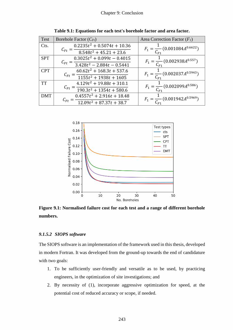
Chapter 9: Conclusion
243
Table 9.1: Equations for each test's borehole factor and area factor.
Test Borehole Factor (CFt) Area Correction Factor (F1)
Cts. 𝐶𝐹𝑡 =
0.2235𝑡2 + 0.5074𝑡 + 10.36
8.548𝑡2 + 45.21 + 23.6 𝐹1 =
1
𝐶𝐹1(0.001084𝐴0.6622)
SPT 𝐶𝐹𝑡 =
0.3025𝑡2 + 0.099𝑡 − 0.4015
3.428𝑡2 − 2.884𝑡 − 0.5441 𝐹1 =
1
𝐶𝐹1(0.002938𝐴0.557)
CPT 𝐶𝐹𝑡 =
60.62𝑡2 + 168.3𝑡 + 537.6
1155𝑡2 + 1938𝑡 + 1605 𝐹1 =
1
𝐶𝐹1(0.002037𝐴0.5943)
TT 𝐶𝐹𝑡 =
4.129𝑡2 + 19.88𝑡 + 310.1
190.3𝑡2 + 1354𝑡 + 580.6 𝐹1 =
1
𝐶𝐹1(0.002099𝐴0.586)
DMT 𝐶𝐹𝑡 =
0.4557𝑡2 + 2.916𝑡 + 18.48
12.09𝑡2 + 87.37𝑡 + 38.7 𝐹1 =
1
𝐶𝐹1(0.001942𝐴0.5969)
Figure 9.1: Normalised failure cost for each test and a range of different borehole
numbers.
9.1.5.2 SIOPS software
The SIOPS software is an implementation of the framework used in this thesis, developed
in modern Fortran. It was developed from the ground-up towards the end of candidature
with two goals:
1. To be sufficiently user-friendly and versatile as to be used, by practicing
engineers, in the optimization of site investigations; and
2. By necessity of (1), incorporate aggressive optimization for speed, at the
potential cost of reduced accuracy or scope, if needed.
Chapter 9: Conclusion
244
Point (1) was achieved through allowing the analysis of a wide variety of single- and
multi-layer soils through a minimalistic text-file interface. Perhaps more importantly, an
extensive, illustrated user manual was created, explaining both the general theory and
user inputs. This manual is provided in Appendix E.
Point (2) was achieved through application of all optimizations described in §9.1.2,
except for those regarding program parallelisation, as they are not needed. In particular,
SIOPS replaces FEA for pile settlement analysis with the PIE method in single layer soils,
and a modified implementation of Mylonakis and Gazetas (1998) in multi-layer soils.
The latter method currently constrains multi-layered soils to have uniform properties in
each layer, which is discussed further in §9.2.8. The combination of optimizations,
together with efficient coding practice, results in a speed increase in the order of
10,000,000 times. This reduces, in approximate terms, an analysis that would have
traditionally taken a year on a single core processor, to a single minute of run-time.
Access:
SIOPS is free and open source, released under the MIT licence. The code-base is
maintained in a git repository at https://github.com/Michael-P-Crisp/SIOPS, where the
latest code, Windows executable, and user manual can be found. Further discussion of
SIOPS’ workings, capabilities and limitations can be found in the current user manual in
Appendix E. As a backup, the research related to this thesis and a copy of the SIOPS
software can also be found at: https://www.researchgate.net/profile/Michael_Crisp2. In
contrast, the software used for earlier chapters, JFIP (Jaksa Framework Implementation
in Python) is not intended for public use for reasons given in Appendix F.
Recreating real-world sites:
A notable feature of SIOPS, that has not been presented in analysis to date, is the ability
to recreate real-world sites based on existing borehole information. When analysing
multiple-layer soils, the user can input layer geometry information at known borehole
locations, as well as expected layer soil parameters. The layers are recreated through the
process described in §9.1.3. The resulting virtual soil will therefore be site-specific, and
a (albeit simplified) representation of what is expected to occur in the ground. As such,
the software is considered highly useful to practicing engineers, due to the increased
Chapter 9: Conclusion
245
precision and specificity of the resulting analysis, with respect to their individual ground
conditions.
The method of recreating real-world sites is described in Appendix E. These virtual sites
are referred to as conditional fields, as they are conditioned or constrained by existing
data. By contrast, all analysis in this thesis has been undertaken using unconditional sites.
Also of note is that the genetic algorithm, used in Chapter 8, can be employed to optimise
borehole locations in these conditional soils.
Some brief recommendations are given here with regards to the multi-layer soil
generation parameters described in Chapter 4, specifically Table 4.2. It is worth noting
that some of the random layer geometry parameters such as nsegx, nsegy, bl, and bu have
not been implemented in SIOPS for two reasons. Firstly, they relate to geometry that is
defined as a grid of points, which was considered too constrained for the more generalised
triangulation interpolation system used in SIOPS. Secondly, when recreating real-world
sites, these randomness parameters are redundant as the geometry is instead defined
directly by the borehole locations, with randomness provided exclusively by the 2D
random field. However, it would be straightforward to re-implement those parameters for
unconditional virtual soils, as the code for this has been released online as supplementary
material with the journal paper publication of Chapter 4 (Crisp et al. (2019)).
When recreating real-world sites, is the main uncertainty in choice of parameters is the
scale of fluctuation (SOF) and standard deviation of depths in the 2D random field. In
contrast, the geometry and average layer stiffnesses are taken directly from borehole
information, and the material properties within each layer are considered constant in the
model. However, as shown in Chapter 6, the results are not sensitive to the specific SOF
value when it is greater than the length or width of the site. Therefore an arbitrarily high
SOF value is suggested. With respect to the standard deviation, it is difficult to identify
an appropriate value due to lack of available information. As such, the engineer may wish
to perform a sensitivity analysis with a range of values. The average stiffness in each
layer can also be made to vary across Monte Carlo realisations for improved
accommodation of the uncertainty present in subsurface material properties. If the SOF
and standard deviation could be back-calculated for a set of sites and collated into a
database of possible input values, that would be a useful accompaniment to the software.
Chapter 9: Conclusion
246
9.2 Limitations and Future Work
There are a number of limitations associated with the current work.
9.2.1 Framework Validation
Perhaps the biggest barrier to practicing engineers adopting the results of this framework
is that it has not yet been validated. However, such a validation is a non-trivial task; if it
were possible to know the true optimal investigation of a real-world site for comparison,
then this framework would not be needed. One possible avenue would be to collate a
database of sites where a reasonable amount of information is known about the subsurface
profile. A group of experienced geotechnical engineers could then independently indicate
what they believe to be an optimal investigation. The results would be compared with
those contained in this thesis to determine if the recommendations are reasonable.
A similar avenue would involve comparing the results from this research with previously
conducted site investigations, comparing whether the real investigation was larger or
smaller in scope, as well as the performance of the real-world foundation.
9.2.2 Elasto-plastic FEA for Pile Analysis
A number of limitations result from the relatively simple linear-elastic assumption used
in pile performance assessment. Soils are known to behave in a plastic manner, although
it is not yet feasible to employ settlement models that reflect this behaviour with current
computing power and available techniques. However, should this change in the future, it
is worth examining as the resulting settlement should be more accurate.
Perhaps a more important consideration in the addition of plastic settlement analysis is
the inclusion of additional geotechnical parameters in the soil model. Currently, only a
single property is treated as being spatially variable; Young’s modulus. However, it is
known that different tests have varying levels of accuracy with regards to different soil
parameters (Lunne 1997). Therefore, incorporating these parameters would reflect the
performance of a test type more accurately with respect to the parameter(s) that an
engineer is most interested in for a particular project.
On the other hand, it is worth noting that several optimizations rely on the linear-elastic
assumption, particularly the pile settlement curves discussed in §9.1.2.1. Therefore, in
Chapter 9: Conclusion
247
addition to the significantly greater processing time that elasto-plastic FEM requires,
there is the further time needed due to the absence of these optimizations.
9.2.3 Advanced Soil Models
The soil model that is derived from investigation results assumes that the properties
within each layer are constant. However, it is not unreasonable to assume that in the
future, soil models could be derived directly from sample locations, using a 3D spatial
interpolation method such as Kriging (Krige 1953; Stein 2012). In this instance, it is
expected that differential settlement values could be notably reduced due to the resulting
accuracy improvement, which could affect the number of samples needed in an optimal
investigation. It should be noted that incorporation of such an interpolation mechanism
into the framework would likely add to a significant increase in processing time. There
are also other approaches which aim to build accurate soil models from limited
information, including sparse modelling (Hastie et al. 2015).
In addition to building more realistic soil models, the use of conditioned random fields
can be used to generate a true knowledge soil profile that more closely matches the known
soil properties at a real site, providing more specific results.
9.2.4 Site Investigations
The current analysis involved investigations where all samples were assessed using the
same test type. Similarly, the borehole depth was constant for all testing locations. In
practice, engineers use a variety of test types and borehole depths within the same
investigation. The option to mix different test types and borehole depths was actually
added to SIOPS fairly late in development, after all papers were submitted. Therefore, it
should be straightforward to perform this analysis in the future. A further step could
involve accounting for multivariate interaction between test types, producing a site-
specific transformation model that may result in significant design savings.
Staged site investigations would also be worth considering. This consists of performing
a modest, initial investigation to obtain basic soil information, which in turn assists in the
planning of a second, more thorough investigation that is used for design. However, it is
difficult to devise an objective procedure that would leverage the first stage results in the
planning of the second stage, as this is typically done from subjective experience.
Chapter 9: Conclusion
248
Further consideration can be given to the use of reduction methods. In particular, it is
worth investigating a form of reduction method that varies its level of conservatism based
on the quantity of available information. For example, the standard deviation method
could decrease the number of standard deviations for greater numbers of boreholes. While
this approach would likely result in overdesign for smaller numbers of boreholes, it would
result in a consistent and minimal level of risk. Indeed, a limitation of this research is that
a single standard deviation was considered. Similarly, only a single percentile was
considered; the 1st quartile.
Site investigations could also be made to account for other areas of a multi-story building
beyond the pile foundation. For example, retaining structures for a basement, tension
piles for basement uplift prevention, and dewatering plans for short- and long-term
dewatering.
9.2.5 Failure Cost
A more sophisticated analysis would also include further sources of failure cost.
Currently, failure costs can only occur due to damage from excessive differential
settlement. However, here are other modes of failure such as excessive absolute
settlement and tilt. Bearing capacity failure should also be considered, although this
would be appropriately captured by excessive absolute settlement in a sufficiently
complex elasto-plastic settlement model. Similarly, construction delays are not
considered, and such delays are arguably a more common unwanted consequence than
structural damage. As such, if a means is created for consistently and objectively
quantifying the expected cost of construction delays, then that would be a notable
improvement to the framework.
9.2.6 Additional Soil Parameters
One soil parameter that has been largely absent from this thesis is that of anisotropy,
which describes soil correlation being higher in the horizontal direction compared to the
vertical. In contrast, all soils here have been isotropic with the correlation being the same
in all directions. This limitation is due to the virtual soil generator used in this thesis, i.e.
the local average subdivision (LAS) method, having a limited capability to capture
anisotropy. However, the authors have implemented a new virtual soil generation
algorithm from recent theory developed by Li et al. (2019); Xiao et al. (2019). This
Chapter 9: Conclusion
249
method, called the stepwise-covariance matrix decomposition (SCMD) method, is
capable of generating anisotropic soils in a fraction of the time, and with a fraction of the
required RAM compared to the original CMD method. Therefore, it should be
straightforward to examine anisotropic soils in the future.
There is also some merit in assessing additional multi-layer soil profiles to examine the
effect of sloping layers. This includes layer boundaries that exhibit an incline.
Alternatively, soil profiles as a whole can be rotated by some angle, as can be found in
practice due to the actions of plate tectonics and fault lines.
9.2.7 Additional Optimization Guidelines
While there is a simple, inaccurate, rule-of-thumb technique for optimising the number
of boreholes, and a complex software program for custom conditions, there is nothing in-
between of intermediate accuracy and intermediate complexity. In other words, there is
no technique for approximately optimising site investigations that is simple to use, while
explicitly accounting for a range of different soil conditions.
One solution could be to build upon the rule-of-thumb method with additional adjustment
factors, for example one for a soil’s coefficient of variation or the standard deviation of
a layer boundary’s depth. Alternatively, one could generate results for a wide range of
soil parameter input values, and then apply a regression tool to predict the output in terms
of normalised failure cost. For example, an artificial neural network could be trained to
predict this value based on input parameters such as the number of piles, building area
and various aspects of soil variability. Once trained, the network could be adapted into
an intuitive and widely available platform such as an Excel spreadsheet.
One of the challenges with this research would be to distil the results into a form that is
suitable for insertion into a site investigation standard. Software such as SIOPS is not
appropriate for this purpose. Equations such as the rule-of-thumb method are more
suitable. However, more thought should be given to this aspiration.
9.2.8 SIOPS Enhancements
SIOPS is currently limited in the soil types that it can produce. For example, it can
generate a variable, single-layer soil, or a soil with multiple layers and uniform properties
Chapter 9: Conclusion
250
within each layer. Each case is subject to its own limitations, with real soils featuring
both multiple layers and varying properties, as was assessed in the JFIP software. These
constraints were implemented primarily as considerable, mutually-exclusive
performance optimizations, as their respective assumptions allowed for massively
simplified or innovative settlement models to be used. However, if an efficient means of
predicting pile settlement for this hybrid scenario were created, then it would produce
more realistic soil profiles. Alternatively, a means of approximating this hybrid case
could be implemented, such as the proposal discussed in Appendix F for soils with an
infinite vertical scale of fluctuation. This proposal has been implemented in SIOPS in an
experimental manner, but has not yet been verified, for example against a single layer
soil with a high vertical SOF.
Other enhancements to the SIOPS program could include the ability to assess different
types of foundations or structures. It should be possible to extend the analysis to pad
foundations by adapting the current settlement model used in the single layer analysis to
design by width instead of depth. In terms of multiple layer analysis, one of the models
investigated by Goldsworthy (2006), capable of incorporating varying soil properties
with depth, could be incorporated. It should also be possible to perform the optimization
procedure for bridges as opposed to multi-storey buildings. This is discussed briefly in
Appendix F. While failure costs have not been derived for bridges, any alterative
performance metric derived from settlement values could be substituted, such as
minimizing the probability of exceedance of a differential settlement threshold.
Another option could be to add functionality to SIOPS that assesses the accuracy of the
soil model as opposed to foundation performance. This functionality would be similar to
the first family of frameworks discussed in §1.2.2. For example, an investigation could
be considered optimal when the standard deviation of the Young’s modulus estimate
across Monte Carlo realisations is minimal. This foundation-agnostic approach would be
better suited to types of geotechnical works not discussed here, such as roads, retaining
walls and dams. However, as discussed in the introduction, it is limited in that the
performance metric asymptotes as the number of tests increases, and so cannot inform a
single, explicitly optimal investigation.
Chapter 9: Conclusion
251
9.3 Conclusion
The work in this thesis has shown that there is very often a benefit to undertaking an
investigation that is larger in scope than the minimum. This is particularly true in multi-
layer soils, which are associated with a failure cost that is several times larger than for
variable single-layer soils.
The recommended investigation effort varies dramatically with both the nature of the soil
and of the structure, where greater effort is needed for more variable or more complex
soils, and buildings that are larger or are supported by more piles. In most cases, more
expensive, yet more accurate, soil tests yield lower total project costs. Similarly, a
conservative interpretation of sample values is recommended, and layer boundaries in the
soil model should be interpolated from borehole locations.
Two tools have been developed for engineers to plan the number of tests. One is a simple
yet straightforward set of equations. The other is a versatile computer program (SIOPS)
that has been extensively optimised for speed, such that it can run within a few minutes
on a desktop computer. Several of these speed optimizations can be applied to other areas
of research. The application of a genetic algorithm for optimising testing locations has
revealed that tests should almost always be undertaken in close proximity to a pile.
With the results presented in this thesis, along with the developed and disseminated tools,
practicing engineers have all the information necessary to optimise the many attributes
of geotechnical site investigations for real-world sites and pile-supported buildings.
9.4 References
Crisp, M. P., Jaksa, M. B., Kuo, Y. L., Fenton, G. A., and Griffiths, D. V. 2019. A method
for generating virtual soil profiles with complex, multi-layer stratigraphy.
Georisk, 13(2), 154-163.
Fenton, G. A., and Griffiths, D. V. 2005. Three-dimensional probabilistic foundation
settlement. Journal of Geotechnical and Geoenvironmental Engineering, 131(2),
232-239.
Goldsworthy, J. S. 2006. Quantifying the risk of geotechnical site investigations. Ph.D
Thesis, School of Civil, Environmental and Mining Engineering, University of
Adelaide, Adelaide.
Hastie, T., Tibshirani, R., and Wainwright, M. 2015. Statistical learning with sparsity:
the lasso and generalizations: CRC press.
Chapter 9: Conclusion
252
Jaksa, M. B., Goldsworthy, J. S., Fenton, G. A., Kaggwa, W. S., Griffiths, D. V., Kuo,
Y. L., and Poulos, H. G. 2005. Towards reliable and effective site investigations.
Géotechnique, 55(2), 109-121.
Krige, D. G. 1953. A Statistical Approach to Some Basic Mine Valuation Problems on
the Witwatersrand. OR, 4(1), 18-18.
Li, D.-Q., Xiao, T., Zhang, L.-M., and Cao, Z.-J. 2019. Stepwise covariance matrix
decomposition for efficient simulation of multivariate large-scale three-
dimensional random fields. Applied Mathematical Modelling, 68, 169-181.
Lunne, T. 1997. Cone penetration testing in geotechnical practice. London: Blackie
Academic & Professional.
Mylonakis, G., and Gazetas, G. 1998. Settlement and additional internal forces of
grouped piles in layered soil. Géotechnique, 48(1), 55-72.
Rawlinsons, A. (2016). Australian Construction Handbook (34 ed., pp. 1005). Perth,
Australia: Rawlhouse Publishing Pty. Ltd.
Snir, M. 1998. MPI--the Complete Reference: The MPI core (Vol. 1): MIT press.
Stein, M. L. 2012. Interpolation of spatial data: some theory for kriging: Springer Science
& Business Media.
Vanmarcke, E. 1983. Random Fields: Analysis and Synthesis. London: MIT Press.
Xiao, T., Zhang, L.-M., Li, D.-Q., and Cao, Z.-J. 2019. Efficient 3-D Random Field
Simulation with Separable Correlation Functions. In Proceedings of the 7th
International Symposium on Geotechnical Safety and Risk, Taipei.
Appendix A: Two-layer, 2D Analysis with Simplified Framework
253
Appendix A : Two-layer, 2D
Analysis with Simplified
Framework
Paper title:
The Influence of Site Investigation Scope on Pile
Design in Multi-layered, 2D Variable Ground

Appendix A: Two-layer, 2D Analysis with Simplified Framework
254


Appendix A: Two-layer, 2D Analysis with Simplified Framework
256
Appendix A: Two-layer, 2D Analysis with Simplified Framework
257
Abstract
When designing foundations, geotechnical site investigations are usually undertaken to
characterize the physical and engineering properties of the ground. Often, the scope of
the site investigation is dictated by budgetary constraints and construction timelines,
rather than on the variability of the ground. Limited investigations have the potential to
impact significantly on the success or otherwise of the completed project. These include
cost over-runs, construction delays, foundation failure and overdesign. This paper
examines the influence of site investigation scope on the design and performance of pile
foundations with respect to pile load capacity and settlement. This is achieved by
carrying out a series of 2D numerical simulations of multi-layered and variable soil
profiles incorporating complex geological features within a Monte Carlo framework. In
this way, the probabilities of design failure and pile over-design are expressed for a range
of site conditions and investigation campaigns via relative design error.
Appendix A: Two-layer, 2D Analysis with Simplified Framework
258
1 Introduction
The scope of geotechnical site investigations is often dictated by the budget and
construction timeline of a structure (Institution of Civil Engineers 1991). Many studies
have demonstrated that the largest component of financial risk is in the ground. However,
expenditure has been as low as 0.025% (Jaksa 2000) to 0.3% (National Research Council
1984) of the total budget. When soil variability is not explicitly considered as part of the
scope of an investigation, there is potential for the ground to be improperly characterized.
Unsurprisingly, several studies have linked foundation failure directly to inadequate site
investigations (Nordlund and Deere 1970; Association of Soil Foundation Engineers
1996). Another consequence is that foundations are overdesigned to compensate for
uncertainty, which incurs increased expenditure.
There are several areas of on-going research attempting to explicitly account for soil
variability. Most recently, there has been a focus on various aspects of reliability-based
design (RBD). Typically, RBD links uncertainty, in terms of the quantity or source of
information available, with the level of redundancy used for foundation design. More
specifically, simplified RBD methods such as load and resistance factor design (LRFD)
(Freudenthal 1945) are being investigated due to their relative ease of use and familiarity
to practicing engineers. There has been some success in adapting the methodology to the
context of geotechnical engineering (Ching et al. 2013; Naghibi et al. 2014). However,
the method does not account for the spatial structure in a soil profile nor the correlation
between samples. In other words, it does not inform a sampling strategy for a site
investigation and cannot guarantee an optimal total cost for a given soil profile.
The methodology of this paper involves an ongoing investigation framework developed
by Jaksa et al. (2003), and undertaken by Goldsworthy (2006) and Arsyad (2009). Using
random field simulations, the research aims to quantify the relationship between
components of a site investigation including sampling pattern, number of boreholes and
test types on the design of various foundations. These analyses were conducted in a
single homogenous soil layer, of which the variability of geotechnical parameters was
represented by a mean, coefficient of variation (COV) and scale of fluctuation (SOF).
The SOF is a measure of the distance within which properties display a strong correlation
(Vanmarcke 1977). In practical terms, soils with low SOF distances exhibit more rapid
fluctuations in properties compared to larger distances. This influence, along with that
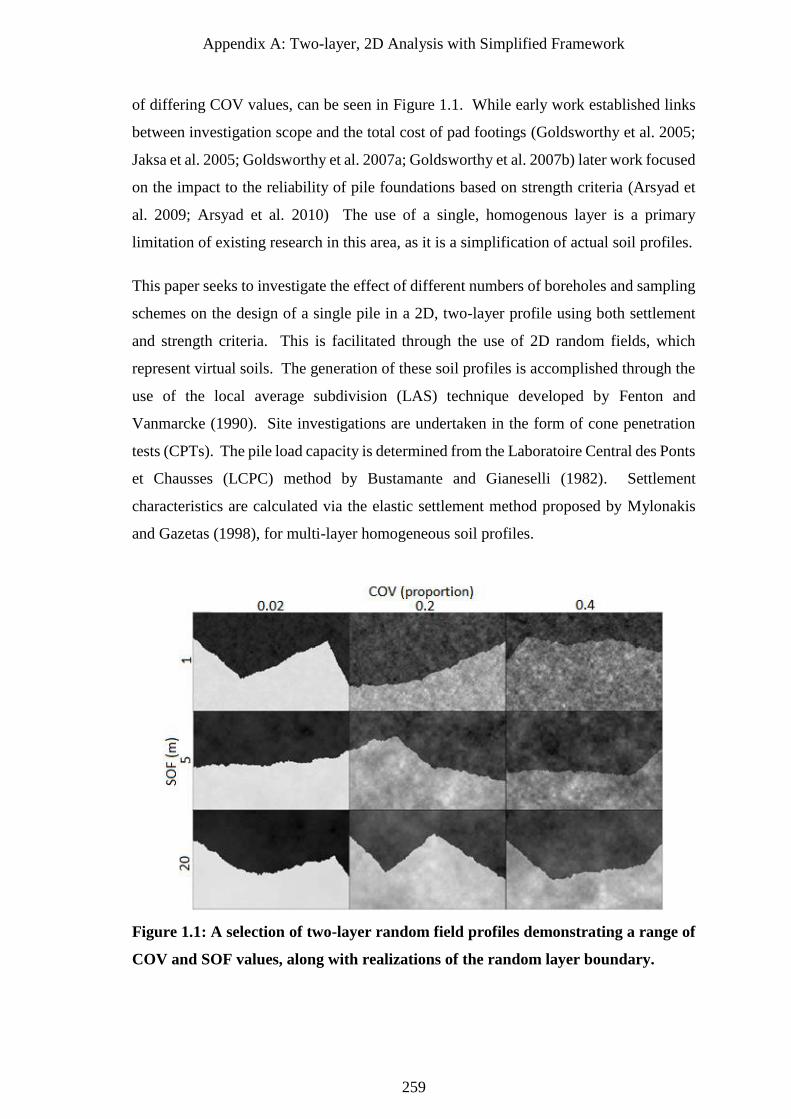
Appendix A: Two-layer, 2D Analysis with Simplified Framework
259
of differing COV values, can be seen in Figure 1.1. While early work established links
between investigation scope and the total cost of pad footings (Goldsworthy et al. 2005;
Jaksa et al. 2005; Goldsworthy et al. 2007a; Goldsworthy et al. 2007b) later work focused
on the impact to the reliability of pile foundations based on strength criteria (Arsyad et
al. 2009; Arsyad et al. 2010) The use of a single, homogenous layer is a primary
limitation of existing research in this area, as it is a simplification of actual soil profiles.
This paper seeks to investigate the effect of different numbers of boreholes and sampling
schemes on the design of a single pile in a 2D, two-layer profile using both settlement
and strength criteria. This is facilitated through the use of 2D random fields, which
represent virtual soils. The generation of these soil profiles is accomplished through the
use of the local average subdivision (LAS) technique developed by Fenton and
Vanmarcke (1990). Site investigations are undertaken in the form of cone penetration
tests (CPTs). The pile load capacity is determined from the Laboratoire Central des Ponts
et Chausses (LCPC) method by Bustamante and Gianeselli (1982). Settlement
characteristics are calculated via the elastic settlement method proposed by Mylonakis
and Gazetas (1998), for multi-layer homogeneous soil profiles.
Figure 1.1: A selection of two-layer random field profiles demonstrating a range of
COV and SOF values, along with realizations of the random layer boundary.
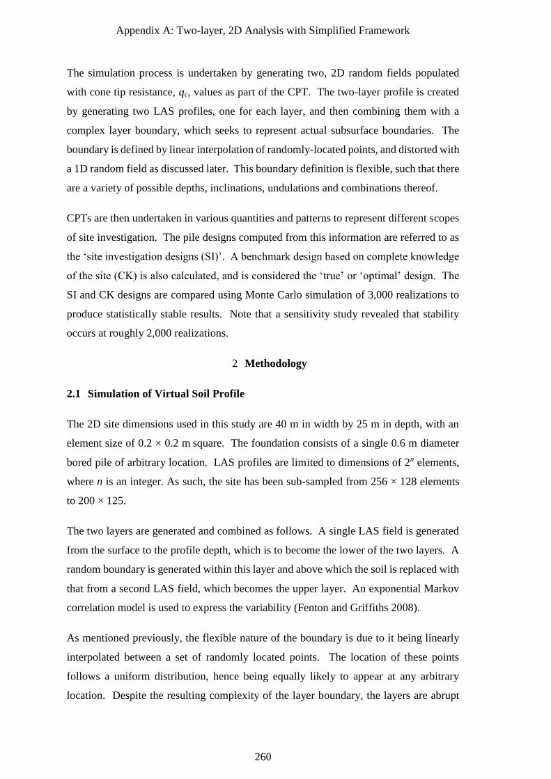
Appendix A: Two-layer, 2D Analysis with Simplified Framework
260
The simulation process is undertaken by generating two, 2D random fields populated
with cone tip resistance, qc, values as part of the CPT. The two-layer profile is created
by generating two LAS profiles, one for each layer, and then combining them with a
complex layer boundary, which seeks to represent actual subsurface boundaries. The
boundary is defined by linear interpolation of randomly-located points, and distorted with
a 1D random field as discussed later. This boundary definition is flexible, such that there
are a variety of possible depths, inclinations, undulations and combinations thereof.
CPTs are then undertaken in various quantities and patterns to represent different scopes
of site investigation. The pile designs computed from this information are referred to as
the ‘site investigation designs (SI)’. A benchmark design based on complete knowledge
of the site (CK) is also calculated, and is considered the ‘true’ or ‘optimal’ design. The
SI and CK designs are compared using Monte Carlo simulation of 3,000 realizations to
produce statistically stable results. Note that a sensitivity study revealed that stability
occurs at roughly 2,000 realizations.
2 Methodology
2.1 Simulation of Virtual Soil Profile
The 2D site dimensions used in this study are 40 m in width by 25 m in depth, with an
element size of 0.2 × 0.2 m square. The foundation consists of a single 0.6 m diameter
bored pile of arbitrary location. LAS profiles are limited to dimensions of 2n elements,
where n is an integer. As such, the site has been sub-sampled from 256 × 128 elements
to 200 × 125.
The two layers are generated and combined as follows. A single LAS field is generated
from the surface to the profile depth, which is to become the lower of the two layers. A
random boundary is generated within this layer and above which the soil is replaced with
that from a second LAS field, which becomes the upper layer. An exponential Markov
correlation model is used to express the variability (Fenton and Griffiths 2008).
As mentioned previously, the flexible nature of the boundary is due to it being linearly
interpolated between a set of randomly located points. The location of these points
follows a uniform distribution, hence being equally likely to appear at any arbitrary
location. Despite the resulting complexity of the layer boundary, the layers are abrupt
Appendix A: Two-layer, 2D Analysis with Simplified Framework
261
with no blending of properties at the interface. Conceptually, the layer-merging
procedure mimics real-life processes of erosion and deposit. While beyond the scope of
the study, this method allows for natural, random formation of complex geological
features, such as lenses in the case of 3 or more layers.
In this study, the boundary is linearly interpolated between 4 points to create 3 segments,
as seen in Figure 1.1. The feasible region in which individual points may appear is shown
in Figure 2.2. Vertically, each point is located anywhere between 25% and 75% of the
full soil depth.
Horizontally, the first and fourth (edge) points are fixed to the left and right side
boundaries, respectively. (Inner) points 2 and 3 can appear anywhere in the first and
second half of the profile width. This horizontal spacing was chosen to encourage a
regular undulation pattern. After the points have been generated, the boundary is then
distorted with random noise. This is accomplished by means of a zero-mean, normally-
distributed random field with a standard deviation of 0.5 m, and a SOF of 10 m. The
purpose of this is to simulate more complex and realistic layer boundaries by decreasing
the linearity of the segments. It also introduces uncertainty to the exact boundary location
as encountered by CPTs, which aids in simulating measurement errors and the engineers’
subjectivity in the design process.
The first layer is composed of “silt and loose sand”, as defined by the LCPC method,
with a selected mean qc of 1,250 kPa. The second layer consists of “moderately compact
sand and gravel” with a mean qc of 5,000 kPa. These types and properties have been
selected in order to have a strength ratio of 1:4 between the first and second layer. Over
a large number of realizations, the layer boundary average should tend towards a
horizontal interface with a depth ratio of 1:1. It is assumed, in this case, that a design
engineer would consider the boundary as horizontal. With regards to settlement
calculations, the Young’s modulus of the soil is calculated using the following
relationship as suggested by Schmertmann (1978) for axisymmetric piles.
E = 2.5qc
Appendix A: Two-layer, 2D Analysis with Simplified Framework
262
2.2 Simulation of CPTs and Pile Foundations
The pile is assumed to be circular in cross section, and discretised to a width of 3-elements
(0.6 m). The length is determined from an iterative design process, whereby the length
is increased successively by one element until the strength and settlement criteria are
satisfied. As such, the pile length is rounded up to the nearest 0.2 m. The applied load
is 400 kN, with a settlement limit of 10 mm. No additional safety factors have been used
besides those specified within the LCPC method. The Young’s modulus of the pile is
selected as 25,000 MPa. All design from multiple CPTs was undertaken by averaging
values horizontally to a single representative CPT.
The CK design is created by performing a CPT at every location across the width of the
profile. In reality, a pile in a multi-layer profile with a non-horizontal layer will behave
as per the layer depths in close proximity, as opposed to the average of the complete site.
However, as mentioned previously, the average layer structure should tend to horizontal,
and is considered as such. The simplifying assumption of a global site average also
guarantees that the SI design should tend towards the CK design as the number of
boreholes increases, which is suitable for the statistical nature of this study. Another
benefit of designing with the global average is that the results are independent of pile
location, removing the pile location variable from the analysis.
Two different investigation plans are examined for the SI design, as shown in Figure 2.1.
Figure 2.1(a) presents a regular grid (RG) pattern, containing between 1 and 5 CPTs at
equal spacing. Similarly, a stratified random (SR) sampling pattern is used. As seen in
Figure 2.1(b), for n CPTs, the full width of the site is subdivided into n segments of equal
width, where a single CPT is randomly located in each segment according to a uniform
distribution. These sampling patterns, among others, are discussed in greater detail by
(Ferguson 1992) in the context of detecting contamination hotspots.
Appendix A: Two-layer, 2D Analysis with Simplified Framework
263
Figure 2.1: Locations of (a) boreholes in the case of the regular grid scheme, and
(b) the range in which each borehole may randomly appear in the stratified
random scheme.
Figure 2.2: Feasible areas for the 4 boundary- defining points, and an example
random layer boundary defined by those points.
3 Results and Discussion
The results of this study are presented in terms of the average relative design error, �̅�E,
which is effectively a form of pile length standardization such that the relative magnitude
of under- and over-design is presented in terms of the optimal pile length. Here, when
�̅�E is less than or greater than zero implies the pile has been under- and over-designed
respectively. Ideally, pile designs should have a �̅�E of zero, implying the design is
optimal.
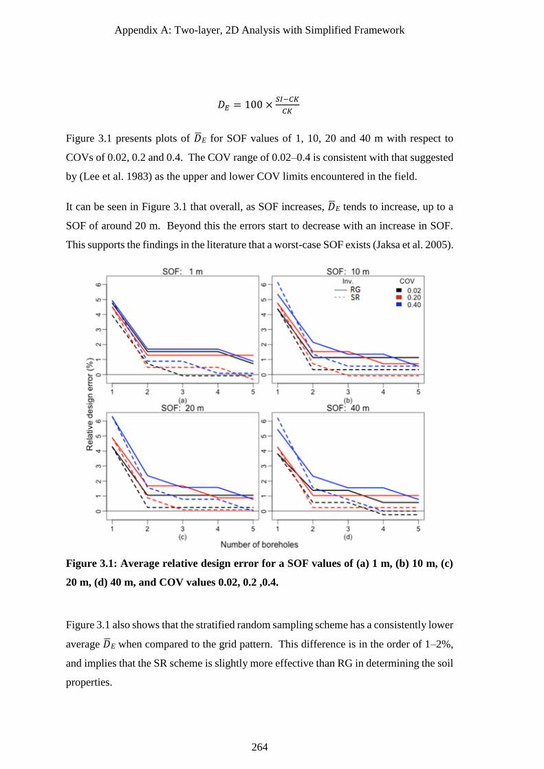
Appendix A: Two-layer, 2D Analysis with Simplified Framework
264
𝐷𝐸 = 100 ×𝑆𝐼−𝐶𝐾
𝐶𝐾
Figure 3.1 presents plots of �̅�E for SOF values of 1, 10, 20 and 40 m with respect to
COVs of 0.02, 0.2 and 0.4. The COV range of 0.02–0.4 is consistent with that suggested
by (Lee et al. 1983) as the upper and lower COV limits encountered in the field.
It can be seen in Figure 3.1 that overall, as SOF increases, �̅�E tends to increase, up to a
SOF of around 20 m. Beyond this the errors start to decrease with an increase in SOF.
This supports the findings in the literature that a worst-case SOF exists (Jaksa et al. 2005).
Figure 3.1: Average relative design error for a SOF values of (a) 1 m, (b) 10 m, (c)
20 m, (d) 40 m, and COV values 0.02, 0.2 ,0.4.
Figure 3.1 also shows that the stratified random sampling scheme has a consistently lower
average �̅�E when compared to the grid pattern. This difference is in the order of 1–2%,
and implies that the SR scheme is slightly more effective than RG in determining the soil
properties.
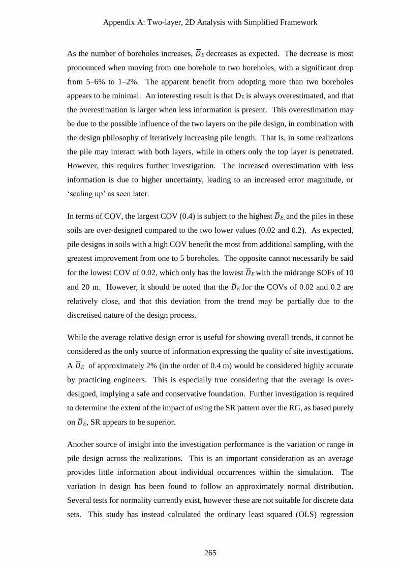
Appendix A: Two-layer, 2D Analysis with Simplified Framework
265
As the number of boreholes increases, �̅�E decreases as expected. The decrease is most
pronounced when moving from one borehole to two boreholes, with a significant drop
from 5–6% to 1–2%. The apparent benefit from adopting more than two boreholes
appears to be minimal. An interesting result is that DE is always overestimated, and that
the overestimation is larger when less information is present. This overestimation may
be due to the possible influence of the two layers on the pile design, in combination with
the design philosophy of iteratively increasing pile length. That is, in some realizations
the pile may interact with both layers, while in others only the top layer is penetrated.
However, this requires further investigation. The increased overestimation with less
information is due to higher uncertainty, leading to an increased error magnitude, or
‘scaling up’ as seen later.
In terms of COV, the largest COV (0.4) is subject to the highest �̅�E, and the piles in these
soils are over-designed compared to the two lower values (0.02 and 0.2). As expected,
pile designs in soils with a high COV benefit the most from additional sampling, with the
greatest improvement from one to 5 boreholes. The opposite cannot necessarily be said
for the lowest COV of 0.02, which only has the lowest �̅�E with the midrange SOFs of 10
and 20 m. However, it should be noted that the �̅�E for the COVs of 0.02 and 0.2 are
relatively close, and that this deviation from the trend may be partially due to the
discretised nature of the design process.
While the average relative design error is useful for showing overall trends, it cannot be
considered as the only source of information expressing the quality of site investigations.
A �̅�E of approximately 2% (in the order of 0.4 m) would be considered highly accurate
by practicing engineers. This is especially true considering that the average is over-
designed, implying a safe and conservative foundation. Further investigation is required
to determine the extent of the impact of using the SR pattern over the RG, as based purely
on �̅�E, SR appears to be superior.
Another source of insight into the investigation performance is the variation or range in
pile design across the realizations. This is an important consideration as an average
provides little information about individual occurrences within the simulation. The
variation in design has been found to follow an approximately normal distribution.
Several tests for normality currently exist, however these are not suitable for discrete data
sets. This study has instead calculated the ordinary least squared (OLS) regression
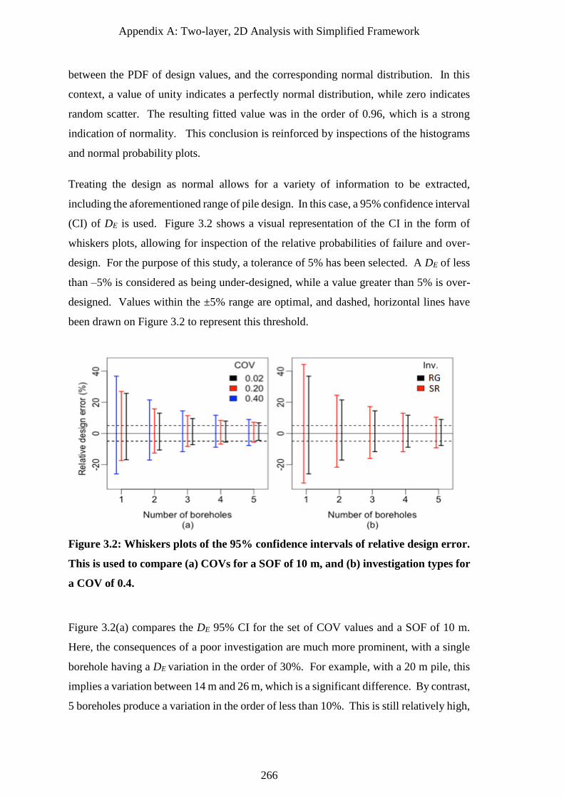
Appendix A: Two-layer, 2D Analysis with Simplified Framework
266
between the PDF of design values, and the corresponding normal distribution. In this
context, a value of unity indicates a perfectly normal distribution, while zero indicates
random scatter. The resulting fitted value was in the order of 0.96, which is a strong
indication of normality. This conclusion is reinforced by inspections of the histograms
and normal probability plots.
Treating the design as normal allows for a variety of information to be extracted,
including the aforementioned range of pile design. In this case, a 95% confidence interval
(CI) of DE is used. Figure 3.2 shows a visual representation of the CI in the form of
whiskers plots, allowing for inspection of the relative probabilities of failure and over-
design. For the purpose of this study, a tolerance of 5% has been selected. A DE of less
than –5% is considered as being under-designed, while a value greater than 5% is over-
designed. Values within the ±5% range are optimal, and dashed, horizontal lines have
been drawn on Figure 3.2 to represent this threshold.
Figure 3.2: Whiskers plots of the 95% confidence intervals of relative design error.
This is used to compare (a) COVs for a SOF of 10 m, and (b) investigation types for
a COV of 0.4.
Figure 3.2(a) compares the DE 95% CI for the set of COV values and a SOF of 10 m.
Here, the consequences of a poor investigation are much more prominent, with a single
borehole having a DE variation in the order of 30%. For example, with a 20 m pile, this
implies a variation between 14 m and 26 m, which is a significant difference. By contrast,
5 boreholes produce a variation in the order of less than 10%. This is still relatively high,
Appendix A: Two-layer, 2D Analysis with Simplified Framework
267
however as seen in the figure, the majority of this range now lies within the 5% tolerance.
The probabilities of both under- and over-design are therefore significantly reduced. It
should be noted that this tolerance, despite being of practical relevance, also helps
account for the discrete nature of the design. This is because there is a notably higher
likelihood of achieving an exactly optimal design when compared to a continuous
variable.
Utilizing the properties of the normal distribution, it can be shown that the probabilities
of under- and over-design fall from 25.4% and 50.9% with one borehole to 9.12% and
14.3% with 5 boreholes respectively. This implies the probability of achieving an
optimal design increases from 23.7% to 76.6%. This noticeable increase in the
probability of an optimal design as the number of boreholes increases shows a noticeable
benefit of increased sampling when compared to the apparent insensitivity of the average
�̅�E. Another benefit of the DE 95% CI is that it shows the relative changes in the average
�̅�E in Figure 3.1 are relatively minor, and that the apparent overall trend of
overestimation can be largely ignored.
In terms of the COV of the soil, the largest value of 0.4 has the largest CI as expected, as
seen in Figure 3.2(a). There is a noticeable reduction in the interval as the COV decreases
to 0.2. This is followed by a smaller reduction in CI when the COV decreases to 0.02.
The difference in variability between the 3 COV values decreases as the number of
boreholes increases. This implies that a larger number of boreholes provides greater
confidence despite the COV.
The CI has also been compared between the SR and RG sampling patterns in Figure
3.2(b). Here it can be seen that the CI for SR is noticeably larger than that of RG,
implying that the SR scheme is less consistent. This offsets the apparent benefit of a
lower average DE seen in Figure 3.1. Certainly, the 1–2% improvement of the average is
negligible in the context of the –30% to 40% lower and upper bound of the CI. This high
variability implies that the RG pattern is superior. The variation itself is due to a higher
likelihood of two boreholes being in close proximity. This would favour the knowledge
of the layer boundary towards these boreholes at the expense of the rest of the site, when
compared to the regular spacing of the RG pattern.
Appendix A: Two-layer, 2D Analysis with Simplified Framework
268
4 Conclusion
This study has examined the effect of the overall trend and variability of pile design when
using different quantities of information in a variety of two-layer soil profiles. The testing
has consisted of CPTs, allowing for design both by the LCPC method for capacity, and
an elastic settlement technique, in virtual soils generated by the LAS method. Rather
than indicate a minimum number of boreholes, it is intended that an engineer refer to the
charts provided and use their judgment when planning an investigation. These charts are
the focus of future research and will generalise the results to a range of broad soil
categories, as well as building heights and sizes. A practicing engineer can infer the
relevant site category based on preliminary data, such as from a desktop study, or can
otherwise assume worst-case conditions.
It has been observed that, as the number of boreholes increases, there is an improvement
in both the average pile design, as well as a reduction in pile variability. The effect on
the latter is noticeably more significant, especially in the context of a 5% tolerance, where
probabilities of under- and over-design are dramatically improved; although, the rate of
this improvement diminishes as the number of boreholes increase. The improvement of
the average design is nominal after approximately two boreholes. However, the
confidence interval reduction implies higher confidence can be achieved with additional
sampling. Arguably, the average relative design error on its own is a poor indicator of
investigation performance.
The average relative design error, as well as the 95% confidence interval of pile design,
is noticeably worse for soils with higher COV. As discussed in previous research, there
appears to be a worst-case SOF in the order of 10–20m. It is possible this may be some
function of site dimensions, however further investigation is required.
The stratified random sampling scheme was also compared to a regular grid pattern.
While there was slight improvement in the average design with stratified random, there
was a noticeably larger confidence interval implying reduced confidence. This lower
confidence level, combined with the practical inconvenience of implementing any kind
of random sampling, leads to the conclusion that a regular grid pattern is superior.
The main limitations of this study include the 2D nature of the analysis, and not
accounting for the relationship between pile and sample location. Future work will
Appendix A: Two-layer, 2D Analysis with Simplified Framework
269
extend the analysis to 3D complex soil profiles, with discrete pile locations. Furthermore,
different levels of design redundancy will be incorporated and total project cost will be
used as the objective function to define an optimal investigation.
5 References
Arsyad, A. 2009. The effect of limited site investigations on the design and performance
of pile foundations. Masters Thesis, School of Civil, Environmental and Mining
Engineering, University of Adelaide, Adelaide.
Arsyad, A., Jaksa, M., Fenton, G., and Kaggwa, W. 2009. The effect of limited site
investigations on the design of pile foundations. In Proceedings of the
International Conference on Soil Mechanics and Geotechnical Engineering (17th:
2009: Egypt).
Arsyad, A., Jaksa, M. B., Kaggwa, W., and Mitani, Y. 2010. Effect of radial distance of
a single CPT sounding on the probability of over-and under-design of pile
foundation. In Proceedings of the tthe First Makassar International Conference on
Civil Engineering, Makassar, Indonesia.
Association of Soil Foundation Engineers. 1996. Case Histories of Professional Liability
Losses: ASFE Case Histories 1-65: Association of Soil and Foundation
Engineers.
Bustamante, M., and Gianeselli, L. 1982. Pile bearing capacity prediction by means of
static penetrometer CPT. In Proceedings of the 2-nd European Symposium on
Penetration Testing.
Ching, J., Phoon, K.-K., and Yu, J.-W. 2013. Linking site investigation efforts to final
design savings with simplified reliability-based design methods. Journal of
Geotechnical and Geoenvironmental Engineering, 140(3), 04013032.
Fenton, G. A., and Griffiths, D. V. 2008. Risk assessment in geotechnical engineering:
Wiley.
Fenton, G. A., and Vanmarcke, E. H. 1990. Simulation of random fields via local average
subdivision. Journal of Engineering Mechanics, 116(8), 1733-1749.
Ferguson, C. 1992. The statistical basis for spatial sampling of contaminated land.
Ground engineering, 25, 34-34.
Freudenthal, A. M. 1945. The safety of structures. In Proceedings of the Selected Papers
by Alfred M. Freudenthal: Civil Engineering Classics.
Goldsworthy, J., Jaksa, M., Fenton, G., Griffiths, D., Kaggwa, W., and Poulos, H. 2007a.
Measuring the risk of geotechnical site investigations. In Proceedings of the Proc.,
Geo-Denver 2007.
Goldsworthy, J., Jaksa, M., Kaggwa, G., Fenton, G., Griffiths, D., and Poulos, H. 2005.
Reliability of site investigations using different reduction techniques for
Appendix A: Two-layer, 2D Analysis with Simplified Framework
270
foundation design. 9th International Conference on Structural Safety and
Reliability, 901-908.
Goldsworthy, J. S. 2006. Quantifying the risk of geotechnical site investigations. Ph.D
Thesis, School of Civil, Environmental and Mining Engineering, University of
Adelaide, Adelaide.
Goldsworthy, J. S., Jaksa, M. B., Fenton, G. A., Kaggwa, W. S., Griffiths, V., and Poulos,
H. G. 2007b. Effect of sample location on the reliability based design of pad
foundations. Georisk, 1(3), 155-166.
Institution of Civil Engineers. 1991. Inadequate Site Investigation. London: Thomal
Telford.
Jaksa, M. 2000. Geotechnical risk and inadequate site investigations: a case study.
Australian Geomechanics, 35(2), 39-46.
Jaksa, M., Goldsworthy, J., Fenton, G., Kaggwa, W., Griffiths, D., Kuo, Y., and Poulos,
H. 2005. Towards reliable and effective site investigations. Géotechnique, 55(2),
109-121.
Jaksa, M., Kaggwa, W., Fenton, G., and Poulos, H. 2003. A framework for quantifying
the reliability of geotechnical investigations. In Proceedings of the 9th
International Conference on the Application of Statistics and Probability in Civil
Engineering.
Lee, I. K., White, W., and Ingles, O. G. 1983. Geotechnical Engineering: Pitmans Books
Limited.
Mylonakis, G., and Gazetas, G. 1998. Settlement and additional internal forces of
grouped piles in layered soil. Géotechnique, 48(1), 55-72.
Naghibi, F., Fenton, G., and Griffiths, D. 2014. Serviceability limit state design of deep
foundations. Géotechnique, 64(10), 787-799.
National Research Council. 1984. Geotechnical Site Investigations for Underground
Projects (Vol. 1). Washington.
Nordlund, R. L., and Deere, D. U. 1970. Collapse of Fargo grain elevator. Journal of Soil
Mechanics & Foundations Div.
Schmertmann, J. H. (1978). Guidelines for Cone Penetration Test.(Performance and
Design). (No. FHWA-TS-78-209).
Vanmarcke, E. H. 1977. Reliability of earth slopes. Journal of the Soil Mechanics and
Foundations Division, 103(11), 1247-1265.
Appendix B: Analysis of Borehole Pattern and Area in a Single Layer Soil
271
Appendix B : Analysis of Borehole
Pattern and Area in a Single Layer
Soil
Paper Title:
Influence of Site Investigation Borehole Pattern and
Area on Pile Foundation Performance

Appendix B: Analysis of Borehole Pattern and Area in a Single Layer Soil
272


Appendix B: Analysis of Borehole Pattern and Area in a Single Layer Soil
274
Appendix B: Analysis of Borehole Pattern and Area in a Single Layer Soil
275
Abstract
Site investigations are the largest element of technical and financial risk in civil
engineering works, with insufficient testing often causing cost over-runs, construction
delays, foundation failure and over-design. However, there is little research on where best
to place boreholes with respect to the foundation. Typically, if the structure location is
known, then boreholes are placed at the centre, or otherwise at the corners, although some
studies indicate that there may be benefit to randomising the sampling location. This
study aims to determine the best of a series of sampling schemes, where each scheme
involves varying degrees of randomness, as well as to examine the effect of investigation
area relative to the building footprint.
The optimal sampling scheme is determined from Monte Carlo analysis, where a random,
variable, single layer, 3D virtual soil is generated. From this, it is possible to carry out a
variety of virtual site investigations, determine true foundation performance, and
determine the magnitude of structural damage resulting from insufficient investigation.
Total cost, calculated from a combination of construction, investigation, and failure costs,
is used as the objective function to be minimised.
Appendix B: Analysis of Borehole Pattern and Area in a Single Layer Soil
276
1 Introduction
Site investigations are an essential part of civil engineering works, as they allow for the
determination of subsoil material properties. As soil profiles are spatially variable in
nature, resulting from varying geological and environmental processes, it is important to
test a range of multiple locations. There are many reported cases where insufficient
testing has led to cost over-runs (Boeckmann and Loehr 2016), construction delays (Jaksa
2000), foundation failure (Moh 2004) and overdesign (Clayton 2001). Clearly, there is
great benefit to conducting a site investigation of satisfactory scope. However, there is
little guidance on what the components of such a scope would consist of (Crisp et al.
2018) (Appendix D). This study aims to investigate the influence of borehole location
on the performance of the resulting foundation.
The work in this study is undertaken with Monte Carlo analysis, based on a framework
originally proposed by Jaksa et al. (2003), and later elaborated and improved upon by
Crisp et al. (2018) (Appendix D). Within each realisation, a virtual soil is generated using
random field theory (Vanmarcke 1983), where each soil can be represented entirely by
three statistical, spatial parameters. These include the two moments of the lognormal
distribution; the mean and the standard deviation, where the latter is often normalised by
the mean to produce the coefficient of variation (COV). The lognormal distribution is
chosen as it has been found to adequately represent soil properties, and is commonly used
in this line of study due to its simplicity and non-negative nature (Fenton and Griffiths
2008). The third parameter is the scale of fluctuation (SOF) which represents the
correlation length, not unlike the range parameter in geostatistics. Alternatively, the SOF
can be described as the distance within which properties are expected to be correlated.
As all details of the soil are known, it is possible to replicate, in a virtual manner, the full
process of planning, construction, and performance of infrastructure. This is achieved by
simulating site investigations, designing resulting foundations, determining the true
performance of those foundations (through 3D linear-elastic finite element analysis,
FEA), and calculating potential damage to the superstructure through foundation failure.
By assigning costs to each of these components (construction, soil testing, failure), an
objective function is assembled in terms of the total, combined cost. This represents an
ideal optimization problem, as the optimal investigation is that with the lowest total cost,
Appendix B: Analysis of Borehole Pattern and Area in a Single Layer Soil
277
incorporating all components as described above, and the optimization implicitly reflects
both economic and risk-based factors.
Currently, there has been little research on the effect of borehole configuration, including
explicit benefits of randomizing locations. Ferguson (1992) has suggested that some
degree of randomness in borehole location may be beneficial, although this is in the
context of detecting localized contamination hotspots, as opposed to foundation design
where the properties over a large area are required. Goldsworthy et al. (2007a) compared
varying degrees of borehole location randomness in the case of pad foundations, although
simplified settlement methods were used instead of the more accurate FEA, and so the
true foundation performance may not be reliable. It was found that a stratified sampling
pattern produced the cheapest total cost for pad foundations. However, it was noted that
the decrease was modest, and Goldsworthy ultimately recommended a regular grid
pattern largely out of practicality. These findings are supported by Crisp et al. (2017)
(Appendix A), who compared a regular grid and stratified random patterns in a 2D, two-
layer soil profile for pile design. It was found that while the average design error was
reduced by up to 6% for the latter scheme, the variability of the design error was
significantly higher. These results indicate that regular grid sampling pattern may be
optimal, or sufficiently close to it. However, further research is required.
Greater focus has been given to optimising the location of a single borehole with respect
to a foundation. Goldsworthy et al. (2007b) found that a centrally-located borehole was
ideal in the case of a pad foundation group where a pad was present at the centre. In the
case without a central pad (i.e with four pads), it was found that sampling near a pad
location yielded best results, in terms of the lowest total cost. On the other hand, Arsyad
et al. (2010) modelled the influence of a single borehole around a single pile foundation
in an attempt to find a ‘critical distance’ between the two, beyond which the probabilities
of under- and over-design became constant. As expected, this distance was a function of
the SOF, and was found to be 5 m and 22m for a SOF of 1 m and 10 m respectively.
Beyond a SOF of 10 m, the critical distance decreased, implying this SOF to be the worst
case. These findings indicate that while boreholes should coincide with a foundation,
ideally they should be within the influence range of all foundations at a site, and that this
range is strongly influenced by the SOF.
Appendix B: Analysis of Borehole Pattern and Area in a Single Layer Soil
278
In terms of multiple boreholes relative to foundation locations, existing research is
minimal. Goldsworthy et al. (2004) studied the effect of varying the location of a
constantly-sized investigation area around a pad foundation. It was found, unsurprisingly,
that the best results in terms of probability of failure and overdesign were obtained when
the investigation area overlays the foundation location centrally, such that the foundation
footprint is entirely contained within the area’s boundary. This central preference is as
opposed to a foundation at least partially located outside of the investigation plan.
Furthermore, Goldsworthy (2006) noted that besides the aforementioned single borehole
case, the number of boreholes was the dominant factor in investigation performance, and
that the exact locations of these boreholes were of secondary relevance. These results
imply that in the case of multiple boreholes, investigation performance is not sensitive to
borehole configuration.
To date, no research has compared the effect of random sampling on the performance of
pile foundations in 3D, or with any foundations using the accurate FEA settlement model.
Furthermore, no study has analysed the influence of varying the size of the investigation
area relative to the foundation footprint. This study therefore examines the influence of
borehole pattern, area and number in a variety of soil profiles. The two aims are as
follows:
1. To investigate potential benefits of using random borehole locations, though a
variety of sampling schemes with different inherent degrees of location
randomness; and
2. To determine the effect of changing the size of the investigation area, centred
around the foundation.
The outcome of this research is key insight into the relationship between total cost and
the number of boreholes, for a variety of soil conditions and borehole configurations. The
degree of sensitivity between these variables and total cost, as well as any identifiable
universally optimal cases, will inform practicing engineers to plan their investigations
more effectively.
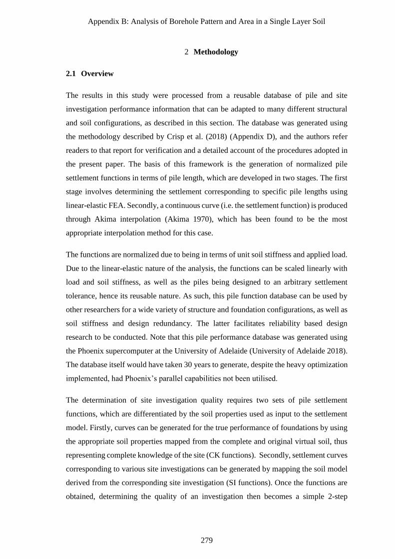
Appendix B: Analysis of Borehole Pattern and Area in a Single Layer Soil
279
2 Methodology
2.1 Overview
The results in this study were processed from a reusable database of pile and site
investigation performance information that can be adapted to many different structural
and soil configurations, as described in this section. The database was generated using
the methodology described by Crisp et al. (2018) (Appendix D), and the authors refer
readers to that report for verification and a detailed account of the procedures adopted in
the present paper. The basis of this framework is the generation of normalized pile
settlement functions in terms of pile length, which are developed in two stages. The first
stage involves determining the settlement corresponding to specific pile lengths using
linear-elastic FEA. Secondly, a continuous curve (i.e. the settlement function) is produced
through Akima interpolation (Akima 1970), which has been found to be the most
appropriate interpolation method for this case.
The functions are normalized due to being in terms of unit soil stiffness and applied load.
Due to the linear-elastic nature of the analysis, the functions can be scaled linearly with
load and soil stiffness, as well as the piles being designed to an arbitrary settlement
tolerance, hence its reusable nature. As such, this pile function database can be used by
other researchers for a wide variety of structure and foundation configurations, as well as
soil stiffness and design redundancy. The latter facilitates reliability based design
research to be conducted. Note that this pile performance database was generated using
the Phoenix supercomputer at the University of Adelaide (University of Adelaide 2018).
The database itself would have taken 30 years to generate, despite the heavy optimization
implemented, had Phoenix’s parallel capabilities not been utilised.
The determination of site investigation quality requires two sets of pile settlement
functions, which are differentiated by the soil properties used as input to the settlement
model. Firstly, curves can be generated for the true performance of foundations by using
the appropriate soil properties mapped from the complete and original virtual soil, thus
representing complete knowledge of the site (CK functions). Secondly, settlement curves
corresponding to various site investigations can be generated by mapping the soil model
derived from the corresponding site investigation (SI functions). Once the functions are
obtained, determining the quality of an investigation then becomes a simple 2-step
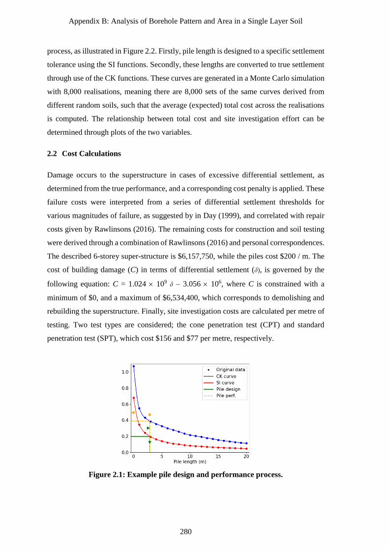
Appendix B: Analysis of Borehole Pattern and Area in a Single Layer Soil
280
process, as illustrated in Figure 2.2. Firstly, pile length is designed to a specific settlement
tolerance using the SI functions. Secondly, these lengths are converted to true settlement
through use of the CK functions. These curves are generated in a Monte Carlo simulation
with 8,000 realisations, meaning there are 8,000 sets of the same curves derived from
different random soils, such that the average (expected) total cost across the realisations
is computed. The relationship between total cost and site investigation effort can be
determined through plots of the two variables.
2.2 Cost Calculations
Damage occurs to the superstructure in cases of excessive differential settlement, as
determined from the true performance, and a corresponding cost penalty is applied. These
failure costs were interpreted from a series of differential settlement thresholds for
various magnitudes of failure, as suggested by in Day (1999), and correlated with repair
costs given by Rawlinsons (2016). The remaining costs for construction and soil testing
were derived through a combination of Rawlinsons (2016) and personal correspondences.
The described 6-storey super-structure is $6,157,750, while the piles cost $200 / m. The
cost of building damage (C) in terms of differential settlement (δ), is governed by the
following equation: C = 1.024 109 δ – 3.056 106, where C is constrained with a
minimum of $0, and a maximum of $6,534,400, which corresponds to demolishing and
rebuilding the superstructure. Finally, site investigation costs are calculated per metre of
testing. Two test types are considered; the cone penetration test (CPT) and standard
penetration test (SPT), which cost $156 and $77 per metre, respectively.
Figure 2.1: Example pile design and performance process.
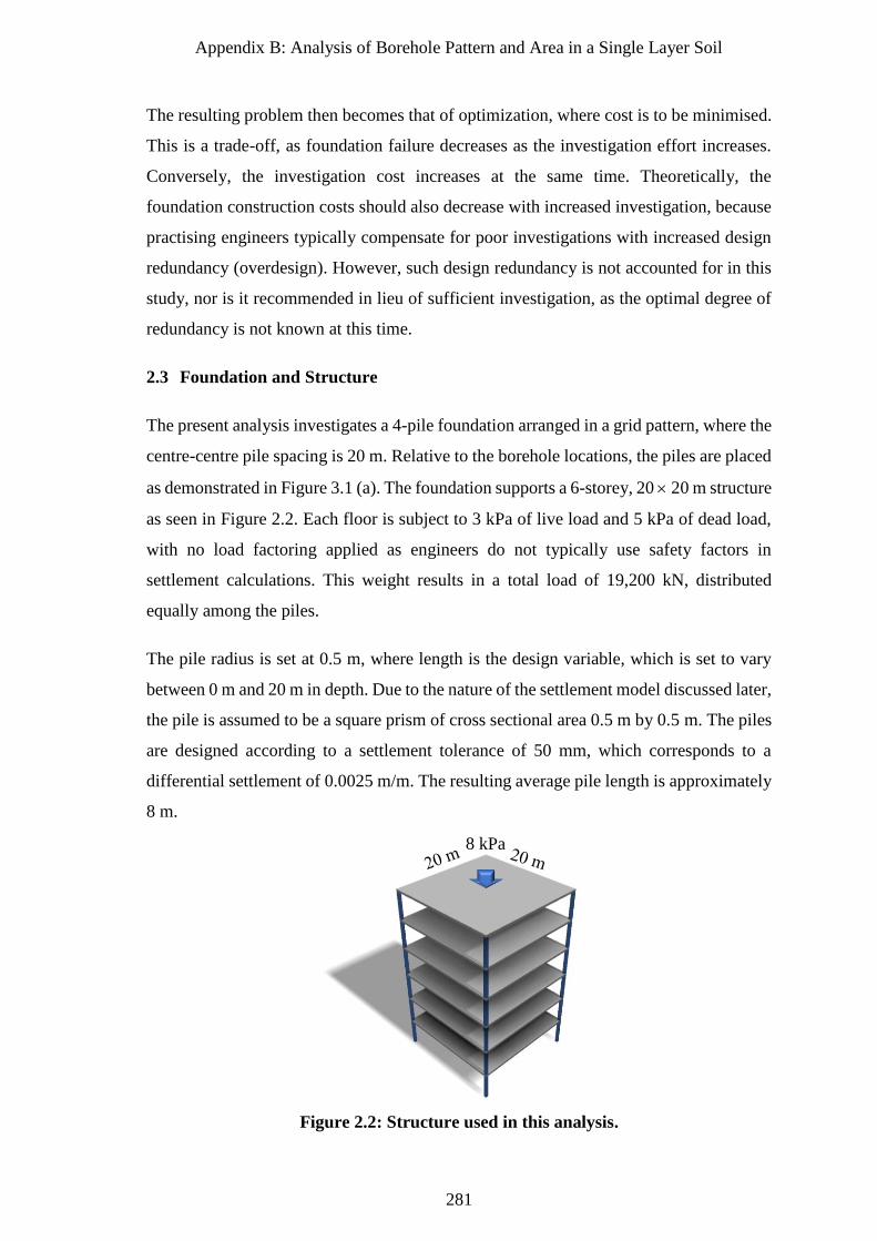
Appendix B: Analysis of Borehole Pattern and Area in a Single Layer Soil
281
The resulting problem then becomes that of optimization, where cost is to be minimised.
This is a trade-off, as foundation failure decreases as the investigation effort increases.
Conversely, the investigation cost increases at the same time. Theoretically, the
foundation construction costs should also decrease with increased investigation, because
practising engineers typically compensate for poor investigations with increased design
redundancy (overdesign). However, such design redundancy is not accounted for in this
study, nor is it recommended in lieu of sufficient investigation, as the optimal degree of
redundancy is not known at this time.
2.3 Foundation and Structure
The present analysis investigates a 4-pile foundation arranged in a grid pattern, where the
centre-centre pile spacing is 20 m. Relative to the borehole locations, the piles are placed
as demonstrated in Figure 3.1 (a). The foundation supports a 6-storey, 20 20 m structure
as seen in Figure 2.2. Each floor is subject to 3 kPa of live load and 5 kPa of dead load,
with no load factoring applied as engineers do not typically use safety factors in
settlement calculations. This weight results in a total load of 19,200 kN, distributed
equally among the piles.
The pile radius is set at 0.5 m, where length is the design variable, which is set to vary
between 0 m and 20 m in depth. Due to the nature of the settlement model discussed later,
the pile is assumed to be a square prism of cross sectional area 0.5 m by 0.5 m. The piles
are designed according to a settlement tolerance of 50 mm, which corresponds to a
differential settlement of 0.0025 m/m. The resulting average pile length is approximately
8 m.
Figure 2.2: Structure used in this analysis.
Norm
aliz
ed p
ile
sett
lem
ent
(MP
a
mm
/kN
)
8
kPa
8 kPa
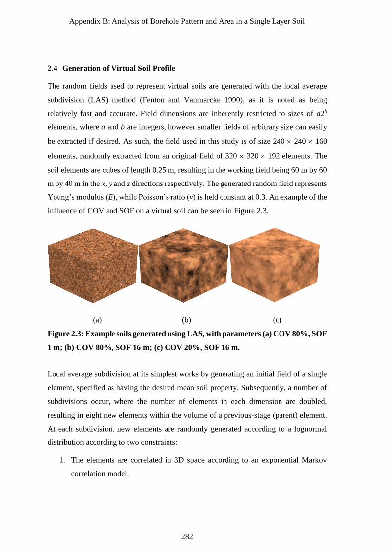
Appendix B: Analysis of Borehole Pattern and Area in a Single Layer Soil
282
2.4 Generation of Virtual Soil Profile
The random fields used to represent virtual soils are generated with the local average
subdivision (LAS) method (Fenton and Vanmarcke 1990), as it is noted as being
relatively fast and accurate. Field dimensions are inherently restricted to sizes of a2b
elements, where a and b are integers, however smaller fields of arbitrary size can easily
be extracted if desired. As such, the field used in this study is of size 240 240 160
elements, randomly extracted from an original field of 320 320 192 elements. The
soil elements are cubes of length 0.25 m, resulting in the working field being 60 m by 60
m by 40 m in the x, y and z directions respectively. The generated random field represents
Young’s modulus (E), while Poisson’s ratio (v) is held constant at 0.3. An example of the
influence of COV and SOF on a virtual soil can be seen in Figure 2.3.
(a) (b) (c)
Figure 2.3: Example soils generated using LAS, with parameters (a) COV 80%, SOF
1 m; (b) COV 80%, SOF 16 m; (c) COV 20%, SOF 16 m.
Local average subdivision at its simplest works by generating an initial field of a single
element, specified as having the desired mean soil property. Subsequently, a number of
subdivisions occur, where the number of elements in each dimension are doubled,
resulting in eight new elements within the volume of a previous-stage (parent) element.
At each subdivision, new elements are randomly generated according to a lognormal
distribution according to two constraints:
1. The elements are correlated in 3D space according to an exponential Markov
correlation model.
Appendix B: Analysis of Borehole Pattern and Area in a Single Layer Soil
283
2. A group of elements generated within the volume of a parent element has an
average value equal to that of the parent element. As such, the global average is
maintained while allowing local variability.
This study involves the use of a single-layer heterogeneous soil profile, following the
assumptions of second order stationarity (weak stationarity). With this assumption, the
soil mean is constant and the correlation between two points depends only on their lag
(i.e. separation distance) and not their locations (Brockwell and Davis 2013). This is used
so that the results can be generalised to a wider range of soils, as opposed to soil profiles
that have specific, complex multi-layer stratigraphy. However, as a result of this
simplifying assumption, any recommendations given in this study, as to the ideal number
of boreholes should be taken as a minimum, as more complex geology would require
more extensive investigation. Further details on LAS are given by Fenton and Griffiths
(2008), along with the corresponding Fortran code for the generation of random fields.
For the soil parameters used in the present study, a mean Young’s modulus of 60 MPa
was chosen, corresponding to hard clay or dense sand. SOFs of 1, 2, 4, 8, 16 and 24 m
were assessed, along with COVs of 20, 40 and 80%.
2.5 Settlement Model
The settlement model used in this study is a 3D linear-elastic FEA Fortran subroutine
adapted from Program 5.6 by Smith et al. (2013). The mesh is comprised of 8-node brick
elements, where nodes at the bottom are fixed in the vertical direction, representing
infinitely-stiff bedrock. Similarly, nodes on the sides of the mesh are laterally restrained
so as not to move out of plane. The subroutine uses an iterative, pre-conditioned,
conjugate gradient solver in lieu of assembling and solving the global stiffness matrix in
order to greatly reduce RAM usage.
The foundation is modelled as a series of rigid piles which are restrained against rotation
and lateral movement, and are assumed to be perfectly bonded to the surrounding soil.
Each pile is modelled separately in an individual, isolated mesh. While this isolation does
not account for pile group settlement effects, it serves to greatly reduce the number of
mesh elements as the required soil volume is reduced, resulting in a significant increase
in computational speed. The number of FEA elements is further reduced by increasing
the size of elements that are located some distance from the pile. While this results in a
discrepancy between the FEA elements and LAS soil elements, direct mapping can be
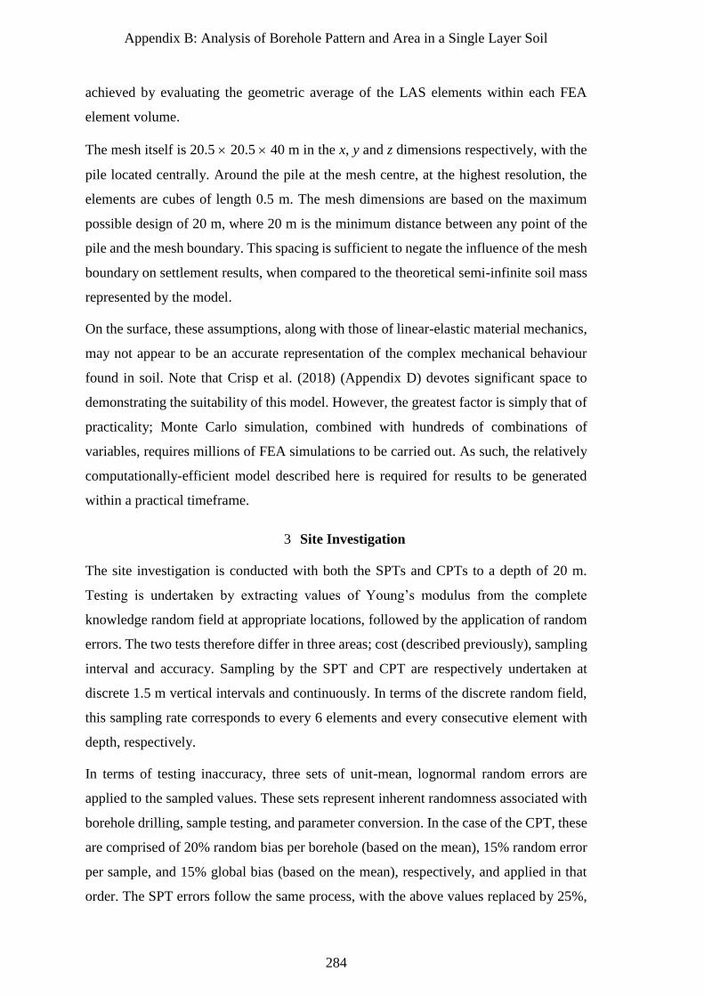
Appendix B: Analysis of Borehole Pattern and Area in a Single Layer Soil
284
achieved by evaluating the geometric average of the LAS elements within each FEA
element volume.
The mesh itself is 20.5 20.5 40 m in the x, y and z dimensions respectively, with the
pile located centrally. Around the pile at the mesh centre, at the highest resolution, the
elements are cubes of length 0.5 m. The mesh dimensions are based on the maximum
possible design of 20 m, where 20 m is the minimum distance between any point of the
pile and the mesh boundary. This spacing is sufficient to negate the influence of the mesh
boundary on settlement results, when compared to the theoretical semi-infinite soil mass
represented by the model.
On the surface, these assumptions, along with those of linear-elastic material mechanics,
may not appear to be an accurate representation of the complex mechanical behaviour
found in soil. Note that Crisp et al. (2018) (Appendix D) devotes significant space to
demonstrating the suitability of this model. However, the greatest factor is simply that of
practicality; Monte Carlo simulation, combined with hundreds of combinations of
variables, requires millions of FEA simulations to be carried out. As such, the relatively
computationally-efficient model described here is required for results to be generated
within a practical timeframe.
3 Site Investigation
The site investigation is conducted with both the SPTs and CPTs to a depth of 20 m.
Testing is undertaken by extracting values of Young’s modulus from the complete
knowledge random field at appropriate locations, followed by the application of random
errors. The two tests therefore differ in three areas; cost (described previously), sampling
interval and accuracy. Sampling by the SPT and CPT are respectively undertaken at
discrete 1.5 m vertical intervals and continuously. In terms of the discrete random field,
this sampling rate corresponds to every 6 elements and every consecutive element with
depth, respectively.
In terms of testing inaccuracy, three sets of unit-mean, lognormal random errors are
applied to the sampled values. These sets represent inherent randomness associated with
borehole drilling, sample testing, and parameter conversion. In the case of the CPT, these
are comprised of 20% random bias per borehole (based on the mean), 15% random error
per sample, and 15% global bias (based on the mean), respectively, and applied in that
order. The SPT errors follow the same process, with the above values replaced by 25%,
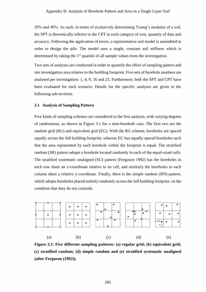
Appendix B: Analysis of Borehole Pattern and Area in a Single Layer Soil
285
20% and 40%. As such, in terms of exclusively determining Young’s modulus of a soil,
the SPT is theoretically inferior to the CPT in each category of cost, quantity of data and
accuracy. Following the application of errors, a representative soil model is assembled in
order to design the pile. The model uses a single, constant soil stiffness which is
determined by taking the 1st quartile of all sample values from the investigation.
Two sets of analyses are conducted in order to quantify the effect of sampling pattern and
site investigation area relative to the building footprint. Five sets of borehole numbers are
analysed per investigation: 1, 4, 9, 16 and 25. Furthermore, both the SPT and CPT have
been evaluated for each scenario. Details for the specific analyses are given in the
following sub-sections.
3.1 Analysis of Sampling Pattern
Five kinds of sampling schemes are considered in the first analysis, with varying degrees
of randomness, as shown in Figure 3.1 for a nine-borehole case. The first two are the
random grid (RG) and equivalent grid (EG). With the RG scheme, boreholes are spaced
equally across the full building footprint, whereas EG has equally spaced boreholes such
that the area represented by each borehole within the footprint is equal. The stratified
random (SR) pattern adopts a borehole located randomly in each of the equal-sized cells.
The stratified systematic unaligned (SU) pattern (Ferguson 1992) has the boreholes in
each row share an x-coordinate relative to its cell, and similarly the boreholes in each
column share a relative y-coordinate. Finally, there is the simple random (RN) pattern,
which adopts boreholes placed entirely randomly across the full building footprint, on the
condition that they do not coincide.
(a) (b) (c) (d) (e)
Figure 3.1: Five different sampling patterns: (a) regular grid; (b) equivalent grid;
(c) stratified random; (d) simple random and (e) stratified systematic unaligned
(after Ferguson (1992)).
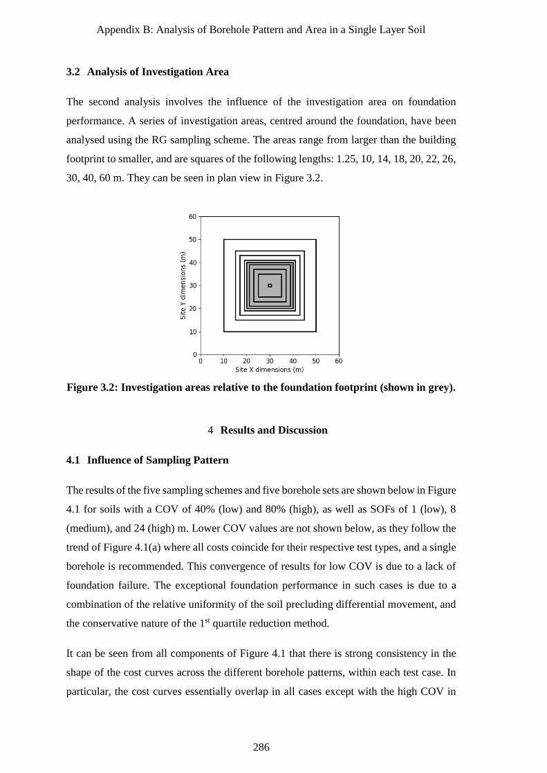
Appendix B: Analysis of Borehole Pattern and Area in a Single Layer Soil
286
3.2 Analysis of Investigation Area
The second analysis involves the influence of the investigation area on foundation
performance. A series of investigation areas, centred around the foundation, have been
analysed using the RG sampling scheme. The areas range from larger than the building
footprint to smaller, and are squares of the following lengths: 1.25, 10, 14, 18, 20, 22, 26,
30, 40, 60 m. They can be seen in plan view in Figure 3.2.
Figure 3.2: Investigation areas relative to the foundation footprint (shown in grey).
4 Results and Discussion
4.1 Influence of Sampling Pattern
The results of the five sampling schemes and five borehole sets are shown below in Figure
4.1 for soils with a COV of 40% (low) and 80% (high), as well as SOFs of 1 (low), 8
(medium), and 24 (high) m. Lower COV values are not shown below, as they follow the
trend of Figure 4.1(a) where all costs coincide for their respective test types, and a single
borehole is recommended. This convergence of results for low COV is due to a lack of
foundation failure. The exceptional foundation performance in such cases is due to a
combination of the relative uniformity of the soil precluding differential movement, and
the conservative nature of the 1st quartile reduction method.
It can be seen from all components of Figure 4.1 that there is strong consistency in the
shape of the cost curves across the different borehole patterns, within each test case. In
particular, the cost curves essentially overlap in all cases except with the high COV in
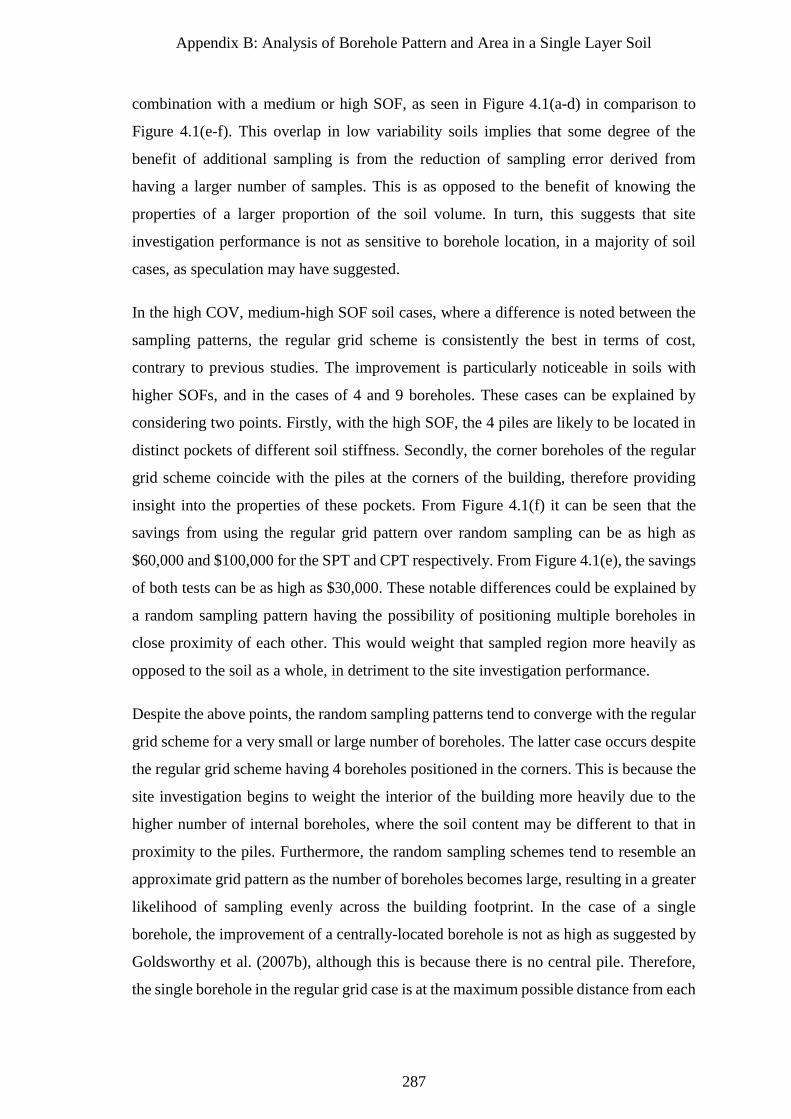
Appendix B: Analysis of Borehole Pattern and Area in a Single Layer Soil
287
combination with a medium or high SOF, as seen in Figure 4.1(a-d) in comparison to
Figure 4.1(e-f). This overlap in low variability soils implies that some degree of the
benefit of additional sampling is from the reduction of sampling error derived from
having a larger number of samples. This is as opposed to the benefit of knowing the
properties of a larger proportion of the soil volume. In turn, this suggests that site
investigation performance is not as sensitive to borehole location, in a majority of soil
cases, as speculation may have suggested.
In the high COV, medium-high SOF soil cases, where a difference is noted between the
sampling patterns, the regular grid scheme is consistently the best in terms of cost,
contrary to previous studies. The improvement is particularly noticeable in soils with
higher SOFs, and in the cases of 4 and 9 boreholes. These cases can be explained by
considering two points. Firstly, with the high SOF, the 4 piles are likely to be located in
distinct pockets of different soil stiffness. Secondly, the corner boreholes of the regular
grid scheme coincide with the piles at the corners of the building, therefore providing
insight into the properties of these pockets. From Figure 4.1(f) it can be seen that the
savings from using the regular grid pattern over random sampling can be as high as
$60,000 and $100,000 for the SPT and CPT respectively. From Figure 4.1(e), the savings
of both tests can be as high as $30,000. These notable differences could be explained by
a random sampling pattern having the possibility of positioning multiple boreholes in
close proximity of each other. This would weight that sampled region more heavily as
opposed to the soil as a whole, in detriment to the site investigation performance.
Despite the above points, the random sampling patterns tend to converge with the regular
grid scheme for a very small or large number of boreholes. The latter case occurs despite
the regular grid scheme having 4 boreholes positioned in the corners. This is because the
site investigation begins to weight the interior of the building more heavily due to the
higher number of internal boreholes, where the soil content may be different to that in
proximity to the piles. Furthermore, the random sampling schemes tend to resemble an
approximate grid pattern as the number of boreholes becomes large, resulting in a greater
likelihood of sampling evenly across the building footprint. In the case of a single
borehole, the improvement of a centrally-located borehole is not as high as suggested by
Goldsworthy et al. (2007b), although this is because there is no central pile. Therefore,
the single borehole in the regular grid case is at the maximum possible distance from each
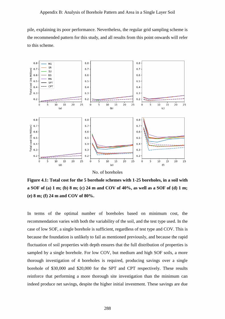
Appendix B: Analysis of Borehole Pattern and Area in a Single Layer Soil
288
pile, explaining its poor performance. Nevertheless, the regular grid sampling scheme is
the recommended pattern for this study, and all results from this point onwards will refer
to this scheme.
No. of boreholes
Figure 4.1: Total cost for the 5 borehole schemes with 1-25 boreholes, in a soil with
a SOF of (a) 1 m; (b) 8 m; (c) 24 m and COV of 40%, as well as a SOF of (d) 1 m;
(e) 8 m; (f) 24 m and COV of 80%.
In terms of the optimal number of boreholes based on minimum cost, the
recommendation varies with both the variability of the soil, and the test type used. In the
case of low SOF, a single borehole is sufficient, regardless of test type and COV. This is
because the foundation is unlikely to fail as mentioned previously, and because the rapid
fluctuation of soil properties with depth ensures that the full distribution of properties is
sampled by a single borehole. For low COV, but medium and high SOF soils, a more
thorough investigation of 4 boreholes is required, producing savings over a single
borehole of $30,000 and $20,000 for the SPT and CPT respectively. These results
reinforce that performing a more thorough site investigation than the minimum can
indeed produce net savings, despite the higher initial investment. These savings are due
Appendix B: Analysis of Borehole Pattern and Area in a Single Layer Soil
289
to a combination of cheaper foundation design and, more importantly, reduced risk of
potential damage.
Soils with a high COV and medium-high SOF are the most interesting case, as significant
gains can be obtained through sufficient sampling, and because there is a divergence in
the optimal number of boreholes for each test. For example, the benefit of conducting 4
boreholes over one in Figure 4.1(f) is $350,000 for both tests. An additional saving, in
the order of $15,000, can be gained with the SPT by conducting 9 boreholes. It should be
noted that $15,000 is the edge of the Monte Carlo analysis error margin, meaning that
this additional saving over 4 boreholes cannot be stated with complete confidence.
However, there is certainly no detriment to conducting 9 boreholes, with the SPT, over 4
in terms of total cost.
Furthermore, it can be seen that the CPT is always cheaper than the SPT for a given
number of boreholes. This is due to both the higher quantity of information being
collected by its continuous sampling, as well as the lower magnitude of errors associated
with the test, with the latter point being the dominant factor. It can also be seen that the
CPT is cheapest overall in all soil cases, and that 4 boreholes with this test yields better
results than any number of SPT samples for the reasons discussed above. As such, the
recommended investigation for the majority of soils is 4 CPTs; one at each of the pile
locations if possible.
4.2 Influence of Investigation Area
The following section discusses the implications of changing the size of an investigation
area with respect to the foundation footprint. The results are given in Figure 4.2 for
different numbers of boreholes in soils with a COV of 80%, and a SOF of 1 m, 8 m and
24 m. The performance of the site investigations does not appear to be highly sensitive
to the site investigation size in high COV. As such, lower COV values correspond to
negligible sensitivity, and so are not included in the analysis. This insensitivity is most
prominent in low SOF soils, where the total cost is constant with investigation width.
Medium SOF soils correspond to minor sensitivity. However, assuming that the
investigation width is greater than or equal to the width of the building, the difference in
cost is negligible. These results indicate that, in all soil cases except high SOF and high
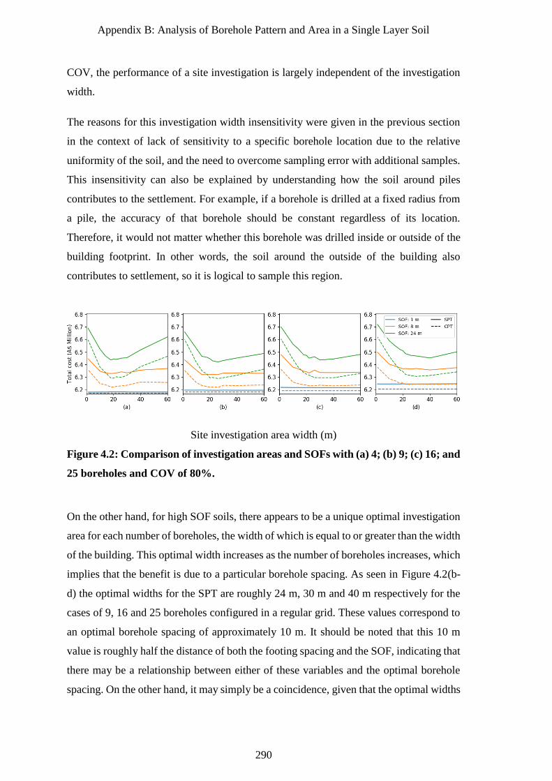
Appendix B: Analysis of Borehole Pattern and Area in a Single Layer Soil
290
COV, the performance of a site investigation is largely independent of the investigation
width.
The reasons for this investigation width insensitivity were given in the previous section
in the context of lack of sensitivity to a specific borehole location due to the relative
uniformity of the soil, and the need to overcome sampling error with additional samples.
This insensitivity can also be explained by understanding how the soil around piles
contributes to the settlement. For example, if a borehole is drilled at a fixed radius from
a pile, the accuracy of that borehole should be constant regardless of its location.
Therefore, it would not matter whether this borehole was drilled inside or outside of the
building footprint. In other words, the soil around the outside of the building also
contributes to settlement, so it is logical to sample this region.
Site investigation area width (m)
Figure 4.2: Comparison of investigation areas and SOFs with (a) 4; (b) 9; (c) 16; and
25 boreholes and COV of 80%.
On the other hand, for high SOF soils, there appears to be a unique optimal investigation
area for each number of boreholes, the width of which is equal to or greater than the width
of the building. This optimal width increases as the number of boreholes increases, which
implies that the benefit is due to a particular borehole spacing. As seen in Figure 4.2(b-
d) the optimal widths for the SPT are roughly 24 m, 30 m and 40 m respectively for the
cases of 9, 16 and 25 boreholes configured in a regular grid. These values correspond to
an optimal borehole spacing of approximately 10 m. It should be noted that this 10 m
value is roughly half the distance of both the footing spacing and the SOF, indicating that
there may be a relationship between either of these variables and the optimal borehole
spacing. On the other hand, it may simply be a coincidence, given that the optimal widths
Appendix B: Analysis of Borehole Pattern and Area in a Single Layer Soil
291
for the CPT are in the order of 25–30 m in the same soils. In either case, the consistency
of the optimal 10 m spacing is notable, and requires further research. The exception to
the above recommendations is the 4-borehole case, which has an optimal spacing of 20
m for both tests, as seen in Figure 4.2(a). This outlier is due to the boreholes being
positioned exactly at the pile locations. As such, this result reinforces that each borehole
should always coincide with a pile if the numbers of both are equal, at least in high SOF
soils.
It may be the case that an engineer wishes to investigate a larger area than that of the
building footprint. This could theoretically allow for the identification of a stable, stiff
region of soil within that area for the building location, resulting in cheaper foundations
and a net saving. As discussed in this section, this strategy appears reasonable in all soils
with a low and medium SOF, where the performance of the site investigation is relatively
insensitive to its width. However, deviating from the recommended investigation widths
mentioned above for high SOF soils results in an increased total cost. In the case of 9 or
more boreholes, as seen in Figure 4.2(b-d), the cost increases linearly with width from
the optimal case in each subplot, to a net additional cost of roughly $50,000 at a width of
60 m for both tests. However, note that this cost corresponds to a high COV of 80%, and
is therefore conservatively large.
Based on these results, an engineer could choose to investigate a larger area in high SOF
soils if it is felt that the foundation construction savings would offset the increased
investigation cost. The exception to the above recommendations is the case where the
number of boreholes and piles is equal, in which case the boreholes should be located
adjacent to the piles. Considering that the optimal investigation width increases with the
number of boreholes, it can be concluded that investigating a wider area is not only
allowed, but is encouraged, should the number of boreholes be sufficiently high. This
recommendation is particularly true considering that there is no notable difference in cost
between the different numbers of boreholes in a high SOF soil. This insensitivity
indicates that the cost of additional sampling is largely offset from improved investigation
performance, as seen in Figure 4.1(e-f).
Appendix B: Analysis of Borehole Pattern and Area in a Single Layer Soil
292
5 Conclusion
A comparison of several different borehole patterns has shown that the regular grid
sampling scheme consistently produces the lowest average total project cost compared
with alternative patterns which incorporate random locations. In the case of high COV
and high SOF, the difference in cost between these patterns can be as high as $100,000.
On the other hand, there are several cases where site investigation performance is not
affected by borehole pattern. In soils with a low COV or SOF, the soils appear relatively
uniform at a macro scale, meaning that the specific locations of boreholes becomes less
important. The results also converge as the number of boreholes increases, due to the
increased probability of the random borehole locations resembling a random grid. This
insensitivity in the majority of cases means that engineers can be flexible in where they
place boreholes in a site investigation, although a regular grid scheme should be utilised
where possible.
Regarding the ideal number of boreholes and choice of test, it was found that 4 CPTs,
one at each of the pile locations was optimal. This is as opposed to the SPT, which had a
higher cost overall, and required up to 9 boreholes to be optimal. The SPT’s inferior
performance was due partly to the smaller number of samples taken, but the primary
factor is the significantly higher sampling error. The exception to this 4 CPT
recommendation is in the case of low SOF soils, where it could be argued that one CPT
is best. However, these types of soils are not particularly common, and the undertaking
of 3 additional boreholes requires negligible additional cost. Therefore, 4 CPTs are
recommended for all soil cases, and can lead to a savings of up to $350,000 over a single
CPT due to improved foundation designs and a reduced likelihood of failure. In the case
where CPTs are not available or impractical, 4 SPTs could generally be substituted. This
SPT recommendation carries additional risk, with a loss of up to $15,000 compared to
the true optimum depending on the nature of the soil, however this value is at the Monte
Carlo error margin, and is therefore deemed negligible.
Regarding the variation of site investigation area, it was found that in all soils with a low
or medium SOF, the investigation performance was insensitive to its width, for reasons
given above. This indicates that an engineer may confidently investigate a larger area if
desired, without repercussions, which is useful if the building location is to be chosen
based on site investigation results. In terms of high SOF soils, it was concluded that the
Appendix B: Analysis of Borehole Pattern and Area in a Single Layer Soil
293
optimal borehole spacing for the SPT is approximately 10 m, meaning that the optimal
width increases with the number of boreholes. On the other hand, the CPT did not exhibit
a consistent optimal borehole spacing, instead showing a more modest increase in optimal
width as the number of boreholes increases, in the order of 25-30 m. Deviating from the
optimal investigation width, in general, results in a linear increase of cost as width
increases.
It is speculated that the optimal investigation width will decrease as the number of piles
increases. This is because the soil within the building footprint becomes more important
as the pile density increases, as that central soil contributes to the settlement of multiple
piles. Therefore one would need to sample closer to, or possibly within, the building
footprint. It is also anticipated that higher numbers of piles will require a more thorough
investigation since the soil properties must be known at a larger number of locations. As
such, future studies should investigate the impact of alternate pile configurations.
While these results generally indicate that modest investigation is required in the majority
of soils, it is important to remember this only applies to single layer, somewhat simplistic,
soils. In reality, soils are comprised of multiple distinct layers, often with complex
geology. Such soils would require additional investigation to delineate the layer
boundaries, and so the recommendations given by this study should be taken as a
minimum. It is also expected that the presence of layers will produce an increased need
to locate boreholes in close proximity to the piles, since it is important to know the depths
of layer boundaries at the pile locations. Therefore, site investigation performance could
become more sensitive to borehole location than the present study suggests. As such,
future analysis should incorporate complex geology with multiple soil layers.
In conclusion, this paper has demonstrated that engineers can indeed expect to save
hundreds of thousands of dollars across a project by implementing a satisfactory
investigation, in contrast often to clients’ desires to minimise site investigations in order
to save money. This is the case for the relatively simple soils and small structure analysed
in this study. It is anticipated that savings could be in the order of millions of dollars for
complex, layered soils and larger projects, due to the optimization of foundation design,
but more importantly the decreased risk, that a thorough investigation provides.
Appendix B: Analysis of Borehole Pattern and Area in a Single Layer Soil
294
6 Acknowledgements
This work was supported with supercomputing resources provided by the Phoenix HPC
service at the University of Adelaide.
7 References
Akima, H. 1970. A new method of interpolation and smooth curve fitting based on local
procedures. Journal of the ACM (JACM), 17(4), 589-602.
Arsyad, A., Jaksa, M., Kaggwa, W., and Mitani, Y. 2010. Effect of radial distance of a
single CPT sounding on the probability of over-and under-design of pile
foundation.
Boeckmann, A. Z., and Loehr, J. E. 2016. Influence of Geotechnical Investigation and
Subsurface Conditions on Claims, Change Orders, and Overruns.
Brockwell, P. J., and Davis, R. A. 2013. Time series: theory and methods: Springer
Science & Business Media.
Clayton, C. 2001. Managing geotechnical risk: time for change? Proceedings of the
Institution of Civil Engineers-Geotechnical Engineering, 149(1), 3-11.
Crisp, M. P., Jaksa, M. B., and Kuo, Y. L. 2017. The influence of Site Investigation Scope
on Pile Design in Multi-layered, 2D Variable Ground. In Proceedings of the Geo-
Risk 2017, Denver, Colorado, USA.
Crisp, M. P., Jaksa, M. B., and Kuo, Y. L. 2018. Framework for the Optimisation of Site
Investigations for Pile Designs in Complex Multi-Layered Soil. , University of
Adelaide, Adelaide, Australia.
Day, R. W. 1999. Forensic geotechnical and foundation engineering: McGraw-Hill New
York.
Fenton, G., and Griffiths, D. 2008. Risk assessment in geotechnical engineering: Wiley.
Fenton, G., and Vanmarcke, E. H. 1990. Simulation of random fields via local average
subdivision. Journal of Engineering Mechanics, 116(8), 1733-1749.
Ferguson, C. 1992. The statistical basis for spatial sampling of contaminated land.
Ground engineering, 25, 34-34.
Goldsworthy, J., Jaksa, M., Fenton, G., Griffiths, D., Kaggwa, W., and Poulos, H. 2007a.
Measuring the risk of geotechnical site investigations. In Proceedings of the Proc.,
Geo-Denver 2007.
Goldsworthy, J., Jaksa, M., Fenton, G., Kaggwa, G., Griffiths, D., Poulos, H., and Kuo,
Y. 2004. Influence of site investigations on the design of pad footings. In
Proceedings of the Australia-New Zealand Conference on Geomechanics (9th:
2004: Auckland, NZ).
Appendix B: Analysis of Borehole Pattern and Area in a Single Layer Soil
295
Goldsworthy, J., Jaksa, M., Fenton, G., Kaggwa, W., Griffiths, D., and Poulos, H. 2007b.
Effect of sample location on the reliability based design of pad foundations.
Georisk, 1(3), 155-166.
Goldsworthy, J. S. 2006. Quantifying the risk of geotechnical site investigations. Ph.D
Thesis, School of Civil, Environmental and Mining Engineering, University of
Adelaide, Adelaide.
Jaksa, M. 2000. Geotechnical risk and inadequate site investigations: a case study.
Australian Geomechanics, 35(2), 39-46.
Jaksa, M., Kaggwa, W., Fenton, G., and Poulos, H. 2003. A framework for quantifying
the reliability of geotechnical investigations. In Proceedings of the 9th
International Conference on the Application of Statistics and Probability in Civil
Engineering.
Moh, Z.-C. 2004. Site investigation and geotechnical failures. In Proceedings of the
Proceeding of International Conference on Structural and Foundation Failures.
Rawlinsons, A. (2016). Australian Construction Handbook (34 ed., pp. 1005). Perth,
Australia: Rawlhouse Publishing Pty. Ltd.
Smith, I. M., Griffiths, D. V., and Margetts, L. 2013. Programming the finite element
method: John Wiley & Sons.
University of Adelaide. 2018. Phoenix High Perfomance Computing Technical
Information. Retrieved from
https://www.adelaide.edu.au/phoenix/training/technical/
Vanmarcke, E. 1983. Random Fields: Analysis and Synthesis. London: MIT Press.

Appendix B: Analysis of Borehole Pattern and Area in a Single Layer Soil
296
Appendix C: Examination of Distance-weighted Samples
297
Appendix C : Examination of
Distance-weighted Samples
Paper Title:
Influence of distance-weighted averaging of site
investigation samples on foundation performance

Appendix C: Examination of Distance-weighted Samples
298

299
Appendix C: Examination of Distance-weighted Samples
300
Abstract
Site investigations, for the purpose of determining the material properties of a variable
subsurface soil, are an essential part of civil engineering projects. However, there is little
research on how best to interpret site investigation data for a soil model. This paper
investigates the potential benefit of weighting soil samples by their distance from pile
foundations, using a variety of weighting and averaging techniques. The performance
metric is total project cost, where construction, site investigation and failure costs are
explicitly quantified through a virtual framework, facilitated through the generation of
variable, single-layer virtual soils in a Monte Carlo analysis. It has been found that a
saving of up to $1.8 million can be achieved by drilling in 9 locations as compared to
one, despite the increased initial investment in soil testing.
Appendix C: Examination of Distance-weighted Samples
301
1 Introduction
Site investigations are an essential part of civil engineering works, as they provide insight
into the otherwise unknown material properties of subsurface soil profiles. Soils exhibit
spatial variability, and so multiple locations must be investigated in order to accurately
determine subsurface conditions. Despite this, it is not known how best to convert the
aggregation of soil property data, from a site investigation, into the idealised soil models
used in practice in the most optimal manner (Crisp et al. 2018a) (Appendix D).
Unfortunately, insufficient site investigations, or inappropriate soil property
idealisations, henceforth termed reduction methods, can lead to a variety of negative
outcomes in engineering projects. Such outcomes include cost overruns and change
orders (Boeckmann and Loehr 2016), construction delays (Jaksa 2000), foundation
failure (Moh 2004) and foundation overdesign (Clayton 2001). In contrast, studies have
shown that there can be considerable financial benefits by conducting investigations
beyond the minimal scope (Goldsworthy 2006; Crisp et al. 2018b) (Appendix B). Clearly,
there is a need to formulate a site investigation optimization guideline.
This study aims to determine the influence of the number of boreholes and the selection
of reduction method on site investigation performance, with a focus on weighting the
importance of samples by the distance from a foundation. These inverse distance methods
(IDMs) reflect the tendency that soil properties, which are in close spatial proximity to
each other, tend to be similar in value, and vice versa. This soil self-similarity with
distance is a result of the processes that formed and continually modify the ground over
time, and is referred to as autocorrelation. Using IDMs allows each individual foundation
to be designed independently, in a separate soil model that more accurately reflects local
soil conditions, as opposed to all foundations for a structure being designed from the same
model. In theory, this should increase the probability of all foundations having the same
settlement, thus decreasing the risk of structural damage through differential settlement,
which is a key design constraint in the design of foundations for buildings.
The method used to determine site investigation performance is based on a framework
described by Crisp et al. (2018a) (Appendix D) and originally proposed by Jaksa et al.
(2003). The framework utilises Monte Carlo simulation where, for any given realisation,
a variable, 3D, single-layer virtual soil is generated. Complete knowledge of this soil
Appendix C: Examination of Distance-weighted Samples
302
allows for virtual site investigations to be undertaken, along with the corresponding
foundation designs. The foundation can then be assessed for differential settlement, using
linear-elastic finite element analysis (FEA) in the full virtual soil, which may result in
structural damage. By assigning costs to the investigation, construction, and repair due to
failure throughout the project, averaged across thousands of Monte Carlo realisations, it
is possible to represent the quality of a site investigation by total project cost. The optimal
investigation is therefore identified by minimising the total cost objective function. As
this metric incorporates both economic and risk-based factors, it is considered an ideal
objective function for practicing engineers.
The randomly-generated virtual soil profiles, or random fields, are volumes of soil
properties represented by a 3D grid of discrete elements. As linear-elastic FEA is used,
the required properties are Young’s modulus (E) and Poisson’s ratio (v). The fields are
generated by local average subdivision (LAS) (Fenton and Vanmarcke 1990), which is a
commonly-used algorithm in probabilistic research in geotechnical engineering (Fenton
and Griffiths 2008). The soil properties within these random fields can be statistically
described by three parameters; the mean, standard deviation, and the scale of fluctuation
(SOF) (Vanmarcke 1983). The SOF is analogous to the autocorrelation distance
mentioned above, and is defined as the distance over which soil properties exhibit strong
similarity. In other words, high SOF values correspond to large pockets of similar
material. Within this study, the standard deviation is normalised by the mean to produce
the coefficient of variation parameter (COV), which is more useful as the results can be
applied to any mean parameter value. The soil properties themselves are generated
according to the lognormal distribution, which has been found to be a reasonable
representation (Fenton and Griffiths 2008), and ensures that stiffness values are strictly
non-negative.
Existing literature on the performance of IDMs is fairly limited, as site investigation
performance has traditionally been difficult to quantify. Goldsworthy (2006);
Goldsworthy et al. (2007) investigated the influence of various reduction techniques on
the performance of site investigations for the design of pad foundations. These included
weighted arithmetic averages of soil properties, where the weights are based on the
inverse of the distance (ID) between the borehole and foundation, and the square of the
inverse distance (I2). It was concluded that IDMs had relatively erratic performance with
Appendix C: Examination of Distance-weighted Samples
303
respect to the number of boreholes. This result was due to cases where borehole locations
coincided with footing locations, resulting in the coincident boreholes having infinite
weight, with the majority of boreholes being ignored, leading to a loss of information.
Furthermore, the ID method resulted in the highest total project cost. It was suggested
that IDM performance could be improved in cases where information from all boreholes
is considered.
On the other hand, Goldsworthy et al. (2005) found that IDMs had the highest reliability
of a range of reduction methods regarding the average design error of pad foundations.
However, it should be noted that, contrary to the studies mentioned above, there were no
sampling errors included in this analysis, which decreased the degree of realism.
Alternative reduction methods examined include the standard arithmetic average (SA),
geometric average (GA) and harmonic average (HA) in increasing order of conservatism.
These are defined mathematically later in the paper. Use of the more conservative GA
and HA techniques, which are low-value dominated, may be more accurate, when
compared to the SA, for a variety of reasons. Firstly, it has been shown that soil settlement
itself is low-value dominated, with less-stiff elements having a greater influence than the
stiffer ones on overall response (Griffiths and Fenton 2009). Secondly, geometric
averaging preserves the median of the lognormal distribution; the distribution used in the
present study and several others (Fenton and Griffiths 2008). Thirdly, the soil below an
infinitely-wide shallow foundation is represented perfectly by the harmonic average,
assuming that soil is constant in the horizontal direction, varying only with depth (Fenton
and Griffiths 2005). If the soil only varied horizontally, then the arithmetic average would
be a perfect representation for the same foundation. As the geometric average lies
between both cases, and that soil varies in both the vertical and horizontal directions, then
this average could be considered the ideal reduction method. However, the infinitely-
wide shallow foundation assumption is not necessarily applicable to a deep foundation of
finite size. In terms of non-averaging reduction methods, Crisp et al. (2018b) (Appendix
B) investigated the technique of taking the 1st quartile of all sample values. It was found
that a cost saving of up to $350,000 could be achieved by drilling 4 boreholes instead of
one for a 4-columned building.
Currently, no study has examined potential benefits of using IDMs with site
investigations with regards to pile design. Furthermore, there is discrepancy in the
Appendix C: Examination of Distance-weighted Samples
304
literature as to the benefits of IDMs, and if they are worth the additional effort over a
simple average of soil properties. Finally, while there appears to be some benefit in using
the more conservative GA and HA average techniques, no study has explored using
weighted versions of these averages, as has been done with the SA in the form of the ID
and I2 methods. The aims of this study are therefore:
1. To examine the potential benefit of distance-weighted reduction methods, both
with and without inherent sampling errors.
2. To compare the SA, GA and HA reduction methods, both in terms of a global
average, and by taking the minimum of the averages within each borehole.
3. To recommend an optimal reduction method and number of boreholes, in the
context of pile design.
2 Methodology
2.1 Overview
The author refers readers to Crisp et al. (2018a) (Appendix D) for details on the general
methodology adopted in the present study, beyond that given in the introduction, as well
as the verification of the methodology. Space restrictions limit the ability to provide such
information in greater detail than that given. In summary, the results presented here were
generated using 8,000 realisations of random soils, along with 3D linear elastic FEA to
determine pile settlement. The resulting database was generated using the Phoenix
supercomputer (University of Adelaide 2018), which reduced 30 years’ worth of
simulation to a matter of weeks. Fortunately, the database is generalised in terms of
possible soil and structural configurations, allowing for site investigations to be optimised
for a wide variety of situations through dynamic post-processing, facilitating the present
results with minimal additional computational time.
The costs used in this study include those associated with the structure ($6,157,750), the
site investigation ($77/m), and foundation ($200/m). Furthermore, failure costs have been
derived from associations between various degrees of structural damage and differential
settlement (Day 1999), where damage has associated repair costs (Rawlinsons 2016). The
resulting failure cost (C) in terms of differential settlement (δ) is given by the linear
equation C = 1.024 109 δ – 3.056 106. This function is bounded by a minimum of $0
at 0.0030 m/m, and a maximum of $6,534,400 at 0.0094 m/m; corresponding to
Appendix C: Examination of Distance-weighted Samples
305
negligible damage and demolishing/rebuilding respectively. As mentioned above, details
of the above are given by Crisp et al. (2018a) (Appendix D).
2.2 Details of Site and Structure
The virtual sites analysed in this study are 60 60 40 m in the x, y, z (depth) dimensions
respectively, and are comprised of cubic elements of dimension 0.25 m. Further
information on the process of generating the soils, along with alternative techniques of
generating random fields, are given by Fenton and Griffiths (2008). Of the two settlement
parameters, v has been set constant to 0.3, as this value is widely-found in nature. On the
other hand, E is spatially variable with a mean of 40 MPa, with a COV of 80%, which is
considered high. Contrary to most studies, COV is not a variable in this analysis, as the
relative performance of inverse-distance weighting would be consistent. On the other
hand, the degree of soil self-similarity with distance may have a significant impact on the
results. As such, three values of SOF are considered: 1 m (low), 8 m (medium) and 24 m
(high). The soils are isotropic, meaning the SOF is constant in all directions.
The adopted structure is 20 20 m in plan and consists of 6 storeys, which are supported
by 9 piles, arranged in a grid pattern, one beneath each column. As each floor is subject
to 8 kPa of combined dead and live load, the total structure weighs 19,200 kN, with no
load factoring applied. The piles are spaced at 10 m intervals and are 0.5 m in diameter.
The corner, edge and internal piles have average lengths of approximately 1.5 m, 4 m and
8 m respectively, and have been designed to an allowable settlement of 25 mm.
2.3 Site Investigation and Reduction Methods
The site investigation consists of 5 sets of boreholes, 1, 4, 9, 16 and 25, arranged in a
regular grid pattern over the building footprint. Testing has been undertaken using the
standard penetration test (SPT) at 1.5 m intervals with depth, both with and without
random errors applied. The errors are unit-mean, lognormally-distributed variables, with
variances of 25% bias per borehole, 20% random error per sample, and 40% parameter
transformation error, as derived by Goldsworthy (2006). These errors seek to model the
uncertainty associated with the SPT. The boreholes were drilled to a depth of 20 m, with
a total of 17 samples in each.
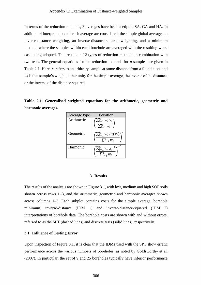
Appendix C: Examination of Distance-weighted Samples
306
In terms of the reduction methods, 3 averages have been used; the SA, GA and HA. In
addition, 4 interpretations of each average are considered; the simple global average, an
inverse-distance weighting, an inverse-distance-squared weighting, and a minimum
method, where the samples within each borehole are averaged with the resulting worst
case being adopted. This results in 12 types of reduction methods in combination with
two tests. The general equations for the reduction methods for n samples are given in
Table 2.1. Here, xi refers to an arbitrary sample at some distance from a foundation, and
wi is that sample’s weight; either unity for the simple average, the inverse of the distance,
or the inverse of the distance squared.
Table 2.1. Generalised weighted equations for the arithmetic, geometric and
harmonic averages.
Average type Equation
Arithmetic (∑ 𝑤𝑖𝑛𝑖=1 𝑥𝑖∑ 𝑤𝑖𝑛𝑖=1
)
Geometric (∑ 𝑤𝑖 𝑙𝑛(𝑥𝑖)𝑛𝑖=1
∑ 𝑤𝑖𝑛𝑖=1
)
𝑒
Harmonic (∑ 𝑤𝑖𝑛𝑖=1 𝑥𝑖
−1
∑ 𝑤𝑖𝑛𝑖=1
)
−1
3 Results
The results of the analysis are shown in Figure 3.1, with low, medium and high SOF soils
shown across rows 1–3, and the arithmetic, geometric and harmonic averages shown
across columns 1–3. Each subplot contains costs for the simple average, borehole
minimum, inverse-distance (IDM 1) and inverse-distance-squared (IDM 2)
interpretations of borehole data. The borehole costs are shown with and without errors,
referred to as the SPT (dashed lines) and discrete tests (solid lines), respectively.
3.1 Influence of Testing Error
Upon inspection of Figure 3.1, it is clear that the IDMs used with the SPT show erratic
performance across the various numbers of boreholes, as noted by Goldsworthy et al.
(2007). In particular, the set of 9 and 25 boreholes typically have inferior performance
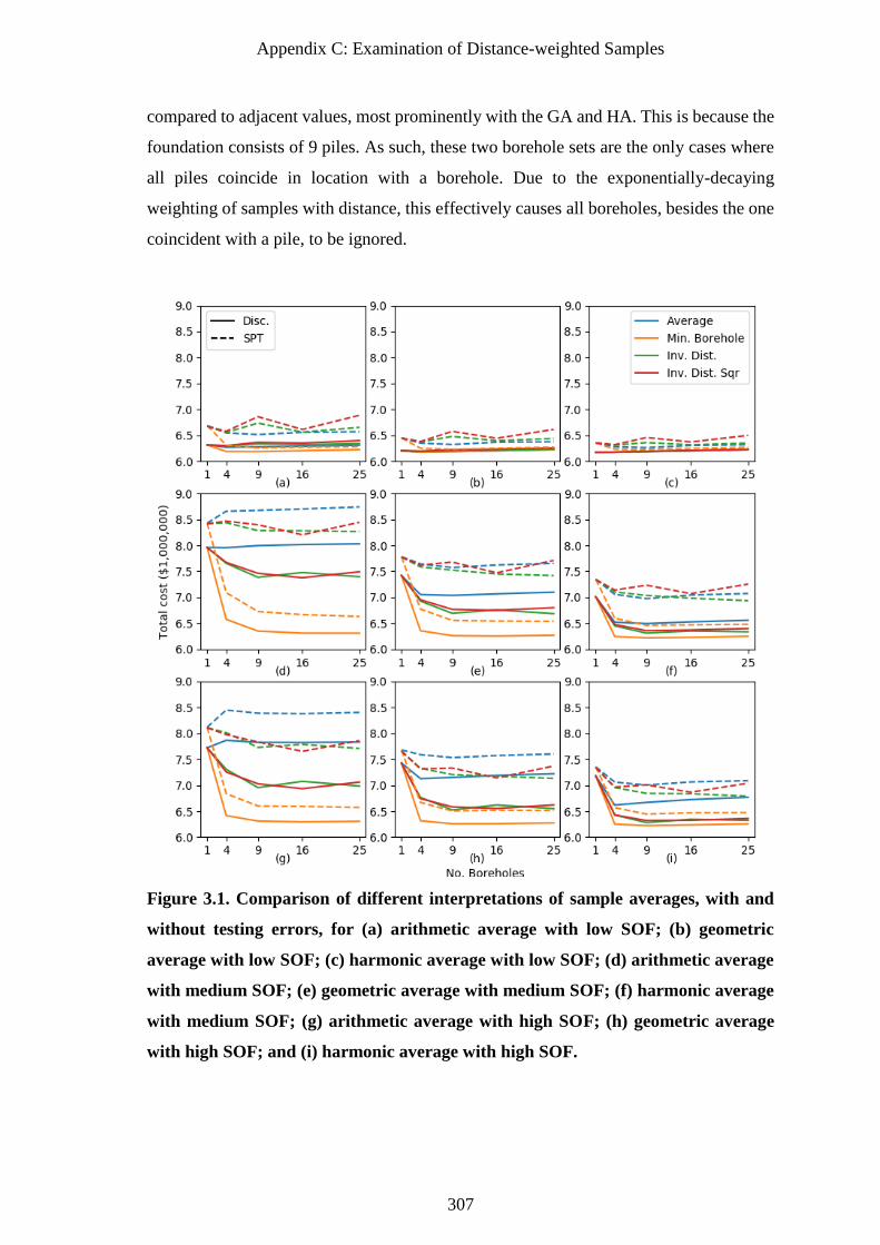
Appendix C: Examination of Distance-weighted Samples
307
compared to adjacent values, most prominently with the GA and HA. This is because the
foundation consists of 9 piles. As such, these two borehole sets are the only cases where
all piles coincide in location with a borehole. Due to the exponentially-decaying
weighting of samples with distance, this effectively causes all boreholes, besides the one
coincident with a pile, to be ignored.
Figure 3.1. Comparison of different interpretations of sample averages, with and
without testing errors, for (a) arithmetic average with low SOF; (b) geometric
average with low SOF; (c) harmonic average with low SOF; (d) arithmetic average
with medium SOF; (e) geometric average with medium SOF; (f) harmonic average
with medium SOF; (g) arithmetic average with high SOF; (h) geometric average
with high SOF; and (i) harmonic average with high SOF.
Appendix C: Examination of Distance-weighted Samples
308
It can also be seen that this erratic behaviour is not present, or at least greatly diminished,
for the discrete test type. Rather, the site investigation performance generally improves
as the number of boreholes increases. This leads to the conclusion that a single borehole
located at a foundation is a good representation of the soil around that foundation, in the
absence of errors. However, when errors are present, as found in practice, a single
borehole is no longer sufficient. In the case of errors, additional boreholes must be
conducted so that the increased number of samples can compensate for the overall test
inaccuracy.
Comparing the SPT and discrete tests, the former performs consistently poorer across all
cases than the latter, due to the presence of errors. The cost increase due to errors can be
as high as $700,000 as seen in Figure 3.1d. However, such errors are unavoidable in
practice, and so subsequent discussion will focus primarily on the SPT, unless stated
otherwise.
3.2 Influence of Inverse-Distance Weighting
Inspecting the different SOF values, it can be seen that the IDMs consistently exhibit the
worst performance when used in low SOF soils, across all averages. This is because the
fluctuation of soil properties is rapid enough such that the soils appear relatively uniform
at a macro scale. In this case, since the soil is generally similar at all locations, there is
no advantage to any kind of distance weighting. In contrast, this weighting is detrimental,
as it makes sense to weight all samples equally to help overcome testing errors, as
discussed in the previous section.
In the case of medium and high SOFs, IDMs exhibit consistently better performance than
the global averages for the SA and, to a lesser extent, the more conservative GA. This
benefit seems to increase as the SOF increases. The cost savings over the average can be
as high as $700,000, as seen in Figure 3.1g, although they can also be negligible as seen
in Figure 3.1f. Furthermore, the difference between the IDMs and global average
decrease as the averaging type becomes more conservative, due to higher design
redundancy for individual piles. In other words, inverse-distance weighting is more
beneficial for less conservative reduction methods.
The increased benefit in higher SOF soils is logical, as a pile is more likely to be located
in a pocket of consistent material, so it makes sense to weight that pocket more heavily.
Appendix C: Examination of Distance-weighted Samples
309
Theoretically, as the SOF increases to infinity, the benefit of distance weighting would
begin to diminish due to the soil appearing to be uniform, as described in the case of low
SOF. However, as stated previously, the benefit of IDMs does not diminish as SOF
increases. Therefore, it is unlikely that soils found in nature would have a high enough
SOF for this diminishing effect to occur.
Comparing the IDM 1 and IDM 2 methods across all cases, minor benefit can be obtained
by using the former, with a cost benefit of up to $300,000 as seen in Figure 3.1f. However,
they both perform similarly well overall as they give significantly higher weighting to the
closest borehole to a foundation.
3.3 Influence of Averaging Type
Regarding the choice of averaging type, site investigation performance generally appears
to increase from SA to GA, to HA. In other words, the performance increases as the
average becomes more conservative, at least in the case of soils with a medium or high
SOF.
The largest discrepancy between the three averages is the SA, where performance
actually decreases with additional sampling when using global averaging, which is
counter-intuitive. Upon closer inspection, it appears that the average SA investigation
results in foundation failure. Therefore, as the number of boreholes increases and the
standard deviation of the reduced values decreases, the proportion of safe designs
decreases. However, this result may change should a heavier building be used; resulting
in a longer mean pile length. There also appears to be minor, if any, improvement with
additional sampling when using the GA and HA global averaging. This latter point is due
to the presence of testing errors, as there is clear improvement from 1–4 boreholes in the
case of the discrete test.
On the other hand, there is no discernible difference between the performance of the three
averages when using the borehole minimum method. This consistency suggests that the
minimising component of the method is the dominant factor of its strong performance, as
opposed to the averaging component within each borehole.
In the case of soils with low SOF, it could be argued that a single borehole is sufficient
for all reduction methods except the borehole minimum where four is recommended.
Appendix C: Examination of Distance-weighted Samples
310
Rather than this being a reflection of the investigation quality, it is instead indicative of
the foundation performance. As mentioned previously, these soils appear largely uniform
at a macro scale. As such, the foundation is unlikely to fail through differential settlement,
meaning the failure cost is largely independent of the investigation scale.
3.4 The minimum Borehole Method
An interesting observation is that the minimum borehole method provides the best site
investigation performance in terms of lowest total cost, across all cases. This
improvement is due to the minimisation of failure costs. The result is surprising, as
speculation would have suggested that differential settlement would be minimised by
ensuring that each pile settles by the same amount. Theoretically, this consistent
settlement would be achieved by an IDM, which considers each pile individually. Instead,
each pile set (corner, edge, internal) is given a consistent length according to the worst-
case borehole. By increasing the pile lengths to the same amount, there is a risk of
increasing differential settlement, should the soil properties at each pile be significantly
different. However, it appears that the added conservativism of having longer piles, with
reduced total settlement, has overcome this risk quite convincingly.
It is also worth noting that there does not appear to be an optimal number of boreholes
with the minimum reduction method, in terms of a clear local minimum cost. In other
words, the cost asymptotes as the number of boreholes increases. This suggests that the
improved reliability attributed to this reduction method generally compensates for the
increased cost of additional sampling. As such, it can be concluded that the borehole
minimum method has a good balance of conservatism, which maximises reliability
without leading to excessively over-designed foundations. Since this strong performance
is seen in soils of all SOFs, this method can be recommended for universal practice over
the other methods examined in this study.
Generally speaking, in the case of medium and high SOFs, the total cost has largely
plateaued at 9 boreholes. The cost savings by conducting 9 boreholes over one and four
boreholes can be as high as $1.8 million and $400,000 respectively, as seen in Figure
3.1d for the SPT. The exception to this is in soils with a low SOF, as discussed in the
previous section.
Appendix C: Examination of Distance-weighted Samples
311
A potential limitation of using the borehole minimum method is that its performance may
depend on the depth of the boreholes, i.e. the number of samples within each borehole.
This is because the previously-discussed desirable conservative balance relies on the
elimination of excessively-weak samples through the averaging process. If the number of
samples in a borehole is small, then this low-value removal may not take place to a
sufficient degree, causing the method to be overly-conservative. This is particularly the
case with the geometric and harmonic averages due to their low-value weighted nature.
As an extreme example, a single zero-valued sample would cause the global average to
be zero. Furthermore, the relative improvement of the borehole minimum method over
the other methods may depend on the soil COV, which has not been assessed in the
present study. Nevertheless, the potential savings are remarkable.
4 Conclusion
It has been found that, while there is some apparent benefit to using inverse-distance
weighting with site investigations in the majority of soils, the benefit is inconsistent. For
example, a single borehole is largely sufficient for soils with a low scale of fluctuation.
However, the savings over a global average can be as high as $700,000 when boreholes
do not coincide in location with all foundations. When boreholes do coincide, the
investigation performance greatly decreases, implying that any given foundation should
not be designed from a single borehole in soils with medium and high scales of
fluctuation, as additional boreholes are required to overcome errors. Inverse distance
methods provide the greater benefits over the global average for less conservative
averages.
Similarly, there is no noteworthy improvement with additional sampling when using the
global averaging techniques, largely due to inherent errors. In particular, the arithmetic
average performs significantly poorer with additional samples. As such, this average
should not be used in practice. In general, the more conservative averages performed
better.
Of the reduction methods assessed in this study, the borehole minimum technique
consistently yielded the best performance, regardless of the choice of averaging method.
This led to a saving of up to $1.8 million with the use of 9 boreholes over one, despite
the higher initial investment. However, this method has not been assessed for different
Appendix C: Examination of Distance-weighted Samples
312
soil coefficients of variation, or with different borehole depths, where it is possible that
performance may vary. Furthermore, it is not currently known whether this method yields
the lowest total cost compared to methods not examined here.
It is noted that this analysis has been conducted in a variable, single-layer soil profile. As
such, recommended numbers of boreholes given here should be taken as a minimum, as
additional boreholes are likely needed to delineate the complex boundaries of multi-
layered soils which have not been assessed here. Furthermore, overcoming testing errors
to adequately represent soils properties within each layer would also require additional
samples. Finally, it is likely that the optimal investigation is related to the structural
configuration, a variable which was not considered in the present study due to use of a
single building size. As such, these situations should be considered in further work.
5 References
Boeckmann, A. Z., and Loehr, J. E. 2016. Influence of Geotechnical Investigation and
Subsurface Conditions on Claims, Change Orders, and Overruns.
Clayton, C. 2001. Managing geotechnical risk: time for change? Proceedings of the
Institution of Civil Engineers-Geotechnical Engineering, 149(1), 3-11.
Crisp, M. P., Jaksa, M. B., and Kuo, Y. L. 2018a. Framework for the Optimisation of Site
Investigations for Pile Designs in Complex Multi-Layered Soil. , University of
Adelaide, Adelaide, Australia.
Crisp, M. P., Jaksa, M. B., and Kuo, Y. L. 2018b. Influence of Site Investigation Borehole
Pattern and Area on Pile Foundation Performance. In Proceedings of the 12th
ANZ Young Geotechnical Professionals Conference, Hobart.
Day, R. W. 1999. Forensic geotechnical and foundation engineering: McGraw-Hill New
York.
Fenton, G. A., and Griffiths, D. V. 2005. Three-dimensional probabilistic foundation
settlement. Journal of Geotechnical and Geoenvironmental Engineering, 131(2),
232-239.
Fenton, G. A., and Griffiths, D. V. 2008. Risk assessment in geotechnical engineering.
Hoboken: Wiley.
Fenton, G. A., and Vanmarcke, E. H. 1990. Simulation of random fields via local average
subdivision. Journal of Engineering Mechanics, 116(8), 1733-1749.
Goldsworthy, J. S. 2006. Quantifying the risk of geotechnical site investigations. Ph.D
Thesis, School of Civil, Environmental and Mining Engineering, University of
Adelaide, Adelaide.
Appendix C: Examination of Distance-weighted Samples
313
Goldsworthy, J. S., Jaksa, M. B., Fenton, G. A., Griffiths, D. V., Kaggwa, W. S., and
Poulos, H. G. 2007. Measuring the risk of geotechnical site investigations. In
Proceedings of the Proc., Geo-Denver 2007.
Goldsworthy, J. S., Jaksa, M. B., Kaggwa, G. S., Fenton, G. A., Griffiths, D. V., and
Poulos, H. G. 2005. Reliability of site investigations using different reduction
techniques for foundation design. 9th International Conference on Structural
Safety and Reliability, 901-908.
Griffiths, D. V., and Fenton, G. A. 2009. Probabilistic settlement analysis by stochastic
and random finite-element methods. Journal of Geotechnical and
Geoenvironmental Engineering, 135(11), 1629-1637.
Jaksa, M. B. 2000. Geotechnical risk and inadequate site investigations: a case study.
Australian Geomechanics, 35(2), 39-46.
Jaksa, M. B., Kaggwa, W. S., Fenton, G. A., and Poulos, H. G. 2003. A framework for
quantifying the reliability of geotechnical investigations. In Proceedings of the
9th International Conference on the Application of Statistics and Probability in
Civil Engineering.
Moh, Z. C. 2004. Site investigation and geotechnical failures. In Proceedings of the
Proceeding of International Conference on Structural and Foundation Failures.
Rawlinsons, A. (2016). Australian Construction Handbook (34 ed., pp. 1005). Perth,
Australia: Rawlhouse Publishing Pty. Ltd.
University of Adelaide. 2018. Phoenix High Performance Computing Technical
Information. Retrieved from
https://www.adelaide.edu.au/phoenix/training/technical/
Vanmarcke, E. H. 1983. Random Fields: Analysis and Synthesis. London: MIT Press.

Appendix C: Examination of Distance-weighted Samples
314
Appendix D: Methodology Report
315
Appendix D : Methodology Report
Report title:
Framework for the Optimization of Site Investigations
for Pile Designs in Complex Multi-Layered Soil

Appendix D: Methodology Report
316

Appendix D: Methodology Report
317

Appendix D: Methodology Report
318
Appendix D: Methodology Report
319
Framework for the Optimization of Site Investigations for Pile Designs in Complex
Multi-Layered Soil
by
M P Crisp, M B Jaksa, Y L Kuo
School of Civil & Environmental Engineering
The University of Adelaide
Research Report No. R 201
February, 2019
Appendix D: Methodology Report
320
Abstract
This research report presents and validates a methodology for assessing the relationship
between the scope of a site investigation and its associated cost and risk. By comparing
a wide range of aspects and outcomes associated with a site investigation, it is possible
determine relative investigation performance, and recommend a set of options that is
optimal for a given type of soil. This report acts largely as a self-contained reference
document which can be used to inform the methodology of such investigation
optimization analysis. The optimization itself requires additional analysis, which is
beyond the scope of this report.
The framework uses Monte Carlo simulation involving randomly-generated virtual soils.
Full knowledge of these soils allows for virtual site investigations to be conducted, and
the resulting foundations’ true performance to be determined using efficient finite
element analysis. One of the key improvements over previous frameworks in this area is
that the full pile length-settlement curve is constructed. This, in combination with the
linear-elastic nature of the analysis, allows for any combination of pile design, load, and
safety factor to be analysed without requiring the intensive analysis to be re-run. The
second key improvement is the incorporation of complex soil geology and stratification,
as opposed to traditionally-simulated, single layer soil profiles. Along with a wide range
of improvements, this framework is more efficient, widely-applicable, accurate, and
realistic than those used in prior studies.
Appendix D: Methodology Report
321
Table of Contents
1 INTRODUCTION ................................................................................................ 331
2 METHODOLOGY OVERVIEW ....................................................................... 334
2.1 PILE FOUNDATIONS .......................................................................................... 334
2.1.1 Justification for Analysis of Piles .......................................................... 334
2.1.2 Piles Types and Transfer Mechanisms .................................................. 335
2.1.3 Design of Piles ....................................................................................... 336
2.2 SITE INVESTIGATIONS ....................................................................................... 337
2.3 OPTIMIZATION FRAMEWORK ............................................................................ 339
2.4 MODIFIED OPTIMIZATION FRAMEWORK WITH EVOLUTIONARY ALGORITHMS . 342
2.5 SOFTWARE PLATFORMS .................................................................................... 346
3 SOIL SIMULATION ........................................................................................... 346
3.1 RANDOM FIELDS AND LOCAL AVERAGE SUBDIVISION ..................................... 347
3.1.1 Justification and Description of LAS Algorithm ................................... 348
3.1.2 Solution to LAS Gridding ...................................................................... 351
3.1.3 Verification of LAS Field Properties ..................................................... 353
3.2 MULTI-LAYER GENERATION ............................................................................. 367
3.3 EFFECT OF ELEMENT SIZE AND LOCAL AVERAGING ON FRAMEWORK ACCURACY
......................................................................................................................... 368
3.3.1 Effect of Parameters on Field Statistics and CK Design ...................... 369
3.3.2 Effect of Parameters on Soil Testing ..................................................... 371
3.3.3 Final Size Selection ............................................................................... 375
Appendix D: Methodology Report
322
3.4 SOIL PROPERTIES .............................................................................................. 376
3.4.1 Viable Ranges of Soil Parameters ......................................................... 376
3.4.2 Literature Review of Soil Parameters on Investigation Performance ... 379
4 SITE INVESTIGATIONS ................................................................................... 381
4.1 SAMPLING SCHEMES ......................................................................................... 381
4.1.1 Influence of Sampling Schemes on Investigation Performance ............. 382
4.2 TEST TYPES AND ERRORS ................................................................................. 385
4.2.1 Implementation of Test Errors ............................................................... 387
4.2.2 Influence of Test Type on Investigation Performance ........................... 389
4.3 REDUCTION METHODS...................................................................................... 390
4.3.1 Description of Reduction Methods ........................................................ 391
4.3.2 Influence of Reduction Methods on Investigation Performance ........... 393
4.4 INTERPRETATION OF MULTIPLE LAYERS .......................................................... 396
4.4.1 Layer Boundaries Between Boreholes ................................................... 396
4.4.2 Accuracy of Layer Boundaries at Boreholes ......................................... 397
5 FOUNDATION DESIGN METHODOLOGY .................................................. 398
5.1 FOUNDATION GEOMETRY ................................................................................. 399
5.2 PILE SETTLEMENT MODEL ................................................................................ 400
5.2.1 Comparison of Simplified Methods and Finite Element Analysis ......... 400
5.2.2 Comparison of Linear and Non-Linear Finite Element Analysis .......... 402
5.3 FINITE ELEMENT MODEL .................................................................................. 406
5.3.1 3D Model Description ........................................................................... 407
Appendix D: Methodology Report
323
5.3.2 2D Model Description ........................................................................... 408
5.3.3 Treatment of Multiple Piles ................................................................... 409
5.3.4 Boundary Effects ................................................................................... 410
5.3.5 Mesh Geometry and Element Size Selection ......................................... 412
5.4 FEM ALTERNATIVE.......................................................................................... 418
5.4.1 Description of Method ........................................................................... 418
5.4.2 Applicability of PIE Method to Pile Settlement ..................................... 420
5.4.3 Validation of PIE Method for Piles ....................................................... 421
5.5 DESIGN APPROACH ........................................................................................... 426
5.5.1 Interpolation and Post-processing ........................................................ 427
5.5.2 Best Guess and Informed Trial-and-Error ............................................ 432
5.5.3 Incorporation of Non-Linear FEA ......................................................... 434
6 MONTE CARLO ANALYSIS AND OPTIMIZATION .................................. 435
6.1 NUMBER OF MONTE CARLO REALISATIONS ..................................................... 435
6.1.1 Literature Review .................................................................................. 436
6.1.2 Sensitivity Analysis ................................................................................ 437
6.2 NUMBER OF FEM ITERATIONS ......................................................................... 442
6.3 PROGRAM PARALLELISATION ........................................................................... 445
6.3.1 Parallel Initialisation ............................................................................ 446
6.4 MINIMISATION OF FEM USAGE ........................................................................ 447
7 FAILURE AND COST ........................................................................................ 448
7.1 DISCUSSION OF PILE PERFORMANCE ................................................................ 448
Appendix D: Methodology Report
324
7.2 STRUCTURAL FAILURE ..................................................................................... 451
7.2.1 Design Criteria ...................................................................................... 451
7.2.2 Failure Modes........................................................................................ 453
7.2.3 Failure Categories ................................................................................. 456
7.2.4 Applicability of Results to Structures .................................................... 456
7.3 COST ................................................................................................................. 461
7.3.1 Failure Costs ......................................................................................... 461
7.3.2 Site Investigation Costs ......................................................................... 465
7.3.3 Construction Costs ................................................................................ 466
8 SUMMARY AND CONCLUSIONS................................................................... 468
9 ACKNOWLEDGEMENTS ................................................................................. 470
10 REFERENCES ..................................................................................................... 471

Appendix D: Methodology Report
325
List of Figures
Figure 2.1: Variation of stresses with radial distance and depth due to a point load
(Source: Craig 2013). .......................................................................................... 336
Figure 2.2: Cost-benefit analysis, after Phoon (1995). ................................................. 340
Figure 2.3: Simulation model flowchart. ...................................................................... 341
Figure 3.1: Examples of (a) low, and (b) high correlation in 2D random fields. ......... 347
Figure 3.2: Development of a 1D random field via Local Average Subdivision, after
Fenton (1990). ..................................................................................................... 349
Figure 3.3: Sample element standard deviation of elastic modulus from a soil with COV
50% and a SOF of (a) 1 m, (b) 4 m and (c) 16 m. ............................................... 351
Figure 3.4: Demonstration of field subset to eliminate gridding. The grid corresponds to
a stage zero field size of 7 × 7 elements. ............................................................. 353
Figure 3.5: The mean and variance of (a) the sample mean, (b) the sample standard
deviation across 50 realisations. .......................................................................... 356
Figure 3.6: Histograms of the distribution of (a) the sample means and (b) the sample
standard deviations across 1,000 realisations with a soil of target mean of 1 MPa,
COV of 50%, and SOF of 32 m. ......................................................................... 357
Figure 3.7: Mean and standard deviation of the sample SOF across 50 realisations for
different soil cases, with target COV of (a) 50%, and (b) 100%. ........................ 360
Figure 3.8: Comparison between observed and theoretical autocorrelation with lag, for a
variety of different target SOF values and COV of 50%, averaged across 50
realisations. .......................................................................................................... 360
Figure 3.9: Autocorrelation with lag in the horizontal and vertical directions for SOFs of
1, 4, 8, 16 m. ........................................................................................................ 364
Figure 3.10: Comparison of vertical SOFs with varying degrees of anisotropy. ......... 365
Appendix D: Methodology Report
326
Figure 3.11: Comparison of horizontal SOF with varying vertical SOFs. ................... 365
Figure 3.12: Soils with anisotropy 1:64 using (a) LAS default, and (b) LAS scaled
techniques. ........................................................................................................... 366
Figure 3.13: Demonstration of time-steps as each soil layer is added to the profile by
erosion and deposition. ........................................................................................ 368
Figure 3.14: Influence of element size expressed in the form of alpha (element
dimension/scale of fluctuation) as a relative reduction of the point statistics for the
(a) mean, and (b) coefficient of variation. After (Fenton and Griffiths 2008). ... 370
Figure 3.15: Comparison of the variation of pile settlement with depth across resolutions
of 0.5, 0.25 and 0.125 m3. .................................................................................... 370
Figure 3.16: Soil yielding surfaces associated with the CPT. After Jaksa (1995). ...... 372
Figure 3.17: Analysis of mean estimate error from continuous and discrete sampling in
soils with element size 0.5, 0.25 and 0.125 m with soil SOF values of: (a) 1 m, (b)
2 m, and (c) 4 m. .................................................................................................. 374
Figure 4.1: Examples of the sampling schemes of (a) grid, (b) stratified random, and (c)
stratified systematic unaligned. ........................................................................... 382
Figure 4.2: Comparison of the (a) RG and (b) SR patterns used by Crisp et al. (2017)
(Appendix A), with the corresponding assumed influence zone of each borehole.
............................................................................................................................. 385
Figure 4.3: The inverse of the reduced values using the SA, GA, and HA methods with
(a) no errors, (b) test errors, (c) test errors with negative values removed and a 99%
CI applied. ........................................................................................................... 389
Figure 5.1: Example structure supported by the foundation in this analysis. ............... 399
Figure 5.2: A comparison between 3D and 2D pile settlement cases with depth in a 0.2
MPa soil to 10 m, underlaid with a 1 MPa soil, with a 1 kN applied load. ......... 409
Figure 5.3: Plan view of FEA mesh. ............................................................................. 413
Appendix D: Methodology Report
327
Figure 5.4: Cross-section view of FEA mesh with dimensions of elements shown (m).
............................................................................................................................. 414
Figure 5.5: 2D axisymmetric mesh with horizontal dimensions given (m). ................. 415
Figure 5.6: Relative settlement error due to averaging soil properties to fit a coarser finite
element mesh. ...................................................................................................... 416
Figure 5.7: Example of complex 6-layered soil with means of 5, 100, 5, 100, 5, 100 MPa,
respectively. ......................................................................................................... 417
Figure 5.8: Example of complex 6-layered soil with means of 5, 100, 5, 100, 5, 100 MPa,
respectively, after averaging to conform to a low-resolution mesh with variable
element sizes. ....................................................................................................... 418
Figure 5.9: A slice of an averaged soil volume at the location of the pile. .................. 419
Figure 5.10: PIE method mean error for various pile lengths and scales of fluctuation.
............................................................................................................................. 422
Figure 5.11: PIE method error standard deviation for various pile lengths and scales of
fluctuation. ........................................................................................................... 422
Figure 5.12: Comparison of PIE error and variable mesh error in a single layer soil with
LAS element size of 0.25 m, and FEA element size of 0.25 m. .......................... 423
Figure 5.13: Comparison of PIE method with FEM in a 2-layer soil profile. .............. 424
Figure 5.14: Total mesh error for 5 different pile lengths in a single layer with COV of
40% and SOF of 1 m. .......................................................................................... 425
Figure 5.15: Total mesh error for 5 different pile lengths in a worst-case multiple-layer
soil with COV 40% and SOF 1 m. ...................................................................... 426
Figure 5.16: Comparison of curves fit to settlement data using the Akima and natural
cubic spline methods. The soil is a 2-layer profile with interface at 10 m and
stiffness ratio of 1:2. ............................................................................................ 430
Appendix D: Methodology Report
328
Figure 5.17: Demonstration of oscillation found with the natural cubic spline method.
............................................................................................................................. 431
Figure 5.18: 95% confidence interval of interpolation error from interpolation of a 1 m
pile length intervals. ............................................................................................ 432
Figure 6.1: Sensitivity analysis for number of realisations, shown as a cumulative average
for various tests, for a total load of (a) 9,600 kN, (b) 4,800 kN, (c) 3,200 kN, and
(d) 2,400 kN. ........................................................................................................ 439
Figure 6.2: Sensitivity analysis for number of realisations, shown as the worst case
relative error for various tests, for a total load of (a) 9,600 kN, (b) 4,800 kN, (c)
3,200 kN, and (d) 2,400 kN. ................................................................................ 441
Figure 6.3: Sensitivity analysis for number of realisations, shown as the worst case
absolute error for various tests, for a total load of (a) 9600 kN, (b) 4800 kN, (c)
3200 kN, and (d) 2400 kN. .................................................................................. 443
Figure 6.4: Scatterplot of the accuracy and relative computation time of 1,000 random
realisations for different tolerances in the case of (a) 0 m pile in CK soil, and (b)
20 m pile. ............................................................................................................. 444
Figure 7.1: Comparison of models for a set of 4 piles exceeding thresholds of differential
settlement. ............................................................................................................ 450
Figure 7.2: Demonstration of relative deflection. ......................................................... 455
Figure 7.3: Failure costs per metre for a range of building heights. ............................. 463
Figure 7.4: Comparison of failure costs associated with differential settlement thresholds
against an equivalent linear function. .................................................................. 464
Figure 7.5: Structural costs per metre for a range of building heights. ........................ 467
Appendix D: Methodology Report
329
List of Tables
Table 2.1: Guidance values for spacing and pattern of investigation points, after European
Standards (2006). ................................................................................................. 339
Table 3.1: Summary of soil properties used through site investigation analysis by
Goldsworthy (2006). ............................................................................................ 377
Table 3.2: Elastic parameters of various soils, after Das (2015). ................................. 378
Table 4.1: Sampling frequency and error components for the selected test types. ....... 386
Table 4.2: Collection of reduction methods .................................................................. 391
Table 6.1: Situations suitable for adoption of 2D axisymmetric mesh. ........................ 447
Table 6.2: Situations suitable for elimination of FEM. ................................................ 448
Table 7.1: Allowable settlement, after Sowers (1962). ................................................ 452
Table 7.2: Failure limits, after Goldsworthy (2006). .................................................... 455
Table 7.3: Failure limits ................................................................................................ 456
Table 7.4: Severity of cracking damage, after Day (1999). .......................................... 457
Table 7.5: Description of refurbishment categories associated with failure levels, after
Rawlinsons (2016). .............................................................................................. 458
Table 7.6: Cracking width and the associated damage and serviceability, safety issues for
residential, commercial and industrial buildings, after Salgado (2008). ............. 460
Table 7.7: Failure costs per square metre for five refurbishment categories, modified after
Rawlinsons (2016) ............................................................................................... 462
Table 7.8: Cost of failure equations for the five refurbishment categories. ................. 463
Table 7.9: Unit prices for the SPT, CPT, DMT and triaxial tests. ................................ 465
Table 7.10: Construction costs associated with number of floors. ............................... 467

Appendix D: Methodology Report
330
Table 7.11: Costs for bored piles, after Durham (2018). .............................................. 468
Appendix D: Methodology Report
331
1 Introduction
Site investigations are conducted to provide a reasonable indication of a soil’s physical
properties (Terzaghi et al. 1996). They are required because soils exhibit spatial
variability, where properties vary with location (Fenton and Griffiths 2008). Therefore, a
soil must be tested at multiple locations to capture this variability, as complete knowledge
of a site cannot be determined without destructively testing the entire subsurface profile.
This spatial variability and corresponding lack of complete knowledge introduces
uncertainty, and hence risk, into the geotechnical engineering design process.
Potential consequences resulting from inadequate site investigations include significant
cost overruns, and construction delays as unexpected problems are discovered (National
Research Council 1984; Institution of Civil Engineers 1991; Littlejohn et al. 1994; Whyte
1995; Albatal 2013; Zumrawi 2014; Boeckmann and Loehr 2016). Foundation failure
and structural collapse are also known to occur in rare yet catastrophic circumstances
(Nordlund and Deere 1970; Association of Soil Foundation Engineers 1996; Moh 2004).
On the other hand, foundations may be overdesigned to account for uncertainty. While
this overdesign manages the risk in most cases, it unnecessarily increases construction
costs in an unquantifiable fashion. The degree of overdesign required is also yet to be
determined in a consistent and reliable manner. As such, the field of risk management in
geotechnical engineering requires further research.
Currently, there is very little guidance for the scope of appropriate site investigations.
Rather, there are non-site specific rules-of-thumb (Lowe III and Zaccheo 1991; Bowles
1997). Standards may provide vague, open-ended and qualitative recommendations
(Australian Standards 2016). Some standards provide guidance in the form of ranges of
recommended sample spacing without regard for soil variability (British Standards 1999;
European Standards 2006). Other standards provide a strict minimum and suggest that
additional sampling is required for highly variable soils, without elaboration (Australian
Standards 2017).
However, the concept of a minimum or general recommendation for particular structures
is inadequate. Firstly, many studies suggest that the level of site investigation should
correspond to the level of variability present at the site (Littlejohn et al. 1994). Therefore,
what may be a suitable minimum for one site might not be appropriate for another.
Appendix D: Methodology Report
332
Secondly, broad guidelines do not inform the optimal investigation scope for a site; one
that results in either the lowest total cost, risk, or some combination thereof. As such,
these guidelines should only be used in the absence of more reliable recommendations,
and in combination with engineering judgement.
The motivation behind this report is the expectation that a more extensive investigation,
over-and-above the minimum, will result in a decreased total cost. Indeed, throughout the
literature there is extensive support for the notion that a more thorough and hence
expensive investigation is highly likely to decrease total cost (Site Investigation Steering
Group 1993; Clayton 2001; Van Staveren and van Seters 2004; Goldsworthy 2006;
Goldsworthy et al. 2007a; Albatal 2013). In spite of this, site investigation expenditure
has been driven down over the last few decades, and has been reported to be as low as
0.025% (Jaksa 2000) and 0.3% (National Research Council 1984) of the total budget.
Clearly there is a need for improved guidelines for optimal investigations.
This report outlines a framework to produce a guideline that optimises site investigations,
and accounts for the effect of various aspects of geology on site investigation
performance. This is achieved through quantifying the relationship between various
aspects of a site investigation scope and the corresponding cost and risk of foundation
design. The framework is an augmented version of that originally introduced by Jaksa et
al. (2003). It involves generating virtual soil profiles, conducting a range of virtual site
investigations, and comparing the cost and performance of foundations designed from
these investigations. The foundation performance is determined by use of finite element
analysis (FEA), which adopts the finite element method (FEM). This analysis is repeated
many times within a Monte Carlo framework to produce probabilistic guidelines for
optimal scopes in various soil categories. An engineer who uses these guidelines would
then match their soil to a particular category, or in the absence of suitable information,
assume a worst-case scenario.
The flexibility of this framework allows for the assessment of a wide variety of site
investigation components and combinations thereof. This includes the number and
spacing of boreholes, the type of test conducted, the impact of test and model
transformation errors, and the method of reducing the data from multiple tests to single
representative values for the soil model. Examples of the adoption of earlier versions of
this framework are given by Goldsworthy (2006); Arsyad (2009). The primary limitation
Appendix D: Methodology Report
333
of these studies is that the analyses have all been conducted in single, statistically
homogenous soil layers, which is an unrealistic assumption as soil formation processes
typically involve prominent layering (Skinner and Porter 1987). Here, homogeneity
refers to soils with variable properties that represent a single soil type. As stated by Jaksa
et al. (2003), multiple soil layers incorporating various geological structures must be
assessed if the results are to be reliably used in practice. Furthermore, these studies have
been conducted for a limited number of structures and foundation configurations, and
therefore cannot be reliably generalised within a guideline.
An extensive review of the literature has shown that research involving site investigation
optimization in multi-layered soils is extremely limited. The sole analysis available is a
chapter by Halim (1991) which focused on the detection of a single anomaly (lens,
pocket) in a layered soil. Other than the anomaly, all layer boundaries were treated as
horizontal with constant depth. This simplification eliminates the layers’ contribution to
geotechnical uncertainty that the Jaksa framework aims to capture. The majority of the
thesis, however, was devoted to determining settlement performance in relation to an
anomaly, and in developing knowledge-based systems. As such, its relevance to the
present study is very modest.
The following sections of this report detail information regarding the key steps of the site
investigation optimization framework, along with the results of supporting simulation.
This process includes the generation of virtual soil profiles and the effect of soil resolution
on the results, descriptions of the various site investigation options that may be carried
out, and the foundation design methodology. Multiple components of the framework have
also been extensively optimised to minimise computational run time. Some optimizations
have led to greatly improved flexibility of the results, which serves to open new lines of
research, as discussed in the following sections.
It is important to note that the site investigation optimization analysis itself is beyond the
scope of this study. Such analysis is reserved for future research which is to be based on
the present framework. In contrast, this report provides complete and specific details of
the implementation and verification of the improved framework.
Appendix D: Methodology Report
334
2 Methodology Overview
This section provides a brief overview of the various components of the framework,
including background information. In addition to the overarching process, discussion is
given on the topics of site investigations and foundation design. As this is a
computationally-simulated framework, the associated software is also discussed.
2.1 Pile Foundations
A prerequisite of performing this framework is the selection of a particular foundation
type from a set of those commonly used in industry. There are two broad classes of
geotechnical foundations: shallow and deep. The distinguishing features between the two
are whether the long dimension is associated with the width or depth respectively. This
study focuses on deep foundations, such as piles, which are generally defined as having
a depth dimension greater than 10 times that of the horizontal dimensions. This focus is
partly the result of the fact that the analysis of shallow foundations has been examined
previously, albeit for a single, homogenous layer Goldsworthy (2006) and Goldsworthy
et al. (2004a); Goldsworthy et al. (2004b); Goldsworthy et al. (2005); Jaksa et al. (2005);
Goldsworthy et al. (2007a); Goldsworthy et al. (2007b).
Piles, on the other hand, have also been studied, but in a much more limited manner by
Arsyad (2009) and Arsyad et al. (2009); Arsyad et al. (2010). The implications of these
studies on the current research is discussed throughout the report. Detailed information
on both the various types of piles, as well as on other common types of foundations, can
be found in many geotechnical engineering textbooks, such as Terzaghi et al. (1996);
Bowles (1997); Craig (2013).
2.1.1 Justification for Analysis of Piles
Pile foundations were selected as a focus for this framework as they are widely
applicable and commonly used in practice. They are required in many situations. These
cases are summarised by Craig (2013):
1. When large concentrated loads are applied to the foundations, i.e. by columns;
2. When near surface soils are low in strength and stiffness;
3. Where large structures are positioned on heterogeneous deposits, or where soil
layers are inclined;
Appendix D: Methodology Report
335
4. For settlement-sensitive structures where displacement and differential
displacement must be kept small; and
5. In marine environments.
These cases further serve to illustrate why piles were chosen for this analysis. Cases 1
and 3 suggest that piles are the dominant foundation type used for large structures, which
are typically more expensive than smaller ones. One would expect that the highest
magnitude of savings can be realised if the research is targeted towards the most
expensive engineering projects. Furthermore, Case 3 implies that soil stratification is
more relevant to deep foundations than shallow footings. As the primary aim of this study
is to investigate the effect of soil layer boundaries on site investigations, it is appropriate
to focus on the footing type where layer effects are greatest.
2.1.2 Piles Types and Transfer Mechanisms
There are a wide variety of pile types, which differ in terms of construction and
installation method, along with associated cost and means of transferring load from
structure to soil. A firm understanding of foundation type and behaviour is relevant to the
specification of models that accurately determine pile performance. As such, a brief
overview of these details is given below.
This study will involve the use of bored piles, although as discussed in §7.3.3, results are
insensitive to the choice of pile, and it is expected that they can be applied to any pile
type adopted in practice. As such, discussion on various pile types will not be provided,
as they can be found in many geotechnical engineering textbooks such as Terzaghi et al.
(1996); Bowles (1997); Craig (2013).
In terms of transfer mechanisms, piles may be classed into one of two categories, based
on the manner by which load is distributed to the surrounding soil. A pile is considered
to be an end-bearing pile when its base is founded on a layer of rock or stiff soil. Here,
the majority of the load is transferred to this layer though the pile’s base. On the other
hand, floating piles distribute their load to the soil through friction or adhesion along the
pile shaft.
The distribution of stress applied to the ground by a pile is known to vary with depth and
radial distance from the pile, which affects many aspects of this study. It is generally
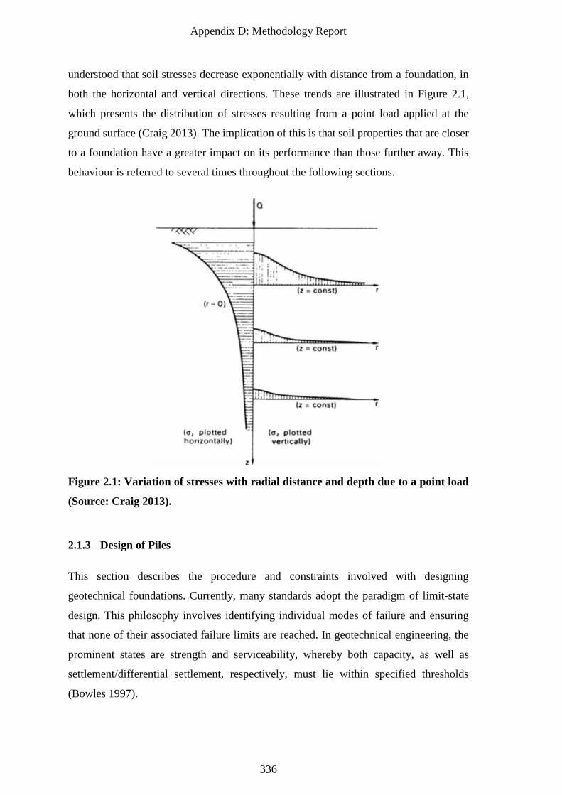
Appendix D: Methodology Report
336
understood that soil stresses decrease exponentially with distance from a foundation, in
both the horizontal and vertical directions. These trends are illustrated in Figure 2.1,
which presents the distribution of stresses resulting from a point load applied at the
ground surface (Craig 2013). The implication of this is that soil properties that are closer
to a foundation have a greater impact on its performance than those further away. This
behaviour is referred to several times throughout the following sections.
Figure 2.1: Variation of stresses with radial distance and depth due to a point load
(Source: Craig 2013).
2.1.3 Design of Piles
This section describes the procedure and constraints involved with designing
geotechnical foundations. Currently, many standards adopt the paradigm of limit-state
design. This philosophy involves identifying individual modes of failure and ensuring
that none of their associated failure limits are reached. In geotechnical engineering, the
prominent states are strength and serviceability, whereby both capacity, as well as
settlement/differential settlement, respectively, must lie within specified thresholds
(Bowles 1997).
Appendix D: Methodology Report
337
Here, settlement refers to immediate settlement resulting from the elastic compression of
the soil, also known as primary settlement, and is related to its material stiffness. There
are other forms of settlement, such as consolidation and creep (Craig 2013).
Piles are often designed in an iterative fashion, such that multiple designs are analysed
through trial-and-error until one is found that satisfies the relevant limit states. Usually,
there is an additional cost criterion, which one attempts to minimise, transforming the
design process into an optimization problem. Therefore, engineers seek to find the most
cost-effective design that satisfies the limit state criteria, which corresponds to the
shortest pile length, in the case of a pile with a fixed diameter.
Additional design variables include the number and positioning of individual footings. A
deep foundation often consists of a series of piles as opposed to an individual footing,
depending on the type of structure being supported. Piles are typically evenly spaced, or
are otherwise specifically located beneath concentrated loads imposed by the
superstructure, such as columns. The configuration of a group of piles affects the applied
load that each pile supports. As such, it is an important design consideration.
2.2 Site Investigations
This section describes the purpose of and overall procedure for undertaking a site
investigation. Investigations provide various aspects of information about the subsurface
conditions at a site. The principal objectives of a site investigation are (Craig 2013):
1. To determine the sequence, thicknesses and lateral extent of the soil strata and,
where appropriate, the level of bedrock;
2. To obtain representative samples of the soils (and rock) for identification and
classification, and, if necessary, for use in laboratory tests to determine relevant
soil parameters; and
3. To identify the groundwater conditions.
Note that groundwater conditions are not considered in this analysis, as it is known to
have minimal impact on pile settlement performance. Many guidelines, including the
above resources recommend undertaking a site investigation in multiple stages. These
stages are summarised as follows:
Appendix D: Methodology Report
338
1. Perform a desktop study, where information about the subsurface profile is gained
from sources, such as soil and geology maps, nearby boreholes taken at previous
points in time, or by inferring information from the surface of the site.
2. A preliminary investigation is then to be undertaken. This consists of a small-
scale investigation, comprising of one or two boreholes or a test pit. This serves
to validate the information of the site investigation, and to suggest the extent and
number of boreholes to be taken in the next stage.
3. A detailed, full-scale site investigation is then to be conducted. Multiple boreholes
are taken over the area of interest, from which the engineering properties of the
soil layers are to be obtained.
However, this multi-step approach is rarely adopted, except for very large-scale projects,
as a result of either time or budgetary constraints. Often, the preliminary phase (i.e. Step
2) is not considered. Depending on the consistency and reliability of results, it may be
decided that additional sampling is to be carried out after completion of the full-scale
investigation. Subsequent additional testing is frequently a source of delays and
additional costs. These detriments are one aspect of site investigations that a thorough,
multi-stage investigation aims to avoid.
Investigation results are used to generate a site model; an approximation of the soil
properties at the site, which facilitates the assessment of foundation performance for the
purpose of design. The soil properties in the model are often simplifications, reducing the
complexity of multiple, varied test data down to single representative values, as discussed
later in §4.3.
Some of the more detailed recommendations for site investigations are provided by the
Eurocode 7: Geotechnical Design international standard, a summary of the
recommendations for which are given in Table 2.1. Note that these values are provided
for guidance, rather than as mandatory requirements. Furthermore, large ranges of
borehole spacings are specified, without instructions on interpretation. Therefore, despite
the presence of quantitative recommendations, the ultimate choice of investigation scope
is subject to engineering judgement. This unavoidable subjectivity underlines the need
for quantitative guidance on investigation optimization.
Appendix D: Methodology Report
339
Table 2.1: Guidance values for spacing and pattern of investigation points, after
European Standards (2006).
Structure Spacing Layout
High-rise and industrial structures 15 – 40 m Grid pattern
Large area 60 m Grid pattern
Linear structures (e.g. roads, railways,
walls etc.)
20 – 200 m Linear
Special structures (e.g. bridges, stacks,
machinery, foundations.)
2 – 6 investigation points per foundation
Dams and weirs 25 – 75 m Along relevant sections
2.3 Optimization Framework
This section presents an overview of the site investigation optimization framework
discussed throughout the report. The framework is largely based on that of Jaksa et al.
(2003). It makes use of the Random Finite Element Method (RFEM), which involves
mapping randomly generated soil properties onto a finite element mesh over a series of
Monte Carlo realisations (Fenton et al. 1996). Other frameworks have been proposed that
aim to account for uncertainty in soils, such as that of Gong et al. (2016), which analyses
the statistical robustness of an investigation for a soil in a manner independent of
foundation type. There is also the concept of reliability-based design, introduced by Spry
et al. (1988), which can relate the uncertainty and risk of design to the amount and quality
of available site investigation information. However, the Jaksa framework is the most
suitable for determining a foundation’s cost and risk with regards to a particular site
investigation scope. It can therefore account for the influence of different foundation
designs and configurations, which may have a large impact on the results. As a result, the
Jaksa framework is adopted for present research project.
As the probability of failure is related to the extent of site knowledge and therefore site
investigation scope, it is logical to conclude that a site investigation can be found that
yields an optimal total cost. In other words, there is expected to be a sampling threshold
beyond which there is no financial benefit to additional sampling. The variables
contributing to this trade-off are the failure and foundation construction costs, which
typically decrease with additional sampling, and the site investigation cost, which
increases. This trend is qualitatively described by Phoon (1995) and illustrated in Figure
2.2.
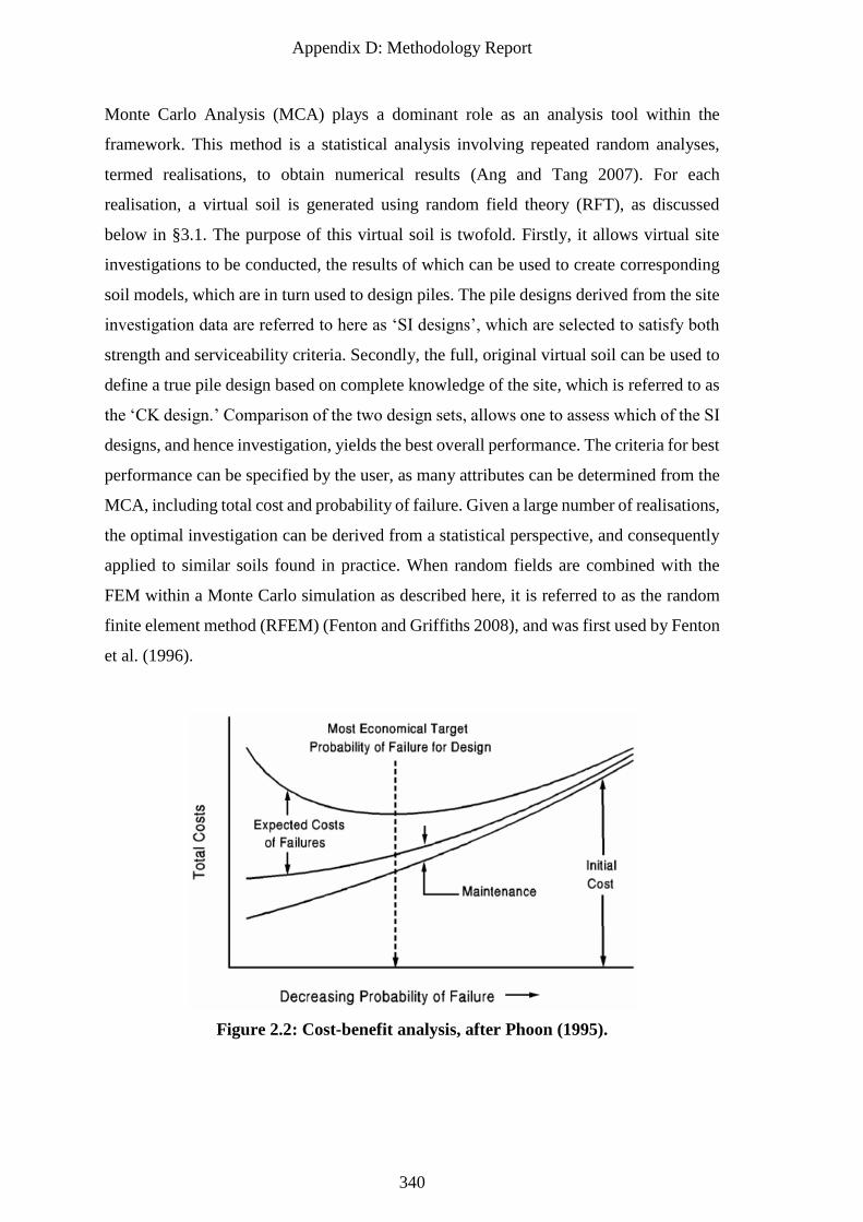
Appendix D: Methodology Report
340
Monte Carlo Analysis (MCA) plays a dominant role as an analysis tool within the
framework. This method is a statistical analysis involving repeated random analyses,
termed realisations, to obtain numerical results (Ang and Tang 2007). For each
realisation, a virtual soil is generated using random field theory (RFT), as discussed
below in §3.1. The purpose of this virtual soil is twofold. Firstly, it allows virtual site
investigations to be conducted, the results of which can be used to create corresponding
soil models, which are in turn used to design piles. The pile designs derived from the site
investigation data are referred to here as ‘SI designs’, which are selected to satisfy both
strength and serviceability criteria. Secondly, the full, original virtual soil can be used to
define a true pile design based on complete knowledge of the site, which is referred to as
the ‘CK design.’ Comparison of the two design sets, allows one to assess which of the SI
designs, and hence investigation, yields the best overall performance. The criteria for best
performance can be specified by the user, as many attributes can be determined from the
MCA, including total cost and probability of failure. Given a large number of realisations,
the optimal investigation can be derived from a statistical perspective, and consequently
applied to similar soils found in practice. When random fields are combined with the
FEM within a Monte Carlo simulation as described here, it is referred to as the random
finite element method (RFEM) (Fenton and Griffiths 2008), and was first used by Fenton
et al. (1996).
Figure 2.2: Cost-benefit analysis, after Phoon (1995).
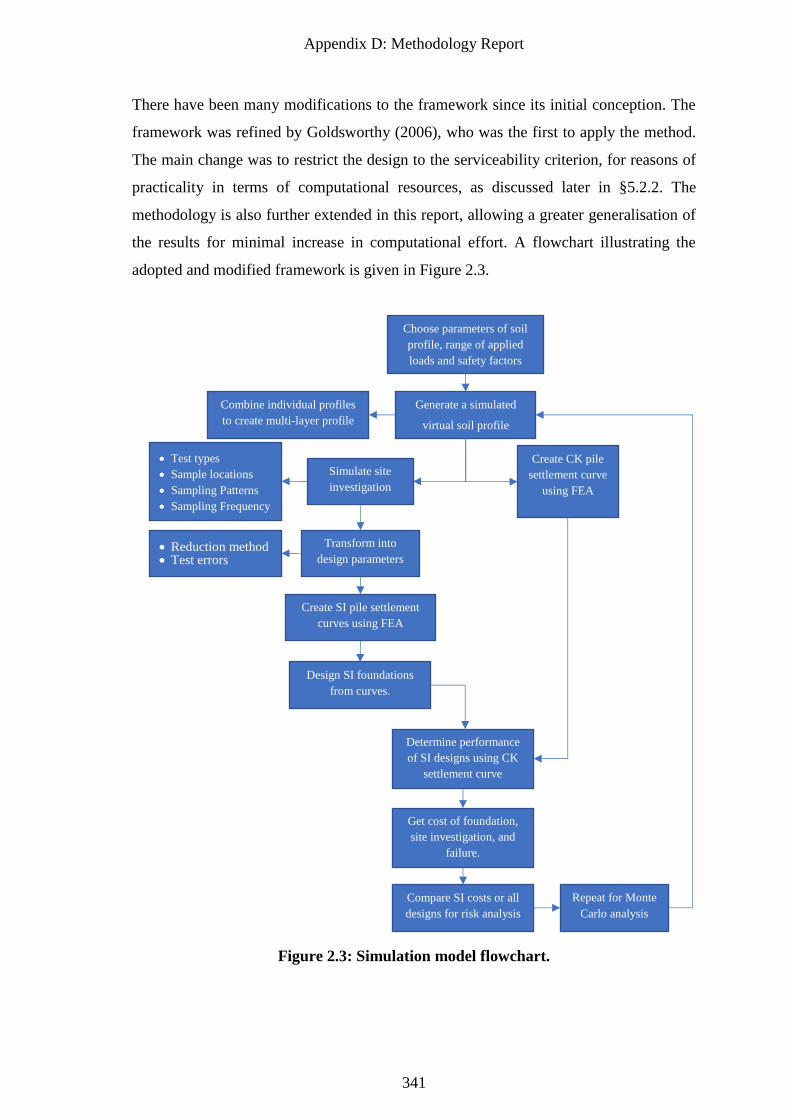
Appendix D: Methodology Report
341
There have been many modifications to the framework since its initial conception. The
framework was refined by Goldsworthy (2006), who was the first to apply the method.
The main change was to restrict the design to the serviceability criterion, for reasons of
practicality in terms of computational resources, as discussed later in §5.2.2. The
methodology is also further extended in this report, allowing a greater generalisation of
the results for minimal increase in computational effort. A flowchart illustrating the
adopted and modified framework is given in Figure 2.3.
Figure 2.3: Simulation model flowchart.
Generate a simulated
virtual soil profile
Simulate site
investigation
Create CK pile
settlement curve
using FEA
• Test types
• Sample locations
• Sampling Patterns
• Sampling Frequency
Transform into
design parameters • Reduction method • Test errors
Create SI pile settlement
curves using FEA
Design SI foundations
from curves.
Determine performance
of SI designs using CK
settlement curve
Get cost of foundation,
site investigation, and
failure.
Compare SI costs or all
designs for risk analysis
Repeat for Monte
Carlo analysis
Combine individual profiles
to create multi-layer profile
Choose parameters of soil
profile, range of applied
loads and safety factors
Appendix D: Methodology Report
342
In terms of foundations, the piles are designed according to the serviceability criterion,
using linear elastic FEA to determine foundation performance. As discussed in §5.3, two
material parameters are required; Young’s modulus (E) and Poisson’s ratio (v). It has
been found that the variability of v has negligible impact on the settlement of foundations
(Fenton et al. 1996). Therefore, in the present research, the generation of a virtual soil
solely involves the simulation of a random field of E values.
This report presents other major enhancements to the framework, which extends its
applicability to other fields of research. The framework now allows for an arbitrary, user-
defined level of design redundancy to be explicitly accounted for. If one so desires, this
could be readily adapted to reliability-based design and other foundation optimization
research. The inclusion of redundancy is advantageous, as it is likely that the lowest
possible total cost is some combination of increased site investigation scope and the
adopted design safety factor. Previous studies have focussed solely on the site
investigation scope itself. This increased functionality is primarily due to a change in the
design philosophy, as discussed later in §5.5.1.
The final major modification to the Jaksa et al. (2003) framework is that cost is now no
longer assigned to the CK for comparative purposes. This is because cost cannot be
assigned to the site investigation, as one is not conducted in this case. Therefore, the
optimal site investigation is determined by comparing the costs of the SI designs
exclusively with each other to determine the optimal case among the specified options.
A discussion of the costs is provided in §7.3.
As there have been a large number of changes to the original framework, as well as a
notable improvement to computational resources since the last study, several new options
are available for analysis. These options each require extensive validation, which are
provided throughout the report.
2.4 Modified Optimization Framework with Evolutionary Algorithms
A fundamental limitation of the primary framework discussed in §2.3 is that a fixed
number of site investigation options are analysed, and that the suggested optimal case is
only the optimal of this fixed subset of options. For this reason, a modified version of the
framework is presented in this section which incorporates evolutionary algorithms (EAs)
(Yu and Gen 2010) to optimise site investigation options. These evolutionary algorithms
Appendix D: Methodology Report
343
including, but not limited to, the genetic (Haupt and Haupt 2004), particle swarm
optimization (Clerc 2010), and imperialist competitive (Atashpaz-Gargari and Lucas
2007) algorithms, can theoretically search the full parameter space to find a global
optimum. Note that EAs, as discussed in this section, are not in the core scope of this
study, and so will not be discussed in detail.
Evolutionary algorithms, as the name suggests, are inspired by biological or social
evolutionary mechanisms, where a population of search points is iteratively improved
until a global optimum is found. An advantage of these techniques is that they do not
make assumptions of the fitness of the parameter search space, meaning that they can be
applied to problems where the nature of the solution is not well understood. However,
EAs are controlled by a variety of search parameters, which usually must be themselves
optimised in order to maximise the effectiveness and efficiency of the algorithm to the
particular problem. These parameters, for a generic EA, include the population size,
mutation rate, and stopping criteria (such as maximum number of iterations, termed
generations), although other parameters may be included depending on the type and
implementation of the algorithm.
The general process involved in optimization using EAs is as follows:
1. Random generation of the initial population of search points.
2. Fitness evaluation of each individual in that population (i.e. lowest cost ($),
probability of failure, etc).
3. Evolution of the population until termination by achieving a sufficient solution,
or reaching the maximum number of generations:
a. Selection of the highest quality individuals for mating.
b. Breeding of new individuals through crossover and mutation mechanisms.
c. Evaluation of the fitness of each new individual.
d. Replacement of least-fit individuals with new ones.
Note that this modified method has only now become feasible due to the optimizations
in this report. This includes use of a 2D axisymmetric mesh for determining site
investigation performance with a speed increase of 2 orders of magnitude, as discussed
in §6.4. More importantly however, is the decoupling of resource-intensive CK
computation from the determination of SI performance, as discussed in §5.5.1. This
Appendix D: Methodology Report
344
means that the quantity of CK FEM analysis is independent of the number of site
investigations analysed, as well as the number of generations performed by the EA.
As mentioned previously, the main advantage of this modified framework is that a true
global optimum can theoretically be identified. Furthermore, some investigation
parameters, such as the number of boreholes, may be held constant, allowing for the
remaining parameters to be optimised for that particular case; for example, the borehole
locations and depths. This approach allows for the creation of a pareto front, which
produces a collection of non-dominated solutions in terms of costs for the fixed
parameters. This kind of multi-objective optimization becomes useful if a particular
engineering company does not have access to certain types of equipment, allowing them
to look elsewhere for a viable solution on the pareto front.
Another advantage is that the number of site investigation options that are explored in
any given generation can be significantly smaller than the total number of options in the
primary framework. However, a notable disadvantage is that the total number of site
investigation options analysed across the full number of generations is higher than that
of the primary framework. Furthermore, there is additional overhead, as the virtual soils
must be re-generated for each generation. Depending on the optimization parameters and
specified soil resolution, this overhead can result in several days’ worth of duplicated
effort. Ideally, once a soil is generated, it could be saved, and then re-loaded at the
required times within subsequent generations. However, the required storage for this
process makes the option prohibitive, and the time savings would likely be minimal.
An additional disadvantage is that, as each new iteration depends on the results of the
previous, this process cannot be parallelised. While the Monte Carlo simulation within
each iteration can still be parallelised, it would no longer be possible to run each
realisation as an independent program, which is a highly-scalable parallelisation, as
discussed in §6.3. By contrast, a single, multi-core program must be developed, which
becomes increasingly inefficient as the number of cores increases. Therefore, the real run
time of a single Monte Carlo simulation is significantly increased.
Finally, a key outcome of this line of research is the understanding of how certain aspects
of soil geology and structural configurations impact the performance of site
investigations. To achieve this, it is necessary to perform a parametric study, where all
Appendix D: Methodology Report
345
parameters are held constant while one is varied in a regular fashion within each analysis.
While this modified framework should allow for true optimal solutions to be found, their
nature is not compatible with that of the parametric study described through the majority
of this report. Furthermore, the primary framework allows for a wide variety of structural
configurations to be analysed from a single set of results, through the use of a post-
processing stage. However, any results obtained through use of EAs would only be
applicable for the particular structure for which the investigation has been optimised. As
such, the EA optimization must be repeated for each new structural configuration. For
these reasons, and for the computational performance factors mentioned above, explain
why the EA framework is not the core focus of this study.
It should be noted that this framework would likely be required for the results of this line
of research to be implemented as a guideline in official site investigation standards. As
such, it is recommended as future research. For example, as single layer soils do not
require FEA of any kind, as discussed in §6.4, the iterative site investigation optimization
process can be performed with minimal computational effort. As the CK information for
single-layer soils can be obtained, several orders of magnitude more efficiently with the
PIE method (discussed in §5.4) compared to FEA, this makes the analysis of multi-staged
site investigations possible. For example, an investigation can be carried out, and then
the location of the building can be chosen based on the site investigation results, such that
the pile designs are minimised, therefore reducing construction costs. While this latter
process isn’t exclusive to the EA framework, it is currently only feasible with single layer
soils due to the PIE method, and as such, is well suited to this line of research.
While the optimization can still be undertaken within a practical timeframe for multi-
layered soils using 2D axisymmetric FEA, it is recognised that further optimization can
be made. Soil models derived from site investigations typically vary only with depth,
where the soil properties are constant in the horizontal direction. As such, the soil can be
represented entirely by 1D information, and theoretically a highly efficient 1D pile
settlement model can be developed and used instead, perhaps in a manner similar to the
model described by Fenton and Griffiths (2007). Such a model would greatly reduce the
run time of the full simulation should it prove to yield similar results to more sophisticated
FEA. However, further work is required in this area that is again beyond the scope of this
study.
Appendix D: Methodology Report
346
2.5 Software Platforms
A variety of software is involved in conducting the analysis and investigating its results,
and their details are given in this section. The majority of the analysis is conducted using
Python 3.6 (Python Software Foundation 2018) combined with some usage of Fortran 95
(GCC team 2018) for computational bottlenecks. This includes a set of Fortran
subroutines dedicated to producing virtual soils, as discussed in §3.1. Another set of
subroutines provide linear-elastic FEM capability in order to calculate pile settlements,
as described in §5.3. These subroutines are adapted from the RFEM suite of programs by
Fenton and Griffiths (2008). Examination of the main program shows that 99% of the
run-time is spent in the FEM subroutines, despite their optimised nature and that it is a
relatively small component of the code base.
Python is also used for analysis and interpretation of results, in terms of statistical analysis
and graphing. A number of commonly-used, third-party packages are adopted to facilitate
this work, including:
• Numerical Python (Numpy) – array management (Stéfan van der Walt 2017);
• Scientific Python (Scipy) – statistics and analysis (Eric Jones 2001-); and
• Matplotlib – graphing suite (Hunter 2007).
In addition, there is some usage of artificial neural networks (ANNs) to aid in the
interpretation of results. This is facilitated through the use of the Tensorflow machine
learning library in conjunction with the Keras front end (Ketkar 2017).
Note that all computational times provided in this report, unless stated otherwise, are
relevant to a MacBook Pro incorporating an Intel 3.3 GHz, Intel Core i7 processor and
16 GB of RAM.
3 Soil Simulation
This section discusses the various components of soil modelling used within the
framework. This includes the generation of soil bodies used to form individual layers,
and a guideline to form complex layer boundaries to produce realistic geology.
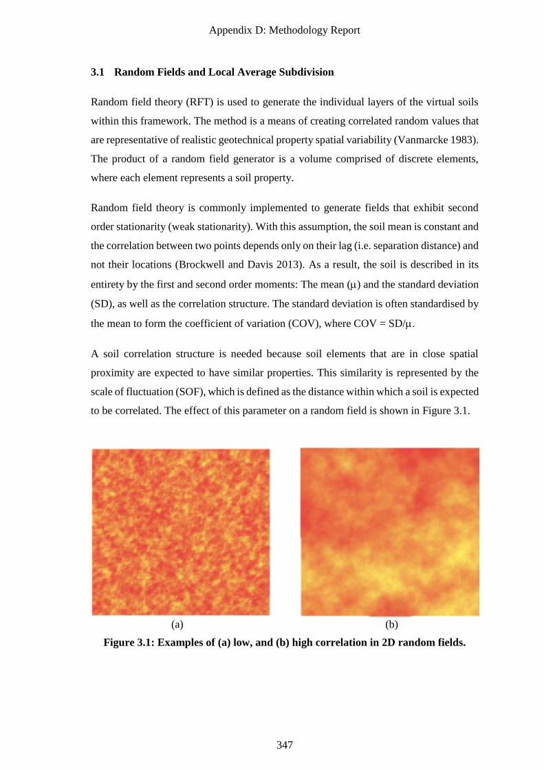
Appendix D: Methodology Report
347
3.1 Random Fields and Local Average Subdivision
Random field theory (RFT) is used to generate the individual layers of the virtual soils
within this framework. The method is a means of creating correlated random values that
are representative of realistic geotechnical property spatial variability (Vanmarcke 1983).
The product of a random field generator is a volume comprised of discrete elements,
where each element represents a soil property.
Random field theory is commonly implemented to generate fields that exhibit second
order stationarity (weak stationarity). With this assumption, the soil mean is constant and
the correlation between two points depends only on their lag (i.e. separation distance) and
not their locations (Brockwell and Davis 2013). As a result, the soil is described in its
entirety by the first and second order moments: The mean () and the standard deviation
(SD), as well as the correlation structure. The standard deviation is often standardised by
the mean to form the coefficient of variation (COV), where COV = SD/.
A soil correlation structure is needed because soil elements that are in close spatial
proximity are expected to have similar properties. This similarity is represented by the
scale of fluctuation (SOF), which is defined as the distance within which a soil is expected
to be correlated. The effect of this parameter on a random field is shown in Figure 3.1.
(a) (b)
Figure 3.1: Examples of (a) low, and (b) high correlation in 2D random fields.
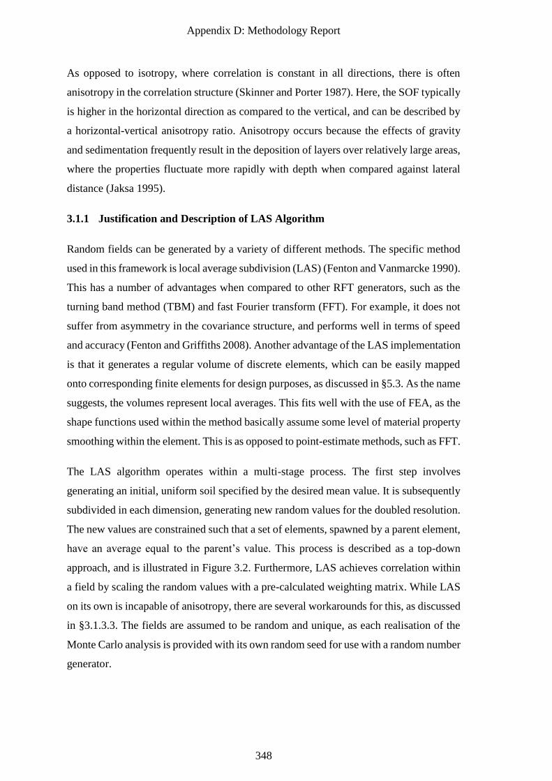
Appendix D: Methodology Report
348
As opposed to isotropy, where correlation is constant in all directions, there is often
anisotropy in the correlation structure (Skinner and Porter 1987). Here, the SOF typically
is higher in the horizontal direction as compared to the vertical, and can be described by
a horizontal-vertical anisotropy ratio. Anisotropy occurs because the effects of gravity
and sedimentation frequently result in the deposition of layers over relatively large areas,
where the properties fluctuate more rapidly with depth when compared against lateral
distance (Jaksa 1995).
3.1.1 Justification and Description of LAS Algorithm
Random fields can be generated by a variety of different methods. The specific method
used in this framework is local average subdivision (LAS) (Fenton and Vanmarcke 1990).
This has a number of advantages when compared to other RFT generators, such as the
turning band method (TBM) and fast Fourier transform (FFT). For example, it does not
suffer from asymmetry in the covariance structure, and performs well in terms of speed
and accuracy (Fenton and Griffiths 2008). Another advantage of the LAS implementation
is that it generates a regular volume of discrete elements, which can be easily mapped
onto corresponding finite elements for design purposes, as discussed in §5.3. As the name
suggests, the volumes represent local averages. This fits well with the use of FEA, as the
shape functions used within the method basically assume some level of material property
smoothing within the element. This is as opposed to point-estimate methods, such as FFT.
The LAS algorithm operates within a multi-stage process. The first step involves
generating an initial, uniform soil specified by the desired mean value. It is subsequently
subdivided in each dimension, generating new random values for the doubled resolution.
The new values are constrained such that a set of elements, spawned by a parent element,
have an average equal to the parent’s value. This process is described as a top-down
approach, and is illustrated in Figure 3.2. Furthermore, LAS achieves correlation within
a field by scaling the random values with a pre-calculated weighting matrix. While LAS
on its own is incapable of anisotropy, there are several workarounds for this, as discussed
in §3.1.3.3. The fields are assumed to be random and unique, as each realisation of the
Monte Carlo analysis is provided with its own random seed for use with a random number
generator.
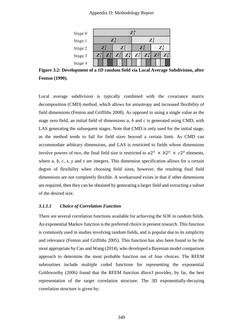
Appendix D: Methodology Report
349
Figure 3.2: Development of a 1D random field via Local Average Subdivision, after
Fenton (1990).
Local average subdivision is typically combined with the covariance matrix
decomposition (CMD) method, which allows for anisotropy and increased flexibility of
field dimensions (Fenton and Griffiths 2008). As opposed to using a single value as the
stage zero field, an initial field of dimensions a, b and c is generated using CMD, with
LAS generating the subsequent stages. Note that CMD is only used for the initial stage,
as the method tends to fail for field sizes beyond a certain limit. As CMD can
accommodate arbitrary dimensions, and LAS is restricted to fields whose dimensions
involve powers of two, the final field size is restricted to 𝑎2𝑥 × 𝑏2𝑦 × 𝑐2𝑧 elements,
where a, b, c, x, y and z are integers. This dimension specification allows for a certain
degree of flexibility when choosing field sizes, however, the resulting final field
dimensions are not completely flexible. A workaround exists in that if other dimensions
are required, then they can be obtained by generating a larger field and extracting a subset
of the desired size.
3.1.1.1 Choice of Correlation Function
There are several correlation functions available for achieving the SOF in random fields.
An exponential Markov function is the preferred choice in present research. This function
is commonly used in studies involving random fields, and is popular due to its simplicity
and relevance (Fenton and Griffiths 2005). This function has also been found to be the
most appropriate by Cao and Wang (2014), who developed a Bayesian model comparison
approach to determine the most probable function out of four choices. The RFEM
subroutines include multiple coded functions for representing the exponential
Goldsworthy (2006) found that the RFEM function dlavx3 provides, by far, the best
representation of the target correlation structure. The 3D exponentially-decaying
correlation structure is given by:
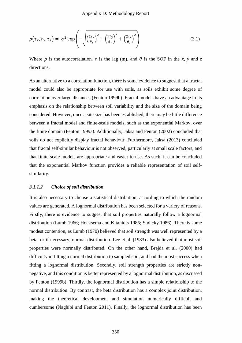
Appendix D: Methodology Report
350
𝜌(𝜏𝑥, 𝜏𝑦, 𝜏𝑧) = 𝜎2 exp(−√(
2𝜏𝑥
𝜃𝑥)2
+ (2𝜏𝑦
𝜃𝑦)2
+ (2𝜏𝑧
𝜃𝑧)2
) (3.1)
Where 𝜌 is the autocorrelation. 𝜏 is the lag (m), and 𝜃 is the SOF in the x, y and z
directions.
As an alternative to a correlation function, there is some evidence to suggest that a fractal
model could also be appropriate for use with soils, as soils exhibit some degree of
correlation over large distances (Fenton 1999b). Fractal models have an advantage in its
emphasis on the relationship between soil variability and the size of the domain being
considered. However, once a site size has been established, there may be little difference
between a fractal model and finite-scale models, such as the exponential Markov, over
the finite domain (Fenton 1999a). Additionally, Jaksa and Fenton (2002) concluded that
soils do not explicitly display fractal behaviour. Furthermore, Jaksa (2013) concluded
that fractal self-similar behaviour is not observed, particularly at small scale factors, and
that finite-scale models are appropriate and easier to use. As such, it can be concluded
that the exponential Markov function provides a reliable representation of soil self-
similarity.
3.1.1.2 Choice of soil distribution
It is also necessary to choose a statistical distribution, according to which the random
values are generated. A lognormal distribution has been selected for a variety of reasons.
Firstly, there is evidence to suggest that soil properties naturally follow a lognormal
distribution (Lumb 1966; Hoeksema and Kitanidis 1985; Sudicky 1986). There is some
modest contention, as Lumb (1970) believed that soil strength was well represented by a
beta, or if necessary, normal distribution. Lee et al. (1983) also believed that most soil
properties were normally distributed. On the other hand, Brejda et al. (2000) had
difficulty in fitting a normal distribution to sampled soil, and had the most success when
fitting a lognormal distribution. Secondly, soil strength properties are strictly non-
negative, and this condition is better represented by a lognormal distribution, as discussed
by Fenton (1999b). Thirdly, the lognormal distribution has a simple relationship to the
normal distribution. By contrast, the beta distribution has a complex joint distribution,
making the theoretical development and simulation numerically difficult and
cumbersome (Naghibi and Fenton 2011). Finally, the lognormal distribution has been
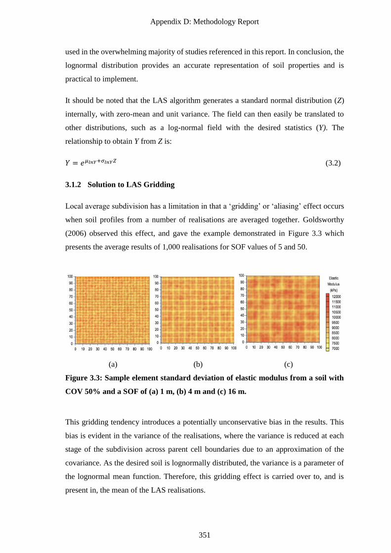
Appendix D: Methodology Report
351
used in the overwhelming majority of studies referenced in this report. In conclusion, the
lognormal distribution provides an accurate representation of soil properties and is
practical to implement.
It should be noted that the LAS algorithm generates a standard normal distribution (Z)
internally, with zero-mean and unit variance. The field can then easily be translated to
other distributions, such as a log-normal field with the desired statistics (Y). The
relationship to obtain Y from Z is:
𝑌 = 𝑒𝜇𝑙𝑛𝑌+𝜎𝑙𝑛𝑌𝑍 (3.2)
3.1.2 Solution to LAS Gridding
Local average subdivision has a limitation in that a ‘gridding’ or ‘aliasing’ effect occurs
when soil profiles from a number of realisations are averaged together. Goldsworthy
(2006) observed this effect, and gave the example demonstrated in Figure 3.3 which
presents the average results of 1,000 realisations for SOF values of 5 and 50.
(a) (b) (c)
Figure 3.3: Sample element standard deviation of elastic modulus from a soil with
COV 50% and a SOF of (a) 1 m, (b) 4 m and (c) 16 m.
This gridding tendency introduces a potentially unconservative bias in the results. This
bias is evident in the variance of the realisations, where the variance is reduced at each
stage of the subdivision across parent cell boundaries due to an approximation of the
covariance. As the desired soil is lognormally distributed, the variance is a parameter of
the lognormal mean function. Therefore, this gridding effect is carried over to, and is
present in, the mean of the LAS realisations.
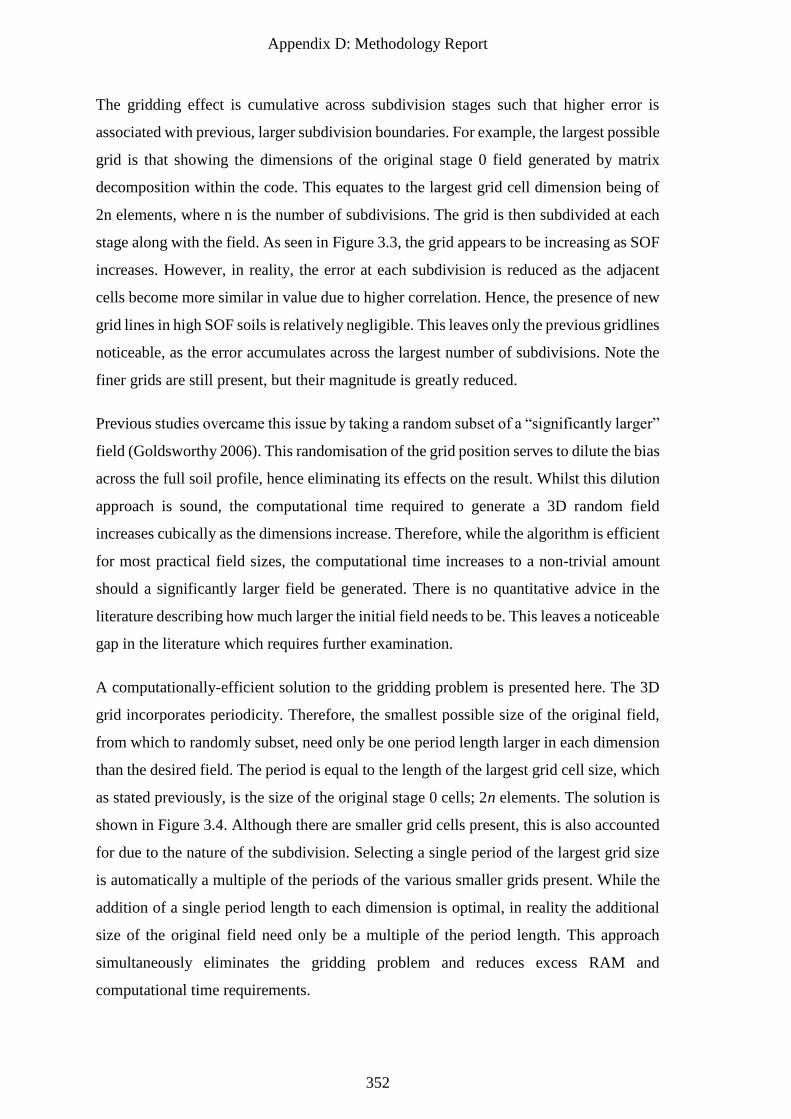
Appendix D: Methodology Report
352
The gridding effect is cumulative across subdivision stages such that higher error is
associated with previous, larger subdivision boundaries. For example, the largest possible
grid is that showing the dimensions of the original stage 0 field generated by matrix
decomposition within the code. This equates to the largest grid cell dimension being of
2n elements, where n is the number of subdivisions. The grid is then subdivided at each
stage along with the field. As seen in Figure 3.3, the grid appears to be increasing as SOF
increases. However, in reality, the error at each subdivision is reduced as the adjacent
cells become more similar in value due to higher correlation. Hence, the presence of new
grid lines in high SOF soils is relatively negligible. This leaves only the previous gridlines
noticeable, as the error accumulates across the largest number of subdivisions. Note the
finer grids are still present, but their magnitude is greatly reduced.
Previous studies overcame this issue by taking a random subset of a “significantly larger”
field (Goldsworthy 2006). This randomisation of the grid position serves to dilute the bias
across the full soil profile, hence eliminating its effects on the result. Whilst this dilution
approach is sound, the computational time required to generate a 3D random field
increases cubically as the dimensions increase. Therefore, while the algorithm is efficient
for most practical field sizes, the computational time increases to a non-trivial amount
should a significantly larger field be generated. There is no quantitative advice in the
literature describing how much larger the initial field needs to be. This leaves a noticeable
gap in the literature which requires further examination.
A computationally-efficient solution to the gridding problem is presented here. The 3D
grid incorporates periodicity. Therefore, the smallest possible size of the original field,
from which to randomly subset, need only be one period length larger in each dimension
than the desired field. The period is equal to the length of the largest grid cell size, which
as stated previously, is the size of the original stage 0 cells; 2n elements. The solution is
shown in Figure 3.4. Although there are smaller grid cells present, this is also accounted
for due to the nature of the subdivision. Selecting a single period of the largest grid size
is automatically a multiple of the periods of the various smaller grids present. While the
addition of a single period length to each dimension is optimal, in reality the additional
size of the original field need only be a multiple of the period length. This approach
simultaneously eliminates the gridding problem and reduces excess RAM and
computational time requirements.
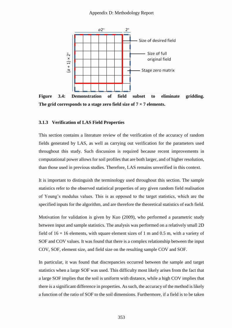
Appendix D: Methodology Report
353
Figure 3.4: Demonstration of field subset to eliminate gridding.
The grid corresponds to a stage zero field size of 7 × 7 elements.
3.1.3 Verification of LAS Field Properties
This section contains a literature review of the verification of the accuracy of random
fields generated by LAS, as well as carrying out verification for the parameters used
throughout this study. Such discussion is required because recent improvements in
computational power allows for soil profiles that are both larger, and of higher resolution,
than those used in previous studies. Therefore, LAS remains unverified in this context.
It is important to distinguish the terminology used throughout this section. The sample
statistics refer to the observed statistical properties of any given random field realisation
of Young’s modulus values. This is as opposed to the target statistics, which are the
specified inputs for the algorithm, and are therefore the theoretical statistics of each field.
Motivation for validation is given by Kuo (2009), who performed a parametric study
between input and sample statistics. The analysis was performed on a relatively small 2D
field of 16 × 16 elements, with square element sizes of 1 m and 0.5 m, with a variety of
SOF and COV values. It was found that there is a complex relationship between the input
COV, SOF, element size, and field size on the resulting sample COV and SOF.
In particular, it was found that discrepancies occurred between the sample and target
statistics when a large SOF was used. This difficulty most likely arises from the fact that
a large SOF implies that the soil is uniform with distance, while a high COV implies that
there is a significant difference in properties. As such, the accuracy of the method is likely
a function of the ratio of SOF to the soil dimensions. Furthermore, if a field is to be taken
Appendix D: Methodology Report
354
as a subset of a larger field, with a high SOF, that may have an impact on the apparent
SOF and COV values, depending on whether the subset is extracted from a pocket of
similar material.
For these reasons, it is necessary to validate the statistical parameters of the final soil.
Furthermore, methods that attempt to compensate for deficiencies are also discussed.
3.1.3.1 Mean and coefficient of variation
This subsection assesses the accuracy of the sample mean and COV in fields generated
using LAS. It has been noted that there is variance in both the sample mean and the
standard deviation across realisations. However, this problem is potentially exacerbated
by the fact that a subset is taken of the field as part of the solution to the LAS gridding
problem discussed in §3.1.2. It is anticipated that, in soils with a high SOF, a subset which
is taken from a fairly continuous pocket of similar material would result in a reduction of
the apparent subset COV, and increased variance in the subset mean across realisations.
It should be noted that in the context of this framework, a sample mean that varies on a
per-realisation basis is not detrimental to the performance of the results, as this bias would
be consistent in both the CK and SI cases, and is therefore self-cancelling. A bias in the
sample mean may potentially be an issue, however, if it is sufficiently large to cause
invalid designs to occur in some realisations. This would happen if the sample mean is
low or high enough to cause the theoretical pile design to be greater than the maximum
or less than the minimum allowable lengths respectively.
However, the sample COV is considered to have a notable impact on the results. This is
because the quality of an investigation is assessed by its total cost, which is heavily
weighted to large differential settlements in the foundation, as discussed in §7.3.1.
Therefore, should variation in the sample COV across realisations result in some soils
having excessively high variability, then the failure cost would likely be overestimated,
regardless of the COV mean.
The proposed solution to the variance in soil mean and COV is to scale the extracted
subset to the target statistics. This should theoretically provide constant sample statistics
across all realisations. The scaling procedure is performed with the following the
following steps:
Appendix D: Methodology Report
355
1. Specify the LAS field to generate a zero-mean, unit-variance normally-distributed
field (which will likely have differing sample statistics).
2. Extract a random subset to overcome gridding, as discussed in §3.1.2.
3. Standardise the field by subtracting the sample mean and dividing by the sample
standard deviation.
4. Apply the lognormal transformation to achieve the desired statistics, as described
in §3.1.1.2.
To examine the magnitude of variation of the soil mean and COV, an analysis of 50 soils
has been undertaken with a variety of isotropic SOFs. The fields are specified with a
mean of 1 MPa and COV of 50%. The soil resolution was set at 256 × 256 × 196 elements,
with an element size of 0.25 m. The analysis has been undertaken on 3 versions of each
generated field:
1. The original, log-normally distributed, and full-resolution field as generated by
the default LAS method.
2. A randomly-extracted subset of the above field with a resolution of 240 × 240 ×
160 elements.
3. A subset, as with the above soil, except with scaled statistics, as described by the
4 steps above, referred to as the ‘corrected field.’
The results are given in Figure 3.5, and the original, non-corrected field (soil 1) is
described throughout the remainder of this section unless specified otherwise. It can be
seen that the variance of both the sample mean and standard deviation increase as the
SOF increases. These results are supported by Kuo (2009), who found that when the SOF
is high, there are large variations in the sample mean and COV across realisations. The
COV of the sample statistics appears to be approximately linearly proportional to the
SOF, increasing to roughly 20% for a soil with SOF of 32 m. This would likely be larger
with higher target COV values.
While the mean of the sample means does not appear to change significantly, it should
be noted that the y-scale is quite large compared to the trend. Kuo (2009) found that, for
a soil with COV of 100%, the mean decreases as the SOF decreases, reaching as low as
0.92 at an SOF of 4 m. This case refers to a cubic element of length 1 m, significantly
higher than the element sizes used throughout the present study. Kuo (2009) found that
the magnitude of the mean reduction decreased as the element sized decreased. Therefore,
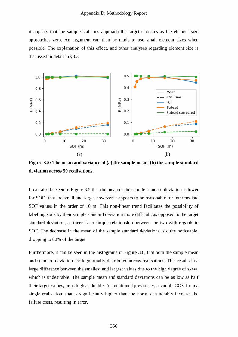
Appendix D: Methodology Report
356
it appears that the sample statistics approach the target statistics as the element size
approaches zero. An argument can then be made to use small element sizes when
possible. The explanation of this effect, and other analyses regarding element size is
discussed in detail in §3.3.
(a) (b)
Figure 3.5: The mean and variance of (a) the sample mean, (b) the sample standard
deviation across 50 realisations.
It can also be seen in Figure 3.5 that the mean of the sample standard deviation is lower
for SOFs that are small and large, however it appears to be reasonable for intermediate
SOF values in the order of 10 m. This non-linear trend facilitates the possibility of
labelling soils by their sample standard deviation more difficult, as opposed to the target
standard deviation, as there is no simple relationship between the two with regards to
SOF. The decrease in the mean of the sample standard deviations is quite noticeable,
dropping to 80% of the target.
Furthermore, it can be seen in the histograms in Figure 3.6, that both the sample mean
and standard deviation are lognormally-distributed across realisations. This results in a
large difference between the smallest and largest values due to the high degree of skew,
which is undesirable. The sample mean and standard deviations can be as low as half
their target values, or as high as double. As mentioned previously, a sample COV from a
single realisation, that is significantly higher than the norm, can notably increase the
failure costs, resulting in error.
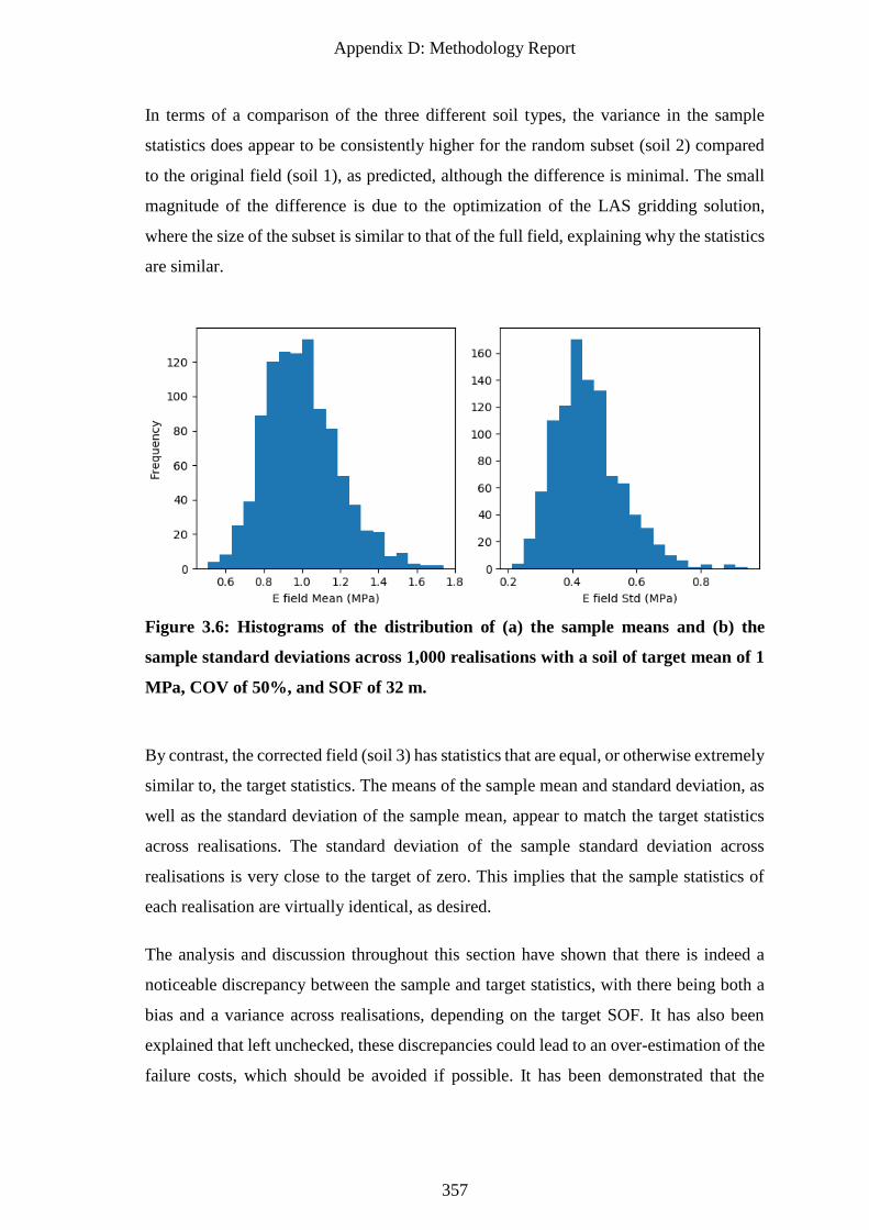
Appendix D: Methodology Report
357
In terms of a comparison of the three different soil types, the variance in the sample
statistics does appear to be consistently higher for the random subset (soil 2) compared
to the original field (soil 1), as predicted, although the difference is minimal. The small
magnitude of the difference is due to the optimization of the LAS gridding solution,
where the size of the subset is similar to that of the full field, explaining why the statistics
are similar.
Figure 3.6: Histograms of the distribution of (a) the sample means and (b) the
sample standard deviations across 1,000 realisations with a soil of target mean of 1
MPa, COV of 50%, and SOF of 32 m.
By contrast, the corrected field (soil 3) has statistics that are equal, or otherwise extremely
similar to, the target statistics. The means of the sample mean and standard deviation, as
well as the standard deviation of the sample mean, appear to match the target statistics
across realisations. The standard deviation of the sample standard deviation across
realisations is very close to the target of zero. This implies that the sample statistics of
each realisation are virtually identical, as desired.
The analysis and discussion throughout this section have shown that there is indeed a
noticeable discrepancy between the sample and target statistics, with there being both a
bias and a variance across realisations, depending on the target SOF. It has also been
explained that left unchecked, these discrepancies could lead to an over-estimation of the
failure costs, which should be avoided if possible. It has been demonstrated that the
Appendix D: Methodology Report
358
described scaling technique is successful in aligning each field to the target statistics, and
therefore serves to eliminate the problem.
3.1.3.2 Scale of fluctuation
There is evidence that the sample SOF may also differ from the target value, which
necessitates an investigation. It should be noted that a moderate degree of variance in the
sample SOF should not significantly impact the results, unlike variance in the COV
discussed in the previous section, as a lower or larger value will not automatically
translate to a decrease in reliability. Furthermore, the presence of a variance in the sample
SOF across realisations may not be undesirable, as the SOF parameter has always been
difficult to determine from sampling (Jaksa 1995). As such, it is not a highly defined
variable to be exactly matched with soils found in practice.
There has been some analysis on the accuracy of the sample SOF in the literature. Kuo
(2009) noted that there is a clear variance in the sample SOF across realisations, although
he found the mean of the sample SOF to match well with the target SOF, implying no
bias in the value. However, it should be noted that this analysis was restricted to 2D LAS
fields. On the other hand, Arsyad (2009) conducted a similar analysis in 3D LAS fields,
and found that the mean of the sample SOF decreased when compared to the target value
as the target SOF decreased.
This discrepancy between accuracy in the 2D and 3D cases can be explained by the
difference in the stage zero field generated by the covariance matrix decomposition
(CMD) method. The stage zero field is considered highly accurate, with no
approximation occurring across parent cell boundaries, as discussed in §3.1.1, as all
values are calculated directly. Typically, the stage zero field is restricted to a finite
number of elements to avoid round-off error (Fenton and Griffiths 2008), and this limit
is fixed regardless of the number of dimensions. Therefore, a 3D stage zero field must
have a smaller number of elements in each direction compared with the 2D field, and
therefore requires a larger number of subdivisions, leading to additional approximation.
The mean and standard deviation of the sample SOF have been determined for a number
of target SOF values, taken across 50 realisations of a field with mean stiffness of 1 MPa
and COVs of 50% and 100%. This information is presented in Figure 3.7. The SOF values
have been determined by fitting the exponential Markov model to the autocorrelation data
Appendix D: Methodology Report
359
(i.e. the curves shown in Figure 3.8) (Jaksa 1995) using non-linear least-squares
regression (Kelley 1999).
Figure 3.7 includes the sample SOFs for the three soil cases of full, subset, and subset
corrected, as discussed in the previous section. Note, that while there appears to be a
slight discrepancy between the three soil cases, this difference is likely due to the
relatively small number of realisations conducted, due to the relatively computationally-
intensive nature of the analysis. Therefore, the difference is the result of random noise,
as there is no mathematical reason why the SOF of a generated random field would
change when scaled or inspecting a subset. This is further evidenced by there being strong
similarity between the three cases with lower SOF values, where the SOF length is
significantly smaller than the field domain, allowing for more samples to be used in the
calculation, increasing its accuracy.
The discrepancies noted by previous studies can be observed in Figure 3.7 for soils with
a COV of both 50% and 100%. Autocorrelation plots for the 50% case are given in Figure
3.8. It can be seen in Figure 3.7 that the deviation of the mean sample SOF below the
target value increases as the target SOF increases, as evidenced by the growing gap
between the observed and theoretical values. Similarly, the standard deviation of the
sample SOF across realisations increases as the target SOF increases. This culminates to
a COV in the SOF of roughly 33%, in the case of a target SOF of 32 m. It is anticipated
that both of these undesirable trends will continue as the target SOF increases past the
values shown. Therefore, it would be prudent to avoid large SOFs if it is desired to have
consistency in SOF across realisations.
There does not appear to be a significant difference between the COV cases of 50% and
100%. This implies that COV is either not a significant factor in the accuracy of sample
SOF, or quickly asymptotes to the observed trends. In either case, it can be concluded
that this sample SOF deviation exists for a wide range of target COV values.
It has been demonstrated that there is both notable bias and variance in the SOF across
realisations, particularly for large SOF values. Unfortunately, unlike the case for the mean
and standard deviation in the previous section, there is no convenient scaling mechanism
to correct these deviations. As such, this report recommends limiting the target input SOF
to small values in order to ensure a reasonable degree of accuracy.
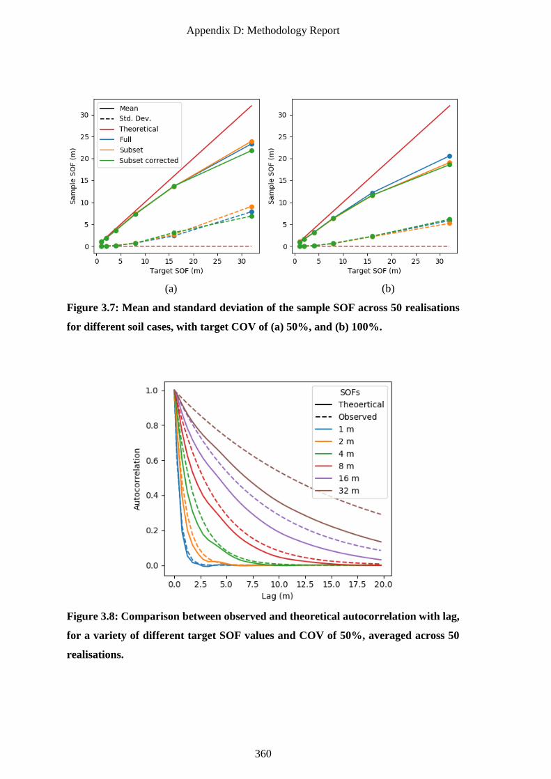
Appendix D: Methodology Report
360
(a) (b)
Figure 3.7: Mean and standard deviation of the sample SOF across 50 realisations
for different soil cases, with target COV of (a) 50%, and (b) 100%.
Figure 3.8: Comparison between observed and theoretical autocorrelation with lag,
for a variety of different target SOF values and COV of 50%, averaged across 50
realisations.

Appendix D: Methodology Report
361
3.1.3.3 Generation of anisotropic soils via local average subdivision
Strictly speaking, the LAS algorithm itself is only capable of generating isotropic fields,
however there are various possible means of implementing anisotropy. However, each of
these methods has its drawbacks. As such, these options, their accuracy, and their
practicality are discussed below. Note that within this subsection, as anisotropy refers to
the increase in horizontal SOF compared to that of the vertical, the base SOF therefore
refers to the vertical SOF.
As mentioned previously, the algorithm has generally been coded to use a stage zero field
generated by the covariance matrix decomposition (CMD) method. As anisotropy can be
achieved through the CMD method, this allows the LAS to exhibit the property at a macro
scale, i.e. the scale of the stage zero field. However, at a micro scale, as new elements are
generated within the original stage zero elements, the properties are isotropic and tend
towards the lowest SOF of the 3 dimensions.
It has also been suggested by (Fenton and Vanmarcke 1990) that anisotropy can be
achieved using LAS by means of scaling the field dimensions. This suggests that the
element size is scaled to be smaller in a particular direction, which would make the
apparent SOF larger in that direction, therefore achieving the desired anisotropy. The
reverse process could also be implemented, with elements specified to have a larger
dimension in a particular direction, which results in the SOF in that direction being
reduced. However, preliminary analysis suggests that this method is ineffective, with
resulting soils appearing to resemble a lesser degree of anisotropy than specified. Given
that this scaling technique was not coded as the primary LAS method for achieving
anisotropy, it suggests that the developers considered this option to be inferior to the
CMD solution. As such, this element scaling method is not considered in the present
analysis.
Instead, a new method for generating anisotropy with LAS is adopted in the present study.
It also makes use of scaling the dimensions, as suggested by Fenton and Vanmarcke
(1990), but is implemented in a different manner. Rather than scaling the size of the
elements, the field itself is scaled by the addition of new elements. This results in an
initially larger field, corresponding to the degree of anisotropy. The final, anisotropic
field can be generated by subdividing the original field at the appropriate depths. The
larger field in turn requires greater RAM for storage, as well as increased generation time;
Appendix D: Methodology Report
362
however preliminary results have shown the method to be successful, and so the analysis
throughout the remainder of the section adopts this method. The steps for implementing
this subset-based anisotropy are as follows:
1. Specify an isotropic SOF, which corresponds to the desired horizontal SOF.
2. Specify the number of elements in the vertical direction to be larger by an order
of a, where a is the degree of anisotropy.
3. Generate the vertically-deeper isotropic field specified in the previous steps.
4. Form a new field that is a subset of the original by extracting every ath element
with depth.
While Goldsworthy (2006) validated the LAS software on isotropic soils, this validation
was not extended to anisotropic soils. Previous studies suggested that anisotropy is
possible up to cases of roughly 1:4, and this is confirmed by inspection of Figure 3.9,
which shows horizontal and vertical autocorrelation of both the CMD and subset-based
anisotropy compared to the theoretical values in soils with a base SOF of 1, 4, 8, 16 m
and anisotropies of 1:2, 1:4,1: 8, 1:32. It can be seen that the CMD-based anisotropy has
an average autocorrelation that is equivalent to the subset method, up to an anisotropy of
1:4. However, the CMD trend begins to deviate from the subset trend in both directions
at an anisotropy of 1:8. This deviation increases as the degree of anisotropy increases.
Inspection of the horizontal autocorrelations in Figure 3.9 show that the subset-based
anisotropy is at least as accurate as the CMD-based method, and is significantly more
accurate in several cases, particularly with high degrees of anisotropy. However, for base
SOF values of 8 m or higher, the horizontal autocorrelation trend begins to diverge from
the theoretical values.
In terms of the vertical direction, both methods appear to produce reasonably similar
autocorrelation trends, and these trends deviate from the theoretical as the base SOF
increases. Following the behaviour of the horizontal autocorrelation, the vertical
autocorrelation appears to decrease.
For both the horizontal and vertical directions, the noted divergence has the appearance
of a decreased SOF compared to the target values. This implies that, even with the
improved subset-based anisotropy, there is an upper limit on the degree of anisotropy that
can be achieved, particularly in combination with a high vertical SOF, due to errors that
Appendix D: Methodology Report
363
begin to manifest under these cases. This degradation of target SOF accuracy is a result
of the inability of LAS to produce high sample SOFs in isotropic fields, as discussed in
the previous section.
Due to the conclusions that anisotropy is only accurate for certain cases, further analysis
must be conducted to determine which cases are viable. This can be achieved by plotting
the sample SOFs of cases that should theoretically be constant. For example, if a vertical
SOF of 1 m is specified, then ideally this value would be observed regardless of the
degree of anisotropy. As such, plotting the vertical SOF values against the degree of
anisotropy should yield a straight, horizontal line.
The plot described above is given in Figure 3.10 for a soil with COV of 50%, for both
CMD- and subset-based anisotropies. It can be seen that a target SOF is achieved for
vertical SOFs of 1 m and 2 m, regardless of the degree of anisotropy, for both anisotropy
methods. Furthermore, the vertical SOF is constant, which is desirable.
However, the sample vertical SOF appears to decrease as both the target vertical SOF
and degree of anisotropy increases. This trend is most apparent in the case of a vertical
SOF of 32 m, where the sample SOF begins at 25 m with an anisotropy of 1:1, but quickly
decreases to 8 m as the degree of anisotropy increases. It appears that the only range of
vertical SOF values that can be confidently used, with any degree of anisotropy, is 4 m
or less. However, a vertical SOF of 8 m could potentially be used with a small degree of
anisotropy, in the order of 1:4 or less. It also appears that the CMD-based anisotropy
performs as well or better than the subset-based anisotropy, in terms of vertical SOF
consistency.
A similar analysis is performed to assess the consistency of horizontal SOFs with
changing degrees of anisotropy. The key difference to the above analysis is that the
number of vertical SOF options decreases as the degree of anisotropy decreases, when
the horizontal SOF is intended to remain constant. As such, the horizontal SOF is plotted
directly against the vertical SOF for various degrees of anisotropy in Figure 3.11, with
different amounts of data.
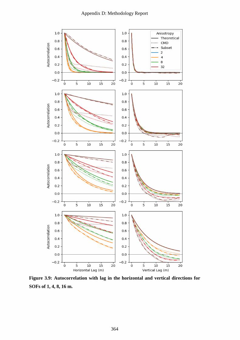
Appendix D: Methodology Report
364
Figure 3.9: Autocorrelation with lag in the horizontal and vertical directions for
SOFs of 1, 4, 8, 16 m.
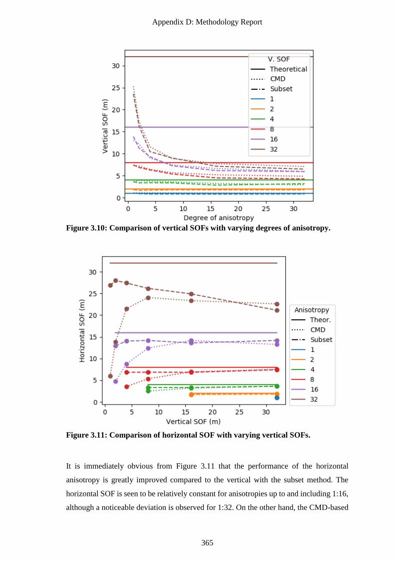
Appendix D: Methodology Report
365
Figure 3.10: Comparison of vertical SOFs with varying degrees of anisotropy.
Figure 3.11: Comparison of horizontal SOF with varying vertical SOFs.
It is immediately obvious from Figure 3.11 that the performance of the horizontal
anisotropy is greatly improved compared to the vertical with the subset method. The
horizontal SOF is seen to be relatively constant for anisotropies up to and including 1:16,
although a noticeable deviation is observed for 1:32. On the other hand, the CMD-based
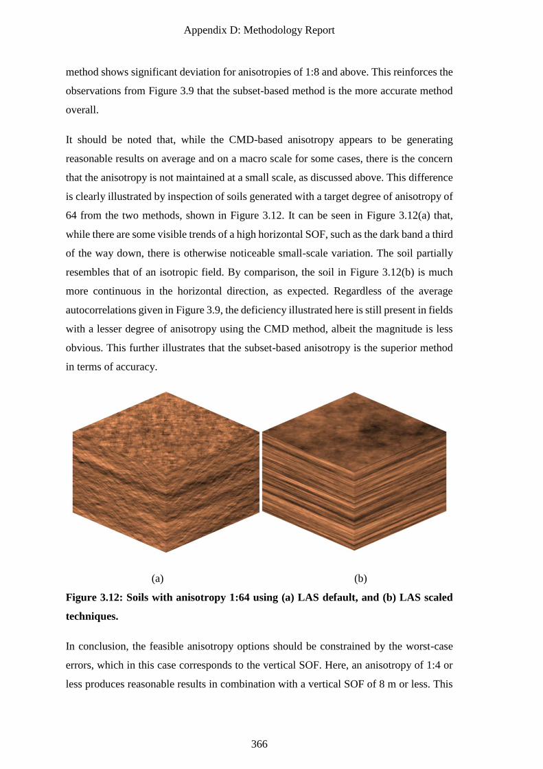
Appendix D: Methodology Report
366
method shows significant deviation for anisotropies of 1:8 and above. This reinforces the
observations from Figure 3.9 that the subset-based method is the more accurate method
overall.
It should be noted that, while the CMD-based anisotropy appears to be generating
reasonable results on average and on a macro scale for some cases, there is the concern
that the anisotropy is not maintained at a small scale, as discussed above. This difference
is clearly illustrated by inspection of soils generated with a target degree of anisotropy of
64 from the two methods, shown in Figure 3.12. It can be seen in Figure 3.12(a) that,
while there are some visible trends of a high horizontal SOF, such as the dark band a third
of the way down, there is otherwise noticeable small-scale variation. The soil partially
resembles that of an isotropic field. By comparison, the soil in Figure 3.12(b) is much
more continuous in the horizontal direction, as expected. Regardless of the average
autocorrelations given in Figure 3.9, the deficiency illustrated here is still present in fields
with a lesser degree of anisotropy using the CMD method, albeit the magnitude is less
obvious. This further illustrates that the subset-based anisotropy is the superior method
in terms of accuracy.
(a) (b)
Figure 3.12: Soils with anisotropy 1:64 using (a) LAS default, and (b) LAS scaled
techniques.
In conclusion, the feasible anisotropy options should be constrained by the worst-case
errors, which in this case corresponds to the vertical SOF. Here, an anisotropy of 1:4 or
less produces reasonable results in combination with a vertical SOF of 8 m or less. This
Appendix D: Methodology Report
367
anisotropy should be generated with the aforementioned subset-based method, which was
found to produce the highest degree of accuracy and consistency, although it comes at a
minor cost to computational time. While there is a slight reduction in the sample vertical
SOF of the 8 m, 1:4 case, this is relatively minor.
While the recommended maximum anisotropy of 1:4 is not the highest found in nature,
as discussed in §3.4.1, it has been found that isotropic soils are in fact the worst case in
terms of foundation performance (Naghibi et al. 2014b). This is due to the fact that larger
vertical SOFs (for a given horizontal SOF) lead to less variance reduction when averaging
over the pile length. Therefore, this software limitation is unlikely to have a significant
impact on the final framework.
3.2 Multi-layer Generation
A primary innovation of this framework is the incorporation of multiple-layer soil
profiles, and a new method for generating these profiles has been developed. A detailed
description of the various processes involved in this multi-layer generation method is
presented by Crisp et al. (2018) (Chapter 4). For clarity and completeness, an overview
is also provided in the following section.
As discussed in §3.1, a limitation of many random field generators, including LAS, is
that they exhibit second order stationarity. The main implication of this is that the mean
of the generated soil is constant; a limitation that is unsuitable for the generation of
multiple layers with individual, distinct means. This framework overcomes this
restriction by generating an individual LAS profile for every soil layer, and then
combining them to form the desired complex stratigraphy.
The combination process is designed to imitate the natural soil processes of erosion and
deposition, as detailed by Skinner and Porter (1987). This involves a series of time steps,
in which the deepest, oldest layer is assumed to comprise the full desired volume. It is
then eroded to a pre-defined boundary and then infilled with a new layer. This process is
repeated until all layers are added to the soil profile. A demonstration of this process is
given in Figure 3.13.
The pre-defined boundary is generated in a 3-stage process. First, random points are
generated in a stratified random pattern (see §4.1), which defines key points in the layer
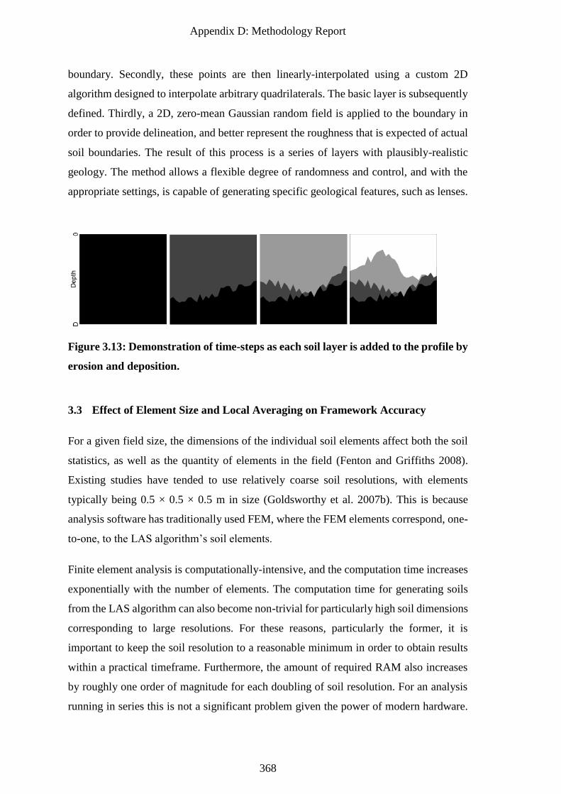
Appendix D: Methodology Report
368
boundary. Secondly, these points are then linearly-interpolated using a custom 2D
algorithm designed to interpolate arbitrary quadrilaterals. The basic layer is subsequently
defined. Thirdly, a 2D, zero-mean Gaussian random field is applied to the boundary in
order to provide delineation, and better represent the roughness that is expected of actual
soil boundaries. The result of this process is a series of layers with plausibly-realistic
geology. The method allows a flexible degree of randomness and control, and with the
appropriate settings, is capable of generating specific geological features, such as lenses.
Figure 3.13: Demonstration of time-steps as each soil layer is added to the profile by
erosion and deposition.
3.3 Effect of Element Size and Local Averaging on Framework Accuracy
For a given field size, the dimensions of the individual soil elements affect both the soil
statistics, as well as the quantity of elements in the field (Fenton and Griffiths 2008).
Existing studies have tended to use relatively coarse soil resolutions, with elements
typically being 0.5 × 0.5 × 0.5 m in size (Goldsworthy et al. 2007b). This is because
analysis software has traditionally used FEM, where the FEM elements correspond, one-
to-one, to the LAS algorithm’s soil elements.
Finite element analysis is computationally-intensive, and the computation time increases
exponentially with the number of elements. The computation time for generating soils
from the LAS algorithm can also become non-trivial for particularly high soil dimensions
corresponding to large resolutions. For these reasons, particularly the former, it is
important to keep the soil resolution to a reasonable minimum in order to obtain results
within a practical timeframe. Furthermore, the amount of required RAM also increases
by roughly one order of magnitude for each doubling of soil resolution. For an analysis
running in series this is not a significant problem given the power of modern hardware.
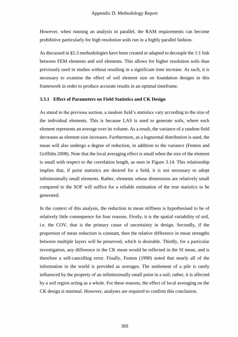
Appendix D: Methodology Report
369
However, when running an analysis in parallel, the RAM requirements can become
prohibitive particularly for high resolution soils run in a highly parallel fashion.
As discussed in §5.3 methodologies have been created or adapted to decouple the 1:1 link
between FEM elements and soil elements. This allows for higher resolution soils than
previously used in studies without resulting in a significant time increase. As such, it is
necessary to examine the effect of soil element size on foundation designs in this
framework in order to produce accurate results in an optimal timeframe.
3.3.1 Effect of Parameters on Field Statistics and CK Design
As stated in the previous section, a random field’s statistics vary according to the size of
the individual elements. This is because LAS is used to generate soils, where each
element represents an average over its volume. As a result, the variance of a random field
decreases as element size increases. Furthermore, as a lognormal distribution is used, the
mean will also undergo a degree of reduction, in addition to the variance (Fenton and
Griffiths 2008). Note that the local averaging effect is small when the size of the element
is small with respect to the correlation length, as seen in Figure 3.14. This relationship
implies that, if point statistics are desired for a field, it is not necessary to adopt
infinitesimally small elements. Rather, elements whose dimensions are relatively small
compared to the SOF will suffice for a reliable estimation of the true statistics to be
generated.
In the context of this analysis, the reduction in mean stiffness is hypothesised to be of
relatively little consequence for four reasons. Firstly, it is the spatial variability of soil,
i.e. the COV, that is the primary cause of uncertainty in design. Secondly, if the
proportion of mean reduction is constant, then the relative difference in mean strengths
between multiple layers will be preserved, which is desirable. Thirdly, for a particular
investigation, any difference in the CK mean would be reflected in the SI mean, and is
therefore a self-cancelling error. Finally, Fenton (1990) noted that nearly all of the
information in the world is provided as averages. The settlement of a pile is rarely
influenced by the property of an infinitesimally small point in a soil; rather, it is affected
by a soil region acting as a whole. For these reasons, the effect of local averaging on the
CK design is minimal. However, analyses are required to confirm this conclusion.
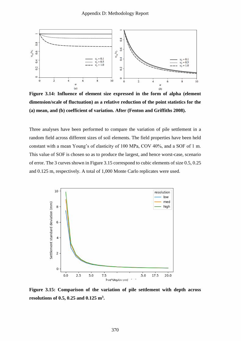
Appendix D: Methodology Report
370
Figure 3.14: Influence of element size expressed in the form of alpha (element
dimension/scale of fluctuation) as a relative reduction of the point statistics for the
(a) mean, and (b) coefficient of variation. After (Fenton and Griffiths 2008).
Three analyses have been performed to compare the variation of pile settlement in a
random field across different sizes of soil elements. The field properties have been held
constant with a mean Young’s of elasticity of 100 MPa, COV 40%, and a SOF of 1 m.
This value of SOF is chosen so as to produce the largest, and hence worst-case, scenario
of error. The 3 curves shown in Figure 3.15 correspond to cubic elements of size 0.5, 0.25
and 0.125 m, respectively. A total of 1,000 Monte Carlo replicates were used.
Figure 3.15: Comparison of the variation of pile settlement with depth across
resolutions of 0.5, 0.25 and 0.125 m3.
Pile length (m)
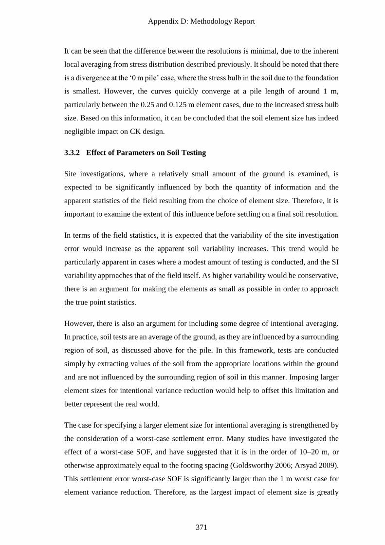
Appendix D: Methodology Report
371
It can be seen that the difference between the resolutions is minimal, due to the inherent
local averaging from stress distribution described previously. It should be noted that there
is a divergence at the ‘0 m pile’ case, where the stress bulb in the soil due to the foundation
is smallest. However, the curves quickly converge at a pile length of around 1 m,
particularly between the 0.25 and 0.125 m element cases, due to the increased stress bulb
size. Based on this information, it can be concluded that the soil element size has indeed
negligible impact on CK design.
3.3.2 Effect of Parameters on Soil Testing
Site investigations, where a relatively small amount of the ground is examined, is
expected to be significantly influenced by both the quantity of information and the
apparent statistics of the field resulting from the choice of element size. Therefore, it is
important to examine the extent of this influence before settling on a final soil resolution.
In terms of the field statistics, it is expected that the variability of the site investigation
error would increase as the apparent soil variability increases. This trend would be
particularly apparent in cases where a modest amount of testing is conducted, and the SI
variability approaches that of the field itself. As higher variability would be conservative,
there is an argument for making the elements as small as possible in order to approach
the true point statistics.
However, there is also an argument for including some degree of intentional averaging.
In practice, soil tests are an average of the ground, as they are influenced by a surrounding
region of soil, as discussed above for the pile. In this framework, tests are conducted
simply by extracting values of the soil from the appropriate locations within the ground
and are not influenced by the surrounding region of soil in this manner. Imposing larger
element sizes for intentional variance reduction would help to offset this limitation and
better represent the real world.
The case for specifying a larger element size for intentional averaging is strengthened by
the consideration of a worst-case settlement error. Many studies have investigated the
effect of a worst-case SOF, and have suggested that it is in the order of 10–20 m, or
otherwise approximately equal to the footing spacing (Goldsworthy 2006; Arsyad 2009).
This settlement error worst-case SOF is significantly larger than the 1 m worst case for
element variance reduction. Therefore, as the largest impact of element size is greatly
Appendix D: Methodology Report
372
removed from the expected worst case within the framework, it is expected to have a
minimal effect on the site investigation optimization proposed in the present research.
An assessment of the theoretical and experimental ranges of influence of various typical
geotechnical tests is presented below. Here, the aim is to determine the expected influence
ranges and match them with the most appropriate (i.e. closest) element size available.
3.3.2.1 Theoretical analysis
Research into the influence zone of in-situ tests is limited. In the case of the cone
penetration test (CPT), determination of such a zone was conducted by Teh and Houlsby
(1991). The study used strain path FEA in an idealised, homogeneous, elastic perfectly-
plastic clay obeying the Von Mises yield criterion. The range of influence was then taken
to be the distance from the centre and bottom of the cone to the sides and bottom of the
yielding surface, respectively. In other words, the distance from the cone to the elastic-
plastic boundary, as shown in Figure 3.16.
Figure 3.16: Soil yielding surfaces associated with the CPT.
After Jaksa (1995).
Using the results of Teh and Houlsby (1991), Jaksa (1995) showed that, for a cone of
diameter of 35.7 mm and cone angle of 60, the influence radius is approximately 150
mm. This implies that a cubic element of length 0.25 m would be most suitable, as the
influence diameter is roughly 0.3 m.
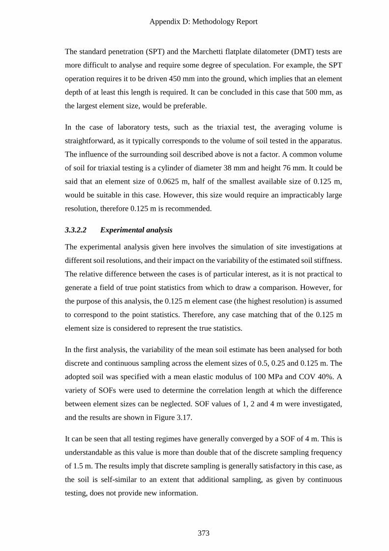
Appendix D: Methodology Report
373
The standard penetration (SPT) and the Marchetti flatplate dilatometer (DMT) tests are
more difficult to analyse and require some degree of speculation. For example, the SPT
operation requires it to be driven 450 mm into the ground, which implies that an element
depth of at least this length is required. It can be concluded in this case that 500 mm, as
the largest element size, would be preferable.
In the case of laboratory tests, such as the triaxial test, the averaging volume is
straightforward, as it typically corresponds to the volume of soil tested in the apparatus.
The influence of the surrounding soil described above is not a factor. A common volume
of soil for triaxial testing is a cylinder of diameter 38 mm and height 76 mm. It could be
said that an element size of 0.0625 m, half of the smallest available size of 0.125 m,
would be suitable in this case. However, this size would require an impracticably large
resolution, therefore 0.125 m is recommended.
3.3.2.2 Experimental analysis
The experimental analysis given here involves the simulation of site investigations at
different soil resolutions, and their impact on the variability of the estimated soil stiffness.
The relative difference between the cases is of particular interest, as it is not practical to
generate a field of true point statistics from which to draw a comparison. However, for
the purpose of this analysis, the 0.125 m element case (the highest resolution) is assumed
to correspond to the point statistics. Therefore, any case matching that of the 0.125 m
element size is considered to represent the true statistics.
In the first analysis, the variability of the mean soil estimate has been analysed for both
discrete and continuous sampling across the element sizes of 0.5, 0.25 and 0.125 m. The
adopted soil was specified with a mean elastic modulus of 100 MPa and COV 40%. A
variety of SOFs were used to determine the correlation length at which the difference
between element sizes can be neglected. SOF values of 1, 2 and 4 m were investigated,
and the results are shown in Figure 3.17.
It can be seen that all testing regimes have generally converged by a SOF of 4 m. This is
understandable as this value is more than double that of the discrete sampling frequency
of 1.5 m. The results imply that discrete sampling is generally satisfactory in this case, as
the soil is self-similar to an extent that additional sampling, as given by continuous
testing, does not provide new information.
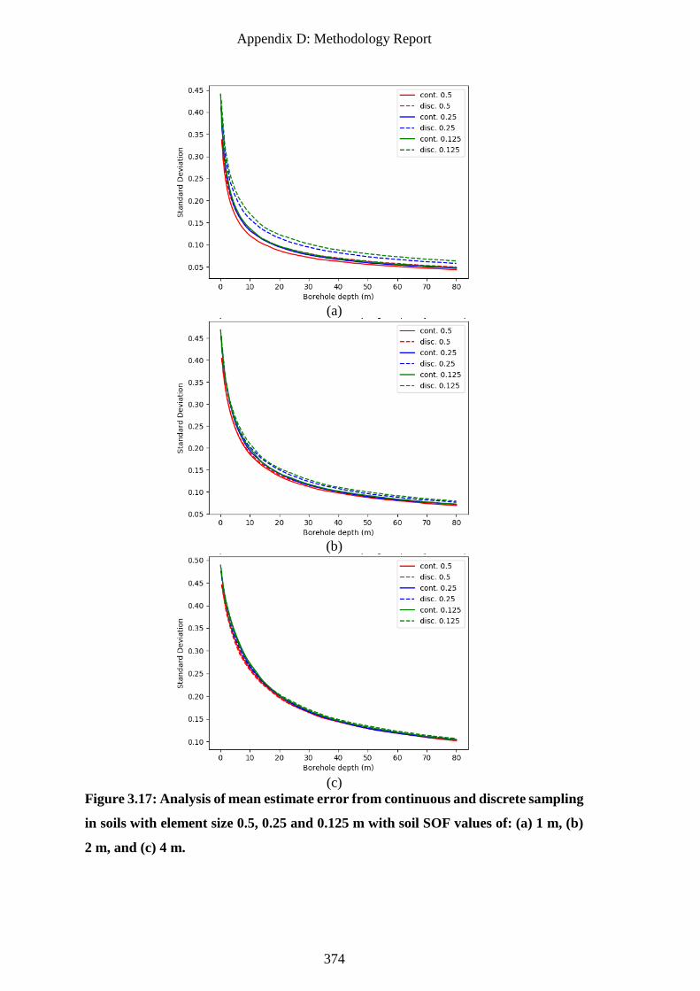
Appendix D: Methodology Report
374
(a)
(b)
(c)
Figure 3.17: Analysis of mean estimate error from continuous and discrete sampling
in soils with element size 0.5, 0.25 and 0.125 m with soil SOF values of: (a) 1 m, (b)
2 m, and (c) 4 m.
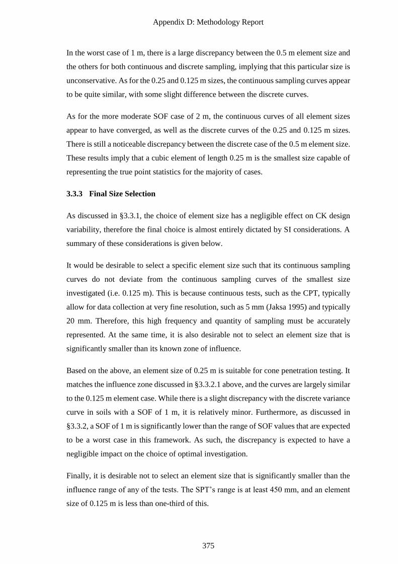
Appendix D: Methodology Report
375
In the worst case of 1 m, there is a large discrepancy between the 0.5 m element size and
the others for both continuous and discrete sampling, implying that this particular size is
unconservative. As for the 0.25 and 0.125 m sizes, the continuous sampling curves appear
to be quite similar, with some slight difference between the discrete curves.
As for the more moderate SOF case of 2 m, the continuous curves of all element sizes
appear to have converged, as well as the discrete curves of the 0.25 and 0.125 m sizes.
There is still a noticeable discrepancy between the discrete case of the 0.5 m element size.
These results imply that a cubic element of length 0.25 m is the smallest size capable of
representing the true point statistics for the majority of cases.
3.3.3 Final Size Selection
As discussed in §3.3.1, the choice of element size has a negligible effect on CK design
variability, therefore the final choice is almost entirely dictated by SI considerations. A
summary of these considerations is given below.
It would be desirable to select a specific element size such that its continuous sampling
curves do not deviate from the continuous sampling curves of the smallest size
investigated (i.e. 0.125 m). This is because continuous tests, such as the CPT, typically
allow for data collection at very fine resolution, such as 5 mm (Jaksa 1995) and typically
20 mm. Therefore, this high frequency and quantity of sampling must be accurately
represented. At the same time, it is also desirable not to select an element size that is
significantly smaller than its known zone of influence.
Based on the above, an element size of 0.25 m is suitable for cone penetration testing. It
matches the influence zone discussed in §3.3.2.1 above, and the curves are largely similar
to the 0.125 m element case. While there is a slight discrepancy with the discrete variance
curve in soils with a SOF of 1 m, it is relatively minor. Furthermore, as discussed in
§3.3.2, a SOF of 1 m is significantly lower than the range of SOF values that are expected
to be a worst case in this framework. As such, the discrepancy is expected to have a
negligible impact on the choice of optimal investigation.
Finally, it is desirable not to select an element size that is significantly smaller than the
influence range of any of the tests. The SPT’s range is at least 450 mm, and an element
size of 0.125 m is less than one-third of this.
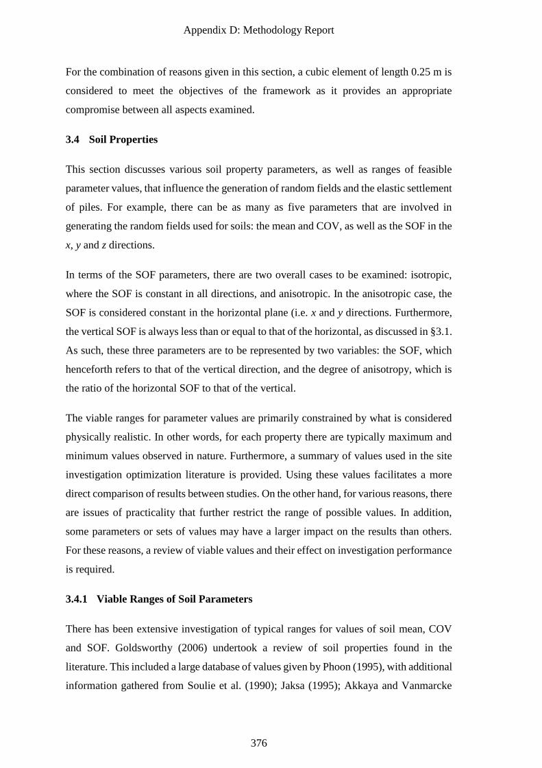
Appendix D: Methodology Report
376
For the combination of reasons given in this section, a cubic element of length 0.25 m is
considered to meet the objectives of the framework as it provides an appropriate
compromise between all aspects examined.
3.4 Soil Properties
This section discusses various soil property parameters, as well as ranges of feasible
parameter values, that influence the generation of random fields and the elastic settlement
of piles. For example, there can be as many as five parameters that are involved in
generating the random fields used for soils: the mean and COV, as well as the SOF in the
x, y and z directions.
In terms of the SOF parameters, there are two overall cases to be examined: isotropic,
where the SOF is constant in all directions, and anisotropic. In the anisotropic case, the
SOF is considered constant in the horizontal plane (i.e. x and y directions. Furthermore,
the vertical SOF is always less than or equal to that of the horizontal, as discussed in §3.1.
As such, these three parameters are to be represented by two variables: the SOF, which
henceforth refers to that of the vertical direction, and the degree of anisotropy, which is
the ratio of the horizontal SOF to that of the vertical.
The viable ranges for parameter values are primarily constrained by what is considered
physically realistic. In other words, for each property there are typically maximum and
minimum values observed in nature. Furthermore, a summary of values used in the site
investigation optimization literature is provided. Using these values facilitates a more
direct comparison of results between studies. On the other hand, for various reasons, there
are issues of practicality that further restrict the range of possible values. In addition,
some parameters or sets of values may have a larger impact on the results than others.
For these reasons, a review of viable values and their effect on investigation performance
is required.
3.4.1 Viable Ranges of Soil Parameters
There has been extensive investigation of typical ranges for values of soil mean, COV
and SOF. Goldsworthy (2006) undertook a review of soil properties found in the
literature. This included a large database of values given by Phoon (1995), with additional
information gathered from Soulie et al. (1990); Jaksa (1995); Akkaya and Vanmarcke
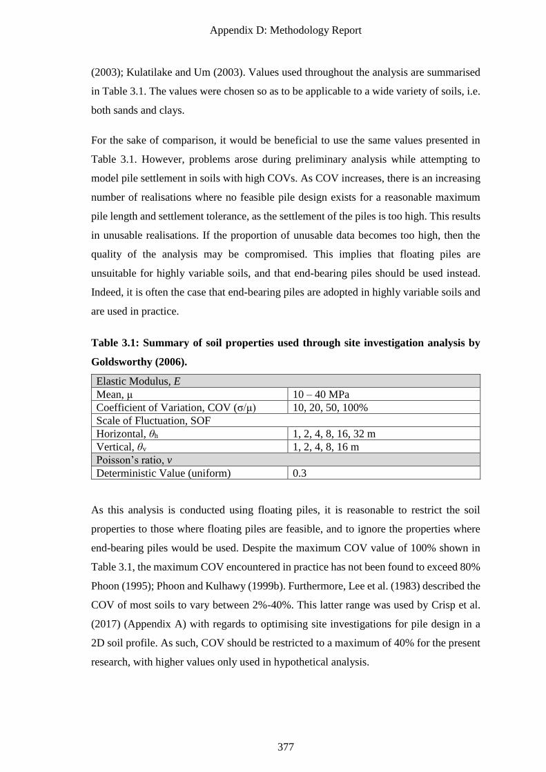
Appendix D: Methodology Report
377
(2003); Kulatilake and Um (2003). Values used throughout the analysis are summarised
in Table 3.1. The values were chosen so as to be applicable to a wide variety of soils, i.e.
both sands and clays.
For the sake of comparison, it would be beneficial to use the same values presented in
Table 3.1. However, problems arose during preliminary analysis while attempting to
model pile settlement in soils with high COVs. As COV increases, there is an increasing
number of realisations where no feasible pile design exists for a reasonable maximum
pile length and settlement tolerance, as the settlement of the piles is too high. This results
in unusable realisations. If the proportion of unusable data becomes too high, then the
quality of the analysis may be compromised. This implies that floating piles are
unsuitable for highly variable soils, and that end-bearing piles should be used instead.
Indeed, it is often the case that end-bearing piles are adopted in highly variable soils and
are used in practice.
Table 3.1: Summary of soil properties used through site investigation analysis by
Goldsworthy (2006).
Elastic Modulus, E
Mean, μ 10 – 40 MPa
Coefficient of Variation, COV (σ/μ) 10, 20, 50, 100%
Scale of Fluctuation, SOF
Horizontal, θh 1, 2, 4, 8, 16, 32 m
Vertical, θv 1, 2, 4, 8, 16 m
Poisson’s ratio, v
Deterministic Value (uniform) 0.3
As this analysis is conducted using floating piles, it is reasonable to restrict the soil
properties to those where floating piles are feasible, and to ignore the properties where
end-bearing piles would be used. Despite the maximum COV value of 100% shown in
Table 3.1, the maximum COV encountered in practice has not been found to exceed 80%
Phoon (1995); Phoon and Kulhawy (1999b). Furthermore, Lee et al. (1983) described the
COV of most soils to vary between 2%-40%. This latter range was used by Crisp et al.
(2017) (Appendix A) with regards to optimising site investigations for pile design in a
2D soil profile. As such, COV should be restricted to a maximum of 40% for the present
research, with higher values only used in hypothetical analysis.
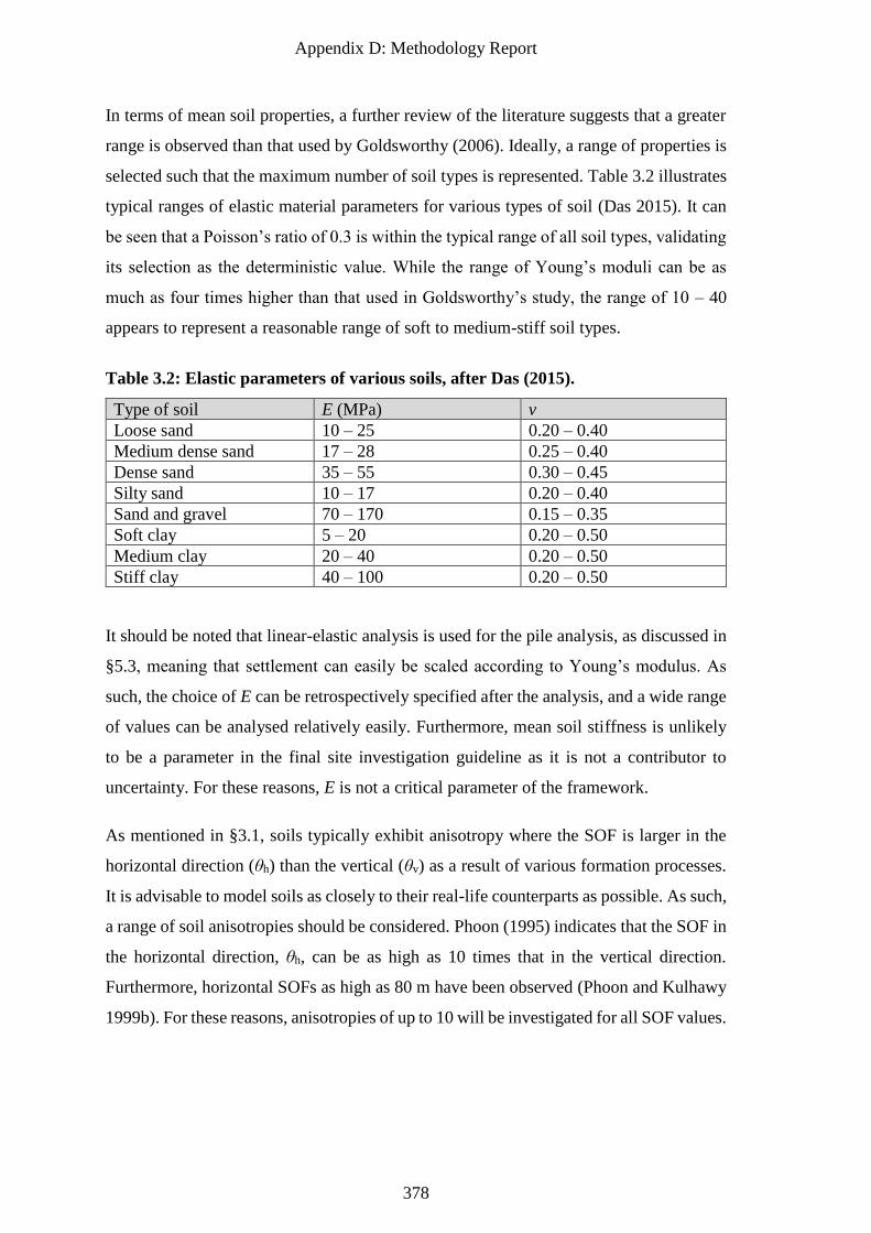
Appendix D: Methodology Report
378
In terms of mean soil properties, a further review of the literature suggests that a greater
range is observed than that used by Goldsworthy (2006). Ideally, a range of properties is
selected such that the maximum number of soil types is represented. Table 3.2 illustrates
typical ranges of elastic material parameters for various types of soil (Das 2015). It can
be seen that a Poisson’s ratio of 0.3 is within the typical range of all soil types, validating
its selection as the deterministic value. While the range of Young’s moduli can be as
much as four times higher than that used in Goldsworthy’s study, the range of 10 – 40
appears to represent a reasonable range of soft to medium-stiff soil types.
Table 3.2: Elastic parameters of various soils, after Das (2015).
Type of soil E (MPa) v
Loose sand 10 – 25 0.20 – 0.40
Medium dense sand 17 – 28 0.25 – 0.40
Dense sand 35 – 55 0.30 – 0.45
Silty sand 10 – 17 0.20 – 0.40
Sand and gravel 70 – 170 0.15 – 0.35
Soft clay 5 – 20 0.20 – 0.50
Medium clay 20 – 40 0.20 – 0.50
Stiff clay 40 – 100 0.20 – 0.50
It should be noted that linear-elastic analysis is used for the pile analysis, as discussed in
§5.3, meaning that settlement can easily be scaled according to Young’s modulus. As
such, the choice of E can be retrospectively specified after the analysis, and a wide range
of values can be analysed relatively easily. Furthermore, mean soil stiffness is unlikely
to be a parameter in the final site investigation guideline as it is not a contributor to
uncertainty. For these reasons, E is not a critical parameter of the framework.
As mentioned in §3.1, soils typically exhibit anisotropy where the SOF is larger in the
horizontal direction (θh) than the vertical (θv) as a result of various formation processes.
It is advisable to model soils as closely to their real-life counterparts as possible. As such,
a range of soil anisotropies should be considered. Phoon (1995) indicates that the SOF in
the horizontal direction, θh, can be as high as 10 times that in the vertical direction.
Furthermore, horizontal SOFs as high as 80 m have been observed (Phoon and Kulhawy
1999b). For these reasons, anisotropies of up to 10 will be investigated for all SOF values.
Appendix D: Methodology Report
379
3.4.2 Literature Review of Soil Parameters on Investigation Performance
A literature review is given on the impact of soil parameters on site investigation
performance, to provide context of optimal investigations across different soil cases, and
aid in their interpretation.
3.4.2.1 Impact of COV and SOF in previous studies
Many studies have investigated the impact of the COV and SOF parameters on both the
settlement of foundations and the performance of site investigations. It has been
universally found that variation of foundation design increases monotonically as COV
increases, with all else being constant, as would be expected (Phoon et al. 1990; Fenton
and Griffiths 2007).
The SOF, on the other hand, has a more complex effect on foundation design. Design
variation has been found to be small in the cases of small and large SOFs, with larger
design variation occurring with intermediate SOF values. This phenomenon has been
found to occur independently in the settlement of foundations , as well as with the
performance of site investigations (Goldsworthy et al. 2004b; Jaksa et al. 2005;
Goldsworthy et al. 2007a; Arsyad et al. 2009); Arsyad et al. (2010). This has been
attributed to two behaviours. Firstly, if SOF is small, then the properties of the region
around the pile tend towards the field average when interpreted at a macro scale.
Furthermore, this rapid fluctuation in properties increases the probability that the
complete soil distribution is sampled by boreholes, improving the estimate of the mean.
On the other hand, as the SOF tends towards infinity, soil properties increase in similarity
to the point of approaching uniformity. Minimal sampling is required in both of these
cases. These boundary conditions imply that a worst-case SOF exists between the two
extremes, where additional sampling effort is required. For example, in the worst case
there would be a higher likelihood of conducting a test in a pocket of soil that has different
properties to those surrounding the pile. The testing of such an isolated soil pocket would
be detrimental to the reliability of the resulting foundation, hence additional samples
would be required.
Unfortunately, there is disagreement regarding worst-case SOF values among the
aforementioned studies on site investigations, ranging from as 4 m to 16 m. The majority
imply that the worst case is approximately in the order of 10 m. The reason for this
Appendix D: Methodology Report
380
inconsistency is due for the variety of foundation types and spacing, as well as different
aspects of site investigations analysed. It is hypothesised that the worst-case SOF is a
function of both foundation and investigation attributes. Further work is needed to
determine the underlying relationship between the relevant parameters.
3.4.2.2 Effect of degree of anisotropy from previous studies
Goldsworthy (2006) investigated various degrees of anisotropy ranging from 1:1 to 1:10
(θv:θh) on the performance of site investigations for pad footings. His results indicate that
θv has the greatest effect on foundation settlement, whereas θh affects site investigation
performance. It was found that the performance of site investigations in anisotropic
conditions is similar to that in isotropic soils, where the SOF is that of the horizontal SOF.
Any difference here in overall site investigation performance is then mostly due to the
discrepancy in settlement. The effects of vertical and horizontal SOFs appear to be
reasonably independent.
On the other hand, Arsyad (2009) investigated the effect of anisotropy on the
performance of site investigations for piles. It was found there was little difference in the
probabilities of over- and under-design as anisotropy increased. However, there a number
of differences to note between the former study and those of the latter, particularly the
Goldsworthy studies. Firstly, the pile design was set to a fixed depth, with the capacities
themselves used for comparative purposes. This is as opposed to setting the foundation
size as the comparison variable, where the foundation is designed to a specified tolerance.
The implication of this is that a higher degree of averaging is occurring over the pile
length, as the maximum pile length was the case examined. If a top-down iterative design
approach were considered, then for the vast majority of cases, the pile length would be
shorter and hence the variability of results would be affected on account of the reduced
averaging effect.
Secondly, and more importantly, the pile capacity was determined using the Laboratoire
Central des Ponts et Chausses (LCPC) method by Bustamante and Gianeselli (1982), as
opposed to FEA. Part of the LCPC method involves essentially truncating the samples to
1.3 times larger and 0.7 times smaller than the mean. This is likely to greatly affect the
influence of the horizontal scale of fluctuation on design and, depending on how the
multiple boreholes were reduced to a single representative sample, the performances of
Appendix D: Methodology Report
381
site investigations as well. Limitations of the LCPC method in the context of this
methodology are discussed in greater detail later in §4.3.2.
Furthermore, in relation to all studies discussed in this subsection, it is possible that the
degree of anisotropy examined was less than that specified in the analyses. This is
because, as discussed in §3.1.3.3, the adopted LAS subroutines are largely incapable of
producing anisotropic soils in 3D. As these soils would be close to isotropic in nature, it
is not surprising that these studies did not find noticeable differences between the
isotropic and anisotropic cases.
4 Site Investigations
There are a large number of options to consider as part of an investigation, including
sampling schemes, number of boreholes, test types, testing errors and borehole depths. A
description of these options, and their hypothesised effects on investigation performance,
are presented throughout the following sections.
Furthermore, this section describes options regarding construction of a soil model based
on an investigation. These include choices for the reduction method, which serves to
reduce the complexity of data gathered from an investigation to a single, equivalent,
constant value for each layer. In addition, there is the manner in which layer boundaries
are reconstructed within the soil model. The soil model options are likely to be significant
to the investigation options themselves and this warrants further examination.
4.1 Sampling Schemes
A sampling scheme refers to the relative position or pattern in which a group of boreholes
are taken. Extensive investigation into the performance of sampling schemes was
conducted by Ferguson (1992) in the context of detecting contamination hotspots. While
several sampling schemes were examined, the analysis in this study will focus on three
in particular, as shown in Figure 4.1:
• Regular grid (RG): Boreholes are evenly spaced;
• Stratified random (SR): Boreholes are randomly located within evenly-spaced
segments: and
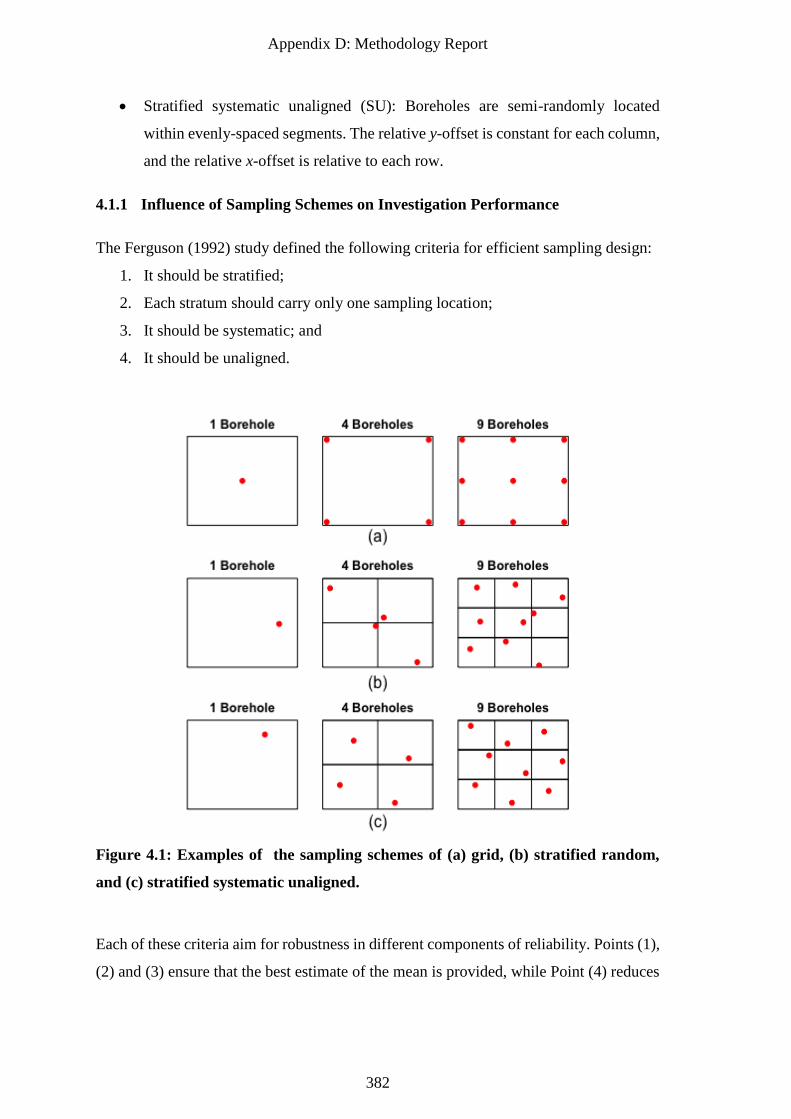
Appendix D: Methodology Report
382
• Stratified systematic unaligned (SU): Boreholes are semi-randomly located
within evenly-spaced segments. The relative y-offset is constant for each column,
and the relative x-offset is relative to each row.
4.1.1 Influence of Sampling Schemes on Investigation Performance
The Ferguson (1992) study defined the following criteria for efficient sampling design:
1. It should be stratified;
2. Each stratum should carry only one sampling location;
3. It should be systematic; and
4. It should be unaligned.
Figure 4.1: Examples of the sampling schemes of (a) grid, (b) stratified random,
and (c) stratified systematic unaligned.
Each of these criteria aim for robustness in different components of reliability. Points (1),
(2) and (3) ensure that the best estimate of the mean is provided, while Point (4) reduces
Appendix D: Methodology Report
383
the effect of sampling periodicity which is advantageous for ‘hitting the target’. Point (4)
also serves to reduce bias if the first point is randomly selected.
Each of the specified sampling schemes satisfy a subset of these criteria in different ways.
RG satisfies points (1), (2) and (3), while SR satisfies (1), (2) and (4), and SU satisfies
all points. Therefore, according to the above criteria, SU would be the most efficient
design, in theory. It should be noted that the preferred scheme of Ferguson (1992) is that
of a herringbone pattern, which can be thought of as a regular grid where the angle of
intersection is skewed to be other than 90°. This herringbone pattern is now
recommended in standards for detection of contamination hotspot detection (Standards
Association of Australia 2005).
On the other hand, several prior studies on sampling schemes for contaminated land have
recommended RG as the appropriate choice. Even though it is not strictly the best choice
as described by the criteria above, it was considered appropriate, or in other words, good
enough given its practicality (Bell et al. 1983). Halim (1991) compared RG and SR
patterns in the detection of a geological anomaly. A wide variety of anomalies were
investigated, including lenses and pockets of various sizes and shapes. It was concluded
that borings in grid patterns were more efficient in delineating the anomaly uncertainties
than randomly located borings. It should be noted that the study was undertaken at the
scale of civil engineering works, and that the anomaly was at the scale of geological
structures, unlike the contamination studies mentioned above. Therefore, it is implied that
the RG pattern is most likely to be the ideal strategy of those listed.
These criteria were developed to detect a single contamination spot, whereby the
contamination could be elongated in the axis of the grid pattern and hence avoid
detection. However, this same reasoning does not hold true for attempting to obtain
general soil properties over the full sampling region. The only case where a grid pattern
would be inferior is when the soil properties follow a cyclic pattern, and the sampling
interval is equal to, or an integer multiple of, the period of this pattern. However,
considering the random nature of soil formation processes, such a cyclic pattern is
unlikely to exist, indicating that a standard grid sampling scheme is likely to be sufficient.
In other words, the schemes involving randomness are intended to ‘hit the target’, but
here there is no specific target to hit, so the advantage is lost.
Appendix D: Methodology Report
384
Practical aspects of sampling also have an impact on sample location. For example, it
may not be possible to sample at some locations due to nearby properties or buildings.
Furthermore, engineers in practice tend to avoid random sampling schemes for a variety
of reasons. This includes the difficulty in determining random numbers and ensuring that
the resulting boreholes are drilled at the correct location. Usually, there is also a-priori
information, which influences the choice of location. For example, if the building location
is known, then samples tend to be taken near the building corners in the case of multiple
boreholes, or otherwise at the building centre. Another consideration is that a relatively
large number of boreholes is required to properly distinguish a regular grid sampling
scheme from one that has random components of sampling in a stratified fashion. If the
random and regular sampling patterns are indistinguishable in these cases, then it is
preferable to utilise the simpler and more practical pattern, i.e. regular grid.
The work done by Arsyad (2009) and Arsyad et al. (2009); Arsyad et al. (2010) is quite
limited in terms of sampling schemes investigated for pile design. The RG sampling
scheme was the sole option investigated for multiple boreholes. In terms of a single
borehole, the impact of a CPT sample at various distances from the foundation was also
assessed. Crisp et al. (2017) (Appendix A) examined the effect of RG and SR for pile
design in a 2-layer, 2D soil profile. It was found that the SR scheme provided a slightly
better estimate of the mean relative design error compared to RG; in the order of 3%. It
was suggested that this improvement might have been due to a correlation inherent in the
method adopted to generate the two-layer profile. It perhaps more likely that the average
SR borehole pattern yielded a consistently smaller (hence more representative) influence
range for the individual boreholes, as each borehole was internal to the soil profile. By
comparison, the RG pattern, in the case of two or more boreholes, had the outer-most
boreholes fixed to the ends, where only one side of the borehole was represented. This
influence range difference is shown in Figure 4.2.
However, the noted 3% improvement in SR over RG is relatively modest and well within
the tolerance of design in practice; hence the difference is negligible. On the other hand,
the SR scheme yielded a significantly larger spread of design values when compared to
RG. This resulted in a notably higher probability of failure and probability of over-design,
in the context of a 5% design tolerance between the SI and CK foundations. This implies
that designs based on the SR scheme are likely to be more costly through foundation
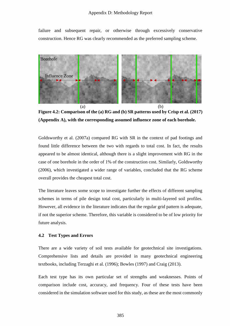
Appendix D: Methodology Report
385
failure and subsequent repair, or otherwise through excessively conservative
construction. Hence RG was clearly recommended as the preferred sampling scheme.
(a) (b)
Figure 4.2: Comparison of the (a) RG and (b) SR patterns used by Crisp et al. (2017)
(Appendix A), with the corresponding assumed influence zone of each borehole.
Goldsworthy et al. (2007a) compared RG with SR in the context of pad footings and
found little difference between the two with regards to total cost. In fact, the results
appeared to be almost identical, although there is a slight improvement with RG in the
case of one borehole in the order of 1% of the construction cost. Similarly, Goldsworthy
(2006), which investigated a wider range of variables, concluded that the RG scheme
overall provides the cheapest total cost.
The literature leaves some scope to investigate further the effects of different sampling
schemes in terms of pile design total cost, particularly in multi-layered soil profiles.
However, all evidence in the literature indicates that the regular grid pattern is adequate,
if not the superior scheme. Therefore, this variable is considered to be of low priority for
future analysis.
4.2 Test Types and Errors
There are a wide variety of soil tests available for geotechnical site investigations.
Comprehensive lists and details are provided in many geotechnical engineering
textbooks, including Terzaghi et al. (1996); Bowles (1997) and Craig (2013).
Each test type has its own particular set of strengths and weaknesses. Points of
comparison include cost, accuracy, and frequency. Four of these tests have been
considered in the simulation software used for this study, as these are the most commonly
Borehole
Influence Zone
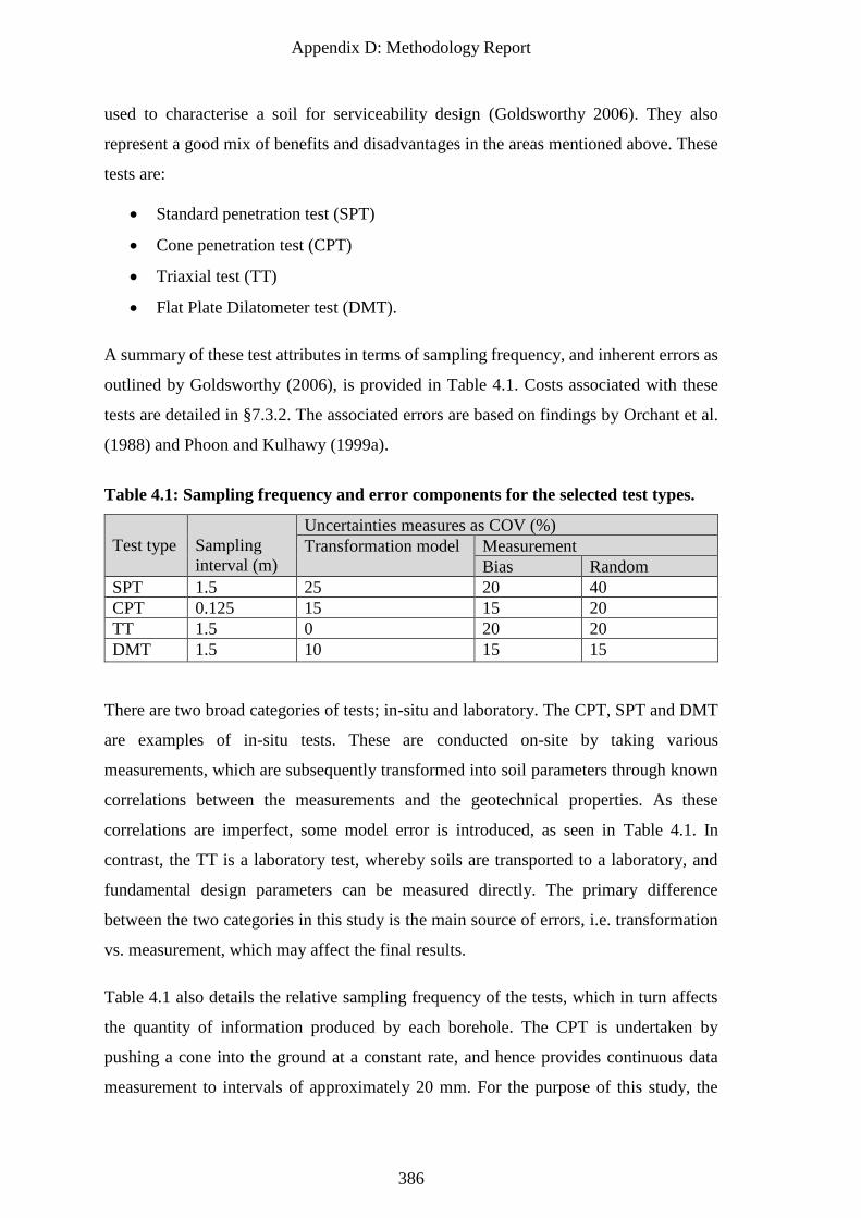
Appendix D: Methodology Report
386
used to characterise a soil for serviceability design (Goldsworthy 2006). They also
represent a good mix of benefits and disadvantages in the areas mentioned above. These
tests are:
• Standard penetration test (SPT)
• Cone penetration test (CPT)
• Triaxial test (TT)
• Flat Plate Dilatometer test (DMT).
A summary of these test attributes in terms of sampling frequency, and inherent errors as
outlined by Goldsworthy (2006), is provided in Table 4.1. Costs associated with these
tests are detailed in §7.3.2. The associated errors are based on findings by Orchant et al.
(1988) and Phoon and Kulhawy (1999a).
Table 4.1: Sampling frequency and error components for the selected test types.
Test type
Sampling
interval (m)
Uncertainties measures as COV (%)
Transformation model Measurement
Bias Random
SPT 1.5 25 20 40
CPT 0.125 15 15 20
TT 1.5 0 20 20
DMT 1.5 10 15 15
There are two broad categories of tests; in-situ and laboratory. The CPT, SPT and DMT
are examples of in-situ tests. These are conducted on-site by taking various
measurements, which are subsequently transformed into soil parameters through known
correlations between the measurements and the geotechnical properties. As these
correlations are imperfect, some model error is introduced, as seen in Table 4.1. In
contrast, the TT is a laboratory test, whereby soils are transported to a laboratory, and
fundamental design parameters can be measured directly. The primary difference
between the two categories in this study is the main source of errors, i.e. transformation
vs. measurement, which may affect the final results.
Table 4.1 also details the relative sampling frequency of the tests, which in turn affects
the quantity of information produced by each borehole. The CPT is undertaken by
pushing a cone into the ground at a constant rate, and hence provides continuous data
measurement to intervals of approximately 20 mm. For the purpose of this study, the
Appendix D: Methodology Report
387
sampling distance must be upscaled to the size of the generated soil elements, i.e. 250
mm. The SPT, DMT and TT are discrete tests obtained at 1.5 m depth intervals. The
quantity of information captured by an investigation, for example through test sampling
frequency, is likely to have a significant impact on its performance.
The practicality of the tests is also influenced by other factors such as soil type. For
example, the SPT and CPT are subject to ground refusal, where the test apparatus is
unable to penetrate the ground and hence cannot provide a measurement. In practice, the
pocket of soil causing refusal would be relief drilled, allowing the test to resume below
the hard layer. Note that this aspect of testing is not considered in the present analysis.
This is not a major concern, however, as soils which are strong enough to cause refusal
tend not to contribute to foundation failure.
The various trade-offs interact with regards to their impact on the results. For example,
the TT has the highest overall accuracy and hence is expected to characterise the soil
well. On the other hand, its low sampling frequency means large proportions of the soil
remain untested, resulting in high statistical error in that regard. The CPT has higher
errors owing to the parameter transformation, however, it is considerably more extensive
in its representation of the soil volume as a result of its high sampling frequency. It should
also be noted that the tests’ feasibility in the context of site investigation optimization is
also weighted by their relative costs. For example, the SPT has the highest degree of
error, and is sampled at discrete intervals, however, it is a relatively cheap option on a
per-test basis. These trade-offs make it difficult to predict which test would yield the best
overall investigation performance, hence test type is an important analysis variable within
the framework.
4.2.1 Implementation of Test Errors
Due to the nature of how errors occur in practice, artificial errors used in this study must
be applied in a specific manner. The application procedure is given in this section.
Furthermore, test errors have been found to yield occasional invalid results in some cases,
and workaround for these cases is also given.
Appropriate errors are added to the samples obtained from testing using the following
relationship:
𝐸𝑟 = 𝑡𝑚(𝑚𝑏𝑚𝑟)𝐸𝑓 (4.1)
Appendix D: Methodology Report
388
Where tm, mb and mr the unit mean, lognormal variables representing the uncertainty due
to transformation model error, bias and random measurement effects, respectively. The
parameter Ef represents values obtained directly from the simulated soil, and Er are the
resulting values incorporating the various errors. The errors must be applied in a specific
order so as to represent realistically what occurs in practice. This order is as follows:
1. Bias is added to every value in the sample as a proportion of the sample mean.
This is performed independently on a per-borehole basis.
2. Random measurement error is added as a proportion of the new, biased sample.
Each sample is treated independently with a different random value.
3. Random transformation error is then added to the above values as a proportion of
the global sample average, as it is based on test measurements.
There is a possibility of invalid values occurring after errors are applied, resulting from
samples with negative stiffness, or otherwise stiffness unrealistically close to zero. For
low value-weighted reduction methods (discussed in §4.3), particularly the geometric,
harmonic and first quartile, this can result in a significant underestimation of the global
soil stiffness. As pile settlement is inversely proportional to soil stiffness, settlement
approaches infinity as stiffness approaches zero. Initial testing shows that near-zero
reduced stiffness values are a common occurrence in soils with high COV and low-to-
moderate SOF. To overcome this, a two-step process is adopted, as follows:
1. All samples with stiffnesses less than or equal to zero are appropriately assumed
to be invalid due to equipment malfunctions or human error. These samples are
removed from the investigation set.
2. A 99% geometric confidence interval (CI) is applied to the remaining data, with
samples outside this range also removed from the set. This serves to eliminate
near-zero values in a manner independent of the specified mean soil stiffness.
The geometric CI is designed for use with lognormal distributions. As this distribution is
used to generate the virtual soils being sampled, the samples themselves must also be
lognormally-distributed. This assumption should still be valid with the addition of log-
normally distributed test errors. The CI is calculated by first evaluating the geometric
average (GA), as given in §4.3.1, followed by the geometric standard deviation (g),
which is most easily calculated for a set of n samples (S) as:
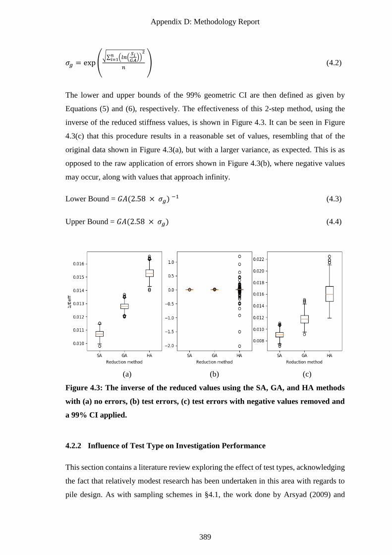
Appendix D: Methodology Report
389
𝜎𝑔 = exp(√∑ (𝑙𝑛(
𝑆𝑖𝐺𝐴))2
𝑛𝑖=1
𝑛 ) (4.2)
The lower and upper bounds of the 99% geometric CI are then defined as given by
Equations (5) and (6), respectively. The effectiveness of this 2-step method, using the
inverse of the reduced stiffness values, is shown in Figure 4.3. It can be seen in Figure
4.3(c) that this procedure results in a reasonable set of values, resembling that of the
original data shown in Figure 4.3(a), but with a larger variance, as expected. This is as
opposed to the raw application of errors shown in Figure 4.3(b), where negative values
may occur, along with values that approach infinity.
Lower Bound = 𝐺𝐴(2.58 × 𝜎𝑔) −1 (4.3)
Upper Bound = 𝐺𝐴(2.58 × 𝜎𝑔) (4.4)
(a) (b) (c)
Figure 4.3: The inverse of the reduced values using the SA, GA, and HA methods
with (a) no errors, (b) test errors, (c) test errors with negative values removed and
a 99% CI applied.
4.2.2 Influence of Test Type on Investigation Performance
This section contains a literature review exploring the effect of test types, acknowledging
the fact that relatively modest research has been undertaken in this area with regards to
pile design. As with sampling schemes in §4.1, the work done by Arsyad (2009) and
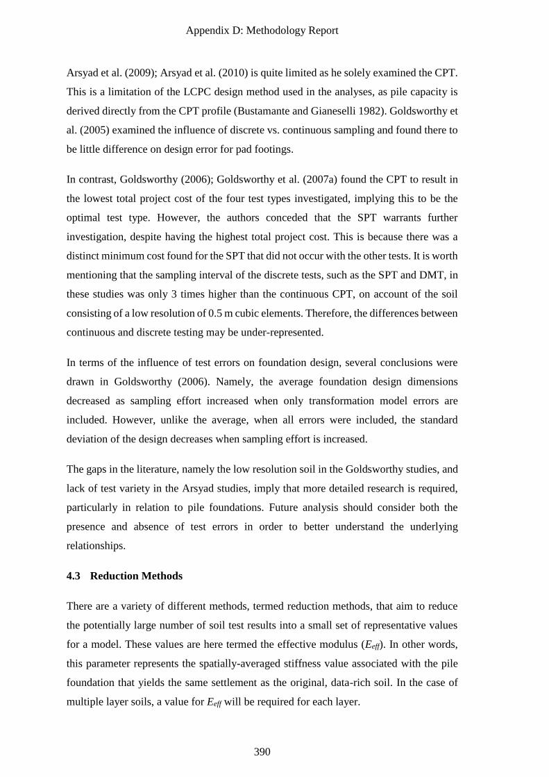
Appendix D: Methodology Report
390
Arsyad et al. (2009); Arsyad et al. (2010) is quite limited as he solely examined the CPT.
This is a limitation of the LCPC design method used in the analyses, as pile capacity is
derived directly from the CPT profile (Bustamante and Gianeselli 1982). Goldsworthy et
al. (2005) examined the influence of discrete vs. continuous sampling and found there to
be little difference on design error for pad footings.
In contrast, Goldsworthy (2006); Goldsworthy et al. (2007a) found the CPT to result in
the lowest total project cost of the four test types investigated, implying this to be the
optimal test type. However, the authors conceded that the SPT warrants further
investigation, despite having the highest total project cost. This is because there was a
distinct minimum cost found for the SPT that did not occur with the other tests. It is worth
mentioning that the sampling interval of the discrete tests, such as the SPT and DMT, in
these studies was only 3 times higher than the continuous CPT, on account of the soil
consisting of a low resolution of 0.5 m cubic elements. Therefore, the differences between
continuous and discrete testing may be under-represented.
In terms of the influence of test errors on foundation design, several conclusions were
drawn in Goldsworthy (2006). Namely, the average foundation design dimensions
decreased as sampling effort increased when only transformation model errors are
included. However, unlike the average, when all errors were included, the standard
deviation of the design decreases when sampling effort is increased.
The gaps in the literature, namely the low resolution soil in the Goldsworthy studies, and
lack of test variety in the Arsyad studies, imply that more detailed research is required,
particularly in relation to pile foundations. Future analysis should consider both the
presence and absence of test errors in order to better understand the underlying
relationships.
4.3 Reduction Methods
There are a variety of different methods, termed reduction methods, that aim to reduce
the potentially large number of soil test results into a small set of representative values
for a model. These values are here termed the effective modulus (Eeff). In other words,
this parameter represents the spatially-averaged stiffness value associated with the pile
foundation that yields the same settlement as the original, data-rich soil. In the case of
multiple layer soils, a value for Eeff will be required for each layer.
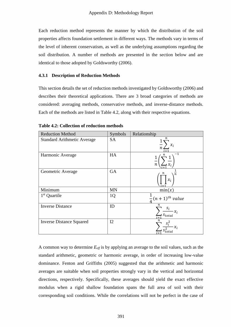
Appendix D: Methodology Report
391
Each reduction method represents the manner by which the distribution of the soil
properties affects foundation settlement in different ways. The methods vary in terms of
the level of inherent conservatism, as well as the underlying assumptions regarding the
soil distribution. A number of methods are presented in the section below and are
identical to those adopted by Goldsworthy (2006).
4.3.1 Description of Reduction Methods
This section details the set of reduction methods investigated by Goldsworthy (2006) and
describes their theoretical applications. There are 3 broad categories of methods are
considered: averaging methods, conservative methods, and inverse-distance methods.
Each of the methods are listed in Table 4.2, along with their respective equations.
Table 4.2: Collection of reduction methods
Reduction Method Symbols Relationship
Standard Arithmetic Average SA 1
𝑛∑𝑥𝑖
𝑛
𝑖=1
Harmonic Average HA 1
𝑛(∑
1
𝑥𝑖
𝑛
𝑖=1
)
−1
Geometric Average GA
(∏𝑥𝑖
𝑛
𝑖=1
)
1𝑛
Minimum MN min (𝑥) 1st Quartile 1Q 1
4(𝑛 + 1)𝑡ℎ 𝑣𝑎𝑙𝑢𝑒
Inverse Distance ID ∑
𝑠𝑖𝑠𝑡𝑜𝑡𝑎𝑙
𝑛
𝑖=1
𝑥𝑖
Inverse Distance Squared I2 ∑
𝑠𝑖2
𝑠𝑡𝑜𝑡𝑎𝑙2
𝑛
𝑖=1
𝑥𝑖
A common way to determine Eeff is by applying an average to the soil values, such as the
standard arithmetic, geometric or harmonic average, in order of increasing low-value
dominance. Fenton and Griffiths (2005) suggested that the arithmetic and harmonic
averages are suitable when soil properties strongly vary in the vertical and horizontal
directions, respectively. Specifically, these averages should yield the exact effective
modulus when a rigid shallow foundation spans the full area of soil with their
corresponding soil conditions. While the correlations will not be perfect in the case of
Appendix D: Methodology Report
392
finite foundations, they should still provide reasonably accurate estimates. Furthermore,
in the context of site investigations, properties of each layer are treated independently.
As such, the apparent benefit of harmonic averaging due to layering may not apply.
Fenton and Griffiths (2005) go on to state that the geometric average is most suitable for
the majority of soils, as soil properties tend to vary in both the horizontal and vertical
directions. This is because, by definition, the geometric average must lie between the
harmonic and arithmetic, which act as lower and upper bounds, respectively.
Furthermore, the geometric average, again by definition, preserves the median of the
lognormal distribution (Fenton and Griffiths 2008). Fenton and Griffiths (2002) found
that the geometric average of soil properties under a finite shallow foundation provides a
reasonable estimate of the effective modulus. Naghibi et al. (2014b) assumed that this
extends to the settlement of piles, however, no analysis was undertaken to validate this
speculation. It should be noted that, of the averages, the standard arithmetic is most
commonly used by practicing engineers, as it is the most familiar.
A second class of reduction techniques exist, which are intentionally conservative by
nature, and contains the first quartile (1Q) and minimum (MN) methods. They both, to
some degree, assume that the samples collected are among the strongest and that the
majority of the soil is considerably weaker. The minimum assumes that the absolute
worst-case scenario of the collected information is the true case. For an extremely limited
number of samples, this may be reasonable, however in the cases where a moderate
amount of information is available, it is considered excessively conservative. It is rarely
used in practice as it is often infeasible from a cost perspective to design according to the
worst case (Terzaghi et al. 1996). The first quartile method by comparison, assumes a
degree of conservatism that scales as a proportion of the number of samples, and is
therefore a more widely applicable method.
The third and final class of reduction techniques are those of distance-weighted methods.
Two sets are detailed here; an inverse distance method (ID) where values are scaled
linearly with respect to distance. The other is an inverse-distance squared method (ID2),
where the weight given to properties decays exponentially with distance. It is well-known
that soil properties closer to a foundation have a greater influence on settlement than those
further away, as discussed in §2.1. These two sets of weightings aim to capture this
behaviour to different degrees. For example, the implication of stress decaying
Appendix D: Methodology Report
393
exponentially with distance, is that the inverse distance-squared method would be most
suitable. By comparison, the inverse-distance methods, on the other hand, produce values
more closely related to the simple average.
While these inverse distance methods would be superior in theory, different degrees of
correlation must be considered. For example, as the scale of fluctuation approaches zero
and the soil becomes independently random, the results of these methods would approach
those of the simple averages. As the scale of fluctuation approaches infinity and the soil
tends towards uniform, the results would also tend to towards those of the averages (as
all values approach being constant). In the case of a moderate scale of fluctuation, there
is the possibility of the pile being founded in a pocket of material, and that if samples
were taken nearby, yet outside the pocket, these incorrect values would be
disproportionately weighted, resulting in high error. This would imply that a worst case
exists for the inverse distance methods, and that this worst case is a function of the ratio
of scale of fluctuation to distance of the sample from the pile.
Another limitation behind the theoretical advantage of inverse-distance weighting is that
the contribution of soil to pile settlement decreases with depth in addition to radial
distance, as observed in Figure 2.1. As all samples at a particular horizontal distance are
weighted evenly, this gives higher weighting to deeper samples than would be expected.
It should be noted that it would be difficult to know the true depth-weighting required,
should a 3D weighting method be devised, therefore this option is not explored in the
present study.
While Goldsworthy (2006) investigated the effect of distance weightings for the
arithmetic average, it is possible to extend this to the other averages as well. Should it be
required, the equations for inverse-distance and inverse-distance squared geometric and
harmonic averages can be derived by elementary mathematical operations.
4.3.2 Influence of Reduction Methods on Investigation Performance
There has been modest analysis on the effect of various reduction methods on site
investigation performance. This section provides a literature review of the various
reduction methods adopted in previous studies. Arsyad (2009) examined the impact of
using the arithmetic, harmonic, and geometric averages with site investigations for pile
design, and found there to be little difference between the three. Other work, such as ,
Appendix D: Methodology Report
394
found that there is an advantage to using the geometric mean with site investigations for
pad foundations.
The discrepancy in the literature implies that reduction methods might perform
differently for different foundation types. It is possible that this difference may partially
be due to piles being vertical in nature as compared to pad footings, and so might be less
sensitive to averages that favour horizontal soils. However, as discussed in §3.4.2.2, the
analysis by Arsyad (2009) is conducted using the LCPC method. Limitations of the LCPC
method in this line of study include the method being a simplification of the soil. It
reduces the richness of information of a large field down to a single representative vertical
set of values. As such, it may not accurately represent the capacity of the CK pile. The
LCPC method was also intended to be used with a single CPT reading taken at the pile
location. Therefore, implementing design from multiple boreholes may not be compatible
with the method’s functionality. This is especially true in the CK case, as the capacity is
obtained from all samples within the pile’s radius of influence, again with the LCPC
method.
Finally, the LCPC method reduces the vertical values represented by boreholes using the
arithmetic average. This implies that a large proportion of the data would have already
been reduced by the arithmetic average before being further reduced by the other two.
Therefore, the results of all three averages would tend towards that of the arithmetic
average and explain their similarity. The other implication of the LCPC method is that it
cannot represent the low-strength dominated nature of soils when compared to the use of
FEM (Griffiths and Fenton (2009).
The combination of these limitations indicates that the results of the reduction method
analysis by Arsyad (2009) cannot be assumed to be valid. There are no other studies
investigating the influence of different reduction methods on pile design from site
investigations. This leaves scope for such an analysis to be undertaken more thoroughly
using one of the design methodologies detailed in this report.
Goldsworthy et al. (2005) investigated the effect of reduction method on pad footing
design error. Results indicated that SA, ID, and I2 methods appeared to be among the
more reliable. The authors concluded that SA overall was the most reliable, with the GA
being more reliable in the case of limited samples, or if sampling uncertainty was high,
Appendix D: Methodology Report
395
due to its conservative nature. This is in contrast to Goldsworthy et al. (2007a), where it
was found that the ID method provided erratic results, and had the highest overall project
cost. The study concluded that the 1Q method provided the lowest total cost. This is
because rehabilitation was found to be the greatest source of contributing cost, and the
conservative tendency of the 1Q method served to sufficiently minimise failure.
One of the main differences between Goldsworthy et al. (2005) and Goldsworthy et al.
(2007a) is that the former used a single pad footing, while the later used a footing group.
The latter study attributed the inconsistency of the inverse-distance methods to cases
where sample locations coincided with the footing locations. Here, the coincident sample
would be given a full weighting of unity, with the remainder of the samples being ignored.
This tendency to completely disregard a large proportion of the information is
detrimental, as it defeats the purpose of additional sampling.
In the Goldsworthy et al. (2005) study, there are several reasons why the geometric
average was not preferred over the arithmetic average, which revolve around the choice
of design models used. The study included the use of so called ‘traditional’ design
methods, such as Newmark (1935), Janbu et al. (1956), Perloff (1975); Schmertmann
(1978). Compared to FEA, these are simplified methods of design. It was argued that by
adopting these methods, which are used by practicing engineers, it allows model error to
be quantified and incorporated into the analysis. However, as discussed with the LCPC
method, they are unable to capture certain behaviours, such as low-strength dominance.
The study was also limited in that it did not fully consider the implications of the design
error. In other words, it only considered the magnitude of the error, as opposed to whether
the designs were conservative or under-conservative. As SA is considered to be the least
conservative of the averages, it is not necessarily appropriate for use, despite technically
producing the lowest magnitude of error.
It should be noted that since these studies were published, FEA has become much more
popular as a settlement method, on account of significant increase in computational
power. Therefore, the results of these studies using other methods may no longer be
necessarily applicable in current practice, due to the obsolete nature of the design methods
considered.
Appendix D: Methodology Report
396
Generally speaking, the literature examined here suggests a tendency towards the
superior performance of conservative reduction methods, implying that the risk of failure
should be minimised wherever possible, even at the expense of higher initial cost.
However, the preference for this conservative reduction method could merely be the
result of a requirement for redundancy in general, rather than these methods specifically
being a good representation of the soil. Therefore, future research should focus on
providing the best possible representation of the soil profile first, and then adding
additional redundancy as needed in order to optimise cost and risk.
4.4 Interpretation of Multiple Layers
A new set of options for this framework, having incorporated layer boundaries for the
first time, is the manner in which these boundaries are represented in a geotechnical soil
model. The quality of layer representation is based on two components of accuracy:
between boreholes and at boreholes.
The accuracy of between-borehole layer recreation, assuming perfect knowledge of the
boundaries at borehole locations, is impacted by the number of boreholes, and the manner
that missing data are interpolated. The more points where depths are known, the more
reliably an engineer is able to represent the boundaries. However, the manner in which
boundaries are interpolated between boreholes is also a notable factor and is anticipated
to have some impact on the apparent site investigation performance.
The at-borehole accuracy of layer recreation is impacted by the frequency and quality of
borehole samples. For example, a continuous test like the CPT is better suited to
identifying the exact location of a layer boundary than a discrete test. Furthermore, the
nature of the soil samples is also significant. Often there is blending and mixing between
soil layers which makes it difficult to specify an exact boundary location, as sample
values appear relatively continuous. This may also occur in cases where consecutive
layers have similar properties, or when test errors are present to a significant degree. As
such, the effect of at-borehole layer accuracy cannot be discounted.
4.4.1 Layer Boundaries Between Boreholes
When a soil model is created incorporating multiple layers in which to design the SI pile,
there are a variety of ways in which to interpret the location of the layer boundaries from
Appendix D: Methodology Report
397
the virtual site investigation. Three types of interpretation have been implemented, in
order of increasing degree of geological representation; multi-layer average, multi-layer
constant, and multi-layer interpolated.
The multi-layer constant approach determines the positions of the layer boundaries by
calculating the average depth of the boundaries encountered by all boreholes. It then sets
the boundary to be a constant at this depth. This particular interpretation is typically used
in practice. The simplification is owed to the relative simplicity of analysis of such
models, and the general difficulty in inferring complex geology from limited and
unreliable information (Baecher and Christian 2005).
However, in the case of a rigorous sampling program, the simple average does not take
full advantage of the wealth of subsurface information collected. Therefore, the two other
interpretations use the data more rigorously. First, a series of SI model layer boundaries
are created using the same 2D linear interpolation algorithm used to create the original
soil profile, as discussed in §3.2. It should be noted that any 2D interpolation algorithm
may be used, if desired. The multi-layer constant interpretation then determines the depth
of the boundaries encountered at the pile of interest and sets the model soil layer
boundaries to be constant at these depths. The multi-layer interpolation method, on the
other hand, uses the complete SI-interpolated boundaries in an effort to mimic the original
generated profile as closely as possible.
A comparison of these approaches will be conducted in future analyses, to provide insight
into how the attempt at recreating the subsurface geology affects foundation performance.
It is anticipated that there will be noticeable improvement from multi-layer constant to
multi-layer average, as this improves the estimate of soil properties in close proximity to
the pile, where it will have the greatest impact. By the same reasoning, there is expected
to be a reduced degree of improvement moving to multi-layer interpolated, as any
changes in soil properties would mostly occur at some distance from the pile, where their
influence is diminished.
4.4.2 Accuracy of Layer Boundaries at Boreholes
There are situations where the erosion and deposition processes lead to blurred rather
than sharp boundaries, which along with discrete sampling and testing errors, create
uncertainty regarding the depths of layer boundaries. If samples in different soil layers
Appendix D: Methodology Report
398
are similar enough, there is also a degree of human error, where the boundary depth
becomes subjective and may vary from person to person.
To account for this subjectivity, a normally distributed offset is applied to the true, mean
layer boundary as originally generated. This offset is best used in combination with
artificial mixing of layer boundaries during the generation of the CK soil profiles,
described by Crisp et al. (2018) (Chapter 4). The mixing is represented as a linear
blending of properties, the length of which can be specified as a linear blending distance
from the true boundary. It is recommended that the normal offset variable has a standard
deviation of half of the blending distance used to create the linear, mixed zone. With this
configuration, the 95% confidence interval of the random interpretation offset roughly
coincides with the linear blending range.
Furthermore, as discussed in §3.3.2.1, there is potential for in-situ tests to be influenced
by layer boundaries beyond the confines of the soil element of interest (Roberston and
Campenella 1983). For example, Ahmadi and Robertson (2005) showed using numerical
analysis that the CPT can detect soil layer interfaces up to 15 cone diameters ahead and
behind the cone, depending on the stiffness of the soil. For cone diameters of 35.7 mm,
this corresponds to a range of over 500 mm, or 2 soil elements. Naturally, this influence
will vary with test type, likely being larger for SPT, and lower for DMT. However, this
potentially justifies implementing some degree of transition zone, regardless of the
degree of mixing during the soil’s formation process.
5 Foundation Design Methodology
This section details several aspects of foundation design within the framework, including
foundation geometry, the choice of settlement model, including its configuration and
validation, and the manner in which design is undertaken. Due to an increase in
computational power since the last major study in this framework, as well as
modifications to the framework itself, a number of new features are available regarding
the settlement model and design procedure. These changes require description and
testing, which are outlined below in the following sections.
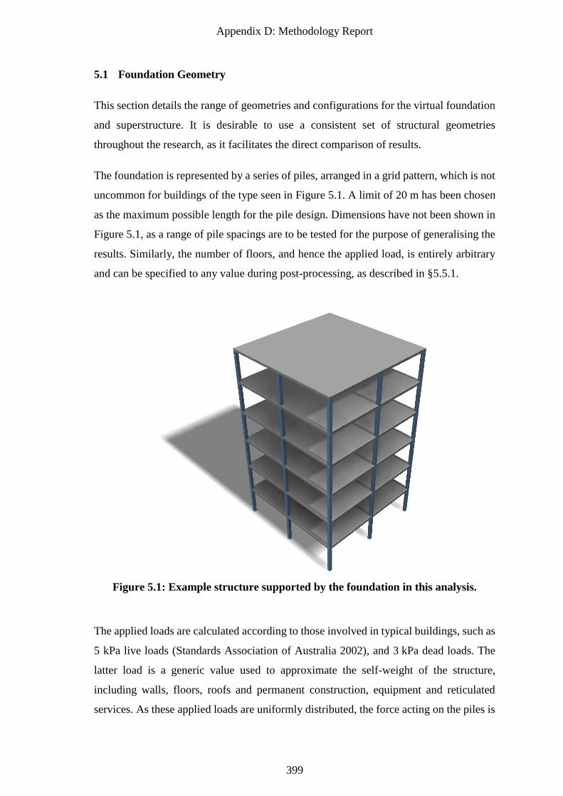
Appendix D: Methodology Report
399
5.1 Foundation Geometry
This section details the range of geometries and configurations for the virtual foundation
and superstructure. It is desirable to use a consistent set of structural geometries
throughout the research, as it facilitates the direct comparison of results.
The foundation is represented by a series of piles, arranged in a grid pattern, which is not
uncommon for buildings of the type seen in Figure 5.1. A limit of 20 m has been chosen
as the maximum possible length for the pile design. Dimensions have not been shown in
Figure 5.1, as a range of pile spacings are to be tested for the purpose of generalising the
results. Similarly, the number of floors, and hence the applied load, is entirely arbitrary
and can be specified to any value during post-processing, as described in §5.5.1.
Figure 5.1: Example structure supported by the foundation in this analysis.
The applied loads are calculated according to those involved in typical buildings, such as
5 kPa live loads (Standards Association of Australia 2002), and 3 kPa dead loads. The
latter load is a generic value used to approximate the self-weight of the structure,
including walls, floors, roofs and permanent construction, equipment and reticulated
services. As these applied loads are uniformly distributed, the force acting on the piles is
Appendix D: Methodology Report
400
a function of both the plan area of the building, as well as the number of storeys. The
distribution of the forces on the individual piles is dependent on their relative position to
the structure, and the corresponding tributary floor areas. For example, piles at the edges
of the building support half the tributary areas of the internal piles, and are therefore
subject to half of the internal pile’s structural load. Similarly, piles at the corner of the
structure support a quarter of the load of the internal piles. As such, these three pile cases
are each to be designed to a different length to reflect their individual loads.
5.2 Pile Settlement Model
Settlement is selected as the dominant and sole criterion examined in the pile design
process adopted in the present framework. Whilst bearing capacity is also often calculated
as part of the design process, it is, in actual fact, another form of settlement evaluation,
albeit implicit. Several methods are available for calculating pile settlement and these
include linear and non-linear methods, as well as computationally-intensive methods such
as FEM, and simpler methods, many of which are empirical, that rely heavily on
assumptions and approximations. A comparison of these models, featuring discussion
from the literature, is given in the following section.
5.2.1 Comparison of Simplified Methods and Finite Element Analysis
Previous studies in this area have typically used simplified, computationally-efficient,
linear-elastic methods for determining foundation performance (Goldsworthy 2006;
Arsyad 2009), so it is worth examining the suitability of their use within the current
framework. Such methods were typically used because sufficient computational
resources were not available at the time to provide the large number of results required
for Monte Carlo analysis. There are equivalent simplified methods for calculating the
vertical settlement of an axially-loaded pile, including Poulos and Davis (1980) and
Mylonakis and Gazetas (1998), which are subject to the same advantages and limitations.
These simplified methods typically reduce any sample values to a single representative
value and treat the soil as uniform, which, in the context of the present research, results
in a loss of information. As discussed in §4.1.1 and §4.3.2, using simplified methods can
have a detrimental impact on the accuracy of the results. This reduction in quality is due
to the CK pile performance being inadequately represented, particularly as settlement is
low-value dominated, an attribute not reflected by the simplified methods. The methods
Appendix D: Methodology Report
401
are also quite limited in how they account for multiple soil layers, the analysis of which
is a key component of this framework.
In addition to the loss of information, there is also the question of how to represent the
complete knowledge of the soil in design. Arsyad (2009) used the reduced value of soil
elements within a radius of six pile diameters, based on suggestions by Jaksa (1995) and
Teh and Houlsby (1991) regarding the influence zone of CPTs. However, this
recommendation was only an approximate guideline; there is no guarantee of a high
degree of accuracy. Increased scepticism is warranted considering the application by
Arsyad of a statically-loaded pile with a large diameter and flat base, is different to that
of Teh and Houlsby (1991) who examined a mobile cone with a diameter that is smaller
by an order of magnitude. To add to the uncertainty of the CK radius procedure, Ahmadi
and Robertson (2005) showed that the radius of influence is significantly affected by the
stiffness of the material. This influence is further compounded by the presence of variable
soil, as opposed to the relatively uniform soil that is present over the small scale of the
CPT’s influence.
Finally, the method of reducing the soil in the CK radius to a single value will also have
a significant impact on the piles’ performance, as detailed in §4.3. While the geometric
average likely provides an approximate representation, this has yet to be validated to a
high degree of accuracy in the case of piles. There is also evidence that anisotropy might
not be sufficiently represented by these methods, as discussed in §3.4.2.2.
For a combination of these reasons, the simplified methods are incapable of reliably
representing the CK soil case with regards to pile design. While some of the limitations
discussed here do not apply to all simplified methods, the uncertainty surrounding CK
representation is beyond reasonable doubt.
It was also shown in §4.1.1 and §4.3.2 that these methods are less sensitive to several site
investigation options, such as choice of reduction method and test type. This reduced
sensitivity could make it more difficult to identify optimal site investigation parameters.
As such, simplified methods are not recommended for SI representations.
While the simplified methods have been shown to be unsuitable for most cases, finite
element analysis (FEA) does not suffer from the same limitations. Finite element analysis
provides accurate representations of the laws of physics within the confines of the
Appendix D: Methodology Report
402
assumed material properties, and when a sufficient mesh resolution is given. For this
reason, a FE mesh preserves the richness of the soil property variability when calculating
settlement, allowing for true CK performance to be obtained reliably. Furthermore, it
allows for accurate assessment of SI foundation performance, as the method operates
directly applicable to the soil model, as generated from an investigation. For these
reasons, FEA is recommended over simplified methods within this framework.
5.2.2 Comparison of Linear and Non-Linear Finite Element Analysis
This section compares the use of linear and non-linear FEA for determining pile
performance within this framework. Generally speaking, non-linear, plastic FEA is more
accurate and linear-elastic FEA is computationally faster. However, the specific details
and difference in accuracy requires further discussion. The linear-elastic FEM model
referred to here is discussed in §5.3. A non-linear plastic model would have a similar
configuration but with the aforementioned material assumptions.
The main implication of the linear-elastic model is that only the serviceability criterion
can be used for design, which is otherwise known as the settlement limit. This is as
opposed to both serviceability and strength criteria, which are both typically adopted in
practice (Bowles 1997). The strength criterion is generally associated with sudden,
catastrophic failure, a mode which can only be achieved with non-linear analysis.
As described below, there is evidence that the strength criterion is not the constraining
limit, and that the linear-elastic assumption is adequate for determining overall pile
performance. This suggests that linear-elastic FEA is the preferable model for this
framework. To support this case, a review of the advantages and disadvantages of linear-
elastic FEA is presented below. It is important to note for the given justifications, that the
piles are being designed to a tolerance of 0.0025C, where C is the centre-to-centre pile
spacing, as discussed in §7.2.1.
5.2.2.1 Advantages of linear-elastic FEA
This sub-section discusses the advantages of linear-elastic analysis FEA for use within
the framework. Perhaps more importantly, it details counterpoints to the use of non-linear
plastic FEA. This covers a range of issues, including aspects of practicality, as well as
the validity of assumption and simplifications.
Appendix D: Methodology Report
403
One of the primary reasons for this linear-elastic assumption is to reduce computational
time, as FEAs are typically computationally-expensive. This factor is significant as the
model will need to be run several million times to achieve a complete set of results, across
many combinations of variables, within the Monte Carlo framework. While a non-linear
analysis is a more accurate representation of reality, and would be capable of assessing
the strength criteria, use of this type in a 3D context is impractical from a computational
time perspective.
It is argued here that the settlement of a pile, as represented by a linear-elastic model, is
sufficient for assessing its overall performance, as opposed to bearing capacity. Although
engineers design foundations according to both strength and settlement limits, many
studies suggest that settlement, in particular differential settlement, is the main cause of
structural distress (Becker 1997; Bowles 1997; Tamaro and Clough 2001). It has also
been found that loads applied in settlement calculations are typically smaller than those
associated with bearing capacity failure (Small 2001). This implies that the suitability of
a model depends on how well it adequately represents pile settlement. However, while
settlement calculations are most often associated with linear-elastic models, non-linear
plastic analysis may yield higher and more accurate settlement values than those obtained
from linear-elastic analyses. This depends on soil conditions, the magnitude of the
applied load, and material property assumptions within the non-linear model (Smith et al.
2013). An important consideration is that many non-linear models incorporate a linear-
elastic component, where these properties are used if material deformation does not
exceed a certain threshold. Therefore, if it can be shown that soil deformation is largely
below this threshold, or if the plastic region is of little consequence, then linear-elastic
models would be suitable for this framework.
There is strong evidence in the literature that pile deformation is largely within the elastic
region in settlement analysis. This is supported by several studies, such as in the
discussion above regarding (Small 2001), where it is said that applied loads are typically
smaller than those causing plastic failure. Furthermore, Leung et al. (2010) investigated
the choice of linear vs non-linear models on the settlement of pile groups. The study
concluded that the linear model was sufficient in cases where the pile spacing is greater
than 2.5 times the pile diameter. For example, a settlement larger than 5-10% of the pile
diameter is required for a substantial mobilisation of pile toe and shaft resistances
Appendix D: Methodology Report
404
corresponding with bearing failure (Geotechnical Engineering Office 1996). In a 500 mm
diameter pile, this corresponds to settlement of 25 mm to 50 mm. The worst-case design
tolerance is 50 mm, and can be as little as 12.5 mm depending on pile spacing, as
discussed in §7.2.1. As such, given that this bearing settlement is not exceeded, it is
unlikely that the plastic region will be reached.
With regards to the comparison of linear and non-linear settlement, Goldsworthy (2006)
found that the choice of model had relatively little impact on the results of the analysis.
For example, any bias that would be present in a particular model was automatically
cancelled out when the SI and CK designs were compared. This argument could be
extended to the choice of linear vs non-linear analysis, where the limitations of the linear
model are negated, to a large extent, when compared against itself.
There is also known to be correlation between soil properties. This implies that if a
foundation plastically fails due to a weak region of soil, then this weak region will also
likely result in a high degree of settlement. Therefore, this correlation means that a breach
of the strength criterion may be captured indirectly through settlement measurement, and
hence may not be required.
Furthermore, in terms of using linear-elastic over non-linear FEA for settlement
calculation, the former is commonly used in industry (Bowles 1997). As the results of
this framework are intended to be used in practice, it is important to seek to model, as
closely as possible, processes adopted by practitioners. This is further evidence that
linear-elastic models are suitable for settlement calculation.
In addition to the validity of linear-elastic FEA discussed above, this model also has
advantages in terms of its generality and breadth of applicability. Use of this relatively
simple model serves to increase its applicability to a wider range of soils. This is because
the results are applicable to all soils with the specified elastic modulus, regardless of soil
type (i.e. coarse-grained vs. fine-grained soils). Implementing additional soil properties,
as required in a non-linear model, would serve to restrict the application of results to those
specific properties. Furthermore, the linear-elastic assumption also greatly increases the
flexibility of post-processing of the results, as discussed in §5.5.1. These are both
considerations that would not be possible under a more complex model.
Appendix D: Methodology Report
405
5.2.2.2 Disadvantages of linear-elastic FEA
Some disadvantages of linear-elastic FEA were implied in the previous section; however,
a closer inspection of these details is given below. In addition, there are some
disadvantages of the particular model used in this framework that are discussed, regarding
the pile-soil interface.
While the settlement performance of non-linear plastic FEA is expected to be similar to
linear-elastic in most cases, there may be scenarios where the latter model provides a
noticeable settlement underestimation. This is most likely to occur in the case of a
multiple-layer soil profile where the lower layer(s) is significantly weaker than the upper
layer. In the scenario where the pile base is founded in the weaker layer, the likelihood
of pile toe mobilisation is increased. However, this settlement underestimation would
only be of concern in the more extreme cases of this specific scenario, and interpretation
of these results should be reasonable given that this limitation is known. In other words,
focus in this framework should be given to soil profiles with stronger lower layers, or that
results from soils with weaker lower layers should be viewed with healthy scepticism. As
previously discussed, since this limitation is present in both the CK and SI settlement
analysis, it is largely a self-cancelling of error, and would have negligible impact on the
comparison of results.
Linear-elastic models can capture immediate settlement, however, they cannot
accommodate consolidation which may occur in saturated clays, as discussed in §2.1.3.
This behaviour can be accounted for with sufficiently-configured non-linear models,
should it be desired. However, practitioners generally account for this by using modified
(drained) soil parameters to include consolidation as part of the total settlement.
Furthermore, there is a tendency for pre-consolidation to be applied to soils prior to
construction, such that any consolidation occurring due to presence of the foundations is
minimal. For these reasons, immediate settlement, as represented by linear-elastic
models, is deemed to be appropriate for use in this framework.
In addition to the simplified material properties of the linear-elastic assumptions, there is
an additional limitation, in that the pile is perfectly bonded to the surrounding soil. This
is not strictly realistic, as some slip does occur along the pile-soil interface, and pile
settlement becomes non-linear after roughly 2% of the pile diameter (Naghibi et al.
2014b). This 2% corresponds to a settlement of 10 mm for a 500 mm diameter pile. This
Appendix D: Methodology Report
406
appears to be a reasonable assumption, given that proposed pile spacing options for this
study include 5 m and 10 m, as discussed in §7.2.1. Given the design tolerance of 0.0025
m/m, these foundations would be designed to 12.5 mm and 25 mm respectively, and are
a similar order of magnitude to the approximate bonding limit. Therefore, the lack of a
pile slip component is likely to have a negligible impact on the results of the present
research.
5.2.2.3 Choice of FEA model
A strong case has been presented above for the suitability of linear-elastic FEA within
this framework. Settlement, and its associated structural distortion, was shown to be the
primary source of structural damage. Furthermore, settlement has been shown to be
accurately represented by this model in the majority of cases. Any remaining limitations
of the model were argued to be minor, or otherwise self-cancelling during the comparison
of SI and CK performance.
Griffith and Fenton have recently stated that this linear pile model is currently the best
available to predict the effects of spatial variability of the soil (Naghibi et al. 2014b). As
they are also the authors of several non-linear plastic FEA libraries, this is an important
recommendation.
Finally, non-linear plastic FEA is simply not practical for use in this framework, primarily
due to its exponentially-longer run time. Furthermore, the power and flexibility of the
post-processing of results facilitated by the linear-elastic assumption, as discussed in
§5.5.1, is a significant innovation in present version of the framework. For a combination
of these reasons, a linear-elastic FEM model is selected.
5.3 Finite Element Model
This section describes the FEA model used to determine pile settlement within the present
framework. This includes discussion of the algorithm, the mesh geometry, boundary
conditions, optimizations, and the manner in which multiple piles are handled.
Furthermore, this framework proposes several innovations that optimise FEA usage for
speed, such as variable-sized elements and a 2D axisymmetric mesh, in some
circumstances. This is the first time such innovations have been applied to the present
line of research, and as such, requires validation.
Appendix D: Methodology Report
407
The models use linear-elastic material mechanics, requiring the specification of Young’s
modulus and Poisson’s ratio. This allows for the assessment of immediate settlement as
determined by solid mechanics. However, it does not accommodate secondary settlement
or consolidation, as may occur in saturated clays (Bowles 1997).
The pile is treated as rigid and is perfectly bonded to the surrounding soil. This rigid
assumption is a modification of the original model used by Naghibi et al. (2014b), which
treated the pile as a stiff, but deformable series of elements, in the order of 30 GPa. The
change to a rigid pile was undertaken to allow pile settlement to be perfectly linearly
proportional to soil stiffness, which allows for flexibility in processing results as
discussed in §5.5.1, as well as cases of FEM optimization as discussed in §6.4. The
rigidity assumption is reasonable for two reasons. Firstly, the overwhelming majority of
the total settlement is a result of soil deformation, as opposed to deformation of the pile
(Poulos and Davis 1980). Secondly, the piles are consistently rigid in both the CK and SI
scenarios. As such, the relative difference between them, as a result of the rigidity, should
be negligible, along with its impact on determining site investigation performance. These
FEM model attributes are consistent across all variations of the model discussed in this
section.
5.3.1 3D Model Description
The main FEA implementation used for the CK analysis is a Fortran subroutine adapted
from Program 5.6 developed by (Smith et al. 2013). It has been independently verified
by the authors of the present report against the FE package, Strand7 (Strand7 Pty. Ltd.
2016). The mesh is constructed of eight-node brick elements. Nodes along the boundary,
on the sides of the mesh, are free to move in the vertical direction, with lateral
displacement fixed.
There are a number of attributes incorporated to increase computational speed. It uses a
preconditioned conjugate gradient solver (PCG), which solves the FEA equations
iteratively (Smith et al. 2013). There are two advantages to using this solver method.
Firstly and primarily, this greatly reduces the RAM usage because it negates the need to
construct the global stiffness matrix, which grows cubically in size as the soil dimensions
increase. Secondly, it was found that this method is faster than solving the global stiffness
matrix, at least for the scale of meshes used in the present and proposed analyses. This
Appendix D: Methodology Report
408
could be partly due to the manner by which the proportion of iterations to the number of
equations (linked to number of elements) decreases as the mesh size increases.
Furthermore, the authors of this report have modified some variables from double-
precision to single-precision. This change results in roughly twice the computational
speed, with negligible loss of accuracy.
5.3.2 2D Model Description
A similar model to that of the 3D case is used for the majority of the SI settlement
analysis, i.e. a 2D axisymmetric subroutine adapted from Program 5.1 (Smith et al. 2013).
The axisymmetric model, which represents the pile as a circular volume in a circular
mesh of soil, provides similar results to that of the 3D mesh. Note that the pile radius has
been increased by a factor of 1.12837, such that its cross-sectional area is equivalent to
that of the 3D square-shaped pile. Four-node quadrilateral elements are used for the mesh.
The increase in computational speed resulting from the use of a 2D rather than a 3D mesh
is roughly in the order of 100. The cases where this model can be safely used are given
in §6.4. A comparison between the 3D and 2D pile cases in a two-layer soil with uniform
properties is shown in Figure 5.2. The elastic modulus of the first and second layer is 0.2
MPa and 1 MPa, separated by a boundary at a depth of 10 m. There is a 1 kN load applied
to the pile head.
While there is a slight discrepancy between the two cases, the proportion of error is very
small and constant for a rigid pile across all variations of Young’s modulus. Therefore, a
correction factor derived by the ratio of the 3D to 2D settlements can be applied to any
2D settlement in order to eliminate this discrepancy. It can also be seen in Figure 5.2 that
the corrected 2D pile settlement coincides exactly with that of the 3D model. This
demonstrates that the axisymmetric condition is an excellent approximation of the 3D
scenario, despite the minor differences in the models, especially when combined with the
correction factor.
Unlike its 3D counterpart, the 2D model solves the global stiffness matrix directly, as
RAM usage is insignificant in the 2D case, and there is negligible difference in
computational time to that of a PCG solver.
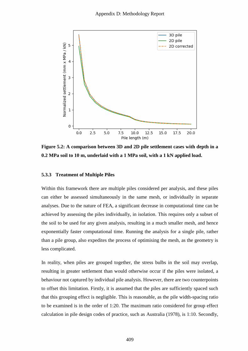
Appendix D: Methodology Report
409
Figure 5.2: A comparison between 3D and 2D pile settlement cases with depth in a
0.2 MPa soil to 10 m, underlaid with a 1 MPa soil, with a 1 kN applied load.
5.3.3 Treatment of Multiple Piles
Within this framework there are multiple piles considered per analysis, and these piles
can either be assessed simultaneously in the same mesh, or individually in separate
analyses. Due to the nature of FEA, a significant decrease in computational time can be
achieved by assessing the piles individually, in isolation. This requires only a subset of
the soil to be used for any given analysis, resulting in a much smaller mesh, and hence
exponentially faster computational time. Running the analysis for a single pile, rather
than a pile group, also expedites the process of optimising the mesh, as the geometry is
less complicated.
In reality, when piles are grouped together, the stress bulbs in the soil may overlap,
resulting in greater settlement than would otherwise occur if the piles were isolated, a
behaviour not captured by individual pile analysis. However, there are two counterpoints
to offset this limitation. Firstly, it is assumed that the piles are sufficiently spaced such
that this grouping effect is negligible. This is reasonable, as the pile width-spacing ratio
to be examined is in the order of 1:20. The maximum ratio considered for group effect
calculation in pile design codes of practice, such as Australia (1978), is 1:10. Secondly,
Appendix D: Methodology Report
410
this group influence would occur in both the CK and SI designs, and as such can be
considered as another self-cancelling model error. Hence, group effects are of secondary
importance to this analysis and can be safely ignored.
There are additional benefits to treating the piles in isolation, in relation to the analysis
of reduction methods. For example, the distance-weighted reduction techniques produce
a soil model value that is unique for each pile. Here, it is simply a matter of setting the
soil element properties of the full mesh to this value, rather than attempting some kind of
transition that would be required for multiple piles in the same mesh.
Using isolated piles also allows for taking advantage of lines of symmetry and redundant
cases for optimization purposes. The former point facilitates use of the axisymmetrical
2D mesh described in §5.3.2. The latter point reduces the number of piles needed to be
analysed in cases where piles are examined within identical conditions. These features
are discussed in detail later in §6.4.
5.3.4 Boundary Effects
This section discusses the boundary conditions of the FEA mesh, as well as motivation
for the overall mesh size. This framework specifies modelling of a floating pile, i.e. one
that exists in a semi-infinite soil mass with no bedrock present. However, due to the
nature of FEA, domain soil boundaries must be specified, as only a finite soil volume can
be analysed. Typically, boundaries are located far enough from the object of interest so
as to have a negligible impact on the result. This then creates a trade-off between speed
and accuracy, since a larger soil volume requires a larger number of elements.
5.3.4.1 Effect of soil depth
As this framework models floating piles within a semi-infinite mass, the mesh must be
configured to produce equivalent results, despite comprising a finite volume, where the
base behaves as bedrock with infinite stiffness. A soil depth-to-pile length ratio of 2 is
selected as this is the minimum ratio where settlement of all pile lengths is independent
of the soil depth. For example, if the base of the soil was located near the tip of a 20 m
long pile, the resulting settlement will be greatly reduced when compared to that of a 1
m long pile in the same soil. No such reduction was observed with the 2:1 ratio. While
the model would underestimate settlement by up to 10%, when compared to a model with
Appendix D: Methodology Report
411
a soil-pile ratio of 3:1, the relative underestimation is constant with pile length. Therefore,
the bottom boundary can be said to have negligible impact on the result. This
underestimation is a model error, and as discussed previously, model errors are of little
consequence, as they cancel themselves out when SI and CK designs are compared.
Indeed, this soil-pile depth ratio is more conservative than those used in other studies
using this model, such as Naghibi et al. (2014a, 2014b).
Having a relatively shallow depth boundary is supported by Seycek (1991), in that it may
be beneficial over a greater depth. It was suggested that FEA tends to overestimate
settlement due to the contribution of small strains at large depths, and that it is suitable to
restrict the zone of deformation within a soil.
5.3.4.2 Effect of soil width
In a similar case to that of the vertical, a mesh width must be specified such that pile
settlement is equivalent to that within an infinitely-wide soil. A key consideration is that
nodes on the edges of the mesh have free vertical movement. The boundary must
therefore be spaced sufficiently far from the pile for these nodes to undergo zero
deformation and have zero vertical stress. This stress condition implies that no soil
beyond the boundary is needed for additional pile support, and hence the mesh is
equivalent to that with an infinite width.
Since stress decreases exponentially with distance, as discussed in §2.1, there is a trend
of diminishing returns with respect to accuracy as the boundary distance increases. Desai
and Abel (1972) indicated that the centre of a footing should be at least 5 times the footing
width from the boundary. However, this was found to be insufficient and likely only
appropriate to shallow footings. This is because, as pile length increases, the load is
distributed to a greater volume of soil, which increases the size of the stress bulb.
Randolph and Wroth (1978) implied that there is some ‘magical’ radius, rm, beyond
which shear stress becomes negligible. This parameter is affected by factors such as soil
type, and is approximately equal to the length of the pile. Mylonakis and Gazetas (1998)
showed that, for the analysis of single piles, the results were rather insensitive to the exact
value of rm. Translating this to FEA confirms that there is little benefit in setting the
horizontal boundary at distances greater than the pile length from the pile itself. Hence,
Appendix D: Methodology Report
412
the boundary radius is set to the maximum pile length examined in the proposed analysis,
i.e. 20 m.
5.3.5 Mesh Geometry and Element Size Selection
This section details the mesh geometry, which consists of variable element sizes, and the
validation of this configuration with regards to error. As mentioned previously,
minimising computational time is an important aspect of the framework presented herein.
While previous authors have used a regular, one-to-one mesh with respect to the soil,
large gains in performance can be achieved by using a mesh of variable element size. By
increasing the size of elements further away from the pile, the number of elements can
be greatly reduced. As computational time increases exponentially with the number of
elements, this reduction has significant benefits.
This increase in element size is made possible by averaging the properties of the original
elements making up that volume. This has been found to have little impact on the
settlement accuracy, as the stresses decrease exponentially with distance from the pile, as
discussed in §2.1. The reasoning is that as stress decreases, the effect of any particular
element in isolation also decreases, hence averaging is appropriate. In particular, there
should be no loss of accuracy through averaging if either of the following two criteria are
met:
1. The values of the soil elements being averaged are approximately equal. This is
certainly valid for single-layer soils with high scales of fluctuation.
2. The weightings (i.e. contribution to settlement) of the elements being averaged
are approximately equal so as to be independent of their configuration within the
averaging volume. This is valid for elements at a large distance from the pile,
where all weightings are either approximately zero, or otherwise similar due to a
low rate of change.
This innovation reduces the computational time from over one minute, to roughly 3
seconds, when compared to a mesh of the same volume with uniform element sizes of
0.5 × 0.5 × 0.5. The width of the elements in close proximity to the pile have been reduced
to 0.25 m for the 0.25 m soil case, with their depth remaining at 0.5 m. These 0.25 m
elements can be combined if a 0.5 m soil resolution is used. As the soil is comprised of
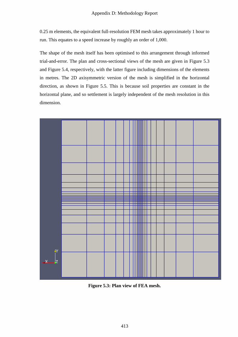
Appendix D: Methodology Report
413
0.25 m elements, the equivalent full-resolution FEM mesh takes approximately 1 hour to
run. This equates to a speed increase by roughly an order of 1,000.
The shape of the mesh itself has been optimised to this arrangement through informed
trial-and-error. The plan and cross-sectional views of the mesh are given in Figure 5.3
and Figure 5.4, respectively, with the latter figure including dimensions of the elements
in metres. The 2D axisymmetric version of the mesh is simplified in the horizontal
direction, as shown in Figure 5.5. This is because soil properties are constant in the
horizontal plane, and so settlement is largely independent of the mesh resolution in this
dimension.
Figure 5.3: Plan view of FEA mesh.
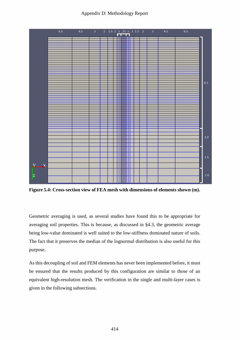
Appendix D: Methodology Report
414
Figure 5.4: Cross-section view of FEA mesh with dimensions of elements shown (m).
Geometric averaging is used, as several studies have found this to be appropriate for
averaging soil properties. This is because, as discussed in §4.3, the geometric average
being low-value dominated is well suited to the low-stiffness dominated nature of soils.
The fact that it preserves the median of the lognormal distribution is also useful for this
purpose.
As this decoupling of soil and FEM elements has never been implemented before, it must
be ensured that the results produced by this configuration are similar to those of an
equivalent high-resolution mesh. The verification in the single and multi-layer cases is
given in the following subsections.
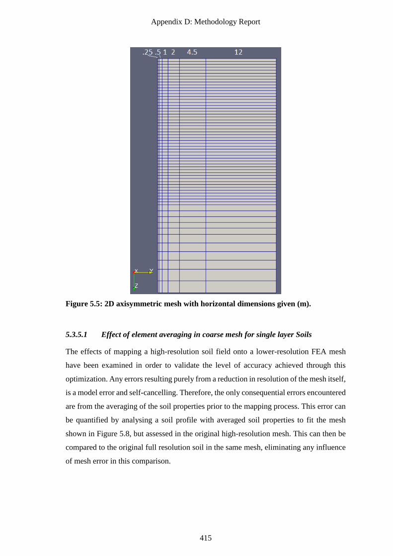
Appendix D: Methodology Report
415
Figure 5.5: 2D axisymmetric mesh with horizontal dimensions given (m).
5.3.5.1 Effect of element averaging in coarse mesh for single layer Soils
The effects of mapping a high-resolution soil field onto a lower-resolution FEA mesh
have been examined in order to validate the level of accuracy achieved through this
optimization. Any errors resulting purely from a reduction in resolution of the mesh itself,
is a model error and self-cancelling. Therefore, the only consequential errors encountered
are from the averaging of the soil properties prior to the mapping process. This error can
be quantified by analysing a soil profile with averaged soil properties to fit the mesh
shown in Figure 5.8, but assessed in the original high-resolution mesh. This can then be
compared to the original full resolution soil in the same mesh, eliminating any influence
of mesh error in this comparison.
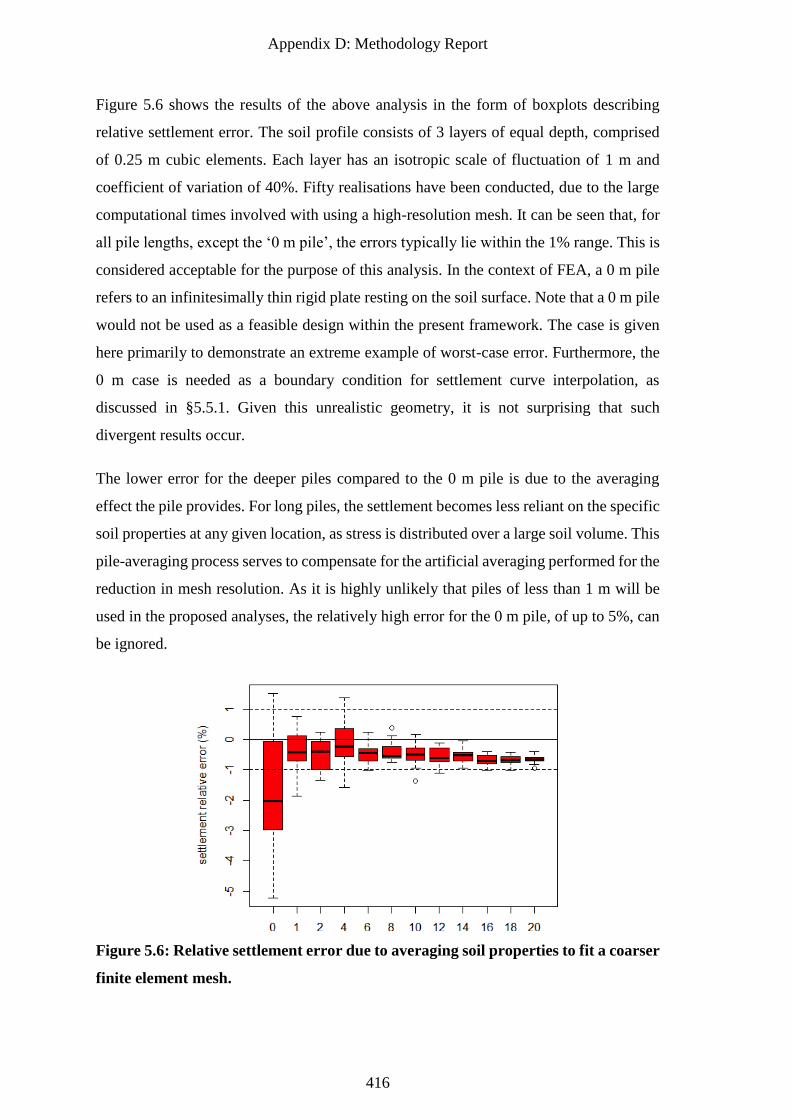
Appendix D: Methodology Report
416
Pile length (m)
Figure 5.6 shows the results of the above analysis in the form of boxplots describing
relative settlement error. The soil profile consists of 3 layers of equal depth, comprised
of 0.25 m cubic elements. Each layer has an isotropic scale of fluctuation of 1 m and
coefficient of variation of 40%. Fifty realisations have been conducted, due to the large
computational times involved with using a high-resolution mesh. It can be seen that, for
all pile lengths, except the ‘0 m pile’, the errors typically lie within the 1% range. This is
considered acceptable for the purpose of this analysis. In the context of FEA, a 0 m pile
refers to an infinitesimally thin rigid plate resting on the soil surface. Note that a 0 m pile
would not be used as a feasible design within the present framework. The case is given
here primarily to demonstrate an extreme example of worst-case error. Furthermore, the
0 m case is needed as a boundary condition for settlement curve interpolation, as
discussed in §5.5.1. Given this unrealistic geometry, it is not surprising that such
divergent results occur.
The lower error for the deeper piles compared to the 0 m pile is due to the averaging
effect the pile provides. For long piles, the settlement becomes less reliant on the specific
soil properties at any given location, as stress is distributed over a large soil volume. This
pile-averaging process serves to compensate for the artificial averaging performed for the
reduction in mesh resolution. As it is highly unlikely that piles of less than 1 m will be
used in the proposed analyses, the relatively high error for the 0 m pile, of up to 5%, can
be ignored.
Figure 5.6: Relative settlement error due to averaging soil properties to fit a coarser
finite element mesh.
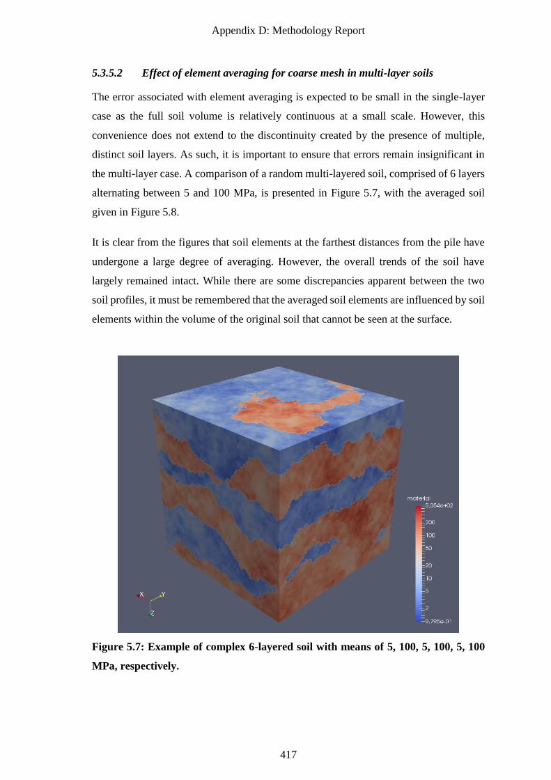
Appendix D: Methodology Report
417
5.3.5.2 Effect of element averaging for coarse mesh in multi-layer soils
The error associated with element averaging is expected to be small in the single-layer
case as the full soil volume is relatively continuous at a small scale. However, this
convenience does not extend to the discontinuity created by the presence of multiple,
distinct soil layers. As such, it is important to ensure that errors remain insignificant in
the multi-layer case. A comparison of a random multi-layered soil, comprised of 6 layers
alternating between 5 and 100 MPa, is presented in Figure 5.7, with the averaged soil
given in Figure 5.8.
It is clear from the figures that soil elements at the farthest distances from the pile have
undergone a large degree of averaging. However, the overall trends of the soil have
largely remained intact. While there are some discrepancies apparent between the two
soil profiles, it must be remembered that the averaged soil elements are influenced by soil
elements within the volume of the original soil that cannot be seen at the surface.
Figure 5.7: Example of complex 6-layered soil with means of 5, 100, 5, 100, 5, 100
MPa, respectively.
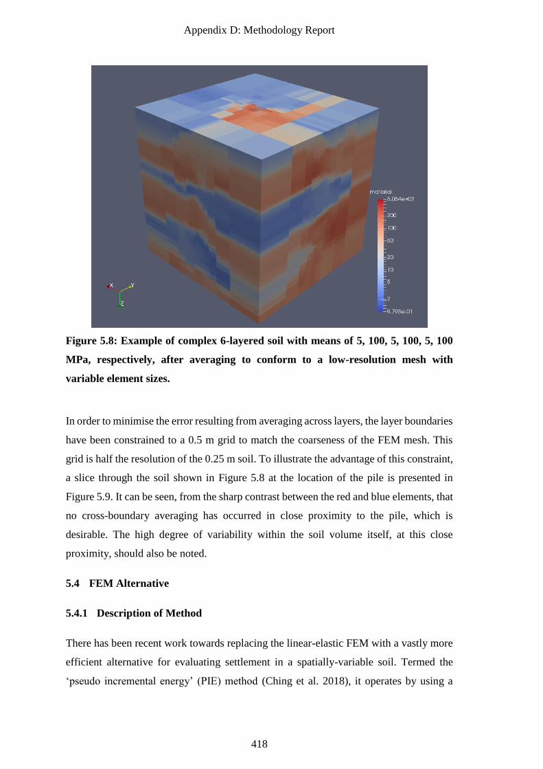
Appendix D: Methodology Report
418
Figure 5.8: Example of complex 6-layered soil with means of 5, 100, 5, 100, 5, 100
MPa, respectively, after averaging to conform to a low-resolution mesh with
variable element sizes.
In order to minimise the error resulting from averaging across layers, the layer boundaries
have been constrained to a 0.5 m grid to match the coarseness of the FEM mesh. This
grid is half the resolution of the 0.25 m soil. To illustrate the advantage of this constraint,
a slice through the soil shown in Figure 5.8 at the location of the pile is presented in
Figure 5.9. It can be seen, from the sharp contrast between the red and blue elements, that
no cross-boundary averaging has occurred in close proximity to the pile, which is
desirable. The high degree of variability within the soil volume itself, at this close
proximity, should also be noted.
5.4 FEM Alternative
5.4.1 Description of Method
There has been recent work towards replacing the linear-elastic FEM with a vastly more
efficient alternative for evaluating settlement in a spatially-variable soil. Termed the
‘pseudo incremental energy’ (PIE) method (Ching et al. 2018), it operates by using a
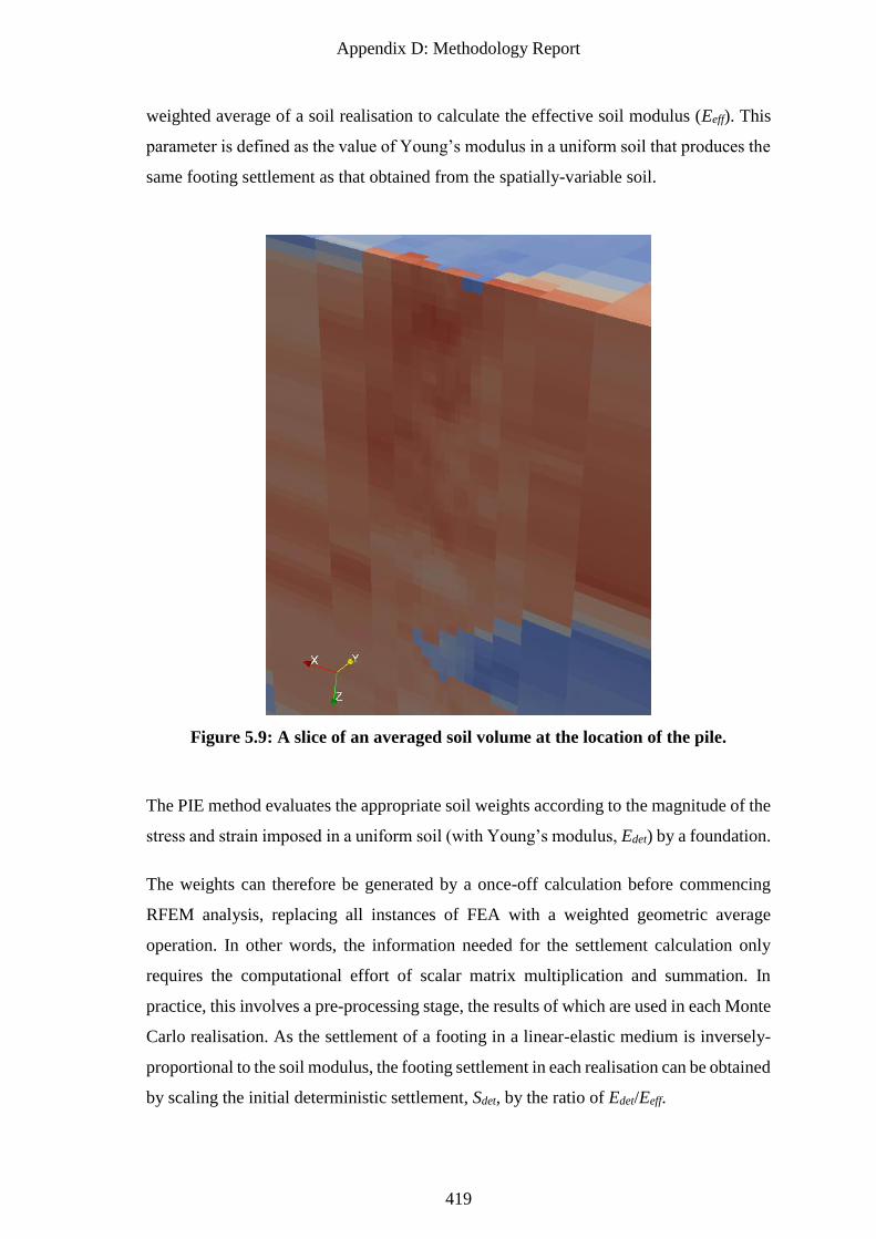
Appendix D: Methodology Report
419
weighted average of a soil realisation to calculate the effective soil modulus (Eeff). This
parameter is defined as the value of Young’s modulus in a uniform soil that produces the
same footing settlement as that obtained from the spatially-variable soil.
Figure 5.9: A slice of an averaged soil volume at the location of the pile.
The PIE method evaluates the appropriate soil weights according to the magnitude of the
stress and strain imposed in a uniform soil (with Young’s modulus, Edet) by a foundation.
The weights can therefore be generated by a once-off calculation before commencing
RFEM analysis, replacing all instances of FEA with a weighted geometric average
operation. In other words, the information needed for the settlement calculation only
requires the computational effort of scalar matrix multiplication and summation. In
practice, this involves a pre-processing stage, the results of which are used in each Monte
Carlo realisation. As the settlement of a footing in a linear-elastic medium is inversely-
proportional to the soil modulus, the footing settlement in each realisation can be obtained
by scaling the initial deterministic settlement, Sdet, by the ratio of Edet/Eeff.
Appendix D: Methodology Report
420
The above operation can be represented by the following equation:
𝑆 =𝐸𝑑𝑒𝑡
∑ 𝑊𝑖𝐸𝑖𝑛𝑖=1
𝑆𝑑𝑒𝑡 (5.1)
Where S is the settlement of the footing in a particular realisation, Wi is the weight of a
particular soil element, Ei is the Young’s modulus of the corresponding soil element, and
n is the number of soil elements in the random field used in the settlement calculation.
The soil weight for any given element required for the PIE method can be obtained from
the following equation, where the terms are derived from a settlement analysis in a
uniform soil as described above:
𝑊 = ∆𝜎𝑥∆휀𝑥 + ∆𝜎𝑦∆휀𝑦 + ∆𝜎𝑧∆휀𝑧 + ∆𝜏𝑥𝑦∆휀𝑥𝑦 + ∆𝜏𝑦𝑧∆휀𝑦𝑧 + ∆𝜏𝑥𝑧∆휀𝑥𝑧 (5.2)
5.4.2 Applicability of PIE Method to Pile Settlement
The PIE method is very recent in terms of its creation, and the method has yet to be
directly applied to studies beyond those involving its verification. As such, at present, its
range of applicability is limited, as its verification is currently in development. For
example, the method has been developed to evaluate settlement of rigid shallow
foundations, and has been shown to represent effectively Eeff for this case. However, there
has been no research to date relating to the method’s applicability with respect to pile
foundations. The primary differences between the pile and shallow foundation cases, in
terms of mechanics, is that the former is dominated by simple shear. This mechanism of
load transfer has yet to be assessed in any manner.
Theoretically, the PIE method should be applicable to the pile model used in the present
framework, as the piles are assumed to be rigid, as discussed in §5.3. If the pile had
remained as a deformable solid, as previously discussed, then settlement would not be
directly proportional to the soil stiffness. This discrepancy is due to the ratio of the soil-
pile stiffnesses as a variable in the settlement equation, which effects a non-trivial
influence (Poulos and Davis 1980). Furthermore, the soil weights would not be constant
for a given mean soil stiffness. For example, Mattes and Poulos (1969) stated that, for an
extremely rigid pile, the distribution of stress along the pile is almost uniform, with the
maximum value occurring near the tip. On the other hand, as the relative stiffness of the
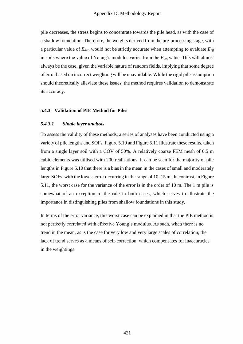
Appendix D: Methodology Report
421
pile decreases, the stress begins to concentrate towards the pile head, as with the case of
a shallow foundation. Therefore, the weights derived from the pre-processing stage, with
a particular value of Edet, would not be strictly accurate when attempting to evaluate Eeff
in soils where the value of Young’s modulus varies from the Edet value. This will almost
always be the case, given the variable nature of random fields, implying that some degree
of error based on incorrect weighting will be unavoidable. While the rigid pile assumption
should theoretically alleviate these issues, the method requires validation to demonstrate
its accuracy.
5.4.3 Validation of PIE Method for Piles
5.4.3.1 Single layer analysis
To assess the validity of these methods, a series of analyses have been conducted using a
variety of pile lengths and SOFs. Figure 5.10 and Figure 5.11 illustrate these results, taken
from a single layer soil with a COV of 50%. A relatively coarse FEM mesh of 0.5 m
cubic elements was utilised with 200 realisations. It can be seen for the majority of pile
lengths in Figure 5.10 that there is a bias in the mean in the cases of small and moderately
large SOFs, with the lowest error occurring in the range of 10–15 m. In contrast, in Figure
5.11, the worst case for the variance of the error is in the order of 10 m. The 1 m pile is
somewhat of an exception to the rule in both cases, which serves to illustrate the
importance in distinguishing piles from shallow foundations in this study.
In terms of the error variance, this worst case can be explained in that the PIE method is
not perfectly correlated with effective Young’s modulus. As such, when there is no
trend in the mean, as is the case for very low and very large scales of correlation, the
lack of trend serves as a means of self-correction, which compensates for inaccuracies
in the weightings.
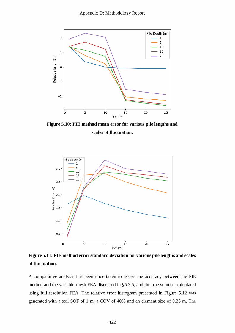
Appendix D: Methodology Report
422
Figure 5.10: PIE method mean error for various pile lengths and
scales of fluctuation.
Figure 5.11: PIE method error standard deviation for various pile lengths and scales
of fluctuation.
A comparative analysis has been undertaken to assess the accuracy between the PIE
method and the variable-mesh FEA discussed in §5.3.5, and the true solution calculated
using full-resolution FEA. The relative error histogram presented in Figure 5.12 was
generated with a soil SOF of 1 m, a COV of 40% and an element size of 0.25 m. The
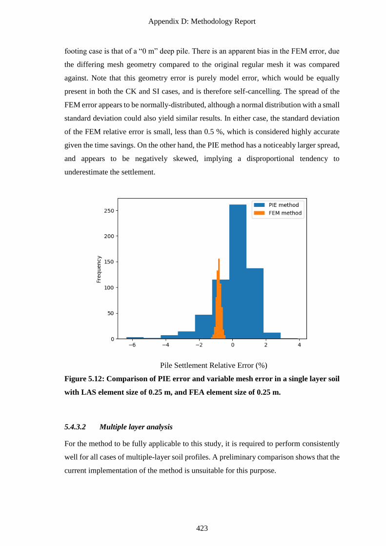
Appendix D: Methodology Report
423
footing case is that of a “0 m” deep pile. There is an apparent bias in the FEM error, due
the differing mesh geometry compared to the original regular mesh it was compared
against. Note that this geometry error is purely model error, which would be equally
present in both the CK and SI cases, and is therefore self-cancelling. The spread of the
FEM error appears to be normally-distributed, although a normal distribution with a small
standard deviation could also yield similar results. In either case, the standard deviation
of the FEM relative error is small, less than 0.5 %, which is considered highly accurate
given the time savings. On the other hand, the PIE method has a noticeably larger spread,
and appears to be negatively skewed, implying a disproportional tendency to
underestimate the settlement.
Pile Settlement Relative Error (%)
Figure 5.12: Comparison of PIE error and variable mesh error in a single layer soil
with LAS element size of 0.25 m, and FEA element size of 0.25 m.
5.4.3.2 Multiple layer analysis
For the method to be fully applicable to this study, it is required to perform consistently
well for all cases of multiple-layer soil profiles. A preliminary comparison shows that the
current implementation of the method is unsuitable for this purpose.
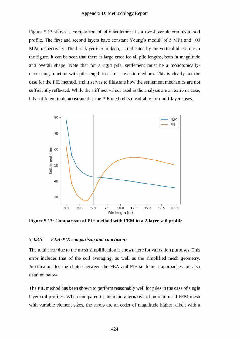
Appendix D: Methodology Report
424
Figure 5.13 shows a comparison of pile settlement in a two-layer deterministic soil
profile. The first and second layers have constant Young’s moduli of 5 MPa and 100
MPa, respectively. The first layer is 5 m deep, as indicated by the vertical black line in
the figure. It can be seen that there is large error for all pile lengths, both in magnitude
and overall shape. Note that for a rigid pile, settlement must be a monotonically-
decreasing function with pile length in a linear-elastic medium. This is clearly not the
case for the PIE method, and it serves to illustrate how the settlement mechanics are not
sufficiently reflected. While the stiffness values used in the analysis are an extreme case,
it is sufficient to demonstrate that the PIE method is unsuitable for multi-layer cases.
Figure 5.13: Comparison of PIE method with FEM in a 2-layer soil profile.
5.4.3.3 FEA-PIE comparison and conclusion
The total error due to the mesh simplification is shown here for validation purposes. This
error includes that of the soil averaging, as well as the simplified mesh geometry.
Justification for the choice between the FEA and PIE settlement approaches are also
detailed below.
The PIE method has been shown to perform reasonably well for piles in the case of single
layer soil profiles. When compared to the main alternative of an optimised FEM mesh
with variable element sizes, the errors are an order of magnitude higher, albeit with a
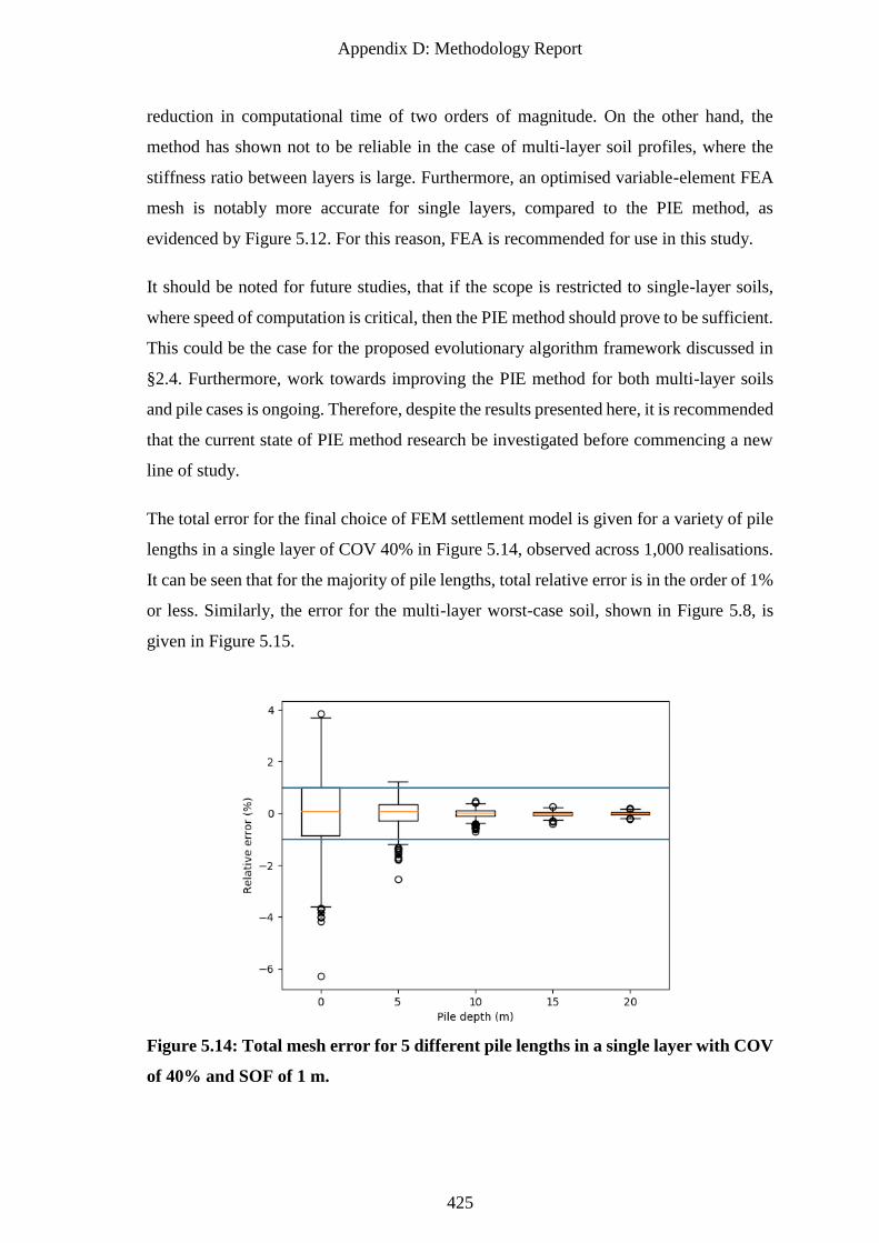
Appendix D: Methodology Report
425
reduction in computational time of two orders of magnitude. On the other hand, the
method has shown not to be reliable in the case of multi-layer soil profiles, where the
stiffness ratio between layers is large. Furthermore, an optimised variable-element FEA
mesh is notably more accurate for single layers, compared to the PIE method, as
evidenced by Figure 5.12. For this reason, FEA is recommended for use in this study.
It should be noted for future studies, that if the scope is restricted to single-layer soils,
where speed of computation is critical, then the PIE method should prove to be sufficient.
This could be the case for the proposed evolutionary algorithm framework discussed in
§2.4. Furthermore, work towards improving the PIE method for both multi-layer soils
and pile cases is ongoing. Therefore, despite the results presented here, it is recommended
that the current state of PIE method research be investigated before commencing a new
line of study.
The total error for the final choice of FEM settlement model is given for a variety of pile
lengths in a single layer of COV 40% in Figure 5.14, observed across 1,000 realisations.
It can be seen that for the majority of pile lengths, total relative error is in the order of 1%
or less. Similarly, the error for the multi-layer worst-case soil, shown in Figure 5.8, is
given in Figure 5.15.
Figure 5.14: Total mesh error for 5 different pile lengths in a single layer with COV
of 40% and SOF of 1 m.
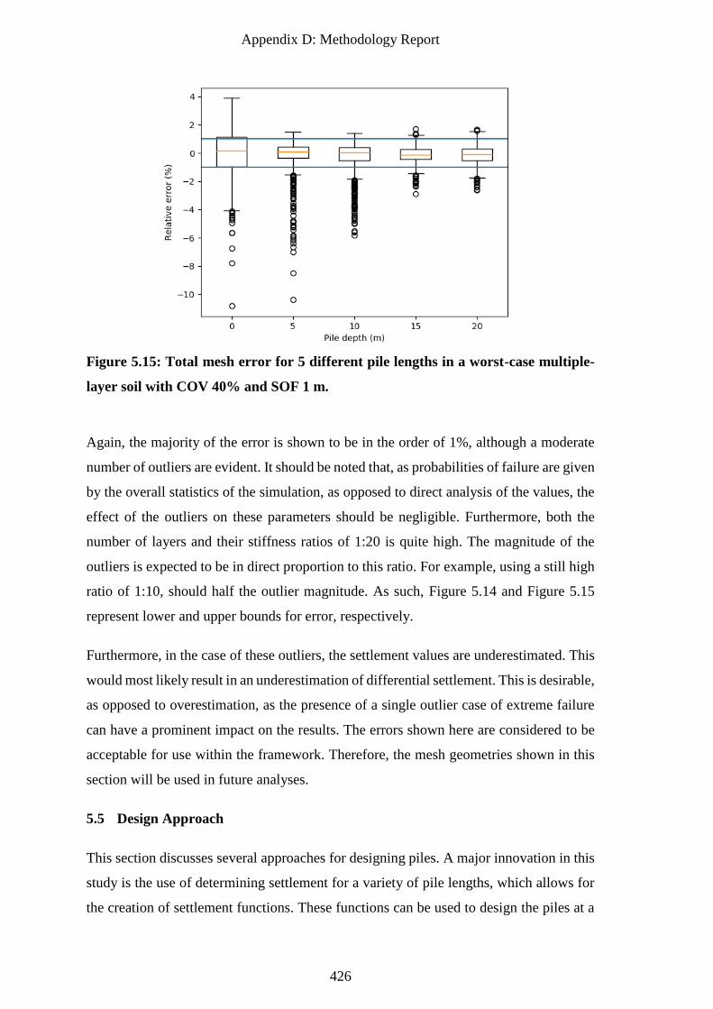
Appendix D: Methodology Report
426
Figure 5.15: Total mesh error for 5 different pile lengths in a worst-case multiple-
layer soil with COV 40% and SOF 1 m.
Again, the majority of the error is shown to be in the order of 1%, although a moderate
number of outliers are evident. It should be noted that, as probabilities of failure are given
by the overall statistics of the simulation, as opposed to direct analysis of the values, the
effect of the outliers on these parameters should be negligible. Furthermore, both the
number of layers and their stiffness ratios of 1:20 is quite high. The magnitude of the
outliers is expected to be in direct proportion to this ratio. For example, using a still high
ratio of 1:10, should half the outlier magnitude. As such, Figure 5.14 and Figure 5.15
represent lower and upper bounds for error, respectively.
Furthermore, in the case of these outliers, the settlement values are underestimated. This
would most likely result in an underestimation of differential settlement. This is desirable,
as opposed to overestimation, as the presence of a single outlier case of extreme failure
can have a prominent impact on the results. The errors shown here are considered to be
acceptable for use within the framework. Therefore, the mesh geometries shown in this
section will be used in future analyses.
5.5 Design Approach
This section discusses several approaches for designing piles. A major innovation in this
study is the use of determining settlement for a variety of pile lengths, which allows for
the creation of settlement functions. These functions can be used to design the piles at a
Appendix D: Methodology Report
427
post-processing stage, allowing for significant flexibility and generalisation of results.
This method is described and verified in this report.
A description of the more traditional trial-and-error design approach is also given, as this
may be beneficial in some studies depending on the circumstances. These situations may
include modest usage of non-linear plastic models. The trial-and-error approach may also
be faster, if a very limited number of options are investigated.
The piles will be designed to a differential settlement tolerance of 0.0025C (Day 1999),
where C is the pile centre-to-centre spacing. For pile spacings of 5, 10 and 20 m, this
corresponds to absolute settlement tolerances of 12.5, 25 and 50 mm, respectively. The
reasoning behind this is detailed in §5.2.2.
5.5.1 Interpolation and Post-processing
The method described here involved designing piles directly from a function, given a
settlement tolerance. The function is created by interpolating a series of settlement values
for different pile lengths using the Akima method (Akima 1970; De Boor 2001), which
is known for producing smooth curves. The main advantages are increased computational
speed of the main analysis, when a large number of variables are considered, and
increased flexibility of the results.
5.5.1.1 Purpose and advantages
Given that the FEAs are linear-elastic in nature it is possible and desirable to produce a
series of pile length-settlement curves. In other words, dimensionless functions of
settlement and applied load for a given pile length. Due to the linear-elastic nature of the
analysis, these curves can be scaled to any applied arbitrary applied load or soil mean
elastic modulus. This allows for a wide variety of analyses to conducted with a single set
of results, as opposed to having to run a new simulation for each new configuration.
As force can be scaled on a per-pile basis, analysis options can include building height,
size, shape and number of piles. In addition, this allows for the effect of redundancy
(safety factor) to be accounted for. This is aspect is not part of the original Jaksa et al.
(2013) framework, but is nevertheless of value. This modified version of the framework
can therefore be used for other aspects of research. Possible applications now include
Appendix D: Methodology Report
428
reliability based design, as it allows for the determination of resistance factors in a manner
similar to Naghibi et al. (2014b).
Once the curve has been generated, the pile design then becomes a matter of scaling the
magnitude to match the appropriate applied load and safety factor, and determining the
smallest pile length that satisfies the specified total settlement limit. Differential
settlement can also be accounted for. However, this mode of failure is typically ignored
in practice in favour of a small absolute total settlement tolerance that minimises the
likelihood of differential settlement (Day 1999).
Use of such settlement functions can greatly reduce the number of required runs of the
CK FEA. As the true performance of pile designs resulting from site investigations must
be known, a new FE analysis must traditionally be conducted for each combination of
site investigation parameters. This results in an exponential increase of FEM runs
required, as the scope of investigation parameters increases. However, by generating a
settlement function, the number of FEM runs required per pile is constant, and merely
that needed to generate the curve. This results in a reduction of CK FEMs needed for a
single design by an order of 1,000. This efficiency allows for a greatly expanded scope
of analysis.
If used on a specific case, the framework also allows for the optimization of the entire
process with regards to cost, including the cheapest design in combination with site
investigation. This is as opposed to the optimization of just the site investigation as has
been traditionally undertaken in this line of research. However, as these results are
intended to be widely-applicable, this case-specific aspect will not be undertaken, except
for potential verification purposes.
As seen in Figure 5.16, the pile length-settlement curve is quite smooth, even in the case
of a multi-layered soil. This lends itself well to interpolation. In the context of this
analysis, interpolation provides two benefits. Firstly, it allows the pile to be designed for
increments smaller than the size of the FEA elements, if so desired, in this case 0.25 m.
Secondly, it leads to the possibility of only a subset of pile lengths needing to be assessed,
instead of every increment along the pile length. This allows for reduced usage of the
FEA subroutine and hence a substantial reduction in overall computational time when
compared to generating the full curve.
Appendix D: Methodology Report
429
The smoothness of this curve, also in relation to variable soil profiles with multiple layers,
can be explained by the nature of FEA. The settlement calculation uses the full knowledge
of the soil profile at every depth, with the only change being that of the additional pile
elements. This is opposed to some of the approximate settlement methods previously
discussed, such as that of Poulos and Davis (1980), which only account for the soil
properties along the shaft of the pile. This can lead to sudden changes as the pile extends
into soil with alternate properties. In contrast, linear FEA does not experience such
changes, as these alternate properties impose a change in pile settlement well before the
pile physically enters the region of these properties.
It is worth reinforcing at this stage the significant advantage of linear analysis vs. non-
linear analysis, as discussed previously in §5.2.2. If non-linear analysis were used, the
pile length-settlement curve could only be used for the particular force it was generated
for, and could not necessarily be scaled to force due to yielding behaviour, greatly
restricting its applicability. Furthermore, the curve might not exhibit the same degree of
smoothness, or monotonically decreasing trend. For example, a pile that is based on a
strong layer would be associated with a particular settlement. However, if the pile were
then extended into a softer layer, this soft material could then yield, resulting in an
increased settlement. So, while a linear-elastic analysis is not strictly realistic, its
assumptions certainly allow for an array of generalised, consistent analysis.
This post-processing approach also minimises another issue with the traditional trial-and-
error approach. As discussed above in §3.4.1, for highly variable soils, it is possible that
no feasible pile design exists for a given load, resulting in unusable realisations. Shifting
the design procedure to a post-processing approach allows the number of unusable
realisations to be known almost instantly. This allows for an appropriate load to be chosen
with confidence, such that that the results are applicable and relevant, without having to
rerun computationally-intensive analyses.
As seen above, there are several reasons why this post-processing design philosophy is
advantageous, and is the method of choice for this framework. Furthermore, as the
settlement functions are reusable, they form a database of pile information that can be
used by future researchers for a variety of purposes. This ensures that the results
generated by this study are of use in both the short and long term.
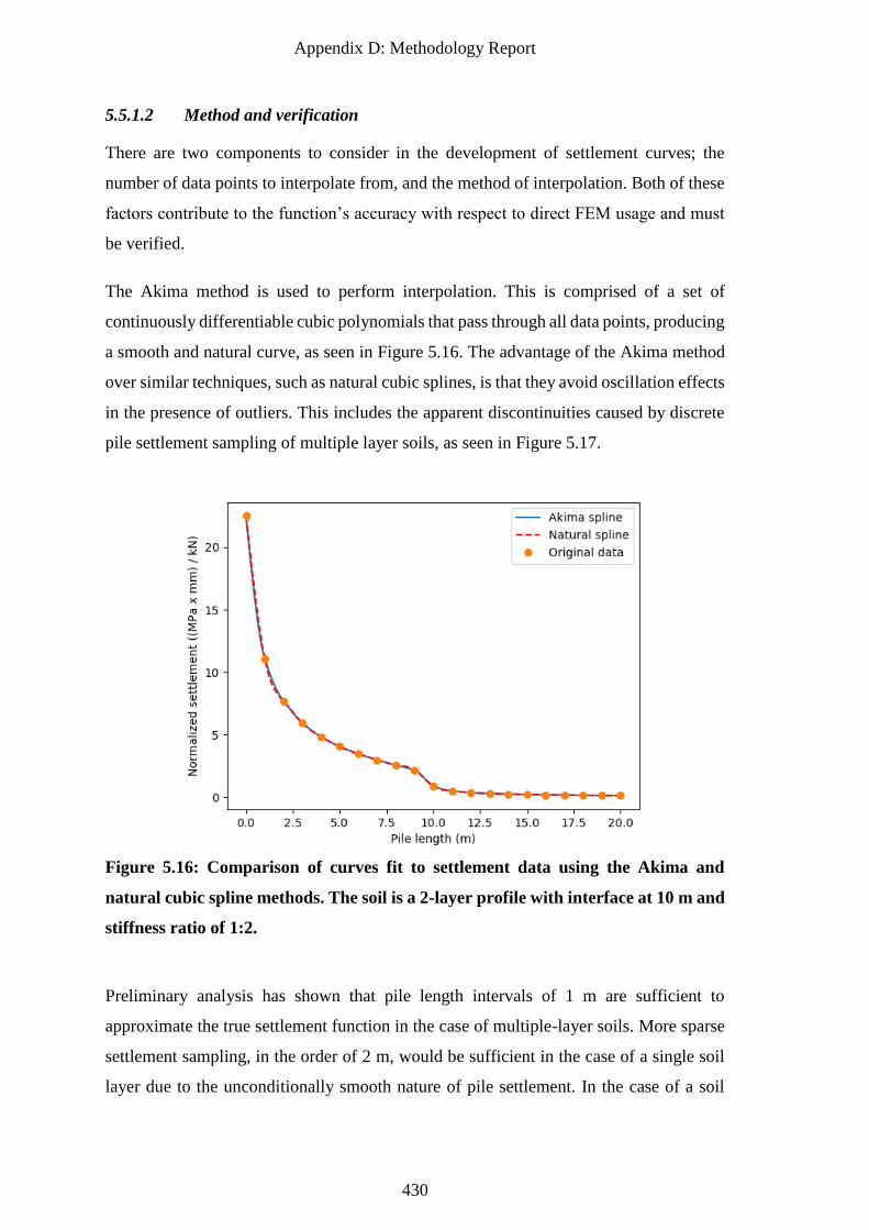
Appendix D: Methodology Report
430
5.5.1.2 Method and verification
There are two components to consider in the development of settlement curves; the
number of data points to interpolate from, and the method of interpolation. Both of these
factors contribute to the function’s accuracy with respect to direct FEM usage and must
be verified.
The Akima method is used to perform interpolation. This is comprised of a set of
continuously differentiable cubic polynomials that pass through all data points, producing
a smooth and natural curve, as seen in Figure 5.16. The advantage of the Akima method
over similar techniques, such as natural cubic splines, is that they avoid oscillation effects
in the presence of outliers. This includes the apparent discontinuities caused by discrete
pile settlement sampling of multiple layer soils, as seen in Figure 5.17.
Figure 5.16: Comparison of curves fit to settlement data using the Akima and
natural cubic spline methods. The soil is a 2-layer profile with interface at 10 m and
stiffness ratio of 1:2.
Preliminary analysis has shown that pile length intervals of 1 m are sufficient to
approximate the true settlement function in the case of multiple-layer soils. More sparse
settlement sampling, in the order of 2 m, would be sufficient in the case of a single soil
layer due to the unconditionally smooth nature of pile settlement. In the case of a soil
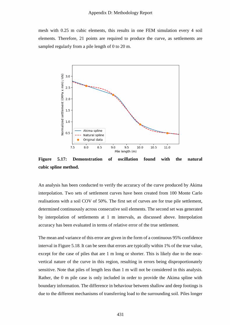
Appendix D: Methodology Report
431
mesh with 0.25 m cubic elements, this results in one FEM simulation every 4 soil
elements. Therefore, 21 points are required to produce the curve, as settlements are
sampled regularly from a pile length of 0 to 20 m.
Figure 5.17: Demonstration of oscillation found with the natural
cubic spline method.
An analysis has been conducted to verify the accuracy of the curve produced by Akima
interpolation. Two sets of settlement curves have been created from 100 Monte Carlo
realisations with a soil COV of 50%. The first set of curves are for true pile settlement,
determined continuously across consecutive soil elements. The second set was generated
by interpolation of settlements at 1 m intervals, as discussed above. Interpolation
accuracy has been evaluated in terms of relative error of the true settlement.
The mean and variance of this error are given in the form of a continuous 95% confidence
interval in Figure 5.18. It can be seen that errors are typically within 1% of the true value,
except for the case of piles that are 1 m long or shorter. This is likely due to the near-
vertical nature of the curve in this region, resulting in errors being disproportionately
sensitive. Note that piles of length less than 1 m will not be considered in this analysis.
Rather, the 0 m pile case is only included in order to provide the Akima spline with
boundary information. The difference in behaviour between shallow and deep footings is
due to the different mechanisms of transferring load to the surrounding soil. Piles longer
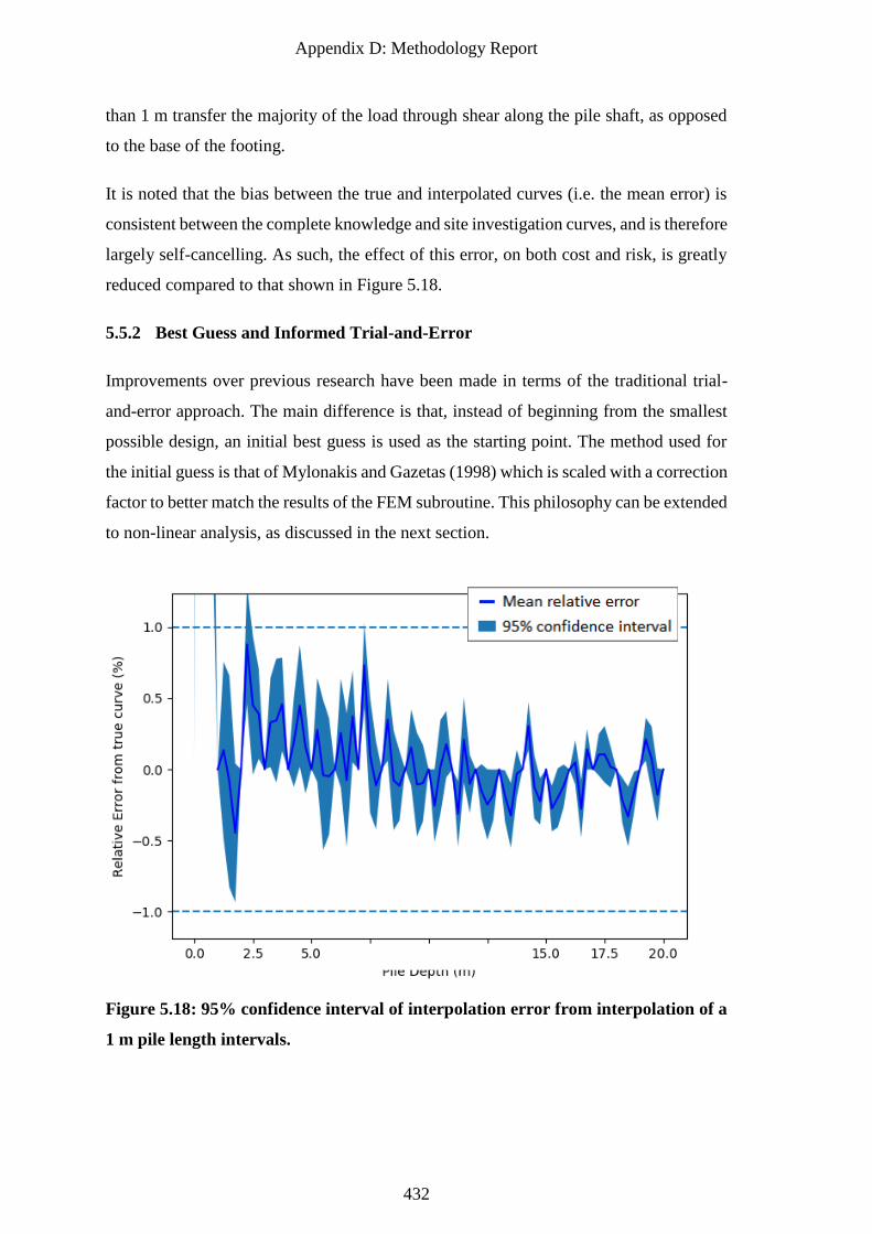
Appendix D: Methodology Report
432
than 1 m transfer the majority of the load through shear along the pile shaft, as opposed
to the base of the footing.
It is noted that the bias between the true and interpolated curves (i.e. the mean error) is
consistent between the complete knowledge and site investigation curves, and is therefore
largely self-cancelling. As such, the effect of this error, on both cost and risk, is greatly
reduced compared to that shown in Figure 5.18.
5.5.2 Best Guess and Informed Trial-and-Error
Improvements over previous research have been made in terms of the traditional trial-
and-error approach. The main difference is that, instead of beginning from the smallest
possible design, an initial best guess is used as the starting point. The method used for
the initial guess is that of Mylonakis and Gazetas (1998) which is scaled with a correction
factor to better match the results of the FEM subroutine. This philosophy can be extended
to non-linear analysis, as discussed in the next section.
Figure 5.18: 95% confidence interval of interpolation error from interpolation of a
1 m pile length intervals.
Pile length (m)
Appendix D: Methodology Report
433
Another innovation is that, instead of continuing to guess what the true design might be
after the initial estimate, the subsequent design attempts can be selected more
intelligently. This is because it can be known whether the true pile length is longer or
shorter than the current design, based on whether the current design satisfies the criteria.
Since the model is linear-elastic, it is known that settlement must decrease monotonically
as pile length increases, as seen in Figure 5.18. The only situation where this is not the
case is when the soil is potentially stiffer than the pile. However, this scenario will not
occur as the pile is set as rigid. This efficient manner of design is only possible as a result
of the linear-elastic nature of the soil model and cannot be assumed to be valid for non-
linear models.
Should the pile not satisfy the settlement criterion, it is then increased in length
incrementally until the criterion is satisfied. If the pile does satisfy the criterion, then the
design will be incremented backwards (making the pile shorter) until the criterion is
satisfied, after which the previous increment is selected. The final design will be that of
the maximum pile length in the group. Therefore, this iteration process is repeated for all
piles, using the current maximum length as an initial point. The pile length is increased
until a new maximum is reached if the criterion is not satisfied. However, if the criterion
is satisfied then the pile can be skipped.
The differential settlement criterion must also be satisfied. It is known that, if all piles
satisfy the absolute settlement criterion described above, they must also satisfy this
criterion for all longer pile lengths. However, the same does not necessarily hold true for
differential settlement. Should one pile decrease in settlement at a greater rate than the
others, when all pile lengths are increased, then this could prove detrimental to meeting
the differential settlement criterion. Therefore, if this criterion is not satisfied after the
initial design, every pile must be rechecked at subsequent design iterations. This is
computationally-expensive.
In initial testing, the initial guess has been shown to be accurate to within 3 design
iterations (1.5 m) and is usually at most one increment off the true value. This results in
vastly reduced usage of the FEM subroutine, and results in overall significantly less
computational time then the interpolation and post-processing method described in
§5.5.1. However, as the results are only applicable for a given load, the results are less
generalisable, which is counter-productive to one of the objectives of this study.
Appendix D: Methodology Report
434
Nevertheless, this design methodology may prove useful in other studies involving pile
design with computationally-intensive linear models.
5.5.3 Incorporation of Non-Linear FEA
If one chooses in the future to implement non-linear, plastic FEA within the framework,
some guidance is given in this section. The SI design method described in §5.5.2 could
be used with this model; however, as the settlement curve may be non-linear, some
modification is required to ensure the correct design is identified. The initial guess of the
pile design can be taken conservatively, i.e. based on the 10th percentile of the soil
stiffness or some other appropriate characteristic derived through testing. The true design
would be known to be longer than the initial estimate and identifying it would become a
matter of iteratively increasing the pile length. Depending on the behaviour of the non-
linear model chosen, i.e. elastic perfectly-plastic vs. a component of strain-hardening, a
linear-elastic FEA model could be a good approximation of the non-linear behaviour.
This is as opposed to the traditional elastic settlement model used in the previous section.
Another option is creating an upper- and lower-bound for non-linear design, then
employing a root-finding algorithm, such as the bisection or Regular Falsi method
(Burden and Faires 2001) to evaluate the next design length without testing consecutive
elements.
Use of a more realistic settlement model for true CK pile performance or design can also
allow for the determination of model error. Assuming that this model is accurate and that
a simpler linear-elastic model is used for SI analysis, the error due to the linear-elastic
assumptions can be quantified. This assumes that linear-elastic methods will continue to
be used for design in practice. However, this will no longer be relevant if industry moves
to adopt similarly complex models in routine design.
Currently, non-linear FEA is too computationally-expensive to be considered as part of
the proposed methodology, even with minimal use, given the large number of Monte
Carlo realisations required. However, it is an area that could be considered for future
research. The most feasible use of non-linear soil mechanics would be in analysis
involving pile design error. This minimises the number of FEM analyses required per-
pile in a manner that is independent of the number of site investigations, as true pile
design is unique for a pile in a given soil.
Appendix D: Methodology Report
435
6 Monte Carlo Analysis and Optimization
There are several areas where optimizations can be made within the framework in order
to reduce overall computational time. This effort is required because of the framework’s
combination of computationally-intensive FEA and high number of Monte Carlo
realisations and variable combinations. This results in extremely large computational
times involved, in the order of weeks to years, depending on the scope of the problem.
To offset this, a large number of framework optimizations have been carried out.
One area of optimization is the number of Monte Carlo realisations, where the resulting
statistics become more precise as the number of realisations increases. This creates a
trade-off between run time and accuracy. Usage of the FEA subroutine can also be
minimised in some cases, which is a significant factor, as FEA accounts for the vast
majority of the run time.
A number of software settings can also be optimised, both the program as a whole, and
FEA specifically. As the 3D FEA subroutine uses an iterative solver, the number of
iterations can be optimised in a similar way to the number of Monte Carlo realisations.
Furthermore, as each realisation is an independent occurrence, the program can readily
be run in parallel, which generally reduces the total run time by the number of CPU cores
available.
6.1 Number of Monte Carlo Realisations
For Monte Carlo results to be useful, their statistics must converge with respect to the
number of realisations, where the determination of this convergence point is a form of
optimization. In other words, there would be a number of realisations beyond which the
result does not change. There is no rule for determining how many realisations are
required, as this varies according to the nature of the problem, and the degree of required
precision. Therefore, an analysis must be conducted to assess the variation of results as
the number of realisations increases. This section presents such an analysis, as well as an
investigation of the number of realisations used in the literature.
Failure costs, which account for a non-trivial part of the total cost, are the most sensitive
part of the analysis due to both the rare occurrence of catastrophic failure, and the variable
cost penalty that provides higher weighting to more significant failure. The combination
Appendix D: Methodology Report
436
of these two attributes in a weighted average results in a highly skewed and hence
unstable distribution compared to other parameters which are either constant, or have a
simple arithmetic average taken across realisations. Therefore, while it is tempting to
determine the number of Monte Carlo realisations by analysing a computationally-
efficient subset of data, this method cannot be deemed reliable. Rather, a complete
analysis needs to be conducted, with failure costs assigned.
6.1.1 Literature Review
Investigation into the number of realisations in prior studies has typically been minimal,
as a sensitivity analysis is highly resource intensive and cannot be undertaken with many
variables. Furthermore, the chosen number of realisations has traditionally been adopted
out from a practicality perspective in order to achieve a reasonable timeframe for the
simulation, as opposed to what is objectively best. Therefore, the motivation to conduct
such a sensitivity analysis is minimal.
As mentioned previously, it is essential to examine the sensitivity of the number of
realisations in terms of failure cost. However, previous studies have not done this.
Goldsworthy (2006) assessed the convergence of a 9-pad system using FEA and a soil of
COV 50% and SOF of 8 m, based on the metric of average footing design area. It was
concluded that 4,000 realisations was optimal, yielding an error within 0.5%, calculated
against a final value from a total of 10,000 realisations. However, 1,000 realisations was
adopted, as it was concluded that this compromise still resulted in reasonable accuracy,
within 1% of the final value. Note that these convergence estimations are highly
unconservative, both for reasons discussed in §6.1, and because a relatively coarse design
increment of 1 m (0.5 m either side) was used as a result of the FEA mesh resolution.
Similarly, Arsyad (2009) conducted a sensitivity analysis for pile capacity based on the
LCPC method using a single CPT across 3,000 realisations. It was concluded that the
results had clearly converged by 1,000 realisations, and so this value was adopted.
However, it should be noted that the SOF of the soil used was 1 m, which as discussed in
§3.4.2.1, results in a soil that appears uniform at a macro scale, implying these results are
indeed quite unconservative. Furthermore, low soil COV values in the order of 10% were
used in the analysis, reinforcing the unconservative nature of the results. In conclusion,
neither of these studies investigated the effect of cost-weighted failure nor compared the
Appendix D: Methodology Report
437
performance of SI and CK designs. Simply analysing the effect of the SI designs, as seen
here, is not representative of the complete simulation and cannot be relied upon.
Nevertheless, a set of 1,000 realisations has been widely adopted across the site
investigation optimization literature (e.g. Goldsworthy (2006) and Goldsworthy et al.
(2004a); Goldsworthy et al. (2004b); Goldsworthy et al. (2005); Jaksa et al. (2005);
Goldsworthy et al. (2007a); Goldsworthy et al. (2007b); Arsyad (2009); Arsyad et al.
(2009); Arsyad et al. (2010)). It should be noted that some of these studies did not use
total cost as the performance metric, and so the convergence assumption may be
reasonable. However, it is hypothesised that studies that do use total cost should not be
assumed to yield accurate results.
With regards to studies that use RFEM to model the effects of foundation settlement as
opposed to site investigation performance, it was found that a higher number of
realisations was used. This can be explained by how such analyses require a smaller
number of FEA runs (one per realisation, per footing) compared with cases were
foundations needed to be designed through iterative use of FEA. Therefore, the analyses
were less computationally intensive, and more results could be obtained within the same
time frame. For example, Fenton et al. (1996); Fenton et al. (2003); Kuo et al. (2004),
along with Naghibi et al. (2014b), used 2,000 realisations. However, the former set of
studies used 2D FEA which is exponentially faster than its 3D equivalent, and the latter
was conducted at a time when significantly more computational power was available.
Another 2D study, by Fenton and Griffiths (2002), used 5,000 realisations, while in
contrast, a 3D study by Fenton and Griffiths (2005) used 1,000. Again, these studies did
not analyse weighted performance metrics and so likely require a lower number of
realisations to achieve stable results.
6.1.2 Sensitivity Analysis
As confirmed by the assessment of the literature above, there has been no cost-based
sensitivity analysis previously conducted that is appropriate to this study, requiring that
one be undertaken. As such, the full analysis, as described in §2.3, is undertaken,
including the calculation of both CK and SI pile settlement, and their comparison for a
resulting average failure cost. The failure costs are calculated as described in §7.3.1.
Appendix D: Methodology Report
438
Due to the computationally-intensive nature of the multiple FEA runs, it would be ideal
to conduct this analysis using a single worst-case set of parameters. Preliminary analysis
indicates that a SOF of 8 m is the most sensitive value with respect to the number of
realisations. This is supported by previous analysis showing that the worst-case SOF for
foundation settlement to be in this order of magnitude, as discussed in §3.4.2.1. In terms
of COV, it is expected that the variability of failure increases as the COV increases.
Therefore, a value of 100% is chosen to be conservative, as this is above that of the 80%
maximum that will be used in the analysis in subsequent studies. Similarly, a single
borehole to a depth of 5 m was used, as this is the minimum amount of site investigation
data that may be examined, and therefore corresponds to the highest degree of variability.
The mean stiffness of the soil is 20 MPa. A total of 10,000 realisations is conducted, as
was performed by Goldsworthy (2006).
A variety of different applied loads have been assessed within this analysis to ensure that
the selected number of realisations is robust across different cases. In particular, the
various applied loads result in different pile lengths. As it has been noted that failure
generally becomes less likely as pile length increases, this provides insight into the
sensitivity of the results to the number of realisations for different failure distributions.
Furthermore, this implicitly results in a shuffling of the order in which catastrophic failure
occurs. This redistribution is important in that it demonstrates that the apparent sensitivity
is a result of the overall trend, as opposed to the particular distribution of costs throughout
the realisations. For example, the case where extreme failure occurs at evenly-spaced
intervals, would likely result in higher stability and less sensitivity, as opposed to the
situation where multiple significant failures occur in close proximity, which would
significantly alter the final results. Therefore, multiple plots of realisation sensitivity
should be inspected.
The foundation in the sensitivity analysis is comprised of a 9-pile system, where the
internal, edge, and corner pile cases are independently designed, as described in §5.1.
The total applied load to the foundation for the four cases is 9,600, 4,800, 3,200 and 2,400
kN.
The results of the analysis are presented in the form of a cumulative average, shown in
Figure 6.1. Note that the scales on the y-axis are unique to each subplot in order to
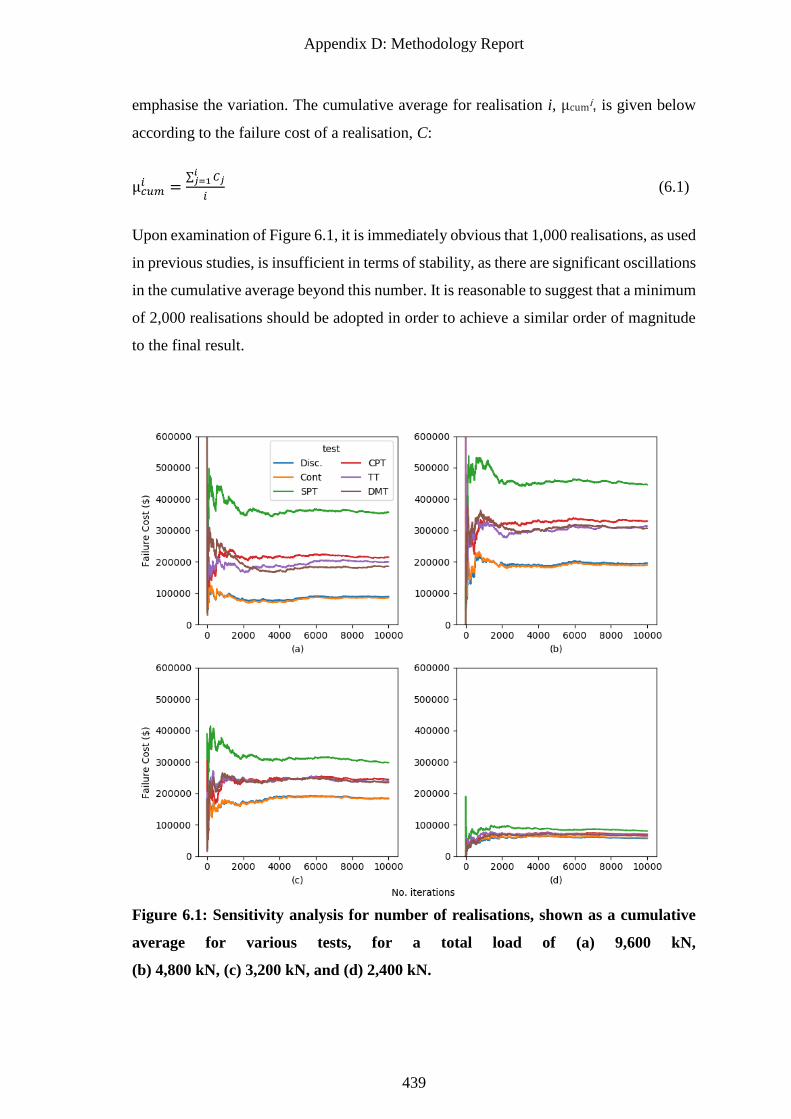
Appendix D: Methodology Report
439
emphasise the variation. The cumulative average for realisation i, μcumi, is given below
according to the failure cost of a realisation, C:
μ𝑐𝑢𝑚𝑖 =
∑ 𝐶𝑗𝑖𝑗=1
𝑖 (6.1)
Upon examination of Figure 6.1, it is immediately obvious that 1,000 realisations, as used
in previous studies, is insufficient in terms of stability, as there are significant oscillations
in the cumulative average beyond this number. It is reasonable to suggest that a minimum
of 2,000 realisations should be adopted in order to achieve a similar order of magnitude
to the final result.
Figure 6.1: Sensitivity analysis for number of realisations, shown as a cumulative
average for various tests, for a total load of (a) 9,600 kN,
(b) 4,800 kN, (c) 3,200 kN, and (d) 2,400 kN.
Appendix D: Methodology Report
440
It is perhaps more insightful to plot the relative error of this cumulative average with
respect to the final cost calculated across 10,000 realisations. However, due to the
undulating nature of the plots in Figure 6.1, which crosses above and below the final
value on multiple occasions, it is deemed that the worst-case relative error is a better
metric. This would result in a monotonically-decreasing plot, ensuring that the relative
error, for a given number of realisations, is lower than or equal to the value indicated.
The worst-case relative error for a given number of realisations, REi, is calculated as
follows:
𝑅𝐸𝑖 = 100 × |max ((𝜇𝑐𝑢𝑚𝑖 ,… ,𝜇𝑐𝑢𝑚
10,000)−𝜇𝑐𝑢𝑚10,000
𝜇𝑐𝑢𝑚10,000 )| (6.2)
The worst-case relative error for the plots given in Figure 6.1 is shown in Figure 6.2. Note
that the y-axis in the plots is set to a maximum of 25%, masking the extreme instability
at low realisation counts, for which the error is higher by several orders of magnitude. It
can be seen that the relative error for an analysis with 1,000 realisations can be in the
order of 20% or greater, as opposed to the 1% suggested by Goldsworthy (2006). This
20% error magnitude is deemed unacceptable. Rather, it can be seen that, if relative error
in the order of 5% or less is to be guaranteed, then 6,000 realisations is required, and
shown in Figure 6.2. An exception to this is Figure 6.2(d). Beyond the use of 6,000
realisations, the worst-case relative error appears to be approximately inversely
proportional to the number of realisations. As such, a realisation count higher than 6,000
appears to provide modest improvement.
While relative error can be a useful metric, it does not adequately represent values which
are near-zero, due to having a near-zero denominator. For this reason, and to determine
the influence of the number of realisations on the final results, a plot of worst-case
absolute error is given in Figure 6.3. Here, the worst-case error in terms of dollars is
given. It can be seen in Figure 6.3(d), which had a 10% relative error at 6,000 realisations,
has the lowest absolute error of less than $10,000. This contrast results from the average
cost of case (d) being relatively low, at $100,000, while the other cases have significantly
higher failure costs. As such, the 10% relative error of that scenario is acceptable. The
remaining cases have an absolute worst-case error in the order of $20,000.
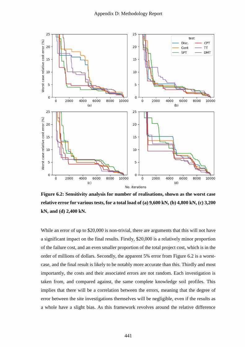
Appendix D: Methodology Report
441
Figure 6.2: Sensitivity analysis for number of realisations, shown as the worst case
relative error for various tests, for a total load of (a) 9,600 kN, (b) 4,800 kN, (c) 3,200
kN, and (d) 2,400 kN.
While an error of up to $20,000 is non-trivial, there are arguments that this will not have
a significant impact on the final results. Firstly, $20,000 is a relatively minor proportion
of the failure cost, and an even smaller proportion of the total project cost, which is in the
order of millions of dollars. Secondly, the apparent 5% error from Figure 6.2 is a worst-
case, and the final result is likely to be notably more accurate than this. Thirdly and most
importantly, the costs and their associated errors are not random. Each investigation is
taken from, and compared against, the same complete knowledge soil profiles. This
implies that there will be a correlation between the errors, meaning that the degree of
error between the site investigations themselves will be negligible, even if the results as
a whole have a slight bias. As this framework revolves around the relative difference
Appendix D: Methodology Report
442
between investigations, the resulting errors can be ignored. This is especially true since
failure is dictated by the CK pile performance, which is a constant for a given realisation.
In conclusion, while it is noted that at least 6,000 realisations are required to ensure
reasonable accuracy, it is suggested that 8,000 realisations be undertaken. This
recommendation is made for two reasons. Firstly, some realisations may contain invalid
pile designs, and will need to be discarded from the analysis; therefore, it is important to
have some redundancy. Secondly, it cannot be guaranteed that the sensitivity analysis
conducted here is indeed the worst case. Therefore, it is important to be conservative in
case some alternative soil profile proves to be more sensitive. While 6,000 realisations
can result in a relative error of up to 5%, and ± $20,000, it is deemed that the undertaking
of additional realisations would result in negligible improvement. Given that the
generation of each realisation is computationally-intensive, this recommendation is made
from the perspective of producing reliable results within a practical timeframe.
6.2 Number of FEM Iterations
A further opportunity for optimization is associated with the number of iterations in the
FEM software used to calculate pile settlement. The FEM solution is determined
iteratively, as it is determined using a conjugate gradient solver rather than solving the
stiffness matrix directly, as discussed in §5.3.1.
As with the number of Monte Carlo realisations, the accuracy of the FEM settlement
increases as the number of iterations increases. However, fewer iterations results in a
faster computation, which is preferred in this framework. The number of iterations can
be controlled by the tolerance used. For this subroutine, the tolerance is the difference in
maximum displacement of the nodes over two consecutive iterations, as a proportion of
the maximum displacement. This ensures consistent accuracy regardless of the applied
load.
It should be noted that the number of iterations needed to reach convergence is not
constant for a given mesh. As described by Smith et al. (2013), the number of iterations
is dependent on the nature of the eigenvalue spectrum of the assembled stiffness matrix.
This means that the count depends on the material properties of the soil mesh.
Considering that the soil mesh is randomly generated for each realisation, and that further
contrast in mesh properties results from the addition of the various pile lengths, it can be
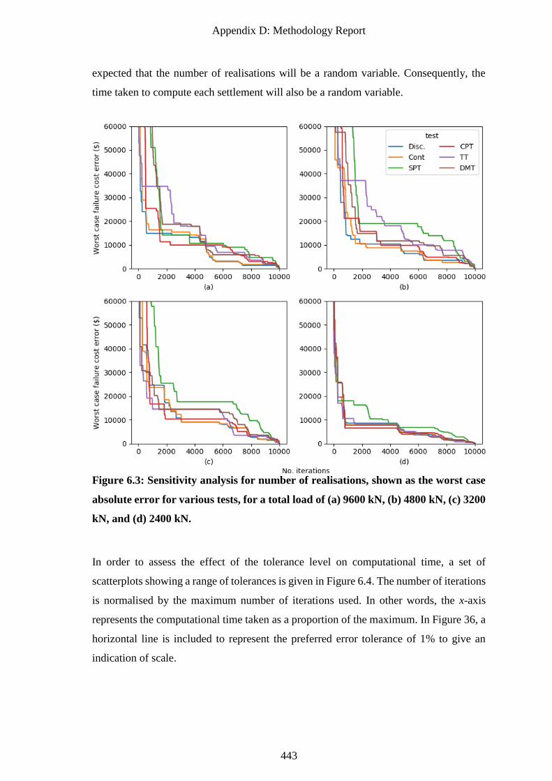
Appendix D: Methodology Report
443
expected that the number of realisations will be a random variable. Consequently, the
time taken to compute each settlement will also be a random variable.
Figure 6.3: Sensitivity analysis for number of realisations, shown as the worst case
absolute error for various tests, for a total load of (a) 9600 kN, (b) 4800 kN, (c) 3200
kN, and (d) 2400 kN.
In order to assess the effect of the tolerance level on computational time, a set of
scatterplots showing a range of tolerances is given in Figure 6.4. The number of iterations
is normalised by the maximum number of iterations used. In other words, the x-axis
represents the computational time taken as a proportion of the maximum. In Figure 36, a
horizontal line is included to represent the preferred error tolerance of 1% to give an
indication of scale.
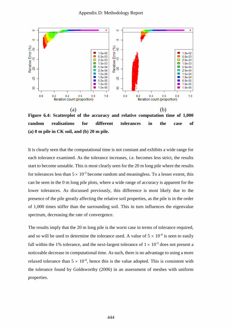
Appendix D: Methodology Report
444
(a) (b) Figure 6.4: Scatterplot of the accuracy and relative computation time of 1,000
random realisations for different tolerances in the case of
(a) 0 m pile in CK soil, and (b) 20 m pile.
It is clearly seen that the computational time is not constant and exhibits a wide range for
each tolerance examined. As the tolerance increases, i.e. becomes less strict, the results
start to become unstable. This is most clearly seen for the 20 m long pile where the results
for tolerances less than 5 10-3 become random and meaningless. To a lesser extent, this
can be seen in the 0 m long pile plots, where a wide range of accuracy is apparent for the
lower tolerances. As discussed previously, this difference is most likely due to the
presence of the pile greatly affecting the relative soil properties, as the pile is in the order
of 1,000 times stiffer than the surrounding soil. This in turn influences the eigenvalue
spectrum, decreasing the rate of convergence.
The results imply that the 20 m long pile is the worst case in terms of tolerance required,
and so will be used to determine the tolerance used. A value of 5 10-4 is seen to easily
fall within the 1% tolerance, and the next-largest tolerance of 1 10-3 does not present a
noticeable decrease in computational time. As such, there is no advantage to using a more
relaxed tolerance than 5 10-4, hence this is the value adopted. This is consistent with
the tolerance found by Goldsworthy (2006) in an assessment of meshes with uniform
properties.
Appendix D: Methodology Report
445
6.3 Program Parallelisation
Monte Carlo analysis lends itself well to various forms of parallelisation, as each
realisation is an independent occurrence that can be run concurrently. Given the
enormous computational times involved with this line of study, parallelisation is essential
for obtaining a rich set of results in a practical timeframe, even with the various
optimizations presented in this report.
The majority of the analyses are intended to be run on the Phoenix High Performance
Computer, owned and used by the University of Adelaide (University of Adelaide 2018).
Currently, Phoenix is a collection of 5,624 cores, 336 GPUs, and 24 TB of RAM. Tasks
are handled by the Slurm Workload Manager (Yoo et al. 2003), allowing programs to be
easily run on a large number of cores, assuming the program is designed to do so.
Traditionally, parallelisation is undertaken with the message passing interface (MPI),
which controls communication to allow a single program to be run concurrently on
multiple processors (Snir 1998). In short, the interface works via a master processor
which sends a subset of information to each of the slave processors, and then receives
and combines the subsequent output. A limitation of MPI is that there tends to be an
optimal number of processors with regards to efficiency. Goldsworthy (2006) observed
that, if fewer than 8 processors are used, then the master processor sits idle while the
slaves conduct the majority of analysis. On the other hand, if more cores are used, then
the master is delayed while compiling the results, explaining the presence of an optimal
configuration.
In the context of the shared nature of Phoenix, MPI has the additional limitation that the
program cannot be started until all cores become available for use. The Slurm manager
also has the tendency to favour small programs over large ones, meaning that there would
be a significant wait time for an MPI program with many cores to commence.
Furthermore, MPI requires intricate modifications to the program to ensure that it is safe
to use in parallel, without any conflicts in processes, random number generation, or
outputs.
To overcome the above limitations, the program was modified such that each realisation
of the analysis is an individual task, i.e. a separate run of the program. This can be used
in conjunction with Slurm’s array functionality, which allows a program to be run in
Appendix D: Methodology Report
446
parallel as individual instances with altered input parameters; in this case the realisation
number. This allows for maximum efficiency, as there is a perfect linear 1:1 relationship
between the number of cores utilised and the increase in computational speed. As the
programs are independent, there is no possibility of conflicting processes. There is also
no limit to the maximum number of realisations undertaken simultaneously. Should the
cores be available, all 1,000 realisations could be executed at once, reducing the total
computational time from potentially weeks to minutes. Furthermore, it does not require
all cores to be available before commencing individual realisations, as they can be
executed as cores become available, reducing the initial wait time.
While this approach to parallelisation does introduce an overhead in terms of setting up
the simulation each time, this pre-calculation step can significantly reduce the overall
simulation time. Data generated in the initial stage are saved in an efficient binary storage.
Use of binary format, as opposed to plain text, allows for maximum read-write speed and
accuracy, as full precision is preserved, and minimum file size.
6.3.1 Parallel Initialisation
An initialisation stage is used for the program to ensure that random processes are truly
independent and to minimise overheads associated with starting individual occurrences.
As each realisation generates a random soil based on a specified random number, care
must be taken to ensure that each realisation is truly unique and random when used in a
parallel context. A solution is to have the initialisation stage generate a list of unique
random seeds, one for each realisation. During the parallel run, the program reads this list
and uses the appropriate seed.
Having an initial run of the program allows for one-off calculations of processes which
are constant throughout the simulation. For example, the LAS algorithm requires the
calculation of a soil correlation matrix, which is then re-used for each realisation. Other
data generation, such as the FEM meshes can also be undertaken at this time. This set of
data can then be quickly read in by each realisation’s program before commencing.
The other benefit is that it allows for the checking of input parameters for conflicts and
compatibilities to ensure that no errors will occur during the actual program run. It is
advantageous to discover input errors immediately, as opposed to some time later when
the program is executed in parallel, or when returning to the computer after expected
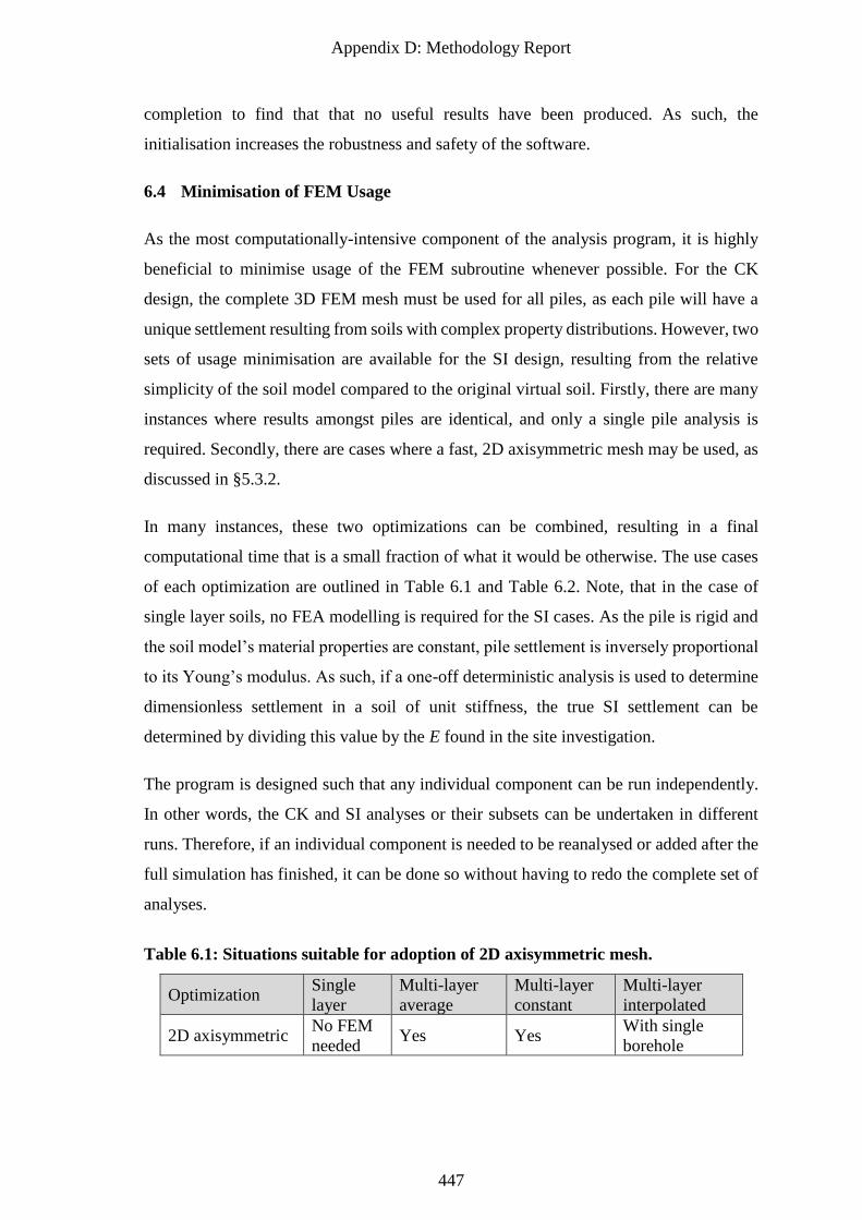
Appendix D: Methodology Report
447
completion to find that that no useful results have been produced. As such, the
initialisation increases the robustness and safety of the software.
6.4 Minimisation of FEM Usage
As the most computationally-intensive component of the analysis program, it is highly
beneficial to minimise usage of the FEM subroutine whenever possible. For the CK
design, the complete 3D FEM mesh must be used for all piles, as each pile will have a
unique settlement resulting from soils with complex property distributions. However, two
sets of usage minimisation are available for the SI design, resulting from the relative
simplicity of the soil model compared to the original virtual soil. Firstly, there are many
instances where results amongst piles are identical, and only a single pile analysis is
required. Secondly, there are cases where a fast, 2D axisymmetric mesh may be used, as
discussed in §5.3.2.
In many instances, these two optimizations can be combined, resulting in a final
computational time that is a small fraction of what it would be otherwise. The use cases
of each optimization are outlined in Table 6.1 and Table 6.2. Note, that in the case of
single layer soils, no FEA modelling is required for the SI cases. As the pile is rigid and
the soil model’s material properties are constant, pile settlement is inversely proportional
to its Young’s modulus. As such, if a one-off deterministic analysis is used to determine
dimensionless settlement in a soil of unit stiffness, the true SI settlement can be
determined by dividing this value by the E found in the site investigation.
The program is designed such that any individual component can be run independently.
In other words, the CK and SI analyses or their subsets can be undertaken in different
runs. Therefore, if an individual component is needed to be reanalysed or added after the
full simulation has finished, it can be done so without having to redo the complete set of
analyses.
Table 6.1: Situations suitable for adoption of 2D axisymmetric mesh.
Optimization Single
layer
Multi-layer
average
Multi-layer
constant
Multi-layer
interpolated
2D axisymmetric No FEM
needed Yes Yes
With single
borehole
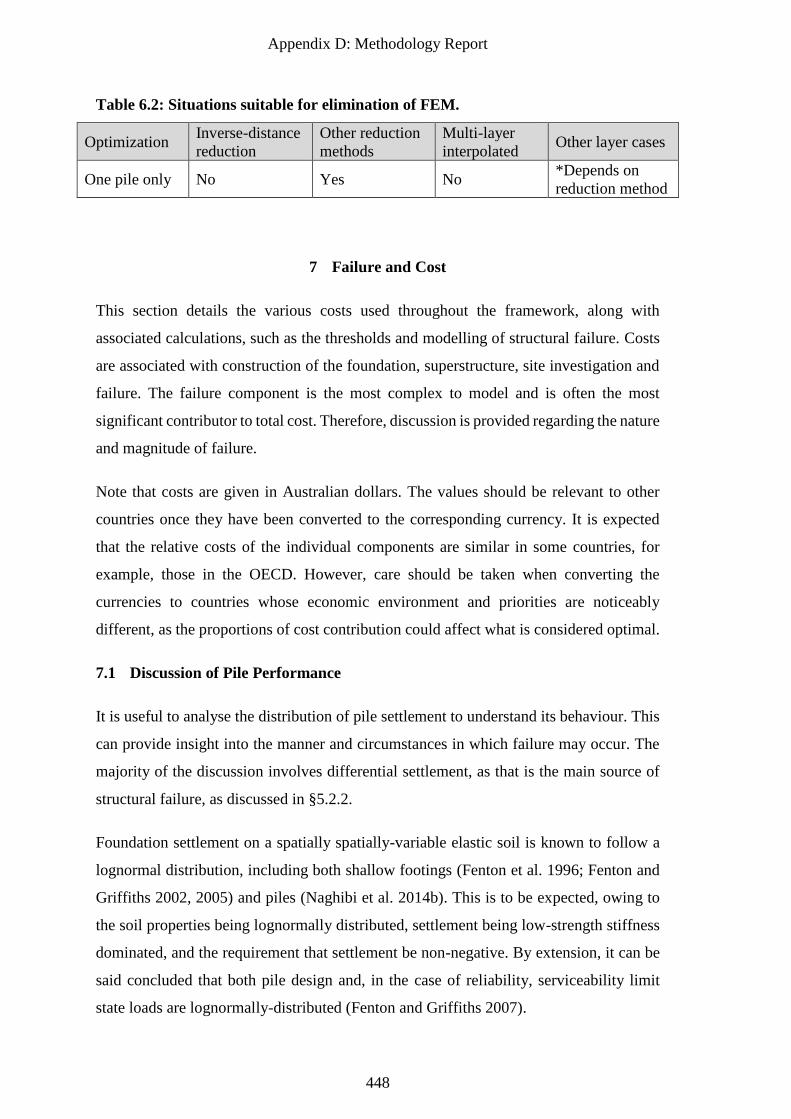
Appendix D: Methodology Report
448
Table 6.2: Situations suitable for elimination of FEM.
Optimization Inverse-distance
reduction
Other reduction
methods
Multi-layer
interpolated Other layer cases
One pile only No Yes No *Depends on
reduction method
7 Failure and Cost
This section details the various costs used throughout the framework, along with
associated calculations, such as the thresholds and modelling of structural failure. Costs
are associated with construction of the foundation, superstructure, site investigation and
failure. The failure component is the most complex to model and is often the most
significant contributor to total cost. Therefore, discussion is provided regarding the nature
and magnitude of failure.
Note that costs are given in Australian dollars. The values should be relevant to other
countries once they have been converted to the corresponding currency. It is expected
that the relative costs of the individual components are similar in some countries, for
example, those in the OECD. However, care should be taken when converting the
currencies to countries whose economic environment and priorities are noticeably
different, as the proportions of cost contribution could affect what is considered optimal.
7.1 Discussion of Pile Performance
It is useful to analyse the distribution of pile settlement to understand its behaviour. This
can provide insight into the manner and circumstances in which failure may occur. The
majority of the discussion involves differential settlement, as that is the main source of
structural failure, as discussed in §5.2.2.
Foundation settlement on a spatially spatially-variable elastic soil is known to follow a
lognormal distribution, including both shallow footings (Fenton et al. 1996; Fenton and
Griffiths 2002, 2005) and piles (Naghibi et al. 2014b). This is to be expected, owing to
the soil properties being lognormally distributed, settlement being low-strength stiffness
dominated, and the requirement that settlement be non-negative. By extension, it can be
said concluded that both pile design and, in the case of reliability, serviceability limit
state loads are lognormally-distributed (Fenton and Griffiths 2007).
Appendix D: Methodology Report
449
The distribution of differential settlement between footings on the other hand is more
difficult to manage. In the case of a stationary field, which should theoretically be the
case with single-layer random fields, the mean differential settlement is zero.
Furthermore, for cases of small scales of fluctuation or soil COV, the COV of pile
settlement will also be small. As a lognormal COV decreases, the distribution begins to
resemble that of a normal case. Therefore, in this situation, the differential settlement will
be normally-distributed (Fenton and Griffiths 2002). However, in the case of larger scales
of fluctuation, the shape of the probability density function diverges from the normal
case.
The details above describe raw differential settlement values between two piles, which is
a relatively simple case. Furthermore, the values have equal likelihood of being positive
or negative depending on the point of reference. As failure occurs when this value
exceeds an absolute threshold, it is appropriate to specify a modulus so that all values are
positive. When the absolute differential settlement is taken for a group of 4 or more piles
in combination, the PDF appears to follow a roughly lognormal distribution. However,
upon closer inspection, there is a more appropriate distribution for this purpose.
There are a series of extreme value distributions that are designed to model the likelihood
of values being the maximum occurrence, in this case differential settlement of a pile
group. The most suitable distribution found for this purpose is that of the Gumbel (Type
I) distribution (Ang and Tang 2007).
The maximum is modelled as follows:
𝐹(𝑥) = exp [−𝑒−𝛼𝑛(𝑥−𝑢𝑛)] (7.1)
And its PDF is:
𝑓(𝑦) = 𝛼𝑛𝑒−𝛼𝑛(𝑥−𝑢𝑛)exp [−𝑒−𝛼𝑛(𝑥−𝑢𝑛)] (7.2)
Where un is the most probable value of the maximums, and αn is the inverse measure of
the dispersion of maxima.
The extreme value distributions are known as asymptotic, as they converge to the true
maximum distribution as the number of variables increases. This implies that the
distribution fit improves as the number of piles, and hence the number of pile
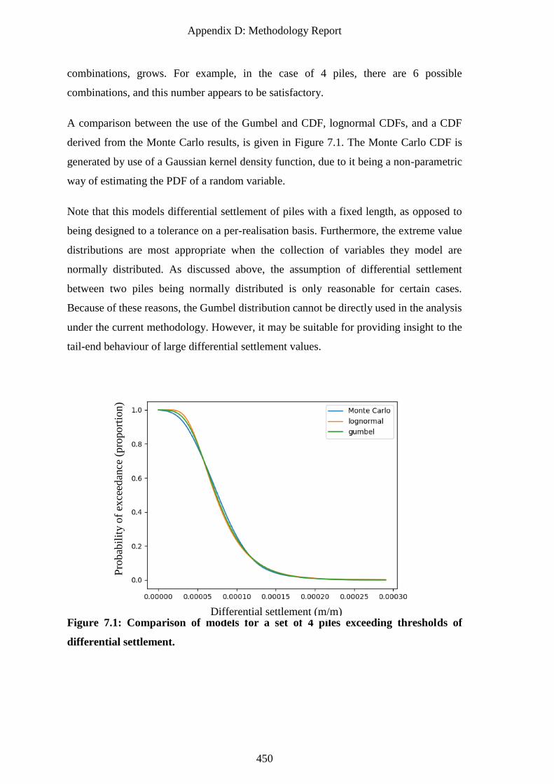
Appendix D: Methodology Report
450
combinations, grows. For example, in the case of 4 piles, there are 6 possible
combinations, and this number appears to be satisfactory.
A comparison between the use of the Gumbel and CDF, lognormal CDFs, and a CDF
derived from the Monte Carlo results, is given in Figure 7.1. The Monte Carlo CDF is
generated by use of a Gaussian kernel density function, due to it being a non-parametric
way of estimating the PDF of a random variable.
Note that this models differential settlement of piles with a fixed length, as opposed to
being designed to a tolerance on a per-realisation basis. Furthermore, the extreme value
distributions are most appropriate when the collection of variables they model are
normally distributed. As discussed above, the assumption of differential settlement
between two piles being normally distributed is only reasonable for certain cases.
Because of these reasons, the Gumbel distribution cannot be directly used in the analysis
under the current methodology. However, it may be suitable for providing insight to the
tail-end behaviour of large differential settlement values.
Figure 7.1: Comparison of models for a set of 4 piles exceeding thresholds of
differential settlement.
Differential settlement (m/m)
Pro
bab
ilit
y o
f ex
ceed
ance
(pro
port
ion)
Appendix D: Methodology Report
451
7.2 Structural Failure
This section details the various ways in which a structure may be damaged due to
foundation failure, various magnitudes of failure, and the applicability of these results to
structures. This framework determines structural damage as realistically as possible
within the constraints of the simplified and generalised analysis. Therefore, discussion of
the feasibility of various modes of failure is required.
Furthermore, the cost of repairing a structure is related to the degree of structural damage.
For example, minor damage requires a modest repair with a low associated cost. To
reflect this relationship, a series of damage categories are specified. Of equal importance
is the choice of design criteria used to determine pile length. The magnitude of the design
tolerance affects how conservative the designs are and hence their likelihood of failure.
It is important to remember that there are many different configurations of buildings,
regarding their shape, type and construction material. The analysis in this framework does
not distinguish between them. Therefore, discussion is provided as to how these results
can be interpreted by practising engineers.
7.2.1 Design Criteria
As discussed in §5.2, the pile performance model used in this framework is capable solely
of determining settlement, as opposed to total capacity. This limits potential modes of
failure to those which can be represented in terms of settlement values. The previous line
of research in this field undertaken by Goldsworthy used differential settlement as the
sole design criterion, despite a range of available choices, with minimal justification. As
such, this subsection discusses potential modes of failure that may be captured.
In Goldsworthy (2006), differential settlement was the sole design criterion used.
Foundation design was undertaken according to a tolerance of 0.0025C, where C is the
centre-to-centre foundation spacing. For the 10 m spacing used throughout the research,
this corresponded to an absolute settlement design tolerance of 25 mm.
As discussed in §5.2, it has been shown that between absolute settlement and differential
settlement, the latter is the leading cause of structural failure. However, the former is still
an important consideration for some aspects of design, such as drainage and building
Appendix D: Methodology Report
452
access. As such, it is common practice for foundations to be designed according to both
failure modes, where the limiting value (in terms of absolute settlement) is dominant.
Alternatively, absolute settlement may be limited to a relatively small value such that the
likelihood of differential settlement is negligible.
Regarding absolute settlement tolerances suggested for various design components, it can
be seen in Table 7.1, that the absolute settlement values are quite large. As such, the
differential settlement tolerances most certainly dominate design, except in the case of
large foundation spacing in the order of 40 m or greater. This is double the spacing
considered within this framework. As such, the absolute settlement criterion will not be
used within the design process.
The choice of a specific threshold for differential settlement is more difficult and requires
discussion, as a range of values are possible. It should be noted that the threshold for
structural damage in this framework is known. As discussed in §7.3.1, it varies slightly
with building height, but is generally 0.003 ± 0.00005C. As such, the design tolerance
must be equal to or lower than 0.003C.
Table 7.1: Allowable settlement, after Sowers (1962).
Settlement Type Limiting factor Maximum settlement
Total
Drainage 150–300 mm
Access 300–600 mm
Probability of differential
settlement (framed structures)
50–100 mm
Differential
Reinforced concrete building
frame
0.0025–0.004C
Steel frame, continuous 0.002C
Regarding the more conservative end of the range, a limit of 0.002C is suggested for steel
frame structures, and also recommended as a general limit by Skempton and MacDonald
(1956) based on observed damage of buildings. However, it has been suggested that
changes in construction materials and practices since these studies were conducted has
led to structures being more robust and easier-to-repair, resulting in the 0.002C value
being overly-conservative (Salgado 2008). As such, a design threshold would ideally be
higher than this value.
As a mid-range option, the choice of 0.0025C as a design value has several advantages:
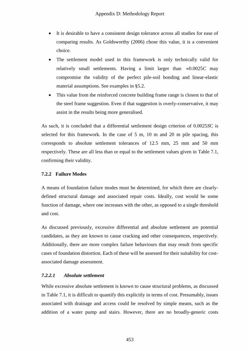
Appendix D: Methodology Report
453
• It is desirable to have a consistent design tolerance across all studies for ease of
comparing results. As Goldsworthy (2006) chose this value, it is a convenient
choice.
• The settlement model used in this framework is only technically valid for
relatively small settlements. Having a limit larger than 0.0025C may
compromise the validity of the perfect pile-soil bonding and linear-elastic
material assumptions. See examples in §5.2.
• This value from the reinforced concrete building frame range is closest to that of
the steel frame suggestion. Even if that suggestion is overly-conservative, it may
assist in the results being more generalised.
As such, it is concluded that a differential settlement design criterion of 0.0025SC is
selected for this framework. In the case of 5 m, 10 m and 20 m pile spacing, this
corresponds to absolute settlement tolerances of 12.5 mm, 25 mm and 50 mm
respectively. These are all less than or equal to the settlement values given in Table 7.1,
confirming their validity.
7.2.2 Failure Modes
A means of foundation failure modes must be determined, for which there are clearly-
defined structural damage and associated repair costs. Ideally, cost would be some
function of damage, where one increases with the other, as opposed to a single threshold
and cost.
As discussed previously, excessive differential and absolute settlement are potential
candidates, as they are known to cause cracking and other consequences, respectively.
Additionally, there are more complex failure behaviours that may result from specific
cases of foundation distortion. Each of these will be assessed for their suitability for cost-
associated damage assessment.
7.2.2.1 Absolute settlement
While excessive absolute settlement is known to cause structural problems, as discussed
in Table 7.1, it is difficult to quantify this explicitly in terms of cost. Presumably, issues
associated with drainage and access could be resolved by simple means, such as the
addition of a water pump and stairs. However, there are no broadly-generic costs
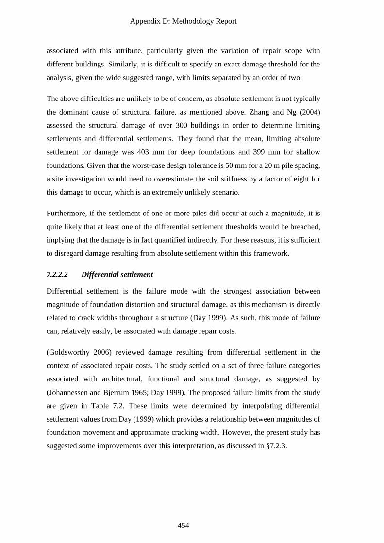
Appendix D: Methodology Report
454
associated with this attribute, particularly given the variation of repair scope with
different buildings. Similarly, it is difficult to specify an exact damage threshold for the
analysis, given the wide suggested range, with limits separated by an order of two.
The above difficulties are unlikely to be of concern, as absolute settlement is not typically
the dominant cause of structural failure, as mentioned above. Zhang and Ng (2004)
assessed the structural damage of over 300 buildings in order to determine limiting
settlements and differential settlements. They found that the mean, limiting absolute
settlement for damage was 403 mm for deep foundations and 399 mm for shallow
foundations. Given that the worst-case design tolerance is 50 mm for a 20 m pile spacing,
a site investigation would need to overestimate the soil stiffness by a factor of eight for
this damage to occur, which is an extremely unlikely scenario.
Furthermore, if the settlement of one or more piles did occur at such a magnitude, it is
quite likely that at least one of the differential settlement thresholds would be breached,
implying that the damage is in fact quantified indirectly. For these reasons, it is sufficient
to disregard damage resulting from absolute settlement within this framework.
7.2.2.2 Differential settlement
Differential settlement is the failure mode with the strongest association between
magnitude of foundation distortion and structural damage, as this mechanism is directly
related to crack widths throughout a structure (Day 1999). As such, this mode of failure
can, relatively easily, be associated with damage repair costs.
(Goldsworthy 2006) reviewed damage resulting from differential settlement in the
context of associated repair costs. The study settled on a set of three failure categories
associated with architectural, functional and structural damage, as suggested by
(Johannessen and Bjerrum 1965; Day 1999). The proposed failure limits from the study
are given in Table 7.2. These limits were determined by interpolating differential
settlement values from Day (1999) which provides a relationship between magnitudes of
foundation movement and approximate cracking width. However, the present study has
suggested some improvements over this interpretation, as discussed in §7.2.3.
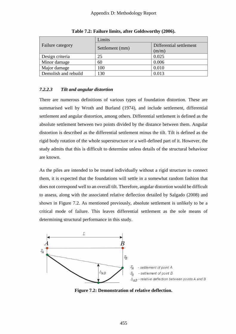
Appendix D: Methodology Report
455
Table 7.2: Failure limits, after Goldsworthy (2006).
Failure category
Limits
Settlement (mm) Differential settlement
(m/m)
Design criteria 25 0.025
Minor damage 60 0.006
Major damage 100 0.010
Demolish and rebuild 130 0.013
7.2.2.3 Tilt and angular distortion
There are numerous definitions of various types of foundation distortion. These are
summarised well by Wroth and Burland (1974), and include settlement, differential
settlement and angular distortion, among others. Differential settlement is defined as the
absolute settlement between two points divided by the distance between them. Angular
distortion is described as the differential settlement minus the tilt. Tilt is defined as the
rigid body rotation of the whole superstructure or a well-defined part of it. However, the
study admits that this is difficult to determine unless details of the structural behaviour
are known.
As the piles are intended to be treated individually without a rigid structure to connect
them, it is expected that the foundations will settle in a somewhat random fashion that
does not correspond well to an overall tilt. Therefore, angular distortion would be difficult
to assess, along with the associated relative deflection detailed by Salgado (2008) and
shown in Figure 7.2. As mentioned previously, absolute settlement is unlikely to be a
critical mode of failure. This leaves differential settlement as the sole means of
determining structural performance in this study.
Figure 7.2: Demonstration of relative deflection.
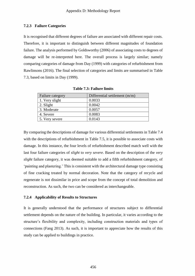
Appendix D: Methodology Report
456
7.2.3 Failure Categories
It is recognised that different degrees of failure are associated with different repair costs.
Therefore, it is important to distinguish between different magnitudes of foundation
failure. The analysis performed by Goldsworthy (2006) of associating costs to degrees of
damage will be re-interpreted here. The overall process is largely similar; namely
comparing categories of damage from Day (1999) with categories of refurbishment from
Rawlinsons (2016). The final selection of categories and limits are summarised in Table
7.3, based on limits in Day (1999).
Table 7.3: Failure limits
Failure category Differential settlement (m/m)
1. Very slight 0.0033
2. Slight 0.0042
3. Moderate 0.0057
4. Severe 0.0083
5. Very severe 0.0143
By comparing the descriptions of damage for various differential settlements in Table 7.4
with the descriptions of refurbishment in Table 7.5, it is possible to associate costs with
damage. In this instance, the four levels of refurbishment described match well with the
last four failure categories of slight to very severe. Based on the description of the very
slight failure category, it was deemed suitable to add a fifth refurbishment category, of
‘painting and plastering.’ This is consistent with the architectural damage type consisting
of fine cracking treated by normal decoration. Note that the category of recycle and
regenerate is not dissimilar in price and scope from the concept of total demolition and
reconstruction. As such, the two can be considered as interchangeable.
7.2.4 Applicability of Results to Structures
It is generally understood that the performance of structures subject to differential
settlement depends on the nature of the building. In particular, it varies according to the
structure’s flexibility and complexity, including construction materials and types of
connections (Fang 2013). As such, it is important to appreciate how the results of this
study can be applied to buildings in practice.
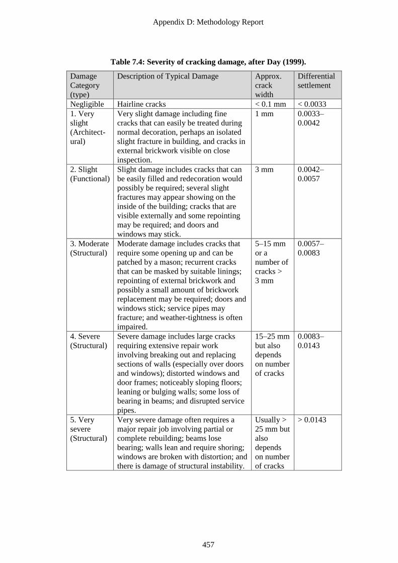
Appendix D: Methodology Report
457
Table 7.4: Severity of cracking damage, after Day (1999).
Damage
Category
(type)
Description of Typical Damage Approx.
crack
width
Differential
settlement
Negligible Hairline cracks < 0.1 mm < 0.0033
1. Very
slight
(Architect-
ural)
Very slight damage including fine
cracks that can easily be treated during
normal decoration, perhaps an isolated
slight fracture in building, and cracks in
external brickwork visible on close
inspection.
1 mm 0.0033–
0.0042
2. Slight
(Functional)
Slight damage includes cracks that can
be easily filled and redecoration would
possibly be required; several slight
fractures may appear showing on the
inside of the building; cracks that are
visible externally and some repointing
may be required; and doors and
windows may stick.
3 mm 0.0042–
0.0057
3. Moderate
(Structural)
Moderate damage includes cracks that
require some opening up and can be
patched by a mason; recurrent cracks
that can be masked by suitable linings;
repointing of external brickwork and
possibly a small amount of brickwork
replacement may be required; doors and
windows stick; service pipes may
fracture; and weather-tightness is often
impaired.
5–15 mm
or a
number of
cracks >
3 mm
0.0057–
0.0083
4. Severe
(Structural)
Severe damage includes large cracks
requiring extensive repair work
involving breaking out and replacing
sections of walls (especially over doors
and windows); distorted windows and
door frames; noticeably sloping floors;
leaning or bulging walls; some loss of
bearing in beams; and disrupted service
pipes.
15–25 mm
but also
depends
on number
of cracks
0.0083–
0.0143
5. Very
severe
(Structural)
Very severe damage often requires a
major repair job involving partial or
complete rebuilding; beams lose
bearing; walls lean and require shoring;
windows are broken with distortion; and
there is damage of structural instability.
Usually >
25 mm but
also
depends
on number
of cracks
> 0.0143
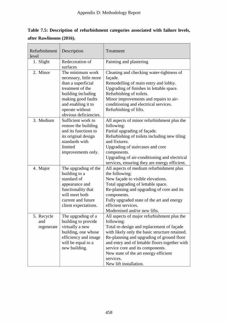
Appendix D: Methodology Report
458
Table 7.5: Description of refurbishment categories associated with failure levels,
after Rawlinsons (2016).
Refurbishment
level
Description Treatment
1. Slight Redecoration of
surfaces
Painting and plastering
2. Minor The minimum work
necessary, little more
than a superficial
treatment of the
building including
making good faults
and enabling it to
operate without
obvious deficiencies.
Cleaning and checking water-tightness of
façade.
Remodelling of main entry and lobby.
Upgrading of finishes in lettable space.
Refurbishing of toilets.
Minor improvements and repairs to air-
conditioning and electrical services.
Refurbishing of lifts.
3. Medium Sufficient work to
restore the building
and its functions to
its original design
standards with
limited
improvements only.
All aspects of minor refurbishment plus the
following:
Partial upgrading of façade.
Refurbishing of toilets including new tiling
and fixtures.
Upgrading of staircases and core
components.
Upgrading of air-conditioning and electrical
services, ensuring they are energy efficient.
4. Major The upgrading of the
building to a
standard of
appearance and
functionality that
will meet both
current and future
client expectations.
All aspects of medium refurbishment plus
the following:
New façade to visible elevations.
Total upgrading of lettable space.
Re-planning and upgrading of core and its
components.
Fully upgraded state of the art and energy
efficient services.
Modernised and/or new lifts.
5. Recycle
and
regenerate
The upgrading of a
building to provide
virtually a new
building, one whose
efficiency and image
will be equal to a
new building.
All aspects of major refurbishment plus the
following:
Total re-design and replacement of façade
with likely only the basic structure retained.
Re-planning and upgrading of ground floor
and entry and of lettable floors together with
service core and its components.
New state of the art energy efficient
services.
New lift installation.
Appendix D: Methodology Report
459
The damage categories in Day (1999) are supported by Thorburn (1985), who linked
serviceability or safety issues directly to crack width for a range of structural
classifications, as seen in Table 7.5. This includes residential, commercial and industrial
categories in increasing order of resilience. It should be noted that commercial buildings,
specifically offices, are the main focus of this study, as described in §7.3.3.
There is some discrepancy between the descriptions of damage in Table 7.4 and Table
7.6. Namely, “serviceability may be compromised” with a damage classification as
minimal as slight, as seen in the industrial case in Table 7.6. In contrast, the slight
category in Table 7.4 corresponds to largely aesthetic and potentially functional damage
without risk to the underlying structure. Furthermore in Table 7.6, the ultimate limit state
may be reached in the moderate category, and risk of collapse may be present in the
severe. This implies that the descriptions of typical damage given in the bottom 2-3 rows
of Table 7.4 may be underestimated. However, given the range of building types included
in the description, it should only be taken as an approximate guide. It can also be seen
that a range of categories are given for a particular crack width. For example, in Table
7.6 cracks larger than 15 mm in commercial buildings are said to be in any category from
moderate to very severe.
There is further evidence to suggest that the effect of differential settlement on buildings
can vary wildly. As mentioned above, Zhang and Ng (2004) found that buildings with
deep foundations had a mean intolerable settlement of 404 mm, with a standard deviation
of 384 mm. The observed intolerable differential settlement was 0.0107, with a standard
deviation of 0.0155. Both cases are lognormally-distributed with COVs in the order of
100%, which is considered extremely variable.
Skempton and MacDonald (1956) determined allowable settlement limits by empirical
analysis of failed buildings in a similar manner to the failure limits presented in Day
(1999). However, Wroth and Burland (1974) used theory derived from a beam analogy.
In the latter case, factors such the structure’s shear and elastic moduli, along with its
length and height, facilitated the determination of a critical tensile strain where cracking
begins. It was found that buildings responded differently to differential settlements
depending on the ratio of their stiffness in shear to their stiffness in bending. The results
were described in terms of relative deflection to length-to-height ratio of a wall.
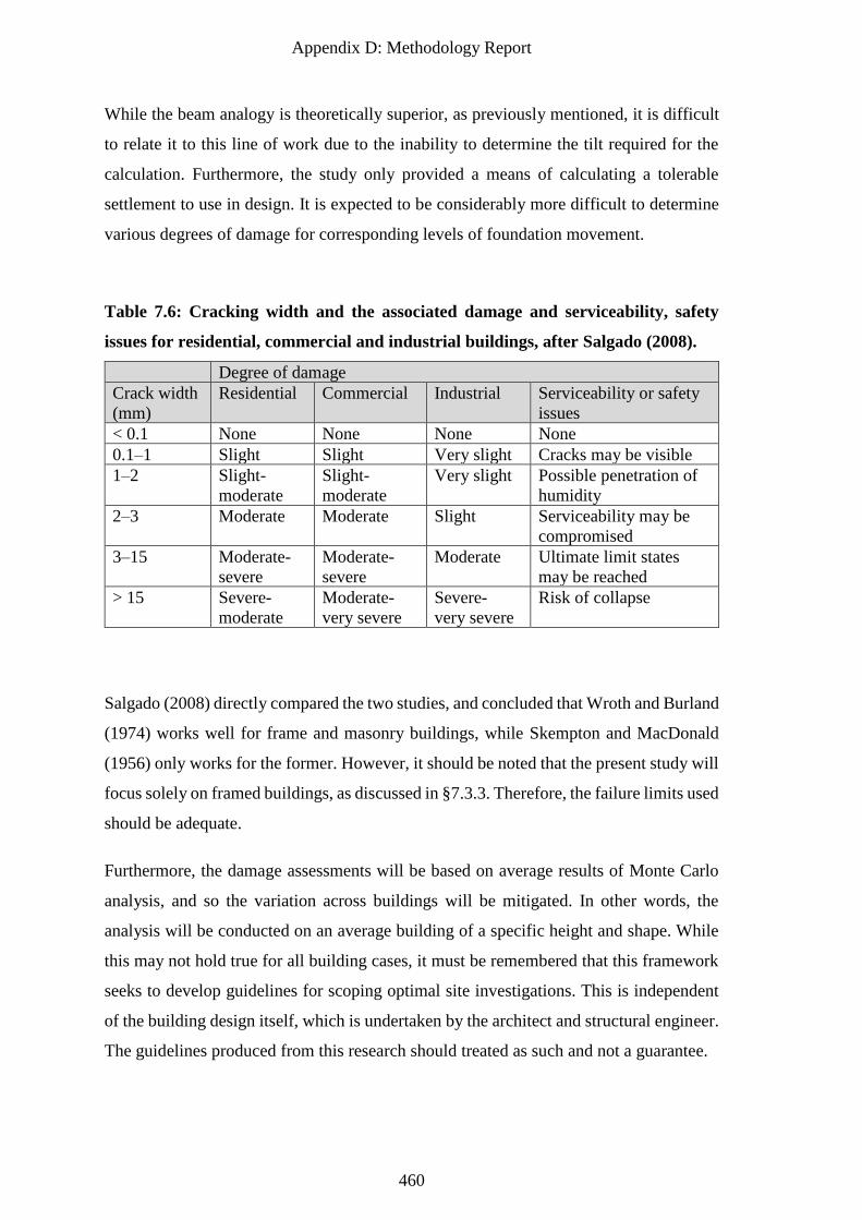
Appendix D: Methodology Report
460
While the beam analogy is theoretically superior, as previously mentioned, it is difficult
to relate it to this line of work due to the inability to determine the tilt required for the
calculation. Furthermore, the study only provided a means of calculating a tolerable
settlement to use in design. It is expected to be considerably more difficult to determine
various degrees of damage for corresponding levels of foundation movement.
Table 7.6: Cracking width and the associated damage and serviceability, safety
issues for residential, commercial and industrial buildings, after Salgado (2008).
Degree of damage
Crack width
(mm)
Residential Commercial Industrial Serviceability or safety
issues
< 0.1 None None None None
0.1–1 Slight Slight Very slight Cracks may be visible
1–2 Slight-
moderate
Slight-
moderate
Very slight Possible penetration of
humidity
2–3 Moderate Moderate Slight Serviceability may be
compromised
3–15 Moderate-
severe
Moderate-
severe
Moderate Ultimate limit states
may be reached
> 15 Severe-
moderate
Moderate-
very severe
Severe-
very severe
Risk of collapse
Salgado (2008) directly compared the two studies, and concluded that Wroth and Burland
(1974) works well for frame and masonry buildings, while Skempton and MacDonald
(1956) only works for the former. However, it should be noted that the present study will
focus solely on framed buildings, as discussed in §7.3.3. Therefore, the failure limits used
should be adequate.
Furthermore, the damage assessments will be based on average results of Monte Carlo
analysis, and so the variation across buildings will be mitigated. In other words, the
analysis will be conducted on an average building of a specific height and shape. While
this may not hold true for all building cases, it must be remembered that this framework
seeks to develop guidelines for scoping optimal site investigations. This is independent
of the building design itself, which is undertaken by the architect and structural engineer.
The guidelines produced from this research should treated as such and not a guarantee.
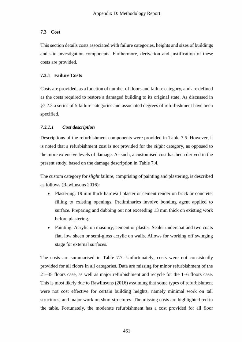
Appendix D: Methodology Report
461
7.3 Cost
This section details costs associated with failure categories, heights and sizes of buildings
and site investigation components. Furthermore, derivation and justification of these
costs are provided.
7.3.1 Failure Costs
Costs are provided, as a function of number of floors and failure category, and are defined
as the costs required to restore a damaged building to its original state. As discussed in
§7.2.3 a series of 5 failure categories and associated degrees of refurbishment have been
specified.
7.3.1.1 Cost description
Descriptions of the refurbishment components were provided in Table 7.5. However, it
is noted that a refurbishment cost is not provided for the slight category, as opposed to
the more extensive levels of damage. As such, a customised cost has been derived in the
present study, based on the damage description in Table 7.4.
The custom category for slight failure, comprising of painting and plastering, is described
as follows (Rawlinsons 2016):
• Plastering: 19 mm thick hardwall plaster or cement render on brick or concrete,
filling to existing openings. Preliminaries involve bonding agent applied to
surface. Preparing and dubbing out not exceeding 13 mm thick on existing work
before plastering.
• Painting: Acrylic on masonry, cement or plaster. Sealer undercoat and two coats
flat, low sheen or semi-gloss acrylic on walls. Allows for working off swinging
stage for external surfaces.
The costs are summarised in Table 7.7. Unfortunately, costs were not consistently
provided for all floors in all categories. Data are missing for minor refurbishment of the
21–35 floors case, as well as major refurbishment and recycle for the 1–6 floors case.
This is most likely due to Rawlinsons (2016) assuming that some types of refurbishment
were not cost effective for certain building heights, namely minimal work on tall
structures, and major work on short structures. The missing costs are highlighted red in
the table. Fortunately, the moderate refurbishment has a cost provided for all floor
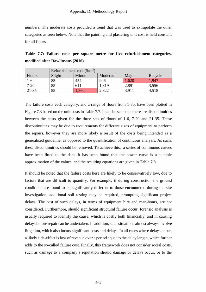
Appendix D: Methodology Report
462
numbers. The moderate costs provided a trend that was used to extrapolate the other
categories as seen below. Note that the painting and plastering unit cost is held constant
for all floors.
Table 7.7: Failure costs per square metre for five refurbishment categories,
modified after Rawlinsons (2016)
The failure costs each category, and a range of floors from 1-35, have been plotted in
Figure 7.3 based on the unit costs in Table 7.7. It can be seen that there are discontinuities
between the costs given for the three sets of floors of 1-6, 7-20 and 21-35. These
discontinuities may be due to requirements for different sizes of equipment to perform
the repairs, however they are more likely a result of the costs being intended as a
generalised guideline, as opposed to the quantification of continuous analysis. As such,
these discontinuities should be removed. To achieve this, a series of continuous curves
have been fitted to the data. It has been found that the power curve is a suitable
approximation of the values, and the resulting equations are given in Table 7.8.
It should be noted that the failure costs here are likely to be conservatively low, due to
factors that are difficult to quantify. For example, if during construction the ground
conditions are found to be significantly different to those encountered during the site
investigation, additional soil testing may be required, prompting significant project
delays. The cost of such delays, in terms of equipment hire and man-hours, are not
considered. Furthermore, should significant structural failure occur, forensic analysis is
usually required to identify the cause, which is costly both financially, and in causing
delays before repair can be undertaken. In addition, such situations almost always involve
litigation, which also incurs significant costs and delays. In all cases where delays occur,
a likely side-effect is loss of revenue over a period equal to the delay length, which further
adds to the so-called failure cost. Finally, this framework does not consider social costs,
such as damage to a company’s reputation should damage or delays occur, or to the
Refurbishment cost ($/m2)
Floors Slight Minor Moderate Major Recycle
1-6 85 454 906 1,620 1,947
7-20 85 611 1,319 2,891 3,556
21-35 85 1,360 2,822 3,911 4,518
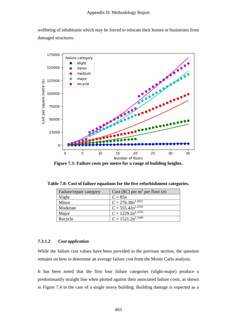
Appendix D: Methodology Report
463
wellbeing of inhabitants which may be forced to relocate their homes or businesses from
damaged structures.
Figure 7.3: Failure costs per metre for a range of building heights.
Table 7.8: Cost of failure equations for the five refurbishment categories.
Failure/repair category Cost ($C) per m2 per floor (n)
Slight C = 85n
Minor C = 276.38n1.4021
Moderate C = 555.42n1.4192
Major C = 1229.2n1.3376
Recycle C = 1521.2n1.3249
7.3.1.2 Cost application
While the failure cost values have been provided in the previous section, the question
remains on how to determine an average failure cost from the Monte Carlo analysis.
It has been noted that the first four failure categories (slight-major) produce a
predominantly straight line when plotted against their associated failure costs, as shown
in Figure 7.4 in the case of a single storey building. Building damage is expected as a
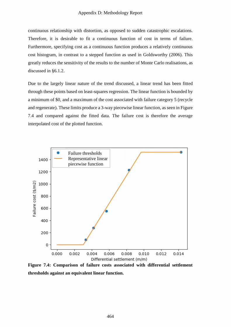
Appendix D: Methodology Report
464
continuous relationship with distortion, as opposed to sudden catastrophic escalations.
Therefore, it is desirable to fit a continuous function of cost in terms of failure.
Furthermore, specifying cost as a continuous function produces a relatively continuous
cost histogram, in contrast to a stepped function as used in Goldsworthy (2006). This
greatly reduces the sensitivity of the results to the number of Monte Carlo realisations, as
discussed in §6.1.2.
Due to the largely linear nature of the trend discussed, a linear trend has been fitted
through these points based on least-squares regression. The linear function is bounded by
a minimum of $0, and a maximum of the cost associated with failure category 5 (recycle
and regenerate). These limits produce a 3-way piecewise linear function, as seen in Figure
7.4 and compared against the fitted data. The failure cost is therefore the average
interpolated cost of the plotted function.
Figure 7.4: Comparison of failure costs associated with differential settlement
thresholds against an equivalent linear function.
Failure thresholds
Representative linear
piecewise function
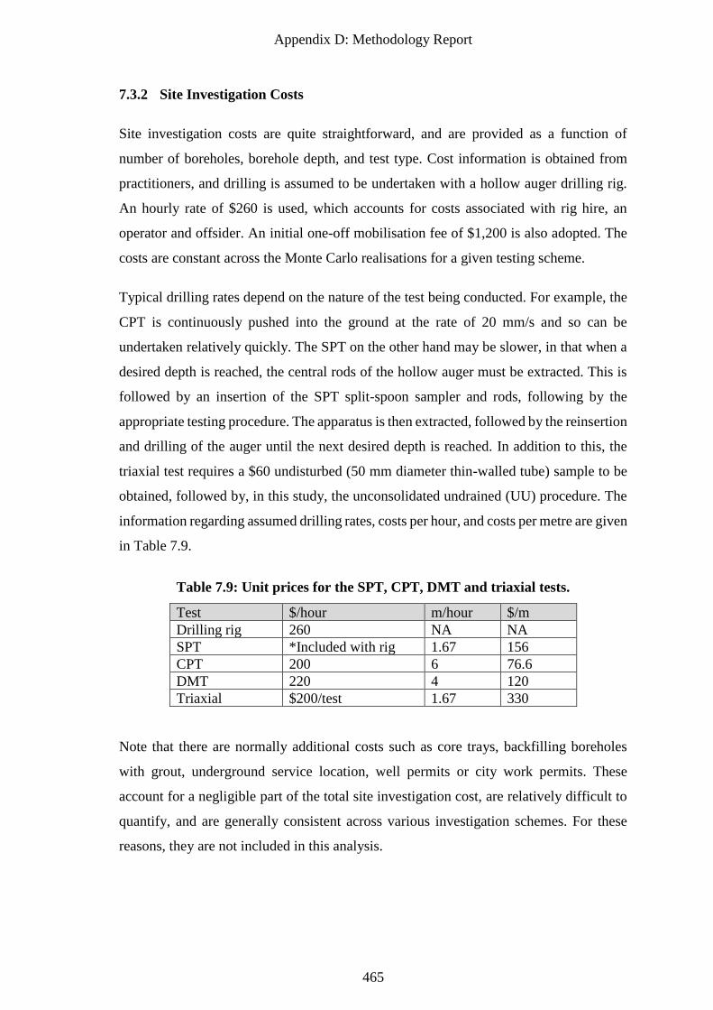
Appendix D: Methodology Report
465
7.3.2 Site Investigation Costs
Site investigation costs are quite straightforward, and are provided as a function of
number of boreholes, borehole depth, and test type. Cost information is obtained from
practitioners, and drilling is assumed to be undertaken with a hollow auger drilling rig.
An hourly rate of $260 is used, which accounts for costs associated with rig hire, an
operator and offsider. An initial one-off mobilisation fee of $1,200 is also adopted. The
costs are constant across the Monte Carlo realisations for a given testing scheme.
Typical drilling rates depend on the nature of the test being conducted. For example, the
CPT is continuously pushed into the ground at the rate of 20 mm/s and so can be
undertaken relatively quickly. The SPT on the other hand may be slower, in that when a
desired depth is reached, the central rods of the hollow auger must be extracted. This is
followed by an insertion of the SPT split-spoon sampler and rods, following by the
appropriate testing procedure. The apparatus is then extracted, followed by the reinsertion
and drilling of the auger until the next desired depth is reached. In addition to this, the
triaxial test requires a $60 undisturbed (50 mm diameter thin-walled tube) sample to be
obtained, followed by, in this study, the unconsolidated undrained (UU) procedure. The
information regarding assumed drilling rates, costs per hour, and costs per metre are given
in Table 7.9.
Table 7.9: Unit prices for the SPT, CPT, DMT and triaxial tests.
Test $/hour m/hour $/m
Drilling rig 260 NA NA
SPT *Included with rig 1.67 156
CPT 200 6 76.6
DMT 220 4 120
Triaxial $200/test 1.67 330
Note that there are normally additional costs such as core trays, backfilling boreholes
with grout, underground service location, well permits or city work permits. These
account for a negligible part of the total site investigation cost, are relatively difficult to
quantify, and are generally consistent across various investigation schemes. For these
reasons, they are not included in this analysis.
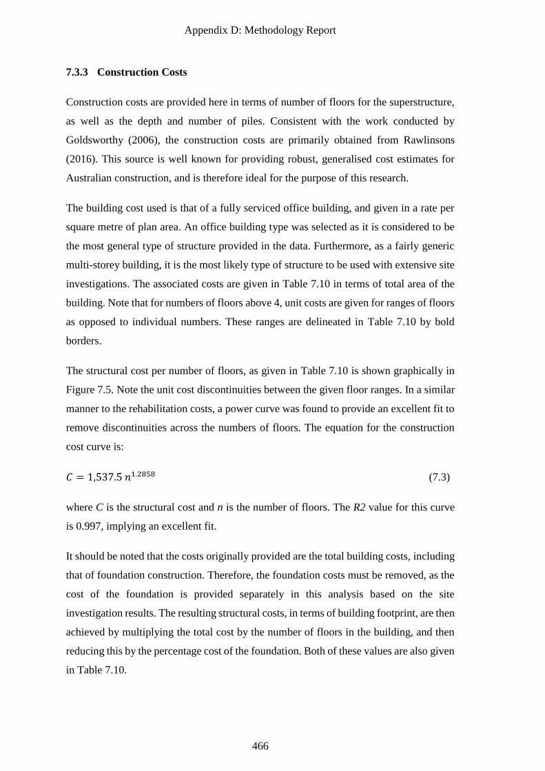
Appendix D: Methodology Report
466
7.3.3 Construction Costs
Construction costs are provided here in terms of number of floors for the superstructure,
as well as the depth and number of piles. Consistent with the work conducted by
Goldsworthy (2006), the construction costs are primarily obtained from Rawlinsons
(2016). This source is well known for providing robust, generalised cost estimates for
Australian construction, and is therefore ideal for the purpose of this research.
The building cost used is that of a fully serviced office building, and given in a rate per
square metre of plan area. An office building type was selected as it is considered to be
the most general type of structure provided in the data. Furthermore, as a fairly generic
multi-storey building, it is the most likely type of structure to be used with extensive site
investigations. The associated costs are given in Table 7.10 in terms of total area of the
building. Note that for numbers of floors above 4, unit costs are given for ranges of floors
as opposed to individual numbers. These ranges are delineated in Table 7.10 by bold
borders.
The structural cost per number of floors, as given in Table 7.10 is shown graphically in
Figure 7.5. Note the unit cost discontinuities between the given floor ranges. In a similar
manner to the rehabilitation costs, a power curve was found to provide an excellent fit to
remove discontinuities across the numbers of floors. The equation for the construction
cost curve is:
𝐶 = 1,537.5 𝑛1.2858 (7.3)
where C is the structural cost and n is the number of floors. The R2 value for this curve
is 0.997, implying an excellent fit.
It should be noted that the costs originally provided are the total building costs, including
that of foundation construction. Therefore, the foundation costs must be removed, as the
cost of the foundation is provided separately in this analysis based on the site
investigation results. The resulting structural costs, in terms of building footprint, are then
achieved by multiplying the total cost by the number of floors in the building, and then
reducing this by the percentage cost of the foundation. Both of these values are also given
in Table 7.10.
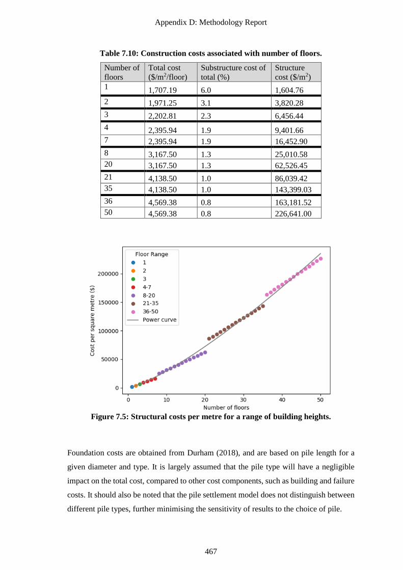
Appendix D: Methodology Report
467
Table 7.10: Construction costs associated with number of floors.
Number of
floors
Total cost
($/m2/floor)
Substructure cost of
total (%)
Structure
cost ($/m2)
1 1,707.19 6.0 1,604.76
2 1,971.25 3.1 3,820.28
3 2,202.81 2.3 6,456.44
4 2,395.94 1.9 9,401.66
7 2,395.94 1.9 16,452.90
8 3,167.50 1.3 25,010.58
20 3,167.50 1.3 62,526.45
21 4,138.50 1.0 86,039.42
35 4,138.50 1.0 143,399.03
36 4,569.38 0.8 163,181.52
50 4,569.38 0.8 226,641.00
Figure 7.5: Structural costs per metre for a range of building heights.
Foundation costs are obtained from Durham (2018), and are based on pile length for a
given diameter and type. It is largely assumed that the pile type will have a negligible
impact on the total cost, compared to other cost components, such as building and failure
costs. It should also be noted that the pile settlement model does not distinguish between
different pile types, further minimising the sensitivity of results to the choice of pile.
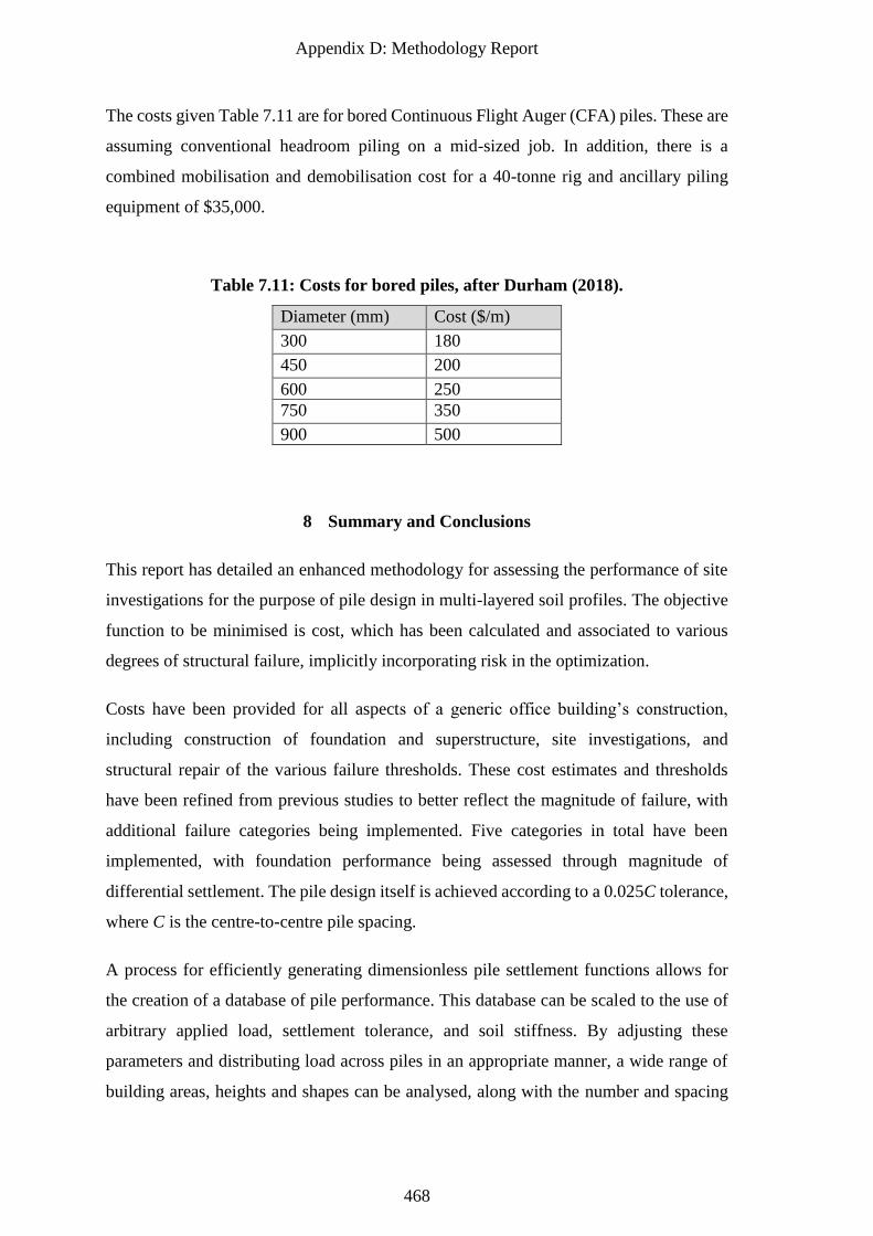
Appendix D: Methodology Report
468
The costs given Table 7.11 are for bored Continuous Flight Auger (CFA) piles. These are
assuming conventional headroom piling on a mid-sized job. In addition, there is a
combined mobilisation and demobilisation cost for a 40-tonne rig and ancillary piling
equipment of $35,000.
Table 7.11: Costs for bored piles, after Durham (2018).
Diameter (mm) Cost ($/m)
300 180
450 200
600 250
750 350
900 500
8 Summary and Conclusions
This report has detailed an enhanced methodology for assessing the performance of site
investigations for the purpose of pile design in multi-layered soil profiles. The objective
function to be minimised is cost, which has been calculated and associated to various
degrees of structural failure, implicitly incorporating risk in the optimization.
Costs have been provided for all aspects of a generic office building’s construction,
including construction of foundation and superstructure, site investigations, and
structural repair of the various failure thresholds. These cost estimates and thresholds
have been refined from previous studies to better reflect the magnitude of failure, with
additional failure categories being implemented. Five categories in total have been
implemented, with foundation performance being assessed through magnitude of
differential settlement. The pile design itself is achieved according to a 0.025C tolerance,
where C is the centre-to-centre pile spacing.
A process for efficiently generating dimensionless pile settlement functions allows for
the creation of a database of pile performance. This database can be scaled to the use of
arbitrary applied load, settlement tolerance, and soil stiffness. By adjusting these
parameters and distributing load across piles in an appropriate manner, a wide range of
building areas, heights and shapes can be analysed, along with the number and spacing
Appendix D: Methodology Report
469
of piles. As the effect of varying applied load can be determined, the incorporation of
reliability-based design can be incorporated into the framework through the assessment
of load redundancy. These settlement functions, as the product of the core analysis, serve
as a re-usable database of pile information. This database can be used by other
researchers, which may save months of computation in the best case. In the worst case,
sufficient computational resources required for such an analysis may not be present, and
this database opens the doors to research that may not otherwise be possible. The
generation and use of these settlement functions serves as one of the major innovations
of this report.
It was determined that, in order to generate pile settlement functions of sufficient
accuracy on a continuous scale, settlement information is required at 1 m intervals. For
the chosen maximum pile length of 20 m, this results in 21 settlements generated through
the use of 3D linear-elastic finite element analysis (FEA). The linear-elastic assumption
is not strictly correct for modelling complex materials such as soils. However, a wealth
of literature supports that it is sufficient for the purpose of this study, particularly when
considering the computationally-intensive nature of more advanced methods. Perhaps
more importantly, it facilitates the use of the aforementioned dimensionless settlement
functions. This would not be possible in conjunction with more complex material models.
In order to optimise the time required to undertake the FEAs, a coarse mesh with variable
element sizes has been adopted. This is the first time such a mesh has been utilised in this
field of research, as studies have traditionally used a 1:1 mapping between soil and finite
elements. As such, a verification was undertaken to show that errors using this mesh were
negligible. Further optimizations were found in the use of 2D axisymmetric FEA, in the
case of soil models derived from site investigation results, where soil properties are
constant in the horizontal plane. Finally, both the tolerance of the 3D FEA iterative solver,
and the number of Monte Carlo realisations were minimised. The combination of these
optimizations, along with use of interpolation of settlement curves, results in the complete
knowledge (CK) component of the analysis running faster by a factor of roughly 20,000.
Similarly, the site investigation (SI) analysis runs faster by a factor of roughly 75,000 in
the case of a 25-pile foundation in a multi-layer soil. FEM is eliminated entirely for the
single-layer SI case, resulting in an increase in speed by a factor of roughly 1,000,000.
Appendix D: Methodology Report
470
Spatially variable soils are generated through the use of the local average subdivision
(LAS) method, and it is determined that soil element sizes of 0.25 m will be used. This
is deemed the most appropriate size based on the sensitivity of site investigation results
to resolution, as well as the theoretical mechanics of the virtual site investigation
procedure. While LAS is limited to producing single-layer soil profiles, an additional
procedure is undertaken to combine multiple LAS instances into a multi-layer profile.
This is undertaken in a random, yet controllable, manner that imitates the natural
processes of erosion and deposition. Guidance has been provided on how to avoid the
‘gridding’ problem encountered when averaging a large number of randomly-generated
soils.
A number of investigation options have been presented, including patterns of borehole
locations, as well as reduction techniques. A strategy is given to eliminate negative or
near-zero stiffness values from an investigation. This was implemented to avoid invalid
values as well as implausibly-low stiffness estimates with low value-weighted reduction
methods in the presence of test errors. The procedure is a two-step process, involving the
removal of negative and zero values, followed by the application of a 99% geometric
confidence interval.
In conclusion, this report has demonstrated several innovations, greatly improving and
verifying the robustness, flexibility, efficiency, and scope of the application of the Jaksa
framework. Many of these advances can be adopted by other lines of research that use
any of this framework’s individual components, such as finite element analysis, or soil
generation. As such, future studies in this area can conduct a wide variety of analysis
without having to validate their procedures, or provide detailed accounts of their
methodology.
9 Acknowledgements
This work was supported with supercomputing resources provided by the Phoenix HPC
service at the University of Adelaide.
Appendix D: Methodology Report
471
10 References
Ahmadi, M., and Robertson, P. 2005. Thin-layer effects on the CPT qc measurement.
Canadian Geotechnical Journal, 42(5), 1302-1317.
Akima, H. 1970. A new method of interpolation and smooth curve fitting based on local
procedures. Journal of the ACM (JACM), 17(4), 589-602.
Akkaya, A. D., and Vanmarcke, E. H. 2003. Estimation of spatial correlation of soil
parameters based on data from the Texas A&M University NGES. Probabilistic
site characterization at the National Geotechnical Experimentation Sites (eds GA
Fenton and EH Vanmarcke), 29-40.
Albatal, A. 2013. Effect of inadequate site investigation on the cost and time of a
construction project. Masters Thesis, Construction and Building Engineering
Department, Arab Academy for Science, Technology and Maritime Transport,
Cairo.
Ang, H.-S. A., and Tang, W. H. 2007. Probability concepts in engineering 2nd Edition.
Planning, 1(4), 1.3-5.
Arsyad, A. 2009. The effect of limited site investigations on the design and performance
of pile foundations. Masters Thesis, School of Civil, Environmental and Mining
Engineering, University of Adelaide, Adelaide.
Arsyad, A., Jaksa, M. B., Fenton, G. A., and Kaggwa, W. S. 2009. The effect of limited
site investigations on the design of pile foundations. In Proceedings of the
International Conference on Soil Mechanics and Geotechnical Engineering (17th:
2009: Egypt).
Arsyad, A., Jaksa, M. B., Kaggwa, W., and Mitani, Y. 2010. Effect of radial distance of
a single CPT sounding on the probability of over-and under-design of pile
foundation. In Proceedings of the tthe First Makassar International Conference on
Civil Engineering, Makassar, Indonesia.
Association of Soil Foundation Engineers. 1996. Case Histories of Professional Liability
Losses: ASFE Case Histories 1-65: Association of Soil and Foundation
Engineers.
Atashpaz-Gargari, E., and Lucas, C. 2007. Imperialist competitive algorithm: an
algorithm for optimization inspired by imperialistic competition. In Proceedings
of the Evolutionary computation, 2007. CEC 2007. IEEE Congress on.
Australia, S. A. o. 1978. SAA piling code: SAA Standards House.
Australian Standards. (2016). Geotechnical Site Investigations AS 1726.
Australian Standards. (2017). Bridge Design Part 3: Foundation and soil-sampling
structures AS 5100.3.
Appendix D: Methodology Report
472
Baecher, G. B., and Christian, J. T. 2005. Reliability and statistics in geotechnical
engineering: John Wiley & Sons.
Becker, D. E. 1997. Eighteenth Canadian geotechnical colloquium: Limit states design
for foundations. Part II. Development for the national building code of Canada.
Canadian Geotechnical Journal, 33(6), 984-1007.
Bell, R., Gildon, A., and Parry, G. 1983. Sampling strategy and data interpretation for
site investigation of contaminated land. Reclamation of Former Iron and
Steelworks Site.
Boeckmann, A. Z., and Loehr, J. E. 2016. Influence of Geotechnical Investigation and
Subsurface Conditions on Claims, Change Orders, and Overruns.
Bowles, J. E. 1997. Foundation analysis and design (5 ed.): McGraw-Hill.
Brejda, J. J., Moorman, T. B., Smith, J. L., Karlen, D. L., Allan, D. L., and Dao, T. H.
2000. Distribution and variability of surface soil properties at a regional scale.
Soil Science Society of America Journal, 64(3), 974-982.
British Standards. (1999). Code of practice for site investigations BS 5930.
Brockwell, P. J., and Davis, R. A. 2013. Time series: theory and methods: Springer
Science & Business Media.
Burden, R. L., and Faires, J. D. 2001. Numerical analysis. 2001. Brooks/Cole, USA.
Bustamante, M., and Gianeselli, L. 1982. Pile bearing capacity prediction by means of
static penetrometer CPT. In Proceedings of the 2-nd European Symposium on
Penetration Testing.
Cao, Z., and Wang, Y. 2014. Bayesian model comparison and selection of spatial
correlation functions for soil parameters. Structural Safety, 49, 10-17. doi:
http://dx.doi.org/10.1016/j.strusafe.2013.06.003
Ching, J., Hu, Y. G., and Phoon, K. K. 2018. Effective Young’s modulus of a spatially
variable soil mass under a footing. Structural Safety, 73, 99-113.
Clayton, C. 2001. Managing geotechnical risk: time for change? Proceedings of the
Institution of Civil Engineers-Geotechnical Engineering, 149(1), 3-11.
Clerc, M. 2010. Particle swarm optimization (Vol. 93): John Wiley & Sons.
Craig, R. F. 2013. Soil mechanics: Springer.
Crisp, M. P., Jaksa, M. B., and Kuo, Y. L. 2017. The influence of Site Investigation Scope
on Pile Design in Multi-layered, 2D Variable Ground. In Proceedings of the Geo-
Risk 2017, Denver, Colorado, USA.
Crisp, M. P., Jaksa, M. B., Kuo, Y. L., Fenton, G. A., and Griffiths, D. V. 2018. A method
for generating virtual soil profiles with complex, multi-layer stratigraphy.
Georisk, (Accepted).
Appendix D: Methodology Report
473
Das, B. M. 2015. Principles of foundation engineering: Cengage learning.
Day, R. W. 1999. Forensic geotechnical and foundation engineering: McGraw-Hill New
York.
De Boor, C. 2001. A practical guide to splines (Vol. 27): Springer-Verlag New York.
Desai, C. S., and Abel, J. F. 1972. Introduction to the finite element method: A numerical
method for engineering analysis: Van Nostrand Reinhold.
Durham, C. 2018. [Personal Communication].
Eric Jones, T. O., Pearu Peterson, Others. 2001-. SciPy: Open source scientific tools for
Python. Retrieved 2017, from http://www.scipy.org/
European Standards. (2006). Eurocode 7 - Geotechnical design - Part2: Ground
investigation and testing (Annex B.3) EN 1997-2.
Fang, H.-Y. 2013. Foundation engineering handbook: Springer Science & Business
Media.
Fenton, G. A. 1990. Simulation and analysis of random fields. Ph.D Thesis, Department
of
Civil Engineering and Operations Research, Princeton University, Prinston, New Jersey.
Fenton, G. A. 1999a. Estimation for stochastic soil models. Journal of Geotechnical and
Geoenvironmental Engineering, 125(6), 470-485.
Fenton, G. A. 1999b. Random field modeling of CPT data. Journal of Geotechnical and
Geoenvironmental Engineering, 125(6), 486-498.
Fenton, G. A., and Griffiths, D. V. 2002. Probabilistic foundation settlement on spatially
random soil. Journal of Geotechnical and Geoenvironmental Engineering, 128(5),
381-390.
Fenton, G. A., and Griffiths, D. V. 2005. Three-dimensional probabilistic foundation
settlement. Journal of Geotechnical and Geoenvironmental Engineering, 131(2),
232-239.
Fenton, G. A., and Griffiths, D. V. 2007. Reliability-based deep foundation design.
Probabilistic Applications in Geotechnical Engineering, 170, 1-12.
Fenton, G. A., and Griffiths, D. V. 2008. Risk assessment in geotechnical engineering.
Hoboken: Wiley.
Fenton, G. A., Paice, G. M., and Griffiths, D. V. 1996. Probabilistic analysis of
foundation settlement. Golden: Geomechanics Research Center, Colorado School
of Mines.
Fenton, G. A., and Vanmarcke, E. H. 1990. Simulation of random fields via local average
subdivision. Journal of Engineering Mechanics, 116(8), 1733-1749.
Appendix D: Methodology Report
474
Fenton, G. A., Zhou, H., Jaksa, M. B., and Griffiths, D. V. 2003. Reliability analysis of a
strip footing designed against settlement. In Proceedings of the 9th International
Conference of Applications of Statistics and Probability in Civil Engineering.
Ferguson, C. 1992. The statistical basis for spatial sampling of contaminated land.
Ground engineering, 25, 34-34.
GCC team. 2018. gfortran - the GNU Fortran compiler. Retrieved from
https://gcc.gnu.org/fortran/
Geotechnical Engineering Office. 1996. Pile design and construction.
Goldsworthy, J. S. 2006. Quantifying the risk of geotechnical site investigations. Ph.D
Thesis, School of Civil, Environmental and Mining Engineering, University of
Adelaide, Adelaide.
Goldsworthy, J. S., Jaksa, M. B., Fenton, G. A., Griffiths, D. V., Kaggwa, W. S., and
Poulos, H. G. 2007a. Measuring the risk of geotechnical site investigations. In
Proceedings of the Proc., Geo-Denver 2007.
Goldsworthy, J. S., Jaksa, M. B., Fenton, G. A., Kaggwa, G. S., Griffiths, D. V., Poulos,
H. G., and Kuo, Y. L. 2004a. Influence of site investigations on the design of pad
footings. In Proceedings of the Australia-New Zealand Conference on
Geomechanics (9th: 2004: Auckland, NZ).
Goldsworthy, J. S., Jaksa, M. B., Fenton, G. A., Kaggwa, W. S., Griffiths, D. V., and
Poulos, H. G. 2007b. Effect of sample location on the reliability based design of
pad foundations. Georisk, 1(3), 155-166.
Goldsworthy, J. S., Jaksa, M. B., Kaggwa, G. S., Fenton, G. A., Griffiths, D. V., and
Poulos, H. G. 2005. Reliability of site investigations using different reduction
techniques for foundation design. 9th International Conference on Structural
Safety and Reliability, 901-908.
Goldsworthy, J. S., Jaksa, M. B., Kaggwa, W. S., Fenton, G. A., Griffiths, D. V., and
Poulos, H. G. 2004b. Cost of foundation failures due to limited site investigations.
In Proceedings of the International Conference on Structural and Foundation
Failures, Singapore.
Gong, W., Tien, Y. M., Juang, C. H., Martin, J. R., and Luo, Z. 2016. Optimization of
site investigation program for improved statistical characterization of
geotechnical property based on random field theory. Bulletin of Engineering
Geology and the Environment, 1-15. doi: 10.1007/s10064-016-0869-3
Griffiths, D. V., and Fenton, G. A. 2009. Probabilistic settlement analysis by stochastic
and random finite-element methods. Journal of Geotechnical and
Geoenvironmental Engineering, 135(11), 1629-1637.
Halim, I. 1991. Reliability of geotechnical systems considering geological anomaly Ph.D
Thesis, Graduate College, University of Illinois, Urbana–Champaign, USA.
Appendix D: Methodology Report
475
Haupt, R. L., and Haupt, S. E. 2004. Practical genetic algorithms (2nd ed. ed.). Hoboken,
N.J: John Wiley.
Hoeksema, R. J., and Kitanidis, P. K. 1985. Analysis of the spatial structure of properties
of selected aquifers. Water Resources Research, 21(4), 563-572.
Hunter, J. D. 2007. Matplotlib: A 2D graphics environment. Retrieved from
https://matplotlib.org
Institution of Civil Engineers. 1991. Inadequate Site Investigation. London: Thomal
Telford.
Jaksa, M. B. 1995. The influence of spatial variability on the geotechnical design
properties of a stiff, overconsolidated clay. Ph.D Thesis, School of Civil,
Environmental and Mining Engineering, University of Adelaide, Adelaide.
Jaksa, M. B. 2000. Geotechnical risk and inadequate site investigations: a case study.
Australian Geomechanics, 35(2), 39-46.
Jaksa, M. B. 2013. Assessing soil correlation distances and fractal behavior. Foundation
Engineering in the Face of Uncertainty: Honoring Fred H. Kulhawy, 405-420.
Jaksa, M. B., and Fenton, G. A. 2002. Assessment of fractal behavior of soils. In
Proceedings of the International Conference on Probabilistics in GeoTechnics,
Graz, Austria. http://hdl.handle.net/2440/29240
Jaksa, M. B., Goldsworthy, J. S., Fenton, G. A., Kaggwa, W. S., Griffiths, D. V., Kuo,
Y. L., and Poulos, H. G. 2005. Towards reliable and effective site investigations.
Géotechnique, 55(2), 109-121.
Jaksa, M. B., Kaggwa, W. S., Fenton, G. A., and Poulos, H. G. 2003. A framework for
quantifying the reliability of geotechnical investigations. In Proceedings of the
9th International Conference on the Application of Statistics and Probability in
Civil Engineering.
Janbu, N., Bjerrum, L., and Kjaernsli, B. 1956. Veiledning ved løsning av
fundamenteringsoppgaver.
Johannessen, I., and Bjerrum, L. 1965. Measurement of the compression of a steel pile to
rock due to settlement of the surrounding clay. In Proceedings of the Soil Mech
& Fdn Eng Conf Proc/Canada/.
Kelley, C. T. 1999. Iterative methods for optimization (Vol. 18): Siam.
Ketkar, N. 2017. Deep Learning with Python. Bangalore, Karnataka, India: Apress.
Kulatilake, P. H., and Um, J.-G. 2003. Spatial variation of cone tip resistance for the clay
site at Texas A&M University. Geotechnical & Geological Engineering, 21(2),
149-165.
Appendix D: Methodology Report
476
Kuo, Y. L. 2009. Effect of soil variability on the bearing capacity of footings on multi-
layered soil. Ph.D Thesis, School of Civil, Environmental and Mining
Engineering, University of Adelaide, Adelaide.
Kuo, Y. L., Jaksa, M. B., Kaggwa, G. S., Fenton, G. A., Griffiths, D. V., and
Goldsworthy, J. S. 2004. Probabilistic analysis of multi-layered soil effects on
shallow foundation settlement. In Proceedings of the 9th Australia-New Zealand
Conference on Geomechanics, Auckland, NZ.
Lee, I. K., White, W., and Ingles, O. G. 1983. Geotechnical Engineering: Pitmans Books
Limited.
Leung, Y., Soga, K., Lehane, B., and Klar, A. 2010. Role of linear elasticity in pile group
analysis and load test interpretation. Journal of Geotechnical and
Geoenvironmental Engineering, 136(12), 1686-1694.
Littlejohn, G., MELLORS, T., and COLE, K. 1994. Without site investigation ground is
a hazard. In Proceedings of the Institution of Civil Engineers - Civil Engineering.
Lowe III, J., and Zaccheo, P. F. 1991. Subsurface explorations and sampling. In
Foundation Engineering Handbook (pp. 1-71): Springer.
Lumb, P. 1966. The variability of natural soils. Canadian Geotechnical Journal, 3(2), 74-
97.
Lumb, P. 1970. Safety factors and the probability distribution of soil strength. Canadian
Geotechnical Journal, 7(3), 225-242.
Mattes, N. S., and Poulos, H. 1969. Settlement of single compressible pile. Journal of
Soil Mechanics & Foundations Div, 92(SM5, Proc Paper 490), 189-207.
Moh, Z. C. 2004. Site investigation and geotechnical failures. In Proceedings of the
Proceeding of International Conference on Structural and Foundation Failures.
Mylonakis, G., and Gazetas, G. 1998. Settlement and additional internal forces of
grouped piles in layered soil. Géotechnique, 48(1), 55-72.
Naghibi, F., Fenton, G. A., and Griffiths, D. V. 2014a. Prediction of pile settlement in an
elastic soil. Computers and Geotechnics, 60, 29-32.
Naghibi, F., Fenton, G. A., and Griffiths, D. V. 2014b. Serviceability limit state design
of deep foundations. Géotechnique, 64(10), 787-799.
Naghibi, M., and Fenton, G. A. 2011. Geotechnical resistance factors for ultimate limit
state design of deep foundations in cohesive soils. Canadian Geotechnical
Journal, 48(11), 1729-1741.
National Research Council. 1984. Geotechnical Site Investigations for Underground
Projects (Vol. 1). Washington.
Appendix D: Methodology Report
477
Newmark, N. M. 1935. Simplified computation of vertical pressures in elastic
foundations, Engineering Experiment Station. University of Illinois at Urbana-
Champaign.
Nordlund, R. L., and Deere, D. U. 1970. Collapse of Fargo grain elevator. Journal of Soil
Mechanics & Foundations Div.
Orchant, C., Kulhawy, F., and Trautmann, C. 1988. Critical Evaluation of In-Situ Test
Methods and their Variability. Report EL-5507, Vol. 2. Electric Power Research
Institute, Palo Alto.
Perloff, W. H. 1975. Pressure distribution and settlement. Chapter, 4, 148-196.
Phoon, K., Quek, S., Chow, Y., and Lee, S. 1990. Reliability analysis of pile settlement.
Journal of Geotechnical Engineering, 116(11), 1717-1734.
Phoon, K.-K. 1995. Reliability-based design of foundations for transmission line
structures. Ph.D Thesis, School of Civil and Environmental Engineering, Cornell
University, Ithaca.
Phoon, K.-K., and Kulhawy, F. H. 1999a. Characterization of geotechnical variability.
Canadian Geotechnical Journal, 36(4), 612-624.
Phoon, K.-K., and Kulhawy, F. H. 1999b. Evaluation of geotechnical property variability.
Canadian Geotechnical Journal, 36(4), 625-639.
Poulos, H. G., and Davis, E. H. 1980. Pile foundation analysis and design.
Python Software Foundation. 2018. Python. Retrieved from https://www.python.org/
Randolph, M. F., and Wroth, C. P. 1978. Analysis of deformation of vertically loaded
piles. Journal of Geotechnical and Geoenvironmental Engineering, 104(ASCE
14262).
Rawlinsons, A. (2016). Australian Construction Handbook (34 ed., pp. 1005). Perth,
Australia: Rawlhouse Publishing Pty. Ltd.
Roberston, P., and Campenella, R. 1983. Interpretation of Cone Penetration Tests, Part
1: Sand. Can. Geotech. J, 20.
Salgado, R. 2008. The engineering of foundations (Vol. 888): McGraw-Hill New York.
Schmertmann, J. H. (1978). Guidelines for Cone Penetration Test.(Performance and
Design). (No. FHWA-TS-78-209).
Seycek, J. 1991. Settlement calculation limited to actual deformation zone. In
Proceedings of the Deformations of Soils and Displacements of Structures,
Proceedings of the 10th European Conference on Soil Mechanics and Foundation
Engineering, Florence, Italy.
Site Investigation Steering Group. 1993. Specification for ground investigation: Thomas
Telford.
Appendix D: Methodology Report
478
Skempton, A. W., and MacDonald, D. H. 1956. The allowable settlements of buildings.
Proceedings of the Institution of Civil Engineers, 5(6), 727-768.
Skinner, B., and Porter, S. 1987. Physical geology.
Small, J. 2001. Shallow foundations. In Geotechnical and Geoenvironmental
Engineering Handbook (pp. 223-259): Springer.
Smith, I. M., Griffiths, D. V., and Margetts, L. 2013. Programming the finite element
method: John Wiley & Sons.
Snir, M. 1998. MPI--the Complete Reference: The MPI core (Vol. 1): MIT press.
Soulie, M., Montes, P., and Silvestri, V. 1990. Modelling spatial variability of soil
parameters. Canadian Geotechnical Journal, 27(5), 617-630.
Sowers, G. (1962). Shallow foundations (Vol. 569): McGraw-Hill, New York, NY.
Spry, M., Kulhawy, F., and Grigoriu, M. 1988. Reliability-based foundation design for
transmission line structures: Geotechnical site characterization strategy. Report
EL-5507 (1).
Standards Association of Australia. 2002. Structural design actions Part 1: Permanent,
imposed and other actions: SAA Standards House.
Standards Association of Australia. (2005). Guide to the investigation and sampling of
sites with potentially contaminated soil AS 4482: Retrieved from Standards
Online.
Stéfan van der Walt, S. C. C., Gaël Varoquaux. 2017. NumPy - Numerical Python.
Retrieved from http://www.numpy.org/index.html
Strand7 Pty. Ltd. (2016). Strand7. Sydney, Australia: Strand7 Software. Retrieved from
http://www.strand7.com/html/Strand7PtyLtd.htm
Sudicky, E. A. 1986. A natural gradient experiment on solute transport in a sand aquifer:
Spatial variability of hydraulic conductivity and its role in the dispersion process.
Water Resources Research, 22(13), 2069-2082.
Tamaro, G. J., and Clough, G. W. 2001. Foundations and ground improvement in the
urban environment.
Teh, C., and Houlsby, G. 1991. Analytical study of the cone penetration test in clay.
Géotechnique, 41(1), 17-34.
Terzaghi, K., Peck, R. B., and Mesri, G. 1996. Soil mechanics in engineering practice:
John Wiley & Sons.
Thorburn, S. 1985. The philosophy of underpinning. Underpinning, 1.
Appendix D: Methodology Report
479
University of Adelaide. 2018. Phoenix High Performance Computing Technical
Information. Retrieved from
https://www.adelaide.edu.au/phoenix/training/technical/
Van Staveren, M. T., and van Seters, A. J. 2004. Smart Site Investigations Save Money!
In Engineering Geology for Infrastructure Planning in Europe (pp. 792-800):
Springer.
Vanmarcke, E. H. 1983. Random Fields: Analysis and Synthesis. London: MIT Press.
Whyte, I. 1995. The financial benefit from a site investigation strategy. Ground
engineering, 28(8), 33-36.
Wroth, C., and Burland, J. 1974. Settlement of buildings and associated damage. In
Proceedings of the SOA Review, Conf. Settlement of structures, Cambridge.
Yoo, A. B., Jette, M. A., and Grondona, M. 2003. Slurm: Simple linux utility for resource
management. In Proceedings of the Workshop on Job Scheduling Strategies for
Parallel Processing.
Yu, X., and Gen, M. 2010. Introduction to evolutionary algorithms: Springer Science &
Business Media.
Zhang, L., and Ng, A. 2004. Probabilistic limiting tolerable displacements for
serviceability limit state design of foundations.
Zumrawi, M. 2014. Effects of Inadequate Geotechnical Investigation on Civil
Engineering Projects. International Journal of Science and Research, 3(6), 927-
931.

Appendix D: Methodology Report
480
Appendix E: SIOPS User Manual
481
Appendix E : SIOPS User Manual

Appendix E: SIOPS User Manual
482


Appendix E: SIOPS User Manual
484
Appendix E: SIOPS User Manual
485
SIOPS User
Manual Site Investigation Optimization of Piles using Statistics
Michael Crisp
V 1.2
Appendix E: SIOPS User Manual
486
Table of Contents
1 ABOUT .......................................................................................................... 489
2 PAPERS BASED ON SIOPS RESULTS ........................................................... 489
3 THEORETICAL OVERVIEW .......................................................................... 490
3.1 THE OPTIMIZATION FRAMEWORK AT A GLANCE .............................................. 490
3.2 ASSUMPTIONS AND LIMITATIONS ..................................................................... 492
3.2.1 Elastic Settlement .................................................................................. 492
3.2.2 Structural Deformation.......................................................................... 493
3.2.3 Soil Geometry and Site Investigations ................................................... 493
3.3 SOIL REPRESENTATION ..................................................................................... 493
3.3.1 Virtual soils............................................................................................ 493
3.3.2 Random Field Parameters ..................................................................... 494
3.3.3 Generation with Local Average Subdivision ......................................... 494
3.3.4 Generation with the Stepwise Covariance Matrix Decomposition method
............................................................................................................... 495
3.3.5 Property Distributions ........................................................................... 497
3.4 SOIL MODES ..................................................................................................... 497
3.4.1 Single Layer Methodology ..................................................................... 498
3.4.2 Multiple Layer Methodology ................................................................. 502
3.4.3 Treatment of Layer Boundaries in Soil Model ...................................... 504
5.1 SITE INVESTIGATIONS ....................................................................................... 509
3.4.4 Soil Test Types and Implementation ...................................................... 509
3.4.5 Data Interpretation – Reduction Methods ............................................. 510
Appendix E: SIOPS User Manual
487
3.5 SITE INVESTIGATION PERFORMANCE METRICS ................................................. 514
3.6 OPTIMISING LOCATIONS WITH A GENETIC ALGORITHM (OPTIONAL) ................ 516
4 PROGRAM INPUT ............................................................................................. 518
4.1 OVERVIEW ........................................................................................................ 518
4.2 EA_INPUT ........................................................................................................ 519
4.2.1 Over-arching Options ............................................................................ 519
4.2.2 Genetic Algorithm Options .................................................................... 524
4.3 SI_INPUT ........................................................................................................... 531
4.4 PILE_INPUT ....................................................................................................... 535
4.4.1 General Parameters .............................................................................. 535
4.4.2 Pile Parameters ..................................................................................... 537
4.4.3 Building Parameters .............................................................................. 540
4.4.4 Cost Parameters .................................................................................... 540
4.5 SOIL_INPUT ....................................................................................................... 541
4.5.2 Single Layer Options ............................................................................. 544
4.5.3 Multiple Layer Options .......................................................................... 544
4.6 OPTIONAL INPUT FILES ..................................................................................... 547
4.6.1 Custom Site Investigations .................................................................... 547
4.6.2 Custom Multi-layer Soils ....................................................................... 548
5 OUTPUT .......................................................................................................... 550
5.2 TEST MODE ...................................................................................................... 550
5.3 FIXED MODE .................................................................................................... 551
Appendix E: SIOPS User Manual
488
5.4 HEATMAP MODE .............................................................................................. 552
5.5 EVOLUTIONARY MODE ..................................................................................... 553
5.5.1 Primary Output ...................................................................................... 553
5.5.2 Optional Output ..................................................................................... 554
5.6 INTERMEDIATE FILES ........................................................................................ 555
5.6.1 Stage 1 Pre-processing .......................................................................... 555
5.6.2 Stage 2 Pre-processing .......................................................................... 556
6 SOURCE CODE INFORMATION .................................................................... 557
6.1 FILE DESCRIPTION ............................................................................................ 557
6.2 THIRD-PARTY CODE ......................................................................................... 558
7 VERSION TRACKING ....................................................................................... 559
7.1 CHANGELOG ..................................................................................................... 559
7.1.1 Version 1.1 ............................................................................................. 559
7.1.2 Version 1.2 ............................................................................................. 559
7.2 PLANNED FEATURES ......................................................................................... 559
7.2.1 Hybrid Soil Model ................................................................................. 559
7.2.2 Bridge Mode .......................................................................................... 561
7.2.3 Generalised Mode.................................................................................. 562
7.2.4 Pad Foundations.................................................................................... 562
7.2.5 User Interface ........................................................................................ 563
8 LICENCE .......................................................................................................... 564
9 ACKNOWLEDGEMENTS ................................................................................. 565
10 REFERENCES ..................................................................................................... 566
Appendix E: SIOPS User Manual
489
SIOPS Manual v1.2
1 About
SIOPS (Site Investigation Optimization for Piles using Statistics) is a program that aids
in the planning and optimization of geotechnical site investigations for pile foundations.
It is open-source (written in Fortran) with a text file-driven interface.
The program was developed by Michael Crisp over the 2018-2020 period as part of his
PhD on site investigation optimization. While this was not the primary software used for
the research, it was written towards the end of the PhD with the explicit intention of being
highly optimised for speed, and being relatively straightforward to use in an industry
setting, while still being robust and versatile. It is released under the MIT licence.
This manual can be thought of as 2 overall sections, where the first half gives an overview
of the general theory and inner workings of the program, while the second half describes
the program input and output.
Any questions and comments regarding the SIOPS software or this manual can be
directed to the author at [email protected]. The most up-to-date version of
SIOPS can always be found at: https://github.com/Michael-P-Crisp/SIOPS. As a backup,
the research related to this thesis and a copy of the SIOPS software can also be found at:
https://www.researchgate.net/profile/Michael_Crisp2.
2 Papers Based on SIOPS Results
Various versions of this software have been used to generate site investigation
performance data used in the following papers:
Crisp, M. P., Jaksa, M. B., and Kuo, Y. L. 2019. Towards Optimal Site Investigations for
Generalised Structural Configurations. In Proceedings of the 7th International
Symposium on Geotechnical Safety and Risk, Taipei. (Chapter 3)
Crisp, M. P., Jaksa, M. B., and Kuo, Y. L. 2020. Effect of borehole location on pile
performance. Georisk: Assessment and Management of Risk for Engineered
Systems and Geohazards, doi: 10.1080/17499518.2020.1757721. (Chapter 7)
Crisp, M. P., Jaksa, M. B., and Kuo, Y. L. 2020. Optimal Testing Locations in
Geotechnical Site Investigations through the Application of a Genetic Algorithm.
Georisk: Assessment and Management of Risk for Engineered Systems and
Geohazards, doi: 10.3390/geosciences10070265. (Chapter 8)
Appendix E: SIOPS User Manual
490
3 Theoretical Overview
3.1 The Optimization Framework at a Glance
SIOPS is capable of generating a wide variety of information about site investigation
performance, including the mean and variability of the designed foundation sizes,
resulting differential settlements, probability of failure, and total project cost. The user
defines attributes for the soil, piles, building and site investigations that they would like
to consider.
Performance of a single investigation is assessed through 4 general steps:
1. Generate a virtual soil.
2. Do a site investigation.
3. Design the foundation according to the Site Investigation (the SI stage).
4. Get true foundation performance using the original, full virtual soil (CK stage)
– Complete Knowledge of soil.
The steps 2-4 can be repeated for different scopes of investigation. By comparing the
resulting performance of the different investigations, it is possible to see which is optimal
as well as the relative improvement gained by using the optimal investigation. The overall
procedure is elaborated in Figure 3.1.
The statistical nature of the framework comes from Monte Carlo analysis. Rather than
performing the above steps on a single virtual soil, thousands of different, equally likely
random soils are generated. Each soil is described by a set of statistics/inputs which can
be matched to a real soil found in practice. For a given investigation, it is the variability
of the soil across different realisations that produces the variability in the results.
Generally speaking, the aim is to minimise the expected value (the average) of the chosen
metric across the Monte Carlo realisations. It is important to note that while the expected
value is the best estimate, it is not intended as a prediction. For example, the overall
cheapest investigation should save money in the long run over a series of many projects.
However, if a result is applied to any individual project in the real world, then the
consequences of that particular instance may be better or worse than this program
suggests.
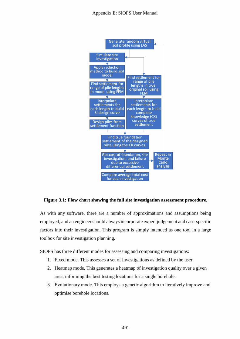
Appendix E: SIOPS User Manual
491
Figure 3.1: Flow chart showing the full site investigation assessment procedure.
As with any software, there are a number of approximations and assumptions being
employed, and an engineer should always incorporate expert judgement and case-specific
factors into their investigation. This program is simply intended as one tool in a large
toolbox for site investigation planning.
SIOPS has three different modes for assessing and comparing investigations:
1. Fixed mode. This assesses a set of investigations as defined by the user.
2. Heatmap mode. This generates a heatmap of investigation quality over a given
area, informing the best testing locations for a single borehole.
3. Evolutionary mode. This employs a genetic algorithm to iteratively improve and
optimise borehole locations.
Appendix E: SIOPS User Manual
492
Furthermore, there are two broad soil classes available; single-layer soils with variable
soil properties and multiple-layer soils with variable layer boundaries but uniform
properties within each layer. The latter is generally recommended, as users can more
explicitly model their site, and there is no explicit pre-processing required, unlike that
extensively done for the former class. It should be noted that Figure 3.1 describes the
procedure for the single layer class. The multiple layer class follows a similar, albeit
simplified process; designing piles and determining settlement directly as opposed to
through the use of pre-generated curves.
3.2 Assumptions and Limitations
3.2.1 Elastic Settlement
The SIOPS program assesses pile performance in terms of linear-elastic settlement.
While a detailed explanation of this decision can be found in Crisp et al. (2019a)
(Appendix D), the main reasons are as follows:
1. A numerically efficient means of determining pile performance is required due
to the large number of piles being analysed within the Monte Carlo simulation.
This is especially true when using the Genetic Algorithm. More sophisticated
models are computationally intensive to the point of being infeasible.
2. In addition to the settlement method itself being computationally faster, the
single-layer soil mode employs additional optimizations that rely on the linear-
elastic nature.
3. The loads and resulting deformations involved in pile settlement calculations are
typically low enough that soil mechanical behaviour is largely in the elastic
region.
4. Finally, the linear-elastic assumption is constant across the full performance
assessment; both in the true soil settlement and soil model settlement. As a
result, any potential model errors are largely self-cancelling.
Appendix E: SIOPS User Manual
493
3.2.2 Structural Deformation
Furthermore, there are some key assumptions in how buildings deform. This impacts the
calculations of differential settlement on which investigation performance is based. As
discussed in point (4) above, these assumptions are consistent across both stages of pile
assessment, limiting their impact on the results.
1. Each pile is treated independently, therefore any additional settlement caused by
the proximity of other piles is not considered. As SIOPS is intended to work for
multi-storey office buildings constructed with individual piles, as opposed to
pile groups, the centre-centre spacing is typically large enough for this not to be
an issue.
2. Building rigidity is not considered. SIOPS assumes that the loading on each pile
does not change with time, and that the building weight is fully supported by the
piles. Therefore, SIOPS does not account for moment redistribution as
differential settlement occurs, nor any additional resistance from the building
resting on the ground surface.
3.2.3 Soil Geometry and Site Investigations
The soil is represented as a rectangular prism. The surface is completely flat and
horizontal. Furthermore, the bottom of the soil (also flat and horizontal) is considered as
perfectly-rigid rock.
3.3 Soil Representation
3.3.1 Virtual soils
Virtual soils are numerical representations of soil properties over a volume. For example,
a 3D grid of discrete elements, where each element has a single set of material properties.
These soils are randomly generated within SIOPS, meaning that a single set of input
parameters can produce vastly different realisations of soils, which are all described by
the same statistics.
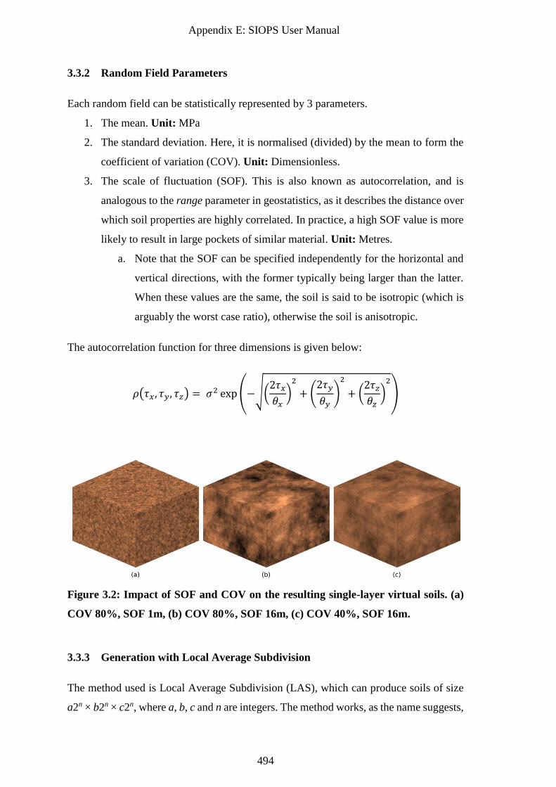
Appendix E: SIOPS User Manual
494
3.3.2 Random Field Parameters
Each random field can be statistically represented by 3 parameters.
1. The mean. Unit: MPa
2. The standard deviation. Here, it is normalised (divided) by the mean to form the
coefficient of variation (COV). Unit: Dimensionless.
3. The scale of fluctuation (SOF). This is also known as autocorrelation, and is
analogous to the range parameter in geostatistics, as it describes the distance over
which soil properties are highly correlated. In practice, a high SOF value is more
likely to result in large pockets of similar material. Unit: Metres.
a. Note that the SOF can be specified independently for the horizontal and
vertical directions, with the former typically being larger than the latter.
When these values are the same, the soil is said to be isotropic (which is
arguably the worst case ratio), otherwise the soil is anisotropic.
The autocorrelation function for three dimensions is given below:
𝜌(𝜏𝑥 , 𝜏𝑦, 𝜏𝑧) = 𝜎2 exp(−√(
2𝜏𝑥𝜃𝑥)2
+ (2𝜏𝑦
𝜃𝑦)
2
+ (2𝜏𝑧𝜃𝑧)2
)
Figure 3.2: Impact of SOF and COV on the resulting single-layer virtual soils. (a)
COV 80%, SOF 1m, (b) COV 80%, SOF 16m, (c) COV 40%, SOF 16m.
3.3.3 Generation with Local Average Subdivision
The method used is Local Average Subdivision (LAS), which can produce soils of size
a2n × b2n × c2n, where a, b, c and n are integers. The method works, as the name suggests,
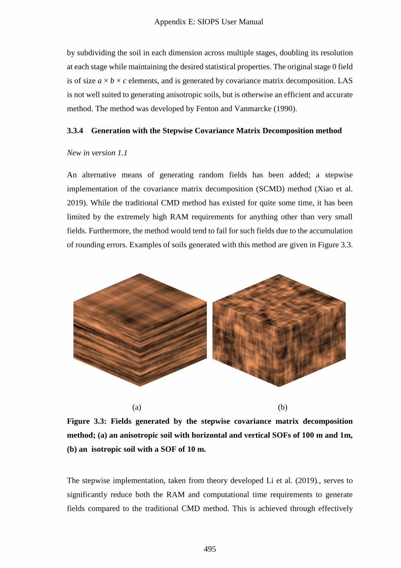
Appendix E: SIOPS User Manual
495
by subdividing the soil in each dimension across multiple stages, doubling its resolution
at each stage while maintaining the desired statistical properties. The original stage 0 field
is of size a × b × c elements, and is generated by covariance matrix decomposition. LAS
is not well suited to generating anisotropic soils, but is otherwise an efficient and accurate
method. The method was developed by Fenton and Vanmarcke (1990).
3.3.4 Generation with the Stepwise Covariance Matrix Decomposition method
New in version 1.1
An alternative means of generating random fields has been added; a stepwise
implementation of the covariance matrix decomposition (SCMD) method (Xiao et al.
2019). While the traditional CMD method has existed for quite some time, it has been
limited by the extremely high RAM requirements for anything other than very small
fields. Furthermore, the method would tend to fail for such fields due to the accumulation
of rounding errors. Examples of soils generated with this method are given in Figure 3.3.
(a) (b)
Figure 3.3: Fields generated by the stepwise covariance matrix decomposition
method; (a) an anisotropic soil with horizontal and vertical SOFs of 100 m and 1m,
(b) an isotropic soil with a SOF of 10 m.
The stepwise implementation, taken from theory developed Li et al. (2019)., serves to
significantly reduce both the RAM and computational time requirements to generate
fields compared to the traditional CMD method. This is achieved through effectively
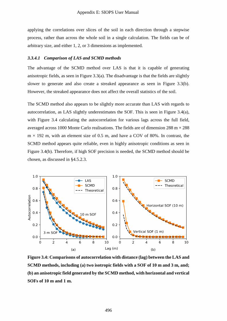
Appendix E: SIOPS User Manual
496
applying the correlations over slices of the soil in each direction through a stepwise
process, rather than across the whole soil in a single calculation. The fields can be of
arbitrary size, and either 1, 2, or 3 dimensions as implemented.
3.3.4.1 Comparison of LAS and SCMD methods
The advantage of the SCMD method over LAS is that it is capable of generating
anisotropic fields, as seen in Figure 3.3(a). The disadvantage is that the fields are slightly
slower to generate and also create a streaked appearance as seen in Figure 3.3(b).
However, the streaked appearance does not affect the overall statistics of the soil.
The SCMD method also appears to be slightly more accurate than LAS with regards to
autocorrelation, as LAS slightly underestimates the SOF. This is seen in Figure 3.4(a),
with Figure 3.4 calculating the autocorrelation for various lags across the full field,
averaged across 1000 Monte Carlo realisations. The fields are of dimension 288 m × 288
m × 192 m, with an element size of 0.5 m, and have a COV of 80%. In contrast, the
SCMD method appears quite reliable, even in highly anisotropic conditions as seen in
Figure 3.4(b). Therefore, if high SOF precision is needed, the SCMD method should be
chosen, as discussed in §4.5.2.3.
Figure 3.4: Comparisons of autocorrelation with distance (lag) between the LAS and
SCMD methods, including (a) two isotropic fields with a SOF of 10 m and 3 m, and;
(b) an anisotropic field generated by the SCMD method, with horizontal and vertical
SOFs of 10 m and 1 m.
Appendix E: SIOPS User Manual
497
It should be noted that both sets of fields are initially created with a zero-mean, unit-
variance, normally-distributed set of random numbers, prior to the necessary
transformations. As a finite set of random numbers is unlikely to match these statistics
perfectly, they are brute-force normalised by subtracting the observed mean from the
values and dividing by the observed standard deviation. This information is mentioned
here as it may result in a small discrepancy against other published results.
3.3.5 Property Distributions
Single-layer, 3D soils are represented by lognormally distributed random values. This
distribution is used because studies indicate it is a reasonable fit for soils found in
practice. Perhaps more importantly, it ensures that all properties are non-negative.
In the case of multiple layers which incorporate random 2D layer boundaries, each
boundary is represented by a normal distribution.
The SOF, which statistically describes the spatial distribution of properties, is
implemented using an exponential Markov correlation model, which has been found to
be the most suitable for describing soils.
3.4 Soil Modes
There are two different soil modes available:
• A single-layer, variable soil.
• A multiple-layer soil with uniform properties in each layer and variable layer
boundaries.
Each mode is a simplification of soils found in practice; for example, there is no mode
with variable layer boundaries and variable soil within each layer. This limitation exists
because each of each of the above methods takes advantage of a different set of
incompatible optimizations. To combine features of both would require the use of, at a
minimum, thousands of finite element analysis simulations; something that is not feasible
without a supercomputer if results are desired within a practical timeframe.
Note that it has found that total uncertainty in complex soil situations tends to be greater
than the sum of individual uncertainties due to layer boundary variability and the spatial
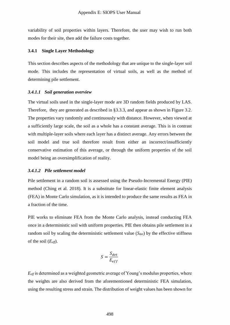
Appendix E: SIOPS User Manual
498
variability of soil properties within layers. Therefore, the user may wish to run both
modes for their site, then add the failure costs together.
3.4.1 Single Layer Methodology
This section describes aspects of the methodology that are unique to the single-layer soil
mode. This includes the representation of virtual soils, as well as the method of
determining pile settlement.
3.4.1.1 Soil generation overview
The virtual soils used in the single-layer mode are 3D random fields produced by LAS.
Therefore, they are generated as described in §3.3.3, and appear as shown in Figure 3.2.
The properties vary randomly and continuously with distance. However, when viewed at
a sufficiently large scale, the soil as a whole has a constant average. This is in contrast
with multiple-layer soils where each layer has a distinct average. Any errors between the
soil model and true soil therefore result from either an incorrect/insufficiently
conservative estimation of this average, or through the uniform properties of the soil
model being an oversimplification of reality.
3.4.1.2 Pile settlement model
Pile settlement in a random soil is assessed using the Pseudo-Incremental Energy (PIE)
method (Ching et al. 2018). It is a substitute for linear-elastic finite element analysis
(FEA) in Monte Carlo simulation, as it is intended to produce the same results as FEA in
a fraction of the time.
PIE works to eliminate FEA from the Monte Carlo analysis, instead conducting FEA
once in a deterministic soil with uniform properties. PIE then obtains pile settlement in a
random soil by scaling the deterministic settlement value (Sdet) by the effective stiffness
of the soil (Eeff).
𝑆 =𝑆𝑑𝑒𝑡𝐸𝑒𝑓𝑓
Eeff is determined as a weighted geometric average of Young’s modulus properties, where
the weights are also derived from the aforementioned deterministic FEA simulation,
using the resulting stress and strain. The distribution of weight values has been shown for
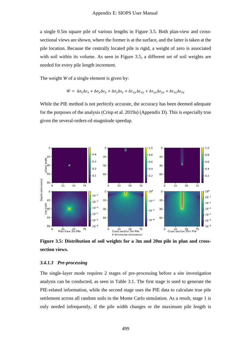
Appendix E: SIOPS User Manual
499
a single 0.5m square pile of various lengths in Figure 3.5. Both plan-view and cross-
sectional views are shown, where the former is at the surface, and the latter is taken at the
pile location. Because the centrally located pile is rigid, a weight of zero is associated
with soil within its volume. As seen in Figure 3.5, a different set of soil weights are
needed for every pile length increment.
The weight W of a single element is given by:
𝑊 = ∆𝜎𝑥∆휀𝑥 + ∆𝜎𝑦∆휀𝑦 + ∆𝜎𝑧∆휀𝑧 + ∆𝜏𝑥𝑦∆휀𝑥𝑦 + ∆𝜏𝑦𝑧∆휀𝑦𝑧 + ∆𝜏𝑥𝑧∆휀𝑥𝑧
While the PIE method is not perfectly accurate, the accuracy has been deemed adequate
for the purposes of the analysis (Crisp et al. 2019a) (Appendix D). This is especially true
given the several-orders-of-magnitude speedup.
Figure 3.5: Distribution of soil weights for a 3m and 20m pile in plan and cross-
section views.
3.4.1.3 Pre-processing
The single-layer mode requires 2 stages of pre-processing before a site investigation
analysis can be conducted, as seen in Table 3.1. The first stage is used to generate the
PIE-related information, while the second stage uses the PIE data to calculate true pile
settlement across all random soils in the Monte Carlo simulation. As a result, stage 1 is
only needed infrequently, if the pile width changes or the maximum pile length is
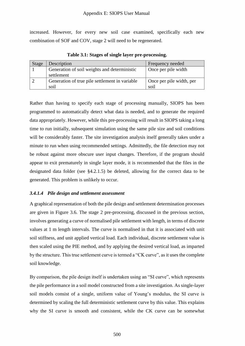
Appendix E: SIOPS User Manual
500
increased. However, for every new soil case examined, specifically each new
combination of SOF and COV, stage 2 will need to be regenerated.
Table 3.1: Stages of single layer pre-processing.
Stage Description Frequency needed
1 Generation of soil weights and deterministic
settlement
Once per pile width
2 Generation of true pile settlement in variable
soil
Once per pile width, per
soil
Rather than having to specify each stage of processing manually, SIOPS has been
programmed to automatically detect what data is needed, and to generate the required
data appropriately. However, while this pre-processing will result in SIOPS taking a long
time to run initially, subsequent simulation using the same pile size and soil conditions
will be considerably faster. The site investigation analysis itself generally takes under a
minute to run when using recommended settings. Admittedly, the file detection may not
be robust against more obscure user input changes. Therefore, if the program should
appear to exit prematurely in single layer mode, it is recommended that the files in the
designated data folder (see §4.2.1.5) be deleted, allowing for the correct data to be
generated. This problem is unlikely to occur.
3.4.1.4 Pile design and settlement assessment
A graphical representation of both the pile design and settlement determination processes
are given in Figure 3.6. The stage 2 pre-processing, discussed in the previous section,
involves generating a curve of normalised pile settlement with length, in terms of discrete
values at 1 m length intervals. The curve is normalised in that it is associated with unit
soil stiffness, and unit applied vertical load. Each individual, discrete settlement value is
then scaled using the PIE method, and by applying the desired vertical load, as imparted
by the structure. This true settlement curve is termed a “CK curve”, as it uses the complete
soil knowledge.
By comparison, the pile design itself is undertaken using an “SI curve”, which represents
the pile performance in a soil model constructed from a site investigation. As single-layer
soil models consist of a single, uniform value of Young’s modulus, the SI curve is
determined by scaling the full deterministic settlement curve by this value. This explains
why the SI curve is smooth and consistent, while the CK curve can be somewhat
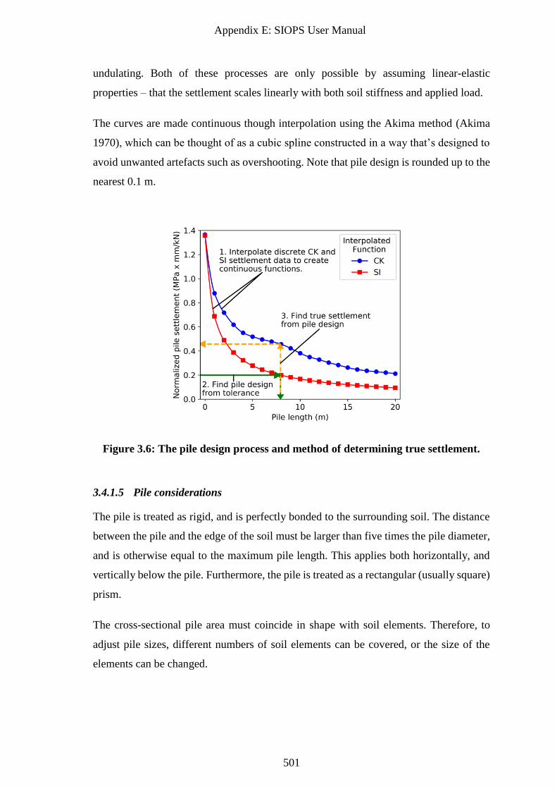
Appendix E: SIOPS User Manual
501
undulating. Both of these processes are only possible by assuming linear-elastic
properties – that the settlement scales linearly with both soil stiffness and applied load.
The curves are made continuous though interpolation using the Akima method (Akima
1970), which can be thought of as a cubic spline constructed in a way that’s designed to
avoid unwanted artefacts such as overshooting. Note that pile design is rounded up to the
nearest 0.1 m.
Figure 3.6: The pile design process and method of determining true settlement.
3.4.1.5 Pile considerations
The pile is treated as rigid, and is perfectly bonded to the surrounding soil. The distance
between the pile and the edge of the soil must be larger than five times the pile diameter,
and is otherwise equal to the maximum pile length. This applies both horizontally, and
vertically below the pile. Furthermore, the pile is treated as a rectangular (usually square)
prism.
The cross-sectional pile area must coincide in shape with soil elements. Therefore, to
adjust pile sizes, different numbers of soil elements can be covered, or the size of the
elements can be changed.
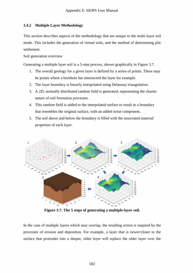
Appendix E: SIOPS User Manual
502
3.4.2 Multiple Layer Methodology
This section describes aspects of the methodology that are unique to the multi-layer soil
mode. This includes the generation of virtual soils, and the method of determining pile
settlement.
Soil generation overview
Generating a multiple layer soil is a 5-step process, shown graphically in Figure 3.7.
1. The overall geology for a given layer is defined by a series of points. These may
be points where a borehole has intersected the layer for example.
2. The layer boundary is linearly interpolated using Delaunay triangulation.
3. A 2D, normally distributed random field is generated, representing the chaotic
nature of soil formation processes.
4. This random field is added to the interpolated surface to result in a boundary
that resembles the original surface, with an added noise component.
5. The soil above and below the boundary is filled with the associated material
properties of each layer.
Figure 3.7: The 5 steps of generating a multiple-layer soil.
In the case of multiple layers which may overlap, the resulting action is inspired by the
processes of erosion and deposition. For example, a layer that is newer/closer to the
surface that protrudes into a deeper, older layer will replace the older layer over the
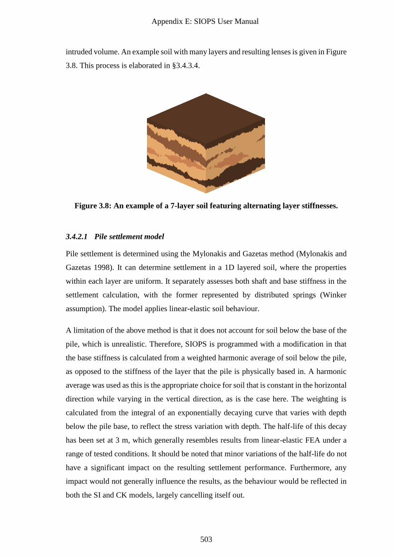
Appendix E: SIOPS User Manual
503
intruded volume. An example soil with many layers and resulting lenses is given in Figure
3.8. This process is elaborated in §3.4.3.4.
Figure 3.8: An example of a 7-layer soil featuring alternating layer stiffnesses.
3.4.2.1 Pile settlement model
Pile settlement is determined using the Mylonakis and Gazetas method (Mylonakis and
Gazetas 1998). It can determine settlement in a 1D layered soil, where the properties
within each layer are uniform. It separately assesses both shaft and base stiffness in the
settlement calculation, with the former represented by distributed springs (Winker
assumption). The model applies linear-elastic soil behaviour.
A limitation of the above method is that it does not account for soil below the base of the
pile, which is unrealistic. Therefore, SIOPS is programmed with a modification in that
the base stiffness is calculated from a weighted harmonic average of soil below the pile,
as opposed to the stiffness of the layer that the pile is physically based in. A harmonic
average was used as this is the appropriate choice for soil that is constant in the horizontal
direction while varying in the vertical direction, as is the case here. The weighting is
calculated from the integral of an exponentially decaying curve that varies with depth
below the pile base, to reflect the stress variation with depth. The half-life of this decay
has been set at 3 m, which generally resembles results from linear-elastic FEA under a
range of tested conditions. It should be noted that minor variations of the half-life do not
have a significant impact on the resulting settlement performance. Furthermore, any
impact would not generally influence the results, as the behaviour would be reflected in
both the SI and CK models, largely cancelling itself out.
Appendix E: SIOPS User Manual
504
3.4.2.2 Pile considerations
In multi-layer analysis, the pile is treated as circular. It is comprised of compressible
elastic material, although is set as being several orders of magnitude stiffer than standard
concrete. The base of the pile is assumed to act as a rigid circular disk.
The pile width must coincide with the width of one or more soil elements. Therefore to
adjust pile sizes, different numbers of soil elements can be covered, or the size of the
elements can be changed.
3.4.3 Treatment of Layer Boundaries in Soil Model
While this section falls under the scope of the previous subsection, 3.4.2, it has been made
its own subsection owing to both its size and its importance. It is vital that engineers
understand how the layers are being applied so that results can be interpreted properly.
3.4.3.1 Interpreting depths at boreholes
The layer boundary depths, at borehole locations are known exactly. Depth uncertainty,
due to soil material ambiguity, is not incorporated in the analysis. As such, if the soil is
consistently sampled with a continuous test type, then the layer would be recreated
exactly in the 3D soil model. In the case of discrete tests, such as the SPT, when the
borehole encounters the 2nd layer, the layer depth is interpreted as being mid-way between
the first sample taken from that layer, and the previous, higher-up sample. In other words,
when a change of layer is detected, it is assumed to be at the average distance between
samples where the change occurred. As such, the maximum deviation the true layer can
have from the interpreted depth is 0.75 m, if the sample depth spacing is 1.5 m.
An illustration of the remaining cases is provided in Figure 3.9, for the scenario of five
layers recreated from information at three boreholes, compared to the original soil layers.
Each boundary refers to the layer that is immediately above it. Note that the layer
interpolation is further elaborated in the subsequent sections.
Layers that exist below an arbitrary borehole, and are therefore not encountered, are
placed just below the bottom of that borehole, as is the case with layer 3 at boreholes 1
and 2 in Figure 3.9. While this isn’t guaranteed to be an ideal solution, it must be stressed
that any estimation of layer boundaries in this circumstance is likely to be error-prone,
reinforcing the need to have sufficiently-deep boreholes.
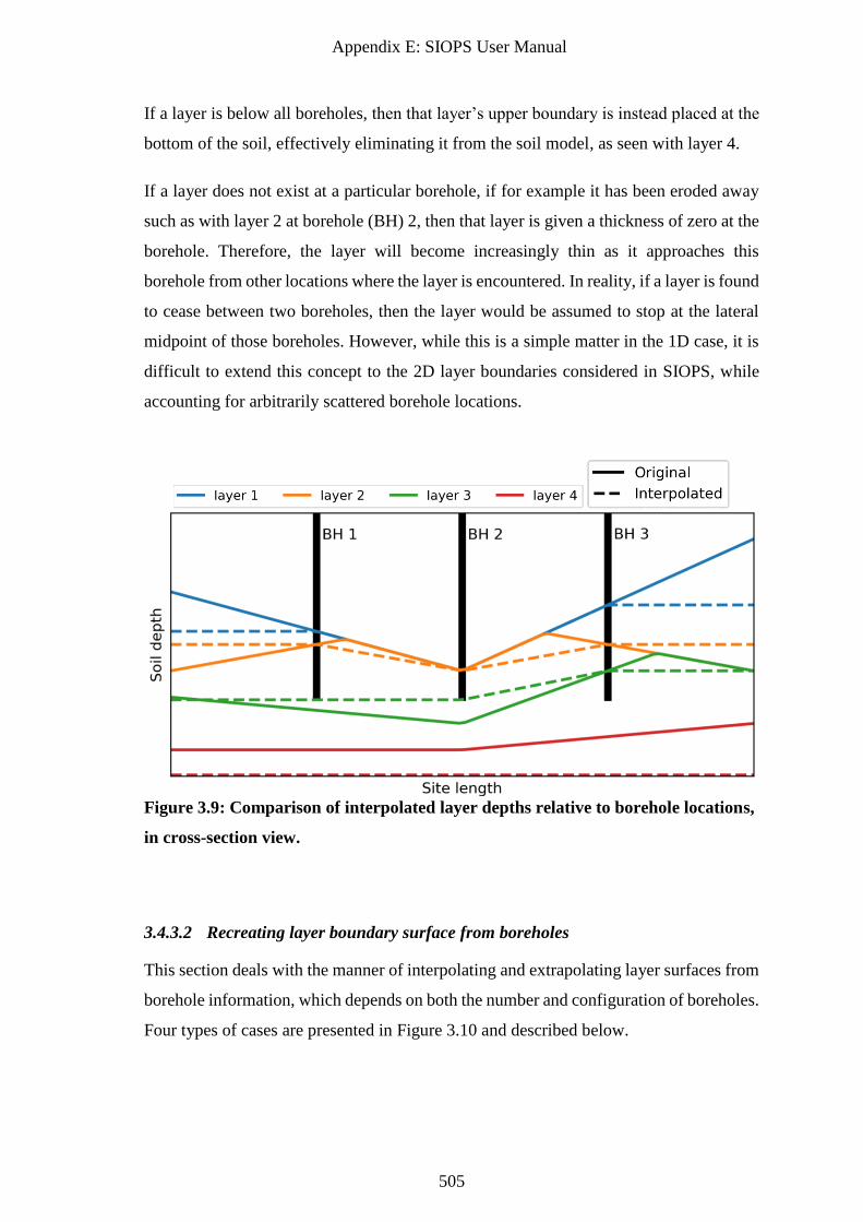
Appendix E: SIOPS User Manual
505
If a layer is below all boreholes, then that layer’s upper boundary is instead placed at the
bottom of the soil, effectively eliminating it from the soil model, as seen with layer 4.
If a layer does not exist at a particular borehole, if for example it has been eroded away
such as with layer 2 at borehole (BH) 2, then that layer is given a thickness of zero at the
borehole. Therefore, the layer will become increasingly thin as it approaches this
borehole from other locations where the layer is encountered. In reality, if a layer is found
to cease between two boreholes, then the layer would be assumed to stop at the lateral
midpoint of those boreholes. However, while this is a simple matter in the 1D case, it is
difficult to extend this concept to the 2D layer boundaries considered in SIOPS, while
accounting for arbitrarily scattered borehole locations.
Figure 3.9: Comparison of interpolated layer depths relative to borehole locations,
in cross-section view.
3.4.3.2 Recreating layer boundary surface from boreholes
This section deals with the manner of interpolating and extrapolating layer surfaces from
borehole information, which depends on both the number and configuration of boreholes.
Four types of cases are presented in Figure 3.10 and described below.
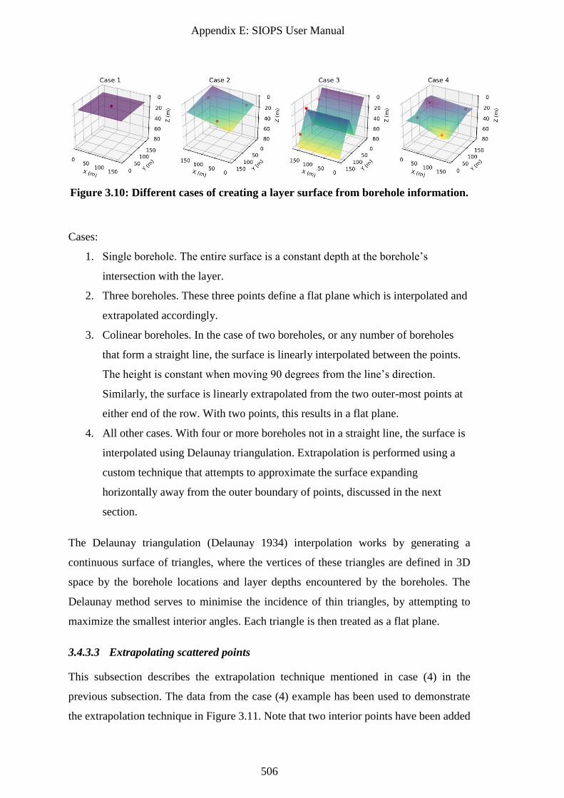
Appendix E: SIOPS User Manual
506
Figure 3.10: Different cases of creating a layer surface from borehole information.
Cases:
1. Single borehole. The entire surface is a constant depth at the borehole’s
intersection with the layer.
2. Three boreholes. These three points define a flat plane which is interpolated and
extrapolated accordingly.
3. Colinear boreholes. In the case of two boreholes, or any number of boreholes
that form a straight line, the surface is linearly interpolated between the points.
The height is constant when moving 90 degrees from the line’s direction.
Similarly, the surface is linearly extrapolated from the two outer-most points at
either end of the row. With two points, this results in a flat plane.
4. All other cases. With four or more boreholes not in a straight line, the surface is
interpolated using Delaunay triangulation. Extrapolation is performed using a
custom technique that attempts to approximate the surface expanding
horizontally away from the outer boundary of points, discussed in the next
section.
The Delaunay triangulation (Delaunay 1934) interpolation works by generating a
continuous surface of triangles, where the vertices of these triangles are defined in 3D
space by the borehole locations and layer depths encountered by the boreholes. The
Delaunay method serves to minimise the incidence of thin triangles, by attempting to
maximize the smallest interior angles. Each triangle is then treated as a flat plane.
3.4.3.3 Extrapolating scattered points
This subsection describes the extrapolation technique mentioned in case (4) in the
previous subsection. The data from the case (4) example has been used to demonstrate
the extrapolation technique in Figure 3.11. Note that two interior points have been added
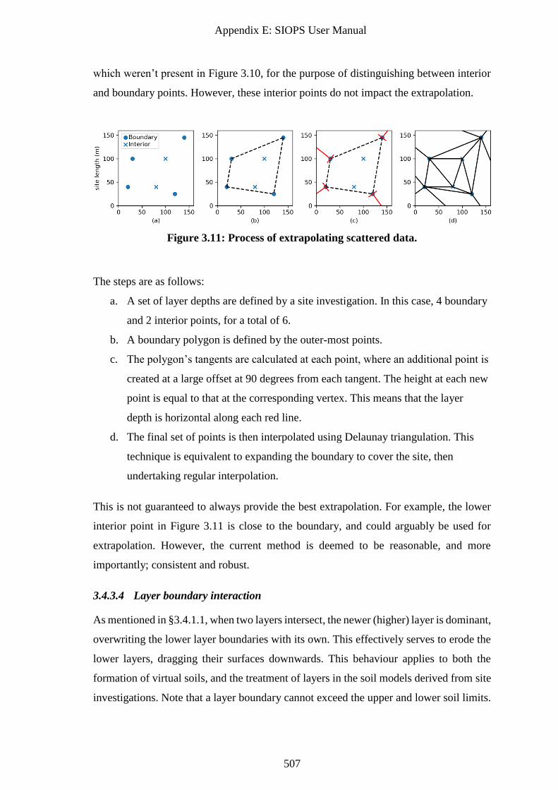
Appendix E: SIOPS User Manual
507
which weren’t present in Figure 3.10, for the purpose of distinguishing between interior
and boundary points. However, these interior points do not impact the extrapolation.
Figure 3.11: Process of extrapolating scattered data.
The steps are as follows:
a. A set of layer depths are defined by a site investigation. In this case, 4 boundary
and 2 interior points, for a total of 6.
b. A boundary polygon is defined by the outer-most points.
c. The polygon’s tangents are calculated at each point, where an additional point is
created at a large offset at 90 degrees from each tangent. The height at each new
point is equal to that at the corresponding vertex. This means that the layer
depth is horizontal along each red line.
d. The final set of points is then interpolated using Delaunay triangulation. This
technique is equivalent to expanding the boundary to cover the site, then
undertaking regular interpolation.
This is not guaranteed to always provide the best extrapolation. For example, the lower
interior point in Figure 3.11 is close to the boundary, and could arguably be used for
extrapolation. However, the current method is deemed to be reasonable, and more
importantly; consistent and robust.
3.4.3.4 Layer boundary interaction
As mentioned in §3.4.1.1, when two layers intersect, the newer (higher) layer is dominant,
overwriting the lower layer boundaries with its own. This effectively serves to erode the
lower layers, dragging their surfaces downwards. This behaviour applies to both the
formation of virtual soils, and the treatment of layers in the soil models derived from site
investigations. Note that a layer boundary cannot exceed the upper and lower soil limits.
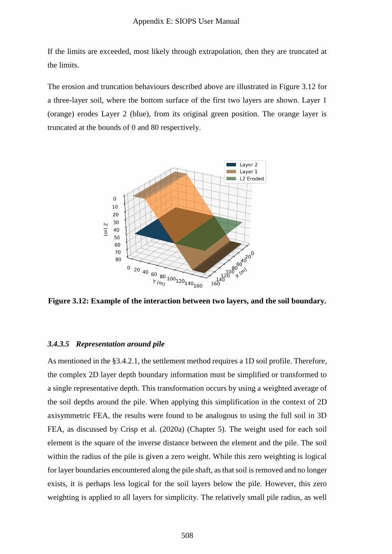
Appendix E: SIOPS User Manual
508
If the limits are exceeded, most likely through extrapolation, then they are truncated at
the limits.
The erosion and truncation behaviours described above are illustrated in Figure 3.12 for
a three-layer soil, where the bottom surface of the first two layers are shown. Layer 1
(orange) erodes Layer 2 (blue), from its original green position. The orange layer is
truncated at the bounds of 0 and 80 respectively.
Figure 3.12: Example of the interaction between two layers, and the soil boundary.
3.4.3.5 Representation around pile
As mentioned in the §3.4.2.1, the settlement method requires a 1D soil profile. Therefore,
the complex 2D layer depth boundary information must be simplified or transformed to
a single representative depth. This transformation occurs by using a weighted average of
the soil depths around the pile. When applying this simplification in the context of 2D
axisymmetric FEA, the results were found to be analogous to using the full soil in 3D
FEA, as discussed by Crisp et al. (2020a) (Chapter 5). The weight used for each soil
element is the square of the inverse distance between the element and the pile. The soil
within the radius of the pile is given a zero weight. While this zero weighting is logical
for layer boundaries encountered along the pile shaft, as that soil is removed and no longer
exists, it is perhaps less logical for the soil layers below the pile. However, this zero
weighting is applied to all layers for simplicity. The relatively small pile radius, as well

Appendix E: SIOPS User Manual
509
as the same model being used for both design and true settlement assessment, mean that
any impact the uniform zero weighting has on results is negligible. The range of this
weighted average is 5 times the pile width.
5.1 Site Investigations
There are two conceptual components of site investigations as represented in SIOPS:
1. The collection of soil stiffness information (soil testing).
2. The interpretation (or reduction) of multiple stiffness samples into a single
representative value. The techniques used to do this are termed “reduction
methods” in the present document.
Therefore, site investigations have 5 attributes that can be specified and controlled, listed
below:
1. The number of boreholes.
2. The plan-view location of each borehole.
3. The borehole depths.
4. The testing method, which dictates the following:
a. The borehole sampling frequency with depth.
b. Testing accuracy.
c. Testing cost.
5. The choice of reduction method.
While the first three points are self-explanatory, the latter two are elaborated in the
following sections.
3.4.4 Soil Test Types and Implementation
The tests are undertaken by extracting samples from the soil along appropriate depths at
each borehole location, then applying random errors to mimic testing inaccuracy.
A set of attributes for 4 test types is given in Table 3.2, derived by Goldsworthy (2006).
These are the standard penetration test (SPT), cone penetration test (CPT), triaxial test
(TT) and flatplate dilatometer (DMT).
The testing inaccuracies are accounted for by applying a set of 3 random errors to each
sample:
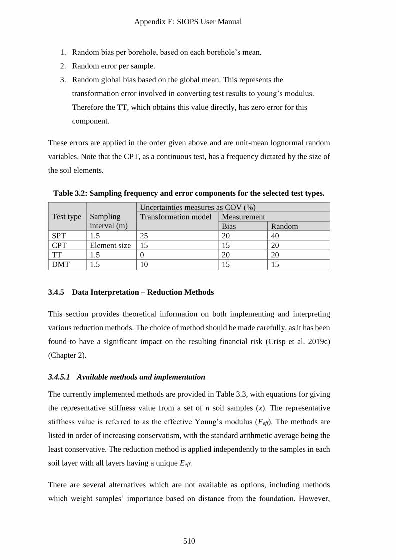
Appendix E: SIOPS User Manual
510
1. Random bias per borehole, based on each borehole’s mean.
2. Random error per sample.
3. Random global bias based on the global mean. This represents the
transformation error involved in converting test results to young’s modulus.
Therefore the TT, which obtains this value directly, has zero error for this
component.
These errors are applied in the order given above and are unit-mean lognormal random
variables. Note that the CPT, as a continuous test, has a frequency dictated by the size of
the soil elements.
Table 3.2: Sampling frequency and error components for the selected test types.
Test type
Sampling
interval (m)
Uncertainties measures as COV (%)
Transformation model Measurement
Bias Random
SPT 1.5 25 20 40
CPT Element size 15 15 20
TT 1.5 0 20 20
DMT 1.5 10 15 15
3.4.5 Data Interpretation – Reduction Methods
This section provides theoretical information on both implementing and interpreting
various reduction methods. The choice of method should be made carefully, as it has been
found to have a significant impact on the resulting financial risk (Crisp et al. 2019c)
(Chapter 2).
3.4.5.1 Available methods and implementation
The currently implemented methods are provided in Table 3.3, with equations for giving
the representative stiffness value from a set of n soil samples (x). The representative
stiffness value is referred to as the effective Young’s modulus (Eeff). The methods are
listed in order of increasing conservatism, with the standard arithmetic average being the
least conservative. The reduction method is applied independently to the samples in each
soil layer with all layers having a unique Eeff.
There are several alternatives which are not available as options, including methods
which weight samples’ importance based on distance from the foundation. However,
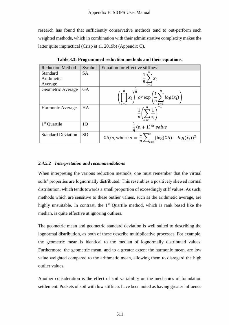
Appendix E: SIOPS User Manual
511
research has found that sufficiently conservative methods tend to out-perform such
weighted methods, which in combination with their administrative complexity makes the
latter quite impractical (Crisp et al. 2019b) (Appendix C).
Table 3.3: Programmed reduction methods and their equations.
Reduction Method Symbol Equation for effective stiffness
Standard
Arithmetic
Average
SA 1
𝑛∑𝑥𝑖
𝑛
𝑖=1
Geometric Average GA
(∏𝑥𝑖
𝑛
𝑖=1
)
1𝑛
𝑜𝑟 exp(1
𝑛∑𝑙𝑜𝑔(𝑥𝑖)
𝑛
𝑖=1
)
Harmonic Average HA 1
𝑛(∑
1
𝑥𝑖
𝑛
𝑖=1
)
−1
1st Quartile 1Q 1
4(𝑛 + 1)𝑡ℎ 𝑣𝑎𝑙𝑢𝑒
Standard Deviation SD GA/𝜎, where 𝜎 =
1
𝑛∑ (log (GA) − 𝑙𝑜𝑔 (𝑥𝑖))
2𝑛
𝑖=1
3.4.5.2 Interpretation and recommendations
When interpreting the various reduction methods, one must remember that the virtual
soils’ properties are lognormally distributed. This resembles a positively skewed normal
distribution, which tends towards a small proportion of exceedingly stiff values. As such,
methods which are sensitive to these outlier values, such as the arithmetic average, are
highly unsuitable. In contrast, the 1st Quartile method, which is rank based like the
median, is quite effective at ignoring outliers.
The geometric mean and geometric standard deviation is well suited to describing the
lognormal distribution, as both of these describe multiplicative processes. For example,
the geometric mean is identical to the median of lognormally distributed values.
Furthermore, the geometric mean, and to a greater extent the harmonic mean, are low
value weighted compared to the arithmetic mean, allowing them to disregard the high
outlier values.
Another consideration is the effect of soil variability on the mechanics of foundation
settlement. Pockets of soil with low stiffness have been noted as having greater influence
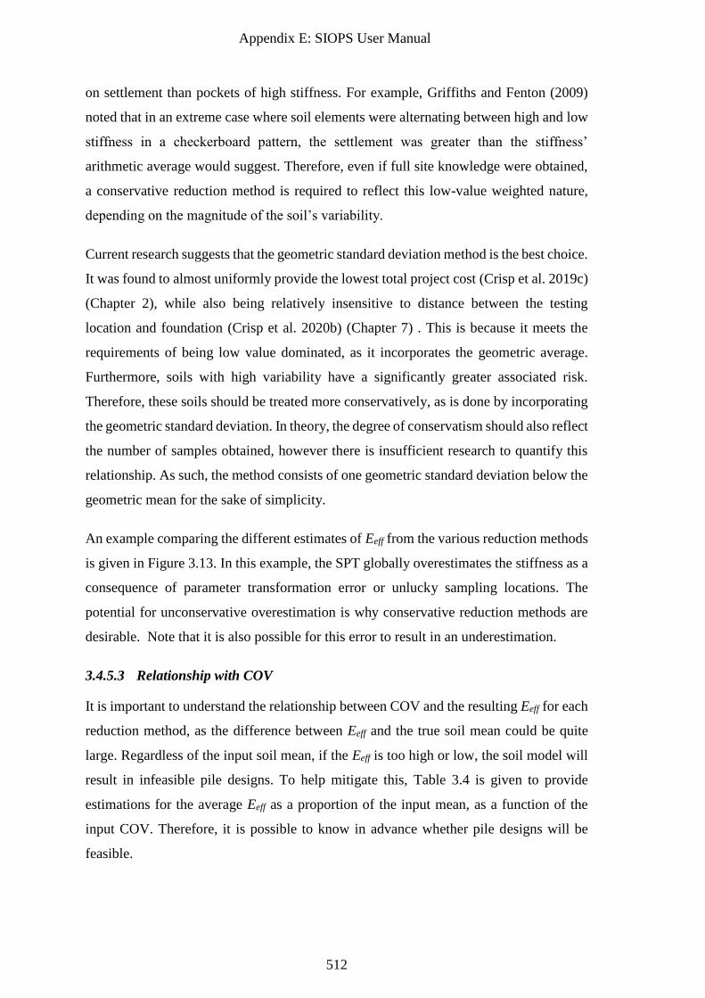
Appendix E: SIOPS User Manual
512
on settlement than pockets of high stiffness. For example, Griffiths and Fenton (2009)
noted that in an extreme case where soil elements were alternating between high and low
stiffness in a checkerboard pattern, the settlement was greater than the stiffness’
arithmetic average would suggest. Therefore, even if full site knowledge were obtained,
a conservative reduction method is required to reflect this low-value weighted nature,
depending on the magnitude of the soil’s variability.
Current research suggests that the geometric standard deviation method is the best choice.
It was found to almost uniformly provide the lowest total project cost (Crisp et al. 2019c)
(Chapter 2), while also being relatively insensitive to distance between the testing
location and foundation (Crisp et al. 2020b) (Chapter 7) . This is because it meets the
requirements of being low value dominated, as it incorporates the geometric average.
Furthermore, soils with high variability have a significantly greater associated risk.
Therefore, these soils should be treated more conservatively, as is done by incorporating
the geometric standard deviation. In theory, the degree of conservatism should also reflect
the number of samples obtained, however there is insufficient research to quantify this
relationship. As such, the method consists of one geometric standard deviation below the
geometric mean for the sake of simplicity.
An example comparing the different estimates of Eeff from the various reduction methods
is given in Figure 3.13. In this example, the SPT globally overestimates the stiffness as a
consequence of parameter transformation error or unlucky sampling locations. The
potential for unconservative overestimation is why conservative reduction methods are
desirable. Note that it is also possible for this error to result in an underestimation.
3.4.5.3 Relationship with COV
It is important to understand the relationship between COV and the resulting Eeff for each
reduction method, as the difference between Eeff and the true soil mean could be quite
large. Regardless of the input soil mean, if the Eeff is too high or low, the soil model will
result in infeasible pile designs. To help mitigate this, Table 3.4 is given to provide
estimations for the average Eeff as a proportion of the input mean, as a function of the
input COV. Therefore, it is possible to know in advance whether pile designs will be
feasible.
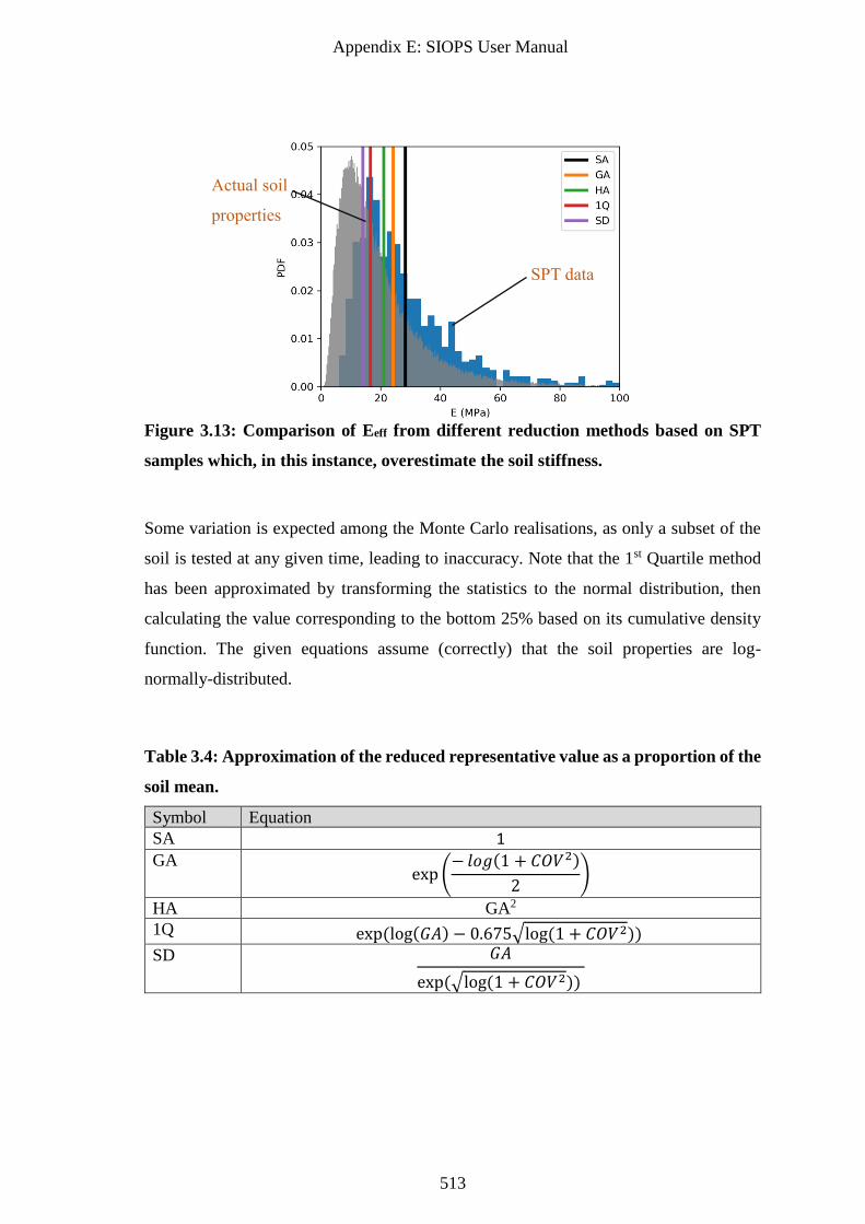
Appendix E: SIOPS User Manual
513
Figure 3.13: Comparison of Eeff from different reduction methods based on SPT
samples which, in this instance, overestimate the soil stiffness.
Some variation is expected among the Monte Carlo realisations, as only a subset of the
soil is tested at any given time, leading to inaccuracy. Note that the 1st Quartile method
has been approximated by transforming the statistics to the normal distribution, then
calculating the value corresponding to the bottom 25% based on its cumulative density
function. The given equations assume (correctly) that the soil properties are log-
normally-distributed.
Table 3.4: Approximation of the reduced representative value as a proportion of the
soil mean.
Symbol Equation
SA 1
GA exp(
− 𝑙𝑜𝑔(1 + 𝐶𝑂𝑉2)
2)
HA GA2
1Q exp (log(𝐺𝐴) − 0.675√log (1 + 𝐶𝑂𝑉2)) SD 𝐺𝐴
exp (√log (1 + 𝐶𝑂𝑉2))
SPT data
Actual soil
properties
Appendix E: SIOPS User Manual
514
3.5 Site Investigation Performance Metrics
SIOPS is programmed with a variety of performance metrics in terms of investigation
quality. It is up to the user to decide which metric they prefer. The equations for each
metric are given in Table 3.5 where n is the number of Monte Carlo realisations, i is
differential settlement in a given realisation, and tol is the differential settlement failure
threshold.
Total cost is arguably the best performance metric to use in practice, as it can be directly
related to real-world consequences. It is defined as the best estimate of what an
investigation will cost the user overall. The total cost is calculated as the sum of the
average failure cost, pile construction cost and site investigation cost. The latter two costs
are simply given by a unit cost ($/m) multiplied by the total lengths of piles and boreholes.
Note that the average pile cost tends to be reasonably constant regardless of the number
of boreholes used. This is because the instances of over-design and under-design largely
cancel themselves out. Therefore, while increased boreholes greatly reduce the variation
of pile length, the average itself is largely unaffected. As such, it could be excluded from
the total cost trade-off.
The failure cost is a function of differential settlement, C(Δδ). Specifically, it is a linear
function, as seen in Figure 3.14. The function is in terms of normalised failure cost as a
proportion of the building’s construction cost. As such, it is bounded by a value of 0,
which represents no failure, and a value of 1, which approximates demolishing and
rebuilding the structure. The original failure costs were derived from Rawlinsons (2016)
and correlated with descriptions of structural damage in terms of differential settlement
by Day (1999). As such, failure cost only considers cracking due to excessive differential
settlement. This is as opposed to excessive total settlement, either due to bearing capacity
failure or gross overestimation of the global soil stiffness.
Furthermore, there are several consequences of failure not explicitly considered, such as
construction delays causing additional expenditure and/or loss of profits, as well as
contract disputes and litigation. Furthermore, there are subjective consequences of failure
not considered, such as damage to the engineering company’s reputation, or
psychological distress to the building owners due to displacement or loss of income.
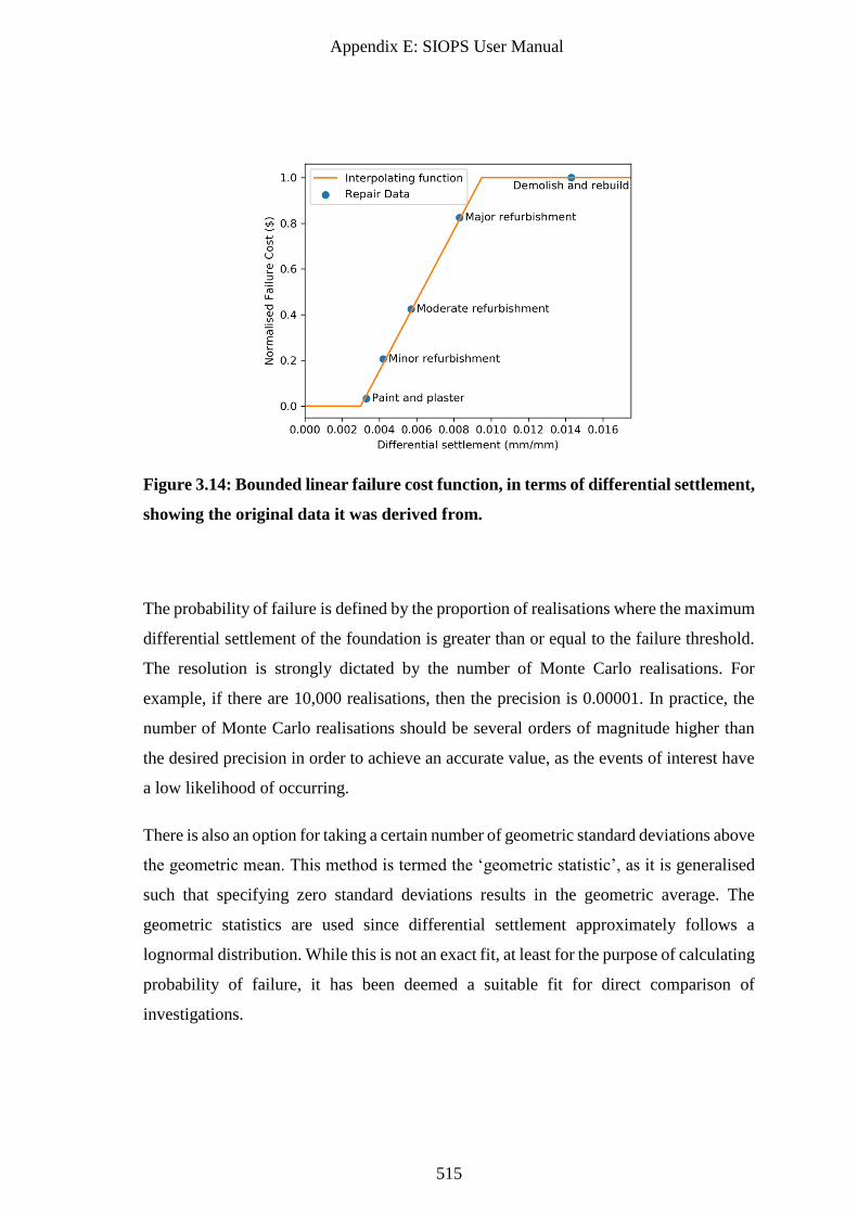
Appendix E: SIOPS User Manual
515
Figure 3.14: Bounded linear failure cost function, in terms of differential settlement,
showing the original data it was derived from.
The probability of failure is defined by the proportion of realisations where the maximum
differential settlement of the foundation is greater than or equal to the failure threshold.
The resolution is strongly dictated by the number of Monte Carlo realisations. For
example, if there are 10,000 realisations, then the precision is 0.00001. In practice, the
number of Monte Carlo realisations should be several orders of magnitude higher than
the desired precision in order to achieve an accurate value, as the events of interest have
a low likelihood of occurring.
There is also an option for taking a certain number of geometric standard deviations above
the geometric mean. This method is termed the ‘geometric statistic’, as it is generalised
such that specifying zero standard deviations results in the geometric average. The
geometric statistics are used since differential settlement approximately follows a
lognormal distribution. While this is not an exact fit, at least for the purpose of calculating
probability of failure, it has been deemed a suitable fit for direct comparison of
investigations.
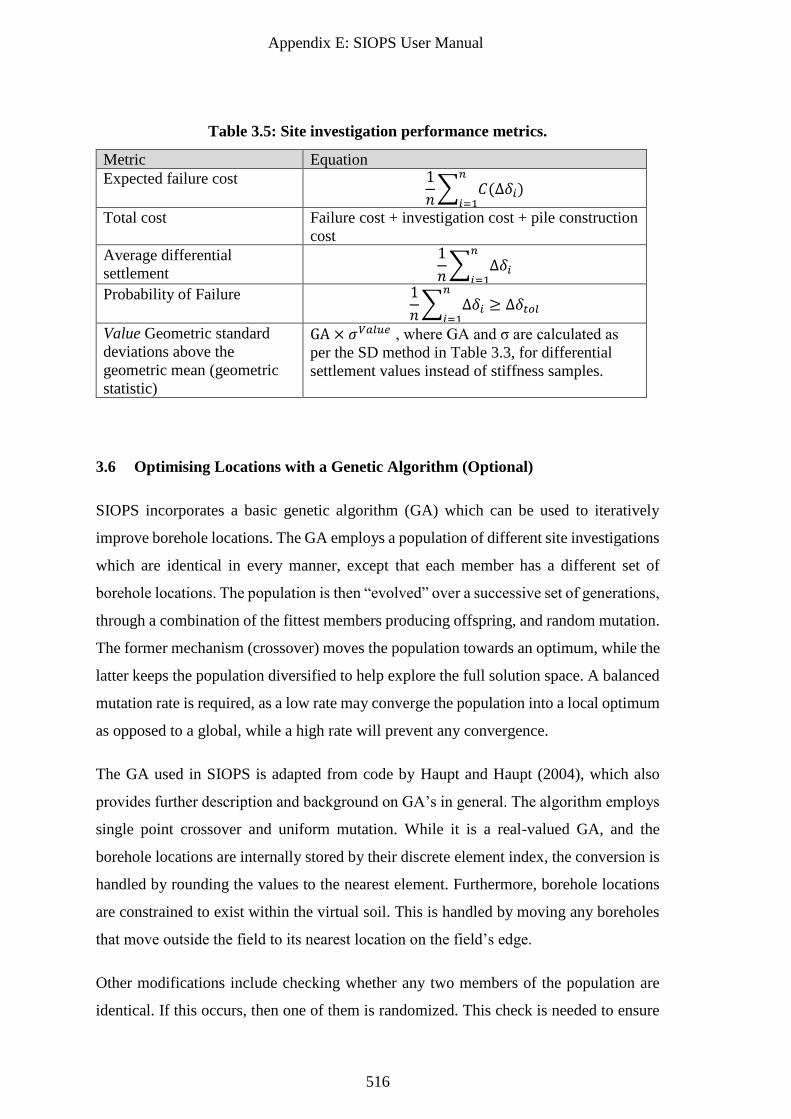
Appendix E: SIOPS User Manual
516
Table 3.5: Site investigation performance metrics.
Metric Equation
Expected failure cost 1
𝑛∑ 𝐶(∆𝛿𝑖)
𝑛
𝑖=1
Total cost Failure cost + investigation cost + pile construction
cost
Average differential
settlement
1
𝑛∑ ∆𝛿𝑖
𝑛
𝑖=1
Probability of Failure 1
𝑛∑ ∆𝛿𝑖 ≥ ∆𝛿𝑡𝑜𝑙
𝑛
𝑖=1
Value Geometric standard
deviations above the
geometric mean (geometric
statistic)
GA × 𝜎𝑉𝑎𝑙𝑢𝑒 , where GA and σ are calculated as
per the SD method in Table 3.3, for differential
settlement values instead of stiffness samples.
3.6 Optimising Locations with a Genetic Algorithm (Optional)
SIOPS incorporates a basic genetic algorithm (GA) which can be used to iteratively
improve borehole locations. The GA employs a population of different site investigations
which are identical in every manner, except that each member has a different set of
borehole locations. The population is then “evolved” over a successive set of generations,
through a combination of the fittest members producing offspring, and random mutation.
The former mechanism (crossover) moves the population towards an optimum, while the
latter keeps the population diversified to help explore the full solution space. A balanced
mutation rate is required, as a low rate may converge the population into a local optimum
as opposed to a global, while a high rate will prevent any convergence.
The GA used in SIOPS is adapted from code by Haupt and Haupt (2004), which also
provides further description and background on GA’s in general. The algorithm employs
single point crossover and uniform mutation. While it is a real-valued GA, and the
borehole locations are internally stored by their discrete element index, the conversion is
handled by rounding the values to the nearest element. Furthermore, borehole locations
are constrained to exist within the virtual soil. This is handled by moving any boreholes
that move outside the field to its nearest location on the field’s edge.
Other modifications include checking whether any two members of the population are
identical. If this occurs, then one of them is randomized. This check is needed to ensure
Appendix E: SIOPS User Manual
517
that the population is utilised to its fullest potential, as duplicates results in the processing
of the same information twice, effectively reducing the population size. Duplicates could
occur by pure chance, or potentially if the population has spent several generations in
convergence. In the latter case, the applied randomisation serves to explore the solution
space while continuing the original convergence. Similarly, a check is applied to make
sure that no two boreholes in a given investigation will occupy the same space. If this
occurs, then one of the boreholes is randomly scattered. This check is needed because
two boreholes in the same physical space does not make sense, and because it would
otherwise crash the program when undertaking the triangulation and interpolation of layer
surfaces.
Note that any investigation that has more than 2/3rds invalid Monte Carlo realisations is
given a worst-case performance to ensure that they don’t reproduce to the next
generation. This is mainly to prevent situations where 2 or 3 boreholes are located close
together resulting in highly inaccurate extrapolation over most of the soil, leading to a
large number of invalid realisations and effectively a random performance.
Other features have been added to GA such as elitism, dynamic mutation, and a 2nd stage
GA for local optimization. Please see §4.2.2 for details.
Appendix E: SIOPS User Manual
518
4 Program Input
4.1 Overview
This section describes the various options and parameters used by the program. There are
4 different input files based on overall categories, as outlined in Table 4.1.
Table 4.1: Input file descriptions.
File Name Description
EA_input.txt Over-arching program options and genetic algorithm parameters.
si_input.txt Site investigation data and parameters.
pile_input.txt Inputs related to both the structure and foundation.
soil_input.txt All soil-related options.
Note that the above files must be in a folder labelled “input” which is located in the same
directory as the SIOPS executable. Similarly, results are saved to a folder named
“si_results” which must be in this directory. When single-layer soils are analysed, some
pre-processed data is saved to a folder directory specified in the EA_input file as
discussed later. These folders are required to exist and be in the expected locations for
the program to function. Note that if the above files do not exist or are in the wrong
location, SIOPS will give the user the option to generate example input files.
The following sections describe the program’s inputs, with varying levels of information
depending on each input’s complexity. Potential information could include: justification,
options, theoretical background, examples.
Note that each row of the tables in the following sections describes one line in the input
file, except where an asterisk is included in the title, which indicates that a table of
information is needed.
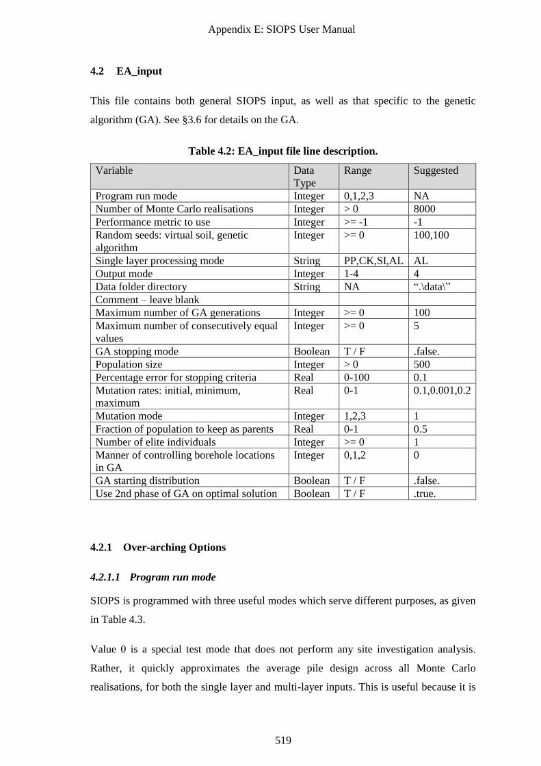
Appendix E: SIOPS User Manual
519
4.2 EA_input
This file contains both general SIOPS input, as well as that specific to the genetic
algorithm (GA). See §3.6 for details on the GA.
Table 4.2: EA_input file line description.
Variable Data
Type
Range Suggested
Program run mode Integer 0,1,2,3 NA
Number of Monte Carlo realisations Integer > 0 8000
Performance metric to use Integer >= -1 -1
Random seeds: virtual soil, genetic
algorithm
Integer >= 0 100,100
Single layer processing mode String PP,CK,SI,AL AL
Output mode Integer 1-4 4
Data folder directory String NA “.\data\”
Comment – leave blank
Maximum number of GA generations Integer >= 0 100
Maximum number of consecutively equal
values
Integer >= 0 5
GA stopping mode Boolean T / F .false.
Population size Integer > 0 500
Percentage error for stopping criteria Real 0-100 0.1
Mutation rates: initial, minimum,
maximum
Real 0-1 0.1,0.001,0.2
Mutation mode Integer 1,2,3 1
Fraction of population to keep as parents Real 0-1 0.5
Number of elite individuals Integer >= 0 1
Manner of controlling borehole locations
in GA
Integer 0,1,2 0
GA starting distribution Boolean T / F .false.
Use 2nd phase of GA on optimal solution Boolean T / F .true.
4.2.1 Over-arching Options
4.2.1.1 Program run mode
SIOPS is programmed with three useful modes which serve different purposes, as given
in Table 4.3.
Value 0 is a special test mode that does not perform any site investigation analysis.
Rather, it quickly approximates the average pile design across all Monte Carlo
realisations, for both the single layer and multi-layer inputs. This is useful because it is
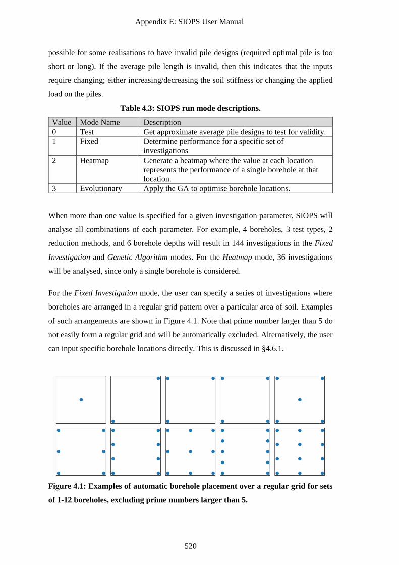
Appendix E: SIOPS User Manual
520
possible for some realisations to have invalid pile designs (required optimal pile is too
short or long). If the average pile length is invalid, then this indicates that the inputs
require changing; either increasing/decreasing the soil stiffness or changing the applied
load on the piles.
Table 4.3: SIOPS run mode descriptions.
Value Mode Name Description
0 Test Get approximate average pile designs to test for validity.
1 Fixed Determine performance for a specific set of
investigations
2 Heatmap Generate a heatmap where the value at each location
represents the performance of a single borehole at that
location.
3 Evolutionary Apply the GA to optimise borehole locations.
When more than one value is specified for a given investigation parameter, SIOPS will
analyse all combinations of each parameter. For example, 4 boreholes, 3 test types, 2
reduction methods, and 6 borehole depths will result in 144 investigations in the Fixed
Investigation and Genetic Algorithm modes. For the Heatmap mode, 36 investigations
will be analysed, since only a single borehole is considered.
For the Fixed Investigation mode, the user can specify a series of investigations where
boreholes are arranged in a regular grid pattern over a particular area of soil. Examples
of such arrangements are shown in Figure 4.1. Note that prime number larger than 5 do
not easily form a regular grid and will be automatically excluded. Alternatively, the user
can input specific borehole locations directly. This is discussed in §4.6.1.
Figure 4.1: Examples of automatic borehole placement over a regular grid for sets
of 1-12 boreholes, excluding prime numbers larger than 5.
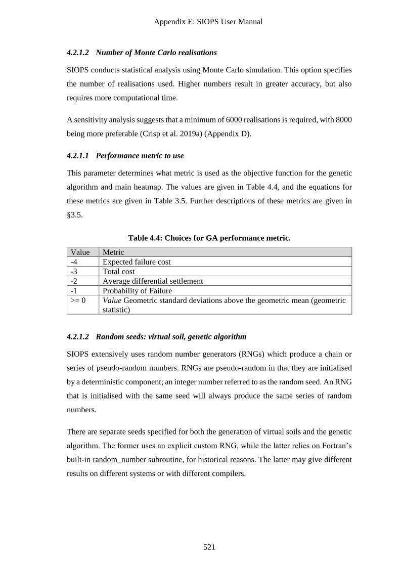
Appendix E: SIOPS User Manual
521
4.2.1.2 Number of Monte Carlo realisations
SIOPS conducts statistical analysis using Monte Carlo simulation. This option specifies
the number of realisations used. Higher numbers result in greater accuracy, but also
requires more computational time.
A sensitivity analysis suggests that a minimum of 6000 realisations is required, with 8000
being more preferable (Crisp et al. 2019a) (Appendix D).
4.2.1.1 Performance metric to use
This parameter determines what metric is used as the objective function for the genetic
algorithm and main heatmap. The values are given in Table 4.4, and the equations for
these metrics are given in Table 3.5. Further descriptions of these metrics are given in
§3.5.
Table 4.4: Choices for GA performance metric.
Value Metric
-4 Expected failure cost
-3 Total cost
-2 Average differential settlement
-1 Probability of Failure
>= 0 Value Geometric standard deviations above the geometric mean (geometric
statistic)
4.2.1.2 Random seeds: virtual soil, genetic algorithm
SIOPS extensively uses random number generators (RNGs) which produce a chain or
series of pseudo-random numbers. RNGs are pseudo-random in that they are initialised
by a deterministic component; an integer number referred to as the random seed. An RNG
that is initialised with the same seed will always produce the same series of random
numbers.
There are separate seeds specified for both the generation of virtual soils and the genetic
algorithm. The former uses an explicit custom RNG, while the latter relies on Fortran’s
built-in random_number subroutine, for historical reasons. The latter may give different
results on different systems or with different compilers.
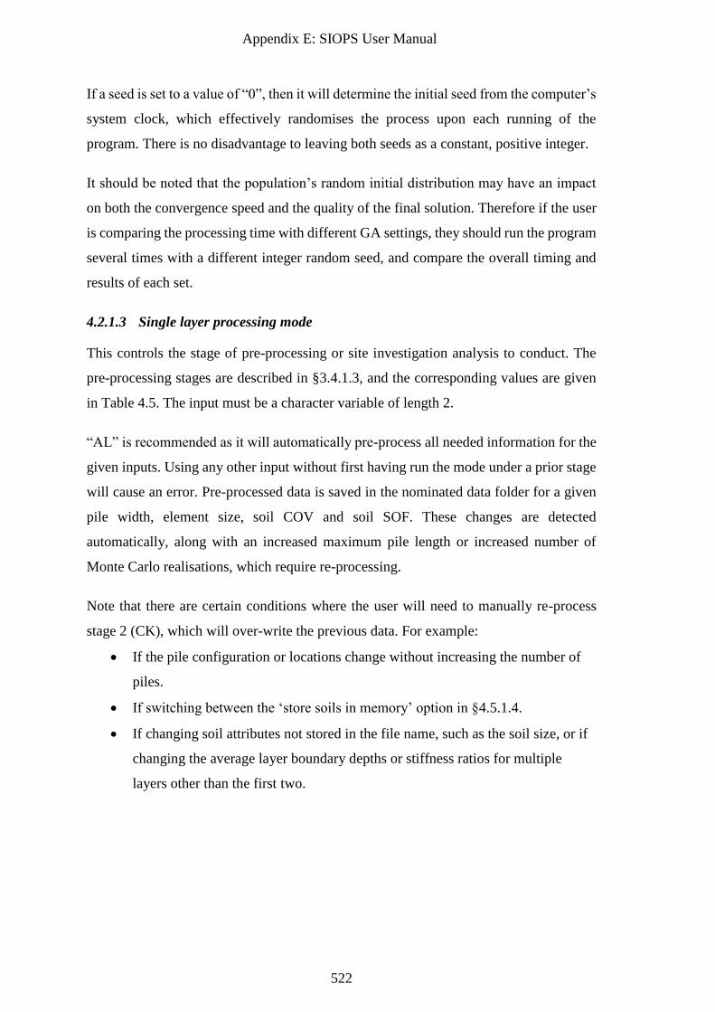
Appendix E: SIOPS User Manual
522
If a seed is set to a value of “0”, then it will determine the initial seed from the computer’s
system clock, which effectively randomises the process upon each running of the
program. There is no disadvantage to leaving both seeds as a constant, positive integer.
It should be noted that the population’s random initial distribution may have an impact
on both the convergence speed and the quality of the final solution. Therefore if the user
is comparing the processing time with different GA settings, they should run the program
several times with a different integer random seed, and compare the overall timing and
results of each set.
4.2.1.3 Single layer processing mode
This controls the stage of pre-processing or site investigation analysis to conduct. The
pre-processing stages are described in §3.4.1.3, and the corresponding values are given
in Table 4.5. The input must be a character variable of length 2.
“AL” is recommended as it will automatically pre-process all needed information for the
given inputs. Using any other input without first having run the mode under a prior stage
will cause an error. Pre-processed data is saved in the nominated data folder for a given
pile width, element size, soil COV and soil SOF. These changes are detected
automatically, along with an increased maximum pile length or increased number of
Monte Carlo realisations, which require re-processing.
Note that there are certain conditions where the user will need to manually re-process
stage 2 (CK), which will over-write the previous data. For example:
• If the pile configuration or locations change without increasing the number of
piles.
• If switching between the ‘store soils in memory’ option in §4.5.1.4.
• If changing soil attributes not stored in the file name, such as the soil size, or if
changing the average layer boundary depths or stiffness ratios for multiple
layers other than the first two.
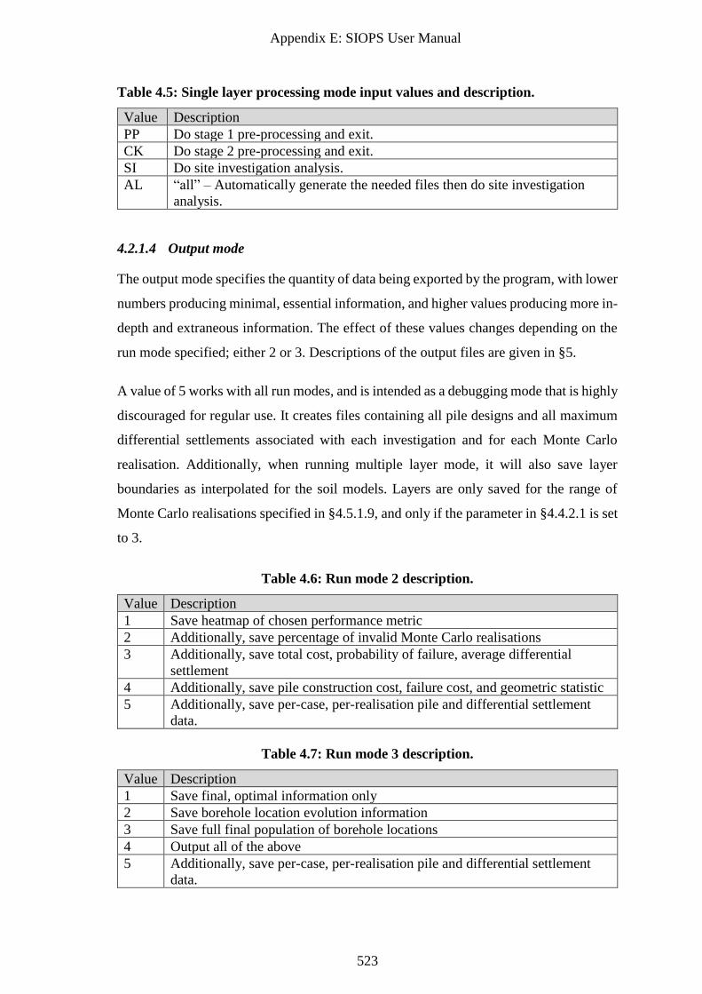
Appendix E: SIOPS User Manual
523
Table 4.5: Single layer processing mode input values and description.
Value Description
PP Do stage 1 pre-processing and exit.
CK Do stage 2 pre-processing and exit.
SI Do site investigation analysis.
AL “all” – Automatically generate the needed files then do site investigation
analysis.
4.2.1.4 Output mode
The output mode specifies the quantity of data being exported by the program, with lower
numbers producing minimal, essential information, and higher values producing more in-
depth and extraneous information. The effect of these values changes depending on the
run mode specified; either 2 or 3. Descriptions of the output files are given in §5.
A value of 5 works with all run modes, and is intended as a debugging mode that is highly
discouraged for regular use. It creates files containing all pile designs and all maximum
differential settlements associated with each investigation and for each Monte Carlo
realisation. Additionally, when running multiple layer mode, it will also save layer
boundaries as interpolated for the soil models. Layers are only saved for the range of
Monte Carlo realisations specified in §4.5.1.9, and only if the parameter in §4.4.2.1 is set
to 3.
Table 4.6: Run mode 2 description.
Value Description
1 Save heatmap of chosen performance metric
2 Additionally, save percentage of invalid Monte Carlo realisations
3 Additionally, save total cost, probability of failure, average differential
settlement
4 Additionally, save pile construction cost, failure cost, and geometric statistic
5 Additionally, save per-case, per-realisation pile and differential settlement
data.
Table 4.7: Run mode 3 description.
Value Description
1 Save final, optimal information only
2 Save borehole location evolution information
3 Save full final population of borehole locations
4 Output all of the above
5 Additionally, save per-case, per-realisation pile and differential settlement
data.
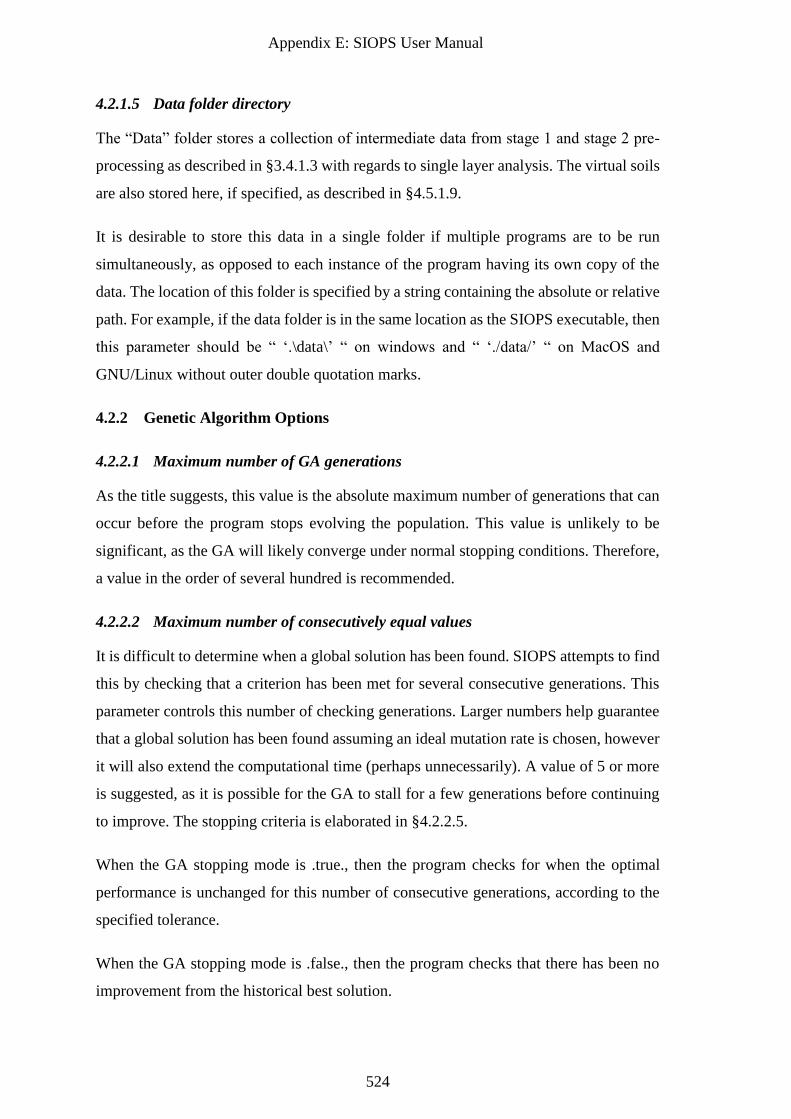
Appendix E: SIOPS User Manual
524
4.2.1.5 Data folder directory
The “Data” folder stores a collection of intermediate data from stage 1 and stage 2 pre-
processing as described in §3.4.1.3 with regards to single layer analysis. The virtual soils
are also stored here, if specified, as described in §4.5.1.9.
It is desirable to store this data in a single folder if multiple programs are to be run
simultaneously, as opposed to each instance of the program having its own copy of the
data. The location of this folder is specified by a string containing the absolute or relative
path. For example, if the data folder is in the same location as the SIOPS executable, then
this parameter should be “ ‘.\data\’ “ on windows and “ ‘./data/’ “ on MacOS and
GNU/Linux without outer double quotation marks.
4.2.2 Genetic Algorithm Options
4.2.2.1 Maximum number of GA generations
As the title suggests, this value is the absolute maximum number of generations that can
occur before the program stops evolving the population. This value is unlikely to be
significant, as the GA will likely converge under normal stopping conditions. Therefore,
a value in the order of several hundred is recommended.
4.2.2.2 Maximum number of consecutively equal values
It is difficult to determine when a global solution has been found. SIOPS attempts to find
this by checking that a criterion has been met for several consecutive generations. This
parameter controls this number of checking generations. Larger numbers help guarantee
that a global solution has been found assuming an ideal mutation rate is chosen, however
it will also extend the computational time (perhaps unnecessarily). A value of 5 or more
is suggested, as it is possible for the GA to stall for a few generations before continuing
to improve. The stopping criteria is elaborated in §4.2.2.5.
When the GA stopping mode is .true., then the program checks for when the optimal
performance is unchanged for this number of consecutive generations, according to the
specified tolerance.
When the GA stopping mode is .false., then the program checks that there has been no
improvement from the historical best solution.
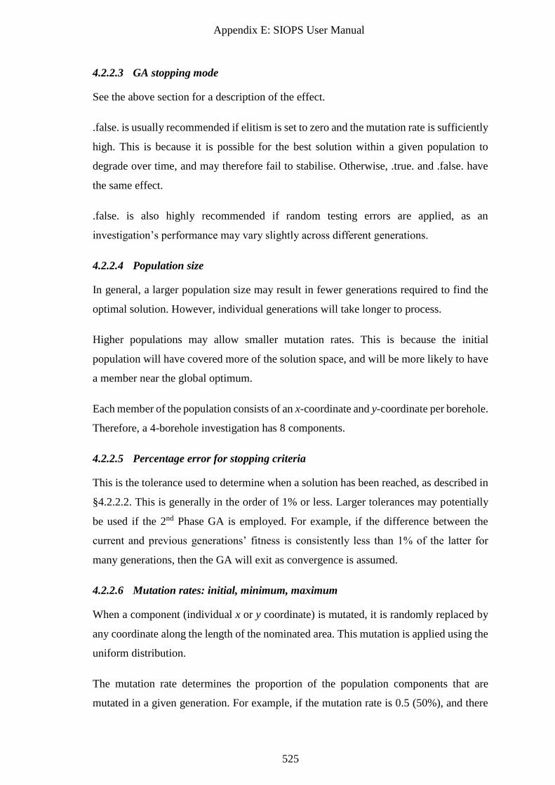
Appendix E: SIOPS User Manual
525
4.2.2.3 GA stopping mode
See the above section for a description of the effect.
.false. is usually recommended if elitism is set to zero and the mutation rate is sufficiently
high. This is because it is possible for the best solution within a given population to
degrade over time, and may therefore fail to stabilise. Otherwise, .true. and .false. have
the same effect.
.false. is also highly recommended if random testing errors are applied, as an
investigation’s performance may vary slightly across different generations.
4.2.2.4 Population size
In general, a larger population size may result in fewer generations required to find the
optimal solution. However, individual generations will take longer to process.
Higher populations may allow smaller mutation rates. This is because the initial
population will have covered more of the solution space, and will be more likely to have
a member near the global optimum.
Each member of the population consists of an x-coordinate and y-coordinate per borehole.
Therefore, a 4-borehole investigation has 8 components.
4.2.2.5 Percentage error for stopping criteria
This is the tolerance used to determine when a solution has been reached, as described in
§4.2.2.2. This is generally in the order of 1% or less. Larger tolerances may potentially
be used if the 2nd Phase GA is employed. For example, if the difference between the
current and previous generations’ fitness is consistently less than 1% of the latter for
many generations, then the GA will exit as convergence is assumed.
4.2.2.6 Mutation rates: initial, minimum, maximum
When a component (individual x or y coordinate) is mutated, it is randomly replaced by
any coordinate along the length of the nominated area. This mutation is applied using the
uniform distribution.
The mutation rate determines the proportion of the population components that are
mutated in a given generation. For example, if the mutation rate is 0.5 (50%), and there
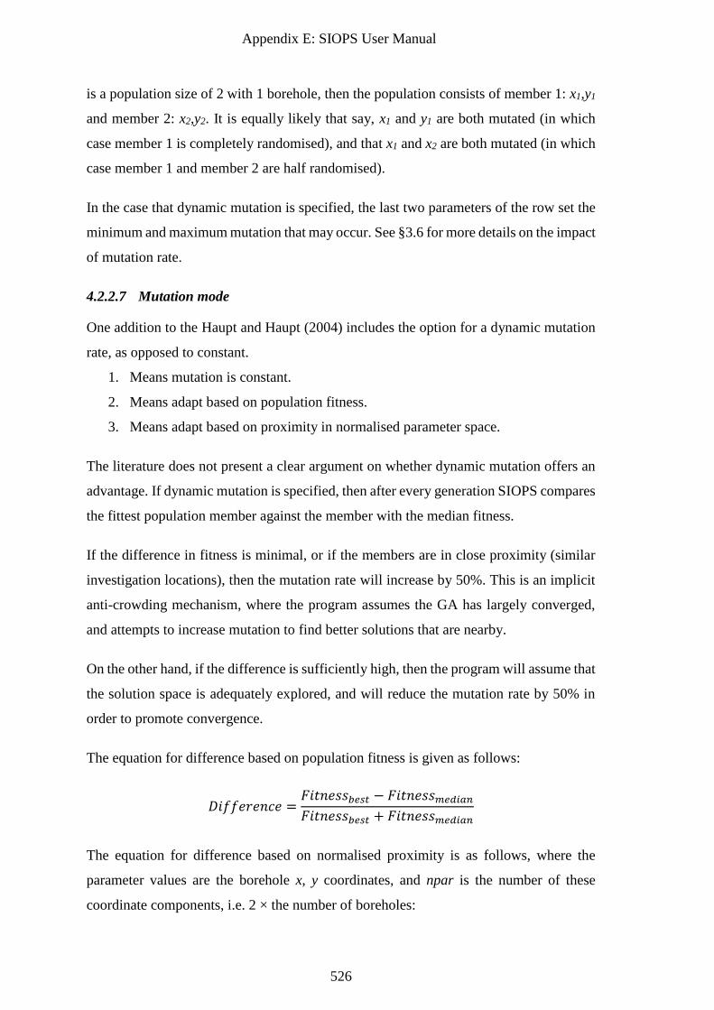
Appendix E: SIOPS User Manual
526
is a population size of 2 with 1 borehole, then the population consists of member 1: x1,y1
and member 2: x2,y2. It is equally likely that say, x1 and y1 are both mutated (in which
case member 1 is completely randomised), and that x1 and x2 are both mutated (in which
case member 1 and member 2 are half randomised).
In the case that dynamic mutation is specified, the last two parameters of the row set the
minimum and maximum mutation that may occur. See §3.6 for more details on the impact
of mutation rate.
4.2.2.7 Mutation mode
One addition to the Haupt and Haupt (2004) includes the option for a dynamic mutation
rate, as opposed to constant.
1. Means mutation is constant.
2. Means adapt based on population fitness.
3. Means adapt based on proximity in normalised parameter space.
The literature does not present a clear argument on whether dynamic mutation offers an
advantage. If dynamic mutation is specified, then after every generation SIOPS compares
the fittest population member against the member with the median fitness.
If the difference in fitness is minimal, or if the members are in close proximity (similar
investigation locations), then the mutation rate will increase by 50%. This is an implicit
anti-crowding mechanism, where the program assumes the GA has largely converged,
and attempts to increase mutation to find better solutions that are nearby.
On the other hand, if the difference is sufficiently high, then the program will assume that
the solution space is adequately explored, and will reduce the mutation rate by 50% in
order to promote convergence.
The equation for difference based on population fitness is given as follows:
𝐷𝑖𝑓𝑓𝑒𝑟𝑒𝑛𝑐𝑒 =𝐹𝑖𝑡𝑛𝑒𝑠𝑠𝑏𝑒𝑠𝑡 − 𝐹𝑖𝑡𝑛𝑒𝑠𝑠𝑚𝑒𝑑𝑖𝑎𝑛𝐹𝑖𝑡𝑛𝑒𝑠𝑠𝑏𝑒𝑠𝑡 + 𝐹𝑖𝑡𝑛𝑒𝑠𝑠𝑚𝑒𝑑𝑖𝑎𝑛
The equation for difference based on normalised proximity is as follows, where the
parameter values are the borehole x, y coordinates, and npar is the number of these
coordinate components, i.e. 2 × the number of boreholes:
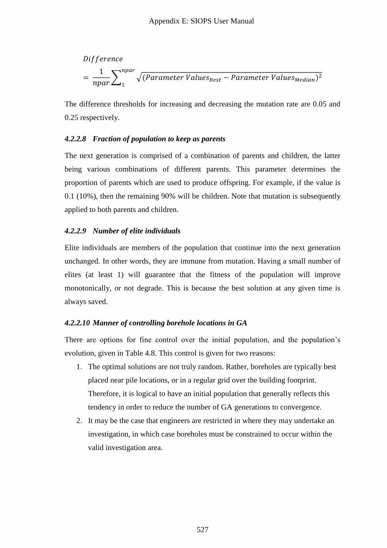
Appendix E: SIOPS User Manual
527
𝐷𝑖𝑓𝑓𝑒𝑟𝑒𝑛𝑐𝑒
= 1
𝑛𝑝𝑎𝑟∑ √(𝑃𝑎𝑟𝑎𝑚𝑒𝑡𝑒𝑟 𝑉𝑎𝑙𝑢𝑒𝑠𝐵𝑒𝑠𝑡 − 𝑃𝑎𝑟𝑎𝑚𝑒𝑡𝑒𝑟 𝑉𝑎𝑙𝑢𝑒𝑠𝑀𝑒𝑑𝑖𝑎𝑛)2
𝑛𝑝𝑎𝑟
1
The difference thresholds for increasing and decreasing the mutation rate are 0.05 and
0.25 respectively.
4.2.2.8 Fraction of population to keep as parents
The next generation is comprised of a combination of parents and children, the latter
being various combinations of different parents. This parameter determines the
proportion of parents which are used to produce offspring. For example, if the value is
0.1 (10%), then the remaining 90% will be children. Note that mutation is subsequently
applied to both parents and children.
4.2.2.9 Number of elite individuals
Elite individuals are members of the population that continue into the next generation
unchanged. In other words, they are immune from mutation. Having a small number of
elites (at least 1) will guarantee that the fitness of the population will improve
monotonically, or not degrade. This is because the best solution at any given time is
always saved.
4.2.2.10 Manner of controlling borehole locations in GA
There are options for fine control over the initial population, and the population’s
evolution, given in Table 4.8. This control is given for two reasons:
1. The optimal solutions are not truly random. Rather, boreholes are typically best
placed near pile locations, or in a regular grid over the building footprint.
Therefore, it is logical to have an initial population that generally reflects this
tendency in order to reduce the number of GA generations to convergence.
2. It may be the case that engineers are restricted in where they may undertake an
investigation, in which case boreholes must be constrained to occur within the
valid investigation area.
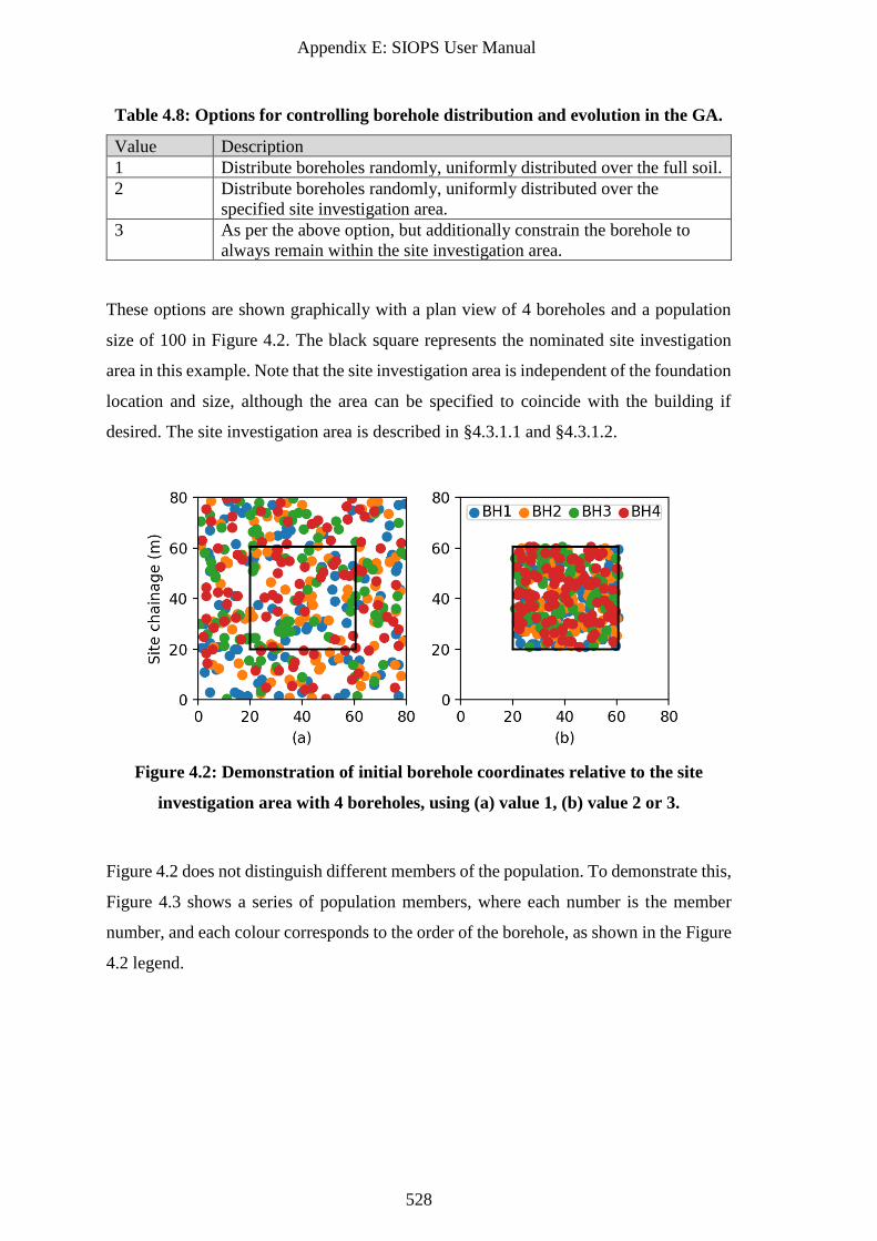
Appendix E: SIOPS User Manual
528
Table 4.8: Options for controlling borehole distribution and evolution in the GA.
Value Description
1 Distribute boreholes randomly, uniformly distributed over the full soil.
2 Distribute boreholes randomly, uniformly distributed over the
specified site investigation area.
3 As per the above option, but additionally constrain the borehole to
always remain within the site investigation area.
These options are shown graphically with a plan view of 4 boreholes and a population
size of 100 in Figure 4.2. The black square represents the nominated site investigation
area in this example. Note that the site investigation area is independent of the foundation
location and size, although the area can be specified to coincide with the building if
desired. The site investigation area is described in §4.3.1.1 and §4.3.1.2.
Figure 4.2: Demonstration of initial borehole coordinates relative to the site
investigation area with 4 boreholes, using (a) value 1, (b) value 2 or 3.
Figure 4.2 does not distinguish different members of the population. To demonstrate this,
Figure 4.3 shows a series of population members, where each number is the member
number, and each colour corresponds to the order of the borehole, as shown in the Figure
4.2 legend.
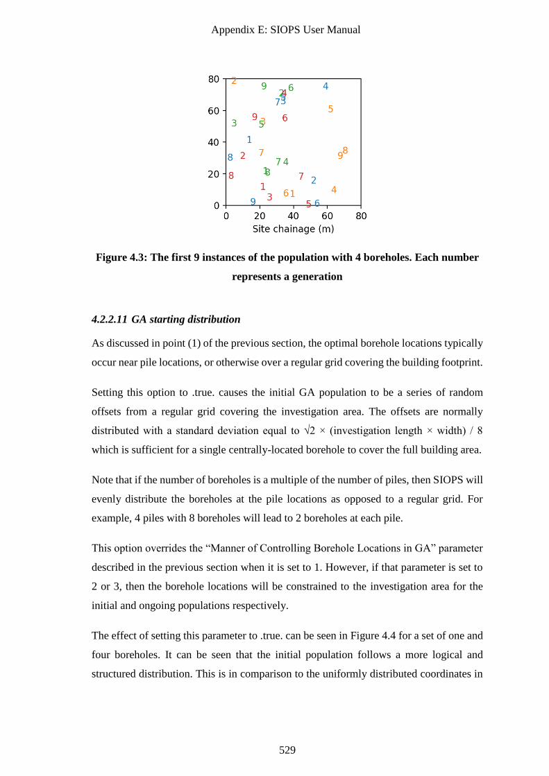
Appendix E: SIOPS User Manual
529
Figure 4.3: The first 9 instances of the population with 4 boreholes. Each number
represents a generation
4.2.2.11 GA starting distribution
As discussed in point (1) of the previous section, the optimal borehole locations typically
occur near pile locations, or otherwise over a regular grid covering the building footprint.
Setting this option to .true. causes the initial GA population to be a series of random
offsets from a regular grid covering the investigation area. The offsets are normally
distributed with a standard deviation equal to √2 × (investigation length × width) / 8
which is sufficient for a single centrally-located borehole to cover the full building area.
Note that if the number of boreholes is a multiple of the number of piles, then SIOPS will
evenly distribute the boreholes at the pile locations as opposed to a regular grid. For
example, 4 piles with 8 boreholes will lead to 2 boreholes at each pile.
This option overrides the “Manner of Controlling Borehole Locations in GA” parameter
described in the previous section when it is set to 1. However, if that parameter is set to
2 or 3, then the borehole locations will be constrained to the investigation area for the
initial and ongoing populations respectively.
The effect of setting this parameter to .true. can be seen in Figure 4.4 for a set of one and
four boreholes. It can be seen that the initial population follows a more logical and
structured distribution. This is in comparison to the uniformly distributed coordinates in
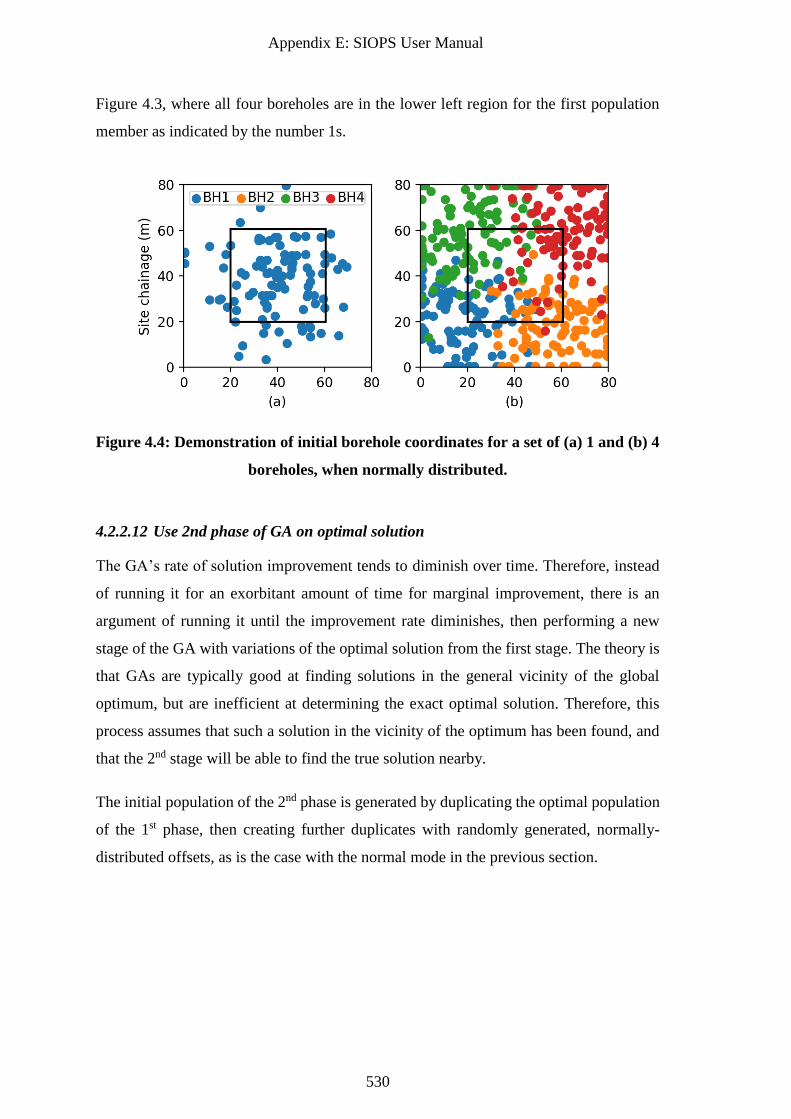
Appendix E: SIOPS User Manual
530
Figure 4.3, where all four boreholes are in the lower left region for the first population
member as indicated by the number 1s.
Figure 4.4: Demonstration of initial borehole coordinates for a set of (a) 1 and (b) 4
boreholes, when normally distributed.
4.2.2.12 Use 2nd phase of GA on optimal solution
The GA’s rate of solution improvement tends to diminish over time. Therefore, instead
of running it for an exorbitant amount of time for marginal improvement, there is an
argument of running it until the improvement rate diminishes, then performing a new
stage of the GA with variations of the optimal solution from the first stage. The theory is
that GAs are typically good at finding solutions in the general vicinity of the global
optimum, but are inefficient at determining the exact optimal solution. Therefore, this
process assumes that such a solution in the vicinity of the optimum has been found, and
that the 2nd stage will be able to find the true solution nearby.
The initial population of the 2nd phase is generated by duplicating the optimal population
of the 1st phase, then creating further duplicates with randomly generated, normally-
distributed offsets, as is the case with the normal mode in the previous section.
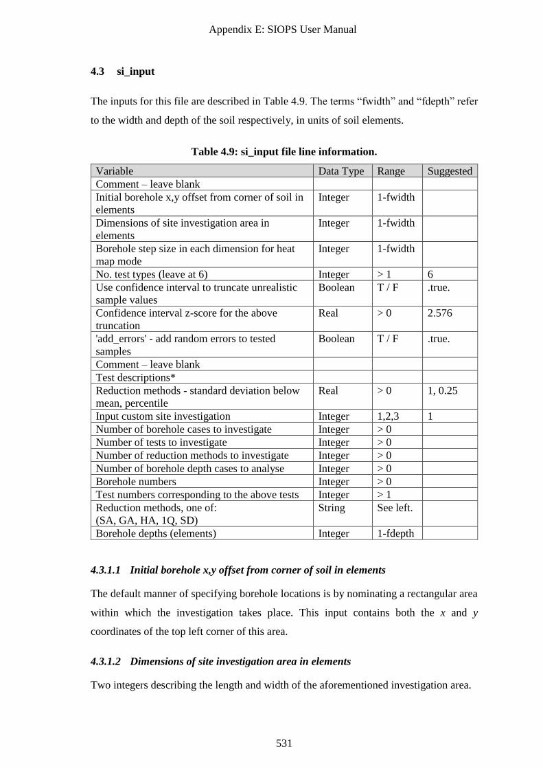
Appendix E: SIOPS User Manual
531
4.3 si_input
The inputs for this file are described in Table 4.9. The terms “fwidth” and “fdepth” refer
to the width and depth of the soil respectively, in units of soil elements.
Table 4.9: si_input file line information.
Variable Data Type Range Suggested
Comment – leave blank
Initial borehole x,y offset from corner of soil in
elements
Integer 1-fwidth
Dimensions of site investigation area in
elements
Integer 1-fwidth
Borehole step size in each dimension for heat
map mode
Integer 1-fwidth
No. test types (leave at 6) Integer > 1 6
Use confidence interval to truncate unrealistic
sample values
Boolean T / F .true.
Confidence interval z-score for the above
truncation
Real > 0 2.576
'add_errors' - add random errors to tested
samples
Boolean T / F .true.
Comment – leave blank
Test descriptions*
Reduction methods - standard deviation below
mean, percentile
Real > 0 1, 0.25
Input custom site investigation Integer 1,2,3 1
Number of borehole cases to investigate Integer > 0
Number of tests to investigate Integer > 0
Number of reduction methods to investigate Integer > 0
Number of borehole depth cases to analyse Integer > 0
Borehole numbers Integer > 0
Test numbers corresponding to the above tests Integer > 1
Reduction methods, one of:
(SA, GA, HA, 1Q, SD)
String See left.
Borehole depths (elements) Integer 1-fdepth
4.3.1.1 Initial borehole x,y offset from corner of soil in elements
The default manner of specifying borehole locations is by nominating a rectangular area
within which the investigation takes place. This input contains both the x and y
coordinates of the top left corner of this area.
4.3.1.2 Dimensions of site investigation area in elements
Two integers describing the length and width of the aforementioned investigation area.
Appendix E: SIOPS User Manual
532
4.3.1.3 Borehole step size in each dimension for heat map mode
The element increment in each dimension when generating a heat map of site
investigation quality. For example, a value of “1, 1” produces a continuous heat map over
the soil elements, “2, 2” assesses every 2nd element. Depending on the size of the heat
map and number of elements, the heat maps can take a moderate amount of time to
generate, and could require prohibitive amounts of RAM. In these circumstances, larger
step sizes are necessary.
4.3.1.4 No. test types
The total number of tests described for the program, regardless of which tests are to be
used in the investigations. Changing test type data is not recommended, and could
arguably be hard-coded within the program, however it is exposed here for experts if
needed.
4.3.1.5 Use confidence interval to truncate unrealistic sample values
When test errors are applied, it is possible that unrealistic sample values are produced.
Examples of this include negative, zero, or near-zero soil stiffnesses. Applying a
confidence interval, such that all samples outside this interval are removed from
consideration, should be applied to mitigate this. The confidence interval is geometric to
account for the lognormal distribution. It is recommended that this value is set to true
when testing errors are applied, and false when they are not, as the latter will noticeably
reduce the program’s run-time. See §4.3.1.7 for more details.
4.3.1.6 Confidence interval z-score for the above truncation
This z-score sets the degree of confidence for the previously described interval. A value
of 2.576 is recommended, which corresponds to 99% confidence.
4.3.1.7 'add_errors' - add random errors to tested samples
This Boolean variable determines whether or not random errors are applied to samples.
Setting this value to false means that all tests are perfectly accurate, which could result
in different tests giving the same results. While setting this value to true provides more
realistic results, it also requires a longer computational run-time. Therefore it may be
desirable to set this to false when running the genetic algorithm, due to its long run time,
and as testing errors are likely to have a negligible impact on optimal borehole location.
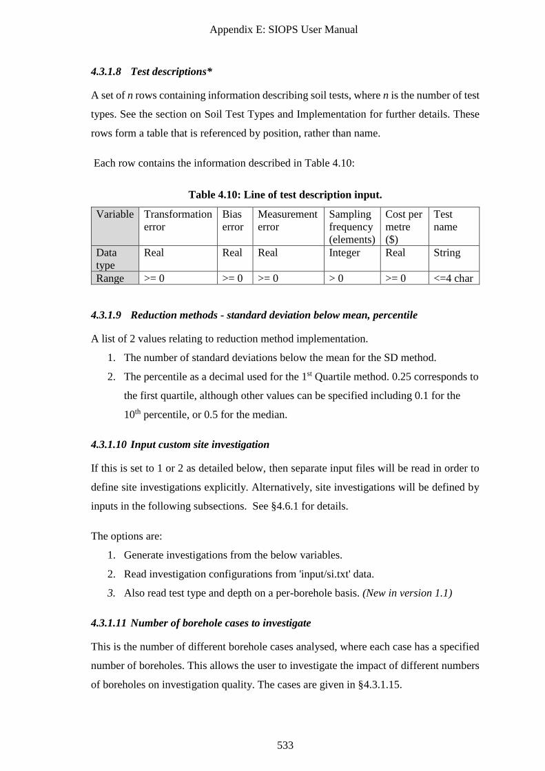
Appendix E: SIOPS User Manual
533
4.3.1.8 Test descriptions*
A set of n rows containing information describing soil tests, where n is the number of test
types. See the section on Soil Test Types and Implementation for further details. These
rows form a table that is referenced by position, rather than name.
Each row contains the information described in Table 4.10:
Table 4.10: Line of test description input.
Variable Transformation
error
Bias
error
Measurement
error
Sampling
frequency
(elements)
Cost per
metre
($)
Test
name
Data
type
Real Real Real Integer Real String
Range >= 0 >= 0 >= 0 > 0 >= 0 <=4 char
4.3.1.9 Reduction methods - standard deviation below mean, percentile
A list of 2 values relating to reduction method implementation.
1. The number of standard deviations below the mean for the SD method.
2. The percentile as a decimal used for the 1st Quartile method. 0.25 corresponds to
the first quartile, although other values can be specified including 0.1 for the
10th percentile, or 0.5 for the median.
4.3.1.10 Input custom site investigation
If this is set to 1 or 2 as detailed below, then separate input files will be read in order to
define site investigations explicitly. Alternatively, site investigations will be defined by
inputs in the following subsections. See §4.6.1 for details.
The options are:
1. Generate investigations from the below variables.
2. Read investigation configurations from 'input/si.txt' data.
3. Also read test type and depth on a per-borehole basis. (New in version 1.1)
4.3.1.11 Number of borehole cases to investigate
This is the number of different borehole cases analysed, where each case has a specified
number of boreholes. This allows the user to investigate the impact of different numbers
of boreholes on investigation quality. The cases are given in §4.3.1.15.
Appendix E: SIOPS User Manual
534
4.3.1.12 Number of tests to investigate
The number of test types to analyse. The cases are given in §4.3.1.16.
4.3.1.13 Number of reduction methods to investigate
The number of reduction methods to analyse. The cases are given in §4.3.1.17.
4.3.1.14 Number of borehole depth cases to analyse
The number of different borehole depths to analyse. The cases are given in §4.3.1.18.
4.3.1.15 Borehole numbers
A list of different numbers of boreholes that the user wishes to compare. The total number
of borehole cases is specified in §4.3.1.11.
4.3.1.16 Test numbers corresponding to the above tests
A list of test types to analyse. Each number refers to the position in the “test descriptions”
table in §4.3.1.8. For example, “1” refers to the test described in the first line. The number
of tests is given in §4.3.1.12.
4.3.1.17 Reduction methods
A list of reduction methods to analyse. A method is specified by a two-character string,
one of: SA, GA, HA, 1Q, SD. These are described previously in §3.4.5. The number of
reduction methods to analyse is given in §4.3.1.13.
4.3.1.18 Borehole depths (elements)
A list of maximum borehole depths to analyse, in terms of elements. The number of
depths to analyse is given in §4.3.1.14. The borehole depths are currently programmed to
be equal for all boreholes in a given investigation.
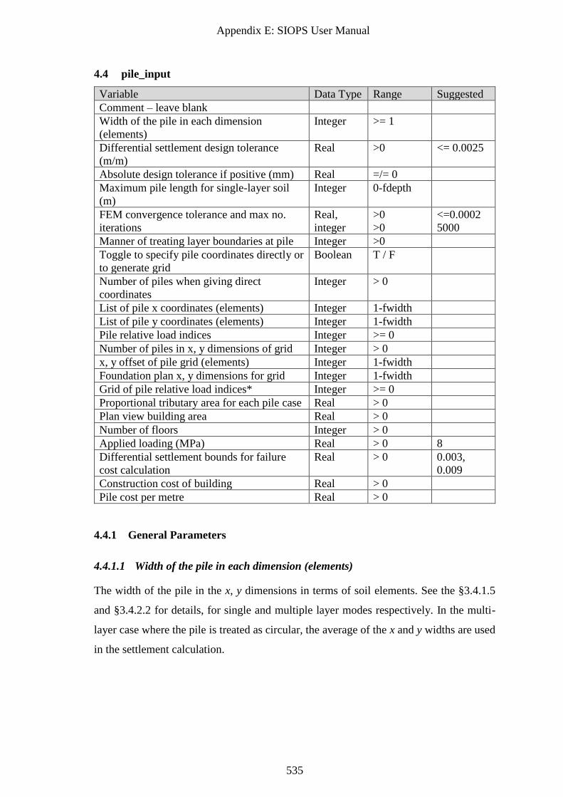
Appendix E: SIOPS User Manual
535
4.4 pile_input
Variable Data Type Range Suggested
Comment – leave blank
Width of the pile in each dimension
(elements)
Integer >= 1
Differential settlement design tolerance
(m/m)
Real >0 <= 0.0025
Absolute design tolerance if positive (mm) Real =/= 0
Maximum pile length for single-layer soil
(m)
Integer 0-fdepth
FEM convergence tolerance and max no.
iterations
Real,
integer
>0
>0
<=0.0002
5000
Manner of treating layer boundaries at pile Integer >0
Toggle to specify pile coordinates directly or
to generate grid
Boolean T / F
Number of piles when giving direct
coordinates
Integer > 0
List of pile x coordinates (elements) Integer 1-fwidth
List of pile y coordinates (elements) Integer 1-fwidth
Pile relative load indices Integer >= 0
Number of piles in x, y dimensions of grid Integer > 0
x, y offset of pile grid (elements) Integer 1-fwidth
Foundation plan x, y dimensions for grid Integer 1-fwidth
Grid of pile relative load indices* Integer >= 0
Proportional tributary area for each pile case Real > 0
Plan view building area Real > 0
Number of floors Integer > 0
Applied loading (MPa) Real > 0 8
Differential settlement bounds for failure
cost calculation
Real > 0 0.003,
0.009
Construction cost of building Real > 0
Pile cost per metre Real > 0
4.4.1 General Parameters
4.4.1.1 Width of the pile in each dimension (elements)
The width of the pile in the x, y dimensions in terms of soil elements. See the §3.4.1.5
and §3.4.2.2 for details, for single and multiple layer modes respectively. In the multi-
layer case where the pile is treated as circular, the average of the x and y widths are used
in the settlement calculation.
Appendix E: SIOPS User Manual
536
4.4.1.2 Differential settlement design tolerance (m/m)
A differential settlement design tolerance can be specified here. SIOPS will calculate the
minimum distance between any two piles, and multiply it by this tolerance value to
automatically obtain an absolute settlement design tolerance. For example, if 0.0025 is
specified and piles are arranged at 10 m spacings, the design tolerance will be 25 mm.
4.4.1.3 Absolute design tolerance if positive (mm)
If this value is positive, then it will be used as the value for absolute differential settlement
design tolerance, regardless of what is set in the previous option. Otherwise, the
differential settlement tolerance is used as described above.
4.4.1.4 Maximum pile length for single-layer soil
This is the maximum length of the pile in metres in the single layer soil. This must be
specified as the required finite element mesh and soil size must increase with pile length.
In multiple-layer soils, the maximum length is taken as the bottom of the soil, as there is
no computational penalty for doing so.
4.4.1.5 FEM convergence tolerance and max no. iterations
Two numbers; the FEM convergence tolerance as a decimal, and the maximum number
of iterations as an integer.
The implementation of linear-elastic FEA uses an iterative conjugate gradient solver to
avoid constructing the full stiffness matrix, thereby greatly reducing RAM usage. As a
result, there is a trade-off between the number of iterations (hence computational time)
and accuracy. Note that it is the number of elements in the mesh that is the main factor
controlling run time.
The convergence tolerance is calculated as the maximum change in deformations
between the current and previous iterations as a proportion of the largest current
deformation. A value of 0.0005 should be taken as an absolute minimum, while 0.0001
or less is ideal. By comparison, the maximum number of iterations is largely arbitrary. It
is incorporated to stop the program in the unlikely event that an infinite loop occurs.
However, hitting this limit will cause the program to exit, so setting an exceedingly large
value like 5000 is recommended. See Crisp et al. (2019a) (Appendix D) for further
information.
Appendix E: SIOPS User Manual
537
4.4.2 Pile Parameters
4.4.2.1 Manner of treating layer boundaries at pile
The pile must be assessed in a 1D soil, where the effective soil layer depths along the pile
are calculated from an inverse-distance-weighted average as discussed in §3.4.3.5.
However, it is faster to approximate the layer depths as simply the average layer boundary
within the pile radius. The user can specify which method to use for either the soil model
(SM), true soil (TS), or both by choice of the following values:
1. Simple average for SM and TS.
2. Simple average for SM, weighted average around pile for TS.
3. Weighted average for SM and TS.
The difference between the modes is usually very small, but can be moderate in highly
random layer boundaries. It is recommended that the simple average is used for the soil
model when the genetic algorithm is used, due to the long processing time involved. It
should arguably also be used for the true soil in this case for the sake of consistency. The
difference in speed between the two methods in the site investigation analysis is that the
full layer surfaces are interpolated with the inverse distance weighting, while only the
needed points are interpolated with the simple average.
4.4.2.2 Toggle to specify pile coordinates directly or to generate grid
There are two options of specifying pile locations in SIOPS. If this option is true, then
the pile coordinates are given directly (see below). If false, then pile coordinates are
derived from a grid (see §4.4.2.7 - §4.4.2.11).
4.4.2.3 Number of piles when giving direct coordinates
This specifies the total number of piles if the above option is set to true.
4.4.2.4 List of pile x coordinates (elements)
A list of x coordinates for the piles in terms of elements.
4.4.2.5 List of pile y coordinates (elements)
A list of y coordinates for the piles in terms of elements.
Appendix E: SIOPS User Manual
538
4.4.2.6 Pile relative load indices
A list of integers corresponding to each pile, where each integer is linked to the
proportional tributary load. See §4.4.2.10 and §4.4.2.11 for details.
4.4.2.7 Number of piles in x, y dimensions of grid
If piles are specified in the grid manner, then these two values give the number of piles
along the x and y dimensions of the grid.
4.4.2.8 x, y offset of pile grid (elements)
These two numbers specify the pile grid’s x, y offset from the corner of the site in terms
of elements.
4.4.2.9 Foundation plan x, y dimensions for grid
This specifies the length and width of the foundation in terms of elements when the piles
are given as a grid (see §4.4.2.2). The piles are spaced equally along each dimension. For
example, if there is a set of 3 × 3 piles and the foundation is given as 20 × 30 elements,
then the pile spacing will be 10 and 15 elements in the x, y dimensions respectively. Note
that this is independent of the building area.
4.4.2.10 Grid of pile relative load indices*
This input consists of a table of integers, where each integer’s relative location in the
table corresponds to the pile’s relative position in the grid. In particular, the integer
specifies the pile’s relative tributary area, in combination with the next set of inputs given
in §4.4.2.11. As such, pile loads are not given directly, rather they are proportional to the
building area and related to the number of piles.
For example, if the next set of inputs after this grid were “0.25, 0.5, 1.0”, then it would
allow for 3 sets of piles, with the 3rd supporting the biggest tributary area, the 2nd
supporting half of this area, and the 1st supporting a quarter. The integers given in the
table correspond to the order of the above tributary proportions, with 1 = 0.25, 2 = 0.5
and 3 = 1.0.
This is further illustrated by 4 examples given in Table 4.11 and Figure 4.5. With “0.25,
0.5, 1.0” specified as proportional tributary areas, the piles corresponding to integers 1, 2
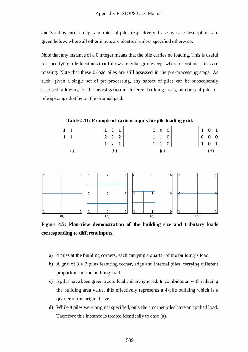
Appendix E: SIOPS User Manual
539
and 3 act as corner, edge and internal piles respectively. Case-by-case descriptions are
given below, where all other inputs are identical unless specified otherwise.
Note that any instance of a 0 integer means that the pile carries no loading. This is useful
for specifying pile locations that follow a regular grid except where occasional piles are
missing. Note that these 0-load piles are still assessed in the pre-processing stage. As
such, given a single set of pre-processing, any subset of piles can be subsequently
assessed, allowing for the investigation of different building areas, numbers of piles or
pile spacings that lie on the original grid.
Table 4.11: Example of various inputs for pile loading grid.
1 1 1 2 1 0 0 0 1 0 1
1 1 2 3 2 1 1 0 0 0 0
1 2 1 1 1 0 1 0 1
(a) (b) (c) (d)
Figure 4.5: Plan-view demonstration of the building size and tributary loads
corresponding to different inputs.
a) 4 piles at the building corners, each carrying a quarter of the building’s load.
b) A grid of 3 × 3 piles featuring corner, edge and internal piles, carrying different
proportions of the building load.
c) 5 piles have been given a zero load and are ignored. In combination with reducing
the building area value, this effectively represents a 4-pile building which is a
quarter of the original size.
d) While 9 piles were original specified, only the 4 corner piles have an applied load.
Therefore this instance is treated identically to case (a).
Appendix E: SIOPS User Manual
540
4.4.2.11 Proportional tributary area for each pile case
A list describing the set of relative tributary areas as a proportion of the largest tributary
area. See the previous input for details.
4.4.3 Building Parameters
4.4.3.1 Plan view building area
The plan view area of the building in terms of square metres. This is used in loading
information, so do not consider voids such as internal gardens which do not carry any
weight. It is assumed that the building has a similar profile on every floor.
4.4.3.2 Number of floors
Number of floors in the building. Used to calculate building weight.
4.4.3.3 Applied loading (MPa)
The uniformly distributed load supported by the structure. This is applied per square
metre, per floor to determine the structure’s total weight.
4.4.4 Cost Parameters
4.4.4.1 Differential settlement bounds for failure cost calculation
Values of differential settlement corresponding to zero damage, and extreme damage
requiring demolition and rebuilding of the structure. Found to generally be at 0.003 and
0.009 for generic multi-storey office buildings. See §3.5 for details on failure cost
calculations.
4.4.4.2 Construction cost of building
The cost of constructing the building. This is used in failure cost calculations described
in §3.5. If the structural cost is unknown, then it can be approximated by the equation
given below, based on Rawlinsons (2016). The equation is only technically valid for the
Australian market and the 2016 Australian dollar. However it can be adjusted for
inflation, and is likely to be reasonable for comparable countries.
𝐶 = 1,537.5𝐴 𝑛1.2858
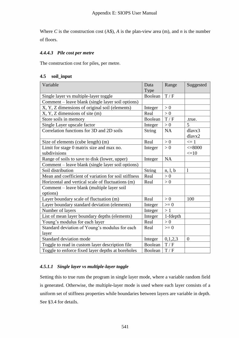
Appendix E: SIOPS User Manual
541
Where C is the construction cost (A$), A is the plan-view area (m), and n is the number
of floors.
4.4.4.3 Pile cost per metre
The construction cost for piles, per metre.
4.5 soil_input
Variable Data
Type
Range Suggested
Single layer vs multiple-layer toggle Boolean T / F
Comment – leave blank (single layer soil options)
X, Y, Z dimensions of original soil (elements) Integer > 0
X, Y, Z dimensions of site (m) Real > 0
Store soils in memory Boolean T / F .true.
Single Layer upscale factor Integer > 0 5
Correlation functions for 3D and 2D soils String NA dlavx3
dlavx2
Size of elements (cube length) (m) Real > 0 <= 1
Limit for stage 0 matrix size and max no.
subdivisions
Integer > 0 <=8000
<=10
Range of soils to save to disk (lower, upper) Integer NA
Comment – leave blank (single layer soil options)
Soil distribution String n, l, b l
Mean and coefficient of variation for soil stiffness Real > 0
Horizontal and vertical scale of fluctuations (m) Real > 0
Comment – leave blank (multiple layer soil
options)
Layer boundary scale of fluctuation (m) Real > 0 100
Layer boundary standard deviation (elements) Integer >= 0
Number of layers Integer > 1
List of mean layer boundary depths (elements) Integer 1-fdepth
Young’s modulus for each layer Real > 0
Standard deviation of Young’s modulus for each
layer
Real >= 0
Standard deviation mode Integer 0,1,2,3 0
Toggle to read in custom layer description file Boolean T / F
Toggle to enforce fixed layer depths at boreholes Boolean T / F
4.5.1.1 Single layer vs multiple-layer toggle
Setting this to true runs the program in single layer mode, where a variable random field
is generated. Otherwise, the multiple-layer mode is used where each layer consists of a
uniform set of stiffness properties while boundaries between layers are variable in depth.
See §3.4 for details.
Appendix E: SIOPS User Manual
542
4.5.1.2 X, Y, Z dimensions of original soil (elements)
This set of 3 integers describes the number of elements of the generated virtual soil in the
x, y, z dimensions. For various reasons, the generated site is at least slightly larger than
the final site used, with the latter being a subset of the original. Each value must be
representable by the equation 2ab, where a and b are integers.
Note that the program will exit if infeasible soil sizes are required. See §3.3.3 and the
next option for further details, along with the option in §4.5.1.8.
4.5.1.3 X, Y, Z dimensions of site (m)
The dimensions of the desired site in metres. Note that these dimensions should be
smaller than the original generated soil. For example, if the desired soil is 10 × 10 × 10
m and the element size is 0.5 m, then the original soil in the previous option must be at
least 20 × 20 × 20 elements. Ideally it should be larger still, to allow the random subset
to eliminate subtle bias inherent to the LAS algorithm.
4.5.1.4 Store soils in memory
When this option is set to .true., the virtual soils for all Monte Carlo realisations are
generated in advance of the site investigation analysis. This results in a greatly reduced
processing time when evolutionary mode is used, as it avoids the recalculation of soil
information for every genetic algorithm generation. The only cases where it is desirable
to set this to .false. would be if a very large and high-resolution soil were specified, or if
a very large number of Monte Carlo realisations (>10,000) were needed, as the RAM
requirements would be prohibitive.
For the multi-layer mode, this pre-processes and stores the true layer boundaries for all
realisations. For the fixed and heatmap modes, this option has no effect on performance.
For the single-layer mode, it is intended that SIOPS generates a significantly larger
random field than the desired site. This allows for individual soils in each Monte Carlo
realisation to be obtained by taking a subset of this large field. As the desired site is much
smaller than the original, with random offsets for each subset, each one is essentially an
independent random field, even if there is significant overlap. Note that setting this option
to .true. will result in a significant speedup regardless of mode, as a single large soil can
be generated much more quickly than many small soils.
Appendix E: SIOPS User Manual
543
4.5.1.5 Single Layer upscale factor
This is the factor by which the original single layer soil size is upscaled when the ‘store
soils in memory’ option is specified. This factor is applied in each dimension. For
example, a value of 2 means the soil is 2 × 2 × 2 = 8 times greater in volume. A value of
5 is sufficient. Alternatively, the user could keep this value at ‘1’ and increase the original
soil x, y, z dimensions manually.
4.5.1.6 Correlation functions for 3D and 2D soils
Different correlation functions are available, describing the manner of self-similarity in
the soil. Almost universally, an exponential Markov correlation function is
recommended. Therefore “’dlavx3’, ‘dlavx2’” should be given on this line.
4.5.1.7 Size of elements (cube length) (m)
The width of the soil elements in metres.
4.5.1.8 Limit for stage 0 matrix size and max no. subdivisions
These two values represent the maximum product of the stage 0 field dimensions, and the
maximum number of soil subdivisions as discussed in §3.3.3.For example, if the first
value is 512, then the generated 3D soil stage 0 field could have a maximum size of 8 ×
8 × 8, 16 × 16 × 2 elements, or some other combination with the product of 512.
2048 and 8 are reasonable choices. As the values increase, so too does the required RAM
usage. These inputs do not need to be very large, as the size of the generated soil grows
exponentially with each subdivision. Rather, one has to be more mindful that these values
are flexible enough to allow the specific dimensions of generated soil requested.
4.5.1.9 Range of soils to save to disk
The user can specify for soils from individual Monte Carlo realisations to be saved as
text files. This is done by specifying a lower and upper bound for the range of realisations.
For example, “1, 10” will output the first 10 realisations, while “11, 20” will output the
second 10.
If the first value is negative, then no soils are saved. To stop the program after soils are
exported, make the upper bound negative. For example, “1, -10” will output the first 10
realisations, then exit without performing site investigation analysis.
Appendix E: SIOPS User Manual
544
The soils are saved as a column vector, given in the X, Y, Z order where X is varying
fastest, and Z is varying slowest. Furthermore, if SIOPS is run in multi-layer mode, then
heatmaps of each layer’s lower boundary surface are also saved, except for the bottom
layer. The surfaces of depths are defined in terms of elements.
Warning: It is advised that the user be selective about which Monte Carlo realisations
they want to export, as saving a large number of soils can require an excessively large
amount of storage space.
4.5.2 Single Layer Options
4.5.2.1 Soil distribution
This string specifies the statistical distribution of soil stiffness values within the single
layer soil. In theory, the normal, lognormal and beta distributions are implemented with
input options “n”, “l” and “b” respectively. The lognormal distribution is strongly
recommended.
4.5.2.2 Mean and coefficient of variation for soil stiffness
The mean and coefficient of variation for Young’s modulus. See §3.3.2 for details.
4.5.2.3 Horizontal and vertical scale of fluctuations (m)
Two values representing the horizontal and vertical scale of fluctuation for Young’s
modulus respectively. Note that LAS is used when the soil is isotropic (vertical and
horizontal SOFs are within 1 mm of each other), otherwise the stepwise CMD method is
used. See §3.3.4.1 for details.
The stepwise CMD method can be forced for isotropic cases by making sure the vertical
and horizontal SOF values differ by a value of 0.01, which is easily small enough to not
affect the field statistics, but big enough to inform the program to use anisotropy.
4.5.3 Multiple Layer Options
4.5.3.1 Layer boundary scale of fluctuation (m)
The scale of fluctuation for the boundary of depths between layers. In practice, it is very
difficult to determine what this value should be, owing to the large quantity of layer depth
information required for its calculation, and the difficulty in obtaining this information.
Appendix E: SIOPS User Manual
545
Limited research has suggested that large values in the order of 100 m should be adopted.
The same SOF is used for all layers’ boundaries.
4.5.3.2 Layer boundary standard deviation (elements)
The standard deviation of layer boundary depths in elements. For example, if the value is
4 and the element size is 0.5 m, then a standard deviation of 2 m is applied.
4.5.3.3 Number of layers
The number of layers in the soil.
4.5.3.4 List of mean layer boundary depths (elements)
Unless a custom boundary input file is used, each layer is assumed to be horizontal on
average, with zero slope. This line of input takes a list of values describing the average
depth of each layer in terms of elements. For n layers, n-1 boundary depths are required,
as only boundaries between layers are considered, excluding the upper and lower bound.
4.5.3.5 Young’s modulus for each layer
This is a list of mean Young’s modulus for each soil layer. Note that the stiffness within
each layer is uniform.
4.5.3.6 Standard deviation of Young’s modulus for each layer
This is a list of standard deviations of Young’s modulus for each layer. As noted above,
the stiffness within each layer is uniform. This list of parameters describes variation of E
across the Monte Carlo realisations. This option accounts for the inherent uncertainty in
knowing the true mean of a layer’s stiffness, which could be higher or lower than what is
measured.
If a real soil is being modelled and there is a standard deviation of samples obtained, then
it is suggested that a standard deviation somewhere between zero and that of the samples
is specified. The random stiffness values are lognormally distributed.
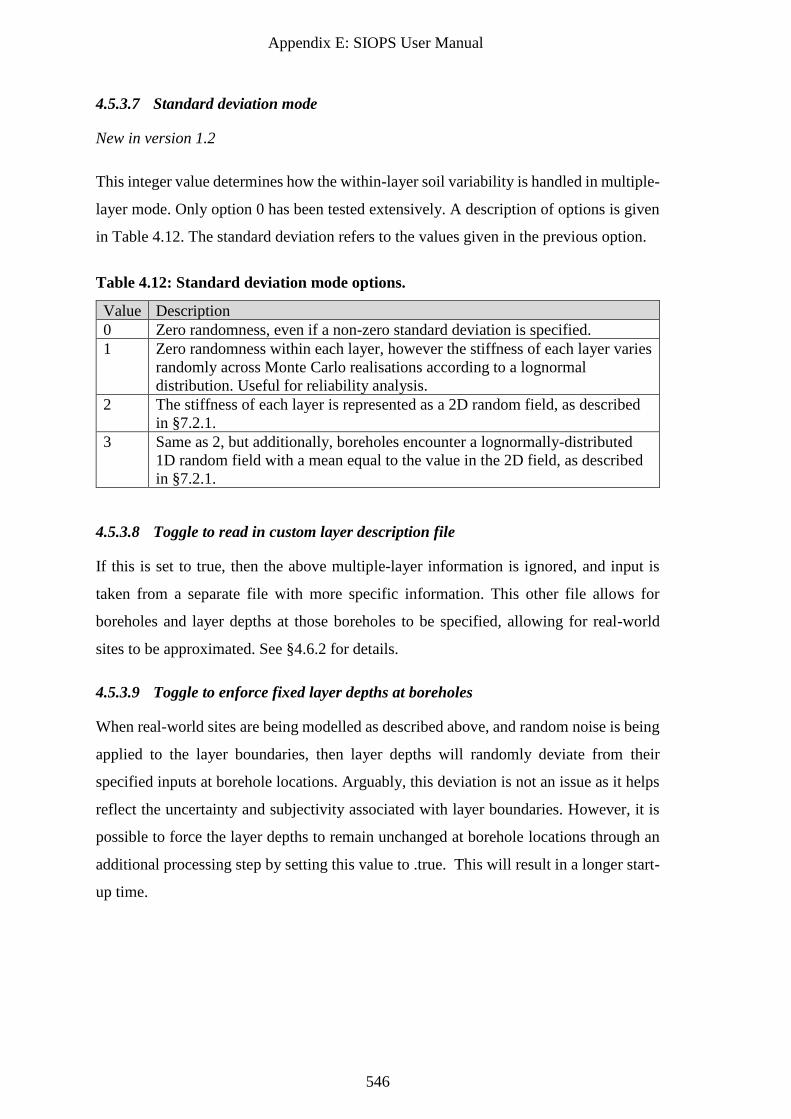
Appendix E: SIOPS User Manual
546
4.5.3.7 Standard deviation mode
New in version 1.2
This integer value determines how the within-layer soil variability is handled in multiple-
layer mode. Only option 0 has been tested extensively. A description of options is given
in Table 4.12. The standard deviation refers to the values given in the previous option.
Table 4.12: Standard deviation mode options.
Value Description
0 Zero randomness, even if a non-zero standard deviation is specified.
1 Zero randomness within each layer, however the stiffness of each layer varies
randomly across Monte Carlo realisations according to a lognormal
distribution. Useful for reliability analysis.
2 The stiffness of each layer is represented as a 2D random field, as described
in §7.2.1.
3 Same as 2, but additionally, boreholes encounter a lognormally-distributed
1D random field with a mean equal to the value in the 2D field, as described
in §7.2.1.
4.5.3.8 Toggle to read in custom layer description file
If this is set to true, then the above multiple-layer information is ignored, and input is
taken from a separate file with more specific information. This other file allows for
boreholes and layer depths at those boreholes to be specified, allowing for real-world
sites to be approximated. See §4.6.2 for details.
4.5.3.9 Toggle to enforce fixed layer depths at boreholes
When real-world sites are being modelled as described above, and random noise is being
applied to the layer boundaries, then layer depths will randomly deviate from their
specified inputs at borehole locations. Arguably, this deviation is not an issue as it helps
reflect the uncertainty and subjectivity associated with layer boundaries. However, it is
possible to force the layer depths to remain unchanged at borehole locations through an
additional processing step by setting this value to .true. This will result in a longer start-
up time.
Appendix E: SIOPS User Manual
547
4.6 Optional Input Files
There are additional input files which may be used in order to specify finer control over
various parameters. These include files for defining multiple-layer soils and custom site
investigations. When specified for use, these files must be in the input folder along with
the mandatory input files.
4.6.1 Custom Site Investigations
While the si_input.txt file is suitable for defining boreholes arranged over a regular grid,
there may be occasions where alterative patterns or irregular sampling is considered. For
this purpose, a set of investigations may be explicitly defined for input through 3 files:
• si.txt – site investigation attributes: number of boreholes, test type, reduction
method, borehole depth.
• si_Xcoords.txt – x coordinates of boreholes in metres.
• si_Ycoords.txt – y coordinates of boreholes in metres.
Table 4.13 describes the overall format of si.txt, while Table 4.14 details the format of
individual lines defining the attributes of each investigation in si.txt.
Each investigation defined from line 7 onwards in si.txt corresponds to borehole
coordinates given in si_Xcoords.txt and si_Ycoords.txt from line 2 onwards. Each column
in these latter two files is associated with a borehole. The first row of si_Xcoords.txt and
si_Ycoords.txt should be blank.
Note that these files are formatted such that one can take the SIOPS output from the fixed
site investigation analysis mode and use the renamed files as input. Therefore please
examine the files generated as referenced in §5.3 if further clarification is needed.
Use of the custom site investigation files is specified through the option in §4.3.1.10.
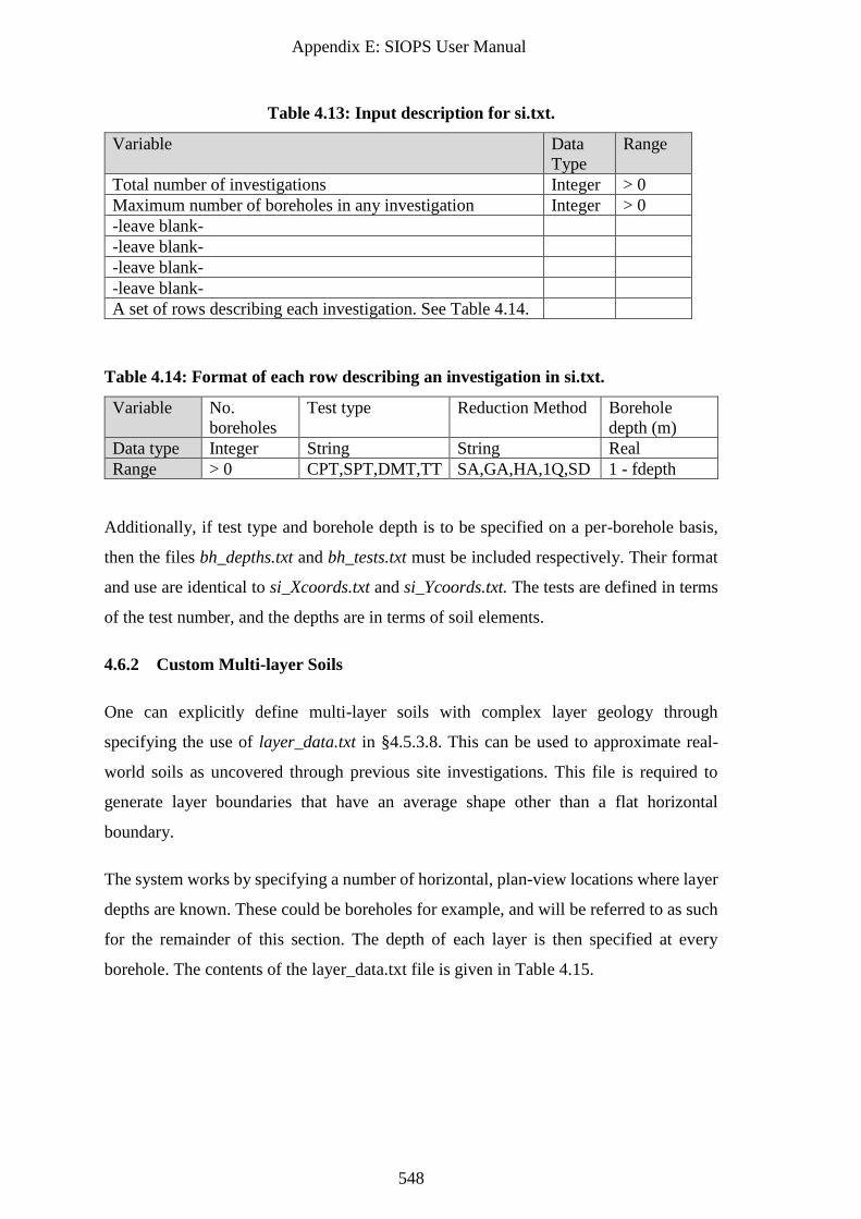
Appendix E: SIOPS User Manual
548
Table 4.13: Input description for si.txt.
Variable Data
Type
Range
Total number of investigations Integer > 0
Maximum number of boreholes in any investigation Integer > 0
-leave blank-
-leave blank-
-leave blank-
-leave blank-
A set of rows describing each investigation. See Table 4.14.
Table 4.14: Format of each row describing an investigation in si.txt.
Variable No.
boreholes
Test type Reduction Method Borehole
depth (m)
Data type Integer String String Real
Range > 0 CPT,SPT,DMT,TT SA,GA,HA,1Q,SD 1 - fdepth
Additionally, if test type and borehole depth is to be specified on a per-borehole basis,
then the files bh_depths.txt and bh_tests.txt must be included respectively. Their format
and use are identical to si_Xcoords.txt and si_Ycoords.txt. The tests are defined in terms
of the test number, and the depths are in terms of soil elements.
4.6.2 Custom Multi-layer Soils
One can explicitly define multi-layer soils with complex layer geology through
specifying the use of layer_data.txt in §4.5.3.8. This can be used to approximate real-
world soils as uncovered through previous site investigations. This file is required to
generate layer boundaries that have an average shape other than a flat horizontal
boundary.
The system works by specifying a number of horizontal, plan-view locations where layer
depths are known. These could be boreholes for example, and will be referred to as such
for the remainder of this section. The depth of each layer is then specified at every
borehole. The contents of the layer_data.txt file is given in Table 4.15.
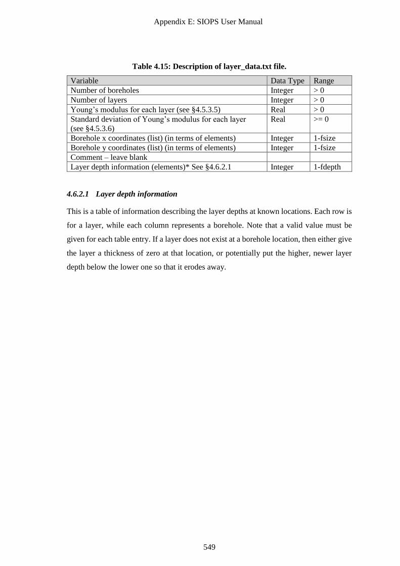
Appendix E: SIOPS User Manual
549
Table 4.15: Description of layer_data.txt file.
Variable Data Type Range
Number of boreholes Integer > 0
Number of layers Integer > 0
Young’s modulus for each layer (see §4.5.3.5) Real > 0
Standard deviation of Young’s modulus for each layer
(see §4.5.3.6)
Real >= 0
Borehole x coordinates (list) (in terms of elements) Integer 1-fsize
Borehole y coordinates (list) (in terms of elements) Integer 1-fsize
Comment – leave blank
Layer depth information (elements)* See §4.6.2.1 Integer 1-fdepth
4.6.2.1 Layer depth information
This is a table of information describing the layer depths at known locations. Each row is
for a layer, while each column represents a borehole. Note that a valid value must be
given for each table entry. If a layer does not exist at a borehole location, then either give
the layer a thickness of zero at that location, or potentially put the higher, newer layer
depth below the lower one so that it erodes away.
Appendix E: SIOPS User Manual
550
5 Output
This section details the SIOPS output; the various text files produced and how to interpret
them. The files can easily be imported into excel, or a scripting environment such as
Matlab or Python.
The following files contain a set of information about the overall analysis conditions in
the filename. Because these attributes are common, they will be represented by
[description], which details the number of piles, building area, and a soil description. For
single layers, the soil description is the COV and SOF. For multiple layer soils, it’s the
number of layers, stiffness ratio of the first two layers (rounded to the nearest integer),
and depth of the 2nd layer.
5.1.1.1 Pile Locations - pile_locations-[description].txt
This file describes the pile locations in metres, and is produced regardless of running
mode. Note that the soil description is absent as the foundation location is independent
of soil conditions. It’s a fixed-width file with two columns, where the first row consists
of the headings “X” and “Y”, and each row after that describes the X, Y coordinates of a
particular pile.
5.2 Test Mode
As described in §4.2.1.1, this mode serves as a quick test to determine whether SIOPS
will produce reasonable pile lengths for the given input. The results are written to
“deterministic_report.txt” saved in the same directory as the executable. There are two
sections in this file for the single- and multiple-layer classes respectively. Pile designs
which are negative mean that no valid design was found.
While these designs approximate the average pile designs across all Monte Carlo
realisations, it should be noted that there may be high variability in such designs across
the realisations themselves. If a portion of the spread of designs is not feasible, then they
are not considered in the final results. As such, if there are a moderate number of invalid
realisations, then the apparent average design could vary from the true one due to being
calculated from a truncated distribution. For both soil classes, the maximum pile length
is given.
Appendix E: SIOPS User Manual
551
For the single layer class, average pile designs for all reduction methods are given,
regardless of which are specified as input. Each row represents settlement associated with
a reduction method, while each column represents a pile load case. As the soil model is
identical at all locations, all piles that have the same applied load will be given the same
design. As such, a design is given for each pile load case, as opposed to each pile. The
pile load cases are headed by their relative tributary area.
For the multiple layer class, the designs of all piles are shown, as they could potentially
vary if the average layer surfaces are anything other than a flat horizontal boundary. Each
column represents a pile, which is headed by the pile load case in terms of relative
tributary area, as well as the piles’ x and y coordinates.
5.3 Fixed Mode
5.3.1.1 Investigation Attributes and Statistics - Population-stats_[description].txt
This file describes the majority of site investigation attributes and results.
The first four rows of the file describe the total number of investigations, the maximum
number of boreholes, the number of tests, the number of borehole depths and the number
of reduction methods analysed. The 5th row has a set of headings describing the following
11 columns:
• Number of boreholes
• Test type
• Reduction method
• Borehole depth (m)
• Failure cost ($)
• Pile construction cost ($)
• Site investigation cost ($)
• Probability of failure (%)
• Average differential settlement (m/m)
• Geometric statistic of differential settlement (m/m)
• Percentage of invalid Monte Carlo realisations (%)
Each row below the headings corresponds to a specific site investigation, the order of
which is consistent across all files.
Appendix E: SIOPS User Manual
552
5.3.1.2 Borehole Locations – Population-X/Ycoords_[description].txt
These two files contain the X and Y coordinates of the boreholes for each investigation in
metres. They are fixed width formatted. The first row is a set of headings describing the
borehole number. Each row after that corresponds to a particular site investigation, the
order of which is consistent across all files. The length of the row corresponds with the
number of boreholes associated with that investigation. As such, the rows will likely have
a variable length.
5.4 Heatmap Mode
The output of this mode consists of a set of heatmaps titled “Heatmap-[attribute]-
[description].txt” where [attribute] describes the contents of the file, which depending on
the choice and/or quantity of information requested, can include the:
• Number of invalid Monte Carlo realisations
• Performance metric of choice, with potential additional metrics (one or more
of):
o Total cost
o Probability of Failure
o Average differential settlement
o Failure cost
o Pile construction cost
o Geometric statistic
The quantity of additional heatmaps depends on the choice of the “output mode”
parameter as described in §4.2.1.4. The performance metrics are described in §3.5, with
input information given in §4.2.1.1.
5.4.1.1 File format
The format is consistent across all heatmap files. The first row features headings for the
second and third rows. These latter two rows describe the X and Y coordinates (m)
respectively for the top left and bottom right corners of the box containing the heatmap,
in case it is a subset of the full soil area. They also give the resolution of the heatmap in
the X and Y dimensions. The resolution is given as “1/element step size”, where the step
size is discussed in §4.3.1.3.
Appendix E: SIOPS User Manual
553
5.5 Evolutionary Mode
5.5.1 Primary Output
The files described in this section contain essential information, and are always generated
when SIOPS is run in evolutionary mode.
5.5.1.1 Investigation attributes and statistics - FinalEA-stats_[description].txt
This file describes the majority of site investigation attributes and results.
The first four rows of the file describe the population size, the maximum number of
boreholes/chosen performance metric, the number of tests, the number of borehole depths
and the number of reduction methods analysed. The 5th row has a set of headings
describing the following 12 columns:
• Number of boreholes
• Test type
• Reduction method
• Borehole depth (m)
• Percentage of invalid Monte Carlo realisations
• Number of genetic algorithm generations
• Time taken to convergence (seconds)
• Failure cost ($)
• Pile construction cost ($)
• Probability of failure (%)
• Average differential settlement (m/m)
• Geometric statistic of differential settlement (m/m)
Each row below the headings corresponds to a specific site investigation, the order of
which is consistent with the borehole location files. The performance metrics are
described in §3.5, with input information given in §4.2.1.1. The site investigation
parameters are described in §4.3.
5.5.1.2 Borehole locations – FinalEA-X/Ycoords_[description].txt
These two files contain the final (optimal) X and Y coordinates of the boreholes for each
investigation in metres. They are fixed width formatted. The first row is a set of headings
Appendix E: SIOPS User Manual
554
describing the borehole number. Each row after that corresponds to a particular site
investigation, the order of which is consistent with the stats file. The length of the row
corresponds with the number of boreholes associated with that investigation. As such, the
rows will likely have a variable length.
5.5.2 Optional Output
The following files may be produced depending on the choice of the “output mode”
parameter described in §4.2.1.4.
5.5.2.1 Borehole evolution - EvolutionEA-coords_Inv-[investigation
No.]_[description].txt
This file describes how the borehole locations evolve with each genetic algorithm
generation. The [investigation No.] in the heading refers to the order of the investigation
analysed, e.g. 1 for the first, 2 for the second, through to the total number of investigations
assessed. As such, each file describes a single investigation.
The first row contains the headings for each column, and each subsequent row
corresponds to a generation. The first column gives the performance associated with the
generation, and the second provides the percentage of invalid Monte Carlo realisations.
The subsequent columns detail the X coordinates for all boreholes, followed by the Y
coordinates for all boreholes, in metres. The number in the headings represents a
particular borehole. For example, the first and second “1” in the first row gives the X, Y
coordinates of the first borehole, and the latter also marks the start of the Y coordinate
columns.
5.5.2.2 Final population - Population-stats_Inv-[investigation No.]_[description].txt
This file describes the final generation’s population used in the genetic algorithm. This
file is arguably the least important of those described in this section, as the population
consists of sub-optimal solutions. It may potentially be useful for showing the sensitivity
of investigation performance with different borehole locations, however the final
generation is not guaranteed to contain solutions similar to the optimum.
Appendix E: SIOPS User Manual
555
The format of this file is identical to that described in the previous section. However,
each row corresponds to a member of the population, rather than the optimal solution at
each generation.
5.6 Intermediate Files
The single layer pre-processing stages save several files to the nominated data folder, to
be re-used in subsequent runs if needed. While it is not important to understand these
files in detail, and since the majority are self-explanatory, the descriptions will be kept
brief.
5.6.1 Stage 1 Pre-processing
The Stage 1 pre-processing, which generates the pile settlement curve and soil weights
for the PIE method, generates three files.
• settlement_prad-[pile width (elements)]_esize-[element size].txt
• model_bounds_prad-[pile width (elements)]_esize-[element size].txt
• soilweights_ prad-[pile width (elements)]_esize-[element size].txt
5.6.1.1 Settlement
This file simply contains the normalised pile settlement (MPa mm/kN) associated with 1
m increments of pile length; the settlement curve. The first line contains the headers of
two columns, with the first being the pile length in metres, and the second being the
settlement values.
5.6.1.2 Model Bounds
When generating the settlement curve and soil weights, a large FEA mesh is initially
required to minimise the impact of boundary effects. However, as subsequent settlement
analysis manipulates the initial FEA results, boundary effects are no-longer a
consideration. As such, it is possible to apply the PIE method with a smaller volume of
soil compared to the FEA mesh volume, which minimises computational time in the 2nd
stage pre-processing.
Appendix E: SIOPS User Manual
556
Moving away horizontally from the pile’s location, and downwards from the pile’s base,
PIE weights are truncated beyond certain slices such that all weights beyond a slice are
less than 0.01% of the field maximum.
This file has three columns, which represent the number of elements from the pile to
truncate the soil in the X, Y and Z directions respectively. Each row represents a pile
length increment in increasing order. Therefore, as lower rows are associated with longer
piles, they should have higher values, corresponding to larger volumes of soil weights to
apply.
5.6.1.3 Soil weights
The soil weights are stored as a single binary file, which reduces the amount of hardware
space required, and results in fast loading times. The downside is that the file is not
human-readable, meaning the PIE values cannot be directly viewed through a text editor
for inspection.
The file stores the soil weights associated with all pile lengths.
5.6.2 Stage 2 Pre-processing
Stage 2 generates a single type of file, albeit in multiple instances. These files contain the
true pile settlement for all piles and pile lengths for the nominated soil properties.
• ck_pile-[Pile number]_prad-[pile width (elements)]_esize-[element size]._sof-
[SOF]_cov-[COV]_anis-1.txt
For n piles, SIOPS generates n files. Each column in the file represents the settlement
associated with a pile length increment, for increasing lengths from left to right. Each
row corresponds to a Monte Carlo realisation.
Appendix E: SIOPS User Manual
557
6 Source Code Information
6.1 File Description
SIOPS consists of 90 Fortran files, largely following the 95 standard with occasional use
of newer features. A set of relevant files are given with a brief description in Table 6.1.
All files not listed are part of the GAF library for generating 2D and 3D random fields.
Table 6.1: Description of Fortran source files.
File Name Description
Main.F90 The main program unit.
Akima.F90 Performs 1D Akima interpolation.
Checkfiles.F90 Checks that necessary files exist for single layer mode, as well
as producing example input files.
Despile.F90 Design piles for the single layer mode.
Detcheck.F90 Perform a deterministic analysis for single and multiple layer
mode to check that inputs produce valid pile designs.
Edivide.F90 Undertake local averaging to fit soil elements into a finite
element mesh with varying element sizes.
ESETT.F90 Various subroutines related to assessing pile settlement for the
multiple-layer mode.
Extrafuncs.F90 Library of subroutines to assist in interpolation.
Fem_2d/3d.F90 Undertake 2D/3D linear elastic finite element analysis.
Fem_*.F90 Remaining “fem_” files contain various subroutines that
support the aforementioned finite element analysis.
Ga.F90 Subroutine for performing the Genetic Algorithm
Getdiff.F90 Calculate differential settlement for single layer soil mode
Getcosts.F90 Calculate failure costs from differential settlement.
Getperfmulti.F90 Over-arching file for obtaining information about the ground,
such as layer properties and boundary depths
Int2D.F90 Various subroutines for different cases of 2D interpolation via
triangulation
Output_results.F90 Save site investigation performance information to disk
PROCESS_CK.F9
0
Over-arching file for pre-processing soil and pile information
prior to site investigation analysis.
PROCESS_SI.F90 Over-arching file for assessing single layer investigation
performance.
PROCESS_SI_
multi.F90
Over-arching file for assessing multiple layer investigation
performance.
pwl_interp_2d_
scattered.F90
Various subroutines that support 2D interpolation.
qsort_c_
module.F90
Sorting a list in increasing order.
r8lib.F90 Arithmetic utility library, also used to support 2D interpolation.
READINM.F90 Various subroutines for reading input information to control the
program’s settings.
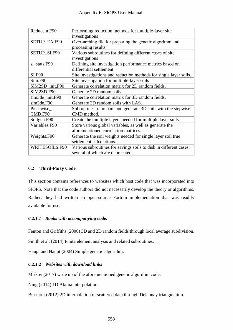
Appendix E: SIOPS User Manual
558
Reducem.F90 Performing reduction methods for multiple-layer site
investigations
SETUP_EA.F90 Over-arching file for preparing the genetic algorithm and
processing results
SETUP_SI.F90 Various subroutines for defining different cases of site
investigations
si_stats.F90 Defining site investigation performance metrics based on
differential settlement
SI.F90 Site investigations and reduction methods for single layer soils.
Sim.F90 Site investigation for multiple-layer soils
SIM2SD_init.F90 Generate correlation matrix for 2D random fields.
SIM2SD.F90 Generate 2D random soils.
sim3de_init.F90 Generate correlation matrix for 3D random fields.
sim3de.F90 Generate 3D random soils with LAS.
Piecewise_
CMD.F90
Subroutines to prepare and generate 3D soils with the stepwise
CMD method.
Soilgen.F90 Create the multiple layers needed for multiple layer soils.
Variables.F90 Store various global variables, as well as generate the
aforementioned correlation matrices.
Weights.F90 Generate the soil weights needed for single layer soil true
settlement calculations.
WRITESOILS.F90 Various subroutines for savings soils to disk in different cases,
several of which are deprecated.
6.2 Third-Party Code
This section contains references to websites which host code that was incorporated into
SIOPS. Note that the code authors did not necessarily develop the theory or algorithms.
Rather, they had written an open-source Fortran implementation that was readily
available for use.
6.2.1.1 Books with accompanying code:
Fenton and Griffiths (2008) 3D and 2D random fields through local average subdivision.
Smith et al. (2014) Finite element analysis and related subroutines.
Haupt and Haupt (2004) Simple genetic algorithm.
6.2.1.2 Websites with download links
Mirkov (2017) write up of the aforementioned genetic algorithm code.
Ning (2014) 1D Akima interpolation.
Burkardt (2012) 2D interpolation of scattered data through Delaunay triangulation.
Appendix E: SIOPS User Manual
559
7 Version Tracking
This section details the improvements and new features compared to older versions of the
program, as well as plans for new features to be added in the future.
7.1 Changelog
7.1.1 Version 1.1
1. The stepwise CMD method was implemented for generating anisotropic, 3D,
variable, single layer soils. See §3.3.4.
2. SIOPS now allows for individual boreholes to have different depths and test
types within the same investigation, when using the custom investigation input
files.
7.1.2 Version 1.2
1. Fixed a crash that occurred when running the SIOPS for the first time in single-
layer mode, but not in subsequent runs.
2. Added an experimental hybrid soil model as described in §7.2.1. It has not yet
been properly tested, and likely needs some modification. Currently, the inverse-
distance squared weighting is used, which does not provide fully accurate costs
for all COV values, implying that the weighting scheme is not appropriate (and
that PIE weights should be investigated), or that some other problem is present,
such as consistency in the random field generator. As such, this feature is not
currently recommended.
7.2 Planned Features
The features discussed in this section are potential candidates for additions to future
SIOPS versions. The author does not guarantee that these features will be implemented,
however they are detailed here to inform users that they are at least hypothetically feasible
to do so.
7.2.1 Hybrid Soil Model
This would be an enhanced version of the multi-layer mode whereby the properties
within each layer will vary in the horizontal direction while being constant in the vertical
direction. As such, the soil properties in each layer can be fully defined by 2D random
Appendix E: SIOPS User Manual
560
fields. The uniform soil properties required for each pile’s true settlement can be
determined by an inverse-distance weighted average as is done with the layer boundaries,
described in §3.4.3.5.
The constant properties with depth is analogous to an infinite vertical SOF, which is a
worst-case scenario from a pile settlement perspective. However, as a short borehole
would provide the same information as a long one, which is unrealistic. To compensate
for this, the soil properties within each layer, as encountered by boreholes, would be
optionally represented by 1D random fields for which the means are defined by the
boreholes’ horizontal location. As such, the soil model for the site investigation would
be decoupled from that of the true pile settlement. However, the two would be very
similar, and in fact identical if the boreholes were sufficiently long in each layer. An
example of the hybrid soil, along with the addition of vertical 1D random fields is given
in Figure 7.1.
It should be noted that if the vertical 1D random fields are added, this should increase
the overall variability of the soil profile. Therefore, both the COV of the 2D horizontal
fields and 1D vertical fields must be reduced to compensate. If two normal distributions
with an equal COV are added together, the COV of both would need to be reduced
(multiplied) by 2-0.5 in order to achieve the original COV of either field. The lognormal
distribution approximates that of the normal at low COV values, such that this method
can be applied. However, as the resulting COV is slightly higher than expected, a slightly
lower reduction factor of 2/3 is suggested as a rule of thumb. This effect would reduce
the differential settlement of piles, such that comparison of results with and without the
1D fields would not be valid. As such, the addition of 1D fields would likely reduce the
overall failure cost, particularly if a conservative reduction method is used. However,
there is an argument that the differential settlement ought to be reduced somewhat in
order to compensate for the unrealistically-high vertical SOF.
This hybrid model would be considered only a rough approximation of the worst case
soil conditions, due to both the unrealistic infinite vertical SOF and the decoupling of the
aforementioned soil models. It is intended to be used as an upper bound of soil variability,
whereas the current multi-layer method with its 0% within-layer variability, would be a
lower bound.
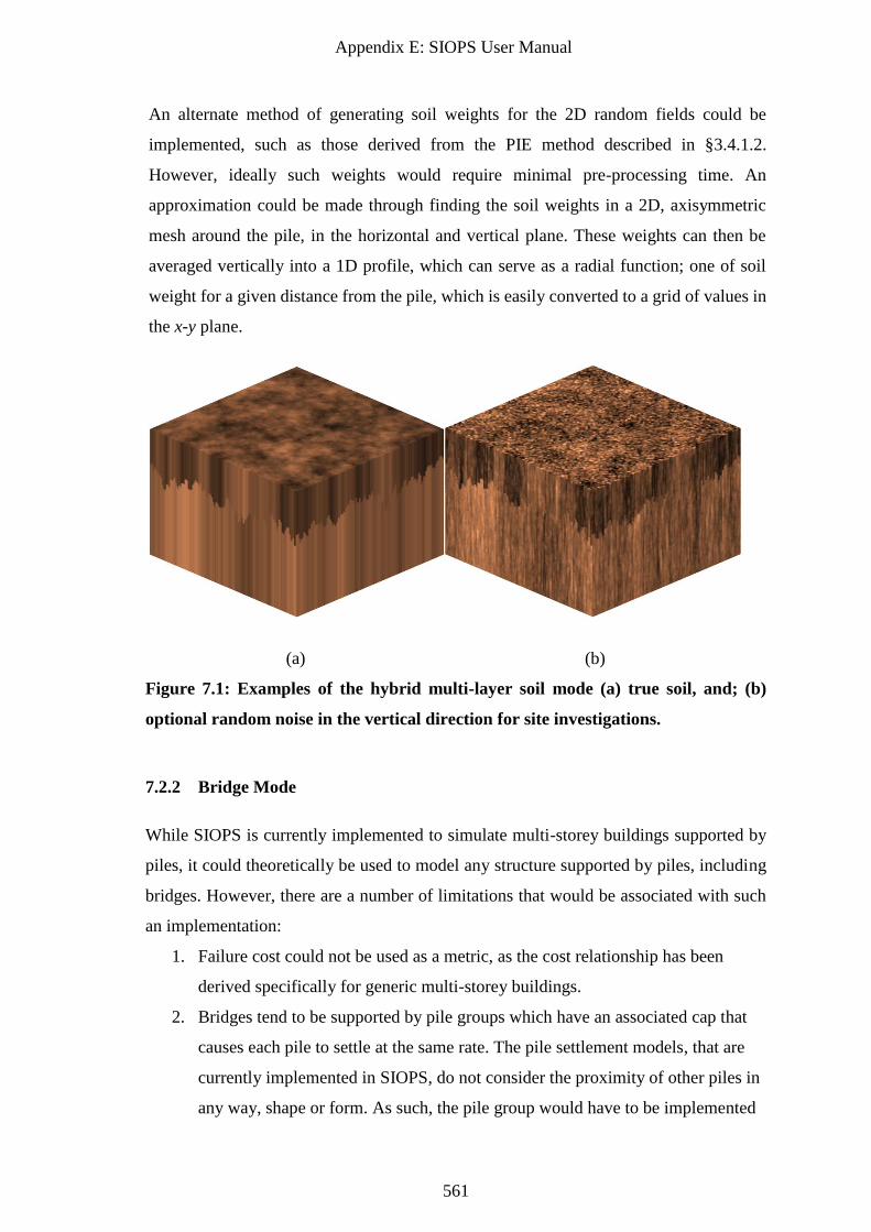
Appendix E: SIOPS User Manual
561
An alternate method of generating soil weights for the 2D random fields could be
implemented, such as those derived from the PIE method described in §3.4.1.2.
However, ideally such weights would require minimal pre-processing time. An
approximation could be made through finding the soil weights in a 2D, axisymmetric
mesh around the pile, in the horizontal and vertical plane. These weights can then be
averaged vertically into a 1D profile, which can serve as a radial function; one of soil
weight for a given distance from the pile, which is easily converted to a grid of values in
the x-y plane.
(a) (b)
Figure 7.1: Examples of the hybrid multi-layer soil mode (a) true soil, and; (b)
optional random noise in the vertical direction for site investigations.
7.2.2 Bridge Mode
While SIOPS is currently implemented to simulate multi-storey buildings supported by
piles, it could theoretically be used to model any structure supported by piles, including
bridges. However, there are a number of limitations that would be associated with such
an implementation:
1. Failure cost could not be used as a metric, as the cost relationship has been
derived specifically for generic multi-storey buildings.
2. Bridges tend to be supported by pile groups which have an associated cap that
causes each pile to settle at the same rate. The pile settlement models, that are
currently implemented in SIOPS, do not consider the proximity of other piles in
any way, shape or form. As such, the pile group would have to be implemented
Appendix E: SIOPS User Manual
562
as a group of individual piles, potentially with their settlement being averaged or
approximated in some other manner. For example, assuming that each pile
settles by the same amount, the total settlement would be equal to the harmonic
average of the individual pile settlements, as the group stiffness would be that of
the arithmetic average of the individual pile stiffnesses. However, since the
method of foundation modelling is consistent in both the soil model and true
soil, any errors from approximation would be minimised, as the discrepancies
are self-cancelling.
7.2.3 Generalised Mode
It is possible to add support for a more general, albeit implicit, optimization of
investigations is through the addition of a ‘generalised mode’. Rather than assessing the
performance of a foundation, the site investigation results can be assessed directly. For
example, the standard deviation of the Young’s modulus estimate across Monte Carlo
realisations can be minimised. Other properties of interest, such as average layer
boundary depth, or other metrics can be investigated. There are also some advanced
statistical estimates of soil knowledge such as a signal-to-noise ratio, as is done in Gong
et al. (2016). However such metrics would require more literature review, be more
complicated to program, and might not be fully trusted by engineers compared to a
more straightforward metric with an easy-to-interpret meaning.
This mode will answer the question of “what level of site investigation should be used,
such that minimal additional ground information can be obtained through further
testing”. This method has the advantage of being independent of the geotechnical
system being considered, which is both an advantage in that is generalised, and a
disadvantage in that the results are not explicitly related to the outcomes.
7.2.4 Pad Foundations
SIOPS can theoretically be extended to support pad foundations in addition to piles. A
review of settlement methods has been given by Goldsworthy (2006). In single layer
soils, a pad can be modelled as a rigid plate on the surface of the soil. As such, pad can
be designed by increasing the diameter of the plate, rather than its depth, as is currently
done for a pile. It is worth noting that the code considers the pile’s position as its
corner, rather than its centre. While this treatment is irrelevant for a plate of a fixed
Appendix E: SIOPS User Manual
563
diameter, it is important to ensure that the pad’s true centre remains fixed in location as
the diameter varies. It is possible to convert the settlement profile of a rigid pad to that
of a flexible pad, if that is desired.
For multiple layer soils, a method capable of incorporating variations in Young’s
modulus with depth is required, such as the Schmertmann method.
7.2.5 User Interface
On the non-technical side, and improvement that would greatly increase SIOPS’ ease of
use is a graphical user interface, as opposed to control through input text files. A
hypothetical interface could take one of the following forms:
• SIOPS could incorporate a native interface through Fortran’s interoperability
with C and C++. The interface would be programmed in one of these two
languages.
• An interface could be created as a separate program that takes user input, then
generates the necessary input files and runs SIOPS externally and automatically.
It could be through:
o An executable coded in C, C++ or another compiled language.
o Python and a graphical interface library such as PyQt. However, this
requires that both Python and the relevant libraries are installed on the
computer of interest.
o Microsoft excel. VBA can be used to create interfaces and manage input
and output. This approach as the benefit that SIOPS’ output data can be
easily imported and graphed. Excel is typically widely available.
Appendix E: SIOPS User Manual
564
8 Licence
SIOPS is released under the MIT licence, which is given below:
MIT License
Copyright (c) 2020 Michael Crisp
Permission is hereby granted, free of charge, to any person obtaining a copy of this
software and associated documentation files (the "Software"), to deal in the Software
without restriction, including without limitation the rights to use, copy, modify, merge,
publish, distribute, sublicense, and/or sell copies of the Software, and to permit persons
to whom the Software is furnished to do so, subject to the following conditions:
The above copyright notice and this permission notice shall be included in all copies or
substantial portions of the Software.
THE SOFTWARE IS PROVIDED "AS IS", WITHOUT WARRANTY OF ANY KIND,
EXPRESS OR IMPLIED, INCLUDING BUT NOT LIMITED TO THE WARRANTIES
OF MERCHANTABILITY, FITNESS FOR A PARTICULAR PURPOSE AND
NONINFRINGEMENT. IN NO EVENT SHALL THE AUTHORS OR COPYRIGHT
HOLDERS BE LIABLE FOR ANY CLAIM, DAMAGES OR OTHER LIABILITY,
WHETHER IN AN ACTION OF CONTRACT, TORT OR OTHERWISE, ARISING
FROM, OUT OF OR IN CONNECTION WITH THE SOFTWARE OR THE USE OR
OTHER DEALINGS IN THE SOFTWARE.

Appendix E: SIOPS User Manual
565
9 Acknowledgements
I would like to thank my PhD supervisors Mark Jaksa and Yien Kuo for their years of
generous guidance, both technical and otherwise. This program would not have been
possible without their support.
I also wish to thank Gordon Fenton and Vaughan Griffiths for their roles in developing
the virtual soil generation and finite element analysis subroutines, which are incorporated
in the program. These components together form the Random Finite Element Method, a
powerful statistical technique which this program is based on. Mark Jaksa also conceived
the initial concept of site investigation optimization, using this technique, that ultimately
led to this program.
Finally, I thank Jason Goldworthy and Ardy Arsyad for their early work in this field, as
well as Jianye Ching for providing early access to the Pseudo-Incremental Energy method
equations that form one of the significant speed optimizations.
Appendix E: SIOPS User Manual
566
10 References
Akima, H. 1970. A new method of interpolation and smooth curve fitting based on local
procedures. Journal of the ACM (JACM), 17(4), 589-602.
Burkardt, J. 2012. Piecewise Linear Interpolant to 2D Scattered Data. Retrieved 2019,
from
https://people.sc.fsu.edu/~jburkardt/f_src/pwl_interp_2d_scattered/pwl_interp_2
d_scattered.html
Ching, J., Hu, Y. G., and Phoon, K. K. 2018. Effective Young’s modulus of a spatially
variable soil mass under a footing. Structural Safety, 73, 99-113.
Crisp, M. P., Jaksa, M. B., and Kuo, Y. L. 2019a. Framework for the Optimisation of Site
Investigations for Pile Designs in Complex Multi-Layered Soil, Research Report,
School of Civil, Environmental and Mining Engineering. doi:
10.13140/RG.2.2.23536.71685
Crisp, M. P., Jaksa, M. B., and Kuo, Y. L. 2019b. Influence of distance-weighted
averaging of site investigation samples on foundation performance. In
Proceedings of the 13th Australia New Zealand Conference on Geomechanics,
Perth.
Crisp, M. P., Jaksa, M. B., and Kuo, Y. L. 2019c. Toward a generalized guideline to
inform optimal site investigations for pile design. Canadian Geotechnical Journal.
Crisp, M. P., Jaksa, M. B., and Kuo, Y. L. 2020a. Characterising Site Investigation
Performance in a Two Layer Soil Profile. Canadian Journal of Civil Engineering.
Crisp, M. P., Jaksa, M. B., and Kuo, Y. L. 2020b. Optimal Testing Locations in
Geotechnical Site Investigations through the Application of a Genetic Algorithm.
Geosciences, 10(7), 265. doi: 10.3390/geosciences10070265
Day, R. W. 1999. Forensic geotechnical and foundation engineering: McGraw-Hill New
York.
Delaunay, B. 1934. Sur la sphere vide. Izv. Akad. Nauk SSSR, Otdelenie
Matematicheskii i Estestvennyka Nauk, 7(793-800), 1-2.
Fenton, G. A., and Griffiths, D. V. 2008. Risk assessment in geotechnical engineering.
Hoboken: Wiley.
Fenton, G. A., and Vanmarcke, E. H. 1990. Simulation of random fields via local average
subdivision. Journal of Engineering Mechanics, 116(8), 1733-1749.
Goldsworthy, J. S. 2006. Quantifying the risk of geotechnical site investigations. Ph.D
Thesis, School of Civil, Environmental and Mining Engineering, University of
Adelaide, Adelaide.
Gong, W., Tien, Y.-M., Juang, C. H., Martin, J. R., and Luo, Z. 2016. Optimization of
site investigation program for improved statistical characterization of
Appendix E: SIOPS User Manual
567
geotechnical property based on random field theory. [journal article]. Bulletin of
Engineering Geology and the Environment, 1-15. doi: 10.1007/s10064-016-0869-
3
Griffiths, D. V., and Fenton, G. A. 2009. Probabilistic settlement analysis by stochastic
and random finite-element methods. Journal of Geotechnical and
Geoenvironmental Engineering, 135(11), 1629-1637.
Haupt, R. L., and Haupt, S. E. 2004. Practical genetic algorithms (2nd ed. ed.). Hoboken,
N.J: John Wiley.
Li, D.-Q., Xiao, T., Zhang, L.-M., and Cao, Z.-J. 2019. Stepwise covariance matrix
decomposition for efficient simulation of multivariate large-scale three-
dimensional random fields. Applied Mathematical Modelling, 68, 169-181.
Mirkov, N. 2017. Practical Genetic Algorithms. Retrieved 2019, from
https://github.com/nikola-m/practical-genetic-algorithm
Mylonakis, G., and Gazetas, G. 1998. Settlement and additional internal forces of
grouped piles in layered soil. Géotechnique, 48(1), 55-72.
Ning, A. 2014. Fortran 1D Akima Implementation. Retrieved 2019, from
https://github.com/andrewning/akima
Rawlinsons, A. (2016). Australian Construction Handbook (34 ed., pp. 1005). Perth,
Australia: Rawlhouse Publishing Pty. Ltd.
Smith, I. M., Griffiths, D. V., and Margetts, L. 2014. Programming the finite element
method (5th ed.): John Wiley & Sons.
Xiao, T., Zhang, L.-M., Li, D.-Q., and Cao, Z.-J. 2019. Efficient 3-D Random Field
Simulation with Separable Correlation Functions. In Proceedings of the 7th
International Symposium on Geotechnical Safety and Risk, Taipei.

Appendix E: SIOPS User Manual
568
Appendix F: JFIP Limitations
569
Appendix F : JFIP Limitations

Appendix F: JFIP Limitations
570
Appendix F: JFIP Limitations
571
1 JFIP Description
The JFIP software (Jaksa Framework Implementation in Python), was developed by the
author over a period from late 2017 to early 2019, in the Python programming language.
JFIP is largely superseded for practicing engineers by SIOPS, a Fortran program
described in Appendix E. As such, JFIP is not intended to be publicly released for reasons
given in this appendix, and is not supported by the author. In summary, JFIP was written
for the purpose of undertaking work in this thesis, while SIOPS was written at a later
stage for use by other researchers and practicing engineers.
1.1 JFIP Advantages
JFIP features a small number of advantages over SIOPS, as follows:
1. A wider range of soils can be examined (e.g. multiple layer soils featuring within-
layer variability).
2. The results are more accurate due to use of FEM for assessing pile settlement.
3. Arguably, Python is a considerably more popular language than Fortran, and is
more likely to be known by civil engineers in the future.
4. The generation of pile settlement curves and their post-processing (see Chapter
9) are done by separate sets of scripts. This increases flexibility, as a greater
quantity of results can be generated from a single analysis. While this is useful
for research purposes, it is less so for practicing engineers where the nature of the
structure tends to be fixed, and known in advance.
1.2 JFIP Disadvantages
Despite some of the important advantages described above, there are a series of
disadvantages that serves as barriers to widespread use.
1.2.1 Processing time
JFIP can be millions of times slower than SIOPS:
1. It uses computationally-intensive FEM for all pile assessment, as opposed to any
of the efficient FEM approximations. It also doesn’t employ a number of smaller
optimizations, such as using a soil volume superset for the single layer case.
Appendix F: JFIP Limitations
572
2. As a compiled language, Fortran is inherently several orders of magnitude faster
than Python, which is an interpreted language.
3. More generally, SIOPS was designed from the ground-up with efficiency in mind,
employing general coding practice for maximum computational speed. In
contrast, JFIP was written primarily to be fit-for-purpose, rather than maximum
efficiency.
1.2.2 Ease of installation
The process of installing JFIP on new computers is highly convoluted due to a large
number of dependencies. This includes the Python interpreter and multiple third party
libraries.
Most notably, Fortran subroutines for LAS and FEM, similar to those used in SIOPS,
must be compiled for inter-language operation with Python. While it may be possible to
convert the Fortran code to Python, or otherwise find 3rd party Python replacements, this
would incur a computational speed penalty.
In contrast, SIOPS is a single, self-contained executable file. Once compiled for an
operating system, i.e. Windows, SIOPS will then run on all Windows computers.
1.2.3 Ease of use
JFIP is quite difficult to use and modify:
1. It was not designed with user-friendliness in mind in terms of its operation or
input.
2. There is no instruction manual available.
3. The JFIP code is convoluted and poorly-organised due to the accumulation of
feature creep over a long period of time. In contrast, SIOPS was designed from
the ground-up with many of these features in mind.
4. More manual work is required by the user for analysing results. This is due to the
separation of post-processing into a separate script, as discussed in the advantages
section. In contrast, SIOPS generates expected costs directly.
Appendix F: JFIP Limitations
573
1.2.4 Missing features
JFIP does not incorporate several important components.
1. Most notably, the genetic algorithm is not included.
2. Due to the nature of the layer interpolation algorithm, the boreholes in each
investigation must be arranged in a grid pattern. This constrains the positions that
boreholes may be located at, and excludes numbers of boreholes that don’t
conform to this pattern.
3. The borehole depth and test type must be identical for each borehole instance in
an investigation.