geotechnical engineering excellence and essentials –
TRANSCRIPT

The HKIE Geotechnical Division 40th Annual Seminar 2020
Quality Assurance
for Design and Construction
Geotechnical Engineering Excellence and Essentials –
Co-organiser Supporting Organisations


We shape a better world | www.arup.com
Quality is more than what we can seeFocusing on the needs of our clients and society as a whole, Arup embeds new ideas and technologies in the planning, design and construction of major infrastructure, delivering high quality and cost-effective solutions that enhance the resilience of our communities.
T E M B U R O N G B R I D G EBrunei
The 30km road link connecting the enclave of Temburong District to the Capital city was opened in mid-March 2020, in time to resolve the problem of border closure between Brunei and Malaysia due to the COVID-19 situation.

香 港 灣 仔 港 灣 道 30 號 新 鴻 基 中 心 24 樓 2421–25 室
Rm. 2421-25, 24/F., Sun Hung Kai Centre, 30 Harbour Road, Wanchai, Hong Kong
TEL : (852) 2511 9001 FAX : (852) 2580 0697


Producing Quality Geotechnical Instrumentation Since 1979.
To learn more, please visit: www.geokon.biz/HKIE
geokon (S) PTE. LTD. | Singapore | +65-6701-8578 | [email protected]
since 1979CE
LEBRATING
years
since 1979
Model 4500HD: Heavy Duty Piezometer
SCAN ME


Distinctly Different
A member of the Group
Lambeth brings together the diverse experience of operations, planning,commercial and design professionals – ensures it remains at the forefront of new techniques and new thinking in Geotechnical Engineering Excellence. We set the standard in innovation and technological for Quality Assurance in different disciplines – foundation, geotechnical, environmental, civil, buildings and safety.
22/F, Tower 1, The Quayside, 77 Hoi Bun Road, Kwun Tong, Kowloon, Hong Kong Tel: 2516 8790 Fax: 2516 6352

Proceedings of the 40th Annual SeminarGeotechnical Division, The Hong Kong Institution of Engineers
Geotechnical EngineeringExcellence & EssentialsQuality Assurance for Design and Construction
22 May 2020Hong Kong
Jointly organised by:Geotechnical Division, The Hong Kong Institution of EngineersThe Hong Kong Geotechnical Society
Supported by:Civil & Structural Divisions, The Hong Kong Institution of Engineers
Soft copy available on the HKIE Geotechnical Division’s website http://assets.hkieged.org/as2020.pdf

The HKIE Geotechnical Division Annual Seminar 2020
ORGANISING COMMITTEE
ChairmanIr Derek Kwok
Members Ir Warren DouIr David HoIr Ken KwokIr Y C LamIr Dr S W LeeIr David MakIr Grace TamIr Terence YauIr Jack Yiu
Any opinions, findings, conclusions or recommendations expressed in this material do not reflect the views of the Hong Kong Institution of Engineers or the Hong Kong Geotechnical Society
Published by:Geotechnical DivisionThe Hong Kong Institution of Engineers9/F., Island Beverley, 1 Great George Street, Causeway Bay, Hong KongTel: 2895 4446 Fax: 2577 7791
Prepared in Hong Kong

The HKIE Geotechnical Division Annual Seminar 2020
FOREWORD
I am glad that the 40th HKIE Geotechnical Division (GD) Annual Seminar can still be held during the outbreak of COVID-19. With the advancement of technology and the efforts made by our organizing committee, this year’s annual seminar is to be held as Webinar, which is the our very first online annual seminar.
The theme of the 40th HKIE GD Annual Seminar is “Geotechnical Engineering Excellence and Essentials – Quality Assurance for Design and Construction”. For the past decades, our geotechnical professionals have played an important role in building Hong Kong as one of the best world cities. Apart from our success, the construction industry is still facing a lot of challenges and public pressures on various aspects such as high construction cost, declining productivity level and recent alleged issues related to the quality of construction delivery. In this seminar, we would like to provide a platform for our practitioners to share their ideas and experiences, with the aim of generating useful insights from the geotechnical profession to pursue higher goals and overcome new challenges. We are particularly grateful to our Keynote Speakers, Ir Dr Raymond Cheung (Deputy Head of GEO (Mainland), CEDD) and Ir Wes Jones (Managing Director of Dragages Hong Kong) for sharing with us their experiences and ideas on innovation as well as the latest development of technology in relation to geotechnical works.
On behalf of the HKIE GD, I would like to express my gratitude to the invited speakers and authors contributing to this seminar. My special thanks go to all members of the Organising Committee, led by Ir Derek Kwok, who have worked hard in making this event happen. I would also like to thank the Hong Kong Geotechnical Society (HKGES) for jointly organizing this seminar, as well as the HKIE Civil Division and Structural Division for their support.
Ir Chris LeeChairman, Geotechnical DivisionHong Kong Institution of Engineers (2019/20 session)May 2020

The HKIE Geotechnical Division Annual Seminar 2020
ACKNOWLEDGEMENTS
The Organising Committee would like to acknowledge the support of the following sponsors for their generous support of the Seminar:-
AECOM Asia Company Limited
Airport Authority Hong Kong
China Geo-Engineering Corporation
C M Wong & Associates Limited
GEOKON (S) PTE. LTD.
Intrafor Hong Kong Limited
Lambeth Associates Limited
Ove Arup & Partners (Hong Kong) Limited

The HKIE Geotechnical Division Annual Seminar 2020
PAPERS Page No.
1. Construction Excellence on Water Tunnel Construction by Method of using 1 – 11 Tunnel Boring Machine (TBM) for Inter-Reservoirs Transfer Scheme (IRTS)
T.K.T. Cheng, A.C.M. Tsang
2. Drone Monitoring on Rock Boulder Movement with Photogrammetry Technology 12 – 17Cliff H.W. Chow, Nigel T.M. Kei, Victon W.L. Wong
3. Review of Quality Control of Fill Compaction Works in Hong Kong 18 – 27P.W.K. Chung, F.L.F. Chu
4. Use of Hot Rolled Threadbars for Geotechnical Applications 28 – 38M. Glassl, L. Wong, T. Wan, M. Wild, C. Irvin
5. Strain-softening of Cement-mixed Soil 39 – 49C.O.A. Leung, S.W. Lee, W.W.L. Cheang
6. A New Generation of Handheld Laser Scanning for Quality Enhancement 50 – 61 in Geotechnical Studies
W.K. Leung, Y.K. Ho
7. The Sky Bridge – the Case Study of a Special Loading Test of the Foundations 62 – 74 Y.W. Leung, Ricky Leung, Victor Li, B.F. Chew, Max L.Y. Ngok
8. Some Challenges in Measuring Small-Strain Stiffness of Undisturbed Soils 75 – 84 for Engineering Projects
S.R. Lo, Victor Li, K.K. Lu, J.H. Yin
9. Breakthrough in Geotechnical Design of Foundation in Grade III or Better 85 – 94 Sedimentary Rock (Siltstone) for the Hong Kong Science Park Expansion Stage 1 (SPX1) at Pak Shek Kok, Tai Po
Tony K.H. Ma, Christopher W.K. Pang, Paris C.W. Wong, Clifford W.C. Phung,Adam S.C. Choy
10. Semi-Automated Preparation of Slope Updating and Risk Scoring Reports 95 – 103Christopher Shardlow, Celia Yang, Haydn Chan, Eddie Chan, Stuart Millis
TABLE OF CONTENTS

The HKIE Geotechnical Division Annual Seminar 2020
11. Hong Kong’s Marine UXO. The Prevalence, Burial Depth, Associated Hazard 104 – 118 and Identification of Marine UXO
C.Y. Shum, P.S. Lee, C.H. Fan, A.J. Mazur, J. Schultze
12. A Practical View on the Proof Core-Drilling and Remedial Works of 119 – 128 Cast In-situ Piles
Arthur K.O. So
13. Prediction of Vibration caused by Chiselling of Rock 129 – 138Arthur K.O. So
14. Digital Technology in Slope Design 139 – 150H.W. Sun, R.C.H. Koo, B.K.C. Cheng, P.F.K. Cheng, L.L.K. Cheung, H.Y. Ho, K.K.S. Ho
15. Application of 3D Reality Model / Laser Scanning to align a Flexible Barrier at 151 – 158 Pre-construction Stage
C.K.L. Tang, Y.Y.Y. Cheu, C.W.S. Ip
16. Mobile Apps to Assure Effectiveness in Site Operation – Soil Nail Construction 159 – 165 Supervision, Site Cleanliness Monitoring and Incident Reporting
Charles K.L. Tang, Thomson M.K. Lai, Daniel C.H. Lo, Frenco K.L. Cheung
17. Corner Effects on Wall Deflections in Deep Excavations 166 – 180L.W. Wong, I.T. Pratama & C.R. Chou

The HKIE Geotechnical Division Annual Seminar 2020
1
Construction Excellence on Water Tunnel Construction by Method of using Tunnel Boring Machine (TBM) for
Inter-Reservoirs Transfer Scheme (IRTS)
T.K.T. Cheng & A.C.M. TsangBouygues Travaux Publics, Hong Kong
ABSTRACT
In February 2019, Bouygues Travaux Publics (BTP) (Hong Kong) has the pride on awarding the first New Engineering Contract (NEC) works contract launched with Drainage Services Department (DSD) of the Government of HKSAR, on project Inter-Reservoirs Transfer Scheme (IRTS) – Water Tunnel Between Kowloon Byewash Reservoir (KBR) and Lower Shing Mun Reservoir (LSMR). For the key scope of works on bored tunnel construction with precast segmental lining by using Tunnel Boring Machine (TBM), the tunnel conserves precious water resources by reducing and transferring the overflow from KBR to LSMR; and alleviate the flood risk in the nearby area. To benefit the TBM excavation controlled by BTP’s in-house developed software, BTP has initiated the installation of automated wireless instrumentation system for the on-site ground condition monitoring. Regarding fabrication workflow and logistic of precast concrete tunnel segments, Radio Frequency Identification (RFID) system has been implemented for identifying the status in segment fabrication process for quality assurance and quality control. Besides, BTP focused on BIM integrations such as, construction visualisation for design review and clash management; sequence simulation and phase planning by 4D Modelling; and asset management by Construction Operations Building Information Exchange (COBie) to manage data for operation.
1 INTRODUCTION
1.1 Project Background and Scopes
This government works contract comprises the construction of a water tunnel of 2.8km long, 3m internal diameter between Kowloon Byewash Reservoir (KBR) and Lower Shing Mun Reservoir (LSMR) and the associated intake and outfall structures at both ends of the tunnel. With design fall gradient of 0.663%, the tunnel is constructed for transferring surplus overflow from the Kowloon Group of Reservoirs, the KBR, to the LSMR. The proposed IRTS in association with Lai Chi Kok drainage tunnel will conserve valuable water resources by transferring the overflow from KBR to LSMR. Another advantage correlated diverting of overflow water resources is to allow optimization of the drainage tunnel size to be constructed under the Lai Chi Kok drainage tunnel project (another drainage tunnel project nearby) to alleviate flood risk in Lai Chi Kok, Kowloon. The works contract was awarded and commenced in February 2019. The planned completion date is in end April 2022.
The project comprises design and construction of a bored tunnel with segmental lining by using Tunnel Boring Machine (TBM); and construction of the reinforced concrete intake and outfall structures (and associated temporary works) at KBR and LSMR respectively, Other key scope of works including slope stabilization and upgrading works; landscaping works; electrical & mechanical works of the

The HKIE Geotechnical Division Annual Seminar 2020
2
electrical actuated penstock and the automatic flow control system; and enhancement works at Kam Shan Country Park with educational and recreational facilities.
1.2 Geology and Hydrogeology Conditions
The assessment of the geological ground model was based on total of 65 ground investigation stations (44 drillholes and 21 trial pits). The regional geology of the site area basically comprises fine to coarse-grained granite, with localized dykes of feldsparphyric rhyolite, pegmatite, basalt and granodiorite composition. At the LSMR, the northern section of the tunnel alignment encounters the inferred Northwest trending faults and photolineaments. For along the TBM tunnel, 3 nos. of Northwest trending inferred faults are anticipated. The major inferred Northeast trending fault passes through near to the KBR. Fresh to moderately decomposed (Grade I to III) rocks are overlain by a mantle of saprolite which varies significantly in thickness along the length of the tunnels. Coarse-grained granite is found in the majority of the tunnel alignment from Chainage 0 to around Chainage 1750. Fine-grained granite appears at Chainage 300 to Chainage 430 portion and from Chainage 1750 to the end of tunnel. Geological faults identified from zones of sheared rock within the relatively intact granite bedrock present with characteristics on high permeability and low shear strength. Along the proposed IRTS tunnel, including the Intake and Outfall Structures, the 5 nos. of geological faults and 8 nos. of photogeological lineaments were identified intersecting with the tunnel alignment.
Figure 1.1: Site layout and isometric views
Figure 1.2: Elevation and Construction Details
Figure 1.3: Geological Longitudinal Section

The HKIE Geotechnical Division Annual Seminar 2020
3
The inferred faults or photolineaments are mostly identified as well-developed drainage lines. They will potentially cause high groundwater flows along the fractured zones from the reservoirs. The hydraulic conductivity was determined from the field tests which show variable conductivity contrast along tunnel alignment indicates portions of heavily jointed rock mass with anticipated adverse water ingress.
1.3 Key Geotechnical Considerations
The key issues and constraints due to geological and geotechnical concerns are as below:• Rock to Soil Transitions and Rock Cover (Rockhead Level) – it is the fundamental consideration
for tunneling works. TBM launching is planned in the portal with mined tunnel sections. Rock cover (Rockhead Level) will not be an issue for TBM but the condition for the mined tunnel section and foundation construction of Intake and Outfall structures.
• Rock Strength and Joint Set Information – the values of high intact rock strength, drillability and boreability are caused by the increase of quartz content in rock. Also, the rock cementation will result in high abrasivity of granite. It is necessary to consider those conditions for the progress of tunnel excavation and wearing of machine to both mined and TBM tunnels. The observed rock joint spacing is typically close but apertures are narrow to extremely narrow providing favorable conditions to limit water ingress.
• Geological Structures and Grouting – extent of the identified fault zone and photogeological lineaments are likely to be manageable. The water inflow could be effectively mitigated. The layer of dykes found in particular extent may induce increased hydraulic conductivity if weathered and form perched water tables.
1.4 TBM Operation and Geotechnical Engineering Excellence and Essentials
To overcome the geological condition for rock excavation, open mode Double Shield type TBM has been chosen (according to project particular specification) to perform excavation in intact rock mass condition. The TBM operates with the combined functional principles of Double (Gripper) and Single Shield TBMs in one machine. The decision to transform the TBM operation to Single Shield mode excavation is done when the tunnel encounters weak and highly fractured rock where satisfactory pressure cannot be maintained by the grippers (radial gripping not possible).
Figure 1.4: Double Shield TBM Operation Diagrams

The HKIE Geotechnical Division Annual Seminar 2020
4
Figure 1.5: Double Shield TBM in IRTS
The application of Double Shield (Gripper) mode for excavation allows the installation of concrete segments efficiently parallel to tunnel excavation. Grippers and stabilizers will be used along with the pushing of the primary thrust rams during tunnel excavation. Reaction on the cutterhead torque and thrust is provided by the excavated tunnel walls through hydraulically extended gripper pads.
Figure 1.6: Precast Concrete Segment Ring
BTP had developed specific in-house software to manage the TBM excavation activities, i.e. “Pyxis” for guidance and survey control to TBM excavation along design tunnel alignment; “Catsby+” on TBM real-time operation & production monitoring, recording and analyzing on TBM activities; and Mobydic – Sensor system installed to the instrumented cutters at TBM cutterhead. The advanced software will provide key data i.e. temperature at cutter disc. of rock excavation for real time monitoring. The parameters obtained from the cutterhead / each cutter disc indicates the conditions of rock for excavation. The TBM pilot / Shift engineer will notice the wear condition of each cutter disc for planning and performing of maintenance or repairing / replacement works if required.
Figure 1.7: MOBYDIC Screenshot and Installation Layout

The HKIE Geotechnical Division Annual Seminar 2020
5
To align with the TBM excavation controlled by BTP’s specific in-house developed software, BTP has initiated a number of innovative technologies for on-site monitoring, quality assurance and quality control and general building information management. The implemented details will be described in the following sections including topics below:
• Advances in supervision and monitoring techniques;• Innovative quality assurance tools and control measures; and• Use of new technology – BIM
2 AUTOMATED WIRELESS INSTRUMENTATIONS AND SITE MONITORING
2.1 System Background
BTP has initiated the installation of automated wireless instrumentation system for the on-site instrumentations and monitoring. The system is formed by linking up the instrumentations including sensor to the nearby gateway via a wireless network. The received data will then be transmitted through 3G/4G network to the online cloud platform for further real-time analyzing and reporting. The “perfect” system operates competently to provide instant alert on exceedance to limits for both geotechnical and structural monitoring. The project team can read the monitoring data and reports in the web-based platform on any computerized devices such as desktop station, notebook, mobile phones, etc. at any time and place. When exceeding the alert, alarm or action levels, an alert message from the platform will be automatically and immediately sent to the project team through an email, SMS or social APPS.
2.2 Application
Automated wireless monitoring sensors (Figure 2.1) including vibrating wire (VW) piezometers, inclinometer sensors, tilt sensors, vibration sensors and vibrating wire (VW) crackmeter will be installed in the existing features and on the existing structures such as grade II historic reservoir dam and valve house, toe wall of the registered feature in the vicinity of tunnel and its portals to monitor the groundwater level, lateral movement of ground, and movement of tilting, vibration and crack width of the sensitive structures.
Figure 2.1: Sensors, Interface Node and Smart Gateway

The HKIE Geotechnical Division Annual Seminar 2020
6
A total of 19 nos. of VW piezometers, 2 nos. of inclinometer sensors, 8 nos. of tilt sensors, 5 nos. of vibration sensors and 4 nos. of VW crackmeters will be installed at LSMR, KBR and along the tunnel for this IRTS project. The proposed of automated wireless instrumentation and monitoring system is presented in the figures 2.2 to 2.4 below.
Figure 2.2: Automated Wireless I&M System at LSMR Figure 2.3: Automated Wireless I&M System at KBR
Figure 2.4: Automated Wireless I&M System along Tunnel
2.3 Operation
All monitoring data measured by a sensor will be collected by a sensor node. The sensor node can act as repeater to relay data to gateway via a battery powered, low power 2.4GHz frequency wireless mesh network system (Figure 2.5) over 100m radio range of individual sensor node or gateway on site. The received data by the gateway will then be transmitted through 3G/4G network to the online cloud platform. In case the network is temporarily suspended, all the monitoring data will be temporarily stored in the sensor nodes and/or gateway until the network resumed.
Figure 2.5: Wireless Mesh Network Monitoring System
The online cloud platform will automatically analyze the data received and present it in tabular form and graphical presentation (Figure 2.6) according to the selected monitoring period.

The HKIE Geotechnical Division Annual Seminar 2020
7
Figure 2.6: Sample of Reporting Format generated by the Cloud Platform
AdvantagesThe advantages of implementation of the automated instrumentation system for IRTS project are as below:
• A secure and quality assurance platform for the monitoring data To have a centralized cloud-based space for storage, analysis and reporting of all the monitoring
data measured from sensors on site. • To provide real-time and continuous monitoring The alert message to the project team automatically via the corresponding platform when the
Alert, Alarm and Action (AAA) levels are exceeded.• Improvement on efficiency of monitoring Eliminate data entry/processing works and manual errors. Minimize the time consuming
manual survey/measuring especially at the remote area. Enable the hourly time-interval monitoring function, which traditional manual monitoring cannot achieve without sufficient amount of man power resources.
• Enhancement on the safety at work To avoid surveyor/technician access to the remote areas for monitoring works. • Prevention on injuries and/or fatal incident To provide advance warning for abnormal movements through data analytics by advanced
computer algorithm and artificial intelligent (AI). It also can minimize the time and cost for rectifying the problems on site.
3 RFID ASSET MANAGEMENT SYSTEM TO PRECAST SEGMENTAL LINING PRODUCTION
3.1 Innovative quality assurance tools and control measures
Radio-frequency identification (RFID) technology has been adopted for tracking logistics and recording casting information of TBM tunnel segments. It provides an electronic and quick method to manage item information for project. The main function of RFID in our project is to track the whole production cycle of precast segments for the TBM tunnel, which will bring the following benefits to the project:
• Save time and cost by advanced collaboration • Increase consistency and accuracy of information• Traceability on as-built (casting) information for quality monitoring• Improve environmental performance by saving unnecessary paper records
3.2 Structure of the RFID system and Development of Checkpoint
The proposed platform is a computer-based RFID Building Components tracking system that provides efficient BC database management using RFID technology as well as convenient means such as BC data management, workflow tracking, data enquiry etc.

The HKIE Geotechnical Division Annual Seminar 2020
8
Figure 3.2: RFID Work Flow Diagram
The system consists of a main web-based program and several handheld devices. In the hardware section, there are Host Server, RFID tags, RFID Handheld Readers and Client Browser. Both the Host Server and Handheld Reader have software installed on them for processing the segment information. The Client can connect to the Host Server Network via general internet network. The RFID Tags would be installed as a cast-in item being embedded into the precast concrete segments. The series of checkpoints have been developed following the flow of segment production, delivery and installation.
3.3 Installation of RFID tags into Precast Segments
The positions and orientation of the embedded type of RFID Tags would be fixed to the rebar cage of the precast segments before concreting as per supplier’s recommendation.
Figure 3.1: List of Checkpoint
Plate 3.3: RFID Tags (Cast-in) Installation to Precast Segment
3.4 Operation of Web-based Application
By scanning RFID tags using the handheld device, data at each checkpoint will be input to the web-based application automatically, i.e. from segment fabrication yard to IRTS site for ring erection, the update precast segment information can be managed in the web application for checking and reporting purpose. Monitoring of the fabrication workflow and logistic of precast concrete tunnel segments is essential to ensure the delivery is meeting the progress of TBM tunnelling works.

The HKIE Geotechnical Division Annual Seminar 2020
9
Plate 3.4: RFID Scanning by the Handheld Reader from Precast Segment Storage Yard to IRTS Site
Quality assurance is essential to the massive quantity production of precast elements. We casted the segments with the cast-in RFID tags to make all tunnel segments become highly trackable through manufacturing, logistic and installation stages. Accurate digitized records will benefit the identification of status for each segment in different fabrication stage by effectively disclosing the required information via the Web-based Application.
Plate 3.5: Web-based Database and Reporting
After login into the web-based system, detailed reports can be generated by users in the main user categories, i.e. checkpoint manager, checkpoint operator and system administrator.
4 APPLICATION OF BIM TO CONSTRUCTION
4.1 BIM process
The BIM modelling in IRTS is performed inclusively comprising of 3D coordination, design authoring and reviewing for the provision of final deliverables based on drawing generation and as-built modelling. Besides, BTP has focused on BIM integrations such as, construction visualisation for design review and clash management; sequence simulation and phase planning by 4D Modelling; integrated with asset management by Construction Operations Building Information Exchange (COBie) to manage data for operation and maintenance parties.
In IRTS, the BIM model has to be prepared in following the set BIM Standard Manual published by Drawing office of WSD, The specific Level of Development (LOD) refer to BIM Standard Manual has to be met for the development of the BIM model. The work flow diagram shows the way of how coordination and information exchange process are properly managed across all disciplines

The HKIE Geotechnical Division Annual Seminar 2020
10
4.2 BIM procedures
Firstly the BIM Project Base Point will be set up for all disciplines. Then the elements will be modelled based on the information from 2D working drawings. The model will be built up refer to drawings by overall length, width, height, orientation and setting out coordinates. The model will be updated regularly and submitted together with BIM progress report. For common practice, the layout of project is divided into separate part, zones, volumes or levels, which are modelled separately based on coordinates.
4.3 Quality control and quality assurance
Along with collaboration procedures, quality assurance and control are valuable for managing BIM model. Clash analysis has been conducted periodically to resolve interferences and collisions between components. Other checking, i.e. Content check, Interference check, Standards Check, Element Check, are being conducted regularly to ensure the model dataset has no undefined or incorrectly defined elements and data attributes.
4.4 Phase Planning (4D Modelling)
By incorporating the working programme into the BIM model, it will make the progress of site activities becomes more visualized to the team. The working sequence and works feasibility (including work progress) can be assessed in detail for verification and programme planning.
4.5 Integration of BIM with RFID
Data from RFID database platform for the precast segments are sychronized in BIM. By using BIM, users can visualize the logistics of precast segments explicitly which benefits on the change management. For facility management, the operation and maintenance manuals will be linked to individual segments installed at the tunnel segmental lining in the BIM model. It will form the system of asset information for future maintenance.
5 CONCLUSIONS
BTP has the motivation to develop and implement new technologies to benefit our project and improve our performance at work. In addition to the mentioned setup of wireless instrumentation monitoring, RFID system and application of BIM, BTP is enthusiasm to improve our performance constantly on different aspects in engineering and construction.
Figure 4.1: BIM Process Work Flow Diagram Figure 4.2: BIM Clash Analysis

The HKIE Geotechnical Division Annual Seminar 2020
11
Figure 4.3: BIM Integration with RFIDFigure 4.3: BIM Phase Planning (4D) Modelling
ACKNOWLEDGEMENTS
BTP, as The Contractor of project IRTS, which is in the form of NEC3 ECC Option C – Target Cost Contract, we work collaboratively with other parties as a team to act in “a spirit of mutual trust and co-operation”. We would like to express our sincere gratitude to The Employer and The Project Manager: Drainage Project Division of Drainage Services Department of the HKSAR government; and The Supervisor: Black & Veatch Hong Kong Limited.
REFERENCES
Fyfe, J.A., Shaw, R., Campbell, S.D.G., Lai, K.W. and Kirk, P.A. (2000). The Quaternary Geology of Hong Kong, Geotechnical Engineering Office, Hong Kong, + 6 maps.
Sewell, R.J., Campbell, S.D.G., Fletcher, C.J.N., Lai, K.W. and Kirk, P.A. (2000). The Pre- Quaternary Geology of Hong Kong, Geotechnical Engineering Office, Hong Kong, + 4 maps.
Geotechnical Engineering Office (GEO), (2006). Geological Map of Hong Kong. Interactive On-line Web Based Edition. Solid Geology, 1:100,000 Series Map,
Hong Kong Government. http://www.cedd.gov.hk/eng/about/organisation/org_geo_pln_map.html

The HKIE Geotechnical Division Annual Seminar 2020
12
Drone Monitoring on Rock Boulder Movement with Photogrammetry Technology
Cliff H.W. Chow, Nigel T.M. Kei & Victon W.L. WongAECOM Asia Company Limited, Hong Kong
ABSTRACT
Conducting regular monitoring on the remote natural hillside conditions prior to landslide occur seems to be impossible. Having considered the remote site with difficult access, adopting drone and photogrammetry to tackle this challenge would be a solution. A drone equipped with a digital camera can fly to capture high resolution surface images of the natural hillside. Photogrammetry applies the principles of stereoscopy to develop 3D models from overlapping photographs. Automated image matching process results in matching pixels and compute their 3D locations. An orthophoto, 3D point cloud and triangulated mesh model accompanying colour photographic overlays will be established. These products represent the natural hillside morphology in high resolution. The aerial photos taken at a specific rock boulder in the early stage can be used as a baseline of Digital Surface Models which was formulated by photogrammetry, and the similar set of aerial photos taken by the drone in the different stages could demonstrate any movement on the rock boulder. It provides a reliable monitoring on the rock boulder movement at the remote area with access difficulties.
1 INTRODUCTION
Hong Kong has been developing from the hilly terrain fishing village to a world-class cityscape over a century. There are densely developed areas close to hilly terrains. Most of the natural hillside landslide hazards have been mitigated but the landslide risk has been increasing due to extreme weather conditions or climate change. The frequency, intensity and acidity of the rainfall are on the upward trend. All those factors impose an adverse effect to the natural hillside stability. It is common to find natural hillside with the exposure of rocky geotechnical features including rock outcrops, rock cliff or rock boulders in Lion Rock, Seymour Cliffs, Tate Cairn or Castle Peak. The rocky geotechnical features are directly exposed to the inclement weather. There is a potential adverse effect to the intact rock and it deteriorates the conditions of the existing rock joints. However, removal of all the potential hazards associated with rock fall is neither feasible nor cost effective. To mitigate the natural terrain hillside hazards, risk-based mechanism has been adopted in the territory and systematically mitigated natural hillside landslide risk. Hazard mitigation works to most of the rock boulders with higher risk ranking have been completed over the years. However, for the overall situations of the rock boulders with completed mitigation works or lower risk ranking of the rocky geotechnical features, it would be better to have routine inspection in order to raise alert of potential hazard development due to extreme rainfall event or climate change.
Conducting routine inspections on the rocky geotechnical features within the natural hillside involves significant manual input such as temporary access provision, vegetated ground cover clearance and equipment mobilisation. In addition, it is undoubtedly encroaching into the sensitive areas such as Sites of Special Scientific Interest, country park, conservation area or heritage surroundings. These are

The HKIE Geotechnical Division Annual Seminar 2020
13
some unavoidable interferences with the environment and a series of statutory procedures to comply. In view of the aforementioned constraints, undertaking the routine inspection on the rocky geotechnical features seems to be cost ineffective with low efficiency with environmental interruption and heavy manual input.
A reliable, effective and safe inspection measure on the potential movement within the rocky geotechnical features is critical. Taking into consideration of innovative technology development in the past decade, Unmanned Aircraft Systems (UAS) with Unmanned Aerial Vehicles (UAVs) or drones equipped with digital camera becomes popular for commercial use. The innovative solution of drone and photogrammetry would be the best option to tackle this challenge.
2 METHODOLOGY
2.1 Unmanned aircraft systems (UAS)
The use of UAVs or drones as a data acquisition platform is quickly becoming a very useful tool for many surveying and mapping applications. GPS, height and tilt sensors and a digital camera are usually mounted on a drone. While a typical drone is equipped with a simple digital camera, multispectral sensors, hyperspectral sensors, thermal sensors and light-weight LiDAR sensors can also be installed for different remote sensing applications such as vegetation analysis, inspection of power lines and pipelines and 3D scanning. Fish-eye digital camera could also be mounted on drone for a full 360-degree photos.
For inspecting slope surfaces, a drone equipped with a simple digital camera was flown around 10m close to the slope and rock boulder to capture high resolution surface images. The photos captured by the drone turned into usable, understandable information ready to be used in CAD, GIS and BIM to be presented for review. The topography condition of the site area was extracted by the drone and then visualized in a 3D environment such as BIM. Engineers would have the latest updated information such as the photos taken from the drone for analysis instead of viewing the topography map and aerial photo with only annually updated frequency as reference information. To inspect and compare the slope properties with temporal difference, drone is a reliable method comparing to purchasing satellite images that would be of much lower resolution and outdated.
2.2 Photogrammetry
Aerial photogrammetry captures photos along a flight path and the camera is usually pointed vertically or at an angle to the ground. Ground features and vertical surfaces can be captured and mapped. Multiple overlapping (stereo) photos generally with 75% frontal and 60% side overlap and different vantage points provide relief displacements. These aerial images are topographic, providing depth and perspectives which contribute to 3D modelling and terrain measurements and distinguish themselves with terrestrial and close-range photogrammetry where camera is usually hand-held or on tripod.
Conventionally, a stereoscope or a stereo-plotter is required for an operator to view two photos at the same time with relief displacement for measurements and calculations. In the recent years, photogrammetry software has been gaining popularity in commercial use for its automated processes. It applies the principles of stereoscopy to construct 3D models from overlapping photographs taken from offset camera stations. Automated image matching process can be applied to identify matching pixels and compute their 3D locations, in addition to the location of the camera stations. Geometric distortion would be corrected and the overlapping photos were stitched into a seamless mosaic. Once the location of each pixel is computed, the software develops an orthophoto, 3D point cloud and triangulated mesh model, which is also accompanying colour photographic overlays. Hence, a high-resolution Digital Surface Model (DSM) of the slope can be produced.
These products represent the slope and rock surface morphology in high details and thus allow accurate identification and retrieval of slope cracks or rock mass discontinuities. Such data can then be used both for the measurement of dip angle, dip direction and persistence of discontinuities, overall angle and orientation of rock cliff face, number of discontinuity sets, etc. and for the deterministic analysis of stability. Figure 1 shows the 3D products developed from the photos taken from the drone. The photos are processed with photogrammetry to derive it.

The HKIE Geotechnical Division Annual Seminar 2020
14
Figure 1: The use of UAV and photogrammetry for slope inspection. (Left) Full colour seamless 3D mesh model
(Right) Digital Surface Model (DSM) by photogrammetry
2.3 Hybrid Approach – Integrating Terrestrial Laser Scanning and Drone
The terrestrial laser scanning (TLS) produces very high-quality 3D laser scanning products, but it is only applied to the area where is easily accessible. On the other hand, drone equipped with simple digital camera is capable of overcoming most of the access difficulties, but it often misses vertical surfaces and produces a less precise deliverable especially for topographic features under tree canopies. The two technologies were integrated together to maximize their benefits . A basic terrestrial hand-held survey was performed, to make sure that the areas of interest and areas where a drone would miss are covered. A survey using drone was also carried out for the whole site.
During post-processing, the two data sets were combined, discarding the aerial data where it conflicts with the more precise TLS data. Essentially, the aerial data is used to fill in the areas where the TLS cannot be covered and merge the photogrammetry product developed from the drone photos. This hybrid can provide a result with a more accurate, complete, and colorized 3D map of site location.
3 RESULTS AND DISCUSSION
3.1 Deliverables and Visualisation
With the integration of the above technologies, the constraints of routine inspection of rocky geotechnical features can be addressed. Multiple analyses can be performed with the following deliverables:
– Geotagged Photo and Video– Orthophoto– Digital Surface Model– 3D Mesh Model– 3D Point Cloud Model– “Before” and “After” Comparison Result
The model shown in Figure 2 was generated by Bentley Context Capture by the photos taken around the site. It is used to investigate the slope stability and identify possible areas for risk mitigation. The model can be shared to engineers through the web for easier review and study. Other videos and photos taken from the drone were also used to show the latest status of the site.
The above deliverables were presented and submitted in both conventional and innovative formats. Taking the benefit of Virtual Reality (VR) and Augmented Reality (AR), and the critical information in drone application, it could create a knowledgeable communication channel with engineers, surveyors and the society. It allows community members and stakeholders to experience the existing and proposed development. A safe solution has been developed that enables inspection of rugged, hazardous or hard-to-reach areas without risking life.

The HKIE Geotechnical Division Annual Seminar 2020
15
Figure 2: 3D Topographic Model of a village in the New Territories
Figure 3: VR model of a rocky slope
The 3D model illustrated in Figures 4 and 5 was developed from the drone photos showing the real time landslide situation of the project site. The model was used to review the landslide impact to the surrounding environment. It was shared on the web and allow user not only to view it from 3D mode, but also in the VR model with light weight cardboard.
3.2 Time-Series Analysis of Rock Boulder Movement
The aerial photos taken at the rock boulder in the early stage can be used as a baseline of DSM which was formulated by photogrammetry, and the similar set of aerial photos taken by the drone in the different stages could demonstrate any movement on the rock boulder by the technique of photogrammetry with the tolerance of rock boulder movement monitoring up to a centimeter subject to control point set up. This photogrammetry technique can provide a reliable monitoring on movement of the boulders or geotechnical features at the remote area with access difficulties; minimise the temporary access provisions; reduce chances of the staff working in the steep natural hillside, enhancing personal safety. Figure 6 shows the DSM change before and after the landsides happened. For example, the landslide volume in Tsing Yi was 1,300 cubic metre which derived from the DSM.

The HKIE Geotechnical Division Annual Seminar 2020
16
Figure 4: 3D Landslide Model in Tsang Yi
Figure 5: VR model for viewing the landslide detail
Figure 6: DSM change before (left) and after (right) landslide

The HKIE Geotechnical Division Annual Seminar 2020
17
3.3 Volume Calculation
The DSM can be constructed by the photogrammetry technique as discussed. With different images captured in different time series, the difference of the DSM can be produced to review the changes. For example, the change of the rock boulder movement and the change of volume can be easily visualized and calculated in the DSM. It allows more scientific and quantitative analysis to substantiate the findings and record into the report.
4 CONCLUSIONS
Having adopted the drone, photogrammetry and TLS techniques, a reliable routine inspection method on the movement of rock boulder or rocky geotechnical feature has been developed to identify the deterioration of the remote natural hillside with the enhanced inspection frequency, efficiency, site safety, environmental preservation and cost effectiveness. The method allows for accurate and efficient identification and assessment of suitable landslide risk mitigation measures.
The drone and photogrammetry, integrated together, can be used not only for slope inspection, but also for landslide modelling and prediction, vegetation health analysis, thermal analysis and gas leakage detection of buildings and so on. With the use of drone, places that are difficult and dangerous to access, like sea cliffs, shorelines or caverns can also be captured and mapped safely, more feasibly and cost-effective. With more robust image-processing and visualisation software, AR and VR can be utilised more frequently to smoothen the planning and design process, and the coordination and communication among stakeholders.
REFERENCES
GEO 2016. Natural Terrain Landslide Hazards in Hong Kong, Geotechnical Engineering Office, Hong Kong.GEO 2018. Innovative Technologies for Planning and Design of Underground Space Development, Geotechnical Engineering
Office, Hong Kong.

The HKIE Geotechnical Division Annual Seminar 2020
18
Review of Quality Control of Fill Compaction Works in Hong Kong
P.W.K. Chung & F.L.F. ChuGeotechnical Engineering Office, Civil Engineering and Development Department,
HKSAR Government, Hong Kong
ABSTRACT
Fill compaction is common in civil and geotechnical engineering works, such as reclamation, earth filling works, site formation works for infrastructure and provision of land. A minimum relative compaction level is commonly specified, e.g. 95%, as a compliance requirement of the compacted fill material in each fill layer. The relative compaction level is determined by comparing the in-situ dry density with the maximum dry density of the fill material. In Hong Kong, in-situ dry density is usually determined from sand replacement test and moisture content test while the maximum dry density is determined from Proctor test. According to the General Specification for Civil Engineering Works (HKSARG, 2006), moisture content of the fill material shall be within ±3% from the optimum moisture content during compaction. This paper presents a review of Proctor test results and sand replacement test results conducted under public works projects between 2014 and 2018. About 55% of the sand replacement test results had the relative compaction level higher than 100% and 37% of the results were with the moisture content outside the moisture content limit. This paper presents the triaxial test results conducted on soil specimens compacted to 95% of its maximum dry density at different moisture contents to study the effect of moisture content variation on the engineering properties of the compacted soil.
1 INTRODUCTION
Fill compaction is common in civil and geotechnical engineering works, such as reclamation, earth filling works, site formation works for infrastructure and provision of land. Compaction is a process to increase the density of soil by packing soil particles closer with a reduction in the volume of air so that the engineering properties of soil can be enhanced, such as increasing shear strength and decreasing compressibility.
According to Section 6 of the General Specification for Civil Engineering Works (HKSARG, 2006), fill material shall meet certain requirements in grading. Fill material shall also not contain any material susceptible to volume change including marine mud, soil with a liquid limit exceeding 65% or a plasticity index exceeding 35%, swelling clays and collapsible soils.
To ensure the compacted material attaining the desired material properties, a minimum relative compaction (RC) level is commonly specified, e.g. 95%, as a compliance requirement of the compacted fill material in each layer. The RC level can be determined by comparing the in-situ dry density with the maximum dry density (MDD) of the fill material. In-situ dry density is usually determined from sand replacement test (SRT) with the moisture content of the excavated fill material while the MDD is determined from either standard Proctor test or modified Proctor test which follows the test procedures in GEOSPEC 3 (GEO, 2017a). The major difference between standard and modified Proctor test is the compaction energy applied to soil. In standard Proctor test, soil is compacted in a standard cylindrical

The HKIE Geotechnical Division Annual Seminar 2020
19
mould (e.g. with volume of 1 litre) in three layers and each layer is compacted by applying 27 blows using a 2.5 kg rammer dropped from a height of 300 mm above soil. The total compactive energy is about 596 kN-m/m3. While in modified Proctor test, soil is compacted in five layers using a 4.5 kg rammer dropped from a height of 450 mm. The corresponding total compactive energy is about 2681 kN-m/m3. Depending on the desired material properties of the compacted fill material, either standard or modified Proctor test can be specified to determine the MDD for controlling the quality of the compaction works. In addition, according to the General Specification for Civil Engineering Works (HKSARG, 2006), moisture content of fill material during compaction shall be within ±3% from the optimum moisture content (OMC) which is determined from either standard Proctor test or modified Proctor test.
2 REVIEW OF PROCTOR TEST AND SAND REPLACEMENT TEST RESULTS
2.1 Proctor test
Results of 16,474 Proctor tests conducted under public works projects between 2014 and 2018 were reviewed. About 83% of the test results was from standard Proctor test and the remaining was from modified Proctor test. The MDD and the OMC determined from the dry density – moisture content curves for all soil types are shown in Figure 1. The curves relating dry density at air void content of 0%, 5% and 10% with moisture content assuming the specific gravity of soil as 2.65 are also plotted. It is clear that, in general, coarser soils have higher value of the MDD and lower value of the OMC. For better visualization of the data, Figure 2 shows zones of MDD and OMC, representing 4 major soil types that cover sandy GRAVEL to sandy SILT/CLAY. Each zone is bounded by a 95% confidence ellipse which is constructed by assuming that both MDD and OMC follow a Gaussian distribution. The “covariance error” ellipse defines the region that contains 95% of the data and it indicates the correlation between MDD and OMC. The size of the ellipse (along major and minor axes) reflects the variance of the data. To facilitate practical use of the data set, Figure 3 shows the MDD – OMC relationship for the fill materials commonly used in Hong Kong, i.e. from sandy GRAVEL to silty/clayey SAND. From about 12,700 number of test results, a relation of MDD (ρd,max) = 3.703*(OMC)-0.266 is established. Curves with ±0.066 Mg/m3 from this equation are also plotted in Figure 3 and the shaded area covers 95% of all the data set. For example, if the OMC of a fill = 10%, the equation predicts a corresponding MDD = 2.007±0.066 Mg/m3 and this range of MDD covers 95% of the data set. To further characterize the 4 basic soil types, Tables 1a and 1b summarize the range, mean value and standard deviation of the MDD and the OMC. Excluding SILT/CLAY, the MDD generally lies between 1.7 Mg/m3 and
Figure 1: MDD and OMC for different soil types

The HKIE Geotechnical Division Annual Seminar 2020
20
2.2 Mg/m3, while the OMC ranges from about 6% and 18% under same compactive energy (i.e. using 2.5 kg rammer). In most cases, the fill material compacted to its MDD at the OMC has an air void content less than 10% and typically around 4-5%.
Table 1a: Range of MDD for 4 major soil types
Soil type Test method No. of data
Maximum of MDD
(Mg/m3)
Minimum of MDD
(Mg/m3)
Mean of MDD
(Mg/m3)
Standard deviation of
MDD (Mg/m3)sandy GRAVEL standard Proctor 1487 2.28 1.50 2.08 0.08gravelly SAND standard Proctor 8084 2.20 1.48 1.92 0.10
silty/clayey SAND standard Proctor 3148 2.15 1.35 1.84 0.09sandy SILT/CLAY standard Proctor 965 1.95 1.02 1.63 0.15
Table 1b: Range of OMC for 4 major soil types
Soil type Test method No. of data
Minimum OMC (%)
Maximum OMC (%)
Mean of OMC (%)
Standard deviation of
OMC (%)sandy GRAVEL standard Proctor 1487 5.2 25 8.7 1.7gravelly SAND standard Proctor 8084 6.6 26 12.3 2.6
silty/clayey SAND standard Proctor 3148 7.4 32 14.3 2.8sandy SILT/CLAY standard Proctor 965 12 46 20.6 5.0
2.2 Sand replacement test
A review was carried out on the results of 42,191 SRTs conducted under public works projects between 2014 and 2018. Majority (93%) of the RC values were calculated from SRT results and the MDD values determined from standard Proctor test. The remaining RC values (7%) were obtained from modified Proctor test. The distribution of different RC values in 4 major soil types are summarized in Tables 2 and 3. As an example, Figure 4 shows the distribution of RC of gravelly SAND (covers more than 35,000 data set). It is noted that a significant proportion of RC values is larger than 100%. Murfitt et al (2013) reviewed about 1,200 compaction and SRT results conducted for the Shatin Height Tunnels (SHT) Project. They noted that a total of 44% of the RC results (mainly on gravelly SAND) exceed 100%. Our review shows that the 55.5% of the RC results calculated for gravelly SAND based on standard Proctor tests, exceed 100% (see Table 2). Tables 4 and 5 show the range of in-situ moisture contents (m.c.) for 4
Figure 2: Zone of MDD and OMC for different soil types Figure 3: Curve fitting for MDD-OMC relationship

The HKIE Geotechnical Division Annual Seminar 2020
21
different soil types used in fill compaction projects. About one third of the results fall outside OMC±3%. With the exception of SILT/CLAY, most of these m.c. are less than OMC–3%. Murfitt et al (2013) noted from their 1,200 data that 8% of the m.c. results were fallen outside the zone of ±3% of OMC and they are all on the dry side of the OMC. It should be noted that, in the present review, most of the in-situ m.c. determination were believed to be carried out on samples taken during the SRT, i.e. they were not measured during the time of compaction.
When the compactive energy increases, it is well known that the dry density – moisture content curve will shift upward and to the left hand side. Hence, a higher value of MDD and a lower value of OMC will be resulted. Our review indicated that a large proportion of the RC results had values > 100% and in-situ moisture contents < OMC–3% may be partly due to a mismatch of the compactive energy provided in the laboratory test and the field compaction.
Table 2: Distribution of RC from SRT with MDD determined using standard Proctor test for 4 major soil types
Soil type sandy GRAVEL gravelly SAND silty/clayey SAND SILT/CLAY
No. of test 3221 35386 65 878
RC < 90% 1.2 % 0.9 % 0 % 4.1 %90% ≤ RC < 95% 6.3 % 5.8 % 7.7 % 10.0 %
95% ≤ RC < 100% 31.9 % 37.8 % 21.5 % 34.4 %RC ≥ 100 60.6 % 55.5 % 70.8 % 51.5 %
Table 3: Distribution of RC of SRT with MDD determined using modified Proctor test for 4 major soil types
Soil type sandy GRAVEL gravelly SAND silty/clayey SAND SILT/CLAY
No. of test 2600 41 0 0
RC < 90% 2.8 % 0 % – –
90% ≤ RC < 95% 10.3 % 2.4 % – –
95% ≤ RC < 100% 43.7 % 70.7 % – –RC ≥ 100 43.2 % 26.8 % – –
Table 4: Distribution of moisture contents from SRT with OMC determined using standard Proctor test for 4 major soil types
Soil type sandy GRAVEL gravelly SAND silty/clayey SAND SILT/CLAY
No. of test 3221 35386 65 878
OMC-3% < m.c. < OMC+3% 65.1 % 61.4 % 41.5 % 71.9 %
m.c. < OMC-3% 34.8 % 38.1 % 58.5 % 17.6 %
m.c. > OMC+3% 0.1 % 0.5 % 0 % 10.5 %
Table 5: Distribution of moisture content from SRT with OMC determined using modified Proctor test for 4 major soil types
Soil type sandy GRAVEL gravelly SAND silty/clayey SAND SILT/CLAY
No. of test 2600 41 0 0
OMC-3% < m.c. < OMC+3% 72.9 % 58.5 % – –
m.c. < OMC-3% 26.9 % 41.5 % – –
m.c. > OMC+3% 0.2 % 0 % – –

The HKIE Geotechnical Division Annual Seminar 2020
22
Figure 4: Distribution of relative compaction of gravelly SAND
3 A PRELIMINARY STUDY OF THE EFFECT OF MOISTURE CONTENT DURING COMPACTION ON ENGINEERING PROPERTIES OF FILL MATERIALS
3.1 Background
There were many studies in the literature on the effect of moisture contents on the engineering properties of compacted cohesive soils, e.g. Lambe (1958). Some of them related the effect to different soil structure on the dry side and wet side of OMC. However, little studies were conducted on granular soils, especially well-graded saprolitic or residual soils.
It is our understanding that the shear strength and compressibility of a soil is essentially controlled by (a) particle size and gradation of the soil; (b) shape of the soil grains; (c) mineralogy of the soil grains; (d) confining stress and (e) density of the soil. With the same type of soils used in this study (see discussions below), the factors (a) to (c) may be ignored. Hence, the shear strength and compressibility of the compacted granular soils is a function of confining stress and density of the soil. As noted from the collected SRT results, there is a significant proportion of the fill materials with its moisture content fell outside the zone of 3% from the OMC. There were many queries in the past on requirement of moisture content of fill material during compaction shall be within ±3% from the OMC. Should the requirement be interpreted as merely a guidance for better use of the compactive effort in the field in achieving the required RC? Or alternatively, will the engineering properties of the compacted soils be materially affected if the OMC±3% requirement is not followed, even though the required RC is reached? This motivates us to conduct a preliminary study of the engineering properties of a compacted well graded granular soil prepared under a range of m.c. but with almost the same dry density (i.e. same RC) (see also Figure 7).
3.2 Soil tested
The soil tested is collected from a public works project. It is described as very gravelly SAND according to Geoguide 3 (GEO, 2017b) with 40% GRAVEL, 50% SAND and 10% FINES. The MDD and the OMC are 2.058 Mg/m3 and 9.5%, respectively.

The HKIE Geotechnical Division Annual Seminar 2020
23
3.3 Specimen preparation and test programme
Soil specimens are prepared with the following 5 moisture contents: OMC-5%, OMC-2.5%, OMC, OMC+3.5% and OCM+5.5%. To bring the soil to the desired moisture content, the soil are first mixed thoroughly with the appropriate amount of water and then placed in a sealed container to soak for at least 12 hours before used for preparing specimens. Cylindrical specimens of about 75 mm diameter and 150 mm diameter are prepared to the target density (i.e. 95% of MDD = 1.955 Mg/m3 by tamping) (see Figure 7). In order to minimize the density variations within a specimen, five equal pre-weighed portions of soil are compacted in a split mould to a pre-determined height portion by portion. The dimensions of the specimens are measured before percolation of carbon dioxide under a low pressure gradient of about 20 kPa for five to ten minutes. Afterwards, back pressure technique is used to saturate the specimens with B-values of at least 0.97. Consolidation is done under an effective confining pressure of 50 kPa. Afterwards, drained shearing is carried out with the measurement of the change in volume of the soil specimens.
3.4 Test results
The dry densities and RC of specimens before shearing are presented in Table 7. Although the final RC of the 5 specimens are slightly different from the targeted 95%, their values are sufficiently closed to each other (RC ≈ 93%).
Table 7: Dry densities and measured parameters of specimens compacted at different moisture contents
Moisture content at
compaction (%)
Dry density before
shearing (Mg/m3)
Relative compaction
before shearing (%)
Fiction angle at peak q (degree)
Friction angle at
constant q (degree)
Dilatancy angle at peak q
(degree)
E50,secant (MPa)
mvi (m2/MN)
OMC-5% 1.908 92.7 52.2 41.3 19.0 46 0.109OMC-2.5% 1.923 93.4 51.0 40.9 17.5 40 0.156
OMC 1.927 93.6 48.4 41.4 13.6 23 0.175OMC+3.5% 1.903 92.5 47.8 41.1 12.5 13 0.243OMC+5.5% 1.917 93.1 46.8 40.1 10.5 8 0.319
Figure 8 shows the stress strain curves of the 5 specimens under consolidated drained triaxial conditions with an effective confining stress of 50 kPa. It is observed in Figure 8 that the overall soil behaviour of specimens compacting at different moisture contents is similar, viz, dilating during shearing. All the curves display a strain-softening characteristics with the strain at peak shear stress
Figure 7: Compacted soil specimens for the study

The HKIE Geotechnical Division Annual Seminar 2020
24
increases with the moisture content at moulding. Table 7 also shows the results of fiction angles and dilatancy angles. The friction angles at maximum q and constant q is given by:
ϕ’ = sin-1 (2)
Adopting a Mohr-Coulomb failure model and by assuming that the elastic strains are negligible relative to the plastic ones, the dilatancy angle in a drained triaxial test is given by:
ψ’ = sin-1 (3)
As the effective confining stress applied is constant in all the triaxial tests, the results seem to suggest that the 5 specimens behave as if they have different densities. The results of the friction angle at peak q, dilatancy angle at peak q, secant Young’s modulus at 50% of deviator stress at peak (E50,secant) and coefficient of volume compressibility (mvi) as shown in Table 7 appear to be consistent with this observation. To further verify this observation, a series of triaxial consolidated drained tests are carried out on the same soil and under the same effective confining pressure (i.e. 50 kPa), but the specimens are prepared with different densities with m.c. equal to OMC. The stress strain behaviour of three specimens are shown in dotted curves in Figure 8 for easy comparison. The RC before shearing of these three specimens are 97.7%, 87.7% and 85.2%. Noted that the specimen marked OMC has a RC before shearing equal to 93.6%.
It can also be seen from Figure 8 and Table 7 that the friction angle at constant q of all specimens are similar, with only a slight variation from 40.1° and 41.4°.
The change of secant Young’s modulus with axial strain is shown in Figure 9. The secant Young’s modulus at 50% of deviator stress at peak determined from the stress-strain curve of the triaxial tests are given in Table 7. It is clear that the specimen compacted at larger m.c. gives a relatively lower secant Young’s Modulus.
The compressibility characteristics of granular materials are also primarily controlled by the same factors that influence the shear strength. In general, the compressibility decreases with higher density
3q⁄p’6+q⁄p’
⎛ ⎞⎜ ⎟⎝ ⎠
dεvdεa
– 2dεvdεa
⎛ ⎞⎜ ⎟⎜ ⎟⎜ ⎟⎜ ⎟⎝ ⎠
Figure 8: Stress-strain curves of specimens compacted at different moisture contents

The HKIE Geotechnical Division Annual Seminar 2020
25
and confining pressure. Table 7 shows that specimens prepared at larger m.c. give a larger mvi . As the confining pressure in this preliminary study is constant, it can be seen that the mvi results as shown in Table 7 suggests the same observation as for the shear strength, that is, the 5 specimens behave as if they have different densities. The mvi values are calculated from the isotropic consolidation stage in the consolidated drained triaxial tests as follows:
mvi = * 1000 (4)
where δVc is the change in volume of the specimen due to consolidation, V0 is the original specimen volume, ui and uc are the pore pressures at the start and end of the consolidation respectively.
δVcV0
ui – uc
⎛ ⎞⎜ ⎟⎜ ⎟⎝ ⎠
Figure 9: Variation of secant modulus with axial strain
Variation of the engineering properties including dilatancy angle at peak q, E50,secant and mvi of specimens compacted at different m.c. and at different RC before shearing are shown in Figures 10 and 11 respectively. The results indicate that the response of specimens compacted to same density with different m.c. is similar to that of the specimens compacted to different densities. Even though the specimens have similar densities before shearing, both the dilatancy angle at peak q, and E50,secant decrease while mvi increases when m.c. at compaction increases. Similarly, the dilatancy angle at peak
Figure 11: Variation of engineeringproperties with RC.
Figure 10: Variation of engineering properties with m.c.

The HKIE Geotechnical Division Annual Seminar 2020
26
q and E50,secant decrease while mvi increases when RC of specimen before shearing decreases. When the m.c. for compacting specimen is changed from OMC-5% to OMC+5%, the decrease of the dilatancy angles at peak q is similar to that when RC of the specimens at shearing decreases from 97% to 92% as shown in Figure 12. Figure 13 shows similar observation in the maximum q. The decrease of the maximum q due to the increase of the m.c. is comparable with that when RC of the specimens at shearing decreases from 97% to 92.5%. Since only one soil type was tested at this stage, more tests on other granular soils with different grading are being arranged.
4 CONCLUSION
This paper has presented the results of about 16,400 proctor tests and about 42,000 sand replacement tests conducted under public works projects between 2014 and 2018. The review shows that the MDD and the OMC of soil were closely related to its grading. The air void content was generally less than 10% when soil is compacted at the MDD. From the results of SRT, it is observed that about 55% of the results of SRT had the RC over 100% and 37% of the results was with the moisture content outside the moisture content limit.
Triaxial tests were carried out to study the effect of moisture content variation on the engineering properties of compacted fill material. The test results show that soil compacted at different m.c. exhibits similar behaviour to that of soil compacted at different densities. Even though the specimens have similar densities before shearing, both the dilatancy angle at peak q, maximum q, and E50,secant decreases while mvi increases when m.c. at compaction increases. The findings suggest that the engineering properties of the compacted soil can be materially affected by the m.c. at compaction. However, as only limited tests were carried out and only one type of soil was tested at this stage, other granular material with different gradation characteristics would be tested.
ACKNOWLEDGEMENTS
This paper is published with the permission of the Head of the Geotechnical Engineering Office and the Director of Civil Engineering and Development, The Government of the Hong Kong Special Administrative Region.
Figure 12: Variation of dilatancy angle at peak q with RC
Figure 13: Variation of maximum q with RC

The HKIE Geotechnical Division Annual Seminar 2020
27
REFERENCES
GEO. 2017a. Model Specification for Soil Testing – GEOSPEC 3, 2017, Geotechnical Engineering Office, Civil Engineering and Development Department.
GEO. 2017b. Guide to Rock and Soil Descriptions – Geoguide 3, 2017, Geotechnical Engineering Office, Civil Engineering and Development Department.
HKSARG. 2006. General Specification for Civil Engineering Works, 2006 Edition, The Government of the Hong Kong Special Administration Region.
Lambe, T. W. 1958. The Structure of Compacted Clay. Journal of the Soil Mech and Foundations Division, ASCE, Vol 84, No. SM2, 1654-1 to 1654-34.
Murfitt, K. et al. 2013. Compaction Control of Granular Fill Used in Reinforced Fill Walls, HKIE Transactions, Vol 15, No. 1, pp43-39.

The HKIE Geotechnical Division Annual Seminar 2020
28
Use of Hot Rolled Threadbars for Geotechnical Applications
M. Glassl, L. Wong, T. WanDYWIDAG Far East, Hong Kong
M. WildDYWIDAG, Munich
C. IrvinDYWIDAG, UK
ABSTRACT
Geotechnical systems, such as ground anchors, rock bolts, soil nails, but also Mini- or Micropiles have significantly contributed to make our infrastructure and building environment safer, stronger and smarter during the last decades. The stabilization of numerous slopes in Hong Kong, starting from the 1970s are a good example of such applications. Hot rolled threadbars, developed in the 1950s and 1960s have been a core element of DYWIDAG s product portfolio for the above-mentioned applications. Continuous research and development, as well as ongoing experience from applications all over the world have helped to come up with a system which serves the highest quality requirements. In difference to other regions the application of hot rolled threadbars for geotechnical applications in Hong Kong has been relatively limited during the last 20 years. This paper provides an overview of the main characteristics of hot rolled threadbars, introduces available steel grades and their application, as well as discussing common corrosion protection systems. Following a summary of recent local case histories, the paper also details a sensor based force measuring system, which can be integrated with cloud based monitoring software used to monitor structures over their lifespan.
1 HISTORY
The application of steel tendons to secure (earth) retaining structures has a long history. According to Fröhlich (1936) first applications came already up in the 1930 s (Fröhlich 1936). More sophisticated research, investigation and project applications of grouted piles, anchors and soil nails started in the 1960 s and 1970 s, largely driven by e.g. Jelinek and Ostermayer (1964) and Littlejohn (1970). DYWIDAG invented and patented the hot-rolled threadbar system with a first patent and product approval for Post tensioning applications back in 1957 (“DYWIDAG Spannverfahren”, 1957). Within 60 years of application extensive experience has been gleaned. Weaknesses of the early days were overcome, such that the hot rolled threadbar systems of today represent an economical and reliable solution for geotechnical applications, which meets the highest quality requirements.
In Hong Kong, the first hot rolled threadbars were installed at the beginning of the 1980s. Subsequent projects included the installation multi-bar (4 No.) Ø36 mm DYWIDAG GEWI Mini-piles for the project at the Police Headquarters, Phase III at Arsenal Street, Wanchai in 2001, and the use of multi-bar (4 No.) Ø63.5 mm GEWI Mini-piles at KCRC Ho Tung Lau (site A) Development, STTL 470, Fot Tan in 2003.

The HKIE Geotechnical Division Annual Seminar 2020
29
2 CHARACTERISTICS OF THE HOT-ROLLED THREADBAR SYSTEM
2.1 Production process of hot-rolled threadbars and resulting characteristics
The main characteristic of a hot rolled threadbar is the feature of the thread being rolled onto the bar at the end of the rolling line, whilst the steel is under high heat. Raw material billets are heated up, deformed into round material and progressively reduced, as part of the rolling process, to the final threadbar diameter. During this process the threadform is rolled on to the bar, over its entire length. Plate 1 shows the threadform over the full length of the bar. Alternative systems, such as rebar, require a thread to be cut at the end of each bar, to enable them to be coupled, or terminated with a nut. The threadform of hot rolled threadbars, over their full length, great assists in the use of the bar for a range of applications, as the bars can be cut and coupled at any point, as well as terminated with a nut. The flexibility of threadbars ensures the risk of delays on site and additional costs is minimized.
As a final production step, high quality mills apply a special treatment on several steel grades such as the tempcore processing (quenching, tempering and transformation of the core) to economically reach the strength of the bar (Noville 2015) whilst not losing ductility. In contrast to slender metric threads, cut on re-bars to facilitate coupling, the robust trapezoidal threads of hot rolled threadbars are very resistant to mechanical damage on site, able to resist impacts during handling or installation. In addition the threadability of the bar affected by any dirt or grout on the bar, as it is self-cleaning, due to the presence of two longitudinal flats over the full length of the bar, therefore fittings such as nuts or couplers do not jam on the bar in site conditions. A very high quality of the load transfer from the bar to the fitting can be guaranteed.
The application of the threadform to the bar, at the time of rolling, brings several technical advantages compared to thread cutting on to rebars: The most obvious is that any cutting of thread is always done by taking away material in order to form the cut thread. Reduction of cross section of the re-bar, required to cut the thread results in a reduction of tendon capacity and potentially shorter lifespans. In addition, when machining a thread the granular structure within the steel matrix can be interrupted, which leads to inferior mechanical properties compared to rolled threads (e.g. notch effect) (Bickford 2008).
Furthermore, hot rolled threadbars are superior to cold-rolled threadbars, where threads are rolled onto smooth bars. This process of cold-rolling leads to a cold forming where the crystals of the metal on the surface of the bar are deformed. The procedure can result in a loss of elasticity and plasticity, also an increase of hardness at the surface. In contrast to hot-rolled bars, ductile behaviour can be lost.
2.2 Portfolio: steel grades and diameters
All hot rolled steel threadbars feature the characteristics outlined above. These threadbars are available in several steel grades and diameters. The most common grades of hot rolled threadbars are:
– Grade B 500/550 (B 555/700 for diameter 63,5), “GEWI” grade
– Grade 670/800, “GEWI-Plus” grade
– Grade 950/1050, DYWIDAG Post-tensioning & Prestressing PT grade (also 930/1030)
Those grades are available in diameters starting from 12 mm and going up to 75 mm with a maximum capacity of yield / ultimate loads of 2960 / 3535 kN per bar (Ø75 mm, GEWI-Plus grade 670/800 N/mm²).
Plate 1: hot rolled threadbar with thread all over the bar length
(DYWIDAG Archive)

The HKIE Geotechnical Division Annual Seminar 2020
30
2.3 Design and capacity of accessories, testing requirements
In order to ensure highest level of quality and to be able to fulfil the demands of high level Technical Approvals (see also 2.4) extensive laboratory testing is conducted on all bars and accessories. The fittings (couplers and nuts) are also subject to the same design and testing evaluation. These requirements for German or European (ETA) Approval, are specified acc. to “Principles for approval and surveillance tests of mechanical reinforcing steel connections” (DIBt 2007). This document is for reinforcing steel connections, e.g. couplers. The requirements are:
Ftest,bar ≥ Rm,nom x As,nom (1)
where Ftest,bar = failure load bar; Rm,nom = nominal tensile strength; As,nom = nominal cross section of the bar.
Ftest,splice ≥ 1.3 x Re,nom x As,nom (2)
where Ftest,splice = failure load coupler splice; Re,nom = nominal yield strength bar; As,nom = nominal cross section of the bar.
Ftest,splice ≥ 1.1 x Re,nom x As,nom and Agt,v ≥ 3 % and Ftest,splice ≥ 0.95 x Rm,act x As,act (3)
where Ftest,splice = failure load coupler splice; Re,nom = nominal yield strength bar; As,nom = - nominal cross section of the bar; Re,nom = nominal tensile strength bar; As,act = actual cross section of the bar
One of the three above mentioned criteria has to be fulfilled. The criteria are stated to prove the tensile strength (ultimate limit sate) and the ductility (yield and elongation criteria) of the system. For applications where the corrosion protection is achieved by concrete cover, additional slip requirements acc. to DIBt (2007) have to be fulfilled (max 0.1 mm at 0.6fy). As anchor systems are stressed after installation, the slip is already eliminated. For other applications which are not stressed on site, e.g. micropiles, the coupling is built with additional lock nuts and a torque moment to reduce the slip.
2.4 Load transfer behavior
In contrast to hot rolled threadbars, re-bars that need to be coupled together or terminated with a nut and plate, require a thread to be cut on to them, as outlined above. A consequence of reduction of section on re-bar tendons with thread cut ends to facilitate a coupler splice can be observed when executing tensile tests: The system, consisting of bars and a coupler fails at the weakest point. This
Plate 3: Failed coupler tensile test sample, hot rolled threadbars: higher failure load, beyond
the coupler (DYWIDAG Archive)
Plate 2: Failed coupler tensile test sample, machined bars: failure in weakest system point
directly at the cut thread change in section (DYWIDAG Archive)

The HKIE Geotechnical Division Annual Seminar 2020
31
point is at the transition from the original bar section to the thread cut section, where the change of section creates a natural failure point, further exasperated by the shoulder position of the coupler. This failure mechanism is common for cut thread systems. In contrast, hot rolled threadbars do not have such mechanical-induced weak points. It is not necessary to remove any material, as the threadform already exists. Avoiding such predetermined failure points is a fundamental requirement to ensure dependable load capacities. Plate 2 shows a re-bar with a cut thread at the coupled point, showing failure at the point of the coupler shoulder. Plate 3 shows a much higher failure load, with bar break occurring beyond the coupler position.
2.5 Technical approvals of threadbar systems
As outlined above, threadbar systems (threadbars, couplers and nuts) are subject to an official technical approval document. Based on the early development in Germany and the demanding technical requirements enshrined within the approvals, German approvals are globally recognized as the benchmark for further, local approvals elsewhere (e.g. all over Europe, Middle east region). Those approvals provide a tight and clear guideline in relation to high quality requirements. An extensive testing scheme is the basis for approvals, in conjunction with comprehensive documentation during production and supply (e.g. batch traceability, grouting records [for factory pre-grouted systems with double corrosion protection]), as well as regular and random supervision by third-party inspectors to ensure system compliance. These procedures enable a high level of quality for the design (e.g. standardized pile cap dimension) and execution of the project to be achieved.
3 APPLICATION OF THE DIFFERENT THREADBAR STEEL GRADES
Within the product portfolio there are low and high alloyed steel grades available (see 2.2). Learning from several failures during the early days, enable the selection of suitable steel grades to made in relation to the site conditions (Donovan et al. 2020).
Low alloyed, mild steel is relatively insensitive to corrosion. In contrast, the use of higher alloyed steel grades (fy > 800 N/mm²) requires additional measures in respect of handling and storage, prior to the application of permanent corrosion protection systems. The main risk of failures results from hydrogen induced stress corrosion cracking, which leads to brittle failures (fib26 2003).
As a consequence, low alloyed, high yield steel grades (yield 500 MPa and 670 MPa) are mainly used for passive applications such as soil nails, rock bolts, micropiles (overseas term)- and mini-piles (Hong Kong’s term). They are installed in order to reduce deformations and transfer loads into the ground. A core characteristic of passive applications is that these systems are not stressed on site. These passive, systems are mainly used in low risk applications (only limited damage in case of a tendon failure), they reduce (do not prevent) deformations (any resistance and retaining function is directly related to the elongation characteristic of the steel) and are normally applied with less sophisticated corrosion protection systems with a lifespan defined by the technical standard, often up to 50 years (refer to e.g. BS 8006, EN14199, EN 14490, FHWA Manual 2015).
In contrast to passive systems, active systems such as ground anchors featuring a debonded free length, are able to be stressed and locked-off on site, ensuring there is no extension under service loads and by those means minimize deformations. This is the fundamental difference between ground anchors and fully bonded tension piles. Tension piles will extend under service loadings, as the pile seeks to mobilise restraint deeper within the borehole, whereas ground anchors (stressed at time of installation) will not extend under service loadings. This characteristic of ground anchors is utilized extensively by engineers, seeking to provide active restraint to structures. The high load requirements of ground anchors, in conjunction necessity for a low relaxation characteristic of the tendon, often requires the use of a prestressing steel grade threadbar, grade 950 / 1050 N/mm2. Furthermore, ground anchor design standards specify double corrosion protection for permanent works.

The HKIE Geotechnical Division Annual Seminar 2020
32
4 CORROSION PROTECTION SYSTEMS
Several corrosion protection systems have been developed and optimized to meet highest quality requirements and ensure a long service lifetime. With focus on the double corrosion protection and reference to well accepted global codes and guidelines, e.g.BS8081, EN1537, EC7 (Chapter 8, Anchors), FHWA Manual 2015 the main state of the art corrosion protection layers are introduced in the following (Irvin 2017):
4:1 Borehole grout
Borehole grout (i.e. grout injected during installation or subsequently) is often considered as an acceptable barrier for corrosion protection. Whilst it will provide a degree of protection, its cover and integrity cannot be verified in-situ, which is mainly an issue for tension applications, where cracks in the grout body can open. Against this background it is very important to provide centralized installation of bars and sufficient grout cover for steel bars (e.g. min. 30 mm for Mini-pile) to ensure adequate protection of the steel tendon.
4.2 Sacrificial corrosion allowance
This method is regularly applied to soil nails and rock bolts (both classified as lightly loaded passive installations). Sacrificial corrosion allowance is a practical method of applying durability to soil nails, but achievable lifespans are dependent on aggressivity levels and required working load of the installation. Sacrificial corrosion allowance is generally applied to low risk installations.
4.3 Hot dip galvanizing
Hot Dip Galvanizing is universally recognised as a method of protecting steel surfaces. Its use on low risk installations such as rock bolts or soil nails is popular as it provides a robust coating, but its use as a protective coating for ground anchor tendons is not accepted. The zinc layer (mean average layer thickness: ≥85 µm, acc. to EN ISO 1461) serves as a sacrificial layer and is subject to corrosion over the years. On that background the lifetime of hot-dip galvanized systems is limited to max. 50 years by most codes. A large advantage when applying hot dip galvanization on hot rolled threadbars is the fact that the whole system is 100% galvanized, no bare areas remain either on the bar threadform, nor in the thread area of the accessories. This is in contrast to machine cut threads, e.g. on rebar ends, where the any zinc in the thread can result in a loss of threadability of the fittings. Hence, the threaded areas of both accessories and bars remain bare and unprotected which compromises the corrosion protection function of the zinc in the critical, load transfer areas, see pictures in plates 4 and 5 for more details. It is the area of least cover that defines the level of protection.
Steel grades with yield strengths above 800 N/mm² are quite sensitive to hydrogen induced stress crack corrosion cracking (HSCC). Hot dip galvanizing applied on high alloyed steel tendons has led to several failures in the past, caused by both the chemical treatment during the galvanization process as well as a chemical reaction of zinc in the alkaline environment of fresh grout (Nürnberger 1998 and fib26 2003).
Plate 4: 100% hot dip galvanized hot rolled threadbar kit (DYWIDAG Archive)

The HKIE Geotechnical Division Annual Seminar 2020
33
4.4 Double corrosion protection:
4.4.1 Definition and requirement of double corrosion protection (DCP) for geotechnical bar systems
Double corrosion protection (DCP) is specified in EN1537 and BS8081 for permanent anchors. A DCP system consists of two independent barriers to corrosion, where both barriers are impermeable. DCP systems are routinely specified for applications with lifespans up to 120 years. For hot rolled threadbars used as anchors or micropiles, the outer corrosion protection barrier comprises a corrugated PE duct. The inner corrosion protection barrier is high quality grout, non-shrinking, completely filling up the corrugated duct and applied under factory conditions, to ensure full encapsulation of the steel tendon (Donovan et al. 2020).
In accordance with EN1537 and BS8081 the cement grout is able to act as a corrosion protection barrier under service loads, where the crack width at each threadform is less than 0.1 mm. Background of crack width limitations are investigations which resulted in the codes for (prestressed) concrete structures, e.g. EN 1992 or BS8110. The crack width limitation for prestressing concrete is acc. to EN 1992-1-1 0.2 mm, for water tight structures down to 0.1 mm. Cracks with 0.1 mm to 0.2 mm a self-healing effect applies (see EN 1992-3). Self-healing means that fine cracks, through which water seeps, usually sinter within a few weeks and thus become tight. The reason for this self-healing is the calcium hydroxide dissolved by water in the concrete, which is deposited in the crack as calcium carbonate.
4.4.2 Crack width testing according to EN 1537 – Setup and test procedure
There are several theoretical models to calculate crack widths which are partially included in standards like EN 1992. According to EN 1537 the corrosion protection system has to be tested in a laboratory test. DYWIDAG charged the laboratory of the Technical University Munich (TUM 2007 and TUM 2008) in order to supervise this test to guarantee that the used corrugated sheathings, the cement mixture and the production process fulfill the high requirement of EN 1537. The test finally has two goals: to prove on one hand that the outer corrosion protection layer is undamaged after testing and, secondly, that the crack width of the cement grout at service load is less or equal to 0.1 mm. In the following the test setup, test procedure, results and resume are explained.
The test specimen were built acc. to Table 1 with a hot rolled threadbar, a corrugated PVC duct and cement grout. The grouting was done with cement CEM I acc. to EN 446 and a water cement ratio of 0.4.
Table 1: Test specimen
Specimen No Bar diameter(mm)
Nom. cross section of bar (mm²)
Yield/ultimate force of bar (kN)
TR-35 35.0 962 645/770TR-43 43.0 1.452 973/1.162TR-63 63.5 3.167 2.122/2.534TR-75 75.0 4.418 2.960/3.535
Plate 5: Machined thread, left: Black thread within a machined HDG coupler, middle/right: Machined threaded bar with unprotected and corroded thread ends of HDG re-bars (DYWIDAG Archive)

The HKIE Geotechnical Division Annual Seminar 2020
34
The test specimens were setup in accordance with the requirements of EN1537. The specimens were loaded up to the testing load FP according to EN 1537 (see Table 2) within a steel testing frame by a hydraulic stressing jack. After reaching the testing load FP, the specimens were unloaded. The corrugated duct was visually inspected and removed from the specimen. After this the specimens were stressed again up to the maximum lock-off load F0. At this load level, the appearing cracks were marked with colour.
Table 2: Test procedure
Specimen No Testing load FP* (kN)
Maximum lock-off load F0** (kN)
TR-35 612 462TR-43 924 697TR-63 1.984 1.462TR-75 2.811 2.120
* 95% of ultimate tensile load, ** 60% of yield load
4.4.3 Crack width testing according to EN 1537 – Results and summary
The compression strength of the grout has been determined by testing of the prism according to EN 196-3 after 5 and 28 days. All samples have been stored at 20° C (±2° C). The determined values of the compression strength (mean values over five tests) were in the area of 33 MPA (after 5days) and 55 MPA (after 28 days).
The corrugated duct was examined visually before removing. No cracks or local damages were observed. The first corrosion protection layer fulfilled the requirements.
All marked cracks were counted. The crack distribution was nearly equidistant (see exemplary for TR-43 in Plate 7). On basis of the effective length for crack distribution and the number of cracks, the average distance between cracks could be calculated. The effective length for crack distribution is the overall length of the grout body reduced by half distances between the first two cracks on each side of the grout body. The elongation of the effective length for crack distribution at maximum lock-off load is calculated by equation 1. Strain hardening effects have been neglected. The test results are shown in Table 4.
Δl = . leff (4)σlockoff
E
Table 4: Test results
Specimen No Number of cracks (-)
Effective length for crack distribution
(mm)
Average distance between cracks
(mm)
Elongation at lock-off load
(mm)
Calculated crack width
(mm)TR-35 35 865 26.2 2.03 0.061TR-43 29 810 30.0 1.90 0.070TR-63 33 830 26.8 1.94 0.063TR-75 40 1.200 31.6 2.81 0.074

The HKIE Geotechnical Division Annual Seminar 2020
35
The crack width calculated on basis of the performed tests was between 0.061 mm and 0.074 mm and less than the maximum allowed crack width of 0.1 mm according to international standards, e.g. EN 1537.
Based on those extensive tests the double corrosion protection system is well accepted globally for permanent use with threadbars. No other protection measures, such as steel casings (e.g. for tension piles), are required to provide a permanent corrosion protection.
5 CASE STUDIES
The application of the above technical criteria of hot rolled threadbars on construction projects is outlined in two recent case studies below:
Project 1: To re-establish an acceptable factor of safety on an unstable slope protection mesh in conjunction with rockbolts, comprising hot rolled threadbars were installed in Macao in 2019. The authority and contractor decided to install hot-dip galvanized threadbars, based on GEWI grade, 500/550 N/mm², diameter 32 mm. Around 6,300 rock bolts of 3-5m length were installed. Where the installed depth varied, it was easy to adjust the bar length at short notice, by coupling the bars on site. The provision of domed nuts allowed angle compensation at the soil nail head. All sections of the bars and the accessories were fully galvanized with a controlled zinc layer thickness of at least 85 µm. Full tensile capacity of the system (up to 1.3 times yield load) was proven in tensile tests.
The installed threadbar system (see plate 8) ensures high-quality corrosion protection for the chosen rock bolt solution and prevents corrosion issues such as shown in plate 9. Where corrosion risks exist, they will compromise the safety of the slope. Furthermore, any maintenance and replacement costs cause high costs which do by far overrun any higher supply costs of hot rolled threadbar systems.
Project 2: Approximately 100 No. Mini-piles, comprising diameter 63.5 mm threadbar were recently designed as the piling system of rigid barrier by AECOM and installed by Dix Construction & Transportation Limited in Hong Kong Island Area. DYWIDAG’s GEWI-Pile system was designed as tensile and compression pile to resist the impact force of 1000 m3 debris deposit upslope. Due to access restrictions on the site for heavy piling rigs, an alternative design with single bar 63.5 diameter of grade GEWI (555/700) and GEWI-Plus (670/800) was adopted to replace the conventional pilecage design of 4xY50 grade 500B with cut threads. The principal reason for selecting the GEWI-Pile system was the simplicity of installation, the reduction of borehole diameter (from 219 to 150mm diameter), enabling the use of a more compact drill rig, and the use of single bar reinforcement (1 bar instead of 4).
Plate 9: Exposed soil nail head without angle compensation, severe signs of
corrosion (DYWIDAG Archive)
Plate 8: Installation of hot dip galvanized threadbar kit, Ø32mm, grade B500B, rockbolt application in Macao (DYWIDAG Archive)

The HKIE Geotechnical Division Annual Seminar 2020
36
6 SENSOR BASED LOAD MONITORING
In line with developing global trends, the requirement to increase the lifespan of existing structures is becoming more prevalent amongst infrastructure owners. To enable lifespans to be extended, monitoring offers a cost-effective solution, to ensure the safety of the structure. In addition, high risk structures such as bridges, dams or deep retaining walls often require monitoring systems to be installed as part of the engineering design. A recent development has been DYNA Force load sensors for bar or strand tendons. This technology provides the option of real-time, cloud-based accessibility to the collected data (Wild 2020).
6.1 DYNA Force General information
DYNA Force is an elastomagnetic load monitoring system. In comparison with conventional load monitoring systems, such as load cells, DYNA Force offer greater long term load measuring stability as the sensor is not permanently under load, is not affected by fluctuations in ambient temperature, and can be recessed on the tendon beneath the bearing plate (therefore no additional projection at the face). The readout systems can be connected to the Cloud, enabling remote monitoring from any location. DYNA Force sensors have been used extensively on dams in Europe and USA as well as the new Hinkley Point C Nuclear Power Station in UK.
6.2 Measurement principle
The sensors generate a magnetic field around the bar or other steel tension members (e.g. strand) and then pick up the changes to the magnetic field, once it has passed through the tendon. The sensor measures without actual contact. Force is measured based on the elastomagnetic properties of ferromagnetic materials, where the magnetic permeability (µ) of steel within a magnetic field changes as a function of the mechanical normal stress state in the steel. The magnetic properties of a steel tendon depend on the material composition and the normal stress in the steel tendon. By measuring the relative change in the magnetic permeability (Δµ), the normal stress within the steel tendon can be derived and transferred into the actual force in kilonewtons. The greater the stress in the tendon, the greater the magnetic permeability.
The sensor is equipped with two coils: an exciter coil and an induction coil. During measurement, electric voltage is produced within the exciter coil and a magnetic field is produced, which induces electric voltage within the induction coil. These induced voltages processed by a readout unit, to convert them to a load reading. The quotient B/H (magnetic flow density/magnetic field strength) provides the magnetic permeability. Based on the hysteresis curve of a prestressed and a non-prestressed steel tendon, the change in the magnetic flow density depends on the mechanical normal stress state, the magnetic field strength and the magnetic permeability of the steel tendon, see plate 10. Subject to the condition that the inter-relationships are known, the mechanical force in the steel tendon is derived from the induced electric voltage.
6.3 System Components
The measuring system consists of elasto-magnetic sensors, cable connections to a multiplexer and a readout unit. Forces are measured in the steel tendons and transferred to a multiplexer where several sensor cables are linked. Data can then be collected with support of the readout unit. As mentioned earlier, wireless remote access can also be added.
6.4 Readout Options
Where measurements are recorded manually, one sensor is connected directly to the readout unit individually. When simultaneous and automated reading of multiple sensors is required, sensors can be connected via multiplexers, which are connected to the readout unit. For conditions, where a continuous and remote recording of data is preferred, wireless access to the readout unit via a modem is possible. The

The HKIE Geotechnical Division Annual Seminar 2020
37
control unit regulates the power supply (e.g. driven by solar power). The system can then be connected with a cloud-based system such as Platform Interactive, which offers a secure website interface.
6.5 Applications
The elasto-magnetic sensors are sleeve cylinders, which are assembled onto the bar (or strands) at the factory or on-site and located in position with a fixing. Sensors are available in a range sizes to match the different bar and strand diameters. Applications for DYNA Force systems include e.g. monitoring of ground anchors used for retaining structures or hybrid soil nails for the stabilization of slopes.
Plate 10: Schematic of DYNA-Force Sensor (left) and qualitative presentation of hysteresis curves of a ferromagnetic material right). (following Zonta et al. 2012)
7 CONCLUSIONS
Hot rolled threadbar systems offer significant benefits over re-bar systems with cut threads in respect of strength and durability. The application of Galvanizing to threadbars, offers additional protection, over the full length of the bar, as opposed to cut thread systems, where the zinc protection is compromised or non-existent.
For permanent lifetimes or in aggressive environments, the application of proven double corrosion protection systems to threadbars enables their use for permanent works. Double corrosion protection constitutes the highest level of protection available for any type of tendon and is routinely specified by engineers worldwide on permanent ground anchors and tension piles.
Experience throughout the last decades has shown that any failures of tendons have always been related to bad installation and insufficient focus on the quality of execution. On that background it is essential to point out that workmanship on site shall be substituted by materials, prefabricated under high quality workshop conditions.
Sensor based load monitoring offers engineers and clients a cost-effective solution to either monitor critical structures or to extend the lifespan of existing structures.
Both threadbar systems and sensor-based monitoring systems can be integral to civil engineering works and complement the high standard of quality in Hong Kong s local infrastructure.
REFERENCES
Bickford, J.. H. 2008. Introduction to the Design and Behavior of Bolted Joints. Taylor & Francis Group.Deutsches Institut für Bautechnik 2007. Grundsätze für Zulassungs- und Überwachungsprüfungen von mechanischen
Betonstahlverbindungen. DIBt.Donovan, F.F., Turner, I., Mothersille, D.. 2020. CIRIA RP1061, Grouted anchors and soil nails, inspection, condition assessment
and remediation. DIRIA (draft)

The HKIE Geotechnical Division Annual Seminar 2020
38
Fib bulletin 26. 2003. Influence of material and processing on stress crack corrosion cracking of prestressed steel. Fib.Fröhlich, H. 1936. Beitrag zur Berechnung von Mastfundamenten. Verlag W. Ernst & Sohn.Irvin, C. 2017. Corrosion Protection Options for Permanent Anchors or Soil Nails used in Slope Stabilisation. Internal training
document, DYWIDAG.Jelinek, R., Ostermayer, H. 1964. Verankerungen von Baugrubenumschließungen. In . DGEG, Vorträge der Baugrundtagung.
München. DGEGLittlejohn, G.S. 1970. Soil anchors. Proc of Conf. Ground Eng. London.Masoudi, R. 2013. Adhesion of epoxy coating to steel reinforcement under alkaline conditions.Novillle, J.F.. 2015. TEMPCORE®, the most convenient process to produce low cost high strength bars from 8 to 75 mm.
METEC & 2d ESTAT 2015. Düsseldorf, 19 June 2015.Nürnberger, U. 1998. Corrosion induced failures in prestressed concrete structures and prev. measures.Recio, F.J., Alonso, M.C. et al. 2011. Hydrogen embrittlement risk of high strength galvanized steel in contact with alkaline
media.Technische Universität München (TUM). 2007. Distribution of cracks in the grouting body of permanent bar anchors (S
670/800) with double corrosion protection according to EN 1537 Enclosure B.Technische Universität München (TUM). 2008. Distribution of cracks in the grouting body of permanent bar anchors S
670/800, diameter 75 mm with double corrosion protection according to EN 1537 Enclosure B.Wild, M., Stewart, J. et al. 2020. Cloud-based monitoring of geotechnical structures -Case study: Hinkley Point nuclear
power plant. In fib conference proceedings. Shanghai (draft).Zonta, D., Espositi, P. et al. 2012. Calibration of elasto-magnetic sensors for bridge-stay cable monitoring. In: 6th European
workshop on structural Health Monitoring. Dresden.
Further photo references:DYWIDAG Archive for site photos, drawings etc.

The HKIE Geotechnical Division Annual Seminar 2020
39
Strain-softening of Cement-mixed Soil
C.O.A. Leung & S.W. LeeGolder Associates (HK) Limited, Hong Kong
W.W.L. CheangBentley Systems (Singapore) Private Limited, Singapore
ABSTRACT
In situ cement-soil mixing is gaining popularity as a ground improvement method to improve soft soils. The strength and stiffness properties of cement-mixed soil usually become similar to those of a soft rock. Generally, the material is not designed to reach its peak stress, such that it is within the serviceability limit state. Based on laboratory test results, the material normally exhibits post-peak strain-softening behaviour due to breakage of inter-particle cement bonds. The strain-softening behaviour is seldom considered due to difficulty in obtaining parameters from laboratory data and in numerical implementation. More commonly, the linearly elastic-perfectly plastic Mohr Coulomb model is typically assumed in design for cement-mixed soil. This paper aims to investigate the potential effect of post-peak strain-softening of cement-mixed soil on a couple of engineering applications. Three-dimensional finite element analyses using an advanced constitutive model, the Concrete Model, in PLAXIS 3D have been performed for illustrative examples of cement-mixed soil.
1 INTRODUCTION In situ cement mixing is a ground improvement technique adopted to improve the mechanical properties of soft soils for a range of engineering applications. Engineering practice often adopts analytical solutions or numerical analyses for the design of ground improvement with cement mixing. The use of unconfined compressive strength (UCS) is commonly relied upon to determine the mechanical parameters for design.
One of the key characteristics of cement-mixed soil (and other cementitious materials) is the post-peak strain-softening under compression and tension, which induces the formation of crushing or cracking. It is common in design to limit the stress of the cement-mixed soil within its intact value such that it avoids any potential problem associated with the strain-softening behaviour.
This paper aims to study the strain-softening behaviour of cement-mixed soil via finite element modelling using a more sophisticated constitutive model. It is well known that when such behaviour is incorporated in a finite element formulation, it could lead to numerical problems such as strain localization resulting in numerical instability and mesh size dependency. These problems can be alleviated by adopting regularization techniques.
A study has been conducted using a PLAXIS (Brinkgreve et al. 2018) built-in constitutive model, the Concrete model (Schadlich & Schweiger 2014), to capture the strain-softening of cement-mixed soil. This paper analyzes a couple of engineering applications of cement-mixed soil. Emphasis is given to any potential effects resulting from the strain-softening of the material. For comparison purposes, the analyses have been repeated without consideration of strain-softening by using the linearly elastic-perfectly plastic Mohr Coulomb constitutive model. This study simulates the behaviour of cement-mixed soil for:

The HKIE Geotechnical Division Annual Seminar 2020
40
(1) a cantilever retaining wall subjected to bending tension; and
(2) a shear panel under embankment slope subjected to lateral movement and shearing.
2 MATERIAL BEHAVIOUR OF CEMENT-MIXED SOIL
Horpibulsuk et al. (2004) states that the intact strength of a cement-mixed soil is mainly due to cementation, not due to interlocking of particles. The interlocking is likely to have a larger influence in the post-peak state.
The UCS test is one of the most common test methods on cement-mixed soil samples. Water/cement/clay ratios are the few governing factors influencing the mechanical behaviour of cemented clay (Nagaraj et al. 1996, Tan et al. 2002, Lorenzo & Bergado 2006). The UCS increases with increasing curing time and cement content. However, with a higher cement content, the treated soil becomes more brittle with more abrupt drops in the post-peak stress with increasing strain (Chew et al. 2004).
The Young’s modulus (E) of the material is correlated to UCS and the ratio of E/UCS has been reported by various researchers (e.g. 80 to 140 by Lee et al. 2005).
For conservative design and simplicity, FHWA (2013) recommends friction angle, ϕ = 0 , cohesion, c = 0.5UCS and tensile strength = 0 kPa for embankment and foundation supports, similar to the state of practice in Japan. However, extensive researches and practical experiences show that intact cement-mixed soils have tensile strength. The tensile strength of cement-mixed soil is typically measured by the direct tension test, Brazilian splitting test (indirect tension) or bending test (bending tension). The tensile strength σt is often correlated to UCS and the ratio of σt/UCS is reported by various researchers (e.g. 0.11 by Saw 2014; 0.1 to 0.15 by Porbaha et al. 2000).
Fractured energy is defined as the amount of energy released per unit crack area, which corresponds to the area below a softening curve in a stress-strain plot, see Section 3. There are shear and tensile fracture energies. Table 1 summarizes the tensile fracture energy of various cement-mixed soils reported in the literature. The values show that the tensile fracture energy is a function of soil particle or aggregate size, where small particles give lower tensile fracture energy. It means that cement-mixed soil with finer soil particles is more brittle.
In comparison, cement-mixed soil exhibits a less brittle behaviour under shear, i.e. the shear fracture energy is larger than the tensile fracture energy. Namikawa & Koseki (2006) reported that cement-mixed sand with a UCS of 1.8 MPa has shear fracture energy Gfs of 100 to 180 N/m and the ratio of shear fracture energy to tensile fracture energy is 15. The brittle response of cement-mixed soil in tension is undesirable in design as it leads to sudden loss of tensile strength. In comparison, the softening response of cement-mixed soil in shear is less brittle, and hence less jeopardizing.
Table 1: Tensile fracture energy of cement-mixed soils
Material Tensile fracture energy, Gt (N/m) Remark Reference
Cement-mixed crushed rock 111 to 179Cement content 5%
for curing period 15 days to 90 days
Zhang et al. (2012)
Cement-mixed rammed earth (crushed limestone) 63 – Ciancio et al. (2015)
Cement-mixed rammed earth 30:60:10 (ratio by
mass silty clay:sand:gravel)1.5 to 36 UCS 0.45 to 3.58 MPa Corbin & Augarde (2014)
Cement-mixed sand 9 to 12 UCS 1.8 MPa Namikawa & Koseki (2006)
Cement-mixed sand 8 to 46 UCS 3.1 to 18.4 MPa Tariq & Maki (2013)
Cement-mixed Singapore Marine Clay 2.6 to 4.4 UCS 0.67 to 1.12 MPa Saw (2014)

The HKIE Geotechnical Division Annual Seminar 2020
41
3 CONCRETE MODEL
The Concrete model was developed by Schädlich & Schweiger (2014) to model the time-dependent strength and stiffness, creep and shrinkage of shotcrete lining. It has also been employed to model the behavior of cement-mixed soil by other researchers (Schweiger et al. 2014).
The model is based on elastoplastic strain hardening and softening plasticity. It captures the following features:
(i) strain hardening and softening in both compression and tension;
(ii) shrinkage and thermal strain; and
(iii) creep behavior based on a creep potential.
For this study, features (ii) and (iii) are considered to have a secondary effect and therefore are not elaborated further. This study focuses on the post-peak strain-softening behaviour.
The model employs a Mohr-Coulomb yield surface Fc for deviatoric loading and a Rankine yield surface Ft in the tensile regime, as shown in Figure 1.
Figure 1: Yield surfaces and failure envelope of Concrete model (Schädlich & Schweiger 2014)
The uniaxial stress-strain curve for compression consists of four zones, as shown in Figure 2. It is described by the normalized uniaxial compressive stress σ3/fc and the hardening/softening parameter Hc , which is given by:
Hc = (1)
where ε3p is the minor (in structural terminology) principal plastic strain and εp
cp is the compressive plastic peak strain.
ε3p
ε pcp
Figure 2: Normalized stress-strain curve in compression (after Schweiger et al. 2014)

The HKIE Geotechnical Division Annual Seminar 2020
42
Five dimensionless material parameters (fcfn , fc0n , fcun , Hcf , Hcu) are required to define the uniaxial stress strain curve. In Zone I, when the stress state reaches the yield surface, the behaviour becomes elasto-plastic. The curve follows a hardening path up to unity at maximum compressive strength fc. Further straining would cause a linear softening until fcfn in Zone II. The area under Zone II is equivalent to the fracture energy in compression Gc. The curve follows a steeper path in softening to the normalized ultimate compressive strength fcun in Zone III, after which the normalized stress remains constant in Zone IV. At this point, the material is equivalent to a completely crushed specimen in a compression test.
When subjected to tension, the material behaviour is linear elastic until the maximum tensile strength ft is reached. In the post-ft region, the curve follows a linear softening to the normalized ultimate tensile strength ftun. The area under the softening portion of the curve is equivalent to the fracture energy in tension Gt.
Figure 3: Normalized stress-strain curve in tension (after PLAXIS manual)
4 IMPLICATIONS OF STRAIN-SOFTENING BEHAVIOUR
Two examples have been selected to study the different modes of loading on cement-mixed soil: (1) bending tension, and (2) lateral movement and shearing. In each example, the Concrete model and the linear elastic-perfectly plastic Mohr Coulomb (MC) model have been employed to model the behaviour of cement-mixed soil. One of the major differences between the two constitutive models is the account of post-peak strain-softening in the Concrete model. Time-dependent behaviour in the Concrete model is intentionally switched off as it is not the scope of this study.
Table 2: Input parameters for Concrete model and MC model
Input parameters Concrete model MC modelUnit weight, γ [kN/m3]
Drainage typeYoung’s modulus, E [MPa]
Poisson’s ratio, ν [-]Cohesion, c [kPa]
Friction angle, ϕ [˚]Uniaxial compressive strength, fc [kPa]
Normalized strengths in compression, fc0n/fcfn/fcun [-]Compressive fracture energy, Gc [N/m]
Tensile strength, σt [kPa]Uniaxial tensile strength, ft [kPa]
Normalized strength in tension, ftun [-]Tensile fracture energy, Gt [N/m]
Uniaxial plastic failure strain in compression, εpcp [-]
Increase of εcp with increase of mean stress, a [-]
16Non-porous
3500.3–
351,0000/0/0
75–
10005
-0.00516
16Non-porous
3500.3
260*35*
–––
100–––––
* Input cohesion c in MC model is derived from the uniaxial compressive strength (fc) based on the relationship:
fc
2tan (45° + [ϕ/2]c = (2)

The HKIE Geotechnical Division Annual Seminar 2020
43
Table 2 summarizes the input parameters for the cement-mixed soil. These parameters are arbitrarily selected and reasonably represent the mechanical behaviour of cement-mixed soil. In practice, the design parameters of cement-mixed soil shall be confirmed by laboratory tests, such as UCS tests, triaxial compression tests and tension tests. Assumption of intact cement-mixed soil column is considered herein; actual site mixing quality shall be confirmed by relevant quality assurance/control (QA/QC) procedures.
Figure 4 illustrates the stress-strain-strength behaviour predicted by the two constitutive models under triaxial compression and extension tests. The Concrete model exhibits elasto-plastic hardening before peak and post-peak strain-softening. An increase in confining stress results in a more ductile stress-strain response, and higher peak and residual stresses due to the effect of friction angle.
Figure 4: Predicted stress-strain-strength behaviours in triaxial compression and extension tests
4.1 Cement-Mixed Soil Cantilever Retaining Wall
This part of the study investigates the behaviour of cement-mixed soil when it is used as a cantilever retaining wall. The cantilever retaining wall is formed by overlapping cement-mixed soil columns which retains a soil height of 3 m with a 7 m embedment. The columns have a diameter of 1 m with a 200 mm overlap. The model shown in Figure 5 represents a 0.8 m wide strip over an infinitely long model into the plane, where the two sides of the strip model represent symmetrical planes. A uniformly distributed load is applied incrementally on the retained side over a 5 m distance behind the cantilever wall until a global failure is predicted. The objective is to investigate the load-displacement behaviour of the cement-mixed soil cantilever wall with consideration of strain-softening. All untreated soils have been modelled with the MC model.

The HKIE Geotechnical Division Annual Seminar 2020
44
Figure 5: PLAXIS 3D model for cement-mixed soil cantilever wall
Figure 6: Load-displacement curve of cement-mixed soil cantilever wall

The HKIE Geotechnical Division Annual Seminar 2020
45
Figure 7: Minor principal strain, ε3 (or tensile strain) and crack propagation in cantilever retaining wall
Figure 6 compares the load-displacement curves of the cantilever wall between the two models. The Concrete model shows that at the onset of bending-induced tensile softening, the load-displacement curve shows a softer behaviour and the maximum load capacity is reduced. The Concrete model predicts a more distinctive kink in the cement-mixed soil columns, where the exposed side of the retaining wall is in tension as a result of bending. This signifies the influence of tensile crack in diminishing the stress-strain-strength behaviour of cement-mixed soil wall when subjected to bending. Contrarily, the MC model has predicted a stiffer and stronger stress-strain-strength response of the cantilever wall.
Figure 7 compares the minor principal strain, ε3 (or tensile strain) predicted by the two models when the maximum ground lateral displacement reaches 5 mm, 50 mm and 200 mm. The Concrete model shows that the ε3 concentrates at the kink location, which indicates a crack formation. As the lateral displacement increases, the crack deteriorates and propagates into the wall, as shown by the increase and propagation of the concentrated ε3. At a lateral displacement of 200 mm, the maximum load capacity is reached as the crack fully propagates across the wall. A brittle failure of the wall would be anticipated afterwards but this could not be captured in the PLAXIS finite element model, because discontinuous cracks or fractures will require discrete element modelling (DEM) (Cundall 2001). In comparison, the MC model does not predict the same concentration of ε3 at the kink location. This

The HKIE Geotechnical Division Annual Seminar 2020
46
comparison demonstrates how the wall bending leads to strain-softening in tension and formation of a crack which propagates across the retaining wall, resulting in a diminished stress-strain-strength behaviour of the cement-mixed soil cantilever wall. In design, it is customary to apply a safety factor to limit the load-displacement curve far below the peak load.
4.3 Cement-Mixed Soil Panel Under Embankment Slope
Cement-mixed soil panels are an option to improve the stability of an embankment slope, where the foundation soil is subject to lateral movement and shearing. Compared to the layout of individual columns, a shear panel is less susceptible to bending failure due to its enhanced rigidity stiffness (EI, where I = second moment of area).
Figure 8 presents the 3D model of an embankment slope with cement-mixed soil shear panels underneath it. The slope is 10 m high at 30˚ angle. A 20 kPa surcharge is applied over the top of the embankment. The 3D model is a 3 m wide strip model where the two sides act as symmetrical planes. Therefore, the model represents an infinitely long embankment slope, for which the shear panels are installed at 6 m centre-to-centre spacing along the slope. The modelled shear panel is 22.6 m wide and 23 m deep. It consists of 28 overlapping cement-mixed soil columns with a diameter of 1.0 m and an overlap of 200 mm, and the area replacement ratio is 17%. The Authors have intentionally adopted a lower area replacement ratio (ARR) compared to normal industry practice in order to demonstrate the potential effect of post-peak strain-softening. The 10 m high fill embankment is placed after activating the shear panel by wished-in-place. All untreated soils have been modelled with the MC model, and the shear panel has been modelled with the Concrete and MC models.
Figure 8: PLAXIS 3D model for cement-mixed soil shear panel under embankment slope
When the embankment fill is placed, the shear panel is subject to an increased lateral load under the embankment. Figure 9 compares the deformed mesh of the shear panel and the load-displacement curves predicted by the two constitutive models. The Concrete model predicts a sub-vertical crack in the upper portion of the panel. The crack is caused by compression of the panel in the lateral direction. Below the sub-vertical crack, horizontal cracks span across the panel as a result of horizontal shearing

The HKIE Geotechnical Division Annual Seminar 2020
47
of the panel. The cracks in the shear panel lead to a larger lateral displacement at the embankment toe. The stability of the embankment slope is also diminished, where the Concrete model predicts the slope failure at the embankment load of approximately 190 kPa. Contrarily, the MC model does not predict any sign of crack in the panel, nor a slope failure at the full embankment load of 200 kPa.
Figure 10 compares the minor principal strain, ε3 (or tensile strain) predicted by the two models when the lateral displacement at embankment toe reaches 200 mm, 500 mm, and 2000 mm (Concrete model only). At 200 mm displacement, the Concrete model predicts a very minor concentration of ε3 within the panel, which represents the incipient development of horizontal cracks. At 500 mm displacement, the horizontal cracks continue to propagate across the panel and the sub-vertical crack begins to develop. When failure is reached at 2000 mm displacement, the sub-vertical crack and horizontal cracks fully develop in the panel. Contrarily, the MC model does not predict a similar crack pattern, and it shows less significant concentration of ε3 spanning horizontally across the panel. This signifies the importance of the Concrete model in modelling the post-peak strain-softening in compression and tension when the cement-mixed shear panel in foundation clay is overstressed.
5 CONCLUSIONS
This study gives some insight into the influence of post-peak strain-softening of cement-mixed soil on a couple of engineering examples. The PLAXIS Concrete model has been adopted to analyze
(1) a cantilever retaining wall subjected to bending tension; and
(2) a shear panel with a relatively low ARR of 17% under embankment slope subjected to lateral movement and shearing.
Figure 9: Deformed mesh of shear panel and load-displacement behavior of embankment slope

The HKIE Geotechnical Division Annual Seminar 2020
48
Figure 10: Minor principal strain, ε3 (or tensile strain) and crack propagation in shear panel
The Concrete model predicts strain-softening in both compression and tension when their respective maximum strengths are reached, i.e. in the post-peak region the compressive and tensile strengths keep reducing with increasing strain. The strain-softening behaviour leads to formation and propagation of cracks. For the two examples analyzed the predicted cracks, as indicated by the concentration of minor principal strains ε3 , have diminished the stress-strain-strength response of the cement-mixed soil wall and shear panel.
This signifies that in routine design, if the strain-softening behavior is not specifically considered, it is necessary to have a sufficient safety margin for not reaching the design maximum strengths of cement-mixed soil. This could be achieved by increasing the ARR of cement-mixed soil columns and/or by installing them in wall/grid/block patterns. Intact cement-mixed soil column is assumed in this study; field construction QA/QC is crucial to confirm/verify this assumption.
REFERENCES
Brinkgreve, R.B.J., Kumarswamy, S. & Swolfs, W.M. 2018. Plaxis Manual, Plaxis bv, the Netherlands.Chew, S.H., Kamruzzaman, A.H.M. & Lee, F.H. 2004. Physicochemical and engineering behavior of cement treated clays.
Journal of Geotechnical and Geoenvironmental Engineering, 130(7): 696-706.Ciancio, D., Beckett, C., Buratti, N. & Mazzotti, C. 2015. Notched mini round determinate panel test to calculate tensile
strength and fracture energy of fibre reinforced cement-stabilised rammed earth. Proc. 1st Int. Conf. on Rammed Earth Construction, Perth, Australia: 75-78.
Corbin, A. & Augarde, C. 2014. Fracture energy of stabilized rammed earth. Procedia Materials Science, 3: 1675-1680.Cundall, P. A. 2001. A discontinuous future for numerical modelling in geomechanics? Proc. Inst. Civ. Eng. - Geotechnical
Engineering, 149(1): 41-47.

The HKIE Geotechnical Division Annual Seminar 2020
49
FHWA. 2013. Federal Highway Administration Design Manual: Deep Mixing for Embankment and Foundation, Publication no. FHWA-HRT-13-046.
Horpibulsuk S., Miura, N. & Bergado, D.T. 2004. Undrained behaviour of cement admixed clay at high water content. Journal of Geotechnical and Geoenvironmental Engineering, 130(10): 1096-1105.
Lee, F.H., Lee, Y., Chew, S.H. & Yong, K.Y. 2005. Stabilisation of clayey soils with high calcium fly ash and cement. Cement and Concrete Composites, 27(2): 301-313.
Lorenzo, G.A. & Bergado, D.T. 2006. Fundamental parameters of cement-admixed clay – New approach. Journal of Geotechnical and Geoenvironmental Engineering, 130(10): 1042-1050.
Nagaraj, T.S., Miura, N., Yaligar, P.P. & Yamadera, A. 1996. Predicting strength development by cement admixture based on water content. Grouting and Deep Mixing, Proc. IS Tokyo, 2nd Int. Conf. on Ground Improvement Geosystems: 431-436.
Namikawa, T. & Koseki, J. 2006. Experimental determination of softening relations for cement treated sand. Soils and Foundations, 46(4): 491-504.
Porbaha, A., Shibuya, S. & Kishida, T. 2000. State of the art in deep mixing technology. Part III: geomaterial characterization. Ground Improvement, 4(3): 91-110.
Saw, A.L. 2014. Characterization and modeling of cement-treated soil column used as cantilever, earth retaining structure. PhD thesis, Department of Civil and Environmental Engineering, National University of Singapore, Singapore.
Schädlich, B. & Schweiger, H. 2014. A new constitutive model for shotcrete. Numerical Methods in Geotechnical Engineering, 8th European Conference on Numerical Methods in Geotechnical Engineering, Delft, Netherlands: 103-108.
Schweiger, H.F., Sedighi, P., Henke, S. & Borchert, K.M. 2014. Numerical modelling of ground improvement techniques considering tension softening. Geotechnical Aspects of Underground Construction in Soft Ground, Seoul, Korea: 209-214.
Tan, T.S., Goh, T.L. & Yong, K.Y. 2002. Properties of Singapore marine clays improved by cement mixing. Geotechnical Testing Journal, 25(4): 422-433.
Tariq, K.A. & Maki, T. 2013. Softening behaviour of cement treated sand. , 35(1): 421-426.Zhang, P., Li, Q.F. & Zhang, Y.P. 2012. Investigation of fracture properties of cement-treated crushed rock. Proc. IMechE
Part L, Journal of Materials Design and Applications, 226(4): 342-349.

The HKIE Geotechnical Division Annual Seminar 2020
50
A New Generation of Handheld Laser Scanning for Quality Enhancement in Geotechnical Studies
W.K. Leung & Y.K. HoGeotechnical Engineering Office, Civil Engineering and Development Department, Hong Kong
ABSTRACTWith the advancement in remote sensing techniques and the processing power of computers, techniques like light detection and ranging (LiDAR), interferometric synthetic aperture radar (InSAR) and photogrammetry are now commonly applied in geotechnical studies. Suitable remote sensing technique has to be selected depending on the targets to be investigated, the environment of measurement, the nature of study and the accuracy level required. Owing to its handy, mobile, speedy and robust nature, handheld laser scanning (HLS) provides high quality data for many geotechnical studies. The functions are further enhanced by the recent advancements in HLS, which allow real-time review of acquisition results and user-friendly data processing. A study on the applicability and accuracy of HLS has been carried out. Site trials on various types of targets were conducted, for example, emergency landslide inspections, natural terrain, man-made slopes, completed landslip prevention and mitigation measures, tunnels and buildings etc. Promising results are obtained under all-weather conditions and in difficult terrains. The advantages of HLS can be best demonstrated in emergency landslide inspections in which reliable three-dimensional geometric information can be provided to facilitate residual risk management and decision-making in difficult terrains and adverse weather conditions. The quick acquisition of site morphological information and post-processing increase the efficiency of volume estimation and profile generation. Traceability of records can also be enhanced for quality assurance. In addition, HLS can provide useful data for other geotechnical studies including rock mass discontinuity survey, provision of site progress and as-built records for construction works as quality control measures and the generation of three-dimensional models for projects etc. The point cloud generated can supplement and be coupled with data obtained by other remote sensing techniques. This paper introduces the underlying principles of HLS, the recent advancements in the techniques and the potential applications in different stages of geotechnical studies including investigation, design and construction for quality assurance. The statistical analysis of the accuracy levels under different weather and brightness conditions is also discussed.
Keywords: remote sensing, handheld laser scanning, geotechnical studies, quality enhancement, quality control
1 INTRODUCTIONUnlike the traditional in-situ field measurements, remote sensing techniques have the advantages of capturing data over a large area and providing spatially continuous measurements without physically in contact with the objects being studied, thus allowing measurements in inaccessible areas. With the advancement in remote sensing techniques and the processing power of computers, techniques like light detection and ranging (LiDAR), interferometric synthetic aperture radar (InSAR) and photogrammetry are now commonly applied in geotechnical studies. Choosing the suitable type of remote sensing

The HKIE Geotechnical Division Annual Seminar 2020
51
technique is crucial to the success of the study, with factors including the study objectives, the nature of the targets to be investigated, the environment of measurement, the frequency of measurements and the accuracy level required etc. to be considered. Comparison of some commonly used remote sensing techniques for geotechnical studies is provided in Table 1.
Table 1: Comparison of some commonly used remote sensing techniques for geotechnical studies
Method Accuracy Deliverables Applications LimitationsPhotogrammetry Varies –
–
–
–
Digital images Digital surface model (DSM)Digital terrain model (DTM) (after data cleaning)Point cloud
––
–
–
Topographic surveyRecord change in landformDetect signs of significant ground movementRock joint measurements
–
–
Quality affected by weatherCannot be used at night
Airborne LiDAR 0.1 m (vertical)0.3 m (horizontal)
––
––
DSMDTM (after data cleaning)Point cloudIntensity image
––
––
–
Topographic surveyIdentification of ground featuresSlope angle maps3D visualisation of landformDetect signs of significant ground movement
–
–
Not applicable to sheltered areasLong mobilisation time
Terrestrial Laser Scanning
About 8 mm within 100 m
––
–––
DSMDTM (after data cleaning)Point cloudPanoramic imagesIntensity images
––
–
–
Topographic surveyRecord changes in landformMonitor signs of significant ground movementRock joint measurements
– Require fixed spot for performing scanning, hence may not be applicable to remote sites or difficult terrains
Mobile Laser Scanning
About 50 mm ––
––
DSMDTM (after data cleaning)Point cloudIntensity images
– Require access for performing scanning, hence may not be applicable to remote sites or difficult terrains
Handheld Laser Scanning
About 30 mm ––
––
–
DSMDTM (after data cleaning)Point cloudPhotos/videos (when coupled with the use of camera)Intensity images
– Relatively short range (up to 100 m)
InSAR Varies ––
DSMPhase/intensity information
––
DSM generationMonitor ground movement
– Quality affected by geometric distortion, spatial and temporal decorrelation, atmospheric conditions and vegetation etc.
High resolution geospatial information is essential to many geotechnical studies. It is important to
have a user-friendly equipment that can be easily mobilised to capture the site conditions for decision-making and record purpose to enhance the quality control. While other surveying techniques, for example, terrestrial laser scanning (TLS), airborne LiDAR, photogrammetry etc., can provide accurate survey results, their applications are constrained by the densely vegetated, rugged and complicated site settings in Hong Kong. Mobilisation and processing time is also long for some of the techniques (So et

The HKIE Geotechnical Division Annual Seminar 2020
52
al. 2015). Handheld laser scanning (HLS) is a good alternative to the above remote sensing techniques in which it can be applied to very remoted and difficult terrains to provide 3-dimensional geospatial information. The operation is also simple with high accuracy (Thomson et al. 2013; James et al. 2014).
The previous model of HLS, Zebedee (Geoslam ZEB1), was introduced to the market in 2012 and found to be suitable for geotechnical uses (So et al. 2015). New generation of HLS equipment, ZEB Revo-rt (Figure 1), which allows instant review of data captured and automatic rotation of laser scanner head, and ZEB Horizon (Figure 2), which includes intensity values in the point cloud collected, were subsequently released. The GEO carried out site trials and accuracy checks at different site settings to further test its suitability in geotechnical applications. This paper outlines the study of HLS including the underlying principles, accuracy levels, advantages, limitations and its potential applications in geotechnical studies for quality enhancement.
Figure 1: The HLS equipment (30 m range) used in the study
Figure 2: Another new model of HLS equipment (100 m range) used in the study
2 HLS DATA COLLECTION
2.1 Data Capture
Laser pulses, which are transmitted at the speed of light, are emitted and collected by the laser scanner head to detect the distance between the scanner and the objects being measured. The built-in inertia measurement unit (IMU) at scanner head provides accurate orientation data. The motion of the scanning head on the motor drive provides the third dimension required to generate 3D information. A 3D simultaneous localisation and mapping (SLAM) algorithm is used to combine the 2D laser scan data with the IMU data, with the help of recognisable features throughout the scanning, to generate accurate

The HKIE Geotechnical Division Annual Seminar 2020
53
3D point clouds and trajectory maps without the need for global positioning signals (GeoSLAM Limited 2017). The scanner head and the data-logger is about 3 kg in weight (depending on the models used). The setup time for scanning is less than 1 minute while each data capture usually takes less than 30 minutes for a sizable man-made slope. Control marks and global positioning signals are only required if the point cloud data has to be geo-referenced (Figure 3).
Point cloud data generated by HLS can also be coupled with data obtained by other remote sensing techniques, for example, photogrammetry, airborne LiDAR, mobile laser scanning, to supplement the limitations of other techniques and to ensure comprehensive coverage of data points.
Figure 3: Geo-referencing of point cloud data can be carried out by taking the x, y coordinates and the elevation of a few targets (for example, survey spheres) on field
2.2 Data Review
Real-time data review (Figure 4) is enabled through wifi connection between smartphone/tablet and the data-logger in the HLS model ZEB Revo-rt. Plan views and 3-dimensional point cloud data can be reviewed right after data capture to ensure high quality scanning results without data gap has been obtained before leaving the site. This function is especially important for certain geotechnical studies, for example, emergency landslide inspections since the site morphology would have changed after prolonged rainfall or the removal of landslide debris.
Figure 4: Real-time review of data captured 2.3 Data processing
Data processing including noise removal, merging of datasets, geo-referencing of scanning results etc. can be carried out using open source software. Products including 3-D models (digital surface models), cross-sections, dimension measurement and volume estimation can be obtained.

The HKIE Geotechnical Division Annual Seminar 2020
54
3 ACCURACY CHECKS THROUGH STATISTICAL ANALYSIS
In order to test the applicability and performance of HLS under different conditions, trials were carried out at daytime, at night and under rainy weather. The point cloud collected for man-made slope under different environmental conditions are shown in Figures 5 to 8.
Figure 5: Point cloud data taken at Feature No. 11NW-D/C90 under fine weather (daytime)
Figure 6: Point cloud data taken at Feature No. 11NW-D/C90 under moderate rain (daytime)
Figure 7: Point cloud data taken at Feature No. 11NW-D/C465 at daytime (fine weather)
Figure 8: Point cloud data taken at Feature No. 11NW-D/C465 at night time (fine weather)
To test the applications of HLS under different environments, dimension checks and statistical analysis were carried out. Scanning was conducted on 20 features using ZEB Revo-rt (30 m range) both under daytime and night time. The in-the-field performance of the system was compared to assess the performance in a real-world application. In order to ensure the suitability of HLS on various

The HKIE Geotechnical Division Annual Seminar 2020
55
geotechnical applications, different types of features, both indoors and outdoors, were surveyed to ensure representative conclusion can be made. The accuracy level of the same objects was compared with site measurements to assess the accuracy of HLS. The features scanned are tabulated in Table 2.
t-test was carried out to compare the accuracy level of scanning undertaken at different brightness environment. It is a type of statistical data analysis used to determine whether there is significant difference between the means of two datasets and whether they come from the same population. The t-test questions whether the difference represents a true difference or occurs by chance.
Table 2: Distribution of site settings for the dimension checks and statistical analysis for daytime and night time scans
Site Setting No. of ScansRigid Barrier 2
Flexible Barrier 2Natural Slope 1
Natural Stream Course 2Garden 3
Seminar Room 1Tunnel 2
Retaining Wall 2Soil Slope (Hard Surface) 1
Soil Slope (Vegetated Surface) 2Rock Slope 2
TOTAL 20 Dimension Checks At least three tape measurements were made for each feature on site. The same object was measured inside the point cloud using open source software ‘CloudCompare’ (CloudCompare 2015) (Figure 9) and was then compared with the site measurement. The objects measured range from 0.23 m to 50.80 m in length. The errors obtained in daytime and night time are shown in Table 3. With the large number of measurements (65 measurements in the study), the effects of other factors, for example, air quality and human errors in affecting the analysis can be minimised.
(b) Tunnel(a) Rigid Barrier

The HKIE Geotechnical Division Annual Seminar 2020
56
Table 3: Results of dimension checks for daytime and night time scans
Difference between point cloud measurement and site measurement Daytime scan (cm) Night time scan (cm)
Mean 3.54 4.05Median 2 2
Standard deviation 4.48 4.37
Statistical Analysis H0 (Null hypothesis): there is NO significant difference between the error of daytime and night time scans.
H1 (Alternative hypothesis): there is significant difference between the error of daytime and night time scans. Degree of freedom: (65-1) + (65-1) = 128 Critical value (5% significance level, 2 tails) = 1.979 t-value = 0.654
t-value < critical value
Null hypothesis is NOT rejected!
Similar dimension checks and statistical analysis of 33 measurements (0.23 m to 50.80 m in length) from 11 features under rainy conditions (daytime) were compared with the results under fine weather (daytime) (Tables 4 and 5).
(c) Rock Slope
(d) Building
Figure 9 (a) to (d): Examples of measurements made on CloudCompare

The HKIE Geotechnical Division Annual Seminar 2020
57
Table 4: Distribution of site settings for the dimension checks and statistical analysis for fine weather and rainy scans
Site Setting No. of ScansGarden 3
Retaining Wall 2Soil Slope (Hard Surface) 2
Soil Slope (Vegetated Surface) 3Rock Slope 1
TOTAL 11
Dimension Checks
Table 5: Results of dimension checks for fine weather and rainy scans
Difference between point cloud measurement and site measurement Fine weather scan (cm) Rainy weather scan (cm)
Mean 2.64 3.18Median 2 2
Standard deviation 2.83 3.50
Statistical Analysis
H0 (Null hypothesis): there is NO significant difference between the error of fine weather and rainy weather scans.
H1 (Alternative hypothesis): there is significant difference between the error of fine weather and rainy weather scans. Degree of freedom: (33-1) + (33-1) = 64 Critical value (5% significance level, 2 tails) = 1.998 t-value = 0.696
t-value < critical value
Null hypothesis is NOT rejected!
The null hypothesis is not ruled out in the t-test analysis for both scenarios proving that the HLS performs equally well under different brightness conditions and even under rain. HLS can be fully applied at night time as the emission and collection of laser pulses is not affected by brightness of the environment. The presence of rain drops would inevitably affect the transmission of laser pulses, for example, scatter, absorb or attenuate the laser pulses. However, the study results show that the impact is small and is statistically insignificant.
Apart from dimension checks carried out under different environmental conditions, dimension checks have also been carried out using the latest 100 m range scanner (ZEB Horizon). Centimetre accuracy similar to that achieved by ZEB Revo-rt (30 m range) can be obtained, which is sufficient for most geotechnical uses. 4 GEOTECHNICAL APPLICATIONS FOR QUALITY ENHANCEMENT IN GEOTECHNICAL
STUDIES
Owing to its handy, mobile, speedy and robust nature, HLS provides high quality geospatial data for many geotechnical studies. HLS can be operated manually without the need of a stable platform with a maximum detection range of 100 m. This technology is capable of providing rapid, high resolution

The HKIE Geotechnical Division Annual Seminar 2020
58
topographic information for landform mapping and slope investigation in difficult site settings (e.g. remote landslide site, bouldery stream, etc.) in a short period of time (each scan only takes a few to tens of minutes). Traceability of records can also be enhanced for cross checking and future reference. The potential applications in different stages of geotechnical studies including investigation, design and construction for quality enhancement are demonstrated with examples in the sections below.
4.1 Investigation Stage
• Emergency landslide inspection (Figures 10 and 11). The landslide morphology, landslide dimensions and the distribution of debris can be readily obtained from the point cloud data collected to facilitate residual risk management and decision-making under emergency conditions. HLS can supplement the use of UAV when UAV flight is not feasible due to adverse weather or obstructions like vegetation. Data collected on site can be uploaded to internet for instant data processing and information sharing in office.
Figure 10: Point cloud data of a man-made slope failure
Figure 11: Cross-section delineated from the point cloud data
• Natural terrain landslide mapping (Figure 12). Landslide morphology and channelisation ratio can be recorded while walking along the landslide source and trail. This increases the efficiency of landslide mapping and provides continuous morphological data. The digital elevation models generated by HLS are sufficiently accurate for landslide investigation and post-landslide management purposes.
HLS was applied to survey a natural terrain landslide above Fan Kam Road, which occurred in August 2018. A mapping team was able to conduct HLS for an area of about 2,700 m2 per man-day. Post-processing of laser scanning data took about twice the amount of time required for field data capturing. This amounts to about 6 man-days to complete a survey of an area about 2,700 m2. The manpower resource demand of HLS is about half of the conventional surveying method using total stations.

The HKIE Geotechnical Division Annual Seminar 2020
59
Figure 12: Point cloud data of a natural terrain landslide above Fan Kam Road
4.2 Design stage
• Topographical survey and record of site conditions. HLS can be used to record site conditions. Provision of site conditions including topography and existing objects like trees, pavilions, buildings, which when incorporated with the proposed structural design in Building Information Modelling (BIM) system, can facilitate the visualisation of design options of geotechnical works for optimising the design, illustrating the site conditions/constraints, showing the design conflict and for public consultation (Figure 13).
Figure 13: Point cloud data of existing site conditions collected by HLS (left) and visualisation of design options in BIM (right)
Although topographic data can be obtained by other remote sensing techniques, the handy, mobile nature of HLS enables topographic information of sheltered areas (for example, natural terrain under dense vegetation, man-made features sheltered by buildings etc.) to be collected. The data point density (>1000 points/m2) is also far higher than the territory-wide airborne LiDAR survey.
• Digital rock mass discontinuity measurement (Figure 14). HLS can facilitate the design of landslip prevention and mitigation (LPMit) measures, for example, rock mass discontinuity mapping (Wong et al. 2019). After geo-referencing the point cloud data, rock joints can be retrieved with the orientation data automatically obtained by remote sensing software after surface smoothing, edge detection and masking (Lato et al. 2012; Lato et al. 2013).
In 2019, the Geotechnical Engineering Office completed a study to acquire the technological know-how in rock mass discontinuity mapping using the state-of-the-art software and point cloud data obtained by HLS. With the advancement in remote sensing technology, HLS can be used to supplement traditional rock mass discontinuity mapping and can collect the point cloud data of rock slopes. Meshes can be generated using geo-referenced point cloud. Discontinuities can then be detected according to parameters input by the users, like search

The HKIE Geotechnical Division Annual Seminar 2020
60
radius for combining individual meshes to form a single plane, minimum area of planes and the overall surface orientation variability etc. (Lato et al. 2013). Cost and time saving can be achieved by digital rock mass discontinuity mapping especially for inaccessible sites such as high rock slopes or slopes at remote areas, since erection of scaffoldings is not necessary. The digital mapping results are traceable. When the digital data is supplemented by suitable field inspection in which information of such as rock joint infilling, aperture, unevenness etc. is obtained, preliminary design of rock slope upgrading works can be produced.
The use of HLS is more applicable in the urban settings in Hong Kong than techniques like TLS and UAV photogrammetry. This is because there are strict controls on the operation of UAV in Hong Kong, for example, no flying is allowed at congested areas, and the UAV has to be away from persons, vessels, vehicles or structures. The capturing of data through TLS is subject to limitations like occlusions due to the stationary of scanning positions. The aforementioned limitations can be solved by the use of HLS ensuring the most complete dataset can be obtained.
4.3 Construction stage
• Topographic surveys using HLS during construction stage to facilitate design modification of geotechnical works, for example, alignment of debris-resisting flexible barriers at drainage courses.
• Record progress of site formation works/change in landform (for example, amount of excavation/filling) by repetitive surveys in different times. The handy, mobile nature of HLS allows surveying to be carried out at active sites, even at nights, without setting up stationary survey stations. This thus increases the flexibility of surveys and causes less disruption to other site works. The easy processing of survey results enables prompt checking of site works with design drawings to ensure the construction works progress properly.
• Provision of as-built construction records (e.g. completed LPMit works) (Figure 15).
Figure 14: (left) The rock joints surveyed (middle) Point cloud data of the rock joints (right) Rock joint measurements generated by open source software
Figure 15: Point cloud data of rigid barrier along Pok Fu Lam Road

The HKIE Geotechnical Division Annual Seminar 2020
61
5 KEY ADVANTAGES AND LIMITATIONS OF HLS
To conclude, the advantages of HLS include:Speedy – Quick for data acquisition, review and processing. Only minimal training is required to acquire and process the data.Handy – Lightweight and easy to carry Accurate – Accuracy high enough for most geotechnical applicationsRobust – Able to be used at night time and in most rainy conditionsPortable – Applicable to remote sites/difficult terrains
However, the relatively short range (30 m to 100 m in the latest models) and the requirement of
recognisable features for registration of point cloud data have limited its applications in certain cases, for example, in feature-poor tunnels.
6 CONCLUSIONS
With the continuous advancement in the HLS technology, for example, longer range and denser data points in the recently released model, further applications of HLS in different stages of geotechnical works, especially in relation to slope stability and emergency landslide inspection, can be achieved. This enhances the quality and traceability of geotechnical studies.
The study has demonstrated that HLS is suitable for acquiring high resolution and accurate geospatial data at various site settings including difficult terrains and under adverse weather, which cannot be accessed using most other remote sensing techniques, for different stages of geotechnical applications. ACKNOWLEDGEMENTS
This paper is published with the permission of the Director of Civil Engineering and Development and the Head of the Geotechnical Engineering Office of the Hong Kong Special Administrative Region of China.
REFERENCES
CloudCompare 2015. CloudCompare Version 2.6.1: User Manual. CloudCompare.GeoSLAM Limited 2017. ZEB-REVO RT: User’s Manual v1.0.0. GeoSLAM Limited.James, M.R., Quinton, J.N. 2014. Ultra-rapid Topographic Surveying for Complex Environments: the Hand-held Mobile
Laser Scanner (HMLS). Earth Surface Processes and Landforms, 39: 138–142.Lato, M.J., Vöge, M. 2012. Automated Mapping of Rock Discontinuities in 3D Lidar and Photogrammetry Models.
International Journal of Rock Mechanics and Mining Sciences, 54: 150–158.Lato, M.J., Vöge, M., Diederichs, M.S. 2013. Automated Rockmass Discontinuity Mapping from 3-dimensional Surface Data.
Engineering Geology, 164: 155-162.So, A.C.T., Pau, L.L.Y., Jonas, D., Weigler, B. 2015. A Pilot Study on the Use of Handheld Laser Scanner for Landform Mapping
and Slope Investigation in Hong Kong, Proceedings of the 36th Asian Conference on Remote Sensing 2015, Manila, 19-23 October 2015. The Asian Association of Remote Sensing.
Thomson, C., Apostolopoulos, G., Backes, D., Boehm, J. 2013. Mobile Laser Scanning for Indoor Modelling. ISPRS Annals of the Photogrammetry, Remote Sensing and Spatial Information Sciences, Volume II-5/W2.
Wong, D., Millis, S., Chan, K. 2019. Digital Mapping of Discontinuities, Proceedings of the 39th HKIE Geotechnical Division Annual Seminar, Hong Kong, 11 April 2019. The Hong Kong Institution of Engineers – Geotechnical Division.

The HKIE Geotechnical Division Annual Seminar 2020
62
The Sky Bridge – the Case Study of a Special Loading Test of the Foundations
Y.W. LeungYWL Engineering Pte Ltd, Singapore
Ricky LeungHong Kong Airport Authority, Hong Kong
Victor LiVictor Li & Associates Ltd., Hong Kong
B.F. ChewYWL Engineering Pte Ltd, Singapore
Max L.Y. NgokChina State Construction Engineering (HK) Ltd, Hong Kong
ABSTRACT
The proposed iconic Sky Bridge with an overall length of 160m spanning over the existing taxilane B7 is located at the Hong Kong Chek Lap Kok Airport connecting the existing North Satellite Concourse and Terminal 1. It allows passengers to commute between the two buildings without the need of shuttle buses.
The steel burr arch truss forming the main bridge of the Sky Bridge structure, weighing over 5000 tons, has recently been installed as a single unit. The arch truss is initially supported by mega-jacks, transported from the assembly yard to the location of the Sky Bridge, lifted up by the mega-jacks and then placed onto the bridge piers. This transfer of loading from hydraulic jacks onto the bridge piers is in essence a large full-scale loading test of the bored pile foundation supporting the main bridge. When the arch truss was placed, horizontal load was induced onto the bridge piers in addition to the transfer of vertical load. The vertical and horizontal movements of the bridge piers were monitored during the placement of the arch truss. This has provided a very good and rare opportunity for evaluating the actual performance of pile foundations based on a large-scale loading test. This paper aims to compare the predicted responses of pile foundation with that inferred from the monitoring results and presents some discussions on the current practice of foundation design.
1 INTRODUCTION
The proposed iconic Sky Bridge with overall length of 160m spanning over the existing taxilane B7 connects the existing North Satellite Concourse (NSC) and Terminal 1. Upon completion, the passengers will be able to commute between the two buildings without the need of shuttle buses. The integrated

The HKIE Geotechnical Division Annual Seminar 2020
63
and seamless design will enhance the users’ positive experience of the Hong Kong International Airport (HKIA). Standing at 29m above the taxilane, it is the world’s largest bridge inside an airport capable of providing clearance to the Airbus A380 aircraft, at present the world’s largest passenger plane.
The Sky Bridge comprises three separate structures including the Main Bridge, the South Podium connecting the Main Bridge and Terminal T1 and the North Podium connecting the Main Bridge and the NSC. Movement joints are provided at the interface of each structure to ensure no interaction between them. Figure 1 shows the artist’s impression of the Sky Bridge.
The structural form of the Main Bridge is a steel burr arch truss (the Arch Truss) which is a combination of an arch and a truss. The Arch Truss has 4 legs, two on each side of the arch and each leg is supported by a concrete pier constructed above the pile cap. The overall length between the main piers is about 160m and the width varies from 18m to 22m. The North Podium and South Podium are building structures which are a combination of concrete and steel frames.
The Arch Truss was placed onto the concrete piers as a single assembled unit. During installation, the stage imposed loadings derived from the Arch Truss were measured and movements of the concrete piers had been monitored before, during and after placement of the Arch Truss. This whole process resembles a full-scale loading test which allows the performance of the foundation supporting the Main Bridge to be reviewed against its design.
Figure 1: Artist’s impression of Sky Bridge
2 FABRICATION AND INSTALLATION OF ARCH TRUSS
The Arch Truss was pre-fabricated in three main modules. While the Arch Truss was being pre-fabricated in the Mainland China, the foundations, pile caps and concrete piers for supporting the Arch Truss were constructed concurrently at the HKIA. To ensure minimum disruption to air traffic, the three modules of the Arch Truss were transported to a yard located at the HKIA and assembled together to form the whole structure completed with partial external claddings, the parts located directly above the taxilane. After passing the quality assurance checks, the entire Arch Truss was lifted off the ground as a whole by self-propelled modular transporters (SPMT) with 4 tower supports, transported to the site location of the Sky Bridge, raised and then placed onto the four concrete piers. The tower supports were formed by stacking layers of jacking beams on top of each other. The height of a tower support was adjusted by raising or lowering of the jacking beams by the mega-jacks and inserting or removing jacking beams from the tower support. After the 4 legs of the Arch Truss had been securely welded onto the anchor plates at the top of the concrete piers, the jacks were fully deactivated to allow the full self-weight of the Arch Truss and the induced lateral loads to be completely transferred to the piers and in turn to the foundation. The whole process of transporting the Arch Truss from the assembling yard to its final installation took 10 days, keeping disruption to the normal operation of the airport to a minimum.

The HKIE Geotechnical Division Annual Seminar 2020
64
Figure 2: Transportation of the Arch Truss to the location of Main Bridge
Figure 2 shows a photograph of the assembled Arch Truss being transported from the assembling yard to the location of the Sky Bridge. Notice that the height of the tower supports was kept at a low level to ensure maximum safety of the operation and stability of the Arch Truss against wind load during transportation.
Figure 3: Jacking up of tower supports to raise the Arch Truss
When the Arch Truss was transported to the planned operation position adjacent to the concrete piers, it was raised by incremental extension of the tower support heights to a pre-defined level above the top of the concrete piers as shown in Figure 3.
When the Arch Truss had reached the target position above the top level of the concrete piers, it was moved in pre-determined steps to the pier locations by the SPMT. Figure 4 shows a photograph of the Arch Truss in its final position, ready for fixing the legs on the anchor plates at top of the concrete piers.
Figure 5 shows a photograph taken after installation of the Arch Truss, indicating that the taxilane can remain operational very soon after placement of the Arch Truss well before full completion of the Sky Bridge structure.
The vertical load at each of the tower supports due to the self-weight of the Arch Truss was measured accurately by the jacks during installation. Once the Arch Truss had been placed onto the anchor plates

The HKIE Geotechnical Division Annual Seminar 2020
65
of the concrete piers, the jacking force was sequentially released so that the load transfer (bending moment) to the Arch Truss would be controlled to within the target design values and at the same time matching of the Arch legs and anchor plates on the top of piers would be within the allowable construction tolerance (15mm). When the target position of the legs had been reached, they were fully connected to the anchor plates by welding. The jacks in the tower supports were then fully released to allow the full load of the Arch Truss to be completely transferred to the concrete piers and finally to the bored pile foundations. During release of the jacking forces in the tower supports, the legs of the Arch Truss will move laterally under the self-weight of the Arch Truss causing equal and opposite loads to be transferred to the concrete piers at opposite sides of the arch. The vertical and lateral movements of the concrete piers had been surveyed before, during and after the placement of the Arch Truss. The whole process of installing the Arch Truss can be treated as full-scale test of applying vertical and lateral loads onto the structure. This allows the performance of the structure as well as the foundation to be evaluated and compared against the values predicted at the design stage.
Figure 4: Arch Truss placed in its final position
Figure 5: A photograph of Arch Truss after installation

The HKIE Geotechnical Division Annual Seminar 2020
66
3 FOUNDATION DESIGN
The foundations for the Main Bridge, South Podium and North Podium are separate systems. Figure 6 shows the foundation system for the Sky Bridge. The Main Bridge is supported by two groups of bored piles, one at the south side for pile cap PC01 and the other at the north side for pile cap PC02. The bored piles have a shaft diameter of 2.5m with a rock socket diameter of 2.3m with no bellout. The foundation design is controlled by need to control the lateral deflection and not by the vertical capacity of piles. For this reason, bellout is not necessary for the bored piles. The four piers to which the Arch Truss are connected are named piers P1 to P4 as shown in Figure 6.
Figure 6: Foundation plan for Sky Bridge
The South Podium is supported by footings founded on the existing fill at locations where the fill layer above the bedrock is thin enough to control the footing settlement to within acceptable limit and by rock socketed H-piles at areas with a thicker soil layer. The existing fill materials are predominately the rockfill used for forming the airport platform in the past. For the North Podium, rock socketed H-piles are used entirely for the supporting the building.
When the Arch Truss was placed onto the piers, the loading will be entirely transferred to the bored pile foundations of the Main Bridge. Figure 7 shows longitudinal sections of the bored piles across the middle of pile caps PC01 and PC02.
The soil profiles at the foundations of the Main Bridge are relatively simple. It comprises a thin layer of rockfill near the ground surface underlain by completely decomposed granite (CDG) of varying thickness before reaching bedrock of Grade IV or better weather granite. The profile of Category 1(c) rock as defined in the Code of Practice for Foundation 2017 (CoPF) (BD, 2017), i.e. Grade III or better rock with total core recovery higher than 85%, is very shallow at pile cap PC02. There is only a thin layer of fill and CDG between pile cap PC02 and the rockhead profile of Category 1(c) rock. Beneath pile cap PC01 at the south side, the rockhead profile of Category 1(c) rock is deeper and dips relatively steeply towards the north. There is a relatively thick layer of predominately Grade IV/III rock above the rockhead of Category 1(c) rock beneath pile cap PC01 as shown in Figure 7(a).
The bored pile foundations of the Main Bridge are designed using the conventional approach of subgrade reaction based on the guidelines of CoPF. The following design assumptions and parameters are adopted in the analysis.
– A single pile cap was used for each pile group at each end of the Main Bridge. Fixed head condition is assumed at the cutoff level for the bored piles and pinned condition at the rockhead level.
– The vertical stiffness of a bored pile is calculated by treating it as a free column from cutoff level to design rockhead level of Category 1(c) rock. This means that the contribution of shaft friction in soils and the subgrade reaction of soil at the bottom of pile cap are both ignored to be conservative.
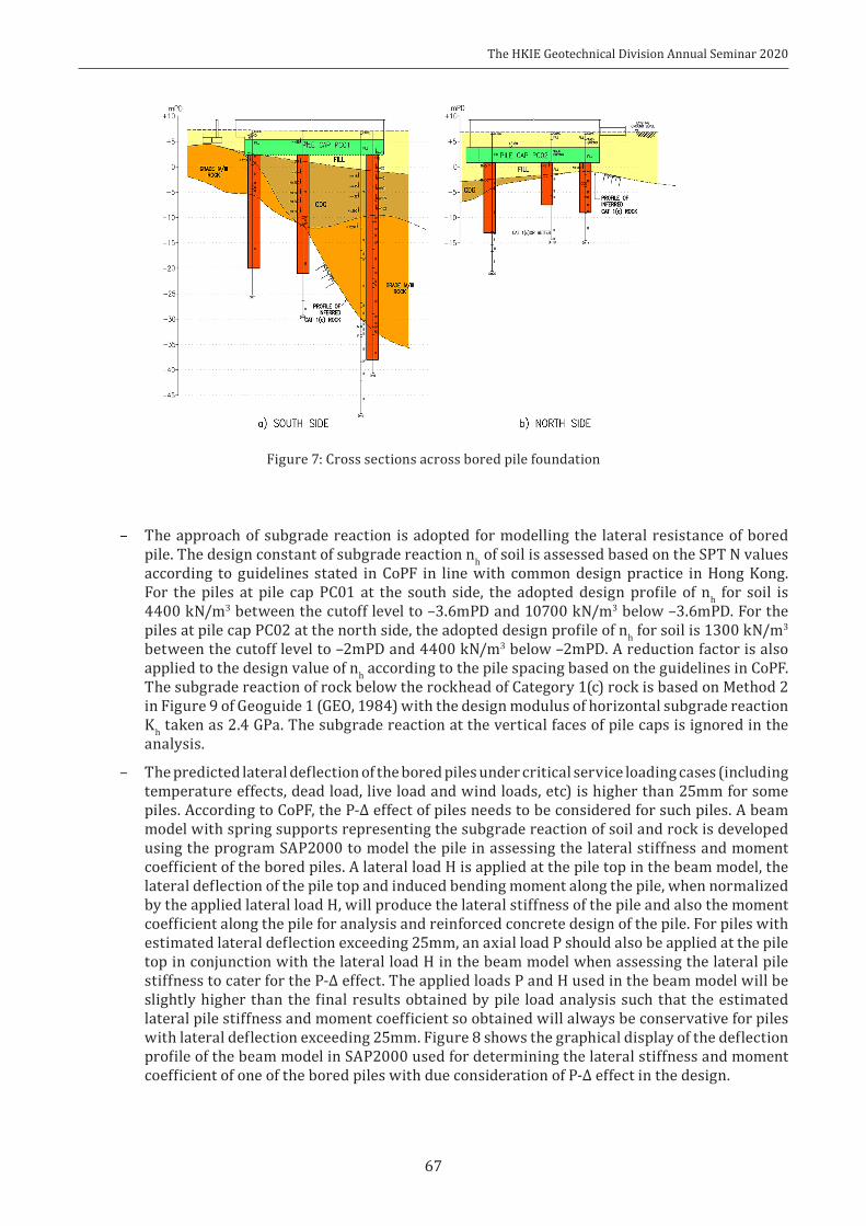
The HKIE Geotechnical Division Annual Seminar 2020
67
– The approach of subgrade reaction is adopted for modelling the lateral resistance of bored pile. The design constant of subgrade reaction nh of soil is assessed based on the SPT N values according to guidelines stated in CoPF in line with common design practice in Hong Kong. For the piles at pile cap PC01 at the south side, the adopted design profile of nh for soil is 4400 kN/m3 between the cutoff level to –3.6mPD and 10700 kN/m3 below –3.6mPD. For the piles at pile cap PC02 at the north side, the adopted design profile of nh for soil is 1300 kN/m3 between the cutoff level to –2mPD and 4400 kN/m3 below –2mPD. A reduction factor is also applied to the design value of nh according to the pile spacing based on the guidelines in CoPF. The subgrade reaction of rock below the rockhead of Category 1(c) rock is based on Method 2 in Figure 9 of Geoguide 1 (GEO, 1984) with the design modulus of horizontal subgrade reaction Kh taken as 2.4 GPa. The subgrade reaction at the vertical faces of pile caps is ignored in the analysis.
– The predicted lateral deflection of the bored piles under critical service loading cases (including temperature effects, dead load, live load and wind loads, etc) is higher than 25mm for some piles. According to CoPF, the P-Δ effect of piles needs to be considered for such piles. A beam model with spring supports representing the subgrade reaction of soil and rock is developed using the program SAP2000 to model the pile in assessing the lateral stiffness and moment coefficient of the bored piles. A lateral load H is applied at the pile top in the beam model, the lateral deflection of the pile top and induced bending moment along the pile, when normalized by the applied lateral load H, will produce the lateral stiffness of the pile and also the moment coefficient along the pile for analysis and reinforced concrete design of the pile. For piles with estimated lateral deflection exceeding 25mm, an axial load P should also be applied at the pile top in conjunction with the lateral load H in the beam model when assessing the lateral pile stiffness to cater for the P-Δ effect. The applied loads P and H used in the beam model will be slightly higher than the final results obtained by pile load analysis such that the estimated lateral pile stiffness and moment coefficient so obtained will always be conservative for piles with lateral deflection exceeding 25mm. Figure 8 shows the graphical display of the deflection profile of the beam model in SAP2000 used for determining the lateral stiffness and moment coefficient of one of the bored piles with due consideration of P-Δ effect in the design.
Figure 7: Cross sections across bored pile foundation

The HKIE Geotechnical Division Annual Seminar 2020
68
Figure 8: SAP2000 model for a bored pile
The foundation analysis is performed using the program SAFE. The deflection profiles of the two pile caps induced by the loading of Arch Truss during placement only are presented in Figure 9.
Figure 9: SAFE model showing deflection profile of pile caps PC01 and PC02
4 MONITORING RESULTS
The monitoring results discussed in this paper include the total load measured at each of the tower supports and the movement of the concrete piers. The 4 towers supporting the Arch Truss during installation are named A to D with locations at the final stage of installation indicated in Figure 6.
The existing ground level of the site is about +7.5mPD. Monitoring of the movement of the concrete piers had been carried out at monitoring points at levels near the bottom, the middle and top of the concrete piers during installation of the Arch Truss. The monitoring points located between the bottom and one third height of the concrete piers as shown in Figure 10 are considered to be more representative of the movement of the pile cap and hence the lateral movement of the bored piles. The levels of these monitoring points vary between +7.8mPD to +10.433mPD, or 2.4m to about 5m above the pile cap top

The HKIE Geotechnical Division Annual Seminar 2020
69
level. The sign conventions for longitudinal movement along the x-direction and transverse direction in the y-direction are also indicated in Figure 10.
The vertical loads due to the self-weight of the Arch Truss as measured by the hydraulic jacks of the tower supports are summarized in Table 1. The average load measured at each tower support is about 12,400 kN and the total self-weight of the Arch Truss at the time of installation was 49,649 kN or about 5000 tons. The variations of vertical loads between tower supports were not significant, being less than 5% from the average value.
Table 1: Loading measured at tower supports
Tower support Location Measured load (kN)A South side nearer to Pier P1 12,214D South side nearer to Pier P2 12,193B North side nearer to Pier P3 12,334C North side nearer to Pier P4 12,908
Average = 12,412Total = 49,649
The vertical and lateral movements measured on the first day and the second after full release of the jack loads from the tower supports are summarized in Table 2.
Table 2: Summary of monitoring results for pier movement
Pier Monitoring points
Level(mPD)
Lateral movement in longitudinal direction
(i.e. x-direction)(mm)
Lateral movement in transverse direction
(i.e. y-direction)(mm)
Vertical movement(mm)
1st day 2nd day Average 1st day 2nd day Average 1st day 2nd day Average
P1P1-5 10.341 0 -4
-1.754 -1
1.5-3 -1
-0.75P1-6 10.433 -1 -2 1 0 0 3
P2P2-5 7.801 -3 -4
-3.751 1
00 1
1P2-6 7.800 -3 -5 -1 -1 1 2
P3P3-5 8.619 2 2
1.50 1
0.753 3
3.25P3-6 8.623 1 1 1 1 3 4
P4P4-5 9.140 1 2
1.01 0
0.752 4
3.25P4-6 9.147 0 1 1 1 3 4
Note: Upward movement +ve and downward movement –ve.
Figure 10: Location of monitoring points

The HKIE Geotechnical Division Annual Seminar 2020
70
There should be little change of loading between the 1st and 2nd day after full release of jacking forces in the tower supports. The differences in readings between the 1st and 2nd day after full release of jacking force will give an indication of the precision of monitoring results obtained by survey measurements. Judging from the results in Table 2, the uncertainty associated with the survey measurements is of the order of ±2mm.
Some observations can be made from the monitoring results of Table 2. Piers P1 and P2 on the south side moved in opposite direction to piers P3 and P4 located on the north side. This is to be expected as piers P1/P2 and piers P3/P4 are located at the opposite sides of the Arch Truss. When the Arch Truss deformed laterally under its own weight upon release of jacking force during installation, it would push the two pairs of concrete piers sideway in an opposite direction.
5 COMPARISON WITH DESIGN
According to results of Table 2, the transverse movement of the piers are small. It is expected as the loadings associated with the placement of the Arch Truss are mainly vertical loads and lateral loads in the longitudinal direction. We will therefore focus on comparing the predicted and observed vertical and longitudinal movement.
When comparing the monitoring results with the predicted performance of the foundation, the reference datum should be taken as the state of the completed foundations, pile caps and concrete piers just before the Arch Truss was welded to the piers. The initial readings at the monitoring points were taken just before placement of the Arch Truss. Having known the self-weight of the Arch Truss before it was placed onto the piers, the vertical loads, lateral loads and bending moments transferred to the concrete piers and the lateral deflections of the piers at the levels of the above-mentioned monitoring points with respect to the reference datum can be predicted by the original structural stage-analysis model developed using the program Midas Civil for analysing the Main Bridge.
Figure 11 shows the predicted deformed shape of the Main Bridge at placement of the Arch Truss predicted by the program Midas Civil in an enlarged vertical scale. The estimated lateral loads transferred by the Arch Truss to the concrete piers and hence to the foundations upon full release of the jacking forces are estimated to be about 8770 kN at each pier..
Figure 11: Deformed shape of the Main Bridge predicted by structural model at placement of Arch Truss
Using the original structural analysis model in design and applying the measured loads during the Arch Truss installation, the theoretical response of the bored pile foundation inferred from the reference datum can be obtained. Table 3 compares the observed vertical movements with those predicted at the respective locations and levels of the monitoring points.
As the monitoring points at the piers are above the pile cap top level, the predicted vertical movement will be a sum of the vertical movement of the pier itself predicted by the structural analysis model and the vertical movement of the pile cap predicted by the foundation analysis model.
According to Table 3, downward movements are predicted at the piers P1 and P2 above pile cap PC01 and small upward movements are estimated at piers P3 and P4 above pile cap PC02. The upward movements at piers P3 and P4 are resulted from superpositioning of small deformations from vertical load and the bigger reverse movements due to pier rotation. The predicted vertical movements at piers P3 and P4 are considered to be in reasonable agreement with the monitored movement given the precision of the survey measurements. For piers P1 and P2 at the south side, a small downward

The HKIE Geotechnical Division Annual Seminar 2020
71
movement was recorded at monitoring point P1-5 and small upward movements were measured at the remaining monitoring points. This is in contrast to the predicted movement of the piers at the south side and may be explained by the following reasons.
a. In the foundation design, the vertical stiffness of pile is determined by treating the pile as a free column between the pile cutoff level and rockhead level of Category 1(c) rock, ignoring all the shaft friction in between that can help to reduce the pile shortening. Referring to Figure 7(a), there is a thick layer of Grade IV and III rock above the Category 1(c) rock beneath pile cap PC01. The design vertical stiffness may be highly underestimated when the shaft friction in the layer of predominately Grade IV and III rock is ignored, leading to over-estimation of vertical movement of pile and hence the pile cap. For the north side, the soils above the Category 1(c) rock are thin and the shaft resistance of the pile in soil will be relatively small. The error of assuming the piles to be a free column will be less significant.
b. The vertical subgrade reaction of soils at the base of pile cap has been ignored in the foundation design. For the pile group at the south side, a downward movement of the pile cap is predicted. Subgrade reaction will be mobilized to some extent at the base of pile cap and it will help to reduce the actual vertical movement of the pile cap.
All in all, the monitoring results indicate that vertical movements of the piers are small, resulting in smaller angular distortions of the structure and better performance of the Arch Truss.
Table 4 compares the predicted longitudinal movements of the piers at the locations and levels of monitoring points with the observed movements.
For piers P3 and P4, the predicted longitudinal movement of the pile cap is small, being 1.7mm or 2.3mm. This may be attributed to the shallow rockhead beneath the pile cap. The bored piles at pile cap PC02 acted as rigid short columns with high lateral stiffness in resisting the lateral loads. The predicted longitudinal movements of piers P3 and P4 differ from observed average movement by up to 2mm and 2.2mm respectively. This is not regarded as a significant difference given the precision of survey measurement.
For piers P1 and P2, the predicted longitudinal is dominated by the lateral deflection of the piles or pile cap PC01. There are more significant differences between the predicted total movement and observed average movement of piers P1 and P2. This warrants further investigation.
Although the longitudinal movement of pile cap PC01 was not directly monitored, it can be estimated approximately by making use of the data in Table 4 as shown in Table 5.
Table 3: Comparison of predicted and observed vertical movements
Monitoring point
Pile cap location
Estimated vertical movement from analysis model (mm)
Monitoring result (mm)
pier movement
pile cap movement total 1st day 2nd day average
P1-5
PC01
-1.3 -6.3 -7.6 -3 -1 -2P1-6 0.0 -5.0 -5.0 0 3 2P2-5 -0.5 -3.8 -4.3 0 1 0.5P2-6 0.1 -2.7 -2.6 1 2 1.5P3-5
PC02
1.2 0.7 1.9 3 3 3P3-6 1.0 0.4 1.3 3 4 3.5P4-5 1.2 0.7 1.8 2 4 3P4-6 1.8 1.5 3.3 3 4 3.5
Note: upward movement is +ve and downward movement –ve.
The HKIE Geotechnical Division Annual Seminar 2020
72
Table 4: Comparison of predicted and observed longitudinal movements
Monitoring point
Estimated deflection from analysis model (mm) Monitoring result (mm)
pier deflection pile cap total 1st day 2nd day
Average value for each
monitoring point
Average value for the two piers
on each sideP1-5 -1.3 -11.4 -12.8 0 -4 -2
-2.75P1-6 -1.3 -11.4 -12.8 -1 -2 -1.5P2-5 -0.5 -11.0 -11.4 -3 -4 -3.5P2-6 -0.5 -11.0 -11.4 -3 -5 -4P3-5 0.8 2.3 3.0 2 2 2
1.75P3-6 0.8 2.3 3.0 1 1 1P4-5 1.1 1.7 2.7 1 2 1.5P4-6 1.1 1.7 2.7 0 1 0.5
Note: Refer to sign convention in Figure 10 for movement direction
Table 5: Estimated longitudinal movement of pile cap PC01
Monitoring point location
Average measured movement
(mm)
Predicted pier deflection
(mm)
Estimated pile cap movement at pier
location (mm)
Average of estimated pile cap movement
(mm)P1-5 2 1.3 0.7
1.75P1-6 1.5 1.3 0.3P2-5 3.5 0.5 2.5P2-6 4 0.5 3.5
When pile cap PC01 is subjected to the lateral load transferred from the Arch Truss during installation, subgrade reaction of soils will be mobilized at the vertical face of the pile cap at the far side away from the piers. A rough estimate of this reaction force can be made using the elastic solution developed by Douglas & Davis (1964) for the lateral movement induced by a uniform pressure acting on a vertical rectangle below an elastic half-space. The soil near ground surface of pile cap PC01 has an average SPT N values of 20. Taking a Young’s modulus of 20 MPa and a Poison’s ratio of 0.2 for the soils, the reaction force that can be mobilized at the vertical face of pile cap PC01 is estimated to be about 750 kN. The estimated reaction force is only about 4.3% of the predicted total lateral load of 8770 × 2 = 17540 kN induced by the Arch Truss at piers P1 and P2 at the time of placement. The predicted longitudinal movement of pile cap PC01 presented in Table 4 is based on the predicted lateral load of 17540 kN. If there is a reaction force of 750 kN due to subgrade reaction acting on the vertical side of pile cap PC01 that will counteract the lateral load induced by the Arch Truss during installation, the predicted longitudinal movement of pile cap PC01 should be slightly adjusted as shown in Table 6.
Table 6: Adjustment to predicted longitudinal movement of pile cap PC01
Pier locationPredicted longitudinal
movement based on lateral loads of 17540 kN (mm)
Adjustment factor
Predicted pile cap movement after discounting the reaction
force from subgrade reaction at vertical side of pile cap (mm)
Average(mm)
P1 11.41 – 0.043 = 0.957
10.910.7
P2 11.0 10.5
A comparison of Table 5 and Table 6 indicates that the predicted average longitudinal movement of pile cap PC01 is significantly higher than the average movement estimated from the monitoring results by over 6 times. Possible reasons for explaining this disparity may include:

The HKIE Geotechnical Division Annual Seminar 2020
73
a. Theory of subgrade reaction The conventional approach of subgrade reaction is an old and at best a crude theory for analysis
of laterally loaded pile. The theory can well be overly conservative.
b. Design soil profile As discussed earlier, there exists a thick layer of predominately Grade IV/III weathered rock
above the rockhead profile of Category 1(c) rock (see Figure 7(a)). In the foundation design, this zone of weathered rock is treated as a dense soil with a design nh of 10700 kN/m3. The actual subgrade reaction provided by this layer of weathered rock is expected to be much higher. This can help to explain in part the smaller observed longitudinal movement of pile cap PC01, but it may not be the major explanation because many of the bored piles in pile cap PC01 are still embedded in over 10m of weaker materials of fill and CDG for which the subgrade reaction would not be very high.
c. Properties of bored pile According to Reese & Matlock (1956) the lateral stiffness for a fixed-head pile embedded in
sand with a uniform value of nh is proportional to EpIp/T3, where Ep and Ip are the Young’s modulus and second moment of area of pile and T is a dimensionless parameter defined by T = (EpIp/nh)0.2. Using the definition of T, the expression EpIp/T3 can be re-written as (EpIp)0.4 × (nh)0.6.
The design concrete grade is 45MPa, with a reduction factor of 0.8 for concrete placed using the tremie method. In the foundation design of the Main Bridge, the design value of Ep is based on Young’s modulus of determined in accordance with the Code of Practice for the Structural Use of Concrete (BD, 2013) using the reduced concrete strength for tremie concrete and Ip is calculated based on the nominal diameter of the pile assuming a circular solid section. The Arch Truss was placed over 6 months after completion of bored piles. From experience, there is no evidence to suggest that placemen of concrete by the tremie method will reduce the concrete strength and so the corresponding reduction of Ep of concrete in foundation design should not be necessary. Aging of concrete will also lead to an increase in strength and hence the Ep of pile. The presence of reinforcement bars, which has higher stiffness than concrete, will also enhance the equivalent value of Ep. Overbreak in the pile bore will result in a bored pile with a larger diameter, thus increasing the value of Ip. The above factors may result in aggregate increase in EpIp by over 50%. Even if there were a 100% increase in the value of EpIp due to the above reasons, the increase in lateral pile stiffness, which is proportional to (EpIp)0.4, would only increase by 30%. This reason alone is not sufficient to explain the larger difference between the predicted and observed longitudinal movement.
d. Design subgrade reaction of soils The values of nh recommended in the CoPF and used for the foundation for the Main Bridge are
based on the suggestion by Terzaghi (1955). Habibaghi & Langer (1984) have revealed field data published in the literature and observed that the value of nh is not constant, but decreases with increasing pile deflection. For instance, the value of nh corresponding to a pile deflection of 0.1 inch (2.5mm) can be about 5 times higher than that at a pile deflection of 1 inch and 8 times higher than that suggested by Terzaghi (1955). Habibaghi & Langer (1984) also remarked that the values of nh suggested by Terzaghi (1955) are applicable to conditions approaching large lateral displacements and appear to be quite conservative for lateral displacement less than 0.5 inch (or 12.7mm).
Based on the discussion earlier, the lateral pile stiffness for a fixed-head pile in a uniform sand is proportional to (nh)0.6. Even if there is an 8-fold increase in value of nh at small pile deflection, the increase in lateral pile stiffness is about 3.5 times. This is still not sufficient to explain the 6 times difference between predicted and observed longitudinal movement.
Based on the above discussion, it is noted that none of the factors (b) to (d) above can singly explain the large difference between predicted and observed longitudinal movement. It is believed that factors (a) to (d) discussed above are all possible contributing factors to the higher pile stiffness for the bored piles.

The HKIE Geotechnical Division Annual Seminar 2020
74
6 CONCLUSION
Although monitoring of the movements of concrete piers was originally intended only for checking the performance of the Main Bridge during erection, the results have provided a good and rare opportunity for also evaluating the performance of the bored pile foundations. Despite the predictions of higher vertical and longitudinal movement at pile cap PC01 due to the longer piles and deeper rockhead level for the pile cap, the monitoring results indicate that the movements of the pile foundations are small in terms of vertical movement and lateral movement in the both longitudinal and transverse directions for both pile caps.
For pile cap PC02, the predicted and observed movements are both small. It can be attributed to the shallow rockhead at this pile cap location, with the bored piles behaving as short rigid columns in limiting the vertical and lateral movement of the pile cap to low values.
For pile cap PC01, the large contrast between predicted and observed results suggests that actual performance of the foundations is much better than the predictions. The small observed vertical movement may be attributed to conservatism in the foundation design in ignoring the subgrade reaction at the base of the pile cap and the shaft friction in the bored pile. The small observed lateral deflection may be a result of a multitude of factors including the design approach of subgrade reaction and the adopted design parameters being conservative.
The design of bored piles for the Main Bridge has been controlled by lateral deflection. Given the small observed movements of the pile caps, adequacy of the current design is confirmed. More radical design theories and methodologies with regard to movement assessment should be explored and introduced in the design codes.
ACKNOWLEDGEMENT
The authors would like to thank the Hong Kong Airport Authority for granting the permission to publish this paper.
REFERENCES
Buildings Department (BD) 2013. Code of Practice for the Structural Use of Concrete. Buildings Department (BD) 2017. Code of Practice for Foundations.Douglas, D.J. and Davis, E.H. 1964. The movements of buried footings due to moment and horizontal load and the movement
of anchor plates. Geotechnique, 14[3]:115-132.Geotechnical Engineering Office (GEO) 1984. Geoguide 1, 2nd Edition.Habibaghi, K. and Langer, J.A. 1984. Horizontal subgrade modulus of granular soils. Laterally Loaded Deep Foundations:
Analysis and Performance. ASTM Special Technical Publication no. 835, 21-34.Reese, L. and Matlock, H. 1956. Non-dimensional solutions for laterally loaded piles with soil modulus assumed
proportional to depth, Proc. 8th Texas Conf. on Soil Mechanics and Foundation Engineering, 41p.Terzaghi, K. 1955. Evaluation of coefficients of subgrade reaction. Geotechnique, 5[4]:297-326.

The HKIE Geotechnical Division Annual Seminar 2020
75
Some Challenges in Measuring Small-Strain Stiffness of Undisturbed Soils for Engineering Projects
S.R. LoThe University of New South Wales, Australia
Victor LiVictor Li & Associates Ltd, Hong Kong
K.K. Lu & J.H. YinThe Hong Kong Polytechnic University, Hong Kong
ABSTRACT
Most geotechnical designs for deep excavations in the urban areas of Hong Kong are governed by the need to limit the soil movement to an acceptably small limit to avoid damaging adjacent buildings or structures. Given such design criteria, the strain levels of soils for most deep excavations in Hong Kong are relatively small. It has been well documented in the literature that the stiffness of soils at small strain is significantly higher than that at a moderate strain level. One may consider it attractive to adopt a design approach that takes advantage of the higher small-strain stiffness of soil when designing deep excavations.
Techniques for measuring small stiffness of soil in triaxial testing are well established in a research setting. However, it is rare for geotechnical engineers to determine small-strain soil stiffness by laboratory testing in their design for deep excavations in Hong Kong. This may be due to the practical challenges that are seldom discussed or addressed in research papers. Based on their recent experiences gained from some excavation projects in Hong Kong, the authors attempt to examine some of the challenges faced by geotechnical engineers in trying to commission laboratory testing for determining small-strain stiffness of soils and applying the results in geotechnical design.
1 INTRODUCTION Urban developments in Hong Kong often require deep excavations in close proximity to existing buildings for construction of basements and pile caps. Very often, the predicted ground settlement at and movement of adjacent buildings need to be controlled to within small limits to prevent building damage. The allowable ground settlement and angular distortion outside the site acceptable to the regulatory authorities are often set at 25mm or 1/500 respectively and perhaps even less for deep excavations near old buildings or existing facilities of the Mass Transit Railway Corporation. Given these stringent requirements, the design of excavation in Hong Kong is more often than not controlled by the magnitude of predicted ground settlement. The settlement/soil movement arising from a deep excavation may be broadly divided into two components:
– Settlement/soil movement occurring before bulk excavation, δ1 . Such soil movements arise from installation of the vertical elements, such as pile foundations, embedded walls for the

The HKIE Geotechnical Division Annual Seminar 2020
76
cofferdam and king posts for supporting struts before commencement of bulk excavation. Settlement due to installation effects can sometimes be significant for certain types of embedded walls or when improper equipment is used for installation.
– Settlement/soil movement occurring during bulk excavation, δ2 . Soil movement which occurs during bulk excavation depends most significantly on the soil stiffness, although other factors such as stiffness of embedded wall, strut levels, preloading force of struts and excavation sequence will also have some bearing on the induced ground movement.
The settlement δ1 is not computable and its design value is usually assigned based on experience. There is no suitable analytical method for calculating such settlement, let alone setting up some conservative guidelines for predicting it. For this reason, the regulatory authorities usually focus on predicted results of δ2 and request geotechnical designers in adopting conservative parameters for the estimation of δ2 .
The design stiffness of soil is arguably the most important parameter that governs the prediction of δ2 . In Hong Kong, it is a common practice to correlate the Young’s modulus of stiffness E with the N values measured from standard penetration tests (SPT) based on the relationship of E = α × N where E is in MPa and α is the correlation factor. Chan & Davies (1984) suggested a correlation factor of α = 1 based on data reported in the literature between 1953 and 1977 and supplemented by their own data. The correlation suggested by Chan & Davies (1984) has been quoted in the publication of GCO (1990) and has since become popular. As pointed out by Li (2007), SPT tests conducted prior to the 1980s were usually performed using hammers operated with manual release. Nowadays, trip hammers, which have smaller energy loss, have become the norm for SPT tests. Due to its higher efficiency, the SPT N values measured by a trip hammer will be smaller than that by a hammer with manual release as demonstrated by the data presented by Li (2007). The correlation based on α = 1 will be conservative if the N values are measured using a trip hammer.
Chan (2003), who had earlier proposed the correlation factor of α = 1 in Chan & Davies (1984), presented updated correlation factors by back-analyzing more recent case studies and recommended a value of α = 1.5 for fill and alluvium and α = 2 for completely decomposed granite (CDG). The correlation factors recommended by Chan (2003), which can give a less conservative design for deep excavations, had been popular for a few years after the publication. Unfortunately, such good times were short-lived. In recent years, designers are rarely allowed to use a correlation factor higher than 1.0 for fill and alluvium and 1.5 for CDG.
It is well recognized by experienced geotechnical engineers in Hong Kong that the settlement δ2 is usually well below the predicted value obtained using the conventional correlation of E = 1 × N. In the authors’ review, the higher correlation factors recommended by Chan (2003) should be closer to the actual soil behaviours.
As basements become increasing deeper for new development projects in Hong Kong, it has become increasingly difficult to control the calculated value of δ2 to a small magnitude, particularly using the conservative correlation E = 1 × N in design. This explains why ground treatment works, such as bentonite cement grouting, deep cement mixing or jet grouting, have become more popular in the design of deep excavations in Hong Kong in recent years for achieving a smaller magnitude of δ2 by strengthening and stiffening the soils. To the designer, this is a very simple solution as all he needs to do is to specify the design strength, modulus and perhaps also the permeability as design requirements, leaving the construction difficulties to the contractor to tackle and the bill to the clients to settle. Sometimes, the panacea of ground treatment works may not work due to the difficulties in carrying out ground treatment works in a site with old pile foundations, old pile caps or boulders/corestones in the soils.
Figure 1 shows the typical shear strain levels for geotechnical structures (Mair, 1993). For deep excavations, a significant portion of the soils will undergo an unloading process, and the shear strain γ of soils is expected to be of the order of 0.1%, which is lower than what conventional triaxial test can measure. It is well established that the stiffness of soils is high at a small strain level and decrease gradually with increasing shear strain (e.g. Atkinson, 2000). Instead of jumping hastily to the decision of ground treatment works as the last resort, one can explore the feasibility of determining and making use of the higher soil stiffness of soils at small strain for obtaining a smaller but more realistic value of δ2.

The HKIE Geotechnical Division Annual Seminar 2020
77
Conventional triaxial testing in commercial laboratories usually cannot achieve the required precision to allow the shear modulus of soils to be determined reliably at strain level below 1%. Special testing equipment needs to be assembled for accurate measurement of soil stiffness at a small strain level of the order of 0.1% relevant to deep excavations.
Figure 1: Typical strain levels for geotechnical structures (after Mair, 1993)
Figure 2: Stress-strain relationship of soil
2 POTENTIAL BENEFITS OF SMALL-STRAIN TESTING
Figure 2 shows a typical stress-strain relationship of soil. Initially, the soil stiffness, as measured by the gradient of the stress-strain curve (or tangent modulus) is high. With increasing strain level, the tangent modulus becomes increasingly smaller. A convenient parameter for characterizing the soil stiffness for geotechnical design is the secant modulus. As the secant modulus depends on the strain level, the adopted design secant modulus should correspond to the expected representative strain levels of the geotechnical structures.
A testing facility has recently been established at the Soil Mechanics Laboratory of the Hong Kong Polytechnic University (PolyU) that will allow the stress-strain curves of soils to be measured accurately even at very small strain levels. Figure 3 shows the test setup for small-strain testing at the PolyU. Details of this testing facility have been reported by Lu et al. (2018) and will not be discussed at length in this paper.

The HKIE Geotechnical Division Annual Seminar 2020
78
Figure 3: Test setup for small-strain testing at PolyU (Lu et al., 2018)
Figure 4: (a) Stress-strain relationship and (b) secant shear modulus of CDG under different confining pressure (Lu et al., 2018)
Figure 4 shows the stress-strain relationship and the corresponding secant shear modulus Gsec of triaxial testing of undisturbed samples of CDG under different effective confining pressure (71 kPa, 180 kPa and 295 kPa for sample C01 to C03 respectively) reported by Lu et al (2018). As demonstrated by the results of Figure 4(b), techniques are now available for accurate measurement of the stress-strain curve even at small strain levels less than 0.005%.
Further tests have recently been conducted at the PolyU on fills and alluvial soils for two projects in Hong Kong. Figure 5 and Figure 6 show some of the results for one site. The results of Figure 5 are for an undisturbed Mazier sample of fill material logged as a clayey silt. Figure 6 presents the results for a Mazier sample of alluvial clayey silt. Both samples were taken as shallow depth of 2 to 3m below ground. The tests conducted were isotropic consolidated drained tests at an effective mean stress of 30.9kPa which is slightly less than the insitu mean stress estimated based on at-rest condition.

The HKIE Geotechnical Division Annual Seminar 2020
79
Figure 5: (a) Stress-strain relationship and (b) secant shear modulus of fill material at small strain
Figure 6: (a) Stress-strain relationship and (b) secant shear modulus of alluvial soil at small strain
Based on the SPT N value measured nearest to the sample location, the correlation factor α corresponding to the Young’s modulus calculated from the secant shear modulus at 0.1% shear strain, denoted by E0.1% , is estimated to be 2.78 for the fill sample of Figure 5 and 2.09 for the alluvial sample of Figure 6. The estimated correlation factors for the two samples are well above 1.0 for a shear strain level of 0.1%.
A similar finding has been observed for the other site for which the estimated correlation factor α corresponding to shear strain of 0.1% was also higher than 1, with some values as high as close to 10 for both fill and alluvial sands (see also data in Figure 8 presented later).
The available results show that efforts spent on small-strain testing of soils do give the potential reward of a higher soil stiffness than that predicted using a correlation factor of 1 for the estimation of soil movement δ2 .
3 CHALLENGES
Despite the advent of the technique of small-strain testing, there are challenges which geotechnical designers need to know when trying to tap the potential advantages of small-strain stiffness for design of deep excavations.

The HKIE Geotechnical Division Annual Seminar 2020
80
3.1 Availability of testing facilities
Specialized testing facilities for soils are usually developed in universities for research purposes, such as that currently available at the PolyU. The tests are usually conducted by research students as part of their own research work or their duties as part-time research assistant in helping their research supervisors in completing a consultancy project. Universities do not encourage their staff to undertake commercial consultancy projects unless such work can potentially generate journal publications which can help raise the university ranking. It may be difficult to persuade a university professor in conducting the testing for practical engineering projects. Even if a university professor is keen to do so, the testing services may have to be suspended when his experienced research students finish their study and can only be resumed when new research students have become sufficiently well trained to carry out testing again.
Commercial soils laboratories may not be keen in providing specialized testing services. There is usually not sufficient demand for such tests to warrant the investment, the cost of maintaining the more expensive testing facilities and the efforts in training and keeping specialized operators for such tests, not to mention the further efforts required if the laboratory chooses to maintain HOKLAS accreditation for such tests.
Unless and until small-strain testing becomes routinely available in commercial soils laboratories or in universities, it will be difficult for design of deep excavations based on test results of small-strain testing to become a common practice.
3.2 Quality of undisturbed sample
The quality of a small-strain test can only be as good as the quality of sample. Unless a dedicated effort is spent in soil sampling, the quality of so-called “undisturbed” samples is often far from being satisfactory to warrant the efforts of small-strain triaxial testing.
Improper handling of sampler tubes during storage or transportation will cause disturbance of sample and may significantly reduce the soil stiffness at small strain. Sometimes, samples are not sealed quickly enough after sampling, leading to drying up and/or shrinkage of samples.
Indiscriminate testing of poor quality samples will do more harm than good as it may have the opposite effect of leading the regulatory authorities to believe that soil stiffness may still be low even at small strain. If there is evidence that the sample has been disturbed, it is preferable to test a properly prepared reconstituted sample to the same density of the “undisturbed” sample than to test the questionable undisturbed sample. Although remoulding of soils will completely destroy the fabric structure of soils, it may still give the correct order of magnitude of soil stiffness at small strain.
3.3 Preparation and testing of test specimens
The process of preparing a test specimen from a high quality sample (such as a block sample) may induce disturbance to varying degree and this aspect has seldom been addressed in published literature. A robust and operator-independent approach must be developed to minimize the disturbance as far as practicable. The following is a brief summary of the procedures recommended by Lu et al. (2018) and proven to be effective.
– Cutting of Mazier sampling liner using a guide frame to ensure that the cut surfaces are parallel to each other and perpendicular to the alignment of the sample.
– Samples are to be extruded vertically from the cut Mazier sample liner by a hydraulic extruder with an alignment system to avoid bending and cracking under its own weight often associated with horizontal extrusion.
– Split former with 1mm thick rubber liner and 0.1mm thick polytetrafluorethylene sheet for holding the test specimen immediately after extrusion from the Mazier sampling liner.

The HKIE Geotechnical Division Annual Seminar 2020
81
For accurate determination of the stress-strain curve at small strain, the stress and strain of the specimens must be measured with high precision. For this reason, high precision internal LVDT and internal load cell become a must (see Figure 3). Load cell, and to a lesser extent LVDT, operating under pressurized cell water have lower longevity, and may malfunction without evident indications. Thus, it is important to check, calibrate and repair or replace the transducers frequently as necessary.
Accurate determination of stiffness requires accurate measurement of both stress and strain. The precision of a load cell is expressed as percentage of its rated capacity (i.e. the maximum “safe” load which the load cell can take). For measurement of small-strain stiffness, testing of the specimen can be terminated well before failure of the specimen occurs. For instance, it may be sufficient to terminate the test at an axial strain of ~0.5%. To ensure the highest accuracy of load measurement, one should estimate the load level at the end of testing, and use a load cell with a commensurate rated capacity. This means that a suite of load cells of different rated capacities should be maintained in the laboratory in order to achieve the highest accuracy for measurement of small-strain stiffness. This is something easier said than done.
3.4 Innate sample non-homogeneity
A triaxial specimen prepared from an “undisturbed” soil sample may have some innate non-homogeneity. A soil sample of silty alluvium may have a thin seam or lens of sand which may cause local slumping or bulging of the specimen. If such a situation occurs, the testing operator should not carry out the test but this may be a difficult call in a commercial testing environment.
Figure 7: Test results for an alluvial soil specimen with sudden increase in tilting
Another form of non-homogeneity is the occurrence of a local loose or weak spot within a triaxial specimen and thus may not be detected during specimen preparation. Such a weak spot may lead to local aberration in the measured deviator stress-strain curve as illustrated in Figure 7, which is for a test on an alluvial soil specimen. Also presented in the figure is the variation of normalized tilt, which is defined as tilt movement divided by axial deformation. For a normal test specimen, the normalised tilt should gradually reduce with shearing as the axial deformation increases. For the test presented in Figure 7, a small regime of “apparent strain softening” started at an axial strain of ~0.1%. This unusual feature correlates well with a sudden increase in normalised tilting at the same axial strain level. Initially, the stress within the specimen could “arch around” the loose spot until it eventually gave way to the applied stress leading to a sudden increase in normalised tilt. Since the local weak spot was located within the

The HKIE Geotechnical Division Annual Seminar 2020
82
specimen, the effects can be contained and both the overall stress-strain response and normalized tilt soon returned to normal after the anomaly. However, the secant shear modulus Gsec at axial strain levels between 0.10% and 0.17% will be significantly reduced if the affected stress-strain curve is used for estimation.
3.5 Correlation factors
Given the very limited availability of testing facilities in Hong Kong at present, it is not practical to conduct a large number of small-strain tests to cover all soil types and/or variations of soil conditions within the same soil layer. An expedient way may be to correlate the measured small-strain stiffness with the SPT N value measured at the location nearest to the soil sample location. Once the mean correlation factor has been established from the test results of a sufficient number of samples for a particular soil type or soil layer, the design profile of E can then be obtained indirectly using the design profile of SPT N values based on the measured mean correlation factor.
When adopting this approach, one should be mindful of the uncertainties associated with the above correlation procedure. The authors’ experiences indicate that a small difference in the soil grading can sometimes lead to a relatively large difference in small-strain stiffness. The soil at the SPT test location will not have exactly the same grading as the soil at the nearby soil sample location. This unavoidable disparity will increase the statistical uncertainty of α.
The number of small-strain tests must be sufficient to produce an acceptably small statistical error for the estimated average value of α. Based on the theory of statistics, if the standard deviation of a random variable is σ, the statistical deviation of its mean value estimated from n tests will be given by σ/√n. For instance, if the coefficient of variation is 30% for the innate variability of α, the minimum number of tests required to control the coefficient of variation of the estimated mean value of α to within 10% will be about 10, i.e. 0.3/√10 ≈ 10%. It is equally important to note that the distribution of α does not follow a normal distribution as the criterion of α being non-negative must be complied with.
3.6 Time and planning
To reap the potential benefits of small-strain testing, geotechnical designers must plan well ahead of the construction works.
Time is needed to convince the client in spending the time and money for small-strain testing in return for potential cost saving. Time is needed to secure a reliable and high quality testing laboratory in Hong Kong or perhaps overseas for performing the tests. Time is also needed to plan for the taking of good quality samples during the ground investigation stage and to allow a sufficiently long period of time for small-strain testing. More importantly, one should allow sufficient time in convincing the regulatory authorities to accept a less conventional approach of design based on small-strain soil stiffness.
3.7 Human factor
In Hong Kong, design consultants are usually under tremendous pressure to complete the design submission quickly to meet the tight programme. Being commercial entities, design consultants would naturally aim to complete the tasks at minimum cost to gain the maximum profit. It is not uncommon that the consultant will produce a conservative design to ensure the earliest and easiest approval by the regulatory authorities and then shift the design responsibility to the contractor as a design-and-build item in the contract. Therefore, design consultants may not have incentives to be innovative.
It may be thought that the contractors who are forced to accept the design responsibility will be more interested in using small-strain soil stiffness for design to achieve a cost saving. As mentioned earlier, it will take a long time for planning before it can be done. Contractors can rarely have a sufficiently long contract period to afford waiting for an alternative design to be developed and approved before starting the construction works. The golden opportunity for cost saving is usually lost if the consultant fails to plan for it from the outset.

The HKIE Geotechnical Division Annual Seminar 2020
83
3.8 Regulatory authority
The use of small-strain soil stiffness for analysis of geotechnical structures is really nothing new and has been discussed in numerous geotechnical publications. Geotechnical designs based on small-strain stiffness can at best be regarded as a less conventional design instead of an innovative one.
As discussed by Li & Lo (2008), most people worry about changes and the psychological barrier to accepting a change is not easy to overcome. When a less conventional design is submitted, the designer may be asked by the regulatory authorities to adopt more conservative parameters, conduct more tests to justify the parameters, enhance the monitoring frequency, carry out regular performance review reports during construction and so on before approval can be granted. In the end, the attractiveness of a seemingly economic approach will be quickly gone after these concessions.
The Geotechnical Engineering Office has recently established a panel for vetting and encouraging innovative geotechnical designs. It is a good beginning. It is hoped that this initiative can lead to a cultural change to the prevailing geotechnical design practice in Hong Kong in a positive direction.
4 DISCUSSIONS AND CONCLUDING REMARKS
The paper discusses some of the challenges that need to be dealt with by geotechnical engineers when trying to take advantage of the higher stiffness of soils at small strain for design of deep excavations. These challenges, when adequately dealt with, can lead to less conservative stiffness parameters as illustrated by the results in Figure 8 for fill materials taken from an old reclamation site in Hong Kong. The figure presents the correlation of E0.1% with the measured N value measured by SPT using a trip hammer.
Figure 8: E0.1% versus N plot for a fill stratum

The HKIE Geotechnical Division Annual Seminar 2020
84
The data in Figure 8 contains both results obtained from undisturbed Mazier samples and reconstituted soil specimens. The reconstituted specimens were prepared from materials taken from Mazier samples and to the same void ratio of the soils in the Mazier samples. The fill materials at the site were relatively heterogeneous. In presenting the data in Figure 8, no attempt has been made to further classify the data according to the grading and void ratio of the fill sample. Two data points giving an exceptionally high of E0.1% (in excess of 100 MPa) were excluded from the plot. The relationship of E0.1% = 2 × N may be considered as a conservative correlation for the small-strain Young’s modulus, with only one data point distinctly below the correlation line. The results in Figure 8 echo the higher correlation factors suggested by Chan (2003).
The design of excavation based on small-strain stiffness discussed above is suited for a linear-elastic-perfectly plastic soil model. More advanced non-linear constitutive soil models are available in the literature such as that presented in Lu et al. (2018). However, intricate synthesis and processing of data are needed and this may make the approval process even more challenging
In conclusion, the major challenge is that there are very few organizations in Hong Kong that can offer accurate and reliable testing services for small-strain triaxial testing of soils and response sufficiently quickly to meet the demand of the geotechnical designer. It is important that the designer should plan well ahead of the construction to obtain the blessing and funding from the client in supporting the proposal and to collect sufficient good quality samples for testing early enough to enable test results to be available in time for performing the design. The most difficult and perhaps of the most interesting part of the endeavour is to convince the regulatory authorities in accepting the design.
REFERENCES
Atkinson, J.H. 2000. Non-linear soil stiffness in routine design. Geotechnique, 50 (5): 487-508.Chan, A.K.C. 2003. Observations from excavation – A reflection. Proc. HKIE Geotechnical Division Annual Seminar, 83-101.Chan, A.K.C. and Davies, J.A. 1984. Some aspects of design and construction of foundation for highrise buildings in Hong
Kong. Proc. of 3rd International Conference on Tall Buildings, Hong Kong & Guangzhou, 107-113.Geotechnical Control Office (GCO) 1990. Review of Design Method for Excavation – GCO Publication 1/90.Li, V. 2007. Analysis of geotechnical data. Bridging Research and Practice - the VLA Experience, Centre for Research &
Professional Development, 121-156.Li, V. and Lo, S.C. 2008. Obstacles to innovative technologies in geotechnical works in Hong Kong, Proc. HKIE Geotechnical
Division Annual Seminar, 191-195.Lu, K.K., Yin, J.H. and Lo, S.C. 2018. Modelling small-strain behaviour of Hong Kong CDG and its application to finite-
element study of basement-raft footing. International Journal of Geomechanics, 18(9).Mair, R.J. 1993. Developments in geotechnical engineering research: application to tunnels and deep excavations. Unwin
Memorial Lecture 1992. Proc. ICE, 97(1):27-41.

The HKIE Geotechnical Division Annual Seminar 2020
85
Breakthrough in Geotechnical Design of Foundation in Grade III or Better Sedimentary Rock (Siltstone) for
the Hong Kong Science Park Expansion Stage 1 (SPX1) at Pak Shek Kok, Tai Po
Tony K.H. Ma, Christopher W.K. Pang, Paris C.W. Wong, Clifford W.C. Phung & Adam S.C. Choy
Meinhardt (Hong Kong) Limited
ABSTRACT
The Hong Kong Science Park Expansion Stage 1 (SPX1) project implemented a non-exemplified foundation design in Grade III or better sedimentary rock (siltstone) to support a new 25m long linkbridge connecting two new buildings (17W & 19W) to an existing building (15W). The ground condition is one of the major challenges for the foundation design. Based on the desk study and the ground investigation works, Grade III or better sedimentary rock was found as the underlying bedrock, which does not fully comply with any of the rock categories defined in Table 2.1 and Table 2.2 of the Code of Practice for Foundations 2017. As such, presumed allowable bond or friction between sedimentary rock and grout cannot be fully covered by the Code of Practice. In this paper, a robust and safe method in structural and geotechnical design for pile foundation system socketed in Grade III or better sedimentary rock is presented.
1 INTRODUCTION
In Hong Kong, the geology is dominated by igneous rocks (including granite and volcanic) which is about 75%, remaining 15% are quaternary superficial deposits and less than 10% are sedimentary rocks and metamorphic rocks located in New Territories. Sedimentary rocks and metamorphic rocks are uncommon to be encountered in Hong Kong.
In the project of Stage 1 expansion (SPX1) development at the Hong Kong Science Park, Tai Po, New Territories, mini-pile is proposed as the foundation scheme. From desk study and boreholes record, the underlying bedrock is Grade III or better sedimentary rock (i.e. siltstone). It is anticipated that sedimentary rocks will be encountered during the piling works.
For the foundation design and with reference to the Code of Practice for Foundations 2017, sedimentary rocks are not defined as any category of rock in Table 2.1 of the Code of Practice. Hence, there is no presumed allowable bond or friction between sedimentary rock (i.e. siltstone) and grout for piles design specified in the Table 2.2 of the Code of Practice for Foundations 2017. To overcome this specific foundation issue, a breakthrough of rational design method is conducted in accordance with the provision of Clause 2.2.1 of the Code of Practice to assess the allowable bond or friction between sedimentary rock and grout.

The HKIE Geotechnical Division Annual Seminar 2020
86
2 SITE BACKGROUND
2.1 Site Description
The site is bounded by Chong San Road at South and Science Park West Avenue at North. In this project, it is proposed to construct a 25m long new linkbridge connecting from the new 17W & 19W buildings to the existing 15W building. The new linkbridge is designed to be supported by a new reinforced concrete (R.C.) pier at one end of the existing 15W building and a corbel extended from the new 17W building at another end. The general layout plan and architectural picture of the new linkbridge is shown in Figure 1 and Plate 1 respectively.
Figure 1: General Layout Plan of the New Linkbridge
Plate 1: Architectural Picture of the New Linkbridge
The new R.C. pier is designed to be supported by a pile foundation and it is located on the existing 5.9m wide footpath in front of the existing 15W building. The allowable working area for proposed foundation works is confined to the existing footpath only. The pile layout plan of the proposed foundation is shown in Figure 2. Plate 2 and 3 show the location of the proposed pile foundation with site condition.

The HKIE Geotechnical Division Annual Seminar 2020
87
Figure 2: Pile Layout Plan of the Proposed Foundation
2.2 Ground Condition
Ground investigation works involve sinking of 60 vertical drillholes including one specific drillhole (BH11) for the linkbridge foundation, the ground profile is mainly comprised of 7.1m to 11m depth of Fill underlain by Alluvium with thickness varying between 1.1m to 6m. Completely Decomposed Siltstone or better soils are found underneath the layer of Alluvium. The bedrock (siltstone) is encountered at depth varying from 40.1m to 61.8m below existing ground. The geological profile of the proposed foundation is illustrated in Figure 3.
Plate 2: General Site Condition of the Proposed Foundation Works
Plate 3: Site Constraint of the Proposed Foundation Works

The HKIE Geotechnical Division Annual Seminar 2020
88
Figure 3: Geological Profile of Proposed Foundation (along Section A-A of Plate 3)
3 CONSTRAINTS ON FOUNDATION DESIGN FOR LINKBRIDGE
For selection of appropriate foundation scheme, review of adjacent existing buildings and site constraints was performed. Various foundation types and/or options had been considered, but most of them were found not viable for this site.
3.1 Driven Steel H-Piles
Since there were sensitive instruments (e.g. vibration check point, settlement check point and tilting check point) installed in the adjacent buildings, the Hong Kong Science Park had posed a great concern on the vibration and noise induced from the proposed foundation works. Percussive piling was therefore not allowed by the Hong Kong Science Park despite that driven steel H-pile founded on decomposed siltstone is one of the viable foundation types.
3.2 Rock Socketed Steel H-piles and Bored Piles
For construction of rock socketed steel H-piles or bored piles, at least one piling rig and one mobile crane are required. Since the proposed working area is closely bounded by the existing 15W building to south, new 17W & 19W buildings to east and the existing footbridge to west, the 5.9m wide footpath provides inadequate working area to accommodate the mobile crane. If the mobile crane is required to be stationed at one of the adjacent traffic lane, it will cause traffic diversion along the Science Park West Avenue. As a result, the daily logistic and operation of the Science Park will be jeopardized. Therefore, rock socketed steel H-piles and bored piles are not feasible.
3.3 Mini-piles
Mini-pile is considered to be the most viable foundation scheme in terms of constructability and disturbance to the surrounding as compared with other piling foundation types. It only induces relatively limited vibration and requires much smaller working area.
3.4 Raft Foundation
Raft footing is not adopted as the allowable bearing capacity is low and limited space for the footing due to the existing utilities and underground structures. Besides, due to the site is located at the reclaimed zone, Marine Deposit and Alluvium are the main concern of the long term differential settlement, and the loading is not capable for future settlement.

The HKIE Geotechnical Division Annual Seminar 2020
89
4 ASSESSMENT ON ALLOWABLE BOND STRENGTH BETWEEN SILTSTONE AND GROUT
The vertical mini-piles are designed to resist vertical loads while the lateral load is resisted by the passive resistance of the pile cap. According to the Code of Practice for Foundations 2017, there are presumed values for allowable capacity for granite and volcanic rock, but no presumed value for the allowable capacity for sedimentary rock is specified. Thus, a rational design method was adopted as allowed in Clause 2.2.1 of the Code in assessing the allowable bond strength between siltstone and grout with reference to international literatures and well-established empirical methods.
The point load test (PLS) is a useful index test for estimating the uniaxial compressive strength (UCS) of the rock, which can be further used for assessing the allowable bearing capacity and bond strength. The point load test results obtained from 17 numbers of pre-drilling for adjacent 15W & 17W buildings are shown in Table 1. The minimum equivalent point load index strength (PLI50) value is 1.00MPa.
Table 1: Summary of Point Load Test
Borehole/Pre-drillhole No. Point Load Index, PLI50 (MPa)15BP3(P) 1.3015BP7(P) 1.2815BP8(P) 1.4115BP9(P) 1.34
15BP10(P)PL1 2.3615BP11(P) 1.8615BP12(P) 1.4715BP19(P) 1.91
PD13(P) 1.69PH17W-BP06 1.20PH17W-BP07 1.00PH17W-BP11 1.10PH17W-BP12 1.40PH17W-BP13 2.60PH17W-BP17 1.20PH17W-BP19 1.00PH17W-BP22 1.40
A review of the international literature for the correlation factor between PLI50 and UCS for the sedimentary rock is performed.
Table 2: Summary of Correlation Factor between PLI50 and UCS
International Literature Correlation Factor between PLI50 and UCSHassani et al (1980) UCS = 29PLI50 (for sedimentary rock)
Read, Thornton and Regan (1980) UCS = 16PLI50 (for sedimentary rock)Read et al (1980) UCS = 20PLI50 (for sedimentary rock)
Das (1985) UCS = 14.7PLI50 (for siltstone)O’Rourke (1988) UCS = 30PLI50 (for sedimentary rock)
Rusnak and Mark (1999) UCS = 20.2PLI50 (for siltstone)
Based on the above summary, the correlation factor for the sedimentary rock ranges from 14.7 to 30. Concerning variations of geotechnical properties in different countries, and in order to reasonably cover the uncertainty of the underground condition, it is proactively proposed an appropriate correlation factor of 10 for siltstone, and the estimated UCS of the siltstone can be expressed as below equation.

The HKIE Geotechnical Division Annual Seminar 2020
90
UCS = 10 PLI50 (1)
To verify the design UCS, the UCS test results obtained from 4 numbers of sample of pre-drilling are shown in Table 3. The minimum UCS value is 47.5MPa which is higher than the design UCS value of 10MPa, hence the design is sufficiently robust.
Table 3: Summary of UCS Test
Sample UCS (MPa)No. 1 64.5No. 2 142.3No. 3 51No. 4 47.5
As stipulated in Clause 6.5.4 of the GEO Publication No. 1/2006 – Foundation Design and Construction
and Williams and Pells (1981), the ultimate bond strength values between sedimentary rock and grout are assessed based on the following equations.
τS = ασc0.5 (2)
τS = αβσc (3)
where τS is the ultimate bond strength between rock and grout;σc is the uniaxial compressive strength of rock;α is the rock socket reduction factor which depends on σc ; andβ is the rock socket correction factor which depends on RQD.
A summary of the assessed allowable bond strength is expressed as below in Table 4.
Table 4: Assessment of Allowable Bond Strength
Reference Equation Parameters Involved Assessed Allowable Bond Strength*
GEO Publication No. 1/2006 τS = ασc0.5 α = 0.2
σc = 10MPa 210kPa
Williams and Pells (1981) τS = αβσc α = 0.14**
β = 0.65***σc = 10MPa
300kPa
* A factor of safety 3 is applied in the above assessment** Obtained from Figure 7.19 of Tomlinson (1986) with consideration of σc = 10MPa*** Obtained from Figure 7.20 of Tomlinson (1986) with consideration of RQD = 0% ~ 25%
With due consideration of the test results of PLI50 , several samples obtained relatively low strength such as 1.0MPa, it is therefore positively recommended to adopt a reasonable value of 150kPa as the allowable bond strength under compression and transient tension between sedimentary rock and grout based on the project specific test results.
5 RESULTS AND FINDINGS
5.1 Design Details of Mini-piles
Eventually, 8 nos. of mini-piles with 9.5m rock socket length are proposed to support the R.C. pier column. The mini-piles is designed as 270mm diameter with 5 nos. of T50 Grade 500 rebar socketed in Grade III or better sedimentary rock (i.e. siltstone). The allowable pile capacity of the mini-pile under

The HKIE Geotechnical Division Annual Seminar 2020
91
compression is taken to be 1200kN (without wind) & 1500kN (with wind), and the allowable uplift resistance (Ra) taking account of the bond resistance and the related soil mass and rock cone is 500kN.
5.2 Proof Test on Trial Piles
In order to avoid solely relying on the correlation between UCS and PLI50 values and ensure the quality of bedrock for forming the rock socket, by considering the adoption of rational design method for pile design under Clause 2.2.1 of the Code of Practice for Foundation 2017 and requirement for rigidity of mini-pile under Clause 6.6.2 of GEO Publication No. 1/2006 – Foundation Design and Construction, it was proposed that a trial pile was to be load-tested up to three times of the design pile capacity to verify the design assumption and ultimate shaft friction along the rock socket.
The acceptance criteria of the loading test for the trial pile shall follow the rationale stated in Clause 8.4 of Code of Practice for Foundations 2017 except with the term “twice the design pile capacity under working load” to be replaced by “three times the design pile capacity under working load” so as to cater for any unforeseeable geotechnical risks.
The loading test should be carried out in accordance with the loading schedule as below Table 5. The trial pile should be fully instrumented with strain gauges installed along the rock-socket at maximum 2m interval such that the load distribution along the rock socket of the trial pile can be monitored during the loading test and the ultimate shaft friction can be interpreted and hence provide realistic design review for the allowable bond between rock and grout.
Table 5: Loading Test Schedule
Incremental Stage Test Load on Trial Pile1st Cycle (kN) 2nd Cycle (kN) 3rd Cycle (kN)
1 0 0 02 600 * 600 * 600 *3 1200 * 1200 * 1200 *4 600 1800 * 1800 *5 0 2400 2400 *6 – 1800 3000 *
7 – 1200 3600(maintain at least 72 hours)
8 – 600 30009 – 0 2400
10 – – 180011 – – 120012 – – 60013 – – 0 **
* The load at each incremental stage should be held for a period of 10 minutes or longer until rate of settlement is less than 0.05mm in 10 minutes.
** The rate of recovery after the removal of the maximum test load is less than 0.1mm/hour observed in a period of not less than 15 minutes.
A total settlement or residual settlement in excess of that calculated from the formulae below shall be deemed to be failure to satisfy the settlement criterion in the test.
Total Settlement = + + 4mm (4)PLAE
D120

The HKIE Geotechnical Division Annual Seminar 2020
92
Residual Settlement
= + 4mm; and 25% of the maximum pile head settlement whichever is greater; (5)
where P is the test load; L is the net length of pile; A is the cross sectional of pile; E is the Young’s modulus of pile; and D is the least dimension of pile.
The test result is shown as below Table 6.
Table 6: Loading Test Result of Trial Pile
Pile Length (m)
Total Pile Settlement (mm)
Total Allowable Settlement (mm)
Final Residual Settlement (mm)
Allowable Residual
Settlement (mm)
Pass / Fail
57.8 33.4 39.9 1.7 6.3 Pass
The test result of the trial pile is found satisfactory for the settlement criteria. As such, it is considered that the piles will perform satisfactorily under the working load condition.
5.3PerformanceReviewforVerificationofMobilizedShaftResistance
12 nos. of strain gauges were installed along the rock-socket of the trial pile to record the change of pile load. The recorded strain readings and calculated load of each layer of strain at the maximum test load in each loading cycle are tabulated as below Table 7.
Table 7: Loading Test Result of Trial Pile
Layer Level (mPD)
1st Cycle(Max Test Load = 1219kN)
2nd Cycle(Max Test Load = 2438kN)
3rd Cycle(Max Test Load = 3657kN)
Strain (kN)
Load (kN)
Load Distribution
Strain (kN)
Load (kN)
Load Distribution
Strain (kN)
Load (kN)
Load Distribution
1st -41.1 41.1 126.1 10% 133.6 409.7 17% 295.5 905.8 25%2nd -42.9 11.7 35.8 3% 40.0 122.6 5% 102.7 314.9 9%3rd -44.7 1.8 5.6 1% 5.8 17.9 1% 14.0 42.8 1%4th -46.5 2.9 8.8 1% 4.1 12.6 1% 5.9 18.2 1%5th -48.3 2.0 6.2 1% 0.6 1.8 1% 1.9 5.9 1%6th -50.1 1.1 3.4 1% 0.3 0.8 1% 1.4 4.1 1%
Based on the above results, it can be observed that most of the loading in pile was taken by the friction resistance in the soil strata. The mobilized shaft resistance in rock-socket was then calculated as below Table 8.
D120

The HKIE Geotechnical Division Annual Seminar 2020
93
Table 8: Calculated Shaft Resistance in Rock Socket
Layer Length(m)
1st Cycle 2nd Cycle 3rd CyclePile
Load(kN)
Change in Load
(kN)
Shaft Friction
(kPa)
PileLoad (kN)
Change in Load
(kN)
Shaft Friction
(kPa)
PileLoad(kN)
Change in Load
(kN)
Shaft Friction
(kPa)Pile Top
to 1st 48.3 1219 1092.9 26.7 2438 2028.3 49.5 3657 2751.2 67.2
1st to 2nd 1.8 126.4 90.2 59.1 409.7 287.1 188.0 905.8 590.9 387.02nd to 3rd 1.8 35.8 30.2 19.8 122.6 104.7 68.6 314.9 272.1 178.23rd to 4th 1.8 5.6 – – 17.9 5.3 3.5 42.8 24.7 16.24th to 5th 1.8 8.8 2.6 1.7 12.6 10.8 7.1 18.2 12.3 8.05th to 6th 1.8 6.2 2.8 1.9 1.8 1.1 0.7 5.9 1.8 1.2
6th to Pile Toe
0.5 3.4 0.8 4.1
From the above results, the maximum mobilized shaft resistance in the rock socket is 387kPa at the
pile load of 905kN in the 3rd loading cycle which is higher than the adopted value of 150kPa. Therefore, the design is robust enough.
6 CONCLUSIONS
An unveiled design approach for mini-piles socketed in the sedimentary rock (i.e. siltstone) for the Hong Kong Science Park Expansion Stage 1 (SPX1) by rational design method, which in accordance with the provision of Clause 2.2.1 of the Code of Practice to assess the allowable bond or friction between siltstone and grout, is presented. With due considerations of the project specific test results, unforeseeable ground condition and the uncertainty of the geotechnical risks of the siltstone, the following design methodologies are proactively proposed, and the piling design works are considered to be structurally and geotechnically feasible and safe.
(i) Proactively adopted an appropriate value of 10 as correlation factor between equivalent point load index strength (PLI50) and UCS after international literature review and consideration of the uncertainty of the underground condition;
(ii) Positively recommended a reasonable value of 150kPa as allowable bond strength after assessment of the project specific test results; and
(iii) Creatively advocated three times the design pile capacity under working load as the acceptance criteria of the loading test for the trial pile in order not to solely rely on the correlation between UCS and PLI50 values.
Compared with Code of Practice for Foundation 2004, it can be traced that presumed allowable bond or friction between rock and grout for piles design in the 2017 Code additionally takes account of meta-sedimentary rock but not sedimentary rock. The design guidelines for foundations in sedimentary rock category is yet to be published in the Code of Practice. Therefore in the interim, following the project experience with the non-exemplified mini-pile foundations design approach, we trust that the conclusions of this paper will provide guidance for practitioners with pile design encountering sedimentary rock. In addition, provide comfort for engineers to reference a proven design approach, based on site specific test results, and in accordance to regulations.
ACKNOWLEDGEMENTS
The authors wish to express their sincere thanks to Hong Kong Science Park for granting permission for publishing the design of mini-piles for Stage 1 Expansion (SPX1) presented in this paper. The authors

The HKIE Geotechnical Division Annual Seminar 2020
94
also thanks the RSE – Adam S.C. Choy of Deputy Managing Director of Meinhardt (C&S) Ltd. and Ir MAK Shu Hei of Consultant of Meinhardt Infrastructure and Environment Ltd. for their knowledge sharing and liaison with BD and GEO.
REFERENCES
Buildings Department (2017). Code of Practice for Foundations 2017. Buildings Department, the HKSAR Government.Geotechnical Engineering Office (2006). GEO Publication No. 1/2006 - Foundation Design and Construction. Civil and
Engineering and Development Department (CEDD), the HKSAR Government.Williams, A. F. and P.J.N Pells (1981). Side Resistance Rock Sockets in Sandstone, Mudstone and Shale. Canadian
Geotechnical J., 18, pp 502-513.Hassani F. P., Scoble M. J., Whittacker B. N. (1980). Application of the Point Load Index Test to Strength Determination
of Rock and Proposals for a New Size Correction Chart. Proceedings of 21st US Symposium on Rock Mechanics, Rolla, Missouri, USA, 543-553.
Read, J. R. L. Thornten P. N., Regan W. M. (1980). A Rational Approach to the Point Load Test. Proceeding of 3th Australia-New Zealand Conference on Geomechanics, Wellington, 2, 35-39.
Das, B. M. (1985). Evaluation of the Point Load strength for soft rock classification. Proceedings of the Fourth International Conference Ground Control in Mining, Morgantown, WV, 220-226.
O’Rourke, J. E. (1988). Rock Index Properties for Geo Engineering Design in Underground Development, SME Pre-print, 88, 48, 5p.
Rusnak, J. A., Mark, C. (1999). Using the Point Load Test to Determine the Uniaxial Compressive Strength of Coal Measure Rock, Proceedings of 19th International Conference on Ground Control in Mining, 362-371.
MJ Tomlinson (1986). Tomlinson Foundation Design and Constriction. Longman.

The HKIE Geotechnical Division Annual Seminar 2020
95
Semi-Automated Preparation of Slope Data Updating and Risk Scoring Reports
Christopher Shardlow, Celia Yang, Haydn Chan, Eddie Chan and Stuart MillisOve Arup & Partners Hong Kong Limited
ABSTRACT
Using an enhanced digital approach, Arup undertook an overhaul of the way data is handled for such works such that we could digitise and automate as many of the data collection, storage, handling and reporting processes as possible. Fundamental to this was the use of a single online and centralised storage database to provide one source of truth for all information gathered. Under the conventional approach, numerous incidences of double handling of data occur as information is collected from desk studies / field works, digitised to record key findings, analysed to determine Risk Scores and then compiled in a report. This database had direct linkage to bespoke data collection apps that were quickly and cheaply developed to facilitate digital data collection in the field using the Microsoft PowerApps tool. Additional digital tools including Python, VBA, K2 and HotDocs were linked to the database such that the NPRS Risk Scores could be automatically calculated and the content of Data Collection Reports directly populated in a semi-automated manner. This approach sets a pioneering example for digitalising traditional workflows to improve the project efficiency and product consistency.
Key Words: Automation, Data Collection, Report Generation, Field Inspection, Mobile Apps, LPMitP, Python, PowerApps, HotDocs, K2
1 INTRODUCTION
One of the core tasks under consultancy agreements for the Landslide Prevention and Mitigation Programme (LPMitP) is the inspection, data collection and risk scoring for several hundreds of man-made features. This task is typically a labour-intensive exercise requiring the compilation of information from numerous datasets, including (but not limited to) existing slope records, aerial photograph interpretation and field inspection. The data collected from these works is used to calculate a quantitative Risk Score following the methodology set out in the GEO’s New Priority Ranking System (NPRS) such that the most deserving features are selected for subsequent detailed study.
In this study of 400 slope features, a new digitally augmented approach was adopted to automate and remove the non-technical processing, such as the data mining all the existing records, filing and documenting all the feature verification updates from the desk studies and field inspections, and compilation of the final reports.
2 METHODOLOGY
2.1 Data Collection & Mining
The raw data used in this project originated from over nearly 3,000 existing records required for the initial review of 300 man-made features, whereby some records required over 100 parameters to be

The HKIE Geotechnical Division Annual Seminar 2020
96
extracted for verification & subsequent NPRS score calculation. As the programming language Python is popular for file interoperability and data science processing, a bespoke Python data mining tool was developed to automatically read all the necessary PDF reports (such as the feature SIS records or SIMAR records), search for all the required key values needed and tabulate them, and then export all values for all features into a single standardized table. This would typically take 2 seconds per file, a significant increase to productivity. The data is then pre-processed and cross-checked to setup the necessary database structure for uploading to the SharePoint List.
Figure 1 – Extract from a SIS record which was parsed using the bespoke Python tool
The only section of the data collection & desk study phase carried out with traditional methods was the Aerial Photograph Interpretation (API), which is fundamentally reliant on human expert-observation. However, our digital approach found that the report content and knowledge management could still be augmented to reduce double-handling and consistency errors. Therefore, an additional Python data mining tool was used to automatically extract key statements and values from each of the project’s Appendix B - API Reports to be further tabulated and cross-referenced in the Appendix D – Checklist for Data Collection report generation.
2.2 Data Aggregation & Management
Typically for inspections, excessive time is required for preparing and subsequently digitizing the inspection records before and after the inspection is carried out. Workflow mapping was carried out to categorize and standardize all possible inspection criteria and subsequent assessment input for each of the feature types (Cut slope, Fill slope, Retaining Wall, and a Mixed slope), totaling nearly 175 possible parameters per feature.
A key requirement for the database was to be accessible and synchronized across every platform/ device used on the project. Therefore, we developed a single holistic cloud database to seamlessly

The HKIE Geotechnical Division Annual Seminar 2020
97
aggregate the records being data mined, as well as the information being verified in the field inspection, and lastly provide a source for the report generation content. Having this infrastructure in place also facilitated live progress tracking, such as querying to completion of features inspected or reviewing site photos immediately from the office. Initial development relied upon using Microsoft OneDrive for its simplicity in integrating site photos and interfacing with the database via Excel Online, however the improved approach instead utilizes a SharePoint site due to SharePoint allowing K2 connector apps within it, which is required for the automated report generation. Establishing a cloud database effectively removed double-handling across multiple teams, as all queries, references and updates can be made via a single platform (the inspection PowerApps App) to the source, which is hidden from the inspection teams. This method successfully connected dozens of users to a single source of truth for validating slope data, instead of multiple teams splitting, overwriting and superseding each other’s data collection, markups, and checking.
For a project with nearly 3,000 records being collected and reviewed, the risk of double-handling and disorganized filing or potentially losing records is a tiresome burden. To manage the collection and creation of nearly a thousand files, an alternate file auditing system was first created using Python & VBA scripts to provide an agnostic summation of the all the files being collected and processed on the project. This approach facilitated easier visibility and simplified rapid filtering, sorting, and searching than the traditional filing methods. These scripts list all of the file names, their format types, and their folder locations within the overall project folder; mapping all of the project files allowed us to routinely audit the data collection progress as well as creating filtered batches for bulk processing, such as automatically finding the location of all of the API reports so that other Python tools can find, open, and extract the key information in a single processing batch.
Figure 2 – Generated output for user checking, which highlights all the parameters automatically collected by the Python tool
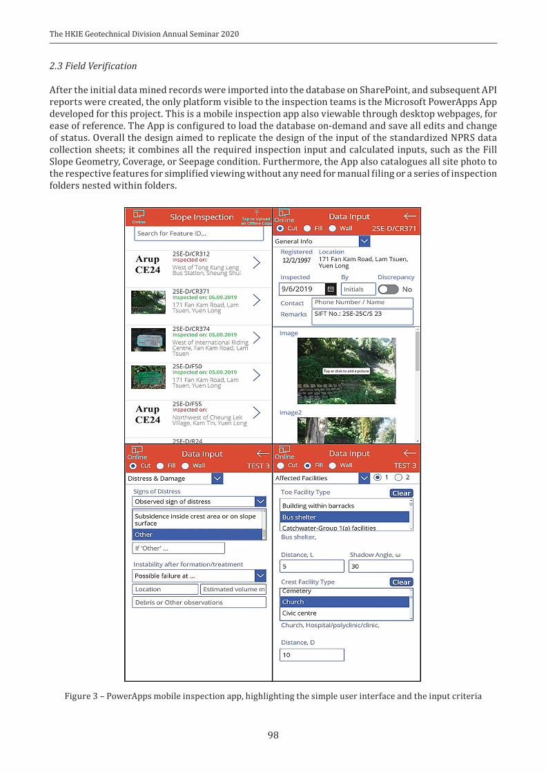
The HKIE Geotechnical Division Annual Seminar 2020
98
2.3FieldVerification
After the initial data mined records were imported into the database on SharePoint, and subsequent API reports were created, the only platform visible to the inspection teams is the Microsoft PowerApps App developed for this project. This is a mobile inspection app also viewable through desktop webpages, for ease of reference. The App is configured to load the database on-demand and save all edits and change of status. Overall the design aimed to replicate the design of the input of the standardized NPRS data collection sheets; it combines all the required inspection input and calculated inputs, such as the Fill Slope Geometry, Coverage, or Seepage condition. Furthermore, the App also catalogues all site photo to the respective features for simplified viewing without any need for manual filing or a series of inspection folders nested within folders.
Figure 3 – PowerApps mobile inspection app, highlighting the simple user interface and the input criteria

The HKIE Geotechnical Division Annual Seminar 2020
99
Implementing this validation platform completely separates the numerous inspection teams from the project records and filing systems. This has helped to significantly improve the inspection efficiency by removing wasteful double-handling of work, hence, significantly improving the control of the standard of report quality by standardizing the input and database structure.
2.4 Report Generation & Compilation
The report automation tool made use of different software and programming tools to facilitate the report generation process. The concept workflow of the report automation is shown in Figure 4.
Figure 4 – Overall Report Generation workflow. Grey indicates manual work, pink indicate MS Word files, and green indicates PDF files

The HKIE Geotechnical Division Annual Seminar 2020
100
Establishing a consistently standardized report for each of the 300 reports required exploring advanced Word templates. HotDocs, supported by K2, was chosen for this to develop a workflow for automated report generation based on templates. HotDocs is for document templating and automated report assembly while K2 is for automated data pipeline and document production workflow. With both software combined, any report can be generated with minimal procedure.
HotDocs will be shown as an add-in in Microsoft Word. Placeholders can be added to the original word template using the HotDocs add-in in Microsoft Word. After the dynamic template is then prepared for each report type (such as the Data Collection Sheet for Fill features, Cut features, and Wall features) as shown in Figure 5, it can be uploaded to the Arup cloud.
Figure 5 – Dynamic Word template prepared using HotDocs, mapping the input placeholders
This cloud connectivity allows further template management and production. If there are no further automation steps to be done in K2, for example, the production of the Aerial Photograph Interpretation Report in Appendix B of the Data Collection report, information can be filled in directly in the cloud

The HKIE Geotechnical Division Annual Seminar 2020
101
interface to generate standard documents. Benefits includes fewer manual input and consistent formatting in all reports, each removing input errors and variations to provide a higher level of quality assurance.
The Aerial Photograph Interpretation in Appendix B of the Data Collection report cannot be fully replaced by automation tool, as interpreting the photos requires human expertise, although the reporting practices can still be streamlined. A standardized HotDocs form was developed for more efficient input of the interpretation data. As the later Checklist of the Data Collection Report in Appendix D of the data collection report refers to a text part of Aerial Photograph Report in HotDocs, standardized report forms simplified the Python data mining procedure to locate and extract the key text for all 300 reports within several seconds.
To complete Site Reconnaissance in Appendix C of the Data Collection report, the HotDocs template needs to be imported into K2 through K2 management. The project database (stored as a SharePoint List) can be uploaded to K2 using the K2 plug-in embedded in SharePoint. Utilizing these shared online resources, a workflow can then be connected and constructed to automate the report generation process. A workflow is where the SharePoint List is mapped against the placeholders in the dynamic HotDocs template, such as assigning the database field “Existing_Toe_Facility” to the report section “Affected Facilities: Toe Facilities Type” part. The K2 workflow could also include logic to instruct report assembly. For example, Figure 6 demonstrates reading the database content to identify slope type of each feature, and depending on the value, choose the appropriate report generation workflow so the appropriate data collection sheet could be assembled. Similarly, it may convert true/false values to tick marks in the template or store the assembled template in preferred location.
Upon one click in the K2 management platform, all 300 reports could be generated at the same time. This process typically required 2-3 hours for each Appendix batch and can be run in the background or whilst out of office. Importantly this task can be handled independently by one engineer, instead of the numerous feature inspectors. This provides an alternative way to handle the labour intensive work to fill in the data collection sheet and reduces duplicative peer review.
The SharePoint List is also used to generate NPRS Ranking Score and Total Score sheets of Appendix C2 of the Data Collection report in conjunction with a bespoke VBA script developed for importing & exporting from Microsoft Access. The project explored various options to automate data importing, exporting, or external calculation, but Microsoft Access was a requirement to calculate the new NPRS scores for each feature, limiting our options to tools native to Access. The VBA script was developed to loop through all the feature records, change the Access input data, then print a new page, allowing all the feature NPRS score sheets to be printed in a single batch.
An additional workflow is also developed for the Checklist for Data Collection Report in Appendix D, using the data from the same SharePoint List and with respective dynamic word template for the appendix. Therefore, production of Appendix D reports for all features can also be automated in batches with a similar HotDocs/K2 workflow as Appendix C1 – Data Collection Sheet.
After each of the Appendices batches for the features are prepared, the files are converted and combined into a single PDF report for each feature for submission using another bespoke Python script for batching all feature report compilations into a single. The file paths of the corresponding PDF of each cover page, Appendix title page, and Appendix reports are collected from the prior auditing tool, totaling over 30 components files to be merged per feature, or nearly 1,000 potential files for the project. The Python script recognizes the corresponding file content, file types and locations, and automatically combines the Data Collection Reports in batches for each feature accordingly. This method significantly reduces the exhaustive need to manually combine hundreds of reports from their corresponding components one by one.
3 CONCLUSIONS
The use of a predominantly digital approach streamlined the way in which data was collected and handled, eliminating the need for manual preparation of several hundreds of report parts. It also enabled Project Managers to track the progress of the works and inspections carried out in near real-time using dashboard platforms also linked to the SharePoint database.
Adopting this digital approach for aggregating data, standardizing reporting, and stream project

The HKIE Geotechnical Division Annual Seminar 2020
102
Figure 6 – Exemplary K2 workflow for mapping and generating reports
data between platforms has been fundamental to increase the productivity and quality control asserted on this project to maintain the project schedule. Despite an inspection team incorporating nearly 30 members, these methods ensured consistency and control of inspection information to the standard required. Throughout the project to inspection 300 features, nearly 6,000 thousand files were processed by Python merging or data mining, extracting over 20,000 parameters, as well as cataloging over 4,000 site photos, and automatically generating 2,000 reports by HotDocs/K2. These automated workflows enable a core team of two people to completely reduce the pre-processing and post-processing to a

The HKIE Geotechnical Division Annual Seminar 2020
103
series of programmed queues to run in the background. A key advantage of the workflow is the efficient scalability, as regardless of the quantity of features, a significant amount labour intensive processing times and data handling can be removed with no loss of the quality assurance.
ACKNOWLEDGEMENTS
This paper is published with the permission of the Head of the Geotechnical Engineering Office and the Director of Civil Engineering and Development Department of the Hong Kong SAR Government for the use of the information concerned.

The HKIE Geotechnical Division Annual Seminar 2020
104
Hong Kong’s Marine UXO. The Prevalence, Burial Depth, Associated Hazard and Identification of Marine UXO
C.Y. Shum, P.S. Lee, C.H. Fan & A.J. MazurFugro, Hong Kong
J. SchultzeFugro, Berlin
ABSTRACT
Unexploded Ordnance (UXO) are military munitions that have been primed, fused or otherwise prepared for use and have been fired, thrown, dropped or propelled but have not detonated either by design or malfunction. Hong Kong saw considerable military action during WWII, with as many as one-third of the munitions used failing to detonate as intended. These UXO remain hidden but probably embedded under, or near much of Hong Kong’s current and proposed infrastructure. Victoria Harbour and her surrounding waters received the majority of this UXO from a variety of sources from 1939 through to the 1980’s. Seabed currents and human activity uncover and transport these UXO, and the source sand for modern day reclamations is extracted from these same areas. This paper reviews the proliferation and mobility of WWII era UXO in Hong Kong waters, the associated risk and modern geophysical methods that can be used for accurate detection.
Keywords: Hong Kong; Unexploded Ordnance; Marine survey; World War 2 munitions.
1 UNEXPLODED ORDNANCE. DEFINITION AND SOURCES 1.1Definition
Unexploded Ordnance (UXO) are military munitions that have been primed, fused or otherwise prepared for use and have been fired, thrown, dropped or propelled but have not detonated either by design or malfunction. For this discussion, we include other explosive remnants of war in this definition, such as unused munitions that have been dumped after an armed conflict and are no longer under any control.
1.2 Sources in Hong Kong
Starting in 1939 with the laying of more than 1,000 Royal Navy sea mines, British, Hong Kong, Imperial Japanese and Allied forces all subsequently deployed military ordnance in Hong Kong during WW2 (1939 – 1945). This activity concluded post-war with the dumping of surplus unexploded military ordnance into Victoria Harbour in haste, followed by the marine dumping of various UXO discoveries through to the 1980’s. The war years in between were marked by periods of intense fighting, enemy occupation and a heavy bombing campaign by Allied forces intended to dislodge the Imperial Japanese forces.
Hong Kong was probably on the receiving end of more than 4,000 tonnes of military munitions (shells, bombs and mines) during WW2. When compared with a reported 70,000 tonnes of enemy munitions fired or dropped on Great Britain over the same period (Exeter 2019), Hong Kong has received 6% of

The HKIE Geotechnical Division Annual Seminar 2020
105
Britain’s quota, but accounts for less than 1% of her land area. Other sources of UXO not often considered are munitions jettisoned by aircrew in an emergency on the way to or from a target.
There have been seven post-war fatalities (HKPF 2019), one serious injury and the total loss of one dredger trailer (Van de Velde 2019) as a consequence of uncontrolled detonation of marine UXO in Hong Kong. It is the larger UXO in Victoria Harbour and her surrounding waters that is reviewed here. These larger munitions used during the conflict are summarized in Table 1.
Table 1: Larger military ordnance deployed during conflict, Hong Kong 1939 – 1945
Item Belligerent / Nomenclature
Weight (lb/kg)
Dimensions(m)
Estimated total quantity
deployed*
Estimated quantity
undetonated
Quantity recovered post-war
Contact Mine, Naval GB / MKXIV 500 / 227 ~ 0.79 D 400
39 –Controlled Mine,
Naval GB / LMK1 650 / 295 0.96 D 700
Aerial bomb IJ / Type 94 GPHE 110/50 1.01 L x 0.18 D 1520 425 - 510 1
Aerial bomb IJ / Type 94 GPHE 220/100 1.32 L x 0.24 D 930 230 - 280 –
Aerial bomb US / AN-M30 100/45 1.02 L x 0.20 D 550 137 - 165 –Aerial bomb US / AN-M57 250/114 1.15 L x 0.27 D 158 39 - 47 -Aerial bomb US / AN-M64 500 / 227 1.44 L x 0.36 D 2139 535 - 640 3Aerial bomb US / AN-M65 1000 / 454 1.70 L x 0.48 D 1316 330 - 365 2Aerial bomb US / AN-M66 2000 / 910 1.78 L x 0.60 D 12 3 2Air dropped
Torpedoe US / Mk-13 1700 / 770 4.18 L x 0.57 D 10 10 –
Air fired Rocket US / FFAR 5-inch 80 / 36 1.65 L x 0.13 D 1273 320 - 380 –Parachute(?) Mines
US / Mark 13, Mark 13-5 1060 / 482 1.73 L x 0.50 D 57 18 –
* Source; original mission reports and Bailey (2019). 40 mm anti-aircraft cannon to 9.2” fixed cannon not included.
Figure 1: One of two WW2 x 1,000 lb AN-M65 bombs discovered on a waterfront construction site. January 2018, Convention Avenue, Wanchai (courtesy South China Morning Post)

The HKIE Geotechnical Division Annual Seminar 2020
106
2 ORDNANCE IN VICTORIA HARBOUR
2.1Coastalmilitaryobjectivesduringconflict
Military objectives were fixed coastal or near-coastal positions in the greater Kowloon area, Stonecutters Is-land and the north shore of Hong Kong Island (the dockyards, the Kai Tak airport, the North Point power station and other infrastructure). Although these objectives were well documented, bombing of this era was not accurate, and munitions often fell short or long of their targets, or were dropped in haste or otherwise jettisoned during fighting.
2.2Marinemilitaryobjectivesduringconflict
The Imperial Japanese Navy imposed a virtual blockade around Hong Kong from 1942. Their light cruisers, destroyers, gunboats, armed cargo ships and tankers were reinforced by commandeering civilian marine craft and salvaging scuttled British naval defense vessels (Lai, B. 2014). These all became marine military objectives for the Allied forces from 1942. However, the attack on the Japanese convoy moored in the harbor on 16 January 1945 dwarfed any other raid on shipping at Hong Kong during the war according to Bailey (2019). Many of the wartime UXO in the harbour are therefore likely have been dropped during this all-day attack, and it is probably this bombing that resulted in the discovery of two unexploded 1,000 lb bombs at a Wanchai north construction site in January 2018 (Figure 1).
There are several other Hong Kong examples of large air-dropped UXO discovered in recent years, but the vast majority of unexploded ordnance remain undiscovered in close proximity to (or underlying) much of the current and proposed construction activities. The seabed is also littered with UXO including mines, torpedoes, shells, rockets and bombs (Figure 2) – either fired during action or dumped, often indiscriminately, after the conflict. Although the latter have been described as “made safe” before dumping into the sea, this terminology has been applied arbitrarily.
Figure 2: Naval contact mine, Cheung Chau 1940-41. (Courtesy Gwulo: Old Hong Kong)
2.3Accuracyandfailuretodetonate
On 24 August 1943, 42 x 500lb bombs all missed their Kowloon targets and were dropped into the sea, and it is consistently reported that 35 - 40% of the air-dropped bombs missed their target (Lee, A. 2014). For three weeks of December 1941, Imperial Japanese aircraft dropped as many as 2,500 Type 94, 50 to 100 kg bombs on Hong Kong. Bombing accuracy was reported by Banham (2003) to be “terrible”, with eye-

The HKIE Geotechnical Division Annual Seminar 2020
107
witness reports of bombs dropped from 2,000m altitude and landing on Kai Tak runway undetonated. Many of the subsequent Allied forces air raids were carried out by B-24 and B-25 bombers and aerial photographs taking during these combat missions confirm the haphazard nature of the bombing. The population of WW2 munitions that failed to detonate as intended is commonly accepted at around 25-30% (Lee, A. 2014). There are many well documented mechanical, environmental and human reasons for this, and for example Lindsay (2005) recounts “about one in three of the Japanese shells” failing to detonate during the Battle for Hong Kong.
2.4Marinedumpingandmunitionsmigration
The official munitions dump site prior to May 1950 is off southwest Tsing Yi (Figure 5). The Marine Fill Committee currently gazette the same pre-1950 ordnance dumping sites as areas for future sand dredging for reclamation purposes (CED, 2000). The same document also mentions ordnance having been dredged in unexpectedly large quantities at Tathong Channel, southwest Stone Cutters Island and south of Junk Bay. This is most likely due to a common practice explained in Alpha (2017) and known as “short-dumping” – where munitions are sea-dumped on the approaches to and exit from, instead of at, official dumping grounds.
However, the effect of munitions migration is likely to have further spread the initial extent of UXO contamination, and the original bomb-drop or mine-laying locations noted in historical records may differ substantially from current UXO locations. These differences can be explained by at least two main reasons. The first is the inadvertent relocation of UXO through fishery activities. UXO can be dragged during trawl fishing activities, or by fishing nets pulling over the seabed surface, hooking UXO and then bringing the explosives up onboard fishing vessels. These finds are not always recorded and reported to responsible clearing authorities, but simply thrown back into the sea. The second reason for location deviation is dynamic seabed movement since the time of placement, which can result in substantial migration of the UXO.
Marine UXO may therefore be widespread and buried for years in the sea floor and then reappear - sometimes repeatedly, due to geological processes and human activity.
3 HAZARD ASSOCIATED WITH WW2 UXO
3.1Hypersensitivityofoldexplosives
Most military explosives are sensitive to compression and heat as well as shock, and UXO can escalate to an extremely dangerous state many years after they have failed to function as designed.
Explosive fills such as Trinitrotoluene (TNT) may originally have been more stable than others however the addition of grit or abrasive material enhances the sensitivity of TNT. Picric Acid is another highly sensitive explosive fill common to WW2 Japanese munitions. It is not only quite sensitive to shock and heat, but also being an acid, it can react in the presence of moisture with the steel components of the bomb. It can then form hydrous ferric picrates and upon crystallisation, anhydrous ferric picrates which are highly sensitive to friction and shock.
Detonators are much more sensitive to heat, friction and shock, so a bomb case without a fuze but containing an explosive fill and a detonator could reasonably be expected to react adversely, if the detonator were to be subjected to shock or compression. In both cases this would cause molecular friction to occur within the detonators’ explosive compound and the result should not be unexpected. In most bombs there is a third component in the explosive chain - a booster charge. The booster charges are made of less sensitive explosive than the content of a detonator, but more sensitive than the main explosive fill. Early bombs often used Picric Acid booster charges, but this was eventually superseded by the use of Tetryl because Picric Acid is not only quite sensitive to shock and heat, but also being an acid, can react in the presence of moisture with the steel components of the bomb. Some recent records of inadvertent UXO detonation on construction projects confirm the enduring hazard presented by these 75-year-old explosives (Table 2).

The HKIE Geotechnical Division Annual Seminar 2020
108
Table 2: Selected construction site fatalities, WW2 UXO
Year Location Comment
26 April 1978 Münsterland Germany Excavator fitted with drilling tool encountered UXO Immediately exploded. Three fatalities.
24 February 1993 Yaumatei, Hong Kong WW2 incendiary bomb. Partial detonation during excavation. 700 persons evacuated.
25 February 1993 Hong Kong HAM308 dredger barge total loss. One injury. 250 / 500 lb WW2 bomb
23 October 2006 Aschaffenburg, Germany Motorway construction. WW2 aircraft bomb detonation. One fatality, one injured.
3 January 2014 Euskirchen, Germany Excavator struck 1,000 lb WW2 bomb. One fatality and eight wounded (two critical).
11 October 2017 Kuala Lumpur, Malaysia MRT construction site explosion. One fatality, two critically injured (loss of limbs).
4 March 2020 South Cotabato, Philippines Construction site, WW2 bomb exploded during mishandling. One fatality.
3.2UnintendeddetonationofUXO
Unintended detonation of UXO may be caused by crushing of casing, friction, static electrical charge, heat, a blow of sufficient energy by heavy equipment, or sympathetic detonation caused by an adjacent UXO. Typical construction activities that can cause inadvertent UXO detonation are percussive and rotary drilling, dredging, jack-up barge leg deployment, excavation by hand or machinery, anchor deployment, jetting, probing or mixing, sheet and percussive piling and bored piling. The main effects of partial or full detonation are shock, blast, heat, shrapnel damage and noise. The effects of the detonation of UXO such as shells or bombs are usually extremely fast, resulting in physical destruction and the effects on the environment. The original performance specification (Office of the Chief Ordnance, 1944) for the AN-M64 500lb bomb which was commonly used in Hong Kong is provided as Figure 3 below. Ten metres from the blast center, a ½” mild steel plate would be consistently perforated every square metre. This bomb is half the size of the 1,000lb AN-M65 discoveries in Wanchai, 2018.
Figure 3: Perforation of ½” mild steel plate. AN-M64 500lb general purpose bomb (Office of the Chief Ordnance, 1944)

The HKIE Geotechnical Division Annual Seminar 2020
109
3.3Environmentalcontamination
Detonation or corrosion will also release environmental contaminants. Heavy metals such as copper or zinc from the bomb’s casing, lead or mercury from the detonator, organic aromatics (TNT, TNB, RDX and other daughter products) from the explosive charge, white phosphorus or other added chemicals on specifically designed devices toxically for humans (Dalhousie, 2015). Undamaged UXO casings corrode in the environment characteristically depending on aeration, electrolyte content, pH, moisture, the soil type and amount of soil bacteria in the environment. If the casing is corroded through, the explosive contaminants and heavy metals can be released into the surrounding soils and dissolve in marine or groundwater/surface waters. Environmental damage includes but is not limited to direct toxic effects on organisms, the effects from pressure changes and further the bioaccumulation in the food web (especially in the shore dumping areas), and effects on drinking water resources (BLMP, 2011).
3.4Munitions“madesafe”
The HKSAR Geotechnical Engineering Office assures the reader that “the majority of ordnance which were dumped into the sea were made safe prior to their disposal” (CED, 2000). However, the war-time definition of the term “rendering safe” in military codes of this era only required the munition to be made sufficiently safe for its temporary handling during disposal of the item, as explained by US forces in NavWeps (1961).
The fuzes in these dumped munitions should have been removed, or, at least made inoperable. However, in both cases the main explosive charge remains intact, and likely so would any booster charge. At the end of conflict in Hong Kong surplus military ordnance were therefore probably made “safe enough” to avoid detonation during disposal, however they could still now be unintentionally detonated. The dumped explosive is then exposed to the elements, susceptible to external influences, particularly if impurities have leeched into the casing and have made the explosive more sensitive due to chemical reaction.
Further, as a general rule, 90% of all military ordnance manufactured during the war years did become surplus and was either buried or dumped at sea. If Hong Kong is typical of other areas of major WW2 conflict, the military ordnance dumped in the harbour post-war will be almost ten times that ‘fired in anger’. The authors estimate therefore is that as much as 36,000 tonnes of munitions could have been dumped post-war into Victoria Harbour, however the loss of reliable records over time does not make any estimation straightforward.
3.5DredgingActivity
More than 270 million m3 of marine sand has already been extracted from the seabed in Hong Kong waters and used as marine fill for Hong Kong reclamation projects (CEDD, 2008). From 2000 to 2002 more than 500 UXO items (mainly shells, mines, bullets) were dredged from East Lamma Channel – an area assumed to be clear of munitions. Dredged sand continues to be a potential source of UXO contamination. Regular maintenance of shipping navigation channels may also contribute to munitions migration. The presence of these navigational channels will be a control on current flow and direction and may increase the rates of sediment erosion and accretion, leading to further UXO migration.
Larger UXO dropped in shallow water (less than 12m) may have penetrated and continue to reside some depth below the sea bed. This is almost certainly the case for ten US Mk-13 air-dropped torpedoes (Figure 4) that almost immediately became “mudders” – a term the crews used to describe these live, undetonated munitions buried in soft ground. The quantity of UXO hauled in fishing nets, displaced by channel maintenance or removed by dredging is not well documented.

The HKIE Geotechnical Division Annual Seminar 2020
110
Figure 4: Ten Mk-13 air-dropped torpedoes, armed, undetonated and missing in Victoria Harbour. (Courtesy Gwulo: Old Hong Kong)
4 ENVIRONMENT
4.1Hydrography
Approximately 70% of the water in Victoria Harbour ranges in depth between 2.5m to 9m. The shipping channels range up to 30m deep (MarDep, 2016). Present day water levels have not changed significantly since the 1940’s, however the erosion and accretion of sea floor sediments is a seasonal occurrence with net gains and losses managed by dredging maintenance.
The harbour is bounded by the Pearl River estuary to the west and the South China Sea to the east. Water deepens in the harbour due east, reaching depths of 25m at Ma Wan Channel, the western coast of Hong Kong Island and Lei Yue Mun. The direction of seabed current flow influences the transportation of marine sediments (Wong & Shaw, 2007) and will also affect the migration of unburied and partially buried UXO in the harbour. There are two major seasonal currents. During summer (June and July), the northeast flowing Hainan Current, associated with the Southwest monsoon, dominates. In winter (October to March), Hong Kong water is mainly affected by the southwest flowing Taiwan Current (South China Coastal Current) which is also mixed with Kuro Shio currents, associated with the Northeast monsoon. During spring and autumn (April to May, and August to September), a transition between the aforementioned major currents occurs, presenting unstable and reversing current directions.
4.2Topographyandextremeweather
Additional factors affecting water energy and direction including topographic influence and extreme weather. Due to the presence of many islands, currents in Hong Kong water are forced into various narrow channels where flow velocity increases. Extreme weather such as typhoon also affects Hong Kong water, particularly in summer, and within the surf zone.
4.3Geology
The sea bed is generally covered with very soft to soft recent deposits, interrupted by older igneous rock of Mesozoic era (Fyfe, J.A. et al, 2000). These superficial deposits vary from discontinuous to laterally extensive mud and sand sheets up to several tens of metres thick in offshore areas. The geological setting is described in Table 3 below.

The HKIE Geotechnical Division Annual Seminar 2020
111
Table 3: The geological setting of Victoria Harbour (after Kirk, P.A. et al., 2000. James, 1999 and Fyfe, J.A. et al. 2000)
Seabed Morphology*
Series / AgeMillion yrs ago (Ma)
Comment
Hang Hau Formation
Holocene(0 – 0.0117 Ma)
Very soft to soft, grey, structureless clayey silt, with common shells and lenses of fine sand” and “muddy, shelly sand overlain by interbedded sand and clayey silt”. Thickness of the formation varies and reaches 60m (maximum) in the southeast of Hong Kong waters.
Waglan Formation
Late Pleistocene(0.0117 – 0.126 Ma)
Interbedded shelly sand and clayey silt and firm, grey, shelly, clayey silt. The thickness increases towards south and east. Confined to the south-eastern waters of Hong Kong with minor younger coastal reclamations
Sham Wat Formation
Late Pleistocene(0.0117 – 0.126 Ma)
Soft to firm silty clays, grey with bands of yellowish mottling, patches of intense mottling with nodules, some thin sand bands, rare shells commonly corroded”. The thickness of Sham Wat Formation varies from a few meters at the northern edges of the subcrop to over 40m at its maximum thickness near the Soko Islands.
Chek Lap KokFormation
Pleistocene(2.588 – 0.126 Ma)
Clays and silts, to sands, gravels and also cobbles and boulders. Variable thickness from a few meters in nearshore areas to over 70m in the south and southeast. Sudden changes in sediment type both horizontally and vertically are common. Most common seabed under reclamation projects.
4.4Reclamations
In many areas along the coast, reclamation materials have been placed over the superficial deposits. Some of these reclamations are more than 120 years old, others are currently in progress. The significance of these reclamations is that WW2 UXO may be sitting on top of older reclamations and/or covered by younger reclamations. UXO burial depth is therefore complicated by reclamation history (Lee, P.S. et al., 2019). Marine sand has often been used as fill material for reclamation in Hong Kong. During 1929-1931 and 1956-1959, hydraulic fill (Guilford, C. M. 1997) and granular seabed material (Henry, J.M. et al., 1961) dredged from Victoria Harbour were used to extend the Kai Tak airport.
In addition to marine sand, the CEDD (2018) refer to extensive hillside cutting carried out to supply fill materials (mainly residual weathered granitic rocks) for extension of coastal sites. Figure 5 presents this historical reclamation history, the approximate footprint of proposed reclamations, areas of intensive WW2 military action, marine geology and the location of ordnance dumping sites and sites gazetted for the extraction of reclamation source sand.
4.5Extentofmilitaryactivityandtheprevailingman-madeandnaturalenvironment
Figure 5 below presents all relevant information (reclamation history, geology, WW2 military activity, weapons dumping sites and sand extraction sites) in the one map. The list of undetonated military ordnance (Table 1) most likely rests within the area marked “most intense WW2 military conflict” on Figure 5, and the extent of UXO penetration depth into the harbour area is provided in Table 4 .
5 UXO Initial Burial Depth Prediction
5.1Impactonwater
Air-dropped and fired munitions enter the sea with significant kinetic energy and may bury deep into the seabed. However, the physical properties of the munition and the environmental conditions limit this potential.
According to the Office of the Chief Ordnance (1944), the AN series air-dropped bombs of WW2 era most likely struck water at a velocity of 170 - 186 m/s and a fall angle of 65 degrees, based on aircraft speeds of 320 kph at 5,000 feet altitude. When a munition moves at high speed through water, the flow separation creates a cavity of air around the body, with full scale tests demonstrating the tail fin will likely break away when hitting the cavitation wall - even with modern weapons (Chu, P.C., et al. 2010a).

The HKIE Geotechnical Division Annual Seminar 2020
112
Figure 5: Hong Kong marine geology, UXO prevalence and reclamation activity (after Bailey, S.K. 2019, Lee, A. 2019, Kirk, P.A. et al., 2000. James, J.W. 1999 and Fyfe, J.A. et al. 2000).
Table 4: Initial seabed penetration. WW2 UXO, Victoria Harbour
Water depths (m) Geology Initial penetration into seabed (m)
2.5m – 6.0mVery soft to soft mud, sandy MUD 2m – 6m
Stiff to firm clay, silt SAND 1m – 4mSAND, muddy SAND 0.5m – 2m
6.0m – 10mVery soft to soft mud, sandy MUD 1m – 3m
Stiff to firm clay, silty SAND 0.5m – 2mSAND, muddy SAND 0.5m – 1m
10m – 15mVery soft to soft mud, sandy MUD 1m – 2m
Stiff to firm clay, silt SAND 0.5m – 1mSAND, muddy SAND 0 – 0.5m
> 15mVery soft to soft mud, sandy MUD 0.5m – 1m
Stiff to firm clay, silt SAND 0.5m SAND, muddy SAND 0 – 0.5m
Further experiments at near vertical striking angles resulted in the bomb orientating to almost parallel to the seafloor at water depths ranging from 0.96m to 6.50m (Chu, P.C., et al. 2010b). The length-to-diameter ratio of the munition should then determine the final pattern of free fall through the column of water – either flat, straight or spiral (Chu, P.C., et al. 2003).
5.2InitialSeabedPenetration
Several existing models may be used to predict the burial depth of UXO in the marine environment. These

The HKIE Geotechnical Division Annual Seminar 2020
113
models are sensitive to aerodynamics, hydrodynamics, environment and geology (Teichman, J. A., et al., 2017) and are useful if the inputs are well defined. To accurately predict the initial penetration depth of UXO in Hong Kong waters, further research on the range of impact velocities, profile types of munitions and seabed morphology is recommended. However, the major influences on seabed penetration are depth of water at the strike zone, and seabed morphology. Upon review of available full-scale tests, hydrography and geology, the authors propose the following guidance in Table 4.
Significant penetration into the sea floor may be expected in shallow water and soft soil conditions. In deep water, undetonated munitions will lose almost all their original kinetic energy and will fall under gravity to rest upon or sink into the seabed. Such items may later migrate across the seabed subject to, amongst other things, their shape, seabed morphology and the marine environment.
6 UXO SUBSEQUENT REBURIAL
The subsequent burial of UXO is influenced by bottom water velocity, erosion and deposition of seabed sediments. Undetonated munitions buried to more than 1/2 of their diameter are considered to be immobile in a lacustrine environment. However, as bed-level velocities gradually increase, the munition will be subject to scour-burial, transient exposure by erosion, equilibrium, frequent exposure and finally mobilization and migration (Rennie, S. & Alan, B., 2015). These processes may be immediate, seasonal or according to Jenkins (2015) even a longer-term phenomenon due to climate changes.
Modelling of seabed changes post-deployment, along with a review of historical records and a detailed understanding of sediment type and hydrography will be necessary for further prediction.
6.1Scourburial
When the exposed part of a partially buried munition can no longer generate sufficient perturbation flow to cause further burial (the Shields number), an equilibrium level is met. When erosion is strong enough, the degree of burial of UXO may be changed. However, Teichman (2017) notes that erosion and accretion are slower processes than scour burial, except during storm events.
A two-dimensional burial regime map developed by the Institution for Defense Analyses illustrates the relationship amongst the state of burial of UXO and velocity of current flow is presented as Figure 6. Note that D is the munition diameter, and UXO are fully buried when d0 > D and partially buried when 0 < d0 < D.
Figure 6: Scour-burial and bottom water velocity (after Teichman 2017)
Amongst the different regions shown in this map, it is worth noting the region of “transient exposure by erosion” which may occur over short term and long-term conditions. As explained by Teichman (2017) this means that the munition will be fully buried due to scour burial in the long term even if it is initially

The HKIE Geotechnical Division Annual Seminar 2020
114
exposed. Since erosion and accretion processes may expose the munition periodically, its exposure will only be temporary due to further scour burial.
7 UXO Detection
The UXO risk mitigation process is most efficient when under the guidance and control of a specialist who can carry out the full spectrum of UXO risk mitigation services. This ranges from the identification of potential risk through to the ultimate issuance of a clearance report and/or certificate (Figure 7). The visual identification process often results in many false positive identifications, with a low percentage proving to be UXO. Many turn out to be ferrous material such as old anchors, lost-at-sea metallic debris, steel wire rope and other fishing gear.
However, the UXO identification serves a dual purpose of allowing these non-UXO targets to be identified.
Geophysical survey should only be conducted after a comprehensive desk study of the area. Non-invasive geophysical survey techniques do allow large study areas to be covered quickly and the focus should be concentrated on the identification of targets and areas of interest. The risk of uncontrolled detonation during geophysical survey is low. However, some detectors such as radio frequency devices can detonate radio or variable time fuses and electrical blasting caps.
Figure 7: UXO risk mitigation procedure
7.1 GeophysicalSurvey
In selection of survey type, the objective is to choose the detectable physical property that can distinguish UXO from the surrounding environment. There are four proposed phases for the field survey programme, and several combinations of sensors and carriers suitable for Hong Kong waters.
7.1.1 Phase1–Bathymetry
Water depth and large underwater obstructions within the research area are assessed. The bathymetry map obtained is used to plan the route of sub-towed sensors in Phase II and avoid equipment damage. Multi-beam echo sonar carried by small boat is preferred for Hong Kong waters.
7.1.2 Phase2–Search,Classify,Map
UXO in Hong Kong is characterized by shell appearance, ferrous properties and acoustic impedance contrasts with the mud and sand environment. After ferrous items have been swept, a non-ferrous survey is recommended. Data processing and interpretation is critical to the success of these surveys and relies heavily on the experience of UXO technicians to avoid overlooking UXO and reduce false positives at the same time. In this phase, sub-towed sensors may be used for various purposes. After the sensors and carriers are selected, a geophysical prove-out is performed to determine whether the selected geophysical investigation approach will work on the study area. A list of Contacts of Interest (COI) with the highest probability is prepared for further identification in Phase 3.

The HKIE Geotechnical Division Annual Seminar 2020
115
Side-Scan SonarSide-Scan Sonar (SSS) is used to efficiently create an image of the sea floor with good resolution and swath coverage, helping us to identify features that may be sea-floor UXO.
Magnetometer For buried UXO, a magnetometer is used to detect the ferrous property of UXO but is not suitable for non-ferrous UXO. In order to distinguish ferrous objects from soil, we have to understand background mineral content of the ground to be aware of natural ferrous objects like magnetic black sand (Fe3O4) and pyrite (FeS2); estimate the buried depth, target weapons type and size to choose suitable sensors, frequency and sensitivity for survey (SERDP, 2006). However, limited information can be obtained from this method. Firstly, magnetometer is not reliable to distinguish between UXOs and metal debris due to their similar ferrous properties and false positives may be expected. Secondly, the received signal is affected by the weapon type, size, amount and also the buried depth. So, the signal intensity can give us hints on the target property, however, any interpretation without further evidence is unconvincing.
Sub-Bottom ProfilerBy deploying the Sub-Bottom Profiler (SBP), we can identify the buried object size and depth from the image and make interpretation with more confidence by their acoustic impedance difference. The SBP detects objects using an acoustic wave, however the data is sensitive to external noise from ships engine or the natural environment. Signal penetration is also affected by the transducer flying height and acoustic source strength. The upper seabed layer in SBP data is often not clear enough for small target detection.
Electromagnetic SurveyElectromagnetic (EM) is an alternative geophysical tool to search for non-ferrous UXO, which transmits a primary EM wave into the soil and detects the secondary EM wave induced by the buried conductive material. Alloy bodied munitions do contain some ferrous metal parts (switches, coils) and it is this material that can be identified using EM.
7.1.3 Phase3–ReacquireandIdentify
Remotely-Operated Vehicles are sent to the Contacts of Interest for an optical or tactile check of its shape. A three-dimensional SBP system allows further identification of a potential UXO. The information obtained from this phase also helps to decide a feasible remedy action.
7.1.4 Phase4–ClearanceCheck
Avoidance, or removal and disposal are the common remedies for a confirmed UXO. A post-removal check is needed to confirm the location is clear as multiple UXOs may exist at the same location. Remapping using magnetometer and/or SBP is important to improve confidence on UXO clearance.
7.2CarrierSelection
All geophysical sensors and data recorders are mounted on a suitable carrier at elevation above the survey object.
The Remotely-Operated Towed Vehicle (ROTV) is our preferred carrier for towed survey in Hong Kong, towed by a vessel with a cable connected to control the elevation and direction during survey (Figure 8). The mobility of the vessel and cable controlled ROTV allows the towed array to move out of the way of traffic. Since the vessel engine is far from the sensors, the electromagnetic and acoustic sensor-carrier interference is minimized. ROTV can carry out acoustic and magnetometer survey at 3-5 knots simultaneously with 4-5m swath at water depths of 3-20m, which has balanced performance in comparison with other carriers.
For some site-specific conditions not suitable for ROTV (e.g. narrow channels and heavy water traffic), a Remotely-Operated Vehicle requires less space and less disturbance to the water traffic during survey and is a suitable substitution.

The HKIE Geotechnical Division Annual Seminar 2020
116
Figure 8: UXO Survey Tools (courtesy Fugro)
8 RISK MANAGEMENT FRAMEWORK
8.1HKSARLegislation
The possession of explosives is highly regulated in Hong Kong (the Firearms & Ammunitions Ordinance, Crimes Ordinance, Chemical Weapons Ordinance and the Dangerous Good Regulations). Other than this legislation, UXO contaminated areas are not managed proactively, but could be by their inclusion in the governments list of Scheduled Areas managed by the Buildings Department (under the Buildings Ordinance). Any UXO risk management framework should therefore be prepared with this future possibility in mind (Figure 9).
8.2ConstructionActivity
The probability of disturbing any UXO increases with any construction or other invasive activity in an area known to be contaminated. The consequences of an uncontrolled detonation will depend on the energy released from a blast, and its proximity to person, the environment or other asset. Construction activities that carry unacceptable risk should be managed with a mitigation strategy until the risk is lowered to a tolerable level – either by lowering the likelihood or consequence.
UXO surveys can effectively lower the risk, however, it is necessary to choose suitable methods that are proven effective and minimise the risk of uncontrolled detonation during survey. The method of handling the UXO needs to be well documented and the actual handling of the UXOs should only be carried out by approved persons
After any mitigation strategy is concluded, a hazard and risk re-assessment is necessary, until all the unacceptable risk becomes tolerable or acceptable. Construction site activities may then resume.
9 CONCLUSIONS
There may be 800 to 1,000 tonnes of WW2 era UXO and 36,000 tonnes of dumped WW2 era munitions on or buried in the sea floor of Victoria Harbour and surrounding waters. Geological processes and human activity have likely transported some of these, so that present day locations are unknown but widespread. They remain dangerous and present a significant hazard, especially to marine construction activities. Modern geophysical survey technology exists to manage this risk and is proposed as part of a risk management framework for Hong Kong waters.

The HKIE Geotechnical Division Annual Seminar 2020
117
ACKNOWLEDGEMENTS
The research presented in this article could not have been possible without the invaluable advice provided by Dr. Stephen Bailey (author of “Bold Venture: The American Bombing of Japanese-Occupied Hong Kong, 1942-1945”), Prof. Steven Davies (HKU), UXO specialists Mark Ranson, Chris Jones and Matt Matulewicz, Hong Kong WW2 historian Craig Mitchell, and UXO specialist Marco Gilissen of Fugro. The authors are most grateful for all this support.
REFERENCES
Alpha 2017. UnexplodedOrdnance(UXO)Threat&RiskAssessmentwithRiskMitigationStrategyforCableInstallation.PDF. Alpha Associates. Available at: http://marine.gov.scot/sites/default/files/northconnect_-_uxo_threat.pdf. [Accessed: 4 Sept 2019].
Banham, T. 2003. Nottheslightestchance.ThedefenceofHongKong,1941. UBC Press Vancouver, BC. Bailey, S.K. 2019. BoldVenture: TheAmericanBombingof Japanese-OccupiedHongKong, 1942-1945 Potomac Books/
University of Nebraska Press.BLMP 2011. Sekretariat Bund/Länder-Messprogramm für die Meeresumwelt von Nord- und Ostsee (BLMP).
MunitionsbelastungderdeutschenMeeresgewässer – Bestandsaufnahme und Empfehlungen.CED. 2000. Civil Engineering Department – Guidance note on incidents involving explosive ordnance during marine
dredging. Marine Fill Committee, Geotechnical Engineering Office of Hong Kong Available at: https://www.cedd.gov.hk/filemanager/eng/content_655/guidance_note.pdf. [Accessed: 3 Sept 2019].
CEDD. 2008. Chapter 7. WorksContractsforaLantauDevelopment. Report No. 50 of the Director of Audit, Hong KongCEDD. 2018. Civil Engineering and Development Department – TheGeologyofHongKong,OnshoreSuperficialDeposits
andFill. Chu, P.C., Fan, C. & Gefken, P. R., 2010a. Diagnostic-PhotographicDeterminationofDrag/Lift/TorqueCoefficientsofaHigh-
SpeedRigidBodyinaWaterColumn. Journal of Applied Mechanics, 77(011015-1).Chu, P.C., J. M. Bushnell, and K. P. Watson. 2010b. TailSeparationandSurfaceImpactEffectsontheUnderwaterTrajectory
oftheJDAM. 9th International Symposium on Technology and Mine Problem, NPS, Monterey, California, 17-20 May 2010.
Figure 9: Proposed Risk Management Framework. Hong Kong Marine UXO

The HKIE Geotechnical Division Annual Seminar 2020
118
Chu, P.C., Fan, C., Evans, A., Gilles, A., Fleischer P. 2003. Three-dimensionalhydrodynamicmodelforpredictionoffallingcylinderthroughwatercolumn. Conference: OCEANS 2003 Volume: Proceedings, 4.
Dalhousie Journal of Interdisciplinary Management (DJIM 2015). 22nd ASCOBANS Advisory committee meeting. 2015 Risk Management For Unexploded Ordinance (UXO) In The Marine Environment. The Hague, Netherlands.
Exeter 2019. ThebombingofBritain1940–1945Exhibition. PDF, The University of Exter, Available at: https://humanities.exeter.ac.uk [Accessed: 28 August 2019].
Fyfe J.A., Shaw, R., Campbell, S.D.G., Lai, K.W. & P.A. Kirk, P.A. 2000. TheQuaternaryGeologyofHongKong. Hong Kong Geological Survey. Geotechnical Engineering Office. Civil Engineering Department. The Government of the Hong Kong SAR.
Guilford, C. M. 1997. Alookback:Civilengineering inHongKong1841-1941. Asia Engineer, Hong Kong Institution of Engineers.
Henry, J. M., Villiers, A. & Gandy, J. 1961. TheconstructionofthenewHongKongairport. Proceedings of the Institution of Civil Engineers, London, Vol. 19, pp. 157-184.
HKPF. 2019. ChronologyofNotableOccasionsandEvents. Hong Kong Police Force. Available at: https://www.police.gov.hk/ppp_en/14_marine/events.html [Accessed: 3 Sept 2019].
James, J. W., 1999. ReclamationsandtheInterpretationofMarineGeologyinHongKong:AComprehensiveApproach. Terra et Aqua, Issue 76, pp. 3-11.
Jenkins, S. 2015. FinalReport -VortexLatticeUXOMobilityModel Integration, SanDiego: Marine Physical Laboratory, Scripps Institution Oceanography.
Lai, B. 2014. HongKong1941–1945.FirststrikeofthePacificWar (1st ed.). Osprey Publishing Ltd., City of Oxford, UK.Lee, A. 2014. HappyValleybomb'partofbigJanuary1945USattackonJapanese. South China Morning Post, 8 February
2014.Lee, P.S., Schultze, J. & Mazur, A. 2019. TheprevalenceanddetectionofUXO fromthewartimebombingofHongKong.
Proceedings, Transformation in Geotechnical Engineering – Technology, Digital and Innovation. Hong Kong Institute of Engineers, Geotechnical Division. Hong Kong. April 2019.
Lindsay, O. 2005. TheBattleforHongKong1941–1945.HostagetoFortune (1st ed.), Spellmount, Gloucestershire.MarDep. 2016. HongKongWatersHK7501"1:75,000 (2nd ed). Marines Department Hydrographic Office, Nautical Chart
Available at: https://www.hydro.gov.hk/eng/papercharts.php. [Accessed: 3 Aug 2019].NavWeps 1961. SurfaceExplosiveOrdnanceDisposalPart1:General. NavWeps Op 2420 (Vol. 1 Pt. 1), Ch.8, The Chief
Bureau of Naval Weapons, Department of the Army, United States of America.Office of the Chief Ordnance, 1944. TerminalBallisticData.Vol1.Bombing. Aug 1944.Rennie, S. & Alan, B., 2015. InterimReport:UnderwaterMunitionsExpertSystemtoPredictMobilityandBurial,SERDP
ProjectMR-2227: Laurel, MD: Johns Hopkins University, Applied Physics Laboratory.SERDP, 2006. Cleanupofchemicalandexplosivemunitions. The Environmental Security Technology Certification Program
(ESTCP), The Interstate Technology & Regulatory Council (ITRC), The Strategic Environmental Research and Development Program (SERDP).
Teichman, J. A., Macheret, J. & Cazares, S. M., 2017. UXOBurialPredictionFidelity:A Summary: Institution forDefenceAnalyses. United States Army.
Van de Velde, M. 2019. Theartofdredging.PDF. The Nautical Institute, Available at: https://www.theartofdredging.com/explosives.htm [Accessed: 3 Sept 2019].
Wong, J.F. & Shaw, R. 2007. High-levelCoastalDepositsinHongKong. Geotechnical Engineering Office. Civil Engineering Department. The Government of the Hong Kong SAR.

The HKIE Geotechnical Division Annual Seminar 2020
119
A Practical View on the Proof Core-Drilling and Remedial Works of Cast In-situ Piles
Arthur K.O. SoAKOS Geotechnical Consulting Limited and
Meinhardt Infrastructure and Environment Limited
ABSTRACT
Piles rest on and/or socketed into rocks are sometimes liable to thin seams in bedrock and base cleanliness problems, and the pile behaviour can be affected. To verify the quality and safety of the piles, proof core-drilling is commonly carried out after pile construction. If the sediments or segregations found are greater than 50mm in thickness or 100mm for piles longer than 30m, high pressure water jetting will be used to remove the loose materials and the void formed will be filled with pressurised grout. In this study, the interface cores and verification cores of 37 shallow diaphragm wall panels of a deep basement project are reviewed. During bulk excavation, the toe/rock interfaces of these panels are exposed which showed that the proof cores and verification cores retrieved are largely affected by the quality of the core-drilling tools and the skills of the operators, and the interpretations are generally over-conservative. Based on the field observations and the findings by other researchers, it is considered unnecessary to carry out any remedial grouting for the interface cores with minor imperfections and even larger imperfections if the inclusions are made up of aggregates and rock fragments. A more practical approach is recommended.
KEY WORDS: Proof Core-Drilling, Drilling Quality, Good/Adequate/Sound Contact, Minor and Major Toe Imperfections, Remedial Jetting and Grouting
1 INTRODUCTION
Piles rest on and/or socketed into rocks are sometimes liable to thin seams in bedrock and base cleanliness problems, and the pile behaviour can be affected. Of the geological imperfections, Kulhawy (1978) has attempted to provide some considerations to their effects on the rock mass stiffness. He established a relationship termed the modulus reduction factor between the equivalent rock mass properties and the individual rock mass properties of the rock materials and the discontinuities. Kulhawy and Carter (1992) have considered the influence of discontinuities on the bearing capacity. They developed a lower bound bearing capacity solution for the foundations in rock in terms of the Hoek and Brown’s (1980) criterion for the jointed rock mass. Poulos (2005) assumed the presence of a clay seam with the strength and Young’s modulus 1/100 times that of the rock into which the pile is founded. Based on the Plaxis analysis, he showed that the seam would provide a path for the failure surface and can lead to a significant reduction in the base capacity and stiffness.
Of the soft toes caused by the unclean pile base, the pile is unlikely to fail because of the confinement by the surrounding soil, but will be expected to deform considerably. Woo and Moh (1990) showed that the load-settlement curves for the piles with clean and unclean bases are quite similar initially, and only separate significantly when the shaft resistance is fully mobilized; thereafter large settlements are experienced by the pile with unclean base. The deeper the pile, the less significant is the effect of the

The HKIE Geotechnical Division Annual Seminar 2020
120
unclean base on the load-settlement behaviour. Routine proof coring examination is therefore commonly carried out after pile construction to ensure the quality and safety of the foundations. If the sizes of the imperfections detected are larger than the tolerable sizes, the imperfections need to be repaired or the imperfect piles need to be replaced. According to Zhang et. al. (2006), if no toe imperfection or toe imperfection is detected and repaired, the distribution of the occurrence probability is significantly modified and the uncertainty in the occurrence probability is substantially reduced; thus the reliability of the pile will be increased.
In Hong Kong before the year 2000, the Building Department (BD) had no specific requirement for the post-construction proof drilling to assess the condition of the pile base (PNAP 66, BD 1980 and 1986). However, according to GEO (1996), for the large diameter bored piles bearing on rock, it is common for core sampling to be stipulated for a selection of the contract piles. This involves the retrieval of minimum 100mm diameter cores through the concrete shaft which may be extended to a minimum of 600mm or a distance of half a pile diameter below the base in order to assess the condition of the pile/rock interface and confirm the nature and state of the founding material. If cores are taken only to assess the base interface, NX size core through a void former cast into the pile would generally be adequate. The frequency of retrieving cores may vary between sites, depending on the contractor’s experience and the designer’s confidence. Where defects at the pile base such as debris and mud are revealed, the interface would need to be flushed out and the void grouted. Several holes may be required to facilitate the flushing of the debris. Further cores may be taken to verify the effectiveness of the remedial grouting in each pile.
Since the year 2000, defects at the base of large diameter bored piles became a significant issue when the size of the pile and bellout is getting larger and larger. In the year 2001, Arup was engaged by the Piling Contractors Committee of the Hong Kong Construction Association to carry out a study on the acceptance criteria of the bored pile interface (HKCA 2003). Interface cores taken at less than 500m from the edge of 263 piles of 1.5m to 3.0m diameter and 18m to 98m long in 5 projects were reviewed. 40% of the cores were found to have unbound concrete aggregates and soil inclusions. Oedometer tests and finite element analyses were carried out at normal stresses up to 15MPa for typical soil inclusion materials, including decomposed granite and decomposed volcanic and 10mm unbound concrete aggregates to prototype their stress-strain behaviour. Based on the assumption of 20mm differential settlement between adjacent piles, an inclusion of 100mm uniform thickness of aggregate or no recovery is considered acceptable without any remedial action. If the soil inclusion thickness is non-uniform, analyses showed that even only 1/25 of the pile area is in direct contact with rock, and the inclusion material is up to 300mm in thickness is still considered acceptable without any remedial actions. This study thereafter provides a basis for prescriptive approach in dealing with defects in bored piles. A typical example at that time is given in Table 1:
Interface Soft Layer Thickness Investigation Remedial Works /
ProposalFurther
InvestigationRemedial Works /
Proposal
S < 100 N/A Flush clean + normal grout N/A N/A
100 < S < 150 N/A Flush clean +pressure grout N/A N/A
150 < S < 200Sonic test (Fan shape)
with satisfactory results
Flush clean + pressure grout N/A N/A
Unsatisfactory results Coring for second hole Flush clean + normal grout
S < 100 Flush clean + pressure grout
100 < S < 150 Flush clean +pressure grout
150 < S < 200S > 200 Further Investigation + submit remedial proposal
Table 1 – Example of Defect and Remedial Measures (Lee et. al. 2005)
The HKIE Geotechnical Division Annual Seminar 2020
121
In 2006, the PNAP 66 (BD 2006) was revised such that it becomes a statutory requirement to carry out core-drilling at the concrete/rock interface for each of the large diameter bored piles, barrettes and the like when these piles are completed. This PNAP was updated and re-categorized according to the nature of content as the current PNAP APP-18 (BD 2012). It is always expected that the concrete should be in good, sound or adequate contact with rock at the interface (BD 2004, 2009, 2012) and the rock is consistently of the required grade beneath the pile base. However, minor imperfection observed during the interface core-drilling, such as a thin layer of sediment, segregated concrete or weathered seam in the rock beneath the pile base, may be considered acceptable provided that the Registered Structural Engineer (RSE) can demonstrate his acceptance with justifications. As an alternative, the RSE may include in the foundation plans, proposals of remedial works for rectifying any such imperfections at the interface if found. The proposals should provide details of the method statement and the supervision required by the RSE. The current practice (GEO 2006) is to use high pressure water jetting to remove the loose sediments at the base, if the sediments or segregations are not greater than 50mm in thickness or 100mm for piles longer than 30m. Pressurised grout is then used to fill any voids. Several holes may be required to facilitate the flushing of the debris. Further cores would be taken to verify the effectiveness of the remedial grouting in each pile. This practice appears to be far more stringent than that required by the study of HKCA (2003). Despite this, many Engineers still tend to be over-conservative in interpreting the cores for the imperfections at the interfaces and the effectiveness of the remedial grouting. On the other hand, some Contractors are tempted to use, e.g. 85% total core recovery of the design grade of rock for the foundations founded on Cat 1(c) rock, as an argument for accepting an interface imperfection up to 225mm thick which clearly contradicts the PNAP requirement for a good, sound and adequate interface (HKIE 2015).
In this study, the interface cores and verification cores of 37 shallow panels of a deep basement project were selected. As their toe levels are above the formation level, they would be exposed and the actual conditions of the toe/rock interface can be checked against the interpretation of the core results. Based on the open-up inspections and the findings of other researchers, the current practice of interpreting the acceptance of post construction proof drilling and remedial measures if required are re-examined.
2 BACKGROUND OF THE PROJECT SITE
The site has a complex history of reclamation and land use. The ground is generally flat at about +5.0mPD and the geological stratigraphy comprises a reclamation fill overlying the marine deposits, alluvium and residual soils, with the rockhead level varying from -13.5mPD to -51.6mPD. A deep basement of about 30m deep was constructed. Perimeter diaphragm wall was designed to serve as a temporary support for bulk excavation and as a permanent basement wall when it is in service. The wall panels were 1.5m thick and mainly 6m wide. Stepped panels were adopted where the rockhead varied abruptly. They were installed using conventional slurry trenching method. Interface coring was then carried out at all panel bites using triple tube core barrel to minimize the disturbance to the core samples during drilling. If imperfections at the interface were found, lugeon tests were carried to determine the seriousness/extent of the imperfections. High pressure water jetting and pressurised grout were adopted to remedy the imperfections. Verification cores, also using triple tube core barrel were taken to proof the effectiveness of the remedial grouting.
3 STUDY OF THE INTERFACE CORES
The interface cores of 37 shallow wall panels are reviewed. As summarized in Table 2, the coring results are categorized into 4 groups for a more systematic assessment. 28 panel bites or 38% of the total number of selected panel bites are found with good contact, 23 bites or 31% with 10-50mm imperfections (minor imperfection as commonly termed by the practitioners) in the form of rock or concrete fragments, silty materials and/or core losses, 17 bites or 23% with 60-300mm (or major) imperfections in the form of rock or concrete fragments, silty materials and/or core losses, and 6 bites or 8% with rock grade weaker than 1(c) and/or core losses.

The HKIE Geotechnical Division Annual Seminar 2020
122
Category Interface Conditions East Wall South Wall Number of Bites % of Bites1 Good Contact 11 17 28 382 10 - 50 mm 7 16 23 313 60 - 100 mm 4 6 10 14
110 - 300 mm 3 4 7 94 Rock Problem 5 1 6 8
Table 2 – Summary of Interface Cores
Visual inspection of interface core logs suggests that the imperfections are largely caused by the poor base cleaning as evidenced by the presence of concrete and rock fragments, aggregates, silts and bentonite adhering to the concrete and rock faces, and the core loses (Plate 1). The imperfections might also be caused and/or magnified due to the poor interface core drilling which can be evidenced from the conical or damaged concrete and rock face, sub-rounded aggregates and rock fragments, drilling breaks
(a) Bentonite on Concrete Face, Concrete andRock Fragments, and Core Loss
(b) Silty Materials and Rock Fragments
Plate 1 – Examples of Poor Base Cleaning
(a) Conical and Damaged Face in Concrete and Rock Cores, Drilling Breaks in Rock Cores
(b) Drilling Break and Irregular Bell-Shaped in Concrete Core
Plate 2 – Examples of Poor Interface Core Drilling
(a) Weak Seams at Interface and in Rock Core (b) Weak Seams and Core Loss in Rock Core
Plate 3 – Examples of Weathered Joints in Rock

The HKIE Geotechnical Division Annual Seminar 2020
123
in concrete and rock cores (Plate 2). This is plausible if the drilling rig is not firmly sit, the concrete and rock core barrel is not sharp, and/or the drilling rate and flushing water pressure are not carefully controlled. However, core losses sometimes are unavoidable at the interface and in the founding rock due to the presence of subvertical weathered joints in the rocks (Plate 3).
4 STUDY OF THE FOUNDING ROCKS
The coring results and rock mass quality of the founding rock determined from the predrilling are then reviewed holistically. Figure 1 is part of the elevation of the east wall from panel DPE1 to panel
Figure 1 – Coring Results and Rock Mass Quality of Founding Rock

The HKIE Geotechnical Division Annual Seminar 2020
124
DPE15. The panel toe levels vary from -14.9mPD to -23.2mPD which are above the formation level of the excavation (-24.5mPD). Predrill hole at each panel shows that the founding rocks are of weathering grade III or better, and are in good to excellent quality with the rock quality designation (RQD) above 75, except panels DPE3 and PPE4 which are fair with RQD equal to 73 and 69 respectively. Re-examination of the rock materials retrieved at the founding levels during construction also confirms the compliance of the founding rock with the design weathering grade. This proves that extensive subvertical weathered joints near the interface and in the founding rocks are unlikely present. However, only 11 bites have their interface in good contact, while 7 bites have 10-50mm or minor imperfections, 7 bites have 60-290mm or major imperfections and 5 bites have 60-150mm imperfections in the founding rock (Table 2). The substantial core losses at the interface are therefore likely caused by the poor base cleaning and/or magnified by the poor interface core drilling, and in the founding rocks by the poor interface core drilling.
Similar study is carried out for the south wall from panel DPS15 to panel DPS35 but the elevation is not shown for the space of this paper. The panel toe levels vary from -13.2mPD to -24.1mPD, and the founding rocks are mostly of weathering grade II. They are in excellent quality with RQD equal to 100, except panel DPS27 of which the founding rock is of weathering grade III or better and has RQD ranging from 25 to 100. Re-examination of the rock materials retrieved at the founding levels during construction also confirms the compliance of the founding rock with the design weathering grade. This again proves that extensive subvertical weathered joints at the interface and in the founding rocks are unlikely present. Likewise, only 17 bites have their interface in good contact, while 16 bites have 10-50mm or minor imperfections, 10 bites have 70-200mm or major imperfections, and 1 bite has 40mm imperfections in the founding rock (Table 2). The substantial core losses at the interface are again likely caused by the poor base cleaning and/or magnified by the poor interface core drilling, and in the founding rocks by the poor interface core drilling.
5 STUDY OF THE REMEDIAL GROUTING
Remedial measures were carried out following the current practice (GEO 2006). Irrespective of the extent of imperfections, high pressure water jetting was used to remove the loose sediments at the base of the panel bites, and pressurised grout was applied to fill the voids. Lugeon tests were carried out and the low permeability proofs that the imperfections are localized. Verification cores were taken to examine the effectiveness of the remedial grouting.
Table 3 shows that in the first remedial grouting, out of the 40 treated bites, 20 or 50% cores have no grout and 20 or 50% cores are partially grouted. In the second remedial grouting, out of the 39 treated bites, 20 or 51% cores have no grout and 19 or 49% cores are partially grouted. This appears to indicate that the remedial grouting is not effective.
ImperfectionsFirst Grouting Second Grouting
no grout partially grouted no grout partially grout10 - 50mm 12 8 15 5
60 - 100mm 5 4 5 4110 - 300mm 2 4 0 6
In Rock 1 4 0 4Total 20 20 20 19
Table 3 – Summary of Verification Cores
Figure 2 shows the correlation between the length of imperfections in the interface cores and the verification cores. Of the 19 bites with minor imperfections at the interface (Figure 2(a)), they were jet cleaned and pressure grouted. The first verification cores show that 13 bites still have minor imperfections while 6 bites were found to have 60-260mm imperfections. Further water jetting and pressure grouting were carried out. The second verification cores show that 14 bites still have minor imperfections while 5 bites (not from the same bites as previous) were found to have 60-290mm imperfections. This again

The HKIE Geotechnical Division Annual Seminar 2020
125
appears to indicate that the remedial grouting is not effective. However, there seems to have no distinct correlation between the length of imperfections in the interface cores and the verification cores. This is likely the result of poor core drilling as explained previous which can be evidenced from the trace of grout, conical or damaged concrete and rock face, sub-rounded aggregates and rock fragments, drilling breaks in concrete and rock cores.
Of the 17 bites with major imperfections (Figure 2(b)), 15 bites were jet cleaned and pressure grouted. The first verification cores show that 7 bites were improved to have minor imperfection of less than 50mm while 8 bites still have major imperfection of 80-290mm. Further water jetting and pressure grouting were carried out. Despite the second verification cores show that 2 bites were improved to have minor imperfection of less than 50mm, 13 bites (not from the same bites as previous) still have major imperfections of 60-360mm. This appears to indicate that the extent of imperfections cover the whole panel base, and to indicate again that the remedial grouting is not effective. Likewise, there seems to have some correlation between the length of imperfections in the interface cores and the verification cores, and the scattering is likely the result of poor core drilling as evidenced from the trace of grout, conical or damaged concrete and rock face, sub-rounded aggregates and rock fragments, drilling breaks in concrete and rock cores.
Figure 2 – Correlation of Imperfections in Interface Cores and Verification Cores
6 VISUAL INSPECTION OF THE EXPOSED INTERFACE AND FOUNDING ROCK
During bulk excavation, the interface of these 37 panels was exposed in small pits by hand-held breaker. According to the coring results, panels DPE5, DPE6, DPE7, DPE9, DPE10 and DPE14 at the east wall and DPS19, DPS22, DPS33 and DPS34 at the south wall have large imperfections of more than 100mm at the interface, in the form of sub-rounded aggregates, rock fragments and some of them with core losses. However, slightly segregated concrete without much fines and lumps of remedial grout were found at the exposed surface as seen in Plate 4 (only east wall panels are shown for illustration). This appears to be contrary to the coring results. This is plausible because concrete and grout are quasi-brittle materials. According to, e.g. Bazant and Oh (1983), the cracking of concrete and mortar involves the formation of a large fracture process zone ahead of the crack. The cracking energy is an essential element for the fracture process, and is associated with the crack arresting materials (aggregates) and the relaxation of the bonding materials (cement mortar and grout) in the zones next to the crack. Thus, the slightly segregated concrete without much fines and remedial grout are more subtle to be fragmented and grinded away, particularly if the core drilling is poor like the rig wobbles or the core run rotates during the core drilling.
Furthermore, because of the presence of these imperfections at the interfaces, the founding rock underneath these panels is interpreted to have weak seams. However, the exposed rock of the area found was actually of largely massive, very strong, medium grained, slightly weathered to fresh granite, with tight and widely spaced joints (see Plate 5 on panels DPE9 and PDE10 for illustration), except at

The HKIE Geotechnical Division Annual Seminar 2020
126
panel DPE12 where a sub-vertical rock joint was found and about 5 litres per minute water was seeping through the wall/rock interface. This is consistent with the rock mass parameters in the predrill logs (Figure 1) that the founding Cat 1(c) rock is in good to excellent quality with the rock quality designation (RQD) above 75 except panels DPE3 and DPE4 which are fair with RQD equal to 73 and 69 respectively, and DPS27 which has RQD ranging from 25 to 100. This is also consistent with the rock materials retrieved at the founding levels as stipulated in Table 6.3 of the Code of Practice for site Supervision (BD 2009). Thus, the substantial rock fragments and losses in the rock cores should be caused by the poor drilling as the exposed surface did not reveal any major sub-vertical weathered joints at the founding rocks. Evidences of poor interface core drilling have been discussed in the section of interface cores. This reaffirms the interpretations/observations in the study of the founding rocks and the study of the remedial grouting.
a) Panel DPE5 b) Panel DPE6
c) Panel DPE7 d) Panel DPE9
e) Panel DPE10 f) Panel DPE14
Plate 4 – Exposed Surface of East Wall Panels with Major Impefections

The HKIE Geotechnical Division Annual Seminar 2020
127
Plate 5 – Rock Mapping of Founding Rock at Panels DPE9 and DPE10
7 CONCLUSIONS AND RECOMMENDATIONS
According to Poulos (2005), thin seam below a pile toe may reduce the axial capacity and stiffness of the pile. The effect of the seam becomes less as the pile length increases, and the effect on pile group is generally more significant than on a single pile. Unclean base giving rise to soft toe may cause a reduction in the pile head stiffness that depends on the soil modulus at the pile tip and the applied load. Based on the Arup’s study (HKCA 2003), an inclusion of 100mm uniform thickness of aggregate or no recovery is considered acceptable without any remedial action. If the soil inclusion thickness is non-uniform, even only 1/25 of the pile area is in direct contact with rock, and the inclusion material is up to 300mm in thickness is still considered acceptable without any remedial actions. This study forms the basis of the current practice for prescriptive approach in dealing with defects. The impact of proof coring on reliability of piles was evaluated for three cases by Zhang et. al. (2006); namely, no toe debris detected, toe debris is detected without repair, and toe debris detected and repaired.
In this study, an open-up inspection of the wall toe/rock interface observes that the results of the proof core-drilling and verification cores are affected largely by the quality of the core-drilling technique. Concrete and cement grout are more subtle to be fragmented and grinded away if the core drilling is poor because the materials are quasi-brittle. This observation is consistent with the statistical analysis that there is no distinct correlation between the length of imperfection in the interface cores and the verification cores, particularly if the imperfection is minor. Because of the observed aggregates, rock fragments and sometimes core losses, Engineers are always over-conservative to interpret the interface as poor or the remedial grouting as ineffective. As a result, despite there is no such requirement by the BD, it becomes common nowadays for the practitioner to use triple tube barrel to ensure the proof core-drilling quality in order to minimize the doubt in the interpretation. Besides this, due cares in the core-

The HKIE Geotechnical Division Annual Seminar 2020
128
drilling should be taken. The drilling rig should be supported on a stable ground to avoid any wobbling during operation. The sharpness of the tools, applied pressure and penetration rate should be properly controlled to minimize the rotation and hence damage to the cores. The core runs should be carefully planned such that the interface is positioned close to the middle length of the core barrel. If super-mud or polymer is used as a drilling medium, sediments like aggregates, sands, silts and rock fragments can be retrieved intact.
It seems to be unanimous in the industry to use high pressure water jetting and pressurised grout to remedy the imperfections irrespective of their magnitudes and causes. Notwithstanding this, based on the above literature reviews and field observations, it is considered by the author to be impractical and unnecessary to carry out remedial grouting and verification core for interface coring with minor imperfections. It is also considered impractical to remove inclusions largely of aggregates and rock fragments because these materials are sound, well compacted and confined in rock and are much stiffer than the clay seam and silty materials. Based on the above findings, a more practical approach in dealing with the imperfections is recommended as summarized in Table 4.
Category Observed Imperfections
Additional Interface Core
Remedial Works Verification Cores
Minor Imperfections(< 50mm for Piles < 30m or < 100mm for Piles > 30m)
Largely Aggregates and Rock Fragments
No Pressure Grout through Interface Core Hole
No
Largely Sands, Silts and Core Losses
No Pressure Grout through Interface Core Hole
No
Major Imperfections (> 50mm for Piles < 30m or > 100mm for Piles > 30m) but < 200mm
Largely Aggregates and Rock Fragments
No Pressure grout through Interface and Additional Core Hole
No
Largely Sands, Silts and Core Losses
Yes Flush Cleaning + Pressure Grout through 3 Core Holes
No
Extreme Imperfections (> 50mm for Piles< 30m or > 100mm for Piles> 30m) but > 200mm
Irrespective of the Appearance of Imperfections
Yes Design Review and Justification by RSE + Flush Cleaning + Pressure Grout through 3 Core Holes
Yes, but % subjected to design review and recommendation by RSE
Table 4 –Recommended Remedial Measures for Different Category of Imperfections
REFERENCES
BD 1980, 1986, 2006, 2012. PNAP APP-18 (formerly PNAP 66). Practice Notes for Authorized Persons and Registered Structural Engineers.
BD 2004. Code of Practice for Foundations.BD 2009. Code of Practice for Site Supervision. GEO 1996. Pile Design and Construction. GEO Publication No. 1/96.GEO 2006. Foundation Design and Construction. GEO Publication No. 1/2006.HKCA 2004. A Study on the Acceptance Criteria of the Bored Pile Interface.HKIE 2015. An Explanatory Handbook to the Code of Practice for Foundations 2004 Hoek, E. and Brown, E.T. 1980. Empirical Strength Criterion for Rock Masses. Journal of Geotechnical and Geoenvironmental
Engineering, Vol. 106(GT9), ASCE, 1013-1035.Kulhawy, F.H. 1978. Geomechanical Model for Rock Foundation Settlement. Journal of Geotechnical Engineering Division,
ASCE, 104(2), 211-227.Kulhawy, F.H. and Carter, J.P. 1992. Settlement and Bearing Capacity of Foundations on Rock Masses. F.G. Bell
Ed.,Butterworth Heinemann, London, 231-245.Poulos, H.G. 2005. Pile Behaviour – Consequences of Geological and Construction Imperfections. Journal of Geotechnical
and Geoenvironmental Engineering, Vol. 131(5), ASCE, 538-563.Woo, S.M. and Moh, Z.C. 1990. Geotechnical Characteristics of Soils in Taipei Basin. Proceedings of 10th Southeast Asian
Geotechnical Conference, Taipei, 2, 51-65.Zhang, L.M., Li, D.Q. and Tang, W.H. 2006. Impact of Routine Assurance on Reliability of Bored Piles. Journal of Geotechnical
and Geoenvironmental Engineering, Vol. 132(5), ASCE, 622-630.

The HKIE Geotechnical Division Annual Seminar 2020
129
Prediction of Vibration caused by Chiselling of Rock
Arthur K.O. SoAKOS Geotechnical Consulting Ltd and
Meinhardt Infrastructure and Environment Ltd
ABSTRACT
There is very limited research on the prediction of vibration caused by chiselling. In Hong Kong, attempts have been made using an empirical formula for the prediction of vibration caused by pile driving to predict the vibration caused by chiselling. This formula has the form of νres = kp [W0.5/rβ] where kp is an empirical scaling factor for piling and 1.5 is adopted. When the measured data of two projects are revisited, the author found that the calculated impact energy adopted in chiselling was only 60% of the actual estimate due to the ignorance of internal frictions, external buoyancy and drag losses in the chisel system. If these energy losses are considered, the kp in the empirical equation for the chisel motion should be about 2.5. Further statistical analysis showed that the vibration would attenuate with an increase in the horizontal distance and not the sloping distance from the source point as assumed. This evidences that the predominant transmission path from the source point at rock should be along the rock stratum, then via the soil layers or the piled foundations to the ground surface. An empirical equation, νres = kc [W0.5/rh
β], in a similar form as that for pile driving is proposed.
KEY WORDS: Rock Chiselling, Ground Vibration, Transmission Path, Wave Attenuation, Prediction Formula, Impact Energy of Chisel, Scaling Factor for Piling kp, Scaling Factor for Chiselling kc
1 INTRODUCTION
Chiselling to overcome rock obstructions is unavoidable in the construction of large diameter bored piles, diaphragm walls or the likes. According to the GEO Publication No. 1/2006 (GEO 2006), there is no official legislation or code of practice for the vibration control. Some guidance on the limits of vibration on sensitive receivers is given in the former Practice Note for Authorized Persons and Registered Structural Engineers (PNAP) No. 77 and 289 of the Buildings Department which are recategorized according to the nature of content as PNAP APP-24 and APP-137 respectively. The research on the prediction of vibration caused by chiselling is very limited. Attempts have been made using an empirical formula for percussive piling given in BS5228-2:2009 (BSI 2009). This formula is one of the formulae derived by Hiller and Crabb (2000) by relating the resultant peak particle velocity (PPV) with a number of other parameters from the field measurements for vibratory compaction, percussive and vibratory piling, dynamic compaction, vibration of stone columns and tunnel boring operations. It can provide an indication to the probability of the predicted value being exceeded and has the form of
νres = kp [W0.5/r1.3] [1]

The HKIE Geotechnical Division Annual Seminar 2020
130
where νre = resultant PPV in mm/s, W = nominal hammer energy in joule, r = sloping distance from the pile toe in m, and kp = scaling factor for piling that depends on the ground conditions. Table 1 shows that kp is assigned with a value between 1 and 5, which increases with an increase in the driving resistance.
Ground Conditions kp
All piles driven to refusal 5
Pile toe being driven through: Very stiff cohesive soil; Dense granular soil; Fill containing obstructions which are large relative to the pile cross section.
3
Pile toe being driven through: Stiff cohesive soils; Medium dense granular soils; Compacted fill.
1.5
Pile toe being driven through: Soft cohesive soils; Loose granular soils; Loose fill; Organic soils.
1
Table 1 – Value of kp for use in Equation [1] for Percussive Piling in Various Conditions (Hiller and Crabb 2000)
W equal to the potential energy of chisel and kp equal to 1.5 are commonly assumed, but kp equal 1.0 is always adopted based on the back-calculation of the measured data from the field trials. However, the author opined that the kp values adopted are too low for a chisel impacting onto rock (see Table 1) and the delivery of the impact energy and transmission of the vibration through the ground in chiselling could be very different from that by pile driving. In this paper, the chiselling vibration transmission model is reviewed and the measured data of two projects is re-analyzed to improve the PPV prediction.
2 GROUND VIBRATION PROPAGATION
If an oscillating point load is applied to an unloaded elastic half-space, three type of waves; namely, the surface wave or the Rayleigh wave and two body waves in the form of a longitudinal wave (P-wave) and a transverse wave (S-wave) will emanate from the source point. These waves will attenuate or decay in amplitude when they propagate due to material damping because of the frictional energy loses which occur during the passage of a wave, and geometric spreading because the energy radiated from the source is spread over an increasingly larger volume of material as the wavefront propagates (Gutowski and Dym 1976, Amick and Gendreau 2000). The effects of material and geometric attenuation are combined by Mintrop (1911, cited by Bornitz 1931) to a general equation of the form
A1 = A0 [r0/r1]β e–α (r1-r0) [2]
where A0 and A1 = vibrations at a distance r0 and r1 from the source point respectively, α = material attenuation or absorption coefficient, and β = geometric attenuation coefficient. The material attenuation or absorption coefficient α depends on the dynamic properties of the soils and the vibration frequency. It can be obtained by assuming Rayleigh wave propagation and fitting the material damping curves to the measured data. Some representative values are given in Table 2.
Soil Types α (m-1)Water Saturated Clay 0.040 – 0.120Loess and Loessial Soil 0.100Sand and Silt 0.040
Table 2 – Representative Material Attenuation or Absorption Coefficients (Gutowski and Dym 1976)
Based on a half-space formulation, the geometric attenuation coefficient corresponding to various propagation models in idealized cases have been determined from the theoretical radiation models. If a line load is applied to the half-space, the response is then a typical of cylindrical energy spreading. Some commonly accepted values are given in Table 3.

The HKIE Geotechnical Division Annual Seminar 2020
131
Source Wave Type Measurement Point βPoint Load on Surface Rayleigh On Surface 0.5Point Load on Surface Body On Surface 2Point Load at Depth Body On Surface 1Point Load at Depth Body At Depth 1Line Load at Surface Rayleigh On Surface Independent of DistanceLine Load at Surface Body On Surface 1Line Load at Surface Body At Depth 0.5This Study Body At Depth 0.5
Table 3 – Theoretical Geometric Attenuation Coefficient based on Wave Types (Gutowski and Dym 1976)
However, many authors reported that the wave attenuation in soils is more rapid than that predicted by the elastic theory. Furthermore, by setting α = 0 and assuming attenuation follows a straight line on a log-log plot of the velocity amplitude as a function of the distance, β can be obtained as the negative slope of the best fit line to the observed field data. Table 4 summarizes some of the published β values.
Authors Soil Type βWiss (1967) Sand 1.0
Clay 1.5Nicholls et al. (1971) Firm Soil and Rock 1.4 – 1.7Attewell and Farmer (1973) Various 1.0Brenner and Chittikuladilok (1975) Sand 1.5
Sand over Soft Clay 0.8 – 1.0Martin (1980) Clay 1.4
Silt 0.8Woods and Jedele (1985) Dense Sand 1.1
Medium Dense Sand 1.5Amick and Ungar (1987) Clay 1.5Ali et al. (2003) Sand 0.88 – 1.02Hajduk et al. (2004) Sand 0.50 – 1.03Fiegel and Farrell (2008) Clay and Silt 1.17 and 1.49Current Study Founding Rock 0.5
Table 4 – Summary of some Published Geometric Attenuation Coefficients (Fiegel and Farrell 2008)
Jaeger and Cook (1976) considered that the material attenuation did not assume significance until a propagation distance of a few orders of magnitude greater than the vibration wavelength. Attewell (1995) concluded that it is the geometric attenuation which dominates with the material attenuation being a secondary effect. Other examples of prediction equations of this form are V = kxβ i.e. the propagation law, v = k [W0.5/r] by Attewell and Farmer (1973) and v = K [D/E0.5]-n by Wiss (1981).
However, the impact of a pile driving process is far more complex. Massarsch and Fellenius (2008) commented the above empirical relations that the location of the source of vibration energy is not well defined because the vibrations can be emitted from the pile shaft or its toe or both at the same time, and also more from some layers penetrated by the pile and less from the others. Based on the theoretical consideration of energy propagation in an elastic medium (Clough and Penzien 1975) and the dynamic pile-soil interaction, they derived more precise multi-parameters wave attenuation equations for the cylindrical waves emitted from the pile shaft, the spherical waves from the pile toe and the surface waves caused by the refraction of the P-waves and S-waves at the ground surface at critical distance. Nevertheless, the wave propagation mechanism in rock chiselling is different from that of pile driving,

The HKIE Geotechnical Division Annual Seminar 2020
132
while Equation [1] and its similar derivatives are very simple for practical use. This equation is to be reviewed in the following sections.
3 DETERMINATION OF IMPACT VELOCITY AND IMPACT ENERGY OF THE CHISEL
Site AThe first site was reclaimed in various periods of time due to development with ground level at about +4.2mPD. Geological profiles vary considerably, with various thicknesses of fill, marine deposits, alluvium and different degrees of weathered granites embedded with a thick layer of corestones. A basement structure is to be constructed. Perimeter diaphragm walls mainly are designed as the lateral supports for the bulk excavation. The diaphragm walls are basically 6m (2 bites) wide, 1.5m thick and 20m-40m deep. Due to the thick layer of corestones, chiselling is used as one of the means to improve the construction progress. Two diaphragm wall panels are selected for the trial chiselling using 7.5t, 10.4t, 12t and 14t chisel at 1.5m, 2m and 3m drop height. Technical data of the chisels used for the trial are summarized in Table 5.
Weight (t) Diameter (m) Projected Area (m2) Volume (m3)7.5 0.95 0.71 0.96
10.4 1.10 0.95 1.3212.0 1.20 1.14 1.5314.0 1.30 1.33 1.78
Table 5 – Technical Data of the Chisels
The impact velocity of the chisel onto rock can be measured directly by a high speed photographic method, but is calculated using the principle of conservation of energy in this project of which the potential energy of the chisel at its initial position is assumed totally transferred to the kinetic energy as a free fall. However, this approach is over-simplified because the frictional and inertial forces within the system, the external forces and the drag losses are ignored. According to Kohlbock (2010), the chiselling motion can be represented by a simplified drive mechanism at the time t with a single degree of freedom as illustrated in Figure 1.
Figure 1 – Simplified Drive Mecahnism for the Determination of Chisel Motion (Kohlbock 2010)

The HKIE Geotechnical Division Annual Seminar 2020
133
He derived linear differential equations for the chisel motion which are simplified to the equations as follows:
–A1(d2z/dt2) + A3 – κ (dz/dt)2 = 0 [3]
A1 = [m1 + (h + h/sinα )ms + Jo/ro2] [4]
A3 = m1g – V1ρf g – Ff [5]
v(z) = [2A3z/A1]0.5 [6]
κ = 0.5ρf AStcw [7]
where A1 and A3 are the auxiliary coefficients, z(t) = falling height of the chisel at time t in m, dz/dt = velocity of the chisel in m/s, dz2/dt2 = acceleration of the chisel in m/s2, κ = total drag coefficient in kg/m, m1 = mass of the chisel in kg, ms = mass of the rope per m in kg/m, h = height of the boom in m, α = angle of the bloom in degree, Jo = moment of inertia of the winch at t = 0 in kgm2, ro = radius of the winch at initial state in m, g = gravitational acceleration in m2/s2, V1 = volume of the chisel in m3, ρ f = density of the fluid in kg/m3, Ff = total friction, v(z) = velocity of the chisel in m/s at a falling height z in m, ASt = area of orthographical projection of the chisel on a plane perpendicular to the direction of the motion in m2, and cw = drag coefficient. He also showed that the difference between the chisel velocities for the dry and water-filled conditions with the free fall velocity can be substantial.
In field, the chisel is operated using a hydraulic crawler crane. Based on the technical data of the model, the mass, radius and moment of inertia of the winch are found equal to 17.55t, 0.375m and 1.234 kgm2 respectively and the total friction loss is about 10%. The crane operates with a 7.13kg/m rope, 18m bloom height and at about 60° bloom angle. 1 part of line pull in the snatch block is used in all chisels except the 14t chisel of which 2 parts of line pull is also used to increase the pull capacity in the winching operation. If a drag coefficient cw = 0.82 for a long cylinder and a bentonite density ρ f = 1.1 kg/m3 are assumed, the buoyancy force Fb = V1ρf g and total drag Fd = κ (dz/dt)2 for different chisels, the impact velocity and impact energy can be calculated by iterations using the above analytical equations as summarized in Table 6.
Chis
el M
ass,
m1 (t
)
Nom
inal
Chi
sel
Dia
met
er (m
)
Chis
el D
rop,
z(t)
(m
)
Auxi
liary
Co
effic
ient
, A1
Auxi
liary
Co
effic
ient
, A3
Buoy
ancy
For
ce,
F b (SG
of b
ento
nite
=
1.1)
Fric
tiona
l For
ce, F
f (a
ssum
e 10
%)
Visc
ous D
rag,
Fd
(tm
/s2 )
Impa
ct V
eloc
ity,
v(z)
(m/s
)
Impa
ct E
nerg
y (t
m2 /s
2 )
Free
Fal
l Vel
ocit
y (m
/s)
Ener
gy T
rans
fer
(%)
7.5 0.95 2.0 15.55 48.90 14% 10% 7.01 5.01 94.31 6.26 64%7.5 0.95 3.0 15.55 42.27 14% 10% 13.64 6.99 183.42 7.67 83%
12.0 1.20 2.0 20.05 69.60 14% 10% 19.85 5.27 166.59 6.26 71%10.4 1.10 1.5 18.45 68.97 14% 10% 8.55 4.10 87.46 5.42 57%10.4 1.10 2.0 18.45 63.57 14% 10% 13.96 5.25 143.29 6.26 70%14.0 1.30 2.0 22.05 77.20 14% 10% 27.16 5.29 196.02 6.26 71%*14.0 1.30 2.0 22.05 95.91 14% 10% 8.45 2.95 60.89 6.26 22%
* Denotes 2 parts line pull
Table 6 – Calculation of Impact Velocity and Impact Energy for Different Chisel Weight and Drop Height
The energy transfer in the impact is shown depending on the chisel weight and drop height, and varies from 57% to 83% for 1 part line pull, but can be reduced substantially from 77% to 22% in the 14t chisel at 2m drop height when 1 part line pull is changed to 2 parts line pull. Considering 60% is

The HKIE Geotechnical Division Annual Seminar 2020
134
a conservative approximation for a variety of chisel weight and drop height, the kp back-calculated in the project should be equal to 1.5/0.6 = 2.5 which appears to be more rational to reflect the ground condition of increased driving resistance (see Table 1).
Vibration and AttenuationWhen the PPV at various horizontal distances rh from the vibration source to the vibration sensors are plotted in a log-log scale as in Figure 2, on comparison with equations [1] and [2], the negative slopes will give the attenuation rates of vibrations β if the effects of α and W are ignored. Only trial panel A is shown for illustration. Same plotting is carried out for the sloping distance between the vibration
Figure 2 – Attenuation Rates on Ground from Trial Panel A to a Steel Footbridge on Mini-Piles and a High-Rise Building on Large Diameter Bored Piles obtained

The HKIE Geotechnical Division Annual Seminar 2020
135
source and the vibration sensors, but is not presented here for simplicity. The distribution of the data is found more scatter, implying that the attenuation rate varies with the horizontal distance instead of the sloping distance from the vibration source like the pile driving as assumed in the project.
The β values obtained from Figure 2 are summarized in Table 7. The vibration transmitted to the ground surface is found to decay with β = 0.5. It will decay more rapidly if it is transmitted via a steel footbridge that is supported on the more flexible mini-pile foundations (β = 0.56), but less rapidly in a highrise building that is supported on the more rigid large diameter bored pile foundation (β = 0.29). These values are smaller than that is used in Equation 1 and in the project (β = 1.3).
ChiselWeight & DropHeight
Attenuation Rate β (-ve slope)
On Ground At SteelFootbridge
At Highrise Building
Trial Panel A 7.5t @ 2m 0.59 – 0.147.5t @ 3m 0.42 0.62 0.4212t @ 2m 0.46 0.34 0.29
Trial Panel B10.4t @ 1.5m 0.53 0.75 0.3110.4t @ 2m 0.53 0.53 0.3214t @ 2m 0.46 - 0.23Average 0.50 0.56 0.29
Table 7 – Attenuation Rates for Various Chisel Weight and Drop Height
These values are also smaller than that is obtained by Attewell and Farmer (1973). Based on the best fit curve of the measured data, Attewell and Farmer (1973) derived β = 0.87 and suggested β = 1.0 is a good approximation over a wide variety of soil types. They observed that the amplitude of Rayleigh waves is much larger than the amplitude of the body waves at the same distance, which implies that the pile driving motion excites primarily the Rayleigh waves. They explained that to obtain a propagation law coefficient of β = 1.0, considerable energy must be lost due to internal dissipation. If spreading losses alone are to be considered, β = 0.5 would result. Likewise, when a chisel is impacted onto rock at depth, body waves are expected to be the predominant waves, not Rayleigh waves as in the pile driving (Attewell and Farmer 1973). Thus, the vibration propagation may be mimicked by a body wave generated from a point load at depth. However, according to Gutowski and Dym (1976), the theoretical β in soil is equal to 1 based on the theoretical radiation models, which is larger than that obtained from the measured data (Table 3).
This can be shown schematically as in Figure 3. The body waves would be transmitted largely along the rock stratum, not soils because they decay much faster in soil than in rock (Ungar and Bender 1973, and Gutowski and Dym 1976). This explains why the measured β is smaller than the theoretical models and the vibrations decay with the horizontal distance. However, the vibration is found to decay more rapidly in the steel footbridge that is supported on the more flexible mini-pile foundations (β = 0.56) and less rapidly in the highrise building that is supported on the more rigid large diameter bored pile foundation (β = 0.29). This is likely due to the effect of ignorance or lumping of the material attenuation α (assuming α = 0) in the statistical regression analysis to obtain the β values for the body waves from the rock surface at depth via the soils or piled foundations to the surface.
Project Site BSimilar analysis is also carried out for Site B. The existing ground level varies from +7.9mPD to +10.3mPD. About 2-5m fill is found at the top, followed by 1-20m alluvial sand or sandy silty clay, and underlain by 35-45m weathered granite before reaching Category 1(c) rockhead. 1200mm thick, 2-6m wide and about 45m deep load bearing diaphragm walls and 800mm thick, 2-6m wide cross walls are designed to reduce the ground movement during excavation. At the predrilling stage, lots of boulders in fill and corestones in the weathered granite are revealed. Chiselling is therefore used to part the boulders

The HKIE Geotechnical Division Annual Seminar 2020
136
Figure 3 – A Schematic Representation of the Chiselling Process
and corestones followed by trench cutter in order to improve the rock excavation rate and avoid any continuous vibration to the existing buildings. Three trial panels were selected using 12t chisel at 1.5m drop height. Based on the measured data, the negative slope β = 0.48, 0.55 and 0.62 with an average of 0.55 on ground was determined. Details of the analysis are not reported here for simplicity.
The Proposed Prediction EquationThe above review evidences that the predominant transmission path is along the rock stratum, then to the ground surface via the soil layers or the piled foundations. Keeping the form of Equation [1], the following equation is proposed for the prediction of vibration caused by chiselling:
νres = kc [W0.5/rhβ] [8]
where νres = resultant PPV in mm/s, W = nominal hammer energy in kJ, rh = horizontal distance from pile toe in m, β = 0.5 for ground, but can vary with the stiffness of the foundations that are supporting the vibration sensitive structures. kc = scaling factor for chiselling (to distinguish from kp in Equation [1]) that depends on the ground conditions, chisel weight and drop height, and kc = 2.5 may be a good approximate value for general use without going into direct measurement by photographic method or detailed calculations. Figures 4 and 5 compare the predictability of Equation [1] adopted by the two projects and the proposed Equation [8]. As sloping distance is used in Equation [1] for the prediction of the vibration, only the most critical case at the first encountered rockhead level (being 15m deep for Site A and 50m deep for Site B) is calculated for clarity.
The figures show that the predictability of the proposed Equation [8] is far better than Equation [1], especially at close distance from the source point because the transmitting distance from the source point will be over-considered when a sloping distance is used. Furthermore, the figures also show that Equation [8] at close distance from the source point better predicts the PPV for chiselling at shallow depths. According to Attewell (1995), it is the geometric attenuation which dominates with the frictional attenuation being a secondary effect. However, Jaeger and Cook (1976) also pointed out that the frictional attenuation did not assume significance until a propagation distance of a few orders of magnitude greater than the vibration wavelength. The insufficiency in the above prediction is therefore not unexpected as the material attenuation through soils has not been considered.
4 CONCLUSIONS
There is very limited research on the prediction of vibration due to chiselling of rock. Projects in Hong Kong have attempted to use an empirical formula for pile driving derived by Hiller and Crabb (2000) for the rock chiselling prediction. However, when the measured data of two projects are revisited, the

The HKIE Geotechnical Division Annual Seminar 2020
137
Figure 5 – Predictability of Proposed Equation [8] at Site B
Figure 4 – Predictability of the Proposed Equation [8] at Site A
author found that the impact energy W was only about 60% of that assumed when all internal frictional and external buoyancy and drag losses are considered. As a result, the back-calculated scaling factor for piling kp should be 2.5 which appears to be more rational to reflect the ground condition and in line with the trend of values suggested by Hiller and Crabb (2000) for piles driven to ground, of which the value will increase with an increase in driving resistance. Statistical analysis showed that the vibration would attenuate with an increase in the horizontal distance from the source point. This evidences that the predominant transmission path is along the rock stratum, then to the ground surface via the soil layers or the piled foundations.

The HKIE Geotechnical Division Annual Seminar 2020
138
An empirical equation in the form of νres = kc [W0.5/rhβ] (Equation [8]) is proposed for the vibration
transmitted along the rock stratum where β = 0.5 through soil, but can vary with the stiffness of the foundations on rock that are supporting the vibration sensitive structures. This may be due to the lumping of the β values with the effect of material attenuation of the body waves from the rock surface at depth to the ground surface or via the piled foundations in the statistical analysis. Notwithstanding this, without consideration of the attenuation in soils will only make the proposed equation slightly conservative, but is still practical and can provide a better indicator of the probability of the predicted value being exceeded than the previous approach.
REFERENCES
Amick, H. and Gendreau, M. 2000. Construction Vibrations and their Impact on Vibration Sensitive Facilities. Proceedings of the 6th ASCE Construction Congress, Orlando, Florida, pp. 1-10.
Attewell, P.B. and Farmer, I.W. 1973. Attenuation of Ground Vibrations from Pile Driving. Ground Engineering, 6(4), pp. 26-29.
Attewell, P.B. 1995. Tunnelling Contracts and Site Investigation. Chapman and Hall, London.BD 2012. PNAP APP-137 – Ground-borne Vibrations and Ground Settlements Arising from Pile Driving and Similar
Operations. Practice Notes for Authorized Persons, Registered Structural Engineers and Registered Geotechnical Engineers, Buildings Department, Hong Kong Government.
BD 2013. PNAP APP-24 – Railway Protection, Railway Ordinance, Mass Transit Railway (Land Resumption and Related Provisions) Ordinance, Area Number 3 of the Scheduled Areas in Schedule 5, Buildings Ordinance, Cap 123. Practice Notes for Authorized Persons, Registered Structural Engineers and Registered Geotechnical Engineers, Buildings Department, Hong Kong Government.
Bornitz, G. 1931. Über die Ausbreitung der von Groszkolben-Maschinen Erzeugten Bodenschwingungen in die Tiefe, J Springer, Berlin.
BSI 2009. Code of Practice for Noise and Vibration Control on Construction and Open Sites – Part 2: Vibration. BS 5228-2:2009, British Standards.
Clough, R.W. and Penzien, J. 1975. Dynamics of Structures. McGraw-Hill, 634p.GEO 2006. Foundation Design and Construction. Geotechnical Engineering Office, Civil Engineering Department, Hong
Kong Government.Fiegel, G.L. and Farrell, T.M. 2008. Measurement of Vibration and Noise during the Installation of Rammed Aggregate
Piers. 6th International Conference on Case Histories in Geotechnical Engineering, Arlington, VA.Gutowski, T.G. and Dym, C. L. 1976. Propagation of Ground Vibration: A Review. Journal of Sound and Vibration, 49(2),
pp. 179-193.Hiller, D.M. and Crabb G.I. 2000. Ground-borne Vibration caused by Mechanised Construction Works. Transport Research
Laboratory, TRL Report 429.Jaeger, J. C. and Cook, N.G.W. 1976. Fundamentals of Rock Mechanics. Chapman and Hall, London. 585pp.Kohlbock, D. 2010. Investigation of Rock Chisel usage in Pile Construction. The Tenth International Conference in Modern
Building Materials, Structures and Techniques, Vilnius, Lithuania, pp. 1130-1135.Massarsch, K.M. and Fellenius, B.H. 2008. Ground Vibrations induced by Impact Pile Driving. The Sixth International
Conference on Case Histories in Geotechnical Engineering, Edited by Prakash, S., Missouri University of Science and Technology, Arlington, Virginia, 38p.
Ungar, E.E. and Bender, E.K. 1973. Guidelines for the Preliminary Estimation of Vibrations and Noise in Buildings near Subways. Bolt Beranek and Newman Inc. Report 2500B.
Wiss, J.F. 1981. Construction Vibrations - State of the Art. ASCE, Journal of Geotechnical Engineering, 107(GT20), pp. 167-181.

The HKIE Geotechnical Division Annual Seminar 2020
139
Digital Technology in Slope Design
H.W. Sun, R.C.H. Koo, B.K.C. Cheng, P.F.K. Cheng, L.L.K. Cheung, H.Y. Ho and K.K.S. Ho
Geotechnical Engineering Office, Civil Engineering and Development Department, The Government of the Hong Kong SAR
ABSTRACT
Since the establishment of the Geotechnical Engineering Office (GEO) in 1977, the overall landslide risk of Hong Kong has been substantially reduced. Over 6,000 man-made slopes and hillside catchments have been upgraded and/or mitigated under the Landslip Preventive Measures (LPM) Programme and the Landslip Prevention and Mitigation (LPMit) Programme.
Under the LPM and LPMit Programmes, the geotechnical assessment and design of slope works has largely been a repetitive and time-consuming process, and relies largely on manual assessment and interpretation of data collected from desk study, field mapping and ground investigation. In recent years, the GEO has been developing digital technologies to facilitate the design and quality assurance process, e.g. the use of Geographic Information System, numerical modelling techniques, etc. The GEO endeavours to further enhance the accuracy and efficiency in data acquisition and processing in the planning and design of slope works with the application of the latest digital technologies including Building Information Modelling (BIM), digital geological data infrastructures, 3-dimensional (3D) geological modelling, remote sensing, virtual reality (VR) simulation, advanced numerical analysis, etc.
This paper presents the initiatives and the latest development by the GEO on the use of digital technologies in geotechnical assessment and design for the LPMit Programme. The digital workflow and practical challenges for the implementation of BIM in LPMit design are discussed. Through the use of digital technologies, complex topography, geological conditions, foliage, utilities matrix and underground facilities are collectively considered in the design and construction of slope safety works. This has contributed greatly to the continuous improvement of the quality and efficiency of the LPMit process as well as to support future digital transformation of geotechnical works and infrastructure development in Hong Kong.
1 INTRODUCTION
Under the LPM and LPMit Programmes, geotechnical assessment and design of slope works has largely been a repetitive and time-consuming process that relies heavily on manual assessment and interpretation of data collected from desk study, field mapping and ground investigation. A more efficient way to carry out the LPMit design with the help of digital technologies is warranted.
In recent years, the GEO has been deploying various digital technologies to facilitate the design and quality assurance process and sharing data with other geotechnical and geological professionals. The GEO endeavours to further enhance the accuracy and efficiency of data acquisition and processing through the latest digital technologies including Building Information Modelling (BIM), digital geological

The HKIE Geotechnical Division Annual Seminar 2020
140
data infrastructures, 3D geological modelling, remote sensing, virtual reality (VR) simulation, advanced numerical analysis, etc. There have been a number of successful applications of innovative and novel technologies to the local geotechnical practice, such as the GEO’s digital platform of Geotechnical Information Infrastructure (GInfo), advanced numerical modelling for debris mobility modelling, etc. The GEO continues to explore new opportunities to promote and apply new technologies for technical excellence and enhanced operational efficiency.
This paper presents how digital technologies have been applied in recent LPMit projects to expedite and enhance the planning and design of slope works. The practical challenges faced in the use of digital technologies in LPMit Programme are also discussed.
2 GEO’S STRATEGIC PLAN FOR DIGITAL TECHNOLOGY
Digital technology is recognised worldwide as the principal driver for economic growth and the key to enhance competitiveness of different industries. The Government has targeted to promote innovative and novel technologies with a view to developing into a smart city. The GEO has accorded priority on advances in digitalisation of our daily work in order to promote a workplace culture to utilise digital technologies in our day-to-day operation and improve public services. Furthermore, GEO aims to instill an innovative culture and promote collaboration with the key industry stakeholders, so as to create synergy for applying new technologies to transform the geotechnical practice.
3 DIGITAL TECHNOLOGIES IN LPMIT PROJECTS
Geohazard assessment for slope design has always been a labour-intensive process that requires expert input in the interpretation of data from desk study, field mapping, ground investigation, etc. The GEO has stepped up the application of digital technology in the acquisition of quality data as well as planning and design of slope works in order to enhance the efficiency of the LPMit process and strive for technical excellence.
3.1 Implementation of BIM
Since the promulgation of the Development Bureau Technical Circular (Works) (DevB TC(W)) No. 7/2017 in adopting BIM for capital works projects in Hong Kong, GEO has stepped up the momentum in promoting and utilising BIM in LPMit design. Owing to the lack of existing standards for use of BIM use in geotechnical design, especially for slope works in Hong Kong, the GEO has spearheaded the development of a set of standard BIM documents including BIM project execution plan (PXP), consultancy agreement brief and construction specifications. A LPMit Task Group on BIM was formed to support and promote development of technical competence of the LPMit project teams in the use of BIM. The objective of the Task Group, which is led by GEO and comprises representatives from LPMit consultants, contractors and slope maintenance departments, is to promote sharing of knowledge and experience in the use of BIM for geotechnical engineering.
BIM is not just a 3D tool but a digital and communication platform to be used by the project teams to holistically manage digital information relating to construction projects from the planning stage, through the design and construction stages, to the operational stage in a quality assured manner. Through the use of BIM, complex topography, geological and hydrogeological conditions, foliage, utility matrices and underground facilities are considered in slope design and works coordination of the works during construction.
3.1.1 BIM standards
A detailed BIM PXP provides the essential information and stipulates the project requirements on the use of BIM in a project. The BIM PXP is aimed at defining the use of BIM throughout the project cycle. It also defines how BIM is implemented including, but not limited to, the workflow of using BIM in co-ordination, information exchange, design authorisation, modelling methodology and level of development (LOD) of BIM models in different stages of a project. The BIM PXP enables the project teams to follow

The HKIE Geotechnical Division Annual Seminar 2020
141
up and monitor BIM implementation during the project. The PXP should be continuously reviewed and updated during the project life cycle.
There are a few BIM PXP standard templates published by various organisations for the construction industry in Hong Kong, but their coverage in geotechnical engineering is limited. With the support of the Geotechnical Division Committee of the Hong Kong Institution of Engineers (HKIE-GDC), the GEO has developed a set of standard BIM PXP template for LPMit works that allows the industry to make reference to in preparing their project specific BIM PXP. Specifications on the use, management, processes, file naming convention, category code, colour scheme, IT solution and quality control are defined in the PXP. This allows the BIM practitioners to adopt a unified approach for BIM implementation in LPMit projects. In addition, GEO has set out a comprehensive list of LOD specifications for different digital models and geotechnical components for LPMit projects including topographical models, geological models, man-made slopes, soil nails, debris-resisting flexible barriers, rigid barriers, etc. An example of a debris-resisting rigid barrier model of LOD 300 is presented in Figure 1.
Figure 1: Debris-resisting rigid barrier BIM model
3.1.2 BIM object library
To further promote the sharing of standarised BIM libraries for geotechnical applications in LPMit Programme, GEO assisted in converting all geotechnical elements from the current CEDD standard drawings to standard BIM objects. In collaboration with CEDD Survey Division, standard geotechnical BIM objects are developed with parametric inputs and sub-assembly computational scripts that enable automation in assemblage of 3D BIM models. The use of these standard objects enhances the efficiency of BIM application in routine geotechnical design. Figure 2 shows an example of parametric BIM standard object of a soil nail. The users tabulate the inputs of the design soil nail spacing, dimension and orientation, based on which layout and alignment of the soil nails can be generated in BIM model through the automatic sub-assembly scripts as shown in Figure 3.
Figure 2: Parametric BIM standard object of a soil nail Figure 3: BIM modelling using standard objects
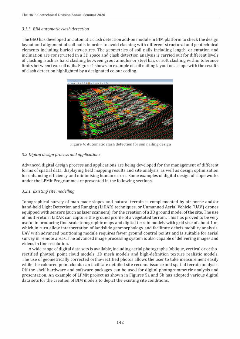
The HKIE Geotechnical Division Annual Seminar 2020
142
3.1.3 BIM automatic clash detection
The GEO has developed an automatic clash detection add-on module in BIM platform to check the design layout and alignment of soil nails in order to avoid clashing with different structural and geotechnical elements including buried structures. The geometries of soil nails including length, orientation and inclination are constructed in a 3D space and clash detection analysis is carried out for different levels of clashing, such as hard clashing between grout annulus or steel bar, or soft clashing within tolerance limits between two soil nails. Figure 4 shows an example of soil nailing layout on a slope with the results of clash detection highlighted by a designated colour coding.
Figure 4: Automatic clash detection for soil nailing design
3.2 Digital design process and applications
Advanced digital design process and applications are being developed for the management of different forms of spatial data, displaying field mapping results and site analysis, as well as design optimisation for enhancing efficiency and minimising human errors. Some examples of digital design of slope works under the LPMit Programme are presented in the following sections.
3.2.1 Existing site modelling
Topographical survey of man-made slopes and natural terrain is complemented by air-borne and/or hand-held Light Detection and Ranging (LiDAR) techniques, or Unmanned Aerial Vehicle (UAV) drones equipped with sensors (such as laser scanners), for the creation of a 3D ground model of the site. The use of multi-return LiDAR can capture the ground profile of a vegetated terrain. This has proved to be very useful in producing fine-scale topographic maps and digital terrain models with grid size of about 1 m, which in turn allow interpretation of landslide geomorphology and facilitate debris mobility analysis. UAV with advanced positioning module requires fewer ground control points and is suitable for aerial survey in remote areas. The advanced image processing system is also capable of delivering images and videos in fine resolution.
A wide range of digital data sets is available, including aerial photographs (oblique, vertical or ortho-rectified photos), point cloud models, 3D mesh models and high-definition texture realistic models. The use of geometrically corrected ortho-rectified photos allows the user to take measurement easily while the coloured point clouds can facilitate detailed site reconnaissance and spatial terrain analysis. Off-the-shelf hardware and software packages can be used for digital photogrammetric analysis and presentation. An example of LPMit project as shown in Figures 5a and 5b has adopted various digital data sets for the creation of BIM models to depict the existing site conditions.

The HKIE Geotechnical Division Annual Seminar 2020
143
Figure 5a: LiDAR topographical model Figure 5b: Aerial photo integrated with 3D mesh model
3.2.2 Ground investigation record database
The GEO has recently developed a 3D geological digital database on subsurface data with the available ground investigation information. Currently, about 200,000 drillhole data in accordance with format of the Association of Geotechnical and Geoenvironmental Specialists (AGS) have been stored in a centralised system kept in GEO. In order to facilitate the sharing of the GI data in digital format, the GEO has enhanced the AGS data such that they are compatible with other GIS and 3D modelling tools including BIM software. Such valuable subsurface information for the generation of geological sections that can be used to create 3D BIM geological models, would be useful for planning of ground investigation works and geotechnical designs. Figure 6 shows the user interface of GInfo for the drillhole locations and the generated geological cross-section.
Figure 6: GEO geological digital database in GInfo
3.2.3 Geological modelling
Geological modelling is essential to evaluate ground conditions for slope projects. Under the LPM and LPMit Programmes, geological modelling has largely been a repetitive and time-consuming process that was highly dependent on manual assessment and interpretation of data collected from desk study, field mapping and ground investigation. In practice, such manual operations cannot easily manipulate complex ground conditions. With the recent technological advances and the use of computational algorithms, 3D digital geological modelling is available to facilitate the workflow of geological modelling in a more pragmatic manner. Such 3D modelling programs allows the users to utilise multi-source geological data and existing ground information such as 3D topographic and AGS borehole log data. The manual interpretation can also be digitised into a single platform to minimise repetitive process through computational system. The reproducibility could also be improved through mathematical modelling from ground investigation data such as generation of geological cross-sections. The GEO has recently developed an advanced geological modelling solution for generating 3D subsurfaces. This is a novel solution for visualising and communicating ground conditions in conjunction with BIM. Figure 7a

The HKIE Geotechnical Division Annual Seminar 2020
144
shows an example of the computer generated 3D subsurface model with AGS borehole data. The design cross-section can be automatically generated from this 3D geological model as shown in Figure 7b, and easily incorporated into other design engineering packages for slope analysis, such as slope stability analysis.
3.2.4 Digital field data acquisition
Significant advances have been made in the application of digital and remote sensing technologies to enhance the capability and efficiency of natural terrain hazard and landslide studies in recent years. An example is the pilot use of UAV equipped with Global Navigation Satellite System, Inertial Measurement Unit (IMU) and high resolution digital camera, to generate digital elevation models (DEM) and orthomosaics to facilitate landside mapping. The quality of field data acquisition can also be greatly enhanced by the development of hand-held mobile laser scanning devices. This latest technology is a fusion of LiDAR, colour imagery and IMU data, which collects a large quantity of 3D measurements and allow real-time scanning. This technique also provides practitioners with a tool to gather rapid and accurate survey data of specific features, such as landslide scars. A detailed landslide source mapping exercise by coupling UAV photogrammetry and LiDAR technology has been carried out for a landslide that occurred in 2016. Due to the steep profile of the hillside, it was very difficult to access the landslide scarp safely for detailed mapping. Close-up photographs (Figure 8) were taken by the UAV to provide detailed information on the failure without having to access the landslide source physically during adverse weather conditions.
Figure 7a: 3D subsurface geological model Figure 7b: Automatic generation of cross-section
By processing the captured UAV photographs, a post-landslide DEM was constructed using a photogrammetry technique known as “Structure from Motion” (see Figure 9). This provided an accurate post-landslide topography for estimating the dimensions of the landslide scar as well as the general orientation of the failure plane. Coupled with the pre-landslide topography generated from the 2011 territory-wide airborne LiDAR data, the landslide source volume could be evaluated by comparing the two DEMs. This case has demonstrated the successful use of UAV to obtain detailed information
Figure 9: DEM generated from UAV photosFigure 8: Photos taken by UAV after the landslide

The HKIE Geotechnical Division Annual Seminar 2020
145
on landslides in difficult terrain. GEO has also undertaken in-house study to explore the possibility of using novel digital technologies for rock discontinuity mapping. The study collected point cloud data by means of hand-held laser scanner and UAV photogrammetry (see Figure 10a). The relevant data are subsequently filtered to generate a de-vegetated 3D surface model of a rock slope. Discontinuities within the 3D surface model are then identified and mapped automatically with the software “PlaneDetect”. The software outputs an analytical model of 3D discontinuity orientations (see Figure 10b) for each detected set of discontinuity as categorised by the same color. These digital technologies supplemented by suitable field inspections would provide an efficient and safe means for rock discontinuity mapping.
3.2.5 Debris mobility assessment
By incorporating the simulation of landslide debris mobility and its 3D runout path in BIM models, the debris impact velocity profile can be easily delineated to achieve a cost-effective barrier design. The buildability of the barrier can also be enhanced by locating barriers judiciously at strategic hillside areas. Figure 11 shows the 3D simulated debris flow runout paths over the complex terrain.
3.2.6 Optimisation of site formation works
Debris-resisting rigid barriers may be constructed on notable drainage lines to protect lives and facilities downslope development from the risk of natural terrain landslides. Advanced BIM techniques are adopted in LPMit projects to optimise the cut and fill balance for the site formation works of rigid barrier construction. The configuration of the rigid barrier could be optimised in BIM to minimise the earthwork required, as well as the environmental and visual impacts. Figure 12 shows the cut and fill volumetric analysis in BIM for the design modelling of a rigid barrier.
Figure 10a: Overview of rock slope portion generated from UAV photogrammetry
Figure 10b: 3-dimensional analytical model showing discontinuities
Figure 11: 3D debris mobility (debris velocity range is represented by
different colours)
Figure 12: Cut and fill volumetric analysis in BIM for design modelling of a rigid barrier

The HKIE Geotechnical Division Annual Seminar 2020
146
3.2.7 Advanced numerical modelling
Coupled numerical analysis is an advanced tool to simulate debris-barrier interaction using the computer program LS-DYNA. Various researchers (e.g. Kwan et al., 2015) have demonstrated that the use of Arbitrary Lagrangian-Eulerian method in LS-DYNA appears to be a promising tool for modelling debris flow and debris-barrier interaction. Such modelling has been benchmarked against laboratory and field flume tests as well as actual landslide cases in terms of debris runout characteristics (Koo et al., 2018). The coupled analyses have also provided insight on the energy dissipation of landslide debris in the debris-barrier dynamic interaction process (see Figure 13). The findings revealed that the overall strain energy absorbed by the flexible barrier upon debris impact is generally less than 40% of the total debris impact energy based on parametric studies. This insight provides opportunities for optimisation of the flexible barrier system design and significantly reduces the design impact loading on the barrier.
GEO is also collaborating with local practitioners to implement advanced numerical models into the BIM work process. As shown in Figure 14, the LS-DYNA model of flexible barrier has been imported into the BIM model. Through the conversion engine, the geometry of the barrier can be altered easily in BIM to suit any site changes or conditions as a digital twin to enhance significantly the modelling efficiency.
Figure 13: LS-DYNA simulation of debris impact on flexible barrier
Figure 14: LS-DYNA model of flexible barrier on BIM platform
A case study has been carried out to optimise the design of flexible barriers in a LPMit site. By using LS-DYNA, the design team simulated the whole process of debris flow mobility and the impact generated from the source failure down to the flexible barrier at the lower end (see Figure 15). The structural components are explicitly modelled including the force-displacement characteristics of various components, including the brake-elements, connections between shackles, ring-nets and cable
Figure 15: Numerical model set-up and simulation of debris-barrier interaction using LS-DYNA

The HKIE Geotechnical Division Annual Seminar 2020
147
ropes. The coupled analysis by LS-DYNA is able to simulate a more realistic debris-barrier interaction. As a result, the induced maximum impact forces are significantly reduced up to 40% in the cable ropes, and hence the design of the anchor foundation could be optimised. The optimisation through the use of LS-DYNA can also minimise the construction materials and dimension of layout, hence also enhance buildability of the structure on steep hillside slopes.
3.2.8 Automation of BIM modelling
The digital design automation transforms the conventional manual processes to become a more dynamic system in a single computational platform such as BIM. A digital modelling workflow saves time and cost significantly in project delivery, and minimises errors in the manual processes. This also facilitates the designers to develop and compare different scenarios and design options before arriving at an optimised option.
The GEO has developed a DYNAMO computation workflow to utilise the BIM standard objects which can be automatically generated in the 3D BIM topographical model, as shown in Figure 16a. Figure 16b shows an example of 3D layout of soil nailing works that can be generated automatically. Analytical functions can be performed to generate other types of mitigation works such as rigid or flexible barriers on natural terrain (see example in Figure 17). The alignment of flexible barriers is generated automatically after importing the coordinates of their alignment or layout into BIM.
The BIM technology is also extended to incorporate the digital data of the field mapping information. Figure 18 shows the computer generated rock slope surface by using the hand-held mobile laser scanner for the proposed design of concrete buttress at the slope toe.
3.2.9 BIM-GIS integration
The opening up and sharing of the available geotechnical data promote collaboration and enable thematic applications in various areas of geotechnical engineering. Apart from managing spatial data, BIM has
Figure 16a: DYNAMO workflow Figure 16b: Automatic generation of soil nails
Figure 17: BIM design automation for flexible barriers
Figure 18: 3D geological field study using hand-held mobile laser scanner

The HKIE Geotechnical Division Annual Seminar 2020
148
been used extensively for spatial modelling and analysis. GIS-BIM data integration system is also being developed for the management of different forms of digital data, displaying field monitoring results, site progress analysis and construction records, as well as design optimisation, enhanced efficiency and minimisation of human errors.
The GEO is developing a smart barrier system incorporating the use of real time wireless sensor data, Internet of Things (IoT) and cloud computing technology in BIM to provide early warning of landslide impact and facilitate timely emergency response (see Figure 19). This new technology serves as an important alert system to the government agencies and relevant stakeholders when debris impact on the barrier is detected. This system has been customised to suit the local site conditions of natural hillsides as shown in Figure 20.
3.2.10 Graphical simulations and virtual reality (VR)
Advanced 3D graphical simulation is a suite of solutions for enhancing BIM 3D and 4D simulations with built-in features to facilitate slope works design, e.g. generate construction sequences, landscaping proposals, identify pertinent site constraints, etc. Digital tools, such as software programs Fuzor, Navisworks, LEGION, etc., have been adopted recently by GEO for 3D visualisation and virtual reality applications in LPMit Programme. Figures 21 and 22 show applications of 3D simulations for the design BIM models enhanced for a man-made feature and natural terrain respectively. These enable the designer to visualise, for example, the potential disturbance to the environment and the subsequent layout revision to suit the site conditions. The slope works and the associated landscape proposals are presented in a 3D model for illustration to the relevant stakeholders. The 3D geometric model facilitates design option assessments, minimise potential construction risk, and thus result in a more cost-effective and environmental friendly design. A VR application can also be utilised to appraise the future visual impact of the completed works for public consultation and education (see Figure 22).
Figure 19: Smart barrier instrumentation system
Figure 20: Smart barrier with sensor monitoring on GIS-BIM data integration platform
Figure 21: Advanced graphical simulation of man-made feature with underground tunnels

The HKIE Geotechnical Division Annual Seminar 2020
149
Figure 22: VR simulation and demonstration of debris-resisting rigid barrier and its surrounding conditions
4 WAY FORWARD AND CHALLENGES AHEAD
BIM has picked up momentum in local practice since the promulgation of DevB TC(W)) No. 7/2017 that requires major capital works projects to adopt BIM in the planning, feasibility, design and construction processes. The GEO has been one of the leading players in implementing digital technologies including BIM to meet new challenges and transform the practice of the industry. The success of the digital development and transformation helps to nurture talented professionals with interest and impetus in adopting innovative and digital technology. The GEO has focused on developing a sustainable workforce to build up capacity for the application of the latest technologies. BIM specialists are also required to accelerate the build-up of BIM capability.
Since there is a lack of suitable geotechnical BIM standards, with the support of HKIE-GDC and LPMit consultants, GEO has spearheaded the development of BIM standards and execution plan for geotechnical works. Apart from BIM standards, there are other hurdles in the adoption of digital technology such as compliance-driven mindset and insufficient expertise (CIC, 2019). In order to enable project teams to realise more of the BIM benefits with collaborative and integrated workflows, GEO will continue to build up in-house BIM capability for both professional and technical staffs and develop digital tools to enhance workflow efficiency.
In addition, rigid workflows are commonly observed in the local practice, for example, substantial double-handling involving conversion between 2D drawings and BIM, with 2D drawings taking precedence over BIM. The GEO has been expending effort to re-engineer the workflow by digitising the work process for future amalgamation and automation in 3D. The development of new digital workflow also needs resources and training for designers to build up BIM expertise and streamline the duplicated work process.
Digital data management also requires specialist input from data analysts and the initial setting up of data infrastructures or database systems. Moreover, the acquisition of quality geotechnical data involves concerted effort by the project teams through co-operation with different contractual parties.
A BIM Common Data Environment (CDE) is the key to collaboration and coordination of the manifold BIM data among designers and other stakeholders such as consultants, contactors and concerned parties in a standard integrated digital working platform. ISO 19650 (ISO, 2018a; 2018b) describes the concepts and principles for digital information management using BIM from design through construction to asset management. A new CDE platform for LPMit Programme is being designed to incorporate the quality objectives and fulfill the key requirements of ISO 19650 in order to achieve an effective and sustainable digital technological development for the various projects.
5 CONCLUSIONS
This paper consolidates the recent development of digital technologies under the LPMit Programme and their practical applications and challenges. The LPM Programme and the subsequent LPMit Programme have evolved progressively with time to address the slope safety challenges by adopting new technologies. The digital development work has helped to enhance the reliability, cost effectiveness and buildability of slope works. An innovative mindset should be maintained in formulating smart and practical solutions

The HKIE Geotechnical Division Annual Seminar 2020
150
by advancing the frontiers of our domain knowledge, leveraging emerging technologies and developing novel, cross-disciplinary approaches through better collaborations. This has been achieved by the GEO through partnership with the geotechnical and geological profession and academia.
GEO will continue to strive for technical excellence in delivering the services by leveraging innovative and new technologies, and integrating these technologies into geotechnical practice.
ACKNOWLEDGEMENTS
This paper is published with the permission of the Head of the Geotechnical Engineering Office and the Director of Civil Engineering and Development, The Government of the Hong Kong SAR. The authors would like to acknowledge the input from the technical officers of the Geotechnical Engineering Office and the support by the Slope Safety Division of the Geotechnical Engineering Office and Survey Division of the Civil Engineering and Development Department, The Government of the Hong Kong SAR.
REFERENCES
CIC 2019. BIM Adoption Survey. Construction Industry Council, Hong Kong, 16 p.ISO 2018a. ISO 19650-1:2018 Organization and digitization of information about buildings and civil engineering works,
including building information modelling (BIM) – Information management using building information modelling – Part 1: Concepts and principles. International Organization for Standardization.
ISO 2018b. ISO 19650-2:2018 ISO 2018. ISO 19650-1:2018 Organization and digitization of information about buildings and civil engineering works, including building information modelling (BIM) – Information management using building information modelling – Part 1: Concepts and principles. International Organization for Standardization. International Organization for Standardization.
Koo, R.C.H., Kwan, J.S.H., Lam, C., Goodwin, G.R., Choi, C.E., Ng, C.W.W., Yiu, J., Ho, K.K.S. & W.K., Pun. 2018. Back-analyses of geophysical flows using 3-dimensional runout model. Canadian Geotechnical Journal, 55: 1081-1094.
Kwan, J.S.H., Koo, R.C.H. & Ng, C.W.W. 2015. Landslide mobility analysis for design of multiple debris-resisting barriers. Canadian Geotechnical Journal, 52 (9): 1345-1359.

The HKIE Geotechnical Division Annual Seminar 2020
151
Application of 3D Reality Model / Laser Scanning to align a Flexible Barrier at Pre-construction Stage
C.K.L. Tang, Y.Y.Y. Cheu, C.W.S. IpAECOM Asia Company Ltd, Hong Kong
ABSTRACT
In recent years, advanced technologies, such as Building Information Modelling (BIM), 3D laser scanning, drone survey, etc, had been adopted and applied on various civil and building design and construction projects. Having realized the benefits of these technologies, we are facing challenges on how to make the best use of these technologies properly for appropriate applications in geotechnical engineering. The project team sometimes encountered site constraints when implementing natural terrain mitigation works based on conventional topographical survey plan, which usually leading to repetitive design review. The project team started exploring whether the design workflow, in terms of time, resources and accuracy, could be significantly improved / enhanced when 3D data of hillside catchments as well as the proposed natural terrain hazard mitigation works are available. This paper summarises the accuracy, benefits and limitations of using 3D laser scanning and BIM technologies for the determination of the alignment of a flexible barrier at pre-construction stage. In addition, comparisons of using 2D topographic survey plan and 3D reality model of existing hillsides for pre-construction design was included.
1 INTRODUCTION
A detailed natural terrain hazard study was carried out on a natural hillside catchment and concluded that debris flow was the identified potential hazard. A flexible barrier at the catchment toe was proposed as the appropriate debris flow hazard mitigation measure. The catchment was generally covered with dense vegetation with mature trees. In current practice, the alignment of a flexible barrier was determined based on land survey during design stage and re-confirmed during the pre-construction stage to suit the actual site conditions. Since the 2D topographic survey information could not provide adequate tree information with respect to their actual spreads of tree stems and branches, we usually encountered site constraints on the proposed flexible barrier clashing with tree stems and branches, leading to repetitive design review on re-aligning the flexible barrier.
In view of the constraints, the project team started exploring whether the design workflow, in terms of time, resources and accuracy, could be significantly improved / enhanced when 3D data of hillside catchments as well as the proposed flexible barrier alignment are available. As such, the captioned natural terrain project site was selected for a trial on 3D laser scanning technology. By capturing 3D reality models of the area where the proposed flexible barrier to be placed, a BIM model was created for checking the feasibility of the proposed alignment of the flexible barrier in 3D environment so that tree felling and pruning could be avoided as far as possible.

The HKIE Geotechnical Division Annual Seminar 2020
152
2 SITE CHARACTERISTICS
2.1 Site Setting
The study catchment is a southeast-facing natural hillside, as delineated in Figure 1, located at Sai Kung. The catchment is a topographic depression catchment draining by two stream courses and bounded at the toe by some village houses. The study catchment falls within the Sai Kung West Country Park except the lower portion. In addition, the whole catchment falls within conservation area and environmental issue is a major concern for the determination of hazard mitigation options. The design retention volume of the barrier is about 110 m3 and the design energy capacity is 8000 kJ. Erection of a flexible barrier outside the conservation area and across the downstream of the drainage lines was therefore considered as the most appropriate to mitigate the debris flow hazards.
2.2 Capture of Existing Site Condition
It is the current common practice to capture the existing site condition and terrain by field survey, i.e. topographic survey, from which positions of any features or any points of landform are determined. A topographic survey was conducted for the lower portion of the hillside catchment and the topography of the site is presented in the topographic survey plan as shown in Figure 2.
Figure 2: Topographic Survey Plan of Study Catchment
Existing trees in the vicinity are represented by a point “tree” symbol and the terrain is represented by contour lines1. However, this 2D presentation could not provide accurate information above the ground. The design engineer could only perform the natural terrain hazard mitigation design with reference to the topographic survey result and the contour lines. Hence, a trail on 3D laser scanning survey has been conducted to explore whether this could facilitate the design workflow.
3 TRIAL ON 3D LASER SCANNING SURVEY
3.1 Selection of 3D Laser Scanning Instrument
There is a technology advancement in the capturing existing features in three-Dimension in recent years, 3D laser scanning is one of them. There has been significant improvement in terms of scanning range,
1 The contour lines are computed and derived from TIN (Triangulated Irregular Network) which are generated from individual field surveyed points.

The HKIE Geotechnical Division Annual Seminar 2020
153
accuracy and weigh etc., as such it is widely adopted in many civil and building projects nowadays. Moreover, there are numerous 3D Laser Scanners readily available in the market.
For selection a 3D Laser Scanner for this project, terrestrial and hand-held type had been studied and compared in terms of scanning range, accuracy, set up, application and price. The comparison is summarized in Table 1.
Table 1: Comparison of Terrestrial and Hand-held Type 3D Laser Scanner
Factors Terrestrial2 Hand-held3
Scanning Range ~300m ~100mAccuracy 2-4mm 1-3cm
Set Up •
••
Tripod / Support on ground is requiredRelatively heavy weight (4.2kg)Relatively less flexible
••
Relatively light weight (1.3kg)Relatively more flexible
Application •
•
Site of accessible condition, e.g. museumObjects / features fine details required, e.g. fittings in a pump station
•
•
Site of less accessible condition, e.g. natural terrainObjects / features with less details required, e.g. slopes / retaining wall
Price Higher (~HK$ 1.3M or above) Lower (~HK$ 600K)Battery Life 4.5 hours 3.5 hours
Having considered all the above factors and their relative significance to this exercise, the hand-held type 3D laser scanner was chosen as the site is less accessible and the price is more competitive.
3.2 Site Trial
A site trial using the selected hand-held 3D laser scanner was conducted at 15:00 on 14 October 2019, and there was a shower on that day. Before starting the site scan, the project team identified the scanning route / path nearby the flexible barrier to be erected, illustrated in Figure 3 and established some control points for geo-referencing the scanned data.
2 Terrestrial Laser Scanner Model: Faro Focuss 350.3 Hand-held Laser Scanner Model : Geoslam ZEB-HORIZON.
Figure 3: Proposed location of flexible barrier and scanning route

The HKIE Geotechnical Division Annual Seminar 2020
154
Subsequent to the field work, a post-survey data processing, such as geo-referencing point cloud data, removing noise and converting the point cloud raw data to Revit data format, was carried out.
2.5 Traditional Topographic Survey Versus 3D Laser Scanning
With reference to the site trial, a preliminary comparison of topographical survey (for this study site) using 3D laser scanning against traditional method using total station was realized. The findings are summarized in Table 2.
Table 2: Comparison of Traditional Method and 3D Laser Scanning Method for Topographical Survey
Factors Traditional 3D Laser ScanningFieldwork Time 1-2 days 20 minData Processing •
•3 hours Common Computer-aided Drawing (CAD) workstation is good enough to view and process the data
•
•
3 days including geo-reference, remove noise and convert to Revit data formatHigh-end workstation is required to view and process the data
Field Team • 2-3 field staff • 1 -2 field staffAccessibility •
•
Field staff is required to go to the survey points / area to collect data directlyRelatively more dangerous for steep slope
•
•
Field staff can collect data without going to the survey points / area if not obstructed by objectsRelatively less dangerous for steep slope
Topography / Landscape
••
2D and conceptual presentationGround details are generalized and accuracy depends on field staff experience / knowledge in identifying appropriate survey points
••
•
3D and reality presentationGround details are more accurate in terms of size / shape and height, e.g. treesData accuracy may be affected by weather
Cost4 • About HK$25.5K (1 survey team of 3 staff took 2 day for field work and 1 staff took 3 hours for office work)
• About HK$12.3K (1 survey team of 2 staff took 20 min field work and 1 staff take 3 days for office work)
The laser scanned point cloud data was further processed to form a BIM model and the ground profile of the existing site. A comparison on LiDAR5 and topographic survey data was conducted to analyze and verify the accuracy and consistency of the hand-held 3D laser scanned data by overlaying.
The verification result is shown in Figure 4. It is realized that the profile generated from hand-held 3D laser scanned data are consistent to profiles generated from LiDAR and topographical survey data.
4 The cost is estimated by assuming a survey staff’s hourly rate is HK$500 and work for 8 hours a day.5 Currently, CEDD of Hong Kong SAR will provide territory-wide ground profile LiDAR (Light Detection and Ranging) Data
for consultants’ references when requested.
Figure 4: Ground profiles of LiDAR Data, Topographical Survey and 3D Scanned Data

The HKIE Geotechnical Division Annual Seminar 2020
155
3.3 Determination of Flexible Barrier Alignment
To facilitate verifying the adequacy of the proposed flexible barrier alignment at the pre-construction stage, a BIM model of the existing site by using the point cloud data was formed as shown in Figure 5 and a flexible barrier BIM object was created as shown in Figure 6. The flexible barrier was incorporated into existing site BIM model along the proposed alignment / position as shown in Figures 7 to 9.
Figure 5: BIM model of existing site Figure 6: Flexible barrier (BIM Object)
Figure 7: Flexible barrier incorporated in existing site BIM model
Figure 8: Lateral view (Back) Figure 9: Lateral view (Front)

The HKIE Geotechnical Division Annual Seminar 2020
156
It was realized that the proposed flexible barrier alignment clashed with existing trees from the incorporated BIM model as shown in Figure 10. This situation, i.e. clashes with tress, could never been visualized from traditional topographic plan where tree location is represented by a point symbol and therefore the tree form, such as slanting direction or angle, cannot be recorded or shown. For example, in Figure 11, based on topographic survey, the tree is projected like a straight pole as illustrated in the model. In reality, the tree is tilting at an angle and will not clash with the proposed flexible barrier.
Figure 10: Flexible barrier clashed with existing trees
Figure 11: Display of tree location between topographical survey and 3D laser scanning survey
According to the existing site condition in three-dimension through the BIM model, the proposed flexible barrier alignment could then be adjusted to suit the actual site condition. Not only to verify the design, but also to facilitate the resource planning, order placing, and environmental impact control for the following-on construction stage.
3.4 Findings and Observations
Various survey data captured by different survey methods, namely LiDAR, topographical survey and 3D laser scanned data, have been used in this pilot study for flexible barrier alignment design and checking basal opening across stream course. The findings and observations for using different data are

The HKIE Geotechnical Division Annual Seminar 2020
157
summarized as Table 3. It shows that 3D laser scan survey has overall highest score among three survey methods and outweigh the topographic survey in all individual application.
Table 3: Findings and Observations of Different Survey
Applications Topographic Survey
LiDAR Survey
3D Laser Scan Survey
Profile Generation (Degree of existing ground representation)
(degree of accuracy± 50 mm)
(degree of accuracy ~ 50 mm)
(degree of accuracy ~ 10-30 mm)
Avoidance of Existing Trees along Flexible Barrier Alignment
N/A
Identification of Basal Opening for the Barrier (across Stream Course)
N/A : Not applicable (as the general topographical information of existing trees is unavailable in LiDAR dataset)
3.5 Potential Application / Way Forward
It is envisaged that 3D laser scanning survey would generate rather good illustration on hard surfaces, such as retaining wall shown as shown in Figures 12 and 13, apart from the soft feature nature terrain. Either elevation or section view can be easily generated from the 3D reality model, which are particularly useful for designing and arranging soil nails and retaining walls. This is more than effective by using traditional 2D topographic survey and photographs.
The hand-held or light weigh laser scanner, once flexible to be mounted on drone with improved scanning range, areas with difficult access could have been surveyed.
For a flexible barrier installed across a stream course, the normal stream flow should be maintained (Plate 1). However, the basal opening between the ring net of the flexible barrier and the stream course should not be excessive. Otherwise, it could be a potential gap for the passage of debris in case of
Figure 12: Laser scanned retaining wall (Elevation View) Figure 13: Section view
Plate 1: Basal Opening across stream course (Extract from TGN 48)

The HKIE Geotechnical Division Annual Seminar 2020
158
landslides. Based on the profile generated from 3D laser scan, the gap between the proposed barrier and base of the stream course can be measured (Figure 14), and the designer could refine the design accordingly.
Figure 14: Measurement of Basal Openings
4 CONCLUSIONS
3D laser scanning technology definitely enhances geotechnical engineering work as it captures the real site condition at the time of survey, i.e. formation of a time-stamped 3D reality model. Not only does this 3D model help identifying tree clashing and large basal openings supporting 3D design optimization but also avoiding unnecessary contractual risk due to construction review. It is envisaged that hand-held laser scanning for nature terrain topographic survey is positively a cost-effective approach in terms of saving staff resources and time for field work and improving design work during pre-construction stage.
Nevertheless, the quality of captured data and formation of BIM model are very much relied on operators’ skill and experiences, proper training for laser scanner field operation and BIM modelling are recommended to both professional engineers and technicians.
ACKNOWLEDGEMENTS
The authors wish to thank the staff of AECOM Asia Company Ltd. who provided support in this exercise.
REFERENCES
GEO. (2019). GEO Technical Guidance Note No. 48 (TGN 48). Detailing of Flexible Debris-resisting Barriers. Civil and Engineering Development Department, Hong Kong SAR.

The HKIE Geotechnical Division Annual Seminar 2020
159
Mobile Apps to Assure Effectiveness in Site Operation – Soil Nail Construction Supervision, Site Cleanliness
Monitoring and Incident Reporting
Charles K.L. Tang, Thomson M.K. Lai, Daniel C.H. Lo & Frenco K.L. CheungAECOM Asia Company Limited
ABSTRACT
In current government slope work contracts, there is a well-established and comprehensive quality assurance / monitoring system for construction supervision. The system involves filling of numerous standard forms and taking of record photos at different stages of workflow. With the technological advancement of smart phones in recent years, some mobile apps were developed to optimize the steps of operation procedures so as to facilitate the frontline site staff to conduct their supervision in a more convenient, effective, safe and accurate way. Three mobile apps have been developed specifically for soil nail supervision, site cleanliness monitoring and incident reporting for government slope works contracts will be described. Examples will be provided to demonstrate the applicability and functionality of these mobile apps in real cases, and the enhancement on the quality assurance and project delivery effectiveness.
1 INTRODUCTION
Mobile Apps are becoming literally significant in our daily lives. We could just use our mobile devices such as smartphones, tablets or watches to run the mobile apps for shopping, communication, banking, entertainment, etc., they make our daily lives more convenient and efficient.
A functional and practical mobile app could help people to handle tasks effectively and independently by themselves. Most of them are designed to be user friendly, and do not need any kind of professional training to use. Moreover, the data input could be properly saved as records for documentation and further analyses.
One of the main characteristics of government slope works contracts is the slopes and retaining walls programmed to be upgraded/improved are usually scattered at different locations over the territories, and normally the construction activities of each slope / retaining wall will be supervised by one full-time resident works supervisor. In association with the supervision of construction activities, there are a number of standard forms required to be completed and numerous photographs to be taken to record the progress and quality of each stage of works, as well as the site conditions.
Mobile apps on soil nail construction supervision, site cleanliness monitoring and incident reporting were developed to facilitate the frontline resident site staff to ease their workload. These 3 site activities selected for mobile app development were due to their natures of routineness, workload on record management, and the requirements on accuracy and timely reporting.

The HKIE Geotechnical Division Annual Seminar 2020
160
2 MOBILE APP ON SOIL NAIL CONSTRUCTION SUPERVISION
2.1 Current Practice
Soil nailing is the most common slope stabilization measures adopted in Hong Kong. Under the current practice, the resident site staff shall fill in the soil nail record on site manually to assure the length, size and grouting of each soil nail are in accordance with the construction drawings and specifications. Moreover, record photographs are required to be taken for the following steps of soil nail installation.
• Measurement of drilling bit• Drilling rig angle• Drilling process• Bar code of soil nails• Coupler connection and heat-shrinkable sleeve installation• Accessories (centralizers, TDR testing wire, grout pipe fixing, etc.)• Soil nail insertion• Grout overflow• Grout refilling
As a causal counting, it involves around 8 to 10 record photographs to be taken for a soil nail. For a typical slope of 5m high and 50m long, it in general requires installing around 100 nos. of soil nails, which in turn about 1,000 of record photographs will be taken and managed by the resident site staff.
Plate 1: Examples of record photographs taken for each step of soil nail installation
Plate 2: Working in a rain shower (the umbrella was mainly used to prevent the paper form from getting soaked)

The HKIE Geotechnical Division Annual Seminar 2020
161
By imagining the soil nail installation is carrying out in a drizzle or a rain shower, the resident site staff has to carry his umbrella and clip board to record the soil nail data and take photographs. It is quite inconvenient.
After the completion of the soil nailing works, the resident site staff will then go back to the depot to file the completed forms and record photographs. In general, it takes 2 to 3 hours in this data management exercise.
Figure 1: Time required for data management
2.2 Adoption of the Mobile App to enhance the Effectiveness
The mobile app of soil nail construction supervision was developed to help the resident site staff to complete the record form and take record photographs by his contract mobile phone only. After the confirmation of soil nail setting out, the design office will provide the confirmed soil nail schedule in MS Excel format to the site office. The resident site staff is required to download the soil nail schedule and the mobile app will read the schedule and display the soil nail details directly.
Figure 2: Soil nail schedule in MS Excel format Figure 3: Mobile App displays the details of soil nail schedule
As shown in Figure 3, the mobile app lists the details of each soil nail according to the soil nail schedule, also it indicates the status of each soil nail. For instance, soil nail no. A5 has not been drilled. The resident site staff could touch the “camera” icon to take record photographs, and the mobile app would automatically save the record photographs with a systematic file name structure, indicating the feature no., soil nail no., the stage of works (drilling) and the photograph no. After the completion of the drilling, the resident site staff would measure the depth and diameter of the drilled hole and he could input and stored the measured data to the mobile app by touching the “len” icon adjacent to the “camera” icon. After the completion of the data input, the resident site staff could tick the white box and save the data.
Similarly, for installation and grouting of soil nail, record photographs will be saved and named systematically, and the details such as the installed nail length, actual grout intake volume of each soil nail, and any abnormal observations or remarks would be recorded and properly saved in a data file.
The mobile app has also a function to display the working status of all soil nails. The colourful circle displays in Figure 4 presents the overall progress of the soil nailing works. The number at the center

The HKIE Geotechnical Division Annual Seminar 2020
162
is the total numbers of soil nails. With reference to the legend, it could be easily noted that there were 39 nos. of soil nails (yellow) with drilling not yet started, 2 nos. of soil nails (green) were drilled but pending bar installation, 2 nos. of soil nails (blue) pending grouting, 2 nos. of soil nails (pink) were grouted and 5 nos. of soil nails (purple) with all works completed.
Figure 5 illustrates a comparison in time consumption on data management amongst the current practice, the adoption of the mobile app on site and with cloud services. The figures on time saving are for reference only as it depends on the site location, the amount of data to be managed and the capability of the resident site staff. However, we have experiences that adoption of the mobile app could achieve significant time saving on data management and effectiveness on data retrieval.
3 MOBILE APP ON SITE CLEANLINESS MONITORING
3.1 Current Practice
Under the current government slope works contracts and capital works contracts, there are requirements under the specifications that the contractor shall perform daily cleaning and weekly tidying of the site for the public areas with an extent of a typical of 2.5m offset from periphery outside hoardings. The contractor shall submit the inspection checklist, records and photographs at or before 10:00am of the day after to the Service Manager / the Engineer for checking and recording. The delegated site staff will, together with the contractor, check and inspect the overall cleanliness and tidiness of the site on the day the record received, and advise the contractor if there are any improvement actions required.
In some cases, problems exist on cleaning records could not be submitted on the day after timely due to site remoteness or negligence, and thus may also lead to no checking records on the cleaning works. Moreover, under a typical government slope works contracts, it involves upgrading works of around 25 man-made features in general. By taken into account the upgrading works for each man-made feature last for 5 months, it will produce over 3,000 records at the end of the contract. It involves considerable paper records and also the record storage space.
3.2 Adoption of the Mobile App to enhance Timely Submission and Record Completeness
The mobile app of site cleanliness monitoring was developed to interact the contractor with the resident site staff to ease the abovementioned problems. After completion of the daily cleaning works, the contractor could use the mobile app to complete the inspection checklist, take record photographs and prepare the location plan, and send the inspection record to the resident site staff by 10:00am the day after the cleaning timely.
Figure 6 demonstrates the workflow by the contractor. After checking the site condition at the end of the cleaning day, the contractor will complete and sign the inspection checklist. The contractor can
Figure 5: Time saving by adoption of Mobile App (for reference only)Figure 4: Mobile App displays the overall working status

The HKIE Geotechnical Division Annual Seminar 2020
163
utilize the camera function to take record photographs. By turning on the GPS of his mobile phone, the locations of the photographs taking will be automatically shown on the site location plan. Of course, the site location plan, will be stored in the mobile phone together with the mobile app installation.
Once the contractor has sent the completed inspection checklist, a notification will be sent to the resident site staff for his review and checking. The resident site staff will log in the mobile app and check the cleaning items the contractor completed and put his remarks on individual item for any improvement actions required. After checking, the resident site staff countersigns the inspection checklist for record. The mobile app has linked to the site office server, and the resident engineer can check and review the inspection records conveniently.
The digital submission of the cleaning inspection checklist will consume less paper and storage space, it will also improve the efficiency of this site operation and strengthen the interaction between the contractor and the resident site staff.
Figure 6: Workflow of the Contractor on Site Cleanliness Reporting
Figure 7: Workflow of the Resident Site Staff on Site Cleanliness Monitoring
4 MOBILE APP ON INCIDENT REPORTING
4.1 Current Practice
For any CEDD slope works / capital works contracts, when an incident occurs, the Engineer’s Representative shall report to the client office and relevant parties the details of the incident according to the procedure as stipulated in CEDD Technical Circular No. 03/2019. The Engineer’s Representative is required to determine whether the incident is a serious incident, and if so, he shall verbally inform relevant parties within 30 minutes in accordance with the flow chart in Appendix B of the Circular and provide written confirmation of verbal report on the serious incident using the template in Appendix C of the Circular.
Although guidelines on the determination of the seriousness of the incident and 24-hour contact list of all relevant parties are provided in the Circular, it is not easy to achieve timely verbal reporting within 30 minutes and written confirmation within 3 hours, especially when the incident occurs in remote site at night where no fax machine and proper work place. Moreover, there is chance to miss calling to relevant parties.

The HKIE Geotechnical Division Annual Seminar 2020
164
4.2 Adoption of the Mobile App to enhance Timely Submission and Accurate Reporting
The mobile app of incident reporting was developed to assist the Engineer’s Representative to perform the reporting correctly and timely. It helps the Engineer’s Representative to have a quick decision to classify the seriousness of the incident. As demonstrated in Figure 10 and 11, by selecting the involved items of the incident, the mobile app will classify the incident, according to the built-in logic following the flow chart of the Circular, as a serious incident or a non-serious incident automatically and generate a list of relevant parties required to be contact for the verbal report. The Engineer’s Representative can touch the telephone icons and perform his verbal reporting. His call log will be auto-saved in the mobile app to ensure no missing calling. Moreover, the mobile app will have a time alert to remind the Engineer’s Representative the time left for his verbal reporting and written confirmation.
After completion of the verbal reporting, the Engineer’s Representative can then complete the built-
Figure 8: Flow chart for Reporting Incident as extracted from CEDD TC No. 03/2019
Figure 9: Part-print of Template of Written Confirmation of Verbal Reporting as extracted from CEDD TC No. 03/2019

The HKIE Geotechnical Division Annual Seminar 2020
165
in template of written confirmation to input the details, take record photographs and mark the location of the incident using the mobile app. The completed written confirmation will then be sent out by the e-fax and e-mail to the relevant parties. The workflow of the mobile app on written confirmation is illustrated in Figure 12.
By adopting the mobile app, the Engineer’s Representative could complete the verbal reporting and written confirmation of serious incident in an accurate, punctual and effective way.
Figure 10: Determination of Incident Seriousness Figure 11: Time Alert and Contact List generated by the Mobile App
Figure 12: Workflow on Written Confirmation Preparation
5 CONCLUSIONS
The adoption of mobile apps could not only to reduce the paper consumption and the record storage space significantly, but it could also allow the project team to obtain quality and traceable site records timely and conveniently, to increase their capability in achieving a more effective record management, and to strengthen the interaction amongst the client and the contractor.

The HKIE Geotechnical Division Annual Seminar 2020
166
Corner Effects on Wall Deflections in Deep Excavations
L.W. WongSMEC Asia Ltd, HKSARG
I.T. Pratama & C.R. ChouMoh and Associates, Inc., Taipei
ABSTRACT
This paper studies the corner effects on wall deflections in various excavation dimensions. Three-dimensional numerical analyses have been conducted on four rectangular excavation cases with the dimensions ranging from 20 m to 160 m. The effects of excavation width and wall thickness to reduction in wall deflections are studied. It has been found that the wall deflections around the corners are mainly attributable to the reduction in the effective width of excavation. The variation on wall deflections along the long and the short sides of the excavation are expressed by empirical equations, which are validated by excavation case histories.
1 INTRODUCTION
The performance of diaphragm walls in deep excavations is commonly assessed by the two-dimensional approach such as the numerical or the semi-empirical beam-on-elastic foundation analytical methods. It is well aware that around the corners of the excavation the wall deflections would be much smaller than those occurring at the mid portion of the excavation. However, estimating the reduction in wall deflections around the corners, which is a three-dimensional problem, would be difficult to be handled by the 2-D analysis models. Ou (2006) indicates that the wall deflections estimated by using the 2-D plane strain approaches can only be regarded as the wall deflections at the central section of excavations.
There are 3-dimensional studies (Ou 2006, Finno et al. 2007, Wu et al. 2010, Hsiung et al. 2016) showing that the corner effects are closely attributed to the excavation geometry and the system stiffness of excavations. The system stiffness of excavation is commonly attributed to the combined effects of the strutting stiffness and the wall flexural rigidity (Clough et al. 1989, Hsieh 2017). Based on these findings, three-dimensional (3-D) analyses have been conducted to assess the corner effects on wall deflections induced by excavations. This paper presents the results of 3-D studies using the PLAXIS 3-D software. The analysis results show that the corner effects on wall deflections are closely related to the wall thickness and the excavation widths. The empirical relationships between the computed wall deflections and these two variables have been established. Several excavation case histories in Hong Kong and in Taipei are collected to validate the applicability of the empirical equations.
2 THREE-DIMENSIONAL NUMERICAL ANALYSES
2.1 Excavation cases
Four hypothetical rectangular excavations were modeled by the PLAXIS 3-D finite element (FE) software. Figure 1 illustrates the configurations of 4 excavation geometry, which are 160 m x 80 m, 80 m x 80 m, 80 m x 40 m and 80 m x 20 m. In order to assess the geometry effect to wall deflections, the

The HKIE Geotechnical Division Annual Seminar 2020
167
notations L and B are assigned to denote the lengths of the walls along the long side and along the short sides of excavation respectively and the L value is larger than or equal to the B value. As summarized in Table 1, the 4 cases to be studied have the geometry ratios ranging from 0.25 to 1. The terms L and B are similar to the primary wall and the complementary wall that adopted by Ou et al. (1996) in their parametric studies on 3-D excavation models.
Figure 1: Configurations of the excavation geometry for Case 1 to Case 4
Table 1: Wall lengths of rectangular excavation
Case number
Excavation dimension, m Geometry ratio, B/LLength L Width B
1 160 80 0.52 80 80 13 80 40 0.54 80 20 0.25
The studies on the corner effects due to excavation comprise 2 tasks. Task 1 is to investigate the effects of wall deflections caused by various excavation widths, excavation depths and wall thicknesses. The wall deflections at the centres of the walls are processed and assessed. Task 2 is to assess the variations of the wall deflections along the walls so that the reduction in deflections around the corners of the excavation could be assessed. The computed lateral wall deflections at the distances of 0.5L, 0.375L, 0.25L, and 0.125L from the corners of the long walls for the 4 cases are extracted for studies. Similarly, lateral wall deflections at the distances of 0.5B, 0.375B, 0.25B, and 0.125B from the corners of the short walls for the 4 cases are presented. In order to study the effect of wall thickness to wall deflections, four types of wall thickness, Tw, namely, 0.6 m, 1 m, 1.5 m and 2 m are adopted in the numerical analysis for the 4 cases. The number of cases computed for the 3-dimensional analyses is 16.
2.2Subsoilprofiles
The case history of Shandao Temple Station of Taipei Metro is selected in this study. This excavation case has been extensively studied and the results of the 2-D FE analyses are calibrated by the observed inclinometer profiles (Hwang et al. 2012). Figure 2a shows the layout of Shandao Temple Station. The site is located in the T2 Geological Zone of the central Taipei Basin (Lee 1996). Figure 2b shows the excavation scheme and soil strata. As depicted in Figure 2b, the ground is composed of the sandy and clayey Songshan Formation of 50 m in thickness underlain by the gravelly Jingmei Formation.
The ground level is approximately 4.0 m above the mean sea level where the datum is located at Keelung Harbour. During the construction period between 1991 and 1994, the piezometric level in the Jingmei Formation was approximately at the elevation -10 m. In this numerical analyses, the piezometric levels of -1.0 m and -10.0 m in Sublayer-V and in Sublayer-III respectively are adopted. The piezometric levels in the clayey Sublayer-IV and Sublayer-II are interpolated from those in the adjacent sandy sublayers. Inside the excavation pit, the groundwater levels lowering to 1 m below the excavation levels are adopted. Diaphragm wall of 1 m in thickness and 30.5 m in depth is constructed as the retaining

The HKIE Geotechnical Division Annual Seminar 2020
168
structure. The excavation is carried out in 7 stages to a final depth of 18.5 m. Six levels of steel struts are installed to support the wall during excavation.
2.3 Soil parameters and structural stiffnesses
The linear elastic-perfectly plastic Mohr-Coulomb (MC) constitutive model is adopted for simulating the non-linear stress-strain relationship of the soils. The clayey soils (CL) are simulated as undrained materials whereas the drained material type is applied to the sandy soils (SM). The stiffnesses for the clayey and the sandy soils are estimated as Eu = 500su and E’ = 2N (in MPa) respectively, where Eu is the undrained Young’s modulus, E’ is the effective Young’s modulus, su is the undrained shearing strength and N is the standard penetration tests number. The Eu/su and the E’/N empirical ratios, which are within the range that commonly adopted for excavations in soft ground, have been calibrated against the actual wall deflections observed in 3 inclinometers installed in the diaphragm wall of the station box. Hwang et al. (2012) reported that matching between the calculated and the observed wall deflections have been obtained in the later stages of the excavation. It is however noted that actual soil moduli are nonlinear with the small-strains stiffness far greater than the secant moduli adopted in the MC model. While the performance of the excavation matches with those in the final stages, the MC model tends to over-estimate the wall deflections in the early stages of excavation. Such small-strains implication and the limitation for using the MC model should not be overlooked.
Figure 2: Shandao Temple Station (a) site plan and (b) excavation scheme (Hwang et al. 2012)
In the numerical analysis, the strengths of the sandy soils are expressed by the effective cohesion (c’) and the effective friction angle (ϕ’). The strengths of the clayey soils are denoted by the undrained shear strengths (su). The values of the soil unit weight (γt), the undrained soil shear strength (su), the effective cohesion (c’) and the effective friction angle (ϕ’) follow those reported by Hwang et al. (2012). Table 2 lists the soil parameters adopted in this study.
The diaphragm wall is simulated as plate elements with the concrete compressive strength (f’c) value of 28 MPa and the Young’s modulus, Ec , of 25,000 MPa. The estimated flexural rigidity (denoted as EcI where I is the moment of inertia) and the axial stiffness (denoted as EcA where A is the sectional area) of the diaphragm wall are 1,464 MNm and 17,570 MN/m respectively. These values are reduced by 30% for accounting tensile cracks and creeping of concrete during excavation. H-steel members are erected for supporting the excavations. The horizontal spacing of the struts (Sst) is 4.5 m. All the struts are preloaded to 50% of their design loads. They are simulated as node-to-node anchors with Young’s modulus of the strut (Est) of 210 GPa. Table 3 lists the strut properties and the preloading forces adopted in this study.

The HKIE Geotechnical Division Annual Seminar 2020
169
Table 2: Soil parameters in Shandao Temple station excavation (Hwang et al. 2012)
Depth m Sublayer Soil
Typeγt
kN/m3N
valuesu
kPac’
kPaϕ’
degψ’
degE’ or Eu
MPa υ’
0.0 – 2.0 VI CL 18.6 3 20 – – 0 10 0.352.0 – 13.5 V SM 18.4 8 – 0 33 3 16 0.35
13.5 – 23.5 IV CL 18.8 6 40 – – 0 20 0.3523.5 – 28.5 III SM 19.3 18 – 0 32 2 36 0.3528.5 – 35.0 IIA CL 19.4 17 150 – – 0 75 0.3535.0 – 43.5 IIB CL 19.4 – 200 – – 0 100 0.3543.5 – 50.0 I SM 21.6 30 – 0 35 5 60 0.30
Table 3: Strut properties (Hwang et al. 2012)
Depth m Strut Type Area,
Ast cm2/strutEstAst/Sst
MN/mPreload
kN1.7 1H350×350×12×19 173.9 811.5 4204.4 1H400×400×13×21 218.7 1020.6 8207.4 1H400×400×13×21 218.7 1020.6 1060
10.2 2H400×400×13×21 218.7 2041.2 220013.0 2H400×400×13×21 218.7 2041.2 168016.0 2H400×400×13×21 218.7 2041.2 2160
The finite element mesh established for the 3-dimensional analysis extends 160 m from the walls along both directions and to the depth of 50 m. Such lateral extent and is approximately 8 times of the maximum depth of excavation of 18.5 m. As depicted in Figure 3, the meshes for Case 1 and Case 4 is 480 m by 400 m and 400 m by 340 m respectively. In the PLAXIS 3-D FE analyses, the medium-coarse for the mesh is adopted. Under this setting, the number of soil elements for Case 1 of 80 m × 160 m is 154,818. There are 18 and 38 struts for each level aligned along the east-west and along the north-south directions respectively for Case 1.
Figure 3: Typical mesh in PLAXIS 3-D for the 160 m × 80 m and the 80 m × 20 m excavations
3 RESULTS OF 3-DIMENSIONAL ANALYSIS
3.1Walldeflectionprofilesatthecentresofwalls
The wall deflections obtained from the analysis of the 3-D FEM for Case 1 to Case 4 and for various wall thicknesses are presented in Figures 4 and 5. The deflection profiles occurring at the centres of the walls in the final stage with the excavation depth of 18.5 m are selected. The deflection profiles at the centres of the long walls and of the short walls are presented in Figures 4 and 5 respectively. The distribution of wall deflections along the walls from the centres to the corners are presented in Figures 6 and 7 and are discussed in Section 4.

The HKIE Geotechnical Division Annual Seminar 2020
170
Figure 4: Wall deflection profiles at the centres of the walls on the long sides of excavation
Figure 5: Wall deflection profiles at the centres of the walls on the short sides of excavation
3.2Walldeflectionsalongthelongandtheshortsides
The computed wall deflection profiles along the walls occurring in the final stage for Case 1 to Case 4 and for various wall thicknesses are presented in Figures 6 and 7. The variations of the maximum wall deflections in the final stage along the long walls for Case 1 to Case 4 are presented in Figure 6. The computed maximum wall deflections in that stage along the short walls are presented in Figure 7. It is noted that the wall deflections shown in Figures 6b and 7b, which are on the perpendicular sides for the square Case 2, are virtually identical. The 3-D FE analysis results show that the wall deflections around the excavation corners are significantly less than those occurring at the central sections of the walls. This reduction in wall deflections, or the corner effect, occurs in all 4 cases along the long and the shorts sides with various wall thicknesses.
In Figures 6 and 7, the dx denotes the maximum wall deflections occurring at the distance x to the corners in the final stage with the 18.5 m excavation depth.
4 VARIATION OF WALL DEFLECTIONS AT CENTRES OF WALLS
4.1Effectsofexcavationwidth
In order to avoid the potential effects from the end walls, the maximum wall deflections occurring at the centres of the long walls in the final stage for Case 1 to Case 4 are selected to study the effects of excavation width to wall deflections. The L values for these cases range from 80 m to 160 m and the B values range from 20 m to 80 m. The computed wall deflections occurring at the centres of the walls for each case are presented in Figure 8, which shows the trend of wall deflections in proportion to the widths of excavation. The 4 trend lines in Figure 8 also show the variations of wall deflections with different thicknesses. With the half-width of excavation 40 m, the computed wall deflections for the wall thicknesses of 0.6 m, 1.0 m, 1.5 m and 2.0 m are 108.7 mm, 81.6 mm, 63 m and 57 mm respectively. The wall deflections for each wall thickness are normalized to the maximum deflections occurring at the

The HKIE Geotechnical Division Annual Seminar 2020
171
Figure 6: Variation of maximum wall deflections at the excavation depth 18.5 m along the long side for Case 1 to Case 4
Figure 7: Variation of maximum wall deflections at the excavation depth 18.5 m along the short side for Case 1 to Case 4
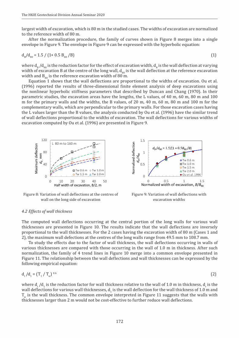
The HKIE Geotechnical Division Annual Seminar 2020
172
largest width of excavation, which is 80 m in the studied cases. The widths of excavation are normalized to the reference width of 80 m.
After the normalization procedure, the family of curves shown in Figure 8 merges into a single envelope in Figure 9. The envelope in Figure 9 can be expressed with the hyperbolic equation:
dB/d80 = 1.5 / (1+ 0.5 B80 /B) (1)
where dB /d80 is the reduction factor for the effect of excavation width, dB is the wall deflection at varying width of excavation B at the centre of the long wall, d80 is the wall deflection at the reference excavation width and B80 is the reference excavation width of 80 m.
Equation 1 shows that the wall deflections are proportional to the widths of excavation. Ou et al. (1996) reported the results of three-dimensional finite element analysis of deep excavations using the nonlinear hyperbolic stiffness parameters that described by Duncan and Chang (1970). In their parametric studies, the excavation areas have the lengths, the L values, of 40 m, 60 m, 80 m and 100 m for the primary walls and the widths, the B values, of 20 m, 40 m, 60 m, 80 m and 100 m for the complementary walls, which are perpendicular to the primary walls. For those excavation cases having the L values larger than the B values, the analysis conducted by Ou et al. (1996) have the similar trend of wall deflections proportional to the widths of excavation. The wall deflections for various widths of excavation computed by Ou et al. (1996) are presented in Figure 9.
4.2Effectsofwallthickness
The computed wall deflections occurring at the central portion of the long walls for various wall thicknesses are presented in Figure 10. The results indicate that the wall deflections are inversely proportional to the wall thicknesses. For the 2 cases having the excavation width of 80 m (Cases 1 and 2), the maximum wall defections at the centres of the long walls range from 49.5 mm to 108.7 mm.
To study the effects due to the factor of wall thickness, the wall deflections occurring in walls of various thicknesses are compared with those occurring in the wall of 1.0 m in thickness. After such normalization, the family of 4 trend lines in Figure 10 merge into a common envelope presented in Figure 11. The relationship between the wall deflections and wall thicknesses can be expressed by the following empirical equation:
dt /d1 = (T1 / Tw) 0.6 (2)
where dt /d1 is the reduction factor for wall thickness relative to the wall of 1.0 m in thickness, dt is the wall deflections for various wall thicknesses, d1 is the wall deflection for the wall thickness of 1.0 m and Tw is the wall thickness. The common envelope interpreted in Figure 11 suggests that the walls with thicknesses larger than 2 m would not be cost-effective to further reduce wall deflections.
Figure 8: Variation of wall deflections at the centres of wall on the long side of excavation
Figure 9: Variation of wall deflections with excavation widths

The HKIE Geotechnical Division Annual Seminar 2020
173
4.3 Effects of excavation depth
In order to assess the effect of excavation depths to wall deflections, the computed deflections of the wall of 1.0 m in thickness at various excavation depths with the excavation widths of 20 m, 40 m, 80 m and 160 m are studied. The computed maximum wall deflections occurring in the intermediate stages with the excavation depths of 5.0 m, 10.8 m, 14.1 m and 18.5 m with various widths of excavation are presented in Figure 12. It is obvious that the deeper the excavation, the larger wall deflections occurs. There is the common trend that the maximum wall deflections occurring for each depth of excavation are proportional to the widths of excavation. The wall deflections for each excavation depth are normalized to that occurring at the same depth with the excavation width of 80 m. The widths of excavation for the various cases are normalized to the reference width of 80 m. After the normalization procedure, the family of curves shown in Figure 12 merges into a single envelope in Figure 13. That single envelope can be described by the empirical Equation 1, which is established for the effect of excavation widths from the maximum wall deflections occurring for the excavation depth of 18.5 m.
The close similarity in the relationships between the wall deflections and the excavation depths and that between the wall deflections and the excavation widths would suggest that the variation of wall deflections, or the corner effects, occurring in the final stage with the excavation depth of 18.5 m would also be applicable for other intermediate depths of excavation.
Figure 10: Variation of wall deflections with wall thicknesses at the centres of the long walls
Figure 11: Common envelope for variation of wall deflections with wall thicknesses
5 CORNER EFFECTS ON WALL DEFLECTIONS
5.1Reductionineffectivewidthofexcavation
As Figures 8 and 9 show that the wall deflections are proportional to the excavation widths, the reduction in wall deflections around the corners could be analogous to the reduction in the effective excavation widths. As depicted in Figure 14, the notations L and B are assigned to the length and the
Figure 13: Common envelope for variation of wall deflections with depths of excavation
Figure 12: Variation of wall deflections with depths of excavation at the centres of long walls

The HKIE Geotechnical Division Annual Seminar 2020
174
width of the excavation area and L is larger than or equal to B. The effective widths of excavation, b, gradually diminish toward the corner and that the distances to the corner, the x values, are essentially the b values. The variation of the wall deflections shown in Figures 6 and 7 could therefore be described by the distances to the corner expressed by Equation 1.
Figure 14 shows that along the long and the short sides of the rectangular excavation, the effective width of excavation, the b value, is limited to B/2. The influence of the corner effect would have the distance around B/2. The wall deflections along the narrow side would be independent on the lengths of excavation. The half-width analogous around the corner is validated by the wall deflection profiles obtained by the 3-D FE analysis.
Figure 14: The effective widths of excavation around the corners
5.2Cornereffectsalongthelongsideofexcavation
As the influence of the corner effects could be related to the excavation widths, the distribution of wall deflections along the long side shown in Figures 6a to 6d are reviewed case by case. The distances to the corners are normalized to the B/2 values for each case. Figure 15 are the variation of the normalized wall deflections against the normalized distances to the corners for Case 1 to Case 4. The variation of the wall deflections along the long side of the excavation area could be expressed by the empirical hyperbolic Equation 3:
dx/dc = α/(1 + β B/2x) (3)
where dx is the lateral wall deflection occurring at the distance x to the corner, dc is the deflection occurring at the central portion of excavation, B is the varying width of the excavation and α and β are the coefficients for the hyperbolic curve describing the distribution of wall deflections around the corners.
The α value corresponds to the horizontal asymptote of dx/dc. For 2x/B approach to infinity, the dx/dc approaches to α. The β value defines the initial tangent or the slope of the hyperbolic curve and can be related to the widths of excavation. Figure 15 show that the α value for Cases 1 to 4 is 1.25. The β values for Case 1, Case 2, Case 3 and Case 4 are 0.25, 0.25, 0.5 and 0.75 respectively. The relationship between the β and the B values is expressed in Equation 4:
β = 0.26 (B80/B)0.8 (4)
Equation 4 shows that the β values are inversely proportional to the widths of excavation B. It is noted that the B values are always the wall lengths along the short sides of the excavation areas. After estimating the wall deflections at the central portions of excavation by the 2-dimensional analysis methods, the variations of wall deflections around the corners can be determined by Equations 1 to 4.

The HKIE Geotechnical Division Annual Seminar 2020
175
Figure 15: Variation of wall deflections with distances to corners along the long walls
5.3Cornereffectsalongtheshortsideofexcavation
For Cases 1 and 3, the wall lengths B on the short sides are 80 m and 40 m respectively. Figure 16 shows that the variations of normalized wall deflections against the normalized distances to the corners for these 2 cases. The distribution of wall deflections can be expressed by the empirical Equations 3 and 4 with the α value of 1.25. The β values for Case 1 and Case 3 along the short sides are 0.25 and 0.5 respectively. It is noted that along the short sides the x values do not exceed B/2. As shown in Figure 16b, the empirical distribution curve fits the deflections for the wall thickness of 1.0 m. For other wall thicknesses, the distribution of dx /dc can be further adjusted by the dt /d1 reduction factors expressed by Equation 2.
Figure 16: Variation of wall deflections with distances to corners along the short walls
5.4Cornereffectsinnarrowexcavation
Figures 17 shows the variation of wall deflections for Case 4 that has the width of excavation as narrow as 20 m. The variation of normalized wall deflections against the normalized distances to the corners for Case 4 can be expressed by the empirical Equation 3 with the α value of 0.7 and the β value of 0.75. Compared with the wall deflections around the corners on the short side of excavation Case 1 and

The HKIE Geotechnical Division Annual Seminar 2020
176
Case 3, the α value for Case 4 reduces from 1.25 to 0.7, which is 0.56 times of those cases with the B values larger than 20 m. The 3-D analysis results show that corner effect is pronounced in this case with narrow excavation width.
Ou et al. (1996) also reported similar analysis result in their 3-D FEM studies. In their analysis, the soil was assumed to behave as an elastic-plastic material described by hyperbolic model (Duncan and Chang 1970). They found that for the relatively small length of primary wall less than 40 m, there is no section in the primary wall that is in a plane strain condition. The effect of the corner also becomes more pronounced with increasing length of the complementary wall. Based on the results of 3-D analysis of the current study and the similar finding by Ou et al. (1996), the authors propose that a further reduction factor 0.6 shall be allowed at narrow excavation areas. In the future studies, the corner effects shall be reviewed by adopting the nonlinear stress-strain model such as the Hardening-Soil model to further investigate the corner effect at narrow end walls.
Figure 17: Variation of wall deflections with distances to corners along the short wall for Case 4
5.4 Validation of empirical equations
As described in Section 2.2, the soil moduli adopted for the MC model have been calibrated with wall deflections observed in the final stages. Due to the small-strain nonlinearity behaviour of the soil, the linear elastic moduli fitting the final stages would inevitably over-estimate the wall deflections in the early stages. However, the normalized empirical equations for predicting the distribution of the wall deflections around the corners would still be applicable for the final stages. In practice the designers are interested on the maximum ground movement occurring in the final stages. The error for ignoring the small-strain nonlinearity soil behaviour and over-estimating the wall deflections in the early stages would be insignificant as the magnitudes of deflections are only a fraction of those occurring in the final stages. The empirical Equations 1 to 4 are however verified with field observations. Excavation case histories are collected to validate Equations 1 to 4 for assessing the corner effects. Four case histories in Hong Kong and in Taipei are presented in Section 6.
6 CASE HISTORIES
6.1Trunkroadtunnel
Wong (2012) reported the effect of end wall on the deflections of diaphragm wall supporting the cut-and-cover construction for a dual-three lane vehicular tunnel located at a coastal reclamation project site in Hong Kong. The tunnel is 0.9 km in length with the widths of excavation ranging from 32 m to 37 m. The depths of excavation vary from 16.3 m to 19.0 m. The diaphragm wall is 1.2 m in thickness and 66 m maximum in length. The wall is embedded in the fill stratum of 20 m in thickness, the alluvial deposits, the completely decomposed granite, in the highly decomposed granite and keyed into the bedrock of slightly decomposed granite by 300 mm. Three types of fill material, the sand, the gravel and the rock fill are encountered in the fill stratum.
There are 8 inclinometers located at the distances to the end walls ranging from 4.1 m to 12.3 m. The maximum wall deflections occurring in these inclinometers in the final excavation stage varied from

The HKIE Geotechnical Division Annual Seminar 2020
177
20.3 mm to 57.0 mm. There are another 6 inclinometers located at 50 m or larger distances to the end walls. The maximum wall deflections at these central portions range from 43.7 mm to 73.7 mm.
Figure 18 shows the distribution of the maximum wall deflections observed in the inclinometers. The reduction in wall deflections around the end walls can be estimated by Equations 2 to 4. Using the excavation width 35 m, the α and the β values are 1.25 and 0.54 respectively. A further reduction factor of 0.9 is applied for the wall thickness of 1.2 m. Figure 18 shows the matching between the observed wall deflections and those predicted by the empirical equations.
6.2 Basement excavation cases in Taipei
Wong and Patron (1993) reported the corner effects observed at 5 basement excavation cases located in the T2 Zone of the Taipei Basin. The subsoil layers in the Songshan Formation for these 5 cases are similar to those for the Shandao Temple Station described in Section 2.2. The typical ground movements and the maximum wall deflections are summarized in Table 4. The typical ground settlements behind the wall ranged from 17 mm to 33 mm. The maximum ground settlements occurred at the distances ranging from 3 m to 14 m from the diaphragm walls. The wall deflections for the 5 excavation cases ranged from 32 mm to 62 mm. The ratios of the maximum ground settlements to the maximum wall deflections range from 0.38 to 0.59, with an average of 0.49. These vertical to horizontal ground movement ratios are within the typical range of 0.5 to 1.0 for excavations in the T2 Zone of the Taipei Basin.
Table 4: Summary of basement excavation cases reported by Wong and Patron (1993)
Case No.
Excavation dimension, m Wall thickness
Tw , m
Distance from wall to maximum
settlement, m
Maximum movement, mmdh-max/dv-max
Wall deflection dh-max
Settlement dv-max
Length L
WidthB
DepthH
2 70 52 11.1 0.6 13.3 40 18 0.453 53 35 11.4 0.6 2.9 45 17 0.385 44 37 12.3 0.6 13.5 60 33 0.556 49 48 12.6 0.6 6.9 32 19 0.597 65 46 21.7 0.7 – 66 – –
The variation of ground settlements along the walls of these basement excavation cases are presented in Figure 19, showing that the ground settlements around the corners of the excavation areas have the same trend of variation in wall deflections that shown in Figure 15. Assuming the vertical to horizontal ground movement ratio around 0.5 is applicable at the ground behind the walls, the distribution of the ground settlements along the walls is essentially identical to the variation of the lateral wall deflections. Using the average excavation width 44 m, the α and the β values are 1.25 and 0.42 respectively. As indicated in Figure 19, the corner effects to wall deflections expressed in Equations 2 to 4 are applicable to the distribution of the ground settlements.
Figure 18: Variation of wall deflections for the trunk road tunnel (after Wong 2012)
Figure 19: Variation of ground settlements for basement excavations in Taipei
(after Wong & Patron 1993)

The HKIE Geotechnical Division Annual Seminar 2020
178
6.3CorePacificCity
Hwang et al. (2007a) reported the performance of the 32 m deep excavation for the Core Pacific City shopping mall. The project site is located in the K1 Zone (Lee 1996) in the southeast of the Taipei Basin. The Songshan Formation in the K1 Zone is dominant with the thick clayey Sublayer IV and Sublayer II, which are encountered at the depths between 7 m and 32 m (25 m in thickness) and between 34 m and 47 m (13 m in thickness) respectively. The sandy Sublayers V, III and I encountering at the depths of 4 m, 32 m and at 47 m respectively. are thinning to 2 m to 3 m in thicknesses. The gravelly Jingmei Formation is encountered at the depth of 49 m.
The excavation area was roughly 118 m by 118 m. The basement excavation was supported by diaphragm wall of 1.5 m in thickness extending to 52 m in depth. Along the northern portion of the perimeter diaphragm wall, buttresses of 3.7 m in length and spacing at 8.75 m were installed to the depths between 10.5 m and 40.0 m. The buttresses are integrated with the diaphragm wall with reinforcements. The T-section has the flexural stiffness equivalent to a rectangular section of 3.0 m. The top-down construction supported by the 7 basement floor slabs was conducted. There are 6 inclinometers installed in the diaphragm wall. The distances of the inclinometers to the corners range from 15.5 m to 48.9 m. Table 5 summarizes the maximum wall deflections observed in the inclinometers. Figure 20 shows the wall deflections at various distances to the corners.
The reduction in wall deflections around the corners can be estimated by Equations 2 to 4. For the excavation widths of 103 m and 40 m, the β values are 0.21 and 0.45 respectively. The α value is 1.25. Further reduction in deflections due to the wall thickness effect can be computed. By using Equation 2, the reduction ratio between the walls with the thicknesses (Tw) of 3.0 m and 1.5 m is 0.66, which is multiplied to the dx/dc values computed by Equation 3. The variation of the normalized deflections for walls of 1.5 m and 3.0 m in thicknesses are presented Figure 20, showing the agreement between the observed deflections and those predicted by the empirical equations.
Table 5: Summary of wall deflections observed in the inclinometers at Core Pacific City (Hwang et al. 2007a)
Inclinometer number
Distance to corner, x, m
Excavation width, B, m
Maximum wall deflection, mm Wall type Equivalent wall
thickness, Tw, mSID7 48.9 103 142 Diaphragm wall 1.5SID5 43.0 103 160 Diaphragm wall 1.5SID8 43.8 103 174 Diaphragm wall 1.5SID2 34.0 103 98 DW+Buttress 3.0SID4 20.7 103 100 DW+Buttress 3.0SID1 15.5 40 111 DW+Buttress 3.0
Figure 21: Variation of wall deflections for the Hai Hua Building excavation
Figure 20: Variation of wall deflections for the Core Pacific City excavation

The HKIE Geotechnical Division Annual Seminar 2020
179
6.4HaiHuabuilding
Ou et al. (1996) reported the 20.3 m deep excavation for the Hai Hua Building, which is located at 600 m east of Shandao Temple Station in the T2 Zone of the Taipei Basin. The ground conditions for this project site are similar to that depicted in Figure 2b. The main excavation area was irregular in plan with the length and the width of 90 m and 65 m respectively. At the southwest corner where the vehicular access is located, the excavation area was 20 m by 25 m. The basement excavation was supported by diaphragm wall of 1.1 m in thickness extending to 42 m depth. The top-down construction using the ground floor and the basement floor slabs as the lateral support was conducted. There are 5 inclinometers installed to the toe levels of the diaphragm wall. The distances of these inclinometers to the corners of the excavation range from 12.5 m to 40 m. Table 6 summarizes the maximum wall deflections observed in those inclinometers.
There are indications of wall toe movements in the inclinometers. The wall deflections at the B2 level observed in inclinometers I2 and I3 were 25 mm and 16 mm in Stage 2 excavation respectively. In the final stage the corresponding wall deflections in inclinometers I2 and I3 were 12 mm. Since the excavation was supported by the basement floor slabs, preloading for temporary steel struts would not be conducted. The apparent backward movement of the wall at the B2 level was likely caused by the inward toe movements. Secondly, the 3-D FE analysis conducted by Ou et al. (1996) shows the occurrence of lateral ground movements of 12 mm and 4 mm at the main excavation and at the corner areas respectively at the depth of 42 m. The wall toe movements ranging from 4 mm to 12 mm as inferred from the inclinometer readings are therefore adopted for correcting the observed wall deflection profiles. Following the procedures recommended by Hwang et al. (2007b), the wall deflections observed in inclinometers I1 to I5 are corrected and are summarized in Table 6.
Figure 21 shows the wall deflections at various distances to the corners. The reduction in wall deflections around the corners can be estimated by Equations 2 to 4. Using the excavation width of 65 m and 25 m, the β values of 0.31 and 0.66 for the main excavation and for the southwest corner respectively are obtained. A further reduction factor of 0.6 is allowed for the narrow width of 25 m at the southwest corner. Figure 21 shows the agreement between the observed wall deflections and those predicted by the empirical equations.
Table 6: Summary of wall deflections observed in the inclinometers at Hai Hua Building (Ou et al. 1996)
Inclinometer number
Distance to corner, x, m
Excavation width, B, m
Wall deflection, mmMaximum observed Tip movement Corrected
I1 40 65 52 12 64I2 27 65 64 4 68I3 20 65 52 4 56I4 15 25 29 4 33I5 12.5 25 17 4 21
7 CONCLUSIONS
The three-dimensional analyses on four hypothetical excavation cases with the lengths and the widths of the excavation areas ranging from 20 m to 160 m have been conducted to study the corner effects to wall deflections. Based on the results of studies the following concluding remarks can be drawn:
(1) The wall deflections occurred at various excavation stages are proportional to the widths of excavation.
(2) The reduction in wall deflections around the corners could be analogous to the reduction in the effective widths of excavation at the corners.

The HKIE Geotechnical Division Annual Seminar 2020
180
(3) The corner effects on reduction in wall deflections have the influence of half-width of excavation, which is the effective width of excavation.
(4) Along the long side of the excavation area, the wall deflections in the central portion can be estimated by the 2-dimensional analysis.
(5) Along the short side of the excavation area, the wall deflections are independent of the excavation width measuring along the long side.
(6) For the excavation areas that have the excavation width as narrow as 20 m, the 3-dimensional effect is more pronounced.
Empirical equations for estimating the variation of wall deflections along the walls from the central portions to the corners have been established. These empirical equations for estimating the corner effect have been validated by comparing the estimated deflections with those observed from 4 case histories on excavations. For the corner effect along the short side of excavation as narrow as 20 m, more case histories shall be collected for further verification.
ACKNOWLEDGEMENTS
The authors wish to express their sincere thanks to Dr R.N. Hwang for his initiating the 3-dimensional parametric studies and to Mr C.W. Lai for his presenting the finite element mesh of the 3-D models.
REFERENCES
Clough, G.W., Smith, E.M. & Sweeney, B.P. 1989. Movement control of excavation support systems by iterative design. In Procofthe1989ASCEFoundationEngineeringCongress,FoundationEngineering:CurrentPrinciplesandPractices,Evanston, 25-29 June 1989. ASCE.
Duncan, J.M. and Chang, C.Y. 1970. Nonlinear analysis of stress and strain in soils. J. Soil Mech. And Found. Div., ASCE, 94: 637-659
Finno, R.J., Blackburn, J.T. & Roboski, J.F. 2007. Three-dimensional effects for supported excavations in clay. Journal of GeotechnicalandGeoenvironmentalEngineering, 133(1): 30-36.
Hsieh, H.S., Huang, Y.H., Hsu, W.T. & Ge, L. 2017. On the system stiffness of deep excavation in soft clay. Journal of GeoEngineering, 12(1): 21-34.
Hsiung, B.C., Yang, K.H., Aila, W. & Hung, C. 2006. Three-dimensional effects of a deep excavation on wall deflections in loose to medium dense sands. Computers and Geotechnics, 80: 138-151.
Hwang, R.N., Moh, Z.C. & Wang, C.H. 2007a. Performance of wall systems in excavation for Core Pacific City. Journal of GeoEngineering, 2(2): 53-60.
Hwang, R.N., Moh, Z.C. and Wang, C.H. 2007b. Toe movements of diaphragm walls and correction of inclinometer readings. JournalofGeoEngineering, 2(2): 61-72.
Hwang, R.N., Lee, T.Y. Chou, C.R. & Su, T.C. 2012. Evaluation of performance of diaphragm walls by wall deflection paths. JournalofGeoEngineering, 7(1): 1-12.
Lee, S.H. 1996. Engineering geological zonation for the Taipei city. Sino-Geotechnics, 54: 25-34. (in Chinese)Ou, C.Y., Chiou, D.C. & Wu, T.S. 1996. Three-dimensional finite element analysis of deep excavations. Journal of Geotechnical
Engineering, 122(5): 337-345.Ou, C.Y. 2006. DeepExcavation:TheoryandPractice. Taylor & Francis.Wong, L.W. 2012. Effect of end wall on the deflection of diaphragm wall. HKIE Geotechnical Division Annual Seminar,:
243-248.Wong, L.W. & Patron B.C. 1993. Settlements induced by deep excavations in Taipei. Proc of the 11th Southeast Asian
GeotechnicalConference,Singapore,4-8May1993, : 787-791.Wu, C.H., Ou, C.Y. & Tung, N.C. 2010. Corner effects in deep excavations-establishment of a forecast model for Taipei basin
T2 zone. JournalofMarineScienceandTechnology,18(1): 1-11.