forecasting geotechnical parameters from

University of Mississippi University of Mississippi

eGrove eGrove

Electronic Theses and Dissertations Graduate School

1-1-2021

FORECASTING GEOTECHNICAL PARAMETERS FROM FORECASTING GEOTECHNICAL PARAMETERS FROM

ELECTRICAL RESISTIVITY AND SEISMIC WAVE VELOCITIES ELECTRICAL RESISTIVITY AND SEISMIC WAVE VELOCITIES

USING ARTIFICIAL NEURAL NETWORK MODELS USING ARTIFICIAL NEURAL NETWORK MODELS

Fatema Tuz Johora University of Mississippi

Follow this and additional works at: https://egrove.olemiss.edu/etd

Part of the Civil Engineering Commons

Recommended Citation Recommended Citation Johora, Fatema Tuz, "FORECASTING GEOTECHNICAL PARAMETERS FROM ELECTRICAL RESISTIVITY AND SEISMIC WAVE VELOCITIES USING ARTIFICIAL NEURAL NETWORK MODELS" (2021). Electronic Theses and Dissertations. 2109. https://egrove.olemiss.edu/etd/2109

This Dissertation is brought to you for free and open access by the Graduate School at eGrove. It has been accepted for inclusion in Electronic Theses and Dissertations by an authorized administrator of eGrove. For more information, please contact [email protected].

https://egrove.olemiss.edu/

https://egrove.olemiss.edu/etd

https://egrove.olemiss.edu/gradschool

https://egrove.olemiss.edu/etd?utm_source=egrove.olemiss.edu%2Fetd%2F2109&utm_medium=PDF&utm_campaign=PDFCoverPages

http://network.bepress.com/hgg/discipline/252?utm_source=egrove.olemiss.edu%2Fetd%2F2109&utm_medium=PDF&utm_campaign=PDFCoverPages

https://egrove.olemiss.edu/etd/2109?utm_source=egrove.olemiss.edu%2Fetd%2F2109&utm_medium=PDF&utm_campaign=PDFCoverPages

mailto:[email protected]

FORECASTING GEOTECHNICAL PARAMETERS FROM ELECTRICAL RESISTIVITY

AND SEISMIC WAVE VELOCITIES USING ARTIFICIAL NEURAL NETWORK MODELS

A Dissertation

presented in partial fulfillment of requirements

for the degree of Doctor of Philosophy

in the Department of Civil Engineering

The University of Mississippi

By

FATEMA TUZ JOHORA

August 2021

Copyright Fatema Tuz Johora 2021

ALL RIGHTS RESERVED

ii

ABSTRACT

Geotechnical measurements of soil parameters used in the design of infrastructure provide

information at a specific point of the ground. The use of limited point data may result in greater

uncertainty and less reliability in design. Geophysical methods are non-invasive, less time-

consuming, and provide continuous spatial information about the soil. However, geophysical

information is not in terms of engineering parameters. Correlations between geotechnical

parameters and geophysical parameters are needed to facilitate the use of geophysical information

in geotechnical designs. The current research is focused on two geophysical methods; electrical

resistivity (ER) and seismic wave velocity (S-wave and P-wave). Artificial neural network (ANN)

models are developed using published data to predict geotechnical parameters from ER and

seismic wave velocity. Results of ANN models from the published data show that ER can predict

geotechnical parameters with moderate to good accuracy and also predict cation exchange capacity

(CEC) better than saturation. Seismic wave velocity helps to predict water content and dry density.

Overall, the performance of ANN is better than regression. Laboratory measurements are

performed on proctor-compacted soil samples with varying clay, sand, and silt proportions

applicable to earthen dam construction. ER, seismic wave velocity and various geotechnical

parameters are measured on the same samples. Results show that ER is most sensitive to Atterberg

limits, specific surface area, CEC, cohesion, water content and saturation. ANN models are in

agreement with the Waxman-Smits formula. In comparison to ER, S-wave and P-wave velocities

are more sensitive to dry density and void ratio. Combining ER and S-wave and P-wave velocities

predicts water content, dry density, saturation, and void ratio more accurately than simply using

iii

individual geophysical parameters. The geophysical parameters in conjunction with the soil mix

proportions allow for good to high accuracy predictions of multiple geotechnical parameters.

iv

DEDICATION

This work is dedicated to Allah Almighty, my creator,

the unique, omnipotent and only deity and creator of the universe

To my mother Jabunnahar, to my father Taher,

for whom I am here today on the way to achieve my dream

To my dearest husband Sharif and my daughter Sidrat,

the most precious gift from Allah and my best friends

To my sister Khodeja and by brother Omar

thank you for the love, support, and encouragement.

ii

LIST OF ABBREVIATIONS AND SYMBOLS

ρ Resistivity

r Resistance

A Cross-sectional area

L Length

ρb Bulk resistivity

ρw Resistivity of the pore fluid

F Formation factor

Φ Porosity of the sand

m Cementation component

sw Degree of saturation

n Saturation exponent

C0 Bulk conductivity of fully saturated soil sample

Cw Conductivity of the pore fluid

a Empirical constant

Ce Conductivity due to the presence of clay content

T Transverse resistance

h Thickness

e Void ratio

BQv Surface conductivity

iii

Ө Volumetric water content

Ɛ Standard error

w Water content

G Shear modulus

M Constraint modulus

B Bulk modulus

d Mass density of the medium

E Young’s modulus

ʋ Poisson’s ratio

BSK Bulk modulus of the skeleton

Bg Bulk modulus of the grains

Bf Bulk modulus of the fluid phase

Beff Effective bulk modulus

Geff Effective shear modulus

GSK Shear modulus of skeleton

Bw Bulk modulus of liquid phase

Ba Bulk modulus of air phase

Cd Normalized consistency ratio

GT Specific gravity of soil at room temperature (0C)

ws Weight of soil (gm)

iv

G20 Specific gravity of soil at 200C

Gw Specific gravity of water

vw Volume of water

vv Volume of void

vs Volume of solid

LL Liquid limit

PL Plastic limit

SL Shrinkage limit

SG Specific gravity

As Specific surface area

XiA Actual value

XiP Predicted value

Xi Mean of XIA

N Total number of data set

σbulkσpf

⁄ Normalized conductivity

ER Electrical resistivity

CEC Cation exchange capacity

MARE Mean absolute relative error

ASE Average squared error

R2 Coefficient of determination/ regression coefficient

v

USACE U.S. army corps of engineers

NID National inventory of dams

ANN Artificial neural network

GPR Ground penetration radar

SP Self-potential

IP Induced polarization

SPT Standard penetration test

DCPT Dynamic cone penetration test

R Coefficient of correlation

MES Mean error squares

MAEP Mean absolute error percent

Vs Shear wave velocity

SCPT Seismic cone penetration tests

qc Cone penetration tip resistance

RMSE Root mean squared error

SMP Soil mix proportion

Opt Optimum

vi

ACKNOWLEDGMENTS

I would like to express my sincere gratitude to my research advisor Dr. Craig Hickey,

Director at the National Center for Physical Acoustics and Research Associate Professor of Physics

and Geological Engineering, for his continuous encouragement and support over the years. The

completion of this study would not have been possible without his expertise.

I would also like to express my sincere gratitude to my academic adviser and committee

member Dr. Hakan Yasarer, Assistant Professor of Civil Engineering, for his valuable

contribution, support, and encouragement. He has devoted his valuable time and energy in helping

me navigate my graduate studies. I would also like to thank Dr. Hunain Alkhateb, Associate

Professor of Civil Engineering, and Dr. Yacoub Najjar, Chair and Professor of Civil Engineering,

for their interest and valuable comments on my work.

I want to thank the U.S. Department of Agriculture under Non-Assistance Cooperative

Agreement 58-6060-6-009 for providing financial support. I also thank Dr. Yacoub Najjar,

Department Chair and Professor, Civil Engineering Department, University of Mississippi for the

ANN software, used for the analysis of this research.

Fatema Tuz Johora

vii

TABLE OF CONTENTS

ABSTRACT ................................................................................................................................... ii

DEDICATION.............................................................................................................................. iv

LIST OF ABBREVIATIONS AND SYMBOLS ........................................................................ ii

ACKNOWLEDGMENTS ........................................................................................................... vi

LIST OF TABLES ...................................................................................................................... xii

LIST OF FIGURES .................................................................................................................... xv

1. CHAPTER 1 ........................................................................................................................... 1

INTRODUCTION......................................................................................................................... 1

1.1 General .................................................................................................................................. 1

1.2 Research Significance ........................................................................................................... 2

1.3 Research Objectives .............................................................................................................. 4

2. CHAPTER 2 ........................................................................................................................... 6

REVIEW OF PREVIOUS WORK ............................................................................................. 6

2.1 General .................................................................................................................................. 6

2.2 Electrical Resistivity ............................................................................................................. 7

2.3 Developed Correlation with ER ............................................................................................ 8

2.4 Seismic Wave Velocity ....................................................................................................... 28

2.5 Developed Correlation with Seismic Wave Velocity ......................................................... 31

2.6 Artificial Neural Network ................................................................................................... 35

2.7 Application of ANN in Geotechnical Engineering ............................................................. 36

2.8 Developed Correlations using ANN ................................................................................... 37

2.9 Findings from Literature Review ........................................................................................ 38

3. CHAPTER 3 ......................................................................................................................... 40

viii

METHODOLOGY ..................................................................................................................... 40

3.1 General ................................................................................................................................ 40

3.2 Soil Type and Parameter Selection ..................................................................................... 40

3.3 Laboratory Measurements ................................................................................................... 43

3.3.1 Sample preparation ....................................................................................................... 43

3.3.2 Geophysical tests .......................................................................................................... 46

3.3.2.1 Electrical resistivity test ......................................................................................... 46

3.3.2.2 Seismic wave velocity test ..................................................................................... 48

3.3.3 Geotechnical tests ......................................................................................................... 49

3.3.3.1 Atterberg limits ...................................................................................................... 49

3.3.3.1.1 Liquid limit test ............................................................................................... 50

3.3.3.1.2 Plastic limit test ............................................................................................... 51

3.3.3.1.3 Shrinkage limit test.......................................................................................... 51

3.3.3.2 Specific gravity test................................................................................................ 52

3.3.3.3 Unconfined compression test ................................................................................. 53

3.3.3.4 Parameters obtained using weight volume relationship......................................... 54

3.3.4 Chemical test (CEC) ..................................................................................................... 55

3.4 Development of ANN Model .............................................................................................. 56

4. CHAPTER 4 ......................................................................................................................... 58

PREDICTING GEOTECHNICAL PARAMETERS FROM ELECTRICAL

RESISTIVITY USING DATA FROM THE LITERATURE ................................................. 58

4.1 General ................................................................................................................................ 58

Performance of the ANN models is evaluated based on the mean absolute relative error

(MARE), coefficient of determination (R2) and the average squared error (ASE). Multilinear

regression analysis is also performed to determine the correlation between parameters.

Effectiveness of ANN models for predicting different parameters is compared to the results

obtained from multilinear regression analysis. Performance of the ANN models developed for

remolded and undisturbed soil samples are also compared4.2 Geotechnical Parameter .......... 58

4.3 Data from Literature ............................................................................................................ 59

4.4 Result and Analysis ............................................................................................................. 61

4.4.1 Predicting ER for remolded versus undisturbed samples ............................................. 61

4.4.2 Predicting saturation for remolded versus undisturbed samples .................................. 64

4.4.3 Predicting CEC for remolded versus undisturbed samples .......................................... 66

ix

4.4.4 Comparison of ANN models for predicting dry density and water content ................. 68

4.5 Comparison of Regression and ANN .................................................................................. 70

4.6 Conclusion ........................................................................................................................... 71

5. CHAPTER 5 ......................................................................................................................... 73

PREDICTING GEOTECHNICAL PARAMETERS FROM SEISMIC WAVE VELOCITY

USING DATA FROM THE LITERATURE ........................................................................... 73

5 .1 General ............................................................................................................................... 73

5.2 Data Collections .................................................................................................................. 74

5.3 ANN Models ....................................................................................................................... 75

5.3.1 ANN Models for Predicting Seismic Wave Velocity ................................................... 76

5.3.1.1.ANN Models Using Field Data.............................................................................. 76

5.3.1.2 ANN models using lab data ................................................................................... 77

5.3.1.3 ANN models using field and lab data .................................................................... 78

5.3.2 ANN models for predicting water content ................................................................... 80

5.3.2.1 Using field data with velocity ................................................................................ 81

5.3.2.2 Using lab data ........................................................................................................ 81

5.3.2.3 Using field plus lab data ........................................................................................ 82

5.3.3 ANN models for predicting dry density ....................................................................... 84

5.3.3.1 Using field data ...................................................................................................... 84

5.3.3.2 Using lab data ........................................................................................................ 85

5.3.3.4 Using field plus lab data ........................................................................................ 86

5.4 Comparison between ANN and regression models............................................................. 88

5.5 Conclusion ........................................................................................................................... 89

6. CHAPTER 6 ......................................................................................................................... 91

PREDICTING GEOPHYSICAL PARAMETERS FROM GEOTECHNICAL

PARAMETERS........................................................................................................................... 91

6.1 Introduction ......................................................................................................................... 91

6.2 Data from Laboratory Measurements ................................................................................. 92

6.2.1 ER predictions from a Single Input .............................................................................. 93

6.2.2 Predicting ER from Multiple Inputs ............................................................................. 98

6.3 Predicting P-Wave............................................................................................................. 101

x

6.3.1 Single Input................................................................................................................. 101

6.3.2 Multiple Input ............................................................................................................. 104

6.4 Predicting S-Wave............................................................................................................. 106

6.4.1 Single Input................................................................................................................. 106

6.4.2 Multiple input ............................................................................................................. 109

6.5 Conclusion ......................................................................................................................... 111

7. CHAPTER 7 ....................................................................................................................... 114

PREDICTING GEOTECHNICAL PARAMETERS FROM GEOPHYSICAL

PARAMETERS......................................................................................................................... 114

7.1 General ........................................................................................................................... 114

7.2 Using ER as input ........................................................................................................... 114

7.2.1 Single geotechnical output....................................................................................... 115

7.2.2 Multiple geotechnical outputs ................................................................................. 117

7.3 Using P-wave as input .................................................................................................... 120


7.3.2. Multiple geotechnical outputs ................................................................................ 121

7.4 Using S-wave as input .................................................................................................... 122


7.4.2. Multiple geotechnical outputs ................................................................................... 123

7.5 Conclusion ......................................................................................................................... 124

8. CHAPTER 8 ....................................................................................................................... 126

PREDICTING GEOTECHNICAL PARAMETERS FROM COMBINED/MULTIPLE

GEOPHYSICAL PARAMETERS .......................................................................................... 126

8.1 General ........................................................................................................................... 126

8.2 Predicting Water Content ............................................................................................... 127

8.2.1 Combined geophysical parameters` ............................................................................ 128

8.3 Predicting Dry Density ...................................................................................................... 131

8.3.1 Combined geophysical parameters ............................................................................. 131

8.4 Predicting Saturation ......................................................................................................... 134

8.4.1 Combined geophysical parameters ............................................................................. 134

xi

8.5 Predicting Void Ratio ........................................................................................................ 137

8.5.1Combined geophysical parameters .............................................................................. 138

8.6 Predicting Water Content, Dry density, Void ratio, Saturation from Combined Geophysical

Parameters ............................................................................................................................... 140

8.6 Conclusion ......................................................................................................................... 141

9. CHAPTER 9 ....................................................................................................................... 143

CONCLUSION ......................................................................................................................... 143

9.1 Conclusion ......................................................................................................................... 143

9.2 Recommendation for Future Research .............................................................................. 146

REFERENCES .......................................................................................................................... 148

APPENDICES ........................................................................................................................... 153

VITA........................................................................................................................................... 160

xii

LIST OF TABLES

Table 1.1: Engineering and geotechnical applications of geophysical techniques (Sharma,

1997). ................................................................................................................................ 2

Table 2.1 : Statistics for three artificial intelligence and regression methods. ........................... 20

Table 2.2: Seismic wave velocities for different materials. ...................................................... 29

Table 2.3: Application of ANN in geotechnical engineering. .................................................... 37

Table 3.1 : Selected soil mixing proportion for laboratory measurements. ............................... 42

Table 3.2: Geophysical and geotechnical parameters chosed for developing correlation......... 43

Table 3.3: Geotechnical and geophysical parameters and ranges. ............................................. 43

Table 4.1: Parameters and ANN ranges. .................................................................................... 62

Table 4.2: Statistical accuracy measures of ANN model predicting ER from CEC and saturation

(remolded samples). ....................................................................................................... 63

Table 4.3: Comparison of ANN models predicting ER between remolded and undisturbed

samples. .......................................................................................................................... 63

Table 4.4: Comparison of ANN models for predicting saturation between remolded and

undisturbed samples. ...................................................................................................... 66

Table 4.5: Comparison of ANN models predicting CEC between remolded and undisturbed

samples. .......................................................................................................................... 67

Table 4.6: Comparison of ANN models predicting dry density. ................................................ 68

Table 4.7: Comparison of ANN models predicting water content. ............................................ 69

Table 4.8: Comparison of ANN and regression models. ............................................................ 71

Table 5.1:Type of soil used for the tests. .................................................................................... 74

Table 5.2: Parameters and ranges. .............................................................................................. 76

Table 5.3: Statistical accuracy measures of model for predicting seismic wave velocity using

field data, with validation). ............................................................................................. 77

Table 5.4: Comparing ANN models (predicting seismic wave velocity). ................................. 79

Table 5.5: Comparing ANN models (predicting water content). ............................................... 84

Table 5.6: Comparing ANN models (predicting dry density). ................................................... 86

Table 5.7: Comparison of ANN and regression models. ............................................................ 88

Table 6.1: Statistical accuracy of ANN models for predicting ER from single geotechnical

parameters. ...................................................................................................................... 96

xiii

Table 6.2 : Statistical accuracy measures of ANN models for predicting ER from multiple

geotechnical parameters (validation of Arcihe’s and Waxman smith’s formula) ........ 101

Table 6.3: Statistical accuracy measures of ANN models for predicting ER from multiple

geotechnical parameters (using different combinations of geotechnical parameters as

input) ............................................................................................................................. 101

Table 6.4: Statistical accuracy measures of ANN models for predicting P-wave velocity from

single geotechnical parameters. .................................................................................... 103


multiple geotechnical parameters. ................................................................................ 105

Table 6.6: Statistical accuracy measures of ANN models for predicting S-wave velocity from

single geotechnical parameters. .................................................................................... 108


multiple geotechnical parameters. ................................................................................ 111

Table 7.1: Statistical accuracy measures of predicting single geotechnical parameters from ER

and SMP. ...................................................................................................................... 116

Table 7.2: Statistical accuracy measures of predicting multiple geotechnical parameters from

ER and SMP ................................................................................................................. 118

Table 7.3: Statistical accuracy measures of predicting single geotechnical parameters from P-

wave velocity and SMP. ............................................................................................... 120

Table 7.4: Statistical accuracy measures of predicting multiple geotechnical parameters from p-


Table 7.5: Statistical accuracy measures of predicting single geotechnical parameters from S-


Table 7.6: Statistical accuracy measures of predicting multiple geotechnical parameters from S-


Table 8.1 :Summary of predicting water content from individual geophysical parameter and

SMP .............................................................................................................................. 128

Table 8.2: Statistical accuracy of ANN models for predicting water content from combined

geophysical parameters. ............................................................................................... 129


geophysical and SMP. .................................................................................................. 130

Table 8.4: Summary of predicting dry density from individual geophysical parameter and SMP

...................................................................................................................................... 131

xiv

Table 8.5: Statistical accuracy of ANN models for predicting dry density from combined



geophysical and other geotechnical parameters. .......................................................... 133

Table 8.7: Summary of predicting saturation from individual geophysical parameter and SMP

...................................................................................................................................... 134

Table 8.8: Statistical accuracy of ANN models for predicting saturation from combined



geophysical and other geotechnical parameters. .......................................................... 136

Table 8.10: Summary of predicting void ratio from individual geophysical parameter and SMP

...................................................................................................................................... 137

Table 8.11: Statistical accuracy of ANN models for predicting void ratio from combined




Table 8.13: Summary of predicting water content, dry density, void ratio, saturation from

individual geophysical parameter and SMP. ................................................................ 141

Table 8.14: Statistical accuracy of ANN models for predicting water content, dry density, void

ratio, saturation from combined geophysical parameters ............................................. 141

Table A1: Experimental results of geotechnical and geophysical laboratory tests (Part-1)…...154

Table A2: Experimental results of geotechnical and geophysical laboratory tests (Part-2)…...155

xv

LIST OF FIGURES

Figure 1.1: Years dams were completed in the United States (NID, 2009) ................................. 3

Figure 1.2 : State-regulated dams in the United States according to hazard potential (FEMA,

2010) ................................................................................................................................. 4

Figure 2.1: Variation of resistivity values derived from the interpreted section (Sudha et al,

2009). ................................................................................................................................ 9

Figure 2.2: Linear relationship between number of blow counts (N-values) and transverse

resistance obtained at (a) Aligarh; (b) Jhansi (Giao, 2003). ............................................. 9

Figure 2.3 : Relationship between the ER and other parameters for Pusan clays, i.e., (a) salinity;

(b) organic content; (c) water content, (d) plasticity, (e) water content (d) depth (Giao,

2003). .............................................................................................................................. 12

Figure 2.4: Relationship between (a) void ratio and normalized conductivity (b) void ratio and

surface conductivity (Bryson and Bathe, 2009). ............................................................ 13

Figure 2.5: Relationship between volumetric water content and surface conductivity (Bryson

and Bathe, 2009). ............................................................................................................ 13

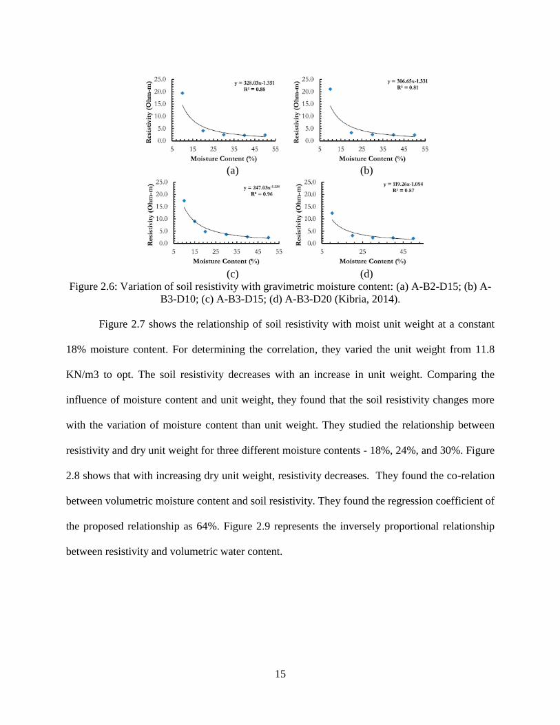
Figure 2.6: Variation of soil resistivity with gravimetric moisture content: (a) A-B2-D15; (b) A-

B3-D10; (c) A-B3-D15; (d) A-B3-D20 (Kibria, 2014). ................................................. 15

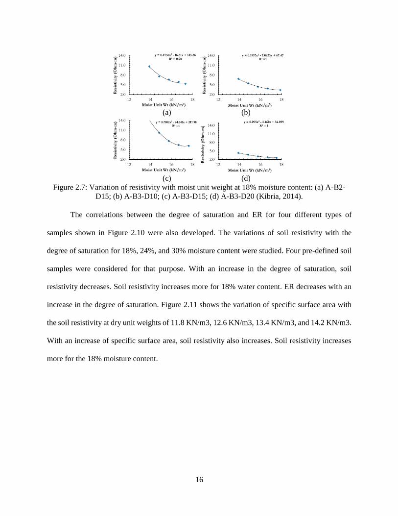
Figure 2.7: Variation of resistivity with moist unit weight at 18% moisture content: (a) A-B2-

D15; (b) A-B3-D10; (c) A-B3-D15; (d) A-B3-D20 (Kibria, 2014). .............................. 16

Figure 2.8: Comparison of the effect of moisture content and unit weight with soil resistivity:

(a) A-B2-D15; (b) A-B3-D15 (Kibria, 2014). ................................................................ 17

Figure 2.9: Variation of soil resistivity with volumetric water content (Kibria, 2014). ............. 17

Figure 2.10: Variation of soil resistivity with the degree of saturation: (a) A-B2-D15; (b) A-B3-

D10; (c) A-B3-D15; (d) A-B3-D20 (Kibria, 2014). ....................................................... 17

Figure 2.11: Variation of soil resistivity with specific surface area at dry unit weight: (a) 11.8

KN/m3, (b) 12.6 KN/m3, (c) 13.4 KN/m3, (d) 14.2 KN/m3 (Kibria, 2014). ................ 18

Figure 2.12: (a) plot of water content variable for ER (b) plot of ER variable for water content

(Bhatt and Jain, 2014). .................................................................................................... 19

Figure 2.13 : Relationship between soil ER and water content for (a) Istanbul area (b) Golcuk

area (Ozcep et al., 2009). ................................................................................................ 20

xvi

Figure 2.14: Relationship between soil ER and water content for all data (Ozcep et al., 2009). 20

Figure 2.15: (a) ER versus % of contamination. (b) ER versus LL (Tiwari and Shah, 2015). .. 21

Figure 2.16: (a) ER versus PL (b) ER versus SL (Tiwari and Shah, 2015). .............................. 22

Figure 2.17: ER versus SG (Tiwari and Shah, 2015). ................................................................ 22

Figure 2.18: Moisture content versus ER for (a) sand (b) silt (c) clay (d) sand and silt + clay

(Osman et. al.,2014). ...................................................................................................... 23

Figure 2.19 : Angle of friction (phi) versus ER for (a) sand (b) silt (c) clay (d) sand and silt plus

clay (Osman et. al.,2014). ............................................................................................... 24

Figure 2.20: Correlation of ER with (a) moisture content (b) unit weight (c) angle of internal

friction and (d) cohesion of soil (Siddiqui and Osman, 2012). ...................................... 25

Figure 2.21: Correlation of ER with (a) moisture content, (b) bulk density (Abidin et. al., 2013)

........................................................................................................................................ 26

Figure 2.22: Relationship of field ER to the moisture content and particle size of soil: (a) 1-

field ER ρ, Ωm; (b) 2- moisture content w, %; (c) 3- particle size (coarse soil) d, mm;

(d) 4- particle size (fine soil) d, mm-μm (Abidin et. al., 2013). ..................................... 27

Figure 2.23: Variations of (basic geotechnical properties) with particular reference to SG, void

ratio, porosity, and density: (a) 1- specific gravity Gs; (b) 2-void ratio e; (c) 3- porosity

φ; (d) 4- bulk density ρbulk, Mg/m3; (e) 5- dry density ρdry, Mg / m3 (Abidin et. al.,

2013). .............................................................................................................................. 27

Figure 2.24: Relationship of field ERV to the Atterberg limit (a) 1- field ER ρ, Ωm (b) 2- LL,

%; (c) 3- PL, %; (d) 4- PI, % (Abidin et. al., 2013). ...................................................... 28

Figure 2.25: Correlations between SPT-N and shear wave velocity (Vs) values: (a) for all soils,

(b) normalized consistency ratio for all soils, (c) for sand soils, (d) normalized

consistency ratio for sand soils, (e) for all silt soils, (f) normalized consistency ratio for

silt soils (g) for clay soils and (h) normalized consistency ratio for clay soils (Dikmen,

2009). .............................................................................................................................. 32

Figure 2.26: Direct correlation between shear wave velocity and cone tip resistance in intact

and fissured clays (Mayne and Rix,1995). ..................................................................... 33

Figure 2.27 : Vs-N correlations for (a) all, (b) silt, and (c) sand of Kathmandu valley (Gautam,

2017). .............................................................................................................................. 35

Figure 3.1: Earth dam section ..................................................................................................... 40

Figure 3.2: Selected soil type for laboratory measurement ........................................................ 41

Figure 3.3: Compaction test ....................................................................................................... 45

xvii

Figure 3.4: Adjusted compaction effort compared to standard compaction effort (Hickey,

2012). .............................................................................................................................. 46

Figure 3.5: Acrylic mold with four electrodes. .......................................................................... 46

Figure 3.6: ER measurement. ..................................................................................................... 47

Figure 3.7: Calibration curve for measured resistance compared to true resistivity. ................. 47

Figure 3.8: Bender element. P source / S receiver (left side), S source / P receiver (right side).

........................................................................................................................................ 48

Figure 3.9: Seismic wave velocity measurements using GDS bender element. ........................ 49

Figure 3.10: Seismic wave velocity (source, P-wave, S-wave). ................................................ 49

Figure 3.11: Atterberg limit. ....................................................................................................... 50

Figure 3.12 : LL test. .................................................................................................................. 51

Figure 3.13: Plastic limit test. ..................................................................................................... 51

Figure 3.14: Shrinkage limit test (a) shrinkage of soil pat after drying (b) wax coating of soil

pat (c) water submersion technique. ............................................................................... 52

Figure 3.15: Specific gravity test. (a) dry soil (b) soil with water

(c) boiling soil-water mixture. ........................................................................................ 53

Figure 3.16: (a) unconfined compression test, (b) stress versus strain graph of sample 1. ........ 54

Figure 3.17: CEC test of sample 15, (a) diluted leachate in the chemical, (b) ammonia

determination. ................................................................................................................. 56

Figure 4.1: Actual data for (a) ER versus saturation, remolded samples, (b) ER versus CEC,

remolded samples, (c) ER versus saturation, undisturbed samples, (d) ER versus CEC,

remolded samples, (e) ER versus dry density, remolded samples, (f) ER versus water

content, remolded samples. ............................................................................................ 61

Figure 4.2: Comparison of ANN models predicting ER (a) remolded samples (input: CEC and

saturation), (b) undisturbed samples (input: CEC and saturation). ................................ 64

Figure 4.3: Comparison of ANN models for predicting saturation: (a) remolded samples (input:

ER), (b) undisturbed samples (input: ER), (c) remolded samples (input: ER and CEC),

(d) undisturbed samples (input: ER and CEC). .............................................................. 65

Figure 4.4: Comparison of ANN models predicting CEC: (a) remolded samples (input: ER), (b)

undisturbed samples (input: ER), (c) remolded samples (input: ER and saturation), (d)

undisturbed samples (input: ER and saturation). ............................................................ 67

Figure 4.5: Comparison of ANN models predicting dry density (a) input: ER, (b) input: ER and

water content. ................................................................................................................. 69

xviii

Figure 4.6: Comparison of ANN models predicting water content (a) input: ER, (b) input: ER

and dry density. .............................................................................................................. 70

Figure 5.1: Graphical prediction accuracy of model for predicting seismic wave velocity, (a)

field, with validation, (b) field, without validation, (c) lab, with validation, (d) lab,

without validation, (e) field plus lab, with validation, (f) field plus lab, without

validation ........................................................................................................................ 80

Figure 5.2: Graphical prediction accuracy of model for predicting moisture content, (a) field,

with velocity, (b) field, without velocity, (c) lab, with velocity, (d) lab, without velocity,

(e) field plus lab, with velocity, (f) field plus lab, without velocity. .............................. 83

Figure 5.3: Graphical prediction accuracy of model for predicting dry density, (a) field, with

velocity, (b) field, without velocity, (c) lab, with velocity, (d) lab, without velocity, (e)

field plus lab, with velocity, (f) field plus lab, without velocity. ................................... 87

Figure 6.1: ER versus (a) water content, (b) saturation, (c) CEC, (d) LL, (e) PL, (f) SL .......... 97

Figure 6.2: ER versus (a) surface area, (b) cohesion, (c) dry density, (d) void ratio, (e) SG. .... 98

Figure 6.3: Predicted versus actual graph of predicting ER from (a) void ratio, saturation, CEC,

soil mix proportion, (b) wet density, water content, SL, soil mix proportion. ............. 101

Figure 6.4: P-wave velocity versus (a) dry density, (b) void ratio, (c) saturation, (d) water

content. ......................................................................................................................... 104

Figure 6.5: Predicted versus actual graph of predicting P-wave velocity from (a) dry density,

water content, void ratio, saturation, soil mix proportion at below opt, (b) opt, (c) above

opt. ................................................................................................................................ 106

Figure 6.6: S-wave velocity versus (a) dry density, (b) void ratio, (c) saturation, (d) water

content. ......................................................................................................................... 109

Figure 6.7: Predicted versus actual graph of predicting S-wave velocity from (a) dry density,

water content, void ratio, saturation, SL, soil mix proportion at below opt, (b) at opt. 111

Figure 7.1: Predicted versus actual graph for predicting (a) LL, (b) PL, (c) SL, (d) CEC from

soil mix proportion and ER. ......................................................................................... 118

Figure 7.2: Predicted versus actual graph for predicting (a) water content, (b) dry density, (c)

saturation, (d) void ratio from soil mix proportion, LL and ER. .................................. 119

Figure 7.3: Predicted versus actual graph at opt for predicting (a) water content, (b) dry density,

(c) saturation, (d) void ratio from soil mix proportion and P-wave velocity................ 122

Figure 7.4:versus actual graph at opt for predicting (a) water content, (b) dry density, (c)

saturation, (d) void ratio from soil mix proportion and S-wave velocity. .................... 124

Figure 8.1: Predicted versus actual graph for predicting water content from ER, S and P-wave

velocity at (a) below opt, (b) at opt, (c) at above opt. .................................................. 129

xix

Figure 8.2: Predicted versus actual graph for predicting water content from (a) ER, S, P-wave

velocity, SMP at below opt, (b) ER, S, P-wave velocity, SMP at opt, (c) ER, S, P-wave

velocity, SMP at above opt. ......................................................................................... 130

Figure 8.3: Predicted versus actual graph for predicting dry density from (a) ER and P-wave

velocity at below opt, (b) ER, S-wave velocity at opt, (c) ER, S and P-wave velocity at

above opt. ..................................................................................................................... 132

Figure 8.4: Predicted versus actual graph for predicting dry density from (a) ER, P-wave

velocity, SMP at below opt, (b) ER, S-wave velocity, SMP at opt, (c) ER, S, P-wave

velocity and SMP at above opt. .................................................................................... 133

Figure 8.5: Predicted versus actual graph for predicting saturation from (a) ER, S and P-wave

velocity at below opt, (b) at opt, (c) at above opt. ........................................................ 135


velocity, SMP at below opt, (b) ER, S and P-wave velocity, SMP at opt, (c) ER, S and

P-wave velocity, SMP at above opt. ............................................................................ 136

Figure 8.7: Predicted versus actual graph for predicting void ratio from (a) ER and P-wave

velocity at below opt, (b) ER, S and P-wave velocity at opt, (c) ER, S and P-wave

velocity at above opt. .................................................................................................... 139

Figure 8.8: Predicted versus actual graph for predicting void ratio from (a) ER, P-wave

velocity, SMP at below opt, (b) ER, S, P-wave velocity, SMP at opt, (c) ER, S, P-wave

velocity, SMP at above opt. .......................................................................................... 140

1

1. CHAPTER 1

INTRODUCTION

1.1 General

Geophysics is the study of the earth, and often involves taking measurements at or near the

earth's surface by applying the principles of physics. The measurements are influenced by the

physical properties of the earth. Historically, geophysical surveys were used to delineate contacts

and boundaries in the subsurface and to map the location of these boundaries between boreholes.

Geophysical techniques have good spatial resolution in both 2D and 3D. These techniques are non-

destructive, thereby allowing for monitoring of changes over time. But geophysical methods have

some demerits in engineering applications. The measurements are in terms of geophysical

attributes rather than engineering parameters, the spatial resolution depends on the geophysical

method and site characteristics, and geophysical anomalies do not necessarily correspond to

inferior subsurface locations. Different kinds of geophysical techniques, such as seismic, gravity,

magnetic, ER, self-potential and radar (Kearey et al., 1984), are used depending on the purpose.

In the last few decades, geophysical techniques have been used to provide additional

information for solving different kinds of civil engineering problems (Sharma, 1997). Some

engineering applications include seismic hazard, foundation testing, locating water, and detection

of abandoned mine shafts, unlogged pipes, and discarded metallic objects. Determination of the

depth and constitution of bedrock, and the physical properties of rock encountered in dam, canal,

2

tunnel shaft, high-level waste disposal vault, railway, highway, subway, and other construction

projects are included in the foundation testing problems. In municipal engineering, the

determination of the location of water and its salinity is necessary to solve water supply, sewage

disposal, irrigation, and drainage problems. Geophysical methods are also used to collect

information on water levels and water-bearing fissures, which are indispensable in the construction

of subways and tunnels. To determine the location of older underground excavations, such as

shafts and tunnels, and to locate buried ammunition and other metal machinery, geophysical

techniques play a very important role (Sharma, 1997). Table 1.1 lists some of the engineering

problems and the appropriate geophysical techniques that may be used.

Table 1.1: Engineering and geotechnical applications of geophysical techniques (Sharma, 1997).

Area of application

Technique Depth to

and

constitution

of bedrock

Rip

ability/

Rock

strength

Fracture/

Flow

seepage

detection

Location of

cavities/voids

Permafrost/

Thaw

zones

delineation

Pipes/

Metal

detection

Gravity + - - + - -

Magnetic + - - + - +

Self-potential - - + - - o

Resistivity +IPa + - + + + o

Electromagnetic o - + o + +

Ground radar + o + + + o

Radioactivity - - o - - -

Seismic

refraction

+ + o o + -

Seismic

reflection

+ + o o o -

Note: + applicable; o limited applicability; - not applicable; a Induced polarization

1.2 Research Significance

This research is focused on determining correlations between geophysical and geotechnical

parameters for application to earthen dam and levee assessment. However, these correlations

could be applied to many investigations involving near-surface soils.

3

Dams are extremely important life-sustaining resources to the people of the world. Dams

can be used for supplying water for domestic, agricultural, industrial, and community use, flood

control, erosion control, and for recreational purposes (ASDSO, 2019). Economic and social

development in the USA is highly dependent on dams (Ho et al., 2017). According to the U.S.

Army Corps of Engineers (USACE), around 20% of dams are used for flood control to reduce the

risks of loss of life and property. The current National Inventory of Dams (NID) statistics show

that nearly 84,000 dams are already constructed in the USA. The average age of these dams is over

50 years. Figure 1.1 shows the dams according to their age of construction based on data in the

NID. In addition to age causing deterioration of the dams, the design criteria and loading estimates

considered at the time of construction are insufficient according to modern design code. As a result,

most of the dams in the USA are considered as unsafe and vulnerable. Figure 1.2 is a map of the

distribution of low, significant, and high hazard potential dams in the USA (FEMA, 2013).

Figure 1.1: Years dams were completed in the United States (NID, 2009)

Preventing failures of these dams requires a rigorous inspection and investigation program.

Based upon inspections, engineering solutions have to be proposed and implemented correctly.

Geotechnical methods for investigation and inspection are very time consuming and destructive.

On the other hand, geophysical methods are noninvasive, have good spatial resolution, and can

4

cover a large area within a relatively short time in comparison to geotechnical methods. But the

geophysical parameters are not engineering parameters, depend on spatial resolution and

sometimes difficult to interpret anomalies. Correlations between geophysical and geotechnical

parameters can assist in the interpretation problem.

Figure 1.2 : State-regulated dams in the United States according to hazard potential (FEMA,

2010)

For this research, correlations between geophysical and geotechnical parameters and

prediction models for geotechnical parameters from geophysical parameters were developed using

an artificial neural network (ANN) approach. ANN is very effective in solving complex problems

in comparison to traditional methods, such as regression.

1.3 Research Objectives

This research is focused on determining correlations between geophysical and

geotechnical parameters. Specific objectives of the research are:

a) Creating a database of measurements for developing ANN models. This requires

conducting laboratory experiments to collect: geotechnical parameters, such as Liquid

limit (LL), plastic limit (PL), shrinkage limit (SL), water content, dry density, void

5

ratio, cohesion, specific gravity (SG), degree of saturation, specific surface area; a

chemical parameter - CEC; and geophysical parameters, such as ER, S-wave and P-

wave velocity. These tests are conducted on common samples prepared using the

Proctor compaction method.

b) Predicting geotechnical parameters from ER applying ANN (using existing data from

literature).

c) Application of ANN to forecast geotechnical parameters from seismic wave velocity

(using existing data from literature).

d) Predicting geophysical parameters from geotechnical parameters (using measured

experimental data).

e) Predicting geotechnical parameters from geophysical parameters (using measured

experimental data).

f) Predicting geotechnical parameters from combined geophysical parameters (using

measured experimental data).

6

2. CHAPTER 2

REVIEW OF PREVIOUS WORK

2.1 General

Geophysical information has been used to solve problems in different fields, such as oil

exploration and mining exploration (Shirgiri, 2012). More recently, geophysical methods are

gaining popularity in archeology, geotechnical engineering, civil engineering, hydrology, and

glaciology. Dams and levees are important civil engineering structures and the design and

assessment of dams and levees require characterization of the soils. Conventional geotechnical

methods for soil characterization are invasive, very expensive, and time-consuming. Sometimes

developers are not willing or are unable to conduct site characterization at the appropriate

resolution due to the high cost of geotechnical investigation (Adewoyin et al., 2017). On the other

hand, geophysical methods can provide subsurface coverage ensuring a cost-effective way of

investigation without physical intervention (Mohd et al., 2012). Geophysical methods are non-

destructive in nature and less time-consuming. Moreover, geophysical techniques can provide

volumetric information and images without disturbing the subsoil physically (Loke, 2015), which

is why geophysical methods are becoming a choice for geotechnical engineers for determining the

spatial distribution of soil properties. The correlations between geophysical properties and

geotechnical engineering properties are necessary to interpret the geophysical data so that

geotechnical engineers can utilize the information in the design Five different kinds of

geophysical methods commonly used in geotechnical investigations are: (a) seismic-based

7

methods, which include refraction, reflection, and surface wave method; (b) electromagnetic

wave-based methods, including ground electrical conductivity and ground penetration radar

(GPR); (c) electrical-based methods that include self-potential (SP), ER, equipotential and induced

polarization (IP); (d) gravity methods; and (e) magnetics (Shirgiri, 2012). Among them, ER testing

and seismic wave velocity measurements are two well-known geophysical methods.

Soil properties important to dam investigation include: moisture content, unit weight,

degree of saturation, N-value, Atterberg limits, cohesion, angle of friction, Specific gravity (SG),

void ratio, etc. Strong correlations between these geotechnical properties and geophysical

properties will be helpful for using the geophysical information for geotechnical problems.

2.2 Electrical Resistivity

ER method was first designed by Schlumberger in France in 1920 (Loke, 2015). Soil

electrical resistivity testing is becoming very popular due to its non-destructive nature and cost-

effectiveness. The ER of a volume of soil is determined by measuring the voltage across a pair of

electrodes in response to a known imposed current. The electrical resistance depends on the

geometric arrangement of electrodes. For measurements on soil samples, it is proportional to the

length and inversely proportional to the cross-sectional area of the material being tested. ER of

soil is the measure of the resistance of current flow through it (Irfan, 2011). It can be

mathematically expressed by the following equation.

ρ = r ∗ A/L 2.1

where, ρ is the resistivity (ohm*m), r is the resistance (ohms), A is the cross-sectional area (m2),

L is the length of soil (m).

ER is sensitive to many soil properties, such as LL, plasticity index, particle size, porosity,

degree of saturation, moisture content, etc. (Kibria, 2014). It is commonly considered as a soil

8

property that is affected by soil particle size distribution (clay content), porosity, and moisture

content.

Archie’s (1942) first law is a relationship between the bulk resistivity of soil and the

porosity for a fully saturated clean sand or coarse-grained material. This model assumes that the

primary pathway for electric current is through the pore fluid. Archie’s first law is expressed as

F =ρb/ρw = aΦ−m 2.2

where ρb is bulk resistivity, ρw is the resistivity of the pore fluid, F is formation factor, Φ is the

porosity of the sand, a is an empirical constant close to 1 and m is the cementation exponent.

For partially saturated sand Archie’s (1952) second law is

ρb/ρw = aΦ−m ∗ sw−n 2.3

where sw is degree of saturation, and n is the saturation exponent.

The assumption of clean sand is usually not valid for most soils because they contain clay

minerals. The presence of clay minerals allows for electric current to flow along the surface of the

clay minerals. Waxman-Smit (1968) developed a relationship for the effective electrical

conductivity of soils that includes surface conduction. The electrical conductivity is the inverse of

ER. The formula provided by Waxman-Smit is

C0 =1

F(Cw + Ce)

2.4

where C0= bulk conductivity of fully saturated soil sample with clay, Cw = conductivity of the

pore fluid, and F is the formation factor of Shaley sand. Ce =Conductivity due to the presence of

clay content.

2.3 Developed Correlation with ER

A significant amount of research has been published on correlations between ER and

various geotechnical parameters. Sudha et al. (2009) developed correlations between transverse

9

resistance of soil with the number of blow counts (N values). N values are obtained from the

Standard Penetration Test (SPT) and Dynamic Cone Penetration Test (DCPT). Two locations were

chosen (Aligarh and Jhansi) in Uttar Pradesh, India. ER data were calibrated with borehole data,

and finally, the transverse resistance was calculated, which was co-related with the N-values. The

resistivity of the sites varies from 1 to 1000 Ωm, which indicates the variation in soil matrix, grain

size distribution, and water saturation. The percentage of sand is dominant at Aligarh. Fine sand

is dominant at Jhansi with a percentage of >70%. At both the sites the percentage of gravel is very

small (<10%). Jhansi contains a higher percentage of clay than the Aligarh site. Figure 2.1

illustrates the fact that they found no specific correlation between resistivity and N-value.

Figure 2.1: Variation of resistivity values derived from the interpreted section (Sudha et al,

2009).

(a) (b)

Figure 2.2: Linear relationship between number of blow counts (N-values) and transverse

resistance obtained at (a) Aligarh; (b) Jhansi (Giao, 2003).

10

Then they used the transverse resistance to determine a correlation with N-values. The transverse

resistance (T) for an m-layer section was calculated as

T =∑ ρihimi=1 2.5

where ρi and hi are the resistivity and thickness of the ith layer, respectively. Figure 2.2 represents

the linear relation between average N-values and the transverse resistance.

Equations 1 and 2 represent the linear relationships at the Aligarh and Jhansi sites as,

y = 0.028x + 10.909 2.6

y = 0.102x + 4.922 2.7

where x is the transverse resistance (Ωm2) and y is the number of blow counts (N values). The

coefficients of correlation (R) for Aligarh and Jhansi sites are 0.974 and 0.975, respectively.

Equations represent the positive correlations between the transverse resistance and average N

values. The coefficients of the linear relationship are influenced by the clay content and lithology

at the investigated sites. The changes in slope in the equation and are due to the change in clay

content. At the Aligarh site, the percentage of clay content is less than the Jhansi sites.

P. H. Giao et. al. (2003) measured ER of Pusan clays of 50 core samples taken from five

sites in the Nakdong river plain (Kimhae, Shinho, Eulsookdo, Yangsan, and Jangyu) in the

laboratory to correlate it with geotechnical parameters such as salinity, organic content, water

content, plasticity, unit weight and sampling depth. The soft clay samples were prepared with a

diameter of 75 mm and a length of 110 mm and the four-electrode configuration. Figure 2.3

illustrates the ER versus geotechnical parameters. They found that ER of Pusan clays varied within

the range of 1 to 3 Ω m. The resistivity of clays located in Kimhae, Yangsan, and Jangyu was

higher (~ 2 to 3 Ω m) than Eulsookdo and Shinho (~ 1 Ω m). No definite relationship was found

11

between ER and geotechnical parameters (water content, plasticity, unit weight, and depth). Only

salinity showed a closer correlation with ER.

Bryson and Bathe (2009) determined correlations between the void ratio (e) and

normalized conductivity (σbulk

σpf⁄ ), void ratio and surface conductivity (BQv), and volumetric

water content (Ө) and surface conductivity. Void ratio is the ratio of volume of voids to the volume

of soil in a soil specimen. Normalized conductivity is the ratio of bulk conductivity and the

conductivity of pore fluids.

12

(a) (b)

(c) (d)

(e) (f)

Figure 2.3 : Relationship between the ER and other parameters for Pusan clays, i.e., (a) salinity;

(b) organic content; (c) water content, (d) plasticity, (e) water content (d) depth (Giao, 2003).

13

(a) (b)

Figure 2.4: Relationship between (a) void ratio and normalized conductivity (b) void ratio and

surface conductivity (Bryson and Bathe, 2009).

(c)

Figure 2.5: Relationship between volumetric water content and surface conductivity (Bryson

and Bathe, 2009).

Figure 2.4a depicts that the normalized conductivity increases with an increase of clay

content although the relative magnitude of the void ratios remains the same. The graph shows a

logarithmic trend represented by

e = 0.18 ln (σbulk

σpf⁄ ) + 0.74 2.8

Figure 2.4b illustrates the correlation between void ratio and surface conductivity. The

graph shows that there exists a strong correlation between void ratio and surface conductivity.

They represented the correlation using the following power function

e = 0.37 (BQv−0.78) 2.9

14

The surface conductivity increases with a decrease in clay content. They attributed this

phenomenon to greater dispersion of clay particles into the sand matrix than into the clay matrix.

The orientation of clay particles is more aligned in the sand matrix and, for that reason, the particles

can hold more water - which results in increased surface conductivity. Figure 2.5 shows the strong

correlation between volumetric water content with surface conductivity, which can be expressed

by the following equation:

Ө = 21.11 (BQv) 0.55 2.10

In Figure 2.5, the points below the curve represent the soil mixtures with degree of

saturation less than 70%. The volumetric water content is strongly correlated with the surface

conductivity for the degree of saturation greater than 70%.

Kibria and Hossain (2012) determined the relationships between soil resistivity and

geotechnical properties of soil (i.e. moisture content, unit weight, degree of saturation, and specific

surface area). They conducted soil resistivity tests in the laboratory at varying unit weights and

moisture contents. They collected disturbed soil samples from Midlothian, Ellis County, Texas,

and considered soil samples of similar geologic information.

The moisture contents were varied from 10 to 50%. Compaction was done at the

optimum(opt) dry unit weight. Four samples, denoted A-B2-D15, A-B3-D10, A-B3-D15, and A-

B3-D20, were considered to determine the correlations, where A represents the site location

highway US 287, the second letter and number are for the borehole and third letter and number

indicate the depth of samples. Figure 2.6 represents the variation of soil resistivity with gravimetric

moisture content. The relationships and coefficients are also shown in Figure 2.6. ER decreases

with an increase in water content up to around 20%. For moisture content above 40%, the soil

resistivity does not change.

15

(a) (b)

(c) (d)

Figure 2.6: Variation of soil resistivity with gravimetric moisture content: (a) A-B2-D15; (b) A-

B3-D10; (c) A-B3-D15; (d) A-B3-D20 (Kibria, 2014).

Figure 2.7 shows the relationship of soil resistivity with moist unit weight at a constant

18% moisture content. For determining the correlation, they varied the unit weight from 11.8

KN/m3 to opt. The soil resistivity decreases with an increase in unit weight. Comparing the

influence of moisture content and unit weight, they found that the soil resistivity changes more

with the variation of moisture content than unit weight. They studied the relationship between

resistivity and dry unit weight for three different moisture contents - 18%, 24%, and 30%. Figure

2.8 shows that with increasing dry unit weight, resistivity decreases. They found the co-relation

between volumetric moisture content and soil resistivity. They found the regression coefficient of

the proposed relationship as 64%. Figure 2.9 represents the inversely proportional relationship

between resistivity and volumetric water content.

16

(a) (b)

(c) (d)

Figure 2.7: Variation of resistivity with moist unit weight at 18% moisture content: (a) A-B2-

D15; (b) A-B3-D10; (c) A-B3-D15; (d) A-B3-D20 (Kibria, 2014).

The correlations between the degree of saturation and ER for four different types of

samples shown in Figure 2.10 were also developed. The variations of soil resistivity with the

degree of saturation for 18%, 24%, and 30% moisture content were studied. Four pre-defined soil

samples were considered for that purpose. With an increase in the degree of saturation, soil

resistivity decreases. Soil resistivity increases more for 18% water content. ER decreases with an

increase in the degree of saturation. Figure 2.11 shows the variation of specific surface area with

the soil resistivity at dry unit weights of 11.8 KN/m3, 12.6 KN/m3, 13.4 KN/m3, and 14.2 KN/m3.

With an increase of specific surface area, soil resistivity also increases. Soil resistivity increases

more for the 18% moisture content.

17

(a) (b)

Figure 2.8: Comparison of the effect of moisture content and unit weight with soil resistivity: (a)

A-B2-D15; (b) A-B3-D15 (Kibria, 2014).

Figure 2.9: Variation of soil resistivity with volumetric water content (Kibria, 2014).

(a) (b)

(c) (d)

Figure 2.10: Variation of soil resistivity with the degree of saturation: (a) A-B2-D15; (b) A-B3-

D10; (c) A-B3-D15; (d) A-B3-D20 (Kibria, 2014).

18

(a) (b)

(c) (d)

Figure 2.11: Variation of soil resistivity with specific surface area at dry unit weight: (a) 11.8

KN/m3, (b) 12.6 KN/m3, (c) 13.4 KN/m3, (d) 14.2 KN/m3 (Kibria, 2014).

Bhatt and Jain (2014) used a statistical approach to determine the correlation between ER

and water content of sand. They prepared the samples in the laboratory at constant dry density and

water contents were varied from dry to saturated condition. Through non-linear regression

analysis, they found the following correlation equation:

ρ = 388.97e0.08w + Ɛ 2.11

where ρ is ER (Ωm), w is water content, and Ɛ is standard error.

Figure 2.12 shows the fitted exponential curve which represents the correlation between

ER and water content. The R2 value was 0.908, which indicates a good correlation between ER

and water content.

19

They performed another statistical analysis to determine the correlation between water

content and ER. In that case, they kept ER as a variable. They established the following correlation

between water content and ER:

w = 29.536 e 0.006ρ + Ɛ 2.12

with an R2 is 0.839, which indicates good correlation. Figure 2.12 represents the correlation

between water content and ER. In both cases with an increase of water content, ER decreases.

(a) (b)

Figure 2.12: (a) plot of water content variable for ER (b) plot of ER variable for water content

(Bhatt and Jain, 2014).

Ozcep et. al. (2009) used artificial intelligence techniques to develop correlations between

ER and soil-water content. They also compared conventional regression analysis to artificial

intelligence techniques. The ranges of ER considered were 1-50 ohm-m and water content 20-

60%. Geotechnical measurements were taken at depths up to 15m. Soil samples for this study were

sandy soils. Three types of artificial intelligence techniques were used: artificial neural networks

(ANN), Fuzzy-Mamdani method, and the Fuzzy-Sugeno method. Again, these methods were

compared with conventional regression analysis methods. Figure 2.13 represents the results of

regression analysis for the correlation between ER and soil-water content for sites near Istanbul

and Golcuk, and Figure 2.14 illustrates all data.

20

(a) (b)

Figure 2.13 : Relationship between soil ER and water content for (a) Istanbul area (b) Golcuk

area (Ozcep et al., 2009).

Figure 2.14: Relationship between soil ER and water content for all data (Ozcep et al., 2009).

The regression coefficient (R2), Mean error squares (MES) and mean absolute error percent

(MAEP) for the four methods are shown in Table 2.1. It was found that even though the regression

analysis method easily estimates a value of water content from ER, the prediction accuracy and

the evaluation of performance of estimation of AI systems are good enough. The ANN method

showed better performance than the other methods.

Table 2.1 : Statistics for three artificial intelligence and regression methods.

ANN MAMDANI SUGENO REGRESSION

MAEP 17.76 19.99 17.63* 20.85

MES 33.62 43.12 32.598* 50.39

R2 0.8844* 0.82688 0.8825 0.7859

Note: Best results are indicated by the sign ‘*’

21

Tiwari and Shah (2015) studied the relationship between index properties and ER of

periodically hydrocarbon contaminated clays. They used 3%, 6%, and 9% hydrocarbon for periods

of 15, 30, 45, and 60 days, and compared the results with non-contaminated marine clay. Soil

resistivity was measured in the laboratory by fabricating a soil resistivity box. Figure 2.15 (a)

represents the correlation between ER and percentage of hydrocarbon contamination. ER increases

by 28%, 40%, and 33%, respectively, for 3%, 6% and 9% of hydrocarbon contamination. But ER

decreases with the increase of period of contamination. Figure 2.15 (b) shows the ER decreases

with an increase in LL. LL of hydrocarbon contaminated clay is lower than the non-contaminated

clay. ER shows a proportional relationship with PL, but PL shows an inversely proportional

relationship with period of contamination as shown in Figure 2.16 (a). PL of contaminated clay is

higher than non-contaminated clay. With an increase in period of contamination, shrinkage limit

(SL) increases; with an increase in SL, the ER increases as shown in Figure 2.16 (b). Figure 2.17

shows the correlation between ER and SG. ER shows an inversely proportional relationship with

SG, and SG shows a proportional relationship with period of contamination.

(a) (b)

Figure 2.15: (a) ER versus % of contamination. (b) ER versus LL (Tiwari and Shah, 2015).

22

(a) (b)

Figure 2.16: (a) ER versus PL (b) ER versus SL (Tiwari and Shah, 2015).

Figure 2.17: ER versus SG (Tiwari and Shah, 2015).

Osman et. al. (2014) established correlations intended to help determine soil strength

parameters, such as cohesion and angle of friction, using ER. They conducted ER tests in the

laboratory for different types of soils by varying compaction energy and moisture content. They

used three types of soil samples - namely clay, silt and sand. Figure 2.18 shows the relationship

between moisture content and ER for three types of soil. Strong correlation was observed for clay

samples (R2 of 0.818) whereas silt showed the lowest correlation (R2 of 0.694). They explained

that the lower correlation for the silt sample was a consequence of using a lower moisture content

(10% to 25%) for the silt sample. Figure 2.18 (d) represents the combined correlation for silt and

clay. In this case, they found a better correlation and suggested that fine-grain soil shows better

correlation between moisture content and ER.

23

(a) (b)

(c) (d)

Figure 2.18: Moisture content versus ER for (a) sand (b) silt (c) clay (d) sand and silt + clay

(Osman et. al.,2014).

The correlations between angle of friction and ER are shown in Figure 2.19. This graph

demonstrates that with an increase of internal friction, ER also increases. Again, the strongest

correlation was for clay (R2 = 0.824) and weakest correlation for silt (R2 = 0.012).

24

(a) (b)

(b) (d)

Figure 2.19 : Angle of friction (phi) versus ER for (a) sand (b) silt (c) clay (d) sand and silt plus

clay (Osman et. al.,2014).

Siddiqui and Osman (2012) also developed correlations between ER and strength

properties of soil. They conducted field measurements of electrical resistivity survey and soil

boring. In laboratory, they performed ER tests and direct shear tests, and they also measured

moisture content and unit weight. Their resistivity values measured in laboratory were higher than

the field resistivity values. They explained that this was due to the change in saturation condition,

temperature difference, and overburden pressure. They combined the field and laboratory

resistivity data for simplicity and generalization. Figure 2.20 describes the relationship between

ER and moisture content, unit weight, angle of internal friction, and cohesion of soil. They

indicated the bad data points by red-circles in the graphs. Figure 2.20 (c) shows that ER increases

with an increase of friction angle. A good correlation exists between angle of internal friction and

ER. The correlation between cohesion and resistivity shown in Figure 2.20 (d) is weak. Moisture

content in Figure 2.20 (a) shows good correlation with resistivity; on the other hand, unit weight

shows a weak correlation with resistivity in Figure 2.20 (b).

25

(a) (b)

(c) (d)

Figure 2.20: Correlation of ER with (a) moisture content (b) unit weight (c) angle of internal

friction and (d) cohesion of soil (Siddiqui and Osman, 2012).

Abidin et. al. (2013) performed 24 resistivity tests to determine the correlations between

ER and moisture content and soil density. The disturbed soil samples were collected to conduct

the geophysical and geotechnical experiments in the laboratory. For resistivity testing, Nilsson

model 400 soil resistance meters were used. Soil samples were prepared by mixing an original

mass of 1500g of oven-dried soil with 1-5% of distilled water. Moisture content was determined

by taking the average of the two samples from each soil box test. Figure 2.21 shows curvilinear

resistivity between water content to ER and bulk density to ER. ER decreased with increasing

water content and bulk density.

26

(a) (b)

Figure 2.21: Correlation of ER with (a) moisture content, (b) bulk density (Abidin et. al., 2013)

Abidin et. al. (2013) developed correlations between field ER values and basic

geotechnical properties. Basic geotechnical properties include soil moisture content, grain size of

geomaterial, density, porosity, void ratio, and Atterberg limit. They collected three disturbed soil

samples from three different sites along the same resistivity line. Based on particle size

distribution, they classified the soil as clayey silt. The three soil samples were different from each

other in terms of percentages of coarse and fine soil. Soil A contains the highest amount of coarse

soil (C- 24.19%) and lowest amount of fine soil (F- 75.81%) followed by soil C ( C-22.86% and

F-77.14%) and B (C-20.51% and F-79.49%), respectively. They presented the general relationship

using a bar chart as shown in Figure 2.22.

Figure 2.22 illustrates that moisture content is inversely proportional to the field ER.

Sample A holds the least moisture content and highest field ER whereas sample B holds the highest

moisture content and lowest field ER. They also showed that ER is proportional to the grain size.

ER increases with an increase of grain size. Sample A has the highest ER and greatest amount of

coarse soil; on the other hand, sample B has lowest ER with the smallest amount of coarse soil.

27

Figure 2.22: Relationship of field ER to the moisture content and particle size of soil: (a) 1- field

ER ρ, Ωm; (b) 2- moisture content w, %; (c) 3- particle size (coarse soil) d, mm; (d) 4- particle

size (fine soil) d, mm-μm (Abidin et. al., 2013).

Figure 2.23 indicates that ER is proportional to the high soil density. Sample A was denser

than C and B, and C was denser than B. They found the highest ER for sample A, then C, and

lowest for sample B.

Figure 2.23: Variations of (basic geotechnical properties) with particular reference to SG, void

ratio, porosity, and density: (a) 1- specific gravity Gs; (b) 2-void ratio e; (c) 3- porosity φ; (d) 4-

bulk density ρbulk, Mg/m3; (e) 5- dry density ρdry, Mg / m3 (Abidin et. al., 2013).

28

Figure 2.24: Relationship of field ERV to the Atterberg limit (a) 1- field ER ρ, Ωm (b) 2- LL, %;

(c) 3- PL, %; (d) 4- PI, % (Abidin et. al., 2013).

Figure 2.24 showed that field ER is inversely proportional to Atterberg limit. Such as

sample B has lowest ERV and highest Atterberg limit.

2.4 Seismic Wave Velocity

Seismic wave methods are sensitive to the mechanical properties of the soil. Soil allows

for the propagation of different types of seismic waves. Waves that deform the material through

shear are referred to as shear waves and those that produce volumetric deformations are referred

to as compressional waves. These are often referred to as S-waves and P-waves, respectively.

There are numerous methods for measuring seismic wave velocity in the field and the laboratory.

In the laboratory, the “time of flight” approach is common. A seismic wave is generated using a

source in contact with one end of the sample, the disturbance passes through the soil and is detected

by a receiver at the opposite end of the sample. Velocity is calculated by dividing the distance

(sample length) by the measured travel time. Typical P-wave and S-wave velocities are shown in

Table 2.2.

29

Table 2.2: Seismic wave velocities for different materials.

Material P-wave velocity, m/s S-wave velocity, m/s

Air 330 0

Water 1450 0

Sands and clays 300-1900 100-500

Glacial till 1500-2700 600-1300

Chalk 1700-3000 600-1500

Strong limestone 3000-6500 1500-3500

Weathered granite 100-3000 500-1500

Fresh granite 3000-6000 1500-3000

Slate 5000-7000 2500-3800

Rock salt 4000-5500 2000-3200

Longitudinal P-wave and the transverse S-wave in an infinite elastic continuum are related to the

elastic properties of the soil:

Vp = √M

d = √

B + 4

3G

d P-waves

2.13

Vs = √G

d S-waves

2.14

where M is the constraint modulus, B is the bulk modulus, G is the shear modulus, and d

is the mass density of the medium. Hence, the propagation velocity increases with the stiffness of

the material and decreases with its mass density (inertia). Velocity of S-waves is smaller than the

velocity of P-waves (Santamarina et al., 2001) The soil shear modulus is sometimes used to derive

some geotechnical properties, such as maximum shear modulus (Gmax), bulk modulus (B),

Young’s modulus (E) and Poisson’s ratio (ʋ).

The coexistence of solid and fluid phases adds significant complexity to the behavior of

particulate or granular materials like soil. Phenomena include the formation of double layers,

seepage, time-dependent pressure diffusion, and the partition of applied stresses into pore fluid

30

pressure and effective skeletal stress. Under dynamic loading, differences in inertia, shear stiffness,

and bulk compressibility add further complexity to the analysis.

For fluid-filled porous media, the effective bulk modulus provided by Gassmann (Dikmen,

2009) is

Beff = BSK + (1−

BSKBg

)2

φ

Bf+

1−φ

Bg−

BSK

Bg2

2.15

where BSK is the bulk modulus of the skeleton, Bg is the bulk modulus of the grains, Bf is the

bulk modulus of the fluid phase, and φ is the porosity. In the Gassmann model, the shear modulus

of the soil, Geff, remains unaffected by the presence of the fluid at low excitation frequencies,

Geff = GSK 2.16

For partially saturated soils, the mass density of the mixture dmix, changes due to the

different densities of the saturating fluids. Ignoring granular effects, fluid substitution can be used

to modify the expression for the effective bulk modulus of the soil. For a soil with a water

saturation of Sw the fluid bulk modulus in equation 2.17 given by

1

Bf =

Sw

Bw+

1−Sw

Ba 2.17

where 𝐵𝑤is the bulk modulus of the liquid phase and 𝐵𝑎 is the bulk modulus of the air phase. Small

volumes of fluid produce a large decrease in the modulus of fluid.

Seismic wave propagation in granular materials like soil is more complicated due to the

complex behavior of solid skeleton and the influence of capillary forces. The skeletons BSK and

GSK depend on the “strength” of the grain contacts and are therefore dependent upon the applied

effective stress. The concept of effective stress for soils at low saturation is still an area of active

research because internal forces associated with capillary forces and electrical forces and grain

31

surface play an important role. That’s why empirical relationships are necessary to predict the

seismic wave propagation in partially saturated particulate mediums.

The velocity of propagation of P-waves reflects the bulk B and shear G stiffness of the

medium, while the velocity of S-waves only depends on the shear stiffness G. Since fluids do not

support shear, P-waves velocity is more sensitive to changes in water content. In general, S-waves

velocity has low sensitivity to water saturation and as such is correlated with soil matrix behavior.

Combining P-waves and S-waves results in a powerful tool for distinguishing the water table from

other geological features.

2.5 Developed Correlation with Seismic Wave Velocity

Various studies have presented correlation between seismic wave velocity and geotechnical

parameters. Dikmen (2009) examined the statistical correlation of uncorrected standard

penetration test (SPT)-N values and shear wave velocity (Vs) for different kinds of soil categories

(i.e. all soil, sand, silt and clay-type soil). He used 193 uncorrected SPT-N and Vs data pairs

considering 82 sand, 76 silt, and 35 clay samples. For statistical analysis, he separated all data

according to high or low plasticity for cohesive soils and uniform or poor gradation for sand soils.

Figure 2.25 represents the correlations between SPT-N values and the shear wave velocity. The

following empirical formulas were derived and it was concluded that the type of soil has no

significant effect on the estimation of Vs. Equation (2.18-2.21) shows that SPT-N values have a

strong correlation with the shear wave velocity.

32

(a) (b)

(c) (d)

(e) (f)

(g) (h)

Figure 2.25: Correlations between SPT-N and shear wave velocity (Vs) values: (a) for all soils,

(b) normalized consistency ratio for all soils, (c) for sand soils, (d) normalized consistency ratio

for sand soils, (e) for all silt soils, (f) normalized consistency ratio for silt soils (g) for clay soils

and (h) normalized consistency ratio for clay soils (Dikmen, 2009).

Vs = 58N0.39 (R = 0.75 for all soils) 2.18

Vs = 73N0.33 (R = 0.72 for sand soil) 2.19

Vs = 60N0.36 (R = 0.71 for silt soil) 2.20

Vs = 44N0.48 (R = 0.82 for clay soil) 2.21

33

Cd = (VSM - VSC) / SPT-N 2.22

Dikmen (2009) calculated a normalized consistency ratio Cd using equation 2.22, where

VSM is the measured Vs from seismic cone penetration tests (SCPT) and seismic experiments, VSC

is the calculated Vs from the equation and SPT-N is the uncorrected SPT-N blow counts

corresponding to VSM. Figure 2.25 (h) shows a comparison between VSM and VSC. The values of

Cd are close to zero, which ensures the good performance of the proposed empirical formula.

Mayne and Rix (1995) estimated the empirical correlations between shear wave velocity (Vs) and

cone penetration tip resistance (qc) using the field data collected from 31 different natural clays.

Figure 2.26 shows the correlation between Vs and qc for both intact and fissured clay deposits. The

increasing trend of shear wave velocities and cone penetration resistance is observed with

consistency from soft to stiff to hard clay materials. Through log regression analysis the following

empirical equation was found with n = 481 and R2 = 0.736:

Vs = 1.75 (qc)0.6278 2.23

where Vs is in units of meters/sec and qc in kpa

Figure 2.26: Direct correlation between shear wave velocity and cone tip resistance in intact and

fissured clays (Mayne and Rix,1995).

Gautam (2017) developed correlations between shear wave velocity and uncorrected

standard penetration resistance for all soils, sand, and clays using 500 secondary data pairs. The

depth, overburden pressure, geological age, fine content, and soil types were not considered, which

34

may also influence the relationship. He conducted a simple power regression analysis to develop

correlations between uncorrected SPT-N values and VS. Data were collected up to 30m in depth.

The correlations were developed for all soils, silt, and sand separately. Figure 2.27 shows the

correlations for all soils, silt, and sand, respectively. The coefficient of determination for silt is

relatively low. Gautam (2017) explained that the coefficient of determination is lower due to a

limited database and to scattered data records. For sand, the coefficient of determination is also

low because of the limited number of data points available for formulation of the governing

equation. He also showed that the developed correlations are in good agreement with existing

correlations.

Hoover and Handy (1970) investigated relationships between seismic wave velocity, water

content, and dry density. Both laboratory and field experiments were conducted on three types of

soils. Microseismic refraction tests were conducted to collect seismic velocities in the field. In the

lab, velocities were measured on compacted samples. Lab velocities were correlated with

conventional dry density and moisture content, and field velocities were correlated to in place

moisture-density.

35

(a) (b)

(c)

Figure 2.27 : Vs-N correlations for (a) all, (b) silt, and (c) sand of Kathmandu valley (Gautam,

2017).

2.6 Artificial Neural Network

During the past few years, artificial neural network (ANN) based modeling has been

gaining popularity in the field of engineering. ANN can predict by learning the complex nonlinear

relationships between parameters from a large number of data sets (Yasarer and Najjar,2014). The

working method of ANN is based on the human brain activity of processing data. Like the human

brain, ANN has large numbers of interconnecting cells called neurons (Najjar and Huang, 2007).

ANN consists of three different layers - input layer, hidden layers, and output layer. Information

is passed from the input layer, through hidden layers to the output layer. There are connecting links

between the neurons to transfer signals from one neuron to others. The hidden layers process the

received signals from the input layer and then transmit the information to the output layer. The

36

output layer receives the processed information from the hidden layer and executes the outputs.

ANN is capable of learning highly complex relationships that are difficult to solve by traditional

computational techniques. The accuracy of the performance of an ANN model depends on the

accuracy of the data and the size of the data set. Erroneous and too small data sets affect the

accuracy of the performance of the model. Depending on the number of layers, activation function,

and training algorithm, ANNs can be of different types, such as feed-forward neural networks,

recurrent networks, and stochastic neural networks (Najjar and Huang, 2007). Another important

part of ANN is the activation function. The activation function introduces nonlinearity to the

network to solve complex problems. It can be of different types (i.e. linear activation function,

binary step activation function, sigmoidal activation function, or hyperbolic tangent sigmoid

activation function).

2.7 Application of ANN in Geotechnical Engineering

ANN has been playing an important role in the field of engineering for research. To solve

critical geotechnical engineering problems, the use of ANN is of great interest to researchers. The

behavior of soil is a complex physical process and formation mechanism (Jaksa, 1995). Complex

behavior and spatial variability introduce difficulties in geotechnical design. One way to mitigate

these difficulties is to simplify the design model by making justified assumptions. Another

alternative technique is the application of ANN (Shahin et al., 2001). ANN was applied in various

fields of geotechnical engineering, such as prediction of load-bearing capacity of deep foundation,

settlement of the shallow foundation, liquefaction potential, evaluation of slope stability,

development of correlations between different parameters, etc. Shahin et. al. (2001) published a

review paper on the application of ANN in the field of geotechnical engineering. Table 2.3 has

been produced to represent the summary of ANN applications discussed in the review paper.

37

Table 2.3: Application of ANN in geotechnical engineering.

Branch Topic Author and published

year

Deep

foundation

Load-bearing capacity of the driven pile in clay and

cohesionless soil

Goh (1995 a, 1996 b)

Driven pile capacity Chanet al. (1995)

Ultimate load caring capacity of pile Lee and Lee (1996)

Static pile capacity The at al. (1997)

Settlement

prediction

Settlement of shallow foundation on granular soil Sivakugan et al

(1998)

Settlement of shallow foundation on cohesionless

soil

Shahin et al (2000)

Settlement of tunnel Shi et al. (1998)

Liquefaction Liquefaction potential investigation Goh (1994 b)

Liquefaction potential from cone penetration test Goh (1996 a), Najjar

and Ali (1998)

Liquefaction potential from standard penetration

test

Agrawal et al. 1997

Soil properties

and behavior

Correlation between relative density and cone

resistance

Goh (1995a, 1995 c)

Correlation between ER and soil-water content Ozcep et al. (2009)

Grain size distribution and stress history model for

sands

Ellis et al (1995)

Modeling the behavior of sand and clay soil Penumadu and Jean-

Lou (1997)

Slope stability Evaluation of slope stability Ni et al (1996)

Site

characterization

Prediction of soil permeability variation Basheer et al. (1996)

Site characterization method Rizzo et al. (1996)

2.8 Developed Correlations using ANN

ANN has been applied successfully to different branches of geotechnical engineering. The

current research proposes to use ANN to predict geotechnical parameters from geophysical

parameters. Two studies where ANN was used to develop correlations between soil parameters

are discussed below.

For normally consolidated and overconsolidated sands, Goh (1995 a, 1995 c) developed a

correlation between cone penetration resistance and relative density. Calibration chamber tests

were performed in the laboratory to collect the data used for training the ANN network. The

38

nonlinear relationship between parameters was successfully developed using the ANN technique.

The ANN model showed high coefficients of correlation of 0.97 and 0.91 for training and testing

data.

2.9 Findings from Literature Review

An extensive literature review was completed to determine previous work in the field of

developing correlations between geophysical parameters and geotechnical parameters. To develop

trustworthy correlations between geophysical parameters and geotechnical parameters, the

following are recommended:

• Correlations should be developed for all types of soils, such as clay, sand, silt, as well as

for synthetic samples (mixing different types of soil with varying percentages) in the

laboratory with varying dry density and water content. Percentages of soil type (clay, sand,

silt) fractions can be included as input parameters in prediction models for better

predictability.

• Cohesion and angle of friction are two important strength parameters of soil. There is little

research on correlation between angle of friction, cohesion, and geophysical parameters

(Osman et al, 2014, Siddiqui et al., 2012). These strength parameters can also be considered

with drained and undrained conditions for developing correlations with geophysical

parameters. Correlations should also be developed for permeability and seepage.

Especially for sand type soils, permeability of compacted clay soils is very low. Those are

two important parameters for earthen dams.

• Large numbers of research articles support that ER is affected by water content (Giao et

al., 2003, Mohd et al., 2012, Kibria, 2014, Bhatt and Jain, 2014, Ozcep et al., 2009, Osman

et al., 2014). Researchers attempted to develop correlations with others parameters (degree

39

of saturation, void ratio, dry density, and so on) but those correlations are still not well

established.

• Literature shows that liquid limit (LL), plastic limit (PL), shrinkage limit (SL), and specific

gravity (SG) are not well correlated with electrical resistivity (ER) (Tiwari and Shah,

2015).

• A large number of correlations have been done with shear wave velocity and N value

(Dikmen, 2009, Mayne and Rix 1995, Gautam, 2017). Other parameters, such as void ratio,

dry density, degree of saturation, and CEC, can be considered in developing correlations

with shear wave velocity.

• P-wave velocity is not commonly used to predict geotechnical parameters. P-wave can also

be considered for developing correlations with the geotechnical parameters.

• No attempt has been made to use ER and seismic wave velocities together to predict

geotechnical parameters. These geophysical parameters can be used together to predict

geotechnical parameters for better predictability.

• Artificial neural networks are capable of solving complex problems (Giao et al., 2003).

ANN has been applied in different fields of geotechnical engineering (Table 2.3) including

for development of correlations between parameters (Goh, 1995a,1995b). Very limited

amounts of research have been done using ANN to predict geotechnical parameters from

geophysical parameters (Ozcept, 2009), but early results indicate that ANN can be

effectively used to get more reliable results and better correlations than has been achieved

with just regression analysis.

40

3. CHAPTER 3

METHODOLOGY

3.1 General

Selection of soil types for laboratory experiments are associated with earth dam and levee

construction materials. Geotechnical and geophysical parameters are determined in the laboratory

for compacted soil samples. Soil parameters that are important for earth dams are considered for

prediction models.

3.2 Soil Type and Parameter Selection

Earth dams consist of three main components: core, upstream, and downstream. Figure 3.1

shows the main components of an earth dam. Usually, the core is constructed with clay-type soil

to make it impermeable, the upstream, which is relatively impermeable, is made with sandy clay

soil, and the downstream is made with sandy soil to allow drainage (Stephens,2010).

Figure 3.1: Earth dam section

This research is focused on soil types optimal for the core and the upstream construction.

The soil types are presented on the soil triangle shown in Figure 3.2 and the soil samples

investigated are listed in Table 3.1

41

Figure 3.2: Selected soil type for laboratory measurement

Geophysical information would be most beneficial for studying excessive seepage and

piping, foundation defects, and slope stability issues. Subsurface indicators that correlate with

erodibility, water velocity, geometry of earth embankment, soil gradation, hydraulic conductivity,

pore pressures, and degree of compaction would be very useful. Erodibility depends on water

content, plasticity index, undrained shear strength, and clay mineral content (Shidlovskaya et al.,

2016).

42

Table 3.1 : Selected soil mixing proportion for laboratory measurements.

No Sand silt clay

1 45 0 55

2 45 5 50

3 45 10 45

4 45 15 40

5 50 0 50

6 50 5 45

7 50 10 40

8 50 15 35

9 60 0 40

10 60 5 35

11 65 0 35

12 20 0 80

13 20 10 70

14 20 20 60

15 25 0 75

16 25 10 65

17 25 20 55

18 30 0 70

19 30 10 60

20 30 20 50

21 35 0 65

22 35 10 55

23 35 20 45

24 40 0 60

25 40 10 50

26 40 20 40

As discussed earlier, ER is sensitive to water content, saturation, and clay content. Seismic

wave velocity is affected by mechanical parameters which are in turn related to porosity,

saturation, degree of compaction, and effective stress. So considering all of these criteria, this

research attempts to establish correlations between the geotechnical and geophysical parameters

listed in Table 3.2. Geotechnical and geophysical parameters and ranges obtained from

experiments are shown in Table 3.3.

43

Table 3.2: Geophysical and geotechnical parameters chosed for developing correlation.

Geophysical parameters Geotechnical parameters

Electrical resistivity

P-wave velocity

S-wave velocity

Moisture content

Degree of saturation

Void ratio

Dry unit weight

Specific surface area

Cation exchange capacity

Liquid limit

Plastic limit

Shrinkage limit

Specific gravity

Cohesion

Table 3.3: Geotechnical and geophysical parameters and ranges.

Parameters Max Min

Clay (%) 80 35

Silt (%) 20 0

Sand (%) 65 20

LL (%) 73.5 34

PL (%) 22.7 13.02

SL (%) 15.94 4.40

Specific gravity 2.65 2.54

Specific Surface Area (m2/kg) 97321.43 26785.71

Cation exchange capacity (cmol/kg) 21.21 9.20

Cohesion (kPa) 50.33 1.07

Dry density Kg/m^3 1734.90 1335.80

wet density Kg/m3 2061.42 1513.17

Water Content % 28.35 11.39

Void Ratio 0.915 0.483

Degree of Saturation (%) 98.41 33.50

True resistivity (Ohm-m) 50.64 3.43

P-wave velocity (m/sec) 670.5 256.9

S-wave velocity (m/sec) 496.8 158.3

3.3 Laboratory Measurements

3.3.1 Sample preparation

Soil behavior depends on compacted conditions. For this study, compacted soil samples

are used to determine the ER, seismic wave velocity, and other geotechnical parameters. To

produce a suite of consistent samples, the soil is compacted following a standard proctor test

44

method (ASTM D698). This approach is used in sample preparation because it simulates the field

compaction. The aim is to find the opt water content at maximum dry density. ASTM D698

procedure is followed to perform the test. The procedure involves mixing water with the soil and,

after assembling the compaction mold, adding soil to the mold in three layers. Each layer is

compacted with a hammer by applying 25 blows per layer. After that, the weight of the soil in the

mold is determined by deducting the weight of the empty mold from the weight of soil with mold

to calculate the dry density. Some soil is taken from the top and bottom of the soil samples to

determine the water content. Dry density increases with the increase of water content up to opt,

which is defined as dry side. Beyond opt moisture content, dry density decreases with the increase

of water content, which is defined as wet side. Compaction changes hydraulic conductivity,

compressibility, and strength of compacted clay by changing soil structure. At dry side of opt, an

undeveloped diffuse double layer of ions around the clay particles results in reduced repulsion

between the particles. This reduction in repulsion makes the particles more flocculated or

randomly oriented. With an increase of moisture content, the double layer expands, and repulsion

increases, which results in less flocculent orientation and an increase in dry unit weight. Dry unit

weight reaches its maximum at opt water content. Beyond opt water content, dry density decreases

even though the double layer expands more, repulsion increases and particles become parallel to

each other. The reason is that after opt, the added water dilutes the concentration of soil solids per

unit volume, which results in decreased dry unit weight. Permeability decreases with the increase

of moisture content until it reaches a minimum value at opt moisture content due to the reduction

of pore spaces. Beyond the opt, permeability increases slightly. The random orientation of the

particles is the reason for the high value of permeability at dry side. Under low pressure, soil

compacted on the dry side is less compressible than the soil compacted on the wet side. At low

45

pressure, the orientation of the particles is more random in dry side than in wet side. At high

pressure, it is possible to have the same type of parallel orientation of the particles at both wet and

dry sides (Stephens, 2010). High earth dams are compacted at 2% dry to 3% wet of opt water

content (Sharma, 1997). To conduct ER measurements, the soil samples must be compacted in an

ER sleeve reducing the traditional volume and cross-sectional area of soil within the Proctor cell.

The ER sleeve is designed in such a way that it can be inserted into a standard compaction mold.

A plastic collar is also placed at the top of the ER sleeve to protect the wires from being broken

during compaction (Figure 3.3).

Figure 3.3: Compaction test

The cross-sectional area of the ER sleeve is approximately 15% less than the standard

compaction mold. Modification of the compaction effort is required due to the reduction of the

cross-sectional area and was determined by testing on clay soils. The number of blows per layer

(bpl) is adjusted for the clay samples using the ER sleeve until the results match a standard

compacting curve. Figure 3.4 represents the matched compaction with and without the ER sleeve.

46

Figure 3.4: Adjusted compaction effort compared to standard compaction effort (Hickey, 2012).

3.3.2 Geophysical tests

3.3.2.1 Electrical resistivity test

ER is measured by passing current through the soil and measuring the resulting potential

difference. Different apparatus have been designed based on the electrode array system, two

electrodes, four electrodes, eight electrodes, and AC- versus DC input current. In the laboratory,

researchers have used different kinds of sample holders or resistivity cells and boxes to measure

the ER. For this research, an acrylic cylindrical mold shown in Figure 3.5 is used to measure the

ER of compacted samples.

Figure 3.5: Acrylic mold with four electrodes.

This acrylic cell is a modified setup used by Kalinski and Kelly (1993). They used a circular

non-conductive resistivity cell with eight equally spaced electrodes around the cell. Our cell

consists of four steel rings; the outer two are current electrodes, and inner two measure the potential

47

difference. The resistance of the compacted soil sample is measured using an Agilent E4980A

LCR meter connected with the resistivity cell. Figure 3.6 shows the entire setup for the ER

measurements of compacted samples. The resistance must be converted to resistivity using a

calibration curve shown in Figure 3.7 (Hickey, 2012). For resistance measurements < 560ohm:

ρ = 0.1788r1.0032 3.1

where, ρ = true resistivity (ohm-m), r = electro resistivity sleeve measured resistance (ohm).

For resistance measurements > 560ohm:

ρ = 0.0459r1.2044 3.2

Figure 3.6: ER measurement.

Figure 3.7: Calibration curve for measured resistance compared to true resistivity.

48

3.3.2.2 Seismic wave velocity test

To measure the S-wave and P-wave velocity, the compacted soil sample is placed between

two end plates holding GDS bender elements. The system uses a pair of bender elements for source

and receiver as shown in Figure 3.8. Each transducer is a combined P and S-wave transducer

consisting of two elements. The elements are wired differently to produce and receive S-waves

and P-waves. The element with the stripy markings works as a S-wave source/ P-wave receiver

and the other element works as P-wave source/ S-wave receiver. The two elements are inserted at

the top and bottom of the soil sample as shown in Figure 3.9. GDS bender element software is

used to run the test. Appropriate amplitude, gain, length of sample, sample frequency, and

sampling time must be selected for the test. Figure 3.10 shows the reference signal that is used to

excite the source (same for both sources), and the vibration signal recorded after it had traveled to

the sample as a P-wave and as an S-wave. The time it takes for the wave to propagate through

the sample is determined from the peak of source to the first peak of the received P-wave or S-

wave signal. The velocities are calculated by dividing the length of the sample by the measured

time.

Figure 3.8: Bender element. P source / S receiver (left side), S source / P receiver (right side).

49

Figure 3.9: Seismic wave velocity measurements using GDS bender element.

Figure 3.10: Seismic wave velocity (source, P-wave, S-wave).

3.3.3 Geotechnical tests

3.3.3.1 Atterberg limits

In the presence of moisture, cohesive soil can be remolded without crumbling. Fine-grained

soil in the presence of clay mineral changes its consistency with varying moisture content. A

Swedish scientist named Atterberg in the early 1900s developed a method to describe the

phenomenon. At very high moisture content, soil behaves like a liquid; at very low moisture

content, soil behaves like a solid. Depending on moisture content, the consistency of soil can be

divided into four basic states; solid, semi-solid, plastic, and liquid. The transitions from one stage

to another are defined by parameters called LL, PL, and SL. These parameters are known as

Atterberg limits (Das and Sobhan, 1985). Figure 3.11 shows the different stages of soil with the

50

increase of moisture content. LL and PL are used to classify fine-grained soil. These parameters

are related to several other engineering parameters, such as permeability, compressibility,

conductivity, compaction, and characteristics of clay-shale minerals subjected to repeated wetting

and drying cycles. Shrinkage potential, swell potential and crack development potential of

cohesive soils depend on SL.

Figure 3.11: Atterberg limit.

3.3.3.1.1 Liquid limit test

Liquid limit is defined as moisture content at the point of transition from a plastic to a

liquid state. Casagrande (1932 b, 1958) developed a LL test which is shown in Figure 3.12.

According to this method, a remolded soil sample is spread into the cup to a depth of about 10

mm. After that, a standard-groove is cut in the soil using a grooving tool. Then blows are applied

to close the groove over a distance of 13 mm (1/2 in). The LL is defined as the water content at

which the groove closure occurs at exactly 25 blows. In practice, it is difficult to close the groove

at exactly 25 blows. A plot of water content versus the number of blows count, which gives a

straight line, helps to determine the water content at 25 blows. This requires a couple of samples

with different water content to be mixed to have groove closure approximately from 18 to 35

blows. For this reason, ASTM D4318-00 standard test procedure for multipoint LL Method A is

used to determine the LL.

51

Figure 3.12 : LL test.

3.3.3.1.2 Plastic limit test

Plastic limit (PL) is the water content at which the transition from plastic to semisolid state

occurs. A soil is considered non-plastic if a thread cannot be rolled out down to 3.2 mm at any

moisture possible. For the current research, the ASTM D 4318 standard test method of PL of soils

is used. A soil sample is mixed with water less than the LL. The sample is then rolled between the

palm and a ground-glass plate by applying sufficient pressure to roll it into a thread of uniform

diameter throughout its length. The sample is rolled until a 1/8 in diameter thread shows signs of

crumbling. The rolled samples are shown in Figure 3.13. The crumbling soil was collected to

determine the water content. The whole procedure is repeated three times to get three

determinations of water content which is averaged to determine the PL of the sample.

Figure 3.13: Plastic limit test.

3.3.3.1.3 Shrinkage limit test

Shrinkage limit (SL) is the water content at which further loss of moisture will not result

in any more volume reduction. In other words, it is the amount of water required to fill the voids

of a given cohesive soil. For this current research, ASTM D4943-08 standard test method by

52

shrinkage factors of soil by wax method is used. A soil sample is mixed with water content close

to its LL to form a uniform paste and placed in a small dish. The initial moisture content of the soil

paste is measured and then the soil pat is oven-dried and the volume change is determined using

the water submersion technique. To prevent the dry soil pat from absorbing moisture during

volume determination, it is coated with wax. The final moisture content of the soil pat is

determined. Then the change in moisture content from the initial condition is determined to

calculate the SL. Figure 3.14 describes the SL test.

(a) (b) (c)

Figure 3.14: Shrinkage limit test (a) shrinkage of soil pat after drying (b) wax coating of soil pat

(c) water submersion technique.

3.3.3.2 Specific gravity test

Specific gravity (SG) of material represents the ratio of the mass of a given volume of that

material to the mass of an equal volume of distilled water at 20°C. SG of soil is an important

parameter in geotechnical engineering. It is used to calculate the phase relationship of soils, such

as void ratio and degree of saturation, and also the density of soil solids. For this current research,

SG of soil solids is determined using a water pycnometer following ASTM D854-02 standard test.

Figure 3.15 shows the SG test of soil passing through the 4.75mm (No.4) sieve. 100 gm of oven-

dry soil sample is placed in a 500 ml dry pycnometer with the help of a funnel. To prepare the soil,

slurry water is added between 13⁄ and ½ of the depth of the main body of the pycnometer. The

53

mixture is agitated to form a soil slurry. Entrapped air in the soil slurry is removed by the heat-

only method by boiling it for 2 hours. After that, the pycnometer is filled with water up to the mark

and allowed to cool to approximately room temperature. The weight of the pycnometer and the

room temperature is recorded. After cleaning the pycnometer it is filled with water and weight is

determined. The SG of the soil is determined by using the following equations:

GT = ws

ws−w1+w2 3.3

G20 = GT * (Gw) at T0c

(Gw) at 200c 3.4

where GT = SG of soil at room temperature (0C), ws = weight of soil (gm), w1 = weight of

pycnometer + water + soil (gm), w2 = weight of pycnometer + water (gm), G20 = SG of soil at

20° C, (Gw) at T0C = SG of water at room temperature, and (Gw) at 200C = SG of water at 20°C

.

(a) (b) (c)

Figure 3.15: Specific gravity test. (a) dry soil (b) soil with water

(c) boiling soil-water mixture.

3.3.3.3 Unconfined compression test

Unconfined compression test is used to determine the unconsolidated undrained shear

strength of clay soil. The unconfined compression strength is the stress at which a cylindrical soil

specimen will fail after applying axial load under an unconfined condition. For this research, the

54

unconfined compression strength of clay and sandy clay are determined according to ASTM D

2166 method. A total of 26 samples are tested following this method. Samples are prepared in a

standard proctor compaction cell at opt water content. The samples are extruded from the

compaction mold and cut into a cylindrical shape with a length to width ratio of between 2 to 2.5.

After taking an initial measurement of diameter and length of the sample, it is placed in a

unconfined compression test machine. Load is applied to produce an axial strain rate of 0.5% to

2% per minute. Load and deformation dial readings are recorded at 30 sec intervals until the sample

fails. Figure 3.16 (a) shows the unconfined compression test of sample 1. Figure 3.16 (b) shows

the stress versus strain graph for sample 1 used to determine the maximum stress (unconfined

compression strength) at failure. Cohesion is half of the unconfined compression strength.

(a) (b)

Figure 3.16: (a) unconfined compression test, (b) stress versus strain graph of sample 1.

3.3.3.4 Parameters obtained using weight volume relationship

Void ratio, degree of saturation and specific surface area are determined from the measured

geotechnical parameters using the weight volume relationship.

The degree of saturation is the ratio of the volume of water to the volume of voids.

Sw = vw

vv 3.5

Void ratio is the ratio of volume of void (air and water) to the volume of solids.

55

e = vv

vs 3.6

Specific surface area is a property of solids defined as the total surface area of a material per unit

of mass. Specific surface area is determined from the LL using the following correlation given by

Farrar and Coleman (1967),

LL = 19 + 0.56*As 3.7

where As is in m2/gm.

3.3.4 Chemical test (CEC)

CEC of a soil is the total amount of negative charge on soil surfaces that can hold positive

cations such as calcium, magnesium, and potassium. From a practical standpoint, CEC indicates

the holding capacity for nutrients and water. CEC depends on soil type and the CEC will increase

with clay fraction. Geotechnical properties and geophysical properties depend on soil type and

water content. So it is expected that geotechnical and geophysical properties could have

correlations with CEC. For this current research, CEC of soil is determined according to ASTM

D7503-10. The ammonium acetate pH 7 measuring method is followed. At first, a 25 g oven-dry

soil sample is placed in a 500 mL Erlenmeyer flask. After that, 125 ml of the 1 M NH4OAc is

added to the soil and shaken thoroughly. The mixture is then kept in the laboratory for 24 hours.

The soil sample is transferred to a 5.5 cm Buchner funnel with moistened filter paper. Then the

soil is gently washed four times with 25 mL of additional NH4OAc. Suction is applied when

necessary to ensure slow filtering. Next, the soil is washed with eight separate additions of 95%

ethanol to remove any excess saturating solution. The adsorbed NH4 is extracted by washing the

soil with eight separate 25 mL additions of 1 M KCl. The leachate is collected in a 250 mL

volumetric flask and diluted to volume with additional KCl. The amount of ammonia is determined

using a spectrophotometer following the salicylate method in the high range. Blank (sample that

56

contains everything except for the analyte of interest) and the sample are prepared by adding

ammonia salicylate and ammonia cyanurate reagents. After that, the concentration of ammonia is

determined using a spectrophotometer. Figure 3.17 (a) and (b) shows diluted leachate in the

chemical and determination of ammonia of sample 15.

(a) (b)

Figure 3.17: CEC test of sample 15, (a) diluted leachate in the chemical, (b) ammonia

determination.

3.4 Development of ANN Model

The architecture of an ANN model is determined based on the characteristics of the

problem and knowledge of ANN. In this study, the feed-forward back propagation technique is

used, and the nonlinear sigmoid function is chosen as the activation function. ANN models are

usually developed following four different steps. In the first step, a database is divided into three

different classes - training, testing, and validation. The training sets include around 50% of the

total data and are selected randomly, including minimum and maximum values of the input data.

The testing and validation sets are also selected randomly and contain about 25% of the data in

each. In the second step, the opt hidden nodes and iteration of network is determined after training

and testing the network. The three best-performing networks are chosen based on their statistics

for comparison. In the third step, the three best networks are also validated using a validation data

57

set. For the final step, the selected three networks are re-trained using all the data in order to

increase the prediction accuracy on the network structure that is determined in the previous step.

The performance of the selected three networks is evaluated based on Mean Absolute Relative

Error (MARE), Coefficient of Determination (R2), and normalized Average Squared Error (ASE)

as calculated using the following formulas:

MARE = ∑ | Xi

P−XiA|N

i=1

N

3.8

R2 = 1- ∑ (Xi

A−Xip

)2Ni=1

∑ (XiA−Xi )2N

i=1

3.9

ASE = ∑ (Xi

A−Xip

)2Ni=1

N

3.10

where, XiA = Actual value, Xi

P = Predicted value, Xi = Mean of XiA, and N = Total number of data

sets.

Basically ASE, MARE and R2 are used for comparative assessment between different

models to evaluate the performance. A 5% change in these parameters is assumed to represent a

significant change in performance of the models. In this study, the performance of the models is

classified as poor, moderate, good, high based on R2 values. If the R2 value fall between 0 to 0.19

the performance is classified as poor, 0.2 to 0.49 as moderate, 0.5 to 0.69 as good and 0.7 to 1 as

high.

58

4. CHAPTER 4

PREDICTING GEOTECHNICAL PARAMETERS FROM ELECTRICAL RESISTIVITY

USING DATA FROM THE LITERATURE

4.1 General

The ER method is a non-invasive surface geophysical method which is less time-

consuming than traditional geotechnical methods and provides continuous spatial information

about the soil. The limitation of the ER method is that the information is not in terms of engineering

parameters. Correlation between geotechnical parameters and ER is needed to facilitate the use of

ER information in geotechnical designs. The artificial neural network (ANN) is a powerful tool to

develop correlations and predict parameters. In this chapter, data from the literature are used to

develop several ANN models to predict saturation, CEC, water content, and dry density for

remolded and undisturbed clay soil.

Performance of the ANN models is evaluated based on the mean absolute relative error

(MARE), coefficient of determination (R2) and the average squared error (ASE). Multilinear

regression analysis is also performed to determine the correlation between parameters.

Effectiveness of ANN models for predicting different parameters is compared to the results

obtained from multilinear regression analysis. Performance of the ANN models developed for

remolded and undisturbed soil samples are also compared4.2 Geotechnical Parameter

Geotechnical parameters used in this study are degree of saturation, CEC, water content

and dry density. Degree of saturation is the ratio of the volume of water to the volume of voids.

59

Several researchers worked on the relationship between degree of saturation and ER. Rinaldi and

Cuestas (2002), and Abu Hassanein et al. (1996) showed that degree of saturation is inversely

proportional to ER. CEC is the total amount of negatively charged ions attached on the surfaces of

soil by the positively charged ions (Ross and Ketterings, 1995). There are a couple of established

relationships (Farrar and Coleman, 1967; Smit et al., 1985; and Yukselen and Kaya, 2006) between

CEC and soil index properties like LL and PL. Several researchers (Giao, 2003; Bryson and Bath,

2009; Kibria, 2014; Bhatt and Jain, 2014; Ozcep et al, 2009; Osman et al, 2014) worked on

correlation development between ER and water content. Some research is also found in the

literature on the correlation between dry density and ER (Kibria, 2014).

4.3 Data from Literature

Two different data sets are acquired from literature (Kibria 2014). The first data set

consisted of soil specimens collected from a slope along highway Loop 12 near Union Pacific Rail

Road (UPRR), Dallas, Texas. The soil specimens were either remolded (44 measurements) or

undisturbed (77 measurements). The remolded clay specimens included four soil types: (a) highly

plastic clay, (b) low plastic clay, (c) Ca-bentonite, and (d) kaolinite. The undisturbed soil samples

included a total six different types based on borehole location and depth. Experiments were

performed at subsequent drying stages for undisturbed samples and at varied moisture content and

dry unit weight for remolded samples. For this data set, the parameters were CEC, ER and degree

of saturation. The second data set is based on soils collected along slopes of highway US 287 and

US 67 in Midlothian, Ellis County, Texas. The measurements consisted of water content, ER and

dry density on 73 remolded samples (Kibria 2011).

All the geotechnical parameters - water content, dry density, saturation, and CEC - were

measured in the lab. Soil samples were also differentiated using sieve analysis, LL, PL, X-ray

60

fluorescent, and scanning electron microscope. The ERs were measured in the lab using super

sting IP resistivity equipment. For remolded soil samples, a soil resistivity box was made with high

strength plexiglass, and two circular stainless-steel electrodes were used for the undisturbed

samples. Moisture content was varied in the ER test using distilled water (conductivity 12.94 µS).

The first data set consisted of 44 remolded samples and 77undisturbed samples. The second

data set consisted of 73 remolded samples. Figure 4.1 shows the distribution of the actual data. For

remolded samples, Figure 4.1(a) shows that saturation varies along with ER, but Figure 4.1(b)

shows different ER values for the same CEC values. There are only four CEC values corresponding

to different ER values. For undisturbed soil samples, Figure 4.1(c) shows only four different

saturation values for the different ER values; Figure 4.1(d) shows that CEC varies with ER. Figure

4.1 (e) and (f) show that for the same dry density, different values of ER exist, and that for the

same ER, different values of water content exist. The distribution of actual data can affect the

distribution of the predicted data. If for different values of ER there are multiple values of

saturation and CEC, this could affect the graphical prediction accuracy. The same thing may

happen for same value of ER for varying water content and same value of dry density for varying

ER.

61

(a) (b)

(c) (d)

(e) (f)

Figure 4.1: Actual data for (a) ER versus saturation, remolded samples, (b) ER versus CEC,

remolded samples, (c) ER versus saturation, undisturbed samples, (d) ER versus CEC, remolded

samples, (e) ER versus dry density, remolded samples, (f) ER versus water content, remolded

samples.

4.4 Result and Analysis

4.4.1 Predicting ER for remolded versus undisturbed samples

The parameters and ranges for ANN model development are shown in Table 4.1. ANN

models are developed to predict ER from CEC and saturation. From the first set of data of remolded

samples, 44 data are subdivided with 24 for training, 10 for testing, and 10 for validation. Several

ANN models are developed. The three best models and their statistics for training, testing,

62

validation and all-trained are shown in Table 4.2. Among them, the 2_ (1_1_500) _1 (input_ (initial

hidden nodes_final hidden nodes_number of iteration) _output) is chosen as the best network based

upon the lower ASE and MARE, and the higher R2 in validation. The actual versus predicted

graph is shown in Figure 4.2(a), which shows the data are well aligned with a 45-degree line. This

represents good accuracy of the model for predicting ER.

Table 4.1: Parameters and ANN ranges.

Sample type Parameters Ranges

Max Min

Remolded

CEC (cmol/kg) 87.15 5.86

Saturation (%) 99 8.28

ER (ohm-m) 530.82 0.01

Undisturbed

CEC (cmol/kg) 108.77 21.01

Saturation (%) 42.11 21.93

ER (ohm-m) 54.84 0

Remolded

Water Content (%) 55.33 4.96

Dry Density (kg/m3) 2473.85 883.26

ER (ohm-m) 23.40 0.2

ANN models are also developed for predicting ER from CEC and saturation measured on

undisturbed field samples. The statistics of the best all-trained trained are shown in Table 4.3 along

with statistics of best model based on the remolded samples. The statistics show good accuracy in

predicting ER using either undisturbed or remolded soil samples. However, the model based upon

remolded samples has lower ASE and higher R2 but higher MARE. ASE is the first criteria for

evaluating the performance of ANN model. The lower the ASE, the higher the accuracy and the

more reliability in prediction. This suggests that predicting ER using remolded samples gives

better accuracy. This is further illustrated in Figure 4.2, where the predicted versus actual graph of

the all-trained models shows more scatter for the undisturbed soil sample data than for the

remolded soil sample. The well-aligned data with the 45-degree line represents the very high

accuracy of the model for remolded samples in comparison to the model built with undisturbed

63

soil samples. Comparing Figure 4.2(a) and Figure 4.2(b) shows that the accuracy of the model of

remolded samples is higher than the model of undisturbed soil samples. Therefore, the model built

with remolded samples is more accurate than the model built with undisturbed soil samples.

Table 4.2: Statistical accuracy measures of ANN model predicting ER from CEC and saturation

(remolded samples).

Model

architecture 2_ (1_1_500) _1 2_ (2_2_500) _1 2_ (3_3_500) _1

Training

ASE 0.0069 0.0078 0.0083

MARE 65.64 80.78 84.57

R2 0.87 0.85 0.84

Testing

ASE 0.0018 0.0019 0.0020

MARE 58.57 69.50 71.51

R2 0.88 0.88 0.88

Validation

ASE 0.0019 0.0021 0.0023

MARE 48.94 55.27 57.89

R2 0.90 0.89 0.89

All-trained

ASE 0.0037 0.0042 0.0040

MARE 58.64 71.03 68.49

R2 0.89 0.88 0.88

Table 4.3: Comparison of ANN models predicting ER between remolded and undisturbed

samples.

Sample type Input

Parameters

Model structure ASE MARE R2

Remolded CEC 2_ (1_1_500) _1

0.0037 58.64 0.89

Saturation

Undisturbed CEC 2_ (4_4_200) _1 0.0072 21.27 0.78

Saturation

64

(a) (b)

Figure 4.2: Comparison of ANN models predicting ER (a) remolded samples (input: CEC and

saturation), (b) undisturbed samples (input: CEC and saturation).

4.4.2 Predicting saturation for remolded versus undisturbed samples

Saturation is an important soil parameter, and knowing its spatial distribution is important

for many applications. Prediction models are now developed for saturation solely from ER and,

subsequently, for saturation from both ER and CEC. Models are developed using measurements

on remolded and undisturbed samples. Statistics of the four models are listed in Table 4.4. The

results show that the prediction model based on undisturbed samples has better performance than

the model based on the remolded samples. This could be due to the number of data points. The

undisturbed soil samples model has more data in comparison to remolded soil model. When CEC

is added as an input, the performance of the models for both remolded and undisturbed samples

are improved. Significant improvements are observed for the remolded soil model in comparison

to the undisturbed soil model. However, the model based on the remolded samples shows better

performance than undisturbed sample model. Figure 4.3 shows the predicted versus actual graphs

of all-trained data for these four models. For remolded samples, the graphs show that the data are

more scattered when only ER is taken as input (Figure 4.3 (a)) than when ER and CEC are used

as inputs (Figure 4.3 (c)). Similarly, scatter is reduced for the undisturbed samples by including

65

CEC. For remolded samples the range of the data has a wide spread in comparison to the

undisturbed model. For the undisturbed models straight lines are observed, which means that for

the same value of actual saturation, different predicted saturation values exist. A similar pattern is

observed in actual data set for ER versus saturation shown in Figure 4.1(c). It proves that the

performance of the ANN model depends on the actual data set.

(a) (b)

(c) (d)

Figure 4.3: Comparison of ANN models for predicting saturation: (a) remolded samples (input:

ER), (b) undisturbed samples (input: ER), (c) remolded samples (input: ER and CEC), (d)

undisturbed samples (input: ER and CEC).

66

Table 4.4: Comparison of ANN models for predicting saturation between remolded and

undisturbed samples.

Sample type Input

Parameters


Remolded ER 1_ (2_5_6200) _1 0.0474 40.99 0.36

Undisturbed ER 1_ (1_11_20000) _1 0.0404 9.70 0.17

Remolded CEC, ER 2_ (2_5_100) _1 0.0182 21.99 0.78

Undisturbed CEC, ER 2_ (7_7_700) _1 0.0366 10.75 0.33

4.4.3 Predicting CEC for remolded versus undisturbed samples

CEC is a time-consuming measurement that must be performed on a laboratory sample.

The ability to predict the CEC from ER or with the addition of saturation would be very beneficial.

Four different ANN models are developed to predict CEC for undisturbed and remolded samples.

Statistics of the all-trained best selected networks for these four models are shown in Table 4.5.

The statistics show that ER has moderate correlation with CEC for remolded samples and good

correlation with undisturbed soil samples. Also the undisturbed soil sample model for predicting

CEC from ER performs with better accuracy than the remolded soil sample model. After adding

saturation as input, the ANN models for both undisturbed and remolded soil samples are improved.

Significant improvement is observed in the case of remolded samples. But the undisturbed soil

sample model performs better when CEC is predicted from ER along with saturation. The

undisturbed soil model has more data points than the remolded soil sample, which could affect the

accuracy of the model. Figure 4.4 shows the predicted versus actual graphs of the four models for

predicting CEC. The graph shows that data are more scattered in Figure 4.4 (a) and (b) in

comparison to (c) and (d), which shows the improvement in prediction after adding saturation as

input. A straight line pattern is observed for remolded soil samples which follows the same pattern

of actual data shown in Figure 4.1(b). Comparison of Table 4.4 and 4.5 shows that ER can predict

67

CEC better than saturation, which could be due to the sensitivity of ER to the surface conductivity

of clay soil, which is also related to CEC.

(a) (b)

(c) (d)

Figure 4.4: Comparison of ANN models predicting CEC: (a) remolded samples (input: ER), (b)

undisturbed samples (input: ER), (c) remolded samples (input: ER and saturation), (d)

undisturbed samples (input: ER and saturation).

Table 4.5: Comparison of ANN models predicting CEC between remolded and undisturbed

samples.

Sample

type

Input Parameters Model structure ASE MARE R2

Remolded ER 1_ (1_1_2100) _1 0.0606 50.42 0.39

Undisturbed ER 1_ (7_8_100) _1 0.0125 12.95 0.76

Remolded Saturation, ER 2_ (3_7_200) _1 0.0309 35.90 0.74

Undisturbed Saturation, ER 2_ (2_3_100) _1 0.0069 9.26 0.87

68

4.4.4 Comparison of ANN models for predicting dry density and water content

The ER depends on porosity, saturation, clay content and the microscopic arrangement of

the soil grains as it controls the pore structure. The dry density depends on the porosity, the

arrangement of soil grains, and, to some extent, the mineralogy. Therefore, ANN models are

developed to evaluate the correlation between dry density and ER. The models are based on 73

soil data from US 287 and US 67 in Midlothian, Ellis County, Texas. To start we ignore the

influence of moisture content and determine relations between dry density and ER. Subsequently,

the water content is added as an input to the model. The statistics of the models are shown in Table

4.6, which indicate that ER has moderate correlation with dry density and it improves when water

content is added as input. The predicted versus actual graph of these two models is shown in Figure

4.5. Even though statistics show a clear improvement in predicting dry density after adding water

content as input, it is hard to see the difference from this figure. The straight-line patterns are

observed in the predicted versus actual graph, which is due to the pattern of the actual data set

shown in Figure 4.1(e).

Table 4.6: Comparison of ANN models predicting dry density.

Sample type Input

Parameters


Remolded ER 1_ (3_12_20000) _1 0.0068 7.53 0.42

Remolded

Water

content

2_ (9_12_20000) _1 0.0047 5.85 0.59

ER

69

(a) (b)

Figure 4.5: Comparison of ANN models predicting dry density (a) input: ER, (b) input: ER and

water content.

The presence of water has a strong influence on the conduction of electricity in soils.

Historically, ER has been used to infer the presence of water in soils. Using the 73 soil data from

US 287 and US 67 in Midlothian, Ellis County, Texas, ANN models are developed to predict water

content from ER and subsequently ER along with dry density. The statistics of the models are

shown in Table 4.7. Statistics show that ER has good correlation with water content and, that after

adding dry density, the prediction performance of the model improves. However, it is hard to see

this improvement in the predicted versus actual graph of these two models shown in Figure 4.6.

Comparison of Table 4.6 and Table 4.7 indicates that ER can predict water content better than dry

density. This is attributed to the fact that ER is more sensitive to water content than porosity.

Table 4.7: Comparison of ANN models predicting water content.

Model Input

Parameters


Remolded ER 1_ (1_12_2900) _1 0.0122 17.34 0.59

Remolded

Dry

density

2_ (1_12_1300) _1 0.0098 15.08 0.66

ER

70

(a) (b)

Figure 4.6: Comparison of ANN models predicting water content (a) input: ER, (b) input: ER

and dry density.

4.5 Comparison of Regression and ANN

Multilinear regression is applied to predict geotechnical parameters and ER to compare the

performance of ANN with multilinear regression. The multilinear regression analysis is conducted

using Excel. Table 4.8 shows the root mean squared error (RMSE), MARE (Equation 3.8), and

unnormalized ASE (Equation 3.10) calculated using unnormalized actual and predicted data and

R2 (Equation 3.9).

The RMSE is defined as

RMSE = √∑ (Xi

A−Xip

)2Ni=1

N

(4.1)

where, XiA = Actual value, Xi

P = Predicted value, Xi = Mean of 𝑋𝑖

𝐴 ,N = Total number of data.

Statistics show that for all the models, RMSE, MARE, and ASE are higher, and R2 are lower for

regression-based models in comparison to ANN-based models. That proves the better performance

accuracy of ANN in comparison to regression. Significant improvement in performance from

regression to ANN is observed in the case of remolded samples more so than undisturbed samples.

71

Table 4.8: Comparison of ANN and regression models.

Model Soil type Regression ANN

RMSE ASE MARE R2 RMSE ASE MARE R2

Predicting

ER from

CEC and

saturation

Remolded 82.95 6881.1 404.54 0.31 34.22 1175.4 58.64 0.9

Undisturbed 9.34 87.2 82.73 0.61 4.56 20.8 21.02 0.78

Predicting

CEC from

ER and

saturation

Remolded 23.27 541.5 74.87 0.19 14.3 204.7 35.9 0.75

Undisturbed 12.25 150.2 17.75 0.61 7.31 53.5 9.18 0.87

Predicting

CEC from

ER

Remolded 23.65 559.5 76.89 0.16 23.65 559.5 76.89 0.39

Undisturbed 12.56 157.8 17.71 0.59 9.82 96.45 12.95 0.76

Predicting

Saturation

from ER and

CEC

Remolded 25.23 636.7 49.36 0.18 13.77 189.8 21.99 0.78

Undisturbed 4.17 17.3 9.17 0.03 3.83 14.6 10.61 0.34

Predicting

Saturation

from ER

Remolded 25.65 657.9 51.17 0.15 22.19 492.7 40.99 0.36

Undisturbed 4.27 18.2 8.82 0.004 4.02 16.2 9.71 0.17

Predicting

dry density

from ER and

water content

Remolded 10.29 105.9 8.73 0.09 6.86 47.0 5.85 0.59

Predicting

dry density

from ER

Remolded 10.30 106.1 8.65 0.08 8.21 67.4 7.53 0.42

Predicting

water content

from ER and

dry density

Remolded 7.18 51.5 21.9 0.31 4.99 24.9 15.08 0.66

Predicting

water content

from ER

Remolded 7.191 51.7 21.82 0.31 5.57 31.0 17.34 0.59

4.6 Conclusion

ER is predicted from the geotechnical parameters and, after that, geotechnical parameters

are predicted from ER alone as well as from ER in conjunction with other geotechnical parameters

for both remolded and undisturbed soil samples. Regression-based models are also developed to

compare the performance of ANN-based models and regression-based models. ANN models are

compared in terms of soil sample preparation - both remolded and undisturbed - using only ER as

72

input and then adding other geotechnical parameters as input along with ER. Analysis shows that

ER can predict CEC better than saturation. This could be due to the dependence of ER on the

surface conductivity of clay soil. For predicting ER and saturation, remolded soil models showed

better performance; for predicting CEC, undisturbed soil models showed better performance.

Again, the number of data points are greater for undisturbed soil models than remolded soil

models. So, it is hard to tell from this analysis which type of sample preparation can give better

results. Correlation of ER with water content is stronger than the correlation of ER with dry

density. The reason could be the lower sensitivity of ER to mechanical properties. Adding

additional geotechnical parameters with ER as input improved the prediction capacity of the

models. And the improvements are more significant for remolded samples than undisturbed

samples.

Overall ER shows good sensitivity to CEC, saturation, dry density and water content. ANN shows

better performance than regression for all the cases but significant differences are observed for

remolded samples.

73

5. CHAPTER 5

PREDICTING GEOTECHNICAL PARAMETERS FROM SEISMIC WAVE VELOCITY

USING DATA FROM THE LITERATURE

5 .1 General

Non-destructive geophysical seismic methods are effective for investigating soil without

affecting the inherent mechanical properties, but the information is not in terms of engineering

parameters that are used for the design of infrastructure. Conventional geotechnical methods are

invasive, point based and time-consuming. Developing correlations between geotechnical and

geophysical methods could solve the associated problems. The current research is focused on

developing models to forecast geotechnical parameters from seismic wave velocity using the

artificial neural networks (ANNs) technique. Published seismic wave velocity, LL, PL, water

content, and dry density from field and laboratory measurements are used to develop ANN models.

Performance of the ANN models is assessed based on mean absolute relative error (MARE),

average squared error (ASE), and coefficient of determination (R2). Due to the small number of

data, models are developed both with the validation step as well as without the validation step,

which saves more data for training. The performance of the models is improved by using more

data for training. For predicting water content and dry density, two different types of models are

developed – one with velocity and one without velocity. These are compared to assess the

performance of adding velocity as an input parameter. Models incorporating the velocity

information yield better predictions in most cases. Multilinear regression analysis is also

74

performed and a comparison of the two methods indicates that ANN models outperform

multilinear regression models.

5.2 Data Collections

This study uses data from a report on seismic wave velocity published by the Engineering

Research Institute of Iowa State University, Ames, Iowa (Hogan and Handy, 1996). Highway

embankments constructed of three types of soils were chosen for field and lab tests. They tried to

correlate laboratory seismic wave velocity with the water content and dry density measured in lab,

and field seismic wave velocity with in-place moisture density. They aimed to find a more

economical and less time-consuming solution as conventional geotechnical tests are time-

consuming. The types of soils investigated are shown in Table 5.1. Field tests were conducted on

the embankment side-slope and sampled for lab measurement. A total of 35 data were generated

from the field measurements and 34 data from laboratory measurements. An additional loess soil

similar to the silty loam was included in the laboratory measurements.

Table 5.1:Type of soil used for the tests.

Soil Type Liquid limit Plasticity index

Clay loam 23 9

Silty clay (gray) 30 13

Silty clay (brown) 40 18

Silty loam 32 6

Loess 32 6

Micro-seismic refraction tests were conducted to measure seismic velocities in the field.

The equipment consists of three components: an impact source, a receiving transducer, and a

seismic timer. A model 217 Micro-Seismic Timer and a transducer were used for these micro-

seismic refraction tests. A tack hammer was used as the impact source on a 5/8-inch diameter steel

75

ball bearing to transmit the energy into the ground. Seismic measurements were taken along a 2 ft

line at 3-in intervals. A total of 10 first-arrival measurements were collected at each station. The

seismic wave velocities were calculated from distance-time plots. At the midpoint of the seismic

line, a standard rubber balloon volumetric density measurement (according to ASTM D2167-15)

and a water content measurement were performed for the field samples.

In the laboratory, compacted samples of 4-inch diameter by 4.58 in high were prepared to

determine seismic wave velocities. Standard and modified AASHO compaction tests procedures

were followed to prepare the samples. Water content, dry density for lab samples (total 34) were

determined in lab and LL, plasticity index for lab, and field samples for individual soil types (total

5) were also determined in the laboratory.

5.3 ANN Models

ANN models are developed to predict seismic wave velocity, water content, and dry

density using the data sampled from the lab and field experiments. Separate ANN models are

developed using lab data, field data, and lab and field data combined. The field data contains 35

datasets, and the lab data includes 34 datasets. As the number of data is limited, two different ANN

approaches are used for predicting seismic wave velocity. The first approach is the typical

approach described in chapter three, where the data is used for training, testing, and validation.

Around 50% of data is used for training, 25% for testing, and 25% for validation. In the second

approach, the validation stage is excluded so that 75% data is used for training and 25% for testing.

The parameters used for developing models are shown in Table 5.2, along with their ranges.

76

Table 5.2: Parameters and ranges.

Type of data Parameters Ranges

Max Min

General Plasticity Index 21.87 2.03

LL 45.43 17.39

Field

Dry density (kg/m3) 2240.58 1465.69

Water content (%) 18 3.87

Velocity (m/s) 1128.99 67.12

Lab

Dry density (kg/m3) 2240.58 1465.69

Water content (%) 20.53 4.74

Velocity (m/s) 1675.07 57.48

Field plus

Lab

Dry density (kg/m3) 2246.59 1484.71

Water content (%) 20.96 3.13

Velocity (m/s) 1705.07 7.23

5.3.1 ANN Models for Predicting Seismic Wave Velocity

Seismic wave velocity is predicted using lab and field data separately and together through

the development of ANN models. Six different models are developed following the two

approaches, with validation and without validation.

5.3.1.1.ANN Models Using Field Data

ANN models are developed to predict velocity using LL, plasticity index, water content,

and dry density. Several models are developed, and the best three networks are selected based on

the statistical measures and opt hidden nodes presented in Table 5.3. The statistics show that ASE,

MARE and R2 of all three networks are very close to each other in training, testing, and all-trained.

But the network 4_ (4_4_3100) _1 (where network structure is denoted as input_ (initial hidden

nodes_final hidden nodes_iteration) _output) shows the best results in the validation stage.

Network 4_ (4_4_3100) _1 is chosen as best among those three. The predicted versus actual graph

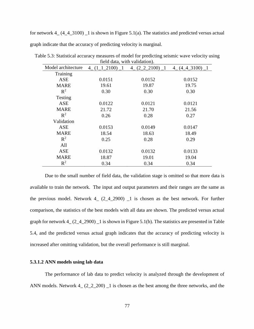
77

for network 4_ (4_4_3100) _1 is shown in Figure 5.1(a). The statistics and predicted versus actual

graph indicate that the accuracy of predicting velocity is marginal.

Table 5.3: Statistical accuracy measures of model for predicting seismic wave velocity using

field data, with validation).

Model architecture 4_ (1_1_2100) _1 4_ (2_2_2100) _1 4_ (4_4_3100) _1

Training

ASE 0.0151 0.0152 0.0152

MARE 19.61 19.87 19.75

R2 0.30 0.30 0.30

Testing

ASE 0.0122 0.0121 0.0121

MARE 21.72 21.70 21.56

R2 0.26 0.28 0.27

Validation

ASE 0.0153 0.0149 0.0147

MARE 18.54 18.63 18.49

R2 0.25 0.28 0.29

All

ASE 0.0132 0.0132 0.0133

MARE 18.87 19.01 19.04

R2 0.34 0.34 0.34

Due to the small number of field data, the validation stage is omitted so that more data is

available to train the network. The input and output parameters and their ranges are the same as

the previous model. Network 4_ (2_4_2900) _1 is chosen as the best network. For further

comparison, the statistics of the best models with all data are shown. The predicted versus actual

graph for network 4_ (2_4_2900) _1 is shown in Figure 5.1(b). The statistics are presented in Table

5.4, and the predicted versus actual graph indicates that the accuracy of predicting velocity is

increased after omitting validation, but the overall performance is still marginal.

5.3.1.2 ANN models using lab data

The performance of lab data to predict velocity is analyzed through the development of

ANN models. Network 4_ (2_2_200) _1 is chosen as the best among the three networks, and the

78

predicted versus actual graph is shown in Figure 5.1(c). The statistics and graph indicate that the

accuracy of the velocity predictions is good. The results compared in Table 5.4 also indicate that

the errors are much lower, and the R2 values are much higher for the network trained using lab

data compared to the network trained using field data.

The ANN models are developed to predict velocity without validation. Network 4_

(1_5_100) _1 is chosen as the best network among the three. Excluding the validation helps to

minimize the errors and increases the R2 values. Accordingly, the accuracy of the model is

improved without the validation stage. The predicted versus actual graph shown in Figure 5.1(d)

and the statistics presented in Table 5.4 indicate that the accuracy of the velocity predictions is

good. The results also show that the errors are much lower, and the R2 values are much higher for

the network trained using lab data in comparison to the network trained using field data.

5.3.1.3 ANN models using field and lab data

The ANN models are developed using field and lab data together to predict the seismic

wave velocity. LL, plasticity index, water content, and dry density are used as input parameters.

The best three models are selected for further analysis based on minimum ASE, minimum MARE,

maximum R2, and opt hidden nodes. Among those three models, network 4_ (1_2_2900) _1 gives

the minimum ASE, minimum MARE, and maximum R2 in validation. So, network 4_ (1_2_2900)

_1 is chosen as the best network. The statistics are shown in Table 5.4. and the predicted versus

actual graphs for the best network shown in Figure 5.1(e). indicates that the accuracy is marginal.

The errors are higher even though the R2 values improve after combining lab and field data in

comparison to the models trained with lab and field data separately.

The ANN model for field and lab data combined are also developed without the validation

stage. Network 4_ (5_10_20000) _1 is chosen as the best network and had significantly smaller

79

errors and increased R2 values than the model with validation. The predicted versus actual graph

is shown in Figure 5.1(f) and the statistics indicate that predicting velocity is good.

The comparison of the results in Table 5.4 indicates that the errors are higher, and the R2

values are lower for the network trained using field data, and the errors are lower and the R2 values

are higher for the network trained using lab data. The statistical measures for the network trained

using field data and lab data together are in between the network statistics of lab data and field

data.

Table 5.4: Comparing ANN models (predicting seismic wave velocity).

Model Model structure ASE MARE R2

Field with validation 4_ (4_4_3100) _1 0.0133 19.04 0.34

without validation 4_ (2_4_2900) _1 0.0128 19.34 0.37

Lab with validation 4_ (2_2_200) _1 0.0079 14.86 0.71


Field plus Lab with validation 4_ (1_2_2900) _1 0.0174 30.75 0.50


80

(a) (b)

(c) (d)

(e) (f)

Figure 5.1: Graphical prediction accuracy of model for predicting seismic wave velocity, (a)

field, with validation, (b) field, without validation, (c) lab, with validation, (d) lab, without

validation, (e) field plus lab, with validation, (f) field plus lab, without validation

5.3.2 ANN models for predicting water content

ANN models are developed to predict water content using lab and field data separately and

together. The models are developed without validation. Six different models are developed

81

without validation and models are developed with and without velocity as input to evaluate if

velocity helps in predicting water content.

5.3.2.1 Using field data with velocity

ANN models are developed using field data to predict water content from LL, plasticity

index, velocity and dry density. Network 4_ (1_5_100) _1 is chosen as the best performing

network. The predicted versus actual graph for the best network is shown in Figure 5.2(a) and the

statistics presented in Table 5.5 indicate that the accuracy of predicting velocity is good.

With the same number of classified data and ranges, ANN models are developed to predict

water content but omitting seismic wave velocity from the input parameters. Network 3_

(2_3_1000) _1 is chosen as the best performing model among the three. The predicted versus

actual graph is shown in Figure 5.2(b) and the statistics presented in Table 5.5 indicate good

accuracy in predicting water content. The results presented in Table 5.5 indicate that the errors

increase and the R2 value decreases when the velocity is omitted as input. So, the results indicate

that including seismic wave velocity improves the prediction of water content.

5.3.2.2 Using lab data

ANN models are developed using lab data to predict water content from LL, plasticity

index, velocity and dry density. Network 4_ (3_3_100) _1 is chosen as best networks and the

statistics are shown in Table 5.5. The predicted versus actual graphs are shown in Figure 5.2(c)

and statistics indicate that the accuracy of predicting moisture content is high. The results

compared in Table 5.5 also indicate that the errors are much lower and the R2 values are much

higher using lab data in comparison to using field data.

82

Excluding seismic wave velocity from input parameters but keeping the other parameters

and ranges, the same ANN network 3_ (4_4_100) _1 is chosen as the best performing model. The

predicted versus actual graph for the best network is shown in Figure 5.2(d) and the statistics

indicate good accuracy in predicting water content. After omitting velocity from the input

parameters, the errors increase and the R2 value decreases. So, the results compared in Table 5.5

indicate that seismic wave velocity helps to predict water content. The results also indicate that the

errors are much lower and the R2 values are much higher for the network built using lab data in

comparison to the network built using field data.

5.3.2.3 Using field plus lab data

Lab and field data are combined to develop ANN models to predict water content from LL,

PL, dry density, velocity. Network 4_ (3_3_1000) _1 is the best network and the predicted versus

actual graph, shown in Figure 5.2(e), and statistics indicate that the accuracy of predicting water

content is good. The results indicate that the errors are higher and the R2 values are lower for the

network built using field data and lab data together in comparison to the network built using lab

data and field data separately. So mixing field and lab data together lowers the performance of the

model.

83

(a) (b)

(c) (d)

(e) (f)

Figure 5.2: Graphical prediction accuracy of model for predicting moisture content, (a) field,

with velocity, (b) field, without velocity, (c) lab, with velocity, (d) lab, without velocity, (e) field

plus lab, with velocity, (f) field plus lab, without velocity.

84

The predicted versus actual graph for the best network omitting seismic wave velocity from

the input parameters is shown in Figure 5.2(f). The statistics indicate good accuracy in predicting

water content. After omitting velocity from the input parameters, the ASE has increased, even

though the MARE has decreased and the R2 value has increased. So, the results do not clearly

indicate whether the seismic wave velocity helps to better predict water content. The results are

almost the same for the model built using field data and field data and lab data together. But the

errors are much lower and the R2 values are higher for the network built using lab data in

comparison to the network built using field and lab data together.

Table 5.5: Comparing ANN models (predicting water content).


Field with velocity 4_ (1_5_100) _1 0.0051 7.78 0.85

without velocity 3_ (2_3_1000) _1 0.0087 10.68 0.75

Lab with velocity 4_ (3_3_100) _1 0.0043 6.63 0.89


Field plus Lab with velocity 4_ (3_3_1000) _1 0.0083 11.61 0.67


5.3.3 ANN models for predicting dry density

ANN models are developed to predict dry density using lab and field data separately and

together. Due to the limited amount of data the validation step is omitted for these models to

reserve more data for training for better accuracy. Six different models are developed with varying

input parameters.

5.3.3.1 Using field data

Dry density is predicted using LL, plasticity index, velocity and water content. Network 4_

(3_5_100) _1 is the best performing network and the predicted versus actual graph, shown in

85

Figure 5.3(a), and the statistics presented in Table 5.6 indicate that the accuracy of predicting the

dry density is high.

Using the same data set but omitting seismic wave velocity from the input parameters,

network 3_ (4_4_2000) _1 is the best performing model. The predicted versus actual graph is

shown in Figure 5.3(b), and the statistics indicate good accuracy in predicting dry density.

Omitting velocity from the input parameters causes the errors to increase and the R2 value to

decrease significantly. The conclusion is that seismic wave velocity helps to predict dry density.

5.3.3.2 Using lab data

The best network and statistics using laboratory LL, plasticity index, velocity and water

content as input parameters to predict dry density are shown in Table 5.6. The predicted versus

actual graph is shown in Figure 5.3(c), and the statistics indicate that the accuracy of predicting

dry density is high. Compared to the lab data in Table 5.6, the errors are lower and the R2 values

are higher for the network built using field data.

Keeping the other criteria the same and excluding velocity to predict dry density is best

represented by network 3_ (4_4_500) _1. The statistics are shown in Table 5.6, and the predicted

versus actual graph is shown in Figure 5.3(d). The statistics indicate good accuracy in predicting

dry density. Omitting velocity from the input parameters, the errors decrease and the R2 increases,

as shown in Table 5.6. But the differences are not that significant. The results indicate that

including seismic wave velocity does not enhance the prediction of dry density using lab data. The

results of the without velocity models also indicate that the errors are lower and the R2 values are

higher for the network built using lab data in comparison to the network built using field data.

86

5.3.3.4 Using field plus lab data

Network 4_ (9_9_400) _1 is chosen as the best ANN model when using field and lab data

to predict dry density and the velocity is included as input. The predicted versus actual graph is

shown in Figure 5.3(e).and the statistics are presented in Table 5.6. The accuracy of predicting dry

density is good, but the errors are higher and the R2 values are lower in comparison to the network

built using lab data and field data separately. So mixing field and lab data together lowers the

performance of the model.

The best ANN model developed using field and lab data and omitting seismic wave

velocity is represented by network 3_ (3_11_19800) _1. The predicted versus actual graph shown

in Figure 5.3(f) and the statistics indicate good accuracy in predicting dry density. Omitting

velocity from the input parameters results in ASE increases and R2 value decreases, even though

MARE decreases. So, the results do not indicate clearly that seismic wave velocity helps to predict

dry density.

Table 5.6: Comparing ANN models (predicting dry density).


Field with velocity 4_ (3_5_100) _1 0.0032 1.81 0.91


Lab with velocity 4_ (4_4_100) _1 0.0056 2.52 0.85


Field plus Lab with velocity 4_ (9_9_400) _1 0.0077 3.00 0.78


87

(a) (b)

(c) (d)

(e) (f)

Figure 5.3: Graphical prediction accuracy of model for predicting dry density, (a) field, with

velocity, (b) field, without velocity, (c) lab, with velocity, (d) lab, without velocity, (e) field plus

lab, with velocity, (f) field plus lab, without velocity.

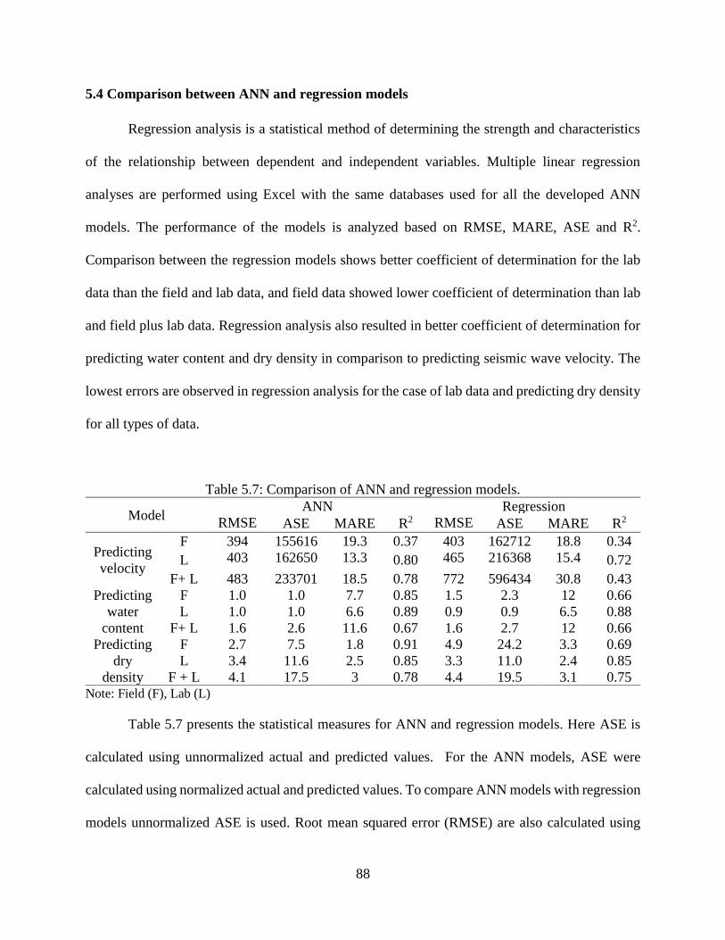
88

5.4 Comparison between ANN and regression models

Regression analysis is a statistical method of determining the strength and characteristics

of the relationship between dependent and independent variables. Multiple linear regression

analyses are performed using Excel with the same databases used for all the developed ANN

models. The performance of the models is analyzed based on RMSE, MARE, ASE and R2.

Comparison between the regression models shows better coefficient of determination for the lab

data than the field and lab data, and field data showed lower coefficient of determination than lab

and field plus lab data. Regression analysis also resulted in better coefficient of determination for

predicting water content and dry density in comparison to predicting seismic wave velocity. The

lowest errors are observed in regression analysis for the case of lab data and predicting dry density

for all types of data.

Table 5.7: Comparison of ANN and regression models.

Model ANN Regression

RMSE ASE MARE R2 RMSE ASE MARE R2

Predicting

velocity

F 394 155616 19.3 0.37 403 162712 18.8 0.34

L 403 162650 13.3 0.80 465 216368 15.4 0.72

F+ L 483 233701 18.5 0.78 772 596434 30.8 0.43

Predicting

water

content

F 1.0 1.0 7.7 0.85 1.5 2.3 12 0.66

L 1.0 1.0 6.6 0.89 0.9 0.9 6.5 0.88

F+ L 1.6 2.6 11.6 0.67 1.6 2.7 12 0.66

Predicting

dry

density

F 2.7 7.5 1.8 0.91 4.9 24.2 3.3 0.69

L 3.4 11.6 2.5 0.85 3.3 11.0 2.4 0.85

F + L 4.1 17.5 3 0.78 4.4 19.5 3.1 0.75 Note: Field (F), Lab (L)

Table 5.7 presents the statistical measures for ANN and regression models. Here ASE is

calculated using unnormalized actual and predicted values. For the ANN models, ASE were

calculated using normalized actual and predicted values. To compare ANN models with regression

models unnormalized ASE is used. Root mean squared error (RMSE) are also calculated using

89

Equation 4.1 to compare ANN and regression models. For all the cases, ANN models resulted in

better R2 values and less error in comparison to regression analysis. Significant improvements are

observed for the case of field data for predicting water content, dry density and for field & lab data

for predicting seismic wave velocity. So it appears that ANN shows better accuracy in prediction

in comparison to regression analysis.

5.5 Conclusion

The aim of this study is to predict geotechnical parameters from seismic wave velocity and

other geotechnical parameters using a published data set. ANN and regression models are

developed to predict seismic wave velocity from geotechnical parameters and also to predict some

geotechnical parameters using seismic wave velocity in conjunction with other geotechnical

parameters. The geotechnical parameters used here are plasticity index, LL, dry density, and water

content.

The standard procedure for ANN model development is training, testing, and validation.

Due to the limited amount of data, the validation step is ignored in some cases to use more data

for training. The statistics indicated that the performance of the models are improved by using

more data for training as shown in Table 5.4 and Figure 5.1. Both laboratory and field data are

analyzed separately and combined. The correlation between parameters for lab data is better in

comparison to field and field plus lab data for both ANN and regression. The coefficient of

determinations are higher, and RMSE, ASE, MARE are lower for ANN models than the regression

models.

For most cases, the seismic wave velocity helps to predict water content and dry density.

The results showed promising statistics for seismic wave velocity prediction models as a cost-

90

effective, less time-consuming, and non-destructive way to collect soil information for engineering

design and analysis of infrastructures.

91

6. CHAPTER 6

PREDICTING GEOPHYSICAL PARAMETERS FROM GEOTECHNICAL PARAMETERS

6.1 Introduction

Geological and geotechnical engineers work in close cooperation to cover the essential

investigation and analysis for civil engineering projects such as earth dam analysis, landslide

evaluation, slope stability analysis, factor of safety evaluation for foundations, etc. Both are an

integral part of a design team to complete a project. Soil parameters investigated by geotechnical

methods are used for the design of foundations, retaining walls, dams, levees and so on.

Geotechnical investigations are precise but are point measurements based on drilled boreholes and

laboratory measurements on disturbed and undisturbed soil samples collected from the field. For

a large construction area or already built infrastructure, the destructive nature and point based

approach of geotechnical methods can be time-consuming and sometimes impossible to carryout.

Geophysical investigations can, in many cases, create a map of the whole area without disturbing

the structure and in less time than geotechnical approaches. Using geophysical information in

engineering problems will help lower the project cost, and reduce completion time with higher

confidence.

In this chapter, the laboratory geophysical and geotechnical measurements described in

Chapter 3 are analyzed using ANN techniques. Geophysical and geotechnical experiments are

conducted on the same soil sample compacted according to the standard proctor method. Different

combinations of sand, silt and clay proportions are used to prepare clay and sandy-clay synthetic

92

samples

The dependence of the geophysical parameters (ER, P-wave velocity, and S-wave velocity)

on geotechnical parameters is examined. The ANN outputs are geophysical properties and the

inputs are various combinations of geotechnical properties. The analysis first examines the

dependence on individual geotechnical inputs. Then the analysis is generalized to include multiple

geotechnical inputs based on theoretical formulations in the literature, i.e., Archies’s Law,

Waxman Smith equation, Gassmann’s formulation. These models are subsequently modified by

replacing some of the geotechnical parameters with more easily obtainable geotechnical

parameters to evaluate optimal measurement approaches.

6.2 Data from Laboratory Measurements

The geotechnical measurements can be subdivided into two groups. The first group is

properties that depend solely on the soil type: soil mix proportions (SMP), Atterberg limits,

specific surface area, SG, and CEC. There are 26 independent measurements of each parameter

in this group. The second group of properties depends on the soil type and degree of compaction

associated with the proctor test: moisture content and dry density, void ratio, saturation, and

porosity. There are 155 measurements in this group. Cohesion is measured on a specific soil type

and compacted at opt or near opt moisture, so there are 26 measurements. The measurements are

compiled in Appendices A1 and A2. The data derived from the proctor test is further subdivided

into below opt moisture content (77 data), at opt moisture content (26 data) and above opt moisture

content (52 data). The geophysical measurements are a function of soil type and proctor

compaction. Geophysical measurements at opt moisture content are used when correlated with

the geotechnical measurements in group 1.

93

6.2.1 ER predictions from a Single Input

Statistics of ANN models to predict ER from individual geotechnical parameters are shown

in Table 6.1. The overall statistics show that ER has good correlation with water content and

saturation when all data are used for ANN model development. Other parameters show poor to

moderate correlation with ER. The reason is that each soil measurement has other parameters that

are changing. For at opt models, only 26 data are available. This limited amount of data could have

an adverse effect on the prediction accuracy. Parameters related to clay type properties show

relatively lower values than others.

Statistics of ANN models to predict ER using all data from water content show good

correlation of ER with water content. ANN models are also developed to predict ER from water

content by separately considering data at below opt, at opt, and above opt. The statistics show that

accuracy of the model is better at below opt in comparison to above opt. The reason is that when

the sample is close to full saturation (above opt), the conductivity remains fairly constant (Bai at

al., 2013). Figure 6.1 (a) shows that with the increase of water content, ER decreases significantly

below opt, but much less above opt. Increasing water content makes the sample more conductive

and reduces ER. Statistics of ANN models to predict ER from saturation using all data shows that

the accuracy of the model is good. Separate ANN models at below opt, at opt and above opt show

that performance of the model decreases at above opt for the same reason as the water content.

Figure 6.1 (b) shows that degree of saturation is inversely proportional to ER for the case of below

opt, at opt and above opt. Statistics presented in Table 6.1 show that CEC is moderately correlated

with ER. Figure 6.1 (c) shows that CEC is inversely correlated with ER. CEC is the capacity of

the soil to hold exchangeable cations. CEC increases with the increase of clay fraction. CEC is

94

also affected by the type of clay minerals. Large clay fraction in the soil makes the soil more

conductive and reduces ER.

Statistics show that PL can predict ER better than LL and that SL shows better accuracy

and good correlation with ER in comparison to LL and PL. Figures 6.1 (d), (e), (f) show that with

an increase of LL, PL, and SL, the ER decreases. The reason is that Atterberg limits are higher for

soils that contain higher percentages of fines or clay, and that tends to reduce the ER (Hassanein

et al., 1996). Statistics of the prediction model to predict ER from specific surface area shows that

ER is moderately correlated with specific surface area. Figure 6.2 (a) shows that ER decreases

with the increase of specific surface area. Specific surface area is correlated with clay size fraction

(Petersen et al., 1996). Clay soils with large specific areas need more water to reach the LL

(Mitchell and Soga, 2005). This means that with the increase of specific surface area, the electric

conductivity increases and resistivity decreases.

Statistics of the ANN model to predict ER from cohesion shows that ER is poorly

correlated with cohesion. There could be other influential parameters that are changing at the same

time that may be used as inputs to get better predictions. Figure 6.2 (b) shows that with an increase

of cohesion, the ER decreases. The reason is that cohesion is related to the amount of clay in the

soil and is positively correlated with the increase of clay fraction (Akayuli et al., 2013). With the

increase of clay fraction, electric conductivity increases so ER decreases. This makes cohesion

inversely proportional to ER.

ANN models to predict ER from dry density show poor correlation. ANN models at below

opt, at opt and above opt show that the sensitivity of the decreasing rate of ER is high at below

opt, and that above opt sensitivity of ER to dry density is very low. Figure 6.2 (c) shows that with

an increase of ER, dry density decreases for the case of below opt. But for at opt and above opt,

95

with the increase of dry density, ER increases. For below opt soil, with the increase of dry density,

water content increases and samples become more conductive so ER decreases. Therefore dry

density is inversely proportional relationship to ER. But at above opt, dry density decreases with

the increase of water content and the sample becomes more conductive, so ER decreases. This

indicates a directly proportional relationship between ER and dry density. ANN models built with

all data show that void ratio is moderately correlated with ER. Separate ANN models at below opt,

at opt and above opt predict less sensitivity of ER to void ratio at above opt in comparison to below

opt. Figure 6.2 (d) shows that ER is positively correlated with void ratio at below opt and at opt,

but above opt ER is negatively correlated with void ratio. At below opt, with the decrease of void

ratio water content increases, so the sample becomes more conductive and ER decreases. That’s

why at below opt, void ratio and ER are positively correlated. At above opt, with the increase of

void ratio , water content increases and ER decreases. This makes relationship between void ratio

and ER at above opt inversely proportional. Statistics of ANN models to predict ER from SG show

that there is almost no correlation between these two parameters. Figure 6.2 (e) implies the same

thing. So it appears that ER is most sensitive to water content and saturation, less sensitive to

parameters related to clay content and moisture such as CEC, Atterberg limits, surface area, even

less sensitive to dry density, void ratio, and cohesion, and shows almost no sensitivity to SG.

96

Table 6.1: Statistical accuracy of ANN models for predicting ER from single geotechnical

parameters.

Input ANN network ASE MARE R2

Water

content

All 1_ (5_5_1100) _1 0.0026 18.54 0.68

Below opt 1_ (3_12_20000) _1 0.0061 7.20 0.64

At opt 1_ (1_1_300) _1 0.0165 7.67 0.30

Above opt 1_ (6_6_1200) _1 0.0086 5.85 0.23

Saturation

All 1_ (12_12_100) _1 0.0038 25.40 0.56

Below opt 1_ (6_6_2100) _1 0.0077 11.05 0.44

At opt 1_ (6_7_100) _1 0.0204 7.63 0.17

Above opt 1_ (8_8_200) _1 0.0110 5.71 0.07

CEC At opt 1_ (1_5_100) _1 0.0117 19.47 0.38

LL At opt 1_ (2_2_3100) _1 0.0141 21.10 0.27

PL At opt 1_ (6_6_100) _1 0.0122 21.15 0.38

SL At opt 1_ (6_6_100) _1 0.0111 18.96 0.42

Surface area At opt 1_ (3_3_3100) _1 0.0138 21.02 0.26

Cohesion At opt 1_ (4_5_19100) _1 0.0150 20.56 0.19

Dry density

All 1_ (9_12_20000) _1 0.0069 35.23 0.17

Below opt 1_ (6_12_20000) _1 0.0199 4.54 0.13

At opt 1_ (1_3_100) _1 0.0225 3.94 0.18

Above opt 1_ (6_6_100) _1 0.0089 3.05 0.04

Void ratio

All 1_ (2_9_20000) _1 0.0067 35.32 0.20

Below opt 1_ (10_12_20000) _1 0.0177 10.34 0.14

At opt 1_ (1_1_1200) _1 0.0204 9.58 0.14

Above opt 1_ (2_9_2000) _1 0.0079 7.21 0.08

SG At opt 1_ (1_1_100) _1 0.0189 27.42 0.005

97

(a) (b)

(c) (d)

(e) (f)

Figure 6.1: ER versus (a) water content, (b) saturation, (c) CEC, (d) LL, (e) PL, (f) SL

98

(a) (b)

(c) (d)

(e)

Figure 6.2: ER versus (a) surface area, (b) cohesion, (c) dry density, (d) void ratio, (e) SG.

6.2.2 Predicting ER from Multiple Inputs

Archie’s (1942) first law is a relationship between the bulk resistivity of soil and the

porosity for a fully-saturated clean sand or coarse-grained material. This model assumes that the

primary pathway for electric current is through the pore fluid. For partially saturated sand,

Archie’s (1952) second law has an explicit dependence on saturation. This suggests that void ratio

and saturation would be good input parameters. The assumption of clean sand is usually not valid

for most soils because they contain clay minerals. The presence of clay minerals allows for electric

99

current to flow along the surface of the clay minerals. A measure of the clay might be accounted

for by using the soil mixture proportions as input. Waxman-Smits (1968) developed a relationship

for the effective electrical conductivity of soils that includes surface conduction. This surface

conduction is sometimes modeled to be proportional to the CEC of the soil. Therefore, the sample

CEC could be used as an input.

Various ANN models are developed for various combinations of void ratio, saturation,

soil mixture proportions and CEC. The statistics of these ANN models, shown in Table 6.2.,

indicate that ANN model accuracy is higher when using multiple geotechnical parameters as input.

At first, following Archie’s second law, ER is predicted from void ratio and saturation. Statistics

show that the accuracy of predicting ER from void ratio and saturation is high. To increase the

prediction accuracy of the model, SMP is added as input and the results show that the accuracy of

the model in predicting ER is improved. Following the Waxman Smits relationship, the CEC could

be an important parameter. Two different models are developed without the soil type and then with

soil type. After adding CEC with void ratio and saturation, the accuracy of the model increased

and, after adding soil properties, the statistics show that the accuracy of the model in predicting

ER is very high. This agrees with Waxman-Smits’s law of predicting ER for soil with clay fraction.

As correlation between ER and void ratio is moderate (Table 6.1), another model is

developed to predict ER from CEC and saturation and SMP, but excluding void ratio. Statistics

show that the accuracy of the model is very close to the model for predicting ER with void ratio.

So the void ratio has less influence on ER in comparison to CEC and saturation.

Other ANN models are developed by replacing the geotechnical parameters with more easily

obtainable geotechnical parameters. It is assumed that void ratio can be replaced by dry density

and saturation by water content and the CEC by the different Atterberg limits: LL, PL or SL. The

100

statistics of these models are shown in Table 6.3. Statistics show that accuracy of the model in

predicting ER from dry density, water content, LL and SMP is high, but is lower than void ratio,

saturation, CEC and SMP model. After that LL is replaced by PL to observe the difference in

performance and the statistics show that accuracy of the model is improved. Replacing PL with

SL improves the performance of the model even more and is very close to void ratio, saturation,

CEC and SMP model. Replacing dry density by wet density shows that the performance of the

model in predicting ER from wet density, water content, SL and SMP is almost the same as the

model predicting ER from void ratio, saturation, CEC and SMP. Figure 6.3 shows the predicted

versus actual graph of these two models. The graphs show that the two graphs are almost identical.

So the best alternative combination is wet density, water content, SL and SMP. An ANN model is

developed exluding dry density to predict ER, and the statistics show that the accuracy of the

model has little change. Water content influences ER more in comparison to dry density. Several

other ANN models are developed to predict ER from different combinations of geotechnical

parameters. ER is predicted from saturation, SL, and SMP, and also from water content, CEC, and

SMP. The statistics show that the accuracy of both models is high. ER is also predicted from water

content, saturation, SL and SMP, and the accuracy of the model is very high - almost the same as

the model predicting ER from wet density, water content, SL and SMP.

101

Table 6.2 : Statistical accuracy measures of ANN models for predicting ER from multiple

geotechnical parameters (validation of Arcihe’s and Waxman smith’s formula)


Void ratio, saturation 2_ (2_12_20000) _1 0.0017 17.59 0.79

Void ratio, saturation, SMP 5_ (2_3_13100) _1 0.0012 16.42 0.85

Void ratio, saturation, CEC 3_ (2_7_20000) _1 0.0013 16.28 0.83

Void ratio, CEC, saturation, SMP 7_ (1_8_20000) _1 0.0007 13.78 0.90

Saturation, CEC, SMP 5_ (4_9_19100) _1 0.0009 15.91 0.88

Table 6.3: Statistical accuracy measures of ANN models for predicting ER from multiple

geotechnical parameters (using different combinations of geotechnical parameters as input)


Dry density, water content, LL, SMP 6_ (2_2_600) _1 0.0021 17.74 0.77 Dry density, water content, PL, SMP 6_ (5_7_14100) _1 0.0009 15.19 0.88

Dry density, water content, SL, SMP 6_ (1_12_5000) _1 0.0008 14.80 0.89 Wet density, water content, SL, SMP 6_ (4_12_5900) _1 0.0008 13.98 0.90

Water content, SL, SMP 5_ (9_10_7100) _1 0.0016 16.89 0.80 Saturation, SL, SMP 5_ (1_3_20000) _1 0.0012 16.93 0.84

Water content, CEC, SMP 5_ (5_11_1100) _1 0.0016 18.49 0.81 Water content, saturation, SMP 5_ (8_12_19200) _1 0.0008 14.93 0.89

(a) (b)

Figure 6.3: Predicted versus actual graph of predicting ER from (a) void ratio, saturation, CEC,

soil mix proportion, (b) wet density, water content, SL, soil mix proportion.

6.3 Predicting P-Wave

6.3.1 Single Input

The statistics of the ANN models are shown in Table 6.4. Overall statistics show that the

correlations are poor except for dry density and void ratio, specifically at opt. The experimental

setup is such that multiple parameters are varying at the same time. So it is expected that the

102

sensitivity will be less with individual parameters with P-wave velocity. At opt showed good

sensitivity because at opt there is less variability in comparison to below and above opt. There are

multiple points below opt and above opt for a single soil mix proportions with varying dry density

and water content, which is adding more variability. Even though in that case, at opt data are

limited and the presence of less variability is the reason for having better correlation than below

and above opt.

P-wave velocity is predicted from water content, dry density, void ratio and saturation

separately for the data at below opt, opt and above opt. Dry density has sensitivity at below opt

and above opt, with a good sensitivity at opt in comparison to below and above opt. Void ratio is

sensitive at opt and above opt. But the performance in predicting P-wave velocity from individual

geotechnical parameters is not good. Statistics show that saturation has sensitivity at below and at

opt and water content has sensitivity at below opt. The relationship pattern of P-wave velocity with

water content, dry density, void ratio and saturation are also analyzed. P-wave velocity depends

on bulk modulus, mass density and shear modulus. With the increase of dry density, P-wave

velocity increases because for fluid-filled particulate material like soil, bulk modulus is a function

of void ratio, bulk density of fluid, bulk density of skeleton, bulk density of solid grains, and mass

density is a function of fluid saturation, void ratio, density of fluid, and density of grains. Here, P-

wave velocity is dominated by bulk modulus more than mass density. Bulk modulus is inversely

proportional to void ratio. So velocity increases with the decreases of void ratio and increases with

the increases of dry density, as shown in Figures 6.4 (d) and (b). Bulk modulus is positively

correlated with saturation. That’s why with the increase of water content/ degree of saturation,

bulk modulus increases, which causes an increase of P-wave velocity as shown in Figures 6.4 (a)

and (b). Statistics show that LL, PL, SL, SG, specific surface area, and CEC are poorly correlated

103

with P-wave velocity. These geotechnical parameters are strongly dependent on the consistency

of the clay soils and clay fractions. Whereas P-wave velocity depends on lots of other factors also,

such as stiffness, mass density, confinement, stress, soil skeleton, etc., it is not possible to have

good correlation from those individual parameters with P-wave velocity. For this research

cohesion is determined from unconfined compression tests by compacting the separate sample

following the same water content and soil proportions with an aim to replicate the same sample

used for determining P-wave velocity. Statistics show cohesion is poorly correlated with P-wave

velocity. This could be a confinement issue, for a change in soil skeleton in the replicated soil

sample as well as other influencing parameters that need to be added to predict P-wave velocity.

So further ANN models are developed to predict P-wave velocity from multiple geotechnical

parameters.


single geotechnical parameters.


Dry density

Below opt 1_ (7_10_6100) _1 0.0108 11.50 0.14

At opt 1_ (2_4_8100) _1 0.0105 11.43 0.38

Above opt 1_ (2_4_20000) _1 0.0137 12.43 0.12

Void ratio

Below opt 1_ (1_1_100) _1 0.0125 12.42 0.01

At opt 1_ (2_4_7100) _1 0.0103 11.10 0.39

Above opt 1_ (2_5_500) _1 0.0257 18.26 0.12

Saturation

Below opt 1_ (3_3_19100) _1 0.0109 11.77 0.12

At opt 1_ (1_1_600) _1 0.0147 14.02 0.19

Above opt 1_ (1_1_400) __1 0.0161 13.96 0.04

Water content

Below opt 1_ (1_1_400) _1 0.0108 11.50 0.1

At opt 1_ (1_1_100) _1 0.0172 14.59 0.0004

Above opt 1_ (2_7_19900) _1 0.0155 13.08 0.03

LL At opt 1_ (4_4_600) _1 0.0171 14.57 0.0002

PL At opt 1_ (5_5_19600) _1 0.0168 14.16 0.005

SL At opt 1_ (4_4_5100) _1 0.0168 14.46 0.004

SG At opt 1_ (1_1_1100) _1 0.0170 14.41 0.0005


CEC At opt 1_ (1_1_8800) _1 0.0125 14.35 0.001

Cohesion At opt 1_ (1_1_100) _1 0.0292 185.07 0.003

104

(a) (b)

(c) (d)

Figure 6.4: P-wave velocity versus (a) dry density, (b) void ratio, (c) saturation, (d) water

content.

6.3.2 Multiple Input

P-wave velocity increases with the stiffness of the material and decreases with its mass

density (inertia). For fluid-filled porous media, the effective bulk modulus is provided by

Gassmann (see equation 2.25). Seismic wave propagation in granular materials like soil is more

complicated due to the complex behavior of the solid skeleton that depends on the “strength” of

the grain contacts. The grain contacts are influenced by the applied effective stress and internal

forces associated with capillary forces and electrical forces at the grain surface. The P-wave

velocity can also be dependent on the degree of compaction and cementation.

Based on the models for the individual parameters (Table 6.4), ANN models are developed

for dry density, water content and SMP as inputs. Separate ANN models are developed for the data

at below opt moisture, at opt moisture and above opt moisture. The statistics of the ANN models

are shown in Table 6.5. The statistics show that after adding multiple geotechnical parameters as

105

inputs, the prediction accuracy increases significantly. At first, P-wave velocity is predicted from

dry density, water content and SMP. At below opt, the accuracy of predicting ER is high. The

accuracy of the model for predicting P-wave velocity at opt is high in comparison to below opt.

Performance of the ANN model at above opt is moderate and accuracy is low in comparison to

below and at opt ANN models. After that, ANN models are developed to predict P-wave velocity

from void ratio, saturation and SMP. At below opt and opt, the accuracy of the model in predicting

P-wave velocity if high, and at above opt the accuracy is moderate. The at opt model shows the

best performance among the three models. And the performance of the models in predicting P-

wave from water content, dry density, void ratio, and saturation are very close to each other. Water

content, dry density, void ratio, saturation and SMP are combined to predict P-wave velocity. The

performance of the model did not improve after combining water content, dry density, saturation

and void ratio. Here, at below and at opt models showed better accuracy in predicting P-wave

velocity in comparison to ANN model at above opt.


multiple geotechnical parameters.


Dry density, water content,

SMP

Bellow opt 5_ (10_11_4100) _1 0.0032 6.40 0.74

At opt 5_ (4_5_900) _1 0.0030 5.80 0.84

Above opt 5_ (3_3_20000) _1 0.0081 9.42 0.49

Void ratio, saturation, SMP

Bellow opt 5_ (10_12_20000) _1 0.0030 6.15 0.76

At opt 5_ (6_7_100) _1 0.0039 6.07 0.79

Above opt 5_ (9_9_4300) _1 0.0089 9.77 0.45


void ratio, saturation, SMP

Bellow opt 7_ (7_8_2100) _1 0.0033 6.42 0.74

At opt 7_ (2_3_700) _1 0.0041 6.44 0.77

Above opt 7_ (3_3_2100) _1 0.0092 10.33 0.43

106

(a) (b) (c)

Figure 6.5: Predicted versus actual graph of predicting P-wave velocity from (a) dry density,

water content, void ratio, saturation, soil mix proportion at below opt, (b) opt, (c) above opt.

The predicted versus actual graph for predicting P-wave velocity from water content,

saturation, void ratio, dry density and SMP are shown in Figure 6.5. The graphs also show that

data are well aligned with a 45-degree line at below, at opt and scattered at above opt. From the

analysis, it is evident that P-wave velocity is correlated with water content, saturation, dry density,

saturation and SMP, all of which play an important role in predicting P-wave velocity. Though the

individual parameters do not show good performance combined, those parameters show high

accuracy in predictions. As all the parameters are changed together and they all are correlated with

P-wave velocity, using only one parameter to predict P-wave velocity cannot show good accuracy.

To get better accuracy in performance, influencing parameters should be combined as input for

predicting P-wave velocity.

6.4 Predicting S-Wave

6.4.1 Single Input

The statistics of the ANN models are shown in Table 6.6. Overall statistics show that the

correlations are poor. The experimental setup is such that multiple parameters are varying at the

same time. So it is expected that there will be less sensitivity with individual parameters with S-

wave velocity. At opt showed good sensitivity because at opt there is less variability in comparison

107

to below opt and above opt. There are multiple points at below and at above opt for a single soil

mix proportions with varying dry density and water content, which is adding more variability.

The statistics of the ANN models for individual geotechnical parameters are shown in

Table 6.6. S-wave velocity is also predicted from water content, dry density, void ratio and

saturation separately for the data at below opt, opt and above opt. Dry density and void ratio are

sensitive to S-wave velocity at opt. Statistics show that water content has sensitivity at below opt

and saturation has sensitivity at opt. The relationship pattern of S-wave velocity with water

content, dry density, void ratio and saturation are also analyzed. S-wave velocity does not depend

on bulk modulus like P-wave velocity but depends on shear modulus and mass density. S-wave is

more dominated by shear modulus than mass density. Mass density is a function of saturation and

void ratio. At the presence of water, the soil shear modulus of the granular skeleton remains

unaffected. So, shear modulus depends on void ratio. With the decrease of void ratio, shear

modulus increases which causes an increase of S-wave velocity. Dry density increases along with

S-wave velocity due to the decrease in void ratio. Saturation and water content are shown to be

inversely proportional to S-wave velocity because saturation is proportional to mass density and

mass density is inversely proportional to S-wave velocity.

Statistics show that LL, PL, SG, specific surface area and CEC are poorly correlated with

S-wave velocity. These geotechnical parameters are strongly dependent on the consistency of the

clay soils, and clay fractions. Whereas S-wave velocity depends on lots of other factors also, such

as stiffness, mass density, confinement, stress, soil skeleton, etc., it is not possible to have good

correlation from those individual parameters with S-wave velocity. Statistics show the sensitivity

of S-wave velocity to SL. For this research, cohesion is determined from unconfined compression

tests by compacting the separate sample following the same water content and soil proportions

108

with an aim to replicate the same sample used for determining S-wave velocity. Statistics show

cohesion is not correlated with S-wave velocity. This could be a confinement issue, for change in

soil skeleton in the replicated soil sample as well as other influencing parameters that need to be

added to predict S-wave velocity. So further ANN models are developed to predict S-wave velocity

from multiple geotechnical parameters.


single geotechnical parameters.


Dry density

Below opt 1_ (2_2_15100) _1 0.0006 10.80 0.01

At opt 1_ (1_2_400) _1 0.0123 9.57 0.16

Above opt 1_ (1_1_300) _1 0.0273 16.74 0.00003

Void ratio

Below opt 1_ (1_2_19800) _1 0.0064 10.86 0.02

At opt 1_ (1_6_1000) _1 0.0129 9.85 0.13

Above opt 1_ (5_5_6100) _1 0.0272 16.58 0.005

Saturation

Below opt 1_ (3_3_19100) _1 0.0065 10.75 0.002

At opt 1_ (3_3_400) _1 0.0132 10.04 0.10

Above opt 1_ (1_1_1100) _1 0.0272 16.87 0.009

Water content

Below opt 1_ (2_5_6700) _1 0.0047 10.13 0.27

At opt 1_ (1_1_100) _1 0.0148 10.59 0.003

Above opt 1_ (9_9_2100) _1 0.0268 16.55 0.02

LL At opt 1_ (1_6_20000) _1 0.0143 9.79 0.01

PL At opt 1_ (1_1_300) _1 0.0146 10.42 0.01

SL At opt 1_ (5_6_20000) _1 0.0119 8.82 0.17

SG At opt 1_ (1_1_300) _1 0.0146 10.46 0.02


CEC At opt 1_ (1_1_500) _1 0.0147 10.45 0.002

Cohesion At opt 1_ (6_6_20000) _1 0.0286 177.53 0.02

109

(a) (b)

(c) (d)

Figure 6.6: S-wave velocity versus (a) dry density, (b) void ratio, (c) saturation, (d) water

content.

6.4.2 Multiple input

For fluid-filled porous media, the description is provided by Gassmann (see equation 2.25)

and does not have a fluid effect on the shear modulus. However, the S-wave propagation in

granular materials is influenced by the applied effective stress and internal forces associated with

fluid capillary forces and electrical forces at the grain surface. The S-wave velocity can also be

dependent on the degree of compaction and cementation. Based on the models for the individual

parameters (Table 6.6), ANN models are developed for dry density, water content and SMP as

inputs. Statistics of the ANN models in predicting S-wave velocity are shown in Table 6.7.

110

Statistics show that after adding multiple parameters as input, the prediction accuracy increases

significantly.

At first S-wave velocity is predicted from water content, dry density and SMP. At below

opt, the accuracy of the model in predicting S-wave velocity is good. Statistics at opt show that

accuracy of the model is moderate. At above opt the accuracy of the ANN model is poor. After

that, S-wave velocity is predicted from void ratio, saturation and SMP. Similar phenomena are

observed as with the ANN models predicting S-wave velocity from dry density, water content, and

SMP. At below opt, the accuracy is good; at opt, the accuracy is moderate; and at above opt, the

accuracy is poor. Water content, dry density, void ratio, saturation and SMP are combined to

predict S-wave velocity. Statistics show that the performance did not improve after combining

water content, dry density, void ratio and saturation. SL is added along with the other geotechnical

parameters of the previous model. The statistics show that at below opt the performance of the

model did not improve but at opt and above opt the performance of the model improved

significantly. The predicted versus actual graph of predicting S-wave velocity from water content,

dry density, void ratio, saturation, SL and SMP are shown in Figure 6.7. Graphs show that the data

are aligned with 45-degree line with little scattering. At above opt, data are more scattered in

comparison to below and at opt. At above opt, most of the models show poor performance in

predicting S-wave velocity. From the analysis it is evident that S-wave velocity is correlated with

water content, saturation, dry density, saturation and SMP – all of which play an important role in

predicting S-wave velocity. Though the individual parameters did not show good performance,

combined those parameters showed high accuracy in predictions. As all the parameters are

changed together and they all are correlated with S-wave velocity, using only one parameter to

111

predict S-wave velocity cannot show good accuracy. To get better accuracy in performance,

influencing parameters should be combined as input for predicting S-wave velocity.


multiple geotechnical parameters.



soil mix proportion

Below opt 5_ (4_5_4100) _1 0.0022 7.22 0.66

At opt 5_ (3_3_5000) _1 0.011 8.52 0.24

At above opt 5_ (8_8_300) _1 0.026 16.66 0.03

Void ratio, saturation, soil

mix proportion

Below opt 5_ (1_2_20000) _1 0.0030 8.75 0.53

At opt 5_ (4_4_3800) _1 0.0109 8.58 0.25

At above opt 5_ (9_9_100) _1 0.0226 16.71 0.02


void ratio, saturation, soil

mix proportion

Below opt 7_ (2_2_20000) _1 0.0027 8.31 0.58

At opt 7_ (2_2_3900) _1 0.0106 8.21 0.27

At above opt 7_ (5_5_100) _1 0.0270 16.77 0.02


void ratio, saturation, SL,

soil mix proportion

Below opt 8_ (3_3_5100) _1 0.0032 9.02 0.51

At opt 8_ (1_3_100) _1 0.0072 8.09 0.53

At above opt 8_ (4_6_1100) _1 0.0141 10.74 0.49

(a) (b) (c)

Figure 6.7: Predicted versus actual graph of predicting S-wave velocity from (a) dry density,

water content, void ratio, saturation, SL, soil mix proportion at below opt, (b) at opt.

6.5 Conclusion

Three geophysical parameters - ER, P-wave and S-wave velocity - are predicted from

geotechnical parameters for clay and sandy clay soils through ANN model development.

112

The analysis shows that water content and saturation have good correlation with ER; CEC, LL,

PL, SL, surface area, void ratio have moderate correlation with ER; cohesion and dry density have

poor correlation with ER; and SG has almost no correlation with ER.

Water content and saturation are inversely correlated with ER. This is because an increase

of water content and saturation allows more current through the interconnecting pores and is

consistent with Archie’s Law. ER deceases as the LL, PL, SL, specific surface area, CEC, and

cohesion increase. These geotechnical parameters are correlated with clay fraction. With the

increase of clay fraction, LL, PL, SL, and specific surface area increase and make the sample more

conductive thereby reducing ER. With the increase of ER, dry density decreases for the case of

below opt. But at opt and above opt, with the increase of dry density ER increases. At below opt,

with the increase of dry density, water content increases, samples becomes more conductive, and

so ER deceases. But at above opt, dry density decreases with the increase of water content as the

sample is becoming more conductive, so ER deceases. The relationship of void ratio with ER is

just the opposite of dry density.

Multiple geotechnical parameters can predict ER with high accuracy. Prediction models of

ER from void ratio, CEC, saturation, SMP showed very high accuracy, which agrees with the

Waxman-Smits formula. Void ratio can be replaced by wet/ dry density, saturation by water

content, and CEC by Atterberg limits to predict ER with similar accuracy. Void ratio and dry

density are less sensitive to ER in comparison to saturation and water content.

Water content, dry density, saturation, and void ratio show poor correlation with P-wave

velocity when used individually. In general, P-wave velocity increases with an increase of water

content, dry density and saturation, and decreases with the increase in void ratio. Atterberg limits,

SG, specific surface area, and CEC are not sensitive to P-wave velocity. Cohesion did not show

113

sensitivity with P-wave velocity. After combining geotechnical parameters, the ANN prediction

models showed good accuracy in predicting P-wave velocity. P-wave velocity can be predicted

from water content, dry density, and SMP with high accuracy at below opt moisture content and

at opt but with moderate accuracy at above opt moisture content. Void ratio, saturation, and SMP

can also predict P-wave velocity with high accuracy at below and opt and moderate accuracy at

above opt. Combining water content, dry density, void ratio, saturation and soil mix proportion

did not improve the performance of predicting P-wave velocity.

Water content, dry density, saturation, and void ratio showed little sensitivity to S-wave

velocity when used individually. However, in general S-wave velocity increases with the increase

of dry density and decreases with the increase of water content, saturation and void ratio. Atterberg

limits, SG, specific surface area, and CEC are not sensitive to S-wave velocity, but SL has

sensitivity to S-wave velocity. Cohesion did not show sensitivity with S-wave velocity. After

combining geotechnical parameters, the ANN prediction models improved. S-wave velocity can

be predicted from water content, dry density, and SMP with good accuracy below opt water content

and with moderate accuracy at opt. Void ratio, saturation, and SMP can also predict S-wave

velocity with good accuracy at below opt moisture content and moderate accuracy at opt.

Combining water content, dry density, void ratio, saturation and soil mix proportion did not

improve the performance of predicting S-wave velocity.

114

7. CHAPTER 7

PREDICTING GEOTECHNICAL PARAMETERS FROM GEOPHYSICAL PARAMETERS

7.1 General

Correlations between geophysical and geotechnical parameters are necessary for optimal

use of geophysical information in engineering assessments. In this chapter, ANN models are

developed to evaluate the added benefit of including geophysical information to predict

geotechnical parameters. For example, to what accuracy can geophysical parameters along with

an estimate of the SMP be used to predict geotechnical parameters for a large area in order to

minimize the time and effort. Geophysical parameters, namely ER, S-wave, P-wave velocities,

are used separately as inputs for predicting geotechnical parameters. Geotechnical parameters of

interest are: Atterberg limits, SG, cohesion, CEC, surface area, water content, dry density, void

ratio, and saturation. ANN models are developed to predict individual geotechnical parameters

from one geophysical parameter and the SMP. The ANN models are then generalized to predict

multiple geotechnical parameters. For P-wave and S-wave velocity, ANN models are developed

separately for data at below opt moisture, at opt moisture content, and above opt moisture content.

7.2 Using ER as input

Chapter 6 described models to predict ER from individual geotechnical parameters. Water

content and saturation have good correlation with ER. LL, PL, SL, CEC, void ratio, and surface

area have moderate correlation, and cohesion and dry density showed poor correlation

115

Incorporating multiple parameters as input improved the performance of the prediction models. In

this section, the ER along with SMP are used as inputs to predict geotechnical parameters.

ER measurements at opt or near opt water content (total 26 data) are used for ANN model

development for cohesion and soil type related properties and do not change with compaction such

as: Atterberg limits (LL, PL, SL), SG, CEC, and specific surface area. As the number of data is

limited for these cases, the validation step is excluded in order to use more data for training. For

other geotechnical parameters, such as water content, dry density, void ratio and saturation, the

data at different compaction stages are used (155 data points), and the entire ANN model

development approach (training, testing, validation, all trained) is followed.

7.2.1 Single geotechnical output

The statistical accuracy of the ANN models for predicting individual geotechnical

parameters from ER along and SMP is shown in Table 7.1. The performance of the models varies

as expected. In general, it appears that properties related to clay content are the best, followed by

moisture related properties, and then porosity related properties. This agrees with the behavior of

ER for clay containing soils.

116

Table 7.1: Statistical accuracy measures of predicting single geotechnical parameters from ER

and SMP.

Input Output ANN network ASE MARE R2

SMP, ER LL 4_ (2_2_100) _1 0.0027 4.80 0.89

SMP, ER PL 4_ (1_6_100) _1 0.0013 2.80 0.95

SMP, ER SL 4_ (3_3_100) _1 0.0043 11.78 0.84

SMP, ER Cohesion 4_ (4_6_3100) _1 0.0018 48.12 0.93

SMP, ER Surface area 4_ (2_4_2100) _1 0.0014 5.23 0.93

SMP, ER CEC 4_ (5_5_300) _1 0.0046 7.65 0.86

SMP, ER Saturation 4_ (1_5_20000) _1 0.0040 7.59 0.78

SMP, ER Water content 4_ (10_10_7100) _1 0.0045 7.62 0.70

SMP, ER Dry density 4_ (1_3_20000) _1 0.0051 2.17 0.68

SMP, ER Void Ratio 4_ (7_8_20000) _1 0.0046 5.53 0.67

SMP, ER SG 4_ (1_1_200) _1 0.0118 0.65 0.29

ANN models for predicting LL, PL, and SL show high accuracy. Atterberg limits are the

water content limits that separate different phases of soil, such as semi-liquid, plastic and solid.

These parameters are very well related to soil type and clay content. ER is also sensitive to water

and clay content. So, predicting Atterberg limits from ER along with SMP gives high accuracy.

Table 7.1 shows the ASE, MARE and R2 values for the ANN model to predict cohesion.

SMP and the ER at opt or near opt moisture content (26 samples) are used. The statistics show

high accuracy of the model in predicting cohesion. High accuracy in predicting cohesion might

be attributed to the ER dependence on the surface conductivity of the cohesive soil.

Specific surface area also shows very high accuracy. Specific surface area of soil is related

to water holding capacity, permeability, and swelling properties, and is closely associated with the

ER sensitivity to the clay fraction.

The accuracy of the model for predicting CEC is also high. CEC is an important soil

parameter which correlates with soil index properties, surface area, cement stabilized soil and

swelling properties of bentonite. CEC depends on grain size distribution, the type and amount of

117

clay mineral, PH values, and the presence of organic matter. Since CEC is a time-consuming test,

the use of ER may help to predict CEC in the lab and evaluate the CEC for large field areas.

The prediction model for saturation also shows high accuracy and this supports the

relationship of the geotechnical parameters with the soil type and ER with water. Table 7.1 shows

that the accuracy of the model for predicting water content is high. ER, which is affected by the

water content, taken along with the soil mix proportions helps to predict water content. The models

built for predicting void ratio and dry density show less coefficient of determination in comparison

to the water content and saturation. This indicates lower sensitivity of ER to dry density and void

ratio in comparison to saturation and water content.

The model using the ER at opt moisture content and SMP to predict SG is moderate. This

means that there are other influential parameters that must be considered as inputs to increase the

accuracy of the model. Only ER and SMP cannot predict SG well.

7.2.2 Multiple geotechnical outputs

Based on the previous results the geotechnical parameters are grouped based on

dependence on clay, moisture content and void space. ER and SMP are used as inputs for

Atterberg limits. Three output parameters are predicted using four input parameters. The statistics

of the model shown in Table 7.2 indicate that ER and SMP are capable of predicting LL, PL, and

SL with high accuracy. The accuracy of the combined output model is within the single output

models. CEC is added to the output parameters now having four output parameters predicted from

four inputs. The accuracy of this model is higher than the previous model. Again the accuracy

lies with the model accuracy for the individual parameters.

118

Table 7.2: Statistical accuracy measures of predicting multiple geotechnical parameters from ER

and SMP


SMP, ER LL, PL, SL 4_ (2_2_100) _3 0.0037 8.10 0.86

SMP, ER LL, PL, SL, CEC 4_ (2_2_200) _4 0.0033 7.14 0.88

SMP, ER Water content, Saturation 4_ (4_5_20000) _2 0.0049 4.96 0.68

SMP, ER Dry density, Void ratio 4_ (4_5_19900) _2 0.0048 3.81 0.67

SMP, ER Water content, Dry density,

Void ratio, Saturation

4_ (1_3_20000) _4 0.0049 5.97 0.69

(a) (b)

(c) (d)

Figure 7.1: Predicted versus actual graph for predicting (a) LL, (b) PL, (c) SL, (d) CEC from soil

mix proportion and ER.

The graphs of predicted versus actual for the LL, PL, SL, and CEC are shown in Figure

7.1. Figure 7.1 (a) shows a scattering of two data on the upper side, but overall the pattern is

good. All the data are well aligned with the 45-degree line indicating the high accuracy of the

model.

119

Water content and saturation depend on moisture whereas void ratio and dry density are

based on porosity. The performance of the ANN model, shown in Table 7.2, is similar for both

sets of parameters. The accuracy is close to the models for the individual parameters. Given the

similarity in performance, a model is developed for water content, dry density, void ratio, and

saturation. The statistics of the model indicate that there is no loss in accuracy by going to four

output parameters. Figure 7.2 shows the predicted versus actual graph of water content, dry

density, saturation and void ratio of these models. Well aligned data with the 45-degree lines

indicates the good accuracy of the model.

(c) (d)

Figure 7.2: Predicted versus actual graph for predicting (a) water content, (b) dry density, (c)

saturation, (d) void ratio from soil mix proportion, LL and ER.

(a) (b)

120

7.3 Using P-wave as input

In Chapter 6 it is shown that Atterberg limits, SG, CEC, cohesion (unconfined shear

strength) and surface area have almost no correlation with P-wave velocity. P wave velocity

showed better dependence on water content, dry density, saturation and void ratio. In this section,

models are developed for predicting these properties from P wave velocity and SMP. ANN models

are developed separately for the data at below opt moisture content (77 data), at opt moisture (26

data) and above opt moisture content (52 data). Since the number of data at opt moisture is limited,

the validation step is excluded in the ANN approach.


The statistics of the models developed to predict water content, dry density, saturation and

void ratio from P-wave velocity are shown in Table 7.3. The models based on P wave velocity as

input are not as consistent as models using ER. The best models are for the dry density below and

at opt moisture content and the void ratio. This may be because the density is indicative of the

compaction which will be reflected in the soil stiffness that controls the P wave velocity.

Table 7.3: Statistical accuracy measures of predicting single geotechnical parameters from P-

wave velocity and SMP.


SMP, P Water content

Below opt 4_ (10_12_19900) _1 0.0106 9.08 0.37

At opt 4_ (1_1_100) _1 0.0105 6.15 0.53

Above opt 4_ (1_1_15100) _1 0.0063 4.84 0.43

SMP, P Dry density

Below opt 4_ (1_10_100) _1 0.0020 1.33 0.91

At opt 4_ (5_5_6100) _1 0.0035 1.57 0.86

Above opt 4_ (2_5_20000) _1 0.0040 2.17 0.56

SMP, P Saturation

Below opt 4_ (1_1_20000) _1 0.0093 12.19 0.31

At opt 4_ (1_1_100) _1 0.0179 7.98 0.33

Above opt 4_ (3_6_20000) _1 0.0051 3.93 0.56

SMP, P Void Ratio

Below opt 4_ (7_9_20000) _1 0.0048 7.78 0.61

At opt 4_ (1_5_1000) _1 0.0030 4.37 0.87

Above opt 4_ (4_5_19100) _1 0.0034 4.79 0.60

121

7.3.2. Multiple geotechnical outputs

Further ANN models are developed to predict multiple geotechnical parameters from P-

wave velocity and SMP. Water content and dry density are predicted together using a single ANN

model. The statistics of the model are shown in Table 7.4. The performance of the models is good

at predicting water content and dry density, and is within the statistics for the individual

predictions. The ANN models developed to predict saturation and void ratio perform similarly to

the better individual model (void ratio). Including a combination of outputs appears to produce

models that are more consistent across the compaction process. Figure 7.3 shows the predicted

versus actual graph of predicting water content, dry density, void ratio and saturation It can be

inferred from the graph that data are well aligned with a 45-degree line for dry density and void

ratio in comparison to water content and saturation.

Table 7.4: Statistical accuracy measures of predicting multiple geotechnical parameters from p-



SMP, P Water content,

Dry density

Below opt 4_ (3_3_1100) _2 0.0071 5.68 0.60

At opt 4_ (5_5_900) _2 0.0067 3.75 0.70

Above opt 4_ (7_7_19100) _2 0.0045 3.14 0.55

SMP, P Saturation, void

ratio

Below opt 4_ (1_3_8100) _2 0.0048 7.10 0.67

At opt 4_ (1_2_1000) _2 0.0066 5.25 0.71

Above opt 4_ (1_9_20000) _2 0.0030 3.70 0.70

122

(a) (b)

(c) (d)

Figure 7.3: Predicted versus actual graph at opt for predicting (a) water content, (b) dry density,

(c) saturation, (d) void ratio from soil mix proportion and P-wave velocity.

7.4 Using S-wave as input

The S-wave velocity is most commonly correlated with a cone penetration test. In Chapter

6, water content, dry density, saturation and void ratio provided the best results for predicting S

wave velocity. In this section, the use of S wave velocity in combination with the soil mixture

proportions is used to predict water content, dry density, saturation and void ratio at opt moisture

content.


The statistics of the models developed to predict water content, dry density, saturation and

void ratio from S-wave velocity are shown in Table 7.5. Much like the P wave velocity, the S

123

wave velocity is better suited for predicting the dry density and void ratio than moisture content

and saturation. Dry density at opt, which is an indicator of optimal compaction, is best correlated

with P-wave velocity (0.86), followed by S wave velocity (0.78) and finally ER (0.68). S-wave

velocity predicts dry density and void ratio better than ER, and ER predicts water content and

saturation better than S-wave velocity.

Table 7.5: Statistical accuracy measures of predicting single geotechnical parameters from S-



SMP, S Water content At opt 4_ (5_5_300) _1 0.0092 5.82 0.55

SMP, S Dry density At opt 4_ (1_1_200) _1 0.0060 2.23 0.78

SMP, S Saturation At opt 4_ (1_6_9100) _1 0.0073 5.90 0.49

SMP, S Void Ratio At opt 4_ (2_2_100) _1 0.0077 6.38 0.72

7.4.2. Multiple geotechnical outputs

The accuracy of models for predicting multiple geotechnical parameters from soil mixture

proportions and S-wave velocity at opt is presented in Table 7.6. The model for predicting water

content and dry density is good and within the performance of the individual models. The

performance of the model for predicting saturation and void ratio is improved relative to predicting

separately. Figure 7.4 shows the predicted versus actual graph of predicting water content, dry

density, void ratio and saturation. It can be inferred from the graph that data is better aligned with

a 45-degree line for dry density and void ratio in comparison to water content and saturation.

Table 7.6: Statistical accuracy measures of predicting multiple geotechnical parameters from S-



SMP, S Water content, Dry density At opt 4_ (5_5_100) _2 0.0086 4.22 0.63

SMP, S Saturation, Void Ratio At opt 4_ (5_6_100) _2 0.0047 4.20 0.81

124

(a) (b)

(c) (d)

Figure 7.4:versus actual graph at opt for predicting (a) water content, (b) dry density, (c)

saturation, (d) void ratio from soil mix proportion and S-wave velocity.

7.5 Conclusion

ANN models for predicting LL, PL, SL, water content, saturation, CEC, cohesion, and

surface area from ER and SMP showed high accuracy due to the sensitivity of ER to clay and

water. Dry density (R2 = 0.68) and void ratio (R2 = 0.67) showed good accuracy and SG (R2 =

0.29) showed moderate accuracy. From the statistics of the ANN models, ER is more sensitive to

water content and saturation in comparison to dry density and void ratio. Accuracy of the final

ANN models for predicting multiple geotechnical parameters showed accuracy in between the

ANN models for predicting single geotechnical parameters.

Analysis shows that P-wave is more sensitive to dry density and void ratio in comparison

to water content and saturation. ANN models for predicting water content and dry density together

125

from P-wave velocity performance is in between the performance of the individual prediction

model. The performance of the ANN models for predicting saturation and void ratio together is

better than individual prediction model.

Similar to the P-wave velocity, the S-wave is more sensitive to dry density and void ratio

in comparison to water content and saturation. Performance of predicting multiple geotechnical

parameters (water content and dry density) show performance in between the performance of

individual parameter prediction. Performance of predicting multiple geotechnical parameters

(saturation and void ratio) show better performance than individual parameter prediction. ANN

models for predicting dry density and void ratio from P-wave velocity is better than the models

based on the S-wave velocity. ER predicts water content and saturation better than P-wave

velocity, and P-wave velocity predicts void ratio and dry density better than ER. Similarly, ER

predicts water content and saturation better than S-wave velocity, and S-wave velocity predicts

void ratio and dry density better than ER. Therefore, there could be advantages to using all three

geophysical properties as a combined input. This is discussed in the next chapter.

126

8. CHAPTER 8

PREDICTING GEOTECHNICAL PARAMETERS FROM COMBINED/MULTIPLE

GEOPHYSICAL PARAMETERS

8.1 General

Erosion, excessive pore water pressure and ground water seepage are very common causes

of earth dam failure. Compaction plays a very important role in earth dam construction and the

maximum dry density at opt water content is an important parameter during construction. Dams

are compacted within specified ranges of the maximum dry density. During operation, the loss

of fine materials increases the void ratio and permeability which can lead to enhanced seepage and

soil piping. Eventually this can lead to failure of the dam by internal erosion.

Geophysical methods can be used to provide a qualitative assessment of the earth dam by

providing internal images of the structure. This information can supplement geotechnical

information by providing continuous spatial data of the internal structure. Correlations between

geophysical and geotechnical parameters allow for a more thorough assessment of the condition

of the earth dam.

Interpretation of geophysical data can lead to multiple scenarios. In other words, the

solution is not unique. For example, consider the impact of loss of fine material on the ER.

Assuming the zone is fully saturated, this loss of fines increases the porosity and causes a decrease

in ER (Archie’s Law); however, the loss fines is a loss of clay and should therefore increase the

127

ER. One approach to reduce this non-uniqueness is to use information from multiple geophysical

methods. In this chapter, water content, dry density, saturation and void ratio are predicted by

combining geophysical parameters.

It was shown in Chapter 6 and 7 that water content, dry density, saturation and void ratio

have correlations with ER, S-wave and P-wave velocity. It was further shown that using the SMP

can increase the performance of the models. For earthen dams, the SMP is fairly well constrained

for the various parts of the dam. However, this approach would assume that these properties are

constant within each section of the dam which could be a source of error.

8.2 Predicting Water Content

In Chapter 7, ANN models were developed to predict water content using only one

geophysical parameter at a time, with and without the use of soil mixture proportions. A summary

of the best models is shown in Table 8.1. The best model using one geophysical parameter is with

ER. The addition of SMP increases the performance of the model.

128

Table 8.1 :Summary of predicting water content from individual geophysical parameter and SMP


ER

Below opt 1_ (3_12_20000) _1 0.0061 7.20 0.64

At opt 1_ (1_1_300) _1 0.0165 7.67 0.30

Above opt 1_ (6_6_1200) _1 0.0086 5.85 0.23

ER + SMP

Below opt 4_ (2_11_20000) _1 0.0035 5.21 0.79

At opt 4_ (6_6_100) _1 0.0104 6.46 0.55

Above opt 4_ (4_4_1300) _1 0.0069 5.09 0.38

P

Below opt 1_ (1_1_400) _1 0.0108 11.50 0.10

At opt 1_ (1_1_100) _1 0.0172 14.59 0.0004

Above opt 1_ (2_7_19900) _1 0.0155 13.08 0.03

P + SMP

Below opt 4_ (10_12_19900) _1 0.0106 9.08 0.37

At opt 4_ (1_1_100) _1 0.0105 6.15 0.53

Above opt 4_ (1_1_15100) _1 0.0063 4.84 0.43

S

Below opt 1_ (2_5_6700) _1 0.0047 10.13 0.27

At opt 1_ (1_1_100) _1 0.0148 10.59 0.003

Above opt 1_ (9_9_2100) _1 0.0268 16.55 0.02

S + SMP

Below opt 4_ (5_5_1100) _1 0.0129 10.28 0.25

At opt 4_ (5_5_300) _1 0.0092 5.82 0.55

Above opt 4_ (7_9_900) _1 0.0043 4.05 0.61

8.2.1 Combined geophysical parameters`

The statistics of ANN models for different combinations of geophysical parameters in

different compaction regimes, below opt moisture content, at opt moisture content and above opt

moisture content, are shown in Table 8.2. The better models are those that include ER as an input

and are compacted below opt moisture content. The addition of seismic information provides little

improvement on the models below opt. However, the use of S and P wave velocity in addition to

ER does improve the performance of the model at opt and above opt moisture content. Overall

the best model is obtained using all three geophysical parameters and, compared to Table 8.1, is

better than using ER individually - especially at and above opt moisture content.

129


geophysical parameters.


ER, S

Below opt 2_ (4_9_19900) _1 0.0057 6.97 0.66

At opt 2_ (1_1_200) _1 0.0191 8.26 0.30

Above opt 2_ (4_7_4200) _1 0.0077 5.79 0.30

ER, P

Below opt 2_ (3_9_20000) _1 0.0058 7.06 0.65

At opt 2_ (4_4_19700) _1 0.0129 7.14 0.34

Above opt 2_ (7_7_1100) _1 0.0085 5.86 0.23

S, P

Below opt 2_ (6_11_19100) _1 0.0117 9.52 0.31

At opt 2_ (3_4_16800) _1 0.0139 7.31 0.29

Above opt 2_ (3_9_5300) _1 0.0092 5.83 0.16

ER, S, P

Below opt 3_ (6_12_20000) _1 0.0057 6.80 0.66

At opt 3_ (3_6_100) _1 0.0086 6.17 0.57

Above opt 3_ (6_6_11000) _1 0.0067 5.09 0.39

Predicted versus actual graphs for predicting water content for the highest performance

networks at below opt, at opt and above opt are shown in Figure 8.1. Graphs show that some data

are scattered and not perfectly aligned with a 45-degree line. Including some other geotechnical

parameters may improve the performance.

(a) (b) (c)

Figure 8.1: Predicted versus actual graph for predicting water content from ER, S and P-wave

velocity at (a) below opt, (b) at opt, (c) at above opt.

130

The addition of the SMP increases the accuracy of all the models. The statistics of ANN

models to predict water content using the three geophysical parameter and SMP as input are shown

in Table 8.3. The statistics show that models including SMP have better performance. The use of

three geophysical inputs is most important for data above opt moisture content. The predicted

versus actual graph for these models are shown in Figure 8.2. The graphs show less scattering of

the data and are well aligned with the 45-degree line. Comparison of the graphs shown in Figure

8.1 (c) and Figure 8.2 (c) shows the improvement in model prediction when SMP is added as input.

Data are closer to the 45-degree and less scattered after adding geotechnical parameters as input.


geophysical and SMP.


Below opt ER, S, P, SMP 6_ (2_7_20000) _1 0.0036 5.46 0.79

At opt ER, S, P, SMP 6_ (5_5_100) _1 0.0086 5.89 0.57

Above opt ER, S, P, SMP 6_ (8_9_2100) _1 0.0031 2.99 0.72

(a) (b) (c)

Figure 8.2: Predicted versus actual graph for predicting water content from (a) ER, S, P-wave

velocity, SMP at below opt, (b) ER, S, P-wave velocity, SMP at opt, (c) ER, S, P-wave velocity,

SMP at above opt.

Table 8.1 shows that ER along with SMP at below opt shows better performance and S

along with SMP show better performance at opt and above opt. Comparison of these models with

the combination of three geophysical parameters along with SMP shows that significant

improvement is only observed at above opt.

131

8.3 Predicting Dry Density

ANN models were developed in Chapter 7 to predict dry density using only one

geophysical parameter at a time, with and without the use of SMP. A summary of the best models

is shown in Table 8.4. Models using a single geophysical input are poor. Addition of SMP provides

a large improvement when combined with any of the geophysical inputs. The best models are for

data below opt moisture content.

Table 8.4: Summary of predicting dry density from individual geophysical parameter and SMP


ER

Below opt 1_ (6_12_20000) _1 0.0199 4.54 0.13

At opt 1_ (1_3_100) _1 0.0225 3.94 0.18

Above opt 1_ (6_6_100) _1 0.0089 3.05 0.04

ER + SMP

Below opt 4_ (2_11_20000) _1 0.0014 1.01 0.93

At opt 4_ (1_3_100) _1 0.0080 2.52 0.70

Above opt 4_ (2_2_100) _1 0.0071 2.83 0.28

P

Below opt 1_ (7_10_6100) _1 0.0108 11.50 0.14

At opt 1_ (2_4_8100) _1 0.0105 11.43 0.38

Above opt 1_ (2_4_20000) _1 0.0137 12.43 0.12

P + SMP

Below opt 4_ (1_10_100) _1 0.0020 1.33 0.91

At opt 4_ (5_5_6100) _1 0.0035 1.57 0.86

Above opt 4_ (2_5_20000) _1 0.0040 2.17 0.56

S

Below opt 1_ (2_2_15100) _1 0.0006 10.80 0.01

At opt 1_ (1_2_400) _1 0.0123 9.57 0.16

Above opt 1_ (1_1_300) _1 0.0273 16.74 0.00003

S + SMP

Below opt 4_ (8_8_100) _1 0.003494 1.615 0.84

At opt 4_ (1_1_200) _1 0.0060 2.23 0.78

Above opt 4_ (3_3_100) _1 0.0066 2.71 0.28

8.3.1 Combined geophysical parameters

The statistics of ANN models to predict dry density for different combinations of

geophysical parameters for different compaction regimes (below opt moisture content, at opt

moisture content and above opt moisture content) are shown in Table 8.5. There is no consistent

trend in model improvements for the different compaction regimes. Based on ASE, MARE and R2

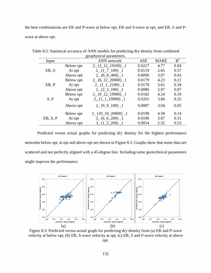
132

the best combinations are ER and P-wave at below opt, ER and S-wave at opt, and ER, S and P-

wave at above opt.




ER, S

Below opt 2_ (3_12_19100) _1 0.0217 4.77 0.04

At opt 2_ (1_7_100) _1 0.0119 2.65 0.57

Above opt 2_ (8_8_400) _1 0.0090 3.07 0.03

ER, P

Below opt 2_ (6_12_20000) _1 0.0179 4.23 0.21

At opt 2_ (1_1_2100) _1 0.0178 3.61 0.34

Above opt 2_ (2_3_100) _1 0.0086 2.97 0.07

S, P

Below opt 2_ (9_12_19900) _1 0.0182 4.24 0.19

At opt 2_ (1_1_19900) _1 0.0201 3.84 0.25

Above opt 2_ (9_9_100) _1 0.0087 3.04 0.05

ER, S, P

Below opt 3_ (10_10_20000) _1 0.0198 4.58 0.14

At opt 3_ (6_6_200) _1 0.0196 3.87 0.31

Above opt 3_ (1_5_200) _1 0.0054 2.55 0.53

Predicted versus actual graphs for predicting dry density for the highest performance

networks below opt, at opt and above opt are shown in Figure 8.3. Graphs show that some data are

scattered and not perfectly aligned with a 45-degree line. Including some geotechnical parameters

might improve the performance.

(a) (b) (c)

Figure 8.3: Predicted versus actual graph for predicting dry density from (a) ER and P-wave

velocity at below opt, (b) ER, S-wave velocity at opt, (c) ER, S and P-wave velocity at above

opt.

133

The statistics of ANN models to predict dry density using the best combination of

geophysical parameter determined above and SMP as input are shown in Table 8.6. The statistics

show that after including SMP as input, the performance of all the models improves. At below opt

and at opt, SMP makes the prediction accuracy significantly better, while at above opt, the

improvement is not that significant. The predicted versus actual graphs for these models are shown

in Figure 8.4. The graphs show less scattering of the data and are well aligned with a 45-degree

line. The improvements of the performance are observed after adding SMP as input from the

comparison of the graphs shown in Figure 8.3 (a) to Figure 8.4 (a) and also Figure 8.3 (b) to Figure

8.4 (b). Data are closer to a 45-degree line and less scattered after adding geotechnical parameters

as inputs.


geophysical and other geotechnical parameters.


Below opt ER, P, SMP 5_ (1_5_100) _1 0.0013 1.03 0.94

At opt ER, S, SMP 5_ (1_3_19100) _1 0.0038 1.65 0.86

Above opt ER, P, S, SMP 6_ (5_5_15200) _1 0.0041 2.14 0.56

(a) (b) (c)

Figure 8.4: Predicted versus actual graph for predicting dry density from (a) ER, P-wave

velocity, SMP at below opt, (b) ER, S-wave velocity, SMP at opt, (c) ER, S, P-wave velocity and

SMP at above opt.

134

8.4 Predicting Saturation

A summary of the best ANN models developed for predicting saturation using only one

geophysical parameter at a time, with and without the use of soil mixture, is shown in Table 8.7.

The best models include ER for compaction below opt, P-wave velocity for compaction at opt

moisture content and at above opt performances are very poor. The addition of SMP increases the

performance of the models.

Table 8.7: Summary of predicting saturation from individual geophysical parameter and SMP


ER

Below opt 1_ (6_6_2100) _1 0.0077 11.05 0.44

At opt 1_ (6_7_100) _1 0.0204 7.63 0.17

Above opt 1_ (8_8_200) _1 0.0110 5.71 0.07

ER + SMP

Below opt 4_ (1_3_6900) _1 0.0041 7.17 0.69

At opt 4_ (1_1_100) _1 0.0200 8.39 0.19

Above opt 4_ (4_4_4100) _1 0.0063 4.43 0.47

P

Below opt 1_ (3_3_19100) _1 0.0109 11.77 0.12

At opt 1_ (1_1_600) _1 0.0147 14.02 0.19

Above opt 1_ (1_1_400) __1 0.0161 13.96 0.04

P + SMP

Below opt 4_ (1_1_20000) _1 0.0093 12.19 0.31

At opt 4_ (1_1_100) _1 0.0179 7.98 0.33

Above opt 4_ (3_6_20000) _1 0.0051 3.93 0.56

S

Below opt 1_ (3_3_19100) _1 0.0065 10.75 0.002

At opt 1_ (3_3_400) _1 0.0132 10.04 0.10

Above opt 1_ (1_1_1100) _1 0.0272 16.87 0.009

S + SMP

Below opt 4_ (1_1_100) _1 0.0132 14.21 0.13

At opt 4_ (1_6_9100) _1 0.0073 5.90 0.49

Above opt 4_ (1_1_100) _1 0.0109 5.61 0.09

8.4.1 Combined geophysical parameters

The statistics of ANN models to predict saturation for different combinations of

geophysical parameters for different compaction regimes, below opt moisture content, at opt

moisture content and above opt moisture content, are shown in Table 8.8.

The better models for samples compacted below opt moisture content are those that include

ER. The addition of seismic information provides little improvement on the models below opt.

135

However, the use of S and P wave velocity in addition to ER does improve the performance of the

models at opt and above opt moisture content. Overall the best models are obtained using all three

geophysical parameters and are better than using just one geophysical input.




ER, S

Below opt 2_ (1_1_1800) _1 0.0078 11.14 0.45

At opt 2_ (1_6_100) _1 0.0117 5.49 0.54

Above opt 2_ (7_7_100) _1 0.0108 5.45 0.09

ER, P

Below opt 2_ (1_6_9000) _1 0.0065 10.12 0.53

At opt 2_ (3_6_100) _1 0.0110 5.72 0.56

Above opt 2_ (6_6_300) _1 0.0106 5.55 0.11

S, P

Below opt 2_ (3_5_2000) _1 0.0080 11.53 0.45

At opt 2_ (2_2_800) _1 0.0191 7.78 0.23

Above opt 2_ (2_2_600) _1 0.0115 5.81 0.03

ER, S, P

Below opt 3_ (5_13_100) _1 0.0055 9.22 0.66

At opt 3_ (5_7_100) _1 0.0105 5.14 0.59

Above opt 3_ (1_1_500) _1 0.0106 5.50 0.11

Predicted versus actual graphs for predicting saturation for the highest performance

networks at below opt, at opt and above opt are shown in Figure 8.5. Graphs show that some data

are scattered and not perfectly aligned with a 45-degree line. Including some geotechnical

parameters may improve the performance.

(a) (b) (c)


velocity at below opt, (b) at opt, (c) at above opt.

136

The statistics of ANN models to predict saturation using the three geophysical parameters

and SMP as inputs are shown in Table 8.9. The statistics show that after including SMP as input,

the performance of the model improves. The errors of the models decreased and R2 increased. At

below opt, SMP makes the prediction accuracy better; at opt and above opt, the performance

significantly improved after adding SMP as input. The predicted versus actual graphs for these

models are shown in Figure 8.6. The graphs show less scattering of the data and are well aligned

with a 45-degree line. The improvements in the performance are observed after adding SMP as

input from the comparison of the graphs shown in Figure 8.5 (b) to Figure 8.6 (b) and also Figure

8.5 (c) to Figure 8.6 (c). Data are closer to a 45-degree and less scattered after adding geotechnical

parameters as input.


geophysical and other geotechnical parameters.


Below opt ER, S, P, SMP 6_ (1_2_700) _1 0.0045 8.20 0.73

At opt ER, S, P, SMP 6_ (3_4_200) _1 0.0046 3.72 0.80

Above opt ER, S, P, SMP 6_ (8_8_7600) _1 0.0056 4.34 0.56

(a) (b) (c)


velocity, SMP at below opt, (b) ER, S and P-wave velocity, SMP at opt, (c) ER, S and P-wave

velocity, SMP at above opt.

137

Statistics of Table 8.7 show that ER along with SMP at below opt, S along with SMP at

opt, and P along with SMP at above opt show better performance. Comparison of these models

with the combination of three geophysical parameters along with SMP shows that at below opt

performance improves and at above opt performance improves significantly.

8.5 Predicting Void Ratio

A summary of the best ANN models developed to predict void ratio using only one

geophysical parameter at a time, is shown in Table 8.10. Models without SMP as input are rather

poor. Either geophysical parameter in conjunction with SMP produces models of moderate

performance.

Table 8.10: Summary of predicting void ratio from individual geophysical parameter and SMP


ER

Below opt 1_ (10_12_20000) _1 0.0177 10.34 0.14

At opt 1_ (1_1_1200) _1 0.0204 9.58 0.14

Above opt 1_ (2_9_2000) _1 0.0079 7.21 0.08

ER + SMP

Below opt 4_ (5_11_1000) _1 0.0012 2.60 0.93

At opt 4_ (1_1_100) _1 0.0089 6.66 0.66

Above opt 4_ (3_4_700) _1 0.0054 6.44 0.43

P

Below opt 1_ (1_1_100) _1 0.0125 12.42 0.01

At opt 1_ (2_4_7100) _1 0.0103 11.10 0.39

Above opt 1_ (2_5_500) _1 0.0257 18.26 0.12

P + SMP

Below opt 4_ (7_9_20000) _1 0.0048 7.78 0.61

At opt 4_ (1_5_1000) _1 0.0030 4.37 0.87

Above opt 4_ (4_5_19100) _1 0.0034 4.79 0.60

S

Below opt 1_ (1_2_19800) _1 0.0064 10.86 0.02

At opt 1_ (1_6_1000) _1 0.0129 9.85 0.13

Above opt 1_ (5_5_6100) _1 0.0272 16.58 0.005

S + SMP

Below opt 4_ (9_9_100) _1 0.0034 3.97 0.82

At opt 4_ (2_2_100) _1 0.0077 6.38 0.72

Above opt 4_ (2_2_100) _1 0.0070 6.83 0.25

138

8.5.1Combined geophysical parameters

The statistics of ANN models for void ratio for different combinations of geophysical

parameters and different compaction regimes are shown in Table 8.11. These models are better

than those using just one geophysical input.

Overall, the best models are obtained using ER and P-wave for at below opt, and ER, S and P-

wave for both at opt and above opt. The combination of ER and P-wave provides improvement to

the model below opt whereas the combination of all three geophysical parameters improves the

performance at opt and significantly improves the performance above opt moisture content.




ER, S

Below opt 2_ (11_12_20000) _1 0.0188 10.76 0.06

At opt 2_ (1_1_3100) _1 0.0146 8.47 0.38

Above opt 2_ (6_12_2900) _1 0.0069 6.64 0.20

ER, P

Below opt 2_ (1_5_20000) _1 0.0165 10.04 0.17

At opt 2_ (1_2_700) _1 0.0148 8.98 0.4

Above opt 2_ (4_7_6900) _1 0.0055 6.64 0.35

S, P

Below opt 2_ (1_2_16300) _1 0.0194 10.95 0.03

At opt 2_ (1_1_100) _1 0.0237 11.50 0.12

Above opt 2_ (3_3_5100) _1 0.0068 6.9 0.20

ER, S, P

Below opt 3_ (3_3_20000) _1 0.0188 10.84 0.05

At opt 3_ (6_6_300) _1 0.0142 9.23 0.40

Above opt 3_ (9_9_20000) _1 0.0042 5.86 0.50

Predicted versus actual graphs for predicting void ratio for the highest performance

networks at below, at opt and above opt are shown in Figure 8.7. Graphs show that some data are

scattered and not perfectly aligned with a 45-degree line.

139

(a) (b) (c)

Figure 8.7: Predicted versus actual graph for predicting void ratio from (a) ER and P-wave

velocity at below opt, (b) ER, S and P-wave velocity at opt, (c) ER, S and P-wave velocity at

above opt.

The statistics of ANN models for the best combination of geophysical parameters

determined above along with the SMP as input are shown in Table 8.12. The statistics show that

after including SMP as input, the performance of the models improves significantly at below opt,

at opt and above opt. The predicted versus actual graph for these models are shown in Figure 8.8.

The improvement of the performance is observed after adding SMP as input from the comparison

of the graphs shown in Figure 8.7 (a) to Figure 8.8 (a), Figure 8.7 (b) to Figure 8.8 (b) and also

Figure 8.7 (c) to Figure 8.8 (c). Data are closer to a 45-degree and less scattered after adding

geotechnical parameters as input.




Below opt ER, P, SMP 5_ (7_10_7200) _1 0.001 2.32 0.94

At opt ER, P, S, SMP 6_ (1_1_200) _1 0.0041 5.11 0.87

Above opt ER, P, S, SMP 6_ (4_5_2100) _1 0.0023 4.07 0.74

140

(a) (b) (c)

Figure 8.8: Predicted versus actual graph for predicting void ratio from (a) ER, P-wave velocity,

SMP at below opt, (b) ER, S, P-wave velocity, SMP at opt, (c) ER, S, P-wave velocity, SMP at

above opt.

Table 8.10 show that ER along with SMP at below opt shows better performance, and P

along with SMP show better performance both at opt and above opt. Comparison of these models

with the best combination of geophysical parameters along with SMP shows that significant

improvement is only observed at above opt.

8.6 Predicting Water Content, Dry density, Void ratio, Saturation from Combined

Geophysical Parameters

ANN models can predict several outputs up to the number of inputs. In Chapter 7 it was

shown that models with more outputs can perform better than models with a single output. Table

8.13 shows the statistics for models predicting all four geotechnical properties - moisture content,

void ratio, dry density and saturation - using the SMP and individual geophysical measurements.

All models are close in performance. The best model is for data below opt and using ER and SMP

as input. The models at opt are of intermediate performance using S wave velocity as input. The

models above opt have lower performance with the ER as input producing the best model.

141

Table 8.13: Summary of predicting water content, dry density, void ratio, saturation from

individual geophysical parameter and SMP.


ER + SMP

Below opt 4_ (10_10_20000) _4 0.0027 4.09 0.83

At opt 4_ (6_6_100) _4 0.0106 5.68 0.57

Above opt 4_ (8_9_1700) _4 0.0041 3.63 0.60

P + SMP

Below opt 4_ (6_7_1000) _4 0.0058 6.31 0.64

At opt 4_ (2_4_100) _4 0.0061 4.20 0.73

Above opt 4_ (5_7_300) _4 0.0045 3.81 0.57

S + SMP

Below opt 4_ (5_10_1000) _4 0.0046 5.51 0.74

At opt 4_ (3_4_2500) _4 0.0053 3.81 0.76

Above opt 4_ (8_10_100) _4 0.0051 4.27 0.49

Comparison of these models with the combination of three geophysical parameters shown in

Table 8.14 indicate slight improvement in performance. Below opt shows an increase in R2 of 0.02, no

change in R2 at opt and an increase in R2 of 0.09 above opt.

Table 8.14: Statistical accuracy of ANN models for predicting water content, dry density, void

ratio, saturation from combined geophysical parameters


ER+ P + S + SMP

Below opt 6_ (11_11_7000) _4 0.0022 3.65 0.86

At opt 6_ (6_6_600) _4 0.0055 3.93 0.76

Above opt 6_ (11_11_7000) _4 0.0031 3.16 0.69

8.6 Conclusion

Predicting water content using combinations of three geophysical parameters shows better

performance versus single parameters. At below opt, SMP makes the prediction accuracy better,

at opt the improvement is not that significant, and at above opt the performance is significantly

improved after adding SMP as input.

To predict dry density, the combination of ER and P-wave provides improvement on the

models below opt, a combination of ER and S-wave at opt, and a combination of three geophysical

parameters at above opt significantly improves the performance. Including SMP with the best

142

combinations makes prediction accuracy significantly better at below opt and at opt, whereas at

above opt, the improvement is not that significant.

To predict saturation, combinations of three geophysical parameters show better

performance, which is similar to water content predictions. At below opt, adding SMP makes the

prediction accuracy better; at opt and at above opt, the performance significantly improves after

adding SMP as input.

To predict void ratio, the combination of ER and P-wave provides improvement on the

models below opt. The combination of three geophysical parameters improves the performance

at opt, but significantly improves at above opt. By including SMP as input, the performance of the

models are improved significantly.

For predicting water content, dry density, void ratio, and saturation together from three

geophysical parameters along with SMP shows only a slight improvement in performance.

143

9. CHAPTER 9

CONCLUSION

.

9.1 Conclusion

In the past, most of the correlations between ER and geotechnical parameters were

developed using traditional regression analysis. An attempt was made to develop ANN models to

predict geotechnical parameters from ER and seismic wave velocity separately using existing data

sets in literature. Analysis of the published data set shows sensitivity of ER to CEC, saturation,

water content and dry density. Results of the ANN models developed using published seismic data

indicate that the performance of the models is improved after using more data for training. The

correlation between parameters for lab data was better in comparison to field and field plus lab

data. For most cases, the seismic wave velocity helps to predict water content and dry density, and

ANN shows better performance than regression for all the cases.

ANN models do predict correlations between geophysical and geotechnical parameters

with better accuracy than regression. However, the datasets are limited and a database of

laboratory measurements was collected where measurements were obtained on the same sample.

The soil types were constrained to typical materials used for the construction of earth dams - clay

and sandy clay soil types. The geotechnical measurements consisted of two groups. The first group

were properties that depend solely on the soil type: soil mix proportions (SMP), Atterberg

limits,specific surface area, SG, and CEC. There were 26 independent measurements for each

parameter in this group. The second group of properties depend on the soil type and the degree

144

of compaction associated with the proctor test: moisture content and dry density, void ratio,

saturation, and porosity. There were 155 measurements in this group. Cohesion was measured on

a specific soil type and compacted at opt or near opt moisture, so there are 26 measurements. The

geophysical measurements consisted of ER, S-wave and P-wave velocity, and there were 155

measurements.

ANN models were developed to predict geophysical parameters from geotechnical

parameters to assess the sensitivity of geotechnical parameters to ER, S-wave and P-wave velocity.

Models for ER versus water content and saturation had good performance; for ER versus CEC,

LL, PL, SL, surface area, and void ratio had moderate performance; for ER versus cohesion and

dry density had poor performance; and ER versus SG had almost no correlation. Combinations of

multiple geotechnical parameters were examined and revealed that ER could be predicted with

better accuracy.

Water content, dry density, saturation, and void ratio had little influence on P-wave and S-

wave velocity when used individually. However, after combining geotechnical parameters, the

ANN prediction models showed good accuracy in predicting P-wave velocity and S-wave velocity.

Atterberg limits, SG, specific surface area, and CEC did not affect the P-wave and S-wave velocity.

SL showed a little sensitivity to S-wave velocity. Somewhat unexpectedly, cohesion did not show

any influence on P-wave and S-wave velocity.

More applicable to problems of geotechnical assessment, ANN models were evaluated to

predict geotechnical parameters from geophysical parameters with and without soil mix

proportions as input. Incorporating soil mixture proportions significantly increased the

145

performance of the models. Using the soil mixture proportion appears feasible for earthen dams

where each section is built with known mixtures. For other situations, unknown variations in the

soil mixture proportions would lead to a source of error.

ANN models for predicting LL, PL, SL, water content, saturation, CEC, cohesion, and

surface area from ER and SMP showed high accuracy due to the sensitivity of ER to clay content

and water. Dry density (R2 = 0.68) and void ratio (R2 = 0.67) showed good accuracy, and SG

showed moderate accuracy.

P-wave and S-wave velocity showed moderate sensitivity to dry density and void ratio at

opt, but poor sensitivity to water content and saturation when individually predicted. But there is

no sensitivity to Atterberg limit, surface area, SG, and CEC. P-wave and S-wave do not show

sensitivity to cohesion due to the confining issue.

Multiple geotechnical were predicted from one geophysical input and SMP with good

accuracy. ANN models for predicting dry density and void ratio from P-wave velocity were better

than the models based on ER and the S-wave velocity. ER measurements predict water content

and saturation better than seismic measurements. Results varied depending on the state of

compaction, i.e. below opt moisture content, at opt or above opt moisture content. However such

results suggest there could be advantages to using multiple geophysical properties as a combined

input.

Subsequent analysis showed that the combination of three geophysical parameters

provided models with better performance at predicting water content and saturation. Dry density

was best predicted using a combination of ER and P-wave for soils compacted below opt, a

146

combination of ER and S-wave at opt, and a combination of three geophysical parameters at above

opt. To predict void ratio, the combination of ER and P-wave provided improvement on the

models below opt. Including SMP as input improves the performance of the models for all of the

cases.

The final analysis was predicting all four geotechnical properties (water content, dry

density, void ratio, saturation) using the three geophysical inputs along with SMP. These all-

encompassing models had high performance below opt (R2=0.82) and at opt ( R2=0.76), and

moderate performance at above opt moisture content (R2=0.69).

9.2 Recommendation for Future Research

For this research, variation in sand, silt and clay fractions within the clay and sandy clay

soil types are used for correlation development. Correlation should be developed for other soil

types. Two different types of clay, namely 80% kaolinite and 20% bentonite of the clay fraction,

are used for this research. Different mixing proportions of kaolinite and bentonite can be used for

further research. Synthetic soil samples are prepared through standard proctor compaction tests for

the current research. Correlation should be developed for actual field soils in either remolded or

undisturbed states.

The suite of geotechnical parameters could be expanded to include soil erodibility,

permeability, cohesion, and angle of friction. Additional parameters, such as those from a

penetration test that might be correlated with seismic wave velocity, should studied.

In this study, the proctor compaction test is used to prepare soil samples. This process

leads to changes in several soil properties from sample to sample, and does not allow for

investigating changes in only one soil parameter. Work could be conducted in triaxial cells to

examine the importance of effective stress and over burden pressure, which are important factors

147

for seismic wave velocity. Future work could focus on experiments isolating individual

parameters or replicating other soil processes. For example, samples could be produced by

reducing the fine content due to flushing with water.

148

REFERENCES

149

Abidin, M.H.Z., Saad, R., Ahmad, F., Wijeyesekera, D.C., and Yahya, A.S. 2013. “Soil moisture

content and density prediction using laboratory resistivity experiment.” IACSIT international

journal of engineering and technology, 5,731-735.

Abu-Hassanein, Z. S., Benson, C. H., and Blotz, L. R. 1996. “Electrical resistivity of compacted

clays.” Journal of geotechnical engineering, 122, 397-406.

Adewoyin, O., Joshua, E.O., and Akinwumi, I.I. 2017. “Evaluation of geotechnical parameters

using geophysical data.” Journal of engineering and technology, 49, 95-113.

Akayuli, C., Ofosu, B., Nyako, S.O., and Opuni, K.O. 2013. “The influence of observed clay

content on shear strength and compressibility of residual sandy soils.” International journal of

engineering research and applications (IJERA), 3, 2538-2542.

Archie, G. E. 1952. “Classification of carbonate reservoir rocks and petrophysical considerations.”

AAPG bulletin, 36, 218–298.

Archie, G.E. 1942. "The electrical resistivity log as an aid in determining some reservoir

characteristics." Petroleum transactions of AIME, 146, 54–62.

Association of state dam safety-ASDSO. 2019. “A 101 on

dams.”https://www.damsafety.org/dams101.

Bhatt, S., and Jain, P.K. 2014. “Correlation between electrical resistivity and water content of

sand-a statistical approach.” American international journal of research in science, technology,

engineering and mathematics, 6, 115-121.

Bryson, L.S., and Bathe, A. 2009. “Determination of selected geotechnical properties of soil using

electrical conductivity testing.” Geotechnical testing journal, 32, 1-10.

Casagrande, A. 1932. “Research of Atterberg limits of soils.” Public roads, 13, 121–136.

Das, B.M., and Sobhan, K. 1985. “Principles of geotechnical engineering.” Global engineering,

Eighth edition.

Dikmen, U. 2009. “Statistical correlations of shear wave velocity and penetration resistance for

soils.” Journal of geophysics and engineering, 6, 61-72

http://archives.datapages.com/data/bulletns/1949-52/data/pg/0036/0002/0250/0278.htm

https://www.damsafety.org/dams101

150

Farrar, D., and Coleman, J. 1967. “The correlation of surface area with other properties of nineteen

British clay soils.” Journal of soil science, 18, 118-124.

Federal emergency management agency. 2010. http://www.fema.gov/.

Federal emergency management agency. 2013. “Summary of existing guidelines for hydrologic

safety of dams.” United States dam inventory data, http://www.fema.gov/media-

library/assets/documents/28555.

Gautam, D. 2017. “Empirical correlation between uncorrected standard penetration resistance (N)

and shear wave velocity (VS) for Kathmandu valley, Nepal.” Geomatics natural hazards and risk,

8, 496-508.

Giao, P.H., Chung, S.G., Kim, D.Y., and Tanaka, H. 2003. “Electric imaging and laboratory

resistivity testing for geotechnical investigation of pusan clay deposits.” Journal of applied

geophysics, 52,157-175.

Goh, A.T.C. 1995a. “Back-propagation neural networks for modeling complex systems.” Artificial

intelligence in engineering, 9, 143-151.

Goh, A.T.C. 1995c. “Modeling soil correlations using neural networks.” J. Computing in civil

engrg. ASCE, 9, 275-278.

Hassanein, Z.S.A., Benson, C.H., and Blotz, L.R. 1996. “Electrical resistivity of compacted clays.”

Journal of geotechnical engineering, 122, 397.

Hickey, C.J. 2012. “Rapid assessment of potential hazards in levees and earthen dams.” SERRI

project final report, National center of physical acoustics, University of Mississippi, USA.

Ho, M., Lall, U., Allaire, M., Devineni, N., Kwon, H. H., Pal, I., Raff, D., and Wegner, D. 2017.

“The future role of dams in the United States of America.” Advancing earth and space science,

982-998.

Hogan, J.M, and Handy, R.L. 1996. “Seismic wave velocity as a means of in-place density

measurement.” Final report-part 2 of 2, Engineering research institute, IOWA State University.

Irfan, F., and Syed, B. 2011. “Correlation of electrical resistivity with some soil properties for

possible assessment of geotechnical problems: A conceptual…” UMI-engineering science

conference, Kuala Lumpur, Malaysia.

Jaksa, M. B. 1995. “The influence of spatial variability on the geotechnical design properties of a

stiff, over consolidated clay.” Ph.D. thesis, The University of Adelaide, Adelaide.

Kalinski, R.J., and Kelly, W.E. 1993. “Estimating water content of soils from electrical resistivity.”

Geotechnical testing journal, 16, 323-329.

Kearey, P., Brooks, M., and Hill, I. 1984. “An introduction to geophysical exploration.” Third

edition, Wiley-Blackwell.

http://www.fema.gov/

http://www.fema.gov/media-library/assets/documents/28555

http://www.fema.gov/media-library/assets/documents/28555

151

Kibria, G. 2014. “Determination of geotechnical properties of clayey soil from resistivity imaging

(RI).” M.Sc. thesis, University of Texas at Arlington.

Kibria, G. 2014. “Evaluation of physico-mechanical properties of clayey soils using electrical

resistivity imaging technique.” Ph.D. thesis, University of Texas at Arlington.

Loke., M.H. 2015. “Tutorial: 2-D and 3-D electrical imaging surveys.” Geotomo software,

Malaysia.

Mayne, P.W., and Rix, G.J. 1995. “Correlations between shear wave velocity and cone tip

resistance in natural clays.” Soils and foundations, 35, 107–110.

Mitchell, J. and Saga, K. 2005. “Fundamentals of soil behavior.” John Willey and sons, Inc.,

Hoboken, NJ.

Mohd, H.Z.A., Rosli, S., Fauziah, A., Devapriya, C.W., and Mohamed, F.T.b. 2012. “Seismic

refraction investigation in near surface landslides at the Kindasang area in Sabah, Malaysia.”

Sciverse science direct, Procedia engineering, 50, 516-531.

Najjar, Y.M., and Huang, C. 2007. “Simulating the stress-strain behavior of Georgia kaolin vis

recurrent neural approach.” Computers and geotechnics, 34, 346-361.

National inventory of dams. 2009. US army corps of engineers (USACE), Corps map,

http://geo.usace.army.mil/pgis/f?p=397:5:0::NO.

Osman, S.B.S., Fikri, M.N., and Siddique, F.I. 2014. “Correlation of electrical resistivity with

some soil parameters for the development of possible prediction of slope stability and bearing

capacity of soil using electrical parameters.” Science and technology, 22, 139-152.

Ozcep, F., Tezel, O., and Asci, M. 2009. “Correlation between electrical resistivity and soil-water

content: Istanbul and Golcuk.” International journal of physical sciences, 4, 362-365.

Petersen, L., Moldrup, P., Jacobsen, O., and Rolston, D. 1996. “Relations between specific surface

area and soil physical and chemical properties.” Soil science, 161, 9-12.

Rinaldi, V. A., and Cuestas, G. A., 2002. "Ohmic conductivity of a compacted silty clay." J.

Geotechnical and geoenvironmental engineering, 128, 824-835.

Ross, D.S., and Ketterings, Q., 2012. “Recommended methods for determining soil cation

exchange capacity.”

https://s3.amazonaws.com/udextension/lawngarden/files/2012/10/CHAP9.pdf.

Santamarina, J.C., Klein, k. a., and Fam, M. A. 2001. “Soils and waves, particulate materials

behavior, characterization and process monitoring.” John Wiley and sons, LTD.

http://geo.usace.army.mil/pgis/f?p=397:5:0::NO

https://s3.amazonaws.com/udextension/lawngarden/files/2012/10/CHAP9.pdf

152

Shahin, M. A., Jaksa, M. B., and Maier, H. R. 2000. “Predicting the settlement of shallow

foundations on cohesionless soils using back-propagation neural networks.” Research report No.

R 167, University of Adelaide, Adelaide.

Sharma, P. V. 1997. “Environmental and engineering geophysics.” Press syndicate of the

University of Cambridge.

Shidlovskaya, A., Briaud, J.L., Chedid, M., and Keshavaza, M. 2016. “Erodibility of soil above

the groundwater level: some test results.” E3S web of conferences.

Shirgiri, N. 2012. “Correlation between geotechnical and geophysical properties of soil.” M.Sc.

thesis, University of Birmingham.

Siddiqui, F.I., and Osman, S.B.A.B.S. 2012. “Integrating geo-electrical and geotechnical data for

soil characterization.” International journal of applied physics and mathematics, 2,104-106.

Smith, C.W., Hadas, A., Dan, J., and Koyumdjisky, H. 1985. “Shrinkage and Atterberg limits

relation to other properties of principle soil types in Israel.” Geoderma, 35, 47-65.

Stephens, T. 2010 “Manual on small earth dams: A Guide to Siting, Design and construction.”

FAO irrigation and drainage paper, http://www.fao.org/docrep/012/i1531e/i1531e00.pdf.

Sudha, K., Israil, M., Mittal, S., and Rai, J. 2009. “Soil characterization using electrical resistivity

tomography and geotechnical investigations.” Journal of applied geophysics, 67, 74-79.

Tiwari, P., and Shah, M.V. 2015. “Correlation between index properties and electrical resistivity

of hydrocarbon contaminated periodic marine clays.” IOP conference series: Earth and

environmental science, International symposium on geohazards and geomechanics, Warwick, UK.

Waxman, M.H., and Smits, L.J.M. 1968. "Electrical conductivities in oil-bearing shaly sands."

SPE journal, 8,107–122.

Yasarer, H., and Najjar, M. Y. 2014. “Characterizing the permeability of Kansas concrete mixes

used in PCC pavements.” ASCE journal, 14, 1-8.

Yukselen, Y., and Kaya, A. 2006. “Prediction of cation exchange capacity from soil index

properties.” Clay minerals, 41, 827-837.

http://www.fao.org/docrep/012/i1531e/i1531e00.pdf

153

APPENDICES

154

Table A1: Experimental results of geotechnical and geophysical laboratory tests (Part-1)

Soil

Type

Silt

(%)

Sand

(%)

Clay

(%)

Kaolinite

(%)

Bentonite

(%)

Atterberg Limit

Specific

gravity

Specific

Surface

Area

(m2/kg)

Cation

exchange

capacity

(cmol/kg)

LL

(%)

PL

(%)

SL

(%)

1 0 45 55 44 11 46 18.21 11.31 2.57 48214.29 16.30

2 5 45 50 40 10 46.5 16.51 10.39 2.61 49107.14 12.20

3 10 45 45 36 9 43.7 16.70 9.60 2.58 44107.14 15.20

4 15 45 40 32 8 39 15.54 8.63 2.62 35714.29 10.27

5 0 50 50 40 10 47.8 15.30 6.74 2.56 51428.57 14.30

6 5 50 45 36 9 42.5 15.92 6.81 2.57 41964.29 10.25

7 10 50 40 32 8 41 15.40 5.06 2.57 39285.71 11.00

8 15 50 35 28 7 36 13.36 4.59 2.57 30357.14 10.89

9 0 60 40 32 8 38 13.28 5.81 2.61 33928.57 11.14

10 5 60 35 28 7 34 13.02 4.40 2.60 26785.71 9.86

11 0 65 35 28 7 34.5 13.69 5.27 2.60 27678.57 9.20

12 0 20 80 64 16 73.5 22.12 15.94 2.56 97321.43 18.73

13 10 20 70 56 14 73 22.70 14.77 2.54 96428.57 21.21

14 20 20 60 48 12 54 17.00 13.73 2.58 62500.00 16.02

15 0 25 75 60 15 61 21.56 13.42 2.56 75000.00 18.18

16 10 25 65 52 13 53 20.40 11.48 2.59 60714.29 17.14

17 20 25 55 44 11 46 17.22 9.33 2.57 48214.29 19.18

18 0 30 70 56 14 62 21.56 14.65 2.58 76785.71 19.11

19 10 30 60 48 12 52.5 18.23 10.80 2.60 59821.43 16.48

20 20 30 50 40 10 45 16.95 12.99 2.56 46428.57 17.11

21 0 35 65 52 13 58 19.36 10.45 2.55 69642.86 19.29

22 10 35 55 44 11 50 17.57 9.91 2.61 55357.14 16.77

23 20 35 45 36 9 42.5 16.18 10.38 2.65 41964.29 16.05

24 0 40 60 48 12 54.5 18.21 9.24 2.56 63392.86 17.48

25 10 40 50 40 10 45 16.77 8.86 2.58 46428.57 16.00

26 20 40 40 32 8 39 15.69 7.93 2.60 35714.29 12.74

155

Table A2: Experimental results of geotechnical and geophysical laboratory tests (Part-2)

Soil

Type

Dry

density

Kg/m^3

wet

density

Kg/m3

Water

Content

%

Void

Ratio

Degree of

Saturation

(%)

True

resistivity

(Ohm-m)

P wave

velocity

(m/sec)

S wave

velocity

(m/sec)

Cohesion

(kPa)

1

1527.233 1754.771 14.90 0.68 55.98 16.09 577.8 362.8

14.13

1533.504 1782.798 16.26 0.68 61.71 15.33 566.6 341.1

1572.143 1880.286 18.40 0.64 74.37 12.04 666.7 325

1616.097 1947.308 20.49* 0.59 89.06 8.43 587.9 322.3

1586.39 1944.871 22.60 0.62 93.49 9.90 471.8 247.9

1521.586 1882.723 23.73 0.69 88.38 8.77 328.2 191.3

2

1562.918 1795.691 14.89 0.67 58.12 15.75 536.7 319.2

5.5

1610.958 1903.731 18.17 0.62 76.63 12.67 589.4 334.3

1651.963 1974.58 19.53 0.58 88.07 10.53 604.7 302.7

1676.657 2013.149 20.07* 0.55 94.29 8.42 528.2 279.9

1573.84 1929.907 22.62 0.66 89.85 10.08 489.5 343.6

1541.408 1922.108 24.70 0.69 93.14 7.44 587.9 350.3

3

1569.363 1802.016 14.82 0.64 59.46 12.57 568 316.2

4.99

1584.579 1846.119 16.51 0.63 67.87 12.81 614.2 304.3

1589.39 1860.057 17.03 0.62 70.58 11.78 529.4 325

1683.978 2013.075 19.54* 0.53 94.90 5.87 559.8 321.4

1578.795 1915.064 21.30 0.63 86.76 8.37 508.7 203.7

1527.565 1880.298 23.36 0.69 87.57 8.62 607.8 310.3

4

1618.932 1851.527 14.37 0.62 61.03 16.10 508 311.2

5.1

1642.487 1923.265 17.09 0.59 75.45 13.74 466.1 271.5

1721.668 2042.029 18.61* 0.52 93.71 8.61 509.8 288.2

1605.109 1925.642 19.97 0.63 82.95 7.28 557.1 305.9

1572.089 1924.399 22.41 0.66 88.29 6.40 572.1 316.2

1512.406 1881.236 24.39 0.73 87.43 7.75 637.6 324.5

5

1563.781 1796.386 14.87 0.64 59.70 14.10 541.7 340.6

22

1597.654 1847.774 15.66 0.60 66.45 15.04 562.5 301.2

1614.579 1895.421 17.39* 0.59 75.94 10.16 517.7 285

1540.713 1875.74 21.21 0.66 81.99 10.57 409.8 204.7

1502.389 1826.497 22.29 0.71 80.98 7.33 473.7 342.1

1438.719 1783.651 23.89 0.78 78.40 5.95 496.8 335.7

6

1534.709 1814.543 15.00 0.67 57.29 12.66 433.3 290

9.22

1564.447 1856.413 17.78 0.64 71.26 13.49 505.4 271

1568.052 1874.449 19.54* 0.64 78.78 10.97 439.8 262.3

1534.085 1852.112 20.73 0.67 79.08 8.90 447.4 212.1

1487.302 1827.179 21.48 0.73 75.99 7.66 518.8 214.7

1455.393 1785.772 22.70 0.76 76.33 6.78 533 210.1

156

Table A2: Experimental results of geotechnical and geophysical laboratory tests (Part-2

continues)

Soil

Type

Dry

density

Kg/m^3

wet

density

Kg/m3

Water

Content

%

Void

Ratio

Degree of

Saturation

(%)

True

resistivity

(Ohm-m)

P wave

velocity

(m/sec)

S wave

velocity

(m/sec)

Cohesion

(kPa)

7

1625.319 1825.949 12.34 0.58 54.51 12.05 558.5 343.1

1.85

1704.834 1939.326 13.75 0.51 69.55 13.78 545.5 350.3

1719.037 2002.011 16.46* 0.50 85.33 14.24 537.9 297.3

1734.902 2050.827 18.21 0.48 97.07 9.08 447.4 275.9

1605.512 1941.617 20.93 0.60 89.44 8.43 485.5 330

1582.531 1929.907 21.95 0.63 90.30 7.42 503.2 242.2

8

1632.233 1872.426 14.72 0.58 65.78 13.63 494.7 301.2

1.71

1641.128 1901.916 15.89 0.57 72.11 18.00 302.3 204.7

1655.608 1950.903 17.84* 0.55 82.94 10.96 479.5 326.4

1565.068 1897.626 21.25 0.64 85.00 6.24 573.5 206.3

1519.343 1864.615 22.73 0.69 84.41 12.32 590.9 328.7

1474.595 1830.043 24.10 0.74 83.35 9.60 574.9 344.1

9

1661.578 1872.389 12.69 0.57 57.90 23.41 505.4 352.4

9.37

1663.877 1888.267 14.37 0.57 65.83 15.71 420.1 334.3

1674.451 1940.399 15.88* 0.56 74.04 12.45 463.4 269.3

1638.687 1929.029 17.72 0.59 77.87 12.29 414.2 208.6

1595.019 1925.13 20.70 0.64 84.73 10.22 570.7 344.1

1557.302 1896.115 21.76 0.68 83.86 8.39 292.1 212.5

10

1622.123 1830.616 12.85 0.60 55.36 28.84 475.6 318.4

1.34

1633.941 1874.583 14.73 0.59 64.68 12.52 425.5 311.6

1638.681 1894.336 15.60 0.59 69.05 13.52 393.3 295.8

1654.891 1982.026 19.77* 0.57 89.87 9.29 577.8 318.8

1618.131 1945.419 20.23 0.61 86.56 10.03 500 323.7

1599.9 1914.516 21.73 0.63 90.27 8.70 472.7 340.6

11

1649.469 1837.416 11.39 0.58 51.48 50.64 400 496.8

1.06

1657.579 1890.363 14.04 0.57 64.31 13.76 422.4 307.5

1660.178 1914.15 15.30 0.56 70.36 15.46 431.7 297.7

1677.419 1968.828 17.37* 0.55 82.24 9.73 487.5 324.1

1596.835 1913.285 19.82 0.63 82.12 15.02 554.5 336.2

1555.372 1898.601 22.07 0.67 85.53 13.77 570.7 317.1

12

1379.164 1589.311 15.24 0.86 45.52 18.67 473.7 295.1

50.33

1406.613 1647.839 17.15 0.82 53.49 16.49 466.1 329.6

1418.536 1683.13 18.65 0.81 59.28 10.53 522.3 201.7

1423.902 1715.203 20.46 0.80 65.58 7.09 558.5 369.7

1440.697 1752.273 21.63* 0.78 71.19 3.43 546.7 298.1

1441.499 1782.591 23.66 0.78 77.99 6.76 524.7 296.2

157


continues)

Soil

Type

Dry

density

Kg/m^3

wet

density

Kg/m3

Water

Content

%

Void

Ratio

Degree of

Saturation

(%)

True

resistivity

(Ohm-m)

P wave

velocity

(m/sec)

S wave

velocity

(m/sec)

Cohesion

(kPa)

13

1421.255 1641.417 15.49 0.78 50.09 14.66 398.6 291.8

38.19

1424.304 1666.374 17.00 0.78 55.22 14.29 442.3 291

1425.61 1688.077 18.41 0.78 59.94 11.56 399.3 314.5

1453.114 1776.206 22.23 0.75 75.66 7.06 468.9 268.3

1474.087 1838.707 24.74* 0.72 87.08 5.98 495.8 259.7

14

1470.411 1617.362 14.93 0.76 51.02 12.78 275 199

8.27

1452.302 1662.121 17.41 0.78 57.82 13.52 495.8 321.4

1453.798 1690.588 16.80 0.78 55.93 9.29 460.6 300

1456.881 1698.045 18.50 0.77 61.87 16.91 488.5 300.4

1458.615 1726.353 21.45 0.77 71.96 11.95 357.8 298.1

1553.813 1771.526 23.38* 0.66 91.27 6.34 512 284.3

15

1355.703 1513.173 11.62 0.89 33.50 32.72 559.8 400.7

21.02

1357.152 1546.428 13.95 0.88 40.32 27.41 542.9 342.1

1395.776 1615.912 17.08 0.83 52.47 11.93 483.5 275.9

1397.857 1647.937 17.89 0.83 55.14 19.64 409.1 303.5

1399.672 1683.398 20.27 0.83 62.66 7.79 256.9 216.7

1335.797 1637.664 22.60* 0.91 63.18 12.35 328.2 300.4

16

1424.029 1605.116 12.72 0.82 40.26 32.67 319.7 158.3

17.92

1453.269 1675.904 15.32 0.78 50.78 16.72 487.5 306.3

1466.485 1698.63 15.83 0.76 53.57 14.33 498.9 316.2

1510.752 1790.256 18.50 0.71 67.15 6.34 579.2 336.7

1497.531 1811.996 21.00* 0.73 74.63 8.49 535.5 377.4

1490.46 1850.442 24.15 0.74 84.88 6.67 490.6 267.7

17

1499.366 1721.406 14.81 0.72 53.18 13.61 456.1 297.3

17.58

1520.568 1775.816 16.79 0.69 62.37 11.96 516.6 300

1535.316 1826.631 18.97 0.68 72.19 9.66 492.6 280.9

1545.99 1866.637 20.74 0.66 80.29 7.34 491.6 277.6

1552.467 1907.485 22.87* 0.66 89.46 6.99 448.3 243.8

1458.516 1818.259 24.67 0.76 83.01 5.78 468 284.3

18

1433.525 1676.683 16.96 0.80 54.85 14.69 548 345.1

8.1

1445.823 1718.286 18.84 0.78 62.13 11.79 516.6 339.6

1454.55 1738.503 19.52 0.77 65.26 9.49 522.3 321

1468.18 1765.945 20.28 0.75 69.27 6.65 508.7 304.7

1541.486 1875.302 21.66* 0.67 83.17 5.46 611 275.3

1544.366 1907.229 23.50 0.67 90.66 5.00 563.9 303.9

158


continues)

oil

Type

Dry

density

Kg/m^3

wet

density

Kg/m3

Water

Content

%

Void

Ratio

Degree of

Saturation

(%)

True

resistivity

(Ohm-m)

P wave

velocity

(m/sec)

S wave

velocity

(m/sec)

Cohesion

(kPa)

19

1490.699 1759.95 18.06 0.75 62.98 13.89 492.6 305.5

8.65

1495.258 1799.53 20.35 0.74 71.46 9.12 539.2 317.5

1550.195 1892.691 22.09 0.68 84.63 7.52 550.6 284.3

1569.497 1933.952 23.22 0.66 91.74 6.64 586.5 421.6

1556.985 1933.952 24.21* 0.67 93.75 5.99 466.1 312

1455.021 1867.564 28.35 0.79 93.50 7.63 489.5 365.6

20

1405.275 1606.7 14.33 0.82 44.57 34.57 324.1 202.4

3.99

1536.345 1789.549 16.48 0.67 63.17 15.33 459.7 272.4

1608.779 1904.426 18.38 0.59 79.36 7.83 557.1 288.2

1635.45 1971.046 20.52 0.57 92.67 6.91 517.7 297

1571.32 1937.133 23.28* 0.63 94.49 7.28 422.4 262.6

1547.735 1921.571 24.15 0.66 94.32 7.66 498.9 253.5

21

1491.093 1698.947 13.94 0.71 49.94 11.96 516.6 352.9

13.78

1494.25 1747.435 16.94 0.71 61.02 14.28 502.1 301.2

1523.138 1816.907 19.29 0.68 72.78 8.45 592.4 341.6

1607.97 1946.857 21.08 0.59 91.49 11.42 596.9 331.4

1550.687 1916.661 23.60* 0.65 93.16 6.86 670.5 296.2

1521.517 1903.183 25.08 0.68 94.41 6.35 535.5 283

22

1521.416 1746.887 14.82 0.72 53.97 15.24 488.5 304.3

2.58

1541.078 1806.841 17.25 0.70 64.78 15.35 512 309.1

1560.499 1858.314 19.08 0.67 73.94 10.88 577.8 318.8

1578.365 1920.134 21.65 0.66 86.31 7.74 553.2 279.9

1538.412 1891.472 22.95* 0.70 85.85 7.63 376.2 252.7

1500.328 1879.165 25.25 0.74 88.97 6.70 351.4 194.7

23

1603.638 1829.495 14.08 0.65 57.17 14.60 491.6 304.7

2.37

1611.062 1876.191 16.46 0.65 67.59 13.54 537.9 298.9

1681.316 1999.22 18.91 0.58 86.91 10.96 570.737 280.2

1713.336 2061.417 20.32* 0.55 98.41 7.68 379.3 296.6

1638.361 2013.734 22.91 0.62 98.27 7.66 544.2 331.4

1526.93 1893.605 24.01 0.74 86.48 5.47 520 309.9

24

1460.972 1694.28 15.97 0.75 54.26 13.05 490.6 313.7

11.11

1477.053 1738.429 17.70 0.74 61.69 15.39 523.5 325

1512.748 1805.903 19.38 0.69 71.54 10.17 545.5 319.7

1579.422 1921.925 21.69* 0.62 89.25 7.63 485.5 390.7

1524.771 1888.84 23.88 0.68 89.88 8.03 427 275.9

1430.138 1793.534 25.41 0.79 82.22 8.06 324.1 202.8

159


continues)

Soil

Type

Dry

density

Kg/m^3

wet

density

Kg/m3

Water

Content

%

Void

Ratio

Degree of

Saturation

(%)

True

resistivity

(Ohm-m)

P wave

velocity

(m/sec)

S wave

velocity

(m/sec)

Cohesion

(kPa)

25

1565.664 1792.779 14.51 0.65 57.70 16.55 483.5 281.6

5.97

1578.31 1842.96 16.77 0.64 68.08 14.75 528.2 318.8

1688.113 1994.675 18.16* 0.53 88.55 6.03 641.1 314.1

1615.954 1952.658 20.84 0.60 89.99 8.28 439.8 256.3

1542.072 1883.539 22.14 0.67 84.78 7.94 509.8 302.3

1494.491 1861.739 24.57 0.73 87.19 7.41 514.3 320.5

26

1554.721 1767.432 13.68 0.67 52.85 25.65 346.7 216.5

2.8

1609.569 1874.132 16.44 0.62 69.36 14.86 389.4 249.5

1620.373 1926.677 18.90 0.61 81.19 10.86 461.5 331

1638.997 1970.888 20.25* 0.59 89.68 8.93 497.9 313.7

1569.637 1901.916 21.17 0.66 83.75 8.42 498.9 287.1

1546.986 1905.108 23.15 0.68 88.32 9.20 535.5 335.2

Note: * Cohesions are determined at opt or near opt moisture content

Optimum moisture contents are in bold letter

160

VITA

Fatema Tuz Johora graduated from Military Institute of Science and Technology,

Bangladesh, with a Bachelor of Science in Civil Engineering in January 2014. After that, she

Joined Military Institute of Science and technology as a lecturer. She worked there from January

2014 to August 2017. During that time, she was doing her part-time M.Sc. in Civil Engineering at

Military Institute of Science and technology from October 2014 to August 2017. She was also

working as a junior consultant engineer in Center for Advisory and Testing Service

(CATS), Military Institute of Science and Technology (MIST), from January 2014 to August

2017. She entered The University of Mississippi, Oxford, Mississippi, in August 2017, and

enrolled in a Civil Engineering Doctorate program. During her graduate study, she worked at the

National Center for Physical Acoustics as a graduate research assistant from August 2017 to

August 2021,

Her experience includes conducting research in the development of prediction models

using ANN. She conducted extensive lab works to determine geotechnical properties such as

Atterberg limits, water content, dry density, saturation, SG, CEC, void ratio, cohesion and so on.

She also has expertise in electrical resistivity and seismic wave velocity lab measurements. In

Bangladesh, she taught a couple of civil engineering courses at the undergrad level. She also has

expertise in consultancy on a good number of structural and geotechnical projects. She has research

experience on seismic vulnerability assessment of concrete buildings using OpenSees software.

She has also research experience in correlation development with concrete compressive strength

and ultrasonic pulse velocity.

forecasting geotechnical parameters from

Documents