RESEARCH PAPER

Spatial estimation of geotechnical parameters for numericaltunneling simulations and TBM performance models

Maria Stavropoulou • George Xiroudakis •

George Exadaktylos

Received: 17 October 2007 / Accepted: 30 August 2008 / Published online: 5 May 2010

� Springer-Verlag 2010

Abstract In this paper, we further elaborate on a meth-

odology dedicated to the modeling of geotechnical data to

be used as input in numerical simulation and TBM per-

formance codes. The expression ‘‘geotechnical data’’ refers

collectively to the spatial variability and uncertainty

exhibited by the boundaries and the mechanical or other

parameters of each geological formation filling a pre-

scribed 3D domain. Apart from commercial design and

visualization software such as AutoCAD Land Desktop�

software and 3D solid modelling and meshing pre-

processors, the new tools that are employed in this meth-

odology include relational databases of soil and rock test

data, Kriging estimation and simulation methods, and a fast

algorithm for forward or backward analysis of TBM logged

data. The latter refers to the continuous upgrade of the soil

or rock mass geotechnical model during underground

construction based on feedback from excavation machines

for a continuous reduction of the uncertainty of predictions

in unsampled areas. The approach presented here is non-

intrusive since it may be used in conjunction with a com-

mercial or any other available numerical tunneling simu-

lation code. The application of these tools is demonstrated

in Mas-Blau section of L9 tunnel in Barcelona.

Keywords CAD solid modeling � Kriging �Simulated annealing � Soil cutting � TBM � Tunneling

1 Introduction

Deterministic numerical tunneling simulation models

relying on Boundary Element Method (BEM), Finite Ele-

ment Method (FEM), Finite Differences Method (FDM),

Distinct Element Method (DEM) or other, with soil or rock

parameters data averaged over very large volumes (geo-

logical units or sections) and assigned uniformly to each

building ‘‘brick’’ (element) of the model, are relatively well

developed and studied. For example, we may refer to the

recent paper [13] investigating the effect of permeability on

the deformations of shallow tunnels; also to the paper [12]

that investigates the effect of the nature of constitutive

model of the soil on the ground deformation behavior

around a tunnel. However, past studies [6, 7, 11, 21] have

shown that inherent variability of soil or rock masses

viewed at the scale of the core or the scale of elements

needed for numerical simulations (mesoscale) can produce

ground deformation behaviors that are qualitatively dif-

ferent from those predicted by conventional deterministic

analyses with averaging of mechanical properties over

large volumes such as this of an entire geological unit

(macroscale). Hence, there could be cases that the latter

approach will lead to significant errors and consequently to

wrong decisions. It is also worth mentioning, the concerns

of Tunnel Boring Machines (TBM) and Roadheader (RH)

developers, regarding the estimation of the spatial distri-

bution of rock or soil strength and wear parameters inside

the geological domain and in particular along the planned

chainage of the tunnel before the commencement of the

excavation.

M. Stavropoulou (&)

Department of Dynamic, Tectonic and Applied Geology,

Faculty of Geology and Geoenvironment,

University of Athens, Athens, Greece

e-mail: mstavrop@geol.uoa.gr

G. Xiroudakis � G. Exadaktylos

Laboratory of Mining Engineering Design,

Department of Mineral Resources Engineering,

Technical University of Crete, Chania, Greece

e-mail: exadakty@mred.tuc.gr

URL: http://minelab.mred.tuc.gr/

123

Acta Geotechnica (2010) 5:139–150

DOI 10.1007/s11440-010-0118-z

In this work, we aim at the transformation of the con-

ceptual qualitative geological model plus collected geo-

technical data, into a 3D geotechnical or ground model that

exhibits variability at the mesoscale. As is shown in the

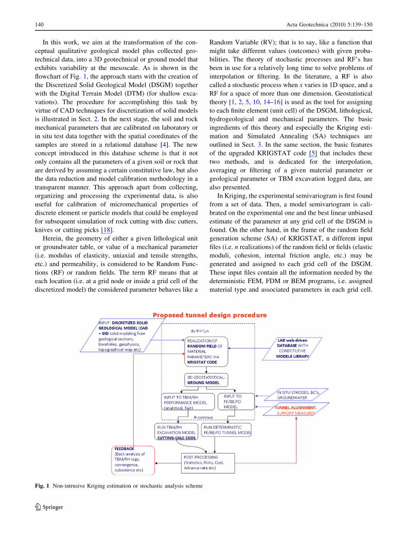
flowchart of Fig. 1, the approach starts with the creation of

the Discretized Solid Geological Model (DSGM) together

with the Digital Terrain Model (DTM) (for shallow exca-

vations). The procedure for accomplishing this task by

virtue of CAD techniques for discretization of solid models

is illustrated in Sect. 2. In the next stage, the soil and rock

mechanical parameters that are calibrated on laboratory or

in situ test data together with the spatial coordinates of the

samples are stored in a relational database [4]. The new

concept introduced in this database scheme is that it not

only contains all the parameters of a given soil or rock that

are derived by assuming a certain constitutive law, but also

the data reduction and model calibration methodology in a

transparent manner. This approach apart from collecting,

organizing and processing the experimental data, is also

useful for calibration of micromechanical properties of

discrete element or particle models that could be employed

for subsequent simulation of rock cutting with disc cutters,

knives or cutting picks [18].

Herein, the geometry of either a given lithological unit

or groundwater table, or value of a mechanical parameter

(i.e. modulus of elasticity, uniaxial and tensile strengths,

etc.) and permeability, is considered to be Random Func-

tions (RF) or random fields. The term RF means that at

each location (i.e. at a grid node or inside a grid cell of the

discretized model) the considered parameter behaves like a

Random Variable (RV); that is to say, like a function that

might take different values (outcomes) with given proba-

bilities. The theory of stochastic processes and RF’s has

been in use for a relatively long time to solve problems of

interpolation or filtering. In the literature, a RF is also

called a stochastic process when x varies in 1D space, and a

RF for a space of more than one dimension. Geostatistical

theory [1, 2, 5, 10, 14–16] is used as the tool for assigning

to each finite element (unit cell) of the DSGM, lithological,

hydrogeological and mechanical parameters. The basic

ingredients of this theory and especially the Kriging esti-

mation and Simulated Annealing (SA) techniques are

outlined in Sect. 3. In the same section, the basic features

of the upgraded KRIGSTAT code [5] that includes these

two methods, and is dedicated for the interpolation,

averaging or filtering of a given material parameter or

geological parameter or TBM excavation logged data, are

also presented.

In Kriging, the experimental semivariogram is first found

from a set of data. Then, a model semivariogram is cali-

brated on the experimental one and the best linear unbiased

estimate of the parameter at any grid cell of the DSGM is

found. On the other hand, in the frame of the random field

generation scheme (SA) of KRIGSTAT, n different input

files (i.e. n realizations) of the random field or fields (elastic

moduli, cohesion, internal friction angle, etc.) may be

generated and assigned to each grid cell of the DSGM.

These input files contain all the information needed by the

deterministic FEM, FDM or BEM programs, i.e. assigned

material type and associated parameters in each grid cell.

Fig. 1 Non-intrusive Kriging estimation or stochastic analysis scheme

140 Acta Geotechnica (2010) 5:139–150

123

Thus, no programming effort is required to change the

existing FEM, BEM code in contrast to the popular spectral

stochastic finite element method [8]. These input files can

be executed automatically in FEM or BEM code with the

aid of the KRIGSTAT software. Once the solution process

is finished, post-processing can be carried out to extract all

the necessary response statistics of interest. The non-intru-

sive stochastic analysis scheme is shown in Fig. 1. The

ground model is completed by specifying the in situ stresses

and ground water table (i.e. Fig. 1).

As is shown in Fig. 1, the 3D Kriging estimation or

stochastic ground model may be also used as an input file

for the Tunnel Boring Machine (TBM) performance model.

The TBM performance forward model is analytical and has

been implemented into CUTTING_CALC code. This fast

code predicts the consumption of the Specific Energy (SE)

or the net advance rate along the planned tunnel alignment

given the ground strength properties, in situ stresses, pore

pressure of the groundwater, cutterhead design and TBM

operational parameters like rotational speed and penetra-

tion depth per revolution, and is outlined in Sect. 4. The

same algorithm has another subroutine that performs sim-

ilar SE calculations for Roadheaders (RH). The backward

TBM model—that is also a subroutine of the code—is used

for the estimation of the ground strength properties from

the measured power consumption, thrust, rotational speed

and penetration depth per revolution of the cutterhead of

the TBM. Back-analysis may be easily achieved since the

TBM performance model is analytical. Hence, the esti-

mated strength properties may be used as a feedback for the

upgrade of the initial ground model and so forth in the

manner illustrated in the flowchart of Fig. 1. The numerical

model is adopted to compute ground deformations induced

by tunneling in each spatially heterogeneous realization of

this random field. Realization means the estimated or

simulated values of a certain variable within the domain.

This non-intrusive scheme does not require the user to

modify existing deterministic numerical simulation codes.

2 Discretized solid geological modeling

The three-step procedure proposed here for the creation of

the DSGM and DTM that could be subsequently used as

input directly to a numerical code, is illustrated by using

geological and borehole exploration data from the Mas-

Blau tunnel of L9 in Barcelona, and is as follows:

1. The geological model of the Mas-Blau section was

created by modeling each interface between the four

layers through the interpolation of borehole litholog-

ical data (see Fig. 2a) on a specified grid using the

geostatistical code KRIGSTAT [3, 5] that is outlined

in Sect. 3. More specifically, the surfaces between

adjacent soil formations were derived from the inter-

polation of elevation data (z values), that were

identified from the 15 boreholes (Fig. 2a), in a pre-

specified (x, y) grid inside the 3D model by using the

Ordinary Kriging (OK) subroutine. Surface models are

derived from interpolation of borehole data using the

OK technique.

2. After constructing the DTM in DXF format, the Solid

Geological Model (SGM) of each geological unit is

created by virtue of AutoCAD Land desktop software

in ACIS format (Fig. 2b).

3. Subsequently, each SGM corresponding to a given soil

formation (R-QL1, QL2, QL3 and QL4) is imported to

geometrical solid modeling pre-processor [9, 19] and is

discretized into tetrahedral elements, thus creating the

final DSGM. In such a manner, a given lithology is

assigned to each grid cell (i.e. Fig. 2c). It is worth

noting that modelling each layer separately permits

one to perform geostatistical analysis inside them, as it

is shown in the next section, by assuming statistical

homogeneity of each considered soil parameter.

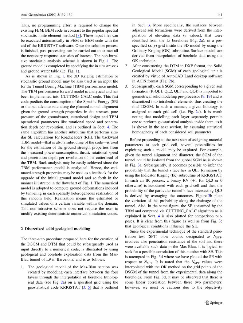
Before proceeding to the next step of assigning material

parameters to each grid cell, several possibilities for

exploiting such a model may be explored. For example,

given the tunnel alignment and diameter, the SGM of the

tunnel could be isolated from the global SGM as is shown

in Fig. 3a. Subsequently, it becomes possible to infer the

probability that the tunnel’s face lies in QL3 formation by

using the Indicator Kriging (IK) subroutine of KRIGSTAT.

In such an IK process, a binary RV (?1 for QL3 or 0

otherwise) is associated with each grid cell and then the

probability of the particular tunnel’s face intersecting QL3

is derived by averaging the outcomes. Figure 3b plots

the variation of this probability along the chainage of the

tunnel. Also, in the same figure, the SE consumed by the

TBM and computed via CUTTING_CALC algorithm as is

explained in Sect. 4 is also plotted for comparison pur-

poses. It is clear from this figure as well as from Fig. 3c

that geological conditions influence the SE.

Since the experimental technique of the standard pene-

tration test (SPT) blow counts, designated as NSPT,

involves also penetration resistance of the soil and there

were available such data in the Mas-Blau, it is logical to

seek for a possible correlation of this number with SE. This

is attempted in Fig. 3d where we have plotted the SE with

respect to NSPT. It is noted that the NSPT values were

interpolated with the OK method on the grid points of the

DSGM of the tunnel from the experimental data along the

boreholes. From Fig. 3d, it may be observed that there is

some linear correlation between these two parameters;

however, we must be cautious due to the objectivity

Acta Geotechnica (2010) 5:139–150 141

123

Es cala H or itzontal 1:301 7

Escala V ertical 1:287

TÍ TO L DE L PROJ EC TE NOM DE L PL ÀN OL CONSUL TO R ES CA LE S CL AU DA TA PL ÀN OL NÚM

NOM FITXER :

FUL L DE

11 /01/08 Projecció de Columne s Metro Línia 9 T M-00509

S1A03660RP A2 2 MB- PA -2

SM-P1 SRA-1

S1A0563R20P A

S-2.2 S1A0562R07EI

S1A0383R05P A P-2.2 S1A0580L07IN

S1A0420L010P A S1A0424L10P A

S1A0426L07EI MB- PA -4

S-2.4 SRA-3

S1B0473R05P A

-60

-50

-40

-30

-2 0

-10

0

10

0 100 200 300 400 500 600 700 800 900 1000 1 100

(a)

(b)

(c)

X

Y

--: Unitat no assignada

R: Rebliments antròpics i sòls vegetals

Ql1: Llims i argiles orgàniques (plana al.luvial actual)

Ql2: Sorres mitjanes a grolleres (complex detritic superior)

Ql2l: Argiles i llims amb sorres disperses (complex detritic superior)

Ql3: Argiles, llims (falca intermèdia)

Ql3s: Sorres fines i llims (falca intermèdia)

Qb3s: Sorres fines i llims (falca intermèdia)

Ql4: Graves i sorres grolleress (Complex detritic inferior)

Fig. 2 Example application of Line 9 Barcelona Metro, Mas-Blau

section: a Longitudinal view of the exploratory boreholes indicating the

lithological units along them (courtesy of GISA); b solid geological model,

and c discretized geological model on a mesh with tetrahedral elements and

lithological data assigned to grid points (example of MIDAS pre-processor

ready for implementation into the numerical simulation code)

142 Acta Geotechnica (2010) 5:139–150

123

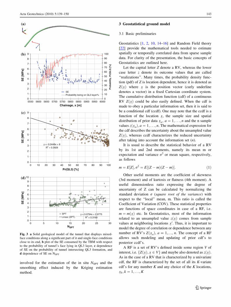
involved for the estimation of the in situ NSPT and the

smoothing effect induced by the Kriging estimation

method.

3 Geostatistical ground model

3.1 Basic preliminaries

Geostatistics [1, 2, 10, 14–16] and Random Field theory

[22] provide the mathematical tools needed to estimate

spatially or temporally correlated data from sparse sample

data. For clarity of the presentation, the basic concepts of

Geostatistics are outlined here.

Let the capital letter Z denote a RV, whereas the lower

case letter z denote its outcome values that are called

‘‘realizations’’. Many times, the probability density func-

tion (pdf) of Z is location dependent, hence it is denoted as

Zðx�Þ where x� is the position vector (curly underline

denotes a vector) in a fixed Cartesian coordinate system.

The cumulative distribution function (cdf) of a continuous

RV Zðx�Þ could be also easily defined. When the cdf is

made to obey a particular information set, then it is said to

be a conditional cdf (ccdf). One may note that the ccdf is a

function of the location x� , the sample size and spatial

distribution of prior data x�a; a ¼ 1; . . .; n and the n sample

values zðx�aÞ; a ¼ 1; . . .; n. The mathematical expression for

the cdf describes the uncertainty about the unsampled value

Zðx�Þ, whereas ccdf characterizes the reduced uncertainty

after taking into account the information set (n).

It is usual to describe the statistical behavior of a RV

by its 1st and 2nd moments, namely its mean m or

expectation and variance r2 or mean square, respectively,

as follows

m ¼ E½Z�; r2 ¼ E½ðZ � mÞðZ � mÞ�: ð1Þ

Other useful moments are the coefficient of skewness

(3rd moment) and of kurtosis or flatness (4th moment). A

useful dimensionless ratio expressing the degree of

uncertainty of Z can be calculated by normalizing the

standard deviation r (square root of the variance) with

respect to the ‘‘local’’ mean, m. This ratio is called the

Coefficient of Variation (COV). These statistical properties

are functions of space coordinates in case of a RF, i.e.

m ¼ mðx�Þ etc. In Geostatistics, most of the information

related to an unsampled value zðx�Þ comes from sample

values at neighboring locations x�0. Thus, it is important to

model the degree of correlation or dependence between any

number of RV’s Zðx�aÞ, a = 1,…, n. The concept of a RF

allows such modeling and updating of prior cdf’s to

posterior ccdf’s.

A RF is a set of RV’s defined inside some region V of

interest, i.e. fZðx�Þ; x� 2 Vg and maybe also denoted as zðx�Þ.As in the case of a RV that is characterized by a univariate

cdf, the RF is characterized by the set of all its K-variate

cdf’s for any number K and any choice of the K locations,

x�k; k ¼ 1; . . .;K

0

1

2

3

4

5

6

7

8

9

5550 5600 5650 5700 5750 5800 5850 5900 5950 6000

Chainage, x [m]

SE

[M

Pa]

0

10

20

30

40

50

60

70

80

90

100

Pro

bab

ility

, Pr(

QL

3) [

% ]

SE Probability being on QL3 layer%

y = -0.0448x + 8 R 2 = 0.3929

0

1

2

3

4

5

6

7

8

9

0 10 20 30 40 50 60 70 80 90 100

Pr(QL3) [%]

SE

[M

Pa]

y = 0.0794x + 2.9775R2 = 0.3169

0

1

2

3

4

5

6

7

8

9

10

0 5 10 15 20 25 30NSPT

SE

[M

Pa]

SPTLinear (SPT)

(a)

(c)

(b)

(d)

Fig. 3 a Solid geological model of the tunnel that displays mixed-

face conditions along a significant part of it and single-face conditions

close to its end, b plot of the SE consumed by the TBM with respect

to the probability of tunnel’s face lying in QL3 layer, c dependence

of SE on the probability of tunnel intersecting QL3 formation, and

d dependence of SE on NSPT

Acta Geotechnica (2010) 5:139–150 143

123

F x�1; . . .;x�k;z1; . . .;zk

� �¼ prob Z x

�1

� ��z1; . . .Z x

�k

� ��zk

n o

ð2Þ

Of particular interest in Geostatistics is the bivariate

(K = 2) cdf of any two RV’s Zðx�1Þ and Zðx

�2Þ, that is to say

F x�1; x�2; z1; z2

� �¼ prob Z x�1

� �� z1; Z x�2

� �� z2

n o: ð3Þ

The covariance of two correlated values (two-point

covariance) in the same ‘‘statistically homogeneous’’

random field (i.e. a field where all the joint probability

density functions remain the same when the set of locations

x�1; x�2; . . . is translated but not rotated in the parameter

space) is defined as the expectation of the product of the

deviations from the mean

RðhÞ ¼ E Zðx�1Þ � m� �

Zðx�2Þ � m� �h i

; h ¼ x�1 � x�2

������ð4Þ

i.e. h is the distance between sampling locations x�1 and x�2.

The field with this property is called stationary or

homogeneous. Dividing R by r leads to the

dimensionless coefficient of correlation q between Zðx�1Þand Zðx�2Þ

qðhÞ ¼ RðhÞr2

ð5Þ

In most cases, the mean is not known beforehand but needs

to be inferred from the data; to avoid this lack of data, it

may be more convenient to work with the semivariogram

that is defined as

cðhÞ ¼ 1

2E Z x�1

� �� Z x�2

� �� �2� �

ð6Þ

By using the semivariogram instead of the covariance

function to analyze the spatial correlation structure of a

geotechnical parameter means that a constant population

mean, m is assumed. This is the so-called ‘‘intrinsic

hypothesis’’ of Geostatistics [16].

It may be also easily shown that for a stationary RV, the

following relationship is valid

cðhÞ ¼ �RðhÞ þ Rð0Þ: ð7Þ

3.2 Kriging estimation

The basic statistical and geostatistical procedures have been

implemented in KRIGSTAT algorithm for the exploratory

data analysis and spatial estimation of geotechnical model

parameters over the defined study area V. KRIGSTAT may

be a stand-alone application or add-onto a commercial

numerical code or risk analysis software. The estimation

procedure starts with exploratory data analysis, normality

tests, searching for trends, declustering to correct for spatial

bias, etc. Kriging assumes that the expected value z�ðxkÞ of

RV Z at location xk can be interpolated as follows

z�ðxkÞ ¼XMi¼1

kizðxiÞ ð8Þ

where z(xi) represents the known value of variable Z at

point xi; ki is the interpolation weight function, which

depends on the interpolation method, and M is the total

number of points used in the interpolation. This technique

apart from being simple gives the Best Linear Unbiased

Estimations (BLUE) at any location between sampling

points and is fast. Kriging uses the experimental

semivariogram for the interpolation between spatial

points. In the case of isotropic conditions and statistical

homogeneity, the experimental semivariogram is

c�ðhÞ ¼ 1

2n

Xn

i¼1

½zðxÞ � zðxþ hÞ�2 ð9Þ

where n is the total number of observations separated by

the distance (lag) h. In practice, Eq. (9) is evaluated for

evenly spaced values of h using a lag tolerance Dh, and n is

the number of points falling between h - Dh and h ? Dh.

A typical semivariogram characteristic of a stationary

random field saturates to a constant value (i.e., sill) for a

distance called ‘‘range’’. The range represents the distance

beyond which there is no correlation between spatial

points. In theory, c(h) = 0 when h = 0; however, the

semivariogram often exhibits a nugget effect at very small

lag distance, which reflects usually measurement errors and

size effects. Experimental semivariograms can be fitted

using spherical, exponential, Gaussian, Bessel, cosine or

hole-effect, mixed semivariogram models, etc. from the

library of KRIGSTAT. The fitted model is then validated

using residuals or other suitable method (i.e. jack-knife,

leave-one-out or cross-validation). Based on an isotropic

semivariogram model, OK determines the coefficients ki by

solving the following system of n ? 1 equations:

Xn

j¼1

kic�ðhijÞ þ b ¼ cðhikÞ i ¼ 1; 2; . . .; n and

Xn

i¼1

ki ¼ 1

ð10Þ

where b is a Lagrange multiplier. The isotropic

semivariogram of Eq. (10) can be generalized for

anisotropic cases when data depend not only on distance

but also on direction. In practice, anisotropic semivariograms

are determined by partitioning data along directional

conical-cylindrical bins with pre-defined geometry.

Anisotropy is detected when the range or sill changes

significantly with direction and may be efficiently tackled

with KRIGSTAT. The present analysis assesses the error

of spatial interpolation using the minimum error variance

144 Acta Geotechnica (2010) 5:139–150

123

(e.g. [1]). The estimated interpolation error at location xk is

the variance (or standard deviation squared) of the error

estimate

r2SKðxkÞ ¼ E½ðz�ðxkÞ � zðxkÞÞ2� ¼

XM

j¼1

kjcðkxk � xjkÞ � b:

ð11Þ

As it may be observed from Eq. (11), the Kriging variance

does not depend on the sample values themselves, but only

on their locations. Therefore, Kriging variance measures

the uncertainty at the estimation location due to the spatial

configuration of the available data for its estimation, rather

than based on the dispersion of the values. The Kriging

variance could be used for the conduction of risk analysis

of the project, as well as for the proposition of optimum

additional exploratory drill holes at strategic locations

inside the geological domain of interest.

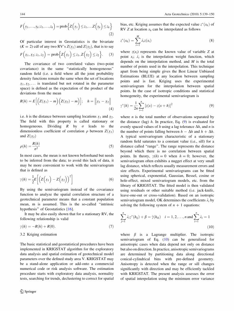
Spatial interpolation of all the Standard Penetration

Tests (SPT) blow counts NSPT (M = 140) conducted in the

exploratory boreholes of Mas-Blau tunnel section on the

3D grid of the DSGM was carried out by virtue of the OK

technique. The calculated experimental semivariogram that

exhibits a geometrical anisotropy (i.e. range along the

vertical direction is 0.35 of the range along any horizontal

direction) and the fitted exponential model are shown in

Fig. 4a. The estimations of NSPT values are presented

separately for each formation in Fig. 4b. The average NSPT

values on the tunnel’s face obtained from this model were

used for the construction of the diagram presented in

Fig. 3d.

3.3 Simulated annealing

KRIGSTAT includes also an adaptive method that starts

from a standard simulation, matching only the histogram

and the covariance (or semivariogram), for example, and

adapts it iteratively until it matches the imposed

constraints. This method is simulated annealing. This is an

optimization method rather than a simulation method and

its use for the construction of geostatistical simulations is

based on arguments that are more heuristic than theoretical.

The name and inspiration come from annealing in metal-

lurgy, a technique involving heating and controlled cooling

of a material to increase the size of its crystals and reduce

their defects. The heat causes the atoms to become unstuck

from their initial positions (a local minimum of the internal

energy) and wander randomly through states of higher

energy; the slow cooling gives them more chances of

finding configurations with lower internal energy than the

initial one.

Stochastic simulation is the process of drawing alter-

native, equally probable models of the spatial distribution

of zðx�Þ, with each such realization denoted with the

superscript r, i.e. fzðrÞðx�Þ; x�2Vg. The simulation is said to

be ‘‘conditional’’ if the resulting realizations obey the hard

data values at their locations, that is zðrÞðx�aÞ ¼ zðx�aÞ 8r.

The RV Zðx�Þ maybe ‘‘categorical’’, e.g. indicating the

presence or absence of a particular geological formation, or

it maybe a continuous property such as porosity, perme-

ability, cohesion of a soil or rock formation.

Simulation differs from Kriging or any other determin-

istic estimation method (e.g. inverse squared distance,

nearest neighbor, etc.) in the following two major aspects:

1. Most interpolation algorithms give the best local

estimate z�ðx�Þ of each unsampled value of the RV

Zðx�Þ at a grid of nodes without regard to the resulting

spatial statistics of the estimates z�ðx�Þ; x�2V . In

contrast, in simulations, the global texture and statis-

tics of the simulated values zðrÞðx�Þ; x�2V take

precedence over local accuracy.

2. As it was already mentioned in the previous paragraph,

for a given set of sampled data, Kriging provides a

single numerical model z�ðx�Þ; x�2V that is the

‘‘best’’ in some local accuracy scheme. On the other

hand, simulation provides many alternative numerical

Fig. 4 a Experimental semivariogram and fitted model of NSPT and

b spatial models of NSPT inside each soil layer obtained from Kriging

analysis

Acta Geotechnica (2010) 5:139–150 145

123

models fzðrÞðx�Þ; x�2Vg; r ¼ 1; . . .;R, each of which is

a ‘‘good’’ representation of the reality in some ‘‘global

sense’’. The difference among these R alternative

models or realizations provides a measure of joint

spatial uncertainty.

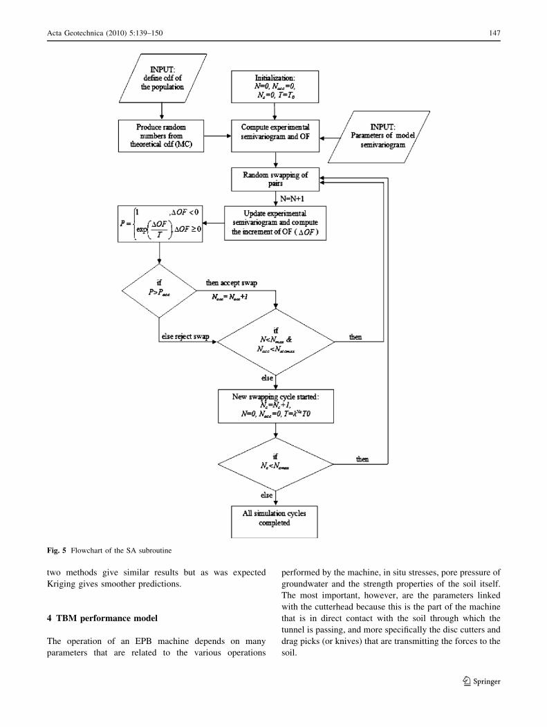
In the context of SA technique, random numbers are

generated via a Monte Carlo simulation technique from a

specified statistical distribution of the field parameter under

investigation. For ‘‘training simulations,’’ conditioning data

are relocated in the nearest grid points. Then, the initial

image is modified by swapping the values in pairs of grid

nodes. A swap is accepted if the objective function is

lowered. In this frame, a global optimization is achieved in

contrast to Kriging in which a local optimization scheme is

followed. The objective function (OF) is defined as the

average squared difference between the experimental and

model semivariogram like:

OF ¼X

h

½cðhÞ � c�ðhÞ�2

cðhÞ2ð12Þ

The division by the square of the model semivariogram

value at each lag h standardizes the units and gives more

weight to closely spaced (low semivariogram) values.

Not all swaps that raise the objective function are

rejected. The success of the method depends on a slow

‘‘cooling’’ of the image controlled by a temperature func-

tion, which decreases with evolution of time. The higher

the temperature denoted by the symbol T0, which is a

control parameter, the greater the possibility that an unfa-

vorable swap will be accepted. The simulation ends when

the image is frozen, that is, when further swaps do not

reduce the value of the objective function. ‘‘Hard data’’

values are relocated at grid nodes and are never swapped,

which allows their exact reproduction.

The following procedure is employed to create an image

that matches the cdf F(z), the model semivariogram c(h)

and other possible conditioning data:

• For each grid node of the DSGM that does not coincide

with a conditioning datum, an outcome is randomly

drawn from the cdf via Monte Carlo (MC) simulation.

This generates an initial realization that matches the

conditioning data and the cdf, but does not probably

match the model semivariogram model c(h).

• The next aim is that the experimental semivariogram

c*(h) of the simulated realization to match the prede-

fined model c(h). This is achieved with the objective

function (12) as it was explained previously.

• The initial image is modified by swapping pairs of

nodal values zi and zj chosen at random, where none of

these nodes represent conditioning data. After each

swap, the objective function (12) is updated.

• As metallurgical analysis suggests, the image must be

cooled slowly (annealed), rather than cooled rapidly

(quenched). In other words, accepting swaps that

increase the objective function allows the possibility

of avoiding a local minimum. The acceptance or not

of a given perturbation is given in terms of Boltzmann

pdf.

Pfacceptg¼1; if OFðiÞ�OFði�1Þexp½(OFði�1Þ�OFðiÞÞ=T �; otherwise

(

ð13Þ

All favorable perturbations (OF(i) B OF(i - 1)) are

accepted, whereas the unfavorable perturbations are

accepted with an exponential probability distribution as it

is shown in Eq. (13). The term ‘‘simulation cycle’’ refers

to the swapping process by using the same simulation

annealing parameters. The selection rule proposed here is

the comparison of the probability of acceptance P of a

successfully swapping cycle with Pacc = 0.95. The spec-

ification of how to decrease T is called ‘‘annealing

schedule’’. The following parameters describe this sche-

dule: T0 = the initial temperature, k = the reduction

factor (0 \ k\ 1), Nacc = index counting the accepted

combinations (if the upper limit is exceeded means that it

must restrict the selection rule by proceeding to the next

cycle by multiplying the current temperature parameter T

with a reduction factor k). The simulation is terminated if

the current cycle (Nc) reaches the total cycles number

(Ncmax) with a proposed value Ncmax = 3. Also, Naccmax =

upper limit of accepted successful swapping combinations

with a proposed value of 10 times the number of esti-

mation points, and Nmax = the maximum number of

swapping combinations at any given temperature (it is of

the order of 100 times the number of nodes).

The flowchart of this subroutine is shown in Fig. 5.

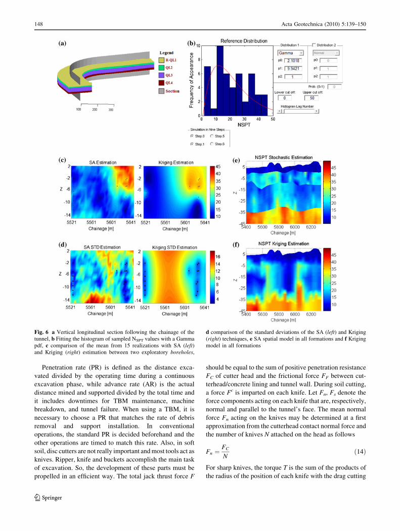
MC simulation is used for modelling the spatial distri-

bution of NSPT in a vertical longitudinal section along the

chainage of the tunnel, as is shown in Fig. 6a, using ini-

tially the statistical distribution shown in Fig. 6b. Then, the

conditional simulation is used for rearranging the data such

as to satisfy the input model semivariogram. The mean SA

spatial estimation obtained from R = 15 alternative real-

izations and a single Kriging estimation between two

boreholes in QL2 formation are displayed in Fig. 6c (data

locations inside the boreholes are shown by the dots),

whereas the standard deviation of the simulations and the

standard deviation rSK of the Kriging estimation are

compared in Fig. 6d. From these figures, the smoothing

effect of the Kriging estimation may be observed. The

results of the two methods inside all formations are com-

pared in Fig. 6e, f, respectively; it may be observed that the

146 Acta Geotechnica (2010) 5:139–150

123

two methods give similar results but as was expected

Kriging gives smoother predictions.

4 TBM performance model

The operation of an EPB machine depends on many

parameters that are related to the various operations

performed by the machine, in situ stresses, pore pressure of

groundwater and the strength properties of the soil itself.

The most important, however, are the parameters linked

with the cutterhead because this is the part of the machine

that is in direct contact with the soil through which the

tunnel is passing, and more specifically the disc cutters and

drag picks (or knives) that are transmitting the forces to the

soil.

Fig. 5 Flowchart of the SA subroutine

Acta Geotechnica (2010) 5:139–150 147

123

Penetration rate (PR) is defined as the distance exca-

vated divided by the operating time during a continuous

excavation phase, while advance rate (AR) is the actual

distance mined and supported divided by the total time and

it includes downtimes for TBM maintenance, machine

breakdown, and tunnel failure. When using a TBM, it is

necessary to choose a PR that matches the rate of debris

removal and support installation. In conventional

operations, the standard PR is decided beforehand and the

other operations are timed to match this rate. Also, in soft

soil, disc cutters are not really important and most tools act as

knives. Ripper, knife and buckets accomplish the main task

of excavation. So, the development of these parts must be

propelled in an efficient way. The total jack thrust force F

should be equal to the sum of positive penetration resistance

FC of cutter head and the frictional force FF between cut-

terhead/concrete lining and tunnel wall. During soil cutting,

a force Fc is imparted on each knife. Let Fn, Fs denote the

force components acting on each knife that are, respectively,

normal and parallel to the tunnel’s face. The mean normal

force Fn acting on the knives may be determined at a first

approximation from the cutterhead contact normal force and

the number of knives N attached on the head as follows

Fn ¼FC

Nð14Þ

For sharp knives, the torque T is the sum of the products of

the radius of the position of each knife with the drag cutting

Fig. 6 a Vertical longitudinal section following the chainage of the

tunnel, b Fitting the histogram of sampled NSPT values with a Gamma

pdf, c comparison of the mean from 15 realizations with SA (left)and Kriging (right) estimation between two exploratory boreholes,

d comparison of the standard deviations of the SA (left) and Kriging

(right) techniques, e SA spatial model in all formations and f Kriging

model in all formations

148 Acta Geotechnica (2010) 5:139–150

123

force Fs, plus the torque due to contact cutterhead frictional

forces TCF, plus the lifting forces of the buckets TLF, plus

the mixers at the rear part of the cutting wheel that move

the material to avoid segregation or sedimentation TCM.

Another term should be added for the case of knives with

wear flats to account for the additional friction. The mean

drag (or tangential) force Fs may be estimated through the

approximate formula

Fs �T

0:3 D Nð15Þ

in which D denotes the cutterhead diameter, D [L]. The

penetration depth per revolution is given by the formula

p ¼ PR

xð16Þ

wherein PR denotes cutterhead (net) penetration rate and xindicates the cutterhead rotational speed, [1/T].

A parameter of major importance is the Specific Energy

(SE) of cutting that is defined as the energy consumed in

removing a unit volume V of material. There are two

definitions of SE, namely one proposed in [17] denoted

herein as SE1

SE1 ¼Fs‘T

V¼ Fs‘T

pS‘T¼ Fs

pSð17Þ

in which ‘T is the total length traveled by the knife and S is the

distance between neighboring cuts of the knives. It may be

noticed that in the definition for SE only the tangential force

of knives are used because the tangential cutting direction

consumes almost all of the cutting energy, whereas the

energy expended in the normal direction is comparatively

negligible. This is an immediate consequence of the fact that

much greater amount of cutter travel takes place tangential to

the face than normal to it, even though the normal force is

much higher than the tangential forces.

Another SE, called SE2, may be also found from the

ratio of the energy consumption of the TBM over the

excavated volume [20],

SE2 ¼gPt

Vð18Þ

where g denotes the efficiency of energy transfer from

motor to the cutterhead, P is the registered power, t denotes

time and V is the excavated volume.

For the Mas-Blau case study, there are plenty TBM logs

collected during tunnel excavation with the EPB machine.

This set of data was collected during the excavation with a

high frequency per concrete ring that was not appropriate

for the purposes of this analysis and moreover was located

at separate files. Therefore, in a first stage of analysis, all

the files were merged into only one Excel spreadsheet and

the data were reduced so that a single row of logged data to

correspond to each concrete ring.

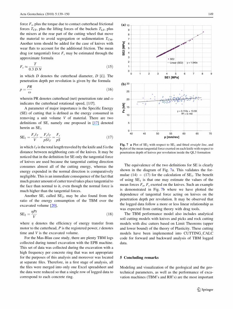
The equivalence of the two definitions for SE is clearly

shown in the diagram of Fig. 7a. This validates the for-

mulae (14) 7 (17) for the calculation of SE1. The benefit

of using SE1 is that one may estimate the values of the

mean forces Fn, Fs exerted on the knives. Such an example

is demonstrated in Fig. 7b where we have plotted the

dependence of tangential force acting on knives on the

penetration depth per revolution. It may be observed that

the logged data follow a more or less linear relationship as

was expected from cutting theory with drag tools.

The TBM performance model also includes analytical

soil cutting models with knives and picks and rock cutting

models with disc cutters based on Limit Theorems (upper

and lower bound) of the theory of Plasticity. These cutting

models have been implemented into CUTTING_CALC

code for forward and backward analysis of TBM logged

data.

5 Concluding remarks

Modeling and visualization of the geological and the geo-

technical parameters, as well as the performance of exca-

vation machines (TBM’s and RH’s) are the most important

y = 1.040x

0

1

2

3

4

5

6

7

8

9

10

0 1 2 3 4 5 6 7 8 9

SE

2 [M

Pa]

SE1 [MPa]

SE2

Linear (SE2)

y = 0.110x + 13.59R² = 0.140

0

5

10

15

20

25

30

40 45 50 55 60 65 70

Fs

[kN

]

p [mm/rev]

(a)

(b)

Fig. 7 a Plot of SE2 with respect to SE1 and fitted straight line, and

b plot of the mean tangential force exerted on each knife with respect to

penetration depth of knives per revolution inside the QL3 formation

Acta Geotechnica (2010) 5:139–150 149

123

tasks in tunneling design. The tunneling design process

should take into account the risk associated with the soil

quality and the design of the excavation machine. The

geological and geotechnical parameters are evaluated from

observations, boreholes, tests, etc. at certain locations, and

interpolation is necessary to model these parameters at the

grid elements of the DSGM. We have shown that the

proposed spatial analysis approach provides an interesting

alternative to more traditional approaches since:

1. It provides a consistent, repeatable and transparent

approach to construct a spatial model of any geotech-

nical parameter needed for subsequent numerical

simulation or TBM performance model.

2. It takes into account the spatial continuity of variables.

3. Apart from the estimation of a variable, it provides a

measure of uncertainty that can be used for risk

assessment or for improvement of the exploration (new

boreholes in areas of high uncertainty).

4. In general, it leads to a better model since local

interpolation performed over restricted neighborhoods

provides a better model compared to zone the model in

homogeneous geotechnical volumes or sections, and

averaging.

5. It provides input data directly to any deterministic

numerical tunneling simulation code that has the

capability to assign different properties to each element.

Furthermore, the proposed TBM model outlined above

may be used in conjunction with the spatial analysis model

to explore any relation between excavation performance

(expressed here with SE) and geotechnical or geological

parameters. If such relation(s) could be found then they

may be used for upgrading the geotechnical model as TBM

advances [5].

Acknowledgments The authors would like to thank the financial

support from the EC 6th Framework Project TUNCONSTRUCT

(Technology Innovation in Underground Construction) with Contract

Number: NMP2-CT-2005-011817, http://www.tunconstruct.org, and

Mr. Henning Schwarz of GISA for his kindness to provide us with

geological, exploratory and TBM data from Mas-Blau.

References

1. Chiles JP, Delfiner P (1999) Geostatistics—modeling spatial

uncertainty. Wiley, New York

2. Deutsch CV, Journel AG (1997) Geostatistical software library

and user’s guide. Oxford University Press, New York

3. Exadaktylos G, Stavropoulou M (2008) A specific upscaling

theory of rock mass parameters exhibiting spatial variability:

analytical relations and computational scheme. Int J Rock Mech

Min Sci 45:1102–1125

4. Exadaktylos G, Liolios P, Barakos G (2007) Some new devel-

opments on the representation and standardization of rock

mechanics data: from the laboratory to the full scale project. In:

Rock mechanics data: representation and standardisation, 11th

ISRM congress, July 12th 2007, Lisbon Congress Centre, Lisbon

Portugal

5. Exadaktylos G, Stavropoulou M, Xiroudakis G, deBroissia M,

Schwarz H (2008) A spatial estimation model for continuous rock

mass characterization from the specific energy of a TBM. Rock

Mech Rock Eng 41:797–834

6. Fenton GA, Griffiths DV (1995) Flow through earth dams with

spatially random permeability. In: Proceedings 10th ASCE

engineering mechanics conference, Boulder, CO, USA, pp 341–

344

7. Fenton GA, Griffiths DV (2002) Probabilistic foundation settle-

ment on spatially random soil. ASCE J Geotech Eng 128(5):381–

390

8. Ghanem RG, Spanos PD (1991) Stochastic finite element: a

spectral approach. Springer, NY

9. GiD (2006) GiD the personal pre- and postprocessor. CIMNE,

Barcelona, http://www.gidhome.com

10. Goovaerts P (1997) Geostatistics for natural resources evaluation.

Oxford University Press, New York

11. Griffiths DV, Fenton GA (2004) Probabilistic slope stability

analysis by finite elements. ASCE J Geotech Geoenv Eng

130(5):507–518

12. Hejazi Y, Dias D, Kastner R (2008) Impact of constitutive models

on the numerical analysis of underground constructions. Acta

Geotech 3:251–258

13. Hoefle R, Fillibeck J, Vogt N (2008) Time dependent deforma-

tions during tunnelling and stability of tunnel faces in fine-

grained soils under groundwater. Acta Geotech 3:309–316

14. Isaaks EH, Srivastava RM (1989) Introduction to applied geo-

statistics. Oxford University Press, Oxford

15. Journel AG, Huijbregts CHJ (1978) Mining geostatistics. Aca-

demic Press, London

16. Kitanidis PK (1997) Introduction to geostatistics: applications in

hydrogeology. Cambridge University Press, Cambridge

17. Kutter H, Sanio HP (1982) Comparative study of performance of

new and worn disc cutters on a full-face tunnelling machine. In:

Tunnelling’82, IMM, London, pp 127–133

18. Labra C, Rojek J, Onate E, Zarate F (2008) Advances in discrete

element modelling of underground excavations. Acta Geotech

3:317–322

19. MIDAS GTSII (2006) Geotechnical and tunnel analysis system,

MIDASoft Inc. (1989–2006), http://www.midas-diana.com

20. Snowdon RA, Ryley MD, Temporal J (1982) A study of disc

cutting in selected British rocks. Int J Rock Mech Min Sci

Geomech Abstr 19:107–121

21. Stavropoulou M, Exadaktylos G, Saratsis G (2007) A combined

three-dimensional geological-geostatistical-numerical model of

underground excavations in rock. Rock Mech Rock Engng

40(3):213–243

22. Vanmarcke E (1983) Random fields: analysis and synthesis. The

MIT Press, Cambridge

150 Acta Geotechnica (2010) 5:139–150

123