dynamic pile-soil- pile interaction part ii. lateral and seismic response

EARTHQUAKE ENGINEERING AND STRUCTURAL DYNAMICS, VOL. 21, 145-162 (1992)

DYNAMIC PILE-SOIL-PILE INTERACTION. PART 11: LATERAL AND SEISMIC RESPONSE

NICOS MAKRIS AND GEORGE GAZETAS Department of Civil Engineering, 212 Ketter Hull, Stole University of New York at Buffalo, N Y 14260, U.S.A.

SUMMARY A simplified three-step procedure is proposed for estimating the dynamic interaction between two vertical piles, subjected either to lateral pile-head loading or to vertically-propagating seismic S-waves. The starting point is the determination of the deflection profile of a solitary pile using any of the established methods available. Physically-motivated approximations are then introduced for the wave field radiating from an oscillating pile and for the effect of this field on an adjacent pile. The procedure is applied in this paper to a flexible pile embedded in a homogeneous stratum. To obtain analytical closed-form results for both pile-head and seismic-type loading pile-soil and soil-pile interaction are accounted for through a single dynamic Winkler model, with realistic frequency-dependent ‘springs’ and ‘dashpots’. Final- and intermediate-step results of the procedure compare favourably with those obtained using rigorous formulations for several pile group configurations. It is shown that, for a homogeneous stratum, pile-to-pile interaction effects are far more significant under head loading than under seismic excitation.

INTRODUCTION

The dynamic stiffness of a group of vertical piles in any mode of vibration can not be computed by simply adding the stiffnesses of the individual piles, since each pile is affected not only by its own load, but also by the load and deflection of its neighbouring piles. Similarly, the seismic response of a pile group may differ substantially from the response of each individual pile taken alone, because of additional deformations transmitted from the adjacent piles. This pile-to-pile interaction is frequency-dependent, resulting from waves that are emitted from the periphery of each pile and propagate to ‘strike’ the neighbouring piles. Several researchers have developed a variety of numerical1-’ and analytical’, methods to compute the dynamic response of pile groups accounting for pile-to-pile interaction. A recent comprehensive review on the subject has been presented by Novak.”

In this paper the dynamic response of laterally-vibrating pile groups is investigated as a continuation of earlier work by the authors,’ which dealt with axial vibration. Simplified closed-form analytical solutions are developed for the problem of dynamic pile-soil-pile interaction for two major types of loading:

(a) lateral harmonic force or moment at the pile cap (‘inertial’-type loading); (b) seismic excitation in the form of harmonic vertical incident shear waves (‘kinematic’ loading).

The obtained results are shown to be in agreement with rigorous solutions.

OUTLINE OF PROPOSED GENERAL METHOD

A general approximate method is proposed that involves the following three consecutive steps, schematically illustrated in Figure 1 (for ‘inertial’ type loading) and in Figure 2 (for ‘kinematic’ type loading):

Step 1. The lateral dejection, u1 l(z), of a single (solitary) pile, subjected to either lateral ‘inertial’ loads at its head or ‘kinematic’ seismic-wave deformations of the surrounding soil, is determined using the best procedure@) available. For instance, one may use a dynamic finite-element code,” - l 3 a boundary-element- type ’ a semi-analytical formulation3~ 4* lo* l4 and a beam-on-Winkler-foundation method

0098-8847/92/020145-18W9.00 0 1992 by John Wiley & Sons, Ltd.

Received 28 May 1991 Revised 27 August 1991

146 N. MAKRIS AND G. GAZETAS

Figure

Support motion PILE 2

pile-soil inferaction springs + dnshpofs

1. Schematic illustration of the developed 3-step procedure for computing the influence lateral head loading, upon the adjacent PILE 2

of PILE 1. deforming under harmonic

along with pertinent complex-valued dynamic ‘springs’l or dynamic ‘ p y ’ curves.’ 6* ’ Alternatively, even well-instrumented lateral pile load tests in the field, on a shaking table, or in the centrifuge could be conceivably used as a guide in constructing u ~ ~ ( z ) . ’ ~ - * ’ In this paper, we present results using a dynamic Winkler model to account for soil-pile interaction; this choice was not a necessity but stemmed solely from the need to derive analytical results for pile-soil-pile interaction in closed form. (Figure 2 illustrates the dynamic Winkler model utilized in Step 1 for computing the ‘kinematic’ response of a single pile.)

Step 2. This step begins by computing the diflerence, Aul = u1 - uff, between single pile deflections and free-field soil displacements. With ‘inertial’ loading this difference is just the deflection of the pile: Aul = u1 ’. For ‘kinematic’ loading, the response of the free-field soil, sketched in Figure 2, is computed by one- dimensional (1 D) ‘soil-amplification’ methods. (Non-vertically-incident waves conceivably could be treated in the same way, by using 2D soil response methods, but this is not explored in this article.) This difference, Aul (z) or simply u1 (z), generates waves at all points along the pile. It is assumed that these waves spread out horizontally, as originally assumed in Novak‘s single pile method (e.g. Reference 15); their attenuation with distance r and ‘angle of departure’ 8 is estimated using plane elastodynamic theory and assuming viscoelastic soil behaviour. Thus, at the location of pile 2, r = S, if this pile were not present, the arriving

DYNAMIC PILESOIL-PILE INTERACTION 147

Figure 2. Schematic illustration of the developed 3-step procedure for computing the influence of PILE 1, deforming under seismic-type excitation, upon the adjacent PILE 2

attenuated waves would produce lateral soil displacements Aus (or simply us for head-loaded pile) determined as illustrated in Figures 1-2, and explained in the sequel.

Step 3. The presence of pile 2 will modify the arriving wave field Au,(z) or u,(z), reflecting and diffracting the incoming waves. As a result, depending on its relative flexural rigidity and the vertical fluctuations of the arriving wave field, pile 2 may just follow closely the ground, experiencing displacements uzl (z) = us(z) Dong-flexible pile and smoothly-varying us = %(z)], or it may remain nearly still uzl(z) z 0 [rigid pile, rapidly fluctuating us = us(z)]. But in general its response uzl(z) will be something in between these two extremes. To account in a simple practical way for this soil-pile interaction, we use a Beam-on-Dynamic- Winkler-Foundation (BDWF) model, in which the excitation takes the form of a support motion, equal to the attenuated displacement field %(z) [or Au,(z)] of Step 2. As illustrated in Figures 1 and 2, the response of the pile-beam to this support motion is the desired response uZ1(z) of pile 2.

One of the main simplifications introduced herein is the decoupling of the ‘mechanism’ that transmits the motion in each of the three steps outlined above. Note that we do not directly connect the interacting piles by springs as was done by Nogami et d3 Once the source of the displacement in the soil is determined in Step 1, we use approximate wave equations to represent the motion in the free field. This is a very natural and effective way to represent the energy dissipation. Radiation damping, hysteretic soil damping and phase- difference effects play independently their role in the wave equation of the free field. Also note that Dobry and Gazetas’ assumed that the pile-head deflection would be equal to the average of the soil induced displacement. This assumption may be quite good for vertical vibration, where the axial rigidity of the pile is usually significant, and the pile displacements are primarily the result of a rigid body motion. But for lateral


vibration this assumption tends to exaggerate the pile-to-pile effect. By contrast the soil-pile interaction model used in Step 3 can be shown to provide a realistic solution to the problem. This general methodology is explained in detail below for a flexible pile under head loading and under seismic excitation.

HARMONIC EXCITATION AT THE PILE HEAD ('INERTIAL' RESPONSE)

Problem definition Under lateral pile-head loading, only the upper portion of a flexible pile experiences significant deforma-

tion. The length of this portion, called 'active length', has been established for both static and dynamic loading.'2*13*22 Th us, there is hardly a need to distinguish between a floating and an end-bearing pile and the pile can be treated as an infinitely-long beam with no appreciable loss in accuracy. This beam is considered linear elastic with circular cross-section A,, diameter d, second moment of area I , , Young modulus Ep and mass density pp.

The soil is modelled as a Winkler foundation resisting the lateral pile motion by continuously-distributed frequency-dependent linear springs k , and dashpots c,. The latter model the energy losses due to radiation of waves and due to hysteretic dissipation. Expressions for these coefficients are available in the l i terat~re '~. 23

on the basis of which the following simple approximations are derived:

k, x 1.2Es ( 1 )

( 2 )

where E, , V,, Ps and ps, are the Young's modulus, shear wave velocity, damping ratio and mass density of the soil; m = ppAp is the mass per unit length of the pile; a , = wd/V, .

k , ps V,d + 2Bs ~

c, % 6a; 0

Dejections of a single (solitary) pile-Step 1

(iot) requires that With reference to Figure 1, dynamic equilibrium during harmonic steady-state motion u1 (z) = U1 (z)exp

Applying Laplace transformation one gets

where the prime denotes derivative with respect to z, and

A = { k, + iwc, - mo2}1t4

4EPIP Laplace-inverting equation (4), while enforcing the boundary relations

which ensure finite displacement amplitude as z tends to infinity, one obtains the final solution:

DYNAMIC PILE-SOIL-PILE INTERACTION 149

where U, = U,,(O) is the displacement amplitude at the pile head and

e 0 e e a = cos - + sin - b = cos - - sin -

4 4' 4 4

II

2 8 = arctan

(9)

Observe that if damping were neglected (c, = 0) equation (7) would reduce to a standing wave

ull(z) = Uoe-"(sin 2z + cos Lz)e'"' (1 1)

and 2 reduces from a complex to a real number

Equation (1 1) is of the same form as the static solution,24 but here of course 1 = A(o). This special case has been discussed by

As an example, Figure 3 compares the distribution with depth of the (normalized) amplitude given by equations (7) and (I l), as well as the phase-angle differences between a point on the pile at depth z and the pile head. Notice that for the chosen E J E , ratio, lo00 and a. = 0.3 the pile 'active' length extends to about 9 diameters from the surface. Moreover, equation (7) predicts that the motion would become substantially out of phase only at a depth where the amplitude is at most 5 to 10 per cent of the head amplitude. Consequently, although the damped and undamped models give a completely different result for the nature of the waves propagating down the pile, the induced displacement distributions to the soil are similar. In the sequel this observation simplifies considerably the algebra in analysing the pile-to-pile interaction, where we make use of equation (11) rather than of equation (7).

E , / E , = 1000

O l

10 0 30 60 90 120

phsse angle (degrees)

Figure 3. Normalized deflection amplitude and phase angle of a fixed-head pile under lateral loading, at a dimensionless frequency a,, = 0 3 . The continuous line is the result of equation (11) (no damping) whereas the dashed line is the result of equation (7)


Next, using the foregoing pile deflection as a displacement ‘source’ we determine the soil displacements, us, at a distance r = S .

Attenuation of soil displacement away from ‘source’ pile-Step 2 P- and S-waves are emitted from the oscillating pile, travelling in all directions and being reflected from the

free surface of the soil. A rigorous formulation of this 3D problem would be a formidable task, especially if one foresees an extension to layered soils. Several approximate models, based on lD, 2D or 3D wave propagation idealizations, are nevertheless available. 14, 5 * 26, 27 They are reviewed briefly below.

assumed that a horizontally moving pile cross-section would generate solely 1D P-waves travelling in the direction of shaking and 1D SH-waves travelling in the direction perpendicular to shaking. Although the simplicity of this model is attractive, the constraints imposed from the 1D consideration lead to frequency-independent radiation damping which achieves unrealistically high values when the Poisson’s ratio v approaches 0.5. Novak et a l l 5 developed a 2D model by solving the problem of a soil slice of infinite extent subjected to horizontal oscillations from a rigid circular inclusion [Figure *a)]. The restriction of vertical deformations (6, = 0) corresponds to a plane-strain problem and a 2D solution. Roesset and co-workersZ3* 27 verified the validity of this 2D model. They used a 3D FE formulation for the developing soil reactions against pile displacements. An alternative approximate 2D plane-strain model, presented by Gazetas and Dobry14 assumes that compression-extension waves propagate in the two quarter-planes along the direction of loading while shear waves are generated in the two quarter-planes perpendicular to the direction of loading [Figure 4(b)]. The apparent phase velocity of the compression-extension waves is approximated by the so-called ‘Lysmer’s analogue’ wave ~elocity’~V~/, , = [3 .4/~(1 - v ) ] V,. The shear waves propagate, of course, with velocity V,.

The models of Gazetas and Dobry14 and of Novak et a l l 5 are both utilized herein. According to the first, at a distance r from the oscillating pile and an angle 0 from the direction of loading the displacement field can be simply expressed as

Berger et

u,(r, 8, z) = Us exp (iwt) = $(r, O)u, , (z) (13)

where ull is given by equation (11) and I)@, 19) is the attenuation function (still to be determined). It is sufficient to compute I)(r, 0) only for 0 = 0 and 0 = n/2 and then use the approximation

$(r , e) z $(r , 0) cos2 e + I) I , - sin2 e ( 3 Honzontal Sectmns

1 0 I f E, = 0 w_ &,=O -

t

”s

Plans

Figure 4. Schematic representation of 2D radiation model: (a) ‘rigorous’ plane-strain model of Novak rt at.”: (b) simplified plane- strain model of Gazetas and Dobry14

DYNAMIC PILE-SOILPILE INTERACTION 151

to obtain a very good estimate for any arbitrary angle il.2*7,28 The following approximate expressions for $(r, 0) and $(r, n/2) have been developed in Reference [S]:

The factor I/& represents the reduction in amplitude due to geometric spreading (radiation) of waves while the factors exp( - Bwr/V) express the amplitude reduction due to hysteresis in the soil. The third factors describe a radially-propagating wave with phase velocity V,, for 0 = 0, and V, for 8 = n/2.

Although the attenuation expressions from equations (14H15) appear to be extremely simple, the results obtained are very close to the more sophisticated solution that we derived:

where

and

in which I f f ) denotes the zero-order second-kind Hankel function and Vp is the soil P-wave velocity. Figure 5 compares the real and imaginary part of equations (14) and (16), plotted as functions of the horizontal distance r normalized by the pile diameter d. The differences are rather small and use of either one set in the subsequent analysis does indeed lead to quite similar results.

We use equation (13) in conjunction with equation (14) to describe the soil displacement field.

Interaction of ‘receiver’ pile with arriving waves-Step 3 Consider now a second (‘receiver’) pile, 2, located at a distance r = S from the ‘source’ pile 1. The soil

displacement field computed in Step 2 [equation (13)] affects pile 2. The flexural rigidity of the pile, however, tends to resist this deflection, and the result is a modified motion at its soil-pile interface. This physical phenomenon is in a sense the reverse of that of Step 1. In Step 1 the ‘source’ pile induces displacements on the soil, whereas in Step 3 the soil induces displacements on the ‘receiver’ pile.

To describe the mechanics of this loading we utilize once again the generalized Winkler model of Step 1. But now it is the supports of the ‘springs’ and ‘dashpots’ that undergo the induced soil displacement us(r, 8, z) and exert along the pile a distributed load equal to the net displacement (us - u21) times the impedance k, + iwC,, where u21 = u21 exp(iwt) denotes the deflexion of the ‘receiver’ pile 2. Dynamic equilibrium for

152

-0.4 - -0.6

N. MAKRIS AND G. CAZETAS

-0.4 - ..___-' -0.6 -

I . 1 ' I . , -0.8 , ~ I ~ I ~ I ~ I

0.6 - 0.6 - /--. ,,, I\

0.4 - 0.4 -

\. .\ ,* 1___,'

-0.2 - I

-0.4 - *-..%/' -0.4 - -0.6 b - 0 . 6 1 8 , r I 1 8 b r I ~

2 4 6 a 10 0 2 4 6 B 1 C

r / d r / d

Figure 5. Real and imaginary part of attenuation factor as a function of distance: comparison between the approximate model by Gazetas and Dobry14 (equation (14+ontinuous line) and the plane-strain model by Novak et ~ 1 . ' ~ (equation ( 1 6 w a s h e d line)

pile 2 gives

or, after substituting U s from equation (13) into equation (18),

+ ( k , + ioc, - rno')Uz1 = (k , + ioc,)+(r, O)Uoe-Az(cosAz + sin Az) (19) d4U21

E P I P 7 The solution of equation (19) is also obtained using the Laplace transform technique. After lengthy calculations one obtains

which is the sought response of the 'receiver' pile. It is useful to express the pile-to-pile interaction through the dynamic interaction factor', 7 3 8 3

additional head deflection of pile 2 caused by pile 1 head deflection of pile 1 (2 1 4 a21 =

From equations (20) and (11) one obtains for z = 0

3 k , + icoc, k , + ioc, - mu2 a21 = , + ( r J )


Equation (21b) is sufficient for computing the lateral response of any group of piles, once the single pile impedance is available. The computation of the group ‘efficiency’ using interaction factors has been extensively presented elsewhere.’. 7 * 8, z8, 29

One of the published solutions derived with rigorous formulations is by Kaynia and Kausel,’ who use closed-form Green’s functions as the basis of computing the dynamic impedance of the group. Using Kaynia and Kausel’s single pile impedance the group impedances are calculated utilizing the interaction factors of equation (21b) [in conjunction with equations (14)-(15)]. Figures 6 and 7 compare the stiffness and damping computed with the two methods for a 2 by 2 and a 3 by 3 pile group, for two separation distances ( s / d = 5 and 10). The results are presented in a normalized form where the group dynamic stiffness and damping are divided by the sum of the static stiffnesses of the individual (identical) piles in the group, and are plotted versus the dimensionless frequency a. . The two methods are in satisfactory agreement. Note that graphs similar to those of Figures 6 and 7 were presented by Dobry and Gazetas (Figures 11 and 12 of Reference 8), where they compared their results with the same rigorous solution of Kaynia and Kausel. In Reference 8 Step 3 was not taken into consideration and the interaction factor was merely: uz1 = $ ( I , 0). For the 2 x 2 pile group (Figure 6 of present paper and Figure 11 of Reference 8), no significant difference between the two approximate methods is observed. However, for the 3 x 3 pile group (Figure 7 of present paper and Figure 12

1.5

1

o] 0.2 0.4 0.6 0.8 1.0

w d a,--

V .

Figure 6. Dynamic stiffness and damping group factors as function of frequency: comparison of presented method with rigorous solution of Kaynia and Kausel for a 2 x 2 square group of rigid-capped piles in a homogeneous halfspace (E, /E, = lO00, pp/pI = 1.42,

L/d = 15, v = 0.4, /Cl = 0.05)

154

Iugonms Solution: ffiynia & Kansel1982 --.___

3 1 2.5 4

N. MAKRIS AND G. GAZETAS

3 x 3 PikGro~p

0.5

0

I I 1 , I 0 0.; 0.4 0.6 0.8 1.0

w d ao-- v, Figure 7. Dynamic stiffness and damping group factors as function of frequency: comparison of presented method with rigorous solution of Kaynia and Kausel for a 3 x 3 square group of rigid-capped piles in a homogeneous halfspace ( E , / E , = 1O00, pp/ps = 1.42,

L/d = 15, v = 0.4, f i = 0.05)

of Reference 8), we observe that the improved interaction factor [equation (21b)l leads to results that are much closer to the rigorous solution, where the maximum discrepancy between approximate and rigourous results is reduced almost by a factor of 2. Consequently the accommodation in the analytical procedure of the Step-3 soil-pile interaction leads to an improved approximation.

HARMONIC EXCITATION BY VERTICAL S-WAVES (KINEMATIC RESPONSE)

Problem dejinition The response of piles and pile groups to vertically propagating S-waves has also been the subject of

research,’. 30-34 although not as extensively as the head-loading problem. With such an excitation a pile would undergo deflections over its entire length; hence the injnite beam model must be replaced with a.finite one. For an end-bearing pile the analysis simplifies considerably because the displacement of the pile tip is equal to the imposed base displacement. However, with floating piles the displacement of the tip is not known a priori and it depends on the wavelength of the input motion.

The study presented herein concentrates only on the response of end-bearing pile groups, excited by a vertically incident S-wave. Pile characteristics remain the same, as does the spring-dashpot system that


reproduces the pile-soil interplay. In the following calculations 'fixed-head' conditions (i.e. zero top rotation) are assumed for the pile, but of course the method can treat as easily other boundary conditions. The pile tip is assumed pinned at the base, following the base motion without separation.

Displacement of single (solitary) pile-Step 1

For flexible piles and low frequencies of incoming waves (large wavelengths) the pile follows closely the oscillating free field. In general, however, because of its bending rigidity, the pile tends to resist the induced deflections. Schematically, the free-field and pile deformation are presented in Figure 2. Let ug = U,exp(iwt) describe the base motion, u1 = UI1 exp(iwt) the pile deflection and uff = Uff exp(iot) the free-field horizontal displacement. Dynamic equilibrium under steady-state conditions gives

(22) d4Ull E,I , 7 + mw2U11 - (k , + ioc,)(Uff - Ull) = 0

in which Uff is determined from the theory of one-dimensional wave propagation (e.g. R o e ~ s e t ~ ~ ) with boundary conditons: zero shear stresses at the free surface and displacement at the base equal to the induced base displacement U,.

For the linear hysteretic soil assumed herein, the total free-field displacement is

where U , is the amplitude of the harmonic base displacement and Vz = V s d a . Substituting equation (23) into equation (22) leads to

cos 62 + (k, + iwc, - mu') U1 = (k, + iwc,) U , - d4Ull E P I P 7 cos 6L

in which the 'wave number' 6 is given by equation (17a) and V, is replaced by V $ . The total solution of this equation, given in equation (25), is the sum of the homogeneous and a particular

solution. (The homogeneous equation is identical to equation (3) but it now applies to a beam of finite length L.)

cos 62 U1 (z) = e"(A cos Az + B sin Az) + e-"(C cos Az + D sin Az) + U,T - cos 6L (25)

where A is given by equation (5) and

k, + iwc, E,Z,d4 + k, + iwc, - mix2

r =

The constants A, B, C, D are determined from the pile boundary conditions. At the soil surface: the slope of the pile is zero and the shear force is equal to the inertia force of the above-ground mass. At the pile tip: moment and relative displacement are zero. The constants A, B, C, D are then derived by solving the system -

1 1 - 1 1

1-- MU2 - 1 -[1+""1] - 1 213~1 223 EI

- 2e"sin aL 2e"cos AL 2e-"sin AL

eucos aL e"sin aL e-ALcos AL e-"sin aL -

f 0

] q;)r u,(i - r)


where M is the mass of the superstructure corresponding to one pile. For the kinematic solution M is set equal to zero. Note that the arguments of the sine and cosine functions in the above matrices are complex numbers owing to the presence of damping.

Parenthetically, it is noted that solution to an equation similar to equation (24), but with real rather than complex coefficients, was presented by Flores-Berrones and whit ma^^,^^ who dropped the homogeneous solution using the argument that the motion is steady-state. This is not exact, since equation (24) (or equation (21) of Reference 32) is a differential equation with respect to depth z and not to time t. Consequently, the homogeneous part of the solution is present even if the motion is harmonic, steady-state. Nevertheless, for most practical cases of interest, the participation of the homogeneous solution is not as important to the total solution and can indeed be neglected. This result is illustrated in Figure 8, where the displacement amplitude and phase angle difference of the displacements corresponding to the particular, the homogeneous and the total solution are plotted versus depth. Accordingly, in the sequel, the participation of the homogeneous solution is ignored and the pile deflection is approximated by

(28)

The ratio of pile to soil total displacement is thus

Figure 9 plots the absolute value of r versus frequency and compares the result obtained from the presented method with a rigorous solution used by Ke Fan et ~ 1 . ~ ~ for E J E , = lo00 and 10000. The agreement is very good indeed.

Total Solution _ _ - _ - - Particular Solution _ _ - Homogeneous Solution

0

0.2

0.4

0.6

0.8

1

0

0.2

0.4

0.6

0.8

1

I u I I (2) I / u g o phase angle (degrees)

Figure 8. Pile deflection due to harmonic vertical S-waves at dimensionless frequency a0 = 0.3: amplitude and phase angle corrcspond- ing to the homogeneous, the particular and the total solution to the governing equation (24)


- Presented Simplified Method % * * Rigorous Solution: Ke Fan et al 1991

1

0.80

I r I 0.60

0.40

0.20

o f I I 1 1 1 0 0.1 0.2 0.3 0.4 0.5

wd Q o = - v,

Figure 9. Normalized kinematic seismic response of single fixed-head pile: comparison of presented method with rigorous results by Ke Fsn et al. (pp/ps = 1.42, L/d = 20, v = 04, fi = 005)

Diflracted soil displacement-field-Step 2 Equation (29) shows that the disparity between pile and soil deflection is controlled by the factor r. As the

frequency approaches zero, r tends to 1 and therefore there is no difference between pile and soil displacement. As the frequency increases, r changes in both magnitude and phase. Therefore, a difference is created between pile response and free-field motion. 7'he pile-to-pile interaction is the result of the existence of this difference Aul = ul - er in Figure 2. Indeed, this difference perturbs the seismic wave field: new waves emanate from the pile-soil interface and spread outward, attenuating in the process. This diffracted wave field is described with the displacement at distance r and angle 8:

cos 6z Aus = $(r,O)Au,, = $(r , 8)u,(r - 1) - cos 6L

where $(r, 0) is given again by equation (14).

Interaction of 'receiver' pile with waves diffracted by 'source' pile-Step 3 To determine the additional displacement that a neighbouring pile 2 located at distance r = S experiences

when it is struck by this diffracted wave field, we proceed exactly as in Step 3 of the head-loading case. Soil-pile interaction is modelled by springs and dashpots, the supports of which undergo displacement Aus. Thus, in the dynamic equilibrium equation, the displacement in the right-hand (forcing) term of equation (18) is now replaced by equation (30)

cos 6z + (kx + ioc, - mo2)Uzl = k, + ioc,)$(r, O)U,(T - 1)- dZ u11 E P I P -&i- cos 6L

The solution

} (32) cos sz cos 6L

e"(Al cos l z + B1 sinlz) + e-"(C1 cos l z + D~ sin Az) + u,r(r - 1) -


where 1 is given again by equation ( 5 ) and A l , B1, C1 and D1 are new integration constants to be determined from the boundary conditions of pile 2. Again, however, the participation of the homogeneous solution is found to be negligible and only the particular solution is kept. Consequently, the additional displacement of pile 2 arising from the diffracted waves is approximated as

Equation (21) yields the following expression for the interaction factor cCzl = Uzl (z)/U1 (z) in seismic loading:

6 1 = w, - 1) (34)

Poulos' superposition procedurez9, verified for dynamic loading by Kaynia and Kausel, and Sanchez- Salinero,28 can then be applied readily to determine the group response.

The following example computes the group displacement of 1 by 3 pile groups.

ILLUSTRATIVE EXAMPLE AND COMPARISON

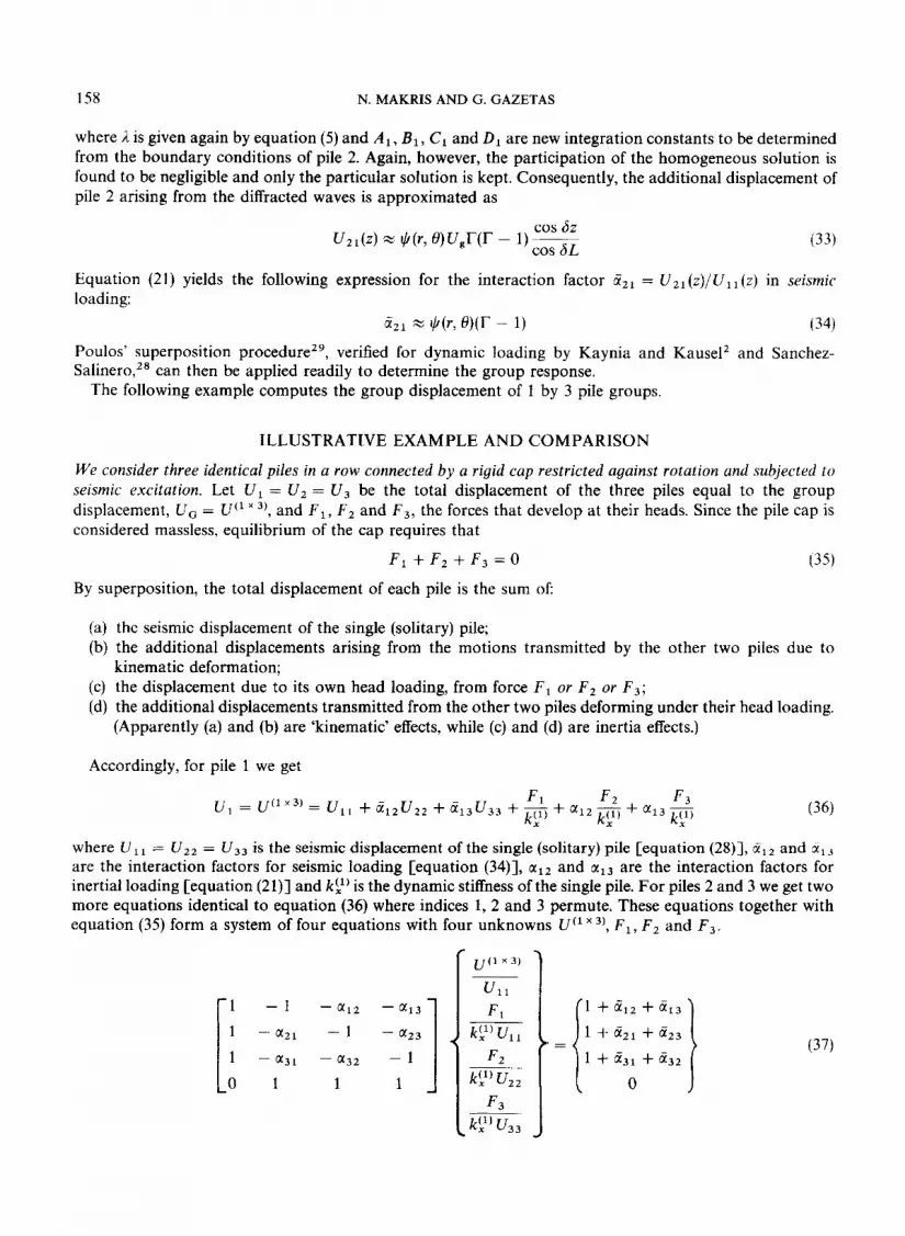
We consider three identical piles in a row connected by a rigid cap restricted against rotation and subjected to seismic excitation. Let U1 = U , = U 3 be the total displacement of the three piles equal to the group displacement, UG = U" ,), and F , , F 2 and F , , the forces that develop at their heads. Since the pile cap is considered massless. equilibrium of the cap requires that

(35) F1 + F2 + F3 = 0

By superposition, the total displacement of each pile is the sum of:

(a) the seismic displacement of the single (solitary) pile; (b) the additional displacements arising from the motions transmitted by the other two piles due to

(c) the displacement due to its own head loading, from force F1 or F 2 or F 3 ; (d) the additional displacements transmitted from the other two piles deforming under their head loading.

kinematic deformation;

(Apparently (a) and (b) are 'kinematic' effects, while (c) and (d) are inertia effects.)

Accordingly, for pile 1 we get

where U I 1 = U 2 2 = U,, is the seismic displacement of the single (solitary) pile [equation (ZS)], Zlz and ii13 are the interaction factors for seismic loading [equation (34)], a l2 and a13 are the interaction factors for inertial loading [equation (21)] and kL1) is the dynamic stiffness of the single pile. For piles 2 and 3 we get two more equations identical to equation (36) where indices 1, 2 and 3 permute. These equations together with equation (35) form a system of four equations with four unknowns U'' r 3 ) , F , , F , and F,.

1 - 1 - a l 2 - a l 3 1 - 1 - a23

1 - a31 - a 3 2 - 1 0 1 1 1

(37)


1 X 3 Pile Group

- Presented Simplified Method X * * Rigorous Solution: Ke Fan et al 1991

0.80 ’. 1\ * 1

\ *

\*

0.20 1 i

O I 1 I I I I 0 0.1 0.2 0.3 0.4 0.5

w d a , - - v s

Figure 10. Normalized kinematic seismic response of 1 x 3 fixed-head pile group: comparison of presented method with rigorous results by Ke Fan et at. (p, /ps = 1.42, L/d = 20, v = 04, j3 = 0.05)

1 x 2 Pile Group

Presented Simplified Method Rigorous Solution: KeFanetal 1991 * * *

1 .oo

0.80

0.40

b.20

* *\

0.00 f I I I 1 0.0 0.1 0.2 0.5 0.4 0.5

wd ao-- V.

Figure 11. Normal id kinematic seismic response of 1 x 2 fixed-head pile group: comparison of presented method with rigorous results by Ke Fan et al. (p,lp. = 1.42, LID = 20, v = 0.4, B = 0.05)


Presented Simplied Method

0 O.'l 04 0.5 0.2 0.5

The solution to equation (37) gives the group displacement UG and the forces developing at each pile head. Figure 10 plots versus a, the ratio of group to free-field displacements for such a 1 x 3 pile group. The results are compared with the rigorous results of Reference 34; the agreement is very encouraging in view of the simplicity of the developed methods.

The success of the presented approximate method is further illustrated in Figures 11 and 12. Figure 11 plots the same ratio as Figure 10 but for a 1 x 2 fixed-head pile group, for two values of E, /E , , loo0 and 10000. Figure 12 plots again the same ratio, but for a 2 x 2 fixed-head pile group for E J E , = 10OO0, for two separation distances ( S / d = 5 and 10). The approximate method captures not only the general trend but also details of the response. For stiffer piles or softer soils the group displacement reduces rapidly as frequency increases. For instance for E,/E, = 10 000 the group response is approximately half the free-field response at a frequency of a, = 0.25, whereas for E J E , = 1000 the group response is approximately 0.9 times the free-field response at the same frequency (ao = 0.25).

Finally, comparing the group responses (Figures 10, 11, 12) with the single-pile response (Figure 9) one should note that the pile-to-pile interaction effects are rather insignificant for seismic excitation, contrary to head-loading excitation where the pile-to-pile interaction effects are indeed very important. This conclusion,

2 X 2 Pile Group

E , / E , = 10000

1

0.8

0.4

0.2

0

1.2

0.2

0

0 0.; 0.5 0.5 0.4 0.b

1

Figure 12. Normalized kinematic seismic response of 2 x 2 fixed-head pile group: comparison of presented method with rigorous results by Ke Fan et al. for two separation distances ( S / d = 5 and 10) (p,/p. = 1.42, L/d = 15, v = 0.4, f l = 0.05)


however, may be applicable only to homogeneous profiles; in heterogeneous deposits, containing consecutive soil layers with drastically different ‘acoustic impedances’ ( p V), soil and individual pile seismic displacements are expected to differ sharply at relatively high frequencies and hence to trigger substantial pile-to-pile interaction. Evidence of this for a single pile is presented by Gazetas et

CONCLUSIONS

A general methodology has been developed to compute dynamic pile-soil-pile interaction problems under both lateral head and seismic loading. The method involves three independent is steps. Pile-soil interaction represented realistically through a dynamic Winkler model and physically-motivated approximations are used to model diffraction and attenuation of waves. Dynamic interaction factors are given by simple closed-form expressions and the group response can be computed simply even by hand calculations. The results obtained are in accord with rigorous solutions, especially for piles in soft and medium-stiff soil E,/E, 2 1OOO). It is shown that pile-to-pile interaction effects are significant mainly in the inertial loading creating a strong dependence on frequency of the group efficiency. In seismic loading the ineraction effects between piles in homogeneous structures are very small and could be neglected.

ACKNOWLEDGEMENT

This work was supported by a grant from the Secretariat for Research & Technology of the Greek government.

REFERENCES

1. J. P. Wolf and G. A. Von Arx, ‘Impedance function of group of vertical piles’, Proc. ASCE specialty con$ soil dyn. earthquake eng. 2,

2. A. M. Kaynia and E. Kausel, ‘Dynamic stiffness and seismic response of pile groups’, Research Report R82-03, Massachusetts

3. T . Nogami, H. W. Jones and R. L. Mosher, ‘Seismic response analysis of pile-supported structure: assessment of commonly used

4. M. Novak and M. James, ‘Dynamic and static response of pile groups’, Proc. 12th int. con$ soil mech. found. eng. Rio de Janerio

5. G. Waas and H. G. Hartmann, ‘Seismic analysis of pile foundations including soil-pile-soil interaction’, Proc. 8th world cont

6. I. M. Roesset, ‘Dynamic stiffness of pile groups’, Pile Foundations, ASCE, New York, 1984. 7. P. K. Banerjee and R. Sen, ‘Dynamic behavior of axially and laterally loaded piles and pile groups’, Dynamic Behauiour of

8. R. Dobry and G. Gazetas, ‘Simple method for dynamic stiffness a damping of floating pile groups’, Gbotechnique 38,557-574 (1988). 9. G. Gazetas and N. Makris, ‘Dynamic pile-soil-pile interaction. Part I: Analysis of axial vibration’, Earthquake eng. struct. dyn. 20,

10241041 (1978).

Institute of Technology Cambridge, Mass., 1982.

approximations’, Proc. 2nd int. con$ recent adu. geotech. earthquake eng. soil dyn. St. Louis 931-940 (1991).

1175-1178 (1989).

earthquake eng. San Francisco 5, 55-62 (1984).

Foundations and Buried Structures, Elsevier Applied Science, New York, 1987, pp. 95-133.

115-132 (1991). 10. M. Novak, ‘Piles under dynamic loads’, 2nd int. con$ recent ado. geotech. earthquake eng. soil dyn. St. Louis 250-273 (1991). 11. G. W. Blaney, E. Kausel and J. M. Roesset, ‘Dynamic stiffness of piles’; Proc. 2nd int. con$ n m r . methods geomech. Virginia

12. R. L. Kuhlemeyer, ‘Static and dynamic laterally loaded floating piles’, J. geotech. eng. diu. ASCE 105, 289-304 (1979). 13. R. Krishnan, G. Gazetas and A. Velez, ‘Static and dynamic lateral deflexion of piles in non-homogeneous soil stratum’, Geotechnique

14. G. Gazetas and R. Dobry, ‘Horizontal response of piles in layered soils’, J . geotech. eng. ASCE 110, 20-40 (1984). 15. M. Novak, T. Nogami and F. Aboul-Ella, ‘Dynamic soil reactions for plane strain case’, J . eng. mech. div. ASCE 104,953-959 (1978). 16. H. Matlock, H. C. Foo and L. M. Bryant, ‘Simulation of lateral pile behavior under earthquake moton’, Proc. ASCE specialty con$

17. G. A. Blaney and M. W. ONeill, ‘Measured lateral response of mass on single pile in clay’, J . geotech. eng. ASCE 112, 443457

18. M. Ochoa and M. W. ONeill, ‘Lateral pile interaction factors in submerged sand’, J . geotech. eng. ASCE 115, 359-378 (1989). 19. T. Tazoh, K. Shimizu and T. Wakahara, ‘Seismic observations and analysis of grouped piles’, Dynamic Response of Pile

20. J. H. Prevost and R. H. Scanlan, ‘Dynamic soil-structure interaction; centrifuge modeling’, Soil dyn. earthquake eng. 2, 212-221

21. R. F. Scott, J. M. Ting and J. Lee, ‘Comparison of centrifuge and full scale dynamic pile tests’, Proc. con$ soil dyn. earthquake eng.

Polytechnic Institute and State University, Blacksburg, VA, I1 101&1012 (1976).

33, 307-325 (1983).

earthquake eng. soil dyn. 2, 600-619 (1978).

(1986).

Foundations-Experiment, Analysis and Observation, Geotechnical Special Publication No. 11, ASCE, New York, 1987.

(1983).

Southampton, U.K. 1, 299-309 (1982).


22. M. F. Randolf, ‘The response of flexible piles to lateral loading’, Gkotechnique 31, 247-259 (1981). 23. J. M. Roesset and D. Angelides, ‘Dynamic stiffness of piles’, Numerical Methods in Ofshore Piling, Institution of Civil Engineers.

24. R. F. Scott, Foundation Analysis, Prentice-Hall, Englewood Cliffs, N.J:, 1981. 25. J. P. Wolf, Dynamic Soil-Structure Interaction, Prentice-Hall, Englewood Cliffs, N.J., 1985. 26. E. Berger, S. A. Mahin and R. Pyke, ‘Simplified method for evaluating soil-pile structure interaction effects’, Proc. 9th offshore

27. J. M. Roesset, ‘Stiffness and damping coefficients of foundations’, Special Technical Pubfication on Dynamic Response of Pile

28. I. Sanchez-Salinero, ‘Dynamic stiffness of pile groups: Approximate solutions’, Geotechnical Engineering Report GR83-5, University

29. H. G. Poulos and E. H. Davis, Pile Foundations Analysis and Design, Wiley, New York, 1980. 30. H. Tajimi, ‘Seismic effects on piles’, State-of-the-art Report 2, Proc. specialty session ICSMFE, 15-26 (1977). 31. T. Kagawa and L. M. Kraft, ‘Lateral pile response during earthquakes’, J . geotech. eng. div. ASCE 107, 1713-1731 (1981). 32. R. Flores-Berrones and R. V. Whitman, ‘Seismic response of end-bearing piles’, J . geotech. eng. div. ASCE 108, 554569 (1982). 33. G. Gazetas, ‘Seismic response of end-bearing single piles’, Soil dyn. earthquake eng. 3, 82-93 (1984). 34. K. Fan, G. Gazetas, A. Kaynia, E. Kausel and S. Ahmad, ‘Kinematic seismic response of single piles and piles groups’, J . geotech.

35. J. M. Roesset, ‘Soil amplification of earthquakes’, Numerical Methods in Geotechnical Engineering (Eds. C. S . Desai and J. T.

36. G. Gazetas, K. Fan, T. Tazoh, K. Simizu, & M. Kavvadas, ‘Seismic response of soil-pile-foundation-structure systems: some

London, England 1989, pp. 75-80.

technol. con5 589-598 (1977).

Foundations: Analytical Aspects (Eds. M. W. ONeil and R. Dobry) ASCE, New York, 1980.

of Texas at Austin, 1983.

eny. ASCE 117, No. 12 (1991).

Christian) McGraw-Hill, New York, 1977.

recent developments’, ASCE publication on Piles under Dynamic Loads, Sept. 1992 (in press).

dynamic pile-soil- pile interaction part ii. lateral and seismic response

Documents