pile capacity predictions using static and dynamic load
TRANSCRIPT

SCHOOL OF CIVIL ENGINEERING
JOINT HIGHWAY RESEARCH PROJECT
FHWA/IN/JHRP-87/l -(
Final Report
PILE CAPACITY PREDICTIONS USINC
STATIC AND DYNAMIC LOAD TESTIN(
Ahmad Amr Darrag
$
UNIVERSITY

JOINT HIGHWAY RESEARCH PROJECT
FHWA/IN/JHRP-87/l -|
Final Report
PILE CAPACITY PREDICTIONS USIN(
STATIC AND DYNAMIC LOAD TESTINt
Ahmad Amr Darrag

FINAL REPORT
PILE CAPACITY PREDICTIONSUSING STATIC AND DYNAMIC LOAD TESTING
by
Ahmad Amr DarragGraduate Instructor in Research
Joint Highway Research Project
Project No.: C-36-36PFile No. : 6-14-16
Prepared for an InvestigationConducted by the
Joint Highway Research ProjectEngineering Experiment Station
Purdue University
in cooperation with the
Indiana Department of Highways
and the
U.S. Department of TransportationFederal Highway Administration
The opinion, findings and conclusions expressed in thispublication are those of the author and not necessarilythose of the Federal Highway Administration.
Purdue UniversityWest Lafayette, Indiana
February 3, 1987
FINAL REPORT
PILE CAPACITY PREDICTIONS USINGSTATIC AND DYNAMIC LOAD TESTING
To: H. L. Michael, DirectorJoint Highway Research Project
From: C. W. Lovell, Research EngineerJoint Highway Research Project
February 3 , 1 987
Project: C-36-36P
File: 6-14-16
Attached is a Final Report on the study, "ComputationalPackage for Predicting Pile Stress and Capacity". This reportwritten by Ahmad Amr Darrag of our staff, who worked under mysupervision .
is
The report is a comprehensive synthesis of pile analysis anddesign technique in several parts: (1) static pile load tests;(2) dynamic measurements made during pile driving; and (3) resi-dual stresses induced in the pile and adjacent soil by piledriving. These chapters have already had one review by the IDOHand the division office of the FHWA.
As a result of this study Mr. Darrag has made definiterecommendations to the IDOH with respect to: (1) how pile loadtests should be run and interpreted; (2) why the IDOH shouldbegin making and using dynamic measurements; and (3) how residualstresses can be estimated and used in pile foundation analysisand design.
Although the report is lengthy (± 300 pages), it is recom-mended that it be printed in its entirety.
The report is submitted for review, comment, and acceptancein fulfillment of the referenced study.
Respectfully submitted,
C. W. LovellResearch Engineer
cc A.G. Altschaef f
1
J.M. BellM.E. CantrallW.F. ChenW.L. DolchR.L. EskewJ.D. Fr ickerD.E. Hancher
R.A. Howden B.K. PartridgeM.K. Hunter G.T. SatterlyJ. P. Isenbarger C.F. ScholerJ.F. McLaughlin K.C. SinhaK.M. Mellinger c.A. VenableR.D. Miles T.D. WhiteP.L. Owens L.E. Wood

Digitized by the Internet Archive
in 2011 with funding from
LYRASIS members and Sloan Foundation; Indiana Department of Transportation
http://www.archive.org/details/pilecapacitypredOOdarr
TECHNICAL REPORT STANDARD TITLE PACE
1. Report No.
FHWA/IN/JHRP-87/
1
"2. Government Accunon No. 3. Recipient's Catalog No.
4. TitU and Subtitle
PILE CAPACITY PREDICTIONS USING STATIC AND DYNAMICLOAD TESTING
5. Report Dot*
February 3, 19876. Performing Organization Code
7. Author! i)
Ahmad Amr Darrag
8. Performing Organization Report No.
JHRP-87/1
9, Performing Organization Nam* and Address
Joint Highway Research ProjectCivil Engineering BuildingPurdue UniversityWest Lafayette, Indiana 46204
10. Work Unit No.
11. Contract or Gront No.
JPR-K24) Part II
12. Sponsoring Agency Nome ond Addree*
Indiana Department of HighwaysState Office Building100 Nouth Senate AvenueIndianapolis, Indiana 46204
13. Type of Report and Period Covered
Final Report
14. Sponsoring Agency Code
IS. Supplementary Notes
Prepared in cooperation with the U.S. Department of Transportation, Federal HighwayAdministration. Study title is "Computational Package for Predicting Pile Stressanrl fapariry" ,
16. Abstract
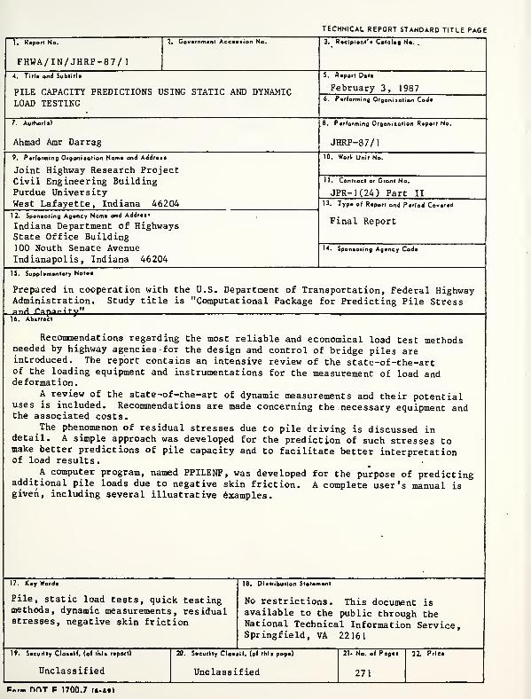
Recommendations regarding the most reliable and economical load test methodsneeded by highway agencies for the design and control of bridge piles areintroduced. The report contains an intensive review of the state-of-the-artof the loading equipment and instrumentations for the measurement of load anddeformation.
A review of the state-of-the-art of dynamic measurements and their potentialuses is included. Recommendations are made concerning the necessary equipment andthe associated costs.
The phenomenon of residual stresses due to pile driving is discussed indetail. A simple approach was developed for the prediction of such stresses tomake better predictions of pile capacity and to facilitate better interpretationof load results.
A computer program, named PPILENF, was developed for the purpose of predictingadditional pile loads due to negative skin friction. A complete user's manual isgiven, including several illustrative examples.
17. Key Words
Pile, static load tests, quick testingmethods, dynamic measurements, residualstresses, negative skin friction
18. Distribution Stotemont
No restrictions. This document isavailable to the public through theNational Technical Information Service,Springfield, VA 22161
19. Security Closslf. (of this report)
Unclassified
20. Security Closslf. (of this page)
Unclassified
21. No. of Pages
271
22. Price
F».« HOT P 1700.7 fa. 69)
ACKNOWLEDGEMENTS
The author would like to express his sincere appreciation to
his major professor, Dr. C. W. Lovell, for his invaluable gui-
dance during the preparation of this report and the critical
review of the manuscript.
The author would also like to thank Mr. Steve Hull of the
Indiana Department of Highways and Mr. Paul Hoffman of the
Federal Highway Administration for their assistance as members of
the Advisory Committee for the project.
Thanks are extended to Mrs. Cathy Ralston and Mrs. Kathie
Roth for the excellent job they did in typing the report.
The financial support for this report was provided by the
Indiana Department of Highways and the Federal Highway Adminis-
tration. The research was administered through the Joint Highway
Research Project, Purdue University, West Lafayette, Indiana.
TABLE OF CONTENTS
Page
LIST OF TABLES Vi
LIST OF FIGURES Vlii
LIST OF SYMBOLS AND NOMENCLATURE xiii
HIGHLIGHT SUMMARY xvi
CHAPTER 1 INTRODUCTION 1
CHAPTER 2 PILE LOAD TESTS 5
2.1 Introduction 5
2.1.1 Purpose of Pile Load Tests 5
2.1.2 Planning the Test Program2.1.3 Types of Pile Load Testing 9
2.1.4 Application of Results 9
2.2 Axial Compression Load Tests 13
2.2.1 Loading and Instrumentation 13
2.2.1.1 Loading Systems 13
2.2.1.2 Measurement of Settlement of PileHead 22
2.2.1.3 Measurement of Pile Movements andLoads at Various Points Along thePile 28
2.2.1.4 Residual Stresses 34
2.2.1.5 Sources of Error in SettlementMeasurements 35
2.2.1.5.1 Errors Resulting fromUse of Reference Beam . 35
2.2.1.5.2 Errors Resulting fromJacking Against AnchorPiles 40
2.2.1.5.3 Errors Resulting fromJacking Against GroundAnchors 42
2.2.2 Test Procedures 45
2.2.2.1 Maintained Loading Test 47
2.2.2.1.1 Procedure 47
2.2.2.1.2 Interpretation of TestResults 53
a. Ultimate Load ... 53
b. Empirical Methods ofWorking Loads ... 55
c. Plastic and ElasticDeformations ... 58
IV
d . Distribution of Loadto Soil 59
e. Settlement Behavior 61
f. Some Factors Influ-encing Interpretationof Test Results . . 62
2.2.2.2 Constant Rate of Penetration Test 63
2.2.2.2.1 Procedure 64
2.2.2.2.2 Interpretation of TestResults 67
2.2.2.3 Method of Equilibrium 72
2.2.2.3.1 Procedure 73
2.2.2.3.2 Discussion and Interpre-tation of Results ... 74
2.2.2.4 Load Testing by the Texas HighwayDepartment 77
2.2.2.4.1. Procedure 81
2.2.2.4.2. Correlation Studies byTHD 85
2.3 Other Types of Pile Load Tests 94
2.3.1 Uplift Tests 94
2.3.2 Lateral Load Tests 96
2.3.2 Torsional Testing 1022.4 Recommended Procedures for Axial Pile Load Tests . 104
2.4.1 General •. 1042.4.2 Texas Quick Load Test Method 107
2.4.3 Method of Equilibrium 117
CHAPTER 3 DYNAMIC MEASUREMENTS FOR PILE DRIVING 120
3.1 Introduction 120
3.1.1 Pile Capacity 120
3 .1 .2 Hammer Performance 121
3.1.3 Pile Performance and Integrity 122
3.2 Technical Background on Dynamic Measurements . . . 123
3.2.1 Acceleration Measurement 124
3.2.2 Force Measurement „ 126
3.2.3 Recording Devices 128
3.2.4 Developments in Dynamic Measurements . . . 131
3.3 Estimation of the Pile Capacity Using DynamicMeasurements 134
3.3.1 Simplified Approach Using Field Computers . 135
3.3.2 Office Analysis Using CAPWAP 141
3.4 Evaluation of the Performance of Pile DrivingSystems Using Dynamic Measurements 149
3.5 Evaluation of the Pile Performance Using DynamicMeasurements 155
3.6 Conclusions and Recommendations 161
CHAPTER 4 RESIDUAL STRESSES DUE TO PILE DRIVING 166
4.1 General 166
4.2 Current Methods Used for Residual Stress Measure-ment 172
4.3 Review of Research on Residual Stresses for Pilesin Cohesionless Soils 176
4.4 Numerical Evaluation of Residual Stresses andFactors Affecting These Stresses 184
4.4.1 Obtaining Residual Stresses 184
4.4.2 Effect of Considering Residual Stresses inthe Dynamic Analysis 188
4.4.3 Distribution of Residual Forces along PileShaft 196
4.4.4 Factors Affecting the Magnitude of ResidualStresses 203
4.4.4.1 Effect of the Driving System andElements 203
4.4.4.2 Effect of Total Soil Resistance . 2054.4.4.3 Effect of Skin Friction Percent . 2084.4.4.4 Effect of Pile Length 2124.4.4.5 Effect of Pile Cross Sectional
Area 2154.4.4.6 Effect of the Pile Material ... 217
4.5 The Development of an Approximate Technique forResidual Stresses Prediction 2194.5.1 The Hunter-Davisson Method 221
4.5.2 The Holloway Procedure 2224.5.3 The Bri aud-Tucker Procedure 2244.5.4 The Procedure Suggested in this Research . 2274.5.5 Comparison of Proposed Procedure with Other
Techniques 241
4.6 Summary and Conclusions 249
CHAPTER 5 SUMMARY AND CONCLUSIONS 254
5.1 Summary 254
5.1.1 Static Pile Load Tests 255
5.1.2 Dynamic Measurements for Pile Driying . . . 256
5.1.3 Residual Stresses Due to Pile Driving . . . 257
5.1.4 Negative Skin Friction 2585.2 Conclusions 258
5.2.1 Pile Load Tests 2585.2.2 Dynamic Measurements 2595.2.3 Residual Stresses Due to Pile Driving . . . 261
5.2.4 Negative Skin Friction 262
LIST OF REFERENCES 264
APPENDIX A-l Pile Loads Due to Negative Skin Friction ... A-l
VI
LIST OF TABLES
Table Page
1. A Suggested System of Load Increments for an MLTest
2. AASHTO 48-24 Hour Test Method
3. Description of Piles, Soil and Hammer
4. Quick Test Method
5. Average Manpower Requirements and Time Delay toContractor
6. Estimated Materials Cost for Quick-Load Test . . .
7. Unit Bid Price for Pile Load Tests in Texas, 1963through 1975
8. Record of Foundation Test Load. Texas Quick TestLoad Method
9. Record of Foundation Test Load. Texas Quick TestLoad Method
10. Record of Foundation Test Load. Texas Quick TestLoad Method
11. Suggested values of j
12. Comparative Results from Automated PredictionMethod
13. Measurement System Price List «...14. Adjustment of Load Test Results by Considering
Residual Loads
15. Residual Stress Analysis Algorithm
16. Effect of Total Soil Resistance on Critical DepthRatio b
c
17. Effect of Hammer Type and Energy on the ResidualStress Percent
18. Effect of Types of Caps and Cushions on the ResidualStress Percent
51
80
86
87
90
91
92
109
m
114
140
144
164
177
187
200
204
206
VI 1
19. Pile Data Used for Residual Stress Analysis
20. The Residual Stress Percent "a " by DifferentMethods
242
244

vm
LIST OF FIGURES
Figure
1 .
2.
3.
4.
5.
6.
7.
8.
9.
10.
11 .
12.
a
12.
b
13.
a
13.
b
Page
Arrangement for Carrying Kentledge Directly onthe Pile Head 14
Testing Rig for Compressive Test on Pile UsingKentledge for Reaction 14
Testing Rig for Compressive Test on Pile UsingTension Piles for Reaction 16
Testing Rig for Compressive Test on Pile UsingCable Anchors for Reaction 18
Method of Sleeving Test Pile to Eliminate SkinFriction Through Fill 23
Arrangement for Applying Tests Loads Directly onPile Cap for Group Tests 23
Possible Arrangement for Applying Load Test toPile Group Using Weighted Platform . . . . . -. . 24
Typical Arrangement for Applying Test to PileGroup 24
Typical Setup for Measurement of Pile Displace-ments 26
The Positions of Load Cells for Measuring The BaseLoads in Bored Piles, (a) Without Base Enlargement;(b) With an Enlarged Base 30
Use of Rod Strain Gauges to Measure Load Transferfrom Pile to Soil at Various Levels Down PileShaft 31
Correction Factor Fc for Friction Pile in DeepLayer of Soil 37
Effect of Layer Depth on Settlement CorrectionFactor 37
Correction Factor Fc for Floating Pile in a DeepLayer Jacked Against Two Reaction Piles 38
Correction Factor Fc for End Bearing Pile on RigidStratum Jacked Against Two Reaction Piles .... 38
IX
13. c Correction Factor Fc Effect of Bearing Stratum forEnd-Bearing Pile Jacked Against Two Reaction Piles
13. d Correction Factor Fc for Friction Pile in a DeepLayer Jacked Against Two Reaction Piles -
Settlement Measured in Relation to Anchor Piles .
14. a Correction Factor Fc for Friction Pile in a DeepLayer Jacked Against Ground Anchors
14. b Correction Factor Fc for End-Bearing Pile JackedAgainst Ground Anchors
15. Compression Load Tests on 305x305mm Pile. Load-Settlement And Time-Settlement Curves for Pile onStiff Clay (ML)
16. Typical Load-Settlement Curves for CompressiveLoad Tests
17. Test-Loading Diagram Showing Relationship BetweenLoading, Settlement, and Time
18. (a) Typical Force-Penetration Diagrams Obtainedwith Friction Piles. The Values of Force Reachedat Points a Represents The Ultimate BearingCapacity in Each Case. (b) Typical Force-Penetration Diagram Obtained for an End BearingPile
19. Results of Six CRP Tests, Each Made In From 30
To 45 Minutes, are Similar to Those of a StaticTest in Which The Pile Was Loaded for a Totalof 40 1/2 Hours
20. Load Cycles for Particular Loads
21. Load Settlement Curves from Maintained Load Testand Method of Equilibrium " . . .
22. Load Settlement Curves from Maintained Load Test,CRP Test and Method of Equilibrium
23. Typical Load Settlement Graph
24. Load-Settlement Graph for a Pile Load Test . . .
25. Load-Settlement Graph for a Drilled Shaft LoadTest
26. Correlation of Proven Design Load Between AASHT048-24 Hour And Texas Quick-Load Methods
39
39
44
44
50
56
60
68
71
75
78
79
82
83
84
88
27. Testing Rig for Uplift Test on H-Section PileUsing Ground as Reaction 95
28. Uplift Load on Test Pile (ML Test) (a) Load-Uplift Curve. (b) Time-Uplift Curve 97
29. Testing Rig for Push And Pull Lateral LoadingTest on Pair of Piles 98
30. Typical Setup for Lateral Load Tests 98
31. Test Rig for Lateral Loading Test on Single Pile 100
32. Load-Deflection Curve for Cyclic HorizontalLoading Test on Pile 100
33. Strain Transducer Design 127
34. Sample Result of Dynamic Measurements Taken ona 60 Ft. Long Pile 130
35. Sample Output of Pile Analyzer 133
36. Comparison of Predicted with Measured Load versusPenetration Curve and Predicted and Measured ForcesForces in Pile at Maximum Dynamic Deflection . . 143
37. Effect of Soil Set-up on Wave Traces Measured atEnd of Initial Driving and at Restriking .... 146
38. Effect When No Soil Set-up is Present on WaveTraces Measured at End of Initial Driving and atRestriking 147
39. Effect of Relaxation of Toe Resistance on WaveTraces Measured at End of Initial Driving and atRestriking 147
40. Sample Plots of Automatically Processed Data . . 152
41. Maximum Stresses for a Test Driven Pile .... 156
42. Determination of Pile Length from a VelocityGraph for a Friction Pile 157
43. Quality Control of an End-Bearing Pile UsingDynamic Measurements: (a) intact pile (b) pilewith a crack 159
XI
44.
45.
46.
47.
48.
49.
50.
51.
52.
53.
54.
55.
56.
57.
58.
59.
60.
61.
Difference between True Loads and Measured Loadsin Conventional Load Tests
Residual Load Distribution
The Hunter-Davisson Method to Obtain ResidualStresses
Effect of Including Residual Stresses on theNumber of Blows/Ft
Determination of the set in WEAP (S ) andCUWEAP (S ) Y
c
Representative Data for the Factor " a^ " ....Upper and Lower Bounds and Recommended Valuesf0r Q
N
Effect of Including Residual Stresses on PileDriving Stresses
Typical Residual Pile Load and Skin FrictionDistribution
Prediction of the Critical Depth Ratio for Sands
Effect of Total Pile Capacity on the Residual StressStress Percent "a "
r
Effect of the Skin Friction Percent "m" on theResidual Stress Percent "a " for ConcretePiles
r
Effect of Skin Friction Percent "m" on theResidual Stress Percent "a " for Steel Piles
r
Effect of Pile Length on Residual Stresses -
Concrete Piles * . .
Effect of Pile Length on Residual Stresses -
Steel Piles
Effect of Pile Cross Section Area on the ResidualStress Percent "a "
r
Unit Shaft Friction Distribution in Loading andUnloading, Interpretation of Results Reported byVesic, 1970, for Pile No. H- 1 5
Correlation Between N ., and Ks ide t
168
170
174
189
190
192
193
195
197
201
207
210
211
213
214
216
223
226
Xll
62. Prediction Charts for the Residual Stress Percent"a " for Concrete Piles
r
63. Prediction Charts for the Residual Stress Percent"a " for Steel Piles
r
64. Factors 8 and 3'ra m
65. Iterative Procedure for Residual Point LoadPrediction from Load Test Results
66. Predicted vs Measured Residual Stress Percent. .
67. Comparison between Different Methods for ResidualStress Prediction
230
231
236
240
246
248
xm
LIST OF SYMBOLS AND NOMENCLATURE
A(t)
b»b
>b
c r m
E ,E'c ' c
s
F(t)
F ,F'c c
12,1
3
= cross-sectional area of the pile
= area of concrete in a combined pile crosss e c t i on
= area of steel in a combined pile crosss e c t i on
= pile acceleration as a function of time
= residual stress percent
= factors describing shape of residualload distribution
= pile embedment length
= elastic modulus of the pile
= elastic moduli of concrete and steel,respectively
= elastic modulus of soil
= force at the pile top as a function of time
= interaction correction factors due tothe effect of the reaction system
= damping constant
= coefficient of lateral earth pressurefor piles
= unloading stiffness in friction
= pile length
= lengths for rods (2), (3) of thetell-tales, respectively
= mass of the piles
= skin friction percent
XIV
mm
Nq
Nside
P
P2
P3
= measured values of m
= bearing capacity factor
= average SPT blow count within the shaftlength considered
= load at the pile head
= load reaching the pile at the level of toeof rod (2) of the tell-tale system
= load reaching the pile at the level ofits toe
p = pile perimeter
Q ,Q = tip and shaft pile loads,respectively
Q = residual tip loadP R
Q„„.„ = maximum residual shaft loadRMAX
q = residual point stressres
R(t) = pile total capacity
R,(t) = pile dynamic capacity as a function oftime
R (t) = pile static capacity as a function oftime
s = measured settlementm
V
s' «• measured settlement relative to reactionpiles
t = time
t time after which a "blip" is observed forx
a pile with a crack
v(t) = pile velocity as a function of time
"' "*' """ X RMAX
Z - depth of point of inflection on residualload distribution
XV
= factor giving the reduction in the numberof blows due to the existence of residualstresses
= factor giving the increase in pile stressesdue to the existence of residual stresses
= factors that introduce the effect ofskin friction percent on the residualstress percent
= distance from the pile top at which a
crack exists
= elastic shortening over length (L)
V A3
elastic shortening of the pile betweenthe pile head and rod (2), and the pilehead and rod (3), respectively, for thetell-tale system
XVI
Highlight Summary
Static pile load testing is the most reliable technique for
pile capacity estimation and for quality control. The main
disadvantage of these tests is the cost involved. Recommenda-
tions regarding the most reliable and economical load test
methods are introduced in this report. It is recommended that
the IDOH use these techniques routinely in the jobs involving
pile foundations. The state-of-the-art for loading systems and
instrumentation for deformation measurements is described as
well.
It has been proven that the performance of the pile and
driving system during driving cannot be monit'ored successfully
without the use of dynamic measurements. These measurements,
together with the wave equation analysis, can be used for many
purposes such as pile capacity prediction, observation of hammer
performance, observation of pile performance and integrity,
checking the efficiency of the driving elements, quality control
and other things. One of the purposes of this report is to fami-
liarize the IDOH with the subject of dynamic measurements, illus-
trate their uses, and review some of the work that has been done
using them. It is recommended that the IDOH acquire the neces-
sary equipment and prepare the trained personnel required for
their operation to utilize the dynamic measurements routinely in
pile foundation jobs.
xvu
Residual stresses accumulating during pile driving have a
very important effect on the pile capacity prediction and the
interpretation of static load test results. The report examines
this phenomenon in detail, including all the factors involved and
the methods that have been suggested thus far for the residual
stresses prediction. A new method has been developed for the
prediction of such stresses. This method, in addition to being
relatively simple, proved to give predictions that compare well
with actual measurements.
In many situations, negative skin friction has a very impor-
tant effect on the design of the pile foundation. A computer
program PPILENF has been developed in order to predict additional
pile loads due to negative skin friction. It is recommended to
use this program for the problems involving negative skin fric-
tion to avoid serious prediction errors for long-term problems.
CHAPTER 1
INTRODUCTION
The analytical determination of pile capacity was discussed
in the interim report by Tejidor (1984). It is essential to com-
plete the subject of pile capacity prediction by discussing pile
load tests. These tests provide the best evidence of pile capa-
city and serve as a reference of accuracy for other load predic-
tion techniques.
The judicious use of load tests can lead to substantial
economic benefits. The costs of performing pile load tests are
relatively small compared to the substantial savings that may be
achieved by their use. However, many organizations remain reluc-
tant to use them because of cost and time delay during construc-
tion. Hence, it is important to improve the test procedures so
as to save money and time.
One of the main objectives of this report is to form a
specification for the best method available for performing load
tests and to recommend its use by the IDOH. In order for the
report to be most valuable, the state-of-the-art of pile load
testing is described in some detail. Emphasis is placed espe-
cially on axial compression load tests, since they are the most
common type for pile testing. Other types of load tests such as
uplift, lateral and torsional tests are described as well. Load-
ing systems and instrumentation for deformation measurements are
described and discussed for each type of test. The major methods
available for performing axial compression load tests are
described in detail as well as the interpretations of their
results (e.g., ultimate loads, allowable working loads, settle-
ment behavior, ...» etc.).
The quick load tests methods have proven to correlate well
with the classical longer-term testing procedures. Since the
short-term tests are more economical, their use can be economi-
cally justified on a greater variety of projects. As these are
used and interpreted, it is possible to gain greater confidence
in static and other load prediction methods.
In spite of the recent developments that resulted in more
accurate methods of predicting pile capacities; improved methods
of construction control; and the use of highly specialized
methods and equipment for driving, some uncertainties still
exist. Thus far, static pile load tests have proven to be the
best way to obtain relatively accurate information regarding the
static capacity of the pile. On the other hand, the performance
of the pile and driving system during driving cannot be monitored
successfully without the use of dynamic measurements. These
measurements have been used by many investigators and organiza-
tions to examine the pile driving procedure. Such investigations
have shown that the dynamic measurements, together with the wave
equation analysis, can be used for many purposes such as pile
capacity prediction, observation of hammer performance,
observation of pile performance and integrity, checking the effi-
ciency of the driving elements, quality control, and other
things. By using such measurements, the number of necessary
static load tests can be reduced and consequently much money can
be saved. One of the purposes of this report is to introduce the
subject of dynamic measurements, illustrate their uses, and
review some of the work that has been done using them. This is
intended to familiarize the IDOH with the subject and to intro-
duce it as a valuable and necessary link in the chain of the
design and construction of pile foundations.
An important factor that has a considerable effect on the
pile capacity prediction and the interpretation of load tests is
the existence of residual stresses in the pile due to driving.
These stresses have a very important effect on the distribution
of loads along the pile shaft and beneath the tip. The report
describes an explanation for such a phenomenon, discusses the
factors affecting it using some parametric studies, and reviews
the methods that have been suggested thus far for the residual
stresses prediction. Based on these studies a new procedure is
developed for such prediction. This procedure is introduced by
means of easy-to-use charts and equations, with the help of some
illustrative examples. Predictions made by this technique are
compared with actual measurements and good agreements are proven.
The subject of negative skin friction was discussed in
detail by Tejidor (1984). Further discussion is given in this

report. A computer program PPILENF for the prediction of addi-
tional pile loads due to negative skin friction was developed at
Purdue. This program is introduced in this report, together with
a user manual, input forms and some illustrative examples. It is
recommended to use this program for the problems involving nega-
tive skin friction to avoid serious prediction errors and long-
term problems.
2 . 1 Introduction
CHAPTER 2
PILE LOAD TESTS
2.1.1 Purpose of Pile Load Tests :
Pile load tests are expensive and can be quite time consum-
ing. In many cases, prior experience combined with adeq uat e. sub-
soil data and sound judgment, can preclude the need for pile
testing, especially if the pile design load is relatively low.
On the other hand, for large projects or for high capacity
piles, load testing may be necessary. Such tests can result in
substantial savings in foundation costs, which can more than
offset the investment in the test program.
Fuller and Hoy (1970) divided the purposes for which pile
load tests are made into two main categories. These are either:
(1) to prove the adequacy of the pile-soil system for the pro-
posed pile design load, or (2) to develop criteria to be used for
the design and installation of the pile foundation. >
The first category, i.e., routine pile load testing, is
often the decision of the foundation engineer, but may be
required by the general specification or building code for a cer-
tain type of construction. The data obtained from this category
should be sufficient to convince the building authorities that
the pile is adequate to support the design load (Lambe and Whit-
man, 1979). Poulos and Davis (1980) cited four reasons for car-
rying out routine load tests:
1. To serve as a proof test to ensure that failure does
not occur before a selected proof load is reached,
this proof load being the minimum required factor of
safety times the working load.
2. To determine the ultimate bearing capacity as a check
on the value calculated from dynamic or static
approaches, or to obtain backfigured soil data that
will enable other piles to be designed.
3. To determine the load settlement behavior of a pile,
especially in the region of the anticipated working
load. These data can be used to predict group settle-
ments and settlements of other groups.
4. To indicate the structural soundness of the pile.
According to Fuller and Hoy (1970), the decision to perform
the second category of tests, i.e. an advanced test program to
develop design criteria, is usually made jointly by the owner and
the foundation engineer. This decision is based on the scope of
the project and the complexities of the foundation conditions.
The prime objective of a test program is to produce data to
determine the most economical and suitable pile foundation,
including the pile types to be used, the most efficient or
highest working load for each type of pile, the required length
for each type of pile, and the installation methods necessary to
achieve the desired results.
2.1.2 Planning the Test Program ;
Planning for pile testing is necessary, especially if the
test program is conducted to develop design criteria. The first
step is a detailed review of the subsoil data, in conjunction
with the design requirements of the proposed structure. This
review leads to the following decisions:
1. Final test data to be developed.
2. Type or types of testing to be performed.
3. Extent of the testing that will be required.
4. Special testing procedures necessary to achieve the
desired results.
5. Selection of test locations.
6. Effects of soil conditions on test results and the
need for any additional subsoil data.
8
7. Selection of the different types of piles to be
t es ted
.
8. Determination of approximate pile lengths.
9. Outline of possible installation methods to be used.
10. Preparation of the technical specifications.
The overall plan should be flexible enough to permit modifica-
tions that may be necessary as driving and testing data are pro-
d uced
.
Fuller and Hoy (1970) state that the following points should
be covered by the technical specifications for the pile test pro-
g ram:
1. Prequalif icat ion of pile contractors, in the cases
when the contract for the pile test program is to be
awarded on the basis of competitive bidding.
2. Types of piles to be tested and maximum lengths to be
furnished.
3. Size and capacity of basic pile driving equipment.
A. Driving criteria and special installation methods that
may be required.
5. Types of tests and maximum testing capacity to be fur-
n ished.
6. Required testing equipment and instrumentation includ-
ing cali brat ion
.
7. Testing procedures to be followed.
8. Data to be recorded and reported.
9. Payment method and schedule of bid items.
2.1.3 Types of Pile Load Testing :
Pile load tests may be static, dynamic, vibratory or explo-
sive. However, most of these tests are of the static type. The
most common type of static load testing is the compression load
test, in which a direct axial load is applied to a single pile.
Static load testing can also involve uplift or axial tension
tests, and lateral tests applied either horizontally or perpen-
dicular to the pile axis (in the case of batter piles). Any of
these tests can be applied to pile groups consisting of vertical
piles, batter piles or a combination of both.y
Fuller and Hoy (1970) state that neither dynamic nor explo-
sive testing is too reliable, and these methods are infrequently
used. Vibratory testing is used only when it simulates the
structure loading conditions.
2.1.4 Application of Results :
The results of the pile testing must be applicable to other
10
piles in the site. Fuller and Hoy (1970) stated that the follow-
ing conditions should exist in order for the results to be appli-
cable for all piles of the project:
1. The other piles are of the same type, material and size as
the test piles.
2. Subsoil conditions are comparable to those at the test pile
locations.
3. Installation methods and equipment used are the same as or
comparable to those used for the test piles.
4. Piles are driven to the same penetration or resistance or
both as the test piles, to compensate for variations in the
vertical position and density of the bearing strata.
The application of the results of the advance test program
to the foundation design and specification can often produce sub-
stantial savings in information costs. Although, as a practical
measure, the test results would lead to the selection of a single
design load, the requirements for various types of piles as to
size, length, shape, weight per foot, installation methods and
driving requirements could vary over a rather wide range. These
differences should be reflected in the specifications and, in
turn, will be reflected in the alternative costs to produce the
most economical foundation tor the conditions involved.
11
Because of the time effects and the group action, the
results of a static load test are not always easy to interpret.
It should be noted that the observed settlements made at the
top of the pile may not necessarily indicate downward movement of
the pile into the ground. Where high load tests are performed,
the possibility of local failure of the pile above the ground
surface, or crushing of the ground under the test plate, should
be recognized as possible factors contributing to observed set-
tlements.
Poulos and Davis (1980) emphasized that in many cases, the
results of a test on a single pile cannot be directly extrapo-
lated to predict the behavior of pile groups or other piles.
Chellis (1961) stated that a pile load test can determine only
the ultimate bearing capacity, and not the settlement charac-
teristics of the pile group. He emphasized that the settlement
computations are a separate matter, and the subject of soil
mechanics calculations. In addition, it is impossible to evalu-
ate tests unless adequate boring records present a complete pic-
ture of the underground at or close to the test pile. Chellis
(1961) further pointed out that the volume of soil influenced by
a single pile is much less than that of a large group, so the
influence of deep-seated compressible layers may not be apparent
in a pile load test, although such layers may critically affect
12
the behavior of a group. Poulos and Davis (1980) then concluded
that the pile load tests should be accompanied by detailed site
investigations to define accurately the entire soil profile.
13
2.2 Axial Compression Load Tests
2.2.1 Loading and Instrumentation :
Most of the existing methods to perform the axial compres-
sion load tests use the same type of loading arrangements and
pile preparation. A square cap is cast onto the head of a con-
crete pile with its underside clear of the ground surface. Steel
piles are trimmed square to their axis and a steel plate. is
welded to the head, stiffened as necessary by gussets.
2.2.1.1. Loading Systems :
Whitaker (1976) summarized the most common methods used for
providing the load (downward force) on the pile to be tested as
f ollows
:
1. A platform is constructed on the head of the pile on
which a mass of heavy material (a kentledge) is
placed. This is illustrated in Fig. (1). The load
must be placed with care to obtain an axial thrust.
Safety supports in the form of wedges or vpackings a
little distance below the platform are needed on which
the platform can rest to prevent the load toppling if
the platform comes out of level as the pile settles.
Whitaker (1976) indicated that this method is
cumbersome and is used only in exceptional cases.
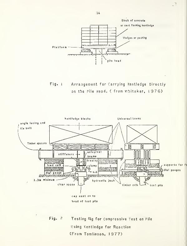
14
Plat for ro
Block of concrete
or cast forming kentledge
Wedges or packing
gSiMggiwI pile head
Fig. l Arrangement for Carrying Kentledge Directly
on the Pile Head. ( from Whitaker, I 976)
kentledge blocks Universal beams
angle lacing and
tie bolt
load cell
I .3m minimum
1*- u.b \
hydraulic Jack
^Mi: y3%$3ffl / supports for fo
zEp dtal gauges
timber crib
cap cast on to
head of test pile
Fig. 2 Testing Rig for Compressive Test on Pile
Using Kentledge for Reaction
(From Tomlinson, I 977)
15
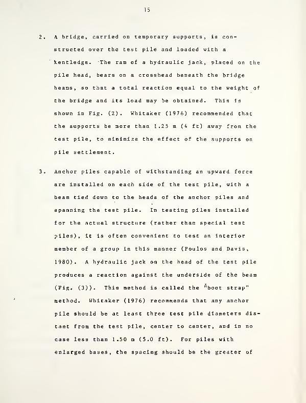
A bridge, carried on temporary supports, is con-
structed over the test pile and loaded with a
kentledge. The ram of a hydraulic jack, placed on the
pile head, bears on a crosshead beneath the bridge
beams, so that a total reaction equal to the weight of
the bridge and its load may be obtained. This is
shown in Fig. (2). Whitaker (1976) recommended that
the supports be more than 1.25 m (4 ft) away from the
test pile, to minimize the effect of the supports on
pile settlement.
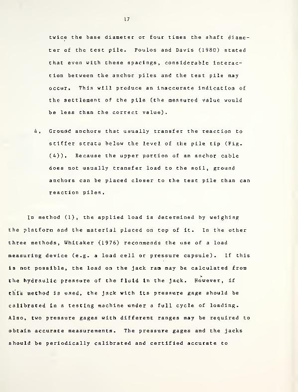
3. Anchor piles capable of withstanding an upward force
are installed on each side of the test pile, with a
beam tied down to the heads of the anchor piles and
spanning the test pile. In testing piles installed
for the actual structure (rather than special test
piles), it is often convenient to test an interior
member of a group in this manner (Poulos and Davis,
1980). A hydraulic jack on the head of the test pile
produces a reaction against the underside of the beam
(Fig. (3)). This method is called the "boot strap"
method. Whitaker (1976) recommends that any anchor
pile should be at least three test pile diameters dis-
tant from the test pile, center to center, and in no
case less than 1.50 m (5.0 ft). For piles with
enlarged bases, the spacing should be the greater of

16
yoke universal tearat
\
c £ p cast on
to head of
test pilK sfl /Y-Vr—fJx/ ft 5ii \c »
1 tension
members
lour dial gauges
3> ^J&anchor piles
K>"'-'^mr\ s
load cell —-Jft
hydraulic jack
test pile
3b
dial gauge
supports
.-5
( not less than 2m )
Fig. 3 Testing Rig for Compressive Test on Pile Using
Tension Piles forReaction (From Tomlinson, 1977)
17
twice the base diameter or four times the shaft diame-
ter of the test pile. Poulos and Davis (1980) stated
that even with these spacings, considerable interac-
tion between the anchor piles and the test pile may
occur. This will produce an inaccurate indication of
the settlement of the pile (the measured value would
be less than the correct value).
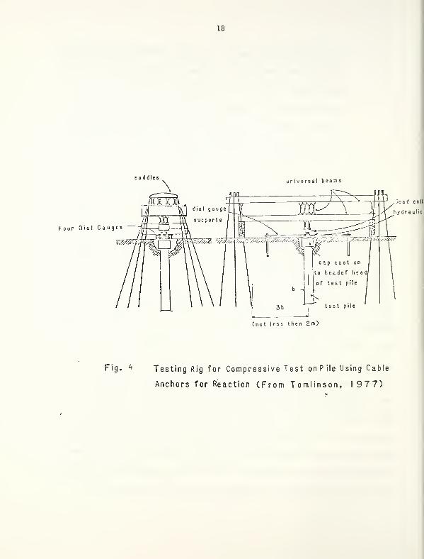
4. Ground anchors that usually transfer the reaction to
stiffer strata below the level of the pile tip (Fig.
(4)). Because the upper portion of an anchor cable
does not usually transfer load to the soil, ground
anchors can be placed closer to the test pile than can
reaction piles.
In method (1), the applied load is determined by weighing
the platform and the material placed on top of it. In the other
three methods, Whitaker (1976) recommends the use of a load
measuring device (e.g. a load cell or pressure capsule). If this
is not possible, the load on the jack ram may be calculated from
the hydraulic pressure of the fluid in the jack. However, if
this method is used, the jack with its pressure gage should be
calibrated in a testing machine under a full cycle of loading.
Also, two pressure gages with different ranges may be required to
obtain accurate measurements. The pressure gages and the jacks
should be periodically calibrated and certified accurate to
18
sa (idlesuniversal beams
Four Dial Gauges
(not less then 2m)
Fig. 4 Testing Rig for Compressive Test on P ile Using Cable
Anchors for Reaction (From Tomlinson, 1977)
19
within five percent. Friction caused by corrosion and wear of
the jack ram, and aging of the sealing ring can cause large
errors. Friction can be reduced to an acceptably low level only
by maintaining the jack in good condition. It is also necessary
to avoid eccentricity of loading, or tilting of the surface
against which the ram bear. Hence, care must be taken to make
certain that the loading surfaces of the reaction beam and pile
or shaft are parallel and that the piston is perpendicular to
both. The possibility of having eccentric loads on the piston
can be minimized by using steel plates or spherical leveling
blocks between the piston and reaction beam, and leveling plates
on top of the pile or shaft (Butler and Hoy, 1977). When testing
drilled shafts or large diameter piles, it is generally necessary
to use more than one hydraulic jack. When using more than one
jack, each should have the same rated capacity and be from the
same manufacturer. All jacks used should be connected to a com-
mon manifold and pressure gage with pressure supplied by one
hydraulic pump. A hand operated pump may be used. However, an
air operated pump significantly increases the efficiency of the
operation. Corrosion is prevented and ram friction vconsiderably
reduced by chromium plating and grinding the cylindrical surface
of the ram.
Fuller and Hoy (1970) stated that the use of hydraulic jacks
has several advantages. For example, it is the only practical
way to apply load-unload-re load cycles, and hydraulic jacks are
20
more suitable for uplift tests, lateral tests and tests on batter
piles.
Regardless of the method of load application, the load
should be kept constant under increasing pile deflection. For
direct loading this presents no problem, but when hydraulic jacks
are used, this can be accomplished by activating the jack pump
with a compressed gas control system.
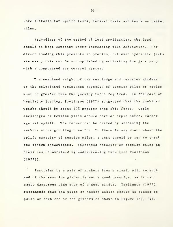
The combined weight of the kentledge and reaction girders,
or the calculated resistance capacity of tension piles or cables
must be greater than the jacking force required. In the case of
kentledge loading, Tomlinson (1977) suggested that the combined
weight should be about 20% greater than this force. Cable
anchorages or .tension piles should have an ample safety factor
against uplift. The former can be tested by stressing the
anchors after grouting them in. If there is any doubt about the
uplift capacity of tension piles, a test should be run to check
the design assumptions. Increased capacity of tension piles in
clays can be obtained by under-reaming them (see Tomlinson
(1977)).
Restraint by a pair of anchors from a single pile to each
end of the reaction girder is not a good practice, as it can
cause dangerous side sway of a deep girder. Tomlinson (1977)
recommends that the piles or anchor cables should be placed in
pairs at each end of the girders as shown in Figure (3), (4).
21
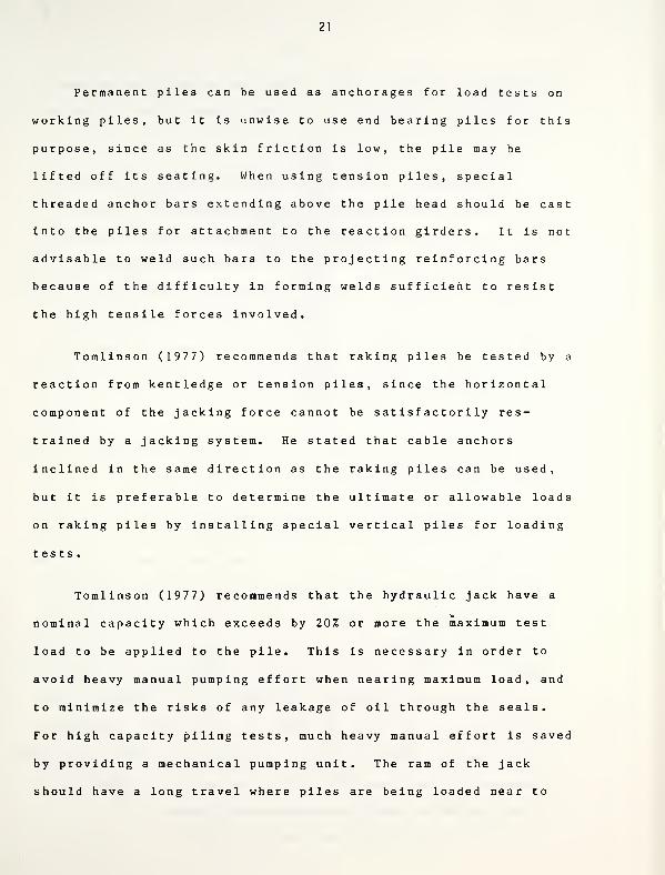
Permanent piles can be used as anchorages for load tests on
working piles, but it is unwise to use end bearing piles for this
purpose, since as the skin friction is low, the pile may be
lifted off its seating. When using tension piles, special
threaded anchor bars extending above the pile head should be cast
into the piles for attachment to the reaction girders. It is not
advisable to weld such bars to the projecting reinforcing bars
because of the difficulty in forming welds sufficient to resist
the high tensile forces involved.
Tomlinson (1977) recommends that raking piles be tested by a
reaction from kentledge or tension piles, since the horizontal
component of the jacking force cannot be satisfactorily res-
trained by a jacking system. He stated that cable anchors
inclined in the same direction as the raking piles can be used,
but it is preferable to determine the ultimate or allowable loads
on raking piles by installing special vertical piles for loading
tests.
Tomlinson (1977) recommends that the hydraulic jack have a
nominal capacity which exceeds by 20% or more the maximum test
load to be applied to the pile. This is necessary in order to
avoid heavy manual pumping effort when nearing maximum load, and
to minimize the risks of any leakage of oil through the seals.
For high capacity piling tests, much heavy manual effort is saved
by providing a mechanical pumping unit. The ram of the jack
should have a long travel where piles are being loaded near to
22
the failure condition. This avoids the necessity of releasing
oil pressure and repacking with steel plates above the ram as the
pile is pushed into the ground.
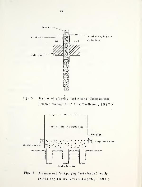
Where piles are installed through fill or soft sensitive
clay, these layers give positive skin resistance to the test
pile, whereas they may affect the permanent piles by negative
skin friction. It may therefore be desirable to sleeve the pile
through these layers. This can be done by using a double sleeve
arrangement as shown in Fig. (5). Alternatively, Tomlinson
(1977) suggested that the outer casing can be withdrawn, after
filling the anchor space between it and the steel tube encasing
the test pile with a bentonite slurry.
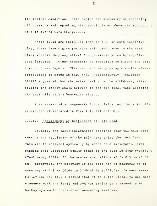
Some suggested arrangements for applying test loads to pile
groups are illustrated in Fig. (6), (7) and (8).
2.2.1.2 Measurement of Settlement of Pile Head:
Usually, the basic information obtained from the pile load
test is the settlement of the pile head under the test load.
This can be measured optically by means of a surveyor's level
reading onto graduated scales fixed to the pile in four positions
(Tomlinson, 1977). If the scales are calibrated in 0.5 mm (0.02
in.) intervals, the movement of the pile can be measured to an
accuracy of ± 1 mm (0.04 in.) which is sufficient in most cases.
Fuller and Hoy (1970) stated that it is quite useful to use meas-
urements with the level and rod (or scale) as a secondary or
backup system to check other measuring systems.
23
Test Pile
steel tube
soft clay
steel ca sing In place
during test
Fig. 5 Method of sleeving Test pile to Eliminate skin
Friction Through Fill ( from Tomlinson , 1977 )
t?concrete cap —
-V -^V A-
test weights or weighted box
- A
a i » ' t :
* A • « »
.y/s*"* /-<; //:/s*t/~
dial gage
St- r ef r er < nc e beam
'<
i
test pile group
Fig. 6 Arrangement for Applying Tests Loads Directly
on Pile cap for Group Tests ( ASTM t 198 1 )
24
Cribbing
Test
Cross
Weights
Beams
Wedges Dial Gages
ft:•£**:&?£'£& Referenceg.fg> %<fo0 -Vol Beam
Concrete Pile Cap
Test Beams
t^K
j.' t*/W/«>AV"«!iw**>i ''/S'ir*»i
Test Pile Group
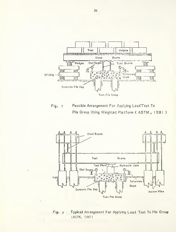
Fig. 7 Possible Arrangement For Applying LoadTest To
Pile Group Using Weighted Platform ( ASTM ,1981)
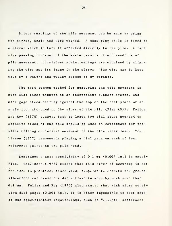
A__ft A ftSteel Beams Li_J^.
Beams
Test Plate. Hydraulic Jack
^li•"^^"jf:"
^-o.° o o o O '0 0, ,
7& iy.,
.,^'./<ey/<.| pr^- Reference *
Concrete Pile Cap
KH kN
\,
J Beam XnJAnchor Piles
Test Pile Group
Fig- 8 Typical Arrangement For Applying Load Test To Pile Group
(ASTM, 1981)
25
Direct readings of the pile movement can be made by using
the mirror, scale and wire method. A measuring scale is fixed to
a mirror which in turn is attached directly to the pile. A taut
wire passing in front of the scale permits direct readings of
pile movement. Consistent scale readings are obtained by align-
ing the wire and its image in the mirror. The wire can be kept
taut by a weight and pulley system or by springs.
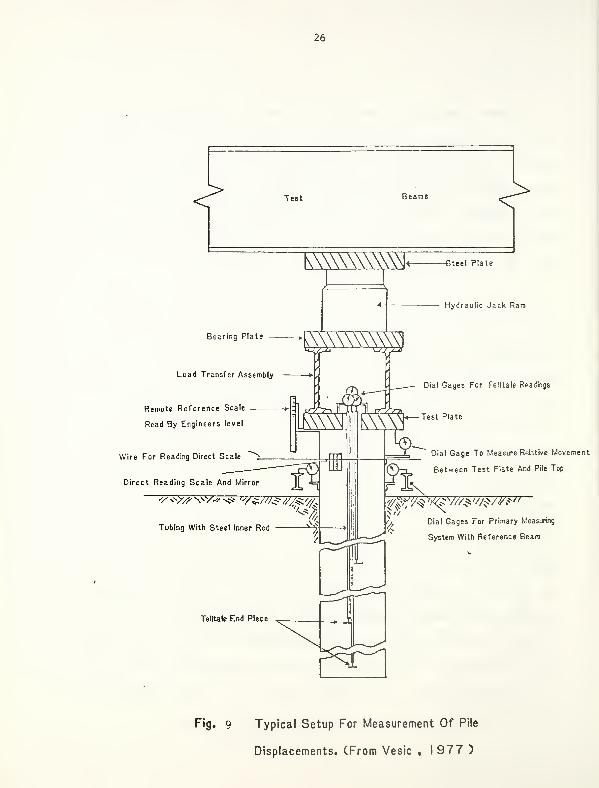
The most common method for measuring the pile movement is
with dial gages mounted on an independent support system, and
with gage stems bearing against the top of the test plate or an
angle iron attached to the sides of the pile (Fig. (9)). Fuller
and Hoy (1970) suggest that at least two dial gages mounted on
opposite sides of the pile should be used to compensate for pos-
sible tilting or lateral movement of the pile under load. Tom-
linson (1977) recommends placing a dial gage on each of four
reference points on the pile head.
Sometimes a gage sensitivity of 0.1 mm (0.004 in.) is speci-
fied. Tomlinson (1977) stated that this order of accuracy is not
realized in practice, since wind, temperature effects and ground
vibrations can cause the datum frame to move by much more than
0.1 mm. Fuller and Hoy (1970) also stated that with ultra sensi-
tive dial gages (0.001 in.), it is often impossible to meet some
of the specification requirements, such as "...until settlement
26
Wire For Reading Direct Scale
Direct Reading Scale And Mirror
Dial Gage To Measure Rebtive Movement
Between Test Plate And Pile Top
>// xDial Gages For Primary Measuring
System With Reference Beam
Fig. 9 Typical Setup For Measurement Of Pile
Displacements. (From Vesic , 1977 )
27
stops". They suggested that gages reading to 0.01 in. (0.25 mm)
produce sufficient accuracy to meet the normal settlement cri-
teria. However, Tomlinson (1977) recommended the use of a preci-
sion of 0.004 in. (0.1 mm) while adding each increment of jacking
force, since the time settlement curve can then be plotted accu-
rately and the rate of decrease of movement is readily obtained.
Fuller and Hoy (1970) also recommended that when the instrumenta-
tion for a compression test is set up, it is often advisable to
mount dial gages to measure lateral movements of the pile under
test. Such movement could be due to eccentric loading, and con-
tribute to the apparent vertical movement of the pile head.
Tomlinson (1977) suggested another way to measure settle-
ment. A linear potentiometer can be used to obtain the pile
movements, which are read on a dial or print-out mechanism at an
instrument station well clear of the pile. Tomlinson (1977)
stated that this method and the optical method avoid the need for
the technicians to crouch under a kentledge stack to read dial
gages. With a well designed kentledge support system, the tech-
nicians should not be in a dangerous position under the stack,
but the working space is usually very confined, causing discom-
fort and fatigue to the technicians controlling a long-duration
test.
The settlement measurement system must be supported independ-
ently from the loading system, with supports protected from
extreme temperature variations, effects of the test load, and
28
accidental disturbance by test personnel. Fuller and Hoy (1970)
recommend the use of a secondary or backup system in case of an
accidental disturbance of the primary one, or the necessity to
reset dial gages so that the continuity of data is maintained.
Poulos and Davis (1980) suggested an alternative means of
settlement measurement in the case where anchor piles are used as
supports for the reaction system. This is to measure the settle-
ment of the test pile with reference to the reaction piles, i.e.
by fixing a dial gage to the cross beam joining the reaction
piles. This is very helpful in minimizing the error in settle-
ment measurement resulting from the interaction between test
pile,, soil and reaction piles. This error is illustrated in
more detail in a subsequent section of this report.
2 .2.1 .3 Measurement o f Pile Movement s and Loadsat Various Points Along the Pile :
Data on load distribution (shaft and base loads are
evaluated separately) and the elastic behaviour of the pile can
be obtained with strain rods (sometimes called "tell-tales") or
strain gages. This type of instrumentation can be installed on
almost all types of conventional piling, but more readily on
>
cas t-in-place concrete piles. Strain gages or the terminal
points of strain rods can be located at various positions along
the pile .
Fuller and Hoy (1970) stated that strain rods are less com-
plicated, are less subject to malfunction, are more easily
29
handled by field personnel, and produce direct elastic shortening
data of a long gage length between the terminal point and the
pile head. The proper installation of strain gages, so as to
avoid malfunction and produce reliable data, is an extremely sen-
sitive operation.
The load on the base of the pile can be measured by insert-
ing load measuring devices in a cylindrical unit interposed
between the pile base and the shaft. A typical installation con-
sists of a ring of pillar-type load cells around the periphery of
the unit, connecting to a data logger at the ground surface
(Hanna, 1973).
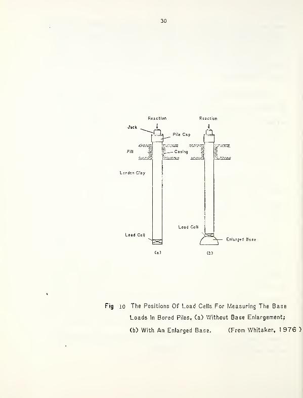
Fig. (10) shows the position of load cells for measuring the
base loads in large bored piles (Whitaker and Cooke, 1966). The
difference between the load cell reading and the applied load
gives the load carried by frictional resistance of the shaft.
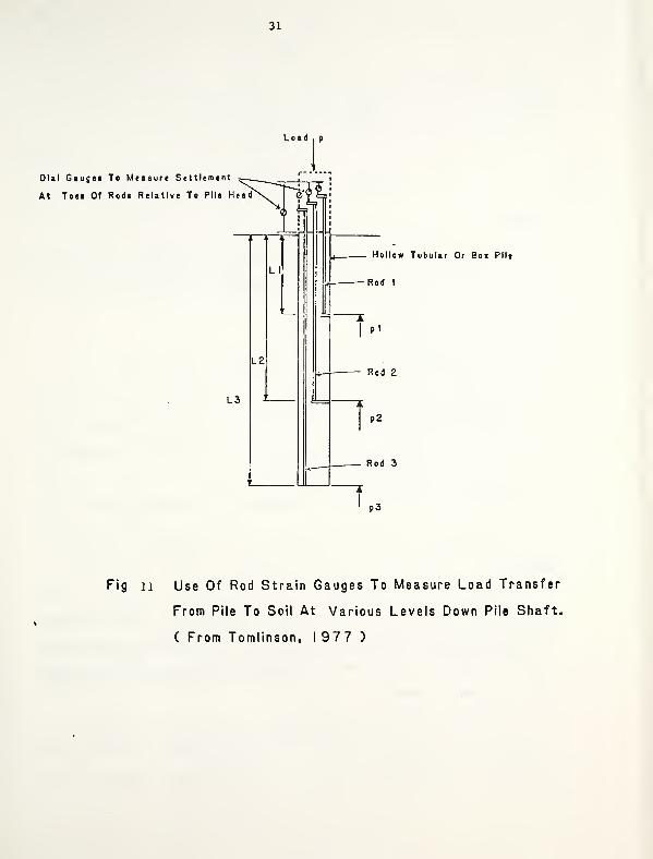
Tomlinson (1977) described the manner of using the tell-tale
system to obtain the distribution of skin friction on the shaft
of long hollow section piles. This system consists of metal rods
installed down the interior of the pile. The rods are terminated
at various levels as shown in Fig. (11), and are free to move in
guides as the pile settles under load. By means of dial gages
mounted on the heads of the rods, the elastic shortening of each
length of pile between the toes of the rods can be measured.
Thus, the load reaching the pile shaft at the toe of each rod is
given by the following expressions:
30
Reaction Reaction
Jack J 4
Pile Cap J
—
L
Fill
London Clay
Load Cell
£ Casing
(a)
Load Cell
/.<^£
^V— Enlarged Base
(b)
Fig io The Positions Of Load Cells For Measuring The Base
Loads In Bored Piles, (a) Without Base Enlargement;
(b) With An Enlarged Base. (From Whitaker, I 976 )
31
Load
Dial Gauge* To Measure Settlement
At Toea Of Rod* Relative To Pile Head
Hollow Tubular Or Box Pile
Rod I
Rod 2
Rod 3
Fig ii Use Of Rod Strain Gauges To Measure Load Transfer
From Pile To Soil At Various Levels Down Pile Shaft.
( From Tomlinson, 1977 )
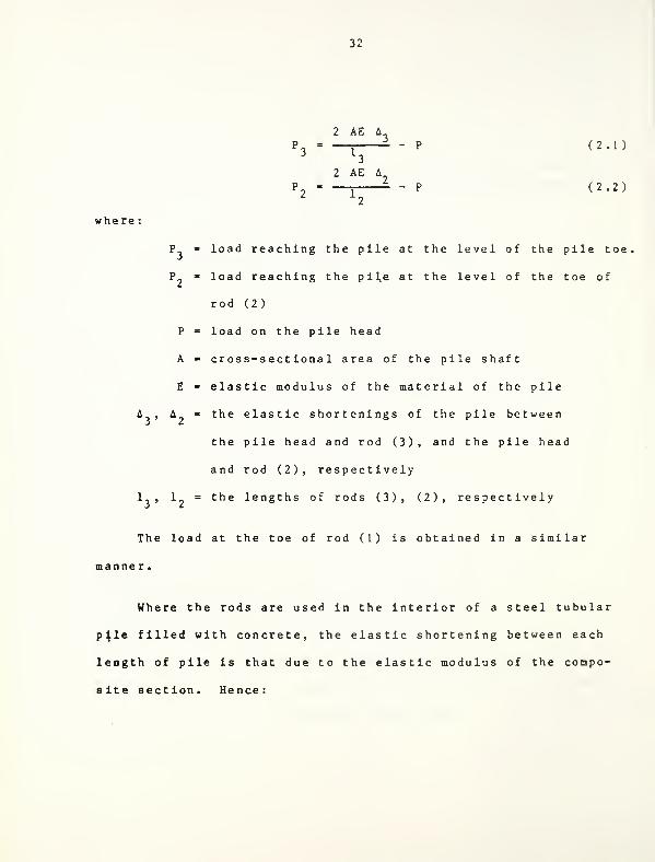
where :
2 AE A.
2 AE A,
P2
=
- P
- P
(2.1)
(2.2)
P_ = load reaching the pile at the level of the pile toe
P„ load reaching the pile at the level of the toe of
rod (2)
P = load on the pile head
A = cross-sectional area of the pile shaft
E = elastic modulus of the material of the pile
A , A the elastic shortenings of the pile between
the pile head and rod (3), and the pile head
and rod (2), respectively
1, , 1„ = the lengths of rods (3), (2), respectively
The load at the toe of rod (1) is obtained in a similar
manne r .
Where the rods are used in the interior of a steel tubular
p^le filled with concrete, the elastic shortening between each
length of pile is that due to the elastic modulus of the compo-
site section. Hence:
33
where:
A , As c
E , Es c
A E
A E (1 + t^'f1 )s s A E
s s
elastic shortening over length L
load on length L
area of steel and concrete in section,
respectively
elastic moduli of steel and concrete,
respectively
(2.3)
The distribution of skin friction on the pile shaft may also
be measured by fixing electrical resistance strain gages onto the
interior surface of a hollow steel pipe, or to a steel pipe
embedded in a precast or cast-in-situ concrete pile. Gages of
this type can withstand the impact of pile driving and have given
satisfactory service on piles which have remained in the ground
for a year or more.
Tomlinson (1977) stated that while these forms of instrumen-
tation (either tell-tales or strain gages) are used mainly for
research-type investigations, they can be adopted for the prelim-
inary test piling stage to give useful design information at a
relatively small additional cost.
Fuller and Hoy (1970) noticed that the installation of
strain rods or gages results in a physical change in the cross
section of the pile and thus its elastic properties. They sug-
34
gested the use of a single strain rod on the pile tip, which is
sufficient to provide the essential information on the elastic
behavior of the pile and the basic load distribution.
The load distribution can also be approximated by driving
and testing piles of different lengths. Some would be driven
just short of the end bearing stratum, while others would be
driven to full embedment. An uplift test might also produce
approximate data on the amount of load carried by friction in a
compression pile.
2.2.1.4 Residual Stresses:
The importance on pile test interpretation of residual
stresses in driven piles has been emphasized by Holloway et al
(1975). Compressive residual loads are likely to exist in the
lower part of the pile. These stresses seem to depend on the
pile-soil system only, and are independent of the impact pile
driving apparatus used, (Poulos and Davis, 1980). When a resi-
dual point load remains after driving, a portion of the point
bearing capacity has already been mobilized. However, if load
distribution measurements are made, the gages are generally
zeroed at the start of the test and the residual loads are
ignored in the test interpretation. In compression load tests to
failure, the measured point bearing value in such cases is only
that mobilized from the start of the load test. The actual point
capacity is the measured value plus the residual point load.
35
Conversely, in tensile load tests, the effect of residual
compressive loads is to cause an apparent tensile resistance at
the point. Poulos and Davis (1980) stated that while the effects
of residual loads are not readily taken into account, recognition
of their effects may at least resolve apparent anomalies in some
load tests. The subject of residual stresses is going to be
dealt with in detail in a separate chapter of the report.
2.2.1.5 Sources of Error in Settlement Measurements
Some of the loading and settlement procedures commonly used
in pile load tests may lead to inaccuracies in the measurement of
the settlement of a test pile. These errors arise from the
effects of the supports of the loading system on the measurement
settlement or the movement of the test pile. Hence a minimum
distance between the test pile and supports should be specified.
It is uneconomical, however, to space the supports so widely
apart such that all effects are eliminated. Hence, the contribu-
tion of these effects should be calculated and allowed for in the
interpretation of the test results. A theoretical examination of
such Inaccuracies caused by the various procedures has been made
b3f
Poulos and Mattes (1975). These errors are summarized and
discussed in this section.
2.2.1.5.1. Errors Resulting from Use of Reference Beam
With this system of settlement measurement (Fig. (2)), the
beam supports settle because of the loaded pile. A theoretical
36
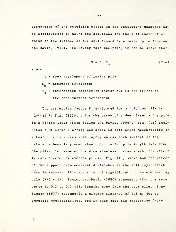
assessment of the resulting errors in the settlement measured may
be accomplished by using the solutions for the settlement of a
point on the surface of the soil caused by a loaded pile (Poulos
and Davis, 1980). Following this analysis, it can be shown that:
S = F S (2.4)c m
where
S = true settlement of loaded pile
S = measured settlementm
F = interaction correction factor due to the effect ofc
the beam support settlement
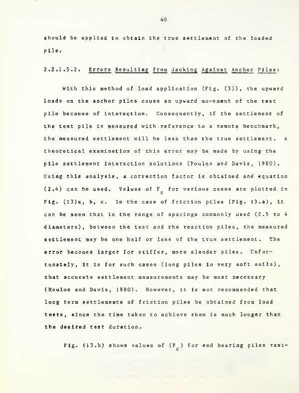
The correction factor F evaluated for a friction pile isc
plotted in Fig. (12)a, b for the cases of a deep layer and a pile
in a finite layer (from Poulos and Davis, 1980). Fig. (12) indi-
cates that serious errors can arise in settlement measurements on
a test pile in a deep soil layer, unless each support of the
reference beam is placed about 0.5 to 1.0 pile length away from
the pile. In terms of the dimens ionless distance r/L, the effect
is more severe for shorter piles. Fig. (13) shows how the effect
of the support beam movement diminishes as the soil layer thick-
ness decreases. This error is not significant for an end bearing
pile (H/L - 1). Poulos and Davis (1980) recommend that the sup-
ports be 0.3 to 0.5 pile lengths away from the test pile. Tom-
linson (1977) recommends a minimum distance of 1.3 m, due to
economic considerations, and in this case the correction factor
37
Fe
2.5
2.0
1.5 -
1.0
0.5
1 1 T
\Al/<j =
- VX/^sJo
k = 1 000
/xs= 0.5
i i i
mV
i^_ i
L
^
•
0.25 0.5 0.75 1.0r/L
True Settlement =Fc (Measured Settlement)
Fig. J2.a Correction Factor Fc For
Friction Pile In Deep Layer Of Soil.
(From Poulos and Davis, 1980)
3.0
Fc
2.0
1.01.0
Fig. 12. b Effect Of Layer Depth On Settlement Correction
Factor. ( From Poulos And Davis. 1980)
38
j1
ii
i Ii -•
L-« * » -« h
d d <)L 1
\
i i
y 1000 .
: \\
--k =
\
\Values or L/d •
\ .
\\25v
100N
100 "**
\jf^~
—
*^.
^
> l__ i
ZZ "
5 10 15 20 25s/d
Fig. 13.2 Correction Factor R For Floating Pile In A Deep Layer
Jacked Against Two Reaction Piles. (From Poulos and Davis, 1980]
d - - d
777777777777777777777
Rigid Stratum
2.0
Fc
Fig.n.bCorrection Factor Fc For End Bearing Pile On Rigid Stratum
Jacked Against Two Reaction PilesCFrom Poulos And Davis,
1980)
Fc
3.0
2.0
1.0
Soil E
Bearing Stratum £..
5 10 15 20 25
s/d
Fig. 13. c Correction Factor F e . Effect Of Bearing Stratum For
End-Bearing Pile Jacked Aggainst Two Reaction Piles.
(From Poulos and Davis, 1980)
*4-Mh
Fc
1 \
1
1
Values Of L/d
1.5
1.0ioov^s
», 100
^25 """*--»
io—-~-^HZa==s==^
0.5 -k= 1000k= »
•1 j
10 15 20 •/*-
Fig.i3.dCorraction Factor F c For Friction Pile In A Deep Layer JackedAgainst Two Reaction Piles-Settlement Measured In Relation ToAnchor Piles.C From Poulos And Davis, I 980)
40
should be applied to obtain the true settlement of the loaded
pile.
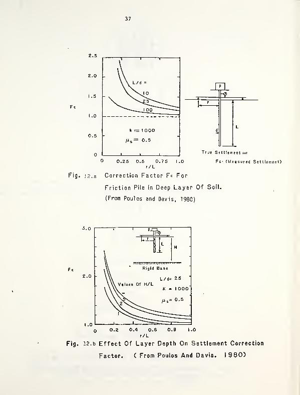
2.2.1.5.2. Errors Resulting from Jacking Against Anchor Piles :
With this method of load application (Fig. (3)), the upward
loads on the anchor piles cause an upward movement of the test
pile because of interaction. Consequently, if the settlement of
the test pile is measured with . reference to a remote benchmark,
the measured settlement will be less than the true settlement. A
theoretical examination of this error may be made by using the
pile settlement interaction solutions (Poulos and Davis, 1980).
Using this analysis, a correction factor is obtained and equation
(2.4) can be used. Values of F for various cases are plotted inc
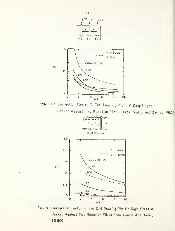
Fig. (13)a, b, c. In the case of friction piles (Fig. 13. a), It
can be seen that in the range of spacings commonly used (2.5 to 4
diameters), between the test and the reaction piles, the measured
settlement may be one half or less of the true settlement. The
error becomes larger for stiffer, more slender piles. Unfor-
tunately, it is for such cases (long piles in very soft soils),
that accurate settlement measurements may be most necessary
(Roulos and Davis, 1980). However, it is not recommended that
long term settlements of friction piles be obtained from load
tests, since the time taken to achieve them is much longer than
the desired test duration.
Fig. (13. b) shows values of (F ) for end bearing piles rest-
41
lng on a rigid stratum. In this case, the interaction is gen-
erally much less for normal spacings.
The effect of relative stiffness of the bearing stratum on
(F ) is shown in Fig. (13. c). As the bearing stratum becomesc
stiffer, interaction decreases, and hence (F ) decreases for a
given pile spacing. However, significant errors in settlement
may still occur at normal pile spacings, unless the bearing stra-
tum has a stiffness more than about 10 times the overlying soil.
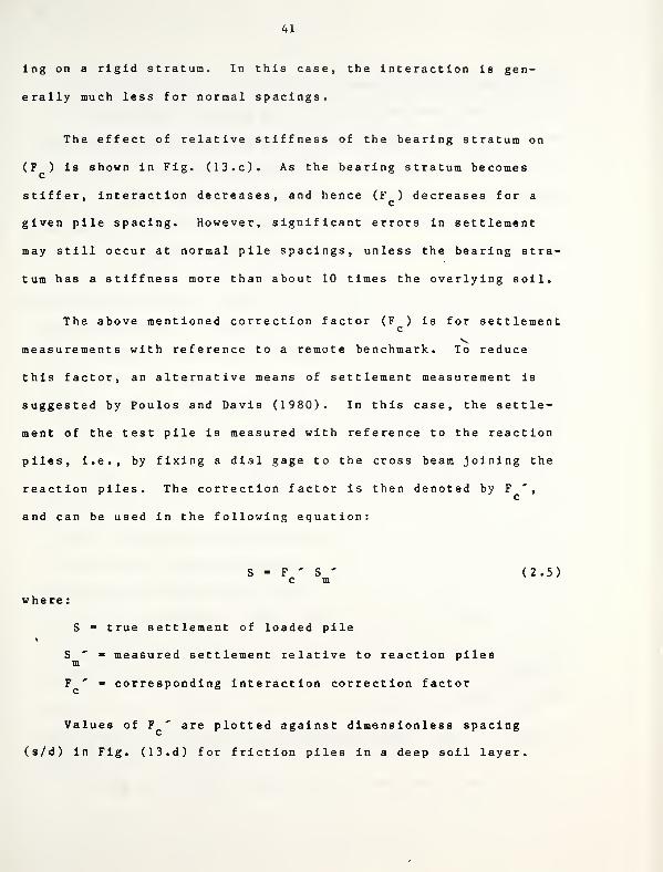
The above mentioned correction factor (F ) is for settlementc
measurements with reference to a remote benchmark. To reduce
this factor, an alternative means of settlement measurement is
suggested by Poulos and Davis (1980). In this case, the settle-
ment of the test pile is measured with reference to the reaction
piles, i.e., by fixing a dial gage to the cross beam joining the
reaction piles. The correction factor is then denoted by F ',c
and can be used in the following equation:
S = F ' S'
c m(2.5)
where
:
S true settlement of loaded pile
' measured settlement relative to reaction pilesm
' ' - corresponding interaction correction factor
Values of F ' are plotted against dimensionless spacing
(s/d) in Fig. (13. d) for friction piles in a deep soil layer.
42
The values of F ' are smaller than those of F shown in Fig.c c
6
(13. a), i.e., less correction of the measured settlement is
required if measurement is made with respect to the anchor piles.
It must be pointed out that at large spacings, or in cases where
little interaction is likely to occur between the test pile and
the reaction piles, F ' will be less than one, i.e., the measured
settlement will be greater than the true settlement.
From the above discussions, it seems that measurement of the
test pile settlement relative to the reaction piles have advan-
tages over other means of settlement measurement. However, in
any such pile test, measurement of the settlement by both of the
alternative methods is desirable, so that a better assessment of
the true settlement may be obtained (Poulos and Davis, 1980).
All the above solutions apply for a homogeneous soil stra-
tum. The expressions in equation (2.4) and (2.5) also apply for
n onhomogeneous soils, provided that appropriate values of the
interaction factors are used. Poulos and Davis (1980) stated
that these factors tend to be smaller for nonhomogeneous soils
than for homogeneous soils. The errors involved in the test pro-
cedures will be correspondingly smaller. However, general
characteristics of behaviour and variation of F and F ' withc c
spacing remain similar.
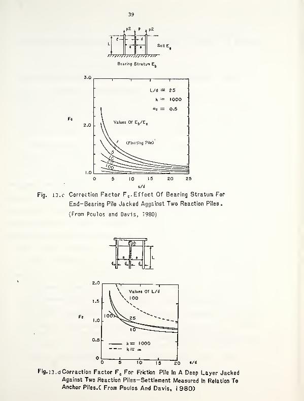
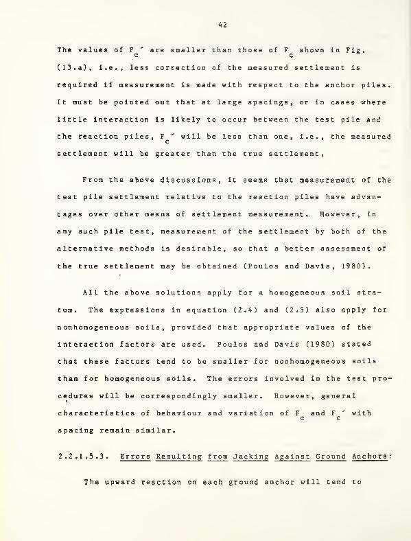
2.2.1.5.3. Errors Resulting from Jacking Against Ground Anchors :
The upward reaction on each ground anchor will tend to
43
reduce the settlement of the test pile. The correction factor
(F ) used in equation (2. A) can be calculated, assuming that the
effect of the ground anchor on the test pile is the same as the
effect on a point located halfway along the pile. (The anchors
are small in relation to the test pile.) (F ) is plotted against
d imension less anchor spacing for various values of embedment of
the anchors in Fig. (14. a). It is clear that the correction fac-
tor is much smaller in this case than in the case of jacking
against anchor piles. Beyond an anchor depth of about 2L, the
radial distance of the anchors from the piles has little effect
on the measured settlement. In addition, the case considered in
Fig. (14. a) is not likely to occur frequently in practice, since
to obtain adequate load capacity, the anchors are usually secured
into a stiffer layer at or below the level of the pile tip. In
such cases, the upward movements caused by the anchors would be
smaller, so that (F ) will be less than indicated in Fig. (14. a).
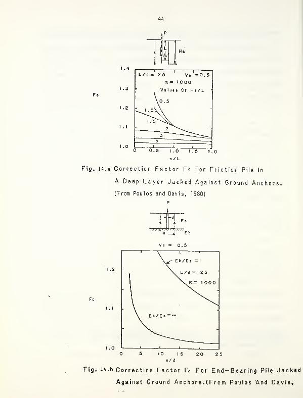
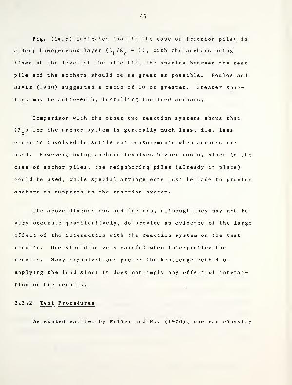
Fig. (14. a) also generally gives an overestimate of (F ) for
an end bearing test pile bearing on a stiff layer (Poulos and
Davis, 1980). Hence, for this case, (F ) is plotted in Fig.c
(14. b), together with the other limiting case of a pile in a
homogeneous deep layer, with anchors at the level of the pile tip
(the curve for H/L = 1.0 in Fig. (14. a)). It can be seen that in
the case where the pile bears on very stiff rock through very
stiff soil (E./E + °°) (F ) is extremely small, even for very
closely spaced anchors.
44
IfB L
1
h'Ha
1 I k 1
Ft
I .4
I .3
1.2
I . I
I .0
I I r~L/d =25 Vs =0.5
K= I 000Value* Of Ha/L
Fig. 14. a Correction Factor Fc For Friction Pile In
A Deep Layer Jacked Against Ground Anchors.
(From Poulos and Davis, 1980)
I .2
Fc
I. I
I .0
20 25
Fig. 14. b Correction Factor Fc For End-Bearing Pile Jacked
Against Ground Anchors. (From Poulos And Davis,
45
Fig. (14. b) indicates that in the case of friction piles in
a deep homogeneous layer (E /E = 1), with the anchors being
fixed at the level of the pile tip, the spacing between the test
pile and the anchors should be as great as possible. Poulos and
Davis (1980) suggested a ratio of 10 or greater. Greater spac-
ings may be achieved by installing inclined anchors.
Comparison with the other two reaction systems shows that
(F ) for the anchor system is generally much less, i.e. less
error is involved in settlement measurements when anchors are
used. However, using anchors involves higher costs, since in the
case of anchor piles, the neighboring piles (already in place)
could be used, while special arrangements must be made to provide
anchors as supports to the reaction system.
The above discussions and factors, although they may not be
very accurate quantitatively, do provide an evidence of the large
effect of the interaction with the reaction system on the test
results. One should be very careful when interpreting the
results. Many organizations prefer the kentledge method of
applying the load since it does not imply any effect of interac-
tion on the results.
2.2.2 Test Procedures
As stated earlier by Fuller and Hoy (1970), one can classify
46
load tests, with respect to the purpose for which they are run,
Into two main categories. The first one is performing tests to
prove the adequacy of the pile soil system for the proposed pile
design load. The second one is performing tests to develop cri-
teria to be used for the design and installation of the pile
foundation. The first type of tests, i.e. most of the routine
tests, are carried to one and one-half or twice the proposed
design load for a single pile, or one and one-half times the
design load for a pile group. Rarely can additional data be used
advantageously, such as for redesign, without seriously affecting
the time schedule.
On the contrary, the second type of tests, i.e. test pro-
grams that are specifically executed to produce design data,
should include testing piles to failure in order to develop the
most efficient design. However, Fuller and Hoy (1970) stated
that this is not always essential, and definite design decisions
can be reached if sufficient routine testing is done on piles of
different types, sizes, shapes and lengths.
In many cases, there should be a certain time interval
between pile driving and testing. This interval depends on the
type of pile and subsoil conditions. For example, sufficient
time should be permitted for the proper curing of cas t-in-place
piles before they are tested. If the pile is driven into a cohe-
sionless sand, there may be a relaxation of the soil around the
pile with a corresponding reduction in load capacity. In the
47
case where test piles are driven into cohesive soils, it is
advisable to wait several days for the soil to regain its shear
strength which was reduced because of the remolding effects of
pile driving. Most existing codes prescribe a minimum waiting
period between driving and testing not exceeding one month.
Although this requirement may be adequate for piles in relatively
pervious soils, such as sands and inorganic silts, it is obvi-
ously not sufficient for piles in clay, particularly if they are
of larger size. Because it may be impractical to prescribe
longer waiting periods, an estimate of additional gains in bear-
ing capacity between pile testing and application of service
loads may be in order (Vesic, 1977).
A variety of test procedures have been developed for carry-
ing out pile load tests. Among the most common procedures for
compression tests are the maintained loading tests (M.L.),
cons tant-rate-o f-penet rat ion tests (C.R.P.), method of equili-
brium load tests, quick load tests, and constant settlement
increment loading tests. In this section, these procedures and
their interpretation are reviewed.
2 ^2 .2 . 1 . Maintained Loading Test
This is the most common method of carrying out a compression
load test, especially if the load settlement relationship is
required .
2.2.2.1.1. Procedure :
The procedure is to apply the load in stages usually about
48
25% of the proposed design load, the load at each stage being
maintained constant until the resulting settlement of the pile
virtually ceases, before applying the next increment.
The Civil Engineering Code of Practice No. 4 (1954) proposes
a rate of movement of 0.012 in./hr (0.305 mm/hr) as the limiting
rate, before addition of the next increment. ASTM D1143-81
requires a rate of settlement less than 0.01 in./hr (0.25 mm/hr)
or until two hours has elapsed, whichever occurs first. Poulos
and Davis (1980) stated that it is doubtful whether a time inter-
val of two hours is always adequate to ensure completion of set-
tlement. However, taking into account that the major proportion
of the settlement of a pile i_n a_ load test occurs as immediate
settlement, they suggested that relatively short intervals
between load increments should be acceptable.
ASTM D1143-81 requires that unless failure occurs first, the
pile should be loaded to 200% of the anticipated pile design load
for tests on individual piles, or to 150% of the group design
load for tests on pile groups. It requires the load to be
applied in increments of 25% of the individual pile or group
design load. However, Fuller and Hoy (1970), for the sake of
saving time, suggested that the increments can be larger during
the early stages of the tests and, in the interest of obtaining
accuracy, they should be smaller as the total load is increased.
49
In case the test pile or pile group has not failed, ASTM
D1143-81 requires the test load to be removed any time after 12
hours if the head settlement over a one-hour period is not
greater than 0.01 in. (0.25 mm); otherwise the total weight
should be allowed to remain on the pile or pile group for 24
hours. After the required holding time, the test load is removed
in decrements of 25% of the total test load, with one hour
between decrements.
In the case of failure, jacking the pile should continue
until the settlement equals 15% of the pile diameter or diagonal
d imens ion
.
The usual procedure followed in this method is to increase
the load in stages until the proposed working load is reached,
and then to unload and to leave the load off until the rise or
rebound substantially ceases. The pile is then reloaded to the
working load or the next higher stage, and the test continued to
the maximum load. The unloading of the pile from the maximum
load is often carried out in stages, with a pause at each stage,
until rebound virtually ceases, before unloading to the next
s tage
.
Tomlinson (1977) suggested a system of load increments for
an ML test up to 1.5 times the working load. Table 1 illustrates
this system.
50
Load On Pile Head In kN
200 400 600 600 1000
Total Elapsed Tine ki Hours
4 6 10
10
15
20
25
30
v 200 f|
400| |
Rgjres
/ 0f
Denote Increment
Load On Pie
it /^^j 1
20_l I
1 i
\ 1
\ i
\ i /|
800\^.1
i i \ /
J 820
Q>>
Fig. 15 Compression Load Tests On 305x305mm Pile.
Load-Settlement And Time-Settlement Curves For Pile On Stiff Clay
(MU-(FromTomlinson f 1977)
51
Table 1 A Suggested System of Load Incrementsfor an ML Test (after Tomlinson, 1977)
Load as percentage Minimum time forof working load holding load
25
50
75
100
75
50
25
100
125
150
125
100
75
50
25
1 .0 hour
1 .0 hour
1 .0 hour
1 .0 hour
10.0 minutes
10.0 minutes
10.0 minutes
1 .0 hour
6 .0 hours
1 .0 hour
6 .0 hours
10.0 minutes
10.0 minutes
10.0 minutes
10.0 minutes
10 .0 minutes
1 .0 hour

52
A similar system can be devised for a test to twice the
working load. Tomlinson (1977) suggested that if it was desired
to obtain the ultimate load on a preliminary test pile, it is
useful to adopt the ML method for up to twice the working load,
and then to continue loading to failure at a constant rate of
p enet rat ion
.
An alternative procedure based on constant time interval
loading was suggested by ASTM-D 1 1 43-8 1 . This procedure follows
the same standards for the traditional maintained load tests,
except that the load is applied in increments of 20% of the pile
or group design load, with one hour between load increments. The
piles are unloaded with one hour between load decrements.
A further modification of the ML test consists of returning
the load to zero after each increment. This form of test is
necessary if the net settlement curve is used as the basis of
defining the failure load (Chellis, 1961). This procedure is
discussed in detail later in this chapter.
Fuller and Hoy (1970) recommend that instrumentation read-
ings should be taken before and after each increment of load and
at! sufficient intermediate intervals to define the load time
deflection curves. They also recommended that when piles are not
tested to failure, and after the full test load has been applied,
readings are taken at least every 30 minutes.
53
It should be noted that if the direct loading method (using
a kentledge) is used (Fig. (1), (2), (6) and (7)), the weight of
the test beam(s) and the platform should be included in the first
load increment. Before adding or removing load increments, the
wedges should be tightened along the platform edges to stabilize
the platform. Load increments should be placed or removed in a
manner which avoids impact, and maintains the load balanced at
all times. After each load increment has been added, the wedges
should be loosened (but not removed) and kept loose to permit the
full load to act on the pile as settlement occurs.
It should be noted that the load increment applied is main-
tained as specified before, in order to achieve a state of
equilibrium between load and the corresponding settlement. Mohan
et al (1967) stated that this ideal state is seldom reached.
With a hydraulic jack, continuous care and occasional pumping is
required to maintain the load, unless a load maintainer is avail-
able, and this is both laborious and time consuming.
2.2.2.1.2 Interpretation of Test Results ;
a) Ultimate Load
:
The ultimate pile capacity is defined in most geotechnical
literature as the load beyond which the pile will begin to break
into the ground, or expressed mathematically as AS/AP °°, i.e.,
when the tangent to the load settlement curve becomes vertical
(Chellis, 1961). However, in pile engineering practice, it is
54
customary to select a point beyond which the rate of change
increases markedly, or the settlement increment increases exces-
sively in comparison with the load increment, to denote failure.
Whitaker (1976) suggests that it is necessary to first estimate
the load capacity, so that a suitable loading and reaction system
may be provided, and then to define some physical event by which
the ultimate bearing capacity (at failure) can be recognized when
that point is reached.
Among the commonly used definitions of the ultimate load
capacity, Tomlinson (1977) selected the following ones (Fig. 15):
1. The load causing a gross settlement of 10% of the
least pile width (Point B) , (Terzaghi, 1942).
2
.
The load beyond which there is an increase in gross
settlement disproportionate to the increase in load
(Point C). This criterion is defined more precisely
by the Swedish Piling Commission as the load which
gives twice the movement of the pile head obtained for
90% of the load.
The load beyond which there is an increase in net set-
tlement disproportionate to the increase of load
(Point D) . (The net settlement is the gross measured
settlement minus the elastic compression of the pile.)

55
4. The load that produces a plastic yielding or net set-
tlement of 6 mm (0.25 in) (Point E).
5. The load indicated by the intersection of tangent
lines drawn through the initial, flatter portion of
the gross settlement curve and the steeper portion of
the same curve (Point F).
With experience, the load settlement curve from a compres-
sion test can be used to interpret the mode of failure of a pile.
A defective pile shaft is also indicated by the shape of the
curve. Some typical load-settlement curves and their interpreta-
tion are shown in Fig. (16) (after Tomlinson, 1977).
b . -Empirical Methods of Working Loads :
Many arbitrary or empirical rules have been used or are con-
tained in codes to serve as criteria for determining the allow-
able working load from test results. Some separate plastic and
elastic deformations, others do not. (Evaluation of elastic and
plastic deformation is discussed later in this chapter.) Chellis
(1961) lists about seventeen rules for determining the allowable
working loads. Poulos and Davis (1980) summarized a few of these
as follows:
1. "The test load shall be twice the design load and
shall be maintained constant for at least 24 hr., and
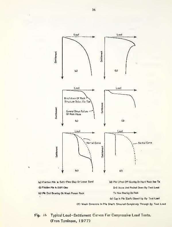
56
Load Load
Load ^
\ * Normal (
i %
4
1
I
1 >
V^ »
f(e) I
Load ^~
*x»
%
CVEJB
VCO
t
i
i
1
1
1
i
i
1
1r CO
Normal Curve
(a) Friction Pile h Soft-Firm Clay Or Loose Sand
00 Friction Pile h Stiff day
(.0 Pie End Bearing On Weak Porous Rock
(d) PDe Lifted Off Seathg On Hard Rock Due Ta
So! Meave And Pushed Down By Test Load
To New Beamg On Rock
(e) Gap h Pile Shaft Cbsed Up By Test Load
(f) Weak Concrete In Pile Shaft Sheared Completely Through By Teat Load
Fig. 16 Typical Load-Settlement Curves For Compressive Load Tests.
(From Tomlinson, 1977)
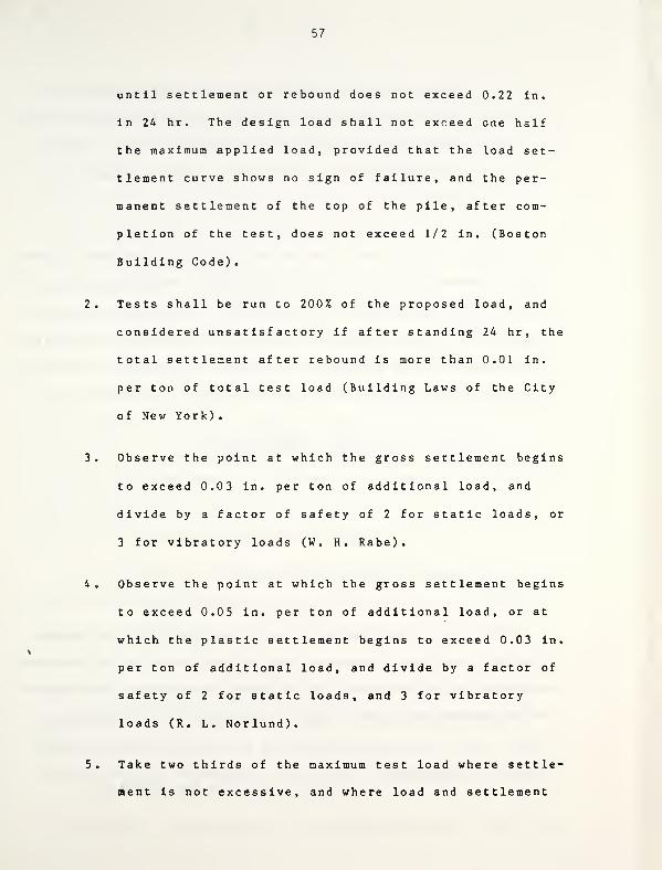
57
until settlement or rebound does not exceed 0.22 In.
in 24 hr. The design load shall not exceed one half
the maximum applied load, provided that the load set-
tlement curve shows no sign of failure, and the per-
manent settlement of the top of the pile, after com-
pletion of the test, does not exceed 1/2 in. (Boston
Building Code).
2. Tests shall be run to 200% of the proposed load, and
considered unsatisfactory if after standing 24 hr, the
total settlement after rebound is more than 0.01 in.
per ton of total test load (Building Laws of the City
of New York)
.
3. Observe the point at which the gross settlement begins
to exceed 0.03 in. per ton of additional load, and
divide by a factor of safety of 2 for static loads, or
3 for vibratory loads (W. H. Rabe).
4. Observe the point at which the gross settlement begins
to exceed 0.05 in. per ton of additional load, or at
which the plastic settlement begins to exceed 0.03 in.
per ton of additional load, and divide by a factor of
safety of 2 for static loads, and 3 for vibratory
loads (R. L. Norlund).
5. Take two thirds of the maximum test load where settle-
ment is not excessive, and where load and settlement

58
are proportional. Where the test load is carried to
failure, take two thirds of the greatest load at which
settlement was not excessive, and at which loads and
settlement were proportionate (United States Steel
Co.)."
Chellis (1961) considered rules (3) and (4) the most reason-
able, although (3) may be too conservative. Poulos and Davis
(1980) stated that rules such as (5) are unreliable, as various
impressions of the steepness of the load settlement curves may be
obtained by varying the scale of the plot. A finite limit of the
change of load to change of settlement ratio is desirable.
c. Plastic and Elastic Deformations :
The total measured movement of pile head is caused by:
a. Elastic deformation of pile and soil.
b. Plastic deformation of soil.
We should be interested in the plastic deformation rather
than the total one. Assuming that all the piles are of the same
material, of approximately equal length, and driven into substan-
tially similar soils, the elastic shortening will be approxi-
mately equal for all piles and thus will not contribute to dif-
ferential settlements. Fig. (17) illustrates the division of
by
total movement into elastic and plastic parts. Chellis (1961)
recommended that the working load and factor of safety should be
detemined using the curve of plastic deformation. To obtain this
curve, cyclic loading can be used, i.e., by removing the load
from the pile several times during the process of adding load
increments and plotting the rebounds as shown in Fig. (17). A
smooth curve could be drawn, connecting the points. By subtract-
ing the values of this curve from those of the curve of total
settlement, the elastic deformation curve may be plotted and com-
pared with the theoretical elastic deformation line of the pile
(Fig. 17). If the actual elastic curve has smaller ordinates
than the theoretical at every point, this indicates that the
upper undesirable strata, not selected for permanent load carry-
ing purposes, are supporting some of the load, at least tem-
porarily. With increasing test load, the ordinates of the actual
elastic curve should eventually increase to coincide with the
theoretical elastic line (Fig. 17).
The theoretical elastic deformation in the case of an end
bearing pile unrestrained by friction can be computed from the
formula S = RL/AE and will be a straight line. For friction
piles, the theoretical elastic deformation of the pile can be
computed by assuming the location of the center of resistance and
considering (L) as the distance down to this point (Chellis,
1961)
.
d. Distribution of Load to Soil:
Van Weele (1957) suggested an approximate method to get the
60
180
160
140
© 120o
£100
80
1.25
120 96 72 48 24 o 20 40 60 80100 120 140160 180
Elapsed TIme.ln Hours Load, In tons
Fig. 17 Test—Loading Diagram Showing Relationship Between Loading,
Settlement, And Time.CFrom Chellis, 1961)

61
distribution of load between friction and end bearing, using
cyclic loading. (This distribution can be determined more accu-
rately using tell-tales as described before.) Van Weele sug-
gested a plotting of the elastic recovery at each unloading cycle
versus the load applied at that cycle. The curve usually becomes
a straight line soon after the early load increments. The dis-
tance between the plotted curve and a line drawn through the ori-
gin and parallel to the straight part of the curve represents the
portion of the load carried by friction. This is, at best, only
an approximation.
Fuller and Hoy (1970) stated that cyclic loading should not
be mandatory for routine testing, because it can add unnecessary
expense without giving significant additional data. Such special
procedures should be included only at the engineer's option.
e. Settlement Behavior:
The load settlement relationship may be used directly to
determine the single pile settlement at the working load. It
should be noted that the observed settlements made at the top of
the pile may not necessarily indicate downward movement of the
pile into the ground where high load tests are performed. The
possibility of local failure of the pile above ground surface, or
crushing of the grout under the test plate, should be recognized
as possible factors contributing toward observed settlements.
62
The complete analysis of the test results should include
consideration of all factors, such as the elastic behavior of the
pile (from instrumentation or cyclic loading) and an evaluation
of the long terra performance. This could involve an analysis and
evaluation of the subsoil data in conjunction with the test
results. In estimating the settlement of a group or the settle-
ment of a pile of different proportions, the average soil modulus
(E ) along the pile may be determined by fitting the measured
load settlement behavior to the theoretical behavior. Poulos and
Davis (1980) described in detail a theoretical approach to esti-
mate the average drained and undrained values of (E ) of the
clay, using the load test results. Knowing the soil modulus, the
stiffness of the pile relative to the soil may be determined,
whereby the appropriate theoretical settlement influence factor
may be determined for a single pile. Also, the appropriate
theoretical group settlement ratio (ratio of group settlement to
single pile settlement at the average pile load) may be deter-
mined for a pile group. In the latter case, the additional
effects of any deep-seated compressible stratum must be carefully
considered in the settlement estimate. For the detailed pro-
cedures used to determine the above mentioned values, the reader
may refer to Poulos and Davis (1980).
f . Some Factors Influencing Interpretation o f Tes t Re sul t s :
There are several factors that should be taken into con-
sideration while interpreting the test results. Some of the more
important of these are:
63
1. Changes in pore water pressure in the soil caused by
pile driving, construction fill, and other construc-
tion operations which may influence the test results
for frictional support in relatively impervious soils
such as clays and silts.
2. Potential residual loads (discussed earlier) in the
pile, which could influence the interpreted distribu-
tion of load at the pile tip and along the pile shaft.
3. Possible interaction of friction loads from test piles
with upward friction transferred to the soil from
anchors or anchor piles (as explained earlier).
4. Differences between conditions at time of installation
and after final construction, such as changes in grade
or groundwater level.
5. Potential loss of soil supporting the test pile from
actions such as excavation and scour.
2.2.2.2 Constant Rate of Penetration Test
This test was developed by Whitaker (1957) for model piles,
and it has proved equally useful for full scale pile tests as
used by Whitaker and Cooke (1961) and by Whitaker (1963). This
test is often called the C.R.P. test. To understand the test, it
64
is helpful to regard the pile as a device for testing the soil,
and the pile movement as the means of mobilizing the resisting
forces. Thus, Whitaker (1976) defines the ultimate bearing capa-
city of a pile applicable to the test as "the load at which the
full resistance of the soil becomes mobilized".
2.2.2.2.1 Procedure
In carrying out the C.R.P. test, the pile is made to
penetrate the soil at a constant speed from its position as
installed, while the force applied at the top of the pile to
maintain the rate of penetration is continuously measured. The
soil supporting the pile is stressed under conditions approaching
a constant rate of strain, until it fails in shear, which means
that the ultimate bearing capacity of the pile has been reached.
The strain rate is adjusted so that the test requires about the
same amount of time as an undrained shear test of a sample of the
soil in the laboratory. Thus, the two tests have a common basis
and connections between them may be legitimately made. The test
in this way also provides a speedy way of evaluation and hence is
helpful for the overall economy of the project.
Whitaker (1976) emphasized that the purpose of the test is
the determination of the ultimate bearing capacity of the pile,
and that the force penetration curve obtained in the test does
not represent an equilibrium relationship between load and set-
tlement, so that the settlement to be expected under working con-
65
ditions is not found. Pile movement should be regarded as neces-
sary for mobilizing the forces of resistance.
Since the force applied must be varied smoothly from zero to
the ultimate bearing capacity, it is most convenient to use a
hydraulic jack. The jack should have a travel greater than the
sum of the final penetration of the pile and the upward movement
of the reaction system. For an end bearing pile, the penetration
in the test may reach 25% of the pile base diameter, while for a
friction pile it may reach about 10% of the shaft diameter.
According to Whitaker (1976), the movement of the reaction system
may be of the order of 7 6 mm (30.0 in.) if kentledge is used, and
about 25 mm (10.0 in.) with a system of anchor piles.
The pump supplying the jack may be hand or mechanically
operated. For forces up to about 2000 kN (about 200 metric ton)
hand pumping is convenient. However, ASTM Dl 143 — 81 recommends
the use of a mechanical pump equipped with a bleed valve, vari-
able speed device, or other means for providing a smooth variable
delivery. Oil cooling may be required if a bleed value system is
used. The jacking force may be measured by a load measuring dev-
ice, or by a pressure gage in the jack supply line, if the jack
is in good condition.
The downward movement of the pile head is conveniently meas-
ured by means of a dial gage supported on a beam. According to
Whitaker (1976), a small movement of the reference beam (not
65
exceeding 2.5 mm) is not likely to affect significantly the value
obtained for the ultimate bearing capacity in a typical C.R.P.
test.
The rate of penetration may be controlled by manually check-
ing the time taken for successive small increments of penetration
and adjusting the pumping rate accordingly. Alternatively, any
mechanical or electrical device may be used to monitor and con-
trol the penetration rate so that it remains constant.
A rate of penetration of about 0.75 mm/min (0.03 in./min.)
has been found suitable for friction piles in clay, for which the
penetration to failure is likely to be less than 25 mm. ASTM
D 1 1 4 3-8 1 suggests a rate of 0.25 to 1.25 mm (0.01 to 0.05
in.)/min for cohesive soils. For end bearing piles in sand or
gravel, considerably larger movements will be required to mobil-
ize the full resistance, and rates of penetration of 1.5 mm/min
or more are required. ASTM Dl 143—81 suggests a rate of 0.75 to
2.5 mm (0.03 to 0.10 in.)/min for granular soils. Whitaker
(1976) stated that the actual rate of penetration, provided that
it is steady, may vary within these specified ranges without sig-
nificantly affecting the results. For tests performed at rates
of penetration varying from 0.018 to 0.128 in. per minute, only
4% variation in the capacity of the piles was observed. A rate
should be chosen that can be held by the pumping equipment avail-
able. Major fluctuations in the rate of penetration produce
corresponding undulations in the force penetration diagram.
67
According to ASTM D1143-81, loading the pile should continue
until no further increase in the load is necessary for continuous
pile penetration at the specified rate. If the pile penetration
continues, the load required to achieve the specified penetration
rate should be held until the total pile penetration is at least
15% of the average pile diameter or diagonal dimension at which
time the load is released. If the pile stops penetrating under
the maximum applied load, this load can be released.
Also according to ASTM D 1 1 43-8 1 for the C.R.P. test, read-
ings of time, load and settlement should be taken at least every
30 seconds or at sufficient intervals to determine the rate of
penetration being achieved. When the test pile has achieved its
specified rate of penetration, readings should be taken for the
duration of the loading. Immediately after unloading, readings
of time, load and rebound should also be taken. Final readings
are taken 1.0 hr after all load has been removed.
2.2.2.2.2 Interpretation of Test Results :
The data resulting from the test are plotted as a graph of
force versus penetration. The curve in the case of a friction
pile will be similar to one of those shown in Fig. 18(a). The
values of force reached at the point marked "A" would represent
the ultimate bearing capacity.
The force penetration curve for an end bearing pile is simi-
lar to that shown in Fig. 18(b). The upper part of the curve is
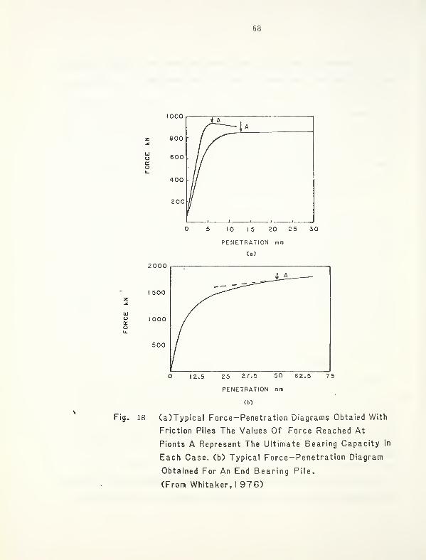
68
1000
Fig. if
5 10 15 20 25 30
PENETRATION mm
(a)
2000
I 500
000
500
O 12.5 25 27.5 50 62.5 75
PENETRATION mm
Cb)
(a)Typical Force — Penetration Diagrams Obtaied With
Friction Piles The Values Of Force Reached At
Pionts A Represent The Ultimate Bearing Capacity In
Each Case, (b) Typical Force-Penetration Diagram
Obtained For An End Bearing Pile.
(From Whitaker,! 976)
69
substantially straight and shows a steady increase in force with
increasing penetration. The ultimate load is taken as the point
"A", which represents the beginning of the straight portion.
This line is found to be a continuation of the force penetration
relationship for installation of the pile from the surface of a
bearing stratum entirely by a C.R.P. technique (Whitaker, 1976).
Identification of the point "A" is often difficult in practice,
and Whitaker (1976) suggests that it is usually satisfactory to
take the ultimate load as the force required to cause a penetra-
tion of 10% of the pile diameter.
Whitaker and Cooke (1961) found that the C.R.P. method pro-
vides higher values when compared to maintained load tests.
Mohan et al (1967), after performing load tests for the Hardu-
agani Power House in India, reported that the loading points
obtained by the C.R.P. method are about 10% higher than the main-
tained load tests. However, tests performed by the Building
Research Station and the British consulting firm of Sir W. Hal-
crow and Partners, in which the C.R.P. test was compared with the
conventional maintained load test procedure, showed that the pile
capacities determined by both test procedures were found to be
essentially identical for piles driven in soft compressible clay
(Fig. 19). For piles driven into granular soils, the C.R.P.
tests gave higher ultimate pile capacity than that obtained by
maintained load tests (Esrig, 1963). No comparisons was made for
piles driven into stiff clay.
70
Esrig (1963) summarized the advantages of the C.R.P. method
over the maintained load method. The major advantage of the
C.R.P. method is that it is considerably more rapid and there-
fore, economical (Fig. (19)). The use of this method on large
projects could result in a substantial decrease in the cost of
pile tests and in the time required to complete a testing pro-
gram. Its use on small projects would be particularly advanta-
geous, because the relatively low cost would make pile testing a
feasible alternative to the current practice of relying almost
exclusively on dynamic pile formulas.
Another advantage of the C.R.P. test is the ease with which
the results may be interpreted. The load-deformation curve
obtained from the performance of this test shows a definite
"break" or change in slope in the vicinity of the maximum load
that can be carried by the pile (Fig. 19). This permits the
results of the C.R.P. test to be interpreted with greater ease
and less reliance on arbitrary definitions of maximum pile capa-
city than the results of the maintained load tests.
A third, and perhaps minor, advantage of the C.R.P. test is
that its use helps to eliminate a possible source of error in
interpretation of the results of the pile load tests. This error
occurs when the results of a test are used to predict the long
term settlements of piles driven into cohesive soils. It is con-
sidered likely that the rapidity of the C.R.P. test will suggest
to almost everyone that long term settlements cannot always be
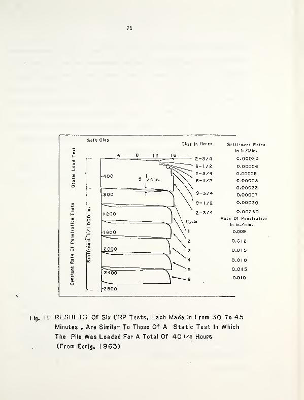
71
Soft ClayTime In Hours Settlement Rotes
In In/Min.
0.00020
0.00006
0.00008
0.00003
0.00023
0.00007
0.00030
0.00250Rate Of Penetration
In in./min.
0.009
0.0 12
0.0 15
0.0 10
0.0 15
0.010
-2800
Fig. 19 RESULTS Of Six CRP Tests, Each Made In From 30 To 45
Minutes , Are Similar To Those Of A Static Test In Which
The Pile. Was Loaded For A Total Of 40 1/2 Hours,
(From Esrig, I 963)
72
predicted by means of pile tests. However, it is a disadvantage
of the C.R.P. test that it cannot determine the short-term set-
tlement of a single tested pile. Hence, it is not possible to
estimate the settlements of pile groups. This is important since
the permissible loads on piles bearing in granular material are a
function, most frequently, of the predicted settlement of the
piles, whereas the permissible loads on piles bearing in cohesive
material are related to both the bearing capacity and estimated
long term settlement of the piles.
The recent introduction of the C.R.P. method in ASTM stan-
dards as an acceptable alternative to the load controlled method
will allow its wider application (Vesic, 1977).
2.2.2.3 Method of Equilibrium:
This method was first introduced by Mohan et al (1967). The
principal purpose of developing this method was to achieve a
state of equilibrium between load and the corresponding settle-
ment. As discussed before, in traditional maintained load test-
ing the applied load is maintained constant either for a fixed
period or until the rate of settlement diminishes to a negligible
value. This is done to achieve a state of equilibrium between
load and settlement. However, this ideal state is seldom
reached. Also, with a hydraulic jack, continuous attention and
occasional pumping is required to maintain the load, unless a
load maintainer is available, and this is both laborious and time
consuming.
73
While carrying out load tests on plates and a number of
short bored piles, Mohan and Jain (1964) noticed that equilibrium
was reached earlier if a load was first applied which was
slightly higher than the desired one. The method has since been
studied further and has been found to be very promising. Conse-
quently, the so called "Method of Equilibrium" was introduced by
Mohan et al (1967). The main advantages of this method are that
it helps to achieve a state of equilibrium between the load and
subsequent settlement more quickly, and it eliminates the need of
a load maintainer or constant pumping of the jacks to maintain
the load at a particular value.
2.2.2.3.1 Procedure:
The principle of this method is to apply to the pile, at
each stage of the test, a load slightly higher than the required
value, and then to allow the load to decrease itself due to the
yielding of the ground, until a state of equilibrium between the
load and the settlement exists. By this means, the rate of set-
tlement diminishes much more rapidly than with the maintained
load procedure, and equilibrium is reached in a matter of minutes
rather than hours. The procedure suggested by Mohan et al (1967)
is to first apply one tenth of the estimated ultimate load by
hydraulic jack in a period of three to five minutes. This load
is maintained for about 5 minutes, and is then allowed to reduce
74
itself via downward movement of the pile. Within a few minutes,
a state of equilibrium is generally reached. The next increment
of load is then applied and the process is repeated. For higher
loads, it is required to maintain the initial load for a period
of 10 to 15 mln. before it is allowed to relax.
While in sandy soils the state of equilibrium is reached
fairly quickly, in clayey soils it takes slightly longer.
According to Mohan et al (1967) the total time required for this
method is generally reduced to about one third of that required
in the maintained load test. At each stage, a cycle of loading
and unloading may also be adopted, and the elastic rebound of the
pile top measured. This could help in separating skin friction
and point bearing capacities (Van Weele, 1957; Jain and Kumar,
1963) .
2.2.2.3.2 Discussion and Interpretation of Re sul t
s
:
This procedure was primarily designed to determine the ulti-
mate load capacity, although it also appears to provide reason-
able settlement data. From the study carried out by Mohan et al
(1967) on long piles, it was evident that the method of equili-
brium provides results similar to the maintained load method. An
explanation of this behavior can be given by reference to Fig.
(20). In a pile load test, it normally takes 3.5 min to apply
smaller loads, and 10-15 min to apply higher loads, when the
hydraulic jack is operated manually. Two loading cycles for
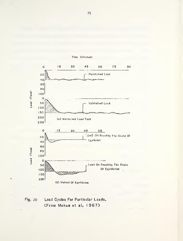
75
15 30 45 60
20
40
60
80
100
50
100
150
200
i:-.Odd On Reaching The State Of
Equilibrium
Load On Reaching The State
01 Equilibrium
Fig. 20 Load Cycles For Particular Loads.
(From Mohan et al, 1967)
76
specific loads in a maintained load test are shown in Fig.
(20. a). It can be observed that the shaded portions of the
curve, which also represent the settlement, are not accounted
for. The load which is maintained ultimately, and which is not
the average, is taken as the load applied for the period.
Another two loading cycles for a test by the method of equili-
brium are shown in Fig. (20. b). The load at which equilibrium is
attained is always lower than the maximum, so it provides a
better average than that obtained in a maintained load test.
Mohan et al (1967) conducted several tests to compare their
method with both the maintained load and C.R.P. tests. A series
of load tests were performed at seven sites on precast, driven
and cast-in-situ piles. A range of pile diameters or sides up to
18 in., was used. Piles penetrated various types of soils,
granular and cohesive, of various consistencies. Pile lengths
were variable up to a length of 80 ft.
To compare any two tests, the same pile has been used for
both tests in order to avoid uncertainties arising from the use
of different piles. Unloading was carried out at each stage
before application of load by the new method, and one method was
immediately followed by the other without allowing any period of
rest. This was done purposely to avoid any changes in soil con-
ditions which had been observed earlier to mar the results of
other test programs (Mohan et al, 1967).
77
Among these studies are those shown in Fig. (21) and (22).
A typical comparison reveals excellent agreement, in regard to
both ultimate load capacity and load settlement behavior, between
the method of equilibrium and the maintained load method. The
C.R.P. seems to give values about 10% higher than the other two
methods (Fig. 22). For more comparison studies refer to Mohan et
al (1967).
It then can be concluded that all the interpretations dis-
cussed before for the maintained load tests, regarding ultimate
and allowable loads and settlements, can be applied to the method
of equilibrium.
2.2.2.4 Load Testing by the Texas Highway Department :
Prior to January 1963, the Texas Highway Department (THD)
had been using the basic AASHTO 48-24 hour test method as modi-
fied by the TDH specifications (1962). Also, Indiana, and sur-
rounding states as well, use the same test. This test is old,
complicated and very time consuming, hence it is relatively
expensive. Table (2) gives some of the results of several 48-24
hour tests. In some cases, the test duration reached 258 hours\
(more than 10 days). The average duration was about 126 hours
(more than 6 days). Hence, this test is almost never used in
other regions. For detailed information about this procedure,
the reader may refer to Fuller and Hoy (1970).
78
(S3H0NI) iN3W31113S
1-CO
*s o >-
>-!£ V>•<<2 1-
_l< _Jo*: co o
o
CO
79
\ •?
t ~ -«»
. - COS .- S
CS3H0NI) 1N3W31113S o
COh-
CL
o
083 d) H4d >a1
u.
•-o —
co
ocaen
co 3llt
With
Of
Clay
avel
C
>» a C3
= a "?« e_ 1=
80
oJ= **4J ©X ON
H OX
ua -o
cb «
-* ucn cu
1 -t00 H<» 3b
Oh ax oW I-
< >u< w
CM
CU
43
«
a6u
MS
C B ^ai oo t: CO
> iH (0 cO 00 o o1- <U _! 4-1
a. o v-*
11
s4-1 4)
a) ~4
z 4J
c0)
a S —co cu '
U 4J ^,O 4J
01
en
T3
s ^ CO
3 4) M ^ne•HX 3 CO
O CX T3 X OCO tt) 4J
r o oo ^J <r
s c3 o •^s v a•H T3 .-1 cX <0 H Oa o Ou 4-1
X
c
N-/
o 4-1
•H GO /*"\
4-1 CU t-<
CO H 4:(1 %-•
3 U-l
a o •
4-1 0)
CD X3a) BH 3z
^OO^cfri-OOaOvCONON^iaO
-h-hOCN-m-^-hOO«*0
CO
eg eg cncoi/\D 43 j2 co to O>co u*i mco' ifl ifl O MO • Os • • Om m m m
1N*-HO\»S>HCNCOCMlfHO"CfvOlfl>Cf^00>O>f>ON-nO-^Ncn^CNfO^Nooooooooooo
—I CN m CN r~» —OfiOC^^CTlfn-*—4c»im»3-mm«a- mfn
ooooooooooo
inooomininoinomo-*cnooiflN-<iO'«HO
oomommoommmMrtO\001flSM>0-<-<0
m c- m in mcn \o cn cm m CN
cMmr^oaOfn^eMtNO-Hommvrmoo-HfOON-^-H
rtN(0'»lrt>0NC00lO'"
5N « C43 H c ^ iH
eg u o 11 ^3
T3 4) m 4J —
i
<D • T3 4-1 3 ts4-1 CO CU H 01 C cu
u u CO u 43 E cO V 3 CJ i-i
a. 4J eg u CO
a. cu CJ u 4J 4_l
3 a 0) 41 XCO o •3 J= c £ >-
\
CO CO 4-1 01 4J oa c O M CO cCO 01 H CO E X -=
CU 4J -a 4J C 3 u43 X 4-1 c u V
CU CO CO en •-u 1) £c 11 1-1 B •
o >, 4-1 • C vH >< 4-1
•H 43 c -c c H - BO
4-) M H CO rt 1) CU
y -o 3 a 4J 73 > :-
CO 0) C m i—
i
CO H ccu c 43 CN f-( £ CJ uM -H • c H n z
CO < o M a u a•O 4J CN iH h =c 43 1 c CO 4) • a (
« o CO CO 4) 4-1 c i) <T« X! -a c <H a C^i
^ CO u H h 1
O CO o c m o CC
CO 3 h CU it >> CN u <ri-l 03 u > -C • D
4-1 -o c M oCJ C C s - O HH CU CO a D J- --4 X 1
^ a u 14- B CO C/3
3 CU CO e iH 3 <CO H 3 CO 11 4J < :
u u 4) 4J E 4-1 3 u >-^
•^ 4J -C c i- 43 — CO
>% 0> u 0) X CO •o4: to e =5 > c CO I
01 4) e T3 o o>N u H ct) 41 )J
-O . 41 4-1 D C •o00 £ 4J JC —
1
H 01 c•o c 3 01 4-1 1-4 CO sc
CU -H CO 4-J a •H
"O -H CO c 3J 4-1 43 X<0 -H CU 4J 4) £ c 11
O Cl CO 0) X U 11 CO D^H <0 c 4J E c •
u o Oj D o •a cCO o 4-1 « i-H iH cu i)
01 J= cu c 4J 4-1 4-1 i-H >r-t u CO II 01 4M 4-1 CO H oH C o c 6 c CU i-H CO uCVi eg M CO 1) 03 3 14-1 —
4J e 11 CJ CJ
u u l-i 4-1 l-l 4-J I
.. c 0! D 1) 1) CO oCU M a. 3 CL c CJ z S«i
4-1
o • • •
z CO 43 ci
81
After the development of the C.R.P. method by Whitaker and
Cooke (1961), described earlier in this report, the Texas Highway
Department performed a slight modification of the method (for
simplification) and performed several comparison tests using both
the standard AASHTO 48-24 hour and the modified C.R.P. methods.
These tests gave very promising results, as will be discussed
later in this chapter.
2.2.2.4.1 Procedure :
The C.R.P. test calls for records of time and jacking force
to be made at equal intervals of movements of the pile head, with
the rate of jacking being adjusted so that readings occur at
equal intervals of time. For convenience and simplicity, the
C.R.P. test was modified by the TDH to produce the quick test
method. It requires that loads be added in increments of 5 or 10
tons, with gross settlement readings, loads, and other data being
recorded immediately before and after the application of each
increment of load. However, ASTM D1143-81 recommends that the
load increments be 10-15% of the proposed design load. Each
increment is held for 2.5 minutes and the next increment is then
Applied. When the load deformation curve obtained from these
test data (Fig. (23), (24) and (25)) shows that the pile is
definitely being failed (i.e., the load on the pile can be held
only by constant pumping of the hydraulic jack and the pile is
being driven into the ground), pumping is stopped. Gross defor-
mation readings, loads and other data are recorded immediately
82
/-N
CD
E
CO
I-
;u»uj9|}je3 epojp
83
r>
03 N~I
s-CL CD
< —
o
CD
E
CO
sa»jou|-}u9uja|;}ag ssojq
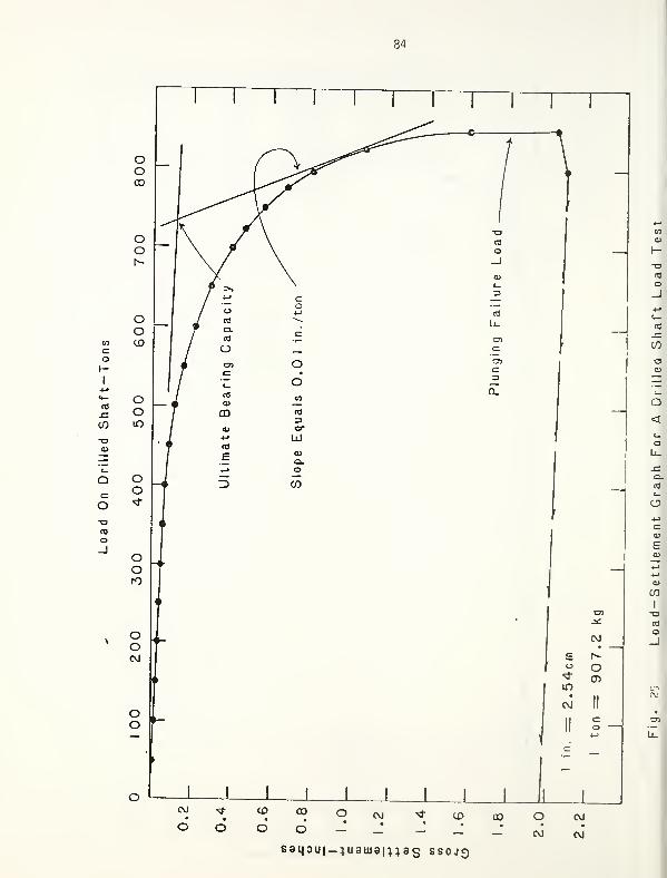
oh-
I
+->
JO.
-o
894ou|-;u9uia|U3S ssojq
85
after pumping has stopped and again after intervals of 2.5
minutes and 5 minutes. The load on he pile for the case of con-
stant pumping is called the "plunging failure load". Next, all
load is removed, and the pile is allowed to recover. However,
ASTM D1143-81 recommends that the full test load be removed in
four approximately equal decrements, with five minutes between
decrements so the shape of the rebound curve may be determined.
All test loads are carried to plunging failure or to the
capacity of the equipment. The maximum proven design load is
considered to be one half of the ultimate bearing capacity, which
is indicated by the intersection of lines drawn tangent to the
two basic portions of the load settlement curve as shown in Figs.
(23), (24) and (25).
2.2.2.4.2 Correlation Studies by TDH :
The Texas Highway Department conducted 11 pile load tests by
using both the standard 48-24 hour and the quick test method.
Table 3 summarizes the range used in these tests for piles, ham-
mers and soil types. Table 4 gives the results of the quick test
method which can be compared to the results of the standard 48-24
hr test given earlier in Table 2. The maximum proven design load
obtained by the quick test method and the 48-24 hour test method
are shown in Fig. (26). The average deviation of the maximum
proven design load values obtained from the quick test method
versus the standard 48-24 hour test method was only about 4%
(Fuller and Hoy, 1970)
.
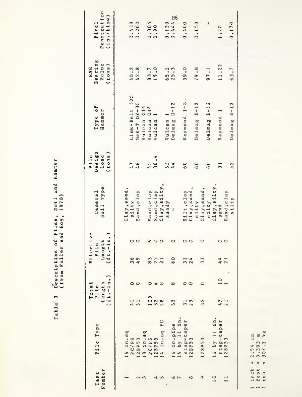
O »-v
•—l t-> O4 g hC l-i -O
H 4-1
tx, CU •
c c
W o) co OCU > 4J
pa %_•
o Mcu
CU Eo. a
h x
V 60 -O CO
h ti »j u
o CT>
en —
<
. .
CD >,0) o-H ss•HCu -o
c<4H CO
OU
c CD
O .H•H •H4J 3O. tK
ftl-> a<J oca u
v 4* >M>Q "—•
CO
<u
H-O<0
H
CO ^t-i Hcu
c r-4
cu •^
o o
t-i j= e4J 0) 4-1 iHUH CO |
1) -H C •
CM Pu CU 4J
<4-l pj CMM ^/
<H .C CCO CU 4-> iHUH bO |
O tH C •
J <*-i
86C7N O m o ~»CN vO 00 o O -3-
-3- CM en <?• —> sr
O CM c> in m ui-3- -3 00 —
•
vO CN
_l I—1 -.
rH W O O —
i
c C C B be CH CO CO CO co co O
1 CJ CJ CJ CJ e B^ rH i-H rH rH rH >,o 3 3 3 3 01 0)
r > > > > O al
O vO-3- C*1
CO -3
-o >. >> >> *->
c CO tO co HCO rH rH -I -Hto >, o CJ o co ^» 4-1 » - * « -o>> rH -o -a •a >, cCO -H c c C CO to
rH CO CO co co •-! CO
CJ en en en cj
cj co >* to >, co
4J >-, rH >-, rH >, C T3 --H
CO CO CrH CO CO
CJ CO
ci in —> o -h <r —
i
oo cn cn vo n cm en
4_> o)
co jocu a
z
cn coCm UI
cj to o ca
vO (X, CN 00 Dm CN -3-
—I CN 0O
c >> cx m•H J3 cu a,
U pQvo sr co cn
u cavO co CN
HE a ^U
in CN-J O •
m CIo
CM o Oi
•H U-t U
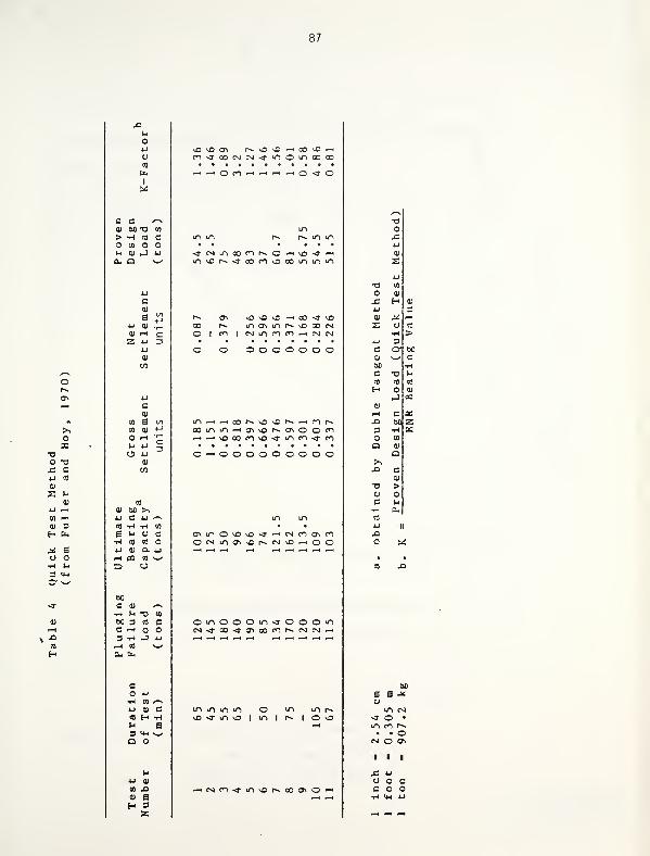
87
CO
fu
u
c c ^N0) 60 T3 to
> H (0 co CO Ou 01 -J 4-1
Pu Q >—
•
ox
o -aj= c
01
0) 3
^ So o
3 <4-(
tu
E-i
Ccu
E4-1 CD
0) r-l
Z 4->
4-1
c0)
u] sco cu
O i-H
M 4J
O 4J
01
en
CO
cu 60 >,4J C 4-1 ^Na H H en
6 s-i CJ c•H CO CO
4-1 0) Q. 4-1
H pa (0 ^—
'
60
C CU /*"**
H u •a CO
60 3 CO cc ^H o3 •H J 4-1
^H CO ^^eu
Co 4J
•H co /-^y
4-1 cu cCO H H1-1 s3 VM •Wo
4-) CU
a .acu gH 3z
<0 ^O Cli r^.\OvO~*CO^O«^m-tCONCvKmO^OCCO-H-^Om—4—<-^-HO-*0
irnON-jcocivOflOininifl
^O vO ^D —i 00 -3" V40
moi in n cc csn i/i n n h n nO o o o o o o
aoinm-HO>v40i~-o>ooroHFHvOCOfO^<l/lCO^f»l
O-hOOOOOOOOO
CX*inO^\0~d"~H CvJcr>^cri
OCMinONvOt^CNvO-HOO
ouiooom<-ooomCM~3-oo~3-ONooc">r^eNCN.-H
m u-i u-i in ovO -* m vo | m l
m i^.
I o vO
i"Nn>}l/1\ONCOO»0'"
aj
£ H a)
4-1 3CD ^ .—
i
s u CO
H >4-> 3c © 60
tu w C6C i-(
C T3 UCO <0 CO
H O 01
J 03
0)
i-H c Pi
J2 so Z3 •H w
CO
a 0)
c>,XI c
60
B B aom CM
<r O •
m d r^• • O
CM O ON
I 1 R
-C 4J
y Cc o•H 14-1 4-1
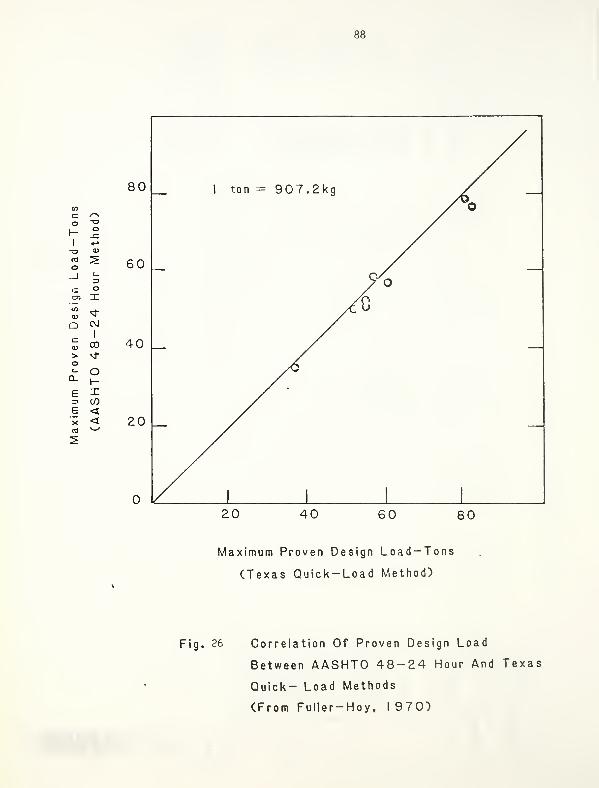
h-ojC
1+->
-o CD
03 ^o
1
c_
3n OCX> XCO
-tf
Q CVl
aCD
1
CO
> sj-
Oc_ oa.
h-
F. XD COE <X <cfl
v_^
Maximum Proven Design Load-Tons
(Texas Quick-Load Method)
Fig. 26 Correlation Of Proven Design Load
Between AASHTO 48-24 Hour And Texas
Quick- Load Methods
(From Fuller-Hoy, I 970)
89
The main advantage of the quick method can be clearly shown
if the reader refers to Tables 4, 5, 6 and 7. The average total
man hours/test for the quick method is only about 1/50 of those
required by the 48-24 hour method. Also the time delay to the
contractor in the quick method is only about one tenth of that In
the other method. This makes full-scale load testing on small
projects feasible because of reduced time and cost. In addition,
the test is very simple and easy to interpret. The quick tests
generally result in more nearly undrained conditions of shear
failure, thus providing a condition for which load capacities can
be more rationally correlated to static analyses utilizing
undrained laboratory shear tests.
According to Butler and Hoy (1977), there are no limitations
on the use of the quick load method when it is used to determine
the load carrying capacity of a particular foundation soil sys-
tem. It can not be used, however, to determine the settlement
behavior of a foundation under a sustained load. In the case
which the settlements need to be defined, i.e. in cases where
piles rest on granular soils, an alternative method should be
utilized .
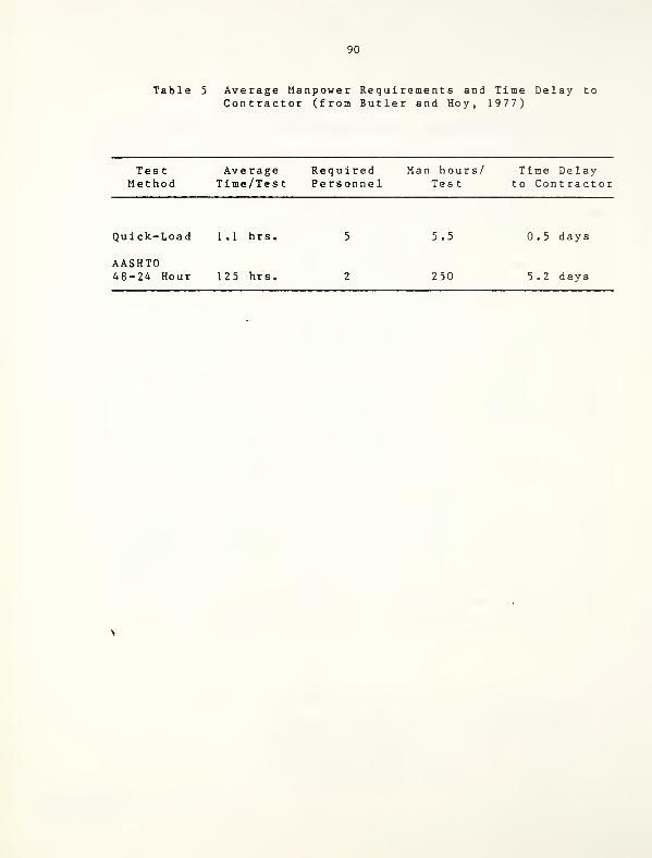
90
Table 5 Average Manpower Requirements and Time Delay toContractor (from Butler and Hoy, 1977)
TestMethod
Average Required Man hours/Time/Test Personnel Test
Time Delayt o Con tractor
Quick-Load 1.1 hrs.
AASHTO48-24 Hour 125 hrs.
5.5
250
0.5 days
5.2 days
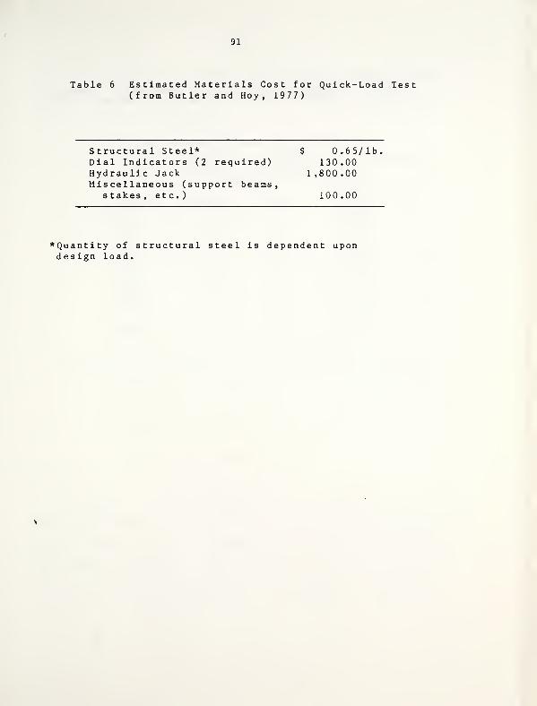
91
Table 6 Estimated Materials Cost for Quick-Load Test(from Butler and Hoy, 1977)
Structural Steel* $ 0.65/lb.Dial Indicators (2 required) 130.00Hydraulic Jack 1,800.00Miscellaneous (support beams,
stakes, etc.) 100.00
*Quantity of structural steel is dependent upondesign load.
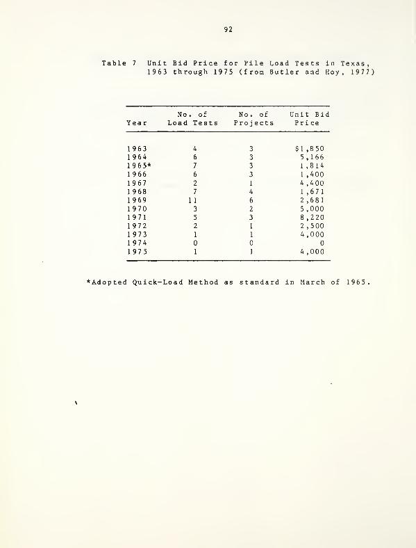
92
Table 7 Unit Bid Price for Pile Load Tests in Texas,1963 through 1975 (from Butler and Hoy, 1977)
No . of No. of Unit BidYear Load Tests Projects Pri ce
1963 4 3 $1 ,8501964 6 3 5,1661965* 7 3 1 ,8141966 6 3 1 ,4001967 2 1 4,4001968 7 4 1 ,6711969 11 6 2 ,6811970 3 2 5,0001971 5 3 8 ,2201972 2 1 2,5001973 1 1 4,00019741975 1 1 4,000
*Adopted Quick-Load Method as standard in March of 1965
93
the pile is adequate to support the design load (Lambe and Whit-
man, 1979). Poulos and Davis (1980) cited four reasons for car-
rying out routine load tests:
1. To serve as a proof test to ensure that failure does
not occur before a selected proof load is reached,
this proof load being the minimum required factor of
safety times the working load.
2. To determine the ultimate bearing capacity as a check
on the value calculated from dynamic or static
approaches, or to obtain backfigured soil data that
will enable other piles to be designed.
3. To determine the load settlement behavior of a pile,
especially in the region of the anticipated working
load. These data can be used to predict group settle-
ments and settlements of other groups.
4. To indicate the structural soundness of the pile.
According to Fuller and Hoy (1970), the decision to perform
the second category of tests, i.e. an advanced test program to
develop design criteria, is usually made jointly by the owner and
the foundation engineer. This decision is based on the scope of
the project and the complexities of the foundation conditions.
94
2.3 Other Types of Pile Load Tests
2.3.1 Uplift Tests :
Uplift or tension tests on piles can be made at either a
continuous rate of uplift (CRU) , or an incremental loading basis
(maintained load).
A loading rig for an uplift test is shown in Fig. (27).
This utilizes nearly the same components as the compressive load
testing rig shown in Fig. (2). The methods used for measuring
the jacking forces and the movement of the pile head are the same
as those used for compressive tests. It is particularly impor-
tant to space the ground beams or bearers at an ample distance
from the test pile. If they are too close, the lateral pressure
on the pile induced by the load on the ground surface will
increase the skin friction on the pile shaft. Tomlinson (1977)
suggested a minimum distance of 2.0 m (6.5 ft), while ASTM 1143-
D75 requires a minimum spacing of 2.40 m (8.0 ft).
Where uplift loads are cyclic in character, as in wave load-
ing on a marine structure, it is good practice to adopt repeti-
tive loading on the test pile (Tomlinson, 1977). The desirable
maximum load for repeated application cannot be readily deter-
mined in advance of the load testing program, since the relation-
ship between the ultimate load for a single application and that
for repeated application is not known. Tomlinson (1977) sug-
gested that a single pile should be subjected to a CRU test to
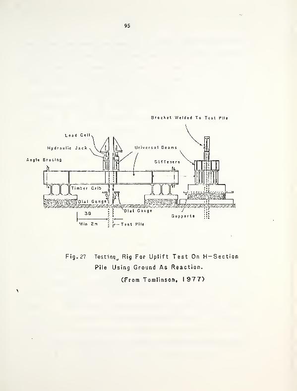
95
Bracket Welded To Test Pile
Load Cell
^£5W3? Dial G a u g e^ f \ fe^^^^g^ [~l '
ill
IJ
Dial Gauge / ;'/.
Supports
M i n 2 m Test Pile
Fig. 27 Testing., Rig For Uplift Test On H-Section
Pile Using Ground As Reaction.
(From Tom I'm son, 1977)
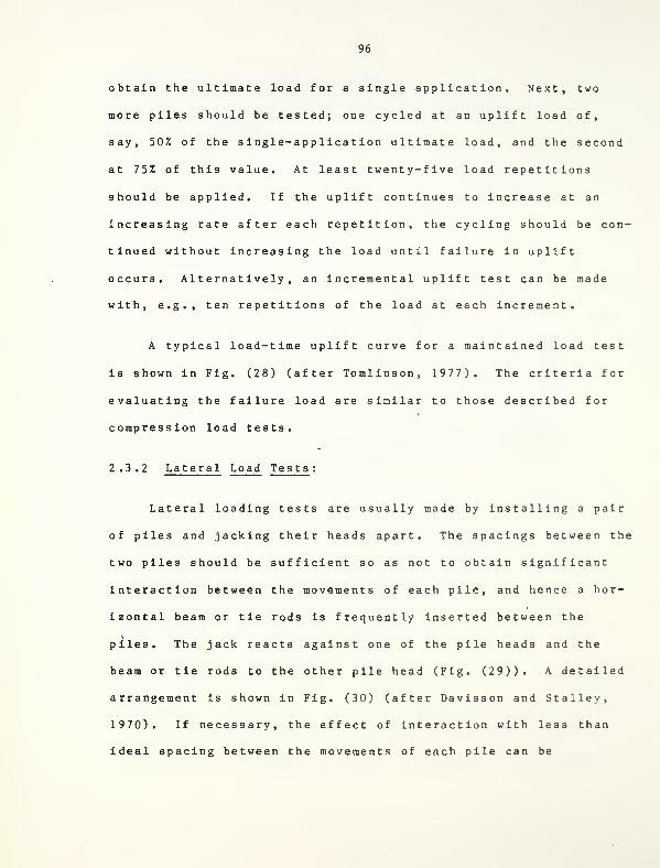
96
obtain the ultimate load for a single application. Next, two
more piles should be tested; one cycled at an uplift load of,
say, 50% of the single-application ultimate load, and the second
at 75% of this value. At least twenty-five load repetitions
should be applied. If the uplift continues to increase at an
increasing rate after each repetition, the cycling should be con-
tinued without increasing the load until failure in uplift
occurs. Alternatively, an incremental uplift test can be made
with, e.g., ten repetitions of the load at each increment.
A typical load-time uplift curve for a maintained load test
is shown in Fig. (28) (after Tomlinson, 1977). The criteria for
evaluating the failure load are similar to those described for
compression load tests.
2.3.2 Lateral Load Tests:
Lateral loading tests are usually made by installing a pair
of piles and jacking their heads apart. The spacings between the
two piles should be sufficient so as not to obtain significant
interaction between the movements of each pile, and hence a hor-
izontal beam or tie rods is frequently inserted between the
piles. The jack reacts against one of the pile heads and the
beam or tie rods to the other pile head (Fig. (29)). A detailed
arrangement is shown in Fig. (30) (after Davisson and Stalley,
1970). If necessary, the effect of interaction with less than
ideal spacing between the movements of each pile can be
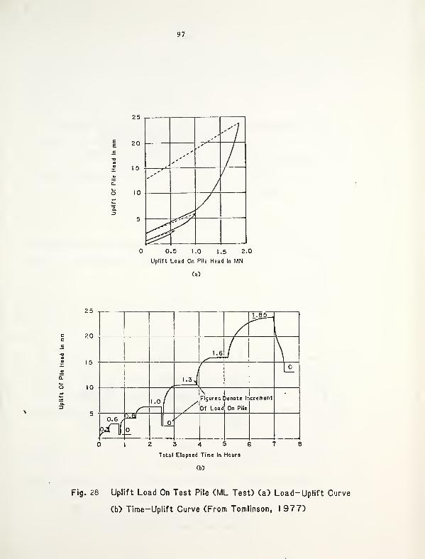
97
25
20
I 5
10
-f^r?
0.5 1.0 1.5 2.0
Uplift Load On Pile Head In MN
(a)
25
20
15
10
1
L8_5 J
1.6
1
i
1 1.3 J
1
1.0 ( /\Figures 1
Of Load
)enote Ir
On Pile
crement
0.6 / L/
2 3 4 5 6
Total Elapsed Time In Hours
Cb)
Fig. 28 Uplift Load On Test Pile (ML Test) (a) Load-Uplift Curve
(b) Time-Uplift Curve (From Tomlinson, I 977)
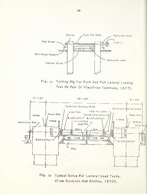
98
Sleeve Four Tie Rods
Dial Gauge
>&.j£
Dial Gauge Support
Tubular Strut
] ,i iIPC
YT^m^x^rm^
IvVVZ-J k//^
Hydraulic Jack
Load c.
Hydraulic Jack
Fig. 29 Testing Rig For Push And Pull Lateral Loading
Test On Pair Of PilesCFrom Tornlinson, 1977)
2 '-I0'
I 6'- 10" 2'-I 0'
Deflection Dial
Fig. 30 Typical Setup For Lateral Load Tests.
(From Davisson And Stalley, I 970).
99
estimated, as explained for vertical tests in Section 2.1.5,
using theories of pile group- soil interactions tor laterally
loaded piles (Poulos and Davis, 1980).
The procedure employed for the test varies, but typically
the load is applied in a number of increments, and each increment
is left on until a specified rate of movement is reached. Aliza-
deh and Davisson (1970) used, for each increment, a minimum
period of one hour, or until the pile head movement was less than
0.01 in. per hour. Tests were carried to lateral deflections
approaching 2 in. Where the lateral loads on piles are of
repetitive character, as in wave loading or traffic loads on a
bridge, it is desirable to make cyclic loading tests (Tomlinson,
1977). This involves alternately pushing or pulling of a pair of
piles, using a rig of the type shown in Fig. (29). Instead of a
pair of piles, a single pile can be pushed or pulled against a
thrust block (Fig. 31).
Diaz et al (1984) performed lateral load tests on pres-
tressed concrete piles penetrating through rockfill in The Port
of Los Angeles. In this study, a separate reaction pile was
driven behind each "p roduct ion"/t es t pile. Each load increment
was 8.0 ton (71 kN) in magnitude and applied at a rate of approx-
imately 2.0 tons (18 kN) per minute. Each load step was main-
tained until the pile head movement stabilized. The loading pro-
cedure and cyclic load application methods are described in
detail by Diaz et al (1984).
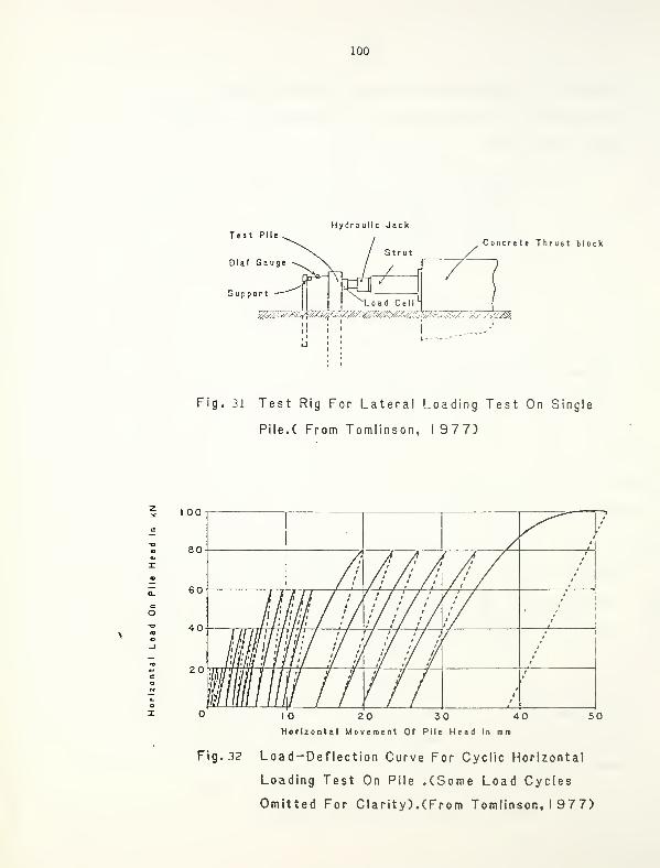
100
Concrete Thrust block
Support^Load Cell
L
1
1
u
Fig. 31 Test Rig For Lateral Loading Test On Single
Pile.C From Tomlinson, 1977)
I oo
80
60
40
20
r I
/ 1
/ 1
/,'/'/> /' //• /.' A'i /' /// // // // /
\
//'/// / •'/'• III' 1 ' /'I'll / >/
'/'/'/if if , /' / ' / i /* f ' / if
1/ ' /
/ // /
/ /
/
l
i
III'
1/'1,
f if }// . / ' / ' i
'/ '/ iftf '/ iftf */ <y
i l
!
/
WilliIII 1
1
if '/ 7
/
/
/
10 20 30 40Horizontal Movement Of Pile Head In roro
50
Fig. 32 Load-Deflection Curve For Cyclic Horizontal
Loading Test On Pile .(Some Load Cycles
Omitted For Clarity). (From Tomlinson, I 977)
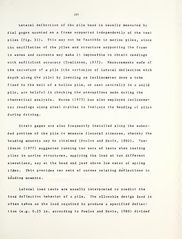
101
Lateral deflection of the pile head is usually measured by
dial gages mounted on a frame supported independently of the test
piles (Fig. 31). This may not be feasible in marine piles, since
the oscillation of the piles and structure supporting the frame
in waves and currents may make it impossible to obtain readings
with sufficient accuracy (Tomlinson, 1977). Measurements made of
the curvature of a pile (the variation of lateral deflection with
depth along the pile) by lowering an inclinometer down a tube
fixed to the wall of a hollow pile, or cast centrally in a solid
pile, are helpful in checking the assumptions made during the
theoretical analysis. Hanna (1973) has also employed inclinome-
ter readings along steel H-piles to indicate the bending of piles
during driving.
Strain gages are also frequently installed along the embed-
ded portion of the pile to measure flexural stresses, whereby the
bending moments may be obtained (Poulos and Davis, 1980). Tom-
linson (1977) suggested running two sets of tests when testing
piles in marine structures, applying the load at two different
elevations, say at the head and just above low water of spring
tides. This provides two sets of curves relating deflections to
bending moments.
Lateral load tests are usually interpreted to predict the
load deflection behavior of a pile. The allowable design load is
often taken as the load required to produce a specified deflec-
tion (e.g. 0.25 in. according to Poulos and Davis, 1980) divided
102
by the required factor of safety. A typical load deflection
curve for cyclic tests are shown in Fig. (32) (from Tomlinson,
1977). The values of the subgrade reaction modulus or the elas-
tic modulus of the soil may also be backfigured from a test, by
fitting the observed behavior to the theoretical. This procedure
enables predictions to be made of movements of piles of other
dimensions or of groups of laterally loaded piles. Poulos and
Davis (1980) stated that for laterally loaded pile groups, the
influence of any soft layers underlying the pile tips is of much
less significance than in the case of vertical loading.
2.3.3 Torsional Testing :
Although axial load tests presently represent the only cer-
tain method of determining the ultimate axial load capacity of
individual piles, conventional procedures and equipment are rela-
tively costly and inconvenient, especially if high load capaci-
ties are anticipated.
An alternative method has been introduced, in which tor-
sional loading tests on piles can be utilized instead of the
ordinary axial load tests. Stoll (1972) devised a simple field
torque shear load test that could be applied to cylindrical
piles. The piles must be capable of carrying the required torque
without failure of the pile material itself, so that in stiffer
soils, relatively short or stiff piles may be necessary (Poulos
and Davis, 1980). The advantage of the test apparatus is that
103
the torque is applied by small capacity hydraulic jacks reactinj
horizontally against adjoining job piles, utilizing the large
mechanical advantage available at the usual spacing (i.e., 3 ft
to 5 ft or wider).
According to Stoll (1972), the pile-soil shear strength from
torsional tests would not exceed the value for axial loading.
Model tests reported by Poulos (1975) showed that in clay, the
values deduced from axial and torsional tests were very similar.
It was also possible in these tests to backfigure the shear
modulus of the soil from the measured torque rotation relation-
ship, using elastic theory, and to use this value to predict the
settlement of an axially loaded pile. Thus, there is some evi-
dence that torsional load tests may be useful for predicting the
behavior of axially loaded piles in clay. For sands, however,
because of the dependence of the pile-soil shear strength on the
stress state, torsional tests may give misleading results. Broms
and Silberman (1964) obtained, for model piles in sand, consider-
ably lower values from torsional tests than from axial tests.
104
2.4 Recommended Procedures for Axial Pile Load Tests
2.4.1 General :
In the previous sections of the report, the importance of
performing pile load tests to obtain the most valuable and accu-
rate data for design of the pile foundations was emphasized.
In order to make the pile load testing a matter of routine
procedure in general practice, costs should be minimized, without
compromising the data obtained. To achieve both goals, and based
on the information presented in the previous sections of the
report, it is recommended that the IDOH uses either the quick
load test method or the method of equilibrium for axial pile load
tests, depending on the pile-soil system. For friction piles or
for piles supported by clayey layers, where settlement data are
not to be obtained from the load test, the quick test method
should be used to obtain the ultimate pile load capacity. For
end bearing piles resting on sand, where settlement information
is necessary for the design, the method of equilibrium should be
utilized. In cases where the pile is supported by both friction
and end-bearing with nearly equal magnitudes, the quick test
method can be used for proof testing and in case no settlement
data are required. If allowable settlement is the main design
criterion, the method of equilibrium should be used.
For both methods, the following general points should be
taken into consideration:
105
1. For driven piles, the test pile should be of the same
type and cross section as the piling that will be used
in the foundation and should be driven with the same
equipment that will be used to drive the foundation
piling. A minimum time interval between driving and
loading the test pile should be provided. A minimum
waiting period of ten days between driving and loading
a test pile is recommended. This permits the soil,
disturbed during the driving operation to regain most
of its natural characteristics before testing, without
causing an excessive delay to the contractor. Local
driving conditions may, however, warrant a different
waiting period.
2. For drilled shafts, the test shaft that is to be
tested should be constructed using the same method
that will be used throughout the structure, i.e., dry
hole, cased or slurry displacement. Before loading a
test shaft, the concrete must have reached its design
strength and the surrounding soil should be given suf-
ficient time to adjust to the changes brought about by
the migration of water and cement particles from the
fresh concrete (Chuang and Reese (1969)). If the sur-
rounding soil is porous, a layer of soil-cement will
form at the concrete-soil interface, resulting in a
gain in the soil shear strength. For soils such as

106
clay, there will be only water migration, and this
will cause a decrease in shear strength. Several
specifications require a minimum waiting period of
seven days between concrete placement and load test-
ing. In any case, testing should not begin before the
concrete has attained its design strength.
3. The reaction system for load testing of a pile or
drilled shaft must be sufficient to withstand the load
required for a plunging failure. Butler and Hoy
(1977) suggests that this load be assumed as four
times that used in the structural foundation design.
4. Anchorage piles for the reaction system should be
spaced to provide a center to center distance from the
supports to the test pile of not less than 7 feet (2
m). Closer spacing may be allowed if anchorage piles
are to be used as permanent piling for the structure.
Using permanent piles as anchorages is preferred when-
ever possible, as this will reduce the cost of the
load test. When this is done, these piles must be
checked against uplift forces created by the test
load. The effect of these piles on the settlement of
the test pile should be investigated.
5. Close attention must be given to the design and fabri-
cation details of the reaction beam because failure
107
under the high loads attained during a load test would
be extremely hazardous. According to Butler and Hoy
(1977), a beam that has a working range of 15 to 30
feet (4.6-9.2 m) should be adequate for normal usage.
In addition to the above mentioned points, attention should
be given to all the considerations discussed in the preceding
sections with respect to loading systems, instrumentation and
settlement measurements.
2.4.2 Texas Quick Load Test Method :
As discussed before, the use of this method could result in
a tremendous reduction in load test costs. The method is limited
to the determination of the pile load capacity, without providing
information about the settlement. Hence, it can be used only for
cases where settlement data can not be obtained from load tests
(e.g., for piles resting on clayey soils). The procedure can be
summarized by the following steps:
1 . The load is applied in increments of 10 to 15% of the
proposed design load with a constant time interval
between increments of 2.5 min. The corresponding
penetrations are measured and plotted.
2. Load increments are added until continuous jacking is
required to maintain the test load (plunging failure),
108
or until the specified capacity of the loading
apparatus is reached, whichever occurs first, at which
time jacking is stopped. The load increments should
be decreased to a minimum as plunging failure
approaches. This procedure will help to define the
ultimate load and point of failure more closely.
3. The following data are recorded immediately preceding
and immediately following the application of an incre-
ment of load: actual time, time interval, load added,
total load, dial indicator readings, and total gross
penetration. A form similar to that presented on
Table 8 is used for recording the data.
4. Load increments are added until plunging failure
occurs (whenever continuous pumping of the hydraulic
jack is required to maintain load or when the settle-
ment becomes disproportionate to the load being
applied). When this occurs pumping should be stopped
and data readings are immediately taken. Without
pumping, the load and settlement should be allowed to
stabilize, making data readings at 2.5 and 5 minutes
after pumping is stopped.
5. Quickly and smoothly all load is removed and immedi-
ately data readings are taken. Two additional sets of
data readings should be taken 2.5 and 5 minutes after
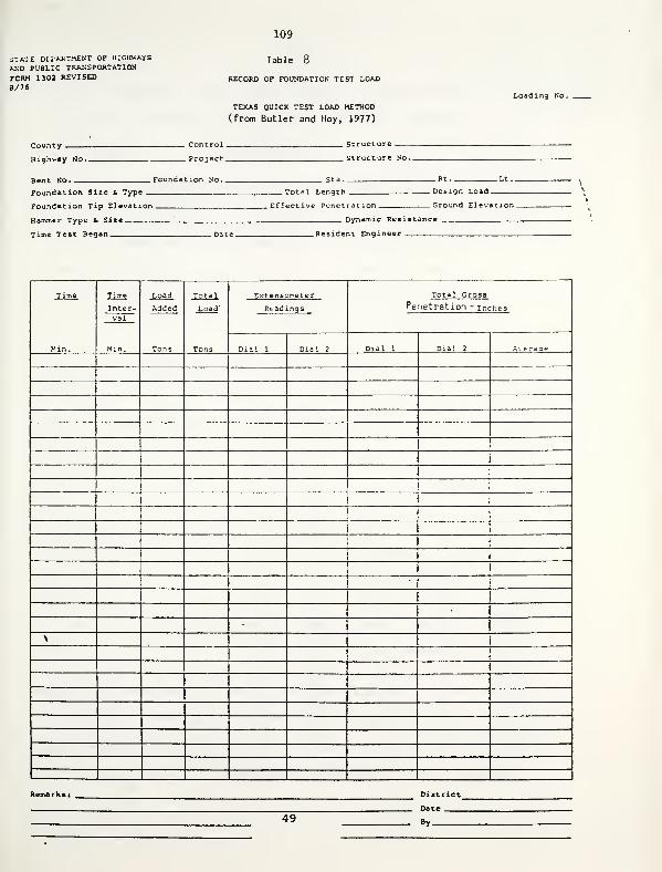
S-.A'IE DEPARTMENT OF HIGHWAYS
AND PUBLIC TRANSPORTATION
FORM 1302 REVISED8/76
109
Table 8
RECORD OF FOUNDATION TEST LOAD
TEXAS QUICK TEST LOAD METHOD
(from Butler and Hoy, 1977)
Loading No.
County
Highway No.
Control
.
. Project
.
Structure
_ Structure No..
Bent No. . Foundation No.
Foundation Size & Type
Foundation Tip Elevation.
Hammer Type & Size
Time Test Began
Sta.
.
. Total Length
Effective Penetration.
.Rt ..
.Design Load
.Ground Elevation.
Dynamic Resistance
.
.Resident Engineer
Time
Min.
Time
Inter-val
Min.
Load
Added
Tons
Total
Load'
Tons
Extensometer
Readings
Total Gross
Penetration - inches
Dial 1 Dial 2 Dial 1 Dial 2 Averaoe
-
>
49
District^
Date
By
110
load removal. Tables 9 and 10 are examples of data
obtained from axial load tests on driven piles and
drilled shafts, respectively.
6. A plot of load versus gross penetration after each 2.5
minutes should be made while the test is being con-
ducted so that its progress can be followed at all
times. Hence, it will be possible to recognize the
approach to plunging failure and the load increment is
then reduced as mentioned before.
7. For the interpretation of load test results, the "dou-
ble tangent" method is recommended. This is done by
the following procedure (refer to Fig. 23).
Plot a graph of load versus gross penetration using any
convenient scale.
Draw one line originating at the point of zero load and
penetration and tangent to the initial flat portion of the
gross penetration curve.
Draw a second line tangent to the steep portion of the
gross penetration curve.
The load at the intersection of the two tangents is defined
as the ultimate bearing capacity of the pile or drilled
shaft and will be used to establish a proven "maximum safe
static" load. This proven safe load for piling is defined
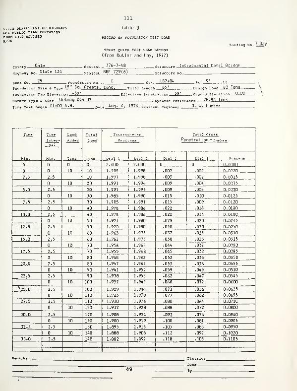
s-.A^E DLFARDENT OF HIGHWAYSAND PUBLIC TRANSPORTATIONFORM 1J02 RXVISED8/76
County
.
Gale
Highway No State 124
Bent No. 29
111
Table 9
RECORD OF FOUNDATION TEST LOAD
TEXAS QUICK TEST LOAD METHOD
(from Butler and Hoy, 1977)
Loading No 7 Day
376-3-48
Project BRF 729(6)
Foundation No.
.
1 Sta
structure Intracoastal Canal Bridge
Structure No —
187+84 „ 9'.Rt .. . Lt ..
Foundation Size & Type 18" Sq. Prestr. Cone
-59'
. Total Lenoth 65'
Foundation Tip Elevation.
Hanger Type s, si*,. Delmaq D46-02
Time Test Began.
.Effective Penetration. 59'
11:00 A.M.
Design Load _6D_LqQ£
Ground Elevation—QiQQ
.Dynamic Resistance 28.86 Tons
Date Aug. 6, 1976 B(,„ lrt ,.ni mg in..«.r J. W. Hunter
Jlme.
Min.
Time
Inter-val
Load
Added
Tons
Total
Load'
Tons
E>:ier,soreter
Pe
Total Gross
F.eadinas netration - inches
Kin. Dial 1 Dial 2 Dial 1 Dial 2 Averaqe
2.000 2.000 0.0000
10 10 1.998 1.998 .002 .002 0.0020
2.5 2.5 10 1.997 1.998 .003 .002 0.0025
10 20 1.991 1.994 .009 .006 0.0075
5.0 2.5 20 1.991 1.995 .009 .005 0.0070
10 30 1.985 1.990 .015 .010 0.0125
7.5 2.5 30 1.985 1.991 .015 .009 0.0120
10 40 1.978 1.986 .022 .014 0.0180
10.0 2.5 40 1.978 1.986 .022 .014 0.0180
10 50 1.971 1.980 .029 .020 0.0245
12.5 2.5 50 1.970 1.980 .030 .020 0.0250
10 60 1.963 1.975 .037 .025 0.0310
15.0 2.5 60 1.962 1.975 .038 .025 0.0315
10 70 1.956 1.968 .044 .032 0.0380
17.5 2.5 70 1.955 1.968 .045 .032 0.0385
10 80 1.948 1.962 .052 .038 0.0450
20.0 2.5 80 1.947 1.962 .053 .038 0.0455
10 90 1.941 1.957 .059 .043 0.0510
22.5 2.5 90 1.938 1.953 .062 .047 0.0545
10 100 1.932 1.948 .068 .052 0.0600
> 25.0 2.5 100 1.929 1.944 .071 .056 0.0635
10 110 1.923 1.938 .077 .062 0.0695
27.5 2.5 110 1.920 1.936 .080 .064 0.0720
10 120 1.912 1.928 .088 .072 0.0800
30.0 2.5 120 1.908 1.924 .092 .076 0.0840
10 130 1.900 1.919 .100 .081 0.0905
32.5 2.5 130 1.895 1.915 .105 .085 0.0950
10 140 1.888 1.908 .112 .092 0.1020
35.0 2.5 140 1.882 1.897 .118 .103 0.1105
49
District_
Date
By
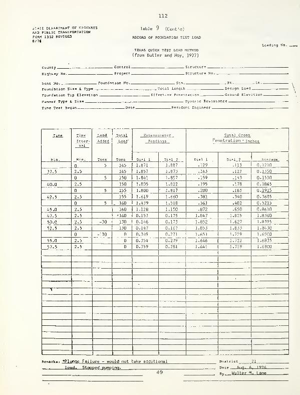
:>-. a:E DLFART-ENT OF HIGHWAYSAKD PUBLIC TRANSPORTATIONfCW 1302 REVISED8/76
112
Table 9 (Cont'd)
RECORD OF FOUNDATION TEST LOAD
TEXAS QUICK TEST LOAD METHOD
(from Butler and Hoy, 1977)
Loading No.
County
Highway No.
Control
.
. Project.
Bent No.
Foundation Size & Type
—
Foundation Tip Elevation.
Hammer Type & Size
Time Test Began
Foundation No..
Structure
.Structure No.
. Total Length
.Effective Penetration.
Rt ..
. Design Load
.Ground Elevation.
Dynamic Resistance.
.Resident Engineer
Time
Kin.
Time
Inter-val
Min.
Load
Added
Tons
Total
Load'
Tons
Extensorreter
Readings
Total Gross
Penetration - inches
Dial 1 Dial 2 Dial 1 Dial 2 Averaqe
5 145 1.871 1.887 .129 .113 0.1210
37.5 2.5 145 1.857 1.873 .143 .127 0.1350
5 150 1.841 1.857 .159 .143 0.1510
40.0 2.5 150 1.805 1.822 .195 .178 0.1865
5 155 1.800 1.817 .200 .183 0.1915
42.5 2.5 155 1.619 1.660 .381 .340 0.3605
5 . 160 1.439 1.518 .561 .482 0.5215
45.0 2.5 160 1.128 1.150 .872 .850 0.8610
47.5 2.5 160 0.153 0.175 1.847 1.825 1.8360
50.0 2.5 -30 130 0.148 0.173 1.852 1.827 1.8395
52.5 2.5 130 0.147 0.167 1.853 1.833|
1.8430
-130 0.349 0.271 1.651 1.729 1.6900
55.0 2.5 0.354 0.279 1.646 1.721 1.6835
57.5 2.5 0.359 0.281 1.641 1.719 1.6800
-
\
Remark* i *Plunae Failure - would not take additional
load. Stopped Dumping.49
21District
Date Ann. A, 197
A
walter M . Lane
113
Table 9 (Cont.)
SUMMARY OF DATA
FOUNDATION TEST LOADING
TEXAS QUICK LOAD TEST METHOD
County
Highway No.
Structure
Control Pro j ect
Date of Test LoadBent No.Location (Station)Description of Pile
Total LengthGround ElevationBtm. of Ftg. Elev.Pilot Hole Elev.Pile Tip Elev.Effective Pen.
Soil Type (General)Design Load per PileType & Size of HammerDynamic Resistance (ENR)Penetration per BlowDescription of Cushion
Type Green OakSize 2 6" 4>
Thickness 6"
Aug. 6, 1976Bent 29187+8418" Sq. Prestr. Cone65'0.00'-0.97'.00'
-59.00'59'
Silt, Sand & Clay60 TonsDelmag D46-0229 Tons2 .0"
Cap BlockPine Plywood
23" Sq.3"
Duration of Quick Test LoadMaximum Load on Pile
Gross PenetrationNet Penetration
7 Day Test57.5 Min.160 Tons1 .843"1 .680"
Plunging Failure LoadUltimate Static Bearing CapacityMaximum Safe Static Load (Proven)"K" Factor (Proven)
Remarks
16015075
2.6
TonsTonsTons
State Department of Highwaysand Public TransportationDistrictDate
i-.hZl DLPAflTHENT OF HIGHWAYSMCD PUBLIC TRANSPORTATIONrow. 1302 REVISED8/76
114
Table 10
RECORD OF FOUNDATION TEST LOAD
TEXAS QUICK TEST LOAD METHOD
(from Butler and Hoy, 1977)
County Morton
Highway No.IH 45
Bent NO.20
Loading Ho.
37-13-2
Project I 45-1(151)037Structure HB&T RR Ovprnass
Structure No
Foundation No..
Foundation Silo t Typn 36" Drilled Shaft
*,» 137+1
.Total Length 60'
. Pt
.
10'. Lt .
. Desic.n Load __3flfl_Lons_
Foundation Tip Elevation.
Harcner Type & Si
Time Test Began.
t-6' Effective Penetration. _iDJ_ .Ground Elevation.
Ha-cner Type & Size
10:00 A.M.
•.aiiic Resistance .
8-18-76 .Resident rr.rpncor J. 8. Thomas
Time
Kin.
Time
Inter-val
Load
Added
Tons
Total
Load'
Tor. s
Extensometer
Readings
Total Gross
Penetration - inches
M i n
.
Dial 1 Dial 2 Dial 1 Dial 2 Averaqe
2.000 2.000 0.000 0.000 0.0000
50 50 1.995 1.995 0.005 0.005 0.0050
2.5 2.5 50 1.995 1.995 0.005 0.005 0.0050
50 100 1.991 1.989 0.009 0.011 0.0100
5.0 2.5 100 1.990 1.988 0.010 0.012 0.0110
50 150 1.984 1.982 0.016 0.018 0.01707.5 2.5 150 1.982 1.980 0.018 0.020 0.0190
50 200 1.977 1.975 0.023 0.025 0.024010.0 2.5 200 1.974 1.972 0.026 0.028 0.0270
50 250 1.966 1.964 0.034 0.036 0.035012.5 2.5 250 1.963 1.961 0.037 0.039 0.0380
50 300 1.957 1.955 0.043 0.045 0.044015.0 2.5 300 1.954 1.952 0.046 0.048 0.0470
50 350 1.946 1 .945 n.ns4 n.nss n n^'i^
17.5 2.5 350 1.943 1.942 0.057 0.058 n.ns7s
50 400 1.928 1.927 0.072 0.073 0.0725
20.0 2.5 400 1.924 1.923 0.076 0.077 0.0765
50 450 1.907 1.905 0.093 0.095 0.0940
22.5 2.5 450 1.902 1.900 0.098 O.100 0.0990
50 500 1.880 1.877 0.120 0.123 0.1215> 25.0 2.5 500 1.874 1.871 0.126 0.129 (1.1775
50 550 1.844 1.841 0.156 0.159 0.1575
27.5 2.5 550 1.837 1.834 0.163 0.166 n.i^is
50 600 1.783 1.779 0.217 0.221 0.2190
30.0 2.5 600 1.776 1.772 0.224 0.228 0.2260
50 650 1.721 1.715 0.279 0.285 0.2820
32.5 2.5 650 1.713 1.707 0.287 0.293 0.2900
50 700 1.603 1.597 0.397 0.403 0.4000
35.0 2.5 700 1.593 1.587 0.407 0.413 0.4100
49
District
Date
By
i'.h-.E DEtAFT.ttNT OF HIGHWAYS
A.ND PUBLIC TRANSPORTATION
FORM 1302 REVISEDB/76
115
Table 10 (Cont'd)
RECORD OF FOUNDATION TEST LOAD
TEXAS QUICK TEST LOAD METHOD
(from Butler and Hoy, 1977)
Loading So.
County
Highway No.
Control
. Project
.
Structure
Structure No.
Sent No . Foundation No.
Foundation Size i. Type —Foundation Tip Elevation.
Hammer Type & Size
Time Test Began
. Total Length
Effective Penetration.
. Design Load
.Ground Elevation.
Dynamic Resistance
.Resident Engineer
y. i n
.
Time
Inter-val
Load
Added
Tons
Total
Load'
Tons
Extenso.-eter Total Gross
Penetration - inchesReadings
Min. Dial 1 Dial 2 Dial 1 Dial 2 Averaae
2.5 725 1.544 1.534 0.456 0.466 0.4610
37.5 2.5 725 1.534 1.524 0.466 0.476 0.4710
2.5 750 1.451 1.441 0.549 0.559 0.5540
40.0 2.5 750 1.441 1.431 0.559 0.569 0.5640
2.5 775 1.334 1.322 0.666 0.678 0.6720
42.5 2.5 775 1.325 1.313 0.675 0.687 0.6810
2.5 800 1.194 1.176 0.806 0.824 0.8150
45.0 2.5 800 1.179 1.161" 0.821 0.839 0.8300
2.5 825 0.977 0.956 1.023 1.044 1.0335
47.5 2.5 825 0.958 0.937 1.042 1.063 1.0525
2.5 850 0.710 0.699 1.290 1.301 1.2955
50.0 2.5 850 0.410 0.388 1.590 1.612 1.601
50.0 850 1.410 1.388 1.590 1.612 1.601
52.5 2.5 **850 0.968 0.946 2.032 2.054 2.043
55.0 2.5 -50 800 0.923 0.901 2.077 2.099 2.088
57.5 2.5 800 0.920 0.898 2.080 2.102 2.0910
-800 1.008 0.986 1.992 2.014 7.nn30
60.0 2.5 1.038 1.020 1.962 1.980 1.9710
62.5 2.5 1.042 1.034 1.958 1.966, 1.9620
\
Remarks: »Extensometers reset with 1" spacers
immediately after reading.
*Plunqe failure load at 850 tons . 49nat> 8-18-76
By H. H. I ntt
116
Table 10 (Cont.)
SUMMARY OF DATA
FOUNDATION TEST LOADING
TEXAS QUICK LOAD TEST METHOD
County
Highway No.
Structure
Control Project
Date of Test LoadBent No.Location (Station)Description of Shaft
Total LengthGround ElevationShaft Top Elev.Shaft Tip Elev.Effective Pen.
Soil Type (General)Method of InstallationDesign Load per ShaftAllowable Point Bearing Load
(Lab. Tests)Allowable Frictional Load
(Lab. Tests)
8/18/7620137+10 (10' Rt.)36"0 Drilled Shaft60'+ 66.2+65.0'+ 6.0'50.0'Clay, Silt, SandCasing w/Slurry300 Tons73 Tons
395 Tons
Duration of Quick Test LoadMaximum Load on Shaft
Gross PenetrationNet Penetration
Plunging Failure LoadUltimate Static Bearing CapacityMaximum Safe Static Load (Proven)"K" Factor (Proven)
62.5 Min,850 Tons2 .200"1 .962"
850 Tons732 Tons366 Tons0.74
Remarks
Date
117
as one-half of the ultimate bearing capacity obtained from
the graph. For the drilled shafts, the same factor of
safety is used, in addition the gross penetration for the
proposed design load should not be more than 0.5 in. (1.3
cm) .
2.4.3 Method of Equilibrium :
The method of equilibrium can be used when settlement data-
are needed and can be quickly obtained. This is the case for end
bearing piles resting on sand, where settlements are needed to
calculate the allowable pile load. The principle of this method
is to apply to the pile, at each stage of the test, a load
slightly higher than the required value and then let it decrease
itself to the the desired value. By this means, the rate of set-
tlement diminishes much more rapidly than with the maintained
load procedure. Equilibrium is reached in a matter of minutes
rather than hours.
The test procedure can be summarized as follows:
1. The test load (ultimate load) is assumed to be twice
the proposed design load.
2. About one tenth of the estimated ultimate load is
applied by a hydraulic jack in a period of 3-5
minutes
.
118
3. The load increment is maintained for about five
minutes, and then allowed to reduce itself due to the
yielding of the ground, until a state of equilibrium
between the load and settlement exists. This usually
takes not more than a few minutes. It takes a
slightly longer time for clayey soils than for sandy
soils. For pile carrying relatively high loads, it is
desirable to maintain the initial load for a period of
10-15 minutes before it is allowed to diminish.
4. The next load increment is then applied and the pro-
cedure is repeated.
5. At each stage of loading, a cycle of loading and
unloading may also be adopted and the elastic rebound
of the pile top measured. This is done only if the
net settlement load curve is required.
6. Loading is continued to the proposed ultimate load,
provided that the test pile has not failed. The total
test load is then left for 12 hours, if the butt set-
tlement over a one-hour period is not greater than
0.01 in. (0.25 mm); otherwise, the load is allowed to
remain on the pile for 24 hrs . If pile failure
occurs, jacking the pile should continue until the
settlement equals 15% of the pile diameter or diagonal
d imension .

119
7. The test load is then removed in decrements of 25Z of
the total test load.
8. The results of this test may be interpreted exactly
like the standard 48-24 hr. method test results.
A data sheet similar to that given in Table 4-1 can also be
used to record the results of load tests performed by the method
of equilibrium. Examples of the plotted results were given in
Fig. (21) and (22).
120
CHAPTER 3
DYNAMIC MEASUREMENTS FOR PILE DRIVING
3 . 1 Introduction
The technology of design and construction of pile founda-
tions has been improving dramatically during the last two
decades. In spite of the recent developments that resulted in:
more accurate methods of predicting pile capacities; improved
methods of construction control; and the use of highly special-
ized methods and equipment for driving, some uncertainties still
exist. Thus far, static pile load tests have proven to be the
best way to obtain relatively accurate information regarding the
static capacity of the pile. On the other hand, the performance
of the pile and driving system during driving cannot be monitored
successfully without the use of dynamic measurements. These
measurements have been used by many investigators and organiza-
tions to examine the pile driving procedure (e.g. by Fellenius,
1984; Goble et al., 1970, 1975, 1978; Rausche, 1985). These
investigations have shown that the dynamic measurements, together
with the wave equation analysis, can be used for many purposes,s
divided into three main categories. These are the pile capacity,
the hammer performance and the pile performance and integrity.
3.1.1 Pile Capacity :
Dynamic measurements can be used in:

121
- Investigating the pile capacity at time of testing, set-up
relaxation or driveabi lity
.
- Quality control by restriking several piles within a few hours.
- Determining capacity versus penetration relationship.
- Searching for adequate bearing strata for a given capacity.
- Confirming if current criteria like blow count or penetration
are adequate for capacity, or reducing driving time with less
risk of pile structural damage with improved criteria.
- Increasing pile allowable load if soil capacity is higher than
expected .
- Reducing the number of necessary static load tests for a pro-
j ect .
- Obtaining force - acceleration data, which later can be used to
determine static soil resistance distribution and damping param-
eters for wave equation input, or to estimate expected pile
deformation by simulating a static load test.
3.1.2 Hammer Performance^
The dynamic measurements can be used to indicate
- The measured energy actually transmitted to the pile. Com-
parison with the manufacturer's rated value evaluates the hammer
per f or nance
.
122
- Effects of changes in cushion properties or helmet assemblies,
by their effect on transmitted energy and forces in the pile.
- The efficiencies of different operating pressures, strokes or
batters, or changes in hammer maintenance conditions by compara-
tive testing of hammers of one type, or of a single hammer over
an extended period of time.
- Relative efficiencies of different hammer types.
- Preignition problems with diesel hammers.
- Whether soil or hammer is responsible for changes in blow
count
.
3.1.3 Pile Performance and Integrity :
The dynamic measurements can be used to indicate:
- Magnitude of driving stresses at the same measuring location.
Thus, piles can be driven in a way to minimize local buckling or
tension cracking.
- The effect on driving stresses due to changes in the driving
system .
The entire stress history in the pile, derived from force and
cceleration at the pile top, with further analysis.
123
- The extent and location of pile structural damage. Thus,
costly extraction is not necessary to confirm damage.
- The total length of existing piles where the lengths are un-
known .
- The structural modulus of elasticity of concrete piles.
- Most economical pile type for given capacity and safe driving
s tresses
.
3.2 Technical Background on Dynamic Measuremen t s
Developments in electronics during the past 30 years provide
a potential for a substantial change in the methods used for
design, construction control and analysis of piles. These
developments have made possible dynamic measurements of force and
acceleration at the pile top.
Dynamic measurements can be used for measuring four major
quantities: force, displacement, velocity and acceleration
(Goble and Rausche, 1970). Force measurements can be made reli-
ably and accurately with the availability of soil resistance
strain gages. Dynamic displacement measurements in the environ-
ment common in pile driving are quite difficult. A fixed refer-
ence must be maintained for instruments with limited stroke as
the pile moves downward. Considerable attention must be given to
the attachment of the transducer to the pile to assure that it is
124
sufficiently rigid to transmit the motion of the pile directly to
the instrument without substantial modification. Goble and
Rausche (1970) recommend the use of two transducers, since the
pile at the point of measurement may rotate due to eccentric
loading. Velocity measurements are complicated by all of the
considerations mentioned above for displacement measurements due
to the basic similarity of the transducers. Acceleration meas-
urements are made somewhat easier by the availability of a wide
variety of commercial devices. The fact that a reference frame
is readily available generally simplifies these measurements.
The above mentioned discussion indicates that it is much
easier to measure acceleration than velocity and displacement.
Since these two quantities can be obtained by integrating
acceleration measurements, emphasis has been given to two meas-
urements only at the pile top, i.e. force and acceleration. In
the beginning available instruments were used for that purpose
(Goble and Rausche, 1970), but they had to be modified or
improved to justify their use on a routine basis.
3.2.1 Acceleration Measurement
Accelerations are measured with an appropriate type of
accelerometer attached to the pile a short distance below its
top. A large variety of accelerometers are commercially avail-
able and probably many of them would be satisfactory in the meas-
urement of acceleration during pile driving. Two general types
125
of accelerome te rs are readily available commercially (Goble and
Rausche, 1970). One of these makes use of a mass mounted on a
very stiff spring with strain gages mounted on the spring. The
other one is the piezoelectric acceleromet er which makes use of
the fact that a weak electronic signal is produced by a quartz
crystal when it is subjected to an acceleraton. This signal can
be calibrated to acceleration. The later type was the one which
was used by Goble and his colleagues for taking acceleratio-n
measurements
.
The most important consideration in the selection of an
a cceleromet er is the frequency response of the device. The
nature of typical pile acceleration records requires that the
a ccele romet er should respond to frequencies from at least 1200-
1500 hertz down to nearly static (Goble and Rausche, 1970).
Again, this requirement is dependent on the use to be made of the
measurements. Strain gage type accelerome ters do not easily
reach the upper end of this requirement but do provide a response
down to static. Piezoelectric acceleromet ers are available with
extremely high frequency limits but must be selected carefully on
the low end. Studies made at Case Western Reserve (Rausche,
1970) showed that the Kistler Model 818 was the best accelerome-
ter to use since it has a built-in amplifier and thus produces a
strong signal. With this transducer, successful acceleration
measurements have been made at the tip of pipe piles (Rausche,
1970) .
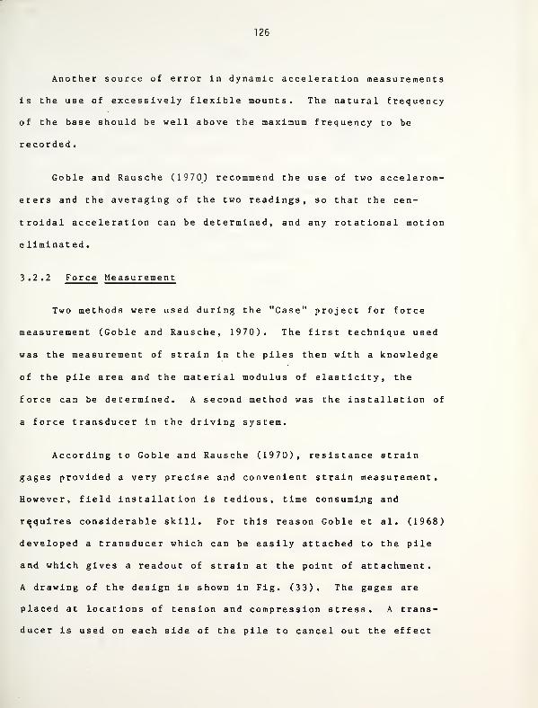
126
Another source of error in dynamic acceleration measurements
is the use of excessively flexible mounts. The natural frequency
of the base should be well above the maximum frequency to be
recorded
.
Goble and Rausche (1970) recommend the use of two accelerom-
eters and the averaging of the two readings, so that the cen-
troidal acceleration can be determined, and any rotational motion
e liminat ed
.
3.2.2 Force Measurement
Two methods were used during the "Case" project for force
measurement (Goble and Rausche, 1970). The first technique used
was the measurement of strain in the piles then with a knowledge
of the pile area and the material modulus of elasticity, the
force can be determined. A second method was the installation of
a force transducer in the driving system.
According to Goble and Rausche (1970), resistance strain
gages provided a very precise and convenient strain measurement.
However, field installation is tedious, time consumi.ng and
requires considerable skill. For this reason Goble et al. (1968)
developed a transducer which can be easily attached to the pile
and which gives a readout of strain at the point of attachment.
A drawing of the design is shown in Fig. (33). The gages are
placed at locations of tension and compression stress. A trans-
ducer is used on each side of the pile to cancel out the effect
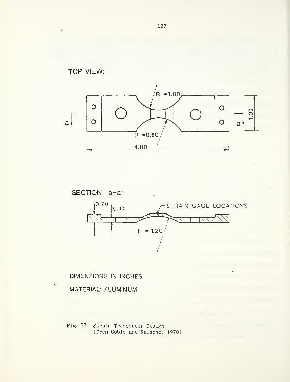
127
TOP VIEW:
at
oo
SECTION a-a:
,0.20,
J J0.10
/-STRAIN GAGE LOCATIONS
R = 1.20
DIMENSIONS IN INCHES
MATERIAL: ALUMINUM
Fig. 33 Strain Transducer Design(from Goble and Rausche, 1970
]
128
of gross bending. The gages of the two transducers are connected
so that those experiencing strains of the same direction are in
series. Thus, the two transducers form 240-ohm arms of the
bridge. The other two arms are contained in a termination box.
The transducers are bolted directly to the pile with self-tapping
bolts. They should be calibrated properly before being used.
Details of the calibration process were described by Goble and
Rausche (1970). The following observations were drawn from
experience with the device at Case Western:
1. Local wall bending is not a problem unless extremely short
lengths are used, therefore, gages on the outside are
unnecessary
.
2. As the transducer length is decreased, the number of strain
gages must be increased.
3. The latest version of the force transducer minimized any
effect on the dynamic behavior, since its elastic and
internal properties are close to those of the pile.
3.2.3 Recording Devices
Two types of instruments can be used for recording the meas-
urements, oscilloscopes and oscillographs. The oscilloscope has
the advantage of very wide ranges of speed and frequency
response. However, for a transient phenomenon it does not
display continuously, and to obtain a permanent record the scope
129
display must be photographed. For this reason it cannot be con-
sidered for any routine repetitive measurements, but it is useful
for checking other recording devices (Goble and Rausche, 1970).
On the other hand, oscillographs have been used extensively in
pile dynamic measurements. The Visicorder type has been found to
be very efficient (Rausche, 1970). Current models of this
instrument operate at speeds up to 160 inches per second. For
pile dynamic recording, 80 inches per second has been found to be
satisfactory, although the additional speed would make record
evaluation easier. Also galvanometers provide a nearly linear
output up to 8 khz, well above the range required. Acceleration
measurements have been satisfactorily recorded using 1500 khz
galvanometers, and the force signal is even less demanding. An
example of the oscillgraph record is shown in Fig. (3A). It is
possible that magnetic tape recorders may provide an even more
desirable system.
The first step in the examination of all pile dynamic data
is to check them. Goble et al., (1970) introduced a simple rela-
tion to make this check. It can be shown that there is a linear
relationship between force, F(t), and velocity, v(t), in the
early part of the record if both are measured at the same loca-
tion. This relation is given by:
F(t) - f^'v(t) (3.1)
where: E « material modulus of elasticity
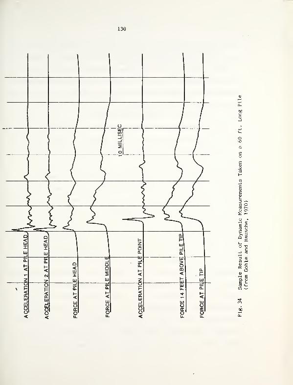
130
c<U
xCO
Eh
WJJca;
ea)L3 -—
-
w OTO r-0) crs: 1-1
u .
HE -C(D UC CO
131
A cross sectional area
c speed of the stress wave
If this relationship is not satisfied, then there are inadequa-
cies in the instrumentation system at some point.
3. 2. A Developments in Dynamic Measurements
The instrumentation system outlined above is satisfactory
for use by experienced personnel. It hardly represents, however,
an acceptable system for routine use by engineers whose primary
concerns are with other activities. To solve this problem,
effort has been made by Goble and his co-workers to design and
develop a special electronic computer and the necessary associ-
ated transducers (the Pile Analyzer). Two types of data acquisi-
tion and processing can be accomplished using this technique.
For the first system, the strain and acceleration signals, after
appropriate conditioning, are recorded on a high-speed oscillo-
graph. They can also be recorded on a four channel, portable
magnetic tape recorder (Goble et al., 1972), and then taken to
the office to be processed and analyzed (using the CAPWAP program
as will be explained later). The first system utilizes the spe-
cial purpose micro-computer. An H-beam force transducer is
inserted between the hammer and the pile top. An accele rometer
is attached to each side of, the transducer. The system is com-
pleted by the computer which provides signal condition, analog
computation, and a digital readout of pile capacity. This system
132
utilizes approximate equations to allow for monitoring the capa-
city and pile behavior in situ within reasonable time (e.g. capa-
city of the pile is displayed directly after each hammer blow).
On the other hand, for more accurate analysis, especially if the
measurements are to be used for the design of the pile foundation
rather than for checking or for quality control, the more sophis-
ticated analysis, using a main frame computer, should be applied.
For the field computer system, a sample result is shown in Fig.
(35). According to Goble et al (1970), the instrumentation is
assembled and all readings taken with only two people.
In addition to the above mentioned measurements, set-rebound
measurements are also taken for every blow as usual. In order to
monitor the hammer performance, the ram jump height may simply be
observed visually, or by using a viedo-tape camera held level
with the top of the hammer. This film is to be projected later
to obtain the necessary hammer data. Further details on the
measurement and processing equipment can be found in Likins
(1984) and Rausche (1984).
133
SdlM Nl 3QyOd
S.9 Nl NOI1VH31300V
oj-> 0)
3Q. <U4-> i-l
3 jOO OO0)ih eQ. OE S-
(TJ C-CO —

134
3.3 Estimation of the Pile CapacityUsing Dynamic Measurements
The idea of using measurements made during pile driving to
estimate pile capacity is an old one. Since pile driving causes
failure of the soil, it is logical to use measurements made dur-
ing driving to predict pile capacity. This was the basis of all
of the dynamic pile formulas that have been used for more than
100 years. Since only the simplest measurements were possible
when the formulas were developed (permanent set per hammer blow),
it was natural to use an energy approach. Unsatisfactory results
have been obtained because of the very poor representation of all
elements of the system, that was necessary in this approach.
Attempts have been made to improve these formulas, but there is
no indication that improvements have been obtained with the more
advanced formulas (Rausche et al., 1985). The results are some-
times not satisfactory due to a lack of knowledge of hammer
energy, poor estimates of losses in cushions, inaccurate set
measurements, substantial strength change after driving, assump-
tion of a resistance which is constant during the blow and other
f actors .
With the developments in electronics, it is now practical to
measure parameters other than pile set, and these measurements
have made improved analysis methods (e.g. using the wave equa-
tion) possible. By the 1930's force measurements were already
being made at the pile head during driving. Both force and
135
acceleration were measured in the driving system in an extensive
pile testing program conducted by the Michigan Highway Department
in 1961 (Michigan State Highway Commission, 1965). Beginning in
1964, a research program at Case Western Reserve University col-
lected large volumes of force and acceleration measurements on
test piles during driving or, more frequently, during restrike
(Goble et al., 1967, 1968, 1970, 1975). This project developed
means of analysis to determine wave equation soil parameters act-
ing during impact, using a program known as the CAPWAP (Case Pile
Wave Analysis Program), (Rausche and Goble, 1972). As mentioned
earlier, the CAPWAP analysis requires a substantial computational
effort and, therefore, is usually carried out in the office, with
more extensive computer hardware (Rausche et al., 1985).
Several simplified methods of analysis using closed form
solutions of the one-dimensional wave propagation theory were
also developed using empirical correlations to static pile test
results. These solutions can be obtained in real time (using a
field computer) for each hammer blow. These methods were
improved over a period of time and they have become known as the
"Case Method". A rational analysis method has been developed
using this approach (Goble et al., 1975).
3.3.1 Simplified Approach Using Field Computers
The basic equation that relates force and acceleration
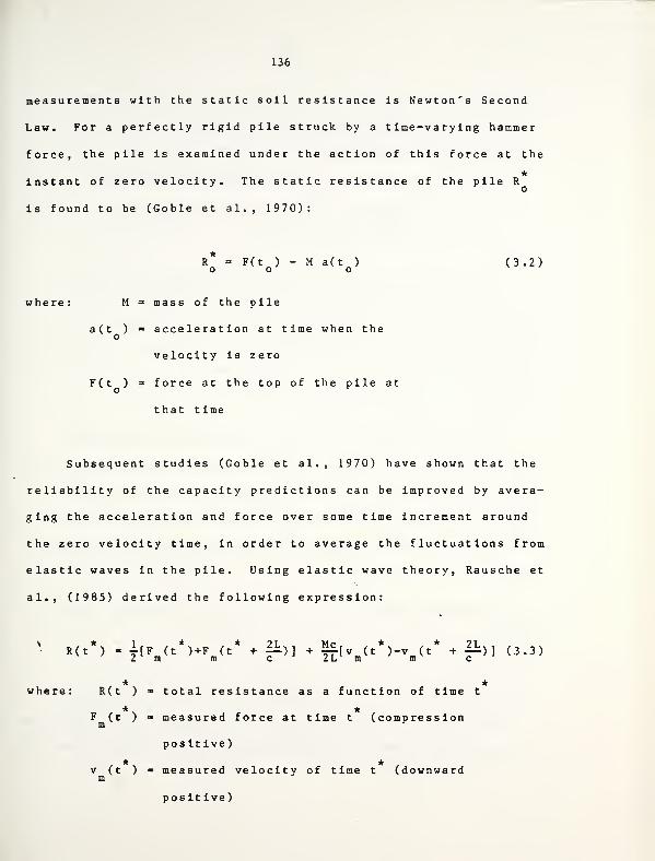
136
measurements with the static soil resistance is Newton's Second
Law. For a perfectly rigid pile struck by a time-varying hammer
force, the pile is examined under the action of this force at the
*instant of zero velocity. The static resistance of the pile R
o
is found to be (Goble et al., 1970):
R = F(t ) - M a(t )o o o
(3.2)
where: M = mass of the pile
a(t ) = acceleration at time when theo
velocity is zero
F(t ) = force at the top of the pile at
that time
Subsequent studies (Goble et al., 1970) have shown that the
reliability of the capacity predictions can be improved by avera-
ging the acceleration and force over some time increment around
the zero velocity time, in order to average the fluctuations from
elastic waves in the pile. Using elastic wave theory, Rausche et
al., (1985) derived the following expression:
\ * 1 * * ?T Mr * * 2TR(t ) = y[F (t )+F(t +7^)] + §f[v(t )-v(t + f^) ] (3.3)
2 m m c 2L m m c
* *where: R(t ) total resistance as a function of time t
* *F (t ) " measured force at time t (compressionm
positive)
* *v (t ) = measured velocity of time t (downwardm
posit ive)
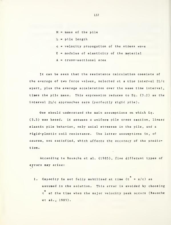
137
M = mass of the pile
L = pile length
c = velocity propagation of the stress wave
E = modulus of elasticity of the material
A = cross-sectional area
It can be seen that the resistance calculation consists of
the average of two force values, selected at a time interval 2L/c
apart, plus the average acceleration over the same time interval,
times the pile mass. This expression reduces to Eq . (3.2) as the
interval 2L/c approaches zero (perfectly rigid pile).
One should understand the main assumptions on which Eq.
(3.3) was based. It assumes a uniform pile cross section, linear
elastic pile behavior, only axial stresses in the pile, and a
rigid-plastic soil resistance. The latter assumptions is, of
course, not satisfied, which affects the accuracy of the predic-
tion.
According to Rausche et al. (1985), five different types of
errors may arise:
1. Capacity is not fully mobilized at time (t + x/c) as
assumed in the solution. This error is avoided by choosing
*t at the time when the major velocity peak occurs (Rausche
et al. , 1985) .
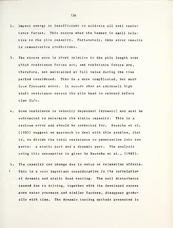
138
2. Impact energy is insufficient to activate all soil resis-
tance forces. This occurs when the hammer is small rela-
tive to the pile capacity. Fortunately, this error results
in conservative predictions.
3. The stress wave is short relative to the pile length over
which resistance forces act; and resistance forces are,
therefore, not maintained at full value during the time
period considered. This is a more complicated, but much
less frequent error. It occurs when an extremely high
shaft resistance causes the pile head to rebound before
time 2L/c.
4. Some resistance is velocity dependent (dynamic) and must be
subtracted to determine the static capacity. This is a
serious error and should be corrected for. Rausche et al.
(1985) suggest an approach to deal with this problem, that
is, to divide the total resistance to penetration into two
parts: a static part and a dynamic part. The analysis
using this assumption is given by Rausche et al., (1985).
5. The capacity can change due to setup or relaxation effects.
» This is a very important consideration in the correlation
of dynamic and static load testing. The soil disturbance
caused due to driving, together with the developed excess
pore water pressure and similar factors, disappear gradu-
ally with time. The dynamic testing methods presented in
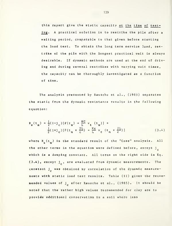
139
this report give the static capacity a_t the t ime of test-
ing. A practical solution is to restrike the pile after a
waiting period, comparable to that given before starting
the load test. To obtain the long term service load, res-
trike of the pile with the longest practical wait is always
desirable. If dynamic methods are used at the end of driv-
ing and during several restrikes with varying wait times,
the capacity can be thoroughly investigated as a function
of time
.
The analysis presented by Rausche et al. , (1985) separates
the static from the dynamic resistance results in the following
equation :
Rs(t
m>=7(1 -J
C)tF(t
m ) + F Vt
(tm )] +
l(1+j )[F(t +
|L}
. Mc+|L2c mc Ltmc (3.4)
where R (t ) is the standard result of the "Case" analysis. Alls m
the other terms in the equation were defined before, except j
which is a damping constant. All terms on the right side in Eq.
(3.4), except j , are evaluated from dynamic measurements. The
constant j was obtained by correlation of the dynamic measure-
ments with static load test results. Table (11) gives the recom-
mended values of j after Rausche et al., (1985). It should bec
noted that the rather high values recommended for clay are to
provide additional conservatism in a soil where less
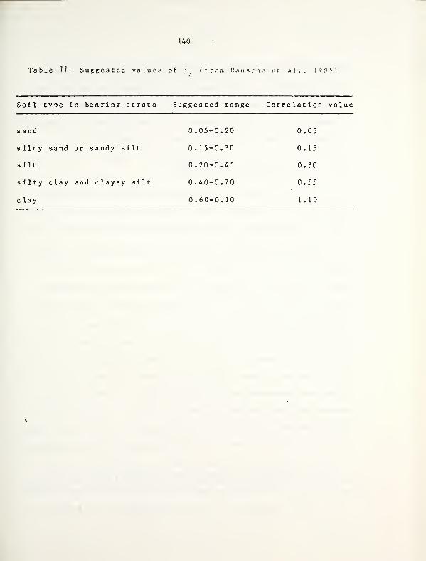
140
Table 11- Suggested values of i (froir. Rausrhp pt al , , 1 o ,<3r< >
Soil type in bearing strata Suggested range Correlation value
s and
silty sand or sandy silt
silt
silty clay and clayey silt
c lay
0.05-0.20
0.15-0.30
0.20-0.45
0.40-0.70
0.60-0.10
0.05
0.15
0.30
0.55
1. 10
141
experience was available. In general, for any type of soil,
higher values of j can be used if a conservative approach is
required by the engineer. Comparisons with other load test data
by Rausche et al., (1985) showed very good agreements between the
proposed correlations and the actual test results.
3.3.2 Office Analysis Using CAPWAP
CAPWAP analysis is a more sophisticated one, which also
utilizes the solution to the one-dimensional wave equation in an
elastic rod to determine the static bearing capacity of a pile.
In the usual dynamics problem where the external boundary
conditions are known, either force or acceleration is used as
input, and the other quantity is then calculated by a dynamic
analysis as the output. In the CAPWAP analysis, both force and
acceleration records are used as input information, and the
characteristics of the soil resistance are calculated as the out-
put, including static and dynamic values. This is done by using
one of the two records (force or acceleration) as input, and soil
resistance parameters are adjusted until the computed output
matches the other measured quantity. Since it is intended to
predict forces exerted by the soil along the pile, it is natural
to compute the force on top of the unsupported pile of length "L"
using the velocity record as an input. The difference between
measured and computed force is the force due to the soil action.
142
The CAPWAP analysis can also be used to predict the load
transfer along the pile, i.e. the distribution of shaft loads
along the pile. It can also be used to predict a load versus
deflection curve. Comparisons between predicted and measured
results from static load tests did not show a very good agree-
ment. This is primarily due to the inadequacy of the soil model
used in the analysis. This is clearly shown in Fig. (36). Table
(12) gives some data which show the difference between the pred-
iction and the actual capacities. According to Goble et al.,
(1970), the correlation between predicted and measured capacity
is better for the piles driven in coarse grained soils than those
i n clayey soils.
In order to record and store the data to be used for CAPWAP,
a magnetic tape recorder is required. It stores an electronic
image of the event measured, and should have the capability of
recreating it at a later time. This makes a fully automatic data
processing system possible. Later in the laboratory, the analog
tape recorder can be converted to digital form, some simple com-
putations can be made on the digital data during the conversion
operation, the data can be stored on digital magnetic tape for
later conversion, and a plotted record can be obtained on a com-
puter controlled plotter.
After acquiring experience in dynamic measurements, the
engineer would be able to reach some interesting conclusions just
by looking at the measurement output. For example, Fig.
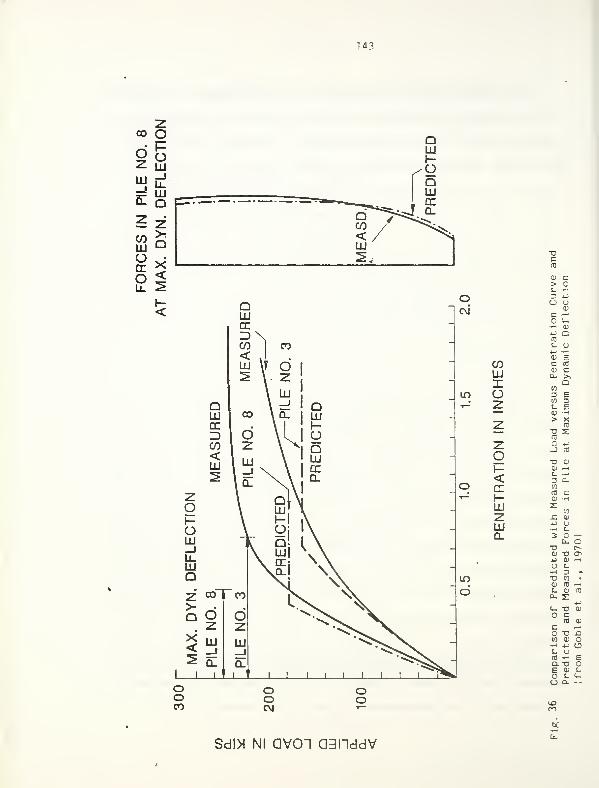
1*3
•octo
0) c> ct_ —
1
o a4J
cvi ca>
t--tH <D*J C<0
£- u4J •^*
<D E(f> C to
LU0) c
>>
inIo to
3
QE
2 to 3E—
0)
2 > Xto
X3to
s:
2o
oto
50)
3
(—
1
a.oi-
10to
a> *-<
UJ sto2 £ <d
LU4-> u
Q_ 3 c —T3 f-a; O CTv
*} tu —
i
u S-•^H 3 -
in •o to •
0) to —
«
d c.a.
QJ CO
u- TJ 4)
o Cto a>
c i—
<
o D .Oto a> o^1 ti ob uto "H EQ.TJ CB d) £-
O J- Cc_> Ou ~-
Sd!* Nl QVOl Q3HddV
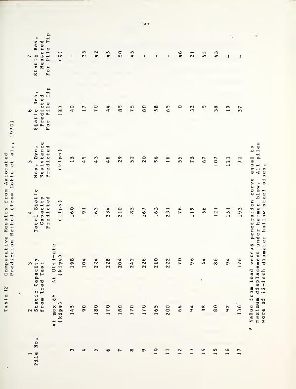
T"
CO "O H0) <u
at u uJ H *"»
f» O CO -H »•«
«H CO 0- w
(BTJ H01 OJ
OS i-i 0)
y ^h
T-4 "Q 0-1
4-1 01
10 S-i u
ihS -tf »H
• U -c
c c OJ
< CO 4J
o 4-1 o01 1H
• TH •a
X CO
to 0) uT. OS 0-
l-~ —I
H ^ ~J
4-1 ^ "O10 4_| 0) /-N
4-1 •rH 4-1 01
tn O O a. o «—
1
tO 1-1 H \C <^>—l a T3 ^ —
1
03 (0 01 ^^4-1 U l-i
o 0-
H
© u"l 1^—
I 0C vOCM -* —
i
vO —'
—
e #*s
>v •H CO 00 <• -*CI 4J 4-> 4-1 0. CX o CM
•H CO i-l H ~H ~H CMu 0) 33 -*CO H %-•
a 4J
« o <© CO
oy JH *4-1 E T3CO O ^v4-1 l-i X CO in o O
CM 1/3 W-l a 0. ««r a\ ooE •H *~* —
<
t- 33 O i—
U H OJ
XI 0)
c 4-1
u 00
*H <D
4-1 E 3CO Eu CO H<J x —
4
01 cc u Xai 01
a. "o uc OJ
CD 3 -
3 0)
00 4-1 E>* C CO
01 0) >rt
> E0)
ac U XCO CO u
1—
I
cH a
to
TH
1
E i-i CMO "O —
«
l-i
IM E 14H
30) E3 H 0)
—4 X uCO CO 01
> E 3
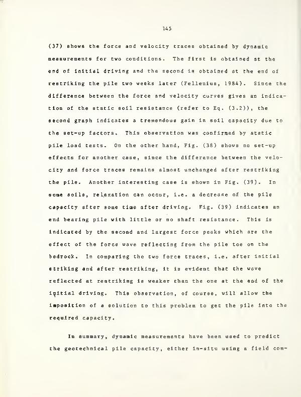
145
(37) shows the force and velocity traces obtained by dynamic
measurements for two conditions. The first is obtained at the
end of initial driving and the second is obtained at the end of
restriking the pile two weeks later (Fellenius, 1984). Since the
difference between the force and velocity curves gives an indica-
tion of the static soil resistance (refer to Eq . (3.2)), the
second graph indicates a tremendous gain in soil capacity due to
the set-up factors. This observation was confirmed by static
pile load tests. On the other hand, Fig. (38) shows no set-up
effects for another case, since the difference between the velo-
city and force traces remains almost unchanged after restriking
the pile. Another interesting case is shown in Fig. (39). In
some soils, relaxation can occur, i.e. a decrease of the pile
capacity after some time after driving. Fig. (39) indicates an
end bearing pile with little or no shaft resistance. This is
indicated by the second and largest force peaks which are the
effect of the force wave reflecting from the pile toe on the
bedrock. In comparing the two force traces, i.e. after initial
striking and after restriking, it is evident that the wave
reflected at restriking is weaker than the one at the end of the
initial driving. This observation, of course, will allow the
imposition of a solution to this problem to get the pile into the
required capacity.
In summary, dynamic measurements have been used to predict
the geotechnical pile capacity, either in-situ using a field com-
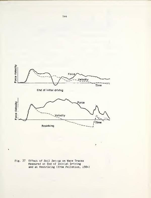
146
Time
End of initial driving
Restriking
/JTime
Fig. 37 Effect of Soil Set-up on Wave TracesMeasured at End of Initial Drivingand at Restriking (from Fellenius, 1984!
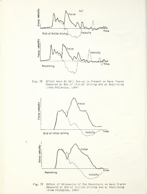
End of initial driving-^ /VelocityTime
oo
><x>
oou.
1 yForce
M \ aJ
^Velocity
vA * i o »
Restriking
\
I
V
1
-N\
| V Time
Fig. 38 Effect When No Soil Set-up is Present on Wave TracesMeasured at End of Initial Driving and at Restriking(from Fellenius, 1984)
iForce
> /"~"/"^v 'J
d> / \ 1
Ut-o / *
LL\ \X \
\\
End of initial driving Velocity- Time
RestrikingTime
Fig. 39 Effect of Relaxation of Toe Resistance on Wave TracesMeasured at End of Initial Driving and at Restriking(from Fellehius, 1984)
f
148
puter, or In the office using a more sophisticated analysis
(CAPWAP). The latter analysis can also be used to predict the
load transfer along the pile shaft and the load-deformation curve
that would be obtained from a pile load test. Experience,
however, indicated only a moderate success in these two predic-
tions. This is primarily due to the lack of a good soil model.
Also the predicted capacity should not be directly used in the
design without verification using other techniques like dynamic
formulas, reliable static formulas or pile load tests. The
measurements have been very successful in calculating the wave
equation parameters and detecting certain phenomena after
driving, e.g. soil set-up or soil relaxation. Therefore, using
the measurements with the wave equation analysis is much better
than just using the wave equation with the arbitrary assumption
of parameters which may not be close enough to reality.
149
3.4 Evaluation of the Performance of PileDriving Systems Using Dynamic Measurements
The understanding of pile driving and pile driving hammers
is difficult. First because of the interaction of many com-
ponents such as ram, impact block, cushion assembly, pile and
soil, and second because of the very short duration of the total
impact phenomenon. Also, a wide variety of hammers is commerci-
ally available and the performance and characteristics of each of
them are quite different. Experience and engineering judgment
have been the best tools to evaluate this problem. However,
problems such as pile overdriving or damage frequently occur and
unnecessary blow count requirements lead to losses of time and
money.
To better understand this situation, force and acceleration
measurements have been used, by means of simple theoretical
models, for a meaningful evaluation of quantities such as energy
transfer and forces in hammer components.
Dynamic measurements, although originally meant for pile
capacity prediction, do provide useful data for the computation
of energy delivered by the driving system to the pile. Of parti-
cular interest is the aspect of hammer performance for an open-
end diesel hammer, since widely differing views are held of its
operating characteristics (Goble et al., 1972).
In order to do that, the ram stroke, force, acceleration and
displacement are recorded simultaneously as described before.
150
The video tape records are processed manually to obtain the ram
stroke for each blow. The automatic data processing system is
used to calculate the delivered energy. The processing system
operates as follows: the measured analog strain record is con-
verted to digital form and then to force. The two acceleration
records (from the two acceleromet ers ) are digitized at the same
time and averaged to obtain a single signal. The digital
acceleration and force records for each blow are stored on digi-
tal magnetic tape for later processing. Calculation of energy is
accomplished by integrating the averaged acceleration, once to
obtain velocity, and a second time to obtain displacement. The
final displacement is automatically checked with the measured
set, and if a difference is observed, the acceleration zero is
adjusted to correct the final displacement. Also, the first
velocity peak is checked for proportionality with the first force
peak. If this proportionality is seriously violated, the results
from that specific blow are ignored. It should be noted that the
peak accelerations measured at impact are usually extremely high,
in some cases over 500 g's, where g is the acceleration of grav-
ity (Goble et al. 1972).
Energy is calculated from the following expression:
E(t ) - / F(t) v(t) dt1
(3.5)

151
where E is the energy at the pile top expressed as a function of
time, and other quantities have been previously defined. Zero
time is taken as some time before the beginning of the blow.
Thus, an energy-time record can be obtained which can be automat-
ically plotted. Typical plots of such relations are shown in
Fig. (40), together with force, velocity and displacement curves.
To demonstrate differences caused by resistance changes, plots of
both an early and a late blow are shown. It is important to note
that in the early blow the maximum value of energy transfer is
reached at a later time after impact and no energy is transferred
back to the hammer (the curve stays horizontal). In the later
blow a peak value is reached after which the energy curve
decreases, indicating that some energy is returned to the hammer.
Comparison with the manufacturers rated value evaluates the ham-
mer performance.
It should be noted that the energy considered is the value
of the energy that was actually transferred from the ram to the
pile during the blow. Obviously, the total energy transferred is
the final value, i.e. a value at a time when the energy curve
stays constant. For constant fuel injection with the same
cumbustion efficiency and with the same hammer losses, this value
should be constant, or, in case not all of these restrictions are
valid, it should be at least independent of the ram stroke (Goble
et al., 1972). Results shown in that reference indicate that
there is only a 3 percent chance that the ram stroke and energy
are related (for the open-end diesel hammer). Rausche and Goble
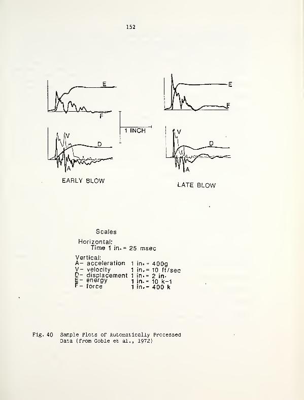
152
EARLY BLOWLATE BLOW
Scales
Horizontal:Time 1 in.= 25 msec
Vertical:A- acceleration 1 in. = 400gV- velocity 1 in.= 10 ft/secD- displacement 1 in.= 2 in.E- energy -|
j n.= 10 k-1r- force 1 in.= 400 k
Fig. 40 Sample Plots of Automatically ProcessedData (from Goble et al., 1972)
153
(1972), based on actual measurements, showed that the driving
ability of a hammer depends on the impact velocity at the pile
top and the pile cross sectional area. The velocity at the pile
depends on the cushion, energy losses in the hammer, the ratio of
ram mass to anvil plus cap mass and in the case of diesel ham-
mers, on the hammer combustion chamber pressure before impact.
The engineer, however, should be cautious when dealing with the
driving process since large portions of the hammer energy can be
stored in the pile and the driving system without producing pile
penetrations. Applications of energy formula, therefore, have to
be considered skeptically even if the exact hammer energy is
known (Rausche and Goble, 1972).
Before dynamic measurements, the criterion for controlling
tension stresses in piles during driving was based on the pile-
ram weight ratios. Measurements showed that this criterion is
quite unsatisfactory when applied to diesel hammers (Goble et
al. , 1976). In that study, the highest measured tension stresses
were generated by the heaviest ram (the opposite could have been
predicted based on the pile-ram weight ratio). Therefore, if
current pile-ram weight ratios are used for selecting driving
equipment, damage problems will be more frequent and severe.
Dynamic measurements also showed that the diesel hammers are less
likely to damage concrete piles by the induced tension forces due
to their low velocity in easy driving.

154
Dynamic measurements can also be used to evaluate the effi-
ciencies of different operating pressures, strokes or batters, or
changes in hammer maintenance conditions by comparative testing
of hammers of one type or of a single hammer over an extended
period of use. Relative efficiencies of different hammer types
can also be evaluated. They are also useful in examining any
preignition problems with diesel hammers. Also if some unex-
plained blow count is recorded, possible changes in hammer per-
formance can be detected. All of the above uses are possible via
the hammer energy output measurement described before.
Furthermore, the driving system as a whole can be checked by
the dynamic measurements, i.e. the cushions, cap blocks, ...,
etc. It is well known that one of the major advantages of the
wave equation analysis is the representation of the elements of
the driving system. The characteristics of these elements,
however, may change as driving proceeds. The dynamic
measurements are very efficient in checking the effects of
changes in cushion properties or helmet assembly by their effect
on transmitted energy and forces in the pile.
155
3.5 Evaluation of the Pile PerformanceUsing Dynaml c Measurements
Dynamic measurements have proven to be very useful In
evaluating the pile performance after driving. In this aspect,
three main characteristics can be checked using the measurements,
namely the driving stresses at the measuring location, the total
length for existing piles where the lengths are unknown and the
extent and location of pile structural damage.
Since the force is measured directly at the pile top,
stresses can be obtained and checked very easily, i.e. excessive
compressive stresses that may exceed the material capacity or
excessive tensile stresses that may cause severe tension crack-
ing. Using the wave equation analysis with the measurements per-
mits the evaluation of stresses along the whole pile shaft.
Various hammers, cushions, cap blocks, ..., etc. can be used and
checked with the measurements to minimize the undesired excessive
stresses. Fig. (41) shows a typical trace of compressive and
tensile stresses in the pile, related to the cumulative blow num-
ber, which can be obtained from dynamic measurement.
Sometimes the actual pile length is not known for some
reason, and it may not be known whether the pile is supported at
the required depth or not. Dynamic measurements can be used to
determine the pile length (L) . The process is illustrated in
Fig. (42). Suppose that the velocity record of a friction pile
is as shown. If the time between two successive peaks is
156
TEST PILE N0.3
DELMAG D-12 HAMMER
SET 1 2 3 4 5 6 7 8 9 10 11I
122.0-
co
¥ 1.6-
C/1 . rAnS\AA'^
\y\yV v i ^A"V
CO s\<\r TOP CLU ^EC 1.0, .it t
CO ,*\ „. .V \*.*
_ ^
0.5-'l
I
"'\y,MID - LENGTH TENSION
I
STRESS | |
200 400 600 800 1000 1200
CUMULATIVE BLOW NUMBER
Fig. 41 Maximum Stresses for a Test Driven Pile(from Goble et al., 1976)
157
L = tc
2ooCD
>t = 2L/C
Time
Fig. 42 Determination of Pile Length from a VelocityGraph for a Friction Pile *
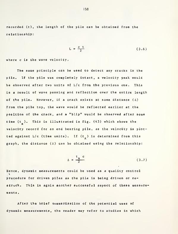
158
recorded (t), the length of the pile can be obtained from the
relationship:
c t
2(3.6)
where c is the wave velocity.
The same principle can be used to detect any cracks in the
pile. If the pile was completely intact, a velocity peak would
be observed after two units of L/c from the previous one. This
is a result of wave passing and reflection over the entire length
of the pile. However, if a crack exists at some distance (A)
from the pile top, the wave would be reflected earlier at the
position of the crack, and a "blip" would be observed after some
time (t ). This is illustrated in Fig. (43) which shows thex
velocity record for an end bearing pile, as the velocity is plot-
ted against L/c (time units). If (t ) is determined from thisx
graph, the distance (A) can be obtained using the relationship:
t cx
(3.7)
Hence, dynamic measurements could be used as a quality control
procedure for driven piles as the pile is being driven or re-
struck. This is again another successful aspect of these measure'
ments .
After the brief summarization of the potential uses of
dynamic measurements, the reader may refer to studies in which
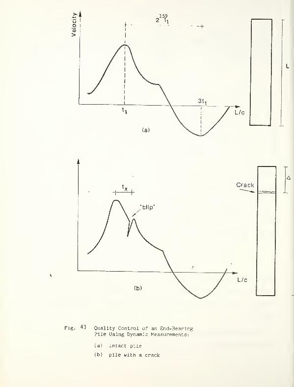
L/c
Crack
L/c
Fig. 43 Quality Control of an End-BearingPile Using Dynamic Measurements:
(a) intact pile
(b) pile with a crack
160
these measurements were applied successfully (e.g. Goble et al.,
1972; Fellenius, 1984; Baker et al., 1984; ..., etc.). One of
the projects in which the dynamic measurements were applied suc-
cessfully is the 1980 Indiana Toll Road improvements project.
Applications that have been discussed in this report were used
for many piles. For example, the piles PB-3j, PB-2B, PB-2I
(ATEC, 1982), and the piles C-2, B-7 (ATEC, 1983) were tested
during Initial driving and during restriking to estimate their
capacities and the induced driving stresses, to determine that
the piles were not damaged. The performance and efficiency of
the hammer used for driving the piles were monitored and
evaluated (ATEC, 1983). All these applications have been suc-
cessful, and have resulted in better design and driving criteria
161
3 . 6 Conclusions and Recommendations
Dynamic measurement techniques are the best ones introduced
thus far for monitoring the pile during driving. They can be
applied, together with the wave equation analysis, in a variety
of aspects. Among their uses are the prediction of pile capacity
and load transfer; the evaluation of the driving system with
respect to the hammer efficiency and performance, cushions, cap
blocks, etc.; the measurement of the pile stresses; and the qual-
ity control of the piles. Prediction of pile capacity by this
technique is of course much better than the driving formulas
(e.g. ENR, Hiley, etc.). On the other hand it is not accurate
enough to be used alone without other techniques of pile design.
This is primarily due to the insufficiency of the soil model
used. The prediction by this technique, however, completes a
spectrum of approaches for pile design, and gives more confidence
in the other procedures, since it is based on direct measurements
during the driving process. On the other hand, dynamic measure-
ments have proven to be quite successful in determining the wave
equation parameters, measuring the actual energy delivered to the
pile, monitoring the driving process with all its elements,
measuring the pile stresses and performing quality control pro-
cedures .
One of the purposes of this report was to introduce the sub-
ject of dynamic measurements to the 1D0H in an easy-to-follow
manner. Some of the complicated mathematical derivations and
162
expressions were omitted to help simplify the subject. The main
purpose was to show the potential uses of these measurements and
to illustrate selected theoretical background points which are
associated with the subject.
As was shown in this report, dynamic measurements have pro-
ven to be very useful in many aspects. Hence, it is recommended
that the IDOH use them in the operations involving pile driving.
This can be achieved through two steps:
1. In the beginning, they can be used with the help of con-
sulting expertise for selected important jobs. In the
meantime, personnel can be trained to be familiar with the
technique and eventually use it with no consulting help.
After the personnel have been well trained, the IDOH can
purchase the equipment, the price of which is decreasing,
and use it for most of its jobs, or even offer consulting
on its use for any interested potential user. The savings
that can be achieved from the various jobs would very soon
cover the price of the equipment. More importantly will be
the improvement in design and execution procedures of pile
foundations, which will not only produce savings on the
short term, but will also reduce maintenance and replace-
ment costs in the long run.
163
A list of the required equipment, with all the options,
along with the prices given by Pile Dynamics, Inc. are given in
Table (13). For further information, the reader may refer to
Pile Dynamics, Inc., 4535 Emery Industrial Parkwa, Cleveland,
Ohio 44128. It should be noted that the average dynamic test
takes about 20 min. including the preparation of the pile for
testing and attaching the necessary instrumentation. In this
case, if all the equipment and the personnel are available, the
test cost/pile would be in the order of $200.00 (according to
Pile Dynamics, Inc.). This does not include performing the
CAPWAP office analysis.
Regarding the personnel required for this procedure, two
people can take care of performing the test. One of them is an
engineer who takes care of the data acquisition system and the
readout of the pile capacity. The other one is a technician who
is responsible for fixing the instruments to the pile and other
relevant technical details. According to Pile Dynamics, Inc.,
the use of the latest simplified equipment (refer to item 3.2.4)
does not require a lot of training. The average engineer or
technician could be easily trained to perform the job satisfac-
torily.
It should be noted that the described dynamic testing is not
a substitute for the classical static load test, which gives a
most realistic indication to the static pile capacity. As stated
earlier, the pile capacity estimated from dynamic measurements
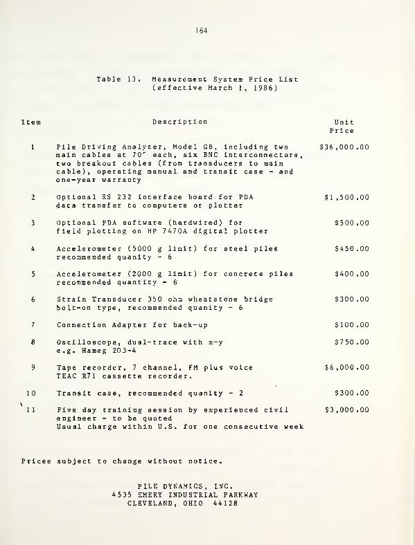
164
Table 13. Measurement System Price List(effective March 1, 1986)
Item Description UnitPrice
1 Pile Driving Analyzer, Model GB, including two $36,000.00main cables at 70' each, six BNC interconnect ors
,
two breakout cables (from transducers to maincable), operating manual and transit case - andone-year warranty
2 Optional RS 232 interface board for PDA $1,500.00data transfer to computers or plotter
3 Optional PDA software (hardwired) for $500.00field plotting on HP 7470A digital plotter
4 Accelerometer (5000 g limit) for steel piles $450.00recommended quanity - 6
5 Accelerometer (2000 g limit) for concrete piles $400.00recommended quantity - 6"
6 Strain Transducer 350 ohm wheatstone bridge $300.00bolt-on type, recommended quanity - 6
7 Connection Adapter for back-up $100.00
8 Oscilloscope, dual-trace with x-y $750.00e.g. Hameg 203-4
9 Tape recorder, 7 channel, FM plus voice $6,000.00TEAC R7 1 cassette recorder.
10 Transit case, recommended quanity - 2 $300.00
>
11 Five day training session by experienced civil $3,000.00engineer - to be quotedUsual charge within U.S. for one consecutive week
Prices subject to change without notice.
PILE DYNAMICS, INC.4535 EMERY INDUSTRIAL PARKWAY
CLEVELAND, OHIO 44128
165
still has the limitation of the inadequacy of the soil model used
in the analysis. More research is still needed to introduce more
realistic soil models into the wave equation analysis to get
better predictions of the pile capacity. Nevertheless, dynamic
measurements have the advantage of being cheaper and faster and
they also allow the engineer to check a larger number of piles in
one site. The best technique would be to perform a static load
test and correlate its results with the dynamic predictions, and
then use this correlation to examine a larger number of piles
using the dynamic measurements.
166
CHAPTER 4
RESIDUAL STRESSES DUE TO PILE DRIVING
4 . 1 General
A very important phenomenon related to pile-soil interaction
is the existence of residual stresses for driven piles after
driving. The discussion of this phenomenon in the literature has
started relatively recently. The first paper that described
residual stresses effects and presented approximate techniques
for their evaluation was published by Hunter and Davisson (1969)
using data from pile tests performed at Lock and Dam No. 4,
Arkansas River Project. Since then, detailed studies of load
transfer from load tests have indicated the presence and effect
of residual loads after driving. The first study that used
direct measurements for residual stresses was published by Gre-
gersen et al. , (1973).
The generation of residual loads is a function of the load-
unload mechanisms of pile installation. During the pile's down-
ward movement, the pile-soil friction is acting upward on the
pile to resist the pile penetration. The soil point resistance
is also acting upward. During the rebound that follows, the soil
under the point pushes the pile upwards while the pile tends to
return to its initial length elastically. The two components of
the rebound create enough upward movement to reverse the direc-
tion of the pile-soil friction, which then acts downward, at
167
least in the upper portion of the pile. This negative friction
is counterbalanced by residual skin friction in the lower portion
of the shaft and also, if the applied compressive load was high
enough, by residual point load on the pile. Equilibrium is
reached when enough of the friction stresses have reversed them-
selves in order to keep the bottom of the pile stressed against
the soil (Vesic, 1977; Briaud et al. , 1983).
Because the impact driving process consists of periodical
loading and unloading of pile head by dynamic impulses, driven
piles usually contain substantial residual loads, the existence
of which has an effect on load-settlement response of the pile.
More careful interpretation of pile load test results may be
needed to avoid undue conservatism in pile foundation design,
especially for piles in cohesionless soils. Since the ordinary
limit equilibrium analyses of bearing capacity do not account for
the existence of residual stresses, using the resulting static
formulas alone, neglecting these stresses, may have serious
design implications. Another effect of neglecting residual
stresses is the incorrect prediction of pile drivability and blow
counts. This may result in important installation difficulties
which should be otherwise anticipated (Briaud and Tucker, 1984-
a).
A qualitative representation of the difference between
"true" loads (including the effect of residual stresses) and
measured loads in conventional load tests is given in Fig. (44).
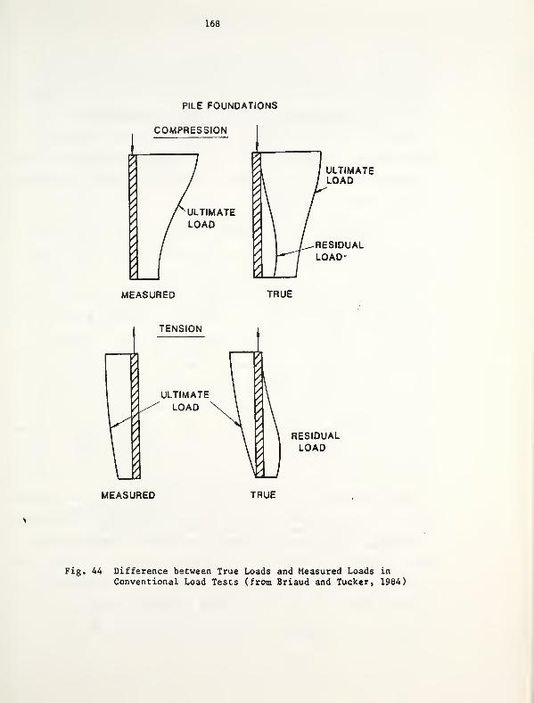
168
PILE FOUNDATIONS
COMPRESSION
ULTIMATELOAD
RESIDUALLOAD-
MEASURED TRUE
TENSION
RESIDUALLOAD
MEASURED TRUE
Fig. 44 Difference between True Loads and Measured Loads in
Conventional Load Tests (from Briaud and Tucker, 1984)
169
Also, Fig. (44) indicates that the presence of residual loads
causes an apparent concentration of skin friction in the upper
part of the shaft, if the pile is loaded in compression. Con-
versely, for piles loaded in tension, after being loaded in
compression or immediately after driving, the apparent load dis-
tribution shows a tensile load at the pile tip equal in magnitude
to the residual point load.
A simple illustration of the effect of residual stresses on
the distribution of unit skin friction and load transfer along
the pile shaft is given in Fig. (45) (Holloway et al., 1975).
If, for simplicity, the distribution of unit skin friction along
the pile shaft is assumed to be linear, as predicted by static
formulas, without any consideration of arching or crushing of
particles below tip, the resulting curves are denoted by 1 and 2
for compression and tension, respectively. The corresponding
load transfer (Q vs. depth) can be obtained from the fact that
its slope is proportional to unit skin friction distribution, as
explained earlier in the discussions. The actual load transfer,
as observed in most load tests performed for piles driven into
cohesionless soils, is indicated by curves 1M and 2M for compres-
sion and tension tests, respectively (provided that instrumenta-
tion was zeroed after installation and prior to the load test).
The differences between the two sets of curves (1, 2 and 1M, 2M)
give the assumed distribution of residual loads along the pile
shaft (curves and 0'). The above discussion illus-
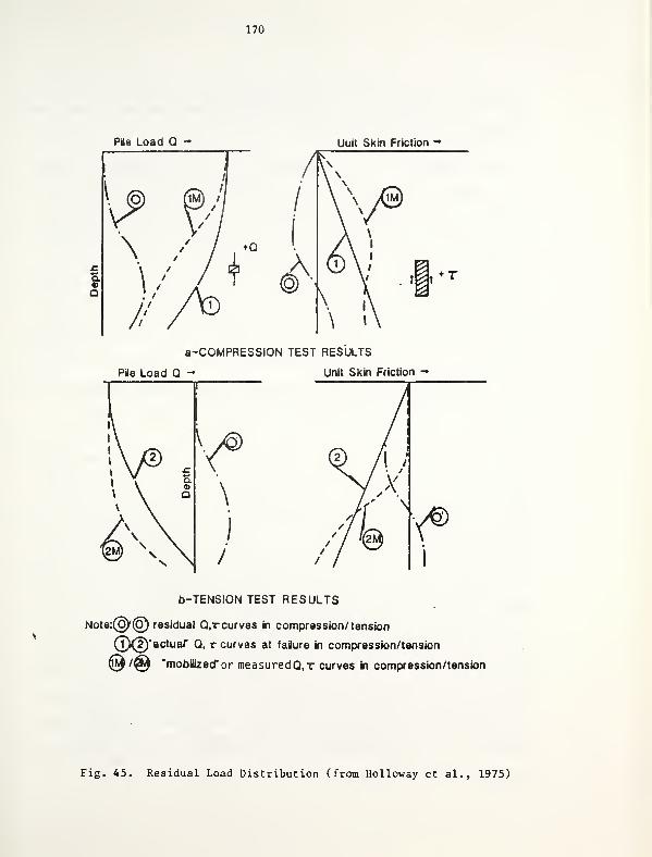
170
Pile Load Q - Uuit Skin Friction -
a-COMPRESSION TEST RESULTS
Pile Load Q - Unit Skin Friction -•
1
1
k1 \ ©\ \ Q
y©\
/-^ \ \© \ \ j
/
b-TENSION TEST RESULTS
Note:^(6) residual Q,t curves in compression/ tension
(?)(2)*actuar Q, t curves at failure in compression/tension
@ /@ "mobilized'or measuredQ.r curves in compression/tension
Fig. 45. Residual Load Distribution (from Holloway et al., 1975)
171
trates one explanation for the observed distribution of unit skin
friction in pile load tests.
It should be noted that the total loads transferred by the
pile are the same whether residual stresses are considered or
not, since the pile is in equilibrium after driving and before
loading (i.e. the summation of shaft and tip residual loads
should be zero). However, the load test data can not be extrapo-
lated to other pile lengths if the actual load transfer is not
known. Also there are many other reasons for the accurate deter-
mination of load transfer (Leonards, 1985). Therefore, it is of
vital importance to determine the residual stresses, which is the
only way to get a correct load transfer for driven piles.
Another very important effect of the residual stresses is
that they may result in a substantial reduction in pile settle-
ment. This is due to the concentration of skin resistance in the
upper portion of the shaft (Vesic, 1978). Approximate analysis
performed by Vesic, which incorporated the residual stress effect
for two major projects which involved driven piles for the foun-
dation, led to settlements prediction in the order of 1/6 - 1/4
of the predicted settlements neglecting the residual stresses.
Load tests fully confirmed this assumption. It should be noted,
however, that although the single pile settlement decreases due
to considering the residual stresses, the group settlement ratio
(which is the ratio between the settlement of the pile group and
a single pile) increases as the load carried by friction
172
increases (Leonards, 1972). This might lead to an increase of
the pile group settlement. These examples indicate clearly the
importance of introducing the residual loads in the prediction of
single pile and pile group settlements. They also demonstrate
the doubtful value of numerous theories of pile settlement
behavior published in the literature in recent years, which do
not consider this phenomenon at all (Vesic, 1978). It seems
necessary to either modify these theories to incorporate the
residual stress effect, or to develop new techniques on a sound
theoretical basis, rather than applying simplified or empirical
app roaches
.
4.2 Current Methods Used for Residual Stress Measurement
Four major techniques have been used to obtain the residual
pile loads from load test data:
The direct way to get residual stresses is to instrument
the pile and to zero the instrumentation before driving
(Gregersen et al. , 1973). In this case, the instrumenta-
tion would be of the strain gage type. Load cells could
also be placed under the pile tip for direct measurements
of the residual point pressure (e.g. see Gurtowski and Wu
,
1984). However, there is a major doubt as to the effect of
driving on the sensitivity of the strain gages. The read-
ings after driving may be of no meaning due to this effect.
Reliable instruments need to be developed to correctly
173
measure the initial pile stresses prior to load testing,
without being affected by the installation procedure. This
technique has been used successfully for tests on model
piles driven into cohesionless soil to obtain the "true"
load transfer (Yazdanbod et al., 1984).
Hunter and Davisson (1969) used a certain testing sequence
in order to determine the residual loads. The pile is
driven and the instrumentation is zeroed afterwards. Next,
the pile is loaded in compression to failure and then
unloaded. After the gages are read, they are zeroed again.
The final step is to load the pile in tension up to failure
and to unload it. To illustrate the reasoning behind this
technique, Fig. (46) is introduced. Curves (1) and (3)
represent the measured ultimate compression or tension load
distribution assuming no stresses in the pile at the start
of the test. Curves (2) and (4) represent the residual
load in the pile after full release of compression or ten-
sion load due to these loads, plus the original residual
loads due to driving. If it is as sumed that tension load-
ing results in no residual loads , then curve 4 represents
the residual compressive loads due to both driving and
compression testing. Therefore, the adjusted (true) ten-
sion load distribution is given by curve 5, which is the
difference between curves 3 and 4. If curve 2 is sub-
tracted from curve 4, the result would be curve 6, which
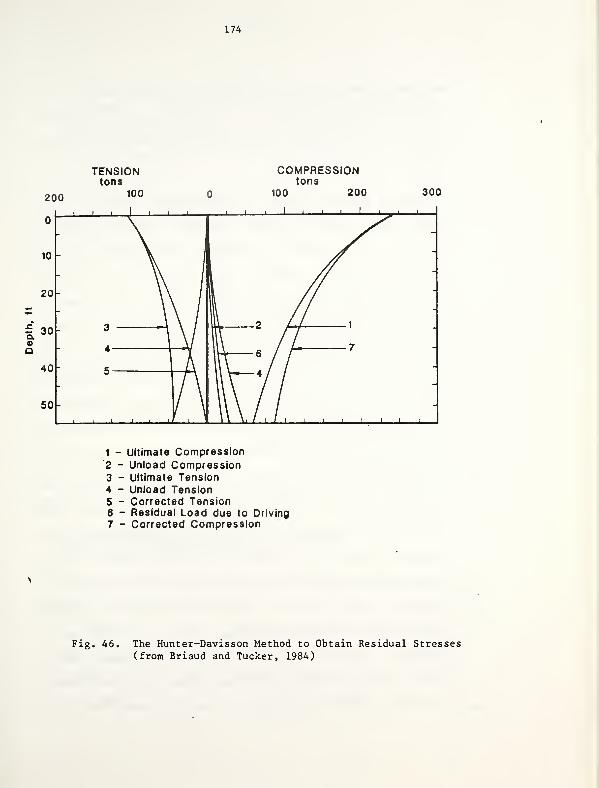
174
200
TENSIONtons
100
COMPRESSIONtons
100 200 300
. , , I , , , i , i i
-
10\ A -
\\ in-
20 \\ /
-
c; \ \ /-
-ILL 2 /ml 1
7 -
£ 30m
™"\
In
—
6 / /Q l ~K
40 c / \-
1\ V*— */ /-
50
, ,i .,1i
\ \ \i / i / i., j i i l J i-
1 - Ultimate Compression2 - Unload Compression3 - Ultimate Tension4 - Unload Tension5 - Corrected Tension6 - Residual Load due to Driving
7 - Corrected Compression
Fig. 46. The Hunter-Davis son Method to Obtain Residual Stresses(from Briaud and Tucker, 1984)
175
represents the residual loads due to driving only. If
curve 6 is added to curve 1, the result would be curve 7,
which is the adjusted (true) load distribution in compres-
s ion .
3. The third method is used if instrumentation was not read
after compression and tension loading (Briaud and Tucker,
1984-a). This means that curves 2 and 4 shown on Fig. (46)
are not available. Hence, it is assumed that no residual
stresses result from compression loading of the pile.
Therefore, the tip load measured in tension is assumed to
be the residual driving tip load, and the residual load
distribution is assumed to be linear from zero at the pile
top to the residual tip load. Obviously the assumption of
this method is not correct and leads to further errors in
using the Hunter and Davisson method.
4. The least reliable method is based on an assumption that
the side friction is the same in tension as in compression.
This is done if only the butt and tip displacements are
measured without instrumenting the whole shaft. In this
case a tension test subsequent to the compression test is
necessary. The tip load is thus the difference between
compression and tension loading results. In this way,
nothing is known about residual stresses although the
"true" load transfer is obtained (since it is included in
both the tension and compression results assuming they are
176
the same). Obviously all the assumptions related to this
approach are incorrect. In addition to the previously
stated assumptions, it was demonstrated earlier that assum-
ing the same friction in tension as in compression is
incorrect. Therefore, it is impossible to get at least an
approximate distribution of the residual loads without
instrumenting the pile.
The demonstration of the available four methods that have
been used to measure residual stresses indicate that none of them
can be used to get the exact or true load transfer, that includes
the residual stress effect. A possible alternative is to get the
residual point load, which can be obtained fairly accurately as
explained earlier using a load cell at the tip or using a pulling
test after the compression test, then to try to get the residual
friction loads that balance the residual tip load, and assume a
reasonable distribution for these loads.
4.3 Review of Research on Residual Stressesfor Piles in Cohesionless Soils
Little research has been done on residual stresses and their
effect on the pile-soil interaction quantitatively. Hunter and
Davisson (1969) used their suggested procedure for evaluating the
residual loads to obtain the adjusted (true) tip and friction
ultimate loads for compression and tension load tests. Table
(14) gives a summarization of the adjusted values and the percen-
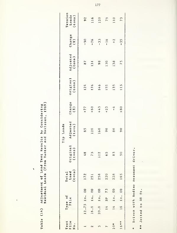
177
co co '-v
H T3 CO
to to cCOO
to ^e
to c3 O
OCCTNC MDW ON(-1 -H
V73 «
•H CCO Oc en
O to
a -h
>>* to
£> OCO "Cu CiH CO
3CO t-i
ai ai
on 4-1
c4-» 3CO Xat
H BO
•O »-
tO >4H
O "sJ
CO
U-l T3
CO
O4J Jc01 t-H
s to
4J 3CO "O
3 T<1—1 CO
•a oi
< «*
CO *-s
C CO
tH C60 O
0)
00C ^vto »•«
u
T5 4J CO
CO y^c CO
H BM-H 4-1
t-i -^^
o
iH "0 CO
a co c4J O OO iJ 4J
O 01
01 -Ha. ex
0) -H OH a, 2
—i COen as
r-~ -h
Q O OO O O
o oo mCM CM \0CM CM -h
a ao o
c c c ouH -H -H «
CM vO O—I —
<
CM
178
tage change in tip and friction loads after considering the resi-
dual loads. A large scatter is easily observed for these percen-
tages, especially for the change in tip load. It is interesting
to notice that using a vibratory hammer resulted in almost no
residual loads (as also observed by Mansur and Hunter, 1970; Hol-
loway et al., 1975). This is to be expected, since resonant pile
driving temporarily displaces the soil, and penetration of the
pile is achieved under the static weight of the pile and hammer.
The vibratory driver causes penetration by transmission of high
frequency, low amplitude longitudinal stress waves in "resonance"
with the pile-soil system. Analysis of more test data made by
Briaud and Tucker (1984-a) indicated that, on the average, the
residual point load was about 56% of the "true" ultimate point
load, while the residual friction load was about 19% of the
"true" ultimate friction load. A thorough examination of these
data, however, indicates a very large scatter in the results, so
that the average figures introduced poorly represent the data
base
.
Holloway, et al. (1975), based on theoretical analysis,
found that the impact driving system has no effect on residual
stress distribution. This means that this distribution is only a
function of the pile-soil system.
Hunter and Davisson (1969) back-calculated values of N andq
K for both measured and adjusted load distributions. Leonardss
J
(1985) also back-calculated N values, including the residualq
179
stress effect. Many other investigators tried to back-calculate
these parameters from load test results to be able to perform the
conventional bearing capacity analyses based on limit equili-
brium. However, these correlations may not be applicable for
soil conditions other than those in which load tests were per-
formed. This is in addition to many other limitations to the
conventional bearing capacity analyses. Hence, the designer
should exercise caution in using this approach. The best avail-
able procedure thus far is probably to use back-calculated param-
eters obtained from load tests, performed in the design stage,
for the specific project at the same site.
Holloway et al., (1975) developed a finite difference solu-
tion to the one-dimensional wave equation approximation behavior
(after Smith, 1960), coupled with a static equilibrium solution
algorithm (after Clough and Duncan, 1971). This better
represents the impact pile driving phenomenon of a "complete"
hammer blow by approximating static equilibrium in the pile at a
point in time when the "useful" work causing pile penetration has
been performed. In this manner, subsequent (single) hammer blows
may be simulated such that residual pile-soil stresses from the
preceding blows are incorporated explicitly. This solution then
may be applied at the end of a sequence of hammer blows to simu-
late an arbitrary axial (static) load test history applied at the
pile butt. In this way, the solution utilized the "transfer
function" concept described by Vesic (1970-b) presented earlier
180
in this chapter. Predictions, using this program, were made for
load test behavior in sites where actual load tests had been per-
formed. Reasonable agreement between the predictions and the
actual test results were observed for compression tests, using
the nonlinear soil simulation, while the agreement was not as
good for uplift tests. Residual stresses, however, were
predicted fairly well using this approach. It was found that
residual stresses were fully introduced after performing the
analysis for five blows. Attempts to correlate the residual
loads with the blow count, however, were not successful (Holloway
et al. , 1978).
Hery (1983) used a similar approach to predict the residual
stresses distribution along the pile shaft. He modified the wave
equation computer program "WEAP" which was developed by Goble and
Rausche (1976) so that it allowed for a multi-blow analysis. The
new version of the program was referred to as "CUWEAP". Residual
stresses were reasonably predicted by this program, which pro-
vides a better p represent at ion of the hammer assembly and the
soil damping parameters.
Briaud et al., (1983), based on great simplifying assump-
tions, performed a theoretical analysis to conclude the major
factors affecting residual stresses. They assumed that the
unloading of the point and friction loads obey a linear elastic
model. They also assumed an average constant value of the unit
skin friction along the pile shaft, rather than using a
181
reasonable distribution. They performed only a static analysis,
which does not simulate the dynamic conditions existing during
the pile driving. The analysis takes, as an initial condition,
the stress and load distribution in the pile at failure (since
soil resistance has already been mobilized by driving the pile).
They obtained an expression for the change in pile stress due to
unloading (i.e. after driving) which gives the change in pile
load at every depth or at the point after unloading (i.e. the
residual stress dis tribut ion) . It is obvious that this analysis is
very simplifying, but it was adequate for its purpose. The above
mentioned expression showed that the magnitude and distribution
of residual loads mainly depend on:
1. Ultimate point and total loads distribution.
2 . Pile length.
3. Relative pile-soil stiffness, and unloading characteristics
of the pile and soil.
If the pile length is small, skin friction will be small
compared to the point load. Similarly, for piles driven through
soft layers into a dense layer, the skin friction will be small.
In these cases, the residual point load will be small since it
can not be higher than the reversed downward friction. As the
pile length increases, the downward friction upon unloading would
be enough to generate a counterbalancing residual point load plus
182
some upward residual friction.
If a stiff pile is driven into a soft soil, the pile rebound
will be small compared to the movement required to reverse fric-
tion. Hence the residual point load will be small. On the con-
trary, if a soft pile is driven into a stiff soil, the pile
rebound may be large enough to reverse the friction and hence,
generate a large residual point load.
If the unloading curve of unit friction-displacement was
stiff, small displacements will be required to reverse the skin
friction leading to the development of large residual point load.
Based on their simplified assumptions, Briaud and Tucker
(1984-b) found that the effect of the term DA is significant (D
is the pile length and ft = . IIP p/E A, where K' is the unloading\
I
x p t&
stiffness in friction, E is the pile modulus of elasticity, p isP
the pile perimeter, and A is the cross sectional area of the
pile). Hence, an attempt was made to correlate the tip residual
stresses and Dft. As would be expected, the tip residual stresses
was found to increase as Dft increases. Some scatter was
ODserved. Such a correlation can give only an idea, not actual
magnitudes, of the residual stresses (as will be discussed
later) .
Attempts were also made by Briaud and Tucker (1984-b) to
correlate the parameters involved with the number of blows
obtained from the standard penetration test. A wide scatter,
103
however, was observed. The authors attributed this to the diffi-
culties associated with the standard penetration test and to the
natural variation of the soil. By modeling the point
resistance-displacement and unit friction-displacement relations
using hyperbolas (Briaud et al. , 1983), together with the above
mentioned correlations with the SPT and a limited data base of
actual load test results, Briaud and Tucker (1984-b) developed a
simplified design method to predict the load-settlement curve
that would have been obtained from a load test. They compared
this prediction with actual test results. It should be noticed
that these comparisons do not give a true idea of accuracy since
they show the precision of the method on the data base used to
develop it. It could have been preferable to compare the method
with other test results. The comparisons showed, however, that
the accuracy of the ultimate load prediction is much greater than
that of settlement prediction.
Briaud and Tucker (1984-a) used an approach similar to that
used by Holloway et al., (1975) based on one dimensional wave
propagation to predict the residual stress distribution. They
found that considering the residual stresses in the analysis
predicts a smaller number of blows to reach certain capacity for
hard driving conditions (i.e. the pile is easier to drive because
of the existence of the residual stresses). Some scatter was
observed when the predicted residual stresses were compared with
those measured in actual load tests, using the available methods
184
summarized earlier (e.g. by Hunter and Davisson, 1969). Briaud
and Tucker (1984-a) concluded that a better method for actually
measuring the residual stresses in the field, from a load test,
should be developed. Correlating the residual stresses with the
blow count was also unsuccessful.
4 .4 Numerical Evaluation of Residual Stressesand Factors Affecting These Stresses
The study performed by the author included obtaining the
residual forces due to driving the piles into cohesionless soils
using the wave equation approach. The effect of considering the
residual stresses in the analysis is demonstrated together with
the main factors that influence the magnitude and distribution of
these stresses. This study led to a general technique developed
by the author to predict the magnitude and distribution of the
residual driving loads below the pile tip and along its shaft.
This technique will be demonstrated in a subsequent chapter.
4.4.1 Obtaining Residual Stresses:
A wave equation technique similar to those used by Holloway
et al., (1975,1978); Hery (1983); and Briaud et al., (1983,1984)>
was used to obtain the magnitude and distribution of residual
forces below the pile tip and along its shaft. The basic concept
of this technique is to interrupt the dynamic phase of the wave
equation analysis at a certain time and, using the values at this
time, to find the displacement and soil resistances at the end of
the blow, that is when the pile is at rest or when a static
185
equilibrium of the system is satisfied (Hery, 1983). Holloway et
al., (1975), in the program "DUKFOR," stop the dynamic process
when the "useful" work is done, i.e. the sum of all the dashpot
forces is less than to a prescribed minimum value (1 kip). Hery
(1983) in the program "CUWEAP" interrupts the dynamic analysis
when the pile tip starts to rebound, which also indicates that
the "useful" penetration work is complete. The output of the
dynamic analysis (forces and displacements) is used to achieve
static equilibrium of the forces. This is a solution for one
hammer blow. All the outcome is then used as initial conditions
for a new blow, i.e. another dynamic analysis followed again by
the imposition of a static equilibrium. According to Holloway et
al., (1975) the residual stress distribution generally remains
unchanged after three blows (i.e. displacements and soil resis-
tances will converge within these three blows). At this stage,
the set from the last blow would be the same as for any subse-
quent blow (since forces are the same). Hence, the set can be
used as a criterion for checking the convergence. In case of
diesel hammers, the stroke is also involved, hence, convergence
of the stroke and of the set must be checked simultaneously.\
Hery (1983) found that the convergence occurred within 2 to 9
\
blows, the latter figure for a very high ultimate capacity. For
common values of the pile load, the convergence criterion was
usually satisfied after 2 to 5 iterations. For further details
about this approach, the reader may refer to Holloway et al.,
( 1975) and Hery (1983)
.
186
The approach used by Holloway et al., (1975) utilized a wave
equation analysis similar to the one proposed by Smith (1960)
which is good only for drop and steam hammers. Hery (1983) used
the wave equation analysis described as the "WEAP" program, which
was developed by Goble and Rausche (1976). This approach gave
better simulation of the diesel hammers, and is now considered to
be one of the best wave equation programs for analyzing pile
driving. The version developed by Hery (1983), which included
the determination of the residual stresses, was called "CUWEAP".
Residual stresses obtained by this program compared quite well
with the reported data, both in magnitude and distribution (Hery,
1983). Briaud et al., (1983,1984) used another wave equation
model for obtaining residual stresses based upon the same ideas.
However, they assumed a uniform shaft friction distribution
rather than another reasonable distribution. In one case (pile
no. 3, Arkansas River Project), the mean value of the ratio of
the predicted residual load over the measured point load was only
0.53, with a coefficient of variation of 0.669 (Briaud et al . ,
1983). This constitutes a fairly poor prediction of the residual
tip load.
> The above mentioned discussion lead to the conclusion that
the "CUWEAP" program is probably the best wave equation computer
program that can be used for the residual forces evaluation.
Hence, it was decided to use it to perform the analysis for the
current study. Table (15) from Hery (1983) summarizes the algo-
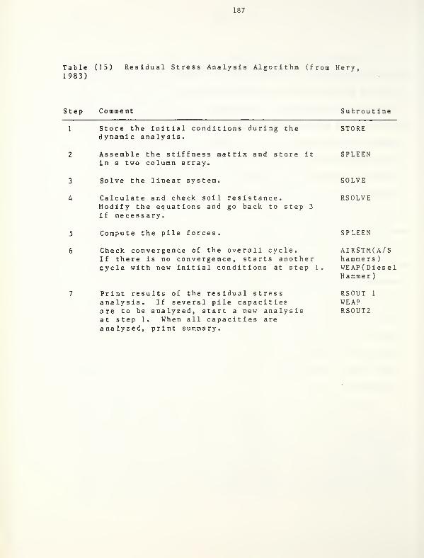
187
Table (15) Residual Stress Analysis Algorithm (from Hery,1983)
Step Comment Subroutine
1 Store the initial conditions during the STOREdynamic analysis.
2 Assemble the stiffness matrix and store it SPLEENin a two column array.
3 Solve the linear system. SOLVE
4 Calculate and check soil resistance. RSOLVEModify the equations and go back to step 3
if ne ce ss ary
.
5 Compute the pile forces.
6 Check convergence of the overall cycle.If there is no convergence, starts anothercycle with new initial conditions at step 1
SPLEEN
AIRSTM(A/Shamme rs )
WEAP(DieselHammer
)
Print results of the residual stressanalysis. If several pile capacitiesare to be analyzed, start a new analysisat step 1. When all capacities areanalyzed, print summary.
RSOUT 1
WEAPRS0UT2
188
rithm used in "CUWEAP" to perform the residual stress analysis.
4.4.2 Effect of Considering Residual Stresses
in the Dynamic Analysis:
The most direct effect of including the residual stresses is
the change in the blow count-total resistance relationship
obtained from the wave equation analysis. Figure (47) shows an
example of such relationship with and without including residual
stresses. It indicates that the pile is easier to drive if resi-
dual stresses are included (i.e. a certain resistance can be
achieved with smaller number of blows). This is logical since
the accumulation of compressive residual stresses below the pile
.tip as the driving proceeds facilitates the driving process. In
the conventional wave equation analysis, the resistance of the
soil spring returns to zero at the end of one blow, while, it
does not return to zero if residual stresses are considered
(because of the existence of some residual forces). This means
that the set should be larger if residual stresses are considered
(i.e. the number of blows/ft. is smaller). This is illustrated
by the simple diagram shown in Figure (48) from Hery (1983).>
The reduction in the number of blows/ft. due to residual
stress consideration is directly related to the magnitude of
these stresses. An attempt was made to correlate this reduction,
expressed as a factor "a " (which is the ratio between the numberN
of blows/ft. with and without considering residual stresses) with
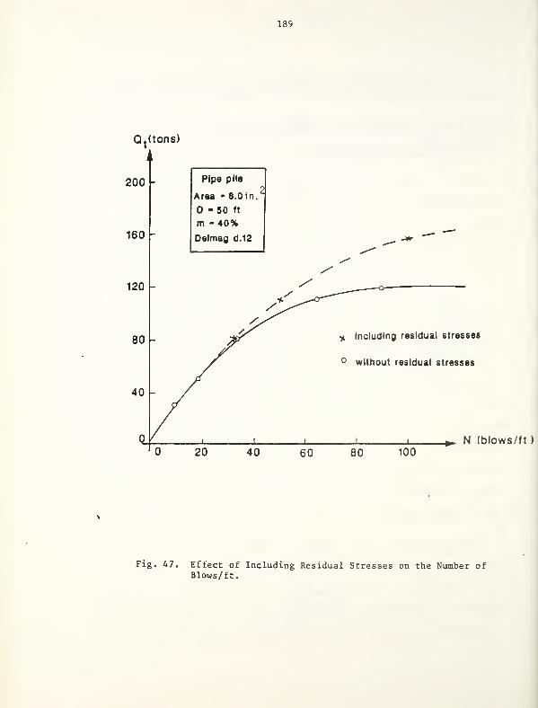
189
Qt(tons)
200
160
120
80
40
Pipe pile
Area - 8.0 in.
D - 50 ft
m -40%Delmag d.12
* Including residual stresses
° without residual stresses
^ N (blows/ft)20 40 60 80 100
Fig. 47. Effect of Including Residual Stresses on the Number ofBlows/ft.
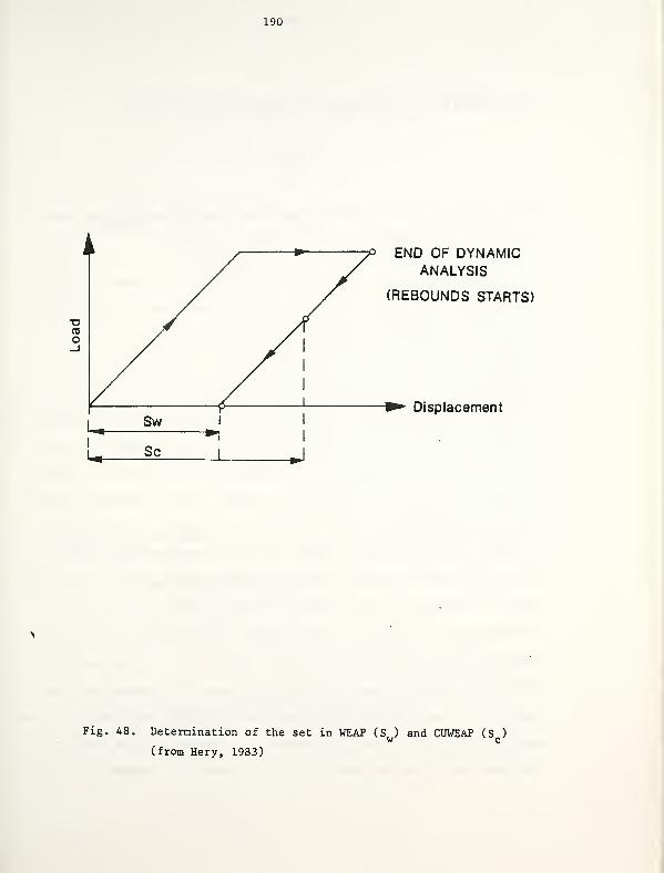
190
END OF DYNAMICANALYSIS
(REBOUNDS STARTS)
Displacement
Fig. 48. Determination of the set in WEAP (S ) and CUWEAP (S )w c
(from Hery, 1983)
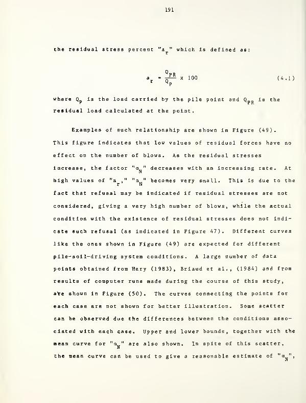
191
the residual stress percent "a " which is defined asr
: PRx 100 (4.1)
where Q is the load carried by the pile point and Q is thet PR
residual load calculated at the point.
Examples of such relationship are shown in Figure (49).
This figure indicates that low values of residual forces have no
effect on the number of blows. As the residual stresses
increase, the factor "a " decreases with an increasing rate. At
high values of "a ," " a " becomes very small. This is due to ther N
fact that refusal may be indicated if residual stresses are not
considered, giving a very high number of blows, while the actual
condition with the existence of residual stresses does not indi-
cate such refusal (as indicated in Figure 47). Different curves
like the ones shown in Figure (49) are expected for different
pile-soil-driving system conditions. A large number of data
points obtained from Hery (1983), Briaud et al., (1984) and from
results of computer runs made during the course of this study,
are shown in Figure (50). The curves connecting the points for
each case are not shown for better illustration. Some scatter
can be observed due the differences between the conditions asso-
ciated with each case. Upper and lower bounds, together with the
mean curve for " o " are also shown. In spite of this scatter,N
the mean curve can be used to give a reasonable estimate of "a ",
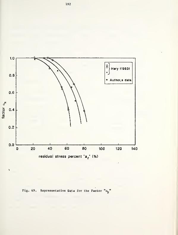
192
1.0
0.8
0.6
0.2 -
»1-> Hery (1983)
* Author, s data
0.0
20 40 60 80 100
residual stress percent "a* (%)
120 140
Fig. 49. Represnetative Data for the Factor "cl,1
193
1.0
0.8
0.6
2 0.4CO
\OV» H +v^a »-e*—&«s:
0.2
recommended
curve
#>Hery (1983)
x
*Briaud (1984)
Author's
data
20 40 60 80 100
residual stress percent "a." (%)
120 140
Fig. 50. Upper and Lower Bounds and Recommended Values for ol^
194
provided that "a " is known. Prediction of "a " will ber r r
described later in this chapter. Hence, if a simple wave equa-
tion analysis is performed, without considering residual
stresses, and if "a " can be predicted, a reasonable estimate of
the actual expected number of blows can be made (multiplying the
number of blows obtained from the simple wave equation analysis
by " a»,")» an d a more reasonable N-resistance relationship can beN
obtained .
Another effect of the residual stresses is the change in the
maximum driving stresses. Wave equation analyses performed by
Hery (1983) indicate that the driving stresses are slightly
higher if residual stresses are considered, which means that not
considering residual stresses in the anlysis will lead to
underestimating the maximum driving stresses. This was confirmed
by a number of computer runs during the course of this study.
Again, a correlation of the increase in driving stresses due to
considering residual forces, expressed as a factor a , wass
attempted with the residual stress percent "a ". Figure (51)
shows some data points for such a relationship. Values of as
ranged between 1.0 (no change in stresses) to about 1.14
(stresses increase by 14% if residual stresses were considered).
The average value of "a " seemed to be constant irrespective ofs
the value of "a ", for values of a greater than about 10Z. Thisr r
average value was about 1.05. However, to be on the safe side,
one may assume that the compressive driving stresses are about
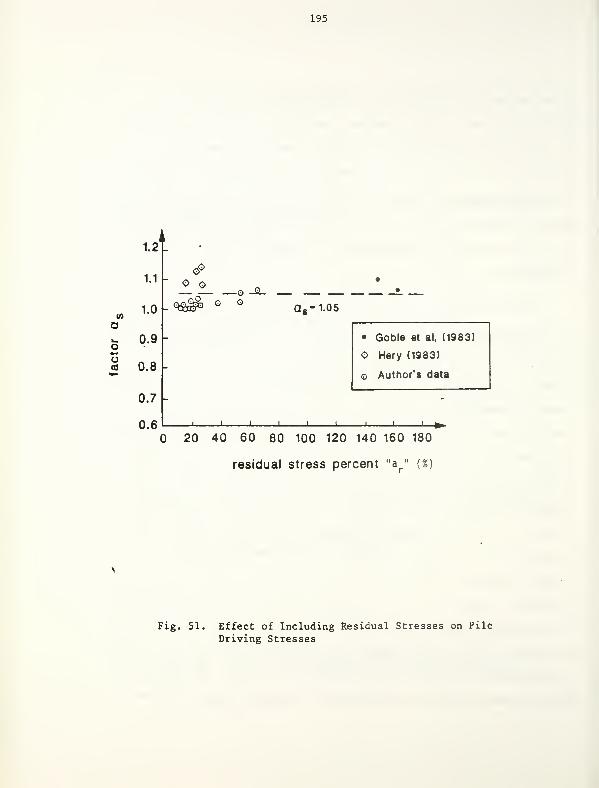
195
(A
a
1.2
1.1
1.0
0.9
0.8
0.7
0.6
o o-o-O-
o oQg-1.05
• Qobie et ai, (1983)
O Hery (1983)
o Author's data
J I I I I I I L
20 40 60 80 100 120 140 160 180
residual stress percent "ar" (%)
Fig. 51. Effect of Including Residual Stresses on Pile
Driving Stresses
196
10% higher than the values obtained from a simple wave equation
analysis that does not take residual stresses into account.
4.4.3 Distribution of Residual Forces along Pile Shaft;
The magnitude of the residual forces after driving can be
obtained using the wave equation analysis outlined before. Fig-
ure (52) shows both the residual skin friction distribution and
the residual pile load distribution for one of the cases studied.
Curve (a) gives the residual load at every pile depth from ground
surface down to this particular depth, while curve (b) gives the
unit skin friction along the pile shaft multiplied by its perime-
ter. It should be noticed that curve (b) resembles the first
derivative, or the slope, of curve (a), as explained by Vesic
(1977) (notice the correspondence of points (1) and (2) on both
curves). It was found that the general shapes of these curves
are typical for all the residual stress analyses made by
"CUWEAP," irrespective of the variables involved in the problem.
These shapes agree with the ones obtained by the Hunter-Davisson
procedure (although the magnitudes are somewhat different, as
will be explained later), and with the direct measurements made>
by Gregersen et al. , (1973). They also agree with the shapes
obtained by the "DUKFOR" program used by Holloway et al., (1975).
They indicate the existence of a negative friction for the upper
portion of the pile, down to a critical depth "Z " below whichcr
there is an upward residual friction load in addition to the
residual tip load. The sum of the upward residual tip load,
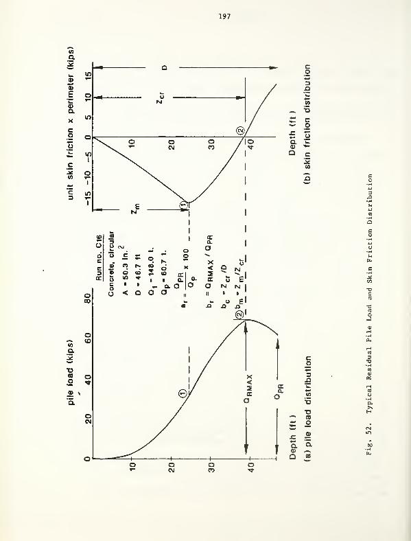
197
T3
to
OJ
u•HP.>»H
198
upward residual friction, and downward negative friction is zero,
since the pile is in equilibrium, as explained earlier.
In order to define the shapes of curves (a) and (b) one
needs to know the residual point load "QDD ", the maximum residual
shaft load "Q„„ ." that corresponds to the depth "Z " , and theXRMAX v v cr '
depths "Z " and "Z " shown on Figure (52). If the residualcr m
stress percent "a " is known (as will be shown later) the resi-
dual point load "QpR
" can be estimated. Three ratios, "b "
,
"b ", and "b " , can be defined for the description of thesec m
curves, such that:
br
- QrMAX^PR (4 ' 2)
b - Z /D (4.3)c cr
and
b - Z /Z (4.4)m m cr
in which "D" is the pile length,
^ large number of computer runs indicated that the ratio "b " for
sands is almost constant, with an average value of 1.05 and a
coefficient of variation of about 1.5%. The same applies to the
ratio "b " which showed an average value of 0.60 and a coeffi-m
cient of variation of about 10%. It should be noted that these
values apply only for piles driven into cohesionless soils, for
199
which this study was performed.
The ratio "b ", which defines the critical depth at whichc r
the residual friction is reversed from negative to positive,
showed greater variability. It was found that the main factors
that govern this ratio are the pile length, the amount of pile
load that is transferred to the soil by friction, expressed in
terms of a parameter "m" which is defined as the percentage of
load carried by skin friction, and the total ultimate soil resis-
tance "Q ". For certain values of "D" and "m", however, the
ratio "b " varied little with "Q ". This is indicated by part ofc t
the data that are shown in Table (16). Figure (53) gives the
data that describe the effect of pile length and skin friction
percent on "b ". If "m" were fixed to a value of 40%, the datac
points that describe the relation between pile length and "b "
are shown on part (a) of Figure (53). A decreasing trend of "b "
with increasing "D" can be observed, which means that as the pile
gets longer, the critical depth "Z " relative to the pile lengthcr
gets smaller. This can be explained by the fact that as the pile
gets longer, there will be a greater amount of downward negative
fViction that needs to be balanced by a residual point load and
an upward friction, which means that the length of the portion in
which there is an upward friction along the pile shaft should
increase. On the other hand, if the pile length were fixed, as
shown on part (b) of Figure (53), the critical depth ratio "b "
should decrease as the skin friction percent "m" increases. The
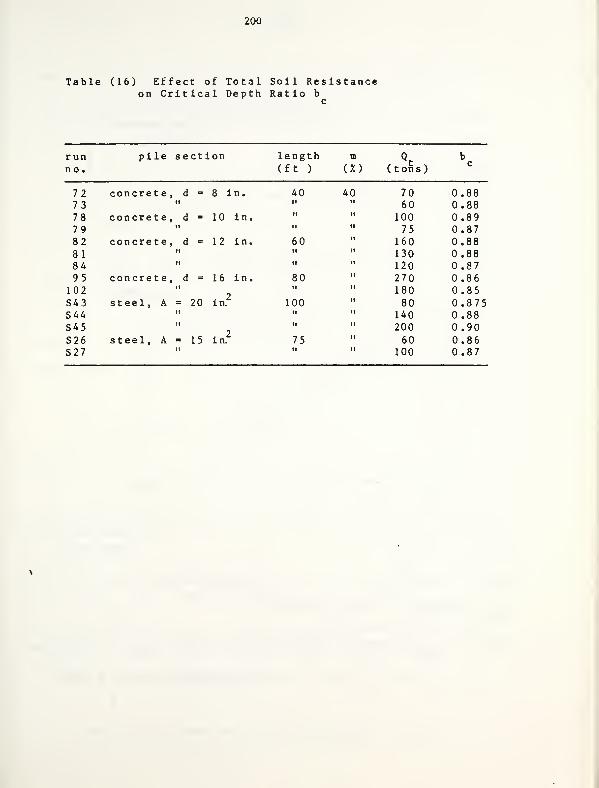
200
Table (16) Effect of Total Soil Resistanceon Critical Depth Ratio b
runno.
pile section length m
(ft ) (%) ( t ons
)
7273787982818495
102S43S44S45S26S27
concrete, d = 8 in.ii
concrete, d = 10 in,ii
concrete , d = 1 2 in.ii
ii
concre te, d = 16 inii
2steel, A = 20 in.
ii
ii
2steel, A = 15 in.
40 40 70 0.88ii 60 0.88ii 100 0.89it 75 0.8760 160 0.88ii 130 0.88ii 120 0.8780 270 0.86ii 180 0.85
100 80 0.875II 140 0.88II 200 0.9075 60 0.86ii 100 0.87
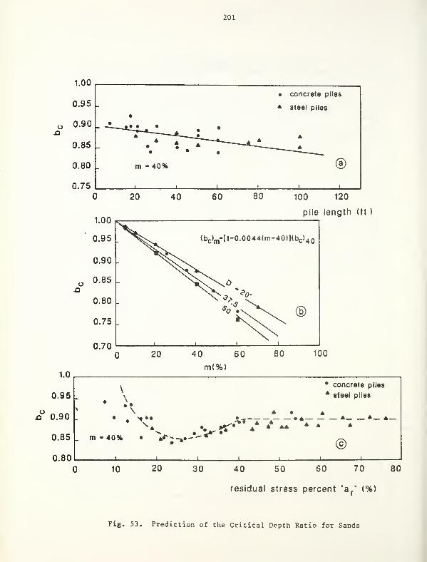
201
o
0.95
• concrete plies
* steel piles
0.90 •_•• • • •
0.85 -
4 *- — •
•
A 4 A
0.80 m - 40% ©0.75 i i
i 1 1 '
20 40 60 80 100 120
pile length (ft )
1.0
0.95
n 0.90
0.85
0.80
40 60
m(%)
100
. * concrete piles
v * steel piles_• ••
\ \ * .- • *•• ^ _ #A A *-*—
^* .. **-• * * ** * *
- m - 40% • **-—»•-""/-n
1 1 1 .. i 1 1 1
10 20 30 40 50 60 70 80
residual stress percent *ar
* (%)
Fig. 53. Prediction of the Critical Depth Ratio for Sands
202
same explanation given above can also be used to explain this
trend. The following correlation between "b " and "m" wasc
derived for a certain constant pile length:
(b ) = [1.0 - 0.0044 (m - 40)] (b ) /ncm c 4U(4.5)
This relation gives the ratio "b " at any value of "m" as ac
function of the ratio "b " at m = 40%. Hence, one can enter withc
the pile length into part (a) of Figure (53) to obtain "b " at mc
= 40%. Then Equation (4.5) can be used to get the correct value
of "b " for the estimated value of "m". The ratio "b " for pilesc c
driven into cohesionless soil ranges between about 0.70 and 1.00,
according to the variables of the problem, as shown in Figure
(53) .
As an example for the prediction of "b ", the data reported
by Gregersen et al., (1973) for pile number (D/A), which was a
circular prestressed concrete pile having a 0.92 ft diameter and
52.5 ft length, were examined. According to Figure (53. a), "b "
c
for 40% skin friction equals 0.87. Using Equation (4.5) with m =
76.5% indicates that the predicted value of "b " is 0.73. Meas-rc
urements reported by Gregersen et al., for this pile indicated a
value for "b " of 0.70. This example shows that the suggestedc
prediction is quite good. Unfortunately, the data reported by
Gregersen et al., (1973) were the only data that could be
obtained in which there were reliable actual measurements of the
203
residual loads along the pile shaft.
4.4.4 Factors Affecting the Magnitude of Residual Stresses:
In order to develop a procedure for predicting the magnitude
of residual stresses, a parametric study was conducted, using
"CUWEAP", to examine the effect of the various parameters
involved. The factors involved in this study were: the driving
system, including the types of hammers, cushions, ... etc.; the
total soil resistance; the percentage of load transferred by
shaft friction; and the pile material, cross section and length.
This study was conducted for piles driven into cohesionless soils
only. The dependent variable that was studied was the residual
stress percent "a ", which indicates the amount of residual loadr
below the pile tip due to driving.
4.4.4.1 Effect of the Driving System and Elements:
Three hammer types were used in this analysis, giving a wide
range of energies delivered to the pile during driving, with
other variables being the same. Table (17) summarized the
results of this analysis. It indicates that the point residual
force slightly increases as the hammer rated energy increases.
The range of "a ", however, that corresponds to the wide range of
hammer energies was quite narrow.
When the hammer used was fixed, and the driving elements,
like caps and cushions, are changed, the results given in Table
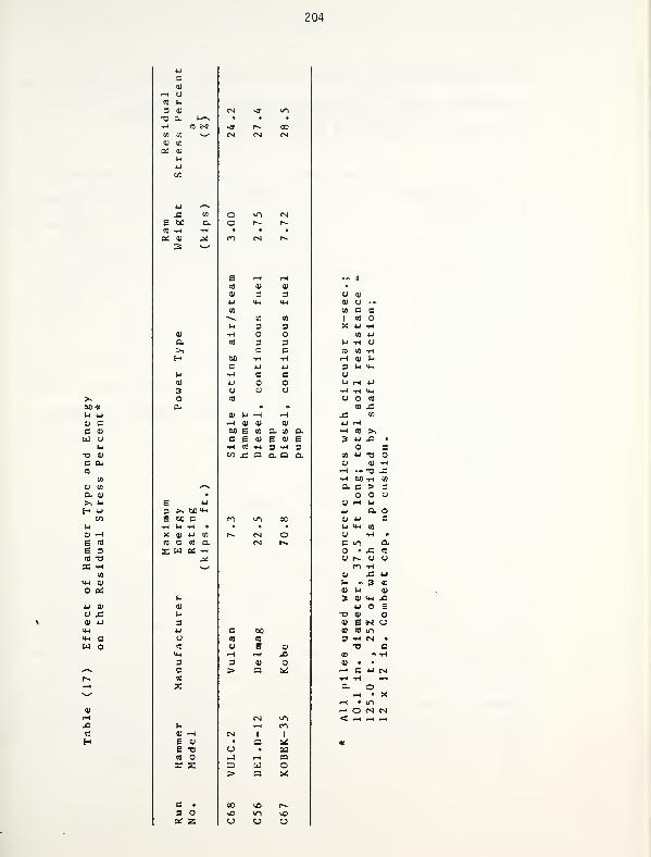
204
>>
60*l- u01 Cc o>
Ed Uu
C 0u
CD
03
Oi 03
a ai
>s U
w
ai .h
S <o
e sm -v
X -H
0)
"4-1 01
oi
4J m<J J=01 4J
U-l
>*H Cu o
(0 u3 01
-o cu k«-,
H CO 9-S
0] 0] x-'
01 03
St 01
J= a oa oo a. otO T-l H •
Oi 0) ^ to
3 •w'
B(0
e *->
3 >^ M>*-i
e so c
X D U 10
CO C <0 O.
S Id tti -H
u01 t-l
E CD
e -aCO o
c •
3 OOi Z
0) 01
3 314-1 4-1
03 03
3 3O3 3
0) l-i H Ht-H 01 0> 01
60 E 03 Q. 00 D.C 6 0) E 0i E•H CO -H 3 iH 3o3 £ o a Q a.
c 60CO 10
O S 01
H r-i JD
3 0> o> a ^
CM 1 1
• a 3^o • IdJ rH M3 Id O> Q *
CO vO r-.
vC u-i vOc_) U o
u 01
0) u0) c1 CO
X t-l
03
i-l HCO 03
u O CO
J=
03 J=03
4-1 -H•H CO ^s 4-1 -O •
O C03 4J -o
0) 0) •Hr-i »n "O £1-H 60 -H 03
o. C > 3o <J
0) ^ 1-1
4-1 a0) 4-1 Cu U-I 03
<J H •>
c m a.• £ CO
u r~ U CJ
n i-l
0) Si 4-1
u • 3 03
Oi hi 03
3 01 14-1 J34J s
T3 0) oCU e X uco CO m3 •H CM •
-o c
H CUMCl o
<H O CM CM
205
(18) were obtained. These results indicate that the type of cap
or cushion used in the driving procedure has almost no effect on
the magnitude of the tip residual stresses.
The above mentioned results indicate that the residual
stress phenomenon is mainly affected by the pile-soil combination
rather than by the driving system and elements. This conclusion
was expected, since the residual stresses are caused by the
load/rebound cycles occurring during the driving process, as
explained earlier. Hence, they should mainly be affected by the
relative pile/soil stiffness, rather than by the driving ele-
ments. The same conclusion was also reached by Holloway et al.,
(1975) using the computer program "DUKFOR". This result makes
the prediction of the magnitude of residual stresses somewhat
simpler, since it may be assumed that they are not affected by
the driving system used.
4.4.4.2. Effect of Total Soil Resistance:
One of the major parameters that is expected to influence
the magnitude of the residual forces is the total resistance pro-
vided by the soil. Figure (54))gives some variations of the
residual stress percent with the total pile capacity, provided
that all other parameters are the same for each curve. As the
total capacity increases, the point residual stress increases
because of the pile elastic rebound, and hence the negative fric-
tion that is balanced by the upward residual forces increases. The
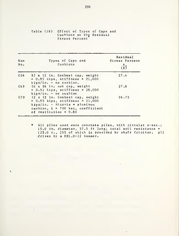
206
Table (18) Effect of Types of Caps andCushions on thg ResidualStress Percent
RunNo.
Types of Caps andCushions
ResidualStress Percent
a
c%5
C56 12 x 12 in. Conbest cap, weight 27.4= 0.95 kips, stiffness = 21,000kips/in. - no cushion.
C69 16 x 16 in. oak cap, weight 27.80.91 kips, stiffness = 28,000
kips/in. - no cushionC70 12 x 12 in. Conbest cap, weight 26.75
= 0.95 kips, stiffness = 21,000kips/in. - Micarta + aluminumcushion, E = 700 ksi, coefficientof restitution = 0.80
* All piles used were concrete piles, with circular x-sec.;10.0 in. diameter, 37.5 ft long; total soil resistance =
125.0 t., 25% of which is provided by shaft friction. Alldriven by a DEL.D-12 hammer.
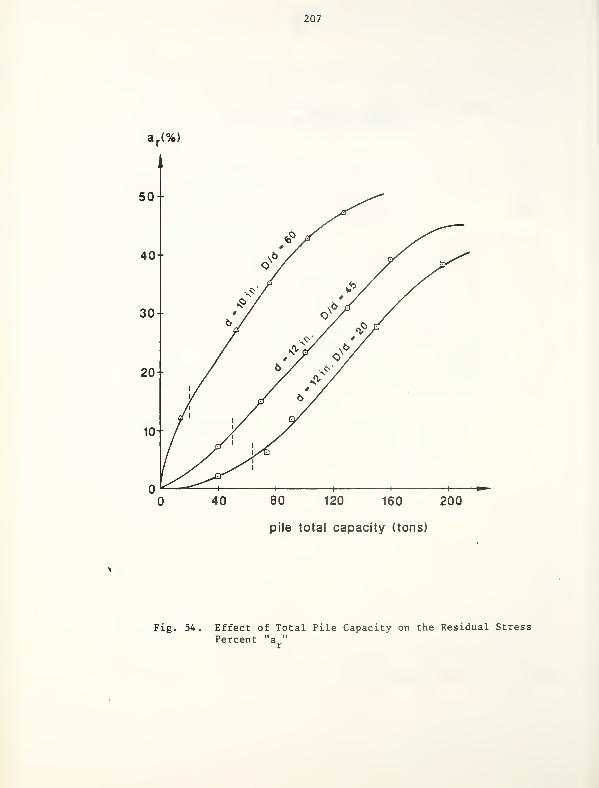
207
50 -
40-
30--
20-
10 -
80 120 160 200
pile total capacity (tons)
Fig. 54. Effect of Total Pile Capacity on the Residual Stress
Percent "a "
208
variation is almost linear except at the early and late stages of
the curve. Similar results were also reported by Hery (1983 ).
For the high values of pile capacity, the strength of the pile
material may be exceeded, which makes the curves become flatter.
On the other hand, the amount of pile rebound should mobilize
some negative friction up to the point where no more friction can
be mobilized, which limits the magnitude of the residual
stresses, giving the tendency of the curve to be flatter at
higher values of the pile capacity. Very low values of ultimate
pile capacities shown on these curves are usually not realistic
for piles driven into cohesionless soils. Hence, the portion of
the curve which begins when it becomes linear can be used in a
prediction procedure as will be shown later.
4.4.4.3. Effect of Skin Friction Percent:
One of the major factors that is expected to have an impor-
tant effect on the magnitude of the tip residual stresses is the
amount of load transferred to the soil by shaft friction, rela-
tive to the total pile capacity. This can be expressed in terms
of the skin friction percent "m" which is defined by:
m - ~ x 100^t
(4.6)
where Q and Q are the shaft and total pile capacities, respec-
tively. The value of Q is the "true" shaft friction, without
including any residual stresses, which is used as an input in the
209
wave equation analysis.
As a matter of fact, there is an interaction between the
mechanism of load transfer and the magnitude of driving residual
stresses. In other words, the residual stresses are influenced
by the nature of load transfer, while this nature changes due to
the existence of the residual forces. Figures (55) and (56) show
the relation between the skin friction percent "m" and the resi-
dual stress percent "a " for selected concrete and steel piles,
respectively. As these curves indicate, "a " increases as the
value of "m" increases, for the same total pile capacity. Since
the amount of residual tip load is a function of the
positive/negative skin friction cycles induced by pile driving
and rebound, it should be expected to increase as the amount of
load transferred by friction increases (larger amount of negative
friction will need to be balanced by some upward residual tip
load). If no load was transferred by friction, no residual'
stresses should occur. As "m" increases, "a " increases, but ther
rate of increase is lower after a value of "m" of about 20%. For
high values of "m", the curves should become flatter to approach
an asymptotic value for m 100%. Any of the curves shown in
Figures (55) and (56) can be approximated by two straight lines
of different slopes before and after m Z 20%, up to a value of m
of about 65%, when they tend to flatten.
As stated earlier, the value of "m" is also affected by
"a ", since the residual stresses tend to increase the shaftr
'
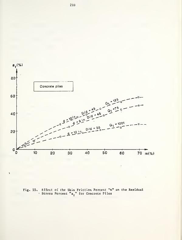
ar(%)
210
80"
60"
40
20-
Concrete piles
Ovtf*
*••?-•" ov-1^
^r*«V-^©
D/d -2° - -Qtrj£I
^. —o -
10 20 30 40 50 60 70 m(%)
Fig. 55. Effect of the Skin Friction Percent "m" on the ResidualStress Percent a for Concrete Piles
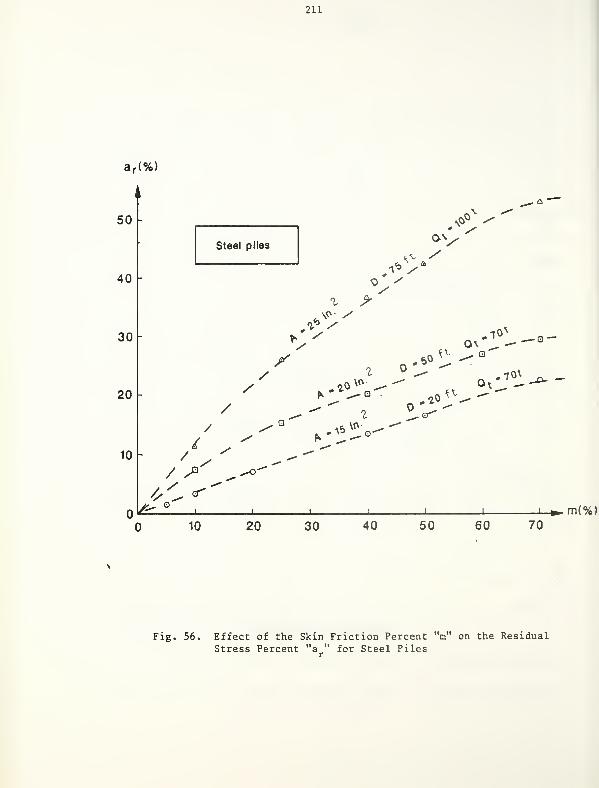
211
a r (%)
50
40
30
20
10
Steal piles
.^^V
X 60
10 V
//
/
//
/
/ ^
-20 ^
m(%)10 20 30 40 50 60 70
Fig. 56. Effect of the Skin Friction Percent "m" on the ResidualStress Percent "a " for Steel Piles
r
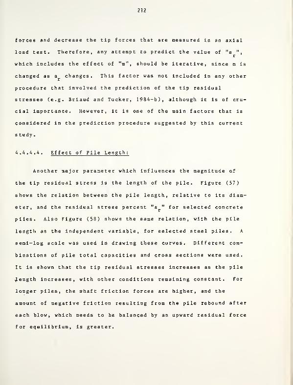
212
forces and decrease the tip forces that are measured in an axial
load test. Therefore, any attempt to predict the value of "a ",r
which includes the effect of "m", should be iterative, since m is
changed as a changes. This factor was not included in any other
procedure that involved the prediction of the tip residual
stresses (e.g. Briaud and Tucker, 1984-b), although it is of cru-
cial importance. However, it is one of the main factors that is
considered in the prediction procedure suggested by this current
study.
4.4.4.4. Effect of Pile Length:
Another major parameter which influences the magnitude of
the tip residual stress is the length of the pile. Figure (57)
shows the relation between the pile length, relative to its diam-
eter, and the residual stress percent "a " for selected concreter
piles. Also Figure (58) shows the same relation, with the pile
length as the independent variable, for selected steel piles. A
semi-log scale was used in drawing these curves. Different com-
binations of pile total capacities and cross sections were used.
It is shown that the tip residual stresses increases as the pile
^ength increases, with other conditions remaining constant. For
longer piles, the shaft friction forces are higher, and the
amount of negative friction resulting from the pile rebound after
each blow, which needs to be balanced by an upward residual force
for equilibrium, is greater.
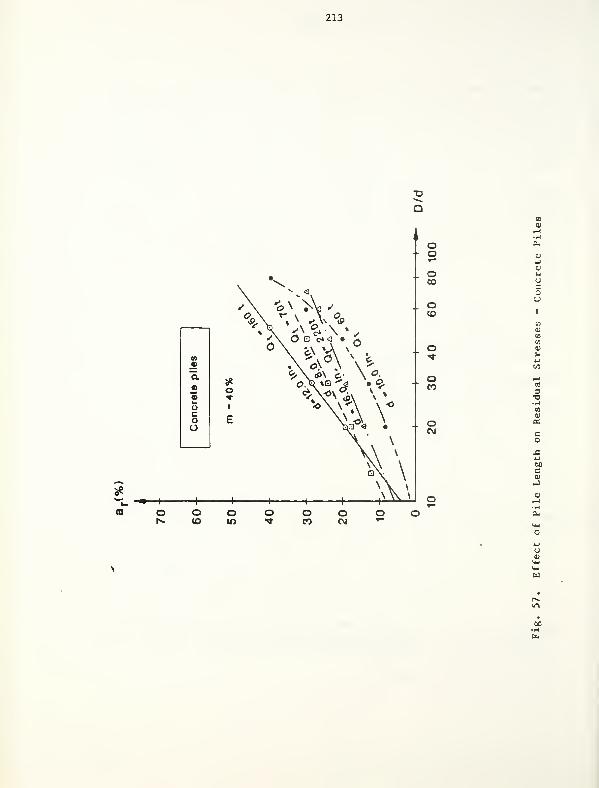
213
1—D
2co
=-o
OS
«s
c
MC
6C
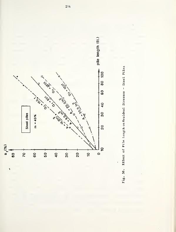
214
c
\V B^ \\ \ \
ss
\ \ ° N Vv
°$\ *x ^. ^%
S\d\ *v
**\
X cX >n v©CL
"5
•
oi
• 7B Q .VI
CO E
*v\ ^'
(%)1 —i
—
xX\—i—i—i—i—i>^
ocCU-J
o00
o oto
oin
o oCO
oCM
001-1
fa
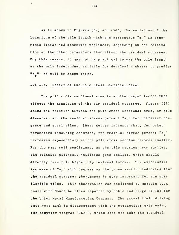
215
As is shown in Figures (57) and (58), the variation of the
logarithm of the pile length with the percentage "a " is some-
times linear and sometimes nonlinear, depending on the combina-
tion of the other parameters that affect the residual stresses.
For this reason, it may not be practical to use the pile length
as the main independent variable for developing charts to predict
"a " , as will be shown later.r
4.4.4.5. Effect of the Pile Cross Sectional Area:
r
The pile cross sectional area is another major factor that
affects the magnitude of the tip residual stresses. Figure (59)
shows the relation between the pile cross sectional area, or pile
diameter, and the residual stress percent "a " for different con-rr
crete and steel piles. These curves indicate that, for other
parameters remaining constant, the residual stress percent "a
increases exponentialy as the pile cross section becomes smaller.
For the same soil conditions, as the pile section gets smaller,
the relative pile/soil stiffness gets smaller, which should
directly result in higher tip residual forces. The
.
exponent ial
increase of "a " with decreasing the cross section indicates that\ r *
the residual stresses phenomenon is more important for the more
flexible piles. This observation was confirmed by certain test
cases with Monotube piles reported by Goble and Hauge (1978) for
the Union Metal Manufacturing Company. The actual field driving
data were much in disagreement with the predictions made using
the computer program "WEAP" , which does not take the residual
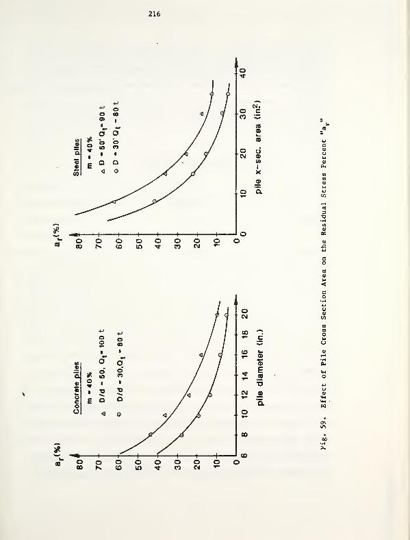
216
#w -*"
CM.o cV) *^
CO©k.
CO
O dCM CD
(0
X
..o
oCO
o oCO
Oin
o OCO
oC\J
<£
M6u
o o o O o o oCO n CD ID *- CO CM
217
stresses into account. Because the Monotube piles are rather
flexible, the discrepancies might be explained in terms of
neglecting residual stresses. Further analysis performed by Hery
(1983) for the same piles, including residual stresses, showed
that the predictions were much closer to the actual field meas-
urements .
4.4.4.6. Effect of the Pile Material:
The pile material is expected to have a great influence on
the residual stresses phenomenon. As the pile becomes stiffer,
residual forces should decrease, for the same soil conditions.
In order to examine the effect of this factor, two piles were
assumed, each having a length of 40.0 ft, cross-sectional area of
220.0 in. , driven to a total capacity of 60.0 tons, 40% of which
is transferred by shaft friction. One of the piles was a con-
crete pile with E = 5,000 ksi, while the other was a steel pile
with E = 30,000 ksi. The residual stress percent "a " obtainedr
by the wave equation analysis for the concrete pile was 66.1%,
while it was only 14.6% for the steel pile. This means that
increasing the pile stiffness by about 6 times resulted in a
decrease of "a " of about 4.5 times. It should be noted, how-
ever, that this does not mean that residual stresses are always
much higher for concrete piles than for steel piles, since the
cross sectional area used in this example was quite small for the
practical range of diameters usually used for concrete piles.
The example demonstrates, however, that predicting residual
218
stresses for different pile materials is quite different. Dif-
ferent charts should be used for different pile materials, as
will be shown later.
For the same pile material, the value of "E" also makes some
difference. To examine this effect, another concrete pile was
considered, having the same characteristics as the ones used in
the previous example; except that it was made of a poorer con-
crete that results in a value of "E" of 3,500 ksi. The value of
"a " obtained was about 10% higher than that for the other con-
crete pile that had a higher value of E. This should also be
taken into account in any prediction procedure.
It should be noted that the curves and relations shown in
the above mentioned sections, regarding the factors affecting
residual stresses, were obtained assuming that the pile was
driven into cohesionless soils, a principal restraint for this
study. For piles driven into cohesive soils, however, the gen-
eral trends may not be different. Certain parameters are dif-
ferent in the latter case, e.g. the shaft friction distribution
in cohesive soils. Briaud et al., (1983) stated that little or
no residual stresses are expected for piles driven in clay. One
can not, however, generalize this statment. This may be true for
piles driven through weak cohesive soils into dense sand or hard
clay strata, in which most of the load is transferred by point
bearing. This means that very small residual stresses are
expected (low values of "m", as explained earlier). In some
219
other cases, however, significant residual stresses can exist for
piles entirely driven in clay. This is particularly the case of
long friction piles driven through soft clay layers. This is
because the stiffness of such piles is usually low (long pile,
small cross section) and most of the load is transferred to the
soil by shaft friction. The significance of this observation was
briefly examined by performing a "CUWEAP" analysis for a steel
pipe pile of 10.0 in. diameter and 0.19 in. wall thickness. Its
length was 100 ft, penetrating soft clay layers. It was assumed
that about 90% of the total load would be transmitted to the soil
by shaft friction. The analysis gave values of residual point
loads as high as one and half times the assumed point load (i.e.,
about 15% of the total pile capacity). This is contrary to what
was stated by Briaud et al., (1983), viz., that these stresses
can not exceed 5% of the total load for clays. It should also be
noted that the parameters describing the shape of the residual
stress distribution for cohesive soils may be somewhat different
from these obtained for cohesionless soils (e.g. the critical
depth relative to the pile length, etc.).
4.5 The Development of an Approximate. Technique for Residual Stresses Prediction
The foregoing discussions illustrated the importance of con-
sidering the residual stresses due to driving in the pile founda-
tion analysis. The prediction of these stresses is still beyond
the current state-of-the-art. Although the direct measurement of
220
these forces is the most accurate technique for their evaluation,
many difficulties and uncertainties still prevent the engineer
from measuring accurate values. Other load test sequences that
have been recommended for the evaluation of these forces imply
invalid assumptions which leads to an incorrect evaluation of the
residual stresses. On the other hand, field determination of
these stresses require pile load tests in the design stage, which
is still not very common in every day practice. Certain predic-
tions were made using the wave equation analyses which have pro-
ven to be quite satisfactory. This analysis requires the availa-
bility of a good wave equation program, plus computer hardware.
The engineer, however, may need a simple technique to make quick
estimates and acquire good first approximations, besides the fact
that the required computer software and hardware may not be
available. Techniques have been recommended to make such predic-
tions. They make, however, too many simplifying assumptions.
Therefore, the author of this study felt the need for such a
prediction procedure and tried to use the wave equation analysis
for the development of this technique, since it was proven to be
the best way available for residual stress evaluation. In this
chapter, the disadvantages of the other techniques that have been
proposed are discussed. A recommended procedure is described and
illustrated by certain numerical examples. Comparisons of these
predictions to reported actual measurements, as well as the other
prediction techniques, are reported. One of the main purposes of
this prediction is to facilitate better interpretation of load
221
test results, especially for these which are used to develop
empirical approaches for pile capacity predictions.
4.5.1 The Hunter-Davisson Method:
The Hunter-Davisson method for obtaining residual stresses
was described in detail in a previous chapter. It requires a
certain sequence for pile testing which involves performing a
pulling test after the main compression test. One major assump-
tion of this procedure is that it assumes that tension loading
results in no residual stresses. Actual measurements, however,
made by Goble et al., (1972) indicated the existence of some
residual stresses just after the pulling test, which means that
some residual loads do exist due to the pulling test only. Sim-
plified approximate analyses performed by Briaud et al., (1983)
and by Briaud and Tucker (1984-b) also indicated that this
assumption is incorrect. This analysis, however, showed that no
significant residual stresses can result after a pulling test if
the pile is not very long. The error is zero at the top and bot-
tom of the pile and peaks towards the middle of the pile, where
the residual tension load can be as high as 251 of the ultimate
tension load for very long piles according to theory (Briaud and
Tucker, 1984-b).
Another implicit assumption of this procedure, although not
realized by Hunter and Davisson (1969), is that the distribution
of shaft friction in loading is the same as in the case of
222
unloading. This assumption enabled them to obtain the residual
load distribution from unloading the pile, despite the fact that
they originally resulted from loading (either from the driving of
the pile or from the compression testing). Load test data, how-
ever, do not support this implicit assumption. For example, the
interpretation of test results reported by Vesic (1970), which
was made by the author of this study, indicates that the unit
friction distribution is totally different for the unloading case
(Figure (60)). Leonards and Lovell (1979) stated that loading
and unloading in compression followed by loading and unloading in
tension can result in considerable changes from the initial con-
ditions, especially in the distribution of shaft friction.
The above discussion shows that the Hunt er-Davisson pro-
cedure can be used with fair success in predicting the residual
tip stresses, but it results in an incorrect evaluation of the
distribution of shaft residual stresses along the pile length.
4.5.2 The Holloway Procedure
Holloway et al., (1975) used the wave equation computer pro-
gram "DUKFOR" to predict the residual stresses, as described ear-
lier. The sequence of analysis was quite reasonable, the wave
equation solution algorithm, however, was not rigorous enough to
include such factors as the diesel hammers modeling, the more
accurate soil damping inclusion, etc., as was done later in the
programs "WEAP" (Goble and Rausche, 1976) and "CUWEAP" (Hery,
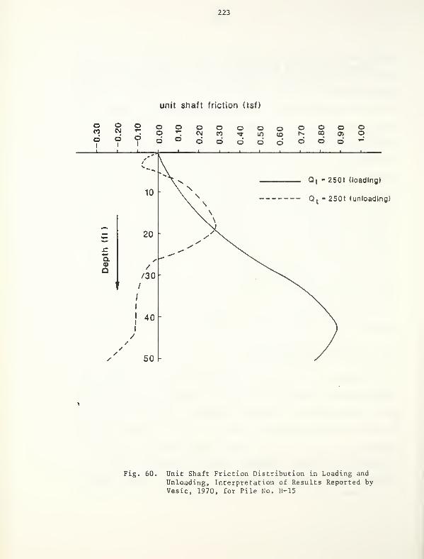
223
unit shaft friction (tsf)
oCO
oCM
d bi i
O o o• o «-;o o o
o oCO
o oin
oo o o o o
o oCO
oo"
oo
Q t -250t (loading)
Qt- 250 1 (unloading)
Fig. 60. Unit Shaft Friction Distribution in Loading and
Unloading, Interpretation of Results Reported by
Vesic, 1970, for Pile No. H-15
224
1983). These deficiencies in the model could result in inaccu-
rate predictions. The main ideas described by Holloway, however,
were the basis for all the prediction procedures that used the
wave equation analysis to predict the residual stresses.
4.5.3 The Briaud-Tucker Procedure:
Briaud and Tucker (1984-b), based on a very approximate
analysis, concluded that the point residual stresses could be
correlated with a certain parameter ft, defined by:
kT
P
A EP P
(4.7)
where
k = loading stiffness for skin friction
p pile perimeter
A • area of pile tipP
E =» pile modulus of elasticityP
The value of k was obtained by the following correlation:
k - 5.01 (N .. )' 27 tsf/in.
T side(4.8)
where N . , is the average SPT blow count within the shaft lengthside ° °
considered, without any of the corrections that have been pro-
posed for the SPT number of blows. The data from which Briaud
and Tucker (1984-b) formed this correlation are shown on Figure
225
(61). The residual point stress, q , can be estimated by
q = 5.57 D U tsfres (4.9)
where D is the pile length in feet.
Several shortcomings of this procedure may be shown. First,
it is assumed that the point residual stresses are related only
to the parameter ft and the pile length. An analysis performed
and described earlier in this study showed that two other major
parameters were not taken into account, namely the fraction of
load transfered into the soil by skin friction, and the magnitude
of the total pile capacity. It was shown that these two parame-
ters are among the controlling factors that govern the magnitude
of the tip residual load. The method also implicitly assumes a
uniform distribution of shaft friction, by computing an average
value for k . The correlation presented for k is quite mislead-
ing. The scatter shown on Figure (61) is large, so that the pro-
posed correlation is not very representative for the measured
values of k that were obtained from pile load tests. It has
also been shown that many uncertainties are associated with the
number of blows obtained from the standard penetration test (e.g.
by Schmertmann, 1975 and many others). Furthermore, it is not
justified to use a strength indicator, like the SPT number of
blows, to obtain a deformation parameter like k . It is well
known that the deformation characteristics of sand are very much
affected by such factors as the fabric and the stress history,
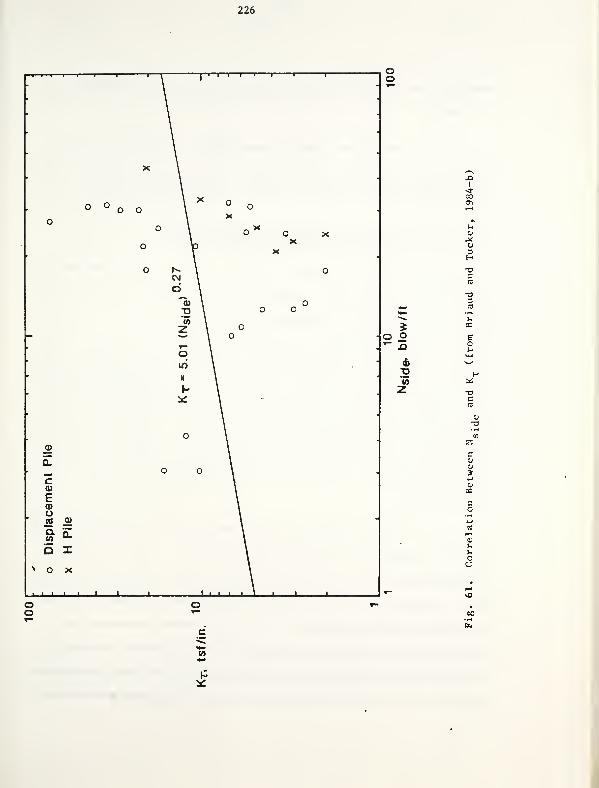
226
1
1
-
•
•
•
X'
•
oo
o
o
o
\ *
Is- \
d \
•- \(0 \z \
X
o* oX
X
o o
X
o
— *»» \ o
q \*
in '
"
N
»-
* \
a.
O
c0)
EO
o o
Q.(0
O
-
\ o X
11 1 1 -1—1 1 \ 1 1—
A
«Z
oo
I
CO
60
£
227
which may not be reflected on the SPT blow count (Leonards et
al., 1986).
All the above mentioned considerations indicate that the
Briaud-Tucker procedure for predicting residual stresses is very
approximate and may sometimes give misleading predictions.
4.5.4 The Procedure Suggested in this Research:
The review of the existing methods for residual stresses
predictions indicated the need for a more accurate procedure that
gives a good approximation which can be used frequently without
the use of a sophisticated computer analysis. It was also indi-
cated that the wave equation analysis is the only approach that
can be used for such prediction,- taking into account all the key
parameters that govern the magnitude of the residual forces.
Therefore, this approach was used to develop a set of charts that
can be easily used to make a reasonable prediction of the resi-
dual stresses .
Two pieces of information are required for such prediction,
viz. the magnitude of the residual tip load, and the magnitude
and distribution of the residual shaft loads. The latter can be
easily determined if the residual point load is known. As was
shown earlier, the shape of this distribution is unique, and
similar to the one shown in Figure (52-a). Assuming that the
residual point load "Qp„" is known from the residual stress per-
cent "a ", that will be predicted later, the maximum residualr

228
shaft load "QDW4V." can be obtained fromRMAX
QRMAX= b
r* QpR (4.10)
where "b " is a factor which equals 1.05 for cohesionless soils,
as concluded earlier.
The value of "Q_ UA " occurs at a depth "Zcr" which can beR MAX
determined from
Z = b * Dcr c
(4.11)
where D is the pile length and b is a factor that can be
obtained using Fig. (53-a) and Eq . (4.5) in terms of the pile
length and the shaft friction percent "m". If the residual
stress percent "a " were obtained from direct field measurements,r
Fig. (53-c) could be used together with Eq. (4.5). The location
of the point of inflection (point "1" on Fig. (52)) at depth Zm
can be determined from
Z - b * Zm m cr
(4-12)
where b » 0.60 for cohesionless soils,m
Once all the above information is known, and considering the
fact that the pile should be in equilibrium under these residual
stresses (residual tip load plus the upward residual friction
load should be equal to the downward friction load in the upper
229
portion of the pile along the length Z ), the distribution of
the shaft residual loads can be defined with fair accuracy.
In order to predict the residual stress percent "a ", more
than 250 computer runs were performed using the program "CUWEAP"
describe.d earlier. The parameters that were changed in this
study were the pile material, the total pile capacity, the pile
cross section, the pile length and the skin friction percent "m",
It was shown that these are the controlling factors that affect
the magnitude of the residual tip load. The abscissa to be used
for the resulting relations was chosen to be the total pile capa-
city, since the shapes of the resulting curves are somewhat
unique, with an extensive straight line portion, as was shown
earlier. Hence, many curves were drawn between the total pile
capacity and the residual stress percent for two pile materials,
concrete with E = 5,000 ksi and steel with E = 30,000 ksi, for
different pile lengths and cross sections. The skin friction
percent was fixed at a value of 40%, considering to take its
effect into account later. The resulting charts are shown on Fig
(62) and (63), corresponding to concrete and steel piles, respec-
tively. For concrete piles having a value of E » 3,500 ksi, the
values of "a " given in Fig. (62) should be increased by 102, as
explained earlier. For other values of E, linear interpolation
could be used.
The effect of changing the value of the skin friction per-
cent "m" can be taken into account using two factors 8 and 6m m
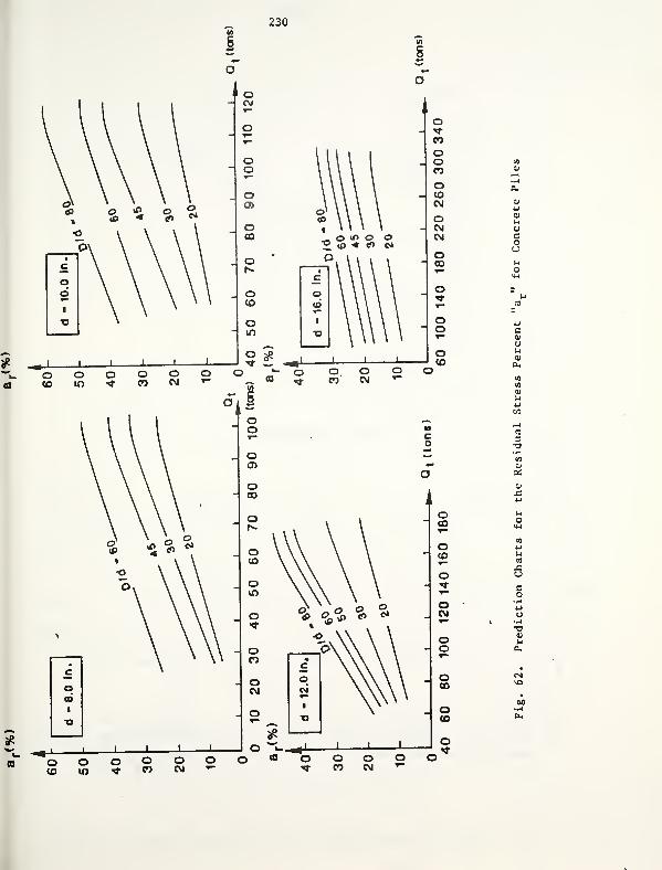
230
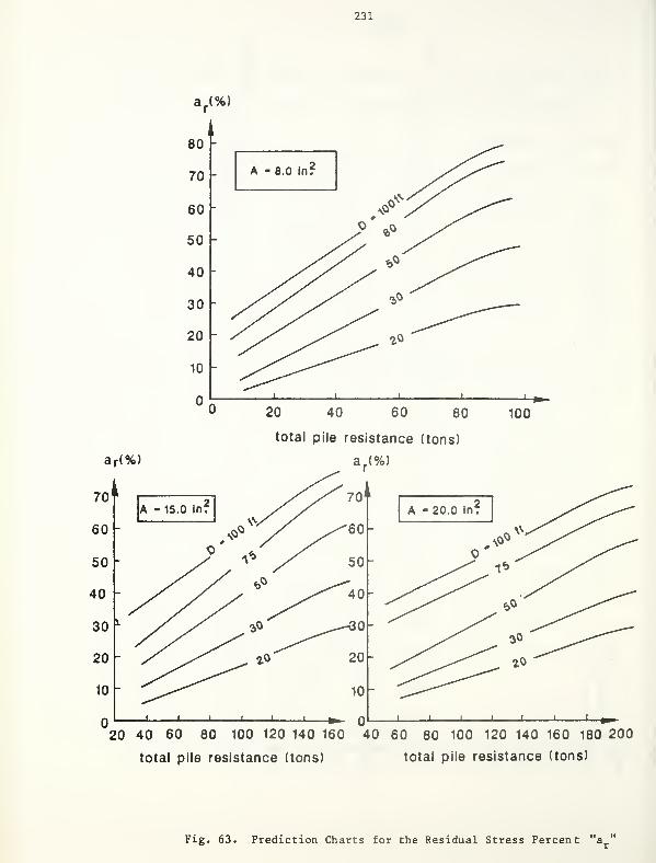
231
a r (%)
20 40 60 80
total pile resistance (tons)
100
20 40 60 80 100 120 140 160 40 60 80 100 120 140 160 180 200
total pile resistance (tons) total pile resistance (tons)
Fig. 63. Prediction Charts for the Residual Stress Percent rta '
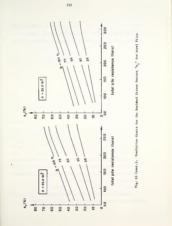
232
#
ooCO
oW ^^CM (A
Co****
<DO UO cC\J a
wwQ)k_o
in a>~a._
_
CO•*—
ooo
o o o o o o oCO t*. <0 m <* CO CM
m
00• --
o o o o o o o00 N (O m * CO CM
233
given in Fig. (64). If the value of "a " at m « 40% is obtained
from the charts given in Fig. (62) and (63), the value of "a " atr
any other value of "m" larger than 20% can be obtained from the
relation :
(a ) - B * (a > (m>20%) (4-13)r m m r 40%
If "m" was less than 20%, the actual value of "a " can be
obtained from the relation:
(a ) = 0.6 * 6 * (a ). n . (m<20%) (4-14)r m m r 4U /.
Two situations can be expected during the design stage of
the pile foundations:
1. The total pile capacity (Q ) , the load carried by the pile
point (Q ) and the load carried by the pile shaft (Q ) areP s
estimated by a reliable procedure, which does not take
residual stresses into account.
2. Load test data on an instrumented pile were available, pro-
vided that the instrumentation was zeroed after the pile
driving so that the residual stresses could not be meas-
ured .
The determination of the residual point load Q is somewhatP R
different for these two situations:
234
Situation No. 1
The charts given in Fig. (62) and (63) are entered with the
available pile data to get the value of "a " at m - 40%. Then
Fig. (64) and Eq. (4-13) or (4-14) are used to obtain a at the
expected value of m. The actual value of E should also be
accounted for as explained earlier. Thus, Q can be calculatedr R
f rom:
QPR 100 * Qp
(4-15)
After Q is obtained, the distribution of the residual load
along the entire pile shaft can be determined as explained ear-
lier.
Situation No. 2
:
If a load test has already been performed on an instrumented
pile, and it is required to obtain the residual forces for a
better interpretation of the results, a different procedure
should be followed. This is because the skin friction percent
that is obtained from the load test results represents the meas-
uVed value of the shaft friction force which was affected by the
existence of the residual stresses. The one used for developing
the prediction charts, however, assumes the existence of no resi-
dual stresses. This means that the value of "m" is affected by
the residual stresses as well as affecting them. Therefore, an
iterative process is essential to get a good estimate about both
235
"m" and a .
r
It is known that the measured value of point load is'
Pm
actually given by:
Qp
" QPR(4-16)
where Q is the true point load with no residual stresses and Qp PR
is the point residual load. The value of Q can be expressed as
a fraction of Q„ in terms of "a ", and hence:xp r
!
p" % " Too * % (1 "To^ % (4 " 17)
QPR=
[Ttt' f ° 7W)] % (4-18)
Q n „ - A * QyPR r xp
(4-19)
where
1 + A(4-20)
Therefore, the procedure for getting Q should be as fol-r K.
lows
236
10 20 30 40 50 60 70 80m(%)
Fig. 64. Factors 8 and B1
m m
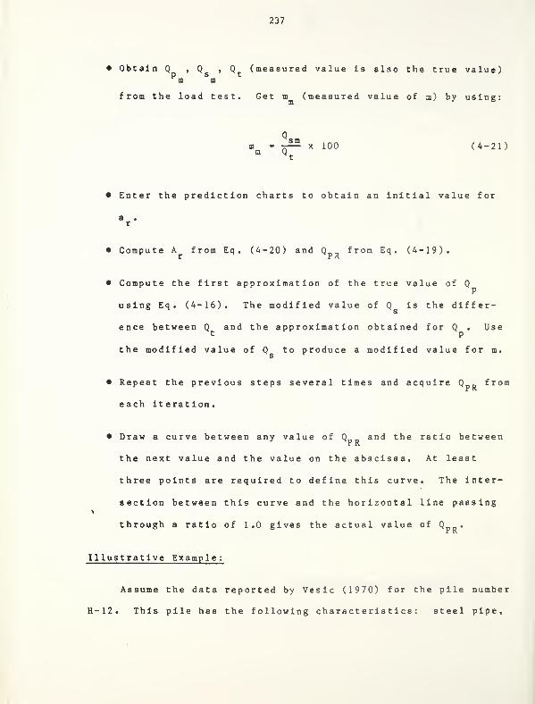
237
Obtain Q , Q , (5 (measured value is also the true value)p s tm m
from the load test. Get m (measured value of m) by usingm
m - -!» x 100m Q
(4-21)
Enter the prediction charts to obtain an initial value for
• Compute A from Eq. (4-20) and Q from Eq. (4-19).r PR
• Compute the first approximation of the true value of QP
using Eq. (4-16). The modified value of Q is the differ-
ence between Q and the approximation obtained for Q . Uset P
the modified value of Q to produce a modified value for m.
• Repeat the previous steps several times and acquire Q fromP R
each it erat ion
.
• Draw a curve between any value of Q and the ratio between
the next value and the value on the abscissa. At least
three points are required to define this curve. The inter-
section between this curve and the horizontal line passing
through a ratio of 1.0 gives the actual value of Q PR'
Illustrative Example
Assume the data reported by Vesic (1970) for the pile number
H-12. This pile has the following characteristics: steel pipe,
238
d - 1.5 ft, D - 20.1 ft, A - 27.49 in fe (modified for the effectB
of the instruments, after Briaud et al., 1983), E 30,000 ksi.
The values measured from the load test were: Q «= 232 t, Q «
m
173 t, Q =59 t, which means that m » 25. 4%. The charts givens m
in Figure (62) indicate that a for m - 40% equals 22%. Figure
(64) indicates that 6 = 0.7, hence a - 0.7 x 22.0 - 15.4%.m r
Therefore
Ar = 100-15.4
= °' 182
and
QPR= A
r* Q
p " °' 182 X 173 " 31 ' 5tm
The first approximation for Q is (173 + 31.5) = 204. 5t
Repeating the previous steps results in the following
results :
Q = 204. 5t * Q = 27. 5t * m = 11.9% ->• a - 7.7%^p s r
> Ar
- 0.082 > Q pR= 14. 3t
Q - 187. 3t * Q = 44. 7t + m » 19.3% + a - 12.9%p s r
A = 0.148 + Q OD = 25. 7tr XPR
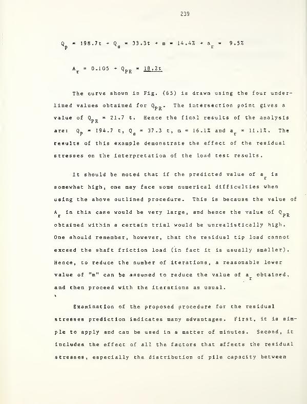
239
Q « 198. 7t + Q - 33. 3t + m - 14.4% + a - 9.5%xp s r
A = 0.105 Q nD = 18. 2tr PR
The curve shown in Fig. (65) is drawn using the four under-
lined values obtained for Qr,,,. The intersection point gives a
value of Q 21.7 t. Hence the final results of the analysis
are: Q n - 194.7 t, Q - 37.3 t , m - 16.1% and a * 11.1%. TheX
P 'xs r
results of this example demonstrate the effect of the residual
stresses on the interpretation of the load test results.
It should be noted that if the predicted value of a isr
somewhat high, one may face some numerical difficulties when
using the above outlined procedure. This is because the value of
A in this case would be very large, and hence the value of Qr PR
obtained within a certain trial would be unrealis t ically high.
One should remember, however, that the residual tip load cannot
exceed the shaft friction load (in fact it is usually smaller).
Hence, to reduce the number of iterations, a reasonable lower
value of "m" can be assumed to reduce the value of a obtained,r
and then proceed with the iterations as usual.
>
Examination of the proposed procedure for the residual
stresses prediction indicates many advantages. First, it is sim-
ple to apply and can be used in a matter of minutes. Second, it
includes the effect of all the factors that affects the residual
stresses, especially the distribution of pile capacity between
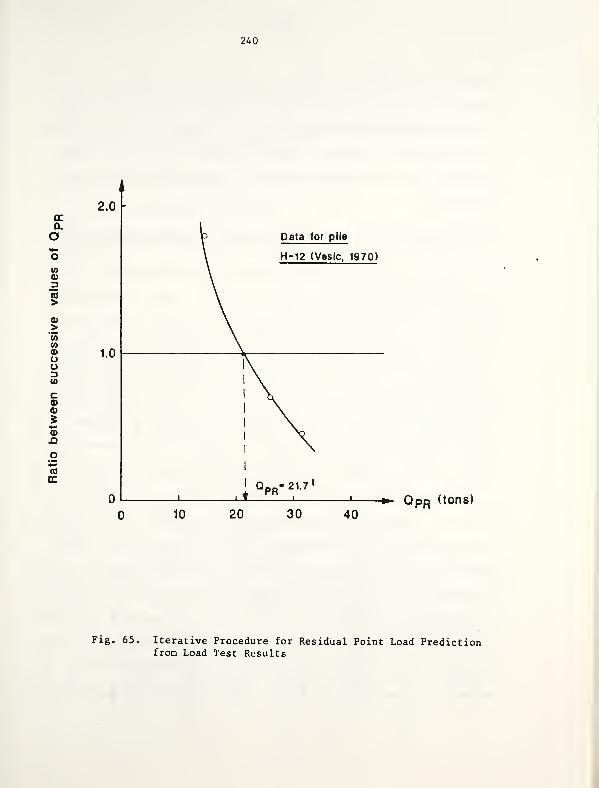
240
CL
O
wa>3CO>
a>>'53
COa>ooD(0
c©
*-Q>.Q
C5
Data for pile
H-12 (Veslc, 1970)
QpR (tons)
Fig. 65, Iterative Procedure for Residual Point Load Predictionfrom Load Test Results
241
point load and side friction. And finally, it does not depend on
results of any in situ tests that may have many uncertainties,
like the standard penetration test. The final step is to compare
this method with available field test data and with the other
procedures that have been proposed for the residual stresses
p redict ion .
A. 5. 5 Comparison of Proposed Procedure with Other Techniques:
The different procedures that have been suggested for the
residual stresses determination, including direct measurements,
were used to compute these stresses for different piles with
available load test data. Table (19) shows the data of the
instrumented test piles that could be located in the literature
such that residual stresses could be predicted by one or more of
the available prediction techniques. These data were used to
predict the tip residual forces for the piles using several pro-
cedures. The methods used were: the direct measurements of the
tip residual load by means of load cells zeroed before driving
the pile, the Hunt er-Da vis s on procedure, the Holloway procedure
(two predictions were made using this procedure, one by using
actual static test measurements and the other by using the static
load test results predictions made by Holloway et al . , 1975), the
Briaud-Tucker procedure and the procedure recommended during the
course of this study. Table (20) summarizes the values of the
residual stress percent "a " obtained by the different pro-
cedures. It can be noticed that the number of values obtained by
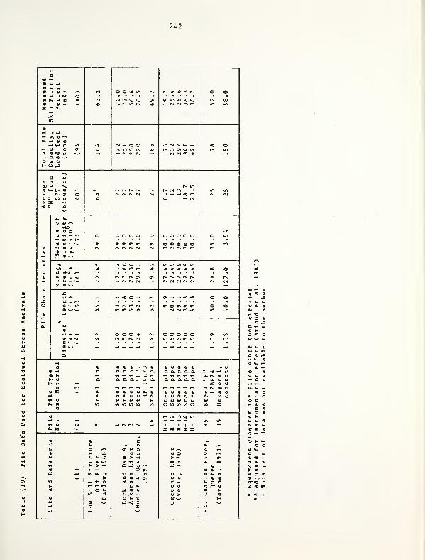
242
c
•D «H01 u uhUC3 -H 0) ^ ^ CM O O ^o *n r** r- -o- •£> m f«* o oCO 1* O M O • • • • • • • • • • • • •
o u. u e — en CM CM s£> O Cfi 0> tA 00 CD CD cm ao0> 01 w ^ sO vO —« CM CM m en tn »n
X s ft.
jrf
CO
01
fH * *J
rl >s (0^ft. 4J 01 OQ
H H C ^ •3" CM —• 00 O in -fi N N h* —
«
CO OfH O O t* **• Mn ui n 10 n n ty> -j r»4 r-» into aj *o w '—
'
— M M N CM CM ro <T•-' a to ^o to
H CJ J^-,
S u01 y-.
bO b ^ f^- in<0 vm H at y-\ f |-^ r-* I-- r-. r-. rs. n n • • m tnWi ft. 3 ao ca CM CM CM CM CM • —< -- CO m CM CM0) r w o -^ B iO —
1
CM> z ^< S J3w
**-. >>O U '-s
»-iO
(COO -3-
3 -H — ^ O o o o o O o o o O O O er»-h U X r** • • • • • • • • • • • • •
3 M-^^ O Q\ C71 0> CX* cr> o o o o o in en00 T3 fl 01 CM CM CM CM CM n n n r^ m enu o ^ a.*4 r ai wCO * in n vO vfi n cm ON ON ON a av
w UK *"» ^D -- cc n n \D ^3- -C1 <• -3 -j GO c
h Ot ATM '"v • • • • • • • • • * • • •
Q) oo at c vo CM s n n ^ Cr r^ r*. r* r^ r- •-< r^4J • t ^ w CM —- CM CM CM — CM CM CM CM CSl CM CMCJ X « w —14 XCO 4J *^v «oo o - r^ a^ r r> r-i o oX Bt W^ • • • • « • • * • • • • •
<J c ^m u"\ to n n fs CM c^ o <7* Ov C^ o oat w w «* %f\ U"> lA in tn CM CM r-i •flf >C ^C
at -J
•H «ft. h
01
u .-\^-». CM O O O -3- CM o o o o o 0> in0» w <j -tf n in n n -J »n m O OB m w • • • • • • • • « •
« w¥«
a^Cfl at at at at - m a> at at at a> 0) h at
at <h a D. CL Q.= r- o. a a a a a : <j- h 4J
a u •H >H -H X X •* •* <H -m x r» to at
>> at a a a a: <r Cl a. a a a a r a. c uH *j ^ pm pa o u
(0 en r-* i—1 r-1 i—t i—
1
^-t -—^ .—i—
i
f-< ^H H CM M cat r w at at o> at at ft. OJ at ot at Cv 0) at — to ofH at at at at at x at oi at at at a; at x cj
«H 13 u It U it u 4-1 ij i-i *~> i_i u 4-i at
ft* C CO « w W w in t/3 tyj « CD w « x03
0) -m cm en -J »n«H • *-\ sO in »aH O CM m h NC1K I I I 1 1 x ->o* z w XXX X X
0) 0) cu L. o u ^^c 3 ^-s sr w a »- ^-s at -.O) u 00 at w 01 o > r^Wt O U \0 B > -h > r^ •H CT»
01 3 at o t0 -H > •H 0*n a: —Mh u > ~- O Pd f0 *—. a; — CJ
01 ^ 4-1 -h a cr- 00 0) •OL — W erf - "O W vO at - at A toW 3 c to -a o> at u H U IB
•D fH •b o It Ul —. x -^ tr 3 CC H ~t i—
t
c t- U CO « a ai
to rt o ^ ^ to at oj at j= >V) 3 O M 4J o> > u a
0) fcu *- c t»c s^ HU 3 -w- J < 3 O • w•H O X UCO •J *** Ul
1* p«4 U.
« o
3 4-1
U CJ 3U. m-rH o(J 3 4J
a ^c -H *-»
u i_i HI
V u ~H
JZ 0J J^*- CO
U-i ^^
11 «H
<0
01 c >.—
t
o^H -^
a u 4J
1C
^ co BIM a. »
e (D
h 3 3II uU ij ffl
•1 m u8 c oO w TJ
v4o 1- U-i
OU U-.
c t->
01 -a 1-
rH 01 !0
m 4J a> U)
•r* 3 gl
3 -^n H0"T3 -C
Ul < H
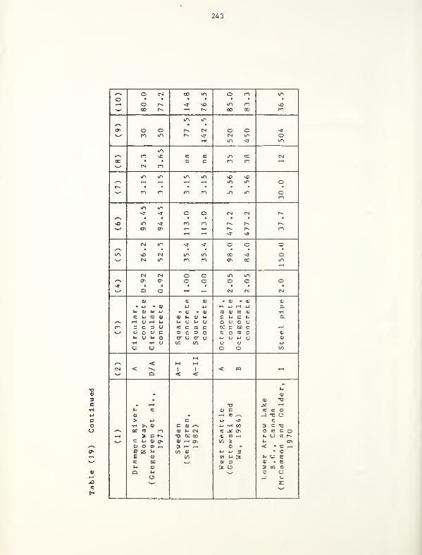
243
/^ o CM 00 u-i o m ino •
•—I o r-» «tf N40 m cn vO^^ 00 r-- — r-» 00 00 n
m U1/"N • •
o> O O t~~ CM o o ~3^^ en m r-~ -3 CM
U-l
m-3
om
u-i
/-*\ n %c CO CO in 00 CM00 • • c C co CO ~iw CM en
LTl m LO inm in o
r^ • • • • • • •
^^ m en r^ CO m m or-i
in u-i
-3 -3 C O CM CM r^/s •
v£> m <T m cn 1^ i~^ r^">-/ <y ffv ~
~~*
~3 -3cn
CM in <j ~3 o o C/-N •
in sC CN m LO 00 -3 O^^ cm u-i cn o~i ON 00 in
CM CM O O m in•"N C ON C O o c O<r •
s-^ o O —
'
—
<
CM CM CM
01 0i 01 . Q) « OJ 01
ft 4-1 . 01 u 4-1 >—1 4J <-\ 4-1 D-
>- 0) u 4-1 OJ . 4) CO Oi CO 01 Hre kl CO 0) 01 U 01 l-i c w c u a.
^v H o -H Ij u CJ t-l <J o o O Vm 3 c 3 O re c «J c oc c bo c ^H*-• CJ O C 3 c 3 o CO O CO o 0>
U o h O cr u a- o 4-1 O 4-1 O 01
•H •H O CT. to O u 4-1
cj> U o o cn
>-i
/""N < (—1 i-i
CM < -^.1 1 < CQ _
i
N^ a < <
t-i
»• 01
• 0J •vft t-i T3 >' tHu CO 01 C CO CO o01 - i-( CO •"N J T) O> 4-1 c 4-1 -3- CO
H >^ 01 c o ^N U -H 00 s C t3/-N oi ro ct 0> b CN CO _* ON o CO c o>H 5 c r-~ •o b£ oo a> to -H M O co r-N^ c l-i 0) on 01 rH ON c/j 3 *-i ON
4) O CO —
.
s ^ ^H O * <: •> c —E z Ij cn 01 4-> 4J 3 • oE 0> oo CO t-i 3 h O Em oc ^-' 01 3 0> • Eu 01 3 O 3 BQ CO
a s-^ OJ U
s:
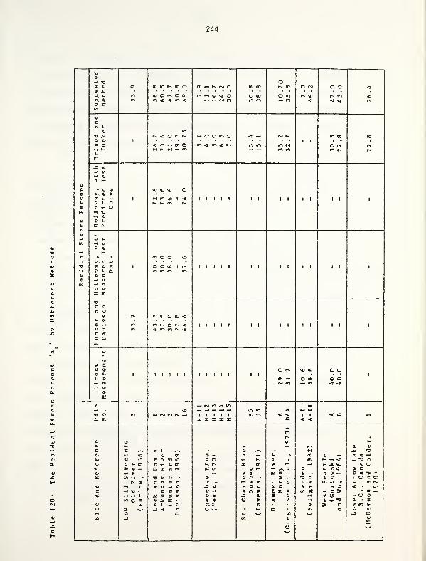
244
•oOi
4J -D otr C0' Xbe u
e OC m f- K C ff - S NC oc oc r~ in O CM c c -3
m -i o t^ O On CM ~- »£> -3 © O 00 o m r«. *c r^- en >C(X o> m in sC •s m -a — — cm cn en en — en -9 -a -» CM3 T.
C/5
ccIC l-
01 in
3 U I
r- >£ C en c- — come 3 — cm r-
1 1
in oc CC
ic r> *3 en -o>o m -3 m >c r~ en m m cm O r^ CM~< H CM CM cm — en P4 M en en en cm CMIh
pe
X *-l
4-1 CO
H 01
3 Huc - •C OJ OC «c vc O01 >-, 0> > • • • •
o re 4j k I CM Cn vC 1 -3 1 I I I 1 1 1 I 1 1 1 I I 1
t- 3 O S r-* r~ cn r**
01 C -H u0-
i-l oK O 1-
0)
oi
U
X 0-
X4-1 *J —CC H 0)
3 c.
~H Hre •> CC c- C C vC3 ^•c 4J • • • •
•c re o re l o c CC 1 f- 1 I I I 1 1 1 1 1 1 1 1 I 1
•*H 3 i- C in in cn in(0 301 i-h KOC -I re
O 01
x rT3C Cre c
cc
l- cr.
01 -rf
r* If in Ccc<r
rn en r^ C r^ -31 1 1 1 1 1 1 1 1 1 1 1 1 1
4-' > m <j cn n cm cc re
s ox
4J
C01
4J Ecj o> © r^ \C oc O OC 1-
I 1 1 1 1 1 I 1 1 I I 1 1• • • • • •
1
I- 3 o- — C 00 c ort ID cm en — cn •a •»es re
01
s:
01 —< cm en *j in h**—« • ie — *H •-« — — m in < l-t t-t
H O m —' CM WN - 1 1 1 1 1 x *-> < -~ 1 1 < CO M
C 2 X X X X X Q < <
cnr--
0> 1/ cr- Uo u u M ^^ 01 0J
c 3 *—
^
<r »- ,-^ k. 01 ^N M CM rf x1 4J OC 01 cr- Cv ^~, > — ll > tt 0) /-» re re —
I
ki V vC E > •o vC > o •** r^ 01 • er> — »4 ~» J "O o0J r i- a re —
i
c a ^ r^ cc c > -H *4 41 ^ K re t;It. c c — C DC re — a: er- tj — — ^ re c (j er er> 3 c01 4J > »N ic oi a. re 01 » re 3 — o re -c <-«
OC t/3 »H - TJ CC u . 01 0) X • 3 4J •o c 01 o M O c CK 3 c re c 0> > —i oi ec c u oi 01 01 W 41 • u « r-
T3 iH O CO cc 4-1 O X u U 3 CO 01 o » »- l- 3 < - e.C -H -O —
l
c c a «J -rt e o c E z c w be *-> 3 S • c —re —. — c- .i' re 3 CO U n X 01 E 01 i—
i
<r. o u o ow c 3 tv M X -H 01 01 (J > eo cc i—
i
0i >^ "C Oi . E01 U. C 1- ^ > bt > re u u V a c 3 CO E4-1 3 >— J < re O w H o cu EC CO o re
H O o 4-1 w H y.' - uCO J c/: 01
u
uE
245
direct measurements is quite limited, which makes it difficult to
evaluate the various prediction techniques. It is of extreme
importance to perform load tests on driven piles in which the
instrumentation is zeroed before driving, at least for research
purposes. Reliable instruments should be developed such that
they are not affected by the driving process and hence can give
reliable measurements for residual stresses.
Figure (66) shows the relationship between the predictions
made by the procedure recommended in this study and actual meas-
urements taken for the residual stress percent, either measured
directly or obtained indirectly by the Hunt er-Daviss on method.
The comparison with the direct measurements (given by solid
points) indicates a very good agreement, except for one data
point reported by Gregersen et al., (1973) for pile number A. A
careful look at the data, however, shows that the measurements of
a for piles (A) and (D/A) are quite similar, although the second
pile is twice as long and was driven to about 67% higher resis-
tance than the first one. This discrepancy suggests that the
measurements for pile "A" may not be correct, especially since
the measurements for pile (D/A) were in good agreement with the
prediction. On the other hand, some differences can be observed
between the predictions and the indirect measurements obtained by
the Hunter-Davisson procedure. Two piles showed good agreement,
while four piles indicated predictions which are generally higher
than the indirect measurements. As mentioned earlier, there are
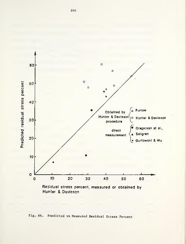
246
cO»-
o>
a.
mv>a>
'55
0)
"D<D
Obtained by I*Fur,ow
Hunter & Davisson\ Hunter & Davissonprocedure L
direct fGre9ersen et al -
measurement (* Sellgren
[• Gurtowskl & Wu
10 20 30 40 50 60
Residual stress percent, measured or obtained byHunter & Davisson
Fig. 66. Predicted vs Measured Residual Stress Percent
247
several limitations for the Hunt er-Davisson procedure. On the
other hand, the data for which this procedure was used were based
on measurements made during the 1960's while the direct measure-
ments were made in the 1970's and 1980's. This suggests that the
instruments used for the direct measurement were more reliable.
Based on this discussion, one may conclude that the suggested
prediction technique is in good agreement with the actual meas-
urements, and can be used reliably for predicting the residual
stresses. More tests, however, need to be performed to gather
more data of either direct or indirect measurements of the tip
residual stresses so that more comparisons could be made.
Figure (67) shows the comparison between all available tech-
niques for obtaining residual stresses, relative to the method
suggested in this study. The first observation that can be drawn
from this figure is that the suggested prediction gives the
closest values of "a " to the direct measurements. Next come ther
values predicted by the Holloway procedure, if the actual static
load test results are used. As mentioned earlier, the basic idea
of the predictions made by Holloway et al., (1975) and by the
suggested method is the same. However, the wave equation model
used for this study is superior to the one used by Holloway. On
the other hand, if the static load test results were predicted by
the computer program "DUKFOR" , rather than being directly meas-
ured, the prediction based on the Holloway procedure was not very
good. This is attributed to the large approximations used in the
248
4 i
D Briaud and TuckerA
A *
70 O
A
Holloway et al., (measured test)
Holloway et al., (predicted test)
Direct measurement
60• Suggested method
50 -
00
-oO+-=
<D
E
40
D f
A A* A
O
-»-)
O>»
X)<D<-<
O
0)J-
re
30
20
10
n
D /
y a
A /
/ °
/ D
/ o
A X/ D D
1 . L _. .. .... > ... i
D
D
DD
i
DD
1 ta.
10 20 30 40 50 60
*ar
" predicted by sugaes+°H "i*+hnd
Fig. 67. Comparison between Different Methods for ResidualStress Prediction
249
analyses performed by Holloway et al., (1975,1978) regarding the
soil-pile model (using the transfer function approach). Finally,
the values obtained by the Br iaud-Tucker technique were quite far
from the other predictions, as well as from the direct measure-
ments. They generally tend to be lower (i.e. this method
underestimates the residual stresses). Several discrepancies can
be observed in Table (20), e.g. the predictions for the Ogeechee
River piles were not very sensitive to the variation of the pile
length and the soil resistance as the recommended procedure was.
As mentioned earlier, there are so many disadvantages and
shortcomings for this procedure that it may be misleading to use
it for predicting the residual stresses.
4 .6 Summary and Conclusions
The residual forces were obtained below the pile tip and
along its shaft for piles driven into cohesionless soils using
the wave equation approach. The following results and conclu-
sions were obtained from this analysis:
1. The existence of residual stresses due to the pile driving
process affects both the static behavior and the drive-
ability of the pile. Although the total pile capacity should
be the same, the distribution of this capacity along the
pile shaft and below the tip may change considerably due to
the existence of the residual stresses. This change has an
effect on many aspects of the pile foundation design (e.g.
250
settlement, negative skin friction, etc.). On the other
hand, the existence of residual stresses facilitates the
driving procedure. In other words, higher resistance can
be reached with a smaller number of blows. In the mean-
time, the driving stresses may increase by about 5% on the
average (up to as much as about 15%) due to the existence
of the residual stresses. Hence, it is of extreme impor-
tance to include these stresses in both static and dynamic
analyses of the pile.
2. The general shape of the residual force distribution along
the pile shaft does not vary, irrespective of the variables
involved in the problem. Only the magnitude of these
forces changes, according to the variations in the dif-
ferent parameters. This distribution indicates the
existence of a negative friction for the upper portion of
the pile, down to a critical depth "Z ", below which therecr
is as upward residual friction load, in addition to the
residual tip load. This study suggested values for shape
factors, b , b , and b , by which the shape and the magni-r c m
tudes of the residual forces along the pile shaft for piles
in cohesionless soils can be approximately determined, pro-
vided that the residual tip load is known.
3. The study showed that the main factors that affect the mag-
nitude and distribution of residual stresses are the total
soil resistance, the percentage of load transferred by
251
shaft friction, and the pile material, length and cross
section. The effect of the driving system and driving com-
ponents is minor. It was found that residual stresses
increase as the total soil resistance Increases, as the
percentage of load carried by skin friction increases, as
the pile length increases and as the cross sectional area
decreases. The pile material greatly affects the residual
forces. As the pile modulus of elasticity increases, the
residual stresses decreases holding other parameters con-
stant .
4. This study led to the development of easy-to-use charts for
the residual stresses prediction. It was felt necessary to
develop such a procedure for many reasons. First, it is
not a common practice to perform pile load tests at the
design stage on instrumented piles, for which the instru-
mentation is zeroed before driving. This means that resi-
dual stresses cannot be obtained. Approximate procedures
used for that purpose, e.g. the Hunt er-Daviss on procedure,
make simplifying assumptions that can lead to incorrect
determination of the residual stresses. The difficulty of
obtaining residual stresses from pile load tests could be
overcome by using the wave equation analysis for their
predictions. Computer programs like "DUKFOR" and "CUWEAP"
have proven to be successful in this respect. However, they
require the availability of both the software and the
252
hardware necessary for their operation, which costs both
time and money, limiting their use in the everyday prac-
tice. A prediction technique suggested by Briaud and
Tucker (1984-b) was based on the average value of the
number of blows/ft obtained from the Standard Penetration
Test. Some important parameters, e.g. the skin friction
percentage and the total pile capacity, were not taken into
account in this procedure. A large scatter was observed
for the data used to develop these correlations. Further-
more, the Standard Penetration Test results cannot be jus-
tified for use in predicting deformation characteristics of
the soil, in addition to all the uncertainties associated
with this test. For these reasons, the method suggested in
this study, which is based on an improved wave equation
analysis, provides a simple approach for predicting resi-
dual stresses for driven piles.
5. Comparisons of actual field measurements with the various
prediction techniques showed that the author's suggested
method gave predictions which are the closest to the meas-
urements. These actual measurements, however, were very
limited in number. It is recommended that more load tests
on instrumented piles, for which the instrumentation is
zeroed before driving, be conducted. The results of these
tests can be used for more comparisons with the suggested
prediction. It is of crucial importance to develop reli-

253
able instruments for this purpose, so that they will not be
severely affected by the driving process.

254
CHAPTER 5
SUMMARY AND CONCLUSIONS
This report was prepared to complete the study "Computa-
tional Package for Predicting Pile Stress and Capacity." While
the interim report (Tejidor, 1984) described the analytical
determination of pile capacity by means of the computer program
"PPILE," this report deals mainly with both static and dynamic
load testing. These tests provide the best evidence of pile
capacity and serve as a reference of accuracy for other load
prediction techniques.
5.1 Summary :
The main objectives of this study were:
1. To emphasize the importance of performing pile load tests
for obtaining the most valuable and accurate data for the
design of pile foundations.
2. To present the state-of-the-art of pile load testing,
regarding the equipment used, the instrumentation, the
testing procedures and the interpretation techniques.
3. To recommend quick, inexpensive methods for pile testing by
IDOH for the sake of minimizing the costs without
compromising the data obtained.
255
4. To familiarize the IDOH with the state-of-the-art of per-
forming dynamic measurements during pile driving, to
briefly illustrate the theoretical background behind their
use and to show the potential uses of these measurements.
5. To study the subject of residual stresses due to driving,
since they greatly affect the interpretation of static load
tests, as well as the mechanism of load transfer, and to
develop a simple approach for the prediction of such meas-
urements .
6. To develop a simplified procedure to account for the
existence of negative skin friction and to compute the
resulting additional loads.
5.1.1 Static Pile Load Tests:
The importance of routine performance of pile load tests,
even for small scale jobs, was emphasized in the report. Plan-
ning the testing program and the application of test results were
discussed. Emphasis was given to axial compression load tests,
although other forms of tests, e.g. lateral, uplift and torsional
testing, were described. For each type of test, the state-of-
the-art information about the following items was given: the
loading systems; the measurement of pile movements; the potential
sources of error; and the available testing procedures with the
interpretation of their results. For axial load tests, the fol-
lowing methods were described: the maintained loading tests
256
(ML);; the constant rate of penetration test (CRP); the method of
equilibrium; and the Texas Highway Department quick testing
method. It was shown that the use of quick load testing tech-
niques correlates well with the traditional time-consuming
methods, besides having the advantage of being much cheaper,
which justifies their routine use for all types of jobs involving
pile foundations. Based on these studies, recommendations were
made to the IDOH regarding the procedure of performing pile load
tests.
5.1.2 Dynami c Measurement s for Pile Driving :
Another type of pile testing involves the use of dynamic
measurements during pile driving. These techniques are the best
ones introduced thus far for monitoring the pile during driving.
They can be applied, together with the wave equation analysis, in
a variety of ways. Among their uses are pile capacity predic-
tions; the evaluation of the driving system with respect to the
hammer efficiency and performance, cushions, capblocks, etc;
measurement of pile stresses; and the verification of the pile
integrity .
The historical background of equipment development was
described. The most recent advances for force, velocity and
acceleration measurements, together with the appropriate record-
ing devices were reviewed. A brief description of the theoreti-
cal background behind these measurements was given. Since the
257
purpose of discussing dynamic measurements in this report was to
familiarize the IDOH with the subject in an easy-to-follow
manner, some of the complicated mathematical derivations and
expressions were omitted to help simplify the subject.
Dynamic measurements have been used to predict the geotechn-
ical pile capacity, either in situ using a field computer and the
approximate CASE method, or in the office using a more sophisti-
cated analysis (CAPWAP). The latter analysis can also be used to
predict the load transfer along the pile shaft and the load
deformation curve that would be obtained from a pile load tests.
Dynamic measurements have been also used to monitor driving ham-
mers; evaluate their efficiencies under different operating pres-
sures, strokes or batters; and to check the driving elements,
i.e., cushions, capblocks, etc. Finally, dynamic measurements
have been used to examine the performance of the pile, detect any
damage and evaluate the actual pile lengths if not known.
5.1.3 Residual Stresses Due to Pile Driving:
To obtain a better interpretation of the static load test
results, the report also discussed the subject of residual
stresses due to driving. The main factors affecting these
stresses were described. These factors were found to be the
total soil resistance, the percent skin friction, the pile
length, the pile cross sectional area and the pile material. The
methods that have been suggested thus far for the residual

258
stresses prediction were reviewed. The review showed that none
of the available methods can give satisfactory predictions.
Based on extensive parametric studies, a new procedure was
developed at Purdue for the prediction of magnitude and distribu-
tion of residual stresses. This procedure was introduced by
means of easy-to-use charts and nomograms, with the help of some
illustrative examples. Predictions made by this technique were
compared with actual measurements and good agreements were pro-
ven .
5.1.4 Negative Skin Friction :
Finally, a computer program PPILENF for the prediction of
additional pile loads due to negative skin friction was
developed. Because there are many uncertainties regarding the
available methods of predicting negative skin friction loads,
upper bound values were used to develop this program. Complete
listing of the program is given in the Appendix A together with
User's manual, input forms, and illustrative examples.
5.2 Conclusions :
5.2.1 Pile Load Tests:
1. Pile load tests are very useful, and sometimes essential,
in all stages of design and construction of pile founda-
tions. They should be routinely used to get better predic-
tions of the pile capacity and short-term settlement, and
259
hence to permit better design and avoid unnecessary costs
due to conservative predictions.
2. In order to minimize the costs involved in performing pile
load tests, quick load testing procedures have been
developed. Examples of these include the constant rate of
penetration test (CRP), the Texas quick load tests, and the
method of equilibrium.
3. It is recommended that the IDOH use either the quick load
test method or the method of equilibrium, depending on the
pile-soil system and the purpose of conducting the test.
In general, the quick tests method can be used for proof
testing and in the case where no settlement data are
required. If allowable settlement is the main design cri-
terion, the method of equilibrium should be used. Specifi-
cations for both methods were described in detail within
the report, together with illustrative examples.
5.2.2 Dynamic Measurements :
1. Dynamic measurements constitute a very efficient way of
monitoring the pile during driving.
2. The main quantities to be measured are the forces, dis-
placements, velocities and/or accelerations. These meas-
urements are usually taken at the pile top.
260
3. The main uses of dynamic measurements are the prediction of
pile capacity and load transfer, the evaluation of the
efficiency of the driving hammer and elements, and the
examination of the integrity of the pile to detect any pos-
sible damage.
4. The prediction of pile capacity by this technique is much
better than the use of a driving formula (e.g. ENR, Hiley,
etc.). On the other hand, it is not accurate enough to be
used alone without other techniques of pile design. This
is primarily due to the insufficiency of the soil model
used. The prediction by this technique, however, completes
the spectrum of pile design procedures and gives more
confidence in the other procedures, since it is based on
direct measurements during the driving process. On the
other hand, dynamic measurements have proven to be quite
successful in determining the wave equation parameters,
measuring the actual energy delivered to the pile, moni-
toring the driving process with all of its elements,
measuring the pile stresses and performing quality control
p rocedures
.
5. It is recommended that the IDOH acquire the equipment used
for dynamic measurements and prepare the required personnel
with the appropriate training. The savings that can be
achieved by using these measurements in several jobs would
very soon cover the price of the equipment. More
251
importantly, the improvement in design and execution pro-
cedures of the pile foundations which will not only save
money in the short term, but will also reduce the mainte-
nance and replacement costs that might have been otherwise
necessary in the long run.
5.2.3 Residual Stresses Due to Pile Driving :
1. At the start of loading, a driven pile, either in a static
load test or by the load coming from the superstructure, is
not stress-free as often assumed. Residual point and shaft
stresses accumulate during driving. Although the total
capacity of the pile is not changed, these stresses can
result in a substantial change in the mechanism of load
transfer between the pile and the soil, and consequently
the settlement of the pile group. The observed tip load is
lower and the observed shaft friction is higher than the
true values.
2. The existence of residual stresses affects the driveability
of the pile. Higher resistance can be reached with a
smaller number of blows. In the meantime, the driving
stresses may increase by about 5% on the average, (to as
much as about 15%) due to the existence of residual
stresses. Hence, it is of extreme importance to include
these stresses in both static and dynamic analyses of the
pile.
262
3. The general shape of the residual force distribution along
the pile shaft does not vary, irrespective of the variables
involved in the problem. Only the magnitude of these
stresses change, according to the variations in the dif-
ferent parameters.
4. The magnitude of the residual loads Increases: as the total
soil resistance increases, as the length of the pile
increases, as the cross sectional area of the pile
decreases, as the elastic modulus of the pile decreases,
and as the percentage of load transferred by the shaft
friction increases. The effect of the driving system and
driving components is minor.
5. The available techniques for predicting residual stresses
are not satisfactory. Hence, a prediction technique based
on easy-to-use charts and nomograms was developed at Pur-
due. Comparisons of actual field measurements with the
various prediction techniques showed that the suggested
method gave predictions which are the closest to the meas-
urements .
5.2.4 Negative Skin Friction:
1. Additional loads due to negative skin friction can lead to
foundation failures if not taken into account in design.

263
2. Available techniques for predicting these loads are not
satisfactory and additional research is needed to overcome
this problem. Until this research is developed, it is
recommended that an upper-bound prediction be used for a
conservative design.
3. A computer program PPILENF was developed at Purdue to give
adequate prediction of additional loads due to negative
skin friction. It is recommended that the IDOH use this
program for the design of pile foundations in the situa-
tions where negative friction is involved. This will avoid
serious prediction errors and long term problems.
264
List of References
1. Alizadeh, M. and Davisson, M. T. (1970), "Lateral LoadTests on Piles - Arkansas River Project", J. Soil Mech. &
Found. Eng. Div., ASCE, Vol. 96, SM5 , pp. 1583-1604.
2. American Society for Testing and Materials (1981), "Stan-dard Method of Tests for Load Settlement Relationship forIndividual Vertical Piles Under Static Axial Loads (D-1143-81)", Annual Book of ASTM Standards, 1981.
3. ATEC Associates, Inc. (1982), "Installation Criterion forProduction Piles, Structure 10.2 and 10.5, Milepost 17 -
Gary East Interchange", 1980 Indiana Toll Road Improve-ments, Gary, Indiana, Project No. 21-22517. ReportPrepared for Reid, Quebe, Allison, Wilcox & Associates,Inc . , South Bend, IN.
4. ATEC Associates, Inc. (1983), "Installation Criteria for 12
in. Diameter Short Pipe Piles, Milepost 10, S.R. 912, SouthInterchange", 1980 Indiana Toll Road Improvements, Gary,Indiana, Project No. 21-22510. Report prepared for Reid,Quebe, Allison, Wilcox & Associates, Inc., South Bend, IN.
5. Baker, V. A., Thomsen, N. A., Nardi, C. R. and Talbot, M.J. (1984), "Pile Foundation Design Using Pile DrivingAnalyzer", Proc, Symp . Design of Pile Foundations, ASCE,pp. 350-372.
6. Bowles, J. E. (1982). Foundation Analysis and Design.McGraw-Hill, New York.
7. Bozozuk, M. (1970). "Field Observations of Negative SkinFriction Loads on Long Piles in Marine Clay", Proc. Conf.on Design and Installation of Pile Foundations and CellularStructures, Lehigh Univ., Envo Publishing Co., April, pp.273-279.
8. Bozozuk, M. (1972). "Downdrag Measurements on a 160-ft.Floating Pipe Test Pile in Marine Clay", Canadian Geotech.Journ., Vol. 9, No. 2, May, pp. 127-136.
9. Briaud, J. L., Tucker, L. M., Lytton, R. L. and Coyle, H.M. (1983). "The Behavior of Piles and Pile Groups in Cohe-sionless Soils", Report No. RD-83-38, Federal HighwayAdministration, October.
10. Briaud, J. L. and Tucker, L. M. (1984-a). "ResidualStresses in Piles and the Wave Equation", Proc., Symposium

265
on the Analysis and Design of Pile Foundations, ASCE,October, pp. 119-137.
11. Briaud, J. L. and Tucker, L. M. (1984-b). "Piles in Sand:A Method Including Residual Stresses", Journ. Geotech. Eng.Div., ASCE, Vol. 110, November, pp. 1666-1680.
12. Broms, B. B. and Silberman, J. (1964), "Skin FrictionResistance for Piles in Cohesionless Soils", Sols Soils,No. 10, 33 pp.
13. Buisson, M., Ahu , J. and Habib, P. (1960). "Le FrottementNegatif", Annales de l'Institut Technique du Batiment etdes Travaux Publics, Vol. 13, No. 145, January, pp. 29-46.
14. Butler, H. D. and Hoy, H. E. (1977), "The Texas Quick LoadMethod for Foundation Load Tes ting .. .User ' s Manual", FHWA-IP-77-8, FHWA, Wash., D.C., 53 pp.
15. Chellis, R. D. (1961). Pile Foundations. New York,McGraw-Hill
.
16. Chuang, J. W. and Reese, L. C. (1969), "Studies of ShearingResistance Between Cement Mortar and Soil", Research Report89-3, Center for Highway Research, The University of Texasat Austin, Texas, May.
17. Clough, G. W. and Duncan, J. M. (1971), "Finite ElementAnalysis of Port Allen Lock", Journ. Soil Mech. Found.Div., ASCE, Vol. 97, No. SM8 , August.
18. Davisson, M. T. and Stalley, J. R. (1970), "Model Study ofLaterally Loaded Pile", J. Soil Mech. & Found. Div., ASCE,Vol. 96, SM5, pp. 1605-1627.
19. Diaz, G. M., Patton, B. W. , Armstrong, G. L. and Joolazade,H. M. (1984), "Lateral Load Tests of Piles in Sloping RockFill", Proc. of a Symposium on Analysis and Design of PileFoundations, Published by ASCE, New York.
20. Endo, M., Minou, A., Kawsaki, T. and Shibata, T. (1969)."Negative Skin Friction Acting on Steel Pipe Pile in Clay",Proc. 7th Intern. Conf. Soil Mech. Found. Eng., Vol. 2,Mexico City, pp. 85-92.
21. Esrig, M. I. (1963), "Load Test on Pile in as Little as TenMinutes", Engineering News Record, Jan. 31, pp. 38-39.
22. Fellenius, B. H. and Broms, B. B. (1969). "Negative SkinFriction for Long Piles Driven in Clay", Proc. 7th Intern.Conf. Soil Mech. Found. Eng., Vol. 2, Mexico City, pp. 93-
266
98.
23. Fellenius, B. H. (1984), "Geotechnically Allowable Stressfor Driven Piles", Civil Engineering, ASCE, pp. 72-75.
24. Fuller, F. M. and Hoy, H. E. (1970), "Pile Load Tests,Including Quick. Load Test Method, Conventional Methods, andInterpretations", Hwy. Res. Record No. 333, pp. 74-86.
25. Furlow, C. R. (1968). "Pile Tests, Jonesville Lock andDam, Quachita and Black Rivers, Arkansas and Loulsana",Technical Report S-68-10, U. S. Army Engineer WaterwaysExp. Station, Vicksburg, MS
26. Garlanger, J. E. (1973). "Prediction of the Downdrag Loadat Cutler Circle Bridge", Symp. on Downdrag of Piles,M.I.T., Boston, March, 16 p.
27. Goble, G. G., Scanlan, R. H. and Tomko, J. J. (1967),"Dynamic Studies on the Bearing Capacity of Piles", Vol. 1
and 2, Case Institute of Technology, Cleveland, Ohio, July.
28. Goble, G. G., Tomki, J. J., Rausche, F. and Green, P. M.,(1968) "Dynamic Studies on the Bearing Capacity of Piles -
Phase II", Vol. 1 and 2, Report No. 31, Case WesternReserve Univ
.
29. Goble, G. G., Moses, F. and Rausche, F. (1970), "Predictionof Pile Behavior from Dynamic Measurements", Proc. Conf. onDesign and Installation of Pile Foundations and CellularStructures, Lehigh Univ., Pa., pp. 281-296.
30. Goble, G. G. and Rausche, F. (1970), "Dynamic Measurementsof Pile Behavior", Proc, Conf. on Design and Installationof Pile Foundations and Cellular Structures, Lehigh Univ.,Pa. , pp. 165-171 .
31. Goble, G. G., Kovacs, W. E. and Rausche, F. (1972), "FieldDemonstration: Response of Instrumented Piles to Drivingand Load Testing", Proc Specialty Conf. on Performance ofEarth and Earth-Supported Structures, Vol. Ill, PurdueUniversity, W. Lafayette, IN, June.
32. Goble, G. G., Likins, G. and Rausche, F. (1975), "PileCapacity by Dynamic Measurements", Department of CivilEngineering, Case Western Reserve University, Cleveland,Ohio, March.
33. Goble, G. G., Fricke, K. and Likins, G. E. (1976), "DrivingStresses in Concrete Piles", Journ. of the Prestressed Con-crete Institute, Vol. 21, No. 1, Chicago, Illinois, Jan.-
267
Feb. , pp. 70-88 .
34. Goble, G. G. and Rausche, F. (1976). "Wave EquationAnalysis of Pile Driving, WEAP Program, Vol. 1 - Back-ground, Vol. 2 - User's Manual, Vol. 3 - Program Documenta-tion", U.S. Dept. of Transportation, FHWA, Off. of Res. andDev., Vol. 76-14.1-76-14.3, Washington, 389 p.
35. Goble, G. G. and Hauge, K. (1978). "Comparative CapacityPerformance of Pipe and Monotube Piles as Determined byWave Equation Analysis", Piling Res Lab., Dept. of Civil,Env., and Arch., Eng., Univ. of Colorado, July.
36. Gregersen, 0. S., Aas, G. and DiBiaggio, E. (1973), "LoadTests on Friction Piles in Loose Sand", Proc. VII Int.Conf. Soil Mech. Found. Eng., Vol. 2.1, Moscow, pp. 19-27.
37. Gognon, J. M. (1972). "Measure In Situ du Frottement Nega-tif", Annales de l'Institute Technique du Batiment et desTravaux Publics, No. 293, May, 12 pp.
38. Gurtowski, T. M. and Wu, M. J. (1984). "Compression LoadTests on Concrete Piles in Alluvium", Symp. on the Analysisand Design of Pile Foundations, ASCE, October, pp. 138-153.
39. Hanna, T. H. (1973), "Foundation Instrumentation", Tran-stech Publications, Ae de rmansdor f f , Switzerland, pp. 35-66.
40. Hardin, B. 0. (1985). "Crushing of Soil Particles", Journ.Geot. Eng. Div., ASCE, Vol. Ill, No. 10, pp. 1177-1192.
41. Heijnen, W. J. (1974). "Penetration Testing in Nether-lands", ES0PT, Stockholm, Vol. 1, pp. 79-83.
42. Hery, P. (1983). "Residual Stress Analysis in WEAP", M.Sc. Thesis, Dept. of Civil, Eng. and Arch. Eng., Univ. ofColorado.
43. Holloway, D. M. (1974). "Pile-Soil Interaction in Cohe-sionless Soils", Draft Submitted for Review, U.S. Army Eng.Water Exp. Station, Vicksburg, MS, April.
44. Holloway, D. M., Clough, G. W. and Vesic, A. S. (1975)."The Mechanics of Pile-Soil Interaction in CohesionlessSoils", U.S. Army Eng. Water Exp. Station, Contract Rep.S-75-5.
45. Holloway, D. M., Audibert, J.M.E. and Dover, A. R. (1978)."Recent Advances in Predicting Pile Driveabi lity " , OffshoreTechnology Conf., 0TC 3273, May.
268
46. Holloway, D. M., Clough, G. W. and Vesic, A. S. (1978)."The Effect of Residual Driving Stresses on Pile Perfor-mance under Axial Loads", Offshore Technology Conf., OTC3306, May.
47. Hunter, A. H. and Davisson, M. T. (1969). "Measurements ofPile Load Transfer", Performance of Deep Foundations, ASTM,STP444, pp. 106-117.
48. Jain, G. S. and Kumar, V. (1963), "Calculations forSeparating Skin Friction and Point Bearing in Piles", J.Materials, Research and Standards, ASTM, pp. 290-293.
49. Lambe, T. W. and Whitman, R. V. (1979). Soil Mechanics -
SI Version. John Wiley & Sons, Inc., New York.
50. Leonards, G. A. (1972). "Settlement of Pile Foundations inGranular Soils", Proc. Spec. Conf. on Performance of Earthand Earth-Supported Structures, Purdue University, June.
51. Leonards, G. A. and Lovell, D. W. (1979). "Interpretationof Load Tests on High Capacity Driven Piles", ASTM Sympo-sium on Behavior of Deep Foundations, ASTM STP 670, pp.388-415.
52. Leonards, G. A. (1985). "Lectures on Pile Foundations - CE683", Purdue University, West Lafayette, IN.
53. Leonards, G. A., Alarcon, A., Frost, D., Mohamadzien, Y.,Santamarina, J. C., and Thomaz, J. (1986). Discussion ofthe paper "Dynamic Penetration Resistance and the Predic-tion of the Compressibility of a Fine Grained Sand — a
Laboratory Study", Geot echnique , Vol. 38, No. 2, pp. 275-279.
54. Likins, G. E. (1984), "Field Measurements and the PileDriving Analyzer", Proc., 2nd Int. Conf. on the Applicationof Stress Wave Theory on Piles, Stockholm, Sweden, May.
55. Mansur, C. I. and Hunter, A. H. (1970), "Pile Tests -
Arkansas River Project", J. Soil Mech. & Found. Div., ASCE ,
Vol. 96, SM5 , pp. 1545-1582.
56. McCammon, N. R. and Golder, H. Q. (1970). "Some LoadingTests on Long Pipe Piles", Geotechnique 20, No. 2, pp.171-184.
57. Michigan State Highway Commission (1965), "A PerformanceInvestigation of Pile Driving Hammers and Piles", FinalReport, Lansing, Michigan, March.
270
No. SM4 , August, pp. 35-61.
71. Stoll, U. W. (1972), "Torque Shear Test on CylindricalFriction Piles", Civil Engrg., ASCE, Vol. 42, No. 4, pp.63-64.
72. Tavenas, F. A. (1971). "Load Test Results on FrictionPiles in Sand", Canadian Geotech. Journ., Vol. 8, pp. 7-22.
73. Tejidor, F. J. (1984), "Computational Package for Predict-ing Pile Stress and Capacity", Interim Report,FHWA/IN/JHRP-84/16
.
74. Terzaghi, K. (1942), "Discussion of the Progress Report ofthe Committee on the Bearing Value of Pile Foundations",Proc. ASCE, Vol. 68, pp. 311-323.
75. Tomlinson, M. J. (1977). Pile Design and ConstructionPractice. London, Viewpoint Publications.
76. Van Weele, A. F. (1957), "A Method of Separating the Bear-ing Capacity of a Test Pile into Skin Friction and PointResistance", Proc. 4th Int. Conf. S.M. and F.E., Vol. 2,p. 76.
77. Vesic, A. S. (1977). "Design of Pile Foundations", TRB,
No. 42.
78. Vesic, A. S. (1978). "On Significance of Residual Loadsfor Load Response of Piles", Proc. IX Int. Conf. Soil Mech.Found. Eng., Tokyo, pp. 374-380.
79. Yazdanbod, A., O'Neill, M. W. and Aurora, R. P. (1984)."Phenomenological Study of Model Piles in Sand", Geot .
Testing Journ., GTJODJ, Vol. 7, No. 3, Sept., pp. 135-144.
80. Whitaker, T. (1957), "Experiments with Model Piles inGroups", Geot., Vol. 7, pp. 147-167.
81. Whitaker, T. and Cooke, R. W. (1961), "A New Approach toPile Testing", Proc. 5th Int. Conf. S.M. and F.E.
82. Whitaker, T. (1963), "The Constant Rate of Penetration Testfor the Determination of the Ultimate Bearing Capacity of a
Pile", Proc. Instn. Civil Engrs., Vol. 26, pp. 119-123.
83. Whitaker, T. and Cooke, R. W. (1966), "An Investigation ofthe Shaft and Base Resistances of Large Bored Piles in Lon-don Clay", Proc. Symp . on Large Bored Piles, pp. 7-49.

271
84. Whitaker, T. (1976).Oxford. Pergamon.
The Design of Piled Foundations
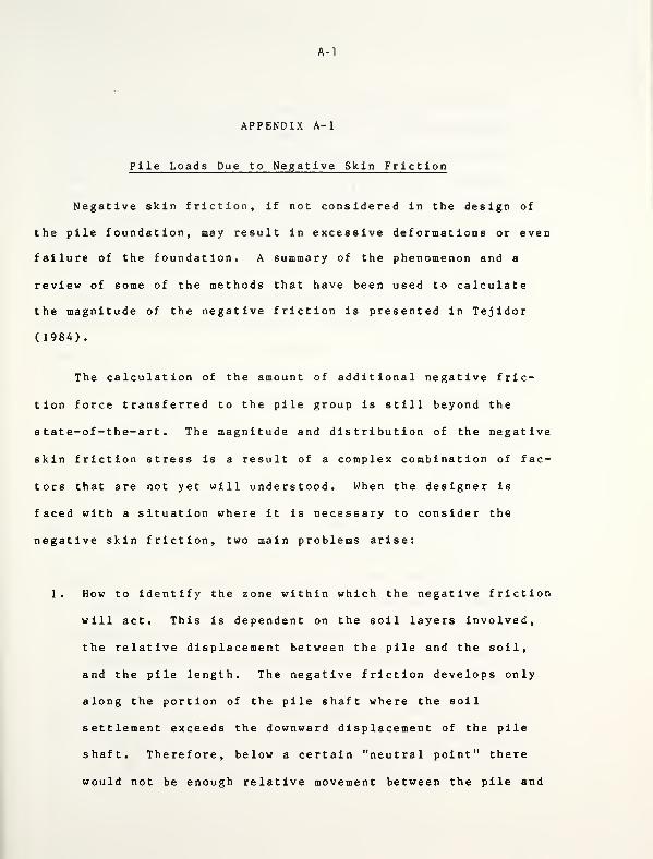
A-l
APPENDIX A-l
Pile Loads Due to Negative Skin Friction
Negative skin friction, if not considered in the design of
the pile foundation, may result in excessive deformations or even
failure of the foundation. A summary of the phenomenon and a
review of some of the methods that have been used to calculate
the magnitude of the negative friction is presented in Tejidor
(1984).
The calculation of the amount of additional negative fric-
tion force transferred to the pile group is still beyond the
state-of-the-art. The magnitude and distribution of the negative
skin friction stress is a result of a complex combination of fac-
tors that are not yet will understood. When the designer is
faced with a situation where it is necessary to consider the
negative skin friction, two main problems arise:
1. How to identify the zone within which the negative friction
will act. This is dependent on the soil layers involved,
the relative displacement between the pile and the soil,
and the pile length. The negative friction develops only
along the portion of the pile shaft where the soil
settlement exceeds the downward displacement of the pile
shaft. Therefore, below a certain "neutral point" there
would not be enough relative movement between the pile and
A-2
the surrounding soil and the friction remains positive. A
wide variety of positions was suggested for the location of
this neutral point (Buisson et al., 1970; Gognan , 1972;
Bozozuk, 1970; Garlanger, 1973; etc.). The uncertainty is
enhanced when the soil nature is relatively heterogeneous.
It is influenced by factors such as relative compressibil-
ity of the pile shaft and underlying soil with respect to
the surrounding soil, relative magnitude of axial load in
the pile with respect to the effective stress change that
causes settlement of surrounding soil, as well as the posi-
tion of the most compressible stratum in the overall soil
profile (Bozozuk, 1970; Buisson et al., 1960).
2. The second problem is the calculation of the magnitude of
the downward drag created by negative friction. Empirical
methods have been suggested (e.g. Bowles, 1982) as well as
theoretical methods based on the assumptions of the classi-
cal theory of elasticity (refer to Poulos and Davis, 1980)
These methods, however, are complicated, and the assump-
tions involved may not correspond closely to reality. It
should also be noticed that the magnitude of the negative
friction is dependent on the horizontal stresses that
develop in the long term (not just after driving). Some
methods account for this effect but they are uncertain and
not reliable (Leonards, 1985).
A-3
Due to the above mentioned problems, the only acceptable way
to include the effect of negative friction is to use upperbound
values. It should be noticed that the magnitude of negative
friction is limited by the ultimate shaft friction that can be
mobilized, and the magnitude of the forces causing the ground to
subside (weight of dry fill, ground water lowering, etc.).
Leonards (1985) recommended the following procedure to get
upperbound values of the amount of negative friction:
1. When the negative friction is caused by a dry fill layer,
which is susceptible to large future amounts of settlement,
the extra load that should be added to the original group
load is the effective weight of the fill that is confined
between two areas. The first one is the pile group area
and the second is the area obtained by a downward slope of
45 from the group area over the thickness of the fill
layer .
2. For the case of groundwater lowering (where the effective
weight of the soil increases) the additional load is the
Increase in the vertical effective stress times the area of
the pile group.
3. For the case of soft or sensitive clay layer subject to
remolding during pile driving or future settlement due to
loads transmitted from the piles, the additional weight is
A-4
the effective unit weight of the soil layer times the area
of the pile group times the height of the layer.
4. In some cases, a fill working platform is required to be
placed over the surficial soft layer to facilitate the
installation procedure. Negative friction may be expected
in this case due to the fill and the soft layer. The
upperbound load that should be added is the sum of the
loads calculated in steps (1) and (3).
It should be noted that for the case of battered piles, the
problem is so complex that it has not yet been dealt with in
research (Leonards, 1985). No technique has been proposed to
solve such a problem. Research is needed to provide even an
approximate solution for this case.
A computer program PPILENF was developed at Purdue to calcu-
late the additional loads due to negative skin friction. The
need to produce another program for the negative friction,
instead of simply modifying the original PPILE program arises for
two reasons :
1. The static load obtained from static analysis is used later
in the program to assess the driving conditions of the
pile. Since the additional load due to negative friction
is anticipated to take effect after the piles have been
driven, it would be erroneous to incorporate the
A-5
distribution of shaft resistance determined from a negative
friction evaluation into the wave equation analysis.
2. Since the amount of negative friction is highly dependent
on the pile group characteristics (pile number and spacing,
etc.), and since the PPILE analysis is only a single-pile
analysis, it is not possible to evaluate the effect of
negative friction correctly from a modified PPILE analysis.
Hence, the designer would obtain the ultimate single pile
capacity from PPILE, assume reasonable factors of safety
and design the group configuration according to the
appropriate considerations of settlement, economy, etc.
Next he would use the PPILENF to evaluate the additional
loads due to negative skin friction and modify the design
a ccordingly .
The PPILENF program incorporates the methods of calculation
suggested by Leonards (1985). Since the effect of the negative
friction is not known in advance, and since the group design and
the magnitude of the additional force due to negative friction
are interrelated, an iterative procedure should be used. The
number of piles is assumed according to the anticipated column
load, with some allowance of an additional force due to negative
friction. Next, the data are input into the computer, and one
run of PPILENF is performed. The assumed number of piles would
automatically be checked by the program and a printout message
A-6
would appear to state if the assumed number of piles is reasona-
ble, too high or too low. The output also would include the
additional single pile and group load due to negative skin fric-
tion. If the assumed number of piles is inappropriate, the group
design should be modified according to the information given by
the output. The use of the program will be illustrated by exam-
ples .
It should be noticed that when the analysis of PPILE (for a
single pile) is performed, no positive friction should be con-
sidered to be provided by the layers that are anticipated to pro-
duce negative skin friction when the static capacity is calcula-
ted using PPILE.
The program assumes that the allowable pile load can be
increased by about 10% since the calculated additional loads are
on the conservative side. Also the structural capacity of the
pile under the additional negative friction loads should be
checked, since this is not included in the program.
Users ' Manual :
A complete listing of the PPILENF is submitted with the
Appendix. The software was written in FORTRAN language. It was
written specifically for the CDC 6500 computer system at Purdue.
It can be used on the IDOH IBM 370 system.
An input form Is also submitted. The variables required to
be input on each card are listed as follows:
A-7
N The number of piles in the pile
group
NF An integer variable that specifies
the case for which the negative
friction is calculated. It can have
a value of 1, 2 , 3 or 4 as follows;
'1' - for the case of dry fill.
'2' - for the case of groundwater
1 owe ring
.
'3' - for the case of soft or
sensitive clay layer.
'A' - for the case of fill overlying
a soft layer.
H The thickness of the layer causing
negative friction. It needs to be
input only for NF=1,2,3 (ft).
2A Area of the pile group (ft ).
Pile group perimeter (ft).
A-8
PA11 Allowable pile load (ton).
GP Load required to be carried by the
pile group ( t on ) .
TITLE Title of the analysis (not more than
40 characters, including spacings).
GAMF Effective unit weight of fill, to
be input for NF=1,4 (pcf).
GAMW Unit weight of water, to be input
for NF=2 (pcf) .
GAMM Effective unit weight of soft layer,
to be input for NF=4 only (ft).
H2 Height of soft layer below fill, to
be input for NF=4 only (ft).
The following should be noticed for the input form:
1. N and NF are input on the first card. They should be
integers.

A-9
A-10
2. H, A, p are input on the second card. They are real varia-
bles. For NF=4, no value of H is provided (blank spaces).
3. PA1 1 , GP are input on the third card.
A. The title (TITLE) is input on the fourth card. It must not
exceed 40 characters.
5. The fifth card should be left blank.
6. The input of the sixth card depends on the value of NF:
NF=1: GAMF is the only input
NF=2: GAMW is the only input
NF=3: GAMM is the only input
NF=4: GAMFF, GAMM, HI, H2 should be input
The input form is given in the following pages, followed by
four illustrative examples.
1 1 lust rat i ve Examples
Example ( 1 ) :
A pile group is required to carry 290.0 tons. The 16 in.
piles used can transfer an allowable load of 60.0 tons each. The
piles are to penetrate an 8.0 ft layer of dry recent fill with
unit weight 90.0 pcf (Fig. A. 1.1). This layer is expected to
A-ll
create negative skin friction on the pile group. It is required
to design the pile group to satisfy the negative friction
requirements (assuming that all other group requirements are
satisfied)
.
Solution :
290.0No. of piles, assuming no negative friction rrr—^— 4.83.
As a first trial, use a group of six piles, in two rows.
Spacing C.L. to C.L between piles 4.0 ft.
The external group dimensions are 8.33 ft x 5.33 ft.
Area of group = 44.4 sq. ft.
Perimeter of group = 27.3 ft.
The input form (1-1) given is prepared, and a PPILENF run is
performed. The output of the run is given.
It can be seen that each pile will be carrying a load of
65.229 tons if the negative friction takes effect. Since this
value is an upper bound, the choice can be considered satisfac-
tory. The designer, however, may change the number of piles in
this case if he does not allow the pile to carry more than 60.0
t ons .
Example (2^) :
A-12
A column load of 275.00 tons is to be carried by a pile
group of the same type used in example (1). A maximum
groundwater lowering of 6.0 ft is expected. As a result the
effective weight of the soil would increase, causing negative
friction to be transferred to the pile group.
Solution
No . of piles =27560
= 4.6 piles
Assume 6 piles arranged the way described in example (1).
The input form (2-1) is shown. PPILENF analysis shows that each
pile would be carrying only 47.2 tons, including the anticipated
additional load due to negative skin friction. This is not
economical since the allowable pile load is 60.0 tons.
Another trial was undertaken with a group of five piles,
four in the corners of a square and one in the center (Fig.
A. 1.2). The external dimensions of the group is 6.33 ft x 6.33
f t . Hence
:
Area of pile group = 40.0 sq . ft.
Perimeter of the group = 25.32 ft.
The input form for this trial (2-2) is shown.
The analysis predicted that the load carried by each pile
including negative friction would be 56.50 tons, which is close
to the allowable load of 60.0 tons. Therefore, this assumption
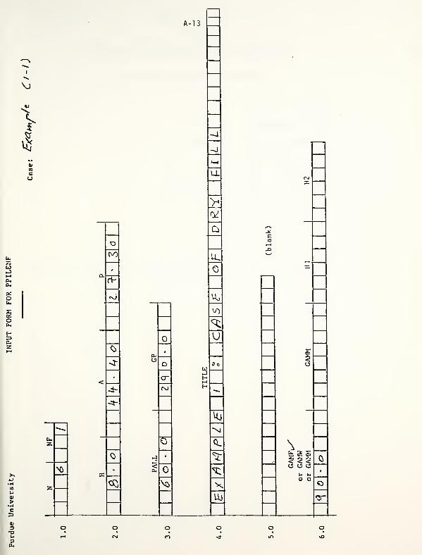
I
A-l 3
-J,—
,
-J
f—
t
LLX
>
c
O to
I—
1
f^) ICN*-'
,=
&
U<Z>
Cu<
1<r
u oIdiJH
Co o
<
-3-
rj H
0. \
"^
•J t ^r& 5 S3 3 <
\> X-
<ft. ^ o o o
Vj I-i
1
z <£ vo
Uj
O O
<5~
oCM
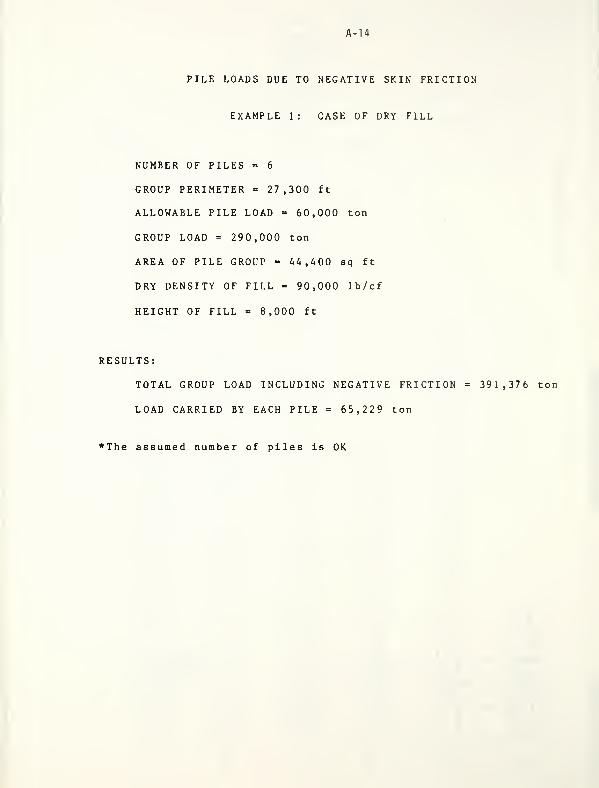
A-14
PILE LOADS DUE TO NEGATIVE SKIN FRICTION
EXAMPLE 1: CASE OF DRY FILL
NUMBER OF PILES = 6
GROUP PERIMETER = 27,300 ft
ALLOWABLE PILE LOAD = 60,000 ton
GROUP LOAD = 290,000 ton
AREA OF PILE GROUP = 44,400 sq ft
DRY DENSITY OF FILL = 90,000 lb/cf
HEIGHT OF FILL = 8,000 ft
RESULTS:
TOTAL GROUP LOAD INCLUDING NEGATIVE FRICTION = 391,376 ton
LOAD CARRIED BY EACH PILE = 65,229 ton
*The assumed number of piles is OK
I
.5
A-15
•
i
$-4
Qd
1- ^-x
cNC
1—1
rn
.c
-
O-
2
3^
IX |O o U
tj
00 o
<H rt-JH
<N>
MH
Uj
\ Q
<N
Z
j t £253 3 3 >>
^X
<* <£
o o o
o o
'
z\9
XO: 1
A-16
PILE LOADS DUE TO NEGATIVE SKIN FRICTION
EXAMPLE 2: GROUNDWATER LOWERING
NUMBER OF PILES = 6
GROUP PERIMETER = 27,300 ft
ALLOWABLE PILE LOAD = 60,000 ton
GROUP LOAD = 275,000 ton
AREA OF PILE GROUP = 44,400 sq ft
UNIT WEIGHT OF WATER = 62,400 lb/cf
HEIGHT OF DEWATERING = 6,000 ft
RESULTS:
TOTAL GROUP LOAD INCLUDING NEGATIVE FRICTION = 283,312 ton
LOAD CARRIED BY EACH PILE = 47,219 ton
Decrease number of piles and repeat the try
A-17
I
Ncn
Pl
uNi
<
O
-J
tsl
Z
X
JJ<U
Z
\&
>
<k
kj
r
^_
$
a
vs
XUi
\33<
NO
on
A-18
PILE LOADS DUE TO NEGATIVE SKIN FRICTION
EXAMPLE 2: GROUNDWATER LOWERING
NUMBER OF PILES = 5
GROUP PERIMETER = 25,320 ft
ALLOWABLE PILE LOAD = 60,000 ton
GROUP LOAD = 275,000 ton
AREA OF PILE GROUP = 40,000 sq ft
UNIT WEIGHT OF WATER = 62,400 lb/cf
HEIGHT OF DEWATERING = 6,000 ft
RESULTS:
TOTAL GROUP LOAD INCLUDING NEGATIVE FRICTION = 282,488 ton
LOAD CARRIED BY EACH PILE = 56,498 ton
*The assumed number of piles is OK
A-19
is acceptable .
Example (3_) :
It is required to design a pile group for the same condi-
tions given in example (1), except that a 15.0 ft of a very soft
clay layer is penetrated by the pile (instead of the fill layer).
The clay layer has a saturated unit weight of 115.2 pcf (effec-
tive unit weight is 52.8 pcf since the layer is submerged).
Solution :
The input form (3.1) is prepared, and a PPILENF run is per-
formed. The output shows that the assumed number of piles is
satisfactory. However, if the designer can arrange a five-pile
group with reasonable pile load (not much higher than 60.0 tons),
that arrangement would be better from the economical point of
view.
Example (4_) :
A pile group is required to carry a load of 130.0 tons. The
top 12.0 ft is formed of an organic and very soft varved silty
clay, with the G.W.T. at the ground surface. The saturated unit
weight of this layer is 111.5 pcf (effective unit weight is 49.1
pcf). Since it would be very difficult for the pile contractor
to do the job because of the very soft layer, a working platform
of fill of 6.0 ft thickness (estimated unit weight of 89.0 pcf)
would be needed. Piles of 16.0 in. diameter are to be used.
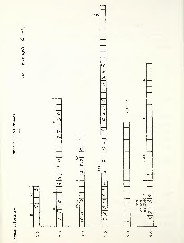
I
A-20
to
\o
o
£
ACh
*>i
ik
_0_
vn
ro
r^_X.Uj
O
\
u o o*0
5l
om
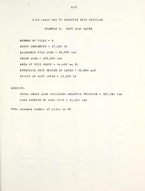
A-21
PILE LOADS DUE TO NEGATIVE SKIN FRICTION
EXAMPLE 3: SOFT CLAY LAYER
NUMBER OF PILES = 6
GROUP PERIMETER = 27,300 ft
ALLOWABLE PILE LOAD = 60,000 ton
GROUP LOAD = 290,000 ton
AREA OF PILE GROUP = 44,400 sq ft
EFFECTIVE UNIT WEIGHT OF LAYER = 52,800 pcf
HEIGHT OF SOFT LAYER = 15,000 ft
RESULTS:
TOTAL GROUP LOAD INCLUDING NEGATIVE FRICTION = 307,582 ton
LOAD CARRIED BY EACH PILE = 51,264 ton
*The assumed number of piles is OK
A-22
They are to be spaced 4.0 ft C.L. to C.L.
Solution :
No. of piles = ~£ = 3.25
Try a group of four piles (group area = 28. A sq ft, group
perimeter - 21.32 ft) (Fig. A. 1.3). It should be noticed that
negative skin friction is anticipated due to both the consolida-
tion of the very soft layer and the settlement of the fill layer
due to any surficial loads, or submergence.
The input form (4.1) is prepared and a PPILENF run is per-
f ormed
.
The results showed that the four piles would not support the
total load, including the anticipated negative skin friction.
Another trial is performed using a group of five piles
arranged in the same manner described in examples (2) (2nd
trial). The input form (4.2) is shown. This time the analysis
showed that the five-pile group would be sufficient for the pur-
pose.
Example (5_) :
A 40.0 ft high embankment is constructed over a soft clay
layer 20.0 ft thick with saturated unit weight of 123.4 psf .
This layer is followed by a thick deposit of very stiff clay. A
structure is to be constructed over the embankment, but the loads
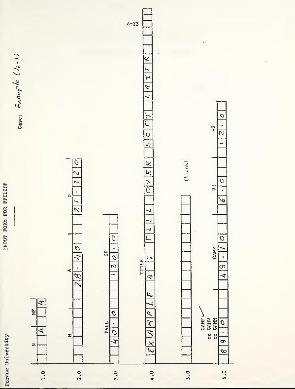
A-23
i
r
^
•
Uj
y^t
vj
P OUs CM '
(\J
V)
.*C5
C
<\> Ujnr—I
f^ >aO
o. * •
•^ \6
^-sj
3
—1
\
^ . S -^
^r3
; ci
1
<<c
\
<r
^ ^-3 . f
fa 3 §3 $<
<tX
<^ ^ o o o
o o
z
1
-^r
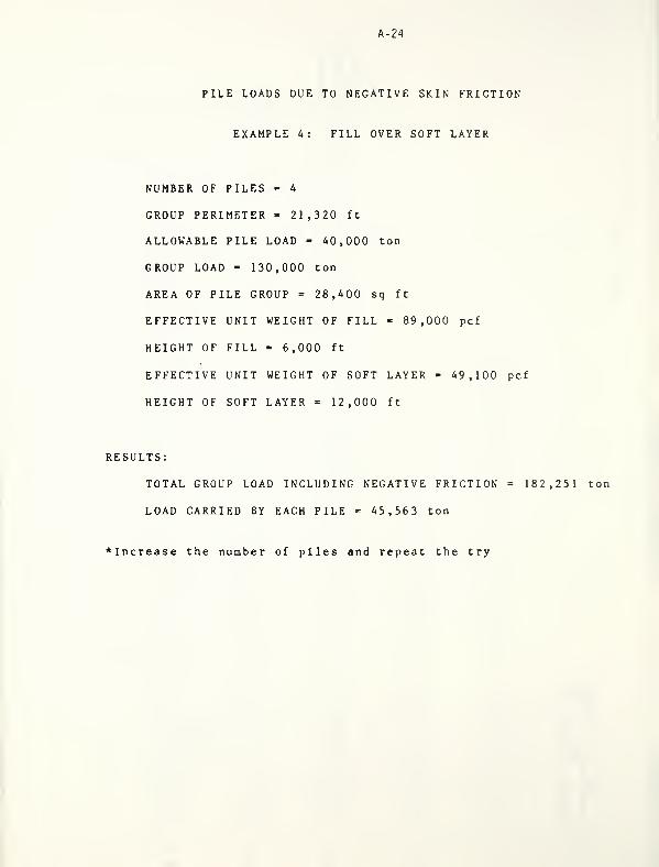
A-24
PILE LOADS DUE TO NEGATIVE SKIN FRICTION
EXAMPLE 4: FILL OVER SOFT LAYER
NUMBER OF PILES « 4
GROUP PERIMETER - 21,320 ft
ALLOWABLE PILE LOAD - 40,000 ton
GROUP LOAD - 130,000 ton
AREA OF PILE GROUP = 28,400 sq ft
EFFECTIVE UNIT WEIGHT OF FILL = 89,000 pcf
HEIGHT OF FILL = 6,000 ft
EFFECTIVE UNIT WEIGHT OF SOFT LAYER = 49,100 pcf
HEIGHT OF SOFT LAYER = 12,000 ft
RESULTS:
TOTAL GROUP LOAD INCLUDING NEGATIVE FRICTION = 182,251 ton
LOAD CARRIED BY EACH PILE = 45,563 ton
*Increase the number of piles and repeat the try
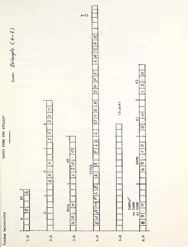
A-25
"\•
r\)
1
'K
\-> Uj
^J >b <a:
tf
£-j
V UwCO
u k CMX
rvj
^
"*—
c
c UJcd
U CO > Nw^
J r^i=
,
as
D
D-
CM
Vo
[14
u_
oHDCM
H04 1
•
oCO o
-r<o-*-
•-»H
-J
\Z
<C
t b a s5 $ 3
>>^
X< ^ o o o
u o o•H01 z Q X O)
(J
HI <r Uj Cfe
• iH
c
<U
3 o o o O O oT3 • • • • • •
U t-i CN CI «* m kO3
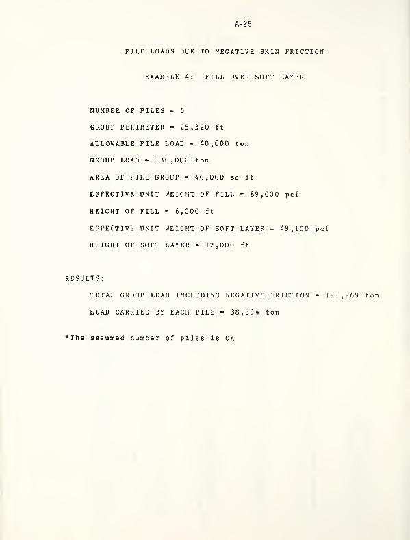
A-26
PILE LOADS DUE TO NEGATIVE SKIN FRICTION
EXAMPLE 4: FILL OVER SOFT LAYER
NUMBER OF PILES = 5
GROUP PERIMETER = 25,320 ft
ALLOWABLE PILE LOAD = 40,000 ton
GROUP LOAD = 130,000 ton
AREA OF PILE GROUP = 40,000 sq ft
EFFECTIVE UNIT WEIGHT OF FILL = 89,000 pcf
HEIGHT OF FILL = 6,000 ft
EFFECTIVE UNIT WEIGHT OF SOFT LAYER = 49,100 pcf
HEIGHT OF SOFT LAYER = 12,000 ft
RESULTS:
TOTAL GROUP LOAD INCLUDING NEGATIVE FRICTION = 191,969 ton
LOAD CARRIED BY EACH PILE = 38,394 ton
*The assumed number of piles is OK
A-27
were heavy enough that pile foundations were required to support
them. A group of 6 piles, 16 in. diameter (same arrangement
given in Fig. A. 1.3) with allowable load of 55.0 tons each is to
be used 6uch that the piles would rest on the very stiff clay
layer (Fig. A. 1.4). It is required to check the adequacy of such
group if the total load = 300.0 tons. The G.W.T. is assumed to
at the top of the soft layer.
Solution :
Using the same arrangement used in Example (1) (A 44.40
2ft
, p = 27.30 ft), the additional load due to negative skin
friction can be checked. It should be noticed that the embank-
ment fill given in this problem cannot be treated the same way as
in Example (4). The 40.0 ft high embankment is likely to be com-
pacted with good control. Hence, the long term settlement that
might cause negative skin friction can be minimized. Some
measures can be taken to reduce the risk of potential problems as
follows
:
1. The embankment should be compacted using water contents at
the wet side of optimum which results in smaller long term
deformations due to saturation, etc., than what would occur
if the same density was achieved at the dry side of
optimum .
2. Stage construction and/or sand drains can be used to facil-
A-28
itate the consolidation process before the construction of
the piles and the application of other loads.
Details about these procedures are beyond the scope of this
report. However, one can assume that if good procedures were
followed for the embankment construction, an upper bound value of
the additional load due to negative skin friction could be calcu-
lated based on the weight enclosed within the soft layer only.
An input form of the data is shown and the output of the
analysis indicates the adequacy of the proposed six-pile group.

1
in
i
d
oz
A-29
<
V>
U.
UJ
rsi
1-
Hc
Uj TO
fO
SPL
r* ^.
<N
lU
gPj - —
—
£-r
u
TowJ
«« o
<-r
H LO
UJ
-J
a. ©cO
© J £ fcS53 3 <
V£>X .
<iO ^ o o e>
t-l 1-1
o o
—
•z.t) in
Uj-'
^
o o c O O ol-l Cvl C-) <r in vD
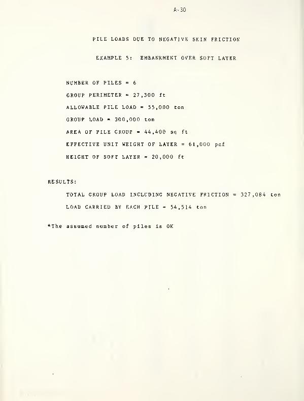
A-30
PILE LOADS DUE TO NEGATIVE SKIN FRICTION
EXAMPLE 5: EMBANKMENT OVER SOFT LAYER
NUMBER OF PILES = 6
GROUP PERIMETER = 27,300 ft
ALLOWABLE PILE LOAD = 55,000 ton
GROUP LOAD = 300,000 ton
AREA OF PILE GROUP = 44,400 sq ft
EFFECTIVE UNIT WEIGHT OF LAYER = 61,000 pcf
HEIGHT OF SOFT LAYER = 20,000 ft
RESULTS:
TOTAL GROUP LOAD INCLUDING NEGATIVE FRICTION = 327,084 ton
LOAD CARRIED BY EACH PILE = 54,514 ton
*The assumed number of piles is OK
A-31
PPILENF LISTING
Program Characteristics:
Core Used = 046000 E octal words
Tice Used = 0. 447 CPU seconds
NL = 7200 words
CX =0. 966 sec
program main ( tap e 5, t ap eh) A-32c
c
c
c * »c «• this program computes the additional pile loads due to *
c * negative skin friction *c * #c »*#******#*#*##******«###******#***#»#**###*##*#*#*##*#•«•c
c
c
dimension title(20)
read (5, 1000)n, nf1000 f ormat
(
iA, i3)read (5, 2000) h, a, p
2000 f OT-mat ( f6. 3, fS. 3, f8 3)read (5, 3000)pal 1, gp
3000 format <2f S. 3)
c
read (5< 1 11 ) tit! e
111 format ( 10a4
)
u>t i te (6, 2)2 format(///lx, 'purdue university'/Z'./25x, 'pile loads due to negative skin friction')on ite (6, 99) title
99 format C////14X, 10a4)c
c
c
write (6»68) n.p,pall,gpia88 format ( //10x / 18hnumb er of piles = , i3,
&//10xi 18hgroup perimeter = , f 8. 3, 3x , 3h f t. ,
&//10x, 22hal lowable pile load = , f 8. 3, 3x , 3hton,ic//10x. 13hgroup load = , f 8. 3, 3x , 3h ton,&//10x, 21harea of pile group = , f 8. 3, 3x> 6h sq. f t. )
c
c
c
if (nf . eq. 1 )goto 10i f (nf . eq. 2)goto 20if(nf.eq.3)goto 30if (nf . eq. 4)goto 40
c
c
c case of dry fill layer subject to future settlementc
10 read ( 5, 3) gamf3 format (f8. 3)
al=a+h*p+4. 0*h**2gpnf=gamf*h*(a+al)/(2. 0*2000. 0)write (6»77)gamfih
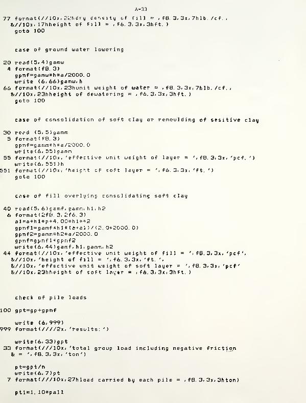
A-33
77 format <//10x, 22hdry density of fill = , f 8 3, 3x , 7h 1 b . /c f . ,
&//10x, 17hheight of fill = , f 6. 3, 3x , 3h f t. )
goto 100
case of ground water lowering
20 read ( 5* A ) gamm4 format(f8. 3)
gpnf = garnw*h*a/2000.write (6»66)gamw. h
66 format <//10x. 23hunit weight of water = , f 8 3, 3x, 7h 1 b. /c f . ,
&//10x, 23hheight of dewatering = , f 6. 3, 3x, 3hf t. )
goto 100
case of consolidation of soft clay or remoulding of sesitive clay
30 read (5i5)gsmm5 f ormat ( f8. 3)
gpnf=gamm*h*s/2000.write(6. 55)gamm
55 format (//10x, 'effective unit weight of layer = ', f 8. 3* 3x* 'pcf. ')
write(6, 551 )h
551 format (//10x, 'height of soft layer = ',f6. 3,3x. 'ft. ')
goto 100
case of fill overlying consolidating soft clay
40 read<5i 6 ) gamf < gamm; h 1 , h26 format(2f8. 3, 2f6. 3)
al=a+hl*p+4. 00*hl**2gpnfl=gamf*hl*(a+al)/<2. 0*2000. 0)gpnf2=gamm*h2*a/2000.gpnf=gpnfl+gpnf2wr i te(6* 44
)gamf . hli gamm. h2
44 format <//10x, 'effective unit weight of fill = ', f 8. 3, 3x, 'pcf ',
&//10x, 'height of fill = ',f6.3,3x, 'ft. ',
&//10x, 'effective unit weight of soft layer = ', f 8. 3, 3x , 'p c f '
&//10x. 23hheight of soft layer = , f 6. 3, 3x , 3h f t. )
check of pile 1 oads
100 gpt=gp+gpnf
write (6,999)999 format(////2x, 'results: ')
write (6, 33) gpt33 format ( ///10x, 'total group load including negative friction
k = ', f8. 3, 3x, 'ton')
pt=gp t/nwrite (6, 7)p
t
7 format (///10x, 27hload carried by each pile = , f8. 3/ 3x, 3hton)
ptl=l. 10*pall