test systems and mathematical models for transmission network expansion planning
TRANSCRIPT
Test systems and mathematical models for transmission network expansion planning
R. Romero, A. Monticelli, A. Garcia and S. Haffner
Abstract: The daVa of four networks that can be used in carrying out comparative studies with methods for transmission network expansion planning are gwen. These networks are of various types and different levels of complexity. The main mathematical formulations used in transmission expansion studies-transportation models, hybrid models, DC power flow models, and disjunctive models are also SummdnSed and compared. The main algorithm families are reviewed-both analytical, cOmbinatOnd1 and heuristic approaches. Optimal solutions are not yet known for some of the four networks when more accurate models (e.g. the DC model) are used to represent the power flow equations-the state of the art with regard to this is also summarised. This should sewe as a challenge to authors searching for new, more efficient methods.
1 Introduction
This paper presents the data of four different systems which can be used for testing altemative algorithms for transmis- sion network expansion planning. The main motivation for giving these data in a systematical and organised way is to allow meaningful comparative studies-the one thing that is certainly lacking in this important research area. In most publications, practitioners have used the well known Garver's six-bus network to illustrate the proposed methods, along with some other networks, for which as a rule the relevant data is not entirely available. Comparative studies using known data are practically non-existent. To a lesser degree, the same is true for the different models used to represent the transmission networks. Comparative studies dealing with the altemative representations for different networks are badly needed to properly evaluate the performances of proposed algorithms. This paper Bves the data of four systems which differ very widely in computa- tional complexity. It also sumarises in a systematic way the alternative models that are normally used for represent- ing a transmissions network in transmission planning studies. A summary of the main methodologies available is also presented.
2 Mathematical modelling
Four main types of model have been used in the literature for representing the transmission network in transmission expansion planning studies: the transportation model, the hybrid model, the disjunctive model, and the DC power flow model. Full AC models are considered only at later
10 IEE. 2002 IEE ProcmLp.s online no. 2W20026 DO/: K.lM9/ip-ptdZMl2W26 Paper first received 14th March 2001 R. Romero is with the Faculty of Enpineefins of llha Solteira, Paulista Swte University. CP 31, Ilha Soltririr 15385-NX1, SP, Brazil A. Monticelli and A. Garcia are with the Departmcnl of Electric Enersy Systems. University of Campinas, CP 6101, Campinns 13081-970. SP. Brazil S. Hafiner is with the Depaitmeni of EImtfimudl Enginee~ing. Pontifical Catholic University of Rio Grande do SUI. CP 1429. Port0 Alepre 90619-9INl RS, Brazil
stages of the planning process when the most attractive topologies have been determined.
2.1 DC model When the power grid is represented by the DC power Bow model, the mathematical model for the one-stage transmis- sion expansion planning problem can be formulated as follows:
Minimise
" = c c z j n , + Ly c r k ( 1 ) (i/) k
Subject to
(2) S,f + 9 + r = d
,h, - y,, (n: + n;,) (0, - Bi) = 0 (3)
I K ~ I 5 (n;.+n,)fi, (4)
0 5 y S G ( 5 )
O S r S d (6)
(7)
(8)
0 5 nil 5 i i j j
ni, integer, .f, and Bi unbounded
( i ; j ) t R, k E I
where cij, yo. n , n$J, and .rj represent, respectively the cost of a circuit that can be added to right-of-way i-j, the susceptance of that circuit, the number of circuits added in right-of-way i-j, the number of circuits in the base case, the power flow, and the corresponding maximum power flow. v i s the total investment, S is the branch-node incidence matrix,fis a vector with elementsf, (power flows), y is a vector with elements gk (generation in bus k ) whose maximum value is :q, ii, is the maximum number of circuits that can be added in right-of-way i-j, Q is the set of all right-of-ways, r is the set of indices for load buses and r is the vector of artificial generations with elements rk (they are used in certain formulations and to represent loss of load,
and normally appear in the formulation multiplied by a cost n measured in $/MW).
The constraint in eqn. 2 represents the conservation of power in each node if we think in terms of an equivalent DC network, this constraint models Kirchhoffs current law (KCL). The constraint in eqn. 3 is an expression of Ohm's law for the equivalent DC network. Notice that the existence of a potential function 0 associated with the network nodes is assumed. and so Kirchhoffs voltage law (KVL) is implicitly taken into account (the ConSeWatiOn Of energy in the equivalent DC network)-these are nonlinear constraints. The constraint in eqn. 4 represents power flow limits in transmission lines and transformers. The con- straints in eqns. 5 and 6 refer to generation (and pseudo- generation) limits.
The transmission expansion problem as formulated above is an integer nonlinear problem (INLP). It is a difficult combinatorial problem which can lead to combi- natorial explosion on the number of alternatives that have to he searched.
2.2 Transportation model This model is obtained by relaxing the nonlinear constraint eqn. 3 of the DC model described above. In this case the network is represented by a transportation model, and the resulting expansion problem becomes an integer linear problem (ILP). This problem is normally easier to solve than the DC model although it maintains the combinatorial characteristic of the original problem. An optimal plan obtained with the transportation model is not necessarily feasible for the DC model, since part of the constraints have been ignored; depending on the case, additional circuits are needed in order to satisfy the constraint in eqn. 3_ which implies higher investment cost.
2.3 Hybrid model The hybrid model combines characteristics of the DC model and the transportation model. There are various ways of formulating hybrid models, although the most common is that which preserves the linear features of the transportation model. In this model it is assumed that the constraint in eqn. 2, KCL, is satisfied for all nodes of the network, whereas the constraint in eqn. 3, which represents Ohm's law (and indirectly, KVL), is satisfied only by the existing circuits (and not necessarily by the added circuits).
The hybrid model is obtained by replacing the cons- traints in eqns. 2 and 3 of the DC model by the following constraints:
s, f + S,f' t g + r = d (9)
f . . i/ ~ y.. ,n,(0i 0 - Oj) = 0 , V ( i , j ) E no ( I O )
lL.>l s ni,& %i) E Q (12)
where So is the branch-node incidence matrix for the existing circuits (initial configuration), f is the vector of flows in the existing circuits (with elements@, and f' is the vector of flows in the added circuits (with elements A,)).
2.4 Disjunctive model A linear disjunctive model has been used in [1-3]. It can he shown that under certain conditions the optimal solution for the disjunctive model is the same as the one for the DC model. This model can be formulated as follows.
28
Minimise
Subject to
Sop +SI f ' + g + r = d (14)
f: - ~ g n i . ( O i - 0,) = 0, V ( i , / ) E Ro (15)
l ~ ~ - ~ ~ ( O ~ - O j ) l ~ ~ ( l - ~ ~ ) : V ( i , , j ) € n (16)
I41 i 3j.i.;. (17)
Mi;l 5 L Y ; (18)
0 5 C I < Y (19)
O s r i d (20)
$ E { O ; I ) : ( i , j ) E n , p = 1 , 2 : . . . : p (21)
fl> $and 8, unbounded
where p is the number of circuits that can be added to a right-of-way (these are binary variables of the type $.), f' is the vector of flows in the circuits of the initial configuration (with elements t), SI is the node-branch incidence matrix of the candidate circuits (which are considered as binary vanables),t is the vector of flows in the candidate circuits (with elements A;), n$. are the circuits of the initial configuration, and M is a number of appropriate size.
The appeal of this model is that the resulting formulation can he approached by binary optimisation techniques. On the other hand, it has two main disadvantages: the increase in the number of problem variables due to the use of binary variables, and the need to determine the value of M. An additional feature of this method is that it can he extended to AC models: this, however, is not of great value in practice, since most of the long term studies are performed with DC models only.
3 Data sets
Is this Section the data sets for transmission expansion planning of four systems are presented. These systems show a wide range of complexities and are of great value for testing new algorithms. The reactance data are in p.u. considering a lOOMW base.
3.1 6-bus system This system has six buses and 15 right-of-ways for the addition of new circuits. The demand is of 760MW and the relevant data are given in Tables 1 and 2. This system was originally used in [4], and since then has become the most popular test system in transmission expansion planning. The initial topology is shown in Fig. I.
3.2 46-bus system This system is a medium sized system that represents the southem part of the Brazilian interconnected network. I t has 46 buses and 79 right-of-ways for the addition of new circuits (all relevant dala can he found in [SI). The total demand for this system is 6800MW. There is no limit for circuit additions in each right-of-ways.
TEE Proc:&ner T,<U,$,>, Dhrrili., Vol 149, No. I , ~0~0,,u",g2002
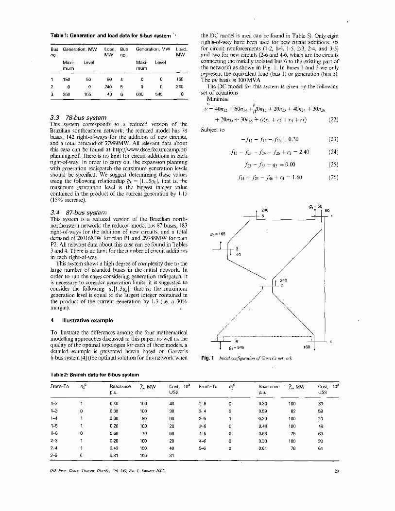
Table 1: Generation and load data for 6-bus system ' * ~ ~
Bus Generation. MW Load, Bus Generation, MW Load, no. MW no. MW
Maxi- Level Maxi- Level mum mum
1 150 50 80 4 0 0 160
2 0 0 240 5 0 0 240
3 360 165 40 6 600 545 0
3.3 78-bus system This system corrcspouds to a reduced version of the Brazilian southeastern network; the reduced model has 78 buses. 142 right-of-ways for the addition of new circuits, and a total demand of 37999MW. All relevant data about this case can be found at http://w.dsee.fee.unicamp.br/ planning.pdf. There is no limit for circuit additions in each right-of-way. In order to carry out the expansion planning with generation redispatch the maximum generation levels should be specified. We suggest determining these values using the following relationship Qa = [l.ISgp], that is. the maximum generation level is the biggest integer value contained in the product of the current generation by 1.15 (15% increase).
3.4 87-bus system This system is a reduced version of the Brazilian north- northeastern network: the reduced model has 87 buses, 183 right-of-ways for the addition of new circuits, and a total demand of20316MW for plan PI and 2974XMW for plan P2. All relevant data about this case can he found in Tables 3 and 4. There is no limit for the number of circuit additions in each right-of-way.
This system shows a high degree of complexity due to the large number of islanded buses in the initial network. In order to nm the cases considering generation redispatch, it is necessary to consider generation limits: it is suggested to consider the following: &[I . 3 g k ] , that is, the maximum generation level is equal to the largest integer contained in the product of the current generation by 1.3 (Le. a 30% margin).
4 Illustrative example
To illustrate the differences among the four inathematical modelling approaches discussed in this paper, as well as the quality of the optimal topologies for each of these models, a detailed example is presented herein based on Garver's 6-bus system [4] (the optimal solution for this network when
the DC model is used can be found in Table 5). Only eight rights-of-way have been used for new circuit additions: six for circuit reinforcements (1.2, 1-4, 1-5, 2-3> 2-4, and 3-5) and two for new circuits (2-6 and 4-6, wtuch are the circuits connecting the initially isolated bus 6 to the existing part of the network) as shown in Fig. 1. In buses 1 and 3 we only represent the equivalent load (bus 1) or generation (bus 3). The pu basis is 100 MVA
The DC model for this system is given by the following set of equations
Minimise
g, = 50 w1
Table2 Branch data for Gbus system
From-To n," Reactance f,. MW Cost, i o3 From-To n,: Reactance 3,. MW Cost. i o3 P U US$ P.U US$
1 -2 1
1-3 0
1-4 1
1 5 1
1-6 0
2-3 1
2-4 1
2-5 0
0.40
0.38
0.60
0.20
0.68 0.20 0.40
0.31
100
100
80
100
70
100
100
100
40 2 6 0 0.30 100 30
38 3-4 0 0.59 82 59
60 3s 1 0.20 100 20
20 34 0 0.48 100 48 68 4-5 0 0.63 75 63
20 46 0 0.30 100 30
40 5 4 0 0.61 78 61
31
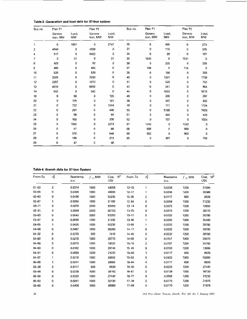
Table3 Generation and load data for 87-bus system
Bus no. Plan P2
Genera- tion, MW
0
4550
6422
0
82
465
538
2260
4312
5900
542
0
0
0
0 0 0 0 0 0 0 0
Bus no. Plan P1 Plan P2
load, Genera- Load, MW tion. MW MW
Plan P1
Genera- tion, MW
1
2
4
7
8
9
10
11
12
13
14
19
20
21
22
23
24
25
26
27
28
29
0
4048
517
0
403
465
538
2200
2257
4510
542
0
0
0
0 0 0 0
0 0 0 0
Load. MW
1857
0 0
31
0 0
0
0 0 0 0
86
125
722
291
58
159
1502
47
378
189
47
Load, MW
2747 30
0 31
0 34
31 35
0 36
0 37
0 39
0 40
0 41
0 42
0 44
125 46
181 48
1044 49
446 50
84 51
230 52
2273 67
68 68 546 69
273 85
68
Genera- tion, MW
0 0 0
1635
0
169
0
0
0
0 0 0 0 0 0 0
0
1242
888
902
0
189 0 273
110 0 225
28 0 107
0 1531 0
225 0 325
0 114 0
186 0 269
1201 0 1738
520 0 752
341 0 494
4022 0 5819
205 0 297
347 0 432
777 0 1124
5189 0 7628
290 0 420
707 0 1024
0 1242 0
0 888 0
0 902 0
487 0 705
Table4: Branch data for 87-bus System
From-To
__ 0 1 4 2 0 2 4 4
0 2 4 0
02-87
03-71
0381 ,
0343
0 3 8 7
04-05
04-06
04-32
04-60 0468
04-69
04-81
04-87
O W 6 OS38
0 5 5 6
O M 8
0540 O M 8
30
Reactance p.u.
2 0.0374
0 0.0406
0 0.0435
1 0.0259
0 0.0078
0 0.0049
0 0.0043 0 0.0058
1 0.0435 0 0.0487
0 0.0233
0 0.0215
0 0.0070
0 0.0162
0 0.0058
1 0.0218
1 0.0241
2 0.0117
0 0.0235
0 0.0220
0 0.0261
0 0.0406
J , , , MW cost, io3 FPXT-T~
-
1000 1000
1000
1000
3200
3200
3200
1200
1000
1000
300
1000
1000
1000
1200
1000
1000
600 1000
1000
1000
1000
uss
44056 48880
52230
31192
92253
60153
53253
21232
52230
58260
7510
26770
10020
20740
21232
26502
29852
8926
29182
27440
32130
48880
~
12-1 5 12-17
12-35
12-84
1 3 1 4
1 3 1 5
13-17
1345
13-59
14-17
14-45 1459
1 5 1 6
1 5 4 5
1 5 4 6
1653
1 6 4 4
1 6 4 5
1-1
l b 7 7
17-18
1 7 5 9
Reactance p.u.
1 0.0256 1 0.0246
2 0.0117
0 0.0058 0 0.0075
0 0.0215
0 0.0232
1 0.0290
1 0.0232
0 0.0232
0 0.0232
0 0.0157
2 0.0197
0 0.0103
1 0.0117
0 0.0423
4 0.0177
0 0.0220
0 0.0128
0 0.0058 2 0.0170
0 0.0170
~
ir,, MW cost, io3 US$
1200 31594 1200 30388
600 8926
1200 2 1232
1200 10690
1200 26770
1200 28780
1200 35480
1200 28780
1200 28780
1200 28780
1200 20070
1200 24760
1200 13906
600 8926
1000 50890
600 8926
1200 27440
1000 16720
1 200 21232
1200 21678
1200 21678
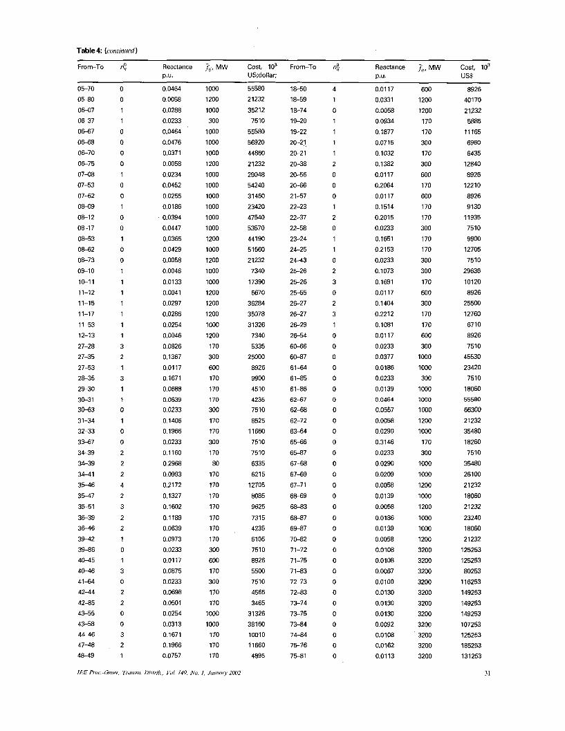
Table4: lconriiiiredd)
0 5 8 0
0607 0637
0667
0668
0670
O M 5
0748
07-53
0742
08-09
oa12
08-17
oa53
o w 3
0-2
Ob10
10-11
11-12
11-15
11-17
11-53
12-13
27-28
27-35
27-53
2a35
29-30
3&31
3 0 6 3
31-34
32-33
3347
34-39
34-39
34-41
35-46
3547
3 5 5 1
3639
3 6 4 6
39-42
39-86
4 w 5
4&46
4144
4244
42-85
m 5
4358
44-46
47-48
e 4 9
0
0
1
1
0
0
0
0
1
0
0
1
0
0
1
0
0
1
1
1
1
1
1
1
3
2
1
3
1
1
0 1
0 0
2
2
2
4
2
3
2
2
1
0
1
3
0
2
2
0
0
3 2
1
Reactance J,, MW cost. io3 From-To "; Reanance x,, MW cost. io3 p.u. US;dollar: p.u. US$
From-To 8,
05-70 0.0464 1000 55580
0.0058
0.0288
0.0233
0.0464
0.0476
0.0371
0.0058
0.0234
0.0452
0.0255
0.0186
0.0394
0.0447
0.0365
0.0429
0.0058
0.0046
0.0133
0.0041
0.0297
0.0286
0.0254
0.0046
0.0826
0.1367
0.0117
0.1671
0.0688
0.0639 0.0233
0.1406
0.1966
0.0233
0.1160
0.2968
0.0993
0.2172
0.1327
0.1602
0.1189
0.0639
0.0973
0.0233
0.0117
0.0875
0.0233
0.0698
0.0501
0.0254
0.0313
0.1671
0.1966
0.0757
1200
1000
300
1000
1000
1000
1200
1000
1000
1000
1000
1000
1000
1200
1000
1200
1000
1000
1200
1200
1200
1000
1200
170
300
600 170
170
170
300
170
170
300
170
80 170
170
170
170
170
170
170
300
600
170
300
170
170
1000
1000
170
170
170
21232
35212
7510
55580
56920
44860
21232
29048
54240
31460
23420
47540
53570
44190
51560
21232
7340
17390
6670
36284
35078
31326
7340
5335
25000
6926
9900
4510
4235
7510
8525
11660
7510
7510
6335
6215
12705
8085
9625
7315
4235
6105
7510
8926
5500 7510
4565
3465
31326
38160
10010
11660
4895
l a 5 0
l a 5 9
18-74
19-20
19-22
20-21
20-21
20-38
2056
2066
21-57
22-23
22-37
22-58
22-24
24-25
24-43
25-26
25-26
25-55
26-27
2€-27
2629
26-54
6&66
M w 7
61-64
61-85
61-86
6267
6248
62-72
6364
6 S 6
6%37
67-68
6749
67-7 1
6869
6883
6887
6 M 7
7 M 2
71-72
71-75
7 1 4 3
72-73
72-83
7374
7 M 5
7 2 4 4
74-84
75-76
7-1
4
1
0
1
1
1
1
2
0
0
0
1
2
0
1
1
0
2
3
0
2
3
1
0
0
0
0
0
0 0 0 0 0 0 0 0 0
0 0 0
0
0 0 0 0
0 0
0 0 0
0 0
0
0
0.0117
0.0331
0.0058
0.0934
0.1877
0.0715
0.1032
0.1382
0.0117
0.2064
0.0117
0.1514
0.2015
0.0233
0.1651
0.2153
0.0233
0.1073
0.1691
0.0117
0.1404
0.2212
0.1081
0.0117
0.0233
0.0377
0.0186
0.0233
0.0139 0.0464
0.0557
0.0058
0.0290
0.3146
0.0233
0.0290
0.0209
0.0058
0.0139
0.0058
0.0186
0.0139
0.0058
0.0108
0,0108
0.0067
0.0100
0.0130
0.0130
0.0130
0.0092
0.0108
0.0162
0.0113
600
1200
1200
170
170
300
170
300
600
170
600
170
170
300
170
170
300
300
170
600
300
170
170
600
300
1000
1000
300
1000 1000
1000
1200
1000
170
300
1000
1000
1200
1000
1200
1000
1000
1200
3200
3200
3200
3200
3200
3200
3200
3200
3200
3200
3200
8926
40170
21232
5885
11165
6960
6435
12840
8926
12210
8926
9130
11935
7510
9900
12705
7510
29636
10120
8926
25500
12760
6710
8926
7510
45530
23420
7510
18060
55580
66300
21232
35480
18260
7510
35480
26100
21232
18060
21232
23240
18060
21232
125253
125253
80253
116253
149253
149253
149253
107253
125253
185253
131253
31
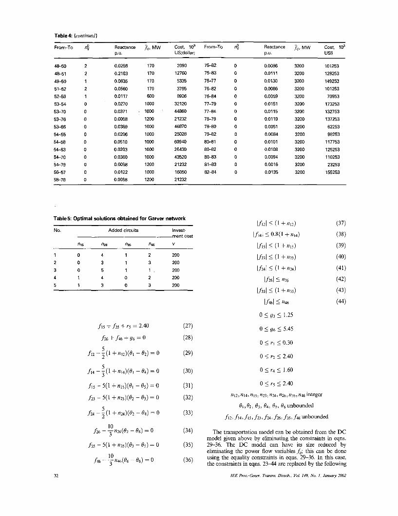
Table4 (confinued)
Reactance x,, MW cost. io3 From-To n?, Reactance x,, MW Cost, lo3 From-To n: D.U. US;dollar: D.U. US$
4850 2 4851 2 4950 1 51-52 2 52-59 1 53-54 0 53-70 0 53-76 0 5386 0 54-55 0 5458 0 54-63 0 54-70 0 54-79 0 5 M 7 0 5a78 0
0.0256 0.2163 0.0835 0.0560 0.0117 0.0270 0.0371 0.00% 0.0389 0.0206 0.0510 0.0203 0.0360 0.0058 0.0122 0.0058
170 170 170 170 600 1000
, 1000 1200 1000 1000 1000 1 coo 1000 1200 1000 1200
2090 12760 5335 3795 8926 32120 44860 21232 46870 25028 60940 25430 43520 21232 16050 21232
7542 0 7543 0 7677 0 7682 0 7684 0 77-79 0 77-84 0 7a79 0 7-0 0 7942 0 80-81 0 80-82 0 8 m 0 81-83 0 82-84 0
0.0086 0.0111 0.0130 0.0086 0.0059 0.0151 0.0115 0.0119 0.0051 0.0084 0.0101 0,0108 0.0094 0.0016 0.0135
3200 3200 3200 3200 3200 3200 3200 3200 3200 3200 3200 3200 3200 3200 3200
101253 128253 149253 101253 70953 173253 132753 137253 62253 98253 117753 125253 110253 23253 155253
Table5: Optimal solutions obtained for Garver network ~ ~ ~ -~ -
No. Added circuits Invest- ment cost
n15 nZ8 nZs n4€ V
1 0 4 1 2 200 2 0 3 1 3 200 3 0 5 1 1 200 4 1 4 0 2 200 5 1 3 0 3 200
32
lfizl i (1 + n l z ) (37)
If141 i 0.8(1 + n d (38)
lf151 5 (1 + nl5) (39)
If231 5 (1 +nu) (40)
If241 i (1 + nw) (41)
If261 i n26 (42)
l h s l i (1 +n35) (43)
If461 i n46 (44)
0 5 93 5 1.25
0 5 96 5 5.45
0 5 rl 5 0.30
0 5 r2 5 2.40
0 5 r4 5 1.60
0 5 rs 5 2.40
n12, n14, nis, n23, n24: n26, n35? n e integer
81,82, 8 3 , 84, 85, &unbounded
f i 2 , f 1 4 r f ~ ~ r fu,f24.f26,f35,f46unbounded
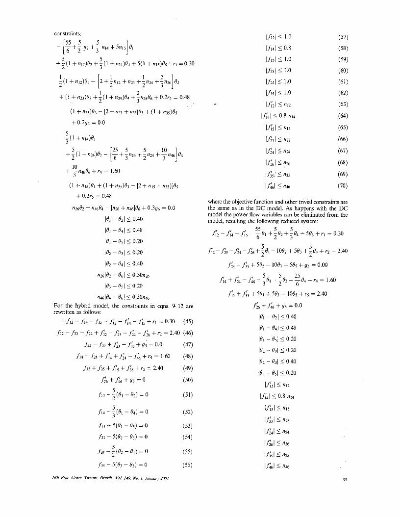
The transportation model can be obtained from the DC model given above by eliminating the constraints in eqns. 29-36. The DC model can have its size reduced by eliminating the power flow variables f,; this can be done using the equality constraints in eqns. 29-36. In this case, the constraints in eqns. 2 3 4 are replaced by the following
IEE Pruc-Gmer. T r a m . Dim+.. Vol. 149, No. 1. Jonunry 2IW2
constraints:
lf;51 i nls (65)
lf&l 5 n23 (66)
lfi41 5 n24 (67)
1~ 5 n26 (68)
If2 i n35 (69)
If&l 5 n46 (70)
where the objective function and other trivial constraints are the same as in the DC model. As happens with the DC model the power flow variables can be eliminated from the model, resulting the following reduced system:
55 5 5 6 2 3
f;2 - fi4 - f ; s --81 + - 8 2 +-Q4+5Bs +rl = 0.30
f ~ ~ - f ~ ~ - f ~ 4 - f ~ 6 + - 8 ~ - 1 0 0 ~ + 5 8 ~ + - 8 4 + r 2 =2.40 5 5 2 2
f;, - f i S + se2 - 108, + sos + Y3 = 0.00
5 5 25 3 2 - 6 f14 + f& - f& +-81 + - 8 7 - -e4 + r4 = 1.60
f i l s + J& + 581 + 583 - 108s + r5 = 2.40
.f& + f& + 96 0.0
181 - 821 5 0.40
181 - 051 5 0.20
182 - 031 5 0.20
183 - os1 5 0.20
lfL 5 n12
lf;41 5 0.8 n14
I&l 5 nls
lfi31 5 n23
181 - 841 i 0.48
102 - 841 5 0.40
Ifi4l 5 n24
If& 5 n26
I f& 5 n3s
If&l5 n 4
33
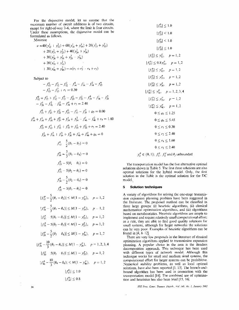
For the disjunctive model, let us assume that the maximum number of circuit additions is of two circuits, except for right-of-way 2 4 , where the limit is four circuits. Under these assumptions, the disjunctive model can be formulated as follows.
Minimise
u =4o(YI2 + ~ $ 2 ) + 6 0 ( ~ ; 4 + d 4 ) + 20(yfs + d s ) + 2o(Yj3 + Y;3) + 40(J’i4 f $4)
+ 30(,& + .& + $6 + + 20(Y:s + K) + 30(y& + y&) + a(ri + r; + r4 + rs)
I f l s l 5 1.0
l f l 3 l i 1.0
If!sl 5 1.0
Iflp21 5 Y; , P = 1:2
l.f{l 5 0.8YP4, P = 1 > 2
I/i?l 5 J f s > P = 1:2
l f ; ; l ~ Y z ” ? : P = l , 2
I.fLl5 &: P = I > 2
If41 5 A;> P = 1,2
If4Pnl5&; P = I ; 2
0 i ~3 5 1.25
0 5 96 5 5.45
0 5 ri 5 0.30
0 5 r? 5 2.40
0 5 r4 5 1.60
0 5 rs i 2.40
J$ E { O , I } ; Lf> h f a n d B, unbounded
5 1.0
If&/ 5 &, P = 1 , 2 > 3 , 4
The transportation model has the five alternative optimal solutions shown in Table 5. The first three solutions are also optimal solutions for the hybrid model. Only, the first solution in the Tabk is the optimal solution for the DC model..
5 Solution techniques
A variety of algorithms for solving the one-stage transinis- sion expansion planning problem have been suggested in the literature. The proposed method can be classified in three large groups: (i) heuristic algorithms, (ii) classical mathematical optimisation algorithms, and (iii) algorithms based on metaheuristics. Heuristic algorithms are simple to implement and require relatively small computational effort: as a rule, they are able to find good quality solutions for small systems, although for larger networks the solutions can be very poor. Examples of heuristic algorithms can be found in [4, 6121.
There are very few proposals in the literature of classical optimization algorithms applied to transmission expansion planning. A popular choice in the area is the Benders decomposition approach. This technique has been used with different types of network model. Although this technique works for small and medium sized systems, the computational effort for larger systems can be prohibitive. Numerical stability problems, as well as local optimal solutions, have also been reported [3, 131. The branch-and- bound algorithm has been used in connection with the transportation model [14]. The combined use of optimisa- tion and heuristics has also been tried [15, 161.
I€€ P r o . ~ G m e r Tmmnt. Dhtrrh. Vol. 149, No. 1. Junuir? Xh’n
More recently metaheuristic algorithms-simulated an- nealing, genetic algorithms, tabu search GRASP. etc. -have been applied to the transmission expansion planning problem [13, 17-19]. These algorithms are usually robust and yield near-optimal solutions for large complex networks. As a rule, these methods require high computa- tional effort. This limitation, however, is not necessarily critical in planning applications. New. more efficient algorithms are still needed to solve the problems classified as very complex (VC) in the next Section.
Even more complex problems such as the dynamic (through time) expansion, integrated generation/transmis- sion planning, and planning in competitive environments have received very little attention in the literature, perhaps due to the fact that the apparently easier part of the problem. the one-stage expansion, still remains unsolved for more complex networks.
6
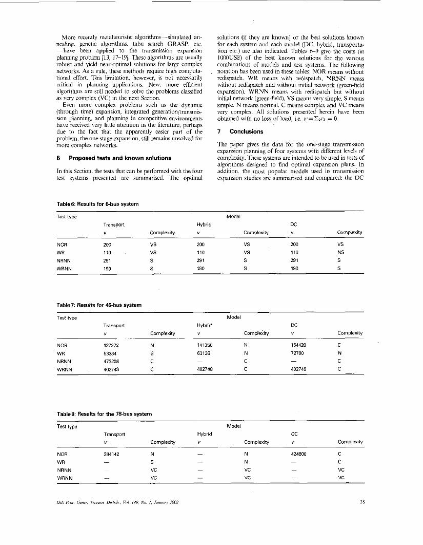
In this Section, the tests that can be performed with the four test systems presented are summarised. The optimal
Proposed tests and known solutions
Table6: Results for Gbus system
solutions (if they are known) or the best solutions known for each system and each model (DC, hybrid, transporta- tion etc.) are also indicated. Tables 6-9 give the costs (in lOOOUS$) of the best known solutions for the various combinations of models and test systems. The following notation has been used in these tables: NOR means without redispatch, WR means with redispatch, NRNN meass without redispatch and without initial network (green-field expansion). WRNN means with redispatch hut without initial network (green-field), VS means very simple, S means simple. N means normal. C means complex and VC means very complex. All solutions presented herein have been obtained with no loss pf load, i.e. )I,= Cxrs, = 0.
7 Conclusions
The paper gives the data for the one-stage transmission expansioii planning of four systems with different levels of complexity. These systems are intended to he used in tests of algorithms designed to find optimal expansion plans. In addition, the most popular models used in transmission expansion studies are summarised and compared: the DC
Test type Model
Transport Hybrid DC
V Complexity V Complexity V Complexity
NOR 200 vs 200 vs 200 vs WR 110 . vs 110 vs 110 NS
NRNN 291 S 291 S 291 S WRNN 190 S 190 S 190 S
Table 7: Results for &-bus system
Test type Model
Transport Hybrid DC
V Complexity Y Complexity V Complexity
NOR 127272 N 141350 N 154420 C
WR 53334 S 63136 N 72780 N
C NRNN 473208 C C
WRNN 402748 C 402748 C 402748 C
~ -
Table8 Results for the 78-bus system
Test type Model
Transpolt Hybrid DC
V Complexity " Complexity " Complexity
~ NOR 284142 N N 424800 C
WR S N C
NRNN vc vc vc WRNN ~ vc - vc vc
~ ~ ~
~ ~ ~
~
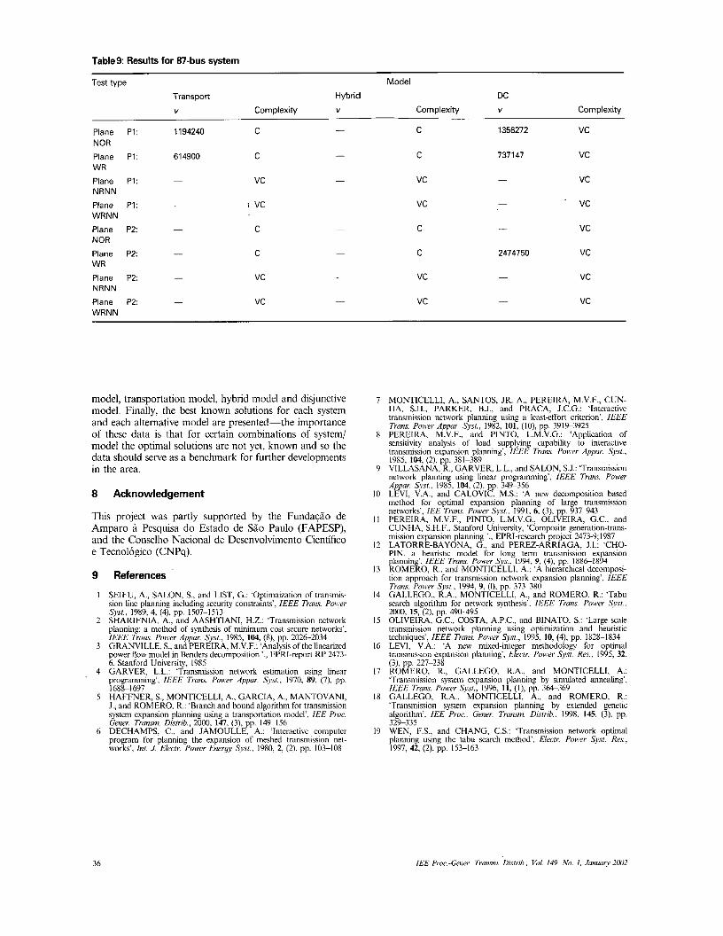
Table9: Results for 87-bus system
Test type Model
~
DC
Y ComDlexiN
Transport Hybrid
V Complexity Y Complexity
C
C
- Plane P1: 1194240 C NOR
Plane P1: 614900 C WR
~ - vc Plane P1: vc NRNN Plane P1: - I vc ~ vc WRNN
-
1356272 vc
737147 vc
~ vc
vc
- vc
2474750 vc
- vc
~ vc
~
Plane P2: NOR
C C
~ Plane P2: - C C WR
Plane P2: - vc - vc NRNN Plane P 2 ~ vc vc ~
WRNN
model, transportation model, hybrid model and disjunctive model. Finally, the best known solutions for each system and each alternative model are presented-the importance of these data is that for certain combinations of system/ model the optimal solutions are not yet, known and so the data should serve as a benchmark for further developments in the area.
8 Acknowledgement
This project was partly supported by the FundaqZo de Amparo i Pesquisa do Estado de SZo Paulo (FAPESP), and the Conselho Nacional de Desenvolvimento Cientifico e Tecnologico (CNPq).
References
SEIFU, A., SALON, S.. and LIST, G.: 'Optimaization of transmis- sion line planning including security constrahs', IEEE P a m Power S j s f . , 1989, 4. (4). pp. 1507-1513 SHARIFNIA. A,. and AASHTIANI. H.Z.: 'Transmission network planning: a method of synthesis of minimum cost secure networks', IEEE Trilnr Poapr A p p m Syrr. 1985, IW, (8). pp. 2026-2034 GRANVILLE. S.. and PEREIRA. M.V.F.: 'Analysis of the lineanred ~ o w e r flow model in Benders decomoosition ... EPRI-nnort RP 2473- k . Stanford University, 1985 CARVER, L.L.: 'Transmission network estimation using linear programming'. IEEE Trom. Power A p p m S ~ I . , 1970, 89, (7). pp. 1688-1697 HAFFNER. S.. MONTICELLI. A,. GARCIA, A,, MANTOVANI, J.. and KOMEKO. R.: 'Branch and bound algorithm for transmission system expansion planning using a transportition model'. IEE Pror Gener. TronFm Dirtrib.. 2000. 147. (3); pp. 149-156 DECHAMPS. C.. and JAMOULLE. A,: 'Interactive comouter ~~ ~. ~ ~~
pro@-dm for planning the expansion of meshed transmission net- works'. Inf. J. Elecrn Power Energy Sysl.. 1980, 2. (2). pp. 103108
1 MONTICELLI, A,. SANTOS. JR. A,. PEREIRA, M.V.F., CUN- HA, S.H., PARKER, B.J.. and PRACA. J.C.G.: 'Interactive transmission network planning using a least-efbrt cntenan', IEEE Trom. Poiier Appur. Syxf.. 1982, 101. (IO), pp. 391W925
8 PEREIRA. M.V.F.. and PINTO. L.M.V.G.: 'Aoolicatian of .. ~~
Sensitivity 'analysis bf load supplying capability to interactive transmission expansion planning', lEEE Tmm Ponrr Appor. Syst., 1985, 104, (2). pp. 381-389 VILLASANA. R.. CARVER. L.L.. and SALON, S.J.: 'Transmission network o lannin~ mine linear Droeramine'. IEEE Tram. Pon.er
9
Appar. S<.yt.. 1985. lWy(2). pp. 3491356 LEVI, V.A., and CALOVIC, M.S.: 'A new decomposition based method for optimal expansion planning of large transmission networks'. IEE Triuri P m v r Sy.st., 1991, 6, (3). pp. 937-943
I I PEREIRA. M.V.F.. PINTO. L.M.V.G.. OLIVEIRA. G.C.. and
10
CUNHA, S.H.F.. Stanford University, 'Composite gen&ion-trans-
phmning', IEEE Trans. Power Sjs..'1994. 9, (4). pp. l886-18$4 13 ROMERO, R.. and MONTICELLI, A,: 'A hierarchical dccomposi-
tion amroach for transmission network exnansion dannine'. IEEE . . Trrrris Power S j x . 1994, 9, (I). pp. 37S380'
14 GALLEGO.. R.A., MONTICELLI. A,. and KOMERO. R.: 'Tabu search algorithm for network synthesis', IEEE Tram Power. Sw.. 2w0, 15, (2). pp. 49a-495
15 OLIVEIRA. G.C.. COSTA, A.P.C.. and BINATO. S.: 'Large scale transmission network planning using optimization and 6eunstic techniques', IEEE Twm. Power Sy.%. 1995. IO, (4). pp. 1828-1834
16 LEVI. V.A.: 'A ncw -4-integer methodology for optimal
'Transmission system expansion planning by extended genetic algo6thm'. /E€ Proc.. Gener. Trumtn. Dim& 1998. 145. (3). pp. 329-335 WEN, F.S., and CHANG, C.S.: 'Transmission network optimal planning using the tabu search method'. Elem Poarr Sy.yt. Rem. 1997.42, (2 ) . pp. 153-163
19
36