math1050 mathematical foundations
TRANSCRIPT

MATH1050
Mathematical
Foundations
Course notes
These important notes belong to:
If you find them, please return them to me!
I can be contacted via:
About these notes
These are the course notes for MATH1050. We will use these notes veryheavily, so it is important that you get your own copy. You can buy thesenotes fairly cheaply at the University Copy shop, or you can downloadthem from the web and print them yourself. Do not try to re-use a copyfrom last year: the notes have changed, and in addition it is important foryou to write things in your own words.
In lectures, we will use overheard projectors and slides. These notescontain copies of all the slides used in lectures, so you have time to listenand think in class, rather than spending your whole time writing.However, there are many spaces in your notes for examples and solutions.We’ll work through the examples in lectures, and you should write downall the solutions to the examples, as well as any annotations that you feelwill help you to understand the course material when you look throughyour notes at a later date.
The notes are divided into sections. The table of contents at the start ofthe notes and the index at the end of the notes should help you to findyour way around. At the back of the notes there are additional practiceproblems (with solutions) for each section of the notes.
Each year, some people accidentally lose their notes, which causes bigproblems for them. You might like to write your name and some contactdetails on the front cover just in case you misplace them.
These notes have been prepared very carefully, but there will inevitably besome errors in them. If you find any errors, or have any suggestions onhow to improve the notes, please tell your lecturer (in person, by email, orusing the MATH1050 forum on the web).
Page 2
Table of contents.
About these notes . . . . . . . . . . . . . . . . . 2
0.0 Table of contents. . . . . . . . . . . . . . . . . . . 3
1.0 Matrices . . . . . . . . . . . . . . . . . . . . . . 7
1.1 Introduction to matrices . . . . . . . . . . . . . . 8
1.2 Adding and subtracting matrices . . . . . . . . . 11
1.3 Scalar multiplication of matrices . . . . . . . . . 14
1.4 Multiplying matrices . . . . . . . . . . . . . . . . 16
1.5 The transpose of a matrix . . . . . . . . . . . . . 22
1.6 Identity and inverse matrices . . . . . . . . . . . 23
1.7 The determinant of a square matrix . . . . . . . 30
1.8 Solving systems of linear equations . . . . . . . . 33
2.0 Vectors . . . . . . . . . . . . . . . . . . . . . . . 38
2.1 Introduction to vectors . . . . . . . . . . . . . . . 39
2.2 Addition of vectors . . . . . . . . . . . . . . . . . 43
2.3 Scalar multiplication of vectors . . . . . . . . . . 46
2.4 Position vectors . . . . . . . . . . . . . . . . . . . 49
2.5 The norm of a vector . . . . . . . . . . . . . . . . 50
2.6 Trigonometry review . . . . . . . . . . . . . . . . 52
2.7 Component form of a vector . . . . . . . . . . . . 56
2.8 More trigonometry . . . . . . . . . . . . . . . . . 60
3.0 Applications of vectors . . . . . . . . . . . . . 68
3.1 Vectors in geometry . . . . . . . . . . . . . . . . 69
3.2 Forces . . . . . . . . . . . . . . . . . . . . . . . . 72
3.3 Displacement, velocity and momentum . . . . . . 76
3.4 The scalar product . . . . . . . . . . . . . . . . . 86
3.5 The vector product . . . . . . . . . . . . . . . . . 93
4.0 Sequences and Series . . . . . . . . . . . . . . 100
4.1 Introduction to sequences . . . . . . . . . . . . . 101
4.2 Review of logarithms . . . . . . . . . . . . . . . . 104
4.3 Arithmetic and geometric sequences . . . . . . . 107
4.4 The Fibonacci sequence . . . . . . . . . . . . . . 112
4.5 Arithmetic and geometric series . . . . . . . . . . 115
4.6 Finite differences and telescoping sums . . . . . . 126
4.7 Applications of sequences . . . . . . . . . . . . . 130
4.8 Mathematical Induction . . . . . . . . . . . . . . 134
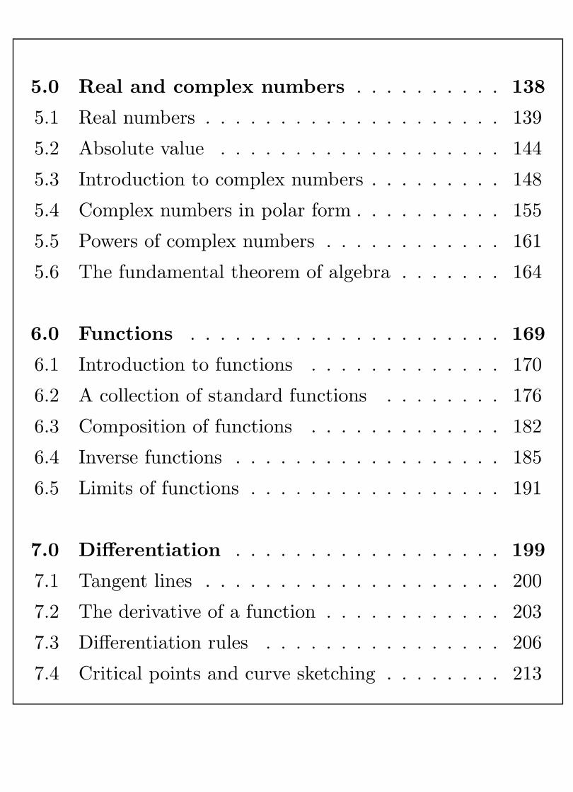
5.0 Real and complex numbers . . . . . . . . . . 138
5.1 Real numbers . . . . . . . . . . . . . . . . . . . . 139
5.2 Absolute value . . . . . . . . . . . . . . . . . . . 144
5.3 Introduction to complex numbers . . . . . . . . . 148
5.4 Complex numbers in polar form . . . . . . . . . . 155
5.5 Powers of complex numbers . . . . . . . . . . . . 161
5.6 The fundamental theorem of algebra . . . . . . . 164
6.0 Functions . . . . . . . . . . . . . . . . . . . . . 169
6.1 Introduction to functions . . . . . . . . . . . . . 170
6.2 A collection of standard functions . . . . . . . . 176
6.3 Composition of functions . . . . . . . . . . . . . 182
6.4 Inverse functions . . . . . . . . . . . . . . . . . . 185
6.5 Limits of functions . . . . . . . . . . . . . . . . . 191
7.0 Differentiation . . . . . . . . . . . . . . . . . . 199
7.1 Tangent lines . . . . . . . . . . . . . . . . . . . . 200
7.2 The derivative of a function . . . . . . . . . . . . 203
7.3 Differentiation rules . . . . . . . . . . . . . . . . 206
7.4 Critical points and curve sketching . . . . . . . . 213
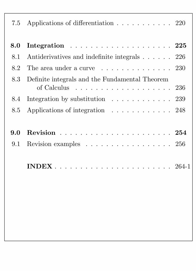
7.5 Applications of differentiation . . . . . . . . . . . 220
8.0 Integration . . . . . . . . . . . . . . . . . . . . 225
8.1 Antiderivatives and indefinite integrals . . . . . . 226
8.2 The area under a curve . . . . . . . . . . . . . . 230
8.3 Definite integrals and the Fundamental Theoremof Calculus . . . . . . . . . . . . . . . . . . . 236
8.4 Integration by substitution . . . . . . . . . . . . 239
8.5 Applications of integration . . . . . . . . . . . . 248
9.0 Revision . . . . . . . . . . . . . . . . . . . . . . 254
9.1 Revision examples . . . . . . . . . . . . . . . . . 256
INDEX . . . . . . . . . . . . . . . . . . . . . . . 264-1
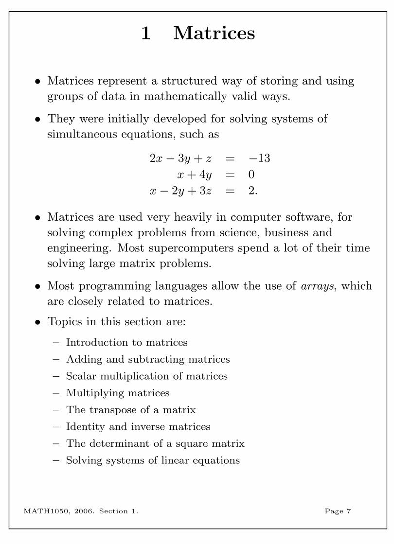
1 Matrices
• Matrices represent a structured way of storing and using
groups of data in mathematically valid ways.
• They were initially developed for solving systems of
simultaneous equations, such as
2x− 3y + z = −13
x+ 4y = 0
x− 2y + 3z = 2.
• Matrices are used very heavily in computer software, for
solving complex problems from science, business and
engineering. Most supercomputers spend a lot of their time
solving large matrix problems.
• Most programming languages allow the use of arrays, which
are closely related to matrices.
• Topics in this section are:
– Introduction to matrices
– Adding and subtracting matrices
– Scalar multiplication of matrices
– Multiplying matrices
– The transpose of a matrix
– Identity and inverse matrices
– The determinant of a square matrix
– Solving systems of linear equations
MATH1050, 2006. Section 1. Page 7
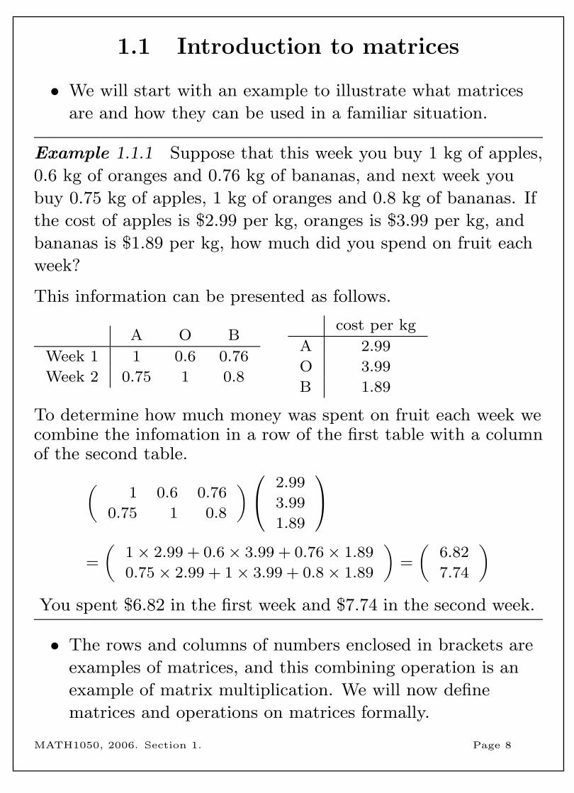
1.1 Introduction to matrices
• We will start with an example to illustrate what matrices
are and how they can be used in a familiar situation.
Example 1.1.1 Suppose that this week you buy 1 kg of apples,
0.6 kg of oranges and 0.76 kg of bananas, and next week you
buy 0.75 kg of apples, 1 kg of oranges and 0.8 kg of bananas. If
the cost of apples is $2.99 per kg, oranges is $3.99 per kg, and
bananas is $1.89 per kg, how much did you spend on fruit each
week?
This information can be presented as follows.
A O B
Week 1 1 0.6 0.76
Week 2 0.75 1 0.8
cost per kg
A 2.99
O 3.99
B 1.89
To determine how much money was spent on fruit each week wecombine the infomation in a row of the first table with a columnof the second table.(
1 0.6 0.76
0.75 1 0.8
) 2.99
3.99
1.89
=
(1× 2.99 + 0.6× 3.99 + 0.76× 1.89
0.75× 2.99 + 1× 3.99 + 0.8× 1.89
)=
(6.82
7.74
)You spent $6.82 in the first week and $7.74 in the second week.
• The rows and columns of numbers enclosed in brackets are
examples of matrices, and this combining operation is an
example of matrix multiplication. We will now define
matrices and operations on matrices formally.
MATH1050, 2006. Section 1. Page 8
• A matrix is a rectangular array of numbers, enclosed in
brackets.
• An m× n matrix has m rows and n columns. The size or
order of a matrix is its number of rows and number of
columns. An m× n matrix has size “m by n”.
• The plural of matrix is matrices.
Example 1.1.2
(1 2 3
4 5 6
)is a 2× 3 matrix.
• Common notation for a general m× n matrix A is
A =
a11 a12 a13 · · · a1n
a21 a22 a23 · · · a2n
......
......
am1 am2 am3 · · · amn
= (aij) .
• The notation aij is used to represent the element or entry in
the ith row and jth column of the matrix A.
• We commonly use an upper case letter to refer to a matrix
and the corresponding lower-case letter (with subscripts) to
refer to the elements of that matrix.
Example 1.1.3 The 2× 3 matrix A = (aij) with entries
aij = i− j is
MATH1050, 2006. Section 1. Page 9
• A matrix with exactly one row may be called a row vector.
A matrix with exactly one column may be called a column
vector. Row and column vectors are often denoted by
lower-case letters in bold type.
• A matrix with one row and one column is just a number
(as we’re all familiar with). Sometimes this is called a
scalar, to distinguish it from matrices with multiple rows or
columns, and we write it without any brackets.
• A matrix in which every entry is 0 is called a zero matrix.
The m× n zero matrix will sometimes be written as 0m×n.
• A matrix with the same number of rows and columns is
called a square matrix.
Example 1.1.4
(1 2 3) is a 1× 3 matrix, also called a row vector.(1
2
)is a 2× 1 matrix, also called a column vector.
2, 3, −4 and π are all examples of scalars.
02×2 =
(0 0
0 0
)is the 2× 2 zero matrix, and it is also a
square matrix.
• Matrices A = (aij) and B = (bij) are equal if and only if
– A and B have the same size, and
– aij = bij for all values of i and j.
MATH1050, 2006. Section 1. Page 10
1.2 Adding and subtracting matrices
• Two matrices can be added or subtracted provided that
they have the same size. Two matrices of different sizes
cannot be added or subtracted!
• Matrix addition: Let A = (aij) and B = (bij) be m× nmatrices. Then A+B = C = (cij) is the m× n matrix with
cij = aij + bij .
• Matrix subtraction: Let A = (aij) and B = (bij) be m× nmatrices. Then A−B = C = (cij) is the m× n matrix with
cij = aij − bij .
Example 1.2.1
Let A =
(0 1 −2
−1 2 4
)and B =
(3 −1 1
2
2 −5 3
). Then
A+B =
A−B =
MATH1050, 2006. Section 1. Page 11
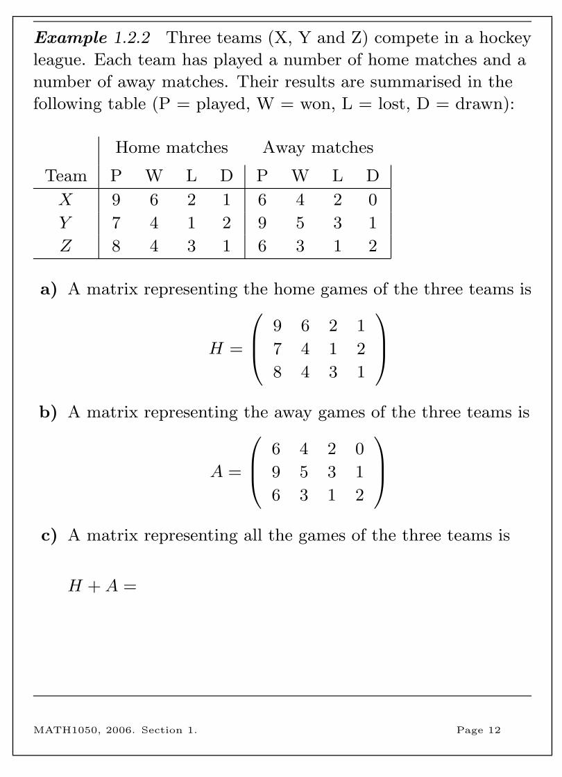
Example 1.2.2 Three teams (X, Y and Z) compete in a hockey
league. Each team has played a number of home matches and a
number of away matches. Their results are summarised in the
following table (P = played, W = won, L = lost, D = drawn):
Home matches Away matches
Team P W L D P W L D
X 9 6 2 1 6 4 2 0
Y 7 4 1 2 9 5 3 1
Z 8 4 3 1 6 3 1 2
a) A matrix representing the home games of the three teams is
H =
9 6 2 1
7 4 1 2
8 4 3 1
b) A matrix representing the away games of the three teams is
A =
6 4 2 0
9 5 3 1
6 3 1 2
c) A matrix representing all the games of the three teams is
H +A =
MATH1050, 2006. Section 1. Page 12
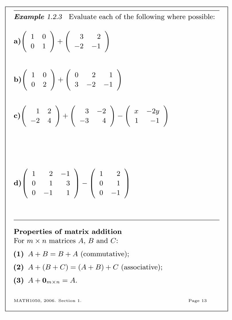
Example 1.2.3 Evaluate each of the following where possible:
a)
(1 0
0 1
)+
(3 2
−2 −1
)
b)
(1 0
0 2
)+
(0 2 1
3 −2 −1
)
c)
(1 2
−2 4
)+
(3 −2
−3 4
)−
(x −2y
1 −1
)
d)
1 2 −1
0 1 3
0 −1 1
− 1 2
0 1
0 −1
Properties of matrix addition
For m× n matrices A, B and C:
(1) A+B = B +A (commutative);
(2) A+ (B + C) = (A+B) + C (associative);
(3) A+ 0m×n = A.
MATH1050, 2006. Section 1. Page 13
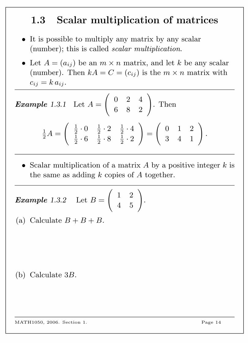
1.3 Scalar multiplication of matrices
• It is possible to multiply any matrix by any scalar
(number); this is called scalar multiplication.
• Let A = (aij) be an m× n matrix, and let k be any scalar
(number). Then kA = C = (cij) is the m× n matrix with
cij = k aij .
Example 1.3.1 Let A =
(0 2 4
6 8 2
). Then
12A =
(12· 0 1
2· 2 1
2· 4
12· 6 1
2· 8 1
2· 2
)=
(0 1 2
3 4 1
).
• Scalar multiplication of a matrix A by a positive integer k is
the same as adding k copies of A together.
Example 1.3.2 Let B =
(1 2
4 5
).
(a) Calculate B +B +B.
(b) Calculate 3B.
MATH1050, 2006. Section 1. Page 14
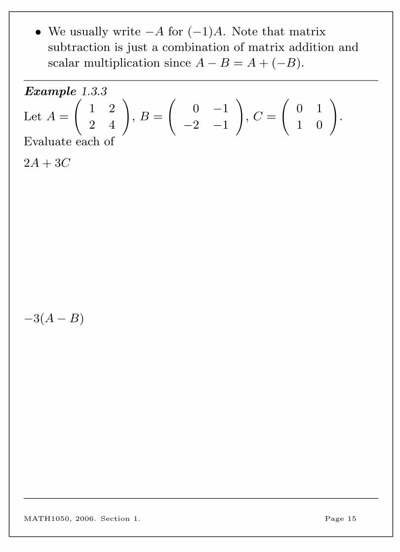
• We usually write −A for (−1)A. Note that matrix
subtraction is just a combination of matrix addition and
scalar multiplication since A−B = A+ (−B).
Example 1.3.3
Let A =
(1 2
2 4
), B =
(0 −1
−2 −1
), C =
(0 1
1 0
).
Evaluate each of
2A+ 3C
−3(A−B)
MATH1050, 2006. Section 1. Page 15
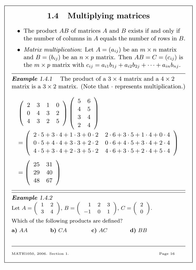
1.4 Multiplying matrices
• The product AB of matrices A and B exists if and only if
the number of columns in A equals the number of rows in B.
• Matrix multiplication: Let A = (aij) be an m× n matrix
and B = (bij) be an n× p matrix. Then AB = C = (cij) is
the m× p matrix with cij = ai1b1j + ai2b2j + · · ·+ ainbnj .
Example 1.4.1 The product of a 3× 4 matrix and a 4× 2
matrix is a 3× 2 matrix. (Note that · represents multiplication.)
2 3 1 0
0 4 3 2
4 3 2 5
5 6
4 5
3 4
2 4
=
2 · 5 + 3 · 4 + 1 · 3 + 0 · 2 2 · 6 + 3 · 5 + 1 · 4 + 0 · 40 · 5 + 4 · 4 + 3 · 3 + 2 · 2 0 · 6 + 4 · 5 + 3 · 4 + 2 · 44 · 5 + 3 · 4 + 2 · 3 + 5 · 2 4 · 6 + 3 · 5 + 2 · 4 + 5 · 4
=
25 31
29 40
48 67
Example 1.4.2
Let A =
(1 2
3 4
), B =
(1 2 3
−1 0 1
), C =
(2
0
).
Which of the following products are defined?
a) AA b) CA c) AC d) BB
MATH1050, 2006. Section 1. Page 16
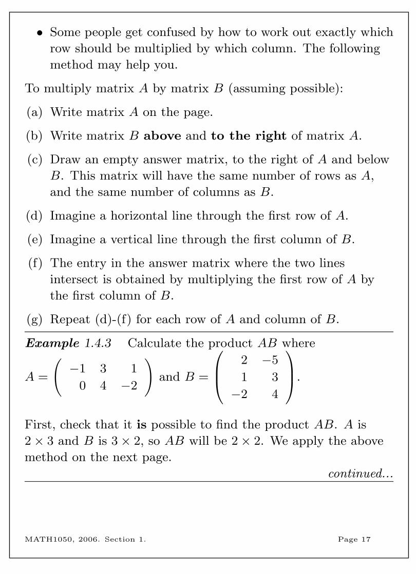
• Some people get confused by how to work out exactly which
row should be multiplied by which column. The following
method may help you.
To multiply matrix A by matrix B (assuming possible):
(a) Write matrix A on the page.
(b) Write matrix B above and to the right of matrix A.
(c) Draw an empty answer matrix, to the right of A and below
B. This matrix will have the same number of rows as A,
and the same number of columns as B.
(d) Imagine a horizontal line through the first row of A.
(e) Imagine a vertical line through the first column of B.
(f) The entry in the answer matrix where the two lines
intersect is obtained by multiplying the first row of A by
the first column of B.
(g) Repeat (d)-(f) for each row of A and column of B.
Example 1.4.3 Calculate the product AB where
A =
(−1 3 1
0 4 −2
)and B =
2 −5
1 3
−2 4
.
First, check that it is possible to find the product AB. A is
2× 3 and B is 3× 2, so AB will be 2× 2. We apply the above
method on the next page.
continued...
MATH1050, 2006. Section 1. Page 17
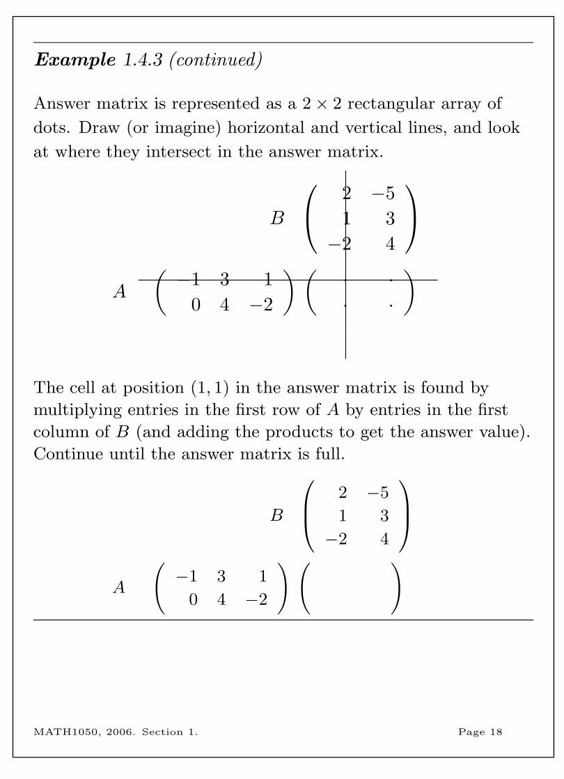
Example 1.4.3 (continued)
Answer matrix is represented as a 2× 2 rectangular array of
dots. Draw (or imagine) horizontal and vertical lines, and look
at where they intersect in the answer matrix.
B
2 −51 3−2 4
A
(−1 3 1
0 4 −2
) (· ·· ·
)
The cell at position (1, 1) in the answer matrix is found by
multiplying entries in the first row of A by entries in the first
column of B (and adding the products to get the answer value).
Continue until the answer matrix is full.
B
2 −5
1 3
−2 4
A
(−1 3 1
0 4 −2
) ( )
MATH1050, 2006. Section 1. Page 18
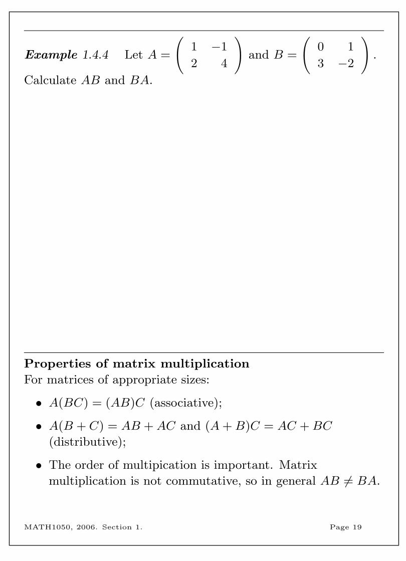
Example 1.4.4 Let A =
(1 −1
2 4
)and B =
(0 1
3 −2
).
Calculate AB and BA.
Properties of matrix multiplication
For matrices of appropriate sizes:
• A(BC) = (AB)C (associative);
• A(B + C) = AB +AC and (A+B)C = AC +BC
(distributive);
• The order of multipication is important. Matrix
multiplication is not commutative, so in general AB 6= BA.
MATH1050, 2006. Section 1. Page 19
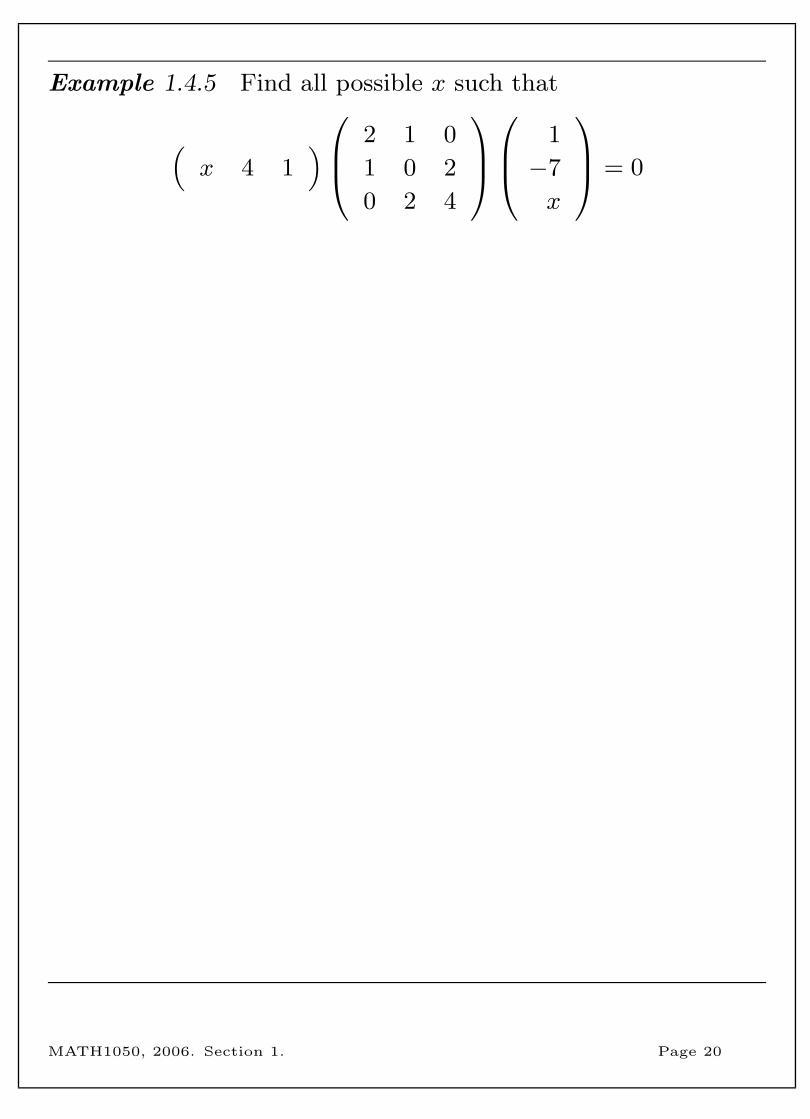
Example 1.4.5 Find all possible x such that
(x 4 1
) 2 1 0
1 0 2
0 2 4
1
−7
x
= 0
MATH1050, 2006. Section 1. Page 20
• For a square matrix A, we can define matrix powers by
repeated matrix multiplication.
A1 = A, A2 = A A, A3 = A A A = A2 A,
. . . , Ak+1 = Ak A.
• The usual exponent laws hold for matrix powers, so
Ak ·Ar = Ak+r and (Ak)r = Akr.
Example 1.4.6 Let A =
(2 −1
3 4
). Calculate A4.
MATH1050, 2006. Section 1. Page 21
1.5 The transpose of a matrix
• Informally, the transpose of an m× n matrix A is the n×mmatrix obtained by exchanging the rows and columns of A.
• Formally, given an m× n matrix A = (aij), the transpose of
A is the n×m matrix C = (cij) where
cij = aji, for all i, j.
• The transpose of A is usually denoted by AT .
Example 1.5.1(0 1 2
−1 3 5
)T=
(1 2
−1 3
)T=
1
2
3
T
=
Properties of transposes
For matrices of appropriate sizes:
• (A+B)T = AT +BT ;
• (AT )T = A;
• (AB)T = BT AT (Be careful!).
MATH1050, 2006. Section 1. Page 22
1.6 Identity and inverse matrices
• In the multiplication of real numbers, the number 1 plays a
special role because 1 · k = k · 1 = k for all real numbers k.
In matrix multiplication, this role is played by the identity
matrix.
• The identity matrix of order n, denoted I or In, is the n× nmatrix A = (aij) where
aij =
{1 if i = j,
0 if i 6= j.
Example 1.6.1 The identity matrices of orders 2 and 3 are:
I2 =
(1 0
0 1
)I3 =
1 0 0
0 1 0
0 0 1
• If A is any m×m matrix, then
Im A = A Im = A.
• More generally, if A is any m× n matrix, then
Im A = A In = A.
• When dealing with matrix powers, if A is an m×m matrix,
we define A0 = Im.
MATH1050, 2006. Section 1. Page 23
Example 1.6.2 Let B =
(−1 2 0
−2 4 3
). Verify that
I2 B = B and B I3 = B.
• The identity matrix is an example of a diagonal matrix.
• A square matrix A = (aij) is a diagonal matrix if and only
if aij = 0 whenever i 6= j.
• Examples of diagonal matrices are:(2 0
0 −1
) −3 0 0
0 12
0
0 0 −4
.
• Matrix powers of diagonal matrices are easy to calculate.
For example(2 0
0 −1
)3
=
(23 0
0 (−1)3
)=
(8 0
0 −1
).
MATH1050, 2006. Section 1. Page 24
The inverse of a square matrix
• A square matrix A is non-singular if there exists a matrix B
such that AB = BA = I. The matrix B is called the
inverse of A, and is denoted A−1.
• A non-singular matrix is said to be invertible.
Example 1.6.3
Let A =
(−1 −4
1 3
). Show that A−1 =
(3 4
−1 −1
).
MATH1050, 2006. Section 1. Page 25
• Not every square matrix is invertible.
• A matrix that does not have an inverse is said to be
singular or non-invertible.
Example 1.6.4 Show that the matrix A =
(0 1
0 2
)is
singular.
Properties of matrix inverses
If A and B are non-singular n× n matrices, then
• (A−1)−1 = A;
• (AB)−1 = B−1A−1 (Be careful!);
• (AT )−1 = (A−1)T .
MATH1050, 2006. Section 1. Page 26
The inverse of a 2× 2 matrix
Consider the 2× 2 matrix A =
(a b
c d
).
• A is invertible if and only if ad− bc 6= 0.
• If ad− bc 6= 0, then the inverse of A is
A−1 =1
ad− bc
(d −b−c a
).
Example 1.6.5 Suppose that ad− bc 6= 0 and verify that
AA−1 = A−1A = I.
MATH1050, 2006. Section 1. Page 27
Example 1.6.6 Let A =
(2 2
3 4
)and B =
(−1 − 2
3
6 4
).
Determine, if possible, A−1 and B−1.
• Note that after you have calculated the inverse of a matrix
A, it is a good idea (and easy) to check your work by
multiplication. If AA−1 6= I then you have made an error.
MATH1050, 2006. Section 1. Page 28
Example 1.6.7 Prove that a matrix A has at most one inverse.
• Suppose that A and B are square matrices of the same size.
If A is invertible and AB = I, then B is the inverse of A
and thus BA must equal I.
AB = I
if and only if A−1AB = A−1I
iff IB = A−1I
iff B = A−1
MATH1050, 2006. Section 1. Page 29
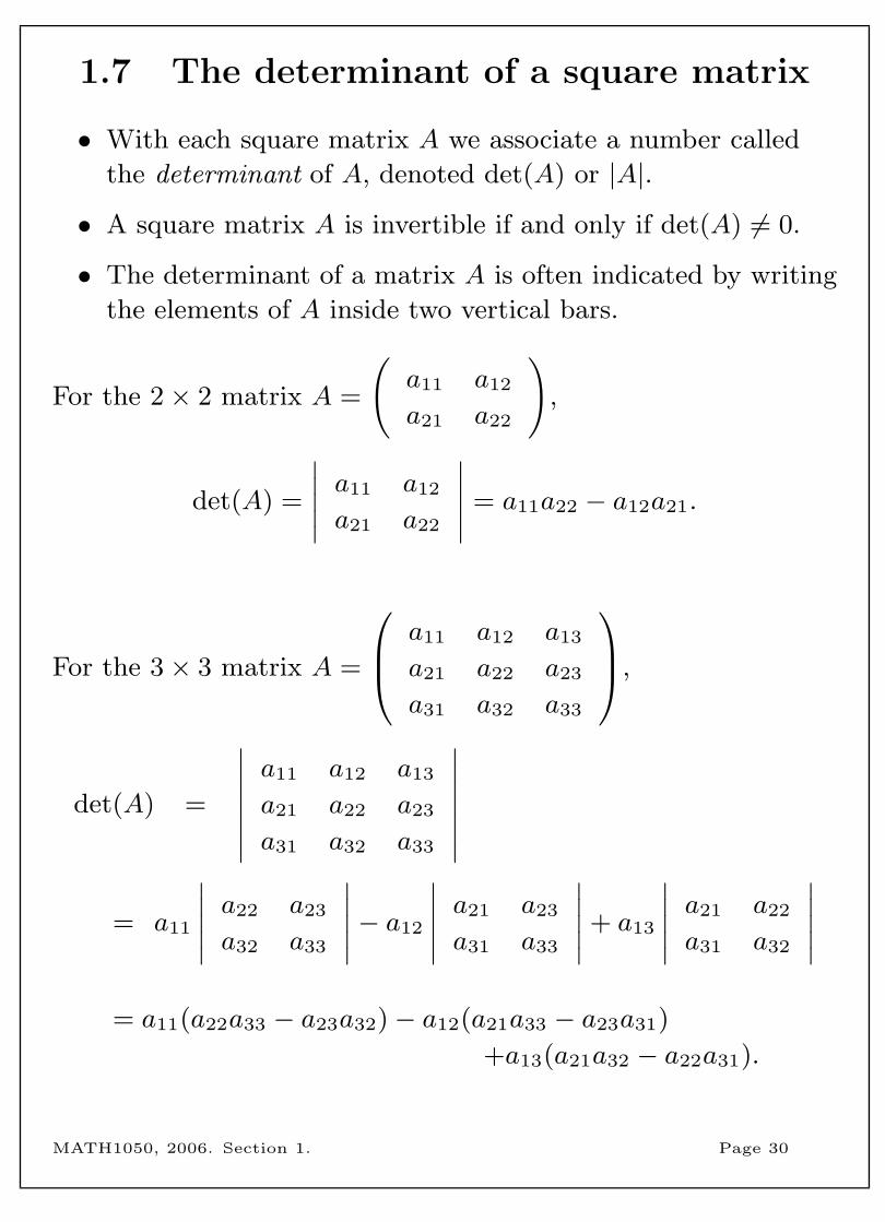
1.7 The determinant of a square matrix
• With each square matrix A we associate a number called
the determinant of A, denoted det(A) or |A|.
• A square matrix A is invertible if and only if det(A) 6= 0.
• The determinant of a matrix A is often indicated by writing
the elements of A inside two vertical bars.
For the 2× 2 matrix A =
(a11 a12
a21 a22
),
det(A) =
∣∣∣∣∣ a11 a12
a21 a22
∣∣∣∣∣ = a11a22 − a12a21.
For the 3× 3 matrix A =
a11 a12 a13
a21 a22 a23
a31 a32 a33
,
det(A) =
∣∣∣∣∣∣∣a11 a12 a13
a21 a22 a23
a31 a32 a33
∣∣∣∣∣∣∣= a11
∣∣∣∣∣ a22 a23
a32 a33
∣∣∣∣∣− a12
∣∣∣∣∣ a21 a23
a31 a33
∣∣∣∣∣+ a13
∣∣∣∣∣ a21 a22
a31 a32
∣∣∣∣∣= a11(a22a33 − a23a32)− a12(a21a33 − a23a31)
+a13(a21a32 − a22a31).
MATH1050, 2006. Section 1. Page 30
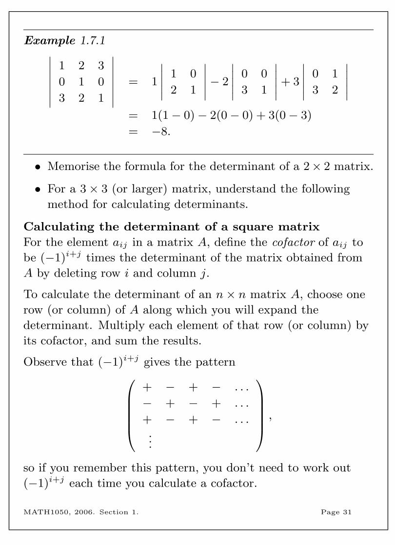
Example 1.7.1∣∣∣∣∣∣∣1 2 3
0 1 0
3 2 1
∣∣∣∣∣∣∣ = 1
∣∣∣∣∣ 1 0
2 1
∣∣∣∣∣− 2
∣∣∣∣∣ 0 0
3 1
∣∣∣∣∣+ 3
∣∣∣∣∣ 0 1
3 2
∣∣∣∣∣= 1(1− 0)− 2(0− 0) + 3(0− 3)
= −8.
• Memorise the formula for the determinant of a 2× 2 matrix.
• For a 3× 3 (or larger) matrix, understand the following
method for calculating determinants.
Calculating the determinant of a square matrix
For the element aij in a matrix A, define the cofactor of aij to
be (−1)i+j times the determinant of the matrix obtained from
A by deleting row i and column j.
To calculate the determinant of an n× n matrix A, choose one
row (or column) of A along which you will expand the
determinant. Multiply each element of that row (or column) by
its cofactor, and sum the results.
Observe that (−1)i+j gives the pattern+ − + − . . .
− + − + . . .
+ − + − . . ....
,
so if you remember this pattern, you don’t need to work out
(−1)i+j each time you calculate a cofactor.
MATH1050, 2006. Section 1. Page 31
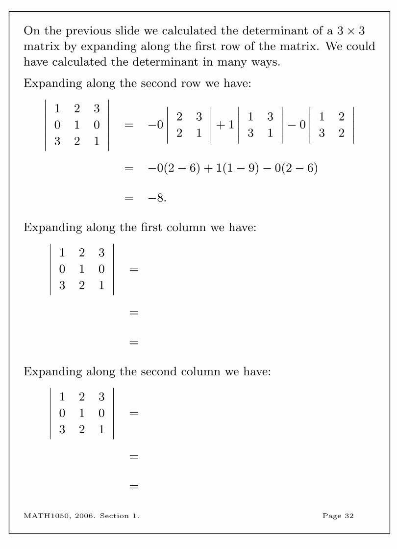
On the previous slide we calculated the determinant of a 3× 3
matrix by expanding along the first row of the matrix. We could
have calculated the determinant in many ways.
Expanding along the second row we have:∣∣∣∣∣∣∣1 2 3
0 1 0
3 2 1
∣∣∣∣∣∣∣ = −0
∣∣∣∣∣ 2 3
2 1
∣∣∣∣∣+ 1
∣∣∣∣∣ 1 3
3 1
∣∣∣∣∣− 0
∣∣∣∣∣ 1 2
3 2
∣∣∣∣∣= −0(2− 6) + 1(1− 9)− 0(2− 6)
= −8.
Expanding along the first column we have:∣∣∣∣∣∣∣1 2 3
0 1 0
3 2 1
∣∣∣∣∣∣∣ =
=
=
Expanding along the second column we have:∣∣∣∣∣∣∣1 2 3
0 1 0
3 2 1
∣∣∣∣∣∣∣ =
=
=
MATH1050, 2006. Section 1. Page 32
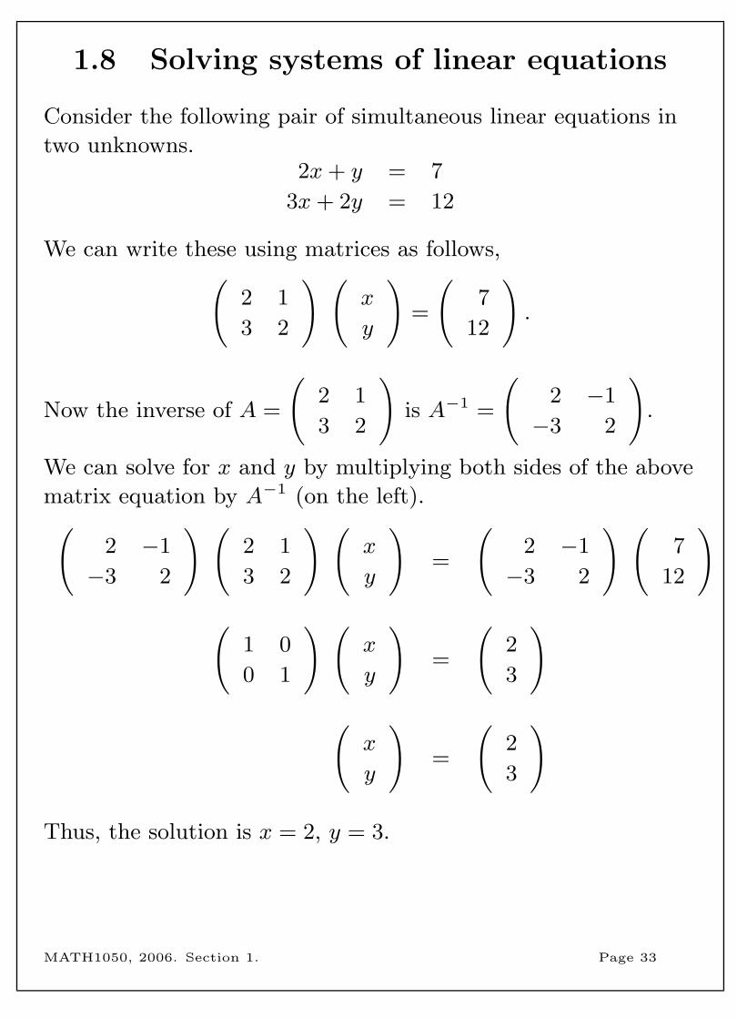
1.8 Solving systems of linear equations
Consider the following pair of simultaneous linear equations in
two unknowns.2x+ y = 7
3x+ 2y = 12
We can write these using matrices as follows,(2 1
3 2
) (x
y
)=
(7
12
).
Now the inverse of A =
(2 1
3 2
)is A−1 =
(2 −1
−3 2
).
We can solve for x and y by multiplying both sides of the above
matrix equation by A−1 (on the left).(2 −1
−3 2
) (2 1
3 2
) (x
y
)=
(2 −1
−3 2
) (7
12
)(
1 0
0 1
) (x
y
)=
(2
3
)(
x
y
)=
(2
3
)
Thus, the solution is x = 2, y = 3.
MATH1050, 2006. Section 1. Page 33
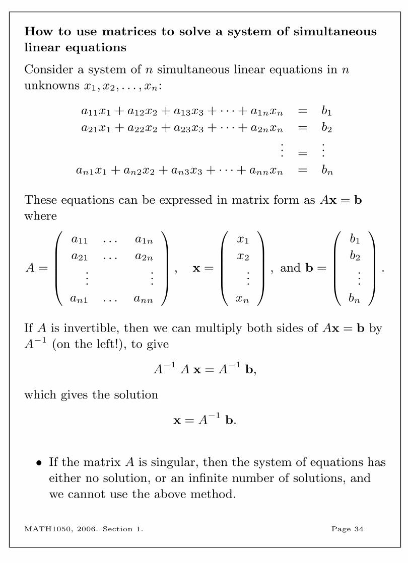
How to use matrices to solve a system of simultaneous
linear equations
Consider a system of n simultaneous linear equations in n
unknowns x1, x2, . . . , xn:
a11x1 + a12x2 + a13x3 + · · ·+ a1nxn = b1a21x1 + a22x2 + a23x3 + · · ·+ a2nxn = b2
... =...
an1x1 + an2x2 + an3x3 + · · ·+ annxn = bn
These equations can be expressed in matrix form as Ax = b
where
A =
a11 . . . a1n
a21 . . . a2n
......
an1 . . . ann
, x =
x1
x2
...
xn
, and b =
b1b2
...
bn
.
If A is invertible, then we can multiply both sides of Ax = b by
A−1 (on the left!), to give
A−1 A x = A−1 b,
which gives the solution
x = A−1 b.
• If the matrix A is singular, then the system of equations has
either no solution, or an infinite number of solutions, and
we cannot use the above method.
MATH1050, 2006. Section 1. Page 34
Example 1.8.1 Use matrices to solve (if possible) the following
pairs of simultaneous equations.
a) x− 2y = 0 and x+ 3y = 5
b) 2x = y − 3 and 2y − 4x = 6
MATH1050, 2006. Section 1. Page 35
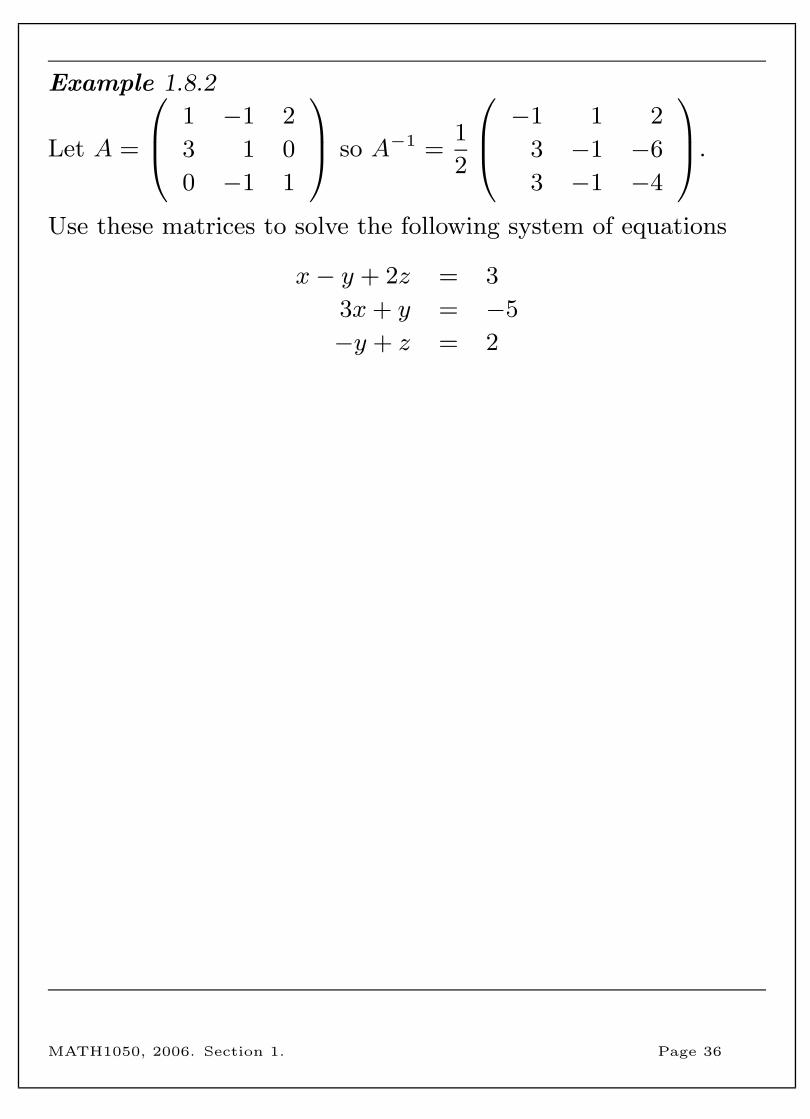
Example 1.8.2
Let A =
1 −1 2
3 1 0
0 −1 1
so A−1 =1
2
−1 1 2
3 −1 −6
3 −1 −4
.
Use these matrices to solve the following system of equations
x− y + 2z = 3
3x+ y = −5
−y + z = 2
MATH1050, 2006. Section 1. Page 36
Example 1.8.3 Ali Baba’s rug store is having a sale on persian
rugs and mats. Peter buys 3 mats and 2 rugs for $1300, and
Dave buys 2 mats and 3 rugs for $1700. How much will it cost
to purchase 4 mats and 4 rugs, at these prices?
MATH1050, 2006. Section 1. Page 37
2 Vectors
• In modelling the real world, some quantities, such as length,
area, time and temperature, can be described by real
numbers. We call these scalar quantities. However, the
description of other quantities, such as displacement,
velocity and force, require more than just one real number.
They are described by both a magnitude and a direction.
We call these vector quantities.
• You have already seen the word vector used in the context
of matrices, and it may seem strange that we use the word
vector also to describe something having both magnitude
and direction, but you will see how the two uses of the word
are related.
• Vectors can be represented in many ways and have many
applications.
• In this section we look at three representations of vectors:
geometric form, matrix form and component form.
• Topics in this section are:
– Introduction to vectors (geometric and matrix form)
– Addition of vectors
– Scalar multiplication of vectors
– Position vectors
– The norm of a vector
– Trigonometry review
– Component form of a vector
– More trigonometry
MATH1050, 2006. Section 2. Page 38
2.1 Introduction to vectors
• A vector quantity is something whose specification requires
both a magnitude and a direction.
• We normally use bold lower-case letters to represent
vectors, or, when handwriting, a lower-case letter with the
∼ symbol below it, for example v∼
.
• Throughout this section we will refer to the (x, y)-plane as
2-space, denoted R2, and (x, y, z)-space as 3-space, denoted
R3. All of our vectors can be depicted in R2 or R3.
Geometric representation of a vector
• A vector can be represented geometrically in R2 or R3 by
an arrow.
• The length of the arrow represents the magnitude of the
vector, and the direction of the vector is indicated by the
direction the arrow is pointing.
• The actual location of the arrow in the diagram is
irrelevant, only its magnitude and direction matter.
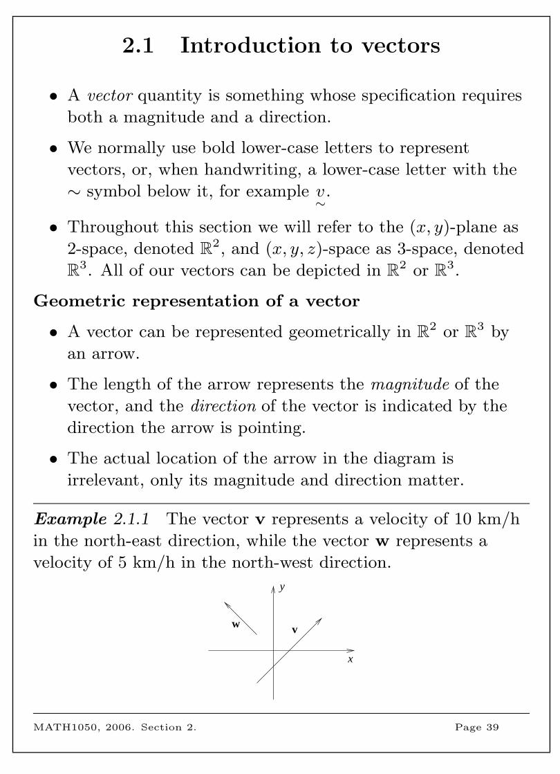
Example 2.1.1 The vector v represents a velocity of 10 km/h
in the north-east direction, while the vector w represents a
velocity of 5 km/h in the north-west direction.
vw
x
y
MATH1050, 2006. Section 2. Page 39
Example 2.1.2 The three arrows shown below each represent
the same vector.
x
y
• If P and Q are points in R2 or R3, then−→PQ denotes the
vector from P to Q. The point P is the tail of the vector
and the point Q is the head of the vector.
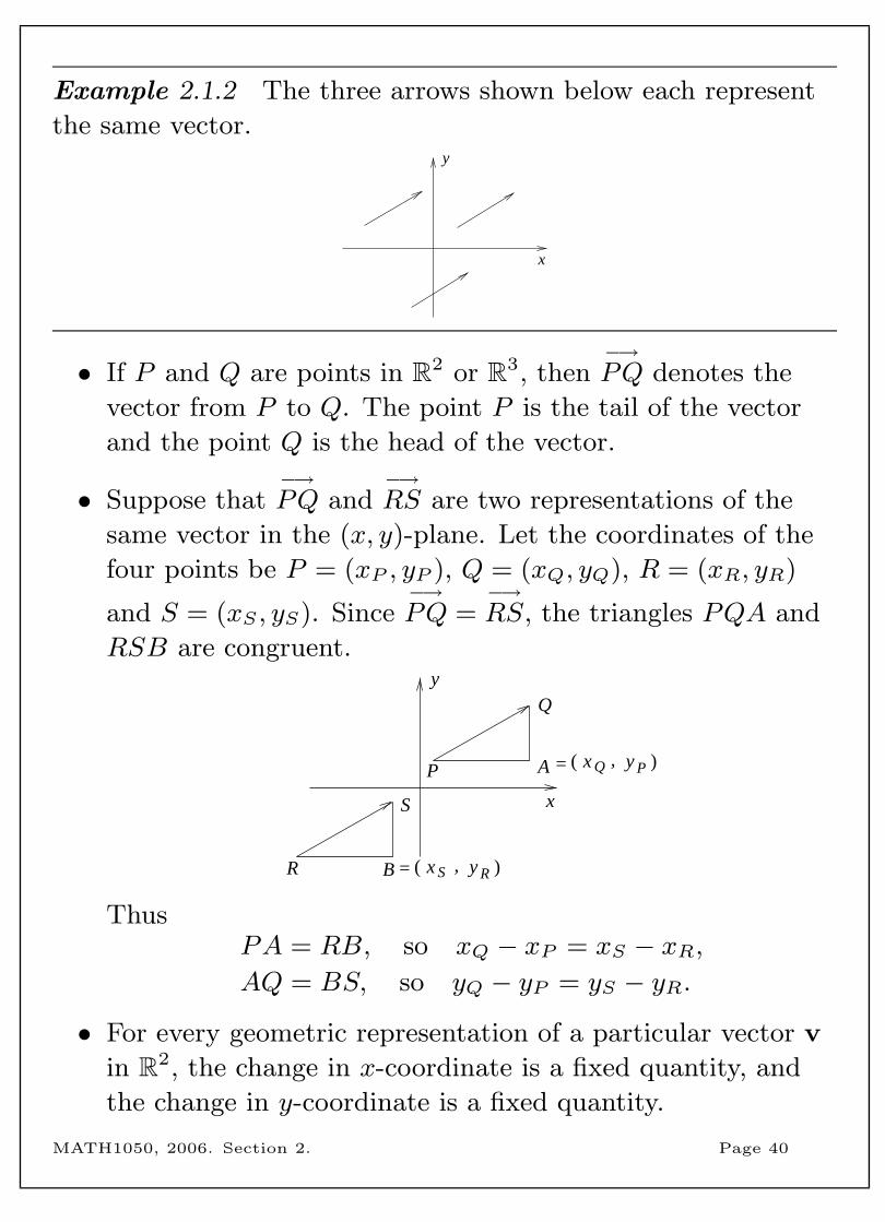
• Suppose that−→PQ and
−→RS are two representations of the
same vector in the (x, y)-plane. Let the coordinates of the
four points be P = (xP , yP ), Q = (xQ, yQ), R = (xR, yR)
and S = (xS , yS). Since−→PQ =
−→RS, the triangles PQA and
RSB are congruent.
R )
x
y
P
Q
A =
R
S
B = y
( x Q , y P )
( x S ,
ThusPA = RB, so xQ − xP = xS − xR,AQ = BS, so yQ − yP = yS − yR.
• For every geometric representation of a particular vector v
in R2, the change in x-coordinate is a fixed quantity, and
the change in y-coordinate is a fixed quantity.
MATH1050, 2006. Section 2. Page 40
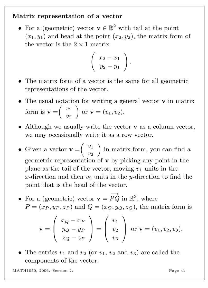
Matrix representation of a vector
• For a (geometric) vector v ∈ R2 with tail at the point
(x1, y1) and head at the point (x2, y2), the matrix form of
the vector is the 2× 1 matrix(x2 − x1
y2 − y1
).
• The matrix form of a vector is the same for all geometric
representations of the vector.
• The usual notation for writing a general vector v in matrix
form is v =(
v1
v2
)or v = (v1, v2).
• Although we usually write the vector v as a column vector,
we may occasionally write it as a row vector.
• Given a vector v =(
v1
v2
)in matrix form, you can find a
geometric representation of v by picking any point in the
plane as the tail of the vector, moving v1 units in the
x-direction and then v2 units in the y-direction to find the
point that is the head of the vector.
• For a (geometric) vector v =−→PQ in R3, where
P = (xP , yP , zP ) and Q = (xQ, yQ, zQ), the matrix form is
v =
xQ − xPyQ − yPzQ − zP
=
v1
v2
v3
or v = (v1, v2, v3).
• The entries v1 and v2 (or v1, v2 and v3) are called the
components of the vector.
MATH1050, 2006. Section 2. Page 41
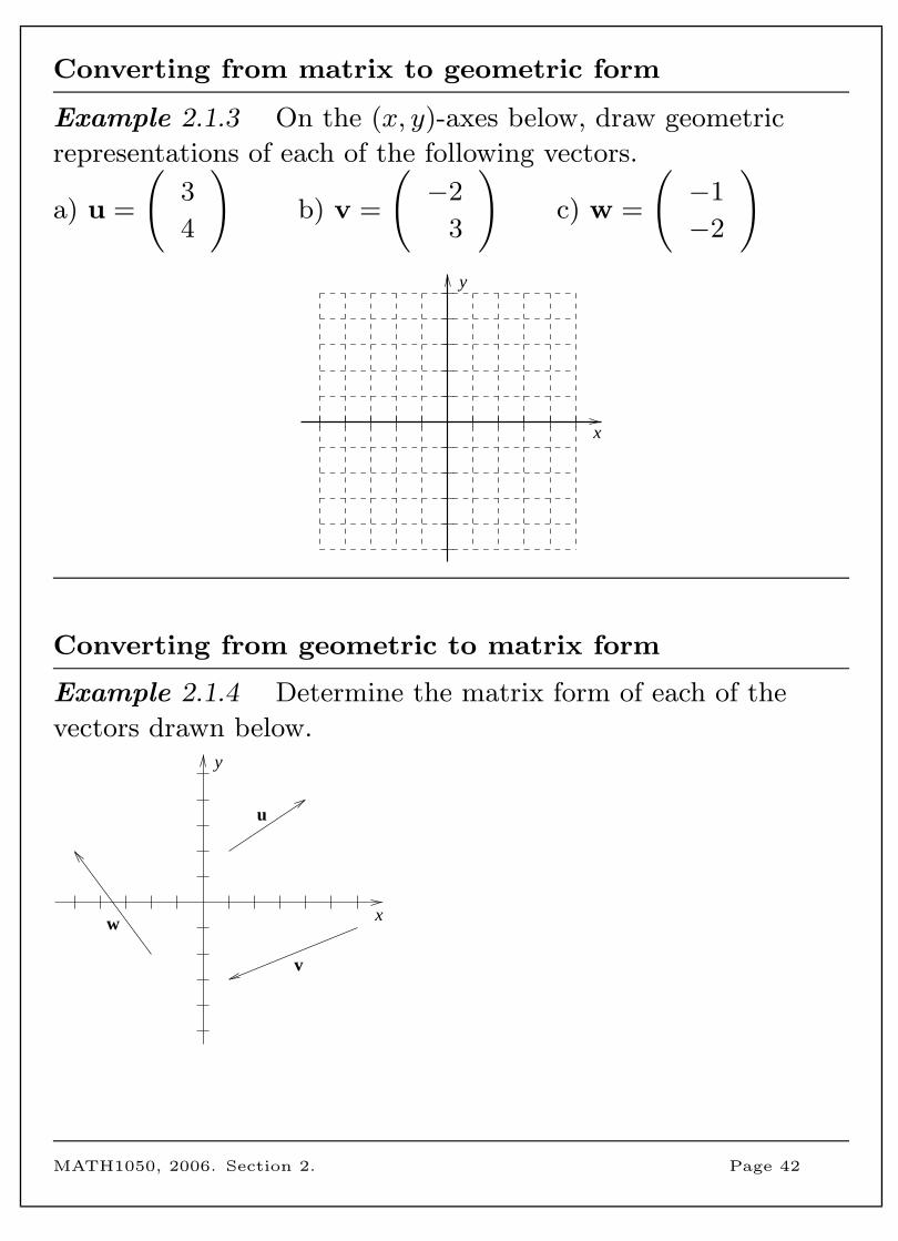
Converting from matrix to geometric form
Example 2.1.3 On the (x, y)-axes below, draw geometric
representations of each of the following vectors.
a) u =
(3
4
)b) v =
(−2
3
)c) w =
(−1
−2
)y
x
Converting from geometric to matrix form
Example 2.1.4 Determine the matrix form of each of the
vectors drawn below.y
x
v
u
w
MATH1050, 2006. Section 2. Page 42
2.2 Addition of vectors
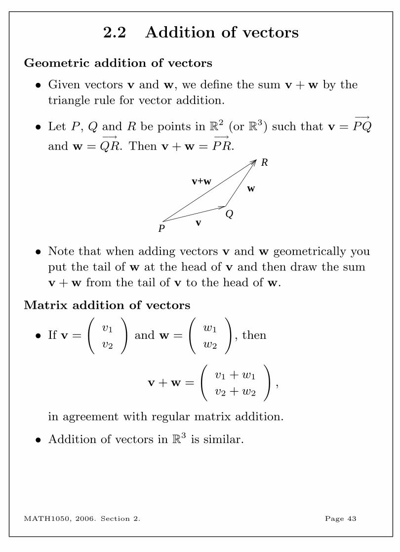
Geometric addition of vectors
• Given vectors v and w, we define the sum v + w by the
triangle rule for vector addition.
• Let P , Q and R be points in R2 (or R3) such that v =−→PQ
and w =−→QR. Then v + w =
−→PR.
PQ
v
w
R
v+w
• Note that when adding vectors v and w geometrically you
put the tail of w at the head of v and then draw the sum
v + w from the tail of v to the head of w.
Matrix addition of vectors
• If v =
(v1
v2
)and w =
(w1
w2
), then
v + w =
(v1 + w1
v2 + w2
),
in agreement with regular matrix addition.
• Addition of vectors in R3 is similar.
MATH1050, 2006. Section 2. Page 43
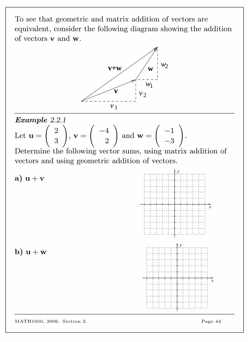
To see that geometric and matrix addition of vectors are
equivalent, consider the following diagram showing the addition
of vectors v and w.
v+w w
v
2w
1w
2v
1v
Example 2.2.1
Let u =
(2
3
), v =
(−4
2
)and w =
(−1
−3
).
Determine the following vector sums, using matrix addition of
vectors and using geometric addition of vectors.
a) u + vy
x
b) u + wy
x
MATH1050, 2006. Section 2. Page 44
• We define the zero vector to be the vector (of an appropriate
size) with each component equal to zero, and denote it by 0.
0 =
(0
0
)or 0 =
0
0
0
• The zero vector has zero magnitude and unspecified
direction, so can be represented geometrically as a point.
Properties of vector addition
(1) Vector addition is commutative, that is, v + w = w + v.
• We have already seen that matrix addition is commutative.
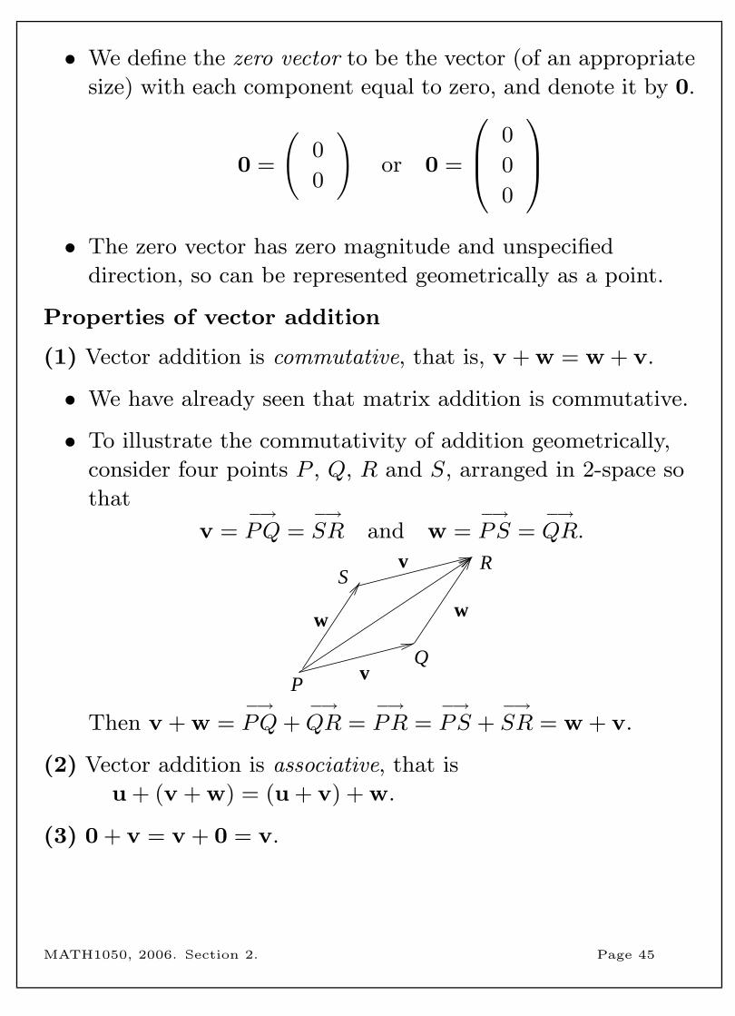
• To illustrate the commutativity of addition geometrically,
consider four points P , Q, R and S, arranged in 2-space so
that
v =−→PQ =
−→SR and w =
−→PS =
−→QR.
PQ
v
w
RS
w
v
Then v + w =−→PQ+
−→QR =
−→PR =
−→PS +
−→SR = w + v.
(2) Vector addition is associative, that is
u + (v + w) = (u + v) + w.
(3) 0 + v = v + 0 = v.
MATH1050, 2006. Section 2. Page 45
2.3 Scalar multiplication of vectors
Geometric scalar multiplication of vectors
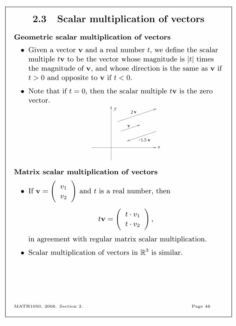
• Given a vector v and a real number t, we define the scalar
multiple tv to be the vector whose magnitude is |t| times
the magnitude of v, and whose direction is the same as v if
t > 0 and opposite to v if t < 0.
• Note that if t = 0, then the scalar multiple tv is the zero
vector.
2 v
−1.5 v
v
y
x
Matrix scalar multiplication of vectors
• If v =
(v1
v2
)and t is a real number, then
tv =
(t · v1
t · v2
),
in agreement with regular matrix scalar multiplication.
• Scalar multiplication of vectors in R3 is similar.
MATH1050, 2006. Section 2. Page 46
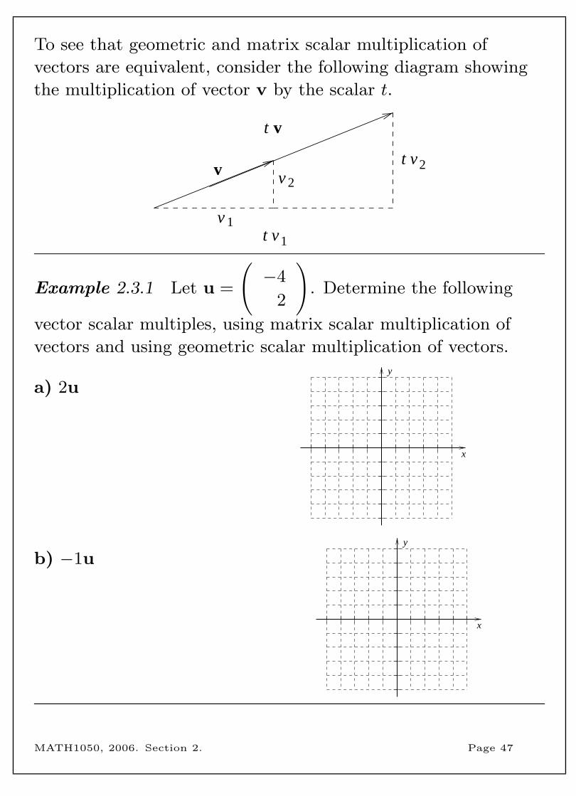
To see that geometric and matrix scalar multiplication of
vectors are equivalent, consider the following diagram showing
the multiplication of vector v by the scalar t.
v
t v
2v2t v
1t v1v
Example 2.3.1 Let u =
(−4
2
). Determine the following
vector scalar multiples, using matrix scalar multiplication of
vectors and using geometric scalar multiplication of vectors.
a) 2uy
x
b) −1uy
x
MATH1050, 2006. Section 2. Page 47
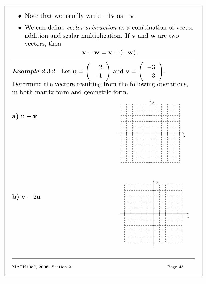
• Note that we usually write −1v as −v.
• We can define vector subtraction as a combination of vector
addition and scalar multiplication. If v and w are two
vectors, then
v −w = v + (−w).
Example 2.3.2 Let u =
(2
−1
)and v =
(−3
3
).
Determine the vectors resulting from the following operations,
in both matrix form and geometric form.
a) u− v
y
x
b) v − 2u
y
x
MATH1050, 2006. Section 2. Page 48
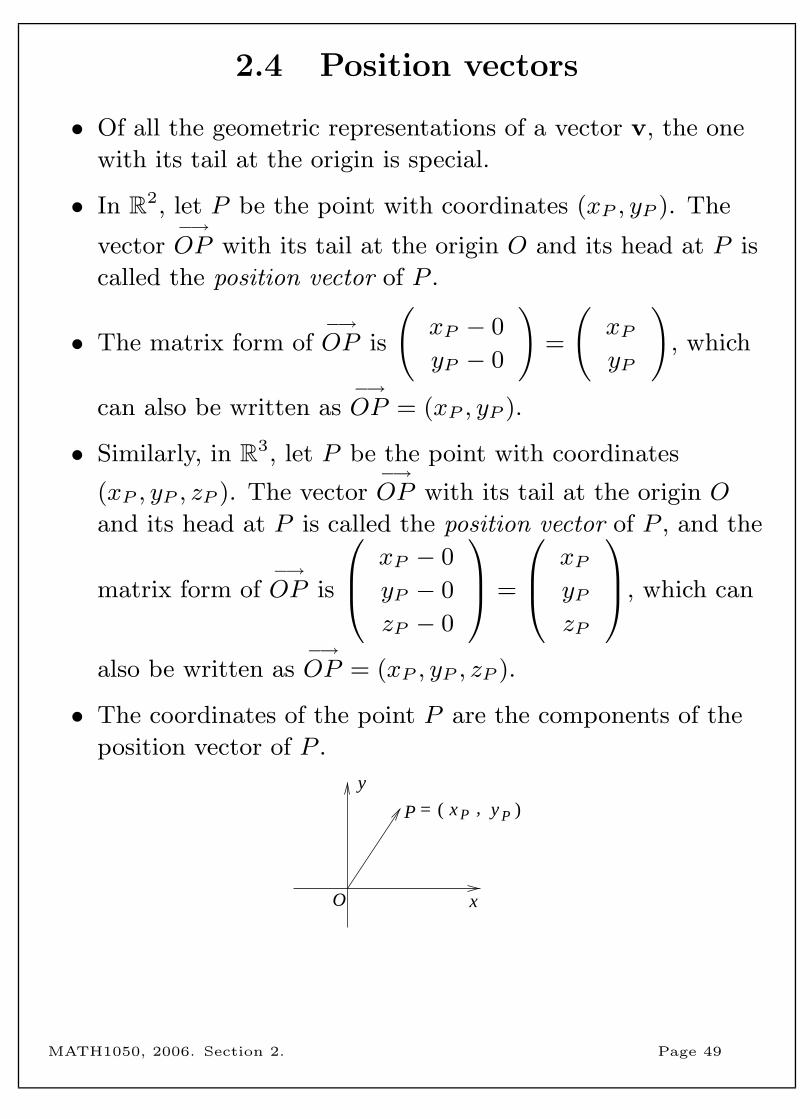
2.4 Position vectors
• Of all the geometric representations of a vector v, the one
with its tail at the origin is special.
• In R2, let P be the point with coordinates (xP , yP ). The
vector−→OP with its tail at the origin O and its head at P is
called the position vector of P .
• The matrix form of−→OP is
(xP − 0
yP − 0
)=
(xPyP
), which
can also be written as−→OP = (xP , yP ).
• Similarly, in R3, let P be the point with coordinates
(xP , yP , zP ). The vector−→OP with its tail at the origin O
and its head at P is called the position vector of P , and the
matrix form of−→OP is
xP − 0
yP − 0
zP − 0
=
xPyPzP
, which can
also be written as−→OP = (xP , yP , zP ).
• The coordinates of the point P are the components of the
position vector of P .
=
O
P
y
x
)Py,Px(
MATH1050, 2006. Section 2. Page 49
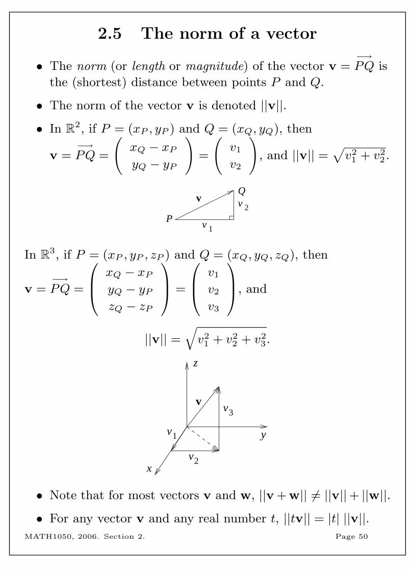
2.5 The norm of a vector
• The norm (or length or magnitude) of the vector v =−→PQ is
the (shortest) distance between points P and Q.
• The norm of the vector v is denoted ||v||.
• In R2, if P = (xP , yP ) and Q = (xQ, yQ), then
v =−→PQ =
(xQ − xPyQ − yP
)=
(v1
v2
), and ||v|| =
√v2
1 + v22 .
1v
2v
P
Qv
In R3, if P = (xP , yP , zP ) and Q = (xQ, yQ, zQ), then
v =−→PQ =
xQ − xPyQ − yPzQ − zP
=
v1
v2
v3
, and
||v|| =√v2
1 + v22 + v2
3 .
v
x
z
y
3v
2v
1v
• Note that for most vectors v and w, ||v + w|| 6= ||v||+ ||w||.
• For any vector v and any real number t, ||tv|| = |t| ||v||.MATH1050, 2006. Section 2. Page 50
• A vector with norm 1 is called a unit vector.
• The notation v will be used to denote a unit vector having
the same direction as the vector v.
• For a given vector v, with norm ||v||, the vector
v =1
||v||v
is a unit vector in the direction of v.
Example 2.5.1 Determine u and v in matrix form where
u =
(3
4
)and v =
2
−1
4
.
MATH1050, 2006. Section 2. Page 51
2.6 Trigonometry review
• So far, the geometric representations of our vectors have
fallen nicely at grid points of the (x, y)-axes so it has been
easy to convert them to matrix form, and to perform
addition, scalar multiplication, etc. In general, this will not
be the case. In this section we quickly review some
trigonometry that will be required in our work with vectors.
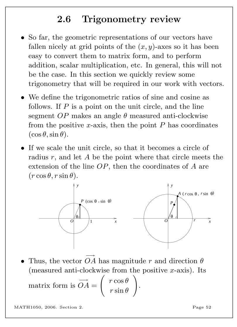
• We define the trigonometric ratios of sine and cosine as
follows. If P is a point on the unit circle, and the line
segment OP makes an angle θ measured anti-clockwise
from the positive x-axis, then the point P has coordinates
(cos θ, sin θ).
• If we scale the unit circle, so that it becomes a circle of
radius r, and let A be the point where that circle meets the
extension of the line OP , then the coordinates of A are
(r cos θ, r sin θ).
( rr ,
y
x
P
A
rθ θ
O O
)
cos θ sin θ,( )
y
x
P
1
sin θcos θ
• Thus, the vector−→OA has magnitude r and direction θ
(measured anti-clockwise from the positive x-axis). Its
matrix form is−→OA =
(r cos θ
r sin θ
).
MATH1050, 2006. Section 2. Page 52

Example 2.6.1 Let v be the vector in R2 with magnitude 5
such that v makes an angle of 5π7
radians with the positive
x-axis. Find the matrix form of v (2 decimal place accuracy).
• The trigonometric function “tangent” is defined as
tan θ = sin θcos θ
.
• In this course we will usually measure angles in radians. To
convert between radians and degrees, use the fact that π
radians is equal to 180 degrees.
• Angles will be measured anti-clockwise from the positive
x-axis, unless otherwise indicated.
• For a right-angled triangle with angle θ as shown, the
values of the trigonometric ratios are
hyp.
adj.θ
opp.
sin θ =opposite
hypotenuse, cos θ =
adjacent
hypotenuse, tan θ =
opposite
adjacent.
MATH1050, 2006. Section 2. Page 53
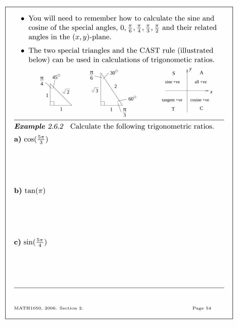
• You will need to remember how to calculate the sine and
cosine of the special angles, 0, π6, π
4, π
3, π
2and their related
angles in the (x, y)-plane.
• The two special triangles and the CAST rule (illustrated
below) can be used in calculations of trigonometic ratios.
1
1
1
2
T
A
all +ve
tangent +ve
x
yS
cosine +ve
sine +ve
C
2 3
π4
45
π3
60
π6
30
Example 2.6.2 Calculate the following trigonometric ratios.
a) cos( 5π3
)
b) tan(π)
c) sin( 5π4
)
MATH1050, 2006. Section 2. Page 54
Example 2.6.3 Calculate the values of the angle θ that satisfy
the following equations, where 0 ≤ θ < 2π.
a) sin θ = 12
(Equivalently θ = arcsin( 12) or θ = sin−1( 1
2).)
b) tan θ = −1 (Equivalently θ = arctan(−1) or θ = tan−1(−1).)
c) cos θ = 0.53 (Use your calculator for this one.)
MATH1050, 2006. Section 2. Page 55
2.7 Component form of a vector
Component form in 2-space
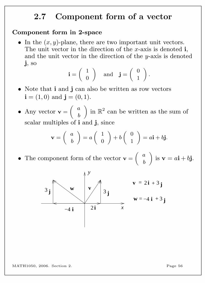
• In the (x, y)-plane, there are two important unit vectors.The unit vector in the direction of the x-axis is denoted i,and the unit vector in the direction of the y-axis is denotedj, so
i =
(1
0
)and j =
(0
1
).
• Note that i and j can also be written as row vectors
i = (1, 0) and j = (0, 1).
• Any vector v =
(a
b
)in R2 can be written as the sum of
scalar multiples of i and j, since
v =
(a
b
)= a
(1
0
)+ b
(0
1
)= ai + bj.
• The component form of the vector v =
(a
b
)is v = ai + bj.
x
y
v+v =
w = +
w
2 i
3 j3 j
2 i 3 j
i−4
i−4 3 j
MATH1050, 2006. Section 2. Page 56
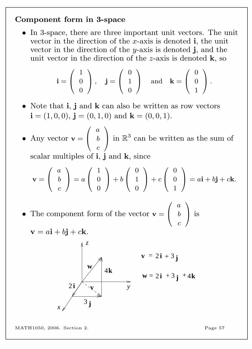
Component form in 3-space
• In 3-space, there are three important unit vectors. The unitvector in the direction of the x-axis is denoted i, the unitvector in the direction of the y-axis is denoted j, and theunit vector in the direction of the z-axis is denoted k, so
i =
1
0
0
, j =
0
1
0
and k =
0
0
1
.
• Note that i, j and k can also be written as row vectors
i = (1, 0, 0), j = (0, 1, 0) and k = (0, 0, 1).
• Any vector v =
a
b
c
in R3 can be written as the sum of
scalar multiples of i, j and k, since
v =
a
b
c
= a
1
0
0
+ b
0
1
0
+ c
0
0
1
= ai + bj + ck.
• The component form of the vector v =
a
b
c
is
v = ai + bj + ck.
y
z
+v =
w =
x
v
w+ +
2 i 3 j
2 i
3 j
2 i 3 j4k
4k
MATH1050, 2006. Section 2. Page 57
Converting vectors from geometric to component form
A vector v in R2, with magnitude ||v|| and direction θ measured
anti-clockwise from the positive x-axis, has component form
v = ||v|| cos θi + ||v|| sin θj.
Example 2.7.1 a) The vector v in R2 has magnitude 4 and
direction 2π3
. Write v in component form and in matrix form.
b) The vector w in R2 has magnitude 3 and direction 3π2
. Write
w in component form and in matrix form.
MATH1050, 2006. Section 2. Page 58
Converting vectors from component to geometric form
A vector v = v1i + v2j has magnitude ||v|| =√v2
1 + v22 . If v is
non-zero, then its direction θ, measured anti-clockwise from the
positive x-axis, is obtained as follows.
• Sketch the position vector v on a set of (x, y)-axes.
• If v = v1i + 0j or v = 0i + v2j, then θ will be one of 0, π2
, π
or 3π2
, and you can determine which it is from the sketch.
• If neither of v1 nor v2 is zero, then calculate
φ = arctan(∣∣∣ v2v1
∣∣∣). The value of φ will be between 0 and π2
.
• The value of θ will be one of φ, π − φ, π + φ, or 2π − φ. You
can identify which it is from your sketch.
Example 2.7.2
a) Find the magnitude and direction of the vector v = i−√
3j.
b) Find the magnitude and direction of the vector v = −2i + 3j.
MATH1050, 2006. Section 2. Page 59
2.8 More trigonometry
• When you work with triangles that are not right-angled
triangles, the following two rules are useful.
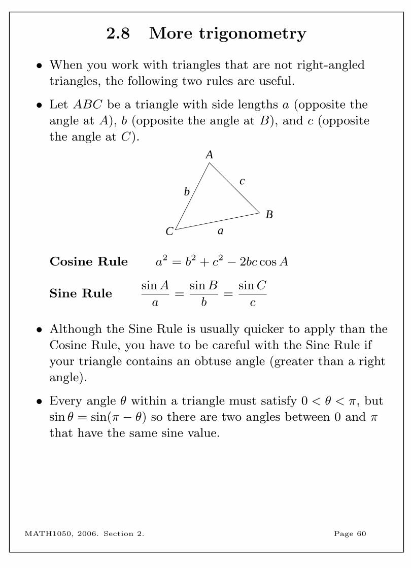
• Let ABC be a triangle with side lengths a (opposite the
angle at A), b (opposite the angle at B), and c (opposite
the angle at C).
A
B
C a
bc
Cosine Rule a2 = b2 + c2 − 2bc cosA
Sine RulesinA
a=
sinB
b=
sinC
c
• Although the Sine Rule is usually quicker to apply than the
Cosine Rule, you have to be careful with the Sine Rule if
your triangle contains an obtuse angle (greater than a right
angle).
• Every angle θ within a triangle must satisfy 0 < θ < π, but
sin θ = sin(π − θ) so there are two angles between 0 and π
that have the same sine value.
MATH1050, 2006. Section 2. Page 60
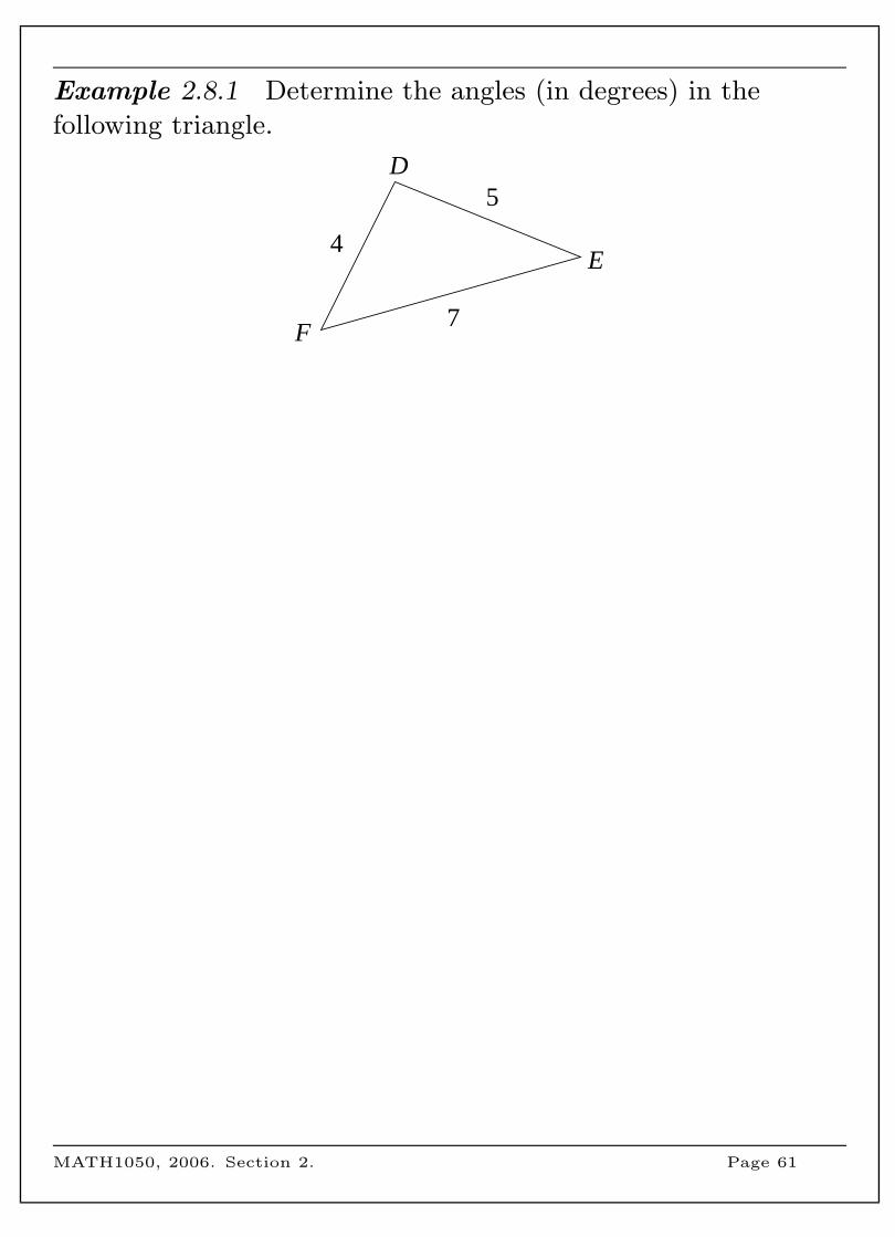
Example 2.8.1 Determine the angles (in degrees) in the
following triangle.
D
E
F
4
5
7
MATH1050, 2006. Section 2. Page 61
• When manipulating algebraic expressions involving the
trigonometric functions, it is useful to be aware of their
relationships to one another.
• An equation that involves trigonometric functions is called
a trigonometric identity. We will now prove several of these.
For future reference, we will label them TI1 through TI19
for trigonometric identities 1 through 19.
• Recall that angles are measured anticlockwise from the
x-axis, so a negative angle can be interpreted in terms of
moving clockwise from the x-axis.
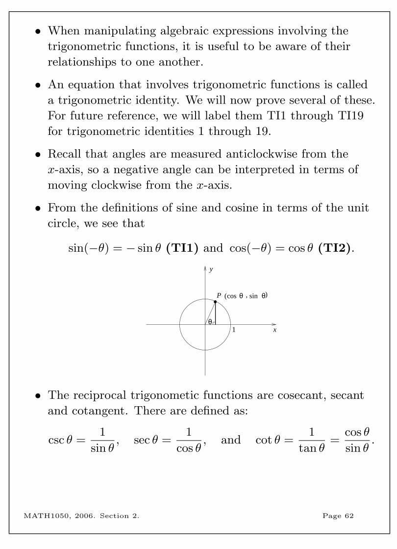
• From the definitions of sine and cosine in terms of the unit
circle, we see that
sin(−θ) = − sin θ (TI1) and cos(−θ) = cos θ (TI2).
θ1
P
x
y
)( , θsinθcos
• The reciprocal trigonometic functions are cosecant, secant
and cotangent. There are defined as:
csc θ =1
sin θ, sec θ =
1
cos θ, and cot θ =
1
tan θ=
cos θ
sin θ.
MATH1050, 2006. Section 2. Page 62
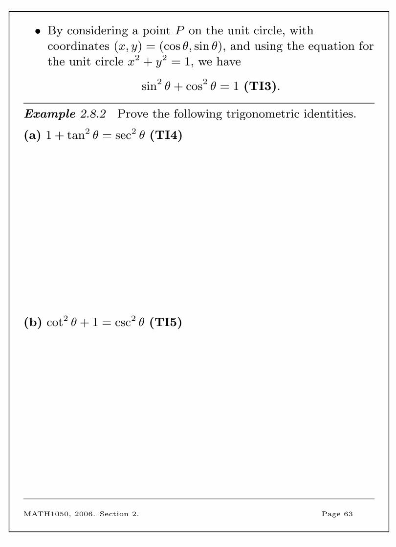
• By considering a point P on the unit circle, with
coordinates (x, y) = (cos θ, sin θ), and using the equation for
the unit circle x2 + y2 = 1, we have
sin2 θ + cos2 θ = 1 (TI3).
Example 2.8.2 Prove the following trigonometric identities.
(a) 1 + tan2 θ = sec2 θ (TI4)
(b) cot2 θ + 1 = csc2 θ (TI5)
MATH1050, 2006. Section 2. Page 63
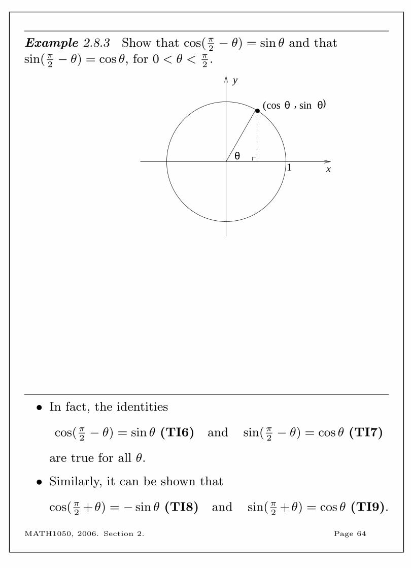
Example 2.8.3 Show that cos(π2− θ) = sin θ and that
sin(π2− θ) = cos θ, for 0 < θ < π
2.
1θ
x
y
)( , θsinθcos
• In fact, the identities
cos(π2− θ) = sin θ (TI6) and sin(π
2− θ) = cos θ (TI7)
are true for all θ.
• Similarly, it can be shown that
cos(π2
+θ) = − sin θ (TI8) and sin(π2
+θ) = cos θ (TI9).
MATH1050, 2006. Section 2. Page 64
• The sum and difference formulas are trigonometric
identities that involve the sine or cosine of the sum or
difference of two angles.
cos(θ + φ) = cos θ cosφ− sin θ sinφ (TI10)
sin(θ + φ) = sin θ cosφ+ cos θ sinφ (TI11)
cos(θ − φ) = cos θ cosφ+ sin θ sinφ (TI12)
sin(θ − φ) = sin θ cosφ− cos θ sinφ (TI13)
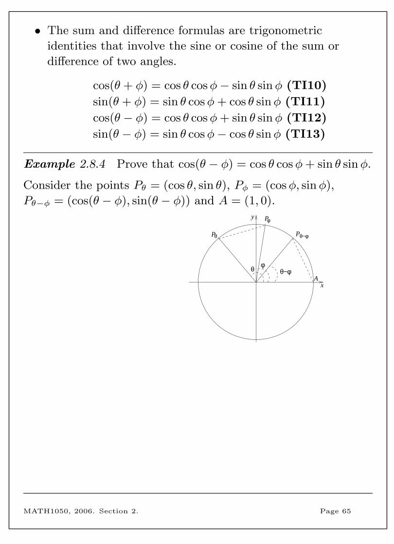
Example 2.8.4 Prove that cos(θ − φ) = cos θ cosφ+ sin θ sinφ.
Consider the points Pθ = (cos θ, sin θ), Pφ = (cosφ, sinφ),
Pθ−φ = (cos(θ − φ), sin(θ − φ)) and A = (1, 0).
θ−φφθ
y
xA
θ−φPθP
φP
MATH1050, 2006. Section 2. Page 65
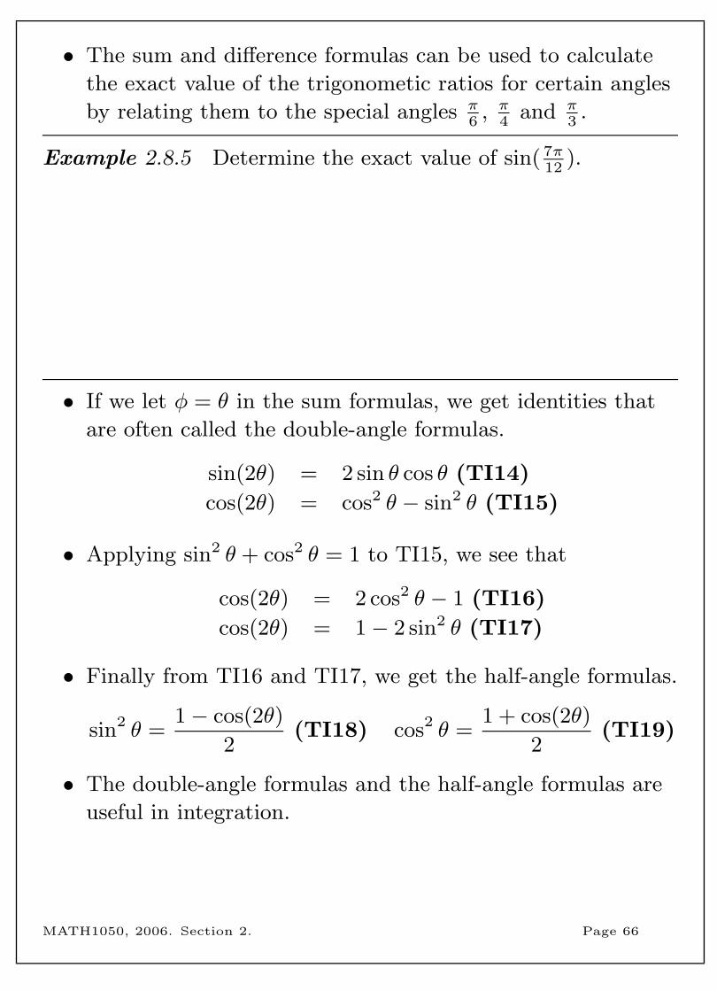
• The sum and difference formulas can be used to calculate
the exact value of the trigonometic ratios for certain angles
by relating them to the special angles π6
, π4
and π3
.
Example 2.8.5 Determine the exact value of sin( 7π12
).
• If we let φ = θ in the sum formulas, we get identities that
are often called the double-angle formulas.
sin(2θ) = 2 sin θ cos θ (TI14)
cos(2θ) = cos2 θ − sin2 θ (TI15)
• Applying sin2 θ + cos2 θ = 1 to TI15, we see that
cos(2θ) = 2 cos2 θ − 1 (TI16)
cos(2θ) = 1− 2 sin2 θ (TI17)
• Finally from TI16 and TI17, we get the half-angle formulas.
sin2 θ =1− cos(2θ)
2(TI18) cos2 θ =
1 + cos(2θ)
2(TI19)
• The double-angle formulas and the half-angle formulas are
useful in integration.
MATH1050, 2006. Section 2. Page 66
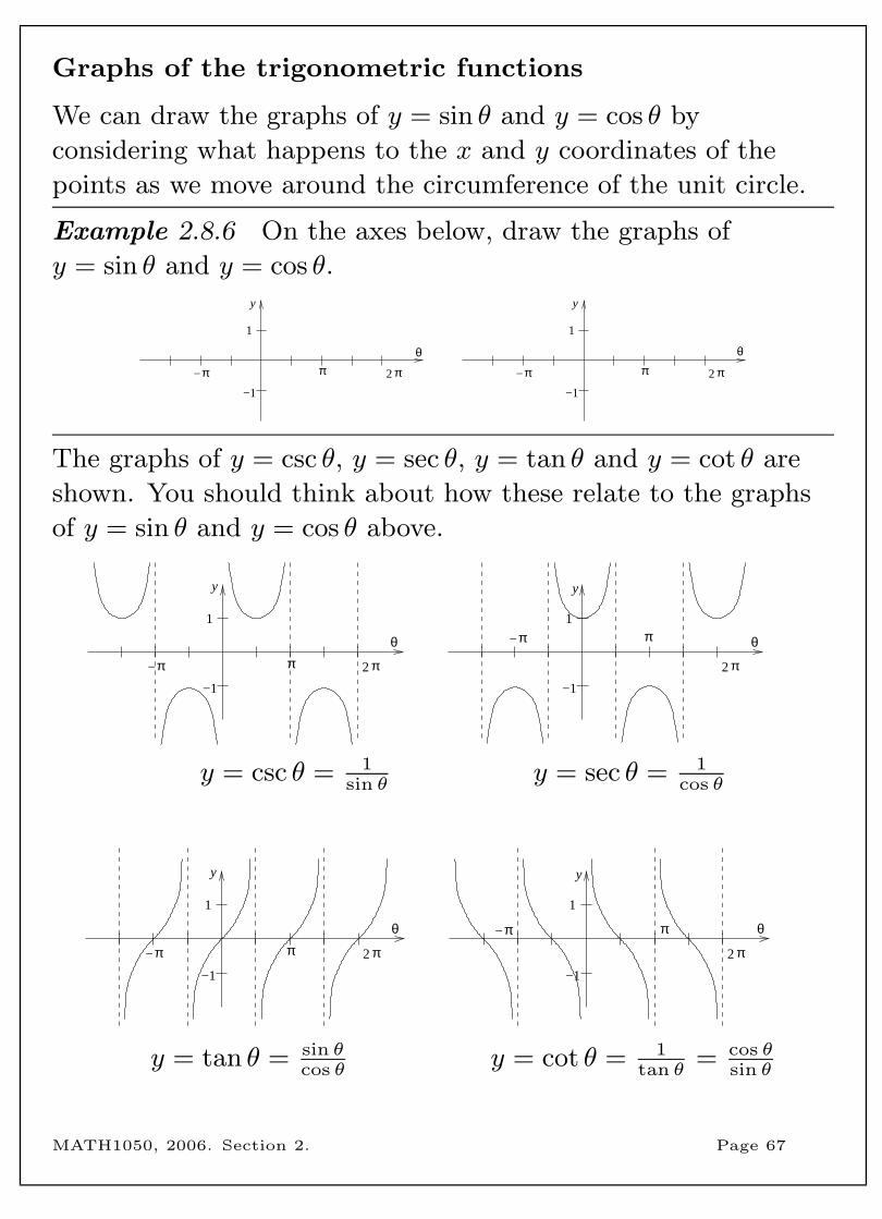
Graphs of the trigonometric functions
We can draw the graphs of y = sin θ and y = cos θ by
considering what happens to the x and y coordinates of the
points as we move around the circumference of the unit circle.
Example 2.8.6 On the axes below, draw the graphs of
y = sin θ and y = cos θ.
π π
1
−1
y y
θ θ
−π2−π π
1
−1
π2
The graphs of y = csc θ, y = sec θ, y = tan θ and y = cot θ are
shown. You should think about how these relate to the graphs
of y = sin θ and y = cos θ above.
1
−1
π
y y
θ θ
π2−π π
1
−1
π2
−π
y = csc θ = 1sin θ
y = sec θ = 1cos θ
1
−1
y y
θ θπ
π2−π π
1
−1
π2
−π
y = tan θ = sin θcos θ
y = cot θ = 1tan θ
= cos θsin θ
MATH1050, 2006. Section 2. Page 67
3 Applications of vectors
• Now that we are familiar with the different representations
of vectors, we can investigate some of the ways vectors are
used to solve mathematical problems.
• In pure mathematics, vectors can be used to solve problems
in geometry.
• In applied mathematics, vectors can be used to model
quantities such as displacement, velocity, or forces acting on
an object, and thus answer questions about such vector
quantities.
• There are two operations on vectors, the scalar product and
the vector product, that also have useful applications.
• In this section we look at several applications of vectors and
investigate the scalar and vector products.
• Topics in this section are:
– Vectors in geometry
– Forces
– Displacement, velocity and momentum
– The scalar product
– The vector product
MATH1050, 2006. Section 3. Page 68
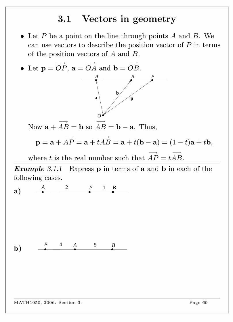
3.1 Vectors in geometry
• Let P be a point on the line through points A and B. We
can use vectors to describe the position vector of P in terms
of the position vectors of A and B.
• Let p =−→OP , a =
−→OA and b =
−→OB.
pb
a
O
B PA
Now a +−→AB = b so
−→AB = b− a. Thus,
p = a +−→AP = a + t
−→AB = a + t(b− a) = (1− t)a + tb,
where t is the real number such that−→AP = t
−→AB.
Example 3.1.1 Express p in terms of a and b in each of the
following cases.
a)P B1A 2
b)BP 4 5A
MATH1050, 2006. Section 3. Page 69
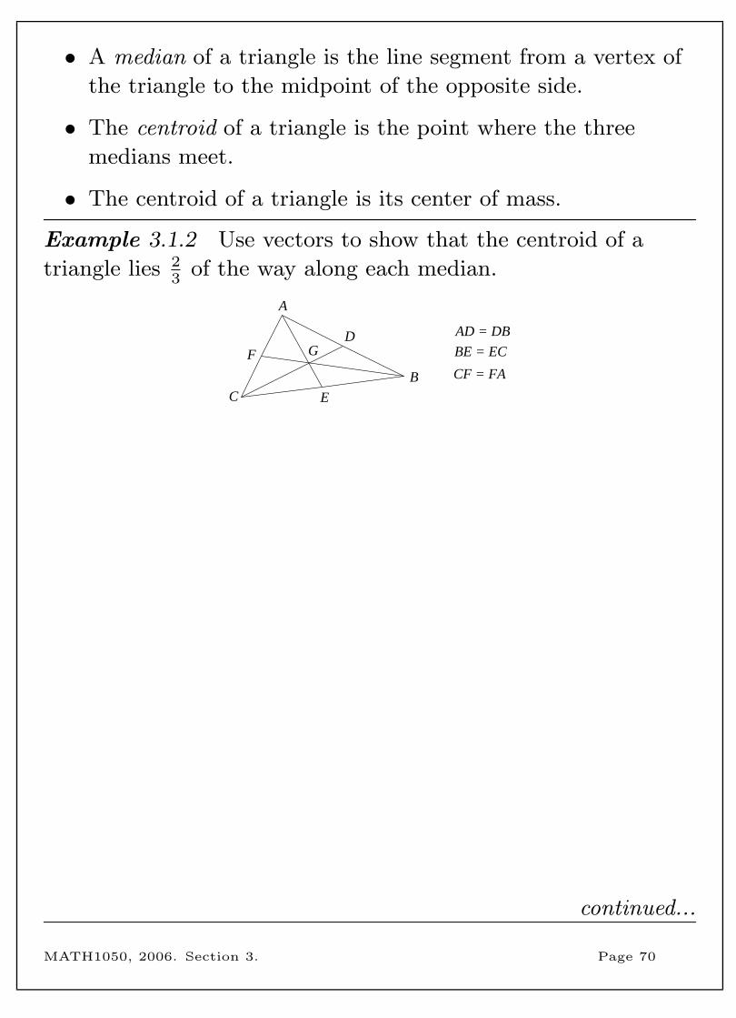
• A median of a triangle is the line segment from a vertex of
the triangle to the midpoint of the opposite side.
• The centroid of a triangle is the point where the three
medians meet.
• The centroid of a triangle is its center of mass.
Example 3.1.2 Use vectors to show that the centroid of a
triangle lies 23
of the way along each median.
AD = DB
CF = FA
BE = ECGF
E
D
CB
A
continued...
MATH1050, 2006. Section 3. Page 70

Example 3.1.2 (continued) Extra space for your working.
MATH1050, 2006. Section 3. Page 71
3.2 Forces
• A force (a push or a pull on an object) can be modelled as a
vector.
• The standard unit of measurement for forces is the newton,
denoted N.
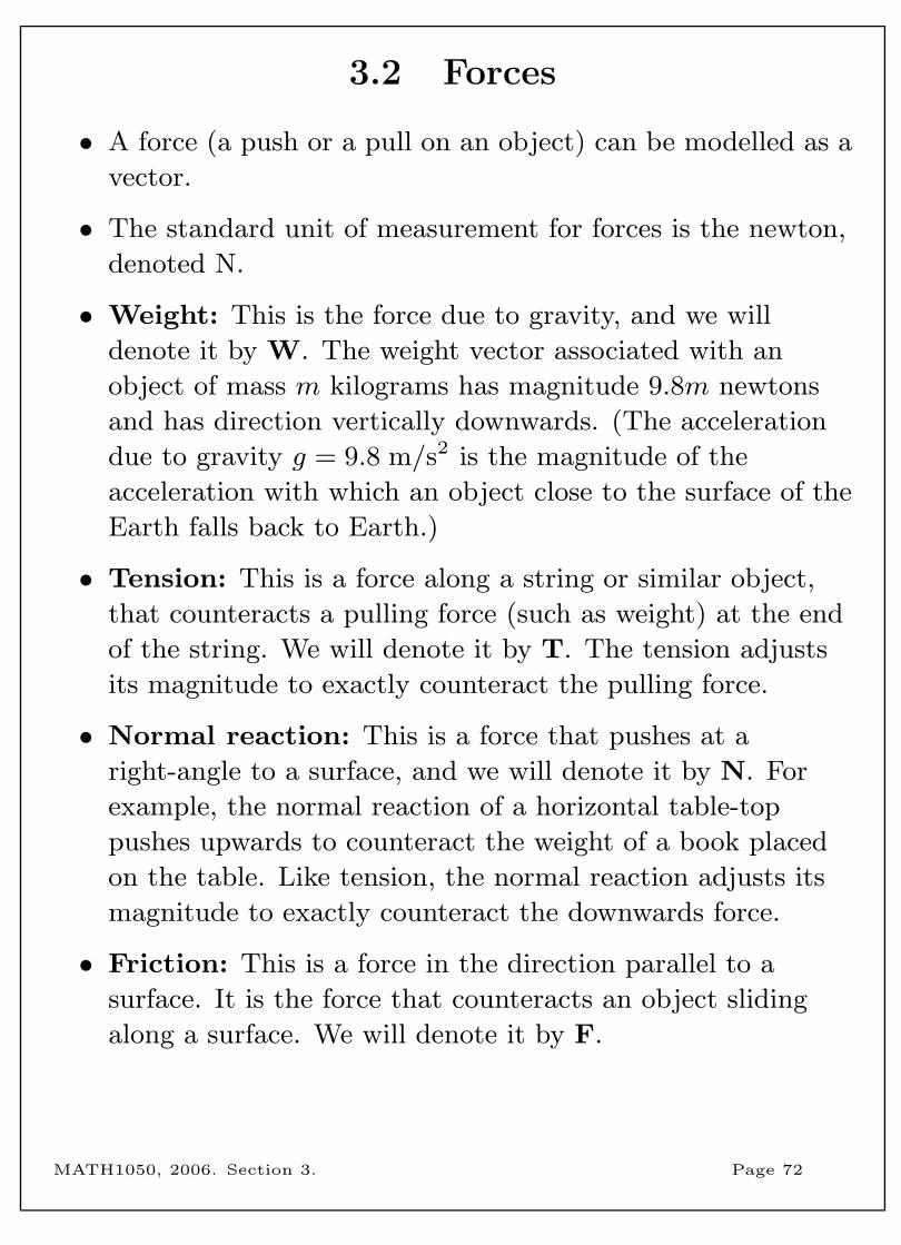
• Weight: This is the force due to gravity, and we will
denote it by W. The weight vector associated with an
object of mass m kilograms has magnitude 9.8m newtons
and has direction vertically downwards. (The acceleration
due to gravity g = 9.8 m/s2 is the magnitude of the
acceleration with which an object close to the surface of the
Earth falls back to Earth.)
• Tension: This is a force along a string or similar object,
that counteracts a pulling force (such as weight) at the end
of the string. We will denote it by T. The tension adjusts
its magnitude to exactly counteract the pulling force.
• Normal reaction: This is a force that pushes at a
right-angle to a surface, and we will denote it by N. For
example, the normal reaction of a horizontal table-top
pushes upwards to counteract the weight of a book placed
on the table. Like tension, the normal reaction adjusts its
magnitude to exactly counteract the downwards force.
• Friction: This is a force in the direction parallel to a
surface. It is the force that counteracts an object sliding
along a surface. We will denote it by F.
MATH1050, 2006. Section 3. Page 72
• In our modelling of forces, we will assume that our objects
can be represented by a particle, so we don’t have to worry
about which part of an object the forces act on. We will
also make other simplifying assumptions in our modelling.
• For an object to be at rest, the forces acting on that object
must be in balance. This is called the equilibrium condition
for forces, and it means that the sum of all the forces acting
on that object must be the zero vector.
Example 3.2.1 An object with a mass of 2 kg is suspended
from the ceiling by a string. Determine the tension acting on
the object.
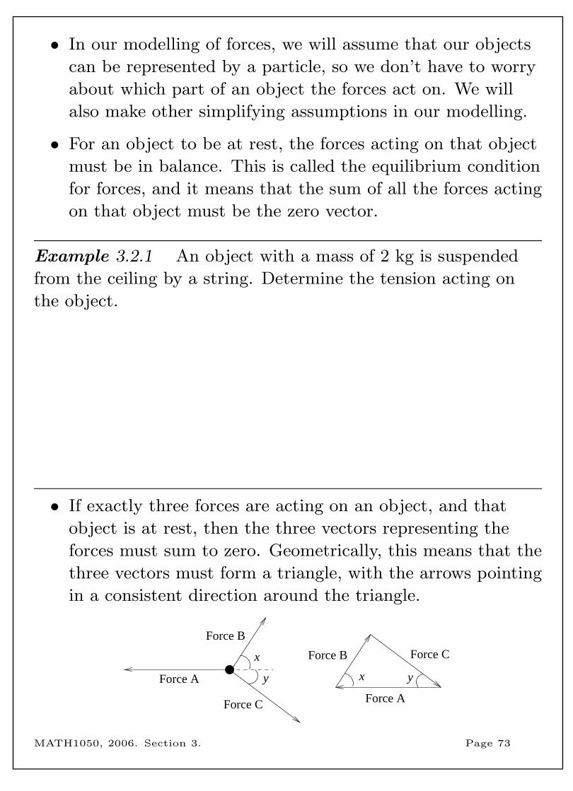
• If exactly three forces are acting on an object, and that
object is at rest, then the three vectors representing the
forces must sum to zero. Geometrically, this means that the
three vectors must form a triangle, with the arrows pointing
in a consistent direction around the triangle.
yxy
x Force B Force C
Force AForce C
Force B
Force A
MATH1050, 2006. Section 3. Page 73
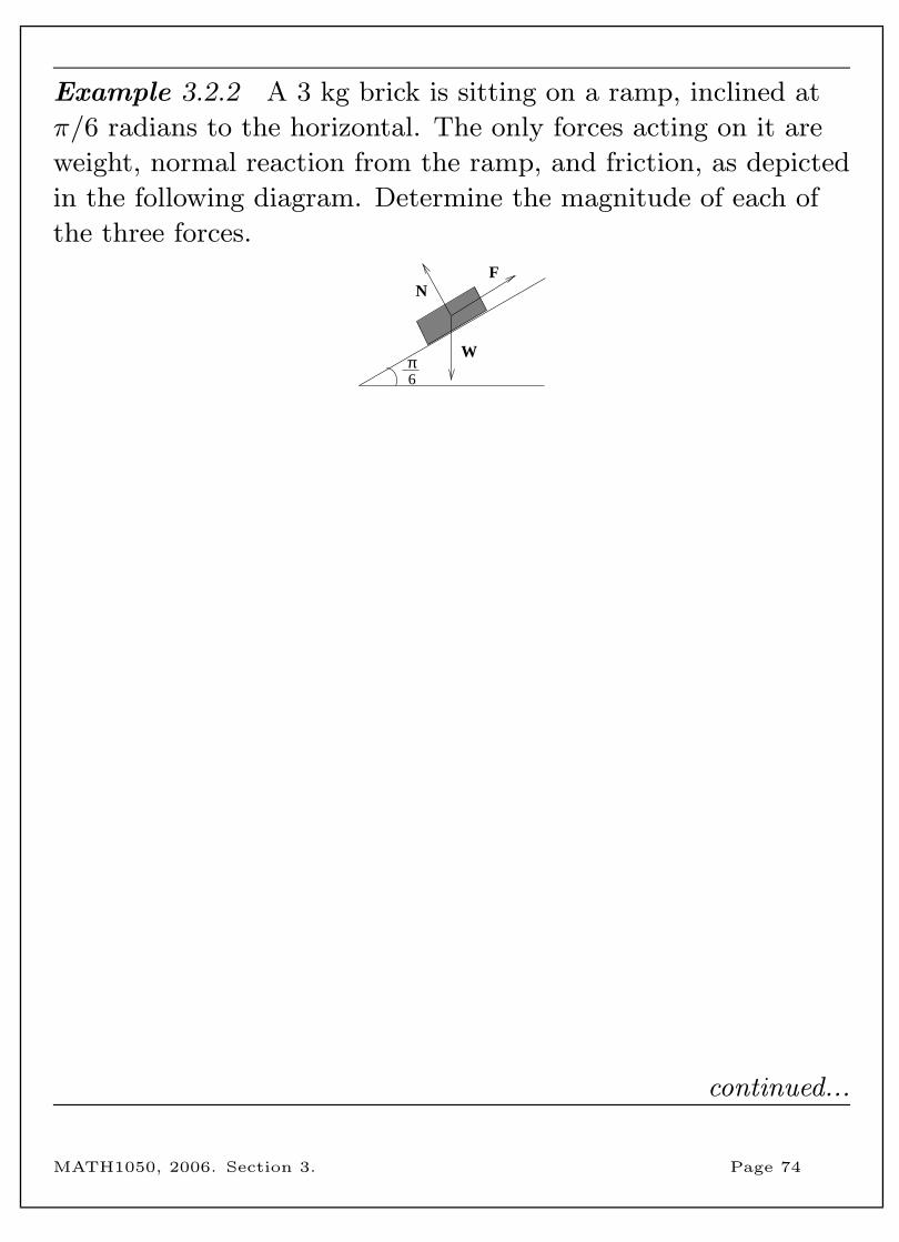
Example 3.2.2 A 3 kg brick is sitting on a ramp, inclined at
π/6 radians to the horizontal. The only forces acting on it are
weight, normal reaction from the ramp, and friction, as depicted
in the following diagram. Determine the magnitude of each of
the three forces.
π6
W
FN
continued...
MATH1050, 2006. Section 3. Page 74

Example 3.2.2 (continued) Extra space for your working.
MATH1050, 2006. Section 3. Page 75
3.3 Displacement, velocity and momentum
Example 3.3.1 A surveyor walks 200 metres due North. He
then turns clockwise through an angle of 2π3
radians and walks
100 metres. Finally he turns and walks 300 metres due West.
Find his resulting displacement, relative to his starting point.
continued...
MATH1050, 2006. Section 3. Page 76

Example 3.3.1 (continued) Extra space for your working.
MATH1050, 2006. Section 3. Page 77
Example 3.3.2 A pilot wishes to fly in the direction N69◦W to
reach her destination. The light plane has a speed of 85 knots
and there is a steady wind blowing from the north-east at 15
knots. What heading should the pilot set and what will be the
speed of the plane relative to the ground?
continued...MATH1050, 2006. Section 3. Page 78

Example 3.3.2 (continued) Extra space for your working.
MATH1050, 2006. Section 3. Page 79
Example 3.3.3 A river flows due East at a speed of 0.3 metres
per second. A boy in a rowing boat, who can row at 0.5 m/s in
still water, starts from a point on the South bank and steers due
North. The boat is also blown by a wind with speed 0.4 m/s
from a direction of N 20◦ E.
a) Find the resultant velocity of the boat.
b) If the river has a constant width of 10 metres, how long does
it take the boy to cross the river, and how far upstream or
downstream has he then travelled?
continued...MATH1050, 2006. Section 3. Page 80

Example 3.3.3 (continued) Extra space for your working.
MATH1050, 2006. Section 3. Page 81
• In order to understand the movement of two objects after
they collide, we need the concept of momentum.
• Momentum is a vector property of a moving object. It is a
scalar multiple of the velocity of the object, and is given by
momentum = mass times velocity.
• The standard unit for the magnitude of momentum is
newton seconds, denoted Ns. To obtain momentum in Ns,
your mass must be in kilograms and your velocity in metres
per second.
• The important property of momentum is that it is
conserved in collisions. That is, when objects collide, the
total momentum before collision is equal to the total
momentum after collision.
Example 3.3.4 A car weighing 1900 kg is travelling east at 22
m/s. A second car travelling north and weighing 2400 kg passes
through a stop sign travelling at 14 m/s. It collides with the
first car, and after the collision the cars move off together.
Calculte their speed and direction after the collision.
(Note that we make some simplifying assumptions, namely that
the cars do not brake, and that there is no friction from the
road or air resistance to slow them down.)
continued...MATH1050, 2006. Section 3. Page 82

Example 3.3.4 (continued) Extra space for your working.
MATH1050, 2006. Section 3. Page 83
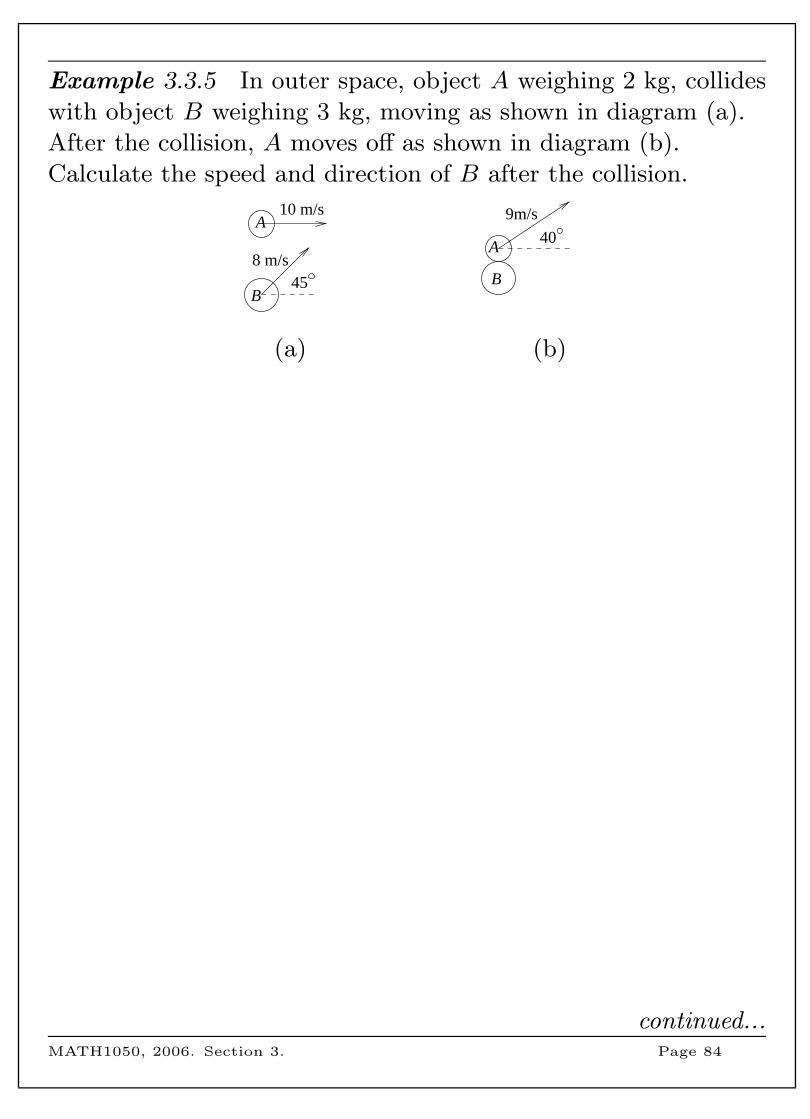
Example 3.3.5 In outer space, object A weighing 2 kg, collides
with object B weighing 3 kg, moving as shown in diagram (a).
After the collision, A moves off as shown in diagram (b).
Calculate the speed and direction of B after the collision.
9m/s
8 m/s
10 m/s
B
A
B
A40
45
(a) (b)
continued...MATH1050, 2006. Section 3. Page 84

Example 3.3.5 (continued) Extra space for your working.
MATH1050, 2006. Section 3. Page 85
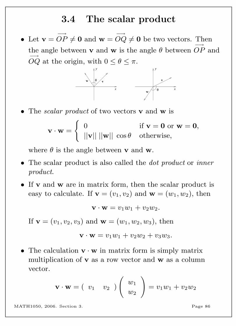
3.4 The scalar product
• Let v =−→OP 6= 0 and w =
−→OQ 6= 0 be two vectors. Then
the angle between v and w is the angle θ between−→OP and
−→OQ at the origin, with 0 ≤ θ ≤ π.
θw
vθw v
y
x
y
x
• The scalar product of two vectors v and w is
v ·w =
{0 if v = 0 or w = 0,
||v|| ||w|| cos θ otherwise,
where θ is the angle between v and w.
• The scalar product is also called the dot product or inner
product.
• If v and w are in matrix form, then the scalar product is
easy to calculate. If v = (v1, v2) and w = (w1, w2), then
v ·w = v1w1 + v2w2.
If v = (v1, v2, v3) and w = (w1, w2, w3), then
v ·w = v1w1 + v2w2 + v3w3.
• The calculation v ·w in matrix form is simply matrix
multiplication of v as a row vector and w as a column
vector.
v ·w = ( v1 v2 )
(w1
w2
)= v1w1 + v2w2
MATH1050, 2006. Section 3. Page 86
Example 3.4.1
a) The vector u has magnitude 5 and direction 5π4
radians. The
vector v has magnitude 3 and direction 7π12
radians. Calculate
u · v.
b) The vector v = (−3, 2) lies in the 2nd quadrant. Find a
vector in the 3rd quadrant that is perpendicular to v.
• If we are given two vectors v and w in matrix or
component form, then we can use the scalar product to
calculate the angle between v and w.
MATH1050, 2006. Section 3. Page 87
Example 3.4.2 Calculate the angle (in both radians and
degrees) between vectors u = (4, 3, 1) and v = (2,−3,−2).
Properties of the scalar product
(1) The scalar product of two vectors is a scalar, not a vector.
(2) v · v = ||v||2 since the angle between v and itself is 0 and
cos 0 = 1.
(3) v ·w = 0 if and only if v and w are perpendicular.
(Perpendicular vectors are also called orthogonal vectors.)
Proof If v 6= 0 and w 6= 0, then
v ·w = 0 iff ||v|| ||w|| cos θ = 0,
iff cos θ = 0,
iff θ = π/2.
(4) For vectors u,v and w, (u + v) ·w = u ·w + v ·w.
(5) For vectors v and w, v ·w = w · v.
(6) For vectors v and w and any real number t,
(tv) ·w = t(v ·w).
MATH1050, 2006. Section 3. Page 88
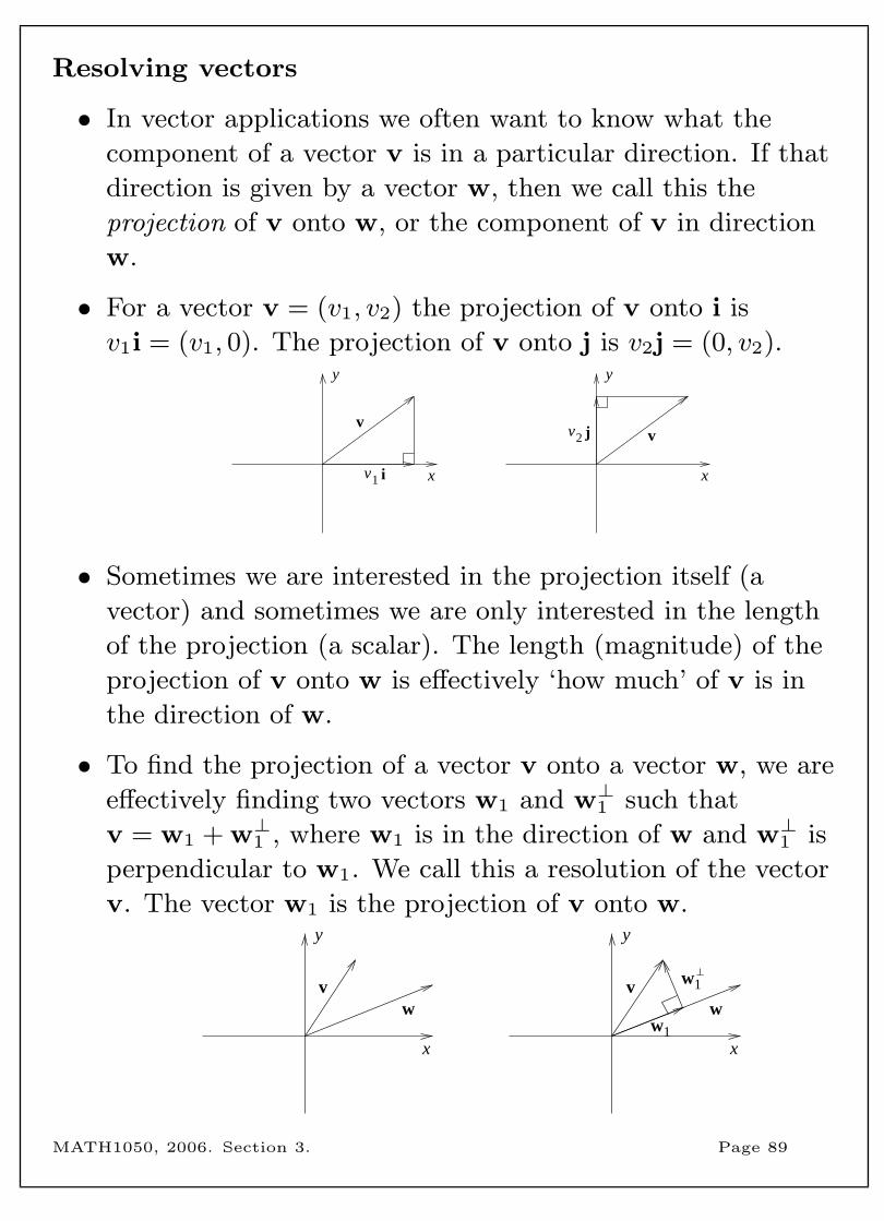
Resolving vectors
• In vector applications we often want to know what the
component of a vector v is in a particular direction. If that
direction is given by a vector w, then we call this the
projection of v onto w, or the component of v in direction
w.
• For a vector v = (v1, v2) the projection of v onto i is
v1i = (v1, 0). The projection of v onto j is v2j = (0, v2).
vv
j2v
y
xi1v
y
x
• Sometimes we are interested in the projection itself (a
vector) and sometimes we are only interested in the length
of the projection (a scalar). The length (magnitude) of the
projection of v onto w is effectively ‘how much’ of v is in
the direction of w.
• To find the projection of a vector v onto a vector w, we are
effectively finding two vectors w1 and w⊥1 such that
v = w1 + w⊥1 , where w1 is in the direction of w and w⊥1 is
perpendicular to w1. We call this a resolution of the vector
v. The vector w1 is the projection of v onto w.
wv
wv 1w
1w
y
x
y
x
MATH1050, 2006. Section 3. Page 89
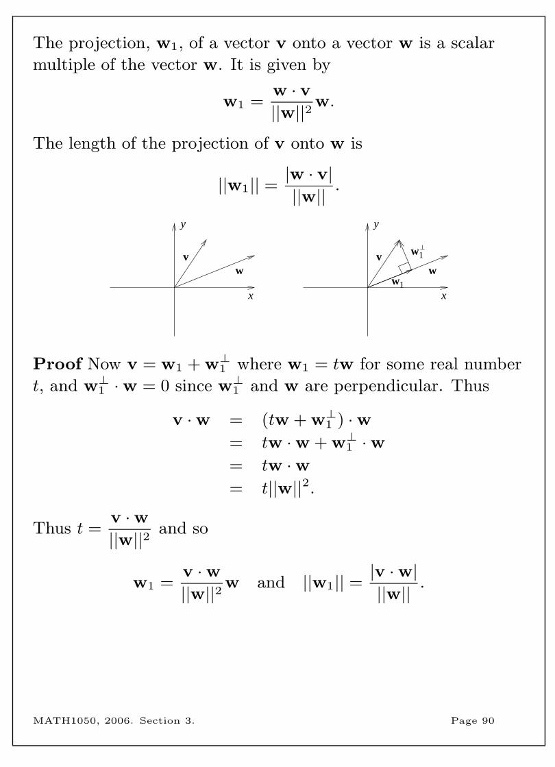
The projection, w1, of a vector v onto a vector w is a scalar
multiple of the vector w. It is given by
w1 =w · v||w||2 w.
The length of the projection of v onto w is
||w1|| =|w · v|||w|| .
wv
wv 1w
1w
y
x
y
x
Proof Now v = w1 + w⊥1 where w1 = tw for some real number
t, and w⊥1 ·w = 0 since w⊥1 and w are perpendicular. Thus
v ·w = (tw + w⊥1 ) ·w= tw ·w + w⊥1 ·w= tw ·w= t||w||2.
Thus t =v ·w||w||2 and so
w1 =v ·w||w||2 w and ||w1|| =
|v ·w|||w|| .
MATH1050, 2006. Section 3. Page 90
Example 3.4.3
a) The vector v has magnitude 5 and direction π/4. The vector
w has magnitude 8 and direction π/6. Find the projection of v
onto w.
b) The vector u = (−2, 4) and the vector v = (1, 5). Find the
projection, v1, of u onto v. Then determine v⊥1 such that
u = v1 + v⊥1 .
MATH1050, 2006. Section 3. Page 91
Work
• The scalar quantity work is a measure of the energy
transfered to an object when a force f moves the object
through a displacement d.
• If the force and the displacement have the same direction,
then the enery gained is ||f || ||d||. If the force and the
displacement do not have the same direction, then only the
component of f in the direction of d contributes to the
energy gained by the object. The component of f in the
direction of d is ||f || cos θ, where θ is the angle between f
and d. Thus Work = f · d.
• If ||f || is in newtons, and ||d|| is in metres, then Work is
measured in Joules.
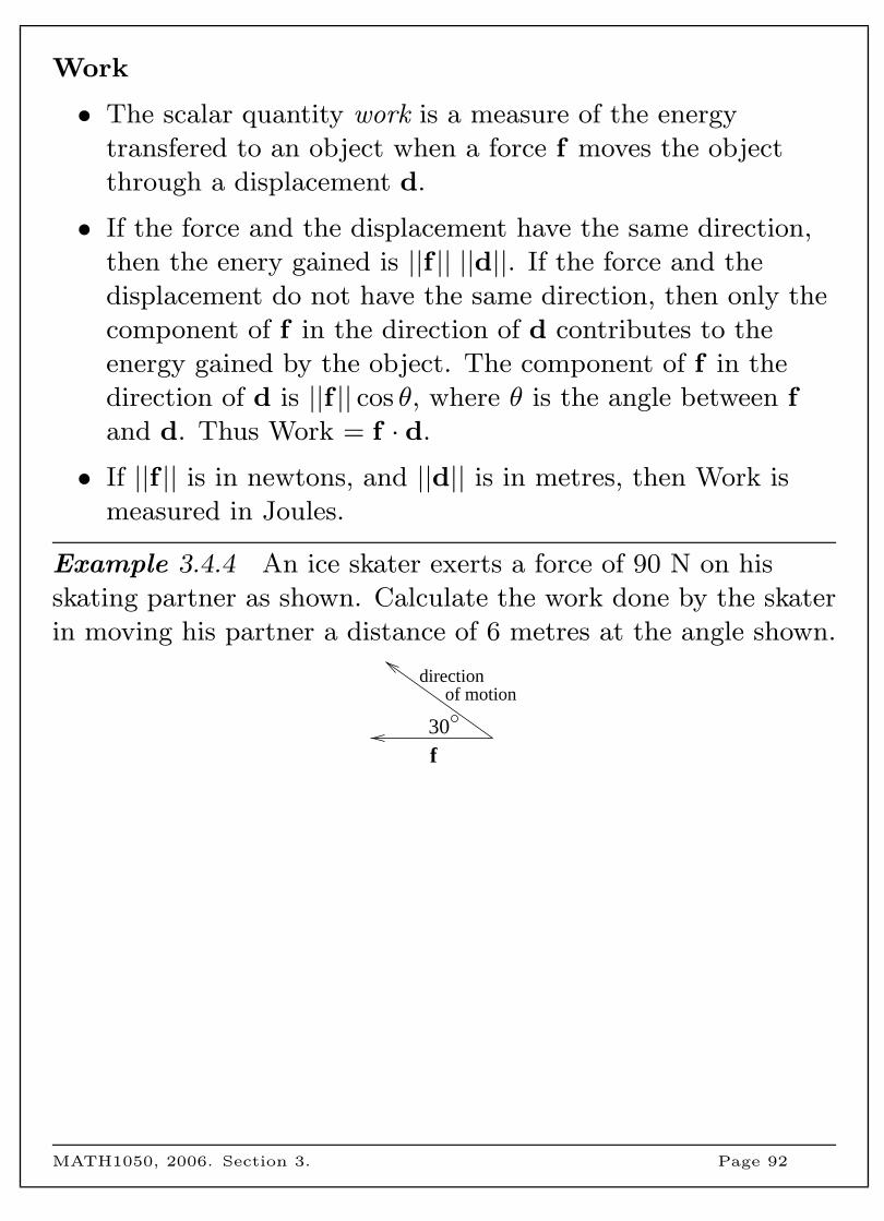
Example 3.4.4 An ice skater exerts a force of 90 N on his
skating partner as shown. Calculate the work done by the skater
in moving his partner a distance of 6 metres at the angle shown.
30f
direction of motion
MATH1050, 2006. Section 3. Page 92
3.5 The vector product
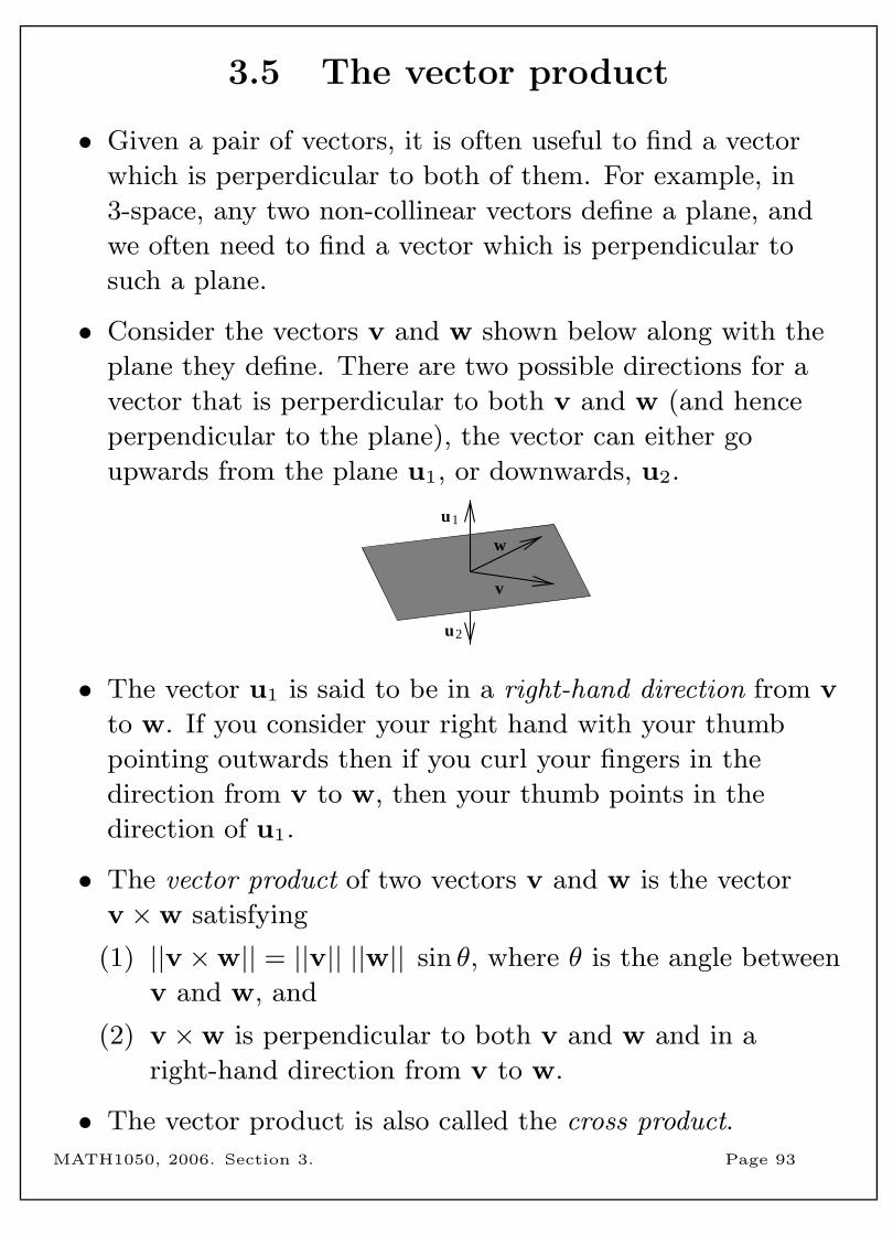
• Given a pair of vectors, it is often useful to find a vector
which is perperdicular to both of them. For example, in
3-space, any two non-collinear vectors define a plane, and
we often need to find a vector which is perpendicular to
such a plane.
• Consider the vectors v and w shown below along with the
plane they define. There are two possible directions for a
vector that is perperdicular to both v and w (and hence
perpendicular to the plane), the vector can either go
upwards from the plane u1, or downwards, u2.
u1
u2
v
w
• The vector u1 is said to be in a right-hand direction from v
to w. If you consider your right hand with your thumb
pointing outwards then if you curl your fingers in the
direction from v to w, then your thumb points in the
direction of u1.
• The vector product of two vectors v and w is the vector
v ×w satisfying
(1) ||v ×w|| = ||v|| ||w|| sin θ, where θ is the angle between
v and w, and
(2) v ×w is perpendicular to both v and w and in a
right-hand direction from v to w.
• The vector product is also called the cross product.
MATH1050, 2006. Section 3. Page 93
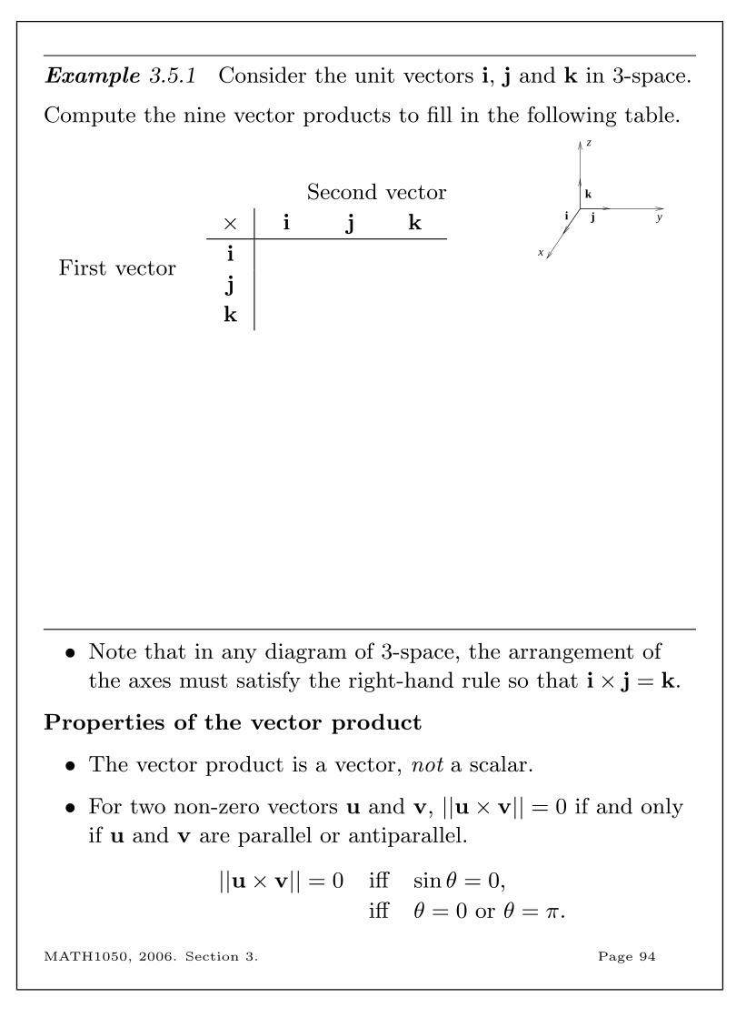
Example 3.5.1 Consider the unit vectors i, j and k in 3-space.
Compute the nine vector products to fill in the following table.
Second vector
First vector
× i j k
i
j
k
y
z
x
i j
k
• Note that in any diagram of 3-space, the arrangement of
the axes must satisfy the right-hand rule so that i× j = k.
Properties of the vector product
• The vector product is a vector, not a scalar.
• For two non-zero vectors u and v, ||u× v|| = 0 if and only
if u and v are parallel or antiparallel.
||u× v|| = 0 iff sin θ = 0,
iff θ = 0 or θ = π.
MATH1050, 2006. Section 3. Page 94
• For any two vectors u and v, u× v = −v × u.
• The vector product is not associative, so for most vectors u,
v and w, u× (v ×w) 6= (u× v)×w.
For example, (i× i)× k = 0 but i× (i× k) = i×−j = −k.
• For vectors u and v and any real number t
t(u× v) = (tu)× v = u× (tv).
• For vectors u, v and w,
u×(v+w) = u×v+u×w, and (u+v)×w = u×w+v×w.
We can use the properties of the vector product and the table of
vector products of i, j and k to calculate the vector product of
any pair of vectors expressed in component form.
Example 3.5.2 If v = 2i− j + 4k and w = i + 2j + 3k,
calculate v ×w.
MATH1050, 2006. Section 3. Page 95
Although this method works, it can be a bit tedious. We can
take a shortcut by making use of a determinant.
If u = u1i + u2j + u3k and v = v1i + v2j + v3k then
u× v = i
∣∣∣∣∣ u2 u3
v2 v3
∣∣∣∣∣− j
∣∣∣∣∣ u1 u3
v1 v3
∣∣∣∣∣+ k
∣∣∣∣∣ u1 u2
v1 v2
∣∣∣∣∣ .
So u× v =
∣∣∣∣∣∣∣i j k
u1 u2 u3
v1 v2 v3
∣∣∣∣∣∣∣where the determinant must
be expanded along its top row.
Warning! This is not a real determinant, we are just using it
as a calculation aid.
Example 3.5.3 For vectors v = (2,−1, 4) and w = (1, 2, 3)
from the previous example, show that the determinant method
gives the same answer for v ×w.
MATH1050, 2006. Section 3. Page 96
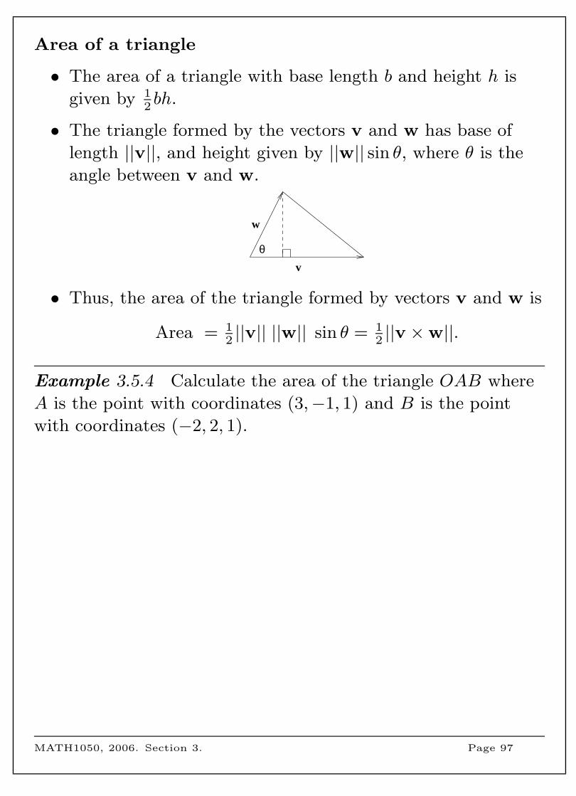
Area of a triangle
• The area of a triangle with base length b and height h is
given by 12bh.
• The triangle formed by the vectors v and w has base of
length ||v||, and height given by ||w|| sin θ, where θ is the
angle between v and w.
w
v
θ
• Thus, the area of the triangle formed by vectors v and w is
Area = 12||v|| ||w|| sin θ = 1
2||v ×w||.
Example 3.5.4 Calculate the area of the triangle OAB where
A is the point with coordinates (3,−1, 1) and B is the point
with coordinates (−2, 2, 1).
MATH1050, 2006. Section 3. Page 97
Torque
• When you use a spanner to turn a nut, or use different
gears while riding a bicycle, your choice of size of spanner
or particular gear on the bike is based on a turning force
called torque.
• The magnitude of the torque is given by ||r× f || where f is
the force and r is the vector from the point of application of
the force to the point (or axis) about which the object is
turning.
• The standard unit for torque is Newton metres, denoted
Nm. To obtain torque in Nm, f should be in newtons and r
should be in metres.
• Since sin θ reaches its maximum at π/2 radians (90◦), the
torque is a maximum when the angle between f and r is
π/2 radians.
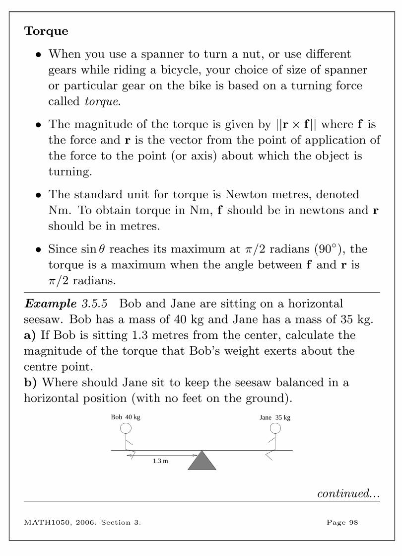
Example 3.5.5 Bob and Jane are sitting on a horizontal
seesaw. Bob has a mass of 40 kg and Jane has a mass of 35 kg.
a) If Bob is sitting 1.3 metres from the center, calculate the
magnitude of the torque that Bob’s weight exerts about the
centre point.
b) Where should Jane sit to keep the seesaw balanced in a
horizontal position (with no feet on the ground).
1.3 m
35 kgJane40 kgBob
continued...
MATH1050, 2006. Section 3. Page 98

Example 3.5.5 (continued)
MATH1050, 2006. Section 3. Page 99
4 Sequences and Series
• A sequence is an ordered set of numbers, and we call the
numbers in the sequence the terms of the sequence.
• Some sequences have an identifiable pattern, allowing us to
develop a formula to calculate any particular term of the
sequence directly, or a formula to calculate the value of a
term from the values of preceding terms.
• As well as illustrating the beauty of mathematics, sequences
have many applications. For instance, the calculation of
mortgage repayments and estimating population growth.
• A series is the sum of the terms of a sequence. We will
investigate mathematical induction, a proof technique that
is useful in proving results about series.
• Topics in this section are:
– Introduction to sequences
– Review of logarithms
– Arithmetic and geometric sequences
– The Fibonacci sequence
– Arithmetic and geometric series
– Finite differences and telescoping sums
– Applications of sequences
– Mathematical induction
MATH1050, 2006. Section 4. Page 100
4.1 Introduction to sequences
• A sequence is an ordered set of numbers.
• We call each number in a sequence a term of the sequence.
• A sequence with a fixed number of terms is a finite
sequence, and a sequence with an infinite number of terms
is an infinite sequence.
• To describe a sequence, we usually choose a particular letter
and combine that letter with subscripts to represent the
terms of the sequence. For example, in the sequence
a1, a2, a3, . . . , a10
a1 represents the first term, a2 the second term, and so on,
and a10 is the 10th and final term of the sequence. The
notation an represents a general term of the sequence, and
we use the notation {an} or {an}10n=1 to represent the entire
sequence.
• The symbol ∞ is used for infinity, and so an infinite
sequence might be written as {an}∞n=1.
Example 4.1.1 Let {an}∞n=0 be a sequence with an = 2n− 1.
List the first four terms of the sequence.
(We could also write this sequence as {2n− 1}∞n=0.)
MATH1050, 2006. Section 4. Page 101
• A general rule that allows you to calculate the terms of a
sequence can be specified in two ways.
• A formula that allows direct calculation of the value of any
particular term of a sequence is called a closed form for the
sequence. For example, the sequence 3, 5, 7, 9, 11 has closed
form 3 + 2n (n = 0, 1, 2, 3, 4).
• A formula that specifies how to calculate the value of a
term using the value(s) of one (or more) preceding terms is
called a recurrence relation. A recursive definition of a
sequence is a recurrence relation combined with initial
conditions giving the value(s) of one (or more) initial terms
of the sequence. For example, the sequence 3, 5, 7, 9, 11 can
be defined recursively as an = an−1 + 2 (n = 1, 2, 3, 4) with
initial condition a0 = 3.
Example 4.1.2 Find both a closed form and a recursive
definition of a sequence whose first four terms are
2, 4, 8, 16.
MATH1050, 2006. Section 4. Page 102
• It is important to be aware that specifying the first few
terms of a sequence does not adequately describe the
sequence.
• You probably thought that the next term of the sequence in
the previous example was 32. The sequence with closed
form
an = 2n (n = 1, 2, . . . )
certainly has 2, 4, 8, 16, 32 as its first five terms.
• However, in the previous example, if we had chosen the
closed form
an = (n− 1)(n− 2)(n− 3)(n− 4) + 2n (n = 1, 2, . . . ),
then the first five terms of the sequence would be
2, 4, 8, 16, 56.
• Simply writing down the first few terms of a sequence is
never enough to specify the remainder of the sequence!
• In order to describe a sequence, if you cannot write down
all the terms of the sequence, then you must give a general
description of the sequence such as a closed form or a
recurrence relation with initial conditions.
MATH1050, 2006. Section 4. Page 103
4.2 Review of logarithms
• Recall the sequence {an}∞n=1 with closed form an = 2n from
the previous section. Which term would be the first term to
exceed 7000? To answer this, we need to find the smallest
value of n such that 2n > 7000. To find n, we could solve
2x = 7000 and then choose n to be the smallest integer that
is greater than or equal to x.
• Solving equations such as 2x = 7000 is best done using
logarithms, which we review briefly here.
• The notation
loga b
means “to what power do we raise a to obtain the value b?”
Hence, the statement loga b = c is equivalent to the
statement ac = b.
• For example, log5 25 = 2, log7 1 = 0 and log9 3 = 12.
• The notation loga b is read as the logarithm of b with base a
or as the logarithm with base a of b.
Example 4.2.1 Evaluate the following:
(a) log4 64 (b) log5125
(c) log27 3
MATH1050, 2006. Section 4. Page 104
• To solve the equation 2x = 7000 we need to evaluate
x = log2 7000. Since 212 = 4096 and 213 = 8192, the value
of x will be between 12 and 13. To find an approximate
value for x, we can use a calculator.
• Most calculators can only evaluate logarithms having one of
two particular bases, 10 or e.
• The number e = 2.71828 . . . is a very important irrational
number, and loge b is called the natural logarithm of b.
• When we write log without a base, the base is understood
to be 10 and when we write ln we mean a natural logarithm.
log 100 = log10 100 = 2 and ln100 = loge 100 ≈ 4.605.
• In order to use a calculator to solve the equation 2x = 7000,
we apply the change of base rule. Provided that a > 0,
a 6= 1 and b > 0,
loga b =log b
log a=
lnb
lna.
• Thus, by converting a single logarithm with base 2 into a
quotient of natural logarithms, we find that
x = log2 7000 =ln7000
ln2≈ 12.773.
Example 4.2.2 Solve for x:
(a) 5x = 32 (b) 9x+1 = 100
MATH1050, 2006. Section 4. Page 105
• Now consider the equation (−3)x = −27. Clearly, this
equation has the solution x = 3. However, we cannot use
the method of Example 4.2.2 to determine this. Very
strange things happen if you use a non-positive number for
the base of a logarithm and also if you try to evaluate a
logarithm of a non-positive number. For the purposes of
this course, the notation loga b is only defined if a > 0 and
b > 0.
• There are some useful rules which allow us to manipulate
expressions involving logarithms.
If a > 0, a 6= 1, x, y > 0 and r is any real number, then
loga(xr) = r loga x
loga(xy) = loga x+ loga y
loga(xy
) = loga x− loga y
• The change of base formula arises from the equation ax = b
by taking the logarithm of both sides of the equation and
then applying the first law from above.
ax = b
log(ax) = log b
x log a = log b
x = log blog a
MATH1050, 2006. Section 4. Page 106
4.3 Arithmetic and geometric sequences
• An arithmetic sequence is a sequence in which the difference
between any two successive terms in a constant.
• The difference between successive terms in an arithmetic
sequence is called the common difference.
• For example, the A.S. with first term 2 and common
difference 3 starts with the five terms
2, 5, 8, 11, 14.
The A.S. with first term 10 and common difference −5
starts with the five terms
10, 5, 0, −5, −10.
Example 4.3.1 Determine whether each of the following could
be the first four terms of an arithmetic sequence.
a) 1, 2 12, 4, 5 1
4.
b) 5, 2, −1, −4.
c) 3, 4 + 2x, 5 + 4x, 6 + 6x.
MATH1050, 2006. Section 4. Page 107
• If we know the values of the first term and the common
difference of an arithmetic sequence, we can determine a
recursive definition or a closed form for the sequence.
• Let {an}∞n=1 be an arithmetic sequence with first term a
and common difference d. Then
an+1 = an + d (n = 1, 2, . . . ) and a1 = a
is a recursive definition of the A.S.
• Let {an}∞n=1 be an arithmetic sequence with first term a
and common difference d. Then
a1 = a
a2 = a+ d so a2 = a+ 1d
a3 = a+ d+ d so a3 = a+ 2d
a4 = a+ d+ d+ d so a4 = a+ 3d
a5 = a+ d+ d+ d+ d so a5 = a+ 4d
Thus,
an = a+ (n− 1)d, (n = 1, 2, . . . ),
is a closed form for the A.S.
Example 4.3.2 The first three terms of an A.S. are 5,−2,−9.
Determine the 100th term of the sequence.
MATH1050, 2006. Section 4. Page 108
Example 4.3.3 The third term of an A.S is 7 and the twelfth
term is 10. Determine a closed form for the sequence.
• A geometric sequence is a sequence in which the ratio
between any two successive terms is a constant, that is,
every term is equal to the previous term multiplied by a
particular number.
• The ratio between successive terms in a geometric sequence
is called the common ratio.
• For example, the G.S. with first term 2 and common ratio 3
starts with the five terms
2, 6, 18, 54, 162,
since 62
= 186
= 5418
= 16254
= 3.
The G.S. with first term 20 and common ratio − 12
starts
with the five terms
20, −10, 5, −2 12, 1 1
4.
MATH1050, 2006. Section 4. Page 109
Example 4.3.4 Determine whether each of the following could
be the first four terms of a geometric sequence.
a) 27, 9, 3, −1.
b) 2, x, 12x2, 1
4x3.
• If we know the values of the first term and the common
ratio of a geometric sequence, we can determine a recursive
definition or a closed form for the sequence.
• Let {an}∞n=1 be a geometric sequence with first term a and
common ratio r. Then
an+1 = an × r (n = 1, 2, . . . ) and a1 = a
is a recursive definition of the G.S.
• Let {an}∞n=1 be a geometric sequence with first term a and
common ratio r. Then
a1 = a
a2 = a× r so a2 = ar1
a3 = a× r × r so a3 = ar2
a4 = a× r × r × r so a4 = ar3
Thus,
an = arn−1 (n = 1, 2, . . . )
is a closed form for the G.S.MATH1050, 2006. Section 4. Page 110
Example 4.3.5 The first three terms of a G.S. are − 13, 1,−3.
Determine the 10th term of the sequence.
Example 4.3.6 The first three terms of a G.S are 4, 8, 16.
Which term would be the first to exceed one million?
MATH1050, 2006. Section 4. Page 111
4.4 The Fibonacci sequence
• The Fibonacci sequence is the sequence {Fn} where
Fn+2 = Fn+1 + Fn (n = 1, 2, 3, . . . ) F1 = 1, F2 = 1.
• The sequence is named after an Italian mathematician
Leonardo of Pisa (1170-1250) who was better known by the
name of Fibonacci.
• The sequence arises from a problem posed by Fibonacci in
1202: Start with one pair of rabbits, and suppose that
– the initial pair of rabbits takes one month to mature,
they produce a new pair at the end of the second
month, and at the end of each subsequent month;
– each new pair becomes adult after one month and
produces its first new pair at the end of its second month
and a new pair at the end of each subsequent month;
– no rabbits die.
How many pairs of rabbits are there after a year?
Example 4.4.1 Determine the number of pairs of rabbits at
the beginning of each month for the first 12 months.
MATH1050, 2006. Section 4. Page 112
• A closed form for the Fibonacci sequence is
Fn =1√5
(1 +√
5
2
)n− 1√
5
(1−√
5
2
)n.
• The golden ratio is the name given to the number
φ =1 +√
5
2≈ 1.618.
Example 4.4.2 The ratio of successive terms of the Fibonacci
sequence tends to a fixed value. Show that
Fn+1
Fn→ φ as n→∞.
MATH1050, 2006. Section 4. Page 113
• The golden ratio and terms of the Fibonacci sequence occur
in many places.
• In art and architecture, often the pictures or buildings that
look most pleasing involve the golden ratio. For example,
the French architect Le Corbusier used the golden ratio in
the design of some of his buildings, and Leonardo da Vinci
used the golden ratio in some of his paintings.
• Composers such as Bartok and Debussy are known to have
used the golden ratio in composing their music.
• Fibonacci numbers occur in the structure of plants. For
example, the number of petals on many flowers is
3, 5, 8, 13, 21 or 34, and the successive leaves along a stem
are often rotated around the stem by the fraction 1/φ of a
full turn.
• The most studied occurence of Fibonacci numbers in nature
is the sunflower. Looking at the head of a sunflower, the
seeds form spirals, and it is common for the numbers of
such spirals to be consecutive Fibonacci numbers. This may
be a mathematical consequence of nature selecting an
approximation to the golden ratio in order to pack
sunflower seeds as efficiently as possible.
MATH1050, 2006. Section 4. Page 114
4.5 Arithmetic and geometric series
• We are often interested in the sum of the terms of a
sequence.
• A short-hand way of writing the sum of the terms of a
sequence uses the Greek capital letter ‘sigma’, written Σ.
• Sigma notation or summation notation is usually of the
form
upperbound∑lowerbound
expression.
• Some examples of sigma notation (and what it means) are:
5∑i=1
i = 1 + 2 + 3 + 4 + 5
50∑j=2
(3 + j2) = (3 + 22) + (3 + 32) + · · ·+ (3 + 502)
• The variable used in the lower bound (and usually in the
expression) is called a dummy variable, because it doesn’t
matter what letter you choose. Thus,
10∑i=1
i2 =
10∑j=1
j2.
• Note that the same sum can be written in slightly different
ways. For example,
10∑i=1
2i+ 1 =
11∑i=2
2i− 1.
MATH1050, 2006. Section 4. Page 115
Example 4.5.1 Write each of the following as an expanded
sum.
a)
7∑i=3
xi
b)
n∑j=1
(−1)jaj
c)
4∑i=1
3
Example 4.5.2 Write each of the following in sigma notation.
a) 6 + 8 + 10 + 12 + 14 + 16
b) 1− 4 + 9− 16 + 25− 36 + 49− 64
c) x2 + 2x4 + 3x6 + 4x8 + 5x10 + 6x12 + 7x14
MATH1050, 2006. Section 4. Page 116
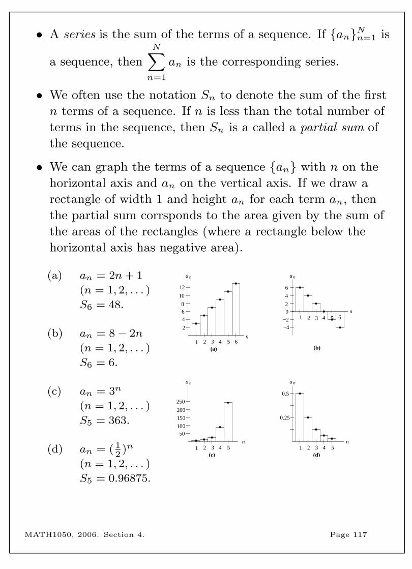
• A series is the sum of the terms of a sequence. If {an}Nn=1 is
a sequence, then
N∑n=1
an is the corresponding series.
• We often use the notation Sn to denote the sum of the first
n terms of a sequence. If n is less than the total number of
terms in the sequence, then Sn is a called a partial sum of
the sequence.
• We can graph the terms of a sequence {an} with n on the
horizontal axis and an on the vertical axis. If we draw a
rectangle of width 1 and height an for each term an, then
the partial sum corrsponds to the area given by the sum of
the areas of the rectangles (where a rectangle below the
horizontal axis has negative area).
(a) an = 2n+ 1
(n = 1, 2, . . . )
S6 = 48.
(b) an = 8− 2n
(n = 1, 2, . . . )
S6 = 6.
(c) an = 3n
(n = 1, 2, . . . )
S5 = 363.
(d) an = ( 12
)n
(n = 1, 2, . . . )
S5 = 0.96875.
(c) (d)
n1 2 3 4 5
50100
150
200
250
1 2 3 4 5
0.25
0.5
n
02
1 2 3 4 5 6n
−4−2
4
6
(a) (b)5 6
n
2
46
10
12
8
a n
a n a n
4
a n
1 2 3
MATH1050, 2006. Section 4. Page 117
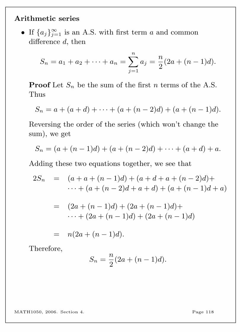
Arithmetic series
• If {aj}∞j=1 is an A.S. with first term a and common
difference d, then
Sn = a1 + a2 + · · ·+ an =
n∑j=1
aj =n
2(2a+ (n− 1)d).
Proof Let Sn be the sum of the first n terms of the A.S.
Thus
Sn = a+ (a+ d) + · · ·+ (a+ (n− 2)d) + (a+ (n− 1)d).
Reversing the order of the series (which won’t change the
sum), we get
Sn = (a+ (n− 1)d) + (a+ (n− 2)d) + · · ·+ (a+ d) + a.
Adding these two equations together, we see that
2Sn = (a+ a+ (n− 1)d) + (a+ d+ a+ (n− 2)d)+
· · ·+ (a+ (n− 2)d+ a+ d) + (a+ (n− 1)d+ a)
= (2a+ (n− 1)d) + (2a+ (n− 1)d)+
· · ·+ (2a+ (n− 1)d) + (2a+ (n− 1)d)
= n(2a+ (n− 1)d).
Therefore,
Sn =n
2(2a+ (n− 1)d).
MATH1050, 2006. Section 4. Page 118
Example 4.5.3 Calculate the sum of the first n natural
numbers.
Example 4.5.4 An arithmetic sequence has first term 3 and
common difference 2 13. If the corresponding arithmetic series is
equal to 3250, calculate the number of terms in the sequence.
MATH1050, 2006. Section 4. Page 119
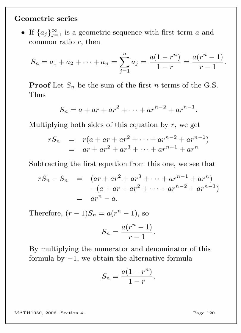
Geometric series
• If {aj}∞j=1 is a geometric sequence with first term a and
common ratio r, then
Sn = a1 + a2 + · · ·+ an =
n∑j=1
aj =a(1− rn)
1− r =a(rn − 1)
r − 1.
Proof Let Sn be the sum of the first n terms of the G.S.
Thus
Sn = a+ ar + ar2 + · · ·+ arn−2 + arn−1.
Multiplying both sides of this equation by r, we get
rSn = r(a+ ar + ar2 + · · ·+ arn−2 + arn−1)
= ar + ar2 + ar3 + · · ·+ arn−1 + arn
Subtracting the first equation from this one, we see that
rSn − Sn = (ar + ar2 + ar3 + · · ·+ arn−1 + arn)
−(a+ ar + ar2 + · · ·+ arn−2 + arn−1)
= arn − a.
Therefore, (r − 1)Sn = a(rn − 1), so
Sn =a(rn − 1)
r − 1.
By multiplying the numerator and denominator of this
formula by −1, we obtain the alternative formula
Sn =a(1− rn)
1− r .
MATH1050, 2006. Section 4. Page 120

Example 4.5.5 A geometric sequence has first three terms
100, 94, 88.36. Calculate the fewest number of terms needed for
the corresponding series to exceed 1000.
MATH1050, 2006. Section 4. Page 121
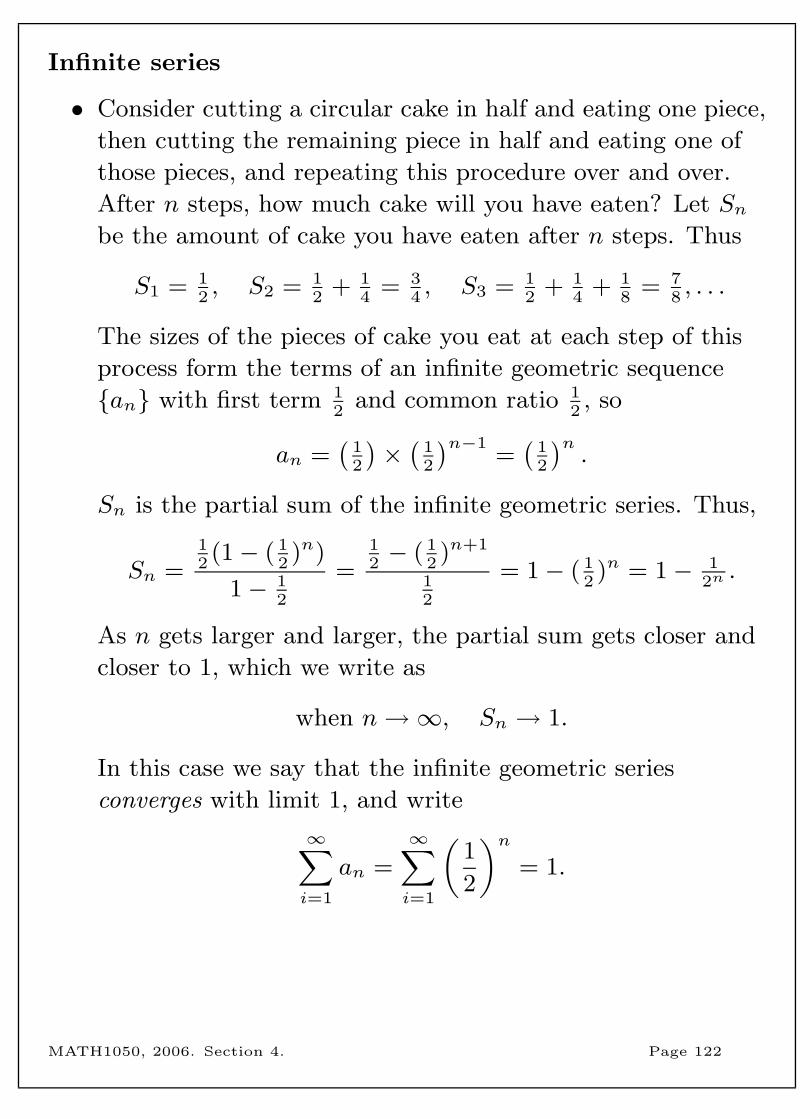
Infinite series
• Consider cutting a circular cake in half and eating one piece,
then cutting the remaining piece in half and eating one of
those pieces, and repeating this procedure over and over.
After n steps, how much cake will you have eaten? Let Snbe the amount of cake you have eaten after n steps. Thus
S1 = 12, S2 = 1
2+ 1
4= 3
4, S3 = 1
2+ 1
4+ 1
8= 7
8, . . .
The sizes of the pieces of cake you eat at each step of this
process form the terms of an infinite geometric sequence
{an} with first term 12
and common ratio 12, so
an =(
12
)×(
12
)n−1=(
12
)n.
Sn is the partial sum of the infinite geometric series. Thus,
Sn =12(1− ( 1
2)n)
1− 12
=12− ( 1
2)n+1
12
= 1− ( 12)n = 1− 1
2n.
As n gets larger and larger, the partial sum gets closer and
closer to 1, which we write as
when n→∞, Sn → 1.
In this case we say that the infinite geometric series
converges with limit 1, and write
∞∑i=1
an =
∞∑i=1
(1
2
)n= 1.
MATH1050, 2006. Section 4. Page 122
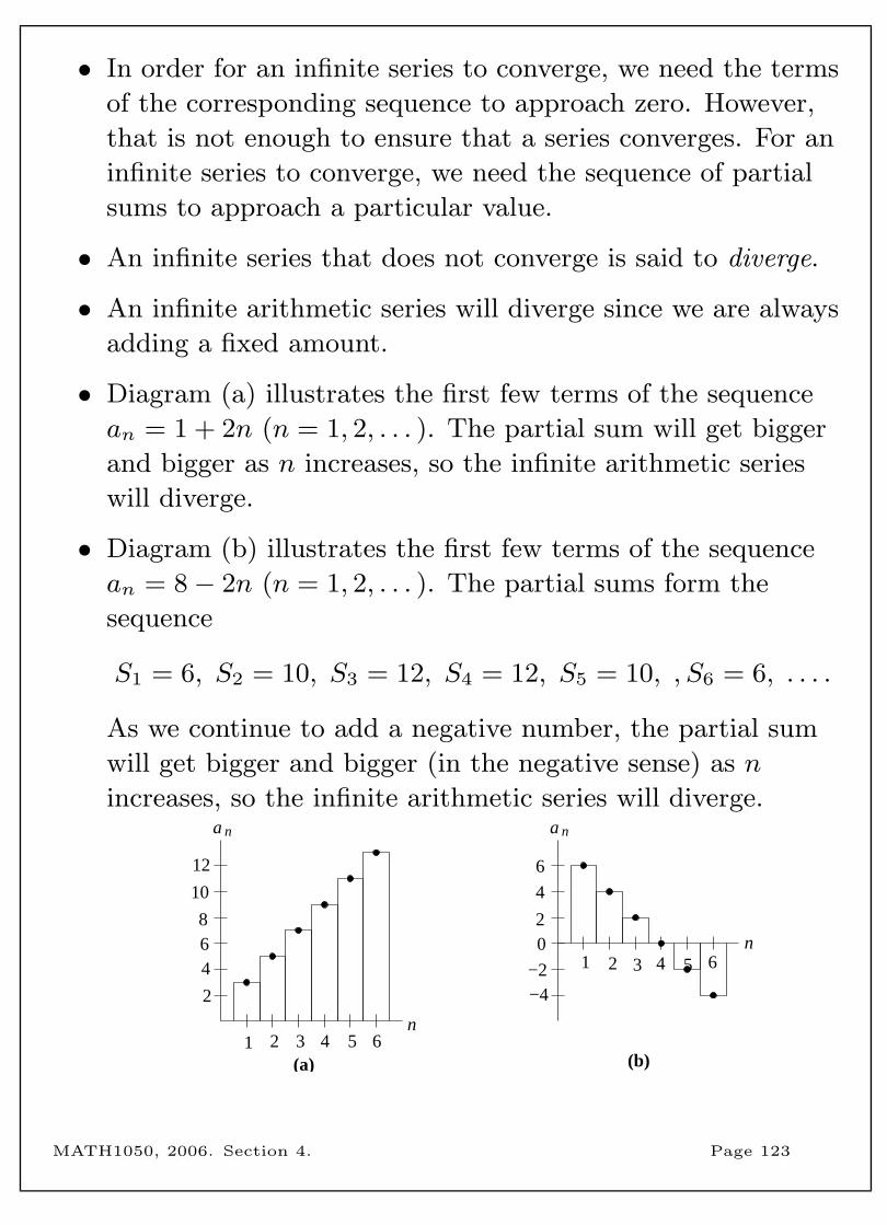
• In order for an infinite series to converge, we need the terms
of the corresponding sequence to approach zero. However,
that is not enough to ensure that a series converges. For an
infinite series to converge, we need the sequence of partial
sums to approach a particular value.
• An infinite series that does not converge is said to diverge.
• An infinite arithmetic series will diverge since we are always
adding a fixed amount.
• Diagram (a) illustrates the first few terms of the sequence
an = 1 + 2n (n = 1, 2, . . . ). The partial sum will get bigger
and bigger as n increases, so the infinite arithmetic series
will diverge.
• Diagram (b) illustrates the first few terms of the sequence
an = 8− 2n (n = 1, 2, . . . ). The partial sums form the
sequence
S1 = 6, S2 = 10, S3 = 12, S4 = 12, S5 = 10, , S6 = 6, . . . .
As we continue to add a negative number, the partial sum
will get bigger and bigger (in the negative sense) as n
increases, so the infinite arithmetic series will diverge.
(b)(a)
6
4
−2−4
n654321
20
54321
na
6
na
8
12
10
64
2
n
MATH1050, 2006. Section 4. Page 123
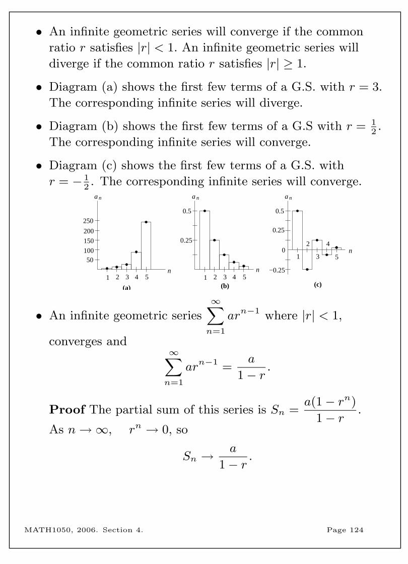
• An infinite geometric series will converge if the common
ratio r satisfies |r| < 1. An infinite geometric series will
diverge if the common ratio r satisfies |r| ≥ 1.
• Diagram (a) shows the first few terms of a G.S. with r = 3.
The corresponding infinite series will diverge.
• Diagram (b) shows the first few terms of a G.S with r = 12.
The corresponding infinite series will converge.
• Diagram (c) shows the first few terms of a G.S. with
r = − 12. The corresponding infinite series will converge.
(c)(b)(a)
n
0.25
0.5
−0.2554321
2 4
0.25
0
0.5
n531
21
na
3
na na
250
200
150
10050
n54
• An infinite geometric series
∞∑n=1
arn−1 where |r| < 1,
converges and∞∑n=1
arn−1 =a
1− r .
Proof The partial sum of this series is Sn =a(1− rn)
1− r .
As n→∞, rn → 0, so
Sn →a
1− r .
MATH1050, 2006. Section 4. Page 124
• We could determine the sum of an infinite G.S. as follows.∞∑i=1
arn−1 = a+ ar + ar2 + ar3 + . . .
r
∞∑i=1
arn−1 = ar + ar2 + ar3 + . . .
(1− r)∞∑i=1
arn−1 = a
Thus∞∑i=1
arn−1 =a
1− r.
Example 4.5.6 A rubber ball is dropped from a height of 5
metres. Each time it hits the ground it bounces back up to one
half the height from which it fell. Calculate the total distance
the ball travels before it comes to rest.
MATH1050, 2006. Section 4. Page 125
4.6 Finite differences and telescoping sums
In this section we look at two methods to find a closed form for
a given sequence.
Method of finite differences
• Arithmetic sequences are easy to work with because the
difference between any two consecutive terms is a constant.
• We call the difference between successive terms of a
sequence the first difference.
• If the first differences are all equal, then we have an
arithmetic sequence and we know that the closed form is a
linear polynomial in n, such as 2n+ 3, 5n− 1 or 3n.
• If the first differences are not all equal, we can look at the
second differences, which are defined to be the differences
between successive first differences.
• If the second differences are all equal, then we have a
sequence whose closed form is a quadratic polynomial in n,
such as 2n2 + 3n− 1, n2 + 4 or 12(n2 + n).
• Similarly, the third differences are defined to be the
differences between successive second differences. If the
third differences are all equal, then the sequence has a
closed form which is a cubic polynomial in n.
MATH1050, 2006. Section 4. Page 126
Example 4.6.1 Determine the first, second and third
differences for the first 6 terms of the sequence {n3 + 2n}∞n=1.
• In general, the ith differences are defined to be the
differences between sucessive (i− 1)th differences. If the ith
differences are all equal, then the sequence has a closed
form which is a polynomial in n, with highest power ni.
• If you know that the closed form of a particular sequence
will be a polynomial, you can set up a system of
simultaneous linear equations and solve them to find the
closed form.
MATH1050, 2006. Section 4. Page 127
Example 4.6.2 Use finite differences to find a closed form for
the sequence 1, 3, 6, 10, 15, 21, 28.
(These numbers are the first seven terms in the sequence of
triangular numbers.)
MATH1050, 2006. Section 4. Page 128

Telescoping sums
• A telescoping sum is a sum of similar expressions in which
many terms pair up to cancel out.
• A telescoping sum can sometimes be used to determine a
closed form for a sequence from its recursive definition.
Example 4.6.3 Use a telescoping sum to find a closed form for
the sequence of triangular numbers, defined recursively by
an = an−1 + n (n = 2, 3, . . . ) where a1 = 1.
MATH1050, 2006. Section 4. Page 129
4.7 Applications of sequences
Simple interest
• When a bank account is paying simple interest, the interest
is calculated as a percentage of the principal deposited into
the account; interest is not paid on any interest previously
deposited into your account.
Example 4.7.1 On January 1 1999, you deposited $1000 into a
savings account that pays simple interest of 7% per year. On
each sucessive January 1, you add another $1000 to the savings
account. After n years, how much money is in the account.
MATH1050, 2006. Section 4. Page 130
Compound Interest
• When a bank account earns compound interest, interest is
calculated on the total amount in the account, including
any interest previously deposited into the account.
• An amount A is invested at an interest rate of r per period,
compounded at the end of each period. Let Vn be the value
of the account after n periods. Thus
V0 = A
V1 = A+Ar = A(1 + r)
V2 = A(1 + r) +A(1 + r)r = A(1 + r)2
...
Vn = A(1 + r)n−1 +A(1 + r)n−1r = A(1 + r)n,
so Vn = V0(1 + r)n = A(1 + r)n.
Example 4.7.2 Suppose you deposit $10,000 in a term deposit
that pays interest at 5% per year, compounded monthly. What
is the value of your term deposit after 5 years.
MATH1050, 2006. Section 4. Page 131
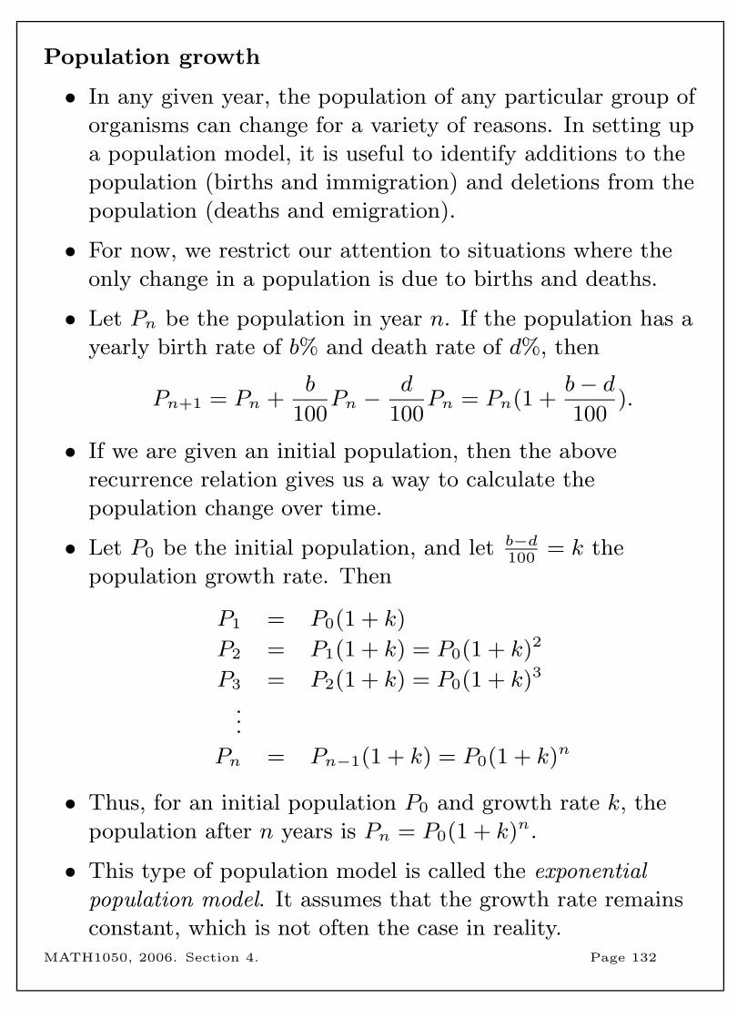
Population growth
• In any given year, the population of any particular group of
organisms can change for a variety of reasons. In setting up
a population model, it is useful to identify additions to the
population (births and immigration) and deletions from the
population (deaths and emigration).
• For now, we restrict our attention to situations where the
only change in a population is due to births and deaths.
• Let Pn be the population in year n. If the population has a
yearly birth rate of b% and death rate of d%, then
Pn+1 = Pn +b
100Pn −
d
100Pn = Pn(1 +
b− d100
).
• If we are given an initial population, then the above
recurrence relation gives us a way to calculate the
population change over time.
• Let P0 be the initial population, and let b−d100
= k the
population growth rate. Then
P1 = P0(1 + k)
P2 = P1(1 + k) = P0(1 + k)2
P3 = P2(1 + k) = P0(1 + k)3
...
Pn = Pn−1(1 + k) = P0(1 + k)n
• Thus, for an initial population P0 and growth rate k, the
population after n years is Pn = P0(1 + k)n.
• This type of population model is called the exponential
population model. It assumes that the growth rate remains
constant, which is not often the case in reality.MATH1050, 2006. Section 4. Page 132
Example 4.7.3 The population of a town on January 1, 2003
was 13,690. The birth rate is estimated at 20% and the death
rate at 18%. Assuming there is no immigration or emigration
from this town, estimate the population on January 1, 2013.
Example 4.7.4 A colony of penguins in Antarctica numbered
26 in the year 1959 and 160 in the year 1969. Assuming that
this population can be modelled accurately by the exponential
population model, determine the annual growth rate of this
population. Then predict what the population was in 1979.
MATH1050, 2006. Section 4. Page 133
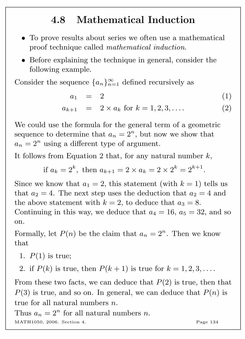
4.8 Mathematical Induction
• To prove results about series we often use a mathematical
proof technique called mathematical induction.
• Before explaining the technique in general, consider the
following example.
Consider the sequence {an}∞n=1 defined recursively as
a1 = 2 (1)
ak+1 = 2× ak for k = 1, 2, 3, . . . . (2)
We could use the formula for the general term of a geometric
sequence to determine that an = 2n, but now we show that
an = 2n using a different type of argument.
It follows from Equation 2 that, for any natural number k,
if ak = 2k, then ak+1 = 2× ak = 2× 2k = 2k+1.
Since we know that a1 = 2, this statement (with k = 1) tells us
that a2 = 4. The next step uses the deduction that a2 = 4 and
the above statement with k = 2, to deduce that a3 = 8.
Continuing in this way, we deduce that a4 = 16, a5 = 32, and so
on.
Formally, let P (n) be the claim that an = 2n. Then we know
that
1. P (1) is true;
2. if P (k) is true, then P (k + 1) is true for k = 1, 2, 3, . . . .
From these two facts, we can deduce that P (2) is true, then that
P (3) is true, and so on. In general, we can deduce that P (n) is
true for all natural numbers n.
Thus an = 2n for all natural numbers n.MATH1050, 2006. Section 4. Page 134
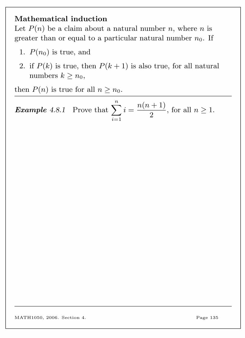
Mathematical induction
Let P (n) be a claim about a natural number n, where n is
greater than or equal to a particular natural number n0. If
1. P (n0) is true, and
2. if P (k) is true, then P (k + 1) is also true, for all natural
numbers k ≥ n0,
then P (n) is true for all n ≥ n0.
Example 4.8.1 Prove that
n∑i=1
i =n(n+ 1)
2, for all n ≥ 1.
MATH1050, 2006. Section 4. Page 135
Example 4.8.2 Prove that
n∑i=1
i2 =n(n+ 1)(2n+ 1)
6, for all
n ≥ 1.
MATH1050, 2006. Section 4. Page 136

Example 4.8.3 Show that 7 divides 8n − 1 for all n ≥ 1.
MATH1050, 2006. Section 4. Page 137
5 Real and complex numbers
• Number systems evolved from a basic need to count and to
measure. As the need arose to solve more sophisticated
problems, less intuitive (but very useful) number systems
were introduced.
• You are probably already familiar with the real numbers.
This section starts with a review of the number systems
that make up the real numbers.
• Complex numbers evolved from the need to solve quadratic
equations that have no solutions in the real number system.
To do this, the symbol i was introduced, where i2 = −1.
Although this seems artificial (and the term ‘imaginary
numbers’ is sometimes used for complex numbers), this
breakthrough had a huge impact and complex numbers are
widely used in mathematics, physics and engineering.
• We will look at several representations of complex numbers
and investigate some important theorems.
• Topics in this section are:
– Real numbers
– Absolute value
– Introduction to complex numbers
– Complex numbers in polar form
– Powers of complex numbers
– Fundamental theorem of algebra
MATH1050, 2006. Section 5. Page 138
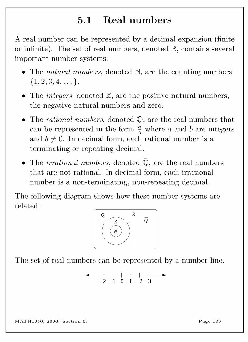
5.1 Real numbers
A real number can be represented by a decimal expansion (finite
or infinite). The set of real numbers, denoted R, contains several
important number systems.
• The natural numbers, denoted N, are the counting numbers
{1, 2, 3, 4, . . . }.
• The integers, denoted Z, are the positive natural numbers,
the negative natural numbers and zero.
• The rational numbers, denoted Q, are the real numbers that
can be represented in the form ab
where a and b are integers
and b 6= 0. In decimal form, each rational number is a
terminating or repeating decimal.
• The irrational numbers, denoted Q, are the real numbers
that are not rational. In decimal form, each irrational
number is a non-terminating, non-repeating decimal.
The following diagram shows how these number systems are
related.
Q
N
ZQ R
The set of real numbers can be represented by a number line.
0 2 3−1−2 1
MATH1050, 2006. Section 5. Page 139
Surds
• A surd is an irrational number which is represented by a
root sign. For example,√
2,√
7 and 3√
15 are surds,
but√
9 and 3√
125 are not surds.
Example 5.1.1 Simplify the following expressions.
a) 5√
3 + 2√
12−√
18
b) 5√
3a3b2√
12a where a and b are positive real numbers.
• Rationalising the denominator is the process of multiplying
the numerator and denominator of a fraction by an
appropriate number so that the result does not have a surd
in the denominator.
Example 5.1.2 Simplify the expression
√6 + 3
√2
3 +√
5.
MATH1050, 2006. Section 5. Page 140
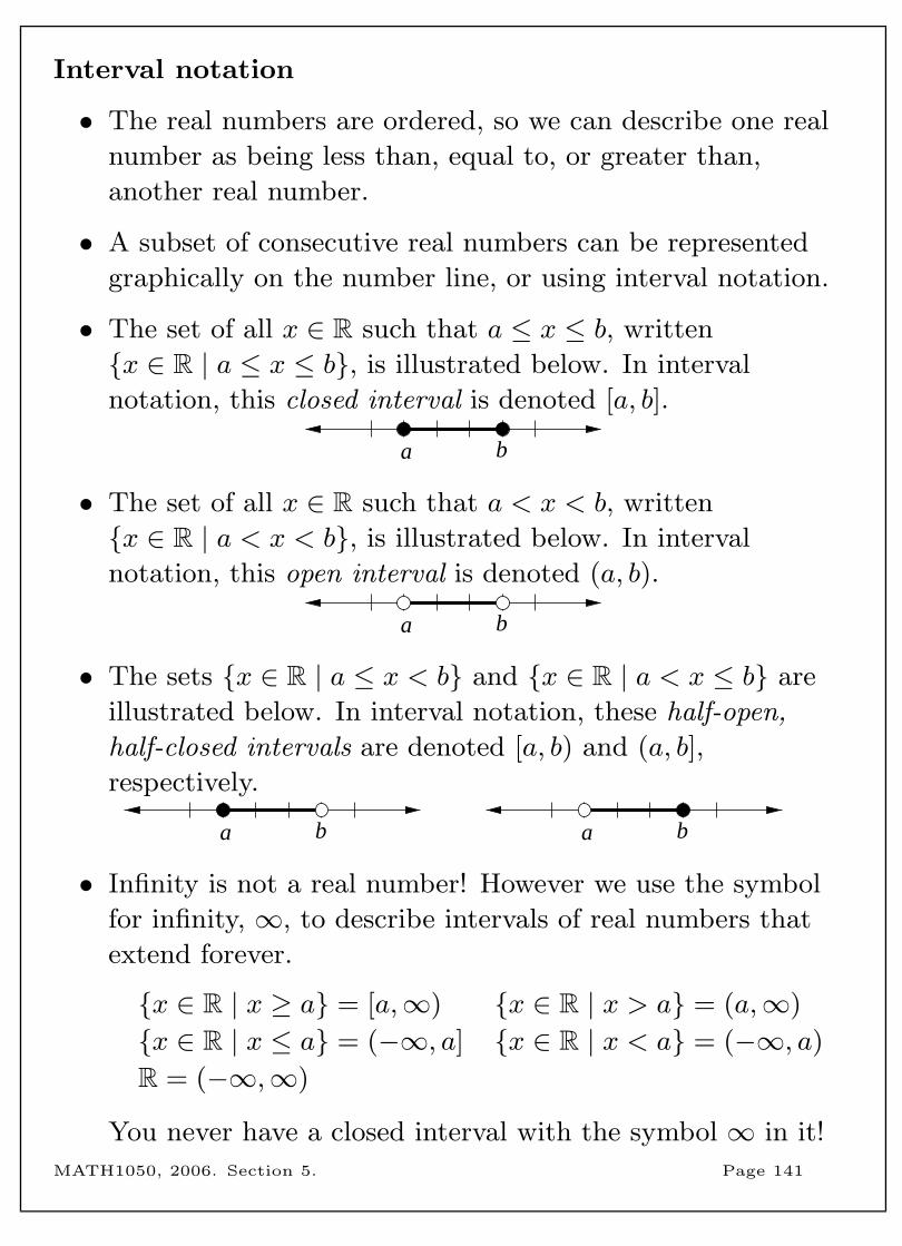
Interval notation
• The real numbers are ordered, so we can describe one real
number as being less than, equal to, or greater than,
another real number.
• A subset of consecutive real numbers can be represented
graphically on the number line, or using interval notation.
• The set of all x ∈ R such that a ≤ x ≤ b, written
{x ∈ R | a ≤ x ≤ b}, is illustrated below. In interval
notation, this closed interval is denoted [a, b].
a b
• The set of all x ∈ R such that a < x < b, written
{x ∈ R | a < x < b}, is illustrated below. In interval
notation, this open interval is denoted (a, b).
a b
• The sets {x ∈ R | a ≤ x < b} and {x ∈ R | a < x ≤ b} are
illustrated below. In interval notation, these half-open,
half-closed intervals are denoted [a, b) and (a, b],
respectively.
baba
• Infinity is not a real number! However we use the symbol
for infinity, ∞, to describe intervals of real numbers that
extend forever.
{x ∈ R | x ≥ a} = [a,∞) {x ∈ R | x > a} = (a,∞)
{x ∈ R | x ≤ a} = (−∞, a] {x ∈ R | x < a} = (−∞, a)
R = (−∞,∞)
You never have a closed interval with the symbol ∞ in it!
MATH1050, 2006. Section 5. Page 141
Inequalities
Example 5.1.3 Determine the values of x for which3
x< 6.
Example 5.1.4 Determine the values of x for which
(x− 2)(x+ 1) ≥ 0.
MATH1050, 2006. Section 5. Page 142
Example 5.1.5 Determine the values of x for which
x− 3
x+ 2≤ 0.
MATH1050, 2006. Section 5. Page 143
5.2 Absolute value
• The absolute value, or modulus, of a real number x is given
by
|x| =
{x if x ≥ 0,
−x if x < 0.
So, for every real number x, |x| ≥ 0.
• The distance between two real numbers a and b is
|b− a| = |a− b| =
{b− a if b ≥ a,a− b if b < a.
Thus |x| gives the distance between x and 0.
Properties of the absolute value
• For every real number x, |x|2 = x2.
Proof If x ≥ 0, then |x| = x, so |x|2 = x2.
If x < 0, then |x| = −x so |x|2 = (−x)(−x) = x2.
• For every pair of real numbers x and y, |xy| = |x| · |y|.
Proof If x ≥ 0 and y ≥ 0 then |xy| = xy and |x| · |y| = xy.
If x < 0 and y < 0 then |xy| = xy and
|x| · |y| = (−x)(−y) = xy.
If x ≥ 0 and y < 0 then |xy| = −(xy) and
|x| · |y| = x(−y) = −xy. Similarly for x < 0 and y ≥ 0.
• For every pair of real numbers x and y, |x+ y| ≤ |x|+ |y|.(This property is called the triangle inequality.)
MATH1050, 2006. Section 5. Page 144
Example 5.2.1 Solve the following equations.
a) |4− 3x| = 3
b) |y − 3| = 3y + 8
c) |a− 2| = |2a+ 5|
MATH1050, 2006. Section 5. Page 145
Example 5.2.2 Solve the following inequalities and illustrate
the solutions on a number line.
a) |2x− 3| < 2
b)1
|x+ 2| ≤ 3
MATH1050, 2006. Section 5. Page 146
Example 5.2.3 Solve
∣∣∣∣y − 2
y + 3
∣∣∣∣ < 2 and illustrate the solution on
a number line.
MATH1050, 2006. Section 5. Page 147
5.3 Introduction to complex numbers
• By the 16th century, it was known that the quadratic
equation
ax2 + bx+ c = 0, where a, b, c ∈ R
has solutions
x =−b±
√b2 − 4ac
2a,
provided that a 6= 0 and b2 − 4ac ≥ 0.
• The quantity b2 − 4ac is called the discriminant of the
quadratic equation. A quadratic equation (with real
coefficients) having a negative discriminant has no solution
over the real numbers.
• In the next century, the first steps were taken to enlarge the
real number system and create a new number system called
the complex numbers, denoted C, in which all quadratic
equations have solutions.
• The idea that allowed the formation of the complex
numbers was the introduction of the symbol i, which
satisfies i2 = −1.
• Eventually engineers and scientists discovered uses for
complex numbers and they are now used extensively in
many applications, including electric circuits and
electromagnetic waves.
MATH1050, 2006. Section 5. Page 148
• A complex number is an expression of the form a+ bi, where
a, b ∈ R and i2 = −1. The set of such numbers is called the
complex numbers and is denoted C.
• If z = a+ bi ∈ C, then we call a the real part of z and b the
imaginary part of z. We write this as a = Re(z) and
b = Im(z).
• The representation of a complex number in the form a+ bi
is called the Cartesian form of the complex number.
Example 5.3.1 Let z = −3 + 4i. Write down Re(z) and Im(z).
• Two complex numbers a+ bi and c+ di are equal if and
only if a = c and b = d.
• Let z = a+ bi and w = c+ di be two complex numbers.
Addition
z + w = (a+ bi) + (c+ di)
= (a+ c) + (b+ d)i
So Re(z + w) = Re(z) + Re(w)
and Im(z + w) = Im(z) + Im(w).
Multiplication
zw = (a+ bi)(c+ di)
= ac+ adi+ bci+ bdi2
= ac+ adi+ bci− bd= (ac− bd) + (ad+ bc)i.
MATH1050, 2006. Section 5. Page 149
Example 5.3.2 Let z = −3 + 2i and w = 4− i. Write each of
the following in Cartesian form.
a) 3z + 2w
b) wz
c) iw
Example 5.3.3 Solve for x ∈ C where x2 + 2x+ 2 = 0.
MATH1050, 2006. Section 5. Page 150
• Let z = a+ bi ∈ C. The complex conjugate of z, denoted z,
is z = a− bi.
• The complex conjugate is useful because the product zz
gives a real number.
zz = (a+ bi)(a− bi) = a2 + b2
• The complex conjugate allows us to divide by a non-zero
complex number.
a+ bi
c+ di=
a+ bi
c+ di× c− dic− di
=(a+ bi)(c− di)
c2 + d2
=ac+ bd
c2 + d2+bc− adc2 + d2
i
Example 5.3.4 Write2 + i
2− i in Cartesian form.
MATH1050, 2006. Section 5. Page 151
• The modulus of the complex number z = a+ bi is denoted
|z|. It is defined to be
|z| =√zz =
√a2 + b2.
Properties of the modulus and complex conjugate
Let z = a+ bi and w = c+ di be complex numbers.
• |z| = |z|
• |z|2 = zz
• z + w = z + w
• zw = z w
•( zw
)=z
w
• z = z if and only if z ∈ R
• ¯z = z
MATH1050, 2006. Section 5. Page 152
Example 5.3.5 Find real numbers x and y such that
(2x+ 1)i− y =x+ yi
1 + i.
MATH1050, 2006. Section 5. Page 153
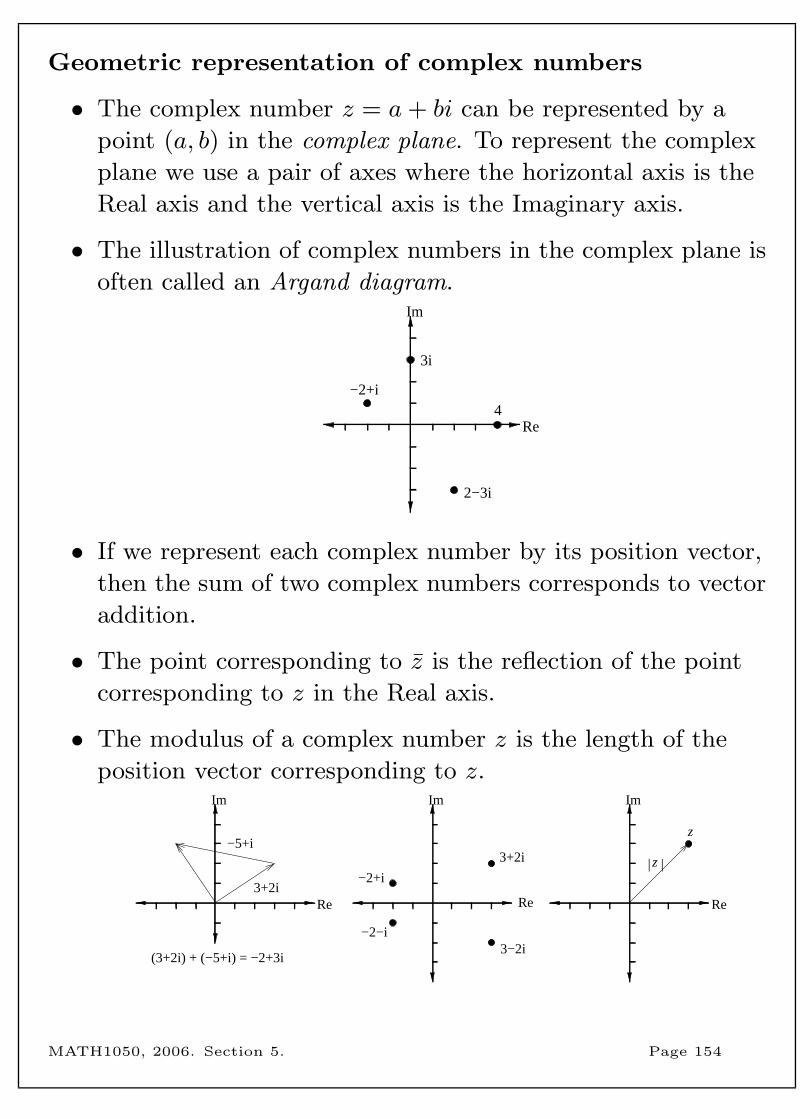
Geometric representation of complex numbers
• The complex number z = a+ bi can be represented by a
point (a, b) in the complex plane. To represent the complex
plane we use a pair of axes where the horizontal axis is the
Real axis and the vertical axis is the Imaginary axis.
• The illustration of complex numbers in the complex plane is
often called an Argand diagram.
−2+i
3i
4
2−3i
Im
Re
• If we represent each complex number by its position vector,
then the sum of two complex numbers corresponds to vector
addition.
• The point corresponding to z is the reflection of the point
corresponding to z in the Real axis.
• The modulus of a complex number z is the length of the
position vector corresponding to z.
z
Re
Im
Re
Im
−2−i
−2+i
3+2i
3−2i(3+2i) + (−5+i) = −2+3i
Im
Re
−5+i
3+2i
| |z
MATH1050, 2006. Section 5. Page 154
5.4 Complex numbers in polar form
Suppose that the complex number z = a+ bi is represented as a
point in the complex plane.
• The modulus of z gives the distance from z to the origin.
• The argument of z, arg(z), is the angle that the position
vector of z makes with the positive Real axis. Note that
there can be many different arguments for a non-zero
complex number z, since the angle θ is equivalent to the
angle θ plus or minus any multiple of 2π radians.
• Note that positive angles are in an anti-clockwise direction
and negative angles are in a clockwise direction from the
positive Real axis.
• We call the argument of z that lies in the interval (−π, π]
the principal argument of z, denoted Arg(z).
• If z = a+ bi then arg(z) = θ where tan θ = ba
. Always draw
a sketch to help you choose the correct value for θ.
Example 5.4.1 Let z = −4 + 4i. Determine |z| and Arg(z).
MATH1050, 2006. Section 5. Page 155
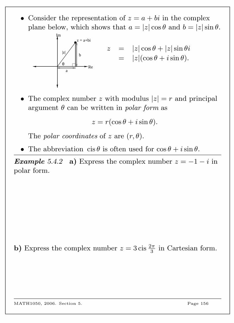
• Consider the representation of z = a+ bi in the complex
plane below, which shows that a = |z| cos θ and b = |z| sin θ.
θ
|z|
z = a+bi
b
a
Im
Re
z = |z| cos θ + |z| sin θi= |z|(cos θ + i sin θ).
• The complex number z with modulus |z| = r and principal
argument θ can be written in polar form as
z = r(cos θ + i sin θ).
The polar coordinates of z are (r, θ).
• The abbreviation cis θ is often used for cos θ + i sin θ.
Example 5.4.2 a) Express the complex number z = −1− i in
polar form.
b) Express the complex number z = 3 cis 2π3
in Cartesian form.
MATH1050, 2006. Section 5. Page 156
• Let z1 = r1 cis θ1 and z2 = r2 cis θ2.
Multiplication in polar form
z1z2 = r1r2 cis (θ1 + θ2)
Division in polar form
z1
z2=r1
r2cis (θ1 − θ2)
Example 5.4.3 Let z = 10 cis 5π6
and w = 6 cis π3
.
a) Calculate zw and express your answer in polar form.
b) Calculatez
wand express your answer in polar form.
MATH1050, 2006. Section 5. Page 157
• Recall that the number e = 2.71828 . . . is an irrational
number. It can be defined as e = limn→∞
(1 + 1n
)n.
• The following important result is known as Euler’s formula:
cos θ + i sin θ = eiθ.
This result was introduced by the Swiss mathematician
Euler in 1748. The proof is beyond the scope of this course.
• Every non-zero complex number z = a+ bi with polar
coordinates (r, θ) can be written as
z = r cis θ (polar form) and z = reiθ (exponential form).
• Some people call both of the above forms the polar form of
z, since they are both based on the polar coordinates of z.
Example 5.4.4 Write the complex number z = 1−√
3i in
exponential form.
MATH1050, 2006. Section 5. Page 158
Example 5.4.5 Let z = reiθ. Write z in exponential form.
Example 5.4.6 Write −1 in exponential form.
It is wonderful that two irrational numbers and the square root
of a negative number combine in this way to give −1.
MATH1050, 2006. Section 5. Page 159
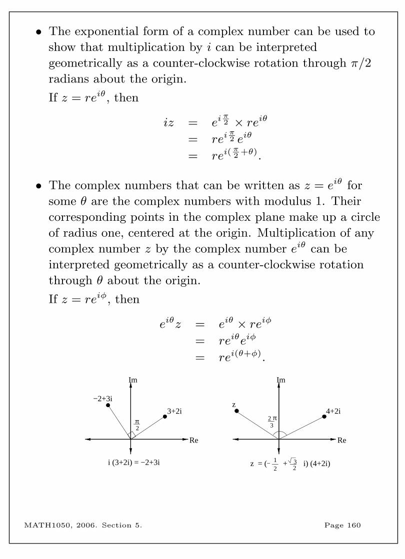
• The exponential form of a complex number can be used to
show that multiplication by i can be interpreted
geometrically as a counter-clockwise rotation through π/2
radians about the origin.
If z = reiθ, then
iz = eiπ2 × reiθ
= reiπ2 eiθ
= rei(π2 +θ).
• The complex numbers that can be written as z = eiθ for
some θ are the complex numbers with modulus 1. Their
corresponding points in the complex plane make up a circle
of radius one, centered at the origin. Multiplication of any
complex number z by the complex number eiθ can be
interpreted geometrically as a counter-clockwise rotation
through θ about the origin.
If z = reiφ, then
eiθz = eiθ × reiφ
= reiθeiφ
= rei(θ+φ).
3+2iz
4+2i
Re
Im
Re
Im
i (3+2i) = −2+3i
−2+3i
z = ( + i) (4+2i)−
π__2
__3
2 π
__12
3__2
MATH1050, 2006. Section 5. Page 160
5.5 Powers of complex numbers
• De Moivre’s Theorem states that if z = r(cos θ + i sin θ) and
n is a natural number, then
zn = rn(cos(nθ) + i sin(nθ)).
This theorem was named after the French mathematician
Abraham de Moivre (1667–1754).
Proof: Let z = r(cos θ + i sin θ). Thus z = reiθ, and
zn = (reiθ)n
= rneiθn
= rn(cos(nθ) + i sin(nθ)).
• Notice that the proof of de Moivre’s theorem is also true for
n ∈ R.
• De Moivre’s Theorem allows us to calculate powers of
complex numbers with ease.
Example 5.5.1 Evaluate (1−√
3i)6.
MATH1050, 2006. Section 5. Page 161
• De Moivre’s Theorem also allows us to calculate the nth
roots of any complex number, where n ∈ N.
• The nth roots of the complex number w are the values of z
such that zn = w. There are exactly n such values of z.
• To solve the equation zn = w for some w ∈ C and n ∈ N.
1. Express w in polar form as w = r cis θ.
2. Since the angle θ is equivalent to the angle (θ + 2kπ) for
any k ∈ Z, we know that
r cis θ = r cis (θ + 2kπ), where k ∈ Z.
3. Thus z = (r cis (θ + 2kπ))1n , and by the extension of de
Moivre’s theorem
z = r1n cis
(θ + 2kπ
n
)for k ∈ Z.
Example 5.5.2 Determine the four values of z for which
z4 = 1. (These are called the fourth roots of unity.)
MATH1050, 2006. Section 5. Page 162

Example 5.5.3 Determine the five values of w for which
w5 = −2− 2i, and draw them on an Argand diagram.
MATH1050, 2006. Section 5. Page 163
5.6 The fundamental theorem of algebra
• A polynomial in the variable z is an expression of the form
anzn + an−1z
n−1 + an−2zn−2 + · · ·+ a2z
2 + a1z + a0,
where n ∈ N is the degree (highest power) of the
polynomial, an, an−1, an−2, . . . , a2, a1, a0 are the coefficients
of z, and an 6= 0.
• If P (z) is a polynomial, then P (z) = 0 is a polynomial
equation.
Example 5.6.1 Determine which of these are polynomials and
which are polynomial equations.
2x3 − 10x = 1, 3z4 + z−2 + 5, (3 + 2i)z4 − 5iz2 + 10.
• Fundamental Theorem of Algebra (FTA) Every polynomial
equation with real or complex coefficients has a solution in
the complex numbers.
• The first proof of this theorem was given by Gauss in his
doctoral thesis in 1799. None of the known proofs are easy,
so we won’t prove it in this course.
• Factor Theorem Let P (z) be a polynomial and let a ∈ C.
Then P (a) = 0 if and only if (z − a) is a factor of P (z).
MATH1050, 2006. Section 5. Page 164
Example 5.6.2 Let P (z) = z3 − 7z2 + 6z + 14. Determine
which of (z + 1) or (z − 2) is a factor of P (z).
• Let P (z) = 0 be a polynomial equation. The FTA
guarantees that there is a solution to P (z) = 0, suppose it is
z = a. Then the factor theorem tells us that (z − a) is a
factor of P (z) and so we can write P (z) = (z − a)Q(z)
where Q(z) is a polynomial equation whose degree is one
less than the degree of P (z). Now the FTA guarantees that
we can find a solution to the polynomial equation Q(z) = 0,
so we can repeat this procedure.
• From Example 5.6.2 above, we know that (z + 1) is a factor
of P (z). Thus
P (z) = (z + 1)Q(z),
where the degree of the polynomial Q(z) is two. Let the
coefficients of Q(z) be a, b and c.
z3 − 7z2 + 6z + 14 = (z + 1)(az2 + bz + c)
= az3 + az2 + bz2 + bz + cz + c
= az3 + (a+ b)z2 + (b+ c)z + c
Equating coefficients on each side we see that
a = 1, b = −8 and c = 14.
Hence
z3 − 7z2 + 6z + 14 = (z + 1)(z2 − 8z + 14).
MATH1050, 2006. Section 5. Page 165
• If we start with a polynomial equation P (z) = 0 where P (z)
has degree n, then we can continue taking out linear factors
of the form (z − a) until we have found n linear factors.
• From Example 5.6.2 above,
z3 − 7z2 + 6z + 14 = (z + 1)(z2 − 8z + 14).
We can use the quadratic formula to solve z2 − 8z + 14 = 0,
as
z =8±√
64− 4× 14
2= 4±
√2.
Thus
z3 − 7z2 + 6z + 14 = (z + 1)(z − (4 +√
2))(z − (4−√
2)).
• Important result Let P (z) be a polynomial of degree n,
where n ∈ N. Then the polynomial equation P (z) = 0 has n
solutions.
• Note that the n solutions may not be distinct.
• Useful factorising results to remember.
– Difference of squares: x2 − y2 = (x− y)(x+ y).
– Perfect square: x2 + 2xy + y2 = (x+ y)(x+ y)
x2 − 2xy + y2 = (x− y)(x− y).
– Quadratic: ax2 + bx+ c = (a1x+ c1)(a2x+ c2), where
a = a1a2, c = c1c2 and b = a1c2 + a2c1.
MATH1050, 2006. Section 5. Page 166
Example 5.6.3 a) Write z4 − 81 as the product of linear
factors and hence find all solutions of z4 − 81 = 0 (over C).
b) Write 6z4 + z2 − 1 as the product of linear factors and hence
find all solutions of 6z4 + z2 − 1 = 0 (over C).
c) Write z2 + 2iz − 1 as the product of linear factors and hence
find all solutions of z2 + 2iz − 1 = 0 (over C).
MATH1050, 2006. Section 5. Page 167
• If a polynomial equation has real coefficients, its solutions
(roots) are either real numbers or occur as pairs of
conjugate complex numbers.
Example 5.6.4 z = 5 + 5√
2i is a solution of
z3 − 8z2 + 55z + 150 = 0.
Find all the other solutions of this equation.
MATH1050, 2006. Section 5. Page 168
6 Functions
• A function is a rule that associates a unique output to each
input.
• Functions are used heavily in all areas of mathematics and
in most applications of mathematics.
• Some examples of functions include:
– A formula that converts temperature in Fahrenheit to
temperature in Celcius, c = 59(f − 32), describes
temperature in degrees centigrade as a function of
temperature in degrees Fahrenheit.
– A formula for the area of a circle in terms of its radius,
A = πr2, describes area as a function of radius.
– A table of values that given the human population of
the world for each year from 1900 to 2000 describes
population as a function of year.
• Topics in this section are:
– Introduction to functions
– A collection of standard functions
– Composition of functions
– Inverse functions
– Limits of functions
MATH1050, 2006. Section 6. Page 169
6.1 Introduction to functions
• A function is a rule that assigns to each element x in a set
A exactly one element from a set B.
• The notation f(x) is used to denote the element in B that
arises from applying the function f to the element x, and
we say that f maps x to f(x). We call f(x) the value of f
at x, or the image of x under f .
• The set A is called the domain of the function. It is the set
of all possible inputs to the function.
• The set of all possible values of the function is called the
range of the function. The range is a subset of the set B.
Example 6.1.1 Let f be the function that takes a real number
as input and returns two plus the square of that real number as
output.
a) Determine f(2), f(−3) and f(x) for some real number x.
b) Determine the domain and range of f .
MATH1050, 2006. Section 6. Page 170
• The following example illustrates some common notation
used to denote functions.
Example 6.1.2 Let f : R→ R where f(x) = 2x and let
g : Z→ Z where g(x) = 2x. Determine the domain and range
for each function f and g.
• Domain convention If a function is given by a formula
and the domain is not specified, the convention is that the
domain is the set of all real numbers for which the formula
defines a real number.
• Although we often use x as the variable in the rule of a
function, this is not required. For example, if f is the
function which computes the area of a circle given its radius
then f(r) = πr2, and we say that f is a function of r.
Example 6.1.3 Let g be the function defined by the rule
g(a) =√a− 1. Determine the domain and range of g.
MATH1050, 2006. Section 6. Page 171
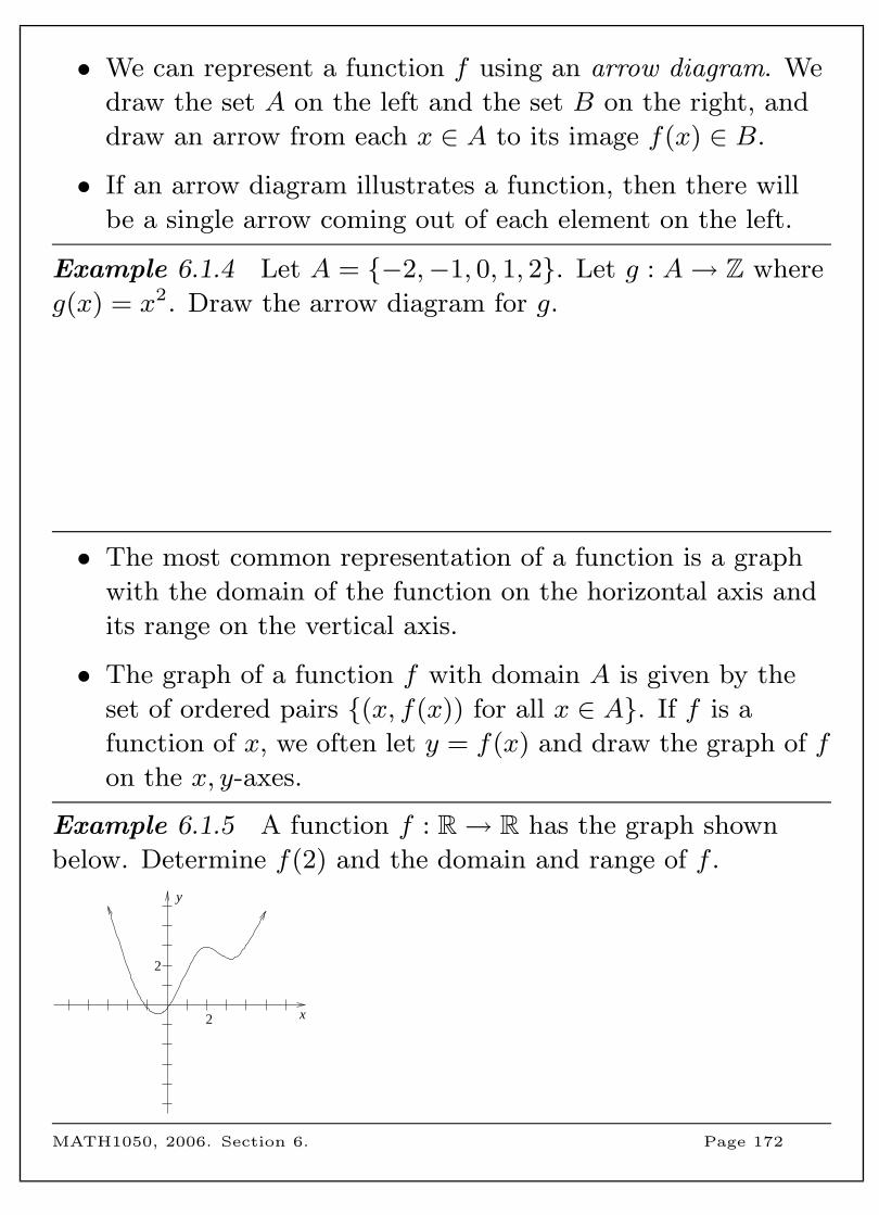
• We can represent a function f using an arrow diagram. We
draw the set A on the left and the set B on the right, and
draw an arrow from each x ∈ A to its image f(x) ∈ B.
• If an arrow diagram illustrates a function, then there will
be a single arrow coming out of each element on the left.
Example 6.1.4 Let A = {−2,−1, 0, 1, 2}. Let g : A→ Z where
g(x) = x2. Draw the arrow diagram for g.
• The most common representation of a function is a graph
with the domain of the function on the horizontal axis and
its range on the vertical axis.
• The graph of a function f with domain A is given by the
set of ordered pairs {(x, f(x)) for all x ∈ A}. If f is a
function of x, we often let y = f(x) and draw the graph of f
on the x, y-axes.
Example 6.1.5 A function f : R→ R has the graph shown
below. Determine f(2) and the domain and range of f .
2
2 x
y
MATH1050, 2006. Section 6. Page 172
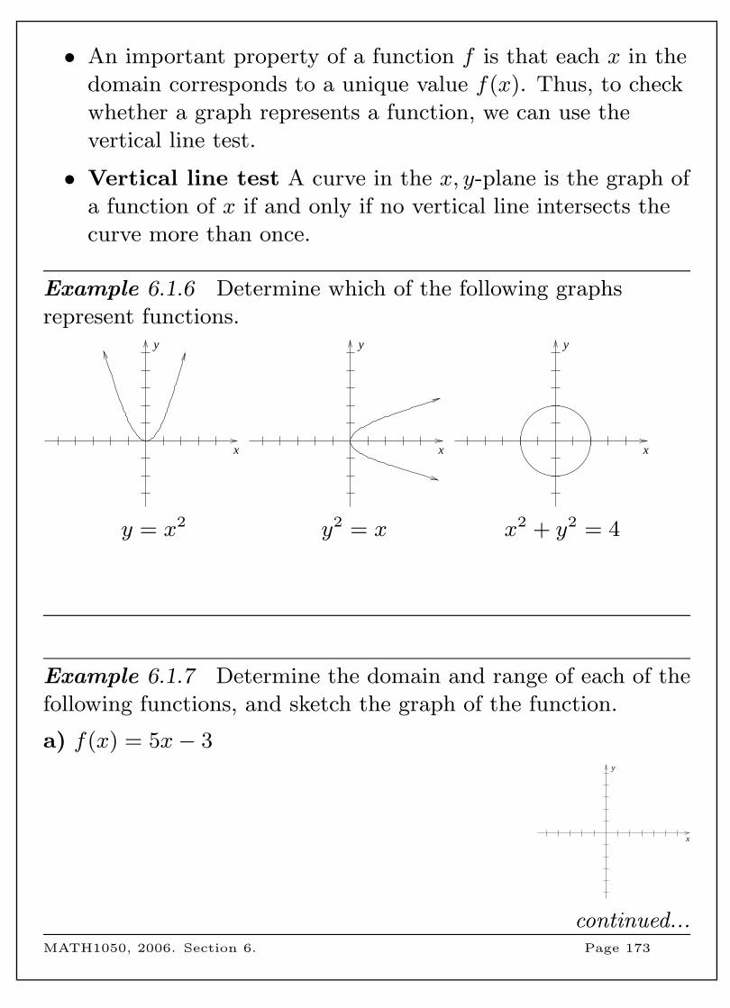
• An important property of a function f is that each x in the
domain corresponds to a unique value f(x). Thus, to check
whether a graph represents a function, we can use the
vertical line test.
• Vertical line test A curve in the x, y-plane is the graph of
a function of x if and only if no vertical line intersects the
curve more than once.
Example 6.1.6 Determine which of the following graphs
represent functions.
x
y
x
y
x
y
y = x2 y2 = x x2 + y2 = 4
Example 6.1.7 Determine the domain and range of each of the
following functions, and sketch the graph of the function.
a) f(x) = 5x− 3
x
y
continued...MATH1050, 2006. Section 6. Page 173
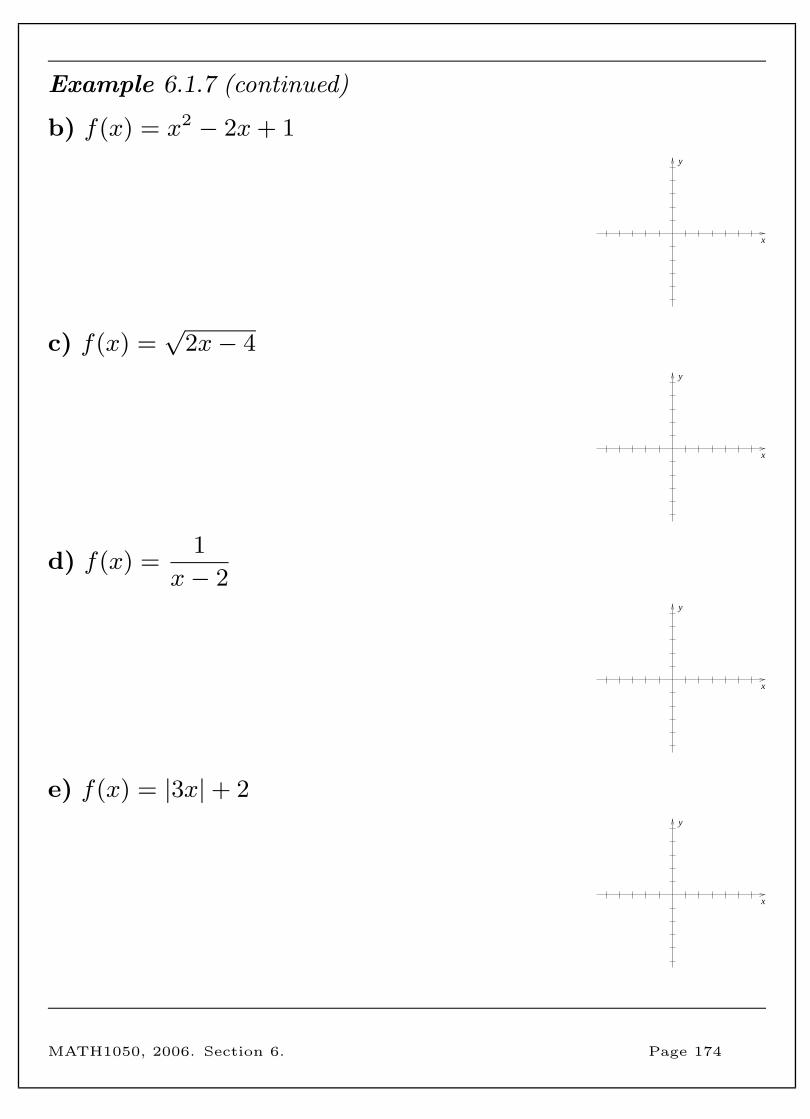
Example 6.1.7 (continued)
b) f(x) = x2 − 2x+ 1
x
y
c) f(x) =√
2x− 4
x
y
d) f(x) =1
x− 2
x
y
e) f(x) = |3x|+ 2
x
y
MATH1050, 2006. Section 6. Page 174
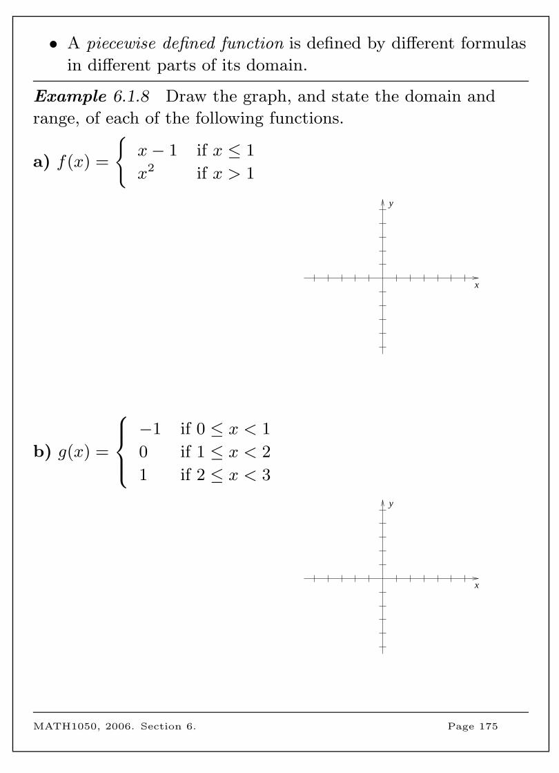
• A piecewise defined function is defined by different formulas
in different parts of its domain.
Example 6.1.8 Draw the graph, and state the domain and
range, of each of the following functions.
a) f(x) =
{x− 1 if x ≤ 1
x2 if x > 1
x
y
b) g(x) =
−1 if 0 ≤ x < 1
0 if 1 ≤ x < 2
1 if 2 ≤ x < 3
x
y
MATH1050, 2006. Section 6. Page 175
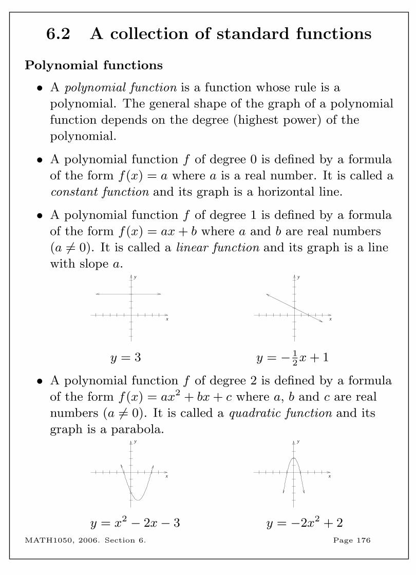
6.2 A collection of standard functions
Polynomial functions
• A polynomial function is a function whose rule is a
polynomial. The general shape of the graph of a polynomial
function depends on the degree (highest power) of the
polynomial.
• A polynomial function f of degree 0 is defined by a formula
of the form f(x) = a where a is a real number. It is called a
constant function and its graph is a horizontal line.
• A polynomial function f of degree 1 is defined by a formula
of the form f(x) = ax+ b where a and b are real numbers
(a 6= 0). It is called a linear function and its graph is a line
with slope a.
x
y
x
y
y = 3 y = − 12x+ 1
• A polynomial function f of degree 2 is defined by a formula
of the form f(x) = ax2 + bx+ c where a, b and c are real
numbers (a 6= 0). It is called a quadratic function and its
graph is a parabola.y
x
y
x
y = x2 − 2x− 3 y = −2x2 + 2MATH1050, 2006. Section 6. Page 176

• A polynomial function f of degree 3 is defined by a formula
of the form f(x) = ax3 + bx2 + cx+ d where a, b, c and d
are real numbers (a 6= 0). It is called a cubic function.y
x
y
x
y = x3 + 2x2 − 2x− 1 y = −x3 + 2x+ 2
• A polynomial function f of even degree greater than two
has a graph that is similar in shape to that of a quadratic
function, but potentially having some bumps in the middle.y
xx
y
y = x4 + 2x2 − 3 y = −x4 + 2x3 + 3x2 − 2x− 1
• A polynomial function f of odd degree greater than three
has a graph that is similar in shape to that of a cubic
function, but potentially having some more bumps in the
middle.y
x
y
x
y = x5 + 2x3−2x−1 y = −x5 +x4 + 2x3−x2−x
MATH1050, 2006. Section 6. Page 177
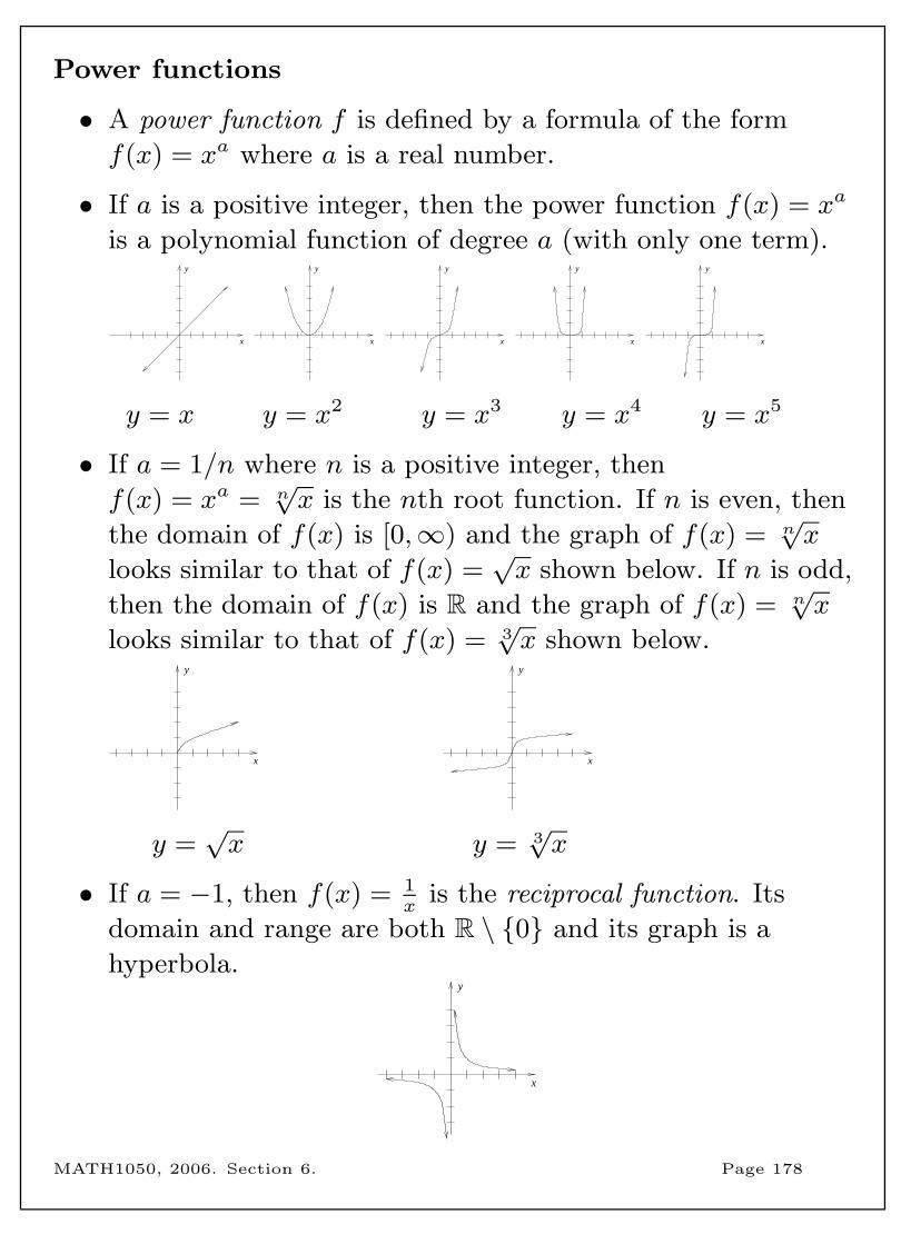
Power functions
• A power function f is defined by a formula of the form
f(x) = xa where a is a real number.
• If a is a positive integer, then the power function f(x) = xa
is a polynomial function of degree a (with only one term).
x
y
x
y
x
y
x
y
x
y
y = x y = x2 y = x3 y = x4 y = x5
• If a = 1/n where n is a positive integer, then
f(x) = xa = n√x is the nth root function. If n is even, then
the domain of f(x) is [0,∞) and the graph of f(x) = n√x
looks similar to that of f(x) =√x shown below. If n is odd,
then the domain of f(x) is R and the graph of f(x) = n√x
looks similar to that of f(x) = 3√x shown below.
x
y
x
y
y =√x y = 3
√x
• If a = −1, then f(x) = 1x
is the reciprocal function. Its
domain and range are both R \ {0} and its graph is a
hyperbola.
x
y
MATH1050, 2006. Section 6. Page 178
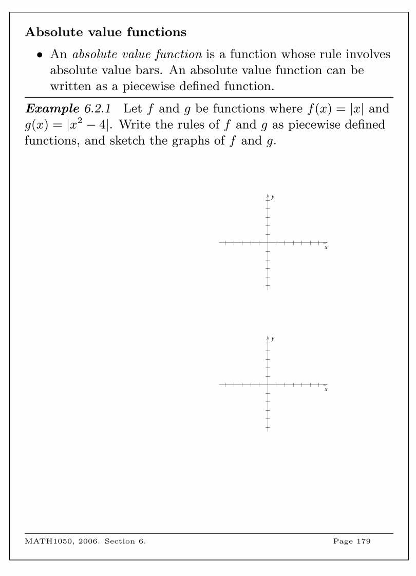
Absolute value functions
• An absolute value function is a function whose rule involves
absolute value bars. An absolute value function can be
written as a piecewise defined function.
Example 6.2.1 Let f and g be functions where f(x) = |x| and
g(x) = |x2 − 4|. Write the rules of f and g as piecewise defined
functions, and sketch the graphs of f and g.
x
y
x
y
MATH1050, 2006. Section 6. Page 179
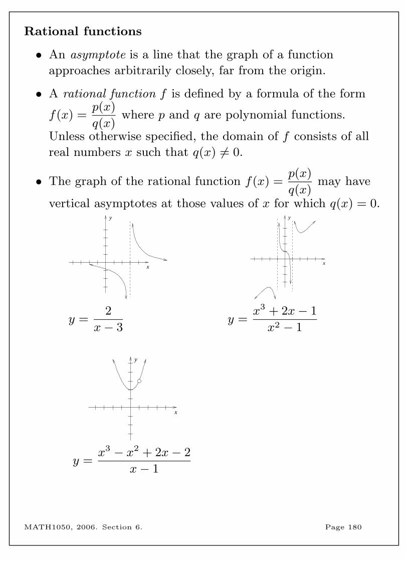
Rational functions
• An asymptote is a line that the graph of a function
approaches arbitrarily closely, far from the origin.
• A rational function f is defined by a formula of the form
f(x) =p(x)
q(x)where p and q are polynomial functions.
Unless otherwise specified, the domain of f consists of all
real numbers x such that q(x) 6= 0.
• The graph of the rational function f(x) =p(x)
q(x)may have
vertical asymptotes at those values of x for which q(x) = 0.
x
y
x
y
y =2
x− 3y =
x3 + 2x− 1
x2 − 1
x
y
y =x3 − x2 + 2x− 2
x− 1
MATH1050, 2006. Section 6. Page 180
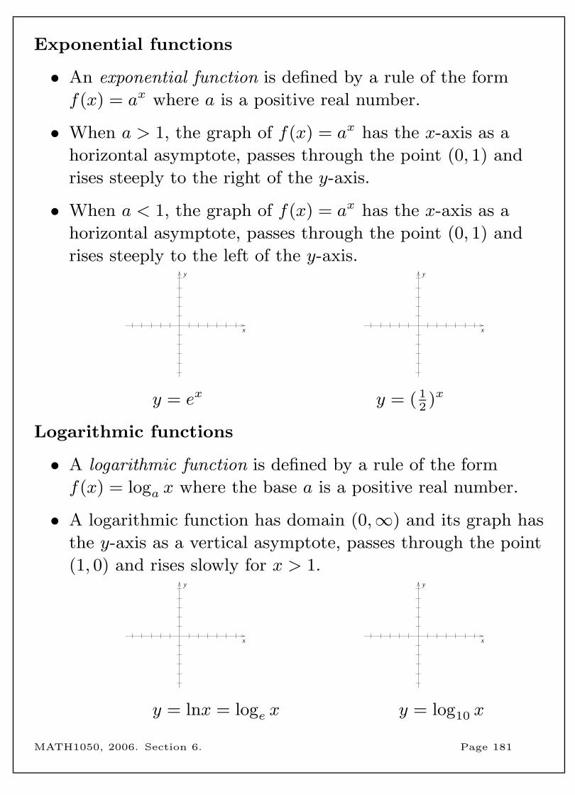
Exponential functions
• An exponential function is defined by a rule of the form
f(x) = ax where a is a positive real number.
• When a > 1, the graph of f(x) = ax has the x-axis as a
horizontal asymptote, passes through the point (0, 1) and
rises steeply to the right of the y-axis.
• When a < 1, the graph of f(x) = ax has the x-axis as a
horizontal asymptote, passes through the point (0, 1) and
rises steeply to the left of the y-axis.
x
y
x
y
y = ex y = ( 12)x
Logarithmic functions
• A logarithmic function is defined by a rule of the form
f(x) = loga x where the base a is a positive real number.
• A logarithmic function has domain (0,∞) and its graph has
the y-axis as a vertical asymptote, passes through the point
(1, 0) and rises slowly for x > 1.
x
y
x
y
y = lnx = loge x y = log10 x
MATH1050, 2006. Section 6. Page 181
6.3 Composition of functions
• Often we apply one function and then apply another
function to the result of the first function.
• Given any two functions f and g, we start with a number x
in the domain of g and determine its image g(x). If this
number is in the domain of f , we can now apply f to the
number g(x) and obtain the value f(g(x)). This process is
called the composition of f and g.
• Given two functions f and g, the function with input x and
output f(g(x)) is called the composite function of f and g
and is denoted f ◦ g.
• The domain of f ◦ g is the set of all x in the domain of g
such that g(x) is in the domain of f .
• To apply the function f ◦ g, we must first apply g and then
apply f .
MATH1050, 2006. Section 6. Page 182

Example 6.3.1 Let f and g be functions defined by the
formulas f(x) =√x− 5 amd g(x) = x2 − 4. Determine the
functions f ◦ g and g ◦ f , and state their domains and ranges.
MATH1050, 2006. Section 6. Page 183
Example 6.3.2 Let F (x) = 1 + 2 cos(x2 − 1). Find functions f
and g such that F = f ◦ g. State the domain and range of F .
MATH1050, 2006. Section 6. Page 184
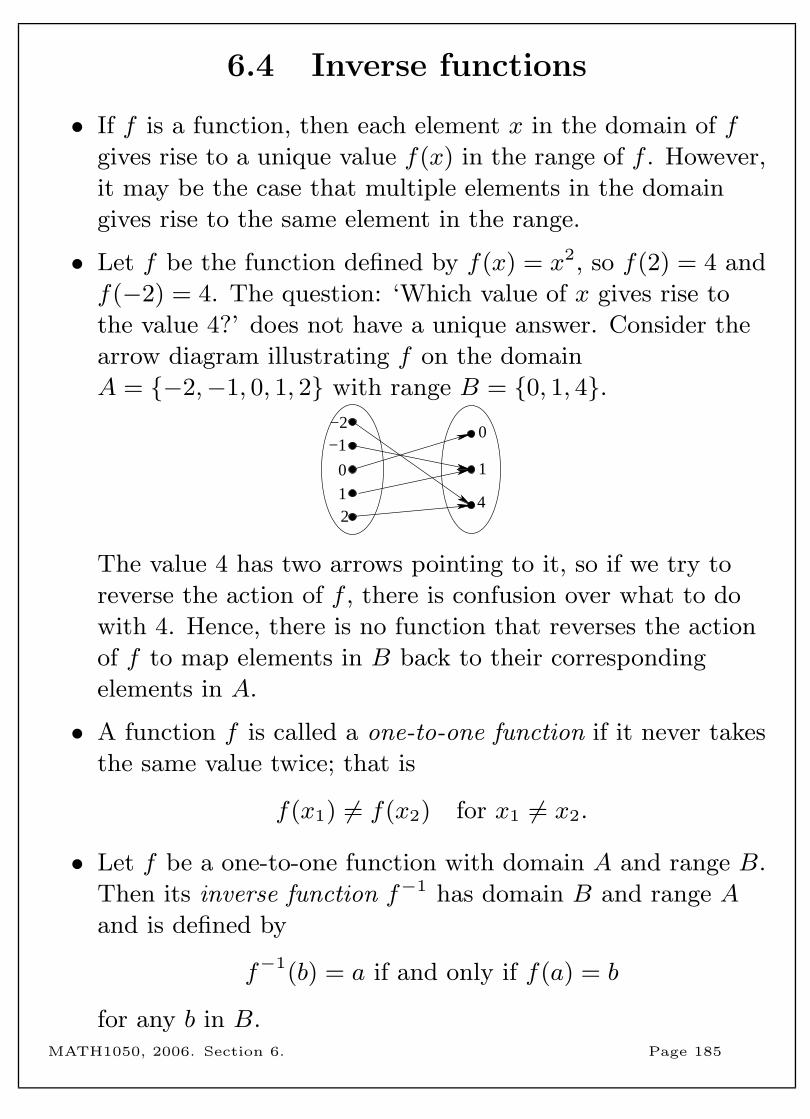
6.4 Inverse functions
• If f is a function, then each element x in the domain of f
gives rise to a unique value f(x) in the range of f . However,
it may be the case that multiple elements in the domain
gives rise to the same element in the range.
• Let f be the function defined by f(x) = x2, so f(2) = 4 and
f(−2) = 4. The question: ‘Which value of x gives rise to
the value 4?’ does not have a unique answer. Consider the
arrow diagram illustrating f on the domain
A = {−2,−1, 0, 1, 2} with range B = {0, 1, 4}.
4
1
0
12
0
−1−2
The value 4 has two arrows pointing to it, so if we try to
reverse the action of f , there is confusion over what to do
with 4. Hence, there is no function that reverses the action
of f to map elements in B back to their corresponding
elements in A.
• A function f is called a one-to-one function if it never takes
the same value twice; that is
f(x1) 6= f(x2) for x1 6= x2.
• Let f be a one-to-one function with domain A and range B.
Then its inverse function f−1 has domain B and range A
and is defined by
f−1(b) = a if and only if f(a) = b
for any b in B.MATH1050, 2006. Section 6. Page 185
Example 6.4.1 Let f(x) be the function defined by f(x) = x2.
Determine a suitable domain for f so that f−1 exists.
• To determine the inverse of a one-to-one function f :
1. Solve the equation y = f(x) for x in terms of y.
2. To express f−1 as a function of x, interchange x and y
in the result of the previous step.
Example 6.4.2 Determine the inverse function of f(x) = 2x+ 3
and sketch the graphs of f and f−1 on the same set of axes.
x
y
MATH1050, 2006. Section 6. Page 186
• If the point (a, b) lies on the graph of a function f , then
f(a) = b. Thus, if f−1 exists, then f−1(b) = a, and the
point (b, a) lies on the graph of f−1.
• The graph of f−1 is obtained by reflecting the graph of f in
the line y = x.
Example 6.4.3 Sketch the graph of the function
f(x) =√x− 2 and its inverse function f−1. Determine f−1
algebraically and verify that your sketch is correct.
x
y
MATH1050, 2006. Section 6. Page 187
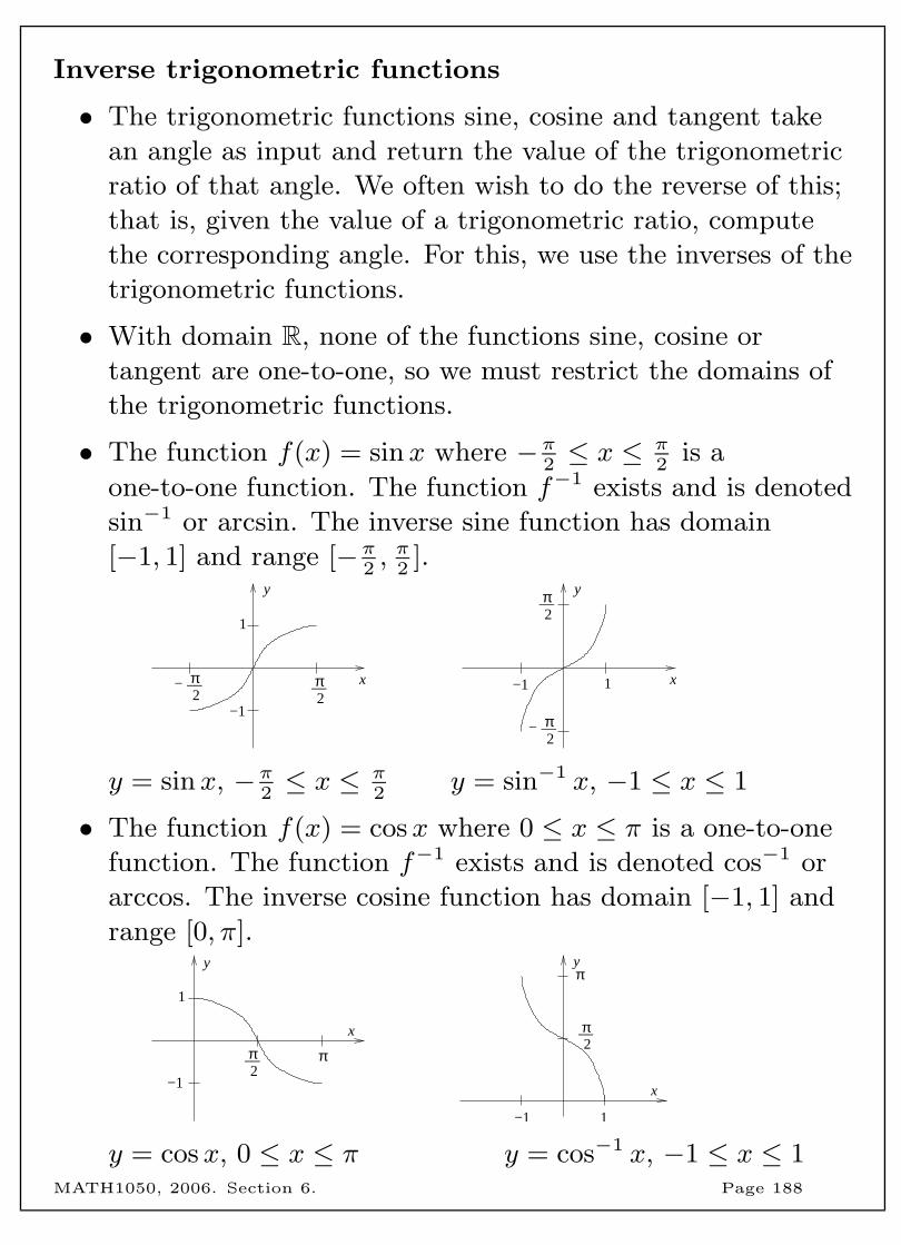
Inverse trigonometric functions
• The trigonometric functions sine, cosine and tangent take
an angle as input and return the value of the trigonometric
ratio of that angle. We often wish to do the reverse of this;
that is, given the value of a trigonometric ratio, compute
the corresponding angle. For this, we use the inverses of the
trigonometric functions.
• With domain R, none of the functions sine, cosine or
tangent are one-to-one, so we must restrict the domains of
the trigonometric functions.
• The function f(x) = sinx where −π2≤ x ≤ π
2is a
one-to-one function. The function f−1 exists and is denoted
sin−1 or arcsin. The inverse sine function has domain
[−1, 1] and range [−π2, π
2].
y
x−2π__
2π__
1
−1
y
x
2π__
−2π__
1−1
y = sinx, −π2≤ x ≤ π
2y = sin−1 x, −1 ≤ x ≤ 1
• The function f(x) = cosx where 0 ≤ x ≤ π is a one-to-one
function. The function f−1 exists and is denoted cos−1 or
arccos. The inverse cosine function has domain [−1, 1] and
range [0, π].y
x
2π
1
−1
π__
x
y
2π__
1−1
π
y = cosx, 0 ≤ x ≤ π y = cos−1 x, −1 ≤ x ≤ 1MATH1050, 2006. Section 6. Page 188
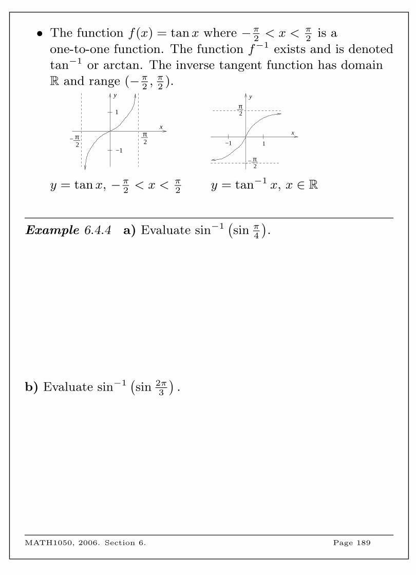
• The function f(x) = tanx where −π2< x < π
2is a
one-to-one function. The function f−1 exists and is denoted
tan−1 or arctan. The inverse tangent function has domain
R and range (−π2, π
2).
y
x
1
−1
__2π__
−2π
y
x
1−1
__
2π__
−2π
y = tanx, −π2< x < π
2y = tan−1 x, x ∈ R
Example 6.4.4 a) Evaluate sin−1(sin π
4
).
b) Evaluate sin−1(sin 2π
3
).
MATH1050, 2006. Section 6. Page 189
Example 6.4.5 a) Let f(x) = cos−1(x2 − 1). Determine the
domain of f .
b) Show that cos(tan−1 x) =1√
1 + x2.
MATH1050, 2006. Section 6. Page 190
6.5 Limits of functions
• When working with functions we often need to know what
the function values are close to a particular value that may,
or may not, be in the domain of the function. To obtain
this type of information, we use limits, which describe
function values for elements of the domain which are close
to the particular value of interest.
• Consider the following example: Let f be the function
defined by f(x) = x2 + 1. What happens to the values of
f(x) as x approaches 2 from the left? What happens to the
values of f(x) as x approaches 2 from the right?
x f(x) x f(x)
1.9 4.61 2.1 5.41
1.99 4.9601 2.01 5.0401
1.999 4.996001 2.001 5.004001
1.9999 4.99960001 2.0001 5.00040001
1.99999 4.99996 2.00001 5.00004
1.999999 4.999996 2.000001 5.000004
It appears that for x approaching 2 from the left (x < 2),
the function value is approaching 5 from below (f(x) < 5),
and for x approaching 2 from the right (x > 2), the function
value is approaching 5 from above (f(x) > 5). From the
table (and from the graph), we see that as x gets closer and
closer to 2, f(x) gets closer and closer to 5. We express this
as ‘the limit of the function f(x) = x2 + 1 as x approaches 2
is equal to 5’. We write this as
limx→2
(x2 + 1) = 5.
MATH1050, 2006. Section 6. Page 191
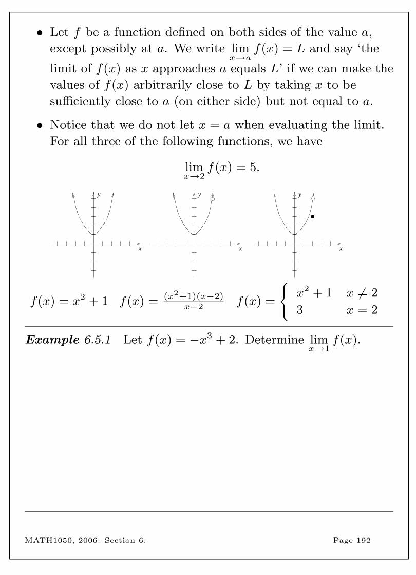
• Let f be a function defined on both sides of the value a,
except possibly at a. We write limx→a
f(x) = L and say ‘the
limit of f(x) as x approaches a equals L’ if we can make the
values of f(x) arbitrarily close to L by taking x to be
sufficiently close to a (on either side) but not equal to a.
• Notice that we do not let x = a when evaluating the limit.
For all three of the following functions, we have
limx→2
f(x) = 5.
x
y
x
y
x
y
f(x) = x2 + 1 f(x) = (x2+1)(x−2)x−2
f(x) =
{x2 + 1 x 6= 2
3 x = 2
Example 6.5.1 Let f(x) = −x3 + 2. Determine limx→1
f(x).
MATH1050, 2006. Section 6. Page 192
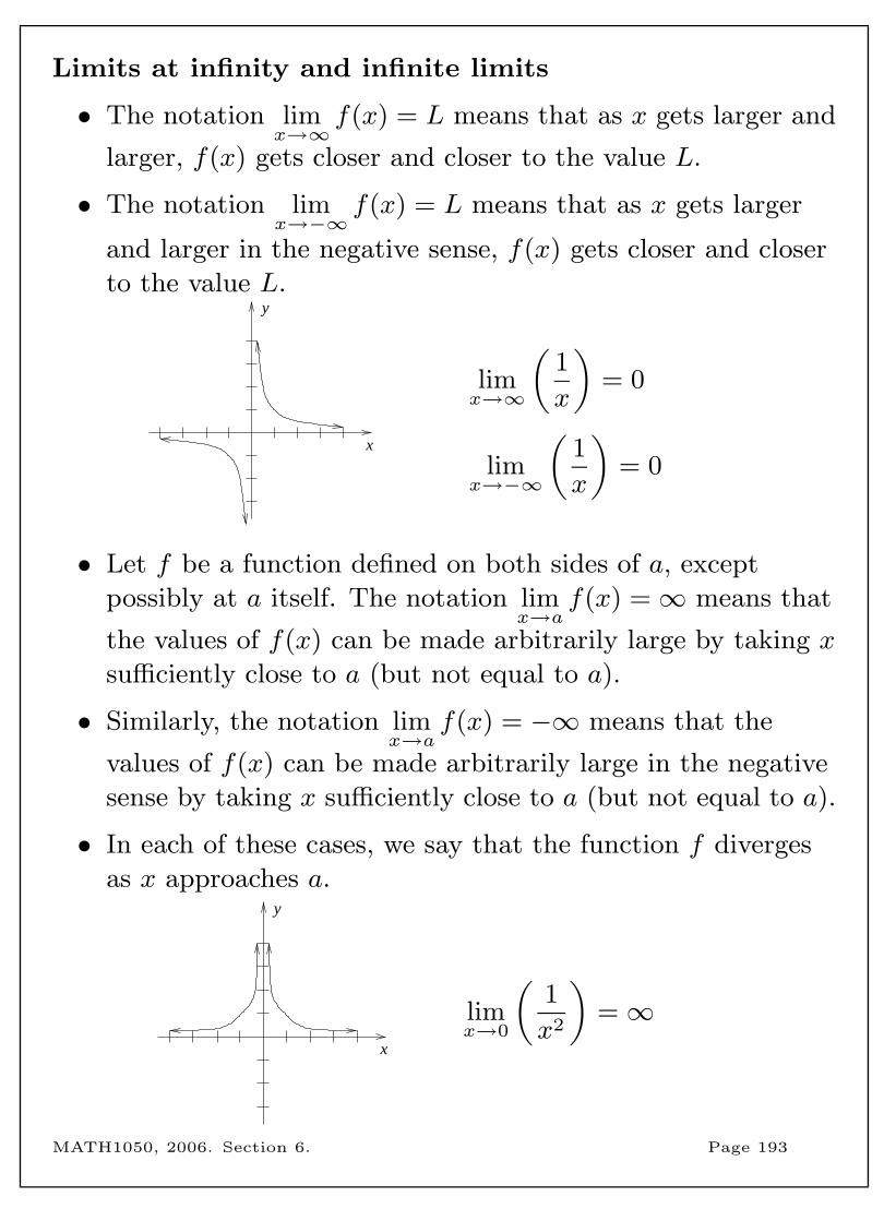
Limits at infinity and infinite limits
• The notation limx→∞
f(x) = L means that as x gets larger and
larger, f(x) gets closer and closer to the value L.
• The notation limx→−∞
f(x) = L means that as x gets larger
and larger in the negative sense, f(x) gets closer and closer
to the value L.
x
y
limx→∞
(1
x
)= 0
limx→−∞
(1
x
)= 0
• Let f be a function defined on both sides of a, except
possibly at a itself. The notation limx→a
f(x) =∞ means that
the values of f(x) can be made arbitrarily large by taking x
sufficiently close to a (but not equal to a).
• Similarly, the notation limx→a
f(x) = −∞ means that the
values of f(x) can be made arbitrarily large in the negative
sense by taking x sufficiently close to a (but not equal to a).
• In each of these cases, we say that the function f diverges
as x approaches a.
x
y
limx→0
(1
x2
)=∞
MATH1050, 2006. Section 6. Page 193
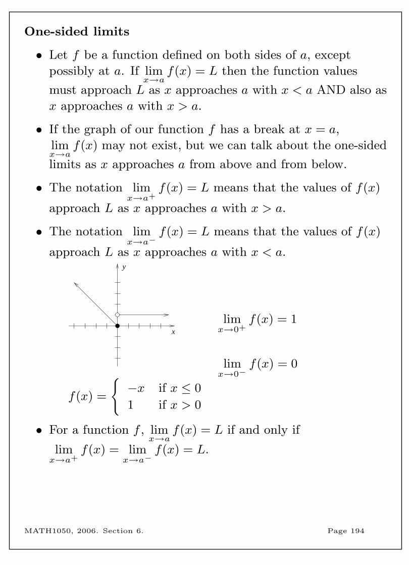
One-sided limits
• Let f be a function defined on both sides of a, except
possibly at a. If limx→a
f(x) = L then the function values
must approach L as x approaches a with x < a AND also as
x approaches a with x > a.
• If the graph of our function f has a break at x = a,
limx→a
f(x) may not exist, but we can talk about the one-sided
limits as x approaches a from above and from below.
• The notation limx→a+
f(x) = L means that the values of f(x)
approach L as x approaches a with x > a.
• The notation limx→a−
f(x) = L means that the values of f(x)
approach L as x approaches a with x < a.
x
y
f(x) =
{−x if x ≤ 0
1 if x > 0
limx→0+
f(x) = 1
limx→0−
f(x) = 0
• For a function f , limx→a
f(x) = L if and only if
limx→a+
f(x) = limx→a−
f(x) = L.
MATH1050, 2006. Section 6. Page 194
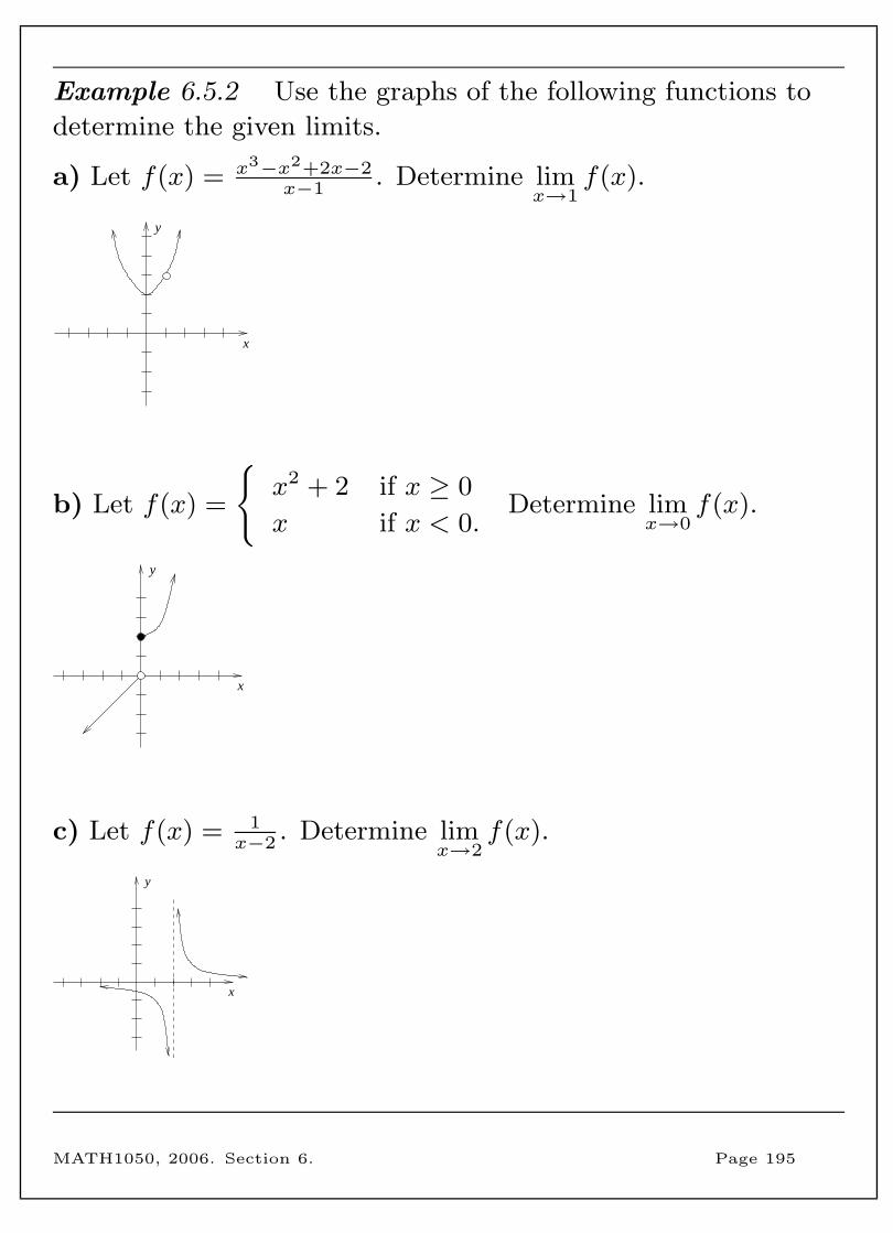
Example 6.5.2 Use the graphs of the following functions to
determine the given limits.
a) Let f(x) = x3−x2+2x−2x−1
. Determine limx→1
f(x).
x
y
b) Let f(x) =
{x2 + 2 if x ≥ 0
x if x < 0.Determine lim
x→0f(x).
x
y
c) Let f(x) = 1x−2
. Determine limx→2
f(x).
x
y
MATH1050, 2006. Section 6. Page 195
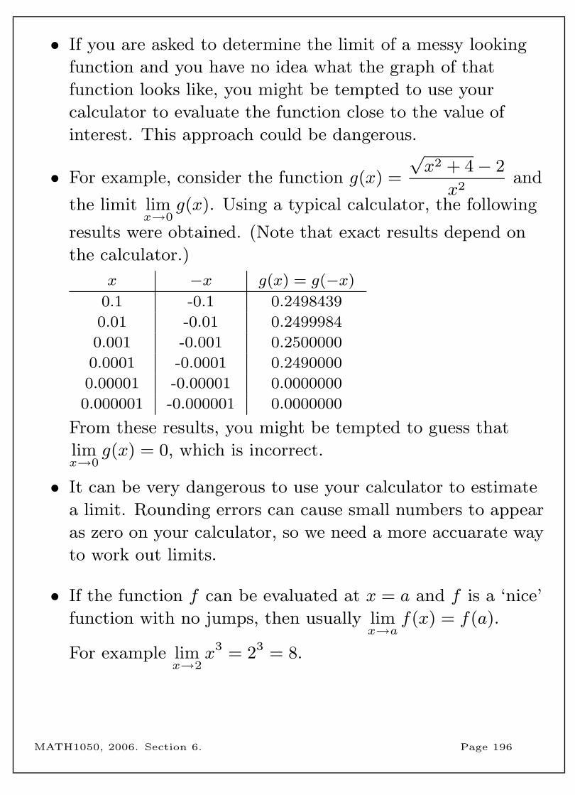
• If you are asked to determine the limit of a messy looking
function and you have no idea what the graph of that
function looks like, you might be tempted to use your
calculator to evaluate the function close to the value of
interest. This approach could be dangerous.
• For example, consider the function g(x) =
√x2 + 4− 2
x2and
the limit limx→0
g(x). Using a typical calculator, the following
results were obtained. (Note that exact results depend on
the calculator.)
x −x g(x) = g(−x)
0.1 -0.1 0.2498439
0.01 -0.01 0.2499984
0.001 -0.001 0.2500000
0.0001 -0.0001 0.2490000
0.00001 -0.00001 0.0000000
0.000001 -0.000001 0.0000000
From these results, you might be tempted to guess that
limx→0
g(x) = 0, which is incorrect.
• It can be very dangerous to use your calculator to estimate
a limit. Rounding errors can cause small numbers to appear
as zero on your calculator, so we need a more accuarate way
to work out limits.
• If the function f can be evaluated at x = a and f is a ‘nice’
function with no jumps, then usually limx→a
f(x) = f(a).
For example limx→2
x3 = 23 = 8.
MATH1050, 2006. Section 6. Page 196
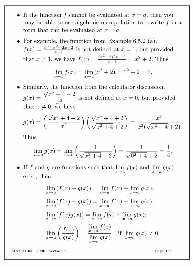
• If the function f cannot be evaluated at x = a, then you
may be able to use algebraic manipulation to rewrite f in a
form that can be evaluated at x = a.
• For example, the function from Example 6.5.2 (a),
f(x) = x3−x2+2x−2x−1
is not defined at x = 1, but provided
that x 6= 1, we have f(x) = (x2+2)(x−1)x−1
= x2 + 2. Thus
limx→1
f(x) = limx→1
(x2 + 2) = 12 + 2 = 3.
• Similarly, the function from the calculator discussion,
g(x) =
√x2 + 4− 2
x2is not defined at x = 0, but provided
that x 6= 0, we have
g(x) =
(√x2 + 4− 2
x2
)(√x2 + 4 + 2√x2 + 4 + 2
)=
x2
x2(√x2 + 4 + 2)
.
Thus
limx→0
g(x) = limx→0
(1√
x2 + 4 + 2
)=
1√02 + 4 + 2
=1
4.
• If f and g are functions such that limx→a
f(x) and limx→a
g(x)
exist, then
limx→a
(f(x) + g(x)) = limx→a
f(x) + limx→a
g(x);
limx→a
(f(x)− g(x)) = limx→a
f(x)− limx→a
g(x);
limx→a
(f(x)g(x)) = limx→a
f(x)× limx→a
g(x);
limx→a
(f(x)
g(x)
)=
limx→a
f(x)
limx→a
g(x)if lim
x→ag(x) 6= 0.
MATH1050, 2006. Section 6. Page 197
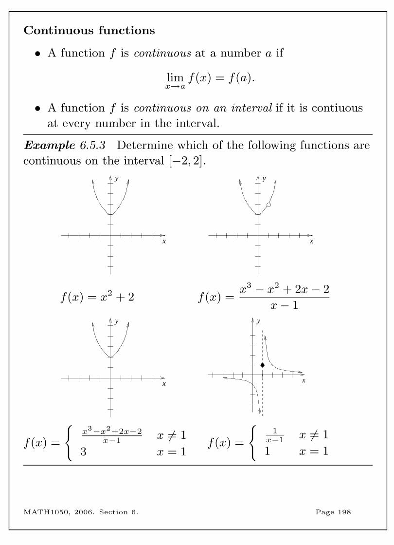
Continuous functions
• A function f is continuous at a number a if
limx→a
f(x) = f(a).
• A function f is continuous on an interval if it is contiuous
at every number in the interval.
Example 6.5.3 Determine which of the following functions are
continuous on the interval [−2, 2].
x
y
x
y
f(x) = x2 + 2 f(x) =x3 − x2 + 2x− 2
x− 1
x
y
x
y
f(x) =
{x3−x2+2x−2
x−1x 6= 1
3 x = 1f(x) =
{1
x−1x 6= 1
1 x = 1
MATH1050, 2006. Section 6. Page 198
7 Differentiation
• In many applications of mathematics, it is very important
to be able to calculate the gradient, or slope, of the graph
of a function at a particular point.
• This gradient is called the derivative of the function at the
point and it measures the rate of change of the function at
that point.
• Derivatives of functions provide useful information about
the graph of a function and also have important
applications in many areas of science and economics.
• In this section we will look at the definition of the
derivative of a function and review some rules that allow us
to calculate the derivatives of many functions.
• We will apply our knowledge of derivatives to sketch the
graphs of functions and to solve optimisation problems and
problems involving rates of change.
• Topics in this section are:
– Tangent lines
– The derivative of a function
– Differentiation rules
– Critical points and curve sketching
– Applications of differentiation
MATH1050, 2006. Section 7. Page 199
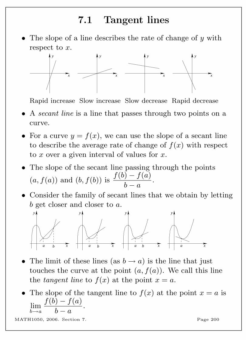
7.1 Tangent lines
• The slope of a line describes the rate of change of y with
respect to x.y
x
y
x
y
x
y
x
Rapid increase Slow increase Slow decrease Rapid decrease
• A secant line is a line that passes through two points on a
curve.
• For a curve y = f(x), we can use the slope of a secant line
to describe the average rate of change of f(x) with respect
to x over a given interval of values for x.
• The slope of the secant line passing through the points
(a, f(a)) and (b, f(b)) isf(b)− f(a)
b− a .
• Consider the family of secant lines that we obtain by letting
b get closer and closer to a.
x
y
a b a b a
y
x
y
ba x
y
x
• The limit of these lines (as b→ a) is the line that just
touches the curve at the point (a, f(a)). We call this line
the tangent line to f(x) at the point x = a.
• The slope of the tangent line to f(x) at the point x = a is
limb→a
f(b)− f(a)
b− a .
MATH1050, 2006. Section 7. Page 200
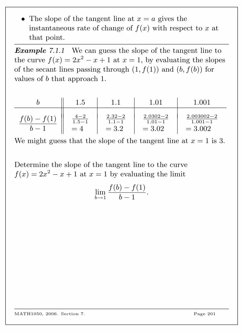
• The slope of the tangent line at x = a gives the
instantaneous rate of change of f(x) with respect to x at
that point.
Example 7.1.1 We can guess the slope of the tangent line to
the curve f(x) = 2x2 − x+ 1 at x = 1, by evaluating the slopes
of the secant lines passing through (1, f(1)) and (b, f(b)) for
values of b that approach 1.
b 1.5 1.1 1.01 1.001
f(b)− f(1)
b− 1
4−21.5−1
= 4
2.32−21.1−1
= 3.2
2.0302−21.01−1
= 3.02
2.003002−21.001−1
= 3.002
We might guess that the slope of the tangent line at x = 1 is 3.
Determine the slope of the tangent line to the curve
f(x) = 2x2 − x+ 1 at x = 1 by evaluating the limit
limb→1
f(b)− f(1)
b− 1.
MATH1050, 2006. Section 7. Page 201
• Another way of writing the slope of the tangent line to f(x)
at x = a is to let b = a+ h. Then b→ a is equivalent to
h→ 0 and the slope of the tangent line to f(x) at x = a is
limh→0
f(a+ h)− f(a)
a+ h− a = limh→0
f(a+ h)− f(a)
h.
Example 7.1.2 a) Determine the slope of the tangent line to
the curve f(x) = x3 − 2x at x = 2.
b) Use your answer from part (a) to determine the equation of
the tangent line to the curve f(x) = x3 − 2x at x = 2.
MATH1050, 2006. Section 7. Page 202
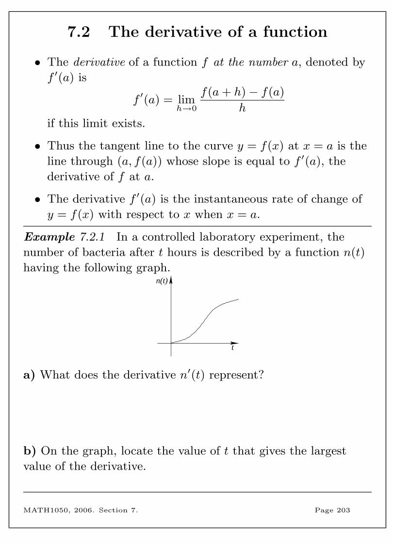
7.2 The derivative of a function
• The derivative of a function f at the number a, denoted by
f ′(a) is
f ′(a) = limh→0
f(a+ h)− f(a)
h
if this limit exists.
• Thus the tangent line to the curve y = f(x) at x = a is the
line through (a, f(a)) whose slope is equal to f ′(a), the
derivative of f at a.
• The derivative f ′(a) is the instantaneous rate of change of
y = f(x) with respect to x when x = a.
Example 7.2.1 In a controlled laboratory experiment, the
number of bacteria after t hours is described by a function n(t)
having the following graph.
t
n(t)
a) What does the derivative n′(t) represent?
b) On the graph, locate the value of t that gives the largest
value of the derivative.
MATH1050, 2006. Section 7. Page 203
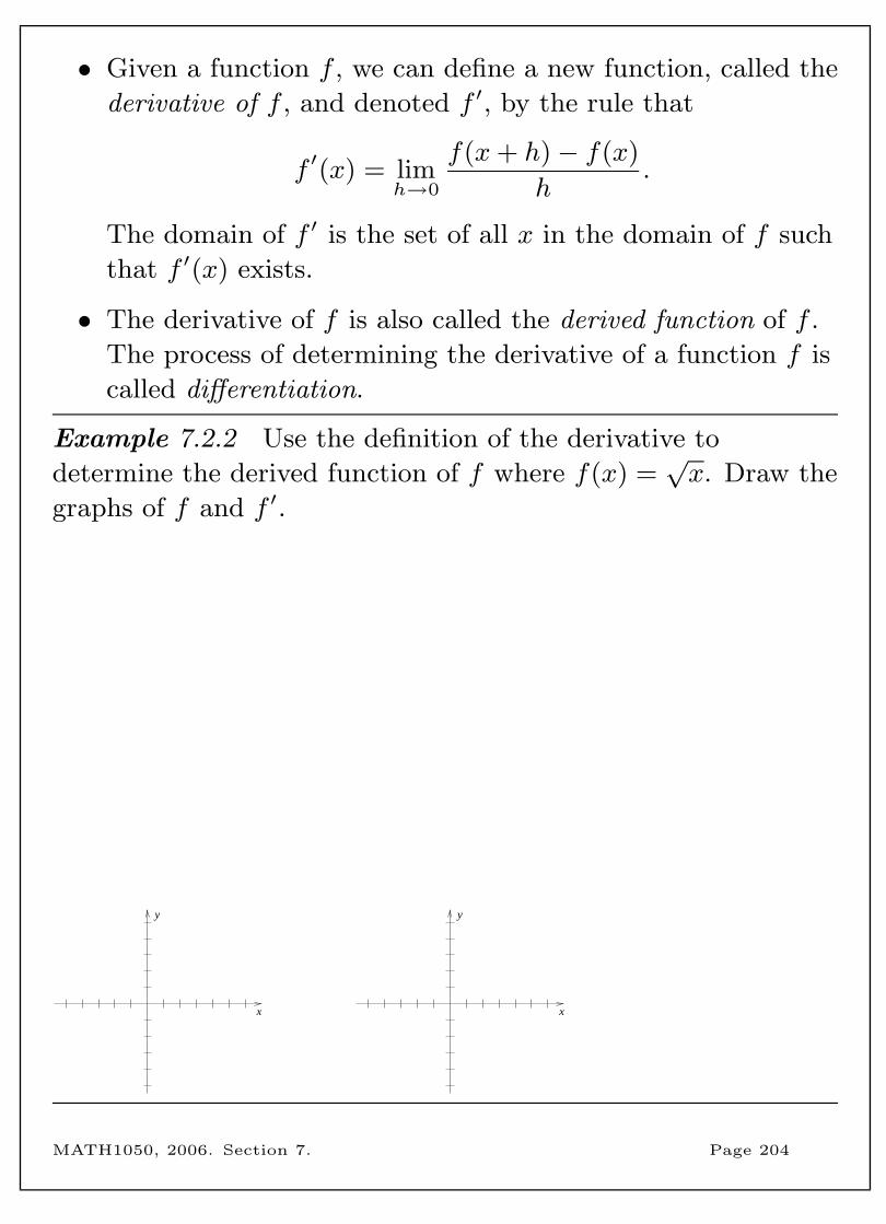
• Given a function f , we can define a new function, called the
derivative of f , and denoted f ′, by the rule that
f ′(x) = limh→0
f(x+ h)− f(x)
h.
The domain of f ′ is the set of all x in the domain of f such
that f ′(x) exists.
• The derivative of f is also called the derived function of f .
The process of determining the derivative of a function f is
called differentiation.
Example 7.2.2 Use the definition of the derivative to
determine the derived function of f where f(x) =√x. Draw the
graphs of f and f ′.
x
y
x
y
MATH1050, 2006. Section 7. Page 204
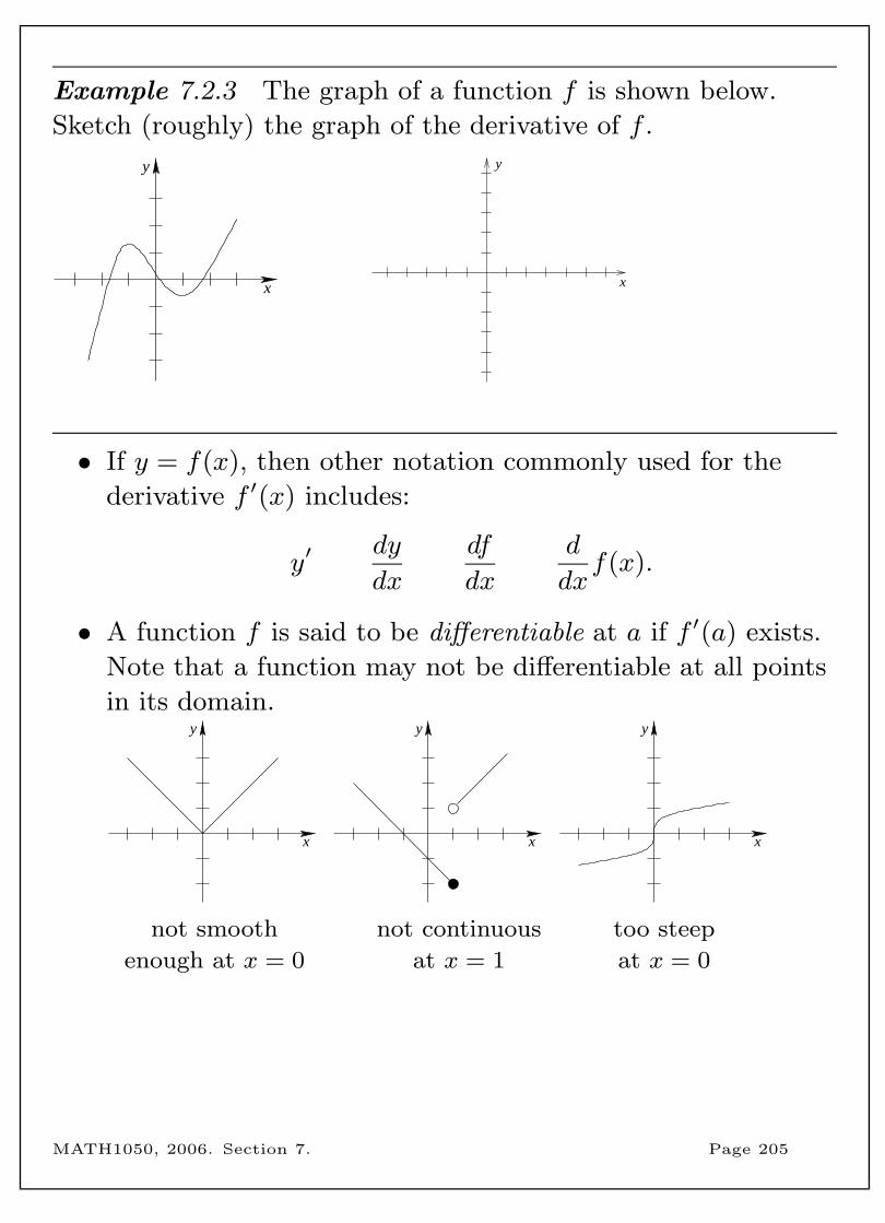
Example 7.2.3 The graph of a function f is shown below.
Sketch (roughly) the graph of the derivative of f .
x
y
x
y
• If y = f(x), then other notation commonly used for the
derivative f ′(x) includes:
y′dy
dx
df
dx
d
dxf(x).
• A function f is said to be differentiable at a if f ′(a) exists.
Note that a function may not be differentiable at all points
in its domain.y
x
y
x
y
x
not smooth not continuous too steep
enough at x = 0 at x = 1 at x = 0
MATH1050, 2006. Section 7. Page 205
7.3 Differentiation rules
• Determining derivatives from the definition can be
time-consuming. Luckily there are some rules for
differentiation that speed up the process. The proofs of
these rules can be found in most calculus textbooks, but
you do not need to know the proofs for this course.
• The derivative of a constant function is zero.
• If f(x) = xn, then f ′(x) = nxn−1 for n ∈ R.
• Constant multiple rule If c is a constant and f is a
differentiable function, then
d
dx(cf(x)) = c
d
dxf(x).
• Sum rule If f and g are both differentiable functions, then
d
dx(f(x) + g(x)) =
d
dxf(x) +
d
dxg(x).
This rule can also be written as (f + g)′ = f ′ + g′.
• Product rule If f and g are both differentiable functions,
then
d
dx(f(x)g(x)) = f(x)
d
dxg(x) + g(x)
d
dxf(x).
This rule can also be written as (fg)′ = fg′ + gf ′.
• Quotient rule If f and g are both differentiable functions,
thend
dx
(f(x)
g(x)
)=g(x) d
dxf(x)− f(x) d
dxg(x)
(g(x))2.
This rule can also be written as
(f
g
)′=gf ′ − fg′
g2.
MATH1050, 2006. Section 7. Page 206
Example 7.3.1 Determine the derivative of each of the
following functions.
a) f(x) = x3 + 4x− 1
b) g(u) =√u(2u− u2)
c) h(n) =4n− n3 + 2
3n4
MATH1050, 2006. Section 7. Page 207
• Chain rule (also called the Composite function rule) If f
and g are both differentiable functions, then
(f ◦ g)′(x) = f ′(g(x))g′(x).
If y = f(u) and u = g(x), then this rule can be written as
dy
dx=dy
du
du
dx.
• To apply the chain rule, think about starting with the
outside function and working your way in.
Example 7.3.2 a) Find h′(x) where h(x) = (2x3 − 3x+ 1)4.
continued...
MATH1050, 2006. Section 7. Page 208
Example 7.3.2 (continued)
b) Find h′(x) where h(x) =√x2 − 3x.
c) Find h′(x) where h(x) = (4x+ (x2 + 1)3)5.
MATH1050, 2006. Section 7. Page 209
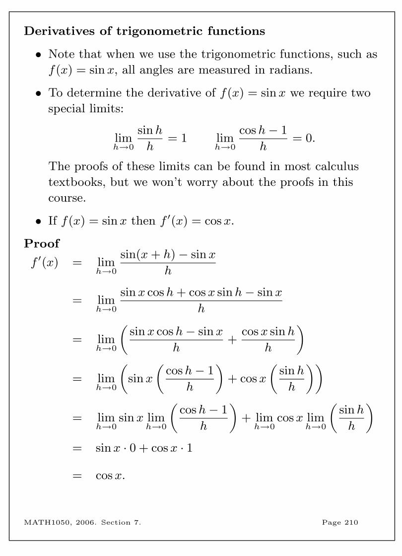
Derivatives of trigonometric functions
• Note that when we use the trigonometric functions, such as
f(x) = sinx, all angles are measured in radians.
• To determine the derivative of f(x) = sinx we require two
special limits:
limh→0
sinh
h= 1 lim
h→0
cosh− 1
h= 0.
The proofs of these limits can be found in most calculus
textbooks, but we won’t worry about the proofs in this
course.
• If f(x) = sinx then f ′(x) = cosx.
Proof
f ′(x) = limh→0
sin(x+ h)− sinx
h
= limh→0
sinx cosh+ cosx sinh− sinx
h
= limh→0
(sinx cosh− sinx
h+
cosx sinh
h
)= lim
h→0
(sinx
(cosh− 1
h
)+ cosx
(sinh
h
))= lim
h→0sinx lim
h→0
(cosh− 1
h
)+ limh→0
cosx limh→0
(sinh
h
)= sinx · 0 + cosx · 1
= cosx.
MATH1050, 2006. Section 7. Page 210
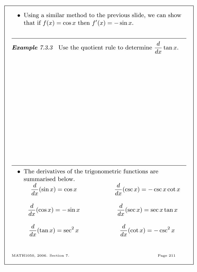
• Using a similar method to the previous slide, we can show
that if f(x) = cosx then f ′(x) = − sinx.
Example 7.3.3 Use the quotient rule to determined
dxtanx.
• The derivatives of the trigonometric functions are
summarised below.d
dx(sinx) = cosx
d
dx(cscx) = − cscx cotx
d
dx(cosx) = − sinx
d
dx(secx) = secx tanx
d
dx(tanx) = sec2 x
d
dx(cotx) = − csc2 x
MATH1050, 2006. Section 7. Page 211
Derivatives of exponential and logarithmic functions
• If f(x) = ex, then f ′(x) = ex.
• Thus, on the graph of f(x) = ex, the slope of the tangent
line at each point is equal to the function value at that
point.
• If f(x) = lnx, then f ′(x) =1
x. Note that here x > 0 since
the domain of f(x) = lnx is x > 0.
Example 7.3.4 Determine the derivative of each of the
following functions.
a) f(x) = xex2
b) g(x) = ln(x3 − 2x)
MATH1050, 2006. Section 7. Page 212
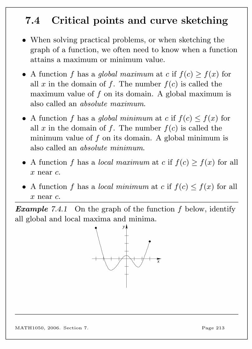
7.4 Critical points and curve sketching
• When solving practical problems, or when sketching the
graph of a function, we often need to know when a function
attains a maximum or minimum value.
• A function f has a global maximum at c if f(c) ≥ f(x) for
all x in the domain of f . The number f(c) is called the
maximum value of f on its domain. A global maximum is
also called an absolute maximum.
• A function f has a global minimum at c if f(c) ≤ f(x) for
all x in the domain of f . The number f(c) is called the
minimum value of f on its domain. A global minimum is
also called an absolute minimum.
• A function f has a local maximum at c if f(c) ≥ f(x) for all
x near c.
• A function f has a local minimum at c if f(c) ≤ f(x) for all
x near c.
Example 7.4.1 On the graph of the function f below, identify
all global and local maxima and minima.
x
y
MATH1050, 2006. Section 7. Page 213
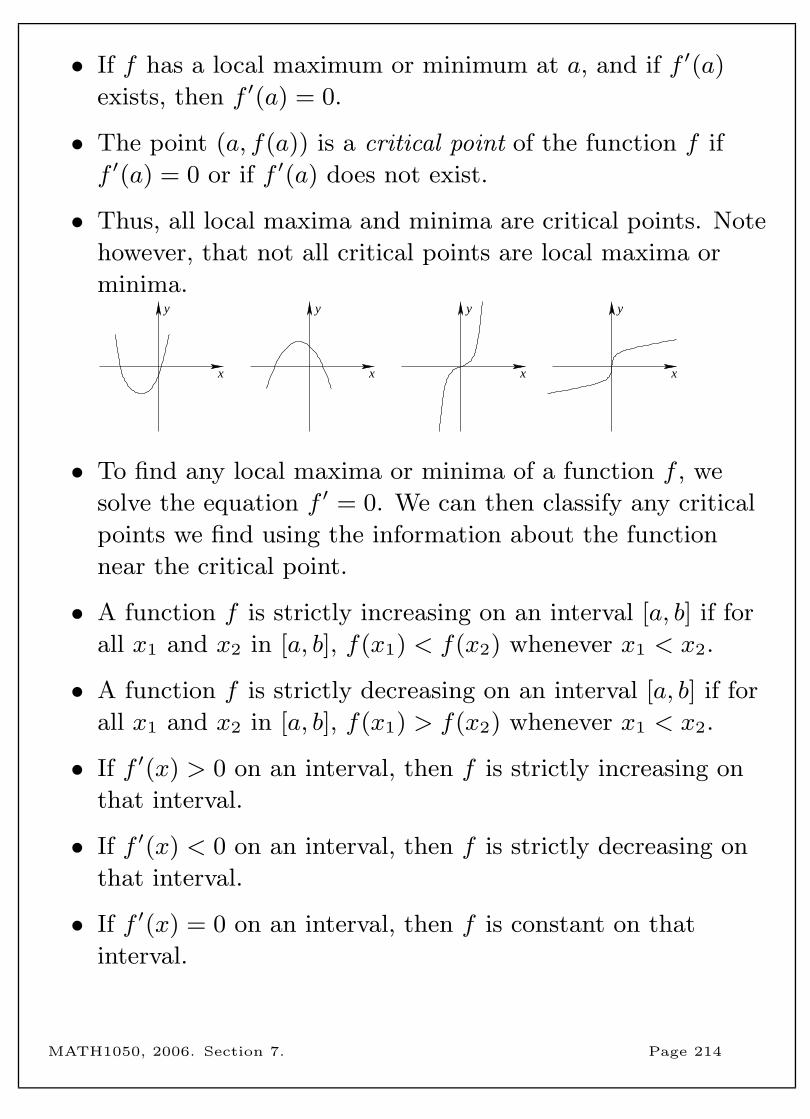
• If f has a local maximum or minimum at a, and if f ′(a)
exists, then f ′(a) = 0.
• The point (a, f(a)) is a critical point of the function f if
f ′(a) = 0 or if f ′(a) does not exist.
• Thus, all local maxima and minima are critical points. Note
however, that not all critical points are local maxima or
minima.y
x
y
x
y
x
y
x
• To find any local maxima or minima of a function f , we
solve the equation f ′ = 0. We can then classify any critical
points we find using the information about the function
near the critical point.
• A function f is strictly increasing on an interval [a, b] if for
all x1 and x2 in [a, b], f(x1) < f(x2) whenever x1 < x2.
• A function f is strictly decreasing on an interval [a, b] if for
all x1 and x2 in [a, b], f(x1) > f(x2) whenever x1 < x2.
• If f ′(x) > 0 on an interval, then f is strictly increasing on
that interval.
• If f ′(x) < 0 on an interval, then f is strictly decreasing on
that interval.
• If f ′(x) = 0 on an interval, then f is constant on that
interval.
MATH1050, 2006. Section 7. Page 214
• First derivative test Suppose that the function f has a
critical point at x = c. Then
– If f ′ changes sign from postive to negative at c, then f
has a local maximum at c.
– If f ′ changes sign from negative to positive at c, then f
has a local minimum at c.
– If f ′ does not change sign at c, then f has neither a
local maximum nor a local minimum at c.
Example 7.4.2 Find all local maxima and minima of
f(x) = x3 − 2x2 + x+ 1 and classify them using the first
derivative test. Use this information to sketch the graph of f .
x
y
MATH1050, 2006. Section 7. Page 215
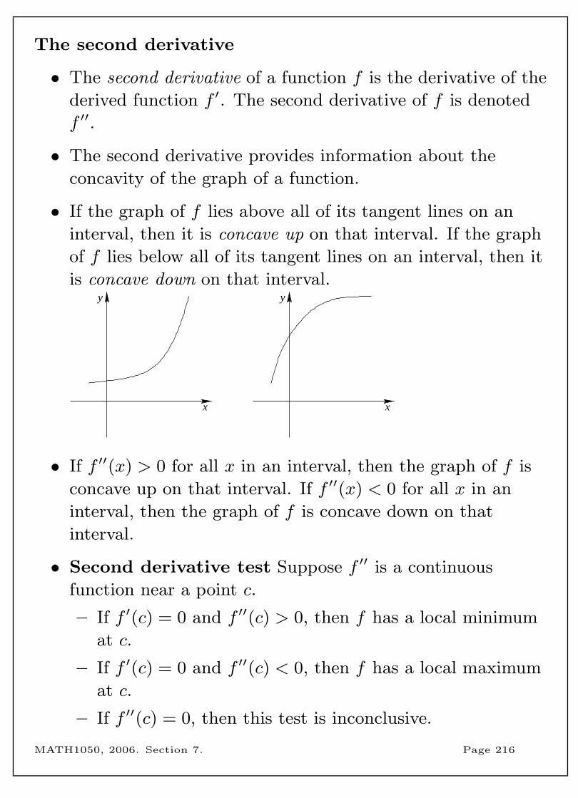
The second derivative
• The second derivative of a function f is the derivative of the
derived function f ′. The second derivative of f is denoted
f ′′.
• The second derivative provides information about the
concavity of the graph of a function.
• If the graph of f lies above all of its tangent lines on an
interval, then it is concave up on that interval. If the graph
of f lies below all of its tangent lines on an interval, then it
is concave down on that interval.
x
y
x
y
• If f ′′(x) > 0 for all x in an interval, then the graph of f is
concave up on that interval. If f ′′(x) < 0 for all x in an
interval, then the graph of f is concave down on that
interval.
• Second derivative test Suppose f ′′ is a continuous
function near a point c.
– If f ′(c) = 0 and f ′′(c) > 0, then f has a local minimum
at c.
– If f ′(c) = 0 and f ′′(c) < 0, then f has a local maximum
at c.
– If f ′′(c) = 0, then this test is inconclusive.
MATH1050, 2006. Section 7. Page 216
Example 7.4.3 Analyse the curve y = x4 − 2x3 with respect to
concavity, and local maxima and minima. Use this information
to sketch the curve.
x
y
MATH1050, 2006. Section 7. Page 217
Curve sketching To sketch the curve of a function y = f(x):
• Determine the domain of f .
• Determine the y-intercept of the graph by evaluating f(0).
• If it is possible to solve the equation f(x) = 0, find the
x-intercepts of the graph.
• Determine f ′ and identify the intervals on which f is
increasing and the intervals on which f is decreasing.
• Find the critical points of f . Determine which critical
points are local maxima or local minima (use first or second
derivative test).
• Determine f ′′ and identify the intervals on which f is
concave up and the intervals on which f is concave down.
• Sketch the graph.
Example 7.4.4 Sketch the graph of the function f(x) = x2ex.
x
y
continued...MATH1050, 2006. Section 7. Page 218

Example 7.4.4 (continued) Extra space for your work.
MATH1050, 2006. Section 7. Page 219

7.5 Applications of differentiation
Optimisation problems
Example 7.5.1 Find two numbers whose difference is 100 and
whose product is a minimum.
MATH1050, 2006. Section 7. Page 220
Example 7.5.2 A box with a square base and open top must
have a volume of exactly 4000 cm3, a height of at least 5 cm,
and a base side length of at least 5 cm.
a) Find the dimensions of the box that minimise the amount of
material used.
continued...
MATH1050, 2006. Section 7. Page 221

Example 7.5.2 (continued) b) Find the dimensions of the box
that maximise the amount of material used.
MATH1050, 2006. Section 7. Page 222
Rates of change
• Rates of change have important applications in many areas.
The derivative of a function f with respect to a variable x
gives the rate of change of f with respect to x.
• If s(t) is a function of displacement with respect to time,
then the derivative s′(t) gives the velocity, since velocity is
the rate of change of displacement with respect to time.
Similarly, s′′(t) gives the acceleration, since acceleration is
the rate of change of velocity with respect to time.
Example 7.5.3 A skier pushes off and heads directly down a
ski slope with an initial velocity of 3 m/s. The distance the skier
has travelled after t seconds is given by s(t) = 3t+ 2t2.
a) Determine the velocity of the skier after 2 seconds.
b) When the skier reaches a velocity of 15 m/s (that is 54
km/h), he makes a turn to slow down. How far has the skier
travelled down the hill when he starts the turn?
MATH1050, 2006. Section 7. Page 223
• In economics, it is often important to study the functions
that describe the cost of producing various quantities of a
given product.
• Let C(x) be the total cost to produce x units of a certain
commodity. The marginal cost is the rate of change of the
cost function with respect to the number of units produced.
• It can be shown that the marginal cost is approximately
equal to the cost of producing one more unit of product.
C′(x) ≈ C(x+ 1)− C(x)
Example 7.5.4 A company has estimated that the cost (in
dollars) of producing x snowboards is
C(x) = 10000 + 18x+ 0.02x2.
a) Determine the marginal cost function and evaluate C′(10).
b) Compare C′(10) with the actual cost of producing the 11th
snowboard.
MATH1050, 2006. Section 7. Page 224
8 Integration
• Situations often arise in which we know the derivative of a
function and we need to determine the function itself. The
reverse process of differentiation is called antidifferentiation
or integration.
• We will start this section by looking at how to determine
antiderivatives for some simple functions.
• We will then investigate how to approximate the area of a
region under the graph of a function.
• An extremely important theorem, called the Fundamental
Theorem of Calculus, tells us how the area under the graph
of a function is related to an antiderivative of that function.
• Determining an antiderivative of a function is usually more
challenging than determining the derivative of a function.
We will take a brief look at the technique of integration by
substitution, which can be thought of as the reverse of the
chain rule for differentiation.
• Just as the process of differentiation has many practical
applications, so does the process of antidifferentiation. We
will end this section with a few practical problems.
• Topics in this section are:
– Antiderivatives and indefinite integrals
– The area under a curve
– Definite integrals and the Fundamental Theorem of Calculus
– Integration by substitution
– Applications of integration
MATH1050, 2006. Section 8. Page 225
8.1 Antiderivatives and indefinite integrals
• A function F is called an antiderivative of f on an interval
I if F ′(x) = f(x) for all x ∈ I.
• For example,
F (x) = 2x3 is an antiderivative of f(x) = 6x2
for all x ∈ R since F ′(x) = 6x2 = f(x) for all x ∈ R.
However, F (x) = 2x3 + 10 is also an antiderivative of
f(x) = 6x2 for all x ∈ R.
• If F is an antiderivative of f on an interval I, then the most
general antiderivative of f on I is
F (x) + C where C is an arbitrary constant.
Rules for antidifferentiation
• Let F be an antiderivative of f and let k be a constant. An
antiderivative of kf(x) is kF (x).
• Let F be an antiderivative of f and let G be an
antiderivative of g. Then F +G is an antiderivative of f + g.
Common antiderivatives
Function Antiderivative Function Antiderivative
xa for a 6= −1 1a+1
xa+1 sinx − cosx
1
xfor x > 0 lnx cosx sinx
ex ex sec2 x tanx
MATH1050, 2006. Section 8. Page 226
Example 8.1.1 Find the most general antiderivative of each of
the following functions.
a) f(x) = 3x2 − 7x+ 2
b) f(x) = 4 sinx
• If we are given a particular value of the antiderivative, we
can use that information to decide which antiderivative to
chose.
Example 8.1.2 Determine the antiderivative F of
f(x) = 4 sinx such that F (0) = −5.
MATH1050, 2006. Section 8. Page 227
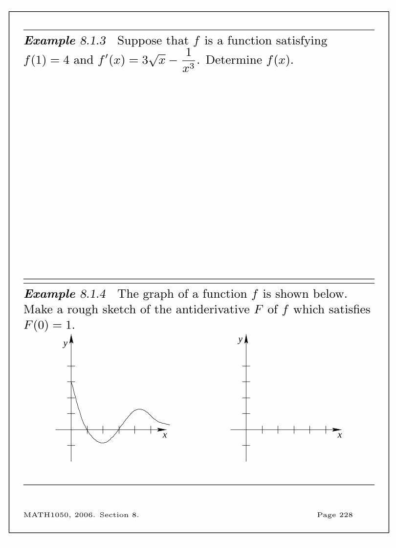
Example 8.1.3 Suppose that f is a function satisfying
f(1) = 4 and f ′(x) = 3√x− 1
x3. Determine f(x).
Example 8.1.4 The graph of a function f is shown below.
Make a rough sketch of the antiderivative F of f which satisfies
F (0) = 1.
x
y
x
y
MATH1050, 2006. Section 8. Page 228
• We need a convenient notation for antiderivatives.
•∫f(x) dx denotes the most general antiderivative of f , and
we call this the indefinite integral of f .
• Thus, the indefinite integral of f is defined by∫f(x) dx = F (x) + C
where F (x) is any antiderivative of f and C is an arbitrary
constant, called the constant of integration.
• The indefinite integral of f gives a family of functions: the
antiderivatives of f as the constant of integration varies.
• After evaluating an indefinite integral, you should always
differentiate your result to check your answer.
Example 8.1.5 Determine the following indefinite integrals.
a)∫x2(2 + x) dx
b)∫
5√u du
MATH1050, 2006. Section 8. Page 229
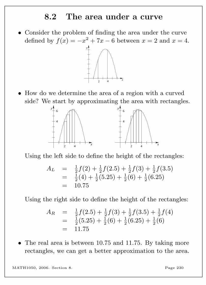
8.2 The area under a curve
• Consider the problem of finding the area under the curve
defined by f(x) = −x2 + 7x− 6 between x = 2 and x = 4.
42
y
x
• How do we determine the area of a region with a curved
side? We start by approximating the area with rectangles.
4
4
6
2
y
x4
4
6
2
y
x
Using the left side to define the height of the rectangles:
AL = 12f(2) + 1
2f(2.5) + 1
2f(3) + 1
2f(3.5)
= 12(4) + 1
2(5.25) + 1
2(6) + 1
2(6.25)
= 10.75
Using the right side to define the height of the rectangles:
AR = 12f(2.5) + 1
2f(3) + 1
2f(3.5) + 1
2f(4)
= 12(5.25) + 1
2(6) + 1
2(6.25) + 1
2(6)
= 11.75
• The real area is between 10.75 and 11.75. By taking more
rectangles, we can get a better approximation to the area.
MATH1050, 2006. Section 8. Page 230
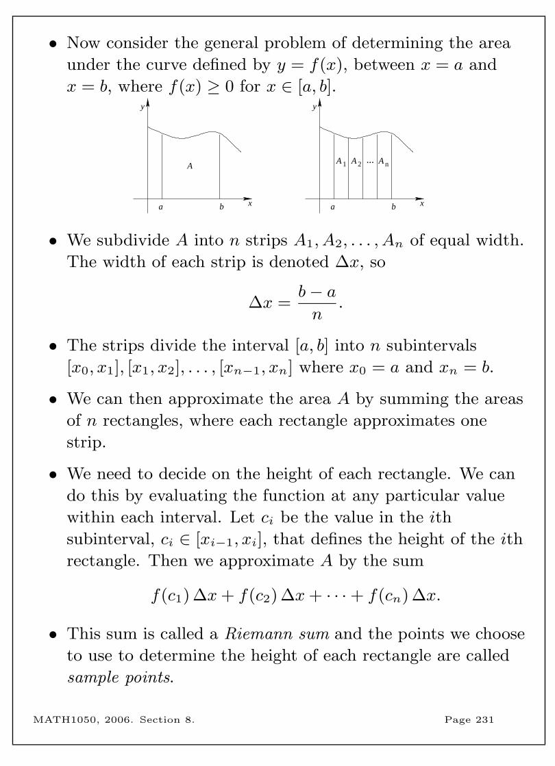
• Now consider the general problem of determining the area
under the curve defined by y = f(x), between x = a and
x = b, where f(x) ≥ 0 for x ∈ [a, b].y
ba
A nA 1 A 2A...
xx
y
ba
• We subdivide A into n strips A1, A2, . . . , An of equal width.
The width of each strip is denoted ∆x, so
∆x =b− an
.
• The strips divide the interval [a, b] into n subintervals
[x0, x1], [x1, x2], . . . , [xn−1, xn] where x0 = a and xn = b.
• We can then approximate the area A by summing the areas
of n rectangles, where each rectangle approximates one
strip.
• We need to decide on the height of each rectangle. We can
do this by evaluating the function at any particular value
within each interval. Let ci be the value in the ith
subinterval, ci ∈ [xi−1, xi], that defines the height of the ith
rectangle. Then we approximate A by the sum
f(c1) ∆x+ f(c2) ∆x+ · · ·+ f(cn) ∆x.
• This sum is called a Riemann sum and the points we choose
to use to determine the height of each rectangle are called
sample points.
MATH1050, 2006. Section 8. Page 231
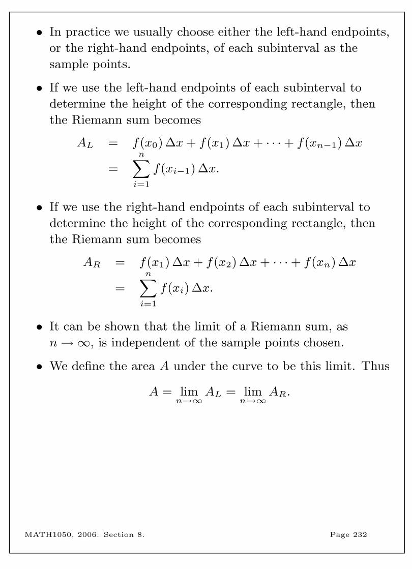
• In practice we usually choose either the left-hand endpoints,
or the right-hand endpoints, of each subinterval as the
sample points.
• If we use the left-hand endpoints of each subinterval to
determine the height of the corresponding rectangle, then
the Riemann sum becomes
AL = f(x0) ∆x+ f(x1) ∆x+ · · ·+ f(xn−1) ∆x
=
n∑i=1
f(xi−1) ∆x.
• If we use the right-hand endpoints of each subinterval to
determine the height of the corresponding rectangle, then
the Riemann sum becomes
AR = f(x1) ∆x+ f(x2) ∆x+ · · ·+ f(xn) ∆x
=
n∑i=1
f(xi) ∆x.
• It can be shown that the limit of a Riemann sum, as
n→∞, is independent of the sample points chosen.
• We define the area A under the curve to be this limit. Thus
A = limn→∞
AL = limn→∞
AR.
MATH1050, 2006. Section 8. Page 232
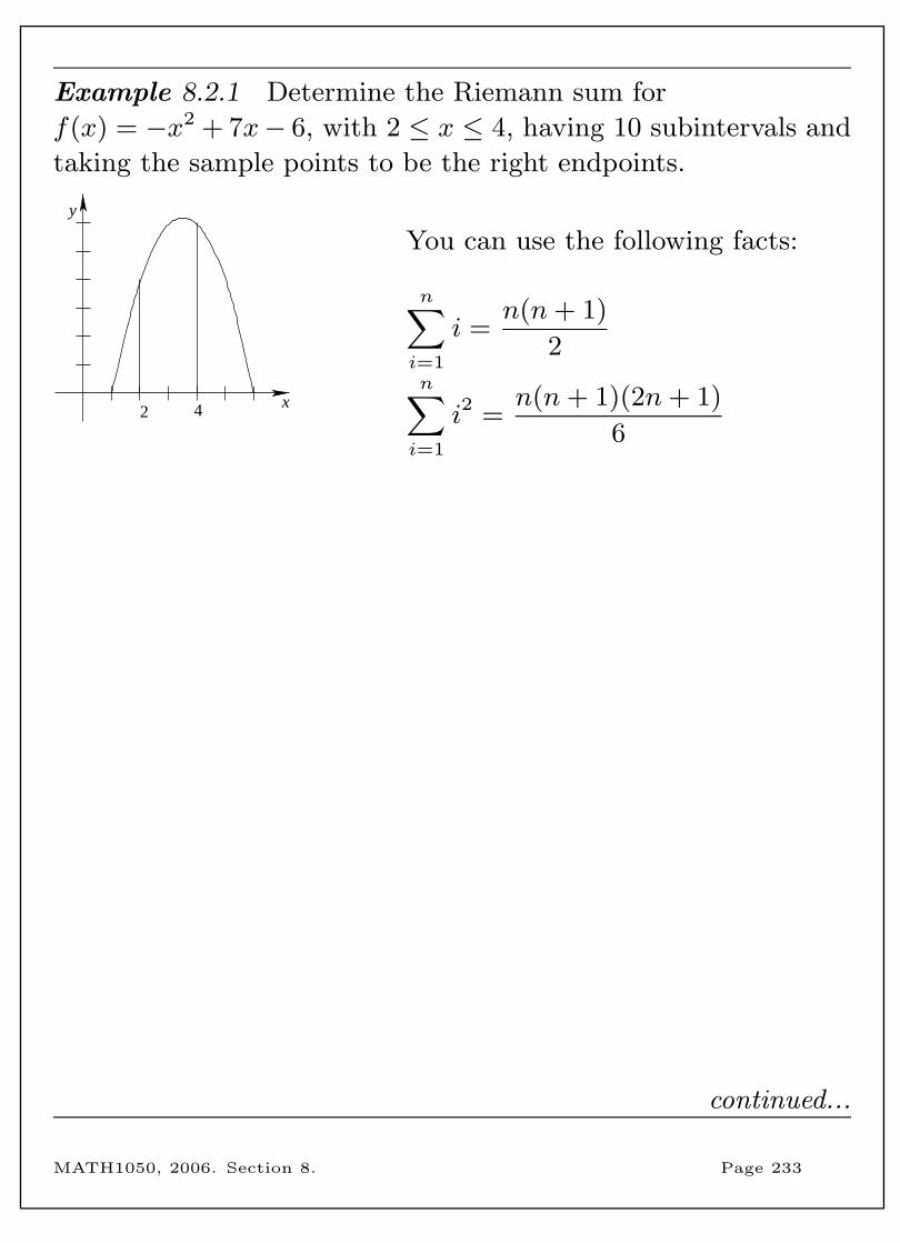
Example 8.2.1 Determine the Riemann sum for
f(x) = −x2 + 7x− 6, with 2 ≤ x ≤ 4, having 10 subintervals and
taking the sample points to be the right endpoints.
42
y
x
You can use the following facts:
n∑i=1
i =n(n+ 1)
2n∑i=1
i2 =n(n+ 1)(2n+ 1)
6
continued...
MATH1050, 2006. Section 8. Page 233

Example 8.2.1 (continued) Extra space for your work.
MATH1050, 2006. Section 8. Page 234
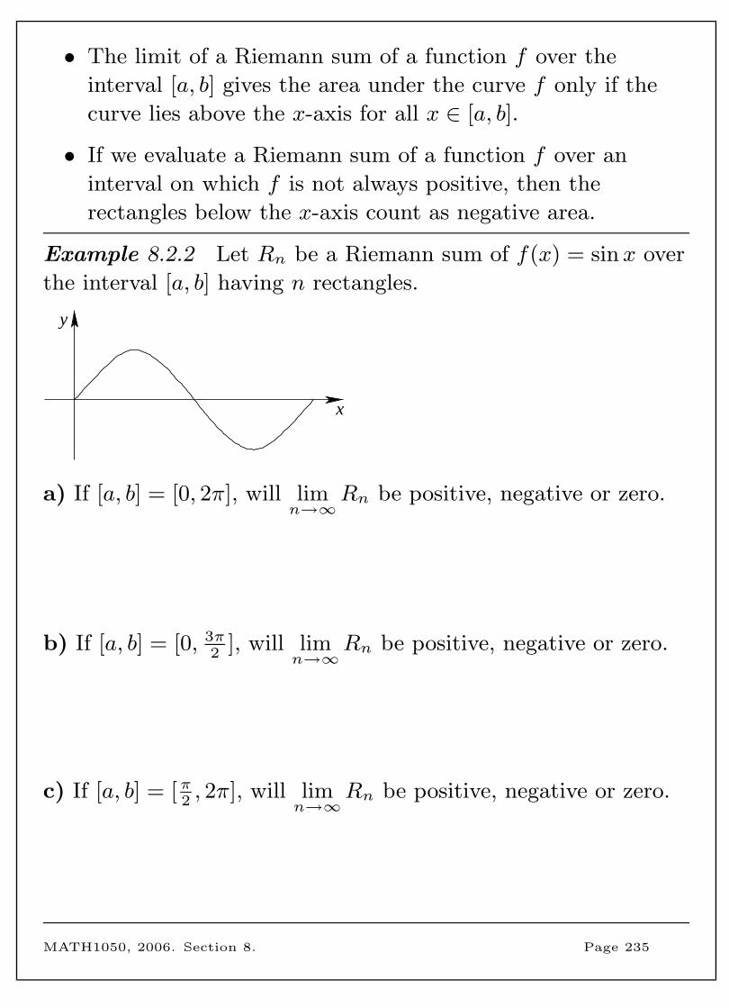
• The limit of a Riemann sum of a function f over the
interval [a, b] gives the area under the curve f only if the
curve lies above the x-axis for all x ∈ [a, b].
• If we evaluate a Riemann sum of a function f over an
interval on which f is not always positive, then the
rectangles below the x-axis count as negative area.
Example 8.2.2 Let Rn be a Riemann sum of f(x) = sinx over
the interval [a, b] having n rectangles.
x
y
a) If [a, b] = [0, 2π], will limn→∞
Rn be positive, negative or zero.
b) If [a, b] = [0, 3π2
], will limn→∞
Rn be positive, negative or zero.
c) If [a, b] = [π2, 2π], will lim
n→∞Rn be positive, negative or zero.
MATH1050, 2006. Section 8. Page 235
8.3 Definite integrals and theFundamental Theorem of Calculus
• Let Rn be a Riemann sum for a continuous function f over
the interval a ≤ x ≤ b, having n subintervals. Then the
definite integral of f from a to b is∫ b
a
f(x) dx = limn→∞
Rn = limn→∞
n∑i=1
f(xi) ∆x.
• The definite integral is also called the Riemann integral.
• We call a and b the limits of integration where a the lower
limit and b the upper limit.
• The integral sign∫
was introduced by Leibniz. It is an
elongated S and was chosen because the integral represents
the limit of a sum.
• Note that the definite integral is a number. Thus∫ baf(x) dx =
∫ baf(u) du =
∫ baf(r) dr.
Properties of the definite integral
•∫ abf(x) dx = −
∫ baf(x) dx
•∫ aaf(x) dx = 0
•∫ bac dx = c(b− a) where c is a constant
•∫ ba
[f(x) + g(x)] dx =∫ baf(x) dx+
∫ bag(x) dx
•∫ bacf(x) dx = c
∫ baf(x) dx where c is a constant
•∫ caf(x) dx+
∫ bcf(x) dx =
∫ baf(x) dx
MATH1050, 2006. Section 8. Page 236
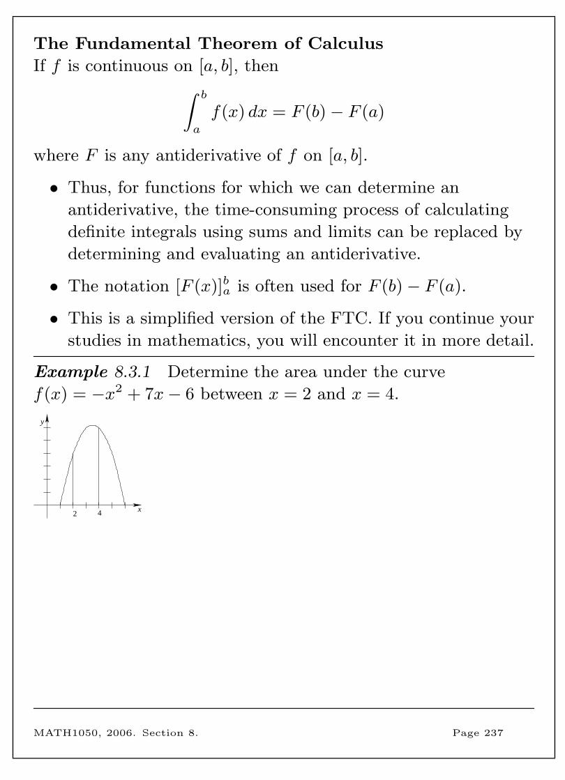
The Fundamental Theorem of Calculus
If f is continuous on [a, b], then∫ b
a
f(x) dx = F (b)− F (a)
where F is any antiderivative of f on [a, b].
• Thus, for functions for which we can determine an
antiderivative, the time-consuming process of calculating
definite integrals using sums and limits can be replaced by
determining and evaluating an antiderivative.
• The notation [F (x)]ba is often used for F (b)− F (a).
• This is a simplified version of the FTC. If you continue your
studies in mathematics, you will encounter it in more detail.
Example 8.3.1 Determine the area under the curve
f(x) = −x2 + 7x− 6 between x = 2 and x = 4.
42
y
x
MATH1050, 2006. Section 8. Page 237
Example 8.3.2 Refer back to Example 8.2.2.
a) Determine∫ 2π
0sinx dx.
b) Use the properties of the definite integral to determine the
area enclosed by the sine curve and the x-axis over the interval
[0, 2π].
Example 8.3.3 Determine
∫ 1
−1
1
x2dx.
MATH1050, 2006. Section 8. Page 238
8.4 Integration by substitution
• Recall the Chain rule for differentiation: If f and g are
differentiable functions, then (f ◦ g)′(x) = f ′(g(x))g′(x).
• Reversing the Chain rule gives the following integration
formula: ∫f ′(g(x))g′(x) dx = f(g(x)) + C.
Example 8.4.1 Determine∫
2xex2dx.
• Sometime it is hard to see that an integrand has the form
f ′(g(x))g′(x), so we need a systematic way to apply the
above integration formula.
• If y = f(x), where f is a differentiable function, then the
differentials dx and dy are related by the equation
dy = f ′(x) dx.
• The geometric meaning of the differentials is that if ` is the
tangent line to f at the point P = (x, f(x)), then the point
R = (x+ dx, f(x) + dy) is also on the line `.
• It can be shown that you can interpret the dx in an
indefinite integral as a differential. Thus, if u = g(x), then
du = g′(x) dx so∫f ′(g(x))g′(x) dx =
∫f ′(u) du.
MATH1050, 2006. Section 8. Page 239
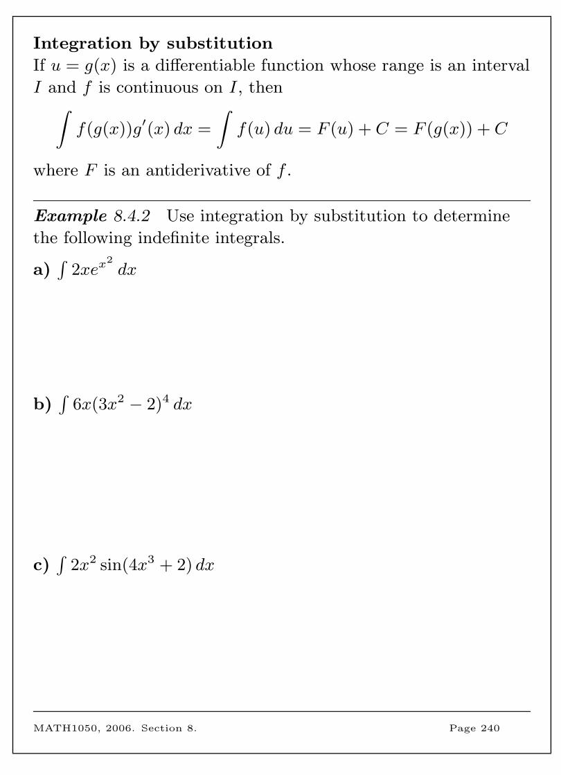
Integration by substitution
If u = g(x) is a differentiable function whose range is an interval
I and f is continuous on I, then∫f(g(x))g′(x) dx =
∫f(u) du = F (u) + C = F (g(x)) + C
where F is an antiderivative of f .
Example 8.4.2 Use integration by substitution to determine
the following indefinite integrals.
a)∫
2xex2dx
b)∫
6x(3x2 − 2)4 dx
c)∫
2x2 sin(4x3 + 2) dx
MATH1050, 2006. Section 8. Page 240
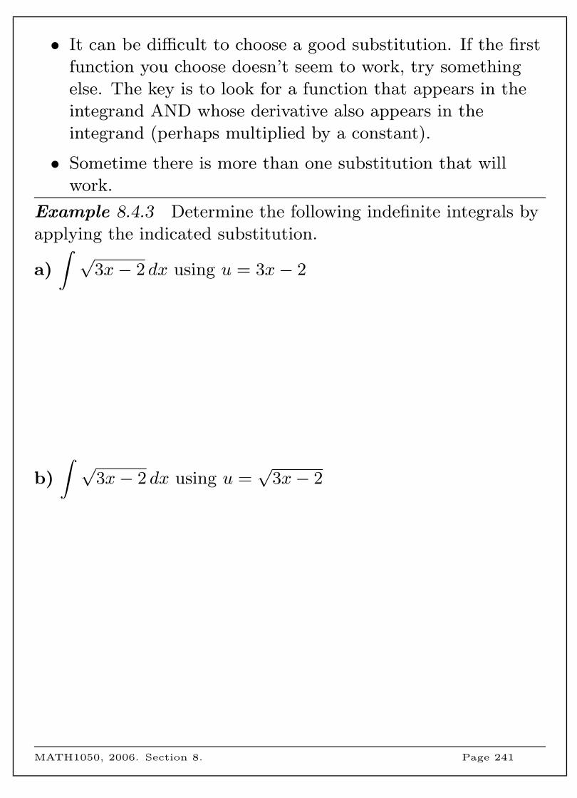
• It can be difficult to choose a good substitution. If the first
function you choose doesn’t seem to work, try something
else. The key is to look for a function that appears in the
integrand AND whose derivative also appears in the
integrand (perhaps multiplied by a constant).
• Sometime there is more than one substitution that will
work.
Example 8.4.3 Determine the following indefinite integrals by
applying the indicated substitution.
a)
∫ √3x− 2 dx using u = 3x− 2
b)
∫ √3x− 2 dx using u =
√3x− 2
MATH1050, 2006. Section 8. Page 241
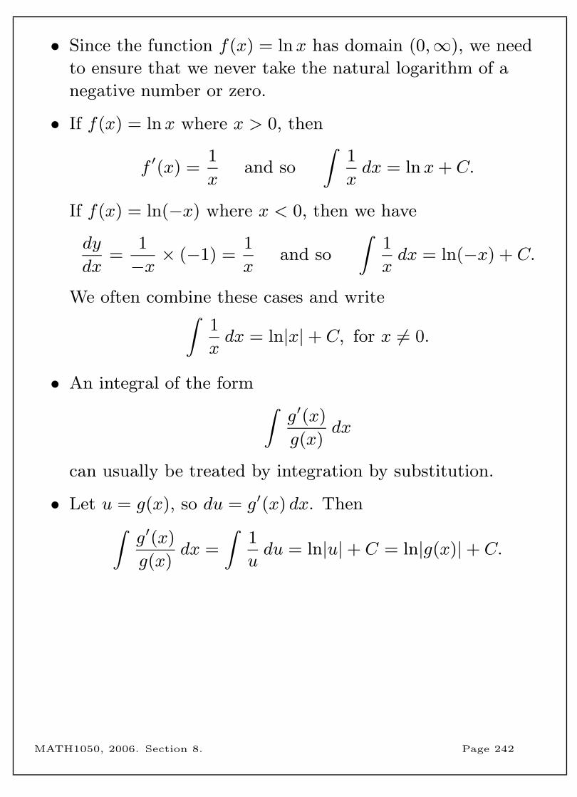
• Since the function f(x) = lnx has domain (0,∞), we need
to ensure that we never take the natural logarithm of a
negative number or zero.
• If f(x) = lnx where x > 0, then
f ′(x) =1
xand so
∫1
xdx = lnx+ C.
If f(x) = ln(−x) where x < 0, then we have
dy
dx=
1
−x × (−1) =1
xand so
∫1
xdx = ln(−x) + C.
We often combine these cases and write∫1
xdx = ln|x|+ C, for x 6= 0.
• An integral of the form ∫g′(x)
g(x)dx
can usually be treated by integration by substitution.
• Let u = g(x), so du = g′(x) dx. Then∫g′(x)
g(x)dx =
∫1
udu = ln|u|+ C = ln|g(x)|+ C.
MATH1050, 2006. Section 8. Page 242
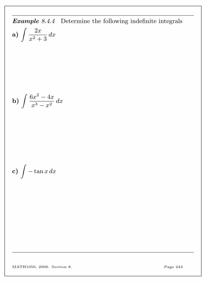
Example 8.4.4 Determine the following indefinite integrals
a)
∫2x
x2 + 3dx
b)
∫6x2 − 4x
x3 − x2dx
c)
∫− tanx dx
MATH1050, 2006. Section 8. Page 243
Integration by substitution for definite integrals
• There are two ways to apply integration by substitution to
a definite integral.
• The first way is to first determine the indefinite integral
using integration by substitution and then use this to solve
the definite integral.
Example 8.4.5 Evaluate∫ 1
−2
18x(10− 3x2)3 dx.
MATH1050, 2006. Section 8. Page 244
• The second way is to change the limits of integration when
the substitution is performed.
• If g′ is continuous on [a, b] and f is continuous on the range
of u = g(x), then∫ b
a
f(g(x))g′(x) dx =
∫ g(b)
g(a)
f(u) du.
Example 8.4.6 Evaluate the following definite integrals.
a)
∫ 1
−2
18x(10− 3x2)3 dx
continued...MATH1050, 2006. Section 8. Page 245
Example 8.4.6 (continued)
b)
∫ 7
0
9√
4 + 3x dx
MATH1050, 2006. Section 8. Page 246
Proof of the substitution rule for definite integrals
We need to prove that if g′ is continuous on [a, b] and f is
continuous on the range of u = g(x), then∫ b
a
f(g(x))g′(x) dx =
∫ g(b)
g(a)
f(u) du. (1)
Let F be an antiderivative of f . Then by the substitution rule
for indefinite integrals, F (g(x)) is an antiderivative of
f(g(x))g′(x).
By applying the FTC to the left-hand side of (1) above,∫ b
a
f(g(x))g′(x) dx = [F (g(x))]ba = F (g(b))− F (g(a)).
By applying the FTC to the right-hand side of (1) above,∫ g(b)
g(a)
f(u) du = [F (u)]g(b)
g(a) = F (g(b))− F (g(a)).
Thus ∫ b
a
f(g(x))g′(x) dx =
∫ g(b)
g(a)
f(u) du.
MATH1050, 2006. Section 8. Page 247
8.5 Applications of integration
• When faced with a practical problem in which we know the
rate at which a quantity is changing, integration can give us
information about that quantity.
• For a particle moving in a straight line, an antiderivative of
the acceleration function a(t) is the velocity function v(t)
and an antiderivative of the velocity function v(t) is the
displacement function s(t).
• Additional information about the velocity or displacement
at a particular time can help us to choose the correct
antiderivative.
Example 8.5.1 A balloon filled with water is thrown upward
from Level 6 of the outside stairs of the Priestley building, with
an initial speed of 10 m/s. The balloon is thrown from an initial
height of 20 metres. Assume that the acceleration due to gravity
is 9.8 m/s (downward).
a) Determine a function v(t) describing the velocity of the
balloon at t seconds.
b) Determine a function s(t) describing the displacement of the
balloon at t seconds.
c) When does the balloon reach its maximum height and what
is this maximum height?
d) When does the balloon hit the ground and what is its
velocity just before it hits the ground?
continued...MATH1050, 2006. Section 8. Page 248

Example 8.5.1 (continued)
MATH1050, 2006. Section 8. Page 249
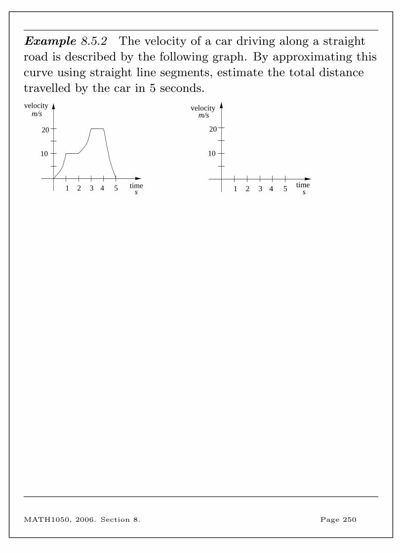
Example 8.5.2 The velocity of a car driving along a straight
road is described by the following graph. By approximating this
curve using straight line segments, estimate the total distance
travelled by the car in 5 seconds.
stime
m/svelocity
2 3 541
20
10
stime
m/svelocity
2 3 541
20
10
MATH1050, 2006. Section 8. Page 250
• It is important to distinguish between the displacement of
an object at time t and the total distance travelled by the
object at time t.
• When an object moves in a straight line and its velocity
changes from positive to negative (or negative to positive)
then the object is backtracking on ground already covered,
so displacement is reduced but total distance continues to
accumulate.
• Displacement is given by a definite integral but total
distance travelled is given by the area enclosed by the
velocity curve and the horizontal axis (time).
• If an object moving in a straight line has displacement
function s(t) and velocity function v(t) = s′(t), then∫ t2
t1
v(t) dt = s(t2)− s(t1)
is the net change of displacement (position) of the object
during the time period from t1 to t2.
• If the object is moving in the same direction for all of the
time interval t1 to t2, then this is also the total distance
travelled during that time.
MATH1050, 2006. Section 8. Page 251
Example 8.5.3 A particle moves along a line with acceleration
at time t of a(t) = 2t+ 2 m/s2. The particle has an initial
velocity of −3 m/s.
a) Determine the displacement of the particle after 2 seconds.
b) Determine the total distance the particle travels in the first
two seconds.
MATH1050, 2006. Section 8. Page 252
Example 8.5.4 Water flows from the bottom of a storage tank
at a rate of r(t) = −6t+ 180 litres per minute, where 0 ≤ t ≤ 30.
a) Find the amount of water that flows from the tank during
the first 10 minutes.
b) If the tank is empty at time t = 30, determine how much
water was in the tank at time t = 0.
MATH1050, 2006. Section 8. Page 253
9 Revision
1. Matrices
• Arithmetic with matrices (addition, multiplication, ...)
• Inverse of a 2× 2 matrix
• The determinant of a square matrix
• Using matrices to solve systems of linear equations
2. Vectors
• Three representations: geometric form, matrix form,
component form
• Arithmetic of vectors (addition, scalar multiplication, ...)
• Trigonometry
3. Applications of vectors
• Vectors in geometry
• Forces
• Displacement, velocity and momentum
• Scalar product and vector product
4. Sequences and series
• Arithmetic and geometric sequences and series
• Finite differences and telescoping sums
• Applications to compound interest and population growth
• Mathematical induction
MATH1050, 2006. Revision. Page 254
5. Real and complex numbers
• Solving inequalities and equations
• Arithmetic of complex numbers
• Polar and exponential form
• De Moivre’s Theorem
• Fundamental Theorem of Algebra
6. Functions
• Domain and range
• Composition of functions
• Inverse functions
• Limits
7. Differentiation
• Tangent lines
• Definition of the derivative
• Differentiation rules
• Curve sketching
• Applications: optimisation and rate of change
8. Integration
• Antidifferentiation
• Area under a curve
• Definite integrals and the Fundamental Theorem of
Calculus
• Integration by substitution
• Applications: rate of changeMATH1050, 2006. Revision. Page 255
9.1 Revision examples
1. Determine whether or not the following system of linear
equations has a unique solution.
x− y + 2z = 3
−3x+ y + z = −4
4x− 6z = 2
MATH1050, 2006. Revision. Page 256
2. Let u = −√
3i + j and let v = 3i− 4j. Determine the angle
(in radians) between u and v. Round your answer to two
decimal place accuracy.
MATH1050, 2006. Revision. Page 257
3. A pilot is steering a plane in the direction N60◦E with an
airspeed (speed in still air) of 250 km/h. There is a wind
blowing from the direction N45◦W at a speed of 50 km/h.
Determine the resultant speed and direction of the plane. Give
the speed to the nearest km/h and the direction as a bearing to
the nearest degree.
MATH1050, 2006. Revision. Page 258
4. Use mathematical induction to prove that, for all n ≥ 1,
n∑i=1
2i = n(n+ 1).
MATH1050, 2006. Revision. Page 259

5. Solve the following inequality and give your solution in
interval form and illustrate it on a number line.
|x+ 2|x− 5
≤ 2
MATH1050, 2006. Revision. Page 260

6. Find all solutions of z5 = 32 over the complex numbers.
Write your answers in polar form using the principal arguments.
MATH1050, 2006. Revision. Page 261
7. Let f(x) = 1x
and let g(x) =√x+ 2.
a) State the domain and range of f and g.
b) Determine (f ◦ g)(x) and state its domain and range.
MATH1050, 2006. Revision. Page 262
8. a) Use the definition of the derivative to determine the
derived function of f where f(x) = 3x2 − x.
b) Use your answer from a) to determine the equation of the
tangent line to the curve y = 3x2 − x at x = −1.
MATH1050, 2006. Revision. Page 263
9. Evaluate the following definite integrals.
a)
∫ 4
2
(1
x2+ 2x3
)dx
b)
∫ 2
−1
2x3 − xx4 − x2 + 5
dx
MATH1050, 2006. Revision. Page 264
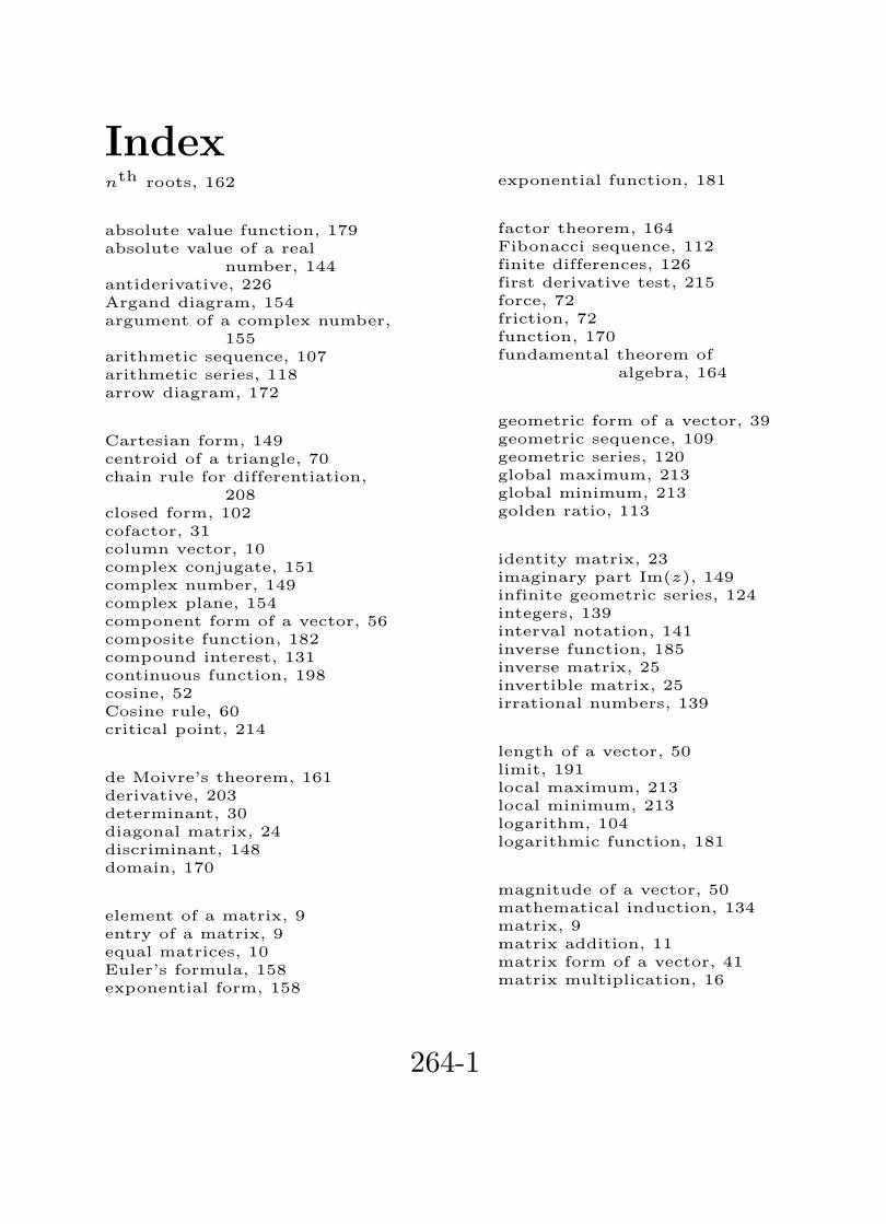
Indexnth roots, 162
absolute value function, 179absolute value of a real
number, 144antiderivative, 226Argand diagram, 154argument of a complex number,
155arithmetic sequence, 107arithmetic series, 118arrow diagram, 172
Cartesian form, 149centroid of a triangle, 70chain rule for differentiation,
208closed form, 102cofactor, 31column vector, 10complex conjugate, 151complex number, 149complex plane, 154component form of a vector, 56composite function, 182compound interest, 131continuous function, 198cosine, 52Cosine rule, 60critical point, 214
de Moivre’s theorem, 161derivative, 203determinant, 30diagonal matrix, 24discriminant, 148domain, 170
element of a matrix, 9entry of a matrix, 9equal matrices, 10Euler’s formula, 158exponential form, 158
exponential function, 181
factor theorem, 164Fibonacci sequence, 112finite differences, 126first derivative test, 215force, 72friction, 72function, 170fundamental theorem of
algebra, 164
geometric form of a vector, 39geometric sequence, 109geometric series, 120global maximum, 213global minimum, 213golden ratio, 113
identity matrix, 23imaginary part Im(z), 149infinite geometric series, 124integers, 139interval notation, 141inverse function, 185inverse matrix, 25invertible matrix, 25irrational numbers, 139
length of a vector, 50limit, 191local maximum, 213local minimum, 213logarithm, 104logarithmic function, 181
magnitude of a vector, 50mathematical induction, 134matrix, 9matrix addition, 11matrix form of a vector, 41matrix multiplication, 16
264-1
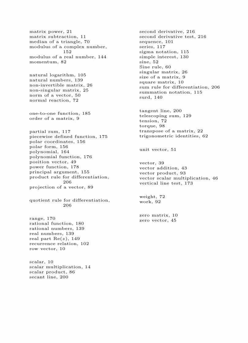
matrix power, 21matrix subtraction, 11median of a triangle, 70modulus of a complex number,
152modulus of a real number, 144momentum, 82
natural logarithm, 105natural numbers, 139non-invertible matrix, 26non-singular matrix, 25norm of a vector, 50normal reaction, 72
one-to-one function, 185order of a matrix, 9
partial sum, 117piecewise defined function, 175polar coordinates, 156polar form, 156polynomial, 164polynomial function, 176position vector, 49power function, 178principal argument, 155product rule for differentiation,
206projection of a vector, 89
quotient rule for differentiation,206
range, 170rational function, 180rational numbers, 139real numbers, 139real part Re(z), 149recurrence relation, 102row vector, 10
scalar, 10scalar multiplication, 14scalar product, 86secant line, 200
second derivative, 216second derivative test, 216sequence, 101series, 117sigma notation, 115simple interest, 130sine, 52Sine rule, 60singular matrix, 26size of a matrix, 9square matrix, 10sum rule for differentiation, 206summation notation, 115surd, 140
tangent line, 200telescoping sum, 129tension, 72torque, 98transpose of a matrix, 22trigonometric identities, 62
unit vector, 51
vector, 39vector addition, 43vector product, 93vector scalar multiplication, 46vertical line test, 173
weight, 72work, 92
zero matrix, 10zero vector, 45