mathematical study of a risk-structured two-group model for chlamydia transmission dynamics

Applied Mathematical Modelling 35 (2011) 3653–3673

Contents lists available at ScienceDirect

Applied Mathematical Modelling

journal homepage: www.elsevier .com/locate /apm

Mathematical study of a risk-structured two-group modelfor Chlamydia transmission dynamics

O. Sharomi, A.B. Gumel ⇑Department of Mathematics, University of Manitoba, Winnipeg, Manitoba, Canada R3T 2N2

a r t i c l e i n f o

Article history:Received 4 April 2010Accepted 9 December 2010Available online 11 February 2011

Keywords:ChlamydiaEquilibriaLow- and high-risk groupsRe-infectionStabilityBackward bifurcation

0307-904X/$ - see front matter � 2011 Elsevier Incdoi:10.1016/j.apm.2010.12.006

⇑ Corresponding author.E-mail address: [email protected] (A.B.

a b s t r a c t

A new two-group deterministic model for Chlamydia trachomatis, which stratifies theentire population based on risk of acquiring or transmitting infection, is designed and ana-lyzed to gain insight into its transmission dynamics. The model is shown to exhibit thephenomenon of backward bifurcation, where a stable disease-free equilibrium (DFE)co-exists with one or more stable endemic equilibria when the associated reproductionnumber is less than unity. Unlike in some of the earlier modeling studies on Chlamydiatransmission dynamics in a population, this study shows that the backward bifurcationphenomenon persists even if individuals who recovered from Chlamydia infection do notget re-infected. However, it is shown that the phenomenon can be removed if all thesusceptible individuals are equally likely to acquire infection (i.e., for the case where thesusceptible male and female populations are not stratified according to risk of acquiringinfection). In such a case, the DFE of the resulting (reduced) model is globally-asymptotically stable when the associated reproduction number is less than unity andno re-infection of recovered individuals occurs. Thus, this study shows that stratifyingthe two-sex Chlamydia transmission model, presented in [1], according to the risk ofacquiring or transmitting infection induces the phenomenon of backward bifurcationregardless of whether or not the re-infection of recovered individuals occurs.

� 2011 Elsevier Inc. All rights reserved.

1. Introduction

Chlamydia trachomatis is a sexually-transmitted disease that continues to inflict major public health and socio-economicburden around the world (see, for instance, [1–9]). The World Health Organization reported 4–5 million cases of Chlamydiain the United States in 2006 [3,9]. Furthermore, the annual cost of Chlamydia and its consequences in the United States aloneexceeds $2 billion [8].

The symptoms of Chlamydia, which are usually mild or absent (three quarters of infected women and about half of in-fected men do not show symptoms [1]), include: abnormal vaginal discharge, discharge from penis, burning sensation whenurinating and itching [7]. Additionally, Chlamydia causes numerous irreversible complications, such as chronic pelvic pain,infertility in females and potentially fatal ectopic pregnancy [1].

Statistical studies have shown that majority of Chlamydia infections are largely generated by individuals in high-riskgroups [7,10,11]. The high-risk populations include:

. All rights reserved.

Gumel).

http://dx.doi.org/10.1016/j.apm.2010.12.006

mailto:[email protected]

http://dx.doi.org/10.1016/j.apm.2010.12.006

http://www.sciencedirect.com/science/journal/0307904X

http://www.elsevier.com/locate/apm

Fig. 1. Age- and sex-specific Chlamydia rates in the United States for 2008 [12].

3654 O. Sharomi, A.B. Gumel / Applied Mathematical Modelling 35 (2011) 3653–3673

(i) young sexually-active individuals between the ages of 15–26 [1,7,10,11];(ii) sexually-active individuals with previous history of sexually-transmitted infections [7,10,11];

(iii) sexually-active individuals with new or multiple sex partners [1,7,10,11];(iv) sexually-active individuals who do not practice safe sex (e.g., those who do not use condoms consistently) [7,10,11].

Furthermore, sexually-active women aged 25 or younger are frequently re-infected if their sex partners are not treated.Fig. 1 depicts the age- and sex-specific rates of Chlamydia infection in the United States for the year 2008 [12].

It is clear from Fig. 1 that majority of the infections (for both males and females) are generated by individuals in the 15–24age bracket. This fact suggests that models for Chlamydia transmission in a population should incorporate the effect of suchrisk groups on the disease dynamics in the population. That is, it is instructive to design (and analyze) a Chlamydia trans-mission model that considers the problem of the variability in risk of acquisition and/or transmission of Chlamydia infectionin a given population. In other words, it is of epidemiological interest to study the effect of risk-structure on Chlamydiatransmission dynamics in a population.

The main objective of this study is to determine whether or not stratifying the entire population (being studied) in termsof risk of acquiring and/or transmitting Chlamydia infection will alter the qualitative (equilibrium) dynamics of the equiv-alent sex-structured (but without risk structure) Chlamydia transmission model presented in [1]. Not much work has beenreported in the literature on Chlamydia transmission dynamics [1]. A few population-level models, of the form of discrete-time [13,14] and continuous-time [15,16] dynamical systems, have been presented. In-host models for the dynamics of Chla-mydia are presented in [17–21]. Other forms of Chlamydia modeling involves the use of individual-based stochastic model[22,23]. Sharomi et al. [1] designed and analyzed a two-group deterministic model for the spread of Chlamydia trachomatis ina population. The current study complements the aforementioned studies (particularly the study in [1]) by designing, andrigorously analyzing, a new Chlamydia transmission model that incorporates risk structure. The paper is organized as fol-lows. The new model is formulated in Section 2, and analyzed in Section 3. The effect of risk of susceptibility to infectionis explored in Section 4.

2. Formulation of model

The formulation of the model follows that of the risk-free sex-structured Chlamydia transmission model presented in [1],and is reproduced here for completeness. The total sexually-active population at time t, denoted by N(t), is divided into twoclasses, namely the total male population, denoted by Nm(t), and the total female population, denoted by Nf(t). The total malepopulation is further sub-divided into 10 mutually-exclusive compartments of, low-risk susceptible males (Sml(t)), high-risksusceptible males (Smh(t)), low-risk exposed males (Eml(t)), high-risk exposed males (Emh(t)), low-risk infectious males show-ing symptoms of Chlamydia (Iml(t)), high-risk infectious males showing symptoms of Chlamydia (Imh(t)), low-risk infectiousmales showing no symptoms of Chlamydia (Aml(t)), high-risk infectious males showing no symptoms of Chlamydia (Amh(t)),low-risk infectious males who have cleared (or recovered from) Chlamydia infection (Rml(t)) and high-risk infectious maleswho have cleared (or recovered from) Chlamydia infection (Rmh(t)).

Similarly, the total female population is sub-divided into low-risk susceptible females (Sfl(t)), high-risk susceptible fe-males (Sfh(t)), low-risk exposed females (Efl(t)), high-risk exposed females (Efh(t)), low-risk infectious females showing symp-toms of Chlamydia (Ifl(t)), high-risk infectious females showing symptoms of Chlamydia (Ifh(t)), low-risk infectious femalesshowing no symptoms of Chlamydia (Afl(t)), high-risk infectious females showing no symptoms of Chlamydia (Afh(t)), low-risk infectious females who have cleared (or recovered from) Chlamydia infection (Rfl(t)) and high-risk infectious femaleswho have cleared (or recovered from) Chlamydia infection (Rfh(t)). Thus,

O. Sharomi, A.B. Gumel / Applied Mathematical Modelling 35 (2011) 3653–3673 3655

NðtÞ ¼ NmðtÞ þ Nf ðtÞ;

where

NmðtÞ ¼ SmlðtÞ þ SmhðtÞ þ EmlðtÞ þ EmhðtÞ þ ImlðtÞ þ ImhðtÞ þ AmlðtÞ þ AmhðtÞ þ RmlðtÞ þ RmhðtÞ;

and

Nf ðtÞ ¼ SflðtÞ þ SfhðtÞ þ EflðtÞ þ EfhðtÞ þ IflðtÞ þ IfhðtÞ þ AflðtÞ þ AfhðtÞ þ RflðtÞ þ RfhðtÞ:

In other words, the model to be developed stratifies the total population in terms of risk of acquisition and transmission ofinfection. Furthermore, the model to be developed lumps all individuals in the various risk groups, defined by Items (i)–(iv)of Section 1, as high-risk (that is, any individual that falls under the Categories (i)–(iv) in Section 1 is considered to be high-risk), while the rest of the sexually-active population is considered to be in the low-risk category (this is done for mathemat-ical tractability; we hope to relax this assumption, in a future study, so that each of the aforementioned risk groups isaccounted for separately). The susceptible populations (for both males and females) are increased by the recruitment ofnew sexually-active individuals (assumed to be susceptible) into the population at a rate Pm(Pf) for the male (female) pop-ulation, respectively. A fraction, pm(pf), of the new recruited sexually-active adults is assumed to be high-risk for the male(female) population, while the remaining fraction, (1 � pm)(1 � pf), is in the low-risk classes for the male (female) population,respectively. Susceptible males (low- and high-risk) acquire Chlamydia infection and become exposed (latent), followingeffective contact with infected females (i.e., those in the Efl, Efh, Ifl, Ifh, Afl and Afh classes), at rates kf and gmkf, respectively,with kf(t) = kfl(t) + kfh(t), where

kflðtÞ ¼cmbf ½EflðtÞ þ h1IflðtÞ þ h2AflðtÞ�

Nf ðtÞ;

kfhðtÞ ¼#f cmbf ½EfhðtÞ þ h1IfhðtÞ þ h2AfhðtÞ�

Nf ðtÞ;

ð1Þ

with kfl(t) and kfh(t) representing the forces of infection for the female low-risk and high-risk populations, respectively.Similarly, susceptible females (both low- and high-risk) acquire Chlamydia infection following effective contact with

males infected with Chlamydia (i.e., those in the Eml, Emh, Iml, Imh, Aml and Amh classes) at rates km and gfkm, withkm(t) = kml(t) + kmh(t), where,

kmlðtÞ ¼cf bm½EmlðtÞ þ h1ImlðtÞ þ h2AmlðtÞ�

NmðtÞ;

kmhðtÞ ¼#mcf bm½EmhðtÞ þ h1ImhðtÞ þ h2AmhðtÞ�

NmðtÞ;

ð2Þ

with kml(t) and kmh(t) representing the forces of infection for the male low-risk and high-risk, respectively. In (1) and (2)above, the parameters bm and bf represent the probabilities of transmission of Chlamydia from males to females and fromfemales to males, respectively. Furthermore, the parameters cm and cf represent the rates at which males and females acquirenew sexual partners, respectively. Thus, the products cfbm and cmbf represent the effective contact rates for male-to-femaleand female-to-male transmission of Chlamydia, respectively. Finally, the parameter gm P 1 (gf P 1) accounts for the fact thathigh-risk individuals are more susceptible to Chlamydia infection than individuals in the low-risk group for males (females)population.

Furthermore, the modification parameters h1 > 1 and h2 > 1 (with h1 – h2) account for the assumed increase in the relativeinfectiousness of individuals in the Iml, Imh and Ifl, Ifh (infectious individuals showing symptoms of Chlamydia) and Aml, Amh

and Afl, Afh (infectious individuals showing no symptoms of Chlamydia) classes in comparison to exposed males and females(in the Eml, Emh and Efl, Efh classes), respectively. That is, it is assumed that infectious females (in the Ifl, Ifh and Afl, Afh classes)are more infectious than exposed females (in the Efl and Efh classes).

Similarly, infectious males (in the Iml, Imh and Aml, Amh classes) are assumed to be more infectious than exposed males (inthe Eml, Emh classes). Furthermore, the modification parameters #m > 1 and #f > 1 account for the assumed increase in the rel-ative infectiousness of infected individuals in the high-risk group in comparison to those in the low-risk group for the maleand female population, respectively. It is assumed that susceptible individuals can change their risk status, by switchingfrom low- to high-risk status or high- to low-risk status. Susceptible males (females) switch from low- to high-risk status

at a rate nm1 nf

1

� �, and switch from high- to low-risk at a rate nm

2 nf2

� �, respectively.

Exposed individuals also change their behavior by switching from low- to high-risk status at a rate nm3 nf

3

� �for males

(females), and switch from high- to low-risk status at a rate nm4 nf

4

� �for males (females), respectively. Exposed individuals

(in the Eml, Emh, Efl and Efh classes) become infectious at a rate qm(qf) for males (females). A fraction, jm(jf), of these individ-uals is assumed to display clinical symptoms of Chlamydia infection (and are moved to the corresponding infectious classeswith symptoms: Iml; Imh(Ifl; Ifh)), while the remaining fraction, (1 � jm)(1 � jf), is assumed not to show clinical symptoms(but still remain capable of infecting others; that is, they are asymptomatically-infectious). It should be recalled that exposedindividuals (i.e., those in the E class) are also assumed to be capable of transmitting infection (albeit at a very small rate in

Table 1Description of variables and parameters for model (3).

Variables Description

Sml(t), Smh(t) Population of low- and high-risk susceptible malesSfl(t), Sfh(t) Population of low- and high-risk susceptible femalesEml(t), Emh(t) Population of low- and high-risk exposed malesEfl(t), Efh(t) Population of low- and high-risk exposed femalesIml(t), Imh(t) Population of low- and high-risk infectious males showing symptoms of ChlamydiaIfl(t), Ifh(t) Population of low- and high-risk infectious females showing symptoms of ChlamydiaAml(t), Amh(t) Population of low- and high-risk infectious males not showing symptoms of ChlamydiaAfl(t), Afh(t) Population of low- and high-risk infectious females not showing symptoms of ChlamydiaRml(t), Rmh(t) Population of low- and high-risk recovered malesRfl(t), Rfh(t) Population of low- and high-risk recovered females

Parameters Description Nominalvalues(year)�1

References

Pm, Pf Recruitment rates for males and females 1000, 1000 [1]pm, pf Fraction of recruited individual that are high-risk

for males and females(0,1)

bm, bf Probability of transmission for males and females 0.11, 0.11 [22,28]cm, cf Average number of new sexual partners for males

and females10; 10NmðtÞ

Nf ðtÞ[14–16,22]

#m, #f Modification parameters for relative infectiousnessof high-risk individuals in comparison to low-riskindividuals

4.2, 4.2 Assumed

h1, h2 Modification parameters for infectiousness ofinfectious individuals in relation to exposedindividuals

1.2, 1.5 [1]

wmh, wfh Rate of loss of immunity for high-risk males andfemales

0.5, 0.5 [1]

jm, jf Fraction of infectious individuals that showdisease symptoms for males and females

0.5, 0.25 [1,7]

qm, qf Rate of symptoms development for exposedmales and females

2/52, 2/52 [1,7]

rml, rfl Re-infection parameters for low-risk males andfemales

0.11, 0.35 [1,26,27]

rmh, rfh Re-infection parameters for high-risk males andfemales

0.11, 0.35 [1,26,27]

l Natural death rate 1/70 [1]cm, cf Rate at which males and females leave the

asymptomatically-infectious class3.65, 1.971 [1]

dm, df Disease-induced mortality rate for males andfemales

0.001, 0.001 [1,9]

hm, hf Natural clearance rate for infectious males andfemales showing symptoms of Chlamydia

(2.5–3)3.65 [1,15,22,24,25]

/mcm, /fcf Natural clearance rate for infectious males andfemales that show no symptoms

(0.27–0.5)3.65

[1,15,22,24,25]

nmj ; nf

j ðj ¼ 1;3; . . . ;9Þ Rate of behavior change from low- to high-risk 1 Assumed

nmj ; nf

j ðj ¼ 2;4; . . . ;10Þ Rate of behavior change from high- to low-risk 1 Assumed

gm,gf Modification parameter for increased Chlamydiasusceptibility of high-risk males and females

1 Assumed


comparison to infectious individuals). Individuals showing clinical symptoms of Chlamydia change their behavior by switch-

ing from low- to high-risk status at a rate nm5 nf

5

� �for males (females), and they switch from high- to low-risk status at a rate

nm6 nf

6

� �for males (females), respectively.

Infectious individuals (both low- or high-risk) that do not show symptoms of the disease (that is, those in the Aml, Amh, Afl

and Afh classes) are expected to suffer severe complications, such as infertility, if untreated. Furthermore, these individualsshow symptoms of the disease at a rate (1 � /m)cm((1 � /f)cf) for the male (female) population; while the remaining frac-tion, /mcm(/fcf), recovers naturally (cleared the infection; see [24,25] for discussion on the clearance rate of Chlamydia).Individuals showing no symptoms of Chlamydia change their behavior by switching from low- to high-risk status at a rate

nm7 nf

7

� �for males (females), and they switch from high- to low-risk status at a rate nm

8 nf8

� �for males (females), respectively.

Infectious individuals showing symptoms of Chlamydia clear the infection at a rate hm(hf) for the male (female) population.Recovered individuals in the low-risk group can be re-infected at rates rmlkf(t) and rflkm(t) for males and females, respec-

tively. Furthermore, recovered individuals in the high-risk group can be re-infected at rates rmhkf(t) and rfhkm(t) for males andfemales, respectively (where rml > 0, rmh > 0 and rfl > 0, rfh > 0 represent the re-infection rates for males and females in the


low- and high-risk groups (see [26] for discussions on re-infection of Chlamydia among females)). Recovered individuals canlose their infection-acquired immunity at a rate (wml; wmh)(wfl; wfh) for males (females) in the low- and high-risk groups,respectively (these individuals then return to the corresponding susceptible class (Sml; Smh)(Sfl; Sfh)). Recovered individualschange their risk behavior by switching from low- to high-risk status at a rate nm

9 nf9

� �for males (females), and switch from

high- to low-risk status at a rate nm10 nf

10

� �for males (females), respectively. Furthermore, natural mortality occurs in all clas-

ses at a rate l. Infectious individuals (in the Iml, Imh, Aml, Amh and Ifl, Ifh, Afl, Afh classes) suffer an additional disease-induceddeath at rates dm and df, for males and females, respectively.

Combining all the aforementioned definitions and assumptions, it follows that the model for the transmission of Chla-mydia, that stratifies the total sexually-active population according to the risk of acquisition and transmission of infection,is given by the following deterministic system of non-linear differential equations (see Table 1 for the description of the vari-ables and parameters of the model):

dSml

dt¼ ð1� pmÞPm þ wmlRmlðtÞ þ nm

2 SmhðtÞ � kf ðtÞSmlðtÞ � k1SmlðtÞ;dSmh

dt¼ pmPm þ nm

1 SmlðtÞ þ wmhRmhðtÞ � gmkf ðtÞSmhðtÞ � k2SmhðtÞ;dEml

dt¼ kf ðtÞSmlðtÞ þ rmlkf ðtÞRmlðtÞ þ nm

4 EmhðtÞ � k3EmlðtÞ;dEmh

dt¼ gmkf ðtÞSmhðtÞ þ rmhkf ðtÞRmhðtÞ þ nm

3 EmlðtÞ � k4EmhðtÞ;dIml

dt¼ jmqmEmlðtÞ þ ð1� /mÞcmAmlðtÞ þ nm

6 ImhðtÞ � k5ImlðtÞ;dImh

dt¼ jmqmEmhðtÞ þ ð1� /mÞcmAmhðtÞ þ nm

5 ImlðtÞ � k6ImhðtÞ;dAml

dt¼ ð1� jmÞqmEmlðtÞ þ nm

8 AmhðtÞ � k7AmlðtÞ;dAmh

dt¼ ð1� jmÞqmEmhðtÞ þ nm

7 AmlðtÞ � k8AmhðtÞ;dRml

dt¼ hmImlðtÞ þ /mcmAmlðtÞ þ nm

10RmhðtÞ � ½k9 þ rmlkf ðtÞ�RmlðtÞ;dRmh

dt¼ hmImhðtÞ þ /mcmAmhðtÞ þ nm

9 RmlðtÞ � ½k10 þ rmhkf ðtÞ�RmhðtÞ;dSfl

dt¼ ð1� pf ÞPf þ wflRflðtÞ þ nf

2SfhðtÞ � kmðtÞSflðtÞ � k11SflðtÞ;dSfh

dt¼ pf Pf þ nf

1SflðtÞ þ wfhRfhðtÞ � gf kmðtÞSfhðtÞ � k12SfhðtÞ;dEfl

dt¼ kmðtÞSflðtÞ þ rflkmðtÞRflðtÞ þ nf

4EfhðtÞ � k13EflðtÞ;dEfh

dt¼ gf kmðtÞSfhðtÞ þ rfhkmðtÞRfhðtÞ þ nf

3EflðtÞ � k14EfhðtÞ;dIfl

dt¼ jf qf EflðtÞ þ ð1� /f Þcf AflðtÞ þ nf

6IfhðtÞ � k15IflðtÞ;dIfh

dt¼ jf qf EfhðtÞ þ ð1� /f Þcf AfhðtÞ þ nf

5IflðtÞ � k16IfhðtÞ;dAfl

dt¼ ð1� jf Þqf EflðtÞ þ nf

8AfhðtÞ � k17AflðtÞ;dAfh

dt¼ ð1� jf Þqf EfhðtÞ þ nf

7AflðtÞ � k18AfhðtÞ;dRfl

dt¼ hf IflðtÞ þ /f cf AflðtÞ þ nf

10RfhðtÞ � ½k19 þ rflkmðtÞ�RflðtÞ;dRfh

dt¼ hf IfhðtÞ þ /f cf AfhðtÞ þ nf

9RflðtÞ � ½k20 þ rfhkmðtÞ�RfhðtÞ;

ð3Þ

where

k1 ¼ nm1 þ l; k2 ¼ nm

2 þ l; k3 ¼ nm3 þ lþ qm; k4 ¼ nm

4 þ lþ qm;

k5 ¼ nm5 þ lþ dm þ hm; k6 ¼ nm

6 þ lþ dm þ hm; k7 ¼ nm7 þ lþ dm þ cm;

k8 ¼ nm8 þ lþ dm þ cm; k9 ¼ nm

9 þ lþ wml; k10 ¼ nm10 þ lþ wmh;

k11 ¼ nf1 þ l; k12 ¼ nf

2 þ l; k13 ¼ nf3 þ lþ qf ; k14 ¼ nf

4 þ lþ qf ;

k15 ¼ nf5 þ lþ df þ hf ; k16 ¼ nf

6 þ lþ df þ hf ; k17 ¼ nf7 þ lþ df þ cf ;

k18 ¼ nf8 þ lþ df þ cf ; k19 ¼ nf

9 þ lþ wfl; k20 ¼ nf10 þ lþ wfh:


In summary, the model (3) is constructed based on the following key assumptions:

(i) Exposed (latent) individuals (in the Eml, Emh, Efl and Efh classes) can transmit infection (albeit at a very small rate incomparison to infectious individuals). Furthermore, infectious individuals with no clinical symptoms of the disease(i.e., those in the Aml, Amh, Afl and Afh classes) can also transmit infection. These assumptions are also made in [1];

(ii) High-risk susceptible individuals acquire infection at a faster rate than low-risk susceptible individuals (with the asso-ciated modification parameters gm P 1, gf P 1 for males and females, respectively);

(iii) High-risk infected individuals transmit infection at a faster rate than low-risk infected individuals (with the associatedmodification parameters #m P 1, #f P 1 for males and females, respectively);

(iv) High-risk recovered individuals become re-infected at a faster rate than low-risk recovered individuals (with the asso-ciated modification parameters rmh P rml and rfh P rfl for males and females, respectively).

The model (3) is an extension of the sex-structured Chlamydia transmission model presented in [1], by incorporating riskstructure into the model (i.e., adding 10 new compartments for low- and high-risk susceptible and infected individuals). Themodel (3) is studied subject to the group contact constraint (see also [1,29,30]:

cmNm ¼ cf Nf ; ð4Þ

a consistency condition which simply states that any small time interval [t, t + Dt], the total number of partnerships formedby females with males must equal total number of partnerships formed by males with females.

2.1. Basic properties

2.1.1. Positivity and boundedness of solutionsFor the model (3) to be epidemiologically meaningful, it is necessary to show that all its state variables are non-negative

for all time t > 0. That is, the solutions of the model system (3), with non-negative initial data, must remain non-negative forall time t > 0.

Theorem 1. Let the initial data Sml(0) > 0, Smh(0) > 0, Eml(0) P 0, Emh(0) P 0, Iml(0) P 0, Imh(0) P 0, Aml(0) P 0, Amh(0) P 0,Rml(0) P 0, Rmh(0) P 0, Sfl(0) > 0, Sfh(0) > 0, Efl(0) P 0, Efh(0) P 0, Ifl(0) P 0, Ifh(0) P 0, Afl(0) P 0, Afh(0) P 0, Rfl(0) P 0,Rfh(0) P 0. Then the solutions (Sml,Smh,Eml,Emh, Iml, Imh,Aml,Amh,Rml, Rmh,Sfl,Sfh,Efl,Efh, Ifl, Ifh,Afl,Afh,Rfl,Rfh) of the model (3) arenon-negative for all t > 0. Furthermore,

lim supt!1

NmðtÞ 6Pm

land lim sup

t!1Nf ðtÞ 6

Pf

l;

with, Nm = Sml + Smh + Eml + Emh + Iml + Imh + Aml + Amh + Rml + Rmh and Nf = Sfl + Sfh + Efl + Efh + Ifl + Ifh + Afl + Afh + Rfl + Rfh.

Proof. Let t1 = sup{t > 0:0Sml > 0, Smh > 0, Eml > 0, Emh > 0, Iml > 0, Imh > 0, Aml > 0, Amh > 0, Rml > 0, Rmh > 0, Sfl > 0, Sfh > 0, Efl > 0,Efh > 0, Ifl > 0, Ifh > 0, Afl > 0, Afh > 0, Rfl > 0, Rfh > 0 2 [0, t]}. Thus, t1 > 0. It follows, from the first equation of the system (3), that

dSml

dt¼ ð1� pmÞPm þ wmlRmlðtÞ þ nm

2 SmhðtÞ � kf ðtÞSmlðtÞ � k1SmlðtÞ;

P ð1� pmÞPm � ½kf ðtÞ þ k1�SmlðtÞ;

which can be re-written as,

ddt

SmlðtÞ expZ t

0kf ðuÞduþ k1t

� �� P ð1� pmÞPm exp

Z t

0kf ðuÞduþ k1t

� �:

Hence,

Smlðt1Þ expZ t1

0kf ðuÞduþ k1t1

� �P Smlð0Þ þ ð1� pmÞPm

Z t1

0exp

Z x

0kf ðmÞdmþ k1x

� �dx;

so that,

Smlðt1ÞP Smlð0Þ exp �Z t1

0kf ðuÞduþ k1t1

� �þ exp �

Z t1

0kf ðuÞduþ k1t1

� �

� ð1� pmÞPm

Z t1

0exp

Z x

0kf ðmÞdmþ k1x

� �dx > 0:

Similarly, it can be shown that Smh > 0, Eml > 0, Emh > 0, Iml > 0, Imh > 0, Aml > 0, Amh > 0, Rml > 0, Rmh > 0, Sfl > 0, Sfh > 0, Efl > 0,Efh > 0, Ifl > 0, Ifh > 0, Afl > 0, Afh > 0, Rfl > 0 and Rfh > 0 for all time t > 0. For the second part of the proof, it should be noted that


0 < Iml(t) 6 Nm(t), 0 < Imh(t) 6 Nm(t), 0 < Aml(t) 6 Nm(t), 0 < Amh(t) 6 Nm(t), 0 < Ifl(t) 6 Nf(t), 0 < Ifh(t) 6 Nf(t), 0 < Afl(t) 6 Nf(t) and0 < Afh(t) 6 Nf(t). Adding the first 10 and the last 10 equations of the model (3) gives

dNm

dt¼ Pm � lNmðtÞ � dm½ImlðtÞ þ ImhðtÞ þ AmlðtÞ þ AmhðtÞ�;

dNf

dt¼ Pf � lNf ðtÞ � df ½IflðtÞ þ IfhðtÞ þ AflðtÞ þ AfhðtÞ�:

ð5Þ

It follows from (5) that,

Pm � ðlþ 4dmÞNmðtÞ 6dNm

dt< Pm � lNmðtÞ;

Pf � ðlþ 4df ÞNf ðtÞ 6dNf

dt< Pf � lNf ðtÞ:

Thus,

Pm

lþ 4dm6 lim inf

t!1NmðtÞ 6 lim sup

t!1NmðtÞ 6

Pm

l;

and,

Pf

lþ 4df6 lim inf

t!1Nf ðtÞ 6 lim sup

t!1Nf ðtÞ 6

Pf

l;

so that,

lim supt!1

NmðtÞ 6Pm

land lim sup

t!1Nf ðtÞ 6

Pf

l: �

2.1.2. Invariant regionsConsider the feasible region

D ¼ Dm [ Df � R10þ � R10

þ ;

with,

Dm ¼ ðSml;Smh;Eml;Emh; Iml; Imh;Aml;Amh;Rml;RmhÞ 2 R10þ : Sml þ Smh þ Eml þ Emh þ Iml þ Imh þAml þAmh þRml þ Rmhes

Pm

l

� �;

and,

Df ¼ ðSfl; Sfh; Efl; Efh; Ifl; Ifh;Afl;Afh;Rfl;RfhÞ 2 R10þ : Sfl þ Sfh þ Efl þ Efh þ Ifl þ Ifh þ Afl þ Afh þ Rfl þ Rfh 6 s

Pf

l

� �:

The following steps are followed to establish the positive invariance of D (i.e., solutions in D remain in D for all t P 0). Itfollows from (5) that

dNm

dt6 Pm � lNmðtÞ and

dNf

dt6 Pf � lNf ðtÞ ð6Þ

so that (by comparison theorem [40])

NmðtÞ 6 Nmð0Þe�lt þPm

lð1� e�ltÞ and Nf ðtÞ 6 Nf ð0Þe�lt þPf

lð1� e�ltÞ: ð7Þ

In particular, NmðtÞ 6 Pml and Nf ðtÞ 6

Pf

l if Nmð0Þ 6 Pml and Nf ð0Þ 6

Pf

l , respectively. Thus, the region D is positively-invariant(that is, every solution of the model (3) with initial conditions inD remains inD for all t > 0). Hence, it is sufficient to considerthe dynamics of the flow generated by (3) in D. In this region, the model can be considered to be well-posed epidemiolog-ically and mathematically [31]. This result is summarized below.

Lemma 1. The region D ¼ Dm [ Df � R10þ � R10

þ is positively-invariant for the model (3) with initial conditions in R20þ .

3. Existence and stability of equilibrium

3.1. Local stability of disease-free equilibrium (DFE)

The model (3) has a DFE, obtained by setting the right-hand sides of the equations in the model (3) to zero, given by

E0 ¼ S�ml; S�mh; E

�ml; E

�mh; I

�ml; I

�mh;A

�ml;A

�mh;R

�ml;R

�mh; S

�fl; S

�fh; E

�fl; E

�fh; I

�fl; I�fh;A

�fl;A

�fh;R

�fl;R

�fh

� �¼ S�ml; S

�mh;0;0; 0;0; 0;0;0;0; S

�fl; S

�fh;0;0; 0;0; 0;0;0;0

� �; ð8Þ


with,

S�ml ¼Pm pmnm

2 þ k2ð1� pmÞ� l lþ nm

1 þ nm2

� ; S�mh ¼Pm nm

1 ð1� pmÞ þ k1pm

� l lþ nm

1 þ nm2

� ;

S�fl ¼Pf pf n

f2 þ k12ð1� pf Þ

h il lþ nf

1 þ nf2

� � ; S�fh ¼Pf nf

1ð1� pf Þ þ k11pf

h il lþ nf

1 þ nf2

� � :

The linear stability of E0 can be established using the next generation operator method on the system (3). Using the notationin [32], the matrices F and V, for the new infection terms and the remaining transfer terms, are, respectively, given by (with0n�n representing a zero matrix of order n),

F ¼06�6 F1

F2 06�6

� and V ¼

V1 06�6

06�6 V2

� ;

where (noting that N�m ¼ pm=l and N�f ¼ pf =l)

F1 ¼

S�mlN�m

#f S�mlN�m

h1S�mlN�m

#f h1S�mlN�m

h2S�mlN�m

#f h2S�mlN�m

gmS�mhN�m

gm#f S�mhN�m

gmh1S�mhN�m

gm#f h1S�mhN�m

gmh2S�mhN�m

gm#f h2S�mhN�m

0 0 0 0 0 00 0 0 0 0 00 0 0 0 0 00 0 0 0 0 0

0BBBBBBBBBB@

1CCCCCCCCCCA

cf bf ;

F2 ¼

S�flN�f

#mS�flN�f

h1S�flN�f

#mh1S�flN�f

h2S�flN�f

#mh2S�flN�f

gf S�fhN�f

gf #mS�fhN�f

gf h1S�fhN�f

gf #mh1S�fhN�f

gf h2S�fhN�f

gf #mh2S�fhN�f

0 0 0 0 0 0

0 0 0 0 0 0

0 0 0 0 0 0

0 0 0 0 0 0

0BBBBBBBBBBBBB@

1CCCCCCCCCCCCCA

cmbm;

V1 ¼

k3 �nm4 0 0 0 0

�nm3 k4 0 0 0 0

�jmqm 0 k5 �nm6 �ð1� /mÞcm 0

0 �jmqm �nm5 k6 0 �ð1� /mÞcm

�ð1� jmÞqm 0 0 0 k7 �nm8

0 �ð1� jmÞqm 0 0 �nm7 k8

0BBBBBBBBBB@

1CCCCCCCCCCA;

and,

V2 ¼

k13 �nf4 0 0 0 0

�nf3 k14 0 0 0 0

�jf qf 0 k15 �nf6 �ð1� /f Þcf 0

0 �jf qf �nf5 k16 0 �ð1� /f Þcf

�ð1� jf Þqf 0 0 0 k17 �nf8

0 �ð1� jf Þqf 0 0 �nf7 k18

0BBBBBBBBBBBBB@

1CCCCCCCCCCCCCA:

Thus,

R0 ¼ qðFV�1Þ ¼ffiffiffiffiffiffiffiffiffiffiffiffiffiRmRf

p; ð9Þ

where q is the spectral radius and,

Rm ¼ Rml þRmh; and Rf ¼ Rfl þRfh;


with,

Rml ¼cf bf Al

1S�ml þ Al2gmS�mh

� �ðS�ml þ S�mhÞ

Qj¼3;5;7

ðkjkjþ1 � nmj nm

jþ1Þ; Rmh ¼

cf bf Ah1S�ml þ Ah

2gmS�mh

� �S�ml þ S�mh

� Qj¼3;5;7

kjkjþ1 � nmj nm

jþ1

� � ;

Rfl ¼cmbm Bl

1S�fl þ Bl2gf S

�fh

� �S�fl þ S�fh� � Q

j¼3;5;7k1jk1jþ1 � nf

j nfjþ1

� � ; Rfh ¼cmbm Bh

1S�fl þ Bh2gf S

�fh

� �S�fl þ S�fh� � Q


j nfjþ1

� � ;

and,

Al1 ¼ k4

Yj¼5;7

kjkjþ1 � nmj nm

jþ1

� �þ ð1� jmÞqmh2 k5k6 � nm

5 nm6

�k4k8 þ nm

3 nm8

�þ qmjmh1 k7k8 � nm

7 nm8

�k4k6 þ nm

3 nm6

�þ qmcmð1� /mÞð1� jmÞh1 nm

3 nm6 k7 þ k4k6k8 þ nm

6 nm7 k4 þ nm

3 nm8 k6

�;

Ah1 ¼ #m nm

3

Yj¼5;7

kjkjþ1 � nmj nm

jþ1


5 nm6

�nm

3 k7 þ nm7 k4


7 nm8

�nm

3 k5 þ nm5 k4

�"

þ qmcmð1� /mÞð1� jmÞh1 k4k5nm7 þ k4k8n

m5 þ k5k7n

m3 þ nm

3 nm5 nm

8

�#;

Al2 ¼ nm

4

Yj¼5;7

kjkjþ1 � nmj nm

jþ1


5 nm6

�nm

4 k8 þ k3nm8


7 nm8

�nm

4 k6 þ k3nm6

�þ qmcmð1� /mÞð1� jmÞh1 k3k6n

m8 þ k6k8n

m4 þ k3k7n

m6 þ nm

4 nm6 nm

7

�;

Ah2 ¼ #m k3

Yj¼5;7

kjkjþ1 � nmj nm

jþ1


5 nm6

�k3k7 þ nm

4 nm7


7 nm8

�k3k5 þ nm

4 nm5

�"

þ qmcmð1� /mÞð1� jmÞh1 nm5 nm

8 k3 þ k3k5k7 þ nm4 nm

5 k8 þ nm4 nm

7 k5 �#

;

Bl1 ¼ k14

Yj¼5;7

k1jk1jþ1 � nfj n

fjþ1

� �þ ð1� jf Þqf h2 k15k16 � nf

5nf6

� �k14k18 þ nf

3nf8

� �þ qf jf h1 k17k18 � nf

7nf8

� �k14k16 þ nf

3nf6

� �

þ qf cf ð1� /f Þð1� jf Þh1 nf3n

f6k17 þ k14k16k18 þ nf

6nf7k14 þ nf

3nf8k16

� �;

Bh1 ¼ #f nf

3

Yj¼5;7

k1jk1jþ1 � nfj n

fjþ1


5nf6

� �nf

3k17 þ nf7k14


7nf8

� �nf

3k15 þ nf5k14

� �"

þ qf cf ð1� /f Þð1� jf Þh1 k14k15nf7 þ k14k18n

f5 þ k15k17n

f3 þ nf

3nf5n

f8

� �#;

Bl2 ¼ nf

4

Yj¼5;7

k1jk1jþ1 � nfj n

fjþ1


5nf6

� �nf

4k18 þ k13nf8


7nf8

� �nf

4k16 þ k13nf6

� �

þ qf cf ð1� /f Þð1� jf Þh1 k13k16nf8 þ k16k18n

f4 þ k13k17n

f6 þ nf

4nf6n

f7

� �;

Bh2 ¼ #f k13

Yj¼5;7

k1jk1jþ1 � nfj n

fjþ1


5nf6

� �k13k17 þ nf

4nf7


7nf8

� �k13k15 þ nf

4nf5

� �"

þ qf cf ð1� /f Þð1� jf Þh1 nf5n

f8k13 þ k13k15k17 þ nf

4nf5k18 þ nf

4nf7k15

� �#:

Consequently, the result below follows from Theorem 2 of [32].

Lemma 2. The DFE of the model (3), given by (8), is locally-asymptotically stable (LAS) whenever R0 < 1, and unstable if R0 > 1.

The threshold quantity, R0, is the basic reproduction number for Chlamydia infection. It measures the average number ofnew Chlamydia infections generated by a single infected individual in a completely susceptible population. The two epide-miological quantities, Rm andRf , are the reproduction numbers for the males and females, respectively (whileRm measuresthe average number of new Chlamydia infections in the male population generated by a single infected female,Rf measuresthe average number of new Chlamydia infections in the female population generated by a single infected male).


Furthermore, RmlðRmhÞ measures the average number of new Chlamydia infections in the male population generated by asingle infected female in the low-(high-) risk group. Similarly, RflðRfhÞ measures the average number of new Chlamydiainfections in the female population generated by a single infected male in the low-(high-) risk group.

Lemma 2 implies that Chlamydia can be eliminated from the community (whenR0 < 1) if the initial sizes of the sub-pop-ulations of the model are in the basin of attraction of the DFE E0.

3.2. Existence of backward bifurcation

Before investigating the global asymptotic property of the DFE (E0), it is instructive to determine the number of possibleequilibrium solutions the model (3) can have. To do so, it is convenient to let

E1 ¼ S��ml; S��mh; E

��ml; E

��mh; I

��ml; I

��mh;A

��ml;A

��mh;R

��ml;R

��mh; S

��fl ; S

��fh ; E

��fl ; E

��fh ; I

��fl ; I

��fh ;A

��fl ;A

��fh ;R

��fl ;R

��fh

� �
be any arbitrary equilibrium of the model (3).
Furthermore, let

k��m ¼ k��ml þ k��mh ¼cf bm E��ml þ h1I��ml þ h2A��ml

� N��m

þ#mcf bm E��mh þ h1I��mh þ h2A��mh

� N��m

k��f ¼ k��fl þ k��fh ¼cmbf E��fl þ h1I��fl þ h2A��fl

h iN��f

þ#f cmbf E��fh þ h1I��fh þ h2A��fh

h iN��f

;

ð10Þ

be the associated forces of infection for males and females, respectively, at steady-state. To find conditions for the existenceof an equilibrium for which Chlamydia infection is endemic in the population (i.e., the components ofE��ml; E��mh; I��ml; I��mh; A��ml; A��mh; E��fl ; E��fh ; I��fl ; I��fh ; A��fl and A��fh are non-zero), the equations in (3) are solved in terms of the afore-mentioned forces of infection at steady-state (k��f and k��m ).

Setting the right-hand sides of the model (3) to zero (at steady-state) gives

S��ml ¼ð1� pmÞPm þ wmlR

��ml þ nm

2 S��mh

k��f þ k1�

Pmðm10ðk��f Þ3 þm11 k��f

� �2þm12k

��f þm13Þ

m00 k��f� �4

þm01 k��f� �3

þm02 k��f� �2

þm03k��f þm04

;

S��mh ¼pmPm þ nm

1 S��ml þ wmhR��mh

k��f þ k2�

Pmðm14ðk��f Þ3 þm15 k��f

� �2þm16k

��f þm17Þ

m00 k��f

� �4þm01ðk��f Þ

3 þm02 k��f

� �2þm03k

��f þm04

;

E��ml ¼k��f ðS

��ml þ rmlR

��ml þ nm

4 E��mhÞk3

�Pmk��f ðm20 k��f

� �3þm21 k��f

� �2þm22k

��f þm23Þ

m00ðk��f Þ4 þm01 k��f


2 þm03k��f þm04

;

E��mh ¼k��f ðS

��mh þ rmhR��mh þ nm

3 E��mlÞk4

�Pmk��f ðm24 k��f

� �3þm25 k��f

� �2þm26k

��f þm27Þ



2 þm03k��f þm04

;

I��ml ¼jmqmE��ml þ ð1� /mÞcmA��ml þ nm

6 I��mh

k5�

qmPmk��f ðm30ðk��f Þ3 þm31 k��f

� �2þm32k

��f þm33Þ

m00 k��f


3 þm02 k��f

� �2þm03k

��f þm04

;

I��mh ¼jmqmE��mh þ ð1� /mÞcmA��mh þ nm

5 I��ml

k6�

qmPmk��f ðm34ðk��f Þ3 þm35 k��f

� �2þm36k

��f þm37Þ

m00 k��f


3 þm02 k��f

� �2þm03k

��f þm04

;

A��ml ¼ð1� jmÞqmE��ml þ nm

8 A��mh

k7�ð1� jmÞqmPmk��f ðm40 k��f

� �3þm41 k��f

� �2þm42k

��f þm43Þ

m00 k��f


3 þm02 k��f

� �2þm03k

��f þm04

;

A��mh ¼ð1� jmÞqmE��mh þ nm

7 A��ml

k8�ð1� jmÞqmPmk��f ðm44 k��f

� �3þm45 k��f

� �2þm46k

��f þm47Þ

m00 k��f

� �4þm01 k��f

� �3þm02 k��f

� �2þm03k

��f þm04

;

R��ml ¼hmJ��ml þ /mcmA��ml þ nm

10R��mh

k9 þ rmlk��f

�qmPmk��f ðm50ðk��f Þ

2 þm51k��f þm52Þ


� �3þm02 k��f

� �2þm03k

��f þm04

;

R��mh ¼hmJ��mh þ /mcmA��mh þ nm

9 R��ml

k10 þ rmhk��f

�qmPmk��f ðm53ðk��f Þ

2 þm54k��f þm55Þ


� �3þm02 k��f

� �2þm03k

��f þm04

;

ð11Þ


S��fl ¼ð1� pf ÞPf þ wflR

��fl þ nf

2S��fhk��m þ k11

�Pf ðn10 k��m

�3 þ n11 k��m �2 þ n12k

��m þ n13Þ

n00 k��m �4 þ n01 k��m

�3 þ n02 k��m �2 þ n03k

��m þ n04

;

S��fh ¼pf Pf þ nf

1S��fl þ wfhR��fhk��m þ k12

�Pf ðn14ðk��m Þ

3 þ n15 k��m �2 þ n16k

��m þ n17Þ

n00 k��m �4 þ n01 k��m

�3 þ n02 k��m �2 þ n03k

��m þ n04

;

E��fl ¼k��m ðS

��fl þ rflR

��fl þ nf

4E��fh Þk13

�Pf k

��m ðn20 k��m

�3 þ n21 k��m �2 þ n22k

��m þ n23Þ

n00 k��m �4 þ n01 k��m

�3 þ n02 k��m �2 þ n03k

��m þ n04

;

E��fh ¼k��m ðS

��fh þ rfhR��fh þ nf

3E��fl Þk14

�Pf k

��m ðn24 k��m

�3 þ n25 k��m �2 þ n26k

��m þ n27Þ

n00 k��m �4 þ n01 k��m

�3 þ n02 k��m �2 þ n03k

��m þ n04

;

I��fl ¼jf qf E��fl þ ð1� /f Þcf A

��fl þ nf

6I��fhk15

�qf Pf k

��m ðn30 k��m

�3 þ n31 k��m �2 þ n32k

��m þ n33Þ

n00 k��m �4 þ n01ðk��m Þ

3 þ n02 k��m �2 þ n03k

��m þ n04

;

I��fh ¼jf qf E��fh þ ð1� /f Þcf A

��fh þ nf

5I��flk16

�qf Pf k

��m ðn34 k��m

�3 þ n35 k��m �2 þ n36k

��m þ n37Þ

n00 k��m �4 þ n01ðk��m Þ

3 þ n02 k��m �2 þ n03k

��m þ n04

;

A��fl ¼ð1� jf Þqf E��fl þ nf

8A��fhk17

�ð1� jf Þqf Pf k

��m ðn40 k��m

�3 þ n41 k��m �2 þ n42k

��m þ n43Þ

n00 k��m �4 þ n01 k��m

�3 þ n02 k��m �2 þ n03k

��m þ n04

;

A��fh ¼ð1� jf Þqf E��fh þ nf

7A��flk18

�ð1� jf Þqf Pf k

��m ðn44 k��m

�3 þ n45 k��m �2 þ n46k

��m þ n47Þ

n00 k��m �4 þ n01 k��m

�3 þ n02 k��m �2 þ n03k

��m þ n04

;

R��fl ¼hf J��fl þ /f cf A��fl þ nf

10R��fhk19 þ rflk

��m

�qf Pf k

��m ðn50 k��m

�2 þ n51k��m þ n52Þ

n00 k��m �4 þ n01 k��m

�3 þ n02 k��m �2 þ n03k

��m þ n04

;

R��fh ¼hf J��fh þ /f cf A��fh þ nf

9R��flk20 þ rfhk

��m

�qf Pf k

��m ðn53 k��m

�2 þ n54k��m þ n55Þ

n00ðk��m Þ4 þ n01 k��m

�3 þ n02 k��m �2 þ n03k

��m þ n04

;

ð12Þ

with mij > 0 and nij > 0 for all i, j = 0, . . . ,7 (the expressions for mij and nij are not reported here, because they are too lengthy).Substituting (11) and (12) into the expressions for k��f and k��m in (10) gives,

k��m ¼k��f k��f

� �3p10 þ k��f

� �2p11 þ k��f p12 þ p13

�

k��f

� �4p14 þ k��f

� �3p15 þ k��f

� �2p16 þ k��f p17 þ p18

;

k��f ¼k��m k��m

�3p20 þ k��m �2p21 þ k��m p22 þ p23

� �k��m �4p24 þ k��m

�3p25 þ k��m �2p26 þ k��m p27 þ p28

;

ð13Þ

where,

p10 ¼ cf bmfm20 þ #mm24 þ qm½h1ðm30 þ #mm34Þ þ h2ð1� jmÞðm40 þ #mm44Þ�g;




p14 ¼ m20 þm24 þ qm½m30 þm34 þ ð1� jmÞðm40 þm44Þ�;

p15 ¼ m10 þm14 þm21 þm25 þ qm½m31 þm35 þ ð1� jmÞðm41 þm45Þ þm50 þm53�;



p18 ¼ m13 þm17;


and,

p20 ¼ cmbf fn20 þ #f n24 þ qf ½h1ðn30 þ #f n34Þ þ h2ð1� jf Þðn40 þ #f n44Þ�g;p21 ¼ cmbf fn21 þ #f n25 þ qf ½h1ðn31 þ #f n35Þ þ h2ð1� jf Þðn41 þ #f n45Þ�g;p22 ¼ cmbf fn22 þ #f n26 þ qf ½h1ðn32 þ #f n36Þ þ h2ð1� jf Þðn42 þ #f n46Þ�g;p23 ¼ cmbf fn23 þ #f n27 þ qf ½h1ðn33 þ #f n37Þ þ h2ð1� jf Þðn43 þ #f n47Þ�g;p24 ¼ n20 þ n24 þ qf ½n30 þ n34 þ ð1� jf Þðn40 þ n44Þ�;p25 ¼ n10 þ n14 þ n21 þ n25 þ qf ½n31 þ n35 þ ð1� jf Þðn41 þ n45Þ þ n50 þ n53�;p26 ¼ n11 þ n15 þ n22 þ n26 þ qf ½n32 þ n36 þ ð1� jf Þðn42 þ n46Þ þ n51 þ n54�;p27 ¼ n12 þ n16 þ n23 þ n27 þ qf ½n33 þ n37 þ ð1� jf Þðn43 þ n47Þ þ n52 þ n55�;p28 ¼ n13 þ n17;

so that the non-zero (endemic) equilibria of the model (3) satisfy:

X16

j¼0

Xj k��m �16�j ¼ 0; ð14Þ

with,

X0 ¼ p14ðp20Þ4 þ p15ðp20Þ

3p24 þ p16ðp20Þ2ðp24Þ

2 þ p17p20ðp24Þ3 þ p18ðp24Þ

4; ð15Þ

and,

X16 ¼ ðp28Þ4p18ð1�R2

0Þ: ð16Þ

Here, too, the expressions for Xj (j = 1, . . . ,15) are too lengthy (and are not reported). It follows from (15) that X0 > 0 (since allthe model parameters are non-negative). Furthermore, it follows from (16) that X16 > 0 whenever R0 < 1. Thus, the numberof possible positive real roots the polynomial (14) can have depends on the signs of Xj (j = 1, . . . ,15). This is analyzed using theDescartes’ Rule of Signs on the quartic

X16

j¼0

Xjz16�j ¼ 0; with z ¼ k��m ;

leading to the following result.

Theorem 2. The model (3) could have 2 or more endemic equilibria if R0 < 1 and at least one endemic equilibrium wheneverR0 > 1.

The existence of multiple endemic equilibria whenR0 < 1 suggests the possibility of backward bifurcation (see [1,33–38]and some of the references therein for general discussion), where the stable DFE (E0) co-exists with a stable endemic equi-librium when the reproduction number (R0) is less than unity. This is explored below via numerical simulations (a morerigorous proof, using center manifold theory (see, for instance [1,33,38])).

The model (3) is simulated using the following set of parameter values: qm ¼ 552 ; qm ¼ 20

52 ; cm ¼ cf ¼ 0:5; wmh ¼ wmh ¼wfh ¼ wfh ¼ 0:005; bm ¼ 0:003; bf ¼ 0:0045; hm ¼ hf ¼ 0:9; /m ¼ /f ¼ 0:9; rmh ¼ rml ¼ 30:8; rfh ¼ rfl ¼ 30:5 and with otherparameters as in Table 1 (so that, Rm ¼ 0:4583; Rf ¼ 0:9356 and R0 ¼ 0:6548). The simulations show that (for the casewhen R0 < 1) the solution profiles can converge to either the DFE ðE0Þ or an endemic equilibrium point (EEP), dependingon the initial sizes of the sub-populations of the model (owing to the phenomenon of backward bifurcation). Fig. 2A showsconvergence to both the DFE and the EEP for the total infected male population when R0 < 1. A similar plot, for the totalinfected female population, is depicted in Fig. 2B. The epidemiological consequence of this result is that the effective controlof Chlamydia in a population (whenR0 < 1) is dependent on the initial sizes of the sub-populations of the model (the diseasewould persist if the number is high, and can be eliminated otherwise). It should be emphasized that the aforementionedparameter values are chosen only to illustrate the backward bifurcation phenomenon of model (3), and may not all be real-istic epidemiologically (the reader may refer to [39] for discussions on whether or not backward bifurcation can occur usinga realistic set of parameter values).

A second set of numerical simulations is carried out for the case where there is no re-infection (of recovered individuals)and disease-induced mortality (i.e., rmh = rml = rfh = rfl = 0 and dm = df = 0), using the following parameter values: l ¼1=50; h1 ¼ 1:5; wmh ¼ wmh ¼ wfh ¼ wfh ¼ 0:5; qm ¼ 10; qf ¼ 3; nm

1 ¼ nm2 ¼ nf

1 ¼ nf2 ¼ nf

3 ¼ 0:001; jm ¼ jf ¼ 0:99; pm ¼ pf ¼ 0:001;#m ¼ #f ¼ 10:1; bm ¼ 0:02; bf ¼ 0:01; hm ¼ hf ¼ 0:99; /m ¼ 0:001; /f ¼ 0:01; cm ¼ cf ¼ 0:5 and with other parameters asgiven in Table 1 (so that, Rm ¼ 0:6875; Rf ¼ 1:3355 and R0 ¼ 0:9582). The simulation results obtained, depicted in Fig. 3Aand B, show that the phenomenon of backward bifurcation still occurs (even though there is no re-infection of recoveredindividuals and disease-induced death). It should be recalled that the two-sex (risk-free) Chlamydia transmission model pre-sented in [1] does not undergo backward bifurcation in the absence of re-infection of recovered individuals. Thus, this studyshows that the backward bifurcation property of Chlamydia disease persists even in the absence of re-infection of recovered

(A)

0 50 100 150 200 250 300

500

1000

1500

2000

2500

3000

3500

4000

4500

Time (years)

Tot

alin

fect

edm

ales

(B)

0 50 100 150 200 250 300

500

1000

1500

2000

2500

3000

3500

4000

Time (years)

Tot

alin

fect

edfe

mal

es

Fig. 2. Backward bifurcation diagram for the model (3) showing the total number of infected males and females as a function of time, using various initialconditions (in the presence of re-infection). Parameter values used are as given in Table 1 with qm ¼ 5

52 ; qm ¼ 2052 ; cm ¼ cf ¼ 0:5;

wmh ¼ wmh ¼ wfh ¼ wfh ¼ 0:005; bm ¼ 0:003; bf ¼ 0:0045; hm ¼ hf ¼ 0:9; /m ¼ /f ¼ 0:9; rmh ¼ rml ¼ 30:8; rfh ¼ rfl ¼ 30:5 (so that, Rm ¼ 0:4583;Rf ¼ 0:9356 and R0 ¼ 0:6548).


individuals. To the authors’ knowledge, this is the first time such a result is established in Chlamydia transmission dynamics.It is instructive, therefore, to determine the ‘‘cause’’ or ‘‘causes’’ of backward bifurcation in the model (3) in the absence of re-infection. This is considered below.

4. Effect of risk of susceptibility to infection

In this section, we consider the model (3) for the case where the susceptible populations (for both males and females) arenot stratified according to risk of acquiring infection (that is, every susceptible male or female is equally likely (no high- orlow-risk) to be infected as every other susceptible male or female, respectively). It should be stated that, in this setting, the

0 50 100 150 200

1000

2000

3000

4000

5000

6000

7000

0 50 100 150 2000

500

1000

1500

2000

2500

3000

3500

4000

Fig. 3. Backward bifurcation diagram for the model (3) showing the total number of infected males and females as a function of time, using various initialconditions (in the absence of re-infection). Parameter values used are as given in Table 1 with rmh ¼ 0; rml ¼ 0; rfh ¼ 0; rfl ¼dm ¼ df ¼ 0; l ¼ 1=50; h1 ¼ 1:5; wmh ¼ wmh ¼ wfh ¼ wfh ¼ 0:5; qm ¼ 10; qf ¼ 3; nm

1 ¼ nm2 ¼ nf

1 ¼ nf2 ¼ nf

3 ¼ 0:001; jm ¼ jf ¼ 0:99; pm ¼ pf ¼ 0:001; #m ¼#f ¼ 10:1; bm ¼ 0:02; bf ¼ 0:01; hm ¼ hf ¼ 0:99; /m ¼ 0:001; /f ¼ 0:01; cm ¼ cf ¼ 0:5 (so that, Rm ¼ 0:6875; Rf ¼ 1:3355 and R0 ¼ 0:9582).


infected and recovered classes (in the E, I, A and R classes) are still stratified according to their risk (low or high) status. LetSf(t) and Sm(t) represent the population of susceptible females and males at time t, respectively. Suppose Pm(Pf) representsthe per capita recruitment of sexually-active males (females) into the population. Furthermore, let mm represent the fractionof new infected males who are in the low-risk category, and the remaining fraction, 1 � mm, are in the high-risk category. Itfollows that the rate of change of the susceptible male population is given by

dSm

dt¼ Pm þ wmhRmhðtÞ þ wmlRmlðtÞ � kf ðtÞSmðtÞ � lSmðtÞ; ð17Þ

(where wml, wmh, kf(t) and l are as defined before). Similarly, it can be shown that

dSf

dt¼ Pf þ wfhRfhðtÞ þ wflRflðtÞ � kmðtÞSf ðtÞ � lSf ðtÞ: ð18Þ


Using (17) and (18) in the model (3), it follows that the reduced model for Chlamydia transmission dynamics, in the absenceof risk structure in the susceptible male and female populations, is given by:

dSm

dt¼ Pm þ wmhRmhðtÞ þ wmlRmlðtÞ � kf ðtÞSmðtÞ � lSmðtÞ;

dEml

dt¼ mmkf ðtÞSmðtÞ þ rmlkf ðtÞRmlðtÞ þ nm

4 EmhðtÞ � k3EmlðtÞ;dEmh

dt¼ ð1� mmÞkf ðtÞSmðtÞ þ rmhkf ðtÞRmhðtÞ þ nm

3 EmlðtÞ � k4EmhðtÞ;dIml

dt¼ jmqmEmlðtÞ þ ð1� /mÞcmAmlðtÞ þ nm

6 ImhðtÞ � k5ImlðtÞ;dImh

dt¼ jmqmEmhðtÞ þ ð1� /mÞcmAmhðtÞ þ nm

5 ImlðtÞ � k6ImhðtÞ;dAml

dt¼ ð1� jmÞqmEmlðtÞ þ nm

8 AmhðtÞ � k7AmlðtÞ;dAmh

dt¼ ð1� jmÞqmEmhðtÞ þ nm

7 AmlðtÞ � k8AmhðtÞ;dRml

dt¼ hmImlðtÞ þ /mcmAmlðtÞ þ nm

10RmhðtÞ � ½k9 þ rmlkf ðtÞ�RmlðtÞ;dRmh

dt¼ hmImhðtÞ þ /mcmAmhðtÞ þ nm

9 RmlðtÞ � ½k10 þ rmhkf ðtÞ�RmhðtÞ;dSf

dt¼ Pf þ wfhRfhðtÞ þ wflRflðtÞ � kmðtÞSf ðtÞ � lSf ðtÞ;

dEfl

dt¼ mf kmðtÞSf ðtÞ þ rflkmðtÞRflðtÞ þ nf

4EfhðtÞ � k13EflðtÞ;dEfh

dt¼ ð1� mf ÞkmðtÞSf ðtÞ þ rfhkmðtÞRfhðtÞ þ nf

3EflðtÞ � k14EfhðtÞ;dIfl

dt¼ jf qf EflðtÞ þ ð1� /f Þcf AflðtÞ þ nf

6IfhðtÞ � k15IflðtÞ;dIfh

dt¼ jf qf EfhðtÞ þ ð1� /f Þcf AfhðtÞ þ nf

5IflðtÞ � k16IfhðtÞ;dAfl

dt¼ ð1� jf Þqf EflðtÞ þ nf

8AfhðtÞ � k17AflðtÞ;dAfh

dt¼ ð1� jf Þqf EfhðtÞ þ nf

7AflðtÞ � k18AfhðtÞ;dRfl

dt¼ hf IflðtÞ þ /f cf AflðtÞ þ nf

10RfhðtÞ � ½k19 þ rflkmðtÞ�RflðtÞ;dRfh

dt¼ hf IfhðtÞ þ /f cf AfhðtÞ þ nf

9RflðtÞ � ½k20 þ rfhkmðtÞ�RfhðtÞ:

ð19Þ

4.1. Basic properties

4.1.1. Positivity and boundedness of solutionsThe approach in Section 2.1.1 can be used to prove the following result.

Theorem 3. Let the initial data Sm(0) > 0, Eml(0) P 0, Emh(0) P 0, Iml(0) P 0, Imh(0) P 0, Aml(0) P 0, Amh(0) P 0, Rml(0) P 0,Rmh(0) P 0, Sf > 0,Efl(0) P 0, Efh(0) P 0, Ifl(0) P 0, Ifh(0) P 0, Afl(0) P 0, Afh(0) P 0, Rfl(0) P 0, Rfh(0) P 0. Then the solutions(Sm,Eml,Emh, Iml, Imh,Aml,Amh,Rml,Rmh,Sf,Efl,Efh, Ifl, Ifh,Afl,Afh,Rfl,Rfh) of the reduced model (19) are non-negative for all t > 0.Furthermore,

lim supt!1

NmðtÞ 6Pm

land lim sup

t!1Nf ðtÞ 6

Pf

l;

with, Nm = Sm + Eml + Emh + Iml + Imh + Aml + Amh + Rml + Rmh and Nf = Sf + Efl + Efh + Ifl + Ifh + Afl + Afh + Rfl + Rfh.

4.1.2. Invariant regionsConsider the biologically-feasible.region

Da ¼ D0m [ D0f � R9þ � R9

þ;

with,

D0m ¼ ðSm; Eml; Emh; Iml; Imh;Aml;Amh;Rml;RmhÞ 2 R9þ : Sm þ Eml þ Emh þ Iml þ Imh þ Aml þ Amh þ Rml þ Rmh 6

Pm

l

� �;


and,

D0f ¼ ðSf ; Efl; Efh; Ifl; Ifh;Afl;Afh;Rfl;RfhÞ 2 R9þ : Sf þ Efl þ Efh þ Ifl þ Ifh þ Afl þ Afh þ Rfl þ Rfh 6

Pf

l

� �:

Using the same approach as in Section 2.1.2, it can be shown that the region Da is positively-invariant for the reduced model(19).

4.2. Stability of DFE

4.2.1. Local stabilityThe reduced model (19) has a DFE, given by,

E2 ¼ S�m; E�ml; E

�mh; I

�ml; I

�mh;A

�ml;A

�mh;R

�ml;R

�mh; S

�f ; E

�fl; E

�fh; I

�fl; I�fh;A

�fl;A

�fh;R

�fl;R

�fh

� �¼ Pm

l;0;0;0; 0;0; 0;0; 0;

Pf

l; 0;0;0;0;0;0;0; 0

� : ð20Þ

For the reduced model (19), the associated next generation matrices (denoted by Fa and V) are given, respectively, by:

Fa ¼06�6 F1a

F2a 06�6

� ;

where

F1a ¼

mm mm#f mmh1 mm#f h1 mmh2 mm#f h2

ð1� mmÞ ð1� mmÞ#f ð1� mmÞh1 ð1� mmÞ#f h1 ð1� mmÞh2 ð1� mmÞ#f h2

0 0 0 0 0 00 0 0 0 0 00 0 0 0 0 00 0 0 0 0 0

0BBBBBBBB@

1CCCCCCCCA

cf bf ;

F2a ¼

mf mf#m mf h1 mf#mh1 mf h2 mf#mh2

ð1� mf Þ ð1� mf Þ#m ð1� mf Þh1 ð1� mf Þ#mh1 ð1� mf Þh2 ð1� mf Þ#mh2

0 0 0 0 0 00 0 0 0 0 00 0 0 0 0 00 0 0 0 0 0

0BBBBBBBB@

1CCCCCCCCA

cmbm;

with the matrix V as defined before. Thus,

R01 ¼ q FaV�1� �

¼ffiffiffiffiffiffiffiffiffiffiffiffiffiffiffiffiffiRm1Rf 1

p; ð21Þ

with,

Rm1 ¼cf bf Al

1mm þ Al2ð1� mmÞ

� iQ

j¼3;5;7kjkjþ1 � nm

j nmjþ1

� � þ cf bf Ah1mm þ Ah

2ð1� mmÞh iQ

j¼3;5;7kjkjþ1 � nm

j nmjþ1

� � ;

Rf 1 ¼cmbm Bl

1mf þ Bl2ð1� mf Þ

h iQ


j nfjþ1

� � þ cmbm Bh1mf þ Bh

2ð1� mf Þh i

Qj¼3;5;7

k1jk1jþ1 � nfj n

fjþ1

� � :

Consequently, the result below follows from Theorem 2 of [32].

Lemma 3. The DFE of the reduced model (19), given by (20), is LAS whenever R01 < 1, and unstable if R01 > 1.The epidemiological quantitiesR01; Rm1 and Rf 1 have similar definitions asR0; Rm andRf , respectively. LIke in the case

of the model (3), the model (19) can be shown to undergo backward bifurcation at R01 ¼ 1.

4.3. Global stability of DFE: special case

Theorem 4. The DFE (E2) of the reduced model (19) is GAS in Da whenever re-infection of recovered individuals does not occur(i.e., rml = rmh = rfl = rfh = 0) and R01 < 1.


Proof. Consider the model (19) with rml = rmh = rfl = rfh = 0. Furthermore, let R01 < 1. The proof is based on using a compar-ison theorem [40]. It is worth noting, first of all, that the equations for the infected components of the reduced model (19)can be written in matrix–vector form as:

ddt

EmlðtÞEmhðtÞImlðtÞImhðtÞAmlðtÞAmhðtÞEflðtÞEfhðtÞIflðtÞIfhðtÞAflðtÞAfhðtÞ

0BBBBBBBBBBBBBBBBBBBBBBBB@

1CCCCCCCCCCCCCCCCCCCCCCCCA

¼ ðFa � VÞ




� J




; ð22Þ

where

J ¼ 1� Sm

Nm

� J1 þ 1� Sf

Nf

� J2;

with,

J1 ¼06�6 F1

06�6 06�6

� ; J2 ¼

06�6 06�6

F2 06�6

� ;

and,

F1 ¼

mm mm#f mmh1 mm#f h1 mmh2 mm#f h2

ð1� mmÞ ð1� mmÞ#f ð1� mmÞh1 ð1� mmÞ#f h1 ð1� mmÞh2 ð1� mmÞ#f h2

0 0 0 0 0 00 0 0 0 0 00 0 0 0 0 00 0 0 0 0 0

0BBBBBBBB@

1CCCCCCCCA

cf bf ;

F2 ¼

mf mf#m mf h1 mf#mh1 mf h2 mf#mh2

ð1� mf Þ ð1� mf Þ#m ð1� mf Þh1 ð1� mf Þ#mh1 ð1� mf Þh2 ð1� mf Þ#mh2

0 0 0 0 0 00 0 0 0 0 00 0 0 0 0 00 0 0 0 0 0

0BBBBBBBB@

1CCCCCCCCA

cmbm:

It should be noted that J1 and J2 are non-negative matrices. Furthermore, since Sm 6 Nm and Sf 6 Nf in Da, it follows thatthe matrix J is a non-negative matrix. Thus, it follows from (22) that

ddt




6 ðFa � VÞ




: ð23Þ


Using the fact that the eigenvalues of the matrix Fa � V all have negative real parts (see local stability result in Section 4.2,where q(FaV�1) < 1 if R01 < 1, which is equivalent to Fa � V having eigenvalues with negative real parts when R01 < 1 [32]),it follows that the linearized differential inequality system (23) is stable whenever R01 < 1. It follows, by comparison the-orem (see, for instance, [40, p. 31] and [41, Theorem B.1; Appendix B]), that

limt!1ðEmlðtÞ; EmhðtÞ; ImlðtÞ; ImhðtÞ;AmlðtÞ;AmhðtÞ; EflðtÞ; EfhðtÞ; IflðtÞ; IfhðtÞ;AflðtÞ;AfhðtÞÞ ! ð0;0;0;0;0;0;0;0;0;0;0;0Þ:

Thus, for any � > 0 sufficiently small, there exists a te > 0 such that if t > te, then Eml(t) < �, Emh(t) < �, Iml(t) < �, Imh(t) < �,Aml(t) < �, Amh(t) < �, Efl(t) < �, Efh(t) < �, Ifl(t) < �, Ifh(t) < �, Afl(t) < � and Afh(t) < �. It is convinient to let M1(t) = Rml(t) + Rmh(t)and M2(t) = Rfl(t) + Rfh(t). Thus, for t > te,

dM1

dt¼ hm½ImlðtÞ þ ImhðtÞ� þ /mcm½AmlðtÞ þ AmhðtÞ� � lM1ðtÞ � wmlRmlðtÞ � wmhRmhðtÞ;

6 2ðhm þ /mcmÞ�� lM1ðtÞ;dM2

dt¼ hf ½IflðtÞ þ IfhðtÞ� þ /f cf ½AflðtÞ þ AfhðtÞ� � lM2ðtÞ � wflRflðtÞ � wfhRfhðtÞ;

6 2ðhf þ /f cf Þ�� lM2ðtÞ;

so that (by comparison argument [40])

M1ðtÞ 62ðhm þ /mcmÞ�

land M2ðtÞ 6

2ðhf þ /f cf Þ�l

: ð24Þ

Since � > 0 is arbitrarily small, letting �? 0 in (24) gives

lim supt!1

M1ðtÞ ¼ 0 and lim supt!1

M2ðtÞ ¼ 0;

so that,

lim supt!1

RmlðtÞ ¼ 0; lim supt!1

RmhðtÞ ¼ 0; lim supt!1

RflðtÞ ¼ 0; lim supt!1

RfhðtÞ ¼ 0:

Noting (from Theorem 3) that Rml(t) P 0, Rmh(t) P 0, Rfl(t) P 0, Rfh(t) P 0, it follows that

lim inft!1

Rml ¼ 0; lim inft!1

Rmh ¼ 0; lim inft!1

Rfl ¼ 0; lim inft!1

Rfh ¼ 0:

Hence,

limt!1

RmlðtÞ ¼ 0; limt!1

RmhðtÞ ¼ 0; limt!1

RflðtÞ ¼ 0; limt!1

RfhðtÞ ¼ 0:

Finally, it follows, from the equations for dSmdt and dSf

dt in (19), that

dSm

dt¼ Pm þ wmhRmhðtÞ þ wmlRmlðtÞ � kf ðtÞSmðtÞ � lSmðtÞ;

P Pm � cf bf ð1þ #f Þð1þ h1 þ h2Þ�� lSmðtÞ;dSf

dt¼ Pf þ wfhRfhðtÞ þ wflRflðtÞ � kmðtÞSf ðtÞ � lSf ðtÞ;

P Pf � cmbmð1þ #mÞð1þ h1 þ h2Þ�� lSf ðtÞ; ð25Þ

so that,

SmðtÞPPm � cf bf ð1þ #f Þð1þ h1 þ h2Þ�

l; Sf ðtÞP

Pf � cmbmð1þ #mÞð1þ h1 þ h2Þ�l

: ð26Þ

Since � > 0 is arbitrarily small, letting �? 0 in (26) gives

lim inft!1

SmðtÞ ¼Pm

land lim inf

t!1Sf ðtÞ ¼

Pf

l:

Thus, in summary,

limt!1ðSmðtÞ; EmlðtÞ; EmhðtÞ; ImlðtÞ; ImhðtÞ;AmlðtÞ;AmhðtÞ;RmlðtÞ;RmhðtÞ; Sf ðtÞ; EflðtÞ; EfhðtÞ; IflðtÞ; IfhðtÞ;AflðtÞ;AfhðtÞ;RflðtÞ;RfhðtÞÞ

¼ Pm

l;0;0;0;0; 0;0; 0;0;

Pf

l;0;0; 0;0; 0;0; 0;0

� ¼ E2:

Hence, every solution to the equations of the reduced model (19) with rml = rmh = rfl = rfh = 0, and initial conditions in Da, ap-proaches the DFE ðE2Þ as t ?1 whenever R01 < 1. h

0 200 400 600 800 1000 1200

500

1000

1500

2000

2500

3000

3500

4000

4500

5000

5500

6000

0 200 400 600 800 1000 1200

500

1000

1500

2000

2500

3000

3500

4000

4500

5000

5500

6000

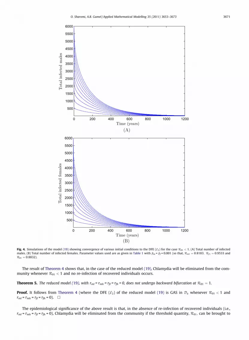
Fig. 4. Simulations of the model (19) showing convergence of various initial conditions to the DFE (E2) for the case R01 < 1. (A) Total number of infectedmales. (B) Total number of infected females. Parameter values used are as given in Table 1 with bm = bf = 0.001 (so that, Rm1 ¼ 0:8183; Rf 1 ¼ 0:9533 andR01 ¼ 0:8832).


The result of Theorem 4 shows that, in the case of the reduced model (19), Chlamydia will be eliminated from the com-munity whenever R01 < 1 and no re-infection of recovered individuals occurs.

Theorem 5. The reduced model (19), with rml = rmh = rfl = rfh = 0, does not undergo backward bifurcation at R01 ¼ 1.

Proof. It follows from Theorem 4 (where the DFE (E2) of the reduced model (19) is GAS in Da whenever R01 < 1 andrml = rmh = rfl = rfh = 0). h

The epidemiological significance of the above result is that, in the absence of re-infection of recovered individuals (i.e.,rml = rmh = rfl = rfh = 0), Chlamydia will be eliminated from the community if the threshold quantity, R01; can be brought to


(and maintained at) a value less than unity. Fig. 4A and B show simulation results converging to the DFE (E2) whenrml = rmh = rfl = rfh = 0 for the case when R01 < 1. These results (Theorems 4 and 5) are consistent with the result in [1], forthe corresponding sex-structured Chlamydia transmission model without risk structure (a Lyapunov function argumentwas, however, used to prove the GAS of the DFE of the model in [1]).

In summary, the reduced model (19) has the following qualitative features:

(i) It has a LAS DFE whenever R01 < 1;(ii) It undergoes backward bifurcation at R01 ¼ 1. This phenomenon is removed in the absence of re-infection;

(iii) It has a GAS DFE whenever R01 < 1 and rml = rmh = rfl = rfh = 0.

Thus, this study shows that stratifying the infected sexually-active population based on ability to transmit infection alone(but not stratifying the susceptible population in terms of their risk of acquiring infection) does not change the (asymptotic)qualitative features of Chlamydia transmission dynamics (with respect to the persistence or elimination of the disease). Inthis setting, the model undergoes a re-infection induced backward bifurcation at R01 ¼ 1; and this phenomenon can be re-moved if no re-infection of recovered individuals occurs. However, if the susceptible population is also stratified according tothe risk of acquiring infection, this study shows that the absence of re-infection cannot remove the backward bifurcationproperty of the model (under this setting).

5. Conclusions

A new sex-structured deterministic model, which stratifies the entire sexually-active population based on the risk ofacquiring or transmitting infection, is designed and used to study the transmission dynamics of Chlamydia in a population.The main theoretical findings of the study are itemized below.

(i) The model (3) has a locally-asymptotically stable disease-free equilibrium whenever the associated reproductionnumber ðR0Þ is less than unity;

(ii) The model (3) exhibits the phenomenon of backward bifurcation, where the stable disease-free equilibrium co-existswith a stable endemic equilibrium, when the associated reproduction number ðR0Þ is less than unity. This phenom-enon persists even in the absence of re-infection of recovered individuals;

(iii) The backward bifurcation property of the model (3) can be removed if the susceptible male and female populations arenot stratified according to risk of acquiring infection and the re-infection parameters (for recovered individuals) areset to zero. In this case (where the susceptible populations are not stratified according to risk of acquiring infection,and rml = rmh = rfl = rfh = 0), the disease-free equilibrium of the reduced model (19) is globally-asymptotically stable ifthe associated reproduction number ðR01Þ is less than unity.

In summary, this study shows (perhaps for the first time) that the phenomenon of backward bifurcation can occur inChlamydia transmission dynamics even in the absence of the re-infection of recovered individuals. Thus, this study extendsthe earlier results on modeling Chlamydia transmission in a population (including that reported in [1]) by showing that there-infection of re-covered individuals, although sufficient, is not necessary for the presence of the backward bifurcation inChlamydia transmission dynamics.

Acknowledgments

One of the authors (ABG) acknowledges, with thanks, the support in part of the Natural Science and Engineering ResearchCouncil (NSERC) and Mathematics of Information Technology and Complex Systems (MITACS) of Canada. OS gratefullyacknowledges the support of the University of Manitoba Graduate Fellowship. The authors are grateful to the referees fortheir constructive comments.

References

[1] O. Sharomi, A.B. Gumel, Re-infection-induced backward bifurcation in the transmission dynamics of Chlamydia trachomatis, J. Math. Anal. Appl. 356(2009) 96–118.

[2] K.A. Fenton, C.M. Lowndes, Recent trends in the epidemiology of sexually transmitted infections in the European Union, Sex. Transm. Infect. 80 (2004)255–263.

[3] Initiative for Vaccine Research (IVR) – Sexually Transmitted Diseases. <http://www.who.int/vaccine_research/diseases/soa_std/en/index.html>(accessed 01.03.2010).

[4] K. Manavi, A review on infection with Chlamydia trachomatis, Best Pract. Res. Clin. Obstet. Gynaecol. 20 (2006) 941–951.[5] W.C. Miller, C.A. Ford, M. Morris, M.S. Handcock, J.L. Schmitz, M.M. Hobbs, M.S. Cohen, K.M. Harris, J.R. Udry, Prevalence of chlamydial and gonococcal

infections among young adults in the United States, JAMA 291 (2004) 2229–2236.[6] J.A. Schillinger, E.F. Dunne, J.B. Chapin, J.M. Ellen, C.A. Gaydos, N.J. Willard, C.K. Kent, J.M. Marrazzo, J.D. Klausner, C.A. Rietmeijer, L.E. Markowitz,

Prevalence of Chlamydia trachomatis infection among men screened in 4 U.S. cities, Sex. Transm. Dis. 32 (2005) 74–77.[7] Sexually Transmitted Diseases (Chlamydia Fact Sheet), 2007. <http://www.cdc.gov/std/Chlamydia/STDFact-Chlamydia.htm#WhatIs>. (accessed

14.03.2010).

http://www.who.int/vaccine_research/diseases/soa_std/en/index.html

http://www.cdc.gov/std/Chlamydia/STDFact-Chlamydia.htm#WhatIs


[8] Trends in Reportable Sexually Transmitted Diseases in the United States, 2004. <http://www.cdc.gov/std/stats04/trends2004.htm>. (accessed01.04.2008).

[9] The World Health Report-Changing History, 2004. <http://www.who.int/entity/whr/2004/en/report04_en.pdf> (accessed 01.04.2008).[10] D.D. Mcdonnell, V. Levy, T.J.M. Morton, Risk factors for chlamydia among young women in a northern California juvenile detention facility:

implications for community Intervention, Sex. Transm. Dis. 36 (2) (2009) S29–S33.[11] C. Navarro, A. Jolly, R. Nair, Y. Chen, Risk factors for genital chlamydial infection Can, J. Infect. Dis. 13 (3) (2009) 195–207.[12] Sexually Transmitted Diseases Surveillance, 2008. <http://www.cdc.gov/std/stats08/chlamydia.htm>. (accessed 17.03.2010).[13] C.F. Martin, L.J.S. Allen, M.S. Stamp, An analysis of the transmission of chlamydia in a closed population, J. Differ. Equat. Appl. 2 (1) (1996) 1–29.[14] K. Mirjam, T.H. Yvonne, P. van Duynhoven, S.J. Anton, Modeling prevention strategies for gonorrhea and Chlamydia using stochastic network

simulations, Am. J. Epidemiol. 144 (3) (1996) 306–317.[15] Brunham et al, The unexpected impact of a Chlamydia trachomatis infection control program on susceptibility to reinfection, JID 192 (2005) 1836–

1844.[16] Regan et al, Coverage is the key for effective screening of Chlamydia trachomatis in australia, JID 198 (2008) 349–358.[17] J.A. Burns, E.M. Cliff, S.E. Doughty, Sensitivity analysis and parameter estimation for a model of Chlamydia trachomatis infection, J. Inverse Ill-Posed

Probl. 15 (3) (2007) 243–256.[18] D. Evenden, P.R. Harper, S.C. Brailsford, V. Harindra, System dynamics modelling of Chlamydia infection for screening intervention planning and cost-

benefit estimation, IMA J. Manage. Math. 16 (3) (2005) 265–279.[19] D.P. Wilson, P. Timms, D.L.S. McElwain, A mathematical model for the investigation of the Th1 immune response to Chlamydia trachomatis, Math.

Biosci. 182 (1) (2003) 27–44.[20] D.P. Wilson, D.L.S. McElwain, A model of neutralization of Chlamydia trachomatis based on antibody and host cell aggregation on the elementary body

surface, J. Theoret. Biol. 226 (3) (2004) 321–330.[21] D.P. Wilson, P. Timms, D.L.S. McElwain, P.M. Bavoil, Type III secretion, contact-dependent model for the intracellular development of Chlamydia, Bull.

Math. Biol. 68 (1) (2006) 161–178.[22] K. Mirjam, W. Robert, A. van den Hoek, P.J. Maarten, Comparative model-based analysis of screening programs for Chlamydia trachomatis infections,

Am. J. Epidemiol. 153 (1) (2001) 90–101.[23] Turner et al, Developing a realistic sexual network model of chlamydia transmission in Britain, Theoret. Biol. Med. Model. 3 (2006) 3. doi:10.1186/

1742-4682-3-3.[24] Molano et al, The natural course of Chlamydia trachomatis infection in asymptomatic Columbian women: A 5-year follow-up study, JID 191 (2005)

907–916.[25] Morre et al, The natural course of asymptomatic Chlamydia infections: 45% clearance and no development of PID after one-year follow-up, Int. J. STD

AIDS 13S2 (2002) 12–18.[26] Charlotte et al, Chlamydia trachomatis reinfection rates among female adolescents seeking rescreening in school-based health centers, Sex. Transm.

Dis. 35 (3) (2008) 233–237.[27] F. Monica, C.S. Katherine, K.K. Charlotte, D.K. Jeffrey, Chlamydial and gonococcal reinfection among men: a systematic review of data to evaluate the

need for retesting, Sex. Transm. Infect. 83 (2006) 304–309. doi:10.1136/sti.2006.024059.[28] Quinn et al, Epidemiologic and microbiologic correlates of Chlamydia trachomatis infection in sexual partnerships, JAMA 276 (1996) 1737–1742.[29] Z. Mukandavire, W. Garira, Age and sex structured model for assessing the demographic impact of mother-to-child transmission of HIV/AIDS, Bull.

Math. Biol. 69 (6) (2007) 2061–2092.[30] O. Sharomi, A.B. Gumel, Dynamical analysis of a sex- structured Chlamydia trachomatis transmission model with time delay, Nonlinear Anal.: Real

World Appl. 12 (2) (2010) 837–866.[31] H.W. Hethcote, The mathematics of infectious diseases, SIAM Rev. 42 (4) (2000) 599–653.[32] P. van den Driessche, J. Watmough, Reproduction numbers and sub-threshold endemic equilibria for compartmental models of disease transmission,

Math. Biosci. 180 (2002) 29–48.[33] C. Castillo-Chavez, B. Song, Dynamical models of tuberculosis and their applications, Math. Biosci. Eng. 1 (2) (2004) 361–404.[34] J. Dushoff, H. Wenzhang, C. Castillo-Chavez, Backwards bifurcations and catastrophe in simple models of fatal diseases, J. Math. Biol. 36 (1998) 227–

248.[35] Z. Feng, C. Castillo-Chavez, F. Capurro, A model for tuberculosis with exogenous reinfection, Theoret. Popul. Biol. 57 (2000) 235–247.[36] C.N. Podder, A.B. Gumel, Qualitative dynamics of a vaccination model for HSV-2, IMA J. Appl. Math. 75 (1) (2009) 75–107.[37] O. Sharomi, C.N. Podder, A.B. Gumel, E.H. Elbasha, J. Watmough, Role of incidence function in vaccine-induced backward bifurcation in some HIV

models, Bull. Math. Biol. 210 (2) (2007) 436–463.[38] O. Sharomi, C.N. Podder, A.B. Gumel, B. Song, Mathematical analysis of the transmission dynamics of HIV/TB co-infection in the presence of treatment,

Math. Biosci. Eng. 5 (1) (2008) 145–174.[39] M. Lipsitch, M.B. Murray, Multiple equilibria: tuberculosis transmission require unrealistic assumptions, Theoret. Popul. Biol. 63 (2) (2003) 169–170.[40] V. Lakshmikantham, S. Leela, A.A. Martynyuk, Stability Analysis of Nonlinear Systems, Marcel Dekker, Inc., New York and Basel, 1989.[41] H.L. Smith, P. Waltman, The Theory of the Chemostat, Cambridge University Press, 1995.

http://www.cdc.gov/std/stats04/trends2004.htm

http://www.who.int/entity/whr/2004/en/report04_en.pdf

http://www.cdc.gov/std/stats08/chlamydia.htm

mathematical study of a risk-structured two-group model for chlamydia transmission dynamics

Documents