LINEAR AND NONLINEAR OPTICAL PROPERTIES OF ARTIFICIALLY STRUCTURED MATERIALS

Suresh Pereira

A thesis submitted in conformity with the requirements for the degree of Doctor of Philosophy

Graduate Depart ment of Physics University of Toronto

Copyright @ 2001 by Suresh Pereira

Natianat tibrafy I * D Bibliothèque nationaie du Canada

395 W ~ g O o n Street 395, nie weniigml Oitawa ON K 1 A W ûtütwaON K 1 A W Canada Canada

The author has granted a non- exclusive licence allowing the National Libmy of Canada to reproduce, loan, districbute or seli copies of t h thesis in rnicroform, paper or electronic formats.

The author retains ownership of the copyright in this thesis. Neither the thesis nor substantial extracts &om it may be printed or otherwise reproduced withouî the author's permission.

L'auteur a accordé une licence non exclusive pennem B la Bibiiothèque nationale du Canada de reproduire, prêter, distribuer ou vendre des copies de cette thèse sous la forme de microfiche/nIm, de reproduction çm papier ou sur fomat 6Iectronique.

L'auteur conserve la propriété du droit d'auteur qui protège cette thèse. Ni la thèse ni des extraits substantiels de celle-ci ne doivent être imprimés ou autrement reproduits sans son autorisation.

Abstract

Linear and Noalineax Opticd Properties of Arti6cially Structurecl Materiais

Suresh Pereira

Doctor of Philosophy

Graduate Department of Physics

University of Toronto

2001

We begin by deriving a set of equations that describe pulse propagation in one di-

mensional, periodic media, in the presence both of birefringence and a Kerr nonlinearity

'Ne use these equations to interpret the results ot a mies of experiments performed in

Bber gatings, which, with the appropriate approximations, c m be considered to have

one effective dimension.

WC ncxt turn to thc consideration of ho diamel a-a'~xguides coupleci bÿ a sequace of

periodicdy spaced microresonators, in the presence of a Kerr nonlinearity. We show that

h o distinct types of gaps open in the dispersion relation of the device. The frequency of

one type of gap is related to the spacing of the resonators. The fkequency of the other

type of gap is related to the radius of the resonators. We derive a set of coupled nonlinear

Schrodinger equations (NLSE) to describe the propagation of light in the system. We

show that the properties of the dispersion reiation in the vicinity of the two types of gaps

are markedly different, and that near the gap associateci wit h the radius of the resonators,

the group velocity dLspersion experienced by a pulse is very small. We then demonstrate

that a gap soliton should be observable at much lower intensities in this latter gap than

in a Bragg gap of the same frequency width.

We study the operation of a grating-~aveguide structure (GWS), where a grating

is used to coupled an incident plane wave into a guided mode of a layered medium.

We derive equations that determine the field everywhere in the presence of a grating of

arbitrary t hiclmes, and a Kerr nonlineari~. We demonstrate that the GWS can be used

as a low-loss, narrow-band ref'iector, or as an ail optical switch.

Finally, we construct a Hamiltonian formulation for pulse propagation equations in

a one dimensional, Kerr nonlinear, periodic medium. In doing so, we clear up some

confusion in the literature surrounding the nature of the conservai quantities associatecl

wit h Kerr nonlinear pulse propagation equations.

Acknowledgement s

This thesis is for Sun Young, Raoul, Phoebe, Kevin, Aubert and the Duck, each of

whom should know what they contnbuted.

I wodd like to thank the foilowing people for helping to make this thesis what it is.

Di. RE. Slusher and Dr. S. Spater for their perseverance on the fiber experiments and

Dr. G. Marowsky, Dr. M-A Bader, Dr. H-M Keller for their enthusiasm and guidance.

1 would also like to thank Dirk and Uwe for the^ generous hospitality in Gottingen!

Furthermore, for t heir help in maintainhg my sanity, 1 am indebted to Dr. J. Levhe and

Dr. S. Winters, the latter of whom, if justice d e s this world, will be Professor Wmters

by the t h e this thesis is bound.

Primarüy, though, 1 would like to thank Dr. J.E. Sipe for his concise explmations of

the ha points of phy~ics; and for providing iui deguit picture of cornpetence during his

imprisonrnent in administration. Hold tight, sir - I'm working on a plan to bust you out

by September 2002.

Contents

1 Introduction 1

2 Pulse propagation in birefrhgent. nonlinear media with deep gratings 11

2.1 Introduction . . . . . . . . . . . . . . . . . . . . . . . . . . . . . . . . . . 11

2.2 Linear Equations and Basis Functions . . . . . . . . . . . . . . . . . . . . 14

2.2.1 Periodic Structures . . . . . . . . . . . . . . . . . . . . . . . . . . 15

2.3 Noniinearity and Multiple Scales Analysis . . . . . . . . . . . . . . . . . 17

2.3.1 Multiple Scales Analysis . . . . . . . . . . . . . . . . . . . . . . . 17

2.4 One Principal Component; s=2: CNLSE . . . . . . . . . . . . . . . . . . 20

2.5 Two Principal Components; s=l: CME . . . . . . . . . . . . . . . . . . . 24

2.5.1 Weak Grating Limit of the NLCME . . . . . . . . . . . . . . . . . 29

2.6 Connecting the CNLSE and the NLCME . . . . . . . . . . . . . . . . . . 30

. . . . . . . . . . . . . . . . . . . . . . . . . . . . 2.7 Numerical Simulations 35

2.7.1 Cornparhg the CNLSE and CME . . . . . . . . . . . . . . . . . . 35

2.8 Conclusion . . . . . . . . . . . . . . . . . . . . . . . . . . . . . . . . . . . 39

3 Polarkation effects in birefringent. periodic. nonlinear media 41

3.1 Introduction . . . . . . . . . . . . . . . . . . . . . . . . . . . . . . . . . . 41

. . . . . . . . . . . . . . . . . . . . . . . . 3.2 Theory for an hfbîte grating 44

. . . . . . . . . . . . . . . . . . . . . . . . 3.2.1 Modelling the Grating 44

3.2.2 Coupled Noniinear Schrddinger E<iuations . . . . . . . . . . . . . 46

3.3 Physicd Grating . . . . . . . . . . . . . . . . . . . . . . . . . . . . . . . 50

3.4 Approximate Solution for Polarization Evolution . . . . . . . . . . . . . . 52

. . . . . . . . . . . . . . . . . . . . . . . . . . . . . . 3.5 Experimental Data 55

3.5.1 Polarizat ion Evolut ion for high det unings . . . . . . . . . . . . . . 58

. . . . . . . . . 3.5.2 Polarization Instability as a function of Phase Lag 60

3.6 Conclusion . . . . . . . . . . . . . . . . . . . . . . . . . . . . . . . . . . . 64

4 Gap soliton propagation in a two-channe1 SCISSOR structure 66

4.1 Introduction . . . . . . . . . . . . . . . . . . . . . . . . . . . . . . . . . . 66

4.2 Linear theory . . . . . . . . . . . . . . . . . . . . . . . . . . . . . . . . . 71

4.2.1 Dispersion relation for the bmChannel SCISSOR . . . . . . . . . 73

. . . . . . . . . . . . . . . . . . . . . . . . . . . . . . . . 4.3 Coupled NLSE 77

4.3.1 Multiple Scales . . . . . . . . . . . . . . . . . . . . . . . . . . . . 79

4.3.2 Nonlinear Response . . . . . . . . . . . . . . . . . . . . . . . . . . 81

4.3.3 Coupled NLSEs . . . . . . . . . . . . . . . . . . . . . . . . . . . . 83

4.4 Discussion . . . . . . . . . . . . . . . . . . . . . . . . . . . . . . . . . . . 86

4.5 Conclusion . . . . . . . . . . . . . . . . . . . . . . . . . . . . . . . . . . . 92

5 Theory for a grating-waveguide structure with Kerr nonlinearity 94

. . . . . . . . . . . . . . . . . . . . . . . . . . . . . . . . . . 5.1 Introduction 94

5.2 The GWS and the Guided Modes . . . . . . . . . . . . . . . . . . . . . . 96

. . . . . . . . . . . . . . . . 5.3 Green Function Theory for Stratifiecl Media 98

5.3.1 Grating, No Nonlinearity . . . . . . . . . . . . . . . . . . . . . . . 104

5.3.2 No grating. Kerr Nonlineariw . . . . . . . . . . . . . . . . . . . . 105

5.3.3 nansfer matrices at the Interface . . . . . . . . . . . . . . . . . . 206

5.4 Numerical Simulations . . . . . . . . . . . . . . . . . . . . . . . . . . . . 108

5.4.1 Low loss rdector in the UV . . . . . . . . . . . . . . . . . . . . . 108

5.4.2 NonlineaxswitchinginaGWS . . . . . . . . . . . . . . . . . . . . 110

5.5 Conclusion . . . . . . . . . . . . . . . . . . . . . . . . . . . . . . . . . . . 113

6 Hamiltonian formulation for pulse propagation equations in a periodic.

nodnear medium 114

6.1 Introduction . . . . . . . . . . . . . . . . . . . . . . . . . . . . . . . . . . 114

6.2 Canonical formulation of Maxwell's Equations . . . . . . . . . . . . . . . 116

6.2.1 Linear. Periodic Medium . . . . . . . . . . . . . . . . . . . . . . . 118

6.2.2 Periodic Medium with a Kerr noniinearity . . . . . . . . . . . . . 119

6.3 Muced Hwniltonian and the NLSE . . . . . . . . . . . . . . . . . . . . 122

6.3.1 Effective Fields and Envelope Functions . . . . . . . . . . . . . . 128

6.4 Conserved Quantities of the Hamiltonian . . . . . . . . . . . . . . . . . . 130

6.5 an the use of the Dual Field . . . . . . . . . . . . . . . . . . . . . . . . . 134

6.6 Conclusion . . . . . . . . . . . . . . . . . . . . . . . . . . . . . . . . . . . 136

7 Conclusion 137

Bibliography

Chapter 1

Introduction

In the past several decades, the wide research into artificidy structured materials (AS&)

has led to numerous technological applications, ranging kom biological sensors to waw

length division multiplexiug devices. Beyond their value to industry, ASiLIs offer a host

of challenges to researchem in basic physics. For cxamplc, the microresonator devices

that have been investigated in the past few years could potentiaily be wed to investigate

opt ical shock formation [Il, and have been used to study cavity quantum electrodynam-

ics [2]. In addition to these effects, ASMs present engaging geometries for the study of

nonlinear dynamics, and can be used as d-optical switches (31, and d-optical logic gates

141 - The material in this thesis is centred around the linear and Kerr nonlinear proper-

ties of optical pulse propagation in AS&. A Kerr nonlineazity is often described by

the introduction of a nonlinear index of refraction coefficient, n,, whereby a pulse with

intemie I will experknce an effective index of refraction nef/ = n + nzI, where n is the

background index of refraction in the lirnit I -r O (51. The pulses considered here are of

picosecond duration, with ca.rrier hequencies in the near IR to near W, so that the en-

velope function of the puise is slowly varying relative to the carrier kequency. There are

two m a h reasons for this. First, some of the most promishg applications of the systerns

that are studied here are in telecornmunicatiors, where the standard pulse duration is

in the picosecond range. Second, it is often better to M y understand nonlinear dects

for slowly varying pulses before moving to shorter pulses, where higher-order nonlinear

efTects can complicate the interpretation of experiments. The derivat ions presented in

this thesis c m alI be extendeci to describe the propagation of shorter pulses.

In chapters two and three of this thesis, the properties of birefnngent, periodic, Kerr

media with one effective dimension are studied. Here periodic means that both the index

of re£raction and the nonlinear index coefficient vary spatially with period d. Bir-gence

refers to the fact that the index of refkaction experienced by the two polarkations of

light are unequal, R, # Q, where x and y are the principal axes of polarization. We

introduce nb = - E, to quantify this birefringence. Examples of media that can

be considered to have one effective dimension include fiber Bragg gratings and etched

dielectric waveguides, when the etching is shallow. In these systems, the transverse

directions can be accotinted for by defining a mnde profile that remaine unchangecl during

propagation. For pulse propagation wit h intensities sufliciently low t hat nonlinear effects

are negligible, a medium is characterized by its dispersion relation, w (k) , which relates

the kequency of the Light, w , to the corresponding wave number, k. It is weil known

that an infinite periodic medium in one dimension always poseses a photonic band

gap - a range of frequencies in which light c m o t propagate [6]. This photonic band

gap is centred around the Bragg frequency, wo, of the medium, which is the bequency

at which the coherent rdections at the va.rious interfaces of the medium can build up.

Heuristically, this requires the reflected light kom one int d a c e t O be phase-matched

with that fiom another interface. The precise value of this Bragg bequency is diçcussed

below, after Equation (1.1).

In many practical periodic systems, such as fiber Bragg gratlligs, the strength of the

periodic variation in the index of rekaction (the index mntrast, bn) is very small relative

to the average background index of refraction (6nF N IO-^). This allowed previous

researchers to treat Light in the medium as a forward-propagating wave that experiencled a

weak coupling to a backward-propagating wave via the grating (and vice versa). A similar

analysis can be carried out with thinly etched waveguides, because there, aithough the

index contrast between the wawguide material and air is quite strong, the region of the

etching is s m d relative to the transverse dimensions of the mode profile. Furthemore,

it was assumed that the intensity of the pulses being described was such that the effect

of the Kerr nonlinearity codd be considered a small perturbation to the linear results.

Such analyses led to the derivation of the heuristic coupled-mode equations (CME), which

describe the evolution of slowly varying endope functions, A* (2, t ) , propagating in the

forward (+) and backward (-) directions , camed at the Bragg wavenumber (ko = r / d )

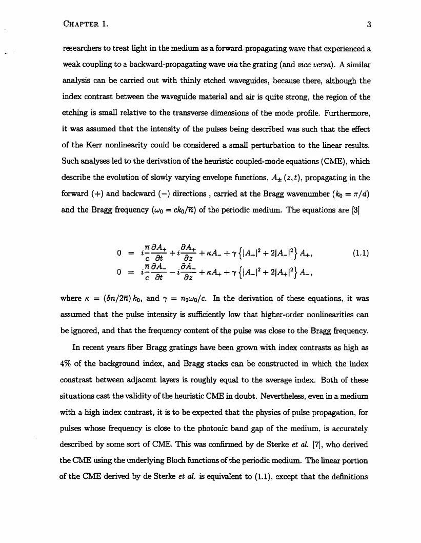
and the Bragg fiequency (wo = cko/x) of the periodic medium. The equations are [3]

5 a A - .dA, O = 2--

c at - 2- + KA+ +r { I A - ~ ~ + 21~+1' ) A-, dz

where n = (6n/2n) ko, and 7 = nzwo/c. In the derivation of these equations, it was

assumed that the pulse intensiw is SufEciently low that higher-order nonlinearities can

be ignored, and that the fkquency content of the pulse was close to the Bragg frequency.

In recent years fiber Bragg gratings have been grown with index contrasts as high as

4% of the background index, and Bragg stacks c m be constructed in which the index

constrast between adjacent layers is roughly equal to the average index. Both of these

situations cast the validity of the heuristic CME in doubt. Nevertheles, even in a medium

with a high index contrast, it is to be expected that the physics of pulse propagation, for

pulses whose &equency is close to the photonic band gap of the medium. is accurately

described by some sort of CME. This was confimeci by de Sterke et al. [7], who derived

the CNE using the underlying Bloch funaions of the periodic medium. The hear portion

of the CME derived by de Sterke et al. is equident to (1. l), except that the definitions

of wo and n are taken directly £rom the dispersion relation of the linear, periodic medium-

The nonlinear portion cont ains the terms in (1.1) , but adds a series of more complicated

nonlinear interactions.

In chapter two of this thesis, the e£Forts of de Sterke et cd. are extendeci to include

the e f k t s of birehgence. When attempting to derive equations that govem the prop

agation of slowly-varying envelope functions, it quickly becornes apparent that there are

a number of different length, t h e , and strength scales in the problem. The period, d,

is much srnatter than the spatial width of the pulse; the carrier frequency of the pulse is

much larger than the spread in frequencies containeci within the pulse; the value of the

background index of rekaction, n, is much Iarger than both the birehgence, nb, and

the nonlinear portion of the effective index, n21. We use the 'method of multiple scaies'

to carefdy account for these different quantities [8]. The value of this method is that it

effectively dram out the underlying physics of the systems being studied.

The equations that are deriveci for bire-ent media are similar in form to (1.1),

but include nonlinear couphg between orthogonal polarbations of light. The C m are

moût usehl when the frequency content of the puise is close to, or within, the photonic

band gap of the medium. When the frequency content of the pulse is away from a

photonic band gap, it is shown that the propagation of light is weli described by a set of

coupled nonlinear Schr&i.inger equat ions (NLSEs) . The orthogonal polarizat ions are st ill

coupled by the nonlinearityl but the effect of the grating is to modify the values of the

group velocity (aw (k) lak), and group velocity dispersion (a2w (k) / a k 2 ) relative to their

values in the absence of a grating. As the carrier hequency of the pulse is tuned closer

to the photonic band gap, the group velocity is reduced, tending towards zero, and the

group velocity dispersion is enhmced (by orders of magnitude relative to typical material

dispersions). The reduced group velociw and enhancd dispersion can be understood as

a consecpence of light being refiected inside the grating, but without the refîections

being entirely phase-matched, so that they do not build up. The reàuction in group

velociw leads to a kequency-dependent effenective nonlinear index co&cient, raYf (w),

that is enhanceci for frequencies cloaer to the band gap for two reasons: first, the puise

is travelling more slowly, and hence has more time to interact with the nonlinea.ri@; and

second, the intensity distribution of the underlying Bloch functions of the periodic system

affects the manner in which the pulse interacts with the nonlinearity in the system.

The CME and NLSEs are connected in the sense that both can be used to accurately

describe pulse propagation when the carrier frequency is near, but not inside the gap.

The CME are the appropriate equations when the c h e r frequency is inside or very close

to the gap; the NLSEs are appropriate when the carrier frequency is detuned from the

gap, or when the pulse width is sctremely broad. In fact, the NLSE can be used to

describe broad pulses whose frequency content is within the gap. It is well known that

the NLSE can support soliton solutions - solutions where the group velocity dispersion

is perfectly balanced by the nonlinearity so that the profile of the pulse does not change

[SI. If one excites a soliton at the band edge, then its group :*clccity is zcm, and thc

resulting energy distribution is c d e d a gap soliton.

The advantage of developing a set of coupled NLSEs is that it allows a convenient

point of connection with existing literature on nonlinear pulse propagation in birefringent

media. In particular, the literature contains a great deal of research on the existence

and observation of vector solitons in optical fibers without a Bragg grating, and on the

phenornenon of nonlinear energy exchange between the polarizations. The initial work on

birefringent d&ts in optical fibers was done under the assumption that the birefringence

(nb) of the system is large relative to the value of nonlinear index of refraction that is

induced by the intensity ( 7 4 . Under such an assumption, the effects of nonlinear energy

exchange between polarizations can be ignored, because it will not be phase-matched, and

hence not build up. This is analogous to the situation of light with fiequency content far

removed £iom a photonic band gap of the syjtem. It was later pointed out that inclusion

of nonlinear energy exchange can have a number of &riking effects, includùig radiation

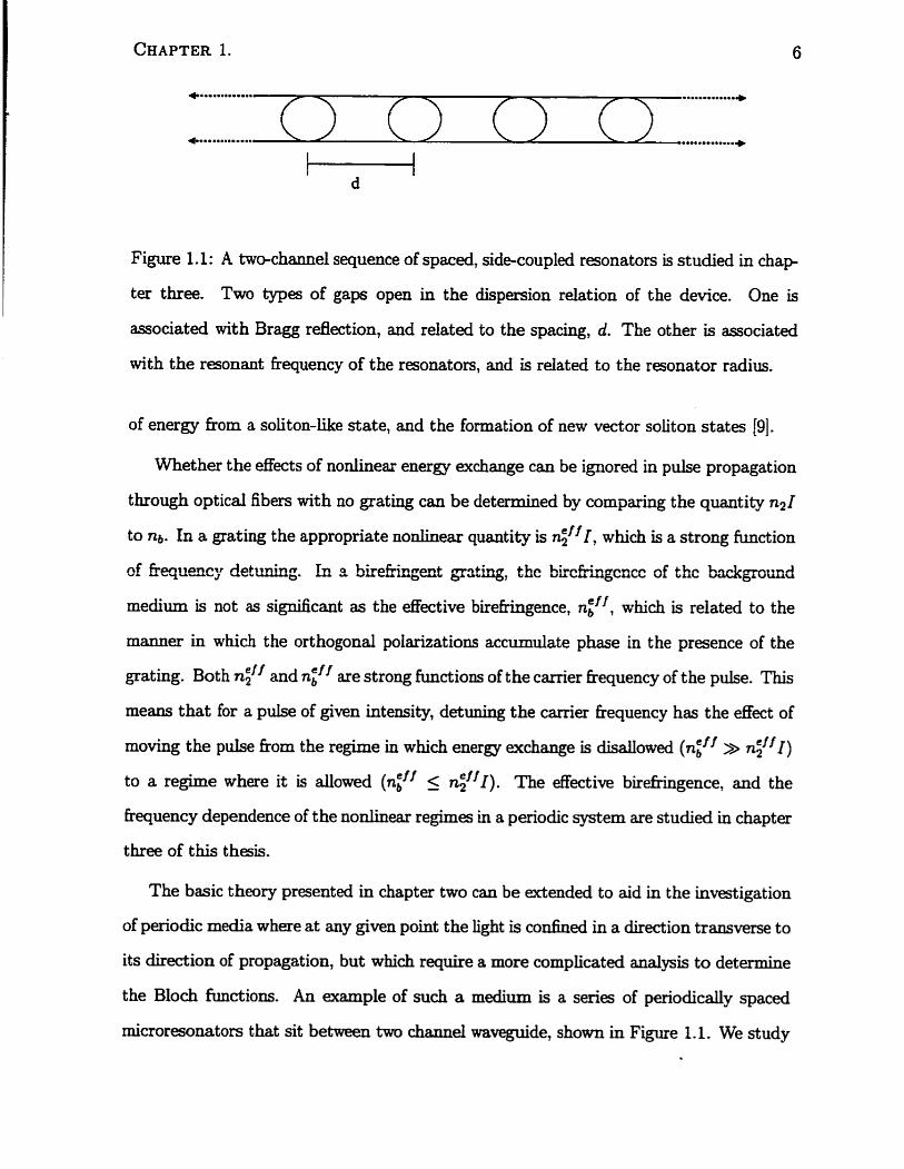
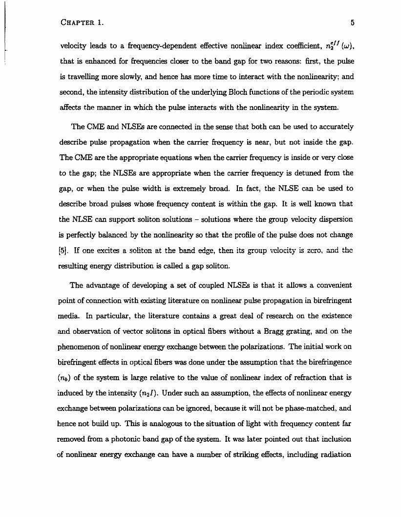
Figure 1.1: A two-chnel sequence of spaced, side-coupled resonators is studied in chag

ter three. T m types of gaps open in the dispersion relation of the device. One is

associated with Bragg reflection, and related to the spacing, d. The other is associated

with the resonant fkequency of the resonators, and is related to the resonator radius.

of energy fiom a soliton-like state, and the formation of new vector soliton states 191.

Whether the effects of nonlinear energy exchange can be ignored in puise propagation

t hrough optical fibers wit h no grating can be detemiined by comparing the quant ity nz 1

to ng. In a grating the appropriate nodinear quanti@ is n 2 1 , which is a strong function

of fkequency dettrning. In s birefringent gmting, the bircfringcncc of thc background

medium is not as si&cmt as the effective birefringence, ntff, which is reiated to the

manner in which the orthogonal polarizations accumulate phase in the presence of the

grating. Both n;lf and nb are stmng functiom of the c-er fkequency of the pulse. This

means that for a pulse of given intensity, detuning the carrier hequency has the &ect of

moving the pulse fkom the regime in which energy evchange is disdowed ( n i f f » nyf 1)

to a regime where it is dowed (niff 5 n F f l ) . The effective birehgence, and the

fkequency dependence of the nonlinear regimes in a periodic system are studied in chapter

three of this thesis.

The basic theory presented in chapter two cm be extended to aid in the investigation

of periodic media where at any given point the light is conhed in a direction transverse to

its direction of propagation, but which require a more complicated analysis to determine

the Bloch fimctions. An example of such a medium is a series of periodically spaced

microresonators that sit between two Channel waveguide, shown in Figure 1.1. We study

this system in chapter four. Light travelling in either of the charineh can couple into,

and circulate around, the microresonators. A pulse sent through such a system will

propagate either forward ûr backward, but the one-dimensional expressions for the Bloch

hinctions that were used in chapter two are no longer appropriate. In moving to a higher

dimensional theory, it is necessary to generalize the mathematical tools of chapters two

and three.

In the 1 s t several years, microresonators have attracted a great deal of interest as

device elements that can couple light between waveguides, or allow light to turn a 90°

bend. They can be fabricated with low los, and high quality factors [IO]. If the medium

from which the microresonator is fabricated is linear, then a given microresonator has a

resonant Bequency w r = M ( C ~ E R ) , where M is an integer, n is the index of refkaction

of the microresonator, and R is its radius. If the resonators are spaced with period

d, then Bragg refktion leads to the opening of a photonic band gap centred around

f rq i i~nc ie s uf = Rr !m! ( ~ d ) ) (a Bragg gap), where N k an integer. Thio reflection

occurs because light travelling in the forward direction in the lower channel of the system

is weakly coupled, via the microresonator, to light travelling in the backward direction of

the upper Channel. However, in addition to the photonic band gaps associated with Bragg

rdection, t here also exist gaps associat ed wit h the resonances of the microresonat or (a

resonator gap). The Bragg gaps open because the relatively s m d coupling between

directions at hequency wb can build up; the resonator gaps open because at fiequency

w, the coupling between directions is immense.

The two types of gaps associated with the microresonator stmcture have a rather

different character. In both cases the group velocity tends t o m & zero, but while the

group velocity dispersion around a Bragg gap can becorne enormous, around a resonator

gap it becornes very s m d . In chapter four it is shown that in the presence of an opticd

Kerr nonhearity, the propagation of pulses with carrier fkquencies near either gap is

w d described by a NLSE, but since the group velocity dispersion near a resonator gap

Incident \

Figure 1.2: In a grating-waveguide structure (GWS) , st udied in chapt er four, an incident

plane wave is coupled to a guided mode of a l a y d medium via a gating. The guided

mode is coupled back out, making the device 100% reflecting when the appropriate

resonance condition is met.

is much smder, it should be possible to excite a gap soliton with much less energy.

In the lirnit where the upper channel is removeci, both types of photonic band gaps

of the system vanish (because it is assumed that coupling into the resonator incurs no

reflection, so the foxward and backward propagation directions are cornpletely uncou-

pled). In such a situation the spacing between resonators becomes irrelewt - only the

average densiw of resonators is important. An interesting feature of this system is that

as the caxrier kequency of a pulse nears w,, the group velocity of the pulse tends towards

zero, and the group velociw dispersion becomes zero (neglecting the dispersion of the

background medium). Roughly speaking, the group velocity becomes s m d because the

iight spends a long tirne circdating in each resonator. For a monochromatic excitation,

the intensity in each resonator can become enormous. This build-up in intensity c m be

used to obsenre low-threshold nonlinear switching, or to observe twephoton absorption

for biologicd sensing applications.

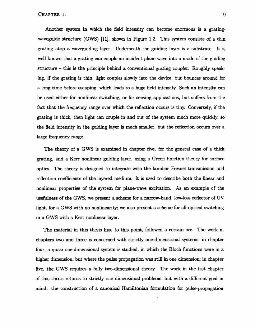
Another system in which the field intensitJt can become enonnous is a grating-

waveguide structure (GWS) (1 11, shown in Figure 1.2. This system consists of a thin

grating atop a waveguidmg layer. Underneath the guiding layer is a substrate. It is

well known that a grating can couple an incident plane wave into a mode of the guiding

structure - this is the principle behind a conventional grating coupler. Roughly speak-

hg, if the grating is t h , light couples slowly into the device, but bounces around for

a long time before escaping, which leads to a huge field intensity. Such an intensity can

be used either for nonlinear switching, or for sensing applications, but suffers bom the

fact that the fiequency range over which the reflection occurs is tiny. Conversely, if the

grating is thick, then light can couple in and out of the system much more quickly, so

the field intensity in the guiding layer is much smder? but the reflection occurs over a

large kequency range.

The theory of a GWS is examineci in chapter five, for the general case of a thick

m~ting, and a Kerr nonünear egcbg layer, ushg a Green Emtion theor). for surface O

optics. The theory is designed to integrate with the familiar Frgnel transmission and

rdection coeflicients of the layered medium. It is used to describe both the linear and

nonlinear properties of the system for plane-wave excitation. As an example of the

u s e f i e s of the GWS, we present a scheme for a narrow-band, low-loss reflector of W

light , for a GWS with no nonlinearity; we also present a scheme for d-optical switching

in a GWS with a Kerr nonlinear layer.

The material in this thesis has, to this point, followed a certain arc. The work in

chapters two and three is concerned with strictly onedimensional systems; in chapter

four, a quasi one-dimemional system is studied, in which the Bloch functions were in a

higher dimension, but where the pulse propagation was stiU in one dimension; in chapter

£ive, the GWS requires a M y dimensiona al th- The work in the last chapter

of this thesis returns to strictly one dimensional problems, but with a different goal in

mind: the construction of a canonical Hamiltonian formulation for pulse-propagation

equations, where 'canonical' means that the Hamiltonian is equal to the energy in the

electromagnetic field, and derives the correct equations of motion using the Heisenberg

equations of motion. The motivation for this work is three-fold. First, the dynamics of

Kerr nonlinear systems have often been studied using an effective IIainiltonian that was

not equd to the energy in the electrornagnetic field but that, newrtheless, generated the

appropriate equations of motion. This led to a certain confusion because it was uncertain

how to interpret the three conserved quantities: energy, momentum, and the effective

Hamiltonian. In this thesis, conhision about the conserved quantities is avoided by using

a Hamiltonian that is equal to the energy in the electromagnetic field. It is then shown

that the quantity previously Iabelled 'energy' is, in fact, the conserved charge associated

with phase-translation symmetry, and is equal to the tme energy oniy to zeroth order.

The second motivation for this work is to develop a more effective methodology for the

constmction of pulse propagation equations in media vvith periodicity in two and three

àimensions. The Harniltonian formulation presented here is used to derive a NLSE, and

it can easily be generalized to two or three dimensions. A third motivation for this work

is that the Hamiltonian formulation presented here can be generalized to give a quantum

mechanical description of the fields.

Chapter two of this thesis has previously been published in Physical Review E. Parts

of chapter three will be published in the near future as a chapter in a Springer-Verlag

adMncd topic book. The work in chapters fonr t h g h six is being prepared for p u b

lication in the near future.

Chapter 2

Pulse propagation in birefringent , nonlinear media wit h deep gratings

2.1 Introduction

In recent years, much effort has been devoted to the study of one dimensional photonic

bandgap materi& in the presence of a Kerr nonlinearity [3] [7] [12] [U] [14] (151. 4 great deal

of the experimental work in this field has concentrateci on fiber Bragg gratings, which

typicdy have refiactive index variations on the order of IO-' [l6] [17] [18]. With such

s m d index variations, it is reasonable to apply the heuristic coupled mode equations, or

the appropriate noalinear Schrodiuger equation, to analyze experimental results [3] [16].

However, index changes as high as 0.04 have been reported in fibers [19], and experiments

employing etched semiconductor waveguides have been proposed [20]. These systems

have SUfEiciently lwge index contrasts so as to cast doubt on the validiw of the heuristic

coupled mode equations. In a recent paper [7], a coupled mode theory was dewloped

that accounts for strong gratings, in which the index contrast varies over a significant

&action of the average background index, with a Kerr nonlinearity.

In this chapter we extend the strong grating, nonlinear coupled mode forrnalism to

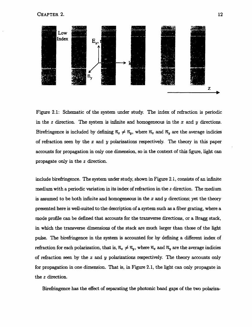
Figure 2.1: Schematic of the system under study. The index of refkaction is periodic

in the z direction. The system is W t e and homogeneous in the x and y directions.

Birefringence is includcd by defimg E, # Q, where E, and E, are the average indicies

of refraction seen by the x and y polarizations respectively. The theory in this papa

accounts for propagation in only one dimension, so in the context of this figure, light can

propagate only in the z direction.

include birefringence. The system under study, shown in Figure 2.1, consists of an infinite

medium with a periodic variation in its index of &action in the z direction. The medium

is assumed to be both infinite and homogeneous in the x and y directions; yet the theory

presented here is wdl-suited to the description of a system such as a fiber grating, where a

mode profile can be dehed t hat accounts for the transverse directions, or a Bragg stack,

in which the transverse dimensions of the stack are much larger than those of the light

pulse. The birefringence in the system is accounted for by defining a Merent index of

refiaction for each polarization, that is, & # %, where E, and are the average indicies

of refiaction seen by the x and y polarizations respectively. The theory accounts ody

for propagation in one dimension. That is, in Figure 2.1, the iight can only propagate in

the z direction.

Birefiingence has the &ixt of separating the photonic band gaps of the two polariza-

tions so that, in certain frequency ranges, light of one polarization can propagate hely

while the other is blocked. This has immediate deleterious consequemes for proposed d e

vice based on circular polarization, where the hearly polarized signais are mixed. The

robustness of nonlinear effects, such as soliton formation and propagation t hrough grat ing

structures, has yet to be studied in the presence of birefringence. Although optical fibers

are nominally isotropie, the process of writing a pating introduces a birefnngence on the

order of loh6 [21]. The dynamics here can be expected to be more complicated than in

a bare optical fiber. In a bare optical fiber the two polarizations have diaerent group

velocities, but can be considered to &r equal dispersion [22]; this is not generally valid

in the presence of a grating. In addition to fiber experiments, semiconductor waveguides

with a X ( 3 ) nonlinearity, which possess TE and TM modes with dXerent group velocities

and dispersions, and which can have large index contrasts, have been stuciied experimen-

t d y [ZO]. Although our formalism is strictly one-dimensional, it provides a quslitative

insight into the properties of such structures. We note, too, that experiments in the

literature, such as the allsptical AND gate demonstrateci by Taverner et al. (181, require

a coupled mode formalism for their convenient a.ndysis, as will other experiments aimed

at exploithg polarization and nonünearity.

Weak-grating coupled mode equations for pulses in a nonlinear, birefringent, peri-

odic medium (231 have previously been reportecl. This chapter indudes derivations for

three sets of equations: weak- and strong- grating coupled mode equations, and coupled

nonlinear Schrodinger equations in the presence of birehgence. We use Bloch theory

to characterize the linear, birefringent problem, and the method of multiple scales to

include the nonlinearity and f i t e pulse width. Both the birefringence and nonlinearity

are assumeci to be weak, in a sense to be made precise below.

The o u t h e of this chapter is as follows. In Section 2.2 we dis= the linear properties

of a one dimensional, birefrkgent, periodic medium. In Section 2.3 we introduce the

method of multiple SC&, which we then use in Section 2.4 to derive a set of coupled

nonlinear Schrodinger equation, and in Section 2.5 to derive a set of of coupled mode

equations. In Section 2.6 we discuss the connection between the nonlinear Schrijdinger

equations and the coupled mode equations, and their respective regions of validity.

2.2 Linear Equations and Basis Functions

We begin with the linear Maxwell equations in the presence of a dielectnc tensor that is

a function of only one Cartesian component, E = ~ ( z ) . We assume that the (x, y) coorai-

nates can be chosen such that for a.il z the tensor is diagonal, E = dzag (E,, ( z ) , e, (2)).

Neglecting magnetic effects by setting the permeabiliw p equal to that of kee space,

p = po, we can then define indices of rehction associated with polarization dong the x

and y axe, n: ( x ) = Eii (2) where €0 is the permittivity of free space and where, for

the remainder of the text, the index i runs over x and y. We seek fields E(r, t ) , H(r, t )

that depend only on the coordinate z. To proceed, we introduce local mode amplitudes

where no is a reference refractive index and Zo = JE^)'/^ is the impedance of kee

space. Using (2.1) in Maxwell's equations we can derive the differential equations that

the A* fields satisfy,

with the cohimn vectors

the matrix differentid operators

where c is the speed of light in vacuum, and the index matrices

The similarity between our equations (2.2) and those of de Sterke et al. [7] dows us

to proceed in a marner analogous to theirs, except for the complication of h a d g both

x and y polarized fields. The idea is to assume an harmonic t h e dependence e-"rlt for

the A, fields, and then formally solve for the z-dependence in terms of the eigenvectors,

?Y,,, of the matrix qlm.

2.2.1 Periodic Structures

To find the @p* the particular E(L) must be specified. Since we assume e(z) is neri-

odic with p&od d, E ( Z + d ) = ~ ( z ) , we c m me Bloch's theorem to constmct the qPi

[24]. To connect with other literature it is convenient to write the in terms of the

correspondhg solutions q&i ( z ) for the electric fieid itself which satisfy (71

where w~ is considered positive, and are of the form

where u,,,*(k; z + d) = h= (k; 2); that is, the %*(k; z) have the periodicity of the lattice.

Note that the index p has been replaced by a discrete band index m and a reduced

wave number k, (-rrld < k 5 rr ld) . If we seek &,(k; z ) that satisfy periodic boundary

conditions over a nomalkation Iength L, then k must be of the form 2 q l L where p is

an integer. We denote the associated eigenfrequencies w,(k). For each po- . . the

Bloch functions are orthogonal through the metnc n!(z),

where the normalization constant N = Lld has been chosen to facilitate passage to the

L -. w Illnit. In terms of the (k; z) we h d [7]

with ic $2; (k; L) = - z) F - 1 a4mi(k; 2)

2 wmi(k) (2.10)

Properties of the dispersion relation such as group velociw and group velocity dispersion

at a given rn, k point, for a given polarization, can be determined via the 'k p' expansion

(7). The use sf the iY&) is prefmed over the use of the mual cl,,$; z ) bmust! the

former leads to a much simpler k p expansion and a much simpler implementation of

a multiple scdes analysis. We here simply give the key results. The velociw matrix

element vpqci)(k), at wavenumber k associated with bands p and q and associated with

polarization i is defined as

The group velocity and group velocity dispersion are giwn by

and

We note that the sum in (2.13) goes over positive and negative kequencies [25].

CHAPTER 2.

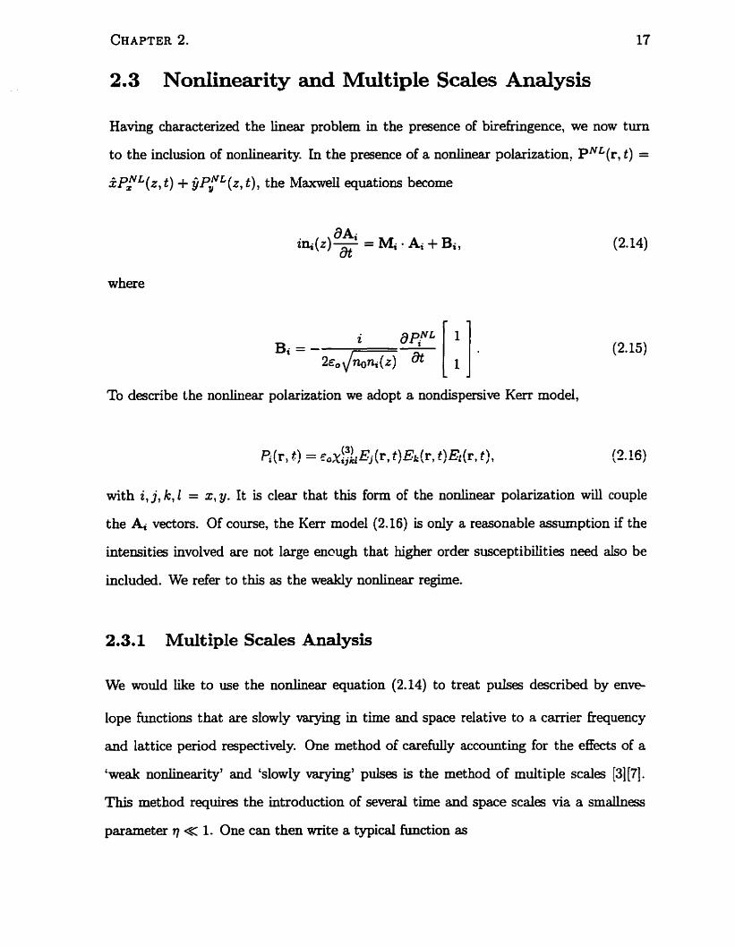
2.3 Nonlinearity and Multiple Scales Analysis

Having characterized the linear problem in the presence of birefringence, we now turn

to the inclusion of nonlinearity. In the presence of a nonlinear polarization, PNL(r, t) =

5PFL(z, t) + ijPYL(z, t ) , the Maxwell equations become

where

To describe the nonlinear polarization we adopt a nondispersive Kerr model,

with 2 , j , k, 2 = x, y. It is clear that this form of the nonünear polarization will couple

the A, vectors. Of course, the Kerr model (2.16) is only a reasonable assumption if the

intensities involveci are not large enough that higher order susceptibilities need also be

included. We refer to this as the weakly nonlinear regime.

2.3.1 Multiple Scales Analysis

We would Like to use the nonlinear equation (2.14) to treat pulsg descnbed by enw-

Lope functions that are slowly varying in time and space relative to a carrier frequency

and lattice period respectivdy. One method of carehlly accounting for the effects of a

'weak nonlinearity' and 'slowly varying' pulses is the method of multiple scales [3][7].

Thiç method requires the introduction of several t h e and Wace scales via a smallness

parmeter 7 < 1. One c m then M t e a typical function as

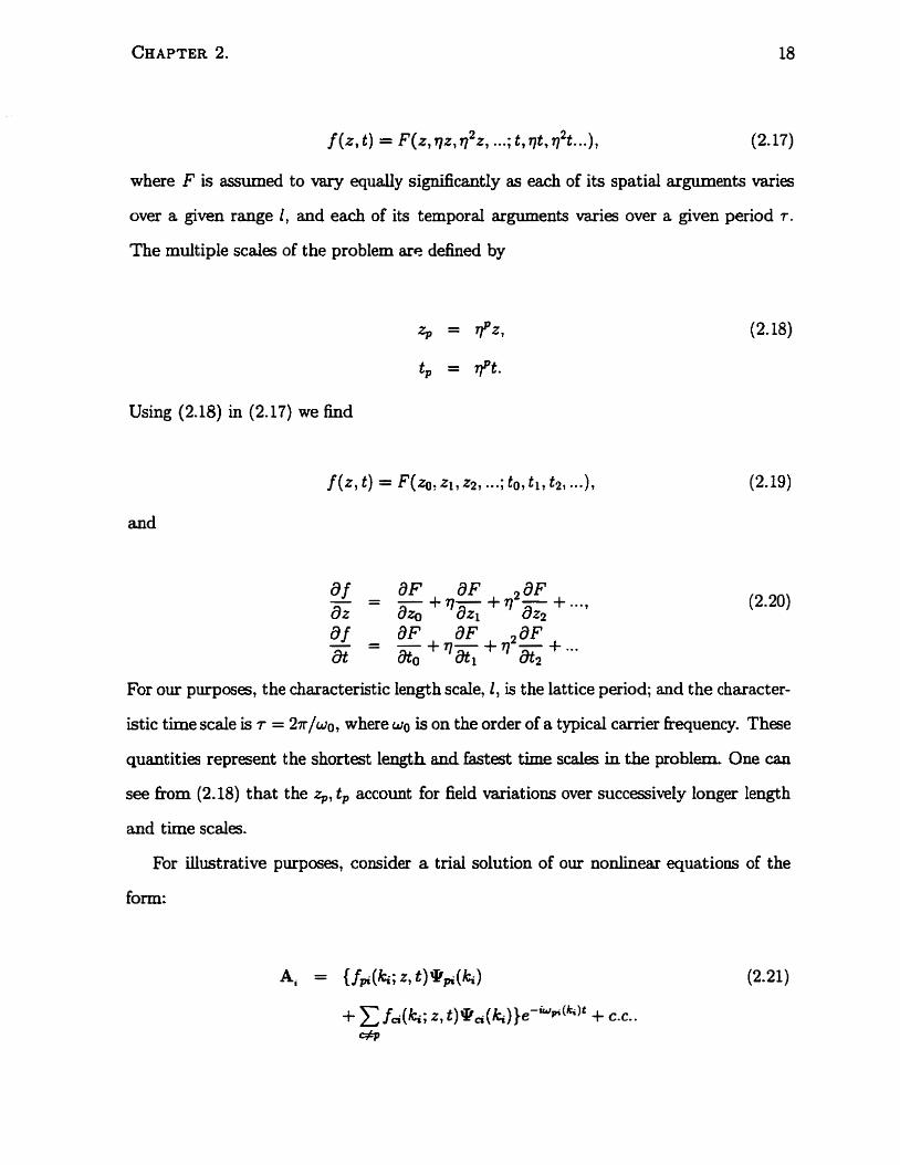
f(r,t) = F ( z , ~ ) z , ~ ~ z , ...; t , q t ~ ~ t ...), (2.17)

where F is assumed to vary equaiiy significantly as each of its spatial arguments varies

over a given range 1, and each of its temporal arguments varies over a given period T .

The multiple scales of the problem are defined by

and

For our purposes, the characteristic length scaie, 1, is the lattice period; and the character-

istic time scale is T = 27r/wo, where wo is on the order of a typicd carrier fkequency. These

quantities represent the shortest length and fastest time s c a k in the prohlem. One can

see fkom (2.18) t hat the rp , t , account for field variations over successively longer lengt h

and t h e scales.

For iliustrative purposes, consider a triai solution of our nonlinear equations of the

fom:

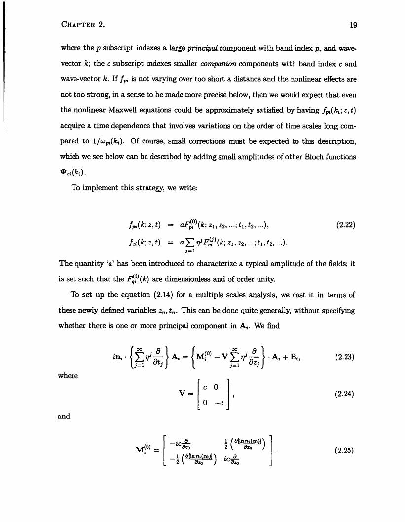
where the p subscript indexes a large principal c~mponent with band index p, and wave

vector k; the c subscript indexes srnaller cornpanion components with band index c and

wave-vector k. If ffi is not varying over too short a distance and the nonlinear dects are

not too strong, in a sense to be made more precise below, then we wouid expect that even

the nonhear Maxwell equations could be a p p r h a t e l y satisfied by having f,(k; z, t)

acquire a time dependence that involves variations on the order of time scdes long com-

pared to l / w * ( k ) . Of course, small corrections must be expected to this description,

which we see below can be described by adding srnail amplitudes of other Bloch functions

%(k)

To implement this strategy, we write:

The quantity 'a' has been introduced to characterize a typical amplitude of the fields; it

is set such that the F$) (k) are dirnensionless and of order uni@.

To set up the equation (2.14) for a multiple scales analysis, we cast it in terms of

these newly d&ed variables h, f. This can be done quite generdy, without specdjmg

whether there is one or more principal component in &. We find

where

and

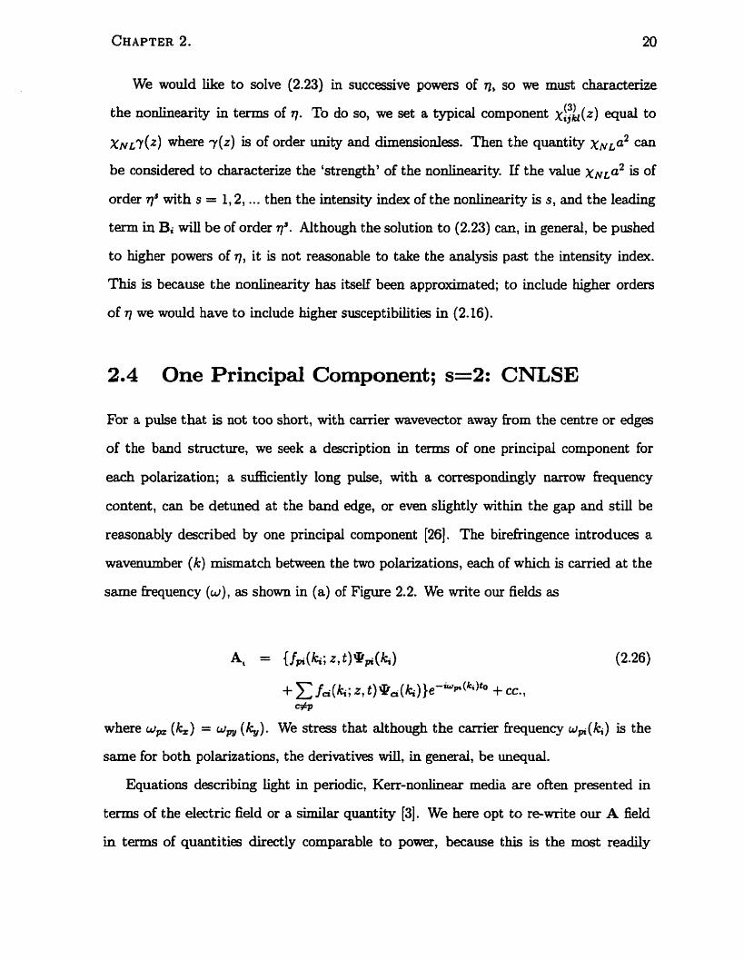
We would like to solve (2.23) in successive powers of q, so we must chasacterize

the nonlinearity in terms of t). To do so, we set a typical component X$L(z) equal to

xNL?(2) where ~ ( z ) is of order and dimensionless. Then the quantity xN,a2 c m

be considered to characterize the 'strength' of the nonlinearity. If the value xNLa2 is of

order q" wit h s = 1,2, . . . t hen the intensity index of the nonlinearity is s, and the leading

term in Bi will be of order qt Although the solution to (2.23) can, in general, be pushed

to higher powers of i), it is not reasonable to take the analysis past the intensity index.

This is because the nonhearity has itself been approximated; to inciude higher orders

of i ) we would have to include higher susceptibilities in (2.16).

2.4 One Principal Component; s=2: CNLSE

For a pulse that is not too short, with carrier wavevector away hom the centre or edges

of the band structure, we seek a description in terms of one principal component for

each polarization; a sufnciently long pulse, with a corresponduigly narrow kequency

content, cm be detuned at the band edge, or even slightly within the gap and stili be

reasonably describeci by one principal component 126). The birefiingence introduces a

wavenumber (k) mismatch between the two polarizations, each of which is carried at the

same fkequency (w) , as shown in (a) of Figure 2.2. We write our fields as

where w, (k;) = w, (b). We stress that although the ca.rrier frequency w, (k,) is the

same for both polarizations, the derivatives will, in general, be unequal.

Equations describing light in periodic, Kerr-nonlinear media are oken presented in

terms of the electric 6eld or a similar quantity [3]. We here opt to rewrite our A field

in terms of quantities directly comparable to power, because this is the most readily

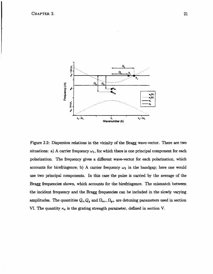
Figure 2.2: Dispersion relations in the vicinity of the Bragg wave-vector. There are two

situations: a) A carrier fkquency w l , for which there is one principal component for each

polarization. The hrequency gives a different wavevector for each polarization, which

accounts for birefigence; b) A carrier hequency w l in the bandgap; here one wodd

use two principal components. In this case the pulse is carrieci by the average of the

Bragg frequencies shown, which accounts for the birefikgence. The mismatch between

the incident hequency and the Bragg fiequencies can be included in the slowly vasring

amplitudes. The quantities Qz,Qu and O,+, are detuning parameters used in section

VI. The quantiw n, is the grating strength parameter, defineci in section V.

accessible experimental quantity. Using the form of the Ai fields in the definition of the

Poynting vector,

S = E(z, t ) x H(z, t ) ,

we find, using the velocity matriv elements, and group velocity expressions given by

(2.11) and (2.12), that we can express the t h e and space average of the Poynting vector

to O($) as

This equation (2.28) suggests a field-dation

where RE is an effective cross-sectional area in the (x, y) plane associateci with the

problem. The X and Y fields are defined such that !XI' is the power in the x-polatized

field and 1 Y l2 is the power in the y-polarized field.

To deal with the nonlinearity, we assume here an intensity index s = 2, which means

t hat our nodhearity enters the equations at the sarne scale as the grating group velocity

dispersion. Under this assumption our eigenvalue equation (2.23) becomes

where the nonlineax term Bi enters at order q2. Note that to order q0 (2.30) is satis

fied because at that order one simply recovers the linear eigenvalue equation (2.2). To

cornpiete the analysis we collect terms first in q1 and then q2, which givg us two sets

of equations for each polarization. By combining these equations we can extract a set

of CNLSE in a manner analogous to that presented by de Sterke et d [71. We hd , to

order ql,

and similar for Y. Rom the q2 order equations we find

The quantity Bi is defined in (2.15), but we oniy need to wite the electric-field

contributions to Bi to order qo to keep (2.32) self-consistent; recall that the nonlinear

susceptibility is of order T ~ , so the last term in (2.32) will be of order qO. The form of the

nonlinear susceptibih@ has been chosen as that of an isotropie medium, but in principle

any X ( 3 ) tensor codd be used. We note. though. that the birehgence is considered

s m d because of a Limitation imposed by our method, discussed after equation (2.33).

Thus, since the effect of the nonlinearity itself is already considered small, the deviations

in X ( 3 ) due to lack of isotropy will typically be of the next lowest order in 7, and hence

can be ignored. The overlap integral in (2.32) is evaluated as

where we note that the quantity e 2 * ( ~ - 4 ) ~ has not been integrated because we assume

that ( I E p - kz) = qK, where K is of the order of the average wavenumber (kz + kJ 12.

In this case 22 (k, - kz) zo = 2iqKzo = 2iKzl. Since zl and zo are considered to be

independent variables the quantity e2'(4-4)' remains. The value of the coeflicients a

are give in Table 2.1.

Table 2.1 : Coefficients fof the €NESE.

The y values are determineci by interchanging x y

a& d4%&)u&(h; Z O ) ~ ~ Z ; Z O ) We now relate our scaled derivatives to full time and space derivatives. Assembling

(2.20) (2.31), (2.32), (2.33), and noting that the equations for the Y fields can be derïved

by interchanging x - y in the preceding, we obtain the following coupled nonlinear

Schr~dmger equat ions,

The quantity

A = 2(k, - kz)

characterizes the birefiingence in the system. The coefncients cr are so subscripted be-

cause a,, accounts for self phase modulation; a,, accounts for cross phase modulation:

and a, accounts for p.hase conjugation. We note that equatims similac to (234) have

been studied extensively in the Literature 191 [22] [ Z j [28] (291.

2.5 Two Principal Components; s=l: CME

We now turn to describing pulses whose carrier bequencies are in or very close to a

photonic bandgap, either at the band center or the band edge. In (b) of Fig. 2.2, we

show the case where the fkequency of the pulse is within the photonic bandgap. The

pulse c m , however, be detuned outside the bandgap and still be well describecl by the

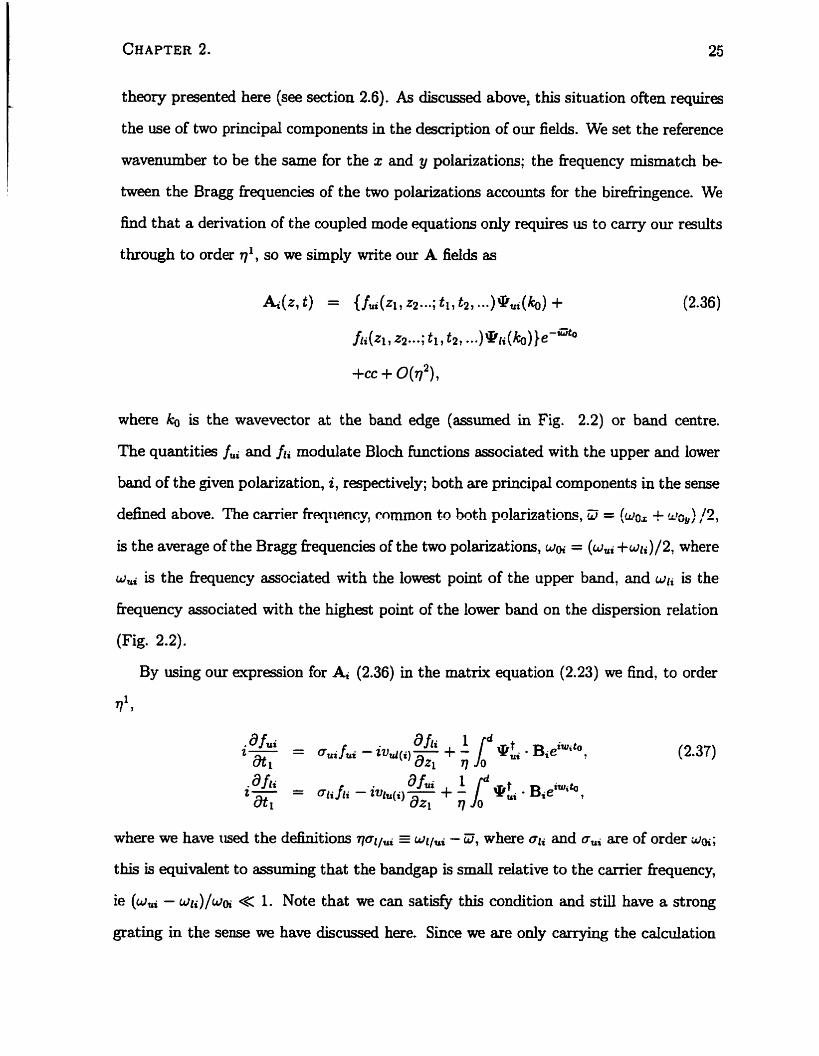
theory presented here (see section 2.6). As discussed above, this situation often requires

the use of two principal components in the description of our fields. We set the reference

wavenumber to be the same for the x and y polarizations; the fiequency mismatch be-

tween the Bragg frequencies of the two polarizations accounts for the birefkingence. We

find that a derivation of the coupled mode equations oniy requires us to carry our results

through to order vl, so we simply write our A fields as

where ko is the wavevector at the band edge (assurned in Fig. 2.2) or band centre.

The quantities fui and fli modulate Bloch functions amciated with the upper and lower

band of the given polarization, 2 , respectively; both are principal cornponents in the sense

defined above. The carrier frq~~ency, rommon to both polarizatinns, J = (wo, f wo9) i 2 ,

is the average of the Bragg fkequencies of the two polarizations, w ~ = (w, + w l i ) / 2 , where

w, is the frequency associateci with the lowest point of the upper band, and mli is the

kequency associateci with the highest point of the lower band on the dispersion relation

(Fig. 2.2) .

By using our expression for A, (2.36) in the matrix equation (2.23) we find, to order

TI 7

.a fui 2- = a, f - 2 - + - y.:, . B;,~W.~O,

l r a21 q 0

where we have iised the defhitions val,, = wl,, - 9 where Q and au, are of order i ~ % ;

this is quivalent to assuming that the bandgap is smaU relative to the ca.rrier frequency,

ie ( - W U < 1 Note that we c m satisfy this condition and still have a strong

grating in the sense we have discusseci here. Since we are only carsring the calculation

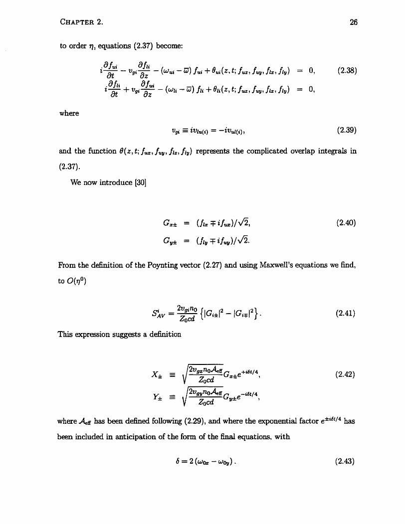
to order 7, equations (2.37) become:

afur 2- af ii at - v*- - (wu* -

dz W) fur + ki(z , 4 f,, fw, fl1 fip) = O, (2.38)

where

and the function B ( t , t ; f,, fup , f', , fi,) represents the complicated overlap integrah in

(2.37).

We now introduce [30]

Rom the definîtion of the Poynting vector (2.27) and using Maxwell's equations we h d ,

to 0(71°)

This expression suggests a definition

where has been defined following (2.29), and where the exponential factor eh6t'4 has

been included in anticipation of the form of the final equations, with

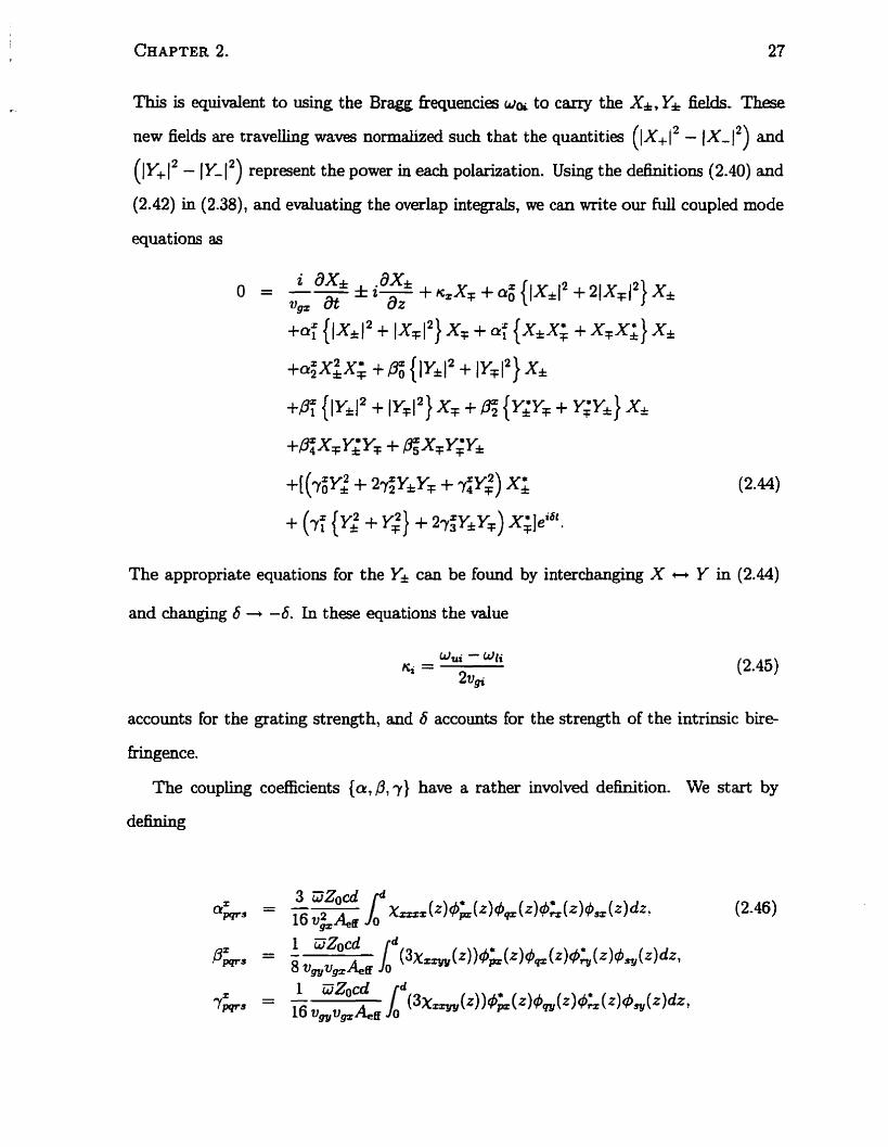
This is quivalent to using the Bragg kquencies w u to c a a y the XI, Y* fields. Thge

new fieids are travelling waws ~orm&ed such that the quantities (1 X+ (* - IX- 12) and

(IY+ 1 * - 1 ~ - 1 *) represent the power in each polarization. Using the definitions (2.40) and

(2.42) in (2.38), and evduating the overlap integrah, we can write our fidl coupled mode

equations as

The appropriate equations for the Y* can be found by interchanging X - Y in (2.44)

and chagging 6 + -6. In these equations the value

accounts for the grating strength, and 6 accounts for the strength of the intrinsic bire-

fkingence.

The coupling coefficients {a, P , y) have a rather involved definition. We st art by

defining

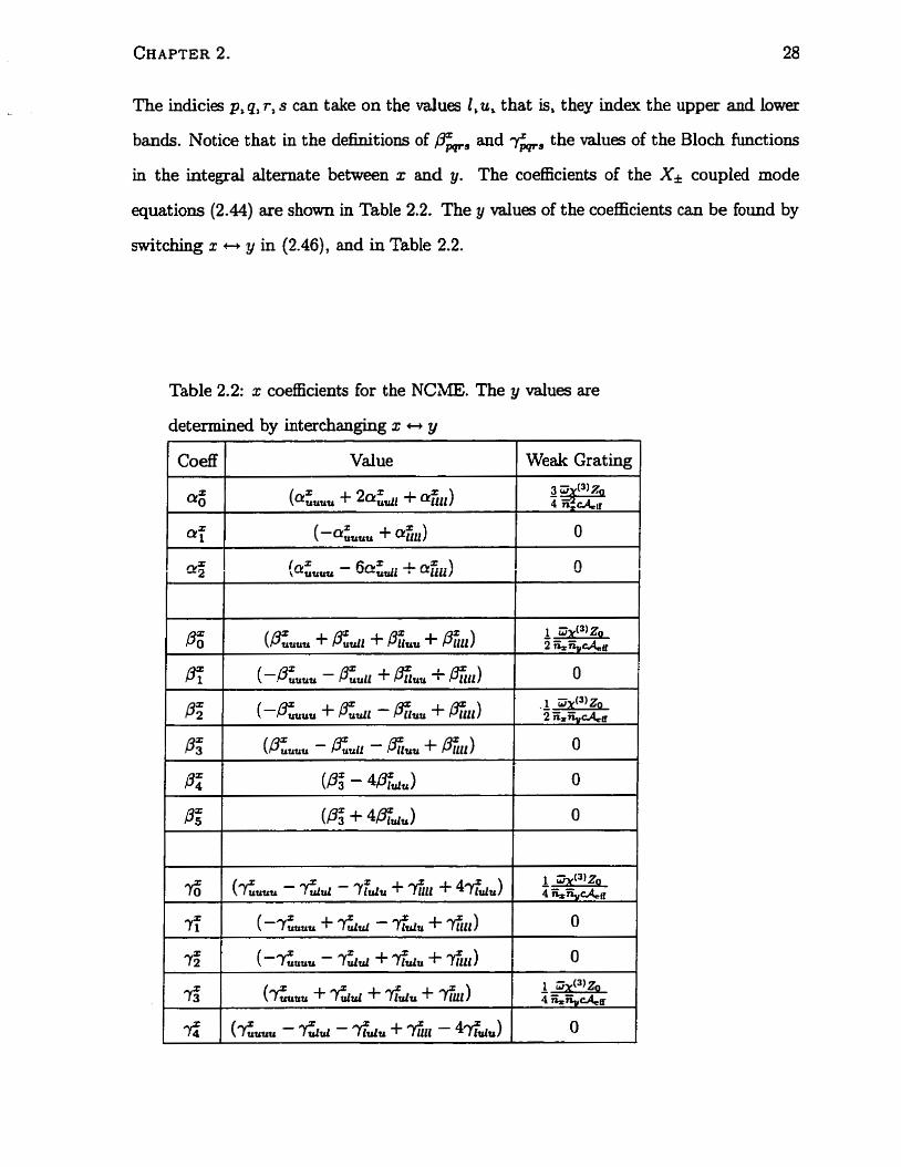
The indicies p,p, r, s can take on the values l,u, that is, they index the upper and lower

bands. Notice that in the definitions of Fm, and y,, the values of the Bloch functions

in the integral alternate bekveen x and y. The coefficients of the X* coupled mode

equations (2.44) are shown in Table 2.2. The y values of the coefficients can be found by

switching x - y in (2.46), and in Table 2.2.

Table 2.2: z coefficients for the NCME. The y values are

Value 1 Weak ~ra&J

2.5.1 Weak Grating Limit ofthe NLCME

Many fiber gratings have small index contrasts, which dows u s to simplify the coupled

mode equations (2.44) by considering a weak grating of the form

nt ( r ) = 4 + 6% c o s ( 2 ~ z ) . (2.47)

where & is the background index, 6n is the index modulation with 6% « n,, and is

the wavenumber that d&es the band edge. In the presence of a weak grating, the Bloch

functions at the band edge can be evaluated, and normalized via (2.8),

If we use these forms for the Bloch functions and assume a d o m nonlinearity, then

many of the coefficients in the coupled mode equations (2.44) are identically zero. We

confirm, using (2. Il), that in this limit the quantity v, is simply equal to the group

velocity in the absence of the grating, v* = c/&. With this in mind we rewrite (2.44)

as

with

The grating coefficient is

the Y* equations can be found by switching x * y and 6 -. -6 in (2.49) and

from which we note that Pz = f19 and 7, = y,.

a very weak birefnngence, where îï, E %, the coefficients in (2.50) are in the

ratio {a : p : +y} = (3 : 2 : l}. In the stationary k t these equations agree with those

given by Samir et al. [31].

2.6 Connecting the CNLSE and the NLCME

In the previous sections we derived two types of equations: a set of coupled nonlinear

Schrddinger equations, typicdy valid outside the bandgap, and a set of nonlinear coupled

mode equations, typicdy valid within or near the bandgap. As we will see in this section,

the coupIed mode equations make very definite predictions about the dispersion relation

and the Bloch functions of the periodic system. When these predict ed Bloch h c t ions and

dispersion relation deviate from the true values of the system, then the approximations

that have been used to derive the coupled mode equations have broken dom; this allows

us to determine the b i t s of validity of the equations. On the other hand, the nonlinear

SchMdinger equation relies on the local properties of the dispersion relation, so if the

nonlineaxit-y is sufficiently small it should always be valid as long as one is sufficiently

far away from a bandgap, or other portion of the dispersion relation with significant

higher-order curvature. If the kequency content of a pulse is very narrow. then higher

order dispersion will have Little &kt, so the Schrodinger equation should be valid at the

band edge and even slightly inside the bandgap.

A hirther point to be discussed is how the solutions to the nonlinear Schrodinger

equation relate to those of the coupled mode equations. Understanding this dows us

to identa the range where either approach could be used, an important goal because

dthough the coupled mode equations are ead,, solveable via niimpsical techniques, they

are diffcult to solve analyticdy. As mentioned, there is a great deal of work in the

literature on equations similar to our CNLSE [9] [22] [27/[28] [29], so if we understand how

solutions of the CNLSE are related to solutions of the NCME, then the CNLSE literature

becornes available to aid in the investigation of birefringence phenornena near the gap.

Specincally we want to know how to relate the two CNLSE fields, X and Y, to the four

NCME fields, X* and YI; and we want to get a sense of how close to the gap we must

be before the CNLSE cease to effectively describe the problern. Our method is to &art

with the weak grating nonlinex coupled mode equations and perform a M h e r multiple

scales analysis to derive the noniinear Schr~dinger equations. The use of the weak grating

equations simplifies the mathematics, and does not significantiy dec t the final results,

for reasons discussed bdow. The rnethod involveci foUows closely the analysis of de Sterke

and Sipe [3], except that in the present case the nonlinear te- are much more involved,

so we only sketch the results.

with which the h e m portion of the coupled mode equations can be written as

where we have used the Pauli spin matrices

and the unit mstrix ao. We seek solutions of (2.53) of the form Fi = te-'(%* '-Qiz) , where

the wavevector detuning is Qi = L - ko If the fidl frequency w, > w&, then we c d the

detuning parameter Q+ and otherwise we c d it Q-, with & = w, - w ~ . The R+ are

associated with the upper and lower band via the dispersion relation

which follows from substituting the Fi in (2.53)- Rom the dispersion r-12 the SQUP

velocity, and group velocity dispersion are

where pi (Q) = %RL(Q)/c is the ratio of the group velocity at a given wave-vector for a

point in the upper band, relative to the group velocity in the absence of the grating. The

eigenvectors have the form

fi(+' (Q

where the f,!') (Q j are associated with the 4+ respectiveiy.

Fkom these eigenvectors one can extract the Bloch functions of the periodic structure,

in the coupled mode equations E t ,

where the factor 1 / J i has been hchtded for propa n m h t i o n via (2.8). The

hinction multiplying eikZ can be identifiecl a s ~ ( * ) ~ ( k ; 2).

If we include the nonlineari~, then we can write the coupled mode equations as

L J

where Ni is the nonlinear term that follows immediately from (2.49). For simplicity we

concentrate on detuning into the upper band, &+(Qi) We represent our field vector Fi

as being mostiy in the upper band, but with a smail component in the lower band. We

&art by writing the field vectors as

where we have introduced the multiple scales variables h, t, as in (2.18). The upper-band

component aj dominates the expansion of Fi, and hence plays the role of a principal corn-

ponent; the bi terms are companion components. The numerical value of the detunings,

n+,(Qi) and Qi, WU be different for each polarization, but in each case we are detuning

to the sarne frequency w , as shown in (a) of Fig. 2.2. The normalization factor 116

has been introduced so that the envelope functions, ai, will be directly related to power.

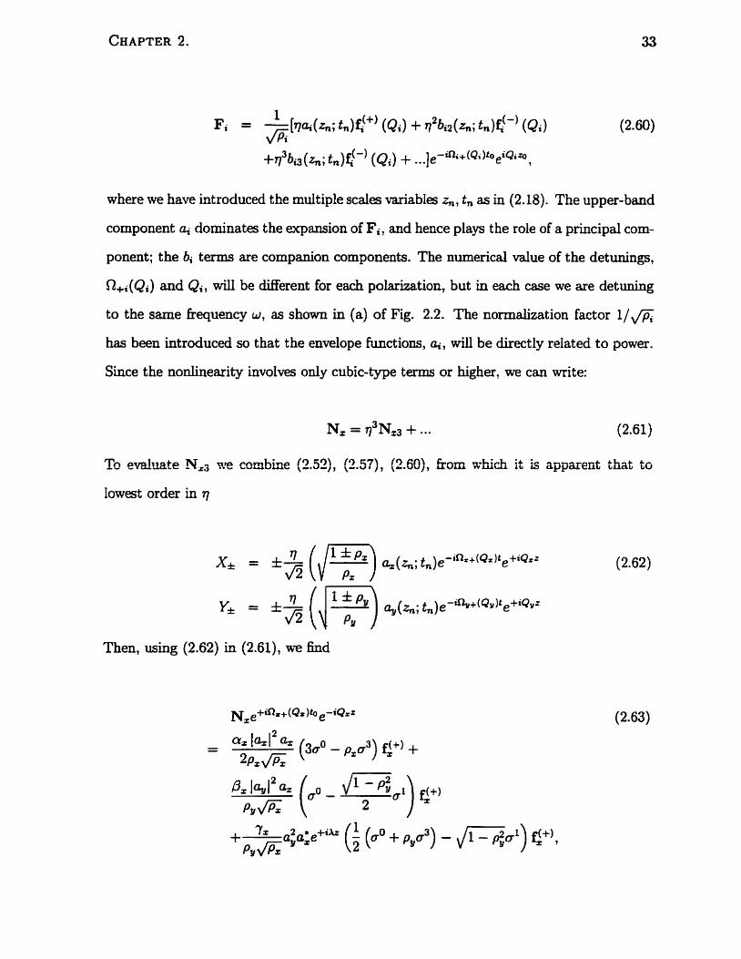
Since the nonlineariw involves only cubic-type terms or higher, we can write:

Nz = r13Nz3 + ... (2.61)

To e d u a t e NZB rire combine (2.52), (ZS?), (Z.60), koxn w k c h it is apparent that to

Iowest order in 7)

where A is the bire£ringence parameter quoted earlier (235). Note that to order q1 the

forward and badrward going fields, XI, are associateci with the multiple scales envelope

fmction a,. This means that, were we to use the strong grating equations, the form

of wodd be the same, but the values of the coefEcients would change. However,

since the values of the weak grating Bloch functions are known, it is straightforward to

compare the nonhem Schrodinger equation derived fiom the weak grating NCME, to

the weak grating CNLSE.

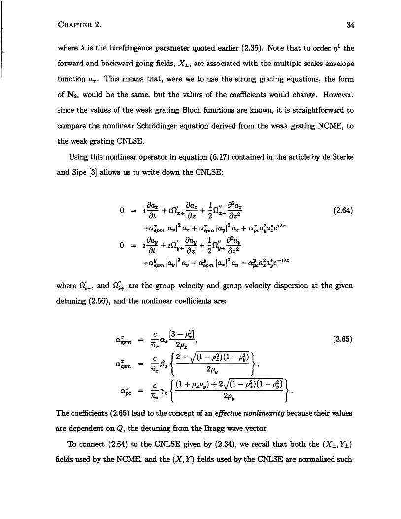
Using this nonlinear operator in equation (6.17) contained in the article by de Sterke

and Sipe [3] dows us to write down the CNLSE:

where ai+, and O:+ are the group velocity and group velocity dispersion at the given

detuning (2.56), and the nonlinear coefEcients are:

The coefncients (2.65) lead to the concept of an effitzue nonl2nearity because their values

are dependent on Q, the detuning fiom the Bragg wavevector.

To connect (2.64) to the CNLSE giwn by (2.34), we recd that both the (X*, Y*)

fields used by the NCME, and the (X, Y) fields used by the CNLSE are normaüzed such

CHAPTER 2. 35

that their squared moduli represMt p0werOwer If we wish ta connect the cMSE and CME

fields we require that

and sirnilady for Y. We have used (2.62) for a,. Hence, our fields X, Y and a,, a, are

equivalent. Using the Bloch functions (2.58) we c m show that the coefncients given

above (2.65) agree with those in table 2.1.

2.7 Numerical Simulations

The simulations are intended to illustrate two points: Grst, we demonstrate the validity

of the CNLSE approximation with respect to the NCME approximation, as discussed

in Section 2.4; second, we investigate the e&ct of energy exchange between the two

poiarizations, which may be of importance in the development of new devices.

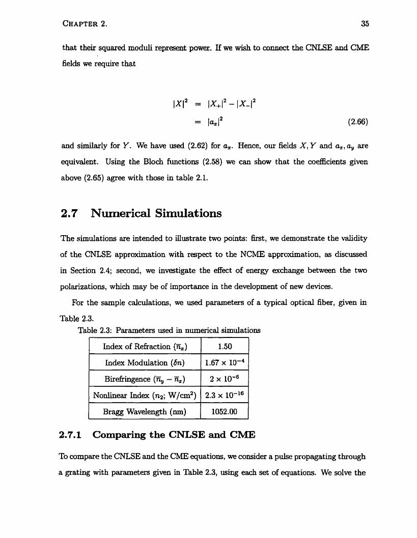
For the sarnple calculations, we used parameters of a typical optical fiber, given in

Table 2.3. Table 2.3: Parax.net ers used in numerical simulations

1 Index of Refraction (R,) 1 1.50 1 1 Index hlodulation ( 6 4 1 1.67 x 10-~ 1

1 Bragg Wavelength (nm) 1 1052.00 1

Bireikingence (% - &)

Nonlinem Index (n2; W / d )

2.7.1 Comparing the CNLSE and CME

2 x IO+

2.3 x 10-l6

To compare the CNLSE and the CME equations, we consider a pulse propagating through

a grating with parameters given in Table 2.3, using each set of equations. We solve the

CNLSE by a split-step Fourier technique: At each time step the hear portion of the

equations are solved in the Fourier domain, while the nonlinear portions are solved using

a 4t h order Runge-Kutta integration scherne [9]; we solve the equations (2.64) in a fiame

travelling with the average velocity of the two pulses. The CME are solved using a

collocation algorit hm [32].

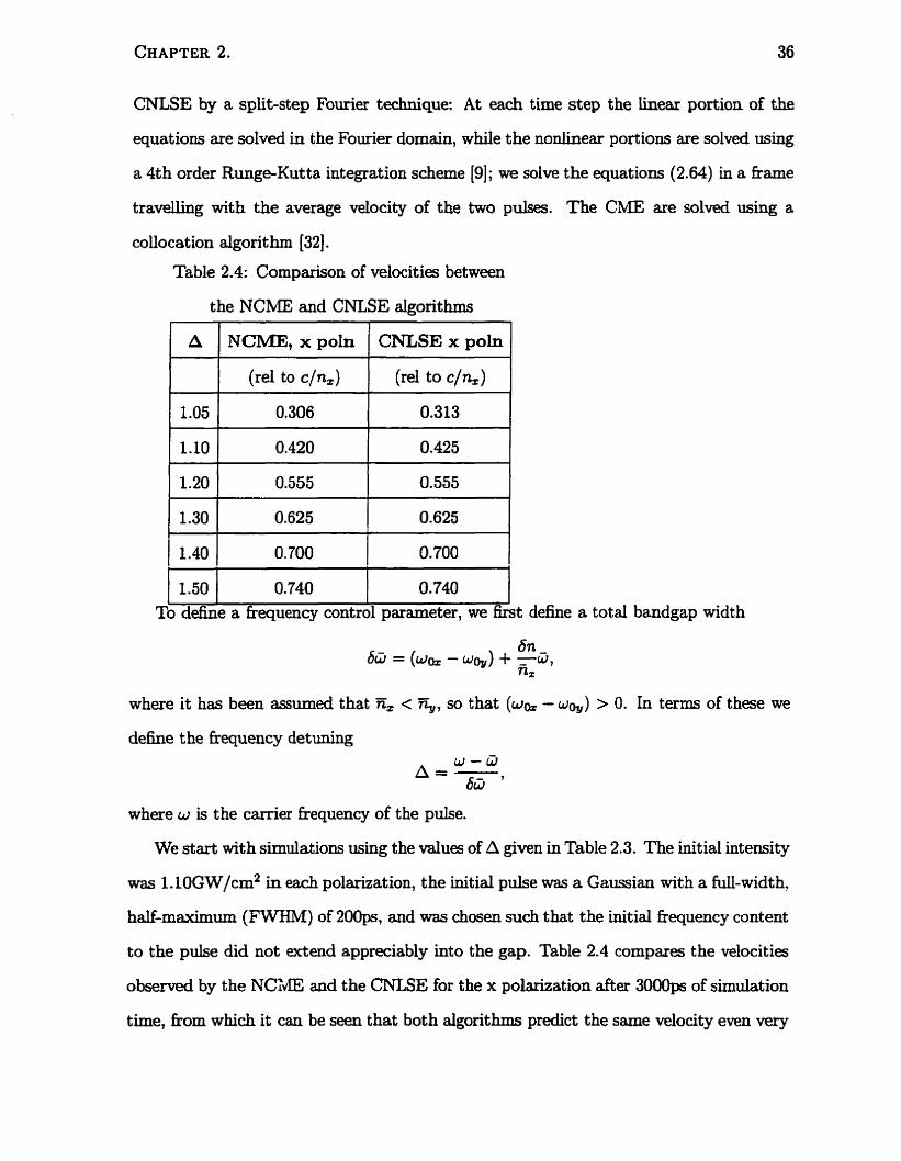
Table 2.4: Cornparison of veiocities between

the NCME and CNLSE algorithms

A

where it has been assumeci that E, < g, so that (uch - uqr) > O. IR terms of these we

1.50 / 0.740

define the kequency detuning

NCME, x poln

0.740

where w is the carrier fiequency of the pulse.

CNLSE x poln

l To define a frrquency control parameter, we fi& define a total bandgap width

We start with simulations using the values of A given in Table 2.3. The initial intensiw

was 1.10GW/cm2 in each polarization, the initial pulse was a Gaussian with a full-width?

half-maximum ( F m ) of 200ps, and was chosen such that the initial frequency content

to the pulse did not extend appreciably into the gap. Table 2.4 compares the wlocities

observeci by the NCiyIE and the CNLSE for the x polazization after 3000ps of simulation

time, from which it can be seen that both algorithms predict the same vdocity even very

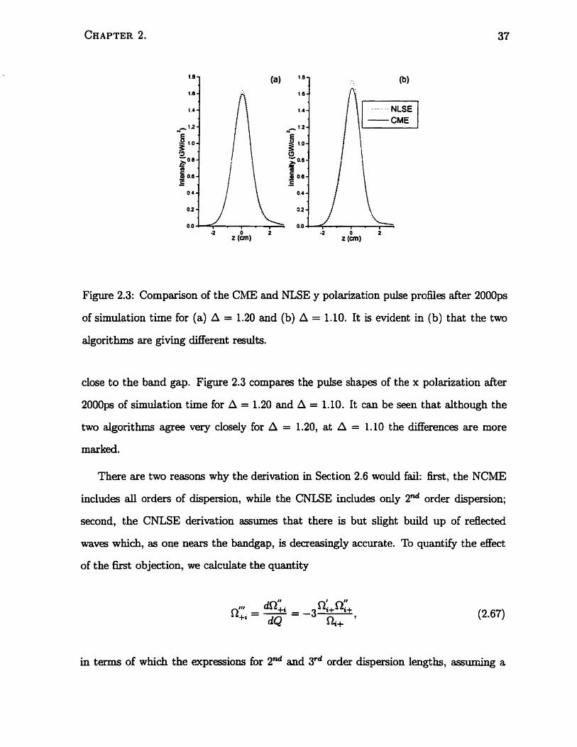
Figure 2.3: Cornparison of the CME and NLSE y polarbation pulse pro& after 2000ps

of simulation time for (a) A = 1.20 and (b) A = 1.10. It is evident in (b) that the two

algorithms are giving different resdts.

close to the band gap. Figure 2.3 compares the pulse shapes of the x polarization after

2000ps of simulation time for A = 1.20 and A = 1.10. It can be seen that although the

two dgonthms agree very closely for A = 1.20, at A = 1.10 the differences are more

maxked.

There are two reasons why the derivation in Section 2.6 wodd fail: firçt, the NCME

includes a l l orders of dispersion, while the CNLSE includes only 2d order dispersion;

second, the CNLSE derivation assumg that there is but slight build up of reflected

waves which, as one mars the bandgap, is decreasingly accurate. To quantify the effect

of the first objection, we calculate the quantity

in terms of which the expressions for 2d and rd order dispersion lengths, assumhg a

Gaussian pulse, [51 are

where TFWHM is the pulse width; if LD3 x LM, then 3rd order dispersion dects become

important. We thus have a criterion on TFwHM that

5 TFWHM >> -, (2.69)

Ri+

for 3rd order &&s to be ignored [33].

To quanti& the second limitation we note [5] that a Gaussian pulse with a given

TFWHM has a frequency width

Thus, for a given carrier fkequency, w, the fkequency spectrum of the pulse wili extend

into the band gap if

However, as the pulse frequency n e m the gap, it will, of course, scperience higher order

dispersion as well as, eventually, reflection, so that this criterion is not completely distinct

from the one presented in the preceding paragraph.

We present simulations to underscore the first objection. We use a gating with the

physical parameters in table 2.3, and a pulse with initial intensity 1 .50GW/cm2 and d e

tuning A = 2.00. We concentrate on a single polarization, since birehgence is incidental

to the higher order dispersion. Using the criterion (2.69) we fuid t hat TmHM > > 1 2 . 5 ~ ~ .

In Fig. 2.4 we plot the sirnulateci pulse profile after 5ûûps of simulation time using both

the NmIE and CNLSE for a TFWHM of 5ûps and 10ps. It can be seen that the lOps

pulse experiences a great deal of higher order dispersion. We note that only a small

amount of reflected mves build up in this simulation, so that the second objection is

irrelemt. We note, too, that since we have not attempted to sirnulate a soliton, the

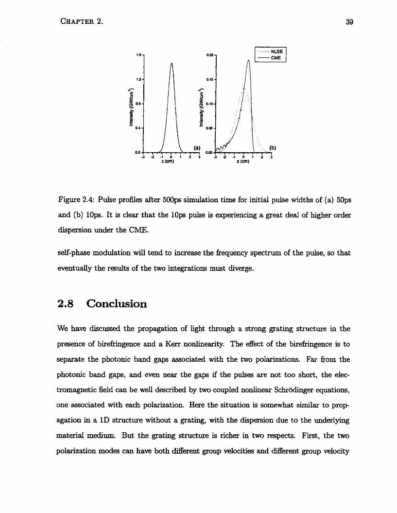
Figure 2.4: Pulse profiles after 500ps simulation t h e for initial pulse widths of (a) 50ps

and (b) 10ps. It is clear that the lOps pulse is experiencing a great deal of higher order

dispersion under the CME.

self-phase modulation will tend to increase the fiequency spectrum of the puise, so that

eventually the results of the two integrations must diverge.

2.8 Conclusion

We have discussed the propagation of light through a strong grating structure in the

presence of birefrmgence and a Kerr nonlineariw. The &ect of the birehngence is to

separate the photonic band gaps associated with the two polarizations. Far fiom the

photonic band gaps, and even near the gaps if the pulses are not too short, the elec-

tromagnetic field can be w d describeci by two coupled nodinear Schrodinger equations,

one associated with each polarization. Here the situation is somewhat sirnilm to prop

agation in a 1D structure without a grating, with the dispersion due to the underlying

material medium. But the grating structure is richer in two respects. First, the two

polarization modes can have both different group velocities and different group wlocity

dispersions, whereas in iinifnrm Il3 structues difkences in the group uelocity dirper-

sions can typicdy be neglected. Second, the effective nonlinearity is a function of the

carrier frequency of the pulse, since it depends on how the appropriate Bloch function

samples the distribution of nonlineariw in the underlying medium.

At carrier frequencies close to the gap or within the gap, the electrornagnetic &Id is

desaibed by two sets of coupled mode equations. These two equations are the analog

of the familiar coupled mode equations in the absence of birefnngence, with one pair

of equations for each polarization. For a range of parameters either set of equations

can be useci, and we identifid the conditions required for this and confirmeci them with

numerical examples. Fkom the generd form of the equations we derive, it is clear that

whole new regimes of nonlinear phenornena can appear when biremgence exists in ID

photonic band gap structures, includuig d-optical switching geometries that have no

analog in isotropie structures. T'us the derivation of the sets of equations we presented

here is of interest not only in its own ri&, but as a starting point for addressing what

to date is the largely unexploreci territory of birehgent, nonlinear, photonic band gap

structures.

Chapter 3

Polarizat ion effect s in birefiingent , periodic, nonlinear media

Introduction

It is weil known that light propagating in an isotropic fiber grating, with frequency con-

tent slightly outside the photonic bandgap, can be described by a nonlinear SchrWger

equation (NLSE) [3j [7] [14] [16][17]. It is also known that the process of growing a UV-

induced fiber grating introduces a weak birefiingence into the nominally isotropic bare

fiber [21j. This birefringence leads to a separation of the photonic bandgaps of the two

orthogonal polaiizations. Propagation of light whose fiequency content is outside both

the photonic bandgaps is well described by a set of coupled NLSEs [23] (343, as was shown

in the previous chapter.

The coupled NLSEk r e l m t to a birefringent grating are similar in form to those used

for bare fibers [35], so rna.ny of the observations in that literature shodd be observable

in gratings as well. However, there are two major digerences between gratings and

bare fibers: h t , the grating dispersion is orders of magnitude higher than in a bare

Bber, so that, for a given pulse width, soliton formation intensities are much higher,

and interaction lengths are much shork~; seeond, the eoupled NLSE parameters, snch as

group velocity and phase velociw are fkequency dependent. Much of the literature on the

coupled NLSE has concentrated on energy exchange between the orthogonal polarizations

[9][28]. This energy exchange, if properly phase matched, can lead to a polarization

instability, whereby intense light polarized near the unstable axis (the axis with the lower

index of refiaction) shifts its energy to the stable axis (with higher index of refiaction)

[36][37]. In a ment paper it was demonstratecl that, unlike in a bare fiber, the threshold

intensity, I P I , for th& instability is a strong funetion of frequency detuning in a fiber

grating [38]. The t hreshold intensity, Igol, for isotropie soliton formation, which occurs

in bkfringent fibers if the light is exactly confineci to one of the principal axes of the

fiber, is also a function of fiquency detuniag [3]. In this chapter we investigate these

two phenornena and show that a grating dows us access to three distinct regimes: at

high detttnings we find IaOl c I p I ; at low detunings we h d Igd > IpI ; and for a middle

region we find I.& -- Ipl

Although the coupled NISEs provide an excellent heuristic guide to nonlinear phe-

nomena in fiber grating systems, in their usud form they are unable to describe accu-

rately the physical gratings used in experiments, because they account neither for the

finite grating length, nor for the apodization profile used to rninimize oscillations in the

linear transmission spectrum of the grating. Furthemore, they must be extendeci [39] if

they are to account for any slow spatial variation in the background index of refraction

of the grating. Therefore, a set of nonlinea,r coupled mode equations (CME) were used

to simulate light propagation [34]. For an infinite, unapodized grating with no slowly

varying spatial variation in the background index of refraction, it is known that the s e

lut ions to t hese nonhear coupled mode equations are àirectly related to the solutions

of the coupled NLSEs [34]. In the fkequency regimes of intergt here, there is a sort of

hierarchy, because the coupled NLSEk can be extracteci kom the nonlinear CME [34].

Thus, although the nonlinear CME provide the better description for pulse propagation,

a quantitative and qualitative understanduig of the iinderlying physics can he d e t d

using the coupleà NLSEs.

When Iad < IpI we can excite pulses that are soiiton-like, and hence maintain a

roughly constant amplitude profile without any nonlineu energy exchange. In this regime

we demonstrate numencaliy that we can use an a p p r h a t e theory (401 to predict the

nonlinear evolution of the Stokes parameters of the pulse. As we detune closer to the

photonic bandgap this approxhate theory breaks down due to reflect ion, more dispersive

&ts, and more nonlinear pulse shaping and energy exchange.

At very high intensities, for pulses with hquency content near but not inside the

photonic band gap, it may be possible to observe the vector solitary wave descnbed by

Akhmediev et aL (401. We present simulations that demonstrate that such a solitary

wave should exist in a fiber grating; its observation, though, would require an oblique

experimental procedure (411, for which the grating used in the experiments reported in

thk &aptw W tuo short. Nevwtheiess, the form of the vector solitary wave suggests that

the phenornenon of polarization instability, in addition to being hequency dependent,

is also strongly dependent on the initial phase lag between the field on the stable and

unstable axes. Eqeriments to v w this dependence on phase lag were performed by

Dr. Richart Slusher of Lucent Technologies, from which it was shown that with a 90'

degree phase lag between the components polarization instability is almost completely

suppressed.

This chapter is divided into six sections. In Section 3.2 a mode1 of a grating which ex-

tends infinitely in space is presented. Rom this model a dispersion relation is determineci,

from which the pulse propagation parameters necgsaxy to write down a set of coupled

NLSEs can be extracted. In Section 3.3 a more complete model of the physical grating

used in the experiment is presented, as are the nonlinear coupled mode equations that we

use to simulate light propagation. In Section 3.4 the approJamate nonlinear evolution of

the Stokes parameters is numerically simulated. In Section 3.5 sorne experimental r d t s

are presented, including the dependence of polarization instabiüty upon input phase 1%.

3.2 Theory for an -te grating

Here we present a mode1 of a birefkhgent grating £rom which we can derive an analytic

expression for the dispersion relation of the grating. Rom the dispersion relation we

extract pulse propagation parameters such as phase velocity mismatch, group velocity

and group velocity dispersion. We then use the pulse propagation parameters to e t e

d o m a set of coupled nonlinear Schrodinger equations that describe iight propagating in

the birefringent grating in the presence of a Kerr nonlinearitsf. Rom the coupled NLSEs

we can determine the threshold intensities required For soliton formation, and for the

onset of polarizaticn instabilky.

3.2.1 Modelling the Grating

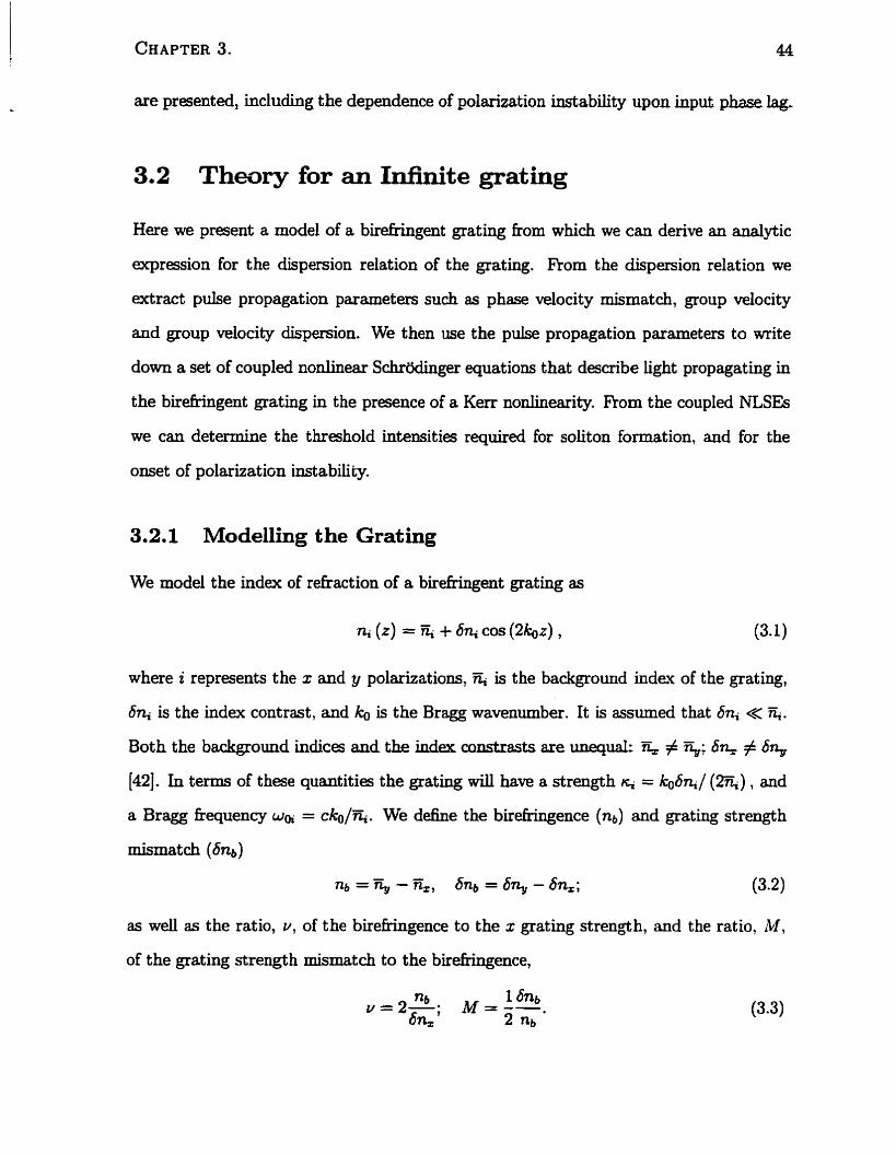
We mode1 the index of refraction of a birefringent grating as

where i represents the x and y polarizations, & is the background index of the gating,

6% is the index contrast, and ko is the Bragg wavenumber. It is assumeci that 6ni « K. Both the background indices and the index constrasts are unequal: # q; 6% # dn,

[42]. In terms of these quantities the grating will have a strength = ko6q / (%) , and

a Bragg hequency wa = ck@+ We dehe the birefnngence (no) and gating strength

mismatch (bnb) - -

nb = % - r a z , anb =b%-anz; (3.2)

as well as the ratio, v , of the birefringence to the s grating strength, and the ratio, iM,

of the grating strength mismatch to the birefkingence,

" JV wi = fi k ni + (kt - 'O) , n,

where the k refer to detunings above and below the Bragg hequency. It is evident that

only fkequencies for which Iwi - w&( 2 CK,/% lie on the dispersion relation for the ith

polarization. If this condition is not met for a given polarization, then the kequency is

said to lie in the photonic bandgap of the grating; the width of the photonic band gap is

2 ~ ~ 4 % . We can invert (3.4) to tind the value of at a given

Using (3.4), the group velocity and group velocity dispersion

given by

fr€!qtleIlcy, W i ,

(3.5)

of the grating system are

In the simulations and experiments it is assumecl that a pulse is injected into the system

with a carrier fiequency common to both polarizations, J = w, = w,. Because the

system is birefiingent, this common carrier frequency will correspond to two dXerent

wave numbers, xz and x9, which can be found using (3.5). For the s m d birehgences

that we are considering, it is reasonable to assume that the group velocity and group

velocity dispersion of the two polarizations at t i j are roughiy equal:

The mismatch in phase accumulation, &, -k,, which is due to the linear birefhngence,

is non-negligible. We d&e a frequency detuning parameter,

where, for definiteness, are have measured the detiininp h m the x-pobnzation Bragg

kequency, and scaled to the half-width of the x-polarization photonic band gap. In terms

of this detuning parameter we can define an efféctive birefringence [42],

where the plus (+) sign refm to detiinings above the Bragg frequency, and the minus

(-) sign to those below the Bragg frequency.

3.2.2 Coupled Nonlinear Schrodinger Equations

A slowly varying pulse with hequmcy content sufnciently far fiom the photonic bandgaps

in a birefringent , Kerr nonlinear medium will satsfy a set of coupled nonlinear Schrodinger

equat ions (341,

where the fields a,, a,, are slowly-va,rying envelope functions, carried at the common fre

quency, g, but at unequal wavenumbers, k, # k,. The envelope functions are normalized

such that ~CQ l2 gives the intensity in the field. The quantity 17 is related to the phase ve-

locity mismatch, 7) = 2 (kg - &) = 2 n r f ~ / c . The quantities Z' and G" are definecl in

(3.7). In the weak grating limit (hi &) we assume here, the nonlinear coefficient a,,

is given by

where n2 is the nonlineax index of rehaction in the absence of a grating, and where f

is the nomalized detuning parameter defined in Equation (3.8). The value of a,, and

cr, can be determined by the ratio {a, : a,, : %} = (3 : 2 : 1). We also define an

effective nonlinear index of rehaction

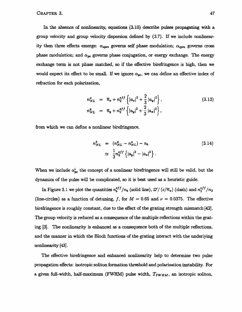
rii the absence O£ equaths (%IO) d k b e pulses propagating wigh a

group velocity and group velocity dispersion defineci by (3.7). If we include nonlinear-

ity then three effects emerge: a,, governs self phase modulation; a,, governs cross

phase modulation; and a, governs phase conjugation, or energy exchange. The energy

exchange term is not phase matched, so if the efktive birefkgence is high, then we

would expect its effect to be small. If we ignore a,, we can define an eflective index of

refiaction for each polarization,

from which we can define a nonlinear birefringence,

When we include crk the concept of a noalinear birefruigence will still be valid, but the

dpamics of the pulse will be complicated, so it is best used as a heuristic guide.

In Figure 3.1 we plot the quantities @/q, (solid line), 3 1 (~/n,) (dash) and n;lf /n2

(linecircles) as a function of detuning, f, for M = 0.65 and v = 0.0375. The effective

birehgence is rougidy constant, due to the effect of the grating strength mismatch [42].

The group velocity is reduced as a consequence of the multiple rdections within the grat-

ing [3]. The nonlinearity is enhanced as a consequence both of the multiple refiections,

and the mamer in which the Bloch functions of the grating interact with the underlying

nonlinearitly (431.

The effective birekingence and enhanced nonheariîy help to determine two pulse

propagation efFects: isotropic soliton formation threshold and polarization instability. For

a given W-width, half-maximum (FWHM) pulse width, TFwHnr, an isotropic soliton,

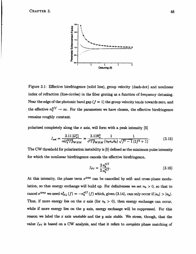
Figure 3.1: Enective birefringence (solid h e ) , group velociS (dash-dot) and nonlinear

index of refraction (linecircles) in the fiber grating as a hindion of kequency detuning.

Near the edge of the photonic band gap (f = 1) the group velocity twds towards zero, and

the effective n q - W. For the parameters we have chosen, the effective birefkingence

rernains roughly constant .

polarized completely dong the x axis, d l form with a peak intensity [5]

The CW threshold for polarization instability is [5] defineci as the minimum pulse intensity

for which the nonlinear birehgence cancels the effective birehingence,

At this intensity, the phase term e*qz can be cancelled by self- and crossphase modu-

lation, so that energy exchange wiU build up. For dennitenes we set nb > O, so that to

cancei e*qz we need nNL (f ) = -niff (f ) which, giwn (3.14), can only occur if 1% 1 > 1% 1. Thus, if more energy lies on the x âxis (for nb > O), then energy exchange can occur,

while if more energy lies on the y axis, energy exchange will be suppressed. For this

reason we label the x axis unstable snd the y axis stable. We stress, though, that the

value IpI is baseci on a CW d y s i s , and that it refers to wmplete phase matchmg of

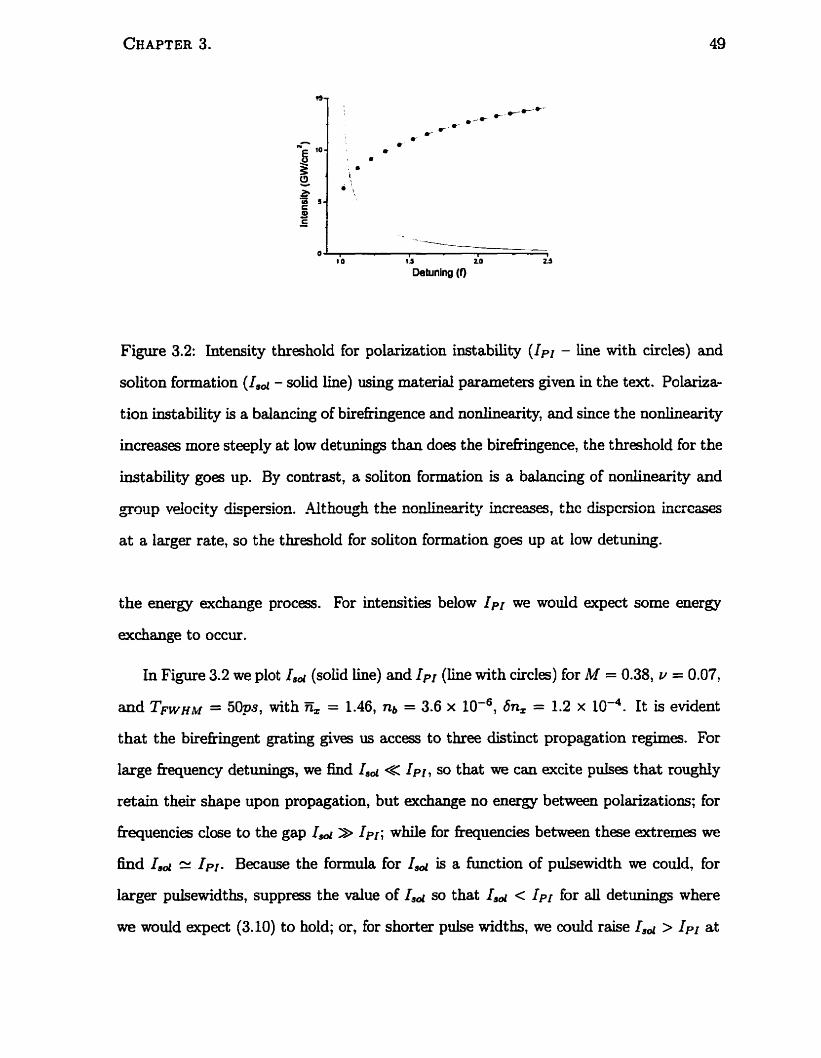
Figure 3.2: Intensity threshold for polarization instability ( IpI - line with circles) and

soliton formation (Isd - solid line) using material parameters given in the text. Polariza-

tion instsbiliv is a balamhg of birefnngence and nonlineari~, and since the nodineariQ

increases more steeply at low detuainp than does the birefiingence, the threshold for the

instability goes up. By contrast, a soliton formation is a balancing of nonlinearity and

group velocity disersion. .4lthough the nonlinearity incre-, the dispersion increass

at a lmger rate, so the threshold for soliton formation goes up at low detuning.

the energy exchange process. For intensities below IpI we would expect some energy

In Figure 3.2 we plot Iad (solid line) and IpI ( h e with circles) for M = 0.38, u = 0.07,

and TWHM = 50p, with ii. = 1.46, nb = 3.6 x 10-~, 6n. = 1.2 x 10-~. It is evident

that the birehgent grating gives us access to three distinct propagation regimes. For

large kequency detunings, we h d Isd < hl, so that we can excite pulses that roughly

retain th& shape upon propagation, but exchange no energy between polarizations; for

fi:equencies close to the gap Isd B IN; while for keqyencies between these extremes we

fkd Isd = I p I . Because the formula for Isd is a function of pulsewidth we could, for

larger pulsewidths, suppress the value of Isd so that Iad < IpI for all detunings where

we would expect (3.10) to hold; or, for shorter pulse widths, we could raise Isd > IPI at

3.3 Physical Grating

In this section we give a more adequate model for the experirnental grating. Since the

model accounts for the apodization of the grating, the concept of a dispersion relation

is no longer va.iid. Furthexmore, the coupled NLSEs will no longer provide an accurate

picture of light propagating in the grating. Instead we use a set of nonlinear coupled

mode equations to d d b e light propagation, but continue to use the coupled NLSEs as

a heuristic guide to nonlinear phenornena.

We model a physicai grating as

where we have allowed both the grating index contrast and the background index to

assume a siowly Msing z dependence. The z dependence accounts for three effects.

First, any experimental gating is of f i t e length, so we define both 6Ni (z) = O and

672, (2) = O for z < O and r > L, where the experimental grating extends only fkom O to

L. Second, it is cornmon to apodize the index contrast of the grating with a smoothly

varying index contrast profile 672 ( z ) , to eliminate sharp oscillations in the transmission

spectnun. Third, it is &O weiI known that the growth of an apodized UV fiber grating

creates both the desireci index contrast, hi (z) , and an overall rise in the background

index of refkaction, bNj (2). This rise in the background index leads to Fabry-Perot effkcts

in the transmission spectnim of the grating. We attempt to correct the background index,

so 6Ni (2) should be zero, but the correction technique is not perfect, and there is always

some z dependent background. The speciiîc model used for 6Ni (2) is given elsewhere

[4a. As a modei for 6% (z), we assume

where L is the length of the grating. This model assumes that the edges of the grating are

Gaussian-apodized with a half-width, half-maximum value zh,, while the centre portion -

bas a constant value of 6~ (2) = 6ni; since most of the grating has a constant index

contrast, the M and Y parameters can be used as defined above to characterize the

grating. In the simulations we use 6 = 2.4 x 10-~, = 1.46, nb = 4.2 x 10-~,

L = 7.7m and z h = 0.25.

As mentioned, we cannot use the coupled NLSEs (3.10) to give quantitative results for

the grating used in the experiments. Instead we rely on a set of nonlinear coupled mode

equations, which more easily amount for the apodization profile of the grating [34][44]:

where

and where J is the average of the two Bragg kequencies Z = (wo. + w ~ ) 12. The a p

propriate equations for the y polarization can be determined fÎom (3.19) by switching

x - y and 6 -+ -6. Here the are dowly varying endope functions modulating

forward and backward travelling waves, and are nomalized such that [AJ2 represents

the intensity in the field. The envelope functions are carried at their Bragg fiequency

( w ~ ) and at wavenumber ko.

3.4 Approximat e Solut ion for Polarizat ion Evolut ion

In a recent paper [40], Akhmediev et ai. presented a simple theory to describe nonlin-

ear pulse propagation governeci by the coupled NLSEs. In this section we summarize

th& theory, and demonstrate that for the correct parameters it provides an excellent de-

scription for pulse propagation through a grating. We 6rst define the nomalized Stokes

parameters

where So (z, t) = luJ2 + 1912. The quantity A$ is the phase lag between the two

polarizations, which we define by writing a= (z, t ) = laz (2, t ) ( e**=(2tt) and g (2, t ) =

1% (2, t)l e i 4 ~ ( z ~ t ) , so that

We now assume that the temporal profile of the two orthogonally polarized pulses is

cornmon and remains constant with propagation, so that

where h ( t ) is the dimensionles temporal profile. Using (3.23) the normalized Stokes

parameters become

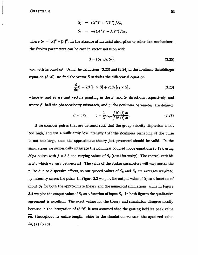
where So = lx12 + IY l 2 h the absence of material absorption or other loss mechanisms,

the Stokes parameters can be cast in wctor notation with

and with So constant. Using the definitions (3.23) and (3.24) in the nonlinear Schrihhger

equation (3. IO), we find the vector S satisifes the differential quation

where ê1 and ê3 Xe unit vectors pointing in the SI and S3 directions respectively, and

where 0, half the phase-velocity mismatch, and g, the nonlinear parameter, are defined

1 / h4 ( t ) dt P = v / ~ , g = ~ a ~ l h 2 ( t ) & .

If we consîder puises that are detuned such that the group velociw dispersion is not

too high, and use a sufticiently l m intensity that the nonlinear reshaping of the pulse

is not too large, then the approximate theory just presented should be valid. In the

simulations we numerically integrate the nonlinear coupled mode equations (3.19), using

8Ops puises with f = 3.5 and Msying values of So (total intensity) . The control d a b l e

is Si, which we vary between f 1. The value of the Stokes parameters will Vary acrass the

pulse due to dispersive effects, so our quoted values of S2 and S3 are averages weighted

by intensity across the pulse. In Figure 3.3 we plot the output value of S2 as a function of

input SI for both the approxirnate theory and the numericd simulations, while in Figure

3.4 we plot the output value of S3 as a function of input Si. In both figures the qualitative

agreement is excellent. The exact d u e s for the theory and simulation disagree mostly

because in the integration of (3.26) it was sssumed that the grating M d its peak value - bn, throughout its eatire length, while in the simulation we used the apodized value

6% ( z ) (3.18).

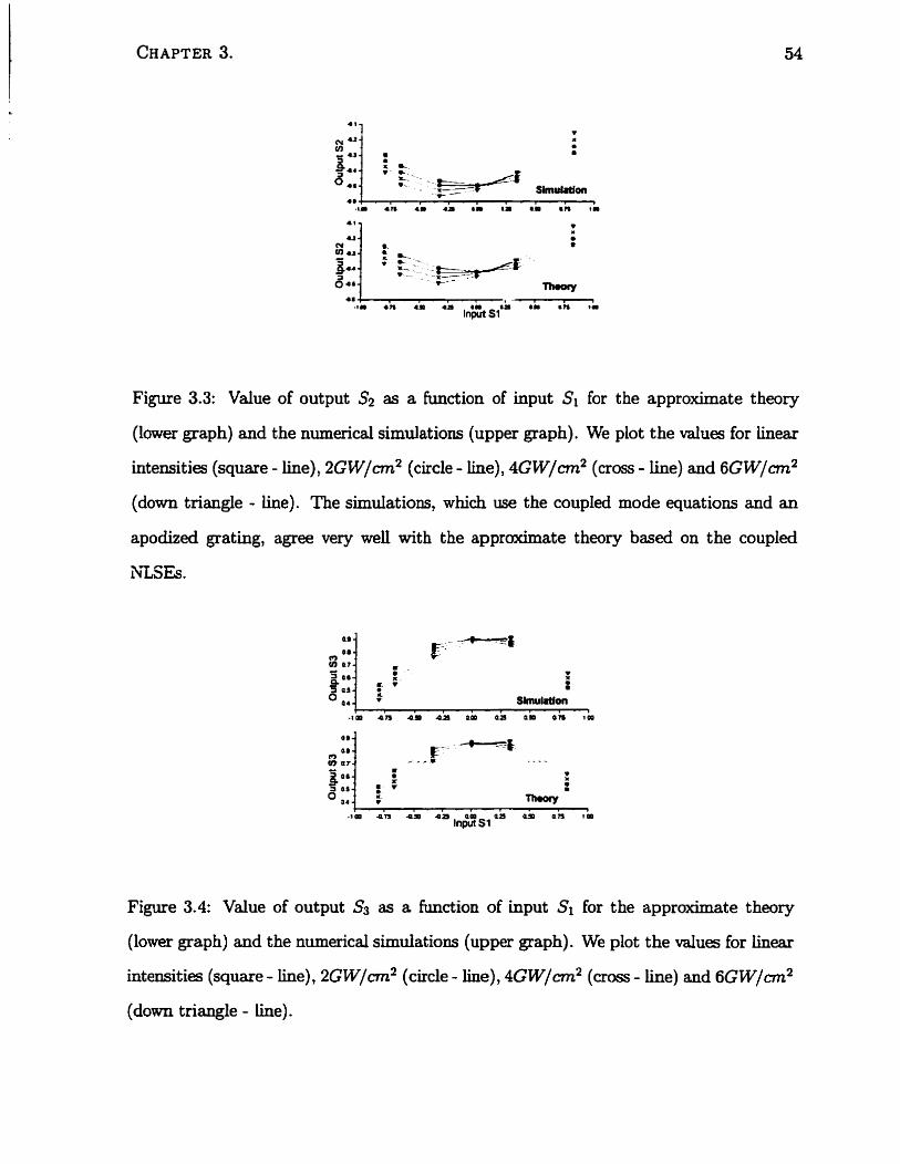
Figure 3.3: Value of output S2 as a function of input Si for the approximate theory

(lower graph) and the numerical simulations (upper graph). We plot the values for iinear

intensities (square - line) ,2G W / n 2 (c ide - h e ) ,4G W / m 2 (cross - line) and 6G W/cm

(down triangle - iine). The simulations, which use the coupled mode equations and an

apodized grating, agree very well with the approximate theory based on the coupled

XLSES.

Figure 3.4: Value of output S3 as a function of input Si for the approximate theory

(lower graph) and the numerical simulations (upper graph). We plot the values for linear

intensit ies (square - Iine) ,2G W / m 2 (circle - line) ,4G W / m 2 (cross - line) and 6G W / m 2

(down triangle - Iine).

As we detune closer to the photonic band gap, the agreement between the apprmrimate

theory and the simulations worsen (for 80ps pulses the threshold is f < 2.5). This occurs

because the group velocity dispersion inmeases, which causes the pulse to broaden and

which makes the approximation of a constant temporal profile invalid. Authermore, at

lower values of f , parts of the incident pulse are rdected, which is not describeci by the

approximats t heory.

3.5 Experirnent al Data

The experimental arrangement. is shown in Figure 3.5. The pulsed light source is a Q

switched mode-locked YLF laser that produces 80ps wide pulses with center wavelengths

near 105311.. wavelengths. A single pulse from each Q-switched, mode-locked pulse train

is transmitted to the fiber using an electreoptic gate. The resulting 500 Hz pulse repeti-

tion rate at the grating is siow enough to eiiminate heating and to reduce the probabîiity

of damage to the input face of the fiber. The incident pulse is slightly chirped due to

n o n l i n e e in the laser gain crystal; this chirp is s m a l l compared to the nonlinear phase

shûts important for the phenornena studied in these experiments. The beam is coilimateci

to a diameter that matches the input microscope objective, and is attenuated using a

rotating neutral density filter. A . energy meter measures the pulse energies before the

input objective. Light exiting the fiber is collectecl by a microscope objective and focused

onto a fiber core at a distance of 2 m. This arrangement ensures that only light ftom

the fiber core is meastueci. Light from the collecting fiber is detected using a diode and

a sampling scope with a combined time response of 20 ps, sdiicient time resolution for

the experiments in this study.

The input polarization state of the optical pulse is set by the combined orientations

of a half-waw (HWPl) and quarter-wave (QWP1) plate immediately before the input

focusing lem as shown in Figure 3.5. The orientation of the polarization ellipse with

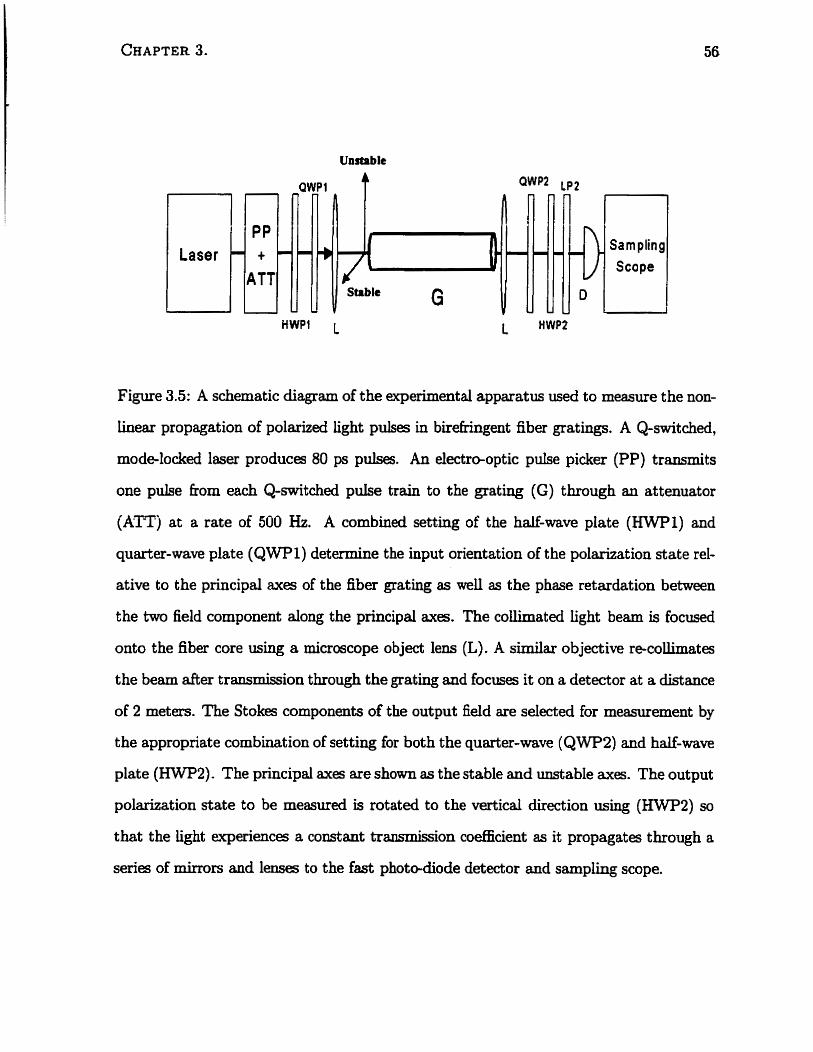
Figure 3.5: A schematic diagram of the experiniental apparatus used to measure the non-

iinear propagation of polarized light pulses in birefringent fiber gratings. A Q-switched,

mode-locked laser produces 80 ps pulses. An electreoptic puise picker (PP) transmits

one pulse fiom each Q-switched pulse train to the grating (G) through an attenuator

jATTj at a rate of 500 Hz. A combined setting of the half-wave plate (HWPI) and

quarter-wave plate (Q WP 1) determine the input orientation of the polarization st ate rel-

ative to the principal axes of the fiber grating as welI as the phase retardation between

the two field component along the principal axes. The collimateci light beam is focused

onto the fiber core ushg a microscope object lem (L). A similar objective recollimates

the beam d e r transmission through the grating and focuses it on a detector at a distance

of 2 meters. The Stokes components of the output field are selected for measurement by

the appropriate combination of setting for both the quarter-wave (QWPZ) and half-wave

plate (HWP2). The principal axes are shown as the stable and unstable axes. The output

polarization state to be measured is rotated to the vertical direction using (HWP2) so

that the light experiences a constant trammision coeflicient as it propagates through a

series of mirrors and lenses to the fast pho tdode detector and sampling scope.

Laser - PP t

ATT

-

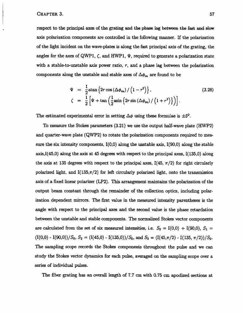
respect to the pciacipal axes cd the gtating and the phase lag between 6he fa& and slow

axis polazïzation components are controlled in the following marner. If the polarization

of the light incident on the waveplates is along the fast principal axis of the grating, the

angles for the axes of QWP1, C, and Ml, Q, required to generate a polarization state

with a stabkto-unstable axis power ratio, r, and a phase lag between the polarization

components along the unstable and stable axes of A&n are found to be

The estimated experimentd error in setting At$ using these formulae is f 5O.

To measure the Stokes parameters (3.21) we use the output half-wave plate (HWP2)

and quarter-wave plate (QWP2) to rotate the polarization components required to mea-

sure the six intensiw components, I(0,O) dong the unstable axis, I(90,O) along the stable

&,I(45,0) along the axis at 45 degrees with respect to the principal axes, I(135,O) along

the axis at 135 degrees with respect to the principal axes, I(45, r / 2 ) for nght circularly

polarized light , and I(135,ir/2) for leR circularly polarized light , onto the transmission

axiç of a fixeci linear polarizer (LP2). This mangement maintains the polarization of the

output beam constant through the remainder of the collection opt ics, including polar-

ization dependent mirrors. The £kt d u e in the measured intensity parentheses is the

angle with respect to the principal axes and the second value is the phase retardation

between the unstable and stable components. The normalized Stokes wctor components

are calculateci fiom the set of six measured intensities, i.e. So = I(0,O) + I(gO,O), SI =

(I(0,O) - 1(90,0))/S0, S 2 = (I(45,O) - 1(135,0))/so, and S3 = ( I ( 4 5 , ~ / 2 ) - I(135, 7r/2))/So.

The sampling scope records the Stokes components throughout the pulse and we can

study the Stokes vector dynamics for each pulse, averaged on the sampling scope over a

series of individual p h .

The fiber grating has an overd Iength of 7 -7 cm with 0.75 cm apodized sections at

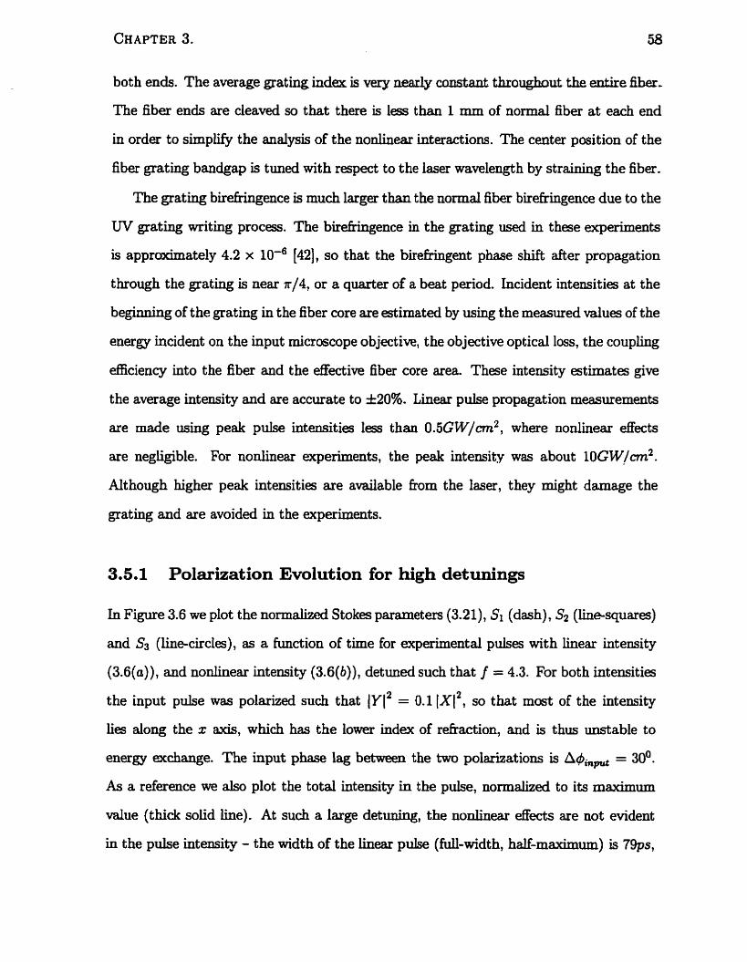
both ends. The average grating index is very d y constant tkoughout the entire fiber-

The fiber ends are cleaved so that there is less than 1 mm of normal fiber at each end

in order to simplify the analysis of the non1inea.r interactions. The center position of the

fiber grating bandgap is tuned with respect to the laser wavelength by strainùig the fiber.

The grating birefringence is much larger than the normal fiber birefringence due to the

UV grating writing process. The buefimgence in the grating used in these experiments

is a p p r k a t e l y 4.2 x IO-' [42], so that the biefringent phase shift after propagation

through the grating is near r / 4 , or a quarter of a beat period. Incident intensities at the

beginning of the grating in the fiber core are estimateci by using the messureci values of the

energy incident on the input microscope objective, the objective optical loss, the coupling

efnciency into the fiber and the effective fiber core area These intensity estimates give

the average intensity and are accurate to f 20%. Linear pulse propagation measurements

are made using peak pulse intensities l es than 0.5GW/cm2, where nonlinear effects

are negligible. For noniinear experiments, the peak intensity was about 10GW/m2.

Although higher peak intensities are available fiom the laser, they might damage the

grating and are avoided in the experiments.

3.5.1 Polarizat ion Evolut ion for high detunings

In Figure 3.6 we plot the normalized Stokes parameters (3.21), Si (dash), Sz (lin+squares)

and S3 (line-circles), as a function of time for experimental pulses with linear intensity

(3.6(0)), and nonlinear intensity (3.6(6)), detuned such that f = 4.3. For both intensities

the input pulse was polarized such that (y12 = 0.1 (x12, so that most of the intensity

lies dong the x axis, which has the lower index of rehction, and is thus unstable to

energy exchange. The input phase lag between the two polarizations is A4mpu, = 30°.

As a reference we also plot the total intensity in the pulse, normalized to its maximum

value (thick soiid line). At such a large detuning, the nonlinear dects are not evident

in the pulse intensiw - the width of the linear pulse (Ml-width, half-maximum) is 79ps,

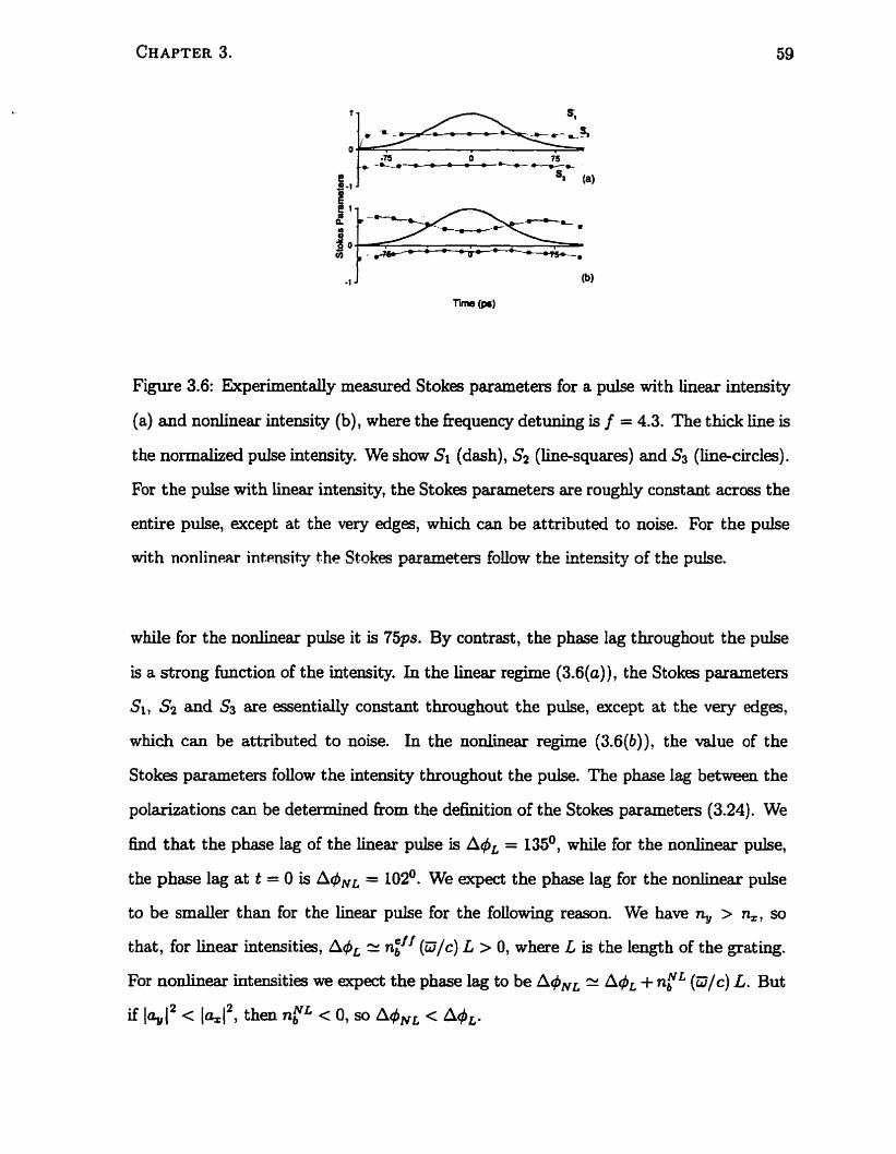
Figure 3.6: Ekperirnentdy measured Stokes parameters for a pulse with Linear intensity

(a) and nonlinear int ensity (b) , where the hequency detuning is f = 4.3. The thick line is

the normaüzed pulse intensity. We show Si (dash), S2 (he-squares) and S3 (line-circles) . For the pulse with linear intensity, the Stokes parameters are roughly constant acmss the

entire pulse, except at the very edges, which can be attributed to noise. For the pulse

with nonlinear intmsity the Stokes parameters foUow the intensity of the pulse.

while for the nonlinear pulse it is 75ps. By contrast , the phase lag throughout the pulse

is a strong function of the intensity. In the h e a r regime (3.6(a)), the Stokes parameters

Si, S2 and S3 me esentidy constant throughout the pulse, except at the very edges,

which can be attributed to noise. In the nonlineax regime (3.6(b)), the value of the

Stokes parameters follow the intensity throughout the pulse. The phase lag between the

polarkations can be determineci from the definition of the Stokes parameters (3.24). We

h d that the phase lag of the linear pulse is A#, = 135O, while for the nonlinear pulse,

the phase lag at t = O is A#NL = 102'. We expect the phase lag for the nonlinear pulse

to be smder than for the linear pulse for the following reason. We have 5 > nz, so

that, for linear intensities, A#, = nif' (Tjlc) L > O, where L is the length of the grating.

For nonlinear intensities we expect the phase lag to be A4,, z A$, + nrL @/c) L. But

if 1912 < 1%12, then n r L < O, so A&L c &.

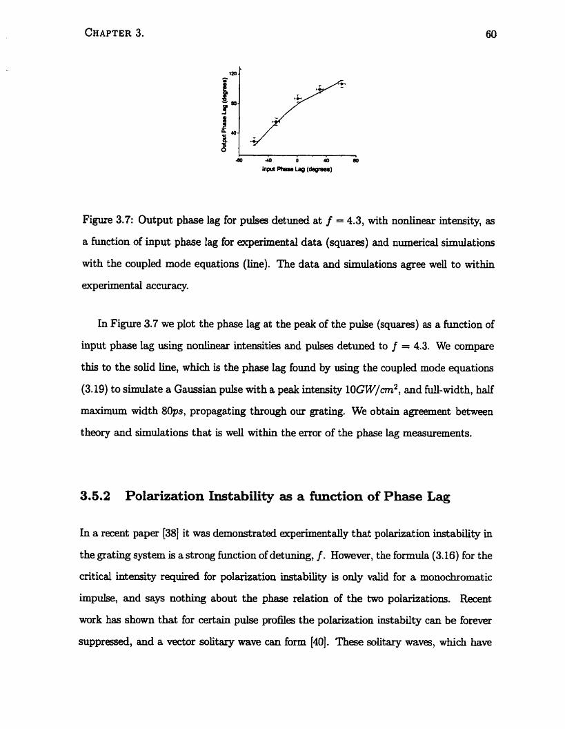
Figure 3.7: Output phase lag for pulses detuned at f = 4.3, with nonlinear intensity, a s

a fundion of input phase lag for experimental data (squares) and numerical simulations

with the coupled mode equations (line). The data and simuiations agree weil to within

experiment al accuracy.

In Figure 3.7 we plot the phase lag at the peak of the pulse (squares) as a function of

input phase Iag using nonlinear intensities and pulses detuned to f = 4.3. We compare

this to the soiid line, which is the phase lag found by using the coupled mode equations

(3.19) to simulate a Gaussian pulse with a peak Uitensity 10GW/n2, and full-width, half

maximum widt h 8Ops, propagating through our grating. We obt ain agreement between

theory and simulations that is well within the error of the phase lag measurements.

3.5.2 Polarization Instability as a function of Phase Lag

In a recent paper [38] it was demonstrated experimentdy that polarization instabiliw in

the grating system is a strong function of detuning, f . Howewr, the formula (3.16) for the

critical intensiw required for polarization instabiliw is only valid for a monochromatic

impulse, and says nothing about the phase relation of the two polarizations. Recent

work has shown that for certain pulse profiles the polarization instabilty can be forever

suppressed, and a vector solitary wave can form [a]. These solitary wavg, which have

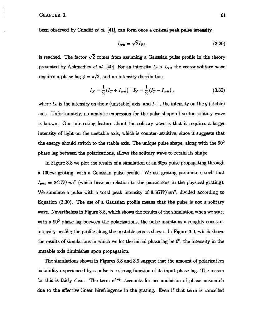
is reached. The factor fi cornes from assuming a Gaussian pulse profile in the theory

presented by Ahkmediev et al. [40]. For an intensiw IT > Ikr the vector solitary wave

requins a phase lag 4 = */2, and an intensity distribution

where Ix is the intensity on the x (unst able) axis, and Iy is the intensity on the y (stable)

axis. Unfortunately, no maiytic expression for the pulse shape of vector solitary wave

is known. One interesthg feature about the solitary wave is that it requirg a larger

intensity of light on the unstable axis, which is couater-intuitive, since it suggests that

the energy should switch to the stable aJEis. The unique pulse shape, along with the 90'

phase Iag between the polarizations, d o w s the soiitary wave to retain its shape.

In Figure 3.8 we plot the results of a simulation of an 80ps pulse propagating through

a 100m grating, with a Gaussian pulse profile. We use grating psrameters such that

Iht = 8GW/cm2 (which bear no relation to the parameters in the physical grating).

We simulate a pulse with a total peak intensiw of 8.5GW/cm2, divided according to

Equation (3.30). The use of a Gaussian profile meam that the pulse is not a solitary

wave. Nevertheless in Figure 3.8, which shows the results of the simulation when we &art

with a 90° phase lag between the polarizations, the pulse maintains a roughly constant

intensity profile; the profile along the unstable avis is shown. In Figure 3.9, which shows

the results of simulations in which we let the initial phase lag be oO, the intensity in the

unstable axis diminishes upon propagation.

The simulations shown in Figures 3.8 and 3.9 suggest that the amount of polarization

instabi1iw experienced by a pulse is a strong hc t ion of its input phase lag. The reason

for this is fairly dear. The term accounts for accumulation of phase mismatch

due to the effective linear birefÎingence in the grating. Even if that term is cancded

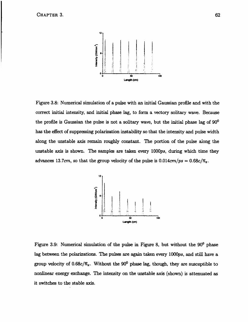
Figure 3.8: Numerical simulation of a pulse with an initial Gaussian profile and with the

correct initial intensity, and initial phase lag, to form a vectory solitary wave. Because

the profile is Gaussian the pulse is not a solitary wave, but the initial phase lag of 90°

has the e f k t of supprgsing polarization instabiiity so that the intensiw and pulse width

dong the unstable axis remain roughly constant. The portion of the pulse dong the

unstable aKis is shown. The samples are taken every 1000ps, during which time they

advances 13.7cm, so that the group velocity of the pulse is O.Ol4cmlps = 0.68c/~,.

Figure 3.9: Numerical simulation of the pulse in Figure 8, but without the 90' phase

lag between the polarizations. The pulses are again taken every 1000ps, and stiU have a

group velocity of 0.68c/EZ. Without the 90' phase lag, though, they are susceptible to

nonlinear energy exchange. The intensit3f on the unstable axis (shown) is attenuated as

it switches to the stable axis.

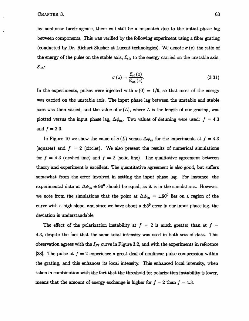
by nonlinear birefringence, there will still be a mismatch due to the initial phase hg

between components. This was verified by the following experiment using a fiber grating

(conducted by Dr. Richart Slusher at Lucent technologies). We denote a (2) the ratio of

the energy of the pulse on the stable axis, Est, to the energy carried on the unst able axis,

L:

In the srperiments, pulses were injecteci with t~ (0) = t/9, so that m a t of the energy

was carrieci on the unstable axis. The input phase lag between the unstable and stable

axes was then varied, and the value of a (L), where L is the length of our grating, was

plotted versus the input phase lag, At&,. Two values of detuning were used: f = 4.3

and f = 2.0.

In Figure 10 we show the value of o (L) versus A#, for the experiments at f = 4.3

(squares) and f = 2 (circles). We &O present the r d t s of nunerical simulations

for f = 4.3 (dashed iinej and f = 2 (soiid linej. The qualitative agreement between

theory and experiment is excellent. The quantitative agreement is also good, but suffers

somewhat from the error involved in setting the input phase lag. For instance, the

experimental data at A#in k 90O should be equd, as it is in the simulations. However,

we note from the simulations that the point at Aqbin = &go0 lies on a region of the

m e with a high dope, and since we have about a &5O error in our input phase lag, the

deviat ion is underst andable.

The effect of the polarization instabiliw at f = 2 is much greater than at f =

4.3, despite the fact that the same total intensiw was used in both sets of data. This

observation agrees with the Ipy curve in Figure 3.2, and with the experiments in reference

[38]. The pulse at f = 2 experience a great deal of nonünear pulse comprgsion within

the grating, and this enhances its local intensity. This enhanced local intensity, when

taken in combination with the fact that the threshold for polarkation instabiliQ is lower,

means that the amount of energy exchange is higher for f = 2 than f = 4.3.

Figure 3.10: Polarization instabilim as a hinction of input phase lag for f = 2 (circles)

and f = 4.3 (squares). Also shown are the results of simulations with the nonlinear CME

for f = 2 (solid line) and f = 4.3 (dash) . The simulations agree wit h the experiments to

within experirnental error.

3.6 Conclusion

In this chapter we have presented a set of coupled NLSEs relevant to the propagation of

optical pulses through a Kerr nonlinear fiber Bragg grating. Using these equations we

have identifid three distinct regimes of nonlinear propagation. For p S e carnet frequen-

cies that are far from the stop band of the grating, we have shown that an approxhate

theos, can be used to predict the polarization evolution of the pulse, if the pulse has

reasonably soliton-like parameters. If the ca.rrier kquencies are closer t o the stop gap,

then it shouid be posible to observe a vector solitary wave. We have presented numericd

simulations, using the nonlinear CME, to support t his claim.

Experiments were conducted to observe a variety of polarization phenornena in a

physical grating. For carrier fkquencies far detuned hom the stop gap, but with intensi-

ties fiil. higher than those required for soliton formation, we have observeci an intensity-

dependence of the Stokes parameters of the pulse. This intensity dependence is wd-

predicted by our nonlinear C m , and accords well with our heuristic understanding of

Ken: naalinear &ects in gratings. F k t h ~ o r e , we have derno&rM the suppfesion

and enhancement of polarization instability as a function of the initial phase lag between

the orthogonal polarizations. For carnier frequencies closer to the stop band, the polar-

ization instability is much larger, due both to the increased value of the coefEicient that

govenis the instability, and to noniinear puise compression.

The work in this chapter can be seen as a springboard for Further investigation of

polarization instability effects either near or even within the stop gap of a birefiingent

grating. Conversely, it can been seen as a cautionary srample for those wishing to exploit

Bragg grating solitons in a nomindy isotropic Bragg grating. Aithough the birefiingence

in a Bragg grating is high, the intensities required to observe Bragg gating solitons near

the gap will almost assuredly put one in a situation where polarization instability becornes

important.

Chapter 4

Gap soliton propagation in a

two-channel SCISSOR structure

4.1 Introduction

A waveguide-coupled rnicrodisk (microresonator) is an d-pass or phase-ody filter - a

100% transrnitting device that imparts a frequency-dependent phase. These microres-

onators have been used in a variety of areas inciuding waveiength division multiplexing

[45], laser fkequency stabilization [46] and cavity quantum electrodynamics [2]. The prop

erties of a sidecoupleci, integrated spaced sequence of resonators (SCISSOR), in which

a number of raonators are coupled to a channel mveguide, have been examineci [1][47].

It has been shown that light whose fiequency corresponds to the resonant frequency of

the microresonators will propagate with a vastly reduced group velocity, and a Mnishing

group velociw dispersion [l]. The reduced group velocity corresponds to a huge build-

up of the electromagentic field intensity in the microresonators, which means that the

nodinear properties of the system are enhanceci.

In (a) of Figure 4.1 a single microresonator coupled to a chaMel waveguide is shown,

dong with the mode profiles of both. The dimensions and materials shown in the figure

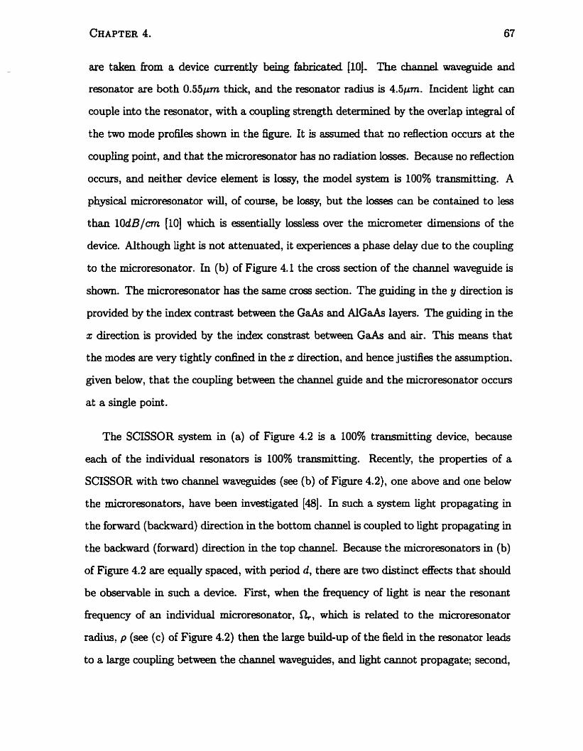
are taken fkom a device cmrentiy being hbzicated [lq. The chaMel wavegu.de and

resonator are both 0.55pm thick, and the resonator radius is 4.5pm. Incident light cm

couple into the resonator, with a coupimg strength determineci by the overlap integral of

the two mode profiles shown in the figure. It is assumed that no rdection occurs at the

coupling point, and that the microremnator has no radiation losses. Because no reflection

occurs, and neither device element is lossy, the mode1 systern is 100% transmitting. A

physical microresonator will, of course, be lossy, but the losses can be contained to l e s

than 10dBlcm [IO] which is essentially lossless over the micrometer dimensions of the

device. Aithough light is not attenuated, it wperiences a phase delay due to the coupling

to the microresonator. In (b) of Figure 4.1 the cross section of the channel waveguide is

shown. The microresonator has the same cross section. The gui* in the y direction is

provided by the index contrast between the GaAs and AlGaAs layers. The guiding in the

x direction is provided by the index constrast between GaAs and air. This means that

the modes are very tightly confinecl in the x direct ion, and hence justifies the assumption.

given below, that the couphg between the channe1 guide and the microresonator occurs

at a single point.

The SCISSOR system in (a) of Figure 4.2 is a 100% transmitting device, because

each of the individual resonators is 100% transmitting. Recently, the properties of a

SCISSOR with two channel waveguides (see (b) of Figure 4.2), one above and one below

the microresonators, have been investigated [44. In such a system light propagating in

the forward (backward) direction in the bottom channe1 is coupled to Lght propagating in

the backward (forward) direction in the top channel. Because the microresonators in (b)

of Figure 4.2 are equdy spaced, with period d, there are two distinct &ects that should

be observable in such a device. First, when the fkequency of light is near the resonant

fkequency of an individual microresonator, a, which is related to the microresonator

radius, p (see (c) of Figure 4.2) then the large build-up of the field in the resonator leads

to a large coupling between the channel waveguides, and light cannot propagate; second,

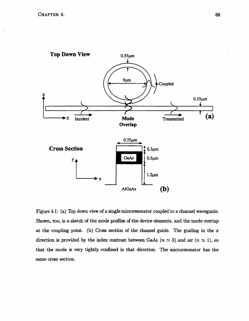
Top Down View

I r

Mode b

T d t t e d Overlap

Cross Section

0)

Figure 4.1: (a) Top dom view of a singIe mïcroresonator coupled to a channe1 waveguide.

Shown, too, is a sketch of the mode profiles of the device elements, and the mode overlap

at the couphg point. (b) Cross section of the chamel guide. The gui- in the x

direction is provided by the index contrast between GaAs (n cz 3) and air (n zz 1), so

that the mode is very tightly confineci in that direction. The microresonator has the

same cross section.

when the frequency of light is near the Braggfkquency of the periodic system, which

is related to the pexiod d, then the small couphg between the channe1 waveguides can

build up vio a Bragg reflection-type effect, so that light cannot propagate. Both of these

effects lead to a gap in the dispersion relation of light in the system, but while the second

&ect corresponds to a wd-known photonic band gap, and can be described by a set of

coupled mode equations (CME), the former e f k t does not. We call the gap that is due

to the field build-up in the resonator a 'rcsonator gap' to distinguish it hrom a Bragg gap.

At a given frequency outside either type of gap, there are two propagation modes

asociated with each propagation direction. We label these modes the bottom and top

modes. For the bottom (top) mode associated with either propagation direction, there iç

a larger field intensity in the bottom (top) c h a e l than in the top ( bottom) channel. The

dispersion relations associated with the upper and lower modes are heavily dependent on

the values of the coupling coefficients a b , ~b and a,, rct where the subscripts b and t label

the bottom md top couphg points. Whcn a fidd in a chme1 guide impings upon a

couphg point, the rc coefficient determines how much of the field amplitude couples into

the resonator, and the D coefficient determines how much continues on in the Channel

guide. When ob = a,, which we c d a symmetric device, then the dispersion relation

associated with either the bottom or the top mode is the same. When a b # a,, which

we cail an asymmetric device, then the dispersion relations associated with the bottom

and top modes are distinct. In the absence of nonlinearity, Iight with kequency content

either outside a gap of the system, or only slightly inside a gap (in a sense to be made

more precise below), is well described by a set of uncoupleci h e a r Schrddinger equations

(LSEs). The two parameters that enter the LSE - group velocity and group velocity

dispersion - are taken hom the dispersion relation of the system. Thus, for a symmetric

device, the parameters of the LSEk that describe light in the bottom and top modes are

quivalent, while for an asymmetric device the parameters of the LSEs are distinct.

In the presence of a Kerr nonlineari@, bght in the upper mode is coupled nonlineazly to

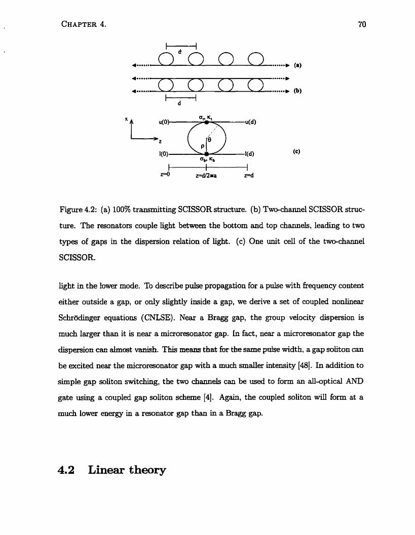
Figure 4.2: (a) 100% transmitting SCISSOR structure. (b) Tmxhannel SCISSOR stmc-

ture. The resonators couple light between the bottom and top channels, leading to two

types of gaps in the dispersion relation of light. (c) One unit cell of the twwAannel

SCISSOR-

light in the lower mode. To describe pulse propagation for a pulse with fkquency content

either outside a gap, or ody slightly inside a gap, we derive a set of coupled nonlin-

Schrodinger equations (CNLSE). Near a Bragg gap, the group velocity dispersion is

much larger than it is near a microresonator gap. in fact, near a microresonator gap the

dispersion am drnost vanish. This means thst for the same pulse width, a gap sotiton can

be excited near the microresonator gap with a much smaller intensity [q. In addition to

simple gap soliton switching, the two chit~ll~lels can be used to form an all-optical AND

gate using a coupled gap soliton scheme [4]. Again, the coupled soliton will form at a

much lower energy in a resonator gap than in a Bragg gap.

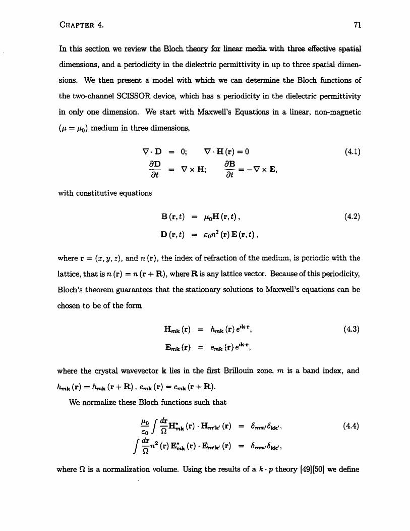
In this section we review the Bloch theary for linear media with thzee effective spatial

dimensions, and a periodicity in the dielectric permittivity in up to three spatial dimen-

sions. We then present a mode1 with which we can determine the Bloch functions of

the tw~channel SCISSOR device, which has a periodicity in the dielectric permittivity

in only one dimension. We start with Maxwell's Equations in a linear. non-magnetic

( p = po) medium in three dimensions,

dD - - - V X H ; -- - -V x E, dB ât ât

with constitutive equations

where r = (2, y, T ) , and n (r), the index of refiaction of the medi*m, is pcriodic aith the

lattice, that is n (r) = n (r + R), where R is any lattice vector. Because of this periodicity,

Bloch's theorem guarantees that the stationary solutions to Maxwell's equat ions can be

chosen to be of the form

where the crystal wavevector k Les in the first Brillouin zone, m is a band index, and

We normalize these Bloch functions such that

/ Z n 2 (r) E h ( r ) (r) = 6,,diW,

where Q is a normalization volume. Using the r d t s of a k - p theory [49] (501 we define

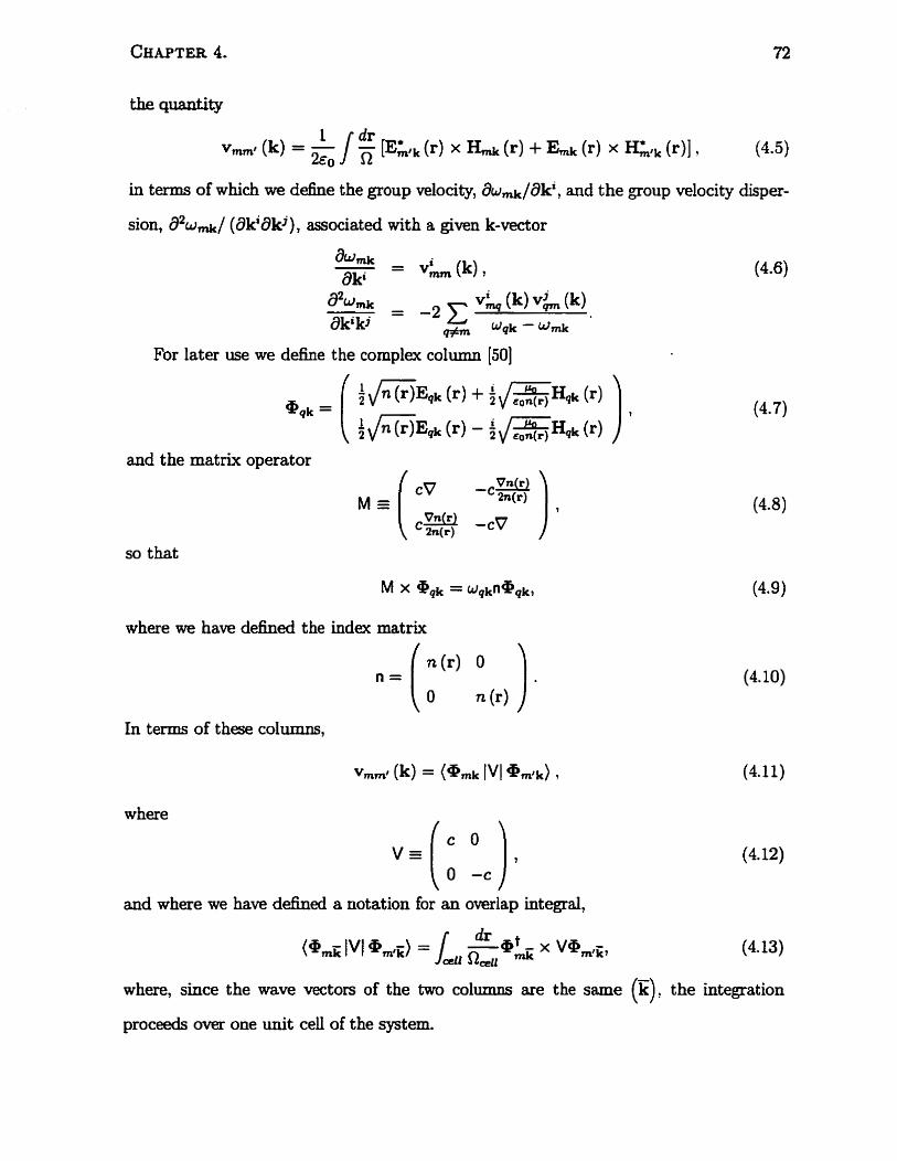
in terms of which we define the group velocity, a w & ? k i , and the group velocity disper-

sion, a2wd/ (aki8kj), associateci with a given k-vector

For later use we define the cornplsr column [50]

and the matrix operator

so that

where we have defineci the index matrix

In terms of these coliimnc,

where

and where we have defined a notation for an overlap integral,

where, since the m e vectors of the two columns are the same (k)? the integration

proceeds over one unit cell of the system.

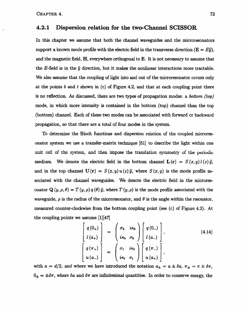
4.2.1 Dispersion relation for the twcShannel SCISSOR

In this chapter we assume that both the chwrnel waveguides and the microresonators

support a known mode profle with the electric field in the transverse direction (E = EY),

and the magnetic field, H, everywhere orthogonal to E. It is not necessary to assume that

the E-field is in the jj direction, but it makes the nonlinear interactions more tractable.

We &O assume that the coupling of light into and out of the microresonator occurs only

at the points b and t shown in (c) of Figure 4.2, and that at each coupling point there

is no refiection. As discussed, there are two types of propagation modes: a bottom (top)

mode, in which more intensity is containeci in the bottom (top) charnel than the top

(bottom) channel. Each of these two modes can be associated with forward or backward

propagation, so that there are a total of four modes in the system.

To determine the Bloch hinctions and dispersion relation of the coupled microres

onator system we use a transfer-matrix technique [51] to describe the light within one

unit cell of the qstem, and then impose the trançlaticin symmetry of the ptsiorlic

medium. We denote the electric field in the bottom channel L (r) = S (z, y) 1 (r) Y, and in the top channel U (r) = S ( x , y) u ( 2 ) y, where S (2, y) is the mode profile as

sociated with the channel mveguides. We denote the electric field in the microres-

onator Q (y, p, 0) = T (y, p) q ( O ) y , where T (y, p) is the mode profile associated with the

waveguide, p is the radius of the microresonator, and B is the angle within the resonator,

measured counter-clockwise from the bottom coupling point ( s e (c) of Figure 4.2). At

the coupling points we assume [l] [47]

[ d o + ) ] = ( - '%) [ " O - ) ] 1

1 (a+) 2 ~ ; ~ cq 1 (a-

with a = d / 2 , and where we have introduced the notation a* = a f 6a, n* = r & 675

Or = f 6?r, where 6a and 67r are infinitesimal quantities. In order to conserve energy, the

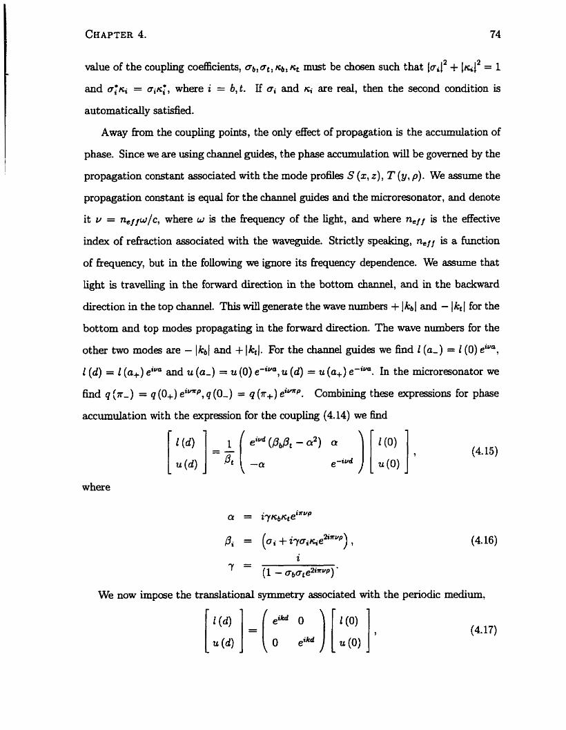
value of the couphg co&cients, obi uti S b r muSt be choscm such that (ail2 + 1&l2 = 1

and orni = o ~ K ~ ? where i = b, t . I f oi and 6 are r d , then the second condition is

Away from the coupling points, the ody effet of propagation is the accumulation of

phase. Since we are using channel guides, the phase accumulation will be gowrned by the

propagation constant associated with the mode profiles S (x, z ) , T (y, p) . We assume the

propagation constant is equal for the channel guides and the microresonator, and denote

it Y = ncffw/c , where w is the frequency of the light, and where nef/ is the effective

index of refraction associated with the waveguide. Strictly speaking, ne,l is a function

of hequency, but in the following we ignore its frequency dependence. We assume that

Light is travelling in the forward direction in the bottom chamel, and in the backward

direction in the top channel. This wili generate the wave numbers + 1 kb 1 and - 1 kt 1 for the

bottom and top modes propagating in the forward direction. The wave numbers for the

other two modes are - (kbl and + 1 hl. For the chamel guides we h d 1 (a- ) = 1 ( O ) eiva,

1 ( d ) = 1 (a,) eiua and u (a-) = u (O) e-iua, u (d) = u (a,) e-lm. In the microresonator we

&d q (n- ) = q (O+) eiY"P, q (O-) = q (A+) eimp. Cornbining these expressions for phase

accumulation with the expression for the coupling (4.14) we find

where

We now impose the translational symmetry associated with the periodic medium,

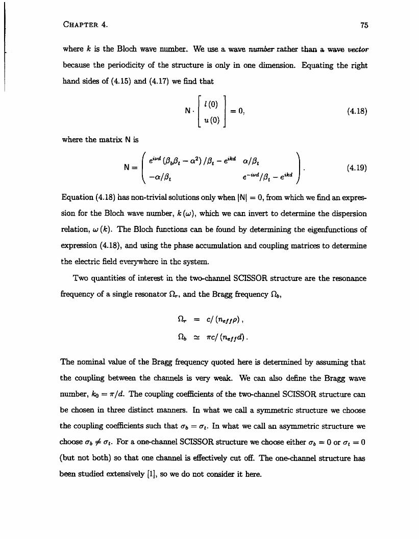
where k is the Bloch wwe niimber, W e use a wave n w n k ra.t.her than a wave v a b r

because the periodicity of the structure is ody in one dimension. Equating the right

hand sides of (4.15) and (4.17) we fmd that

where the matrix N is

Equation (4.18) has non-trivial solutions only when (NI = O, h m which we fllid an expres-

sion for the Bloch wave number, k (w ) , which we can invert to determine the dispersion

relation, w (k) . The Bloch functions can be found by determinhg the eigenfunctions of

expression (4.18), and using the phase accumulation and coupling matrices to detennine

the electric M d ewxyxhcrc in thc s)stem.

Two quantities of interest in the twcxhaanel SCISSOR structure are the resonance

frequency of a single resonator a, and the Bragg frequency Q,,

The nominal value of the Bragg hequency quoted here is determined by assuming that

the coupling between the ch=& is very weak. We can &O define the Bragg wave

number, ko = ald. The coupling coefncients of the two-charnel SCISSOR stmcture can

be chosen in three distinct manners. In what we caU a symmetric structure we choose

the couphg coefficients such that ab = oc. In what we c d an nsymmetric structure we

choose us # a,. For a onechannel SCISSOR structure we choose either ab = O or a, = O

(but not both) so that one chamel is effectively cut off. The one-channel stmcture has

been studied extensively [Il, so we do not consider it here.

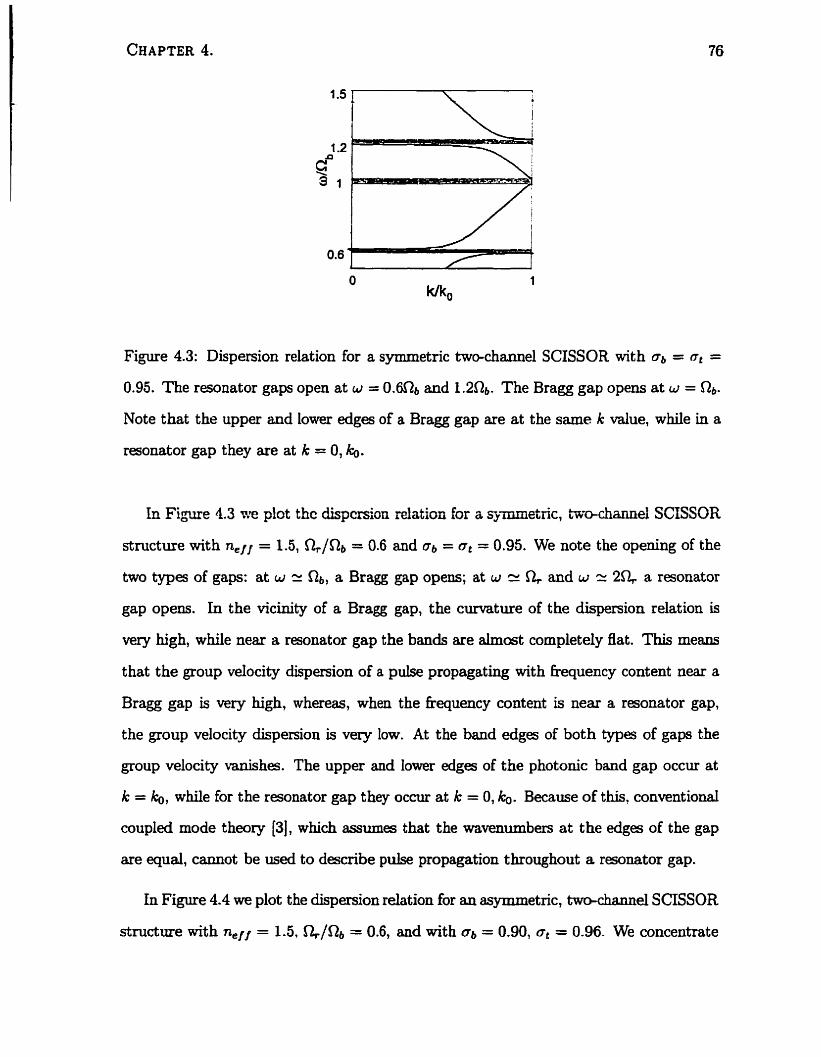
Figure 4.3: Dispersion relation for a symmetric tw~chasu1el SCISSOR with q, = nt =

0.95. The resonator gaps open at w = 0.6nb and 1 .2Qb. The Bragg gap opens at w = Rb.

Note that the upper and lower edges of a Bragg gap are at the same k value, while in a

resonator gap they are at k = O, b.

In Fibwe 4.3 nTe plot thc dispersion relation for a qmmetr ic , b-cxhannel SCISSOR

structure with n,/l = 1.5, %/Rb = 0.6 and = at = 0.95. We note the opening of the

two types of gaps: at w 2 Clb, a Bragg gap opens; at w zz and w = 2% a resonator

gap opens. In the vicinity of a Bragg gap, the curvature of the dispersion relation is

very high, while near a resonator gap the bands are almost completely Bat. This means

that the group velocity dispersion of a pulse propagating with kequency content near a

Bragg gap is very high, whereas, when the hequency content is near a resonator gap,

the group velocity dispersion is v q low. At the band edges of both types of gaps the

group velocity Mnishes. The upper and lower edges of the photonic band gap occur at

k = b, while for the resonator gap they occur at k = O, b. Because of this, conventional

coupled mode theory (31, which assumes that the wavenumbers at the edges of the gap

are equal, cannot be used to describe pulse propagation throughout a resonator gap.

In Figure 4.4 we plot the dispersion relation for an asymmetric, two-charnel SCISSOR

stmcture with nef/ = 1.5. %/Ob = 0.6, and with 06 = 0.90, a, = 0.96. We concentrate

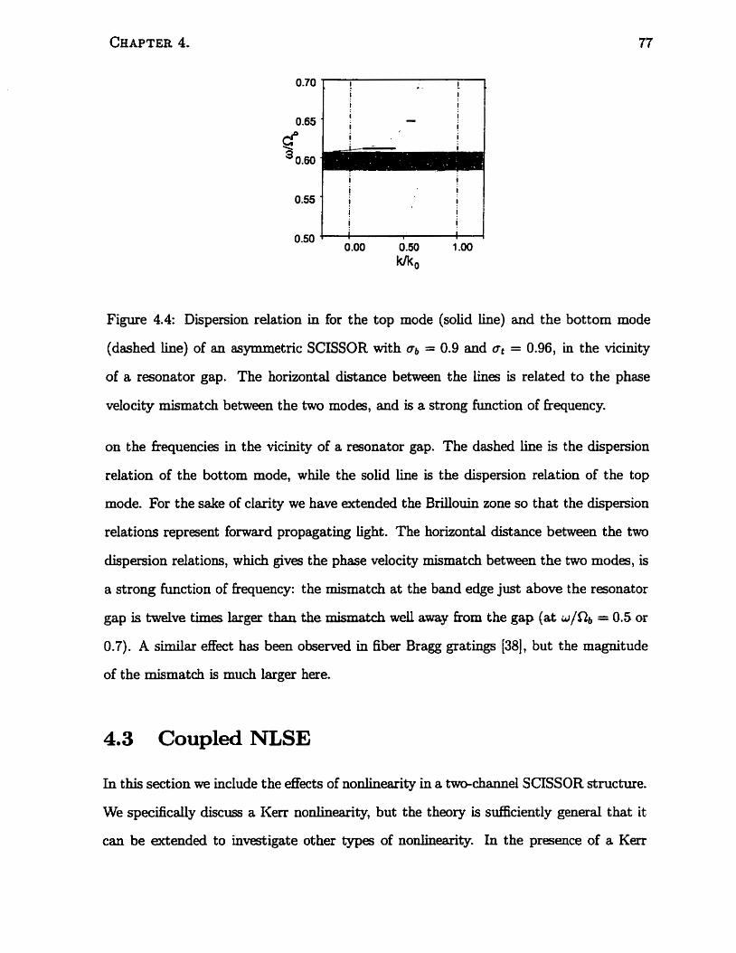
Figure 4.4: Dispersion relation in for the top mode (solid h e ) and the bottom mode

(dashed line) of an asymmetric SCISSOR with 0 6 = 0.9 and a, = 0.96, in the vicinity

of a resonator gap. The horizontal distance between the ling is related to the phase

velocity mismatch between the two moda, and is a strong function of fkequency.

on the hequencies in the vicinity of a resonator gap. The dashed line is the dispersion

relation of the bottom mode, while the solid line is the dispersion relation of the top

mode. For the s&e of clarity we have extended the Brillouin zone so that the dispersion

relations represent forward propagat h g light . The horizontal distance between the two

dispersion relations, which gives the phase velocity mismatch between the two modes, is

a strong function of frequency: the mismatch at the band edge just above the resonator

gap is twelve times larger than the mismatch w d away h m the gap (at w/Q, = 0.5 or

0.7). A similar effect has been observed in fiber Bragg gratings [38], but the magnitude

of the mismatch is much larger here.

4.3 Coupled NLSE

In this section we include the &ts of nonünearity in a twc+channel SCISSOR structure.

We specificaily discuss a I k r nonlinearity, but the theory is suffciently general that it

can be extended to invgtigate other typg of nonlinearity. In the presence of a Kerr

nonlineaxity we derive a set of coupled NLSEs that are Müd for pulses with fiequency

content anywhere on the dispersion relation that is not too deep withui either a resonator

or photonic band gap [7][34]. In such a situation we expect the pulse to be weU-described

by one Bloch function, centred at the carrier wave number of the pulse, and modulateci

by a slowly-varying envelope function.

When we introduce nonlinearity into the system, we must stiil satisfy the MaxweU

equations (4.1) , but the constitutive relation for D becornes

D (r, t ) = €on2 (r) E (r, t ) + P N L (r, t ) . (4.20)

Rat her than working directly wit h the electric and magnetic field, we first introduce the

potentials A and N, with

B = V x A ,

These potentials automaticdy satisfy the divergence equation of (4.1). It is easy to

verify hom the curl equations of (4.1) that the A and N fields ais0 satisfy

We write the dynamical equations (4.22) in matrix form as

a* in- = M x !P +i9, at

where the column Q of cornplex vector fields is given by

and the column

The index ma& n, and the matruc operator M, are dPfinPrl in Eqwtions (4.10) and

(4.8) respectively.

For an arbitrary complex column, 8, we can construct a column @ + $ representing

real potentials, where the physical conjugate, 9, of a column vector (4.24) is defined

- We write a real column as \y+ + \Y- where @- = a+. Defhing the operator

we see that the physical conjugate of L9+ is -Lq-. Hence, if we likewise have 8 =

0, + 8- and satisfy

LIS+ = ie+, (4.28)

then the dpamical equations will he .satifid. W' extract a set of coupled mEs h m

(4.28) using the method of multiple scales.

4.3.1 Multiple Scales

The vector notation introduced above is designed to deal with systems that have a one,

two or three dimensional perîodicity in their dielectric constant. In the ~ c h a . n n e l

SCISSOR structure, the periodicity is only in one dimension, so that the wave vectors

associated with the Bloch functions point in the z-direction. Because of the existence of

the two distinct modes, associated with light in the upper and lower channels respectively,

we label an arbitraxy wave vector k (w) = k, (w) 2, where for the remainder of the chapter

the subscript i = b, t indexes the bottom and top modes respectively.

In the absence of nonlinearity, the general solution of (4.28) is of the form

where the f& are r)imPnsidess expansion CQ* a ciirries the units of ?Zr+, and

the column 9<lki (r) is defined in Equation (4.7). In the presence of nonlinearity such a

solution cannot be used. Instead, we use the method of multiple scales [50] (71 to constmct

approximate solutions to (4.28). We replace the constant coefncients fqk in (4.29) with

hinctions fqk, (2, t) that vary slowly in space and time. To keep track of the slowness

we explicity separate different length and time scales in the problem by introducing a

smallness parameter, 7, and writing functions as

It is assumed that F va.ries equaily significsntly as each of its arguments varies over a

range d, or a period, r. These are chosen to be the shortest length and time scales in

the problem; d is taken as the size of a lattice constant, and T as l/w, where wili be

identifieci below. Then the ranges and periods d(") = d/qn and dn) = r/vn define the

multiple scales of the problem. We wiU quantify the value of below (after Equation

(4.55)). Derivatives are given by, for example,

We seek to describe the propagation of light pulses that v a q slowly relative to a given

carrier frequency? W. We define = kb (G) and & = kt (G). We seek an approha te

solution to (4.28) of the form

where we assume we have light in a bottom mode and a top mode, but we have not

specified the propagation direction of either mode. We have separated the cornponents

fmG (2, t) fkom the rest of the components because it is assumed that the fiequency and

wavenumber content of the pulse describeci by (4.32) is such that functions in band m

contribute most to the value of a+. These components will be called the principal comp*

nents. The 0 t h components, f&, (2, t), with q # rn, are called cornpanion components,

and are asstlmed to be smaller thaa the 1'. (z,t). To capture the relative stnmgths of

the principal and cornpanion components, we take

These slowly-varying quantities have no dependence on ro or to. Rom the dependence

of !P on N and A (4.24), we see that the ansatz for @+ (4.32) leads to

2 (2) ~ z ~ ~ ~ k ~ (r) f FS~H,,,~~ (r) + [r)f"i: + 11 Fqz, + ..] Ha& (i) i=u,l q#m

We construct an expansion of 138, in powers of r),

This construction requires us to find the expansions of the terms that appear in 13. These

tue s h p l y

where

and, for j > O,

where the matrix V is defineci in Equation (4.12).

We assume that the nonlinearity is weak and due to a third-order response which, at

kequencies of interest, is far off resonance. Then an appropriate mode1 for the nonlinear

polazization Par. (r , t ) is [52]

We ignore third harmonic generation on physical grouuds. We have assumed that the

underlying material is nondispersive, and while this may be valid for fiequencies near Y,

it will likely not be valid for frequency ranges extending to w 2 3W; furthmore, the

assumption of no absorption at w 2 3W will likely be in error. We expect, on physical

grounds, that in many cases the actual materia. dispersion and absorption will mske any

buildup of the third hannonic iinlikely, so that our mode1 will be adequate. Under these

assumpt ions the expression (4.38) reduces to

Then, since we have assumed that our electric field is polarized in the ij direction, we

find

PnL (r, t ) = PNL (r, t) 6 = ~ Q X ~ W Y Y (r) ( E (r, t)12 E (r, t ) e-"y + cc, (4.40)

where E (r, t) = E (r, t) y . To use this nonlinear polarization in our multiple scales

formalism, we make the following assumption for the strength of x" (r),

where €0- (r) has units of permittivity and is assumed to be on the order of the largest

linear media permittivity, or smaller.

Using the ansatz for N (r: t) (4.33), the definition of N (r, t) (4.21) and the Maxwell

equations (4.1) we find that , in light of the fact that the nonlinear terms are considered

to be O (q2) :

Using the expression for the ekctric field (442) we c m àetefmine an -ession for the

nonlinear polarization, which we write as

with

where

4.3.3 Coupled NLSEs

Using (4.34) and (4.45) we can solve the pulse propagation equation (4.28) in te= of

the multiple scales quantities. The mechanics of the derivation have been performed else-

where for a system with only one carrier wave vector (501. To include the nonlinear terrn

we follow previous work on birefkingence in periodic systems which expiicitly accounted

for the inclusion of two wave numbers (341. We find

The nonlinear co&cients are

where e,, (r) is the periodic portion of the Bloch function (4.3). The values of a z , a=

and fldt cm be determineci fkom those above by interchanging b t in aU expessions.

The noniinear coefficients are superscripted in such a m m e r because a x accounts for

self-phase modulation, ax accounts for cross-phase modulation, and #si accounts for

phase conjugat ion ra]. When the group velocity in (4.47) is non-zero, then the equations can be used to

describe two distinct situations: 1) the light in both modes is travelling in the same

direction; or 2) the Iight in one mode is t ravehg in the forward direction, while the

light in the other mode is travehg in the badcward direction. In the first situation,

the value of < is much smder than either a" and a", because in every portion

of the unit cell the light associated with the two Bloch functions is counterpropagating,

so the overlap integral is smd. In the second situation the light associated with the

Bloch functions is cepropagating, so the < codcient is simüar in strength to the other

nonlinear coefficients, but since the pulses would then have wave vectors of the opposite

sign, the quantity C would be enormous, and the phase conjugation process would still

not build up. A third situation occurs when the group velocity in (4.47) is zero. This only

occurs when the carrier fiequency of the light is considered to be at a band edge. h such

a situation the four modes of the system (top and bottom travelling in the forward and

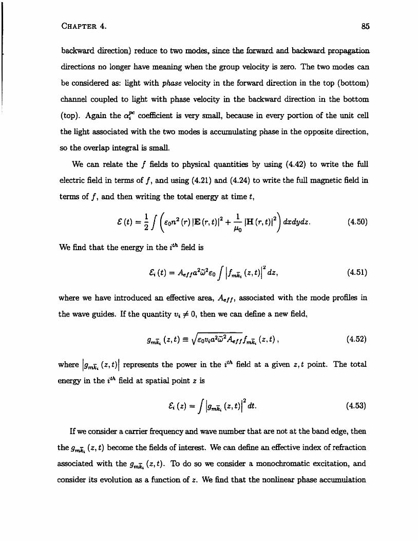
backward direction) reduce to two modes, since the h a r d and backward propagation

directions no longer have meaning when the group velocity is zero. The two modes can

be considered as: light with phase velocity in the forward direction in the top (bottorn)

channel coupled to Iight with phase velocity in the backward direction in the bottom

(top). Again the < coefncient is very s d , because in every portion of the unit ceil

the light associated with the two modes is accumulating phase in the opposite direction,

so the overlap integral is s m d .

We can relate the f fields to physical quantities by using (4.42) to mite the full

eiectric field in terms of f , and using (4.21) and (4.24) to write the full magnetic field in

tems of f , and then writing the total energy at time t ,

We find that the energy in the ith fieid is

where we have introduced an effective area, Aeff, associated with the mode profiles in

the wave guides. If the quantity v, # O, then we can d&e a new field,

where lgd, ( z , t ) 1 represents the power in the ith field at a given z, t point. The total

energy in the ith field at spatial point z is

If we consider a carrier kequency and wave number that are not at the band edge, then

the g a (r, t) become the fields of interest. We can d&e an effective index of &action

associated with the g&, (r , t). To do so we consider a monochromatic excitation, and

consider its evolution as a b c t i o n of z. We h d that the nonlinear phase accumutation

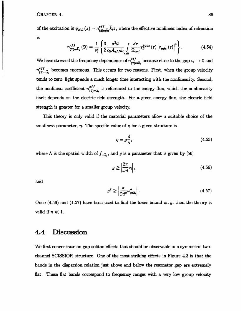
CHAPTER 4. 86

- of the excitation is 4N, (2) = nef'

t 2 e kg, where the effective mnlincri.r index of &action

We have stresseci the hequency dependence of n;;{& because close to the gap vi 4 O and

nef' becomes enormous. This occurs for two reasons. First, when the group velocity (2)m;k,

tends to zero, Iight spends a much longer time interacting with the nonlinearity. Second,

the nonlinem coefkient n ; z i is referenced to the energy flw, which the nonlinearity

itself depends on the electric field strength. For a given energy flux, the electnc field

strength is greater for a smder group velocity.

This theory is only valid if the material parameters d o w a suitable choice of the

smallnes parameter, 7. The specific value of q for a given structure is

where A is the spatiai width of fmG, and g is a parameter

and

(4.55)

that is given by $01

Once (4.56) and (157) have been used to find the lotver bound on g, then the theory is

valid if q « 1.

4.4 Discussion

We first concentrate on gap soliton effects that should be obsewable in a symmetric hm

channel SCISSIOR structure. One of the most striking dec ts in Figure 4.3 is that the

bands in the dispersion relation just abow and below the resonator gap are extremely

%at. These Bat bands correspond to frequency ranges with a very low group velocity

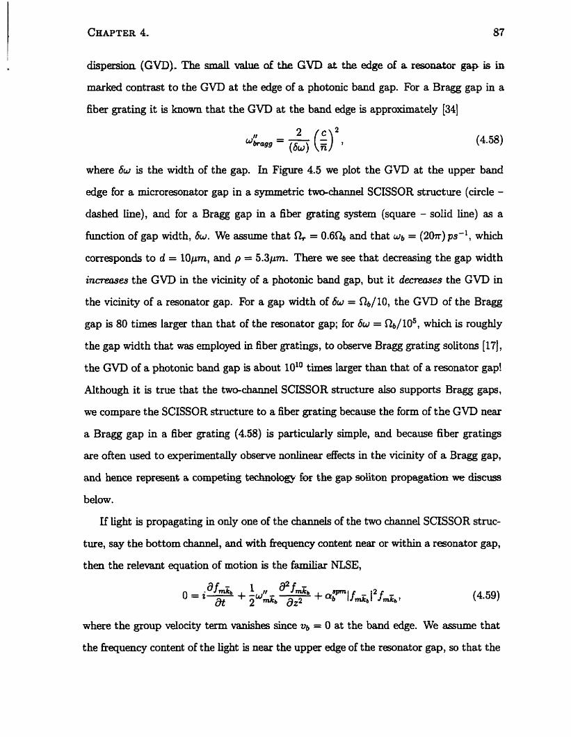
dispersion (GVD). The d value of the GVD a& the edge of a resonabr gap is in

marked contrast to the G M at the edge of a photonic band gap. For a Bragg gap in a

fiber grating it is known that the GVD at the band edge is apprmimately (341

2 2 .b,, = - (C) , ( 6 4 n

where bw is the width of the gap. In Figure 4.5 we plot the G M at the upper band

edge for a microresonator gap in a synunetric ~ c h m e l SCISSOR structure (circle -

dashed iine), and for a Bragg gap in a fiber grating system (square - solid line) as a

function of gap width, 6w. We assume that 0, = 0.64 and that wb = (207r) ps - l , which

corresponds to d = 10pm, and p = 5.3pm. There we see that decreasing the gap width

i n m e s the GVD in the vicinity of a photonic band gap, but it derreases the GVD in

the vicinity of a resonator gap. For a gap width of 6w = Rb/lO, the GVD of the Bragg

gap is 80 times larger than that of the resonator gap; for 6w = 4 /105 , which is roughly

the gap width that was employed in fiber gratings, to observe Bragg grating solitons [l?] ,

the GVD of a photonic band gap is about 101° times Iarger than that of a resonator gap!

Although it is true that the two-chamel SCISSOR structure also supports Bragg gaps,

we compare the SCISSOR structure to a fiber grating because the form of the GVD near

a Bragg gap in a fiber grating (4.58) is particulady simple, and because fiber gatings

are often used to experimentdy observe nonlinear dects in the vicinity of a Bragg gap,

and hence ~epresent a competing teckoiogy for the gap &ton propagation we diseusa

below.

If light is propagating in only one of the channels of the two c h d SCISSOR stmc-

tue , Say the bottom channel, and with fiequency content near or within a raonator gap,

then the relevant equation of motion is the familiar NLSE,

where the group velocity term vanishes since vb = O at the band edge. We assume that

the fiequency content of the light is near the upper edge of the resonator gap, so that the

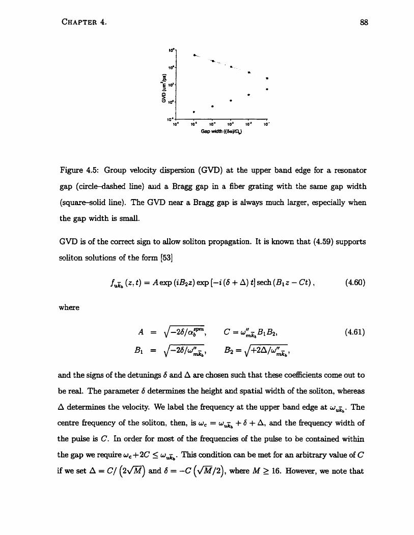
Figure 4.5: Group wlocity dispersion (GVD) at the upper band edge for a resonator

gap (circledashed line) aud a Bragg gap in a fiber grating with the same gap width

(squaresolid line). The GVD near a Bragg gap is always much larger, especiaily when

the gap width is smd.

GVD is of the correct sign to d o w soliton propagation. It is known that (4.59) supports

soliton solutions of the fom [53]

where

and the signs of the deturings 6 and A are chosen such that these coefficients corne out to

be real. The parameter 6 detennines the height and spatial width of the soliton, whereas

A determines the velocity. We label the frequency at the upper band edge at w z b . The

centre hequency of the soliton, then, is w, = w z b + 6 + A, and

the pulse is C. In order for most of the fkequencies of the pulse

the gap we require w, + 2C 5 w a b . This condition can be met f o ~

if we set A = C/ (2@) and 6 = -C (m/2), where M 2 16.

the frequency width of

to be cont ained wit hin

an arbitrary value of C

However, we note that

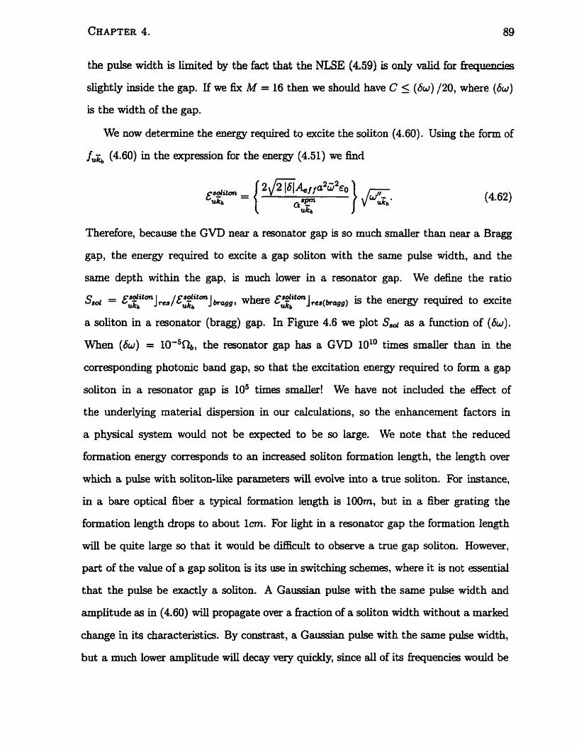
the pulse width is limited by the fact that the NLSE (4.59) is d y valid for f i ~ u m c k s

slightly inside the gap. If we fix M = 16 then we should have C 5 (6w) /20, where (6w)

is the width of the gap.

We now determine the energy required to excite the soiiton (4.60). Using the form of

f~ (4.60) in the expression for the energy (4.51) we find

Therefore, because the GVD near a resonator gap is so much smder than near a Bragg

gap, the energy required to excite a gap soliton with the same pulse width, and the

same depth within the gap, is much lower in a resonator gap. We define the ratio

Sad = &sGattm adittm ukb Jres/Ezb Jbom, where E,btmJ,(~qg) is the energy required to excite

a soliton in a resonator (bragg) gap. In Figure 4.6 we plot Ssd as a function of (6w).

When (6w) = 10-5nb26, the resonator gap has a GVD 10'' timg smaller than in the

correspondhg photonic band gap, so that the excitation energy required to form a gap

soliton in a resonator gap is los times smaller! We have not included the e t of

the underlying material dispersion in our calculations, so the enhancement factors in

a physical system would not be expected to be so large. We note that the reduced

formation energy corresponds to an inmeased soliton formation length, the length over

which a pulse with soliton-iike parameters will evolve into a true soliton. For instance,

in a bare optical fiber a typical formation length is 100m, but in a fiber grating the

formation length drops to about lem. For light in a resonator gap the formation length

will be quite large so that it would be difficdt to o b s m a true gap soliton. However,

part of the value of a gap soliton is its iw in switchmg schemes, where it is not essential

that the pulse be exactly a soliton. A Gaussian pulse with the same pulse width and

amplitude as in (4.60) will propagate over a fraction of a soliton width without a marked

change in its characteristics By constrast, a Gaussian pulse with the same pulse width,

but a much lower amplitude wilI decay very quiddy, since all of its hequencies w d d be

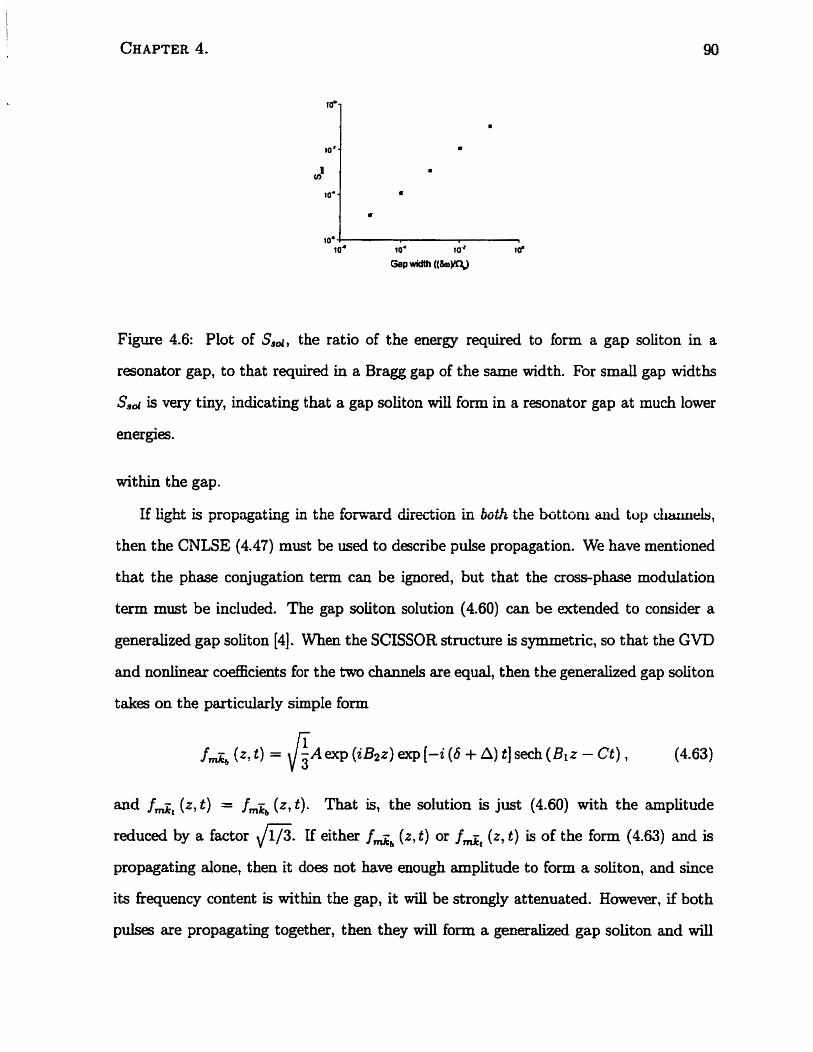
Figure 4.6: Plot of SSd, the ratio of the energy required to form a gap soliton in a

raonator gap, to that required in a Bragg gap of the same width. For s m d gap widths

Ssd is very tiny, indicating that a gap soliton will form in a resonator gap at much lower

energies .

within the gap.

If light is propagating in the fom-ard direction in both the bottom mcl top cliaf~lleis,

then the CNLSE (4.47) must be used to describe pulse propagation. We have mentioned

that the phase conjugation term can be ignoreci, but that the crossphase modulation

term m u t be included. The gap soliton solution (4.60) can be actended to consider a

generalized gap soliton [4]. When the SCISSOR stmcture is symmetric, so that the GVD

and nonlineax coefficients for the two c h m & are equal, then the generalized gap soliton

takes on the particularly simple form

fAb (L, t ) = \ I i ~ e x ~ (iBzz) exp [-i (6 + A) t] sech (Bir - Ct) ,

and f& (2, t ) = jmzb ( z , t). That is, the solution is just (4.60) with the amplitude

reduced by a factor If either fdb ( 2 , t) or fdt ( z , t ) is of the form (4.63) and is

propagating alone, then it d o s not have enough amplitude to form a soliton, and since

its frequency content is within the gap, it will be strongly attenuated. However, if both

pulses are propagating together, then they will form a generalized gap soliton and will

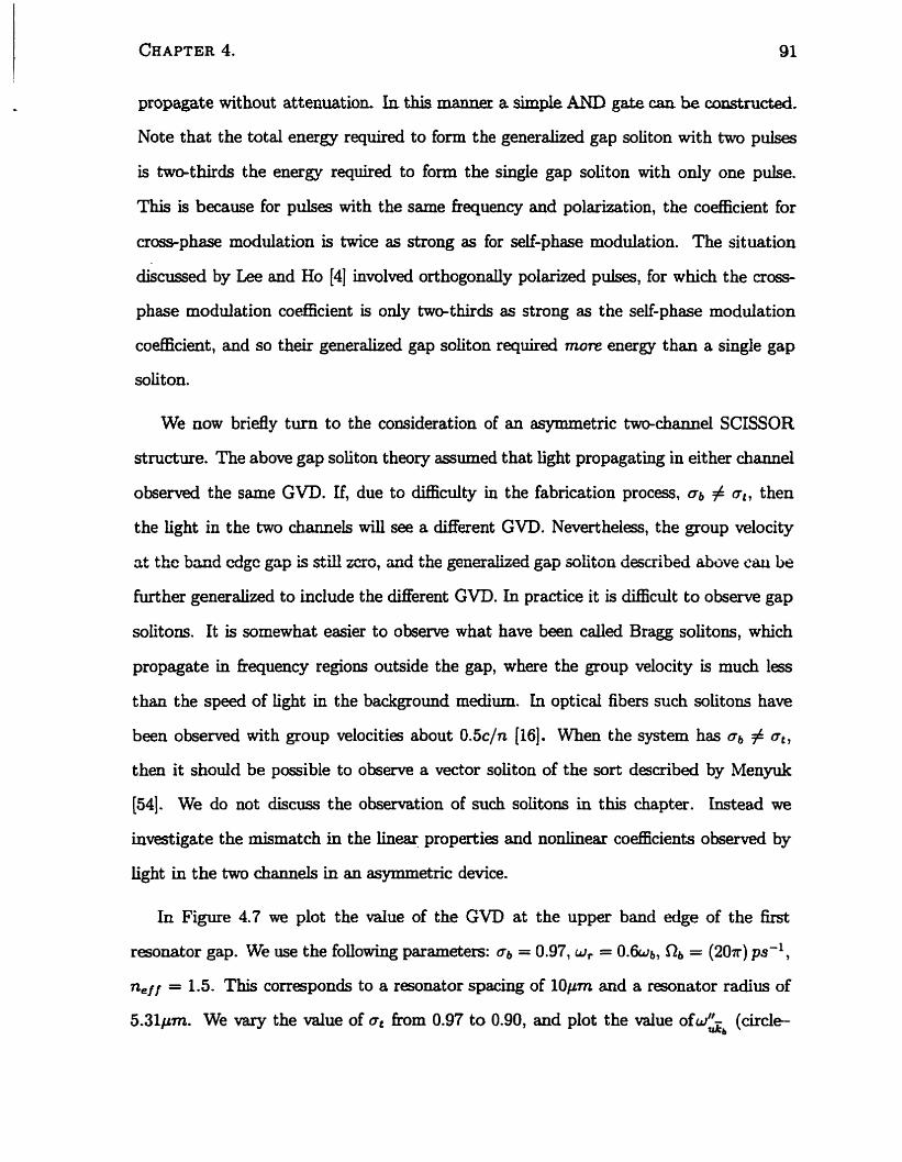
propagate without attenuation. La this mariner a simple AND gate c m he constmcted.

Note that the total energy requireà to form the generalized gap soliton with two puises

is twethiràs the energy requireà to form the slngie gap soliton with only one pulse.

This is because for pulses with the same hequency and polarization, the coefkient for

cross-phase modulation is twice as strong as for self-phase modulation. The situation

discussed by Lee and Ho (41 involveci orthogonally polarized pulses, for which the cross-

phase modulation codcient is only tw&hirds as strong as the self-phase modulation

coefncient, and so thek generalized gap soliton required more energy than a single gap

solit on.

We now briefly turn to the consideration of an asymmetric two-channe1 SCISSOR

structure. The above gap soliton theory assumeci that light propagating in either chamel

observed the same GVD. If, due to difEculty in the fabrication process, q, # a,, then

the light in the two cha.nneIs will see a different GVD. Nevertheless, the group velocity

at the band cdgc gcrp is still zero, and the generdized gap soliton describe3 above cm Le

further generalized to include the different GVD. In practice it is di€Ecult to obsewe gap

solitons. It is somewhat easier to observe what have been cded Bragg solitons, which

propagate in fiequency regions outside the gap, where the group velocity is much less

than the speed of light in the background medium. In optical fibers such solitons have

been observed with group velocities about 0.5c/n [16]. When the system has a b # a,,

then it should be possible to observe a vector soliton of the sort describeci by Menyuk

[54]. We do not discuss the observation of such solitons in this chapter. Mead we

investigate the mismatch in the Iinear properties and nonlinear coefEcients observed by

light in the two ch-& in an asymmetric device.

In Figure 4.7 we plot the value of the GVD at the upper band edge of the £kt

rgonator gap. We use the following parameters: Q = 0.97, w, = 0.6wb, SIb = (20n) ps- l ,

ne/f = 1.5. This corresponds to a resonator spacing of lOpm and a resonator radius of

5.31pm. We vary the value of a, hom 0.97 to 0.90, and plot the value ofwkb (circle-

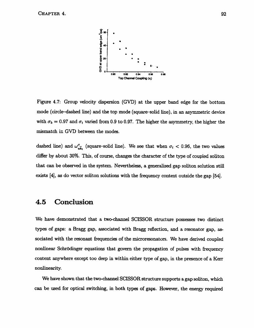
Figure 4.7: Group velocity dispersion (GVD) a t the upper band edge for the bottom

mode (circledashed line) and the top mode (square-solid h e ) , in an asymmetric device

with ab = 0.97 and a, mried fiom 0.9 to 0.97. The higher the asymmetry, the higher the

mismatch ir: GVD between the modes.

dashed h e ) and wUEt (squaresolid line). We see that when ol < 0.96, the two values

diffa by about 30%. This, of course, changes the character of the type of coupled soliton

that c m be observed in the system. Nevertheless, a generalized gap soliton solution stiil

exists [4], as do vector soliton solutions with the fiequency content outside the gap (541.

4.5 Conclusion

We have demonstrated that a tw~chwinel SCISSOR structure posçesses two distinct

types of gaps: a Bragg gap, associateci with Bragg rdection, and a resonator gap, as

sociated with the resonant fkquencies of the microresonators. We have derived coupled

nonlinear Schr6dinge.r equations that govern the propagation of pulses with frequency

content anywhere except too deep iri within either type of gap, in the presence of a Kerr

nonIineariQ.

We have shown that the twcdmmel, SCISSOR structure supports a gap soliton, which

can be used for optical switching, in both types of gaps. However, the energy required

to observe such a gap soliton is much smaller if it is within a resonator gap. This is a

direct consequeme of the very flat dispersion relation in the vicinity of a resonator gap.

W e have shown, too, that the structure supports a coupled gap soiiton that can be used

to constmct a logical AND gate. Again, the energy requirements in the v i c i n i ~ of a

resonator gap are much smder. In a future work we will discuss the issue of coupling

iight into a gap soliton field pattern.

Chapter 5

Theory for a grat ing-waveguide

structure with Kerr nonlinearity

5.1 Introduction

The refiection properties of multilayer didectric based grating-waveguide structures (GWS) ,

comprised of a substrate, a waveguiàe layes, and a grating, have been investigated for

some t ime (1 11 [55] [56] [57] [Ml. It is known t hat such systems exhibit a resonant response

to an incident plane wave caused by a coupling of the plane wave to a waveguide mode

of the system via the grating (551. Such resonances, which Iead to a sharp spike in the

reflection spectrum, and a sharp dip in the t r d i o n spectrum of the GWS, have

been observed experiment aUy [55] [56] [SB], and described theoretically [56] (571. However,

both the theoretical and experimental discussions of the GWS have concentrated on thin

gratine in linear optical media, where by thin we mean that the thickness of the grating

is much less than the wavelength of light in the medium. In this chapter we consider the

general case of a GWS with a grating of arbitrary thickness in which one or more of the

layers is Kerr nonlinear.

In the absence of a Kerr nonlinearity, we deve1op a transfer-mat& formulation of the

GWS. The transfer matrix formulation is well h w n as a bol for waveguide design in

the absence of a grating, and for andyzing stacked dielectric layers [591. G' ~ven a mon*

chromatic impulse of known frequency and wave vector, each layer of the waveguide can

be characterized as supporthg either plane waves or ewescent waves, travelling either

upwards or downwards. The field in a given layer is related to the field in a neigh-

bouring Iayer vio Maxwell's saltw conditions, and the application of physical boundary

conditions determines the total field everywhere inside the structure. The addition of a

grating element complicates the transfer rnatrix approach, because the grating couples

light between a countably infinite set of diffrâction orders. We use a Green fùnction

approach [60] to derive the transfer matrix associateci with a grating for both TE and

TM polarized light. We also use the Green fùnction approach to describe the effects of a

Kerr nonlinearity in one or more of the layers. However, in the presence of nonlinearity a

simple tramfer-matrix approach cannot be used. Instead, we present a set of differential

equations that describe the build-up of the various fields in the system.

We examine the dec t of gating thickness on the GWS, in the absence of nonlinearity.

For a thin g r a t a , the bandwidth over which refiection occurs is nanow, and the intensity

of the field inside the waveguide mode can be very large. Conwsely, for a thicker grating,

the bandwidth of the reflection spectrum is larger, but the intensiw of the field in the

waveguide mode is much smder. We include the efFects of materiai absorption in the

system by defining a complex dielectric constant in one or more of the layers. We show

that since the intensity of the field in the waveguide mode is much smailer in the presence

of a thick grating, the thick grating GWS is much more tolerant to material absorption.

This allows us to design a low-loss rdector for W light.

In the presence of nonlinearity, it is known t hat the GWS exhibits optical bistabiliw

[61] [62]. Bistability can be used for ail-optical switching, but there is a tradeoff inwlwd,

because to obtain a low intensity threshold for the switching, a thin grating is required,

but a thin grating has a narrow bandwidth, and will thus lead to a slow device. In this

chapter we present a simple scheme based on crossphase modiilatinn that should d o w

for a much faster switching time-scale. We consider a CW beam being 100% rdected

by a very thin grating. We then inject a short pulse into the waveguide mode which will

change the effective index of refiaction of the guiding layer of the GWS. If the short puise

is sutiiciently intense, t hen it will shift the resonant wavelength of the system so t hat the

100% rdecting device becornes almost M y tr&tting for the duration of the pulse.

The theory in this chapter considers a grating that consists of a periodic variation in

the dielectric permittivity in one direction. The GWS, then, has two effective dimensions:

the dimension of the periodicity (x), and the dimension of the stacking of the layers (2).

However, the theory c m easily be extendecl to consider a medium in which the periodicity

in the dieletric permittivity extends in two dimensions (x, y) [63] (641. Such a system has

been investigated in the presence of a X ( 2 ) nonlinearity (641, but not X ( 3 ) , and mt in the

presence of material absorption.

This chapter is dividecl into fiw sections. Tn Section 5.2 we give a heuristic picture

of the operation of a GWS. In Section 5.3 we deveiop the transfer mat& theory for

a linear system, and derive the appropriate differential equations for a nonünear layer.

In Section 5.4 we present numerical simulations for the low-loss reflector, and for the

nonlinear switching scheme.

5.2 The GWS and the Guided Modes

We fbt give a generd description of the operation of the GWS in the absence of non-

lineari@. In the absence of both a grating and nonlinearily, it is well known that the

stratfied medium of Figure 5.1 can support guided modes [65] so that, for a giwn fie

quency, light cm propagate dong the x direction with an electric field profde

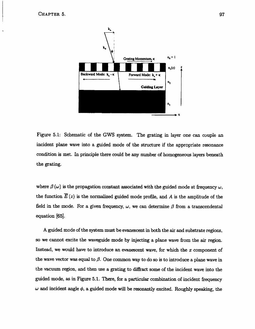
1 B a ~ h a d Mode: 4 - K \ F o w d Mode: k,+ r 1 I 1 - \ la, I

Figure 5.1: Schematic of the GWS system. The grating in layer one can couple an

incident plane wave into a guided mode of the stmcture if the appropriate resonance

condition is met. In principle there couid be any number of homogeneous layers beneath

the grating.

where ,û (w ) is the propagation constant associateci with the guided mode at frequency w,

the function Ê (r) is the normalized guided mode profile, and A is the amplitude of the

field in the mode. For a given fkequency, u, we cm determine P from a transcendentd

equation [65J.

A guided mode of the system must be evanescent in both the air and substrate regions,

so we cannot excite the waveguide mode by injecting a plane wave £rom the air region.

Instead, we would have to introduce an ev811escent wave, for which the z component of

the wave vector was equd to P. One common way to do so is to introduce a plane wave in

the vacuum region, and then use a grating to difbact sorne of the incident wave into the

guided mode, as in Figure 5.1. There, for a partiniltu combination of incident frequency

w and incident angle 4, a guided mode wiU be resonantly excited. Roughly speaking, the

where K = 27r/A is the momentum irnparted by the grating, and A is the period of

the grating. We can excite either a forward or backward propagating waveguide mode

(f respectively), and when # = O these two conditions become degenerate. For a fixeci

fiequency, w, the two angles associatecl with phase matchmg are

For a fixed angle, q50, we note that p - 2 m e J f /&, where Xo is the wavelength of light

in vacuum, and where nef , is only a weak function of wavelength, so that to good

approximation the forward and backward modes are atcited at vacuum wavelengths

In addition to coupling light into a waveguide mode, a grating will also couple light

out of a waveguide mode. Close to the resonance condition the reflection is enhanceci

because iight coupled into the waveguide mode by the grating is also coupled back out.

In fact, for a nmow range of wavelengths, almost 100% rdection can be achieved. The

presence of a Kerr nonlinearity in one or more of the waveguide layers will, of course,

affkct the position and the nature of the reaonmce, a d andits iheshape.

5.3 Green Function Theory for

We seek a physical description of the situation shown

S trat ified Media

in Figure 5.1, where a plane wave

with frequency w is incident from vacuum (layer O) ont0 a stratifieci, non-magnetic

(p = po) medium. The first layer (layer 1) of the stratifieci medium is a grating with

periodicity A, and with associated grating-momentum K = 27r/A. The grating materials

will have, in general, a cornplex dielectric constant. The subsequent layers are d o m ,

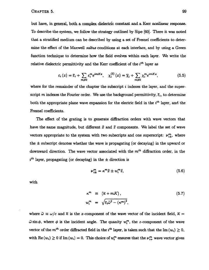
c c m & a n t a n d a K e r r m but have, in genera both a rnmpkx dielectnc ~esponSe,

To describe the system, we follow the strategy outiined by Sipe [60]. There it was noted

that a stratifieci medium can be describeci by using a set of fiesne1 co&cients to deter-

mine the &ect of the Maxweil salbtrs conditions at each interface, and by using a Green

hrnction technique to determine how the field evo1ves within each layer. We write the

relative dielectric permittivity and the Kerr co&cient of the ith layer as

where for the rernainder of the chapter the subscript i indexes the layer, and the super-

script rn indexes the Fourier order. We use the background permittivity, &, to determine

both the appropriate plane wave expansion for the electnc field in the ith layer, and the

Fresnel coefficients.

The &ect of the grating is to generate dSraction orders with wave vectors that

have the same magnitude, but different 4 and Z components. We label the set of wave

vectors appropriate to the system with two subscripts and one superscript: us, where

the f subscript denotes whether the wave is propagating (or decaying) in the upward or

downward direction. The wave vector associated with the mth diffraction order, in the

itqayer, propagating (or decaying) in the f direction is

with

where W r w / c and it is the x-component of the wave vector of the incident field, n =

W sin$, where t$ is the incident angle. The quaniw w?, the z-component of the wave

vector of the mth order ciifhacted field in the ih layer, is taken such that the ùn (tui) 2 O,

with Re (wi) 2 O if Im (wi) = O. This choice of up ensures that the v z wave vector gives

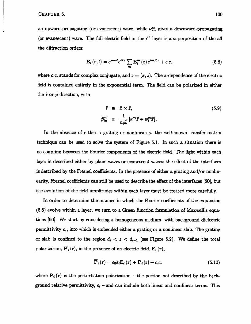
an upward-propagating (or ewescent) wave, while v: gives a domward-propagating

(or evangcent) wave. The full electric field in the ith layer is a superposition of the ail

the diffraction orders:

E, (r, t ) = e-"eG Er ( z ) eldx + c.c., m

where C.C. stands for complex conjugate, and r = (x, 2) . The x-dependence of the electric

field is contained entireiy in the exponential term. The field can be polarized in either

the s or p direction, with

In the absence of either a grating or nonlineanty, the weU-known transfer-matrix

technique can be used to solve the system of Figure 5.1. In such a situation there is

no couphg between the Fourier components of the electric field. The light within each

layer is described either by plane waves or evanescent waves; the &ect of the interfaces

is describeci by the Resnel coefficients. In the presence of either a grating and/or nonlin-

carie, Fresnel co&cients c m stil be used to describe the &kt of the interfaces [60], but

the evolution of the field amplitudes within each layer must be treated more carefully.

In order to determine the manner in which the Fourier co&cients of the expansion

(5.8) evolve within a layer, we turn to a Green function Eormitlatim of ~ldaxwell's qua-

tions [60]. We start by considering a homogeneous medium, with background dielectric

permittivity Fi, into which is embedded either a grating or a nonlinear slab. The grating

or slab is confinecl to the region 4 c z < 4-1 (see Figure 5.2). We define the total

poiarization, Fi (r), in the presence of an electric field, Ei (r),

- Pi (r) = E&& (P) + Pi (r) + C.C. (5.10)

where Pi (r) is the perturbation polarization - the portion not described by the back-

ground relative permittivityl 5, - and can include both linear and nonlinear terms. This

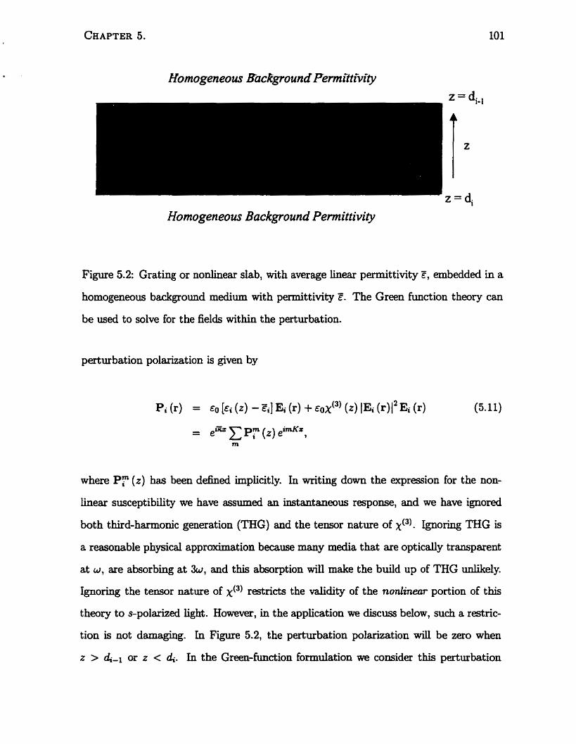
Homogeneous Background Penniftttvity z = d,,

i z z = di

Homogeneous Background Pennittivity

Figure 5.2: Grating or nonlinear slab, with average linear permittivity E , embedded in a

hornogeneous background medium with permittivity 2. The Green function theory c m

be used to soive for the fields within the perturbation.

perturbation polarization is given by

where PT (2) has been defined implicitly. In writing down the expression for the non-

linear susceptibility we have assumeci an instantanmus response, and we have ignored

both third-hannonic generation (THG) and the tensor nature of ~ ( ~ 1 . Tgn~ring THG is

a reasonable physical approximation because many media that are opticdy transparent

at w, are absorbing at 3w, and this absorption will make the build up of THG iinlikely.

lgnoring the tensor nature of reStrictS the validiw of the naLineor portion of this

theory to s-polarized light. H o ~ e ~ e r , in the application we discuss below, such a restric-

tion is not damaghg- In Figure 5.2, the perturbation polarization will be zero when

z > or r < 6 In the Greemfunction formulation we consider this perturbation

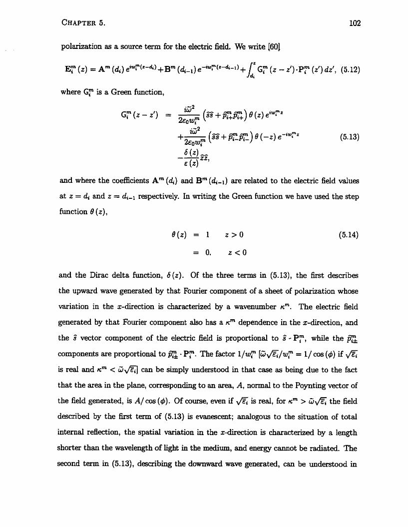
polarization as a source term for the electnc field. We write [601

EY (*) = p (4) p ? ' ( z - 4 > +p (di.,) e*F(-4-d + 1 Gr ( z - z') Pr (z') dzl, (5.12)

where G," is a Green function,

and where the coefficients Am (4) and Bm are related to the electric field d u e s

at z = di and z = &1 respectively. In writing the Green function we have used the step

function 8 (z),

and the Dirac delta function, 6(z). Of the three terms in (5.13), the first describes

the upward wave generated by that Fourier component of a sheet of polarization whose

variation in the x-direction is characterized by a wavenumber nm. The electric field

generated by that Fourier component also has a nm dependence in the x-direction, and

the s vector component of the electric field is proportional to s Pr, while the p z

components are proportional to - Pr. The factor l / w r [W&/wl = 1/ cos (4) if \lE;

is real and nm < W\IE;l can be simply understood in that case as being due to the fact

that the area in the plane, corresponding to an area, A, normal to the Poynting vector of

the field generated, is A/ cos (6). Of course, even if & is real, for nm > W& the field

dexribed by the first term of (5.13) is evanescent; analogous to the situation of total

interna1 refiection, the spatial variation in the x-direction is characterized by a length

shorter than the wavelength of light in the medium, and energy cannot be radiatecl. The

second term in (5. El), describing the downward wave generated, can be understood in

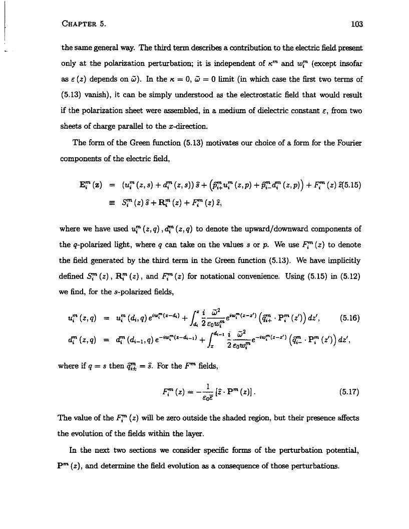
the same generd way. The third term d e s d e s a contribution to the electric field present

ody at the polarization perturbation; it is independent of n" and zur (except insofar

as e ( z ) depends on 2). In the n = O, W = O limit (in which case the first two terms of

(5.13) vaaish), i t can be sirnply understood as the electrostatic field that would result

if the polarization sheet were assembled, in a medium of dielectric constant E , fiom two

sheets of charge pardel to the x-direction.

The form of the Green function (5.13) motivata our choice of a form for the Fourier

components of the electric field,

where we have used UT (2, q) , (2, q) to denote the upward/downward components of

the q-polarized light, where q can take on the values s or p. We use y (2) to denote

the field generated by the t h d term in the Green function (5.13). We have Mplicitly

defineci (2) , Rm (2) , and ( 2 ) for notational convenience. Using (5.15) in (5.12)

we End, for the s-polarized fields,

The value of the F ( z ) will be zero outside the shaded region, but their presence affects

the mlution of the fields within the layer.

In the next two sections we consider specific forms of the perturbation potential,

Pm (z), and determine the field evolution as a consequence of those perturbations.

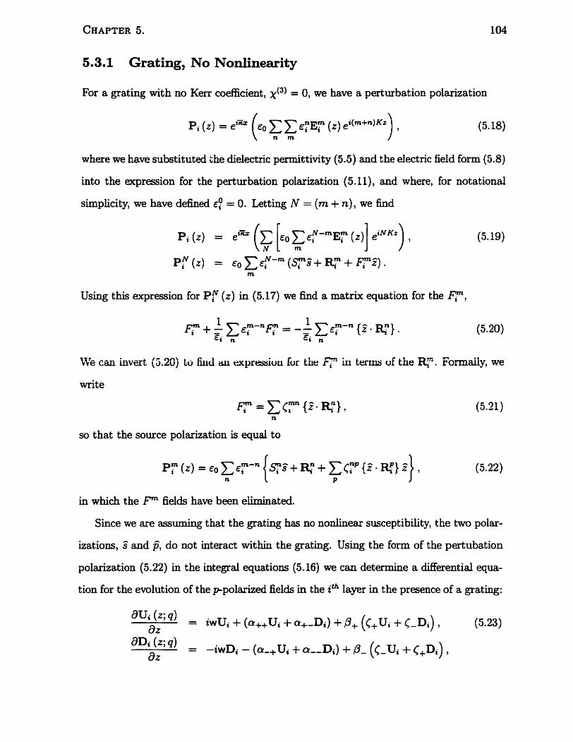
5.3.1 Grating, No Nonlinearity

For a grating with no Kerr coefEicient, X ( 3 ) = 0, we have a perturbation polarization

where we have substituted the dielectric permittivity (5.5) and the electric field form (5.8)

into the expression for the perturbation polarization (5. Il), and where, for notational

simplicity, we have definecl E: = O. Letting N = (m + n), we find

Using this expression for Pr (2) in (5.17) we find a matrix equation for the y,

so that the source polarization is equal to

in which the r" fields have been elhinateci.

Since we are assiiming that the grating has no nonlinem susceptibilitsf, the two polar-

izations, s and @, do not interad within the grating. Using the fom of the pertubation

polarization (5.22) in the integral equations (5.16) we can determine a dinerential equa-

tion for the ewlution of the ppolarized fields in the ith layer in the presence of a grating:

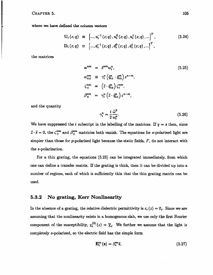
the matrices

and the quantity

We have suppressed the i subscript in the labelling of the matrices. If q = s then, since

2 - s = 0. the (tm and matricies both vanish. The equations for s-polarized light are

simpler than those for ppolarized light because the static fields, F, do not interact with

the s-polarizat ion.

For a thin pating, the equations (5.23) can be integrated immediately, Erom which

one can define a transfer matrix. If the grating is thick, then it can be divided up into a

number of regions, each of which is sufliciently thin that the thin grating mat& can be

used.

5.3.2 No grating, Kerr Nonlinearity

In the absence of a grat hg, the relative dielettric permit tivity is ~i (2) = Fi. Since we are

assuming that the nonlineaxity acists in a humogenous slab, we use only the Fourier

component of the susceptibility, Xy) (2) = Xi. We further we asnune that the light is

completely s-polarized, so the electric field hes the simple furm

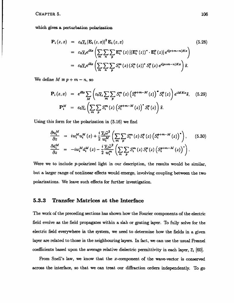
Wedefme h . I = p + r n - n , so

Pi (2.3) = ex= C (s& (2 ) (Fm- (i)) 9 (2) eiMKx& (5.29) M f " P

Using t his form for the plarization in (5.16) we find

au( M M i x,z2 - = iwi ui ( z ) + - - (x st (z) $ ( z ) (Spirn- (2)) a) , (5 .XI) bz 2w,M m p

Were we to include ppolarized light in our description, the results would be similar,

but a larger range of nonlinear effects would ernerge, involving coupling between the two

polarizations. We lem such effects for hirther investigation.

5.3.3 Transfer Matrices at the Interface

The work of the preceding sections has shown how the Fourier wmponents of the electric

field evolve as the field propagates within a slab or grating layer. To fully solve for the

electric field everywhere in the system, we need to determine how the fields in a given

layer are related to those in the neighbouring lam. h fact, we can use the usual Fresnel

c d c i e n t s based upon the average relative dielectnc permittivity in each layer, Éi [60].

h m Snell's law, we know that the x-component of the wave-vector is conserved

across the interface, so that we can treat our difhction orders independently. To go

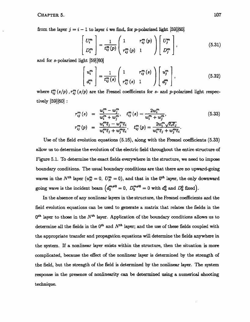
fmm the hyer j = i - 1 to l a . i we fin& for ppalarizedlight [59][601

[ u q - -- 1 ( 1 rq"] 1

Dr t g @ ] ( p ) 1 Dj"

and for or-polarized light (591 [6O]

[z ] = - ( 1 TC (s) r z ( 3 ) ) 1 [: 1 , where tg ( s / p ) , r c (slp) are the fiesne1 coefficients for s- and ppolarized light r g p e c -

t ively (593 (603 :

Use of the field evolution equations (5.16), along with the -ne1 coefficients (5.33)

d o w us to detennine the emlution of the electric field throughout the e n t i . structure of

Figure 5.1. To detemine the exact fields everywhere in the structure, we need to impose

boundary condit ions. The usual boundary conditions are that t here are no upward-going

waves in the Nth laYer (UN = O, Up = O), and that in the 0" layer, the only downward

going wave is the incident beam (dg* = O, D~~ = O with 4 and fixed).

In the absence of any nonlinear layas in the stmcture, the fiesne1 coefncients and the

field emlution equations can be used to generate a m a t e that relates the fields in the

O* layer to those in the N* layer. Application of the boundary conditions dows us to

determine dl the fields in the oth a d ndh layer; and the use of t hese fields coupled with

the appropriat e transfer and propagation equations will determine the fields anywhere in

the system. If a nonhem layer exîsts within the structure, then the situation is more

complicated, because the &ect of the nonlinear layer is determined by the strength of

the field, but the strengt h of the field is detemineci by the nonlinear layer. The system

response in the presence of nonlinearXty can be determined using a numerid shooting

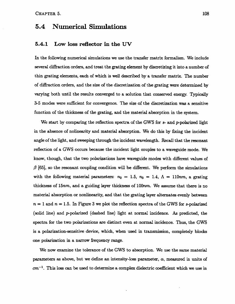
5.4 Numerical Simulations

5.4.1 Low Ioss reflector in the UV

In the following numerical sirnulat ions we use the transfer matri. formalism. We include

several diffraction orders, and treat the grating element by discretizing it into a number of

t hin grat ing elements, each of which is well describeci by a tramfer matrk. The number

of diffraction orders, and the size of the discretization of the grating were deterrnined by

varying both until the results conver& to a solution that conserved energy. Typicdy

3-5 modes were sufEcient for convergence. The size of the discretization was a sensitive

hnction of the thickness of the grating, and the material absorption in the system.

We start by cornparhg the reflection spectra of the GWS for s- and ppolarized Light

in the absence of nolinearity and materid absorption. We do this by fMng the incident

angle of the light, and sweeping through the incident wavelength. &al1 that the resonant

refiection of a GWS occurs because the incident iight couples to a waveguide mode. We

know, though, that the two polarkations have waveguide modes with different values of

/3 (651, so the resonent couphg condition will be different . We perforrn the simulations

with the following materid parameters: n2 = 1.5, na = 1.4, A = IlOnm, a grating

thickness of 15nm, and a guiding layer thicknes of 100nm. We assume that there is no

material absorption or nonlinearity, end that the grating layer alternates evenly between

n = 1 and n = 1.5. In Figure 3 we plot the reflection spectra of the GWS for s-polarid

(solid line) and ppolarized (dashed line) iight at normal incidence. As predicted, the

spectra for the two polarizations are distinct even at normal incidence. Thus, the GWS

is a polarization-sensitive device, which, when used in transmission, completeiy blocks

one polarization in a narrow kquency range.

We now examine the toleninfe of the GWS to absorption. We use the same material

parameters as above, but we d&e an intensity-loas parameter, a, measured in units of

cm-'. This loss can be used to determine a cornplex dielectric coeEcient which we use in

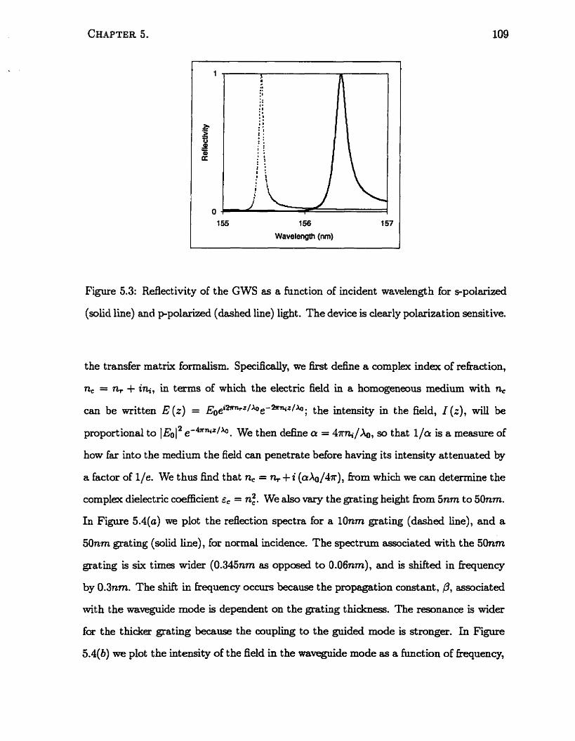
1 55 1 56

Wavelength (nm)

Figure 5.3: Reflectivity of the GWS as a hinction of incident wavelength for s-polarized

(solid line) and ppolarized (dashed line) light. The device is dearly polarization sensitive.

the transfer matrix fornalism. SpecScally, we first define a cornplex index of rehact ion,

n, = n, + iw, in terms of which the electric field in a homogeneous medium with n,

can be written E (r) = ~ ~ e ' - ~ l ~ e - " ~ ~ l ~ ; the intensity in the field, 1 (;), will be

proportional to I E ~ I * e-4*mz/.b. We then define cr = $ml&, so that l/a is a measure of

how far into the medium the field can penetrate before having its intensity attenuated by

a factor of l/e. We thus find that n, = n,+i (c&/4x), kom which we can determine the

cornplex dielectric coefficient E, = n:. We also vary the grating height h m 5nm to 50nm.

In Figure 5.4(a) we plot the refiection spectra for a lOnm grating (dashed line), and a

50nm grating (solid line) , for normal incidence. The spectrum associated with the 50nm

grating is six t h e s wider (0.345nm as opposed to 0.06nm), and is shiRed in fkquency

by 0.3nm. The shift in kequency occurs because the propagation constant, 0, associated

with the mveguide mode is dependent on the grating thickness. The resonance is wider

for the thicker grating because the coupling to the guided mode is stronger. In Figure

5.4(b) we plot the intensity of the fkld in the waveguide mode as a hinction of kequency,

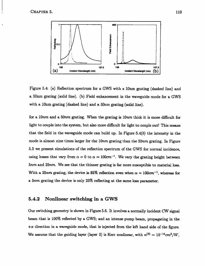
Figure 5.4: (a) Re£iection spectrum for a GWS with a 1On.m gr& ing (dashed line) and

a 50nm grating (solid line). (b) Field enhancement in the waveguide mode for a GWS

wit h a l h m grating (dashed line) and a 50nm grating (solid line) .

for a lOnm and a 50nm grating. When the grating is lOnm thick it is more difficult for

light to couple into the system, but also more difEcult for light to couple out! This means

t hat the field in the mveguide mode c m build up. In Figure 5.4(b) the intensity in the

mode is almost nine times larger for the lOnm grating than the 50nm grat ing. In Figure

5.5 we present simulations of the refkction spectrum of the GWS for normal incidence,

using losses that vary from cr = O to a = 100cm-'. We vary the grating height between

5nm and 25nm. We see t hat the t hinner grating is far more susceptible to material loss.

With a 25nm grating, the device is 85% dar ion even when tr = 100mt-l, wherects for

a 5 n m grating the device is only 23% rdecting at the same loss parameter.

5.4.2 NonIinear switching in a GWS

Our swit ching geometry is shown in Figure 5.6. It involves a normdy incident CW signal

beam that is 100% reflected by a GWS; and an intense pump beam, propagating in the

+x direction in a mveguide mode, that is injectecl from the left hand side of the figure.

We assume that the guiding layer (layer 2) is Kerr nonlinear, with d2) = 10- 14cm2/W,

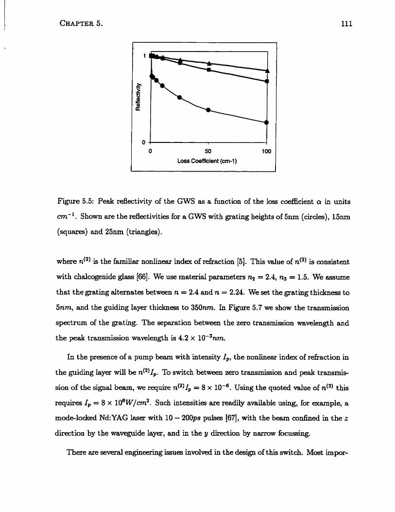
O O 50 100

Loss Coefficient (cm-1 )

Figure 5.5: Peak re£lectivity of the GWS as a hinction of the los coefficient ai in units

cm-'. Shown are the rdectivities for a GWS with grating heights of 5- (circles), 15nm

(squares) and 25nm (triangles).

where d2) is the familiar nonlinear index of refkaction [5]. This value of is consistent

wit h chalcogenide glas (661. We use materid parameters nz = 2.4, n3 = 1.5. We assume

that the grating aiternates between n = 2.4 and n = 2.21. We set the grating thickness to

5nm, and the guiding layer thicknes to 350nm. In Figure 5.7 we show the transmission

spectrum of the grating. The separation between the zero transmission wavelength and

the peak transmission wavelength is 4.2 x 10-'nm.

In the presence of a pump beam with intensity I . , the nonlinear index of refraction in

the guiding layer will be d2) I,. To switch between zero transmission and peak transmis-

sion of the signal b m , we require d 2 ) I , = 8 x Using the quoted value of d2) this

requires I, = 8 x 108 W / m 2 . SU& intensities are mdiiy available using, for example, a

mode-locked Nd:YAG laser with 10 - 200ps pulses [67], with the beam confinecl in the ;

direction by the waveguide layer, and in the y direction by narrow focusing.

There are several engineering issues invohd in the design of this h t c h . Most impor-

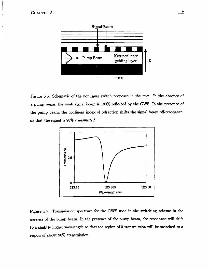
Kerr nonlinear guiding layer

Figure 5.6: Schematic of the nonlinear switch proposed in the tact. In the absence of

a pump beam, the weak signal beam is 100% reflected by the GWS. In the presence of

the pump barn, the nonlinear indsc of rehction shifts the signal beam off-resonance,

so that the signal is 90% trarumitted

523.85 523.865

Wavelength (nm)

Figure 5.7: Trmmision spectnun for the GWS used in the switching scheme in the

absence of the pump beam. In the presenœ of the pump bearn, the resonanoe will shift

to a slightly higher wavelength so that the region of O transmission wiU be switched to a

region of about 90% trammMon.

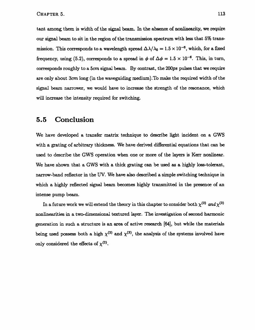
tant among them is width of the signal beam. h the absence of nnnlinPnrity? we require

our signal beam to sit in the region of the trançmission spectruxn with less that 5% t rans

mission. This corresponds to a wavelengt h spread A A/& = 1.5 x IO-', which, for a k e d

frequency, using (5.2), corresponds to a spread in # of A4 = 1.5 x IO-'. This, in tum,

corresponds roughly to a 5cm signal beam. By contrast, the 200ps pulses t hat we requk

are only about 3 n long (in the waveguiding medium) .To make the required width of the

signal beam naxrower, we would have to increase the strength of the resonance, which

will increase the intensity required for switchuig.

5.5 Conclusion

We have developed a transfer mat& technique to describe light incident on a GWS

with a grating of arbitrary thickness. We have derived differentid equations that can be

used to describe the GWS operation when one or more of the layers is Kerr nonlinear.

We have shown that a GWS with a thick grating can be used as a highly loss-tolerant,

narrow-band reflector in the W. We have also described a simple switching technique in

which a highly reflected signal beam becornes highly transmitted in the presence of an

intense pump beam.

In a fûture work we wiU extend the theory in this chapter to consider both X(2) and ~ ( ~ 1

nnnlinearities in a twdimensional textured kyer. The investigation of second harmonie

generation in such a structure is an area of active research [Ml, but while the materials

being used possess both a hi& X(2) and ~ ( ~ 1 , the analysis of the systems involved have

only considered the effets of x(*).

Chapter 6

Hamiltonian formulation for pulse

propagation equat ions in a periodic,

nonlinear medium

6.1 Introduction

The investigation of optical pulse propagation in nonlinear Kerr media ofken proceeds

via the slowly-varying envelope hinction apprcxïmation [3] [5][22], wherein the kequency

content of an optical pulse is mnsidered to be narrowly centred around a giwn carrier

bequency, c. This apprcximation d o w s one to separate the pulse dyna~nics, containeci

in the slowly-varying envelope huictions, hom the phase accumulation due to the carrier

frequency. When applied to a homogenous, isotropic medium, the slowly-varying a p

praJcimation has been used to derive the familiar nonlinear Schrodinger equation (NLSE)

[5] as the dynamical equations for the envelope function; when applied t o a periodic,

isotropic medium the approximation has been used to derive bot h a NLSE [7] [Ml and a

set of nonlinear coupled mode equations (CME) [3] [?]. In the presence of birefringence,

a set of coupled NLSEs have been derived for a homogeneous medium (221; for a pe-

riodie me di^^^^, both a set of coupled NUES and a set of nnnlins CMEa have been

derived [34]. The dynamics of these envelope-hinction equations have often been studied

by const mct ing a Hamiltonian formulation of the dynamical equations [9] [29] (311 [40] (681.

Fkom such a Hamihonian two conserveci quantities can be identifiai, one energy-iike, and

one momentum-like. But the Hamiltonian itself is not equal to the energy-like quantity,

leading to a certain conhision in the literature [69]. One would naively scpect that a

nonlinear optical system would have two conserved quantities - energy and momentum.

But since the IIamiltonian itself is also conserved, the optical system has Mree c o n s e d

quantities, and the interpretation of this third conservecl quantity presented some dif-

ficulties [31] [68] [69]. A correct understanding of these three conserveci quantities is the

goal of this chapter.

In Section 6.2 of this chapter we construct a auionical Hamiltonian formulation of

Maxwell's equations in a one dimensional, periodic medium with a Kerr nonlinearity,

using a dual field h t p r o p e d by Hillery and Mlodinow [70][71][72]. By monical we

mean that our Hamiltonian can be used to derive the exact equations of motion using

the canonical commutation relations, und that it is numerically qua1 to the energy of

the (nonlinear) electrornagnetic field. Although we here only consider classical fields we

formally replace the canonical Poisson brackets with the associated cornmutators, with

a view towards eventudy quantizing the theory. In Section 6.3 we specialize our for-

mulation to consider an effective field that varies slowly relative to the underlying Bloch

h c t i o n s of the periodic medium. We then generate a reduced canonical Hamiltonian

in terms of this effective field. The dynsmical equation grnrerned by this reduced Hamil-

tonian is the farniliar NLSE. In Section 6.4 we use the reduced Hamiltonian, which,

within our apprmimations, is conserved and equd to the energy, to identify two more

conserved quant it ies: the moment um, asçociated with space-translation symmetry; and

a conserved charge, associated with phase-translation symmetry. We demonstrate that

the 'energy' of the electromagnetic field quoted in many papers is, in fact, the c o d

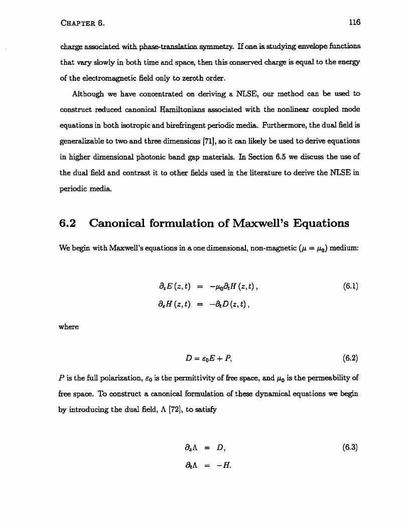
charge associateci with phase-translation symmetry- If ane is studying envelope hctian_c:

that vary slowly in both t h e and space, then this conserveci charge is equd to the energy

of the electromagnetic field only to zeroth order.

Although we have concentrated on deriving a NLSE, our rnethod c m be used to

construct reduced canonical Hamihonians associateci with the non1inea.r coupled mode

equat ions in bot h isotropie and birefringent periodic media. F'urthermore, the dud field is

generalizable to two and t hree dimensions [?'Il, so it can Uely be used t o derive equations

in higher dimensional photonic band gap materialS. ùi Section 6.5 we discuss the use of

the dual field and contraçt it to other fie1ds used in the literature to derive the NLSE in

periodic media.

6.2 Canonical formulation of Maxwell's Equat ions

We begin with Maxwell's equations in a one dimensional, non-magnetic ( p = po) medium:

where

P is the hll polarizat ion, €0 is the permit t ivity of kee space, and p, is the permeability of

free space. To wnstruct a canonid formulation of these dynamical equations we begh

by introducing the dual field, A [72], to satisfy

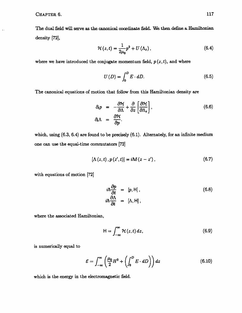
ThedualfkldwillsemeastheriuinnicalorwrUfiP.ld-

density [72], 1

where we have introduced the conjugate momentum fieid,

The canonical equations of motion that follow from this Hamiltonian density are

which, using (6.3,6.4) are found to be precisely (6.1). Alternately, for an infinite medium

one can use the equal-tirne cornmutators [72]

with equations of motion [72]

where the associated Hamiltonian,

which is the energy in the electromagnetic field.

6.2J Linear, Periodic Medium

For a linear, perioàic medium,

where E (z) = E (z + d) characterizes the linear dielectric response of the medium, and

d is the periodicity of the lattice. We have introduced the notation H L to stress that

t his Hamilt onian generates the linear dynamics of the electromagnet ic field. Using the

equations of motion (6.6) we find a l i n s wave equation that A must satisfy:

To determine the Bloch bc t i ons of (6.12) we use the usual ansatz [74]

where C.C. stands for 'complec conjugate'. The units of O, (t) are definecl by the orthog-

onality condit ion given below (6.16). Substitut ion of (6.13) in the wave equation (6.12)

gives an equation for the Bloch functions, O,,

Because the operator in the equation is self-adjoint, it admits r d eigenvalues and or-

thogonal eigenfunctions.

Rom Bloch's theorem [74], we c m write our Bloch functions in tenns of a discrete

band index m, and a reduced wave number, k (-sr/d < k 5 *Id), 0, + Bd, with

0, (2) = (i) e". (6.15)

We note that Wmk = Wm(-k) , so we can choose our Bloch hc t ions such that Bd (2) =

amc-, , . The h k have the periodicity of the lat t ice, (2) = ( z + d) . We normalize

the Bloch functions via

ly,: (2) 8,,,tkt ( r ) d* = N&nmtbkkt*

where L is a nomalization length, and where we have chosen the DSIIllâliZ&tian CQIlStazLt

N = L/d . This choice of L and N means that o u wave numbers take on only discrete

values, and that the difference between taro adjacent mve numbers is 2?r/L. The Bloch

huictions also sat isfy

where = dOmr/dz; this follows by using (6.16) and (6.14). An aample of a dispersion

relation in this reduced-wavenurnber scheme is shown in Figure 6.1.

6.2.2 Periodic Medium with a Kerr nonlinearity

We now turn to a periodic, Kerr nonlineaz medium. At hequencies far below any rem-

nances in the medium, for our one dimensional geometry the constitutive re la t i~a takes

the form [5]

D = E ( I ) E + ~ o ~ ( ~ ) (2) E ~ , (6.18)

where we assume that the nonlinearity ooefficient, X(3) ( z ) is periodic with period d,

~ ( ~ 1 (i + d) = x ( ~ ) ( z ) . To constmct the Hamiltonian we k t invert (6.18) t o get

where we have assumed that X(3) ( z ) E3 < E (2) E. This assumption of a weak nonhear-

ity is judfhd on phyucal groundsr we d y want ta discuss third order nonlinear eects,

but if the asnimption of a weak X(3) were not valid, then we w o d d have no justification

for not including fifth order or higher nonlinear &mts in (6.18). Using (6.19) in (6.5) we

h d

where HL is defineci above (6.1 1) and HNL is the portion of the full Hamiltonian respon-

able for the nonlinearity in the dynamics of the electromagnetic field. The expression

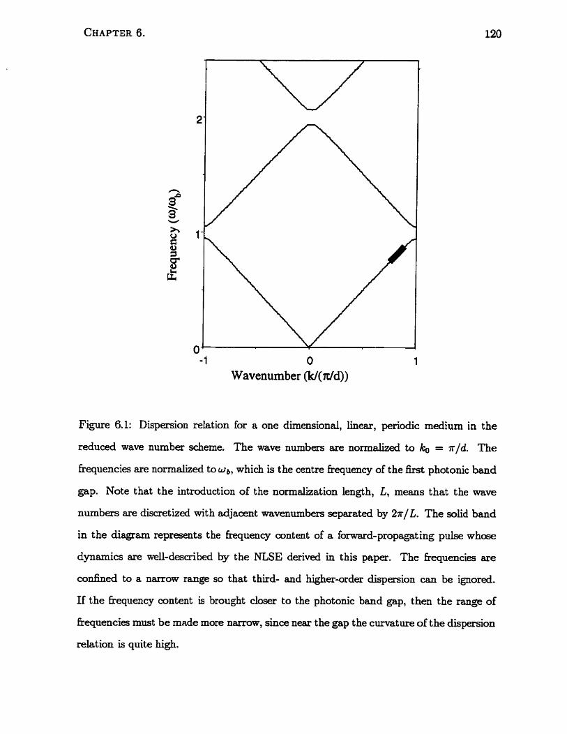
- 1 O 1 Wavenumber (k/(x/d))

Figure 6.1: Dispersion relation for a one dimensional, linear, periodic medium in the

reduced wave number scheme. The wave numbers are nomahed to = ~ / d . The

frequencies are nomalized to wb, which is the centre frequency of the fmt photonic band

gap. Note that the introduction of the nomaikation length, L, means that the wave

numbers are discretized with adjacent wavenumbers separated by 2n/ L. The solid band

in the diagram represents the hequency content of a forward-propagating pulse whoçe

dyna,rn.ics are well-described by the NLSE derived in this paper. The kequencies are

confineci to a narrow range so that third- and higher-order dispersion can be ignorecl.

If the Erequency content is brought closer to the photonic band gap, then the range of

bequencies must be made more narrow, since near the gap the curvature of the dispersion

relation is quite high.

equations of motion for A within the a p p r h a t i o n of a weak nonlinearity (6. El),

It will be usehl to express H in terms of the classical d o g of the raishg and lowering

operators associated with the Bloch modes. To do so, we k t q a n d A (2, t ) and p (z, t)

in terms of the Bloch modes of the periodic medium. We let

The reality of p and A requires that p h = and 4 = A,,+kl, so we can express

both the complex quantities p d and & in terms of one mode amplitude, a,,,k (t),

Using the (t ), the expansion (6.22) becomes

We note that since A (2, t ) and p (2, t) are written in terms of Bloch huictions that are

n o m M in the region -LI2 < z < L/2, they will bemme periodic with period L.

This has no &et on the underlying physics, because we can dways consider the lllnit

where L -r m. However, it does mean that when evaluating the Hamiltonian (6.20) in

te= of the A(z , t) and p ( r , t ) given by (6.24) we must restrict the integration t o the

region - L / 2 < 2 < L/2; and when evduating the equal-tirne commutation relations (6.7)

between A (2, t) and p (2, t) we mu& restrict both z and 2 to be within & L/2. Adhering

to these restrictbq we Itid that usin= (6.24) in (UQ), and applying the o r h g d t y

relations (6.16) to the portion of the Hamiltonian that generates the linear dynamics,

the full Hamiltonian

H =

Adopt ing cornmut at ion relations

guarantees the commutation relations between A (r , t ) and p ( 2' , t) (6.7) for z and z' wit hin

the nomalization length. In terms of the mode amplitudes, the canonical equations of

motion (6.8) become [73],

which, using (6.25) for H, give

This equation (6.28) is equivalent bo (6.1) and (6.2) wibh (6.19).

6.3 Reduced Hamiltonian and the NLSE

In this section we re-cast our H d t o n i a n in a form more suitable to the study of pulse

propagation. We build effective fields, g, (2, t), as a Fourier superposition of the 43 and

assume that the effective fields are centred at a given wave number, k, which corresponds

to a kquency w,. The g,,, (2, t ) can be used to rewrite the Hamiltonian (6.25) without

any l o s of generality.

This effective fields a p p r d is most valuable when the kequency amtent a£ the field

is narrow relative to a central kquency, w s , that lies in band m = 7E wit h wave number - k. We assume that is far fkorn a photonic band gap, and that the frequency content

of the pulse is entùely containeci within band B. Because the hquency content of our

effective fields is narrowly centered around w-,, we can ~tpand a fiequency ~ ~ p + ~ ) in

a Taylor series which wil l involve the local group velocity and group velocity dispersion.

We use a smallness parameter, , to characterize the strength of the tenns in our

Harniltonian. We examine the situation where the terms that are related to the group

velocity of the pulse are O (q) , and the t a m s that are relateà to the Kerr nonlinearity

and the group velocity dispersion of the pulse are both O (q2) relative to the kgest terms

in the Hamiltonian. Higher-order nonlinear &?ects, and higher order dispersion are not

considered, because both are assumeci to bc O ( $ 3 ) . We denote the resulting Hamiltonian

the 'reduced Hamiltonian' since it is equal to the energy of the electromagnetic field to

O (v2). Although our mode1 formdy includes third harmonic generation, we ignore its

effets in the following. We are justined in doing so by physical considerations. We

have assumed that the underlying matMd is nondispersive, and while this may be valid

for Erequencies nea. w*, it WU likely not be valid for fiequency ranges extending ta

w = 3wmE; fbrthermore, the assumption of no absorption at w E Ls will like1y be in

error. We expect, on physical grounds, that in many cases the actual material dispersion

and absorption will make any b d d u p of the third harmonic unIikely, so that our modd

will be adequate.

We start by using the Q (t) to d&e an effective field, g, (2, t), that is centred -

around the wave number k = k,

where we have intmduced the àetuniag

~ = k - k ,

and the mode amplitudes

Ultimately we seek to describe the evolution of our field A (z , t ) , which we asnune is a

smoothly varying b c t i o n of z as we rnove fiom a point in a unit cell to the corresponding

point in a neighbouring unit c d The function g, (z, t) will be such a smoothly varying

hnction of t only if the (t) are srnmthly varying hinctions of k. To ensure that the

amk ( t ) vary smoothly in k, one must choose the Bloch functions to vary smoothly in k,

which can be done using a k p expansion [7] [49] about k.

Using (6.26), we find that the equal-the commutation relations for the g, (2, t ) are

for r and z' both in our normslization length L, where the Dirac delta function, 6 (z - 3)

in (6.32) strictly appears only in the L -r oc Iimit. By inverting (6.29) we find

Using (6.33), the Harniltonian (6.25) can be wntten in tenns of the gm (r , t ) .

In the foilowing we restrict ourselves to consideration of effective fields for which at

t = O the hequency content of the pulse is contained entirely in band rn = m, and narrowly centred around so that, replacing the a++,) (t) with the g,, ( t ) , and

restricting the surnmation in the Harniltonian (6.25) to one band, we h d a reduced

where the Ki are waue number detltnings Sinœ are a ~ e &dering ooly one band,

m = m, we drop the rn subscript in the remainder of the chapter. We stress that

the Hamiltonian (6.34) is still exactly equal to the energy in the system at t = O. At

later tirnes the nonlinear interaction will generate new fiequencies, but in the foilowing

we ignore third harmonic generation, as discussed, so that for reasonable propagation

times and pulse intensities, the new frequencies that are generated will still lie in band

rn = m, and the reduced Hamiltonian will st il1 represent the exact energy in the system.

Mhermore , we assume that at t = O o d y fomd-travelling waves are present, so that

at Iater times there will be no interaction with any backward-travelling mves.

We fird consider the linear portion of the reduced Hamiltonian (6.34). We expaad

the frequency w P+K) as

where w = q, J' = l)wF+,)!8K! ~~0 and w" = 8 2 ~ C * + , ) / a K 2 ] K = o . Substituthg th&

expression for w F+K) and the expression for the effective fields (6.29) into the reduced

Hamiitonian (6.34) we find that the portion of the reduced Hamiltonian asociated with

the linear dynarnics of the field is

where 7 is a smahess parameter used to diaracterize the relative strength of terms in

the Hamiltonian. We can quantify i ) by letting I ) = g (,Id), where i, is an appropriate

measure of the width of the pulse, and the factor g must satisfy

where I<. is an appropriate m e m e of the width of the pulse- As discussed, the third-

and higher-order dispersion terms are mnsidered to be O (q3). The values of 3 and 8'

will depend on the dispenion relation itself; a w&ty QE techniques exist to àekrmhe

the dispersion relation of a one-dimensional, periodic system [74].

Turning to the portion of the reduced Hamiltonian (6.34) t hat generates the nonlinear

dynamics of the fields, we fi& recall that we are dealing with a weak nonlinearity (see

note foilowing (6.19)). We quantify the weahess of this nonlinearity by asserting that

the ratio of the largest nonlinear term to the large& linear term is O (q2). Because we are

only keeping te- in HR to O (v2), t hk means that we can replace 9k+,) with GeiKz,

and the s m d error that it introduces will enter at the nact level in the perturbation.

Similady, we replace w (*+KI with Z. The value of q set above determines the strength

of the nonlinear term that can be accomodated by this theory. For a stronger nonlinear

term (either through a lazger X(3), or through a higher intensity in the pulse), more

complicated nonlinear effects must be indudeci. We find

An integral that wiil be important in Hz, is

The portion in the square brackets contains only periodic quantities, with period d, and

can be expanded as a Fourier series

00 (n) ei2n.irz/d

7 G - - n-dl

with

where the integration proceeds over the length, d, of one unit ceil. Using the expansion

(6.40) in the integral (6.39) we b d

The integralwill be zero upless ( K r - K2+&- i C , + h / d ) =O, but we haveprevi-

ously st ipulated t hat aU our detunings are ail < ~ / d , so IKim only has a value for n = 0.

This means

[,, = ~ ( 0 ) lL" dle'(Ki-K2+K3-I(.)z - LI2

(6.43)

and

h writing down we are only considering the integrals that will mise in (6.38) that

contain terms with two complex conjugates. Terms with zero or four complex conjugates

lead to third harmonic generation which, as discussed, is ignored here. Terrns with one

or three complex conjugates vanish for the following reason. The expansion (6.40) could -

be made because the eh portions of the Bloch Function (see (6.15)) cancel out. If1 on the

other hand, we consider terms where e i t ha one or three of the Bloch funct ions are oonju-

gated, then the expansion (6.40) would be multiplieci by a prefactor e*". The integral

correspondhg to (6.423 muid be nonzero oniy if (k-1 - h; + K3 - K4 + 2 m j d f = O

which, since the detunings are all srnall, c m never occur. Thus all integrals with one or

t hree conjugates vanish.

R o m (6.38), there are six ways to generate the term l g14 so that, including counting

considerations, we find

where, t o sirnphfjr the expressions, we have definecl the nonlinear c d c i e n t

Collecting our results (6.36) and (6.45) we h d a reduced Hamiltonian,

with a reduced Hamiltonian density

where we have suppressed the z,t dependence of g(z, t). The Heisenberg equations of

motion foilow from (6.27)'

so that, using the commutation relations (6.32), the differential equation that governs

the dynamics of the g (z, t) field is

6.3.1 Effective Fields and Envelope hinctions

In Our treatment of the NLSE, we have constructed an effective field as a Fourier superpo-

sition of the mode amplitudes in the Harniltonian. This diners &om previous derivations

of the NLSE in a periodic medium, in which the field of interest was a slowly-varying

nnvelolopo fiincrion that modulatecl a Bloch function at a &en vave number, k, and byld

index, [?] [34]. In this section we relate our effective fields to the envelope functions

that would emage if we used the dual field in the approach of previous derivations of

the NLSE.

We start by noting that an arbitrsry (2) can be written as

where the detunine are defined in (6.30), and where the value of the connections, -

YI(E+K) ' can be determinecl using 'k + p' t heory [7] [49]. Using this expansion for the

?&& w e h d -

,gd = Crckr ,g -e'Kz r n k - t ~ ) (6.52)

C

and, using (6.52) in (6.24)' we 6nd

CWTER 6-

where

fc (LI t , = { 5 7 f F + K t a m P + K ) (t) PZ} .

The j, ( 2 , t), which are envelope functions that modulate Bloch functions at k, are related

to the a, Ir+K C ) eiKz via the connections. Previous derivations of t h e NLSE would require

the field A ( z , t) to be separated as foIlows,

where If, (2, t ) 1 < 1 fm ( z , t ) 1, since the kequency content of the field is assumed to be

narrowly centred around w - ~ . The f* ( 2 , t ) are typicdy calleci 'cornpanion' terms,

while fm (2, t ) is cded the 'principal' term. Using a method presented elsewhere [7]

it can be shown that the principal term f'(z,t) obeys a dynamical equation analgous

to (6.50). However, we have verified that the Hamiltonian h m which the dynamical

equation of the fm ( z , t) can be derived is not equal to the energy in the electromagnetic

field to the required order in perturbation theory.

We can use ( 6 . 5 4 ) to relate

We start by recognizing that,

series

the envelope h c t ion fni (2, t ) to the effective field g (2, t) . - ..

using k p theory, the y$ can be expandeci as a Taylor

b i n g this, and recalling that since the fkequency content of the pulse is confined to the

band E, so that u ~ F + ~ ) (t) O if p # TE, we find

where for envelope h c t i o n s that vary slowly in space, the first term on the right hand

side of t his equat ion will be much large. than the other terms.

6.4 Conserved Quant ities of the Hamiltonian

In t his section we discuss the conmeci quantities associated with the reduced Hamil-

tonian system described by (6.47). We h t use (6.29) to exhibit the reduced Hamiltonian

(6.47) in terms of the Fourier modes of the effective fields,

We re-mite this reduced Hamiltonian in terms of the field and mnjugate momentum

variables, which in t his problem are real and can be writ ten in terms of the g and gt as

Substitut ing t hese int O (6.47) the reduced Hamilt onian becornes

with equations of motion

R o m (6.58) it is clear that the reduced Hamiltonian is invariant under the two infki-

i tesimal transfomat ions

where it is assumed that o and uK are infinitesimal quantities. If we convert back to real

space, we can ident* the k t t rdormat ion as expressing the phase invariance of our

r e d u d Hamiltoniaq and the second exp~essing the translatid invariaxa We note

that the system itself does not possess fdl translational symmetry. Howwer, at the levd

of the effective fields, the periodicity of the underlying stmcture has been capt ured in the

dispersion relation, and the reduced H d t onian does possess transiat ional invariance.

The periodicity of the system is accounted for by the Bloch huictions. In terma of the

real coordinates, #K and XK, the two infinitesimal transformations correspond to

where p is either a or vK. We use the invaxiance of the reduced Hamiltonian to construct

the conserved quant it ies associated wit h t hese infinitesimai transformations. Under eit her

transformation

where we have used the equations of motion (6.61), and where we set 6HR = O since the

reduced Hamiltonian is invariant. We End two c o m e d quant ities. The first , associated

wit h phase invariance, we c d the charge, Q. The second, associated wit h translational

invariance, we c d the momentum, P. In Fourier space, the two conserved quantities

have the value

Q = &jL/* 1 9 1 2 d i , - L/2

The reduced

with

p = -Fi- a J ~ / ~ (g$gt - &3&) d i . 2 c - L i 2

Hamiltonian can be written in terms of the conservecl charge,

where Ht is obviously also conserved.

To understand the nature of these consenrd quantities, we wnsida the dikent ia1

equation satisfied by the g-field (6.50). In the absence of group velocity, group velocity

dispersion or nonlinearity (Gt = 3' = a = O), the solution to the differential equation

(6.50) is g ( z , t ) = g ( ~ , O ) e - = ~ , where & is a constant. With 3 = O, it is clear that

P = O. h thermore , the phase accumulation, e-zt, is directly related to the increase in

tirne, t, so that the accumulation of time and phase are proportional. This means that

the reduced Hamiltonian, HR, is identical to the charge, Q, and we effectively have only

one conserved quantity. If we adow group veIocity, 3 # O, but keep 3' = a = O, then the

equation of motion (6.50) describes a pulse that propagates a t a speed 3, and does not

distort its shape. We can solve the equations of motion as g (2, t ) = g (r - Jt , O) e-'zt,

h m which it is clear that an increase in the thne variable is equivalent to a displacement

in space plus an increas in the phase. That is, only two of the three displacements in

tirne, space and phase, are independent and henœ required to M y describe the effective

field dynamics. Associated with this, one of the conserved quantities can be expresed in

terms of the other two, HR = Q + cP, which means that only two of the three conserved

quantities are independent. Findy, if we place no restrictions on the coefficients in (6.50)

then there are no simple solutions to the equation of motion, and we find that time,

space and phase displacements mu& be braebed independently; and the tbee eoneerved

quant ities, H R l Q , P are independent. The independence of t hese quantities is forced upon

us by the introduction of eit her the group velocity dispersion, or the Kerr nonlinearity,

so the linear Schrodinger equation (a = O), will also have three independent conserved

quantit ies associated wit h t ime, spaœ and phase invanance.

To connect wit h the lit erat ure on nonlinear optical pulse propagation, we write our g

field as the product of an effective field and a carrier £kequency,

then

and

which le& to

ifiw4 HI = j-L)iz (T ( r&rt - cc) - i ~ f 1 lazr12 -

Although H' correctly determines the dynamics of the r fields, it is clearly not equal to the

energy in the elect romagnet ic field. In previous discussions, the nonlinear S chrodinger

equation (6.69) has been derived directly from Maxweil's equations, and the r fields

- effective fields that vary slowly in space and thne - have been the primary fields of

interest 131153 [7] [22]. It was o k e d that the quantity H' could be used in a Hamiltonian

formulation, such that the correct equations of motion (6.69) were derived 1681 (691; but

the quant ity Hl waa clearly not equal to the energy of the system. Thus, Hl was wnsidered

to be a conserved quantity that could be used to generate the correct equations of motion,

while the consenred quantity Q = $ /r l a d z was cded the energy. In iight of the preceding

we see why this appmch makes some sense. When the r fields are dective fields that

v a q slowly in time we find that

su that, ta zeroth ader, the energy of the syséem is

with Q conservecl since it is the conserved charge. Nevertheles, the quantity Q is not the

energy of the system, as sometimes clairned [9] [a]. This can be seen, too, by not ing t hat

the assertion that Q is the energy is quivalent to stating that each mode has the same

frequency, J, regardes of its wavenumba. This is a reasonable apprmimation only if

the spread in Eequencies is small relative to c.

Although we have discussed these consaved quantities in the context of the NLSE,

the concepts behind this extend to o t h a nonlinear systems of interest. The coupled

NLSEk relevant to birekngent systems are often daived h m a Hamiltonian that is

unequal to the energy (91 [4O], as are the nonlinear coupled mode equations that describe

periodic, Ken media (both isotropie and birefringent [31]). These equations can dI be

derived using the rnethociobgy in this chapter; a Hamiitonian can be identifieci that is

both equal to the energy in the systern, and derives the correct equations of motion.

6.5 On the useof the Dual Field

The reduced Hamihonian (6.47), used in conjuct ion wit h the commutation relations

(6.32) and the equations of motion (6.49), gives a NLSE t hat describes pulse propagation

in a periodic medium, under the restriction point4 out at the beginning of Section 6.3. A

similar equation was derived in by de Sterke et d [7]. The advantage to the formulation in

this chapter is that the reduced Hamiltonian is presented in a form ready for quantization.

However, since both approaches &LTived at the NLSE, it might be asked whether one could

constmct a canonical Hamiltonian using the fomalism of de Sterke e t al., rather than

introducing the dual field, A. In this section we point out ciifference between these two

approaches, and show the advantages of using the dual field.

with

where n (t) is the index of rekaction and Zo = ,/z is the impedance of kee space.

In a Kerr nonlinear, periodic medium, the field A was shown to satisfy

('12 { [ A + + A-]3} 1 1 -- 2 nZ ( r ) ût

where n' (2) = y. One can readily construct a quantity, EA (A+, A-), which is equd

to the energy in the EM field. However, the construction of a canonical Hamiltonian

in te- of the mode amplitudes of the A field appears impossible. To show this, we

fùst imagine that one has constructeci such a Hamiltonian, HA (ak), where ak are the

appropriate mode amplitudes of the A field, with canonical commutation relations. One

muid then apply the Heisenberg equat ions of mot ion to h d

The portion on the right hand side will be some complicated combination of modes, a k .

Unfortunately, the 2& term on the right-hand side of equation (6.70) rnakes clear that

the time derivatives of the modes, ar, must be e x p r d in terms of combinations of

modes and their t irne derivat ives, so that the equations of motion (6.n) cannot be exact.

Nevert heless, if the nonlinearity itseif is weak, then the nonlinear contribut ion to the

time derivative, aA/ût wiU also be weak. In the spirit of perturbation, then, we can

replace the time derivatives of the nonlinear portion of (6.70) by their linear value. This

strategy a b w s the construction of e Ehdtonien Eowulekion of M d s etpebions

in the presence of a weak nonlinearity. We have verifid that such a Harniltonian can,

indeed, be constructed, but we do not present the results here.

The Hamiltonian generated by the use of the A field is of as much practical value as

that generated by the use of the dual field, A. The advantage to the dual field formulation

is that once a form of the hinction U (D) is chosen, no further apprcaimations need to be

made. Thus, for the investigation of the forma1 pmperties of the Hamiltonian system the

dual field approach is more usehil, while for the cdculation of Bcperimentd quantities

either approach will work.

6.6 Conclusion

We have constructed a canonical Hamiltonian formulation for light in a nonlinear, pe-

riodic Kerr medium, with the appropriate fiequency content such that the NLSE is the

relevant equation of motion. To do so we have introduced a reduced Hamiltonian that

is equal to the energy in the electromagnetic field to the required order in perturbation

theory. Using the reduced Hamiltonian we investigated the conserved quantities of the

system. We found that the quantity oRen labellecl energy in the literature is more prop

erly the conserved charge associated with phasetranslation symmetry. In the context of

the slowly-varying apprmùmabion the ~FKZ indueed by t h mistake is 3m&, st least as

concerns the cornparison of theoretical results to qeriments. However, for the purposes

of canonical quantization, it is essential that the Hamiltonian be equal to the energy of

the system. To underscore its later use in quantization, we have presented Hamilton's

equations of motion in terms of canonical commutation relations, although we stress

that the resdts in this chapter are purely classical. In a later work we will return to the

quantization of the EM field in a periodic, Kerr-nonlinear medium.

Chapter 7

Conclusion

We have examinecl the linear and Kerr nonlinear properties of a variety of artificidy

structured materials (ASMs). In chapter two we exLunineci a one dimensional, periodic

medium that was birefringent and Kerr nonlinear. W e derived a set of coupled nonlinear

Sduodingn cquations (NLSEs) and a çet of nonlinear coupled mode equations (CS=)

t hat describe pulse propagation in the system for pulses that are slowly-varying relative to

a central carrier hequency. We based o u . derivat ion on the Bloch funct ions of the periodic

medium in the absence of nonlinearity, so that the results are valid even for media with

very strong index contrasts. In chapter three we ex&ed some of the consequences of

the derivations presented in chapter two. Experiments on fiber gratine, which can be

considered to have only one effective dimension, were p e r f o d by scientists at Lucent

technology, and interpreted using the work in this thesis. We showed the hequency

dependenœ of the effective birefkingence in a periodic syçtem. We also showed that

hi&-intensity puises in the fiber were susceptible to polarizat ion instability (or energy

exchange between the polarizations), and that the initial phase lag between the two

orthogonal polarizations had a large &ect on the amount of this polarization instability.

In chapter four we examhed a system in which two channel waveguides were coupled

by a series of periodically spaced microresonators. W e showed that two distinct types

of gaps opened in the dispersion relation of the structure, OIE type, the &agg gap,

opened as a consequence of a weak coupling between the channels that built up due to

the spacing of the resonators. The other type, the resonator gap, opened because of the

enormous coupling between the channels when the resonant frequency of the resonators

was matched. We showed, too, that the gmup veiocity dispersion e x p d œ d by a

pulse whose Erequency content is near a resonator gap is much lower than a pulse show

hequency content is near a Bragg gap. This, then, led us to observe that it should be

possible to =cite a gap soliton in a resonator gap with much less energy relative to a gap

soliton with the same parameters within a Bragg gap of the same width.

In chapter five we exarnined a grating-waveguide structure in which an incident plane

wave is coupied, via a grating, to a guideci mode of a layered medium. We used a Green

function technique to describe the system with a grating of arbitrary thidmess, and a

Kerr nonlinearity in the layered medium. We showed that the device could be used as a

narrow-band, las-tolerant reflector in the W, or as an d-optical switch.

In chapter six we constmcted a Harniltonian formulation for pulse propagation q u a -

tions in a one dimensional, periodic, Kerr nonlinear medium. Because our Hamiltonian

is eqiial to the energy in the system, we were able to clear up some issues about the

nature of the conserved quant it ies in nonlinear pulse propagation equat ions. S pecificdy,

we showed that the quantity previously considered to be the energy of the system was,

in fact, the conswed charge associated with phase invariance.

Bibliography

(11 John E. Heebner, Robert W. Boyd and Q-Han Park, submitted to Phys. Rev. Lett.

[2] D. W. Vernooy, V. S. Ilchenko, H. ibbuchi, E. W. Streed and H. 3. Khble, Opt.

Lett. 23, 247-249 (1998).

[3] Cg M. de Sterke and J. E. Sipe, in Pmgress in Optics, edited by E. Wolf (North-

Hoiland, Amsterdam, 1994), Vol. 33, pp. 203-260.

141 Sangjae Lee and Seng-Tiong Ho, Opt. Lett. 18. 962-9ç;4 [ 1993).

[5] G . P. Agrawal, Non-Linenr Filer Optics (Academic, San Diego, 1989).

[6] John D. Joannopoulos, Robert D. Meade and Joshua N . W i n , Photonic Crystals

(Princeton University Press, Princeton, 1995).

[7] C. M. de Sterke, D. G. Salinas, and J. E. Sipe, Phys. Rev. E 54, 1969 (1996).

[8] Ali Nayfeh, Perturbation Methods (John W i e y and Sons, New York, 1973).

[9] N. Akhrnediev and J. M. SoteCrespo, Phys. Rev. E 49, 5742 (1994).

[IO] Brent E. Little and Sai T. Chu, Optics and Photonics News, Nov. 2000, 2429.

(111 A. Sharon, D. Rosenblatt, and A. A. Fkiesem, Appl. Phys. Lett. 69, 4154-4156

(1996).

[i2] H. G. Winful, J. H. Marburger, and E. Garmire, AppL Phys. Lett. 35, 379 (1979).

[131 W. Chen aad D. L Mills, Phys Rsu. Letk 58,160 (1987).

[14] C. M. de Sterke and J. E. Sipe, Phys. Rev. A 38, 5149 (1988).

[15] S. Radic, N. George, and G. P. Agrawal, J. Opt. Soc. Am. B 12, 671 (1995).

[16] B. J. Eggleton, C. M. de Sterke, and R. E. Slusher, J. Opt. Soc. Am. B 16, 587

(1999).

[17] B. J. Eggleton et al., Phys. Rev. Lett. 76, 1627 (1996).

1181 D. Taverne. et al., Opt. Lett. 20, 246 (1998).

[19] V. MiPahi et al., Appl. Phys. Lett. 63, 1727 (1993).

[20] N. G. R. Broderick et al., Quantum ElecEronics and Laer Sczmce Conference, OSA

Technicd Digest (Optical Society of America, Washington DC, lgW), p. 9.

[21] T. Erdogan and V. Mimahi, J. Opt. Soc. Am. B 11, 2100 (1994).

[22] C. R. Menyuk, Opt. Lett. 12, 614 (1987).

[23] Suresh Pereira and J. E. Sipe, Opt. Exp. 3, 418 (1998).

[24] P. S. J. Russell, J. Mod. Opt. 38, 1599 (1991).

[2q R o m Bloch's theorem we &te 8, (k) = h, (k) eh, where the periodic depen-

dence of (k) and hi (k) on z is suppressed. In the k p method h, (K + bk) is expanded in t erms of the h,,,, ( K) . ClearIy t hese include a,ll the hi ( K) . But note t hat

if e,, (K) is an eigenvector of M, with eigenvalue w, (K) , t hen @kï (K) is an

eigenvector of n; l IV& with eigendue -wmj(K). Hence, since wd(- K) = w d ( K ) ,

e k i ( - K ) is an eigenvector of %' M, with eigenvalue -wmi(K) = w ~ ( K ) ,

and is characterized by a crystal momentum K. We define h,.,,,(K) according to

82 (- K) = hmi (K)etKZ . When we wish to acpand h,,,(k) we must use the full set

k ( K ) , where the range of pussihie Z i i indudes the m and E This wap not dane

explicitly in de S terke et al. (71

[26] C. M. de Sterke and J. E. Sipe, Phys. Rev. A 42,550 (1990).

[27] Y. Silberberg and Y. Barad, Opt. Lett. 20, 246 (lCl95).

(281 J. M. Soto-Crespo, N. Akhmediev, and A. Ankiewicz, J. Opt. Soc. Am. B 12, 1100

(1995).

124 Y. Chen, Phys. Rev. E 57, 3542 (1998).

[30] C. M. de Sterke, Phys. Rev. E 48,4136 (1993).

[31] W. Samir, S. J. Garth, and C. Pask, J. Opt. Soc. Am. B 11, 64 (1994).

[32] C. M. de Sterke, K. R. Jackson, and B. D. Robert, J. Opt. Soc. Am. B 8,403 (1991).

[33] G. k n z , B. J. Eggleton, and N. Litchinit~er, J. Opt. Soc. Au. B 15, 715 (1998).

[34] Suresh Pereira and J. E. Sipe, Phys. Rw. E 62, 5745 (2000).

[35] Nail N. Akhmediev and Adrian Ankiewicz, Solitow: Nmlinem Pulses and Bearns

(Chapman and Hd, London, 19%').

[36] H. G. Winful, Appl. Phys. Lett. 47, 213 (1985).

[37] H. G. Wuifid, Opt. Lett. 11, 3 (1986).

(381 R. E. Slusher et al., Opt. Lett. 25, 749 (2000).

[39] C. M. de Sterke, Opt. Express 3, 418 (1998).

1401 Nail Akhmediev, Alexander Buryak and J. M. SotuCrespo, Opt. Comm. 112, 278

(1994).

[41] S. T. Cundin et d, Phys. Rev. Lett. 82, 3988 (1999).

[43] Hans-Martin Keller, Swesh Pereira and J. E. Sipe, Opt. Cornm. 170, 35 (1999).

[44] J. E. Sipe, L. Poladian, and C. M. de Sterke, J. Opt. Soc. Am. A 11, 1307 (1994).

[a] B. E. Little, S. T. Chu, H. A. Haus, J. Foresi and J.-P. Laine, J. Lightwave Technol.

15, 99S1005, 1997.

[46] V. V. Vassiliev et d, Opt. Comm. 158, 305-311 (1998).

[47j John E. Heebner, Robert W. Boyd and QHan Park, submitted to JOSA.

[a] Suresh Pereira et al, in preparation.

[49] M. Lax, Symmetry principles in solid stote and molecvlar physics, (Wiley, New York,

1974).

i50j N. A. R. Bhat and J. E. Sipe, accepteci for publication in Phys. h v . E.

[51] D. R. Smith et aL, J. Opt. Soc. Am. B 10, 314 (1993).

[52] R. W. Bayd, Nonlinear Optzcs, (Academic, San Diego, 1991).

[53] C. M. de Sterke and J. E. Sipe, Opt. Lett. 14, 871-873 (1989).

(541 Curtis R Menyuk, Opt. Lett. 12, 614616 (1987).

[55] A. Sharon, D. Rosenblatt, and A. A.. fiesem, J. Opt. Soc. Am. A 14, 2985-2993

(1997).

[56] S. Glasberg, A. Sharon, D. Rosenblatt, A. A. Ftiesem, Opt. Comm. 145, 291-299

(1998).

[57] S. M. Notron, T. Erdogan, and G. M. Morris, J. Opt. Soc. h. A 14, 629-639

(19%').

[581 Scott -W N a r t ~ f ~ , G. MichaeL Mnms, and ' h a n Erdogan, J. Opt. Soc Am. A 15,

464-472 (1998).

[59] Max Born and Emil WoLf, Principles of Dptics (Pergamon Press, New York, 1980).

[60] J. E. Sipe, J. Opt . Soc. Am. B 4, 481-489 (1987).

[61] R. Reinisch, M. Neviere, P. Vincent and G. Vitrant, Opt. Cornm. 91,51-56 (1992).

[62] U. Peschel et al., J. Opt. Soc. Am. B 12, 1249-1258 (1995).

[63] V. Pacradouni et al., Phys. Rev. B 62, 4204-4207 (2000).

[64] A. R Cowan and Jeff Young, in preparation.

[65] Dietrich Marcuse, Theory of Dielechic Optical Waveguides (Academic Press, New

York, 1974).

[66] G. Lenz et al., Opt. Lett. 25, 254256 (2000).

(671 Swesh Pereira, J. E. Sipe and R. E. Slusher, in preparation.

[681 C . M . de Sterke and J. E. Sipe, Phys. Rev. A 39, 5163 (1989).

[69] C. Pask, D. R. Rowland and W. Samir, J. Opt. Soc. Am. B 15, 1871 (1998).

[70] M. HiUery and L. D. Mlodinow, Phys. Rev. A 30, 1860 (1984).

[71] P. D. Drummond, Phys. Rw. A 42,6&15 (1990).

[72] P. D. Drummond, in Recent Developments zn Quantum @tics, edited by R. kiguva,

(Plenum Press, New York, 1993). pp. 65-76.

[73] L. Mandel and E. Wolf, Opticai Cohemce and Qaanturn Optics (Cambridge Uni-

versity Press, Cambridge, 1995). .

[741 N. W- Ashcxoft; and N, D. Mermin, SdidStafe Physics, (Saunders College, Philadel-

phia, 1976).

[75] F. Mandl and G. Shaw, Quantum Field Theory (Wiley, New York, 1984).