mathematical programming - lix
TRANSCRIPT
L E O L I B E R T I
M AT H E M AT I C A LP R O G R A M M I N G
E C O L E P O LY T E C H N I Q U E

Copyright © 2018 Leo Liberti
published by ecole polytechnique
typeset using LATEX on template https://tufte-latex.github.io/tufte-latex/
Zeroth printing, February 2018
Contents
I An overview of Mathematical Programming 11
1 Imperative and declarative programming 13
1.1 Turing machines 13
1.2 Register machines 14
1.3 Universality 14
1.4 Partial recursive functions 14
1.5 The main theorem 15
1.5.1 The Church-Turing thesis and computable functions 16
1.6 Imperative and declarative programming 16
1.7 Mathematical programming 17
1.7.1 The transportation problem 17
1.7.2 Network flow 19
1.7.3 Extremely short summary of complexity theory 20
1.7.4 Definitions 21
1.7.5 The canonical MP formulation 22
1.8 Modelling software 22
1.8.1 Structured and flat formulations 23
1.8.2 AMPL 23
1.8.3 Python 24
1.9 Summary 26
2 Systematics and solution methods 27
2.1 Linear programming 27
2.2 Mixed-integer linear programming 28
2.3 Integer linear programming 30
4
2.4 Binary linear programming 30
2.4.1 Linear assignment 30
2.4.2 Vertex cover 31
2.4.3 Set covering 31
2.4.4 Set packing 32
2.4.5 Set partitioning 32
2.4.6 Stables and cliques 32
2.4.7 Other combinatorial optimization problems 33
2.5 Convex nonlinear programming 33
2.6 Nonlinear programming 34
2.7 Convex mixed-integer nonlinear programming 36
2.8 Mixed-integer nonlinear programming 37
2.9 Quadratic programming formulations 37
2.9.1 Convex quadratic programming 37
2.9.2 Quadratic programming 38
2.9.3 Binary quadratic programming 39
2.9.4 Quadratically constrained quadratic programming 40
2.10 Semidefinite programming 40
2.10.1 Second-order cone programming 42
2.11 Multi-objective programming 43
2.11.1 Maximum flow with minimum capacity 44
2.12 Bilevel programming 44
2.12.1 Lower-level LP 45
2.12.2 Minimum capacity maximum flow 46
2.13 Semi-infinite programming 46
2.13.1 LP under uncertainty 47
2.14 Summary 48
3 Reformulations 51
3.1 Elementary reformulations 52
3.1.1 Objective function direction and constraint sense 52
3.1.2 Liftings, restrictions and projections 52
3.1.3 Equations to inequalities 52
3.1.4 Inequalities to equations 52
3.1.5 Absolute value terms 52
5
3.1.6 Product of exponential terms 53
3.1.7 Binary to continuous variables 53
3.1.8 Discrete to binary variables 53
3.1.9 Integer to binary variables 53
3.1.10 Feasibility to optimization problems 54
3.1.11 Minimization of the maximum of finitely many functions 54
3.2 Exact linearizations 54
3.2.1 Product of binary variables 54
3.2.2 Product of a binary variable by a bounded continuous variable 55
3.2.3 Linear complementarity 55
3.2.4 Minimization of absolute values 55
3.2.5 Linear fractional terms 57
3.3 Advanced examples 57
3.3.1 The Hyperplane Clustering Problem 57
3.3.2 Selection of software components 61
3.4 Summary 64
II In-depth topics 65
4 Constraint programming 67
4.1 The dual CP 67
4.2 CP and MP 68
4.3 The CP solution method 69
4.3.1 Domain reduction and consistency 69
4.3.2 Pruning and solving 70
4.4 Objective functions in CP 71
4.5 Some surprising constraints in CP 71
4.6 Sudoku 72
4.6.1 AMPL code 72
4.7 Summary 73
5 Maximum cut 75
5.1 Approximation algorithms 76
5.1.1 Approximation schemes 76
6
5.2 Randomized algorithms 76
5.2.1 Randomized approximation algorithms 77
5.3 MP formulations 78
5.3.1 A natural formulation 78
5.3.2 A BQP formulation 79
5.3.3 Another quadratic formulation 79
5.3.4 An SDP relaxation 79
5.4 The Goemans-Williamson algorithm 82
5.4.1 Randomized rounding 82
5.4.2 Sampling a uniform random vector from Sn−184
5.4.3 What can go wrong in practice? 85
5.5 Python implementation 85
5.5.1 Preamble 85
5.5.2 Functions 86
5.5.3 Main 89
5.5.4 Comparison on a set of random weighted graphs 90
5.6 Summary 91
6 Distance Geometry 93
6.1 The fundamental problem of DG 93
6.2 Some applications of the DGP 94
6.2.1 Clock synchronization 94
6.2.2 Sensor network localization 94
6.2.3 Protein conformation 94
6.2.4 Unmanned underwater vehicles 95
6.3 Formulations of the DGP 95
6.4 The 1-norm and the max norm 95
6.4.1 The 2-norm 96
6.5 Euclidean Distance Matrices 96
6.5.1 The Gram matrix from the square EDM 97
6.5.2 Is a given matrix a square EDM? 98
6.5.3 The rank of a square EDM 98
7
6.6 The EDM Completion Problem 99
6.6.1 An SDP formulation for the EDMCP 99
6.6.2 Inner LP approximation of SDPs 100
6.6.3 Refining the DD approximation 101
6.6.4 Iterative DD approximation for the EDMCP 102
6.6.5 Working on the dual 103
6.6.6 Can we improve the DD condition? 103
6.7 The Isomap heuristic 104
6.7.1 Isomap and DG 104
6.8 Random projections 104
6.8.1 Usefulness for solving DGPs 105
6.9 How to adjust an approximately feasible solution 105
6.10 Summary 106
Bibliography 107
Index 115

Introduction
These lecture notes are a companion to a revamped INF580
course at DIX, Ecole Polytechnique, academic year 2015/2016. Thecourse title is actually “Constraint Programming” (CP), but I intendto shift the focus to Mathematical Programming (MP), by which Imean a summary of techniques for programming computers bysupplying a mathematical description of the solution properties.
This course is about stating what your solution is like, and thenletting some general method tackle the problem. MP is a paradigmshift from solving towards modelling. This course is different fromtraditional MP courses. I do not explain the simplex method, orBranch-and-Bound, or Gomory cuts. Heck, I don’t even explainwhat the linear programming dual is! (There are other courses atEcole Polytechnique for that.) I want to convey an overview aboutusing MP as a tool: the many possible types of MP formulations,how to change formulations to fit a solver requirement or improveits performance, how to use MP within more complex algorithms,how to scale MP techniques to large sizes, with some commentsabout how MP can help you when your client tells you he has aproblem and does not know what the problem is, let alone how tosolve it!
A word about notation: letter symbols (such as x) usually denotetensors1 of quantities. So xi could be an element of x, and xij an 1 I.e. multi-dimensional arrays.
element of xi. And so on. Usually the correct dimensions are eitherspecified, or can be understood from the context. If in doubt, ask(write to [email protected]) — I will clarify andperhaps amend the notes.

Part I
An overview ofMathematicalProgramming

1Imperative and declarative programming
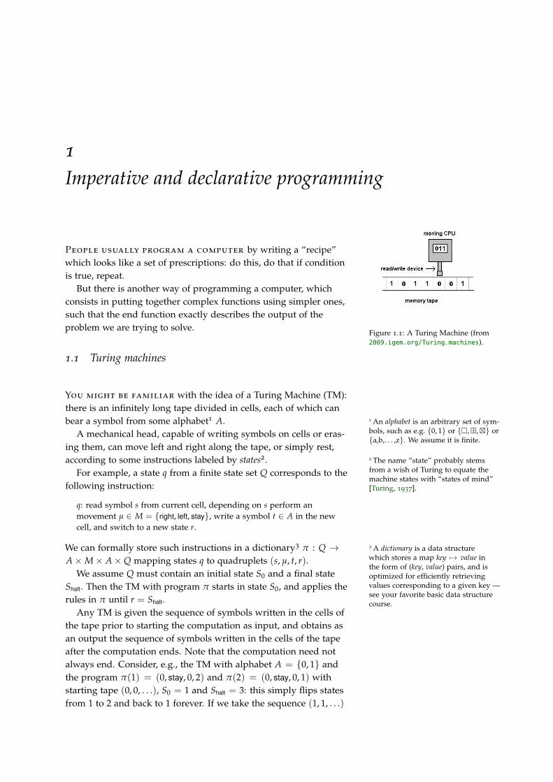
People usually program a computer by writing a “recipe”which looks like a set of prescriptions: do this, do that if conditionis true, repeat.
Figure 1.1: A Turing Machine (from2009.igem.org/Turing_machines).
But there is another way of programming a computer, whichconsists in putting together complex functions using simpler ones,such that the end function exactly describes the output of theproblem we are trying to solve.
1.1 Turing machines
You might be familiar with the idea of a Turing Machine (TM):there is an infinitely long tape divided in cells, each of which canbear a symbol from some alphabet1 A. 1 An alphabet is an arbitrary set of sym-
bols, such as e.g. {0, 1} or {�,�,�} or{a,b,. . . ,z}. We assume it is finite.
A mechanical head, capable of writing symbols on cells or eras-ing them, can move left and right along the tape, or simply rest,according to some instructions labeled by states2. 2 The name “state” probably stems
from a wish of Turing to equate themachine states with “states of mind”[Turing, 1937].
For example, a state q from a finite state set Q corresponds to thefollowing instruction:
q: read symbol s from current cell, depending on s perform anmovement µ ∈ M = {right, left, stay}, write a symbol t ∈ A in the newcell, and switch to a new state r.
We can formally store such instructions in a dictionary3 π : Q → 3 A dictionary is a data structurewhich stores a map key 7→ value inthe form of (key, value) pairs, and isoptimized for efficiently retrievingvalues corresponding to a given key —see your favorite basic data structurecourse.
A×M× A×Q mapping states q to quadruplets (s, µ, t, r).We assume Q must contain an initial state S0 and a final state
Shalt. Then the TM with program π starts in state S0, and applies therules in π until r = Shalt.
Any TM is given the sequence of symbols written in the cells ofthe tape prior to starting the computation as input, and obtains asan output the sequence of symbols written in the cells of the tapeafter the computation ends. Note that the computation need notalways end. Consider, e.g., the TM with alphabet A = {0, 1} andthe program π(1) = (0, stay, 0, 2) and π(2) = (0, stay, 0, 1) withstarting tape (0, 0, . . .), S0 = 1 and Shalt = 3: this simply flips statesfrom 1 to 2 and back to 1 forever. If we take the sequence (1, 1, . . .)
14 mathematical programming
as a starting tape, we find no relevant instruction in π(1) whichstarts with 1, and hence the TM simply “gets stuck” and neverterminates.
1.2 Register machines
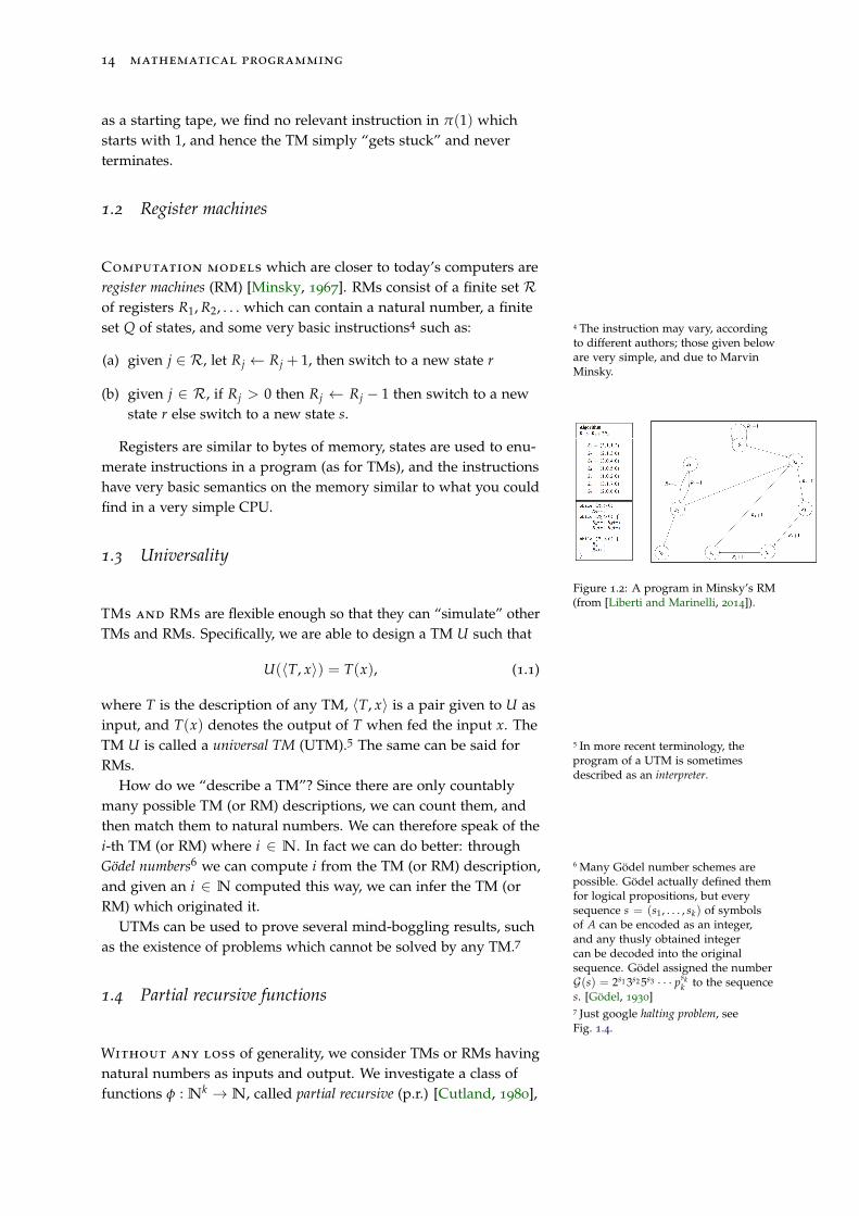
Computation models which are closer to today’s computers areregister machines (RM) [Minsky, 1967]. RMs consist of a finite set Rof registers R1, R2, . . . which can contain a natural number, a finiteset Q of states, and some very basic instructions4 such as: 4 The instruction may vary, according
to different authors; those given beloware very simple, and due to MarvinMinsky.
(a) given j ∈ R, let Rj ← Rj + 1, then switch to a new state r
(b) given j ∈ R, if Rj > 0 then Rj ← Rj − 1 then switch to a newstate r else switch to a new state s.
Figure 1.2: A program in Minsky’s RM(from [Liberti and Marinelli, 2014]).
Registers are similar to bytes of memory, states are used to enu-merate instructions in a program (as for TMs), and the instructionshave very basic semantics on the memory similar to what you couldfind in a very simple CPU.
1.3 Universality
TMs and RMs are flexible enough so that they can “simulate” otherTMs and RMs. Specifically, we are able to design a TM U such that
U(〈T, x〉) = T(x), (1.1)
where T is the description of any TM, 〈T, x〉 is a pair given to U asinput, and T(x) denotes the output of T when fed the input x. TheTM U is called a universal TM (UTM).5 The same can be said for 5 In more recent terminology, the
program of a UTM is sometimesdescribed as an interpreter.
RMs.How do we “describe a TM”? Since there are only countably
many possible TM (or RM) descriptions, we can count them, andthen match them to natural numbers. We can therefore speak of thei-th TM (or RM) where i ∈ N. In fact we can do better: throughGödel numbers6 we can compute i from the TM (or RM) description, 6 Many Gödel number schemes are
possible. Gödel actually defined themfor logical propositions, but everysequence s = (s1, . . . , sk) of symbolsof A can be encoded as an integer,and any thusly obtained integercan be decoded into the originalsequence. Gödel assigned the numberG(s) = 2s1 3s2 5s3 · · · psk
k to the sequences. [Gödel, 1930]
and given an i ∈ N computed this way, we can infer the TM (orRM) which originated it.
UTMs can be used to prove several mind-boggling results, suchas the existence of problems which cannot be solved by any TM.7
7 Just google halting problem, seeFig. 1.4.
1.4 Partial recursive functions
Without any loss of generality, we consider TMs or RMs havingnatural numbers as inputs and output. We investigate a class offunctions φ : Nk → N, called partial recursive (p.r.) [Cutland, 1980],
imperative and declarative programming 15
for all values of k ≥ 0, built recursively using some basic functionsand basic operations on functions.
The basic p.r. functions are:
• for all c ∈N, the constant functions constc(s1, . . . , sk) = c;
• the successor function succ(s) = s + 1 where s ∈ N, defined fork = 1 only;
• for all k and j ≤ k, the projection functions projkj (s1, . . . , sk) = sj.
Figure 1.3: Alonzo Church, greyeminence of recursive functions.
The basic operations are:
• composition: if f : Nk → N and g : N → N are p.r., theng ◦ f : Nk →N mapping s 7→ g( f (s)) is p.r.
• primitive recursion:8 if f : Nk → N and g : Nk+2 → N are p.r.,
8 For example, the factorial functionn! is defined by primitive recursionby setting k = 0, f = const1 = 1,g(n) = n(n− 1)!.
then the function φ f ,g : Nk+1 →N defined by:
φ(s, 0) = f (s) (1.2)
φ(s, n + 1) = g(s, n, φ(s, n)) (1.3)
is p.r.
• minimalization: if f : Nk+1 → N, then the function ψ : Nk → N
maps s to the least9 natural number y such that, for each z ≤ y, 9 This is a formalization of an opti-mization problem in number theory:finding a minimum natural numberwhich satisfies a given p.r. property fis p.r.
f (s, z) is defined and f (s, y) = 0 is p.r.
Notationally, we denote minimalization by means of the searchquantifier µ:10
10 The µ quantifier is typical of com-putability. Eq. (1.4) is equivalentto ψ(s) = min{y ∈ N | ∀z ≤y ( f (s, y) is defined) ∧ f (s, y) = 0}.
ψ(s) ≡ µy (∀z ≤ y ( f (s, z) is defined) ∧ f (s, y) = 0). (1.4)
1.5 The main theorem
Figure 1.4: The Halting Problem(vinodwadhawan.blogspot.com).
The main result in computability states that TMs (or RMs) andp.r. functions are both universal models of computation. Moreprecisely, let T be the description of a TM taking an input s ∈Nk and producing an output in N, and let ΦT : Nk → N theassociated function s 7→ T(s). Then ΦT is p.r.; and, conversely, forany p.r. function f there is a TM T such that ΦT = f .
Here is the sketch of a proof. (⇒) Given a p.r. function, wemust show there is a TM which computes it. It is possible, and nottoo difficult,11 to show that there are TMs which compute basic
11 See Ch. 3, Lemma 1.1, Thm. 3.1, 4.4,5.2 in [Cutland, 1980]
p.r. functions and basic p.r. operations. Since we can combine TMsin the appropriate ways, for any p.r. function we can construct aTM which computes it.
(⇐) Conversely, given a TM T with input/output functionτ : Rn → R, we want to show that τ(x) is a p.r. function.12 We 12 This is the most interesting direction
for the purposes of these lecture notes,since it involves “modelling” a TM bymeans of p.r. functions.
assume T’s alphabet is the set N of natural numbers, and that theoutput of T (if the TM terminates) is going to be stored in a given
16 mathematical programming
“output” cell of the TM tape. We define two functions:
ω(x, t) =
{value in output cell after t steps of T on input xτ(x) if T stopped before t steps on input x
σ(x, t) =
{state label of next instruction after t steps of T0 if T stops after t steps or fewer,
where we assumed that Shalt = 0. Now there are two cases: either Tterminates on x, or it does not. If it terminates, there is a number t∗
of steps after which T terminates, and
t∗ = µt(σ(x, t) = 0) (1.5)
τ(x) = ω(x, t∗). (1.6)
Note that Eq. (1.5) says that t∗ is the least t such that σ(x, t) = 0 andσ(x, u) is defined for each u ≤ t.
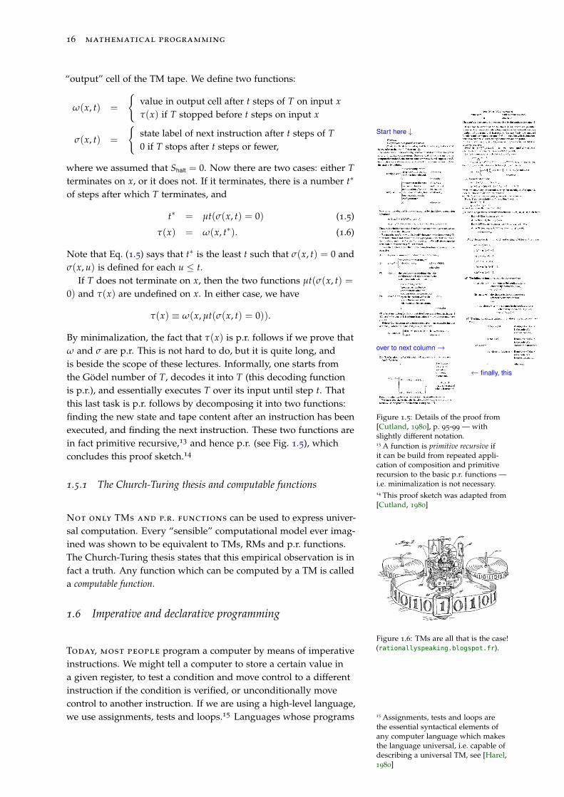
Start here ↓
over to next column→
← finally, this
Figure 1.5: Details of the proof from[Cutland, 1980], p. 95-99 — withslightly different notation.
If T does not terminate on x, then the two functions µt(σ(x, t) =0) and τ(x) are undefined on x. In either case, we have
τ(x) ≡ ω(x, µt(σ(x, t) = 0)).
By minimalization, the fact that τ(x) is p.r. follows if we prove thatω and σ are p.r. This is not hard to do, but it is quite long, andis beside the scope of these lectures. Informally, one starts fromthe Gödel number of T, decodes it into T (this decoding functionis p.r.), and essentially executes T over its input until step t. Thatthis last task is p.r. follows by decomposing it into two functions:finding the new state and tape content after an instruction has beenexecuted, and finding the next instruction. These two functions arein fact primitive recursive,13 and hence p.r. (see Fig. 1.5), which 13 A function is primitive recursive if
it can be build from repeated appli-cation of composition and primitiverecursion to the basic p.r. functions —i.e. minimalization is not necessary.
concludes this proof sketch.14
14 This proof sketch was adapted from[Cutland, 1980]
1.5.1 The Church-Turing thesis and computable functions
Figure 1.6: TMs are all that is the case!(rationallyspeaking.blogspot.fr).
Not only TMs and p.r. functions can be used to express univer-sal computation. Every “sensible” computational model ever imag-ined was shown to be equivalent to TMs, RMs and p.r. functions.The Church-Turing thesis states that this empirical observation is infact a truth. Any function which can be computed by a TM is calleda computable function.
1.6 Imperative and declarative programming
Today, most people program a computer by means of imperativeinstructions. We might tell a computer to store a certain value ina given register, to test a condition and move control to a differentinstruction if the condition is verified, or unconditionally movecontrol to another instruction. If we are using a high-level language,we use assignments, tests and loops.15 Languages whose programs 15 Assignments, tests and loops are
the essential syntactical elements ofany computer language which makesthe language universal, i.e. capable ofdescribing a universal TM, see [Harel,1980]
imperative and declarative programming 17
consist of finite lists of imperative instructions are called imperativelanguages.16
16 E.g. Fortran, Basic, C/C++, Java,Python.
The execution environment of an imperative language is a TM,or RM, or similar — in short, a “real computer”. As is well known,CPUs take instructions of the imperative type, such as “move avalue from a register to a location in memory” or “jump to instruc-tion such-and-such”.
We saw in previous sections that p.r. functions have the sameexpressive capabilities as imperative languages. And yet, we donot prescribe any action when writing a p.r. function. This begsthe question: can one program using p.r. functions? This is indeedpossible, as the many existing declarative languages testify.17 17 E.g. LISP, CAML.
Declarative languages based on p.r. functions usually consist ofa rather rich set of basic functions, and various kinds of operatorsin order to put together new functions.18 The complicated functions 18 Although it would be theoretically
possible to limit ourselves to the basicfunctions and operators above, thiswould yield unwieldy programs for ahuman to code.
obtained using recursive constructions from the basic ones arethe “programs” of a declarative language. Each such function isevaluated at the input in order to obtain the output. Since eachcomplex function is the result of various operators being appliedrecursively to some basic functions, its output can be obtainedaccordingly.
The natural execution environment of a declarative languagewould be a machine which can natively evaluate basic functions,and natively combine evaluations using basic operators. In practice,interpreters are used to turn declarative programs RM descriptionswhich can be executed on real computers.
Figure 1.7: Academic journals in MP.
1.7 Mathematical programming
We now come to the object of these notes. By “MathematicalProgramming” we indicate a special type of declarative program-ming, namely one where the interpreter varies according to themathematical properties of the functions involved in the program.
For example, if all the functions in a MP are linear in the vari-ables, and the variables range over continuous domains,19 one can 19 Optimizing a linear form over
a polyhedron is known as linearprogramming.
use very efficient algorithms as interpreters, such as the simplex20
20 From any vertex of the polyhedron,the simplex method finds the adjacentvertex improving the value of thelinear form, until this is no longerpossible.
or barrier21 methods [Matoušek and Gärtner, 2007]. If the functions
21 From any point inside a polyhedron,the barrier method defines a centralpath in the interior of the polyhedron,which ends at the vertex whichmaximizes or minimizes a given linearform.
are nonlinear or the variables are integer, one must resort to enu-merative methods such as branch-and-bound. [Liberti, 2006] Workingimplementations of these solution methods are collectively referredto as solvers. They read the MP (the program), the input of the prob-lem, and they execute an imperative program which runs on thephysical hardware.
1.7.1 The transportation problem
MP is commonly used to formulate and solve optimization prob-lems. A typical, classroom example is provided by the transportation
18 mathematical programming
problem22 [Munkres, 1957]. 22 The transportation problem isone of the fundamental problems inMP. It turns up time and again inpractical settings. It is at the basis ofthe important business concern ofassignment: who works on which task?
Given a set P of production facilities with production capacitiesai for i ∈ P, a set Q of customer sites with demands bj for j ∈ Q,and knowing that the unit transportation cost from facility i ∈ P tocustomer j ∈ Q is cij, find the optimal transportation plan.
a1
a2
a3
b1
b2
c11c12
c21
c22 c 31
c32
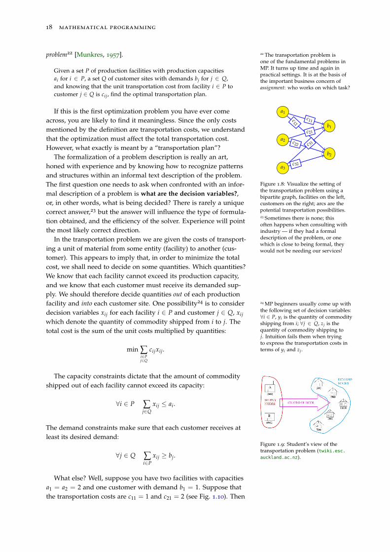
Figure 1.8: Visualize the setting ofthe transportation problem using abipartite graph, facilities on the left,customers on the right; arcs are thepotential transportation possibilities.
If this is the first optimization problem you have ever comeacross, you are likely to find it meaningless. Since the only costsmentioned by the definition are transportation costs, we understandthat the optimization must affect the total transportation cost.However, what exactly is meant by a “transportation plan”?
The formalization of a problem description is really an art,honed with experience and by knowing how to recognize patternsand structures within an informal text description of the problem.The first question one needs to ask when confronted with an infor-mal description of a problem is what are the decision variables?,or, in other words, what is being decided? There is rarely a uniquecorrect answer,23 but the answer will influence the type of formula-
23 Sometimes there is none; thisoften happens when consulting withindustry — if they had a formaldescription of the problem, or onewhich is close to being formal, theywould not be needing our services!
tion obtained, and the efficiency of the solver. Experience will pointthe most likely correct direction.
In the transportation problem we are given the costs of transport-ing a unit of material from some entity (facility) to another (cus-tomer). This appears to imply that, in order to minimize the totalcost, we shall need to decide on some quantities. Which quantities?We know that each facility cannot exceed its production capacity,and we know that each customer must receive its demanded sup-ply. We should therefore decide quantities out of each productionfacility and into each customer site. One possibility24 is to consider 24 MP beginners usually come up with
the following set of decision variables:∀i ∈ P, yi is the quantity of commodityshipping from i; ∀j ∈ Q, zj is thequantity of commodity shipping toj. Intuition fails them when tryingto express the transportation costs interms of yi and zj.
decision variables xij for each facility i ∈ P and customer j ∈ Q, xij
which denote the quantity of commodity shipped from i to j. Thetotal cost is the sum of the unit costs multiplied by quantities:
min ∑i∈Pj∈Q
cijxij.
Figure 1.9: Student’s view of thetransportation problem (twiki.esc.auckland.ac.nz).
The capacity constraints dictate that the amount of commodityshipped out of each facility cannot exceed its capacity:
∀i ∈ P ∑j∈Q
xij ≤ ai.
The demand constraints make sure that each customer receives atleast its desired demand:
∀j ∈ Q ∑i∈P
xij ≥ bj.
What else? Well, suppose you have two facilities with capacitiesa1 = a2 = 2 and one customer with demand b1 = 1. Suppose thatthe transportation costs are c11 = 1 and c21 = 2 (see Fig. 1.10). Then
imperative and declarative programming 19
the problem reads:
min x11 + 2x21
x11 ≤ 2
x21 ≤ 2
x11 + x21 ≥ 1.2.0
2.0
1.0
1.0
2.0
Figure 1.10: A very simple transporta-tion instance.
The optimal solution is x11 = 2, x21 = −1: it satisfies theconstraints and has zero total cost.25 This solution, however, cannot
25 Every solution on the line x11 + x21 =1 satisfies the constraints; in particular,because of the costs, the solutionx11 = 1 and x21 = 0 has unit cost.
be realistically implemented: what does it mean for a shippedquantity to be negative (Fig. 1.11)?
This example makes two points. One is that we had forgotten aconstraint, namely:
∀i ∈ P, j ∈ Q xij ≥ 0.
Figure 1.11: Negative shipments lookweird (artcritique.wordpress.com).
The other point is that forgetting a constraint might yield a solu-tion which appears impossible to those who know the problem setting.If we had been given the problem in its abstract setting, withoutspecifying that xij are supposed to mean a shipped quantity, wewould have had no way to decide that x21 = −1 is inadmissible.
1.7.2 Network flow
In the optimization of industrial processes, the network flow prob-lem26 [Ford and Fulkerson, 1956] is as important as the transporta-
26 Network flow is another fundamen-tal MP problem. Its constraints can beused as part of larger formulations inorder to ensure network connectivity.
tion problem.
Consider a rail network connecting two cities s, t by way of a numberof intermediate cities, where each link of the network has a numberassigned to it representing its capacity. Assuming a steady statecondition, find a maximal flow from city s to city t.
Note that the network flow problem is also about transportation.
• We model the rail network by a directed graph27 G = (V, A), 27 A directed graph, or digraph, is apair (V, A) where V is any set andA ⊆ V ×V. We shall assume V is finite.Elements of V are called nodes andelements of A arcs.
and remark that s, t are two distinct nodes in V.
• For each arc (u, v) ∈ A we let Cuv denote the capacity of the arc.
The commodity being transported over the network (people,freight or whatever else) starts from s; we assume this commoditycan be split, so it is routed towards t along a variety of paths. Wewant to find the paths which will maximize the total flow rate.28 28 Assuming a constant flow, this is
equivalent to maximizing the totalquantity.
We have to decide which paths to use, and what quantities ofcommodity to route along the paths. Since paths are sequences ofarcs, and the material could be split at a node and follow differentpaths thereafter, we define decision variables xuv indicating the flowrate along each arc (u, v) ∈ A.
Figure 1.12: A negative flow couplerfrom starships of the rebellion era(starwars.wikia.com).
A solution is feasible if the flow rates are non-negative (Fig. 1.12):
∀(u, v) ∈ A xuv ≥ 0,
if the flow rates do not exceed the arc capacities:
∀(u, v) ∈ A xuv ≤ Cuv,
20 mathematical programming
and if the positive flow rates along the arcs define a set of pathsfrom s to t.
Figure 1.13: A Max Flow instance.
How do we express this constraint? First, since the flow orig-inates from the source node s, we require that no flow actuallyarrives at s:
∑(u,s)∈A
xus = 0. (1.7)
Next, no benefit29 would derive from flow leaving the target node t: 29 Eq. (1.8) follows from (1.7) and (1.9)(prove it), and so it is redundant. Ifyou use these constraints within aMILP, nonconvex NLP or MINLP,however, they might help certainsolvers perform better.
∑(t,v)∈A
xtv = 0. (1.8)
Lastly, the total flow entering intermediate nodes on paths betweens and t must be equal to the total flow exiting them:30 30 These constraints are called flow
conservation equations or materialbalance constraints.∀v ∈ V r {s, t} ∑
(u,v)∈Axuv = ∑
(v,u)∈Axvu. (1.9)
Figure 1.14: An optimal solution forthe instance in Fig. 1.13.
The objective function aims at maximizing the amount of flowfrom s to t. Since flow is conserved at any node but s, t, it followsthat however much flow exits s must enter t, and hence that itsuffices to maximize the amount of flow exiting s:31
31 We could equivalently have maxi-mized the amount of flow entering t(why?).
max ∑(s,v)∈A
xsv.
1.7.3 Extremely short summary of complexity theory
Formally, decision and optimization problems are defined as setsof infinitely many instances (input data) of increasing size. Thisis in view of the asymptotic worst-case complexity analysis ofalgorithms, which says that an algorithm A is O( f (n)) (for somefunction f ) when there is an n0 ∈ N such that for all n > n0 theCPU time taken by A to terminate on inputs requiring n bits ofstorage is bounded above by f (n).
If a problem had finitely many (say m) instances, we could pre-compute the solutions to these m instances and store them into ahash table, then solve any instance of this problem in constant time,making the problem trivial.
We say a decision problem is in P when there exists a polynomial-time algorithm that solves it, and in NP if every YES instance has asolution which can be verified to be YES in polynomial time.
Problems are NP-hard when they are as hard as the hardest prob-lems in NP: NP-hardness of a problem Q is proved by reducing(i.e. transforming) a known NP-hard problem P to Q in polynomialtime, such that each YES instance in P maps to a YES instance in Qand every NO instance in P to a NO instance in Q.
Figure 1.15: Hardness/completenessreductions.
This method works since, if Q were any easier than P, we couldsolve P by reducing it to Q, solve Q, then map the solution of Qback to P; hence P would be “as easy as Q” (under polynomial-timereductions), contradicting the supposition that Q is easier than P.
These notions are informally applied to optimization problemsby referring to their decision version: given an optimization problem
imperative and declarative programming 21
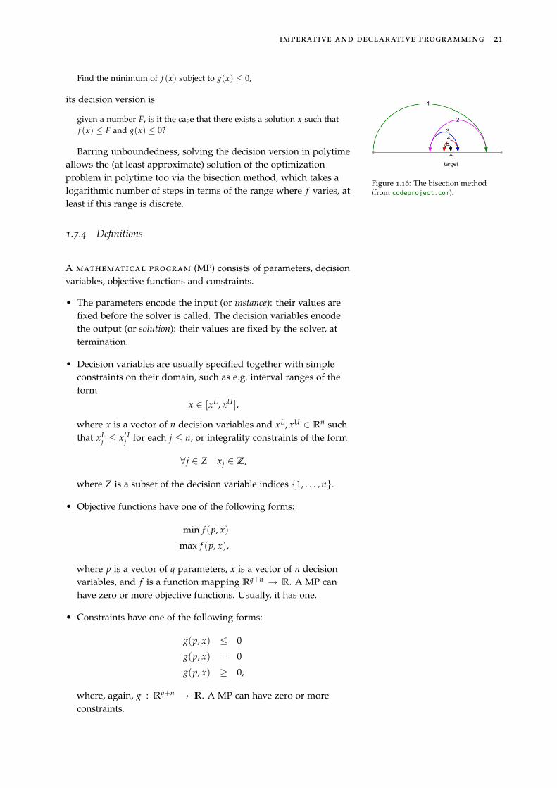
Find the minimum of f (x) subject to g(x) ≤ 0,
its decision version is
given a number F, is it the case that there exists a solution x such thatf (x) ≤ F and g(x) ≤ 0?
Figure 1.16: The bisection method(from codeproject.com).
Barring unboundedness, solving the decision version in polytimeallows the (at least approximate) solution of the optimizationproblem in polytime too via the bisection method, which takes alogarithmic number of steps in terms of the range where f varies, atleast if this range is discrete.
1.7.4 Definitions
A mathematical program (MP) consists of parameters, decisionvariables, objective functions and constraints.
• The parameters encode the input (or instance): their values arefixed before the solver is called. The decision variables encodethe output (or solution): their values are fixed by the solver, attermination.
• Decision variables are usually specified together with simpleconstraints on their domain, such as e.g. interval ranges of theform
x ∈ [xL, xU ],
where x is a vector of n decision variables and xL, xU ∈ Rn suchthat xL
j ≤ xUj for each j ≤ n, or integrality constraints of the form
∀j ∈ Z xj ∈ Z,
where Z is a subset of the decision variable indices {1, . . . , n}.
• Objective functions have one of the following forms:
min f (p, x)
max f (p, x),
where p is a vector of q parameters, x is a vector of n decisionvariables, and f is a function mapping Rq+n → R. A MP canhave zero or more objective functions. Usually, it has one.
• Constraints have one of the following forms:
g(p, x) ≤ 0
g(p, x) = 0
g(p, x) ≥ 0,
where, again, g : Rq+n → R. A MP can have zero or moreconstraints.
22 mathematical programming
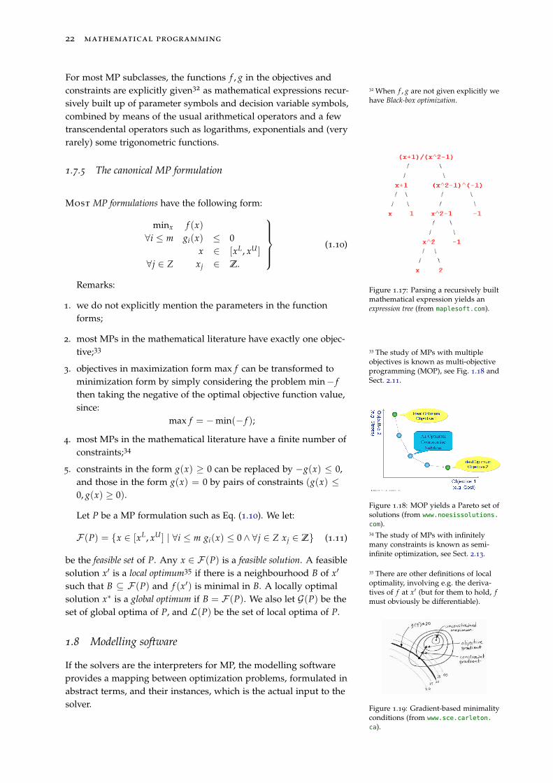
For most MP subclasses, the functions f , g in the objectives andconstraints are explicitly given32 as mathematical expressions recur- 32 When f , g are not given explicitly we
have Black-box optimization.sively built up of parameter symbols and decision variable symbols,combined by means of the usual arithmetical operators and a fewtranscendental operators such as logarithms, exponentials and (veryrarely) some trigonometric functions.
1.7.5 The canonical MP formulation
Most MP formulations have the following form:
minx f (x)∀i ≤ m gi(x) ≤ 0
x ∈ [xL, xU ]
∀j ∈ Z xj ∈ Z.
(1.10)
Figure 1.17: Parsing a recursively builtmathematical expression yields anexpression tree (from maplesoft.com).
Remarks:
1. we do not explicitly mention the parameters in the functionforms;
2. most MPs in the mathematical literature have exactly one objec-tive;33 33 The study of MPs with multiple
objectives is known as multi-objectiveprogramming (MOP), see Fig. 1.18 andSect. 2.11.
Figure 1.18: MOP yields a Pareto set ofsolutions (from www.noesissolutions.
com).
3. objectives in maximization form max f can be transformed tominimization form by simply considering the problem min− fthen taking the negative of the optimal objective function value,since:
max f = −min(− f );
4. most MPs in the mathematical literature have a finite number ofconstraints;34
34 The study of MPs with infinitelymany constraints is known as semi-infinite optimization, see Sect. 2.13.
5. constraints in the form g(x) ≥ 0 can be replaced by −g(x) ≤ 0,and those in the form g(x) = 0 by pairs of constraints (g(x) ≤0, g(x) ≥ 0).
Let P be a MP formulation such as Eq. (1.10). We let:
F (P) = {x ∈ [xL, xU ] | ∀i ≤ m gi(x) ≤ 0∧ ∀j ∈ Z xj ∈ Z} (1.11)
be the feasible set of P. Any x ∈ F (P) is a feasible solution. A feasiblesolution x′ is a local optimum35 if there is a neighbourhood B of x′ 35 There are other definitions of local
optimality, involving e.g. the deriva-tives of f at x′ (but for them to hold, fmust obviously be differentiable).
such that B ⊆ F (P) and f (x′) is minimal in B. A locally optimalsolution x∗ is a global optimum if B = F (P). We also let G(P) be theset of global optima of P, and L(P) be the set of local optima of P.
Figure 1.19: Gradient-based minimalityconditions (from www.sce.carleton.
ca).
1.8 Modelling software
If the solvers are the interpreters for MP, the modelling softwareprovides a mapping between optimization problems, formulated inabstract terms, and their instances, which is the actual input to thesolver.
imperative and declarative programming 23
1.8.1 Structured and flat formulations
Compare the transportation problem formulation given above:
min ∑i∈Pj∈Q
cijxij
∀i ∈ P ∑j∈Q
xij ≤ ai
∀j ∈ Q ∑i∈P
xij ≥ bj
x ≥ 0,
(1.12)
given in general terms, to its instantiation
min x11 + 2x21
x11 ≤ 2x21 ≤ 2
x11 + x21 ≥ 1x11, x21 ≥ 0,
(1.13)
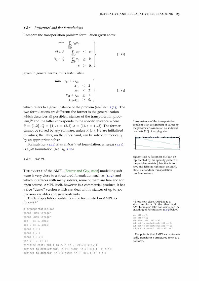
which refers to a given instance of the problem (see Sect. 1.7.3). Thetwo formulations are different: the former is the generalizationwhich describes all possible instances of the transportation prob-lem,36 and the latter corresponds to the specific instance where 36 An instance of the transportation
problem is an assignment of values tothe parameter symbols a, b, c indexedover sets P, Q of varying size.
P = {1, 2}, Q = {1}, a = (2, 2), b = (1), c = (1, 2). The formercannot be solved by any software, unless P, Q, a, b, c are initializedto values; the latter, on the other hand, can be solved numericallyby an appropriate solver.
Figure 1.20: A flat linear MP can berepresented by the sparsity pattern ofthe problem matrix (objective in toprow, and RHS in rightmost column).Here is a random transportationproblem instance.
Formulation (1.12) is as a structured formulation, whereas (1.13)is a flat formulation (see Fig. 1.20).
1.8.2 AMPL
The syntax of the AMPL [Fourer and Gay, 2002] modelling soft-ware is very close to a structured formulation such as (1.12), andwhich interfaces with many solvers, some of them are free and/oropen source. AMPL itself, however, is a commercial product. It hasa free “demo” version which can deal with instances of up to 300
decision variables and 300 constraints.The transportation problem can be formulated in AMPL as
follows.37 37 Note how close AMPL is to astructured form. On the other hand,AMPL can also take flat forms: see theencoding of Formulation (1.13) below.
var x11 >= 0;var x21 >= 0;minimize cost: x11 + x21;subject to production1: x11 <= 2;subject to production2: x21 <= 2;subject to demand1: x11 + x21 >= 1;
The point is that AMPL can automat-ically transform a structured form to aflat form.
# transportation.mod
param Pmax integer;
param Qmax integer;
set P := 1..Pmax;
set Q := 1..Qmax;
param a{P};
param b{Q};
param c{P,Q};
var x{P,Q} >= 0;
minimize cost: sum{i in P, j in Q} c[i,j]*x[i,j];
subject to production{i in P}: sum{j in Q} x[i,j] <= a[i];
subject to demand{j in Q}: sum{i in P} x[i,j] >= b[j];
24 mathematical programming
The various entities of a MP (sets, parameters, decision variables,objective functions, constraints) are introduced by a correspondingkeyword. Every entity is named.38 Every entity can be quantified 38 This is obvious for sets, parameters
and variables, but not for objectivefunctions and constraints.
over sets, including sets themselves. The cartesian product P× Qis written {P,Q}. AMPL formulations can be saved in a file withextension .mod.39 Note that comments are introduced by the # 39 E.g. transportation.mod.
symbol at the beginning of the line.The instance is introduced in a file with extension .dat.40 40 E.g. transportation.dat
AMPL .dat files have a slightly differ-ent syntax with respect to .mod or .runfiles. For example, you would define aset using
set := { 1, 2 };
in .mod and .run files, but using
set := 1 2;
in .dat files. Also, there are ways tobi-dimensional arrays in tabular formsand transposed tabular forms. Multi-dimensional arrays can be written asmany bi-dimensional array slices. Forsimplicity, I suggest you stick with thebasic syntax.
# transportation.dat
param Pmax := 2;
param Qmax := 1;
param a :=
1 2.0
2 2.0
;
param b :=
1 1.0
;
param c :=
1 1 1.0
2 1 2.0
;
Every param line introduces one or more parameters as func-tions41 from their index sets to the values. 41 The parameter tensor pi1 ,...,ik , where
P is the set of tuples (i1, . . . , ik) isencoded as the function p : P →ran(p). Each pair (i1, . . . , ik) 7→ pi1 ,...,ikis given as a line i1 i2 ... ik
p_value.
In order to actually solve the problem numerically, another file(bearing the extension .run) is used.42
42 The AMPl .run file functionality canbe much richer than this example, andimplement nontrivial algorithms. Theimperative part of the AMPL languageis however severely limited by the lackof a function call mechanism.
# transportation.run
model transportation.mod;
data transportation.dat;
option solver cplexamp;
solve;
display x, cost;
The transportation.run file is executed in a command line en-vironment by running43 ampl < transportation.run. The output 43 AMPL actually has an Integrated
Development Environment (IDE). Iprefer using the command line sinceit allows me to pipe each commandinto the next. For example, in Unix(including Linux and MacOSX) youcan ask for the optimal value byrunning
ampl < transportation.run
| grep optimal
(all on one line).
should look as follows.
CPLEX 12.6.2.0: optimal solution; objective 1
1 dual simplex iterations (0 in phase I)
x :=
1 1 1
2 1 0
;
cost = 1
which corresponds to x11 = 1, x21 = 0 having objective functionvalue 1.
Figure 1.21: The Python languagenamesake.
1.8.3 Python
Python is currently very popular with programmers because of thelarge amounts of available libraries: even complex tasks requirevery little coding.
imperative and declarative programming 25
Python is a high-level,44 general purpose, imperative interpreted44 A programming language is high-level when it is humanly readable (theopposite, low-level, would be said ofmachine code or assembly language).The opposite of “interpreted” is“compiled”: in interpreted languages,the translation to machine code occursline by line, and the correspondingmachine code chunks are executedimmediately after translation. Incompiled languages, the program iscompletely translated to an executablefile prior to running.
programming language. We assume at least a cursory knowledge ofPython.
The transportation problem can be formulated in Python asfollows. First, we import the PyOMO [Hart et al., 2012] libraries:
# define concrete transportation model in pyomo and solve it
from pyomo.environ import *from pyomo.opt import SolverStatus, TerminationCondition
import pyomo.opt
Next, we define a function which creates an instance of thetransportation problem, over the sets P, Q and the parameters a, b, c(see Eq. (1.12)).45 45 PyOMO also offers an “abstract”
modelling framework, through whichyou can actually read the instancedirectly from AMPL .dat files.
def create_transportation_model(P = [], Q = [], a = {}, b = {}, c = {}):
model = ConcreteModel()
model.x = Var(P, Q, within = NonNegativeReals)
def objective_function(model):
return sum(c[i,j] * model.x[i,j] for i in P for j in Q)
model.obj = Objective(rule = objective_function)
def production_constraint(model, i):
return sum(model.x[i,j] for j in Q) <= a[i]
model.production = Constraint(P, rule = production_constraint)
def demand_constraint(model, j):
return sum(model.x[i,j] for i in P) >= b[j]
model.demand = Constraint(Q, rule = demand_constraint)
return model
Finally, we write the “main” procedure,46 i.e. the point of entry
46 What you do with the solution onceyou extract it from PyOMO usingsolutions.load_from is up to you(and Python). Since Python offersconsiderably more language flexibilityand functionality than the imperativepart of AMPL, the Python interface isto be preferred whenever solving MPsis just a step of a more complicatedalgorithm.
to the execution of the program.
# main
P = [1,2]
Q = [1]
a = {1:2,2:2}
b = {1:1}
c = {(1,1):1, (2,1):2}
instance = create_transportation_model(P,Q,a,b,c)
solver = pyomo.opt.SolverFactory(’cplexamp’, solver_io = ’nl’)
if solver is None:
raise RuntimeError(’solver not found’)
solver.options[’timelimit’] = 60
results = solver.solve(instance, keepfiles = False, tee = True)
if ((results.solver.status == SolverStatus.ok) and
(results.solver.termination_condition == TerminationCondition.optimal)):
# feasible and optimal
instance.solutions.load_from(results)
xstar = [instance.x[i,j].value for i in P for j in Q]
print(’solved to optimality’)
print(xstar)
else:
print(’not solved to optimality’)
Note that these three pieces of code have to be saved, in se-quence, in a file named transportation.py, which can be executedby running python transportation.py. The output is as follows.
timelimit=60
26 mathematical programming
CPLEX 12.6.2.0: optimal solution; objective 1
1 dual simplex iterations (0 in phase I)
solved to optimality
[1.0, 0.0]
Are you wondering how I producedFig. 1.20? Take transportation.py andmodify it as follows: (i) include
import numpy as np
import itertools
import np.random as npr
import matplotlib.pyplot as plt
at the beginning of the code. Thenreplace the definition of a, b, c after #main to
U=10; p=10; q=6
P=range(1,p+1); Q=range(1,q+1)
avals=npr.random_integers(1,U,size=p)
bvals=npr.random_integers(1,U,size=q)
cvals=npr.random_integers(1,U,size=p*q)
a=dict(zip(P,avals))
b=dict(zip(Q,bvals))
c=dict(zip(list(itertools.product(P,Q)),cvals))
M=np.zeros((1+p+q, p*q+1))
for i in P:
for j in Q:
M[0,q*(i-1)+(j-1)]=c[(i,j)]
for i in P:
for j in Q:
M[i,q*(i-1)+(j-1)]=1
M[i,p*q] = a[i]
for j in Q:
for i in P:
M[p+j,p*(j-1)+(i-1)]=1
M[p+j,p*q] = b[j]
plt.matshow(M, cmap = ’bone_r’)
plt.show()
Essentially, I’m sampling random in-teger dictionaries for a, b, c (note theuse of zip: look it up, it’s an importantfunction in Python), then I’m construct-ing the problem matrix M consistingin the objective function coefficients(top row), the constraint matrix, andthe right hand side (RHS) vector in therightmost column.
1.9 Summary
• Most people are used to imperative programming
• There is also declarative programming, and it is just as powerful
• Mathematical programming is a kind of declarative program-ming for optimization problems
• Using parameters, decision variables, objectives and constraints,optimization problems can be “modelled” using MP
• Efficient solution algorithms exist for different classes of MP
• Algorithms are implemented into solvers
• MP interpreted as “modelling, then calling an existing solver”shifts focus from creating a solution algorithm for a given problem(perceived as more difficult) to modelling the problem using MP(perceived as easier)
• MP formulations are created by humans using quantifiers, sets,and tensors/arrays of variables and constraints (structured form);solvers require their input to be MP formulation as explicitsequences of constants, variables, objectives, constraints (flatform)
• Modelling software is used to turn structured form to flat form,submit the flat form to a solver, then retrieve the solution fromthe solver and structure it back to the original form
• We look at two modelling environments: AMPL and Python.
2Systematics and solution methods
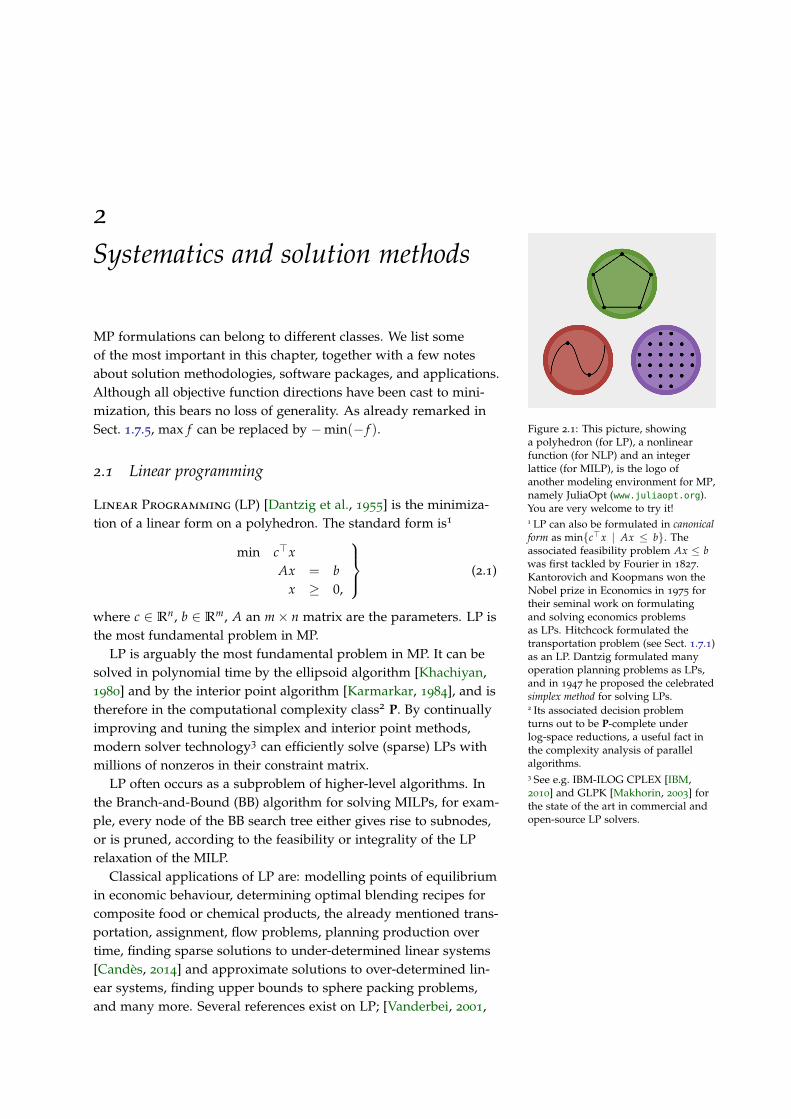
Figure 2.1: This picture, showinga polyhedron (for LP), a nonlinearfunction (for NLP) and an integerlattice (for MILP), is the logo ofanother modeling environment for MP,namely JuliaOpt (www.juliaopt.org).You are very welcome to try it!
MP formulations can belong to different classes. We list someof the most important in this chapter, together with a few notesabout solution methodologies, software packages, and applications.Although all objective function directions have been cast to mini-mization, this bears no loss of generality. As already remarked inSect. 1.7.5, max f can be replaced by −min(− f ).
2.1 Linear programming
Linear Programming (LP) [Dantzig et al., 1955] is the minimiza-tion of a linear form on a polyhedron. The standard form is1 1 LP can also be formulated in canonical
form as min{c>x | Ax ≤ b}. Theassociated feasibility problem Ax ≤ bwas first tackled by Fourier in 1827.Kantorovich and Koopmans won theNobel prize in Economics in 1975 fortheir seminal work on formulatingand solving economics problemsas LPs. Hitchcock formulated thetransportation problem (see Sect. 1.7.1)as an LP. Dantzig formulated manyoperation planning problems as LPs,and in 1947 he proposed the celebratedsimplex method for solving LPs.
min c>xAx = b
x ≥ 0,
(2.1)
where c ∈ Rn, b ∈ Rm, A an m× n matrix are the parameters. LP isthe most fundamental problem in MP.
LP is arguably the most fundamental problem in MP. It can besolved in polynomial time by the ellipsoid algorithm [Khachiyan,1980] and by the interior point algorithm [Karmarkar, 1984], and istherefore in the computational complexity class2 P. By continually 2 Its associated decision problem
turns out to be P-complete underlog-space reductions, a useful fact inthe complexity analysis of parallelalgorithms.
improving and tuning the simplex and interior point methods,modern solver technology3 can efficiently solve (sparse) LPs with
3 See e.g. IBM-ILOG CPLEX [IBM,2010] and GLPK [Makhorin, 2003] forthe state of the art in commercial andopen-source LP solvers.
millions of nonzeros in their constraint matrix.LP often occurs as a subproblem of higher-level algorithms. In
the Branch-and-Bound (BB) algorithm for solving MILPs, for exam-ple, every node of the BB search tree either gives rise to subnodes,or is pruned, according to the feasibility or integrality of the LPrelaxation of the MILP.
Classical applications of LP are: modelling points of equilibriumin economic behaviour, determining optimal blending recipes forcomposite food or chemical products, the already mentioned trans-portation, assignment, flow problems, planning production overtime, finding sparse solutions to under-determined linear systems[Candès, 2014] and approximate solutions to over-determined lin-ear systems, finding upper bounds to sphere packing problems,and many more. Several references exist on LP; [Vanderbei, 2001,
28 mathematical programming
Matoušek and Gärtner, 2007] are among my favorites; the latter, inparticular, contains a very interesting chapter on the application ofLP to upper bounds for error correcting codes and sphere packingproblems [Delsarte, 1972].
2.2 Mixed-integer linear programming
Mixed-Integer Linear Programming4 (MILP) consists in the 4 The first exact method for solving
MILPs was proposed by Ralph Go-mory [Gomory, 1958]. After joiningIBM Research, he exploited integer pro-gramming to formulate some cuttingproblem for a client, and derived muchof the existing theory behind cuttingplanes from the empirical observationof apparently periodic data in endlesstabulations of computational results.
minimization of a linear form on a polyhedron, restricted to a non-negative integer lattice cartesian product the non-negative orthant.The standard form is
min c>xAx = b
x ≥ 0∀j ∈ Z xj ∈ Z+,
(2.2)
where c, b, A are as in the LP case, and Z ⊆ {1, . . . , n}.This is another fundamental problem in MP. It is NP-hard5; 5 A problem P is NP-hard when any
other problem in the class NP canbe reduced to it in polynomial time:from this follows the statement thatan NP-hard problem must be at leastas hard to solve (asymptotically, in theworst case) as the hardest problem ofthe class NP (see Sect. 1.7.3).
many problems can be cast as MILPs — its combination of contin-uous and integer variables give MILP a considerable expressivepower as a modelling language. It includes ILP (integer variablesonly, see below), BLP (binary variables only, see below) and LP asspecial cases. MILPs can either be solved heuristically [Fischetti andLodi, 2005, Fischetti et al., 2005] or exactly, by BB6 6 The state of the art BB implementa-
tion for MILP is given by IBM-ILOGCPLEX [IBM, 2010]; the SCIP solver[Berthold et al., 2012], also very ad-vanced, is free for academics. Otheradvanced commercial solvers areXPress-MP and GuRoBi.
Here is an example of a problem which can be formulated as aMILP.
∗types
ofpower
plants
Power Generation Problem. There are Kmax types∗
of powergeneration facilities, and, for each k ≤ Kmax, nk facilities of typek, each capable of producing wk megawatts. Switching on or off afacility of type k ≤ Kmax has a fixed cost fk and a unit time costck. This set of power generation facilities has to meet demandsdt for each time period t ≤ Tmax, where Tmax is the time horizon.The unmet demand has to be purchased externally, at a cost Cper megawatt. Formulate a minimum cost plan for operating thefacilities.
Some of the decision variables7 are defined as the number of fa- 7 Try and formulate this problem asa MILP — use variables xkt ∈ Z+ tomean the number of facilities of typek generating at period t, y1
kt ∈ Z+ tomean the number of facilities of typek that are switched on at time t, y0
ktswitched off, and zt ∈ R+ to mean thequantity of power purchased externallyat period t.
cilities of a certain type used at a given period (these are integervariables). And yet other decision variables will be the quantity ofpower which needs to be purchased externally (these are continu-ous variables). Every relation between variables is linear, as well asthe expression for the costs.
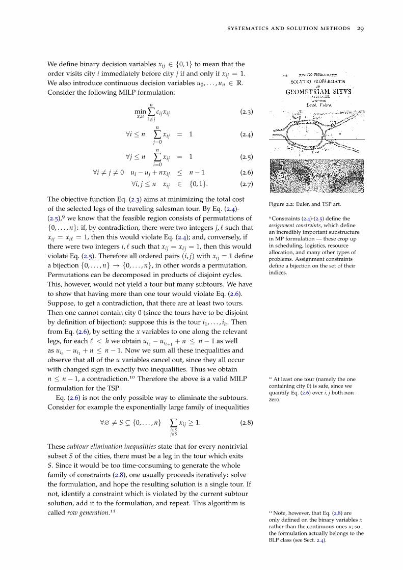
Another example is the following problem, which has its roots in[Euler, 1736] (see Fig. 2.2).
Traveling Salesman Problem8 (TSP) [Flood, 1956]. Consider a 8 There is an enormous amount of
literature about the TSP — it appearsto be the most studied problem incombinatorial optimization! Entirebooks have been written about it[Applegate et al., 2007, Gutin andPunnen, 2002].
traveling salesman who has to visit n + 1 cities 0, 1, . . . , n spending theminimum amount of money on car fuel. Consumption is assumedto be proportional to inter-city distances cij for each pair of citiesi < j ≤ n. Determine the optimal order of the cities to be visited.
systematics and solution methods 29
Figure 2.2: Euler, and TSP art.
We define binary decision variables xij ∈ {0, 1} to mean that theorder visits city i immediately before city j if and only if xij = 1.We also introduce continuous decision variables u0, . . . , un ∈ R.Consider the following MILP formulation:
minx,u
n
∑i 6=j
cijxij (2.3)
∀i ≤ nn
∑j=0
xij = 1 (2.4)
∀j ≤ nn
∑i=0
xij = 1 (2.5)
∀i 6= j 6= 0 ui − uj + nxij ≤ n− 1 (2.6)
∀i, j ≤ n xij ∈ {0, 1}. (2.7)
The objective function Eq. (2.3) aims at minimizing the total costof the selected legs of the traveling salesman tour. By Eq. (2.4)-(2.5),9 we know that the feasible region consists of permutations of 9 Constraints (2.4)-(2.5) define the
assignment constraints, which definean incredibly important substructurein MP formulation — these crop upin scheduling, logistics, resourceallocation, and many other types ofproblems. Assignment constraintsdefine a bijection on the set of theirindices.
{0, . . . , n}: if, by contradiction, there were two integers j, ` such thatxij = xi` = 1, then this would violate Eq. (2.4); and, conversely, ifthere were two integers i, ` such that xij = x`j = 1, then this wouldviolate Eq. (2.5). Therefore all ordered pairs (i, j) with xij = 1 definea bijection {0, . . . , n} → {0, . . . , n}, in other words a permutation.Permutations can be decomposed in products of disjoint cycles.This, however, would not yield a tour but many subtours. We haveto show that having more than one tour would violate Eq. (2.6).Suppose, to get a contradiction, that there are at least two tours.Then one cannot contain city 0 (since the tours have to be disjointby definition of bijection): suppose this is the tour i1, . . . , ih. Thenfrom Eq. (2.6), by setting the x variables to one along the relevantlegs, for each ` < h we obtain ui` − ui`+1
+ n ≤ n − 1 as wellas uih − ui1 + n ≤ n − 1. Now we sum all these inequalities andobserve that all of the u variables cancel out, since they all occurwith changed sign in exactly two inequalities. Thus we obtainn ≤ n− 1, a contradiction.10 Therefore the above is a valid MILP 10 At least one tour (namely the one
containing city 0) is safe, since wequantify Eq. (2.6) over i, j both non-zero.
formulation for the TSP.Eq. (2.6) is not the only possible way to eliminate the subtours.
Consider for example the exponentially large family of inequalities
∀∅ 6= S ( {0, . . . , n} ∑i∈Sj 6∈S
xij ≥ 1. (2.8)
These subtour elimination inequalities state that for every nontrivialsubset S of the cities, there must be a leg in the tour which exitsS. Since it would be too time-consuming to generate the wholefamily of constraints (2.8), one usually proceeds iteratively: solvethe formulation, and hope the resulting solution is a single tour. Ifnot, identify a constraint which is violated by the current subtoursolution, add it to the formulation, and repeat. This algorithm iscalled row generation.11 11 Note, however, that Eq. (2.8) are
only defined on the binary variables xrather than the continuous ones u; sothe formulation actually belongs to theBLP class (see Sect. 2.4).
30 mathematical programming
2.3 Integer linear programming
Integer Linear Programming (ILP) consists in the minimizationof a linear form on a polyhedron, restricted to the non-negativeinteger lattice. The standard form is
min c>xAx = b
x ∈ Zn+,
(2.9)
where c, b, A are as in the LP case. ILP is just like MILP but withoutcontinuous variables. Consider the following problem.
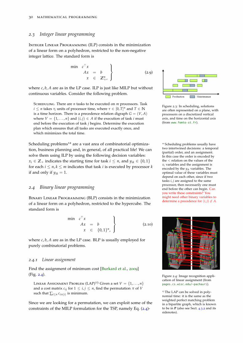
Figure 2.3: In scheduling, solutionsare often represented on a plane, withprocessors on a discretized verticalaxis, and time on the horizontal axis(from www.femto-st.fr).
Scheduling. There are n tasks to be executed on m processors. Taski ≤ n takes τi units of processor time, where τ ∈ [0, T]n and T ∈ N
is a time horizon. There is a precedence relation digraph G = (V, A)
where V = {1, . . . , n} and (i, j) ∈ A if the execution of task i mustend before the execution of task j begins. Determine the executionplan which ensures that all tasks are executed exactly once, andwhich minimizes the total time.
Scheduling problems12 are a vast area of combinatorial optimiza- 12 Scheduling problems usually havetwo intertwined decisions: a temporal(partial) order, and an assignment.In this case the order is encoded bythe < relation on the values of thexi variables and the assignment isencoded by the yik variables. Theoptimal value of these variables mustdepend on each other, since if twotasks i, j are assigned to the sameprocessor, then necessarily one mustend before the other can begin. Canyou write these constraints? Youmight need other binary variables todetermine a precedence for (i, j) 6∈ A.
tion, business planning and, in general, of all practical life! We cansolve them using ILP by using the following decision variables:xi ∈ Z+ indicates the starting time for task i ≤ n, and yik ∈ {0, 1}for each i ≤ n, k ≤ m indicates that task i is executed by processor kif and only if yik = 1.
2.4 Binary linear programming
Binary Linear Programming (BLP) consists in the minimizationof a linear form on a polyhedron, restricted to the hypercube. Thestandard form is
min c>xAx = b
x ∈ {0, 1}n,
(2.10)
where c, b, A are as in the LP case. BLP is usually employed forpurely combinatorial problems.
Figure 2.4: Image recognition appli-cation of linear assignment (frompages.cs.wisc.edu/~pachauri).
2.4.1 Linear assignment
Find the assignment of minimum cost [Burkard et al., 2009](Fig. 2.4).
Linear Assignment Problem (LAP)13 Given a set V = {1, . . . , n}
13 The LAP can be solved in poly-nomial time: it is the same as theweighted perfect matching problemin a bipartite graph, which is knownto be in P (also see Sect. 4.3.2 and itssidenotes).
and a cost matrix cij for 1 ≤ i, j ≤ n, find the permutation π of Vsuch that ∑i≤n ciπ(i) is minimum.
Since we are looking for a permutation, we can exploit some of theconstraints of the MILP formulation for the TSP, namely Eq. (2.4)-
systematics and solution methods 31
(2.5):min ∑
i,j≤ncijxij
∀i ≤ n ∑j≤n
xij = 1
∀j ≤ n ∑i≤n
xij = 1
∀i, j ≤ n xij ∈ {0, 1}.
(2.11)
Figure 2.5: Vertex cover: locationof communication towers (fromwww.bluetronix.net).
2.4.2 Vertex cover
Find the smallest set of vertices such that ever edge is adjacent to avertex in the set14 (see Fig. 2.5).
14 In other words, the edge is covered bythe vertex.Vertex Cover.15 Given a simple undirected graph G = (V, E), find15 This is an NP-hard problem [Karp,1972].the smallest subset S ⊆ V such that, for each {i, j} ∈ E, either i or j is
in S.
Since we have to decide a subset S ⊆ V, we can represent S by itsindicator vector16 x = (x1, . . . , xn), where n = |V|, xi ∈ {0, 1} for all 16 In combinatorial problems, subsets
are very often represented by indi-cator vectors. This allows a naturalformalization by MP.
i ≤ n, and xi = 1 if and only if i ∈ S.
min ∑i≤n
xi
∀{i, j} ∈ E xi + xj ≥ 1∀i ≤ n xi ∈ {0, 1}.
(2.12)
The generalization of Vertex Cover to hypergraphs17 is the 17 In a hypergraph, hyperedges arearbitrary sets of vertices instead of justbeing pairs of vertices.Minimum Hypergraph Cover. Given a set V and a family E =
{E1, . . . , Ek} of subsets of V, find the smallest subset S ⊆ V such thatevery set in E has at least one element in S.
Figure 2.6: A minimum hypergraphcover is useful to choose the smallestnumbers of optimally placed sites froma set (from support.sas.com).
Generalizing from Vertex Cover, every edge e ∈ E has beenreplaced by a set E` in the family E . We now have to generalize thecover constraint xi + xj ≥ 1 to a set.
min ∑i≤n
xi
∀` ≤ k ∑i∈E`
xi ≥ 1
∀i ≤ n xi ∈ {0, 1}.
(2.13)
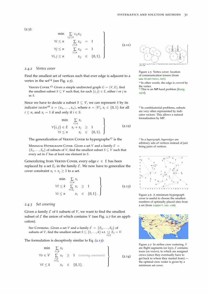
2.4.3 Set covering
Given a family E of k subsets of V, we want to find the smallestsubset of E the union of which contains V (see Fig. 2.7 for an appli-cation).
Set Covering. Given a set V and a family E = {E1, . . . , Ek} ofsubsets of V, find the smallest subset S ⊆ {1, . . . , k} s.t.
⋃`∈S
E` = V.
Figure 2.7: In airline crew rostering, Vare flight segments (or legs), E containstours (or rosters), to which are assignedcrews (since they eventually have toget back to where they started from) —the optimal crew roster is given by aminimum set cover.
The formulation is deceptively similar to Eq. (2.13):
min ∑`≤k
x`
∀v ∈ V ∑`≤k
v∈E`
x` ≥ 1 (covering constraint)
∀` ≤ k x` ∈ {0, 1}.
(2.14)
32 mathematical programming
The covering constraints state that every v ∈ V must belong to atleast one set E`. Set Covering is NP-hard.
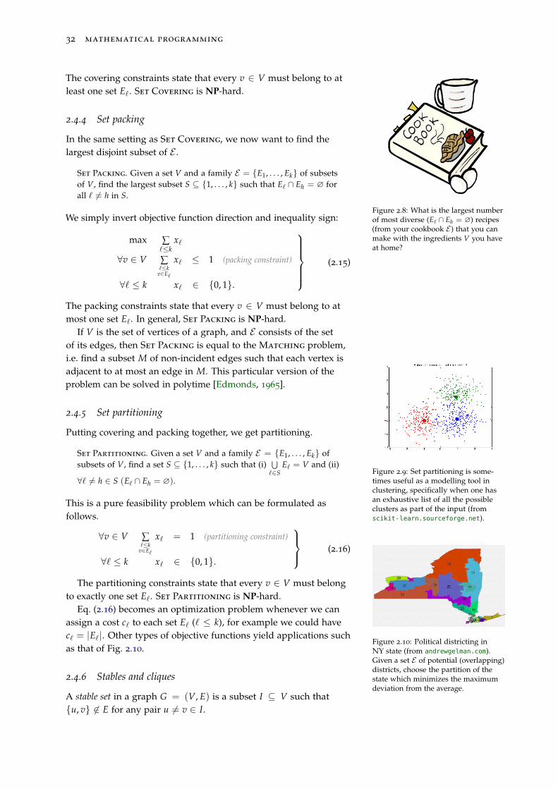
2.4.4 Set packing
In the same setting as Set Covering, we now want to find thelargest disjoint subset of E .
Figure 2.8: What is the largest numberof most diverse (E` ∩ Eh = ∅) recipes(from your cookbook E ) that you canmake with the ingredients V you haveat home?
Set Packing. Given a set V and a family E = {E1, . . . , Ek} of subsetsof V, find the largest subset S ⊆ {1, . . . , k} such that E` ∩ Eh = ∅ forall ` 6= h in S.
We simply invert objective function direction and inequality sign:
max ∑`≤k
x`
∀v ∈ V ∑`≤k
v∈E`
x` ≤ 1 (packing constraint)
∀` ≤ k x` ∈ {0, 1}.
(2.15)
The packing constraints state that every v ∈ V must belong to atmost one set E`. In general, Set Packing is NP-hard.
If V is the set of vertices of a graph, and E consists of the setof its edges, then Set Packing is equal to the Matching problem,i.e. find a subset M of non-incident edges such that each vertex isadjacent to at most an edge in M. This particular version of theproblem can be solved in polytime [Edmonds, 1965].
2.4.5 Set partitioning
Putting covering and packing together, we get partitioning.
Figure 2.9: Set partitioning is some-times useful as a modelling tool inclustering, specifically when one hasan exhaustive list of all the possibleclusters as part of the input (fromscikit-learn.sourceforge.net).
Set Partitioning. Given a set V and a family E = {E1, . . . , Ek} ofsubsets of V, find a set S ⊆ {1, . . . , k} such that (i)
⋃`∈S
E` = V and (ii)
∀` 6= h ∈ S (E` ∩ Eh = ∅).
This is a pure feasibility problem which can be formulated asfollows.
∀v ∈ V ∑`≤k
v∈E`
x` = 1 (partitioning constraint)
∀` ≤ k x` ∈ {0, 1}.
(2.16)
Figure 2.10: Political districting inNY state (from andrewgelman.com).Given a set E of potential (overlapping)districts, choose the partition of thestate which minimizes the maximumdeviation from the average.
The partitioning constraints state that every v ∈ V must belongto exactly one set E`. Set Partitioning is NP-hard.
Eq. (2.16) becomes an optimization problem whenever we canassign a cost c` to each set E` (` ≤ k), for example we could havec` = |E`|. Other types of objective functions yield applications suchas that of Fig. 2.10.
2.4.6 Stables and cliques
A stable set in a graph G = (V, E) is a subset I ⊆ V such that{u, v} 6∈ E for any pair u 6= v ∈ I.
systematics and solution methods 33
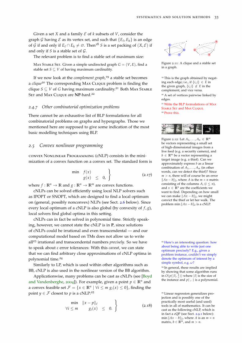
Given a set X and a family E of k subsets of V, consider thegraph G having E as its vertex set, and such that {E`, Eh} is an edgeof G if and only if E` ∩ Eh 6= ∅. Then18 S is a set packing of (X, E) if 18 Prove it.
and only if S is a stable set of G.
Figure 2.11: A clique and a stable setin a graph.
The relevant problem is to find a stable set of maximum size:
Max Stable Set. Given a simple undirected graph G = (V, E), find astable set S ⊆ V of having maximum cardinality.
If we now look at the complement graph,19 a stable set becomes 19 This is the graph obtained by negat-ing each edge; i.e., if {i, j} ∈ E inthe given graph, {i, j} 6∈ E in thecomplement, and vice versa.
a clique20 The corresponding Max Clique problem is finding the
20 A set of vertices pairwise linked byedges.
clique S ⊆ V of G having maximum cardinality.21 Both Max Stable
21 Write the BLP formulations of Max
Stable Set and Max Clique.
Set and Max Clique are NP-hard.22
22 Prove this.
2.4.7 Other combinatorial optimization problems
There cannot be an exhaustive list of BLP formulations for allcombinatorial problems on graphs and hypergraphs. Those wementioned here are supposed to give some indication of the mostbasic modelling techniques using BLP.
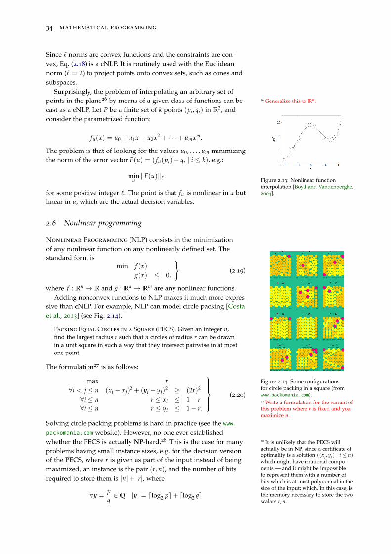
Figure 2.12: Let A1, . . . , An ∈ Rm
be vectors representing a small setof high-dimensional images from alive feed (e.g. a security camera), andb ∈ Rm be a vector representing atarget image (e.g. a thief). Can weapproximately express b as a linearcombination of A1, . . . , Am (in otherwords, can we detect the thief)? Sincem > n, there will of course be an error‖Ax− b‖2, where A is the m× n matrixconsisting of the columns Ai (i ≤ n),and x ∈ Rn are the coefficients wewant to find. Depending on how smallwe can make ‖Ax − b‖2, we mightconvict the thief or let her walk. Theproblem min ‖Ax− b‖2 is a cNLP.
2.5 Convex nonlinear programming
convex Nonlinear Programming (cNLP) consists in the mini-mization of a convex function on a convex set. The standard form is
min f (x)g(x) ≤ 0,
}(2.17)
where f : Rn → R and g : Rn → Rm are convex functions.cNLPs can be solved efficiently using local NLP solvers such
as IPOPT or SNOPT, which are designed to find a local optimumon (general, possibly nonconvex) NLPs (see Sect. 2.6 below). Sinceevery local optimum of a cNLP is also global (by convexity of f , g),local solvers find global optima in this setting.
cNLPs can in fact be solved in polynomial time. Strictly speak-ing, however, we cannot state the cNLP is in P, since solutionsof cNLPs could be irrational and even transcendental — and ourcomputational model based on TMs does not allow us to writeall23 irrational and transcendental numbers precisely. So we have 23 Here’s an interesting question: how
about being able to write just oneoptimum precisely? E.g., given aproblem instance, couldn’t we simplydenote the optimum of interest by asimple symbol, e.g. ω?
to speak about ε error tolerances: With this caveat, we can statethat we can find arbitrary close approximations of cNLP optima inpolynomial time.24
24 In general, these results are impliedby showing that some algorithm runsin O(p(|I|, 1
ε )) where |I| is the size ofthe instance and p(·, ·) is a polynomial.
Similarly to LP, which is used within other algorithms such asBB, cNLP is also used in the nonlinear version of the BB algorithm.
Applicationwise, many problems can be cast as cNLPs (see [Boydand Vandenberghe, 2004]). For example, given a point p ∈ Rn anda convex feasible set F = {x ∈ Rn | ∀i ≤ m gi(x) ≤ 0}, finding thepoint y ∈ F closest to p is a cNLP:25 25 Linear regression generalizes pro-
jection and is possibly one of thepractically most useful (and used)tools in all of mathematics. It can becast as the following cNLP, which isin fact a cQP (see Sect. 2.9.1 below):min ‖Ax − b‖2, where A is an m× nmatrix, b ∈ Rm, and m > n.
min ‖x− p‖`∀i ≤ m gi(x) ≤ 0.
}(2.18)
34 mathematical programming
Since ` norms are convex functions and the constraints are con-vex, Eq. (2.18) is a cNLP. It is routinely used with the Euclideannorm (` = 2) to project points onto convex sets, such as cones andsubspaces.
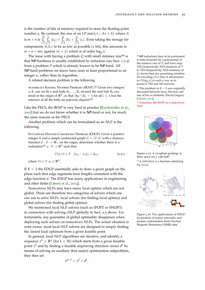
Surprisingly, the problem of interpolating an arbitrary set ofpoints in the plane26 by means of a given class of functions can be 26 Generalize this to Rn.
cast as a cNLP. Let P be a finite set of k points (pi, qi) in R2, andconsider the parametrized function:
Figure 2.13: Nonlinear functioninterpolation [Boyd and Vandenberghe,2004].
fu(x) = u0 + u1x + u2x2 + · · ·+ umxm.
The problem is that of looking for the values u0, . . . , um minimizingthe norm of the error vector F(u) = ( fu(pi)− qi | i ≤ k), e.g.:
minu‖F(u)‖`
for some positive integer `. The point is that fu is nonlinear in x butlinear in u, which are the actual decision variables.
2.6 Nonlinear programming
Nonlinear Programming (NLP) consists in the minimizationof any nonlinear function on any nonlinearly defined set. Thestandard form is
min f (x)g(x) ≤ 0,
}(2.19)
where f : Rn → R and g : Rn → Rm are any nonlinear functions.Adding nonconvex functions to NLP makes it much more expres-
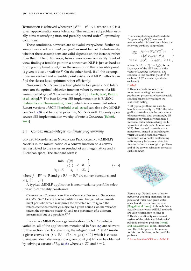
sive than cNLP. For example, NLP can model circle packing [Costaet al., 2013] (see Fig. 2.14).
Packing Equal Circles in a Square (PECS). Given an integer n,find the largest radius r such that n circles of radius r can be drawnin a unit square in such a way that they intersect pairwise in at mostone point.
Figure 2.14: Some configurationsfor circle packing in a square (fromwww.packomania.com).
The formulation27 is as follows:
27 Write a formulation for the variant ofthis problem where r is fixed and youmaximize n.
max r∀i < j ≤ n (xi − xj)
2 + (yi − yj)2 ≥ (2r)2
∀i ≤ n r ≤ xi ≤ 1− r∀i ≤ n r ≤ yi ≤ 1− r.
(2.20)
Solving circle packing problems is hard in practice (see the www.
packomania.com website). However, no-one ever establishedwhether the PECS is actually NP-hard.28 This is the case for many 28 It is unlikely that the PECS will
actually be in NP, since a certificate ofoptimality is a solution ((xj, yj) | i ≤ n)which might have irrational compo-nents — and it might be impossibleto represent them with a number ofbits which is at most polynomial in thesize of the input; which, in this case, isthe memory necessary to store the twoscalars r, n.
problems having small instance sizes, e.g. for the decision versionof the PECS, where r is given as part of the input instead of beingmaximized, an instance is the pair (r, n), and the number of bitsrequired to store them is |n|+ |r|, where
∀y =pq∈ Q |y| = dlog2 pe+ dlog2 qe
systematics and solution methods 35
is the number of bits of memory required to store the floating pointnumber y. By contrast, the size of an LP min{cx | Ax ≤ b} where A
is m× n ism∑
i=1
n∑
j=1|aij|+
m∑
i=1|bi|+
n∑
j=1|cj|. Even taking the storage for
components A, b, c to be as low as possible (1 bit), this amounts tom + n + mn, against |n|+ |r| which is of order log2 n.
The issue with having a problem Q with small instance size29 is 29 NP reductions have to be performedin time bounded by a polynomial ofthe instance size of P, and have mapYES (respectively, NO) instances of Pto YES (respectively, NO) instances ofQ. Inever had any promising intuitionfor encoding O(n) bits of informationin O(log2 n) in such a way as topreserve YES and NO answers.
that NP-hardness is usually established by reduction (see Sect. 1.7.3)from a problem P which is already known to be NP-hard. AllNP-hard problems we know have sizes at least proportional to aninteger n, rather than its logarithm.
A related decision problem is the following.
feasibility Kissing Number Problem (fKNP).30 Given two integers 30 This problem in K = 3 was originallydiscussed between Isaac Newton andone of his ex students, David Gregory[Liberti, 2012].
n, K, can we fit n unit balls B1, . . . , Bn around the unit ball B0 cen-tered at the origin of RK , so that |B0 ∩ Bi| = 1 for all i ≤ n but theinteriors of all the balls are pairwise disjoint?31
31 Formulate the fKNP as a nonconvexNLP.Like the PECS, the fKNP is very hard in practice [Kucherenko et al.,
2007] but we do not know whether it is NP-hard or not, for muchthe same reasons as the PECS.
Figure 2.15: A 12-sphere packing: isthere space for a 13th ball?
Another problem which can be formulated as an NLP is thefollowing.
Euclidean Distance Geometry Problem (EDGP). Given a positiveinteger K and a simple undirected graph G = (V, E) with a distancefunction d : E → R+ on the edges, determine whether there is arealization32 x : V → RK such that:
32 A realization is a function satisfyingEq. (2.21).
∀{u, v} ∈ E ‖xu − xv‖2 = duv, (2.21)
where ∀v ∈ V xv ∈ RK .
If K = 2 the EDGP essentially asks to draw a given graph on theplane such that edge segments have lengths consistent with theedge function d. The EDGP has many applications in engineeringand other fields [Liberti et al., 2014].
Figure 2.16: Two applications of EDGP:localization of sensor networks, andprotein conformation from NuclearMagnetic Resonance (NMR) data.
Nonconvex NLPs may have many local optima which are notglobal. There are therefore two categories of solvers which onecan use to solve NLPs: local solvers (for finding local optima) andglobal solvers (for finding global optima).
We mentioned local NLP solvers (such as IPOPT or SNOPT)in connection with solving cNLP globally in Sect. 2.5 above. Un-fortunately, any guarantee of global optimality disappears whendeploying such solvers on nonconvex NLPs. The actual situation iseven worse: most local NLP solvers are designed to simply findingthe closest local optimum from a given feasible point.
In general, local NLP algorithms are iterative, and identify asequence xk ∈ Rn (for k ∈ N) which starts from a given feasiblepoint x0 and by finding a feasible improving direction vector dk bymeans of solving an auxiliary (but easier) optimization subproblem,they then set
xk+1 = xk + dk.
36 mathematical programming
Termination is achieved whenever ‖xk+1 − xk‖ ≤ ε, where ε > 0 is agiven approximation error tolerance. The auxiliary subproblem usu-ally aims at satisfying first, and possibly second order33 optimality 33 For example, Sequential Quadratic
Programming (SQP) is a class ofmethods which is based on solving thefollowing auxiliary subproblem:
mind∈Rn
f (xk) + [∇x f (xk)]>d+
+ 12 d>∇xxL(xk , λk)d
∀i ≤ m gi(xk) + [∇x gi(xk)]>d ≤ 0
where L(x, λ) = f (x) + λg(x) is theLagrangian of the NLP, and λ is thevector of Lagrange coefficients. Thesolution to this problem yields dk ateach step k (λk are also updated ateach step).
conditions.These conditions, however, are not valid everywhere: further as-
sumptions called constraint qualifications must be met. Unfortunately,whether these assumptions are valid depends on the instance ratherthan the problem. Moreover, from a worst-case complexity point ofview, finding a feasible point in a nonconvex NLP is just as hard asfinding an optimal point,34 so the assumption that a feasible point
34 Why?
is given is also unrealistic.35 On the other hand, if all the assump-
35 These methods are often usedto improve existing business orproduction processes, where a feasiblesolution can be derived from thereal-world setting.
tions are verified and a feasible point exists, local NLP methods canfind the closest local optimum rather efficiently.
Nonconvex NLPs can be solved globally to a given ε > 0 toler-ance (on the optimal objective function value) by means of a BBvariant called spatial Branch-and-Bound (sBB) [Liberti, 2006, Belottiet al., 2009].36 The best-known sBB implementation is BARON
36 BB type algorithms are used tohandle nonconvexity. In MILP, the inte-grality constraints are the only sourceof nonconvexity, and, accordingly, BBbranches on variables which take afractional value when solving the LPrelaxation at each node. In nonconvexNLP, objective and constraints arenonconvex. Instead of branching onvariables taking fractional values,we branch on variables contributinga discrepancy between an objectivefunction value of the original problemand of the convex relaxation solved ateach sBB node.
[Sahinidis and Tawarmalani, 2005], which is a commercial solver.Recent versions of SCIP [Berthold et al., 2012] can also solve MINLP(see Sect. 2.8) and hence, in principle, NLPs as well. The only opensource sBB implementation worthy of note is Couenne [Belotti,2011].
2.7 Convex mixed-integer nonlinear programming
convex Mixed-Integer Nonlinear Programming (cMINLP)consists in the minimization of a convex function on a convexset, restricted to the cartesian product of an integer lattice and aEuclidean space. The standard form is
Figure 2.17: Optimization of waternetworks: deciding diameters for allpipes and water flow given waterat each node over a time horizon[Bragalli et al., 2012]. Although this isactually a nonconvex cMINLP methodsare used heuristically to solve it.
min f (x)g(x) ≤ 0
∀j ∈ Z xj ∈ Z,
(2.22)
where f : Rn → R and g : Rn → Rm are convex functions, andZ ⊆ {1, . . . , n}.
A typical cMINLP application is mean-variance portfolio selec-tion with cardinality constraints:
Cardinality Constrained Mean-Variance Portfolio Selection
(CCMVPS).37 Decide how to partition a unit budget into an invest-
37 This is a cardinality constrainedvariant of the celebrated Markowitz’portfolio selection problem [Konnoand Wijayanayake, 2001]. Markowitzwon the Nobel prize in Economicsfor his contributions on the portfolioproblem.
ment portfolio which maximizes the expected return (given thereturn coefficient vector ρ) subject to a given bound r on the variance(given the covariance matrix Q) and to a maximum of k differentinvestments out of a possible K.38
38 Formulate the CCPS as a cMINLP.
Insofar as cMINLPs are a generalization of cNLP to integervariables, all of the applications mentioned in Sect. 2.5 are relevantto this section, too. For example, the integral point x∗ ∈ Zn insidea given convex set {x ∈ Rn | ∀i ≤ m gi(x) ≤ 0} which is closest(using euclidean distances) to a given point p ∈ Rn can be obtainedby solving a variant of Eq. (2.18) where x ∈ Zn and ` = 2.
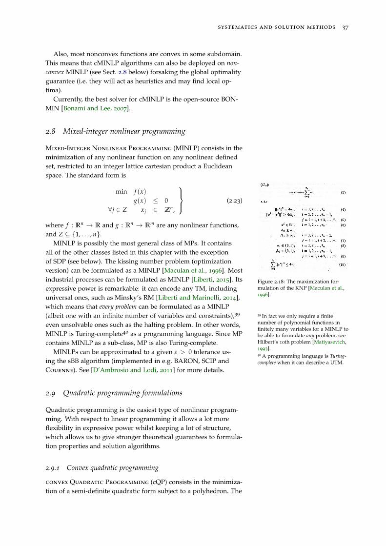
systematics and solution methods 37
Also, most nonconvex functions are convex in some subdomain.This means that cMINLP algorithms can also be deployed on non-convex MINLP (see Sect. 2.8 below) forsaking the global optimalityguarantee (i.e. they will act as heuristics and may find local op-tima).
Currently, the best solver for cMINLP is the open-source BON-MIN [Bonami and Lee, 2007].
2.8 Mixed-integer nonlinear programming
Mixed-Integer Nonlinear Programming (MINLP) consists in theminimization of any nonlinear function on any nonlinear definedset, restricted to an integer lattice cartesian product a Euclideanspace. The standard form is
min f (x)g(x) ≤ 0
∀j ∈ Z xj ∈ Zn,
(2.23)
where f : Rn → R and g : Rn → Rm are any nonlinear functions,and Z ⊆ {1, . . . , n}.
Figure 2.18: The maximization for-mulation of the KNP [Maculan et al.,1996].
MINLP is possibly the most general class of MPs. It containsall of the other classes listed in this chapter with the exceptionof SDP (see below). The kissing number problem (optimizationversion) can be formulated as a MINLP [Maculan et al., 1996]. Mostindustrial processes can be formulated as MINLP [Liberti, 2015]. Itsexpressive power is remarkable: it can encode any TM, includinguniversal ones, such as Minsky’s RM [Liberti and Marinelli, 2014],which means that every problem can be formulated as a MINLP(albeit one with an infinite number of variables and constraints),39 39 In fact we only require a finite
number of polynomial functions infinitely many variables for a MINLP tobe able to formulate any problem, seeHilbert’s 10th problem [Matiyasevich,1993].
even unsolvable ones such as the halting problem. In other words,MINLP is Turing-complete40 as a programming language. Since MP
40 A programming language is Turing-complete when it can describe a UTM.
contains MINLP as a sub-class, MP is also Turing-complete.MINLPs can be approximated to a given ε > 0 tolerance us-
ing the sBB algorithm (implemented in e.g. BARON, SCIP andCouenne). See [D’Ambrosio and Lodi, 2011] for more details.
2.9 Quadratic programming formulations
Quadratic programming is the easiest type of nonlinear program-ming. With respect to linear programming it allows a lot moreflexibility in expressive power whilst keeping a lot of structure,which allows us to give stronger theoretical guarantees to formula-tion properties and solution algorithms.
2.9.1 Convex quadratic programming
convex Quadratic Programming (cQP) consists in the minimiza-tion of a semi-definite quadratic form subject to a polyhedron. The
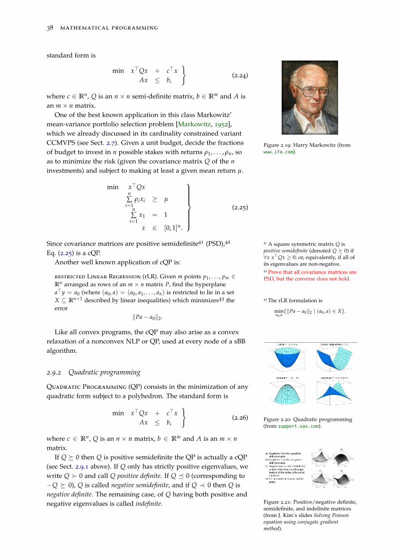
38 mathematical programming
standard form is
min x>Qx + c>xAx ≤ b,
}(2.24)
where c ∈ Rn, Q is an n× n semi-definite matrix, b ∈ Rm and A isan m× n matrix.
Figure 2.19: Harry Markowitz (fromwww.ifa.com).
One of the best known application in this class Markowitz’mean-variance portfolio selection problem [Markowitz, 1952],which we already discussed in its cardinality constrained variantCCMVPS (see Sect. 2.7). Given a unit budget, decide the fractionsof budget to invest in n possible stakes with returns ρ1, . . . , ρn, soas to minimize the risk (given the covariance matrix Q of the ninvestments) and subject to making at least a given mean return µ.
min x>Qxn∑
i=1ρixi ≥ µ
n∑
i=1x1 = 1
x ∈ [0, 1]n.
(2.25)
Since covariance matrices are positive semidefinite41 (PSD),42 41 A square symmetric matrix Q ispositive semidefinite (denoted Q � 0) if∀x x>Qx ≥ 0; or, equivalently, if all ofits eigenvalues are non-negative.42 Prove that all covariance matrices arePSD, but the converse does not hold.
Eq. (2.25) is a cQP.Another well known application of cQP is:
restricted Linear Regression (rLR). Given m points p1, . . . , pm ∈Rn arranged as rows of an m × n matrix P, find the hyperplanea>y = a0 (where (a0, a) = (a0, a1, . . . , an) is restricted to lie in a setX ⊆ Rn+1 described by linear inequalities) which minimizes43 the 43 The rLR formulation is
mina0 ,a{‖Pa− a0‖2 | (a0, a) ∈ X}.error
‖Pa− a0‖2.
Like all convex programs, the cQP may also arise as a convexrelaxation of a nonconvex NLP or QP, used at every node of a sBBalgorithm.
2.9.2 Quadratic programming
Figure 2.20: Quadratic programming(from support.sas.com).
Quadratic Programming (QP) consists in the minimization of anyquadratic form subject to a polyhedron. The standard form is
min x>Qx + c>xAx ≤ b,
}(2.26)
where c ∈ Rn, Q is an n × n matrix, b ∈ Rm and A is an m × nmatrix.
If Q � 0 then Q is positive semidefinite the QP is actually a cQP(see Sect. 2.9.1 above). If Q only has strictly positive eigenvalues, wewrite Q � 0 and call Q positive definite. If Q � 0 (corresponding to−Q � 0), Q is called negative semidefinite, and if Q ≺ 0 then Q isnegative definite. The remaining case, of Q having both positive andnegative eigenvalues is called indefinite. Figure 2.21: Positive/negative definite,
semidefinite, and indefinite matrices(from J. Kim’s slides Solving Poissonequation using conjugate gradientmethod).
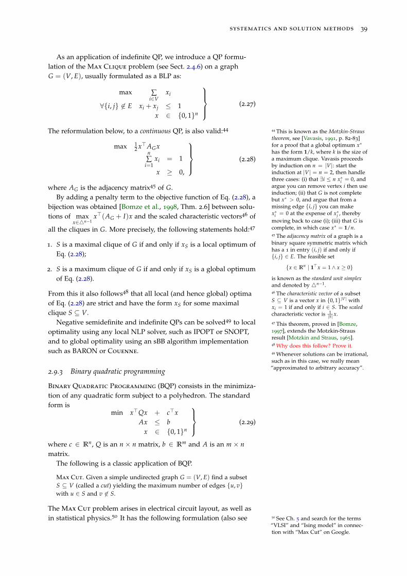
systematics and solution methods 39
As an application of indefinite QP, we introduce a QP formu-lation of the Max Clique problem (see Sect. 2.4.6) on a graphG = (V, E), usually formulated as a BLP as:
max ∑i∈V
xi
∀{i, j} 6∈ E xi + xj ≤ 1x ∈ {0, 1}n
(2.27)
The reformulation below, to a continuous QP, is also valid:44 44 This is known as the Motzkin-Straustheorem, see [Vavasis, 1991, p. 82-83]for a proof that a global optimum x∗
has the form 1/k, where k is the size ofa maximum clique. Vavasis proceedsby induction on n = |V|: start theinduction at |V| = n = 2, then handlethree cases: (i) that ∃i ≤ n x∗i = 0, andargue you can remove vertex i then useinduction; (ii) that G is not completebut x∗ > 0, and argue that from amissing edge {i, j} you can makex∗i = 0 at the expense of x∗j , therebymoving back to case (i); (iii) that G iscomplete, in which case x∗ = 1/n.
max 12 x>AGx
n∑
i=1xi = 1
x ≥ 0,
(2.28)
where AG is the adjacency matrix45 of G.
45 The adjacency matrix of a graph is abinary square symmetric matrix whichhas a 1 in entry (i, j) if and only if{i, j} ∈ E. The feasible set
{x ∈ Rn | 1>x = 1∧ x ≥ 0}
is known as the standard unit simplexand denoted by 4n−1.
By adding a penalty term to the objective function of Eq. (2.28), abijection was obtained [Bomze et al., 1998, Thm. 2.6] between solu-tions of max
x∈4n−1x>(AG + I)x and the scaled characteristic vectors46 of
46 The characteristic vector of a subsetS ⊆ V is a vector x in {0, 1}|V| withxi = 1 if and only if i ∈ S. The scaledcharacteristic vector is 1
|S| x.
all the cliques in G. More precisely, the following statements hold:47
47 This theorem, proved in [Bomze,1997], extends the Motzkin-Strausresult [Motzkin and Straus, 1965].
1. S is a maximal clique of G if and only if xS is a local optimum ofEq. (2.28);
2. S is a maximum clique of G if and only if xS is a global optimumof Eq. (2.28).
From this it also follows48 that all local (and hence global) optima
48 Why does this follow? Prove it.
of Eq. (2.28) are strict and have the form xS for some maximalclique S ⊆ V.
Negative semidefinite and indefinite QPs can be solved49 to local
49 Whenever solutions can be irrational,such as in this case, we really mean“approximated to arbitrary accuracy”.
optimality using any local NLP solver, such as IPOPT or SNOPT,and to global optimality using an sBB algorithm implementationsuch as BARON or Couenne.
2.9.3 Binary quadratic programming
Binary Quadratic Programming (BQP) consists in the minimiza-tion of any quadratic form subject to a polyhedron. The standardform is
min x>Qx + c>xAx ≤ b
x ∈ {0, 1}n
(2.29)
where c ∈ Rn, Q is an n × n matrix, b ∈ Rm and A is an m × nmatrix.
The following is a classic application of BQP.
Max Cut. Given a simple undirected graph G = (V, E) find a subsetS ⊆ V (called a cut) yielding the maximum number of edges {u, v}with u ∈ S and v 6∈ S.
The Max Cut problem arises in electrical circuit layout, as well asin statistical physics.50 It has the following formulation (also see 50 See Ch. 5 and search for the terms
“VLSI” and “Ising model” in connec-tion with “Max Cut” on Google.
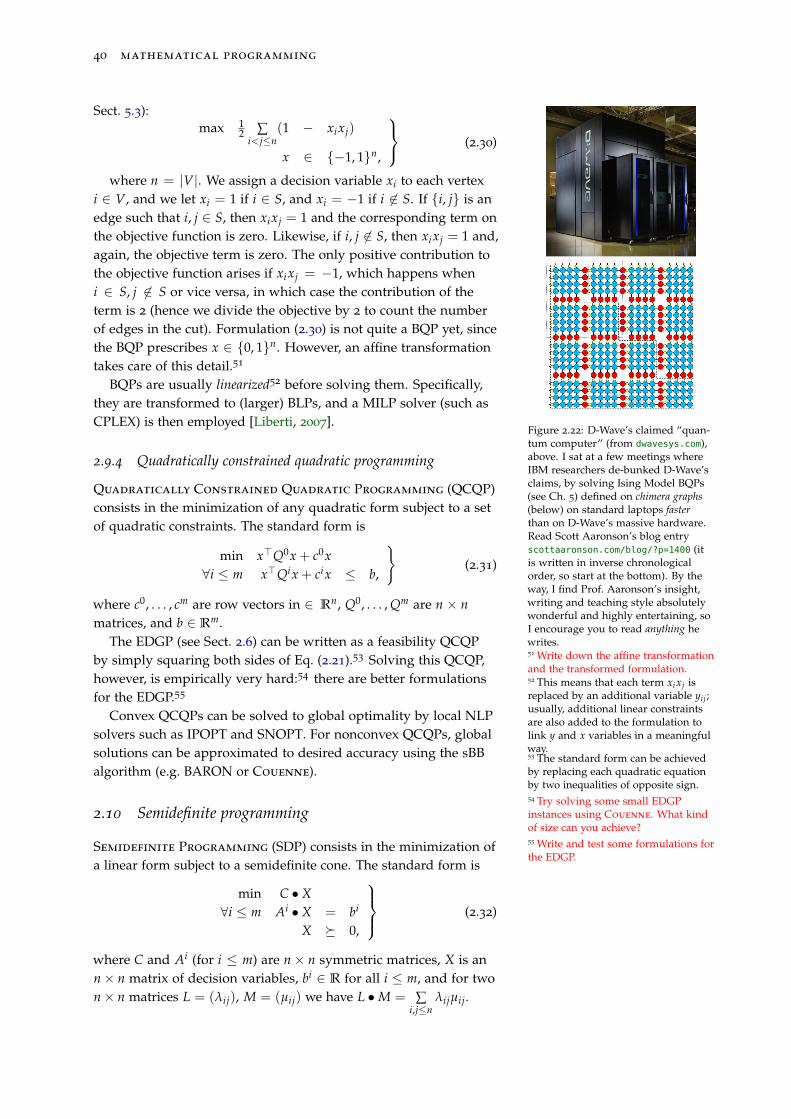
40 mathematical programming
Sect. 5.3):max 1
2 ∑i<j≤n
(1 − xixj)
x ∈ {−1, 1}n,
(2.30)
Figure 2.22: D-Wave’s claimed “quan-tum computer” (from dwavesys.com),above. I sat at a few meetings whereIBM researchers de-bunked D-Wave’sclaims, by solving Ising Model BQPs(see Ch. 5) defined on chimera graphs(below) on standard laptops fasterthan on D-Wave’s massive hardware.Read Scott Aaronson’s blog entryscottaaronson.com/blog/?p=1400 (itis written in inverse chronologicalorder, so start at the bottom). By theway, I find Prof. Aaronson’s insight,writing and teaching style absolutelywonderful and highly entertaining, soI encourage you to read anything hewrites.
where n = |V|. We assign a decision variable xi to each vertexi ∈ V, and we let xi = 1 if i ∈ S, and xi = −1 if i 6∈ S. If {i, j} is anedge such that i, j ∈ S, then xixj = 1 and the corresponding term onthe objective function is zero. Likewise, if i, j 6∈ S, then xixj = 1 and,again, the objective term is zero. The only positive contribution tothe objective function arises if xixj = −1, which happens wheni ∈ S, j 6∈ S or vice versa, in which case the contribution of theterm is 2 (hence we divide the objective by 2 to count the numberof edges in the cut). Formulation (2.30) is not quite a BQP yet, sincethe BQP prescribes x ∈ {0, 1}n. However, an affine transformationtakes care of this detail.51
51 Write down the affine transformationand the transformed formulation.
BQPs are usually linearized52 before solving them. Specifically,
52 This means that each term xixj isreplaced by an additional variable yij;usually, additional linear constraintsare also added to the formulation tolink y and x variables in a meaningfulway.
they are transformed to (larger) BLPs, and a MILP solver (such asCPLEX) is then employed [Liberti, 2007].
2.9.4 Quadratically constrained quadratic programming
Quadratically Constrained Quadratic Programming (QCQP)consists in the minimization of any quadratic form subject to a setof quadratic constraints. The standard form is
min x>Q0x + c0x∀i ≤ m x>Qix + cix ≤ b,
}(2.31)
where c0, . . . , cm are row vectors in ∈ Rn, Q0, . . . , Qm are n × nmatrices, and b ∈ Rm.
The EDGP (see Sect. 2.6) can be written as a feasibility QCQPby simply squaring both sides of Eq. (2.21).53 Solving this QCQP,
53 The standard form can be achievedby replacing each quadratic equationby two inequalities of opposite sign.
however, is empirically very hard:54 there are better formulations
54 Try solving some small EDGPinstances using Couenne. What kindof size can you achieve?
for the EDGP.55
55 Write and test some formulations forthe EDGP.
Convex QCQPs can be solved to global optimality by local NLPsolvers such as IPOPT and SNOPT. For nonconvex QCQPs, globalsolutions can be approximated to desired accuracy using the sBBalgorithm (e.g. BARON or Couenne).
2.10 Semidefinite programming
Semidefinite Programming (SDP) consists in the minimization ofa linear form subject to a semidefinite cone. The standard form is
min C • X∀i ≤ m Ai • X = bi
X � 0,
(2.32)
where C and Ai (for i ≤ m) are n× n symmetric matrices, X is ann× n matrix of decision variables, bi ∈ R for all i ≤ m, and for twon× n matrices L = (λij), M = (µij) we have L •M = ∑
i,j≤nλijµij.
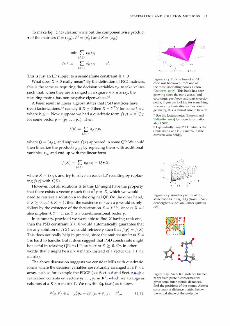
systematics and solution methods 41
To make Eq. (2.32) clearer, write out the componentwise product• of the matrices C = (cjh), Ai = (ai
jh) and X = (xjh):
Figure 2.23: This picture of an SDPcone was borrowed from one ofthe most fascinating books I know[Dattorro, 2015]. This book has beengrowing since the early 2000s (andcounting): part book and part encyclo-pedia, if you are looking for somethingin convex optimization or Euclideangeometry, this is almost sure to have it!
min ∑j,h≤n
cjhxjh
∀i ≤ m ∑j,h≤n
aijhxjh = bi.
This is just an LP subject to a semidefinite constraint X � 0.What does X � 0 really mean? By the definition of PSD matrices,
this is the same as requiring the decision variables xjh to take valuessuch that, when they are arranged in a square n × n array, theresulting matrix has non-negative eigenvalues.56
56 See the lecture notes [Laurent andVallentin, 2012] for more informationabout SDP.
A basic result in linear algebra states that PSD matrices have(real) factorizations,57 namely if X � 0 then X = Y>Y for some k× n
57 Equivalently: any PSD matrix is theGram matrix of a k × n matrix Y (theconverse also holds).
where k ≤ n. Now suppose we had a quadratic form f (y) = y>Qyfor some vector y = (y1, . . . , yn). Then
f (y) = ∑j,h≤n
qjhyjyh,
where Q = (qjh), and suppose f (x) appeared in some QP. We couldthen linearize the products yjyh by replacing them with additionalvariables xjh, and end up with the linear form
f (X) = ∑j,h≤n
qjhxjh = Q • X,
where X = (xjh), and try to solve an easier LP resulting by replac-ing f (y) with f (X).
Figure 2.24: Another picture of thesame cone as in Fig. 2.23 (from L. Van-denberghe’s slides on Convex optimiza-tion).
However, not all solutions X to this LP might have the propertythat there exists a vector y such that y>y = X, which we wouldneed to retrieve a solution y to the original QP. On the other hand,if X � 0 and rk X = 1, then the existence of such a y would surelyfollow by the existence of the factorization X = Y>Y, since rk X = 1also implies rk Y = 1, i.e. Y is a one-dimensional vector y.
Figure 2.25: An EDGP instance (namedtiny) from protein conformation:given some inter-atomic distances,find the positions of the atoms. Above:color map of distance matrix; below:the actual shape of the molecule.
In summary, provided we were able to find X having rank one,then the PSD constraint X � 0 would automatically guarantee thatfor any solution of f (X) we could retrieve y such that f (y) = f (X).This does not really help in practice, since the rank constraint rk X =
1 is hard to handle. But it does suggest that PSD constraints mightbe useful in relaxing QPs to LPs subject to X � 0. Or, in otherwords, that y might be a k× n matrix instead of a vector (i.e. a 1× nmatrix).
The above discussion suggests we consider MPs with quadraticforms where the decision variables are naturally arranged in a K× narray, such as for example the EDGP (see Sect. 2.6 and Sect. 2.9.4): arealization consists on vectors y1, . . . , yn in RK, which we arrange ascolumns of a K× n matrix Y. We rewrite Eq. (2.21) as follows:
∀{u, v} ∈ E y>u yu − 2y>u yv + y>v yv = d2uv, (2.33)
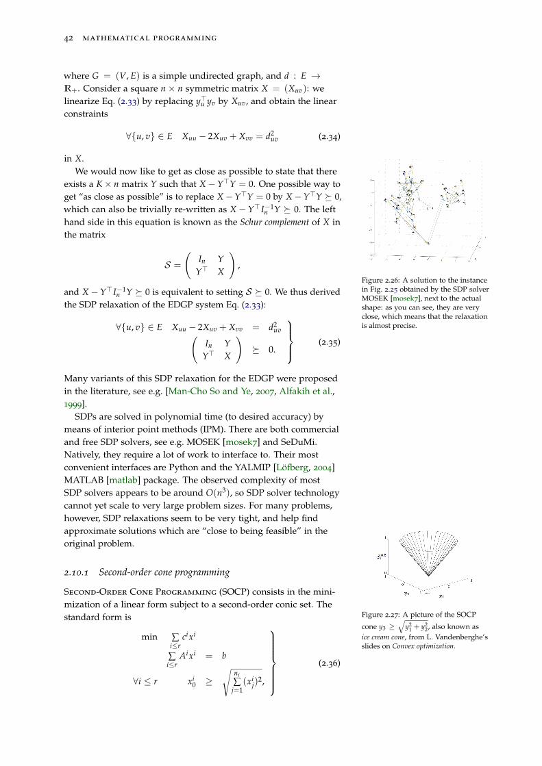
42 mathematical programming
where G = (V, E) is a simple undirected graph, and d : E →R+. Consider a square n × n symmetric matrix X = (Xuv): welinearize Eq. (2.33) by replacing y>u yv by Xuv, and obtain the linearconstraints
∀{u, v} ∈ E Xuu − 2Xuv + Xvv = d2uv (2.34)
in X.We would now like to get as close as possible to state that there
exists a K× n matrix Y such that X−Y>Y = 0. One possible way toget “as close as possible” is to replace X−Y>Y = 0 by X−Y>Y � 0,which can also be trivially re-written as X − Y> I−1
n Y � 0. The lefthand side in this equation is known as the Schur complement of X inthe matrix
Figure 2.26: A solution to the instancein Fig. 2.25 obtained by the SDP solverMOSEK [mosek7], next to the actualshape: as you can see, they are veryclose, which means that the relaxationis almost precise.
S =
(In Y
Y> X
),
and X−Y> I−1n Y � 0 is equivalent to setting S � 0. We thus derived
the SDP relaxation of the EDGP system Eq. (2.33):
∀{u, v} ∈ E Xuu − 2Xuv + Xvv = d2uv(
In YY> X
)� 0.
(2.35)
Many variants of this SDP relaxation for the EDGP were proposedin the literature, see e.g. [Man-Cho So and Ye, 2007, Alfakih et al.,1999].
SDPs are solved in polynomial time (to desired accuracy) bymeans of interior point methods (IPM). There are both commercialand free SDP solvers, see e.g. MOSEK [mosek7] and SeDuMi.Natively, they require a lot of work to interface to. Their mostconvenient interfaces are Python and the YALMIP [Löfberg, 2004]MATLAB [matlab] package. The observed complexity of mostSDP solvers appears to be around O(n3), so SDP solver technologycannot yet scale to very large problem sizes. For many problems,however, SDP relaxations seem to be very tight, and help findapproximate solutions which are “close to being feasible” in theoriginal problem.
2.10.1 Second-order cone programming
Figure 2.27: A picture of the SOCP
cone y3 ≥√
y21 + y2
2, also known asice cream cone, from L. Vandenberghe’sslides on Convex optimization.
Second-Order Cone Programming (SOCP) consists in the mini-mization of a linear form subject to a second-order conic set. Thestandard form is
min ∑i≤r
cixi
∑i≤r
Aixi = b
∀i ≤ r xi0 ≥
√ni∑
j=1(xi
j)2,
(2.36)
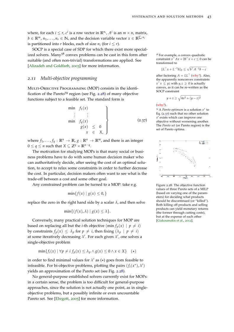
systematics and solution methods 43
where, for each i ≤ r, ci is a row vector in Rni , Ai is an m× ni matrix,b ∈ Rm, n1, . . . , nr ∈ N, and the decision variable vector x ∈ R∑i ni
is partitioned into r blocks, each of size ni (for i ≤ r).SOCP is a special case of SDP for which there exist more special-
ized solvers. Many58 convex problems can be cast in this form after 58 For example, a convex quadraticconstraint x>Ax + 2b>x + c ≤ 0 can betransformed to
‖L>x + L−1b‖2 ≤√
b>A−1b− c
after factoring A = LL> (why?). Also,the apparently nonconvex constraintsx>x ≤ yz with y, z ≥ 0 is actuallyconvex, as it can be re-written as theSOCP constraint
y + z ≥√
4x2 + (y− z)2
(why?).
suitable (and often non-trivial) transformations are applied. See[Alizadeh and Goldfarb, 2003] for more information.
2.11 Multi-objective programming
Multi-Objective Programming (MOP) consists in the identi-fication of the Pareto59 region (see Fig. 2.28) of many objective
59 A Pareto optimum is a solution x∗ toEq. (2.37) such that no other solutionx′ exists which can improve oneobjective without worsening another.The Pareto set (or Pareto region) is theset of Pareto optima.
functions subject to a feasible set. The standard form is
min f1(x)...
...min fq(x)
g(x) ≤ 0x ∈ X,
(2.37)
where f1, . . . , fq : Rn → R, g : Rn → Rm, and there is an integer0 ≤ q ≤ n such that X ⊆ Zq ×Rn−q.
Figure 2.28: The objective functionvalues of three Pareto sets of a MILP(based on varying one of the param-eters) for deciding what productsshould be discontinued (or “killed”).Both killing off products and sellingproducts can yield monetary returns(the former through cutting costs),but at the expense of each other[Giakoumakis et al., 2012].
The motivation for studying MOPs is that many social or busi-ness problems have to do with some human decision maker whocan authoritatively decide, after seeing the cost of an optimal solu-tion, to accept to relax some constraints in order to further decreasethe cost. In particular, decision makers often want to see what is thetrade-off between a cost and some other goal.
Any constrained problem can be turned to a MOP: take e.g.
min{ f (x) | g(x) ≤ 0, }
replace the zero in the right hand side by a scalar λ, and then solve
min{( f (x), λ) | g(x) ≤ λ}.
Conversely, many practical solution techniques for MOP arebased on replacing all but the i-th objective (min fp(x) | p 6= i)by constraints fp(x) ≤ λp for p 6= i, then fixing (λp | p 6= i)at some iteratively decreasing λ′. For each given λ′, one solves asingle-objective problem
min{ fi(x) | ∀p 6= i fp(x) ≤ λp ∧ g(x) ≤ 0∧ x ∈ X} (?)
in order to find minimal values for λ′ as (?) goes from feasible toinfeasible. For bi-objective problems, plotting the pairs ( fi(x∗), λ′)
yields an approximation of the Pareto set (see Fig. 2.28).No general-purpose established solvers currently exist for MOPs:
in a certain sense, the problem is too difficult for general-purposeapproaches, since the solution is not actually one point, as in single-objective problems, but a possibly infinite or even uncountablePareto set. See [Ehrgott, 2005] for more information.
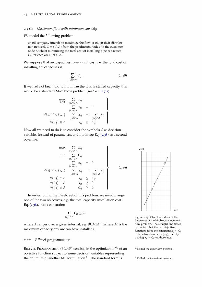
44 mathematical programming
2.11.1 Maximum flow with minimum capacity
We model the following problem:
an oil company intends to maximize the flow of oil on their distribu-tion network G = (V, A) from the production node s to the customernode t, whilst minimizing the total cost of installing pipe capacitiesCij for each arc (i, j) ∈ A.
We suppose that arc capacities have a unit cost, i.e. the total cost ofinstalling arc capacities is
∑(i,j)∈A
Cij. (2.38)
If we had not been told to minimize the total installed capacity, thiswould be a standard Max Flow problem (see Sect. 1.7.2):
maxx≥0
∑(s,j)∈A
xsj
∑(i,s)∈A
xis = 0
∀i ∈ V r {s, t} ∑(i,j)∈A
xij = ∑(j,i)∈A
xji
∀(i, j) ∈ A xij ≤ Cij.
Now all we need to do is to consider the symbols C as decisionvariables instead of parameters, and minimize Eq. (2.38) as a secondobjective.
max ∑(s,j)∈A
xsj
min ∑(i,j)∈A
Cij
∑(i,s)∈A
xis = 0
∀i ∈ V r {s, t} ∑(i,j)∈A
xij = ∑(j,i)∈A
xji
∀(i, j) ∈ A xij ≤ Cij
∀(i, j) ∈ A xij ≥ 0∀(i, j) ∈ A Cij ≥ 0.
(2.39)
flow
cost
Figure 2.29: Objective values of thePareto set of the bi-objective networkflow problem. The straight line arisesby the fact that the two objectivefunctions force the constraint xij ≤ Cijto be active on all arcs (s, j), therebymaking xij = Cij on those arcs.
In order to find the Pareto set of this problem, we must changeone of the two objectives, e.g. the total capacity installation costEq. (2.38), into a constraint:
∑(i,j)∈A
Cij ≤ λ,
where λ ranges over a given interval, e.g. [0, M|A|] (where M is themaximum capacity any arc can have installed).
2.12 Bilevel programming
Bilevel Programming (BLevP) consists in the optimization60 of an 60 Called the upper-level problem.
objective function subject to some decision variables representingthe optimum of another MP formulation.61 The standard form is: 61 Called the lower-level problem.
systematics and solution methods 45
minx,y
f (x, y)
g(x, y) ≤ 0y ∈ arg min{φx(y) | γx(y) ≤ 0∧ y ∈ ζ}x ∈ X,
(2.40)
where x is a sequence of n decision variables, y is a sequence of pdecision variables, f : Rn+p → R, g : Rn+p → Rm, φx : Rq → R,γx : Rq → R`, and there are integers 0 ≤ s ≤ n and 0 ≤ t ≤ psuch that ζ ⊆ Zt ×Rp−t and X ⊆ Zs ×Rn−s. Note that φx, γx arefunctions which are parametrized by the decision variables x of theupper-level problem.
The motivation62 for bilevel programs comes from studying how 62 Typical application: a firm wants toplan operations (upper-level) subject toa certain unit revenue based on priceswhich are decided (lower-level) bynegotiations with customers.
optimization is carried out when multiple stakeholders, orderedhierarchically, make decisions to optimize different goals. As in thecase of MOP, solutions in bilevel programming are not necessarilywell defined, as they may depend on whether lower-level decisionmakers take decisions favorably (the case of a division of a largerfirm) or adversarially (competing entities ordered hierarchically).Accordingly, there are no general-purpose solvers — some assump-tions must be made on the structure of the problem.63 See [Colson 63 A promising solution approach, in
the case the lower-level problem is aMILP, consists in approximating thelower level problem by means of apolytope where each face is generateddynamically and added as a constraintto the upper-level problem.
et al., 2005] for more information.
2.12.1 Lower-level LP
Certain bilevel formulations can be transformed to single-level.Assume that:
• the objective f (x, y) is only a function of x;
• among the constraints g(x, y) ≤ 0 only one is actually a functionof both x and y, specifically
miny
c(x) · y ≥ α,
where c(x) is an n-vector of functions of x and α is a parameter;
• the lower-level problem has the form:
miny≥0
c(x) · y
A(x) · y = b(x),
(2.41)
where A(x) is an m× n matrix having components in function ofx, and b is an m-vector of functions of x.
Remark that, when x is fixed, Eq. (2.41) is an LP.Under these conditions, Eq. (2.40) can be formulated as a single-
level problem by replacing the lower-level LP with its dual. For xfixed, the dual of Eq. (2.41) is:
maxλ
λ · b(x)
λ · A(x) ≤ c(x),
}(2.42)
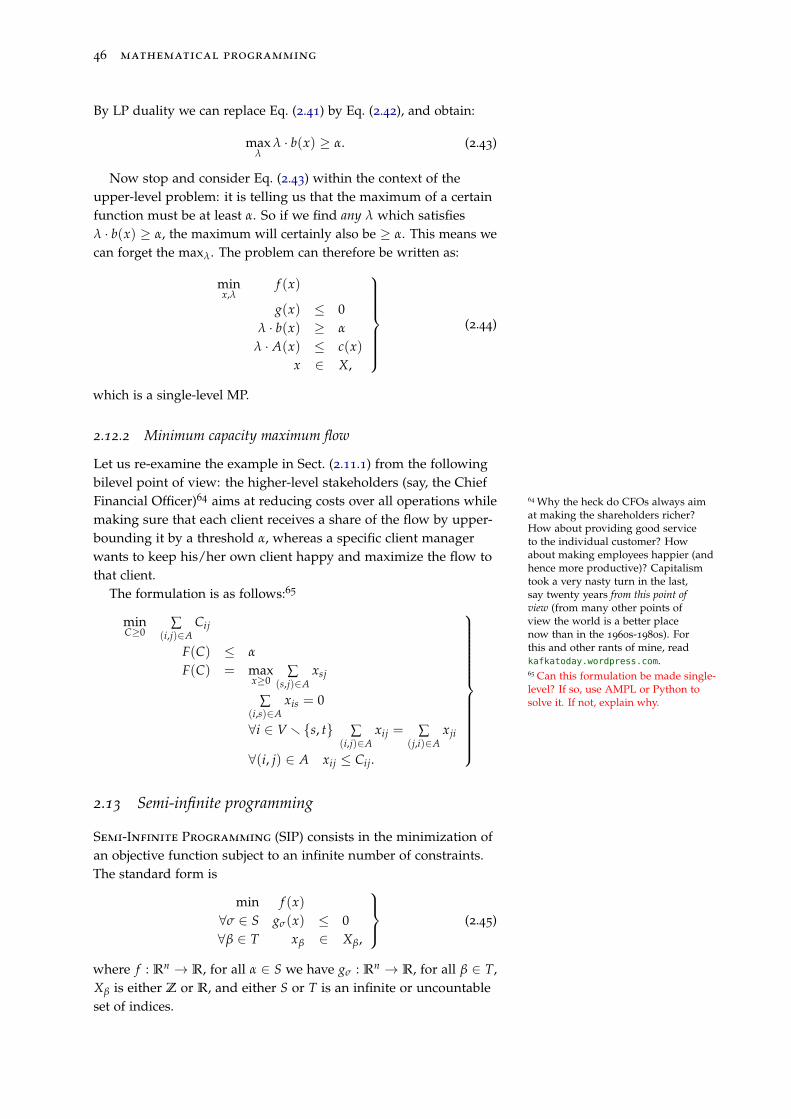
46 mathematical programming
By LP duality we can replace Eq. (2.41) by Eq. (2.42), and obtain:
maxλ
λ · b(x) ≥ α. (2.43)
Now stop and consider Eq. (2.43) within the context of theupper-level problem: it is telling us that the maximum of a certainfunction must be at least α. So if we find any λ which satisfiesλ · b(x) ≥ α, the maximum will certainly also be ≥ α. This means wecan forget the maxλ. The problem can therefore be written as:
minx,λ
f (x)
g(x) ≤ 0λ · b(x) ≥ α
λ · A(x) ≤ c(x)x ∈ X,
(2.44)
which is a single-level MP.
2.12.2 Minimum capacity maximum flow
Let us re-examine the example in Sect. (2.11.1) from the followingbilevel point of view: the higher-level stakeholders (say, the ChiefFinancial Officer)64 aims at reducing costs over all operations while 64 Why the heck do CFOs always aim
at making the shareholders richer?How about providing good serviceto the individual customer? Howabout making employees happier (andhence more productive)? Capitalismtook a very nasty turn in the last,say twenty years from this point ofview (from many other points ofview the world is a better placenow than in the 1960s-1980s). Forthis and other rants of mine, readkafkatoday.wordpress.com.
making sure that each client receives a share of the flow by upper-bounding it by a threshold α, whereas a specific client managerwants to keep his/her own client happy and maximize the flow tothat client.
The formulation is as follows:65
65 Can this formulation be made single-level? If so, use AMPL or Python tosolve it. If not, explain why.
minC≥0
∑(i,j)∈A
Cij
F(C) ≤ α
F(C) = maxx≥0
∑(s,j)∈A
xsj
∑(i,s)∈A
xis = 0
∀i ∈ V r {s, t} ∑(i,j)∈A
xij = ∑(j,i)∈A
xji
∀(i, j) ∈ A xij ≤ Cij.
2.13 Semi-infinite programming
Semi-Infinite Programming (SIP) consists in the minimization ofan objective function subject to an infinite number of constraints.The standard form is
min f (x)∀σ ∈ S gσ(x) ≤ 0∀β ∈ T xβ ∈ Xβ,
(2.45)
where f : Rn → R, for all α ∈ S we have gσ : Rn → R, for all β ∈ T,Xβ is either Z or R, and either S or T is an infinite or uncountableset of indices.
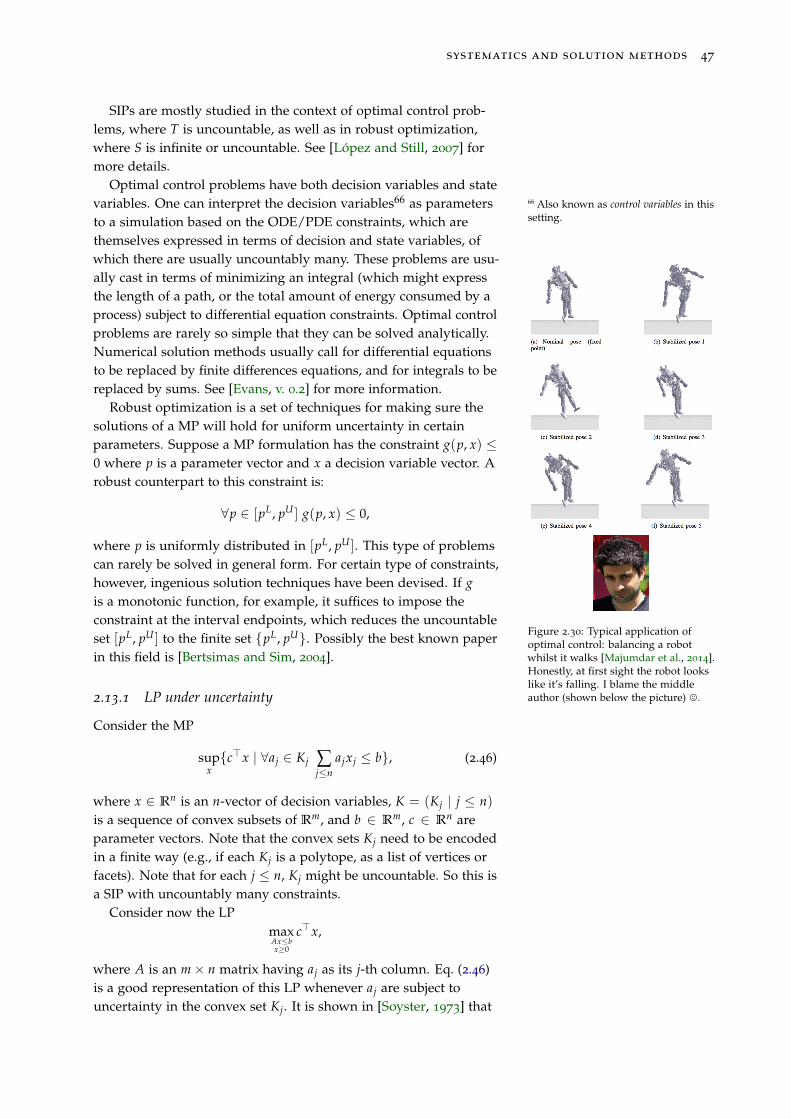
systematics and solution methods 47
SIPs are mostly studied in the context of optimal control prob-lems, where T is uncountable, as well as in robust optimization,where S is infinite or uncountable. See [López and Still, 2007] formore details.
Optimal control problems have both decision variables and statevariables. One can interpret the decision variables66 as parameters 66 Also known as control variables in this
setting.to a simulation based on the ODE/PDE constraints, which arethemselves expressed in terms of decision and state variables, ofwhich there are usually uncountably many. These problems are usu-ally cast in terms of minimizing an integral (which might expressthe length of a path, or the total amount of energy consumed by aprocess) subject to differential equation constraints. Optimal controlproblems are rarely so simple that they can be solved analytically.Numerical solution methods usually call for differential equationsto be replaced by finite differences equations, and for integrals to bereplaced by sums. See [Evans, v. 0.2] for more information.
Figure 2.30: Typical application ofoptimal control: balancing a robotwhilst it walks [Majumdar et al., 2014].Honestly, at first sight the robot lookslike it’s falling. I blame the middleauthor (shown below the picture) ,.
Robust optimization is a set of techniques for making sure thesolutions of a MP will hold for uniform uncertainty in certainparameters. Suppose a MP formulation has the constraint g(p, x) ≤0 where p is a parameter vector and x a decision variable vector. Arobust counterpart to this constraint is:
∀p ∈ [pL, pU ] g(p, x) ≤ 0,
where p is uniformly distributed in [pL, pU ]. This type of problemscan rarely be solved in general form. For certain type of constraints,however, ingenious solution techniques have been devised. If gis a monotonic function, for example, it suffices to impose theconstraint at the interval endpoints, which reduces the uncountableset [pL, pU ] to the finite set {pL, pU}. Possibly the best known paperin this field is [Bertsimas and Sim, 2004].
2.13.1 LP under uncertainty
Consider the MP
supx{c>x | ∀aj ∈ Kj ∑
j≤najxj ≤ b}, (2.46)
where x ∈ Rn is an n-vector of decision variables, K = (Kj | j ≤ n)is a sequence of convex subsets of Rm, and b ∈ Rm, c ∈ Rn areparameter vectors. Note that the convex sets Kj need to be encodedin a finite way (e.g., if each Kj is a polytope, as a list of vertices orfacets). Note that for each j ≤ n, Kj might be uncountable. So this isa SIP with uncountably many constraints.
Consider now the LPmaxAx≤bx≥0
c>x,
where A is an m× n matrix having aj as its j-th column. Eq. (2.46)is a good representation of this LP whenever aj are subject touncertainty in the convex set Kj. It is shown in [Soyster, 1973] that
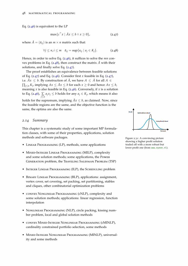
48 mathematical programming
Eq. (2.46) is equivalent to the LP
max{c>x | Ax ≤ b ∧ x ≥ 0}, (2.47)
where A = (aij) is an m× n matrix such that:
∀j ≤ n, i ≤ m aij = sup{aij | aj ∈ Kj}. (2.48)
Hence, in order to solve Eq. (2.46), it suffices to solve the mn con-vex problems in Eq. (2.48), then construct the matrix A with theirsolutions, and finally solve Eq. (2.47).
The proof establishes an equivalence between feasible solutionsof Eq. (2.47) and Eq. (2.46). Consider first x feasible in Eq. (2.47),i.e. Ax ≤ b. By construction of A, we have A ≤ A for all A ∈∏j≤n Kj, implying Ax ≤ Ax ≤ b for each x ≥ 0 and hence Ax ≤ b,meaning x is also feasible in Eq. (2.46). Conversely, if x is a solutionto Eq. (2.46), ∑
j≤najxj ≤ b holds for any aj ∈ Kj, which means it also
holds for the supremum, implying Ax ≤ b, as claimed. Now, sincethe feasible regions are the same, and the objective function is thesame, the optima are also the same.
2.14 Summary
Figure 2.31: A convincing pictureshowing a higher profit solutiontraded off with a more robust butlower profit one (from www.eyeon.nl).
This chapter is a systematic study of some important MP formula-tion classes, with some of their properties, applications, solutionmethods and software packages.
• Linear Programming (LP), methods, some applications
• Mixed-Integer Linear Programming (MILP), complexityand some solution methods; some applications, the Power
Generation problem, the Traveling Salesman Problem (TSP)
• Integer Linear Programming (ILP), the Scheduling problem
• Binary Linear Programming (BLP), applications: assignment,vertex cover, set covering, set packing, set partitioning, stablesand cliques, other combinatorial optimization problems
• convex Nonlinear Programming (cNLP), complexity andsome solution methods; applications: linear regression, functioninterpolation
• Nonlinear Programming (NLP), circle packing, kissing num-ber problem, local and global solution methods
• convex Mixed-Integer Nonlinear Programming (cMINLP),cardinality constrained portfolio selection, some methods
• Mixed-Integer Nonlinear Programming (MINLP), universal-ity and some methods
systematics and solution methods 49
• Quadratic formulations: convex Quadratic Programming
(cQP) and restricted linear regression, (nonconvex) Quadratic
Programming (QP) and definite/indefinite matrices, Motzkin-Straus’ clique formulation, Binary Quadratic Programming
(BQP) and the Max Cut problem, Quadratically Constrained
Quadratic Programming (QCQP) and Euclidean distancegeometry
• Semidefinite Programming (SDP), QP/QCQP relaxations,matrix factorization, some methods
• Second-Order Cone Programming (SOCP)
• Multi-Objective Programming (MOP) and trade-offs; somesolution methods
• Bilevel Programming (BLevP) and hierarchical optimization
• Semi-Infinite Programming (SIP) and control problems.

3Reformulations
Figure 3.1: The preface of the specialissue 157 of Discrete Applied Mathe-matics dedicated to Reformulations inMathematical Programming [Libertiand Maculan, 2009].
Reformulations are symbolic transformations in MP. We usuallyassume these transformations can be carried out in polynomialtime. In Ch. 2 we listed many different types of MP. Some are easierto solve than others; specifically, some are motivated by a real-life application, and others by the existence of an efficient solver.Usually, real-life problems naturally yield MP classes which areNP-hard, while we are interested in defining the largest MP classsolvable by each efficient (i.e. polytime) solver we have. Ideally,we would like to reformulate1 a given formulation belonging to a 1 I do not mean that any NP-hard
problem can just be reformulatedin polytime to a problem in P, andno-one knows yet if this is possible ornot: the P 6= NP is the most importantopen problem in computer science.
“hard” class to an equivalent one in an “easy” class.Hard problems will remain hard,2 but certain formulations be-
2 This is because if P is NP-hard andQ is obtained from P by means of apolynomial time reformulation, thenby definition Q is also NP-hard.
long to a hard class simply because we did not formulate them inthe best possible way.3 This chapter is about transforming MPs into
3 More precisely, NP-hard problemscontain infinite subclasses of instanceswhich constitute a problem in P,e.g. the class of all complete graphsis clearly a trivially easy subclass ofClique.
other MPs with desirable properties, or features. Such transforma-tions are called reformulations. In this chapter, we list a few usefuland elementary reformulations.
Informally speaking, a reformulation of a MP P is another MPQ, such that Q can be obtained from P in a shorter time than isneeded to solve P, and such that the solution of Q is in some wayuseful to solving P. We list four main types of reformulation: exact,narrowing, relaxation, approximation. More information can befound in [Liberti, 2009, Liberti et al., 2009a].
Figure 3.2: Exact reformulation.
3.0.1 Definition• A reformulation is exact if there is an efficiently computable surjective4
4 We require φ to be surjective so thatwe can retrieve all optima of P fromthe optima of Q.
map φ : G(Q) → G(P). Sometimes we require that φ also extends tolocal optima (L(Q) → L(P)), or feasible solutions (F (Q) → F (P)),or both.
• A reformulation is a narrowing if φ maps G(Q) to a nontrivial5 subset
5 In narrowings, we are allowed tolose some optima of the originalproblem P; narrowings are mostlyused in symmetric MPs, where we areonly interested in one representativeoptimum per symmetric orbit.
of G(P). Again, we might want to extend φ to local optima or feasiblesolutions.
• A reformulation is a relaxation if the objective function value at theglobal optima of Q provides a bound to the objective function value atthe global optima of P in the optimization direction.
• A reformulation is an approximation6 if Q is a formulation of a se- 6 Note that, aside from the asymptoticbehaviour, there may be no relationbetween Q and P; in other words,solving Q really only provides aheuristic method for solving P.
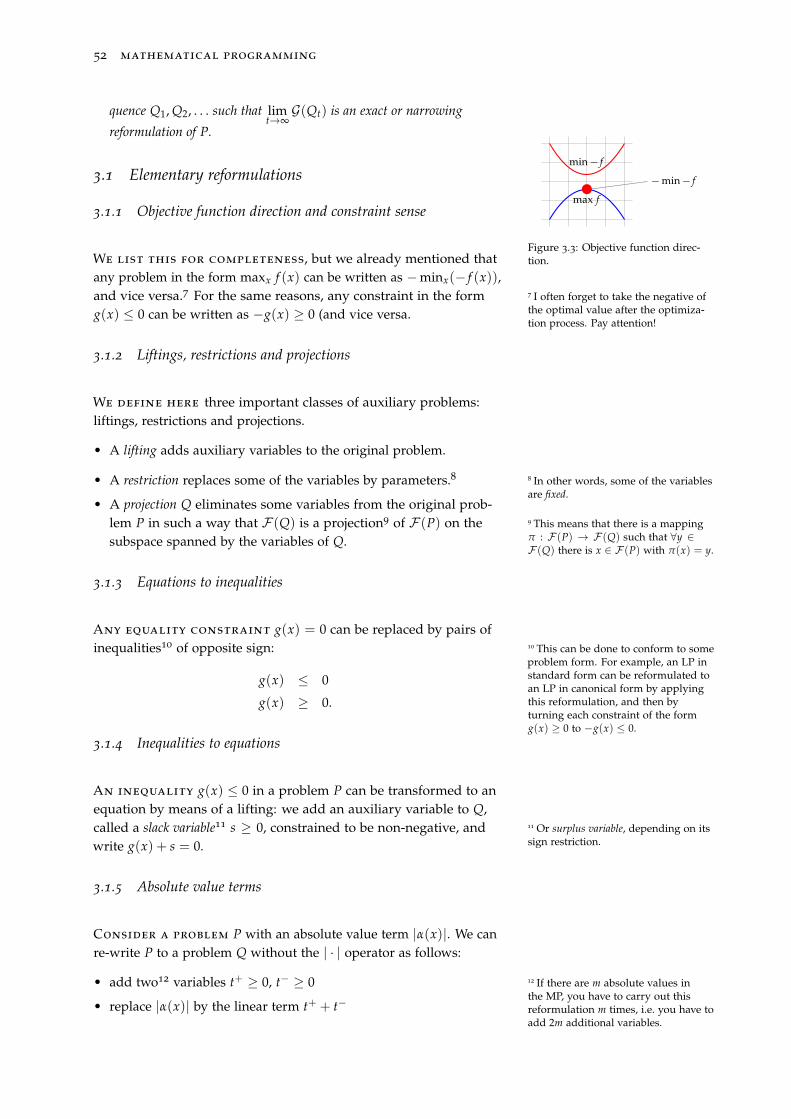
52 mathematical programming
quence Q1, Q2, . . . such that limt→∞G(Qt) is an exact or narrowing
reformulation of P.
3.1 Elementary reformulationsmax f
−min− f
min− f
Figure 3.3: Objective function direc-tion.
3.1.1 Objective function direction and constraint sense
We list this for completeness, but we already mentioned thatany problem in the form maxx f (x) can be written as −minx(− f (x)),and vice versa.7 For the same reasons, any constraint in the form 7 I often forget to take the negative of
the optimal value after the optimiza-tion process. Pay attention!
g(x) ≤ 0 can be written as −g(x) ≥ 0 (and vice versa.
3.1.2 Liftings, restrictions and projections
We define here three important classes of auxiliary problems:liftings, restrictions and projections.
• A lifting adds auxiliary variables to the original problem.
• A restriction replaces some of the variables by parameters.8 8 In other words, some of the variablesare fixed.
• A projection Q eliminates some variables from the original prob-lem P in such a way that F (Q) is a projection9 of F (P) on the 9 This means that there is a mapping
π : F (P) → F (Q) such that ∀y ∈F (Q) there is x ∈ F (P) with π(x) = y.
subspace spanned by the variables of Q.
3.1.3 Equations to inequalities
Any equality constraint g(x) = 0 can be replaced by pairs ofinequalities10 of opposite sign: 10 This can be done to conform to some
problem form. For example, an LP instandard form can be reformulated toan LP in canonical form by applyingthis reformulation, and then byturning each constraint of the formg(x) ≥ 0 to −g(x) ≤ 0.
g(x) ≤ 0
g(x) ≥ 0.
3.1.4 Inequalities to equations
An inequality g(x) ≤ 0 in a problem P can be transformed to anequation by means of a lifting: we add an auxiliary variable to Q,called a slack variable11 s ≥ 0, constrained to be non-negative, and 11 Or surplus variable, depending on its
sign restriction.write g(x) + s = 0.
3.1.5 Absolute value terms
Consider a problem P with an absolute value term |α(x)|. We canre-write P to a problem Q without the | · | operator as follows:
• add two12 variables t+ ≥ 0, t− ≥ 0 12 If there are m absolute values inthe MP, you have to carry out thisreformulation m times, i.e. you have toadd 2m additional variables.
• replace |α(x)| by the linear term t+ + t−
reformulations 53
• add the constraint t+ − t− = α(x)
• add the constraint t+t− = 0.
The last constraint ensures that only one in t+, t− can be nonzeroat any time, which means that if α(x) < 0 then t− = α(x) and ifα(x) > 0 then t+ = α(x), and consequently that t+ + t− has thesame value as |α(x)|.
3.1.6 Product of exponential terms
We can replace a product of exponential terms13 ∏i e fi(x) by an 13 Exponential terms like these are notso common in applications, but theymay occasionally happen, e.g. whenexpressing probability of chains ofevents.
additional variable w ≥ 0 and the constraint ln(w) = ∑i fi(x).
3.1.7 Binary to continuous variables
We can replace any binary variable x ∈ {0, 1} to a continuousvariable by removing the integrality constraints and adding thequadratic constraint14 x2 = x, a quadratic equation which only has 14 This constraint is sometimes also
written as x(x− 1) ≥ 0 ∧ x ≤ 1 [Sutouand Dai, 2002].
0, 1 as solutions.In principle, this would reduce all binary MPs to QCQPs. How-
ever, most NLP solvers do not handle the constraint x2 = x well,empirically speaking.15 In practice, it is much better to deal with 15 Many researchers have used this re-
formulation, but mostly for theoreticalrather than practical reasons.
the binary constraint and use branching. One notable exceptionarises when the resulting QCQP is used to derive an SDP relaxationof the original BLP.
3.1.8 Discrete to binary variables
A discrete variable x ∈ {p1, . . . , pk} can be reformulatedby relaxing it to a continuous variable,16 then adding a vector 16 Essentially, this reformulation pro-
vides an assignment of the allowablevalues to the relaxed variable by meansof assignment constraints.
y = (y1, . . . , yk) of k binary variables, as well as the constraints:
∑h≤k
yh = 1
∑h≤k
phyh = x
to the original problem.
3.1.9 Integer to binary variables
If p1 , . . . , pk are consecutive integers {L, L + 1, . . . , L + k − 1},then we can write x by means of a binary encoding.17 Let b be the 17 Many researchers have used this, see
e.g. [Boulle, 2004, Vielma, 2015].smallest integer such that k ≤ 2b. Then add a vector z = (z1, . . . , zb)
of b binary variables, relax x to a continuous variable, and add theconstraints:
x = L +b−1
∑h=0
zh2h
to the original problem.
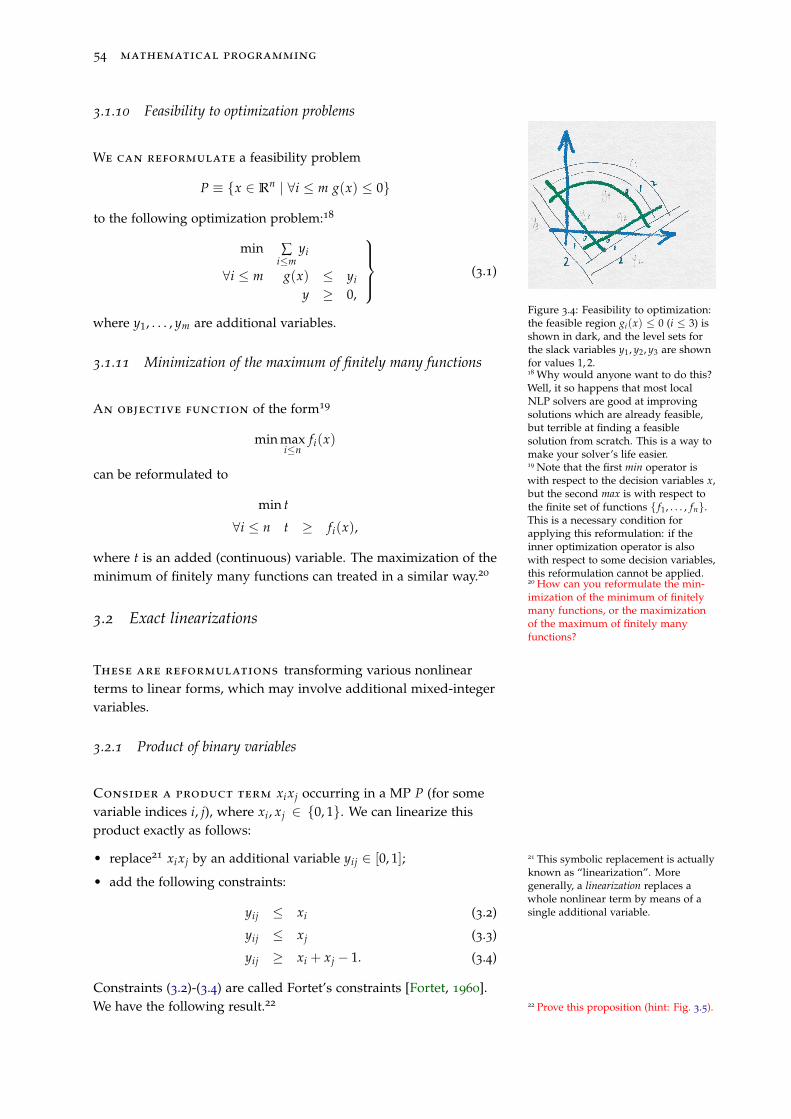
54 mathematical programming
3.1.10 Feasibility to optimization problems
Figure 3.4: Feasibility to optimization:the feasible region gi(x) ≤ 0 (i ≤ 3) isshown in dark, and the level sets forthe slack variables y1, y2, y3 are shownfor values 1, 2.
We can reformulate a feasibility problem
P ≡ {x ∈ Rn | ∀i ≤ m g(x) ≤ 0}
to the following optimization problem:18
18 Why would anyone want to do this?Well, it so happens that most localNLP solvers are good at improvingsolutions which are already feasible,but terrible at finding a feasiblesolution from scratch. This is a way tomake your solver’s life easier.
min ∑i≤m
yi
∀i ≤ m g(x) ≤ yi
y ≥ 0,
(3.1)
where y1, . . . , ym are additional variables.
3.1.11 Minimization of the maximum of finitely many functions
An objective function of the form19
19 Note that the first min operator iswith respect to the decision variables x,but the second max is with respect tothe finite set of functions { f1, . . . , fn}.This is a necessary condition forapplying this reformulation: if theinner optimization operator is alsowith respect to some decision variables,this reformulation cannot be applied.
min maxi≤n
fi(x)
can be reformulated to
min t
∀i ≤ n t ≥ fi(x),
where t is an added (continuous) variable. The maximization of theminimum of finitely many functions can treated in a similar way.20
20 How can you reformulate the min-imization of the minimum of finitelymany functions, or the maximizationof the maximum of finitely manyfunctions?
3.2 Exact linearizations
These are reformulations transforming various nonlinearterms to linear forms, which may involve additional mixed-integervariables.
3.2.1 Product of binary variables
Consider a product term xixj occurring in a MP P (for somevariable indices i, j), where xi, xj ∈ {0, 1}. We can linearize thisproduct exactly as follows:
• replace21 xixj by an additional variable yij ∈ [0, 1]; 21 This symbolic replacement is actuallyknown as “linearization”. Moregenerally, a linearization replaces awhole nonlinear term by means of asingle additional variable.
• add the following constraints:
yij ≤ xi (3.2)
yij ≤ xj (3.3)
yij ≥ xi + xj − 1. (3.4)
Constraints (3.2)-(3.4) are called Fortet’s constraints [Fortet, 1960].We have the following result.22 22 Prove this proposition (hint: Fig. 3.5).
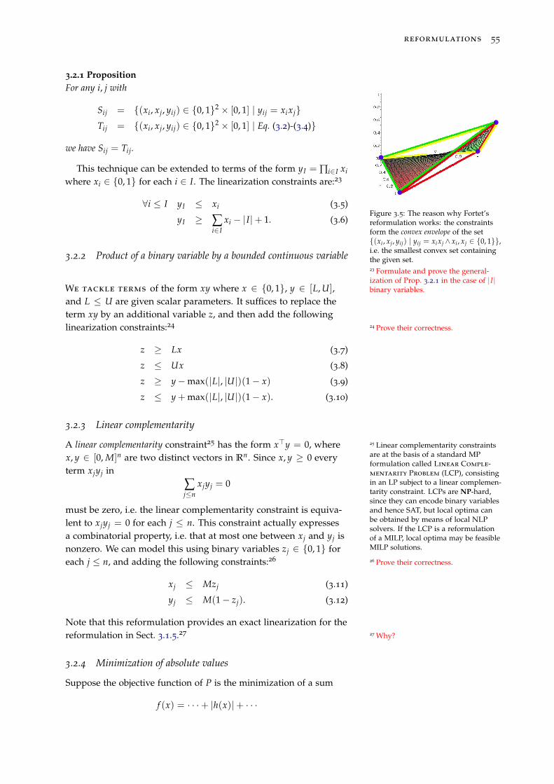
reformulations 55
3.2.1 PropositionFor any i, j with
Sij = {(xi, xj, yij) ∈ {0, 1}2 × [0, 1] | yij = xixj}Tij = {(xi, xj, yij) ∈ {0, 1}2 × [0, 1] | Eq. (3.2)-(3.4)}
we have Sij = Tij.
Figure 3.5: The reason why Fortet’sreformulation works: the constraintsform the convex envelope of the set{(xi , xj, yij) | yij = xixj ∧ xi , xj ∈ {0, 1}},i.e. the smallest convex set containingthe given set.
This technique can be extended to terms of the form yI = ∏i∈I xi
where xi ∈ {0, 1} for each i ∈ I. The linearization constraints are:23
23 Formulate and prove the general-ization of Prop. 3.2.1 in the case of |I|binary variables.
∀i ≤ I yI ≤ xi (3.5)
yI ≥ ∑i∈I
xi − |I|+ 1. (3.6)
3.2.2 Product of a binary variable by a bounded continuous variable
We tackle terms of the form xy where x ∈ {0, 1}, y ∈ [L, U],and L ≤ U are given scalar parameters. It suffices to replace theterm xy by an additional variable z, and then add the followinglinearization constraints:24 24 Prove their correctness.
z ≥ Lx (3.7)
z ≤ Ux (3.8)
z ≥ y−max(|L|, |U|)(1− x) (3.9)
z ≤ y + max(|L|, |U|)(1− x). (3.10)
3.2.3 Linear complementarity
A linear complementarity constraint25 has the form x>y = 0, where 25 Linear complementarity constraintsare at the basis of a standard MPformulation called Linear Comple-mentarity Problem (LCP), consistingin an LP subject to a linear complemen-tarity constraint. LCPs are NP-hard,since they can encode binary variablesand hence SAT, but local optima canbe obtained by means of local NLPsolvers. If the LCP is a reformulationof a MILP, local optima may be feasibleMILP solutions.
x, y ∈ [0, M]n are two distinct vectors in Rn. Since x, y ≥ 0 everyterm xjyj in
∑j≤n
xjyj = 0
must be zero, i.e. the linear complementarity constraint is equiva-lent to xjyj = 0 for each j ≤ n. This constraint actually expressesa combinatorial property, i.e. that at most one between xj and yj isnonzero. We can model this using binary variables zj ∈ {0, 1} foreach j ≤ n, and adding the following constraints:26 26 Prove their correctness.
xj ≤ Mzj (3.11)
yj ≤ M(1− zj). (3.12)
Note that this reformulation provides an exact linearization for thereformulation in Sect. 3.1.5.27 27 Why?
3.2.4 Minimization of absolute values
Suppose the objective function of P is the minimization of a sum
f (x) = · · ·+ |h(x)|+ · · ·
56 mathematical programming
This can be reformulated as in Sect. 3.1.5, and will result in
f (x) = · · ·+ (t+ + t−) + · · ·
subject to the constraint t+ − t− = h(x).Since we are minimizing f , at least one of the global optima will
have either t+ = 0 or t− = 0 even without the complementarityconstraint t+t− = 0. Whether this optimum will be found by thesolver28 really depends on how the solver works. For example, if 28 It would be more desirable to assert
properties which hold for any solver,so as not to depend on the nature ofthe solver, which may vary greatly.On the other hand, getting rid of theproblematic product term t+t− is agreat benefit.
the problem reformulation is a MILP, and solutions at every node ofthe BB are obtained using the simplex method, which finds optimaat vertices of the feasible polyhedron, this is going to be the case.29
29 Prove this.
We can also consider t− as a surplus variable of t+ ≥ h(x), andt+ as a slack variable of t− ≤ h(x), and re-write the above as
f (x) = · · ·+ t+ + t− + · · ·
subject tot− ≤ h(x) ≤ t+.
Finally, since −|h(x)| ≤ h(x) ≤ |h(x)|, we can simply replacet− by −t+ in the constraints (and rename t+ as t for simplicity), toobtain
f (x) = · · ·+ t + · · · (3.13)
−t ≤ h(x) ≤ t (3.14)
t ≥ 0, (3.15)
which reduces the number of added variables by half. Note that there represents |h(x)|, so we only need to sum it once on the ob-jective function, i.e. we do not want to replace t− in the objective,otherwise we would end up with 2t, which would count |h(x)|twice, and is therefore wrong. Note also that Eq. (3.13)-(3.15) canalso be used when |h(x)| appears in terms other than just the objec-tive function: consider for example the case of diagonal dominanceof an n× n matrix A = (aij) (see Sect. 6.6.2)
∀i ≤ n aii ≥ ∑j 6=i|aij|.
We can reformulate this to:
∀i ≤ n aii ≥ ∑j 6=i
tij (3.16)
∀i, j ≤ n − tij ≤ aij ≤ tij (3.17)
∀i, j ≤ n tij ≥ 0. (3.18)
Suppose (a, t) are feasible in the reformulation ((3.16)-(3.18)): thenwe have
aii ≥ ∑j 6=i
tij ≥ ∑j 6=i|aij|
as claimed, where the first inequality is Eq. (3.16), the secondfollows because Eq. (3.17) implies tij ≥ |aij|.
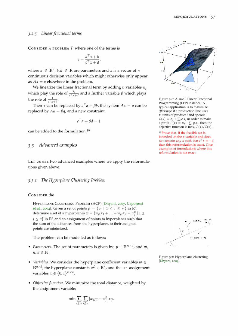
reformulations 57
3.2.5 Linear fractional terms
Consider a problem P where one of the terms is
τ =a>x + bc>x + d
,
where a ∈ Rn, b, d ∈ R are parameters and x is a vector of ncontinuous decision variables which might otherwise only appearas Ax = q elsewhere in the problem.
Figure 3.6: A small Linear FractionalProgramming (LFP) instance. Atypical application is to maximizeefficiency: if a production line usesxi units of product i and spendsC(x) = c0 + ∑i cixi in order to makea profit P(x) = p0 + ∑i pixi , then theobjective function is maxx P(x)/C(x).
We linearize the linear fractional term by adding n variables αj
which play the role ofxj
c>x+d and a further variable β which plays
the role of 1c>x+d .
Then τ can be replaced by a>α + βb, the system Ax = q can bereplaced by Aα = βq, and a new constraint
c>α + βd = 1
can be added to the formulation.3030 Prove that, if the feasible set isbounded on the x variable and doesnot contain any x such that c>x = −d,then this reformulation is exact. Giveexamples of formulations where thisreformulation is not exact.
3.3 Advanced examples
Let us see two advanced examples where we apply the reformula-tions given above.
3.3.1 The Hyperplane Clustering Problem
Consider the
Hyperplane Clustering Problem (HCP) [Dhyani, 2007, Caporossiet al., 2004]. Given a set of points p = {pi | 1 ≤ i ≤ m} in Rd,determine a set of n hyperplanes w = {wj1χ1 + . . . + wjdχd = w0
j | 1 ≤j ≤ n} in Rd and an assignment of points to hyperplanes such thatthe sum of the distances from the hyperplanes to their assignedpoints are minimized.
Figure 3.7: Hyperplane clustering[Dhyani, 2009].
The problem can be modelled as follows:
• Parameters. The set of parameters is given by: p ∈ Rm×d, and m,n, d ∈N.
• Variables. We consider the hyperplane coefficient variables w ∈Rn×d, the hyperplane constants w0 ∈ Rn, and the 0-1 assignmentvariables x ∈ {0, 1}m×n.
• Objective function. We minimize the total distance, weighted bythe assignment variable:
min ∑i≤m
∑j≤n|wj pi − w0
j |xij.
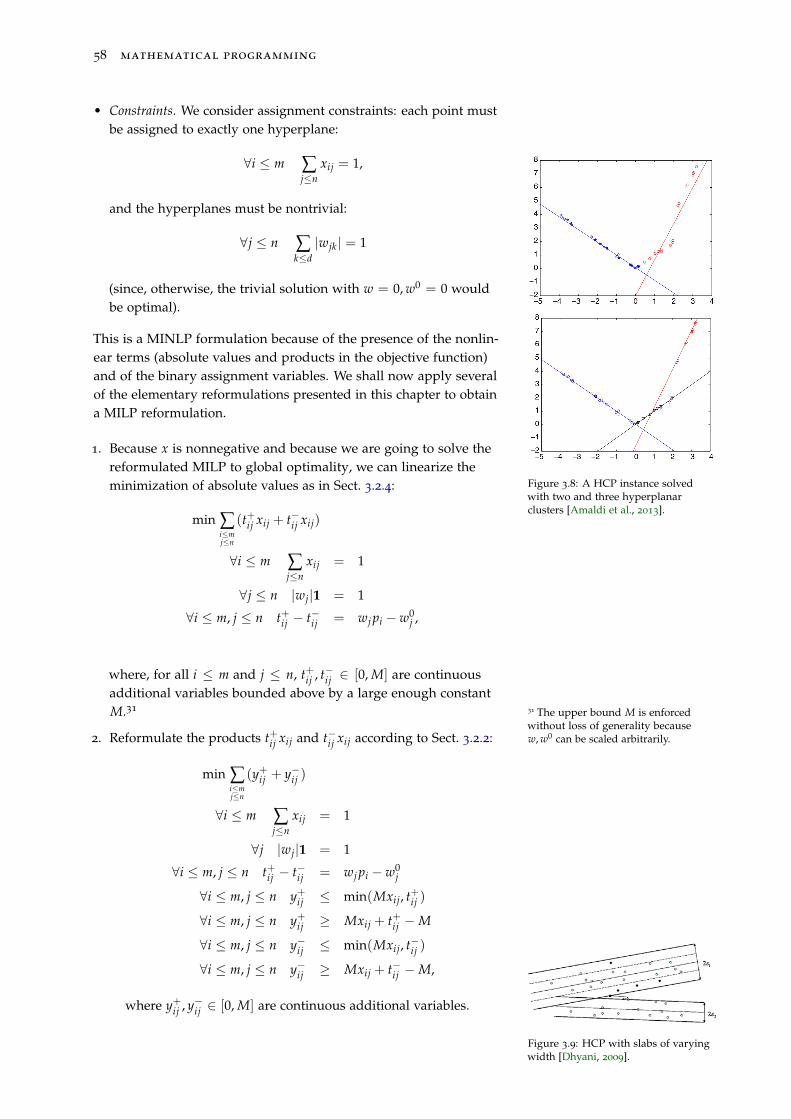
58 mathematical programming
• Constraints. We consider assignment constraints: each point mustbe assigned to exactly one hyperplane:
∀i ≤ m ∑j≤n
xij = 1,
and the hyperplanes must be nontrivial:
∀j ≤ n ∑k≤d|wjk| = 1
(since, otherwise, the trivial solution with w = 0, w0 = 0 wouldbe optimal).
Figure 3.8: A HCP instance solvedwith two and three hyperplanarclusters [Amaldi et al., 2013].
This is a MINLP formulation because of the presence of the nonlin-ear terms (absolute values and products in the objective function)and of the binary assignment variables. We shall now apply severalof the elementary reformulations presented in this chapter to obtaina MILP reformulation.
1. Because x is nonnegative and because we are going to solve thereformulated MILP to global optimality, we can linearize theminimization of absolute values as in Sect. 3.2.4:
min ∑i≤mj≤n
(t+ij xij + t−ij xij)
∀i ≤ m ∑j≤n
xij = 1
∀j ≤ n |wj|1 = 1
∀i ≤ m, j ≤ n t+ij − t−ij = wj pi − w0j ,
where, for all i ≤ m and j ≤ n, t+ij , t−ij ∈ [0, M] are continuousadditional variables bounded above by a large enough constantM.31 31 The upper bound M is enforced
without loss of generality becausew, w0 can be scaled arbitrarily.2. Reformulate the products t+ij xij and t−ij xij according to Sect. 3.2.2:
min ∑i≤mj≤n
(y+ij + y−ij )
∀i ≤ m ∑j≤n
xij = 1
∀j |wj|1 = 1
∀i ≤ m, j ≤ n t+ij − t−ij = wj pi − w0j
∀i ≤ m, j ≤ n y+ij ≤ min(Mxij, t+ij )
∀i ≤ m, j ≤ n y+ij ≥ Mxij + t+ij −M
∀i ≤ m, j ≤ n y−ij ≤ min(Mxij, t−ij )
∀i ≤ m, j ≤ n y−ij ≥ Mxij + t−ij −M,
Figure 3.9: HCP with slabs of varyingwidth [Dhyani, 2009].
where y+ij , y−ij ∈ [0, M] are continuous additional variables.
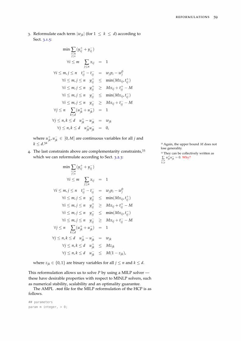
reformulations 59
3. Reformulate each term |wjk| (for 1 ≤ k ≤ d) according toSect. 3.1.5:
min ∑i≤mj≤n
(y+ij + y−ij )
∀i ≤ m ∑j≤n
xij = 1
∀i ≤ m, j ≤ n t+ij − t−ij = wj pi − w0j
∀i ≤ m, j ≤ n y+ij ≤ min(Mxij, t+ij )
∀i ≤ m, j ≤ n y+ij ≥ Mxij + t+ij −M
∀i ≤ m, j ≤ n y−ij ≤ min(Mxij, t−ij )
∀i ≤ m, j ≤ n y−ij ≥ Mxij + t−ij −M
∀j ≤ n ∑k≤d
(u+jk + u−jk) = 1
∀j ≤ n, k ≤ d u+jk − u−jk = wjk
∀j ≤ n, k ≤ d u+jku−jk = 0,
where u+jk , u−jk ∈ [0, M] are continuous variables for all j and
k ≤ d.32 32 Again, the upper bound M does notlose generality.
4. The last constraints above are complementarity constraints,33
33 They can be collectively written as∑j≤nk≤d
u+jku−jk = 0. Why?which we can reformulate according to Sect. 3.2.3:
min ∑i≤mj≤n
(y+ij + y−ij )
∀i ≤ m ∑j≤n
xij = 1
∀i ≤ m, j ≤ n t+ij − t−ij = wj pi − w0j
∀i ≤ m, j ≤ n y+ij ≤ min(Mxij, t+ij )
∀i ≤ m, j ≤ n y+ij ≥ Mxij + t+ij −M
∀i ≤ m, j ≤ n y−ij ≤ min(Mxij, t−ij )
∀i ≤ m, j ≤ n y−ij ≥ Mxij + t−ij −M
∀j ≤ n ∑k≤d
(u+jk + u−jk) = 1
∀j ≤ n, k ≤ d u+jk − u−jk = wjk
∀j ≤ n, k ≤ d u+jk ≤ Mzjk
∀j ≤ n, k ≤ d u−jk ≤ M(1− zjk),
where zjk ∈ {0, 1} are binary variables for all j ≤ n and k ≤ d.
This reformulation allows us to solve P by using a MILP solver —these have desirable properties with respect to MINLP solvers, suchas numerical stability, scalability and an optimality guarantee.
The AMPL .mod file for the MILP reformulation of the HCP is asfollows.
## parameters
param m integer, > 0;
60 mathematical programming
param n integer, > 0;
param dim integer, > 0;
set N := 1..n; # planes
set M := 1..m; # points
set D:=1..dim; # spatial dimensions
param p{M,D}; # the points
param P{d in D} := (max{i in M} p[i,d]) - (min{i in M} p[i,d]); # ranges
# used for approximate linearization
param small default 1e-6;
param big default 1e3;
# w (hyperplane coefficients) variable bounds
param wL := -1; #-big;
param w0L := -big;
param wU := 1; #big;
param w0U := big;
## variables
var w0{N} <= w0U, >= w0L;
var w{N,D} <= wU, >= wL;
var x{M,N} binary;
var tplus{M,N} >= 0, <= big;
var tminus{M,N} >= 0, <= big;
var yplus{M,N} >= 0, <= big;
var yminus{M,N} >= 0, <= big;
var uplus{N,D} >= 0, <= big;
var uminus{N,D} >= 0, <= big;
var z{N,D} binary;
## objective function
minimize fitting_error: sum{i in M, j in N} (yplus[i,j] + yminus[i,j]);
## constraints
subject to assignment {i in M} : sum{j in N} x[i,j] = 1;
subject to minabs_ref {i in M, j in N} :
tplus[i,j] - tminus[i,j] = sum{k in D} w[j,k] * p[i,k] - w0[j];
subject to yplus_lin1 {i in M, j in N} : yplus[i,j] <= big * x[i,j];
subject to yplus_lin2 {i in M, j in N} : yplus[i,j] <= tplus[i,j];
subject to yplus_lin3 {i in M, j in N} :
yplus[i,j] >= big * x[i,j] + tplus[i,j] - big;
subject to yminus_lin1 {i in M, j in N} : yminus[i,j] <= big * x[i,j];
subject to yminus_lin2 {i in M, j in N} : yminus[i,j] <= tminus[i,j];
subject to yminus_lin3 {i in M, j in N} :
yminus[i,j] >= big * x[i,j] + tminus[i,j] - big;
subject to one_norm1_ref{j in N}: sum{k in D} (uplus[j,k] + uminus[j,k]) = 1;
subject to one_norm2_ref{j in N, k in D}: uplus[j,k] - uminus[j,k] = w[j,k];
subject to one_norm3_ref{j in N, k in D}: uplus[j,k] <= big*z[j,k];
subject to one_norm4_ref{j in N, k in D}: uminus[j,k] <= big*(1 - z[j,k]);
A small instance consisting of 8 points and 2 planes in R2, withp = {(1, 7), (1, 1), (2, 2), (4, 3), (4, 5), (8, 3), (10, 1), (10, 5)} is solvedto optimality by the ILOG CPLEX solver [IBM, 2014] to produce thefollowing output:
Assignment of points to hyperplanar clusters:
cluster 1 = { 2 3 4 8 }
cluster 2 = { 1 5 6 7 }
The hyperplane clusters
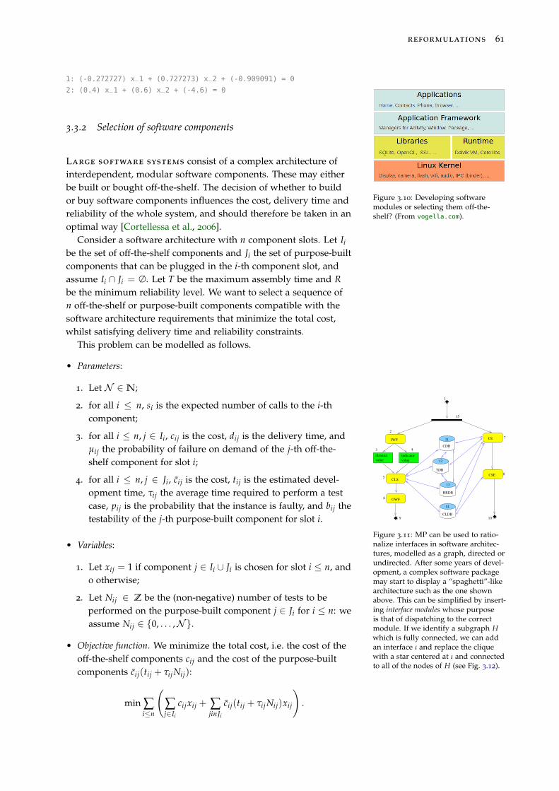
reformulations 61
1: (-0.272727) x_1 + (0.727273) x_2 + (-0.909091) = 0
2: (0.4) x_1 + (0.6) x_2 + (-4.6) = 0
3.3.2 Selection of software components
Figure 3.10: Developing softwaremodules or selecting them off-the-shelf? (From vogella.com).
Large software systems consist of a complex architecture ofinterdependent, modular software components. These may eitherbe built or bought off-the-shelf. The decision of whether to buildor buy software components influences the cost, delivery time andreliability of the whole system, and should therefore be taken in anoptimal way [Cortellessa et al., 2006].
Consider a software architecture with n component slots. Let Ii
be the set of off-the-shelf components and Ji the set of purpose-builtcomponents that can be plugged in the i-th component slot, andassume Ii ∩ Ji = ∅. Let T be the maximum assembly time and Rbe the minimum reliability level. We want to select a sequence ofn off-the-shelf or purpose-built components compatible with thesoftware architecture requirements that minimize the total cost,whilst satisfying delivery time and reliability constraints.
This problem can be modelled as follows.
• Parameters:
1. Let N ∈N;
2. for all i ≤ n, si is the expected number of calls to the i-thcomponent;
3. for all i ≤ n, j ∈ Ii, cij is the cost, dij is the delivery time, andµij the probability of failure on demand of the j-th off-the-shelf component for slot i;
4. for all i ≤ n, j ∈ Ji, cij is the cost, tij is the estimated devel-opment time, τij the average time required to perform a testcase, pij is the probability that the instance is faulty, and bij thetestability of the j-th purpose-built component for slot i.
IWF
2
distance
value
3
indicator
value
4
CLS5
OWF6
���
���
9
15
���
���1
CE 7
CSE 8
����
10
CLDB
14
HRDB
13
TDB
12
11
CDB
Figure 3.11: MP can be used to ratio-nalize interfaces in software architec-tures, modelled as a graph, directed orundirected. After some years of devel-opment, a complex software packagemay start to display a “spaghetti”-likearchitecture such as the one shownabove. This can be simplified by insert-ing interface modules whose purposeis that of dispatching to the correctmodule. If we identify a subgraph Hwhich is fully connected, we can addan interface ι and replace the cliquewith a star centered at ι and connectedto all of the nodes of H (see Fig. 3.12).
• Variables:
1. Let xij = 1 if component j ∈ Ii ∪ Ji is chosen for slot i ≤ n, and0 otherwise;
2. Let Nij ∈ Z be the (non-negative) number of tests to beperformed on the purpose-built component j ∈ Ji for i ≤ n: weassume Nij ∈ {0, . . . ,N}.
• Objective function. We minimize the total cost, i.e. the cost of theoff-the-shelf components cij and the cost of the purpose-builtcomponents cij(tij + τijNij):
min ∑i≤n
(∑j∈Ii
cijxij + ∑jinJi
cij(tij + τijNij)xij
).
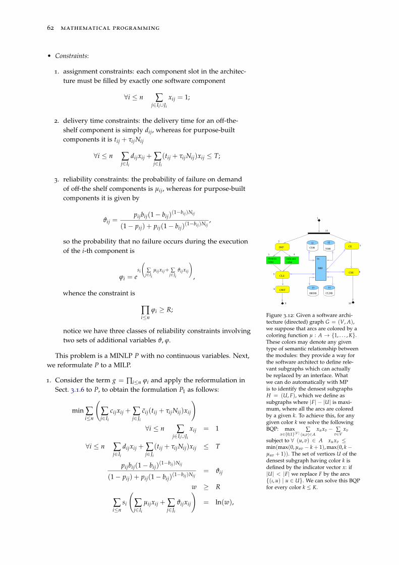
62 mathematical programming
• Constraints:
1. assignment constraints: each component slot in the architec-ture must be filled by exactly one software component
∀i ≤ n ∑j∈Ii∪Ji
xij = 1;
2. delivery time constraints: the delivery time for an off-the-shelf component is simply dij, whereas for purpose-builtcomponents it is tij + τijNij
∀i ≤ n ∑j∈Ii
dijxij + ∑j∈Ji
(tij + τijNij)xij ≤ T;
3. reliability constraints: the probability of failure on demandof off-the shelf components is µij, whereas for purpose-builtcomponents it is given by
ϑij =pijbij(1− bij)
(1−bij)Nij
(1− pij) + pij(1− bij)(1−bij)Nij
,
so the probability that no failure occurs during the executionof the i-th component is
ϕi = esi
(∑
j∈Iiµijxij+ ∑
j∈Jiϑijxij
),
whence the constraint is
∏i≤n
ϕi ≥ R;
notice we have three classes of reliability constraints involvingtwo sets of additional variables ϑ, ϕ.
IWF
2
distance
value
3
indicator
value
4
CLS5
OWF6
���
���
9
15
���
���1
CE 7
CSE 8
����
10
TDB
1211
CDB
HRDB
13
CLDB
14
16
DBI
Figure 3.12: Given a software archi-tecture (directed) graph G = (V, A),we suppose that arcs are colored by acoloring function µ : A → {1, . . . , K}.These colors may denote any giventype of semantic relationship betweenthe modules: they provide a way forthe software architect to define rele-vant subgraphs which can actuallybe replaced by an interface. Whatwe can do automatically with MPis to identify the densest subgraphsH = (U, F), which we define assubgraphs where |F| − |U| is maxi-mum, where all the arcs are coloredby a given k. To achieve this, for anygiven color k we solve the followingBQP: max
x∈{0,1}|V|∑
(u,v)∈Axuxv − ∑
v∈Vxv
subject to ∀ (u, v) ∈ A xuxv ≤min(max(0, µuv − k + 1), max(0, k −µuv + 1)). The set of vertices U of thedensest subgraph having color k isdefined by the indicator vector x: if|U| < |F| we replace F by the arcs{(ι, u) | u ∈ U}. We can solve this BQPfor every color k ≤ K.
This problem is a MINLP P with no continuous variables. Next,we reformulate P to a MILP.
1. Consider the term g = ∏i≤n ϕi and apply the reformulation inSect. 3.1.6 to P, to obtain the formulation P1 as follows:
min ∑i≤n
(∑j∈Ii
cijxij + ∑j∈Ji
cij(tij + τijNij)xij
)∀i ≤ n ∑
j∈Ii∪Ji
xij = 1
∀i ≤ n ∑j∈Ii
dijxij + ∑j∈Ji
(tij + τijNij)xij ≤ T
pijbij(1− bij)(1−bij)Nij
(1− pij) + pij(1− bij)(1−bij)Nij
= ϑij
w ≥ R
∑i≤n
si
(∑j∈Ii
µijxij + ∑j∈Ji
ϑijxij
)= ln(w),
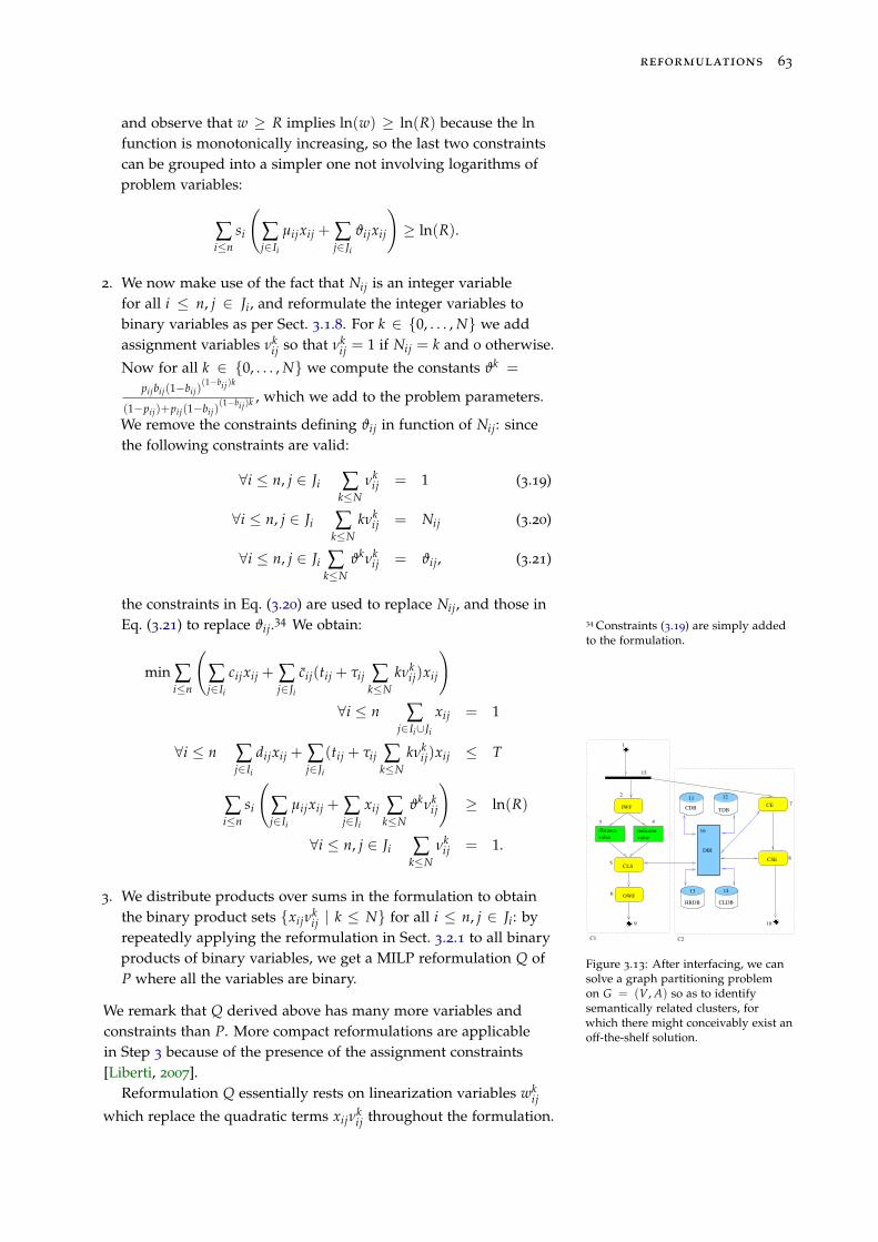
reformulations 63
and observe that w ≥ R implies ln(w) ≥ ln(R) because the lnfunction is monotonically increasing, so the last two constraintscan be grouped into a simpler one not involving logarithms ofproblem variables:
∑i≤n
si
(∑j∈Ii
µijxij + ∑j∈Ji
ϑijxij
)≥ ln(R).
2. We now make use of the fact that Nij is an integer variablefor all i ≤ n, j ∈ Ji, and reformulate the integer variables tobinary variables as per Sect. 3.1.8. For k ∈ {0, . . . , N} we addassignment variables νk
ij so that νkij = 1 if Nij = k and 0 otherwise.
Now for all k ∈ {0, . . . , N} we compute the constants ϑk =
pijbij(1−bij)(1−bij)k
(1−pij)+pij(1−bij)(1−bij)k
, which we add to the problem parameters.
We remove the constraints defining ϑij in function of Nij: sincethe following constraints are valid:
∀i ≤ n, j ∈ Ji ∑k≤N
νkij = 1 (3.19)
∀i ≤ n, j ∈ Ji ∑k≤N
kνkij = Nij (3.20)
∀i ≤ n, j ∈ Ji ∑k≤N
ϑkνkij = ϑij, (3.21)
the constraints in Eq. (3.20) are used to replace Nij, and those inEq. (3.21) to replace ϑij.34 We obtain: 34 Constraints (3.19) are simply added
to the formulation.
min ∑i≤n
(∑j∈Ii
cijxij + ∑j∈Ji
cij(tij + τij ∑k≤N
kνkij)xij
)∀i ≤ n ∑
j∈Ii∪Ji
xij = 1
∀i ≤ n ∑j∈Ii
dijxij + ∑j∈Ji
(tij + τij ∑k≤N
kνkij)xij ≤ T
∑i≤n
si
(∑j∈Ii
µijxij + ∑j∈Ji
xij ∑k≤N
ϑkνkij
)≥ ln(R)
∀i ≤ n, j ∈ Ji ∑k≤N
νkij = 1.
IWF
2
distance
value
3
indicator
value
4
CLS5
OWF6
���
���
9
CE 7
CSE 8
����
10
TDB
1211
CDB
HRDB
13
CLDB
14
������
������1
15
16
DBI
C1 C2
Figure 3.13: After interfacing, we cansolve a graph partitioning problemon G = (V, A) so as to identifysemantically related clusters, forwhich there might conceivably exist anoff-the-shelf solution.
3. We distribute products over sums in the formulation to obtainthe binary product sets {xijν
kij | k ≤ N} for all i ≤ n, j ∈ Ji: by
repeatedly applying the reformulation in Sect. 3.2.1 to all binaryproducts of binary variables, we get a MILP reformulation Q ofP where all the variables are binary.
We remark that Q derived above has many more variables andconstraints than P. More compact reformulations are applicablein Step 3 because of the presence of the assignment constraints[Liberti, 2007].
Reformulation Q essentially rests on linearization variables wkij
which replace the quadratic terms xijνkij throughout the formulation.
64 mathematical programming
A semantic interpretation of step 3 is as follows. We notice that fori ≤ n, j ∈ Ji, if xij = 1, then xij = ∑k νk
ij (because only one value k
will be selected), and if xij = 0, then xij = ∑k νkij (because no value k
will be selected). This means that
∀i ≤ n, j ∈ Ji xij = ∑k≤N
νkij (3.22)
is a valid problem constraint. We use it to replace xij everywherein the formulation where it appears with j ∈ Ii, obtaining a opt-reformulation with xij for j ∈ Ii and quadratic terms νk
ijνhlp. Now,
because of (3.19), these are zero when (i, j) 6= (l, p) or k 6= h andare equal to νk
ij when (i, j) = (l, p) and k = h, so they can be
linearized exactly by replacing them by either 0 or νkij according
to their indices. What this really means is that the reformulationQ, obtained through a series of automatic reformulation steps, is asemantically different formulation defined in terms of the followingdecision variables:
∀i ≤ n, j ∈ Ii xij =
{1 if j ∈ Ii is assigned to i0 otherwise.
∀i ≤ n, j ∈ Ji, k ≤ N νkij =
1 if j ∈ Ji is assigned to i and there
are k tests to be performed0 otherwise.
This is an important hint to the importance of automatic reformula-tion in problem analysis: it is a syntactical operation, the result ofwhich, when interpreted, can suggest a new meaning.
3.4 Summary
This chapter is about reformulations as a means to change a for-mulation so it can be solved using a given solver, so that someoptimality properties are preserved.
• Motivation and main definitions
• Elementary reformulations: changing objective direction andconstraint sense, lifting – restrictions – projections, turning equa-tions into inequalities and vice versa, absolute values, productof exponentials, turning binary variables to continuous, turningdiscrete variables to binary, turning integer variables to binary,turning feasibility to optimization problems, minimization of amaximum
• Exact linearizations: product of binary variables, product of abinary variable by a continuous one, linear complementarity,minimization of absolute values, linear fractional terms
• Applying reformulations to turn the hyperplane clusteringproblem from MINLP to MILP.
Part II
In-depth topics

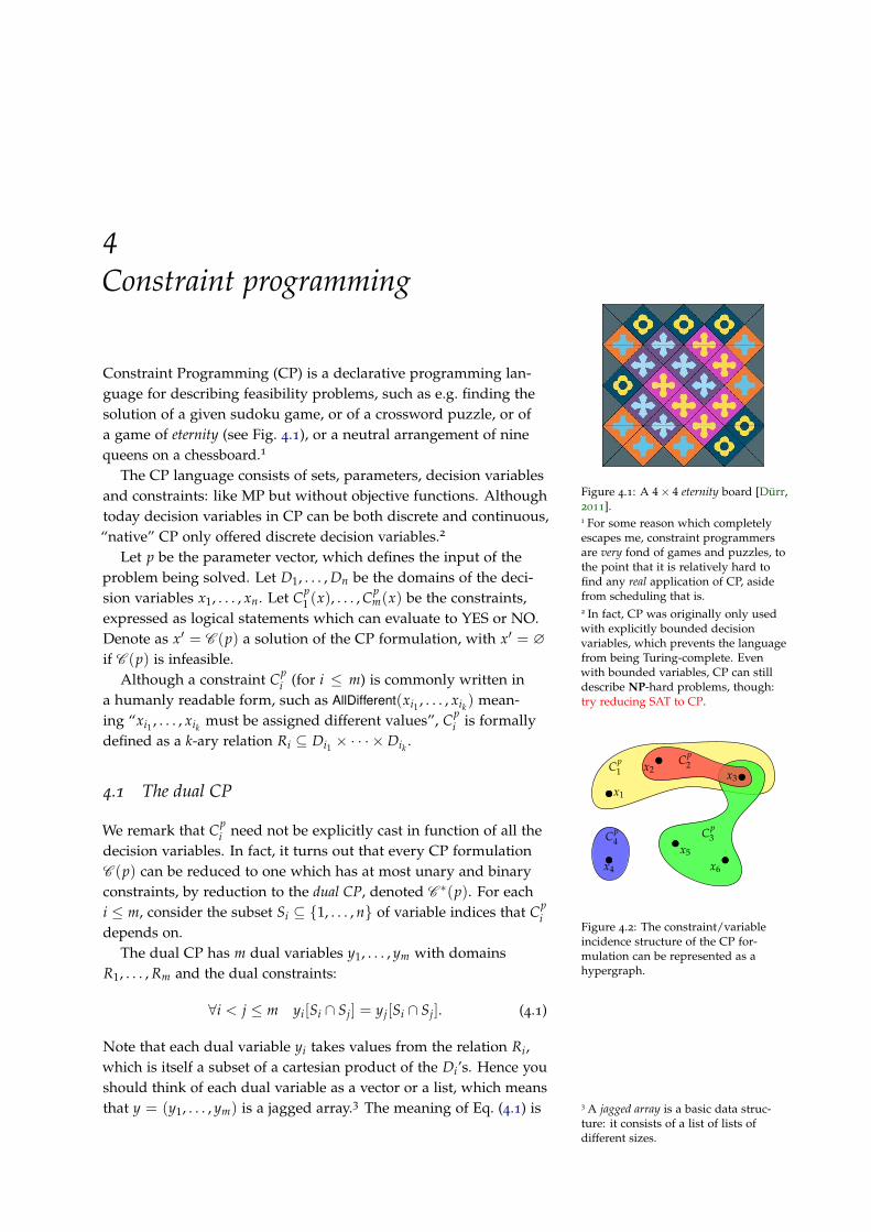
4Constraint programming
Figure 4.1: A 4× 4 eternity board [Dürr,2011].
Constraint Programming (CP) is a declarative programming lan-guage for describing feasibility problems, such as e.g. finding thesolution of a given sudoku game, or of a crossword puzzle, or ofa game of eternity (see Fig. 4.1), or a neutral arrangement of ninequeens on a chessboard.1
1 For some reason which completelyescapes me, constraint programmersare very fond of games and puzzles, tothe point that it is relatively hard tofind any real application of CP, asidefrom scheduling that is.
The CP language consists of sets, parameters, decision variablesand constraints: like MP but without objective functions. Althoughtoday decision variables in CP can be both discrete and continuous,“native” CP only offered discrete decision variables.2
2 In fact, CP was originally only usedwith explicitly bounded decisionvariables, which prevents the languagefrom being Turing-complete. Evenwith bounded variables, CP can stilldescribe NP-hard problems, though:try reducing SAT to CP.
Let p be the parameter vector, which defines the input of theproblem being solved. Let D1, . . . , Dn be the domains of the deci-sion variables x1, . . . , xn. Let Cp
1 (x), . . . , Cpm(x) be the constraints,
expressed as logical statements which can evaluate to YES or NO.Denote as x′ = C (p) a solution of the CP formulation, with x′ = ∅if C (p) is infeasible.
x1
x2 x3
x4
x5
x6
Cp1
Cp2
Cp3Cp
4
Figure 4.2: The constraint/variableincidence structure of the CP for-mulation can be represented as ahypergraph.
Although a constraint Cpi (for i ≤ m) is commonly written in
a humanly readable form, such as AllDifferent(xi1 , . . . , xik ) mean-ing “xi1 , . . . , xik must be assigned different values”, Cp
i is formallydefined as a k-ary relation Ri ⊆ Di1 × · · · × Dik .
4.1 The dual CP
We remark that Cpi need not be explicitly cast in function of all the
decision variables. In fact, it turns out that every CP formulationC (p) can be reduced to one which has at most unary and binaryconstraints, by reduction to the dual CP, denoted C ∗(p). For eachi ≤ m, consider the subset Si ⊆ {1, . . . , n} of variable indices that Cp
idepends on.
The dual CP has m dual variables y1, . . . , ym with domainsR1, . . . , Rm and the dual constraints:
∀i < j ≤ m yi[Si ∩ Sj] = yj[Si ∩ Sj]. (4.1)
Note that each dual variable yi takes values from the relation Ri,which is itself a subset of a cartesian product of the Di’s. Hence youshould think of each dual variable as a vector or a list, which meansthat y = (y1, . . . , ym) is a jagged array.3 The meaning of Eq. (4.1) is 3 A jagged array is a basic data struc-
ture: it consists of a list of lists ofdifferent sizes.
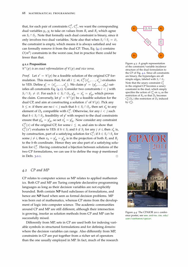
68 mathematical programming
that, for each pair of constraints Cpi , Cp
j , we want the correspondingdual variables yi, yj to take on values from Ri and Rj which agreeon Si ∩ Sj. Note that formally each dual constraint is binary, since itonly involves two dual variables. Note also that when Si ∩ Sj = ∅,the constraint is empty, which means it is always satisfied and wecan formally remove it from the dual CP. Thus, Eq. (4.1) containsO(m2) constraints in the worst case, but in practice there could befewer than that.
y1 y2
y3y4
{2, 3}
{3}{3}
Figure 4.3: A graph representationof the constraint/variable incidencestructure of the dual formulation tothe CP of Fig. 4.2. Since all constraintsare binary, the hyperedges are allsimple edges, labeled with Si ∩ Sj.Note that the unary constraint Cp
4in the original CP becomes a unaryconstraint in the dual, which simplyspecifies the action of Cp
4 on x6 as therestriction of R4 so that D6 becomesCp
4 (D6) (the restriction of D6 inducedby Cp
4 ).
4.1.1 PropositionC ∗(p) is an exact reformulation of C (p) and vice versa.
Proof. Let x′ = C (p) be a feasible solution of the original CP for-mulation. This means that, for all i ≤ m, Cp
i (x′i1 , . . . , x′ik ) evaluatesto YES. Define y′i = (x′i1 , . . . , x′ik ). We claim y′ = (y′1, . . . , y′m) sat-isfies all constraints Eq. (4.1). Consider two constraints i < j withSi ∩ Sj 6= ∅. For each h ∈ Si ∩ Sj, y′ih = x′h = y′jh, which provesthe claim. Conversely, let y′ = C ∗(p) be a feasible solution for thedual CP, and aim at constructing a solution x′ of C (p). Pick anyh ≤ n: if there are no i < j such that h ∈ Si ∩ Sj, then set x′h to anyelement of Dh compatible with Cp
i . Otherwise, for any i < j suchthat h ∈ Si ∩ Sj, feasibility of y′ with respect to the dual constraintsensure that y′ih = y′jh, so set x′h = y′ih. Now consider any constraint
Cpi (x) of the original CP, for some i ≤ m, and aim to show that
Cpi (x′) evaluates to YES: if h ∈ Si and h 6∈ Sj for any j 6= i, then x′h is,
by construction, part of a satisfying solution for Cpi ; if h ∈ Si ∩ Sj for
some j 6= i, then xh = y′ih = y′jh is in the projection of both Ri and Rj
to the h-th coordinate. Hence they are also part of a satisfying solu-tion for Cp
i . Having constructed a bijection between solutions of thetwo CP formulations, we can use it to define the map φ mentionedin Defn. 3.0.1. 2
4.2 CP and MP
Figure 4.4: The CPAIOR 2011 confer-ence poster, see www.andrew.cmu.edu/
user/vanhoeve/cpaior.
CP relates to computer science as MP relates to applied mathemat-ics. Both CP and MP are Turing complete declarative programminglanguages as long as their decision variables are not explicitlybounded. Both contain NP-hard subclasses of formulations, andhence are NP-hard when seen as formal decision problems. MPwas born out of mathematics, whereas CP stems from the develop-ment of logic into computer science. The academic communitiesaround CP and MP are still different, although their intersectionis growing, insofar as solution methods from CP and MP can besuccessfully mixed.
Differently from MP, sets in CP are used both for indexing vari-able symbols in structured formulations and for defining domainswhere the decision variables can range. Also differently from MP,constraints in CP are put together from a richer set of operatorsthan the one usually employed in MP. In fact, much of the research
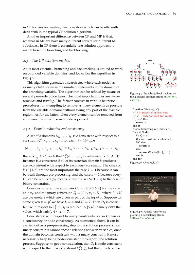
constraint programming 69
in CP focuses on creating new operators which can be efficientlydealt with in the typical CP solution algorithm.
Another important difference between CP and MP is that,whereas in MP we have many different solvers for different MPsubclasses, in CP there is essentially one solution approach: asearch based on branching and backtracking.
4.3 The CP solution method
At its most essential, branching and backtracking is limited to workon bounded variable domains, and looks like the algorithm inFig. 4.6.
Figure 4.5: Branching/backtracking onthe 4 queens problem (from ktiml.mff.
cuni.cz).
This algorithm generates a search tree where each node hasas many child nodes as the number of elements in the domain ofthe branching variable. The algorithm can be refined by means ofseveral per-node procedures. The most important ones are domainreduction and pruning. The former consists in various heuristicprocedures for attempting to remove as many elements as possiblefrom the variable domains without losing any part of the feasibleregion. As for the latter, when every element can be removed froma domain, the current search node is pruned.
4.3.1 Domain reduction and consistency
function CPsolve(J, x′)// J = indices of unfixed vars// x′ = vector of fixed var. valuesif J = ∅ then
return x′
end ifchoose branching var. index j ∈ Jfor v ∈ Dj do
fix x′j ← vif some constraint evaluates toNO then
return ∅else
return CPsolve(J ∪ {j}, x′)end if
end forFigure 4.6: CPsolve(J, x′)
A set of k domains Di1 , . . . , Dik is k-consistent with respect to aconstraint Cp
i (xi1 , . . . , xik ) if for each (k− 1)-tuple
(ai1 , . . . , aij−1, aij+1, . . . , aik ) ∈ Di1 × · · · × Dij−1, Dij+1 × · · · × Dik−1
there is aij ∈ Dij such that Cpi (ai1 , . . . , aik ) evaluates to YES. A CP
instance is k-consistent if all of its cartesian domain k-productsare k-consistent with respect to each k-ary constraint. The cases ofk ∈ {1, 2} are the most important: the case k = 1 because it canbe dealt through pre-processing, and the case k = 2 because everyCP can be reduced (by means of duality, see Sect. 4.1) to the case ofbinary constraints.
Figure 4.7: Patrick Winston ex-plaining 1-consistency (fromMITOpenCourseWare).
Consider for example a domain D1 = {2, 3, 5, 6, 9} for the vari-able x1, and the unary constraint Cp
1 ≡ [L ≤ x1 ≤ U], where L ≤ Uare parameters which are given as part of the input p. Suppose forsome given p = p′ we have L = 4 and U = 7. Then D1 is consis-
tent with respect to Cp′1 if D1 is reduced to {5, 6}, namely only the
values which satisfy 4 ≤ x1 ≤ 7.Consistency with respect to unary constraints is also known as
1-consistency or node-consistency. As mentioned above, it can becarried out as a pre-processing step to the solution process: sinceunary constraints cannot encode relations between variables, oncethe domain becomes consistent w.r.t. a unary constraint, it mustnecessarily keep being node-consistent throughout the solutionprocess. Suppose, to get a contradiction, that Dj is node-consistentwith respect to the unary constraint Cp
i (xj), but that, due to some
70 mathematical programming
other constraint Cp` involving xj, Dj becomes node-inconsistent
w.r.t. Cpi . Since constraints can never add values to domains, the
effect of Cp` on Dj must yield a domain D′j ⊆ Dj. Of course, if D′j is
node-inconsistent w.r.t Cpi , any superset of D′j must also be node-
inconsistent, which means that Dj is, against the initial assumption.Consistency with respect to binary constraints of the form
Cpi (xj, xh) is also known as 2-consistency or arc-consistency. The do-
mains Dj, Dh are 2-consistent with respect to Cpi if for each aj ∈ Dj
there is ah ∈ Dh such that Cpi (aj, ah) evaluates to YES. Consider
for example the domain D2 = {1, 2, 3, 4} for x2 and the constraintx1 < x2: then D1, D2 are arc-consistent with respect to x1 < x2 if D1
is reduced to {2, 3} and D2 to {3, 4}.
Figure 4.8: Branching in CP (fromwww.info.ucl.ac.be/~pschaus).
Domain reduction through consistency is usually performed be-fore choosing the branching variable index in the search algorithm(Fig. 4.6).
4.3.2 Pruning and solving
After a certain amount of branching and domain reduction, theremight4 be leaf nodes of the search tree where the domain product 4 If all the domains have a finite
number of values, then you can replace“might” by “will”.
D = D1 × Dn is either empty, or consists of exactly one elementa = (a1, . . . , an). In the former case, the leaf node is pruned, i.e. nochild nodes are further appended to the pruned node. In the lattercase, the solution x = a is returned to the user, and the algorithmterminates.
Next, we illustrate how the AllDifferent constraint impacts pruningand finding solutions in CP. Suppose D1 = . . . ,= Dn = D such that|D| = n, and x1, . . . , xn ∈ D. By stating
AllDifferent(x1, . . . , xn)
we are really saying that x1, . . . , xn encode a permutation of D.We know from Sect. 2.2 and 2.4 that permutations correspond tolinear assignments, which are special cases of matchings.5 Finding 5 A matching M in a graph G =
(V, E) is a set of edges which arepairwise non-incident. The relevantoptimization problem is to findmatchings of maximum size. A linearassignment is a maximum perfectmatching in a bipartite graph (also seeSidenote 13 in Ch. 2).
matchings in graphs can be done in polytime [Edmonds, 1965]∗
,which implies that we can efficiently test search tree nodes forpruning or finding candidate solutions.
More specifically, the matching arising from an AllDifferent con-straint is defined on a bipartite graph (x, D, E) between the n-variable vector x and the n-valued domain D; E denotes the setof variable/value assignments which are feasible with respect tothe current node of the search tree. At this point we invoke Hall’stheorem6 6 Also known as stable marriage theo-
rem. You can look at [Dürr, 2011] for ashort proof.4.3.1 Theorem ([Hall, 1935])
There exists a perfect matching7 in a bipartite graph (U, V, E) if and only 7 A matching is perfect if every vertexis adjacent to exactly one edge inthe matching. Referred to a bipartitegraph (U, V, E) the existence of aperfect matching obviously impliesthat |U| = |V|.
if∀S ⊆ U |S| ≤ |Γ(S)|, (4.2)
where Γ(S) ⊆ V is the set of vertices in V adjacent to the vertices in S.
constraint programming 71
By Thm. 4.3.1, there is no perfect matching if the contrapositive ofEq. (4.2) is true, namely
∃S ⊆ U |S| > |Γ(S)|,
and it turns out that the certificate S can be found in polytime.This offers the perfect tool for pruning a node using the AllDiffer-
ent constraint: at some level of the search tree, nodes will be createdwhere the edge set E is sparse enough (edges having been removedat prior nodes) so as not to allow perfect matchings, with thiscondition being efficiently verifiable. Conversely, since maximummatchings can also be found in polytime, the AllDifferent constraintoffers an efficient way to find candidate solutions to the CP.
Figure 4.9: An unforeseen glitch inHall’s stable marriage theorem (fromsnipview.com).
4.4 Objective functions in CP
CP formulations do not natively have objective functions f (x) tooptimize, but there are at least two approaches in order to handlethem.
A simple approach consists in enforcing a new constraintf (x) ≤ d, and then update the value of d with the objective functionvalue of the best solution found so far during the solution process(Sect. 4.3). Since a complete search tree exploration lists all of thefeasible solutions, the best optimum at the end of the exploration isthe global optimum.
In the case of discrete bounded variable domains another ap-proach consists in using bisection, which we explain in more detail.Let C (p) be a CP formulation, with p a parameter vector represent-ing the instance; and let x′ = C (p), with x′ = ∅ if p is an infeasibleinstance.
while L < U dod← (L + U)/2x ← C (p, d)if x = ∅ then
L← delse
U ← dend if
end whilereturn x
Figure 4.10: The bisection algorithm(see Fig. 1.16).
Given some lower bound fL and upper bound fU such thatfL ≤ minx f (x) ≤ fU , we select the midpoint d = fL+ fU
2 andconsider the formulation C (p, d) consisting of all the constraints ofC (p) together with the additional constraint f (x) ≤ d. We computex = C (p, d): if x = ∅ we update fL ← d, otherwise fU ← d,finally we update the midpoint and repeat. This process terminateswhenever fL = fU , in which case x is a feasible point in C (p) whichminimizes f (x).
Bisection may fail to terminate unless fL, fU can only take finitelymany values (e.g. fL, fU ∈ N).8 Since CP formulations are mostly 8 We remark that fL can only increase
and fU can only decrease during thebisection algorithm, hence if both areinteger they can only range betweentheir initial values.
defined over integer or discrete decision variables, this requirementis often satisfied.
The complexity of bisection is O(t log2(|U − L|)) where t is thecomplexity of calling C (p, d), which makes it attractive in caseC (p, d) can be solved efficiently.
4.5 Some surprising constraints in CP
Modelingwise, we already mentioned that CP offers a lot morevariety than MP in the constraints it can deal with.
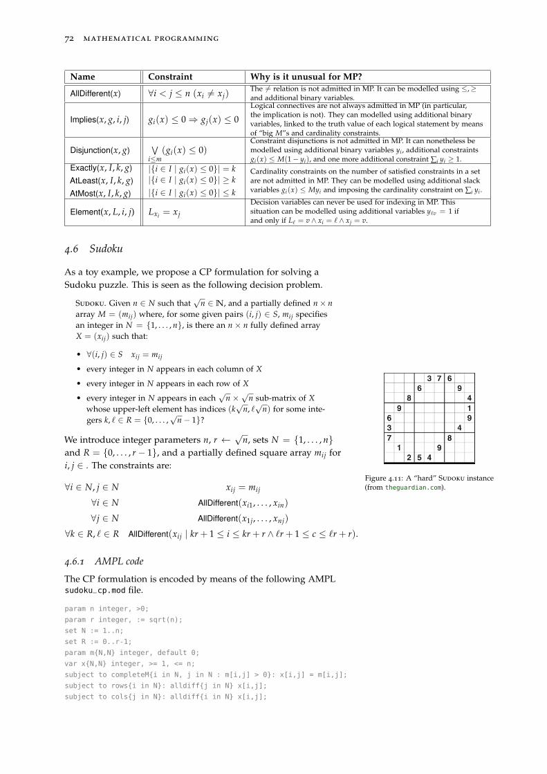
72 mathematical programming
Name Constraint Why is it unusual for MP?
AllDifferent(x) ∀i < j ≤ n (xi 6= xj)The 6= relation is not admitted in MP. It can be modelled using ≤,≥and additional binary variables.
Implies(x, g, i, j) gi(x) ≤ 0⇒ gj(x) ≤ 0
Logical connectives are not always admitted in MP (in particular,the implication is not). They can modelled using additional binaryvariables, linked to the truth value of each logical statement by meansof “big M”s and cardinality constraints.
Disjunction(x, g)∨
i≤m(gi(x) ≤ 0)
Constraint disjunctions is not admitted in MP. It can nonetheless bemodelled using additional binary variables yi , additional constraintsgi(x) ≤ M(1− yi), and one more additional constraint ∑i yi ≥ 1.
Exactly(x, I, k, g)
AtLeast(x, I, k, g)
AtMost(x, I, k, g)
|{i ∈ I | gi(x) ≤ 0}| = k|{i ∈ I | gi(x) ≤ 0}| ≥ k|{i ∈ I | gi(x) ≤ 0}| ≤ k
Cardinality constraints on the number of satisfied constraints in a setare not admitted in MP. They can be modelled using additional slackvariables gi(x) ≤ Myi and imposing the cardinality constraint on ∑i yi .
Element(x, L, i, j) Lxi = xj
Decision variables can never be used for indexing in MP. Thissituation can be modelled using additional variables y`v = 1 ifand only if L` = v ∧ xi = ` ∧ xj = v.
4.6 Sudoku
As a toy example, we propose a CP formulation for solving aSudoku puzzle. This is seen as the following decision problem.
Sudoku. Given n ∈ N such that√
n ∈N, and a partially defined n× narray M = (mij) where, for some given pairs (i, j) ∈ S, mij specifiesan integer in N = {1, . . . , n}, is there an n × n fully defined arrayX = (xij) such that:
• ∀(i, j) ∈ S xij = mij
• every integer in N appears in each column of X
• every integer in N appears in each row of X
• every integer in N appears in each√
n ×√
n sub-matrix of Xwhose upper-left element has indices (k
√n, `√
n) for some inte-gers k, ` ∈ R = {0, . . . ,
√n− 1}?
Figure 4.11: A “hard” Sudoku instance(from theguardian.com).
We introduce integer parameters n, r ←√
n, sets N = {1, . . . , n}and R = {0, . . . , r− 1}, and a partially defined square array mij fori, j ∈ . The constraints are:
∀i ∈ N, j ∈ N xij = mij
∀i ∈ N AllDifferent(xi1, . . . , xin)
∀j ∈ N AllDifferent(x1j, . . . , xnj)
∀k ∈ R, ` ∈ R AllDifferent(xij | kr + 1 ≤ i ≤ kr + r ∧ `r + 1 ≤ c ≤ `r + r).
4.6.1 AMPL code
The CP formulation is encoded by means of the following AMPLsudoku_cp.mod file.
param n integer, >0;
param r integer, := sqrt(n);
set N := 1..n;
set R := 0..r-1;
param m{N,N} integer, default 0;
var x{N,N} integer, >= 1, <= n;
subject to completeM{i in N, j in N : m[i,j] > 0}: x[i,j] = m[i,j];
subject to rows{i in N}: alldiff{j in N} x[i,j];
subject to cols{j in N}: alldiff{i in N} x[i,j];
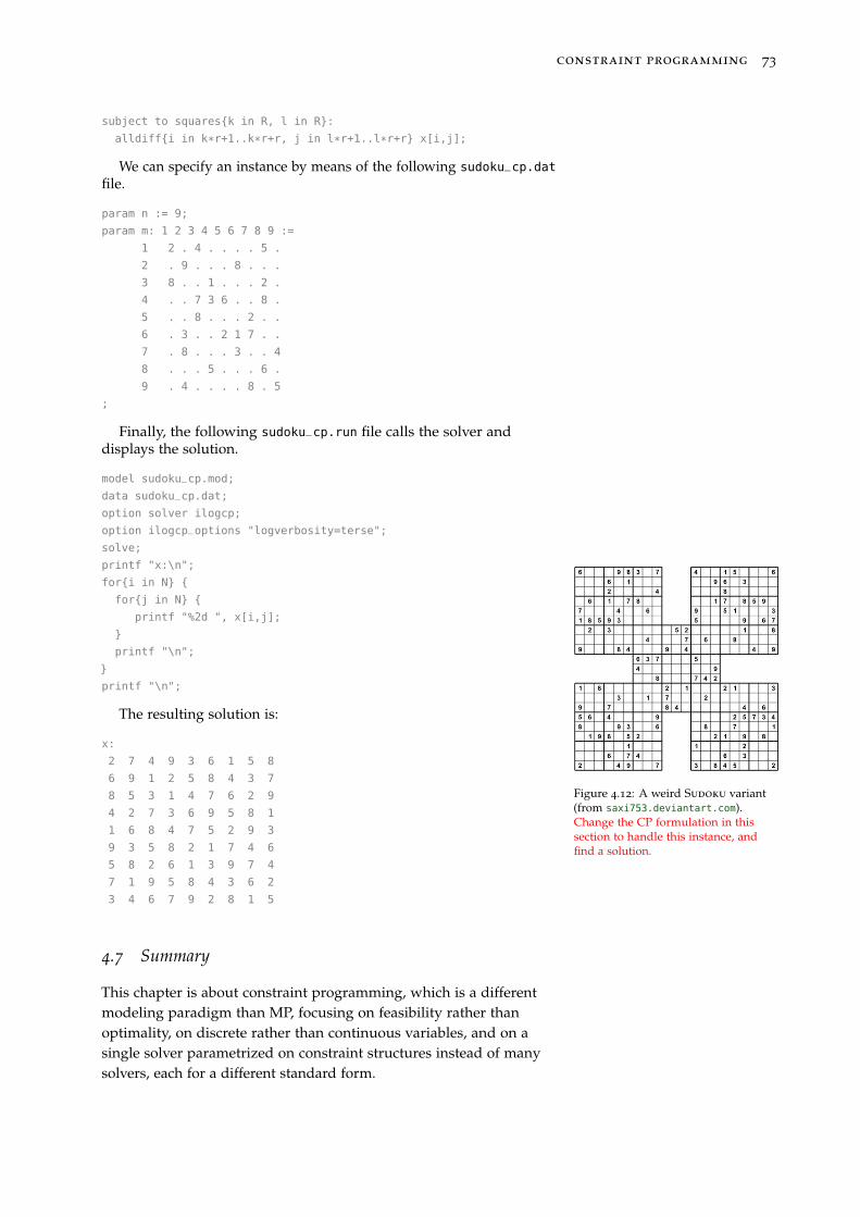
constraint programming 73
subject to squares{k in R, l in R}:
alldiff{i in k*r+1..k*r+r, j in l*r+1..l*r+r} x[i,j];
We can specify an instance by means of the following sudoku_cp.datfile.
param n := 9;
param m: 1 2 3 4 5 6 7 8 9 :=
1 2 . 4 . . . . 5 .
2 . 9 . . . 8 . . .
3 8 . . 1 . . . 2 .
4 . . 7 3 6 . . 8 .
5 . . 8 . . . 2 . .
6 . 3 . . 2 1 7 . .
7 . 8 . . . 3 . . 4
8 . . . 5 . . . 6 .
9 . 4 . . . . 8 . 5
;
Finally, the following sudoku_cp.run file calls the solver anddisplays the solution.
model sudoku_cp.mod;
data sudoku_cp.dat;
option solver ilogcp;
option ilogcp_options "logverbosity=terse";
solve;
printf "x:\n";
for{i in N} {
for{j in N} {
printf "%2d ", x[i,j];
}
printf "\n";
}
printf "\n";
Figure 4.12: A weird Sudoku variant(from saxi753.deviantart.com).Change the CP formulation in thissection to handle this instance, andfind a solution.
The resulting solution is:
x:
2 7 4 9 3 6 1 5 8
6 9 1 2 5 8 4 3 7
8 5 3 1 4 7 6 2 9
4 2 7 3 6 9 5 8 1
1 6 8 4 7 5 2 9 3
9 3 5 8 2 1 7 4 6
5 8 2 6 1 3 9 7 4
7 1 9 5 8 4 3 6 2
3 4 6 7 9 2 8 1 5
4.7 Summary
This chapter is about constraint programming, which is a differentmodeling paradigm than MP, focusing on feasibility rather thanoptimality, on discrete rather than continuous variables, and on asingle solver parametrized on constraint structures instead of manysolvers, each for a different standard form.

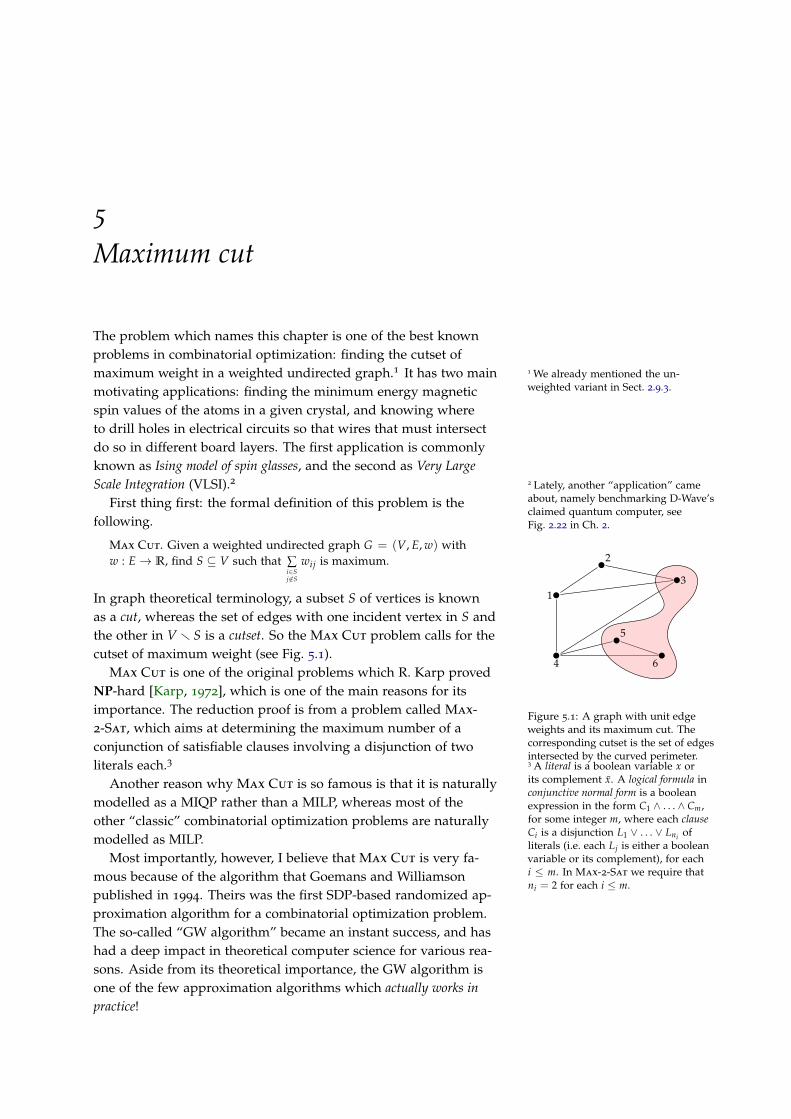
5Maximum cut
The problem which names this chapter is one of the best knownproblems in combinatorial optimization: finding the cutset ofmaximum weight in a weighted undirected graph.1 It has two main 1 We already mentioned the un-
weighted variant in Sect. 2.9.3.motivating applications: finding the minimum energy magneticspin values of the atoms in a given crystal, and knowing whereto drill holes in electrical circuits so that wires that must intersectdo so in different board layers. The first application is commonlyknown as Ising model of spin glasses, and the second as Very LargeScale Integration (VLSI).2 2 Lately, another “application” came
about, namely benchmarking D-Wave’sclaimed quantum computer, seeFig. 2.22 in Ch. 2.
1
2
3
4
5
6
Figure 5.1: A graph with unit edgeweights and its maximum cut. Thecorresponding cutset is the set of edgesintersected by the curved perimeter.
First thing first: the formal definition of this problem is thefollowing.
Max Cut. Given a weighted undirected graph G = (V, E, w) withw : E→ R, find S ⊆ V such that ∑
i∈Sj 6∈S
wij is maximum.
In graph theoretical terminology, a subset S of vertices is knownas a cut, whereas the set of edges with one incident vertex in S andthe other in V r S is a cutset. So the Max Cut problem calls for thecutset of maximum weight (see Fig. 5.1).
Max Cut is one of the original problems which R. Karp provedNP-hard [Karp, 1972], which is one of the main reasons for itsimportance. The reduction proof is from a problem called Max-2-Sat, which aims at determining the maximum number of aconjunction of satisfiable clauses involving a disjunction of twoliterals each.3 3 A literal is a boolean variable x or
its complement x. A logical formula inconjunctive normal form is a booleanexpression in the form C1 ∧ . . . ∧ Cm,for some integer m, where each clauseCi is a disjunction L1 ∨ . . . ∨ Lni ofliterals (i.e. each Lj is either a booleanvariable or its complement), for eachi ≤ m. In Max-2-Sat we require thatni = 2 for each i ≤ m.
Another reason why Max Cut is so famous is that it is naturallymodelled as a MIQP rather than a MILP, whereas most of theother “classic” combinatorial optimization problems are naturallymodelled as MILP.
Most importantly, however, I believe that Max Cut is very fa-mous because of the algorithm that Goemans and Williamsonpublished in 1994. Theirs was the first SDP-based randomized ap-proximation algorithm for a combinatorial optimization problem.The so-called “GW algorithm” became an instant success, and hashad a deep impact in theoretical computer science for various rea-sons. Aside from its theoretical importance, the GW algorithm isone of the few approximation algorithms which actually works inpractice!
76 mathematical programming
5.1 Approximation algorithms
In order to understand this mysterious business of algorithmswhich “surprisingly work4 in practice”, let us see what an approx- 4 The literature is full of approximation
algorithms which prove a theoreticalapproximation property, but havenever been tested in practice. Everytime I can, I ask presenting authorsof new approximation algorithmswhether they have tested their algo-rithms computationally: more oftenthan not, the answer is “why? what isthe point in that?”.
imation algorithm is. Suppose we are trying to solve an instance Iof a minimization problem P ≡ min
x∈Xf (I , x) having minimum ob-
jective function value f ∗. We design an algorithm A, but we cannotprove it will find an exact global optimum,5 so it finds a feasible
5 In other words, the algorithm is notexact.
point x′ ∈ X with objective function value f ′ > f ∗. If we can provethat A yields a ratio f ′
f ∗ which is bounded above by a quantity φ forall instances of P, then A is a φ-approximation algorithm for P.
Now let I be an instance of a maximization6 problem P ≡6 Since Max Cut is a maximizationproblem, this is the relevant point ofview.
maxx∈X
f (I , x) with optimal objective function value f ∗. As before, we
have an algorithm A which is not exact, so it finds a feasible pointx′ ∈ X with value7 f ′ < f ∗. If we can prove that A yields a ratio f ′
f ∗7 Note the inequality sense haschanged, since we are maximizing.which is bounded below by a quantity φ for all instances of P, then
A is a φ-approximation algorithm for P.
5.1.1 Approximation schemes
The quantity φ is a function φ(|I|) of the size taken to store theinstance I . The best case occurs when φ is a constant, the closer to1 the better. Among the constant approximation algorithms, thosegiving the best solutions are those which, for any given ε > 0,provide an approximation ratio 1 + ε (for minimization) and 1− ε
(for maximization) in polynomial time. Such algorithms are calledpolynomial-time approximation schemes (PTAS).
In general, we only consider approximation algorithms whichterminate in polynomial time. The reason is that simple, brute-forceexponential time exact algorithms exist to solve any NP-completeproblems and many interesting NP-hard problems. Forsaking anexactness guarantee is customarily considered acceptable if, inexchange, we can find an approximate solution in polynomial time.
PTAS, specifically, can take as much as φ(|I|1/ε) time to termi-nate, where φ is a polynomial. Obviously, as ε becomes smaller, 1/ε
can become very large. Those PTAS which run in polynomial timeof both |I| and 1/ε are called fully polynomial time approximationschemes, or FPTAS.
5.2 Randomized algorithms
A randomized algorithm employs a source of randomness as partof its input. We are interested in Monte Carlo randomized algo-rithms, which may output a wrong result with bounded probability.
In order to make this statement more precise, consider a decisionproblem P, and an algorithm R which, when presented with aNO instance of P, outputs NO with certainty, but when presentedwith a YES instance, only outputs YES with probability pR >12 . The class of all such problems is called RP (which stands for
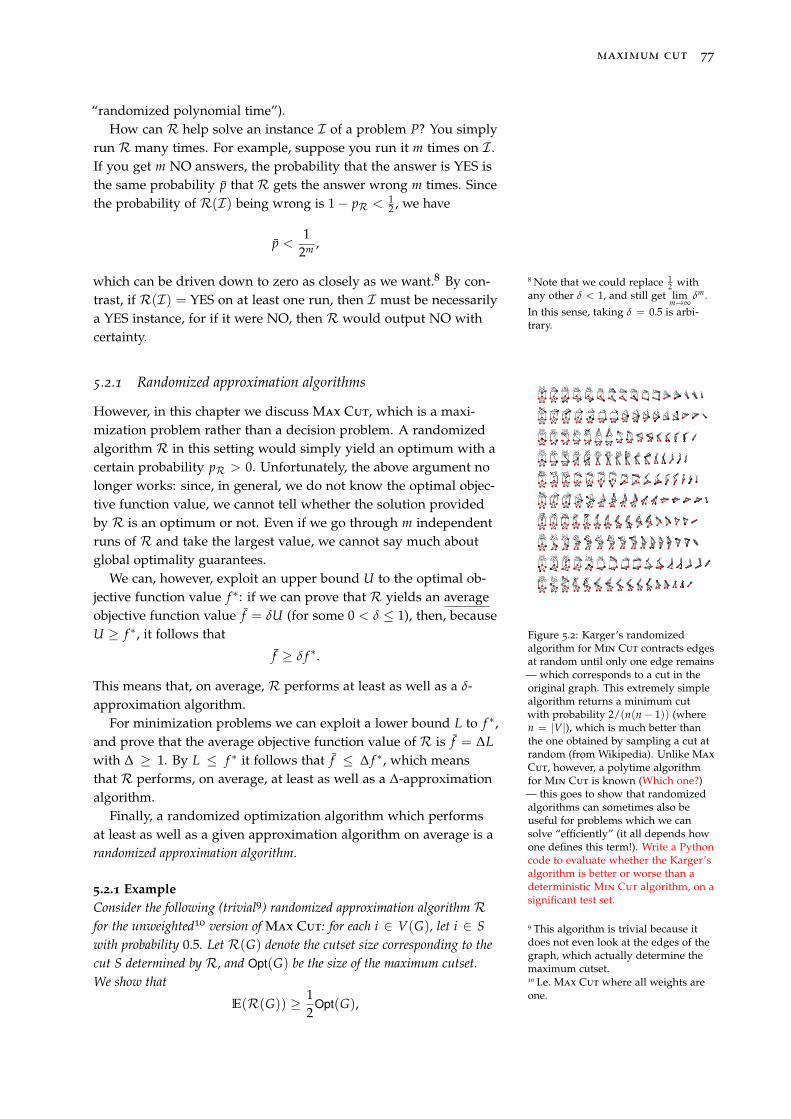
maximum cut 77
“randomized polynomial time”).How can R help solve an instance I of a problem P? You simply
run R many times. For example, suppose you run it m times on I .If you get m NO answers, the probability that the answer is YES isthe same probability p that R gets the answer wrong m times. Sincethe probability of R(I) being wrong is 1− pR < 1
2 , we have
p <1
2m ,
which can be driven down to zero as closely as we want.8 By con- 8 Note that we could replace 12 with
any other δ < 1, and still get limm→∞
δm.
In this sense, taking δ = 0.5 is arbi-trary.
trast, if R(I) = YES on at least one run, then I must be necessarilya YES instance, for if it were NO, then R would output NO withcertainty.
5.2.1 Randomized approximation algorithms
However, in this chapter we discuss Max Cut, which is a maxi-mization problem rather than a decision problem. A randomizedalgorithm R in this setting would simply yield an optimum with acertain probability pR > 0. Unfortunately, the above argument nolonger works: since, in general, we do not know the optimal objec-tive function value, we cannot tell whether the solution providedby R is an optimum or not. Even if we go through m independentruns of R and take the largest value, we cannot say much aboutglobal optimality guarantees.
Figure 5.2: Karger’s randomizedalgorithm for Min Cut contracts edgesat random until only one edge remains— which corresponds to a cut in theoriginal graph. This extremely simplealgorithm returns a minimum cutwith probability 2/(n(n− 1)) (wheren = |V|), which is much better thanthe one obtained by sampling a cut atrandom (from Wikipedia). Unlike Max
Cut, however, a polytime algorithmfor Min Cut is known (Which one?)— this goes to show that randomizedalgorithms can sometimes also beuseful for problems which we cansolve “efficiently” (it all depends howone defines this term!). Write a Pythoncode to evaluate whether the Karger’salgorithm is better or worse than adeterministic Min Cut algorithm, on asignificant test set.
We can, however, exploit an upper bound U to the optimal ob-jective function value f ∗: if we can prove that R yields an averageobjective function value f = δU (for some 0 < δ ≤ 1), then, becauseU ≥ f ∗, it follows that
f ≥ δ f ∗.
This means that, on average, R performs at least as well as a δ-approximation algorithm.
For minimization problems we can exploit a lower bound L to f ∗,and prove that the average objective function value of R is f = ∆Lwith ∆ ≥ 1. By L ≤ f ∗ it follows that f ≤ ∆ f ∗, which meansthat R performs, on average, at least as well as a ∆-approximationalgorithm.
Finally, a randomized optimization algorithm which performsat least as well as a given approximation algorithm on average is arandomized approximation algorithm.
5.2.1 ExampleConsider the following (trivial9) randomized approximation algorithm R
9 This algorithm is trivial because itdoes not even look at the edges of thegraph, which actually determine themaximum cutset.
for the unweighted10 version of Max Cut: for each i ∈ V(G), let i ∈ S
10 I.e. Max Cut where all weights areone.
with probability 0.5. Let R(G) denote the cutset size corresponding to thecut S determined by R, and Opt(G) be the size of the maximum cutset.We show that
E(R(G)) ≥ 12
Opt(G),
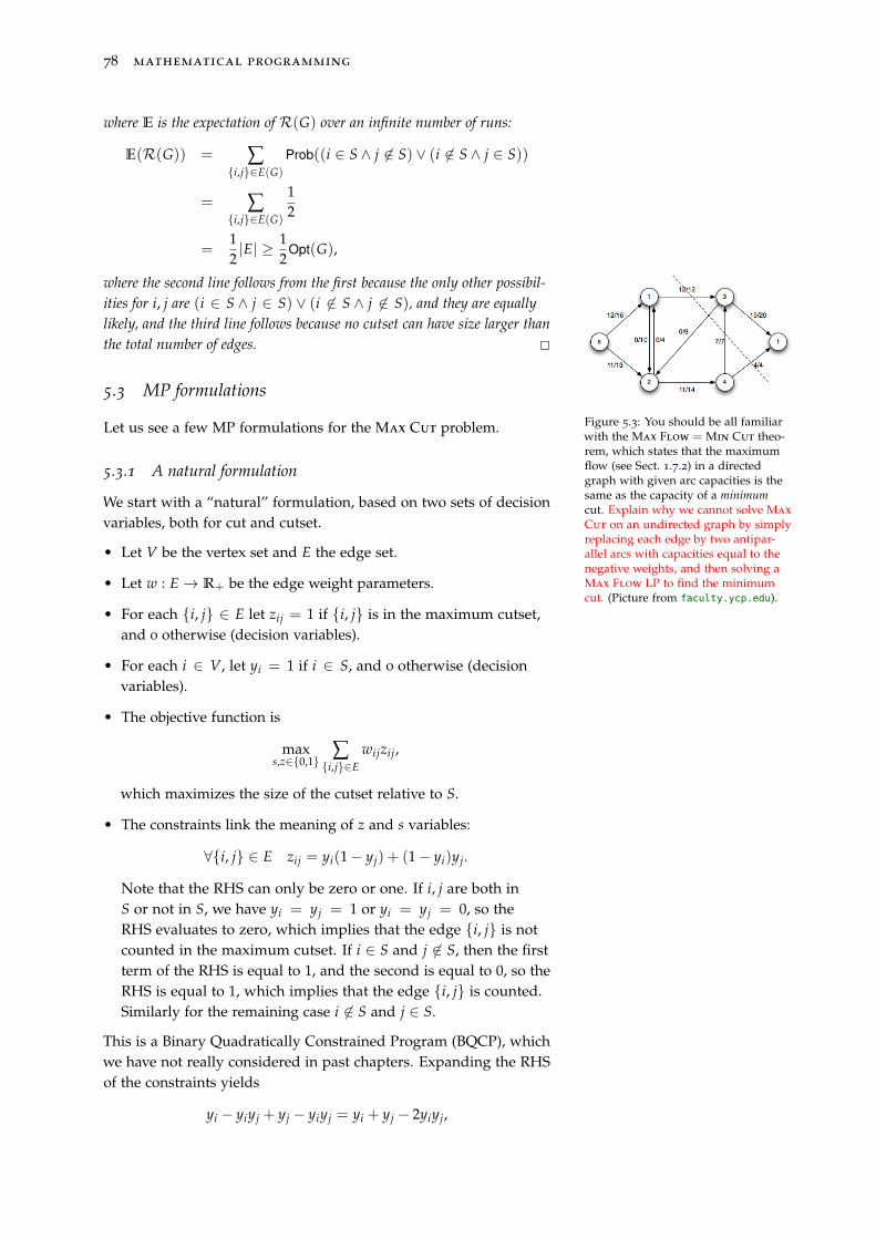
78 mathematical programming
where E is the expectation of R(G) over an infinite number of runs:
E(R(G)) = ∑{i,j}∈E(G)
Prob((i ∈ S ∧ j 6∈ S) ∨ (i 6∈ S ∧ j ∈ S))
= ∑{i,j}∈E(G)
12
=12|E| ≥ 1
2Opt(G),
where the second line follows from the first because the only other possibil-ities for i, j are (i ∈ S ∧ j ∈ S) ∨ (i 6∈ S ∧ j 6∈ S), and they are equallylikely, and the third line follows because no cutset can have size larger thanthe total number of edges. 2
5.3 MP formulations
Let us see a few MP formulations for the Max Cut problem. Figure 5.3: You should be all familiarwith the Max Flow = Min Cut theo-rem, which states that the maximumflow (see Sect. 1.7.2) in a directedgraph with given arc capacities is thesame as the capacity of a minimumcut. Explain why we cannot solve Max
Cut on an undirected graph by simplyreplacing each edge by two antipar-allel arcs with capacities equal to thenegative weights, and then solving aMax Flow LP to find the minimumcut. (Picture from faculty.ycp.edu).
5.3.1 A natural formulation
We start with a “natural” formulation, based on two sets of decisionvariables, both for cut and cutset.
• Let V be the vertex set and E the edge set.
• Let w : E→ R+ be the edge weight parameters.
• For each {i, j} ∈ E let zij = 1 if {i, j} is in the maximum cutset,and 0 otherwise (decision variables).
• For each i ∈ V, let yi = 1 if i ∈ S, and 0 otherwise (decisionvariables).
• The objective function is
maxs,z∈{0,1}
∑{i,j}∈E
wijzij,
which maximizes the size of the cutset relative to S.
• The constraints link the meaning of z and s variables:
∀{i, j} ∈ E zij = yi(1− yj) + (1− yi)yj.
Note that the RHS can only be zero or one. If i, j are both inS or not in S, we have yi = yj = 1 or yi = yj = 0, so theRHS evaluates to zero, which implies that the edge {i, j} is notcounted in the maximum cutset. If i ∈ S and j 6∈ S, then the firstterm of the RHS is equal to 1, and the second is equal to 0, so theRHS is equal to 1, which implies that the edge {i, j} is counted.Similarly for the remaining case i 6∈ S and j ∈ S.
This is a Binary Quadratically Constrained Program (BQCP), whichwe have not really considered in past chapters. Expanding the RHSof the constraints yields
yi − yiyj + yj − yiyj = yi + yj − 2yiyj,
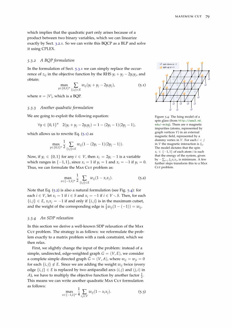
maximum cut 79
which implies that the quadratic part only arises because of aproduct between two binary variables, which we can linearizeexactly by Sect. 3.2.1. So we can write this BQCP as a BLP and solveit using CPLEX.
5.3.2 A BQP formulation
In the formulation of Sect. 5.3.1 we can simply replace the occur-rence of zij in the objective function by the RHS yi + yj − 2yiyj, andobtain:
maxy∈{0,1}n ∑
{i,j}∈Ewij(yi + yj − 2yiyj), (5.1)
where n = |V|, which is a BQP.
5.3.3 Another quadratic formulation
Figure 5.4: The Ising model of aspin glass (from http://www3.nd.
edu/~mcbg). There are n magneticimpurities (atoms, represented bygraph vertices V) in an externalmagnetic field, represented by adummy vertex in V. For each i < jin V the magnetic interaction is Jij.The model dictates that the spinxi ∈ {−1, 1} of each atom i is suchthat the energy of the system, givenby −∑i<j Jijxixj, is minimum. A fewfurther steps transform this to a Max
Cut problem.
We are going to exploit the following equation:
∀y ∈ {0, 1}n 2(yi + yj − 2yiyj) = 1− (2yi − 1)(2yj − 1),
which allows us to rewrite Eq. (5.1) as
maxy∈{0,1}n
12 ∑{i,j}∈E
wij(1− (2yi − 1)(2yj − 1)).
Now, if yi ∈ {0, 1} for any i ∈ V, then xi = 2yi − 1 is a variablewhich ranges in {−1, 1}, since xi = 1 if yi = 1 and xi = −1 if yi = 0.Thus, we can formulate the Max Cut problem as:
maxx∈{−1,1}n
12 ∑{i,j}∈E
wij(1− xixj). (5.2)
Note that Eq. (5.2) is also a natural formulation (see Fig. 5.4): foreach i ∈ V, let xi = 1 if i ∈ S and xi = −1 if i ∈ V rS. Then, for each{i, j} ∈ E, xixj = −1 if and only if {i, j} is in the maximum cutset,and the weight of the corresponding edge is 1
2 wij(1− (−1)) = wij.
5.3.4 An SDP relaxation
In this section we derive a well-known SDP relaxation of the Max
Cut problem. The strategy is as follows: we reformulate the prob-lem exactly to a matrix problem with a rank constraint, which wethen relax.
First, we slightly change the input of the problem: instead of asimple, undirected, edge-weighted graph G = (V, E), we considera complete simple directed graph G = (V, A), where wij = wji = 0for each {i, j} 6∈ E. Since we are adding the weight wij twice (everyedge {i, j} ∈ E is replaced by two antiparallel arcs (i, j) and (j, i) inA), we have to multiply the objective function by another factor 1
2 .This means we can write another quadratic Max Cut formulationas follows:
maxx∈{−1,1}n
14 ∑
i,j∈Vwij(1− xixj). (5.3)
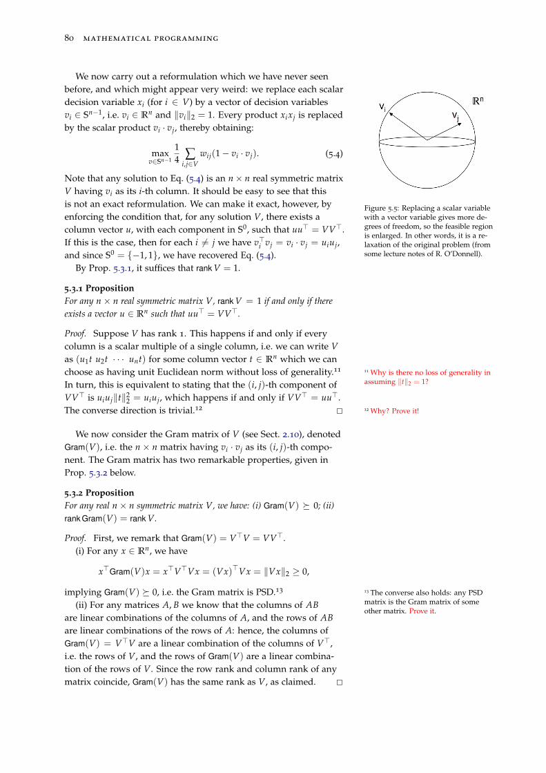
80 mathematical programming
We now carry out a reformulation which we have never seenbefore, and which might appear very weird: we replace each scalardecision variable xi (for i ∈ V) by a vector of decision variablesvi ∈ Sn−1, i.e. vi ∈ Rn and ‖vi‖2 = 1. Every product xixj is replacedby the scalar product vi · vj, thereby obtaining:
Figure 5.5: Replacing a scalar variablewith a vector variable gives more de-grees of freedom, so the feasible regionis enlarged. In other words, it is a re-laxation of the original problem (fromsome lecture notes of R. O’Donnell).
maxv∈Sn−1
14 ∑
i,j∈Vwij(1− vi · vj). (5.4)
Note that any solution to Eq. (5.4) is an n× n real symmetric matrixV having vi as its i-th column. It should be easy to see that thisis not an exact reformulation. We can make it exact, however, byenforcing the condition that, for any solution V, there exists acolumn vector u, with each component in S0, such that uu> = VV>.If this is the case, then for each i 6= j we have v>i vj = vi · vj = uiuj,and since S0 = {−1, 1}, we have recovered Eq. (5.4).
By Prop. 5.3.1, it suffices that rank V = 1.
5.3.1 PropositionFor any n× n real symmetric matrix V, rank V = 1 if and only if thereexists a vector u ∈ Rn such that uu> = VV>.
Proof. Suppose V has rank 1. This happens if and only if everycolumn is a scalar multiple of a single column, i.e. we can write Vas (u1t u2t · · · unt) for some column vector t ∈ Rn which we canchoose as having unit Euclidean norm without loss of generality.11 11 Why is there no loss of generality in
assuming ‖t‖2 = 1?In turn, this is equivalent to stating that the (i, j)-th component ofVV> is uiuj‖t‖2
2 = uiuj, which happens if and only if VV> = uu>.The converse direction is trivial.12 2 12 Why? Prove it!
We now consider the Gram matrix of V (see Sect. 2.10), denotedGram(V), i.e. the n × n matrix having vi · vj as its (i, j)-th compo-nent. The Gram matrix has two remarkable properties, given inProp. 5.3.2 below.
5.3.2 PropositionFor any real n× n symmetric matrix V, we have: (i) Gram(V) � 0; (ii)rank Gram(V) = rank V.
Proof. First, we remark that Gram(V) = V>V = VV>.(i) For any x ∈ Rn, we have
x>Gram(V)x = x>V>Vx = (Vx)>Vx = ‖Vx‖2 ≥ 0,
implying Gram(V) � 0, i.e. the Gram matrix is PSD.13 13 The converse also holds: any PSDmatrix is the Gram matrix of someother matrix. Prove it.
(ii) For any matrices A, B we know that the columns of ABare linear combinations of the columns of A, and the rows of ABare linear combinations of the rows of A: hence, the columns ofGram(V) = V>V are a linear combination of the columns of V>,i.e. the rows of V, and the rows of Gram(V) are a linear combina-tion of the rows of V. Since the row rank and column rank of anymatrix coincide, Gram(V) has the same rank as V, as claimed. 2
maximum cut 81
5.3.3 CorollaryIf X = (Xij) = Gram(V) and rank X = 1, then there exists a vector usuch that Xij = uiuj.
Proof. Since rank X = 1 and X is the Gram matrix of V, thenrank V = 1 by Prop. 5.3.2, which, by Prop. 5.3.1 implies the existenceof u such that uu> = VV> = Gram(V) = X. 2
By Cor. 5.3.3, we can reformulate Eq. (5.4) as:
max 14 ∑
i,j∈Vwij(1− Xij)
Diag(X) = IX � 0
rank X = 1,
(5.5)
where Diag(X) is the matrix consisting of the diagonal entries of X,and I is the identity matrix.
Lastly, we look at the objective function of Eq. (5.5) more closely:
∑i,j∈V
wij(1− Xij)
= ∑i,j∈V
wij1− ∑i,j∈V
wijXij
Diag(X) = 1⇒ ∀i ∈ V Xii = 1 = ∑
i,j∈VwijXii − ∑
i,j∈VwijXij
= ∑i∈V
(∑j∈V
wij
)Xii − A • X
= D • X− A • X
= (D− A) • X,
where A = (wij) is the weighted adjacency matrix of the inputdigraph G, and D is the matrix having ∑
j∈Vwij on the i-th diagonal
element, and 0 elsewhere. Note that the matrix L = D − A iscommonly known as the weighted Laplacian of the graph14 G. 14 Why is the weighted Laplacian
defined on undirected graphs, yet werefer it to an input which is a directedgraph?
Our matrix formulation of the Max Cut is therefore:
max 14 L • X
Diag(X) = IX � 0
rank X = 1.
(5.6)
An SDP relaxation of Eq. (5.6) can now be easily derived by drop-ping the constraint rank X = 1:
max 14 L • X
Diag(X) = IX � 0.
(5.7)
As mentioned in Sect. 2.10, SDPs can be solved in polynomial timeto any desired ε accuracy by means of IPM.
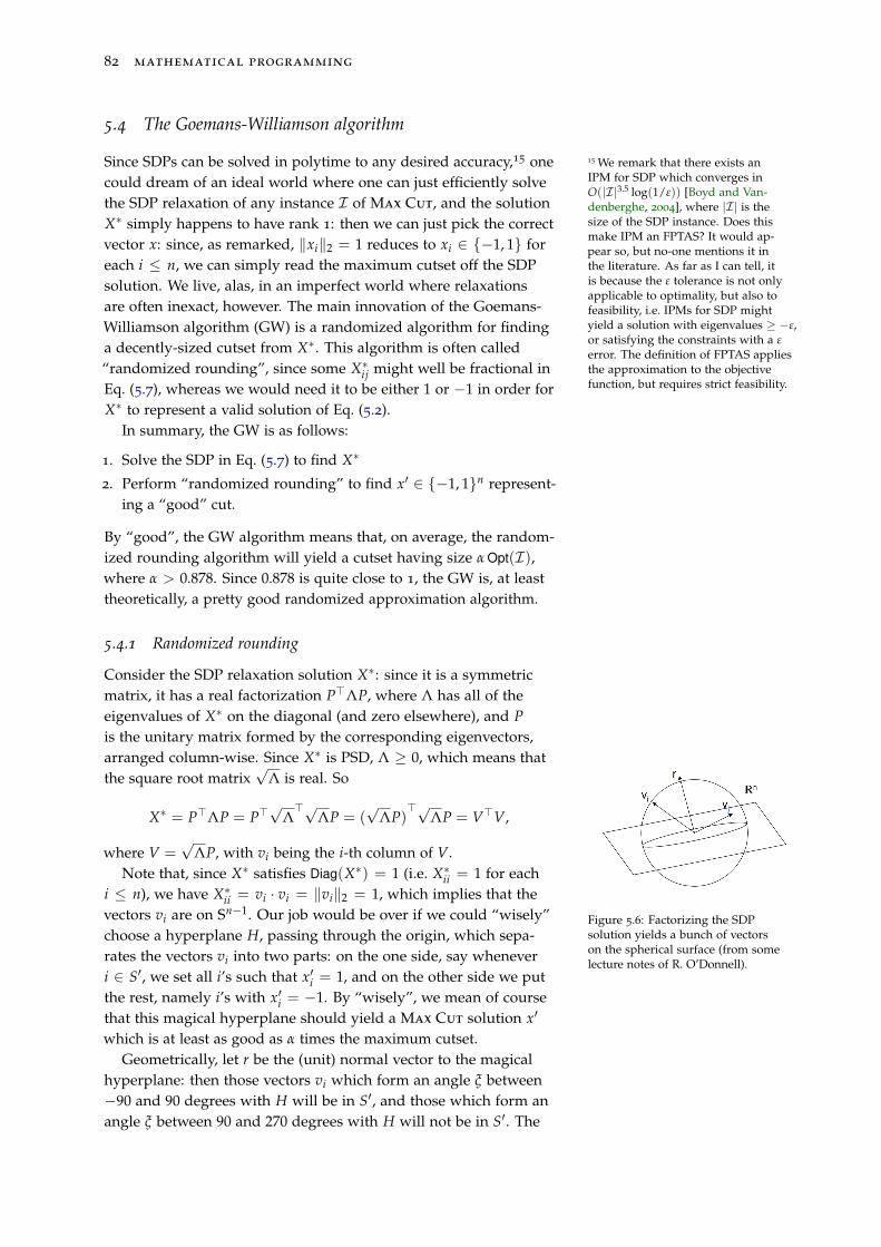
82 mathematical programming
5.4 The Goemans-Williamson algorithm
Since SDPs can be solved in polytime to any desired accuracy,15 one 15 We remark that there exists anIPM for SDP which converges inO(|I|3.5 log(1/ε)) [Boyd and Van-denberghe, 2004], where |I| is thesize of the SDP instance. Does thismake IPM an FPTAS? It would ap-pear so, but no-one mentions it inthe literature. As far as I can tell, itis because the ε tolerance is not onlyapplicable to optimality, but also tofeasibility, i.e. IPMs for SDP mightyield a solution with eigenvalues ≥ −ε,or satisfying the constraints with a εerror. The definition of FPTAS appliesthe approximation to the objectivefunction, but requires strict feasibility.
could dream of an ideal world where one can just efficiently solvethe SDP relaxation of any instance I of Max Cut, and the solutionX∗ simply happens to have rank 1: then we can just pick the correctvector x: since, as remarked, ‖xi‖2 = 1 reduces to xi ∈ {−1, 1} foreach i ≤ n, we can simply read the maximum cutset off the SDPsolution. We live, alas, in an imperfect world where relaxationsare often inexact, however. The main innovation of the Goemans-Williamson algorithm (GW) is a randomized algorithm for findinga decently-sized cutset from X∗. This algorithm is often called“randomized rounding”, since some X∗ij might well be fractional inEq. (5.7), whereas we would need it to be either 1 or −1 in order forX∗ to represent a valid solution of Eq. (5.2).
In summary, the GW is as follows:
1. Solve the SDP in Eq. (5.7) to find X∗
2. Perform “randomized rounding” to find x′ ∈ {−1, 1}n represent-ing a “good” cut.
By “good”, the GW algorithm means that, on average, the random-ized rounding algorithm will yield a cutset having size α Opt(I),where α > 0.878. Since 0.878 is quite close to 1, the GW is, at leasttheoretically, a pretty good randomized approximation algorithm.
5.4.1 Randomized rounding
Consider the SDP relaxation solution X∗: since it is a symmetricmatrix, it has a real factorization P>ΛP, where Λ has all of theeigenvalues of X∗ on the diagonal (and zero elsewhere), and Pis the unitary matrix formed by the corresponding eigenvectors,arranged column-wise. Since X∗ is PSD, Λ ≥ 0, which means thatthe square root matrix
√Λ is real. So
X∗ = P>ΛP = P>√
Λ>√
ΛP = (√
ΛP)>√
ΛP = V>V,
where V =√
ΛP, with vi being the i-th column of V.
Figure 5.6: Factorizing the SDPsolution yields a bunch of vectorson the spherical surface (from somelecture notes of R. O’Donnell).
Note that, since X∗ satisfies Diag(X∗) = 1 (i.e. X∗ii = 1 for eachi ≤ n), we have X∗ii = vi · vi = ‖vi‖2 = 1, which implies that thevectors vi are on Sn−1. Our job would be over if we could “wisely”choose a hyperplane H, passing through the origin, which sepa-rates the vectors vi into two parts: on the one side, say wheneveri ∈ S′, we set all i’s such that x′i = 1, and on the other side we putthe rest, namely i’s with x′i = −1. By “wisely”, we mean of coursethat this magical hyperplane should yield a Max Cut solution x′
which is at least as good as α times the maximum cutset.Geometrically, let r be the (unit) normal vector to the magical
hyperplane: then those vectors vi which form an angle ξ between−90 and 90 degrees with H will be in S′, and those which form anangle ξ between 90 and 270 degrees with H will not be in S′. The
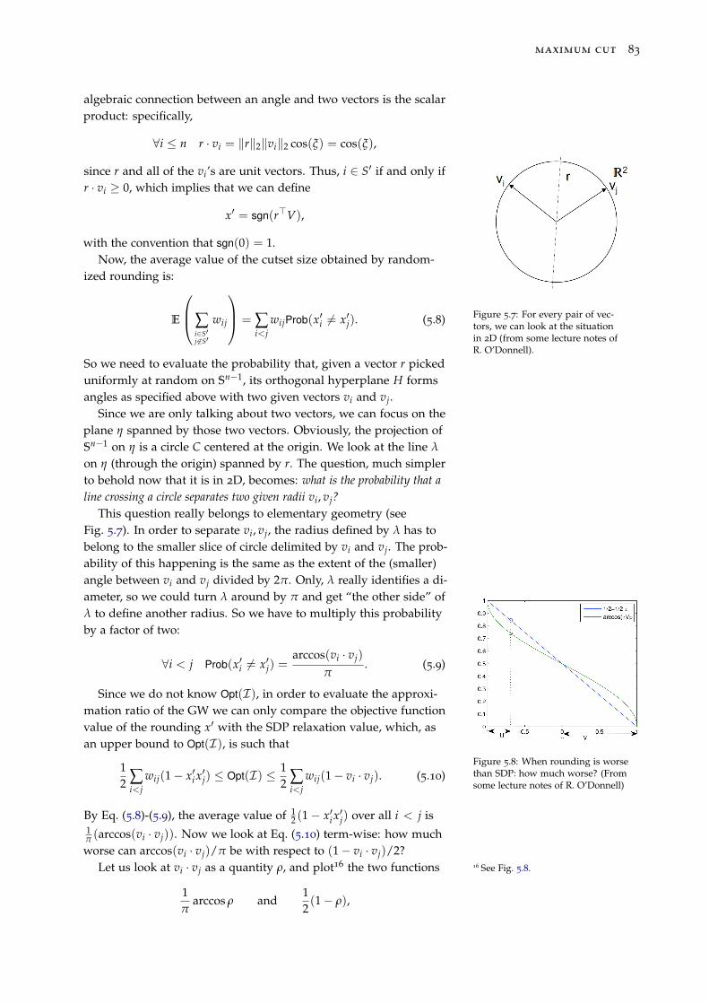
maximum cut 83
algebraic connection between an angle and two vectors is the scalarproduct: specifically,
∀i ≤ n r · vi = ‖r‖2‖vi‖2 cos(ξ) = cos(ξ),
since r and all of the vi’s are unit vectors. Thus, i ∈ S′ if and only ifr · vi ≥ 0, which implies that we can define
x′ = sgn(r>V),
with the convention that sgn(0) = 1.
Figure 5.7: For every pair of vec-tors, we can look at the situationin 2D (from some lecture notes ofR. O’Donnell).
Now, the average value of the cutset size obtained by random-ized rounding is:
E
∑i∈S′j 6∈S′
wij
= ∑i<j
wijProb(x′i 6= x′j). (5.8)
So we need to evaluate the probability that, given a vector r pickeduniformly at random on Sn−1, its orthogonal hyperplane H formsangles as specified above with two given vectors vi and vj.
Since we are only talking about two vectors, we can focus on theplane η spanned by those two vectors. Obviously, the projection ofSn−1 on η is a circle C centered at the origin. We look at the line λ
on η (through the origin) spanned by r. The question, much simplerto behold now that it is in 2D, becomes: what is the probability that aline crossing a circle separates two given radii vi, vj?
This question really belongs to elementary geometry (seeFig. 5.7). In order to separate vi, vj, the radius defined by λ has tobelong to the smaller slice of circle delimited by vi and vj. The prob-ability of this happening is the same as the extent of the (smaller)angle between vi and vj divided by 2π. Only, λ really identifies a di-ameter, so we could turn λ around by π and get “the other side” ofλ to define another radius. So we have to multiply this probabilityby a factor of two:
∀i < j Prob(x′i 6= x′j) =arccos(vi · vj)
π. (5.9)
Figure 5.8: When rounding is worsethan SDP: how much worse? (Fromsome lecture notes of R. O’Donnell)
Since we do not know Opt(I), in order to evaluate the approxi-mation ratio of the GW we can only compare the objective functionvalue of the rounding x′ with the SDP relaxation value, which, asan upper bound to Opt(I), is such that
12 ∑
i<jwij(1− x′i x
′j) ≤ Opt(I) ≤ 1
2 ∑i<j
wij(1− vi · vj). (5.10)
By Eq. (5.8)-(5.9), the average value of 12 (1− x′i x
′j) over all i < j is
1π (arccos(vi · vj)). Now we look at Eq. (5.10) term-wise: how muchworse can arccos(vi · vj)/π be with respect to (1− vi · vj)/2?
Let us look at vi · vj as a quantity ρ, and plot16 the two functions 16 See Fig. 5.8.
1π
arccos ρ and12(1− ρ),
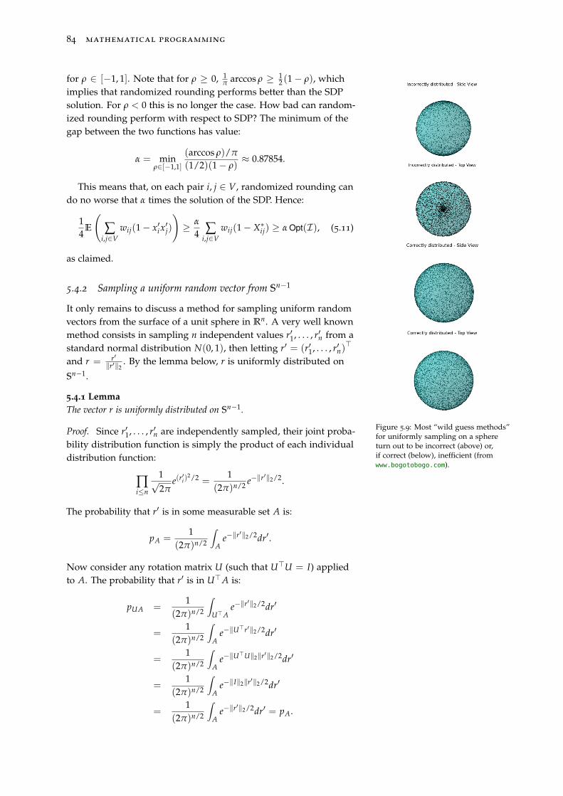
84 mathematical programming
for ρ ∈ [−1, 1]. Note that for ρ ≥ 0, 1π arccos ρ ≥ 1
2 (1− ρ), whichimplies that randomized rounding performs better than the SDPsolution. For ρ < 0 this is no longer the case. How bad can random-ized rounding perform with respect to SDP? The minimum of thegap between the two functions has value:
α = minρ∈[−1,1]
(arccos ρ)/π
(1/2)(1− ρ)≈ 0.87854.
This means that, on each pair i, j ∈ V, randomized rounding cando no worse that α times the solution of the SDP. Hence:
14
E
(∑
i,j∈Vwij(1− x′i x
′j)
)≥ α
4 ∑i,j∈V
wij(1− X∗ij) ≥ α Opt(I), (5.11)
as claimed.
Figure 5.9: Most “wild guess methods”for uniformly sampling on a sphereturn out to be incorrect (above) or,if correct (below), inefficient (fromwww.bogotobogo.com).
5.4.2 Sampling a uniform random vector from Sn−1
It only remains to discuss a method for sampling uniform randomvectors from the surface of a unit sphere in Rn. A very well knownmethod consists in sampling n independent values r′1, . . . , r′n from astandard normal distribution N(0, 1), then letting r′ = (r′1, . . . , r′n)
>
and r = r′‖r′‖2
. By the lemma below, r is uniformly distributed on
Sn−1.
5.4.1 LemmaThe vector r is uniformly distributed on Sn−1.
Proof. Since r′1, . . . , r′n are independently sampled, their joint proba-bility distribution function is simply the product of each individualdistribution function:
∏i≤n
1√2π
e(r′i)
2/2 =1
(2π)n/2 e−‖r′‖2/2.
The probability that r′ is in some measurable set A is:
pA =1
(2π)n/2
∫A
e−‖r′‖2/2dr′.
Now consider any rotation matrix U (such that U>U = I) appliedto A. The probability that r′ is in U>A is:
pUA =1
(2π)n/2
∫U>A
e−‖r′‖2/2dr′
=1
(2π)n/2
∫A
e−‖U>r′‖2/2dr′
=1
(2π)n/2
∫A
e−‖U>U‖2‖r′‖2/2dr′
=1
(2π)n/2
∫A
e−‖I‖2‖r′‖2/2dr′
=1
(2π)n/2
∫A
e−‖r′‖2/2dr′ = pA.
maximum cut 85
Thus, if s 6= t are points in Sn−1, the probability that r′ = s is thesame as the probability that r′ = t. Hence r, the normalized versionof r′, is uniformly distributed on the unit sphere, as claimed. 2
5.4.3 What can go wrong in practice?
We said at the beginning of this chapter that GW is an approxima-tion algorithm which actually works in practice. We shall see this inSect. 5.5. One word of caution, however: as mentioned in Sidenote15, it is possible that SDP solvers would find slightly infeasiblesolutions, due to their error tolerance, which is in turn due to float-ing point computations. So X∗ might have some slightly negativeeigenvalues, or not satisfy Diag(X∗) = 1 exactly. This has to be dealtwith at the implementation level, rather than algorithmically.
For example, the closest PSD matrix A to a given symmetricmatrix B can be obtained by factorization: let B = P>ΛP, where Λis a diagonal matrix with the eigenvalues (ordered from largest tosmallest) on the diagonal, and the columns of P are the correspond-ing eigenvectors. If Λii ≥ 0 for all i ≤ n, we have a certificate thatB is PSD. However, if there is ` ≤ n such that Λ` < 0 (even thoughperhaps |Λ`| is tiny), then we define Λ+ as Λ, with all eigenvaluesfrom the `-th to the n-th replaced by zeros. We then compute17 17 Note that, since this computation
also involves floating point operations,some error might make some eigen-value of A slightly negative: this isa game of hide-and-seek, where youhave to artfully tune the number ofvery small eigenvalues which you zeroin Λ+.
A = P>Λ+P.Since GW really only relies in the factorization of X∗ into V>V,
you can also address these issues by designing a factorizationalgorithm which is robust to slightly negative eigenvalues in X∗.Most implementations (e.g. in NumPy or Matlab) are not robust inthis sense.
5.5 Python implementation
We now present and discuss a Python program which solves:
• the MIQP formulation in Eq. (5.1), using Pyomo calling CPLEX18; 18 Note that the objective function inEq. (5.1) is quadratic: even thoughCPLEX excels at solving MILPs, itcan solve convex MIQPs quite well(including those with convex nonlinearconstraints). I know, I know: theobjective of Eq. (5.1) is not evenconvex! Ever since version 12.6, CPLEXhas been able to solve also nonconvexMIQPs with nonconvex objectivefunctions (the constrains have to beconvex quadratic, however), by meansof a special-purpose sBB-type solver.
• the MILP formulation derived from applying the binary variableproduct reformulation (Sect. 3.2.1) to Eq. (5.1), using Pyomocalling CPLEX;
• the SDP relaxation in Eq. (5.7) using the alternative19 Picos MP
19 We need an alternative becausePyomo currently does not interface toSDP solvers.
modelling environment in Python, which interfaces to SDPsolvers (through the Python library CvxOpt);
• the Max Cut problem using our own implementation of the GWalgorithm.
5.5.1 Preamble
We import the following libraries:
import time
import sys
86 mathematical programming
import math
import numpy as np
from pyomo.environ import *from pyomo.opt import SolverStatus, TerminationCondition
import pyomo.opt
import cvxopt as cvx
import cvxopt.lapack
import picos as pic
import networkx as nx
We first discuss the standard libraries. We use the time library tocollect CPU timings in order to perform an empirical comparison ofthe different solution approaches. The sys library allows us to passa command line argument to our Python program. The math librarygives direct access to functions such as sqrt, which computes thesquare root of its argument. The numpy library is necessary formany floating point computations, including linear algebra; notewe import numpy as the shortened string np, which makes our codesomewhat neater.
We also import some specific MP-related libraries. We alreadysaw the import sequence for Pyomo. We then import the cvxopt
library and its cvxopt.lapack linear algebra module. We do not usethese libraries explicitly, but they are used by picos, the MP pythonmodelling environment which is specifically suitable for convexoptimization, and can interface with SDP and SOCP solvers. Finally,we store and manipulate graphs using the networkx library, whichwe import as the shortened string nx.
We rely on a few globally defined variables:
GWitn = 10000
MyEpsilon = 1e-6
cplexTimeLimit = 100
GWitn is the maximum number of iterations of the randomizedrounding phase of the GW algorithm. MyEpsilon is used as a float-ing point error tolerance. cplexTimeLimit is the maximum numberof seconds of user20 CPU that CPLEX is allowed to run for. Note 20 CPU timings in most operating
systems (OS) nowadays are reportedas either user, system or total. Theformer is the actual amount of secondsthat the CPU devotes to running thespecific given task being monitored,whereas the latter is user+system.Usually, people are mostly interestedin user CPU time, since the time thecomputer spends doing somethingelse is not relevant to code efficiency —one might consider devoting a wholecomputer to running the relevanttask in single-user mode. With theadvent of multi-core computers, thesetime statistics have become fuzzier:is the time taken to transfer controlor register data from one core toanother classified as system or user?After all the parallelized code wouldnot work without these control anddata transfers. I believe differentOSes employ different definitions ofuser and system times in multi-corecomputers.
that CPLEX, as well as many other MP solvers, does not check thesystem clock very often, probably in an attempt to devote everysingle CPU cycle to finding the solution efficiently. As a result, evenif you set a time limit of 100 seconds, CPLEX might well go oncrunching numbers for considerably more time.
5.5.2 Functions
Next, we briefly introduce the functions we use. In create_maxcut_miqpwe take an undirected graph G (in the form of a networkx object)and use the Pyomo library to model a MIQP formulation of Max
Cut.
def create_maxcut_miqp(G):
maxcut = ConcreteModel()
# 0-1 vars: 0 if node in S, 1 if in \bar{S}
maxcut.y = Var(G.nodes(), within = Binary)
maximum cut 87
# objective: max sum_{ij in E} w_ij * (y_i + y_j - 2 y_i*y_j)
def max_cut(model):
return sum(G[i][j][’weight’] * (model.y[i] + model.y[j] - \
2*model.y[i]*model.y[j]) for (i,j) in G.edges())
maxcut.maxcutobj = Objective(rule = max_cut, sense = maximize)
return maxcut
In create_maxcut_milp we do the same, but we add Fortet’sinequalities to MIQP formulation, and linearize the products yiyj,replacing each bilinear term with a new variable zij (Sect 3.2.1).
def create_maxcut_milp(G):
maxcut = ConcreteModel()
# 0-1 vars: 0 if node in S, 1 if in \bar{S}
maxcut.y = Var(G.nodes(), within = Binary)
# linearization variables z_ij = y_iy_j
maxcut.z = Var(G.edges(), within = PercentFraction)
# objective: max sum_{ij in E} w_ij * (y_i + y_j - 2 z_ij)
def max_cut(model):
return sum(G[i][j][’weight’] * (model.y[i] + model.y[j] - \
2*model.z[i,j]) for (i,j) in G.edges())
maxcut.maxcutobj = Objective(rule = max_cut, sense = maximize)
# Fortet’s linearization constraints
def fortet1(model, i,j):
return model.z[i,j] <= model.y[i]
maxcut.fortet1 = Constraint(G.edges(), rule = fortet1)
def fortet2(model, i,j):
return model.z[i,j] <= model.y[j]
maxcut.fortet2 = Constraint(G.edges(), rule = fortet2)
def fortet3(model, i,j):
return model.z[i,j] >= model.y[i] + model.y[j] - 1
maxcut.fortet3 = Constraint(G.edges(), rule = fortet3)
return maxcut
For the SDP relaxation of Max Cut, we employ a different MPmodelling environment in Python, namely Picos. Note that theargument of create_maxcut_sdp is not the graph, but its Laplacianmatrix. You can hopefully make out what the various instructionsdo by the comments.
def create_maxcut_sdp(Laplacian):
n = Laplacian.shape[0]
# create max cut problem SDP with picos
maxcut = pic.Problem()
# SDP variable: n x n matrix
X = maxcut.add_variable(’X’, (n,n), ’symmetric’)
# constraint: ones on the diagonal
maxcut.add_constraint(pic.tools.diag_vect(X) == 1)
# constraint: X positive semidefinite
maxcut.add_constraint(X >> 0)
# objective function
L = pic.new_param(’L’, Laplacian)
# note that A|B = tr(AB)
maxcut.set_objective(’max’, L|X)
return maxcut
In the GW algorithm the output of the SDP relaxation phase isX∗, but the input to the randomized rounding phase is a matrixfactor V of X∗. The rank_factor function computes this factor.
88 mathematical programming
Note that we try and bound the “negative zero” eigenvalues due tofloating point errors.
def rank_factor(X, rk):
n = X.shape[0]
evl, evc = np.linalg.eigh(X) # extract eigeninfo
# get closest nonneg eigenvals (small neg number --> 0)
evl[evl < 0] = 0
if rk < n:
V = np.transpose(evc[:,-rk:])
for k in range(rk):
V[k] *= math.sqrt(evl[-rk-1])
else:
V = np.transpose(evc[::-1])
for k in range(n):
V[k] *= math.sqrt(evl[::-1][k])
return V
The function closest_sdp removes small negative eigenvaluesfrom a matrix X which should be PSD. We factor X it using eigen-vectors and eigenvalues, we replace negative eigenvalues by zeros,then we multiply the factor and its transpose to retrieve an updatedmatrix X which is PSD. This somehow replicates some of the in-structions found in the function rank_factor above. The point isthat, as emphasized in Sect. 5.4.3, multiplying the factors involvesmany floating point operations, which might introduce new float-ing point errors. Replicating some of these “cleaning” actions helpsreduce the chances of an error in the call to square root functions.21 21 Honestly, I’m not really sure this
further “cleaning step” is whollyjustified — I must have inserted thiscode in consequence of some negativesquare root error occurring in the codeon some instance I was testing. Trya version of the program where youdo not call this function, and see whathappens.
def closest_psd(X):
evl, evc = np.linalg.eigh(X) # extract eigeninfo
# get closest nonneg eigenvals (some -1e-27 --> 0)
evl[evl < 0] = 0
return evc.T.dot(np.diag(evl).dot(evc))
We now come to the randomized rounding algorithm: the func-tion gw_randomized_rounding is wholly commented, so it should beeasy to understand.
def gw_randomized_rounding(V, objX, L, iterations):
n = V.shape[0]
# repeat max iterations times
count = 0
obj = 0
print "maxcut(GW/rnd): improv_itn objfun"
while (count < iterations):
r = np.random.normal(0,1,n) # rnd unfrm vector on unit sphere
r /= np.linalg.norm(r) # normalization
x = np.sign(np.dot(V,r)) # signs of V . r
x[x >= 0] = 1 # in case there’s some zeros
o = np.dot(x.T,np.dot(L,x)) # objective function value
if o > obj:
x_cut = x
obj = o
print count, "\t", obj
count += 1
return (x_cut, obj)
maximum cut 89
5.5.3 Main
We now step through the instructions of the “main” part of ourPython program. First, we read the input file having name given asthe first argument on the comand line.
# read edge list file as input
if len(sys.argv) < 2:
# not enough args on cmd line, error
print "error: need an edge list filename on cmd line"
quit()
# each line of input is arc (i,j) weight w: i j w
G = nx.read_weighted_edgelist(sys.argv[1], nodetype = int)
# make G undirected
G = nx.Graph(G)
For example, the triangle graph with unit weights is:
1 2 1
1 3 1
2 3 1
Figure 5.10: The logo of PICOS (frompicos.zib.de).
Secondly, we solve the MIQP formulation using the standardPyomo constructs (see Sect. 1.8.3).
miqp = create_maxcut_miqp(G)
solver = pyomo.opt.SolverFactory(’cplexamp’, solver_io = ’nl’)
solver.options[’timelimit’] = cplexTimeLimit
solver.options[’mipdisplay’] = 2
t0 = time.time() # start the stopwatch
results = solver.solve(miqp, keepfiles = False, tee = True)
t1 = time.time() # stop it
miqpcpu = t1 - t0 # this is the time taken by the solver
miqp.solutions.load_from(results) # this is an indicator vector
# retrieve the set of the indicator vect. as a dictionary (key:val)
ymiqp = {i:miqp.y[i].value for i in G.nodes()}
miqpcut = [i for i,y in ymiqp.iteritems() if y == 1]
miqpobj = miqp.maxcutobj()
Note the use of the time Python library: we call time.time()around the solver.solve() command, then we take the differenceof the two timings to compute the duration of solver.solve().
Third, we solve the MIQP formulation using the standard Pyomoconstructs (see Sect. 1.8.3).
milp = create_maxcut_milp(G)
t0 = time.time()
results = solver.solve(milp, keepfiles = False, tee = True)
t1 = time.time()
milpcpu = t1 - t0
milp.solutions.load_from(results)
ymilp = {i:milp.y[i].value for i in G.nodes()}
milpcut = [i for i,y in ymilp.iteritems() if y == 1]
milpobj = milp.maxcutobj()
Fourth, we solve the SDP relaxation. Since we modelled the SDPusing Picos, the instructions are different.
L = np.array(1/4.*nx.laplacian_matrix(G).todense()) # compute Laplacian
sdp = create_maxcut_sdp(L) # create max cut SDP relaxation
90 mathematical programming
t0 = time.time() # start watch
sdp.solve(verbose = 0) # solve
t1 = time.time() # stop watch
sdpcpu = t1 - t0 # time difference
sdpobj = sdp.obj_value() # retrieve obj fun value
Xsdp = closest_psd(np.array(sdp.get_valued_variable(’X’))) # retrieve solution
Fifth, we run factor Xsdp and apply randomized rounding.
t0 = time.time()
N = len(G.nodes())
V = rank_factor(Xsdp, N)
(gwcut,gwobj) = gw_randomized_rounding(V, sdp.obj_value(), L, GWitn)
t1 = time.time()
gwcpu = t1 - t0
Lastly, we output our comparison statistics: objective functionvalue and CPU time.
print "maxcut(out): MIQPobj=", miqpobj, ", MIQPcpu=", miqpcpu
print "maxcut(out): MILPobj=", milpobj, ", MILPcpu=", milpcpu
print "maxcut(out): SDPobj=", sdpobj, ", SDPcpu=", sdpcpu
print "maxcut(out): GWobj=", gwobj, ", GWcpu=", gwcpu
This code resides in a text file called maxcut.py, and can be runusing the command line
python maxcut.py file.edg
where file.edg is the instance file with the edge list, as detailedabove (two integers and a floating point number per line, where theintegers are the indices of the vertices adjacent to each edge and thefloating point is its weight).
5.5.4 Comparison on a set of random weighted graphs
I have created22 a set of file in .edg format, each storing a weighted 22 You should do this too! A piece ofadvice: don’t do this by hand — usePython, or another scripting language.
graph generated using the Erdos-Renyi random model. This isas follows: given an integer n and a real p ∈ [0, 1], generate agraph with n vertices, where each edge has probability p of beingcreated. I set the range of n to {10, 20, . . . , 90}, and the range of p to{0.3, 0.5, 0.7}.
I then launched the maxcut.py Python program on each of thefiles, saved the output to a similarly-named .out file, and thenproceeded to collect23 the output data in the table below. Note 23 Again, don’t do this by hand! Parse
the .out file using a program, andoutput a tabular format — or simplyedit the maxcut.py script to write itsoutput in tabular format.
that, since the time limit for CPLEX is set to 100s, CPLEX doesnot have the time to solve all instances will not be solved to globaloptimality.
The first two columns of the table contain the generation param-eters for the random graph. The following four columns containthe objective function values of MIQP, MILP, SDP and randomizedrounding (RR) applied to the SDP solution. The last four columnscontain the user CPU time taken to solve MIQP, MILP, SDP andperform RR (the time for RR includes factoring the output of theSDP solution). Thus, the time taken to run the GW algorithm is
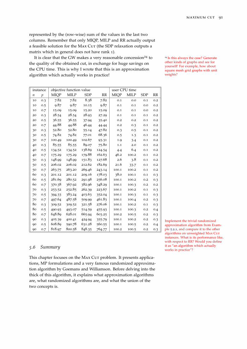
maximum cut 91
represented by the (row-wise) sum of the values in the last twocolumns. Remember that only MIQP, MILP and RR actually outputa feasible solution for the Max Cut (the SDP relaxation outputs amatrix which in general does not have rank 1).
It is clear that the GW makes a very reasonable concession24 to 24 Is this always the case? Generateother kinds of graphs and see foryourself! For example, how aboutsquare mesh grid graphs with unitweights?
the quality of the obtained cut, in exchange for huge savings onthe CPU time. This is why I wrote that this is an approximationalgorithm which actually works in practice!
instance objective function value user CPU timen p MIQP MILP SDP RR MIQP MILP SDP RR10 0.3 7.82 7.82 8.38 7.82 0.1 0.0 0.1 0.210 0.5 9.87 9.87 10.15 9.87 0.1 0.1 0.0 0.210 0.7 15.09 15.09 15.20 15.09 0.1 0.1 0.0 0.220 0.3 28.54 28.54 28.93 27.29 0.1 0.1 0.1 0.220 0.5 36.55 36.55 37.94 35.40 0.2 0.2 0.1 0.220 0.7 44.88 44.88 46.44 44.44 0.2 0.3 0.1 0.230 0.3 52.80 52.80 55.14 47.82 0.3 0.5 0.1 0.230 0.5 74.82 74.82 77.01 68.36 0.5 1.3 0.1 0.230 0.7 100.49 100.49 102.67 93.31 1.9 3.4 0.1 0.240 0.3 85.55 85.55 89.07 75.80 1.1 2.0 0.1 0.240 0.5 134.52 134.52 138.69 124.54 4.4 6.4 0.1 0.240 0.7 175.29 175.29 179.88 162.63 46.2 100.2 0.1 0.250 0.3 148.99 148.99 151.83 127.68 2.6 3.8 0.1 0.250 0.5 206.02 206.02 212.62 182.69 21.6 33.7 0.1 0.250 0.7 263.75 263.20 269.46 243.14 100.1 100.2 0.1 0.260 0.3 201.12 201.12 209.16 178.03 38.0 100.1 0.1 0.360 0.5 281.69 280.52 291.98 256.08 100.1 100.2 0.2 0.360 0.7 370.38 367.92 382.96 348.29 100.1 100.3 0.2 0.270 0.3 253.52 252.85 262.39 223.67 100.1 100.2 0.1 0.370 0.5 394.33 383.24 403.63 352.04 100.1 100.3 0.1 0.370 0.7 497.64 487.58 509.99 461.83 100.1 100.4 0.2 0.380 0.3 309.52 309.52 321.58 276.06 100.1 100.2 0.1 0.380 0.5 490.93 493.07 514.59 455.93 100.1 100.3 0.2 0.480 0.7 648.89 628.01 665.94 603.25 100.2 100.5 0.2 0.390 0.3 405.39 400.41 424.94 355.79 100.1 100.2 0.2 0.390 0.5 608.89 590.78 631.28 560.55 100.1 100.5 0.2 0.490 0.7 818.97 800.58 848.35 764.77 100.2 100.5 0.2 0.3
Implement the trivial randomizedapproximation algorithm from Exam-ple 5.2.1, and compare it to the otheralgorithms on unweighted Max Cut
instances. What is its performance like,with respect to RR? Would you defineit as “an algorithm which actuallyworks in practice”?
5.6 Summary
This chapter focuses on the Max Cut problem. It presents applica-tions, MP formulations and a very famous randomized approxima-tion algorithm by Goemans and Williamson. Before delving into thethick of this algorithm, it explains what approximation algorithmsare, what randomized algorithms are, and what the union of thetwo concepts is.

6Distance Geometry David Hilbert
Leopold Kro-
neckerErnst Zermelo
Adolf FraenkelKurt Gödel
Karl Menger
Distance Geometry (DG) is a sub-field of geometry based on theconcept of points and distances rather than points, lines, planes, hy-perplanes or general manifolds. By far the most common setting iswhere the distances are Euclidean, although early axiomatizationsof DG worked with general (semi)metrics [Menger, 1931, Blumen-thal, 1953]. This novel axiomatization of geometry was proposedat a time where the “old” way of doing mathematics (read: up to1900) was being formalized1 into our current setting. To be honest, 1 Up to 1900, many proofs had ele-
ments of “hand-waving” in them. Atthe end of the 19th century, DavidHilbert decided he’d had enoughof being unable to prove anyonewrong formally (specifically LeopoldKronecker, who kept saying that exis-tential proofs did not prove anything– only constructive proofs were good),and decided to use his extensive in-fluence to steer the community intodefining things formally once and forall. His valiant attempt succeeded toa large extent, insofar as we now havethe Zermelo-Fraenkel-Choice (ZFC)system of axioms, which appear to beenough to do almost anything of inter-est in mathematics, but was ultimatelycrushed by Gödel’s incompletenesstheorem in its aim of having a finitisticmechanical procedure for provingevery true sentence from the axioms.
mathematicians still use a lot of hand-waving [Krantz, 2010], butnow at least they know they could do things completely formally ifthey wanted to.2
2 What if the only way to write acertain proof formally takes longerthan the maximum extent of thehuman life? Well, use computers!What about reading a proof? Today wehave formal proofs, partly or whollywritten out by computers, whichno-one can possibly hope to read in alifetime, much less understand. Canthey still be called proofs? This issimilar to the old “does the universestill exist if no-one’s around to notice?”
6.1 The fundamental problem of DG
The reason why DG and MP are related is through the fundamentalproblem of DG:
Distance Geometry Problem (DGP). Given a positive integer K anda simple undirected weighted graph G = (V, E, d) where d : E → R+
is an edge weight function, is there a realization3 x : V → RK such
3 A realization of a graph is a function,mapping each vertex to a vector ofa Euclidean space, which satisfiesEq. (6.1).
that the constraints:
∀{i, j} ∈ V ‖xi − xj‖ = dij (6.1)
are satisfied?
When the norm in Eq. (6.1) is the 2-norm, the DGP is also calledEuclidean DGP (EDGP), which was introduced in Sect. 2.6.
Because it consists of a set of constraints for which we needto find a solution, the DGP is a CP problem (see Ch. 4). On theother hand, CP problems usually have integer, bounded variables,whereas the DGP has continuous unbounded ones. So it makesmore sense to see it as a feasibility NLP, i.e. an NLP with zeroobjective function.
As mentioned in Sect. 2.6, it is difficult to solve DGPs as systemsof nonlinear constraints, as given in Eq. (6.1). Usually, MP solversare better at improving optimality than ensuring feasibility. A nicefeature of DGPs is that we can write them as a minimization of
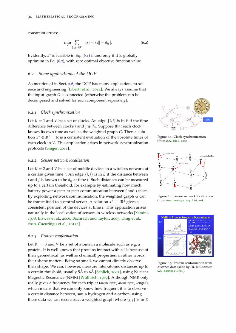
94 mathematical programming
constraint errors:
minx ∑{i,j}∈E
| ‖xi − xj‖ − dij |. (6.2)
Evidently, x∗ is feasible in Eq. (6.1) if and only if it is globallyoptimum in Eq. (6.2), with zero optimal objective function value.
6.2 Some applications of the DGP
As mentioned in Sect. 2.6, the DGP has many applications to sci-ence and engineering [Liberti et al., 2014]. We always assume thatthe input graph G is connected (otherwise the problem can bedecomposed and solved for each component separately).
6.2.1 Clock synchronization
Figure 6.1: Clock synchronization(from www.mdpi.com).
Let K = 1 and V be a set of clocks. An edge {i, j} is in E if the timedifference between clocks i and j is dij. Suppose that each clock iknows its own time as well as the weighted graph G. Then a solu-tion x∗ ∈ R1 = R is a consistent evaluation of the absolute times ofeach clock in V. This application arises in network synchronizationprotocols [Singer, 2011].
6.2.2 Sensor network localization
Figure 6.2: Sensor network localization(from www.commsys.isy.liu.se).
Let K = 2 and V be a set of mobile devices in a wireless network ata certain given time t. An edge {i, j} is in E if the distance betweeni and j is known to be dij at time t. Such distances can be measuredup to a certain threshold, for example by estimating how muchbattery power a peer-to-peer communication between i and j takes.By exploiting network communication, the weighted graph G canbe transmitted to a central server. A solution x∗ ∈ R2 gives aconsistent position of the devices at time t. This application arisesnaturally in the localization of sensors in wireless networks [Yemini,1978, Biswas et al., 2006, Bachrach and Taylor, 2005, Ding et al.,2010, Cucuringu et al., 2012a].
6.2.3 Protein conformation
Figure 6.3: Protein conformation fromdistance data (slide by Dr. B. Chazottewww.campbell.edu).
Let K = 3 and V be a set of atoms in a molecule such as e.g. aprotein. It is well known that proteins interact with cells because oftheir geometrical (as well as chemical) properties: in other words,their shape matters. Being so small, we cannot directly observetheir shape. We can, however, measure inter-atomic distances up toa certain threshold, usually 5Å to 6Å [Schlick, 2002], using NuclearMagnetic Resonance (NMR) [Wüthrich, 1989]. Although NMR onlyreally gives a frequency for each triplet (atom type, atom type, length),which means that we can only know how frequent it is to observea certain distance between, say, a hydrogen and a carbon, usingthese data we can reconstruct a weighted graph where {i, j} is in E
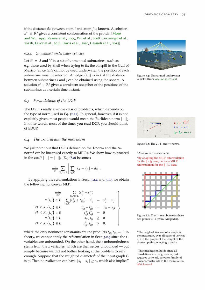
distance geometry 95
if the distance dij between atom i and atom j is known. A solutionx∗ ∈ R3 gives a consistent conformation of the protein [Moréand Wu, 1999, Reams et al., 1999, Wu et al., 2008, Cucuringu et al.,2012b, Lavor et al., 2011, Davis et al., 2010, Cassioli et al., 2015].
6.2.4 Unmanned underwater vehicles
Figure 6.4: Unmanned underwatervehicles (from www.swissint.ch).
Let K = 3 and V be a set of unmanned submarines, such ase.g. those used by Shell when trying to fix the oil spill in the Gulf ofMexico. Since GPS cannot be used underwater, the position of eachsubmarine must be inferred. An edge {i, j} is in E if the distancebetween submarines i and j can be obtained using the sonars. Asolution x∗ ∈ R3 gives a consistent snapshot of the positions of thesubmarines at a certain time instant.
6.3 Formulations of the DGP
The DGP is really a whole class of problems, which depends onthe type of norm used in Eq. (2.21). In general, however, if it is notexplicitly given, most people would mean the Euclidean norm ‖ · ‖2.In other words, most of the times you read DGP, you should thinkof EDGP.
Figure 6.5: The 2-, 1- and ∞-norms.6.4 The 1-norm and the max norm
We just point out that DGPs defined on the 1-norm and the ∞-norm4 can be linearized exactly to MILPs. We show how to proceed 4 Also known as max norm.
in the case5 ‖ · ‖ = ‖ · ‖1. Eq. (6.2) becomes: 5 By adapting the MILP reformulationfor the ‖ · ‖1 case, derive a MILPreformulation for the ‖ · ‖∞ case.
minx ∑{i,j}∈E
∣∣∣∣∣ ∑k≤K|xik − xjk| − dij
∣∣∣∣∣ .
Figure 6.6: The 1-norm between thesetwo points is 12 (from Wikipedia).
By applying the reformulations in Sect. 3.2.4 and 3.1.5 we obtainthe following nonconvex NLP:
minx,s
∑{i,j}∈E
(s+ij + s−ij )
∀{i, j} ∈ E ∑k≤K
(t+ijk + t−ijk)− dij = s+ij − s−ij
∀k ≤ K, {i, j} ∈ E t+ijk − t−ijk = xik − xjk
∀k ≤ K, {i, j} ∈ E t+ijk t−ijk = 0
∀{i, j} ∈ E s+ij , s−ij ≥ 0
∀k ≤ K, {i, j} ∈ E t+ijk, t−ijk ≥ 0,
where the only nonlinear constraints are the products t+ijk t−ijk = 0. Intheory, we cannot apply the reformulation in Sect. 3.2.3 since the tvariables are unbounded. On the other hand, their unboundednessstems from the x variables, which are themselves unbounded — butsimply because we did not bother looking at the problem closelyenough. Suppose that the weighted diameter6 of the input graph G
6 The weighted diameter of a graph isthe maximum, over all pairs of verticesu, v in the graph, of the weight of theshortest path connecting u and v.
is γ. Then no realization can have ‖xi − xj‖ ≥ γ, which also implies7
7 This implication holds since alltranslations are congruences, but itrequires us to add another family of(linear) constraints to the formulation.Which ones?
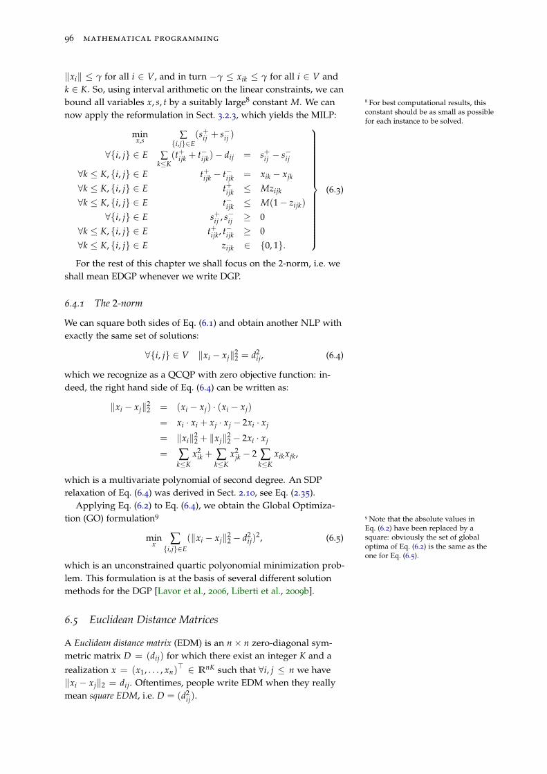
96 mathematical programming
‖xi‖ ≤ γ for all i ∈ V, and in turn −γ ≤ xik ≤ γ for all i ∈ V andk ∈ K. So, using interval arithmetic on the linear constraints, we canbound all variables x, s, t by a suitably large8 constant M. We can 8 For best computational results, this
constant should be as small as possiblefor each instance to be solved.
now apply the reformulation in Sect. 3.2.3, which yields the MILP:
minx,s
∑{i,j}∈E
(s+ij + s−ij )
∀{i, j} ∈ E ∑k≤K
(t+ijk + t−ijk)− dij = s+ij − s−ij
∀k ≤ K, {i, j} ∈ E t+ijk − t−ijk = xik − xjk
∀k ≤ K, {i, j} ∈ E t+ijk ≤ Mzijk
∀k ≤ K, {i, j} ∈ E t−ijk ≤ M(1− zijk)
∀{i, j} ∈ E s+ij , s−ij ≥ 0
∀k ≤ K, {i, j} ∈ E t+ijk, t−ijk ≥ 0
∀k ≤ K, {i, j} ∈ E zijk ∈ {0, 1}.
(6.3)
For the rest of this chapter we shall focus on the 2-norm, i.e. weshall mean EDGP whenever we write DGP.
6.4.1 The 2-norm
We can square both sides of Eq. (6.1) and obtain another NLP withexactly the same set of solutions:
∀{i, j} ∈ V ‖xi − xj‖22 = d2
ij, (6.4)
which we recognize as a QCQP with zero objective function: in-deed, the right hand side of Eq. (6.4) can be written as:
‖xi − xj‖22 = (xi − xj) · (xi − xj)
= xi · xi + xj · xj − 2xi · xj
= ‖xi‖22 + ‖xj‖2
2 − 2xi · xj
= ∑k≤K
x2ik + ∑
k≤Kx2
jk − 2 ∑k≤K
xikxjk,
which is a multivariate polynomial of second degree. An SDPrelaxation of Eq. (6.4) was derived in Sect. 2.10, see Eq. (2.35).
Applying Eq. (6.2) to Eq. (6.4), we obtain the Global Optimiza-tion (GO) formulation9 9 Note that the absolute values in
Eq. (6.2) have been replaced by asquare: obviously the set of globaloptima of Eq. (6.2) is the same as theone for Eq. (6.5).
minx ∑{i,j}∈E
(‖xi − xj‖22 − d2
ij)2, (6.5)
which is an unconstrained quartic polyonomial minimization prob-lem. This formulation is at the basis of several different solutionmethods for the DGP [Lavor et al., 2006, Liberti et al., 2009b].
6.5 Euclidean Distance Matrices
A Euclidean distance matrix (EDM) is an n × n zero-diagonal sym-metric matrix D = (dij) for which there exist an integer K and a
realization x = (x1, . . . , xn)> ∈ RnK such that ∀i, j ≤ n we have
‖xi − xj‖2 = dij. Oftentimes, people write EDM when they reallymean square EDM, i.e. D = (d2
ij).
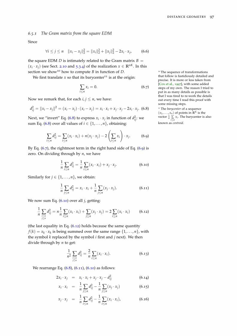
distance geometry 97
6.5.1 The Gram matrix from the square EDM
Since
∀i ≤ j ≤ n ‖xi − xj‖22 = ‖xi‖2
2 + ‖xj‖22 − 2xi · xj, (6.6)
the square EDM D is intimately related to the Gram matrix B =
(xi · xj) (see Sect. 2.10 and 5.3.4) of the realization x ∈ RnK. In thissection we show10 how to compute B in function of D. 10 The sequence of transformations
that follow is fastidiously detailed andprecise. It is more or less taken from[Cox et al., 1997], with some addedsteps of my own. The reason I tried toput in as many details as possible isthat I was tired to re-work the detailsout every time I read this proof withsome missing steps.
We first translate x so that its barycenter11 is at the origin:
11 The barycenter of a sequence(x1, . . . , xn) of points in RK is thevector 1
n ∑i≤n
xi . The barycenter is also
known as centroid.
∑i≤n
xi = 0. (6.7)
Now we remark that, for each i, j ≤ n, we have:
d2ij = ‖xi− xj‖2 = (xi− xj) · (xi− xj) = xi · xi + xj · xj− 2xi · xj. (6.8)
Next, we “invert” Eq. (6.8) to express xi · xj in function of d2ij: we
sum Eq. (6.8) over all values of i ∈ {1, . . . , n}, obtaining:
∑i≤n
d2ij = ∑
i≤n(xi · xi) + n(xj · xj)− 2
(∑i≤n
xi
)· xj. (6.9)
By Eq. (6.7), the rightmost term in the right hand side of Eq. (6.9) iszero. On dividing through by n, we have
1n ∑
i≤nd2
ij =1n ∑
i≤n(xi · xi) + xj · xj. (6.10)
Similarly for j ∈ {1, . . . , n}, we obtain:
1n ∑
j≤nd2
ij = xi · xi +1n ∑
j≤n(xj · xj). (6.11)
We now sum Eq. (6.10) over all j, getting:
1n ∑
i≤nj≤n
d2ij = n
1n ∑
i≤n(xi · xi) + ∑
j≤n(xj · xj) = 2 ∑
i≤n(xi · xi) (6.12)
(the last equality in Eq. (6.12) holds because the same quantityf (k) = xk · xk is being summed over the same range {1, . . . , n}, withthe symbol k replaced by the symbol i first and j next). We thendivide through by n to get:
1n2 ∑
i≤nj≤n
d2ij =
2n ∑
i≤n(xi · xi). (6.13)
We rearrange Eq. (6.8), (6.11), (6.10) as follows:
2xi · xj = xi · xi + xj · xj − d2ij (6.14)
xi · xi =1n ∑
j≤nd2
ij −1n ∑
j≤n(xj · xj) (6.15)
xj · xj =1n ∑
i≤nd2
ij −1n ∑
i≤n(xi · xi), (6.16)
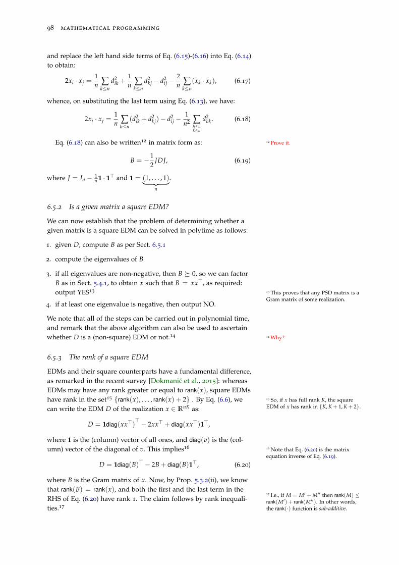
98 mathematical programming
and replace the left hand side terms of Eq. (6.15)-(6.16) into Eq. (6.14)to obtain:
2xi · xj =1n ∑
k≤nd2
ik +1n ∑
k≤nd2
kj − d2ij −
2n ∑
k≤n(xk · xk), (6.17)
whence, on substituting the last term using Eq. (6.13), we have:
2xi · xj =1n ∑
k≤n(d2
ik + d2kj)− d2
ij −1n2 ∑
h≤nk≤n
d2hk. (6.18)
Eq. (6.18) can also be written12 in matrix form as: 12 Prove it.
B = −12
JDJ, (6.19)
where J = In − 1n 1 · 1> and 1 = (1, . . . , 1)︸ ︷︷ ︸
n
.
6.5.2 Is a given matrix a square EDM?
We can now establish that the problem of determining whether agiven matrix is a square EDM can be solved in polytime as follows:
1. given D, compute B as per Sect. 6.5.1
2. compute the eigenvalues of B
3. if all eigenvalues are non-negative, then B � 0, so we can factorB as in Sect. 5.4.1, to obtain x such that B = xx>, as required:output YES13 13 This proves that any PSD matrix is a
Gram matrix of some realization.4. if at least one eigenvalue is negative, then output NO.
We note that all of the steps can be carried out in polynomial time,and remark that the above algorithm can also be used to ascertainwhether D is a (non-square) EDM or not.14 14 Why?
6.5.3 The rank of a square EDM
EDMs and their square counterparts have a fundamental difference,as remarked in the recent survey [Dokmanic et al., 2015]: whereasEDMs may have any rank greater or equal to rank(x), square EDMshave rank in the set15 {rank(x), . . . , rank(x) + 2} . By Eq. (6.6), we 15 So, if x has full rank K, the square
EDM of x has rank in {K, K + 1, K + 2}.can write the EDM D of the realization x ∈ RnK as:
D = 1diag(xx>)> − 2xx> + diag(xx>)1>,
where 1 is the (column) vector of all ones, and diag(v) is the (col-umn) vector of the diagonal of v. This implies16 16 Note that Eq. (6.20) is the matrix
equation inverse of Eq. (6.19).
D = 1diag(B)> − 2B + diag(B)1>, (6.20)
where B is the Gram matrix of x. Now, by Prop. 5.3.2(ii), we knowthat rank(B) = rank(x), and both the first and the last term in theRHS of Eq. (6.20) have rank 1. The claim follows by rank inequali-ties.17
17 I.e., if M = M′ + M′′ then rank(M) ≤rank(M′) + rank(M′′). In other words,the rank(·) function is sub-additive.
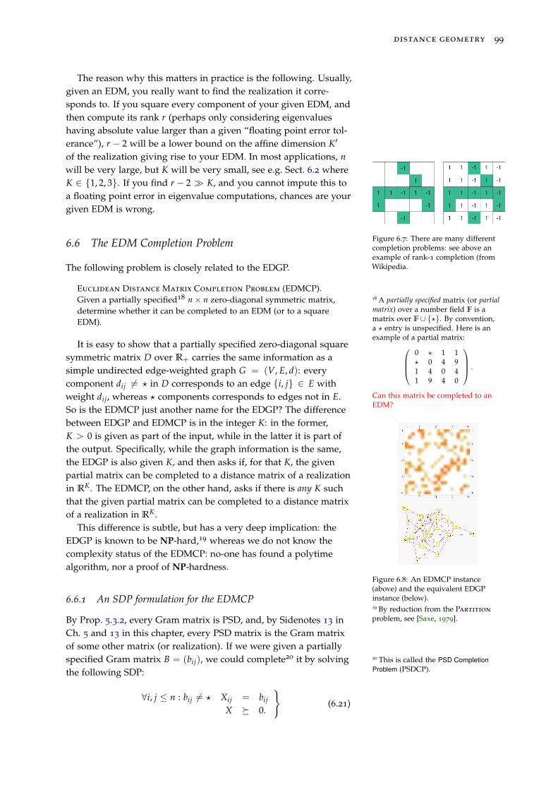
distance geometry 99
The reason why this matters in practice is the following. Usually,given an EDM, you really want to find the realization it corre-sponds to. If you square every component of your given EDM, andthen compute its rank r (perhaps only considering eigenvalueshaving absolute value larger than a given “floating point error tol-erance”), r − 2 will be a lower bound on the affine dimension K′
of the realization giving rise to your EDM. In most applications, nwill be very large, but K will be very small, see e.g. Sect. 6.2 whereK ∈ {1, 2, 3}. If you find r− 2 � K, and you cannot impute this toa floating point error in eigenvalue computations, chances are yourgiven EDM is wrong.
Figure 6.7: There are many differentcompletion problems: see above anexample of rank-1 completion (fromWikipedia.
6.6 The EDM Completion Problem
The following problem is closely related to the EDGP.
Euclidean Distance Matrix Completion Problem (EDMCP).Given a partially specified18 n× n zero-diagonal symmetric matrix, 18 A partially specified matrix (or partial
matrix) over a number field F is amatrix over F ∪ {?}. By convention,a ? entry is unspecified. Here is anexample of a partial matrix:
0 ? 1 1? 0 4 91 4 0 41 9 4 0
.
Can this matrix be completed to anEDM?
determine whether it can be completed to an EDM (or to a squareEDM).
Figure 6.8: An EDMCP instance(above) and the equivalent EDGPinstance (below).
It is easy to show that a partially specified zero-diagonal squaresymmetric matrix D over R+ carries the same information as asimple undirected edge-weighted graph G = (V, E, d): everycomponent dij 6= ? in D corresponds to an edge {i, j} ∈ E withweight dij, whereas ? components corresponds to edges not in E.So is the EDMCP just another name for the EDGP? The differencebetween EDGP and EDMCP is in the integer K: in the former,K > 0 is given as part of the input, while in the latter it is part ofthe output. Specifically, while the graph information is the same,the EDGP is also given K, and then asks if, for that K, the givenpartial matrix can be completed to a distance matrix of a realizationin RK. The EDMCP, on the other hand, asks if there is any K suchthat the given partial matrix can be completed to a distance matrixof a realization in RK.
This difference is subtle, but has a very deep implication: theEDGP is known to be NP-hard,19 whereas we do not know the
19 By reduction from the Partition
problem, see [Saxe, 1979].
complexity status of the EDMCP: no-one has found a polytimealgorithm, nor a proof of NP-hardness.
6.6.1 An SDP formulation for the EDMCP
By Prop. 5.3.2, every Gram matrix is PSD, and, by Sidenotes 13 inCh. 5 and 13 in this chapter, every PSD matrix is the Gram matrixof some other matrix (or realization). If we were given a partiallyspecified Gram matrix B = (bij), we could complete20 it by solving 20 This is called the PSD Completion
Problem (PSDCP).the following SDP:
∀i, j ≤ n : bij 6= ? Xij = bij
X � 0.
}(6.21)
100 mathematical programming
Any solution X∗ to Eq. (6.21) is a PSD matrix having bij in thecomponents specified by B.
However, we are not given B but the square EDM matrix D =
(d2ij). We therefore use Eq. (6.6) and replace xi · xj by Xij (for all
i, j ≤ n):
∀i, j ≤ n : d2ij 6= ? Xii + Xjj − 2Xij = d2
ij
X � 0.
}(6.22)
Note the similarity of the first constraint of Eq. (6.22) with Eq. (2.34),written in terms of weighted graphs instead of partial matrices.Any solution X∗ to Eq. (6.22) is a PSD matrix, and hence a Grammatrix, such that Xii + Xjj − 2Xij = d2
ij in the components specifiedby D. In other words, if we apply Eq. (6.20) with B replaced by X∗,we get an EDM with the specified entries.
Compare the two SDP formulations for the EDGP (Eq. (2.35))and for the EDMCP (Eq. (6.22)). The former is different, in thatwe use the Schur complement:21 while in the EDGP we require a 21 The Schur complement being PSD
states X � xx>, which is a relaxationof X = xx>. The fact that x (and henceits rank) is explicitly mentioned in theSDP makes the relaxation tighter withrespect to the rank constraint.
PSD solution of a given rank K, in the EDMCP we only want a PSDsolution of any rank (or, in other words, any PSD solution). This iswhy Eq. (2.35) is only a relaxation of the EDGP, whereas Eq. (6.22)is an exact formulation of the EDMCP.
Since SDPs can be solved in polytime and the SDP in Eq. (6.22) isan exact formulation for the EDMCP, why am I saying that no-onefound a polytime algorithm for solving the EDMCP yet? Essentially,because of floating point errors: the IPMs that solve SDPs areapproximate methods: they find a matrix which is approximatelyfeasible with respect to the constraints and approximately PSD (seeSect. 5.4.3). Worst-case complexity classes such as P or NP, however,are defined for precise solutions only. As discussed in Sidenote 15
in Ch. 5, approximate feasibility disqualifies the algorithm frombeing defined as an “approximation algorithm”.
6.6.2 Inner LP approximation of SDPs
SDPs are nice because they usually provide tight relaxations andcan be solved in polytime. On the other hand, current technologycan solve relatively small SDPs, say with matrices of up to around1000 components. In practice, it is not uncommon to see DGP appli-cations where K ∈ {1, 2, 3} but n ≥ 1000. This would yield an SDPvariable matrix with at least one million components. Since SDPsolvers are usually based on IPMs, at each iteration the solver hasto deal with O(106) floating point numbers. Unless the structureof the problem can be exploited to simplify the formulation, SDPsolvers will generally fail. In Sect. 6.7 we will present a heuristicalgorithm which scales better.
Figure 6.9: Amir Ali Ahmadi is themain architect behind the work inSDP approximations by DD matrices.You’ve already seen his mug inFig. 2.30.
Here we discuss an extremely recent method [Majumdar et al.,2014] which can be used to approximate an SDP by means of anLP. Since the LP is based on an inner approximation, any solution X′
found by the LP is also a feasible solution for the SDP. This method
distance geometry 101
is based on diagonal dominance.22 22 An n × n matrix A = (aij) isdiagonally dominant (DD) if Eq. (6.23)holds.
Recall that an SDP is simply an LP defined on a matrix X ofdecision variables, subject to a further PSD constraint X � 0. Wereplace the PSD constraint by the DD constraint:
∀i ≤ n aii ≥ ∑j 6=i|aij|, (6.23)
and remark that any matrix X which is DD is also SDP; this followsdirectly from Gershgorin’s theorem.23 Lastly, we reformulate the 23 The proof on Wikipedia is very clear,
search for “Gershgorin circle theorem”.absolute values in Eq. (6.23) using Eq. (3.16)-(3.18) in Sect. 3.2.4,obtaining the following LP, which will yield solutions of the SDPrelaxation in Eq. (2.35):
∀{i, j} ∈ E Xii + Xjj − 2Xij = d2ij
∀i ∈ V ∑j 6=i
tij ≤ Xii
∀i 6= j ∈ V −tij ≤ Xij ≤ tij.
(6.24)
Note that this is a feasibility LP. We can solve it “as such”, or try tomake the entries of X as small as possible (which might reduce itsrank if many of them become zero) by using min ∑ij tij.
6.6.3 Refining the DD approximation
An iterative refinement method for improving the approximationquality of the solution X of Eq. (6.24) with respect to the SDP isdescribed in [Ahmadi and Hall, 2015]. We present it here in fullgenerality, applied to any SDP.
Figure 6.10: An example of diagonaldominance (from www.voonik.com).
For any n× n matrix U, we have U>U � 0. This follows becauseany Gram matrix is PSD, and, trivially, U>U = Gram(U). Moreover,for any X � 0, we have
U>XU � 0,
since X being PSD means that it is the Gram matrix of some othermatrix V, so
U>XU = U>V>VU = (VU)>VU � 0
as the Gram matrix of VU must be PSD. This means that the set
D(U) = {U>XU | X is DD}
only contains PSD matrices.Let us go back to the general SDP formulation in Eq. (2.32). As
mentioned above, we obtain an inner approximation of this SDPby replacing X � 0 by “X is DD”, which can be reformulated to anLP. This LP has no “adjustable parameters” by which we can tryand improve the approximation; in other words, it is an LP ratherthan a family of LPs — and this is one of those cases where havinga parametrized family of LP approximations could help in adaptingthe approximation to the original SDP. By replacing “X is DD” by
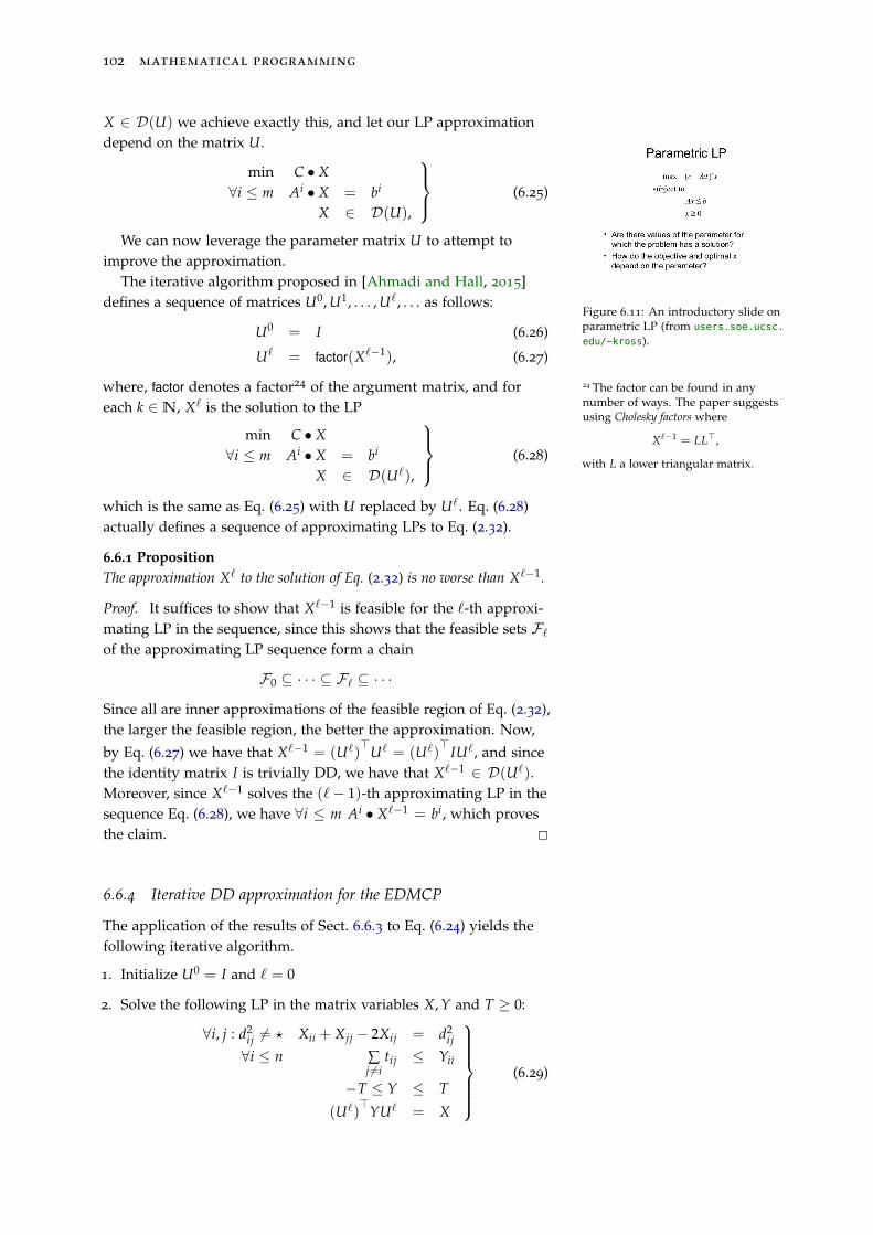
102 mathematical programming
X ∈ D(U) we achieve exactly this, and let our LP approximationdepend on the matrix U.
min C • X∀i ≤ m Ai • X = bi
X ∈ D(U),
(6.25)
Figure 6.11: An introductory slide onparametric LP (from users.soe.ucsc.
edu/~kross).
We can now leverage the parameter matrix U to attempt toimprove the approximation.
The iterative algorithm proposed in [Ahmadi and Hall, 2015]defines a sequence of matrices U0, U1, . . . , U`, . . . as follows:
U0 = I (6.26)
U` = factor(X`−1), (6.27)
where, factor denotes a factor24 of the argument matrix, and for 24 The factor can be found in anynumber of ways. The paper suggestsusing Cholesky factors where
X`−1 = LL>,
with L a lower triangular matrix.
each k ∈N, X` is the solution to the LP
min C • X∀i ≤ m Ai • X = bi
X ∈ D(U`),
(6.28)
which is the same as Eq. (6.25) with U replaced by U`. Eq. (6.28)actually defines a sequence of approximating LPs to Eq. (2.32).
6.6.1 PropositionThe approximation X` to the solution of Eq. (2.32) is no worse than X`−1.
Proof. It suffices to show that X`−1 is feasible for the `-th approxi-mating LP in the sequence, since this shows that the feasible sets F`
of the approximating LP sequence form a chain
F0 ⊆ · · · ⊆ F` ⊆ · · ·
Since all are inner approximations of the feasible region of Eq. (2.32),the larger the feasible region, the better the approximation. Now,
by Eq. (6.27) we have that X`−1 = (U`)>U` = (U`)
> IU`, and sincethe identity matrix I is trivially DD, we have that X`−1 ∈ D(U`).Moreover, since X`−1 solves the (`− 1)-th approximating LP in thesequence Eq. (6.28), we have ∀i ≤ m Ai • X`−1 = bi, which provesthe claim. 2
6.6.4 Iterative DD approximation for the EDMCP
The application of the results of Sect. 6.6.3 to Eq. (6.24) yields thefollowing iterative algorithm.
1. Initialize U0 = I and ` = 0
2. Solve the following LP in the matrix variables X, Y and T ≥ 0:
∀i, j : d2ij 6= ? Xii + Xjj − 2Xij = d2
ij
∀i ≤ n ∑j 6=i
tij ≤ Yii
−T ≤ Y ≤ T
(U`)>YU` = X
(6.29)
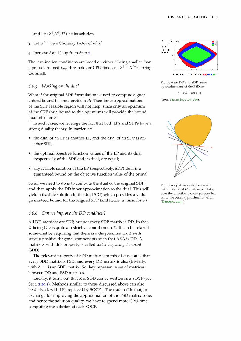
distance geometry 103
and let (X`, Y`, T`) be its solution
3. Let U`+1 be a Cholesky factor of of X`
4. Increase ` and loop from Step 2.
Figure 6.12: DD and SDD innerapproximations of the PSD set
I + xA + yB � 0
(from aaa.princeton.edu).
The termination conditions are based on either ` being smaller thana pre-determined `max threshold, or CPU time, or ‖X` − X`−1‖ beingtoo small.
6.6.5 Working on the dual
What if the original SDP formulation is used to compute a guar-anteed bound to some problem P? Then inner approximationsof the SDP feasible region will not help, since only an optimumof the SDP (or a bound to this optimum) will provide the boundguarantee for P.
Figure 6.13: A geometric view of aminimization SDP dual: maximizingover the direction vectors perpendicu-lar to the outer approximation (from[Dattorro, 2015]).
In such cases, we leverage the fact that both LPs and SDPs have astrong duality theory. In particular:
• the dual of an LP is another LP, and the dual of an SDP is an-other SDP;
• the optimal objective function values of the LP and its dual(respectively of the SDP and its dual) are equal;
• any feasible solution of the LP (respectively, SDP) dual is aguaranteed bound on the objective function value of the primal.
So all we need to do is to compute the dual of the original SDP,and then apply the DD inner approximation to the dual. This willyield a feasible solution in the dual SDP, which provides a validguaranteed bound for the original SDP (and hence, in turn, for P).
6.6.6 Can we improve the DD condition?
All DD matrices are SDP, but not every SDP matrix is DD. In fact,X being DD is quite a restrictive condition on X. It can be relaxedsomewhat by requiring that there is a diagonal matrix ∆ withstrictly positive diagonal components such that ∆X∆ is DD. Amatrix X with this property is called scaled diagonally dominant(SDD).
The relevant property of SDD matrices to this discussion is thatevery SDD matrix is PSD, and every DD matrix is also (trivially,with ∆ = I) an SDD matrix. So they represent a set of matricesbetween DD and PSD matrices.
Luckily, it turns out that X is SDD can be written as a SOCP (seeSect. 2.10.1). Methods similar to those discussed above can alsobe derived, with LPs replaced by SOCPs. The trade-off is that, inexchange for improving the approximation of the PSD matrix cone,and hence the solution quality, we have to spend more CPU timecomputing the solution of each SOCP.
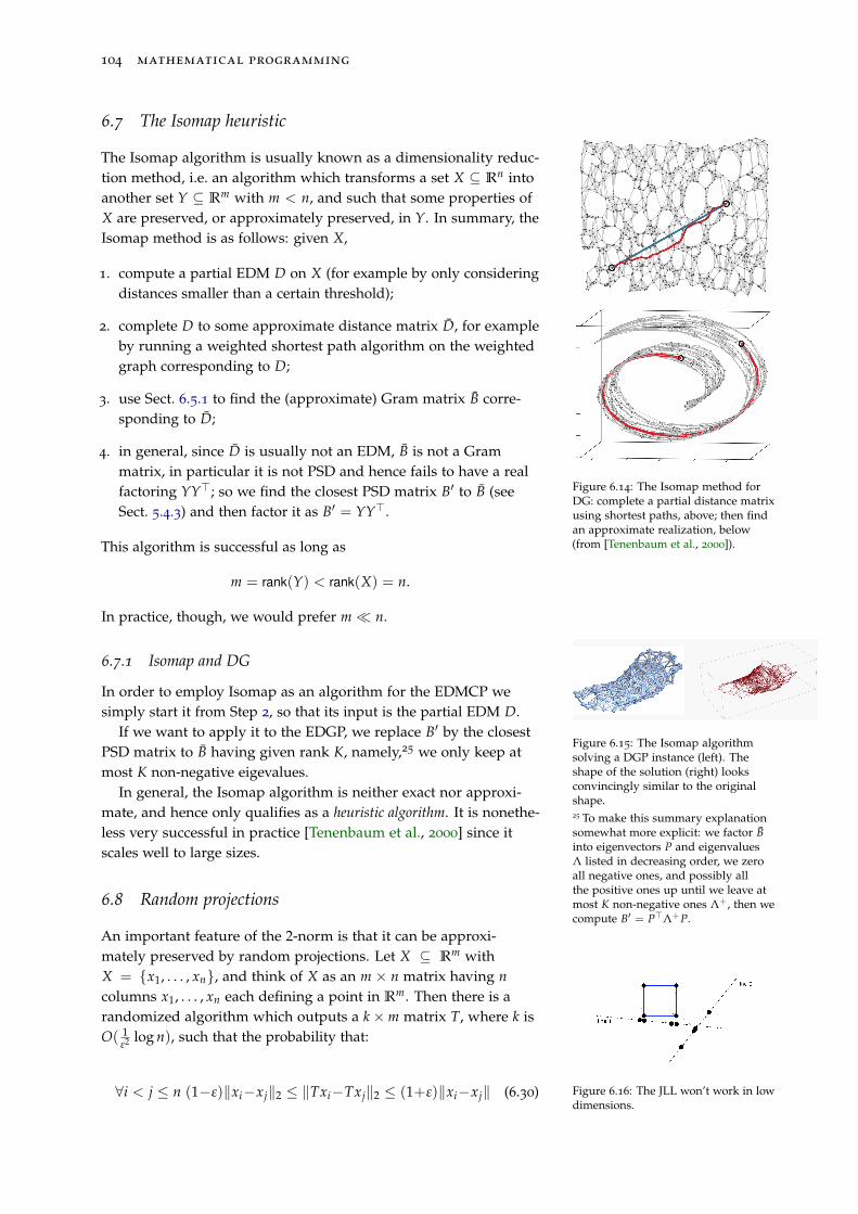
104 mathematical programming
6.7 The Isomap heuristic
The Isomap algorithm is usually known as a dimensionality reduc-tion method, i.e. an algorithm which transforms a set X ⊆ Rn intoanother set Y ⊆ Rm with m < n, and such that some properties ofX are preserved, or approximately preserved, in Y. In summary, theIsomap method is as follows: given X,
Figure 6.14: The Isomap method forDG: complete a partial distance matrixusing shortest paths, above; then findan approximate realization, below(from [Tenenbaum et al., 2000]).
1. compute a partial EDM D on X (for example by only consideringdistances smaller than a certain threshold);
2. complete D to some approximate distance matrix D, for exampleby running a weighted shortest path algorithm on the weightedgraph corresponding to D;
3. use Sect. 6.5.1 to find the (approximate) Gram matrix B corre-sponding to D;
4. in general, since D is usually not an EDM, B is not a Grammatrix, in particular it is not PSD and hence fails to have a realfactoring YY>; so we find the closest PSD matrix B′ to B (seeSect. 5.4.3) and then factor it as B′ = YY>.
This algorithm is successful as long as
m = rank(Y) < rank(X) = n.
In practice, though, we would prefer m� n.
6.7.1 Isomap and DG
In order to employ Isomap as an algorithm for the EDMCP wesimply start it from Step 2, so that its input is the partial EDM D.
Figure 6.15: The Isomap algorithmsolving a DGP instance (left). Theshape of the solution (right) looksconvincingly similar to the originalshape.
If we want to apply it to the EDGP, we replace B′ by the closestPSD matrix to B having given rank K, namely,25 we only keep at
25 To make this summary explanationsomewhat more explicit: we factor Binto eigenvectors P and eigenvaluesΛ listed in decreasing order, we zeroall negative ones, and possibly allthe positive ones up until we leave atmost K non-negative ones Λ+, then wecompute B′ = P>Λ+P.
most K non-negative eigevalues.In general, the Isomap algorithm is neither exact nor approxi-
mate, and hence only qualifies as a heuristic algorithm. It is nonethe-less very successful in practice [Tenenbaum et al., 2000] since itscales well to large sizes.
6.8 Random projections
An important feature of the 2-norm is that it can be approxi-mately preserved by random projections. Let X ⊆ Rm withX = {x1, . . . , xn}, and think of X as an m × n matrix having ncolumns x1, . . . , xn each defining a point in Rm. Then there is arandomized algorithm which outputs a k×m matrix T, where k isO( 1
ε2 log n), such that the probability that:
Figure 6.16: The JLL won’t work in lowdimensions.
∀i < j ≤ n (1−ε)‖xi−xj‖2 ≤ ‖Txi−Txj‖2 ≤ (1+ε)‖xi−xj‖ (6.30)
distance geometry 105
holds can be made arbitrarily close to 1. This is known as theJohnson-Lindenstrauss Lemma (JLL) [Johnson and Lindenstrauss,1984], and is one of the cornerstones of clustering large-dimensionaldatasets (such as image databases).
The most striking feature26 of the JLL is that k is not a function 26 Edo Liberty (of Yahoo! Labs) oncetold me that the way he sees the JLL isthat, in any Euclidean space, you canfit exponentially many (in function of thedimension) “approximately pairwiseorthogonal” vectors . Prove that this isequivalent to the JLL.
of m. In other words, the actual number of dimensions you need inorder to “pack” the projections of the vectors in X, so that the pair-wise distances are approximately preserved to within ε, does notdepend on the number of dimensions of X. Another striking fea-ture is that the number of dimensions grows only logarithmically inthe number of vectors.27 27 The upshot is that the perfect
application setting for the JLL is whenX contains a moderate to large numberof vectors in a huge dimensional space.Image or movie databases have thisproperty, which is why the randomprojections are used when clusteringimages.
A few comments on the JLL are in order.
• O(ε−2 log n) is not really a number, but a short-hand for Cε−2 log nfor some constant C which does not depend on n or m. To usethe JLL in practice, this constant must be estimated somehow.28
28 There is not much literature on this,unfortunately [Venkatasubramanianand Wang, 2011].
• Cε−2 log n is not always smaller than m — aside from C, it de-pends on ε and n, of course. But asymptotically, the term in log ngrows very slowly with respect to how fast ε−2 grows.
• If you want the approximation to be very accurate, then ε shouldbe very small, so 1/ε2 is going to be very large. If m is huge,there will be a saving. The trade-off is between ε and m. Forsmaller m’s, you would need a larger error tolerance ε.
The randomized algorithm to find T is very simple.
1. Sample each of the km components of T independently from anormal distribution with mean 0 and standard deviation 1√
k
2. Does TX verify Eq. (6.30)? If not, repeat from Step 1.
The elementary proof of the JLL given in [Dasgupta and Gupta,2002] shows that the number of iterations of this algorithm is O(n).
6.8.1 Usefulness for solving DGPs
A possible use of random projections for solving EDGPs is given bythe observation that it is easier to satisfy Eq. (6.1) if K is large thanif K is small. On the other hand, most applications require a smallK. So, for extremely large-scale EDGP instances, one might trydeploying any heuristic method to find an acceptably good solutionin a high-dimensional space, and then use a random projectionmatrix T to scale the dimensions down to a more acceptable level.One would then need a heuristic such as Isomap (Sect. 6.7) to drivethe dimensions down to a given K.29
29 More in general, the JLL is applica-ble to any algorithm which only (ormostly) uses Euclidean distances, suchas e.g. the popular k-means heuris-tic for solving Euclidean clusteringproblems.
6.9 How to adjust an approximately feasible solution
Working with SDP and heuristic solutions exposes us to the issueof infeasibility: what if our solution x to a EDGP does not satisfyEq. (6.1)? A practical and usually acceptably fast way to do so is
106 mathematical programming
to use x as a starting point for a local search with respect to theGO formulation Eq. (6.5). A good, open-source local NLP solverwhich can be employed for this purpose is IPOPT. There is still noguarantee of feasibility, but at least the infeasibility error shoulddecrease.
6.10 Summary
This chapter is about Distance Geometry, and introduces the funda-mental problem of DG. It argues that it is useful for scientific andengineering applications, it presents formulations for the 1-, ∞- and2-norms. It introduces Euclidean distance matrices and draws aparallel between the DGP and the completion problem for partiallyspecified EDMs. It presents an SDP formulation for this problem,and discusses a very new method for finding feasible SDP solu-tions by solving an LP. It then presents the famous dimensionalityreduction Isomap heuristic as a solution algorithm for the DGP,and briefly introduces random projections which approximatelypreserve Euclidean distances.
Bibliography
A. Ahmadi and G. Hall. Sum of squares basis pursuit withlinear and second order cone programming. Technical Report1510.01597v1, arXiv, 2015.
A. Alfakih, A. Khandani, and H. Wolkowicz. Solving Euclidean dis-tance matrix completion problems via semidefinite programming.Computational Optimization and Applications, 12:13–30, 1999.
F. Alizadeh and D. Goldfarb. Second order cone programming.Mathematical Programming B, 95:3–51, 2003.
E. Amaldi, K. Dhyani, and L. Liberti. A two-phase heuristic forthe bottleneck k-hyperplane clustering problem. ComputationalOptimization and Applications, 56:619–633, 2013.
D. Applegate, R. Bixby, V. Chvátal, and W. Cook. The TravelingSalesman: a Computational Study. Princeton University Press, Prince-ton, 2007.
J. Bachrach and C. Taylor. Localization in sensor networks. InI. Stojmenovic, editor, Handbook of Sensor Networks, pages 3627–3643. Wiley, 2005.
P. Belotti. Couenne: a user’s manual. Dept. of MathematicalSciences, Clemson University, 2011.
P. Belotti, J. Lee, L. Liberti, F. Margot, and A. Wächter. Branch-ing and bounds tightening techniques for non-convex MINLP.Optimization Methods and Software, 24(4):597–634, 2009.
T. Berthold, G. Gamrath, A. Gleixner, S. Heinz, T. Koch, andY. Shinano. Solving mixed integer linear and nonlinear problems usingthe SCIP Optimization Suite. ZIB, http://scip.zib.de/, 2012.
D. Bertsimas and M. Sim. The price of robustness. OperationsResearch, 52(1):35–53, 2004.
P. Biswas, T. Lian, T. Wang, and Y. Ye. Semidefinite programmingbased algorithms for sensor network localization. ACM Transactionsin Sensor Networks, 2:188–220, 2006.
L. Blumenthal. Theory and Applications of Distance Geometry. OxfordUniversity Press, Oxford, 1953.
108 mathematical programming
I. Bomze. Evolution towards the maximum clique. Journal of GlobalOptimization, 10:143–164, 1997.
I. Bomze, M. Budinich, P.M. Pardalos, and M. Pelillo. The max-imum clique problem. In D.-Z. Du and P.M. Pardalos, editors,Handbook of Combinatorial Optimization, Supp. A, volume supp. A,pages 1–74. Kluwer Academic Publishers, Dordrecht, 1998.
P. Bonami and J. Lee. BONMIN user’s manual. Technical report, IBMCorporation, June 2007.
M. Boulle. Compact mathematical formulation for graph partition-ing. Optimization and Engineering, 5:315–333, 2004.
S. Boyd and L. Vandenberghe. Convex Optimization. CambridgeUniversity Press, Cambridge, 2004.
C. Bragalli, C. D’Ambrosio, J. Lee, A. Lodi, and P. Toth. On theoptimal design of water distribution networks: a practical minlpapproach. Optimization and Engineering, 13:219–246, 2012.
R. Burkard, M. Dell’Amico, and S. Martello. Assignment problems.SIAM, Providence, 2009.
E. Candès. The mathematics of sparsity. In S.Y. Jang, Y.R. Kim, D.-W. Lee, and I. Yie, editors, Proceedings of the International Congress ofMathematicians, volume I. Kyung Moon SA, Seoul, 2014.
G. Caporossi, D. Alamargot, and D. Chesnet. Using the computerto study the dyamics of the handwriting processes. In DS 2004Proceedings, volume 3245 of LNAI, pages 242–254. Springer, 2004.
A. Cassioli, B. Bordeaux, G. Bouvier, A. Mucherino, R. Alves,L. Liberti, M. Nilges, C. Lavor, and T. Malliavin. An algorithm toenumerate all possible protein conformations verifying a set ofdistance constraints. BMC Bioinformatics, page 16:23, 2015.
B. Colson, P. Marcotte, and G. Savard. Bilevel programming: asurvey. 4OR, 3:87–107, 2005.
V. Cortellessa, F. Marinelli, and P. Potena. Automated selection ofsoftware components based on cost/reliability tradeoff. In V. Gruhnand F. Oquendo, editors, EWSA 2006, volume 4344 of LNCS, pages66–81. Springer, 2006.
A. Costa, P. Hansen, and L. Liberti. On the impact of symmetry-breaking constraints on spatial branch-and-bound for circle pack-ing in a square. Discrete Applied Mathematics, 161:96–106, 2013.
D. Cox, J. Little, and D. O’Shea. Ideals, Varieties and Algorithms.Springer, Berlin, second edition, 1997.
M. Cucuringu, Y. Lipman, and A. Singer. Sensor network local-ization by eigenvector synchronization over the Euclidean group.ACM Transactions on Sensor Networks, 8:1–42, 2012a.
bibliography 109
M. Cucuringu, A. Singer, and D. Cowburn. Eigenvector synchro-nization, graph ridigity and the molecule problem. Information andInference: a journal of the IMA, 1:21–67, 2012b.
N. Cutland. Computability: an introduction to recursive functiontheory. Cambridge University Press, Cambridge, 1980.
C. D’Ambrosio and A. Lodi. Mixed-integer nonlinear programmingtools: a practical overview. 4OR, 9:329–349, 2011.
G. Dantzig, A. Orden, and P. Wolfe. The generalized simplexmethod for minimizing a linear form under linear inequalityrestraints. Pacific Journal of Mathematics, 5(2):183–196, 1955.
S. Dasgupta and A. Gupta. An elementary proof of a theorem byjohnson and lindenstrauss. Random Structures and Algorithms, 22:60–65, 2002.
J. Dattorro. Convex Optimization and Euclidean Distance Geometry.Mεβoo, Palo Alto, 2015.
R. Davis, C. Ernst, and D. Wu. Protein structure determination viaan efficient geometric build-up algorithm. BMC Structural Biology,10(Suppl 1):S7, 2010.
Ph. Delsarte. Bounds for unrestricted codes by linear programming.Philips Research Reports, 27:272–289, 1972.
K. Dhyani. Personal communication, 2007.
Kanika Dhyani. Optimization models and algorithms for the hyperplaneclustering problem. PhD thesis, Politecnico di Milano, 2009.
Y. Ding, N. Krislock, J. Qian, and H. Wolkowicz. Sensor networklocalization, Euclidean distance matrix completions, and graphrealization. Optimization and Engineering, 11:45–66, 2010.
I. Dokmanic, R. Parhizkar, J. Ranieri, and M. Vetterli. Euclideandistance matrices: Essential theory, algorithms and applications.IEEE Signal Processing Magazine, 1053-5888:12–30, Nov. 2015.
C. Dürr. Programmation par contraintes et programmationmathématique, 2011. Lecture notes, École Polytechnique.
J. Edmonds. Paths, trees and flowers. Canadian Journal of Mathemat-ics, 17:449–467, 1965.
M. Ehrgott. Multicriteria Optimization. Springer, New York, 2005.
L. Euler. Solutio problematis ad geometriam situs pertinentis.Commentarii Academiæ Scientiarum Imperialis Petropolitanæ, 8:128–140, 1736.
L. Evans. An introduction to mathematical optimal control theory. v. 0.2.math.berkeley.edu/ evans/control.course.pdf.
110 mathematical programming
M. Fischetti and A. Lodi. Local branching. Mathematical Program-ming, 98:23–37, 2005.
M. Fischetti, F. Glover, and A. Lodi. The feasibility pump. Mathe-matical Programming, 104(1):91–104, 2005.
M. Flood. The traveling salesman problem. Operations Research, 4
(1):61–75, 1956.
L. Ford and D. Fulkerson. Maximal flow through a network.Canadian Journal of Mathematics, 8(3):399–404, 1956.
R. Fortet. Applications de l’algèbre de Boole en recherche opéra-tionelle. Revue Française de Recherche Opérationelle, 4:17–26, 1960.
R. Fourer and D. Gay. The AMPL Book. Duxbury Press, PacificGrove, 2002.
V. Giakoumakis, D. Krob, L. Liberti, and F. Roda. Technologicalarchitecture evolutions of information systems: trade-off andoptimization. Concurrent Engineering Research and Applications, 20
(2):127–147, 2012.
K. Gödel. Über formal unentscheidbare Sätze der Principia Mathe-matica und verwandter Systeme, I. Monatshefte für Mathematik undPhysik, 38:173–198, 1930.
R.E. Gomory. Essentials of an algorithm for integer solutions tolinear programs. Bulletin of the American Mathematical Society, 64(5):256, 1958.
G. Gutin and A. Punnen, editors. The traveling salesman problem andits variations. Kluwer, Dordrecht, 2002.
P. Hall. On representatives of subsets. Journal of the LondonMathematical Society, 10(1):26–30, 1935.
D. Harel. On folk theorems. Communications of the ACM, 23(7):379–389, 1980.
W. Hart, C. Laird, J.-P. Watson, and D. Woodruff. Pyomo — Opti-mization modelling in Python. Springer, New York, 2012.
IBM. ILOG CPLEX 12.2 User’s Manual. IBM, 2010.
IBM. ILOG CPLEX 12.6 User’s Manual. IBM, 2014.
W. Johnson and J. Lindenstrauss. Extensions of Lipschitz mappingsinto a Hilbert space. In G. Hedlund, editor, Conference in ModernAnalysis and Probability, volume 26 of Contemporary Mathematics,pages 189–206, Providence, 1984. American Mathematical Society.
N. Karmarkar. A new polynomial time algorithm for linearprogramming. Combinatorica, 4(4):373–395, 1984.
bibliography 111
R. Karp. Reducibility among combinatorial problems. In R. Millerand W. Thatcher, editors, Complexity of Computer Computations,volume 5 of IBM Research Symposia, pages 85–104, New York, 1972.Plenum.
L. Khachiyan. Polynomial algorithms in linear programming. USSRComputational Mathematics and Mathematical Physics, 23(1):53–72,1980.
H. Konno and A. Wijayanayake. Portfolio optimization problemunder concave transaction costs and minimal transaction unitconstraints. Mathematical Programming, Series B, 89(2):233–250, 2001.
S. Krantz. The Proof is in the pudding. Springer, New York, 2010.
S. Kucherenko, P. Belotti, L. Liberti, and N. Maculan. New formula-tions for the kissing number problem. Discrete Applied Mathematics,155(14):1837–1841, 2007.
M. Laurent and F. Vallentin. Semidefinite optimization. TechnicalReport Lecture Notes, CWI and TU Delft, 2012.
C. Lavor, L. Liberti, and N. Maculan. Computational experiencewith the molecular distance geometry problem. In J. Pintér, editor,Global Optimization: Scientific and Engineering Case Studies, pages213–225. Springer, Berlin, 2006.
C. Lavor, A. Mucherino, L. Liberti, and N. Maculan. On thecomputation of protein backbones by using artificial backbones ofhydrogens. Journal of Global Optimization, 50:329–344, 2011.
L. Liberti. Writing global optimization software. In L. Liberti andN. Maculan, editors, Global Optimization: from Theory to Implementa-tion, pages 211–262. Springer, Berlin, 2006.
L. Liberti. Compact linearization of binary quadratic problems.4OR, 5(3):231–245, 2007.
L. Liberti. Reformulations in mathematical programming: Defini-tions and systematics. RAIRO-RO, 43(1):55–86, 2009.
L. Liberti. Symmetry in mathematical programming. In J. Lee andS. Leyffer, editors, Mixed Integer Nonlinear Programming, volume154 of IMA, pages 263–286. Springer, New York, 2012.
L. Liberti. Optimization and sustainable development. Computa-tional Management Science, 12(3):371–395, 2015.
L. Liberti and N. Maculan. Preface to special issue on reformula-tions in mathematical programming. Discrete Applied Mathematics,157(6), 2009.
L. Liberti and F. Marinelli. Mathematical programming: Turingcompleteness and applications to software analysis. Journal ofCombinatorial Optimization, 28(1):82–104, 2014.
112 mathematical programming
L. Liberti, S. Cafieri, and F. Tarissan. Reformulations in mathemat-ical programming: A computational approach. In A. Abraham,A.-E. Hassanien, P. Siarry, and A. Engelbrecht, editors, Founda-tions of Computational Intelligence Vol. 3, number 203 in Studies inComputational Intelligence, pages 153–234. Springer, Berlin, 2009a.
L. Liberti, C. Lavor, N. Maculan, and F. Marinelli. Double variableneighbourhood search with smoothing for the molecular distancegeometry problem. Journal of Global Optimization, 43:207–218, 2009b.
L. Liberti, C. Lavor, N. Maculan, and A. Mucherino. Euclideandistance geometry and applications. SIAM Review, 56(1):3–69, 2014.
J. Löfberg. YALMIP: A toolbox for modeling and optimization inMATLAB. In Proceedings of the International Symposium of Computer-Aided Control Systems Design, volume 1 of CACSD, Taipei, 2004.IEEE.
M. López and G. Still. Semi-infinite programming. European Journalof Operational Research, 180(2):491–518, 2007.
N. Maculan, P. Michelon, and J. MacGregor Smith. Bounds on thekissing numbers in Rn: Mathematical programming formulations.Technical report, University of Massachusetts, Amherst, USA,1996.
A. Majumdar, A. Ahmadi, and R. Tedrake. Control and verificationof high-dimensional systems with dsos and sdsos programming. InConference on Decision and Control, volume 53, pages 394–401, LosAngeles, 2014. IEEE.
A. Makhorin. GNU Linear Programming Kit. Free Software Founda-tion, http://www.gnu.org/software/glpk/, 2003.
A. Man-Cho So and Y. Ye. Theory of semidefinite programmingfor sensor network localization. Mathematical Programming B, 109:367–384, 2007.
H. Markowitz. Portfolio selection. The Journal of Finance, 7(1):77–91,1952.
matlab. MATLAB R2014a. The MathWorks, Inc., Natick, MA, 2014.
Y. Matiyasevich. Hilbert’s Tenth Problem. MIT Press, Boston, 1993.
J. Matoušek and B. Gärtner. Understanding and using Linear Pro-gramming. Springer, Berlin, 2007.
K. Menger. New foundation of Euclidean geometry. AmericanJournal of Mathematics, 53(4):721–745, 1931.
M. Minsky. Computation: Finite and infinite machines. Prentice-Hall,London, 1967.
J. Moré and Z. Wu. Distance geometry optimization for proteinstructures. Journal of Global Optimization, 15:219–234, 1999.
bibliography 113
mosek7. The mosek manual, Version 7 (Revision 114). Mosek ApS,2014. (www.mosek.com).
T. Motzkin and E. Straus. Maxima for graphs and a new proof ofa theorem of Turán. Canadian Journal of Mathematics, 17:533–540,1965.
J. Munkres. Algorithms for the assignment and transportationproblems. Journal of SIAM, 5(1):32–38, 1957.
R. Reams, G. Chatham, W. Glunt, D. McDonald, and T. Hayden. De-termining protein structure using the distance geometry programAPA. Computers and Chemistry, 23:153–163, 1999.
N.V. Sahinidis and M. Tawarmalani. BARON 7.2.5: Global Optimiza-tion of Mixed-Integer Nonlinear Programs, User’s Manual, 2005.
J. Saxe. Embeddability of weighted graphs in k-space is stronglyNP-hard. Proceedings of 17th Allerton Conference in Communications,Control and Computing, pages 480–489, 1979.
T. Schlick. Molecular modelling and simulation: an interdisciplinaryguide. Springer, New York, 2002.
A. Singer. Angular synchronization by eigenvectors and semidefi-nite programming. Applied and Computational Harmonic Analysis, 30:20–36, 2011.
A. Soyster. Convex programming with set-inclusive constraints andapplications to inexact linear programming. Operations Research, 21
(5):1154–1157, 1973.
A. Sutou and Y. Dai. Global optimization approach to unequalsphere packing problems in 3D. Journal of Optimization Theory andApplications, 114(3):671–694, 2002.
J. Tenenbaum, V. de Silva, and J. Langford. A global geometricframework for nonlinear dimensionality reduction. Science, 290:2319–2322, 2000.
A. Turing. On computable numbers, with an application to theEntscheidungsproblem. Proceedings of the London MathematicalSociety, 42(1):230–265, 1937.
R. Vanderbei. Linear Programming: Foundations and Extensions.Kluwer, Dordrecht, 2001.
S.A. Vavasis. Nonlinear Optimization: Complexity Issues. OxfordUniversity Press, Oxford, 1991.
S. Venkatasubramanian and Q. Wang. The Johnson-Lindenstrausstransform: An empirical study. In Algorithm Engineering andExperiments, volume 13 of ALENEX, pages 164–173, Providence,2011. SIAM.

114 mathematical programming
J.P. Vielma. Mixed integer linear programming formulationtechniques. SIAM Review, 57:3–57, 2015.
D. Wu, Z. Wu, and Y. Yuan. Rigid versus unique determination ofprotein structures with geometric buildup. Optimization Letters, 2(3):319–331, 2008.
K. Wüthrich. Protein structure determination in solution by nuclearmagnetic resonance spectroscopy. Science, 243:45–50, 1989.
Y. Yemini. The positioning problem — a draft of an intermedi-ate summary. In Proceedings of the Conference on Distributed SensorNetworks, pages 137–145, Pittsburgh, 1978. Carnegie-Mellon Uni-versity.
Index
k-consistent, 69
1-consistency, 69
1-norm, 95
2-consistency, 70
2-norm, 96, 104
absolute value, 52
accuracy, 42, 82
arbitrary, 39
adjacency matrix, 39
weighted, 81
adjacent, 31
vertex, 70
algorithmanalysis, 20
approximation, 75, 76, 100
cMINLP, 37
exact, 76
GW, 85–87
iteration, 105
iterative, 102
Monte Carlo, 76
polytime, 99, 100
randomized, 75–77, 104, 105
randomized approximation, 77, 91
randomized rounding, 88
AllDifferent, 70–72
alphabet, 13
AMPL, 23, 59
dat file, 24, 25
dat syntax, 24
IDE, 24
mod file, 24
run, 24
run file, 24
angle, 82
extent, 83
applied mathematics, 68
approximate algorithm, 104
approximate feasibility, 100
approximate method, 100
approximation, 33, 39, 101, 102
accurate, 105
improvement, 103
inner, 100–103
inner, SDP, 103
ratio, 76, 83
scheme, 76
approximation algorithm, 76, 77, 85
constant, 76
randomized, 77
approximation error, 36
approximation quality, 101
approximation reformualation, 51
arc, 19
antiparallel, 79
capacity, 19
arc capacity, 44
arc-consistency, 70
architecture, 61
spaghetti, 61
arraybi-dimensional, 24
multi-dimensional, 9, 24
partially defined, 72
slice, 24
square, 41, 72
assembly language, 25
assignment, 16, 27, 53, 57
constraint, 53
feasible, 70
linear, 30
variables, 58
assignment constraint, 29
asymptotic complexity, 20
atom, 75, 94, 95
position, 41
axiomatization, 93
backtracking, 69
BARON, 36, 37, 39, 40
barrier method, 17
barycenter, 97
batterypower, 94
BB, 27, 28, 33, 36, 56
node, 36
big M, 72
bijection, 29
bilevel programming, 44, 45
binaryvariable, 55
binary encoding, 53
bipartitegraph, 70
bisection, 21, 71
algorithm, 71
complexity, 71
bitstorage, 20
blending, 27
BLevP, 44
BLP, 30, 53, 79
BONMIN, 37
boundguarantee, 103
guaranteed, 103
lower, 71
upper, 71
bounded above, 76
bounded below, 76
bounded probability, 76
BQCP, 78
BQP, 39, 79
branch, 36
branch-and-bound, 17, 27
spatial, 36
branching, 36, 53, 69
variable, 69
branching variable, 70
brute force, 76
byte, 14
canonical formLP, 27
capacity, 18
carbon, 94
cardinality constraint, 36
cartesian, 69
cartesian product, 24, 28, 36, 37
CCMVPS, 38
cell, 13
certificate, 71
PSD, 85
chain, 102
116 mathematical programming
characteristic vector, 39
scaled, 39
chessboard, 67
Choleskyfactor, 103
Cholesky factor, 102
Church-Turing thesis, 16
circle, 34
slice, 83
circle packing, 34
circuit, 75
clause, 75
clausessatisfiable, 75
Clique, 51
clique, 33, 61
largest, 39
max, 33
maximal, 39
maximum, 39
clock, 94
synchronization, 94
clustering, 57
Euclidean, 105
images, 105
cMINLP, 36
cNLP, 33, 35, 36
codeparallelized, 86
code efficiency, 86
column, 72, 80, 85
combinatorialproperty, 55
combinatorial optimization, 75
command line, 89, 90
argument, 86
commodity, 18, 19
comparisonempirical, 86
compiled, 25
complement, 75
complement graph, 33
complementarity, 55
constraint, 56
linear, 55
complexityworst-case, 20, 36, 100
component, 105
composition, 15
computation, 13
computation model, 14, 15
computational model, 33
computermulti-core, 86
real, 17
computer science, 68
condition
restrictive, 103
cone, 34
cone programmingsecond-order, 42
congruence, 95
conjunction, 75
conjunctive normal form, 75
connectivity, 19
consistency, 69
arc, 70
node, 69
consistentdomain, 69
constant time, 20
constraint, 21, 53, 67, 69, 70, 78, 93
k-ary, 69
additional, 72
assignment, 58, 62
binary, 53, 67, 69
cardinality, 36, 72
convex nonlinear, 85
convex quadratic, 85
DD, 101
disjunction, 72
dual, 67
equality, 52
infinite, 46
integrality, 21, 53
nonconvex, 36
nonlinear, 93, 95
number, 72
PSD, 41, 101
quadratic, 40, 53
qualification, 36
rank, 41, 79
reliability, 62
simple, 21
unary, 67, 69
uncountable, 47
uncountably many, 47
constraint matrix, 26
constraint programming, 9, 67
contradiction, 69
contrapositive, 71
control transfer, 86
control variables, 47
convexfunction, 33, 34
set, 33
subset, 47
convex relaxation, 36
convexity, 33
cost, 61
minimization, 44
unit transportation, 18
COUENNE, 37, 39, 40
Couenne, 36
covariance matrix, 36, 38
CP, 9, 67, 68, 71, 93
dual, 67, 68
formulation, 67, 71, 72
language, 67
CP formulationoriginal, 68
CPLEX, 40, 60, 79, 85, 90
convex MIQP, 85
MILP, 85
nonconvex MIQP, 85
sBB, 85
system clock, 86
v. 12.6, 85
CPU, 14
time, 86, 90, 91, 103
timings, 86
user, 86
CPU time, 20
cQP, 37, 38
crossword, 67
crystal, 75
customer site, 18
cut, 39, 75, 77, 91
maximum, 39
cutset, 75
maximum, 77–79, 82
maximum weight, 75
size, 78
cutset sizeaverage, 83
CvxOpt, 85
cycledisjoint, 29
Dantzig, 27
data transfer, 86
DD, 101–103
inner approximation, 103
decision problem, 20, 27, 68, 72, 76,77
decision variable, 21, 41, 43, 44, 47,67, 68, 78
binary, 29
bounded, 67
continuous, 29
discrete, 67
matrix, 40, 101
scalar, 80
symbol, 22
vector, 80
decision version, 20
decomposition, 94
demand, 18
derivative, 22
device, 94
mobile, 94
index 117
DG, 93
fundamental problem, 93
DGP, 93, 95
application, 100
solution methods, 96
diagonal, 82
diagonal componentstrictly positive, 103
diagonal dominance, 56
diagonally dominant, 101
scaled, 103
diameter, 83
weighted, 95
dictionary, 13
random, 26
differentiable, 22
digraph, 19, 30, 81
dimension, 105
dimensionality reduction, 104
directionfeasible improving, 35
discrepancy, 36
Disjunction, 72
disjunction, 75
distance, 93–95
Euclidean, 93, 105
euclidean, 36
inter-atomic, 41, 94
minimum, 57
pairwise, 105
distance geometry, 35, 93
Distance Geometry Problem, 93
distributeproducts over sums, 63
distributionnormal, 105
domain, 21, 67–70
bounded, 69
reduction, 69, 70
domain product, 70
dual, 103
LP, 103
SDP, 103
duality, 69
economic equilibrium, 27
edge, 35, 77, 79, 99
list, 90
probability, 90
set, 78
total number, 78
weight, 78, 90
weight function, 93
EDGP, 35, 41, 93, 95, 99, 100, 105
algorithm, 104
instance, 41
relaxation, 42
EDM, 96, 99
partial, 104
square, 96, 98, 99
EDMCP, 99, 100
algorithm, 104
efficiencymaximization, 57
eigenvalue, 38, 88, 98
negative, 88, 98, 104
negative zero, 88
non-negative, 38, 41, 98
ordered, 85
slightly negative, 85
small negative, 88
strictly positive, 38
eigenvector, 82, 85, 88
elementone, 70
upper-left, 72
ellipsoid algorithm, 27
encodingfinite, 47
energyminimum, 75
enumerative method, 17
equality constraint, 52
equation, 40, 52
quadratic, 53
erase, 13
Erdos-Renyimodel, 90
error, 88
floating point, 100
minimization, 94
tolerance, 33, 85
error minimization, 38
eternity, 67
exact algorithm, 104
exact reformulation, 51
execution environment, 17
expected reutrn, 36
exponential, 22, 53
exponential time, 76
expressionboolean, 75
mathematical, 22
facet, 47
factor, 79, 102
Cholesky, 102, 103
transpose, 88
factorization, 41, 85
feasibility, 40, 54, 82, 93
strict, 82
feasibility problem, 27, 32, 67
feasible, 94
approximately, 100
set, 22
solution, 22
feasible point, 35, 36
feasible polyhedron, 56
feasible region, 69
feasible set, 102
feasible solution, 68, 103
fileformat, 90
line, 90
finite differenceequation, 47
fixed cost, 28
fKNP, 35
floating point, 85, 86
error, 88
error tolerance, 86
number, 90
operation, 88
flow, 19, 27, 44
conservation, 20
positive, 20
total, 20
formlinear, 41
quadratic, 41
standard, 27
formattabular, 90
formulalogical, 75
formulation, 22, 23, 34, 96, 100
bilevel, 45
exact, 100
MIQP, 86
MP, 27, 44
natural, 78, 79
quadratic, 79
SDP, 99, 101, 103
structured, 68
Fortetinequalities, 87
Fortet reformulation, 54
Fourier, 27
FPTAS, 76, 82
fractional value, 36
frequency, 94
function, 20
basic, 15
computable, 16
constant, 15
convex, 33, 36
nonlinear, 27, 34, 37
objective, 21
partial recursive, 14
projection, 15
successor, 15
118 mathematical programming
trigonometric, 22
function call, 24
Gödel, 93
Gödel number, 14, 16
gapminimum, 84
general-purpose, 43, 45
geometry, 93
elementary, 83
Gershgorin’s theorem, 101
global optimality, 77
global optimization, 96
global optimum, 94
GO, 96, 106
goal, 45
gobal solution, 36
Goemans-Williamson, 82
Gram matrix, 80, 97
partial, 99
graph, 35, 39, 61
adjacency matrix, 39
bipartite, 30, 70
connected, 94
diameter, 95
directed, 19, 62
directed complete, 79
drawing, 35
edge-weighted, 99
mesh grid, 91
random, 90
simple, 31, 33, 42
simple undirected, 93
triangle, 89
undirected, 86
undirected edge-weighted, 79
weighted, 90, 94, 100
growthlogarithmic, 105
slow, 105
guaranteeexactness, 76
GW, 82, 83, 85, 91
Hall’s theorem, 70
halting problem, 14
hash table, 20
HCP, 57, 59
head, 13
heuristic, 37, 69, 105
algorithm, 104
k-means, 105
method, 51
hierarchical stakeholders, 45
Hilbert, 93
Hitchcock, 27
hydrogen, 94
hypercube, 30
hyperedge, 31
hypergraph, 31, 33
cover, 31
hyperplane, 38, 57, 82, 93
Hyperplane Clustering Problem, 57
ILOG, 60
ILP, 30
image database, 105
implementation, 85
implication, 72
Implies, 72
incompleteness theorem, 93
indefinite, 38
index, 29
indexing, 72
indicator vector, 31
inequalityFortet, 87
linear, 38
opposite sign, 40, 52
infeasibility, 105
error, 106
information, 99
input, 13, 69, 76, 79, 99
input data, 20
input graph, 94
instance, 21–23, 25, 71, 76, 77
CP, 69
file, 90
finitely many, 20
infeasible, 71
NO, 20, 35, 76
size, 33
YES, 20, 35, 76
instance size, 34
small, 35
instantiation, 23
instruction, 13
basic, 14
imperative, 16
integer, 90
consecutive, 53
lattice, 30
smallest, 53
integral, 47
integrality constraint, 21
integrality constraints, 36
interface, 62
interface module, 61
interior point, 27, 42
method, 27
interpreter, 14, 17, 22
intervalendpoint, 47
range, 21
IPM, 42, 81, 100
SDP, 82
IPOPT, 33, 35, 39, 40, 106
irrational, 33
irrational component, 34
Ising model, 75
Isomap, 104
iterationsmaximum number, 86
iterative algorithm, 35
JLL, 105
proof, elementary, 105
Johnson-Lindenstrauss lemma, 105
k-means, 105
Kantorovich, 27
kissing number, 35, 37
Koopmans, 27
Kronecker, 93
Lagrange coefficient, 36
Lagrangian, 36
languageAMPL, 24
declarative, 17
general purpose, 25
high-level, 25
imperative, 17, 24, 25
interpreted, 25
LAP, 30
Laplacianmatrix, 87
latticeinteger, 27, 28, 30, 36, 37
layer, 75
LCP, 55
leaf node, 70
left, 13
LFP, 57
librarystandard, 86
lifting, 52
line, 93
linear, 17
linear complementarity, 55
linear algebra, 41
computation, 86
linear assignment, 70
linear combination, 80
linear form, 27, 28, 30, 40–42
linear fractionalprogramming, 57
linear fractional term, 57
linear programming, 27
binary, 30
integer, 30
index 119
mixed-integer, 28
linear regression, 33
restricted, 38
linear term, 52
linearization, 40, 41, 54, 55
exact, 79, 95
product, 54
Linux, 24
literal, 75
local optimum, 36, 37
localizationsensor network, 94
log-space reductions, 27
logarithm, 22, 35, 63
logarithmic, 21
logical connective, 72
logistics, 29
loop, 16, 103
lower bound, 77
LP, 27, 41, 55, 100–103
approximating, 102
canonical form, 52
dual, 103
family, 101
parametric, 102
parametrized, 101
sequence, 102
solution, 102
standard form, 52
LP relaxation, 36
machine code, 25
MacOSX, 24
magnetic spin, 75
manifold, 93
Markowitz, 36
matching, 70
maximum, 70, 71
perfect, 30, 70
matching problem, 32
materialbalance, 20
mathematical programming, 9, 17
MATLAB, 42
MatLab, 85
matrix, 38, 41, 99, 101
adjacency, 39
binary, 39
Cholesky, 102
closest PSD, 85, 104
component, 45
covariance, 38
DD, 103
diagonal, 81, 85, 103
diagonanly dominant, 101
distance, 99
Euclidean distance, 96
factor, 87, 98, 102
Gram, 41, 97, 98, 101
identity, 81, 102
lower triangular, 102
partial, 99, 100
PSD, 38, 41, 80, 98, 99, 101
PSD, closest, 104
rank 1, 91
real symmetric, 80
SDP, 103
sequence, 102
symmetric, 80, 85, 99
unitary, 82
zero-diagonal, 96, 99
matrix problem, 79
max clique, 33
Max Cut, 76, 79, 85
formulation, 78
instance, 82
MILP formulation, 85
MIQP formulation, 85
relaxation, 79
SDP relaxation, 85
solution, 82
unweighted, 77, 91
max cut, 39
Max Flow, 20, 44
Max-2-Sat, 75
maximization, 22
mean, 105
megawatt, 28
memory, 14, 34
methoditerative, 101
metric, 93
midpoint, 71
MILP, 27, 28, 36, 56, 58, 63, 75, 90, 95
reformulation, 59
solver, 59
minimalization, 15, 16
minimization, 22
error, 93
maximum, 54
unconstrained, 96
MINLP, 36, 37, 58, 62
solver, 59
MIQP, 75, 90
mixed-integernonlinear programming, 37
modelling, 15
modelling language, 28
molecule, 94
monotonically increasing, 63
Monte Carlo, 76
MOP, 22, 43, 45
MOSEK, 42
MP, 9, 21, 27, 55, 62, 68, 71, 93
binary, 53
formulation, 22
modelling environment, 85
solver, 86, 93
subclass, 69
symmetric, 51
MP class, 51
MP formulation, 27
multi-objective, 22
multi-objective programming, 43
MVCCPS, 36
narrowing reformulation, 51
natural number, 14
negativedefinite, 38
semidefinite, 38
neighbourhood, 22
networkwireless, 94
network flow, 19
nine queens, 67
NLP, 27, 34, 95, 96
feasibility, 93
nonconvex, 38
solver, 106
NLP solver, 53
NMR, 35, 94
Nobel prize, 36
node, 19, 38, 69
child, 69
customer, 44
leaf, 70
prior, 71
production, 44
pruned, 70
search tree, 70
node-consistency, 69
node-consistent, 69
nonconvex, 34, 38
NLP, 35
nonconvex MINLP, 37
nonconvex NLP, 36
nonconvexity, 36
nonlinear, 17
nonlinear programming, 34
convex, 33
convex mixed-integer, 36
mixed-integer, 37
nonlinear term, 54
nonzero, 53
norm, 34
Euclidean, 34, 95
infinity, 95
max, 95
one, 95
two, 96
120 mathematical programming
NP, 20, 100
hardest, 20
NP-complete, 76
NP-hard, 20, 28, 32–35, 51, 55, 67, 68,76, 99
proof, 99
nuclear magnetic resonance, 35, 94
number of bits, 34
number theory, 15
NumPy, 85
objective, 23, 45
approximation, 82
coefficients, 26
direction, 27
nonconvex, 36
objective function, 21, 44, 46, 67, 71,78, 79, 81
average value, 77
nonconvex, 85
optimal value, 103
quadratic, 85
value, 90, 94
zero, 93
open source, 23
operating system, 86
operationbasic, 15
operator, 52
arithmetical, 22
transcendental, 22
optimal control, 47
optimal order, 28
optimal point, 36
optimal value, 36
optimality, 82, 93
certificate, 34
global, 39
guarantee, 35, 59
local, 39
optimality condition, 36
optimality guaranteeglobal, 37
optimizationblack-box, 22
problem, 17
optimization problem, 15, 20
optimum, 56, 77
global, 22, 33, 35, 39, 58, 76
local, 22, 33, 35, 39, 51, 55
Pareto, 43
strict, 39
orbit, 51
ordered pair, 29
origin, 82, 97
original problem, 42, 51
orthant, 28
OS, 86
output, 13, 99
format, 90
P, 20, 33, 100
P 6=NP, 51
p.r., 14, 17
pairwise intersection, 34
parameter, 21, 22, 24, 44, 47, 52, 67,69, 78
integer, 72
symbol, 22, 23
tensor, 24
vector, 47, 67, 71
parameter matrix, 102
Paretooptimum, 43
region, 43
set, 43
Pareto set, 22, 44
infinite, 43
partitioninggraph, 63
path, 19
path length, 47
PECS, 34
permutation, 29, 30, 70
Picos, 85
plane, 93
point, 38, 93
closest, 36
feasible, 76
integral, 36
polyhedron, 27, 28, 30, 37–39
polynomialquartic, 96
polynomial size, 34
polynomial time, 27, 28, 30, 33, 35, 42
reformulation, 51
polytime, 20, 21, 32, 70, 71, 81, 98,100
randomized, 77
polytope, 47
portfolio, 36
Markowitz, 38
position, 95
positivedefinite, 38
semidefinite, 38
power generation, 28
pre-processing, 69
precedence relation, 30
primal, 103
probability, 83
problemdecision, 35
halting, 37
input, 67
maximization, 76, 77
minimization, 76, 77
optimization, 22, 70
transportation, 18
problem structure, 100
processor, 30
product, 80, 95
binary, 63
binary variables, 79
reformulation, 55
scalar, 80
product term, 56
production facility, 18
program, 17
main, 89
MP, 17
programming language, 37, 67
declarative, 68
projection, 34, 52
random, 104
proofhand-waving, 93
protein, 94, 95
conformation, 94
protein conformation, 35, 41
protocolsynchronization, 94
pruning, 69–71
PSD, 41, 80, 99, 101
approximately, 100
cone, 103
PSD matrix, 38, 88
PSDCP, 99
PTAS, 76
PyOMO, 25
Pyomo, 85, 86
Python, 25, 42, 85, 90
CvxOpt, 85
cvxopt, 86
math, 86
MP, 85
networkx, 86
numpy, 86
Picos, 85
picos, 86, 87
program, 86, 90
pyomo, 86
sys, 86
time, 86, 89
QCQP, 40, 53, 96
feasibility, 40
QP, 38, 41
indefinite, 39
nonconvex, 38
original, 41
index 121
SDP relaxation, 41
quadraticequation, 40
quadratic form, 37–41
quadratic programming, 38
binary, 39
convex, 37
quadratically constrained, 40
quadruplet, 13
radius, 34, 83
largest, 34
random projection, 105
EDGP, 105
matrix, 105
randomized algorithm, 76
approximation, 77
randomized rounding, 82–84, 90
phase, 86, 87
randomness, 76
rangediscrete, 21
rank, 98
column, 80
constraint, 41
one, 41
row, 80
rank constraint, 79
ratio, 76
realization, 35, 41, 96, 98, 99
function, 93
recursionprimitive, 15
reduction, 35
polytime, 20
reformulation, 51, 56, 80, 95
approximation, 51
automatic, 64
exact, 51, 57, 79, 80
narrowing, 51
polynomial time, 51
product, 85
relaxation, 51
regionfeasible, 102
register, 14
register machine, 14
relationk-ary, 67
relations, 69
relaxation, 51
convex, 38
EDGP, 42
SDP, 42, 79, 85
tight, 100
reliability, 61
representative, 51
resource allocation, 29
rest, 13
restriction, 52
RHS, 23, 26, 78
right, 13
rLR, 38
RM, 14
Minsky, 37
robust, 85
robust optimization, 47
row, 38, 72
row generation, 29
RP, 76
RR, 90, 91
rule, 13
SAT, 55, 67
sBB, 36, 37, 39, 40, 85
algorithm, 38
node, 36
scalability, 59
scalar, 34
scalar product, 83
scaled diagonally dominant, 103
scheduling, 29, 30, 67
Schur complement, 100
SCIP, 36, 37
SDD, 103
SDP, 37, 40, 41, 75, 81, 82, 90, 99–101,103
dual, 103
formulation, 100
instance, 82
polytime, 82
relaxation, 79, 81–83, 101
small, 100
solution, 82
solver, 42, 85, 86, 100
variable, 100
SDP relaxation, 53
phase, 87
search algorithm, 70
search quantifier, 15
search tree, 70, 71
secondsCPU, 86
SeDuMi, 42
semantic interpretation, 64
semantic relationship, 62
semantics, 14
semi-infinite optimization, 22
semi-infinite programming, 46
semidefinite, 37
cone, 40
positive, 38
semidefinite programming, 40
semimetric, 93
sensor network, 35
sequence, 35
server, 94
set, 67
convex, 33, 36
edge, 71
feasible, 43
finite, 54
second-order conic, 42
uncountable, 47
vertex, 70
set covering, 31
set packing, 32
set partitioning, 32
shortest pathweight, 95
simplexmethod, 27
simplex method, 17, 27, 56
single level, 45
single-level, 45
single-objective, 43
single-user mode, 86
SIP, 46, 47
sizeincreasing, 20
slack variable, 52
SNOPT, 33, 35, 39, 40
SOCP, 42, 103
solver, 86
softwarearchitecture, 61
component, 61
system, 61
software architecture, 61, 62
solution, 21, 53, 77
acceptable, 105
approximate, 21, 42, 76
aulity, 103
candidate, 70, 71
feasible, 19, 51, 54, 91
heuristic, 105
improvement, 54
rank 1, 82
SDP, 105
slightly infeasible, 85
YES, 20
solver, 17, 22, 23, 35, 59, 69
efficient, 51
global, 35
local, 35
local NLP, 33, 35, 39, 54, 55
polytime, 51
sBB, 85
SDP, 42
solver-dependentproperty, 56
122 mathematical programming
sonar, 95
source, 20
spaceEuclidean, 36, 37, 93
high-dimensional, 105
sphere packing, 27
spin glass, 75
SQP, 36
square, 34, 96
EDM, 96
unit, 34
square root, 86
function, 88
stabilitynumerical, 59
stablelargest, 33
standard form, 30
standard deviation, 105
standard form, 27, 28, 30, 33, 34,36–40, 42–44, 46
LP, 52
star, 61
state, 13, 16
final, 13
initial, 13
step, 16
sub-matrix, 72
subarine, 95
subdomain, 37
subgraphdensest, 62
fully connected, 61
subproblem, 35
subspace, 34
subtour, 29
subtour elimination, 29
sudoku, 67, 72
surplus variable, 52
symbol, 13
sequence, 13
systemsoftware, 61
system clock, 86
system CPU, 86
tabular form, 24
tape, 13, 16
target, 20
task, 30
tensor, 9
termquadratic, 63
termination, 36
termination condition, 103
test, 16
threshold, 94, 103
timedifference, 94
instant, 95
time horizon, 28, 30
time limit, 86
TM, 13, 33, 37
universal, 37
tolerance, 36, 37, 82
total cost, 29
total CPU, 86
total energy, 47
tour, 29
trade-off, 105
transcendental, 33
translation, 95, 97
transportationcost, 18
problem, 18
random instance, 23
transportation problem, 19, 23, 25, 27
traveling salesman, 28
triplet, 94
TSP, 28
tuple, 24, 69
Turing complete, 37, 67, 68
Turing machine, 13
universal, 14
unboundedness, 21
uncountable, 47
undefined, 16
underwater vehiclesunmanned, 95
undirected, 31
unit revenue, 45
universality, 14
unix, 24
upper bound, 77
upper-level, 46
user CPU, 86
variable, 69, 79
additional, 41, 52–55, 58, 62, 72
assignment, 63
auxiliary, 52
binary, 53, 72, 85
boolean, 75
bounded, 55
continuous, 28, 53
continuous unbounded, 93
control, 47
decision, 21, 72
discrete, 53
dual, 67
index, 67
integer, 17, 28, 36, 63
integer bounded, 93
linearization, 63
matrix, 102
non-negative, 52
product, 85
relation between, 69
slack, 52, 56, 72
surplus, 52, 56
symbol, 68
unbounded, 95
uncountable, 47
variable domaindiscrete bounded, 71
vectorbinary variable, 53
column, 80
vertex, 47, 56
adjacent, 90
cover, 31
incident, 75
pair, 95
set, 78
vertex cover, 31
VLSI, 75
weightmaximum, 75
weighted matching, 30
wireintersection, 75
write, 13
YALMIP, 42
YES, 69, 70
Zermelo-Fraenkel-Choice, 93
zero, 88
ZFC, 93
zip, 26