mathematical morphology
TRANSCRIPT

Chapter 14
MATHEMATICAL MORPHOLOGY
Isabelle BlochEcole Nationale Superieure des Telecommunications
Henk HeijmansCentrum voor Wiskunde en Informatica, Amsterdam
Christian RonseCNRS-Universite Louis Pasteur, Strasbourg I
Second Reader
Johan van BenthemUniversity of Amsterdam & Stanford University
1. Introduction
Mathematical morphology (MM) is a branch of image processing, whicharose in 1964. It is associated with the names of Georges Matheron and JeanSerra, who developed its main concepts and tools, expounded it in several books(Matheron, 1975; Serra, 1982; Serra, 1988), and created a team at the Centrede Morphologie Mathematique on the Fontainebleau site of the Paris Schoolof Mines.
MM truly deserves the adjective “mathematical”, as it is heavily mathema-tized. In this respect, it contrasts with the various heuristic or experimentalapproaches to image processing that one sees in the literature. It stands also asan alternative to another strongly mathematized branch of image processing, theone that bases itself on signal processing and information theory, following theworks of prestigious pioneers named Wiener, Shannon, Gabor, etc. Indeed,these classical approaches proved their value in telecommunications. However
857
M. Aiello, I. Pratt-Hartmann and J. van Benthem (eds.), Handbook of Spatial Logics, 857–944.c© 2007 Springer.

858 HANDBOOK OF SPATIAL LOGICS
MM claims that analysing the information of an image is not like transmittinga signal on a channel, that an image should not be considered as a combinationof sinusoidal frequencies, nor as the result of a Markov process on individualpoints. It considers that the purpose of image analysis is to find spatial ob-jects, therefore images contain geometrical shapes with luminance (or colour)profiles, which can be investigated by their interactions with other shapes andluminance profiles. This makes the morphological approach especially relevantin situations where image grey-levels (or colours) correspond directly to sig-nificant material data, as in medical imaging, microscopy, industrial inspectionand remote sensing.
In its development, MM has borrowed concepts and tools from variousbranches of mathematics: algebra (lattice theory), topology, discrete geom-etry, integral geometry, geometrical probability, partial differential equations,etc.; in fact any mathematical theory that deals with shapes, their combinationsor their evolution, can be brought to contribute to morphological theory.
MM started by analysing binary images (sets of points) with the use ofset-theoretical operations. In order to apply it to other types of images, forexample grey-level ones (numerical functions), it was necessary to generalizeset-theoretical notions, such as the relation of inclusion and the operations ofunion and intersection. This was done by using the lattice-theoretical notions ofa partial order relation between images, for which the operations of supremum(least upper bound) and infimum (greatest lower bound) are defined. Thereforethe central structure in MM is that of a complete lattice, and the basic morpho-logical operators (dilation, erosion, opening and closing) can be characterizedin this framework.
When analysing sets, one considers their topology: is the set in one orseveral pieces, how many holes has it, etc. Some topological notions, in partic-ular connectedness, have been generalized in the framework of complete lat-tices. Nowadays, most morphological techniques combine lattice-theoreticaland topological methods.
The computer processing of pictures quickly led to digital models of geometry.The pioneering work in this field is that of Azriel Rosenfeld, who died in2004 after having contributed to digital geometry and image processing for40 years. Thanks to its algebraic formalism, mathematical morphology is per-fectly adapted to the digital framework. Moreover, the topology of digitalfigures can be studied in the framework of combinatorial topology, a field thatwas developed in the first half of the 20th century by mathematicians like PaulAlexandroff (Alexandroff, 1937; Alexandroff, 1956; Alexandroff and Hopf,1935). In particular the latter proposed in 1935 to subdivide the Euclidean planeinto rectangular cells, in such a way that cell interiors, sides, and corners areconsidered as points in an abstract space, whose combinatorial relations providethe topology. This idea prefigured the notion of pixels, and the corresponding

Mathematical Morphology 859
Alexandroff topology was formally developed by Efim Khalimsky and popu-larized by Vladimir Kovalevsky; it has been shown that many “paradoxes” ofdigital geometry (like non-parallel lines which do not intersect) find a naturalsolution in that topology.
MM has also borrowed tools from integral geometry in order to measure someparameters on images. However these measurements are usually preceded bysome image processing operations, in order to restrict the measure to someappropriate features: for example, to estimate the average length of particleswhose width is at least w, we apply first an operator eliminating all particlesnarrower than w, then we make a length measurement on the remaining ones.
MM has also a probabilistic aspect, where images and shapes can be con-sidered as random events. Suppose for example that one asks n experts toextract a certain set S from an image, say n anatomists have to extract the lefthalf of the liver from an X-ray scanner hepatic image; they will disagree, andextract n different sets S1, . . . , Sn; now, how does one derive the “average”of these n sets, or their “standard deviation”? Furthermore, if one designs acomputer algorithm for extracting that set, which produces the set Sauto, howdoes on evaluate the statistical significance of Sauto w.r.t. to the distributionS1, . . . , Sn? Such problems are studied in geometric probability, through thetheory of random sets and functions (Matheron, 1975; Serra, 1982; Serra, 1988).This should not be confused with Markov field models for image processing:there the random variable is the grey-level of an individual pixel, and it evolvesin space by a Markov process.
Image analysis has considered the varying scales at which things are seen.This has been formalized by multi-scale models governed by partial differentialequations (PDEs). This has happened also for morphological operators, forwhich new PDEs have been given, leading to a new understanding of theirfunctioning.
The theory of morphological operators relies on the formalism of lattice the-ory, and the latter underlies also several theoretical aspects of computer science:fuzzy sets, formal concept analysis and abstract interpretation of programming.In fact, the lattice-theoretical tools developed in each speciality can be used forthe other ones. For example, a research on fuzzy morphology has been under-taken since several years. Also, the tools of MM, developed for the purpose offiltering and segmenting images, have found applications for modelling spatialconcepts, like “close to” or “between”.
The link between logic and lattice theory is obvious. Boole’s logic is the firstexample of a Boolean algebra, while non-classical logics have been modeledas non-Boolean lattices. As MM analyses spatial shapes by means of lattice-theoretical operations, it is adapted to the logical analysis of spatial relations,while its abstract mathematical tools can be used in order to illuminate some

860 HANDBOOK OF SPATIAL LOGICS
aspects of logic, for example modal logic, and to build new operations in sucha framework.
The purpose of this chapter is to present the basic theory of MM (Sec. 2),then to show how its tools can be applied to various specialities dealing with theanalysis of spatial shapes and spatial relations, such as formal concept analysis,rough sets and fuzzy sets (Sec. 3), and finally to show its relevance in logic(Sec. 4).
Let us now describe the basic operations of mathematical morphology, firstin the case of sets (or binary images), and next in the case of numerical functions(or grey-level images). We must warn the reader that in several works (includ-ing important ones, for instance Serra, 1982; Soille, 2003), the definitions givenfor the basic operations (Minkowski addition and subtraction, dilation, erosion,opening and closing) differ from ours in that in some cases the structuring el-ement must be replaced by its symmetrical; also the notation can be different(in particular Serra, 1982). The definitions given here for morphological oper-ations are standard (Heijmans, 1994), in the sense that they are consistent withthe original definitions given by Minkowski, 1903 for the Minkowski additionand Hadwiger, 1950 for the Minkowski subtraction, and that they follow the al-gebraic theory (see Sec. 2), which allows to give a unified treatment (Heijmansand Ronse, 1990; Ronse and Heijmans, 1991) of such operators in the case ofsets, numerical functions, and many other structures.
1.1 Morphology on sets
Consider the space E = Rn or Z
n, with origin o = (0, . . . , 0). GivenX ⊆ E, the complement of X ⊆ E is Xc = E \ X , and the transpose orsymmetrical of X is X = −x | x ∈ X. For every p ∈ E, the translationby p is the map E → E : x → x + p; it transforms any subset X of E into itstranslate by p, Xp = x + p | x ∈ X.
Most morphological operations on sets can be obtained by combining set-theoretical operations with two basic operators, dilation and erosion. Thelatter arise from two set-theoretical operations, the Minkowski addition ⊕(Minkowski, 1903) and subtraction ' (Hadwiger, 1950), defined as followsfor any X,B ∈ P(E):
(14.1)
X ⊕B =⋃
b∈BXb ,
=⋃
x∈XBx ,
= x + b | x ∈ X, b ∈ B ;X 'B =
⋂
b∈BX−b ,
= p ∈ E | Bp ⊆ X .

Mathematical Morphology 861
Formally speaking, X and B play similar roles as binary operands. However,in real situations, X will stand for the image (which is big, and given bythe problem), and B for the structuring element (a small shape chosen bythe user), so that X ⊕ B and X ' B will be transformed images. We definethe dilation by B, δB : P(E) → P(E) : X → X ⊕ B, and the erosion byB, εB : P(E) → P(E) : X → X ' B. It should be noted that dilation anderosion are dual by complementation, in other words dilating a set is equivalentto eroding its complement with the symmetrical structuring element:
(14.2) (X ⊕B)c = Xc ' B , (X 'B)c = Xc ⊕ B .
Therefore the properties of erosion are derived from those of dilation by duality:dilation inflates the object, deflates the background and deforms convex cornersof the object; thus erosion deflates the object, inflates the background anddeforms concave corners of the object. By Equation (14.2), we can also obtainalternate formulations for Minkowski addition and subtraction:
(14.3)X ⊕B = p ∈ E | (B)p ∩X = ∅ ;X 'B = p ∈ E | ∀z /∈ X, p /∈ (B)z .
We illustrate in Fig. 14.1 the dilation and erosion of a cross by a triangularstructuring element.
Dilation and erosion are the basic elements from which most morphologicaloperators are built. The first example is the hit-or-miss transform, which usesa pair of structuring elements. Let A and B be two disjoint subsets of E; Awill be the foreground structuring element and B the background structuringelement; we then define:
X⊗⊕ (A,B) = p ∈ E | Ap ⊆ X and Bp ⊆ Xc ,= (X 'A) ∩ (Xc 'B) = (X 'A) \ (X ⊕ B) .
This will give the locus of all points where A fits the foreground and B fitsthe background. This operation corresponds to what is usually called templatematching.
The main operators derived from dilation and erosion are opening and clos-ing. We define the binary operations and • by setting for any X,B ∈ P(E):
(14.4)
X B = (X 'B)⊕B ,
=⋃Bp | p ∈ E and Bp ⊆ X ;
X •B = (X ⊕B)'B .
The operator γB : P(E) → P(E) : X → X B is called the opening by B; itis the composition of the erosion εB , followed by the dilation δB . On the otherhand, the operator ϕB : P(E) → P(E) : X → X • B is called the closing

862 HANDBOOK OF SPATIAL LOGICS
Figure 14.1. Top: The figure X is the cross, and the structuring element B is the triangle; theposition of the origin is indicated by a thick dot. Bottom: The dilationX⊕B ofX byB. Right:The erosion X B of X by B is obtained as the complement of the dilation Xc ⊕ B of thecomplement Xc by the symmetrical structuring element B.
by B; it is the composition of the dilation δB , followed by the erosion εB . Thetwo are dual by complementation:
(14.5) (X B)c = Xc • B , (X •B)c = Xc B .
Hence the properties of closing are derived from those of opening by duality:opening removes narrow parts of the object and deforms convex corners of theobject; thus closing fills narrow parts of the background and deforms concavecorners of the object. We illustrate in Fig. 14.2 the opening and closing of across by a triangular structuring element.
Given a family B of structuring elements, the opening by B, written γB, isthe union of openings by elements of B, while the closing by B, written ϕB, is

Mathematical Morphology 863
Figure 14.2. We use the same figureX and structuring elementB as in Fig. 14.1. Top left: Theopening X B of X by B is the union of all translates of B which are included in X . Bottomright: The closing X • B of X by B is obtained as the complement of the opening Xc B ofthe complement Xc by the symmetrical structuring element B.
the intersection of closings by elements of B:
(14.6)
γB(X) =⋃
B∈B(X B) ,
ϕB(X) =⋂
B∈B(X •B) .
For example, ifH andV are respectively a horizontal and a vertical line segmentof length a, γH,V will extract from a line drawing all horizontal and verticallines of length at least a (as well as all blobs whose height or width is at least a).
The most interesting properties of the opening and closing (by one or severalstructuring elements) is that they are idempotent: γB(γB(X)) = γB(X) andϕB(ϕB(X)) = ϕB(X). This means that if we consider them as filters, they dotheir job completely, and there is no need to repeat them. This contrasts withthe behaviour of other image processing operators, like the median filter, whererepeated applications can further modify the image, without a guarantee that it

864 HANDBOOK OF SPATIAL LOGICS
will reach a stable result after a finite number of iterations (indeed, the medianfilter can produce oscillations). The opening can be used to filter out positivenoise, that is, to remove noisy parts of the object, typically small components;on the other hand, the closing can be used to remove negative noise, that is,to add to the object noisy parts of the background, typically small holes. Byrepeated composition of an opening and a closing, one can obtain four newfilters:
opening followed by closing;
closing followed by opening;
opening followed by closing, then by opening;
closing followed by opening, then by closing.
All four are idempotent, and no other operator can be obtained by further com-position (Serra, 1988). They can be used as filters to remove both positive andnegative noise; for example, they constitute an alternative to median filteringfor removing speckle noise.
These operators have a drawback: they deform the frontier between the objectand background. Typically, if one uses a disk-shaped structuring element, theywill round the corners of objects. However, one may want to filter out smallcomponents or holes of the object, without modifying the shape of the othercomponents and holes. In other words, we look for filters which do not actat the level of pixels, but of connected components of the foreground (calledgrains) and of the background (called pores).
The basic operation for this purpose is shown in Fig. 14.3: from a figure F ,we extract the union of all connected components of F (grains) that intersect amarker R.
Figure 14.3. Left: We have a figure F (shown hatched) and a marker R (grey). Right: Allconnected components of F that intersect R are shown hatched.
We can formalize this operation as follows. We assume that E is a digitalspace (E = Z
n or a bounded grid in Zn), and that the connectivity arises from

Mathematical Morphology 865
an adjacency graph onE, for example, the 4- or 8-adjacency on Z2, the 6- or 26-
adjacency on Z3 (Rosenfeld and Kak, 1976). Let V be the structuring element
comprising the origin o and the pixels adjacent to it, so that for any pixel p, theset comprising p and its neighbours is Vp; note that V is symmetrical (V = V ).Given a set F (called the mask) and a subset R of F (called the marker), wedefine the geodesical reconstruction by dilation (from marker R in the mask F )as the limit
rec⊕(F,R) =⋃
n∈N
Rn
of the increasing sequence of sets Rn, n ∈ N, defined recursively as follows:
R0 = R ∩ F and ∀n ∈ N, Rn+1 = (Rn ⊕ V ) ∩ F .
This will indeed give the union of all grains of F marked by (i.e., intersecting)the marker R.
The dual operation is the geodesical reconstruction by erosion; here themarker R is a superset of the mask F (F ⊆ R), and it is defined as
rec(F,R) =[rec⊕(F c, Rc)
]c.
This is in fact the limit⋂n∈N
Rn of the decreasing sequence of setsRn, n ∈ N,defined recursively by
R0 = R ∪ F and ∀n ∈ N, Rn+1 = (Rn ' V ) ∪ F .
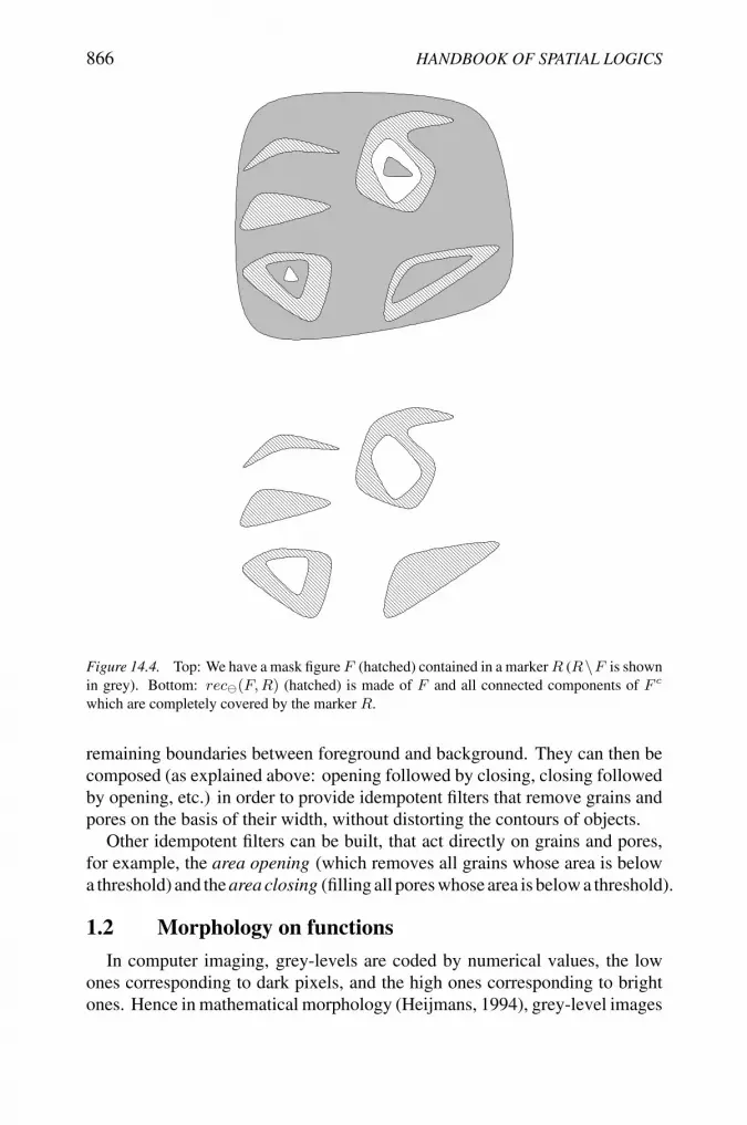
The behaviour of rec is to reconstruct all pores of F which are not completelycovered by the marker R; in other words, all connected components of thebackground F c which are included in R, are added to F . We illustrate thisoperation in Fig. 14.4.
Given an opening γ, we define the opening by reconstruction γrec as thegeodesical reconstruction by dilation using the opening as marker:
γrec(X) = rec⊕(X, γ(X)) .
Similarly for a closing ϕ, we define the closing by reconstruction ϕrec as thegeodesical reconstruction by erosion using the closing as marker:
ϕrec(X) = rec(X,ϕ(X)) .
Note that for a connected structuring element B containing the origin, we have
rec⊕(X,X B) = rec⊕(X,X 'B)and rec(X,X •B) = rec(X,X ⊕B) .
The opening and closing by reconstruction are again idempotent operators; theyrespectively remove small grains and fill small pores, but they do not deform the
866 HANDBOOK OF SPATIAL LOGICS
Figure 14.4. Top: We have a mask figure F (hatched) contained in a markerR (R\F is shownin grey). Bottom: rec(F,R) (hatched) is made of F and all connected components of F c
which are completely covered by the marker R.
remaining boundaries between foreground and background. They can then becomposed (as explained above: opening followed by closing, closing followedby opening, etc.) in order to provide idempotent filters that remove grains andpores on the basis of their width, without distorting the contours of objects.
Other idempotent filters can be built, that act directly on grains and pores,for example, the area opening (which removes all grains whose area is belowa threshold) and the area closing (filling all pores whose area is below a threshold).
1.2 Morphology on functions
In computer imaging, grey-levels are coded by numerical values, the lowones corresponding to dark pixels, and the high ones corresponding to brightones. Hence in mathematical morphology (Heijmans, 1994), grey-level images

Mathematical Morphology 867
are usually considered as numerical functions E → T , where E is the spaceof points and T is the set of grey-levels; it is always a subset of R = R ∪−∞,+∞. The grey-levels are numerically ordered, and morphological op-erations usually compute at each point inE a combination of numerical supremaand infima of grey-level values. Thus one supposes that T is closed under theoperations of non-empty numerical supremum and infimum; in the terminologythat we will introduce in Sec. 2, T is a complete lattice. Usually one takes forT one of the sets R, Z = Z ∪ −∞,+∞, [a, b] = x ∈ R | a ≤ x ≤ b(with a, b ∈ R and a < b), or [a . . . b] = [a, b] ∩ Z (with a, b ∈ Z and a < b).We write t0 and t1 respectively for the least and greatest element of T (thust0 = −∞ and t1 = +∞ for T = R or Z, while t0 = a and t1 = b for T = [a, b]or [a . . . b]).
The set TE of functions E → T inherits the numerical order on T by thepointwise ordering of functions:
(14.7) F ≤ G ⇐⇒ ∀p ∈ E, F (p) ≤ G(p) .
This is the analogue for functions of the inclusion relation for sets. Now theanalogues for functions of the union and intersection operations for sets, are thesupremum (least upper bound) and infimum (greatest lower bound), obtainedby pointwise supremum and infimum operations:
(14.8)∨
i∈IFi : E → T : p → sup
i∈IFi(p) ,
∧
i∈IFi : E → T : p → inf
i∈IFi(p) .
We write F ∨G and F ∧G for the supremum and infimum of two functions (cf.the union and intersection of two sets); as the two binary operations∨ and∧ arecommutative and associative, we can writeF1∨· · ·∨Fn andF1∧· · ·∧Fn, whichare in fact respectively equal to
∨i∈1,...,n Fi and
∧i∈1,...,n Fi. The least and
greatest functions are the ones with constant values t0 and t1 respectively, theyare the analogues of the empty set ∅ and the whole space E.
Given a function F : E → T and a point p ∈ E, the translate of F by p isthe function Fp whose graph is obtained by translating the graph (x, F (x)) |x ∈ E by p in the first coordinate, that is,
(y, Fp(y)) | p ∈ E = (x + p, F (x)) | x ∈ E ,
in other words∀y ∈ E, Fp(y) = F (y − p) .
We have thus the analogues for functions of the union, intersection and trans-lation operations for sets. It is then possible to define the dilation, erosion,opening and closing of a function by a structuring element, by making ana-logues of Eqs. (14.1, 14.4).

868 HANDBOOK OF SPATIAL LOGICS
There is however a systematic method for extending operators on sets tooperators on functions (Heijmans, 1991; Heijmans, 1994; Ronse, 2003). Itrelies on the notions of thresholding and stacking. Given a functionF : E → T ,the umbra (or hypograph) of F is the set
U(F ) = (p, t) | p ∈ E, t ∈ T, F (p) ≥ t ,
and for any value t ∈ T , consider the threshold set
Xt(F ) = p ∈ E | F (p) ≥ t ;
thus (p, t) ∈ U(F ) iff p ∈ Xt(F ). We illustrate these notions in Fig. 14.5.
Et
t 1
0
F
t
T
X (F)t
Figure 14.5. The graph of F , and below it the umbraU(F ) (in grey). For t ∈ T , the horizontalline at level t crosses the umbra in a section whose projection in E is the threshold set Xt(F ).
Given an operator ψ : P(E) → P(E), the flat operator corresponding to ψ(or flat extension of ψ) is the operator ψT : TE → TE constructed as follows:
1 Thresholding: For every t ∈ T , we take the horizontal cross-section ofthe umbra U(F ) at level t, that is the set Xt(F )× t.
2 Horizontal operation: We apply ψ horizontally to every such cross-section, that is, for every t ∈ T we obtain the set ψ (Xt(F ))× t.
3 Stacking: The upper envelope of these sets ψ (Xt(F )) × t, t ∈ T ,defines a function which gives ψT (F ).
We illustrate this construction in Fig. 14.6, in the case where ψ = δB , thedilation by a structuring element B. In fact, the values taken by ψT (F ) aregiven by the following formula:
(14.9) ∀p ∈ E, ψT (F )(p) =∨t ∈ T | p ∈ ψ (Xt(F )) .
Rather than using Equation (14.9) to compute the values ψT (F )(p), we canrely on the fact that the flat extension of operators transforms the operations on

Mathematical Morphology 869
F B
E
F
T
EB
E
T
E
T
Figure 14.6. Top left: The graph ofF , the umbraU(F ) (in grey), and horizontal cross-sectionsXt(F ) × t of the umbra. Top right: The structuring element B (the position of the originis indicated by a dot). Bottom left: We apply δB , the dilation by B, horizontally to the cross-sectionsXt(F )×t, obtaining the sets (Xt(F ) ⊕B)×t. Bottom right: The upper envelopeof the dilated cross-sections gives the dilated function δTB(F ), also written F ⊕B.
sets into the corresponding ones on functions, as it follows from the propertieslisted below (for the sake of brevity, in the formulas we omit the quantifications∀X ∈ P(E) and ∀F ∈ TE):
Identity: If ψ(X) = X , then ψT (F ) = F .
Translation: If ψ(X) = Xp, then ψT (F ) = Fp.
Union: If ψ(X) =⋃i∈I ξi(X), then ψT (F ) =
∨i∈I ξ
Ti (F ).
Intersection: If ψ(X) =⋂i∈I ξi(X), then ψT (F ) =
∧i∈I ξ
Ti (F ).
Composition: If ψ(X) = η(ζ(X)), then ψT (F ) = ηT (ζT (F )).
These properties can for example be used to give formulas for the flat extensionsof dilation and erosion. As δB(X) =
⋃b∈B Xb and εB(X) =
⋂b∈B X−b (see
Equation (14.1)), we obtain for every F ∈ TE :
(14.10) δTB(F ) =∨
b∈BFb and εTB(F ) =
∧
b∈BF−b .

870 HANDBOOK OF SPATIAL LOGICS
We get then for every p ∈ E:
(14.11)δTB(F )(p) = supb∈B F (p− b) = supq∈(B)p F (q)
and εTB(F )(p) = infb∈B F (p + b) = infq∈Bp F (q) .
It is customary to write F ⊕ B and F ' B for δTB(F ) and εTB(F ). FollowingEquation (14.4), we define F B = (F 'B)⊕B and F •B = (F ⊕B)'B;clearly F B = γTB(F ) and F • B = ϕTB(F ). Note that here the operations⊕, ', and • have a function as first operand, a set as second, and a functionagain as result.
All set operators built by combining dilations and erosions through unions,intersections and translations, extend thus naturally as flat operators. Thenthe properties of the set operators translate directly to their flat extensions; forexample, openings and closings are idempotent, and composing them leads toidempotent filters. In practice, flat operators behave on bright and dark partsof a grey-level image in the same way as the corresponding set operators doon foreground and background. For example, dilation inflates bright areas anddeflates dark ones, while erosion does the contrary; opening darkens narrowbright zones, while closing brightens narrow dark zones; dilation and openingdeform corners which are convex on the bright side, while erosion and closingdeform corners which are convex on the dark side. In particular, filters obtainedby composing opening and closing can be used to remove small defects in animage, such as speckle noise.
There is still a duality between erosion and dilation, and between openingand closing. Let n be an inversion of T , that is a bijection T → T whichreverses the order: t < t′ ⇐⇒ n(t) > n(t′); for example, if T = [a . . . b], wehave n(t) = a+ b− t; we extend it to an inversion N on functions, by settingN(F ) : p → n(F (p)) (here n and N stand for negative, in the photographicsense). Then:
N(F ⊕B
)= N(F )' B , N
(F 'B
)= N(F )⊕ B ,
N(F B
)= N(F ) • B , N
(F •B
)= N(F ) B .
This expresses formally the fact that the behaviour of erosions and closings isderived of that of dilations and openings, by exchanging the roles of bright anddark points or zones in the grey-level image.
It is also possible to give flat extensions of geodesical reconstruction bydilation or erosion. For a mask function and a marker function R, such thatR ≤ F , we define the geodesical reconstruction by dilation
rec⊕(F,R) =∨
n∈N
Rn ,
where the functions Rn, n ∈ N, are defined recursively by
R0 = R ∧ F and ∀n ∈ N, Rn+1 = (Rn ⊕ V ) ∧ F.

Mathematical Morphology 871
(HereV is the neighbourhood of the origin.) ForR ≥ F , we have the geodesicalreconstruction by erosion
rec(F,R) =∧
n∈N
Rn ,
where
R0 = R ∨ F and ∀n ∈ N, Rn+1 = (Rn ' V ) ∨ F .
In fact, the two are dual:
rec(F,R) = N[rec⊕
(N(F ), N(R)
)].
In the same way as the geodesical reconstructions on sets acted on grains andpores (connected components of the foreground and background), here theseoperators will act on flat zones, that is, maximal connected sets having a con-stant grey-level value. In particular, we can design openings and closings byreconstruction, as in the case of sets, and these filters will remove some brightor dark objects, and simplify the grey-levels of remaining objects, but they willnot deform the contours between objects. They are thus very interesting imagefilters.
The extension of morphology on sets that we have described, is called flatmorphology. This terminology arises from the fact that we work on the “hori-zontal” structure of functions (see Fig. 14.6). We will now see morphologicaloperators on functions that act both “horizontally” and “vertically” on them.
As the operators will combine grey-levels by arithmetical additions and sub-tractions, it will no longer be possible to take a bounded interval for the grey-level set T , otherwise the grey-levels resulting from these operations mightoverflow out of this interval. Thus T must extend from −∞ to +∞. LetT ′ = T \ −∞,+∞; formally we have the following two requirements:
T is closed under the operations of non-empty numerical supremum andinfimum (thus T is a complete lattice);
T ′ is closed under the operations of addition and subtraction (in otherwords, T ′ is a subgroup of R).
It is then easily seen that either T = R and T ′ = R, or there is some a > 0such that T ′ = aZ = az | z ∈ Z and T = aZ = aZ ∪ −∞,+∞; inthe second case, we can make a scaling of grey-levels by 1/a, so here we cansuppose without loss of generality that T = Z and T ′ = Z.
We gave above grey-level analogues of some set-theoretical operations. Wehave to extend this analogy further. First we redefine the umbra or hypographof a function F : E → T , it is the set
U(F ) = (p, t) ∈ E × T ′ | t ≤ F (p) .

872 HANDBOOK OF SPATIAL LOGICS
The difference with the previous definition is that we restrict t to T ′, whilebefore we had t ∈ T . The points (p, t) of the umbra U(F ) are the analogues ofthe points x ∈ X for a set X . We have now to give the analogue of a singleton,namely a set p verifying p ⊆ X ⇔ p ∈ X; it is the impulse ip,t, for(p, t) ∈ E × T ′, defined as follows:
∀x ∈ E, ip,t(x) =
t if x = p,−∞ if x = p.
We verify indeed that for a function F and an impulse i(p,t), we have ip,t ≤F ⇔ (p, t) ∈ U(F ).
We call the support of a function F the set
supp(F ) = p ∈ E | F (p) > −∞ .
Note that p ∈ supp(F ) iff there exists some t ∈ T ′ with (p, t) ∈ U(F ). Wewill see below that points outside the support are redundant in calculations; infact, we can assume that F is defined only on its support; conversely if F isdefined only on a subset S of E, we extend it to a function on E by settingF (p) = −∞ for all p ∈ E \ S.
We defined above the translation of a function by a point. We extend itto the translation by a pair (p, t). Given a function F : E → T and a pair(p, t) ∈ E × T ′, the translate of F by (p, t) is the function F(p,t) whose graphis obtained by translating the graph (x, F (x)) | x ∈ E by p in the firstcoordinate and by t in the second, that is,
(y, F(p,t)(y)) | p ∈ E = (x + p, F (x) + t) | x ∈ E ,
in other words
∀y ∈ E, F(p,t)(y) = F (y − p) + t .
We can now define the Minkowski addition and subtraction of two functionsE → T , by analogy with Equation (14.1). Such an analogy already appearedpartially in the definition of the dilation and erosion of a function by a set,Equation (14.10), but we have to extend it further. Given two functions F,G :E → T , we define their Minkowski addition F ⊕G and subtraction F 'G asfollows:
(14.12)
F ⊕G =∨
(p,t)∈U(G)
F(p,t) ,
=∨
(p,t)∈U(F )
G(p,t) ,
=∨i(p+p′,t+t′) | (p, t) ∈ U(F ), (p′, t′) ∈ U(G) ;
F 'G =∧
(p,t)∈U(G)
F(−p,−t) ,
=∨
i(p,t) | (p, t) ∈ E × T ′, G(p,t) ≤ F.

Mathematical Morphology 873
T
E
FG
o-o
Figure 14.7. Top left: The two grey-level functions F andG, both having value −∞ outside abounded support. (In the next three illustrations, F andG are shown dotted.) Top right: F ⊕Gis the supremum of translates of F by all points of U(G). Bottom left: It is also the supremumof translates of G by all points of U(F ). Bottom right: F G is the supremum of all impulsesi(p,t) such thatG(p,t) ≤ F ; in fact there is a unique point p for which this is possible, so F Gis an impulse.
These two operations are illustrated in Fig. 14.7. Usually, F plays the role of agrey-level image, while G is the grey-level analogue of a structuring element,and we call it then a structuring function.
We can give a numerical expression for the values of F ⊕G and F 'G; forall p ∈ E we have
(14.13)
(F ⊕G)(p) = suph∈E
(F (p− h) + G(h)
)
= suph∈supp(G)
(F (p− h) + G(h)
),
(F 'G)(p) = infh∈E
(F (p + h)−G(h)
)
= infh∈supp(G)
(F (p + h)−G(h)
),
with the following convention for dealing with expressions of the form +∞−∞inside the parentheses: if F (p − h) + G(h) takes the form +∞−∞, we set

874 HANDBOOK OF SPATIAL LOGICS
it equal to −∞, while if F (p + h)−G(h) takes the form +∞−∞, we set itequal to +∞.
The operators δG : TE → TE : F → F ⊕ G and εG : TE → TE : F →F ' G are called dilation and erosion by G. We can now define the binaryoperations and • as for sets, byF G = (F'G)⊕G andF •G = (F⊕G)'G,leading thus to the opening byG, γG : TE → TE : F → F G, and the closingby G, ϕG : TE → TE : F → F •G; note that
F G =∨G(p,t) | (p, t) ∈ E × T ′, G(p,t) ≤ F ,
which is analogous to the second line in Equation (14.4). We still have theduality by inversion. Define the transpose or symmetrical G of G by G(x) =G(−x); we have the grey-level inversionN on functions (given byN(F )(p) =−F (p)); we get then
(14.14)N(F ⊕G
)= N(F )' G ; N
(F 'G
)= N(F )⊕ G ;
N(F G
)= N(F ) • G ; N
(F •G
)= N(F ) G .
All properties of these operations⊕,', and • in the case of sets, extend to thecase of functions. For example, the opening and closing by G are idempotent.Operators on functions E → T built from these operations, together with thesupremum and infimum, constitute what is called grey-level morphology orfunctional morphology.
Note finally that the dilation and erosion of functions by a set structuringelement, Eqs. (14.10,14.11), are a particular case of dilation and erosion bya structuring function, Eqs. (14.12,14.13). Given a set B ⊆ E, define thefunction B0 : E → T having value 0 on B, and −∞ elsewhere:
∀x ∈ E, B0(x) =
0 if x ∈ B,−∞ if x /∈ B.
Then for every function F : E → T , we have F ⊕B = F ⊕B0 and F 'B =F ' B0. The function B0 is thus called a flat structuring function. Hence flatmorphology is a particular case of grey-level morphology, with a restriction ofstructuring functions to flat ones.
We explained above that flat operators behave on bright and dark parts ofa grey-level image in the same way as the corresponding set operators do onforeground and background. This remains true here, but now the action isnot only on the shape of these parts, but also on their grey-level profiles. Forexample, dilation and opening deform the grey-level profile on peaks, whileerosion and closing do it on valleys. This is illustrated in Fig. 14.8; we see thatthe opening removes narrow peaks and the closing removes narrow valleys (asexpected), but also the slope of jumps is reduced at the top with the opening,and at the bottom with the closing.

Mathematical Morphology 875
E
T
F
o
G
-o
E
T
Figure 14.8. Top left: The grey-level function F . Top right: The structuring function G.Bottom left: F G, the opening of F (dashed) by G. Bottom right: F • G, the closing of F(dashed) by G.
For most practical problems concerning grey-level images, flat morpholog-ical operators are applied, instead of functional ones. Indeed, their expressionis simpler (as it does not involve adding or subtracting grey-levels), and theywork correctly for bounded grey-levels (functional ones can lead to overflow).In fact, flat operators have the same potential as functional ones for dealing withspatial shapes of objects in a grey-level image. However, there are sometimessituations where the grey-level profile of objects matters as much as their shape,and in such situations one will use functional morphological operators.
Let us say a few words about the computational complexity of morpholog-ical operations. Without any optimization, the complexity of the Minkowskioperations is in O(N × S), where N is the size of the image and S is the sizeof the structuring element. However, thanks to various approaches, such as thedecomposition of structuring elements, or the use of redundancies, it is possi-ble for some particular types of structuring elements (say, rectangles), to havea complexity in O(N ×
√S), O(N × logS), or even O(N). In digital grids
using the usual connectivities based on neighbourhoods, geodesical reconstruc-tion has a complexity in O(N), thanks to the use of queues. In the binary case,pixels are inserted in the queue as soon as they receive a connected componentlabel, and leave the queue when they transmit the label to their neighbours. Forgrey-level reconstruction, one uses a set of queues, one for each grey-level,with a priority order corresponding to the grey-level (e.g., for reconstructionby dilation, priority is given to the highest grey-levels).

876 HANDBOOK OF SPATIAL LOGICS
2. Algebra
We saw in the Introduction how to define morphological operations on sets bycombinations of unions, intersections and translations, and how these operationscan be adapted to numerical functions by translating union and intersection intosupremum and infimum. For many practical applications, such a frameworkresting on the analogy between sets and numerical functions, where foregroundand background correspond to bright and dark image areas, is sufficient. How-ever, if one wants to deepen the understanding of morphology, two questionscome forward:
Instead of extending the morphology on sets to the one on functions“by analogy”, is there not a systematic approach that would give bothas particular cases? Indeed, the early studies of grey-level morphologyanalysed the latter in terms of umbras of functions, they even attempted tomake grey-level morphology a particular case of set morphology appliedto umbras; however the correspondence between operations on functionsand those on umbras is exact only for discrete grey-levels (Ronse, 1990).
Can we define similarly morphological operations on other types of ob-jects? For example, on the family F(Rn) of closed subsets of R
n: herean intersection of closed sets is closed, while a union of closed sets isnot closed, but one could take instead the closure of their union; can weadapt Minkowski addition and subtraction in order to obtain all othermorphological operators?
The answer to both questions is yes. Morphology on sets, on functions, andon several other types of objects (closed sets, convex sets, etc.) can be seenas particular cases of a general framework based on complete lattices. Thiswas first introduced by Serra, 1988, then developed by Heijmans and Ronse,1990, Ronse and Heijmans, 1991, Heijmans, 1991 and Heijmans, 1994. In thissection, we present the algebraic fundamentals of mathematical morphology.
2.1 Complete lattice framework for images and operators
The basic idea is to generalize the notions of inclusion, union and intersectionof sets, to other objects.
Definition 14.1 A partial order is a relation ≤ that is reflexive, anti-symmetrical and transitive. Write ≥ for the inverse of ≤ (x ≥ y iff y ≤ x), itis also a partial order. A partially ordered set or poset is a pair (X,≤), whereX is a set and ≤ a partial order on X .
A complete lattice is a poset (X,≤) in which every non-void part Y ofX hasa least upper bound or supremum
∨Y , and a greatest lower bound or infimum∧
Y .

Mathematical Morphology 877
It follows in particular that a complete lattice (X,≤) has always a greatestelement, namely
∨X , and a least element, namely
∧X . By analogy with
Boolean algebras, the greatest (resp., least) element is also called the one (resp.,zero), and it is written 1 or (resp., 0 or ⊥). Note also that every x ∈ X isboth lower bound and upper bound of the empty set. Hence:
1 =∨
X =∧∅ and 0 =
∧X =
∨∅ .
A complete sublattice of X is given by a subset Y of X , such that with therestriction to Y of the order ≤ on X , (Y,≤) is a complete lattice in which thesupremum and infimum operations, as well as the zero and one, are identicalto those in X; equivalently, it is a subset Y of X such that for every Z ⊆ Y ,∨Z,∧Z ∈ Y (also for Z = ∅, i.e., 0,1 ∈ Y ).
Some examples of complete lattices are particularly useful for mathematicalmorphology:
The power set P(E), ordered by the set inclusion; here the supremumand infimum are the union and intersection. It represents the family ofbinary images.
The grey-level sets R, Z, [a, b] and [a . . . b] considered in Sec. 1.2 arecomplete lattices, and Z is a complete sublattice of R.
Given T one of the above complete lattices, and a space E, consider theset TE of numerical functions E → T . It is a complete lattice, in fact apower lattice of T , in the sense that its ordering, supremum and infimumderive from those on T by pointwise application, see Eqs. (14.7, 14.8).It represents the family of grey-level images.
The family F(Rn) of closed subsets of Rn is a complete lattice for the
ordering by inclusion; here the infimum of a family of closed sets is itsintersection, while its supremum is the closure of its union. Despite thesame ordering as inP(E), it is not a complete sublattice ofP(E), becausethe supremum operation is not the same. Many metrics and topologies onsets are defined properly only for closed sets (Ronse and Tajine, 2004).
We can represent RGB colours as triples (r, g, b) of numerical values, soT 3 is the complete lattice of RGB colours, with componentwise ordering;now we represent a RGB colour image as a functionE → T 3 associatingto each point p ∈ E a triple
(r(p), g(p), b(p)
)coding the RGB colour of
p; thus the family of RGB colour images constitutes the complete lattice(T 3)E , with the componentwise ordering.
Given a set E, the set Π(E) of partitions on E is ordered as follows:given two partitions π1 and π2, we write π1 ≤ π2 is π1 is finer than π2,

878 HANDBOOK OF SPATIAL LOGICS
or equivalently π2 is coarser than π1; this means that every class of π1 isincluded in a class of π2. Then Π(E) is a complete lattice. In fact, thereis a one-to-one correspondence between partitions onE and equivalencerelations onE; then the lattice structure of Π(E) corresponds by bijectionto the one of the family Equiv(E) of equivalence relations on E, con-sidered as a subset of E2: the ordering on partitions corresponds to theinclusion order between equivalences, and the infimum and supremumof a family of partitions correspond respectively to the intersection and tothe transitive closure of the union, of the associated equivalence relations.
Image processing operations can then be viewed as mappingsL→ L, whereL is the complete lattice of images under consideration; we can also considermappings from one complete lattice to another, for example, TE → P(E)(binarization of grey-level images), or TE → Π(E) (segmentation). Suchmappings are usually written by Greek letters, and are called operators; anoperator is said on Lwhen it is a mapping L→ L. Given a set L (which can bea complete lattice or not) and a complete latticeM , the setML of operatorsL→M is a complete lattice, which inherits the order and complete lattice structureof M “componentwise”, as happened for functions, see Eqs. (14.7,14.8): fortwo operators η, ζ : L→M , we have
η ≤ ζ ⇐⇒ ∀x ∈ L, η(x) ≤ ζ(x) ,
and for a family ψi (i ∈ I) of operators L→M , their supremum and infimumare given by:∨
i∈Iψi : L→M : x →
∨
i∈Iψi(x) and
∧
i∈Iψi : L→M : x →
∧
i∈Iψi(x) .
There is another operation on operators, composition; given η : L → M andζ : M → N , the composition of η followed by ζ is the operator ζη : L →N : x → ζ(η(x)). Of particular interest is the composition of operatorson L: the composition of two operators ζ, η : L → L is always defined,and this gives an associative operation having as neutral element the identityid : L→ L : x → x, in other words the set LL of operators on L is what onecalls a monoid. Given an operator ψ on L, we define recursively the power ψn
for every n ∈ N: ψ0 = id, ψn+1 = ψ[ψn]. Let us recall some morphologicalterminology (Serra, 1988; Heijmans, 1994):
Definition 14.2 Given two posets L and M , an operator ψ : L→M is
increasing (or isotone, Birkhoff, 1995) if for all x, y ∈ L, we have x ≤y ⇒ ψ(x) ≤ ψ(y).
decreasing (or antitone, Birkhoff, 1995) if for all x, y ∈ L, we havex ≤ y ⇒ ψ(x) ≥ ψ(y).

Mathematical Morphology 879
an isomorphism if ψ is an increasing bijection, whose inverse ψ−1 isincreasing.
a dual isomorphism if ψ is a decreasing bijection, whose inverse ψ−1 isdecreasing.
Given a poset L, an operator ψ on L is
extensive if ψ ≥ id, that is, for every x ∈ L we have ψ(x) ≥ x.
anti-extensive if ψ ≤ id, that is, for every x ∈ L we have ψ(x) ≤ x.
an automorphism of L if ψ is an isomorphism L→ L.
a dual automorphism of L if ψ is a dual isomorphism L→ L.
Given a set L, an operator ψ on L is idempotent if ψψ = ψ, that is, for everyx ∈ L we have ψ(ψ(x)) = ψ(x).
Note that if L is a complete lattice and ψ is an increasing operator on L, thenwe have (Heijmans and Ronse, 1990):
(14.15) ∀(xi, i ∈ I) ⊆ L,
⎧⎪⎪⎨
⎪⎪⎩
ψ(∨
i∈Ixi
)≥
∨
i∈Iψ(xi),
ψ(∧
i∈Ixi
)≤
∧
i∈Iψ(xi).
Some other properties and specific families of operators (in particular, dilations,erosions, openings and closings) will be defined in the following subsections.
Given an operator ψ on a set L, the invariance domain of ψ is the setInv(ψ) = x ∈ L | ψ(x) = x. Given an operator ψ : L → M , therange (or image) of ψ is the set of ψ(x) for x ∈ L; we write it ψ(L).
In the latticeP(E) of parts of a Euclidean or digital spaceE = Rn or Z
n, thedilation, erosion, opening and closing by a structuring element, Eqs. (14.1,14.4),are translation-invariant, in other words they commute with any translation ofE. We can generalize this notion as follows. LetTbe a group of automorphismsof the complete latticeL; in other words for every τ ∈ T, τ is an automorphismof L and τ−1 ∈ T, and for every τ1, τ2 ∈ T, τ1τ2 ∈ T. An operator ψ onL is said to be T-invariant if it commutes with every element of T: ∀τ ∈ T,τψ = ψτ .
There is an important principle: duality. We saw above that the inverse≥ ofa partial order ≤ is a partial order. Therefore every notion concerning posetsand complete lattices admits a dual, which is the same notion expressed w.r.t.the inverse order ≥; as the inverse of ≥ is again ≤, the duality is symmetrical.For example, the dual of the supremum operation is the infimum operation (andvice versa); for an operator, being extensive and being anti-extensive are dual

880 HANDBOOK OF SPATIAL LOGICS
properties. Note that all notions relying only on composition of operators, andnot on order, are auto-dual; this is for example the case for the identity operatorand for the property of idempotence.
An inversion of a poset L is a dual automorphism of L which is its owninverse, in other words a decreasing operator ν on L such that ν2 = id. Thenevery operator ψ on L has a dual by inversion, ψ∗ = νψν, whose propertiesare dual to those of ψ. For example, the set complementation in P(E), and thegrey-level inversion (image negative) N in TE , are inversions; in P(E) thedilation (resp., opening) by B is the dual by complementation of the erosion(resp., closing) by B, Eqs. (14.2,14.5), and in TE the dilation and opening byG are the duals by inversion of the erosion and closing by G, Equation (14.14).
2.2 Moore families, algebraic closings and openings
There are many mathematical situations where an object is “closed” undersome operation: a closed set in a topological space, a convex set in R
n, asubgroup of a group, a transitive relation. The interesting thing is that when anobject is not closed, one can close it in a unique smallest possible way. Fromthe algebraic point of view, it is thus fundamental to describe both the structureof the family of closed sets, and the properties of the closure operator.
Definition 14.3 Let L be a poset.
1 A subsetM ofL is a Moore family if every element ofL has a least upperbound in M :
∀x ∈ L,(∃y ∈M,y ≥ x and
[∀z ∈M, (z ≥ x ⇒ z ≥ y)
]).
2 A closing (or closure operator) on L is an increasing, extensive andidempotent operator L→ L.
The Moore family stands for the family of closed objects. The equivalencebetween the two concepts of closed object and closing an object, is expressedas follows:
Proposition 14.4 Let L be a poset. There is a one-to-one correspondencebetween Moore families in L and closings on L, given as follows:
To a Moore family M we associate the closing ϕ defined by setting forevery x ∈ L: ϕ(x) is equal to the least y ∈M such that y ≥ x.
To a closingϕ one associates the Moore familyM which is the invariancedomain of ϕ: M = Inv(ϕ).
Note that M = ϕ(x) | x ∈ L. Let us now consider the case where L is acomplete lattice.

Mathematical Morphology 881
Theorem 14.5 Let L be a complete lattice. A subset M of L is a Moorefamily iff M is closed under the infimum operation:
∀S ⊆M,∧
S ∈M .
In particular,∧∅ = 1 ∈ M . Given a Moore family M corresponding to a
closingϕ, (M,≤) is a complete lattice with greatest element1 and least elementϕ(0) =
∧M , and where the supremum and infimum of a family N ⊆ M are
given by ϕ(∨
N)
and∧N , respectively.
Note that ϕ(1) = 1 and ϕ(∧
N)
=∧N . Let us mention also the following
property:
(14.16) ∀X ⊆ L, ϕ( ∨
x∈Xϕ(x)
)= ϕ
(∨X).
Let us illustrate the above results with the family F of closed sets in a topo-logical space E. Clearly F is a Moore family of P(E) (ordered by inclusion),which means that F is closed under arbitrary intersections, and contains theempty intersection
⋂∅ = E; now F corresponds to a closing, which is the
topological closure operator cl, where for X ⊆ E, cl(X) is the least elementof F containing X . However the Moore family F has two further properties:
1 ∅ ∈ F ; by Theorem 14.5, this is equivalent to cl(∅) = ∅.
2 F is closed under binary union: for C1, C2 ∈ F , C1 ∪ C2 ∈ F . ByTheorem 14.5, this means that cl(C1 ∪ C2) = C1 ∪ C2. Now F is theset of cl(X) for X ∈ P(E), and we can write Ci = cl(Xi), so in viewof Equation (14.16), the condition is equivalent to:
∀X1, X2 ∈ P(E), cl(X1 ∪X2) = cl(X1) ∪ cl(X2) .
Therefore one can characterize a topology, given by the family of closed sets,through the associated closure operator cl, which must be a closing (increasing,idempotent and extensive), preserve the empty set, and distribute binary union(Everett, 1944).
Let us now consider the dual concepts and results:
In a poset L, a dual Moore family is a subset M such that every elementof L has a greatest lower bound in M .
The dual of a closing is an opening on L: an increasing, anti-extensiveand idempotent operator L→ L.
There is a one-to-one correspondence between dual Moore families in Land openings on L, where the corresponding opening γ and dual Moore

882 HANDBOOK OF SPATIAL LOGICS
family M verify: γ(x) is equal to the greatest y ∈ M such that y ≤ x,and M is the invariance domain of γ.
In a complete lattice L, M is a dual Moore family iff M is closed underthe supremum operation; in particular 0 ∈ M . Given a dual Moorefamily M corresponding to an opening γ, (M,≤) is a complete latticewith greatest element γ(1) =
∨M and least element 0, and where the
supremum and infimum of a family N ⊆ M are given by∨N and
γ(∧
N), respectively.
A topology on a space E can be characterized by its topological interioroperation int, which is an opening verifying int(E) = E and int(X1 ∩X2) = int(X1) ∩ int(X2).
Let us now describe the structure of the families of openings and closings.This will lead to some standard methods to construct them.
Proposition 14.6 Let L be a complete lattice.
1 The supremum of any family of openings on L is an opening, and theset of openings on L is a dual Moore family in LL. For every in-creasing operator ψ on L, the greatest opening ≤ ψ is Γ(ψ), it verifiesInv(Γ(ψ)) = Inv(id ∧ ψ).
2 The infimum of any family of closings is a closing, and the set of closingson L is a Moore family in LL. For every increasing operator ψ on L,the least closing ≥ ψ is Φ(ψ), it verifies Inv(Φ(ψ)) = Inv(id ∨ ψ).
By Proposition 14.4 (and its dual), for any x ∈ L, Γ(ψ)(x) is the greatesty ∈ Inv(id ∧ ψ) such that y ≤ x, and Φ(ψ)(x) is the least y ∈ Inv(id ∨ ψ)such that y ≥ x.
By Theorem 14.5 (and its dual), the set of openings (resp., closings) is acomplete lattice, where id is the greatest opening (resp., the least closing), andthe least opening is the constant operator L → L : x → 0 (resp., the greatestclosing is the constant operator L→ L : x → 1).
One can construct openings and closings by specifying some of their invari-ants. Let b ∈ L and let T be a group of automorphisms of L. The structuralopening and closing γb,T and ϕb,T are defined by
(14.17) ∀x ∈ L,
γb,T(x) =
∨τ(b) | τ ∈ T, τ(b) ≤ x,
ϕb,T(x) =∧τ(b) | τ ∈ T, τ(b) ≥ x.
More generally, given a family S ⊆ L, we define then
(14.18) γS,T =∨
s∈Sγs,T and ϕS,T =
∧
s∈Sϕs,T ,

Mathematical Morphology 883
and we have
(14.19) ∀x ∈ L,
γS,T(x) =
∨τ(s) | s ∈ S, τ ∈ T, τ(s) ≤ x,
ϕS,T(x) =∧τ(s) | s ∈ S, τ ∈ T, τ(s) ≥ x.
These operators are a T-invariant opening and closing, respectively, and in factevery T-invariant opening and closing takes this form:
Proposition 14.7 Let L be a complete lattice. For any S ⊆ L, let 〈S〉supT
(resp., 〈S〉infT ) be the least subset of L containing S which is closed under T
and under the supremum (resp., infimum) operation. We have
〈S〉supT =
∨
(τ,s)∈Xτ(s) | X ⊆ T× S
and 〈S〉infT =
∧
(τ,s)∈Xτ(s) | X ⊆ T× S
.
Then γS,T and ϕS,T are a T-invariant opening and closing, respectively, withthese sets as their respective invariance domain:
Inv(γS,T) = 〈S〉supT and Inv(ϕS,T) = 〈S〉inf
T .
Conversely, every T-invariant opening γ and closing ϕ take this form: γ =γInv(γ),T and ϕ = ϕInv(ϕ),T.
A well-known example is when L = P(E), for E = Rn or Z
n, and T isthe group of translations of E. Then the structural opening and closing givethe opening and closing by a structuring element: for every X,B ∈ P(E)we have γB,T(X) = X B and ϕB,T(X) = (Xc Bc)c = X • [B]c (withb ∈ [B]c ⇔ −b /∈ B). For a family S of structuring elements, we get theopenings and closings of the form given in Equation (14.6). We obtain thusthe well-known fact that every translation-invariant opening (resp., closing) isa union of openings (resp., intersection of closings) by structuring elements.
When T reduces to the identity id, we simply write γb, ϕb, γS and ϕS . Thenthe above result characterizes arbitrary openings and closings as being γS andϕS for some S ⊆ L.
In the next subsection, we will see how openings and closings arise fromdilations and erosions.
2.3 Galois connections and adjunctions
At the beginning of the 19th century, Evariste Galois built a connectionbetween fields of numbers generated by roots of equations, and groups of per-mutations of these roots. This type of correspondence is the first example of a

884 HANDBOOK OF SPATIAL LOGICS
general technique used in algebra to build an association between two types ofstructures. It has thus been named after him.
Definition 14.8 Let A and B two posets, with two operators α : B → Aand β : A→ B. We say that α and β form a Galois connection if
(14.20) ∀a ∈ A, ∀b ∈ B, a ≤ α(b) ⇐⇒ b ≤ β(a) .
Note that α and β play symmetrical roles. Galois connections are often usedin mathematical morphology to establish a dual isomorphism between two typesof structures, thanks to the following result:
Proposition 14.9 Let A and B two posets, and let α : B → A and β :A→ B form a Galois connection. Then:
1 α and β are decreasing, α = αβα and β = βαβ.
2 αβ is a closing on A, βα is a closing on B, Inv(αβ) = α(B) andInv(βα) = β(A) (so that α(B) and β(A) are Moore families).
3 The restriction of β to α(B) is a dual isomorphism α(B) → β(A) whoseinverse β(A) → α(B) is the restriction of α to β(A).
One can generally characterize the types of maps α and β which may appearin a Galois connection, but in the case of complete lattices, this characterizationis straightforward:
Definition 14.10 Let A and B be complete lattices. An operator α : B →A is a Galois map if it exchanges supremum and infimum:
∀(xi, i ∈ I) ⊆ B, α(∨
i∈Ixi
)=∧
i∈Iα(xi) .
In particular (for I = ∅), α maps the least element 0B of B onto the greatestelement 1A of A.
Proposition 14.11 Let A and B be complete lattices. Then:
1 Given α : B → A and β : A → B forming a Galois connection, α andβ are Galois maps.
2 Conversely, given a Galois map α : B → A, there is a unique Galoismap β : A → B such that α and β form a Galois connection (and viceversa).
3 Given α1, α2 : B → A and β1, β2 : A → B such that αi and βi form aGalois connection for i = 1, 2, we have α1 ≤ α2 ⇔ β1 ≤ β2.

Mathematical Morphology 885
4 Given αi : B → A and βi : A → B forming a Galois connection fori ∈ I ,
∧i∈I αi and
∧i∈I βi form a Galois connection.
In other words, Galois maps form a Moore family in the complete lattice of oper-ators A→ B (or B → A), and Galois connection establishes an isomorphismbetween the two complete lattices of Galois maps A→ B and B → A.
Of particular interest are Galois connections between subsets of two sets,which were characterized by Ore, 1944 in terms of a relation between thepoints of the two sets:
Theorem 14.12 Let V and W two sets.
1 Given a relation ρ between elements of V and of W , define
αρ : P(W ) → P(V ) : Y → v ∈ V | ∀w ∈ Y, v ρ w,βρ : P(V ) → P(W ) : X → w ∈W | ∀v ∈ X, v ρ w.
Then αρ and βρ form a Galois connection.
2 Conversely, given α : P(W ) → P(V ) and β : P(V ) → P(W ) forminga Galois connection, there is a unique relation ρ between elements of Vand of W , such that α = αρ and β = βρ; the relation ρ is given by
∀v ∈ V,∀w ∈W, v ρ w ⇐⇒ v ∈ α(w) ⇐⇒ w ∈ β(v).
Following Birkhoff, 1995, the Galois maps αρ and βρ are called polarities.Galois connections between sets expressed in such a form, arise in many aspectsof mathematics and computer science. See for example Sec. 3.1.
We turn now to the notion of adjunction, which is “semi-dual” to the oneof Galois connection, in the sense that we reverse the ordering on one of theposets, but not on the other.
Definition 14.13 LetA andB two posets, with two operators and δ : A→B and ε : B → A. We say that (ε, δ) is an adjunction if
(14.21) ∀a ∈ A, ∀b ∈ B, δ(a) ≤ b ⇐⇒ a ≤ ε(b) .
We say that δ is lower adjoint of ε, and ε is upper adjoint of δ.
Compared with Galois connections (see Definition 14.8), we have reversedthe ordering on B, since we have δ(a) ≤ b instead of b ≤ δ(a). Hence ε and δdo not play symmetrical roles, that is why we write the ordered pair (ε, δ). Weobtain then the analogue of Proposition 14.9:
Proposition 14.14 Let A and B two posets, and let δ : A → B andε : B → A such that (ε, δ) is an adjunction. Then:

886 HANDBOOK OF SPATIAL LOGICS
1 ε and δ are increasing, ε = εδε and δ = δεδ.
2 εδ is a closing on A, δε is an opening on B, Inv(εδ) = ε(B) andInv(δε) = δ(A) (so that ε(B) is a Moore family and δ(A) is a dualMoore family).
3 The restriction of δ to ε(B) is an isomorphism ε(B) → δ(A) whoseinverse δ(A) → ε(B) is the restriction of ε to δ(A).
Proposition 14.15 Let L be a poset, T a group of automorphisms of L,and ε, δ : L→ L such that (ε, δ) is an adjunction. Then ε is T-invariant iff δis T-invariant.
Let us now characterize adjunctions in the case of complete lattices.
Definition 14.16 Let A and B be complete lattices.
1 An operator ε : B → A is an erosion if it commutes with the infimumoperation:
∀(xi, i ∈ I) ⊆ B, ε(∧
i∈Ixi
)=∧
i∈Iε(xi) .
In particular (for I = ∅), ε maps the greatest element 1B of B onto thegreatest element 1A of A.
2 An operator δ : B → A is a dilation if it commutes with the supremumoperation:
∀(xi, i ∈ I) ⊆ B, δ(∨
i∈Ixi
)=∨
i∈Iδ(xi) .
In particular (for I = ∅), δ maps the least element 0B ofB onto the leastelement 0A of A.
Note that dilations and erosions are increasing. Also the set of δ(x) (x ∈ B)is closed under the supremum operation, while the set of ε(x) (x ∈ B) is closedunder the infimum operation. We obtain now the analogue of Proposition 14.11:
Theorem 14.17 Let A and B be complete lattices. Then:
1 Given δ : A → B and ε : B → A such that (ε, δ) is an adjunction, δ isa dilation and ε is an erosion.
2 Conversely, (a) given a dilation δ : A → B, there is a unique erosionε : B → A such that (ε, δ) is an adjunction, and

Mathematical Morphology 887
(b) given an erosion ε : B → A, there is a unique dilation δ : A → Bsuch that (ε, δ) is an adjunction.
3 Given δ1, δ2 : A → B and ε1, ε2 : B → A such that (εi, δi) is anadjunction for i = 1, 2, we have δ1 ≤ δ2 ⇔ ε1 ≥ ε2.
4 Given δi : A→ B and εi : B → A such that (εi, δi) is an adjunction fori ∈ I ,
(∧i∈I εi,
∨i∈I δi
)is an adjunction.
In other words, in the complete lattice of operators A → B (or B → A),erosions form a Moore family, while dilations form a dual Moore family, andadjunctions establish a dual isomorphism between the two complete lattices ofdilations A→ B and erosions B → A.
The classical example of adjunction is given by the erosion and dilation bya structuring element or function, Eqs. (14.1, 14.10, 14.12), arising from theMinkowski addition and subtraction. They are both translation-invariant (cf.Proposition 14.15). Here A = B = P(E) or TE . In fact, every translationinvariant dilation/erosion on sets arises from Minkowski operations, Equa-tion (14.1), while for functions, every flat dilation/erosion invariant under spa-tial translations takes the form of Equation (14.10), and every dilation/erosioninvariant under both spatial and grey-level translations arises from Minkowskioperations, Equation (14.12).
In Heijmans and Ronse, 1990, there is a general study of complete latticeswhere it is possible to define such Minkowski operations, and to obtain for themproperties similar to those verified for sets. Particular cases include of coursesP(E) and TE (E = R
n or Zn, T = R or Z), for which we obtain the form
given in Eqs. (14.1, 14.12), but also: the lattice of convex subsets of Rn (here
the supremum is the convex hull of the union, but Minkowski operations are thesame as in P(Rn)), the lattice F(Rn) of closed sets of R
n (here the supremumis the closure of the union, and the Minkowski addition is the closure of the oneobtained in P(Rn), but the Minkowski subtraction is the one of P(Rn)), uppersemi-continuous functions Rn → R, etc.
In the case whereA = B, the operators ε, δ areA→ A, and can be composedarbitrarily in any order. It is then easily checked that in a poset A we have
(14.22) δ ≥ id ⇔ δ ≥ εδ ⇔ δε ≥ ε ⇔ id ≥ ε
and(14.23)δ2ε ≤ id ⇔ δ2 ≤ δ ⇔ δ ≤ εδ ⇔ δε ≤ ε ⇔ ε ≤ ε2 ⇔ id ≤ ε2δ .
This gives then the following result, which will be used later on, in the case ofsets:

888 HANDBOOK OF SPATIAL LOGICS
Proposition 14.18 Let A be a poset, and let (ε, δ) be an adjunction (forδ, ε : A → A). Then the following five statement are equivalent: (a) δ is aclosing, (b) ε is an opening, (c) δε = ε, (d) εδ = δ, (e) δ and ε verify onestatement of Equation (14.22) and one statement of Equation (14.23). Then wehave
Inv(εδ) = Inv(δε) = Inv(δ) = Inv(ε)= εδ(A) = δε(A) = δ(A) = ε(A) .
This set is both a Moore family and a dual Moore family in A; when A is acomplete lattice, it is a complete sublattice of A.
Let us now consider dilations, erosions and adjunctions on sets. Let V andW two sets, and let ρ be a relation between elements of V and ofW . We defineδρ : P(V ) → P(W ), the dilation by ρ, and ερ : P(W ) → P(V ), the erosionby ρ, as follows:
(14.24)∀X ∈ P(V ), δρ(X) = w ∈W | ∃v ∈ X, v ρ w,∀Y ∈ P(W ), ερ(Y ) = v ∈ V | ∀w ∈W, v ρ w ⇒ w ∈ Y .
Alternately, we can define dilation erosion in terms of a map N : V → P(W )and the dual map N : W → P(V ), corresponding to the relation ρ by
(14.25) ∀v ∈ V,∀w ∈W,
⎧⎨
⎩
w ∈ N(v) ⇔ v ∈ N(w) ⇔ v ρ w,that is, N(v) = w ∈W | v ρ w.
and N(w) = v ∈ V | v ρ w.
WhenV = W , the setN(v) can be considered as the window or neighbourhoodof point v, and N is called a neighbourhood function or a windowing function.Now Equation (14.24) can be written(14.26)
∀X ∈ P(V ), δN (X) =⋃
v∈XN(v) = w ∈W | N(w) ∩X = ∅ ,
∀Y ∈ P(W ), εN (Y ) = v ∈ V | N(v) ⊆ Y .
We have then the analogue for adjunctions of Ore’s characterization of Galoisconnections on sets (Theorem 14.12):
Theorem 14.19 Let V and W two sets.
1 Given a map N : V → P(W ), (εN , δN ) is an adjunction.
2 Conversely, given δ : P(V ) → P(W ) and ε : P(W ) → P(V ) such that(ε, δ) is an adjunction, there is a unique map N : V → P(W ) such thatδ = δN and ε = εN ; for every v ∈ V , N(v) = δ(v).

Mathematical Morphology 889
Note that δ˜N
is a dilationP(W ) → P(V ), ε˜N
is an erosionP(V ) → P(W ),(ε
˜N, δ
˜N) is an adjunction, and that δ
˜Nand ε
˜Nare dual by complementation of
εN and δN respectively, as
∀Y ∈ P(W ), δ˜N(Y ) = V \ εN (W \ Y )
and ∀X ∈ P(V ), ε˜N(X) = W \ δN (V \X).
In fact δ˜N
= δρ−1 and ε˜N
= ερ−1 , where ρ−1 is the relation inverse of ρ(w ρ−1 v ⇔ v ρ w).
A classical example is given for V = W = E for E being the Euclideanspace R
n or the digital space Zn, and the neighbourhoods being built from a
structuring elementB ⊆ E: for every p ∈ E,N(p) = Bp. Then N(p) = (B)pfor all p ∈ E, δN = δB , εN = εB , δ
˜N= δB and ε
˜N= εB . These operators
are translation-invariant. In fact, from Proposition 14.15, for an adjunction(εN , δN ), εN is translation-invariant iff δN is translation-invariant, and in sucha case it is easily seen that they are the erosion and dilation by the structuringelement B = N(o).
Proposition 14.20 The following are equivalent:(∀v ∈ V, N(v) = ∅
)⇔ εN (∅) = ∅ ⇔ δ
˜N(W ) = V ⇔ εN ≤ δ
˜N.
Dually, the following are equivalent:(∀w ∈W, N(w) = ∅
)⇔ ε
˜N(∅) = ∅ ⇔ δN (V ) = W ⇔ ε
˜N≤ δN .
This result will intervene later on, in particular in Sec. 3.2 and Sec. 4. Notethat in the case where V = W = E (E = R
n or Zn) and N(p) = Bp for all
p ∈ E, the two equivalences reduce both to B = ∅.Consider now the case where V = W = E. Here ρ is a relation on E,
and both N and N are E → P(E). The following two results will be used inSec. 3.2:
Proposition 14.21 Consider a relation ρ on a setE, and the correspondingmaps N, N : E → P(E). Then:
1 The following five statements are equivalent: (a) ρ is reflexive, (b) δNis extensive, (c) εN is anti-extensive, (d) δ
˜Nis extensive, (e) ε
˜Nis
anti-extensive.
2 The following five statements are equivalent: (a) ρ is symmetrical, (b)ε
˜NδN is extensive, (c) δNε ˜N
is anti-extensive, (d) εNδ ˜Nis extensive, (e)
δ˜NεN is anti-extensive.
3 The following five statements are equivalent: (a) ρ is transitive, (b)δ2N ≤ δN , (c) ε2N ≥ εN , (d) δ2
˜N≤ δ
˜N, (e) ε2
˜N≥ ε
˜N.

890 HANDBOOK OF SPATIAL LOGICS
Combining items 1 and 3 with Proposition 14.18, we deduce:
Proposition 14.22 Consider a relation ρ on E, and the correspondingmaps N, N : E → P(E). Then the following nine statements are equiva-lent: (a) ρ is reflexive and transitive, (b) δN is a closing, (c) εN is an opening,(d) δNεN = εN , (e) εNδN = δN , (f) δ
˜Nis a closing, (g) ε
˜Nis an opening,
(h) δ˜Nε
˜N= ε
˜N, (i) ε
˜Nδ
˜N= δ
˜N. We have then
Inv(εNδN ) = Inv(δNεN ) = Inv(δN ) = Inv(εN )= εNδN (Z) | Z ∈ P(E) = δNεN (Z) | Z ∈ P(E)= δN (Z) | Z ∈ P(E) = εN (Z) | Z ∈ P(E) ,
and the same with N in place ofN . The two families Inv(εNδN )=Inv(δNεN )and Inv(ε
˜Nδ
˜N)=Inv(δ
˜Nε
˜N) are closed under arbitrary union and inter-
section, and contain E and ∅ (in other words they are complete sublatticesof (P(E),⊆)).
An Alexandroff topology (Alexandroff, 1937; Alexandroff and Hopf, 1935)is a topological space (E,G) where the family G of open sets is closed underarbitrary intersection; in other words G is a complete sublattice of (P(E),⊆).It is equivalent to require that every point ofE has a least open neighbourhood.By the Alexandroff specialization theorem (Alexandroff, 1956), there is a one-to-one correspondence between Alexandroff topologies on E and reflexive andtransitive relations on E; in fact, for x, y ∈ E, x ρ y iff x is in the closureof y, i.e., iff y belongs to the least neighbourhood of x. It follows then thatfor x ∈ E, N(x) is the least neighbourhood of x and N(x) is the topologicalclosure of x, while for X ∈ P(E), δN (X) is the least open set containingX (called the star of X), εN (X) is the topological interior of X , δ
˜N(X) is the
topological closure of X , and ε˜N(X) is the greatest closed subset of X . Note
that Inv(εNδN ) = Inv(δNεN ) is the family of open sets and Inv(ε˜Nδ
˜N) =
Inv(δ˜Nε
˜N) is the family of closed sets.
We saw in Sec. 2.2 that a closing ϕ on P(E) is the closure operator in atopology onE iff it satisfies the following two additional constraints: ϕ(∅) = ∅and ϕ(X1 ∪ X2) = ϕ(X1) ∪ ϕ(X2) for all X1, X2 ∈ P(E); we have thenϕ(X1∪· · ·∪Xn) = ϕ(X1)∪· · ·∪ϕ(Xn) for allX1, . . . , Xn ∈ P(E). In otherwords the commutation with the union operation, ϕ
(⋃i∈I Xi
)=⋃i∈I ϕ(Xi),
is verified for I being empty or finite. This is weaker than ϕ being a dilation,where this identity is verified also for an infinite family I; but then the set ofclosed sets ϕ(X) is closed under infinite unions, which means indeed that wehave an Alexandroff topology.
2.4 Morphological filters
The word “filter” is used in several scientific and technological contexts, withvarious meanings. In image processing, one knows the linear filters, namely

Mathematical Morphology 891
convolution operators, in particular the bandpass filter from signal processing,which preserves all frequencies within a band, and eliminates all others. Innon-linear image processing, the well-known median filter has been used toremove impulsive noise, without the blurring effect of linear smoothing filters.The morphological approach to filtering is similar to that of signal processing,namely preserving some parts of an image and eliminating some others, ex-cept that the separation of these parts is not based on frequencies. The modelproposed is that of an ideal filter, i.e., one that keeps the wanted components un-altered, and eliminates completely the unwanted ones. In order to characterizean ideal filter, rather than describing the features to be preserved or removed,one takes an algebraic point of view: if the filter does not alter the wanted partsand eliminates completely the unwanted ones, then applying the filter a secondtime will not change anything. Hence the main characteristic of an ideal filteris its idempotence. This is important from a theoretical point of view, but alsofor practical applications: if after applying the filter on an image the result isnot satisfying, then we know that another filter must be applied. This contrastswith the behaviour of the median filter: after one application, some noise re-mains, that could be eliminated by a second or third application; then one canrepeat the application of the filter, without guarantee that this will lead to astable final result, as the median filter can produce oscillations (Serra, 1988).This is related to the fact that one cannot characterize precisely what are thefeatures preserved or eliminated by this filter.
Besides idempotence, mathematical morphology demands that the behaviourof a filter should be related to the order and complete lattice structure of thefamily of images. Therefore one calls a morphological filter (or simply, a filter)an increasing and idempotent operator on a poset (or complete lattice). WriteFilt(L) for the set of filters on L. We have already encountered some filters:openings and closings. There are many other ones, and we will describe heresome techniques for constructing them. This requires some terminology:
Definition 14.23 Let L be a poset and ψ an operator on L. We say that:
1 ψ is underpotent if ψ2 ≤ ψ.
2 ψ is overpotent if ψ2 ≥ ψ.
3 ψ is an underfilter if ψ is increasing and underpotent.
4 ψ is an overfilter if ψ is increasing and overpotent.
We saw in Proposition 14.6 that in a complete lattice, the set of openings is adual Moore family and the set of closings is a Moore family. They constitutethus two complete lattices. We have a similar result for filters (Serra, 1988):
Proposition 14.24 Let L be a complete lattice.

892 HANDBOOK OF SPATIAL LOGICS
1 The set of overfilters on L is a dual Moore family in LL, i.e. it is closedunder the supremum operation.
2 The set of underfilters onL is a Moore family inLL, i.e. it is closed underthe infimum operation.
3 The set Filt(L) of filters on L is a complete lattice. For any family ψi(i ∈ I) of filters, their supremum inFilt(L) is the least underfilterψ suchthat ψ ≥
∨i∈I ψi, and their infimum in Filt(L) is the greatest overfilter
ψ such that ψ ≤∧i∈I ψi.
This gives a first method for constructing a filter from a family of filters. Thesecond one arises from composition (Serra, 1988):
Proposition 14.25 LetL be a complete lattice and let ξ andψ be two filterson L such that ξ ≥ ψ. Then:
1 The only operators that can be obtained by repeated compositions of ψand ξ are ψξ, ξψ, ψξψ and ξψξ. They are all filters and
ξ ≥ ξψξ ≥
ψξξψ
≥ ψξψ ≥ ψ.
2 Inv(ξ) ∩ Inv(ψ) ⊆ Inv(ξψξ) = Inv(ξψ) ⊆ Inv(ξ) andInv(ξ) ∩ Inv(ψ) ⊆ Inv(ψξψ) = Inv(ψξ) ⊆ Inv(ψ).
3 In Filt(L), the supremum and infimum of ξψ and ψξ are ξψξ and ψξψrespectively.
Note that items 1 and 2 do not require L to be a complete lattice, they arevalid in any poset. A classical example is when ξ is a closing and ψ is anopening: the opening filters out positive noise, the closing filters out negativenoise, so the composition of the two should filter out both types of noise (cf.Sec. 1.1).
The above result is at the basis of a well-known filter introduced in the1980s, the alternate sequential filter. Suppose that we have an image wherefeatures of foreground and background are imbricated. To extract an object ofa given size, it is necessary to filter its holes at a smaller size, and this requirefiltering objects at an even smaller size, etc. Thus we will apply openingsand closings at increasing scales in order to simplify the image. Consider nopenings γ1, . . . , γn such that γn ≤ · · · ≤ γ1, and n closings ϕ1, . . . , ϕnsuch that ϕ1 ≤ · · · ≤ ϕn. From the previous proposition, the compositionsµi = γiϕi, νi = ϕiγi, ρi = ϕiγiϕi and σi = γiϕiγi are filters. Alternatesequential filters are then defined as:
(14.27)µiµi−1 · · ·µ2µ1 = (γiϕi)(γi−1ϕi−1) · · · (γ2ϕ2)(γ1ϕ1),νiνi−1 · · · ν2ν1 = (ϕiγi)(ϕi−1γi−1) · · · (ϕ2γ2)(ϕ1γ1),

Mathematical Morphology 893
or as the following variants:(14.28)
ρiρi−1 · · · ρ2ρ1 = (ϕiγiϕi)(ϕi−1γi−1ϕi−1) · · · (ϕ2γ2ϕ2)(ϕ1γ1ϕ1)= ϕiµiµi−1 · · ·µ2µ1 ,
σiσi−1 · · ·σ2σ1 = (γiϕiγi)(γi−1ϕi−1γi−1) · · · (γ2ϕ2γ2)(γ1ϕ1γ1)= γiνiνi−1 · · · ν2ν1 ,
for i = 1, . . . , n. They are all filters. They are useful for filtering imageswhere grains (bright zones) are imbricated with pores (dark zones) at all sizes.Typically, the γi’s and ϕi’s can be:
openings and closings by structuring elements of increasing sizes;
openings and closings by reconstruction, based on structuring elementsof increasing sizes;
area openings and closings (removing grains and pores on the basis oftheir area), with increasing area thresholds;
hence as i increases, the alternating sequential filters will progressively removegrains and pores of increasing sizes, thus simplifying the image. (We willdiscuss further the notion of removing “features of increasing sizes” in Sec. 2.5.)An example is provided in Fig. 14.9 and 14.10.
Schonfeld and Goutsias, 1991 noticed that besides Eqs. (14.27,14.28), anycomposition of openings γi and closings ϕi, in any order, is a filter. Theirargument was generalized by Heijmans, 1997 as follows:
Proposition 14.26 Let ψ1, . . . , ψn be overfilters and ξ1, . . . , ξn be under-filters such that
ψn ≤ · · · ≤ ψ1 ≤ ξ1 ≤ · · · ξn .
Then any composition of these operators, containing at least one ψi and oneξj , is a filter.
A consequence is the following surprising result:
Proposition 14.27 Let (ε, δ) be an adjunction in a poset L. Then anyrepeated composition of ε and δ in any order, containing the same number ofinstances of ε and of δ, is a filter.
More precisely, an operator of the form ψ1 · · ·ψ2n, where for each i =1, . . . , 2nwe haveψi ∈ δ, ε, and cardi = 1, . . . , 2n | ψi = δ = cardi =1, . . . , 2n | ψi = ε, is a filter.
For more results on filters, the reader is referred to Heijmans, 1994, Heijmans,1997, Ronse and Heijmans, 1991, Serra, 1988 and Soille, 2003.

894 HANDBOOK OF SPATIAL LOGICS
(a) (b)
(c) (d)
Figure 14.9. Original image (a) and three steps (b, c, d) of an alternate sequential filter basedon opening-closing by reconstruction using an hexagon as structuring element.
2.5 Granulometries and size distributions
As openings remove parts of an object (they are anti-extensive), one cancompare two openings γ1 and γ2 in such terms; thus we say that γ2 is moreactive than γ1 if γ2 removes from any object more than γ1 does, in other wordsif γ2 ≤ γ1. On the other hand, as closings add parts to an object, given twoclosingsϕ1 andϕ2, we say thatϕ2 is more active thanϕ1 ifϕ2 adds to an objectmore than ϕ1 does, in other words if ϕ2 ≥ ϕ1.
In the case of the complete lattice P(E), given two structuring elementsA,B ∈ P(E), we define the relation8 by B 8 A iff B is a union of translates
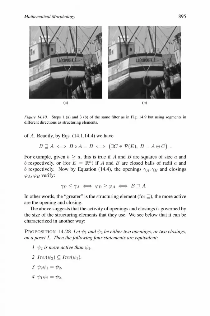
Mathematical Morphology 895
(a) (b)
Figure 14.10. Steps 1 (a) and 3 (b) of the same filter as in Fig. 14.9 but using segments indifferent directions as structuring elements.
of A. Readily, by Eqs. (14.1,14.4) we have
B 8 A ⇐⇒ B A = B ⇐⇒(∃C ∈ P(E), B = A⊕ C
).
For example, given b ≥ a, this is true if A and B are squares of size a andb respectively, or (for E = R
n) if A and B are closed balls of radii a andb respectively. Now by Equation (14.4), the openings γA, γB and closingsϕA, ϕB verify:
γB ≤ γA ⇐⇒ ϕB ≥ ϕA ⇐⇒ B 8 A .
In other words, the “greater” is the structuring element (for8), the more activeare the opening and closing.
The above suggests that the activity of openings and closings is governed bythe size of the structuring elements that they use. We see below that it can becharacterized in another way:
Proposition 14.28 Let ψ1 and ψ2 be either two openings, or two closings,on a poset L. Then the following four statements are equivalent:
1 ψ2 is more active than ψ1.
2 Inv(ψ2) ⊆ Inv(ψ1).
3 ψ2ψ1 = ψ2.
4 ψ1ψ2 = ψ2.

896 HANDBOOK OF SPATIAL LOGICS
The second item indicates that the activity increases as the domain of invari-ance decreases. The last two suggest a notion of a filtering absorption orderassociated to activity: if ψ2 is more active than ψ1, then as a filter ψ2 is moresevere, so ψ1 does not improve in any way upon the result of ψ2, whether ap-plied before of after it; thus ψ2 absorbs ψ1. We can now consider an orderedsequence of openings:
Definition 14.29 A granulometry (on a posetL) is a family of operators ψr(r ∈ R ⊆ R
+) such that:
1 ∀r ∈ R, ψr is anti-extensive;
2 ∀r ∈ R, ψr is increasing;
3 ∀r, s ∈ R, ψrψs = ψsψr = ψmax(r,s).
Applying item 3 with r = s, ψr is idempotent, so it is an opening. In fact,ψr (r ∈ R) is a granulometry iff ψr is an opening for every r, and ψr decreases(becomes more active) as the parameter r increases: ∀r, s ∈ R, r ≥ s impliesψr ≤ ψs, or equivalently Inv(ψr) ⊆ Inv(ψs).
For binary images in a digital framework (L = P(Zn)), we take R =2, . . . , rmax and ψr to be the opening by a structuring element Br corre-sponding to size r (say, a r×r-square). Then for a setX ⊆ Z
n, it is interestingto measure the area (number of pixels) of γr(X) for all r; this gives a decreasingfunction R → N, the granulometry curve of X , it displays the area of the ob-jects according to the size of the opening. Positions where this curve decreasessharply indicate that there are substantial parts of X having the correspondingwidth. This is illustrated in Fig. 14.11.
One defines similarly an anti-granulometry by replacing, in item 1 of Def-inition 14.29, “anti-extensive” by “extensive”. Then ψr (r ∈ R) is an anti-granulometry iff ψr is a closing for every r, and ψr increases (becomes moreactive) as the parameter r increases: ∀r, s ∈ R, r ≥ s implies ψr ≥ ψs,or equivalently Inv(ψr) ⊆ Inv(ψs). In a digital framework, we define theanti-granulometry curve, which gives an indication on the width of the holesof the set.
It is possible to combine a granulometry γr (r ∈ R1 ⊆ R+) and an anti-
granulometry ϕr (r ∈ R2 ⊆ R+) into a two-sided sequence ψr, r ∈ R =
R1 ∪ 0 ∪ (−R2) by setting ψr = γr for r ∈ R1, ψ0 = id, and ψ−r = ϕr forr ∈ R2. Then the axioms are: (1) ψr is anti-extensive for r ≥ 0 but extensivefor r ≤ 0, (2) ψr is increasing, (3) ψrψs = ψsψr = ψm(r,s) for r, s having thesame sign, where m(r, s) = max(r, s) for r, s ≥ 0, but m(r, s) = min(r, s)for r, s = 0 (we have no such identity for r > 0 and s < 0). We generalizethen the granulometry curve into a function R→ N where the parts r < 0 andr > 0 deal with the sizes of holes and grains respectively.

Mathematical Morphology 897
Figure 14.11. A binary image of coffee beans, and its granulometry curve, showing a sharpdecrease between 10 and 15; this indicates that most beans have such a width.
3. Related approaches
As we said in the Introduction, there are other fields of research which arebased on the same lattice-theoretical foundations as mathematical morphology.We present here three of them, which we think are relevant to the logic of spatialrelations: formal concept analysis, rough sets and fuzzy sets. Roughness canbe represented by using mathematical morphology operators to define upperand lower approximations in the framework of roughs sets (Sec. 3.2). We thenshow why mathematical morphology can be considered as a spatial reasoningtool (Sec. 3.3), with its two components: spatial knowledge representation andreasoning. As for the first one, we present in Sec. 3.4 an extension of mathe-matical morphology to fuzzy sets, which leads to an extended representationpower coping with spatial imprecision. Modeling spatial relationships basedon fuzzy morphology allows reasoning under imprecision and with structuralspatial information, as shown in Sec. 3.5. This reasoning component will befurther explored in Sec. 4.
3.1 Formal Concept Analysis
It is a lattice-based theory (Ganter and Wille, 1999) of relations betweenobjects and features. It can be applied to spatial objects and spatial relationslike visibility, enclosure, etc.
Let Ω be a set of objects, Π a set of properties, and ∼ a relation between Ωand Π, where o ∼ p means that object o has property p. The triple (Ω,Π,∼) is

898 HANDBOOK OF SPATIAL LOGICS
called a context. Following Theorem 14.12 we define the two maps
ω : P(Π) → P(Ω) : P → o ∈ Ω | ∀p ∈ P, o ∼ p ,π : P(Ω) → P(Π) : O → p ∈ Π | ∀o ∈ O, o ∼ p .
Thus ω(P ) is the set of objects sharing all properties in P , while π(O) is theset of properties shared by all objects in O. A concept is a pair (O,P ), whereO ∈ P(Ω) and P ∈ P(Π), such thatO = ω(P ) and P = π(O); O is the extentof the concept and P is the intent of the concept.
The set of concepts ordered by inclusion of object sets, or equivalently bythe inverse inclusion on property sets:
(O1, P1) ≤ (O2, P2) ⇐⇒ O1 ⊆ O2 ⇐⇒ P1 ⊇ P2 .
It forms then a complete lattice with the following supremum and infimumoperations:
∨
i∈I(Oi, Pi) =
(ωπ[⋃
i∈IOi
],⋂
i∈IPi
),
∧
i∈I(Oi, Pi) =
(⋂
i∈IOi, πω
[⋃
i∈IPi
]).
Here we used the complete lattice structure of the two Moore families of ex-tents (possible Oi’s) and of intents (possible Pi’s), cf. Proposition 14.9 andTheorem 14.5.
A possible example of application of formal concept analysis is to considertwo subsets S and V of the space R
n or Zn, where S represents an object to
be visually examined, and a V is a set of viewpoints. We define a relation ∼between the boundary ∂S of S and V , namely s ∼ v if s is visible from v, i.e.,the open segment ]s, v[ is disjoint from S. Then a concept is given by a pair(T,W ), where T ⊆ ∂S and W ⊆ V , such that T is the set of positions visibleby all viewpoints in W , and W is the set of all viewpoints from which T isentirely visible.
3.2 Mathematical morphology and rough sets
Rough set theory has been introduced by Pawlak, 1982, as an extension ofset theory, mainly in the domain of intelligent systems. The objective was todeal with incomplete information, leading to the idea of indistinguishabilityof objects in a set. It is therefore related to the concept of approximation,and of granularity of information (in the sense of Zadeh, 1979). This theorywas applied successfully in several applications, e.g. information analysis, dataanalysis and data mining, knowledge discovery (for instance discovery of whichfeatures are relevant for data description), i.e., all applications for which a needarises for intelligent decision support. Let us mention in particular the works

Mathematical Morphology 899
of Lin, 1995, Lin and Liu, 1994, Yao, 1998 and Yao and Lin, 1996. There havealso been studies towards a fuzzy approach to rough sets (Dubois and Prade,1990), and on their relations with logic (Orlowska, 1993; Pawlak, 1987).
In this framework, a set X is approximated by two sets, called upper andlower approximations, and denoted by A(X) and A(X), such that A(X) ⊆X ⊆ A(X). It is interesting to investigate the algebraic properties of the two setoperators A and A: the first one is extensive, the second one is anti-extensive,and probably they should be increasing. But then, are they respectively adilation and an erosion? In particular, do they constitute an adjunction (arisingfrom a reflexive relation, cf. Proposition 14.21)? Or are they a closing andan opening? Or is A both a closing and a dilation, and A both an openingand an erosion (cf. Proposition 14.22)? Are they dual by complementation?Surprisingly, there have not been many studies on the relation between roughsets and MM; let us mention a few of them. On the one hand Polkowski,1998 built a hit-or-miss (Fell) topology on rough sets, similar to the one usedin MM for closed sets (Heijmans, 1994; Matheron, 1975; Ronse and Tajine,2004; Serra, 1982). On the other hand Bloch, 2000b studied the algebraicproperties of the upper and lower approximation operators, and established ananalogy between them and the classical morphological operators on Euclideanor digital sets, namely dilation, erosion, opening and closing by a structuringelement. Also Duntsch and Gediga, 2003 considered the algebraic aspects ofrough sets, in particular their links with Galois connections.
Here we will investigate rough sets in light of the theory of adjunctions onsets; in some sense, this is a generalization of Bloch, 2000b. At the same timewe will address topological aspects. But let us first recall the basic definitionsof rough sets, in particular those based on a similarity relation.
In rough set theory (Pawlak, 1982), the two approximationsA(X) andA(X)such that A(X) ⊆ X ⊆ A(X) are defined from an equivalence relation. Let Udenote the universe of discourse (X being a subset ofU). We consider attributeswhich are functions defined on U , and write A for the set of attributes. To eachx ∈ U we associate an information vector Inf(x), which is the set of attributesassociated to x. We define an equivalence relation RA (with respect to the setA of attributes on U) by the equality of the information vector:
x RA y ⇐⇒ Inf(x) = Inf(y) .
Assuming that each element of U is known only through its attributes, x RA ymeans that x and y are undistinguishable on the basis of available information.The pair (U , RA) is called an approximation space. For x ∈ U , let [x]A denotethe equivalence class of x under RA:
[x]A = y ∈ U | x RA y .

900 HANDBOOK OF SPATIAL LOGICS
Then upper and lower approximations of a subset X of U are defined as:
(14.29)A(X) = x ∈ U | [x]A ∩X = ∅ ,A(X) = x ∈ U | [x]A ⊆ X .
The lower approximation of X contains all points of U that are distinguishablefrom every elements of Xc, while its upper approximation contains all pointsof U that are undistinguishable from some element of X . We call a rough seta pair (A(X), A(X)).
Let us refer to the terminology used for dilations and erosions on sets: ifRA stands for ρ, then by Eqs. (14.24,14.25,14.26) we have [x]A = N(x),A = εN = εRA and A = δ
˜N= δR−1
A. Clearly A and A are dual under
complementation: A(X) =[A(Xc)
]c. The fact thatRA is symmetrical (RA =
R−1A ) means that N = N , so (A,A) forms an adjunction. Now as RA is
reflexive and transitive, by Proposition 14.22, the erosion A is also an opening,while the dilationA is also a closing, withAA = A andAA = A. In particular,we have
∀X ∈ P(U), A(X) ⊆ X ⊆ A(X) .
By Proposition 14.22 again, εN (P(U)) = δN (P(U)), i.e., the families of lowerand upper approximations coincide:
A(X) | X ∈ P(U) = A(X) | X ∈ P(U) ;
in fact this family consists of all sets which are unions of equivalence classes[x]A. With the topological interpretation given after Proposition 14.22, it con-stitutes an Alexandroff topology on U , where open sets coincide with closedones, the upper approximation A(X) is the closure and the star (least opensuperset) of X , while the lower approximation A(X) is the interior and thegreatest closed subset of X .
This definition can be extended to any relation R, leading to the notionof generalized approximate space (see e.g. Yao, 1998). Simply we take anarbitrary relation R instead of the equivalence RA, and the set
r(x) = y ∈ U | x R y
instead of the equivalence class [x]A; here r(x) corresponds to the set N(x)according to Equation (14.25), with R standing for ρ. Then Equation (14.29)becomes
(14.30)R(X) = x ∈ U | r(x) ∩X = ∅ ,R(X) = x ∈ U | r(x) ⊆ X .
In our terminology, R = εr = εR and R = δr = δR−1 . Now R and R are stilldual under complementation.

Mathematical Morphology 901
Equivalently, we can define R and R as two set operators which are dualunder complementation (R(X) =
[R(Xc)
]c), and such thatR is an erosion (or
equivalently: R is a dilation). This is in accordance with the operator-orientedview of rough sets (Lin and Liu, 1994; Yao, 1998).
IfR is an equivalence relation, we get Pawlak’s definition, Equation (14.29);indeed, we can define Inf(x) = [x]R, the equivalence class of x under R. Letus consider weaker conditions on R. We require that R(X) ⊆ R(X) for allX ∈ P(U), which means that εr ≤ δr; according to Proposition 14.20, this isverified iff
∀x ∈ U , r(x) = ∅.Usually, one requires that R is anti-extensive and R is extensive, that is,
∀X ∈ P(U), R(X) ⊆ X ⊆ R(X);
by Proposition 14.21, this is verified iff R is reflexive.By Proposition 14.21, R is symmetrical iff RR is extensive, iff RR is anti-
extensive. Then r = r, and (R,R) is an adjunction. If R is reflexive andsymmetrical, we call it a tolerance relation.
By Proposition 14.22,R is reflexive and transitive iffR is both an erosion andan opening, iff R is both a dilation and a closing. Here we have an Alexandrofftopology on U , where for every X ∈ P(U), R(X) is the topological interiorof X and R(X) is the topological closure of X . The family of open sets,R(X) | X ∈ P(U), and the family of closed sets,R(X) | X ∈ P(U), donot coincide, unless R is also symmetrical (i.e., an equivalence relation).
WhenR is reflexive but not transitive, the upper and lower approximations dogenerally not correspond to a topology. However they correspond to the closureand interior in a pre-topology, that is: R andR are dual under complementation,they are both increasing,R is extensive whileR is anti-extensive,R(∅) = ∅ andR(U) = U . Let us mention the use by Emptoz, 1983 of pre-topology for thedescription of spatial objects. This may be of interest for pattern recognitionpurposes, since a non-idempotent closure allows to aggregate patterns usingiterated closure operations.
In Yao, 1998, various properties are given for the operators R and R, whichmay or may not be satisfied, according to the properties of the relation R. InBloch, 2000b, a parallel is made between these properties and those of dilations,erosions, openings and closings. In fact, all these properties follow from theones given in Sec. 2.3 for dilations and erosions on sets, those of openings andclosings in Sec. 2.2, and from Equation (14.15).
Using the operator-oriented point of view (Lin and Liu, 1994; Yao, 1998),one could also define the lower and upper approximation as an opening and aclosing. However, such operators cannot be defined in terms of a relation or aneighbourhood function, as was the case with dilations and erosions. Openings

902 HANDBOOK OF SPATIAL LOGICS
and closings are characterized by their invariance domain: for an opening, it isa dual Moore family, i.e., a family closed under arbitrary unions and contain-ing ∅; for a closing it is a Moore family, i.e., a family closed under arbitraryintersections and containing U . Let L be an opening and let S be a family ofnonvoid parts ofU such that Inv(L) is the set of all arbitrary unions of elementsof S (including the empty union ∅); in fact L is the opening γS defined afterEqs. (14.18,14.19), as for every X ∈ P(U) we have
L(X) =∨A ∈ S | A ⊆ X.
For example, if U = E and L is the opening by a structuring element B, thenS is the set of translates Bp (p ∈ E) of B. Now let H be the closing which isthe dual of L by complementation; then Inv(H) = Ac | A ∈ Inv(L), andInv(H) is the set of arbitrary intersections of Ac for A ∈ S. For X ∈ P(U)we have
H(X) =(∨
A ∈ S | A ⊆ Xc)c.
We can interpret the elements of S as “blocks”, and a point x can be in-cluded in the lower approximation L(X) only through its membership of a“block” included in X , while a point x can be excluded from the upper ap-proximation H(X) only through its membership of a “block” excluded fromX . However these blocks do not make a partition, as with Pawlak’s definition,Equation (14.29).
An interesting particular case is when L and H are the interior and closureoperators in a topological space. One speaks then of a topological approxima-tion space. As explained after Proposition 14.22, this is weaker than requiringH to be both a dilation and a closing, and dually L to be both an erosion andan opening.
Other operators could be used for lower and upper approximations. In Serra,1988, it is shown that every increasing operator on a complete lattice, whichfixes the greatest element, is a supremum of erosions. Thus an increasingoperator ψ on P(U) such that ψ(U) = U , is a union of erosions; in particular ψis anti-extensive iff these erosions are anti-extensive. Consider the followingdefinition of lower and upper approximations (Lin, 1995). Suppose that to eachx ∈ U we associate a family N (x) of parts of U which are “neighbourhoods”of x; N (x) is called a neighbourhood system of x. Now we define the upperand lower approximations N and N as follows:
(14.31)N(X) = x ∈ U | ∀A ∈ N (x), A ∩X = ∅,N(X) = x ∈ U | ∃A ∈ N (x), A ⊆ X.
ClearlyN is the dual by complementation of N , so let us analyse the latter. Wehave
N(U) = x ∈ U | N (x) = ∅,

Mathematical Morphology 903
so in order to have N(U) = U , we suppose that N (x) = ∅ for all x ∈ U .Then N is a union of erosions, and we can describe them precisely. For everyx ∈ U and for every A ∈ N (x), let N [x,A] : U → P(U) be defined byN [x,A](x) = A and N [x,A](y) = U for y ∈ U \ x. Then εN [x,A] verifiesfor every X ∈ P(U):
εN [x,A](X) =
⎧⎨
⎩
U if X = U ,x if A ⊆ X = U ,∅ otherwise.
We obtain thenN(X) =
⋃
x∈U
⋃
A∈N (x)
εN [x,A](X).
Dually, we get
N(X) =⋂
x∈U
⋂
A∈N (x)
δN [x,A]
(X).
This view is particularly interesting for shape recognition, since in morpho-logical recognition, an object has often to be tested or matched with a set ofpatterns, like directional structuring elements. Thus we apply the union of theerosions by all those patterns, which is a particular case of the above operator.
In Bloch, 2000b, some other extensions are presented, using as lower andupper approximations morphological thinning and thickening (Serra, 1982).There is also an extension to rough functions, using the grey-level morpholog-ical operations described in Sec. 1.2.
To conclude, let us remark that the general theory of adjunctions, dilations,erosions, openings and closings on sets provides a good formal framework forexpressing the notion of coarseness underlying rough sets. It allows to charac-terize precisely their algebraic properties and their relations with topology. InSec. 3.4 and 4, we will examine the relationship of rough sets with fuzzy setsand modal logic, especially in the morphological framework.
3.3 Mathematical morphology and spatial reasoning
Spatial reasoning has been largely developed in artificial intelligence, in par-ticular using qualitative representations based on logical formalisms. In imageinterpretation and computer vision it is much less developed and is mainlybased on quantitative representations. On the contrary, mathematical morphol-ogy is widely used in these domains. A typical example concerns model-basedstructure recognition in images, where the model represents spatial entitites andrelationships between them. Based on this example, spatial reasoning can bedefined as the domain of spatial knowledge representation, in particular spa-tial relations between spatial entities, and of reasoning on these entities and

904 HANDBOOK OF SPATIAL LOGICS
relations. This definition exhibits two main components: spatial knowledgerepresentation and reasoning. In particular spatial relationships constitute animportant part of the knowledge we have to handle and imprecision is often at-tached to it. The reasoning component includes fusion of heterogeneous spatialknowledge, decision making, inference, recognition. Two types of questionsare raised when dealing with spatial relationships:
1 given two objects (possibly fuzzy), assess the degree to which a relationis satisfied;
2 given one reference object, define the area of space in which a relationto this reference is satisfied (to some degree).
In order to answer these questions and address both representation and reasoningissues, different frameworks and their combination can be used. Fuzzy settheory has powerful features to represent imprecision at different levels, tocombine heterogeneous information and to make decision (Dubois and Prade,1985; Dubois et al., 1999). Formal logics and the attached reasoning andinference power are widely used too, usually in a qualitative context. Butmathematical morphology, which is an algebraic theory that has extensions tofuzzy sets and to logical formulas, is a very promising tool, since it can elegantlyunify the representation of several types of relationships (Bloch, 2003b). Theassociation of different frameworks for spatial reasoning allows us to matchtwo requirements such as axiomatization, expressiveness and completenesswith respect to the types of spatial information we want to represent (Aiello,2002). Complexity issues are not addressed here, but it should be noted thatefficient algorithms exist for digital morphology.
Mathematical morphology provides tools for spatial reasoning at severallevels. It provides tools for representing objects or object features (see e.g.Sec. 1.1 and 2). For instance skeletons provide compact and expressive rep-resentations of shapes; morphological tools for shape decomposition lead tostructured representations, such as graphs for instance; spatial imprecision canbe represented by a pair of dilation and erosion; tools for selecting objects orparts of objects having specific properties can be derived from morphologicaloperators such as hit-or-miss transformations for instance, etc. These aspects,quite traditional in mathematical morphology, are not detailed here, and wewill concentrate rather on tools for representing spatial relations. The notion ofstructuring element captures the local spatial context and leads to analysis of ascene using operators involving the neighbourhood of each point. At a moreglobal level, several spatial relations between spatial entities can be expressedas morphological operations, in particular using dilations. Let us provide a fewexamples, of metric and topological relationships.
Several distances between objects can be expressed in terms of dilation. Theminimum or nearest point distance between two setsX and Y is defined (in the

Mathematical Morphology 905
discrete finite case) as:
dN (X,Y ) = min(x,y)∈X×Y
dE(x, y)
= minx∈X
dE(x, Y ) = miny∈Y
dE(y,X),(14.32)
where dE denotes the Euclidean distance in S (note that this function is improp-erly named distance since it is not separable and does not satisfy the triangularinequality). This has an equivalent morphological expression:
dN (X,Y ) = infn ∈ N, X ∩ δn(Y ) = ∅= infn ∈ N, Y ∩ δn(X) = ∅.(14.33)
Another morphological expression is, for n > 0:
(14.34) dN (X,Y ) = n⇔ δn(X) ∩ Y = ∅ and δ(n−1)(X) ∩ Y = ∅
or equivalently the symmetrical expression. For n = 0 we have:
(14.35) dN (X,Y ) = 0 ⇔ X ∩ Y = ∅.
The Hausdorff distance is defined as:
(14.36) Hd(X,Y ) = max[supx∈X
dE(x, Y ), supy∈Y
dE(y,X)].
Similarly as for the nearest point distance, this distance can be expressed inmorphological terms as:
(14.37) Hd(X,Y ) = infn,X ⊆ δn(Y ) and Y ⊆ δn(X).
Alternatively, we can write:
(14.38) Hd(X,Y ) = 0 ⇔ X = Y,
and for n > 0:
Hd(X,Y ) = n⇔ X ⊆ δn(Y ) and Y ⊆ δn(X)and
(X ⊆ δ(n−1)(Y ) or Y ⊆ δ(n−1)(X)
).(14.39)
From these representations, several types of knowledge about distance canbe expressed. For instance, Fig. 14.12 shows a spatial representation of “B isat a distance between n1 and n2 from A”, i.e. B should be in the dilation ofradius n2 of A but not in the dilation of radius n1 of A.
Another example is adjacency. Here, we restrict ourselves to the digital case,and use discrete topology as derived from digital connectivity for defining

906 HANDBOOK OF SPATIAL LOGICS
n1
n2
n2
n1
B
A
(A)
(A)
δ
δ
Figure 14.12. Illustration of a distance relation expressed by an interval.
adjacency between two regions X and Y , subsets of the digital space (seeCh. 12 of this book for further details about digital topology). Let us consideran n-dimensional digital space (typically Z
n), and any discrete connectivitydefined on this space, denoted c-connectivity (for instance, for n = 3, wemay consider 6-, 18- or 26-connectivity on a cubic grid). Let nc(x, y) be theBoolean variable stating that x and y are neighbours in the sense of the discretec-connectivity. Let Bc be the set of c-neighbours of the origin. For any twosubsets X and Y in Z
n, X and Y are adjacent according to the c-connectivityif: X ∩ Y = ∅ and ∃x ∈ X, ∃y ∈ Y : nc(x, y).
This definition can also be expressed equivalently in terms of morphologicaldilation, as:
(14.40) X ∩ Y = ∅ and δBc(X) ∩ Y = ∅,
where δBc(X) denotes the dilation of X by the structuring element Bc.Another topological relation, often used in the context of mereotopology for
instance, is tangential proper part. Again this can be expressed in morphologicalterms, as illustrated in Fig. 14.13.
These expressions extend to different frameworks, including fuzzy set the-ory and formal logics, thus benefiting from the reasoning power of theseframeworks.
3.4 Fuzzy mathematical morphology
Dealing with spatial imprecision can be adequately addressed by definingobjects or regions of space as fuzzy objects. We denote byS the spatial domain,typically Z
2 or Z3 for digital 2D or 3D images, or, in the continuous case, R
2
or R3. A fuzzy object is a fuzzy set defined on S, i.e. a spatial fuzzy set. Its

Mathematical Morphology 907
X
Y(Y)
(X)
ε
δ
Figure 14.13. Illustration of tangential part relationship, and its expression in terms of dilationand erosion: X is included in Y while its dilation is not (equivalently, X is not included in theerosion of Y ).
membership function µ represents the imprecision in the spatial extent of theobject. For any point x of S, µ(x) is the degree to which x belongs to the fuzzyobject. We denote by F the set of fuzzy sets on S.
Several definitions of fuzzy mathematical morphology have been proposedsince a few years. Some of them just consider grey level as membership func-tions (Goetcherian, 1980; Giardina and Sinha, 1989; Laplante and Giardina,1991; di Gesu, 1988; di Gesu et al., 1993; Nakatsuyama, 1993), or use binarystructuring elements (Rosenfeld, 1984). Here we restrict the presentation toreally fuzzy approaches, where fuzzy sets have to be transformed according tofuzzy structuring elements. Initial developments can be found in the definitionof fuzzy Minkowski addition (Dubois and Prade, 1983; Kaufmann and Gupta,1988). Then this problem has been addressed by several authors independently(Bloch, 1993; Bloch and Maıtre, 1995; Sinha and Dougherty, 1992; de Baets andKerre, 1993; de Baets, 1995; Bandemer and Nather, 1992; Popov, 1995; Sinhaet al., 1997; Nachtegael and Kerre, 2000; Maragos et al., 2001; Deng and Hei-jmans, 2002).
Attention will be paid here only to the 4 basic operations of mathematicalmorphology (erosion, dilation, opening, closing), but it should be clear forthe reader that for every definition, a complete set of morphological operationscould be derived. Extensions of mathematical morphology have been proposedfor instance for defining more complex operations (like filtering) (Bloch andMaıtre, 1995; Sinha et al., 1997), and geodesic operations (Bloch, 2000a).
Although a fuzzy set is defined through its membership function, functionalapproaches are not appropriate. For instance, the classical dilation of a functiontaking values in [0, 1] by a functional structuring element taking values in [0, 1]generally provides a function with values in [0, 2] which has no direct interpre-tation in terms of fuzzy sets. Therefore a set theoretical approach is preferred,

908 HANDBOOK OF SPATIAL LOGICS
where set operations are converted into their fuzzy equivalents, thus preservingthe compatibility with classical morphology in case the fuzzy sets reduce tocrisp ones.
General methods for extending an operation to fuzzy sets. Commonand generic methods that can be used for defining a fuzzy operator or fuzzyrelationship from the corresponding binary ones can be categorized in threemain classes. The first type relies on the “extension principle”, as introducedby Zadeh (Zadeh, 1975; Dubois and Prade, 1980). The second class relies oncomputation on α-cuts (e.g. Dubois and Jaulent, 1987; Krishnapuram et al.,1993; Bloch and Maıtre, 1995). These two classes of definitions explicitlyinvolve the operations or relations on crisp sets. The third class of methodsconsists in providing directly fuzzy definitions of the operations or of the rela-tionships, by substituting all crisp expressions by their fuzzy equivalents. Thistype of translation is used in the following.
This translation is generally done term by term. For instance, intersectionis replaced by a t-norm, union by a t-conorm, sets by fuzzy set membershipfunctions, etc. A triangular norm (or t-norm) is a function from [0, 1] × [0, 1]into [0, 1] which is commutative, associative, increasing, and for which 1 isunit element and 0 is null element (Menger, 1942; Schweizer and Sklar, 1963).Examples of t-norms are min, product, etc. (Dubois and Prade, 1980). At-conorm is its dual with respect to complementation. This type of translationis particularly straightforward if the binary relationship can be expressed in settheoretical and logical terms.
Let us take a simple example to illustrate this method. A fuzzy set µ is saidto be included in another fuzzy set ν if ∀x ∈ S, µ(x) ≤ ν(x). This is acrisp definition of inclusion of fuzzy sets. We may also consider that if twosets are imprecisely defined, their inclusion relationship may be imprecise too.Therefore inclusion of fuzzy sets becomes a matter of degree. This degree ofinclusion can be obtained using the translation principle. In the crisp case, theset equation expressing inclusion of a setX in a set Y can be written as follows:
(14.41) X ⊆ Y ⇔ Xc ∪ Y = S ⇔ ∀x ∈ S, x ∈ Xc ∪ Y.
In the fuzzy case, X and Y become fuzzy sets having membership functions µand ν and we have the following correspondences:
∀x ∈ S ↔ infx∈S
,(14.42)
x ∈ Xc ↔ c[µ(x)],(14.43)
x ∈ Y ↔ ν(x),(14.44)
Xc ∪ Y ↔ T [c(µ), ν].(14.45)

Mathematical Morphology 909
Finally, the degree of inclusion of µ in ν is defined as:
(14.46) I(µ, ν) = infx∈S
T [c(µ(x)), ν(x)],
where T is a t-conorm and c a fuzzy complementation.
Fuzzy morphology by formal translation based on t-norms and t-conorms.The first attempts to build fuzzy mathematical morphology based on this
translation principle were developed in Bloch, 1993 and Bloch and Maıtre,1995, and coincide with the definitions independently developed in Bandemerand Nather, 1992. An important property that was put to the fore in this approachis the duality between erosion and dilation.
From the following set equivalence (where εB(X) denotes the erosion of theset X by B): x ∈ εB(X) ⇔ Bx ⊆ X , a natural way to define the erosion ofa fuzzy set µ by a fuzzy structuring element ν is to use the degree of inclusiondefined above:
(14.47) ∀x ∈ S, εν(µ)(x) = infy∈S
T [c(ν(y − x)), µ(y)].
By duality with respect to the complementation c, fuzzy dilation is thendefined by:
(14.48) ∀x ∈ S, δν(µ)(x) = supy∈S
t[ν(x− y), µ(y)],
where t is the t-norm associated to the t-conorm T with respect to the com-plementation c . This definition of dilation corresponds to the following setequivalence:
(14.49) x ∈ δB(x) ⇔ Bx ∩X = ∅ ⇔ ∃y ∈ S, y ∈ Bx ∩X.Here, intersection∩ has been translated in terms of a t-norm t and the existentialsymbol by a supremum.
This form of fuzzy dilation and fuzzy erosion are very general, and severaldefinitions found in the literature appear as particular cases (such asBandemer and Nather, 1992; de Baets and Kerre, 1993; Sinha and Dougherty,1992; Rosenfeld, 1984; Kaufmann and Gupta, 1988; Goetcherian, 1980).
Finally, fuzzy opening (respectively fuzzy closing) is simply defined as thecombination of a fuzzy erosion followed by a fuzzy dilation (respectively a fuzzydilation followed by a fuzzy erosion), by using dual t-norms and t-conorms.
Weak t-norms and t-conorms are weaker forms of t-norms and t-conorms:they are not associative and do not admit 1 (respectively 0) as unit element,in general. If we replace t-norms and t-conorms by these weaker forms in theprevious construction, then Eqs. (14.47,14.48) appear as a generalization of thedefinitions proposed in Sinha and Dougherty, 1993. But they lead to weakerproperties, and are therefore somewhat less interesting from a morphologicalpoint of view.

910 HANDBOOK OF SPATIAL LOGICS
Properties of basic fuzzy morphological operations. The detail of prop-erties for various definitions can be found in Bloch and Maıtre, 1995. Wesummarize here the main properties when using t-norms and t-conorms:
duality of erosion and dilation (respectively opening and closing) withrespect to the complementation c;
compatibility with classical morphology if the structuring element isbinary;
translation-invariance (see Sec. 2);
local knowledge property;
continuity if the t-norm is continuous (which is most often the case);
increasingness of all operations with respect to inclusion;
extensivity of dilation and anti-extensivity of erosion iff ν(0) = 1 (thiscorresponds to the condition that the origin should belong to the struc-turing element in the crisp case);
extensivity of closing, anti-extensivity of opening and idempotence ofthese two operations iff t[b, T (c(b), a)] ≤ a, which is satisfied forLukasiewicz t-norm (t(a, b) = max(0, a+b−1)) and t-conorm (T (a, b) =min(1, a + b));
commutation of dilation with union (and of erosion with intersection);
iteration property of dilation (δrδs = δr+s) and of erosion.
Fuzzy morphology using adjunction and residual implications. A sec-ond type of approach is based on the notion of adjunction and fuzzy implications.Here the algebraic framework is the main guideline, which contrasts with theprevious approach where duality was imposed in first place.
Fuzzy implication is often defined as (Dubois and Prade, 1991):
(14.50) Imp(a, b) = T [c(a), b].
Fuzzy inclusion is related to implication by the following equation:
(14.51) I(ν, µ) = infx∈S
Imp[ν(x), µ(x)],
which allows to relate directly fuzzy erosion to fuzzy implication, leading tothe general definition using t-conorm, and by duality also fuzzy dilation.

Mathematical Morphology 911
This suggests another way to define fuzzy erosion (and dilation), by usingother forms of fuzzy implication. One interesting approach is to use residualimplications:
(14.52) Imp(a, b) = supε ∈ [0, 1], t(a, ε) ≤ b.
This provides the following expression for the degree of inclusion:
(14.53) I(ν, µ) = infx∈S
supε ∈ [0, 1], t(ν(x), ε) ≤ µ(x).
This definition coincides with the previous one for particular forms of t, typi-cally Lukasiewicz t-norm.
The derivation of fuzzy morphological operators from residual implicationhas been proposed in de Baets, 1995, and then developed e.g. in de Baets, 1997and Nachtegael and Kerre, 2000. One of its main advantages is that it leadsto idempotent fuzzy closing and opening. This approach was formalized fromthe algebraic point of view of adjunction, as developed in Deng and Heijmans,2002. This approach has then been used by other authors, such as in Maragoset al., 2001 and Maragos, 2005. This leads to general algebraic fuzzy erosionand dilation. Let us detail this approach. A fuzzy implication I is a mappingfrom [0, 1]×[0, 1] into [0, 1] which is decreasing in the first argument, increasingin the second one and satisfies I(0, 0) = I(0, 1) = I(1, 1) = 1 and I(1, 0) =0. A fuzzy conjunction is a mapping from [0, 1] × [0, 1] into [0, 1] which isincreasing in both arguments and satisfies C(0, 0) = C(1, 0) = C(0, 1) = 0and I(1, 1) = 1. If C is also associative and commutative, it is a t-norm. Apair of operators (I, C) are said adjoint if:
(14.54) C(a, b) ≤ c⇔ b ≤ I(a, c).
The adjoint of a conjunction is a residual implication.Fuzzy dilation and erosion are then defined as:
(14.55) δν(µ)(x) = supyC(ν(x− y), µ(y)),
(14.56) εν(µ)(x) = infyI(ν(y − x), µ(y)).
Note that (I, C) is an adjunction if and only if (εν , δν) is an adjunction.Opening and closing derived from these operations by combination have
all required properties, whatever the choice of C and I . Some properties ofdilation and erosion, such as iterativity, require C and I to be associative andcommutative.
If C is a t-norm, then the dilation is exactly the same as the one obtainedin the first approach. To understand the relation between both approaches for

912 HANDBOOK OF SPATIAL LOGICS
erosion, we define I(a, b) = I(c(a), b) where c is a fuzzy complementation. Inthe following, we simply take c(a) = 1−awhich is the most usual complemen-tation. Then I is increasing in both arguments, and if I is further assumed to becommutative and associative, I is a t-conorm. Equation (14.56) can be rewrit-ten as: εν(µ)(x) = infy I(1−ν(y−x), µ(y)), which corresponds to the fuzzyerosion of the first approach. The adjunction property can also be written asC(a, b) ≤ c⇔ b ≤ I(1−a, c). However, pairs of dual t-norms and t-conormsare not identical to pairs of adjoint operators. Let us take a few examples. ForC = min, its adjoint is I(a, b) = b if b < a, and 1 otherwise. But the derived Iis the dual of the conjunction defined asC(a, b) = 0 if b ≤ 1−a and b otherwise.Conversely, the adjoint of this conjunction is I(a, b) = max(1−a, b), the dualof which is the minimum conjunction. Lukasiewicz operators are both adjointand dual, which explains the exact correspondence between both approaches forthese operators. Moreover, it can be proved that the condition for t-norms andt-conorms leading to idempotent opening and closing (i.e. t(b, T (c(b), a) ≤ a)is equivalent to the adjunction property between C and I for t = C and T = I .This new result completes the link between both approaches.
Fuzzy rough sets. We can now extend the links between rough sets andmorphological operators derived in Sec. 3.2 to fuzzy rough sets. Using fuzzymathematical morphology operators leads to fuzzy rough sets that have exactlythe same properties as crisp rough sets, at least for particular t-norms and t-conorms (Bloch, 2000b). It turns out that these definitions using fuzzy erosionand dilation are generalizations of the ones proposed in Dubois and Prade,1990, for t = min and T = max in a completely different context, using afuzzy relation µR. The equivalence is obtained as in the crisp case by setting:
(14.57) µR(x, y) = ν(y − x).
The interpretation is similar as in the crisp case: the degree of relation betweenx and y is equal to the degree to which y−x belongs to the structuring element,i.e. to the degree to which y belongs to the structuring element translated at x.This approach has also been used in Nachtegael et al., 2000.
This extension brings together three different aspects of the information:rough sets represent coarseness, fuzzy sets represent vagueness and mathemat-ical morphology brings a geometrical, topological and morphological aspect.
3.5 Spatial relationships and spatial reasoning from fuzzymathematical morphology
Fuzzy distances derived from fuzzy dilation. The importance of dis-tances in spatial reasoning is well established. Their extensions to fuzzy setscan be useful for dealing with imprecision and reasoning with semi-qualitative

Mathematical Morphology 913
(or semi-quantitative) information. Several definitions can be found in the lit-erature for distances between fuzzy sets (which is the main addressed problem).They can be roughly divided into two classes (see Bloch, 2003a for a review):distances that take only membership functions into account and that comparethem pointwise, and distances that additionally include spatial distances. Thedefinitions which combine spatial distance and fuzzy membership comparisonallow for a more general analysis of structures in space, for applications wheretopological and spatial arrangement of the structures of interest is important(such as spatial reasoning).
Morphological dilations are a convenient tool to define distances in the sec-ond class (Bloch, 1999b). The relations described in Sec. 3.3 express distancesin set theoretical terms, and are therefore easier to translate with nice proper-ties than usual analytical expressions. We detail the examples of nearest pointdistance and Hausdorff distance.
Fuzzy nearest point distance. By translating Equation (14.33), wedefine a distance distribution (Rosenfeld, 1985) ∆N (µ, µ′)(n) that expressesthe degree to which the distance between µ and µ′ is less than n by:
(14.58) ∆N (µ, µ′)(n) = f [supx∈S
t[µ(x), δn(µ′)(x)], supx∈S
t[µ′(x), δn(µ)(x)]],
where δn is a fuzzy dilation of radius n (δn = (δ1)n), t is a t-norm, and fis a symmetrical function. The structuring element used in the dilatation δ1can simply be a unit ball, or a fuzzy set representing for instance the smallestsensitive unit in the image, along with the imprecision attached to it. In thiscase, it has to have a membership value equal to 1 at origin, in order to guaranteeextensivity of dilations.
A distance density (Rosenfeld, 1985), i.e. a fuzzy number DN (µ, µ′)(n)representing the degree to which the distance between µ and µ′ is equal to n,can be obtained implicitly by:
(14.59) ∆N (µ, µ′)(n) =∫ n
0DN (µ, µ′)(n′)dn′.
Clearly, this expression is not very tractable and does not lead to a simpleexplicit expression of DN (µ, µ′)(n). Therefore, we suggest to use an explicitmethod, exploiting the other morphological expressions if nearest point distance(see Sec. 3.3). The translation of these equivalences provides, for n > 0, thefollowing distance density:(14.60)
DN (µ, µ′)(n) = t[supx∈S
t[µ′(x), δn(µ)(x)], c[supx∈S
t[µ′(x), δ(n−1)(µ)(x)]]]

914 HANDBOOK OF SPATIAL LOGICS
or a symmetrical expression derived from this one, and:
(14.61) DN (µ, µ′)(0) = supx∈S
t[µ(x), µ′(x)].
Fuzzy Hausdorff distance. From Equation (14.37), a distance distribu-tion can be defined, by introducing fuzzy dilation:(14.62)
∆H(µ, µ′)(n) = t[ infx∈S
T [δn(µ)(x), c(µ′(x))], infx∈S
T [δn(µ′)(x), c(µ(x))]],
where c is a complementation, t a t-norm and T a t-conorm. A distance densitycan be derived implicitly from this distance distribution.
A direct definition of a distance density can be obtained from the expressionofHd(X,Y ) = n (see Sec. 3.3). Translating this expression leads to a definitionof the Hausdorff distance between two fuzzy sets µ and µ′ as a fuzzy number:
(14.63) Hd(µ, µ′)(0) = t[ infx∈S
T [µ(x), c(µ′(x))], infx∈S
T [µ′(x), c(µ(x))]],
(14.64)Hd(µ, µ′)(n) = t[ inf
x∈ST [δn(µ)(x), c(µ′(x))], inf
x∈ST [δn(µ′)(x), c(µ(x))],
T (supx∈S
t[µ(x), c(δ(n−1)(µ′)(x))], sup
x∈St[µ′(x), c(δ(n−1)(µ)(x))])].
Properties. These definitions of fuzzy nearest point and Hausdorffdistances (defined as fuzzy numbers) between two fuzzy sets do not necessarilyshare the same properties as their crisp equivalent. All distances are positive, inthe sense that the defined fuzzy numbers have always a support included in R
+.By construction, all defined distances are symmetrical with respect to µ and µ′.The separability property (i.e. d(µ, ν) = 0 ⇔ µ = ν) is not always satisfied.However, if µ is normalized (i.e. ∃x, µ(x) = 1), we have for the nearest pointdistanceDN (µ, µ)(0) = 1 andDN (µ, µ)(n) = 0 for n > 1. For the Hausdorffdistance, Hd(µ, µ′)(0) = 1 implies µ = µ′ for Lukasiewicz t-conorm, while itimplies µ and µ′ crisp and equal for T = max. Also the triangular inequalityis not satisfied in general.
Fuzzy adjacency from fuzzy dilation and set operations. Adjacencyhas a large interest in image processing, pattern recognition, spatial reasoning(Rosenfeld and Kak, 1976). A crisp definition of adjacency between crispobjects often leads to a low robustness, since the fact that two objects areadjacent or not may depend on one point only.
In order to account for possible errors or imprecisions, the framework offuzzy sets is very useful. Two completely different ways for representing im-precision can be considered. In the first one, the satisfaction of the adjacency

Mathematical Morphology 915
property between two objects is considered to be a matter of degree; this canbe more appropriate than a binary index (Rosenfeld, 1979; Rosenfeld, 1984).The second one consists in introducing imprecision in the objects themselves,and to deal with fuzzy objects. Then obviously adjacency is also a matter ofdegree. Only the second way is addressed here. More details can be found inBloch et al., 1997.
Adjacency is defined using fuzzy dilation, by translating Equation (14.40)into fuzzy terms. The degree of adjacency between µ and ν involving fuzzydilation is then:
(14.65) µadj(µ, ν) = t[µ¬int(µ, ν), µint[δBc(µ), ν], µint[δBc(ν), µ]].
This definition represents a conjunctive combination of a degree of non-intersection µ¬int between µ and ν and a degree of intersection µint betweenone fuzzy set and the dilation of the other. The degree of intersection can bedefined using a supremum of a t-norm (as for fuzzy dilation):
(14.66) µint(µ, ν) = supx∈S
t[µ(x), ν(x)],
or using the normalized fuzzy surface (or volume) of t(µ, ν). The degree ofnon-intersection is simply defined by µ¬int = 1 − µint. Bc can be taken asthe elementary structuring element related to the considered connectivity, or asa fuzzy structuring element, representing for instance spatial imprecision (i.e.the possibility distribution of the location of each point).
This degree of adjacency (with any structuring element) is symmetrical,consistent with the binary case and decreases when the distance between bothfuzzy sets increases.
Fuzzy directional relative position from conditional fuzzy dilation. Re-lationships between objects can be partly described in terms of relative position,like “to the left of”. Since such concepts are rather ambiguous, although humanbeings have an intuitive and common way of understanding and interpretingthem, they may find a better modeling in the framework of fuzzy sets as fuzzyrelationships. This framework makes it possible to propose flexible definitionswhich fit the intuition and may include subjective aspects, depending on theapplication and on the requirements of the user. Almost all existing methods fordefining fuzzy relative directional spatial position (see Bloch and Ralescu, 2003for a review) rely on angle measurements between points of the two objects ofinterest (Krishnapuram et al., 1993; Miyajima and Ralescu, 1994; Keller andWang, 1995; Matsakis and Wendling, 1999), and concern 2D objects (some-times with possible extension to 3D).
Another approach was proposed in Bloch, 1999a. It is based on fuzzy dilationand consists of two steps:

916 HANDBOOK OF SPATIAL LOGICS
1 We first define a fuzzy “landscape” around the reference object R as afuzzy set such that the membership value of each point corresponds tothe degree of satisfaction of the spatial relation under examination. Thisfuzzy region is defined by a fuzzy dilation of the reference object by afuzzy structuring element expressing the direction of interestu along withits imprecision. For instance, the structuring element ν can be definedas:
(14.67) ∀P ∈ S, ν(P ) = f(arccosOP · u‖ OP‖
), and ν(O) = 1,
where O is the center of the structuring element and f is a decreasingfunction of [0, π] into [0, 1]. An example is shown in Fig. 14.14. A fastalgorithm for computing this fuzzy dilation is described in Bloch, 1999a.
Figure 14.14. Fuzzy structuring element representing the relation “to the right of”, a fuzzyreference object, and its dilation representing the region to the right of it (high grey valuesrepresent high membership values).
2 We then compare an object A to the fuzzy landscape attached to R, inorder to evaluate how well this object matches with the areas havinghigh membership values (i.e. areas that are in the desired direction). Thisis done using a fuzzy pattern matching approach (Dubois et al., 1988),which provides an evaluation as an interval instead of one number only.This makes a major difference with respect to all the previous approachesand, to our opinion, it provides a richer information about the consideredrelationship.
This definition is invariant with respect to translation, rotation and scaling,for 2D and 3D objects (crisp and fuzzy). When the distance between the objectsincreases, the objects are seen as points. The value of their relative positioncan be predicted only from the direction of interest and the direction in whichone object goes far away from the reference object. Therefore the shape of theobjects does no longer play any role in the assessment of their relative position.Finally, the behavior of the definition in cases where the reference object hasstrong concavities corresponds to what can be intuitively expected.

Mathematical Morphology 917
Reasoning on spatial relationships. Now, we address the second im-portant issue in spatial reasoning. This includes fusion, since heterogeneousinformation has often to be combined in spatial reasoning, decision making andrecognition (with a special focus on model-based recognition). Inference andlogical reasoning are addressed in Sec. 4.
Fusion. Spatial reasoning aiming for instance at recognizing structuresin an image has to deal with the combination of knowledge and informationrepresented and modeled as described above. Usually, to achieve recogni-tion, several spatial relationships to one or several spatial entities have to becombined, as well as information extracted from the image itself. For thiscombination step, the advantages of fuzzy sets lie in the variety of combina-tion operators, which may deal with heterogeneous information expressed ina semi-quantitative framework (Dubois and Prade, 1985; Yager, 1991; Duboiset al., 1999). A classification of these operators with respect to their behavior(in terms of conjunctive, disjunctive, and compromise), the possible controlof this behavior, their properties and their decisiveness proved to be useful forchoosing an operator (Bloch, 1996).
Let us give a few examples. If we have different constraints about an object(for instance concerning the relations it should have with respect to anotherobject) which have all to be satisfied, these constraints can be combined usinga t-norm (a conjunction). This is typically the case when an object is describedusing relations to several objects or several relations of different types to thesame object. If one object has to satisfy one relation or another one then adisjunction represented by a t-conorm has to be used. This occurs for instancewhen two symmetrical structures with respect to the reference object can befound. Mean operators can be used to combine several estimations and try tofind a compromise between them.
Decision making and recognition. Let us now consider the introduc-tion of fusion in model-based recognition procedures. We summarize here twodistinct approaches. A first recognition approach, called global, uses the firsttype of question (1) raised at the beginning of Sec. 3.3 (define the degree towhich a relation is satisfied between to given objects). The idea is to representall available knowledge about the objects to be recognized. A typical exampleconsists of graph-based representations. The model is then represented as agraph where nodes are objects and edges represent links between these objects.Both nodes and edges are attributed. Node attributes are characteristics of theobjects, while edge attributes quantify spatial relationships between the objects.A data graph is then constructed from each image where the recognition hasto be performed. Each region of the image (obtained after some processing)constitutes a node of this data graph, and edges represent spatial relationships

918 HANDBOOK OF SPATIAL LOGICS
between regions, as for the model graph. The comparison between represen-tations is performed through the computation of similarities between modelgraph attributes and data graph attributes. The fusion takes mainly place atthis level, in order to combine the similarity values for different relationships.The fusion results constitute an objective function to be optimized by a match-ing procedure. This approach can benefit from the huge literature on fuzzycomparison tools (see e.g. Bouchon-Meunier et al., 1996) and from recent de-velopments on fuzzy morphisms (Perchant and Bloch, 2002). It has been usedin facial feature recognition based on a rough model of a face (Cesar et al.,2002) and brain structure recognition based on an anatomical atlas (Perchantet al., 1999; Bengoetxea et al., 2002).
A second type of approach relies on the second type of question (2) raisedat the beginning of Sec. 3.3 (define the area of space in which a relation to agiven reference object is satisfied), and is called here progressive. In such aprogressive approach, objects are recognized sequentially and their recognitionmakes use of knowledge about their relations with respect to other objects.Relations with respect to previously obtained objects can be combined at twodifferent levels of the procedure. First, fusion can occur in the spatial domain,using spatial fuzzy sets (Bloch et al., 2003). The result of this fusion allows tobuild a fuzzy region of interest in which the search of a new object will takeplace, in a process similar to focalization of attention. In a sequential procedure,the amount of available spatial relations increases with the number of processedobjects. Therefore, the recognition of the most difficult structures, usuallytreated in the last steps, will be focused in a more restricted area. This approachhas been used in medical imaging (Bloch et al., 2003; Colliot et al., 2004),as well as in mobile robotics to reason about the spatial position of the robotand the structure of its environment (Bloch and Saffiotti, 2002). Another fusionlevel occurs during the final decision step, i.e. segmentation and recognition of astructure. For this purpose, it was suggested in Colliot et al., 2004 to introducerelations in the evolution scheme of a deformable model, in which they arefused with other types of numerical information, usually edge and regularityconstraints.
4. Logics
In this section, we explain how mathematical morphology relates to logicsof space. As seen in Sec. 3.3, mathematical morphology can be considered asa spatial reasoning tool, with its two components: spatial knowledge represen-tation and reasoning. Now we go one step further about the reasoning aspect,and we show how morphological operators can be applied on logical formulas(Sec. 4.1), and can be used to define a modal logic (Sec. 4.2). This leads to

Mathematical Morphology 919
qualitative representation of spatial relationships (Sec. 4.3), thus enhancing thepower of logical reasoning with morphological aspects.
4.1 Morphology and propositional logics
We first consider the framework of propositional logics (note that this sub-section is partly reproduced from Bloch and Lang, 2000).
In the knowledge representation community, propositional formulas are usedto encode either pieces of knowledge (which may be generic—for instance, in-tegrity constraints—or factual) or “preference items” (such as opinions, desiresor goals), and are then used for complex reasoning or decision making tasks.These tasks often make use of operations on propositional formulas which arevery similar to those considered in mathematical morphology. We give a (non-exhaustive) list of examples:
belief revision (as shown by Katsuno and Mendelzon, 1991) consists ofthe following operation: let ϕ and ψ be two propositional formulas. Themodels of the revision ϕ ψ of ϕ by ψ are the models of ψ which areclosest (with respect to a given distance) to a model of ϕ. Intuitively,using the language of mathematical morphology, it means that ϕ has tobe dilated enough to intersect with some models of ψ. Belief update(Katsuno and Mendelzon, 1991) proceeds to the same kind of dilationbut on each individual model ofϕ and then takes the union of all obtainedsets of models.
belief merging (Konieczny and Pino-Perez, 1998) consists in finding thebest compromise between a finite set of formulas ϕ1, . . . , ϕn, whichamounts to selecting the models which minimize the aggregation (usingsome given operator) of the distances to each of the ϕ’s. This amountsintuitively to dilate simultaneously all theϕ’s until they intersect. Similaroperations are at work for the aggregation of preferences in group decisionmaking as proposed in Lafage and Lang, 2000.
one of the tasks involved in similarity-based reasoning (Esteva et al.,1997; Dubois et al., 1997) consists in determining if a formula ϕ ap-proximatively entails a formula ψ by looking to what extent ψ has to beextended so as to contain all models of ϕ, which again corresponds to adilation (and to directed Hausdorff distance).
reasoning with supermodels (Ginsberg et al., 1998) uses models of aformula ϕwhich are robust enough to resist some perturbations. In somecases, obtaining supermodels consists in eroding the formula so as tobe far enough from the countermodels of ϕ. Again this corresponds toa classical operation of mathematical morphology (erosion). Another

920 HANDBOOK OF SPATIAL LOGICS
close notion, evoked by Lafage and Lang, 2000, is the search for themost representative worlds of a formula.
in abductive reasoning (Pino-Perez and Uzcategui, 1999), preferred ex-planations of a formula are defined based on a set of axioms, severalof which being close to properties of morphological operators. Erosionappears as a useful tool in this context (Bloch et al., 2001; Bloch et al.,2004).
In this section, we investigate how and why mathematical morphology canbe applied on logical formulas. First we note that the fact that a propositionalformula can be equivalently defined by the set of its models enables us to ap-ply easily all (set-theoretic) definitions of mathematical morphology to logicalobjects (worlds, formulas). This will lead us not only to rewriting well-knownlogical operations used for reasoning or decision making, but also to design-ing new kinds of logical objects or notions by transposing basic morphologi-cal operations to propositional logic. One may view morphological operatorsas transformations applied on formulas, leading to reasoning or decisionmaking tools.
Basic logical concepts. LetPS be a finite set of propositional symbols. Theset of formulas (generated by PS and the usual connectives) is denoted by Φ.Well-formed formulas will be denoted by Greek letters ϕ, ψ... Interpretationswill be denoted byω, ω′ and the set of all interpretations for Φ by Ω. Mod(ϕ) =ω ∈ Ω | ω |= ϕ is the set of all models of ϕ (i.e. all interpretations for whichϕ is true).
The underlying idea for constructing morphological operations on logi-cal formulas is to consider formulas and interpretations from a set theoret-ical perspective. Since Φ is isomorphic to 2Ω, i.e., knowing a formula isequivalent to knowing the set of its models (and conversely, any set of mod-els corresponds to a formula), we can identify ϕ with the set of its modelsMod(ϕ), and then apply set-theoretic morphological operations. We recallthatMod(ϕ∨ψ) = Mod(ϕ)∪Mod(ψ),Mod(ϕ∧ψ) = Mod(ϕ)∩Mod(ψ),Mod(ϕ) ⊆Mod(ψ) iff ϕ |= ψ, and ϕ is consistent iff Mod(ϕ) = ∅.
Dilation and erosion of a formula. Using the previous equivalences, wepropose to define dilation and erosion of a formula as follows:
(14.68) Mod(δB(ϕ)) = ω ∈ Ω | Bω ∧ ϕ consistent,
(14.69) Mod(εB(ϕ)) = ω ∈ Ω | Bω |= ϕ.
In these equations, the structuring element B represents a relation betweenworlds, i.e. ω′ ∈ Bω iff ω′ satisfies some relationship with ω, and Bω is defined

Mathematical Morphology 921
by ω′ ∈ Bω ⇔ ω ∈ Bω′ . The condition in Equation (14.68) expresses thatthe set of worlds in relation to ω should be consistent with ϕ. The condition inEquation (14.69) expresses that all worlds in relation toω should be models ofϕ.
Structuring element. There are several possible ways to define struc-turing elements or more generally binary relations between worlds in a contextof formulas. We suggest here a few ones. The relation between worlds de-fines a “neighbourhood” of worlds (equivalent to the neighbourhood functionin Sec. 2.3). If it is symmetrical, it leads to symmetrical structuring elements.If it is reflexive, it leads to structuring elements such that ω ∈ Bω, which leadsto interesting properties, as will be seen later. For instance, this relationship canbe an accessibility relation as in normal modal logics (Hughes and Cresswell,1968). An interesting way to choose the relationship is to base it on distancesbetween worlds. This allows to define sequences of increasing structuring ele-ments defined as the balls of a distance. From any distance d between worlds,a distance from a world to a formula is derived as a distance from a point to aset: dN (ω, ϕ) = minω′|=ϕ d(ω, ω′).
The most commonly used distance between worlds in knowledgerepresentation—especially in belief revision (Dalal, 1988), belief update(Katsuno and Mendelzon, 1991), merging (Konieczny and Pino-Perez, 1998) orpreference representation (Lafage and Lang, 2000)—is the Hamming distancedH where dH(ω, ω′) is the number of propositional symbols that are instantiateddifferently in both worlds. By default, we take d to be dH .
Then dilation and erosion of size n are defined from Eqs. (14.68,14.69) byusing the distance balls of radius n as structuring elements:
Mod(δn(ϕ)) = ω | ∃ω′, ω′ |= ϕ and dH(ω, ω′) ≤ n= ω | dN (ω, ϕ) ≤ n,(14.70)
Mod(εn(ϕ)) = ω | ∀ω′, dH(ω, ω′) ≤ n⇒ ω′ |= ϕ= ω | dN (ω,¬ϕ) > n.(14.71)
From operations with the unit ball we define the external (respectively inter-nal) boundary of ϕ as δ1(ϕ)∧¬ϕ (respectively ϕ∧¬ε1(ϕ)), corresponding tothe worlds that are exactly at distance 1 of ϕ (resp. of ¬ϕ).
Properties. The main properties of dilation and erosion, which are satis-fied in mathematical morphology on sets, hold also in the logicalsetting proposed here, since the algebraic frameworks are the same up to anisomorphism.

922 HANDBOOK OF SPATIAL LOGICS
Monotonicity: Both operators are increasing with respect to ϕ, i.e. if ϕ |= ψ,then δB(ϕ) |= δB(ψ) and εB(ϕ) |= εB(ψ), for any relation B. Dilationis increasing with respect to the relation, while erosion is decreasing, i.e.if ∀ω ∈ Ω, Bω ⊆ B′
ω, then δB(ϕ) |= δB′(ϕ) and εB′(ϕ) |= εB(ϕ).
Extensivity: Dilation is extensive (ϕ |= δB(ϕ)) ifB is derived from a reflexiverelation (as is the case for distance based dilation, since if ω |= ϕ, thendN (ω, ϕ) = 0), and erosion is anti-extensive (εB(ϕ) |= ϕ) under thesame conditions.
Iteration: Dilation and erosion satisfy an iteration property. For instance fordistance based operations, we have:
δn+n′(ϕ) = δn′ [δn(ϕ)] = δn[δn′(ϕ)],
εn+n′(ϕ) = εn′ [εn(ϕ)] = εn[εn′(ϕ)].
Commutativity with union or intersection: Dilation commutes with union ordisjunction: for any familyϕ1, . . . ϕm of formulas, we have: δB
(∨mi=1 ϕi
)
=∨mi=1 δB(ϕi). Erosion on the other hand commutes with intersection
or conjunction.
In general dilation (resp. erosion) does not commute with intersection(resp. union), and only an inclusion relation holds: δB(ϕ∧ψ) |= δB(ϕ)∧δB(ψ).
Adjunction relation: (εB, δB) is an adjunction (moreover, if two operatorsform an adjunction, they are an erosion and a dilation respectively), i.e.δB(ψ) |= ϕ iff ψ |= εB(ϕ).
Duality: Dilation and erosion (respectively opening and closing) are dualoperators with respect to the negation: εB(ϕ) = ¬δB(¬ϕ) which allowsto deduce properties of an operator from those of its dual operator.
Relations to distances: Equation (14.70) is an example of how to derive adilation from a distance. Conversely, we have: dN (ω, ϕ) = minn ∈N | ω |= δn(ϕ). Distances between formulas can also be derivedfrom dilation, as minimum distance and Hausdorff distance. For in-stance the minimum distance (i.e. nearest world distance) is expressedas: dN (ϕ,ψ) = minω|=ϕ,ω′|=ψ dH(ω, ω′) = minn ∈ N | δn(ϕ) ∧ ψ =∅ and δn(ψ)∧ϕ = ∅. This means that the minimum distance is attainedfor the minimum size of dilation of each formula such that it becomesconsistent with the other.
Opening and closing are defined classically by composition and have thesame properties as the corresponding operators on sets. Filters, as described

Mathematical Morphology 923
in Sec. 2.4, can be applied on formulas as well, for instance for approximationand simplification purposes.
All these definitions and properties allow us to formalize problems of fusion,revision, abduction mentioned at the beginning of this subsection in morpho-logical terms.
4.2 Morphological modal logic
When looking at the algebraic properties of mathematical morphology oper-ators on the one hand, and of modal logic operators on the other hand, severalsimilarities can be shown, and suggest that links between both theories are worthto be investigated. A pair of modal operators (,) is defined in Bloch, 2002,as morphological erosion and dilation. This section summarizes this approach.
Until now mathematical morphology has been used mainly for quantitativeand semi-quantitative (or semi-qualitative) representations of spatial relations.For qualitative spatial reasoning, several symbolic approaches have been devel-oped, but mathematical morphology has not been widely used in this context.In Bloch, 2002, it was shown how modal operators based on morphologicaloperators can be used for symbolic representations of spatial relations.
In a similar way as in Jeansoulin and Mathieu, 1994, the modal operatorsare used here for representing spatial relationships, and classical predicatesrepresent the semantic part of the information. While inclusion and adjacencyare considered in Jeansoulin and Mathieu, 1994, we consider here more spatialrelationships, including metric ones, and model all of them using mathematicalmorphology.
Lattice structure. We use the same notations as in Sec. 4.1. We usestandard Kripke’s semantics and denote by M a model composed of a set ofworlds Ω, a binary relationR between worlds and a truth valuation. Consideringthe inclusion relation on 2Ω, (2Ω,⊆) is a Boolean complete lattice. Similarlya lattice (which is isomorphic to 2Ω) is defined on Φ≡, where Φ≡ denotes thequotient space of Φ by the equivalence relation between formulas (with theequivalence defined as ϕ ≡ ψ iff Mod(ϕ) = Mod(ψ)). In the following, thisis implicitly assumed, and we simply use the notation Φ. Any subset ϕi of Φhas a supremum
∨i ϕi, and an infimum
∧i ϕi (corresponding respectively to
union and intersection in 2Ω). The greatest element is and the smallest one is⊥ (corresponding respectively to 2Ω and ∅). This lattice structure is importantfrom the algebraic point of view of mathematical morphology. Indeed, it is thefundamental structure on which adjunctions and morphological operators canbe defined.
A canonical formula ϕω associated with a world ω is defined by:
(14.72) Mod(ϕω) = ω.

924 HANDBOOK OF SPATIAL LOGICS
Let C be the subset of Φ containing all canonical formulas. The canonicalformulas are sup-generating, i.e:
(14.73) ∀ϕ ∈ Φ, ∃ϕi ⊆ C, ϕ ≡∨
i
ϕi.
The formulas ϕi are associated with the worlds ωi which satisfy ϕ: for all ωisuch that ωi |= ϕ, ϕi ≡ ϕωi . This decomposition is useful for some proofs.
Neighborhood function (or structuring element) as accessibility relation.The structuring elementB representing a relationship between worlds defines a“neighbourhood” of worlds. This corresponds to the notion of neighbourhoodfunction of Sec. 2.3. We propose to define this relationship as an accessibilityrelation as in normal modal logics (Hughes and Cresswell, 1968; Chellas, 1980).
An interesting way to choose the relationship is to base it on distances be-tween worlds, as mentioned in Sec. 4.1. Another way to choose the relation-ship is to rely on an indistinguishability relation between worlds (Orlowska,1993; Balbiani and Orlowska, 1999), for instance based on spatial attributes ofspatial entities represented by these worlds. Interestingly enough, as shown inOrlowska, 1993, modal logics based on such relationships show some links withPawlak’s work on rough sets and rough logic (Pawlak, 1982; Pawlak, 1987),while rough sets can be constructed from morphological operators as shown inBloch, 2000b. Also, the modal logic based on rough sets described e.g. in Yaoand Lin, 1996, has links with the morphological modal logic described below.An accessibility relation can be defined from any neighbourhood function B asfollows:
(14.74) R(ω, ω′) iff ω′ ∈ B(ω).
Conversely, a neighbourhood function can be defined from an accessibilityrelation using this equivalence. This is similar to the notions of Sec. 2.3.
The accessibility relation R is reflexive iff ∀ω ∈ Ω, ω ∈ B(ω). It is sym-metrical iff ∀(ω, ω′) ∈ Ω2, ω ∈ B(ω′) iff ω′ ∈ B(ω). In general, accessibilityrelations derived from a neighbourhood function are not transitive. Indeed ingeneral if ω′ ∈ B(ω) and ω′′ ∈ B(ω′), we do not necessarily have ω′′ ∈ B(ω).
Modal logic from morphological dilations and erosions. Modal opera-tors (necessity) and (possibility) are usually defined from an accessibilityrelation (Chellas, 1980) as:
(14.75) M, ω |= ϕ iff ∀ω′ ∈ Ω such that R(ω, ω′),M, ω′ |= ϕ,
(14.76) M, ω |= ϕ iff ∃ω′ ∈ Ω, R(ω, ω′) and M, ω′ |= ϕ,

Mathematical Morphology 925
whereM is a standard model related toR, that we will omit in the following inorder to simplify notations (it will be always implicitly related to the consideredaccessibility relation).
Equation (14.75) can be rewritten as:
ω |= ϕ ⇔ ω′ ∈ Ω | R(ω, ω′) |= ϕ
⇔ ω′ ∈ Ω | ω′ ∈ B(ω) |= ϕ
⇔ B(ω) |= ϕ,
which corresponds exactly to the definition of the erosion of a formula as definedin Equation (14.69).
Similarly, Equation (14.76) can be rewritten as:
ω |= ϕ ⇔ ω′ ∈ Ω | R(ω, ω′) ∩Mod(ϕ) = ∅⇔ ω′ ∈ Ω | ω′ ∈ B(ω) ∩Mod(ϕ) = ∅⇔ B(ω) ∩Mod(ϕ) = ∅,
which exactly corresponds to a dilation according to Equation (14.68).This shows that we can define modal operators based on an accessibility
relation as erosion and dilation with a neighbourhood function:
(14.77) ϕ ≡ εB(ϕ),
(14.78) ϕ ≡ δB(ϕ).
Let us now list the main properties of these operators. All results below canbe found in Bloch, 2002, along with the corresponding proofs. Note that someresults are direct consequences of the results of Sec. 2.3. For instance, T isdeduced from Proposition 14.21, from which 5c and 4c are derived.
Lemma 14.30 The modal logic built from morphological erosions and dila-tions has the following theorems and rules of inference (we use similar notationsas in Chellas, 1980):
T: ϕ→ ϕ and ϕ→ ϕ iff ∀ω ∈ Ω, ω ∈ B(ω) (reflexive accessibilityrelation).
Df: ϕ↔ ¬¬ϕ and ϕ↔ ¬¬ϕ.
D: ϕ→ ϕ iff R is serial (or in other words, ∀ω ∈ Ω, B(ω) = ∅).
B: ϕ→ ϕ and ϕ→ ϕ for symmetrical B.
5c: ϕ→ ϕ and ϕ→ ϕ iff ∀ω ∈ Ω, ω ∈ B(ω).
4c: ϕ→ ϕ and ϕ→ ϕ iff ∀ω ∈ Ω, ω ∈ B(ω).

926 HANDBOOK OF SPATIAL LOGICS
N: and ¬ ⊥.
M: (ϕ ∧ ψ) → (ϕ ∧ψ) and (ϕ ∨ψ) → (ϕ ∨ ψ).
M’: (ϕ ∧ ψ) → (ϕ ∧ψ) and (ϕ ∨ψ) → (ϕ ∨ ψ).
C: (ϕ ∧ψ) → (ϕ ∧ ψ) and (ϕ ∨ ψ) → (ϕ ∨ψ).
R: (ϕ ∧ψ) ↔ (ϕ ∧ ψ) and (ϕ ∨ ψ) ↔ (ϕ ∨ψ).
RN:ϕ
ϕ.
RM:ϕ→ ψ
ϕ→ ψand
ϕ→ ψ
ϕ→ ψ.
RR:(ϕ ∧ ϕ′) → ψ
(ϕ ∧ϕ′) → ψand
(ϕ ∨ ϕ′) → ψ
(ϕ ∨ϕ′) → ψ.
RE:ϕ↔ ψ
ϕ↔ ψand
ϕ↔ ψ
ϕ↔ ψ.
K: (ϕ→ ψ) → (ϕ→ ψ) and by duality (¬ϕ∧ψ) → (¬ϕ∧ψ).
Since the proposed system contains Df, N, C and is closed by RM, it is anormal modal logic (Chellas, 1980).
Lemma 14.31 On the contrary, the following expressions are not satisfied ingeneral:
5: ϕ → ϕ (since for a symmetrical B the dilation followed by anerosion is a closing which does not necessarily contains the dilation).
4: ϕ→ ϕ (since eroding a region twice produces a smaller regionif ω ∈ B(ω)).
Let us now denote by n the iteration of n times (i.e. n erosions by thesame structuring element). Since the succession of n erosions by a structuringelement is equivalent to one erosion by a larger structuring element, of size n(iterativity property of erosion), n is a new modal operator, constructed as inEquation (14.77). In a similar way, we denote by n the iteration of n times, which is again a new modal operator, due to iterativity property of dilation,constructed as in Equation (14.78) with a structuring element or neighbourhoodof size n. We set 1 = and 1 = .

Mathematical Morphology 927
We also have the following theorems for symmetrical B and ω ∈ B(ω):
nn′ϕ ↔ n+n′
ϕ, and nn′ϕ ↔ n+n′
ϕ (iterativity properties ofdilation and erosion). This property holds also in a more general case,without assumption on the symmetry of B.
ϕ↔ ϕ, and ϕ↔ ϕ (idempotence of opening andclosing). This is actually a theorem from any KB logic: ϕ →ϕ is B applied to ϕ and ϕ→ ϕ comes from B appliedto ϕ and from RM.
ϕ↔ ϕ, and ϕ↔ ϕ.
More generally, we derive from properties of opening and closing thefollowing theorems:
nnn′n′
ϕ↔ max(n,n′)max(n,n′)ϕ,
andnnn′
n′ϕ↔ max(n,n′)max(n,n′)ϕ.
See also the paragraph on granulometries in Sec. 2.4.
For n < n′, the following expressions are theorems (if R is reflexive):nϕ → n′
ϕ, n′ϕ → nϕ, nnϕ → n′
n′ϕ, n′
n′ϕ →
nnϕ.
Modal operators from adjunction. Now, we consider the more generalframework of algebraic erosions and dilations and the fundamental propertiesof adjunction (Heijmans and Ronse, 1990; Heijmans, 1994, Sec. 2.3).
Generalizing the definitions of Bloch and Lang, 2000, an algebraic dilationδ on Φ is defined as an operation which commutes with disjunction, and analgebraic erosion ε as an operation which commutes with conjunction, i.e. wehave the two following expressions for any family ϕi:
(14.79) δ(∨
i
ϕi
)≡∨
i
δ(ϕi),
(14.80) ε(∧
i
ϕi
)≡∧
i
ε(ϕi).
One of the fundamental concept in the algebraic framework is the one of ad-junction (see Sec. 2.3). Using similar concepts modal operators can be definedon Φ. A pair of modal operators (,′) is an adjunction on Φ iff:
(14.81) ∀(ϕ,ψ) ∈ Φ2, |= (′ϕ→ ψ ≡ ϕ→ ψ),

928 HANDBOOK OF SPATIAL LOGICS
or in other words:ϕ→ ψ
′ϕ→ ψand
′ϕ→ ψ
ϕ→ ψ.
In terms of worlds, this can also be expressed as:
(14.82) ∀(ϕ,ψ) ∈ Φ2, Mod(′ϕ) ⊆Mod(ψ) iff Mod(ϕ) ⊆Mod(ψ).
At this point, we use the notation (,′) instead of the classical notation (,)because, as will be seen later, the two operators are not necessarily dual. Ingeneral they are two different modal operators.
Lemma 14.32 If (,′) is an adjunction on Φ, then is an algebraic erosion,and ′ is an algebraic dilation, i.e. for any family ϕi, we have:
(14.83) ∧
i
ϕi ≡∧
i
ϕi,
(14.84) ′∨
i
ϕi ≡∨
i
′ϕi.
These equivalences are also true for empty families, since we have ≡ and ′⊥ ≡ ⊥.
Lemma 14.33 Let (,′) be an adjunction on the lattice of logical formulas.The modal logic based on these operators has the following theorems and rulesof inference (we use similar notations as in Theorem 14.30 but has to bereplaced by ′): B, N, M, M’, C, R, RN, RM, RR, RE, K.
The proof is derived mainly from Theorem 14.32, from Eqs. (14.73, 14.81–14.84) and from the following result:
Lemma 14.34 We can write and ′ as:
(14.85) ϕ ≡∨ψ ∈ Φ, ′ψ → ϕ,
(14.86) ′ϕ ≡∧ψ ∈ Φ, ϕ→ ψ.
Again formulas are considered up to the equivalence relation, and therefore∨and
∧are taken over a finite family.
Lemma 14.35 T, 5c and 4c are not always satisfied, and we have the followingresults:
T iff ∀ω ∈ Ω, ω |= ′ϕω,

Mathematical Morphology 929
5c iff ∀ω ∈ Ω, ω |= ′ϕω,
4c iff ∀ω ∈ Ω, ω |= ′ϕω.
Note that the condition on B for T in Theorem 14.30 corresponds to the oneabove, and we have B(ω) = Mod(ϕω).
Lemma 14.36 We have the two following additional theorems:
′ϕ↔ ϕ and ′′ϕ↔ ′ϕ.
′′ϕ↔ ′ϕ and ′′ϕ↔ ′ϕ.
Lemma 14.37 Let (,′) be an adjunction on Φ. Let ∗ϕ ≡ ¬¬ϕ and′
∗ϕ ≡ ¬′¬ϕ. Then (′∗,∗) is an adjunction.
This property expresses a kind of duality between both operators.
Note that we do not always have: Df: ′ϕ ↔ ¬¬ϕ and ϕ ↔ ¬′¬ϕ,nor D: ϕ→ ′ϕ.
Lemma 14.38 Df is satisfied by an adjunction (,′) if and only if ′ sat-isfies the following property:
(14.87) ∀(ω, ω′) ∈ Ω2, ω |= ′ϕω′ iff ω′ |= ′ϕω.
D is satisfied by an adjunction (,′) if ′ satisfies one of the two followingproperties:
(14.88) ∀ω ∈ Ω, ω |= ′ϕω
or(14.89)∀(ω, ω′) ∈ Ω2, ω |= ′ϕω′ iff ω′ |= ′ϕω and ω′, ω′ |= ′ϕω = ∅.
The last result (see Proposition 14.20) means in particular that we can haveD without having T.
In cases where Df is satisfied, then we note simply instead of ′.
Lemma 14.39 The operators (,) defined by Eqs. (14.77,14.78) build anadjunction in the case B is symmetrical.
This shows that modal operators derived from morphological erosions anddilations are particular cases of modal operators derived from algebraic erosionsand dilations.
All these results show that the use of general algebraic dilations and erosionsdefined from the adjunction property lead to the properties of normal modallogics. This justifies the use of Kripke’s semantics. This also guarantees acompleteness result.

930 HANDBOOK OF SPATIAL LOGICS
Characterizing modal logics in terms of morphological operators. Con-versely, the following result shows that modal operators satisfying some axiomscan be expressed in morphological terms.
Lemma 14.40 If two modal operators and satisfy B and RM, then (,)is an adjunction on Φ, is an algebraic erosion and is an algebraic dilation.
Moreover, if we define a relation R between worlds by R(ω, ω′) iff ω |=ϕω′ , where ϕω is a canonical formula associated with ω (Mod(ϕω) = ω),then and are exactly given by:
(14.90) Mod(ϕ) = ω ∈ Ω | ∀ω′, R(ω′, ω) ⇒ ω′ |= ϕ,
(14.91) Mod(ϕ) = ω ∈ Ω | ∃ω′, R(ω, ω′), ω′ |= ϕ.
These equations are similar to the ones used for defining modal operatorsfrom an accessibility relation and a structuring element, except that here weconsider R(ω, ω′) for one operator, and R(ω′, ω) for the other. If R is sym-metrical, both are equivalent. In cases where the structuring element (and theaccessibility relation) is not symmetrical, we consider its symmetrical in oneof the operations.
Modal operators from morphological opening and closing. We candefine modal operators from opening and closing on formulas as:
(14.92) ϕ ≡ O(ϕ),
(14.93) ϕ ≡ C(ϕ).
Unfortunately, this leads to weaker properties than operators derived fromerosion and dilation. This comes partly from the fact that no accessibilityrelation can be derived from opening and closing as easily as from erosion anddilation.
However, it would be interesting to link this approach with the topologicalinterpretation of modal logic as proposed in Aiello and van Benthem, 1999,since opening and closing are related to the notions of topological interior andclosure. Note that considering erosion and dilation only leads to a pre-topology(where closure is not idempotent).
Another interesting direction could be to consider the neighbourhood se-mantics (Aiello and van Benthem, 1999), where here the neighbourhoods of ωwould be all elements of the set N(ω) = B(ω′) | ω′ ∈ Ω and ω ∈ B(ω′).With this semantics, we can prove:
(14.94) ω |= ϕ⇔ ∃ω′ ∈ Ω | B(ω′) ∈ N(ω) and B(ω′) |= ϕ.

Mathematical Morphology 931
The proof of this expression comes from the following rewriting of opening:
(14.95) Mod(ϕ) = ω ∈ Ω | ∃ω′ ∈ Ω, ω ∈ B(ω′) and B(ω′) |= ϕ.
Kripke’s semantics can be seen as a particular case, where the neighbourhoodof ω is reduced to the singleton B(ω).
Lemma 14.41 The modal logic constructed from opening and closing satisfiesT, Df, D, 4, 4c, 5c, N, M, M’, RM, RE, but not 5, B, K, C, R, RR.
The fact that K is not satisfied goes with the interpretation in terms of neigh-bourhood semantics, which leads to a weaker logic, where RM (monotonicity)is satisfied, but not K in general (Aiello and van Benthem, 1999).
Extension to the fuzzy case. We now consider fuzzy formulas, i.e. formulasϕ for which Mod(ϕ) is a fuzzy subset of Ω and use the fuzzy morphologicaloperators of Bloch and Maıtre, 1995, (see Sec. 3.4). However, what followsapplies as well if other definitions are used.
Modal operators in the fuzzy case can then be constructed from fuzzy erosionand dilation in a similar way as in the crisp case using Eqs. (14.77, 14.78). Thefuzzy structuring element can be interpreted as a fuzzy relation between worlds.The properties of this fuzzy modal logic are the same as in the crisp case, sincefuzzy dilations and erosions have the same properties as the binary ones.
This extension can also be considered from the algebraic point of view ofadjunction, based on the results of Deng and Heijmans, 2002, and on a definitionof fuzzy erosion in terms of residual implication.
The use of fuzzy structuring elements will appear as particularly useful forexpressing intrinsically vague spatial relationships such as directional relativeposition.
It is also interesting to relate this approach to the possibilistic logic proposedfor belief fusion in Boldrin and Saffiotti, 1995, and to similarity-based reasoning(Esteva et al., 1997; Dubois et al., 1997).
4.3 Qualitative representation of spatial relationships andreasoning
For qualitative spatial reasoning, worlds (or interpretations) can representspatial entities, like regions of the space. Formulas then represent combinationsof such entities, and define regions, objects, etc., which may be not connected.For instance, if a formula ϕ is a symbolic representation of a region X of thespace, it can be interpreted for instance as “the object we are looking at is inX”. In an epistemic interpretation, it could represent the belief of an agent thatthe object is in X . The interest of such representations could be also to deal ina qualitative way with any kind of spatial entities, without referring to points.

932 HANDBOOK OF SPATIAL LOGICS
Using these interpretations, ifϕ represents some knowledge or belief about aregion X of the space, then ϕ represents a restriction of X . If we are lookingat an object in X , then ϕ is a necessary region for this object. Similarly,ϕ represents an extension of X , and a possible region for the object. In anepistemic interpretation, ϕ can represent the belief of an agent that the objectis necessarily in the erosion of X while ϕ is the belief that it is possibly inthe dilation of X . Interpretations in terms of rough regions are also possible.
In this subsection, we address the problem of qualitative representation ofspatial relationships between regions or objects represented by logical formulas.
Topological relationships. Let us first consider topological relationships.Let ϕ and ψ be two formulas representing two regions X and Y of the space.Note that all what follows holds in both crisp and fuzzy cases. Simple topo-logical relations such as inclusion, exclusion, intersection do not call for moreoperators than the standard ones of propositional logic (e.g. Bennett, 1995).But other relations such that X is a tangential part of Y can benefit from themorphological modal operators. Such a relationship can be expressed as:
(14.96) ϕ→ ψ and ϕ ∧ ¬ψ consistent,
or, equivalently,
(14.97) ϕ→ ψ and ϕ ∧ ¬ψ consistent.
Indeed, if X is a tangential part of Y , it is included in Y but its dilation isnot, and equivalently it is not included in the erosion of Y , as illustrated inFig. 14.13.
In a similar way, a relation such that X is a non tangential part of Y isexpressed, for a reflexive accessibility relation, as:
(14.98) ϕ→ ψ,
or, equivalently,
(14.99) ϕ→ ψ,
(i.e. in order to verify that X is a non tangential part of Y , we have to provethese relations).
If we also wantX to be a proper part, we have to add the following condition:
(14.100) ¬ϕ ∧ ψ consistent.
Let us now consider adjacency (or external connection). Saying that X isadjacent to Y means that they do not intersect and as soon as one region is

Mathematical Morphology 933
dilated, it has a non empty intersection with the other one. In symbolic terms,this relation can be expressed as:
(14.101) ϕ∧ψ inconsistent and ϕ∧ψ consistent (or ϕ∧ψ consistent).
Actually, this expression holds in a discrete domain. If ϕ and ψ representspatial entities in a continuous spatial domain, some problems may occur ifthese entities are closed sets and have parts of local dimension less than thedimension of the space (see Bloch et al., 1997 for a complete discussion). Suchproblems can be avoided if the entities are reduced to regular ones, i.e. thatare equal to the closure of their interior (and by considering an asymptoticdefinition of adjacency). Using the topological interpretation of modal logic,this amounts to deal with formulas for which we can prove ϕ↔ ϕ.
It is interesting to link these types of representations with the ones devel-oped in the community of mereology and mereotopology, where such relationsare defined respectively from parthood and connection predicates (Asher andVieu, 1995; Randell et al., 1992; Cohn et al., 1997; Varzi, 1996; Renz andNebel, 2001). Interestingly enough, erosion is defined from inclusion (i.e.a parthood relationship) and dilation from intersection (i.e. a connection re-lationship). Some axioms of these domains could be expressed in terms ofdilation. For instance from a parthood postulate P (X,Y ) between two spatialentities X and Y and from dilation δ, tangential proper part could be defined asTPP (X,Y ) = P (X,Y )∧¬P (Y,X)∧¬P (δ(X), Y ). Further links certainlydeserve to be investigated, in particular with the work presented e.g. in Cohnet al., 1997, Cristani et al., 2000 and Galton, 2000.
Distances. Distances between objectsX andY can be expressed in differentforms, as the distance between X and Y is equal to n, the distance between Xand Y is less (respectively greater) than n, the distance between X and Y isbetween n1 and n2. Several distances can be related to morphological dilation,as minimum distance and Hausdorff distance, as explained in Sec. 3.3.
Based on algebraic expressions of distances using dilation, the translationinto a logical formalism is quite straightforward. Expressing that dN (X,Y ) =n leads to:
(14.102)
∀m < n,mϕ ∧ ψ inconsistent, and mψ ∧ ϕ inconsistentand nϕ ∧ ψ consistent (or nψ ∧ ϕ consistent).
Expressions like dN (X,Y ) ≤ n translate into:
(14.103) nϕ ∧ ψ consistent (or nψ ∧ ϕ consistent).
Expressions like dN (X,Y ) ≥ n translate into:
(14.104) ∀m < n,mϕ ∧ ψ inconsistent (or mψ ∧ ϕ inconsistent).
934 HANDBOOK OF SPATIAL LOGICS
Expressions like n1 ≤ dN (X,Y ) ≤ n2 translate into:
(14.105)
∀m < n1,
mϕ ∧ ψ inconsistent (or mψ ∧ ϕ inconsistent)and n2ϕ ∧ ψ consistent (or n2ψ ∧ ϕ consistent).
Similarly for Hausdorff distance, we translate Hd(X,Y ) = n by:
(14.106)
∀m < n,ψ ∧ ¬mϕ consistent or ϕ ∧ ¬mψ consistentand ψ → nϕ and ϕ→ nψ.
The first condition corresponds to Hd(X,Y ) ≥ n and the second one toHd(X,Y ) ≤ n.
Let us consider an example of possible use of these representations for spatialreasoning. If we are looking at an object represented by ψ in an area which is ata distance in an interval [n1, n2] of a region represented by ϕ, this correspondsto a minimum distance greater than n1 and to a Hausdorff distance less thann2. This is illustrated in Fig. 14.12.
Then we have to check the following relation:
(14.107) ψ → ¬n1ϕ ∧n2ϕ,
or equivalently:
(14.108) ψ → n1¬ϕ ∧n2ϕ.
This expresses in a symbolic way an imprecise knowledge about distancesrepresented as an interval. If we consider a fuzzy interval, this extends directlyby means of fuzzy dilation (see Bloch, 2000c, for detailed expressions of thesedilations).
These expressions show how we can convert distance information, which isusually defined in an analytical way, into algebraic expressions through mathe-matical morphology, and then into logical expressions through morphologicalexpressions of modal operators.
Directional relative position. We use for this relation the same approach asin Sec. 3.4, based on dilation. Let us denote by Dd the dilation correspondingto a directional information in the direction d, and by d the associated modaloperator (this assumes that directions can be defined over the set of spatialentities represented as logical formulas). Expressing that an object representedby ψ has to be in direction d with respect to a region represented by ϕ amountsto check the following relation:
(14.109) ψ → dϕ.
In the fuzzy case, this relation can hold to some degree.Usually for spatial reasoning several relationships have to be used together.
This aspect can benefit from the developments in information fusion, both in anumerical and in a logical setting.

Mathematical Morphology 935
Logical reasoning and inference. One of the advantages of logical rep-resentations is their inference and reasoning power. Rule-based systems canmake use of the proposed representations in a quite straightforward way. Butit is also interesting to note that several spatial logics contain ingredients thatcan be expressed equivalently in morphological terms. We show here some ofthese links but do not pretend to be exhaustive.
Some links with mereotopology and region connection calculus (RCC) havealready been mentioned above. They allow us to combine the expressive-ness power of mathematical morphology and the reasoning power of RCC andmereotopology.
The “egg-yolk” structures, as developed e.g. in Cristani et al., 2000 can alsolead to interpretations in terms of mathematical morphology. For instance inthis model, establishing if a yolk can be a mobile part (in translation) of its egg isbased on the notion of congruence. This characterization can be expressed in avery simple way using morphological opening (erosion followed by a dilation):the opening of the egg by the yolk considered as the structuring element shouldbe connected.
Let us now consider two examples of logics of distances. The first onedefines a modality A≤a by Kutz et al., 2002:
(14.110) ω |= A≤aϕ iff ∀u, d(ω, u) ≤ a⇒ u |= ϕ,
where d is a distance between worlds. It is straightforward to show thatA≤aϕ isequivalent to the erosion of ϕ by a ball of the distance d of radius a. The dual ofA≤a is equivalent to a dilation. Then we have direct correspondences betweenthe axioms of this distance logics and the axioms of the modal morpho-logicsas presented in Bloch, 2002. Some theorems can be also directly deduced fromproperties of dilation or erosion. For instance, the following is proved to be atheorem:
(14.111) A≤bϕ→ A≤aϕ for a ≤ b.
Using the morphological equivalence, this theorem is directly deduced from thedecreasingness of erosion with respect to the size of the structuring element.
The second example concerns nearness logics (Aiello and van Benthem,2002), where the notion of “nearest than” is modeled as:
(14.112) x |=< N > ϕ,ψ iff ∃y, z, (y |= ϕ ∧ z |= ψ) ∧N(x, y, z)
where N(x, y, z) means that y is closer to x than z is. The meaning of thisexpression is that the nearest point distance of x to ϕ is less than the nearestpoint distance of x to ψ. An equivalent expression is therefore:
(14.113) x |= δn(ψ) → x |= δn(ϕ)

936 HANDBOOK OF SPATIAL LOGICS
which expresses that x is reached faster from ϕ than from ψ by dilations ofthese formulas.
Other links between linear logics or arrow logics and mathematical morphol-ogy exist, as already established in Aiello and van Benthem, 2002.
Finally, let us consider logics of convexity (Aiello and van Benthem, 2002):
(14.114) x |= Cϕ iff ∃y, z, (y |= ϕ ∧ z |= ϕ) ∧ (x ∈ y − z)
which expresses a linear closure, the iteration of which provides convexity. Thisiterative closure is clearly equivalent to morphologic closing, where structuringelements are segments in all directions of infinite length (in practice, larger thanthe largest diameter of the considered spatial entities).
All these examples show interesting links between different spatial logicswhich have not been exhibited before for most of them. They can be exploitedin two ways: the properties of morphological operators can provide additionaltheorems to these logics; conversely spatial logics endow mathematical mor-phology with powerful inference and reasoning tools.
Other links between mathematical morphology and non-classical logics areexplored in Fujio and Bloch, 2004.
5. Conclusion
This chapter provides an overview of the algebraic basis of mathematicalmorphology. It shows how this lattice-theoretical formalism can be appliedin different frameworks for spatial reasoning, thanks to the representation ofshapes and of spatial relations it provides. In particular, it is highly adapted tothe modelling of logical relations.
Further links with other chapters in this book are worth to be mentioned,such as mereotopology, modal logics of space and topology.
It should be stressed that we have not given here a complete overview of themethods, techniques and tools of mathematical morphology. Nor have we givenany idea of the way to use them (alone or in conjunction with other approaches)in practical image processing problems. This by far exceeds the scope of thischapter. For this, we advise reading classical books such as Heijmans, 1994,Serra, 1982, Serra, 1988 and Soille, 2003, as well as image processing journalsand conference proceedings.
Complexity issues have not been addressed in this chapter, except a fewwords at the end of Sec. 1. The interested reader should consult standard bookson morphological image processing (for example, Soille, 2003) for more detailson algorithms and data structures for morphology.

Mathematical Morphology 937
References
Aiello, M. (2002). Spatial Reasoning, Theory and Practice. PhD thesis, Uni-versity of Amsterdam.
Aiello, M. and van Benthem, J. (1999). Logical Patterns in Space. TechnicalReport UVA PP-99-24, University of Amsterdam.
Aiello, M. and van Benthem, J. (2002). A Modal Walk Through Space. Journalof Applied Non Classical Logics, 12(3-4):319–364.
Alexandroff, P. (1937). Diskrete Raume. Mat. Sb., 2:501–518.Alexandroff, P. and Hopf, H. (1935). Topologie, Erster Band. Springer-Verlag,
Berlin.Alexandroff, P. S. (1956). Combinatorial Topology, Vol. 1. Graylock Press,
Rochester, NY.Asher, N. and Vieu, L. (1995). Toward a Geometry of Common Sense:ASeman-
tics and a Complete Axiomatization of Mereotopology. In IJCAI’95, pages846–852, San Mateo, CA.
Balbiani, P. and Orlowska, E. (1999). A Hierarchy of Modal Logics with Rel-ative Accessibility Relations. Journal of Applied Non-Classical Logics, 9:303–328.
Bandemer, H. and Nather, W. (1992). Fuzzy Data Analysis. Theory and DecisionLibrary, Serie B: Mathematical and Statistical Methods. Kluwer AcademicPublisher, Dordrecht.
Bengoetxea, E., Larranaga, P., Bloch, I., Perchant, A., and Boeres, C. (2002).Inexact Graph Matching by Means of Estimation of Distribution Algorithms.Pattern Recognition, 35:2867–2880.
Bennett, B. (1995). Modal Logics for Qualitative Spatial Reasoning. Bulletinof the IGPL, 4(1):23–45.
Birkhoff, G. (1995). Lattice Theory. Vol. 25 of American Mathematical SocietyColloquium Publications. American Mathematical Society, 3rd edition, 8thprinting.
Bloch, I. (1993). Triangular Norms as a Tool for Constructing Fuzzy Mathemat-ical Morphologies. In International Workshop on “Mathematical Morphol-ogy and its Applications to Signal Processing”, pages 157–161, Barcelona,Spain.
Bloch, I. (1996). Information Combination Operators for Data Fusion: A Com-parative Review with Classification. IEEE Transactions on Systems, Man,and Cybernetics, 26(1):52–67.
Bloch, I. (1999a). Fuzzy Relative Position between Objects in Image Process-ing: a Morphological Approach. IEEE Transactions on Pattern Analysis andMachine Intelligence, 21(7):657–664.
Bloch, I. (1999b). On Fuzzy Distances and their Use in Image Processing underImprecision. Pattern Recognition, 32(11):1873–1895.

938 HANDBOOK OF SPATIAL LOGICS
Bloch, I. (2000a). Geodesic Balls in a Fuzzy Set and Fuzzy Geodesic Mathe-matical Morphology. Pattern Recognition, 33(6):897–905.
Bloch, I. (2000b). On Links between Mathematical Morphology and RoughSets. Pattern Recognition, 33(9):1487–1496.
Bloch, I. (2000c). Spatial Representation of Spatial Relationships Knowledge.In Cohn, A. G., Giunchiglia, F., and Selman, B., editors, 7th InternationalConference on Principles of Knowledge Representation and Reasoning KR2000, pages 247–258, Breckenridge, CO. Morgan Kaufmann, San Francisco,CA.
Bloch, I. (2002). Modal Logics based on Mathematical Morphology for SpatialReasoning. Journal of Applied Non Classical Logics, 12(3-4):399–424.
Bloch, I. (2003a). On Fuzzy Spatial Distances. In Hawkes, P., editor,Advances inImaging and Electron Physics, Volume 128, pages 51–122.Elsevier, Amsterdam.
Bloch, I. (2003b). Unifying Quantitative, Semi-Quantitative and QualitativeSpatial Relation Knowledge Representations using Mathematical Morphol-ogy. In Asano, T., Klette, R., and Ronse, C., editors, LNCS 2616 Geometry,Morphology, and Computational Imaging, 11th International Workshop onTheoretical Foundations of Computer Vision, Dagstuhl Castle, Germany,April 7–12, 2002, Revised Papers, pages 153–164. Springer.
Bloch, I., Geraud, T., and Maıtre, H. (2003). Representation and Fusion ofHeterogeneous Fuzzy Information in the 3D Space for Model-Based Struc-tural Recognition - Application to 3D Brain Imaging. Artificial Intelligence,148:141–175.
Bloch, I. and Lang, J. (2000). Towards Mathematical Morpho-Logics. In 8thInternational Conference on Information Processing and Management ofUncertainty in Knowledge based Systems IPMU 2000, volume III, pages1405–1412, Madrid, Spain.
Bloch, I. and Maıtre, H. (1995). Fuzzy Mathematical Morphologies: A Com-parative Study. Pattern Recognition, 28(9):1341–1387.
Bloch, I., Maıtre, H., and Anvari, M. (1997). Fuzzy Adjacency between ImageObjects. International Journal of Uncertainty, Fuzziness and Knowledge-Based Systems, 5(6):615–653.
Bloch, I., Pino-Perez, R., and Uzcategui, C. (2001). Explanatory Relationsbased on Mathematical Morphology. In ECSQARU 2001, pages 736–747,Toulouse, France.
Bloch, I., Pino-Perez, R., and Uzcategui, C. (2004). A Unified Treatment ofKnowledge Dynamics. In International Conference on the Principles ofKnowledge Representation and Reasoning, KR2004, pages 329–337, Canada.
Bloch, I. and Ralescu, A. (2003). Directional Relative Position between Objectsin Image Processing: A Comparison between Fuzzy Approaches. PatternRecognition, 36:1563–1582.

Mathematical Morphology 939
Bloch, I. and Saffiotti, A. (2002). On the Representation of Fuzzy Spatial Rela-tions in Robot Maps. In IPMU 2002, volume III, pages 1587–1594, Annecy,France.
Boldrin, L. and Saffiotti, A. (1995). A Modal logic for merging Partial Belief ofMultiple Reasoners. Technical Report TR/IRIDIA/95-19, IRIDIA, Univer-site Libre de Bruxelles.
Bouchon-Meunier, B., Rifqi, M., and Bothorel, S. (1996). Towards GeneralMeasures of Comparison of Objects. Fuzzy Sets and Systems, 84(2):143–153.
Cesar, R., Bengoetxea, E., and Bloch, I. (2002). Inexact Graph Matching usingStochastic Optimization Techniques for Facial Feature Recognition. In In-ternational Conference on Pattern Recognition ICPR 2002, volume 2, pages465–468, Quebec.
Chellas, B. (1980). Modal Logic, an Introduction. Cambridge University Press,Cambridge.
Cohn, A., Bennett, B., Gooday, J., and Gotts, N. M. (1997). Representing andReasoning with Qualitative Spatial Relations about Regions. In Stock, O.,editor, Spatial and Temporal Reasoning, pages 97–134. Kluwer.
Colliot, O., Camara, O., Dewynter, R., and Bloch, I. (2004). Description ofBrain Internal Structures by Means of Spatial Relations for MR Image Seg-mentation. In SPIE Medical Imaging, volume 5370, pages 444–455, SanDiego, CA, USA.
Cristani, M., Cohn,A. G., and Bennett, B. (2000). Spatial Locations via Morpho-Mereology. In Cohn, A. G., Giunchiglia, F., and Selman, B., editors, 7thInternational Conference on Principles of Knowledge Representation andReasoning KR 2000, pages 15–25, Breckenridge, CO. Morgan Kaufmann,San Francisco, CA.
Dalal, M. (1988). Investigations into a Theory of Knowledge Base Revision:Preliminary Report. In AAAI’88, pages 475–479.
de Baets, B. (1995). Idempotent Closing and Opening Operations in FuzzyMathematical Morphology. In ISUMA-NAFIPS’95, pages 228–233, CollegePark, MD.
de Baets, B. (1997). Fuzzy Morphology: a Logical Approach. In Ayyub, B. andGupta, M., editors, Uncertainty in Engineering and Sciences: Fuzzy Logic,Statistics and Neural Network Approach, pages 53–67. Kluwer Academic.
de Baets, B. and Kerre, E. (1993). An Introduction to Fuzzy MathematicalMorphology. In NAFIPS’93, pages 129–133, Allentown, Pennsylvania.
Deng, T.-Q. and Heijmans, H. (2002). Grey-Scale Morphology Based on FuzzyLogic. Journal of Mathematical Imaging and Vision, 16:155–171.
di Gesu, V. (1988). Mathematical Morphology and Image Analysis: A FuzzyApproach. In Workshop on Knowledge-Based Systems and Models of LogicalReasoning, Reasoning.

940 HANDBOOK OF SPATIAL LOGICS
di Gesu, V., Maccarone, M. C., and Tripiciano, M. (1993). Mathematical Mor-phology based on Fuzzy Operators. In Lowen, R. and Roubens, M., editors,Fuzzy Logic, pages 477–486. Kluwer Academic.
Dubois, D., Esteva, F., Garcia, P., Godo, L., and Prade, H. (1997). A LogicalApproach to Interpolation based on Similarity Relations. International Jour-nal of Approximate Reasoning, 17(1):1–36.
Dubois, D. and Jaulent, M.-C. (1987). A General Approach to Parameter Eval-uation in Fuzzy Digital Pictures. Pattern Recognition Letters, 6:251–259.
Dubois, D. and Prade, H. (1980). Fuzzy Sets and Systems: Theory and Appli-cations. Academic Press, New-York.
Dubois, D. and Prade, H. (1983). Inverse Operations for Fuzzy Numbers. InSanchez, E. and Gupta, M., editors, Fuzzy Information, Knowledge Represen-tation and Decision Analysis, IFAC Symposium, pages 391–396, Marseille,France.
Dubois, D. and Prade, H. (1985). A Review of Fuzzy Set Aggregation Connec-tives. Information Sciences, 36:85–121.
Dubois, D. and Prade, H. (1990). Rough Fuzzy Sets and Fuzzy Rough Sets.International Journal of General Systems, 17:191–209.
Dubois, D. and Prade, H. (1991). Fuzzy Sets in Approximate Reasoning, Part I:Inference with Possibility Distributions. Fuzzy Sets and Systems, 40:143–202.
Dubois, D., Prade, H., and Testemale, C. (1988). Weighted Fuzzy Pattern Match-ing. Fuzzy Sets and Systems, 28:313–331.
Dubois, D., Prade, H., and Yager, R. (1999). Merging Fuzzy Information. InBezdek, J.C., Dubois, D., and Prade, H., editors, Handbook of Fuzzy SetsSeries, Approximate Reasoning and Information Systems, chapter 6. Kluwer.
Duntsch, I. and Gediga, G. (2003). Approximation operators in qualitative dataanalysis. In de Swart, H., Orlowska, E., Schmidt, G., and Roubens, M., edi-tors, Theory and Application of Relational Structures as Knowledge Instru-ments, volume 2929 of Lecture Notes in Computer Science. Springer Verlag,Heidelberg.
Emptoz, H. (1983). Modele pretopologique pour la reconnaissance des formes.Applications en neurophysiologie. These de Doctorat d’Etat, Univ. ClaudeBernard, Lyon I, Lyon, France.
Esteva, F., Garcia, P., and Godo, L. (1997). A Modal Account of Similari-ty-Based Reasoning. International Journal of Approximate Reasoning, 16:235–260.
Everett, C. J. (1944). Closure Operators and Galois Theory in Lattices. Trans.Amer. Math. Soc., 55:514–525.
Fujio, M. and Bloch, I. (2004). Non-Classical Logic via Mathematical Morphol-ogy. Technical Report 2004D010, Ecole Nationale Superieure desTelecommunications.

Mathematical Morphology 941
Galton, A. (2000). Continous Motion in Discrete Space. In Cohn,A. G., Giunchiglia, F., and Selman, B., editors, 7th International Confer-ence on Principles of Knowledge Representation and Reasoning KR 2000,pages 26–37, Breckenridge, CO. Morgan Kaufmann, San Francisco, CA.
Ganter, B. and Wille, R. (1999). Formal Concept Analysis. Springer Verlag.Giardina, C. R. and Sinha, D. (1989). Image Processing using Pointed Fuzzy
Sets. In SPIE Intelligent Robots and Computer Vision VIII: Algorithms andTechniques, volume 1192, pages 659–668.
Ginsberg, M. L., Parkes,A. J., and Roy,A. (1998). Supermodels and Robustness.In Fifteenth National Conference on Artificial Intelligence AAAI’98, pages334–339, Madison, Wisconsin.
Goetcherian, V. (1980). From Binary to Grey Tone Image Processing usingFuzzy Logic Concepts. Pattern Recognition, 12:7–15.
Hadwiger, H. (1950). MinkowskischeAddition und Subtraktion beliebiger Punk-tmengen und die Theoreme von Erhard Schmidt. Math. Z., 53:210–218.
Heijmans, H. J. A. M. (1991). Theoretical Aspects of Gray-Level Morphology.IEEE Trans. Pattern Analysis and Machine Intelligence, 13:568–582.
Heijmans, H. J. A. M. (1994). Morphological Image Operators. AcademicPress, Boston.
Heijmans, H. J. A. M. (1997). Composing Morphological Filters. IEEE Trans.Image Processing, 6(5):713–723.
Heijmans, H. J. A. M. and Ronse, C. (1990). The Algebraic Basis of Mathemati-cal Morphology – Part I: Dilations and Erosions. Computer Vision, Graphicsand Image Processing, 50:245–295.
Hughes, G. E. and Cresswell, M. J. (1968). An Introduction to Modal Logic.Methuen, London, UK.
Jeansoulin, R. and Mathieu, C. (1994). Une logique modale des inferencesspatiales. Revue Internationale de Geomatique, 4:369–384.
Katsuno, H. and Mendelzon, A. O. (1991). Propositional Kowledge Base Re-vision and Minimal Change. Artificial Intelligence, 52:263–294.
Kaufmann, A. and Gupta, M. M. (1988). Fuzzy Mathematical Models in Engi-neering and Management Science. North-Holland, Amsterdam.
Keller, J. M. and Wang, X. (1995). Comparison of Spatial Relation Definitionsin Computer Vision. In ISUMA-NAFIPS’95, pages 679–684, College Park,MD.
Konieczny, S. and Pino-Perez, R. (1998). On the Logic of Merging. In 6thInternational Conference on Principles of Knowledge Representation andReasoning, pages 488–498, Trento, Italy.
Krishnapuram, R., Keller, J. M., and Ma, Y. (1993). Quantitative Analysis ofProperties and Spatial Relations of Fuzzy Image Regions. IEEE Transactionson Fuzzy Systems, 1(3):222–233.

942 HANDBOOK OF SPATIAL LOGICS
Kutz, O., Sturm, H., Suzuki, N.-Y., Wolter, F., and Zakharyaschev, M. (2002).Axiomatizing Distance Logics. Journal of Applied Non Classical Logics,12(3–4):425–440.
Lafage, C. and Lang, J. (2000). Logical Representation of Preferences for GroupDecision Making. In Cohn,A. G., Giunchiglia, F., and Selman, B., editors, 7thInternational Conference on Principles of Knowledge Representation andReasoning KR 2000, pages 457–468, Breckenridge, CO. Morgan Kaufmann,San Francisco, CA.
Laplante, P. A. and Giardina, C. R. (1991). Fast Dilation and Erosion of TimeVarying Grey Valued Images with Uncertainty. In SPIE Image Algebra andMorphological Image Processing II, volume 1568, pages 295–302.
Lin, T. Y. (1995). Neighborhood Systems: A Qualitative Theory for Fuzzy andRough Sets. In 2nd Annual Joint Conference on Information Science, pages255–258, Wrightsville Beach, NC.
Lin, T. Y. and Liu, Q. (1994). Rough Approximate Operators: Axiomatic RoughSets Theory. In Ziarko, W. P., editor, Rough Sets, Fuzzy Sets and KnowledgeDiscovery, pages 256–260. Springer Verlag, London.
Maragos, P. (2005). Lattice Image Processing: A Unification of Morphologicaland Fuzzy Algebraic Systems. Journal of Mathematical Imaging and Vision,22:333–353.
Maragos, P., Tzouvaras, V., and Stamou, G. (2001). Synthesis and Applicationsof Lattice Image Operators Based on Fuzzy Norms. In IEEE Int’l Conferenceon Image Processing (ICIP-2001), pages 521–524, Thessaloniki, Greece.
Matheron, G. (1975). Random Sets and Integral Geometry. J. Wiley & Sons,New York.
Matsakis, P. and Wendling, L. (1999). A New Way to Represent the RelativePosition between Areal Objects. IEEE Trans. on Pattern Analysis and Ma-chine Intelligence, 21(7):634–642.
Menger, K. (1942). Statistical Metrics. Proc. National Academy of SciencesUSA, 28:535–537.
Minkowski, H. (1903). Volumen und Oberflache. Math. Ann., 57:447–495.Miyajima, K. and Ralescu,A. (1994). Spatial Organization in 2D Segmented Im-
ages: Representation and Recognition of Primitive Spatial Relations. FuzzySets and Systems, 65:225–236.
Nachtegael, M. and Kerre, E. E. (2000). Classical and Fuzzy Approaches to-wards Mathematical Morphology. In Kerre, E. E. and Nachtegael, M., edi-tors, Fuzzy Techniques in Image Processing, Studies in Fuzziness and SoftComputing, chapter 1, pages 3–57. Physica-Verlag, Springer.
Nachtegael, M., Kerre, E. E., and Raszikowska,A. M. (2000). On Links betweenFuzzy Morphology and Fuzzy Rough Sets. In Information Processing andManagement of Uncertainty IPMU 2000, pages 1381–1388, Madrid.

Mathematical Morphology 943
Nakatsuyama, M. (1993). Fuzzy Mathematical Morphology for Image Process-ing. In ANZIIS-93, pages 75–79, Perth, Western Australia.
Ore, O. (1944). Galois Connexions. Trans. Amer. Math. Soc., 55:493–513.Orlowska, E. (1993). Rough Set Semantics for Non-Classical Logics. In In-
ternational Workshop on Rough Sets, Fuzzy Sets and Knowledge Discovery,pages 143–148, Banff, Canada.
Pawlak, Z. (1982). Rough Sets. International Journal of Information and Com-puter Science, 11(5):341–356.
Pawlak, Z. (1987). Rough Logic. Bulletin of the Polish Academy of Sciences,35(5-6):253–258.
Perchant, A. and Bloch, I. (2002). Fuzzy Morphisms between Graphs. FuzzySets and Systems, 128(2):149–168.
Perchant, A., Boeres, C., Bloch, I., Roux, M., and Ribeiro, C. (1999). Model-based Scene Recognition Using Graph Fuzzy Homomorphism Solved byGenetic Algorithm. In GbR’99 2nd International Workshop on Graph-BasedRepresentations in Pattern Recognition, pages 61–70, Castle of Haindorf,Austria.
Pino-Perez, R. and Uzcategui, C. (1999). Jumping to Explanations versus jump-ing to Conclusions. Artificial Intelligence, 111:131–169.
Polkowski, L. (1998). Rough Set Approach to Mathematical Morphology: Ap-proximate Compression of Data. In Information Processing and Manage-ment of Uncertainty IPMU’98, pages 1183–1189, Paris.
Popov, A. T. (1995). Morphological Operations on Fuzzy Sets. In IEE ImageProcessing and its Applications, pages 837–840, Edinburgh, UK.
Randell, D., Cui, Z., and Cohn, A. (1992). A Spatial Logic based on Regionsand Connection. In Nebel, B., Rich, C., and Swartout, W., editors, Principlesof Knowledge Representation and Reasoning KR’92, pages 165–176, SanMateo, CA. Kaufmann.
Renz, J. and Nebel, B. (2001). Efficient Methods for Qualitative Spatial Rea-soning. Journal of Artificial Intelligence Research.
Ronse, C. (1990). Why Mathematical Morphology Needs Complete Lattices.Signal Processing, 21(2):129–154.
Ronse, C. (2003). Flat Morphological Operators on Arbitrary Power Lattices.In Asano, T., Klette, R., and Ronse, C., editors, LNCS 2616 Geometry, Mor-phology, and Computational Imaging, 11th International Workshop on The-oretical Foundations of Computer Vision, Dagstuhl Castle, Germany, April7–12, 2002, Revised Papers, pages 1–21. Springer.
Ronse, C. and Heijmans, H.J.A.M. (1991). TheAlgebraic Basis of MathematicalMorphology – Part II: Openings and Closings. Computer Vision, Graphicsand Image Processing: Image Understanding, 54:74–97.
Ronse, C. and Tajine, M. (2004). Morphological Sampling of Closed Sets.Image Analysis & Stereology, 23:89–109.

944 HANDBOOK OF SPATIAL LOGICS
Rosenfeld, A. (1979). Fuzzy Digital Topology. Information and Control, 40:76–87.
Rosenfeld, A. (1984). The Fuzzy Geometry of Image Subsets. Pattern Recog-nition Letters, 2:311–317.
Rosenfeld, A. (1985). Distances between Fuzzy Sets. Pattern Recognition Let-ters, 3:229–233.
Rosenfeld, A. and Kak, A. C. (1976). Digital Picture Processing. AcademicPress, New-York.
Schonfeld, D. and Goutsias, J. (1991). Optimal Morphological Pattern Restora-tion from Noisy Binary Images. IEEE Trans. Pattern Analysis and MachineIntelligence, 13:14–29.
Schweizer, B. and Sklar, A. (1963). Associative Functions and Abstract Semi-groups. Publ. Math. Debrecen, 10:69–81.
Serra, J. (1982). Image Analysis and Mathematical Morphology. AcademicPress, London.
Serra, J., editor (1988). Image Analysis and Mathematical Morphology, Vol. 2:Theoretical Advances. Academic Press, London.
Sinha, D. and Dougherty, E. (1992). Fuzzy Mathematical Morphology. Journalof Visual Communication and Image Representation, 3(3):286–302.
Sinha, D. and Dougherty, E. R. (1993). Fuzzification of Set Inclusion: Theoryand Applications. Fuzzy Sets and Systems, 55:15–42.
Sinha, D., Sinha, P., Dougherty, E. R., and Batman, S. (1997). Design andAnalysis of Fuzzy Morphological Algorithms for Image Processing. IEEETrans. on Fuzzy Systems, 5(4):570–584.
Soille, P. (2003). Morphological Image Analysis: Principles and Applications(2nd edition). Springer Verlag.
Varzi, A. (1996). Parts, Wholes, and Part-Whole Relations: The Prospects ofMereotopology. Data and Knowledge Engineering, 20(3):259–286.
Yager, R. R. (1991). Connectives and Quantifiers in Fuzzy Sets. Fuzzy Sets andSystems, 40:39–75.
Yao, T. Y. (1998). Contructive and Algebraic Methods of the Theory of RoughSets. Journal of Information Science, 109:21–47.
Yao, Y. Y. and Lin, T. Y. (1996). Generalization of Rough Sets using ModalLogics. Intelligent Automation and Soft Computing, 2(2):103–120.
Zadeh, L. A. (1975). The Concept of a Linguistic Variable and its Applicationto Approximate Reasoning. Information Sciences, 8:199–249.
Zadeh, L. A. (1979). Fuzzy Sets and Information Granularity. In Gupta, M.,Ragade, R., and Yager, R., editors, Advances in Fuzzy Set Theory and Appli-cations, pages 3–18. North-Holland, Amsterdam.