mathematical topics - springer
TRANSCRIPT

Appendix A
Mathematical Topics
A.I Scaling and Dimensionless Variables
Initial-boundary value problems, arising from physical problems, frequentlycontain many parameters. By introducing dimensionless independent and dependent variables, the number of physical parameters can often be reducedbecause only certain combinations of the parameters appear in the resultingequations. Moreover, by finding the right scales when converting variables todimensionless form, it is possible to precisely identify the relative size of thevarious terms in the equations. This is crucial for simplifying models by omitting terms or invoking special approximation techniques such as perturbationmethods. Successful scaling relies on physical understanding of the problemin question, although the technical steps of the scaling procedure are simple.These steps are briefly explained in the following. More information aboutscaling can be found in [85, Ch. 6.3], [44, Ch. 2]' or [87, Ch . 1.3].
Scaling a Two-Point Boundary- Value Problem. Our first example concernspressure-driven steady viscous flow between two flat plates, x = a and x = b.Let u(x) be the velocity in the direction of the planes, let f3 be the magnitudeof the pressure gradient, and let J.L denote the viscosity of the fluid. From theNavier-Stokes equations one can derive the following model for u(x):
u(a)=u(b)=O. (A.I)
The scaling consists of introducing dimensionless independent and dependentvariables. In general, a quantity q is made dimensionless by
_ q - qoq=--,
qc
where qo is a characteristic reference value and qc is a characteristic magnitude of q-qo . Note that if q is measured in a certain unit (meter for instance),qo and qc must be measured in the same unit . Thus, the units cancel and qbecomes dimensionless.
The ultimate goal of the scaling is to obtain a unit magnitude of q. Physical insight into the problem is usually required to find the right scale 'lc - Inthe present problem we can introduce
x-ax = -b-- '-a
uu=-,Uc

634 A. Mathematical Topics
where U c is the (unknown) maximum velocity or average velocity. Sometimesit can be convenient to just perform the scaling and postpone the preciseestimation of some scales. Noting that
du d(ucu) dx U c dudx ~dx=b-adx'
we can derive the dimensionless version ofthe boundary-value problem (A.1).
u(O) = u(l) = 0, (A.2)
where a is a dimensionless parameter.How can we estimate uc? The easiest way in the present problem is to
derive the exact solution of (A.1): u(x) = (J(x-a)(b-x)/(2fL). The maximumvalue of u(x) appears at the mid point x = (a + b)/2, which results in U c =(J(b - a)2/(8fL), or a = 8. Normally, we do not know any relevant exactsolutions.
Sometimes we know a maximum principle for the PDE problem in question. For example, the solution of the scaled problem (A.2) has the followingproperty see [143, Ch. 1]: sUPxE[o,ljlu(x)1 :::; a/8. The inequality is sharpso we may conclude that a unit maximum value of u corresponds to takinga = 8. With a = 8 we have the velocity scale U c = (J(b - a)2/(8fL).
A more general approach to determining U c is to argue as follows. If thescaling is successful, u and its derivatives should have a magnitude of orderunity. From the PDE (A.2) we easily see that choosing a = 1 gives a unit sizeof u". This determines the scale as U c = {J(b - a)2/fL. Now lui:::; 1/8 (fromthe analytical solution), but one can claim that lui still has a magnitude oforder unity. The key point is to avoid a very large or very small lui.
What Has Been Gained? The original problem (A.1) involved four physical input parameters to the problem: a, b, {J, and fl. It is thus appropriate to write the solution as u(x; a, b, (J, fL). To obtain a complete descriptionof this problem, by numerical experimentation, it is necessary to investigate the u(Xj a, b,(J, fL) function in a four-dimensional parameter space. Thedimensionless version of the boundary-value problem does not involve anyphysical parameters. A single graph of u(x) contains all information aboutu(x;a,b,{J,fL), because
{J(b - a)2 _ x - au(Xj a, b,(J, fL) = u(-b-).
8fL - a
Numerical investigation of the original function u(Xj a, b,(J, fL), by letting eachof the parameters a, b, {J, and fL vary on (say) ten levels, requires 10,000computer experiments. A single experiment with the scaled problem producesthe same (and much more) information in a dramatically clearer way.
A.I. Scaling and Dimensionless Variables 635
We remark that after the scaling is carried out, it is common to omit thebars (or other labels) in the dimensionless quantities. That is, one proceedswith x, u, etc. as the scaled variables and writes (A.2) simply as
d2udx2 = -1, u(O) = u(l) = 0,
if we choose the scaling U e corresponding to a = 1.
Increasing the Complexity. The heat conduction problem from Chapter 1.3.1is a natural extension of the problem (A.l):
d2u-k dx2 = s(x), u(O) = Ts, -ku'(b) = -Q. (A.3)
Again, x is scaled according to x = »[b such that x E [0,1]. We mightchoose u = (u - Ts)lue , where the scale U e must be determined from insightinto the problem. A scaling of s is performed according to s = s]S e , wherethe characteristic value S e is taken as SUPxE[O,bJ Is(x)l, since s(x) is a knownfunction. With the special choice s(x) = Rexp (-xlL R ) , as in Chapter 1.3.1,we get that Se = R. These steps result in
u(O) = 0, u'(I) = kbQ
.Ue
(A.4)
How should we choose ue? Of course, we could find the analytical solutionalso in this case and choose U e as the maximum value of lui. However, thex value for which the maximum value occurs, depends on the parameters inthe problem. Furthermore, reasoning in this direction is likely to fail in morecomplicated problems. We therefore argue more generally and determine U e
such that lui or its derivatives gets a magnitude of order unity according tothe scaled PDE problem. In the present case we can aim at having u'(I) = 1,which gives U e = bQIk and
bR'Y= Q' u(O) = 0, u'(I) = 1. (A.S)
This scaling could also arise from the following argument. Let Tb be theunknown temperature at x = b. If the heat generation is not a dominatingeffect, we expect that U will lie between the boundary values, such that U e canbe taken as Ti, - Ts. A rough estimation of Tb can be based on the boundarycondition (Fourier's law) -Q = -ku'(b) , and then approximating u'(b) bythe finite difference (Tb - Ts)lb = uc/b. This gives U e = Qblk and (A.S).
The scaled problem (A.S) ensures u'(I) = 1, but if'Y » 1, one can showfrom the analytical solution of (A.S) (see Exercise A.l) that the maximumvalue of lui is of order 'Y. In other words , fixing u'(I) = 1 may result in verylarge lui or lu"l values if bR » Q, i.e., the size of the heat generation term

636 A. Mathematical Topics
is typically much larger than the size of the boundary heat flux. Under suchcircumstances we should base our scaling on a unit order of lu"l, implyingthat "I = 1 and hence U c = b2R]k, The corresponding scaled problem reads
1u(O) = 0, u'(I) = -,
"I(A.6)
This scaling is not relevant when "1« 1 since one can then show that lui andlu/l has the size of "1-1 (see Exercise A.l).
Through this example we have shown that a particular scaling may betied to a particular regime of the parameters in the problem. The problem(A.6) is suitable for large "I, whereas the problem (A.5) handles small valuesof "I. When "I rv 0(1) both scalings are appropriate. The numerical exampleat the end of Chapter 1.3.6 applies the formulation (A.5) to a case where"I = 103 . The resulting plot in Figure 1.3 shows that u is not at all of orderunity. Switching to the scaling in (A.6), which in fact is a matter of dividingu in (A.5) by "I, leads to a solution whose maximum value is of order unity.
Any of our two scalings leads to a problem with one dimensionless parameter "I. To explore the model, we would compute curves u(x; "I) for variouschoices of "Iand shapes of s(x). For the particular choice s(x) = Rexp (-xjLR) ,s(x) = exp (-f3x), where f3 = bjLR is another dimensionless parameter. Instead of experimenting with different shapes of s(x), we can experiment withdifferent values of f3. The problem has been reduced to studying u(x; f3,"I).
Exercise A .1. Assume that LR ~ 00 and R = 1 in (A.5) and (A.6) suchthat we can approximate s(x) by a unit constant. Solve the two problemsanalytically in this simplified case and discuss the sizes of the solutions forsmall, unit order, and large "I values (hint: plot the solutions) . This will revealthe appropriateness of the scalings. c
Scaling a Transient 2D Heat Equation. Our next example concerns the twodimensional heat equation
where e is the density, C is the heat capacity, k is the heat condution coefficient, and u(x, y, t) is the unknown function. The domain is taken as(a, b) x (c, d). We assign the boundary value u = 0 on x = a, band y = d, and-k8uj8n = Q, where Q is a constant , on y = c. The initial condition readsu(x, y,0) = f(x , y).
The obvious dimensionless form of the coordinates is
x-ax= -b--'-a
_ y-cy=-d-'-c
Nevertheless, this scaling give rise to anisotropic dimensionless diffusion. Using the same length scale for x and y preserves the isotropic diffusion term.

A.I. Scaling and Dimensionless Variables 637
In the following we scale both x and y by b - a. The time coordinate isscaled by te, whose value must be estimated. Similarly, u(x, y, t) is scaled bythe unknown quantity U e, whereas f(x, y) is scaled by its maximum absolutevalue, here referred to as I.: Inserting the new dimensionless variables in theinitial-boundary value problem results in
OU (02u 02u)of = a ox2 + ofP ,ou- on = /3, y = 0,
u = 0, x = 0,1 , Y = 0,u(x,y,0) = , nx, y) .
The dimensionless parameters a, /3, " and 0 are given as
kt;a= ,
eQ(b - a)2/3 = Q(b - a),
ku;fe,=-,Ue
d-c0= -b-'-a
It remains to determine the scales t e and U e. An obvious choice of U e is fe,i.e, , = 1 and a unit size of the initial lui. This is a relevant scaling if U
does not grow significantly with time. In the present case, we know that U
will be decreasing, because the current PDE has a fundamental property:U is bounded above by its initial value (see [143, Ch. 4] for more preciseinformation about this property in a 1D problem with Dirichlet boundaryconditions) . However, in the case we have force terms in the PDE, the solutionmay grow in time and determining U e is more challenging.
The value of t e could be adjusted such that terms in the PDE are of unitorder. That is, a = 1 is a reasonable choice , leaving the first derivative in timeand the second derivatives in space of u as unit quantities. The correspondingt e value reads
te = k-1eC(b - a)2 .
Another way of reasoning consists in finding a solution of the PDE thatdisplays the principal characteristics of u. A possible guess is
x-a y-cu(x, y, t) = e- v t sin n-
b- - sin r:-,-a -c
which upon insertion in the heat equation gives
kn 2
1/ = eC
((b - a)-2 + (d - c)-2)
The characteristic time te can be chosen such that the solution is reduced bya factor of e at time t e, i.e, u(x, y, t e) = e-1u(x, y, 0) , giving t e = 1/1/, whichis often referred to as the e-folding time. We simplify the expression for t e byreplacing d - c by the other length scale b - a. The result becomes
eC(b - a)2te = 2n2k '

638 A. Mathematical Topics
which implies a = 211"2. We could skip the 211"2 factor in t e without anysignificant loss of important information in the time scale. Then a equalsunity, which corresponds to our previous reasoning based on choosing scalessuch that terms in the PDE have unit size.
We can now summarize the scaled initial-boundary value problem:
8u 82u 82u
8t = 8x 2 + 8fP '8u
- (3 y- = 0,- 8n - ,
u = 0, x = 0,1 , Y = 8,
u(x ,y,0) = !(x, y) .
The original problem, involving u(x, y, tj (!, C, k, a, b,c, d,Q) and f(x, y), isnow reduced to a problem involving u(x, y,t; (3, 8) and /(x ,y). This is a significant reduction in complexity when it comes to investigation of the problemthrough computer experiments.
Scaling the Wave Equation. Our next example is devoted to the one-dimensionalwave equation with a variable coefficient q(x):
x E (a,b) .
The boundary conditions read u(a) = u(b) = 0, whereas the initial conditionsare taken as u(x,O) = f(x) and 8u(x,0)/8t = O. With x = (x - a)/(b - a),t = t/te, u = u/ue, if = q/qe, qe = SUPxE[a,bjlq(x)l , /(x) = f(a +x(b - a))/ fe ,fe = sUPxE[a,bj f(x), we obtain
82u 8 ( 8U)Bt"""2 = "I 8x if(x) 8x ' x E (0,1),
u(O) = 0,
u(l) = 0,
u(x,O) = 8/(x),88tu(x,0) = O.
The dimensionless parameters "I and 8 read
t~qe 8 = fe ."I = (b - a)2' Ue
It remains to determine U e and t e • Again, we could do this by looking at thescaled PDE problem and requiring unit initial condition (i.e. 8 = 1) and unitorder of magnitude of the space-derivative term in the PDE (i.e. "I = 1). Weget
b-at e = In' U e = fe .
yqe

A.!. Scaling and Dimensionless Variables 639
Alternatively, we may study a prototype solution of the PDE. Let q(x) = q.:The general solution of the wave equation is then
u(x, t) = F(x - ..fikt) + G(x + ..fikt) ,
which is easily justified by inserting this expression in the PDE. With u = fand au/at = 0 at t = 0, we get F = G = f /2 such that u(x, t) = (J(x y7kt) + f(x + y7kt))/2. It follows that U e = fe and consequently 0 = 1.The characteristic time scale t e can be chosen equal to the traveling time ofa wave across the domain: t e = (b - a)/y7k, realizing that the function f(i.e. the wave pulse) is propagated to the left and right with velocity y7k.Then 'Y becomes equal to unity. Notice that when q(x) is constant (equalto qe), all physical parameters are "scaled away" from the initial-boundaryvalue problem. It can be convenient , nevertheless, to keep 'Y in front of thea2u/ax2 term just for labeling this term in hand calculations.
(A.7)
Scaling the Convection-Diffusion Equation. The convection-diffusion equation
_ x _ v ux = L' v = U' u = u
e'
where U e is a characteristic size of the solution. Inserting these expressionsin (A.7) results in
au 2- + v . \lu = k\l uat
appears in many fluid flow contexts. Scaling of initial and boundary conditions for this equation will be similar to the previous heat equation example,so we just focus at scaling the PDE (A.7) in the following. It is assumedthat v in (A.7) is a prescribed spatially varying vector (velocity) field, k isa known parameter, and u(x , t) is the primary unknown . Equation (A.7) isreferred to as a convection-diffusion equation.
Let L be the characteristic length of the domain [2 in which the equationabove is to be solved. Furthermore, let U be a characteristic measure of thevelocity field v. It is then natural to introduce the following dimensionlessvariables:
- 1- 2e \lu = Pe \l u.
The bar in '\7 indicates derivation with respect to scaled coordinates x. Contrary to the previous examples, the present one has a dimensionless parameterin the governing PDE. This parameter is the Peclet number Pe = UL / k. Wecan interpret the Peclet number as the ratio between the Iv ,\lui and kl\l2ulterms, which physically expresses the relative importance of convective anddiffusive effects:
Iv·\lul UL-1ue ULIk\l2ul kL-2ue = k = Pe.
If we extend (A.7) with a time derivative term, au/at on the left-handside, we also need to scale the time: f = t/te . The natural time scale depends

640 A. Mathematical Topics
(A.8)
on whether diffusion or convection dominates. Assuming that convection ismost important, the typical velocity in the problem is U. Then t c can betaken as the time it takes to propagate a signal through the medium, i.e.,tc = L/U. The resulting equation becomes
au _ - _ 1 - 2 -at + v . V'u = Pe V' u.
(A.9)
However, if diffusion is dominant, we should choose a time scale as we didin the heat equation example. With our present symbols this results in t c =L2/k. The corresponding dimensionless PDE reads
au --2at+Pev .V'u=V' u.
In the limit Pe -t 00, when convection dominates over diffusion, equation(A.8) tends to the expected form where the diffusion term is neglected. Conversely, when Pe -t 0 we can neglect the term v·V'u, which is clearly indicatedby (A.9).
Exercise A.2. Consider the Navier-Stokes equations
av 1 2-a + (v· V')v = --V'p + vV' v ,
t e (A.I0)
av - - 1- 2at + (v . vje = -EuV'p + Re V' e, (A.H)
where Re = UL/v and Eu = pc/(eU2) are dimensionless numbers, and thebar indicates dimensionless quantities. The parameters U, L, and Pc are thecharacteristic velocity, length, and pressure of the problem, respectively. Inmany flows, the motion depends on pressure differences and not on pressurelevels like Pc. This implies that Eu can be taken as unity. Re is called theReynolds number and playa fundamental role in viscous fluid flow. (An excellent treatment of the present exercise is found in [123, Ch. 5.2], while [147,Ch. 3.9], [84, Ch. 2], and [149, Ch. 2.9] represent alternative references thatcontain more advanced material on scaling the equations of fluid flow.) <>
where eand v are known constants, representing the density and the viscosityof the fluid, while v is the fluid velocity, and P is the fluid pressure. Explainhow we can derive the following dimensionless form of the Navier-Stokesequations,
Exercise A.3. Extend the Navier-Stokes equations (A.lO) with an additionalterm -gk on the right-hand side . This term models gravity forces, with 9being the constant acceleration of gravity and k being an associated unitvector. Perform the scaling and identify an additional dimensionless number,the so-called Froude number Fr = U/ W. o

A.2. Indicial Notation 641
Scaling of Models with Many Parameters. The examples in this sectiondemonstrate the three main strengths of scaling:
- the size of each term in a PDE is reflected by a dimensionless coefficient,
- the number of parameters in the problem is reduced because only certaincombinations of the parameters appear in the scaled equations,
- the expected size of the unknown and its time scale becomes evident (thisis important when assessing the correctness of simulations).
In more complicated mathematical models, involving systems of PDEs and alarge number of parameters, the advantages of scaling might be more limited.The scaling is normally restricted to a particular physical regime. Advancedmodels typically exhibit several different physical regimes. Equations (A.8)and (A.g) illustrate that even for a simple convection-diffusion equation thereare two possible time scales. Furthermore, the reduction in active parametersin the model is not as substantial as in simpler problems. The danger of introducing errors through tedious manipulations in scaling procedures is anothernegative aspect. Therefore, if the aim is to develop a flexible simulation codefor exploring a complicated mathematical model, it is often convenient touse quantities with dimension, or to introduce only a partial scaling, if themagnitude of some variables is far from unity and thereby can cause numerical problems. These comments explain why the simple PDE examples in thistext are usually written in dimensionless form, while the more complicatedmodels in the application chapters appear in their original form with physicaldimensions. Nevertheless, the reasoning behind scaling reveals the expectedsize of the unknown and the time scale, and this insight is always useful.
A.2 Indicial Notation
This appendix introduces an indicial notation that helps to condense largemathematical expressions, yet with a syntax that translates directly to program code . In this notation, Vi denotes a vector and aij represents a tensor" .Whether the notation Vi means component no. i of the vector, or the wholevector, will be evident from the context. The same convention applies to tensors as well. The index i in Vi is just a dummy index ; we could also havewritten Vj or Vr, or a r s for aij' In this book we often use rand s for indicesranging from one to the number of space dimensions, while i and j are frequently used for indexing basis functions , nodes , grid points, or unknowns inlinear systems.
1 Readers who are unfamiliar with the tensor concept can roughly think of tensorsas matrices when reading the present book. Explanation of the properties oftensors are given in most books on continuum mechanics [92,97,126,140]. Thesereferences also provide more comprehensive introductory material on the indicialnotation.

642 A. Mathematical Topics
Let d be the number of space dimensions. Using Einstein's summationconvention, we can writeL:~=1 akbk simply as akbk. That is, we sum over anindex that is repeated twice in an expression.
Let Xi denote the spatial coordinates. We can then to introduce a convenient and compact notation for differentiation:
8vrVr s == -8 ', X
s
d,,",8ar s
ars,s == L..J -8.s=1 X s
In other words, a comma in the index expression denotes derivation. As wesee, the comma notation and summation convention are useful tools for reducing the size of equations and thereby improving the readability. For example,the incompressible Navier-Stokes equations can easily fit within a line:
1Vr,t + vsvr,s = -P,r + Re vr,ss + b; .
The reader is encouraged to write out these equations for a 3D problem(r, s = 1,2,3) and observe the amount of space that is saved.
The comma notation is also much in use when the subscripts are X , y,and z, rather than 1, 2, or 3. For example,
Repeated X, y, and z does not imply summation: w, xx == 82wj8x2 •
The identity tensor is denoted by 8r s , also referred to as the Kroneckerdelta. We have that 8r s = 0 when r #- s, while 8r r (without sum) equals 1.
Normally, 8r r implies a sum , L:~=1 8r r = L:~=1 1 = d, so we must explicitlystate if the summation convention is not to be applied. There are manyimportant rules for contracting products of vectors (or tensors) with theKronecker delta. For example,
These results are easily shown by writing out the sums (over r) , choosingsome specific values of free indices (s and q), and using the values of 8r s .
Remark. The indicial notation explained above is in its presented form restricted to Cartesian coordinate systems. Other tools, e.g. dyadic notation,are attractive for hand calculations with cylindrical or spherical coordinates.However, in Cartesian coordinates the indicial notation offers compact expressions and at the same time the details of the algorithm for computingthe expressions.
Exercise A.4. Explain that the divergence operator, 'V. v , can be written asvr,r using the indicial notation. o

A.3. Compact Notation for Difference Equations 643
Exercise A .5. Express the matrix-vector product using the indicial notation.Develop a similar formula for a vector times a matrix. 0
Exercise A .6. Explain that the Laplace term \72u can be written as u,rrusing the indicial notation. (Notice that r is a dummy index such that, e.g. ,u ,rr and U ,jj are equivalent forms.) 0
Exercise A.7. Explain that the variable-coefficient Laplace operator can bewritten as (ku ,r) ,r' Generalize this result to the case where k is a tensor. 0
Exercise A.B. Write explicitly out all terms in the vector equation <7r s ,s = 0,r ,s=1, ... ,3. 0
Exercise A. 9. Write the heat equation
using the indicial notation. o
Exercise A .10. Explain why <7ik8kj = <7ij and Ui,j8i ,j = Uk,k . These resultsare useful when deriving numerical methods for the elasticity and the NavierStokes equations. 0
Exercise A .ll. Given the relations <7ij ,j = 0, <7ij = - p 8i j + 2J.Li ij, iij
(Vi,j + vj,i)/2, and Vi ,i = 0, show that these relations can be combined into
-P,i + J.LVi ,jj = °.This is essentially the derivation of a simplified version of the Navier-Stokesequations, where acceleration and body force terms are neglected. Similarmathematical manipulation with index expressions appears in the derivationof the equations for linear elasticity. 0
A.3 Compact Notation for Difference Equations
The discrete equations arising from finite difference or finite element techniques become much more lengthy than the underlying PDEs. It can thereforebe convenient to introduce a compact notation that aids to make differenceequations short, clear, and intuitive. Furthermore, mathematical manipulation of difference schemes, which is required in accuracy and stability calculations (cf. Appendix A.4) , is significantly simplified using the compactnotation.
Let Uf,j,k be the numerical approximation to the function u(x, y, z, t) . Wethen define the difference operator

644 A. Mathematical Topics
with similar definitions for Oy, oz , and Ot. Sometimes we need a differenceover two cells,
U i . _ ui .[r ]i ,+l ,J,k , - l ,J,kU2xU i,j,k == 2L1x
Compound operators, like oxox can now be defined . To simplify the subscript expressions, we restrict the attention to functions u(x, t) without lossof generality. We then have
In equations with variable coefficients we need the arithmetic average operator
[- x]i _ 1 ( e i)U i = 2 ui+! + ui_! .
Sometimes we also need one-sided differences , like the forward difference
i i
[r+ ]f = ui+l - u iU x u, - L1x '
and the corresponding backward difference
i i
[r - ]i = u i - u i - 1U x u, - L1x
Example A.i. The equation -u"(x) = f(x), with conditions u(O) = u(l) = 0and grid points (i - l)L1x, i = 1, .. . , n , can now be written
-[OxOxU]i = [f(X)] i' i = 2, . . . , n - 1, [uJI = [u]n = O.
It is convenient to place the whole discrete equations inside brackets:
With this notation we have a strong link between the original differentialequation and the discretized version. <>
Example A.2. The wave equation
cPu _ 282u8t 2 -"'( 8x2 ' XE(O,l), t>O,

A.3. Compact Notation for Difference Equations 645
for u(x, t), with initial and boundary conditions u(x, 0) = I(x), %t u(x, 0) = 0,u(O, t) = 0, and u(l, t) = 0, can be discretized by a standard finite differencemethod as in Chapter 1.4.2. Using the compact notation, the difference equation corresponding to the PDE can be written
(A.12)
whereas the discrete initial and boundary conditions can be expressed as[u = f]?, [<5t u = OJ?, [u = Oh, and [u = O]n. Observe the clear similarity inthe notation of the continuous and discrete problem. 0
Example A.3. The variable-coefficient PDE (AU')' = 0 is normally discretizedaccording to
_1_ (~(A' A' )ui+1 - Ui _ ~(A ' A.)Ui - Ui- 1 ) = 0..:1x 2 • + .+1 ..:1x 2 .-1 +·..:1x ' (A.13)
see Chapter 1.3.6. This can be compactly and more intuitively written as
(A.14)
Observe again the close similarity between the continuous and discrete notation. The reader is encouraged to write out the left-hand side of (A.14) indetail and verify that the expression becomes identical to the more conventional form (A.13). 0
Example A.4. The 3D wave equation 82u/8t2 = \7 . (A\7u) can be discretizedusing standard centered (second-order accurate) finite differences in time andspace, combined with arithmetic averaging of A. The specification of such ascheme in the compact notation reads
We see that the compact notation not only saves space, it also gives a moreintuitive explanation of the reasoning behind the discretization. 0
Example A.5. Discretizing the 2D heat equation 8u/8t = K,\72u with a forward difference in time and standard centered differences in space, yields a(forward Euler) scheme that takes the following form in the compact notation:
(A.15)
o
Example A.6. The O-rule for the heat equation 8u/8t = K,82u/8x2 can bewritten
[ ]l - ! _ [ ]l ( ) [ j£-l<5t u i-OK, <5x<5x u i + 1 - 0 K, <5x<5x u i ' (A.16)
Chapter 1.7.6 introduces this scheme in detail. o

646 A. Mathematical Topics
A.4 Stability and Accuracy of DifferenceApproximations
A fundamental concern of all numerical methods is the errors arising fromthe approximations. Another critical aspect is accumulation of round-off errors due to finite precision arithmetic, as such accumulation may destroythe solution. These topics bring us to measures of the accuracy of finitedifference approximations and to the concept of stability. The forthcomingdiscussion of accuracy and stability is centered around exact solutions of thedifference equations, which also enables easy construction of test problemsfor verifying computer implementations. This approach is somewhat differentfrom the standard approach in many other textbooks. Nevertheless, we alsopresent classical subjects like truncation error, consistency, and the von Neumann method for investigating stability. A comprehensive extension of theapproach advocated in this appendix, using the convection-diffusion equationas example, appears in the recent text by Gresho and Sani [48, Ch. 2].
The methods of analysis presented in the following are traditionally applied to finite difference schemes only. However, the methods can equally wellbe used to analyze finite element approximations. This is demonstrated inChapter 204. The reader should be familiar with the compact finite differencenotation from Appendix A.3 before studying Appendices Ao4.5-Ao4.ll.
A.4.1 Typical Solutions of Simple Prototype PDEs
Separation of Variables. Homogeneous linear PDEs with constant coefficientsallow exponential or trigonometric functions as solutions. Separation of variables might be used to show this property. Consider, for instance, the dampedwave equation,
a2u au 2 2{! at2 + (3 at = "f \l u, (A.17)
which represents a mixture of the standard wave equation, the heat equation,and the Laplace equation. The coefficients {!, (3, and "f are assumed to beconstant in space and time. Separating the variables in the solution accordingto
U(Xl,"" Xd, t) = X1(Xl)' " Xd(Xd)T(t),
inserting this expression in the equation, and dividing by U gives
The left-hand side is a function of t only, whereas each term on the righthand side depends on X s only, s = 1, .. . , d. If the equation is to be fulfilled,the left-hand side must be a constant, and each term on the right-hand sidemust also be constant. The constants must sum up to zero for the equation to

A.4. Stability and Accuracy of Difference Approximations 647
hold. In other words , separation of variables lead to d+1 ordinary differentialequations for T and X s :
(]T"(t) + (3T'(t) - >"T(t) = 0,
and,..'?X;'(xs) - J..tsXs = 0, S = 1, . .. , d.
The constants X and J..ts fulfill >.. = L s J..t s·
(A.18)
(A.19)
Solution of the Separated Equations. The solution of equations (A.18) and(A.19) takes the form T = exp (wt) and X, = exp (ksxs), where wand ksare complex numbers to be determined. The total solution u is then exp(wt +L s ksxs).
Inserting the exponential solution for T and X; into (A.18) and (A.19)gives (]W2 + (3w - >.. = °and ,..,? k; - J..ts = 0 for s = 1, . .. , d. The wandk; parameters are hence solutions of quadratic algebraic equations, and ingeneral we achieve two complex roots. Denoting the two w roots as w(l) andW(2) , the function T(t) is the linear combination
T(t) = Aexp (w(l)t) + B exp (w(2)t),
where A and B are unknown constants. The same reasoning applies equallywell for the X, functions. The constants in all these functions, as well as >..and J..ts, must be determined from the initial and boundary conditions.
Complex Notation. Any complex number w can be written as w = Wr + iWi,where Wr is the real part of w, Wi is the imaginary part, and i is the imaginaryunit: i = yCI. By elementary properties of complex numbers we have
(A.20)
A simil ar decomposition of ks is also useful.In many physical applications, the trigonometric behavior is often dom
inating in space, which means that ks is often purely imaginary. Therefore,it is convenient to seek X, = exp (iksxs), such that k; becomes real. Forwave phenomena, the same comments apply to w, and it is again convenientto write T = exp (iwt). Diffusion problems, on the other hand, have theirtypical time dependence as exp (-wt) , with w real and greater than zero .
We will mainly work with solutions u,...., exp (i(Ls ksxs - wt)) in the following. The physical solution is not complex, so we must take the real orimaginary part of exp (i(Ls ksxs - wt)) prior to physical interpretation. Ifwe multiply by a factor ei<l>, where ¢ is free, we can always take the realpart: Re exp (i(Ls ksxs - wt + ¢)); adding ¢ = rr/2 in this function argument leads to the same results as taking the imaginary part when ¢ = O.
The outlined example demonstrates the basic ideas behind the techniqueknown as separation of variables. This is a general technique for calculating

648 A. Mathematical Topics
analytical solutions of linear constant-coefficient PDEs [87,132,143]. The purpose of separating variables in the current context is mainly to show that thesolution of linear homogeneous PDEs with constant coefficients can be conveniently sought on the form exp (i(I:~ ksxs - wt + ¢)), with complex w. Weshall make use of this generic form of the solution when analyzing propertiesof mathematical models and numerical schemes .
Working with complex functions might seem unnecessarily complicated,but the complex notation is very efficient for practical hand calculations,and we only make use of a few very basic properties of complex numbers,essentially formulas like (A.20) and i 2 = -l.
A One-Dimensional Example. Let us restrict the governing PDE (A.17) toone space dimension. We write k == kl , X == Xl, and insert the candidatesolution u = Aexp (i(kx - wt + ¢)), with A being a constant amplitude, inthe governing PDE. This yields
_f2W2 - iwf3 + ·..lk2 = O.
With f3 = 0 (no damping) we have w = ±,k/.je, otherwise we have twocomplex w values as solution. In both cases we see that w = w(k) . Thesolution is hence parameterized by k, and we can write
u(x, tj k) = A(k)ei(kx-w(k)tH) .
In the following, it appears to be convenient to work with the solution of thePDE, u(x, t; k), as a complex quantity. It then goes without saying that onlythe real part is of physical significance.
Forming the General Solution. The general solution of the one-dimensionalversion of our PDE (A.17) can now be obtained by forming the linear combination of the different u(x, t; k) over the set of legal k values. If the PDE isdefined on an interval, some boundary conditions will usually restrict k to aset of discrete values. A typical example is the condition u(O, t) = u(l, t) = o.These are fulfilled when u rv sin qnx, q E IN. Hence, k = qtt and ¢ = rr/2,ensuring that Re exp (iqrrx + in/2) = sin qtt», The general solution is now alinear combination of all u(x, t; q):
00 00
u(x,t)= L u(x,tjq) = L Aqexp(i(qrrx-w(qrr)t+rr/2)). (A.21)q=-oo q=-oo
The generally complex amplitudes Aq are unknown and can be determinedfrom the initial conditions. Setting t = 0 in (A.21) gives an ordinary complex Fourier series, and the coefficients Aq are then determined by standardFourier techniques.
When the PDE is defined on an infinite interval, there are usually norestrictions on the k values so the linear combination is an integral:
u(x, t) = 1: A(k) exp (i(kx - w(k)t))dk. (A.22)
A.4 . Stability and Accuracy of Difference Approximations 649
Notice that the coefficient A(k) is now a continuous function. StandardFourier integral or transform techniques can be used to calculate A(k). Nevertheless, in this book we will not need explicit expressions for the amplitudesA(k) or Aq, and therefore Fourier transforms or Fourier series are not usedfurther. It appears that the nature of the solution is sufficiently well reflectedby the argument kx - w(k)t of the exponential solution function.
A.4.2 Physical Significance of Parameters in the Solution
The parameters wand k have important physical interpretations, especiallyin wave phenomena when wand k are frequently real numbers. Consider thesolution
u(x, t) rv Reei(kx-w(k)t) = cos(kx - wt),
with real k and w. The reader should verify that this is a solution of theone-dimensional wave equation
(A.23)
provided w2 = ",pk2 , i.e., w = ±,k. This means that two values of wareallowed and that the complete solution is a linear combination on the form
u(x, t) = 0 1 cos k(x -,t) + 02 cos k(x + It) . (A.24)
If the initial conditions are au/at = 0 and u(x, 0) = A cos kx we simply get0 1 = O2 = A/2.
The purpose now is to give a physical interpretation of such a solution.Since u is a solution of a wave equation, we expect u to reflect typical properties of "waves". Fixing t, say t = 0 for simplicity, we see that u = A cos kx,which is a periodic wave-like function with amplitude A and period 21T/ k.The period is actually the spatial length between two peaks of the function,usually referred to as the wave lenqth ). = 21T/k . Fixing x, say x = 0, givesu = Acoswt, which means that we watch the up and down movement of afixed x point on the u surface. The period of this up and down movement is21T/w, a quantity that is obviously referred to as the period T of the wave.
Another important physical quantity is the phase velocity of the wave,which can be defined as the velocity of a peak. The peaks of cos e are givenbye = 2n1T, n E :if. In the present example the peaks are characterized by e=kx - wt = 21Tn, or by using ,X and T: xf );- tiT = n. A particular peak xp(t)then moves in time according to xp/ ,X - t /T = n, that is, xp(t) = 'xn + ,Xt/T.The velocity of the peak is therefore dXp/dt = 'x/T. We refer to this velocityas the phase velocity c. If w = w(k) it follows that T = T('x), which meansthat c depends in general on the wave length: c = c('x) = 'x/T('x) = w(k)/k .The following sketch exemplifies the central parameters in the mathematicaldescription of waves:

650 A. Mathematical Topics
The relation c = c(A) or w = w(k) is referred to as the dispersion relation.It connects the wave length and the phase velocity of a wave component.The general solutions (A.21) or (A.22) can be interpreted as a discrete orcontinuous weighted sum of wave components u(x, t; k) with generally different phase velocities . Because the wave components propagate with differentspeed, the shape of u is modified as time increases. This effect is called dispersion. Nondispersive waves are recognized by c being a true constant orw being a linear function of k. That is, all wave components move with thesame velocity and the graph of u(x,t) moves with preserved shape in time.Solutions of (A.23) have this property. Oral communication relies on thenondispersive nature of pressure waves in the air; the pressure signal resulting from our voice propagates with undisturbed shape through the air andcan be recognized by other humans at different positions.
More information about basic description of waves can be found in mosttextbooks on general physics, see e.g. [3, Ch. 28] or [109, Ch. 15-18].
Also in problems where w (or k) is complex, it makes sense to think ofthesolution as composed of waves, but in those cases the waves will be damped or,more seldom, amplified . Fundamental qualitative properties of the solutionare reflected in an arbitrary wave component u(x, t ; k). We shall thereforefocus on studying a single wave component in the following. The techniqueof analysis is often referred to as dispersion relation analysis and is widespreadin geophysics and fluid mechanics. The strength of the method is its simplicityand that it gives a strong coupling between numerical properties of the schemeand the underlying properties of the physical phenomenon. Moreover , themethod can be used to study accuracy and stability of numerical schemes.
A.4.3 Analytical Dispersion Relations
The analytical dispersion relation w = w(k) is found by inserting the exponential solution
d
U(Xl ,"" Xd, t) = Aexp (i(L ksxs - wt + ¢))s

A.4. Stability and Accuracy of Difference Approximations 651
in the PDE. For the one-dimensional wave equation (A.23) we get the relation w = ±"Yk. Some examples and exercises concerning analytical dispersionrelations are given next.
Example A.7. One important property of the dispersion relation w = w(k)for the wave equation is that w is real ; that is, there is no damping or growthof the waves. Turning our attention to the heat equation
au a2u
-=Ii-at ax2
and inserting a wave component u = Aexp (i(kx - wt + ¢)) , we easily findthat w = -ilik2, which means that w is imaginary. The typical wave solutionof the heat equation is then
(A.25)
This is a damped wave since Ii > 0 is an important physical condition inthe heat equation (in fact, Ii < 0 implies that heat flows from cold to hotregions!). Notice that high frequency wave components (k large) are significantly damped, since the damping factor behaves like exp (-lik2t ). Thisproperty is demonstrated in detail in Example A.8.
We can add wave components, either as Fourier series or Fourier integrals, to obtain an analytical solution that fulfills the prescribed initial andboundary conditions. If the aim is just to construct an analytical solution,e.g. for verifying a computer implementation, we can look at (A.25) and adjust the initial and boundary conditions. For instance, working on a domain(0,1) with u = 0 at the boundary, requires the spatial part of the solution,exp (i(kx + ¢)), to be sinq1l'x, q E IN. That is, k = qn, Moreover, using thereal part of (A.25) as the physical significant part, implies ¢ = 11'/2. It then remains to fit a suitable initial condition. The simplest choice is to use only onek value, say k = 11' (q = 1). The analyt ical solution with physical significanceis then u(x,t) = ReAexp(-1i1l'2t+i1l'x+i1l'/2) = Aexp (-1i1l'2t) sin rrz foran arbitrary real constant A. 0
Example A.B. Suppose we have the rapidly varying initial condition u( x, 0) =sin 1I'x+0.6 sin 1001l'x in the one-dimensional heat equation. The general solution for a wave component is given in (A.25), and in the present case the totalsolution can be obtained by adding two such components with wave numbersk = 11' and k = 10011'. Choosing 1i1l'2 = 1 to condense the expressions, we get
u(x , t) = «:' sin 1I'X + e-10000tO.6 sin 1001l'x .
The highly oscillatory component, which is significant at t = 0, is very quicklydamped. Figure A.l shows that after 1/1000 second, all the oscillations havedisappeared and u looks like an average of the initial shape. This is an illustration of the property that the solutions of the heat equation are smoothlyvarying, regardless of the initial function . 0

652 A. Mathematical Topics
u(I,O)- u(J.o.OO11-
(a) (b)
Fig. A.I. Illustration of the damping properties in the heat equation: (a) initialcondition; (b) solution after 1/1000 s,
Example A.9. Consider the 3D wave equation fPu/8t2 = ')'2'V2u. A wavecomponent can then be written as
u(x, Y, z , t) = Aexp (i(kxx + kyY + kzz - wt + ¢)).
Now k = (k x , ky, kz) is the wave-number vector, indicating the spatial direc
tion ofthe wave. The wave length is A = 27r/k , with k = Jk; + k; + k~. The
phase velocity becomes C(A) = c(A)k/k, C being the length of c. Inserting thewave component in the PDE gives
that is, w = ±')'k as in the one-dimensional counterpart. o
Example A .l0. We can extend the analysis in Example A.7 to a 2D heatequation, Bu/Bt = K.'V2u . A characteristic wave component can now be written
u(x, Y, t) = Aexp (i(kxx + kyY - wt + ¢)).
Inserting this u in the equation gives the dispersion relation w = -iK.(k;+k~).
Again we can use this information to construct a special analytical solution tothe 2D heat equation to help us in program verification. Suppose the PDE isto be solved on n = (0,1) x (0,1) with Bu/Bn = 0 on the boundary. To fulfillthe boundary conditions, u rv cos nqa: cos7rry, q, r E IN. This gives kx = qn ,k y = rtt , and ¢ = O. Let us pick q = 2 and r = 1. The solution then becomes
o

AA. Stability and Accuracy of Difference Approximations 653
Exercise A.12. Sound or light waves in three-dimensional space, propagatingwith perfect spherial symmetry from some source, can be described by thewave equation in spherical coordinates with radial symmetry:
82u
_ 2 (82U
~ 8U)8t2 - "'( 8r2 + r 8r '
82ru 282ru8t2 = "'( 8r2 .
Find the dispersion relation and discuss whether the waves are damped ornot. <>
where r represents the distance to the origin. Show that we can write thisequation alternatively as
A.4.4 Solution of Discrete Equations
Consider a linear homogeneous difference equation, for example,
Uj-l - 2uj + Uj+1 = aUj . (A.26)
The solution of this equation takes the form Uj = Qj, where Q can be determined by inserting Uj = Qj in (A.26) . This gives
Q=l+~±Ja(l+~).
The general solution is a linear combination of the two roots:
(A.27)
Uj = A (1 + ~ + Ja(l + ~)) j + B (1 + ~ - Ja(l + ~)) j ,
where A and B are constants to be determined from the boundary conditions.We see that the solution Qj can be written in exponential form if desired:Qj = ej In Q = ej(~ , now with Q = In Q as the unknown quantity to becalculated.
When a = 0 we have a double root Q = 1. Two linearly independentsolutions are then Qj (= 1) and jQj (= j) . We can now write Uj = AQj +BjQj =A+Bj.
Separation of variables works in the case of multi-dimensional problems.For example, ur ,s = QrP " = exp (r In Q + s in P), where the parameters Qand P (or In Q and In P) are determined by inserting the assumed solutionin the discrete equations. As in the continuous case, we find that linear homogeneous difference equations allow complex exponential solutions. In fact ,if ujl ,...,j d is the discrete solution at the point with spatial indices Ul, .. . ,jd)and time level £, a generic form of ujJ, ...,jd is
d
uL...,jd = exp (i(L ksUs - l)Llxs - w£Llt + ¢)) .s

654 A. Mathematical Topics
Here , L1xl, ... , L1xd are the constant spatial grid spacings, and L1t is the timestep. The exact appearance of the indices is depends on the numbering ofthe grid points; we see that is = 1 corresponds to x; = O. Changing thenumber of grid points is equivalent to multiplying the exponential functionby a constant, which is of no significance in a linear homogeneous differenceequation. We will therefore usually writeL:s ksi sL1xs to keep the argument inthe exponential function as simple as possible. As in the continuous problem,only the real part of the right-hand side in (A.27) has physical significance.The ks parameters are supposed to be the same as in the analytical case,but wis in general different from w (otherwise the discrete solution would beidentical to the exact solution). We can determine wby inserting (A.27) inthe discrete equations. This results in a numerical dispersion relation takingthe form
w = w(k1 , . . . , kd' L1Xl, . . . , L1xd, L1t).
That is, the dispersion properties depend on the discretization parameters.In difference equations arising from PDEs with first-order time derivative,
like the heat equation, the calculations are often more conveniently carriedout by introducing e= exp (-wL1t), i.e., we seek solutions on the alternativeform e- exp (i L:s ksi sL1xs + </J).
We have seen that the analytical dispersion relation is calculated bystraightforward differentiation. Calculation of numerical dispersion relationsrequires much more algebra. By using the discrete operator notation fromAppendix A.3 and some convenient rules from Table A.I, the algebra is substantially reduced. Having these tools at hand, we look at explicit expressionsfor numerical dispersion relations in Appendix A.4.5 .
Table A.I. Usefulformulasinvolving difference operations on complexexponentialfunctions.
operator
[8",8",u]j
[8,tub
[8;ub
[8",u]j
[82",U]j
Uj
exp (ikxj)
exp (ikxj)
exp (ikxj)
exp (ikxj)
exp (ikxj)
result
Uj~ (coskLlx - 1) = -Uj~ sin2 kLlx/2
Uj 1", (exp (ikLlx) - 1)
Uj 1", (1 - exp (-ikLlx))
Uj 1., i sin kLlx /2
Uj 1", i sin kLlx
Example A.ll. With the aid of Table A.I we can study the accuracy of numerical derivatives of wave-like functions. Assume that u = exp (ikx). We

A.4. Stability and Accuracy of Difference Approximations 655
Table A.2. Useful formulas involving difference operations on quadratic and linearpolynomials. The result of applying any of the present difference operators to aconstant equals zero .
operator Uj result
[oxoxu]j j2 2/ fJ.x2
[oiu]j j2 (2j + 1)/fJ.x[o;u]j j2 (2j - 1)/fJ.x[02xU]j j2 2j / fJ.x
[Ox Oxub j 0[oiu]j j 1/ fJ.x[o;u]j j 1/fJ.x[02xU]j j 1/fJ.x
then have
(A.28)
(A.29)
and
[I JxJxu I] = (2- . kh)2 = 1 - .!:-k2h2 O(k4h4 )d2u/dx2 j kh sm 2 12 + .
As we see, the critical quantity is the dimensionless number (kh)2 = 41T2(h/>.)2 ,or in other words, the square of the ratio of the wavelength and the grid spacing. Having 20 cells per wavelength, we obtain a relative error of 1.6% in thefirst derivative and 0.8% in the second derivative, using the leading termsin the expressions above. With only 4 cells per wavelength, the relative errors are 41% and 21%, respectively. It is therefore crucial to resolve wave-likefunctions sufficiently in the grid. 0
Exercise A.13. A possible higher-order finite difference approximation to u"is
112h2 (-Ui-2 + 16ui-l - 30uj + 16ui+l - Ui+2) . (A.30)
Calculate the relative error of the second-order derivative approximation asindicated in (A.29). Show that the accuracy of the five-point difference issuperior to the accuracy of the three-point scheme for u" on fine grids , butthat neither scheme is accurate on coarse grids. 0

656 A. Mathematical Topics
A.4.5 Numerical Dispersion Relations
It was stated in Appendix AAA that the numerical dispersion relation isfound by inserting the discrete exponential solution in the discrete equations. Let us demonstrate the relevant calculations in an example concerning the ID discrete wave equation, [8t8tu = ,28x8xul~. A solution u~ =Aexp(i(kjh-w£.6.t)) is inserted into the discrete equations. Using the formulas from Table A.I, we easily get
4 . 2 W.6.t 2 4 . 2 kh---sm -- = -, -sm -
.6.t2 2 h2 2 '
which is simplified to
. w.6.t ±,.6.t. khsm-- = --sm-2 h 2 . (A.3I)
2 . w.6.t 2 . khn= -sm-- K= -sm-.6.t 2' h 2 '
we see that the numerical dispersion relation takes the form nMoreover,
Solving with respect to wand then inserting this expression in the discretewave component yield an analytical solution of the finite difference equation.
If we define
(A.32)
lim n = W, lim K = k.L1t-+O h-+O
In the limit h, .6.t ~ 0 we therefore recover the analytical dispersion relation.
Example A.12. The numerical dispersion relation of the scheme
[8t8tu = ,2(8x8xu + 8y8yu + 8z8zu)I~,q,r
for the 3D wave equation can be obtained by inserting
U~,q,r = Aexp (i(kxp.6.x+ kyq.6.y + kzr.6.z - w£.6.t)).
With the aid of Table A.I, we find that
n2 = ,2 (K; + K; + K;) .
Here ,
K2. kx.6.x
x = .6.x sin -2- '
with similar definitions of K y and K z . Again we see that the analytical dispersion relation is recovered as the grid parameters .6.x, .6.y,.6.z,.6.t go tozero. To find W, we multiply (A.32) by .6.t2/4 and take the square root,
. w.6.t ± At (1 . 2 kx.6.x 1. 2 ky.6.y 1 . 2 kx.6.X) !sm-- = 'L.J. --sm -- + --sm -- + --sm --2 .6.x2 2 .6.y2 2 .6.z2 2 .(A.33)
This equation can be solved with respect to W, thus yielding an explicitexpression for the numerical dispersion relation. o

AA. Stability and Accuracy of Difference Approximations 657
Example A.lB. It was explained in Appendix A.4.4 how the analytical solution of the discrete equations could in principle be calculated. Such solutionsare of fundamental importance for verifying computer implementations, because these solutions should be exactly reproduced by the program (withinmachine precision), regardless of the uniform grid size.
Suppose we have found an analytical formula for the numerical frequencyw. The physical solution of the discrete equations can be taken as
u i = ReAei(kx j-wiLlt+¢)J
in a one-dimensional problem. This solution can be adapted to a particulartest problem. Assume that the aim of our simulator is to solve a wave equationproblem like (1.48)-(1.52). To fulfill the boundary and initial conditions, wecan have an exact discrete solution that behaves like sin kXj cos weL1t, whichis obtained by letting ¢ = -rr/2 and k = qtr, q E IN. Thus we can try
with
u~ = Asin(-rr(j -l)h) cos(ewL1t), (A.34)
- 2 . -1 (1'L1t . kh) (A )W = ± L1t sm h sm2 .35
from (A.31). It suffices to use the plus sign in (A.35) since cos -w = cosw.This discrete solution (A.34) is compatible with the boundary conditionsu(O, t) = u(l , t) and the initial conditions u(x,O) = A sin -rrx and au/at = O.
The case C == 1'L1t/h = 1 was used for testing the implementation of thenumerical method for (1.48)-(1.52) in Chapter 1.4. We see from (A.35) thatC = 1 implies w = ±1'k = W j that is, the numerical dispersion relation isexact, and the discrete solution coincides with the analytical solution at thegrid points.
The solver in src/fdm/Wave1D/steepl/error computes the difference between the analytical solution (A.34) of the discrete equations and the u~
values computed from the numerical scheme. Run this solver with 4 cells,Courant number 0.7 and integrate to, e.g., t = 294: .lapp -n 4 -C 0 .7 -t294. The error should be as close to zero as the machine precision allows.(We remark that the solver employs programming techniques introduced inChapters 1.7 and 3.4.6.) 0
A.4.6 Convergence
The numerical scheme is said to be convergent when the difference betweenthe discrete and continuous problem approaches zero as the grid parameters (h, L1t) go to zero. This is of course a fundamental requirement of anynumerical method, but proving convergence of a scheme is normally a difficult task. Nevertheless, we managed in the previous analysis, based on exactrepresentation of the numerical solution, to quite easily show that a numerical wave component converges to the corresponding analytical component

658 A. Mathematical Topics
as h, Llt -t O. By means of a famous theorem by Lax, convergence can fortunately be established by simple arguments in a wide range of problemswithout constructing exact prototype solutions of the discrete equations.
Theorem A.14. The Lax Equivalence Theorem. Given a well-posed mathematical problem and a consistent finite difference approximation to it, stability is a necessary and sufficient condition for convergence.
Proof. See [120] or [133] for a full proof. LeVeque [82, Ch. 10] presents anintuitive justification of the theorem. 0
To establish convergence, we do not need to show that the error itself goes tozero; it is sufficient (i) to show that the scheme is consistent, which is normallyquite trivial, and (ii) to find the conditions for stability. Consistency is treatedin Appendix A.4.9, whereas stability is the topic of the next section.
A.4.7 Stability
The concept of stability can be approached in many different ways. Here, wesay that the numerical scheme is stable if the numerical solution
u~ = Aexp (i(kxj - wtt))
mirrors the qualitative properties of the corresponding solution
u(X,t) = Aexp (i(kx - wt))
of the continuous problem. For example, we know that w is real in our waveequation example. This means that a wave is neither damped nor amplifiedin time. A similar requirement of the numerical solution demands that w isreal, which is the case when the right-hand side of (A.31) is less than orequal to unity. Otherwise, the sine function on the left-hand side of (A.31)has a magnitude larger than unity and the argument of the sine functionmust then be complex (recall that sin i.,p = i sinh .,p). Requiring the righthand side of (A.31) to have a magnitude less than or equal to unity leads toC = 'YLlt/h S. 1.
We might tolerate a slight damping in the numerical scheme; that is, wecan accept that wis complex, with a small negative imaginary part. Complexsolutions of (A.31) are possible when the right-hand side is greater than 1 orless than -1. However, in those cases the roots of (A.31) when C > 1 willappear in complex conjugate pairs w= wr ± iWi. The negative imaginary partcorresponds to damping, but the positive imaginary part leads to exponentialgrowth, which will dominate the whole solution after sufficiently long time.This is not in accordance with the properties of the continuous problem andcannot be accepted. We are therefore left with real roots of (A.31) and therequirement C S. 1. The stability criterion on Llt becomes Llt S. hh.To showthat this criterion is of great practical importance, the reader is encouraged torun the wave equation simulator from Chapter 1.4.3 with C > 1 and observethat instabilities grow in time and destroy the solution.

AA. Stability and Accuracy of Difference Approximations 659
Example A .15. Let us investigate the stability of the numerical scheme for the3D wave equation treated in Example A.12 on page 656. We see from (A.33)that wEIR demands the right-hand side to be equal to or less than unity.The squared sine functions can at most be unity in size , with a correspondingmagnitude of the right-hand side
(1 1 l)tc = 'YL\t L\x2 + L\y2 + L\z2
The stability criterion therefore becomes C ~ 1, and this C is the Courantnumber for the 3D problem. 0
We remark that stability is also an issue in stationary problems, seeProject 1.5.2.
A.4.8 Accuracy
The optimal measure of numerical accuracy is of course the numerical erroras a function of the grid spacing parameters as well as the space and timecoordinates. Our wave component analysis provides tools for investigatingthe numerical error and will be demonstrated below.
Since we have expressions for the analytical solution of the continuousand discrete problems, it is natural to define the error at the point (Xj, te) as
e(xj , tei k, h, L\t) = Aei(kxrwtl) _ Aei(kxj-wtl)
= Aei(kxj-wtl) (1 _ei(W-W)tl)
The critical quantity in e(xj , tei k , h, L\t) is then the error in frequency:
Ew(k, h, L\t) == w(k) - W(ki h, L\t).
The expression for Ew is normally quite complicated due to the functionalform of W. Thus it is customary to make a Taylor-series expansion of w inpowers of hand L\t.
The multi-dimensional extension of e and Ew follows straightforwardly;it is just a matter of additional independent variables in the Taylor series.
We shall now analyze the accuracy of the ID wave equation problem fromAppendix AA.5. There we had
_ 2. -1 ('YL\t . kh)w = L\t sm h sin 2" .
By means of, e.g., a few Maple commands, we can easily compute the Taylorseries expansion of Ew as

660 A. Mathematical Topics
It turns out that when L\t = hl,,/, i.e, C = 1, all terms in Ew cancel, and thesolution of the continuous problem is obtained at all grid points (recall thatwe have evaluated e at the grid points), regardless of the size of h or L\t.
When C < 1 we see that Ew = O(h2 , L\t2 ) . We say that the scheme is ofsecond order in hand L\t . Investigating the error in the numerical dispersionrelation is only one way of determining the accuracy and the order of ascheme. The most common technique involves the truncation error, which iscovered in Appendix A.4.9.
Let us examine the error Ec in the numerical phase velocity:
Note that we have replaced L\t by Chh. The shortest wave that can berepresented on the grid has wave length Amin = 2h, with values ±A at thegrid points. The corresponding minimum value of k in a uniform grid is hencekmin = 21r1Amin = 1r1h. It is of interest to plot the normalized error Ech as afunction of p == kh E (0,1r] for various Courant numbers, see Figure A.2. Wesee from the figure or the formula for Ecl"/ that the relative error decreaseswith increasing C and decreasing p = kh. With C = 0.9 the relative error isless than two percent for p < 1.5. For practical purposes one needs at leastfour grid points per wave length, i.e, A = 4h, which implies p = tt12 ~ 1.57.This is therefore the largest relevant value of p. The important message froma practical computational point of view is that reducing L\t increases theerror unless h is reduced correspondingly. The optimal ratio of L\t and h is tohave C as close to unity as possible. We remark that this information aboutthe accuracy is not evident from the order of the scheme.
Figure A.2 can be used to explain numerical artifacts when solving thewave equation. Consider the initial function
f(x) = {0.5 - 1r- 1 arctan(O"(x - 2)), x > 0,0.5 + 1r- 1 arctan(O"(x + 2)), x ~ O.
(A.36)
Here, 0" is a parameter that controls the steepness of f(x). The wave equation with the above f(x) is solved in an application found in the directorysrc/fdm/WaveiD/steep1. The source code is designed according to ideas presented in Chapter 1.7, but for the present purpose it is not necessary to lookinto and understand the program. You can start the program either throughthe GUI script guLpy or through a command like
./app -C 0.9 -s 1000 -t 20 -n 60
The -s option is used to set the 0" value, -C is used for the Courant number,and the -t option assigns the time when the simulation is to be stopped.Animation of the string movie is enabled by the Visualize button in the GUI orby the a simple curveplotmovie command. You should observe an undesiredphenomenon: small, nonphysical waves are created. Choosing a smaller 0"

A.4. Stability and Accuracy of Difference Approximations 661
0.36
0.34
0.32
0.3
0.28
0.26
0.24
0.22
0.2
0.18
0.18
0.14
0.12
0.1
0.08
0.08
0.04
0.02
O~~~;;:::;:;;::::=:"'~,--...,.o:"""""',....-r'~~-=-=~o 0.2 0.4 0.8 0.8 1 1.2 1.4 ~.6 1.8 2 2.2 2.4 2.8 2.8 3
Fig. A.2. Error in numerical phase velocity, normalized by the exact phase velocity,as a function of p = kh. The different curves correspond to different Courantnumbers; C = 0.9 (bottom curve), C = 0.5, and C = 0.1 (top curve).
value, e.g. a = 10, leads to a smoother initial profile f(x) and the noise ismuch smaller. The script Verify/demo .py runs a series of examples illustratingthe effect of numerical noise.
A feature of the initial condition (A.36) is that the derivative is discontinuous at the origin. An initial profile with a continuous first derivative" ,
x
f(x) = 1 - 4>((x - 3)a), 4>(x) =~ Je-!T2dr
-00
(A.37)
is implemented in the application in src/fdm/Wave1D/steep2. The programhas the same command-line interface as the one in the steep1 directoryso it is easy to repeate the above experiments with the new solver anda smoother initial condition. The a controls the steepness of the profilein (A.37). You can go to the steep2/Verify directory and run the script. .t . . /steep1/Verify/demo .py to automatically execute and visualize somenumerical examples.
The reader is encouraged to play around with the steep1 and steep2solvers, especially for C < 1, and observe the generation of numerical noise.Much of the visual effects can be explained by the information in the numerical dispersion relation.
The analytical solution of the discrete equations, taking the initial condition u(x,O) = f(x) into account, can be viewed as a sum (or integral)
2 The cP(x) function is seen to be the cumulative normal distribution from statistics,obtained in Diffpack by calling NormalDistr: :cum [78] .

662 A. Mathematical Topics
of an infinite number of wave components. The amplitudes of the variouswave components are determined from the initial condition by Fourier seriesmethods. If I(x) is a smooth function the wave components with small k(long wave length) will have the dominating amplitudes A(k), whereas A(k)becomes more significant for larger k values when I(x) has steep gradients.We know that the numerical error in the phase velocity grows with kh fora fixed Courant number. Hence, when the initial condition requires shortwaves with significant amplitude to build up the steep initial profile, and weknow that short waves move with wrong velocities, the inexact movementof high frequency wave components becomes visible. This is what we havedemonstrated in our steep1 and steep2 experiments. Lowering the value ofa decreases the amplitude of the shorter waves, and the wrong velocities ofthese waves are more difficult to observe.
A.4.9 Truncation Error
Consider a PDE written on the form £(u) = I, where L is a linear partialdifferential operator. The corresponding discrete problem reads £(u) = j,with u being the solution of the discrete problem. If we insert the solutionu of the continuous problem in the discrete equations, the equations will ofcourse normally not be fulfilled, and we get a residual T:
T=£(U)-f.
The £ and j quantities involve sampling functions at some neighboringpoints, which allows us to express £(u) and j in terms of Taylor-series expansions of u and I in powers of the grid parameters. This enables us toinvestigate the size of the residual T as a function of the grid parameters.Our primary interest is of course the error u - u as a function of the gridparameters, but this error may be difficult to estimate in many problems,whereas the residual can always be computed. We refer to T as the localtruncation error of the numerical scheme. It will be apparent that T typicallycontains the error terms in the finite difference approximations to spatialand temporal derivatives. The computation of T is demonstrated throughtwo examples.
Example A .16. Our first example is a simple two-point boundary-value problem, -u" = I, i.e., £(u) = -u", solved by the scheme [oxoxu = - I]i . Wehave £(u) = [OxOxU]i and j = [/]i ' In the following, it is important to distinguish clearly between the expressions [OxOxU]i and [OxOxU]i ' The definition ofT applied to this example becomes
The expression on the right-hand side involves quantities like Ui-l, Ui , andUi+1, that is, the analytical solution of the continuous problem, u, sampled

A.4. Stability and Accuracy of Difference Approximations 663
at Xi-1, Xi , and xH1. We make a Taylor series of these quantities around theprincipal point of the equation, Xi. For example,
We then achieve
[d2
U ] h2 [d4U ]
T = dx 2 + f i + 12 dx4 i + O(h4)
.
The first term vanishes since the differential equation is supposed to be fulfilledby the solution u at all points in the domain. Therefore,
The Taylor-series expansion of Ii is of course trivial. The truncation errorhence reads
We observe that residual tends to zero as h -+ O. Schemes with this propertyare said to be consistent. Inconsistent schemes are recognized by the fact thatthey do not necessarily solve the original PDE when the grid spacings tendto zero . The residual also reflects the quality of the approximation; here wesee that T = O(h2 ) . One can hope that a small residual (truncation error)corresponds to a small error. For some model PDEs this property can beproved, see e.g. Chapter 2.10.5. 0
Example A .17. Let us consider the 1D wave equation with the numericalscheme [c5tc5t'f7 = 1'2 c5x c5x iJ]f. Inserting the solution of the continuous problemyields
T = [c5tc5t17 -1'2c5x c5x 17]f .
Taylor-series expansion of 17 around the space-time point (Xi , te) results in
The second-order derivatives cancel since the solution of the continuous problem fulfills the PDE at all grid points. We then obtain
T = O(h2, Llt2
) •
This result is consistent with our previous measures of the quality of theapproximation, obtained from an expression for the real numerical error. 0

664 A. Mathematical Topics
Table A.3. Taylor-series expansions of some common finite difference operatorsapplied to the solution u of a continuous problem. The table is useful for calculatingthe truncation error and for evaluating the error of finite difference approximationsto derivatives.
operator
[otU]i
[02x U ]i
Taylor-series expansion
Table A.3 is useful for calculating the truncation error of finite differenceschemes, since it gives the contribution to 7' from many of the common finitedifference operators. Equivalently, this table provides a list of the errors infinite difference approximations to derivatives.
Exercise A.14. Calculate the truncation error of the scheme (A.15) for the2D heat equation. o
Exercise A.15. Calculate the truncation error of the scheme
[8tU]L = ~B[8",8",u + 8y8yu]f,j + ~(l - B) [8",8",u + 8y8yu]f,jl
for the 2D heat equation.
Exercise A.16. The truncation error of the ID variable-coefficient equation(A.14) can be calculated by expanding>. and u in Taylor series around X i ,
inserting the series in the discrete equations, multiplying the series with eachother, and collecting terms with hO, hI , h2, etc . Show that 7' = [>.']i[U']i +[>']i[U"]i + O(h2). The scheme is hence of second order in h. 0
Exercise A.17. Calculate the truncation error of the following scheme forthe 2D wave equation: [8t8tu = ')'2(8",8", + 8y8y)u]f,j' Extend the analysis tothe variable-coefficient case
[8t8tu = ')'2(8",>.'"8", + 8y>.Y8y)u]L .
Exercise A.1B. Set up a finite difference method for the Poisson equation- \72u = f in 3D and find the truncation error of the scheme. 0

A.4. Stability and Accuracy of Difference Approximations 665
A.4.10 Traditional von Neumann Stability Analysis
A popular definition of stability is described next. As model problem wechoose the one-dimensional wave equation
with initial conditions
u(x,O) = j(x),
The corresponding scheme reads"
auat (x ,0) = o.
-1 0 1C2( 0 2 0 0 )u. =u ·+- u ·+1- U·+U · l ' (A.38)J J 2 J J J-
for 1 ~ j ~ n , £ ~ 0, and C = "ILJ.tjh. Suppose we perturb the initialcondition by a function E(X), where Ecan represent approximation and roundoff errors in the representation of the initial function . The solution of thisperturbed problem is denoted by v. Intuition tells that the error e = U - vshould be small if E is small. Hence, we can define stability in terms of theproperty that the error e(x, t) should be bounded in space and time. Thenwe require the scheme for e to preserve this prop erty.
Let us first indicate that our requirement of bounded e in space and timeis reasonable. By subtracting the equations for u and v, we see that thefunction e(x, t) also fulfills the wave equation, but with e(x,O) = E(X) andaejat = 0 as initial conditions. The solution e(x, t) has the form
1 1e(x, t) = "2E(x - "It) + "2E(x + "It) .
That is, the error is of the same order as the perturbation for all times.The von Neumann method for stability analysis usually starts with the
discrete problem for the error. The error e is then represented as a Fourierseries of wave components. As explained before, it is sufficient to study onewave component in a linear problem, for instance,
e~ = exp (i(kjh - w£LJ.t)) = ~R exp (ikjh),
where ~ = exp (-iwLJ.t). Demanding that e~ is bounded as t -. 00 leads toI~I ~ 1 as the primary stability requirement. Notice that this is equivalentwith requiring w to be real in our previous stability analysis. The numericalscheme for the error is identical to (A.38), with Ii replaced by Ej . We insert
3 Contrary to Appendix A.4.9, we drop the special notation it for the numericalsolution. It is only when we compute the truncation error that we really need aspecial notation to distinguish between u and it .

666 A. Mathematical Topics
the exponential form for e~ in the scheme and find a condition on .1t fromthe requirement 1'1 :::; 1. The calculations end up with .1t :::; h/'y. For moredetails on this type of von Neumann stability analysis, or the alternativematrix method, see Fletcher [43, Ch. 4]. Tveito and Winther's book [143]also covers other methods for stability analysis, including energy argumentsand maximum principles.
Alternative versions of the von Neumann stability analysis work with theoriginal equation for u rather than the PDE for the error. The demand isthen that the discrete u~ remains bounded as t ~ 00, leading to 1'1 :::; 1 whenu~ = eexp(ikjh) . This is a suitable definition for many physical problems,including the wave and heat equation models dealt with in this appendix.Note that if the underlying PDE is homogeneous and linear (otherwise theexponential solution will not work), the discrete equation for u and e aresimilar.
This latter von Neumann stability analysis approach is actually mathematically equivalent to our previous method on page 658. This will also beclear from the example in the next section.
Exercise A .19. Go through the details of applying the von Neumann methodto the discrete 1D wave equation problem. o
A.4.11 Examples: Analysis of the Heat Equation
The ideas from the previous sections concerning the analysis of finite difference schemes via dispersion relations are now applied to the heat equation.An explicit finite difference scheme for the heat equation
au a2u
at = /'i, ax2
can be compactly written as [otu = /'i,oxoxu]~. We have already seen thatthe heat equation allows damped wave solutions according to (A.25) . Forcalculations regarding stability and accuracy, we can either work with theform u~ = Aexp (i(kxj - wt£)) or we can utilize the analytical knowledgethat w is imaginary, which points us to
as a more appropriate form. Inserting the latter expression for u~ in thescheme yields
(A.39)
and hence
(4.1t . kh)£ ' .u~ = A 1 - /'i,-- sm2 - e~kxJ
J h2 2 . (A.40)

(A.41)
A.4. Stability and Accuracy of Difference Approximations 667
As in Example A.13 on page 657, we can easily construct a test problem fora heat equation solver such that (A.40) is the exact solution, which shouldbe obtained to machine precision.
The stability of the scheme follows directly from the principle that I~I :::; 1for the solution to be damped, and this gives
h2
.1t < -.- 2/1;
Working with u~ = Aexp(i(kxj -wte)) , instead ofu~ = Ae exp (ikxj),demands more algebra, but it can be instructive to go through these generalcalculations. After inserting the proposed u~ in the scheme, we solve for W:
- .1I (1 4.1t. 2 kh)w=z- n -/I;--sm-.1t h2 2'
The argument a == 1 - /I;~ sin2 k; in the In function requires some considerations since we deal with complex variables. We know from the solution ofthe continuous problem that the waves are damped. Hence, we should findW = wr + iWi with wr = 0 and Wi < O. For 0 < a < 1 these requirements arefulfilled, while a > 1 implies Wi > 0, i.e, growth of waves, which is unacceptable . When a < 0, the logarithmic function has complex values. In this case,In a = In lal + in . The imaginary term only gives rise to a factor -1 wheninserted in the wave component so it is of no importance. To obtain a numerical solution that has the damping properties of the solution of the continuousproblem, we must require -1 :::; a :::; 1. This results in .1t :::; h2/(2/1;).
Discussion of accuracy follows the same lines as in the example involvingthe wave equation. We can consider the difference Ew = w - Wi between thecontinuous and discrete dispersion relations. Taylor-series expansion of In ahelps us to simplify the expression for Wi , such that we get
The scheme is hence of first order in .1t and of second order in h. This is ofcourse expected from the approximation properties of the finite differencesinvolved.
An alternative way of assessing the accuracy of the scheme is to compare the numerical ~ with the exact expression, i.e., we analyze the errorin the damping of the solution. The wave component exp (-/I;k2t + ikx) fulfills the heat equation. This expression can be written as ~~ exp (ikx) , with~e = exp (-/I;k2 .1t). The subscript e is used to distinguish the exact dampingfactor, ~e, from a numerical damping factor ~. We may thus study the errormeasure

668 A. Mathematical Topics
Example A.1B. Let us demonstrate the von Neumann method for investigating the stability ofthe forward (Euler) scheme (A.I5) for the two-dimensionalheat equation. The appropriate form of the wave component is
U~,q = eexp (i(k xpL1x + kyqL1y)) .
By inserting this expression in the scheme and applying useful formulas fromTable A.I, we get
(1 . 2 kxL1x 1 . 2 kyL1y)
~ = 1 - 4KL1t -- sm -- + -- sm --L1x2 2 L1y2 2
Requiring -1 ~ ~ s 1 leads to
11(1 1)-1L1t<-- -+-- 2K 2 L1x2 L1y2
as the stability criterion.
(A.42)
o
Example A.19. Let us find ~ associated with a backward (Euler) scheme forthe ID heat equation,
[t5; u = Kt5xt5xU]j .
Inserting uj = eexp (ikj L1x) in the scheme results in
[4L1t. 2 kh] -1
~= I+Kh2"sm T
Since the expression in the parenthesis is real and always greater than orequal to unity, we see that I~I ~ 1 for all choices of L1t. The backward schemeis therefore unconditionally stable. 0
Example A.20. For the Crank-Nicolson scheme for the ID heat equation,
we get
Because "Y 2:: 0, we see that -1 ~ ~ ~ 1. The scheme is therefore unconditionally stable. 0
Let us compare the exact damping with the numerical damping from theCrank-Nicolson scheme and the forward and backward schemes. We chooseL1t = qh2/(2K), Le., the time step is q times the stability limit of the forward
(A.46)
(A.43)
(A.44)
(A.45)
A.4. Stability and Accuracy of Difference Approximations 669
scheme. Since the shortest wave in the grid has wavelength 2h, kh E (0,11'].Introducing p = kh, we can now write the damping factors eas
e= [1 + 2qa(p)t 1 backward scheme
e= 1 - 2qa(p) forward scheme
c = 1- qa(p)" Crank-Nicolson scheme
1 + qa(p)
e= e-O.5qp2 exact
where a(p) = sin2 p/2. If e> 0 the waves are purely damped, whereas e< 0can give rise to oscillations in the solution (recall that the solution behavesas eleikxj). In Figure A.3a we use a time step equal to the stability limitof the forward scheme. With such a small time step, Crank-Nicolson gives adamping very close to the exact expression, whereas the backward schemeprovides too much damping and the forward scheme leads to oscillations ofshort waves. Choosing q > 1 makes e< 0 for some p values in the CrankNicolson scheme, whereas eis always positive for the backward scheme. Thismeans that Crank-Nicolson gives nonphysical oscillations in the solution (exemplified in Chapter 1.7.6). With a time step that is 20 times longer than thelargest possible time step for the forward scheme, we see from Figure A.3bthat short waves are hardly damped, and they are damped in an oscillatoryway (e < 0), by the Crank-Nicolson scheme. The backward scheme providestoo much damping, but its e(p) curve is quite close to the exact one, at leastwhen compard with the e(p) curve of the Crank-Nicolson scheme. The forward scheme cannot be applied when q > 1. The e(p) curve for that scheme inFigure A.3b illustrates that long waves are damped, and waves shorter thanabout 12 grid cells (p = 0.5) are amplified (e < -1), thus causing unstablesolutions.
Example A. 21. The convection-diffusion equation
au au a2uat +vax = ",ax2 '
with constant v and n, can be discretized by a backward difference in timeand centered differences in space: [OtU + V02xU = ",oxoxu]j . Inserting thewave component uj = eexp (ikjh) in the scheme leads to
(.vLlt . 4",Llt . 2 kh)-1e= l+tTsmkh+~sm"'2
The expression inside the parenthesis has a magnitude greater than or equalto unity when kh E [0,11'] . Therefore, lei::; 1.
Changing the discretization of the convection term to an upwind difference(assuming v ~ 0), l.e. [o;u]j, leads to
(vLlt . . 4",Llt 2 kh)-1e= 1 + T(l-coskh+tsmkh) + ~sin "'2

670 A. Mathematical Topics
q=! q=20
0.5
o
-0.5
Crank -Nicolson scheme --..' , backward scheme --
,.~ rward scheme ==
~...........
<;0.5 1.5 2 2.5 3
(a)
0.5
o
-0.5
Crank-Nicolson scheme -backward scheme - -
forward scheme .exact - -
0.5 1.5 2 2.5 3
(b)
Fig. A.3. Illustration of the damping factor ~ for a time step in the Crank-Nicolsonscheme, the forward scheme, the backward scheme, and the exact solution. (a) q = 1(Llt is the stability limit of the forward scheme); (b) q = 20 (Llt is 20 times longerthan the stability limit of the forward scheme).
Knowing that la-II = lal- l for a complex number a, we get
2 -!
( (v.dt 4,;;.dt . 2 kh) . 2 )
I~I = 1 + --,:;:(1- coskh) + -,;;2 sm"2 + sin kh
Since 1 - cos kh ;::: 0 when kh ::; 1r, the sum of the terms inside the squareroot is larger than or equal to unity, making I~I ::; 1 for all hand .dt. o
A.5 Exploring the Nature of Some PDEs
Linear PDEs with first- or second-order derivatives are frequently classified ashyperbolic, parabolic, or elliptic. The qualitative properties of the solution of aPDE depend on this classification, which in turn influences the numerical discretization strategies. We refer to the literature, for instance Fletcher [43], forprecise mathematical approaches to the classification of PDEs. Here we shallfocus on some specific prototype hyperbolic, parabolic, and elliptic PDEs,and briefly demonstrate the most important characteristic properties of theirsolutions.
A.5.l A Hyperbolic Equation
A typical hyperbolic equation is the wave equation
fpu _ 2fPu8t2 - 'Y 8x2'

A.5. Exploring the Nature of Some PDEs 671
whose physical significance is treated in Chapter 1.4.1. The general form ofthe solution reads
u(x ,t) = f(x - ,t) + g(x + ,t),
where f and 9 are functions determined by the initial conditions involvingu(x ,O) and ou(x,O)/ot. From the general form of the solution we see thatthe initial u profile, u(x ,0) = f(x) + g(x) , is split into two parts, moving inpositive and negative x direction with speed-y. An important property of thesolution is that the shapes of f and 9 are preserved in time; the argument x ±,t just leads to a translation of f and g. This means that if the initial profileis discontinuous, the discontinuity will propagate (with speed ,) through thedomain" . This feature is best demonstrated through visualizing the resultsof a simulation, where we start with u(x ,O) as a plug: u(x,O) = 1 for x E
[004 ,0.6], and u(x ,0) = °elsewhere on the unit interval [0,1]. The boundaryconditions might be taken as u(O, t) = u(l , t) = 0. A suitable simulator forthis problem is located in the directory src/fdm!Wave1D/bc. Running
./app -n 61 -C 1.0 --casename t1
solves the wave equation with 61 grid points and Courant number equal to1.0. A movie can thereafter be produced by
curveplot gnuplot -f t1 .map -r ' .' 'u' ' .' -animate -fps 1-0 'set yrange [-1.2 :1.2] i set data style lines'
Alternatively, you can use the matlab option to curveplot. The script gui. pyprovides a graphical user interface for simulation and visualization (usingGnuplot).
We observe from the animation that the init ial plug is split into two partswith identical shape, but traveling in opposite directions. At the boundary,the waves are reflected in an anti-symmetric fashion, i.e., u changes sign.
An interesting question is how the solution is affected by changing theboundary condition at, e.g., x = 1. Let us apply the alternative conditionBu] ox = °at x = 1. This is enabled by the -b 2 option to the solver ( -b1 is default and implies u(l, t) = 0). The condition can alternatively be seton a pull-down menu in the GU! (gui.py) . (A physical interpretation of thecurrent problem can be sound waves in a clarinet, where u is the air pressure.The clarinet is modeled as a straight pipe with a closed end (vanishing airvelocity, ou/ox = 0) at x = 1, where the blowing is done, and an effectiveopen end (u = 0) at the location x = °of an open side hole.)
Making an animation out of the wave motion now shows that the leftcomponent of the initial profile is reflected from x = 0, as in the previouscase , but the right component is reflected from x = 1 in a symmetric fashion.When the two components meet again, they cancel each other. Figure AAcompares the two solutions at four points of time. One can clearly see that
4 From a mathematical point of view, discontinuous solutions demand a reformu-lation of the original PDE [88] , such that differentiation of u is avoided.

672 A. Mathematical Topics
U(X,O) -
._-_. __._..._..._..
-0.5
u(x,0.333334) u(x,0.333334) -------
0: J_J'-------'L...._.._.. L
0.80.60.40.2o
-1
0.80.60.40.2o
-1
o
0.5
-0.5
(a) (b)
u(x,I) -u(x,I) ----_.
---------
-1
o
0.5
-0.5
u(x,0.750002) u(x,0.750002) ------.
-1
0.5 r ----------iI \i \
o n·--·---- - ·---,----------jl +---
.0 .5 1 \ I
o 0.2 0.4 0.6 0.8 o 0.2 0.4 0.6 0.8
(c) (d)
Fig. A.4. Solution of the wave equation with initial plug profile, au/at = 0 att = 0, and u(O, t) = O. The solid line corresponds to a solution with boundaryconditions u(l, t) = 0, whereas the dashed line corresponds to a simulation withboundary condition au/ax= 0 at x = 1. (a) Initial condition; (b) t = 1/3, the twodisturbances are moving away from each other, but they have not yet reached theboundaries; (c) t = 3/4, the two pulses have been reflected from the boundariesand are approaching each other; (d) t = 1, the solution is a superposition of thetwo pu lses.

(A.47)
A.5 . Exploring the Nature of Some PDEs 673
a qualitative difference in the wave to the right arises from changing theboundary condition.
Changing the initial conditions changes the shape of the wave for all times.In both simulation examples the value of u, at a point xp , is not affected bythe type of boundary condition before the reflected wave propagates into themedium again and hits the point xp ' The solution of the wave equation at thepoint xp is therefore unaffected by the boundary conditions up to a certaintime point. The wave velocity, determines how fast information is exchangedin the model. This is a characteristic feature of hyperbolic equations. Anotherfeature is that we can solve for new values (at a time level) of u at the gridpoints separately, Le., the finite difference scheme is explicit.
Project 1.5.1 deals with another hyperbolic equation,
au auat +,ax = 0,
where the information is transported with speed, in one direction only.
Example A .22. In many wave applications it is desirable to transmit wavesout of the domain with no reflections. This is enabled by so-called radiationor open boundary conditions. For the constant-coefficient 1D wave equation,an exact radiation condition at x = 1 takes the form
au auat +,ax = o.
The solution to this equation is a wave u(x, t) = F(x - ,t) , i.e., a wavetraveling to the right, while a reflected wave traveling to the left , u(x , t) =G(x - ,t) is not permitted. Equation (A.47) can be discretized by centereddifferences in space and time:
Solving this equation with respect to the fictitious value u~+l and insertingthe result in the scheme for the wave equation at the space-time point (n, £),leads to a special difference formula at x = 1. This formula is activatedin the solver in src/fdm/Wave1D/bc by giving the option -b 3. Run the caseagain, but with the new radiation condition at x = 1, and observe from themovie that the wave traveling to the right leaves the domain without anyreflections. We remark that construction of radiation condititions that workwell for variable-coefficient or higher-dimensional wave equat ions is a verydifficult task. 0
Exercise A.20. This is a continuation of Example A.22. Now we want to impose a radiation condition at x = O. Derive the correct form of this conditionand the corresponding difference equation to be implemented at the spacetime point (1, e). Perform the implementation and demonstrate through ananimation the effect of the two radiation conditions. 0

674 A. Mathematical Topics
A .5.2 An Elliptic Equation
The simple equation -u"(x) = f(x), with boundary conditions at x = 0and x = 0, is an example of an elliptic equation. In higher dimensions thisequation generalizes to -\1. (A\1U) = f, or just -\12u = f, which are two"famous" elliptic equations. Let us set f(x) = 2, u(O) = 0, and investigate theeffect of u(l) = 0 or u'(l) = 0, as we did for the wave equation. Straightforward integration twice, with determination of the integration constants fromthe boundary conditions, give u(x) = l-x2 when u(l) = 0 and u(x) = 2x-x2
when u'(l) = O. Now, the boundary conditions affect the solution at all pointsin the domain, see also Figure A.5. This is a typical feature of elliptic equa-
1.2 ...-----r----,.--.,---,----,
0.80.60.40.2
u(O)=O u' (0)=0 -- ---.
»>:..--:
.':Olt::----'------'---'----'--~
o
0.8
0.2
0.4
0.6
Fig. A.5. Solution of the elliptic equation -u"(x)u(l) = 0 or (b) u'(l) = o.
2 with u(O) o and (a)
tions. Numerically, we have to solve for all discrete values of u simultaneously,i.e., the discrete equations are coupled in a linear system. The resulting set ofprogram statements in the computational algorithm are therefore completelydifferent from a simulator for the wave equation.
(A.48)
A .5.3 A Parabolic Equation
A time-dependent version of our elliptic model problem, -u" = f , can read
au a2uat = ax2 + f(x) .
This is an example on a parabolic equation. A corresponding multi-dimensionalparabolic equation is
au 2at = \1 u + I . (A.49)
Now we focus on (A.48) , with f = 2, in combination with the initial conditionu(x,O) = O. The boundary condition at x = 0 reads u = O. As in the other

A.5. Exploring the Nature of Some PDEs 675
examples, we shall investigate the difference between u = 0 and 8u/8x = 0at X = 1. As t ---- 00, the solution u(x, t) becomes independent of time(8u/8t = 0) and (A.48) approaches the elliptic model problem -u" = 2 andthe solutions in Figure A.5. A suitable simulator for this test case can befound in src/fdm/Heat1D. (Numerical methods and software for (A.48) is thetopic of Chapter 1.7.6.) Running
./app -b 1 -n 41 -t 'dt=0.015 [0,3]' -theta 0.5
corresponds to using Crank-Nicolson-type time scheme (-theta 0.5), u = 0at X = 1 (-b 1),41 grid points (-n 41), .I1t = 0.015, and a total time interval[0,3] (the -t option). The case 8u/8x = 0 at X = 1 is simulated by giving theoption -b 2 and enlarging the time interval to, e.g., [0,2]. An extra option -iallows to play with different initial conditions: -i 1 gives u = 0, -i 2 givesuncorrelated random u values between 0 and 0.1, and -i 3 gives an initialstep function: u = 0.1 for x < 1/2 and u = 0 for x > 1/2. There is alsoa graphical user interface gui.py, where the user can perhaps more easilyadjust the input data.
Animation of the resulting curves reveals a smooth development of thesolution from u(x, 0) = 0 towards the stationary profiles in Figure A.5. Again ,we observe that changing the boundary condition affects the solution at allpoints and all times. The initial condition influences the solution at all finitetimes, but parabolic equations have "fading memory" such that the impactof the initial condition decreases with time. Different initial conditions endup with the same stationary solution.
Contrary to hyperbolic equations, parabolic equations quickly smooth discontinuities. This property is demonstrated in a two-dimensional problem inExercise 3.15 on page 415, where we solve a parabolic equation like (A.49). AnMPEG movie of the evolution of the discontinuities in this example is foundin the file discont3d.mpeg in the directory src/fem/Heat2. More experimentswith discontinuities in a ID heat equation appear in Chapter 1.7.6. There wereport numerical noise when a scheme with centered differences in time andspace (Crank-Nicolson scheme) is applied to problems with discontinuities.Such features are explored and analyzed further here, utilizing results fromAppendix A.4.
Running the Heat1D simulator for comparing B = 0.5 versus B = 1,with n = 161 and random initial values, shows clearly different behavior ofthe two time-discretization schemes. The rapid oscillations in u are quicklydamped with the backward scheme (B = 1), while they tend to be onlymodestly damped in the Crank-Nicolson scheme (B = 0.5). We can try thesrc/fdm/Heat1D simulator as follows:
./app --casedir BE --casename BE -t 'dt=O.OOl [0,0.005]'-b 'u(l,t)=O' -p 'f(x)=O' -i 'u random' -n 160 -theta 1
./app --casedir CN --casename CN -t 'dt=O.OOl [0,0 .005]'-b 'u(l,t)=O' -p 'f(x)=O' -i 'u random' -n 160 -theta 0.5
# compare the two schemes in the same plot:

676 A. Mathematical Topics
curveplot gnuplot -f CN/BE .map -f CN/CN.map \-r '.' 'u\(X,O\.005\), '.'
Repeating this experiment for a time step ..:1t = 0.0001 as well, gives us thetwo plots in Figure A.6. Note that the scale on the y axis is different in thetwo plots. We clearly see that the Crank-Nicolson scheme gives oscillations
0.1BE..u(x,o.OOS) -
0.06811_0(1,0.005) -
CN_u(x,o.OOS) - CN_u(x,O.OOS) -
0.08 O.OS
0.06
0.04
0.02
0.01
-0.02 00 0.2 D.' 00 0.8 0 0.2 D.' 0.0 0 8
Fig. A.6. Plot of u(x , t) computed with () = 1 (BE) and () = 1/2 (eN) in a heatconduct ion problem with random initial values at 160 grid points. To the left :.1t = 0.001. To the right: .1t = 0.0001.
that are not apparent in the backward Euler scheme. As ..:1t is reduced from0.001 to 0.0001 , the two schemes provide the same result within the accuracyof a plot. Hence, we would believe that the exact solution at t = 0.005 issmooth and that the solution produced by the Cr ank-Nicolson scheme with..:1t = .001 is qu alitatively wrong. The next paragraph justifies this conclusionmathematically.
From the analysis in Example A.8 on page 651 it is evident that highfrequency oscillations in the exact solution u are very quickly damped out.The random initial condit ion is realized by dr awing independent randomnumbers at each grid point. This results in a function with typical wave length2h, i.e., the shortest possible wave length in the grid . The corresponding kvalue is nih. From the expressions (A.43)-(A.46) for ~ on page 669, witha(p) = sin 2 n 12 = 1, we see that ~ --+ 1 as ..:1t --+ O. We also realize that as..:1t grows, ~ t ends to zero (the correct value) for the backward Euler scheme,whereas ~ t ends to -1 for the Cr ank-Nicolson scheme. That is, large ..:1t valuesin the latter schem e fail to damp the short waves in the random signal.Figure A.7 displ ays the damping factors for the shortest wave graphica lly.Although the damping for ..:1t = 0.0001 in the Crank-Nicolson scheme ismu ch sm aller than the exact expression, the effect of 50 time steps with adamping of (about) -0.9 results in a total damping of 0.005 of the initialrandom roughness. This is sufficient for producing a curve with no visiblerandom signal in the rightmost plot in Figure A.6 . For ..:1t = 0.001 , the

A.5. Exploring the Nature of Some PDEs 677
Crank-Nicolson damping is very close to -1, and the wave nature of therandom initial condition is apparent for a long time. However, as t --+ 00, theCrank-Nicolson scheme approaches the correct steady solution (here u = 0) .
xi_BE -xi_eN oooooooooooo.
xi_exact ·
0.0010.00050.0001
-0.8
-I
-0.6
-0.2
-0.4
Fig. A.7. Plot of the damping factor ~ of the solution of a heat equation from onetime step to another. The damping factor is evaluated for the shortest wave in thegrid (relevant for a random initial condition) and plotted against .:1t.
From a numerical point of view, parabolic equations like (A.48) can besolved either by explicit schemes, of the nature we used for the wave equation,or by implicit schemes, where we need to solve linear systems of equationsat each time level, as in the elliptic model problem. Explicit schemes havequite strict stability requirements'' on dt, while implicit schemes can be madestable for all values of dt (cf. Appendix A.4 .1l) .
A.5.4 The Laplace Equation Solved by a Wave Simulator
The Laplace equation \72u = 0 in 2D is an elliptic equation whose discretization leads to a linear system. Generating and solving this linear system isconsiderably more complicated in 2D and 3D than in ID. (Details about algorithms and implementations are given in Appendices C and D.) However,looking at the equation,
and rewriting this ascPu cPu8y2 - 8x2
5 In the present problem we have .:1t ::; h2/2 , to be compared with .:1t ::; h for thewave equation (when, = 1).

678 A. Mathematical Topics
indicates a possible interpretation of the Laplace equation as a wave equationwith "wrong" sign. It could then be tempting to apply a simple explicit finitedifference scheme for solving the Laplace equation. We shall here exploit theidea in a specific problem, V'2 u = 0 on the unit square (0,1) x (0,1) , withu = 1 + x 2 - y2 on the boundary. The exact solution is then also given byu = 1 + x 2 _ y2.
One immediate problem is that the Laplace equation is associated withboundary conditions at all points in the 2D (x,y) domain, while the waveequation in this example requires a condition on both u and 8u/8y at y = 0and no condition at y = 1. Two conditions at y = 0 and none at y = 1 wouldalso normally be unphysical in problems leading to the Laplace equation.However, since we have the exact solution, we can straightforwardly calculatethe consistent condition on 8u/8y for y = O. Changing the name of y to t,leads to the following alternative mathematical formulation of the Laplaceequation problem:
(x, t) E (0,1) x (0,1),
x E [0,1],
82u 82u8t2 - 8x2'
u(x, 0) = 1 + x2,
88t u(x ,0) = 0, x E [0,1],
u(O, t) = 1 - t2, t > 0,
u(1 ,t)=2-t2, t>O.
(A.50)
(A.51)
(A.52)
(A.53)
(A.54)
A comparison with, e.g., (1.48)-(1.52) on page 35 reveals that we can apply aWave1D-like simulator for solving the present problem - the only modificationis the minus sign in front of the second-order spatial derivative and different values in the initial and boundary conditions. An appropriate programis found in src/fdm!Wave1D/ill-posed. The algorithm consists of solving foru(x, t) along a line t = te, one point at a time, and then proceed with the nextline t = t£+l . We stop the simulation when t = 1 and compare the resultingprofile at t = 1 with the analytical solution u(x, 1) = x2.
The simulation program takes two command-line options, -n for the number of grid points (1 + l/h) and -c for the Courant number C = t1t/h.Alternatively, you can use the graphical interface gui. py with ready-madevisualization commands. Let us first use 21 grid points and run varying t1t ,corresponding to C = 1,0.8,0.05. Figure A.8a shows that the error in thefirst two solutions may be acceptable, while the C = 0.05 profile exhibitssignificant numerical noise in the form of oscillations. Running 11, 21, and22 grid points, all with C = 0.8, see Figure A.8b , shows an alarming phenomenon: As we refine the grid, the oscillations grow (!). The problem turnsout to be completely unstable as we go from 21 to 22 grid points. In fact, thesolution corresponding to 22 grid points has values of magnitude 106 . The

A.5. Exploring the Nature of Some PDEs 679
particular behavior of the solution, as referred in detail here, may depend onthe hardware and compiler".
error1.5 ,----,---.,.-----r---,---,
e(x,I), C=I, 0=21 etx.t), C=O.8,0=21 -+--
e(x,I), C=O.05, 0=21 ··e····
1.4
1.2
error
e(x,1.04) , C=O.8, 0=11 e(x,I), C=O.8, 0=21 -+-
e(x,1.02857), C=O.8, 0=22 ··e ····
0.8o 0.2 0.4 0.6 0.8
0.8
0.6
0.4
0.2
O /\/\ --<,J\",
......, V V V V
-0.2 '-----'---'---'---'----'o 0.2 0.4 0.6
(a) (b)
Fig. A.B. The error in the solution of the Laplace equation in 2D by a wave equationalgorithm. (a) 21 grid points and varying .1t = Chi (b) Fixed Courant number,i.e., .1t = O.8/(n-1) for varying n. The solution curve in plot (b) that correspondsto n = 22 leads to values of order 106 and is hence not visible in the plot.
The reason for the observed instability could be bugs in the implementation, a too large L1t in the numerical scheme (i.e. numerical instability),or that the underlying mathematical problem is unstable. That we run intoproblems, should not come as a big surprise. We said that all boundary values influence the solution of an elliptic PDE at any point in the domain, buthere we applied an algorithm where no information about u at y = 1 had achance to be communicated throughout the domain.
The Laplace equation problem, with boundary values on all parts of theboundary, is a stable problem in the sense that if we perturb the boundaryvalues, the perturbation in the solution is bounded. (The precise form of thisstability estimate follows from Theorem 2.5 on page 227 and Exercise 2.22on page 232, if we transform \72u = 0 with u = 9 on the boundary to theform - \72v = f = \729 with v = 0 on the boundary (v = u - g).) However,when we try to solve the Laplace equation problem as an initial-boundaryvalue problem (A.50)-(A.54), small perturbations in the "initial" conditionsat y = 0 (t = 0) can give arbitrary large perturbations in the solution at y = 1(t = 1). To show this, we first set the right-hand sides in (A.51)-(A.54) tozero. This results in the trivial solution u = O. Then we perturb the condition
6 I used an Intel PC running Linux and the GNU C++ compiler.

680 A. Mathematical Topics
(A.52) sligthly,
~ ( 0) = sin n7rX []
8u x, , x E 0,1,
t n7r
which is close to zero for large n. The function
( )sinh natt sin n7rX
U x, t = 2 2n7r
is easily verified to be a solution of the perturbed problem. Although the perturbation is small for t = 0 (if n is large), the perturbation is proportional toexp (n7r) at t = 1, which is definitely large when n is large. The mathematicalproblem is therefore unstable. Small perturbations, e.g., due to finite precisionarithmetic, are always present in a numerical simulation, and such perturbations will then destroy the solution. This means that it does not make senseto apply a modified wave equation solver to the Laplace equation. Zauderer[152, p. 139] presents an alternative analysis of the present problem in termsof dispersion-relation tools (of the kind we cover in Appendix A.4).
A.5.5 Well-Posed Problems
An initial-boundary value problem is said to be well-posed mathematically ifthe following three conditions are fulfilled: (i) the solution exists, (ii) the solution is unique, and (iii) the solution depends continuously on the input data.The latter requirement means that small changes in the initial or boundarydata, or in the coefficients in the PDEs, should only lead to small changesin the solution. Before we can start finding numerical solutions to PDEs,the underlying mathematical problems must obviously be well-posed. If thesolution of the continuous problem does not exist, there is nothing to compute. Fundamental algorithmic problems arise if the solution is not unique.Finally, if the third condition is not fulfilled, small round-off errors, due tofinite precision in arithmetic operations, can alter the solution dramatically.
When a well-posed mathematical problem is discretized by numericalmethods, we must ensure that also the resulting discrete problem is wellposed. That is: (i) the discrete solution exists, (ii) the discrete solution isunique, and (iii) the discrete solution depends continuously on the approximate representation of initial/boundary data and prescribed functions in thePDEs. In addition, we want the discrete solution to be close, in some sense ,to the solution of the continuous problem.
Unfortunately, well-posedness has only been established for rather simplemodel problems. With the lack of such fundamental theoretical results, onemust approach computer experiments with care. One of the major challengesin scientific computing is therefore to interpret the computational results inlight of knowledge from physics, numerical analysis, mathematical analysis,and previous experience in order to determine the quality of the results.

Appendix B
Diffpack Topics
B.1 Brief Overview of Important Diffpack Classes
Table B .l. List of the most important classes in Diffpack simulators. Thetable is continued on the next page .
classname description
VeeSimplest C++ encapsulation of a primitive C vectorVeeSimple VeeSimplest with operator=, print, and scan
VeeSort VeeSimple with sort functionalityVee VeeSort with numerics (inner product etc.)ArrayGenSimplest VeeSimplest with multiple indices and free base indexArrayGenSimple ArrayGenSimplest with VeeSimple functionalityArrayGen Vee with multiple indices and arbitrary index baseArrayGenSel ArrayGen with ghost (fictitious) boundaryVector base class for Vee, ArrayGen, ArrayGenSel
MatSimplest C++ encapsulation of a primitive C matrixMatSimple MatSimplest with operator=, print,
Mat MatSimple with numerics (matrix-vector product etc.)MatDense synonym for Mat
MatTri tridiagonal matrixMatDiag diagonal matrixMatBand banded matrixMatStruetSparse structured sparse matrix (nonzeroes on diagonals)MatSparse general sparse matrixMatrix base class for Mat, MatTri, MatSparse , etc .GridFE ordinary finite element gridGridFEAdB adaptive finite element grid, box elementsGridFEAdT adaptive finite element grid, triangles/tetrahedraGridDynFE dynamic finite element grid (lists of nodes/elements)BasisFuneGrid GridFE overlay for, e.g., mixed interpolationField abstract base class for scalar fieldsFields abstract base class for vector fieldsFieldFune explicit function (formula) as scalar fieldFieldsFune explicit function (formula) as vector field

682 B. Diffpack Topics
FieldFE scalar field over GridFE
FieldsFE vector field over GridFE
FieldsFEatItgPt fields at discrete (integration) points in elementsFieldPiWisConst scalar field, constant over materials or elementsFieldsPiWisConst vector field, constant over materials or elementsGridLattice (finite difference) lattice grid with uniform partitionFieldLattice scalar field over GridLattice
FieldsLattice vector field over GridLattice
DegFreeFE mapping: field d.o.f, f-t linear system d.o .f.LinEqAdmFE simple interface to linear systems and solversLinEqSummary summary statistics of linear solver performanceNonLinEqSolver solvers for systems of nonlinear algebraic eq.NonLinEqSolver_prm governing parameters for NonLinEqSolver
NonLinEqSolverUDC interface to nonlinear solversNonLinEqSolvers flexible switch between NonLinEqSolver objectsNonLinEqSolvers_prm governing parameters for NonLinEqSolvers
NonLinEqSummary summary statistics of nonlinear solver performanceTimePrm L\t, time interval for simulation, etc.SaveSimRes administrator for storing fields on simres filesSimRes2xxx filters simres data to visualization package xxx
FEM base class for and interface to finite element solversErrorNorms tool for error computationsErrorRate estimation of convergence ratesMenuSystem reading input data from a menuSimCase general interface to a simulatorMultipleReporter tool for automatic report generation
Table B .2. Overview of the most important features in some central Diffpackclasses. See the man page for each class for more detailed information. Thetable is continued on the next pages.
class MenuSystem
addItem
addSubMenu
get ("length")
forceAnswer
multipleLoop
init
defines a menu itemstarts a submenureturns menu answer for item length as String
specifies menu answers inside the programcontrols program executioninitialization of a menu system object
class String
const char* c_str 0 returns string as a standard C char array

contains ("bit")
int getIntO
real getRealO
bool getBoolO
bool operator==
makeSystem
calcElmMatVec
numltgOverElm
integrands
numltgOverSides
integrands4side
makeFlux
makeMassMatrix
B.l. Brief Overview of Important Diffpack Classes 683
returns true if string contains the word bit
extracts an integerextracts a realextracts a booleantrue if two strings are equal
class FEM
standard finite assembly algorithmcomputes element matrix and vectornumerical integration over elementsamples the integrands at a pointnumerical integration over sides of an element"integrands" function for numltgOverSides
compute smooth flux -k"Vu from umakes a mass matrix
global functions
initDiffpack
initFromCommandLineArg
warningFP
errorFP
fatalerrorFP
readOrMakeGrid
init function for all Diffpack codesdefines a command-line option and reads its valueissues a warningissues an error messageissues an error message and abort executionreads grid from file or run a preprocessor
class OpSysUtil
execute (" cmd") executes the operating system command cmd
removeFile(lIf1. p") removes the file f1.p
renameFile("f1. p l,lf2.p") moves the file f1.p to f2 .p
makeDir("myplots") makes a subdirectory myplots
fileExists("f3.p") returns true if file f3.p existsdirExists("myplots") returns true if subdirectory myplots existsappendFile(lf4.pl,"fold.p") appends file f4.p to fold.p
class FieldFE
Vec(real)& values()
fill(5.3)
valueFEM
valuePt
derivativeFEM
derivativePt
GridFE& grid 0
Vee (real) & values()
fill(5.3)
returns nodal values vectorsets all nodal values to 5.3evaluates the field at a point in an elementevaluates the field at an arbitrary global pointas valueFEM, but for the gradientas valuePt, but for the gradientreturns access to the underlying grid
class FieldLattice
returns vector of grid-point valuessets all grid-point values to 5.3

684 B. Diffpack Topics
valueFEMvaluePtderivativeFEMderivativePtGridLattice& grid()
evaluates the field at a point in an elementevaluates the field at an arbitrary global pointas valueFEM, but for the gradientas valuePt, but for the gradientreturns access to the underlying grid
class GridLattice
real Delta(int i)int getBase(int i)int getMaxI(int i)real xMin(int i)real xMax(int i)int getDivisions(intint getPt(int k, intint getNoPoints()
int getNoSpaceDimint getNoNodesint getNoElmsint getNoNodeslnElmString getElmTypebool boNodegetCoorgetMinMaxCoordaddBolndNodesredefineBolndsaddMaterialgetMaterialTypesetMaterialTypescanLatticeisLatticegetLatticemovefindElmAndLocPtint getNoPoints()
returns cell size in Xi directionstart index in Xi directionmaximum index in Xi directionminimum Xi value in gridmaximum Xi value in grid
i) number of cells in Xi directionL) Xk coord. of grid-point i in k dir.
returns number of grid points
class GridFE
returns number of space dimensionsreturns number of nodesreturns number of elementsreturns the number of nodes in an elementreturns the ElmDef class name of an elementchecks if a node is subject to boundary indicatorsextracts the coordinates of a nodecomputes a hypercube surrounding the gridadds nodes to a boundary indicatorredefines boundary indicatorsdefines a patch of elements as a new materialgets the material number of an elementsets the material number of an elementinits GridFE object by a GridLattice init stringtrue if the grid is actually a latticeextracts underlying GridLattice object (if lattice)deforms the grid according to a displacement fieldfinds element and local coord. of a global pointreturns number of grid points
class FiniteElement
setLocalEvalPtgetGlobalEvalPtgetLocalEvalPtreal N(int i)real dN(int i, int j)
specifies evaluation point in local coordinatesfinds current eval. point in physical coordinatesgets current eval. point in local coordinatesreturns value of N, at current eval. pointreturns value of 8Ni/8xj

B.!. Brief Overview of Important Diffpack Classes 685
real detJxWO returns det J times numerical integration weightint getNoBasisFunc 0 returns number of basis func. in elementbool boSide
initEssBCfillEssBCgetEssBCinsertEssBCvec2fieldfield2vecloc2globGridFE& gridO
real DeltaOreal timeOsetTimeStepinitTimeLoopgetTimeStepNoincreaseTimebool finished 0stopTimeLoopstepBack
smoothtriangle2prism
valuePtderivativePt
checks if a side is subject to a boundary indicator
class DegFreeFE
init object, destroy previous informationassigns known values to degrees of freedomextracts known values of degrees of freedominserts known values of degrees of freedom in a vectortransforms vector to field representationtransforms field representation to vectortransforms local d.o.f. number to global d.o.fgets access to underlying grid
class TimePrm
returns current L1treturns current timesets new L1t valueinits object for monitoring a time loopreturns the time step numberupdates t, time step number, etc.is the time loop finished? true if t > t stop
forces next finished call to return truet ;- t - L1t, ready to increase time with new L1t
class Prepro
smooths an unstructured gridextends a 2D grid to a 3D volume
class FieldFunc
evaluates field formula at an arbitrary global pointgradient at a point (formula or difference approx.)

686 B. Diffpack Topics
B.2 Diffpack-Related Operating System Interaction
B .2.! Unix
Customizing Your Unix Environment. To get access to Diffpack, you need togo through the following steps once. The specific actions to be made dependson whether your default Unix shell is bash, sh, csh, or tcsh (type echo $SHELL
to see your current shell).
- bash:Load your $HOME/ .bashrc file into a text editor and add the line
source pathdp/NO/etc/setup/dpshrc
at the end of the file.
- sh:Load your $HOME/ .profile file into a text editor and add the line
. pathdp/NO/etc/setup/dpshrc
at the end of the file. The opening dot in this statement is important!
- csh, tcsh:Load your - / . cshrc file into a text editor and add the line
source pathdp/NO/etc/setup/dpcshrc
at the end of the file.
In these instructions, the string pathdp is a textual representation of the pathto the Diffpack installation on the system", For example, pathdp could be/usr/local/diffpack. Never just type the characters "pathdp"! To activatethe set up, either make a new window (i.e. start a new shell) or log outand in again. Then type echo $NOR and check that the output equals theproper Diffpack path (pathdp/NO). We remark that prior to the initi alizationcommand listed above, you need to set the environment variable MACHINE_TYPEto a proper value'' . Consult the Diffpack installation instructions for youroperating system type or ask your computer system manager.
Utilities Required by Diffpack. Diffpack consists partly of C++ code, collectedin large libraries, and partly of scripts written in Bourne shell, Perl, andPython. The scripts make use of several software packages that must beinstalled for the scripts to work. Failure of successfully reproducing examplesin this book is most likely due to missing software packages. The followingpackages are required:
- Gnuplot v3.7.1 or later,
- Perl v5.6.0 or later, with the Tk module ,
1 More precisely, the complete package is located in the directory tree pathdp/NO.2 MACHINE_TYPE reflects the C++ compiler and operating system type.

B.2 . Diffpack-Related Operating System Interaction 687
Python v2.2 or later, with the Numeric, Tkinter, and Pmw modules,
an MPEG movie player (e.g., mpeg.pl.ay, xanim, gtv, vlc , or plaympeg),
- mpeg..encode ,
Plotmtv vIA or later,
Ghostscript v6.50 or later,
- ImageMagick v4.2.8 or later,
- Bourne shell,
- Gawk.
For visualization, it will be good to have Vtk, Matlab , IRIS Explorer, or AVSinstalled.
Copying a Directory. Say you want to copy a directory from this book , forexample src/fem/PoissonO, to your own directory tree such that you can editand compile the files and run the application. You must then recall that allpaths in this book are given relative to the root $NOR/doc/Book. The propercopy command is therefore
cp -r $NOR/doc/Book/src/fem/PoissonO .
The -r option copies the PoissonO directory and all its subdirectories, andthe final dot specifies that the files are to be copied to your current workingdirectory.
Cleaning up the Disk. Diffpack applications tend to fill up the disk space,unless you have installed Diffpack with shared libraries. You should thereforeremove your big app files regularly. Diffpack offers a cript Clean for automaticremoval of app files as well as lots of other redundant files" recursively in adirectory tree: *-, *. bak , core , *tmp, tmp* , to mention a few (the wildcard* in a filename denotes any sequence of characters) . Executing the Unixcommand Clean dir results in a clean up of files in the directory dir andall its subdirectories. For instance, Clean $HOME starts in your home directoryand cleans all your directories. If you make temporary files that you need fora while, but that should be automatically removed at some later stage, youcan use tmp at the beginning or end of a filename, since the Clean commandremoves all such files.
Compiling and Linking Diffpack Applications . Compilation is performed using the Make script , which is nothing but an intelligent search for and execution of GNU's make program. If you know the path to GNU's make programon your computer system, you can always substitute Make by this path. TheMake command allows several options:
3 If you think Clean removes too many files, you can adjust the file specificationin $NOR/bin/Clean, see the initialization of the targetnames array.

688 B . Diffpack Topics
- MODE=opt turns on compiler optimization. All safety checks of, e.g. , arrayindices and null pointers in Diffpack are turned off.
- MODE=nopt (default) turns on internal safety checks in Diffpack and canthereby detect, for example, array indices out of bounds or null pointerhandles". Moreover, MODE=nopt also generates debugging information sothat you can run the program inside a debugger and set breaks, examinevariables, etc. Always use the MODE=nopt option during program development!
- CXXUF=specifies the user 's flags to the C++ compiler, as in Make MODE=opt
CXXUF=I-DDP.J)EBUG=2", where the compiler option -D is used to define thepreprocessor variable (macro) DP-DEBUG5. When you mix C++ code withC or Fortran codes, there are similar flags CCUF and FFUF for the C andFortran compilers. The LDUF= option is used for specifying flags to thelinker.
The FAQ [71] contains information on how to change the default compilerflags permanently.
- clean removes files that can be regenerated by Make (e.g., app and . 0 files).
Compiling in Emacs. We strongly recommend compiling programs inside theEmacs editor, since Emacs automatically moves to the line in the source codefiles where a compiler error has occured. This makes it very easy to locateand correct errors. To compile in Emacs, write M-x compile, where M-x isusually typed as ESC x, and edit the compilation command to the form youwould have used on the Unix command line, e.g. , Make. If the compilationresults in errors, type ctrl-x ' (control-x and then a backquote) to move thecursor to the file and line where the error occurred. More information aboutcompilation inside Emacs can be found in [89, p. 77].
Profiling. Unix systems offer programs, called prof or gprof, for analyzingthe CPU-time consumption of the various functions in an application. Suchanalysis is referred to as profiling and constitutes an indispensable tool foroptimizing numerical codes. Profiling can point out computational bottlenecks and thereby direct the programmer's attention to a few critical partsof the code. To allow for profiling, the code must be compiled and linked witha special option, normally -p or -pg. This can be done either by the commandMake MODE=prof or more manually by
Make MODE=opt CXXUF=-p LDUF=-p
4 MODE=nopt defines the macro SAFETY_CHECKS that is used in preprocessor directives to enclose tests on array indices, null pointers, and other checks for consistency. You can use this macro in your own simulators as well.
5 See page 317 for examples on how to use DP-DEBUG for debug output.

8.2. Diffpack-Related Operating System Interaction 689
Note that some compilers require the option -pg instead of -po Run theprogram with input data that give a CPU time of at least 20 seconds . Thenyou can produce the profile by gprof app or prof app . The amount of outputis quite comprehensive so printing only the first 30 lines can occasionally beconvenient, e.g.,
gprof app I head -30 > profile .tmp
The file src/fem/Heat2/Verify/testprof . sh contains a test case involving thesteps in profiling. We refer to Appendix B.7 for various ideas regarding optimization of Diffpack applications.
Customizing Makefiles. The Diffpack makefiles should never be edited, because they are under constant improvement, and new versions of Diffpackusually require all the old makefiles to be replaced by new ones (using thescript CpnewMakefiles , which automatically copies the right makefiles fromthe repository $NOR/etc/Makefiles to the actual application directories). Customization of makefiles takes place in two separate files, named . cmake2 and. cmake1, which are found in every Diffpack application directory (generatedby Mkdir) . In these latter files the user can set various makefile variables andin this way customize the compilation. This is seldom necessary for the average Diffpack user. More information about makefile variables can be foundin [71] and in the .cmake2 and . cmake1 files.
B.2.2 Windows
Customizing the Visual C++ Environment. The description given here assumes that you are using the Microsoft Visual C++ compiler 5.0 or newer.
First, you have to set the paths used when searching for header files.Choose the menu item Options from the Tools menu. This pops up a newwindow with several tabbed property pages. Choose the property page labeledDirectories. To the right you have a list of categories, from which you shouldchoose Include files. In the list of include directories enter:
- pathdp\WinDP\src\bt\include
- pathdp\WinDP\src\la\include
- pathdp\WinDP\src\dp\include
- pathdp\WinDP\src\extern\include
Here, pathdp should be replaced by the name of your installation's root directory, e.g. c : \Program Files.
Moreover, you have to provide paths leading to the library files. From thesame window, choose the category Library files and enter:
- pathdp\WinDP\src\bt\lib
- pathdp\WinDP\src\la\lib

690 B. Diffpack Topics
- pathdp\WinDP\src\dp\lib
- pathdp\WinDP\src\extern\lib
still replacing pathdp with your installation's root directory.After these simple steps, your C++ compiler is all set for DifIpack devel
opment, and you can try the example applications located in the directorypathdp\WinDP\src\extern\projects.
For the rest of this description, we assume that you are working withthe application located in a typical DifIpack finite element solver, e.g., thePoisson2 application.
Load the Visual Studio workspace by double-clicking the file DP. dsw orusing the Open Workspace option from the File menu. In the subdirectory Sim
you will find the application code for this problem. Notice that this is onlythe DifIpack application code, which with a few exceptions is identical to itsUnix counterpart. When compiling the application (using the Build menu)it is linked to the DifIpack GUI library, thus leading to an application withintegrated visualization and a fully functional GUI. The compiled executableshave the file extension . exe and are located in the subdirectories Debug andRelease, respectively for the debug and release compilation modes.
Naturally, this procedure can be repeated for any of the supplied demoapplications.
Creating a New DifJpack Application. When making an application on yourown, you should start by copying the directory GUI Application Template. Inthe subdirectory Sim you will find a dummy application that can be replacedby your own code (or files). Ifyou introduce new files, add them to the projectdescription using the option Add To Project/Files from the Project menu, andrepeat the compilation procedure sketched above.
If you want to layout the workspace yourself, please make sure that thefollowing preprocessor macros are defined:
- Debug mode: ...DEBUG, WIN32 , _WINDOWS, _AFXDLL, MFCDP-MENUS, NUMT=double,VTK_GRAPHICS, SAFETY_CHECKS
- Release mode: NDEBUG, WIN32 , _WINDOWS, -AFXDLL, MFCDP_MENUS, NUMT=double,VTK_GRAPHICS, POINTER-ARITHMETIC
Also, you have to link to MFC and use multi-threaded versions of thesystem libraries. This can be set using the option Settings from the Projectmenu. This menu choice results in a window in which you should select theproperty page named C/C++ and the category called Code Generation.
If you want to create a console application without the graphical user interface, omit the definition of the preprocessor macro MFCDP-MENUS and disablelinkage to MFC. Further details are given below.

B.2. Diffpack-Related Operating System Interaction 691
Moving a Diffpack Application from Unix to Windows . First, you shouldeither make a copy of a template project or create a new project from theFile menu in Visual Studio. Then, place your Unix application source codein the subdirectory Sim. Check that the file extension of all implementationfiles is *. cpp. All source code files can now be added to your project usingthe option Add To Project/Files from the Project menu.
Depending on the type of application you are going to make, you willhave to impose a few minor adjustments to the applicat ion code. These adjustments are explained below.
Win32 Console Applications. Edit the file containing your application's mainfunction and insert the include directive
#include <dpgui/LibsDP.h>
This include file contains special instructions on which libraries to link with.Make sure that your project defines the preprocessor macros listed above,except for MFCDP..MENUS which should be left undefined. In case you startedout by creating a new Win32 console application project, you will only haveto define NUMT=double, and if you also want internal Diffpack consistencychecks in a non-optimized version, SAFETY_CHECKS must be defined.
Your project must link the multi-threaded version of the Windows runtime libraries, otherwise you will encounter duplicate definitions of run-timesymbols during linkage.
MFC-Based Applications with a GUI. In order to utilize the graphical userinterface, add the MFCDP..MENUS preprocessor macro to your project settings.You also have to:
- Rename your main (drrt , char**) function to GUlmain(int, char**) .
- Add the include directives
II MFC Specific includes#include <dpgui/stdafx .h> II For precompiled header#include <dpgui/WinDPGlobals.h>#include <dpgui/LibsGUI.h>
to the file containing the function GUlmain. Note that you should nowuse the include file LibsGUI. h instead of LibsDP.h which is used for theconsole applicat ions.
- For each of the * . cpp files, insert the following include directives at thebeginning of the file:
II MFC Specific includes#include <dpgui/stdafx .h> II For precompiled header#include <dpgui/WinDPGlobals.h>

692 B. Diffpack Topics
- In the header file for your simulator's base class (typically derived fromclass FEM) , add the include statement
II MFC specific includes#if defined(WIN32) && defined(MFCDP_MENUS)#include <dpgui/GUIGlue.h>#endif
and add GUIGlue as a public base class to the simulator class.
Optionally you may add calls to the functions synchronize (needed toupdate the status of the simulation thread) and setProgressCtrlData. Seeone of the supplied examples for further details.
Once the listed modifications are done, you can compile your application.With a little practice you will be able to port a Unix application to a fullyfledged Windows GUI application in the matter of minutes.
A Quick Tour of the Diffpack Application CUI. The Diffpack GUI has threemain window areas. At the top there is a browser for Diffpack simulationresults integrated with the visualization rendered in the bottom right window.To the left you will find property pages for control of the simulator and fordifferent visualization options, see Figure B.1.
Most of the GUI widgets have associated tool tips. Let the mouse pointerrest for half a second over a button or list item to view a short description ofits functionality.
The Toolbar. In the toolbar there are two special buttons to the right givingyou online access to the web server with Diffpack information. The rightmostbutton will load the online reference manuals. This functionality requires thepresence of Internet Explorer 3.01 or newer.
The Simres Browser Window. From the simres browser window you can loaddata for visualization in the rendering window. Notice that the scale factorsfor scalar and vector data manipulates the data set by multiplying the fieldvalues by the specified factor. Using the check box below the rendering buttonallows you to toggle between processing of vector fields or viewing a singlecomponent of the vector data as a scalar field.
The Simulation Control Window. From the simulation control window youcan choose and edit input files to the menu system. Pressing the Run Simulatorbutton invokes the menu system dialog in which you can give values to theindividual menu items. Please notice that when you change a menu item youhave to explicitly accept the change by clicking the button labeled Click toaccept new value.

B.2. Diffpack-Related Operating System Interaction 693
Fig. Bs L, An example of a Diffpack application using the MFC-based graphicaluser interface.
The Visualization Control Window. In the visualization control window youcan choose between different tools :
General: From this page you have the possibility of adding a bounding box foryour data set and axes to show the orientation of the scene. The origin ofthe axes is always placed in the corner of the bounding box correspondingto the minimum value in each spatial direction.
This property page also provides information on the type of data setcurrently loaded in the rendering window.
Camera: You can choose between a number of predefined camera positionsor move (with immediate rendering) the camera through different angles .The three buttons at the bottom of this property page give you thepossibility of zooming in or out step by step or resetting to normal view.
Light: You have the possibility of choosing between an infinite light model(default) or positional light. In each case you can vary the intensity ofthe light . For positional lighting you can also set the source point andthe focal point. Any movement of the scene will switch back to infinitelighting.

694 B. Diffpack Topics
Color preferences: Depending on whether you have chosen Light or Backgroundyou can set the color of the light source and the background, respectively. Each color channel (red, green, blue) can be adjusted individually.Checking the Lock channelsoption causes all channels to be simultaneouslyadjusted to identical values, resulting in different grayscale levels. Thereare also two buttons for shortcuts to black and white colors, respectively.
Colormap: Using the sliders you can set the minimum and maximum valuesof the colormap. By default, these values correspond to the range ofthe visualized data set. The bottom slider sets the range for the twoother sliders by specifying an enlargement factor of the data range. Ifthis factor is one, the sliders for minimum and maximum values of thecolormap will be limited to the data range. The reset button reverts theextreme colormap values to the range of the chosen data set and sets theenlargement factor to 2.
Extract: From this page you can extract a subdomain of your data set bysetting minimum and maximum values of the interesting volume eitherin x, y, z coordinates (unstructured data) or as I, J, K indices (structureddata). The button labeled Apply must be switched on to have immediaterendering effect. To get an impression of the location of the subdomain,turn on the bounding box for the complete data set.
Surface: You can scale the surface depicting a scalar field by using the slideror supplying a numerical value as text input. The reset button reverts toscale value 1.
Contour/isosurface: This option gives you the possibility of providing a minimum and maximum value to be used for computation of contour curves(2D scalar data) or isosurfaces (3D scalar data). You can also vary thenumber of contours/isosurfaces to be computed. In order to render theresult you have to click the Apply button. Leaving the Apply button ongives immediate rendering of the contour curves and isosurfaces.
Slice: For 3D scalar data sets you can render plane slices by specifying theorigin (a point located in the slice plane) and the normal of the sliceplane. You must click the Apply button to render the slice.
Vector: As for the surface rendering, you have the possibility of scaling thevector data by numerical text input or a slider. The Reset button revertsto scale value 1.
You are also allowed to switch between different vector visualization techniques like hedgehogs, stream ribbons, and stream tubes. For the lattercase , there is also a slider setting the number of sides used for the tubeprofile. The effect of these visualization modes depends heavily on thecurrent data set and the scaling used for its presentation.
Animation : By providing a root file name (using a relative path such as.. \Data\Anim\lat2D) and the number of the first and last frame, a click on

B.3. Combining Diffpack with Other Types of Software 695
the Apply button shows an animation based on the data files. All framesmust be stored as Vtk data files.
Export field(s): You can export one or more fields to different file formatsincluding Plotmtv, UCD (used by IRIS Explorer and AVS), Vtk, andVRML. See Projects\Data\VRML for samples generated this way.
Save Image(s): Here, you can save one or more fields as PPM images. Theseimages can be processed by several Unix utilities or the Windows shareware program LViewPro.
The Rendering Window. This is a standard Vtk rendering window. You can
- move the object when pressing the left mouse button,
- zoom when pressing the right mouse button,
- pan when holding the shift key and pressing the left mouse button,
- switch to wireframe rendering by pressing the W key,
- switch to surface rendering by pressing the 5 key,
- resetting the scene by pressing the R key.
B.3 Combining Diffpack with Other Types of Software
This section explains how to couple Diffpack with other applications or libraries. First we explain how to call external software from a Diffpack application, and then we explain how other applications can call Diffpack as alibrary.
B.3.! Calling Other Software Packages from Diffpack
Calling software written in C, C++, or Fortran is easy from Diffpack. Thissection explains the basic technicalities of the call syntax as well as the actionsrequired to compile and link such software.
Compiling and Linking a Set of Files. In the case in which you have a collection of files with non-Diffpack software, say
file1 .f file2 .h file2 .c file3.h file3.cpp
you can just place these in the Diffpack application directory. The DiffpackMakefile will detect all C, C++, and Fortran files from the filename extensions (.f for Fortran 77, .c for C, and .cpp for C++). The files will becompiled and linked with your Diffpack files. The choice of compilers andassociated options can be controlled by arguments to Make, e.g.,
Make MODE=opt F77=g77 CXX=g++ CC=gcc FFUF=I-01"

696 B. Diffpack Topics
The F77 flag specifies the Fortran 77 compiler , the cxx flag specifies the C++compiler, and the cc flag specifies the C compiler. F77 compiler options areset by the FFUF flag (similar flags for the C and C++ compilers exist, CCUF
and CXXUF, see page 688).C, C++, or Fortran files in another directory can be compiled and linked
with your Diffpack application using the AddMakeSrc script (see page 294).
Linking with Libraries. Sometimes you may want to link your Diffpack application to C, C++, or Fortran libraries. The library names are specified bythe LIBS variable in the Diffpack makefiles and can be set in the file . cmake2,which resides in the application directory and is included in Makefile (seepage 689). As an example, suppose you want to link the application to thelibraries libmylibl. a and libmylib2. a. You can then write, in the . cmake2file, one of the following three assignments to LIBS:
# add additional libraries to the end of the LIBS list:LIBS += -lmylibl -lmylib2# add to the end of the LIBS list (equivalent):LIBS = $(LIBS) -lmylibl -lmylib2# add to the start of the LIBS list :LIBS = -lmylibl -lmylib2 $(LIBS)
The linking command will not be successful unless the new libraries are foundin one of the directories specified by the -L flags. Suppose the mentioned library files are located in a directory $mysoft/lib, where $mysoft is an environment variable. You then need to add -L$mysoft/lib in the linking command.The LDPATH variable in the makefiles holds the -L options, so you can, in the. cmake2 file, add the line
LDPATH += -L$(mysoft)/lib
You can now type Make and inspect that the new options are inserted correctlyin the commands appearing on the screen. Instead of launching a compilation,you can write
Make vars
to let the makefile dump the contents of important variables (including LIBSand LDPATH) .
Diffpack always sets up the directory
$DPEXTSOFT/$MACHINE_TYPE/lib
as part of the LDPATH variable. Putting library files of external software packages in this directory thus eliminates the need for extending the LDPATH variable . The DPEXTSOFT environment variable is set when initializing Diffpack inthe shell set-up file (page 686). DPEXTSOFT normally equals $NOR/ext.

B.3. Combining Diffpack with Other Types of Software 697
Calling C++ Code. Calling non-Diffpack C++ code from Diffpack followsthe same strategy as calling native Diffpack code; just include the relevantheader files and write the calls. For the linking phase you need to set the LIBSand LDPATH variables as explained above, unless the non-Diffpack source filesare compiled with the application.
Calling C Code. Calling C code from Diffpack is almost as easy, but the Cfunctions must be prototyped inside an extern "c" statement. Suppose youwant to call a C function
void addl (int *a, int *b, int *a_plus_b){
return *a + *b;}
This function may be prototyped in C++ as
extern "C" {void addl (int* a, int* b, int* a_plus_b);
}
Then you can make the call
int p=3, q=2, r ;addl (&p, &q, &r);
from C++. Again the C code must be compiled (use AddMakeSre to notifyMake where the source is), or if the C code is pre-compiled in a library, thelibrary must be linked with Diffpack (set LIBS and LDPATH).
In many cases you can just write #include <somelib. h> inside the externstatement and thereby make all functions prototyped in a C header filesomelib .h available to C++.
Arrays are transferred to C functions as pointers. The Diffpack familyof vector classes (Vee, ArrayGen, VecSimple, etc.) all have a function getPtrO,which returns a plain pointer to the memory segment containing the arrayentries. The following example illustrates how to send an ArrayGen(real)array to a C function :
extern "C" {real norm (real* a, int n);
}
ArrayGen(real) a(4,6); a = -1 .1 ;real a_norm = norm(a.getPtrO(), a .size());
Note that the ArrayGen object is treated as a single-indexed vector in the Ccode .
Diffpack objects of dense matrix type (Mat, MatSimple, MatSimplest) canbe sent to the norm function by calling the matrix object's getDataO function,which extracts a pointer to the beginning of the memory segment cont aining

698 B. Diffpack Topics
the matrix entries. One can also extract the underlying double-pointer inmatrix classes (call getPtr1 0) and send it to C functions requiring real**type of arguments. However, the double-pointer is manipulated such that[1] [1] is the first entry in the matrix. Most C libraries assume that [0] [0]
is the first entry, so be careful with sending double-pointers.
Calling Fortran Functions . Normally, Fortran is a bit more cumbersome tocall than C, because some compilers add an underscore to Fortran subroutineand function names while others do not. Diffpack has a macro FORTRANnamethat eliminates the need to puzzle with underscores, making calls to Fortranas simple as calls to C code. For example, a Fortran subroutine ADD1,
SUBROUTINE ADD1(A,B,A_PLUS_B)INTEGER A,B,A_PLUS_BA_PLUS_B = A + BRETURNEND
can in the C++ code be prototyped as
extern "C" {void FORTRANname(add1,ADD1) (int* a, int* b, int* a_pIus_b);
}
That is, all Fortran subroutine or function arguments are considered as pointers . The FORTRANname macro takes the subroutine or function name in lowerand upper case letters as arguments and translates the name into add1, addL,ADD1, or ADDL, depending on the compiler" . The call to ADD1 from C++ maytake the form
int p=3, q=2, r;FORTRANname(add1,ADD1) (&p, &q. &r);
The prototyping of Fortran subroutines and functions can be done in amore informative way. Instead of declaring the arguments as pointers, we canuse references for output variables and constant references for input variables.The current example would then read
extern "C" {void FORTRANname(add1,ADD1)
(const int& a, const int& b, int& a_pIus_b);}
Array arguments are handled as in C; that is, we just transfer a pointer tothe underlying memory segment. The principal steps are illustrated next.
6 Look in $NOR/bt/include/Dpmacros.h to see how FORTRANname is defined, in caseyou need to tweak the definition on your platform.

B.3. Combining Diffpack with Other Types of Software 699
extern "e" {real FORTRANname(norm,NORM) (const real a[) , int n);
}
ArrayGen(real) a(4,6) ; a = -1.1 ;real a_norm = norm(a.getPtrO() , a .size());
More details about calling Fortran from C++ can be found in the report [26].There is a complete example on calling Fortran code from a Diffpack
simulator in src/fdm/Wave2D/optimize (see also Appendix B.7.4) .
B.3.2 Calling Diffpack from Other Types of Software
The standard way of creating applications in this book is to make a separatedirectory with Mkdir and use an automatically generated Diffpack-specificmakefile. This set-up is less attractive if you already have non-Diffpack application with a special makefile and want to call Diffpack functionality fromthis applic ation. What you then need is some information in your makefileon how to compile code with Diffpack calls and how to link your applicationwith the Diffpack libraries. Fortunately, the Diffpack makefiles have a featurethat writes this type of information for inclusion in other makefiles.
We shall, through a very simple example, illustrate the basic steps of calling Diffpack from another application. Consider the following non-DiffpackC++ main function in a file main. cpp:
#include <iostream>
double dpnorm (double* a, int n) ; II use Diffpack for computing
int mainO{#define N 4
double a[N);int i;for (i=O; i<N; i++) { a[i) = i-2; } II fill vector adouble norm = dpnorm(a, N);std ::cout « "\nnorm=" « norm « std: :endl;
}
Here we call a function dpnorm, which is supposed to wrap the a array in aDiffpack vector class Vec(real) and call an appropriate member function ofVec(real) to compute the norm of the vector. The dpnorm function can beavailable in a separate file dpnorm. cpp, containing the lines
#include <Vec_real .h>
real dpnorm(real* a, int n){
Vec(real) a_dp(a , n. 0); II lend a to a_dpa_dp.print(s_o, "a_dp") ;real norm = a_dp .norm(12);return norm;
}

700 B. Diffpack Topics
We remark that the construction of a.dp utilizes a as the underlying memorysegments. Changing a changes a.dp and vice versa.
We can compile main .cpp by the very simplest compilation command,but dpnorm. cpp needs to be compiled with options specifying where Diffpackheader files are found (among other things). The linking step also requiresinformation about the names and locations of the Diffpack libraries.
Go to a Diffpack application directory and write
Make MODE=opt link2dp > DpMakefile .defs
This command dumps a segment of a makefile for inclusion in other makefiles. The segment contains variables reflecting Diffpack libraries, locationof header files, etc . The variables are explained in the output - just readDpMakefile. defs . For example, DP_CXX reflects the compiler used to compileDiffpack on the current platform, DP..LD is the linker , DP_CXXFLAGS containsall compiler flags, DP..LDFLAGS contains all linker flags, DP..LIBS lists the Diffpack libraries, whereas DP...sYSLIBS holds the system libraries demanded whenlinking the Diffpack libraries.
We can now write a simple makefile based on these variables:
include DpMakefile.defscomp:
$(DP_CXX) $(DP_CXXFLAGS) -c dpnorm.cpp$(DP_CXX) -0 -c main.cpp$(DP_LD) $(DP_LDFLAGS) -0 app main.o dpnorm.o \
$(DP_LIBS) $(DP_SYSLIBS)
In practice, one will insert similar type of commands in an existing makefilefor the application calling Diffpack, Readers having experience with makefileswill hopefully see how to extend this example to suit their own needs.
The source code files for the example in the present section can be foundin the directory src/examples/call-Dp.
BA Basic Diffpack Features
B.4.1 Diffpack Man Pages
Every Diffpack class has an associated manual page ("man page") wheretechnical details of the class are documented. The man page is automaticallygenerated from information in the corresponding header file. To invoke theman page for class x, load
$NOR/html/class_X .html
into a Web browser or invoke the index
$NOR/html/classes .html

B.4. Basic Diffpack Features 701
and click on the link x. The man page for parameterized classes , like Vec (real) ,appear with the name Vec_Type in the index or in the file class_Vec_Type .html.The nice thing with the HTML class documentation is that you get a fulloverview of the base and subclasses of a particular class . You can also get alist of all the available functions in a class, i.e., all the member functions plusthe ones inherited from base classes.
Man pages might be difficult to read for novice Diffpack programmers.However, extracting useful information from comprehensive documentation,far beyond one 's own competence, is in general a very important ability todevelop.
B.4.2 Standard Command-Line Options
Diffpack programs automatically process several command-line options:
• --help writes an updated list of the standard command-line options inDiffpack . Options related to initFromCommandLineArg calls or the menusystem are not listed (run the command DpMenu --HTML to obtain documentation of these simulator-dependent command-line options).
• --casename sets a casename for the run. The global variable casename isa String object that contains the current casename. The casename is automatically manipulated in multiple loops, being in the form casename-lllXin run no. X (the global variable casenama.crdg then contains the originalcasename as given by the --casename command-line option).
• --casedir mydir changes the application's current working directory tomydir. That is, all files generated by the application are stored in thesubdirectory mydir.
• --tolerance sets the global variable comparison_tolerance used for theeq, It, gt, and also some operator== functions in Diffpack. For example,the statement if (It(a,b,comparison_tolerance)) actually performs thetest if (a<b-1. Oe-4), if we have given the option --tolerance 1.0e-4 toapp. The man pages for Ptv and genic list some useful eq, It, and Iefunctions. A suitable size of the tolerance is often governed by the spatialscales of a problem, e.g., the smallest element size divided by a factor .The function GridFE: :calcTolerance returns a suggested tolerance basedon a finite element grid" ,
• --advice turns on some internal analysis in Diffpack for checking if inappropriate numerical methods or Diffpack options are being used. Forexample, --advice can detect if banded Gaussian elimination is used on
7 Some grid generation algorithms test if two spatial points are identical, usingcomparison_tolerance. If the characteristic length of the grid is several ordersof magnitude different from unity, one should adjust the global tolerance variable,either on the command line or in the program.

702 B. Diffpack Topics
an unstructured grids with large bandwidth - one of the most commonreasons for extreme CPU times and memory consumption.
• --nowarnings turns off all warning messages.
• --nounix avoids execution of operating system commands and saves themin a file casename. unix, which can be executed after the simulation, e.g.,on another machine. This option works only if you run operating systemcommands through OpSysUtil :: execute. Always use this function andavoid the C library's system function. The global variable nounix is set totrue if --nounix is present as command-line argument.
• --noreport avoids automatic report generation by turning off calls tothe simulator class' openReport , closeReport , and resultReport functionsfrom the MenuSystem : :mul t i p l eLoop function. This can save substantialexecution time, especially during debugging of small test problems, wherethe generation of reports take much longer time than computing thenumerical results . For this option to work, the main program must runthe code through a mUltipleLoop call. The global variable noreport is setto true if --noreport is present as command-line argument.
• --nographics turns off generation of graphics during executions. All theassociated graphics commands are available in an executable script, whichafter the run has the name casename. makegraphics . The global variablenographics equals a true value if the --nographics option is present ascommand-line argument.
The combination of --nounix and --nographics can be used to suppressexecution of time-consuming operating system and visualization tasksduring a simulation. The options are also useful for batch runs on highperformance computers where there is no appropriate visualization support. Once the simulation is finished, the scripts can be run (first theoperating system commands, then the graphics commands) to completeplots etc.
• - - ver bos e Ntriggers extra output from the Diffpack libraries, often aimedat debugging or getting detailed information about numerical actions.The amount of output increases with increasing value of the integer N. Theoption --verbose 1 results in messages about major steps in numericalsolution of PDEs, for example, LU factorization, (R)ILU factorization inpreconditioners, linear system assembly, and linear system solution. Thisinformation, combined with output of memory usage from --allocreport,
is useful when optimizing the code.
The integer verbose is a global variable containing the value of N. Bydefault, N is zero. You can use verbose in applications to turn debugoutput on or off at run times .
8 This represents an alternative to the DBP macros and #ifdef DP...DEBUG preprocessor directive outlined on page 317, which turn debug output on or off at compiletime.

BA. Basic Diffpack Features 703
• --allocreport N reports allocation and deallocation of int and real matrices and vectors that are larger than N megabytes. This option is usefulfor tracking the memory usage of large-scale numerical applications. Werecommend using the option together with --verbose 1 as the total output is then more readable.
• --GUI turns on a graphical user interface in the menu system.
• --batch (or --iscl) turns on the command-line mode for reading menuanswers.
• --prompt (or --iss) turns on the terminal (standard input) prompt modefor reading menu commands and answers (this is the default menu systeminterface) .
• --nodump turns off all dumping of field and grid data structures from theSaveSimRes class. The feature is useful for saving disk space and CPUtime when you run large-size numerical experiments and do not need thecomplete fields afterwards. There is an associated global variable nodump,which is true if the --nodump option appears on the command line.
• --exceptions T tells Diffpack how to handle error messages (exceptions).When T equals LIBRARY (default) , the Diffpack libraries try and catchexceptions, i.e., error messages are reported directly in textual form fromthe libraries. With T as USER, the libraries throw exceptions and the user(application programmer) is responsible for the try and catch statements.See the FAQ [71] for more information about various types of exceptionsthrown by your current Diffpack version. A corresponding global integervariable exceptions equals a if the libraries handle exceptions or 1 if itis the responsibility of the application programmer. You can use thisvariable to enforce a particular exception behavior in an application.
B.4.3 Generalized Input and Output
The Background for Generalized I/O. As Diffpack programmer you can dealwith I/O in basically three different ways: (i) use basic printf-like C functions, (ii) use iostream classes in the standard C++ library, or (iii) use Is andOs classes in the Diffpack library. We recommend that you use the Is and Osclasses since they are more flexible and general than the other alternatives.
The background for the Is and Os classes was that C++ I/O syntax isdifferent for iostream, strings, and C files. Ideally, a programmer would liketo write a single print function that can be applied to various output sinks ,such as ostream (standard output), ofstream (files), strings (Diffpack's Stringclass), and file pointers in C. Using only standard C++, we would need towrite several overloaded print functions to support these different outputmedia.
Class Os is an interface to various output sinks and offers a unified syntaxto ostream, ofstream, strings, and C file pointers. Moreover, output in ASCII

704 B. Diffpack Topics
and binary format is transparent in class Os. In case of the C file pointer onecan employ the xdr binary format",
Similar functionality for reading input sources like istream, ifstream,strings, and C file pointers is provided by class Is.
Many of the library classes in Diffpack provide general print (Os) andscan(Is) functions for writing and reading the contents of the class.
Example on Writing scan and print Functions. Let us assume that we wantto write a class MyClass that holds the following data: an interval [a, b], a realvector, and an integer vector. The class is to be equipped with read and writefunctionality based on the following format.
6 numbers in [0,2]1 .1 1.2 1.4 1 .6 1.65 0 .1014289
The two last rows contain the real and integer vectors and should be writtenor read in binary format if the output or input medium is set in binarymode. The first line should always be in ASCII form-P. For full flexibility inthe choice of input and output media we use the Is and Os classes. As thereader will notice, the interface to the Is and Os tools is much inspired bythe interface to the iostream library [112, Ch. 15]. The move from standardinput and output in C++ to our Is and Os classes should therefore be trivial.The following code illustrates some of the most important functions in theIs and Os classes.
(int n, real a=O, real b=1);(Is is);(Os os) const;
class MyClass {real a,b;VecSimple(real)VecSimple(int)
public:void initvoid scanvoid print
};
reals;ints;
II ignore all text up to [ (including [)II or is->get(a); read a from isII ignore all text up to next comma
void MyClass:: scan (Is is){
II first part is in ASCII (save format of is)Format_type orig_format = is->getFormat();is->setFormat(ASCII); II force ASCII output formatint n; is» n;is->ignore('[');is » a;is->ignore(',');
9 The xdr format is hardware independent and makes it easy to exchange binaryfiles between different platforms.
10 Only sequence of numbers should be written in binary format , whereas stringsshould always be in pure ASCII, since the string termination character '\0' canonly be properly treated in the ASCII format .

B.4. Basic Diffpack Features 705
II or is->get(b); read b from is
}
is » b;is->ignore ( '] ') ;reals.redim(n); ints.redim(n);is->setFormat(orig_format);reals .scan(is); ints .scan(is);
II set back to original formatII read vectors (binary or ASCII)
void MyClass :: print (Os os) const{
II first part is written in ASCIIFormat_type orig_format = os->getFormat();os->setFormat(ASCII);os « oform("'lod numbers in ['log, 'log] \n" ,reals. size 0, a, b) ;os->setFormat(orig_format);if (os->getFormat() == ASCII) os« '\n';reals.print(os); II write in ASCII/BINARY formatif (os->getFormat() ASCII) os« '\n';ints .print(os) ;if (os->getFormat() ASCII) os« '\n';
}
Example on Using Is and Os. Here is an example demonstrating the flexibility of the scan(Is) and print (Da) functions.
MyClass t;t .scan (cin); II read from std i nput (istream)t .scan (s_i); II read from std input (=cin)String s = "2 [4,9] 4 .1 4.2 8 9";t .scan (s); II read from stringt .scan ("FILE=td .2"); II read from file "td .2"t.scan (Is("td .2",INFILE»; II read from file "td.2"ifstream ifile ("td .2" , i os : :in);t .scan (ifile); II read from file "td.2"Is ixdr1 ("td.2",BINARY,INFILE,true); II binary xdr file sourcet .scan (ixdr1); II read from file using C file ptrIs i xdr2 ("td.2",ASCII,INFILE,false); II ordinary C file (ASCII)t.scan (ixdr2); II read from file using xdr formatIs ixdr3 ("td.2",BINARY,INFILE,false) ; II ordinary C file (BINARY)t.scan (ixdr3); II read from file using C file ptrt .print (cout ) : II print to std output (ostream)t .print (s_o); II print to std output (=cout)t.print (Os("td.2.0s",NEWFlLE»;11 print to file "td.2 .0s"t .print (Os("td.2.0s",APPEND»; II append to file "td.2.0s"Os ofile ("td.2.0sb",NEWFILE); II declare output file "td.2.0sb"ofile->setFormat(BINARY) ; II binary output formatt .print (ofile); II write t in binary formatOs oxdr1 ("td .2 .0sxdr",BINARY,NEWFILE,true); II xdr filet.print (oxdr1); II print to file in xdr formatOs oxdr2 ("td.2.0sC",BINARY,NEWFILE,false); II standard C file ptrt.print (oxdr2); II print to file in BINARY format
When you write to strings, the appropriate syntax is as follows:
String s = "";Os ostr (s);t .print (ostr);
II we intend to write to sII output destination as a stringII append output to string s

706 B. Diffpack Topics
The observant reader has probably noticed that there is automatic typeconversion to Is and Os from the standard I/O objects such as istream,
ifstream, ostream, ofstream, String, as well as const char« strings.If you have a file tied to an Os object, e.g. Os ofile (" myfile" ,APPEND) , the
file will be closed when ofile goes out of scope, or you can close it manuallyby ofile->closeO .
The Input/Output Class Hierarchies. The classes Is and Os are basicallypointers (handles) to class hierarchies for input and output. Figure B.2 depicts the relations between the classes for input. This explains why most ofthe Is and Os functionality must be accessed by an arrow ->; the class Ishas a pointer to class Is_base, which serves as base class, defining the generalized input interface. Various subclasses represent different input sources:Is_istream is an encapsulation of the standard istream class that comes withC++, Is_ifstream is the corresponding encapsulation of class ifstream forfile handling in C++, Is..string offers reading of Diffpack String objects(through the La.baae interface) , and Is..xdr offers reading of files, using C filepointers, possibly combined with the binary xdr format. The design of generalized output is similar: Class Os has a pointer to class Os_base, which actsas base class for Os_ostream, Os_of stream, Os..string, and Os..xdr. The manpage for class Is contains most of the information about generalized I/O inDiffpack.
The Is and Os classes do not give access to all the features of the iostream
library. Suppose you work with an ifstream object hidden by an Is_ifstreamobject and accessed by a general Is object. If you want to use the seekg
function, this is not supported by our generalized input interface, and youwill need to extract the underlying ifstream object and call its seekg function.This is accomplished by casting the Is object's pointer to the Is_base classto the Is_ifstream subclass object. The latter object contains an ifstream
member that can be accessed directly. Here is an appropriate code segment:
II we have Is inp, check if it is really an Is_ifstream:if CTYPEID_REF(inp.getRef(),Is_ifstream» {
Is_ifstream& inps = CAST_REF(inp .getRef(),Is_ifstream);II inps.inputfile is now a reference to an ifstream object :ifstream& file = inps.inputfile;II call, e.g. , file.seekg
Similar casts can be performed for other input and output media.The tools TYPEID-REF and CAST-REF enable run-time checking of the class
type and safe downward casting from a base class object (here Is_base) to asubclass object (here IS_ifstream). With the corresponding TYPEID-PTR andCAST-PTR one can also check and cast pointers instead of references. Otheruseful type identification tools cover TYPEID-NAME(p), which returns a const
char» string containing the name of the class object being pointed to by p,

BA. Basic Diffpack Features 707
Fig. B .2. Sketch of the class hierarchy for generalized input.
and TYPEID_STR(FieldFE), which converts the class name FieldFE to a constchar» string!",
BAA Automatic Verification of a Code
The Make command has a convenient feature that allows automatic verification of a program in terms of regression test s. Suppose you have developed aprogram and made a test example with results that are thoroughly verified.You can then use this test case to check that future versions of the programproduce results that are in accordance with the verified results. The followingsteps implement the automatic verification procedure.
- Make a subdirectory Verify of the application directory. Move to Verify.
- Choose a name for your test example, say myex1.
- If needed, make an input file (to the program) for the test example:myex1.i.
- Make a script myexl . sh that executes . . lapp for this example and collectsall the relevant results in a file myexl. v. Here is an example on such ascript, written in plain Bourne shell:
#!/bin/sh. . /app --casename myexl < myexl.i > myexl .v# append key results:simres2summary -f myexl -n u -s -A » myexl .vcat myexl.dp » myexl .v
As long as the filename ends in .sh, you can use any scripting languageinside the script, for example, Bourne shell, C shell, Korn shell, Perl ,Python, or Perl. The first line specifies the interpreter to be used andthereby the language of the script.
- Run the script myexl. sh, If you believe the results are correct, copymyex1. v to myex1. r . This latter file will be the reference file for laterverifications.
11 Note that this works for TYPEID-STR (MatBand (Type) ) , while simply puttingquotes around MatBand(Type) will not work!

708 B. Diffpack Topics
You can have many *.i, *.r, and *.sh files in the same Verify directory, oryou can collect files in subdirectories of Verify.
Numerical results will normally change slightly when you run the programon different hardware. It may therefore be convenient to mark the result fileswith the machine type; that is, one can work with myex1. v-$MACHINE_TYPE
instead of myex1. v. This ensures that new results of the test are always compared to old results on the same hardware. A more sophisticated approach tohandling round-off errors in results files is offered by the Regression Pythonmodule mentioned at the end of the present section.
To perform the verification, issue the command Make verify. The makeprogram will now look for * . sh files in the Verify directory, and all its subdirectories, execute each one of them and compare the recently generated *. v*
files with the reference files *.r*. The differences are detected by the standardUnix command diff , and the output of diff is stored in the file verify. log
in the application directory. Sometimes you have changed the output formator the amount of output from your program. This will result in differencesreported in the verify .log file. If these differences are expected to be permanent, it is necessary to use the new results in *. v* as reference results. Thecommand Make newverify copies the present *. v* files to their corresponding* .r* files.
Making Verify directories for all your applications enables easy checkingof whether new versions of the program work satisfactorily or not. Furthermore, the perhaps most practical application of the verification proceduredescribed above is for documenting the usage of your code; each *.sh file tellsothers how to run your program, how input data can look like, and where tofind the expected results of the test case.
A more comprehensive approach to code verification is offered by thePython module Regression, explained in detail in [68] and available in thesoftware collection that comes with [68]. The verification scripts are thenwritten in Python, and recursive run of tests is performed by a Python scriptinstead of Make. The test results are available in HTML reports with lots ofhypertext links to ease navigation. There is also a framework for comparingfloating-point numbers in result files generated on different hardware. Verification of the Diffpack libraries and core applications is based on Pythonscripts the Regression module.
B.5 Visualization Support
Simulation software for numerical solution of PDEs tend to generate verylarge amounts of data. The user therefore needs tools for browsing large datasets and selecting a fraction of the data for visualization. Diffpack supportsstorage of data for later browsing and visualization. The tools aim at twodifferent classes of simulation data:
- curves y = f(x),

B.5. Visualization Support 709
- stationary or time-dependent scalar and vector fields.
This classification is motivated from a purely practical point of view, becausethe visualization tools for curves and fields are usually quite different. Forcurves one applies sophisticated curve-plotting programs, like Matlab, Gnuplot, or Xmgr, which offer axes, labels , titles, multiple curves in the sameplot, etc. Visualization of fields normally requires a real visualization system,like Vtk, Matlab, IRIS Explorer, or AVS. These are big codes, offering advanced visualization algorithms for 2D and 3D fields. Simpler programs, likePlotmtv, can be used for fast 2D visualization. Some curve-plotting programs,e.g, Gnuplot, also offer primitive visualization of 2D functions z = f(x , y),and some visualization systems support curve plotting (e.g. Matlab and AVS).
The programmer of a Diffpack application can anywhere in the simulatorsimply dump a curve or a field to a special graphics database. Examples onrelevant calls are found in the wave equation simulator from Chapter 1.4,where curves are dumped using the CurvePlot class directly. Storage of scalarand vector fields is exemplified in the Poisson! simulator from Chapter 3.2,where the SaveSimRes utility is used to dump the fields.
The dumped fields and curves are stored in a database, represented asa collection of files. Normally, the compact storage format for fields cannotbe directly used in visualization programs. After having selected the fields tobe plotted, one must run a filter to transform the Diffpack-specific storageformat to a format that the visualization system can interpret. For curvessuch format transformation is seldom required.
Below we describe some details of the basic tools in Diffpack for storingcurves and fields and browsing the stored data sets. The reader should befamiliar with the corresponding tutorial material in Chapters 1.4 and 3.3.
B.5.! Curves
The term curves is used for data consisting of (x ,y) pairs , and visualizationimplies , e.g., drawing a line between the data points. Diffpack applies the classCurvePlot to represent a single curve. Since there might be hundreds of curvesfrom a simulation, a managing class CurvePlotFile is used to administerthe storage of the individual curves. We normally recommend to use oneCurvePlotFile object in a simulator such that all curves appear to be inthe same database. Any CurvePlot object needs to be linked to a managingCurvePlotFile object. Class SaveSimRes contains a data member cplotfile
of type CurvePlotFile that can be used as managing object, especially infinite element simulators, which normally contains a SaveSimRes object (seeclass Poisson!). Simpler applications, such as those from Chapter 1.4, needto declare and store a CurvePlotFile object explicitly.
Dumping Curves. A curve database with name casename is declared andinitialized according to

710 B. Diffpack Topics
CurvePlotFile cplotfilej cplotfile.init(casename)j
To make a specific curve , one first declares a CurvePlot object and binds itto a CurvePlotFile managing object:
CurvePlot CPj cp.bind(cplotfile)j II or: CurvePlot cp(cplotfile)j
A curve is recognized by three items: the title, the function name (sometimesalso referred to as curve name) , and a comment. These data are set in theinitialization call to cp . initPairs, e.g.,
cp .initPairs ("Displacement", "u", "t", aform("u(t=%g)",t»j
This is an appropriate initPairs call if the curve would be mathematicallywritten as y = u(t), and u has the interpretation of being a displacement.Hence, the title is Displacement, the curve name is u, the name of the independent variable is t , and the final argument to initPairs is the comment. Assoon as the curve is initialized, we can dump pairs to cp by calling addPair:
cp.addPair(t, u(t» . Each addPair call adds a new discrete point to the curve .When all pairs are dumped, the curve is closed by the call cp .finishO .
The CurvePlot object can then be reused for a new curve, starting with acp. initPairs call.
CurvePlot objects can be used for spatiallD functions, time series , convergence rates, time step evolution, and so on. Some of the curves are thereforedeclared and dumped locally in a simulator, while others are open throughthe whole simulation. Sometimes it is necessary to work with n related curvesthroughout the whole simulation. This is straightforwardly done by workingwith a vector of CurvePlot objects: VecSimplest (CurvePlot) .
When dumping a ID field, there is a simplified interface to CurvePlot ,
SimRes2gnuplot::makeCurvePlot(v , I I 10 FieldLattice or FieldFE objectcplotfile, II CurvePlotFile manager"velocity", I I title of plot"v" , I I curve (function) nameaform("v at t =%g",t»j /I comment
which was used in the WavelO solver in Chapter 1.7.4. This function declaresits own local CurvePlot object and performs the initialization, add, and finishsteps. The pairs of (x, v(x)) are dumped, and v can be a one-dimensionalFieldLattice or FieldFE object.
The CurvePlot object stores the data pairs in a file. Each curve has itsown file, whose name is generated by the managing CurvePlotFile object.The stem of the filename is specified when initializing the CurvePlotFile
object. Say the stem is S. The data pairs of curve no. 15 handled by thisCurvePlotFile object are then stored in the file .S_15. The CurvePlotFile
object keeps track of all its curves in a mapfile, whose name is S .map. Thecontents of this file is a list of all the dumped curves, with the data file name,

B.S. Visualization Support 711
title, function name, and comment written line by line12 . Class SaveSimRes
applies the stem. easename . curve for its CurvePlotFile object eplotfile, sowith a casename mel, the map file has the name .meLeurve.map and curvesare stored in . .meL curve.X, X being the curve number.
Generation of hundreds of curves in a simulation causes a blow-up of datafiles in the directory. In practice it is difficult for a programmer to assignsensible filenames to all these curves , and a system as we have describedabove is then useful. Notice that the name of all data files starts with a dotsuch that the files are "invisible" in standard Unix directory listings. This isconvenient when a large number of curves are generated.
Browsing and Selecting Curves. The reader is encouraged to compile and runan application that dumps curve plots, e.g., the simulator from Chapter 1.4,the WavelD simulator from Chapter 1.7.4, or one of the simulators from Chapter 3. Take a look at the mapfile (the mapfile syntax might be a bit odd sinceit is aimed at being interpreted by an awk or perl script; you can run thescript emappr, with the mapfile name as argument, to get a nice output of thecontents of the mapfile).
There are four ways of plotting the curves: (i) using the graphical interface, eurveplotgui .mcI , curve .map , or the similar functionality in the GUIonWindows platforms, (ii) using the Diffpack curve-plotting script eurveplot,
(iii) plotting curve files ( . .mcI , eurve_13 etc.) directly in a plotting program,and (iv) making your own tailored script13 for collecting curves in a plot.
After having gained access to the list of all stored curves , the next step isto select a few curves for plotting. The selection can be performed by clickingon the desired curves in the graphical interface or by specifying regular expressions for the title, function name , and comment of a set of curves. Bothprocedures are briefly described in Chapter 1.4. Here , we dive a bit more intothe specification of regular expressions, because this is a powerful tool andbecause this is the way we select curves in the Diffpack curve-plotting scripts.
Suppose you specify the following regular expressions for the title, thefunction name, and the comment:
' .' 'f[(]x=O,t=[3-6]\.O' '.'
The first' .' matches everything, and the plot title can therefore be arbitrary.The next pattern specifies that the function name must start with f (x=O , t=
(notice that the parenthesis 0 are special characters in regular expressionsso we need a backslash or brackets to turn off their special interpretation,e.g. as in f\(x or f[(]x) . The next characters in the function name mustbe among the numbers 3, 4, 5, or 6, followed by a dot (which has a special
12 The data items are separated by the special symbol so it is easy to extract theitems by using, e.g., Awk, Perl, or Python to split each line with respect to .
13 This is explained in detailed in the book [68] . See in particular the sre/psedirectory associated with [68].

712 B. Diffpack Topics
interpretation of matching everything, so when we mean the character '.' itmust be preceded by a backslash) and O. No more specification of the functionname is given. Examples on names that match the given regular expressionare
f(x=O,t=3.0) f(x=O,t=3 .01) f(x=O,t=6.03253)
This is perhaps not what we intended. If the goal was to extract the curveswith names
f(x=O,t=3.0) f(x=O,t=4.0) f(x=O,t=5.0) f(x=O,t=6 .0)
we should add a quoted ) at the end of the regular expression. We refer to[146, Ch . 2] and [46] for a thorough explanation of regular expressions andtheir many applications in modern software development.
If you intend to produce plots in batch, in a program during execution orfrom a script, you will need to access the scripting interfaces to curve plotting in Diffpack. These interfaces are briefly demonstrated in Chapter 1.4.4.Diffpack offers a script curveplot for selecting and plotting curves, interactively or in batch. The important advantage of this script is that the plottingprogram is just a parameter; that is, the script provides a unified interfaceto several plotting programs. The script allows for single plots or animations (both with multiple curves) . The visualization is shown on the screenor stored in PostScript format. From the PostScript files one can easily generate MPEG movies or animated GIF images (see Chapter 1.4.4) . Here is alist of the most common options to the curveplot script.
-f mapfile specifies the mapfile that should be used when searching forcurves.
-r title funcname comment specifies three regular expressions, for the plottitle, the function name, and the comment, of the curves to be selectedfor visualization.
-g WxH+X+Y specifies the geometry and position of the window (in standardXlI syntax).
-ps psfile indicates that the plot is not to be shown on the screen. Instead,a PostScript file psf i.Le, containing the plot, is produced. Some plottingprograms, such as Xmgr and Plotmtv, offer buttons in their plottingwindow for dumping the graph in PostScript format. However, the -ps
option suppresses the graphical interface of the plotting program and ishence convenient for non-interactive plotting.
-c commandfile specifies that the plotting program-specific commands usedto produce the plot are to be stored in a file commandfile. By default,the curveplotgui and curveplot store the actual plotting commands in afile .prog . commands, where prog means the name of the plotting program(Gnuplot, Xmgr, or Plotmtv). The command file can be used for examining or editing the plotting commands, which is particularly useful when

B.5. Visualization Support 713
you need to adjust the fine details of a plot. Studying this file also helpsto learn the basics of the plotting programs. When running curveplot
matlab, -c is used to set the name of the resulting Matlab script file(dpc.m by default, see below).
-0 'plotting program specific commands' is an option that enables the userto give some plotting program-specific commands regarding the plot. Forexample, when using curveplot gnuplot one might say
-0 'set title "F-curve"; set xrange [-1:1];'
-animate makes an animation (only available if first argument to curveplot
is gnuplot or matlab).
-psanimate works as -animate, but instead of displaying the movie on thescreen, all plots (frames) are stored consecutively in PostScript files withnames tmpdpcNNNN. ps, where NNNN is a four digit number. Having generated the PostScript files, one can run ps2mpeg timpdpc«. ps to producean MPEG movie movie.mpeg or use the convert program to create ananimated GIF file (see page 44).
Sometimes you want to build the movie with a special opening page, e.g. ,with a sketch of the problem being solved, values of various parameters,etc. You can then create a PostScript file with the front page in a drawingprogram and save the file as, e.g., front .ps . Rebuilding the movie withfront. ps as the first frame is then accomplished by the command ps2mpeg
front. ps tmpdpc«. ps. Several front pages are trivially added if desired.
-fps N results in an animation visualized with N frames per second. Thisoption is useful for playing movies in slow motion. Notice that insideMatlab, you can issue the command movie(M,N ,FPS) for playing the movieMN times at FPS frames per second.
-fg runs the plotting program in the foreground, i.e., the curveplot scripthalts until you have quit the plotting program. This is the preferred modeif you want to display several animations after each other.
-bg runs the plotting program in the backround, i.e., you get the Unix command prompt right after you have issued the curveplot command andcan go on with other tasks. This is the default behavior and is convenientwhen showing many plots on the screen at the same time.
-stop avoids starting up the plotting program. All the commands are avail-able in a script file (. prog . commands or dpc .m, see the -c option above).
When using curveplot with matlab as first argument , the plotting session isavailable in a Matlab script, with default name dpc .m (can be set by the -c
option). Matlab is run silently if you request hardcopy plots in PostScriptformat. Otherwise Matlab is invoked by with the -nodesktop option suchthat you get the Matlab command prompt, but no graphical desktop. At thecommand prompt, you can rerun the plotting session by typing the name of

714 B. Diffpack Topics
the script file [dpc}, All the curve data are stored in internal Matlab variablesand can be manipulated and used in various ways. The script file providesdocumentation of the meaning of these variables. If you apply curveplotmatlab for animation, the movie is available as the variable M, such that youcan replay the movie by movie (M), perhaps augmented with extra argumentsfor controlling the speed and the number of repetitions.
The curve-plotting tools in Diffpack are built in layers. The curveplotgui
interface is a fairly short script that calls curveplot, which builds a commandfile for the actual plotting program. A user has of course the possibility toinvoke the most convenient layer for the problem at hand. For example, inan application where you know exactly the names of the curve files to beplotted, you can create sophisticated commands as we demonstrate in thexmgr .pI and xmgr. py scripts in srclapp/SqueezeFilmlcoupling. Such tailoredplotting scripts offer a degree of user control that is of course not possiblewith tools like curveplot or curveplotgui. However, one can use the latterscripts to simply generate a basic command file (with the -c) option andthen develop this file manually or through a script to the desired level ofsophistication. Examples are provided in Chapters 1.4.5, 3.6.5, and 3.13.6.
Run- Time Plotting of Curves. Sometimes it is desirable to plot curves duringthe simulation. If the curve is already stored on file by a CurvePlot object,one can execute a standard curveplot command. For example,
OpSysUtil::execute(aform (II curveplot gnuplot -f . Yes . curve. map -r I . I I U I • II
casename.c_str())) j
Class CurvePlot can also store the data pairs in internal arrays, which canbe sent directly to a curve-plotting program. Xmgr and Matlab allow datato be piped, i.e., the arrays can be visualized directly as soon as they arecomputed.
B.5.2 Scalar and Vector Fields
The support for visualization of scalar and vector fields in Diffpack enablesfields to be dumped in a compact binary- or ASCII-based file format anywherein the simulator. It is also easy and efficient to locate and retrieve a particular group of data from the file. The connection to visualization programs isconstructed in such a way that one can select among several programs forvisualizing the data. Interactive visualization during the simulation is alsosupported.
File formats for visualization programs can be classified in two categories:geometric formats containing lists of geometric primitives, like points, lines,and triangles, and field formats containing specification of field values (scalaror vector) over a grid . Data in a field format are usually piped throughsome sort of drawing algorithms, whose output is in a geometric format.

SimRes2mtv
B.5. Visualization Support 715
SimRes2vtk
Fig. B.3. Sketch of the class hierarchy for simres filters.
The drawing algorithms and the associated transformation of field data togeometric data are performed inside the visualization system. The normalway of visualizing Diffpack fields is therefore to filter Diffpack's field formatto a visualization program specific field format and then handle the wholevisualization process over to the visualization system.
The simulation program can write field data to file in the Diffpack-specificsimres format using class SaveSimRes. There exist a number of different programs for filtering the simres format to various visualization system-specificfile formats. An introduction to the SaveSimRes tool and associated filters isgiven in Chapters 3.3 and 3.12.
Writing Fields Directly in a Specific Format. If the simulator is supposedto be tightly integrated with a particular visualization system, it might beconvenient to produce data files with the right format at once instead ofgoing through the intermediate simres format step. Various subclasses ofSimResFilter, see Figure B.3, offer functions that take a Diffpack scalar orvector field object and dumps the field to file in a plotting program specificformat . These functions are normally static. For example, the SimRes2ucd classexports fields to the ucd format which can be read by AVS or IRIS Explorer.The usage is simple : One sends a vector field object to SimRes2ucd : :plotVector
or a scalar field object to SimRes2ucd : :plotScalar. Alternatively, we can dumpfields in Vtk format by calling the function SimRes2vtk: :plotVector or itscounterpart for scalar fields: SimRes2vtk : :plotScalar.
The SimRes2vtk class also contains many functions for transforming Diffpack field objects to the corresponding objects in Vtk, e.g., FieldLattice canbe converted to vtkStructuredGrid. This is convenient for interactive visualization by means of Vtk in a Diffpack simulator.
It is also possible to use drawing algorithms in class SimRes2gb to transform field data to a geometric format inside Diffpack. An example, providedby src/fem/Poisson1/Verify/s2gb.demo, involves contouring of finite elementfields.
Writing Fields to a Simres Database. Class SaveSimRes is only a high-levelinterface to class SimResFile, which is again an interface to the low-level

716 B. Diffpack Topics
classes FieldWriter and FieldReader, which actually perform the reading ofand writing to simres databases. This layered design enables both easy-to-usetools as well as detailed control of the storage and retrieval of fields.
..- ......::( SlmResFile rnl SaveSimRes )-<--1 MySlm I
Fig. B.4. Layers of interfaces to the simres functionality.
SaveSimRes offers dumping of a scalar or vector field u to the simres databaseby the call database->dump(u), where database is a SaveSimRes object.
SimResFile gives slightly more control than class SaveSimRes. With this classone can read and write fields of unknown type from and to a simresdatabase. If the type of the field is known, some simpler functions areoffered as well. Suppose you want to load a FieldFE structure u, withname temp, at time 3.2 from a simres database. Having a SimResFile
resfile connected to this simres dataset, one can write
real time = 3.2;SimResFile: : r eadFi e l d (u , resfile, "temp", time);
If there is no temp field stored at time 3.2, the readfield function willfind the field that is closest to time 3.2 among all the stored temp fields.
FieldWriter is the low-level class for writing fields to a simres database andFieldReader is its counterpart.
Browsing and Filtering Simres Data. Suppose you have generated a simresdataset with casename mye1. There are basically two ways of browsing thecontents of this dataset, either examining the text file .mye1. s i mr es or executing the graphical simres browser simresgui myel (on Win32 platformsthe general aUI contains a special simres browser). Both the file and thegraphical tool should be self-explanatory. Having chosen some interestingfields to visualize , one can filter the data to the desired format by runninga simres2xxx filter as explained in Chapter 3.3 or one can click on Filter inthe graphical interface. During intensive experimentation with a simulationprogram one will normally write a tailored script that runs the simulator andproduces the right kind of visualization automatically. Such scripts must ofcourse rely on executing the non-interactive simres2xxx filters. An exampleon the approach is provided in Chapter 3.12.9.

B.B. Details on Finite Element Programming 717
The Storage Structure of the Simres Format. When storing a field usingSaveSimRes: : dump, the grid is stored on a file .casename. grid, while the fieldvalues are stored on . casename. field. If several fields are dumped to file,they can share the same grid information in the . casename. grid file. Thereader is encouraged to run a simulator, say Poisson1, with a small grid andexamine the field and grid files. During the test phase of a simulator, it isoften convenient to look at the field file directly to examine the nodal valuesof the solution.
Writing New Filters . Writing a new filter for transforming the simres formatto a new visualization format is most easily accomplished by copying andmodifying an existing filter . The functions that may differ from problem toproblem are declared as virtual in class SimResFilter and can be redefinedin the subclass. Frequently, only a couple of the virtual functions need to beimplemented. The class hierarchy of some filters appear in Figure B.3.
B.6 Details on Finite Element Programming
B.6.1 Basic Functions for Finite Element Assembly
Overview. Diffpack-based finite element simulators are normally implementedas subclasses of class FEM. Class FEM contains default versions of the mostimportant finite element algorithms, such as assembly of the linear system(makeSystem), computation of the element matrix and vector (calcElmMatVec),
as well as numerical integration over elements (numltgOverElm) and sides(numItgOverSide). The numltgOverElm routine calls the user-defined functionintegrands for sampling the integrands in the volume integrals in the weakformulation at an integration point in an element. Similarly, numItgOverSide
calls the user-defined function integrands4side for evaluating the integrandsin surface or line integrals entering the weak formulation.
The makeSystem, calcElmMatVec, numltgOverElm, and numltgOverSide functions are virtual. Class FEM provides general versions of these functions, butthe programmer can customize the functions in the finite element simulatorif desired. When line or surface integrals enter the weak formulation, as inthe problem solved by class Poisson2 in Chapter 3.5, it is necessary to extendthe default version of the calcElmMatVec function in the finite element solverclass and provide both integrands and integrands4side.
The Body of the Finite Element Assembly Functions. To increase the understanding of the finite element toolbox in Diffpack, it might be instructive to study the source code of some functions in class FEM, for example,makeSystem, calcElmMatVec, numltgOverElm, and numltgOverSide. The bodiesof these functions are very short, mainly due to the rich functionality of classFiniteElement. This means that customization of the toolbox, according tospecial needs in an application, is straightforwardly accomplished. Before we

718 B. Diffpack Topics
present the bodies of the functions, we need to know about three basic datamembers in class FEM:
FiniteE1ement finite_elm;ElmMatVec e1m_matvec;ElmltgRu1es itg_ru1es;
The ElmltgRu1es object handles various integration rules over the interior ofelements and over the sides. The element matrix and vector are representedby the ElmMatVec object. Finally, the FiniteE1ement object represents basisfunctions, their derivatives, the Jacobian of the isoparametric mapping, andthe integration rule . By the default, the FiniteE1ement object uses a pointerto the itg..ru1es object, but if the programmer implements a customizedca1cElmMatVec function , one can feed other integration-rule objects into theFiniteE1ement object if desired .
Let us start with the code of the makeSystem function.
void FEM::makeSystem (DegFreeFE& dof, LinEqAdmFE& 1ineq,boo1 compute_A, boo1 compute_RHS, boo1 dummy)
{II if compute_A is false: preserve coefficient matrixII if compute_RHS is false: preserve right-hand side
1ineq.initAssemb1e (dof, compute_A, compute_RHS);e1m_matvec.attach (dof);finite_elm. attach (dof .grid());const int ne1 = dof.grid().getNoE1ms();for (int e = 1; e <= ne1: e++)
{e1m_matvec.refi11 (e):ca1cE1mMatVec (e, elm_matvec, finite_elm):e1m_matvec.enforceEssBC ():1ineq.assemb1e (elm_matvec):
}}
The algorithm starts with initializing the global coefficient matrix and righthand side in the linear system to zero. The boolean arguments can markthe LinEqAdmFE object such that the existing matrix and/or right-hand sideare preserved (d. Appendix B.7.!) . Thereafter we initialize the E1mMatVec andFiniteE1ement objects. The E1mMatVec object needs a pointer to the DegFreeFEobject for direct access to the number of degrees of freedom in an element,i.e, the size of the element matrix and vector, as well as the relation betweenthe local and global degrees of freedom numbering needed when assemblingelement contributions. The FiniteE1ement object is of course dependent onsome information about the grid .
The loop over all elements starts with initializing the element matrixand vector, that is, loading the mapping between local and global degreesof freedom and setting all matrix and vector entries to zero. Thereafter,the e1m...matvec object is computed by invoking either the default version ofca1cElmMatVec or the programmer's own version in the finite element solver.
B.B. Details on Finite Element Programming 719
If some of the local degrees of freedom are subjected to essential boundaryconditions, the element matrix and vector are modified accordingly. Finally,the element matrix and vector are assembled in the global linear system (depending on the state of compute.A and compute-RHS) .
The default calcElmMatVec function is very short:
void FEM: :calcElmMatVec(int elm_no,ElmMatVec& elmat,FiniteElement& fe){
fe .refill (elm_no, this I*attach solver to fe*/)jfe .setLocalEvalPts (itg_rules)j II tell fe about intgr. pointsnumItgOverElm (elmat, fe);
}
The numItgOverElm function applies some functionality in class FiniteElementto implement the loop over the integration points.
void FEM: :numItgOverElm (ElmMatVec& elmat, FiniteElement& fe){
fe.initNumItg ();while (fe .moreItgPoints()) {
fe .update4nextItgPt ();integrands (elmat, fe);
}}
In case of line or surface integrals, calcElmMatVec must be extended as demonstrated on page 303, with an additional loop over the sides and associatedcalls to numItgOverSide. The latter function has the form
void FEM::numItgOverSide(int side, int boind, ElmMatVec& elmat, FiniteElement& fe)
{fe.refil14side (side);fe .initNumItg ();while (fe.moreItgPoints()) {
fe.update4nextItgPt ()jintegrands4side (side, boind, elmat, fe);
}}
Example: Integrating the Numerical Error. Suppose you have computed afinite element field FieldFE and want to compute the L2 norm e of the error,provided that a suitable analytical solution functor (FieldFunc) is available .To compute the error, we need to integrate the squared difference between thenumerical and exact solution over all the elements. This is straightforwardlyaccomplished in the solver class by using some finite element tools and thematerial in the preceding text:
II given Handle(GridFE) grid, Handle(FieldFE) u, andII Handle(FieldFunc) a (for the exact solution)ElmItgRules rules (GAUSS_POINTS, 0 I*std order of the rule*/) ;FiniteElement fe (*grid)j

720 B. Diffpack Topics
const int nel = grid->getNoElms();real L2_norm = 0;for (int e=l; e<=nel; e++) {
fe .refill (e , this I*attach solver to fe*/);fe.setLocalEvalPts (rules); II tell fe about intgr. pointsfe.initNumltg();while (fe.moreltgPoints()) { II integration loop in an elm.
fe .update4nextltgPt();L2_norm += sqr(u->valueFEM(fe) - a->valueFEM(fe))*fe.detJxW();
}}L2_norm = sqrt(L2_norm);
}
Such integration can be made simpler using the IntegrateOverGridFE tooldescribed in Appendix B.6.3.
B .6 .2 Using Functors for the Integrands
The standard way of providing information about the weak formulation is towrite an integrands (and perhaps an integrands4side) funct ion. If we needto work with several weak formulations, we face a fundamental problem sincethere is only one virtual integrands function available in a simulator class.The most obvious solution is to declare a data member in the simulator classthat keeps track of which weak formulation that is to be evaluated. With anif-else statement in the integrands function we can easily jump to an appropriate local routine for evaluating the relevant integrands. Chapters 6.2.5and 6.3.4 briefly comment on these technical issues in concrete applications.However, class FEM offers another flexible possibility, namely representationof the integrands function as a functor. (The functor concept is introducedin Chapter 3.4.4.)
The integrands functors must be derived from class IntegrandCalc, whichdefines two virtual functions , integrands and integrands4side, with the samesignature as the corresponding virtual functions in class FEM. When usinga functor for the integrands function, one must also use a functor for thecalcElmMatVec function. Such functors are derived from class ElmMatVecCalc,which (not surprisingly) has a virtual function calcElmMatVec with the samesignature as in class FEM. The ElmMatVecCalc functor also allows specification of a (virtual) integrands function. Since most problems can utilize avery simple calcElmMatVec function, like the default one in class FEM, there isa ready-made functor, class ElmMatVecCalcStd, that implements a standardthree-line calcElmMatVec function. A programmer can therefore often use thisfunctor and only write a problem-dependent IntegrandCalc functor .
A typical IntegrandCalc functor, tied to a finite element solver MySim, canhave a MySim* pointer as data member for accessing the solver's data in theintegrands function of the functor. If boundary integrals appear in the weakformulation, the functor must also provide an integrands4side function. Thebody of the integrands (and integrands4side) function is the same as it would

B.6. Details on Finite Element Programming 721
be in class MySim, except that access to physical data in class MySim is nowenabled through the MySim* pointer. All functors in Diffpack follow the samebasic philosophy, so understanding a functor for representing an analyticalsolution (see Chapter 3.4.4) is sufficient for understanding the IntegrandCalc
and ElmMatVecCalc functors.The assembly of a linear system, using functor representation of the
calcElmMatVec and integrands functions , can be performed as follows.
HelpPDE1 integrand1 (*this); II functor, derived from IntegrandCalcElmMatVecCalcStd emv; II standard functor provided by FEM .hmakeSystem (*dof, emv, &integrand1, *lineq);
A null pointer as IntegrandCalc functor indicates that we use our ownElmMatVecCalc functor , which contains the integrands and integrands4side
functions. An example on using integrand functors in a simulator appears onpage 569. Other examples are found in Appendix B.6.3.
Class FEM contains numerous functions that allow assembly into Matrix
and Vector structures (cf. Chapter 3.15.2 and Appendix B.7.2) . With theaid of functors for representing the integrands in the weak formulation, onecan therefore operate with several coefficient matrices, right-hand sides, andweak formulations .
B.6.3 Integrating Quantities over the Grid or the Boundary
Integrating the solution, or a derived quantity, over the domain or a part ofthe boundary, is often demanded in physical applications. For example, theintegral of a certain quantity over the domain may represent the total mass ofthe system, which should be conserved or balance some injection/production.The integral of a quantity over a part of the boundary is central when computing forces on structures submerged in fluids. Boundary integrals also arisewhen checking the consistency of flux-in and flux-out quantities in global balance equations.
The code segment at the end of Appendix B.6.1, illustrating how to integrate the error over the grid , serves as a model for how to integrate quantitiesover the grid in general. The example can also be extended to cover integration over a part of the boundary. However, most of the code segment isgeneric and must be repeated from application to application. It then makessense to provide a library class that contains the main loop over elementsand integration points and that "jumps out" to a problem-independent codesegment for sampling the integrand of the integral. Diffpack offers a classIntegrateOverGridFE for doing this. A simple example will explain how youcan easily integrate what you want over the grid or parts of the boundary.
Suppose you have some simulator, implemented as class MySim, which computes some field f. You want to perform an integration of f over the grid andover a part of the boundary using the IntegrateOverGridFE utility. You mustthen provide the integrand for the domain as a functor, here called Volumelnt ,

722 B. Diffpack Topics
and the integrand for the boundary integral, here called FluxInt , as functorsderived from class IntegrandCalc. The integrations are then accomplishedby feeding these functors and a GridFE object into the volumeIntegral andsurfaceIntegral functions in an IntegrateOverGridFE object. You can declare local IntegrateOverGridFE objects wherever you want the in the code(the objects are very small). The part of the boundary for integration by thesurfaceIntegral function is specified by boundary indicators.
The minimum sketch of the simulator may look as follows14 :
class MySim{protected:
Handle (GridFE)Handle (FieldFE)
grid;f; II test field
real field_volume, flux_on_boind3;friend class VolumeInt; II functorfriend class FluxInt; II functor
public :MySim 0 {}
-MySim 0 {}void init 0;void computeFlux ();void computeFieldVolume();
};
II integration resultsfor volume integrationfor surface integration
The volume and surface integral functors are derived from class IntegrandCalc.These functors are not supposed to create element matrices and vectors.Therefore, there is no use of the ElmMatVec objects in the integrands andintegrands4side functions of an IntegrandCalc functor. Class IntegrandCalctherefore provides two generalized integrands and integrands4side functions,named integrandsG and integrands4sideG. The latter two functions differfrom the former two in that there is no output object ala ElmMatVec. Instead,the functors, or a simulation class they have a pointer to, must have localvariables for summing up the integral contributions. This will be clear fromthe code segments below.
For the volume integral, we introduce a variable field_volume in the simulator class MySim. The functor VolumeInt has a pointer sim to our simulationclass. In the VolumeInt: : integrandsG function we add the contribution of theintegral of sim->f (at the current integration point) to sim->field_volume:
class VolumeInt : public IntegrandCalc{
MySim* sim;public:
VolumeInt (MySim* sim_) {sim sim_;}void integrandsG (const FiniteElement& fe); II integrate sim->f
};
14 This fake simulator does not solve PDEs, it just fills a field f for simplicity.

B.6. Details on Finite Element Programming 723
void Volumelnt :: integrandsG (const FiniteElement& fe){
II sum up integral contributions in MySim's field_volumesim->field_volume += sim->f->valueFEM(fe)*fe .detJxW();
}
The flux integration along the boundary marked with indicator 3 is carriedout along the same lines:
class Fluxlnt : public IntegrandCalc{
MySim* sim ;public:
Fluxlnt (MySim* sim_) { sim = sim_; }void integrands4sideG (int side, int boind, const FiniteElement& fe) ;
} ;
void Fluxlnt :: integrands4sideG(int side, int boind, const FiniteElement& fe)
{if (boind == 3) { II integrate where bo.ind . 3 is on
sim->flux_on_boind3 += sim->f->valueFEM(fe)*fe.detSideJxW();}
}
In class MySim we must set field_volume and flux_on_boind3 to zero beforecalling up the integrations:
void MySim: : computeFieldVolume (){
IntegrateOverGridFE integrator;Volumelnt integrand (this) ;field_volume = 0.0 ;integrator .volumelntegral (integrand, *grid);s_o « "integral of f = " « field_volume « "\ n" ;
}
void MySim : : computeFlux (){
IntegrateOverGridFE integrator;Fluxlnt integrand (this);flux_on_boind3 = 0 .0;integrator .surfacelntegral (3, integrand , *grid);s_o « "flux of f = " « flux_on_boind3 « "\n";
}
When calculating fluid forces on bodies , the integral often involves the normal vector to the boundary. The integral JpndS is an example; n is anoutward unit normal vector and p is a scalar field. In this case, the result ofthe integral is a vector, and the simulator class (or the functor) must declarea Ptv(real) variable (say) p-force to hold the accumulated result. In a surface integral functor we can easily get the outward unit normal vector fromFiniteElement : :getNormalVectorOnSide. A typical integrands4sideG functionmay take the form

724 B. Diffpack Topics
void Fluxlnt:: integrands4sideG (int side, int boind,const FiniteElement& fe)
{if (boind == 5 I I boind == 6) { II body boundary?
Ptv(real) n; fe .getNormalVectorOnSide(n);II call Ptv(real)::add for x = x + a*y :sim->p_force.add (sim->p->valueFEM(fe)*fe.detSideJxW(), n);
}}
II corresponding call in the simulator:IntegrateOverGridFE integrator;PressureForcelnt integrand (this);p_force .fill(O.O):VecSimple(int) boinds(2); boinds(1)=5: boinds(2)=6:integrator.surfacelntegral (*boinds, integrand, p->grid(»:s_o « "total force = " « p_force.printAsStringO « ...
With these examples and the man page of class IntegrateOverGridFE, youshould be able to integrate far more complicated quantities than what wehave addressed here.
B.6.4 Class Relations in the Finite Element Engine
Although Diffpack programmers normally see only the high-level classes ofthe finite element and linear algebra toolboxes, it is advantageous for thegeneral understanding of the toolboxes to have an overview of the key classesat lower levels. These classes can also be used directly to build new toolboxesor extend the present ones.
A map of the most important classes and their relations in a typicalDiffpack finite element simulator is outlined in Figure B.5. The principalcode of the simulator is class MyPDE, as usual derived from class FEM, whichagain is derived from class SimCase. The latter class acts as base class forall Diffpack simulators. It is derived from Handleld such that any Diffpacksimulator can be accessed through handles.
Specialization or generalization of the simulator MyPDE takes place in subclasses, of which MyPDE2 is an example in Figure B.5. The MyPDE class containsthree fundamental data structures: a grid (GridFE) , a field (FieldFE) for theunknown function in the PDE, and a linear system with solvers (LinEqAdmFE).These structures are built of lower-layer classes in the Diffpack libraries.
Let us start with the field structure. The principal content is a vectorVec(real) of nodal values and a pointer to a grid . This grid is actually notan ordinary GridFE object, but rather an overlay grid (oftype BasisFuncGrid)that adds information about basis functions and element types in an ordinary (GridFE) grid. The GridFE class is basically used as information aboutthe grid geometry only. In case of isoparametric elements, the functions usedfor mapping reference elements are also used as basis functions in the finiteelement expansion. Sufficient grid information for finite element computations is in this case provided by a GridFE object. However, one can think of

B.7. Optimizing Diffpack Codes 725
elements where the geometry is like the 4-node quadrilateral (ElmB4n2D), butwhere the basis function is constant, i.e., there is only one basis function.Such type of elements appear in mixed finite element methods. We can thenuse a BasisFuncGrid to add information about the basis functions over thegrid geometry. Many fields may share the same grid geometry, but have different BasisFuncGrid overlays. For isoparametric elements, the BasisFuncGrid
is merely a transparent overlay; all functionality in BasisFuncGrid is providedby the underlying GridFE object.
The field structure needs to perform interpolation inside the element;that is, it needs to evaluate the basis functions and their derivatives. This isenabled by an internal FiniteElement object. The FiniteElement object hasinformation about integration rules (ElmltgRules), i.e., points where the basisfunctions are frequently evaluated, the collection of elements in Diffpack (theElmDef class hierarchy), and arrays with the values of basis functions andtheir derivatives at a point (BasisFuncAtPt). For optimization purposes, theFiniteElement object can use a table of BasisFuncAtPt objects for efficientswitch between basis functions at different points. This yields a significantspeed-up in problems where all elements are equal, because the basis functionsand associated quantities can be computed only once.
The linear system and linear solver tools are managed by class LinEqAdmFE.
It contains a pointer to a linear solver class hierarchy (LinEqSolver) and apointer to a linear system (LinEqSystemPrec). The latter structure consistsnaturally of the matrix (LinEqMatrix), the vector of unknowns and the righthand side (two LinEqVector objects), as well as a pointer to a class hierarchyof preconditioners (Prncond}. We refer to Appendix D for more detailed information about the linear algebra classes.
B.7 Optimizing Diffpack Codes
The example programs presented in this text mainly demonstrate flexibleC++ and Diffpack constructions for making codes that are easy to read anddebug. Moreover, the codes should be straightforward to extend to morecomplicated models and allow any type of grid to be used. There is of coursean efficiency penalty due to this reliability and flexibility. Experience showsthat the efficiency concern is usually limited to the makeSystem function (andthe function it calls) in finite element simulators. Compared with solution oflinear systems, the assembly prooess'P involves lots of initializations for eachelement, short loops, and many scattered function calls. The consequence isthat the degree of code optimization depends strongly on the problem athand and especially on the element type being employed. On the other hand,the linear algebra part of a Diffpack simulator traverses long arrays and is inthis respect efficient and general at the same time.
15 By assembly process we here mean all the tasks in Algorithm 2.1 on page 175,not just the addition of the element contribution into the global linear system.

726 B. Diffpack Topics
L1nEqSolver J
FieidFE
GridFE-l,, ) BasisFuncGrid J,~
(-~---I Vec(real) I JBaslsFuncAtPtI
'1 FiniteElement ( ~ - -·1 ElmDef I'.....1 J, ElmltgRules
LinEqAdmFE liII,
LinEqSystemPrec,,
LinEqMatrix JIIII,
,
"I Precond II LlnEqVector I
Fig. B.S. A sketch of a simulator class (MyPDE) , its base classes, and some layers ofthe Diffpack library classes that are used by the solver . A solid line indicates classderivation ("is-a" relationship) , whereas dashed lines represent a handle ( "has-a"relationship) .

B.7. Optimizing Diffpack Codes 727
The default generic finite element assembly in Diffpack is usually sufficiently efficient in nonlinear problems when complicated constitutive relations enter the coefficients of the PDE, because in those cases most of theCPU time is spent on evaluating constitutive relations anyway. For simpleconstant-coefficient PDEs, on the contrary, fine tuning of makeSystem-relatedoperations can improve the performance significantly, depending on the particular PDE problem at hand and the willingness to tailor the code to aspecial class of simulation cases.
The optimization is usually a combination of improving the numericalsolution method and making the C++ statements more efficient. The modifications to be done to achieve a performance close to that of a special-purposeprogram for the problem are normally limited to a couple of pages of extracode. Combination of safety, flexibility, and high performance can thereforebe accomplished in Diffpack.
At this point we must emphasize the importance of a proper attitudetowards optimization. Too many numerical programmers tend to performpremature optimizations [128, Ch. 1.5.1] at places in the code where the effect is hardly noticeable and where "efficient statements" only decrease thereadability and extensibility. Most of the CPU time is spent in small partsof the code, which means that one should first develop a simulator that issafe and flexible, then thoroughly verify this implementation, and thereafterperform a profiling (see page 688). The profiling can uncover unexpected bottlenecks and point the programmer to (usually a few) CPU-critical functionsin the code. Diffpack and C++ offer various tools to keep the old code intact along with several new optimized versions. At any time the old reliableresults can be compared with new ones to quickly detect errors (which areindeed very easy to introduce in an optimization process!).
The relatively simple PDE simulators in Chapters 3, 4.2, 5.1, 6.1-6.3 canbenefit greatly from the optimizations suggested below, at the cost of limitedextension of the optimized versions to more demanding applications.
B.7.! Avoiding Repeated Matrix Factorizations
Optimizing Heat Equation Solvers. The heat equation simulators Heat! andHeat2 from Chapters 3.10 and 3.11, respectively, solve a problem where thecoefficient matrix in the linear system at each time level remains the same ,but the implementation does not exploit this feature. If we choose a directsolver (GaussElim) , the code performs in addition a costly LU factorizationand a forward-backward solve at every time step. Since the coefficient matrixis constant for all time steps, it is more efficient to construct and factorize this matrix only at the first time step. Normally, one would apply aniterative solver to the linear system with e.g. the popular incomplete LU factorization (ILU) preconditioner (see Appendix C.3.3). Also in this case oneshould reuse an initial incomplete factorization. In addition to avoiding refactorization of matrices that are constant in time, the assembly process of the

728 B. Diffpack Topics
matrix should of course also be carried out only once, but the right-hand sidedepends, unfortunately, on u at the previous time level and must be assembled. With a certain adjustment of the algorithm, we can completely avoidthe assembly process after the first time step. The details are given in Appendix B.7.2. Optimization ofthe assembly process itself, which is of primaryconcern when the matrix changes in time and the coefficient matrix must berecalculated, is a technically more comprehensive subject that is dealt within Appendix B.7 .3. Right now we shall limit the attention to optimizing thecalls to FEM : :mak eSys t em and LinEqAdmFE: : solve such that repeated costlyfactorizations are avoided.
Implementation. The function LinEqAdmFE: : solve can take a boolean argument, indicating whether the coefficient matrix has changed since the lastcall to solve. If this argument is false, the old factorization can still be used.In (R)ILU preconditioned iterative methods, solve will instead utilize thepreconditioner computed in the last call . When we want to reuse a factorizedcoefficient matrix, we must make sure that makeSystem does not overwritethe matrix with new element matrices in the assembly process. This is accomplished by a third boolean argument to makeSystem. The following codesegment exemplifies the modified calls to makeSystem and solve in the functionsolveAtThisTimeStep in class Heat1 or Heat2:
bool first_step = getbool(tip->getTimeStepNo ()==1); II NEWmakeSystem (*dof. *lineq. first_step); II MODIFIEDlineq->solve (first_step); II MODIFIED
Notice that this modification is only correct if the coefficients in the PDEare independent of time such that the coefficient matrix is constant. A flexible heat equation solver should have the statements related to special caseslocated in subclass solvers like we explained in Chapter 3.5.7 . The presentoptimizations are therefore performed in a subclass Heat1iLU of Heat1 in thesubdirectory iLU. Since the source code is so short, it is put together withthe main function in one file. The code is coupled to the Heat1 files by usingthe AddMakeSrc tool.
Computational Results. To investigate the effect of the proposed optimizations, we need to have a measure of the CPU time of various parts of thesimulator. This is obtained by specifying the command-line option --verbose
1. The particular timings to be reported here were obtained on an Intel 200MHz processor running Linux and the egcs C++ compiler.
Our first test concerns an unstructured 2D grid with the shape of a quarterof a disk and 2016 triangular elements (1084 nodes). The gridfile, found iniLU/Verify/disk-orig.grid was created with the PreproStdGeom preprocessor(which actually called the Geompack software in this case). Using the defaultlinear solver, i.e, Gaussian elimination on a banded matrix, results in a CPUtime of 87 s. For comparison, generation of the linear system takes only 0.4 s,

B.7. Optimizing Diffpack Codes 729
Grid generation techniques that result in unstructured grids usually lead tolarge a bandwidth. This is exactly the case with our quarter of a disk; thehalf-bandwidth is 1083. In fact , using a dense matrix is more efficient than abanded matrix! By giving the command-line option --advice to app, Diffpackwill notify you about this undesired phenomenon.
Running the Diffpack program redband16 on the gridfile reduces the bandwidth from 1083 to 41. Now the storage of the coefficient matrix is dramatically reduced and the CPU time of the solver is only 0.16 s. Nevertheless, ifwe apply an iterative solver, more precisely the Conjugate Gradient methodwith MILU preconditioning on a sparse (MatSparse) matrix, which is a natural and good choice for the present problem with a symmetric and positivedefinite coefficient matrix, the CPU time of the solve phase is reduced to0.03 s using the original grid with large bandwidth. The corresponding CPUtime for the renumbered grid was in fact unchanged. This shows that iterative methods operating on sparse matrix storage structures exhibit minorsensitivity to the nodal numbering and the bandwidth17. Also the assemblyprocess is much faster when using the bandwidth-reduced banded matrix orthe sparse matrix, since it is faster to access a compact matrix structure thana very large banded matrix, especially if the large structure implies use ofvirtual memory. In the current example, the CPU time of the assembly phasewas reduced by a factor of 4.
The next computational example concerns a box-shaped grid with 7 x7 x 7 triquadratic elements and 3375 nodes. The bandwidth produced by thePreproBox preprocessor is large, but optimal, in this special case. The assembly process took 4.5 s and the solve process , using Gaussian elimination ona banded matrix, required 99 s. Most of the time of the solve process is devoted to factorization of the matrix. This is evident by running Heat1iLU andobserving that the solve process takes only 0.4 s when we avoid factorization at the second and later time levels. The efficiency gain of our improvedsolveAtThisTimeStep function is hence a factor of over 200. Switching to aniterative solver, i.e. the Conjugate Gradient method with MILU preconditioning, led to 1.8 s for solving the linear system at the first time level, andonly 0.4 s at later time levels when the initial MILU factorization could bereused.
From these test examples we summarize five important (and widely known)observations: (i) the factorization part of the Gaussian elimination processis often very much more time consuming than the forward elimination andbackward substitution process and the assembly the linear system, (ii) thespeed of a solver can be dramatically improved by factorizing the matrixonly once, (iii) renumbering the unknowns in unstructured grids, with the
16 This program calls functionality in class Puttonen to renumber the unknowns ina grid with the purpose of reducing the bandwidth.
17 This is not completely true ; the MILD preconditioner will throwaway less fill-inentries if the bandwidth is smaller, cf. Appendix C.3.3.

730 B. Diffpack Topics
purpose of reducing the bandwidth, is an essential step before trying to apply Gaussian elimination, (iv) iterative solution of linear systems avoids mostof the concerns in point (i)-(iii), and (v) avoiding repeated factorizations ofILU /MILU-type preconditioners can speed up the solve phase by a significantfactor .
B.7.2 Avoiding Repeated Assembly of Linear Systems
In the HeatiiLU solver from the previous section, all element matrices andvectors were computed at each time level, but only the vectors were used inthe assembly process. Below we will show how one can avoid the assemblyprocess completely, after the first time step, and thereby obtain a significantspeed-up of the code. This important optimization consists in adjusting thenumerical algorithm, using some DifIpack tools that support such adjustments. We shall modify the Heat2 solver and place the optimizations in asubclass Heat2eff .
Formulation of an Efficient Algorithm. The linear systems corresponding to(3.47)-(3.53), with a O-rule in time and a Galerkin method in space, can bewritten
(M + OL1tK)ul = (M + (0 - 1)L1tK)ul- 1 + c, (B.1)
where M is the mass matrix with entries Mi,j = In {3NiNjdJl and K is amatrix with entries
tc., = Jk\ln, . \lNj sa+ JaNiNj so.n ann
The vector c contains contributions from f and the surface integral of prescribed quantities,
Ci = OL1t Jf(x, tl)Ni sa+ (1 - O)L1t Jf(x, tl-l)Ni oan n
+L1t JUONidJl .ann
Notice that we here assume Uo to be time independent.To avoid the finite element assembly process when computing the system
(B.1), we must be able to reuse M, K, and c from an initial computation.This is straightforward if {3, k, and f are independent of time, because thenM, K, and c are also independent of time.
Exercise B.l. If the time dependency in {3, k, and f is separable, thatis, if we can write (3 = (3T(t)jj(X), k = kT(t)k(x), and f = fr(t)f(x), thelinear system can be written as a sum of time-independent matrices and

B.7. Optimizing Diffpack Codes 731
vectors, multiplied by appropriate factors consisting of Llt, 0, {JT, kT , andfr oFor example, In k\lNi· \lNjdrl is factorized into kT(t)Ki,j, where Ki ,j =
In k(x)\lN, . \lNjdrl. Carry out the details in this generalization. 0
For the rest of this section we assume that {J, k, and f are time independent and that Llt and 0 are constant, as this gives a simpler algorithm thanwhat is demanded in the more general case considered in Exercise B.l. Thecomputational steps are summarized in Algorithm B.l.
Algorithm B .lo
Solving the heat equation with time-independent coefficients.
for£=1,2,3 .. .if £ = 1
compute A = M + OLltK, Arhs = M + (0 - l)LltK , and c.compute b = ArhsU£-1 + csolve Au£ = b with respect to u£
Notice that the key to avoiding the assembly process at each time level isto write b = ArhsU£-1 + c and update b from the precomputed Arhs and c.The computation of b at every time level in Algorithm B.1 then involves veryefficient matrix-vector operations. The result is that the simulation code willspend almost all its time on solving linear systems. When we recompute b bya complete assembly process for each £, the formation of the linear systemthrough a call to FEM : :makeSystem is often a significantly time-consuming partof the simulation. One should notice, however, that the assembly algorithmis a process involving GIn arithmetic operations, where G1 is a constant.A method for solving linear systems typically requires G2n 1+<>, where G2 isanother constant, usually smaller than G1 , and a ~ O. For small n, generatinglinear systems can therefore be more time consuming than solving them, whileas n ~ 00, the solution of linear systems will always dominate, unless oneapplies special multigrid or domain decomposition methods for which a = O.
When implementing Algorithm B.1, it would be convenient not to touchthe original solver Heat2 to minimize the danger of introducing errors in awell-tested code. The new algorithm can be realized in a subclass of Heat2,
where we simply provide a more efficient makeSystem function. Recall thatmakeSystem is a virtual function that can be redefined in any simulator classderived from FEM (cf. Appendix B.6.1) . The new makeSystem must computeA, Arhs, and c at the first time level. At all later times, makeSystem justcomputes b = Arhsui-1 + c directly from a matrix-vector product and avector addition.
Handling of Essential Boundary Conditions. Our standard procedure for incorporating essential boundary conditions affects the entries in A and b.

732 B. Diffpack Topics
Assuming that ailE! and ailE2 are fixed in time, we can modify A initiallyto incorporate essential boundary conditions. The matrix Arhs and the vectorc are computed without any adjustments due to essential boundary conditions. The vector b, however, must be modified at each time level to reflectthe prescribed Ui values. These modifications consist in the following steps.First, one computes a vector q = - LiEJ aiA(i). Here, J is the set of degreesof freedom (node) numbers subject to essential boundary conditions. Theconstant ai is the value of the primary unknown (u) at degree of freedomno. i E J, and A(i) is the ith column of A. The reader can see the full algorithm for incorporation of a single essential boundary condition on page 166.The next step is to compute b = Arhsul.- 1 +C +q, and finally one overwritesentry no. i in b with ai.
The standard behavior of FEM: :makeSystem is to enforce essential boundaryconditions by modifying both the element matrix and vector simultaneously.However, in the present context we want to modify A, but not Arhs, whilethe modifications of b are to be performed at the global level as a postprocess.Diffpack offers this flexibility through the DegFreeFE class. It has two functions
void modifyMatDue2essBC (boolonoff);void modifyVecDue2essBC (boolonoff);
used to indicate whether or not the element matrix and vector should bemodified due to essential boundary conditions during the assembly process.If the modifications are not carried out, the DegFreeFE object assembles theelement contributions to - LiEJ aiA(i) in a local vector b.mod. This meansthat the DegFreeFE object computes our q vector.
Class DegFreeFE has another useful function for the present application:
void insertEssBC(VecSimple(NUMT)& rhs, bool account4multiplicity = false);
The insertEssBC function replaces entries in the vector rhs by known valuesof the unknowns in the linear systems. If the coefficient matrix has been modified at the element level, the value of a modified diagonal entry in the globalmatrix is not unity, but an integer that equals the number of element contributions to this degree of freedom. This integer number must also multiply thecorresponding known values in the right-hand side vector (rhs), which is thecase if the second argument to insertEssBC is true. Otherwise, insertEssBC
inserts the known value in rhs , assuming that the coefficient matrix has aunit entry on the diagonal.
How to Maximize Reuse of the Original Solver Code. The optimized solution algorithm for the heat equation is to be included in the Heat2 solveras an extension in a subclass. We would expect that the Heat2: : integrands
and Heat2: : integrands4side functions are well tested. Perhaps other typesof optimization, such as analytical integration, have also been implemented

B.7. Optimizing Diffpack Codes 733
in class Heat2. Our new optimized algorithm should therefore utilize the existing, hopefully well-tested, implementations of the discrete equations to aslarge degree as possible . Ideally, we would compute A , Arhs, and c by justcalling FEM: :mak eSys t em, which then can jump to the integrands functions ofclass Heat2 for evaluating the finite element formulas . However, this requiresthat we can control the parts of the integrands of the weak formulation to befilled in the coefficient matrix and right-hand side and that we can controlthe handling of essential boundary conditions.
Looking at the discrete equations (B.l), we see that a standard makeSystem
operation in class Heat2 fills the coefficient matrix in the LinEqAdmFE object with a matrix M + 8t1tK, whereas the right-hand side vector in theLinEqAdmFE object becomes equal to (M + (8 - 1)t1tK)ue- 1 + c. These observations lead to the following conclusions regarding reuse of class Heat2
code.
- We can at the first time step compute A by a call to FEM: :makeSystem,
which then invokes existing Heat2 functionality for making the matrixA = M +8t1tK and the right-hand side b = (M + (8 -l)t1tK)uO + c.(The A and b arrays are after assembly accessible through the functionsLinEqAdmFE: :A0 and LinEqAdmFE: :b 0 .)
- We can compute Arhs by a call to FEM : :makeSystem, provided that we hav eredefined 8 as 1 - 8.
- Having Arhs and b, we can compute c = b - ArhsUo .
These steps explain how we can carry out the special actions for e = 1 inAlgorithm B.l. A precise computational plan is presented in Algorithm B.2.

734 B. Diffpack Topics
Algorithm B.2.
Computation of A , Arhs , and c by reusing class Heat2 code.
Given DegFreeFE dof and LinEqAdmFE lineqcompute Arhs without impl. essential boundary cond. :(}orig = (}j () = (}orig - 1dof.modifyMatDue2essBC (OFF)dof .modifyVecDue2essBC (OFF)FEM::makeSystem (dof, lineq, true, false)astore Arhs in a matrix A..rhsA..rhs = lineq.A()compute A and b:
()= (}orig
dof.modifyMatDue2essBC (ON)dof.modifyVecDue2essBC (OFF)FEM ::makeSystem (dof, lineq, true, true)
compute c = b - Arhsuo with b in lineq .bO :A..rhs() .prod (u_prev().values(), scratch);c.add (lineq.b(), '-', scratch);
a The FEM: :makeSystem function takes two boolean arguments,compute-A and compute-RHS, which are true by default and indicate whether we should assemble contributions from the elementmatrix and vector or not (see also page 728). The present calltells makeSystem to throwaway all right-hand side contributions,but compute the coefficient matrix in the normal way.
In the second call to FEM : :makeSystem in this algorithm, b is not modified due to essential boundary conditions, but the q vector is computed andavailable as the vector do£. b.mod. Moreover, the LinEqAdmFE object containsthe correct coefficient matrix A = M + (}.e1tK , but not the correct righthand side b in the linear systems to be solved at each time level. To computethe correct b vector at a time level, we first evaluate b = Arhsul-1 + c + q.Thereafter we call dof. insertEssBC to insert correct boundary values in b.Finally, we load the computed b into lineq. b O . The LinEqAdmFE object nowcontains the proper matrix and right-hand side, and we can proceed with thecall to lineq's solve function.
The implementation of the optimized version of the Heat2 solver is realizedas a subclass Heat2eff of Heat2 (or rather ReportHeat2 so we get the reportfacilities as well) . The definition of class Heat2eff is shown next.

B.7. Optimizing Diffpack Codes 735
ReportHeat2class Heat2eff : public{protected:
Handle(Matrix(real»Vec(real)Vec(real)real
A_rhs ;c;scratch;c_norm;
II right-hand side matrixII source terms, Neumann conditionsII used to compute the right hand sideII if zero: no need to calculate c
public:Heat2eff 0 ;
-Heat 2ef f 0 {}II modify Heat2's solveAtThisTimeStep:virtual void solveAtThisTimeStep ();II extend makeSystem:virtual void makeSystem (DegFreeFE& dof_, LinEqAdmFE& lineq_,
bool compute_A, boo1 compute_RHS,bool only_safe_opt = true);
};
The algorithm above can be coded directly in a new function makeSystem.
void Heat2eff: : makeSystem(DegFreeFE& dof_, LinEqAdmFE& lineq_,bool compute_A, bool compute_RHS, bool only_saie_opt)
{II ye use dof_ and lineq_ here to avoid conf us i on Yith theII inherited variables dof and lineq from class Heat2
FEM: :cpu.initTime() ;FEM: :cpu .lock();
II measure CPU time of the assembly processII no FEM functions can noy alter cpu state
II assemble matrices (and help vectors)?
DBP(lIassembling matrices and vectors in Heat2eff : :makeSystem") ;II First ye compute the coefficient matrix on the right-handII side , i .e. A_rhs, yhich is simply the coefficient matrixlion the left hand side Yith theta replaced by theta-i, i .e .,II ye can call FEM : :makeSystem (and Heat2 ::integrands) toII compute lineq_ .A and then load lineq_ .A into A_rhs .II Do not modify the matrix due to essential boundary condoII Notice that the right-hand side is never used.
const real theta_orig = theta;theta = theta_orig - i;dof_ .modifyMatDue2essBC (OFF); II default ONdof_ .modifyVecDue2essBC (OFF) ;FEM ::makeSystem (dof_, lineq_, true, false, only_saie_opt);
II make A_rhs of the same type and size as lineq_.A :lineq_.A().makeltSimilar (A_rhs);*A_rhs = lineq_.A();
II Noy, compute A, the real coefficient matrix in the linearII systems at each time level, and c . Modifications due toII essential boundary conditions should be performed for theII left-hand side, but not for the right hand side .

736 B. Diffpack Topics
theta = theta_orig;dof_.modifyMatDue2essBC (ON);dof_.modifyVecDue2essBC (OFF);
II if theta = 0 we could use a lumped mass matrix andII explicitly demand lineq to use MatDiag and GaussElimII (global_menu.forceAnswer("basic method = GaussElim") etcII and lineq .scan(global_menu) ... otherwise theta=O impliesII consistent mass and full (but efficient) solution of Mu= .. .
FEM::makeSystem (dof_, lineq_, true, true, only_safe_opt);
const int n = lineq_.b() .getNoEntries(); II no of equationsscratch.redim(n); scratch.fill(O.O); c.redim(n); c.fill(O.O);II compute c = lineq_ .b - A_rhs*u_prev :A_rhs() .prod (u_prev() .values(),scratch);c.add (lineq_.b(), '- ', scratch);II c is often zero, which can save some operations . . .c_norm = c.norm();
}if (compute_RHS)
{II always compute right-hand side of the linear system :II lineq_ .b = A_rhs*u_prev + c + dof_.b_modII use the scratch vector for intermediate computationsA_rhs->prod (u_prev->values(),scratch);if ( !eq(c_norm,O.O,comparison_tolerance» II c approx O?
scratch.add (scratch, c);scratch.add (scratch, dof_.b_mod);II overwrite degrees of freedom by the boundary values :dof_ .insertEssBC (scratch, true);II store the computed result in lineq's right-hand side:lineq_.b() = scratch;II lineq_ .A and lineq_.b are ready for lineq_.solve()
}FEM ::cpu.unlock();FEM: :cpu_time_makeSystem = FEM : :cpu.getlnterval();if (compute_A)
FEM : :reportCPUtime ("Heat2eff : :makeSystem(full assembly, step 1) II) ;else
FEM: :reportCPUtime("Heat2eff : :makeSystem(optimized, rhs only)");
if (verbose> 1 && lineq_ .b().getNoEntries() < 20) {lineq->A0 .print (s_o, "Heat2eff: :makeSystem: A=M+dt*K");lineq->b 0 .print (s ,», "Heat2eff : :makeSystem: b");
}}
Remark. Instead of letting the first call to FEM: :makeSystem fill a LinEqAdmFEobject and then copying it over to a separate matrix A-rhs, we can use anoverloaded FEM: :makeSyst em function that computes on A-rhs directly. Werefer to the WaveO : :sol vePr obl em function in Chapter 3.15 for an example onthis approach. We also mention that mult iplying A-rhs by u.pzev-ovatues 0is correct only when the vector of nodal values in u has the same numberingas the unknown vector in the linear system. In general one needs to apply

B.7. Optimizing Diffpack Codes 737
DegFreeFE: : field2vec for loading u_prev into a Vec (real) array (and backagain). The latter vector object is then to be multiplied by the A.rhs matrix.
Looking at the boolean arguments in the new makeSystem function , we seethat compute_A must be true at the first time step, when A, Arhs, and c are tobe assembled. At future time steps, computeJ. must be false. The computeJUIS
argument should always be true, since we always need to compute b. Moreover, the LinEqAdmFE object should never touch the coefficient matrix (or itsderived preconditioners) after the first step. We recall from page 728 thatLinEqAdmFE: : solve has a boolean parameter that should match computeJ..
The adjustments of the makeSystem and lineq->solve calls make it necessary to redefine the first part of the solveAtThisTimeStep function in classHeat2eff :
void Heat2eff:: solveAtThisTimeStep (){
fillEssBC 0;bool first_step = getbool(tip->getTimeStepNo()==1);
makeSystem (*dof, *lineq, first_step, true);
II NEW
II MODIFIED
dof->field2vec (*u, linsol); II most recent sol. as start vectorlineq->solve (first_step); II solve linear system II MODIFIED
No other modifications of the original Heat2 solver should be necessary. Noticethat the makeSystem call invokes the Heat2eff : :makeSystem which (at the firsttime level) calls FEM: :makeSystem to compute subexpressions in the linearsystem.
Figure 3.32 on page 416 depicts a model problem in heat conduction.For a mesh with 1280 triangular elements the Heat2eff solver increases theefficiency by a factor of about 3.5. (The CPU time of the assembly phasecan easily be examined by giving the option --verbose 1 to app or by lookingat the casename . dp file.) A 3D extension of the example in Figure 3.32 hasalso been tried. The efficiency factor then becomes about 8 for a grid with82944 tetrahedra. One should observe that the relative efficiency of the Heat2
and Heat2eff solvers depends on the element type. The effect of the Heat2eff
optimizations become larger when the ratio of elements and nodes increases,i.e., the maximum gain occurs for tetrahedral elements.
More Flexible Approaches to Precomputed Matrices. A main goal of thecustomized makeSystem function in the preceding section was to reuse asmuch of the Heat2 code as possible, with particular emphasis on utilizingthe integrands (and possibly the integrands4side) function for computingA , Arhs, and c. The technique was based on the observation that a routinefor computing A can also compute Arhs if e is replaced by e- 1. Such simplestrategies are not always possible . Also, if L1t or echanges during the simulation, or if we have time-variable coefficients as explained in Exercise B.1, weneed to compute and store separate matrices and vectors instead of A and

738 B. Diffpack Topics
Arhs' We shall now show how this can be done, but we still limit the detailsto the case where the coefficients {3, k, and f are independent of time.
One way to flexibly compute two matrices M and K in addition to thevector c is to introduce an indicator as class member:
enum Integrands_term { M_term, K_term, c_term }jIntegrands_term integrands_termj
Using this indicator, we can in integrands turn on or off the terms that relateto M, K , and c:
if (integrands_term == M_term) {for (i = 1; i <= nbf; i++) {
for (j = 1; j <= nbf; j++) {elmat.A(i,j) += beta_value*fe.N(i)*fe.N(j)*detJxWj
}}
}if (integrands_term == K_term) {
for (i = 1; i <= nbfj i++) {for (j = 1; j <= nbf ; j++) {
gradNi_gradNj = 0;for(s = 1; s <= nsdj s++)
gradNi_gradNj += fe.dN(i,s)*fe.dN(j,s) j
}}
}if (integrands_term == c_term) {
for (i = 1; i <= nbfj i++) {elmat.b(i) += dt*fe .N(i)*f_value*fe.N(i)*detJxW;
}}
The makeSystem function follows the same structure as Heat2eff: :makeSyst em,but we now need to compute two versions of M, one without modificationsfor essential boundary conditions that is to be used for the right-hand sidecomputations, and one with modifications for essential boundary conditionsthat is to be used as part of the coefficient matrix M + BJ1tK:
II M matrix , with and without modifications due to ess. b .c .lineq_.A() .makeltSimilar (M); II without ess. b.c .lineq_ .A() .makeltSimilar (M_webc); II with ess . b.c .
1*When splitting the finite element assembly and themodification of the rhs due to essential boundary conditions,we need to make use of the DegFreeFE::b_mod vector,containing the modifications of the rhs in the linear systemwhen columns in the coefficient matrix (times the essentialboundary condition value) are subtracted from the rhs jDegFreeFE: :b_mod holds these subtractions.
The DegFreeFE::b_mod vector is computed when

8.7. Optimizing Diffpack Codes 739
DegFreeFE: :modifyVecDue2essBC(OFF) has been called .We need to compute this b_mod vector for the M and theK matrix and store the vector in local variables b_mod_Mand b_mod_K, because our _total_ b_mod vector isb_mod_M + dt*theta*b_mod_K.This means that we need to be careful with turning onand off DegFreeFE: :b_mod modifications (modifyVecDue2essBC),to store the b_mod computations locally .
*1integrands_term = M_term;dof_ .modifyMatDue2essBC (OFF);dof_ .modifyVecDue2essBC (ON) ; II no dof_ .b_mod comp .FEM: :makeSystem (dof_ , *M);dof_.modifyMatDue2essBC (ON) ;dof_ .modifyVecDue2essBC (OFF); II compute dof_.b_moddof_ .initAssemble();FEM::makeSystem (dof_, *M_webc);b_mod_M = dof_.b_mod;
To compute M, we call an overloaded makeSystem function in class FEM thatfills a matrix directly instead of a LinEqAdmFE object.
The same procedure is repeated for the K matrix, except that we inthis case must ensure that zeroes are placed on the main diagonal whenmodifying the matrix for essenti al boundary conditions (M is also modified).The function unitMatDiagonalDue2essBC in class DegFreeFE is used to switchbetween zero or unity on the diagonal in the element matrix.
The c vector needs to exist in only one version where essential boundaryconditions are not taken into account. Finally, we compute the coefficientmatrix and the right-hand side by efficient matrix-matrix and matrix-vectoroperations. We refer to Heat2eff2 : :makeSystem for the remaining details regarding the computation of the linear system.
We remark that instead of using the integrands_term indicator, we couldapply integrand functors for M, K, and c as outlined in Appendix B.6.2.
B .7 .3 Optimizing the Assembly Process
The optimizations in Appendix B.7.2 apply only to transient PDEs withtime-independent coefficients . For other (e.g. nonlinear) PDEs, the assemblyprocess must be repeated for each linear system. In such cases one can oftengain a significant speed-up by optimizing the assembly process itself. This isthe topic of the present section.
We still consider the heat equation solver , in this case class Heat1 fromChapter 3.10 augmented with a O-rule for the time discretization. Of course ,the optimal finite element implementation for this particular numerical problem was devised in Appendix B.7.2, but the simplicity of the Heat1 codemakes it well suited for illustrating and comparing various optimization techniques, although these are suboptimal for the particular test case at hand.Our purpose here is to list a series of modifications of class Heat1 thatwill increase the computational efficiency of the assembly process. All the

740 B. Diffpack Topics
listed items have been implemented in a subclass Heat1opt, see the directorysrc/fem/Heati/optimize, thus allowing the reader to study the optimizationsin detail and experiment with the code. We remark that most of the suggestedoptimizations are directly applicable to any Diffpack finite element solver forstationary or nonlinear PDEs as well.
1. Writing large fields to file, e.g. by using the SaveSimRes tool , is frequentlya time-consuming process. All dump functions in SaveSimRes can be madeinactive by the --nodump command-line option. Alternatively, one canintroduce a user-given flag, which controls the calls to all features notstrictly required for the numerical compuatations, including dump actionsin the SaveSimRes object. The reader can study the usage of such a flag,stripped_code, in the Heat Iopt class.
2. The makeFlux function computes smooth finite element representations ofthe flux -k"Vu, but the default smoothing algorithm involves d assemblyprocesses for a problem in IRd
, thus requiring makeFlux to be called withcare. In class HeatLopt we call makeFlux only if stripped_code is false.
3. There is a command-line option --FEM: :optimize ON that turns on someinternal optimizations in Diffpack's finite element toolbox. These optimizations are not always safe so the option must be used with care andalways after the program is thoroughly verified.
4. The integrands function in classes like PoissonO, Poisson1, Poisson2,Heati, and Heat2 are written for clarity and safety and can be optimizedby utilizing the fact that the element matrix is symmetric and by movingas many arithmetic operations as possible outside the i-j loops. Moreover, not all C++ compilers are able to inline and optimize calls likefe .dN(i,s). Instead of calling fe .dN(i,s) , we can extract a reference tothe underlying array and index the array structure directly. This willnormally improve the performance.
The following extract from an optimized version of an integrands functionfrom class Heatiopt should be compared to the original code on page 396.
// compute the contribution to the element matrix/vector :const real dt_k_detJxW = dt*k_value*detJxWjconst real rhs = detJxW*up_pt + dt*f_value*detJxWjint i,j,sj real N_ijconst Vec(real)& N = fe.N()jconst Mat(real)& dN = fe .dN()j
for (i = 1j i <= nbf; i++) {N_i = N(i)jfor (j = 1j j <= ij j++) {
gradNLgradNj = 0 jfor (s = 1j s <= nsdj s++)
gradNi_gradNj += dN(i,s)*dN(j,s)j

B.7. Optimizing Diffpack Codes 741
}elmat.b(i)+= N_i * rhsj
}for (i = 1j i < nbfj i++)
for (j = i+1 j j <= nbf; j++)elmat.A(i,j) = elmat.A(j,i) j
5. Restricting the integrands routine to a specific element, e.g., the ElmT4n3Delement, allows removal of all the short loops. A typical code segmentmight take this form:
II specialized code for ElmT4n3D :const real dt_k_detJxW = dt*k_value*detJxWjconst real rhs = detJxW*up_pt + dt*f_value*detJxWj
gradNi_gradNj=dN(1,1)*dN(1,1)+dN(1.2)*dN(1,2)+dN(1,3)*dN(1,3)jelmat .A(1,1) += detJxW*N(1)*N(1) + dt_k_detJxW*gradNi_gradNj;
gradNi_gradNj=dN(2,1)*dN(1,1)+dN(2.2)*dN(1.2)+dN(2,3)*dN(1,3)jelmat .A(2,1) += detJxW*N(2)*N(1) + dt_k_detJxW*gradNi_gradNj;
gradNi_gradNj=dN(2.1)*dN(2.1)+dN(2,2)*dN(2 .2)+dN(2 ,3)*dN(2,3)jelmat.A(2,2) += detJxW*N(2)*N(2) + dt_k_detJxW*gradNi_gradNj j
6. The numerical integration over elements is costly, and a significant performance improvement can be achieved by turning to analytical integration.This means that we restrict the element type to triangles or tetrahedra and use the formulas from Chapters 2.7.3 and 2.7.5. For example,In
eNiNjdD and In
e'VNi . 'VNjdD are easily calculated from these for
mulas . The analytical expressions for the element matrix and vectors arethen loaded into the ElmMatVec object in the function calcElmMatVec.
In nonline ar problems one can also take advantage of analytical integration. Consider the term Ia, >.(u)'VN, . 'VNjdD. Expanding >.(u) ~
L.k >'(uk)Nk leaves us with the integral aijk = 'VN, . 'VNj IneNkdD onlinear elements. The aijk expressions on each element can be stored in anarr ay a (k , i, j , e) , where e runs over the elements and i, j , k run from 1 to3 (2D) or 4 (3D). One can also merge the i and j indices into one indexand take advantage of symmetry. The contribution to the element matrixcan now be efficiently computed by a loop over the k index and multiplying by the most recently computed u values. This type of optimizationtechnique is explained in detail in Chapter 6.5.2.
7. The default makeSystem function in class FEM performs a series of nestedloops with calls to several virtual functions , including the calcElmMatVecand integrands routines. One can merge the whole assembly process intoone function , with the integrands statements in the inner loop. An example on such a function is Heat1opt : :makeSystem2.

742 B. Diffpack Topics
It appears that the overhead of having virtual functions calcElmMatVec,numltgOverSide, and integrands is negligible, because the number of arithmetic operations in the innermost function, i.e. integrands, is quite large.
8. Grids containing linear triangular and tetrahedral elements allow for special optimizations. There are two classes in Diffpack supporting such optimizations: ToolsElmT3n2D and ToolsElmT4n3D. With these tools, one canimplement an efficient combination of analytical and numerical integration. Furthermore, Diffpack offers optimized versions of class ElmMatVec
for representing element matrices and vectors, called ElmMatT3n2D forElmT3n2D elements and ElmMatT4n3D for ElmT4n3D elements. Examples onusing these techniques are found in makeSystem3-6 in the Heatlopt class.
9. After the first time step it is not necessary to recompute the coefficient matrix. One can introduce a flag for this in the makeSystem andLinEqAdmFE: : solve calls , like we demonstrated in Appendix B.7.1. (Withthis technique one also avoids unnecessary recalculation of incomplete factorizations in the RlLU preconditioner.) Class Heatiopt has a user-givenflag, recompute-A, that can be used to control if the coefficient matrixshould be recomputed or not. All relevant functions in class Heatlopt canmake use of recompute-A.
10. The functions f, k , and g are called quite heavily. These can be madeinline instead of virtual. In class Heatlopt this is enabled by a conditionalcompilation command.
11. We mention that Heatiopt:: makeSysteml implements the optimal algorithm where there is no assembly except at the first time leveJl8 (seeAppendix B.7.2).
12. The computational work when computing element matrices and vectorsis proportional to the number of integration points in the element. Reducing the number of integration points by changing the relative quadrature
order menu item is therefore a quickly performed optimization trick, ifit is numerically sufficient to apply a rule with fewer points. For example, the default rule for ElmT3n2D elements in Diffpack has three points,but integration of the term Jn X\l N, . \1N j d[l , A = Lk AkNk, only involves linear functions Nk in the integrand and a one-point rule is sufficient. With the ElmB4n2D and ElmB8n3D a one-point rule for the termJa, A\1N, . \1Njd[l is also feasible , but this requires special stabilizationtechniques [86] .
13. Finally, we can make a list of actions that reduce the efficiency: (i) usingvaluePt to evaluate fields when valueFEM could be called instead (thismight be very inefficient in integrands routines), (ii) using a too stricttermination criterion for linear or nonlinear solvers, (iii) using inefficient
18 Notice the difference between items 9 and 11: In 9 an assembly over the righthand side contributions to the linear system is performed at every time level,whereas in 11 no assembly takes place after the first time step .

B.7. Optimizing Diffpack Codes 743
linear solvers or preconditioners, (iv) forgetting the ampersand & in thedeclaration of a potentially large data structure as argument in a function, and (v) using the generic ElmTensorProd1 element when a tailoredelement like ElmB4n2D or ElmB8n3D would be more efficient (avoid all theElmTensorProd-type elements if you are concerned about efficiency) .
Table B.3. Effectof various optimizations in the solverHeat1opt. The optimizationstrategy numbers correspond to the list in the text. The tests were run on a dualPentium 200 MHz Intel processor under the Linux operating system and the egcsC++ compiler with -03 optimization.
optimization CPU timestrategy total assembly solve
default 58.63 63% 4%1+2 38.67 94% 6%1+2+3 37.01 94% 6%1+2+3+4 23.97 89% 10%1+2+3+5 19.86 88% 11%1+2+3+6 13.18 81% 18%1+2+3+4+7 21.76 87% 11%1+2+3+4+8 7.16 66% 31%1+2+3+4+8+9 4.44 46% 50%1+2+11 4.02 40% 55%
Let us exemplify the effect of the suggested optimizations in the numericalproblem from Chapter 3.10. We run the Heat.Lopt code on a grid consistingof 10 x 10 x 10 boxes, where each box is divided into six tetrahedra, giving atotal of 6000 elements. The heat equation is integrated over 60 time steps. Asequation solver we used the Conjugate Gradient method with SSOR preconditioning and an absolute residual (CMAbsResidual) less than 10-7 as stoppingcriterion. The fields are dumped via SaveSimRes at every time point in thesimulation. Table B.3 shows some timing results.
The specification of the optimizations in the first column of Table B.3corresponds to the preceding list. A striking result is that the suggested optimizations speed up the code by a factor of almost 15! The best result corresponds, not surprisingly, to the method in Appendix B.7.2, which we actuallyhas defined as not relevant in the current section because we want to focuson problems where the assembly process must be repeated at each time level.Turning off file writing and just optimizing the integrands routine, keepingall generality of the code, gives almost a factor of 2.5 in speed-up. Analyticalintegration gives another factor of two. Specializing the code to the ElmT4n3Delement also contributes with a factor of two , but the flexibility with respectto extension and choice of elements is reduced and the implementational and

744 B. Diffpack Topics
debugging work becomes significant. A clear conclusion is that the overheadof having calcElmMatVec and integrands as virtual functions is negligible .
Reordering the Loops in the Assembly Procedure. Let us briefly mention somefurther possible optimizations of the assembly process. The assembly algorithm is essentially a series of nested for loops:
for e=1,2, ,no of elementsfor p=1,2, ,no of integration points
for i=1,2 • . ..•no of element degrees of freedomfor j=1 .2, ... ,no of element degrees of freedom
assemble contribution from point p in element e to (i,j) entry
When the elements are of the same type and size, the efficiency of the nestedloops increases if we avoid nested function calls, have the longest loop as theinnermost loop, and operate directly on a large array in the inner statements.Hence, we could "reverse" the loops:
for i=1.2 •...•no of element degrees of freedomfor j=1,2, ,no of element degrees of freedom
for p=1,2, ,no of integration pointsfor e=1,2, ,no of elements
compute contribution from point p in element e to (i.j) entry
The inner details of integrands could be copied into this loop. An additionalset of loops is needed for the line or surface integrals. To improve the efficiency, all the element matrices can be stored in a three-dimensional array,em(e.j,i), the purpose being to avoid function calls and indirect array addressing in the innermost loop. A new loop over i , j, and e is thereafterinvoked for assembling the element contributions into a specific Diffpack matrix format for the global matrix. (Appendix B.7.4 explains why the threedimensional array em should have the counter in the longest loop as the firstindex.)
B.7.4 Optimizing Array Indexing
Developing a simulation program is conveniently done by writing a shortcode utilizing high-level abstractions. A typical Diffpack simulator follows thisapproach, but in Diffpack we lower the abstraction level in the "heart" of thesimulator, i.e., where some intensive key numerical calculations takes place . Ina finite element simulator the "heart " is the specification of the integrands inthe weighted residual formulation, whereas the "heart" of a finite differencesolver is the nested loops involving the finite difference scheme. The C++syntax of the integrands in a weighted residual statement or the indexing inloops encountered in a finite difference context is close to the mathematicalnotation used in the specification of the discretization method. This has twoadvantages: (i) the close connection between C++ code and the mathematicaltypesetting simplifies debugging, and (ii) the code is easier to optimize by the

B.7. Optimizing Diffpack Codes 745
programmer. We shall in this section look at techniques for optimizing theloops in finite difference simulators.
Implementation of finite difference schemes are conveniently done in termsof grids and fields abstractions (GridLattice and FieldsLattice). The computationally intensive part of finite difference schemes is the traversal of thegrid points, involving indexing in the underlying ArrayGenSel array of pointvalues in the field object.
Nested Function Calls. Having a Handle (FieldLattice) object with the nameu, we can index the field values by u->values 0 (L, j .k), However this is actually a quite complicated set of nested function calls:
Handle(FieldLattice)::operator-> II field access through a handleFieldLattice::values() II returns an ArrayGenSel(real)ArrayGenSel(real): :operator() II inherits base class operator()ArrayGenSimplest(real)::operator() II calls multiple2singleArrayGenSimplest(real)::multiple2single II (i,j,k) -> single index
The final return statement makes an array look up of the form A[a*k+b*j+i],where A is the basic one-dimensional C array containing the array entries anda and b are constants. Although all these functions are defined as inline inthe source code, many C++ compilers have problems with really performingthe inlining and optimizing the resulting expressions to the fullest extent. Wehave therefore in this book emphasized extracting references to lower levelstructures, e.g.,
ArrayGen(real)& Up = u->values();
and then indexing the ArrayGen(real) object19 Up(i,j .k) since we then getrid of two nested function calls compared with u->valuesO (i,j .k),
Model Simulator. We have developed a test simulator src/fdm/Wave2D forsolving the two-dimensional wave equation on a rectangular lattice. The application and the numerics involved are explained in detail in Chapters 1.4.6 ,1.4.7, and 1.7.5. The "heart" of this simulator is a nested loop
ArrayGen(real)& up_v = up_ .values();const ArrayGen(real)& u_v = u_ .val ues () ;const ArrayGen(real)& um_v = um_.values();const ArrayGen(real)& lambda_v = lambda->values();
II update inner points according to finite difference scheme :for (j = 2 ; j <= ny-1; j++)
for (i = 2; i <= nx-1; i++)up_v(i,j) = a*2*u_v(i,j) - b*um_v(i,j)
+ c*LaplaceU(u_v,lambda_v,i,j,i-1,i+1,j-1,j+1);
19 ArrayGen is a base class for the ArrayGenSel array, returned by the values 0function in FieldLattice objects, see page 88, but we could also used anArrayGenSel reference, or an ArrayGenSimplest reference for that sake.

746 B. Diffpack Topics
The LaplaceU construction is a macro used to make the implementation saferand more compact, see Chapter 1.4.7 for a detailed explanation. For now itsufficies to know that LaplaceU involves several array look-ups of the type
u_v(i,j-1) u_v(i,j+1) u_v(i-1 ,j) u_v(i+1,j)lambda_v(i,j-1) lambda(v_i+1,j) etc
The main point is that we need to look up the index pairs (i,j) and (i±l,j±1). Because array entries are normally stored consecutively in a contiguousmemory segment, the i ± 1 or j ± 1 indices imply a jump in memory location.For example, the Diffpack arrays in the ArrayGen family store the entries asin Fortran, i.e., column by column. The first index has the fastest variation,the second index has the second fastest variation, and so on. An array withindices (1 : 2,1 : 3) have its entries stored in the following sequence :
(1,1) , (2,1), (1,2) , (2,2), (1,3)' (2,3).
This implies that an index (i ± 1, j) requires look-up of two neighboringstorage locations in memory, while (i, j ± 1) demands a jump in memorylocation, the jump being equal to the size of the first dimension of the array(the number of i values) .
Long memory jumps may have a bad effect on performance. When grabbing an array value from memory, the computer actually grabs a chunk ofmemory, containing the desired entry and some neighboring memory locations. This chunk of memory is stored in a local fast-access memory calledcache. Look-up in the cache is very efficient. Hence, looking up (i ± l,j) indices means accessing entires that are in the cache. Looking up (i,j ± 1) maycause a cache miss, i.e., the desired value is not in the cache and a new chunkof memory must be grabbed. Whether a cache miss takes place or not is ofcourse dependent on the size of the cache and the size of the first dimensionof the array.
We have implemented several versions of the inner loops over the finitedifferent scheme in the Wave2D simulator. The different versions are availablein the directory
src/fdm/Wave2D/optimize
The inner loops are collected in separate files. The original loops shown aboveare available in the WAVE1. cpp file. The script cpuloop. py automates the execution of the various versions of the loops in combination with differentcompiler optimization flags. You can run this benchmark test on your ownmachine; the results will probably be considerably dependent on the compilerand machine type.
Remark. Before we report the results of various loop constructions we shouldemphasize that this type of application is a worst case scenario for numericalC++ code. Optimization of array operations in nested loops has been the

B.7. Optimizing Diffpack Codes 747
topic of Fortran compiler development for five decades. The layered designof classes in C++ array and field abstractions introduces constructions thatcan easily destroy Fortran-type optimization techniques or at least make itdifficult for the compiler to see through the code and apply the techniquesefficiently. It is therefore probably correct to assert that the results in thepresent section show the potential speed-up of using Fortran 77 over C++.On the other hand, our message is that we can easily get the ultimate Fortranspeed in this Diffpack simulator. We should also mention that C++ can geteven worse than shown here; for example, implementing operator 0 as avirtual function in array or field classes degrades performance significantly.
Indexing the Array Object. The original Wave2D code (WAVE1.cpp) requires 17sto complete the test problem on a 200 x 200 grid 20 • We index in this testthe underlying ArrayGen array of a FieldLattice object. A slight variation,namely extracting the base class ArrayGenSimplest and performing the indexoperations with this class (see WAVE5 .cpp), rather than the subclass ArrayGen,
hardly changed the timings.
Indexing the Field Object. For comparison we could index the FieldLattice
object more directly, using constructions like
u .values()(i,j-1)
The implementation of the loop in this case is found in WAVE2. cpp. Now we callthe values function of the FieldLattice object u, which calls the operatorO
function of the underlying ArrayGenSel object, and so on . We could hopethat good compilers would see that the calls to FieldLattice: :values 0 andArrayGenSel: :operator 0 remain constant throughout the loop such that thecode can be simplified . This was not the case on my machine; the executiontime of the test problem increased to 23s. Therefore, the strategy of extractingthe array object from the field and store access to the array in a reference, aswe do in this book's finite difference examples, may have an important effecton efficiency.
Indexing the Underlying Plain C/C++ Array. The seemingly ultimate speedof this type of loops in C/C++ code would access the pure C/C++ arrays directly. We have done this in WAVE3 .cpp. The nested loop then looks somethinglike this:
real* up_v = up_.values().getPtrO();const real* u_v = u_ .values() .getPtrO();const real* um_v = um_.values().getPtrO();const real* lambda_v = lambda->values() .getPtrO();
II transformation formula :
20 For these experiments I used my 500MHzIBM 570Elaptop with 128Mb memory.As C++ compiler I used g++ version 2.95.

748 B. Diffpack Topics
II (i,j) -> (j-1)*nx + i-1 = j*nx + i + c, c=-nx-1
int ic; II center index (i,j)int in, ie , is, iw; II the four neighbors (north , east, ... )int iO = -nx-1;II update inner points according to finite difference scheme:for (j = 2; j <= ny-1; j++) {
for (i = 2; i <= nx-1; i++) {ic = j*nx + i + iO;in = ic + nx;is = ic - nx;ie = ic + 1;iw = ic - 1;up_v[ic] = a*2*u_v[ic] - b*um_v[ic] +
c*LaplaceU1(u_v,lambda_v,ic,in,is ,iw,ie);}
}
with the LaplaceU macro modified for plain C/C++ array subscripting:
#define LaplaceU1(u_v,lambda_v,ic,in,is,iw,ie) \sqr(dt/dx)*\( O.5*(lambda_v[ie]+lambda_v[ic])*(u_v[ie]-u_v[ic]) \-O.5*(lambda_v[ic]+lambda_v[iw])*(u_v[ic]-u_v[iw]»\
+sqr(dt/dy)*\( O.5*(lambda_v[in]+lambda_v[ic])*(u_v[in]-u_v[ic]) \-O.5*(lambda_v[ic]+lambda_v[is])*(u_v[ic]-u_v[is]»
The code is more complicated, and it is much simpler to make errors, butthe compiler sees a single-indexed plain C/C++ array and will easier makethe right optimizations. This is reflected in the timing results; the benchmarkproblem required only 5s. This is a speed-up of 3.4 over the ArrayGen-typeindexing and a speed-up of 4.6 over the FieldLattice-type indexing. Thisexample also shows how important it may be to base a C++ library on primitive array structures at the lowest abstraction level. Since we can (almost)always extract a plain C/C++ array from the higher-level Diffpack objects,we can always perform optimizations of the type shown here.
Jumping out to Fortran Code. The implementation of the "heart" of thesimulator (the nested loops) fills roughly a page of code . We can easily migratethis short code segment to Fortran 77. To this end, we need to extract theunderlying plain C/C++ arrays and make a call to a Fortran 77 functionimplementing the loops. Diffpack has a macro FORTRANname which simplifiescalling Fortran code, see page 698 for details. The Fortran code itself is foundin the file F77WAVE.f, but I actually wrote the code in the F77WAVE .fcp file,using the convenient LaplaceU macro. Since Fortran 77 does not supportmacros, I ran the C/C++ preprocessor cpp to expand the macros (of course,the translation to plain Fortran 77 was done in a Python script, see fCpp,py),The speed of the Fortran code was slightly lower than the C code (!): 6.2swith g77 and 8s with the FUjitsu Fortran 95 Compiler vl.O.

B.7 . Optimizing Diffpack Codes 749
Blitz++ Wrapping of Diffpack Arrays. The Blitz++ library [72, Ch. 2] byVeldhuizen is a highly optimized C++ array library. Would it be advantageous to extract the underlying plain C/C++ arrays from the Diffpack arraysand wrap them in Blitz++ objects and then apply the highly optimized indexing provided by Blitz++? This strategy is implemented in WAVE6 . cpp.Basically, the wrapping of an array is a statement on the form
blitz ::Array<real, 2> u_v «real*) u_ .values().getPtrO(),blitz::shape(nx,ny), blitz: :neverDeleteData,blitz: :FortranArray<2>(»;
The code using u.v is identical to the previously shown loops, where u.v
is assumed to a Diffpack array object. That is, switching from Diffpack toBlitz++ is an easy task. The timings show that Blitz++ demands 8.8s inthe test problem. This is twice as fast as Diffpack's array indexing but slowerthan indexing the plain C/C++ arrays directly.
Final Remark.. It goes without saying that the optimized version of the simulator should not be considered before the safe version is thoroughly verified.With a working code at hand, you can write out intermediate results anywhere in the program to help detecting bugs in the optimized version. Thesafe and optimized versions should all co-exist such that you can easily switchbetween the versions , especially if you suspect the optimized implementationto be erronous. A useful set-up for having different optimizations side by sideis provided by the Wave2D solver in the directory src/fdm/Wave2D/optimize.

Appendix C
Iterative Methods for Sparse LinearSystems
When discretizing PDEs by finite difference or finite element methods, weoften end up solving systems of linear algebraic equations (frequently justcalled linear systems). For large classes of problems, the computational effort spent on solving linear systems dominate the overall computing time.Consequently, it is of vital importance to have access to efficient solvers forlinear systems (often called linear solvers). Since the optimal choice of a linear solver is highly problem dependent, this calls for software that allowsand even encourages you to test several alternative methods. The linear algebra tools available in Diffpack provide a flexible environment tailored forthis purpose. The current appendix aims at introducing the basic conceptsof common iterative methods for linear solvers and thereby equipping thereader with the required theoretical knowledge for efficient utilization of thecorresponding software tools in Diffpack. The next appendix is devoted tothe practical usage of the software tools .
Linear systems can be solved by direct or iterative methods. The termdirect methods normally means some type of Gaussian elimination, wherethe solution is computed by an algorithm with precisely known complexity,independent of the underlying PDE and its discretization. On the contrary,the performance of an iterative method is often strongly problem dependent .
For most large-scale applications arising from PDEs, iterative methodsare superior to direct solvers with respect to computational efficiency. Themain reason for this superiority is that iterative methods can take great advantage of the sparse matrices that arise from finite difference and finiteelement discretizations of PDEs. The effect is especially pronounced in 3Dproblems, where the pattern of the corresponding coefficient matrices tendto be extremely sparse. To exemplify, only 0.004% of the coefficient matrixwill be occupied by nonzeroes when the 3D Poisson problem is discretized ona 60 x 60 x 60 grid by standard finite differences. This mesh spacing, leadingto n = 216,000 unknowns, is moderate and further refinements would decrease the sparsity factor considerably. In general, the fraction of nonzeroesin the coefficient matrix is about 7q-6 on a q x q x q grid. Even such roughestimates reveal the potential of iterative methods that compute with thenonzeroes only. In contrast to most direct methods, iterative solvers can usually be formulated in terms of a few basic operations on matrices and vectors,e.g. matrix-vector products, inner products, and vector additions. The way

752 C. Iterative Methods for Sparse Linear Systems
these operations are combined distinguish one iterative scheme from another.Naturally, the critical issue for any iterative solver is whether the iterationswill converge sufficiently fast. For this reason, a major concern in this fieldis the construction of efficient preconditioners capable of improving the convergence rate.
Bruaset [17] presents some exact figures on the efficiency of preconditioned iterative methods relative to direct methods for the finite differencediscretized 3D Poisson equation on the unit cube with homogeneous Dirichlet boundary conditions. The direct solver was banded Gaussian elimination,whereas a MILU preconditioned Conjugate Gradient method was used asiterative solver. The ratio C of the CPU time of the direct and iterativemethods as well as the ratio M of the memory requirements were computedfor various grid sizes". For a small grid with 3 375 unknowns, C = 72 andM = 20, which means that the MILU preconditioned Conjugate Gradientmethod is 72 times faster than banded Gaussian elimination and reduces thememory requirements by a factor of 20. For 27,000 unknowns , the largestgrid where the direct method could be run on the particular computer usedin [17],C = 924 and M = 95. As the number of unknowns increases, the effectof using iterative methods become even more dramatic. With 8,000,000 unknowns, theoretical estimates give C = 107 and M = 4871. This means thatthe iterative method used about 2,600 seconds, wheras the direct methodwould use 832 years, if there had been a machine with 2,400 Gb RAM tostore the banded matrix!
We begin the presentation of iterative solvers with a compact review ofthe simple classical iterative methods, such as Jacobi and Gauss-Seidel iteration. Then we describe the foundations for Conjugate Gradient-like methodsand show that we can reuse much of the reasoning from Chapter 2 on finiteelement methods also for solving algebraic equations approximately. Thereafter we treat some fundamental preconditioning techniques. The fundamental ideas of domain decomposition and multigrid methods are described atthe end of the appendix.
C.l Classical Iterative Methods
Classical iterative methods, like Jacobi, Gauss-Seidel, SOR, and SSOR iteration, are seldom used as stand-alone solvers nowadays . Nevertheless, thesemethods are frequently used as preconditioners in conjugate gradient-liketechniques and as smoothers in multigrid methods. Our treatment of classical iterative methods is here very brief as there is an extensive literatureon the subject. An updated and comprehensive textbook is Hackbusch [54],
1 On large grids, banded Gaussian elimination is too slow for practical computations, but the expected CPU time, neglecting the effect of swapping, etc., canbe estimated from the formula for the work involved in the Gaussian eliminationalgorithm.

C.l. Classical Iterative Methods 753
while Bruaset [17] is well suited as a compact extension of the present exposition.
C.l.I A General Framework
The linear system to be solved is written as
Ax = b, A E lRn,n, x, b E lRn .
Let us split the matrix A into two parts M and N such that A = M - N,where M is invertible, and linear systems with M as coefficient matrix arein some sense cheap to solve. The linear system then takes the form
Mx=Nx+b,
which suggests an iteration method
Mx k = Nx k- 1 + b, k = 1,2, . . . (C.1)
where x k is a new approximation to x in the kth iteration. To initiate theiteration, we need a start vector xo .
An alternative form of (C.1) is
(C.2)
where r k - 1 = b - Axk - 1 is the residual after iteration k - 1. For furtheranalysis, but not for the implementation, the following version of (C.1) isuseful
x k = Gxk-
1 + c, k = 1,2, ... ,
where G = M-1Nand c = M-1b. The matrix G plays a fundamental rolein the convergence of this iterative method, because one can easily show that
Xk_X=Gk(XO-X) .
That is, limk--+oo IIGkl1 = 0 is a necessary and sufficient condition for convergence of the sequence {xk } towards the exact solution x . This is equivalentlyexpressed as
(}(G) < 1,
where (}(G) is the spectral radius of G. The spectral radius is defined as(}(G) = maxi=l ,...,n IAil, where Ai are the real or complex eigenvalues of G.Making (}(G) smaller increases the speed of convergence. Of special interest isthe asymptotic rate of convergence Roo (G) = -In (}(G). To reduce the initialerror by a factor c, that is, Ilx - xk-111 ~ cllx-xoll, one needs -lnc/Roo(G)iterations [17] .
We shall first give examples on popular choices of splittings (i.e. the matrices M and N) that define classical iterative solution algorithms for linear

754 C. Iterative Methods for Sparse Linear Systems
systems. Thereafter, we will return to the convergence issue and list somecharacteristic results regarding the value of Roo (G) for the suggested iterative methods in a model problem.
In the following, we need to write A as a sum of a diagonal part D, alower triangular matrix L, and an upper triangular matrix U :
A=L+D+U .
The precise definition of these matrices are Li,j = Ai,j if i > j, else zero,Ui,j = A i, j if i < i . else zero, and Di,j = A,j if i = j , else zero.
As a PDE-related example on a common linear system, we shall make useof the five-point 2D finite difference discretization of the Poisson equation- 'V2u = f with u = 0 on the boundary. The domain is the unit square, withm grid points in each space direction. The unknown grid-point values U i,j arethen coupled in a linear system
Ui,j-l +Ui-l,j + Ui+1,j +Ui,j+1 - 4Ui,j = _h2Aj, (C.3)
for i,j = 2, ... ,m-l. The parameter h is the grid increment: h = 1/(m -1).In the start vector we impose a zero value at the boundary points i = 1, m,j = I,m. Updating only the inner points, 2 ~ i,j ~ m -1, then preservesthe correct boundary values in each iteration.
C.1.2 Jacobi, Gauss-Seidel, SOR, and SSOR Iteration
Simple Iteration . The simplest choice is of course to let M = I and N =I - A, resulting in the iteration
(C.4)
Jacobi Iteration. Another simple choice is to let M equal the diagonal of A ,which means that M = D and N = -L - U. From (C.2) we then get theiteration
x k = x k - 1 +D-1rk-1 .
We can write the iteration explicitly, component by component,
(C.5)
i = 1, ... ,n. (C.6)
An alternative (and perhaps more intuitive) formula arises from just solvingequation no. i with respect to Xi , using old values for all the other unknowns:
i = 1, . . . , n .

C.l. Classical Iterative Methods 755
Applying this iteration to our model problem (C.3) yields
k 1 k-1 k-1 k-1 k-1 2U- -=-(U - - l+U - 1 -+U -+1-+U - -+l + h Ii J-) , (C.7)t ,J 4 t ,J- t-,J t ,J t ,J '
for i, j = 2, ... , m - 1.
Relaxed Jacobi Iteration. Let x* denote the predicted value of x in iteration k with the Jacobi method. We could then compute x k as a weightedcombination of x* and the previous value X k- 1:
x k = wx* + (1 - W)Xk- 1
. (C.8)
(C.9)
For w E [0,1] this is a weighted mean of x* and X k- 1. The correspondingscheme is called relaxed Jacobi iteration. As an example, the relaxed Jacobimethod applied to the model problem (C.3) reads
k w ( k-1 k-1 + k-l k-1 + h2f ) + (1 ) k-1u - - = - u- - 1 +U- 1 - U-+1 -+ U- -+ 1 ij -W U- - ,t,J 4 t,J- t- ,J t ,J t,J ' t,J
for i , j = 2, .. . , m - 1.
On the Equivalence of Jacobi Iteration and Explicit Time Stepping . Considerthe heat equation
au 2aat =\7 u+f (C.10)
on a 2D grid over the unit square. If we assume that a stationary state, definedas au/at = 0, is reached as t ---+ 00, we can solve the associated stationaryproblem -\72u = f by solving the time-dependent version (C.lO) until au/atis sufficiently close to zero. This is often called pseudo time stepping. Let usdiscretize (C.10) using an explicit forward Euler scheme in time, combinedwith the standard 5-point finite difference discretization of the \72u term.With uf,j as the approximation to u at grid point (i, j) and time level k, thescheme reads
k k-l L\t ( k-l k-l k-l k-l k-l 2 )Ui,j = Ui,j + ah2 Ui,j_l + Ui_1 ,j + Ui+1 ,j + Ui,j+l - 4Ui,j + h hj ,
(C.ll)with L\t being the time step length. This scheme can alternatively be expressed as
k ( L\t) k-l L\t ( k-l k-l k-1 k-l 2)Ui,j = 1 - 4 ah2 Ui,j + ah2 Ui ,j-l + Ui-1,j + ui+l,j + ui,j+l + h hj .
(C.12)Comparison with (C.9) reveals that (C.12) is nothing but a relaxed Jacobiiteration for solving a finite difference form of - \72u = f. The relaxationparameter W is seen to equaI4L\t/(ah2
) . The stability criterion of the explicitforward scheme for the heat equation in two dimensions is given by (A.42):

756 C. Iterative Methods for Sparse Linear Systems
Llt ::; ah2/4, or equivalently, w ::; 1. The original Jacobi method is recoveredby the choice w = 1, which in light ofthe transient problem indicates that thisis the most efficient value of the relaxation parameter since it corresponds tothe largest possible time step.
The analogy between explicit time integration of a heat equation and Jacobi iteration for the Poisson equation, together with the smoothing properties of the heat equation (see Example A.7 on page 651), suggest that Jacobi'smethod will efficiently damp any irregular behavior in xo . This property isutilized when relaxed Jacobi iteration is used as a smoother in multigridmethods, and w = 1 is in this context not the optimal value with respect toefficient damping of high frequencies in the solution (cf. Exercise C.4).
Gauss-Seidel Iteration . Linear systems where the coefficient matrix is upperor lower triangular are easy to solve. Choosing M to be the lower or uppertriangular part of A is therefore attractive. With M = D +Land N = -Uwe obtain Gauss-SeideL's method:
(D + L)xk = _UXk - 1 + b. (C.13)
Combining this formula on component form with the standard algorithm forsolving a system with lower triangular coefficient matrix yields
i = 1, ... ,n. (C.14)
This equation has a simple interpretation; it is similar to the ith equation inJacobi's method, but we utilize the new values x~, ... , Xf-I ' which we havealready computed in this iteration, on the right-hand side . In other words,the Gauss-Seidel always applies the most recently computed approximationsin the equations.
For our Poisson equation scheme, the Gauss-Seidel iteration takes theform
k 1 ( k k k-I k-I h2f)Ui,j = 4" Ui,j-I + Ui-I,j +ui+l,j + U i,j+1 + i ,j' (C.15)
We here assume that we run through the (i , j) indices in a double loop,with i and j going from 1 to m. However, if we for some reason shouldreverse the loops (decrementing i and j), the available "new" (k) valueson the right-hand side change. The efficiency of the Gauss-Seidel method isstrongly dependent on the ordering of the equations and unknowns in manyapplications. The ordering also affects the performance of implementationson parallel and vector computers. A quick overview of various orderings andversions of Gauss-Seidel iteration is provided in [148, Ch . 4.3].
From an implementational point of view, one should notice that the newvalues xf or uL can overwrite the corresponding old values X~-I and u~,j I .
This is not possible in the Jacobi algorithm.

C.l. Classical Iterative Methods 757
Example C.l. Consider the Poisson equation V'2u = 2 on the unit square,with U = 0 for x = 0, and U = 1 for x = 1. At the boundaries y = 0,1 weimpose homogeneous Neumann conditions: au/ay = O. The exact solutionis then u(x, y) = x 2 . We introduce a grid over (0,1) x (0,1) with pointsi,j = 1, ... , m as shown in Figure C.l. The discrete equations are to besolved by the Gauss-Seidel method. At all inner points, i, j = 2, .. . , m - 1,we can use the difference equation (C.15) directly. At j = 1 we have by theboundary condition Ui,2 = Ui,O' Similarly, Ui,m-l = Ui ,m+l ' These relationscan be used to eliminate the fictitious values Ui,m+l and Ui ,O in the differenceequations at j = 1 and j = m:
k 1 ( k k k-l k-l h2f)Ui ,l =:4 ui ,2 + ui-l ,l + ui+l,l + ui ,2 + i,l,
k 1 ( k k k-l k-l h2f)ui,m =:4 ui,m-l + u i-l,m + ui+l,m + ui,m-l + i,l
The start values u?,j can be arbitrary as long as U~,j = 0 and U~,j = 1 suchthat the preceding iteration formulas sample the correct values at i = 1, m .
The demo program src/linalg/GaussSeidelDemo/main. cpp contains a suggested implementation of the solution algorithm. In that program, the fieldvalues uL overwrite u~,j1 . Moreover, the start values are u?,j = a or u?,j =(_l)i , except for Ul ,j and Um,j, which must equal the prescribed boundaryconditions. Included in this directory is a little Perl script play. py that takesm and the start-vector type as argument, runs the program, and thereafterdisplays an animation of the error along x as the iteration index k increases.
For small values of m the Gauss-Seidel method is seen to converge rapidlyto the exact solution. For m = 80 we see that the error is initially steep, andduring the first iterations it is effectively reduced and smoothed. However,the convergence slows down significantly. After 1000 iterations the maximumerror is still as high as 20 percent of the initial maximum error.
The property that the first few Gauss-Seidel iterations are very effectivein reducing and smoothing the error, is a key ingredient in multigrid methods.o
Su ccessive Over-Relaxation. The idea of relaxation as introduced in the Jacobi method is also relevant to Gauss-Seidel iteration. If x* is the new solutionpredicted by a Gauss-Seidel step , we may set
x k = wx* + (1 - W)Xk- l
. (C.16)
The resulting method is called Successive Over-Relaxation, abbreviated SOR.It turns out that w > 1 is a good choice when solving stationary PDEs of thePoisson-equation type. One can prove that w E (0,2) is a necessary conditionfor convergence. In terms of M and N , the method can be expressed as
1M=-D+L,
wN=l-wD_ U.
w

758 C. Iterative Methods for Sparse Linear Systems
j
m•. . . . . . .. .
. . . . J. .. . i··.··;.. .. ~ ....~ .. .i....~ ...;... .~ ....1. . .I : : : : : : : : : I
::: ~::: :~: : ::t ::: l::::t:::1: :::l::::t:::1:::t:rI : : : : : : : ; : I
::TJ :] 'J]J: 'J ::F :LFT:~.. . 1.•••: ••• , •••. :••••: ••• ;•••. : •••.: •.. :•..• : . •. 1....
I : : : : : : : : : I· · · r ·· · : · ···:· · · ·! · · · · ~ · · ··:· · · ·: · · · ·;· · · · : · ·· · :· · · · ]' · ... . . 1.. . . : . . . .:. •. . : . ...: •.. ; ••••: . •••: •••:•.• .: •••1. . . .
I : : : : : : : : : I.•.1'•••, . .••:•. . . ;. ... , .. •; .... , .• . ., . .. ;.. .. , . . . ]' ...
··· :····!··; ··j····r·· ··:····!····:··· ·1···+·· :····•
I Im
Fig. C.l. Sketch of a grid for finite difference approximation of V 2u = 2 on the unitsquare, with u prescribed for i = 1, m and au/ay = 0 for j = 1, m . The differenceequations must be modified for points at j = 1, m by using the boundary conditionau/ay = 0, involving the points marked with bullets. The boundary points markedwith circles have prescribed u values and can remain untouched.
The algorithm is a trivial combination of (C.14) and (C.16):
(C.17)
for i = 1, ... , n. The SOR method for the discrete Poisson equation can bewritten as
k W ( k k k-l k-l h2f) ( ) k-l ( )Ui,j = 4" Ui ,j-l +Ui-1,j + ui+l ,j + Ui,j+l + i ,j + 1 - W Ui,j' C.18
for i,j = 2, .. . , m - 1. By a clever choice of w, the convergence of SOR canbe much faster than the convergence of Jacobi and Gauss-Seidel iteration. Aguiding value is W = 2-0(h) , but the optimal choice of W can be theoreticallyestimated in simple model problems involving the Laplace or Poisson equations. One should observe that SOR with w = 1 recovers the Gauss-Seidelmethod.
Symmetric Successive Over-Relaxation. The Symmetric SOR method, abbreviated SSOR, is a two-step SOR procedure where we in the first step applya standard SOR sweep, whereas we in the second SOR step run through theunknowns in reversed order (backward sweep). The matrix M is now givenby
(C.19)

C.l. Classical Iterative Methods 759
In the algorithm we need to solve a linear system with M as coefficientmatrix. This is efficiently done since the above M is written on a factorizedform. The solution can hence be performed in three steps, involving twotriangular coefficient matrices and one diagonal matrix. As for SOR, w E
(0,2) is necessary for convergence, but SSOR is less sensitive than SOR tothe value of w. To formulate an SSOR method for our Poisson equationproblem, we make explicit use of the ideas behind the algorithm, namely aforward and backward SOR sweep. We first execute
k;» w ( k,* k,« k-l k-l h2f) (1 ) k-l (C 20)Ui,j ="4 Ui,j-l + Ui-1,j + ui+l,j + U i ,j+l + i ,j + - W Ui,j' .
for i, j = 2, . .. , m - 1. The second step consists in running through the gridpoints in reversed order,
U~,j = ~ (U~,j*_l + U~':"*l,j + U~+l,j + U~,j+l + h2Aj) + (1 - w)u7,j*, (C.21)
for i, j = m - 1, m - 2, ... ,2. Notice that U~,j* are the "old" values in steptwo.
Line BOR Iteration. The methods considered so far update only one entryat a time in the solution vector. The speed of such pointwise algorithmscan often be improved by finding new values for a subset of the unknownssimultaneously. For example, in our Poisson equation problem we could findnew values of U~,j simultaneously along a line. The SOR algorithm could thenbe formulated as
* 4 * * k k-l h2f-Ui-l,j + Ui,j - ui+l,j = Ui,j-l + Ui,j+l + i ,j ,
k * + (1 ) k-lu· . = wu · . -w u ·· .'L ,J 'L ,J 'L ,]
(C.22)
(C.23)
For a fixed j , (C.22) is a tridiagonal system coupling U values along a linej = const. We can solve for these values simultaneously and then continuewith the line j + 1. The algorithm is naturally called line BOR iteration.Instead of working with lines, we could solve simultaneously for an arbitrarylocal block of unknowns. This general approach is referred to as block BORiteration. The ideas of lines and blocks apply of course to Jacobi and GaussSeidel iteration as well.
The solution of a stationary PDE (like the Poisson equation) at a pointis dependent on all the boundary data. Therefore, we cannot expect an iterative method to converge properly before the boundary conditions haveinfluenced sufficiently large portions of the domain. The information in thepointwise versions of the classical iterative methods is transported one gridpoint per iteration, whereas line or block versions transmit the informationalong a line or throughout a block per iterative step. This gives a degree ofimplicitness in the iteration methods that we expect to be reflected in anincreased convergence rate. The figures in the next section demonstrate thisfeature.

760 C. Iterative Methods for Sparse Linear Systems
Exercise C.l. Implement the line SOR method in the program from Example <J .1. 0
Convergence Rates for the Poisson Problem. Bruaset [17] presents some estimates of Roo(G) when solving the 2D Poisson equation -\72u = f by astandard centered finite difference method on a uniform grid over the unitsquare, with u = a on the boundary. For the point Jacobi, Gauss-Seidel,SOR, and SSOR methods we have the asymptotic estimates:
rate Jacobi Gauss-Seidel SOR SSOR
2rrh > nh.
The estimates for the SOR and SSOR methods are based on using a theoretically known optimal value of the relaxation parameter w for the presentmodel problem.
Similar convergence results for the line versions of the classical iterativemethods are given in the next table.
rate Jacobi Gauss-Seidel SOR SSOR
Recalling that 1/Roo(G) is proportional to the expected number of iterationsneeded to reach a prescribed reduction of the initial error, we see that GaussSeidel is twice as fast as Jacobi, and that SOR and SSOR are significantlysuperior to the former two on fine grids (h vs. h2 ) . The line versions are abouttwice as fast as the corresponding point versions.
From the results above it is clear that Jacobi iteration is a slow method.However, because of its explicit updating nature, this type of iterative approach, either used as a stand-alone solver, as a preconditioner, or as asmoother in multigrid, has been popular on vector and parallel machines,where more sophisticated methods may have difficulties in exploiting thehardware features.
C.2 Conjugate Gradient-Like Iterative Methods
A successful family of methods, usually referred to as Conjugate Gradient-likealgorithms, can be viewed as Galerkin or least-squares methods applied to alinear system Ax = b. This view is different from the standard approachesto deriving the classical Conjugate Gradient method in the literature. Nevertheless, the Galerkin or least-squares framework makes it possible to reuse

C.2. Conjugate Gradient-Like Iterative Methods 761
the principal numerical ideas from Chapter 2.1 and the analysis from Chapter 2.10 when solving linear systems approximately. We believe that this viewmay increase the general understanding of variational methods and their applicability.
Our exposition focuses on the basic reasoning behind the methods, anda natural continuation of the material here is provided by two review texts;Bruaset [17] gives an accessible theoretical overview of a wide range of Conjugate Gradient-like methods, whereas Barrett et al. [9] present a collection ofcomputational algorithms and give valuable information about the practicaluse of the methods. Every Diffpack practitioner who needs to access librarymodules for iterative solution of linear systems should spend some time onthese two references. For further study of iterative solvers we refer the readerto the comprehensive books by Hackbusch [54] and Axelsson [7] .
C.2.1 Galerkin and Least-Squares Methods
Given a linear system
Ax = b, x,b E IRn, A E IRn,n (C.24)
and a start vector xo, we want to construct an iterative solution method thatproduces approximations Xl, x 2 , ••• , which hopefully converge to the exactsolution x. In iteration no. k we seek an approximation
k
x k= X
k- l + L ajqj'j=l
(C.25)
where qj E IRn are known vectors and aj are constants to be determined bya Galerkin or least-squares method. The corresponding error in the equationAx = b, the residual, becomes
k
r k = b - Axk = r k- l - LajAqj'j=l
The Galerkin Method. Galerkin's method states that the inner product ofthe residual and k independent weights qi vanish:
(C.26)
Here (-,.) is the standard Euclidean inner product on IRn. Inserting the expression for r k in (C.26) gives a linear system for aj:
k
L(Aqi,%)aj = (rk-l,qi)' i = 1, oo .,k.j=l
(C.27)

762 C. Iterative Methods for Sparse Linear Systems
The Least-Squares Method. The idea of the least-squares method is to minimize the square of the norm of the residual with respect to the free parametersQl, .•. , Qk· That is, we minimize (r k, r k):
8 k k 8rk k-8(r ,r )=2(-8,r )=0, i=I, ... ,k .
Qi Qi
Since 8rk /8Qi = -Aqi' this approach leads to the following linear system:
k
~)Aqi' Aqj)Qj = (rk- l, Aqi), i = 1, ... , k . (C.28)j=l
Equation (C.28) can be viewed as a weighted residual method with weightsAqi, also called a Petrov-Galerkin method.
A More Abstract Formulation. The presentation of the Galerkin and leastsquares methods above follow closely the reasoning in Chapter 2. We can alsoview these methods in a more abstract framework as we did in Chapter 2.10.1.Let
B={ql,· .. ,qd
be a basis for the k-dimensional vector space Vk C IRn. The methods can
then be formulated as: Find x k - X k- 1 E Vk such that
(rk,v) = 0, "Iv E Vk (Galerkin)
(rk,Av) = 0, "Iv E Vk (least-squares)
Provided that the solutions of the resulting linear systems exist and areunique, we have found a new approximation x k to x. When k = n, theonly solution to the equations above is r" = O. This means that the exactsolution is found in at most n iterations, neglecting effects of round-off errors.
The Galerkin condition can alternatively be written as
a(xk,v) = L(v), "Iv E Vk,
with a(u,v) = (Au,v) and L(v) = (b,v). The analogy with the abstractformulation of the finite element method in Chapter 2.10.1 is hence clearlydemonstrated.
Krylov Subspaces. To obtain a complete algorithm, we need to establish arule to update the basis B for the next iteration. That is, we need to computea new basis vector qk+l E Vk+l such that
B={ql, ... ,qk+l} (C.29)
is a basis for the space Vk+l that is used in the next iteration. The presentfamily of methods applies the Krylov subspace
Vk = span {ro, Aro, A 2rO, ... A k-lrO} . (C.30)
Some frequent names of the associated iterative methods are therefore Krylovsubspace iteration, Krylov projection methods, or simply Krylov methods.

C.2. Conjugate Gradient-Like Iterative Methods 763
Computation of the Basis Vectors. Two possible formulas for updating qk+l'such that qk+1 E Vk+1, are
k
qk+l = r k +L (3jqk,j=l
k
qk+l = Ark + L(3jqk ,j=l
(C.31)
(C.32)
where the free parameters (3j can be used to enforce desirable orthogonalityproperties of q1' ... ,qk+l' For example, it is convenient to require that thecoefficient matrices in the linear systems for C¥1 , ... , C¥k are diagonal. Otherwise, we must solve a k x k linear system in each iteration. If k shouldapproach n, the systems for the coefficients C¥i are of the same size as ouroriginal system Ax = b! A diagonal matrix ensures an efficient closed formsolution for C¥1 , . . . , C¥k. To obtain a diagonal coefficient matrix, we require inGalerkin's method that
whereas we in the least-squares method require
We can define the inner product
(u, v) == (Au, v) = uTAv, (C.33)
provided A is symmetric and positive definite . Another useful inner productis
[u,v] == (Au,Av) = u TATAv . (C.34)
These inner products will be referred to as the A product, with the associatedA norm, and the ATA product, with the associated ATA norm.
The orthogonality condition on the qi vectors are then (qk+l ' qi) = 0 inthe Galerkin method and [qk+l' qi] = 0 in the least-squares method, wherei runs from 1 to k, A standard Gram-Schmidt process can be used for constructing qk+1 orthogonal to q1" ' " qk' This leads to the determination ofthe (31, . .. ,13k constants as
for i = 1, .. . ,k.
13i = (rk,
qi) (Galerkin)(qi' qi)
13i = [rk,
qi] (least squares)[qi' qi]
(C.35)
(C.36)

764 C. Iterative Methods for Sparse Linear Systems
Computation of a New Solution Vector. The orthogonality condition on thebasis vectors qi leads to the following solution for at, . . . , a k:
(C.37)
(C.38)
In iteration k - 1, (r k - 1 , qi) = °and (r k - \ Aqi) = 0, for i = 1, . . . , k - 1,in the Galerkin and least-squares case, respectively. Hence, ai = 0, for i =1, ... , k - 1. In other words ,
When A is symmetric and positive definite, one can show that also f3i = 0,for i = 1, ... , k - 1, in both the Galerkin and least-squares methods [17].This means that x k and qk+l can be updated using only qk and not theprevious ql"'" qk-l vectors. This property has of course dramatic effectson the storage requirements of the algorithms as the number of iterationsincreases.
For the suggested algorithms to work, we must require that the denominators in (C.37) and (C.38) do not vanish. This is always fulfilled for theleast-squares method, while a (positive or negative) definite matrix A avoidsbreak-down ofthe Galerkin-based iteration (provided qi 1= 0).

C.2. Conjugate Gradient-Like Iterative Methods 765
The Galerkin solution method for linear systems was originally devised asa direct method in the 1950s. After n iterations the exact solution is found inexact arithmetic, but at a higher cost compared with Gaussian elimination.Naturally, the method did not receive significant popularity before researchersdiscovered (in the beginning of the 1970s) that the method could produce agood approximation to x for k « n iterations.
Finally, we mention how to terminate the iteration. The simplest criterionis Ilrkll ~ lOr, where lOr is a small prescribed quantity. Sometimes it is appropriate to use a relative residual, Ilrkll/llroll ~ lOr. Termination criteria forConjugate Gradient-like methods is a subject on its own [17], and Diffpackoffers a framework for monitoring convergence and combining terminationcriteria. Appendix D.6 deals with the details of this topic.
C.2.2 Summary of the Algorithms
Summary of the Least-Squares Method . In Algorithm C.l we have summarized the computational steps in the least-squares method. Notice that weupdate the residual recursively instead of using r k = b - Axk in each iteration since we then avoid a possibly expensive matrix-vector product.
Algorithm c.i.
Least-squares K rylov iteration.
given a start vector xO,compute rO = b - Axo and set ql = rO.for k = 1,2, .. . until termination criteria are fulfilled:
Ok = (rk- 1, Aqk)/[qk , qklx k = Xk- 1 + °kqkr k = r k- 1 - okAqkif A is symmetric then
13k = [rk,qkl![qk,qk]
qk+l = r k - (3kqkelse
(3j = [r k, qjl![q{, qj], j = 1, . . . , k
qk+l = rk
- L:j=l (3jqj
Exercise C.2. Write the previous algorithm on implementational form , readyfor coding. Store the Aqj vectors for computational efficiency, but otherwisetry to minimize the storage requirements. 0
Remark. The previous algorithm is just a summary of the steps in the derivation of the least-squares method and should not be directly used for practicalcomputations without further developments .

766 C. Iterative Methods for Sparse Linear Systems
Truncation and Restart. When A is nonsymmetric, the storage requirementsof q1' . . . ,qk may be prohibitively large. It has become a standard trick toeither truncate or restart the algorithm. In the latter case one restarts thealgorithm every Kth step, i.e., one aborts the iteration and starts the algorithm again with Xo = x K . The other alternative is to truncate the sum2:;=1 (3jqj and use only the last K vectors:
k
x k = Xk-1 + L (3jqj .j=k-K+1
Both the restarted and truncated version of the algorithm require storage ofonly K basis vectors qk-K+1"'" qk ' The basis vectors are also often calledsearch direction vectors, and this name is used in Diffpack. The truncatedversion of the least-squares method in Algorithm C.1 is widely known as Orthomin, often written as Orthomin(K) to explicitly indicate the number ofsearch direction vectors. In the literature one encounters the name Generalized Conjugate Residual method, abbreviated CGR, for the restarted versionof Orthomin. When A is symmetric, the method is known under the nameConjugate Residuals.
One can devise very efficient implementational forms of the truncatedand restarted Orthomin algorithm. We refer to [70] for the details of such analgorithm.
Summary of the Galerkin Method. In case of Galerkin's method, we assumethat A is symmetric and positive definite. The resulting computational procedure is the famous Conjugate Gradient method, listed in Algorithm C.2.Since A must be symmetric, the recursive update of qk+1 needs only oneprevious search direction vector qk' that is, (3j = 0 for i < k.
Algorithm C.2.
Galerkin Krylov iteration (Conjugate Gradient method).
given a start vector xo,compute rO = b - Axo and set q1 = rO.
for k = 1,2, . .. until termination criteria are fulfilled:Qk = (r k- 1, qk)/ (qk' qk)
x k = Xk- 1 + Qkqkr k = r k- 1 - QkAqk
(3k = (rk , qk) / (qk ' qk)
qk+1 = r k - (3kqk
The previous remark that the listed algorithm is just a summary of thesteps in the solution procedure, and not an efficient algorithm that should be

C.2. Conjugate Gradient-Like Iterative Methods 767
implemented in its present form, must be repeated here . An efficient Conjugate Gradient algorithm suitable for implementation is given in [9, Ch. 2.3].
Looking at Algorithms C.1 and C.2, one can notice that the matrix Ais only used in matrix-vector products. This means that it is sufficient tostore only the nonzero entries of A. The rest of the algorithms consists ofvector operations of the type y f- ax + y, the slightly more general variantq f- ax + y , as well as inner products.
C.2.3 A Framework Based on the Error
Let us define the error ek = x - x k . Multiplying this equation by A leads tothe well-known relation between the error and the residual for linear systems:
(C.39)
Using r k = Aek we can reformulate the Galerkin and least-squares methodsin terms of the error. The Galerkin method can then be written
For the least-squares method we obtain
(rk,Aqi) = [ek,qil = 0, i = 1, . .. ,k.
This means that
(C.40)
(C.41)
(ek, v) = 0 Vv E Vk (Galerkin)
[ek,v] = 0 Vv E Vk (least-squares)
In other words , the error is A-orthogonal to the space Vk in the Galerkinmethod, whereas the error is ATA-orthogonal to Vk in the least-squaresmethod. This formulation of the Galerkin principle should be compared withsimilar statements in the finite element method, see the proof of Theorem 2.13in Chapter 2.10.2.
We can unify these results by introducing the inner product (u, v) B ==(Bu ,v), provided B is symmetric and positive definite. The associated norm
1
reads IlvilB = (v,v)1. Given a linear space Vk with basis (C.29), x k
X k- 1 + l::j (Xjqj can be determined such that
(C.42)
When the error is orthogonal to a space Vk, the approximate solution x k
is then the best approximation to x among all vectors in Vk . A proof ofthis well-known result was given on page 233. In the present context, wherethat proof must be slightly modified for an XO t= 0, we can state the bestapproximation principle more precisely as [17]
(C.43)

768 C. Iterative Methods for Sparse Linear Systems
One can also show that the error is nonincreasing: IlekllB ~ Ilek-11IB, whichis an attractive property. The reader should notify the similarities betweenthe results here and those for the finite element method in Chapter 2.10.
Exercise C.3. Let (C.42) be the principle for determining all' .. , ak in anexpansion (C.25). The updating formula for qk+1' like (C.31) and (C.32),
can be written more generally as qk+1 = Zk + E~=l (3jQk' where differentchoices of Zk yield different methods. Derive the corresponding generalizedalgorithm and present it on the same form as Algorithms C.1 or C.2. o
Choosing B = A when A is symmetric and positive definite gives theConjugate Gradient method, which then minimizes the error in the A norm.With B = ATA we recover the least-squares method. Many other choicesof B are possible , also when (".)B is no longer a proper inner product. IfBA = ATB, the recurrence is short, and there is no need to store all thebasis vectors Qi (cf. Algorithm C.1 in the case A is symmetric). We referto Bruaset [17] for a framework covering numerous Conjugate Gradient-likemethods based on (C.42).
Several Conjugate Gradient-like methods have been developed during thelast two decades, and some of the most popular methods do not fit directly into the framework presented here. The theoretical similarities betweenthe methods are covered in [17], whereas we refer to [9] for algorithms andpractical comments related to widespread methods, such as the SYMMLQmethod (for symmetric indefinite systems), the Generalized Minimal Residual(GMRES) method, the BiConjugate Gradient (BiCG) method, the QuasiMinimal Residual (QMR) method, and the BiConjugate Gradient Stabilized(BiCGStab) method. When A is symmetric and positive definite, the Conjugate Gradient method is the optimal choice with respect to computationalefficiency, but when A is nonsymmetric, the performance of the methods isstrongly problem dependent. Diffpack offers all the aforementioned iterativeprocedures.
C.3 Preconditioning
C.3.1 Motivation and Basic Principles
The Conjugate Gradient method has been subject to extensive analysis, andits convergence properties are well understood. To reduce the initial erroreO = x - x O with a factor 0 < e « 1 after k iterations, or more precisely,IlekllA ~ flleollA' it can be shown that k is bounded by
1 2-In - 'K,2 f yr.,

C.3. Preconditioning 769
where K, is the ratio of the largest and smallest eigenvalue of A. The quantityK, is commonly referred to as the spectral condition number2 of A . Actually,the number of iterations for the Conjugate Gradient method to meet a certaintermination criterion is influenced by the complete distribution of eigenvaluesof A.
Common finite element and finite difference discretizations of Poissonlike PDEs lead to K, rv h-2 , where h denotes the mesh size. This impliesthat the Conjugate Gradient method converges slowly in PDE problems withfine grids, as the number of iterations is proportional to h-1 . However, theperformance is better than for the Jacobi and Gauss-Seidel methods, whichin our example from page 760 required O(h-2 ) iterations. Although SORand SSOR have the same asymptotic behavior as the Conjugate Gradientmethod, the latter does not need estimation of any parameters, such as w inSOR and SSOR. The number of unknowns in a hypercube domain in IRd isapproximately n = (1/h)d implying that .Jii and thereby number of iterationsgoes like n 1/ d .
To speed up the Conjugate Gradient method, we should manipulate theeigenvalue distribution. For instance, we could reduce the condition numberK,. This can be achieved by so-called preconditioning. Instead of applying theiterative method to the system Ax = b, we multiply by a matrix M- 1 andapply the iterative method to the mathematically equivalent system
(C.44)
The aim now is to construct a nonsingular preconditioning matrix M suchthat M-1A has a more favorable condition number than A.
For increased flexibility we can write M - 1 = C LCR and transform thesystem according to
(C.45)
where C L is the left and C R is the right preconditioner. If the original coefficient matrix A is symmetric and positive definite , C L = c'k leads topreservation of these properties in the transformed system. This is importantwhen applying the Conjugate Gradient method to the preconditioned linearsystem". It appears that for practical purposes one can express the iterativealgorithms such that it is sufficient to work with a single preconditioningmatrix M only [9,17]. We shall therefore speak of preconditioning in termsof the left preconditioner M in the following.
Optimal convergence rate for the Conjugate Gradient method is achievedwhen the coefficient matrix M-1A equals the identity matrix I. In the algorithm we need to perform matrix-vector products M-1Au for an arbitrary
2 The spectral condition number is defined as the ratio of the magnitudes of thelargest and the smallest eigenvalue of A [114, Ch . 2].
3 Even if A and M are symmetric and positive definite, M-1A does not necessarilyinherit these properties.

770 C. Iterative Methods for Sparse Linear Systems
u E IRn. This means that we have to solve a linear system with M as coeffi
cient matrix in each iteration since we implement the product y = M- 1Auin a two step fashion: First we compute v = Au and then we solve the linear system My = v for y. The optimal choice M = A therefore involvesthe solution of Ay = v in each iteration, which is a problem of the samecomplexity as our original system Ax = b. The strategy must hence be tocompute an M ::::::: A such that the algorithmic operations involving Marecheap.
The preceding discussion motivates the following demands on the precon-ditioning matrix M:
1. M should be a good approximation to A ,
2. M should be inexpensive to compute,
3. M should be sparse in order to minimize storage requirements, and
4. linear systems with M as coefficient matrix must be efficiently solved.
Regarding the last property, such systems must be solved in O(n) operations,that is, a complexity of the same order as the vector updates in the ConjugateGradient-like algorithms. These four properties are contradictory and somesort of compromise must be sought.
C.3.2 Classical Iterative Methods as Preconditioners
Consider the basic iterative method (C.4),
Applying this method to the preconditioned system M-1Ax = M- 1b results in the scheme
x k = Xk- 1 +M-1r k- 1,
which is nothing but a classical iterative method, cf. (C.2) . This motivatesfor choosing M from the matrix splittings in Appendix C.1 and therebydefining a class of preconditioners for Conjugate Gradient-like methods. Tobe specific, the appropriate choices of the preconditioning matrix M are asfollows.
- Jacobi preconditioning: M = D.
- Gauss-Seidel preconditioning: M = D + L.
- SOR preconditioning: M = w-1D + L.
- SSOR preconditioning:
M = (2 - w)-l (w- 1D + L) (w- 1D) -1 (w- 1D + U)

C.3. Preconditioning 771
Line and block versions of the classical schemes can also be used as preconditioners.
Turning our attention to the four requirements of the preconditioningmatrix, we realize that the suggested M matrices do not demand additionalstorage, linear systems with M as coefficient matrix are solved effectively inO(n) operations, and M needs no initial computation. The only questionableproperty is how well M approximates A, and that is the weak point of usingclassical iterative methods as preconditioners.
The implementation of the given choices for M is very simple; solving linear systems My = v is accomplished by performing exactly one iteration ofa classical iterative method. The Conjugate Gradient method can only utilizethe Jacobi and SSOR preconditioners among the classical iterative methods,because the M matrix in that case is on the form M-1 = GLGI, which isnecessary to ensure that the coefficient matrix of the preconditioned systemis symmetric and positive. For certain PDEs, like the Poisson equation, it canbe shown that the SSOR preconditioner reduces the condition number withan order of magnitude, i.e., from O(h- 2 ) to O(h- 1 ) , provided we use theoptimal choice of the relaxation parameter w. The performance of the SSORpreconditioned Conjugate Gradient method is not very sensitive to the choiceof w, and for PDEs with second-order spatial derivatives a reasonably optimalchoice is w = 2/(1 + ch), where c is a positive constant.
We refer to [9,17] for more information about classical iterative methodsas preconditioners.
C.3.3 Incomplete Factorization Preconditioners
Imagine that we choose M = A and solve systems My = v by a directmethod. Such methods typically first compute the LU factorization M = Laand thereafter perform two triangular solves. The lower and upper triangular factors L and a are computed from a Gaussian elimination procedure.Unfortunately, L and a contain nonzero values, so-called fill-in, in many locations where the original matrix A contains zeroes. This decreased sparsityof L and a increases both the storage requirements and the computationalefforts related to solving systems My = v. An idea to improve the situation is to compute sparse versions of the factors L and a.This is achievedby performing Gaussian elimination, .!?ut ne~ecting the fill-in. In this waywe can compute approximate factors Land U that become as sparse as A.The storage requirements are hence only doubled by introducing a preconditioner, and the triangular solves become an O(n) operation since the numberof nonzeroes in the i. and ff matrices (and A) is O(n) when the underlying PDE is discretized by finite difference or finite element methods. We callM = iff an Incomplete LU Factorization preconditioner, often just referredto as the ILU preconditioner.
Instead of throwing away all fill-in entries, we can add them to the maindiagonal. This yields the Modified Incomplete LU Factorization method, com-

772 c. Iterative Methods for Sparse Linear Systems
monly known as the MILU preconditioner. If the fill-in to be added on themain diagonal is multiplied by a factor w E [0,1], we get the Relaxed Incomplete LU Factorization preconditioner, with the acronym RlLU. MILU andILU preconditioning are recovered with w = 1 and w = 0, respectively.
For certain second-order PDEs with associated symmetric positive definite coefficient matrix, it can be proven that the MILU preconditioner reducesthe condition number from O(h- 2 ) to O(h- 1 ) . This property is also presentin numerical experiments going beyond the limits of existing convergencetheory. When using ILU or RlLU factorization (with w < 1), the conditionnumber remains of order O(h- 2 ) , but the convergence rate is far better thanfor the simple Jacobi preconditioner. Some work has been done on estimatingthe optimal relaxation parameter w in model problems. For the 2D Poissonequation with u = 0 on the boundary, the optimal w is 1 - Sh; where h isthe mesh size and 0 is independent of h. It appears that w = 1 can often givea dramatic increase in the number of iterations in the Conjugate Gradientmethod, compared with using an w slightly smaller than unity. The valuew = 0.95 could be regarded as a reasonable all-round choice. However, in aparticular problem one should run some multiple loops in Diffpack to determine a suitable choice of wand other parameters influencing the efficiency ofiterative solvers.
The general algorithm for RlLU preconditioning follows the steps of traditional exact Gaussian elimination, except that we restrict the computationsto the nonzero entries in A. The factors Land f) can be stored directly inthe sparsity structure of Aj that is, the algorithm overwrites a copy M of Awith its RlLU factorization. The steps in the RlLU factorizations are listedin Algorithm C.3.
We also remark here that Algorithm C.3 needs careful refinement beforeit should be implemented in a code. For example, one will not run througha series of (i, j) indices and test for each of them if (i, j) E I. Instead oneshould run more directly through the sparsity structure of A. See [69] for anILU/MILU algorithm on implementational form.
The RlLU methodology can be extended in various ways. For example,one can allow a certain level of fill-in in the sparse factors. This will improvethe quality of M, but also increase the storage and the work associated withsolving systems My = v . Block-oriented versions of the pointwise RlLUalgorithm above have proven to be effective. We refer to [9,17] for an overviewof various incomplete factorization techniques. A comprehensive treatment ofincomplete factorization preconditioners is found in the text by Axelsson [7].
When solving systems of PDEs it may be advantageous to write the matrixsystem in block form and utilize block preconditioners. This topic is treatedin [95] along with associated Diffpack tools.

CA. Multigrid and Domain Decomposition Methods 773
Algorithm C.3.
Incomplete L U factorization.
given a sparsity pattern as an index set Icopy Mi,j +- Ai,j, i,j = 1, . .. , nfor k = 1,2, ... , n
for i = k + 1, . . . , nif (i, k) E I then
Mi,k +- Mi,k/Mk,kelse
Mi,k = 0r = Mi,kfor j = k + 1, ... ,n
if j = i thenMi,j +- Mi,j - rMk ,j + W l:;=k+l (Mi,p - rMk ,p)
elseif (i,j) E I then
Mi,j +- Mi,j - rMk,jelse
Mi,j = 0
CA Multigrid and Domain Decomposition Methods
The classical iterative methods and the Conjugate Gradient-like procedureswe have sketched so far are general algorithms that have proven to be successful in a wide range of problems. A particularly attractive feature is thesimplicity of these algorithms. However, the methods are not optimal in thesense that they can solve a linear system with n unknowns in O(n) operations.The MILU preconditioned Conjugate Gradient method typically demandsO(nl+1/ 2d ) operations, which means O(n1.l7 ) in a 3D problem. RILU preconditioning in general leads to O(n1.33 ) operations in 3D. This unfavorableasymptotic behavior has motivated the research for optimal algorithms.
Two classes of optimal iterative strategies that can solve a system with nunknowns in O(n) operations, are the multigrid and domain decompositionmethods. These methods are more complicated to formulate and analyze,and the associated algorithms are problem dependent, both with respect tothe algorithmic details and the performance. On parallel computers, however,multigrid and domain decomposition algorithms are much easier to deal withthan RILU-like preconditioned iterative methods [24] .
The book by Smith et al. [128] gives a comprehensive introduction to thealgorithms and analysis of domain decomposition and multigrid methods andtheir applications to several types of stationary PDEs. Shorter introductionsto domain decomposition are provided in [27] and [24]. The latter reference

774 C. Iterative Methods for Sparse Linear Systems
addresses parallel computing with domain decomposition and implementation in particular. Good multigrid tutorials have been written by Briggs [15]and Wesseling [148], Hackbusch [53] provides a more theoretical exposition.Other recommended multigrid books are those of Bramble [13] and Riiede[122] . Flexible programming with multigrid methods in Diffpack simulatorsis treated in [96] . Our very brief introduction to the subject in the presentsection is meant as an appetizer for further reading.
CA.1 Domain Decomposition
We consider again our model problem - V'2u = f in {l E IRd with u = gon the boundary {){l. As the name implies, domain decomposition methodsconsists in decomposing the domain {l into subdomains {ls, s = 1, ... , D.The basic idea is then to solve the PDE in each sub domain rather than inthe complete {l. A fundamental problem is to assign appropriate boundary conditions on the inner nonphysical boundaries. The classical alternatingSchwarz method accomplishes this problem through an iterative procedure.The sub domains must in this case be overlapping. Let u~ be the solution on{ls after k iterations. Given an initial guess u~, we solve for s = 1, . .. ,D thePDE - V'2u~ = f on {ls using u~ = g on physical boundaries. On the innerboundaries of {ls we apply Dirichlet conditions with values taken from themost recently computed solutions in the overlapping neighboring subdomains.These values are of course not correct, but by repeating the procedure we canhope for convergence towards the solution u. This can indeed be proved forthe present model problem.
The Schwarz method can be viewed as a kind of block Gauss-Seidelmethod, where each block corresponds to a subdomain. If we only use Dirichlet values on inner boundaries from the previous iteration step, a block Jacobilike procedure is obtained. All the subproblems in an iteration step can nowbe solved in parallel. This is a very attractive feature of the domain decomposition approach and forms the background for many parallel PDE solvers.Parallel computing with Diffpack is also founded on such domain decomposition strategies [18]. The sub domain solvers can be iterative or direct andperhaps based on different discretization techniques. The approach can alsobe extended to letting the physical model, i.e, the PDEs, vary among thesubdomains.
Although domain decomposition can be used as an efficient stand-alonesolver, the Schwarz method is frequently applied as preconditioner for aKrylov subspace iteration method. There is only need for an approximatesolve on each sub domain in this case. A popular class of domain decompositionbased preconditioners employs non-overlapping grids. We refer to [9] for aquick overview of domain decomposition preconditioners and to [128] for athorough explanation of the ideas and the associated computational algorithms.

CA. Multigrid and Domain Decomposition Methods 775
The primitive alternating Schwarz method, as explained above, exhibitsrather slow convergence unless it is combined with a so-called coarse grid correction. This means that we also solve the PDE on the complete [l in eachiteration, using a coarse grid. The coarse grid solution over [l is then combined with the fine grid subdomain solutions. Such combination of differentlevels of discretizations is the key point in multigrid methods.
C.4.2 Multigrid Methods
In Example C.1 we developed a demo program for the 2D Poisson equation,where the linear system arising from a finite difference discretization is solvedby Gauss-Seidel iteration. The animation of the error as the iteration indexk grows, shows that the error is efficiently smoothed and damped during thefirst iterations, but then further reduction of the error slows down. Considering a one-dimensional equation for simplicity, -u" = I, we can easily writedown the Gauss-Seidel iteration in terms of quantities uj,where j = 1, . . . ,mis the spatial grid index and /! represents the iteration number:
2 e e £-1 h2fUj = Uj_l + u j+1 + i :
2 e e £-1 (C 46)ej = ej_l + ej+1 . .
As explained in Appendix A.4.4, we may anticipate that the solution of (C.46)can be written as a sum of wave components:
The error ef = uf - u'r satisfies the homogeneous version of the differenceequation:
e~ = L Ak exp (i(kjh - w/!<1t)) .k
An alternative form, which simplifies the expressions a bit, reads
e~ = LAk~£exp(ikjh) , ~ = exp(-iw<1t) .k
Inserting a wave component in the Gauss-Seidel scheme results in
._ exp (ikh)~ = exp (-2W<1t) = 2 ( 'kh)'- exp -2
(C.47)
The reduction in amplitude due to one iteration is represented by the factor ~, because ej = ~e~-I . The absolute value of this damping factor, herenamed F(kh) , follows from (C.47) : F(kh) = (5 - 4 cos kh)-1 /2 . In the gridwe can represent waves with wave length>' --t 00 (a constant) down to waveswith wave length>' = 2h. The corresponding range of k becomes (0,11'/h].Figure C.2 shows a graph of F(p), p = kh E [0,11'] . As we see, only the shortest waves are significantly damped. This means that if the error is rough,

776 C. Iterative Methods for Sparse Linear Systems
i.e. , wave components with short wave length have significant amplitude, theGauss-Seidel iteration will quickly damp these components out, and the errorbecomes smooth relative to the grid. The convergence is then slow becausethe wave components with longer wave length are only slightly damped fromiteration to iteration.
0 .7
e.
0.5
0.'
0.5
Fig. C.2. Damping factor F(p) of the error in one Gauss-Seidel iteration for theequation _u" = j, where p = kh (>' = 27r/k being the wave length and h being thegrid cell size).
The basic observation in this analysis is that F(p) decreases as p = khincreases. Hence, if the error is dominated by wave components whose pvalues are too small for efficient damping, we can increase h. That is, transferring the error to a coarser grid turns low-frequency wave components intohigh-frequency wave components on the coarser grid. These high-frequencycomponents are efficiently damped by a few Gauss-Seidel iterations. We canrepeat this process, and when the grid is coarse enough, we can solve theerror equation exactly (e.g. by a direct method). The error must then betransferred back to the original fine grid such that we can derive the solution of the fine-grid problem. An iterative method that is used to damphigh-frequency components of the error on a grid is often called a smoother.Instead of Gauss-Seidel iterat ion, one can use a relaxed version of Jacobi'smethod or incomplete factorization techniques as smoothers [148].
Exercise C.4. Apply the relaxed Jacobi method from page 755 to the onedimensional error equation [llxllxe]j = 0 and analyze its damping properties.<>

C.4. Multigrid and Domain Decomposition Methods 777
We now assume that we have a sequence of K grids , G", q = 1, . . . , K,where the cell size decreases with increasing q. That is, q = 1 correspondsto the coarsest grid and q = K is the fine grid on which our PDE problemof interest is posed. With each of these grids we associate a linear systemA qu q = bq, arising from discretization of the PDE on the grid G", Any vectorv q of grid point values can be transferred to grid Cq- 1 by the restrictionoperator Rq: v q- 1 = Rqvq. The opposite action, i.e., transferring a vector v q
on C q to v q+1 on a finer grid C q+1 , is obtained by the prolongation operatorP": v q+1 = pqvq. We mention briefly how the restriction and prolongationoperators can be defined. Consider a one-dimensional problem and assumethat if Cq has grid size h; then Cq
- 1 has grid size 2h. Going from the finegrid C q to the coarse grid Cq - 1 can be done by a local weighted average asillustrated in Figure C.3a, whereas the prolongation step can make use ofstandard linear interpolation (Figure C.3b).
On every grid we can define a smoother and introduce the notationS(uq, v q, i" ,vq, q) for running "« iterations of the smoother on the systemA qx q = r, yielding the approximation v q to x q, with uq as start vector forthe iterations.
In the multigrid method, we start with some guess uq for the exact solution on some grid Cq and proceed with smoothing operations on successivelycoarser grids until we reach the coarsest grid q = 1, where we solve the associated linear system by a direct method (or a sufficiently accurate iterativemethod). One can of course also use an iterative method at the coarsest level;the point is to solve the linear system with sufficient accuracy. The method iscommonly expressed as a recursive procedure, as the one in Algorithm CA.The LMG(uq, v q, i" ,q) function in that algorithm has the arguments uq forthe start vector for the current iteration, vq for the returned (improved) approximation, t" for the right-hand side in the linear system, and q is thegrid-level number.

778 c. Iterative Methods for Sparse Linear Systems
simple restriction
weighted restriction
fine grid function
1 2 3 4 5 q-l
1 234 5 6 789
(a)
q
o 0 0 interpolated fine grid function
coarse grid function
1 2 3 4 5 q-l
1 2 3 4 5 678 9
(b)
q
Fig. C.3. Example on (a) restriction and (b) prolongation on one-dimensional grids,where the cell size ratio of C q
-1 and G" equals two. The weighted restriction sets
a coarse grid value Uj equal to O.25u~j_l + O.5u~j + O.25u~j+l ' where superscript fdenotes a fine grid value and j is a coarse grid-point number in the figure . At theends, the boundary conditions (here zero) must be fulfilled.

CA . Multigrid and Domain Decomposition Methods 779
Algorithm C.4.
Multigrid method for linear systems.
routine LMG(uq, v q
, i" .q)if q = 1
solve A qv q = fq sufficiently accuratelyelse
S(uq, v", I",vq , q)
r q = fq - Aqvq
r:' = Rqrq
uq-
1 = 0for i = 1, ... , "t«
LMG(uq-
1 , v q- 1, r:' .q - 1)uq - 1 = v q - 1
v q (- v q + pq-1vq- 1
S(vq, v" , i" ,/-lq , q)
Let us write out Algorithm CA in detail for the case of two grids , i.e.,K = 2. We start the algorithm by calling LMG(u2 , u 2,b,2), where u 2 isan initial guess for the solution u 2 of the discrete PDE problem on the finegrid. The algorithm then runs a smoother for V2 iterations and computesthe residual r 2 = b - A 2V2 , where now v 2 is the result after V2 iterationsof the smoother. This is called pre-smoothing. We then restrict r 2 to r 1. Ina two-grid algorithm we branch into the q = 1 part of the LMG routinein the next recursive call LMG(O,VI, t', 1). The system A Iv1 = r 1 is thensolved for the error, represented by the symbol VI on this grid level (noticethat we change the right-hand side from b on the finest level to the residualr q on coarser levels. The solution of linear systems with a residual on theright-hand side is then an error quantity, see (C.39)) . In a two-grid algorithmit does not make sense to perform the inner call to LMG more than once,hence "{k = 1. We then proceed with prolongating the error VI to the finegrid and add this error as a correction to the result v 2 obtained after thefirst smoothing process. Finally, we run the smoothing procedure /-l2 times,referred to as post-smoothing, to improve the v 2 values.
The parameters vq , /-lq, and "t« can be varied, yielding different versionsof the multigrid strategy. Figure C.4 illustrates how the algorithm visits thevarious grid levels in the particular example of K = 4 and two choices of"{q : 1 and 2. This results in the well-known V- and W-cycles. The readeris encouraged to work through the LMG algorithm in order to understandFigure CA. To solve a given system of linear equations by multigrid, one runsa number of cycles, i.e., the LMG routine is embedded in a loop that runsuntil a suitable termination criterion is fulfilled.

780 c. Iterative Methods for Sparse Linear Systems
q
4
3
2
o coarse grid solve
• smoothing
Fig. C.4. The LMG algorithm and the sequence of smoothing and coarse gridssolves for the particular choice of K = 4; 'Yq = 1 (V-cycle) and 'Yq = 2 (W-cycle) .
Multigrid can also be used as a preconditioner for Conjugate Gradientlike methods. Solving the system My = w can then consist in running onemultigrid cycle on Ay = w.
The perhaps most attractive feature of multigrid is that one can prove formany model problems that the complexity of the algorithm is O(n), where nis the number of unknowns in the system [1481. Moreover, the LMG algorithmcan be slightly modified and then applied to nonlinear systems. We refer to[148] for intuitive analysis and extension of the concepts.
Diffpack offers extensive support for multigrid calculations as describedin [961. In Chapter 6.4 we present a simulator for incompressible viscous fluidflow, where a special-purpose multigrid implementation is used for solvinga 3D Poisson equation problem that arises in a solution algorithm for theNavier-Stokes equations.

Appendix D
Software Tools for Solving LinearSystems
This appendix presents various functionality in Diffpack for storing and solving linear systems. The importance of such tools is explained in the introduction to Appendix C. Appendix C also provides the necessary theoreticalbackground for reading the present appendix. We also assume that the readeris familiar with the material in Chapter 1.
We start with describing various vector and matrix formats in Diffpack.Several examples demonstrate how to load a finite difference scheme into thematrix formats and how to create objects representing linear systems. Wethen outline in Appendix D.2 the syntax for using banded Gaussian elimination or the Conjugate Gradient method to solve the linear system. How toaccess basic iterative algorithms in general is treated in Appendices D.6-DA,whereas preconditioning tools constitute the topic of Appendix D.5. Termination criteria and convergence monitors are covered in Appendix D.6. Thefinal section D.7 combines various software tools discussed in this appendixwith finite difference solvers from Chapter 1 for solving a transient 2D diffusion problem. This example is the major reference for programming implicitfinite difference solvers in Diffpack.
Most of the material in Appendices D.I-D.2 is not needed when buildingfinite element solvers, because the finite element toolbox in Diffpack offersan easy-to-use high-level interface to the construction and solution of linearsystems. Nevertheless, Appendix D.2 contains many program examples whichcan be valuable for novice Diffpack programmers in general.
D.1 Storing and Initializing Linear Systems
As pointed out in Chapter 1.6.3, there are a number of different vector andmatrix formats in Diffpack, see Figure 1.11. The reason for this diversity indata types is that different combinations of problem classes and solution algorithms lead to algebraic systems with different structural properties. Of particular importance is the sparsity structure of the coefficient matrix. FigureD.1 illustrates some common sparsity structures arising from discretizationof partial differential equations. In this section we briefly review the availablestorage formats for vectors and matrices, before showing how Diffpack combines vector and matrix objects into a useful software abstraction for linearsystems.

782 D. Software Tools for Solving Linear Systems
(dj
(bi (ci
-,-..' .
".'.
(fi
Fig. D.l. Different matrix formats supported by Diffpack. Each dot represents anonzero matrix entry.
D.l.I Vector and Matrix Formats
Vector Formats. In the context of algebraic systems, Diffpack offers threedifferent data types representing vectors, Vee, ArrayGen, and ArrayGenSel.
These classes are derived from the abstract base class Vector. Thus, you canallocate a Handle(Veetor) variable in your program and at run time decidewhether this should refer to a Vee, an ArrayGen, or an ArrayGenSel object.
In Chapter 1.6.3 it was demonstrated that these vector classes are basedon lower-level array types like VeeSimplest and VeeSimple. While Vee offersa standard vector representation as a collection of entries Vi, i = 1,2, ... ,n,the classes ArrayGen and ArrayGenSel employ an index mapping that allowsmultiple indices, typically in two and three dimensions. The latter option isuseful when the vector represents data sampled for the nodes in a box-shapedgrid . For instance, this situation occurs for finite difference problems posedon rectangular domains.
For details of vector syntax we refer to the examples in Chapter 1.6.3 andto the man pages for the different vector classes.
Matrix Formats. Let A be an mxn matrix with entries ai,i for i = 1,2, . .. , mand j = 1,2, ... , n. If A is sparse, like the matrices shown in Figure D.1, itis important to utilize the sparsity in the implementation of numerical algorithms. This leads to the requirement of various matrix formats. The mostwidely applicable formats are dense matrices, banded matrices, general sparsematrices, structured sparse matrices, diagonal matrices, tridiagonal matrices,

D.l. Storing and Initializing Linear Systems 783
and matrices represented in terms of finite difference stencils. Diffpack offersthe mentioned matrix formats. Each format is represented by a class. On thetop of the matrix hierarchy we have the abstract class Matrix that offers aunified interface to all matrix formats. In the subclasses, the natural subscript operator function , operator0, is used for efficient inline indexing ofthe matrix entries. Inline in C++ means that the function body is copied directly into the calling code, thus avoiding overhead related to function calls.The operator 0 function is optimized for each format, and its arguments depend on the internal storage structure of the matrix entries. This ensuresuser-friendly and highly efficient indexing syntax.
All matrix classes also offer a virtual function elm(i,j) for accessing entryai,j ' Virtual functions cannot be inlined, because it is not known at compiletime which version of a virtual function that will actually be called at runtime. A common indexing function for all matrix formats, like our elm(i,j) ,
will always lead to a function call, which is much more costly than the simplearray look-up in the function body. A loop over the elements in a matrix, using elm(i, j) to access the entries, will therefore spend most of the CPU timeon calling the elm (d , j) function rather than processing the underlying arraystructures. Nevertheless, there are situations where matrix-format independent access to array entries is more important than computational efficiency,and elm (d , j) can be useful in such circumstances. Notice that assignment toelm(i,j) might not always be possible; in a sparse matrix only some of theindex pairs (i,j) exist.
From a practical programming point of view, it turns out that efficient initialization of the matrix entries should be done in a code segment where thematrix storage structure is known and where efficient operator 0 functionscan be used . In the rest of the code, including linear solvers, finite elementassembly, etc., one can work with matrices through the generic Matrix interface only. This hides all storage-specific details and makes programming withmatrices more compact, easier, and less error-prone.
Here is a short list of Diffpack's matrix formats and their typical syntaxwith respect to construction and entry assignment.
Class Mat: In dense m x n matrices", the values ai,j are stored for i1,2, . .. ,m and j = 1,2, .. . ,n, see Figure D.1a.
Example:
int m = 9; n = 6;Mat(real) A(m,n)jA(3,4) = 3.14jA.elm(3,4) = 3 .14;
II 3rd roy, 4th columnII 3rd roy, 4th column
1 Alternatively, dense matrices can be handled as MatDense objects. The nameMatDense is a synonym for Mat.

784 D. Software Tools for Solving Linear Systems
Here, A(3,4) and A.elm(3,4) are identical functions, except that the latteris virtual and hence less efficient in a loop construct since it cannot beinlined.
Class MatBand: In banded n x n matrices, the values ai,j are stored for indices(i,j) satisfying the inequality Ij - il ::; q for i,j = 1,2, ... , n. Here, q + 1is the half of the total bandwidth.
Example:
int n = 9, q = 3;MatBand(real) A(n,n,q+1);A(3 ,4) = 3.14;A.elm(3,4) = 3 .14;
II storing 2q+1 diagsII 3rd rov, 4th diag from belovII 3rd rov, 4th column
A(i,j) employs indices that refer to the internal storage of a bandedmatrix. The storage structure makes use of a rectangular array, such thateach diagonal is stored as a column . The transformation from a densematrix index pair (i ,j) to the actual storage location in the rectangulararray is given by a function denselndex2bandlndex.
Class MatDiag: In diagonal n x n matrices, the values ai,j are stored for j = i,i = 1,2, ... ,n, see Figure D.1c.
Example:
int n = 9;MatDiag(real) A(n,n);A(3,3) = 3.14;A.elm(3,3) = 3 .14;
II 3rd rov, 3rd columnII 3rd rov, 3rd column
We remark that A(3,4) is an illegal (out of range) subscript, while 5_0 «A.elm(3,4) is legal (a zero is printed) , and A.elm(3 ,4)=3 .14 results in anerror message. This natural behavior when indexing the matrix outsideits sparsity pattern is common to all matrix classes.
Class MatTri: In tridiagonal n x n matrices, the values ai,j are stored forj = i -l,i,i + 1, i = 1,2, .. . ,n, see Figure D.1d.
Example:
int n = 9;MatTri(real) A(n,n);A(3,1) = 3.14;A.elm(3,4) = 3.14;
II 3rd rov, superdiagonalII 3rd rov, 4th column
A(3,O) denotes the main diagonal (3rd row), while A(3,-1) is the subdiagonal.
Class MatStructSparse: In structured sparse n x n matrices, only the maindiagonal and the 2q sub- and super-diagonals are stored, see Figure D.1e.The diagonals are numbered from 1 to 2q + 1, starting with the lowermost sub diagonal. This numbering is used directly in efficient indexingof MatStructSparse objects, as the example below demonstrates.

D.l. Storing and Initializing Linear Systems 785
int n = 9; ndiag = 5; II 5 diagonalsII set the offset from the main diagonal for each diagonal:VecSimple(int) offset(ndiag);offset(1) = -q; offset(2) = -1; offset(3) = 0;offset(5) = q; offset(4) = 1;MatStructSparse(real) A(m,n,ndiag ,offset) ;A(3,1) 1.14; II 3rd row, 1st diagonalA(3,2) 1.14; II 3rd row, 2nd diagonalA(3,3) = 3 .14; II 3rd row, 3rd diagonal (main diag)A(3,4) = 2 .14; II 3rd row, 4th diagonalA(3,5) = 2 .14; II 3rd row, 5th diagonalA.elm(3,3+q) = 2.14; II 3rd row, column 3+q = 5th diag
If qk is the offset of diagonal k , then A(i,j) means ai ,Hqj ' In the current example, q5 is offset(5)=q, so the array entry A(3,5) correspondsto a3 ,3+q ' A more comprehensive and instructive example is given onpage 792.
Class MatSparse: In general sparse n x n matrices, the values ai ,j are storedfor indices (i,j) E P, where Pc {(i,j) : i,j = 1,2, . .. , n} is a symmetricuser-defined sparsity pattern, represented by a Diffpack object of classSparseDS. Typically, P consists of the matrix positions corresponding tothe nonzero entries in A , see Figure D.H.
Example:
int n = 9, nnz = 14; II nnz is max no of nonzero entriesSparseDS pattern(n ,nnz);II initialize sparsity pattern ...
MatSparse(real) A(pattern) ;A(3,4) = 3 .14 ; II 3rd row, 4th columnA.elm(3,4) = 3.14 ; II 3rd row, 4th column
Here, we must remark that the assignments above are in general inefficient , because the syntax implies locating where in the sparse storagestructure the entry (3,4) is actually stored. When implementing numerical algorithms that employ general sparse matrices, one should accessthe entries in the sequence they are stored in memory.
As illustrated in Figure 1.11, all matrix data types in Diffpack are derivedfrom a common abstract base class Matrix. This encourages transparent use ofmatrix formats in the sense that the application can be based on the commonMatrix interface,
Handle(Matrix) A;
At run time, the handle A can be rebound to a user-selected matrix representation, e.g.
A.rebind(new Mat(real) (m,n));
or
A.rebind(new MatBand(real) (n,bandwidth));

786 D. Software Tools for Solving Linear Systems
The Parameter Class for Initializing Matrix Objects. A common feature ofmany Diffpack class hierarchies is the existence of an associated parameterclass. Such parameter classes are capable of holding any set of informationneeded for constructing objects of any class in the relevant hierarchy. Usually,such parameter classes are linked to the menu system as separate submenus,thus allowing the user to fill in the relevant data from input files or a graphicaluser interface.
The parameter class for the Matrix hierarchy is called Matrix_prm. If youbrowse the man page for Matrix_prm, you will see something like
class Matrix_prm(Type){public:
String storage;bool symm_storage;
public Handleld
II name of subclass of Matrix(Type)II symmetry indicator (cheap storage)
intint
nrows;ncolumns;
II no of equations (no of rows in matrix)II no of unknowns (no of columns in matrix)
int bandwidth; II half-bandwidth (if banded matrix)bool pivot_allowed; II true: allow pivoting (affects storage)
int ndiagonals; II no of diags in struct. sparse matricesVecSort(int) offset; II offset values for each stored diagonalHandle (SparseDS) sparse_adrs; II sparse matrix data structurereal threshold; II for compression of sparsity patterns
};
The meaning of each data item should be pretty clear from the above comments. The parameter object is usually filled from the menu system (usingscan, see Chapter 3.2). We can of course also initialize the members manually in a program. Here is an example concerning the creation of a structuredsparse matrix capable of holding the five-point finite difference molecule forthe 2D Laplacian on a q x q grid.
int q = 100, n = q*q;Matrix_prm(real) pm;pm.storage = "MatStructSparse";pm.ncolumns = pm .nrows = n ; pm .diagonals = 5;pm.offset.redim(pm.ndiagonals);pm .offset(l) = -q; pm.offset(l) -1; pm.offset(l) 0;pm.offset(l) = 1; pm.offset(l) q;Handle(Matrix(real)) AjA.rebind(pm.create());II *A has right size, but is not initialized
Calling pm.createEmpty 0 instead of pm.create 0 creates the right matrix type(provided pm . storage is initialized), but no other information from the parameter object is transferred to the matrix. You will then have to call theresulting matrix object's member function redim in order to complete theinitialization.
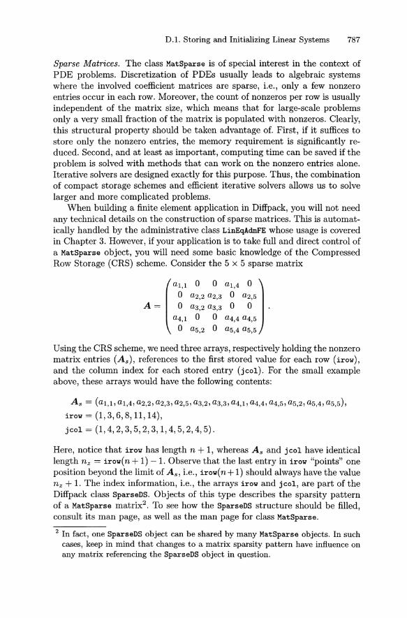
D.l. Storing and Initializing Linear Systems 787
Sparse Matrices. The class MatSparse is of special interest in the context ofPDE problems. Discretization of PDEs usually leads to algebraic systemswhere the involved coefficient matrices are sparse, i.e., only a few nonzeroentries occur in each row. Moreover, the count of nonzeros per row is usuallyindependent of the matrix size, which means that for large-scale problemsonly a very small fraction of the matrix is populated with nonzeros . Clearly,this structural property should be taken advantage of. First, if it suffices tostore only the nonzero entries, the memory requirement is significantly reduced. Second, and at least as important, computing time can be saved if theproblem is solved with methods that can work on the nonzero entries alone.Iterative solvers are designed exactly for this purpose. Thus, the combinationof compact storage schemes and efficient iterative solvers allows us to solvelarger and more complicated problems.
When building a finite element application in Diffpack, you will not needany technical details on the construction of sparse matrices. This is automatically handled by the administrative class LinEqAdmFE whose usage is coveredin Chapter 3. However, if your application is to take full and direct control ofa MatSparse object, you will need some basic knowledge of the CompressedRow Storage (CRS) scheme. Consider the 5 x 5 sparse matrix
[a~ l a~2 a~a a~c a~s l
A = 0 aa,2 aa,a 0 0 .aC,1 0 0 ac,c ac,so as,2 0 as,c as,s
Using the CRS scheme, we need three arrays, respectively holding the nonzeromatrix entries (As) , references to the first stored value for each row (irew),and the column index for each stored entry (jcel). For the small exampleabove, these arrays would have the following contents:
As = (c i .i . al ,C , a2,2, a2,a, a2 ,S , aa,2, aa,a, aC,I,ac,c, ac,s, as,2 ,as,c,as,s),irew = (1,3,6,8,11,14),
jcel = (1,4,2,3 ,5 ,2 ,3 ,1,4,5,2,4,5).
Here, notice that irew has length n + 1, whereas As and jcel have identicallength n z = irew(n+ 1) -1. Observe that the last entry in irew "points" oneposition beyond the limit of As, i.e. , irew(n+ 1) should always have the valuen z + 1. The index information, i.e., the arrays irew and jcel, are part of theDiffpack class SparseDS. Objects of this type describes the sparsity patternof a MatSparse matrix''. To see how the SparseDS structure should be filled,consult its man page, as well as the man page for class MatSparse.
2 In fact, one SparseDS object can be shared by many MatSparse objects . In suchcases, keep in mind that changes to a matrix sparsity pattern have influence onany matrix referencing the SparseDS object in question.

788 D. Software Tools for Solving Linear Systems
While MatSparse allows general sparsity patterns, MatStructSparse provides a more efficient representation of sparse matrices for which the nonzerosare located along matrix diagonals. Many PDE problems discretized on regular geometries lead to matrices with such structured patterns. As indicatedabove, the MatStructSparse constructor accepts a VecSimple object containing the offset of each diagonal to be stored. In this context, an offset valueis the distance from the main diagonal, where negative (positive) values indicate a position in the lower (upper) triangular part of the matrix. That is,the matrix entry ai ,j belongs to the diagonal with offset j - i. In particular,the main diagonal (zero offset) should always be stored.
Also the general sparse matrix format MatSparse accepts an offset vector.In this case, a sparsity pattern of type SparseDS is automatically constructedsuch that the same matrix positions are populated as for the correspondingMatStructSparse object. Moreover, the MatSparse class contains a constructorthat accepts a dense matrix of type Mat and a drop tolerance. This constructorgenerates a sparsity pattern that corresponds to the dense matrix' entries thatby magnitude are larger than the specified tolerance value. Only the entriesfulfilling the drop tolerance test will then be copied to the sparse matrix.This approach can be a convenient way of constructing sparse matrices fortest purposes, but due to the extremely low efficiency it is unsuitable forlarge- and medium-sized problems.
D.1.2 Detailed Matrix Examples
Consider the 3D Poisson problem
- V 2u = 1 on n = (0, 1) x (0, 1) x (0, 1)
subject to the homogeneous Dirichlet condition u = 0 on the boundary an.Let this problem be discretized by centered differences on a uniform q x q x qgrid (not counting the boundary nodes). This procedure results in an n x nlinear system Ax = b where n = q3 and A is a sparse matrix correspondingto the well-known seven-point stencil in Figure D.2. Using our finite differenceoperator notation from Appendix A.3, the discrete problem can be writtenas
[8x8x u + 8y8yu + 8z8z u = -l]i,j,k.
In the following examples we present four overloaded versions of a global function genLaplace3D that constructs A as a Mat, MatBand , MatStructSparse, orMatSparse object, respectively. The compilable source code for these examplesis located in the directory src/linalg/genLaplace3D.
Using a Dense Matrix. When using a Mat object to represent the 3D Laplacian, the matrix indexing behaves as normal, i.e., the entries are addressedas A(i,j) where i and j are allowed to run from 1 to n . Consequently, theonly tricky point is to treat the special cases where the stencil in Figure D.2

D.l. Storing and Initializing Linear Systems 789
1
1
1
1
-6
1
1
kL{i
Fig. D.2. The seven-point stencil corresponding to a centered finite difference discretization of the 3D Laplace operator V'2 U • This stencil can be compared to the2D counterpart in Figure 1.9 on page 55.
meets the boundary. These situations lead to "holes" (single zero entries) incertain positions along the six sub- and superdiagonals in A, see Figure D.3.
void genLaplace3D (Mat(real)& A, int q){
const int q2 = q*q;const int n = q*q*q; II using a q x q x q grid
A.redim(n); II square n x n matrixA.fill(O.O);
int row = 0; II row counter
II run through all nodes in the q x q x q gridint i,j ,k;for (k = 1; k <= q; ++k) {
for (j = 1; j <= q; ++j) {for (i = 1; i <= q; ++i) {
row++; II treat next rowif (k > 1) A(row,row-q2) = -1;if (j > 1) A(row,row-q) -1;if (i > 1) A(row,row-1) -1;A(row,row) = 6; II main diagonal present for all rowsif (i < q) A(row,row+1) -1;if (j < q) A(row,row+q) -1;if (k < q) A(row,row+q2) = -1;
}}
}}
We emphasize that this code is written for clarity, not for maximum computational efficiency. If the latter subject is in focus, we should avoid theif-tests inside the nested loops, but this requires expansion of the code segment (d. Exercise D.l and the solver associated with Appendix D.7).

790 D. Software Tools for Solving Linear Systems
..... ... ..... .. ..
Fig. D.3. The sparsity pattern for the 3D Laplacian using a uniform 3 x 3 x 3discretization of the unit cube. Each dot represents a nonzero entry.
Using a Banded Matrix. Clearly, the use of a dense matrix is a waste ofmemory and computing time when all nonzero entries are located in a bandcentered around the main diagonal. This is the case even when the matrixwill be subject to Gaussian elimination, since this process does not introducenew nonzero entries outside the band". In contrast to the dense Mat representation, the class MatBand for banded matrices utilizes a different conventionfor indexing. In the present example the band consists of 2q2 + 1 diagonalsand the half-bandwidth is q2 + 1. This discussion assumes that we store thefull band instead of exploiting the symmetry that is present for the Laplacian.Use of the symmetry option would need roughly half the storage space of thefull band. The MatBand class can also set aside space for pivoting during theGaussian elimination. Pivoting is not necessary when A stems from a finitedifference (or finite element) discretization of the Laplace equation.
Internally in MatBand the diagonals are stored as columns in a n x (2q2 +1)array. The numbering convention is that the lower-most diagonal is stored incolumn 1, the next diagonal in column 2, etc. This scheme will place the maindiagonal in column q2 + 1 and the upper-most diagonal in column 2q2 + 1.In case of symmetric storage, the main diagonal is located in column 1 andthe subdiagonals are not stored. All columns are adjusted such that the rowindex of the physical data structure matches the row index in the "logicalmatrix view". The operator(int,int) function works in the physical indexspace, while the member function elm assumes logical (dense matrix) indicesi, j = 1,2, ... , n. The member function denselndex2bandlndex maps indicesfrom the logical to the physical index space. All matrix formats in Diffpackhave an elm function using logical indexing regardless of the physical datastructure used, but the elm function is inefficient since it cannot be inlined.
3 However, the Gaussian elimination will generate fill-in inside the band. (This factmakes the implementation of direct solvers for general sparse matrices ratherintricate.)

D.l. Storing and Initializing Linear Systems 791
The following piece of code builds the 3D Laplacian as a MatBand objectusing the physical indexing strategy:
void genLaplace3D (MatBand(real)& A, int q){
const int n = q*q*q; II using a q x q x q gridconst int halfbw = q*q+1 ; II half bandwidth (incl . main diag.)
II column indices for the seven diagonals, counting from belowconst int d1=1, d2=q*(q-1)+1, d3=q*q, d4=q*q+1 ,
d5=q*q+2, d6=q*(q+1)+1, d7=2*q*q+1 ;
II don't use symmetric storage; MatBand is a suboptimal storageII structure for this problem anyway .. .A.redim (n, halfbw, false I*no symmetry*l, false I*no pivoting*/);A.fill(O .O);
int row = 0; II row counter
II run through all nodes in the q x q x q gridint i,j,k;for (k = 1; k <= q; ++k) {
for (j = 1; j <= q; ++j) {for (i = 1; i <= q; ++i) {
row++ ; II treat next rowII NB! operator(int,int) uses data structure indexingif (k > 1) A(row,d1) = -1;if (j > 1) A(row,d2) = -1;if (i > 1) A(row,d3) = -1 ;II main diagonal present for all rowsA(row,d4) = 6;if (i < q) A(row,d5) -1 ;if (j < q) A(row,d6) -1;if (k < q) A(row,d7) -1 ;
}}
}}
It might seem rather odd to present the internal data structure of the different matrix representations, and even encourage the use of highly specializedindexing functionality. After all, one of the most important issues in OOP isthe use of data encapsulation which encourages the construction and use ofblack-box software where private details are hidden and only the public interface is known. However, the need for computational efficiency puts certainconstraints on the use of object-oriented paradigms in numerical applications.For the present example this is evident since a general (logical) matrix indexing would be extremely expensive in terms of CPU time compared with thetailored indexing schemes utilizing knowledge of the data structure. Thus,this is a case where we deliberately break one fundamental rule of OOP. Itis due to the same reason of efficiency that CPU-intensive functionality (e.g .matrix-vector products) is implemented as member functions in the variousmatrix classes , instead of relying on the general elm-type indexing. However ,

792 D. Software Tools for Solving Linear Systems
this design consideration is fully compatible with the concept of data encapsulation.
Using a Structured Sparse Matrix. The banded matrix approach used aboveis reasonable if we want to use Gaussian elimination to solve the associatedsystem. However, if we instead turn to iterative methods where only thenonzero entries of A are needed, we can reduce memory cost and computingtime by use of sparse matrices, see Appendix D.4. In the present case thematrix A has a regular sparsity pattern with only seven nonzero diagonals, seeFigure D.3. Thus, we can use class MatStructSparse which only stores thesediagonals. The underlying data structure is related to the one in MatBand,except that the columns representing the zero diagonals inside the band areremoved. Thus the seven diagonals are stored as columns 1,2, . . . ,7 in arectangular array structure. The row index of this array structure matchesthe row index of the logical matrix indexing. In order to carry out operationson this data structure, there is need for an index vector offsets which tellshow each stored diagonal is placed relatively to the main diagonal. Thatis, the entry located in row i of the kth diagonal corresponds to the entry(i, i +off set (k) in the matrix.
Here is a function that generates a MatStructSparse representation of the3D Laplacian:
void genLaplace3D (MatStructSparse(real)& A, int q){
const int ndiags = 7iconst int n = q*q*qi
II 3D 7-point stencilII using a q x q x q grid
VecSimple(int) offsets(ndiags);offsets(1) -q*qioffsets (2) -q;offsets (3) -1ioffsets (4) Oi II main diagonaloffsets (5) 1 ioffsets (6) q;offsets (7) q*q;
A.redim(n,ndiags,offsets);A.fill(O.O);
int row = 0; II row counter
II run through all nodes in the q x q x q gridint i,j ,kifor (k = 1; k <= q; ++k) {
for (j = 1; j <= qi ++j) {for (i = 1; i <= q; ++i) {
row++; II treat next row;II A(int,int) uses efficient data structure indexingif (k > 1) A(row,1) = -1;if (j > 1) A(row,2) = -1;if (i > 1) A(row,3) = -1;II main diagonal present for all rows

D.l. Storing and Initializing Linear Systems 793
A(row,4) = 6 ;if (i < q) A(row,S) -1;if (j < q) A(row,6) -1;if (k < q) A(row,7) -1 ;
}}
}}
Using a General Sparse Matrix. For the present case, the structured variantof a sparse matrix format would be the best. However, in many applicationsthe resulting sparsity pattern is highly irregular, thus calling for the use ofthe eRS scheme implemented in class MatSparse. The details of this formatare presented on page 787. The generic format requires slightly more bookkeeping than the structured one in order to keep track of the matrix indices.Below you will find a MatSparse construction of the 3D Laplacian:
void genLaplace3D (MatSparse(real)& A, int q){
const int q2const int nconst int nnz
q*q ;q*q*q;7*n-6*q2 ;
II using a q x q x q gridII nonzeros for 3D 7-point stencil
Handle(SparseDS) pattern; II allocate pattern storagepattern.rebind(new SparseDS(n,nnz)) ;A.redim(*pattern); II give A access to patternA.fill(O .O);int row 0; II row counterint entry = 0 ; II entry counter (row by row)
II run through all nodes in the q x q x q gridint i,j,k;for (k = 1; k <= q; ++k) {
for (j = 1; j <= q; ++j) {for (i = 1; i <= q; ++i) {
row++; II treat next row;pattern->irow(row) = entry+1 ; II mark start of rowII NB! operator(int) uses data structure indexingII (sliding down row by row)if (k > 1) { A(++entry) = -1; pattern->jcol(entry)if (j > 1) { A(++entry) = -1; pattern->jcol(entry)if (i > 1) { A(++entry) = -1; pattern->jcol(entry)II main diagonal present for all rowsA(++entry) = 6;pattern->jcol(entry) = row;if (i < q) {A(++entry) -1 ; pattern->jcol(entry)if (j < q) {A(++entry) -1; pattern->jcol(entry)if (k < q) { A(++entry) = -1; pattern->jcol(entry)
}}
row-q2 ;}row-q;}row-1;}
row+1;}row+q;}row+q2;}
}
}pattern->irow(n+1) nnz+1;

794 D. Software Tools for Solving Linear Systems
Exercise D.l. Looking at the genLaplace3D functions, we see that there are iftests inside the nested loops over i, i . and k. This normally prevents compilersfrom optimizing the loops to the fullest extent. In this exercise we shall rewritethe loops to avoid the if-tests. This can be accomplished by letting the loopsrun from 2 to q-l and then treat the indices 1 and q by special code segments.For example, we first set k = 1 and invoke a loop over i and j from 1 to q. Allthe points we visit in this loop are influenced by the boundary z = O. Insidethe loop we increment the rows counter as usual and fill all diagonals, exceptthe lower-most one, with mathematical index (row,row-q*q). Thereafter weconstruct a loop over k from 2 to q - 1. Inside this loop we first make aspecial treatment of the j = 1 boundary by running through a loop overi from 1 to q and filling all diagonals, except the one corresponding to themathematical index (row ,row-q). Then we continue with the internal j points,but make special treatment of the first and last i index. Follow these ideasand implement an optimized version of genLaplace3D for the MatStructSparse
matrix format. Choose q = 300 and compare the CPU time of the two versionsof the routine. <>
D.l.3 Representation of Linear Systems
The general vector classes discussed in Chapter 1.6.3 and Appendix D.1.1 canserve as a basis for more abstract entities. The main focus of this chapter is tosolve linear systems like Ax = b. It is then convenient to collect the entitiesA, x, and b in a separate class representing the linear system. If this newclass refers to the abstract base classes Matrix and Vector, the representationis independent of technical details concerning the storage schemes.
As explained in Chapter 1.6.3 and Appendix D.1.1, the use of virtualfunctions is vital in the Matrix and Vector hierarchies. Numerical efficiency isachieved by implementing local versions of CPU-intensive algorithms (suchas the LU factorization and the matrix-vector product) as virtual memberfunctions for each matrix format. Thus, when a particular matrix instanceis accessed by a Matrix base class pointer (handle) or reference, the tailoredfunctionality is automatically invoked by the C++ run-time mechanisms fordynamic binding. The overhead of calling a virtual function is negligible whenthe function performs a few arithmetic operations. In a PDE context ourvirtual functions in the Matrix and Vector hierarchies normally process largearray structures and often constitute the most time-consuming parts of asimulation program.
Block Matrices and Vectors. In many applications it would also be advisableto extend the concept of matrices and vectors into block structures. For instance, the discretized Laplacian posed on a q x q uniform, rectangular grid

D.l. Storing and Initializing Linear Systems 795
results in the block tridiagonal matrix structure
BII B I
where
and
A= E IRn,n for n = q2,
I B IIB
1= diag(l, 1, ... , 1) E IRq,q
-4 11 -4 1
B=
1 -4 11 -4
A convenient representation of A can utilize the following block matrix:
class LinEqMatrix{protected:
MatSimplest(Handle(Matrix» matmat; II matrix of matricespublic :
LinEqMatrix (int nblockrows, int nblockcolumns);-LinEqMatrix ();
const Matrix(NUMT)& operator(int i, int j) const;Matrix(NUMT)& operator(int i, int j) ;
II matrix-vector product:void prod (const LinEqVector& x, LinEqVector& result) const;
};
The class LinEqMatrix organizes matrix blocks in a two-dimensional arraystructure with indices running from unity to nblkrows and nblkcols. Sinceeach block is referenced by handles to Matrix objects, any matrix formatmay be used for the individual blocks. The only constraint in this respect isthat individual blocks must have consistent sizes and that they match thedimensions and storage formats used for the corresponding blocks in otherLinEqMatrix or LinEqVector4 objects.
The NUMT parameter stands for NUMerical Type and is used in Diffpack toindicate real or Complex. One can usually think of NUMT as real, which is thedefault value. The presence of NUMT allows Diffpack to handle complex-valued
4 Using a design quite similar to LinEqMatrix, the class LinEqVector representsblock vectors.

796 D. Software Tools for Solving Linear Systems
linear systems and corresponding PDEs by simply compiling the applicationwith a special option.
Returning to the example of the discretized Laplacian, the matrix A canbe represented by a LinEqMatrix object with pointers to B and I, where Bis a MatTri object and I is of type MatDiag. It is then sufficient to allocatesingle instances of B and I. This storage scheme will be conservative withrespect to memory usage and will be an efficient alternative as long as theLinEqMatrix object has a fixed structure. We should mention that some numerical algorithms, e.g. in the field of mixed finite element methods, requirethe matrix and vectors in a linear system to be partitioned into blocks.
Having established a metaphor for block matrices and vectors, it is natural to express the linear system Ax = b in terms of the LinEqMatrix andLinEqVector classes. It should be noticed that in many cases the matrixand vectors involved in a system will consist of single blocks, although theLinEqMatrix and LinEqVector classes are employed. These classes treat thesingle block case intelligently, thus resulting in negligible efficiency overhead.A standard linear system has the following representation in Diffpack.
II coefficient matrixII solution vectorII right-hand side
Amat;sol;rhs;
class LinEqSystemStd : public LinEqSystem{protected:
Handle (LinEqMatrix)Handle (LinEqVector)Handle (LinEqVector)
public:LinEqSystemStd (LinEqMatrix& A, LinEqVector& x, LinEqVector& b);LinEqSystemStd (Matrix(NUMT)& A, Vector(NUMT)& x, Vector(NUMT)& b);
-LinEqSystemStd ();
void residual (LinEqVector& r); II r = A*x-bII matrix-vector product: result = A*y:void matvec (const LinEqVector& y, LinEqVector& result) const;
};
Here, the base class LinEqSystem is abstract and only serves the purpose ofdefining an interface to be obeyed by all possible representations of a linear system. The actual storage of data for the coefficient matrix, the solution vector, and the right-hand side is not addressed in class LinEqSystem,but rather in its subclass LinEqSystemStd. We remark that the code of classLinEqSystemStd is very short since the various functions, like matvec, are implemented by a call to LinEqMatrix : :prod. Preconditioned linear systems areconveniently introduced as a subclass of LinEqSystemStd. A sketch of theLinEqSystem hierarchy is found in Figure D.5.

D.2. Programming with Linear Solvers 797
LinEqSolver ~inEqSy.temIIterativeSolver
Fig. D.4. Linear solvers are organized in a class hierarchy, where the abstract baseclass LinEqSolver provides a transparent interface to all implemented methods,direct as well as iterative. The dotted line indicates a handle to the LinEqSystemobject.
D.2 Programming with Linear Solvers
Regardless of the chosen algorithm for solving linear systems, the core operations that turn out to be CPU-intensive are implemented as member functionsin the vector and matrix classes. In this way, the actual solver does not needto worry about efficiency considerations for a special matrix format sincethis is catered for by the low-level functionality, typically in virtual memberfunctions like prod and factLU (in the Matrix hierarchy) . In fact, the solvercannot see any of the details of matrix and vector storage formats. This allowsa close relation between the solver's implementation and the correspondingmathematical algorithm without loss of efficiency.
As indicated in Figure D.4, all linear solvers are organized in a classhierarchy with base class LinEqSolver. At the next level it is natural to splitthis hierarchy into two subhierarchies, thus reflecting the division into direct(DirectSolver) and iterative (IterativeSolver) methods.
D .2.1 Gaussian Elimination
Direct methods are usually based on some variant of the Gaussian elimination procedure. Typically, such methods impose structural changes to thematrix through generation of fill-in. The term fill-in refers to nonzero values that occur during the elimination process in matrix positions that wereinitially occupied by zeroes . When employing a sparse matrix format whereonly nonzero entries are stored, we realize that direct methods will be closelytied to the technical details of each storage format. For instance, it maybe advisable to renumber the unknowns of the original system in order to

798 D. Software Tools for Solving Linear Systems
achieve certain sparsity patterns. It is also very common that sparse elimination algorithms start out with a symbolic elimination process that predictsthe worst-case need for storage. When the resulting data structure has beenbuilt and initialized, the numerical computations are carried out. From theseobservations it is evident that most direct solvers will primarily consist of twoor three calls to member functions of the Matrix hierarchy. Typically, this canbe the combination of factLU and forwBackLU. For instance, the program inChapter 1.3.3 addressing the two-point boundary-value problem, solves theresulting system by explicit calls to these functions. Alternatively, this problem could be solved by the use of the LinEqSolver derivative GaussElim:
II given Matrix A and Vector x, bLinEqSystemStd system (A,x,b);GaussElim gauss;gauss .solve(system);x.print(s_o,"The solution Xli);
As will be demonstrated in the examples below, the use of the GaussElimsolver is more flexible than hardcoded calls to the functions performing thefactorization and triangular solves, as it makes it fairly easy to switch to aniterative solution method. This is especially true when the solver is accessedthrough its base class interface LinEqSolver, such that we can select theparticular solution method at run time.
II coefficient matrixII solution vector and rhsII linear systemII parameters for linear solverII linear solverII file with matrix data
A',x , b;system;solv_prm;solver;filename;
D .2.2 A Simple Demo Program
Let us implement a class that can read a matrix system, i.e, A and b, fromfile and solve the system by means of Diffpack tools. The name of the classis LinSysl and the source code is found in the directory src/linalg/LinSys1.
class LinSysl{protected :
Mat(real)Vee(real)Handle (LinEqSystem)Handle (LinEqSolver_prm)Handle (LinEqSolver)String
public:LinSysl 0 {}
-LinSysl 0 {}void scan 0;void solveProblem ();void resultReport ();
};
In this class we require the coefficient matrix to be of type Mat, while theactual solver is accessed through a LinEqSolver handle named solver. Thefunction scan loads the coefficient matrix and the right-hand side from thefile specified by filename:
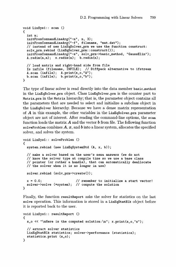
D.2. Programming with Linear Solvers 799
void LinSys1 :: scan (){
int n;initFromCommandLineArg(l-n", n, 3);initFromCommandLineArg(l-f", filename, "mat.dat")jII instead of new LinEqSolver_prm we use the function construct:solv_prm.rebind (LinEqSolver_prm : :construct())jinitFromCommandLineArg(l-s", solv_prm->basic_method, IGaussElim")jA.redim(n,n); x .redim(n)j b .redim(n)j
II load matrix and right-hand side from fileIs infile (filename, INFILE) ; II Diffpack alternative to ifstreamA.scan (infile)j A.print(s_o,IA");b.scan (infile)j b .print(s_o,"b");
}
The type of linear solver is read directly into the data member bas i.c.metihod
in the LinEqSolver_prm object. Class LinEqSolver_prm is the counter part toMatrix_prm in the Matrix hierarchy; that is, the parameter object contains allthe parameters that are needed to select and initialize a subclass object inthe LinEqSolver hierarchy. Because we have a dense matrix representationof A in this example, the other variables in the LinEqSolver_prm parameterobject are not of interest. After reading the command-line options, the scanfunction loads the matrix A and the vector b from file. The following functionsolveProblem combines A , x, and b into a linear system, allocates the specifiedsolver, and solves the system.
void LinSys1 :: solveProblem (){
system.rebind (new LinEqSystemStd (A, x, b));
II make a solver based on the user's menu answers (we do notII know the solver type at compile time so we use a base classII pointer (or rather a handle), that can automatically deallocateII the solver when it is no longer in use)
solver.rebind (solv_prm->create());
}
x = 0 .0 ;solver->solve (*system)j
II remember to initialize a start vector!II compute the solution
Finally, the function resultReport asks the solver for statistics on the lastsolve operation. This information is stored in a LinEqStatBlk object beforeit is reported back to the user.
void LinSys1 :: resultReport (){
s _o « "\nHere is the computed solution:\n" ; x .print(s_o,"x") ;
II extract solver statisticsLinEqStatBlk statistics; solver->performance (statistics)jstatistics.print (s_o);
}

800 D. Software Tools for Solving Linear Systems
The main program using the LinSysl class looks like this:
int main (int argc, const char* argv[]){
initDiffpack (argc, argv);LinSysl problem;problem.scan(); problem .solveProblem(); problem.resultReport();return 0;
}
The resulting toy program can be run by typing app, thus using the defaultchoices of solving the 3 x 3 system stored in the file mat. dat by the GaussElimmethod. You can specify the 5 x 5 system in mat2.dat by entering the command .lapp -n 5 -f mat2.dat. Alternatively, you can try the test problem inmat3. dat that contains the 27 x 27 matrix corresponding to the 3D Laplaciandiscretized on a 3 x 3 x 3 grid.
D.2.3 A 3D Poisson Equation Solver
The purpose of the present section is to develop a Diffpack application forsolving the three-dimensional Poisson equation on a unit cube, discretized bythe common 7-point finite difference stencil:
for i, i. k = 0,1, .. . , q + 1. The boundary points are left out of the linearsystem, i.e., the number of unknowns is n = q3.
The solver, represented by class LinSys2, involves generation of the matrixentries and solution of the linear system by iterative methods. Appendix Cpresents algorithms and Diffpack tools for iterative solution of linear systems.Here, we merely show the syntax for calling some common iterative solution methods for linear systems, like the Conjugate Gradient (CG) methodand the Successive Over-Relaxation (SOR) method. Iterative methods mightcontain several parameters that affect the computational performance. Therelaxation parameter win SOR and SSOR constitute one example. Such parameters are collected in a LinEqSolver_prm object. This parameter object ismost conveniently initialized using Diffpack's menu system, and the LinSys2class is therefore coupled hereto. Programming with and use of the menusystem are thoroughly explained in Chapter 3.2. Here, we just outline thevery basic steps in working with the menu system.
The LinSys2 solver is not equipped with preconditioning. However, thereare extended versions of LinSys2, implemented as the classes LinSys3 andLinSys4, which offer preconditioning. These solvers are presented in Appendices D.5 and D.6.
The definition of class LinSys2 becomes as follows.

D.2. Programming with Linear Solvers 801
public SimCaseclass LinSys2{protected:
intMatStructSparse(real)Vec(real)Handle (LinEqSystem)Handle (LinEqSolver_prm)Handle (LinEqSolver)
q;A;x, b ;system ;solv_prm;solver ;
II q+1 grid points in each dir .II coefficient matrixII solution vector and rhsII linear systemII parameters for linear solverII linear solver
public :LinSys2 0 {}
-LinSys2 0 {}virtual void adm (MenuSystem& menu);virtual void define (MenuSystem& menu, int levelvirtual void scan ();virtual void solveProblem ();virtual void resultReport ();
} ;
MAIN);
Deriving the simulator from class SimCase enables access to support for numerical exp erimentation, for instance, the multiple loop feature (see Chapter 3.4.2) and automatic report gener ation (see App endix D.6 and Chapter 3.5.6).
As any module utilizing the menu system, the entry point adm is needed :
void LinSys2 : : adm (MenuSystem& menu){
}
SimCase: : attachdefine (menu);menu.prompt 0 ;scan 0;
(menu); II enables later access to menu databaseII definelbuild the menuII prompt user, read menu answersII read menu answers into class variables and init
The function adm relies on the presence of the functions define and scan:
void LinSys2: : define (MenuSystem& menu, int level){
II define menu itemsmenu.addltem (level, II menu level
"gr i d size q", II menu command"grid has q*q*q points", II help"3") ; I I default answer
II parameter objects are initialized by their construct function:solv_prm .rebind (LinEqSolver_prm: :construct());II define solvers parameter menu as a submenu (level+1):solv_prm->define (menu,level+1);
}
void LinSys2 :: scan (){
II connect to the menu system databaseMenuSystem& menu = SimCase: :getMenuSystem();
q = menu.get("grid size q").getIntO; II read int (q)

802 D. Software Tools for Solving Linear Systems
const int n = q*q*q;solv_prm->scan (menu); II read menu answers into an object
x.redim(n); b .redim(n) ;}
You should take notice of the first statement in scan, which is necessary inorder to access the menu system object that was attached in adm,
The solveProblem function is almost identical to its counterpart in classLinSysl, but now we have an algorithm genLaplace3D, see page 792, for filling the MatStructSparse matrix object with entries according to the finitedifference scheme.
void LinSys2:: solveProblem (){
genLaplace3D (A,q); II generate coefficient matrixb = 1.0/sqr(q+l); II rhs in Poisson problem is f=lif (q < 4) {
s_0->setReaIFormat(IY,6 .3f"); II change default output formatA.printAsciHs_o,IA") ;
}
system. rebind (new LinEqSystemStd (A, x, b));
II create solver according to user's menu choicesolver.rebind (solv_prm->create());
x = 0.0; II initialize a start vector!solver->solve (*system); II perform the linear solve
}
The present finite difference code is programmed at a fairly low level wherethe programmer is responsible for initializing the matrix entries. We remarkthat there exists a module in Diffpack which gives a flexible interface to finitedifference programming, much like the finite element toolbox (see Chapter 3).
The function resultReport is slightly modified, now allowing a completereport in HTML format:
void LinSys2:: resultReport (){
if (q < 4) {s_o « "\nHere is the solution computed by II
« solv_prm->basic_method « ":\n"; x.print(s_o,"x");}II extract solver statisticsLinEqStatBlk statistics; solver->performance (statistics);statistics.print (s_o);
II write detailed convergence statistics, including plotsHTMLReporter report (casename+".report");statistics.print (report, DETAILED I*print as much as possible*/);
}
Instead of an HTMLReporter, we could instead have declared a LaTeXReporteror a pure ASCIIReporter.

D.2. Programming with Linear Solvers 803
Due to the introduction of the menu system, also the main function hasbeen changed. Now it reads:
#include <LinSys2 .h>
int main (int argc, const char* argv[]){
initDiffpack (argc, argv);global_menu.init ("Poisson eq. FDM solver","LinSys2");LinSys2 problem;problem.adm (global_menu); II define menu, prompt user, and scanproblem.solveProblem();problem.resultReport();return 0;
}
The global menu object g'l.oba'l..menu must be initialized. Moreover, the usualcall to scan is now replaced by adm, which calls scan after the menu is defined .
Copy the directories src/linalg/LinSys2 and src/linalglgenLaplace3D toyour own directory tree, such that these two directories remain parallel'' andcompile the LinSys2 application. You can now play with the BOR and CGmethods, as well as with other solution methods. Here is an example on aninput file sor. i for setting some of the menu items:
set grid size q = 3sub LinEqSolver_prmset basic method = SORset relaxation parameter = 1.8set use default convergence criterion = ONokok
The first command sets the size of the linear system. The next commandinvokes the submenu for the LinEqSolver_prm parameters. The BOR methodcontains a relaxation parameter w E (0,2) that influences the convergencespeed. The current value of w is set to 1.8. Finally, we specify the defaulttermination (convergence) criterion for the iterative method. The defaultconvergence test for the BOR method is that the Euclidean norm of theresidual r k = b - Axk in the kth iteration is less than 10-4 . When thiscriterion is satisfied, the approximation x k to x is taken as the solution(the vector x in the program). More sophisticated tools for monitoring theconvergence of iterative methods are described in Appendix D.6.
Now run the program with the sor. i file as input to the menu system:
./app --casename sortest < Verify/sor.i
After completing the computation, use a web browser to view the HTMLreport named sortest . report .html. If you want to examine and adjust allthe menu items through a graphical user interface, type
5 The LinSys2 application needs the file .. I genLaplace3DIgenLaplace3D . cpp inthe compilation.

804 D. Software Tools for Solving Linear Systems
. / app --GUI --casename sortest --Default Verify/sor.i
provided that your program was compiled with the Make option GUIMENU=tcl(this option is often default - check the $NOR/bt/src/MakeFlags file).
Use Verify/conjgrad .i as input if you want to run the CG method. Weremark that the default convergence criterion for the CG method is slightlydifferent from the classical iterations: Ilrkl12/llroll2 :::; 10-4 • Gaussian elimination is enabled in the Verify/gauss. i file.
Exercise D.2. Choose q = 60 and find the sensitivity of BOR to variationsin the relaxation parameter w. Aslo try to find, through experimentation, anw that minimizes the number of SOR iterations. Compare the efficiency ofSOR, with this optimal w value, and the CG method. The efficiency measuredin terms of "work cost" is listed in the HTML report. 0
D.3 Classical Iterative Methods
We recall from Appendix C.l.l that the classical iterations (Jacobi, GaussSeidel, SOR, and SSOR) have a very simple structure on the form Mx k =Nxk - 1 + b, where A = M - Nand k = 1,2, . . . is the iteration index. Theimplementation of these methods is therefore not much more than a loop supervised by some convergence test. Inside this loop we have to administer thetwo iterates x k and x k - 1 , and issue a call to low-level functionality that performs a given number of iterations. That is, in addition to the infrastructureoffered by class IterativeSolver (see Figure DA), the basic iterations needa vector object in order to store the previous iterate. This entity is a partof the derived class BasicItSolver, which serves as base class for the actualimplementations of classical methods, exemplified by the classes Jacobi andSSOR in Figure DA.
In order to play with the classical iterative methods, we may use thesimple LinSys2 program from Appendix D.2.3 or any of the finite elementsolvers from Chapters 3 or 4.2. To keep the numerics simple , we stick to thefinite difference example as provided by the LinSys2 solver, whose usage wasexplained in Appendix D.2.3. An appropriate input file for the LinSys2 program, specifying Jacobi iteration as the solution method for linear systems,might look like this:
set grid size q = 3sub LinEqSolver_prmset basic method = Jacobiset startvector mode = USER_START ! Let user set start vectorset use default convergence criterion = ONokok

D.4. Conjugate Gradient-like Methods 805
This input file explicitly tells the program to use the current value of thesolution vector x as start vector when it enters the function solver->solve.
Other alternatives to the default value USER-START are RANDOM_START, ZERO_START,
and RHS-START which causes the start vector to be a random vector with entries in the interval [-1 ,1], the zero vector, or the right-hand side b. To viewall possible menu items , run the program once and use the script DpMenu (seeChapter 3.4.1).
SOR and SSOR iteration are enabled by changing basic method on themenu to SoR or SSoR. Recall that the Gauss-Seidel method corresponds toSOR with w = 1.
D.4 Conjugate Gradient-like Methods
In contrast to the classical iterations, the more sophisticated family of Conjugate Gradient-like methods, also known as Krylov subspace methods, putsmore complicated demands on its surroundings. For instance, most Krylov iterations will recursively update the residual vector r k = b- Axk , while otherswill also work on a preconditioned residual sk = M-1(b - Axk ) = M-1r k .
The framework from which the implementations of Krylov methods wouldbe derived should take care of the allocation and initi alization of the residualvectors needed by the given combination of a system and a solver. This alsoincludes the detection of special cases, such as using an identity preconditioner C = I which forces sk = r k for all k. In this case the two entities r k
and sk should actually share the same storage space. Such effects are easilyobtained when accessing the residual vectors through handles.
To further complicate the internal picture of a flexible package for Krylovsolvers, many of these methods compute certain values (residual norms , inner products, etc .) that can be used outside the iteration for different purposes, such as monitoring of convergence, estimation of extreme eigenvalues,or tuning of some adaptive preconditioner. This type of information shouldbe reused whenever needed in order to avoid recomputations. Diffpack takescare of this housekeeping by deriving Krylov methods from a specializedbase class KrylovltSolver, see Figure DA. Thus, the application programmershould not worry about these technical details.
D.4.1 Symmetric Systems
Many classes of PDEs lead to symmetric systems of algebraic equations.Krylov subspace methods can take advantage of the symmetry in the sensethat the iterations will then be inexpensive in terms of computational costand storage requirements.
The Conjugate Gradient Method. For problems where the coefficient matrixis symmetric positive definite, i.e., AT = A and yT Ay > a for all y # 0,

806 D. Software Tools for Solving Linear Systems
the Conjugate Gradient method (see Appendix C.2) is the de facto choiceof solver. In Diffpack this method is available as the class named ConjGrad.Since this solver does not require any user-specified parameters, assigningConjGrad to the basic method menu item is the only initialization needed inthe LinEqSolver_prm object.
Solving Symmetric Indefin ite Problems. For symmetric problems lacking theproperty of positive definiteness, the class Symmlq provides an alternativestrategy. To choose this method, simply set basic method on the menu equalto Symmlq.
D.4.2 Nonsymmetric Systems
In general, solving nonsymmetric systems is much harder than solving symmetric ones, and it is often impossible to predict what will be the mostefficient solution strategy. Thus, it is very important that the software allowseasy switching between different solvers and easy access to the correspondingperformance statistics. As seen by the input files below, a Diffpack programlike the one based on class LinSys2 caters for such needs .
The Methods of Orthomin and GeR. The method called Orthomin is a popular member of the family of nonsymmetric Krylov solvers (see Appendix C.2).Usually this method has a name containing a parameter K, which specifieshow many generations of basis vectors that should be kept for the update ofthe next iterate. In reports generated by Diffpack this truncated method isdenoted T-OM(K) . In general, the convergence rate and stability of the algorithm improves as K gets larger. However, large values of K also indicate asignificant storage expense and a high computational cost per iteration, thussuggesting a tradeoff against convergence speed. The following input sets theK parameter to 5:
set basic method = Orthominset no of search vectors = 5set restart = OFF
In the special case of K = 0, the Orthomin algorithm takes on a simpler form,and the implementation can be made more efficient. The resulting method iscalled Minres'' and can be invoked as follows:
set basic method = MinRes
Finally, a close relative of Orthomin is the Generalized Conjugate Residual(CGR) method. Instead of the truncation to K basis vectors, the GCR algorithm uses restarting. That is, it runs for a specified number of iterations, K,
6 This nonsymmetric solver should not be confused with the symmetric indefinitesolver Mimes, see [17] . This symmetric solver is not available in Diffpack.

D.5. Preconditioning Strategies 807
before it starts over again using the last computed iterate as the new startingvector. For this reason the method is often denoted GCR(K) . To emphasizethat this algorithm is really a restarted Orthomin solver, reports generatedby Diffpack refer to this method as R-OM(K). The following example usesK=7:
set basic method = Orthominset no of search vectors = 7set restart = ON
The GMRES Method. One of the best known (and also one of the mostrobust) nonsymmetric iterations is called the Generalized Minimal Residualmethod, or GMRES for short. This method uses restarting, just like GCR.A restart cycle of K iterations is therefore denoted by GMRES(K). Thecorresponding Diffpack class GMRES can be activated by the following input:
set basic method = GMRESset no of search vectors = 5set restart = ON
The CGS and BiCGStab Methods. In order to avoid the long recursionsand high memory cost of the Orthomin, GCR, and GMRES methods, otherKrylov methods like the Bi-Conjugate Gradient algorithm has been developed . However, this approach, which uses an auxiliary system to get rid ofthe expensive recursions, suffer from bad stability properties. In order to improve the stability without adding computational cost, the Conjugate Gradient Squared (CGS) algorithm was introduced. This method is self-containedand does not require any user-specified parameters. Its implementation inclass CGS can be accessed by setting basic method equal to CGS on the menu.A newer variant with smoother convergence behavior is known as BiCGStab,with the class and menu name BiCGStab.
Transpose-Free QMR . The family of Quasi-Minimal Residual (QMR) methods constitutes yet another Krylov strategy based on short recurrences. Inparticular, there exist variants of the QMR algorithm that avoids the use ofthe transposed coefficient matrix AT. One such variant is the Transpose-FreeQMR method available in class TFQMR.
D .5 Preconditioning Strategies
As explained in Appendix C.3.1, Krylov subspace solvers are usually combined with a preconditioner in order to speed up the convergence rate. Thatis, instead of solving Ax = b, we consider the equivalent system M-1Ax =M-1b. In each iteration of Krylov subspace methods we have solve a linearsystem with M as coefficient matrix. Alternatively, the preconditioner may

808 D. Software Tools for Solving Linear Systems
Ax=b
'- .." ~:--~I Precond IFig. D.5. Combining matrix, vector, and preconditioner classes to form a linearsystem of equations.
be indirectly given in terms of a procedure implementing its action M-1v onthe vector argument v. We mention that Diffpack actually implements leftand right preconditioning, CLACRY = CLb for Y = CI/X, see page 769.
Based on the LinEqSystemStd class introduced in Appendix D.1.3, an obvious extension for representation of preconditioned systems is
class LinEqSystemPrec : public LinEqSystemStd{
II A. x, and b structures are inherited from LinEqSystemStd.protected:
Handle(Precond) Cleftj II left preconditionerHandle(Precond) Crightj II right preconditioner
public:LinEqSystemPrec
(Precond& C, LinEqMatrix& A, LinEqVector& x. LinEqVector& b) jLinEqSystemPrec
(Precond& C, Matrix(NUMT)& A. Vector(NUMT)& x, Vector(NUMT)& b):void residual (LinEqVector& r)j II r = b - A*xII matrix-vector product A*y :void matvec (const LinEqVector& y, LinEqVector& result) constjII apply M: M-{-l}y (e .g. by solving M*result = y)void applyPrec (const LinEqVector& y, LinEqVector& result) constj
}j
We notice that the preconditioner is present in terms of a handle toPrecond, which is the abstract base class in a hierarchy of different preconditioners, see Figure D.6. The most important change from the LinEqSystembase class, is the function applyPrec that actually computes the preconditioning step of applying M-1 to y. The relation between LinEqSystemStdand LinEqSystemPrec is depicted in Figure D.5.
The applyPrec function is virtual in the LinEqSystem class hierarchy, despite the lack of a preconditioner in class LinEqSystemStd. However, we canthink of the standard linear system as a special case of the preconditionedsystem, where the preconditioner is the identity operator. This means that

D.5. Preconditioning Strategies 809
Precond'preCNone l--->__..,.__......
PrecProcedure
JLinEqSystemIr--......--~
') LinEqSolver IIPrecSORlter I
Fig. n.6. All preconditioners implemented in Diffpack are derived from the baseclass Precond as shown in this class hierarchy.
all iterative schemes in Diffpack are implemented in the presence of a preconditioner. Sending a LinEqSystemStd object to the solver, or a LinEqSystemPrecobject with no preconditioner, simply results in a few calls to empty functions when the iterative algorithm executes statements involving the preconditioner.
A Sample Program with Preconditioning. By a few extra lines , the LinSys2code can be equipped with support for preconditioning. The resulting solveris called LinSys3. Two basic statements in the declaration of class LinSys3are new:
Handle (Precond_prm) prec_prm; II parameters for preconditionerHandle (LinEqSystemPrec) system; II linear system
The preconditioning parameter object is put on the menu in define andinitialized in scan, just as the LinEqSolver_prm object in class LinSys2. Thecreation of the linear system is slightly altered in the solveProblem function:
system.rebind (new LinEqSystemPrec(A, x, b»;II attach preconditioner (send in A since it is often demanded)system->attach (*prec_prm, A)j
Notice that the coefficient matrix A is used as argument to the functionattach which initializes the preconditioner. Most preconditioners are constructed on basis of a matrix or differential operator. In the general case, thesimulator itself can have PrecProcedure as base class and implement a properapplyPrec function.
The rest of the code is identical to what we had in class LinSys2. Thisexample is typical when programming in Diffpack; as soon as you have aprototype solver for a problem up and going, more advanced algorithms andsoftware features can usually be added with small adjustments of the simulator class.

810 D. Software Tools for Solving Linear Systems
Classical Iterative Methods (Matrix Splittings) . Well-known classical iterative methods, like Jacobi and SSOR, can be used as preconditioners (seeSect C.3.2). The simplest choice is of course the Jacobi preconditioner, whereM is simply the diagonal of A. We can specify Jacobi preconditioning onthe Precond.prm submenu:
set grid size q = 5sub LinEqSolver_prmset basic method = ConjGradset startvector mode =USER_STARTset use default convergence criterion = ONset max iterations = 300oksub Precond_prmset preconditioning type = PrecJacobiset left preconditioning = ONset automatic init = ONokok
The SSOR preconditioner is also in frequent use, especially in combinationwith the Conjugate Gradient method. Notice that the SOR preconditioneris not applicable to iterative methods that require the coefficient matrix ofthe preconditioned system to be symmetric and positive definite. In order tochange the Jacobi preconditioner used above to an SSOR preconditioner, thefollowing menu items must be set:
set preconditioning type = PrecSSORset (S)SOR relaxation parameter = 1.0
Inner Iterations. In addition to defining preconditioners in terms of matrixsplitt ings, classical iterations may be used for inner iterations. This consistsin performing iterations with a given classical method. Since most Krylovmethods require a fixed preconditioner, i.e., M is unchanged throughout theKrylov iterations, such inner iterations should run for a fixed number of stepsand always use the same starting vector, e.g. the null vector. Numerical experiments indicate that this type of preconditioning can be efficient even forcomplicated nonsymmetric systems. It has also been shown that inner iterations based on classical iterative schemes are intimately related to polynomialpreconditioners, see [17] and references therein.
Here are the necessary changes to the input file needed to run 10 SORiterations as an inner solver:
set preconditioning type = PrecSORlterset (S)SOR relaxation parameter = 1.6set inner steps = 10
Naturally, the SOR solver used for the inner iteration is itself implementedas an instance of the corresponding SOR solver in the LinEqSolver hierarchy.
D.6. Convergence History and Stopping Criteria 811
Incomplete Factorizations. Preconditioning by incomplete factorization isusually a simple and widely applicable technique for improving the convergence rates of iterative solvers. In Diffpack we have implemented the RILUpreconditioner, where fill-in entries during the incomplete factorization process are multiplied by a factor w before adding them to the main diagonal.The well-known ILU and MILU preconditioners are thus obtained by usingRILU and w = 0 and w = 1, respectively. Specification of a RILU preconditioner with the all-round choice w = 0.95 takes the following form on theLinSys3 menu:
set preconditioning type = PrecRILUset RILU relaxation parameter = 0 .95
User-Defined Preconditioners. Any preconditioner in Diffpack must be derived from the base class Precond. The application programmer can extendthis hierarchy by inheritance, thus bringing new preconditioners transparently into the existing framework. In many cases this can be done by implementing derivations of the base classes PrecAlgebraic and PrecProcedure.
These classes are tailored to implementation of preconditioners expressed interms of a matrix operator or as a procedure, respectively. For example, onecan think of using a fast solver for the Laplace equation V'2u = 0 as preconditioner for an equation involving the variable coefficient Laplace operatorV' . (..\(x)V'u). The simulator can then be derived from PrecProcedure andimplement a fast constant-coefficient Laplace solver in the virtual applyPrecfunction. Attaching the this pointer (i.e, the simulator) as preconditioner inthe linear system couples the tailored applyPrec function to the general linearsolver and preconditioner library. In other words, the simulator becomes apart of the preconditioner hierarchy and provides a special-purpose preconditioner, closely connected to the PDE being solved. We refer to the manpages for the various preconditioner classes for further information.
Multigrid and Domain Decomposition. Finally, we mention that Diffpacksupports iterative solvers and preconditioners based on multilevel techniques,including traditional multigrid algorithms as well as overlapping domain decomposition methods [24,96]. Non-overlapping (Schur complement) domaindecomposition has also been implemented in Diffpack [23]. The programmercan develop ordinary solvers using simple and generic algorithms for linearsystems, and with the multigrid toolbox [96], the programmer can as a postprocess extend the solver with support for optimal multigrid methods.
D.6 Convergence History and Stopping Criteria
So far we have used iterative solvers without explicitly stating how to stopthe iterations. Instead, we have relied on the (default) menu setting

812 D. Software Tools for Solving Linear Systems
set use default convergence criterion = ON
which uses the default convergence test associated with the solver of yourchoice. However, it is clear that different problems will need different measuresof convergence. Moreover, it might be useful to combine several measuresin a compound test, or even monitor certain entities without letting theminfluence the convergence test itself. For these purposes Diffpack offers theconcept of convergence monitors. A conceptual discussion of convergencemonitors and of how this abstraction fits into the Diffpack framework foriterative solvers can be found in [22].
Let us start by considering an example that illustrates two main points,the use of convergence monitors, and the possibility of providing a run-timechoice of matrix formats7 :
ononvoid adm (MenuSystem& menu);void define (MenuSystem& menu,void scan 0;void solveProblem ();void resultReport ();
matx_prm;A;x , b;prec_prm;conv_prm;system;solv_prm;solver;n,q;report;
class LinSys4 : public SimCase{protected:
Handle(Matrix_prm(real»Handle(Matrix(real»Vec(real)Handle (Precond_prm)ConvMonitorList_prmHandle (LinEqSystemPrec)Handle (LinEqSolver_prm)Handle (LinEqSolver)intMultipleReportervoid makeSystem ();virtual void openReport();virtual void closeReport();
public:LinSys4
-LinSys4virtualvirtualvirtualvirtualvirtual
};
II parameters for coeff matrixII coefficient matrixII solution vector, rhsII parameters for preconditionerII parameters for conv. monitorII linear systemII parameters for linear solverII linear solverII grid has n=q*q*q pointsII automatic report generation
int level = MAIN);
Compared with the previous example, the new class LinSys4 has been equippedwith a parameter class of type ConvMonitorList_prm. This class can hold theinformation needed to initialize one or more convergence monitors and arrange them in a linked list for compound evaluation. The new class has alsoa parameter class of type Matrix_prm needed for run-time selection of matrix formats. The MultipleReporter object, explained in Chapter 3.5.6, is ageneralization of the HTMLReporter utility in the LinSys2 and LinSys3 solvers.
7 Those using the Diffpack administrator LinEqAdmFE to solve the systems arisingfrom finite element problems will have immediate access to these two facilities.

D.6. Convergence History and Stopping Criteria 813
A Slight Digression: Choosing Matrix Format s. In the previous examples wehave used an explicit instance of the dense matrix class Mat in the linearsystem. Now, we have replaced this matrix object by a Handle(Matrix). Oncethe user has made his choice, the function Matrix_prm : : createEmpty is calledto set this handle,
A.rebind(matx_prm.createEmptY()) j
In this particular case we only pass the name of the matrix format (availableas matx_prm.storage) instead of the complete Matrix_prm obj ect . This is necessary since we want the relevant instance of the genLaplace3D function toset the matrix sizes and fill in the actual entries.
Since we still are solving the 3D Poisson problem, we want to utilize thefunctions developed in App endix D.1.2. However , the C++ run-time systemdoes not know how to automatically map a generic Matrix object to specificformat like MatSparse or MatBand. This mapping must be done explicit ly bythe programmer. Such mapping between classes in the same hierarchy isreferred to as casting. Upward casting, i.e., a mapping from a class back toits base class is always valid and is done automat ically by the C++ runtime system. Downward casting must be st ated explicitly and will cause fatalerrors in situations where the cast ing is invalid . For further information see[10, pp. 342-343]. Since fatal errors will occur in the case that the objectis of a different type than the one we assume, special care must be taken.In Diffpack there are two macros CAST..REF and CAST-PTR that can be usedfor safe downward cast ing of references and pointers , respectively. In thecurrent example we have used the CAST...REF macro in combinat ion with themacro TYPEIDJ>TR to cast the generic Matr ix object entering genLaplace3D toits relevant subtype:
void LinSys4: : makeSystem (){
II since the functions generating the 3D Laplacian allocatesII the appropriate memory segments, we allocate empty matricesII by calling Matrix_prm(real) : :createEmpty (which invokes aII constructor where no memory for the matrix entries is allocated)A.rebind(matx_prm->createEmptY()) j
x.redim(n)j b .redim(n)jb = 1.0/sqr(q+1); II rhs in Poisson problem is f=1
II we need to test for matrix types in order to do explicit castsjII downward cast ing is necessary to ensure optimal efficiency whenII assigning the matrix entries
if (TYPEID_PTR(A .getPtr(),Mat(real))){
Mat (r eal ) & A_dense = CAST_REF(A(),Mat(real))j II A() is *AgenLaplace3D (A_dense,q)j II global function
}else if (TYPEID_PTR(A .getPtr(),MatBand(real)))
{

814 D. Software Tools for Solving Linear Systems
MatBand(real)& A_banded = CAST_REF(A(),MatBand(real));genLaplace3D (A_banded,q);
}else if (TYPEID_PTR(A.getPtr(),MatStructSparse(real)))
{MatStructSparse(real)& A_struct =
CAST_REF(A(),MatStructSparse(real));genLaplace3D (A_struct,q);
}else if (TYPEID_PTR(A.getPtr(),MatSparse(real)))
{MatSparse(real)& A_sparse = CAST_REF(A(),MatSparse(real));genLaplace3D (A_sparse,q);
}else
fatalerrorFP("LinSys4: :genLapl ace3D" ,"Cannot make Laplacian in 'los format", TYPEID_NAME(A));
}
Illegal situations are caught by the last else clause in this function.
Adding Convergence Monitors to the Sample Program. Returning to this section's main issue of convergence monitors, we look at the bodies of the functions in class LinSys4 8 . The functions adm and resultReport are unchangedfrom the LinSys3 example, while the define and scan functions have minorchanges in order to present and read the menu items concerning matrix formats and convergence monitors:
#define MAX_CONV_MONITORS 2matx_prm.define (menu,level+1);conv_prm.define (menu,level+1,MAX_CONV_MONITORS);
and
matx_prm.scan (menu);conv_prm.scan (menu);
Here, the value of MAX-CONV-MONITORS decides how many submenus will becreated in which input data for different convergence monitors can be set. Ifthis value is omitted in the call to conv.prm .defme, a default value of 1 is used.You should notice that this parameter determines the maximum number ofmonitors that can be associated with your solver. For instance, the command
set no of additional convergence monitors = 1
in the LinEqSolver submenu tells that this particular run will use only oneof the monitor submenus (actually the first one listed).
The most important change has taken place in solveProblem:
8 The source code is located in the directory src/linalg/LinSys4.

(D.l)
D.6. Convergence History and Stopping Criteria 815
II attach stopping criteria (convergence monitors), this canII only be done if the solver is iterative
if (TYPEID_PTR(solver.getPtr(),GaussElim))warningFP("main","Your solver is not iterative (you have\n""chosen the \"%s\" method - cannot attach convergence monitors)",solv_prm->basic_method.c_str());
else {II cast solver to the base class for iterative solvers andII attach the convergence monitor info:IterativeSolver* itsolver =
CAST_PTR(solver.getPtr(),IterativeSolver);itsolver->attach (conv_prm) ;
}
As seen above, the input concerning the convergence monitors is handed overto the solver which then will allocate and initialize the relevant ConvMonitorobjects, before organizing them as a list structure.
Other changes in class LinSys4, compared with the LinSys3 program, concern the MultipleReporter object. We simply refer to Chapter 3.5.6 and explanations in the source code of class ReportPoisson2 for information regardingthis subject. The purpose of the LinSys4 solver is to utilize the automaticreport generation tools in a simple way and thereby provide an environmentfor playing around with iterative methods for the Poisson equation problemdiscretized by finite differences.
Finally, we show the main program that has been slightly modified inorder to allow automatic generation of loops over different set of input data(see Chapter 3.4.2).
#include <LinSys4 .h>int main (int argc, const char* argv[]){
initDiffpack (argc, argv);global_menu .init ("Solving the 3D Poisson problem","LinSys4");LinSys4 problem;
II solve one or several problems, let the menu system functionII multipleLoop take care of the adm, solveProblem, andII resultReport calls and allowing multiple answers to menu itemsglobal_menu.multipleLoop (problem) ;return 0 ;
}
The input file to be presented below shows how to input multiple values forcertain menu items.
Residual-Based Monitors. All convergence monitors are implemented as subclasses in the ConvMonitor hierarchy. The two most commonly used tests areresidual-based ,
or(D.2)

816 D. Software Tools for Solving Linear Systems
where r k = b-Axk • These tests are implemented as the classes CMAbsResidua1and CMRe1Residua1, respectively. Consider the following input file":
set grid size q = { 3 &6 } ! try two values of qsub Matrix_prm! try different matrix formats :set matrix type = {MatBand &Mat &MatStructSparse &MatSparse}oksub LinEqSo1ver_prmset basic method = ConjGradset use default convergence criterion = falseset no of additional convergence monitors = 1set max iterations = 300ok
sub Precond_prmset preconditioning type = PrecJacobiok
sub ConvMonitorList_prmsub Define ConvMonitor #1set #1: convergence monitor name = CMRe1Residua1set #1: residual type = ORIGINAL_RESset #1: convergence tolerance = 1.0e-6set #1: norm type = 12set #1: monitor mode = ONset #1: run time plot = OFFset #1: criterion mode = ONset #1: relative to rhs = OFF
okokok ! leave menu and start simulation
One should note that the problem size and the matrix format has beensubject to multiple choices. Consequently, this input file will cause the solution of 2 x 4 = 8 different problem scenarios, one for each set of inputparameters, see Chapter 3.4.2 for more details.
Let us dissect the other items in the input file.
use default convergence criterion: This item is set to off in order to avoidautomatic insertion of the solver's default convergence test. The defaultis false .
no of additional convergence monitors: This value (here equal to 1) decideshow many convergence monitors that will be attached to our solver. Thisvalue must be in the range from 1 to the value we previously have calledMAX_CONVJMONITORS.
max iterations: This value gives the maximum number of iterations. If theconvergence test has not been satisfied before this limit is reached, theiterations will stop and the solver statistics will tell that we failed to findthe solution with specified accuracy. In the current input file this valueis set to 100. The default value is 300.
9 This file and associated input files are located in the directorysrc/1ina1g/LinSys4/Verify.

D.6. Convergence History and Stopping Criteria 817
#1: convergence monitor name: This is the name of the first convergencemonitor in our list. The name specifies the type of convergence test, seeTable D.1 for a list of available alternatives.
Table D.l. The convergence monitors available in Diffpack are listed showing theirclass names and the corresponding convergence measure. The "generic residual" v k
can be replaced by r", s", or Zk depending on the system and solver in question.The user can choose among different norms . For further information we refer to therelevant man pages.
Monitor class name Convergence measure Comment
computes v" explicitly
computes v k explicitlyuser-defined base valueEuclidean inner product
CMAbsResidual Ilv k IICMAbsTrueResidual Ilv k IICMRelResidual Ilvkll/llvollCMRelTrueResidual Ilvkll/llvollCMRelResidualUB IlvklllbasevalueCMRelMixResidual (r k, vk)/(rO, VO)CMRelResSolution Ilvkll/llxkllCMAbsSeqResidual Ilvk- Vk-111CMAbsSeqSolution Ilxk- Xk-111CMRelSeqResidual Ilvk- Vk-11I/llvk-IIICMRelSeqSolution IIxk_ xk-1Il/llxk-IIICMAbsRefSolution IIxk- xrerll needs reference solutionCMRelRefSolution Ilxk
- xrer II/l1xreril needs reference solution
#1: residual type: For the residual-based monitors, this item defines whetherwe are using the original residual r k (ORIGINAL-RES), the preconditionedresidual sk (LEFTPREC-RES), or the pseudo-residual zk (PSEUDO-RES). Thedefault value is ORIGINAL-RES.
#1 : convergence tolerance: This item defines the tolerance value e neededin all types of monitors . The default value is e = 10-4 .
#1 : norm type: From this menu item the user can choose between the norms£,,'0 (Linf), l1 (11), l2 (12), L 1 (t.i) , or L 2 (L2). The default value is 12.
#1 : monitor mode: If this item is ON, the convergence history corresponding tothe chosen measure is recorded for later presentation, analysis, plotting,etc. The default value is ON.
#1: run time plot: If this item is ON, a convergence history plot is automatically displayed (using curveplot gnuplot) . The default value is OFF.
#1: criterion mode: If this item is ON, the corresponding measure is used asa convergence test. That is, when the specified tolerance is reached, thecurrent convergence test is flagged as satisfied. The default value is ON.

818 D. Software Tools for Solving Linear Systems
#1: relative to rhs: When this item is ON, the base value for the relativetest uses the right-hand side rather than the initial residual. That is, whenobserving the original residual the base value is Ilbll, but when observingany preconditioned residual it is IIM-1bll. The default value is OFF.
The input file listed above uses the absolute residual criterion. If we wantto use the relative monitor (D.2) instead, the following statement,
set #1: convergence monitor name = CMRelResidual
must be inserted.
Special Residual-Based Monitors. It should also be mentioned that there arealternative implementations of the residual-based criteria discussed above,CMAbsTrueResidual and CMRelTrueResidual. The only difference from the twopreviously discussed monitors is that these two classes force the explicit computation of the residual. That is, at least the work of a matrix-vector productand a vector addition is spent extra. In the preconditioned case, this also involves the application of the left (and eventually the right) preconditioner(s).This might seem as a waste of computing time, but this type of criteria isneeded for solvers that do not update the residuals themselves, e.g. as in Jacobi, SOR and SSOR. Moreover, even Krylov methods can make use of these"expensive" monitors for problems where the recursive residual updates become inaccurate due to poor conditioning.
There is a special version of the relative residual monitor, CMRelResidualUBthat allows the user to set a specific base value instead of using the initialresidual norm. In this case, the menu command
set #1: user base = 2.5
can be used. However, this particular criterion is usually explicitly codedto use data from another variable to generate the base value. When solvingnonlinear PDEs, the base value might depend on parameters in the outernonlinear iterations. For example,
II Handle(LinEqSolver) solver;IterativeSolver* itsolver =
CAST_PTR(solver .getPtr(),IterativeSolver);Handle(ConvMonitorList) cmlist; itsolver->getConvMonitors(cmlist);const int nmonitors = cmlist.getNoEntries()for (i = 1 ; i <= nmonitors; ++i) {
II can monitor no. i set a user base value?if (cmlist()(i).userDefinedBaseValue(»
cmlist()(i).setBaseValue (mybasevalue);}
Finally, the monitor CMRelMixResidual is based on
(rk,vk)/(rO ,vO)::; e,
where v k is either r k, sk , or zk .
(D.3)

D.6. Convergence History and Stopping Criteria 819
Solution-Based Monitors. Another type of convergence measures focuses onthe computed solution. For instance, the monitor CMAbsSeqSolution observesthe evolution of
Ilxk - Xk-111 ~ c.Similarly, there is a relative criterion
(D.4)
(D.5)
(D.6)
available as CMRelSeqSolution. Also, in cases where a reference solution isavailable, the variants
and(D.7)
are available as CMAbsRefSolution and CMRelRefSolution.
Presenting the Convergence History. As mentioned earlier, it is possible torequest run-time plots of the convergence history. However, this informationcan also be extracted after execution, either by directly manipulating thegenerated CurvePlot files, or by generation of performance statistics in e.g.an HTML report. For instance, to view the convergence history of the LinSys4examples, try
curveplot gnuplot -f tmp.convhist_figures.pl.map -r ' .' '.' ' .'
This command will select all available convergence plots and show them in aGnuplot window. If you add the option -ps hist.ps, you will get a PostScriptfile containing the selected curve plot(s). The plot in Figure D.7 is generatedthis way.
The sample program LinSys4 uses the HTML approach as well, and youare encouraged to examine the generated report in order to find informationon the linear solver's performance.
Compound Convergence Tests. In the example above we used only one monitor to test for convergence. However, Diffpack offers the possibility of combining several monitors into one compound test. Consider this excerpt froman input file:
sub LinEqSolver_prmset basic method = ConjGradset use default convergence criterion = OFFset no of additional convergence monitors = 2
sub ConvMonitorList_prmsub Define ConvMonitor #1set #1: convergence monitor name = CMAbsResidualset #1: residual type = ORIGINAL_RESset #1: max error = 1.0e-6

820 D. Software Tools for Solving Linear Systems
Convergence monitor #10
-0.5 log10(CMReIResidual) --+-
-1
-1.5
-2
-2.5
-3
-3.5
-4
-4.5
·50 2 3 4 5 6 7 8 9
Fig. D.7. A sample curve plot showing the convergence history for a run of theLinSys4 program. The horizontal axis shows the iteration number, while the verticalaxis shows the monitored value (here IlrkI12/llrOI12) on a loglO scale. Here, thetolerance for the test was set to c = 10-4
, thus reaching convergence in the 9thiteration.
set #1: norm type = 12set #1: monitor mode = ONset #1: run time plot = OFFset #1: criterion mode = ONset #1: append at end of list = ONset #1: relational operator = CM_ANDok
sub Define ConvMonitor #2set #2: convergence monitor name = CMRelSeqSolutionset #2: max error = 1.0e-4set #2: norm type = 12set #2: monitor mode = ONset #2: run time plot = ONset #2: criterion mode = ONset #2: append at end of list OFFok
okok
This input will cause a combined convergence test consisting of (D.l) and(D.5) . The residual based monitor will be put at the end of the list and bothcriteria need to be satisfied before the compound test is evaluated as true (using operator CM.AND instead of CM_OR) . The evaluation of the list goes alwaysfrom start to end, and both relational operators have the same precedence.Clearly, this scheme allows for the construction of quite complicated convergence tests, where all or some of the involved monitors contribute to theconvergence test, while some or all also are used for pure reporting purposes.

D.7. Example: Implicit Methods for Transient Diffusion 821
D.7 Example: Implicit Methods for Transient Diffusion
(D.8)
(D.9)
(D.lO)u(x, y, 0) = I(x, y), (x, y) E [0, a] x [0,a] .
We shall end our treatment of software tools for large sparse linear systemswith an example on implementing implicit finite difference methods for a 2Dtime-dependent diffusion problem:
8u = k (82U 8
2U) ( ) ( ) ( )8t 8x2 + 8y2 ' X, yEO, a x 0, a , t > 0,
u = 0, x = 0, a, y = 0, a,
The primary unknown u(x, y, t) is the concentration of the diffusing specie ,k is a diffusion coefficient, and I(x, y) is a known initial distribution of thespecie. Chapter 1.7.6 provides a brief background for diffusion problems. Theproblem (D.8)-(D.1O) can also be physically interpreted as heat conductionin a 2D square, u being a measure of the temperature.
First, we introduce a uniform grid on [0,a] x [0,a], with grid points (i,j) ,i,j = 1, ... , m . The grid increment h = .dx = .dy then becomes 1/(m 1). A quite flexible finite difference scheme for (D.8) is the a-rule combinedwith centered spatial differences. Using the compact notation explained inAppendix A.3, and in particular in Example A.6 on page 645, the scheme forthe current problem can be written as follows:
(D.ll)
When a = 0, this is an explicit scheme where new uf,j values are computedby an explicit formula involving only known values uf,j1. The basic corresponding computational algorithm and implementation can then follow theideas from Chapters 1.4.6 and 1.4.7, or from Chapter 1.7.5 if a more advancedDiffpack simulator is desired . Unfortunately, the results of Project 1.8.1 orExample A.18 on page 668 show that the explicit scheme has a severe stability requirement. When a 2:: 1/2, there is no stability restriction on .dt, whichcan be convenient from an application point of view. However, a > a resultsin an implicit scheme; that is, the new uf,j values are coupled in a systemof linear algebraic equations: Au = b, where A is a sparse n x n matrix,u is the vector of new uf,j values, and b is the right-hand side. The number of unknowns, n , equals m2 in our grid. Furthermore, assuming that thegrid points are numbered according to a double loop over j and i, with thefastest variation over i (i.e. the innermost loop runs over i) , grid point (i, j)corresponds to the single index (j - l)m + i in the linear system Au = b.
The accuracy of the scheme (D.ll) depends on a. For a =1= 1/2 the truncation error becomes (h2, .dt), while a = 1/2, corresponding to the CrankNicolson scheme, leads to a more favorable truncation error: O(h2, .dt2). Thechoice a = 1/2 is therefore popular, since it appears to be the optimal combination of stability and accuracy.

822 D. Software Tools for SolvingLinear Systems
Writing out (D.ll) in detail and collecting the terms at time level £ onthe left-hand side of the equation, gives
f. () (f. f. 4f. f. f.)u · . - "V U " 1 + U · 1 . - U " + U '+1 . + U · '+1 ='& ,J I '&,3 - '&- ,J 1. ,3 '& ,J t ,J
f.-I (1 ()) ( f.-l + f.- I 4 f.-I + f.-I + f.-I )u · · + - I u · . 1 U · 1 . - U· · U·+1· U · '+ 1 ,'£ ,3 ',3 - t - , ] 'I.,] '& ,J '&,3 (D.12)
where I = kL1t/h2 • The coefficients on the left-hand side now determine theentries in row (j - 1)m + i in A, whereas the term on the right-hand sideis to be placed in row (j - 1)m + i in b. The examples in Appendix D.1.2,combined with the suggested optimization in Exercise D.1, might be of greathelp when formulating a computational algorithm for generating the linearsystem at each time level.
Solution of the linear systems is definitely the most computationally intensive part of a finite difference-based simulator for (D.8)-(D.1O). It is thereforecrucial to apply efficient iterative solution methods, with preconditioning, asexplained in Appendix C. A suitable solver for the present problem is theConjugate Gradient method combined with MILD preconditioning. The mostnatural matrix storage format for finite difference equations on a square is thestructured sparse matrix format, represented through class MatStructSparsein Diffpack.
The development of a simulator for (D.8)-(D.10) can start with the quiteflexible LinSys4 program from Appendix D.6, which is an extension of simpler demo programs from Appendices D.3-D.5. The LinSys4 code must beextended with software tools from Chapters 1.6.5 and 1.7.4, that is, finite difference grids (GridLattice), scalar fields of type (FieldLattice) for U at thecurrent and previous time level, time discretization parameters (TimePrm) ,and a time loop. In addition, we might want to have a flexible interfaceto visualization. The SaveSimRes class, covered in Chapters 3.3 and 3.12, isthen a convenient tool that allows for interaction with many visualizationsystems (Plotmtv, Matlab, Vtk, AVS, IRIS Explorer). Although a simulator for (D.8)-(D.10) can be implemented in almost any computer languageusing direct array manipulation, we highly recommend using the more highlevel tools outlined above. These tools provide greater flexibility when thesimulator is used for investigating a physical problem through extensive numerical experimentation. Furthermore, if the shape of the domain changes,and hence calls for finite element-based solution methods, the step from thecurrently suggested solver to a full finite element solver is conceptually smallfrom an implementational point of view, despite the fact that the increasein numerical complexity is substantial. This is the advantage of using classesand high-level abstractions also in simple problems.
Readers having already studied classes LinSys4, WaveiD, and perhaps Wave2D,are strongly encouraged to create a new solver for (D.8)-(D.10). A suggestedresult is provided in the directory src/linalg/Diffusion2D.

D.8. High-Level Stencil Programming of Finite Difference Schemes 823
D.8 High-Level Stencil Programming of FiniteDifference Schemes
The finite difference solvers for the Poisson equation examples so far in thisappendix are coded at a fairly low abstraction level; hand-derived expressionsfor all the discrete equations are inserted directly in the matrix and righthand side vector of linear system objects. Solution of linear systems are obtained by working with LinEqSystem, LinEqSolver, Precond, LinEqSolver_prm,
convergence monitor objects, etc. The programming is straightforward, butmany readers familiar with our more high-level style of developing finite element simulators for the same problem (see Chapters 3.1-3.2) may wonder ifa similar programming style can be applied in a finite difference context. Theanswer is positive; we have developed counterparts to the classes DegFreeFEM,
LinEqAdmFE, and FEM, together with an abstraction of finite difference stencils.Using these classes, in combination with grids and fields, gives the possibilityof creating finite difference solvers in the well-known Diffpack style for finiteelement solvers .
We shall , as usual, employ an example-oriented approach for presentingthe basic usage of the tools for high-level finite difference programming. Assoon as you have grasped the basic ideas from this example, the man pagesshould provide sufficient information for adopting the ideas in more complicated settings. The example is the same as covered in Appendix D.7, thatis, a two-dimensional transient diffusion equation solved by an implicit finite difference scheme. The benefit of programming with the high-level toolscovered in the present section is apparent only when we have implicit finitedifference schemes and thus the need for solving linear systems. The readershould be familiar with the Diffusion2D code from Appendix D.7 as well asbasic concepts of finite difference methods in two space dimensions and time(from, e.g., Chapters 1.4.6 and 1.4.7). Moreover, we have based the exposition on familiarity with basic finite element programming from Chapters 3.1and 3.2.
D.B.1 Finite Difference Stencils
The finite difference stencil concept is introduced early in this book, see Figure 1.9 on page 55. For example, second-order finite difference approximationsto the second-order derivatives in a 2D Laplace term \J2ul give rise to a 5point stencil. On the contrary, a two-point finite difference approximationto a term like au/at results in two I-point stencils (uf,j and uf,j1), becauseit will be natural to distinguish between quantities at different time levelswhen forming the stencils. This will hopefully be clear from the forthcomingcomplete example.

(D.13)
824 D. Software Tools for Solving Linear Systems
The initial-boundary value problem used as example in the present sectioninvolves the 2D diffusion equation
8u = k (82U+ 8
2U)8t 8x2 8y2
on a uniformly partitioned rectangular domain, with u = 0 on the boundary.The precise mathematical formulation of the problem is formulated throughthe equations (D.8)-(D.I0) on page 821. Discretizing this PDE by secondorder differences in space and a a-rule in time gives a finite difference schemeof the form (see Appendix D.7 for more details)
ul. . + a", (-u~ . 1 - u~ 1 . + 4u~ . - U~+l . - u~ '+1) =1. ,3 f 1,,3- f,- ,J 1,,3 7. ,3 1.,3
ul.-. 1 _ (1 - a)", (-ul.-. 11 - U~-11 . + 4ul.-.1 - U~+-11 . - u~-.+ll) .
'I.,} I 1.,3- t- ,} 1. ,3 1. ,3 1. ,3
The factor "( depends on the grid parameters; it equals i1t/h2 in the presentcase, where we have assumed that the grid spacings i1x and i1y in the twospatial directions are equal (i1x = i1y = h).
We can interpret (D.13) as a sum of finite difference stencils. The first termon the left-hand-side of (D.13) can be viewed as a l-point stencil, whereas thea-term can be viewed as a 5-point Laplace stencil scaled by a"(. On the righthand side we also have the sum of a l-point and 5-point Laplace stencil.Actually, a stencil is an operator operating on a finite difference field. Onthe left-hand side of (D.13), the stencils operate on the discrete u field attime level e. On the right-hand side of the equation, the stencils operate onthe discrete u field at the previous time level e- 1. Introducing the 5-pointLaplace stencil as the operator Laplacef-), and the l-point stencil operatoras Identityf-) , we can write (D.13) in the form
Identityfu'') + a"(Laplace(ul.) = Identity(ul.-1) - (1- a)"(Laplace(ul.- 1) .
The stencils are linear operators in this example so we can view a termLaplace(u) as a matrix-vector product, where the stencil represents the matrix and the unknown field u represents the vector. This is, in fact, how thestencil notation is transformed to a linear system Au = b. Having the schemeexpressed as a linear system, we can apply tools from numerical linear algebrato solve the system, i.e., compute the uf,j values.
The three basic steps of our working strategy can be summerized as follows:
- discretization of derivatives in the PDE,
- rewriting the finite difference equations in terms of stencils,
- employing Diffpack tools for specifying the stencils and calculating theassociated linear system.
The latter point is addressed in the following.

D.8. High-Level Stencil Programming of Finite Difference Schemes 825
D.8.2 Basic Structure of a Stencil-Based Simulator
We shall now present in detail how to program with finite difference stencils in Diffpack simulators. The basic structure of the simulat or follows theDiffpack standard as introduced in Chapter 1.7, i.e., we apply the grid andfield abstractions GridLattice and FieldLattice for t he finite difference gridand t he associated discrete u field. The st andard function scan for readinginput dat a and allocating dat a structures is included, as well as t he requiredfunctions solveProblem and resultReport. Moreover, our finite difference simulator employs t he menu system, which is introduced in Chapter 3.2.2 (in afinite element context ).
Regarding programming with finit e difference stencils, the simulator classhas
class FDM as base class,
an obj ect of type LinEqAdmFD containing the linear syst em for the currentproblem and providing access to various solvers for linear syste ms,
a degree of freedom handl er obj ect of type DegFreeFD, which performs themapping between field values and the vector of unknowns in the linearsyste m,
- two StencilCollection obj ects for defining t he finite difference schemesfor the matrix A and t he right-hand side b in the linear system,
a function initStencils for defining t he involved stencils (this functionacts as the counterpart to t he integrands function in finite element simulators).
T he sample simulator is called Diffusion2DStencil , and t he applicationdirectory is located as src/fdm/stencil. The declaration of the simulato r classis listed next .
class Diffusion2DStencil : public FDM{
friend class testproblem ;protected:
II general data:Handle (GridLattice)Handle (DegFreeFD)Handle (FieldLattice)Handle (FieldLattice)Handle (TimePrm)realrealrealint
grid;dof;u;u_prev;tip;theta;diff;a;problem_tp ;
II finite difference gridII map: field <-> lin. systemII primary unknownII u at previous time stepII time step etcII time difference prm.II diffusion coefficientII domain is (O,a)(O.a)II test problem type
Vec(real)Handle (LinEqAdmFD)Handle (SaveSimRes)Handle (StencilCollection)
linear_solution;lineq; II linear system & solutiondatabase;A_stencils ; II stencils for the A matrix

826 D. Software Tools for Solving Linear Systems
Handle(StencilCollection) b_stencils; II stencils for the b vector
virtual void setIC ();virtual void timeLoop ();virtual void solveAtThisTimeStep ();virtual void fillEssBC () ;virtual void initStencils ();
public:Diffusion2DStencil ();
-Diffusion2DStencil ();
virtual void adm (MenuSystem& menu);virtual void define (MenuSystem& menu, int levelvirtual void scan ();
virtual void solveProblem ();virtual void resultReport ();
} ;
MAIN);
Let us go through the most important functions and expla in the use of thenew tools DegFreeFD, LinEqAdmFD, and StencilCollection. A natural start isthe define function, although not much is unexpected:
void Diffusion2DStencil: : define (MenuSystem& menu, int level){
menu.addItem (level, II menu level (level+1 is a submenu)"grid size q" , II command"size of grid in each direction", II (help)"3"); I I default answer
menu.addItem (level,"time parameters","TimePrm: . scan Cla) syntax","dt=O.1 t in [0,1]");
menu.addItem Clevel, "theta", "prm in theta-rule", "1.0"):menu.addItem (level, "diffusion coefficient", "", "1.0");menu.addItem (level, "problem type","1: exp (-2*sqr (pi/a) *k*t) *sin(pi*x_) *sin(pi*y) ""analytical solution, 2: initial plug", "1");
II submenus:SaveSimRes: : defineStatic (menu, level+1);LinEqAdm: : defineStatic (menu, level+1) ;
}
The scan function has many familiar statements, but also some new lines:
void Diffusion2DStencil:: scan (){
II connect to the menu system databaseMenuSystem& menu = SimCase ::getMenuSystem();
a = 1.0;int q = menu.get ("grid size q") .get Int O ;grid.rebind (new GridLattice(»: II make an empty gridgrid->scan (aform("d=2 [O,%g]x[O,%g] [1 :%d]x[1 :%d] ",a,a,q,q»;

D.8. High-Level Stencil Programming of Finite Difference Schemes 827
grid->initBolnds (); II set up default boundary indicatorsII here ye introduce only one boundary indicator, i.e.,II map the four default indicators to the one ye yill use:grid->redefineBolnds ("nbind=l, names= u=O 1=(1 234)");
tip .rebind (ney TimePrm(»;tip->scan (menu.get ("time parameters"»;theta = menu.get ("theta") .getReal 0 ;diff = menu.get ("diffusion coefficient") .getReaIO;problem_tp = menu.get ("problem type") .getlnt 0 ;
database .rebind (ney SaveSimRes(»;database->scan (menu, grid->getNoSpaceDim(»;
lineq.rebind (ney LinEqAdmFD(»;lineq->scan (menu);u.rebind (ney FieldLattice (*grid, "u"»;u_prev.rebind (ney FieldLattice (*grid, "u_prev"»;
II Set up the indexsets, one for each boundary indicator,II plus one for inner nodes:IndexSetCollection& indexsetcoll = grid->createlndexSetCollection() ;dof .rebind (ney DegFreeFDLattice (*grid, indexsetcoll, 1»;
linear_solution.redim (dof->getTotaINoDof(»;lineq->attach (linear_solution);II all data structures are allocated
}
When working with GridLattice objects in previous sections of the book,we have not used the concept of boundary indicators (see Chapter 3.5.1) tomark different segments of the boundary. This is necessary (and natural) inthe present more flexible context. The GridLattice : : initBolnds sets up adefault set of boundary indicators, introducing four indicators for the foursides in 2D. The numbering of the indicators is the same as that employedby the PreproBox preprocessor. That is, in the present example boundaryindicator 1 marks the right boundary x = a, indicator 2 marks the upperboundary y = a, indicator 3 marks the left boundary x = 0, and indicator 4marks the bottom boundary y = 0. As explained on page 297, we can mapthe default set of indicators to a new set adapted to our problem (using thegrid object's redefineBolnds function). In the present example, we need onlyone indicator since we have only one type of boundary condition (u = 0).
The nodes in the grid are grouped into index sets. Typically, the nodesmarked with a particular boundary indicator constitute an index set. Allinterior nodes are also grouped into an index set. Each index set is represented by a subclass of class IndexSet, and all the index sets are stored in anIndexSetCollection in a given order. The creation of index sets is automatically done by a call to
GridLattice ::createlndexSetCollection
In particular, one should note that while, e.g., all nodes with indicator 1 willbe in one index set and nodes with indicator 2 are placed in another index

828 D. Software Tools for Solving Linear Systems
5
3
,,, ,.. I
7 8;---- ---- -- -- --. ;-- --.,,- ,I
, , ,- - - --- -- -- -,- -, ---- - - -- -,, ,
, , , ,, ,9
, ,, , , ,, , , ,, , , ,, , , ,, , , ,, , , ,, , , ,-, ,- - - - - - - - - -, ,-
- -, , - --- ---- -, ,,, ,
1 2
6
,,,: ..! ~ - - - - - - - - - - - _ _ I
.. - --,, ,I
41
- - - -- -- -- -- ---+,,,,,,,,,,I
,,- - - - - - - - - - - - - - - ,, T -,-I
: I t__1_ - - - - - - - - - - - - - - - - + - - 1- I
1 __ 1 4 1 _ _ 1
I I 2 I I;-1"- -,- - - - - - - - - - - - - - - - - T - - ,-II I I I- + - I
3
Fig. D .S. Default boundary indicators for a 2D Grid Latt i ce object to the left , andthe corresponding IndexSetCollection to the right. Note the separate index setsfor the corner nodes, which is due to these nodes having two indicators set on thesame node.
set, nodes marked with both indicators 1 and 2 will be part of a third indexset. The order in which t he index sets are stored in the IndexSetCollectionobject is determined by the order in which the boundary indicators arefound when iterating through the grid. The ite ration is done using the standard Gri dLat t ice iterat ion functions, i.e., the index is varying fastest in thefirst coordinate direction (x), then the second coordinate direction (y), andso on . Figure D.8 shows an example of default boundary indicators on a2D lat t ice grid and the corresponding index sets and their order in theIndexSetCollection. T he collection of index sets is supplied to the DegFreeFDand is used when building the linear equation system.
When solving (D.8)-(D.1O), the bou ndary conditions are the same on theentire boundary. Hence, all the boundary nodes might be represented by thesame stencil. Redefining the boundary indicators so that all boundary nodeswill have the same indicator, entails that the call to cr eatelndexSetCollectioncreates a collection consisting of two index sets, one for all the boundary nodesand one for the inner nodes.
D .8 .3 D efin ing the Stencils
The "heart" of the finite difference simulator is the i nitSt encil function ,where we program the mathematical expressions of the problem to be solved,Le., the stencils. We first list the function and then exp lain t he contents inmore detail. Hopefully, the basic steps of the code should be meaningful evenbefore you read the proceeding text with the exp lanations.
void Di f fus i on2DStencil :: i nitSt encils (){

D.8. High-Level Stencil Programming of Finite Difference Schemes 829
II useful local variablesint nsd = grid().getNoSpaceDim();const real gamma = tip->Delta()*diff/sqr(grid->Delta(1));const real c_1 theta *gamma;const real c_2 = (1-theta)*gamma;
II All nodes on the boundary are subject to boundary ind o 1.II The StencilCollections will therefore only consist of 2II stencils each, the first for the boundary nodes, and theII second for the inner points.
new StencilCollection (nsd, 2 1*2 stencils*l,1 I*one dof*/) ;
new StencilCollection (nsd, 2 1*2 stencils*l,1 I*one dof*/) ;
11================================================II Build stencil system for the coefficient matrix11================================================
II The boundary points have essential boundary conditions, whichII only require a single 1 point identity stencil, alreadyII in the stencil collection by default .
II The inner points of the grid have the contributionII u_{i,j} + c_1*( - u_{i-1,j} - u_{i,j-1} + 4u_{i,j}II - u_{i+1,j} - u3i,j+1})II Create a StencilUnion of an Identity stencil andII a Laplace stencil :StencilUnion A_main (2 I*union of 2 stencils*/);StencilIdentity A_main_id (nsd); II i-point identity stencilStencilLaplace A_main_Ip (nsd); II 5-point Laplace stencil
II Insert the two stencils into the StencilUnionA_main.insert(*A_main_id.getStencil());A_main.insert(*A_main_Ip .getStencil(), c_1 I*scale factor*/);
11=========================================II Build stencil system for right-hand side11=========================================
II The inner grid points for the right hand side system (Vec b)II have the contributionII u_{i,j} - c_2*(-up_{i-1,j} -up_{i,j-1}II + 4up_{i,j} -up_{i+1,j} -up_{i,j+1})II Create a Stencil Union of an Identity and a Laplace stencil :StencilUnion b_main (2 I*union of 2 stencils*/);StencilIdentity b_main_id (nsd) ;StencilLaplace b_main_Ip (nsd);
II Both stencils should be applied on the field u_prevb_main_id .attach (*u_prev) ;b_main_Ip .attach (*u_prev)j
II Insert the two stencils into the StencilUnionb_main.insert (*b_main_id .getStencil());b_main .insert (*b_main_Ip.getStencil(),-c_2 I*scaling factor*/);

830 D. Software Tools for Solving Linear Systems
II Insert the stencils into their respective stencil collectionsA_stencils->insert(A_main,2,1); II stencil no. 2 in the collectionb_stencils->insert(b_main,2,1); II stencil no. 2 in the collection
#ifdef DP_DEBUGA_stencils->print(s_o);b_stencils->print(s_o);
#endif}
For each IndexSet in the collection, a stencil must be created, matching thenumerical scheme valid for the nodes in the index set over which the stencilshould be applied. Each stencil is placed in a StencilCollection, in the sameposition as the corresponding IndexSet has in the IndexSetCollection. Thestencils should be of type Stencil or StencilUnion. The Stencil class allowsthe user to create a stencil of any size and shape, and the stencil weights canbe constant values or [unciors'", The StencilUnion is a stencil made up ofseveral other stencil objects, and is used when a finite difference scheme mosteasily is described as a sum of several stencils.
There are predefined classes available for the most common stencils:StencilLaplace for stencils representing the Laplacian and Stencilldentityfor representing a one point stencil with unit value. (In addition to providing full Laplace stencils in ID, 2D, and 3D for inner nodes, the classStencilLaplace can provide Laplace stencils adjusted to the boundary in alldirections. Readers are encouraged to study the man page and the application examples for documentation of boundary stencils.) As identity stencilsare widely used, e.g., it is always used for representing essential boundaryconditions, the StencilCollection is filled with identity stencils by default.
As we have already shown, our finite difference scheme can be expressedin terms of identity and Laplace stencils. The StencilUnion class is used tocombine stencils. Note that on the left side of the scheme's equation we wantto collect the stencils as operators into a matrix A. On the right side we wantto collect the application of the stencils to u.prev into a vector b. This latteraction is accomplished by attaching the field to the two stencils before theyare inserted into the StencilUnion.
The initStencils function should be called once by the user during theinitialization of the simulator. In a time dependent problem it would be natural to call this function in timeLoop, after u_prev has been initialized by initialconditions in setIC:
void Diffusion2DStencil:: timeLoop (){
tip->initTimeLoop();setICO;initStencils ();database->dump (*u, tip.getPtrO, "initial condition");
10 See Chapter 3.4.4 for an introduction to functors .

D.8 . High-Level Stencil Programming of Finite Difference Schemes 831
while(!tip->finished(»{
tip->increaseTime(); II update time for the next stepsolveAtThisTimeStep (); II solve spatial problem by the FDMLattice*u_prev = *u; II update fields for next stepdatabase->dump (*u, tip.getPtrO, "u"); I I store u on file
}}
Finally, the stencils defining the A matrix and the b vector must be providedto makeSystem together with the DegFreeFD object, in order to assemble thelinear equation system at each time step:
void Diffusion2DStencil:: solveAtThisTimeStep (){
fillEssBC (); II set essential boundary conditionmakeSystem (*dof, *A_stencils, *b_stencils, *lineq);
II use most recent u as start vector for iterative solvers:dof->field2vec (*u_prev, linear_solution)j
lineq->solve (); II solve linear system
s_o « "t= " « tip->getTimeO « end'l,;int niterations; bool c; II for iterative solver statisticsif (lineq->getStatistics(niterations,c» II iterative solver?
s_o «oform(" solver'l.sconverged in 'l.3d iterations\n",c ? " " : " not ",niterations) ;
II the solution is now in linear_solution,II it must be copied to the u field:dof->vec2field (linear_solution, *u);
}
Known u values on the boundary, or essential boundary conditions as we callthem in a finite element context, are set in a function fillEssBC (just as forfinite element simulators, d. Chapter 3.1):
void Diffusion2DStencil:: fillEssBC (){
dof->initEssBC ();const int uno = grid->getNoPoints();
for (int i = 1; i <= uno; i++)II is node i subjected any boundary indicator?if (grid->boNode (i» {
dof->fillEssBC (i, 0.0); II u = 0.0 on boundary}
#ifdef DP_DEBUGdof->printEssBC(s_o);
#endif}
The number 0.0 can , of course, be replaced by any desired boundary value.
832 D. Software Tools for Solving Linear Systems
Note that boundary conditions involving derivatives of u modify the stencils. In that case we will therefore have different stencils at the boundariesand in the interior. Sample simulators are provided in src/fdm/stencil.
Exercise D.3. Modify the Diffusion2DStencil class such that you can haveu = 0 as initial condition and u = 1 as boundary condition. Visualize howu(x, y , t) develops in time. o
Exercise D.4. Modify the Diffusion2DStencil class such that you can haveu = 0 as initial condition, u = 0 at x = 0, y = 0 and y = a, and u = 1 atx = a. Visualize how u(x, y , t) develops in time. <>

Bibliography
[1] E. Acklam and H. P. Langtangen. Tools for simplified programmingwith staggered grids . Research report 2002-06, Simula Research Laboratory, 2002. See URL http://www.simula.no.
[2] J . E. Akin . Finite Elements for Analysis and Design. Academic Press,1994.
[3] M. Alonso and E. J . Finn. Physics. Adison-Wesley,1992.
[4] J. D. Anderson. Computational Fluid Dynamics - The Basics withApplications. McGraw-Hill, 1995.
[5] E. Arge, A. M. Bruaset, P. B. Calvin, J. F. Kanney, H. P. Langtangen,and C. T . Miller. On the efficiency of C++ in scientific computing. InM. Deehlen and A. Tveito, editors, Mathematical Models and SoftwareTools in Industrial Mathematics, pages 91-118. Birkhiiuser, 1997.
[6] E. Arge, A. M. Bruaset , and H. P. Langtangen, editors. Modern Software Tools for Scientific Computing. Birkhauser, 1997.
[7] O. Axelsson . Iterative Solution Methods. Cambridge University Press,1994.
[8] 1. Babuska, T . Strouboulis, and C. S. Upadhyay. A model study ofthe quality of a posteriori error est imators for linear elliptic problems.Comput. Methods Appl. Mech. Engrg., 114:307-378 , 1994.
[9] R. Barrett, M. Berry, T . F. Chan, J . Demmel, J . Donato, J. Dongarra,V. Eijkhout, P Pozo, C. Romine, and H. van der Vorst . Templates forthe Solut ion of Linear Systems: Building Blocks for Iterative Methods.SIAM, 1993.
[10] J. J . Barton and L. R. Nackman. Scientific and Engineering C++ - AnIntroduction with Advanced Techniques and Example s. Addison-Wesley,1994.
[11] K. J. Bathe. Finite Element Procedures in Engineering Analysis.Prentice-Hall, 1982.
[12] W. B. Bickford. A First Course in the Finite Elem ent Method. Irwin ,2nd edition, 1994.
[13] J. H. Bramble. Multigrid Methods, volume 294 of Pitman ResearchNotes in Mathematical Scien ces. Longman Scientific & Technical, 1993.
[14] S. C. Brenner and L. R. Scott. The Mathematical Theory of FiniteElement Methods. Text in Applied Mathematics . Springer, 1994.
[15] W. L. Briggs. A Multigrid Tutorial. SIAM Books, Philadelphia, 1987.

834 Bibliography
[16] A. N. Brooks and T. J. R. Hughes. A streamline upwind/PetrovGalerkin finite element formulation for advection domainated flowswith particular emphasis on the incompressible Navier-Stokes equations. Comput. Meth. Appl. Mech. Engrg., pages 199-259, 1982.
[17] A. M. Bruaset. A Survey of Preconditioned Iterative Methods. AddisonWesley Pitman, 1995.
[18] A. M. Bruaset, X. Cai , H. P. Langtangen, and A. Tveito. Numerical solution of PDEs on parallel computers utilizing sequential simulators. InY. Ishikawa, R. R. Oldehoeft, J. V. W. Reynders, and M. Tholburn, editors, Scientific Computing in Object-Oriented Parallel Environments,Lecture Notes in Computer Science, pages 161-168. Springer, 1997.
[19] A. M. Bruaset, E. Holm, and H. P. Langtangen. Increasing the efficiencyand reliability of software development for systems of PDEs. In E. Arge,A. M. Bruaset, and H. P. Langtangen, editors, Modern Software Toolsfor Scientific Computing. Birkhauser, 1997.
[20] A. M. Bruaset and H. P. Langtangen. Basic tools for linear algebra. InM. Deehlen and A. Tveito, editors, Mathematical Models and SoftwareTools in Industrial Mathematics , pages 27-44. Birkhauser, 1997.
[21] A. M. Bruaset and H. P. Langtangen. A comprehensive set of toolsfor solving partial differential equations; Diffpack. In M. Deehlen andA. Tveito, editors, Mathematical Models and Software Tools in Industrial Mathematics, pages 61-90. Birkhauser, 1997.
[22] A. M. Bruaset and H. P. Langtangen. Object-oriented design of preconditioned iterative methods in Diffpack. Transactions on MathematicalSoftware, 23:50-80, 1997.
[23] A. M. Bruaset, H. P. Langtangen, and G. W. Zumbusch. Domaindecomposition and multilevel methods in Diffpack. In P. Bjerstad,M. Espedal, and D. Keyes, editors, Proceedings of the 9th Conferenceon Domain Decomposition. Wiley, 1997.
[24] X. CaL Domain decomposition. In H. P. Langtangen and A. Tveito, editors, Advanced Topics in Computational Partial Differential Equations- Numerical Methods and Diffpack Programming. Springer, 2003.
[25] X. Cai, E. Acklam, H. P. Langtangen, and A. Tveito. Parallel computing in Diffpack. In H. P. Langtangen and A. Tveito, editors, AdvancedTopics in Computational Partial Differential Equations - NumericalMethods and Diffpack Programming. Springer, 2003.
[26] D. Calhoun and H. P. Langtangen. Writing C++ interfaces to FORTRAN packages . Research report 2002-07, Simula Research Laboratory, 2002. See URL http://www.simula.no.
[27] T . F. Chan and T. P. Mathew. Domain decomposition algorithms. InActa Numerica 1994, pages 61-143. Cambridge University Press, 1994.

Bibliography 835
[28] A. J. Chorin. Numerical solution of the Navier-Stokes equations. Math.Comp. , 22:745-762,1968.
[29] P. G. Ciarlet. The Finite Element Method for Elliptic Problems. NorthHolland, 1978.
[30] P. G. Ciarlet. Finite element approximation theory. In H. Kardestuncer,editor, Finite Element Handbook. McGraw-Hill, 1987.
[31] R. D. Cook, D. S. Malkus, and M. E. Plesha. Concepts and Applicationsof Finite Element Analysis. Wiley, 3rd edition, 1989.
[32] D. A. Barry, C. T. Miller and P. J. Culligan-Hensley. Temporal discretization errors in non-iterative split-operator approaches to solvingchemical reaction/groundwater transport models. J. of ContaminantHydrology, 22:1-17 ,1996.
[33] G. Dahlquist and A. Bjork. Numerical Methods. Prentice-Hall, 1974.
[34] L. Demkowicz, J . T . Oden, W. Rachowicz, and O. Hardy. Toward auniversal h - p adaptive finite element strategy. Part 1. Constrained approximation and data structure. Comput. Methods Appl. Mech. Engrg.,77:79-112 , 1989.
[35] Diffpack software package. http://www.diffpack.com.
[36] K. Eriksson, D. Estep, P. Hansbo, and C. Johnson. Introduction toadaptive methods for differential equations. Acta Numerica, pages 154, 1995.
[37] K. Eriksson, D. Estep, P. Hansbo, and C. Johnson. ComputationalDifferential Equations. Cambridge University Press, 1996.
[38] M. J. Fagan. Finite Element Analysis. Longman Scientific & Technical,1992.
[39] Fastflo software package.http ://www.nag.co.uk/simulation/Fastfto/fastfto. html.
[40] FEMLAB software package. http ://www.femlab.com.
[41] J. H. Ferziger and M. Perle. Computational Methods for Fluid Dynamics. Springer, 1996.
[42] B. A. Finlayson. Numerical Methods for Problems with Moving Fronts.Ravenna Park Publishing, Seattle, USA, first edition, 1992.
[43] C. A. J . Fletcher. Computational Techniques for Fluid Dynamics, VolI and II. Springer Series in Computational Physics. Springer, 1988.
[44] N. D. Fowkes and J. J. Mahony. An Introduction to MathematicalModelling. Wiley, 1994.
[45] FreeFEM software package.http://www. asci.frF prudhomm/gfem-html.
[46] J . E. F. Friedl. Mastering Regular Expressions. O'Reilly, 1997.

836 Bibliography
[47] R. Glowinski. Numerical Methods for Nonlinear Variational Problems.Springer, 1984.
[48] P. M. Gresho and R. L. Sani. Incompressible Flow and the FiniteElement Method. Wiley, 1998.
[49] M. Griebel, T. Dornseifer, and T. NeunhoefIer. Numerical Simulationin Fluid Dynamics: A Practical Introduction. SIAM, 1997.
[50] GRUMMP software package. http://tetra.mech.ubc.ca/GRUMMP.
[51] M. D. Gunzburger and R. A. Nicolaides. Incompressible computationalfluid dynamics; Trends and advances. Cambridge University Press,1993.
[52] W. G. Habashi and M. M. Hafez. Compressible inviscid flow. InH. Kardestuncer, editor, Finite Element Handbook. McGraw-Hill , 1987.
[53] W. Hackbusch. Multi-Grid Methods and Applications. Springer, Berlin,1985.
[54] W. Hackbusch. Iterative Solution of Large Sparse Systems of Equations.Springer, 1994.
[55] D. Harms and K. McDonald. The Quick Python Book. Manning, 1999.
[56] J. P. Den Hartog. Advanced Strength of Materials . Dover, 1987. (original edition published by McGraw-Hill, 1952).
[57] E. J. Holm and H. P. Langtangen. A uniform mesh refinement methodwith applications to porous media flow. Int. J. Num. Meth . Fluids ,28:679-702, 1998.
[58] E. J . Holm and H. P. Langtangen. A method for simulating sharp fluidinterfaces in groundwater flow. Adv. Water Res., 23:83-95 , 1999.
[59] T. J. R. Hughes. Recent progress in the development and understandingof SUPG methods with special reference to the compressible Euler andNavier-Stokes equations. Int. J. Num. Meth . Fluids, 14(7):1261-1275,1987.
[60] T . J. R. Hughes , W. K. Liu, and A. Brooks. Finite element analysisof incompressible viscous flows by the penalty function formulation. J.Compo Phys. , 30:1-60, 1979.
[61] S. C. Hunter. Mechanics of Continuous Media. Wiley, 2nd edition,1983.
[62] M. B. Allen III, G. A. Behie, and J . A. Trangenstein. Multiphaseflow in porous media. Lecture notes in engineering. Lecture notes inengineering. Springer, 1988.
[63] M. B. Allen III, 1. Herrera, and G. F. Pinder. Numerical Modeling inScience and Engineering. Wiley, 1988.
[64] B. Joe. GEOMPACK - a software package for the generation of meshesusing geometric algorithms. Adv. Eng. Software, 13:325-331, 1991.

Bibliography 837
[65] C. Johnson. Numerical Solutions of Partial Differential Equations bythe Finite Element Method. Cambridge University Press, 1987.
[66] A. Kjeldstad, H. P. Langtangen, J. Skogseid, and K Bjerlykke, Simulation of deformations, fluid flow and heat transfer in sedimentarybasins. In H. P. Langtangen and A. Tveito, editors, Advanced Topicsin Computational Partial Differential Equations - Numerical Methodsand Diffpack Programming. Springer, 2003.
[67] L. D. Landau and E. M. Lifshitz. Theory of Elasticity. Course ofTheoretical Physics, Volume 7. Pergamon Press, 2nd edition, 1970.
[68] H. P. Langtangen. Scripting Tools for Scientific Computing. Textbookin Computational Science and Engineering. Springer. In preparation.
[69] H. P. Langtangen. Conjugate gradient methods and ILU preconditioning of non-symmetric matrix systems with arbitrary sparsity patterns.Int. J. Num. Meth. Fluids, 10:213-223, 1989.
[70] H. P. Langtangen. Implicit finite element methods for two-phase flowin oil reservoirs. Int . J. Num. Meth. Fluids, 20:651-681, 1990.
[71] H. P. Langtangen. Tips and frequently asked questions about Diffpack.Numerical Objects Report Series, Numerical Objects A.S., 2002.http://www.nobjects .com/Diffpack/FAQ.
[72] H. P. Langtangen, A. M. Bruaset, and E. Quak, editors. Advances inSoftware Tools for Scientific Computing. Springer, 1999.
[73] H. P. Langtangen and K-A. Mardal. A software framework for mixedfinite element programming. In P. M. A. Sloot, C. J. K Tan, J . J . Dongarra, and A. G. Hoekstra, editors, Proceedings of the 2nd InternationalConference on Computational Science, Lecture Notes in Computer Science. Springer, 2002.
[74] H. P. Langtangen and K-A. Mardal. Using Diffpack from Pythonscripts. In H. P. Langtangen and A. Tveito, editors, Advanced Topicsin Computational Partial Differential Equations - Numerical Methodsand Diffpack Programming. Springer, 2003.
[75] H. P. Langtangen, K-A. Mardal, and R. Winther. Numerical methodsfor incompressible viscous flow. Adv. Water. Res., 2002.
[76] H. P. Langtangen and O. Munthe. Solving systems of partial differentialequations using object-oriented programming techniques with coupledheat and fluid flow as example. ACM Transactions on MathematicalSoftware , 27(1):1-26, March 2001.
[77] H. P. Langtangen, N. Nunn, G. Pedersen, K Samuelsson, H. Semb,and W. Shen. Finite element preprocessors in Diffpack. Numerical Objects Report Series, Numerical Objects A.S., 2002. See URLhttp://www.nobjects.com/Reports.

838 Bibliography
[78] H. P. Langtangen and H. Osnes. Stochastic partial differential equations . In H. P. Langtangen and A. Tveito, editors, Advanced Topicsin Computational Partial Differential Equations - Numerical Methodsand Diffpack Programming. Springer, 2003.
[79] H. P. Langtangen and G. Pedersen. Computational methods for weaklydispersive and nonlinear water waves. Comput. Meth . Appl. Mech.Engrg., 160:337-358, 1998.
[80] H. P. Langtangen and G. Pedersen. A Lagrangian model for run-upof shallow water waves. In M. Hafez and J. C. Heinrich, editors, Theproceedings of the Tenth International Conference on Finite Elementsin Fluids, 1998.
[81] H. P. Langtangen and A. Tveito, editors . Advanced Topics in Computational Partial Differential Equations - Numerical Methods and DiffpackProgramming. Springer, 2003.
[82] R. J. LeVeque. Numerical Methods for Conservation Laws. Birkhauser,1992.
[83] R. J. LeVeque. Finite Volume Methods for Hyperbolic Problems. Cambridge University Press, 2002.
[84] J. A. Liggett. Fluid Mechanics. McGraw-Hill, 1994.
[85] C. C. Lin and L. A. Segel. Mathematics Applied to Deterministic Problems in the Natural Sciences. SIAM, 1988.
[86] W. K. Liu and T. Belytschko. Efficient linear and nonlinear heat conduction with a quadrilateral element. Int. J. Num. Meth . Engng.,20:931-948, 1984.
[87] J. D. Logan. Applied Mathematics; A Contemporary Approach. Wiley,1987.
[88] J. D. Logan. An Introduction to Nonlinear Partial Differential Equations. Wiley, 1994.
[89] M. Loukides and A. Oram. Programming with GNU Software. O'Reilly,1997.
[90] B. Lucquin and O. Pironneau. Introduction to Scientific Computing.Wiley, 1998.
[91] M. Lutz and D. Ascher. Learning Python. O'Reilly, 1999.
[92] L. E. Malvern. Introduction to the Mechanics of a Continuous Medium.Prentice-Hall, 1969.
[93] K.-A. Mardal, E. Acklam, and D. Calhoun. How to use Matlab in C++programs. Research report 2002-08, Simula Research Laboratory, 2002.See URL http://www.simula.no.
[94] K.-A. Mardal and H. P. Langtangen. Mixed finite elements. In H. P.Langtangen and A. Tveito, editors, Advanced Topics in Computational

Bibliography 839
Partial Differential Equations - Numerical Methods and Diffpack Programming. Springer, 2003.
[95] K-A. Mardal, J. Sundnes, A. Tveito, and H. P. Langtangen. Block preconditioning for systems of PDEs. In H. P. Langtangen and A. Tveito,editors, Advanced Topics in Computational Partial Differential Equations - Numerical Methods and Diffpack Programming. Springer, 2003 .
[96] K-A. Mardal, G. W. Zumbusch, and H. P. Langtangen. Multigridsoftware tools . In H. P. Langtangen and A. Tveito, editors, AdvancedTopics in Computational Partial Differential Equations - NumericalMethods and Diffpack Programming. Springer, 2003.
[97] G. E. Mase. Theory and Problems of Continuum Mechanics. Schaum'sOutline Series in Engineering. McGraw-Hill, 1970.
[98] Mayavi Vtk visualization interface.http";/mayavi.sourceforge.net.
[99] C. C. Mei. The Applied Dynamcsi of Ocean Surface Waves. WorldScientific, 1989 .
[100] C. T . Miller and A. J. Rabideau. Development of split-operator, PetrovGalerkin methods to simulate transport and diffusion problems. WaterResources Research, 29:2227-2240, 1993.
[101] K W. Morton. Numerical Solution of Convection-Diffusion Problems.Chapman & Hall, 1996.
[102] O. Munthe and H. P. Langtangen. Finite elements and object-orientedimplementation techniques in computational fluid dynamics. Comput.Meth . Appl. Mech. Engrg., 190:865-888,2000.
[103] M. Nelson. C++ Programmers Guide to the Standard Template Library. IDG Books, 1995.
[104] C. D. Norton. Object-Oriented Programming Paradigms in ScientificComputing. PhD thesis, Rensselaer Polytechnic Institute, 1996.
[105] Object-Oriented Numerics.http";/www.oonumerics.orgj.
[106] J. T. Oden, L. Demkowicz, W. Rachowicz, and T. A. Westermann. Toward a universal h-p adaptive finite element strategy. Part 2. A posteriori error estimates. Comput . Methods Appl. Mech. Engrg., 77:113-180,1989.
[107] H. Olsson. Object-oriented solvers for initial value problems. In E. Arge,A. M. Bruaset, and H. P. Langtangen, editors, Modern Software Toolsfor Scientific Computing. Birkhauser, 1997.
[108] D. R. J. Owen and E. Hinton. Finite Elements in Plasticity: Theoryand Practice. Pineridge Press Ltd., 1980.
[109] S. B. Palmer and M. S. Rogalski. Advanced University Physics. Gordonand Breach Publishers, 1996 .

840 Bibliography
[110] D. H. Peregrine. Equations for water waves and the approximationbehind them. In R. E. Meyer, editor, Waves on beaches, pages 357412. Academic Press, New York, 1972.
[111] R. Peyret and T. D. Taylor. Computational Methods for Fluid Flow.Springer Series in Computational Physics. Spriver, 1983.
[112] S. Prata. C++ Primer Plus. Waite Group Press, 2nd edition, 1995.
[113] W. H. Press, S. A. Teukolsky, W. T. Vetterling, and B. P. Flannery.Numerical Recipes in C; The Art of Scientific Computing. CambridgeUniversity Press, 2nd edition, 1992.
[114] A. Quarteroni and A. Valli. Numerical Approximation of Partial Differential Equations. Springer Series in Computational Mathematics.Springer, 1994.
[115] B. D. Reddy. Functional analysis and boundary-value problems: anintroductory treatment. Longman Scientific & Technical, 1986.
[116] J . N. Reddy. On penalty function methods in the finite element analysisof flow problems. Int. J. Num. Meth. Fluids, 2:151-171, 1982.
[117] J. N. Reddy and D. K. Gartling. The Finite Element Method in HeatTransfer and Fluid Dynamics. CRC Press, 1994.
[118] G. Ren and T. Utnes. A finite element solution of the time-dependentincompressible Navier-Stokes equations using a modified velocity correction method. Int . J. Num. Meth. Fluids, 17:349-364, 1993.
[119] M. Renardy and R. C. Rogers . An Introduction to Partial DifferentialEquations. Text in Applied Mathematics. Springer, 1993.
[120] R. D. Richtmyer and K. W. Morton. Difference Methods for InitialValue Problems. Wiley, 1967.
[121] P. J . Roache. Verification and Validation in Computational Scienceand Engineering. Hermosa Publishers, 1998.
[122] U. Riiede, Mathematical and Computational Techniques for MultilevelAdaptive Methods. Frontiers in Applied Mathematics. SIAM, 1993.
[123] R. H. Sabersky, A. J. Acosta, and E. G. Hauptmann. Fluid Flow: AFirst Course in Fluid Mechanics. Maxwell Macmillian, 3 edition, 1989.
[124] R. Sampath and N. Zabaras. An object-oriented implementation ofadjoint techniques for the design of complex continuum systems. Int.J. Num. Meth. Engng., 1999.
[125] W. Schroeder, K. Martin, and B. Lorensen. The Visualization Toolkit;an Object-Oriented Approach to 3D Graphics. Prentice-Hall, 2nd edition, 1998.
[126] L. A. Segel. Mathematics Applied to Continuum Mechanics. Dover,1987. (original edition published by Macmillan, 1977).

Bibliography 841
[127] J. R. Shewchuk. Triangle: Engineering a 2D quality mesh generatorand delaunay triangulator.http://www.cs.cmu.eduFquake/tripaper/triangleO.html, 1996.
[128] B. Smith, P. Bjerstad, and W. Gropp. Domain Decomposition - Parallel Multilevel Methods for Elliptic Partial Differential Equations. Cambridge University Press, 1996.
[129] 1. M. Smith and D. V. Griffiths . Programming the Finite ElementMethod. Wiley, 3 edition, 1998.
[130] M. R. Spiegel. Theory and Problems of Theoretical Mechanics.Schaum's Outline Series in Science. McGraw-Hill, 1967.
[131] A. Srikanth and N. Zabaras. A computational model for the finite element analysis of thermoplasticity with ductile damage at finite strains.Int. J. Num. Meth . Engng., 1999.
[132] W. A. Strauss. Partial Differential Equations: An Introduction. Wiley,1992.
[133] J. C. Strikwerda. Finite Difference Schemes and Partial DifferentialEquations. Wadsworth and Brooks/Cole, 1989.
[134] T. Strouboulis and K. A. Haque. Recent experiences with error estimation and adaptivity, Part I: Review of error estimators for scalar ellipticproblems. Comput. Methods Appl. Mech. Engrg., 97:399-436, 1992.
[135] T. Strouboulis and K. A. Haque. Recent experiences with error estimation and adaptivity, Part II: Error estimation for h-adaptive approximations on grids of triangles and quadrilaterals. Comput. MethodsAppl. Mech. Engrg., 100:359-430, 1992.
[136] B. Stroustrup. The C++ Programming Language. Addison-Wesley,3rdedition, 1997.
[137] B. Szabo and 1. Babuska. Finite Element Analysis. Wiley, 1991.
[138] M. Tabbara, T . Blacker, and T. Belytschko. Finite element derivativerecovery by moving least squares interpolants. Comput. Meth. Appl.Mech. Engrg., 117:211-223, 1994.
[139] R. Temam. Sur l'approximation de la solution des equations de NavierStokes par la methode des pas fractionnaires. Arc. Ration. Mech. Anal.,32:377-385, 1969.
[140] S. P. Timoshenko. Theory of Elasticity. McGraw-Hill, 3rd edition,1982.
[141] D. L. Turcotte and G. Schubert. Geodynamics - Applications of Continuum Physics to Geological Problems. Wiley, 1982.
[142] S. Turek. Efficient Solvers for Incompressible Flow Problems. Springer,1999.
[143] A. Tveito and R. Winther. Introduction to Partial Differential Equations - A Computational Approach. Springer, 1998.
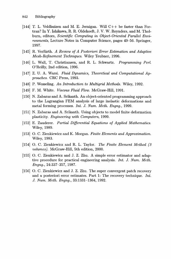
842 Bibliography
[144] T. L. Veldhuizen and M. E. Jernigan. Will C++ be faster than Fortran? In Y. Ishikawa, R. R. Oldehoeft, J. V. W. Reynders, and M. Tholburn, editors, Scientific Computing in Object-Oriented Parallel Environments, Lecture Notes in Computer Science, pages 49-56. Springer,1997.
[145] R. Verfiirth. A Review of A Posteriori Error Estimation and AdaptiveMesh-Refinement Techniques. Wiley Teubner, 1996.
[146] L. Wall, T . Christiansen, and R. L. Schwartz. Programming Perl.O'Reilly, 2nd edition, 1996.
[147] Z. U. A. Warsi. Fluid Dynamics, Theoretical and Computational Ap-proaches. CRC Press, 1993.
[148] P. Wesseling. An Introduction to Multigrid Methods. Wiley, 1992.
[149] F. M. White. Viscous Fluid Flow. McGraw-Hill, 1991.
[150] N. Zabaras and A. Srikanth. An object-oriented programming approachto the Lagrangian FEM analysis of large inelastic deformations andmetal forming processes. Int. J. Num. Meth. Engng., 1999.
[151] N. Zabaras and A. Srikanth. Using objects to model finite deformationplasticity. Engineering with Computers, 1999.
[152] E . Zauderer. Partial Differential Equations of Applied Mathematics.Wiley, 1989.
[153] O. C. Zienkiewicz and K. Morgan. Finite Elements and Approximation.Wiley, 1983.
[154] O. C. Zienkiewicz and R. L. Taylor. The Finite Element Method (3volumes) . McGraw-Hill, 5th edition, 2000.
[155] O. C. Zienkiewicz and J. Z. Zhu. A simple error estimator and adaptive procedure for practical engineering analysis. Int. J. Num. Meth.Engng., 24:337-357, 1987.
[156] O. C. Zienkiewicz and J. Z. Zhu. The super convergent patch recoveryand a posteriori error estimates. Part 1: The recovery technique. Int.J. Num . Meth. Engng., 33:1331-1364, 1992.

Index
\7 . A(X)\7 operator, 53au/an, 56
a posteriori error estimates, 245a priori error estimates, 238accuracy- a posteriori estimates (FEM), 245- a priori estimates (FEM) , 238- numerical dispersion relations, 659- numerical experiments, 241, 286,
329, 396- truncation error, 662- wave equation (FDM), 659- wave equation (FEM), 179adaptivity, 243, 362addBolndNodes, 299, 684addltem, 264, 330, 682AddMakeSrc, 294addMaterial, 301, 684addSubMenu, 682adm, 263, 334, 801--advice, 701aform,23--allocreport, 703animation- of waves, 41, 451, 556- using Gnuplot, 41- using Matlab, 41, 556- using Plotmtv, 407- using Vtk, 408app, 7application overview , 7archiving simulation results, 41array- classes in Diffpack, 81- plain C/C++, 74ArrayGen, 81, 681, 782ArrayGenSel, 98, 681ArrayGenSimple, 86, 681ArrayGenSimplest, 86, 681artificial diffusion, 63, 214
assembly process (FEM)- algorithm, 167- Diffpack code , 718- example in 1D, 167- example in 2D, 201assignEnum, 330automatic report generation, 319,
399automatic verification, 707axisymmetric problems, 194, 332
backward Euler scheme, 125, 155,470
.bashrc, 686basis function , 142BasisFuncGrid, 681--batch, 331, 703BiCGStab, 807bilinear elements, 196, 267binary storage of fields, 276biquadratic elements, 203, 268Blitz++, 749boNode, 297, 684boundary conditions- boundary indicators, 296- Dirichlet, 257- essential, 151- essential (impl .), 257- in weighted residual method, 148- natural, 151- natural (impl .), 302- Neumann, 56, 302- redefinition, 298- Robin, 189, 302, 323, 399boundary indicators, 296boundary-layer problems, 63, 214boundary-value problem , 12Boussinesq wave equations, 559Buckley-Leverett equation, 136Burgers' equation, 136

844 Index
calcElmMatVec, 302, 683, 719calcTolerance, 701calling C functions, 697calling Fortran functions, 698--casedir, 42casename, 42, 701--casename, 42, 701casenane.m», 285. casename . f i el d, 717casename .files, 285. casename .grid, 717casename.makegraphics, 321.casename.simres, 269casename .unix, 321casename_orig, 701CAST-PTR, 706CAST..REF, 706CAST-PTR, 813CAST..REF, 813cast ing, 706 , 813Cauchy-Schwartz ' inequality, 229CdBase, 542CdEff,542CdNonlin, 542CdStefan, 546CGS, 807cLargc, 104cLargv, 104class hierarchy, 85, 90, 95, 321, 706Clean, 44, 687clean up of files, 42, 687CloGUI.py, 118closeReport , 321CM-AND, 820CM_OR,820CMAbsRefSolution, 819CMAbsResidual, 398, 816CMAbsSeqSolution, 819CMAbsTrueResidual, 818.cmakel, 689.cmake2, 294 , 689, 696cmappr, 711CMRelMixResidual, 818CMRelRefSolution, 819CMRelResidual, 398, 816
CMRelResidualUB, 818CMRelSeqSolution, 819CMRelTrueResidual, 818code optimization, 291, 488, 725- array indexing, 555- assembly process, 739- initial assembly only, 447, 730- integrands function, 740- LU/ILU factorization, 727collect ing simulation results, 41collocat ion, 143command prefix (menu), 606command-line arguments , 265, 281- menu system, 282- standard Diffpack arg., 701- user-defined, 103 , 282CommonRel, 621compact difference notation, 643complex exponential functions, 647complex PDEs, 795ConjGrad, 806conjugate-gradient method, 760consistent mass matrix, 178const, 76, 258constructor, 75continuation methods, 476 , 572continuationSolve, 620continuing a simulation, 457continuous problem, 16, 680ConvDiffl , 388convect ion-diffusion equation- discretization, 63 , 212, 387, 541- scaling, 639- simulator, 387, 542convergence monitor, 397 , 812- compound test, 819- plotting, 819convergence rate, 238, 241, 329convergence tests, 396ConvMonitor, 815ConvMonitorList_prm, 812copy constructor, 76copying files/directories, 687Couette flow- circular, 193

- starting, 131Courant number, 37CpnewMakefiles, 689crack modeling, 536Cr ank-Nicolson scheme, 125, 155,
603create, 95createEmpty, 786.cshrc,686curve integrals (FEM) , 302CurvePlot, 709, 819curveplot, 42, 129, 281, 358, 711CurvePlotFile, 709curveplotgui, 42curveplotmovie, 41CXXUF,688
-D, 281Darcy's law, 208debugging, 316--Default, 281default menu answers, 281#define, 80define, 263, 334, 801defineStatic, 264DegFreeFD, 825DegFreeFE, 254, 259, 682, 685delta function, 143, 181, 524Delta, GridLattice, 684Delta, TimePrm, 685derivativePt , 685derivedQuantitiesAtltgPt, 291destructor, 79difference equations- analytical solution, 653- compact notation, 643difference operators, 643differential equations, 32Diffpack- application directory, 6- array classes, 81- boundary indicators, 296- calling C, 697- calling Fortran, 698
casting, 706
Index 845
- clean up of files, 42, 687- command-line arguments, 265, 281,
701- compilat ion, 7, 20, 294, 687,695- continuing a simulation, 457- contouring, 715- CPU time, 23- curve plotting, 41, 709- default menu answers, 281- directory, 6- drawing algorithms, 715- element types, 268- examples, overview, 7- fields, 98, 454- files generated, 285- filters, 268, 402- graphical filters , 268, 402- grids, 98, 254, 364- I/O, 703, 715- linking, 7, 687, 695, 696- make directory, 6- makefiles , 689, 695- man pages, 700- material subdomains, 301- menu interface, 265- menu system , 262- MLS smoothing, 289, 292- optimization of code, 291, 488,
555,725- overriding the menu, 326- overview, 3- profiling, 688- programming standard, 103- random grid distortion, 323- redefine boundary indicators, 298- restart of simulation, 457- smoothing of derivatives, 289- subdomain markers , 301- tolerance, 300, 701- Verify directory, 707diffusion/heat equation, 189, 391,
477, 631, 674, 821dimensionless variables, 633Dirac delta function , 143, 181,524DirectSolver, 797

846 Index
Dirichlet boundary condition, 14Dirichlet condition, 257discrete problem, 16, 680dispersion relations- analytical, 650- numerical, 656distorted grids, 323domain decomposition, 774downward casting, 706dpc .m,713dpcshrc, 686dpd.m, 277, 409$DPEXTSOFT, 696DpList,86DpMenu, 284dpshrc, 686DUMMY, 286
elastic vibrations, 518elasticity, 494Elasticityl, 502Elasticity2, 502ElasticVibl, 520elasto-plasticity, 522elasto-viscoplasticity, 522ElastoVP1, 533ElastoVP2, 534element matrix/vector- \72u term (triangles) , 201- u term, 177- u" term, 166- assembly, 167- definition, 164- implementation, 257- numerical integration, 167, 719elliptic equations, 670ElmMatVec, 253ElmMatVecCalc, 720ElmMatVecCalcStd, 720ElmTensorProdl-3, 483embed1.py, 414#endif,80Energy, 621energy norm, 229EnergyS, 621
enthalpy formulation, 545environment variables- $DPEXTSOFT, 696- $MACHINE_TYPE, 686- $NOR,686error analysis- a posteriori (FEM), 245- a priori (FEM), 238- numerical dispersion relations, 659- numerical experiments, 241, 286,
329, 396- truncation error, 662- wave equation (FDM), 659- wave equation (FEM), 179error estimation- a posteriori, 369- a posteriori (FEM), 245- a priori (FEM), 238- exact, 286, 396error norms, 286errorFP, 95, 683ErrorNorms, 286, 682ErrorRate, 329, 682essential boundary conditions, 151--exceptions, 703explicit difference schemes, 32explicit schemes, 124, 821extreme values, 407
fatalerrorFP, 683FDM, 825FEM, 253, 682, 683Field, 454, 681.*.field,717field objects in Diffpack, 98, 454field2vec, 685FieldConst, 454FieldFE, 254, 454, 682, 683FieldFormat, 454FieldFunc, 681, 685FieldLattice, 99,454,554,682,683FieldPiWisConst, 682Fields, 454, 681FieldsConst, 454FieldsFE, 454, 682

FieldsFEatltgPt, 291, 682FieldsFunc, 454, 681FieldsLattice, 454, 682FieldsPiWisConst, 291, 454, 682fillEssBC, 334, 685fillEssBC2zero, 480filter (simres), 268, 402findElmAndLocPt, 684finished, 685finite differences- accuracy, 659- arithmetic average, 25, 557- basic ideas, 15- diffusion/heat equation, 821- explicit schemes, 36- geometric average, 25, 557
harmonic average, 25- heat/diffusion equation, 821- implicit schemes, 668, 821- Navier-Stokes equation, 578- notation, 643- stability, 658- st aggered grids, 549, 578- stencil representation, 55, 823- systems of PDEs, 549, 578- truncation err or, 662- upwind, 63- variable coefficients , 24- visualization, 101- wave equ ation, 32, 53, 549finite elements
assembly, 167, 201, 718basic ideas , 142
- bilinear, 196, 267biquadratic, 203, 268
- convect ion-diffusion, 212, 387, 541- cylindrical coordinates, 194,332- derivatives, 206- Diffpack element types, 268- elasticity, 494- element level, 164- error analysis, 238- expansion, 142
interpolation, 455- isoparametric, 164
Index 847
- jumps in coefficients , 209, 323- Lagrange type, 203- line integral, 302- linear, 160, 198, 205, 268- many unknowns per node, 503,
565- mapping, 164- mixed methods, 558, 562- Neumann condition, 302- nonlinear PDEs, 460- quadratic, 160, 171, 203- quadrature, 167- radial coordinate, 194- Robin condition, 189, 302, 323,
399- serendipity type, 203- surface integral, 302- system of PDEs, 497, 564, 615- tensor product, 196- thermo-elasticity, 494- trilinear, 197, 268- triquadratic, 205, 268finite volume methods, 17FiniteElement, 253, 289, 684five-point Laplace operator, 54fluid-structure interaction, 595flux computation, 209, 290, 721forceAnswer, 326, 682formatting of reals, 22FORTRANname, 698forward Euler scheme , 125, 155Fourier- series , 146, 648- transform/integral, 649fractional step, 488fracture mechanics, 536freezing problems, 544Froude number, 640functor, 108, 119, 287, 394
Galerkin's method, 145Gauss-Legendre rules, 167Gauss-Lobatto rules , 167Gauss-Seidel iteration, 756GAUSSJ>OINTS, 286, 330

848 Index
GaussElim, 798Gaussian elimination- linear solver, 798- on a matrix, 19- pivoting, 790gdb, 318generalized I/O, 703getBool, 683getCoor, 684getElmType, 684getEnumValue, 330getEssBC, 685getInt, 683getLattice, 684getMaterialType, 684getMinMaxCoord, 684getPtrO, 84, 697getReal , 683getTime, 685getTimeStepNo, 685global..menu. init , 263GMRES,807GNU debugger, 318grading (of mesh) , 267graphical user interface, 118, 281Green's lemma, 149.*.grid,717grid generation, 253, 266 , 304, 311,
350, 426grid objects in Diffpack, 98, 254,
364grid refinement , 364GridDynFE, 681GridFE, 254 , 681, 684GridFEAdB, 364, 681GridFEAdT, 364, 681gridfile, 263, 266, 285GridLattice, 98, 682, 684GridLatticeC, 554GridRefAdm, 368group finite element method, 462GUl , 118, 281--GUI, 281, 330, 703gui.py, 110GUlMENU, 281
Handle, 100, 255, 316Handleld, 101has a (class relationship) , 94header files, 80heat/diffusion equation, 189, 391,
477, 631, 674, 821Heati, 392HeatlD, 127, 675HeatiiLU, 728Heatiopt , 740Heat2,399Heat2analsol, 400Heat2eff, 734Heat2weld, 402HeatSteadylD, 102Heaviside function, 524--help, 701hollow disk, 323hollow sphere, 323hyperbolic conservation laws , 136hyperbolic equations, 670
I/O, 703, 715#ifndef, 80ifstream, 703ignore, 704ILU preconditioning, 771, 811implicit schemes, 124, 821include files, 5, 255increaseTime, 685index optimization, 291, 555Indicators, 301, 624inheritance, 293initDiffpack, 6, 683initEssBC, 300, 685initFromCommandLineArg, 103, 683initial-boundary value problem, 32initTimeLoop, 685InputPrmDp, 434InputPrmDpGUI, 440insertEssBC, 685integer arrays, 82IntegrandCalc, 720integrands ,257,334,484,683,719,
720

integrands functor , 570, 720integrands4side , 302,335 ,683,719integrate- over boundary (flux), 721- over side, 721- over the grid , 721integrated flux computations, 721IntegrateOverGridFE, 721integration- by parts in ID, 148- by parts in 2Df3D, 149- Green's lemma, 149- numerical, 167- over sides, 302- reduced, 567- rules, 167interpolant, 237IRIS Explorer, 279irregular nodes , 364irrotational flow, 228, 385, 489Is , 703is a (class relationship), 94--iscl, 703isLattice, 684isoparametric mapping, 164, 203--iss , 703IterativeSolver, 797
Jacobi , 804Jacobi iteration, 754Jacobian- isoparametric mapping, 165, 252- nonlinear systems, 465
Kronecker delta, 497Krylov space, 762Krylov subspace methods, 805Kutta-Joukowski condition, 385
Lagrange elements, 203Lax Equivalence Theorem, 658Lax-Milgram Theorem, 226Lax-Wendroff scheme, 218- MacCormack, 137- Richtmyer, 137
Index 849
LDPATH,696Leap-Frog scheme , 592- heat equation, 472- hyperbolic equation, 137least squares, 143LIBS, 696lift on airfoil, 385line integrals, 302line integrals, 721linear elements, 160, 198, 205, 268linear solvers- BiCGStab, 807- CGS, 807- conjugate gradients, 766, 806- convergence monitor, 397, 812- direct, 797- Gauss-Seidel, 756- GCR, 766,806- generalized conjugate residuals,
766- GMRES, 807- iterative, 751, 805- Jacobi, 754, 804- menu system input, 282,397,438,
512- minimum residuals, 766- Mimes, 806- multigrid, 775- Orthomin, 766, 806- preconditioning, 768, 805, 807- pseudo time stepping, 755- R-OM , 766, 807- restarted iterations, 806, 807- SOR, 757, 804- SSOR, 758, 804- start vector, 397, 812- Symmlq, 806- T-OM, 766, 806- termination criteria, 397, 812- TFQMR, 807- truncated iterations, 806linear systems- class representation, 794, 808- complex-valued, 795- first encounter, 16

850 Index
- interface for FDM, 825- interface for FEM, 254- iterative solvers, 751- preconditioned, 768, 808lineCurves, 281LinEqAdmFD, 825LinEqAdmFE, 254, 682, 787, 812LinEqMatrix, 795LinEqSolver, 797, 814LinEqSummary, 682LinEqSystem, 796LinEqSystemPrec, 808LinEqSystemStd, 796, 808LinEqVector, 796linking with external libraries, 696LinSys1 , 798LinSys4, 812Lnorm, 286loc2glob, 685local mesh refinements, 362LongWave1, 553loop optimization, 291, 555lumped mass matrix, 178, 290, 519,
588
MacCormack's method, 137$MACHINE_TYPE, 686main, 6Make, 20, 294, 707- clean, 688- MODE=nopt, 21, 688- MODE=opt , 21, 688- newverify, 708- verify, 707makefiles, 294, 689, 695makeFlux, 290,683makegrid, 268,298, 310, 372, 517,
536makeMassMatrix, 683makeSystem, 259, 683, 718man pages (for Diffpack) , 700mass computations, 721mass matrix, 154Mat, 81, 681, 783, 788MatBand , 681, 784, 790
MatDense, 681MatDiag, 681, 784material subdomains, 301Matlab, 41, 97, 277, 409MatlabEngine, 97, 409Matrix, 681matrix- banded, 784, 790- blocks, 794- compressed row storage, 787- dense, 783, 788- diagonal, 784- formats , 782- general sparse, 785, 787, 793- structured sparse, 784, 788, 792- tridiagonal, 23, 784matrix classes, 81Matrix_prm, 812Matrix_prm: : createEmpty, 813MatSimple, 681MatSimplest, 681MatSparse, 681, 785, 787, 793MatStructSparse, 681, 784, 788,792MatTri, 24, 681, 784max/min field values, 407MAX_CONV..MONITORS, 814melting and solidification, 544menu command prefix, 606menu interface, 265menu system, 262- answers, 263, 285- callback, 282- comments, 283- get answers, 264- input data manual, 284- input file, 263- input file generation, 284- iterative solvers, 283- multiple loop, 285menu. get, 264, 682MenuSystem, 263, 682.menutree, 284mesh refinement, 364MILU preconditioning, 771, 811minimization

- functionals, 227- quadratic forms, 235minmax_simres2summary, 439Minres , 806mixed finite elements, 558, 562, 725Mkdir,6.ml, 285MODE,21Momentum, 620MomentumS, 621move , 684moving least squares, 292MovingLS, 292MPEG movie- examples, 451
front page, 713Gnuplot, 44Matlab, 44, 409Plotmtv, 407
- Vtk, 408multigrid, 582, 775multiple index array, 81multiple menu answers, 285multiple unknowns per node, 503,
565 , 626multipleLoop, 285 , 682MultipleReporter, 682MyVector, 73
naming conventions, 103natural boundary conditions, 151Navier equations, 494Navier-Stokes equations, 562- finite differences, 576- finite elements, 564 , 586- reduced, 613- scaling , 640Neumann boundary condition, 14,
302Newmark scheme, 603Newton's cooling law, 190Newton 's method, 464, 480 , 484Newton-Raphson's method, 464NewtonRaphson, 478NIHeatl, 477
Index 851
NIHeat1e, 483NIHeatSteadylD, 107NODAL_POINTS, 286, 330--nodump, 703--nographics, 321, 702non-optimized compilation, 21, 688nonlin_solution, 479nonlinear algebraic equations, 477nonlinear PDEs, 459, 477nonlinear systems- continuation methods, 476- continuous Newton method, 473- Diffpack tools, 477- examples, 466- Newton 's method, 464- Picard iteration, 464- simple iterations, 464- Successive Substitutions, 464NonLinEqSolver , 478 , 682NonLinEqSolver_prm, 478, 682NonLinEqSolvers, 682NonLinEqSolvers_prm, 682NonLinEqSolverUDC, 682NonLinEqSummary, 486, 682$NOR,686--noreport , 321 , 702normal derivative, 56--nounix, 321 , 702--nowarnings, 702NsPenaltyl , 568null pointers, 316numerical integration, 167, 286numItgOverElm, 683 , 719numItgOverSide , 719numItgOverSides, 683NUMT,795
object-oriented programming, 87,325, 542 , 603, 619, 781
ODE solvers, 87ODESolver, 90oform,22of stream, 703open boundary condition, 673openReport , 321

852 Index
operator splitting, 473, 487, 551,559, 576, 586, 615
OpSysUtil, 683optimization of Diffpack, 291,488,
555,725optimized compilation, 21, 688order of a scheme, 660ordinary differential equations, 87organizing simulation files, 41Orthomin, 806Os, 19, 91, 703output- ASCII formatting, 22- binary storage, 276overriding menu answers, 326
parabolic equations, 670parallel computing, 555parameter class, 95, 786Peclet number, 213, 639Perl, 67, 415perturbation in data, 227, 232, 665Petrov-Galerkin formulation, 145,
217,762phase transitions (heat transfer),
544Picard iteration, 464, 484plane stress/strain, 496, 500plasticity- crack-tip flow, 536- explicit strategy, 529- fully implicit scheme, 528- viscoplastic model, 522- viscoplastic steady state, 522- yield criteria, 525PlateVib, 604PlateVibS, 604PlateVibSin, 604Plotmtv, 272, 407plotmtvEL .py, 510plotting, 21, 41, 268, 269, 402, 709,
714Poi2disk, 323Poi2estimates , 242Poi2f1ux, 323
Poi2randgrid, 323Poi2Robin, 304Poi2sinesum, 323Poincare's inequality, 229Poiseuille flow, 133, 190, 192Poisson's equation, 252, 788Poisson's ratio, 500PoissonO, 253Poisson1, 261Poisson2, 295porous media flow- single phase, 208- two phase (lD), 136positive definite matrix, 235PrecAlgebraic, 811PrecJacobi, 810Precond, 811preconditioning, 768- classical iterations, 770, 810- Gauss-Seidel, 770, 810- ILU, 771, 811- incomplete factorization, 771, 811- inner iterations, 810- Jacobi, 770, 810- matrix (def.), 769- matrix splittings, 770, 810- MILU, 771, 811- RlLU, 771, 811- SOR, 770, 810- SSOR, 770, 810- user-defined, 811PrecProcedure, 811PrecRILU, 811PrecSORlter, 810PrecSSOR, 810Prepro, 685PreproBox, 267preprocessor, 253, 266, 304PreproStdGeom, 304PreproSupElDef , 313_prm, 95, 786product approximation, 462.profile, 686profiling, 688--prompt , 703

ps2mpeg, 44, 409, 713pseudo time stepping, 755Ptv, 81, 257Python, 48, 67,313,352,359,412,
433
quadratic elements, 160, 171, 203,268
quadrature, 167, 286
radiation condition, 673Rayleigh-Ritz' method, 237reaction-diffusion equation, 631readOrMakeGrid, 266, 683real,6redefineBolnds, 298, 684reduced integration- finite element derivatives, 207- selective (penalty methods), 567reference counting, 100Refinement Ind, 368Refinement Ind_prm, 368regression tests, 707report generation, 319, 399ReportPoisson2, 320residual, 142, 223, 245, 474, 662,
753restarting a simulation, 457resultReport, 103, 334, 799, 802Reynolds number, 640RILU preconditioning, 771, 811RmCase,42Robin condition, 189, 302, 323, 399
s .L, 6a,o, 6SAFETY_CHECKS, 78saveResults, 335SaveSimRes, 268, 682scaling, 633scan, 103, 253, 263, 321, 334, 801scanLattice, 684scripting, 45, 412, 433search (direction) vectors, 766selective reduced integration, 567
Index 853
semi-norm, 226separation of variables, 646serendipity elements, 203setCommandPrefix, 606setMaterialType, 684SetOfNo, 86SetSimplest, 86setTimeStep, 685shape function, 142SimCase, 682, 724simple nonlinear iteration, 464simres, 268, 402, 715. simres, 269simres2explorer, 279simres2gnuplot, 276simres2matlab, 277simres2mpeg, 407simres2mtv, 272simres2summary, 407simres2vtk, 277SimRes2xxx, 682simresgui, 271, 716SIMULATIONJn*, 285simulation results
animation, 41, 407, 408, 713- archiving, 41- binary storage, 276- boundary plot, 275- browsing data, 716- curve plotting, 41, 709- extreme values , 407- field file, 717- filtering, 268, 402- Gnuplot, 41, 276, 712- grid file, 717- grid plot, 275- GUI browser, 271, 716- IRIS Explorer, 279- Matlab, 41, 277, 409, 712- organizing, 41- Plotmtv, 272, 407, 712- plotting, 41, 268, 402, 709- report generation, 319, 399- simres format, 717- table of fields, 269

854 Index
- Vtk, 277,408- Xmgr, 41, 712SIMULATION .dp,23.SIMULATION. field, 717SIMULATION.files, 285.SIMULATION.grid, 717SIMULATION.makegraphics, 321SIMULATION .map, 41SIMULATION .unix, 321simulator overview, 7simvizGUI.py, 441SimVizPrmGUI, 440smooth,685smoother (multigrid) , 776solidification and melting, 544solve, 259solveAtThisTimeStep, 335,395,480solveProblem, 103, 258, 334SOR iteration, 757sound waves , 138source code for all examples, 1SparseDS, 787spectral method, 145, 155, 599spectral radius, 753Squeeze, 604squeeze film, 595SqueezeS, 604SSOR,804SSOR iteration, 758stability- cont inuous est imate, 227, 232, 665- discr ete estimate, 235- numerical, 45, 658, 665- von Neumann's method, 665- wave equat ion, 665staggered grids, 549, 578standard template library, 87start vector- linear solvers, 258, 395, 397, 753,
805, 812- nonlinear solvers, 464, 480static function , 265, 286SteadyHeating, 338Stefan problems, 544stepBack, 685
STL ,87stopTimeLoop, 685storing data on file, 269stream function , 374, 571String, 23, 682sub domain collocat ion, 144Successive Over-Relaxation, 757Successive Substitution, 464, 484SuccessiveSubst, 464supel.py, 313super element preprocessor, 311, 350,
426surface integrals, 302, 721Symmetric SOR, 758symmetry of PDE problems, 355,
381Symmlq, 806system of PDEs- finit e difference implementation,
134, 549- finit e element implementation, 502,
558, 568, 589, 603, 619
Taylor-Galerkin method, 218Tcl/Tk, 67, 281te nsor-product elements, 196te rmination criteria- linear solvers, 360, 397, 811- Newton-Raphson iteration, 465TFQMR,807thermo-elasticity, 494B~u~, 125, 155, 483, 821this , 76time points for plot, 403time series points, 404TimePrm, 682, 685tmpdpc«.ps, 44, 713--tolerance, 300, 701traction, 499trial function , 142Triangle preprocessor , 310triangle2prism, 685trilinear elements, 197, 268triquadratic elements, 205, 268truncation err or , 662

two-point boundary-value problem,12
type casting, 813type identification (run-time), 706TYPEID-NAME, 706TYPEIDJ'TR, 706, 813TYPEID-REF, 706TYPEID_STR, 707
unfillEssBC2zero, 480Unix, 2, 687unsetCommandPrefix, 606upwind differences, 63, 64, 137UpwindFE, 388, 543user's manual (for menu) , 284
valueFEM, 289, 455, 456valuePt , 455, 685variational formulation, 222variational principle, 228variational problem, 222Vee, 81, 681, 782vec2field, 259, 480, 504, 685VecSimple, 681VecSimplest, 681VecSort, 681Vector, 681, 782vector- block,794- classes, 81- formats, 782velocity potential, 228, 385, 489,
558--verbose, 284,317,432,702,728Verify, 707viscoplasticity- crack-tip flow, 536- explicit time scheme , 529- fully implicit scheme, 528- physical model, 522- plastic steady state, 522- yield criteria, 525visualization, 41, 268, 269, 402, 709,
714- during execution, 97, 409
Index 855
von Neumann stability, 665Vtk, 277, 408
warningFP, 683wave equation- analysis of accuracy, 657- finite difference stencil, 55- finite differences, 32, 53- finite elements, 447- qualitative properties, 670- radiation condition, 673- spectral method, 155WaveO, 450Wave!,454Wave1D, 115Wave2D, 119weak formulation, 222weighted residual method, 142weld! (simulation case) , 402welding, 401, 630well-posed problem, 680wildcard (Unix shell-style), 44Windows platform, 2, 689
yield criteria, 525Young's modulus , 500
Editorial Policy
§ 1.Textbooks on topics in the field of computational science and engineering will beconsidered. They should be written for courses in CSE education. Both graduate andundergraduate textbooks will be published in TCSE. Multidisciplinary topics andmultidisciplinary teams of authors are especially welcome.§2. Format: Only works in English will be considered. They should be submitted incamera-ready form according to Springer-Verlag'sspecifications. Electronic materialcan be included if appropriate. Please contact the publisher. Technical instructionsand/or TEX macros are available viahttp://www.springer.de/math/authors/help-momu.html.§3. Those considering a book which might be suitable for the series are stronglyadvised to contact the publisher or the series editors at an early stage. Addresses aregiven on the next page.
GeneralRemarks
TCSEbooks are printed by photo-offset from the master-copy delivered in cameraready form by the authors. For this purpose Springer-Verlag provides technicalinstructions for the preparation of manuscripts. See also Editorial Policy.
Careful preparation of manuscripts will help keep production time short and ensurea satisfactory appearance of the finished book.
The following terms and conditions hold:
Regarding free copies and royalties, the standard terms for Springer mathematicsmonographs and textbooks hold. Please write to [email protected] for details.
Authors are entitled to purchase further copies of their book and other Springer booksfor their personal use, at a discount of 33,3 % directly from Springer-Verlag.

Series Editors
Timothy J. BarthNASA Ames Research CenterNASDivisionMoffett Field, CA 94035, USAe-mail: [email protected]
Michael GriebelInstitut fur Angewandte Mathematikder Universitat BonnWegelerstr. 6D-53115 Bonn, Germanye-mail: griebelrsiam.uni-bonn.de
David E. KeyesComputer Science DepartmentOld Dominion UniversityNorfolk, VA 23529-0162, USAe-mail: [email protected]
Risto M. NieminenLaboratory of PhysicsHelsinki University of Technology02150 Espoo, Finlande-mail: [email protected]
Dirk RooseDepartment of Computer ScienceKatholieke Universiteit LeuvenCelestijnenlaan 200A3001 Leuven-Heverlee, Belgiume-mail : [email protected]
Tamar SchlickDepartment of ChemistryCourant Institute of MathematicalSciencesNew York Universityand Howard Hughes Medical Institute251 Mercer StreetNew York,NY 10012,USAe-mail : [email protected]
Editor at Springer: Mart in PetersSpringer-Verlag, Mathematics Editorial IVTiergartenstrasse 17D-69121 Heidelberg, GermanyTel.:*49 (6221) 487-8185e-mail: [email protected]://www.springer.de/math/peters.html

Lecture Notesin Computational Scienceand Engineering
Vol.1 D. Funaro, Spectral Elements for Transport-Dominated Equations. 1997.X, 2U pp. Softcover. ISBN3-540-62649-2
Vol.2 H. P.Langtangen, Computational Partial Differential Equations. Numerical Methods and Diffpack Programming. 1999. XXIII, 682 pp. Hardcover.ISBN3-540-65274-4
Vol.3 W.Hackbusch, G.Wittum (eds.), Multigrid Methods V. Proceedings ofthe Fifth European Multigrid Conference held in Stuttgart, Germany, October1-4,1996. 1998. VIII, 334 pp. Softcover. ISBN3-540-63133-X
Vol.4 P.Deuflhard, J.Hermans, B.Leimkuhler, A.E. Mark, S. Reich, R. D. Skeel(eds.), Computational Molecular Dynamics: Challenges, Methods, Ideas. Proceedings of the znd International Symposium on Algorithms for Macromolecular Modelling, Berlin, May 21-24, 1997. 1998. XI, 489 pp. Softcover. ISBN3-540-63242-5
Vol.5 D. Kroner, M. Ohlberger, C. Rohde (eds.), An Introduction to Recent Developments in Theory and Numerics for Conservation Laws. Proceedings of the International School on Theory and Numerics for Conservation Laws, Freiburg I Littenweiler, October 20-24, 1997. 1998. VII, 285pp. Softcover. ISBN3-540-65081-4
Vol.6 S.Turek, Efficient Solvers for Incompressible Flow Problems. An Algorithmic and Computational Approach. 1999. XVII, 352pp, with CD-ROM. Hardcover.ISBN3-540-65433-X
Vol.7 R. von Schwerin, Multi Body System SIMulation. Numerical Methods,Algorithms, and Software . 1999. XX,338pp. Softcover. ISBN3-540-65662-6
Vol.8 H.-J. Bungartz, F. Durst, C. Zenger (eds.), High Performance Scientific andEngineering Computing. Proceedings ofthe International FORTWIHR Conferenceon HPSEC, Munich, March 16-18,1998. 1999. X, 471pp. Softcover. 3-540-65730-4
Vol.9 T.J. Barth, H. Deconinck (eds.), High-Order Methods for ComputationalPhysics. 1999. VII, 582pp. Hardcover. 3-540-65893-9
Vol.I0 H. P. Langtangen, A. M. Bruaset, E. Quak (eds.), Advances in SoftwareToolsfor Scientific Computing. 2000. X, 357pp. Softcover. 3-540-66557-9
Vol.u B. Cockburn, G. E. Karniadakis, C.-w. Shu (eds.), Discontinuous GalerkinMethods. Theory, Computation and Applications. 2000. XI, 470 pp. Hardcover.3-540-66787-3

Vol.12 U.van Rienen, Numerical Methods in Computational Electrodynamics.Linear Systems in Practical Applications. 2000. XIII, 375 pp. Softcover.3-540-67629-5
Vol.13 B.Engquist, L. [ohnsson, M. Hammill, F. Short (eds.), Simulation and Visualization on the Grid. Parallelldatorcentrum Seventh Annual Conference, Stockholm, December 1999, Proceedings. 2000. XIII, 301pp. Softcover. 3-540-67264-8
Vol.14 E. Dick, K. Riemslagh, J.Vierendeels (eds.), Multigrid Methods VI. Proceedings of the Sixth European Multigrid Conference Held in Gent, Belgium,September 27-30, 1999. 2000. IX, 293pp. Softcover. 3-540-67157-9
Vol.15 A. Frommer, T. Lippert, B.Medeke, K.Schilling (eds.), Numerical Challenges in Lattice Quantum Chromodynamics. Joint Interdisciplinary Workshop ofJohn von Neumann Institute for Computing, Iulich and Institute of Applied Computer Science, Wuppertal University, August 1999. 2000. VIII, 184 pp. Softcover.3-540-67732-1
Vol.16 J. Lang, Adaptive Multilevel Solution ofNonlinear Parabolic PDE Systems.Theory, Algorithm, and Applications. 2001. XII, 157 pp. Softcover. 3-540-67900-6
Vol.17 B. I. Wohlmuth, Discretization Methods and Iterative Solvers Based on Domain Decomposition. 2001. X, 197pp. Softcover. 3-540-41083-X
Vol.18 U.van Rienen, M. Gunther, D.Hecht (eds.), Scientific Computing in Electrical Engineering. Proceedings of the 3rd International Workshop, August 20-23,2000 , Warnemunde, Germany. 2001. XII, 428 pp. Softcover. 3-540-42173-4
VOI.19 I. Babuska, P.G. Ciarlet, T.Miyoshi (eds.), Mathematical Modeling andNumerical Simulation in Continuum Mechanics. Proceedings of the InternationalSymposium on Mathematical Modeling and Numerical Simulation in ContinuumMechanics, September 29 - October 3,2000, Yamaguchi, Japan. 2002. VIII, 301pp.Softcover. 3-540-42399-0
Vol.20 T.J.Barth, T.Chan, R. Haimes (eds.), Multiscale and Multiresolution Methods. Theory and Applications. 2002. X, 389 pp. Softcover. 3-540-42420-2
Vol.21 M. Breuer, F. Durst, C. Zenger (eds .), High Performance Scientific and Engineering Computing. Proceedings of the 3rd International FORTWIHR Conference on HPSEC, Erlangen, March 12-14, 2001. 2002. XIII, 408 pp. Softcover.3-540-42946-8
Vol. 22 K. Urban, Wavelets in Numerical Simulation. Problem Adapted Construction and Applications. 2002. XV, 181 pp. Softcover. 3-540-43055-5
Vol.23 L. F. Pavarino, A. Toselli (eds.), Recent Developments in Domain Decomposition Methods. 2002. XII, 243 pp. Softcover. 3-540-43413-5
Vol.24 T.Schlick, H. H. Gan (eds.), Computational Methods for Macromolecules:Challenges and Application s. Proceedings of the 3rd International Workshop onAlgorithms for Macromolecular Modeling, New York, October 12-14, 2000 . 2002.IX, 504 pp. Softcover. 3-540-43756-8

Vol.25 T.J. Barth, H. Deconinck (eds.), ErrorEstimation and Adaptive Discretization Methods in Computational Fluid Dynamics. 2003. VII, 344 pp. Hardcover.3-540-43758-4
Vol. 26 M. Griebel, M. A. Schweitzer (eds.), Meshfree Methods for Partial Differential Equations. 2003. IX, 466 pp. Softcover. 3-540-43891-2
Vol. 27 S. Muller, Adaptive Multiscale Schemes for Conservation Laws. 2003. XlV,181pp. Softcover. 3-540-44325-8
Vol. 28 C. Carstensen, S. Funken, W. Hackbusch, R. H. W.Hoppe, P.Monk (eds.),Computational Electromagnetics. Proceedings of the GAMM Workshop on "Computational Electromagnetics", Kiel, Germany, January 26-28, 2001. 2003. 220 pp.Softcover. 3-540-44392-4
For further information on these books please have a look at our mathematicscatalogue at the following URL: http://www.springer .de/math/index .html