mathematical physics - project euclid
TRANSCRIPT
Commun. Math. Phys. 142, 217-244 (1991) Communications IΠ
MathematicalPhysics
© Springer-Verlag 1991
A Mathematical Approach to the Effective Hamiltonianin Perturbed Periodic Problems
C. Gerard1, A. Martinez2 and J. Sjδstrand3
1 Centre de Mathematiques, Ecole Polytechnique, F-91128 Palaiseau Cedex, France2 Universite de Paris-Nord, Departement de Mathematiques, Av. J.B. Clement, F-93430Villetaneuse, France3 Universite de Paris-Sud, Departement de Mathematiques, F-91405 Orsay Cedex, France
Received April 5, 1990; in revised form April 1, 1991
Abstract. We describe a rigorous mathematical reduction of the spectral study fora class of periodic problems with perturbations which gives a justification of themethod of effective Hamiltonians in solid state physics. We study the partialdifferential operators of the form P = P(hy,y,Dy + A(hy}} on R" (when h>0 issmall enough), where P(x, y, η) is elliptic, periodic in y with respect to some latticeΓ, and admits smooth bounded coefficients in (x,y). A(x) is a magnetic potentialwith bounded derivatives. We show that the spectral study of P near any fixedenergy level can be reduced to the study of a finite system of /i-pseudodifferentialoperators ^(x, hDx, h\ acting on some Hubert space depending on 7". We thenapply it to the study of the Schrδdinger operator when the electric potential isperiodic, and to some quasiperiodic potentials with vanishing magnetic field.
Introduction
The purpose of this paper is to give a rigorous mathematical treatment of anapproximation widely used in solid state physics, namely the method of the effectiveHamiltonian.
Let us briefly describe the essential ideas of this method: a typical problem towhich this approximation is applied is the motion of an electron in a periodiccrystal with a small external magnetic field. This problem is described by thefollowing Hamiltonian:
3
H = Σ(Dy. + Aj(hy))2 + V(y), (0.1)1
where V is a real potential, /"-periodic for a lattice Γ in 1R3 describing the periodiccrystal, and A(x) is a function from R3 into R3* (in other words a 1-form), which
218 C. Gerard, A. Martinez and J. Sjostrand
is the vector potential of the magnetic field B = dA. We assume that all thederivatives (of order ^ 1) of A are bounded functions.
The effective Hamiltonian approximation is to replace, for h small, H by thecollection of /ί-pseudodifferential operators:
Ej(hDx + A(x)) for jeN, (0.2)
where Ej(θ) are the Bloch eigenvalues of D2
y + V(y).In solid state physics, one then usually uses W.K.B. approximations to study
the spectrum of Ej(hDx + A(x)). In the case of constant magnetic fields (i.e. whenAJ are linear) rigorous reductions from (0.1) to (0.2) have been given by Nenciu[Ne] (single band case) and by Helffer-Sjόstrand [He-Sjl]. These reductions useWannier functions.
We refer to the article of Guillot-Ralston-Trubowitz [Gu-Ra-Tr] and thesurvey by Buslaev [Bu], where the problem of constructing W.K.B. solutions usingan effective Hamiltonian is studied in detail. An extensive bibliography on thephysics literature about the effective Hamiltonian method can also be found in[Bu].
Our goal in this paper is to give a rigorous way to recover the spectrum of Hnear some energy level λ0 (and possibly also the nature of the spectrum) by studyingsystems of /ι-pseudodifferential operators which have a principal symbol quiteclose to Ej(ξ + A(x)) — λ, where λ is the spectral parameter.
Using our results we can for example justify the use of the effective Hamiltonianapproximation for (0.1) modulo error terms of order (9(h) near a simple band ofthe spectrum of D2
y + V(y).Let us now describe our results more in detail:We consider partial differential operators of the form P0 = P(hy, y, Dy + A(hy))9
where P(x, y, η) is an elliptic polynomial in η, /"-periodic in y for some lattice Γ,and with smooth bounded coefficients in (x,y). A(y) is a vector potential with allits non zero derivatives bounded. (See Sect. I for the precise hypotheses.)
The observation of Buslaev [Bu] (implicitly also by Guillot-Ralston-Trubowitz[Gu-Ra-Tr]), which is directly related to the two-scale expansion method is thefollowing one: if tφc, y)eD'(IR" x R") is a solution Γ-periodic in y of:
P(x, y, hDx + Dy + A(x))u = λu (0.3)
then ύ = u(hy,y) satisfies:
P0w = λύ. (0.4)
Buslaev then uses this idea to construct asymptotic solutions of (0.4) by consideringP(x,y,hDx + Dy + A(x)) as a /z-pseudodifferential operator in x with operatorvalued symbol. This in turn is related to the study of operators (0.2). While thisprocedure gives asymptotic solutions of (0.4), it is not clear how to relate thespectrum of P0 near an energy level λ0 to that of P = P(x,y, hDx + Dy + A(x)).
We give a complete answer to this question in two cases. We obtain a N x Nsystem of /ι-ρseudodifferential operators of order 0, £_ +(x, hDx + A(x\ λ, h\ (whichwill be our effective Hamiltonian) such that the symbol E _ + (x, ξ, λ, h) is /^-periodicin ξ where Γ* is the dual lattice of 7" (note that this property is shared by theEj(ξ) in (0.2)) and such that one has the following equivalence:
For h small enough, λ is in the spectrum of P0 (with its natural domain, see

Mathematical Approach to the Effective Hamiltonian 219
Sect. I) if and only if 0 is in the spectrum of E _ + (x, hDx + A(x\ λ, h) acting on theHubert space (K0)
N, where
(See Theorem 3.7 and Corollary 3.8.)In the case when all the operators Pz = P(z + hy,y,Dy + A(z + hy)) are iso-
spectral to P0 then the same result holds if we consider now £_ + (x, hDx + A(x\ λ, h)acting simply on L2(R", CN). (See Remark 1 .2 and Theorem 2.4.) This is for examplethe case for (0.1) when A is linear. We then apply these general results to Schrodingeroperators. We consider periodic Schrodinger operators with magnetic fields andalso some quasiperiodic Schrodinger operators.
For instance we construct a quasiperiodic Schrodinger operator in onedimension which yields an effective Hamiltonian arbitrarily close to Harper'soperator cos hDx + cos x.
Let us now give the plan of the paper.In Sect. I, a general reduction scheme is introduced. This reduces the spectral
study of P0 to that of P acting on a suitable Hubert space.In Sect. II, a "Grushin problem" is constructed to study the spectrum of P on
L2(IR", L2(R"/T)). This is done by considering P as an /i-pseudodifferential operatorin x with operator valued symbol. With the help of this Grushin problem, weprove Theorem 2.4.
In Sect. Ill, the methods of Sect. II are applied directly to the spectrum of P0
to prove the above mentioned spectral equivalence.Finally some examples are discussed in Sect. IV, including periodic and some
quasiperiodic Schrodinger operators with magnetic fields.Some technical results on magnetic Sobolev spaces and on pseudodifferential
calculus with operator valued symbols are given in an Appendix.
I. A General Reduction Scheme
In this section we introduce a method inspired by a work of Buslaev [Bu] to studythe spectrum of partial differential operators of the type (0.1).
We consider a function P(x,y,η)εCco$ί3n) which is real valued and satisfiesthe following properties:
P is a polynomial of degree m with respect to η, (H.I)
' P(x,y+ y,η) = P(x,y,η) Vye/",n
where Γ is a lattice ffi Zet (H.2)
If
. for a basis (e1 , . . . , en) of Rn.
P(x,y,η)= X αα(x,y>/α and Pj(χ,y,η)= £ aΛ(x,y)ηa,H^m | α | = j
220 C. Gerard, A. Martinez and J. Sjόstrand
then
\8p
x3v
yaΛ(x9y)\^CβtY Vα,jS,yeK" (H.3)
defp(x, y, η) = /?m(x, y, η) satisfies:
p(x9y9η)^ — \η\m for some C0 > 0. (H.4)CO
We shall also admit a magnetic field and the corresponding vector potential willbe given by A = A(x)eC°°(JRn,JfLn*).
We assume that
VαeNn\{0}, 3 Ca such that \d*A\^ CΛ. (H.5)
Before going on, let us say a word about the quantization we use in this work.We will always use the standard Weyl quantization of symbols: if P(x, η) is afunction on T*RW satisfying suitable estimates, Pw(y, Dy) is the operator defined by:
(1.1)
for weS(Rn).Sometimes we will quantize a function P(x,y,ξ,η) only with respect to the
variables (y, η): in this case we will denote by Pw(x, y, ξ, Dy) the operator obtainedas above by considering (x, ξ) as parameters.
Finally when P(x,ξ) is a function on Γ*R" (possibly operator valued, seeAppendix B), we denote by Pw(x, hDx) the semiclassical quantization obtained asabove by quantizing P(x, hξ).
We start by considering the operator P = P™(x,y,hDx + Dy + A(x)\ which isthe quantization of P(x, y, hξ + η + A(x)). We will see later in this section that theoperator P0 = Pw(hy,y,Dy + A(hy)) can be viewed as the restriction of P to thelinear subspace x = hy.
To study P we make the change of variables:
(x,y)*-+(x,y) = (x-hy,y). (1.2)
Then using the invariance of WeyΓs quantization by metaplectic transformations(see [Ho]) we see, by conjugating P by the change of variables (1.2), that P istransformed into:
P = Pw(x + hy, y, Dy~ + A(x + hy)).
We will see in Appendix A that P is essentially self adjoint on C*(R2n) and selfadjoint with domain
fm = {weL2(R2n)|(D,~+ A(x + ̂ ))αweL2(R2n), V |α| g m}.
Using the change of variables (1.2) (which can be realized as a unitary trans-*formation) we get that P is essentially self adjoint on C*(R2π) and self adjoint
with domain:
hDx + Λ(x))αweL2(R2n), V |α| ̂ m}.

Mathematical Approach to the Effective Hamiltonian 221
To study P we will use the Floquet-Bloch reduction in the y variable (see forexample [Sk]).
For θeR"*/Γ*, where Γ* is the dual lattice of Γ consisting of all y*GR"*such that γ* γe2πZ for every yeΓ, we put:
vu(x9y9θ)=Σeto'°u(χ,y-y). (1-3)yer
°U is unitary from L2(R^) into
c(R3")|ι;(x,y 4- y,0) = e^θv(^y,θ\
= v(x,y,θ) and |t;(v,θ)|6L2(lRw*/^*^2(R" x RJ/Π)}
when J*^ is equipped with its natural scalar product.We see that ̂ commutes formally with (hDx + Dy + >4(x))α, so for every fceN, ̂
is unitary from Sk into
^k = {ve^0\(hDx + Dy + A(x))*υε^V\«\ίk}.
In particular P with domain $m is unitarily equivalent to the same formal differentialoperator P acting on ̂ 0 with domain J*w.
In order to eliminate the 0-dependence as much as possible, we now considerthe operator:
Then it is straightforward to check the following facts:
! is unitary from L2(R2π) into
")| υ(x, y + γ,θ) = v(x, y, θ\
(1.4)υ(x9 y,θ + 7*) = ei(x/h -y»*v(x9 y, θ\
\v(x,y,θ)\2dxdydθ<+<X)." x R"/Γ x R"*/Γ*
sends Sm into ^m = {veJ4?0\(hDx + Dy + Λ(x))βue Jf0» l « l ^ w}. (1.5)
~ 1 = P, where P in the right-hand side is the differential operator
Pw(x, y, hDx + Dy + A(x)) acting on Jf 0 with domain JTM.
We can also write the operator P in the right-hand side of (1.6) as:
P=\Pdθ, (1.7)£*
where we consider Jf0 as the space of measurable functions v(θ) with values inthe space
JT0 = \ueLl!(Rl*y)\u(x9y + γ) = u(x,y\ f |ιι(x,3;)|2dx^ < oo 1I R; x RJ/Γ J
222 C. Gerard, A. Martinez and J. Sjostrand
such that: ι;( , , θ + γ*) = *'<*>* ->> "*ι;( , , θ) and:
J
and where £* c Rπ* is a fundamental domain for Γ*.Accordingly P in the right-hand side of (1.7) is the differential operator
P = Pw(x,y,hDx + Dy + A(x)) acting in Jf0 which is selfadjoint with domain
JίTm = {uetf0\(hDx + Dy + A(x))"uetf0, V |α| ̂ m}.
Since the spectrum of P in the right-hand side of (1.7) is ^-independent, we haveproven the following result:
Proposition 1.1. The spectrum of P acting on L2(R2n) with domain $m is the sameas the spectrum of P acting on Jf0 with domain Jfm.
(Remark that the nature of the spectrum is not necessarily the same for the twooperators.)
Remark 1.2. Let us now indicate how one can use Proposition 1.1 to study thespectrum of P0 in some cases.
Assume that P(x, y, η) is such that the spectrum of Pz = Pw(z + hy, y,Dy + A(zacting on L2(IR") with domain
;, \(Dy + A(hy))*uεL2(lS.n
y), αeN",|α| ̂ m}
is independent of z. (Pz is selfadjoint in HmA and essentially selfadjoint on CJ(R")by the arguments of Appendix A.)
This happens when P0 is the Hamiltonian of a particle in a constant magneticfield with a periodic potential or with some class of quasiperiodic potentials. (SeeSect. IV.)
Then it is straightforward to justify the following formal identity:e
P= J Pzdz.R"
In fact (see [Re-Si]) we just have to check that zi— >(PZ -hi)"1 ^ weakly measurable,which follows easily from the second resolvent formula and hypotheses (H.3), (H.5).
Then we get: σ(P) = σ(P) = (J σ(Pz) = σ(P0). So in this case P0 has the samezeR*
spectrum as P acting on JΓ0 with domain Jfm.In Sect. II, we will study P with domain Km by considering it as an operator
valued /i-pseudodifferential operator in x with symbol Pw(x,y, ξ + Dy + A(x)).We now consider the operator P0 as a restriction of P to the linear subspace
x = hy.Let us consider P0 = P™(hy,y,Dy + A(hy)) with domain HmA.In Appendix A, we show that P0 is essentially selfadjoint on CJ(1RΠ) and
selfadjoint on HmΛ.Using the change of variables (1.1) it is easy to see that P0 acting on L2(R")
with domain HmA is unitarily equivalent to P acting on the Hubert space:2
y)}, (1.8)

Mathematical Approach to the Effective Hamiltonian 223
with domain:
{u(y)δ(x-hy),ueHm.A}. (1.9)
(The norm of u(y)δ(x — hy) is the norm of u in the corresponding space.)This follows from the fact that
Pw(x + hy, y, Dy + A(x + hy))(δ(x) ® u(y)) = δ(x) ® P™(hy, y, Dy~ + A(hy))u.
ίΛIn (1.8), (1.9) we can replace u(y) by υ(x) = til - 1, so the Hubert space (1.8) can bewritten as: ^ /
{v(x)δ(x-hy)9υεL2(Rn
x)}, with the norm fc""/2||u||L2(Rn). (1.10)
Similarly the domain (1.9) can be written as:
{v(x)δ(x - hy)\(hDx
/ \ l / 2
with the norm h ~n'21 Σ \\(hDx + A(x))Λu\\l2(^n}] - (U1)
To further reduce the study of P0, we apply the same method as for P.The image of v(x)δ(x — hy) under the map ei(x/h~y}'θ<% is the distribution
v(x) Σ δ(x — hy + hy) which does not depend on θ. From this we get that P actingγeΓ
on (1.10) with domain (1.11) is unitarily equivalent to P acting on
LO = I Σ v(x)δ(x -hy + hy)9 veL2(Wx)
with obtain
Γ _\<m•-{,?/<
Summing up, we have proved:
Proposition 1.3. P0 = Pw(hy,y,Dy + A(hy)) acting on L2(Rp with domain HmΛ isunitarily equivalent to P = Pw(x, y, hDx + Dy H- A(x)) acting on L0 with domain Lm.
P acting on L0 will be further studied in Sect. III.
II. Spectral Reduction of P
In this section we consider more in detail the operator P = Pw(x, y, Dy + hDx 4- A(x)).We will give a reduction of the study of σ(P) by considering P as an Λ-pseudo-differential operator in the x variables with an operator-valued symbolV(x,ξ + A(x)) = P™(x,y,Dy + ξ + A(x)), and by introducing a suitable "Grushinproblem." A review of some basic results we will use about operator valued pseudo-differential operators is given in the Appendix, Sect. B.
To describe the estimates satisfied by some operator valued symbols, we
224 C. Gerard, A. Martinez and J. Sjόstrand
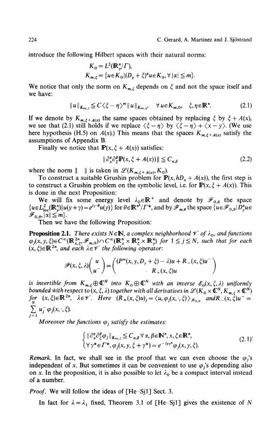
introduce the following Hubert spaces with their natural norms:
Kmtζ = {uεK0\(Dy + ξ)*ueK0, V |α| ̂ m}.
We notice that only the norm on Km tξ depends on ξ and not the space itself andwe have:
\\u\\Kmtζ£C(ξ-ηy*\\u\\Kmt,9 VWeKm, 0, <^eR". (2.1)
If we denote by Kmfξ+A(x) the same spaces obtained by replacing ξ by ξ + A(x\we see that (2.1) still holds if we replace <ξ — ήy by <£ — η) + <x — y>. (We usehere hypothesis (H.5) on A(x).) This means that the spaces Kmtξ+A(x) satisfy theassumptions of Appendix B.
Finally we notice that IP(x, ξ + A(x)) satisfies:
\\d xdF>(x9ξ + A(X))\\£CΛ9β (2.2)where the norm || || is taken in £f(Kmtξ+A(x}9K0).
To construct a suitable Grushin problem for P(x, W)x + A(x)), the first step isto construct a Grushin problem on the symbolic level, i.e. for lP(x, ξ + A(x)). Thisis done in the next Proposition:
We will fix some energy level A0eR+ and denote by ^Oθ the spacefor θeK*/Γ*9 and by J^t
Then we have the following Proposition:
Proposition 2.1. Γ/iere exists ΛfeN, α complex neighborhood ^ o/Λ,0, and functionsφX^^^eC^ίR^jzΓ^πC^ίR^xR^xR") /or l^ ^N, SMC/Z ίftαί /or(x, ξ)eR2n, and £#c/ι Aef^ the following operator:
™(x, y, Dy + ξ)-λ)u + R_ (x, £)κ
is invertible from Kmξ 0 C* into K0 © <C* wiίfc an inverse ^0(x, ξ, A) uniformlybounded with respect to (x, ξ, A) together with all derivatives in &(KQ x <CN, Km ξ x (CN)
Moreover the functions φj satisfy the estimates:
M
Remark. In fact, we shall see in the proof that we can even choose the φ/sindependent of x. But sometimes it can be convenient to use φ/s depending alsoon x. In the proposition, it is also possible to let λ0 be a compact interval insteadof a number.
Proof. We will follow the ideas of [He-Sjl] Sect. 3.
In fact for λ = λ1 fixed, Theorem 3.1 of [He-Sjl] gives the existence of N
Mathematical Approach to the Effective Hamiltonian 225
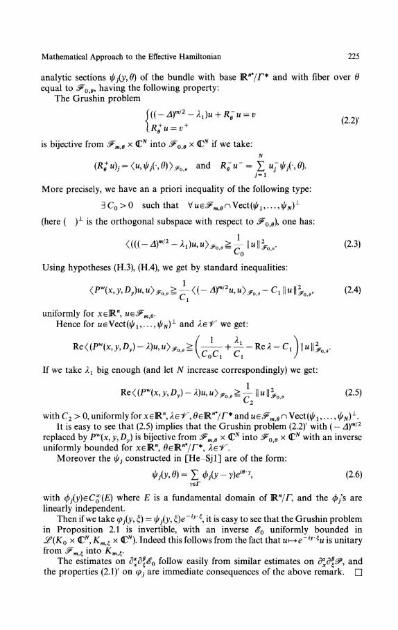
analytic sections ψj(y, θ) of the bundle with base RΛ*/^* an^ with fiber over θequal to J*0>0, having the following property:
The Grushin problem
is bijective from 3Fm# x (CN into ^Otθ x <CN if we take:N
(*>),. = <u,</^0)>^ and K,-tt-=£i<7^(-,0)..7=1
More precisely, we have an a priori inequality of the following type:
3C 0>0 such that VweJ^nVectO/^,...,^)1
(here ( )λ is the orthogonal subspace with respect to ^0,0)? one has:
9. (2.3)
^0
Using hypotheses (H.3), (H.4), we get by standard inequalities:
<P"(x,.y,D>, «>*,..£-!-<(- 4f2ιι,u>Λ,.- C, ||u||^oβ, (2.4)
uniformly for xeR",Hence for weVect^,...,^)1 and λεi^ we get:
o i !
If we take λ± big enough (and let N increase correspondingly) we get:
x,y,Dy)-λ)u,uy^θ^-\\u\\2^θ (2.5)C2
with C2 > 0, uniformly for xeR", λe'T, θeR"*/^* and ue^mtβn Vect(^ι, . . . , ψN)L.It is easy to see that (2.5) implies that the Grushin problem (2.2)' with (— Δ)m/2
replaced by Pw(x, y, Dy) is bijective from 2Fm θ x CN into ^0θx(CN with an inverseuniformly bounded for xeR", fleR^/r*, ϊe^.
Moreover the ψj constructed in [He-Sjl] are of the form:
Ψj(y,θ)=ΣΦj(y-y)eiθ'\ (2.6)γeΓ
with φj(y)eCQ(E) where £ is a fundamental domain of ΈLn/Γ, and the (/>/s arelinearly independent.
Then if we take ψj(y, ξ) = φj(y, ξ)e~iy'ξ, it is easy to see that the Grushin problemin Proposition 2.1 is invertible, with an inverse <ί0 uniformly bounded inJS?(K0
x <CN, Kmtξ x (C*). Indeed this follows from the fact that u\-+e~ίy'ξu is unitaryfrom ̂ ξ into km>ξ.
The estimates on B*xdβ
ξ$Q follow easily from similar estimates on δ"δ^, andthe properties (2.1)' on φj are immediate consequences of the above remark. Π
226 C. Gerard, A. Martinez and J. Sjostrand
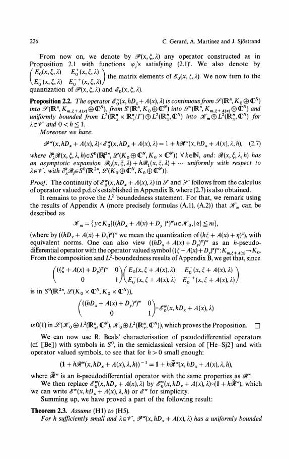
From now on, we denote by ^(x,£,λ) any operator constructed as inProposition 2.1 with functions <p/s satisfying (2.1)'. We also denote by
£0(x, ξ, λ) £0
+ (x, {, λ) \ the matriχ elements Qf g( ξ λ} W
E-(x9ξ9λ) E-+(x9ξ9λ)Jquantization of ^(x, ξ, λ) and δΌ(x9 ξ, A).
Proposition 2.2. T/ze operator δ%(x, hDx + Λ(x), λ) is continuous from ^(R", X0 0 C*)inίo ^(R^m,^(x)©CN),/rom S'(RM, K0 0 C") into '̂(RM, Km,^(JC) 0 C") anduniformly bounded from L2(R^ x R;/Γ)0L2(R;,<CN) mίo Jfm0L2(R^,<C") /or
Moreover we have:
^w(x, M), + Λ(x), λ)°£™(x, hDx + A(x), A) = 1 + fc#w(x, W)x + A(x), A, Λ), (2.7)
where dk
λ^(x,ξ,λ9h)ES0(l^2n^(K0®(CN,K0 x CN)) V/ceN, and: Λ(x,ξ,λ,h) fcasan asymptotic expansion <%Q(x9 ξ9 λ) + hόl^x, ξ, λ) 1 ---- uniformly with respect toλer, with dk
λ^jGS0(R2n^(K0φ€N,K0®(CN)).
Proof. The continuity of δ™(x, hDx + A(x\ λ) in y and 9" follows from the calculusof operator valued p.d.o's established in Appendix B, where (2.7) is also obtained.
It remains to prove the L2 boundedness statement. For that, we remark usingthe results of Appendix A (more precisely formulas (A.I), (A.2)) that Jfm can bedescribed as
A(x) + Dy )T«eJf0, |α| ̂ m},
(where by ((hDx -f A(x) + Dy)T we mean the quantization of(hξ + A(x) + ^/)α), withequivalent norms. One can also view ((hDx + X(χ) + Dy)
Λ)w as an /z-pseudo-differential operator with the operator valued symbol ((ξ + ̂ l(x) + Dy)
a)w:Kmtξ+A(x)^K0.From the composition and L2 -boundedness results of Appendix B, we get that, since
0
s n S π , J^(K x
i5 0(1) in J^(Jf0 0 L2(R^, CN), JΓ00L2(R^, CN)), which proves the Proposition. Π
We can now use R. Beals' characterisation of pseudodifferential operators(cf. [Be]) with symbols in 5°, in the semiclassical version of [He-Sj2] and withoperator valued symbols, to see that for h > 0 small pnough:
(1 -h /i^Πx, hDx + A(x\ λ, Λ)) - 1 = 1 + h Jw(x, hDx + A(x), A, Λ),
where @Γ is an /ι-pseudodifferential operator with the same properties as ̂ w.We then replace g™(x9 hDx + ̂ (x), A) by δ™(x9 hDx + ^(x), λ)°(l + /z^w), which
we can write (fw(x, ftD^. H- >4(x), λ, h) or <? w for simplicity.Summing up, we have proved a part of the following result:
Theorem 2.3. Assume (HI) to (H5).For h sufficiently small and λei^, ^(x,hDx + ,4(x), A) /zαs α uniformly bounded

Mathematical Approach to the Effective Hamiltonian , 227
inverse of the form <f w(x, hDx 4- A(x\ λ, h), where
δ(x, ξ, λ, h)eS°(R2",
has an asymptotic expansion ^w(x, ξ, λ,h)~Σ $ i (x> £> λ)h J, <?0
=: (̂*> £> A) ~ * asabove. °
77ϊ/s inverse has the same continuity properties as $0(x, hDx -f- A(x\ λ, h) inProposition 2.2.
Proof. From the constructions above it is clear that δ = ̂ w(x, hDx + A(x\ λ, h) isa right inverse for ̂ w(x, /ιDx + Λ(x)9 λ) with all the properties stated in the Theorem.We only have to show that δ is also a left inverse. If λe'T nR, 0>w(x, /ιDx + /l(x), A)is self adjoint on X00L2(]RM,CN) with domain Xm 0 L2(RW, CN). Then£w(x,hDx + A(x)9λ,h) is also a left inverse for ΛeiΓnlR, and also for λei^ byanalytic continuation.
This proves the theorem. Q
We denote by [ + ) the matrix elements of δ and remark they\E-(λ,h) E
E_+(λ,h) = Ew_ + (x,hDx + A(x\λ,h) is a /z-pseudodifferential operator with itssymbol in S°(R2n, ̂ ((CN, <CN)). In particular E_+(/U) is bounded on L2(Rrt,CN).
We come now to the main result of this section, namely the reduction of thespectral study of P:
Theorem 2.4. Under assumptions (HI) to (H.5\for λεi^, h small enough, one hasthe following equivalence:
Proof. We use the following formulas which can be checked easily:
(P - λΓ 1 = E(λ, h) - E+(λ, h)E_ +(λ, hΓlE-(λ, Λ), (2.8)
E_ +(/l, Λ)" 1 = -R"(x, hDx + A(x))(P - λ)' lR"(x, hDx -h A(x)). (2.9)
Here R^.(x, hDx -f A(x)) is the Weyl quantization of R ± (x, hζ + A(x)) in Proposition2.1. Then (2.8), (2.9) and the continuity properties of $ established in Theorem 2.3imply Theorem 2.4. Π
As a preparation for the next section, we will now establish some commutationproperties of $.
Because of (2.1)', we have:
_ - ,
+(x,ξ + y*) = R+(x,ξ)eiy ?*.
On the operator level we get:
e-iχ vΊi>R»(x9hDx + A(x))eix'y*/h = e-iy'**Rw_(x,hDx 4-
e-ίxγ*/hR™(x,hDx -f A(x))eix'^/h = Rw
+(x,hDx + A(x))
Combining this with the fact that
P*(x,y, ξ + y* + Dy) = e~iy'y*Pw(x,y, ξ -f Dy)eiy'y
228 C. Gerard, A. Martinez and J. Sjόstrand
we get
e-iyy* 0\ / £<>•?* 0
. 0 ιy x ' * * "v o iThis can be rewritten as:
'ei(χlh-y)-r*
Of course (2.11) stays true if we replace 0>w(x,hDx + ^4(x)) by its inverse <f, whichis what we will need in the next section.
III. Spectral Reduction of P(}
In this section, we give a reduction of the study of the spectrum of P0 by usingProposition 1.3. Hence we replace P0 by P acting on L0 with domain Lm (see Sect. I)and we shall use the Grushin problem of Sect. II to study this operator.
First, let us remark that a distribution u = ]Γ v(x)δ(x — h(y — y)) in L0 can alsoyer
be written as Σ δ(x — h(y — γ))v(h(y — y)), i.e. as an element of '̂(R"; K0) where,yeΓ
as before, K0 = L2(R"/T): indeed, if
φe^(Rn,K0)^ {<x>Na>6L2(lRw x F), VΛΓ,α}
def
(where F is a fundamental domain of JR"/Γ\ then φ(x, y) = φ(Jc -f Λy, y) is also in
KQ\ and we have:
yeΓF
which can be bounded by seminorms of φ in ̂ (R", K0), and thus also by seminorms
Hence, we can hope to adapt some results of Sect. II for the study of P actingon L0.
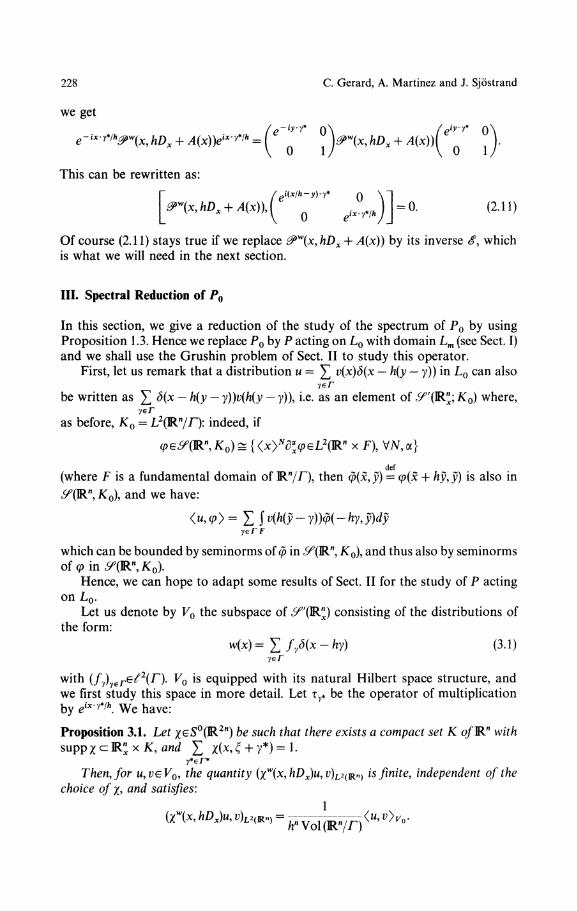
Let us denote by V0 the subspace of <^(R") consisting of the distributions ofthe form:
W(X)=ΣΛ^-M ί3'1)yeΓ
with (fy)yeΓe^2(Γ). V0 is equipped with its natural Hubert space structure, andwe first study this space in more detail. Let τy* be the operator of multiplicationby eix'γ*/h. We have:
Proposition 3.1. Let χe5°(R2π) be such that there exists a compact set K o/Rπ withsupp χ c R£ x X, and £ χ(x9 ξ + γ*)=l.
y*eΓ*
Then, for u,veV0, the quantity (χw(x,hDx)u,v)L2(^n} is finite, independent of thechoice of χ, and satisfies:
(χ-ίx, W», PW, =
Mathematical Approach to the Effective Hamiltonΐan 229
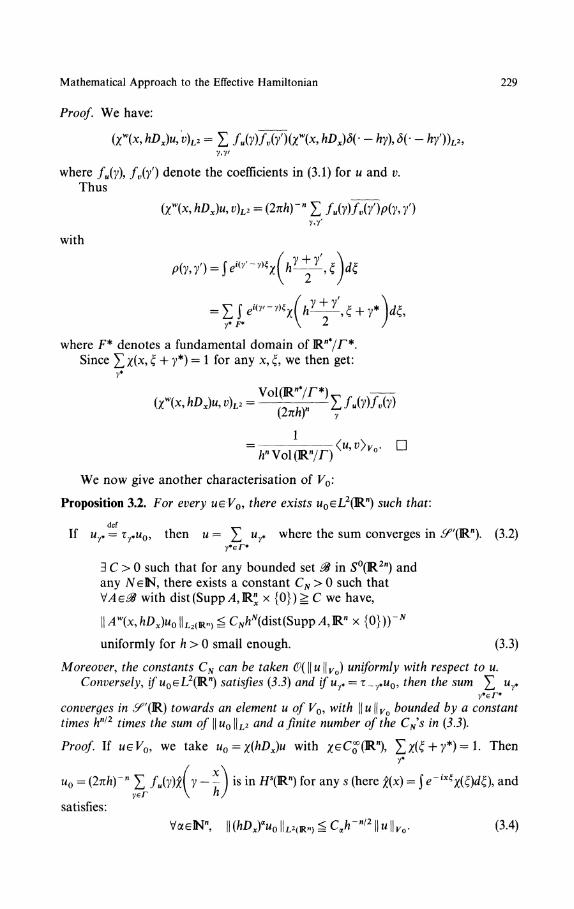
Proof. We have:
(χ»(x9 hDx)u, v)L2 = £ /M(y)/.(/)θr(*. «W - hy\ δ( - A/))L,ϊ.y
where fu(y), /„(/) denote the coefficients in (3.1) for u and v.Thus
(χ"(x, ADJii, »)„ = (2πΛ)-" £y,y'
with
y*F* \ 2
where F* denotes a fundamental domain of R"*/^*-Since £χ(x, £ + 7*) = 1 for any x, ξ, we then get:
/z"Vol(R"/ΓΓ
We now give another characterisation of K0:
Proposition 3.2. For every ueV0, there exists M0eL2(Rn) such that:
defIf wy* = τy*M0, then u = ^ wy* where the sum converges in '̂(R"). (3.2)
y*eΓ*
3 C > 0 such that for any bounded set ̂ in 5°(R2π) andany NeN, there exists a constant CN > 0 such that
with dist(SuppΛ,R" x {0})^ C we have,
uniformly for h > 0 small enough. (3.3)
Moreover, the constants CN can be taken &(\\u\\Vo) uniformly with respect to u.Conversely, ϊ/w0eL2(Rn) satisfies (3.3) and ifuy* = τ_ y *w 0 , then the sum ]Γ wy*
y*eΓ*
converges in '̂(R) towards an element u ofV0, with \\u\\Vo bounded by a constanttimes hn/2 times the sum of \\ w 0 | |L2 and a finite number of the CN's in (3.3).
Proof. If weK0, we take u0 = χ(hDx)u with χeC£(Rn), Σχ(ξ + 7*)=l. Theny*
u0 = (2πh)~n X /M(y)χ 7 - is in HS(R") for any s (here χ(x) = f e-^χ(ξ)^), andyeΓ \ Λ /
satisfies:
VαeN", || (ΛDJ-tto ||L2(RΛ) ̂ C,^"/2 1| u ||Ko. (3.4)

230 C. Gerard, A. Martinez and J. Sjostrand
The property (3.3) follows then, by integrating by parts in the oscillatory integralwhich gives Aw(x, hDx)u0, and using the Calderon-Vaillancourt theorem.
To prove (3.2), we only remark that My* = τy*χ(hDx)τ-y*u = χ(hDx — y*)u.Let us now prove the converse statement:If MO satisfies (3.3), we can find for any y*eΓ* a real function
Ay.(ξ)eC£(\ξ\<±\γ*\) such that the family (Ay*)y*eΓ* is bounded in S°(R2w) and
\\(l-Ay4hDx))u0\\L2^CN\y*\-NhN
for 1 7* I large enough. Then, if φey(R"), we can write
(uy, φ)L> = (MO, τ _ y*φ)L2 = (ιι0, Ay*(hDx)τ _ y*φ)L2 + 0(hN \y*\~N)
and, because of the condition on the support of A^9 we have
We conclude from this that £ My* converges in &". It remains to show that u = ]Γ My*is in V0.
Let us take χ as before, and consider
(χ(hDx)u^ uβ*)Lι = (χ(hDx + α*)w0, w^_α*)L2.
If we take another cutoff function χ such that χχ = χ, we get:
(χ(hDx)u^ uβ*)L2 = (χ(hDx + α*)u0, χ(hDx + α*)M^ _α<)
= (τ+.pχ(hDx + α*)w0, χ(ΛD, 4- j8*)tt0).
Hence, using (3.3), we get:
I (χ(WλX*, M/r )L2 1 ̂ || χίW), + α*K || || jRfcD, + Γ K I I
gCX(|α*| + |jS*|)^ (3.5)
when |α*| + \β*\ is sufficiently large. Here, CN can be estimated by the sum of|| M0 1| and a finite number of the CN's in (3.3).
It follows from (3.5) that (χ(hDx)u9 u)L2 is well defined and finite, and we concludeby Proposition 3.1 that u in V0. Π
We next study the action of pseudodiίferential operators on K0:
Proposition 3.3. Let B(x, ξ)εS°(Ί&2n) with B(x, ξ + 7*) - B(x, ξ)for any 7* eΓ*. Then,Bw(x, hDx) ίs bounded on F0, uniformly with respect to h small enough.
Proof. Let MeF0 and let us write M = £MV* as in Proposition 3.2. Then
Bw(x, hDx)u = X ty, where vy* = Bw(x, hDx)uy*.r*
Then since B(x, ξ + y*) = J3(x, ξ), we get that t;y* = τ _ y,t?0, where ι;0 = 5w(x, hD*x)uQ
is in L2(Rn). This shows that ι;y, satisfy (3.2).Using standard pseudodifferential operator calculus, we see easily that VQ
satisfies (3.3), with constants CN estimated by similar constants for MO. This provesthat υe K0 and that || v ||Ko ̂ C0 1| M ||Ko, by Proposition 3.2. Π
Remark 3.4. An alternative proof of it would have been to conjugate βw(x, hDx)by a Fourier transform, and then get a pseudodifferential operator acting onL2(RΠ7^*) However, this kind of proof cannot be easily generalized to the spaceLO we have now to consider.

Mathematical Approach to the Effective Hamiltonian 231
Remark 3.5. Under _the assumptions of Proposition 3.3, the adjoint of Bw(x,hDx)on KO is given by (B)w(x,hDx).
We will now see that essentially the same discussion applies to L0. Indeed ifu = Σ v (χ)δ(χ — hy — hy\ we can consider for each fixed y:
yeΓ
uy = Σ v(hy + hγ)δ(x -hy- hy).γeΓ
It turns out that up to the translation by hy, uy is an element of F0 for almostall y. This follows from the following identity:
) = Λ" f
= *" ί KlUA <3-6>R"/Γ
If we take now χ as in Proposition 3.1, and consider χ(x9hDx) as acting ony'(R" x R") with y as a parameter, we see by (3.6) that the analog of Proposition3.1 holds for L0. Namely:
I I « llίo = h"Cn(χ"(x, hDx)u, u)2 χ . (3.7)
We will now prove the analog of Proposition 3.2 for L0. Let Γy* be the operatormultiplication by ei((xlh)~y)y* and notice that Tγ*u = u for u in L0 and γ*eΓ*.
Proposition 3.6. For any weL0, ί/iere exists w0eL2(IR" x R^F) SMC/I ί/iαί:
T/ze property (3.2) holds for A = A(x,ξ) (independent of y,η)if we replace L2(RΠ) by L2(R^ x R /Γ). (3.8)
constants CN are 0( \\ u \\ Lo).
i^ series converges in S"(R", X0). (3.9)
Conversely if u0eL2(R" x RJJ/F) satisfies (3.8) and if wy* = Ty*w0, ί/ien ί/ie series]Γ wy* converges in ^"(JR.n
x,K0) towards a distribution u in L0 wiί/i | |w||L o boundedy*eΓ*
fry α constant times hn/2 times the sum of \\ u0 \\ and a finite number of theL (JR x R IF)
CN in (3.8).
The proof is similar to that of Proposition 3.2 and we omit it.Proposition 3.6 gives a proof of the fact that L0 c ̂ '(R£, K0). A more direct
proof can be obtained by computing the scalar product of u = Σ v(x)δ(x — h(y — γ))γeΓ
with (pe^(R" x RJ//") and by estimating it by ||^||L2(Rr l) times a seminorm of φ
The same argument gives also that
where ΛΛ(ξ) is the operator valued symbol ((ξ + Dy)α)w.
One also gets that:
(3.10)
232 C. Gerard, A. Martinez and J. Sjostrand
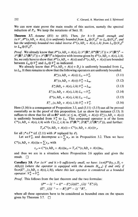
We can now state prove the main results of this section, namely the spectralreduction of P0. We keep the notations of Sect. II:
Theorem 3.7. Assume (HI) to (H5). Then, for h>Q small enough andλe-r,0>w(x9hDx + A(x),λ) is uniformly bounded from Lm®(V0)
N to L0®(V0)N, and
has the uniformly bounded two sided inverse ^w(x, hDx + A(x\ λ, h) from L0 © (V0)N
to Lm@(V0)N.
Proof. We already know that ^w(x, hDx + A(x\ /ί):y"(Rw; #m(Rn/Γ)) x &"(Rn)N ->'̂(Rn; L2(R"/Γ)) x &"(Rn)N is bijective with inverse given by £™(x, hDx + A(x)9 λ\ h).
So, we only have to show that ̂ w(x, hDx + A(x)) and <Tw(x, hDx + A(x)) are boundedbetween Lm® V% and L0Θ ̂ o as indicated.
We already know that Pw(x,hDx -f A(x) + Dy) is uniformly bounded from Lw
to LQ. It then remains to show that the following operators are uniformly bounded:
R»(x9hDx + A(x)):LQ-+V»9 (3.11)
R»(x9hDx + A(x)):V»-+Lm9 (3.12)
El(hDx + A(x)9 λ; h): F^Lm, (3.13)
EϋXx, hDx + A(x)9 λ; h):L0 -> V», (3.14)
£w(x, hDx 4- A(x), ̂ Λ):L0 -> Lm, (3.15)
£ί +(x, hDx + ̂ (x), A; A): K£ -, Fj. (3.16)
Here (3.16) is a consequence of Proposition 3.3, and (3.11)-(3.15) can all be provedessentially as in the proof of this proposition. Let us show for instance (3.13). Itsuffices to show that for all αeN" with |α| ̂ m, Λ™(hDx + A(x))°E™(x, hDx + A(x))is uniformly bounded from V% to L0. This composed operator is of the formCw(x9hDx + A(x)9λ9h) with C(x9ξ9λ;h) in 5°(R2π;j^(CN;L2(RVΓ))), and further:
Γy*Cw(x, hDx -f A(x)) = Cw(x, ftDx -f ^l(x))τy*
for all y*eΓ* (cf. (2.11) with & replaced by g).Let U€VQ, and decompose u = Σu
y* as in Proposition 3.2. Then we have
Cw(x, hDx + A(x))u = X t?y* with
, hDx -h A(x))My* = Γy*Cw(x, hDx + A(x))uQ,
and thus we are in a situation where Proposition 3.6 applies and gives theresult. Π
Corollary 3.8. For λei^ and h>0 sufficiently small, we have: λeσ(Pw(hy,y,Dy +A(hy))) (where the operator is equipped with the domain Hm^A) if and only ifQeσ(Ew_+(x,hDx + A(x\λ\h)\ where this last operator is considered as a boundedoperator: Fj[->Fj[.
Proof. This follows from the last theorem and the two formulas:
(Pw - λ) ~ l = E™ - El (λ)(Ew_ + (λ)) - 1 Ew_ (A),
(E™+(λ)Γl = -Rl(P"-λΓlR™,
where all these operators have to be considered as bounded ones on the spacesgiven by Theorem 3.7. Q
Mathematical Approach to the Effective Hamiltonian 233
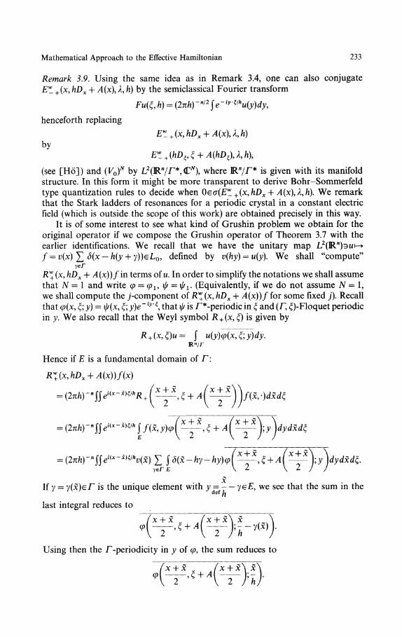
Remark 3.9. Using the same idea as in Remark 3.4, one can also conjugateE"L + (x, hDx + A(x\ λ, h) by the semiclassical Fourier transform
Fu(ξ,h) = (2πhΓn/2$e-iy'ξ/hu(y)dy,
henceforth replacing
Eby
E™
(see [Ho]) and (VQ)N by L2(Rn/Γ*,<CN)9 where Rrt/Γ* is given with its manifoldstructure. In this form it might be more transparent to derive Bohr-Sommerfeldtype quantization rules to decide when Oeσ(E^+(x,Λ£)JC + A(x),λ,h). We remarkthat the Stark ladders of resonances for a periodic crystal in a constant electricfield (which is outside the scope of this work) are obtained precisely in this way.
It is of some interest to see what kind of Grushin problem we obtain for theoriginal operator if we compose the Grushin operator of Theorem 3.7 with theearlier identifications. We recall that we have the unitary map L2(IR")9Mi—>f = v(x) Σ δ(x — /ι(y + y))eL0, defined by v(hy) = u(y). We shall "compute"
yerR + (x, hDx + A(x))fm terms of u. In order to simplify the notations we shall assumethat JV = 1 and write φ = φί9 φ = ι/^. (Equivalently, if we do not assume N = 1,we shall compute the j-component of JR + (x, hDx + A(x))f for some fixed ;'). Recallthat φ(x9 ξ; y) = ψ(x, ξ; y)e~iy'ξ, that ̂ is Γ*-periodic in ξ and (Γ9 ξ)-Floquet periodicin y. We also recall that the Weyl symbol R + (x,ξ) is given by
R + (x,ξ)u= J u(y)φ(x9ξ;y)dy.
Hence if E is a fundamental domain of Γ\
( v -4- Y / γ-4- γ\ \
^-,ξ + A(~-);y )dydxdξ.2. \ 2 / /
XIf y = γ(x)εΓ is the unique element with y = — ye£, we see that the sum in the
def/ j
last integral reduces to
Using then the /"-periodicity in y of φ, the sum reduces to
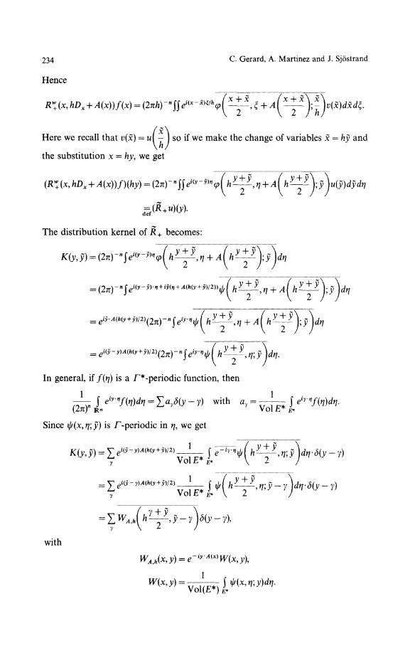
234 C. Gerard, A. Martinez and J. Sjostrand
Hence
^
Here we recall that v(x) = u( - | so if we make the change of variables x = hy and\lϊ /
the substitution x = hy, we get
^
The distribution kernel of R+ becomes:
In general, if f(η) is a Γ*-periodic function, then
— f eiy'ηf(η)dη = Σa?δ(y - y) with ay = ίΓ27C)" IRn i> I L*t Ύ ^ I' y \7-_i r?* J
Since ψ(x, Y\\ y) is /"-periodic in η, we get
1 ,—7Γ-
f
J. V 2
with
f ψ(x,η',y)dη.
Mathematical Approach to the Effective Hamiltonian 235
In the situation studied in [He-Sjl] we can take ψ independent of x and thenW(y) is a Wannier type function used in that work as well as in [Ne].
We get R + u(y) = ̂ R + u(y)δ(y - y\ where R + we/2(Γ) is given by:
. (3.17)
In the situation of [He-Sjl] we start with a constant magnetic fieldh- ΣΣbj,kdXj Λ dxk with bjtk = — bkj, where contrary to [He-Sjl] we do not assume
that I bjjk I are small. (In that paper h = 1 at this stage.) We can then take Ax = — ̂ Bx,and a simple computation shows that
where Th
y
B is the magnetic translation defined in [He-Sjl]. This means that R +is the same operator as Rh* in the terminology of [He-Sjl].
Since the various identifications in our computation are unitary and sinceR™(x9hDx + A(x)) = R^(x9hDx + A)*9 it is clear that this operator is naturallyidentified with R_ = R* . Summing up we have proved:
Corollary 3.10. Define R*_=R + by (3.17) or rather the natural generalization ofthis relation for arbitrary N. Thus for λ in a neighbourhood of Λ0, the operator
R++
is bijective with bounded inverse I ^ ^ + 1. The matrix ofE.+ is equal to the\£_ E_ + J
matrix of E™(x, hDx + A, λ\ h) acting on KQ, if we identify the latter space with/2(Γ;CN) in the natural way.
IV. The Case of the Schrodinger Operator
In this section, we assume that A(x) is a linear function of x (corresponding to thecase of a constant magnetic field). Let K(x,y)eC°°(R2") be F-periodic with respectto y and satisfy
I^K(x,y)|^CM, (4.1)
on R2n for every (α,/?)eN2π. We are then interested in the operator
£(D,, + hAj(y))2 + V(hy, y) = P™(hy, y, Dy + A(hy))9 (4.2)
where
). (4.3)
Following the procedure of Sect. II, we fix an energy level z0, and we chooseΨι(x9ξiy)9 ' 9ψN(x,ξ,y) smooth in all variables, /^-periodic in ξ and with
236 C. Gerard, A. Martinez and J. Sjόstrand
ψj(x, ξ', y + y) = eiy'ξψj(x, ξ; y), such that the problem:
V κ°(x,ξ) ois bijective for ξeR"*, and z close to z0. Here the spaces ^k ξ are defined in Sect. IIand R°_ = R°+*, (R°+(x9ξ)u)j = (u\ψj). Let £0_+(x,£,z) be the N x N matrix whichappears in the lower right corner of the inverse of (4.4). Putting P(x, ξ) = Pw(x, y, ξ + Dy\
ξ) 0we then know from Sect. II that when h is small enough,
0>w(x9hDx
is bijective and has the uniformly bounded inverse £"v(x,hDx + A(x\z\h\ IfE_+(x,hDx + A(x\z\h) is the NxN block in the lower right corner, then£_+(x, ξ,z;/ι)eS° has a complete asymptotic expansion in powers of h and theleading term is £0_+(x, ξ,z). Moreover we know that E_+ is /^-periodic withrespect to ξ. The main result of Sect. Ill tells us that zeσ(Pw(hy,y,Dy + A(hy)))(as an operator acting on L2(Rn)) iff Qeσ(E*+(x,hDx + A(x),z;h))), where E™_ +
now acts on the space V% (of functions which are F*-periodic in the dual variable).We now discuss two special cases:
]. The Case of Periodic Potentials. We here assume that V = V(y) is independentof x (and F-periodic in y). If we choose φj = φ^ξ; y) independent of x, then thesymbol & — &(ξ) is independent of x. The operator gP™(hDx + A(x)) then acquiressome additional symmetry properties: We introduce the magnetic translation
T^u(x) = e~iA(v)'xlhu(x - v), (4.8)
and check that [T*,hDXj + A/x)] =0, VvelR", ;'=l,...,n. T* may be viewedas a /i-Fourier integral operator associated to the affϊne linear map: (y,η)\-+(y + v, f/ — v4(v)), and we have for symbols q of class 5°:
(T?Γ V(x, hDx)TΪ = q?(x9 hDx), qv(x, ξ) = q(x + v, ξ - A(v)). (4.9)
This remains true also for operator valued symbols and in particular £P™(hDx -f A(x\ z)commutes with T*, for all veR". This is then also true for $™(x,hDx + A(x\z\h)and using (4.9) we conclude that $(x,ξ\h} is independent of x:
\h). (4.10)
In particular for z in a neighborhood of z0:
zeσ(Σ(Dyj + Aj(hy))2 + F(y))oOeσ(£^ +(hDx + A(x\ z; h}\ (4.1 1)
where £_+(ξ,z;/ι) is F*-periodic in ξ and Ew_+ acts on V%.We further notice in this case that the operators Pz in Remark 1.2 have the
same spectrum since
Σ(DW + Aj(z 4- hy))2 + F(y) = e'^A^(^(Dyj +
Hence Pw(y, hDx -f A(x) + Dy) has the same spectrum as

Mathematical Approach to the Effective Hamiltonian 237
so we may ignore Sect. Ill, and consider E™_+(hDx + A(x\z\h) as a boundedoperator on L2(R";(PN) in the equivalence (4.11). This result was obtained in[He-Sjl] by use of Wannier functions and some implicit arguments. See alsoNenciu [Ne].
2. Quasiperiodic Potentials with Vanishing Magnetic Fields. We assume that V(x, y)is /"-periodic with respect to y (as before) and Aperiodic with respect to x, wheref is a second lattice. We shall not assume that A vanishes right away. We canthen Choose φ, in (4.4) with the additional property: φ/x + y, £; y) = φ/(x, £; y),Vyef (trivially since we may even take φj independent of x). This implies that^(x, ξ9z) appearing in (4.5) is not only "/^-periodic with respect to ξ", butalso Aperiodic with respect to x. Considering magnetic translations T* as in
case 1, we see that ^w(x, hDx + A(x\ z) commutes with all T* with veΓ. Then<^w(x, hDx + A(x\ z; h) will have the same property and we conclude that ^(x, ξ9 z; h)is Aperiodic with respect to x. In particular:
zeσ(Σ(Dyj + hAj(y))2 + V(hy9y))oOeσ(E»_ + (x,hDx + A(x)9r9h))9 (4.12)
where E^+ acts on V% and E_ + (x, ξ h) is Aperiodic with respect to x and/^-periodic with respect to ξ.
Iff + h Γ is dense in Rn, (4. 1 3)
then we can let E"L+(x,hDx + A(x),z;h) operate on L2(R";C*), the reason beingagain that for every xeRw, the operator
Px = Pw(x + hy, y Dy + A(x + hy)) = Pw(x + hy, y\ Dy + hA(y) + A(x))
is isospectral to jP0.In fact, conjugating Px with e ~ iA(x)'y, we see that Px is unitarily equivalent to:
(4.14)
Let f* be defined as T^ but with h replaced by 1/fc. Then T^ commutes with(Dy + hA(y) )w. Conjugating (4.14) with T^,yeΓ and using also that P(x,y;η) isAperiodic in x and Γ-periodic in y9 we see that for all yeΓ, γeΓ, the operator(4.14) is unitarily equivalent to:
Pw(x + hy + y + hy, y; Dy + hA(y)). (4. 1 5)
Using the assumption (4.13) we can take a sequence (γj9 y^eΓ x Γ9 j = 1, 2, . . . suchthat x -h hjj -h TJ -> 0. Then K(x -f ̂ + 7^, 3;) -> K(0, 3;) uniformly and we concludethat Px is isospectral to P0, as stated.
We now take n = 1, >4 = 0, and we shall see that we can get an effectivehamiltonian which is close to Harper's operator cos(hDx) -f cos x. We take Vλ(x9 y) =Uλ(x) + λ2 W(y\ where λ ̂ 1 is a large parameter. We also let Γ = Z, Γ = Γ* = 2πZ.We assume that W(y) ^ 0 with equality precisely on Zζ, and also that W"(ϋ) > 0.We first consider
D2 -h λ2 W(y] = λ2((hDy)2 -h W(y)\ h = ~. (4.16)
Λ
We can here apply known results concerning the tunnel effect in periodic semi-
238 C. Gerard, A. Martinez and J. Sjδstrand
classical situations of Harrell [Ha], Outassourt [Ou], Simon [Si], and we knowthat the first band in the spectrum of (4.16) is of the form
λ5/2a(λ)e~s°\ λE(λ) + λ5l2a(λ)e~SGλl (4.17)
where 50 > 0 is a certain complex action between neighboring wells, and£(A),α(λ)eS^0(R+) are real valued classical symbols of order 0 with asymptoticexpansions:
ao + M"1*"'* (4.18)
with £0,α0>0. Moreover, for λ>Q large enough, the band (4.17) is all of thespectrum of (4.16) in the half axis ] — oo,21E0].
The band (4.17) is generated by the Floquet eigenvalue:
μλ(ξ) = λE(λ) + λ5'2a(λ)e-s°λ(cos ξ + r(λ, 0), (4.19)
where
\d\d\r(λ, ξ)\ ̂ Ck^e~(ll2}S°\ (4.20)
for all A:,/.We take
U=Uλ(x) = μλ(x)-2λE(λ). (4.21)
Choosing i^ to be a complex neighborhood of the interval (4.17), we can takeN=l in our choice of Grushin problem with φ1 independent of x,(D2 + λ2 W)φl = μλ(ξ)φι, and choose this problem in such a way that
E0_ + (x, ξ,z) = z- λ5l2a(λ)e-Soλ(cos ξ + r(A, ξ) + cos* + r(λ,x)). (4.22)
We are therefore quite close to Harper's operator. It is quite likely that (4.20) canbe extended to a large band around the real axis and that we get a correspondingresult for £_ + (x, ξ, z; h). In order to apply the results of [He-Sj3], one would alsoneed Fourier invariance: £L+(x, ξ,zm,h) = E_+(ξ, — x,z;/ι) (and another simplerproperty which may be less important). Perhaps this is also possible to obtain bymeans of some delicate correction terms depending both on x and y in the choiceof Vλ(x,y). A more natural solution would be however to extend the study in[He~Sj3] to the case without Fourier invariance.
Appendix A. Magnetic Differential Operators and Sobolev Spaces
Here, we shall discuss magnetic Sobolev spaces, and we assume (H.5). We definefor weN:
H% = {w6L2(Rπ);(Dx + A(x))«ueL2(Rn\ |α| ̂ m}.
Using the composition formula for Weyl quantizations, and the fact that for anyαeJN", jSeN2", |j8| ̂ 1, we have:
γ<Λ
where the αα/3y's and all their derivatives are bounded functions on 1R", it is notdifficult to see (by induction on |α|) that for any αeNn and any function α(x),
Mathematical Approach to the Effective Hamiltonian 239
bounded with all its derivatives:
a(x)(Dx + A(x)Y = ίa(x)(Dx + A(x))*Y + £ [_bΛβ(x)(Dx + A(x))^ (A.I)β<Λ
where the bα/3's and all their derivatives are bounded on IRΛWe can also deduce from (A.I) that:
la(x)(Dx + A(x))Ύ = a(x)(Dx + A(x))* + £ cΛβ(x)(Dx + A(x))', (A.2)β<a
where the cα/?'s have the same property as the baβ$.In view of (A.I), (A.2), we then get the same space Em
A if we replace (Dx + A(x))a
by l(Dx + A(x))*]* in its definition.
Proposition A.I. Hm
A is a Hilbert space in which CQ is dense.
Proof. It is enough to prove the density. Let utHm
A and χjeCJ(|x| < j + 1) withXj(x) = 1 for |x| ^ j and |d% (x)| ^ Cα for all αeN" with Cα independent of; ( eN).Clearly XjU€H*omp(R
n) c //^. Moreover, for |α| ̂ m:
where the Cα/?'s are constants, and Cα0 = 1. Thus
(D, + A(x))«(χju) -> (Dx + A(x)γu in L2 (as -» + oo).
Hence, every u in H^ can be approximated by elements with compact support,and each u in H™ with compact support can be approximated by CJ -functionsby means of a standard regularization. Π
Notice that we have the inclusion:
We next introduce differential operators. Let
P(x,ξ)= X a.(x)ξ. . H^m
with\dβ
xaa(x)\^Cβ (Vα,/U). (A.4)
Then \d'xdβ
ξP(x,ξ)\ ^ Cα/Om~^' (where <{>=(! + ̂ 2)1/2) for any χ,ξ in Rπ and
We then put p7 (x, ξ) = ^ «α(^)ξα, p = pm, and we assume that m is even andM=J
for some C0 > 0:
(A.5)
We are interested in Op^(P) = Pw(x,Dx -h ^(x)), which can also be written:
OpΛP)= Σ bαWΦx + ̂ W)", (A.6)|α |^m
where the foα's satisfy (A.4), and ba = aΛ when |α| = m.It is easy to see that Oρ^(P) is bounded H™+k^>Hk
A for every fceN.
240 C. Gerard, A. Martinez and J. Sjόstrand
If we fix x0e]R" and put ξ0 = A(x0), we have:
γ. (A.7)
This operator is bounded: H™^k
ξQ-+Hk
A_ξo. If Ω is an open set of RM, we write:
ll«l& ( α > = Σ \\(Dx + A(X))"u\\l(ΩΓA k i ^ f c
Then, thanks to (H.5), we see that the norms || ||Hk (β(Xo,2)) an^ I I ' \\Hk(B(x0,2)) are
equivalent uniformly with respect to x0. (Here B(x0,2) denotes the open ball ofcenter x0 and radius 2.)
The operator (A.7) can be written:
£ cα(x,x0)/)« (A.8)|α |^m
with eα(x,x0) = αα(x) for |α| = w, and |dfcα(x)| ^ C^ for any α, xe£(x0,2), and withCβ independent of x0.
Standard a piori estimates for elliptic operators then give for any u inH* + "(B(x0,2)):
II u UH-^O,I)) ̂ C*t 'I °P^M " i f* c uo.2)) + I I u «L>c^.2))l (A 9)
where Cfc is independent of x0.If we also assume, as we shall do from now on, that P is real valued, then
OpA(P) is formally selfadjoint and the classical Garding inequality becomes:
(OpA(P)u, u)L2 Z±-\\u \\2
am/2 - Co || « II I (A.10)C0 *
for all Me^/(5(x0,2))n//^/2, and with C0 independent of x0.Combining (A.9) with a simple covering argument, we get:
Proposition A.2. // weL2(RM) and OpA(P)ueHk
A(J^nl then ueHk
A
+m(J^n) and wehave:
\\ + || ιι || tϊ], (A. 11)A UA
where Ck is independent ofu.
Using a partition of unity, we also get from (A.10) (with a new constant C0):
(Op^(P)M, u)L2 £ -L U u || 2 - C0 1| u \\2
L2 (A. 12)C0
for all ueH™. (The commutator terms are estimated by C || u \\ (m/2)-1 -\\u\\ m/2 andwe can use that || u \\ H, _ t ^ ε || w || ̂ -f- Cε>k || u ||L2 for any ε > 0). A
If we consider Oρ^(P) as a symmetric operator with domain C^IR"), (A. 12)shows that Op^(P) is semibounded from below, and admits at least one self-adjointextension (the Friedrichs one). Proposition A.2 actually shows that Op^(P) isessentially self-adjoint, and that the domain of its unique self-adjoint extension is
Mathematical Approach to the Effective Hamiltonian 241
Appendix B. Pseudodifferential Operators with Operator Valued Symbols
We review some standard facts. Our main reference is here the unpublished workof A. Balazard-Konlein [Ba].
We denote a point (x, ξ)eR2π by X. We shall consider a family of Hubertspaces j / X 9 XeR2π satisfying:
j/χ = s#Ύ as vector spaces for all X, YeR2", (B.I)
There exist N0 ^ 0 and C ̂ 0 such that|| ιι || Λ g C(X - 7>No || u || ̂ for all uε^ X, YeR2". (B.2)
Let έ$x,XεΈί2n be a second family with the same properties. We say thatpeCw(R2^(^0,^o)) belongs to S°(R2π;J^(j/x,^)) if for every αeN2", thereis a constant Cα such that
IIW*(Λ.fc)^Cβ, *eR2". (B.3)
If p depends on the additional parameter /ιe]0, Λ0], h0 > 0, we say that p belongsto S°(R2"; JS?(j^,#x)) if so is the case for every fixed h and if (B.3) holds withconstants Cα which are independent of h.
Proposition B,l. Let peS°(R2w; &(s/x, 8X)\ where stfx, @x satisfy (B.I), (B.2). ThenOpΛ(p) = pw(x,W)x) is uniformly continuous
Proof. We neglect certain standard density arguments like approximating thesymbols by symbols with compact support. In the formula
OpΛ(P)«(x) = f J e « * - » < / * p , ί « ω , (B.4)
where ue^^R",^) we use the fact that:
(1 + \x - y\2 + Iξl2)'1^ - ξ hDy + (χ- y) hDξ)ei(χ-*™h = ««*-')«/*, (B.5)
and obtain after N steps:
(B.6)
Here
q(x,y, ξ h) = <P(1)(1 + \ξ\ + \x- y\ΓN(ί + |x| + M + lίl)2Λr°(l + |jΊΓw in 00.
This implies:
ϊ(x,y, ξ h) = Θ(\)(l + \ξ\)-ww*(i + \x- y\ΓN'2(l + \y\ΓN+2N°(l + \x\)2N"
ζ&(i)(i+\ξ\Γ(Nm+2No(i + \χ-y\Γ{NI2ί+2No(i + \y\ΓN+*No in a0,and choosing N sufficiently large we see from this and (B.6) that
l|Op»(p)«(x)IU0 = 0(1)(1 + |x|Γ* for every N.
The derivatives in x can be estimated similarly. Π

242 C. Gerard, A. Martinez and J. Sjόstrand
The formal complex adjoint of Oph(p) is Oph(p*), and using this remark wesee that under the same assumptions as in Proposition B.I.
We next review the composition. Let %>x be a third family of Hubert spaceswhich also satisfies (B.I), (B.2).
Proposition B.2. Let /?eS°(R2"; &(ΛX9 Vx))9 4eS°(R2"; X(s/X9 3tx)\ Then OpΛ(p)°Oph(q) = OpΛ(r), where reS°(R2π; &(s/x,<gx)) is given by
r = exp σ(Dx9 Dξ; Dy, Dη) (p(x9 ξ)q(y, η))2
where σ is the usual symplectic 2-form.We have the asymptotic formula:
Σ
(B.7)
(B.8).
in the following standard sense: write Sk = h kS°. If SjeSmj
9 ; = 0,1,2,... with
0 ̂ nij \ — oo, j-> oo, then we write s ~ ̂ s7 if s — ̂ sy eSmk+ * /or βuerj fe.
. The only slightly new fact to check (compared to the scalar case) is that(B.7) really defines a symbol of class S° and that we have (B.8). Write (x, ξ) = X,
(y9η) = y. Then exp — σ(Dx;Dy) can be viewed as the operator of convolution with
CM/ι~2 nexp( -- σ(X'9 Y) ), where the constant Cn only depends on the dimension.\ ft /
Modulo the usual density arguments starting with the case when /?, q have compactsupport, we get:
Y = X
-X)q(X-Ϋ)dXdΫ. (B.9)
Here we introduce a function χeC^(R2n) which is equal to 1 near 0 and weintroduce χ(X)χ(Y) as a cutoff function inJB.9). We first examine the contributionfor the remainder, that is for 1 - χ ( X ) χ ( Ϋ ) . On the support of the integrand we
~ 1then have \X\ + | Y\ ̂ — for some C0 > 0. With
L_ i(Vχ<r(X,Ϋ)) Dχ~2~^
we have
and we also notice that
,f) = e-(2i/h)σ(X,f)

Mathematical Approach to the Effective Hamiltonian 243
The contribution to (B.9) under study, then becomes:
/ι"-2"cJJe-<2ί/Λ)*^= Cnh
N-2ntfe-(2i/h}ff(*>Y}tN(X,X, Ϋ-9h)dXdΫ. (B.11)
Here
tN = Θ((l + \ X [ + \ Ϋ \ Γ N ) in
so
tN = 0(1)(1 + |*| + | Γ|Γ")(1 + \X\)2No(l + I Y\)2No in
The contribution (B.ll) in therefore Θ(hN) in &(s/x,<gx) for every N, and the sameholds for all derivatives with respect to X.
We then turn to the main contribution, from χ(X)χ(Ϋ\ which we write as
with
u(X9X9 Y) = χ(X - X)P(X)χ(X - Ϋ)q(Ϋ). (B.13)
Here u has its support in a domain \X — X\ + \Ϋ — X\^ const., so we can workdirectly in &(ΛX9<βx)°&(jiX9dix)c:&(s/x,<βx\ and analyze (B.12) by using theFourier transform. Π
The L2-boundedness can be established exactly as in the scalar case:
Proposition B.3. Assume ^x = s/0, »x = ̂ 0,VXeR2". // peS°(R2";then OpΛ(p) is uniformly bounded:
This is the classical Calderon-Vaillancourt result which can be proved as usualwith the help of Collar's lemma. We also have the following result proved in[He-Sj2] in the scalar case:
Proposition B.4. Let ^^ = ̂ Q,^X = ̂ Q, and assume that Ψι,ψ2> P belong tobounded sets of S0(R2π;^0,^0)), 5°(lR2π;j^(j/0,^0)), 5°(R2w;^(^0,^0))respectively.
We also assume that dist(supp I/Ί, supp φ2) = εo > 0 for some fixed ε0. Then forevery NeN there exists a constant CN, such that
References
[Ba] Balazard-Konlein, A.: Calcul fonctionnel pour des operateurs h-admissibles asymbole operateur et applications. These 3eme cycle, Nantes 1985
[Be] Beals, R.: Characterization of pseudodifferential operators and applications. DukeMath. J. 44 (1), 45-57 (1977)
[Bu] Buslaev, V. S.: Semiclassical approximation for equations with periodic coefficients.Russ. Math. Surv. 42 (6), 97-125 (1987)

244 C. Gerard, A. Martinez and J. Sjostrand
[Gu-Ra-Tr] Guillot, J. C., Ralston, J., Trubowitz, E.: Semi-classical methods in solid statephysics. Commun. Math. Phys. 116, 401-415 (1988)
[Ha] Harrell, E. M.: The band structure of a one dimensional periodic system in thescaling limit. Ann. Phys. 119, 351-369 (1979)
[He-Sj] Helffer, B., Sjostrand, J.:[1] On diamagnetism and de Haas-Van Alphen effect. Ann. I.H.P. (physique
theorique) 52 (4), 303-375 (1990)[2] Analyse semi-classique pour Γequation de Harper. Bull. S.M.F., Memoire n° 34,
T. 116, Fasc. 4(1988)[3] Semiclassical analysis for Harpers equation III - Cantor structure of the spectrum.
Bull. S.M.F., Memoire (to appear)[Ho] Hormander, L.: The Weyl calculus of pseudodifferential operators. Commun. Pure
App. Math. 32, 359-443 (1979)[Ne] Nenciu, G.: Dynamics of band electrons in electric and magnetic fields: rigorous
justification of the effective Hamiltonians. Rev. Mod. Phys. 63, 91-127 (1991)[Ou] Outassourt, A.: Analyse semi-classique pour des operateurs de Schrόdinger avec
potential periodique, J. Funct. Anal. 72 (1), (1987)[Re-Si] Reed, M., Simon, B.: Methods of modern mathematical physics, Tome IV.
New York: Academic Press 1975[Si] Simon, B.: Semiclassical analysis of low lying eigenvalues III - Width of the ground
state band in strongly coupled solids. Ann. Phys. 158, 415-420 (1984)[Sk] Skriganov, M. M.: Geometric and arithmetic methods in the spectral theory of
multidimensional periodic operators. Proceedings of the Steklov Institute ofMathematics, n° 2 (1987)
Communicated by B. Simon