1. introduction - project euclid

Publ. Mat. 53 (2009), 83–110

A CHARACTERIZATION OF GROMOV

HYPERBOLICITY OF SURFACES WITH VARIABLE

NEGATIVE CURVATURE

Ana Portilla and Eva Tourıs

Abstract

In this paper we show that, in order to check Gromov hyperbol-icity of any surface with curvature K ≤ −k2 < 0, we just need toverify the Rips condition on a very small class of triangles, namely,those contained in simple closed geodesics. This result is, in fact,a new characterization of Gromov hyperbolicity for this kind ofsurfaces.

1. Introduction

The theory of Gromov hyperbolic spaces is a useful tool in orderto understand the connections between graphs and Potential Theory(see e.g. [5], [14], [19], [25], [26], [27], [28], [36], [37], [41]). Besides,the concept of Gromov hyperbolicity grasps the essence of negativelycurved spaces, and has been successfully used in the theory of groups(see e.g. [20], [21], [22] and the references therein).

A geodesic metric space is called hyperbolic (in the Gromov sense) ifthere exists an upper bound of the distance of every point in a side of anygeodesic triangle to the union of the two other sides (see Definition 2.3).This condition is known as Rips condition.

In general it is not easy to determine whether a given space is Gro-mov hyperbolic or not. In recent years several investigators have beeninterested in showing that metrics used in geometric function theory areGromov hyperbolic. For example, the Gehring-Osgood metric ([24]) isalways Gromov hyperbolic, and the Klein-Hilbert metric ([10], [29]) is

2000 Mathematics Subject Classification. 53C15, 53C21, 53C22, 53C23.Key words. Gromov hyperbolicity, Riemannian surface, negatively curved Riemann-ian surface.Research partially supported by three grants from M.E.C. (MTM 2006-13000-C03-02, MTM 2006-11976 and MTM 2006-26627-E), and a grant from U.C.III M./C.A.M.(CCG07-UC3M/ESP-3339), Spain.

84 A. Portilla, E. Tourıs

also Gromov hyperbolic for certain domains. However, the Vuorinenmetric ([24]) is not Gromov hyperbolic except in a particular case. Re-cently, Balogh and Buckley [7] have made significant progress on thehyperbolicity problem of Euclidean domains with respect to the quasi-hyperbolic metric (see also [12], [42] and the references therein). An-other interesting instance is that of a Riemann surface endowed withthe Poincare metric. With such metric structure a Riemann surface isalways negatively curved, with K = −1, but not every Riemann surfaceis Gromov hyperbolic, since topological obstacles may impede it: forinstance, the two-dimensional jungle-gym (a Z

2-covering of a surface ofgenus two) is not hyperbolic. In [3], [30], [31], [32], [38], [40] there areresults about the hyperbolicity of Riemannian surfaces.

We are interested in studying when Riemannian surfaces with neg-ative curvature are Gromov hyperbolic. The following theorem is themain result of this paper, which is a new characterization of Gromovhyperbolicity for negatively curved surfaces (see Theorem 4.1):

A Riemannian surface S with K ≤ −k2 < 0 is hyperbolic if and onlyif the triangles contained in simple closed geodesics of S satisfy the Ripscondition.

In general, one has to check the Rips condition for all triangles. Ourresult states that, for negatively curved surfaces, you only have to checkit for quite a smaller class of triangles.

Furthermore, this theorem provides a bound for the hyperbolicityconstant: in Riemannian surfaces with K ≤ −k2 < 0, if the trian-gles contained in simple closed geodesics satisfy the Rips condition withconstant δ0, then every geodesic triangle also satisfies it, with con-stant δ < 62/k+ δ0.

This result is known if the curvature K is constantly equal to −1(see [39]). The argument in the proof of Theorem 4.1 is similar to theone in the proof of the constant curvature case. Unfortunately, everystandard fact used in the proof in [39] is false when the curvature is notconstant (in fact, the proof in [39] uses heavily hyperbolic trigonome-try; however, if K ≤ −k2 we just have some trigonometric inequalities).Hence, it is necessary to prove alternative results that are valid for vari-able curvature. Here we develop new techniques that also improve severalresults in [39]. We also prove in Section 5 several consequences of The-orem 4.1, which are new in the context of variable negative curvature.

Acknowledgements. We would like to thank Professor Jose M. Ro-drıguez for some useful discussions. Also, we would like to thank the

Gromov Hyperbolicity with Variable Curvature 85

referee for his/her careful reading of the manuscript and for some helpfulsuggestions.

2. Background in Gromov spaces and Riemanniansurfaces

In our study of hyperbolic Gromov spaces we use, in general, thenotation of [20]. We give now the basic facts about these spaces. Werefer to [20] for more background and further results.

Definition 2.1. Let us fix a point w in a metric space (X, d). We definethe Gromov product of x, y ∈ X with respect to the point w as

(x|y)w :=1

2

(d(x,w) + d(y, w) − d(x, y)

)≥ 0.

We say that the metric space (X, d) is δ-hyperbolic (δ ≥ 0) if

(x|z)w ≥ min{(x|y)w , (y|z)w

}− δ,

for every x, y, z, w ∈ X . We say that X is hyperbolic (in the Gromovsense) if the value of δ is not important.

It is convenient to remark that this definition of hyperbolicity is notuniversally accepted, since sometimes the word hyperbolic refers to neg-ative curvature or to the existence of Green’s function. However, in thispaper we only use the word hyperbolic in the sense of Definition 2.1.

Examples.

(1) Every bounded metric spaceX is (diamX)-hyperbolic (see e.g. [20,p. 29]).

(2) Every complete simply connected Riemannian manifold with sec-tional curvature bounded from above by −k, with k > 0, is hyper-bolic (see e.g. [20, p. 52]).

(3) Every tree with edges of arbitrary length is 0-hyperbolic (seee.g. [20, p. 29]).

Definition 2.2. If γ : [a, b] −→ X is a continuous curve in a metricspace (X, d), the length of γ is

L(γ) := sup

{n∑

i=1

d(γ(ti−1), γ(ti)) : a = t0 < t1 < · · · < tn = b

}.

We say that γ is a geodesic if it is an isometry, i.e.L(γ|[t,s]) = d(γ(t), γ(s)) = |t − s| for every s, t ∈ [a, b]. We say thatX is a geodesic metric space if for every x, y ∈ X there exists a geodesicjoining x and y; we denote by [x, y] any of such geodesics (since we


do not require uniqueness of geodesics, this notation is ambiguous, butconvenient as well).

Definition 2.3. If X is a geodesic metric space and J is a polygonwhose sides are J1, J2, . . . , Jn, we say that J is δ-thin if for every x ∈ Ji

we have that d(x,∪j 6=iJj) ≤ δ. If x1, x2, x3 ∈ X , a geodesic triangleT = {x1, x2, x3} is the union of three geodesics [x1, x2], [x2, x3] and[x3, x1]. The space X is δ-thin (or satisfies the Rips condition withconstant δ) if every geodesic triangle in X is δ-thin.

If we have a triangle with two identical vertices, we call it a “bigon”.Obviously, every bigon in a δ-thin space is δ-thin. It is also clear thatevery geodesic polygon with n sides in a δ-thin space is (n− 2)δ-thin.

Definition 2.4. Given a geodesic triangle T = {x, y, z} in a geodesicmetric space X , let TE be a Euclidean triangle whose sides have thesame lengths as those of T . Since there is no possible confusion, we willuse the same notation for the corresponding points in T and TE . Themaximum inscribed circle in TE meets the side [x, y] (respectively [y, z],[z, x]) in a point z′ (respectively x′, y′) such that d(x, z′) = d(x, y′),d(y, x′) = d(y, z′) and d(z, x′) = d(z, y′). We call the points x′, y′, z′,the internal points of {x, y, z}. There is a unique isometry f of thetriangle {x, y, z} onto a tripod (a tree with one vertex w of degree 3, andthree vertices x′′, y′′, z′′ of degree one, such that d(x′′, w) = d(x, z′) =d(x, y′), d(y′′, w) = d(y, x′) = d(y, z′) and d(z′′, w) = d(z, x′) = d(z, y′)).The triangle {x, y, z} is δ-fine if f(p) = f(q) implies that d(p, q) ≤ δ.The space X is δ-fine if every geodesic triangle in X is δ-fine.

A basic result is that hyperbolicity is equivalent to Rips condition andto the property of being fine:

Theorem 2.5 ([20, p. 41]). Let us consider a geodesic metric space X.

(1) If X is δ-hyperbolic, then it is 4δ-thin and 4δ-fine.

(2) If X is δ-thin, then it is 4δ-hyperbolic and 4δ-fine.

(3) If X is δ-fine, then it is 2δ-hyperbolic and δ-thin.

We present now the class of maps which play the main role in thetheory.

Definition 2.6. A function between two metric spaces f : X −→ Y isa quasi-isometry if there are constants a ≥ 1, b ≥ 0 such that the twofollowing statements are true


(1) 1adX(x1, x2) − b ≤ dY (f(x1), f(x2)) ≤ a dX(x1, x2) + b, for every

x1, x2 ∈ X,

(2) for any y ∈ Y , there is some x ∈ X with dY (y, f(x)) ≤ b.

Such a function is called an (a, b)-quasi-isometry. An (a, b)-quasigeodesicin Y is a function f : I −→ Y , with I an interval contained in R, verify-ing (1). An (a, b)-quasigeodesic segment in Y is an (a, b)-quasigeodesicbetween a compact interval of R and Y .

Notice that a quasi-isometry can be discontinuous.

Quasi-isometries are important since they are maps which preservehyperbolicity:

Theorem 2.7 ([20, p. 88]). Let us consider an (a, b)-quasi-isometrybetween two geodesic metric spaces f : X −→ Y . Then X is δ′-hyperbolicif and only if Y is δ-hyperbolic.

Definition 2.8. Let us consider H > 0, a metric space X , and subsetsY, Z ⊆ X . The set VH(Y ) := {x ∈ X : d(x, Y ) ≤ H} is called theH-neighborhood of Y in X . The Hausdorff distance between Y and Z isdefined by H(Y, Z) := inf{H > 0 : Y ⊆ VH(Z), Z ⊆ VH(Y )}.

The following is a beautiful and useful result:

Theorem 2.9 ([20, p. 87]). For each δ ≥ 0, a ≥ 1 and b ≥ 0, thereexists a constant H = H(δ, a, b) with the following property:

Let us consider a δ-hyperbolic geodesic metric space X and an (a, b)-quasigeodesic g joining x and y. If γ is a geodesic joining x and y, thenH(g, γ) ≤ H.

This property is known as geodesic stability. Mario Bonk has provedthat, in fact, geodesic stability is equivalent to hyperbolicity [11].

In the next sections of this paper we will work with submanifolds ofRiemannian surfaces. There is a natural way to define a distance insubspaces contained in geodesic metric spaces.

Definition 2.10. Let X be a path-connected subset of a Riemanniansurface. The intrinsic metric on X is defined as follows:

dX(x, y) := inf{L(γ) : γ ⊂ X is a continuous curve joining x and y

}.


The following result in [38] shows that we can just deal with triangleswhose sides are simple curves.

Lemma 2.11 ([38, Lemma 2.1]). Consider a geodesic metric space X.If every geodesic triangle in X which is a simple closed curve is δ-thin,then X is δ-thin.

Remark 2.12. This theorem allows to avoid self-intersecting triangles.

Definition 2.13. Let (X, d) be a metric space, and let {Xn}n ⊆ X be afamily of geodesic metric spaces such that ηnm := ηmn := Xn ∩Xm arecompact sets. Further, assume that for any n and m the set X \ ηnm isnot connected, and that a and b are in different connected componentsof X\ηnm for any a ∈ Xn\ηnm, b ∈ Xm\ηnm, with m 6= n. If there existpositive constants c1 and c2 such that diamXn

(ηnm) ≤ c1 for every n, m,and dXn

(ηnm, ηnk) ≥ c2 for every n and m 6= k, we say that {Xn}n is a(c1, c2)-tree decomposition of X .

Theorem 2.14 ([38, Theorem 2.4] and [30, Theorem 2.9]). Let us con-sider a metric space X and a family of geodesic metric spaces {Xn}n ⊆X which is a (c1, c2)-tree decomposition of X. Then X is δ-hyperbolic ifand only if there exists a constant c3 such that Xn is c3-hyperbolic forevery n. Furthermore, δ (respectively c3) is a universal constant whichonly depends on c1, c2 and c3 (respectively c1, c2 and δ).

Definition 2.15. Any divergent curve σ : [0,∞) −→ Y , where Y isa non-compact Hausdorff space, determines an end E of Y . Given acompact set F of Y , one defines E(F ) to be the arc component of Y \Fthat contains a terminal segment σ([a,∞)) of σ. A set U ⊂ Y is aneighborhood of an end E if U contains E(F ) for some compact set Fof Y . An end E in a surface S is collared if E has a neighborhoodhomeomorphic to (0,∞) × S

1. A neighborhood U of E will be calledRiemannian collared if there exists a C1 diffeomorphism X : (0,∞) ×S

1 −→ U such that the metric in U relative to the coordinate system Xis written ds2 = dr2 + G(r, θ)2 dθ2, where G is a positive continuousfunction. We say that a closed curve γ bounds a collared end E in S ifsome arc component of S \ γ is a neighborhood of E.

Definition 2.16. Given a Riemannian surface S, a geodesic γ in S, anda continuous unit vector field ξ along γ, orthogonal to γ, we define theFermi coordinates based on γ as the map Y (θ, r) := expγ(θ) rξ(θ).


It is well known that the Riemannian metric can be expressed in Fermicoordinates as ds2 = dr2 +G(θ, r)2 dθ2, where G(θ, r) is the solution ofthe scalar equation

(2.1)∂2G

∂r2(θ, r) +K(θ, r)G(θ, r) = 0, G(θ, 0) = 1,

∂G

∂r(θ, 0) = 0,

(see e.g. [15, p. 247]).

Definition 2.17. A bordered surface is a surface with boundary.A halfplane is a bordered Riemannian surface which is simply con-

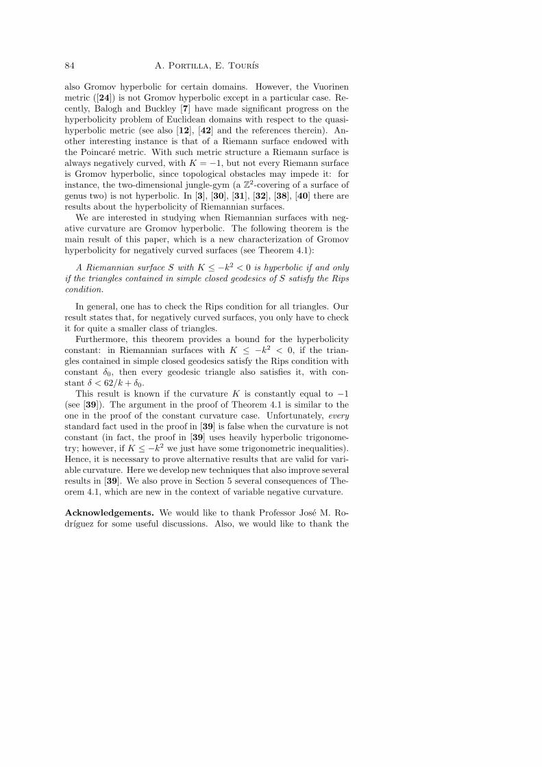
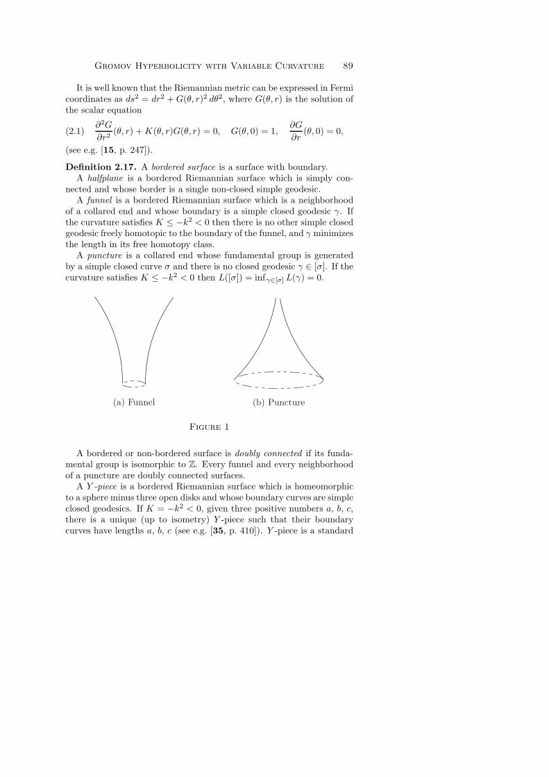
nected and whose border is a single non-closed simple geodesic.A funnel is a bordered Riemannian surface which is a neighborhood

of a collared end and whose boundary is a simple closed geodesic γ. Ifthe curvature satisfies K ≤ −k2 < 0 then there is no other simple closedgeodesic freely homotopic to the boundary of the funnel, and γ minimizesthe length in its free homotopy class.

A puncture is a collared end whose fundamental group is generatedby a simple closed curve σ and there is no closed geodesic γ ∈ [σ]. If thecurvature satisfies K ≤ −k2 < 0 then L([σ]) = infγ∈[σ] L(γ) = 0.

(a) Funnel (b) Puncture

Figure 1

A bordered or non-bordered surface is doubly connected if its funda-mental group is isomorphic to Z. Every funnel and every neighborhoodof a puncture are doubly connected surfaces.

A Y -piece is a bordered Riemannian surface which is homeomorphicto a sphere minus three open disks and whose boundary curves are simpleclosed geodesics. If K = −k2 < 0, given three positive numbers a, b, c,there is a unique (up to isometry) Y -piece such that their boundarycurves have lengths a, b, c (see e.g. [35, p. 410]). Y -piece is a standard


tool for constructing Riemannian surfaces with negative curvature. Aclear description of these Y -pieces and their use are given in [13, Chap-ter 1] and [15, Chapter X.3].

A generalized Y -piece is a Riemannian surface (with or without bound-ary) which is homeomorphic to a sphere without n open disks andm points, with integers n,m ≥ 0 such that n+m = 3, the n boundarycurves are simple closed geodesics and the m deleted points are punc-tures. Observe that a generalized Y -piece is topologically the union of aY -piece and m cylinders.

The following result assures that if K ≤ −k2 < 0, there always existsa closed geodesic in every free homotopy class, except for punctures, inwhich case it is impossible to have one.

Theorem 2.18 ([34, Theorem 3.7]). Let S be a complete Riemanniansurface with K ≤ −k2 < 0. Assume the boundary of S either is empty ora (finite or infinite) union of pairwise disjoint simple closed geodesics.Let α be a homotopically non-trivial closed curve in S. Then there existsa minimizing closed geodesic γ ∈ [α] if and only if LS([α]) > 0.

Remark 2.19. The conclusion of this theorem does not hold if we replacethe hypothesis K ≤ −k2 < 0 by the weaker one K < 0, as shown by therevolution surface of the graph of f(x) = 1 + ex around the horizontalaxis (with the standard metric induced by the Euclidean metric in R

3).

3. Technical lemmas

For the proof of Lemma 3.3 we will need to compare two functions G1

and G2 as in (2.1) corresponding to two different metrics. In order toachieve our objective, we prove now some technical lemmas:

Lemma 3.1. Let us consider the positive function G(θ, r) which is thesolution of the equation (2.1). If K ≤ −k2 < 0, then G(θ, r) ≥ coshkrfor every θ, r ∈ R.

Proof: According to the equation (2.1), and bearing in mind thatG(θ, r) > 0, we have that ∂2G/∂r2 = −KG ≥ k2 G > 0 for ev-ery θ, r ∈ R. This fact implies that ∂G/∂r is an increasing functionin r ∈ R for each fixed θ.


If r ≥ 0 then ∂G/∂r ≥ 0 and we can deduce

∂2G

∂r2(θ, r) ≥ k2G(θ, r),

∂2G

∂r2(θ, r)

∂G

∂r(θ, r) ≥ k2G(θ, r)

∂G

∂r(θ, r),

∂G

∂r(θ, r)2 − ∂G

∂r(θ, 0)2 ≥ k2

(G(θ, r)2 −G(θ, 0)2

),

∂G

∂r(θ, r)2 ≥ k2

(G(θ, r)2 − 1

),

∂G/∂r(θ, r)√G(θ, r)2 − 1

≥ k,

ArcoshG(θ, r) ≥ kr.

If r < 0 then ∂G/∂r < 0, and an argument similar to the above givesthe same inequality.

In both cases we have obtained the desired result: G(θ, r) ≥ coshkrfor every θ, r ∈ R.

Lemma 3.2. Let us consider R2 = {(θ, r) : θ, r ∈ R} with two dif-

ferent metrics given in Fermi coordinates as ds21 = dr2 + G1(θ, r)2 dθ2

and ds22 = dr2 +G2(θ, r)2 dθ2, such that their respective curvatures, K1

and K2, satisfy K1 ≤ K2 = −k2 < 0. Let us consider two curves σ1

and σ2 in R2 with the same endpoints, such that σi is a geodesic for dsi

(i = 1, 2). Then, Lds1(σ1) ≥ Lds2

(σ2).

Proof: Let us notice that G2(θ, r) := coshkr. By Lemma 3.1, we havethat G1 ≥ G2 for every (θ, r) ∈ R

2. Hence, if σ1(θ) = (θ, r(θ)) with θ ∈[a, b],

Lds1(σ1) =

∫

σ1

ds1 =

∫ b

a

√r′(θ)2 +G1(θ, r(θ))2 dθ

≥∫ b

a

√r′(θ)2 +G2(θ, r(θ))2 dθ = Lds2

(σ1) ≥ Lds2(σ2).

Lemma 3.3. Let us consider a simply connected locally geodesic quadri-lateral Q in a complete Riemannian surface S with curvature K ≤ −k2 <0, whose sides A, B, C and η have respective lengths a, b, c and l, andsuch that C meets orthogonally the sides A and B. Then there exists apositive constant λ := log(5 + 2

√6) such that a + b + c − λ/k ≤ l, for

every c ≥ λ/k.


Remark 3.4. Let us notice that we have that l ≤ a+b+c by the triangleinequality.

Proof: First of all, let us recall that any trigonometric formula withK = −1 involving lengths x1, . . . , xn holds for K = −k2 if we replacex1, . . . , xn by k x1, . . . , k xn, respectively.

We start the proof assuming that C an η are disjoint; then the quadri-lateral Q is the boundary of a simply connected open set. Using Fermicoordinates based on C, we represent C as the Euclidean segment join-ing (0, 0) and (c, 0), A as the Euclidean segment joining (0, 0) and (0, a),and B as the Euclidean segment joining (c, 0) and (c, b); the side η isthe geodesic joining (0, a) and (c, b). Now, let us consider a simplyconnected locally geodesic quadrilateral Q′ in a complete Riemanniansurface S with curvature K = −k2 < 0, whose sides A′, B′, C′ and η′

have respective lengths a, b, c and l′, and such that C′ meets orthog-onally the sides A′ and B′. Applying the same before construction,it is, using Fermi coordinates, based now on C′, we can represent C′

as the Euclidean segment joining (0, 0) and (c, 0), A′ as the Euclideansegment joining (0, 0) and (0, a), and B′ as the Euclidean segment join-ing (c, 0) and (c, b); the side η′ is the geodesic joining (0, a) and (c, b),with length l0. By Lemma 3.2, we know that LS(η) = l ≥ l0.

We are going to use the next hyperbolic trigonometry formula withconstant curvature K = −k2 < 0 (see [18, p. 88]) and the comparisonof lengths l ≥ l0:

coshkl ≥ coshkl0 = coshka coshkb coshkc− sinh ka sinh kb.

Using now the facts that, on the one hand, 2(cosh t−1)e−t = (1−e−t)2

and, on the other hand, for λ := log(5 + 2√

6) it is satisfied the equality18 (1 − e−λ)2 = e−λ, we have:

ekl ≥ coshkl ≥ cosh ka coshkb coshkc− sinh ka sinhkb

≥ (cosh kc− 1) coshka coshkb

=1

2(1 − e−kc)2ekc coshka coshkb

≥ 1

8(1 − e−kc)2ek(a+b+c)

≥ 1

8(1 − e−λ)2ek(a+b+c)

= e−λek(a+b+c),

for every c ≥ λ/k. Therefore l ≥ a+ b+ c− λ/k.


If C an η are not disjoint we use the hyperbolic trigonometry formulawith constant curvature K = −k2 < 0 (see [18, p. 88]) and, once again,Fermi coordinates and Lemma 3.2 give:

coshkl ≥ coshkl0 = coshka coshkb coshkc+ sinh ka sinh kb.

By a similar argument to the previous one:

ekl ≥ coshkl ≥ cosh ka coshkb coshkc+ sinh ka sinhkb

≥ coshkc coshka coshkb ≥ 1

8ek(a+b+c),

with no restriction about the length c.Notice that in this case we obtain a sharper inequality

a+ b+ c− (3 log 2)/k ≤ l.

Lemma 3.5. Let us consider a simply connected locally geodesic quadri-lateral Q in a complete Riemannian surface S with curvature K ≤ −k2 <0, with sides A, B, C and η, such that C meets orthogonally the sides Aand B, and LS(C) ≥ λ/k with λ := log(5 + 2

√6). We also assume that

η is a geodesic in S. If we define σ := A ∪C ∪B, then the curve σ is a(1, λ/k)-quasigeodesic with its arc-length parametrization.

Proof: Denoting by a, b, c and l the lengths of the sides A, B, C and ηrespectively, since σ : [0, a + b + c] −→ S is a continuous curve, it isclear that d(σ(t), σ(s)) ≤ LS(σ([t, s])) = |t− s| always. Without loss ofgenerality, from now on we are assuming that t < s.

We are going to prove that |t − s| ≤ d(σ(t), σ(s)) + λ/k. In order toprove it, let us assume that it is false, and let us seek a contradiction.Suppose then that |t− s| > d(σ(t), σ(s)) + λ/k and define a curve σ0 asthe union of the next three curves: σ([0, t]), a geodesic connecting σ(t)with σ(s), and σ([s, a+ b+ c]). Let us denote by u, v the endpoints of σ(notice that they are also the endpoints of the geodesic η); since σ0 is acontinuous curve connecting u and v, we have that, applying Lemma 3.3,

d(u, v) = LS(η) = l ≤ LS(σ0) = LS(σ) − LS(σ([t, s])) + d(σ(t), σ(s))

= LS(σ) − |t− s| + d(σ(t), σ(s))

< LS(σ) − λ/k = a+ b+ c− λ/k ≤ l = d(u, v),

which is a contradiction. Therefore we can assert that

|t−s|−λ/k ≤ d(σ(t), σ(s)) ≤ |t−s|, for every 0 ≤ t, s ≤ a+b+c.


Lemma 3.6. Given a complete Riemannian surface S, let us considera continuous curve g joining u, v ∈ S. If LS(g) ≤ α, then g is a (1, α)-quasigeodesic with its arc-length parametrization.

Proof: Let g : [0, l] −→ S with its arc-length parametrization. Since g iscontinuous, it is clear that d(g(t), g(s)) ≤ LS(g([t, s])) = |t− s|. Let usnotice now |t− s| ≤ LS(g) ≤ α ≤ d(g(t), g(s)) + α.

Therefore, we can assert that

|t− s| − α ≤ d(g(t), g(s)) ≤ |t− s|, for every 0 ≤ t, s ≤ l.

Lemma 3.7. Let S be a complete Riemannian surface with K ≤ −k2 <0, δ1 := 1

klog(1 +

√2 ) and let Q be a simply connected locally geodesic

quadrilateral in S. Assume the sides, A, B, C and η of Q satisfy thefollowing two conditions: (i) LS(C) > 4δ1, (ii) C meets orthogonally thesides A and B.

Then, we have that d(z, η) ≤ 4δ1 for every z ∈ C.

Proof: To start, note that the sides C and η might meet or might not(but if they do, it must be in a single point). However we use an argumentwhich covers both cases.

Without loss of generality we can assume that S is simply connected,since otherwise we can lift Q to the universal covering of S (recall thatQ is simply connected and that the distances in the universal cover aregreater than in the surface). Consequently, Q is a geodesic quadrilateral(in a simply connected Riemannian surface with K ≤ −k2, every localgeodesic is, in fact, a geodesic).

Since S is a simply connected and complete Rimannian surface, it isδ1-thin (see [6, p. 130] and [20, p. 52]).

Let us consider the geodesic C as an oriented curve joining A and B.By hypothesis LS(C) > 4δ1; therefore we can assert that there existtwo points α and β (with α < β) in the oriented geodesic C defined asα := max{z ∈ C : d(z,A) ≤ 2δ1}, and β := min{z ∈ C : d(z,B) ≤ 2δ1}.

Since Q is 2δ1-thin, d(z,A ∪ B ∪ η) ≤ 2δ1 for every z ∈ C. If z ∈(α, β) ⊂ C then d(z,A ∪ B) > 2δ1 and, therefore, d(z,A ∪ B ∪ η) =d(z, η) ≤ 2δ1; consequently, d(z, η) ≤ 2δ1 for every z ∈ [α, β]. If z ∈ C \[α, β] it is verified that d(z, [α, β]) ≤ 2δ1 and, therefore, d(z, η) ≤ 4δ1.

Definition 3.8. Let λ be the constant in Lemma 3.3 and S a completeRiemannian surface with K ≤ −k2 < 0. A λ-triangle in S is defined tobe a triangle with continuous injective (1, λ/k)-quasigeodesic sides withits arc-length parametrization.


Lemma 3.9. Let us consider a complete Riemannian surface S withK ≤ −k2 < 0, a simple closed geodesic γ with length l and a λ-triangle Tcontained in γ and homotopic to γ. Then, every side of T has lengthless than or equal to l

2 + λk. Furthermore, at least two of the sides of T

have length greater than or equal to l4 − λ

2k.

Proof: If T := {a, b, c}, let us denote by l1 := LS([a, b]), l2 := LS([b, c])and l3 := LS([a, c]).

Seeking for a contradiction, let us assume that one side of T , forexample [a, c], is “long”, i.e. l3 > l/2 + λ/k. However [a, c] is, as aside of T , a (1, λ/k)-quasigeodesic with its arc-length parametrizationσ3 : [0, l3] −→ γ. Then, l3 − λ/k ≤ d(a, c) ≤ l3 + λ/k.

But d(a, c) ≤ l/2 since a and c belong to a closed curve with length l.Therefore, l3 − λ/k ≤ d(a, c) ≤ l/2, which implies that l3 ≤ l/2 + λ/kand this fact contradicts the assumption about l3 being “long”.

Finally, we prove the last part of the lemma. Seeking again for acontradiction, let us assume that two sides, for example [a, b] and [b, c],are “short”, that is, l1, l2 < l/4 − λ/(2k). Then l3 > l/2 + λ/k, sincel = l1 + l2 + l3, which is, in fact, a contradiction.

Lemma 3.10. Let us consider a doubly connected complete Riemanniansurface S with curvature K ≤ −k2 < 0, and let l be the length of thesimple closed geodesic γ in it. Then S is (18δ1 + 2l)-thin, with δ1 :=

log(1 +√

2)/k.

Remark 3.11. According to the above lemma, every geodesically convexsubset of a surface like the one described in it, is (18δ1 +2l)-thin as well.Further, every funnel F in a Riemannian surface with K ≤ −k2 < 0 andLS(∂F ) = l is (18δ1 + 2l)-thin.

Proof: Let us consider a geodesic triangle T = {a, b, c} in S. By Lem-ma 2.11 we can assume that T is a simple closed curve. Notice thatT is homotopic to either to a point or the simple closed geodesic γ. IfT is homotopic to a point, then it is the boundary of a simply connectedclosed set E, and consequently E, with its intrinsic distance, is isometric

to some subset of the universal covering surface S; this implies that T is

δ1-thin (recall that S is δ1-thin). Therefore, to finish the proof we mayassume that T is homotopic to the simple closed geodesic γ of S.

In this case, there are two possible situations:

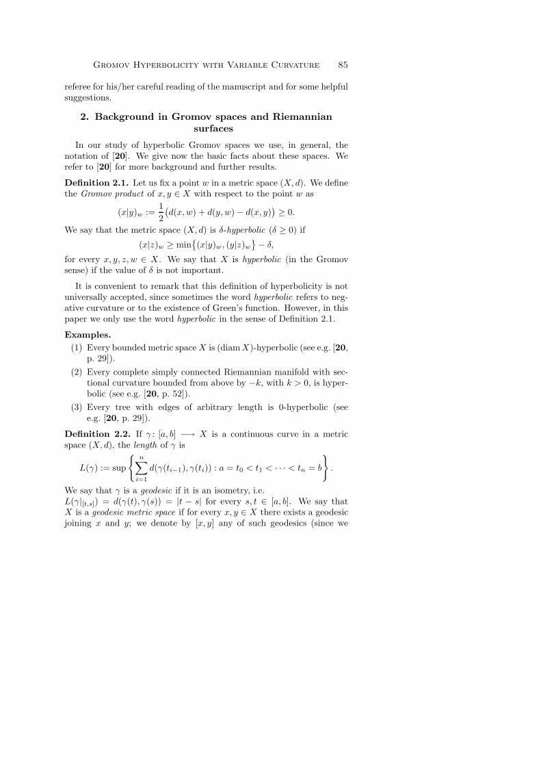
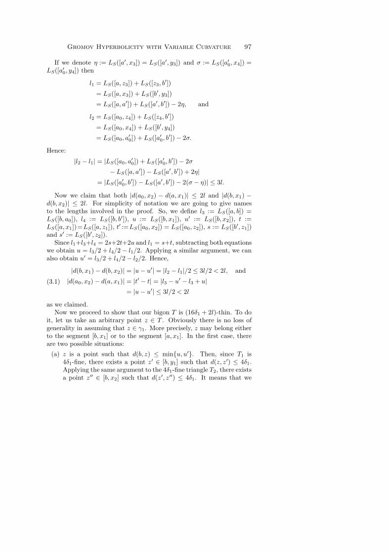
(1) Two of the vertices of the triangle coincide. Then T is a geodesicbigon whose two sides are two geodesics γ1 and γ2 with the same length.Now, we have Figure 2 (drawn in the universal covering surface). In


it, the vertices a and a0 must be considered as coincident, but we havemaintained both names to be able to identify clearly γ1 with [a, b] and γ2

with [b, a0]. Let us call a′, b′ and a′0 their respective projections over γ(where [a′, b′] is the projection of γ1 over γ and [b′, a′0] is the projectionof γ2 over γ; although all the projections are obviously orthogonal, inthe Figure 2 we have not used right angles to emphasize that the lengthsof the segments [a′, b′] and [b′, a′0] might be very different, since thecurvature is not constant).

a

b

a0 (= a)

a′b′ a′

0

x1 x2

y1

y2

z1 z2

x3

x4

y3 y4

z3

z4

η σ

t t′

ση

u u′

t′t

Figure 2. T is a geodesic bigon.

Let us draw now the geodesics [a, b′] and [a0, b′] and let l1 and l2 be

their respective lengths. Next, we are going to prove that |l1−l2| ≤ 3l. Inorder to do it, we need to consider the following four geodesic triangles:T1 = {a, b, b′} (with internal points x1, y1, z1), T2 = {b, a0, b

′} (withinternal points x2, y2, z2), T3 = {a, a′, b′} (with internal points x3, y3, z3)and T4 = {a0, a

′0, b

′} (with internal points x4, y4, z4). Notice that T1,T2, T3 and T4 are, all of them, 4δ1-fine, because they are homotopicallytrivial and then their lifts to the universal covering surface are 4δ1-fine.


If we denote η := LS([a′, x3]) = LS([a′, y3]) and σ := LS([a′0, x4]) =LS([a′0, y4]) then

l1 = LS([a, z3]) + LS([z3, b′])

= LS([a, x3]) + LS([b′, y3])

= LS([a, a′]) + LS([a′, b′]) − 2η, and

l2 = LS([a0, z4]) + LS([z4, b′])

= LS([a0, x4]) + LS([b′, y4])

= LS([a0, a′0]) + LS([a′0, b

′]) − 2σ.

Hence:

|l2 − l1| = |LS([a0, a′0]) + LS([a′0, b

′]) − 2σ

− LS([a, a′]) − LS([a′, b′]) + 2η|= |LS([a′0, b

′]) − LS([a′, b′]) − 2(σ − η)| ≤ 3l.

Now we claim that both |d(a0, x2) − d(a, x1)| ≤ 2l and |d(b, x1) −d(b, x2)| ≤ 2l. For simplicity of notation we are going to give namesto the lengths involved in the proof. So, we define l3 := LS([a, b]) =LS([b, a0]), l4 := LS([b, b′]), u := LS([b, x1]), u

′ := LS([b, x2]), t :=LS([a, x1])=LS([a, z1]), t

′ :=LS([a0, x2]) = LS([a0, z2]), s := LS([b′, z1])and s′ := LS([b′, z2]).

Since l1+l3+l4 = 2s+2t+2u and l1 = s+t, subtracting both equationswe obtain u = l3/2 + l4/2 − l1/2. Applying a similar argument, we canalso obtain u′ = l3/2 + l4/2 − l2/2. Hence,

(3.1)

|d(b, x1) − d(b, x2)| = |u− u′| = |l2 − l1|/2 ≤ 3l/2 < 2l, and

|d(a0, x2) − d(a, x1)| = |t′ − t| = |l3 − u′ − l3 + u|= |u− u′| ≤ 3l/2 < 2l

as we claimed.Now we proceed to show that our bigon T is (16δ1 + 2l)-thin. To do

it, let us take an arbitrary point z ∈ T . Obviously there is no loss ofgenerality in assuming that z ∈ γ1. More precisely, z may belong eitherto the segment [b, x1] or to the segment [a, x1]. In the first case, thereare two possible situations:

(a) z is a point such that d(b, z) ≤ min{u, u′}. Then, since T1 is4δ1-fine, there exists a point z′ ∈ [b, y1] such that d(z, z′) ≤ 4δ1.Applying the same argument to the 4δ1-fine triangle T2, there existsa point z′′ ∈ [b, x2] such that d(z′, z′′) ≤ 4δ1. It means that we


have been able to find a point z′′ ∈ γ2 verifying that d(z, z′′) ≤d(z, z′) + d(z′, z′′) ≤ 8δ1.

(b) z is a point such that d(b, z) > min{u, u′}. If this is so, the firstthing to do is getting another point z0 ∈ [b, x1] such that d(b, z0) ≤min{u, u′} and then apply the previous case to that z0. Notice that,as |u − u′| ≤ 2l by (3.1), z0 can be found easily by moving to theright at most a distance 2l along γ1 starting at x1. Then, by thearguments used before, we are able to find a point z′′ ∈ γ2 suchthat d(z, z′′) ≤ d(z, z0) + d(z0, z

′) + d(z′, z′′) ≤ 2l+ 8δ1.

Now, if z ∈ [a, x1] we repeat the same arguments but taking intoaccount that besides T1 and T2, the triangles T3 and T4 are 4δ1-fine aswell (recall that by (3.1) we also have |t′− t| ≤ 2l). Hence, we know thatthere exists a point z′′ ∈ γ2 such that d(z, z′′) ≤ 16δ1 +2l, which impliesour conclusion.

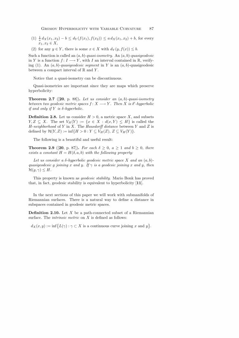
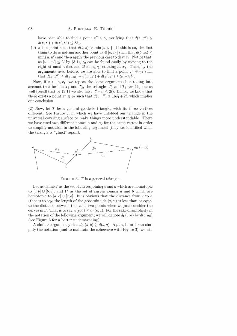
(2) Now, let T be a general geodesic triangle, with its three verticesdifferent. See Figure 3, in which we have unfolded our triangle in theuniversal covering surface to make things more understandable. Therewe have used two different names a and a0 for the same vertex in orderto simplify notation in the following argument (they are identified whenthe triangle is “glued” again).

a

b

c

a0 (= a)b′

σ1

σ2T1

T2

Figure 3. T is a general triangle.

Let us define Γ as the set of curves joining c and a which are homotopicto [c, b] ∪ [b, a], and Γ′ as the set of curves joining a and b which arehomotopic to [a, c] ∪ [c, b]. It is obvious that the distance from c to a(that is to say, the length of the geodesic side [a, c]) is less than or equalto the distance between the same two points when we just consider thecurves in Γ. That is to say, d(c, a) ≤ dΓ(c, a). For the sake of simplicity inthe notation of the following argument, we will denote dΓ(c, a) by d(c, a0)(see Figure 3 for a better understanding).

A similar argument yields dΓ′(a, b) ≥ d(b, a). Again, in order to sim-plify the notation (and to maintain the coherence with Figure 3), we will


denote dΓ′(a, b) simply by d(a, b), and we will refer to the length of thegeodesic side [b, a] as d(b, a0).

Let us define now a function f(x) := d(x, a) − d(x, a0). Since f(c) =d(c, a)−d(c, a0) ≤ 0 and f(b) = d(b, a)−d(b, a0) ≥ 0, it means that theremust exist a point b′ ∈ [b, c] such that f(b′) = d(b′, a) − d(b′, a0) = 0.

Notice that there are two non-homotopic geodesics joining the vertex awith the point b′. Let σ1 be the geodesic homotopic to [a, c]∪[c, b′]; σ2 thegeodesic homotopic to [b′, b] ∪ [b, a0]. Then σ1 ∪ σ2 is a geodesic bigonwhose sides have the same length. If we apply the previous case to thisbigon, we can state that it is (16δ1 + 2l)-thin.

Next, let us consider the two simply connected triangles T1 = [a, c] ∪[b′, c] ∪ σ1 and T2 = [a0, b] ∪ [b, b′] ∪ σ2, both of them δ1-thin. So, givenany point z ∈ [a, c], there exists a point z′ ∈ [b′, c]∪σ1 with d(z, z′) ≤ δ1.If z′ ∈ [b′, c] ⊂ [b, c] we have finished the proof, and we conclude thatd(z,A) ≤ δ1. If z′ ∈ σ1, we know that there exists a point z′′ ∈ σ2

such that d(z′, z′′) ≤ 16δ1 + 2l since the bigon σ1 ∪ σ2 is (16δ1 + 2l)-thin. Hence, d(z, σ2) ≤ 17δ1 + 2l; since T2 is also δ1-thin, it means thatd(z,A) ≤ 18δ1 + 2l, and therefore our general triangle T is (18δ1 + 2l)-thin, which finishes the proof.

Corollary 3.12. Let us consider a doubly connected complete Riemann-ian surface S with no simple closed geodesic, and with curvature K ≤−k2 < 0. Then S is 18δ1-thin, with δ1 := log(1 +

√2)/k.

Remark 3.13. According to the above corollary, every geodesically con-vex subset of a surface like the one described in it, is 18δ1-thin as well.

Proof: As the proof is almost identical to that of Lemma 3.10, we willjust explain the only difference. Let us consider a geodesic bigon T ={a, b} as in the proof of Lemma 3.10. Since there is no simple closedgeodesic in S homotopic to T , and the curvature K is strictly negative,there exist non-trivial closed curves with arbitrarily small length whichare homotopic to T . For any fixed ε > 0 let us choose one of theseclosed curves with length smaller than ε and let us call it σ0. Then, wecan repeat the same construction used in the proof of Lemma 3.10 forgeodesic bigons, but projecting the vertices a and b of T over σ0 ratherthan over a simple closed geodesic (which does not exist in our situation).Let us call a′ and b′ the respective projections of a and b over σ0. It isclear that there exist two non-homotopic geodesic segments σ1 and σ2

joining a′ and b′. We choose now σ = σ1 ∪ σ2. Then we can repeatthe same arguments used in the proof of Lemma 3.10 replacing [a′, b′]


and [b′, a′0] by σ1 and σ2, and conclude that the bigon T is (16δ1 + 2ε)-thin.

Applying this result to a general geodesic triangle T as in the proofof Lemma 3.10, we can conclude that T is (18δ1 + 2ε)-thin.

Since ε can be arbitrarily small, a passage to the limit (making ε→ 0)implies that our general triangle is also 18δ1-thin.

4. The main result

Theorem 4.1. Let S be a complete Riemannian surface with K ≤−k2 < 0 (with or without boundary); if S has boundary, we also re-quire that ∂S is the union of local geodesics (closed or non-closed). Let

λ := log(5 + 2√

6); then S is δ-hyperbolic if and only if every λ-trianglecontained in a simple closed geodesic of S is δ0-thin.

More precisely, if S is δ-thin, then every λ-triangle contained in asimple closed geodesic in S is δ0-thin with δ0 = δ + 2H, where H =H(4δ, 1, λ/k) is the constant in Theorem 2.9; and if every λ-trianglecontained in a simple closed geodesic in S is δ0-thin then S is δ-thin,with δ := max{18δ1 + 20λ/k, 12δ1 + δ0} and δ1 := 1

klog(1 +

√2).

Remark 4.2. Let us notice that, as log(1 +√

2) ≈ 0.8814 and λ :=

log(5 + 2√

6) ≈ 2.2924, the hyperbolicity constant δ can be bounded inthe following way: δ ≤ δ0 + 18δ1 + 20λ/k < δ0 + 62/k

Proof: Let us assume first that S is δ-hyperbolic and let us check thatevery λ-triangle contained in a simple closed geodesic of S is δ0-thin,with δ0 = δ + 2H . Let T be a λ-triangle with sides g1, g2, g3, con-tained in a simple closed geodesic γ. Theorem 2.9 implies that for everyquasigeodesic side gi there exists a geodesic γi with the same endpointsas gi, such that H(gi, γi) ≤ H = H(4δ, 1, λ/k). We have to prove thatthe distance from any point in a side of T to the union of the other twosides is bounded from above by δ0. Without loss of generality let usassume that z ∈ g1. Hence, for every z ∈ g1, there is a point z0 ∈ γ1

with d(z, z0) ≤ H . Since S is δ-thin, we can find z′0 ∈ γ2 ∪ γ3 withd(z0, z

′0) ≤ δ. Finally, we also have a point z′ ∈ g2∪g3 with d(z′, z′0) ≤ H .

Consequently d(z, g2 ∪ g3) ≤ d(z, z′) ≤ δ + 2H .

Now, let us assume that every λ-triangle contained in a simple closedgeodesic of S is δ0-thin and let us prove that S is δ-hyperbolic.

First, notice that if S has boundary, the hypothesis implies that∂S is the union of pairwise disjoint simple local geodesics (closed or non-closed). In this case, we can construct a complete Riemannian surface Rwithout boundary and with K ≤ −k2 by pasting to S a cylinder along


each simple closed geodesic, and a halfplane in each non-closed simplegeodesic. If γ0 ⊆ ∂S is a closed geodesic with length l, we can considerthe Fermi coordinates based on γ0. The Riemannian metric can be ex-pressed in Fermi coordinates as ds2 = dr2 + G(θ, r)2 dθ2, with G(θ, r)satisfying (2.1), where the function K(θ, r) is C∞ in R × (−∞, 0] andl-periodic in θ; actually, K(θ, r) ∈ C∞(R × (−∞, 3ε)), for some ε > 0.Let ψ(r) ∈ C∞(R) be a function satisfying

ψ(r) =

{1, r ≤ ε,

0, r ≥ 2ε,

and 0 ≤ ψ(r) ≤ 1. We define K(θ, r) := K(θ, r)ψ(r)− (1−ψ(r))k2 ; then

K(θ, r) = K(θ, r) in R × (−∞, ε] and K(θ, r) = −k2 in R × [2ε,∞).

Therefore, K(θ, r) is C∞ in R × R, l-periodic in θ and K ≤ −k2.

Now we consider the function G(θ, r) associated to K(θ, r) and satis-fying (2.1). This allows to attach a cylinder to S along each simpleclosed geodesic γ0 ⊆ ∂S. If γ0 ⊆ ∂S is a non-closed geodesic we can ap-ply a similar argument to the previous one. We must consider anotherfunction ψ(θ, r) depending on θ and r since, in this case, G need not beperiodic, and then K(θ, r) ∈ C∞(R × (−∞, 3 ε(θ))), for some positivefunction ε(θ). This allows to attach a halfplane to S along each simplenon-closed geodesic γ0 ⊆ ∂S.

In any case we get a complete Riemannian surface R containing S andwith curvature less than or equal to −k2. Since S is geodesically convexin R (every geodesic connecting two points of S is contained in S), thendR(z, w) = dS(z, w) for every z, w ∈ S, and any simple closed geodesicin R is contained in S. Therefore, it is sufficient to prove the theoremfor surfaces without boundary.

Since the universal covering map, ∂ : S −→ S is a local isometry, theuniversal covering S (which is a simply connected and complete surfacesatisfying that K ≤ −k2) is δ1-thin (see [6, p. 130] and [20, p. 52]).

Now, let us consider a geodesic triangle T = {a, b, c} in S. ByLemma 2.11, we can assume that T is a simple closed curve. Thereare three possibilities: T is homotopic to a point, T is homotopic to apuncture, or T is freely homotopic to a simple closed geodesic in S.

If T is homotopic to a point, then it is the boundary of a simplyconnected closed set E, and consequently E, with its intrinsic distance,is isometric to some geodesically convex subset of S; this implies thatT is δ1-thin (recall that S is δ1-thin).

If T is homotopic to a puncture, then it is the boundary of a closeddoubly connected set, which is, with its intrinsic distance, isometric to


some geodesically convex subset of a doubly connected surface verifyingthe hypothesis in Corollary 3.12. This implies that T is 18δ1-thin.

Otherwise, T = {a, b, c} is freely homotopic to a simple closed geo-desic γ in S.

We are going to deal with two cases.

If LS(γ) ≤ 10λ/k, we consider a doubly connected complete Riemann-ian surface, S0, with K ≤ −k2 < 0 containing a simple closed geodesic γof length l, such that the closed set in S bounded by T and γ is, withits intrinsic distance, isometric to a subset in S0, bounded by γ and atriangle T0. We know that S0 is 18δ1 + 2l-thin by Lemma 3.10. Thesefacts imply that T is (18δ1 + 20λ/k)-thin.

We consider now the case LS(γ) > 10λ/k.The main idea of the proof is to project the three vertices of T onto

the simple closed geodesic γ to obtain a new triangle T ′ ⊆ γ. We willcheck that T ′ is a λ-triangle and hence it is δ0-thin by hypothesis.

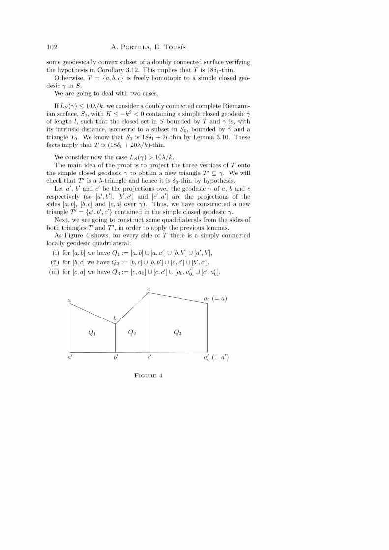
Let a′, b′ and c′ be the projections over the geodesic γ of a, b and crespectively (so [a′, b′], [b′, c′] and [c′, a′] are the projections of thesides [a, b], [b, c] and [c, a] over γ). Thus, we have constructed a newtriangle T ′ = {a′, b′, c′} contained in the simple closed geodesic γ.

Next, we are going to construct some quadrilaterals from the sides ofboth triangles T and T ′, in order to apply the previous lemmas.

As Figure 4 shows, for every side of T there is a simply connectedlocally geodesic quadrilateral:

(i) for [a, b] we have Q1 := [a, b] ∪ [a, a′] ∪ [b, b′] ∪ [a′, b′],

(ii) for [b, c] we have Q2 := [b, c] ∪ [b, b′] ∪ [c, c′] ∪ [b′, c′],

(iii) for [c, a] we have Q3 := [c, a0] ∪ [c, c′] ∪ [a0, a′0] ∪ [c′, a′0].

a

b

c

a0 (= a)

a′ b′ c′ a′

0(= a′)

Q1 Q2 Q3

Figure 4


In the figure we have unfolded again our triangle in the universal cov-ering surface to make things more understandable, and we have used twodifferent names, a and a0, for the same vertex for the sake of simplicityin notation in the following argument. They are identified when the tri-angle is “glued” again (similarly for a′ and a′0 of γ). Every Qi, 1 ≤ i ≤ 3is 2δ1-thin (its lift in the universal cover is a geodesic quadrilateral).

We claim that T ′ = {a′, b′, c′} is a λ-triangle. Let us check it just forone side, for example [a′, b′] ∈ Q1:

(1) If LS([a′, b′]) > λ/k then, by Lemma 3.5, [a, a′] ∪ [b, b′] ∪ [a′, b′]is a (1, λ/k)-quasigeodesic, so [a′, b′] ⊂ γ is also a (1, λ/k)-quasi-geodesic.

(2) If LS([a′, b′]) ≤ λ/k then, by Lemma 3.6, the side [a′, b′] ⊂ γ is a(1, λ/k)-quasigeodesic.

It follows that, on the one hand, T ′ is δ0-thin (by hypothesis) and, onthe other hand, the lengths of at least two sides of T ′ are greater than orequal to l/4−λ/(2k) (by Lemma 3.9). In our current case, as l > 10λ/k,it is easy to check that, actually, these lengths are greater than 2λ/k.Besides, note that:

(4.1)l

4− λ

2k>

2λ

k=

2 log(5 + 2√

6)

k>

2 log 9

k

=4 log 3

k>

4 log(1 +√

2)

k= 4δ1.

This means that, at least two sides have length strictly greaterthan 4δ1.

Let z be a point of one of the sides of T and σ the union of theother two sides; we are going to prove that d(z, σ) ≤ 12δ1 + δ0. Withoutloss of generality we can assume that z ∈ [a, b], and then there existsz0 ∈ [a, a′] ∪ [b, b′] ∪ [a′, b′] with d(z, z0) ≤ 2δ1, since Q1 is 2δ1-thin.

If z0 ∈ [a′, b′], since the triangle T ′ is δ0-thin, there exists z′0 ∈ [b′, c′]∪[c′, a′0] with d(z0, z

′0) ≤ δ0. There is no loss of generality in assuming that

z′0 ∈ [b′, c′]. There are two possibilities:

(1) If LS([b′, c′]) > 4δ1, applying Lemma 3.7 we have that d(z′0, [b, c]) ≤4δ1. Therefore d(z, σ) ≤ 6δ1 + δ0.

(2) If LS([b′, c′]) ≤ 4δ1, then d(z′0, c′) ≤ 4δ1. Note that LS([c′, a′0]) >

4δ1 by (4.1) and by Lemma 3.7, d(c′, [c, a0]) ≤ 4δ1. Therefored(z, σ) ≤ 10δ1 + δ0.


If z0 ∈ [a, a′] ∪ [b, b′], without loss of generality we can assume thatz0 ∈ [b, b′] ∈ Q2. Since Q2 is 2δ1-thin, once again, there exists z′0 ∈[b, c]∪ [c, c′]∪ [b′, c′] with d(z0, z

′0) ≤ 2δ1. If z′0 ∈ [b, c] then d(z, σ) ≤ 4δ1

and we are done. If z′0 ∈ [b′, c′] ∪ [c, c′], then there are two possibilities:

(1) If LS([b′, c′]) > 4δ1, then we can choose z′0 with z′0 ∈ [b′, c′]: this is

because we can lift Q2 to the universal covering S, obtaining in it anew geodesically convex quadrilateral (let us use the same notation

for the points in S), hence dS([b, b′], [c, c′]) = LS([b′, c′]) > 4δ1. The

new geodesic quadrilateral in S is 2δ1-thin as well, so we can takea point z′0 ∈ [b′, c′] ⊂ S such that d(z0, z

′0) ≤ dS(z0, z

′0) ≤ 2δ1.

Applying now Lemma 3.7 we have that d(z′0, [b, c]) ≤ 4δ1, andtherefore d(z, σ) ≤ 8δ1.

(2) If LS([b′, c′]) ≤ 4δ1, there are two possible situations: either z′0 ∈[b′, c′] or z′0 ∈ [c, c′].

In the first case, dS(z′0, c′) ≤ 4δ1 and, since LS([c′, a′0]) > 4δ1

(by (4.1)), applying Lemma 3.7 we have that d(c′, [c, a0]) ≤ 4δ1;thus d(z, σ) ≤ 12δ1.

In the second case, when z′0 ∈ [c, c′], notice that now we are inthe quadrilateral Q3 where L[c′, a′0] > 4δ1, and repeating the samearguments we obtain d(z, σ) ≤ 12δ1.

Hence, S is δ-thin, with δ := max{18δ1 + 20λ/k, 12δ1 + δ0}.

One might think that the λ-triangle T ′ contained in the simple closedgeodesic is geodesic; however, the following example shows that T ′ in theproof of Theorem 4.1 does not need to be geodesic, even in the constantcurvature case.

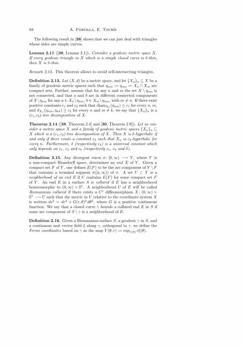
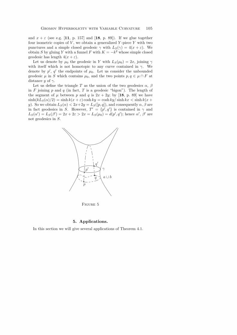
Example. There is a geodesic triangle T in a complete Riemanniansurface S with constant curvature K = −k2 < 0, such that the corre-sponding T ′ is not geodesic. That is, at least one of the sides of T ′ isnot geodesic (see Figure 5).

Given x0 > 0 satisfying kx0 < Arcsinh 1, let us fix y > 0 withsinhk(x0 + y) > coshky. Then sinh k(x + y) > cosh ky for any x satis-fying kx0 ≤ kx < Arcsinh 1, and consequently we can choose x > 0 suchthat kx < Arcsinh 1 and sinhkx sinh k(x+ y) > coshky.

Let ε := 1k

Arcsinh(1/ sinhkx) − x > 0, then sinh kx sinh k(x + ε) =1. Let us consider a geodesic quadrilateral V in the Cartan-Hadamardsurface Hk with constant curvature K = −k2, with three right anglesand an angle equal to zero, such that the two finite sides have length x


and x + ε (see e.g. [11, p. 157] and [18, p. 89]). If we glue togetherfour isometric copies of V , we obtain a generalized Y -piece Y with twopunctures and a simple closed geodesic γ with LS(γ) = 4(x + ε). Weobtain S by gluing Y with a funnel F with K = −k2 whose simple closedgeodesic has length 4(x+ ε).

Let us denote by µ0 the geodesic in Y with LS(µ0) = 2x, joining γwith itself which is not homotopic to any curve contained in γ. Wedenote by p′, q′ the endpoints of µ0. Let us consider the unboundedgeodesic µ in S which contains µ0, and the two points p, q ∈ µ ∩ F atdistance y of γ.

Let us define the triangle T as the union of the two geodesics α, βin F joining p and q (in fact, T is a geodesic “bigon”). The length ofthe segment of µ between p and q is 2x + 2y; by [18, p. 89] we havesinh(kLS(α)/2) = sinhk(x + ε) coshky = coshky/ sinhkx < sinh k(x +y). So we obtain LS(α) < 2x+2y = LS([p, q]), and consequently α, β arein fact geodesics in S. However, T ′ = {p′, q′} is contained in γ andLS(α′) = LS(β′) = 2x+ 2ε > 2x = LS(µ0) = d(p′, q′); hence α′, β′ arenot geodesics in S.

p

q

p′q′

a ∪ b

γ

Figure 5

5. Applications.

In this section we will give several applications of Theorem 4.1.


Definition 5.1. We say that a complete Riemannian surface S (withor without boundary) is of finite type if its fundamental group is finitelygenerated.

Corollary 5.2. Let us consider a complete Riemannian surface S (withor without boundary) with K ≤ −k2 < 0; if S has boundary, we alsorequire that ∂S is the union of local geodesics (closed or non-closed). IfS is of finite type, then it is hyperbolic. More precisely, if S is of finitetype and every simple closed geodesic γ in S verifies LS(γ) ≤ l, thenS is δ-thin, with δ = max

{18δ1 + 20λ/k, 12δ1 + l/4 + λ/(2k)

}, where

δ1 := 1k

log(1 +√

2) and λ := log(5 + 2√

6).

Proof: Since the number of simple closed geodesics in S which are ho-motopic to a geodesic triangle is finite, {γ1, . . . , γk}, we have LS(γj) ≤ lfor every j = 1, . . . , k. Every continuous injective (1, λ/k)-quasigeodesicwith its arc-length parametrization g ⊂ γj verifies LS(g) ≤ l/2 + λ/kby Lemma 3.9; hence d(z, ∂g) ≤ l/4 + λ/(2k) for every z ∈ g. Thenthe hypothesis of Theorem 4.1 is verified with δ0 := l/4 + λ/(2k).Hence S is δ-thin with δ = max

{18δ1 + 20λ/k, 12δ1 + l/4 + λ/(2k)

}≤

18δ1 + 20λ/k + l/4.

A consequence of this corollary is the following result.

Corollary 5.3. Every generalized Y -piece S with LS(γi) ≤ l, whereγi (i = 1, 2, 3) are the simple closed geodesics in ∂S, is δ-thin, with

δ = max{18δ1 + 20λ/k, 12δ1 + l/4 + λ/(2k)

}, where δ1 := 1

klog(1 +

√2)

and λ := log(5 + 2√

6).

Remark 5.4. As usual, we view a puncture as a simple closed geodesicwith length equal to zero.

It is clear that a funnel contains infinitely many halfplanes.

Two additional results can be deduced from Theorem 4.1. The firstone (see Theorem 5.5 below) allows us to simplify the topology of asurface in order to study its hyperbolicity: it assures that deleting fun-nels and halfplanes does not change the hyperbolicity of a Riemanniansurface.

Theorem 5.5. Let us consider a complete Riemannian surface S (withor without boundary); if S has boundary, we also require that ∂S is theunion of local geodesics (closed or non-closed). Let us denote by F theunion of some pairwise disjoint funnels and halfplanes of S. Let S0 bethe bordered complete Riemannian surface obtained by deleting from Sthe interior of F . Then S is hyperbolic if and only if S0 is hyperbolic.


More precisely, if S is δ-thin (respectively, δ-hyperbolic) then S0 isδ-thin (respectively, δ-hyperbolic); and if S0 is δ′-hyperbolic, then S isδ-thin, with δ = max{18δ1 + 20λ/k, 12δ1 + 4δ′ + 2H(δ′, 1, λ/k)} where

δ1 := 1k

log(1 +√

2), λ := log(5 + 2√

6) and H is the constant in Theo-rem 2.9.

Remark 5.6. We want to emphasize that in Theorem 5.5 there is nohypothesis about the length of the boundary curves of the funnels (thisis not the case in Corollaries 5.2 and 5.3). This is an important fact sincethere are complete hyperbolic Riemannian surfaces containing funnels Fn

with LS(∂Fn) −→ ∞ as n→ ∞.

Proof: Let us assume that S is δ-thin (respectively, δ-hyperbolic). AsS0 is geodesically convex in S (every geodesic connecting two points of S0

is contained in S0), we have d(z, w) = dS0(z, w) for every z, w ∈ S0.

Therefore S0 is also δ-thin (respectively, δ-hyperbolic).Let us assume now that S0 is δ′-hyperbolic. By [39, Lemma 3.3] (or

the first part of the proof of Theorem 4.1), every λ-triangle T in S0 is(δ′ + 2H(δ′, 1, λ/k))-thin, where H is the constant in Theorem 2.9. Letus observe that any simple closed geodesic in S is contained in S0. Sinced(z, w) = dS0

(z, w) for every z, w ∈ S0, every λ-triangle in S (containedin a simple closed geodesic in S) is also a λ-triangle in S0. Let us observe

also that H ≥ 1 > log(1 +√

2 ). Then Theorem 4.1 implies that S isδ-thin, with δ = max{18δ1 + 20λ/k, 12δ1 + 4δ′ + 2H(δ′, 1, λ/k)}.

Many Riemannian surfaces can be decomposed as a union of funnelsand generalized Y -pieces (see [4] and [34, Theorem 4.1]). The followingresult uses this decomposition in order to obtain hyperbolicity.

Theorem 5.7. Let us consider a complete Riemannian surface S with−k2

1 ≤ K ≤ −k22 < 0 (with or without boundary), with genus equal to

zero. If there is a decomposition of S as a union of funnels {Fm}m∈M

and generalized Y -pieces {Yn}n∈N with LS(γ) ≤ l for every simple closedgeodesic γ ⊂ (∪n∂Yn) ∪ (∪m∂Fm), then S is δ-hyperbolic, where δ is aconstant depending only on k1, k2 and l.

Proof: The Collar Lemma in variable negative curvature (see [16]) statesthat there exists a constant c0, which only depends on k1, k2 and l, suchthat d(γ1, γ2) ≥ c0 for every γ1, γ2 ⊂ (∪n∂Yn) ∪ (∪m∂Fm) with γ1 6= γ2.

Hence, {Fm, Yn}m,n is a (l/2, c0)-tree decomposition of S.

By Lemma 3.10, Fm is δ-hyperbolic for every m ∈ M , where δ isa constant which just depends on k2 and l. By Corollary 5.3, Yn isδ∗-hyperbolic for every n ∈ N , where δ∗ is a constant which just dependson k2 and l. Now the result follows from Theorem 2.14.


References

[1] H. Aikawa, Positive harmonic functions of finite order in a Denjoytype domain, Proc. Amer. Math. Soc. 131(12) (2003), 3873–3881(electronic).

[2] V. Alvarez, D. Pestana, and J. M. Rodrıguez, Isoperimet-ric inequalities in Riemann surfaces of infinite type, Rev. Mat.Iberoamericana 15(2) (1999), 353–427.

[3] V. Alvarez, A. Portilla, J. M. Rodrıguez, and E. Tourıs,Gromov hyperbolicity of Denjoy domains, Geom. Dedicata 121(2006), 221–245.

[4] V. Alvarez and J. M. Rodrıguez, Structure theorems for Rie-mann and topological surfaces, J. London Math. Soc. (2) 69(1)(2004), 153–168.

[5] V. Alvarez, J. M. Rodrıguez, and D. V. Yakubovich, Esti-mates for nonlinear harmonic “measures” on trees, Michigan Math.J. 49(1) (2001), 47–64.

[6] J. W. Anderson, “Hyperbolic geometry”, Springer UndergraduateMathematics Series, Springer-Verlag London, Ltd., London, 1999.

[7] Z. M. Balogh and S. Buckley, Geometric characterizations ofGromov hyperbolicity, Invent. Math. 153(2) (2003), 261–301.

[8] A. Basmajian, Constructing pairs of pants, Ann. Acad. Sci. Fenn.Ser. A I Math. 15(1) (1990), 65–74.

[9] A. Basmajian, Hyperbolic structures for surfaces of infinite type,Trans. Amer. Math. Soc. 336(1) (1993), 421–444.

[10] Y. Benoist, Convexes hyperboliques et fonctions quasisymetri-

ques, Publ. Math. Inst. Hautes Etudes Sci. 97 (2003), 181–237.[11] M. Bonk, Quasi-geodesic segments and Gromov hyperbolic spaces,

Geom. Dedicata 62(3) (1996), 281–298.[12] M. Bonk, J. Heinonen, and P. Koskela, Uniformizing Gromov

hyperbolic spaces, Asterisque 270 (2001), 99 pp.[13] P. Buser, “Geometry and spectra of compact Riemann surfaces”,

Progress in Mathematics 106, Birkhauser Boston, Inc., Boston,MA, 1992.

[14] A. Canton, J. L. Fernandez, D. Pestana, and J. M. Ro-

drıguez, On harmonic functions on trees, Potential Anal. 15(3)(2001), 199–244.

[15] I. Chavel, “Eigenvalues in Riemannian geometry”, Including achapter by Burton Randol. With an appendix by Jozef Dodziuk,Pure and Applied Mathematics 115, Academic Press, Inc., Orlando,FL, 1984.


[16] I. Chavel and E. A. Feldman, Cylinders on surfaces, Comment.Math. Helv. 53(3) (1978), 439–447.

[17] P. Eberlein, Surfaces of nonpositive curvature, Mem. Amer.Math. Soc. 20(218) (1979), 90 pp.

[18] W. Fenchel, “Elementary geometry in hyperbolic space”, With aneditorial by Heinz Bauer, de Gruyter Studies in Mathematics 11,Walter de Gruyter & Co., Berlin, 1989.

[19] J. L. Fernandez and J. M. Rodrıguez, Area growth andGreen’s function of Riemann surfaces, Ark. Mat. 30(1) (1992),83–92.

[20] E. Ghys and P. de la Harpe, La propriete de Markov pour lesgroupes hyperboliques, in: “Sur les groupes hyperboliques d’apresMikhael Gromov” (Bern, 1988), Progr. Math. 83, BirkhauserBoston, Boston, MA, 1990, pp. 165–187.

[21] M. Gromov, Hyperbolic groups, in: “Essays in group theory”,Math. Sci. Res. Inst. Publ. 8, Springer, New York, 1987, pp. 75–263.

[22] M. Gromov, “Metric structures for Riemannian and non-Rie-mannian spaces”, Based on the 1981 French original. With ap-pendices by M. Katz, P. Pansu and S. Semmes. Translated fromthe French by Sean Michael Bates, Progress in Mathematics 152,Birkhauser Boston, Inc., Boston, MA, 1999.

[23] A. Haas, Dirichlet points, Garnett points, and infinite ends of hy-perbolic surfaces. I, Ann. Acad. Sci. Fenn. Math. 21(1) (1996),3–29.

[24] P. A. Hasto, Gromov hyperbolicity of the jG and jG metrics, Proc.Amer. Math. Soc. 134(4) (2006), 1137–1142 (electronic).

[25] I. Holopainen and P. M. Soardi, p-harmonic functions ongraphs and manifolds, Manuscripta Math. 94(1) (1997), 95–110.

[26] M. Kanai, Rough isometries, and combinatorial approximationsof geometries of noncompact Riemannian manifolds, J. Math. Soc.Japan 37(3) (1985), 391–413.

[27] M. Kanai, Rough isometries and the parabolicity of Riemannianmanifolds, J. Math. Soc. Japan 38(2) (1986), 227–238.

[28] M. Kanai, Analytic inequalities, and rough isometries betweennoncompact Riemannian manifolds, in: “Curvature and topol-ogy of Riemannian manifolds” (Katata, 1985), Lecture Notes inMath. 1201, Springer, Berlin, 1986, pp. 122–137.

[29] A. Karlsson and G. A. Noskov, The Hilbert metric and Gromovhyperbolicity, Enseign. Math. (2) 48(1–2) (2002), 73–89.


[30] A. Portilla, J. M. Rodrıguez, and E. Tourıs, Gromov hy-perbolicity through decomposition of metrics spaces. II, J. Geom.Anal. 14(1) (2004), 123–149.

[31] A. Portilla, J. M. Rodrıguez, and E. Tourıs, The topologyof balls and Gromov hyperbolicity of Riemann surfaces, DifferentialGeom. Appl. 21(3) (2004), 317–335.

[32] A. Portilla, J. M. Rodrıguez, and E. Tourıs, The role offunnels and punctures in the Gromov hyperbolicity of Riemann sur-faces, Proc. Edinb. Math. Soc. (2) 49(2) (2006), 399–425.

[33] A. Portilla, J. M. Rodrıguez, and E. Tourıs, A real variablecharacterization of Gromov hyperboicity of flute surfaces, Preprint.

[34] A. Portilla, J. M. Rodrıguez, and E. Tourıs, Structure The-orem for Riemannian surfaces with arbitrary curvature, Preprint.

[35] J. G. Ratcliffe, “Foundations of hyperbolic manifolds”, GraduateTexts in Mathematics 149, Springer-Verlag, New York, 1994.

[36] J. M. Rodrıguez, Isoperimetric inequalities and Dirichlet func-tions of Riemann surfaces, Publ. Mat. 38(1) (1994), 243–253.

[37] J. M. Rodrıguez, Two remarks on Riemann surfaces, Publ. Mat.38(2) (1994), 463–477.

[38] J. M. Rodrıguez and E. Tourıs, Gromov hyperbolicity throughdecomposition of metric spaces, Acta Math. Hungar. 103(1–2)(2004), 107–138.

[39] J. M. Rodrıguez and E. Tourıs, A new characterization of Gro-mov hyperbolicity for negatively curved surfaces, Publ. Mat. 50(2)(2006), 249–278.

[40] J. M. Rodrıguez and E. Tourıs, Gromov hyperbolicity of Rie-mann surfaces, Acta Math. Sin. (Engl. Ser.) 23(2) (2007), 209–228.

[41] P. M. Soardi, Rough isometries and Dirichlet finite harmonic func-tions on graphs, Proc. Amer. Math. Soc. 119(4) (1993), 1239–1248.

[42] J. Vaisala, Hyperbolic and uniform domains in Banach spaces,Ann. Acad. Sci. Fenn. Math. 30(2) (2005), 261–302.

Departamento de MatematicasUniversidad Carlos III de Madrid28911 Leganes (Madrid)SpainE-mail address: [email protected]

E-mail address: [email protected]

Primera versio rebuda el 7 de setembre de 2007,

darrera versio rebuda el 8 d’abril de 2008.

1. introduction - project euclid

Documents