The Annals of Statistics2010, Vol. 38, No. 5, 2652–2677DOI: 10.1214/10-AOS794© Institute of Mathematical Statistics, 2010

MODELING THE VARIABILITY OF RANKINGS

BY PETER HALL AND HUGH MILLER

University of Melbourne

For better or for worse, rankings of institutions, such as universities,schools and hospitals, play an important role today in conveying informationabout relative performance. They inform policy decisions and budgets, andare often reported in the media. While overall rankings can vary markedlyover relatively short time periods, it is not unusual to find that the ranks of asmall number of “highly performing” institutions remain fixed, even when thedata on which the rankings are based are extensively revised, and even whena large number of new institutions are added to the competition. In the presentpaper, we endeavor to model this phenomenon. In particular, we interpret asa random variable the value of the attribute on which the ranking should ide-ally be based. More precisely, if p items are to be ranked then the true, butunobserved, attributes are taken to be values of p independent and identi-cally distributed variates. However, each attribute value is observed only withnoise, and via a sample of size roughly equal to n, say. These noisy approx-imations to the true attributes are the quantities that are actually ranked. Weshow that, if the distribution of the true attributes is light-tailed (e.g., normalor exponential) then the number of institutions whose ranking is correct, evenafter recalculation using new data and even after many new institutions areadded, is essentially fixed. Formally, p is taken to be of order nC for any fixedC > 0, and the number of institutions whose ranking is reliable depends verylittle on p. On the other hand, cases where the number of reliable rankingsincreases significantly when new institutions are added are those for whichthe distribution of the true attributes is relatively heavy-tailed, for example,with tails that decay like x−α for some α > 0. These properties and othersare explored analytically, under general conditions. A numerical study linksthe results to outcomes for real-data problems.

1. Introduction. There are many contemporary settings in which rankingplays an important role. For example, universities, schools and hospitals are regu-larly ranked in a variety of contexts, the results of which typically generate interestand can often drive policy decisions. In many of these situations, a given rankingcan carry a high degree of uncertainty, with this effect particularly pronounced inhigh-dimensional cases; that is, where there are very many populations or institu-tions to be ranked.

Received June 2009; revised October 2009.AMS 2000 subject classifications. Primary 62G32; secondary 62E20.Key words and phrases. Bootstrap, exponential distribution, exponential tails, extreme values, or-

der statistics, Pareto distribution, performance rankings, regularly varying tails.

2652

RANKING 2653

Despite this, one feature of many rankings reported over time is that the orderingat the extreme top or bottom remains relatively invariant. For example, in the THE-QS university rankings,1 Harvard University has ranked first for each of the years2005–2008, while New York University’s rankings are 56, 43, 49 and 40. If webelieve that the observed data used for ranking are measures of true underlyingvalues, distorted by noise, then we can reinterpret this behavior as a tendency toobtain correct rankings at extremes, but not otherwise. It is this phenomenon thatwe explore in this paper, using both theoretical and numerical arguments.

Intuitively, this behavior has a natural explanation. Those scores at the extremeof a range are more likely to be sufficiently “spaced out” to overcome the prob-lems of data noise, whereas less extreme scores are likely to be bunched moreclosely together. We introduce models that describe this behavior and explore theirproperties. Related to this, it turns out that one important consideration for correctranking at the extremes is whether the possible scores used for ranking have infi-nite support but nevertheless have light tails. If this is the case and the tail of thedistribution of the underlying scores is smooth, we can expect accurate ranking ofthe top portion of the institutions, even when dimension is very large. Moreover,even when the support is bounded, there remains potential for correct ranking atextremes, although now there is greater likelihood that the ranking will change ifnew institutions are added. Such results have a variety of practical implications;we briefly present two of these here, with more detail provided in the numericalsection.

EXAMPLE 1 (University rankings). Suppose we attempt to rank universitiesand other research institutions by counting how many papers their faculty mem-bers publish in Nature2 each year. This is a high-dimensional example due to thelarge number of institutions competing to be published. Figure 1 shows the rank-ing of the top 50 institutions on this measure. The institutions are aligned alongthe horizontal axis, with the each dot denoting the point estimate of the rank andthe vertical line a corresponding estimated 90% prediction interval. The four plotsshow how the confidence intervals change as we increase the number of years, n,of data used for the ranking.

The two main observations are that the prediction intervals are widest when asmaller number of years are considered, and that the prediction intervals for thehighest ranked universities are the smallest. In fact, the intervals are small enoughin the extremes to give us genuine confidence in that aspect of the ranking. Evenwhen n = 1, we can be reasonably sure that the top ranked institution (HarvardUniversity) is in fact ranked correctly. When n = 15, the top four universities areknown with a high degree of certainty, and the next set of ten or so is fairly stable

1www.topuniversities.com.2www.nature.com/nature/index.html.

2654 P. HALL AND H. MILLER

FIG. 1. Prediction intervals for top-ranked universities based on publications in Nature, averagedover various numbers of years.

too. Thus, it is possible to have correctness in the upper extreme of this ranking,even when the lower ranks remain highly variable. In the present paper, we modelthis phenomenon by addressing the underlying stochastic properties of the institu-tions; the data provide only a noisy measure of this random process, and we assessthe impact of the noise on the ranking.

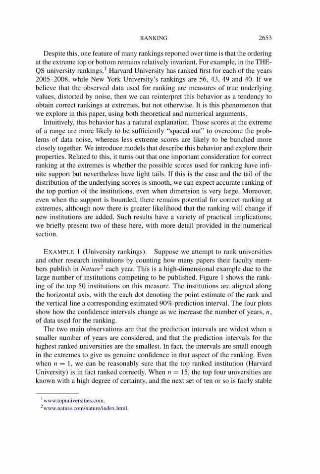
EXAMPLE 2 (Microarray data). We take the colon microarray data firstanalysed by Alon et al. (1999). It consists of 62 observations in total, each ofwhich indicates either a normal colon or a tumor. For each observation, there arealso expression levels for p = 2000 genes. It is of interest to determine whichgenes are most closely related to the response, so that they can be investigated fur-ther. This of course amounts to a ranking and we are interested in stability at theextreme, since we seek only a small number of genes. Here, the genes are rankedbased on the Mann–Whitney U test statistic, which is a nonparametric assessmentof the difference between the two distributions.

Figure 2 plots the top 30 genes, ranked by the lower tail of an estimated 90%prediction interval, rather than the point estimate of the rank. In this situation,we cannot authoritatively conclude that any of the top genes are ranked exactlycorrectly, but the top four genes appear much more stable than the others. Thisstability is highly important; if the length of all prediction intervals were roughlythe same as the average length (1400 genes), then there would be little hope ofdiscovering useful genes from such datasets.

RANKING 2655

FIG. 2. Prediction intervals for top-ranked genes in colon dataset.

There is a literature on the bootstrap in connection with rankings. See Goldsteinand Spiegelhalter (1996), who discuss bootstrap methods for constructing predic-tion intervals for rankings; Langford and Leyland (1996), who address bootstrapmethods for ranking the performance of doctors; Cesário and Barreto (2003), Hui,Modarres and Zheng (2005) and Taconeli and Barreto (2005), who take up theproblem of bootstrap methods for ranked set sampling; Mukherjee et al. (2003),who develop methods for gene ranking using bootstrapped p-values; and Xie,Singh and Zhang (2009) and Hall and Miller (2009), who focus on consistentbootstrap methods for assessing rankings. More generally, there is a vast litera-ture on ranking problems in statistics, and we cite here only the more relevantitems since 2000. Joe (2000, 2001) discusses ranking problems in connection withrandom utility models, and points to connections to multivariate extreme valuetheory. Murphy and Martin (2003) develop mixture-based models for rankings.Mease (2003) and Barker et al. (2005) treat methods for ranking football players.McHale and Scarf (2005) study the problem of ranking immunisation coveragein U.S. states. Brijs et al. (2006, 2007) introduce Bayesian models for the rank-ing of hazardous road sites, with the aim of better scheduling road safety policies.Chen, Stansy and Wolfe (2006) discuss ranking accuracy in ranked-set samplingmethods, and Opgen-Rhein and Strimmer (2007) examine the accuracy of generankings in high-dimensional problems involving genomic data. Nordberg (2006)addresses the reliability of performance rankings. Corain and Salmaso (2007) andQuevedo, Bahamonde and Luaces (2007) discuss ways of constructing rankings.

Section 2 describes our model for the ranking problem, and discusses the mainproperties of this framework. The formal theoretical results which underpin thediscussion in Section 2 are given in Section 3. Section 4 presents simulated andreal-data numerical work, including details on the examples presented above.Technical proofs are deferred to Section 5.

2656 P. HALL AND H. MILLER

2. Model. We consider a set of underlying parameters θ1, . . . , θp correspond-ing to the objects to be ranked, hereafter referred to as items. The error in theestimation is controlled by the number of observed data points, n. In our analysis,we take p = p(n) to diverge with n as the latter increases. An obvious difficultyhere is in establishing where the newly added items should fit into the ranking.A natural solution is to take the θj ’s to be randomly generated from some distribu-tion function. In the setup below, we interpret the �j ’s as values of means; see theend of this section for generalizations.

Let �1, . . . ,�p denote independent and identically distributed random vari-ables, and write

�(1) ≤ · · · ≤ �(p)(2.1)

for their ordered values. There exists a permutation R = (R1, . . . ,Rp) of (1, . . . , p)

such that �(j) = �Rjfor 1 ≤ j ≤ p. If the common distribution of the �j ’s is con-

tinuous, then the inequalities in (2.1) are all strict and the permutation is unique.We typically do not observe the �j ’s directly, only in terms of noisy approxi-

mations which can be modelled as follows. Let Qi = (Qi1, . . . ,Qip) denote inde-pendent and identically distributed random p-vectors with finite variance and zeromean, independent also of � = (�1, . . . ,�p). Suppose we observe

Xi = (Xi1, . . . ,Xip) = Qi + �(2.2)

for 1 ≤ i ≤ n. The mean vector

X = (X1, . . . , Xp) = 1

n

n∑i=1

Xi = Q + �(2.3)

is an empirical approximation to �. (Here, Q = n−1 ∑i Qi equals the mean of the

p-vectors Qi .) The components of X can also be ranked, as

X(1) ≤ · · · ≤ X(p),(2.4)

and there is a permutation R1, . . . , Rp of 1, . . . , p such that X(j) = XRjfor each j .

If the common distribution of the �j ’s is continuous then, regardless of the distrib-ution of the components of Qi , the inequalities in (2.4) are strict with probability 1.

The permutation R = (R1, . . . , Rp) serves as an approximation to R, and wewish to determine the accuracy of that approximation. In particular, for what valuesof j0 = j0(n,p), and for what relationships between n and p, is it true that

P(Rj = Rj for 1 ≤ j ≤ j0) → 1(2.5)

as n and p diverge? That is, how deeply into the ranking can we go before theconnection between the true ranking and its empirical form is seriously degradedby noise?

The answer to this question depends to some degree on the extent of dependenceamong the components of each Qi . To elucidate this point, let us consider the case

RANKING 2657

where all the components of Qi are identical; this is an extreme case of strongdependence. Then the components of Q are also identical. Clearly, in this settingRj = Rj for each j , and so (2.5) holds in a trivial and degenerate fashion. Otherstrongly dependent cases, although not as clear-cut as this one, can also be shownto be ones where Rj = Rj with high probability for many values of j .

The case which is most difficult, that is, where the strongest conditions areneeded to ensure that (2.5) holds, occurs when the components of Qi are inde-pendent. To emphasize this point we give sufficient conditions for (2.5), and showthat when the components of each Qi are independent, those conditions are alsonecessary. Our arguments can be modified to show that the conditions continue tobe necessary under sufficiently weak dependence, for example if the componentsare m-dependent where m = m(n) diverges sufficiently slowly as n increases.

The assumptions under which (2.5) holds are determined mainly by the lowertail of the common distribution of the �j ’s. If that distribution has an exponen-tially light left-hand tail, for example, if the tail is like that of a normal distribution,then a sufficient condition for (2.5) is that j0 should increase at a strictly slowerrate than n1/4(logn)c, where the constant c, which can be either positive or nega-tive, depends on the rate of decay of the exponential lower tail of the distributionof �. For example, c = 0 if the distribution decays like e−|x| in the lower tail,and c = −1

4 if it is normal. As indicated in the previous paragraph, the conditionj0 = o{n1/4(logn)c} is also necessary for (2.5) if the components of the Qi ’s areindependent.

These results have several interesting aspects, including: (a) the exponent 14

in the condition j0 = o{n1/4(logn)c} does not change among different types ofdistribution with exponential tails; (b) the exponent is quite small, implying thatthe empirical rankings Rj quite quickly become unreliable as predictors of the truerankings Rj ; and (c) the critical condition j0 = o{n1/4(logn)c} does not depend onthe value of p. (We assume that p diverges at no faster than a polynomial rate in n,but we impose no upper bound on the degree of that polynomial.)

The condition on j0 such that (2.5) holds changes in important ways if thelower tail of the distribution of the �j ’s decays relatively slowly, for example,at the polynomial rate x−α as x → ∞. Examples of this type include Pareto,nonnormal stable and Student’s t distributions, and more generally, distribu-tions with regularly varying tails. Here a sufficient condition for (2.5) to hold isj0 = o{(nα/2p)1/(2α+1)}, and this assumption is necessary if the components ofthe Qi ’s are independent. In this setting, unlike the exponential case, the value ofdimension, p, plays a major role in addition to the sample size, n, in determiningthe number of reliable rankings.

In practical terms, a major way in which this heavy-tailed case differs fromthe light-tailed setting considered earlier is that if a polynomially large number ofnew items are added to the competition in the heavy-tailed case, and all items arereranked, the results will change significantly and the number of correct rankings

2658 P. HALL AND H. MILLER

will also alter substantially. By way of contrast, if a polynomially large number ofnew items are added in the light-tailed, or exponential, case then there will againbe many changes to the rankings, but now there will be relatively few changes tothe number of items that are correctly ranked.

The exponential case can be regarded as the limit, as α → ∞, of the polynomialcase. More generally, note that as the left-hand tail of the common distribution ofthe �j ’s becomes heavier, the value of j0 can be larger before (2.5) fails. That is, ifthe distribution of the �j ’s has a heavier left-hand tail then the empirical rankingsRj approximate the true rankings Rj for a greater number of values of j , beforethey degenerate into noise.

The analysis above has focused on cases where the ranks of the Xj ’s are es-timated by ranking empirical means of noisy observations of those quantities;see (2.4). However, similar results are obtained if we rank other measures of lo-cation. Such a measure need only satisfy moderate deviation properties similar to(5.3) and (5.4) in the proof of Theorem 1. Thus, the results are applicable to awide range of ranking contexts. For example, Lq location estimators for generalq ≥ 1 enjoy moderate deviation properties under appropriate assumptions. There-fore, if we take the variables Qij to have zero median, rather than zero mean, andcontinue to define Xi by (2.2) but replace the ranking in (2.4) by a ranking ofmedians, then the results above and those in Section 3 continue to hold, modulochanges to the regularity conditions. Other suitable measures include the Mann–Whitney test used in the genomic example, quantiles and some correlation-basedmeasures.

The model suggested by (2.2), where data on � arise in the form of p-vectorsX1, . . . ,Xn, is attractive in a number of high-dimensional settings, for example,genomics. There, the j th component Xij of Xi would typically represent the ex-pression level of the j th gene of the ith individual in a sample. However, in othercases the means X1, . . . , Xp at (2.3), or medians or other location estimators, mightbe computed from quite different datasets, one for each component index j . More-over, those datasets might be of different sizes, n1, . . . , np say, and then the argu-ment that they arise naturally in the form of vectors would be inappropriate. Thiscan happen when data are used to rank items, for example schools where the rank-ing is based on individual student performance. The conclusions discussed earlierin this section, and the theoretical properties developed in Section 3 below, con-tinue to apply in this case provided there is an “average” value, n say, of the nj ’swhich represents all of them, in the sense that

n = O(

min1≤j≤p

nj

)and max

1≤j≤pnj = O(n)(2.6)

as n diverges. Additionally, in such cases it is often realistic to make the assump-tion that the corresponding centred means (or medians, etc.) Qj = n−1 ∑

i Qij arestochastically independent of one another, and so the particular results that arevalid in this case are immediately available.

RANKING 2659

The distribution of the �j ’s has been taken to be continuous. This is usually ap-propriate although there can be contexts in which the distribution is discrete. Notethat assumption of discreteness of the �j ’s is different from that of discreteness ofthe observations Xij . In such cases, the analysis still holds, except that allowancemust be made for ties (any reordering of tied �j ’s is still “correct”), and the taildensity assumptions should be characterized in integral form.

The model has been set up so that it focuses on the populations with lowestparameters �j . Obviously, similar arguments apply to the largest parameters too,so the results are applicable to both the most highly and lowly ranked populations.

3. Theoretical properties. For the most part, we shall assume one of twotypes of lower tail for the common distribution function, F , of the random vari-ables �j : either it decreases exponentially fast, in which case we suppose thatF(−x) � xβ exp(−C0x

α) as x → ∞, where α > 0 and −∞ < β < ∞; or itdecreases polynomially fast, in which case F(−x) � x−α as x → ∞, whereC0, α > 0. [The notation f (x) � g(x), for positive functions f and g, will betaken to mean that f (x)/g(x) is bounded away from zero and infinity as x → ∞.]The former case covers distributions such as the normal, exponential and Subbotin;the latter, distributions such as the Pareto, Student’s t and nonnormal stable laws(e.g., the Cauchy).

It is convenient to impose the shape constraints on the densities, which we as-sume to exist in the lower tail, rather than on the distribution functions. Therefore,we assume that one of the following two conditions hold as x → ∞:

(d/dx)F (−x) � (d/dx)xβ exp(−C0xα),(3.1)

(d/dx)F (−x) � (d/dx)x−α.(3.2)

In both (3.1) and (3.2), α must be strictly positive, but β in (3.1) can be any realnumber. The constant C0 in (3.1) must be positive. We assume too that

for fixed constants C1, . . . ,C5 > 0, where C2 > 2(C1 +1) and C4 < C5,p = O(nC1) as n → ∞, and, for each j ≥ 1, E|Qj |C2 ≤ C3, E(Qj) =0, and E(Q2

j ) ∈ [C4,C5].(3.3)

Recall from Section 1 that we wish to examine the probability that the trueranks Rj , and their estimators Rj , are identical over the range 1 ≤ j ≤ j0. Weconsider both j0 and p to be functions of n, so that the main dependent variablecan be considered to be n. With this interpretation, define

νexp = νexp(n) = n1/4(logn){(1/α)−1}/2,(3.4)

νpol = νpol(n) = (nα/2p)1/(2α+1),

where the subscripts denote “exponential” and “polynomial,” respectively, and re-fer to the respective cases represented by (3.1) and (3.2). In the theorem below, weimpose the additional condition that, for some ε > 0,

n = O(p4−ε).(3.5)

2660 P. HALL AND H. MILLER

This restricts our attention to problems that are genuinely high dimensional, in thesense that, with probability converging to 1, not all the rankings are correct. Caseswhere p diverges sufficiently slowly as a function of n are easier and will gener-ally permit all ranks to be correctly determined with high probability. Assumption(3.5) is also very close, in both the exponential and polynomial cases, to the basiccondition j0 ≤ p, as can be seen via a little analysis starting from (3.6) and (3.7)in the respective cases; yet, at the same time, (3.5) is suitable to both cases, and sohelps to unify our account of their properties. Note too that (3.5) implies that, inboth the exponential and polynomial cases, νexp = O(p1−δ) and νpol = O(p1−δ)

for some δ > 0.

THEOREM 1. Assume (3.3), (3.5) and that either (a) (3.1) or (b) (3.2) holds.In case (a), if

j0 = o(νexp)(3.6)

as n → ∞ then (2.5) holds. Conversely, when the components of the vectors Qi

are independent, (3.6) is necessary for (2.5). In case (b), if

j0 = o(νpol),(3.7)

then (2.5) holds. Conversely, when the components of the vectors Qi are indepen-dent, (3.7) is necessary for (2.5).

It can be deduced from Theorem 1 that when a new item (e.g., an institution)enters the competition that leads to the ranking, we are still able to rank the top j0institutions correctly. In this sense, the institutions that make up the cohort of sizej0 do not need to be fixed.

It is also of interest to consider cases where the common distribution, F , of the�j ’s is bounded to the left, for example, where F(x) � xα as x ↓ 0. However, itcan be shown that in this context, unless p is constrained to be a sufficiently lowdegree polynomial function of n, very few of the estimated ranks Rj will agreewith the correct values Rj .

To indicate why, we first recall the model introduced in Section 1, where theestimated ranks Rj are derived by ordering the values of Qj + �j . Here Qj =n−1 ∑

1≤i≤n Qij is the average value of n independent and identically distributedrandom variables with zero mean. Therefore the means, Qj , are of order n−1/2. Byway of contrast, if we take α = 1 in the formula F(x) � xα as x ↓ 0, for example,if F is the uniform distribution on [0,1], then the spacings of the order statistics�(1) ≤ · · · ≤ �(p) are approximately of size p−1. (More concisely, they are of sizeZ/p where Z has an exponential distribution; an independent version of Z is usedfor each spacing.) Therefore, if p is of larger order than n1/2 then the errors of the“estimators” Qj + �j of �j , for 1 ≤ j ≤ p, are an order of magnitude larger thanthe spacings among the �j ’s. This can make it very difficult to estimate the ranks

RANKING 2661

of the �j ’s from the ranks of values of Qj + �j . Indeed, it can be shown that, inthe difficult case where the components of the Qi ’s are independent, and even forfixed j0, if α = 1 and p is of larger order than n1/2 then in contrast to (2.5),

P(Rj = Rj for 1 ≤ j ≤ j0) → 0.(3.8)

This explains why, when F(x) � xα , it can be quite rare for the estimated ranksRj to match their true values. Indeed, no matter what the value of α and no mat-ter what the value of j0, property (2.5) will typically fail to hold unless p is nogreater than a sufficiently small power of n, in particular unless p = o(nα/2), asthe next result indicates. Thus, the differences between the cases of bounded andunbounded distributions are stark, as can be seen by contrasting Theorem 1 withthe properties described below.

THEOREM 2. Assume that (d/dx)F (x) � xα−1 as x ↓ 0, where α > 0, andthat (3.3) holds. Part (a): instances where (2.5) holds and p2/nα → 0. Under thelatter condition, (i) if α < 1

2 then (2.5) holds even for j0 = p; (ii) if α = 12 then

(2.5) holds provided that

(log j0)2α(p2/nα) → 0;(3.9)

and (iii) if α > 12 then (2.5) holds provided that

j0 = o{(nα/2/p)1/(2α−1)}.(3.10)

Part (b): converses to (a)(ii) and (a)(iii). If p2/nα → 0 and the components of thevectors Qi are independent then, if (2.5) holds, so too does (3.9) (if α = 1

2 ) or(3.10) (if α > 1

2 ). Part (c): instances where (3.8) holds. If α > 0 and p2/nα → ∞,and if the components of the vectors Qi are independent, then (3.8) holds even forj0 = 1.

The proof of Theorem 2 is similar to that of Theorem 1, and so is omitted.Theorem 1 is derived in Section 5. Both results continue to hold if the samplefrom which Xj is computed is of size nj for 1 ≤ j ≤ p, rather than n, providedthat (2.6) holds.

4. Numerical properties. This section discusses three real-data and threesimulated examples linked to the theoretical properties in Section 3. The real-dataexamples make use of the bootstrap to create prediction intervals [Xie, Singh andZhang (2009), Hall and Miller (2009)]. In each simulated example, the error is rel-atively light-tailed, and any discussion of tails refers to the distribution of the �j ’s.In our real-data examples, the noise has been averaged and so it is also generallylight-tailed. Thus, any heavy-tailed behavior present in the real-data examples islikely to be due to heavy tails of the distribution of the �j ’s, rather than the noise.

2662 P. HALL AND H. MILLER

EXAMPLE 1 (Continued). The originating institutions of Nature articles wereobtained using the ISI Web of knowledge database3 for each of the years 1999through 2008. A point ranking was obtained by taking the average number of ar-ticles published per year. Of course, there are implicit simplifying assumptionsin doing this, most significantly concerning the independence of articles betweenyears, and the stationarity of means time. These assumptions appear reasonable incontext, and are consistent with most publication-based analyses.

When constructing prediction intervals the bootstrap resamples for each insti-tution were drawn independently, conditional on the data. [See Hall and Miller(2009).] The number of observations in the resample can be varied to create dif-ferent time windows, as illustrated in Figure 1. The most natural question from aranking correctness viewpoint is determining the behavior at the right tail; thereare many institutions with mean at or near the hard threshold of zero, so there islittle hope for ranking correctness in the left tail. Furthermore, the right tail appearsto be long. Harvard University has an average of 67.5 papers per year, followed bymeans of 34.6, 29.6 and 28.2 for Berkeley, Stanford and Cambridge, respectively.

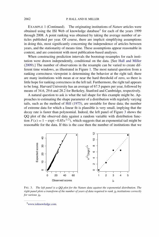
A natural question to ask is what the tail shape for this example might be. Ap-proaches to estimating the shape parameter of a distribution with regularly varyingtails, such as the method of Hill (1975), are unstable for these data; the numberof extreme data for which a linear fit is plausible is very small, implying that thedecay rate is faster than polynomial. Indeed, the left panel of Figure 3 shows theQQ plot of the observed data against a random variable with distribution func-tion F(x) = 1 − exp(−0.85x1/2), which suggests that an exponential tail might bereasonable for the data. If this is the case then the number of institutions that we

FIG. 3. The left panel is a QQ plot for the Nature data against the exponential distribution. Theright panel plots a transform of the number of years of data required to rank j0 institutions correctlyfor various j0.

3www.isiknowledge.com.

RANKING 2663

expect to be ranked correctly should depend, to first order, only on n, not on p, andbe of order up to n1/4(logn)1/2. One way to explore this further is to take j0 asgiven, and to resample from the data, seeking, for example, the number of years, n,needed to obtain correct ranking of the first j0 institutions at least 90% of the time.A plot of j0 against n1/4(logn)1/2 should be roughly linear. The right-hand panelof Figure 3 plots results of this experiment and appears to support the hypothesis.The flatness between j0 = 3 and j0 = 4 indicates that these two institutions arequite difficult to separate from each other.

EXAMPLE 2 (Continued). The Mann–Whitney test statistic can be written as

max{∑

i,j

I (xi < yj ),∑i,j

I (xi > yj )

},

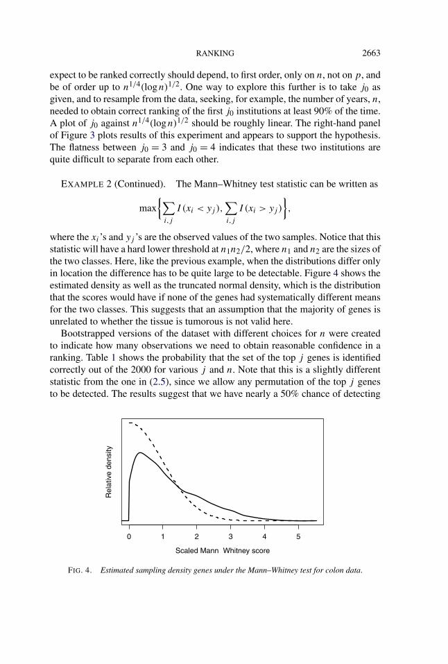
where the xi ’s and yj ’s are the observed values of the two samples. Notice that thisstatistic will have a hard lower threshold at n1n2/2, where n1 and n2 are the sizes ofthe two classes. Here, like the previous example, when the distributions differ onlyin location the difference has to be quite large to be detectable. Figure 4 shows theestimated density as well as the truncated normal density, which is the distributionthat the scores would have if none of the genes had systematically different meansfor the two classes. This suggests that an assumption that the majority of genes isunrelated to whether the tissue is tumorous is not valid here.

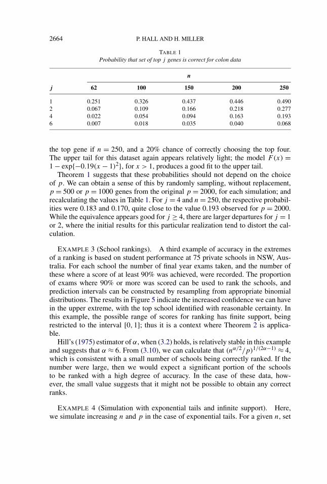
Bootstrapped versions of the dataset with different choices for n were createdto indicate how many observations we need to obtain reasonable confidence in aranking. Table 1 shows the probability that the set of the top j genes is identifiedcorrectly out of the 2000 for various j and n. Note that this is a slightly differentstatistic from the one in (2.5), since we allow any permutation of the top j genesto be detected. The results suggest that we have nearly a 50% chance of detecting

FIG. 4. Estimated sampling density genes under the Mann–Whitney test for colon data.

2664 P. HALL AND H. MILLER

TABLE 1Probability that set of top j genes is correct for colon data

n

j 62 100 150 200 250

1 0.251 0.326 0.437 0.446 0.4902 0.067 0.109 0.166 0.218 0.2774 0.022 0.054 0.094 0.163 0.1936 0.007 0.018 0.035 0.040 0.068

the top gene if n = 250, and a 20% chance of correctly choosing the top four.The upper tail for this dataset again appears relatively light; the model F(x) =1 − exp{−0.19(x − 1)2}, for x > 1, produces a good fit to the upper tail.

Theorem 1 suggests that these probabilities should not depend on the choiceof p. We can obtain a sense of this by randomly sampling, without replacement,p = 500 or p = 1000 genes from the original p = 2000, for each simulation; andrecalculating the values in Table 1. For j = 4 and n = 250, the respective probabil-ities were 0.183 and 0.170, quite close to the value 0.193 observed for p = 2000.While the equivalence appears good for j ≥ 4, there are larger departures for j = 1or 2, where the initial results for this particular realization tend to distort the cal-culation.

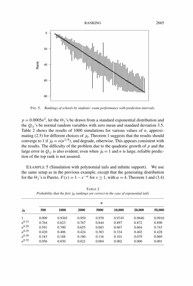
EXAMPLE 3 (School rankings). A third example of accuracy in the extremesof a ranking is based on student performance at 75 private schools in NSW, Aus-tralia. For each school the number of final year exams taken, and the number ofthese where a score of at least 90% was achieved, were recorded. The proportionof exams where 90% or more was scored can be used to rank the schools, andprediction intervals can be constructed by resampling from appropriate binomialdistributions. The results in Figure 5 indicate the increased confidence we can havein the upper extreme, with the top school identified with reasonable certainty. Inthis example, the possible range of scores for ranking has finite support, beingrestricted to the interval [0,1]; thus it is a context where Theorem 2 is applica-ble.

Hill’s (1975) estimator of α, when (3.2) holds, is relatively stable in this exampleand suggests that α ≈ 6. From (3.10), we can calculate that (nα/2/p)1/(2α−1) ≈ 4,which is consistent with a small number of schools being correctly ranked. If thenumber were large, then we would expect a significant portion of the schoolsto be ranked with a high degree of accuracy. In the case of these data, how-ever, the small value suggests that it might not be possible to obtain any correctranks.

EXAMPLE 4 (Simulation with exponential tails and infinite support). Here,we simulate increasing n and p in the case of exponential tails. For a given n, set

RANKING 2665

FIG. 5. Rankings of schools by students’ exam performance with prediction intervals.

p = 0.0005n2, let the �j ’s be drawn from a standard exponential distribution andthe Qij ’s be normal random variables with zero mean and standard deviation 3.5.Table 2 shows the results of 1000 simulations for various values of n, approxi-mating (2.5) for different choices of j0. Theorem 1 suggests that the results shouldconverge to 1 if j0 = o(n1/4), and degrade, otherwise. This appears consistent withthe results. The difficulty of the problem due to the quadratic growth of p and thelarge error in Qij is also evident; even when j0 = 1 and n is large, reliable predic-tion of the top rank is not assured.

EXAMPLE 5 (Simulation with polynomial tails and infinite support). We usethe same setup as in the previous example, except that the generating distributionfor the �j ’s is Pareto, F(x) = 1 −x−α for x ≥ 1, with α = 4. Theorem 1 and (3.4)

TABLE 2Probability that the first j0 rankings are correct in the case of exponential tails

n

j0 500 1000 2000 5000 10,000 20,000 50,000

1 0.909 0.9365 0.959 0.970 0.9745 0.9840 0.9910n0.15 0.764 0.823 0.767 0.844 0.897 0.872 0.890n0.20 0.591 0.700 0.655 0.683 0.667 0.664 0.743n0.25 0.420 0.406 0.424 0.383 0.334 0.402 0.428n0.30 0.183 0.188 0.180 0.116 0.101 0.079 0.069n0.35 0.056 0.030 0.021 0.004 0.002 0.000 0.001

2666 P. HALL AND H. MILLER

TABLE 3Probability that the first j0 rankings are correct in the case of exponential tails

n

j0 500 1000 2000 5000 10,000 20,000 50,000

(1/5)n0.35 0.884 0.832 0.908 0.920 0.898 0.921 0.945(1/5)n0.40 0.694 0.672 0.708 0.731 0.801 0.786 0.803(1/5)n4/9 0.477 0.510 0.586 0.568 0.569 0.520 0.540(1/5)n0.50 0.283 0.242 0.252 0.161 0.140 0.120 0.096(1/5)n0.55 0.071 0.086 0.031 0.020 0.006 0.002 0.001

suggest that the rate n4/18p1/9 = n4/9 is critical for j0, and this is consistent withthe results in Table 3. This is an easier problem than that in the previous example,because of the polynomial decay of the tail. For instance, the top right-hand resultin the table suggests that the top nine ranks can be correctly ascertained more than90% of the time when p > 50,000, whereas the figure 0.890 in the last column ofTable 2 suggests that, for the distribution represented there, only the top five rankshave this level of reliability.

EXAMPLE 6 (Simulation with polynomial tails with finite support). Theo-rem 2 has many interesting consequences, but the present example focuses oncase (iii), where α > 1

2 . First, let the �j ’s be uniformly distributed on [0,1], andconsider a case where the entire ranking is correct. Using the notation of Section 3and taking α = 1, Theorem 2 implies that p � n1/4 defines the critical growth in di-mension. For simulation, we took p = 2nk for various k, and scaled the (normallydistributed) error for each k such that the n = 500 case had probability approxi-mately 0.5 of correctly identifying all ranks. Each simulation was repeated 10,000times, with results summarized in Table 4. As predicted, growth rates in dimen-

TABLE 4Probability all ranks identified correctly when �j is uniformly distributed

n

k 500 1000 2000 5000 10,000 20,000 50,000

1/6 0.502 0.494 0.525 0.593 0.635 0.658 0.7011/5 0.498 0.511 0.471 0.558 0.568 0.578 0.6061/4 0.497 0.478 0.492 0.505 0.517 0.496 0.5021/3 0.500 0.457 0.395 0.343 0.289 0.259 0.2121/2 0.502 0.369 0.249 0.107 0.046 0.011 0.000

RANKING 2667

TABLE 5Probability that lowest 10nk scores identified correctly

n

k 5 × 103 1 × 104 2 × 104 5 × 104 1 × 105 2 × 105 5 × 105 1 × 106

0.05 0.500 0.539 0.553 0.583 0.603 0.609 0.628 0.6410.07 0.502 0.532 0.506 0.546 0.558 0.580 0.555 0.5911/11 0.497 0.486 0.489 0.516 0.489 0.463 0.513 0.4960.11 0.497 0.481 0.471 0.432 0.461 0.447 0.452 0.4210.13 0.506 0.492 0.461 0.481 0.445 0.427 0.387 0.385

sion slower than n1/4 have probability of correct ranking tending to 1, while thosefaster than n1/4 degrade.

Next, we examine the case p = 5 × 10−6n2, where dimension grows at aquadratic rate; and F(x) = xα on [0,1], with α = 6, implying a reasonably severetail. Theorem 2 suggests that if j0 = o(p1/22), or equivalently if j0 = o(n1/11), then(2.5) should hold. Table 5 shows the probability of ranking the smallest j0 = 10nk

scores correctly for various k and n, with 10,000 simulations. Again the normalerror is tuned so that the n = 5000 case has probability of close to 1

2 . The resultssuggest that n1/11 indeed separates values of k for which correct ranking is possi-ble.

5. Technical arguments. We begin by giving a brief sketch of the proof ofTheorem 1. Two steps in the proof are initially presented as lemmas, the first usingmoderate deviation properties to approximate sums related to the object of interest,and the second employing Taylor’s expansion applied to Rényi representationsof order statistics to show that the gaps �(j+1) − �(j) have a high probabilityof being of reasonable size. In the proof itself, we use Lemma 1 to bound theprobability in (2.5) from below [see (5.19)] and then show that the last two termsin this expression converge to zero, implying that the probability converges to 1if (3.6) holds. For the converse, assuming independence, we find an upper boundto the probability in (5.20) and show that if this probability tends to one then thesum s(n), introduced at (5.21), must converge to zero, which in turn implies (3.6).Only the exponential tail case is presented in detail; comments at the end of theproof describe the main differences in the polynomial tail case.

Throughout, we let E (j0) denote the event that QRj+ �Rj

> QRj0+ �Rj0

for

j0 + 1 ≤ j ≤ p, we define Ej to be the event that �(j+1) − �(j) ≥ −(QRj+1 −QRj

), and we take E (j0) and Ej to be the respective complements. Also, we letζj = �(j+1) − �(j) denote the j th gap, where �(0) = −∞ for convenience.

In Lemma 1 below, we write O to denote the sigma-field generated by the �j ’s,N for a standard normal random variable independent of O, δn for any given se-

2668 P. HALL AND H. MILLER

quence of positive constants δn converging to zero, and for a generic randomvariable satisfying P(|| ≤ δn) = 1.

LEMMA 1. For any positive integer j0 < p, let J denote the set of positive,even integers less than or equal to j0. Put

T1j = min(ζj−1, ζj )

2(var QRj)1/2

, T2j = ζj

{var(QRj+1 − QRj)}1/2

.

Then

j0∑j=1

P

{|QRj

| > 1

2min(ζj−1, ζj )

}(5.1)

= 2{1 + o(1)}j0∑

j=1

P(|N | > T1j ) + o(1).

If in addition the components of the Qi ’s are independent then

E

[exp

{− ∑

j∈JP(Ej | O)

}](5.2)

≤ {1 + o(1)}E[exp

{−(1 + )

∑j∈J

P(N > T2j | O)

}].

PROOF. Using the arguments of Rubin and Sethuraman (1965) and Amosova(1972), it can be shown that, if the constant C2 in (3.3) satisfies C2 > B2 +2 whereB > 0, then as n (and hence, also p) diverges,

P {|Qj | > x(var Qj )1/2} = {1 + o(1)}2{1 − �(x)},(5.3)

P [−(Qj1 − Qj2) ≥ x{var(Qj1 − Qj2)}1/2] = {1 + o(1)}{1 − �(x)},(5.4)

uniformly in 0 < x < B(logp)1/2 and j, j1, j2 ≥ 1 such that j1 = j2. Expres-sion (5.4) requires the independence assumption. Therefore, since C2 > 2(C1 + 1)

in (3.3), we can take B = (2 + ε)1/2 for some ε > 0, and then (5.3) and (5.4) holduniformly in 0 < x < {(2 + ε) logp}1/2. Thus, as n → ∞, they hold uniformly inall x > 0, modulo an o(p−1) term. We use (5.3) to derive (5.1), while (5.4) impliesthat ∑

j∈JP(Ej ) = {1 + o(1)} ∑

j∈JP(N > T2j ) + o(1),

which leads to (5.2). �

RANKING 2669

LEMMA 2. If (3.1), indicating the case of exponential tails, holds then thereexist B4,B5 > 0 such that, for any choice of constants c1, c2 satisfying 0 < c1 <

c2 < (4 − ε)−1 with ε as in (3.5), and for all B6 > 0,

infj∈[1,nc1 ]

P{ζjZ

−1j+1(logn)1−(1/α) ≥ B4n

−c1} = 1 − O(n−B6),(5.5)

infj∈[nc1 ,nc2 ]

P{B4 ≤ jζjZ

−1j+1(logn)1−(1/α) ≤ B5

} = 1 − O(n−B6).(5.6)

Note further that the constraint on c2 permits nc2 to be of size νexpnε1 (where

ε1 > 0).

PROOF. If U(1) ≤ · · · ≤ U(p) denote the order statistics of a sample of size p

drawn from the uniform distribution on [0,1] then, for each p, we can construct acollection of independent random variables Z1, . . . ,Zp with the standard negativeexponential distribution on [0,∞], such that, for 1 ≤ j ≤ p, U(j) = 1 − exp(−Vj )

where

Vj =j∑

k=1

Zk

p − k + 1= wj + Wj.

For details, see Rényi (1953). Further, uniformly in 1 ≤ j ≤ 12p and 2 ≤ p < ∞,

wj =p∑

k=p−j+1

1

k= j

p+ O(j2/p2) = O(j/p),(5.7)

Wj =p∑

k=p−j+1

k−1(Zp−k+1 − 1), sup1≤j≤p/2

j−1/2|Wj | ≤ p−1W(p),(5.8)

sup1≤j≤p/2

j−3/2

∣∣∣∣∣Wj − 1

p

p∑k=p−j+1

(Zp−k+1 − 1)

∣∣∣∣∣ ≤ p−2W(p),(5.9)

where the nonnegative random variable W(p), which without loss of generality,we take to be common to (5.8) and (5.9), satisfies the expression P {W(p) > pε} =O(p−C) for each C,ε > 0.

Using the second identity in (5.7), and (5.8), we deduce that

U(j+1) − U(j) = (Vj+1 − Vj )

{1 − 1

2(Vj+1 + Vj )

+ 1

6(V 2

j+1 + VjVj+1 + V 2j ) − · · ·

}(5.10)

= Zj+1

p − j

{1 + �j1

(j

p+ Sj1

p1/2

)},

2670 P. HALL AND H. MILLER

uniformly in 1 ≤ j ≤ 12p, where the random variable �j1 satisfies, for k = 1,

P(

max1≤j≤p/2

|�jk| ≤ A)

= 1,(5.11)

A > 0 is an absolute constant, and for each C,ε > 0 the nonnegative random vari-able Sj1 satisfies, with k = 1,

P(

sup1≤j≤p/2

Sjk > pε)

= O(p−C).(5.12)

Using the third identity in (5.7) and (5.9), we deduce that

0 ≤ U(j) = wj + Wj − 1

2(wj + Wj)

2 + · · ·(5.13)

= j

p+ �j2

(j2

p2 + j1/2Sj2

p

),

where �j2 and Sj2 ≥ 0 satisfy (5.11) and (5.12), respectively.Define Dj = U(j+1) − U(j) and without loss of generality, C0 = 1 in (3.1). If

the common distribution function of the �j ’s is F , then by Taylor’s expansion,

ζj = F−1(U(j) + Dj

) − F−1(U(j)

)= Dj(F

−1)′(U(j) + ωjDj

)(5.14)

= �j

Dj

U(j) + ωjDj

{− log(U(j) + ωjDj

)}(1/α)−1,

where 0 ≤ ωj ≤ 1 and the last line makes use of (3.1). The random variable �j

satisfies, for constants B1, B2 and B3 satisfying 0 < B1 < B2 < ∞ and 0 < B3 < 1,

P(B1 ≤ �j ≤ B2 for all j such that U(j+1) < B3

) = 1.

The required result then follows from (5.10), (5.13) and (5.14). �

PROOF OF THEOREM 1. Take j0 < p a positive integer. Note that, takingE (jo), Ej , E (jo), Ej , O and J as for Lemma 1,

{Rj = Rj for 1 ≤ j ≤ j0}⊇ {|QRj

| ≤ 12 min(ζj−1, ζj ) for 1 ≤ j ≤ j0

} ∩ E (j0),

where we define �(j−1) = −∞ if j = 1 as before. Therefore, defining π(j0) =P(Rj = Rj for 1 ≤ j ≤ j0), we deduce that

π(j0) ≥ 1 −j0∑

j=1

P

{|QRj

| > 1

2min(ζj−1, ζj )

}− P {E (j0)}.(5.15)

RANKING 2671

Also,

{Rj = Rj for 1 ≤ j ≤ j0}= {

XR1 ≤ · · · ≤ XRj0and Xj > XRj0

for j /∈ {R1, . . . ,Rj0}}

= {ζj ≥ −(QRj+1 − QRj

) for 1 ≤ j ≤ j0

and �j − �(j0) ≥ −(Qj − QRj0) for j /∈ {R1, . . . ,Rj0}

},

and so

π(j0) ≤ P {ζj ≥ −(QRj+1 − QRj) for 1 ≤ j ≤ j0}.(5.16)

Letting π1(j0) denote the probability that Ej holds for all j ∈ J , by (5.16),

π(j0) ≤ π1(j0).(5.17)

Note that if the components of each Qi are independent, then the events Ej , forj ∈ J , are independent conditional on O. Therefore,

π1(j0) = E

{P

( ⋂j∈J

Ej | O)}

= E

[ ∏j∈J

{1 − P(Ej | O)}]

(5.18)

≤ E

[exp

{− ∑

j∈JP(Ej | O)

}].

Using Lemma 1, we have the following inequalities regarding π(j0):

π(j0) ≥ 1 − 2{1 + o(1)}j0∑

j=1

P(|N | > T1j ) − P {E (j0)} + o(1),(5.19)

π(j0) ≤ {1 + o(1)}E[exp

{−(1 + )

∑j∈J

P(N > T2j | O)

}].(5.20)

To show that (3.6) implies (2.5), by (5.19) it is sufficient to show that P {E (j0)}and

∑j0j=1 P(|N | > T1j ) are both o(1), which we shall do in turn.

Define � = (logn)(1/α)−1, let N be a standard normal random variable indepen-dent of O, and let Z be independent of N and have the standard negative expo-nential distribution. Let K1 be a positive constant. If an is a sequence of positivenumbers and fn is a sequence of nonnegative functions, write an

.= fn(K) to meanthat, for constants L1,L2 > 1, either (a) an ≤ L1fn(K) whenever K ≥ L2 and n

is sufficiently large, and an ≥ L−11 fn(K) whenever K ≤ L−1

2 and n is sufficientlylarge, or (b) an ≥ L−1

1 fn(K) whenever K ≥ L2 and n is sufficiently large, andan ≤ L1fn(K) whenever K ≤ L−1

2 and n is sufficiently large. Let 0 < c1 < c2 < 12

and c1 < 14 , and let j0 and j1 denote integers satisfying |j1 − nc1 | ≤ 1, j1 ≤ j0 ≤

nc2 and j1/j0 → 0.

2672 P. HALL AND H. MILLER

When (3.1) holds with C0 = 1, Lemma 2 implies that, for each B6 > 0 andletting γj = n−1/2j�−1,

s(n) ≡j0∑

j=1

P {|N | > K1n1/2(ζj )}

.= O{j1P(|N | > K2Zγ −1j1

) + n−B6} + ∑j1<j≤j0

P(|N | > KZγ −1j )

.= O

{j1

(P(Z ≤ γj1) + E

[Z−1γj1 exp

{−1

2(KZγ −1

j1)2

}I (Z > γj1)

])}(5.21)

+ ∑j1<j≤j0

(P(Z ≤ γj ) + E

[Z−1γj exp

{−1

2(KZγ −1

j )2}I (Z > γj )

]).= O

{j1

(γj1 + E

[Z−1γj1 exp

{−1

2(KZγ −1

j1)2

}I (Z > γj1)

])}+ ∑

j1<j≤j0

(γj + E

[Z−1γj exp

{−1

2(KZγ −1

j )2}I (Z > γj )

]).

Now,

E

[Z−1γj exp

{−1

2(KZγ −1

j )2}I (Z > γj )

]=

∫ ∞γj

z−1γj exp{−1

2(KZγ −1

j )2 − z

}dz

= γj

∫ ∞1

u−1 exp{−1

2(Ku)2 − γju

}du � γj

= n−1/2j�.

(Here, we have used the fact that j ≤ j0 ≤ nc2 where c2 < 12 .) Therefore,

s(n) � j1 · n−1/2j1�−1 + ∑

j1<j≤j0

n−1/2j�−1

� n−1/2j21 �−1 + n−1/2j2

0 �−1(5.22)

� n−1/2j20 �−1.

(Here, we have used the fact that j1/j0 → 0.)The right-hand side of (5.22) converges to zero if and only if (3.6) holds. More-

over, in view of the fact that

P(|N | > T1j ) ≤ P

(|N | > ζj−1

2(var QRj)1/2

)+ P

(|N | > ζj

2(var QRj)1/2

),

RANKING 2673

and depending on the choice of K1 in the definition of s(n) at (5.21), s(n) can bean upper bound to the series

∑j0j=1 P(|N | > T1j ) on the right-hand side of (5.1).

Hence,

j0∑j=1

P(|N | > T1j ) = o(1).(5.23)

This deals with the second term on the right-hand side of (5.19). Similarly, if r ∈[2,∞) is a fixed integer, and if j0 = o(n1/4�1/2), then

s1(n) ≡j0+r−1∑j=j0+1

P {|N | > K1n1/2(ζj )} = o(1).(5.24)

Moreover, if j1 denotes the integer part of nc2 − j0 then, for constants K2 and K3

satisfying K1 > K2 > K3 > 0, and for any B > 0,

s2(n) ≡j0+j1∑

j=j0+r

P{|N | > K1n

1/2(�(j+1) − �(j0)

)}

≤j1∑

j=r

P

{|N | > K2n

1/2�

j∑k=1

(j0 + k)−1Zk

}+ O(n−B)

(5.25)≤ j1P {|N | > K2n

1/4�1/2(Z1 + · · · + Zr)} + O(n−B)

= O{j1(n1/2�2)−r},

where we have assumed that j0 = o(n1/4�1/2) and also used the fact that Z1 +· · ·+Zr has a gamma(r,1) distribution. If we choose r so large that pn−r/2 = O(n−ε)

for some ε > 0, then we can deduce from (5.24) and (5.25) that s1(n)+ s2(n) → 0,and hence, by (5.6), that

nc2∑j=j0+1

P(QRj+ �Rj

> QRj0+ �Rj0

) → 0.(5.26)

A more crude argument can be used to prove that if r is so large that p2n−r/2 =O(n−ε) for some ε > 0, and if j0 = o(n1/4�1/2), then∑

nc2<j≤p

P (QRj+ �Rj

> QRj0+ �Rj0

) → 0.(5.27)

Together, (5.26) and (5.27) imply that if j0 = o(n1/4�1/2) then

P {E (j0)} → 0.(5.28)

2674 P. HALL AND H. MILLER

Thus, in light of (5.19), we see (5.23) and (5.28) imply that (3.6) is sufficientfor (2.5).

We next show that (2.5) implies (3.6) in the independent case. If (2.5) holds,then by (5.20), ∑

j∈JP(N > T2j | O) → 0

in probability. Therefore, by Lemma 2, with j0 and j1 as above, there exists K1 > 0such that ∑

j1<j≤j0

P {|N | > n1/2K1(ζj ) | O} → 0

in probability. (We can take the sum over all j ∈ [j1 + 1, j0], rather than just overeven j , since (5.2) holds for sums over odd j as well as over even j .) Hence,arguing as in the lines below (5.21), we deduce that for sufficiently large K2 > 0,∑

j1<j≤j0

f (Zj/δj ) → 0(5.29)

in probability, where the random variables Zj are independent and have a commonexponential distribution, δj = n−1/2j�−1 and

f (z) = z−1 exp(−K2z2)I (z > 1).

We claim that this implies that the expected value of the left-hand side of (5.29)also converges to 0: ∑

j1<j≤j0

E{f (Zj/δj )} → 0(5.30)

or equivalently that∑

j1<j≤j0δj → 0, and thence [using the argument leading to

(5.22)] that s(n) � n−1/2j20 �−1 → 0, which is equivalent to (3.6). Therefore, if we

establish (5.30) then we shall have proved that (2.5) implies (3.6).It remains to show that (5.29) implies (5.30). This we do by contradiction.

If (5.30) fails then, along a subsequence of values of n, the left-hand side of(5.30) converges to a nonzero number. For notational simplicity, we shall makethe inessential assumptions that the number is finite and that the subsequence in-volves all n, and we shall take K2 = 1 in the definition of f . In particular,

t (n) ≡ ∑j1<j≤j0

E{f (Zj/δj )} → t (∞),(5.31)

where t (∞) is bounded away from 0. Now, t (n) = {1 + o(1)}μ(1)δ(n), whereδ(n) = ∑

j1<j≤j0δj and, for general λ ≥ 1, μ(λ) = ∫

z>λ z−1 exp(−z2) dz. There-

RANKING 2675

fore,

δ(n) → δ(∞) ≡ t (∞)/μ(1).(5.32)

For each λ > 1 the left-hand side of (5.29) equals 1 + 2, where, in view of(5.31),

E(2) = ∑j1<j≤j0

E{f (Zj/δj )I (Zj > λδj )}(5.33)

= {1 + o(1)}μ(λ)δ(n)

and

1 = ∑j1<j≤j0

f (Zj/δj )I (Zj ≤ λδj ) = ∑j1<j≤j0

f (Wj )Ij

with Wj = Zj/δj and Ij = I (δj ≤ Zj ≤ λδj ). However,∑j1<j≤j0

P(Ij = 1) = μ1(λ)δ(n) + o(1) = δ(∞)μ1(λ) + o(1),

where μ1(λ) = ∫1<z<λ z−1 exp(−z2) dz. Therefore, in the limit as n → ∞, 1

equals a sum, Sλ say, of N independent random variables each having the distribu-tion of f (W), where W is uniformly distributed on [1, λ], N has a Poisson distrib-ution with mean δ(∞)μ1(λ), and N and the summands are independent. The dis-tribution of Sλ is stochastically monotone increasing, in the sense that P(Sλ > s)

increases with λ. On the other hand, since μ(λ) → 0 as λ → ∞ then, by (5.32)and (5.33),

limλ→∞ lim sup

n→∞E(2) = 0.

Combining these results, we deduce that 1 + 2, that is, the left-hand side of(5.29), does not converge to zero in probability. This contradicts (5.29) and soestablishes that t (∞) must equal zero; that is, (5.30) holds.

Comments on proving the polynomial case: the proof for the case of polynomialtails proceeds similarly. The main difference is that in the proof of Lemma 2 we use(3.2) instead of (3.1), which forces a factor of p−1/α into the results of the lemma,rather than (logn)1−(1/α). This in turn implies that s(n) � n−1/2j

2+1/α0 p−1/α ,

entailing that convergence occurs if (and, in the case of independence, only if)j0 = o(νpol), as required. �

REFERENCES

ALON, U., BARKAI, N., NOTTERMAN, D. A., GISH, K., YBARRA, S., MACK, D. and LEVINE,A. J. (1999). Broad patterns of gene expression revealed by clustering analysis of tumor andnormal colon tissues probed by oligonucleotide arrays. Proc. Natl. Acad. Sci. 96 6745–6750.

2676 P. HALL AND H. MILLER

AMOSOVA, N. N. (1972). Limit theorems for the probabilities of moderate deviations. VestnikLeningrad. Univ. No. 13 Mat. Meh. Astronom. Vyp. 5–14, 148. MR0331484

BARKER, L. E., SMITH, P. J., GERZOFF, R. B., LUMAN, E. T., MCCAULEY, M. M. and STRINE,T. W. (2005). Ranking states’ immunization coverage: An example from the National Immuniza-tion Survey. Stat. Med. 24 605–613. MR2134528

BRIJS, T., VAN DEN BOSSCHE, F., WETS, G. and KARLIS, D. (2006). A model for identifying andranking dangerous accident locations: A case study in Flanders. Statist. Neerlandica 60 457–476.MR2291385

BRIJS, T., KARLIS, D., VAN DEN BOSSCHE, F. and WETS, G. (2007). A Bayesian model forranking hazardous road sites. J. Roy. Statist. Soc. Ser. A 170 1001–1017. MR2408989

CESÁRIO, L. C. and BARRETO, M. C. M. (2003). Study of the performance of bootstrap confidenceintervals for the mean of a normal distribution using perfectly ranked set sampling. Rev. Mat.Estatíst. 21 7–20. MR2058492

CHEN, H., STANSY, E. A. and WOLFE, D. A. (2006). An empirical assessment of ranking accuracyin ranked set sampling. Comput. Statist. Data Anal. 51 1411–1419. MR2297530

CORAIN, L. and SALMASO, L. (2007). A non-parametric method for defining a global preferenceranking of industrial products. J. Appl. Statist. 34 203–216. MR2364253

GOLDSTEIN, H. and SPIEGELHALTER, D. J. (1996). League tables and their limitations: Statisticalissues in comparisons of institutional performance. J. Roy. Statist. Soc. Ser. A 159 385–443.

HALL, P. and MILLER, H. (2009). Using the bootstrap to quantify the authority of an empiricalranking. Ann. Statist. 37 3929–3959. MR2572448

HILL, B. M. (1975). A simple general approach to inference about the tail of a distribution. Ann.Statist. 3 1163–1174. MR0378204

HUI, T. P., MODARRES, R. and ZHENG, G. (2005). Bootstrap confidence interval estimation ofmean via ranked set sampling linear regression. J. Stat. Comput. Simul. 75 543–553. MR2162545

JOE, H. (2000). Inequalities for random utility models, with applications to ranking and subset choicedata. Methodol. Comput. Appl. Probab. 2 359–372. MR1836406

JOE, H. (2001). Multivariate extreme value distributions and coverage of ranking probabilities.J. Math. Psych. 45 180–188. MR1820238

LANGFORD, I. H. and LEYLAND, A. H. (1996). Discussion of “League tables and their limitations:Statistical issues in comparisons of institutional performance” by Goldstein and Spiegelhalter.J. Roy. Statist. Soc. Ser. A 159 427–428.

MCHALE, I. and SCARF, P. (2005). Ranking football players. Significance 2 54–57. MR2224085MEASE, D. (2003). A penalized maximum likelihood approach for the ranking of college football

teams independent of victory margins. Amer. Statist. 57 241–248. MR2016258MUKHERJEE, S. N., SYKACEK, P., ROBERTS, S. J. and GURR, S. J. (2003). Gene ranking using

bootstrapped p-values. Sigkdd Explorations 5 14–18.MURPHY, T. B. and MARTIN, D. (2003). Mixtures of distance-based models for ranking data. Com-

put. Statist. Data Anal. 41 645–655. MR1973732NORDBERG, L. (2006). On the reliability of performance rankings. In Festschrift for Tarmo Pukkila

on His 60th Birthday (E. P. Liski, J. Isotalo, J. Niemelä and G. P. H. Styan, eds.) 205–216. Univ.Tampere, Tampere, Finland. MR2412962

OPGEN-RHEIN, R. and STRIMMER, K. (2007). Accurate ranking of differentially expressed genesby a distribution-free shrinkage approach. Stat. Appl. Genet. Mol. Biol. 6 Art. 9, 20pp. (elec-tronic). MR2306944

QUEVEDO, J. R., BAHAMONDE, A. and LUACES, O. (2007). A simple and efficient method forvariable ranking according to their usefulness for learning. Comput. Statist. Data Anal. 52 578–595. MR2410003

RÉNYI, A. (1953). On the theory of order statistics. Acta Math. Acad. Sci. Hungar. 4 191–232.MR0061792

RANKING 2677

RUBIN, H. and SETHURAMAN, J. (1965). Probabilities of moderate deviations. Sankhya Ser. A 27325–346. MR0203783

TACONELI, C. A. and BARRETO, M. C. M. (2005). Evaluation of a bootstrap confidence intervalapproach in perfectly ranked set sampling. Rev. Mat. Estatíst. 23 33–53. MR2304506

XIE, M., SINGH, K. and ZHANG, C. H. (2009). Confidence intervals for population ranks in thepresence of ties and near ties. J. Amer. Statist. Assoc. 104 775–787. MR2541594

DEPARTMENT OF MATHEMATICS AND STATISTICS

UNIVERSITY OF MELBOURNE

MELBOURNE, VIC 3010AUSTRALIA

E-MAIL: halpstat@ms.unimelb.edu.auh.miller@ms.unimelb.edu.au