1

Stochastic Transmission Capacity ExpansionPlanning with Special Scenario Selection for

Integrating N − 1 Contingency AnalysisMohammad Majidi-Qadikolai, Student Member, IEEE, Ross Baldick, Fellow, IEEE

Abstract—In this paper, we propose an iterative framework forsolving the stochastic transmission capacity expansion planning(TCEP) optimization problem with N−1 contingency analysis. Athree-level filtering algorithm is designed that uses developed im-portant scenario identification index (ISII) and similar scenarioelimination (SSE) technique to decrease the number of reliabilityconstraints in stochastic TCEP in a systematic and trackable way.This filter decreases structural constraints in our TCEP mixed-integer programming formulation in each iteration (up to 99.8%in the first iteration), and the iterative framework adds reliabilityconstraints into the optimization problem gradually in order todecrease the total simulation time. A lower bound is calculatedto quantify the quality of results. To verify capabilities of theproposed method, it is applied to a reduced ERCOT system with317 buses, 427 binary variables, and 10 scenarios. The numericalresult shows that the proposed method can solve large-scalestochastic TCEP optimization problems faster, and its relativeperformance improves with increasing number of scenarios andthe system size.

Index Terms—Transmission capacity expansion planning, N−1criterion, Reliability, Stochastic programming, Uncertainties

NOMENCLATURE

Sets and Indices:Nb: Set of buses; index i, k, nNg: Set of all generators; index gNo: Set of all existing lines; index l, mNn: Set of all candidate lines; index l, mNυu : Set of all existing lines and selected candidate lines;

index l, mLk: Set of lines connected to bus kGk: Set of all generators connected to bus kWk: Set of wind generators connected to bus kΦω,υl : Set of lines with violated post-contingency flows underoutage of line l in scenario ωΩ: Set of scenarios; index ωNω,υs : Set of system operation states under scenario ω;

index c (c = 1 represents the normal operation condition)ICLω,υ: Set of important lines for contingency analysis inscenario ωυ: Superscript/index for iteration number| |: Size of a setParameters :qi: Per MWh load shedding penalty at bus iγi: Per MWh wind curtailment penalty at bus iCog: Per MWh generation cost for generator gζl: Annual cost of line l constructiondωi : Demand at bus i in scenario ω

Pmaxg : Maximum capacity of generator gPming : Minimum capacity of generator gfmaxl : Maximum capacity of line lfminl : Minimum capacity of line lMl: Big M is a large positive number for line lCω,υ: Matrix of contingencies (operation states) that specifiesthe status of lines under different contingencies (1 for inservice and 0 for out of service lines) for scenario ω; indexcΓω,υm,l : Magnitude of violation in flow of line m when line lis on outage in scenario ωCIIω,υl : Contingency identification index for outage of line lin scenario ωδ: Relaxation factor for CIIω,υl

α: Line capacity modification factor for contingencyconditions (Emergency capacity Rating = (1 + α) ×Normal capacity Rating)Random Variables :ξ1: load in MWξ2: Available wind output in MWDecision Variables :xl: Binary decision variable for line lri,c: Load curtailment at bus i under operating state cCWi: Aggregated wind curtailment at bus ipg: Output power of generator gfl,c: Power flow in line l under operation state cθi,c: Voltage angle at bus i under operating state c. ∆θl,c isvoltage angle difference across line l under operating state c.∆θl,c= θk,c-θn,c for line l from bus k to bus n .

I. INTRODUCTION

WITH increasing penetration of intermittent renewableresources, uncertainty in both power system operation

and planning increases. Ignoring these uncertainties in trans-mission capacity expansion planning (TCEP) can result in overor under investment, and will affect system reliability andoperation costs. However, integrating uncertainties into TCEPmakes this large-scale non-convex optimization problem evenlarger and more complex. To make it a solvable optimizationproblem, different simplifications are applied. In this paper, weformulate TCEP for one planning horizon (static planning),which is a subproblem of dynamic planning that considersmultiple planning horizons (for example planning for nextthree horizons 10, 20, and 30 years).

Using direct current (DC) power flow formulation instead ofalternating current (AC) is a common simplification in long-

2

term TCEP. In [1] and [2], transmission planning is formulatedas a linear optimization problem with continuous variables.Different mixed-integer programming (MIP) formulations forTCEP are developed in [3]–[6]. A simple MIP formulationis used in [3] to represent decision variables for new lineswith binary variables. In [4], a MIP with disjunctive modelis proposed to represent Kirchoff’s second law with betterconditioning properties, and [5] improved the DC powersystem modeling by integrating network losses in lines aslinear piecewise functions. A three phase hierarchical decom-position method is proposed in [6] to find the global minimumsolution for a non-convex TCEP optimization problem. All theabove papers ignored uncertainties and contingency analysisin TCEP. In [7] and [8], the authors provided a comprehen-sive review of different methods for transmission expansionplanning.

Based on North American Electric Reliability Corporation(NERC) standard 51, power systems operation should bereliable and adequate [9]. System adequacy and security iscategorized in four levels A-D by NERC in this standard.To conform with this standard, system operators use SecurityConstrained Optimal Power Flow (SCOPF) or Security Con-strained Unit Commitment (SCUC) to dispatch/commit powerplants. To decrease extra operation costs as a result of usingSCOPF/SCUC instead of OPF/UC, authors in [10] proposeda new SCOPF with corrective post-contingency dispatch,and in [11]–[16] transmission switching, FACTS devices andphase shifters are integrated into power system operation torelieve congestion and manage flow in lines. Authors in [17]integrated transmission switching with the TCEP optimizationproblem, and showed line switching can affect planning bychanging operation costs in systems with high penetration ofwind.

Integrating uncertainties and reliability studies into theTCEP optimization problem makes it very large and almostunsolvable for large-scale power systems. Authors in [18]–[20]evaluated the impact of ignoring uncertainties on transmissionplanning by comparing the results of deterministic, heuristic,and stochastic TCEP for different case studies. Their resultshows that stochastic TCEP may select some lines that willnot be selected by either deterministic or heuristic methods. Atwo-stage stochastic model with sequential approximation isdeveloped in [21]. They modeled load and wind as dependentuncertain variables to evaluate their impact on transmissionplanning. In [22], a new hybrid stochastic model for TCEP isdeveloped by combining evolutionary algorithms with Ben-ders decomposition technique. In [23], authors integrateduncertainties and risks in load and availability of genera-tion and transmission lines into a stochastic generation andtransmission capacity expansion planning, and formulated theproblem as a non-linear mixed-integer optimization problem.A probabilistic method for capturing uncertainties in TCEPis proposed in [24]. They developed probabilistic locationalmarginal pricing (LMP) index, and suggested value-basedcriteria i.e. decreasing congestion cost and reducing weighteddeviation of mean of LMPs for selecting new transmissionlines. In [25], Benders decomposition with aggregated multi-cuts is used to solve TCEP under uncertainties. Authors

in [26] used Least-Square Monte Carlo dynamic programmingto solve stochastic TCEP. They deployed sensitivity analysisto determine decision regions to execute, postpone, or rejecttransmission investment candidates. In [27], stochastic TCEPis formulated as mixed-integer linear optimization problem,and a heuristic method is developed to reduce the number ofcandidate lines (number of binary variables) to decrease thecomputational time for large-scale problems.

References [17]–[27] ignored transmission reliability issuesin TCEP. O’Neill et al proposed a comprehensive mathe-matical formulation for dynamic transmission and generationexpansion planning in [28] by integrating unit commitment,transmission switching, and N − 1 contingency analysis intothe optimization problem. This complex formulation takes a lotof computational effort for solving even a small network.More practical models for TCEP with N − 1 contingency aredeveloped in [29]–[37]. A nodal capacity market frameworkis developed in [29] that uses the flow cancellation techniqueto model line outages in a MIP problem. Authors in [30] useda genetic algorithm to solve TCEP with N − 1 contingencyanalysis. In [31], the network model is improved by addinglinear approximation of reactive power, off-nominal bus volt-age magnitudes and network losses. They also integratedN − 1 contingency analysis into TCEP as a sub-problem.Authors in [32] integrated Available Transmission Capacity(ATC) constraints into a multi-stage stochastic TCEP problem.They used GAMS/SCENRED as a tool to reduce randomlygenerated scenarios (very large number of scenarios) andsolved TCEP with all contingencies for IEEE-24 bus system.The impact of adding ATC constraint on TCEP is evaluated;however, the performance of the model for large-scale systemsis not discussed.

A three-stage TCEP formulation with Benders decomposi-tion is developed in [33]. They integrated transmission switch-ing with TCEP, and considered N − 1 contingency analysisfor all existing and candidate lines. Authors in [34] modeledstochastic TCEP as a bi-level optimization problem, in whichin the upper-level investment for transmission expansion isminimized and, in the lower-level, social-welfare is maximizedgiven the expansion decisions from the upper-level problem.They used the dual of the lower-level problem to convertthe problem into a single level optimization problem. Theymodeled outage of a pre-defined list of lines as differentscenarios in the optimization problem. In [35], transmissionexpansion and reinforcement is formulated as a stochasticoptimization problem to reduce vulnerability of the system incase of deliberate attacks. They developed a set of scenariosto model different plans for destroying a set of transmissionlines. Authors in [36] proposed stochastic flexible transmissionplanning by considering adding phase shifter or non-networkoptions such as energy storage devices and demand response.They used Benders decomposition to solve this problem. Theyapplied the proposed model on the IEEE-RTS case with 24buses, and the performance of the method for large-scalenetworks is not evaluated.

The above mentioned papers considered a short list ofcandidate lines and/or lines for contingency analysis to reducethe problem size, and they did not provide any systematic way

3

to select that short list. Authors in [37] showed that it is notnecessary to explicitly integrate a single outage of all linesinto TCEP to satisfy the N − 1 criterion, and they developedan algorithm to decrease the list of explicitly considered linesfor contingency analysis by selecting only those lines such thattheir outage will cause overload in other network components,and thereby reduce computational time by decreasing the sizeof the TCEP problem. A drawback of this method is thatwhen it is applied to stochastic TCEP, it will not have a verygood performance because adding several scenarios to captureuncertainties will increase the problem size rapidly again (aswill be shown in numerical result section). In [38], the VCLalgorithm is integrated with a candidate line reduction heuristicmethod to solve stochastic TCEP faster, but the there is noguarantee for optimality of results, and the quality of resultscannot be quantified.

In this paper, building on our previous work, we movetoward stochastic TCEP with N − 1 contingency analysis forlarge-scale systems. We propose a new framework that addsreliability constraints gradually (by adding more importantlines first) through an iterative process to reduce the compu-tation time, which makes it possible to solve stochastic TCEPoptimization problem with N − 1 contingency analysis forlarger-scale systems.

In this paper we have the following contributions:• Designing a three-level filter to decrease the number of

lines for contingency analysis in a systematic, automatedand trackable way,

• Developing Important Scenario Identification Index(ISII) to detect important/special scenario(s) for con-tingency analysis if there are any, and create ImportantScenarios List (ISL),

• Developing Similar Scenario Elimination (SSE) tech-nique to eliminate similar scenarios from contingencyanalysis in early iterations,

• Improving the variable contingency list (VCL) algorithmproposed in [37],

• Proposing an iterative framework for stochastic TCEPwith contingency analysis.

By implementing the proposed method on networks withdifferent numbers of scenarios, it is demonstrated that ithas a great capability for decreasing computational time. Wecompared the performance of the proposed method in thispaper with the integrated model (in which all contingencies areintegrated into TCEP optimization problem) and the proposedmethod in [37]. For the reduced ERCOT system with 317buses, 427 branches and 10 scenarios, we obtained the answerin less than 20 minutes, which is more than 910 times fasterthan [37], which needed over 12 days to solve the problem,whereas for the integrated model we could not obtain ananswer after 34 days.

The rest of the paper is organized as follows: in section II,the main concepts and the proposed optimization processare explained. The mathematical formulation of stochasticTCEP, updated VCL formulation and the three-level filteringalgorithm are presented in section III. In section IV, theproposed method is applied to different case studies. Section Vhas a conclusion and future work.

II. PROPOSED OPTIMIZATION PROCESS

A. Integrating Expert Knowledge with TCEP

Using expert knowledge (EK) for solving large-scale TCEPoptimization problem is inevitable with current existing ma-chines and software. But there are different points of viewon how EK should be integrated into the transmission plan-ning decision making process. In one approach, decisionsare mainly made by experts based on their expertise insteadof using an optimization based method. A second approachintegrates EK into the TCEP decision making process asinput data for an optimization problem such as the worst casescenario for planning, list of possible contingencies, a reducedlist of candidate lines and so on. A third approach converts EKto some criteria (where applicable), and tries to integrate theminto the TCEP optimization problem. Compared to the secondapproach, this method is systematic and trackable on the onehand, and more challenging from the modeling perspective onthe other hand. The last approach tries to use EK as little aspossible, and solve the problem through pure mathematicalformulation. These purely mathematically driven methods areusually computationally very expensive, and are not practicalfor large-scale problems. Authors in [39] explained that thecurrent practices for TCEP in the United States mostly followapproaches one and two.

In this paper, we tried to move TCEP decision makingprocess from approach two to three by developing a newframework that makes it possible to integrate EK into theTCEP optimization problem in a trackable way.

B. Main Concepts Description

In this subsection, concepts that mainly affect our TCEPmodeling and the proposed method are explained. These con-cepts include long vs. short-term planning, how uncertaintiesare modeled, and the purpose and main tasks of the filter alongwith different components that are involved in the design of thefilter i.e. the VCL algorithm, important scenario identificationindex and similar scenario elimination technique.

1) Long-term vs. short-term TCEP: By introducing newtechnologies, developing smart grids, flexible transmissionoperation and wide area monitoring systems, system oper-ators will have more flexibility in real-time operation, andcan take several corrective actions to operate power systemsreliably. Decisions regarding adding these components to thetransmission network are usually made in short-term TCEP, inwhich “corrective expansion plans” such as installing specialprotection schemes, phase shifters, FACTS devices, PMUs andexpansion of existing substation (by increasing transformerand/or circuit breaker capacity and so on) and existing trans-mission lines (by reconductoring or double circuiting currentlysingle circuit lines) are proposed to improve power systemreliability. These short-term expansion plans usually can beimplemented in less than 5 years.

On the other hand, in long-term TCEP (which is the mainfocus of this paper), decisions regarding building new trans-mission lines, substations, or increasing the highest voltagelevel of the network (for example an increase from 345kV to765kV) are made. Implementing long-term expansion plans

4

usually takes more than 5 years (10-20 years are commonlong-term transmission planning horizons). For system oper-ation modeling in the long-term TCEP, day-ahead unit com-mitment/dispatch is used without integrating corrective actionsmainly because these extra flexibilities are usually consideredas transmission network reserve for real-time operation, inwhich system should be reliable for N − 1 − 1. Moreover,most of them have settings that depend on current networkconfiguration, so by expanding the network and changingnetwork configuration (for next 20 years) their current settingmostly will not be valid and should be revised (needingdetailed information about the status of the system in the futuresuch as accurate new line characteristics that are not usuallyavailable during long-term planning).

2) Uncertainties and scenarios: Due to increasing environ-mental concerns, permitting and building transmission linestakes longer, and it raises the need for longer-term TCEP thatincreases uncertainties [27]. Uncertainties can be categorizedas micro uncertainties, which are mostly related to variationsin load and wind (modeled in [21], [32], [33]) and macrouncertainties, which are mostly related to uncertainties in long-term generation expansion, environmental and market regula-tion changes (considered by [18], [40]). From the statisticalmodeling perspective, uncertainties are also categorized asrandom and nonrandom as explained in [24] in detail.

To capture all these uncertainties, usually a large numberof scenarios are generated in the early stages of planning(there are different methods to generate scenarios to representuncertainties such as Monte Carlo method (used by [32]) andusing historical data with statistical modeling (used by [21])),and different clustering techniques are developed to reducethe number of scenarios [19], [21]. There are also somecommercial packages such as SCENRED (by GAMS group)that can be used for this purpose (used by [32]). In this paper,we consider wind availability and load variations as uncertainparameters, and historical data with statistical modeling isused to generate scenarios to capture uncertainties in windand load for stochastic TCEP. It is assumed all scenarioreduction techniques are already applied, and we have a set ofscenarios (Ω) that should be integrated into TCEP to captureuncertainties in the future. The type of uncertainty and howit is modeled will affect the selected expansion plan in TCEP.However, we are not here concerned about the origin of sce-narios as the proposed iterative framework with the designedfiltering algorithm for integrating contingency analysis intostochastic TCEP is applicable for different scenario generationtechniques.

3) The Filter: As stated in section II-A, using expertknowledge can be very helpful for reducing computationaltime in large-scale problems, and when uncertainty increases itwill be much harder (and less trackable) to directly use expertknowledge in the decision making process. For integratingcontingency analysis into the TCEP problem, we developeda filtering mechanism to select a subset of important lines forcontingency analysis that should be integrated into stochasticTCEP in each iteration instead of asking experts to manuallychoose some lines for these analysis. The filter uses an updatedversion of the VCL algorithm (proposed firstly in [37]) and

two new indicies developed in this paper (explained in thefollowing subsections) to select a subset of scenarios and linesfor contingency analysis. The advantage of this filter is that itprovides a systematic and trackable way for integrating con-tingency analysis into TCEP optimization problem gradually.More detail about the filter is given in sections II-C (step 7)and III-C.

4) Updated VCL algorithm: The developed VCL algorithmin [37] finds all important lines for contingency analysis(ICLωs), and integrates them into the TCEP at once. But forlarge-scale stochastic TCEP problems, the size of contingencylist (|CL| =

∑Ω |ICLω|) will increase rapidly and makes the

TCEP optimization problem unsolvable or extremely computa-tionally expensive. In this paper we added two new features tothe VCL algorithm that will let us select a subset of importantlines for contingency analysis. The first one is the relaxationfactor δ that selects a subset of lines with high contingencyidentification index (see section III-B for more detail), and thesecond one is the ability to select a fixed fraction of lines thatadds more flexibility on managing the size of contingency list.

5) Important Scenario Identification Index (ISII): Differentscenarios affect power system operation differently undernormal operation condition (for example, more power plantswill be committed/dispatched when demand is high comparedto low load condition at midnight). For under contingencyoperation states, the VCL algorithm will select different linesunder different scenarios, and the size of ICLω may signifi-cantly change from one scenario to another.

We define a set of scenarios “normal” for contingencyanalysis if its contingency statistics vector (referred as CS),which contains the number of important lines for contin-gency analysis in each scenario (|ICLω|s), has a normaldistribution (there are different tests to check normality ofa distribution such as Kolmogorov-Smirnov, Lilliefors, andJarque-Bera [41]). Based on this definition, we set ISII = 0for a scenario set with CS having a normal distribution withsmall standard deviation. It means |ICLω|s are mostly closeto the mean of the set with a few far from it that shows anormal behavior of the scenario set from contingency analysisperspective; therefore there is no special scenario in this setto be evaluated separately. Otherwise, ISII is set to one(ISII = 1) that shows there are some scenarios that havesignificantly different behavior compared to the average in theset from the contingency analysis perspective; so we wouldlike to separate them from the rest and analyze them separately.

To find important scenarios for the case with ISII = 1, anormal distribution is fitted to CS vector, and scenarios with|ICLω| larger than mean plus one standard deviation of thefitted normal distribution are tagged as important scenarios,and are stored in Important Scenarios List (ISL). If the ISLis not empty, lines for contingency analysis will be selectedfrom lines in ICLs of the scenarios in ISL. It will result ina short list of more effective lines for contingency analysis inthe first iteration.

6) Similar Scenario Elimination (SSE) technique: By usingISII , we separated specific scenarios from the rest. Howabout the scenarios such that their ICLωs have relativelythe same size? Should we assume they are all the same?

5

We cannot judge about them just based on the size of thelist, because there might be totally different lines in eachICLω . For example in a high-wind/low-load scenario differentlines might be selected by the VCL algorithm compared to alow-wind/high-load scenario; therefore, we need to look atlines in ICLω of each scenario ω to compare them. Whentwo scenarios have relatively similar lines in their ICLs,we can eliminate one of them from contingency analysis astheir impact on contingency analysis will not be significantlydifferent. The Similar Scenario Elimination (SSE) techniqueworks based on this concept. ICLω is a list that containsimportant lines for contingency analysis for scenario ω. InISII , a vector of |ICLω|s is used to make decision aboutscenarios, and in SSE we look inside these lists to makea decision. SSE checks the similarity of lines in ICLsof a scenario set/subset to find scenarios with more thana specific percent of similarity in their lists. Then, amongsimilar scenarios, one with a greater number of important lineswill be selected to create contingency list (CL) vector basedon its ICLωs, and ICLs of other similar scenarios will beeliminated from contingency analysis in that iteration. SSEcan be applied to scenario sets with both ISII = 0 andISII = 1 to decrease the number of lines for contingencyanalysis.

It should be emphasized that we do not remove any scenariofrom stochastic TCEP, and the size of operation states setfor scenario ω in iteration υ, which is represented by Nω,υ

s ,is always greater than or equal to 1 (|Nω,υ

s | ≥ 1 ∀ω, ∀υ).In other words, in each iteration that TCEP optimization issolved (in step 9 of the proposed framework) all scenariosare included in the optimization problem at least for theirnormal operation state. We create CL from ICLs of a subsetof scenarios by using the designed three-level filter to reducecomputational time in early iterations. However, the iterativeframework is terminated if and only if all important lines forcontingency analysis are integrated into the TCEP optimizationproblem; therefore the contingency list (CL) will contain allICLs of all scenarios in the last iteration.

C. The Proposed Framework

In this paper, a framework is designed to iteratively solvestochastic TCEP with N − 1 contingency analysis. The pro-posed three-level filter is used to select a subset of importantreliability constraints for the optimization problem in eachiteration to increase the problem size gradually and therebyreduce overall computational time compared to considering allconstraints explicitly from the start. The proposed frameworkis summarized in the following 10 steps:Step 1 : Load input data, set υ = 1.Step 2 : Check system islanding

In this step, an algorithm checks for island buses in a networkin which all candidate lines are tentatively built. If any islandbuses are found in this step, they will be deleted from datapermanently as they will never be connected to the network.

Step 3 : Solve a relaxed version of TCEPIn this step, all constraints related to contingency analysisare ignored, and a relaxed version of the original integrated

TCEP is solved. This optimization problem is much easier tosolve and provides a lower bound for the original problem.The existing network (No) is updated by adding the selectedcandidate lines and creates updated network Nυ

u . The newsystem is referred to as Sυu .

Step 4 : Temporarily remove island busesIf there is any island bus in the updated system (Sυu ), it willbe removed temporarily from data as it will not have anyimpact on ICL and filtering. The new reduced system iscalled Sυr .

Step 5 : Create ICL for all scenariosFor Sυr , ICLω,υ will be created for all scenarios withrelaxation factor value δ = 1. Mathematical formulation andfull definition of relation factor are given in section III-B.

Step 6 : Create Contingency Statistics (CSυo ) and Contin-gency Lines (CLυo ) vectorsFor this step, the contingency statistics vector that containsthe size of ICLω,υs for each scenario (|ICLω,υ|s) is labeledCSυo , and all important lines for contingency analysis areadded to the contingency list (CLυo ) vector.

Step 7 : Three-Level Filtering for contingency analysisA three-level filter is designed to further decrease the totalnumber of lines for contingency analysis in TCEP based onnetwork and scenario set characteristics. In each iterationonly one level of the filter will be selected to modify CSυo andCLυo to form currently considered vectors CSυ and CLυ .• High-Level Filter: The algorithm gets into this level ifISII = 1 and υ = 1. After running ISII and creatingISL, if |ISL| = 1, the updated VCL algorithm is runwith a δ value close to 1. If |ISL| > 1, SSE algorithmis run to eliminate similar scenarios in ISL if there areany. Therefore, a relatively small subset of lines in CLυoare selected at the end of this level of filtering, and CSυ

and CLυ are created.• Medium-Level Filter: The algorithm gets into this level in

an iteration if it did not get into the previous level and themean of CSυo is large enough. In this level, SSE is usedto find and eliminate similar scenarios. If the number ofremaining lines for contingency is still large, the updatedVCL algorithm with δ 1 is run to select a fraction oflines to reduce the size of contingency lines list. At theend of this level CSυ and CLυ are created.

• Low-Level Filter: If the algorithm did not get into the firstor the second levels in an iteration, it will get into thislevel. In this step only the updated VCL algorithm withδ ≥ 1 will be run to reduce the size of contingency lineslist and create CSυ and CLυ .

The filter is designed in a way to ensure that sum of CSυ

elements in iteration υ is greater than or equal to iterationυ − 1. Otherwise CSυ = CSυo and CLυ = CLυo , whichmeans all important lines will be selected for contingencyanalysis (all scenarios are included in contingency analysis).Contingency matrices Cω,υ are created based on CSυ andCLυ in each iteration. See section III-C for more detail.

Step 8 : Check Stopping CriteriaThe iterative process will stop when CSυ = CSυo in aniteration. In this case, the variable Flag is set to 1.

6

Step 9 : Solve TCEP optimization problemIn this step, Sυu is used as the base case for TCEP. Aftersolving TCEP optimization problem, set υ = υ + 1, andupdate Nυ

u and Sυu based on the selected plan in this step. IfFlag = 1 go to step 10, otherwise return to step 4.

Step 10 : We have the optimal/near-optimal expansion planthat satisfies N − 1 criterion.

We can confirm that the selected plan satisfies the N − 1criterion by running a DC-SCOPF with all contingencies forthe selected expansion plan to make sure there is no violationin constraints, and if there is any, the algorithm will returnto step 4 to update CS and CL. As selected lines in eachiteration are considered as the built lines for the next iteration(by updating Nυ

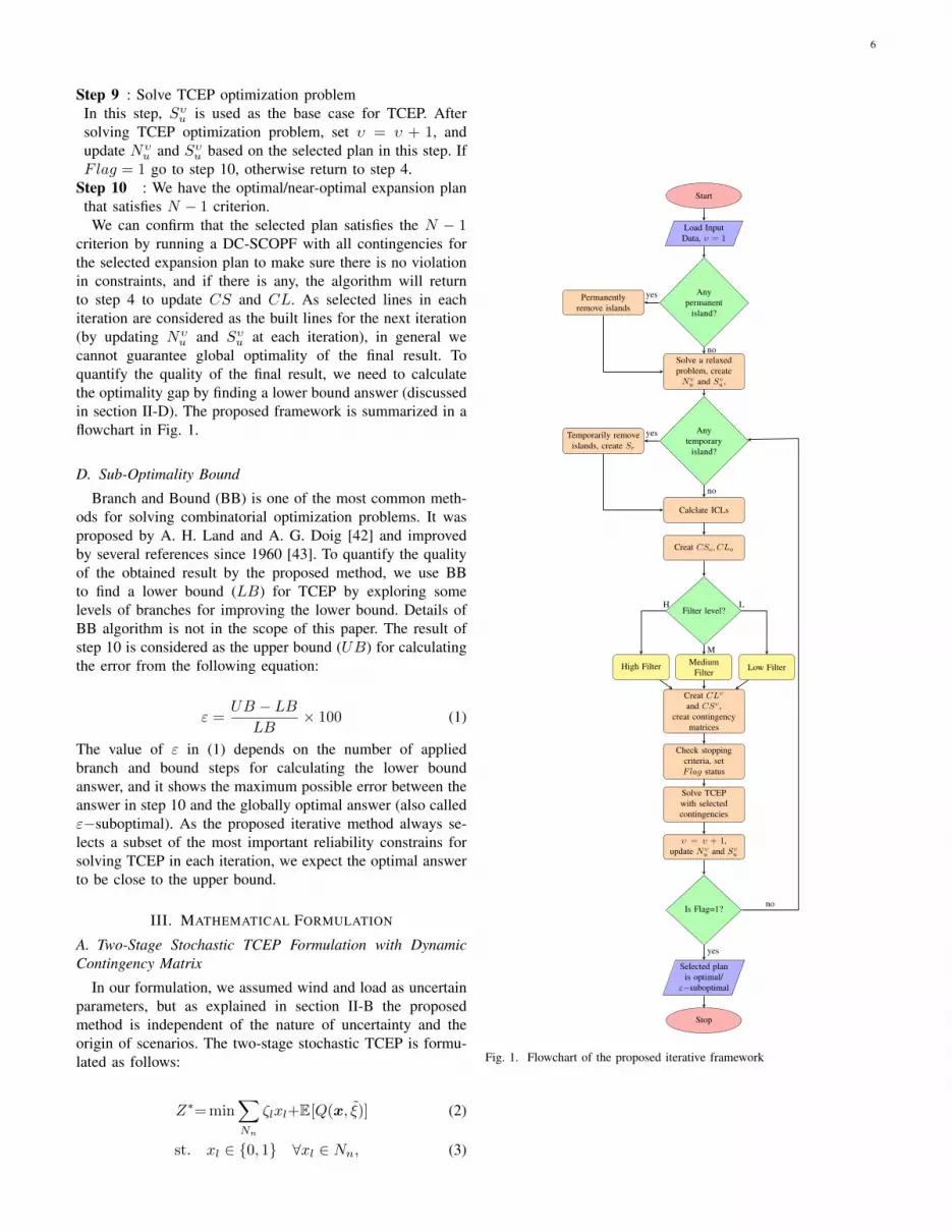
u and Sυu at each iteration), in general wecannot guarantee global optimality of the final result. Toquantify the quality of the final result, we need to calculatethe optimality gap by finding a lower bound answer (discussedin section II-D). The proposed framework is summarized in aflowchart in Fig. 1.

D. Sub-Optimality Bound

Branch and Bound (BB) is one of the most common meth-ods for solving combinatorial optimization problems. It wasproposed by A. H. Land and A. G. Doig [42] and improvedby several references since 1960 [43]. To quantify the qualityof the obtained result by the proposed method, we use BBto find a lower bound (LB) for TCEP by exploring somelevels of branches for improving the lower bound. Details ofBB algorithm is not in the scope of this paper. The result ofstep 10 is considered as the upper bound (UB) for calculatingthe error from the following equation:

ε =UB − LB

LB× 100 (1)

The value of ε in (1) depends on the number of appliedbranch and bound steps for calculating the lower boundanswer, and it shows the maximum possible error between theanswer in step 10 and the globally optimal answer (also calledε−suboptimal). As the proposed iterative method always se-lects a subset of the most important reliability constrains forsolving TCEP in each iteration, we expect the optimal answerto be close to the upper bound.

III. MATHEMATICAL FORMULATION

A. Two-Stage Stochastic TCEP Formulation with DynamicContingency Matrix

In our formulation, we assumed wind and load as uncertainparameters, but as explained in section II-B the proposedmethod is independent of the nature of uncertainty and theorigin of scenarios. The two-stage stochastic TCEP is formu-lated as follows:

Z∗= min∑Nn

ζlxl+E[Q(x, ξ)] (2)

st. xl ∈ 0, 1 ∀xl ∈ Nn, (3)

Start

Load InputData, υ = 1

Anypermanent

island?

Solve a relaxedproblem, createNυu and Sυu ,

Permanentlyremove islands

Anytemporary

island?

Calclate ICLs

Temporarily removeislands, create Sr

Creat CSo, CLo

Filter level?

High Filter MediumFilter Low Filter

Creat CLυ

and CSυ ,creat contingency

matrices

Check stoppingcriteria, setFlag status

Solve TCEPwith selectedcontingencies

υ = υ + 1,update Nυ

u and Sυu

Is Flag=1?

Selected planis optimal/

ε−suboptimal

Stop

yes

no

yes

no

H

M

L

yes

no

Fig. 1. Flowchart of the proposed iterative framework

7

where ξ is a random variable vector that represents load andwind uncertainties (ξ = (ξ1, ˜ξ2)). E[Q(x, ξ)] represents theexpected value of operation costs that contains load sheddingand wind curtailment penalty and generation costs. This ex-pected value is approximated with a weighted sum of a limitednumber of scenarios as follows [44]:

E[Q(x, ξ)] ≈∑Ω

PωQ(x, ξω) (4)

where Q(x, ξ) is the optimal value of power system operationfor given load and wind represented by ξ.

Q(x, ξ)= min∑Ns

(∑Nb

qiri,c)+∑Nb

γiCWi+∑Ng

Cogpg (5)

st. −∑Lk

fl,c+∑Gk

pg+rk,c=dk (6)

−Ml(1− Cl,cxl) ≤ fl,c−Bl,l∆θl,c (7)Ml(1− Cl,cxl) ≥ fl,c−Bl,l∆θl,c (8)

CWk ≥∑Wk

(Pmaxg − pg) (9)

(Cl,cxl)fminl ≤ fl,c ≤ fmaxl (Cl,cxl) (10)

Pming ≤ pg ≤ Pmaxg (11)

0 ≤ rk,c ≤ dk (12)

−π2≤ θk,c ≤

π

2(13)

CWk ≥ 0 (14)xl=1, ∀l ∈ No (15)xl ∈ 0, 1, ∀l ∈ Nl (16)

This optimization problem is solved in every iteration. Inequation (5), load shedding is penalized over all operatingstates (Ns) to satisfy the N − 1 criterion (no load sheddingis accepted during both normal and under single contingencystates). Equation (6) enforces power balance at each bus.Equations (7) and (8) show DC representation of flow in trans-mission lines with big M technique. Equation (9) measureswind curtailment at each bus. Equation (10) shows flow in alllines should always be between their maximum and minimumcapacity limits. These limits will be modified based on thegiven value for α for emergency conditions (contingency in thenetwork). Equations (11)-(13) enforce power plants’ dispatch,load shedding and voltage angles to be between their minimumand maximum limits. Equation (14) enforces non-negativityof wind curtailment. Equation (15) sets decision variables forexisting lines to 1. Equation (16) enforces that x is a binarydecision variable for transmission lines (x = 1 when a line isbuilt and x = 0 when a line is not built).

B. Updated Variable Contingency List (VCL) Algorithm

Modified Line Outage Distribution Factor (LODF) is usedto calculate post-contingency flow in transmission lines whenone line is on outage. The following equations are used tocreate important contingency lists for different scenarios.

Γω,υm,l =fω,υm,l − fmaxm

fmaxm

,∀m, l ∈ Nυu ,∀ω ∈ Ω (17)

Φω,υl = m ∈ Nυu |Γ

ω,υm,l ≥ α ,∀l ∈ Nυ

u ,∀ω ∈ Ω (18)

CIIω,υl =

∑Φω,υl

Γω,υm,l

|Φω,υl | , if |Φω,υl | 6= 0

0, if |Φω,υl | = 0(19)

ICLω,υ = l ∈ Nυu |CII

ω,υl ≥ αδ ,∀ω ∈ Ω (20)

δ ≥ 1, (21)

where (17) calculates over/under loading on line m when linel is out. In this equation, fω,υm,l represents the magnitude ofpost-contingency flow in line m when line l is on outage.Equations (18)-(19) are used to calculate Contingency Iden-tification Index (CII) for each scenario with α as the linecapacity modification factor during contingencies (see [37] formore details). Equation (20) creates important contingency list(ICL) based on CII . To be able to select a fraction of linesin ICLs, a relaxation factor δ is included in (20). This newcapability is useful for managing the size of CL in differentiterations.

C. Three-Level Filtering Algorithm

Algorithm 1 explains the proposed three-level filter in step 7in section II-C in more detail. To develop this algorithm,concepts explained in section II-B are used.

Algorithm 1 Three-Level FilteringRequire: CSυo , CLυo and υH ← 0 (if CSυo is not Normal)µ← mean of CSυoσ ← standard deviation of CSυoISII ← 1 (if H = 0 OR σ ≥ µ/2)if υ = 1 AND ISII = 1 (High-Level)then

ISL← Scenarios with |ICL| ≥ (µ+ σ)if |ISL| > 1 then

CSυ, CLυ ← Run SSE for ISLelse

CSυ, CLυ ← Run updated V CL for ISLend if

else if υ ≤ 3 AND µ is large (Medium-Level)then

CSυ, CLυ ← Run SSEif sum(CSυ) is still large then

CSυ, CLυ ← Run updated V CL with δ 1end if

else (Low-Level)CSυ, CLυ ← Run updated V CL with δ ≥ 1

end ifEnsure: Sum(CSυ) ≥ Sum(CSυ−1) OR CSυ = CSυo

As shown in Algorithm 1, after checking the normality ofCSυo distribution in iteration υ (H), mean (µ) and standarddeviation (σ) of the fitted normal distribution is calculated.Then the status of ISII will be set (based on H, µ, σ). In the

8

next step, conditions for selecting a filter level is checked. Forthe high-level filter, first the ISL is created, then based on thenumber of important scenarios (|ISL|), the filter goes throughSSE or the updated VCL algorithms. For the medium-levelfilter, SSE and the updated VCL algorithms (if applicable) arerun to reduce contingency lines list. The low-level filter appliesthe updated VCL algorithm to create CLυ and CSυ . In eachiteration to guarantee the algorithm’s eventual termination, itis always checked that the number of selected lines increasesor that all lines will be selected. It is critical to design thefilter in a way that effectively creates CLυ and CSυ basedon the size of the network and the number of scenarios. Insection IV-A, the detail of applying all filtering steps on anumerical case study is given.

IV. CASE STUDY AND SIMULATION RESULTS

In this section, we run numerical analysis for five casestudies on a 13-bus system (three of the cases) and a reducedERCOT system (two of the cases). All simulations are donewith a personal computer with 2.4-GHz CPU and 16 GB ofRAM. The proposed method is implemented in MATLABR2014a [45] by using YALMIP R20140221 package [46]as a modeling software and GUROBI 5.6 [47] as a solver.To calculate “Total Time”, MATLAB built-in function tictoc is used to evaluate elapsed wall clock time, and “SolverTime” is calculated by YALMIP. The case studies are solvedfor three methods i.e. the proposed method in this paper,the VCL algorithm [37] and the integrated model (in whichN − 1 contingency analysis is modeled for all lines) and theirperformance are evaluated.

A. 13-Bus System

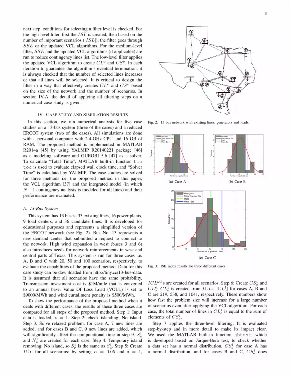
This system has 13 buses, 33 existing lines, 16 power plants,9 load centers, and 36 candidate lines. It is developed foreducational purposes and represents a simplified version ofthe ERCOT network (see Fig. 2). Bus No. 13 represents anew demand center that submitted a request to connect tothe network. High wind expansion in west (buses 3 and 6)also introduces needs for network reinforcements in west andcentral parts of Texas. This system is run for three cases i.e.A, B and C with 20, 50 and 100 scenarios, respectively, toevaluate the capabilities of the proposed method. Data for thiscase study can be downloaded from http://tiny.cc/13-bus-data.It is assumed that all scenarios have the same probability.Transmission investment cost is $1M/mile that is convertedto an annual base. Value Of Loss Load (VOLL) is set to$9000/MWh and wind curtailment penalty is $500/MWh.

To show the performance of the proposed method when itdeals with different cases, the results of these three cases arecompared for all steps of the proposed method. Step 1: Inputdata is loaded, υ = 1. Step 2: check islanding: No island.Step 3: Solve relaxed problem: for case A, 7 new lines areadded, and for cases B and C, 9 new lines are added, whichwill significantly affect the computational time in step 9. S1

u

and N1u are created for each case. Step 4: Temporary island

removing: No island, so S1r is the same as S1

u. Step 5: CreateICL for all scenarios: by setting α = 0.05 and δ = 1,

Fig. 2. 13 bus network with existing lines, generators and loads.

0 5 10 15 20 250

2

4

6

8

10

12

Number of Important Lines

Fre

qu

an

cy

Histogram

Fitted Normal Dist.

Mean

Mean+Std

(a) Case A

−5 0 5 10 15 20 250

2

4

6

8

10

12

14

Number of Important Lines

Fre

qu

an

cy

Histogram

Fitted Normal Dist.

Mean

Mean+Std

(b) Case B

−5 0 5 10 15 20 250

5

10

15

20

25

30

Number of Important Lines

Fre

qu

an

cy

Histogram

Fitted Normal Dist.

Mean

Mean+Std

(c) Case C

Fig. 3. ISII index results for three different cases

ICLω,1s are created for all scenarios. Step 6: Create CSυo andCLυo : CL1

o is created from ICLs. |CL1o| for cases A, B and

C are 219, 538, and 1041, respectively. These numbers showhow fast the problem size will increase for a large numberof scenarios even after applying the VCL algorithm. For eachcase, the total number of lines in CL1

o is equal to the sum ofelements of CS1

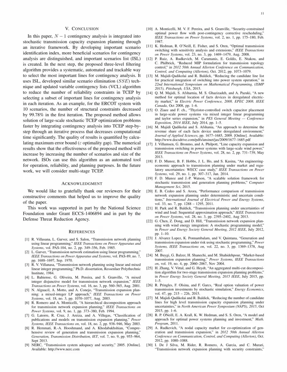
o .Step 7 applies the three-level filtering. It is evaluated

step-by-step and in more detail to make its impact clear.We used the MATLAB built-in function jbtest, whichis developed based on Jarque-Bera test, to check whethera data set has a normal distribution. CS1

o for case A hasa normal distribution, and for cases B and C, CS1

o does

9

not have a normal distribution. ISII is calculated for threecases and ISIIA = 0, ISIIB = 1, ISIIC = 1. Thehistogram and fitted normal distribution on CS1

o vector areshown in Fig. 3 for each case in the first iteration. Gray barsshow the frequency of |ICLω,1|s, and the red bell shape curverepresents the normal distribution fitted to CS1

o . Green dashedline indicates mean (µ) of the fitted normal distribution andblue solid line represents mean+std (µ+ σ). If ISII is equalto 1, then scenarios on the right side of the blue line will betagged as important scenarios. Important Scenarios List (ISL)for each case is given in the second row of Table I. Case Ahas no important scenario, as its CS1

o distribution is normaland its standard deviation is less than half of its mean (seeFig. 3(a)). For case B and C (see Fig. 3(b),(c)) ISII = 1, andthere are 5 and 10 important scenarios for these two cases. Forthe first iteration, the filter selects 108 lines for contingencyanalysis for case A (

∑Ω |N

ω,1sA | = 128 operation states), 70

lines for case B (∑

Ω |Nω,1sB | = 120) and 153 lines for case C

(∑

Ω |Nω,1sC | = 253). To evaluate the impact of the proposed

filter on the problem size, the total number of operation states(∑

Ω |Nω,1s |) that should be considered by different methods

is given in Table II. With only using the VCL algorithmfrom [37] (without using the filter introduced in this paper),TCEP with 239, 588 and 1141 operation states should besolved for these three cases, which are much harder to solveand need significantly more computational time. Based on thelast row of the table, for the integrated model that considersall lines for contingency analysis, the problem size will beso large as to easily make medium and large scale problemsunsolvable. Fig. 4 shows the impact of the filter on reducingthe size of CLυ in different iterations. Blue, red, and greencolors represent case A, B and C respectively. Dashed linesshow the original number of important lines (|CLυo |), and solidlines show selected lines by the filter (|CLυ|) in each iteration.The difference between dashed and solid lines in each iterationshows the impact of the filter on reducing |CL| for each case.Reducing |CLυo | from one iteration to another is because of thedeveloped framework that iteratively solves TCEP and updatesNu and Su. As cases B and C have important scenarios, linesin CL1 are selected among ICLs of scenarios in their ISLscompared to case A, in which CL1 is created from ICLs ofall scenarios in the first iteration. CLυo and CLυ are gettingcloser and closer to each other from iteration υ to iterationυ+1 and this guarantees the algorithm’s termination. The thirdrow of Table I shows how the algorithm moves between thefilter’s levels during iterations for different cases. During twoiterations for case A, the algorithm selects medium and lowlevels respectively. For cases B and C, it selects High, Medium,Medium, Low and Low levels. The number of iterations andfiltering levels are selected based on problem characteristicsthat demonstrates the dynamic behavior of the filter.

In step 8, stopping criteria is checked. As shown in Fig. 4,at iterations 2, 5 and 5, respectively, CSυ = CSυo and Flagis set to 1 for cases A, B and C, respectively. In step 9, TCEPoptimization problem with selected contingencies is solved,υ = υ + 1, and Nυ

u and Sυu are updated in each iteration.The algorithm gets to step 10 after 2, 5 and 5 iterations for

TABLE IISLS AND SELECTED FILTER LEVELS FOR 13-BUS SYSTEM

Case A Case B Case C

ISL −− 17, 32, 41, 42, 50 17, 32, 41, 42, 50,57, 78, 94, 96,97

FilterLevels

Medium,Low

High, Medium,Medium, Low, Low

High, Medium,Medium, Low, Low

TABLE IITOTAL NUMBER OF OPERATING STATES IN THE FIRST ITERATION FOR

DIFFERENT CASE STUDIES

Case A Case B Case C

Proposed method 128 120 253

VCL algorithm 239 588 1141

Integrated model 1400 3500 7000

cases A, B and C. Selected lines and total costs are givenin the second and third rows in Table III. Case A adds 11new lines, and case B and C add 16 lines to the network.The simulation time for the proposed method is given in thefourth row in Table III. The difference between total time andsolver time in the fourth row of this table represents the timethat the filter and the modeling language need in the processof solving the TCEP optimization problem. The design of thefilter will affect both solver and total time. To make sure thatthese results satisfy N − 1 criterion, DC-SCOPF is run for allcontingencies, and no violation occurs.

To calculate ε to quantify the quality of results in step 10,a lower bound is calculated by applying a few steps in a BBalgorithm. It is possible to apply more steps to get a betterlower bound answer. The error bounds for three cases aregiven in the last row in Table III. It shows 1.3%, 2.25%and 2.9% as the upper bound error for cases A, B and Crespectively. However, these are not the actual error betweenoptimal answer and our results.

To compare the actual error with ε and show the impactof the proposed method on reducing computational time, werun these three cases with the proposed algorithm in [37] andthe integrated model. The actual error is shown in the lastrow in Table III. It shows that for all three cases the actualerror is zero, which means the proposed method found theoptimal plan for these cases. It should be mentioned that asin real cases we do not know the exact answer, the quality ofour answer is quantified by the calculated ε. In other words,our answer is ε−suboptimal. The performance of these threedifferent methods is compared in Table IV. Each row in thistable shows the simulation time each method needs to solvethese case studies. The ratio of the third row to the secondrow in this table shows how much the proposed method inthis paper performs better compared to [37] for stochasticTCEP. This ratio is more than 35, 420 and 650 for cases A, Band C respectively and shows the relative performance ofthe proposed method increases with increasing problem size.Compared to the integrated model, the proposed method gets

10

1 2 3 4 50

200

400

600

800

1000

1200

Iteration

Nu

mb

er

of

Imp

ort

an

t L

ine

s

Case C (100 scenarios)

Case A (20 scenarios)

Case B (50 scenarios)

Fig. 4. Impact of the iterative framework and the three-level filtering on|CLυo | and |CLυ | in different iterations

TABLE IIITRANSMISSION EXPANSION PLANNING FOR 13-BUS SYSTEM

Case A Case B Case C

SelectedLines

2-1, 2-1,3-2, 3-2,3-6, 6-9,7-10, 8-12,13-5, 13-6,13-6

2-1, 2-1, 1-6,1-6, 3-2, 3-2,3-6, 4-10, 4-11,7-10, 8-10, 8-10,8-12, 13-5, 13-5,13-6

2-1, 2-1, 1-6,1-6, 3-2, 3-2,3-6, 4-10, 4-11,7-10, 8-10, 8-10,8-12, 13-5, 13-5,13-6

Total Cost ($ M) 4889 4986.4 4945.9

Solver (sec) 27.2 177.8 1252Total (sec) 33.15 243.6 1443

ε 1.3% 2.25% 2.9%Actual Err 0% 0% 0%

the answer more than 15657 times faster for case A, and wecould not get any answer even after 12 days for cases B and C.This great performance is achieved because of huge problemsize reduction using the filter through the iterative framework.For example for case C, in the first iteration, the proposedmethod decreases the number of structural constraints by 85%compared to [37] and by 98% compared to the integratedmodel.

B. Reduced ERCOT System

A reduced model of the ERCOT system is provided in [21].This model is developed for evaluating the impact of highpenetration of wind power on west Texas network. Therefore,the west part of ERCOT network in modeled in detail, and therest of ERCOT is simplified into three zones. This networkcontains 317 buses, 427 branches, 489 conventional powerplants, 36 wind farms and 182 load centers. The number ofcandidate lines is equal to the number of existing lines. In thisTCEP optimization problem, there are 427 binary variables,which makes it a challenging problem to solve. All parametersare set the same as the 13-bus system. We consider two casesfor the ERCOT system i.e. case A with 5 scenarios and caseB with 10 scenarios. Scenarios are generated using historicalload and wind data [21]. For case A, scenario 5 is selectedas the important scenario, and scenarios 5 and 6 are in ISL

TABLE IVTOTAL SIMULATION TIME FOR DIFFERENT METHODS [MINUTES]

Case A Case B Case C

Proposed method 0.55 4.06 24.05

VCL algorithm 19.9 1714 15659

Integrated model 8768 (6+ days) NA NA

TABLE VTRANSMISSION EXPANSION PLANNING FOR REDUCED ERCOT SYSTEM

Case A Case B

SelectedLines

1311-1064,1310-1309,1312-1310,1313-1312,1315-1313,1067-1315,1065-1064,1066-1065,5905-5902

1311-1064, 1310-1309,1312-1310, 1313-1312,1315-1313, 1067-1315,1065-1064, 1066-1065,5905-5902, 60042-6216,60042-60040

Total Cost ($ M) 16298 16857

Solver (sec) 358 871Total (sec) 630 1160

ε 0.96% 1.01%Actual Err 0% 0%

for case B. The original number of important lines (|CL1o|)

is 23 and 52 respectively, and the three-level filter selects 10and 19 lines for the first iteration in case A and B. Both casestake two iterations to converge, and go through High and Lowlevel filters.

The selected plan, total costs, solver and total time withε and actual error are shown in Table V. The number ofselected lines is 9 and 11 for case A and B respectively. εis around 1% for the reduced ERCOT system (the answer is1%−suboptimal). Both cases are also solved with the devel-oped algorithm in [37] and the integrated model to comparethe results with the proposed method in this paper. As shownin the last row in Table V, actual errors for both cases arezero, which shows the proposed method found the optimalexpansion plan for this system. The solver and total time areshown in the fourth row. For case A, the proposed methodin [37] needs 181 minutes to solve the problem (comparedto 10.5 minutes required with the proposed method in thispaper), and for case B, [37] needs 12 days and 6 hours and56 minutes to solve the problem (compared to 19.3 minutesrequired by the proposed method in this paper). We did notget the answer from the integrated model after 34 days (stillmore than 75% optimality gap). Although the number ofscenarios are not large for this system (compared to the 13-Bussystem), the proposed method gets the answer more than 910times faster than [37], and the relative performance improvesmore when the number of scenarios increases. Moreover, therelative performance improvement of the proposed methodgrows faster for larger networks, as the ratio for the ERCOTcase B with 10 scenarios is more than 27 times larger thanthe ratio for the 13-bus case A with 20 scenarios.

11

V. CONCLUSION

In this paper, N − 1 contingency analysis is integrated intostochastic transmission capacity expansion planning throughan iterative framework. By developing important scenarioidentification index, more beneficial scenarios for contingencyanalysis are distinguished, and important scenarios list (ISL)is created. In the next step, the proposed three-level filteringalgorithm provides a systematic, automated and trackable wayto select the most important lines for contingency analysis. Ituses ISL, developed similar scenario elimination (SSE) tech-nique and updated variable contingency lists (VCL) algorithmto reduce the number of reliability constraints in TCEP byselecting a subset of important lines for contingency analysisin each iteration. As an example, for the ERCOT system with10 scenarios, the number of structural constraints decreasedby 99.78% in the first iteration. The proposed method allowssolution of large-scale stochastic TCEP optimization problemsfaster by integrating contingency analysis into TCEP step-by-step through an iterative process that decreases computationaltime significantly. The quality of results is quantified by calcu-lating maximum error bound (ε optimality gap). The numericalresults show that the effectiveness of the proposed method willincrease by increasing the number of scenarios and size of thenetwork. ISOs can use this algorithm as an automated toolfor operation, reliability, and planning purposes. In the futurework, we will consider multi-stage TCEP.

ACKNOWLEDGMENT

We would like to gratefully thank our reviewers for theirconstructive comments that helped us to improve the qualityof the paper.

This work was supported in part by the National ScienceFoundation under Grant ECCS-1406894 and in part by theDefense Threat Reduction Agency.

REFERENCES

[1] R. Villasana, L. Garver, and S. Salon, “Transmission network planningusing linear programming,” IEEE Transactions on Power Apparatus andSystems, vol. PAS-104, no. 2, pp. 349–356, Feb. 1985.

[2] L. Garver, “Transmission network estimation using linear programming,”IEEE Transactions on Power Apparatus and Systems, vol. PAS-89, no. 7,pp. 1688–1697, Sep. 1970.

[3] R. V. Villanasa, “Transmission network planning using linear and mixedlinear integer programming,” Ph.D. dissertation, Ressenlaer PolythechnicInstitute, 1984.

[4] L. Bahiense, G. Oliveira, M. Pereira, and S. Granville, “A mixedinteger disjunctive model for transmission network expansion,” IEEETransactions on Power Systems, vol. 16, no. 3, pp. 560–565, Aug. 2001.

[5] N. Alguacil, A. Motto, and A. Conejo, “Transmission expansion plan-ning: a mixed-integer LP approach,” IEEE Transactions on PowerSystems, vol. 18, no. 3, pp. 1070–1077, Aug. 2003.

[6] R. Romero and A. Monticelli, “A hierarchical decomposition approachfor transmission network expansion planning,” IEEE Transactions onPower Systems, vol. 9, no. 1, pp. 373–380, Feb. 1994.

[7] G. Latorre, R. Cruz, J. Areiza, and A. Villegas, “Classification ofpublications and models on transmission expansion planning,” PowerSystems, IEEE Transactions on, vol. 18, no. 2, pp. 938–946, May 2003.

[8] R. Hemmati, R.-A. Hooshmand, and A. Khodabakhshian, “Compre-hensive review of generation and transmission expansion planning,”Generation, Transmission Distribution, IET, vol. 7, no. 9, pp. 955–964,Sept 2013.

[9] NERC, “Transmission system adequacy and security,” 2005. [Online].Available: http://www.nerc.com

[10] A. Monticelli, M. V. F. Pereira, and S. Granville, “Security-constrainedoptimal power flow with post-contingency corrective rescheduling,”IEEE Transactions on Power Systems, vol. 2, no. 1, pp. 175–180, Feb.1987.

[11] K. Hedman, R. O’Neill, E. Fisher, and S. Oren, “Optimal transmissionswitching with sensitivity analysis and extensions,” IEEE Transactionson Power Systems, vol. 23, no. 3, pp. 1469–1479, Aug. 2008.

[12] P. Ruiz, A. Rudkevich, M. Caramanis, E. Goldis, E. Ntakou, andC. Philbrick, “Reduced MIP formulation for transmission topologycontrol,” in 2012 50th Annual Allerton Conference on Communication,Control, and Computing (Allerton), Oct. 2012, pp. 1073–1079.

[13] M. Majidi-Qadikolai and R. Baldick, “Reducing the candidate line listfor practical integration of switching into power system operation,” in22nd International Symposium on Mathematical Programming, (ISMP2015), Pittsburgh, USA, 2015.

[14] Q. M. Majidi, S. Afsharnia, M. S. Ghazizadeh, and A. Pazuki, “A newmethod for optimal location of facts devices in deregulated electric-ity market,” in Electric Power Conference, 2008. EPEC 2008. IEEECanada, Oct 2008, pp. 1–6.

[15] O. Ziaee and F. ch., “Thyristor-controlled switch capacitor placementin large-scale power systems via mixed integer linear programmingand taylor series expansion,” in PES General Meeting — ConferenceExposition, 2014 IEEE, July 2014, pp. 1–5.

[16] M. Majidi Qadikolai and S. Afshania, “An approach to determine therevenue share of each facts device under deregulated environment,”Journal of Applied Sciences, pp. 1677–1685, 2009. [Online]. Available:http://www.docsdrive.com/pdfs/ansinet/jas/2009/1677-1685.pdf

[17] J. Villumsen, G. Bronmo, and A. Philpott, “Line capacity expansion andtransmission switching in power systems with large-scale wind power,”IEEE Transactions on Power Systems, vol. 28, no. 2, pp. 731–739, May2013.

[18] F. D. Munoz, B. F. Hobbs, J. L. Ho, and S. Kasina, “An engineering-economic approach to transmission planning under market and regu-latory uncertainties: WECC case study,” IEEE Transactions on PowerSystems, vol. 29, no. 1, pp. 307–317, Jan. 2014.

[19] F. D. Munoz and J.-P. Watson, “A scalable solution framework forstochastic transmission and generation planning problems,” ComputerManagement Sci, 2015.

[20] E. B. Cedeo and S. Arora, “Performance comparison of transmissionnetwork expansion planning under deterministic and uncertain condi-tions,” International Journal of Electrical Power and Energy Systems,vol. 33, no. 7, pp. 1288 – 1295, 2011.

[21] H. Park and R. Baldick, “Transmission planning under uncertainties ofwind and load: Sequential approximation approach,” IEEE Transactionson Power Systems, vol. 28, no. 3, pp. 2395–2402, Aug 2013.

[22] G. Chen, Z. Dong, and D. Hill, “Transmission network expansion plan-ning with wind energy integration: A stochastic programming model,”in Power and Energy Society General Meeting, 2012 IEEE, July 2012,pp. 1–10.

[23] J. Alvarez Lopez, K. Ponnambalam, and V. Quintana, “Generation andtransmission expansion under risk using stochastic programming,” PowerSystems, IEEE Transactions on, vol. 22, no. 3, pp. 1369–1378, Aug2007.

[24] M. Buygi, G. Balzer, H. Shanechi, and M. Shahidehpour, “Market-basedtransmission expansion planning,” Power Systems, IEEE Transactionson, vol. 19, no. 4, pp. 2060–2067, Nov 2004.

[25] H. Zhang, V. Vittal, and G. Heydt, “An aggregated multi-cut decomposi-tion algorithm for two-stage transmission expansion planning problems,”in Power Energy Society General Meeting, 2015 IEEE, July 2015, pp.1–5.

[26] R. Pringles, F. Olsina, and F. Garcs, “Real option valuation of powertransmission investments by stochastic simulation,” Energy Economics,vol. 47, pp. 215 – 226, 2015.

[27] M. Majidi-Qadikolai and R. Baldick, “Reducing the number of candidatelines for high level transmission capacity expansion planning underuncertainties,” in North American Power Symposium (NAPS), 2015, Oct2015, pp. 1–6.

[28] R. P. ONeill, E. A. Krall, K. W. Hedman, and S. S. Oren, “A model andapproach for optimal power systems planning and investment,” Math.Program, 2011.

[29] A. Rudkevich, “A nodal capacity market for co-optimization of gen-eration and transmission expansion,” in 2012 50th Annual AllertonConference on Communication, Control, and Computing (Allerton), Oct.2012, pp. 1080–1088.

[30] I. De J Silva, M. Rider, R. Romero, A. Garcia, and C. Murari,“Transmission network expansion planning with security constraints,”

12

Generation, Transmission and Distribution, IEE Proceedings-, vol. 152,no. 6, pp. 828–836, Nov 2005.

[31] H. Zhang, G. Heydt, V. Vittal, and J. Quintero, “An improved networkmodel for transmission expansion planning considering reactive powerand network losses,” Power Systems, IEEE Transactions on, vol. 28,no. 3, pp. 3471–3479, Aug 2013.

[32] T. Akbari, A. Rahimikian, and A. Kazemi, “A multi-stage stochastictransmission expansion planning method,” Energy Conversion and Man-agement, vol. 52, no. 89, pp. 2844 – 2853, 2011.

[33] A. Khodaei, M. Shahidehpour, and S. Kamalinia, “Transmission switch-ing in expansion planning,” IEEE Transactions on Power Systems,vol. 25, no. 3, pp. 1722–1733, Aug. 2010.

[34] L. Garces, A. Conejo, R. Garcia-Bertrand, and R. Romero, “A bilevelapproach to transmission expansion planning within a market environ-ment,” Power Systems, IEEE Transactions on, vol. 24, no. 3, pp. 1513–1522, Aug 2009.

[35] M. Carrion, J. Arroyo, and N. Alguacil, “Vulnerability-constrainedtransmission expansion planning: A stochastic programming approach,”Power Systems, IEEE Transactions on, vol. 22, no. 4, pp. 1436–1445,Nov 2007.

[36] I. Konstantelos and G. Strbac, “Valuation of flexible transmission in-vestment options under uncertainty,” Power Systems, IEEE Transactionson, vol. 30, no. 2, pp. 1047–1055, March 2015.

[37] M. Majidi-Qadikolai and R. Baldick, “Integration of N-1 contingencyanalysis with systematic transmission capacity expansion planning:ERCOT case study,” IEEE Transactions on Power Systems, 2015.

[38] ——, “Large-scale transmission capacity expansion planning under n-1 contingency analysis,” in INFORMS Annual Meeting, Philadelphia,Nov. 2015.

[39] F. D. Munoz, J.-P. Watson, and B. F. Hobbs, “Optimizing your options:Extracting the full economic value of transmission when planning underuncertainty,” The Electricity Journal, vol. 28, no. 5, pp. 26 – 38, 2015.

[40] ——, “New bounding and decomposition approaches for MILP in-vestment problems: Multi-area transmission and generation planningunder policy constraints,” Sandia National Laboratories (SNL-NM), no.SAND2014-4398J, 2014.

[41] H. C. Thode, Testing For Normality. CRC Press, 2002.[42] A. H. Land and A. G. Doig, “An Automatic Method for Solving Discrete

Programming Problems,” Econometrica, vol. 28, pp. 497–520, 1960.[43] J. Clausen, Branch and Bound Algorithms-Principles and Examples,

March 1999.[44] Y. Ermoliev and R. J.-B. Wets, Numerical Techniques for Stochastic

Optimization. Springer series in computational mathematics, 1988.[45] MATLAB, version 8.3.0.532 (R2014a). Natick, Massachusetts: The

MathWorks Inc., 2014.[46] J. Lofberg, “Yalmip : A toolbox for modeling and optimization in

MATLAB,” in Proceedings of the CACSD Conference, Taipei, Taiwan,2004. [Online]. Available: http://users.isy.liu.se/johanl/yalmip

[47] Gurobi Optimization, Inc., “Gurobi optimizer reference manual,” 2014.[Online]. Available: http://www.gurobi.com

Mohammad Majidi-Qadikolai (S’14) received his BSc and MSc in elec-trical engineering from Power and Water University of Technology and theUniversity of Tehran respectively. He is currently pursuing his PhD programin electrical engineering at The University of Texas at Austin. His researchinterests include power system planning and operation under uncertainties,stochastic programming, renewable energy integration and electricity markets.

Ross Baldick (F’07) received the B.Sc. degree in mathematics and physicsand the B.E. degree in electrical engineering from the University of Sydney,Australia, and the M.S. and Ph.D. degrees in electrical engineering andcomputer sciences in 1988 and 1990, respectively, from the University ofCalifornia, Berkeley, Berkeley, CA, USA.

From 1991 to 1992, he was a Post-Doctoral Fellow at the LawrenceBerkeley Laboratory. In 1992 and 1993, he was an Assistant Professor atWorcester Polytechnic Institute, Worcester, MA, USA. He is currently aProfessor in the Department of Electrical and Computer Engineering at TheUniversity of Texas at Austin, Austin, TX, USA.