arX

iv:0

909.

4821

v1 [

mat

h.ST

] 2

5 Se

p 20

09

Hierarchical subspace models for contingency tables

Hisayuki Hara∗, Tomonari Sei† and Akimichi Takemura‡§

September 25, 2009

Abstract

For statistical analysis of multiway contingency tables we propose modeling in-teraction terms in each maximal compact component of a hierarchical model. Bythis approach we can search for parsimonious models with smaller degrees of free-dom than the usual hierarchical model, while preserving conditional independencestructures in the hierarchical model. We discuss estimation and exacts tests of theproposed model and illustrate the advantage of the proposed modeling with somedata sets.

Keywords : context specific interaction model, divider, Markov bases, split model, uniformassociation model.

1 Introduction

Modeling of the interaction term is an important topic for two-way contingency tables,because there is a large gap between the independence model and the saturated model.This problem is clearly of importance for contingency tables with three or more factors.However modeling strategies of higher order interaction terms have not been fully dis-cussed in literature. In this paper we propose modeling interaction terms of multiwaycontingency tables by considering each maximal compact component of a hierarchicalmodel.

For two-way contingency tables the uniform association model (Goodman [1979, 1985])and the RC association model (Goodman [1979, 1985], Kuriki [2005]) are often usedfor modeling interaction terms. In the analysis of agreement among raters, where dataare summarized as square contingency tables with the same categories, many modelswith interaction in diagonal elements and their extension to multiway tables have beenconsidered (e.g. Tanner and Young [1985], Tomizawa [2009]). Hirotsu [1997] proposed

∗Department of Technology Management for Innovation, University of Tokyo†Graduate School of Information Science and Technology, University of Tokyo‡Graduate School of Information Science and Technology, University of Tokyo§CREST, JST

1

a two-way change point model and Hara et al. [2009] generalized it to a subtable summodel. For multiway contingency tables Højsgaard [2003] considered the split model asa generalization of graphical models. The context specific interaction model defined byHøjsgaard [2004] is a more general model than the split model.

We give a unified treatment of these models as submodels of hierarchical models.Malvestuto and Moscarini [2000] showed that a hierarchical model possesses a compaction,i.e. the variables are grouped into maximal compact components separated by dividers.Variables of different maximal compact components separated by a divider are condition-ally independent given the variables of the divider. Furthermore the likelihood functionfactors as a rational function of marginal likelihoods, where the numerator corresponds tomaximal compact components and the denominator corresponds to dividers. By this fac-torization, statistical inference on a hierarchical model can be localized to each maximalcompact component. In the case of decomposable model, maximal compact componentsand dividers reduce to maximal cliques and minimal vertex separators of a chordal graph,respectively, and the above factorization is well known (e.g. Section 4.4 of Lauritzen[1996]).

In a usual hierarchical model each maximal interaction effect is saturated, i.e. thereis no restriction on the parameters for maximal interaction effects. However, as in thetwo-way tables, we can consider submodels for interaction effects. In the modeling pro-cess, it is advantageous to treat each maximal compact component of a hierarchical modelseparately and to keep the compaction of the hierarchical model. By respecting the com-paction of the hierarchical model, conditional independence property and the localizationproperty of the hierarchical model are preserved. We call a resulting model a hierarchi-cal subspace model. We prove some properties of our proposed model and illustrate itsadvantage with some data sets.

The organization of the paper is as follows. For the rest of this section, as a motivatingexample, we consider a submodel of the conditional independence model for three-waycontingency tables. In Section 2 we define the hierarchical subspace model and discuss thelocalization of inference through the decomposition of the model into maximal extendedcompact components. We also discuss maximum likelihood estimation of the proposedmodel. In Section 3 we study the split model in the framework of this paper. In Section4 we present construction of Markov bases for conditional tests of the model. Fitting ofthe proposed model to several real data sets is presented in Section 5. Some concludingremarks are given in Section 6.

1.1 A motivating example: subspace conditional independence

model for three-way tables

As an illustration of hierarchical subspace models we discuss a submodel of conditionalindependence model for three-way tables. Denote the sample size by n = x+++. Consideran I × J ×K contingency table and let pijk denote the probability of the cell. Marginalprobabilities are denoted by pi++, pij+, etc. Similar notation is used for the frequenciesx = {xijk} of the contingency table. Consider the conditional independence model i ⊥⊥

2

k | j, which is expressed bylog pijk = aij + bjk. (1)

In the usual conditional independence model, aij ’s and bjk’s are free parameters. Nowsuppose that we have known functions φij depending on i and j and ψjk depending onj and k. Separating main effects, consider the following submodel of the conditionalindependence model

log pijk = αi + βj + γk + δφij + δ′ψjk. (2)

The parameters of this model are {αi}Ii=1, {βj}

Jj=1, {γk}

Kk=1 and δ, δ′. The uniform associ-

ation model is specified by φij = ij. The two-way change point model in Hirotsu [1997]is specified by

φij =

{

1, if i ≤ I1 and j ≤ J1,

0, otherwise,

where 1 ≤ I1 < I, 1 ≤ J1 < J . Similarly we can specify ψjk according to many wellknown models.

As a submodel of the conditional independence model, i ⊥⊥ k | j holds for (2) and wecan write

pijk =pij+p+jk

p+j+.

Moreover, since {βj}Jj=1 are free parameters, the model is saturated for the main effect

of the second factor. This implies that the maximum likelihood estimate (MLE) of themodel is obtained as

pijk =pij+p+jk

x+j+/n. (3)

Here pij+ is the MLE of the following model for the marginal probability

log pij+ = αi + βj + δφij (4)

and pij+ only depends on the marginal frequencies {xij+}. Similarly p+jk is the MLE for(j, k)-marginal probabilities:

log p+jk = βj + γk + δ′ψjk. (5)

In this way the maximum likelihood estimation of the model (2) is localized to estimationsof two marginal models.

In our model (2) it is important to note that δ and δ′ are free parameters. Consideran additional constraint H : δ = δ′ to (2):

log pijk = αi + βj + γk + δ(φij + ψjk). (6)

This model is still log-affine and contained in the conditional independence model. How-ever, because both the (i, j)-marginals and the (j, k)-marginals are relevant for the esti-mation of the common value of δ, we can not localize estimation of the parameters totwo marginal tables. This consideration shows that it is convenient to set up a log-affine

3

model, which is “conformal” to the conditional independence model. We will appropri-ately define the notion of conformality in Section 2.

In our model we can also allow certain patterns of structural zeros. Consider the dataon song sequence of a wood pewee in Section 7.5.2 of Bishop et al. [1975]. The data isshown in Table 1. The wood pewee has a repertoire of four distinctive phrases. Theobserved data consists of 198 triplets of consecutive phrases (i, j, k) ∈ {1, 2, 3, 4}3. It is a4× 4× 4 contingency table with the cells of the form (i, i, k) and (i, j, j) being structuralzeros.

Table 1: Triples of phrases in a song sequence of a wood pewee, with repeats deleted.

Third placeFirst place Second place A B C D

A A — — — —B 19 — 2 2C 2 26 — 0D 12 5 0 —

B A — 9 6 12B — — — —C 24 1 — 1D 1 2 0 —

C A — 4 22 0B 3 — 22 0C — — — —D 1 0 0 —

D A — 11 0 4B 5 — 1 1C 0 0 — 0D — — — —

Source: Craig [1943]

The model considered in Bishop et al. [1975] is written as

pijk = 1{i6=j}eaij1{j 6=k}e

bjk , (7)

where aij and bjk are free parameters. With some abuse of notation (7) can be written as

log pijk = aij1{i6=j} + (−∞)1{i=j} + bjk1{j 6=k} + (−∞)1{j=k}.

As (2), this model is a conditional independence model and also it is saturated for themain effect of the second factor. Therefore the MLE for this model is again expressed as(3). An appropriate handling of (−∞) and further analysis are given in Section 5.

In Section 3, we also consider the split model defined by Højsgaard [2003] as animportant example of the hierarchical subspace model. Here we give an example of the

4

split model for the three-way table {xijk} by

log pijk = ai + bj + ck + (dij + ejk)1{j∈J1},

where J1 is a subset of {1, . . . , J}. This model means that the interaction between i andj (resp. j and k) exists only if j ∈ J1. The general definition of split models is given inSection 3 and a numerical example of it is given in Section 5.

We now consider the conditional goodness of fit test of the model based on the Markovbasis methodology (Diaconis and Sturmfels [1998]). Assume that φij ’s and ψjk’s in (2) areintegers. Furthermore suppose that Markov bases B12 and B23 are already obtained for twomarginal models (4) and (5). Following the notation in Section 2 of Dobra and Sullivant[2004], write a particular move z = {z(i, j)} of degree d in the Markov basis B12 for (4)as

z = [{(i1, j1), . . . , (id, jd)}‖{(i′1, j

′1), . . . , (i

′d, j

′d)}], (8)

where (i1, j1), . . . , (id, jd) are cells (with replication) of positive elements of z and (i′1, j′1),

. . . , (i′d, j′d) are cells of negative elements of z. By replication we mean that the same cell

(i, j) is repeated |z(i, j)| times in (8). Extend the move z to three-way table as

zk1,...,kd = [{(i1, j1, k1), . . . , (id, jd, kd)}‖{(i′1, j

′1, k1), . . . , (i

′d, j

′d, kd)}],

where k1, . . . , kd ∈ {1, . . . , K} are arbitrary. Similarly for a move

z = [{(j1, k1), . . . , (jd, kd)}‖{(j′1, k

′1), . . . , (j

′d, k

′d)}] ∈ B23

letzi1,...,id = [{(i1, j1, k1), . . . , (id, jd, kd)}‖{(i1, j

′1, k

′1), . . . , (id, j

′d, k

′d)}].

Let B{1,2},{2,3} denote a Markov basis for conditional independence model (1). Followingthe argument in Dobra and Sullivant [2004] we easily see that

B = B{1,2},{2,3} ∪ {zk1,...,kdeg z , z ∈ B12, 1 ≤ k1, . . . , kdeg z ≤ K}

∪ {zi1,...,ideg z , z ∈ B23, 1 ≤ i1, . . . , ideg z ≤ I}

is a Markov basis for (2). Therefore the problem of conditional test of the model (2) isalso localized to two marginal models.

For the rest of this paper, we generalize the above results to a log-affine model.

2 Hierarchical subspace models and their decompo-

sitions

In this section we give a definition of hierarchical subspace models for I1 × · · · × Imcontingency tables and discuss its decomposition by partial edge separators. In Section2.1 we define a hierarchical subspace model. In Section 2.2 we prove that for any log-affinemodel there exists a natural smallest decomposable model, such that the the log-affinemodel is a hierarchical subspace model of the decomposable model. In Section 2.3 wediscuss properties of hierarchical models containing a given log-affine model.

5

2.1 Definition of a hierarchical subspace model

We give a definition of a hierarchical subspace model and also discuss the localization ofmaximum likelihood estimation of the proposed model. We follow notation of Lauritzen[1996] and Malvestuto and Moscarini [2000].

Let V = RI1×···×Im denote the set of I1 × · · · × Im tables with real entries, where

Ij ≥ 2 for all j. V is considered as an I1 × · · · × Im-dimensional real vector space offunctions (tables) from I = [I1] × · · · × [Im] to R, where [J ] denotes {1, . . . , J}. Aprobability distribution over I is denoted by {p(i), i ∈ I}. Let L be a linear subspaceof V containing the constant function 1 ∈ L. A log-affine model specified by L is givenby log p(·) ∈ L, where log p(·) denotes {log p(i), i ∈ I}. In the following we only considerlinear subspaces of V containing the constant function 1.

Let D be a subset of [m] = {1, . . . , m}. iD = {ij , j ∈ D} is a D-marginal cell. p(iD)denotes the marginal probability of a probability distribution p(·). Similarly x(iD) denotesthe marginal frequency of the contingency table x = {x(i), i ∈ I}. As in Sei et al. [2008]let

LD = {ψ ∈ V | ψ(i1, . . . , im) = ψ(i′1, . . . , i′m) if ih = i′h, ∀h ∈ D}

denote the set of functions depending only on iD. LD is considered as RID , where ID =

∏

h∈D Ih. Hence we have L[m] = V . For a subspace L and D ⊂ [m], we say that D issaturated in L if LD ⊂ L. D is saturated in L if and only if the sufficient statistic for Lfixes all the D-marginals of the contingency table. Note that if D is saturated in L, thenevery E ⊂ D is saturated in L.

Let ∆ denote a simplicial complex on [m] and let red ∆ denote the set of maximalelements, i.e. facets, of ∆. Then the hierarchical model associated with ∆ is defined as

log p(·) ∈ L∆def=

∑

D∈red ∆

LD,

where the right-hand side is the summation of vector spaces. We note that red ∆ isconsidered as a hypergraph. Here we summarize some notions on hypergraphs accordingto Malvestuto and Moscarini [2000]. A subset of a hyperedge of red ∆ is called a partialedge. A partial edge S is a separator of red ∆ if the subhypergraph of red ∆ induced by[m] \ S is disconnected. A partial edge separator S of red ∆ is called a divider if thereexist two vertices u, v ∈ [m] that are separated by S but by no proper subset of S. Iftwo vertices u, v ∈ [m] are not separated by any partial edge, u and v are called tightlyconnected. A subset C ⊂ [m] is called a compact component if any two variables in C aretightly connected. Denote the set of maximal compact components of red ∆ by C. Thenthere exists a sequence of maximal compact components C1, . . . , C|C| such that

(C1 ∪ · · · ∪ Ck−1) ∩ Ck = Sk

and Sk, k = 2, . . . , |C| are dividers of red ∆. We denote S = {S2, . . . , S|C|}. S is a multisetin general.

6

Let W1, . . . ,WK be linear subspaces of V and let W = W1 + · · · + WK . We say thata subspace L is conformal to {Wj}

Kj=1 if

L = (L ∩W1) + · · · + (L ∩WK).

Any L conformal to {Wj}Kj=1 is clearly a subspace of W . Note that the relation L =

L ∩W ⊃ (L ∩W1) + · · · + (L ∩WK) always holds but the inclusion is strict in general.Consider the models (2) and (6) in Section 1.1. Let K = 2 and let W1 := L{1,2} andW2 := L{2,3}. In the case of the model (2),

L ∩W1 = {αi + βj + δφij}, L ∩W2 = {βj + γk + δ′ψjk},

where αi, βj, γk, δ, δ′ ∈ R are free parameters. Hence L = (L ∩W1) + (L ∩W2) and (2) is

conformal to two marginal spaces {L{1,2}, L{2,3}}. In the case of the model (6), however,

L ∩W1 = {αi + βj}, L ∩W2 = {βj + γk}.

Hence (L ∩ W1) + (L ∩ W2) = {αi + βj + γk} and the model (6) is not conformal to{L{1,2}, L{2,3}}.

Given a subspace L consider a hierarchical model L∆ ⊃ L. We present the followingdefinition of a hierarchical subspace model.

Definition 1. L is a hierarchical subspace model (HSM) of L∆ if the following conditionshold:

1. L ⊂ L∆.

2. Each divider S ∈ S of red ∆ is saturated in L, i.e. LS ⊂ L.

3. L is conformal to the set of subspaces {LC , C ∈ C}.

Condition 2 guarantees that the MLE p(i) satisfies

p(i) =

∏

C∈C p(iC)∏

S∈S p(iS)=

∏

C∈C p(iC)∏

S∈S x(iS)/n. (9)

By Condition 3 the marginal probability p(iC) in the numerator of (9) coincides withthe MLE of the model L ∩ LC , which is computed only on the marginal table x(iC).We confirm this fact. By induction, it is sufficient to consider the case C = {C,R}with S = C ∩ R. The MLE of the model L is the maximizer of

∑

i x(i) log p(i) subjectto log p(·) ∈ L and

∑

i p(i) = 1. By Condition 3 we write log p(·) = θC + θR withθC ∈ L ∩ LC and θR ∈ L ∩ LR. Since LS is saturated both in L ∩ LC and L ∩ LR, wecan assume

∑

iC\SeθC(iC) = 1 for each iS without loss of generality. Hence the problem

is decomposed into two parts: maximization of∑

iCx(iC)θC(iC) subject to θC ∈ L ∩ LC

and∑

iC\SeθC(iC) = 1, and maximization of

∑

iRx(iR)θR(iR) subject to θR ∈ L∩LR and

∑

iReθR(iR) = 1. Since the maximizer θC does not depend on R, it is computed from the

case R = S. We have θC(i) = log{p(iC)/(x(iS)/n)}, where p(iC) is the MLE of the modelL∩LC . Hence the computation of the MLE of an HSM of L∆ is localized to each C ∈ C.

7

2.2 Ambient decomposable model of a log-affine model

In Definition 1, L is an HSM of a particular L∆. Note that by definition every log-affinemodel L is an HSM of the saturated model L[m]. Therefore every log-affine model L hasa hierarchical model for which L is an HSM and a natural question is to look for a smallsimplicial complex ∆ such that L is an HSM of L∆. As the main theoretical result ofthis paper we show in Theorem 1 below that for each log-affine model L there exists anatural smallest decomposable model LH such that L is an HSM of LH. We call such LH

the ambient decomposable model of L.We want to define the ambient decomposable model in such a way that the condi-

tional independence model i ⊥⊥ k | j is the ambient decomposable model for (2) and thesaturated model L[3] is the ambient decomposable model for (6).

In order to define the ambient decomposable model, we first define connectedness ofL and a partial edge separator of L. L is called disconnected if there exists a non-emptyproper subset A of [m] such that L is conformal to {LA, LAC}, where AC denotes thecomplement of A. This means that the variables in A and the variables in AC are inde-pendent and independently modeled in L. We call L connected if L is not disconnected. Itis obvious that under this definition L can be decomposed into its connected componentsand each connected component can be investigated separately. Therefore from now on weassume that L is connected.

Definition 2. A non-empty subset S of [m] is called a partial edge separator of L if [m]is partitioned into three non-empty and disjoint subsets {A1, A2, S} such that

1. S is saturated in L.

2. L is conformal to {LA1∪S, LA2∪S}.

Then we call the triple (A1, A2, S) a decomposition of L. When the model L has a partialedge separator, we call L reducible. A pair of vertices i and j are called tightly connectedin L if there does not exist a decomposition (A1, A2, S) of L such that i ∈ A1 and j ∈ A2.When L is not reducible, we call L prime.

A set of vertices such that any two of them are tightly connected in L is called extendedcompact component of L. The set of maximal extended compact components of L isconsidered as a hypergraph and is denoted by H. Denote by LH the hierarchical modelinduced by H. Then we have the following theorem.

Theorem 1. LH is the smallest decomposable model with respect to inclusion relationsuch that L is an HSM of LH.

The following corollary is obvious from (9).

Corollary 1. The MLE p(i) satisfies

p(i) =

∏

C∈H p(iC)∏

S∈S x(iS)/n,

where S is the set of dividers of H and p(iC) depends only on the marginal table x(iC).

8

The rest of this subsection is devoted to a proof of Theorem 1. Before we give theproof, we present some lemmas required to prove the theorem.

Lemma 1. If S is a partial edge separator of L, S is also a partial edge separator of H.

Proof. Since S is saturated in L, S is an extended compact component. Hence S is apartial edge of H. Denote by H([m] \ S) the subhypergraph of H induced by [m] \ S.Assume that S is not a separator of H. Then H([m] \ S) is connected.

Since S is a separator of L, there exists a decomposition (A,B, S) of L by definition.Define H(A) and H(B) by

H(A) := {C ∈ H | A ∩ C 6= ∅}, H(B) := {C ∈ H | B ∩ C 6= ∅}.

Then we have H(A)∩ H(B) = ∅ which contradicts the fact that H([m] \ S) is connected.

By using Lemma 1, we can prove the following lemma in the same way as Theorem 5in Malvestuto and Moscarini [2000].

Lemma 2. H is acyclic.

Denote by S the set of dividers of H.

Lemma 3. Suppose S ∈ S is a divider of H with a decomposition (A,B, S). Then S isa partial edge separator of L with a decomposition (A,B, S).

Proof. Since S is a divider, there exists a pair of vertices {u, v} such that S is the uniqueminimal partial edge separating u and v. Then there exists a decomposition (A,B, S)such that u ∈ A and v ∈ B. Any vertices in A and any vertices in B are not tightlyconnected in L. This implies that there exists a partial edge separator S ′ ⊂ S of L anda decomposition (A′, B′, S ′) of L satisfying A′ ⊃ A and B′ ⊃ B. From Lemma 1, S ′ isalso a partial edge separator of H. Noting that S is the unique minimal partial edge ofH separating u and v, we have S ′ = S. Then (A,B, S) is a decomposition of L.

Now we provide a proof of Theorem 1.

Proof of Theorem 1. It is obvious that L ⊂ LH. From Lemma 3, every divider S ∈ Sof H is a partial edge separator of L and hence saturated in L. From Lemma 2, H isconsidered as the set of maximal cliques of a chordal graph GH. Let Ck, k = 1, . . . , K, bea perfect sequence of maximal cliques in GH (see e.g. Section 2.1.3 of Lauritzen [1996]).Let

Bk := C1 ∪ C2 ∪ · · · ∪ Ck, Rk := (CK ∪ CK−1 ∪ · · · ∪ Ck) \ Sk, Sk := Bk−1 ∩ Ck.

It is known that SK is a divider of H with a decomposition (BK−1, RK , SK). From Lemma3, SK is a partial edge separator in L with the same decomposition. Hence L is conformalto {LBK−1

, LCK}, i.e.

L = (L ∩ LBK−1) + (L ∩ LCK

).

9

In the same way SK−1 is a partial edge separator in L with a decomposition (BK−2, RK−1, SK−1)and hence L is conformal to {LBK−2

, LCK∪CK−1}, i.e.

L = (L ∩ LBK−2) + (L ∩ LCK∪CK−1

)

=[(

(L ∩ LBK−1) + (L ∩ LCK

))

∩ LBK−2

]

+[(

(L ∩ LBK−1) + (L ∩ LCK

))

∩ LCK−1∪CK

]

= (L ∩ LBK−2) + (L ∩ LCK−1

) + (L ∩ LCK).

By iterating this procedure, we can obtain L = (L ∩ LC1) + · · · + (L ∩ LCK). Hence L is

conformal to {LC , C ∈ H}. Therefore L is an HSM of LH.Suppose that there exists a smaller decomposable model LH′ ⊂ LH for which L is an

HSM. Then there exist C ∈ H and a divider S ′ of H′ such that S ′ ⊂ C. This contradictsthe fact that any vertices in C are tightly connected in L.

2.3 Hierarchical models containing a log-affine model

In Theorem 1 we have shown the existence of the smallest decomposable model containinga log-affine model. Then a natural question is to ask whether there exists the smallesthierarchical model containing a log-affine model. In general this does not hold and wehere discuss properties of hierarchical models containing a log-affine model.

As an example consider the model (6). Although (6) is a submodel of the conditionalindependence model i ⊥⊥ k | j, (6) is not an HSM of the conditional independence model.The difficulty lies in the fact that a hierarchical model containing L may have a partialedge separator which is not a partial edge separator of L.

Given a log-affine model L, consider the set of hierarchical models L∆ containing L:{L∆ | L∆ ⊃ L}. Because of the relation L∆ ∩L∆′ = L∆∩∆′ it follows that there exists thesmallest hierarchical model in {L∆ | L∆ ⊃ L}. We call the smallest hierarchical modelcontaining L as hierarchical closure of L and denote the corresponding simplicial complexand the hierarchical model by ∆(L) and L∆(L), respectively. Note that for both (2) and(6), the hierarchical closure is the three-way conditional independence model (1).

We call a log-affine model L a tight hierarchical subspace model if L is an HSM ofL∆(L). If L is a tight HSM, obviously ∆(L) is the smallest simplicial complex such thatL is its HSM.

We now present an example of a log-affine model L of a 5-way contingency table,which has two minimal hierarchical models ∆1, ∆2, such that L is an HSM of both L∆1

and L∆2 . Consider the following model L of 5-way contingency tables:

log p(i1, . . . , i5) =5∑

j=1

α{j}(ij) + θ(

ψ{1,2}(i1, i2) + ψ{1,3}(i1, i3) + ψ{2,3}(i2, i3)

+ ψ{2,4}(i2, i4) + ψ{3,5}(i3, i5) + ψ{4,5}(i4, i5))

,

where the main effects α{j}’s and θ are parameters and ψ{j,j′}’s are fixed functions. Thehierarchical closure of this model is given by

red ∆ = {{1, 2}, {1, 3}, {2, 3}, {2, 4}, {3, 5}, {4, 5}}

10

which has a divider {2, 3}. Hence L is not tight. Note that L is an HSM of any L∆, suchthat L∆ does not possess a partial edge separator and L ⊂ L∆. As in Figure 1 define

red ∆1 = red ∆ ∪ {{1, 4}}, red ∆2 = red ∆ ∪ {{1, 5}}.

Then L is an HSM of both L∆1 and L∆2 .

1

2 3

4 5

1

2 3

4 5

1

2 3

4 5

or

Figure 1: Two ways to cross a divider of the hierarchical closure

3 Split model as a hierarchical subspace model

We consider the split model by Højsgaard [2003]. An example of the split model for three-way tables is L = Li2=1

{1} + Li2=1{3} + Li2=2

{1,3}, which represents that there exists a conditionalinteraction of i1 and i3 given i2 only if i2 = 2. A precise definition is given below.

We first define the context specific interaction (CSI) model (Højsgaard [2004]). Thesplit model is a particular case of the CSI model. Recall that V = R

|I| is the set of alltables. For any subset B of [m] and jB ∈ IB, we consider a subspace LjB of V in thatonly the jB-slice has nonzero components, that is,

LjB = {ψ ∈ V | ψ(i) = 0 if iB 6= jB} .

={

ψ ∈ V | ψ(i) = f(i[m]\B)1{iB=jB}, f : I[m]\B → R}

.

If B is empty, we define Lj∅ = V with a dummy symbol j∅. For any subsets B and D of[m] and any level jB ∈ IB, we define a subspace

LjB

D = LD∪B ∩ LjB ={

ψ ∈ V | ψ(i) = f(iD\B)1{iB=jB}, f : ID\B → R}

.

The subspace LjB

D represents a context specific interaction, that is, an interaction over iD

exists only if iB = jB. The following relation is easily proved:

LD∪B =∑

jB∈IB

LjB

D . (10)

A context specific interaction (CSI) model is a direct sum of subspaces LjB

D for a set of(jB, D)’s. It is easily shown that any hierarchical model is a CSI model.

11

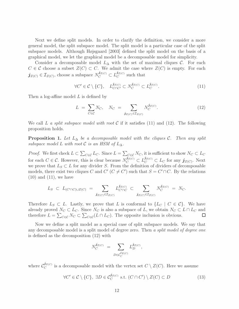
Next we define split models. In order to clarify the definition, we consider a moregeneral model, the split subspace model. The split model is a particular case of the splitsubspace models. Although Højsgaard [2003] defined the split model on the basis of agraphical model, we let the graphical model be a decomposable model for simplicity.

Consider a decomposable model L∆ with the set of maximal cliques C. For eachC ∈ C choose a subset Z(C) ⊂ C. We admit the case where Z(C) is empty. For each

jZ(C) ∈ IZ(C), choose a subspace NjZ(C)

C ⊂ LjZ(C)

C such that

∀C ′ ∈ C \ {C}, LjZ(C)

C∩C′ ⊂ NjZ(C)

C ⊂ LjZ(C)

C . (11)

Then a log-affine model L is defined by

L =∑

C∈C

NC , NC =∑

jZ(C)∈IZ(C)

NjZ(C)

C . (12)

We call L a split subspace model with root C if it satisfies (11) and (12). The followingproposition holds.

Proposition 1. Let L∆ be a decomposable model with the cliques C. Then any splitsubspace model L with root C is an HSM of L∆.

Proof. We first check L ⊂∑

C∈C LC . Since L =∑

C∈C NC , it is sufficient to show NC ⊂ LC

for each C ∈ C. However, this is clear because NjZ(C)

C ⊂ LjZ(C)

C ⊂ LC for any jZ(C). Nextwe prove that LS ⊂ L for any divider S. From the definition of dividers of decomposablemodels, there exist two cliques C and C ′ (C 6= C ′) such that S = C ′∩C. By the relations(10) and (11), we have

LS ⊂ L(C′∩C)∪Z(C) =∑

jZ(C)∈IZ(C)

LjZ(C)

C′∩C ⊂∑

jZ(C)∈IZ(C)

NjZ(C)

C = NC .

Therefore LS ⊂ L. Lastly, we prove that L is conformal to {LC | C ∈ C}. We havealready proved NC ⊂ LC . Since NC is also a subspace of L, we obtain NC ⊂ L ∩ LC andtherefore L =

∑

C∈C NC ⊂∑

C∈C(L ∩ LC). The opposite inclusion is obvious.

Now we define a split model as a special case of split subspace models. We say thatany decomposable model is a split model of degree zero. Then a split model of degree oneis defined as the decomposition (12) with

NjZ(C)

C =∑

D∈CjZ(C)C

LjZ(C)

D ,

where CjZ(C)

C is a decomposable model with the vertex set C \ Z(C). Here we assume

∀C ′ ∈ C \ {C}, ∃D ∈ CjZ(C)

C s.t. (C ∩ C ′) \ Z(C) ⊂ D (13)

12

to assure the condition (11). Split models of degree greater than one are defined recur-sively. See Højsgaard [2003] for details.

In Section 5, we will consider an example of the split model (of degree one). Thefollowing elementary lemma is useful to obtain the MLE of split models.

Lemma 4. Let I =⋃

λ Jλ be a partition of I and consider subspaces Nλ ⊂ V such that

Nλ ⊂ {ψ ∈ V | ψ(i) = 0 if i /∈ Jλ}.

Then the MLE of the model∑

λNλ is given by p(i) =∑

λ(nλ/n)pλ(i)1{i∈Jλ}, where pλ(i)is the MLE of the model Nλ with the total frequency nλ =

∑

i∈Iλx(i).

4 Conditional tests of hierarchical subspace models

via Markov bases

In this section we discuss conditional tests of our proposed model via Markov basestechnique. In Section 1.1, we have discussed that the divide-and-conquer approach ofDobra and Sullivant [2004] still works for the model (2). In this section we generalize theargument to an HSM L.

Let x = {x(i)}i∈I denote an m-way contingency table, where x(i) denotes the fre-quency of the cell i ∈ I. Let b be the set of sufficient statistics for L. We assume that theelements of b are integer combinations of the frequencies x(i). For a hierarchical modelL∆, b is written by

b = {xD(iD), iD ∈ ID, D ∈ red ∆},

where xD(iD) =∑

iDC∈I

DCx(iD, iDC). We consider b as a column vector with dimension

ν. We order the elements of x appropriately and consider x as a column vector. Then therelation between the joint frequencies x and the marginal frequencies b is written simplyas

b = Ax,

where A is a ν × |I| integer matrix. A is called the configuration for L.For a subset D ⊂ [m], denote L(D) := L ∩ LD. Let (A1, A2, S) be a decomposition

of L and define V1 := A1 ∪ S and V2 := A2 ∪ S. Since L is conformal to {LV1 , LV2}, wenote that L(V1) and L(V2) are marginal models corresponding to V1 and V2, respectively.Denote by AV1 = {aV1(iV1)}iV1

∈IV1and AV2 = {aV2(iV2)}iV2

∈IV2the configurations for the

marginal models L(V1) and L(V2), where aV1(iV1) and aV2(iV2) denote column vectors ofAV1 and AV2 , respectively. Noting that iV1 = (iA1iS) and iV2 = (iSiA2), the configurationA for L is written by

A = AV1 ⊕S AV2 = {aV1(iA1iS) ⊕ aV2(iSiA2)}iA1∈IA1

,iS∈IS ,iA2∈IA2

,

where

aV1(iA1iS) ⊕ aV2(iSiA2) =

(

aV1(iA1iS)aV2(iSiA2)

)

.

13

Given b, the setFb = {x ≥ 0 | b = Ax}

of contingency tables sharing the same b is called a fiber. An integer array z = {z(i)}i∈I

of the same dimension as x is called a move if Az = 0. As in (8), we denote z with degreed as

z = [{i1, . . . , id}‖{i′1, . . . , i

′d}],

where i1, . . . , id ∈ I are cells (with replication) of positive elements of z and i′1, . . . , i′d ∈ I

are cells of negative elements of z. Moves are used for steps of Markov chain Monte Carlosimulation within each fiber. If we add or subtract a move z to x ∈ Fb, then x± z ∈ Fb

and we can move from x to another state x + z (or x − z) in the same fiber Fb, as longas there is no negative element in x + z (or x − z). A finite set M of moves is called aMarkov basis if for every fiber the states become mutually accessible by the moves fromM.

Assume that B(V1) and B(V2) are Markov bases for L(V1) and L(V2), respectively. Letz1 = {z1(iV1)}iV1

∈IV1∈ B(V1) and z2 = {z2(iV2)}iV2

∈IV2∈ B(V2). Since S is saturated, we

have∑

iV1\S∈IV1\S

z1(iV1) = 0,∑

iV2\S∈IV2\S

z2(iV2) = 0.

Hence z1 and z2 can be written as

z1 = [{(i1, j1), . . . , (id, jd)}||{(i′1, j1), . . . , (i

′d, jd)}], (14)

z2 = [{(j1,k1), . . . , (jd,kd)}||{(j1,k′1), . . . , (jd,k

′d)}],

respectively, where ik, i′k ∈ IA1 , jk ∈ IS and kk,k

′k ∈ IA2 for k = 1, . . . , d.

Definition 3 (Dobra and Sullivant [2004]). Define z1 ∈ B(V1) as in (14). Let k :={k1, . . . ,kd} ∈ IA2 × · · · × IA2. Define zk

1 by

zk1 := [{(i1, j1,k1), . . . , (id, jd,kd)}||{(i

′1, j1,k1), . . . , (i

′d, jd,kd)}].

Then we define Ext(B(V1) → L) by

Ext(B(V1) → L) := {zk1 | k ∈ IA2 × · · · × IA2}.

In the same way as Lemma 5.4 in Dobra and Sullivant [2004] we can obtain the fol-lowing lemma.

Lemma 5. Suppose that z1 ∈ B(V1) as in (14). Then Ext(B(V1) → L) is the set of movesfor L.

Proof. Let z ∈ Ext(B(V1) → L). Then we have

Az =

(

∑

iV1∈IV1

aV1(iV1)zV1(iV1)∑

iV2∈IV2

aV2(iV2)zV2(iV2)

)

,

14

wherezV1(iV1) =

∑

iV C1

∈IV C1

z(i), zV2(iV2) =∑

iV C2

∈IV C2

z(i).

Since zV1(iV1) = z1(iV1) and z1 ∈ B(V1),∑

iV1∈IV1

aV1(iV1)zV1(iV1) = 0. From Definition

3, zV2(iV2) = 0 for all iV2 ∈ IV2 . Hence Az = 0.

Theorem 2. Let B(V1) and B(V2) be Markov bases for L(V1) and L(V2), respectively. LetBV1,V2 is a Markov basis for the hierarchical model with two cliques V1 and V2. Then

B := Ext(B(V1) → L) ∪ Ext(B(V2) → L) ∪ BV1,V2. (15)

is a Markov basis for L.

We can prove the theorem in the same way as Theorem 5.6 in Dobra and Sullivant[2004]. Suppose that L is an HSM of LH. Then Theorem 2 implies that a Markovbasis for L is obtained from B(C), C ∈ H, by recursively using (15). This shows thatthe computation of a Markov basis can be localized according to the maximal extendedcompact components of L.

Concerning Markov bases of the split model of Section 3 we state the following lemma.

Lemma 6. With the same notation as in Lemma 4, a Markov basis of the model∑

λNλ

is given by union of Markov bases of Nλ.

5 Examples

In this section we give several applications of HSMs. In Section 5.1 we analyze the dataon song sequence of a wood pewee, which we already discussed in Section 1.1. In Section5.2 we consider an example of a split model.

5.1 Sequences of unrepeated events

Consider the data on song sequence of a wood pewee in Table 1. As mentioned in Section1.1, it is a 4 × 4 × 4 contingency table with the cells of the form (i, i, k) and (i, j, j)being structural zeros. The probability function {pijk} satisfies the condition piik = 0 andpijj = 0, or equivalently, log piik = −∞ and log pijj = −∞. Hence {log pijk} is not anelement of V = R

4×4×4. However we can replace V by R|I|, where

I = I \(

{(i, i, j), i, j ∈ [4]} ∪ {(i, j, j), i, j ∈ [4]})

,

and consider log-affine models of R|I|. Formally it is more convenient to proceed withV = R

4×4×4 allowing log piik = log pijj = −∞.We first consider the conditional independence model

LModel1 = L{1,2} + L{2,3},

15

which corresponds to (7). The MLE of this model is explicitly given by

pijk =xij+x+jk

nx+j+

=xij+1{i6=j}x+jk1{j 6=k}

nx+j+

.

A Markov basis of the model is BModel1 = B{1,2},{2,3} (see Theorem 2 for the notation). Anexperimental result that compares the saturated model and Model 1 is given in Figure 2.Both the asymptotic and experimental estimates of the p-value are almost zero.

Although Model 1 does not fit the data, we proceed to consider a submodel of Model 1for theoretical interest. Let

Lmodel2 ={

αi + βj + γk + φi1{i=j} + ψj1{j=k}

}

.

This model is an HSM of L{1,2} +L{2,3}. It represents a quasi-independence model for thethree-way table. The MLE of the model is

pijk =p

(1)ij p

(2)jk

x+j+/n,

where p(1)ij and p

(2)jk are the MLE of the 2-way quasi-independence models with the diagonal

structural zeros, that is,

p(1)ii = eαieβj1{i6=j}, p

(1)i+ = xi++/n, p

(1)+j = x+j+/n,

p(2)jj = eβjeγk1{j 6=k}, p

(2)j+ = x+j+/n, p

(2)+k = x++k/n.

They are computed by the iterative proportional fitting method. By Theorem 2, a Markovbasis is given by

BModel2 = B{1,2},{2,3} ∪ Ext(B({1, 2}) → V ) ∪ Ext(B({2, 3}) → V )

where B({1, 2}) and B({2, 3}) are the Markov bases of the 2-way quasi-independencemodel with structural zeros obtained by Aoki and Takemura [2005]. An experimentalresult that compares the Model 1 and Model 2 is given in Figure 2.

5.2 WAM data

Here we deal with a real data called women and mathematics (wam) data used in Højsgaard[2003]. The data is shown in Table 2. The data consists of the following six factors: (1) At-tendance in math lectures (attended=1, not=2), (2) Sex (female=1, male=2), (3) Schooltype (suburban=1, urban=2), (4) Agree in statement “I’ll need mathematics in my futurework” (agree=1, disagree=2), (5) Subject preference (math-science=1, liberal arts=2) and(6) Future plans (college=1, job=2). We consider two models Højsgaard [2003] treated.The first model is a decomposable model

LModel1 = L{1,2,3,5} + L{2,3,4,5} + L{3,4,5,6}.

16

deviance

Den

sity

0 20 40 60 80 100 120 140

0.00

0.02

0.04

0.06

0.08

deviance

Den

sity

0 10 20 30 40 50 60 70

0.00

0.02

0.04

0.06

0.08

0.10

(a) Deviance of Model 1 (G2 = 142.4). (b) Deviance of Model 2 from Model 1 (G2 = 66.9).

Figure 2: The empirical distribution and asymptotic distribution of deviance G2 for thewood pewee data. The degree of freedom is 16 and 10, respectively. The number of stepsin the MCMC procedure is 105.

By Theorem 2, a Markov basis of this model is given by

BModel1 = B{1,2,3,5},{2,3,4,5,6} ∪ B{1,2,3,4,5},{3,4,5,6}.

The second model is a split model

LModel2 = L{1,2,3,5} + Lj3=1{2,5} + Lj3=1

{4,5} + Lj3=2{2,4,5} + L{3,4,5,6}.

This model is indeed a split model (of degree one) with

C = {{1, 2, 3, 5}, {2, 3, 4, 5}, {3, 4, 5, 6}},

Z({1, 2, 3, 5}) = ∅, Cj∅{1,2,3,5} = {{1, 2, 3, 5}},

Z({2, 3, 4, 5}) = {3}, Cj3=1{2,3,4,5} = {{2, 5}, {4, 5}}, Cj3=2

{2,3,4,5} = {{2, 4, 5}},

Z({3, 4, 5, 6}) = ∅, Cj∅{3,4,5,6} = {{3, 4, 5, 6}}.

The condition (13) is easily checked. The MLE is calculated if one decomposes the tableinto those for j3 = 1 and j3 = 2 and then calculates the MLE separately (Lemma 4). ByTheorem 2 and Lemma 6, a Markov basis of this model is

BModel2 = Bi3=1{1,2,5},{4,5,6} ∪ B{1,2,3,5},{2,3,4,5,6} ∪ B{1,2,3,4,5},{3,4,5,6},

where we put Bi3=1{1,2,5},{4,5,6} = B{1,2,5},{4,5,6} ∩ L

i3=1.We calculate the p-value of the deviance of Model 2 from Model 1 by the MCMC

method. The number of steps in the MCMC procedure is 105. The result is as follows.

17

Table 2: Survey data concerning the attitudes of high-school students in New Jerseytowards mathematics.

School Suburban school Urban school

Sex Female Male Female MalePlans Preference Attend Not Attend Not Attend Not Attend Not

College Math-sciencesAgree 37 27 51 48 51 55 109 86Disagree 16 11 10 19 24 28 21 25Liberal artsAgree 16 15 7 6 32 34 30 31Disagree 12 24 13 7 55 39 26 19

Job Math-sciencesAgree 10 8 12 15 2 1 9 5Disagree 9 4 8 9 8 9 4 5Liberal artsAgree 7 10 7 3 5 2 1 3Disagree 8 4 6 4 10 9 3 6

Source: Fowlkes et al. [1988]

deviance

Den

sity

0 5 10 15 20

0.0

0.1

0.2

0.3

0.4

0.5

Figure 3: The empirical and asymptotic distributions of the deviance of Model 2 fromModel 1.

Deviance df p-value (asymptotic) p-value (MCMC)1.851 2 0.396 0.399±0.012

The confidence interval of the p-value is computed on the basis of the batch-means method.The empirical distribution and asymptotic distribution of the deviance are given in Fig-ure 3. Since the sample size of the data is large, the results of the asymptotic method

18

and MCMC method are almost the same.

6 Concluding remarks

We proposed a hierarchical subspace model, by defining the notion of conformality of linearsubspaces to a given hierarchical model. The notion of an HSM gives a modeling strategyof multiway tables and unifies various models of interaction effects in the literature. Weillustrated practical advantage of our modeling strategy with some data sets.

In this paper we only considered log-affine model. Note that there are some nonlinearmodels of interaction terms for two-way tables, such as the RC association model. It seemsclear that we can separately fit a nonlinear model to each maximal compact component of ahierarchical model, as long as the models for dividers are saturated. However conformalityof a general nonlinear model with respect to a given hierarchical model has to be carefullydefined and this is left to our future study.

The separation by dividers are closely related to the notion of collapsibility (e.g.Asmussen and Edwards [1983]) of hierarchical models. Localization of statistical infer-ence to the marginal table of a maximal compact component seems to correspond to thecollapsibility to the component. Also our results for Markov bases for HSMs are closelyrelated to those of Sullivant [2007]. Sullivant [2007] is more concerned with Markov basesfor models with latent variables and marginalization of latent variables. Collapsibilityand marginalization properties of HSM require further investigation.

In the computation of the MLE for the hierarchical models, it is known that the algo-rithm can be localized into the marginal tables of maximal cliques for chordal extensionof the simplicial complex associated with the model, which is smaller than maximal com-pact component (e.g. Badsberg and Malvestuto [2001]). By using the notion of ambienthierarchical model discussed in Section 2.3, it may be possible to localize the inference tosmaller units than maximal extended compact component also in the HSMs.

Another important question on hierarchical subspace model is the necessity of sat-uration of the model for dividers. Saturation of the model for dividers is a sufficientcondition for localization of statistical inference, but it may not be a necessary condition.There may exist some important models, for which statistical inferences can be localizedto extended compact components without the requirement of saturation of dividers. Thisquestion also needs a careful investigation.

References

Satoshi Aoki and Akimichi Takemura. Markov chain Monte Carlo exact tests for incom-plete two-way contingency table. Journal of Statistical Computation and Simulation,75(10):787–812, 2005.

Søren Asmussen and David Edwards. Collapsibility and response variables in contingencytables. Biometrika, 70(3):567–578, 1983. ISSN 0006-3444.

19

J. H. Badsberg and F. M. Malvestuto. An implementaition of the iterative proportionalfitting procecure by propagation trees. Comput. Statist. Data. Anal., 37:297–322, 2001.

Yvonne M. M. Bishop, Stephen E. Fienberg, and Paul W. Holland. Discrete multivariateanalysis: theory and practice. The MIT Press, Cambridge, Mass.-London, 1975. Withthe collaboration of Richard J. Light and Frederick Mosteller.

W. Craig. The song of the wood pewee. Bull. N. Y. State Museum, 334:1–186, 1943.

Persi Diaconis and Bernd Sturmfels. Algebraic algorithms for sampling from conditionaldistributions. Ann. Statist., 26(1):363–397, 1998. ISSN 0090-5364.

Adrian Dobra and Seth Sullivant. A divide-and-conquer algorithm for generating Markovbases of multi-way tables. Comput. Statist., 19(3):347–366, 2004. ISSN 0943-4062.

E. B. Fowlkes, A. E. Freeny, and J. M. Landwehr. Evaluating logistic models for largecontingency tables. J. Amer. Statist. Assoc, 83:611–622, 1988.

Leo A. Goodman. Simple models for the analysis of association in cross-classificationshaving ordered categories. J. Amer. Statist. Assoc., 74(367):537–552, 1979. ISSN 0003-1291.

Leo A. Goodman. The analysis of cross-classified data having ordered and/or unorderedcategories: association models, correlation models, and asymmetry models for contin-gency tables with or without missing entries. Ann. Statist., 13(1):10–69, 1985. ISSN0090-5364.

Hisayuki Hara, Akimichi Takemura, and Ruriko Yoshida. Markov bases for two-way subtable sum problems. J. Pure Appl. Algebra, 213(8):1507–1529, 2009.doi:10.1016/j.jpaa.2008.11.019.

Chihiro Hirotsu. Two-way change-point model and its application. Australian Journal ofStatistics, 39(2):205–218, 1997.

Søren Højsgaard. Split models for contingency tables. Comput. Statist. Data. Anal., 42:621–645, 2003.

Søren Højsgaard. Statistical inference in context specific interaction models for contin-gency tables. Scand. J. Statist., 31:143–158, 2004.

Satoshi Kuriki. Asymptotic distribution of inequality-restricted canonical correlation withapplication to tests for independence in ordered contingency tables. J. MultivariateAnal., 94(2):420–449, 2005. ISSN 0047-259X.

Steffen L. Lauritzen. Graphical Models. Oxford University Press, Oxford, 1996.

F. M. Malvestuto and M. Moscarini. Decomposition of a hypergraph by partial-edgeseparators. Theoret. Comput. Sci., 237:57–79, 2000.

20

Tomonari Sei, Satoshi Aoki, and Akimichi Takemura. Perturbation method for determin-ing group of invariance of hierarchical models. arXiv:0808.2725v1, 2008. Advances inApplied Mathematics, doi:10.1016/j.aam.2009.02.005.

Seth Sullivant. Toric fiber products. J. Algebra, 316(2):560–577, 2007. ISSN 0021-8693.

Martin A. Tanner and Michael A. Young. Modeling agreement among raters. J. Amer.Statist. Assoc., 80:175–180, 1985.

Sadao Tomizawa. Analysis of square contingency tables in statistics. In Selected Paperson Probability and Statistics, volume 227 of Translations, Series 2, pages 147–174.American Mathematical Society, Providence, Rhode Island, 2009.

21