stiffness degradation and shear strength of silty sands

Stiffness degradation and shear strength of siltysands

Junhwan Lee, Rodrigo Salgado, and J. Antonio H. Carraro

Abstract: Soils behave nonlinearly from very early loading stages. When granular soils contain a certain amount offines, the degree of nonlinearity also changes, as stiffness and strength characteristics vary with fines content. Hyper-bolic stress–strain models and variations of these models are often used for description of the nonlinear behavior. Amodified hyperbolic stress–strain relationship is used in this paper for representing the degradation of the elastic modu-lus of silty sands. The model is based on two modulus degradation parameters that determine the magnitude and rateof modulus degradation as a function of stress level. Realistic representation of soil behavior using this nonlinear rela-tionship requires estimation of the degradation parameters as a function of silt content and relative density DR. A seriesof triaxial test results on sands containing different amounts of nonplastic silt were analyzed with this purpose. Rela-tionships between the degradation parameters and cone penetration test (CPT) cone resistance qc are also proposed.

Key words: hyperbolic model, silty sands, triaxial tests, modulus degradation, stress–strain response, shear strength,Gmax.

Résumé : Les sols se comportent de façon non linéaire dès les premiers stades de chargement. Lorsque les sols pulvé-rulents contiennent une certaine quantité de particules fines, le degré de non linéarité change aussi puisque la rigidité etles caractéristiques de cisaillement varient avec la teneur en particules fines. On utilise souvent des modèles hyperboli-ques contrainte–déformation et des variations de ces modèles pour décrire le comportement non linéaire. Une relationhyperbolique contrainte–déformation modifiée à été utilisée dans cet article pour représenter la dégradation du moduleélastique des sables limoneux. Le modèle est basé sur deux paramètres de module de dégradation qui déterminentl’amplitude et le taux de dégradation du module en fonction du niveau de contrainte. Une représentation réaliste ducomportement du sol utilisant la relation non linéaire requiert une estimation des paramètres de dégradation en fonctionde la teneur en limon et de la densité relative DR. On a analysé à cette fin une série de résultats d’essais triaxiaux surdes sables contenant différentes quantités de limon non plastique. On propose également des relations entre les paramè-tres de dégradation et la résistance qc au cône CPT.

Mots clés : modèle hyperbolique, sables limoneux, essais triaxiaux, module de dégradation, réponse contrainte-déformation, résistance au cisaillement, Gmax.

[Traduit par la Rédaction] Lee et al. 843

Introduction

Foundation design, in general, requires that both a stabil-ity analysis based on the shear strength of the soil and asettlement analysis be done to ensure the safety and service-ability of the superstructure. For both analyses, use of appro-priate soil parameters that can represent the real soilbehavior is key for the design to be successful. In particular,for the settlement analysis, description of nonlinear stress–strain behavior is necessary, as the structure serviceability

limits are defined most likely within the range of nonlinearstress–strain response.

It is widely recognized that soils behave nonlinearly fromvery early stages of loading. To describe this nonlinear be-havior of soils before failure, several stress–strain modelshave been proposed (Kondner 1963; Duncan and Chang1970; Tatsuoka et al. 1993; Fahey and Carter 1993). Theoriginal hyperbolic model of Kondner (1963) was a pure hy-perbolic relationship between stress and strain. Subsequentmodels included modifications to the hyperbolic stress–strain relationship geared to better fit real soil behavior(Duncan and Chang 1970; Hardin and Drnevich 1972; Faheyand Carter 1993).

The hyperbolic family of soil models has the importantadvantages of easy numerical implementation and sufficientaccuracy for practical purposes. The conventional hyperbolicsoil models, however, are not complete constitutive models,as they make no reference to a yield surface, flow rule, orhardening rule. In addition, the observed degradation of elas-tic modulus with increasing stress–strain levels differs fromthat provided by the hyperbolic stress–strain model. Where-as the degradation of elastic modulus in the conventional hy-

Can. Geotech. J. 41: 831–843 (2004) doi: 10.1139/T04-034 © 2004 NRC Canada

831

Received 2 December 2002. Accepted 29 March 2004.Published on the NRC Research Press Web site athttp://cgj.nrc.ca on 24 September 2004.

J. Lee.1 School of Civil and Environmental Engineering,Yonsei University, 134 Shinchon-dong, Seodaemun-gu,Seoul 120-749, South Korea.R. Salgado and J.A.H. Carraro. School of Civil andEnvironmental Engineering, Purdue University, WestLafayette, IN 47907-1284, USA.

1Corresponding author (e-mail: [email protected]).

perbolic model is linear when plotted versus mobilized shearstress, the observed degradation for real soils is nonlinear.Nonetheless, the hyperbolic model has been used in manycases with reasonably satisfactory results because of self-compensating effects during model parameter determination.This will be discussed in a later section.

To represent modulus degradation more realistically,Fahey and Carter (1993) and Lee and Salgado (2000, 2002)modified the hyperbolic stress–strain model for two-dimensional (2D) and three-dimensional (3D) stress states,respectively. The degradation of elastic modulus in thesemodels is set as a function of the ratio of current shear stressto the maximum shear stress at failure. The key model pa-rameters are f and g. Lee and Salgado (1999, 2000, 2002)proposed values of the degradation parameters f and g as afunction of the relative density DR for clean sand. Accordingto these authors, as the relative density DR increases, the val-ues of f and g decrease and increase, respectively.

In the present study, the modulus degradation of sandscontaining different amounts of silts is investigated with ref-erence to the model of Lee and Salgado (1999, 2000, 2002).Values of f and g are proposed as a function of DR and siltcontent. A methodology for estimating the modulus degrada-tion parameters based on cone penetration test (CPT) resultsand their relationship to the peak friction angle of silty sandare also addressed.

Nonlinear behavior of granular soil

Hyperbolic stress–strain relationshipThe hyperbolic types of soil models have been widely

used in a number of geotechnical engineering analyses thatrequire nonlinear stress–strain modeling. The conventionalhyperbolic equation for stress–strain curves by Kondner(1963) is written for either triaxial or plane-strain conditionsas

[1] σ σ εε1′ − ′ =

+3a b

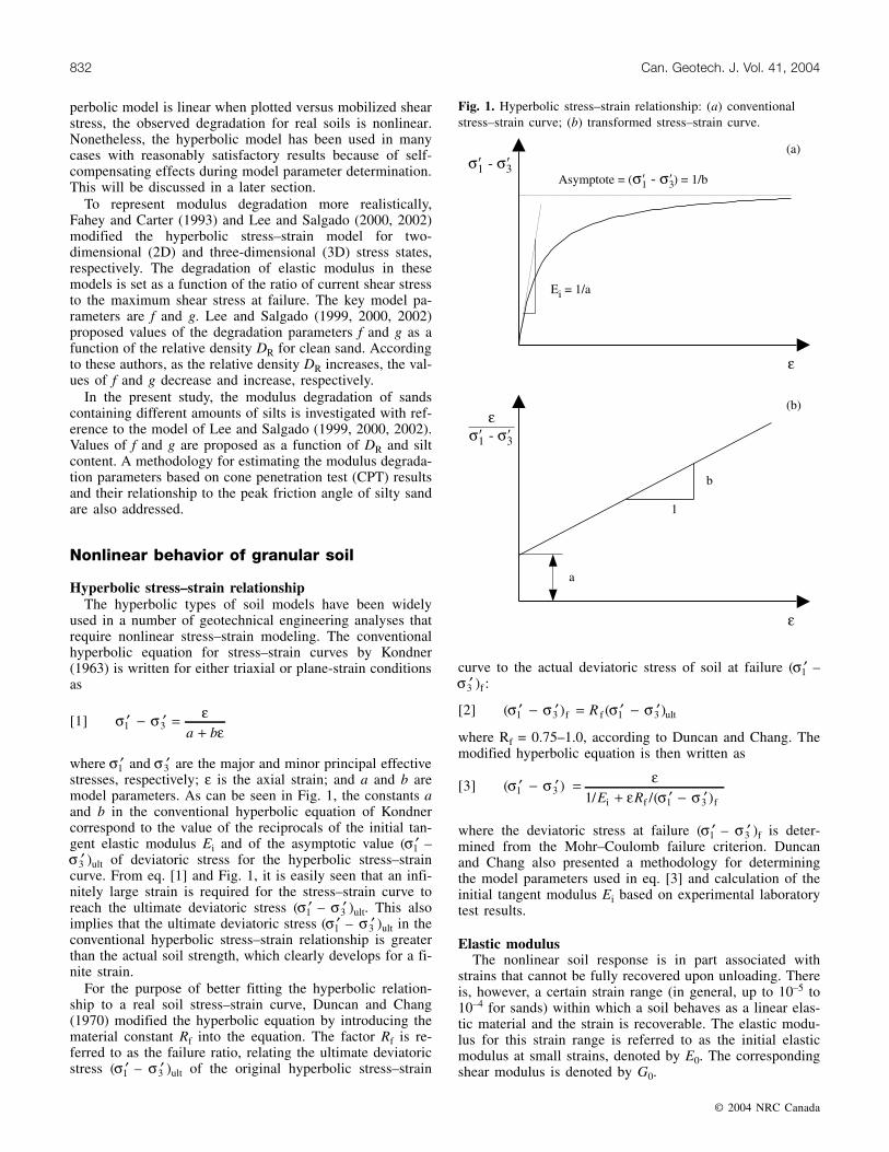
where σ1′ and σ3′ are the major and minor principal effectivestresses, respectively; ε is the axial strain; and a and b aremodel parameters. As can be seen in Fig. 1, the constants aand b in the conventional hyperbolic equation of Kondnercorrespond to the value of the reciprocals of the initial tan-gent elastic modulus Ei and of the asymptotic value (σ1′ –σ3′ )ult of deviatoric stress for the hyperbolic stress–straincurve. From eq. [1] and Fig. 1, it is easily seen that an infi-nitely large strain is required for the stress–strain curve toreach the ultimate deviatoric stress (σ1′ – σ3′ )ult. This alsoimplies that the ultimate deviatoric stress (σ1′ – σ3′ )ult in theconventional hyperbolic stress–strain relationship is greaterthan the actual soil strength, which clearly develops for a fi-nite strain.

For the purpose of better fitting the hyperbolic relation-ship to a real soil stress–strain curve, Duncan and Chang(1970) modified the hyperbolic equation by introducing thematerial constant Rf into the equation. The factor Rf is re-ferred to as the failure ratio, relating the ultimate deviatoricstress (σ1′ – σ3′ )ult of the original hyperbolic stress–strain

curve to the actual deviatoric stress of soil at failure (σ1′ –σ3′ )f :

[2] ( ) ( )σ σ σ σ1 1′ − ′ = ′ − ′3 3f f ultR

where Rf = 0.75–1.0, according to Duncan and Chang. Themodified hyperbolic equation is then written as

[3] ( )/ /( )

σ σ εε σ σ1

1′ − ′ =

+ ′ − ′331 E Ri f f

where the deviatoric stress at failure (σ1′ – σ3′ )f is deter-mined from the Mohr–Coulomb failure criterion. Duncanand Chang also presented a methodology for determiningthe model parameters used in eq. [3] and calculation of theinitial tangent modulus Ei based on experimental laboratorytest results.

Elastic modulusThe nonlinear soil response is in part associated with

strains that cannot be fully recovered upon unloading. Thereis, however, a certain strain range (in general, up to 10–5 to10–4 for sands) within which a soil behaves as a linear elas-tic material and the strain is recoverable. The elastic modu-lus for this strain range is referred to as the initial elasticmodulus at small strains, denoted by E0. The correspondingshear modulus is denoted by G0.

© 2004 NRC Canada

832 Can. Geotech. J. Vol. 41, 2004

Fig. 1. Hyperbolic stress–strain relationship: (a) conventionalstress–strain curve; (b) transformed stress–strain curve.

There are a number of ways to evaluate the initial shearmodulus for a given soil type and state, including in situtests, laboratory tests, and empirical equations (Janbu 1963;Hardin and Richart 1963; Yu and Richart 1984; Baldi et al.1989; Viggiani and Atkinson 1995; Salgado et al. 1997). Thecross-hole test and the seismic cone penetration test (SCPT)are examples of in situ testing methods that can be used forthis purpose. In the laboratory, the resonant column test andthe bender element test are often used. The empirical equa-tions for the initial shear modulus are usually expressed inthe form

[4]Gp

C F epp

n

0

A

m

A

= ′

( )

where G0 is the initial shear modulus, pA is the referencestress used for stress normalization, C is a nondimensionalmaterial constant, F(e) is a function of the void ratio, n is amaterial constant, and pm′ is the mean effective stress ex-pressed in the same units as pA. Equation [4] indicates de-pendence of the initial shear modulus on the degree of soilcompactness and the magnitude of the confining stress. Oneof the commonly used empirical equations for the initialshear modulus of sand is that suggested by Hardin and Black(1966) and given as follows:

[5]Gp

Ce e

epp

n

0 02

01Ag

g m

A

g

=−+

′

( )

where Cg, eg, and ng are material constants that depend onlyon the nature of the soil; e0 is the initial void ratio; and pA isthe reference stress. Hardin and Black proposed values ofCg, eg, and ng for well-rounded particles (Ottawa sand) andangular particles (crushed quartz).

If the shear modulus G is used, a complete description ofthe elastic stress–strain relationship requires another elasticparameter, bulk modulus K, which is a pressure-dependentelastic parameter. To include variation of K with stress, theK–G model by Naylor et al. (1981) was adopted in thisstudy. In the K–G model, the value of K varies as a functionof the mean effective stress σm′ .

Modulus degradation modelIt is more useful in most analyses to express the stress–

strain relationship in terms of shear stress and strain. Equa-tion [3] then takes the form

[6] τ γγ τ

=+1 0/ / maxG Rf

where G0 is the initial shear modulus at small strains; τmax isthe maximum shear stress at failure; and τ and γ are the cur-rent shear stress and strain, respectively. Considering thateq. [6] is of the form τ = Gγ, it follows that

[7]GG

R0

1= − fτ

τmax

where G is the secant shear modulus.Equation [7] implies linear degradation of the soil stiff-

ness with shear stress from its initial maximum value G0. As

shown in Fig. 2, however, the degradation of the elasticmodulus obtained experimentally for real soils under staticor quasi-static loading is not linear. To describe more realis-tically the modulus degradation relationship, Fahey andCarter (1993) proposed a modified hyperbolic model withthe introduction of a parameter g into eq. [7]:

[8]GG

f

g

0

1= −

τ

τmax

The parameter f in eq. [8] has the same role as Rf ineq. [7]. The parameter g determines the shape of the degra-dation curve as a function of stress level. If f = 0, eq. [8]represents the linear elastic relationship. If g = 1, theDuncan–Chang hyperbolic relationship results. Based on themodel of Fahey and Carter, Lee and Salgado (2000, 2002)proposed the modified hyperbolic relationship for 3D stressstates in natural soil deposits, with consideration of stressconfinement, as follows:

[9]GG

fJ J

J J

II

g

0

2 2

2 2

1

1

1= −−

−

o

o omax

ng

where J21 2/ , J2

1 2o

/ , and J21 2

max/ are the second invariants of

the deviatoric stress tensor corresponding to 3D equivalentsof the current, initial, and maximum shear stresses, respec-tively; I1 and I1o are the first invariants of the stress tensor atthe current and initial states, respectively. The parameter ngis the same as appears in eq. [5]; in both equations, ng repre-sents the dependence of shear modulus on the confiningstress. The rate of the modulus degradation clearly dependson the values of f and g. It follows that, to describe soil be-havior realistically using eq. [9], accurate knowledge of thevalues of f and g is necessary. In the next section, we focuson the estimation of f and g values for silty sands.

© 2004 NRC Canada

Lee et al. 833

Fig. 2. Modulus degradation relationship for normally consoli-dated (N.C.) sands for monotonic and cyclic loading (afterTeachavorasinskun et al. 1991).

Degradation of elastic modulus for siltysands

ExperimentsIn general, the presence of nonplastic fines in granular

soils results in higher dilatancy because of increasing inter-locking of particles, with the fines wedging themselves be-tween larger particles. This is true up to a certain percentageof fines. The upper limit of silt content, up to which increas-ing dilatancy is observed, is on the order of 20% (Salgado etal. 2000). For fines contents greater than this limit, the be-havior of the soil would be dominated by the fines (i.e., silts,in this study) rather than by the larger particles.

Soil parameters can be classified as either intrinsic or statevariables. Intrinsic variables do not change with soil stateand are only a function of soil particle mineralogy, shape,and size distribution (Been et al. 1991; Salgado et al. 1997).These variables include the friction angle at critical state(φcv′ ), maximum and minimum void ratios (emax, emin), andspecific gravity (Gs). If the amount of fines in a soilchanges, the values of the intrinsic soil variables alsochange. State variables, on the other hand, are dependent onthe soil state. The in situ vertical and horizontal effectivestresses (σv′ , σh′ ) and the initial void ratio (e0) are examplesof state variables.

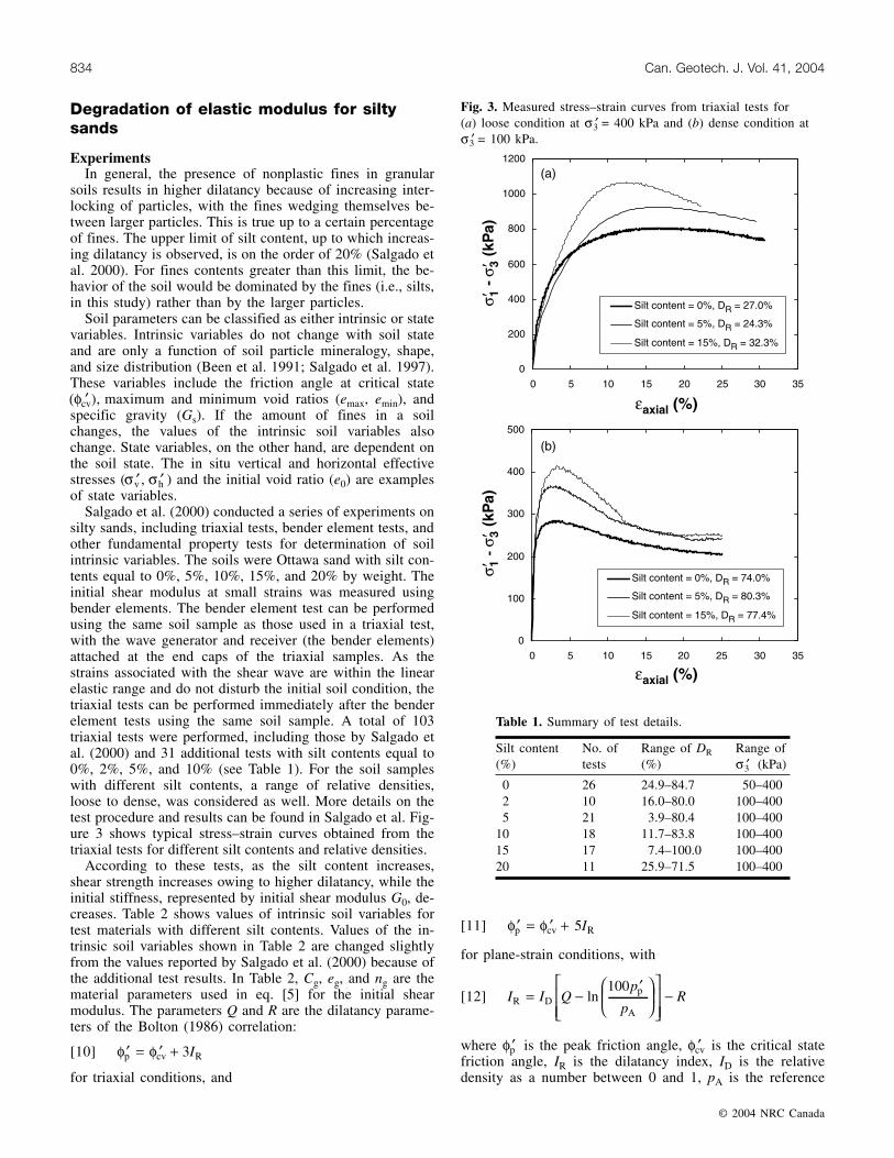
Salgado et al. (2000) conducted a series of experiments onsilty sands, including triaxial tests, bender element tests, andother fundamental property tests for determination of soilintrinsic variables. The soils were Ottawa sand with silt con-tents equal to 0%, 5%, 10%, 15%, and 20% by weight. Theinitial shear modulus at small strains was measured usingbender elements. The bender element test can be performedusing the same soil sample as those used in a triaxial test,with the wave generator and receiver (the bender elements)attached at the end caps of the triaxial samples. As thestrains associated with the shear wave are within the linearelastic range and do not disturb the initial soil condition, thetriaxial tests can be performed immediately after the benderelement tests using the same soil sample. A total of 103triaxial tests were performed, including those by Salgado etal. (2000) and 31 additional tests with silt contents equal to0%, 2%, 5%, and 10% (see Table 1). For the soil sampleswith different silt contents, a range of relative densities,loose to dense, was considered as well. More details on thetest procedure and results can be found in Salgado et al. Fig-ure 3 shows typical stress–strain curves obtained from thetriaxial tests for different silt contents and relative densities.

According to these tests, as the silt content increases,shear strength increases owing to higher dilatancy, while theinitial stiffness, represented by initial shear modulus G0, de-creases. Table 2 shows values of intrinsic soil variables fortest materials with different silt contents. Values of the in-trinsic soil variables shown in Table 2 are changed slightlyfrom the values reported by Salgado et al. (2000) because ofthe additional test results. In Table 2, Cg, eg, and ng are thematerial parameters used in eq. [5] for the initial shearmodulus. The parameters Q and R are the dilatancy parame-ters of the Bolton (1986) correlation:

[10] φ φp cv R′ = ′ + 3I

for triaxial conditions, and

[11] φ φp cv R′ = ′ + 5I

for plane-strain conditions, with

[12] I I Qp

pRR D

p

A

= −′

−ln100

where φp′ is the peak friction angle, φcv′ is the critical statefriction angle, IR is the dilatancy index, ID is the relativedensity as a number between 0 and 1, pA is the reference

© 2004 NRC Canada


Fig. 3. Measured stress–strain curves from triaxial tests for(a) loose condition at σ3′ = 400 kPa and (b) dense condition atσ3′ = 100 kPa.

Silt content(%)

No. oftests

Range of DR

(%)Range ofσ3′ (kPa)

0 26 24.9–84.7 50–4002 10 16.0–80.0 100–4005 21 3.9–80.4 100–400

10 18 11.7–83.8 100–40015 17 7.4–100.0 100–40020 11 25.9–71.5 100–400

Table 1. Summary of test details.

stress (=100 kPa), and pp′ is the mean effective stress atpeak strength in the same units as pA.

Degradation behavior of elastic modulusThe parameters f and g appearing in eqs. [8] and [9] deter-

mine the degradation characteristics of the elastic modulusas a function of the stress level. Figure 4 shows some modu-lus degradation curves resulting from different values of fand g. As can be seen in Fig. 4, the value of f determinesthe ratio of the secant elastic modulus at failure to the initialelastic modulus, G0 or E0 (i.e., the value of this ratio when(σ1′ – σ3′ )/(σ1′ – σ3′ )f = 1). As the value of f approaches 1,the value of the secant modulus approaches zero. This im-plies that the strains at failure for materials with lower f val-ues are lower than those for materials with higher f values,representing stiffer stress–strain response. Hence, the higherthe soil dilatancy and the strength, the lower the value of thefailure ratio f. The value of g, on the other hand, defines themodulus degradation rate, or the shape of the modulus deg-radation curve. As shown in Fig. 4, when the value of g isequal to 1, the degradation curve is linear. For g values lessthan 1, the lower the g value, the faster the modulus degra-dation rate.

According to Teachavorasinskun et al. (1991) and Lee andSalgado (1999, 2000), stiffer soils, such as overconsolidated(i.e., overconsolidation ratio (OCR) > 1) or dense soils, havehigher values of g than loose soils. Figure 5 shows modulusdegradation curves and values of initial shear modulus G0obtained from triaxial (TX) and bender element (BE) testswith different OCRs for a silt content equal to 0%. FromFig. 5a, it can be seen that the overconsolidated conditionproduces stiffer modulus degradation behavior under thesame relative density and stress state, which is consistentwith findings by Teachavorasinskun et al. On the other hand,results from BE tests in Fig. 5b show that no significant ef-fect of OCR exists on values of G0, whereas the absolutevalue of void ratio (e0) appears to be important. Effects ofageing as for real soils may also be a factor in modulus deg-radation. According to Howie et al. (2002), aged sands showconsiderable increase of initial elastic modulus values withlower degradation rate. As ageing effects were not includedin this study, therefore, the results obtained in this study maynot directly apply to aged soils.

To obtain the modulus degradation parameters f and g forsilty sands, the triaxial test results described previously wereanalyzed. As shown in Fig. 6, values of f and g can bedetermined from modulus degradation curves in terms ofnormalized elastic modulus and stress ratio. The modulus

degradation curves were obtained from conventional triaxialstress–strain curves based on values of secant elastic modu-lus corresponding to each loading increment. Since the se-cant shear modulus cannot be directly obtained from triaxialstress–strain curves, the modulus degradation curves wereestablished in terms of normalized Young’s modulus E/E0and normalized deviatoric stress (σ1′ – σ3′ )/(σ1′ – σ3′ )f. Thisis based on an assumption that the degradation behavior of Eis the same as that of G. This assumption would not hold ifPoisson’s ratio varied significantly during the loading pro-cess. The initial Young’s modulus E0 for each test was cal-culated from the initial shear modulus G0, which can beobtained from either bender element tests or eq. [5], and theinitial Poisson’s ratio, assumed equal to approximately 0.15.The maximum deviatoric stress (σ1′ – σ3′ )f was taken as thepeak stress on the stress–strain curves. Figure 7 shows mea-sured and calculated modulus degradation curves for twotests using the estimated values of f and g.

Degradation parameters with different silt contentsAccording to Lee and Salgado (1999, 2000), who ana-

lyzed the modulus degradation relationship for clean sands,the relative density DR is the most important factor deter-mining the values of f and g. As the relative density in-creases, the value of f decreases and the value of g increases,all of which indeed leads to a stiffer stress–strain response.

© 2004 NRC Canada

Lee et al. 835

Fig. 4. Elastic modulus degradation with different values of fand g.

Silt content (%) emin emax Cg eg ng φc′ (°) Q R

0 0.48 0.78 611 2.17 0.44 29.5 9.9 0.862 0.45 0.71 514 2.17 0.58 29.6 10.3 –0.355 0.42 0.70 453 2.17 0.46 31.0 9.1 –0.30

10 0.36 0.65 354 2.17 0.58 32.0 9.3 –0.3315 (DR > 38%) 0.32 0.63 238 2.17 0.75 32.5 11.4 1.2915 (DR < 38%) 0.32 0.63 238 2.17 0.75 32.5 7.9 0.0420 (DR > 59%) 0.29 0.62 270 2.17 0.69 33.0 10.1 0.8520 (DR < 59%) 0.29 0.62 207 2.17 0.81 33.0 7.3 0.08

Table 2. Intrinsic soil variables for silty sands (Salgado et al. 2000).

For silty sands, it was found that the fines content was an-other factor bearing on the values of f and g. This is becausethe degree of interlocking between particles and thus thedilatancy vary with the fines content, resulting in differentstiffness and strength characteristics (Salgado et al. 2000).Figure 8 shows values of f and g for silt contents (s/c) equalto 0%, 2%, 5%, 10%, 15%, and 20% as a function of the rel-ative density DR along with the best fit lines. Although themagnitudes of f and g are different for different silt contents,the dependence of f and g on DR observed in Fig. 8 appearsto be consistent with the findings by Lee and Salgado forclean sands.

For the parameter f, most values fall within the range0.86–0.99, depending on the silt content and the relativedensity, whereas greater scatter is observed in the values ofg. As discussed earlier, values of f are evaluated based on thepeak stress–strain level at failure, which is relatively insensi-tive to minor differences in the initial condition of the sam-ples resulting from sample preparation. The values of greflect prefailure modulus degradation, however, which issensitive to initial sample conditions, leading to more scatterin the results. Nonetheless, it is observed that there is a rea-sonably good relationship between g values and relative den-sity DR.

© 2004 NRC Canada


Fig. 5. Effect of OCR on modulus degradation: (a) modulus deg-radation curves for different OCRs; (b) values of G0 for differentOCRs.

Fig. 6. Stress–strain curve and corresponding modulus degrada-tion: (a) stress–strain curve; (b) corresponding modulus degrada-tion curve.

Fig. 7. Measured modulus degradation for loose and densesands.

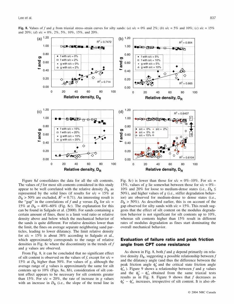
Figure 8d consolidates the data for all the silt contents.The values of f for most silt contents considered in this studyappear to be well correlated with the relative density DR asrepresented by the solid lines (if results for s/c = 15% atDR > 50% are excluded, R2 = 0.71). An interesting result isthe “gap” in the correlations of f and g versus DR for s/c =15% at DR ≈ 40%–60% (Fig. 8c). The explanation for thiscan be found in Salgado et al. (2000). For sands containing acertain amount of fines, there is a limit void ratio or relativedensity above and below which the mechanical behavior ofthe sands is quite different. For relative densities lower thanthe limit, the fines on average separate neighboring sand par-ticles, leading to lower dilatancy. The limit relative densityfor s/c = 15% is about 38% according to Salgado et al.,which approximately corresponds to the range of relativedensities in Fig. 8c where the discontinuity in the trends of fand g values are observed.

From Fig. 8, it can be concluded that no significant effectof silt content is observed on the values of f, except for s/c =15% at DR higher than 50%. For values of g, although theaverage range of g values is approximately the same for siltcontents up to 10% (Figs. 8a, 8b), consideration of silt con-tent effect appears to be necessary for silt contents greaterthan 15%. For s/c = 20%, the rate of increase in g valueswith an increase in DR (i.e., the slope of the trend line in

Fig. 8c) is lower than those for s/c = 0%–10%. For s/c =15%, values of g lie somewhat between those for s/c = 0%–10% and 20% for loose to medium-dense states (i.e., DR ≤50%), and higher values of g (i.e., stiffer degradation behav-ior) are observed for medium-dense to dense states (i.e.,DR > 50%). As described earlier, this is on account of thegap observed for silty sands with s/c = 15%. This result sug-gests that the effect of silt content on the modulus degrada-tion behavior is not significant for silt contents up to 10%,whereas silt contents higher than 15% result in differentrates of modulus degradation as fines start dominating theoverall mechanical behavior.

Evaluation of failure ratio and peak frictionangle from CPT cone resistance

As shown in Fig. 8, both f and g depend primarily on rela-tive density DR, suggesting a possible relationship between fand the dilatancy angle (and thus the difference between thepeak friction angle φp′ and the critical state friction angleφcv′ ). Figure 9 shows a relationship between f and g valuesand the φ φp cv′ − ′ obtained from the same triaxial testsresults as in Fig. 8. Figure 9 shows that f decreases asφ φp cv′ − ′ increases, irrespective of silt content. It is also ob-

© 2004 NRC Canada

Lee et al. 837

Fig. 8. Values of f and g from triaxial stress–strain curves for silty sands: (a) s/c = 0% and 2%; (b) s/c = 5% and 10%; (c) s/c = 15%and 20%; (d) s/c = 0%, 2%, 5%, 10%, 15%, and 20%.

served that the values of φ φp cv′ − ′ obtained from the testsare not greater than the 12° specified by Bolton (1986) asthe upper limit of this quantity for triaxial tests. Regardingthe value of g, although the correlation is not as strong asthat for f, a trend of increasing g values with increasingφ φp cv′ − ′ values is also observed.

The modulus degradation parameters f and g can be evalu-ated through appropriate laboratory tests, such as triaxialtests and torsional shear tests with the capability of measur-ing small strains. It is extremely difficult to obtain un-disturbed samples of sandy soil, however, hence thepredominant use of standard penetration testing (SPT) orCPT testing in these cases. It would be desirable to have acorrelation between f, g, and qc that could be used in esti-mates of f and g values. To fully describe the stress–strainrelationship of the soil for practical purposes, it would alsobe desirable to have a simple correlation between φp′ and qc.

To investigate the relationship between f, g, and qc, thecone resistance qc was normalized and plotted together withvalues of f and g in Fig. 10. The cone resistance qc for eachsoil condition used in the triaxial tests was calculated usingthe widely tested program CONPOINT (Salgado et al. 1997,1998; Salgado and Randolph 2001) with input data preparedfrom the soil parameters in Table 2. In Fig. 10, qc was nor-malized in two ways: (i) in terms of the horizontal effectivestress σh′ (equal to σ3′ for triaxial test conditions) (Figs. 10a,10b), and (ii) in terms of the initial shear modulus G0(Figs. 10c, 10d). It is observed that, for qc/σh′ values lowerthan approximately 300, the correlation between f and qc/σh′is quite good. For higher qc/σh′ values, the relationship be-tween f and qc/G0 appears to be superior. Overall, the datasuggest that a unique relationship between f and the normal-ized qc may be assumed in practice for all the silt contentsconsidered. On the other hand, significant scatter and a lowerdegree of correlation are observed for correlations of g and qcin Figs. 10b and 10d. As discussed previously, this is due tothe fact that g values reflect prefailure modulus degradation,whereas qc represents the soil plunging state at failure.

Figure 11 shows the relationship between the peak frictionangle φp′ from the triaxial test results and the normalizedcone resistances qc/σh′ . As shown in Fig. 11, a fairly clearrelationship between qc/σh′ and φp′ was observed. It shouldbe noted that the relationship in Fig. 11 includes results ofall the silt contents considered from 0% to 20%. There ap-pears to be a slight increase of φp′ with an increase in siltcontent, but for practical purposes the relationship may betaken as unique. The relationship between φp′ and qc shownin Fig. 11 can be approximated as

[13] φσp

c

h

0.1714

15.575′ =′

q

where φp′ is the peak friction angle in degrees, qc is the coneresistance, and σh′ is the initial horizontal effective stress.Equation [13] can be used to estimate the peak friction angleφp′ for both clean and silty sands with silt content up to ap-proximately 15%–20%.

The proposed relationship for φp′ and qc (eq. [13]) is com-pared with those by Robertson and Campanella (1983) andDurgunoglu and Mitchell (1975) in Fig. 12. The φp′ – qc re-lationships by Robertson and Campanella and Durgunoglu

and Mitchell were originally proposed for clean sands. Asshown in Fig. 12, the proposed relationship shows reason-ably good agreement with those of Durgunoglu and Mitchelland Robertson and Campanella. It is also observed that theproposed relationship tends to produce higher friction anglesas the values of qc/σh′ increase beyond 300. The results inFig. 12 can be used to evaluate φp′ of silty sands directlyfrom CPT results.

The combined use of the relationship between φp′ and qc,the relationship between f and qc, and an appropriate correla-tion for G0 allows an effective, yet simple way of obtainingthe parameters necessary for using eqs. [8] or [9] to quantifythe stress–strain response of sands and silty sands under nor-mally consolidated conditions in practical problems.

Conventional versus modified hyperbolicstress–strain model

The conventional hyperbolic stress–strain relationship ofeq. [3] by Duncan and Chang (1970) corresponds to the

© 2004 NRC Canada


Fig. 9. Relationship of (a) f and (b) g versus dilatancy frictionangle for silty sands.

modified hyperbolic relationship of eqs. [8] and [9] with themodulus degradation parameter g equal to 1, which impliesthat G/G0 decreases linearly with an increase in τ/τmax. Ascan be seen in Fig. 2, however, the assumption of linearmodulus degradation is not in agreement with observed be-havior for most soils under static loading conditions. Despiteits lack of conformity with experimental observations, theconventional hyperbolic models have been used in the de-sign and analysis of foundations (Goh et al. 1997; Budek etal. 2000; Rajashree and Sitharam 2001; Castelli and Maugeri2002).

The procedure advocated by Duncan and Chang (1970)for obtaining the hyperbolic stress–strain relationship basedon triaxial compression tests is as follows:(1) Plot the stress–strain curve from a triaxial test in a space

with vertical axis εaxial/(σ1′ – σ3′ ) and with horizontalaxis εaxial.

(2) Obtain a linear regression line for the transformedstress–strain curve plotted in such a way. The linear re-

gression line is determined from two data pointscorresponding to 70% and 95% strength mobilized.

(3) Calculate the intercept with the vertical axis and theslope of the transformed stress–strain curve. Reciprocalvalues of the intercept and the slope correspond to theinitial tangent Young’s modulus Ei and the peak devia-toric stress (σ1′ – σ3′ )f, respectively.

Duncan and Chang’s (1970) hyperbolic parameters (σ1′ –σ3′ )f and Ei were obtained for the silty sands of this study byapplying this procedure to the stress–strain curves for thetriaxial tests on these soils. Figure 13 shows measured andcalculated peak deviatoric stresses (σ1′ – σ3′ )f and initial tan-gent Young’s modulus Ei. In the figure, E0 represents the ini-tial elastic modulus at small strains, obtained from eq. [5].As can be seen in Fig. 13a, there is good agreement betweenthe peak deviatoric stresses from the Duncan and Changprocedure and those measured directly for values less than1 MPa. On the other hand, the difference between the Dun-can and Chang modulus Ei and the initial modulus E0 calcu-

© 2004 NRC Canada

Lee et al. 839

R = 0.63642

0.80

0.84

0.88

0.92

0.96

1.00

0 100 200 300 400 500 600

q /c hσ�

f

Silt content = 0%Silt content = 2%Silt content = 5%Silt content = 10%Silt content = 15%Silt content = 20%

R = 0.73732

0.80

0.84

0.88

0.92

0.96

1.00

0.0 0.2 0.4 0.6 0.8

f


(a) (b)

R = 0.57162

0.00

0.20

0.40

0.60

0.80

1.00

0 100 200 300 400 500 600

g


R = 0.29052

0.00

0.20

0.40

0.60

0.80

1.00

0.0 0.2 0.4 0.6 0.8

g


(c) (d)

q /c hσ�

q /Gc 0 q /Gc 0

Fig. 10. Relationship of f and g versus normalized cone resistance qc: (a) f versus qc/σh′ ; (b) g versus qc/σh′ ; (c) f versus qc/G0; (d) gversus qc/G0.

lated using eq. [5] is substantial. As can be seen in Fig. 13b,values of Ei were significantly lower than those of E0 andnever higher than approximately 15% of E0. Figure 14shows ratios of Ei to E0 versus the dilatancy index IR givenby eq. [12]. It is observed that the ratio of Ei to E0 increasesas the dilatancy index increases. This indicates that, as thesoil becomes more dilative, underestimation of the initialmodulus by the procedure of Duncan and Chang becomesless pronounced.

The significant underestimation of the initial elasticmodulus Ei when the Duncan and Chang (1970) procedure is

followed is owing to the assumption that stress–strain curvesare hyperbolic. After the small strain range, for which thesoil is linear elastic, the elastic modulus degrades exponen-tially. The conventional hyperbolic model, however, ne-glects the existence of this linear elastic range and does notadequately represent the rate of modulus degradation after-wards for most soils. As mentioned earlier, the value of gequal to 1 assumed in the conventional hyperbolic model re-sults in excessively stiff soil behavior compared with whatwould be observed in experiments. This excessive stiffnessis compensated by the use of the underestimated initial tan-gent elastic modulus Ei, so in many practical applicationsthe conventional hyperbolic model may give satisfactory re-sults. In more sophisticated analyses, particularly those in-cluding soil response within the small strain range, it maynot accurately represent the real soil behavior.

© 2004 NRC Canada


Fig. 11. Estimation of peak friction angle from normalized coneresistance qc.

Fig. 12. Relationship between peak friction angle and normalizedcone resistance qc.

Fig. 13. (a) Measured and calculated peak stresses. (b) Values ofEi from conventional hyperbolic model and E0 observed at smallstrain.

Numerical simulation of triaxial stress–strain response

To assess the reasonableness of the values of the modulusdegradation parameters f and g presented in this study, finiteelement analysis of the triaxial tests was performed andcompared with the measured stress–strain responses. In thefinite element analysis, the Drucker–Prager failure criterionwith nonlinear failure surfaces defined by eqs. [10] and [12]was also included for describing the postfailure soil behav-ior. Detailed formulation and description of the model canbe found in Lee and Salgado (1999, 2000).

The well-known finite element program ABAQUS wasused to simulate the triaxial tests. Instead of using one of thematerial models available in the program, a subroutine waswritten for the stress–strain relationship, including thedegradation characteristics of elastic modulus described previ-ously and the nonlinear Drucker–Prager plastic model. Eight-noded axisymmetric elements were used to model the triaxialsoil samples. The initial stress states of the samples adoptedin the finite element analysis were those corresponding to theconfining stresses used in actual triaxial tests.

Two soil samples were selected for the analyses, one withsilt content equal to 0% at DR ≈ 45% and the other with siltcontent equal to 10% at DR ≈ 70%. In the finite elementanalyses, values of the modulus degradation parameters fand g were those obtained from Fig. 8 corresponding to eachsilt content and relative density of the triaxial tests. Valuesof f and g, respectively, were 0.98 and 0.21 for silt contentequal to 0% and 0.95 and 0.32 for silt content equal to 10%.All other soil intrinsic input parameters for the silt contentswere obtained from Table 2.

Figure 15 shows the finite element mesh of the triaxialsoil samples before loading and after application of a devia-toric stress leading to 15% axial strain. The deformed meshcorresponds to sample configurations observed in the triaxialsoil samples at the end of the tests. The stress–strain rela-tionships measured and predicted from the finite elementanalyses are given in Fig. 16. As shown in Fig. 16, the mea-

sured and calculated stress–strain curves show a good matchfor both test samples.

Summary and conclusions

Soils behave nonlinearly from the very early stages ofloading. Hyperbolic stress–strain models have often been

© 2004 NRC Canada

Lee et al. 841

Fig. 14. Ratio of Ei/E0 versus dilatancy index IR. Fig. 15. Initial (a) and deformed (b) finite element models fortriaxial test.

used to describe such behavior. In the hyperbolic soil mod-els, the stress–strain relationship follows a hyperbolic law.Based on observed degradation of elastic modulus, Faheyand Carter (1993) and Lee and Salgado (1999, 2000, 2002)proposed modified hyperbolic stress–strain models for 2Dand 3D stress states, respectively, using the modulus degra-dation parameters f and g. To describe realistic soil behav-ior, determination of the modulus degradation parameters fordifferent soil conditions, including soils containing a certainamount of fines (which is common in practice), is necessary.

In the present study, values of f and g for granular soilswere investigated as a function of silt content and relativedensity DR. A series of triaxial stress–strain curves were an-alyzed for the determination of the modulus degradation pa-rameters. The soil for the triaxial tests was Ottawa sand,with silt contents equal to 0%, 2%, 5%, 10%, 15%, and20%. Test results indicated that, as the relative densityincreases, the value of f decreases while the value of g in-creases, irrespective of the silt content. This result is consis-tent with what was observed by Lee and Salgado (2000) forclean Ticino sand.

The parameter f, referred to as the failure ratio, fallsmostly within the range 0.86–0.99, depending on the siltcontent and the relative density. Both f and g correlate wellwith the relative density DR, although the correlation for gshows more scatter. A relationship between the CPT coneresistance qc and the failure ratio f was also obtained. Thiswas done by calculating qc for the initial state of all the soilsamples using CONPOINT and relating that to the observedf value for each sample. It was observed that values of f de-crease as qc normalized with respect to horizontal effectivestress σh′ increases. Nonlinear soil stress–strain behavior canbe quantified in a simple way by relying on correlations be-tween f and φp′ with CPT cone resistance qc.

The differences between the conventional and the modi-fied hyperbolic models were discussed. Although the con-ventional hyperbolic model produces satisfactory results inmany practical situations, it includes unrealistic model pa-rameter determination, which does not reflect real soil be-havior in the small-strain range. The initial tangent elasticmodulus Ei used in the conventional hyperbolic model is sig-

nificantly lower than the real initial elastic modulus E0.Modulus degradation rate, on the other hand, is excessivelystiff, with g = 1. These two unrealistic assumptions, how-ever, self-compensate, giving reasonably satisfactory resultsin practice.

Acknowledgments

Analysis and result development of this research weresupported by Korea Research Foundation Grant KRF-2003-041-D00566.

References

Baldi, G., Bellotti, R., Ghiona, V.N., Jamiolkowski, M., andLoPresti, D.C.F. 1989. Modulus of sands from CPT and DMT.In Proceedings of 12th International Conference on Soil Me-chanics and Foundation Engineering, Rio de Janeiro, 13–18 Au-gust 1989. A.A. Balkema, Rotterdam, The Netherlands. Vol. 1,pp 165–170.

Been, K., Jefferies, M.G., and Hachey, J. 1991. The critical state ofsands. Géotechnique, 41(3): 365–381.

Bolton, M.D. 1986. The strength and dilatancy of sands. Géo-technique, 36(1): 65–78.

Budek, A., Priestley, M., and Benzoni, G. 2000. Inelastic seismicresponse of bridge drilled-shaft RC pile/columns. Journal ofStructural Engineering, ASCE, 126(4): 510–517.

Castelli, F., and Maugeri, M. 2002. Simplified nonlinear analysisfor settlement prediction of pile groups. Journal of Geotechnicaland Geoenvironmental Engineering, ASCE, 128(1): 76–84.

Duncan, J.M., and Chang, C.Y. 1970. Nonlinear analysis of stress–strain in soils. Journal of the Soil Mechanics and FoundationsDivision, ASCE, 96(SM5): 1629–1653.

Durgunoglu, H.T., and Mitchell, J.K. 1975. Static penetration resis-tance of soils I: Analysis. In Proceedings of the ASCE SpecialConference on In Situ Measurement of Soil Properties, Raleigh,N.C. ASCE, New York. Vol. 1, pp. 151–171.

Fahey, M., and Carter, J.P. 1993. A finite element study of thepressuremeter test in sand using a nonlinear elastic plasticmodel. Canadian Geotechnical Journal, 30: 348–361.

Goh, A., The, C., and Wong, K. 1997. Analysis of piles subjectedto embankment induced lateral soil movements. Journal of Geo-technical and Geoenvironmental Engineering, ASCE, 123(9):792–801.

Hardin, B.O., and Black, W.L. 1966. Sand stiffness under varioustriaxial stresses. Journal of the Soil Mechanics and FoundationsDivision, ASCE, 92(SM2): 27–42.

Hardin, B.O., and Drnevich, V.P. 1972. Shear modulus and damp-ing in soils; design equations and curves. Journal of the SoilMechanics and Foundations Division, ASCE, 98(SM7): 667–692.

Hardin, B.O., and Richart, F.E. 1963. Elastic wave velocities ingranular sands. Journal of the Soil Mechanics and FoundationsDivision, ASCE, 89(SM1): 33–65.

Howie, J.A., Shozen, T., and Vaid, Y.P. 2002. Effect of ageing onstiffness of very loose sand. Canadian Geotechnical Journal, 39:149–156.

Janbu, N. 1963. Soil compressibility as determined by oedometerand triaxial tests. In Proceedings of the European Conferenceon Soil Mechanics and Foundation Engineering, Wiesbaden,Germany. A.A. Balkema, Rotterdam, The Netherlands. Vol. 1,pp. 19–25.

© 2004 NRC Canada


Fig. 16. Measured and calculated stress–strain curves.

Kondner, R.L. 1963. Hyperbolic stress–strain response: cohesivesoil. Journal of the Soil Mechanics and Foundations Division,ASCE, 89(SM1): 115–143.

Lee, J.H., and Salgado, R. 1999. Determination of pile base resis-tance in sands. Journal of Geotechnical and GeoenvironmentalEngineering, ASCE, 125(8): 673–683.

Lee, J., and Salgado, R. 2000. Analysis of calibration chamberplate load tests. Canadian Geotechnical Journal, 37: 14–25.

Lee, J., and Salgado, R. 2002. Estimation of footing settlement insand. International Journal of Geomechanics, 2(1): 1–20.

Naylor, D.J., Pande, G.N., Simpson, B., and Tabb, R. 1981. Finiteelements in geotechnical engineering. Pineridge Press, Swansea,Wales.

Rajashree, S., and Sitharam, T. 2001. Nonlinear finite-elementmodeling of batter piles under lateral load. Journal of Geo-technical and Geoenvironmental Engineering, ASCE, 127(7):604–612.

Robertson, P.K., and Campanella, R.G. 1983. Interpretation ofcone penetration tests I: sand. Canadian Geotechnical Journal,19: 1449–1459.

Salgado, R., and Randolph, M.F. 2001. Analysis of cavity expan-sion in sands. International Journal of Geomechanics, 1(2): 175–192.

Salgado, R., Mitchell, J.K., and Jamiolkowski, M. 1997. Cavityexpansion and penetration resistance in sand. Journal of Geo-technical and Geoenvironmental Engineering, ASCE, 123(4):344–354.

Salgado, R., Mitchell, J.K., and Jamiolkowski, M. 1998. Chambersize effects on penetration resistance measured in calibrationchambers. Journal of Geotechnical and Geoenvironmental Engi-neering, ASCE, 124(9): 878–888.

Salgado, R., Bandini, P., and Karim, A. 2000. Stiffness andstrength of silty sand. Journal of Geotechnical and Geoenviron-mental Engineering, ASCE, 126(5): 451–462.

Tatsuoka, F., Siddiquee, M.S.A., Park, C., Sakamoto, M., and Abe,F. 1993. Modeling stress–strain relations in sand. Soils andFoundations, 33(2): 60–81.

Teachavorasinskun, S., Shibuya, S., and Tatsuoka, F. 1991. Stiff-ness of sands in monotonic and cyclic torsional simple shear. InProceedings of Geotechnical Engineering Congress, Boulder,Colo., 10–12 June 1991. Edited by F.G. McLean, D.A. Camp-bell, and D.W. Harris. ASCE Geotechnical Special Publication27, Vol. 1, pp. 863–878.

Viggiani, G., and Atkinson, J.H. 1995. Interpretation of bender ele-ment tests. Géotechnique, 45(1): 149–154.

Yu, P., and Richart, F.E. 1984. Stress ratio effects on shear modulusof dry sands. Journal of Geotechnical Engineering, ASCE, 110:331–345.

List of symbols

a hyperbolic model parameterb hyperbolic model parameter

C nondimensional material parameter for G0 equationCg small-strain shear modulus number in G0 equationDR relative density (%)

e void ratioeg small-strain shear modulus void ratio number in G0

equationemax maximum void ratioemin minimum void ratio

e0 initial void ratioE Young’s modulusEi initial tangential Young’s modulus used in hyperbolic

modelE0 initial Young’s modulus at small strain

f material parameter in modulus degradation relationshipg material parameter in modulus degradation relationshipG secant shear modulus

G0 initial shear modulus at small strainGmax maximum shear modulus

Gs specific gravityI1 first invariant of stress tensor at a current state

I1o first invariant of stress tensor at an initial stateID relative density as a number between 0 and 1IR dilatancy indexJ2 second invariant of deviatoric stress tensor at a current

stateJ2max second invariant of deviatoric stress tensor at failure

J2o second invariant of deviatoric stress tensor at an initialstate

K bulk modulusn material constant

ng small-strain shear modulus exponent in G0 equationpA atmospheric pressurepm′ mean effective stresspp′ mean effective stress at peak strengthqc CPT cone resistance

Q, R intrinsic soil variables in the correlation for the peakfriction angle

Rf failure ratio in hyperbolic models/c silt content

ε axial strainεaxial axial strain

φcv′ friction angle at critical stateφp′ peak friction angleσ1′ major principal stressσ3′ minor principal stressσh′ horizontal effective stressσm′ mean effective stressσv′ vertical effective stress

γ shear strainτ shear stress

τmax maximum shear stress

© 2004 NRC Canada

Lee et al. 843

stiffness degradation and shear strength of silty sands

Documents